quadratic differentials as stability conditions
TRANSCRIPT

QUADRATIC DIFFERENTIALS AS STABILITY CONDITIONS
TOM BRIDGELAND AND IVAN SMITH
Abstract. We prove that moduli spaces of meromorphic quadratic differentials withsimple zeroes on compact Riemann surfaces can be identified with spaces of stabilityconditions on a class of CY3 triangulated categories defined using quivers with poten-tial associated to triangulated surfaces. We relate the finite-length trajectories of suchquadratic differentials to the stable objects of the corresponding stability condition.
Contents
1. Introduction 12. Quadratic differentials 133. Trajectories and geodesics 224. Period co-ordinates 325. Stratification by number of separating trajectories 426. Colliding zeroes and poles: the spaces Quad(S,M) 567. Quivers and stability conditions 648. Surfaces and triangulations 759. The category associated to a surface 8410. From differentials to stability conditions 9311. Proofs of the main results 10012. Examples 112References 121
1. Introduction
In this paper we prove that spaces of stability conditions on a certain class of tri-angulated categories can be identified with moduli spaces of meromorphic quadraticdifferentials. The relevant categories are Calabi-Yau of dimension three (CY3), and aredescribed using quivers with potential associated to triangulated surfaces. The observa-tion that spaces of abelian and quadratic differentials have similar properties to spacesof stability conditions was first made by Kontsevich and Seidel several years ago. Onthe one hand, our results provide some of the first descriptions of spaces of stabilityconditions on CY3 categories, which is the case of most interest in physics. On theother, they give a precise link between the trajectory structure of flat surfaces and thetheory of wall-crossing and Donaldson-Thomas invariants.
T.B. is supported by All Souls College, Oxford.I.S. is partially supported by a grant from the European Research Council.

2 TOM BRIDGELAND AND IVAN SMITH
Our results can also be viewed as a first step towards a mathematical understandingof the work of physicists Gaiotto, Moore and Neitzke [14, 15]. Their paper [14] de-scribes a remarkable interpretation of the Kontsevich-Soibelman wall-crossing formulafor Donaldson-Thomas invariants in terms of hyperkahler geometry. In the sequel [15]an extended example is described, relating to parabolic Higgs bundles of rank two. Themathematical objects studied in the present paper are very closely related to their phys-ical counterparts in [15], and some of our basic constructions are taken directly fromthat paper. We hope to return to the relations with Hitchin systems and cluster vari-eties in a future publication. In another direction, the CY3 categories appearing in thispaper also arise as Fukaya categories of certain quasi-projective Calabi-Yau threefolds.That relation is the subject of a sequel [6] currently in preparation.
In this introductory section we shall first recall some basic facts about quadratic differ-entials on Riemann surfaces. We then describe the simplest examples of the categorieswe shall be studying, before giving a summary of our main result in that case, togetherwith a very brief sketch of how it is proved. We then state the other version of our resultinvolving quadratic differentials with higher-order poles. We conclude by discussing therelationship between the finite-length trajectories of a quadratic differential and thestable objects of the corresponding stability condition.
As a matter of notation, the triangulated categories we consider here are most natu-rally labelled by combinatorial data consisting of a smooth surface S equipped with acollection of marked points M ⊂ S, all considered up to diffeomorphism. Initially Swill be closed, but in the second form of our result S can have non-empty boundary.The quadratic differentials we consider live on Riemann surfaces S whose underlyingsmooth surface is obtained from S by collapsing each boundary component to a point.To avoid confusion, we shall try to preserve the notational distinction whereby S refersto a smooth surface, possibly with boundary, whereas S is always a Riemann surface,usually compact. All these surfaces will be assumed to be connected.
We fix an algebraically closed field k throughout.
1.1. Quadratic differentials. A meromorphic quadratic differential φ on a Riemannsurface S is a meromorphic section of the holomorphic line bundle ω⊗2
S . We empha-size that all the differentials considered in this paper will be assumed to have simplezeroes. Two quadratic differentials φ1, φ2 on Riemann surfaces S1, S2 are considered tobe equivalent if there is a holomorphic isomorphism f : S1 → S2 such that f ∗(φ2) = φ1.
Let S be a compact, closed, oriented surface, with a non-empty set of marked pointsM ⊂ S. We assume that if g(S) = 0 then |M| > 3. Up to diffeomorphism the pair (S,M)is determined by the genus g = g(S) and the number d = |M| > 0 of marked points.We use this combinatorial data to specify a union of strata in the space of meromorphicquadratic differentials; this will be less trivial later when we allow S to have boundary.

QUADRATIC DIFFERENTIALS AS STABILITY CONDITIONS 3
By a quadratic differential on (S,M) we shall mean a pair (S, φ), where S is a compactand connected Riemann surface of genus g = g(S), and φ is a meromorphic quadraticdifferential with simple zeroes and exactly d = |M| poles, each one of order 6 2. Notethat every equivalence class of such differentials contains pairs (S, φ) such that S is theunderlying smooth surface of S, and φ has poles precisely at the points of M.
A quadratic differential (S, φ) of this form determines a double cover π : S → S, calledthe spectral cover, branched precisely at the zeroes and the simple poles of φ. Thiscover has the property that
π∗(φ) = ψ ⊗ ψfor some globally-defined meromorphic 1-form ψ. We write S◦ ⊂ S for the complementof the poles of ψ. The hat-homology group of the differential (S, φ) is defined to be
H(φ) = H1(S◦;Z)−
where the superscript indicates the anti-invariant part for the action of the coveringinvolution. The 1-form ψ is holomorphic on S◦ and anti-invariant, and hence defines ade Rham cohomology class, called the period of φ, which we choose to view as a grouphomomorphism
Zφ : H(φ)→ C, γ 7→∫γ
ψ.
There is a complex orbifold Quad(S,M) of dimension
n = 6g − 6 + 3d
parameterizing equivalence-classes of quadratic differentials on (S,M). We call a qua-dratic differential complete if it has no simple poles; such differentials form a dense opensubset Quad(S,M)0 ⊂ Quad(S,M).
The homology groups H(φ) form a local system over the orbifold Quad(S,M)0. Aslightly subtle point is that this local system does not extend over Quad(S,M), butrather has monodromy of order 2 around each component of the divisor parameteriz-ing differentials with a simple pole. It therefore defines a local system on an orbifoldQuad♥(S,M) which has larger automorphism groups along this divisor. There is anatural map
Quad♥(S,M)→ Quad(S,M),
which is an isomorphism over the open subset Quad(S,M)0, and which induces anisomorphism on coarse moduli spaces. Fixing a free abelian group Γ of rank n, we canalso consider an unramified cover
QuadΓ(S,M) −→ Quad♥(S,M)
of framed quadratic differentials, consisting of equivalence classes of quadratic differen-tials as above, equipped with a local trivalization Γ ∼= H(φ) of the hat-homology localsystem.

4 TOM BRIDGELAND AND IVAN SMITH
In Section 4 we shall prove the following result, which is a variation on the usualexistence of period co-ordinates in spaces of quadratic differentials. For this we need toassume that (S,M) is not a torus with a single marked point.
Theorem 1.1. The space of framed differentials QuadΓ(S,M) is a complex manifold,and there is a local homeomorphism
(1.1) π : QuadΓ(S,M) −→ HomZ(Γ,C),
obtained by composing the framing and the period.
In the excluded case the space QuadΓ(S,M) is not a manifold because it has genericautomorphism group Z2.
1.2. Triangulations and quivers. Suppose again that S is a compact, closed, orientedsurface with a non-empty set of marked points M ⊂ S. For the purposes of the followingdiscussion we will assume that if g(S) = 0 then |M| > 5.
By a non-degenerate ideal triangulation of (S,M) we mean a triangulation of S whosevertex set is precisely M and in which every vertex has valency at least 3. To each suchtriangulation T there is an associated quiver Q(T ) whose vertices are the midpoints ofthe edges of T , and whose arrows are obtained by inscribing a small clockwise 3-cycleinside each face of T , as illustrated in Figure 1.
Figure 1. Quiver associated to a triangulation.
There are two obvious systems of cycles in Q(T ), namely a clockwise 3-cycle T (f) ineach face f , and an anticlockwise cycle C(p) of length at least 3 encircling each pointp ∈M. We define a potential W (T ) on Q(T ) by taking the sum
W (T ) =∑f
T (f)−∑p
C(p).

QUADRATIC DIFFERENTIALS AS STABILITY CONDITIONS 5
Consider the derived category of the complete Ginzburg algebra [16, 21] of the quiverwith potential (Q(T ),W (T )) over k, and let D(T ) be the full subcategory consisting ofmodules with finite-dimensional cohomology. It is a CY3 triangulated category of finitetype over k, and comes equipped with a canonical t-structure, whose heartA(T ) ⊂ D(T )is equivalent to the category of finite-dimensional modules for the completed Jacobialgebra of (Q(T ),W (T )).
Suppose that two non-degenerate ideal triangulations Ti are related by a flip, in whichthe diagonal of a quadilateral is replaced by its opposite diagonal, as in Figure 2. Thepoint of the above definition is that the resulting quivers with potential (Q(Ti),W (Ti))are related by a mutation at the vertex corresponding to the edge being flipped; see Fig-ure 2. It follows from general results of Keller and Yang [21] that there is a distinguishedpair of k-linear triangulated equivalences Φ± : D(T1) ∼= D(T2).
Figure 2. Effect of a flip.
Labardini-Fragoso [25] extended the correspondence between ideal triangulations andquivers with potential so as to encompass a larger class of triangulations containingvertices of valency 6 2. He then proved the much more difficult result that flips inducemutations in this more general context. Since any two of these more general ideal trian-gulations are related by a finite chain of flips, it follows that up to k-linear triangulatedequivalence, the category D(T ) is independent of the chosen triangulation. We looselyuse the notation D(S,M) to denote any triangulated category D(T ) defined by an idealtriangulation T of the marked surface (S,M).
1.3. Stability conditions. A stability condition on a triangulated category D is apair σ = (Z,P) consisting of a group homomorphism Z : K(D)→ C called the centralcharge, and an R-graded collection of objects
P =⋃φ∈R
P(φ) ⊂ D
known as the semistable objects, which together satisfy some axioms (see Section 7.5).
For simplicity, let us assume that the Grothendieck group K(D) is free of some finiterank n. There is then a complex manifold Stab(D) of dimension n whose points arestability conditions on D satisfying a further condition known as the support property.The map
(1.2) π : Stab(D) −→ HomZ(K(D),C)

6 TOM BRIDGELAND AND IVAN SMITH
taking a stability condition to its central charge is a local homeomorphism. The manifoldStab(D) carries a natural action of the group Aut(D) of triangulated autoequivalencesof D.
Now suppose that (S,M) is a compact, closed, oriented surface with marked points, andlet D be the CY3 triangulated category D(S,M) defined in the last subsection. Thereis a distinguished connected component
Stab4(D) ⊂ Stab(D),
containing stability conditions whose heart is one of the standard hearts A(T ) ⊂ D(T )discussed above. We write
Aut4(D) ⊂ Aut(D)
for the subgroup of autoequivalences of D which preserve this component. We alsodefine Aut4(D) be the quotient of Aut4(D) by the subgroup of autoequivalences whichact trivially on Stab4(D).
The first form of our main result is
Theorem 1.2. Let (S,M) be a compact, closed, oriented surface with marked points.Assume that one of the following two conditions holds
(a) g(S) = 0 and |M| > 5;(b) g(S) > 0 and |M| > 1.
Then there is an isomorphism of complex orbifolds
Quad♥(S,M) ∼= Stab4(D)/Aut4(D).
The assumption on the number of punctures in the g(S) = 0 case of Theorem 1.2 comesfrom a similar restriction in a crucial result of Labardini-Fragoso [27]. We conjecturethat the conclusion of the Theorem holds with the weaker assumptions that |M| > 1and that if g(S) = 0 then |M| > 3. The case of a once-punctured surface is special inmany respects, and we leave it for future research; see Section 11.6 for more commentson this. The case of a three-punctured sphere is also special, and is treated in Section12.4.
1.4. Horizontal strip decomposition. The main ingredient in the proof of Theorem1.2 is the statement that a generic point of the space Quad(S,M) determines an idealtriangulation of the surface (S,M), well-defined up to the action of the mapping classgroup. We learnt this idea from Gaiotto, Moore and Neitzke’s work [15, Section 6],although in retrospect, it is an immediate consequence of well-known results in thetheory of quadratic differentials.
Away from its zeroes and poles, a quadratic differential φ on a Riemann surface Sinduces a flat metric, together with a foliation known as the horizontal foliation. One

QUADRATIC DIFFERENTIALS AS STABILITY CONDITIONS 7
way to see this is to write φ = dz⊗2 for some local co-ordinate z, well-defined up toz 7→ ±z + constant. The metric is then given by pulling back the Euclidean metric onC using z, and the horizontal foliation is given by the lines Im(z) = constant.
The integral curves of the horizontal foliation are called trajectories. The trajectorystructure near a simple zero and a generic double pole are illustrated in Figure 3. Note
Figure 3. Local trajectory structure at a simple zero and a generic dou-ble pole.
that generic double poles behave like black holes: any trajectory passing beyond acertain event horizon eventually falls into the pole. Thus for a generic differential oneexpects all trajectories to tend towards a double pole in at least one direction.
In the flat metric on S induced by φ, any pole of order > 2 lies at infinity. Therefore,assuming that S is compact, any finite-length trajectory γ is either a simple closedcurve containing no critical points of φ, or is a simple arc which tends to a finite criticalpoints of φ (zeroes or simple poles) at either end. In the first case γ is called a closedtrajectory, and moves in an annulus of such trajectories known as a ring domain. In thesecond case we call γ a saddle trajectory. Note that the endpoints of a saddle trajectoryγ could well coincide; when this happens we call γ a closed sadddle trajectory.
The boundary of a ring domain has two components, and each usually consists of unionsof saddle trajectories. There is one other possibility however: a ring domain may consistof closed curves encircling a double pole p with real residue; the point p is then one ofthe boundary components. We call such ring domains degenerate.
Figure 4. A saddle trajectory, a ring domain and a degenerate ring domain.
There is a dense open subset B0 ⊂ Quad(S,M) consisting of differentials (S, φ) withno simple poles and no finite-length trajectories; we call such differentials saddle-free.For saddle-free differentials, each of the three horizontal trajectories leaving a given

8 TOM BRIDGELAND AND IVAN SMITH
zero eventually tend towards a double pole. These separating trajectories divide thesurface S into a union of cells, known as horizontal strips (see Figure 5). Taking a
Figure 5. The separating (solid) and generic trajectories (dotted) for asaddle-free differential; the black dots represent double poles.
single generic trajectory from each horizontal strip gives a triangulation of the surfaceS, whose vertices lie at the poles of φ, and this then induces an ideal triangulation Tof the surface (S,M), well-defined up to the action of the mapping class group. This iswhat is referred to as the WKB triangulation in [15].
The dual graph to the collection of separating trajectories is precisely the quiver Q(T )considered before. In particular, the vertices of Q(T ) naturally correspond to the hori-zontal strips of φ. In each horizontal strip hi there is a unique homotopy class of arcs `ijoining the two zeroes of φ lying on its boundary. Lifting `i to the spectral cover gives aclass αi ∈ H(φ), and taken together, these classes form a basis. There is thus a naturalisomorphism
ν : K(D(T ))→ H(φ),
which sends the class of the simple module Si at a vertex of Q(T ), to the class αi definedby the corresponding horizontal strip hi.
Using the isomorphism ν, the period of φ can be interpreted as a group homomorphismZφ : K(D(T ))→ C. More concretely, this is given by
Zφ(Si) = 2
∫`i
√φ ∈ C,
where the sign of√φ is chosen so that ImZφ(Si) > 0. We thus have a triangulated
category D(T ), with its canonical heart A(T ), and a compatible central charge Zφ. Thisis precisely the data needed to define a stability condition on D(T ).
We refer to the connected components of the open subset B0 as chambers; the horizontalstrip decomposition and the triangulation T are constant in each chamber, although

QUADRATIC DIFFERENTIALS AS STABILITY CONDITIONS 9
the period Zφ varies. As one moves from one chamber to a neighbouring one, thetriangulation T can undergo a flip. Gluing the stability conditions obtained from allthese chambers using the Keller-Yang equivalences Φ± referred to above eventually leadsto a proof of Theorem 1.2.
1.5. Higher-order poles. We can extend Theorem 1.2 to cover quadratic differentialswith poles of order > 2. Such differentials correspond to stability conditions on cate-gories defined by triangulations of surfaces with boundary. For this reason it will beconvenient to also index the relevant moduli spaces of differentials by such surfaces, aswe now explain.
A marked, bordered surface (S,M) is a pair consisting of a compact, oriented, smoothsurface S, possibly with boundary, together with a collection of marked points M ⊂ S,such that every boundary component of S contains at least one point of M. The markedpoints P ⊂ M lying in the interior of S are called punctures. We shall always assumethat (S,M) is not one of the following:
(i) a sphere with 6 2 punctures;
(ii) an unpunctured disc with 6 2 marked points on its boundary.
These excluded surfaces have no ideal triangulations, and hence our theory is vacuous.
The trajectory structure of a quadratic differential φ near a higher-order pole is illus-trated in Figure 6; just as with double poles there is an event horizon beyond whichall trajectories tend to the pole, but at a pole of order k + 2 there are, in addition, kdistinguished tangent vectors along which all trajectories enter.
Figure 6. Local trajectory structure at a pole of order 5.
A meromorphic quadratic differential φ on a compact Riemann surface S determines amarked, bordered surface (S,M) by the following construction. To define the surfaceS we take the underlying smooth surface of S and perform an oriented real blow-up ateach pole of φ of order > 3. The marked points M are then the poles of φ of order 6 2,considered as points of the interior of S, together with the points on the boundary of Scorresponding to the distinguished tangent directions.

10 TOM BRIDGELAND AND IVAN SMITH
Let us now fix a marked, bordered surface (S,M). Let Quad(S,M) denote the spaceof equivalence classes of pairs (S, φ), consisting of a compact Riemann surface S, to-gether with a meromorphic quadratic differential φ with simple zeroes, whose associatedmarked bordered surface is diffeomorphic to (S,M).
More concretely, the pair (S,M) is determined up to diffeomorphism by the genusg = g(S), the number of punctures p = |P|, and a collection of integers ki > 1 encodingthe number of marked points on each boundary component of S. The space Quad(S,M)then consists of equivalence classes of pairs (S, φ) consisting of a meromorphic quadraticdifferential φ on a compact Riemann surface S of genus g, having p poles of order 6 2,a collection of higher-order poles with multiplicities ki + 2, and simple zeroes.
The space Quad(S,M) is a complex orbifold of dimension
n = 6g − 6 + 3p+∑i
(ki + 3).
We can define the spectral cover π : S → S, the hat-homology group H(φ), and thespaces QuadΓ(S,M) and Quad♥(S,M) exactly as before. We can also prove the analogueof Theorem 1.1 in this more general setting.
The theory of ideal triangulations of marked bordered surfaces has been developedfor example in [11]. The results of Labardini-Fragoso [25] apply equally well in thismore general situation, so exactly as before, there is a CY3 triangulated categoryD = D(S,M), well-defined up to k-linear equivalence, and a distinguished connectedcomponent Stab4(D).
The second form of our main result is
Theorem 1.3. Let (S,M) be a marked bordered surface with non-empty boundary. Thenthere is an isomorphism of complex orbifolds
Quad♥(S,M) ∼= Stab4(D)/Aut4(D).
There are six degenerate cases which have been suppressed in the statement of Theorem1.3. Firstly, if (S,M) is one of the following three surfaces
(a) a once-punctured disc with 2 or 4 marked points on the boundary;(b) a twice-punctured disc with 2 marked points on the boundary;
then Theorem 1.3 continues to hold, but only if we replace Aut4(D) by a certain index2 subgroup Aut allow
4 (D). The basic reason for this is that a triangulation T of such asurface is not determined up to the action of the mapping class group by the associatedquiver Q(T ). Secondly, if (S,M) is one of the following three surfaces
(c) an unpunctured disc with 3 or 4 marked points on the boundary;

QUADRATIC DIFFERENTIALS AS STABILITY CONDITIONS 11
(d) an annulus with one marked point on each boundary component;
then the space Quad(S,M) has a generic automorphism group which must first be killedto make Theorem 1.3 hold. See Section 11.6 for more details on these exceptional cases.
Particular choices of the data (S,M) lead to quivers of interest in representation theory.See Section 12 for some examples of this. In particular, we can recover in this way somerecent results of T. Sutherland [34, 35], who used different methods to compute thespaces of numerical stability conditions on the categories D(S,M) in all cases in whichthese spaces are two-dimensional.
1.6. Saddle trajectories and stable objects. In the course of proving the Theoremsstated above, we will in fact prove a stronger result, which gives a direct correspondencebetween the finite-length trajectories of a quadratic differential and the stable objectsof the corresponding stability condition.
To describe this correspondence in more detail, fix a marked bordered surface (S,M)satisfying the assumptions of one of our main theorems, and let D = D(S,M) bethe corresponding triangulated category. Let φ be a meromorphic differential on acompact Riemann surface S defining a point φ ∈ Quad(S,M), and let σ ∈ Stab(D)be the corresponding stability condition, well-defined up to the action of the groupAut4(D). We shall say that the differential φ is generic if for any two hat-homology
classes γi ∈ H(φ)
R · Zφ(γ1) = R · Zφ(γ2) =⇒ Z · γ1 = Z · γ2.
Generic differentials form a dense subset of Quad(S,M), and for simplicity we shallrestrict our attention to these.
To state the result, let us denote by Mσ(0) the moduli space of objects in D that arestable in the stability condition σ and of phase 0. This space can be identified witha moduli space of stable representations of a finite-dimensional algebra, and hence bywork of King [22], is represented by a quasi-projective scheme over k.
Theorem 1.4. Assume that φ is generic. Then Mσ(0) is smooth, and each of its con-nected components is either a point, or is isomorphic to the projective line P1. Moreover,there are bijections{
0-dimensional components of Mσ(0)}←→
{non-closed saddle trajectories of φ
};{
1-dimensional components of Mσ(0)}←→
{non-degenerate ring domains of φ
}.
Note that with our conventions, all trajectories are assumed to be horizontal, andcorrespond to stable objects of phase 0. In particular, a stability condition σ has astable object of phase 0 precisely if the corresponding differential φ has a finite-lengthtrajectory. Stable objects of more general phases θ correspond in exactly the same way

12 TOM BRIDGELAND AND IVAN SMITH
to finite-length straight arcs which meet the horizontal foliation at a constant angleπθ. This more general statement follows immediately from Theorem 1.4, because theisomorphisms of our main theorems are compatible with the natural C∗-actions on bothsides.
Standard results in Donaldson-Thomas theory imply that the two types of moduli spacesappearing in Theorem 11.6 contribute +1 and −2 respectively to the BPS invariants,although we do not include the proof of this here. These exactly match the contri-butions to the BPS invariants described in [15, Section 7.6]. In physics terminology,non-closed saddle trajectories correspond to BPS hypermultiplets, and non-degeneratering domains to BPS vectormultiplets.
It is a standard open question in the theory of flat surfaces to characterise or constrainthe hat-homology classes which contain saddle connections. Theorem 1.4 relates this tothe similar problem of identifying the classes in the Grothendieck group which supportstable objects. Here one has the powerful technology of Donaldson-Thomas invariantsand the Kontsevich-Soibelman wall-crossing formula [24], which in principle allows oneto determine how the spectrum of stable objects changes as the stability conditionvaries. It would be interesting to see whether these techniques can be usefully appliedto the theory of flat surfaces.
1.7. Structure of the paper. The paper splits naturally into three parts.
The first part, consisting of Sections 2–6, is concerned with spaces of meromorphic qua-dratic differentials. Section 2 reviews basic notions concerning quadratic differentials,and introduces orbifolds Quad(g,m) parameterizing differentials with simple zeroes andfixed pole orders. Section 3 consists of well-known material on the trajectory structureof quadratic differentials. Section 4 is devoted to proving that the period map onQuad(g,m) is a local isomorphism. Section 5 studies the stratification of the spaceQuad(g,m) by the number of separating trajectories. Finally, Section 6 introduces thespaces Quad(S,M) appearing above, in which zeroes of the differentials are allowed tocollide with the double poles.
The second part, comprising Sections 7–9, is concerned with CY3 triangulated cate-gories, and more particularly, the categories D(S,M) described above. Section 7 con-sists of general material on quivers with potential, t-structures, tilting and stabilityconditons. Section 8 introduces the basic combinatorial properties of ideal and taggedtriangulations. Section 9 contains a more detailed study of the categories D(S,M),including their autoequivalence groups, and gives a precise correspondence relating t-structures on D(S,M) to tagged triangulations of the surface (S,M).
The geometry and algebra come together in the last part, which comprises Sections 10–12. Section 10 describes the WKB triangulation associated to a saddle-free differential,and the way it changes as one passes between neighbouring chambers. Section 11

QUADRATIC DIFFERENTIALS AS STABILITY CONDITIONS 13
contains the proofs of our main results identifying spaces of stability conditions withspaces of quadratic differentials. We finish in Section 12 with some illustrative examples.
The reader is advised to start with §§2–3, the first half of §6, and §§7–9, since thesecontain the essential definitions and are the least technical. It may also help to look atsome of the examples in §12.
Acknowledgements. Thanks most of all to Daniel Labardini-Fragoso, Andy Neitzke andTom Sutherland, all of whom have been enormously helpful. Thanks too to SergeyFomin, Bernhard Keller, Alastair King, Howard Masur, Michael Shapiro and AntonZorich for helpful conversations and correspondence. This paper owes a significant debtto the work of Davide Gaiotto, Greg Moore and Andy Neitzke [15].
2. Quadratic differentials
We begin by summarizing some of the basic properties of meromorphic quadratic dif-ferentials on Riemann surfaces. This material is mostly well-known, although we wereunable to find any references dealing with the moduli spaces of differentials with higher-order poles that we shall be using. Our standard reference for quadratic differentials isStrebel’s book [33].
2.1. Quadratic differentials. Let S be a Riemann surface, and let ωS denote itsholomorphic cotangent bundle. A meromorphic quadratic differential φ on S is a mero-morphic section of the line bundle ω⊗2
S . Two such differentials φ1, φ2 on surfaces S1, S2
are said to be equivalent if there is a biholomorphism f : S1 → S2 such that f ∗(φ2) = φ1.
In terms of a local co-ordinate z on S we can write a quadratic differential φ as
φ(z) = ϕ(z) dz ⊗ dz
with ϕ(z) a meromorphic function. We write Zer(φ),Pol(φ) ⊂ S for the subsets ofzeroes and poles of φ respectively. The subset Crit(φ) = Zer(φ) ∪ Pol(φ) is the set ofcritical points of φ.
At a point of S \ Crit(φ) there is a distinguished local co-ordinate w, uniquely definedup to transformations of the form w 7→ ±w + constant, with respect to which
φ(w) = dw ⊗ dw.
In terms of an arbitrary local co-ordinate z we have w =∫ √
ϕ(z) dz.
A quadratic differential φ determines two structures on S \Crit(φ), namely a flat metric(called the φ-metric) and a foliation (the horizontal foliation). The φ-metric is definedlocally by pulling back the Euclidean metric on C using a distinguished co-ordinate w.

14 TOM BRIDGELAND AND IVAN SMITH
The horizontal foliation is given in terms of a distinguished co-ordinate by the linesIm(w) = constant.
The φ-metric and the horizontal foliation on S \ Crit(φ) together determine both thecomplex structure on S and the differential φ. Note that the set of quadratic differentialson a fixed surface S has a natural S1 -action given by scalar multiplication : φ 7→ eiπθ ·φ.This action has no effect on the φ-metric, but alters which in the circle of foliationsdefined by Im(w/eiπθ) = constant is regarded as being horizontal.
In terms of a local co-ordinate z on S, the length of a smooth path γ in the φ-metric is
(2.1) `φ(γ) =
∫γ
|ϕ(z)|1/2 |dz|.
It is important to divide the critical set into a disjoint union
Crit(φ) = Crit<∞(φ) ∪ Crit∞(φ),
where Crit<∞(φ) consists of finite critical points, namely zeroes and simple poles, andCrit∞(φ) consists of infinite critical points, that is poles of order > 2. We write
S◦ = S \ Crit∞(φ)
for the complement of the infinite critical points.
Note that the integral (2.1) is well-defined for curves passing through points of Crit<∞(φ).This gives the surface S◦ the structure of a metric space, in which the distance betweentwo points p, q ∈ S◦ is the infimum of the lengths of smooth curves in S◦ connecting pto q. The topology on S◦ defined by this metric agrees with the standard one inducedfrom the surface S.
2.2. GMN differentials. All the quadratic differentials considered in this paper liveon compact surfaces and have simple zeroes and at least one pole. Since it will beconvenient to eliminate certain degenerate situations we make the following definition.
Definition 2.1. A GMN differential is a meromorphic quadratic differential φ on acompact, connected Riemann surface S such that
(a) φ has simple zeroes,(b) φ has at least one pole,(c) φ has at least one finite critical point.
Condition (c) excludes polar types (2, 2) and (4) in genus 0; differentials of these typeshave unusual trajectory structures, and infinite automorphism groups.
Given a GMN differential (S, φ) we write g for the genus of the surface S and d forthe number of poles of φ. The polar type of φ is the unordered collection of d integers

QUADRATIC DIFFERENTIALS AS STABILITY CONDITIONS 15
m = {mi} giving the orders of the poles of φ. We define
(2.2) n = 6g − 6 +d∑i=1
(mi + 1),
A GMN differential (S, φ) is said to be complete if φ has no simple poles, or in otherwords, if all mi > 2. This is exactly the case in which the φ-metric on S \ Pol(φ) iscomplete. At the opposite extreme, (S, φ) is said to have finite area if φ has only simplepoles, or in other words, if all mi = 1.
2.3. Spectral cover and periods. Suppose that φ is a GMN differential on a compactRiemann surface S, with poles of order mi at points pi ∈ S. We can alternatively viewφ as a holomorphic section
(2.3) ϕ ∈ H0(S, ωS(E)⊗2), E =∑i
⌈mi
2
⌉· pi,
with simple zeroes at both the zeroes and the odd order poles of φ. The spectral coverof S defined by φ is the compact Riemann surface
S ={
(p, l(p)) : p ∈ S, l(p) ∈ Lp such that l(p)⊗ l(p) = ϕ(p)}⊂ L,
where L is the total space of the line bundle ωS(E). This is a manifold because ϕ hassimple zeroes.
The obvious projection map π : S → S is a double cover, branched precisely over thezeroes and the odd order poles of the original meromorphic differential φ. There is acovering involution τ : S → S, commuting with the map π. The surface S is connectedbecause Definition 2.1 implies that π has at least one branch point.
We define the hat-homology group of the differential φ to be
H(φ) = H1(S◦;Z)−,
where S◦ = π−1(S◦), and the superscript denotes the anti-invariant part for the actionof the covering involution τ .
Lemma 2.2. The group H(φ) is free of rank n given by (2.2).
Proof. The Riemann-Hurwitz formula applied to the spectral cover π : S → S impliesthat
(2.4) 2g − 2 = 2(2g − 2) + (4g − 4 +d∑i=1
mi) + (d− e),
where g is the genus of S, and e is the number of even mi. The group H1(S◦;Z) isfree of rank 2g + d − s − 1, where s is the number of simple poles. Similarly, using

16 TOM BRIDGELAND AND IVAN SMITH
equation (2.4), and noting that each even order pole has two inverse images in S, the
group H1(S◦;Z) is free of rank
r = 2g + d+ e− s− 1 = 8g − 6 +d∑i=1
mi + 2d− s− 1.
Since the invariant part of H1(S◦;Z) can be identified with H1(S◦;Z), the anti-invariant
part H1(S◦;Z)− is therefore free of rank n. �
The spectral cover S comes equipped with a tautological section ψ of the line bundleπ∗(ωS(E)) satisfying π∗(ϕ) = ψ ⊗ ψ and τ ∗(ψ) = −ψ. There is a canonical mapη : π∗(ωS)→ ωS and we can form the composition
OSψ−−→ π∗(ωS(E))
η(E)−−−−→ ωS(E),
where E = π−1(E). This defines a meromorphic 1-form on S, which we also denote byψ.
Since the canonical map η vanishes at the branch-points of π, the differential ψ is regularat the inverse images of the simple poles of φ, and hence restricts to a holomorphic 1-form on the open subsurface S◦. By construction ψ is anti-invariant for the action ofthe covering involution τ , and therefore defines a de Rham cohomology class
[ψ] ∈ H1(S◦;C)−
called the period of φ. We choose to view this instead as a group homomorphism
Zφ : H(φ)→ C.
2.4. Intersection forms. Consider a GMN differential φ on a Riemann surface S, andits spectral cover π : S → S. Write
D∞ = π−1(Crit∞(φ)).
Thus S◦ = S \ D∞. There are canonical maps of homology groups
H1(S◦;Z) = H1(S \ D∞;Z)g−−→ H1(S;Z)
h−−→ H1(S, D∞;Z).
The intersection form on H1(S;Z) is a non-degenerate, skew-symmetric pairing, andinduces a degenerate skew-symmetric form
H1(S◦;Z)×H1(S◦;Z)→ Z,
which we also call the intersection form, and write as (α, β) 7→ α ·β. On the other hand,Lefschetz duality gives a non-degenerate pairing
(2.5) 〈−,−〉 : H1(S \ D∞;Z)×H1(S, D∞;Z)→ Z.

QUADRATIC DIFFERENTIALS AS STABILITY CONDITIONS 17
These bilinear forms restrict to the anti-invariant eigenspaces for the actions of thecovering involutions.
For each pole p ∈ S of φ of even order there is an associated residue class
βp ∈ H1(S◦;Z)−,
well-defined up to sign. It is obtained by taking the inverse image under π of a smallloop in S◦ encircling the point p, and then orienting the two connected components sothat the resulting class is anti-invariant.
The residue of φ at p is defined to be
(2.6) Resp(φ) = Zφ(βp) = ±2
∫δp
√φ,
and is well-defined up to sign.
Lemma 2.3. The classes βp ∈ H1(S◦;Z)− are a Q-basis for the kernel of the intersec-tion form.
Proof. If p ∈ S is an even order pole of φ, let {sp, tp} be the classes in H1(S◦;Z) defined
by small clockwise loops around the two inverse images of p in the spectral cover S.Similarly, if p ∈ S is a pole of odd order > 3, let up ∈ H1(S◦;Z) be the class defined bya small loop around the single inverse image of p. Standard topology of surfaces showsthat there is an exact sequence
0 −→ Z i−→ Z⊕k f−−→ H1(S◦;Z)g−−→ H1(S;Z) −→ 0,
where the map g is induced by the inclusion S◦ ⊂ S, the map f sends the generatorsto the classes sp, tp and up respectively, and the image of i is the element (1, 1, . . . , 1).
The covering involution exchanges sp and tp, and fixes up, and we have βp = ±(sp− tp).Since the image of the map i lies in the invariant part of H1(S;Z), the elements βpare linearly independent. The intersection form on H1(S;Z)− is non-degenerate, so the
kernel of the induced form on H1(S◦;Z)− is precisely the kernel of the surjective map
g− : H1(S◦;Z)− → H1(S;Z)−.
The group H1(S;Z)− has rank 2(g − g), which by (2.4) is equal to n − e, where e isthe number of even order poles of φ. Thus the kernel of g− is spanned over Q by the eelements βp. �
2.5. Moduli spaces. We now consider moduli spaces of GMN differentials of fixedpolar type. For this purpose we fix a genus g > 0 and an unordered collection of d > 1positive integers m = {mi}.

18 TOM BRIDGELAND AND IVAN SMITH
Define Quad(g,m) to be the set of equivalence-classes of pairs (S, φ) consisting of acompact, connected Riemann surface S of genus g, equipped with a GMN differentialφ having polar type m = {mi}.
Proposition 2.4. The space Quad(g,m) is either empty, or is a complex orbifold ofdimension n given by (2.2).
Proof. LetM(g, d) be the moduli stack of compact Riemann surfaces of genus g with anordered set of d marked points (pi). This is a smooth algebraic stack of finite type overC. Choose an ordering of the integers mi, and let Sym(m) ⊂ Sym(d) be the subgroupof the symmetric group consisting of permutations σ such that mσ(i) = mi.
At each point of M(g, d)/ Sym(m) there is a Riemann surface S with a well-defineddivisor D =
∑imipi. The spaces of global sections H0(S, ω⊗2
S (D)) fit together to forma vector bundle
(2.7) H(g,m) −→M(g, d)/ Sym(m).
To see this, note first that if g = 0 then we can assume that the divisor D has degreeat least 4, since otherwise the vector spaces are all zero, and the space Quad(g,m) isempty. Serre duality therefore gives
H1(S, ω⊗2S (D)) ∼= H0(S, ωS(D)∨)∗ = 0
which proves the claim. It then follows using Riemann-Roch that the rank of the bundle(2.7) is 3g − 3 +
∑di=1mi.
The stack Quad(g,m) is the Zariski open subset of H(g,m) consisting of sections withsimple zeroes disjoint from the points pi. Since M(g, d) is connected of dimension3g−3+d, the stack Quad(g,m) is either empty, or is smooth and connected of dimensionn.
The final step is to show that the automorphism groups of the relevant quadratic differ-entials are finite. This claim is clear if g > 1 or d > 3, because the same property holdsfor M(g, d). When g = 0 the claim is also clear if the total number of critical points is> 3. Since there is at least one pole, and the number of zeroes is
∑mi − 4, the only
other possibilities are polar types (1, 3), (4), (5) and (2, 2).
In the first three of these cases there is a single quadratic differential up to equivalence,namely φ = zk dz⊗2 with k = −1, 0, 1 respectively. The corresponding automorphismgroups are {1}, Z2 n C and Z3 respectively. In the remaining case (2, 2) the possibledifferentials are φ = r dz⊗2/z2 for r ∈ C∗. Each of these differentials has automorphismgroup Z2 n C∗. By Definition 2.1(c), a GMN differential must have a zero or a simplepole; this exactly excludes the troublesome cases (2, 2) and (4). �
Example 2.5. Consider the case g = 1,m = (1). The corresponding space Quad(g,m)is empty, even though the expected dimension is n = 2. Indeed, this space parameterizes

QUADRATIC DIFFERENTIALS AS STABILITY CONDITIONS 19
pairs (S, φ), where S is a Riemann surface of genus 1, and φ is a meromorphic differ-ential on S having only a simple pole. On the surface S the bundle ωS is trivial, so φdefines a meromorphic function with a single simple pole. The Riemann-Roch theoremshows that no such function exists.
We shall often abuse notation by referring to the points of the space Quad(g,m) asGMN differentials, and by denoting such a point simply by φ ∈ Quad(g,m). Thisis shorthand for the statement that φ is a GMN differential on a compact Riemannsurface S, such that the equivalence class of the pair (S, φ) defines a point of the spaceQuad(g,m).
The homology groups H1(S◦;Z)− form a local system over the orbifold Quad(g,m)because we can realise the spectral cover construction in families, and the Gauss-Maninconnection gives a flat connection in the resulting bundle of anti-invariant homologygroups. Often in what follows we will be studying a small neighbourhood
φ0 ∈ U ⊂ Quad(g,m)
of a fixed differential φ0. Whenever we do this we will tacitly assume that U is con-tractible, and use the Gauss-Manin connection to identify the hat-homology groups ofall differentials in U .
2.6. Framings and the period map. As in the last section, we fix a genus g > 0 anda collection of d > 1 positive integers m = {mi}. Let us also fix a free abelian group Γof rank n given by (2.2).
As before, we consider pairs (S, φ) consisting of a Riemann surface S of genus g,equipped with a GMN differential φ of polar type m = {mi}. A Γ-framing of sucha pair (S, φ) is an isomorphism of groups
θ : Γ→ H(φ).
Suppose (Si, φi) for i = 1, 2 are two quadratic differentials as above, and f : S1 → S2
is an isomorphism such that f ∗(φ2) = φ1. Then f lifts to an isomorphism f : S◦1 →S◦2 , which is unique if we insist that it also satisfies f ∗(ψ2) = ψ1, where ψi are thedistinguished 1-forms defined in Section 2.3.
Let QuadΓ(g,m) be the set of equivalence classes of triples (S, φ, θ) consisting of acompact, connected Riemann surface S of genus g equipped with a GMN differential φof polar type m = {mi} together with a Γ-framing θ. We define triples (Si, φi, θi) to beequivalent if there is an isomorphism f : S1 → S2 such that f ∗(φ2) = φ1 and such that

20 TOM BRIDGELAND AND IVAN SMITH
the distinguished lift f makes the following diagram commute
(2.8) Γθ1
~~~~~~~~~~θ2
@@@@@@@@
H(φ1)f∗
// H(φ2)
We can define families of framed differentials in the obvious way, and the forgetful map
(2.9) QuadΓ(g,m)→ Quad(g,m)
is then an unbranched cover. Thus the set QuadΓ(g,m) is naturally a complex orb-ifold. The group Aut(Γ) of automorphisms of the group Γ acts on QuadΓ(g,m), andthe quotient orbifold is precisely Quad(g,m). Note that QuadΓ(g,m) will not usuallybe connected, because the monodromy of the local system of hat-homology groups pre-serves the intersection form, and hence cannot relate all different framings of a givendifferential. But since all such framings are related by the action of Aut(Γ), the differentconnected components of QuadΓ(g,m) are all isomorphic.
The period of a framed GMN differential (S, φ, θ) can be viewed as a map Zφ◦θ : Γ→ C.This gives a well-defined period map
(2.10) π : QuadΓ(g,m)→ HomZ(Γ,C).
In Section 4.7 we shall prove that, with the exception of the six special cases consideredin the next section, the space QuadΓ(g,m) is a complex manifold, and the period mapπ is a local homeomorphism.
2.7. Generic automorphisms. In certain special cases the orbifolds Quad(g,m) andQuadΓ(g,m) have non-trivial generic automorphism groups. In this section we classifythe polar types when this occurs.
Lemma 2.6. The generic automorphism group of a point of Quad(g,m) is trivial, withthe exception of the polar types
(5); (6); (1, 1, 2); (3, 3); (1, 1, 1, 1),
in genus g = 0, and the polar type m = (2) in genus g = 1.
Proof. Suppose first that if g = 0 then d > 5, and that if g = 1 then d > 2. With theseassumptions it is well-known that the stack M(g, d)/ Sym(d) parameterizing compactRiemann surfaces of genus g with an unordered collection of d marked points has trivialgeneric automorphism group. The same is therefore true of the stackM(g, d)/ Sym(m)appearing in the proof of Proposition 2.4. The space Quad(g,m) is an open subset of avector bundle over this stack, so again, the generic automorphism group is trivial.
Consider the case g = 1 and d = 1. The stack Quad(g,m) then parameterizes pairsconsisting of a Riemann surface S of genus 1, together with a meromorphic function

QUADRATIC DIFFERENTIALS AS STABILITY CONDITIONS 21
on S with simple zeroes and a single pole, necessarily of order m > 2. For a genericsuch surface S, the group of automorphisms preserving the pole is generated by a singleinvolution, and using Riemann-Roch it is easily seen that if m > 3 then the zeroes ofthe generic such function are not permuted by this involution.
When g = 0 Riemann-Roch shows that there exist differentials with any given con-figuration of zeroes and poles, providing only that the number k of zeroes is equal to∑mi− 4. Thus if a generic point φ ∈ Quad(g,m) has non-trivial automorphisms, then
|Crit(φ)| 6 4. Moreover, if |Crit(φ)| = 4 then the critical points must consist of twopairs of the same type, since the generic automorphism group of M(0, 4)/ Sym(4) actson the marked points via permutations of type (ab)(cd). Similarly, if |Crit(φ)| = 3 thenat least two of the critical points must be of the same type.
Suppose that the generic point of Quad(0,m) does have non-trivial automorphisms.Since there is at least one pole, we must have 0 6 k 6 3. We cannot have k = 3 sincethere would then be 4 critical points whose types do not match in pairs. If k = 2 theremust be two poles of the same degree, giving the (3, 3) case, or a single pole, giving the(6) case. If k = 1 there must be just one pole, which gives the case (5), since if therewere 2 poles they would have to have the same degree. Finally, if k = 0 we get thecases (1, 1, 2) and (1, 1, 1, 1), since the cases (2, 2) and (4) have already been excludedby the defintion of a GMN differential, and the case (1, 3) leads to a single differentialwith trivial automorphism group, as discussed in the proof of Proposition 2.4. �
Examples 2.7. We consider differentials (S, φ) ∈ Quad(g,m) corresponding to someof the exceptional cases in the statement of Lemma 2.6.
(a) Consider the case g = 0 and m = (1, 1, 2). Taking the simple poles to be at{0,∞} ∈ P1 we can write any such differential in the form
φ(z) =c dz⊗2
z(z − 1)2
for some c ∈ C∗. Thus φ is invariant under the automorphism z 7→ 1/z. The
spectral cover S is again P1 with co-ordinate w =√z and covering involution
w 7→ −w. The automorphism z 7→ 1/z lifts to the automorphism w 7→ 1/w of
the open subsurface S◦ = P1 \{±1} and acts trivially on the hat-homology group,
which is H1(S◦;Z) = Z. Thus every element of QuadΓ(g,m) has automorphismgroup Z2.
(b) Consider the case g = 0, m = (3, 3). Any such differential is of the form
φ(z) = (tz + 2s+ tz−1)dz⊗2
z2,
for constants s, t ∈ C∗ with s ± t 6= 0, and is invariant under z 7→ 1/z. The
spectral cover S has genus 1, and the covering involution is the hyperellipticinvolution. The open subset S◦ is the complement of 2 points, the inverse images

22 TOM BRIDGELAND AND IVAN SMITH
of the poles of φ. The automorphism z 7→ 1/z of P1 lifts to a translation by
a 2-torsion point of S. It acts trivially on the hat-homology group, which isH1(S;Z) = Z⊕2. Thus every point of QuadΓ(g,m) has automorphism group Z2.
(c) Consider the case g = 0, m = (1, 1, 1, 1). Such differentials are of the form
φ(z) =dz⊗2
p4(z),
where p4(z) is a monic polynomial of degree 4 with distinct roots, and are in-variant under any automorphism of P1 permuting these roots. The spectralcover S has genus 1, and the covering involution is the hyper-elliptic involution.The automorphisms of P1 preserving φ lift to translations by 2-torsion pointsof S. These automorphisms act trivially on the hat-homology group, which isH1(S;Z) = Z⊕2. Thus every point of QuadΓ(g,m) has automorphism groupZ⊕2
2 .
In each of the other cases of Lemma 2.6 the orbifold QuadΓ(g,m) also has non-trivialgeneric automorphism group. The case g = 0, m = (5) is elementary, and the caseg = 0, m = (6) is very similar to Example 2.7(a). The case g = 1, m = (2) is treated inExample 12.4 below.
3. Trajectories and geodesics
In this section we focus on the global trajectory structure of a fixed quadratic differential,and the basic properties of the geodesic arcs of the associated flat metric. This materialis all well-known, but since it forms the basis for much of what follows we thought itworthwhile to give a fairly detailed treatment. The reader can find proofs and furtherexplanations in Strebel’s book [33].
3.1. Trajectories. Let φ be a meromorphic quadratic differential on a compact Rie-mann surface S. A straight arc in S is a smooth path γ : I → S \ Crit(φ), defined onan open interval I ⊂ R, which makes a constant angle πθ with the horizontal foliation.In terms of a distinguished local co-ordinate w as in Section 2.1 the condition is thatthe function Im(w/eiπθ) should be constant along γ. The phase θ of a straight arc is awell-defined element of R/Z; in the case θ = 0 the arc is said to be horizontal.
We make the convention that all straight arcs are parameterized by arc-length in theφ-metric. Straight arcs differing by a reparameterization (necessarily of the form t 7→±t+constant) will be regarded as being the same. A straight arc is called maximal if itis not the restriction of a straight arc defined on a larger interval. A maximal horizontalstraight arc is called a trajectory. Every point of S \Crit(φ) lies on a unique trajectory,and any two trajectories are either disjoint or coincide.

QUADRATIC DIFFERENTIALS AS STABILITY CONDITIONS 23
We define a saddle trajectory to be a trajectory γ whose domain of definition is a finiteinterval (a, b) ⊂ R. Since S is compact, we can then extend γ to a continuous pathγ : [a, b] → S, whose endpoints γ(a) and γ(b) are finite critical points of φ. We tendnot to distinguish between the saddle trajectory γ and its closure. By a closed saddletrajectory we mean a saddle trajectory whose endpoints coincide.
More generally, a saddle connection is a maximal straight arc of some phase θ whosedomain of definition is a finite interval. Thus a saddle trajectory is a horizontal saddleconnection, and a saddle connection of phase θ is a saddle trajectory for the rotateddifferential e−iπθ · φ.
If a trajectory γ intersects itself, then it must be periodic, and have domain I = R. Inthis situation we usually restrict the domain of γ to a primitive period [a, b] ⊂ R, andrefer to γ as a closed trajectory. By a finite-length trajectory we mean either a closedtrajectory or a saddle trajectory.
3.2. Hat-homology classes. Let us again fix a meromorphic quadratic differentialφ on a compact Riemann surface S. The inverse image of the horizontal foliation ofS \ Crit(φ) under the covering map π defines a horizontal foliation on S \ π−1 Crit(φ).In more detail, the 1-form ψ of Section 2.3 can be written locally as ψ = dw, and thehorizontal foliation of S is then given by the lines Im(w) = constant. This foliationcan be canonically oriented by insisting that ψ evaluated on the tangent vector tothe oriented foliation should lie in R>0 rather than R<0. Note that since ψ is anti-invariant, the covering involution τ preverses the horizontal foliation on S, but reversesits orientation.
Suppose that γ : [a, b] → S is a finite-length trajectory. The inverse image π−1(γ) is
then a closed curve in the spectral cover S, which could be disconnected (if γ is a closedtrajectory), or singular (if γ is a closed saddle trajectory, see Figure 7). In all cases weorient π−1(γ) according to the orientation discussed in the previous paragraph. Since
the covering involution flips this orientation, we obtain a class γ ∈ H(φ) called the hat-homology class1 of the trajectory γ. Note that, by definition, it satisfies Zφ(γ) ∈ R>0.
Similar remarks apply to maximal straight arcs of finite-length and nonzero phase θ.The only difference is that we orient the inverse image of the arcs on S by insisting thatψ evaluated on the tangent vector should have positive imaginary part. This meansthat the corresponding hat-homology classes have periods Zφ(γ) lying in the upperhalf-plane.
1With this definition it is not necessarily the case that γ is primitive, cf. Figure 7. In the literatureone often sees a more complicated definition of the hat-homology class of a saddle trajectory whichboils down to taking the unique primitive multiple of our γ.

24 TOM BRIDGELAND AND IVAN SMITH
Figure 7. A closed saddle trajectory γ, and its preimages γ± in thespectral cover, whose union define its (imprimitive) hat-homology class.
3.3. Critical points. We now describe the local structure of the horizontal foliationnear a critical point of a meromorphic quadratic differential, following Strebel [33, §6 ].
Let φ be a meromorphic quadratic differential on a Riemann surface S. Suppose firstthat p ∈ Crit<∞(φ) is either a simple pole of φ, in which case we set k = −1, or a zeroof some order k > 1. Then there are local co-ordinates t such that
φ(t) = c2 · tk dt⊗ dt, c = 12(k + 2).
At nearby points of S \ {p}, a distinguished local co-ordinate is w = t12
(k+2). The localtrajectory structure is illustrated in the cases k = ±1 in Figure 8.
Figure 8. Local trajectory structures at a simple zero and a simple pole.
Note that three horizontal rays emanate from each simple zero; this trivalent structurewill be the basic reason for the link with triangulations.
Next suppose that p ∈ Crit∞(φ) is a pole of order 2. Then there are local co-ordinatest such that
φ(t) = rdt⊗2
t2,
for some well-defined constant r ∈ C∗. The residue of φ at p is
(3.1) Zφ(βp) = Resp(φ) = ±4πi√r,
and is well-defined up to sign.
At nearby points of S \ {p} any branch of the function w =√r log(t) is a distinguished
local co-ordinate, and the structure of the horizontal foliation near p is determined bythe residue as follows:

QUADRATIC DIFFERENTIALS AS STABILITY CONDITIONS 25
(i) if Resp(φ) ∈ R the foliation is by concentric circles centred on the pole;
(ii) if Resp(φ) ∈ iR the foliation is by radial arcs emanating from the double pole;
(iii) if Resp(φ) /∈ R∪ iR the leaves of the foliation are logarithmic spirals which wraponto the pole.
Figure 9. Local trajectory structures at a double pole.
These three cases are illustrated in Figure 9. In cases (ii) and (iii) there is a neighbour-hood p ∈ U ⊂ S such that any trajectory entering U tends to p.
Finally, suppose that p ∈ Crit∞(φ) is a pole of order m > 2. If m is odd, there are localco-ordinates t such that
φ(t) = c2 · t−m dt⊗ dt, c = 12(2−m).
as before. If m > 4 is even, there are local co-ordinates t such that
φ(t) =(ct−m/2 +
b
t
)2dt⊗ dt, c = 1
2(2−m).
The residue of φ at p is then
Zφ(βp) = Resp(φ) = ±4πib,
and is well-defined up to sign.
Figure 10. Local trajectory structures at poles of order m = 3, 4, 5.
The trajectory structure in these cases is illustrated in Figure 10. There is a neighbour-hood p ∈ U ⊂ S and a collection of m− 2 distinguished tangent directions vi at p, suchthat any trajectory entering U eventually tends to p and becomes asymptotic to one ofthe vi.

26 TOM BRIDGELAND AND IVAN SMITH
3.4. Global trajectories. Let φ be a GMN differential on a compact Riemann surfaceS. We now consider the global structure of the horizontal foliation of φ, again follow-ing Strebel [33, §§ 9–11]. Every trajectory of φ falls into exactly one of the followingcategories:
(1) saddle trajectories approach finite critical points at both ends;
(2) separating trajectories approach critical points at each end, one finite and oneinfinite;
(3) generic trajectories approach infinite critical points at both ends;
(4) closed trajectories are simple closed curves in S \ Crit(φ);
(5) divergent trajectories are recurrent in at least one direction.
Since only finitely many horizontal arcs emerge from each finite critical point, the num-ber of saddle trajectories and separating trajectories is finite. Removing these from S,together with the critical points Crit(φ), the remaining open surface splits as a disjointunion of connected components which can be classified as follows2
(1) A half-plane is equivalent to the upper half-plane
{z ∈ C : Im(z) > 0} ⊂ C
equipped with the differential dz⊗2. It is swept out by generic trajectories whichconnect a fixed pole of order m > 2 to itself. The boundary is made up of saddletrajectories and separating trajectories.
(2) A horizontal strip is equivalent to a region
{z ∈ C : a < Im(z) < b} ⊂ C,
equipped with the differential dz⊗2. It is swept out by generic trajectories con-necting two (not necessarily distinct) poles of arbitrary order m > 2. Eachcomponent of the boundary is made up of saddle trajectories and separatingtrajectories.
(3) A ring domain is equivalent to a region
{z ∈ C : a < |z| < b} ⊂ C∗,
equipped with the differential r dz⊗2/z2 for some r ∈ R<0. It is swept out byclosed trajectories. Each component of the boundary is either made up of saddletrajectories or is a single double pole of φ with real residue.
2See [33, Section 11.4]. Strictly speaking the decomposition is into maximal horizontal strips, half-planes etc, but since all such domains we consider will be maximal, we drop the qualifier. Recall thatwe have outlawed various degenerate cases: by assumption φ has at least one finite critical point, andat least one pole.

QUADRATIC DIFFERENTIALS AS STABILITY CONDITIONS 27
(4) A spiral domain is defined to be the interior of the closure of a divergent tra-jectory. The only fact we shall need is that the boundary of a spiral domain ismade up of saddle trajectories. In particular there are no infinite critical pointsin the closure of a spiral domain.
A ring domain A will be called degenerate if one of its boundary components consists ofa double pole p. The residue Resp(φ) is then necessarily real, and A consists of closedtrajectories encircling p. Conversely, any double pole p with real residue is containedin a degenerate ring domain. A ring domain A will be called strongly non-degenerateif its boundary consists of two, pairwise disjoint, simple closed curves on S. Not allnon-degenerate ring domains are strongly non-degenerate; for example, in the case offinite area differentials, there is a dense subspace of Quad(g,m) consisting of differentialswhich have a single dense ring domain [33, Theorem 25.2].
3.5. Saddle-free differentials. We say that a GMN differential is saddle-free if it hasno saddle trajectories. The following simple but crucial observation comes from [15,§6.3].
Lemma 3.1. If a GMN differential φ is saddle-free, and Crit∞(φ) is non-empty, thenφ has no closed or divergent trajectories.
Proof. Since Crit∞(φ) is non-empty the surface S cannot be the closure of a spiraldomain. On the other hand, the boundary of a spiral domain consists of saddle tra-jectories. Thus there can be no spiral domains, and hence no divergent trajectories.Similarly the boundary of a ring domain must contain saddle trajectories, except forthe case when both boundary components are double poles with real residue. This canonly occur when g = 0 and the polar type is m = (2, 2); such differentials are not GMNsince they have no finite critical points. �
Let φ be a saddle-free GMN differential such that Crit∞(φ) is non-empty. Removingthe finitely many separating trajectories from S \Crit(φ) gives an open surface which isa disjoint union of horizontal strips and half-planes swept out by generic trajectories.
Each of the two components of the boundary of a horizontal strip contains exactly onefinite critical point of φ. If these are both zeroes, then embedded in the surface thereare two possibilities, depending on whether the two zeroes are distinct or coincide; wecall the corresponding strips regular or degenerate respectively. These two possibilitiesare illustrated in Figure 12; note though that the two double poles in the first of thesepictures could well coincide on the surface.
A horizontal strip containing a simple pole in one of its boundary components is almostalways of the form illustrated in Figure 13. The one exception occurs in genus 0 andpolar type (1, 1, 2): the moduli space of such differentials consists of a single C∗-orbit,

28 TOM BRIDGELAND AND IVAN SMITH
Figure 11. The generic (dotted) and separating trajectories (solid) fora saddle-free GMN differential having only double poles. All horizontalstrips in the picture are non-degenerate.
Figure 12. Two types of strip, regular and degenerate.
Figure 13. Horizontal strip with a simple pole on its boundary; thesimple pole is in the centre of the diagram with a double pole above anda simple zero below.
and the trajectory structure for a generic element consists of a single horizontal stripcontaining two simple poles in its boundary.
3.6. Standard saddle connections. Let φ be a saddle-free GMN differential on aRiemann surface S, and assume that Crit∞(φ) is non-empty. The interior of eachhorizontal strip is equivalent to a strip in C equipped with the differential dz⊗2. In each

QUADRATIC DIFFERENTIALS AS STABILITY CONDITIONS 29
such strip h there is a unique saddle connection `h connecting the two finite criticalpoints on the opposite sides of the strip.
Figure 14. A horizontal strip in C with its standard saddle connection.
Since φ is saddle-free, `h must have nonzero phase. As in Section 3.1, there is anassociated hat-homology class αh ∈ H(φ), which by definition satisfies ImZφ(αh) > 0.We call the arcs `h the standard saddle connections of the differential φ. The classes αhwill be called the standard saddle classes.
Lemma 3.2. The standard saddle classes αh form a basis for the group H(φ).
Proof. In each horizontal strip hi we can choose a generic trajectory and then take oneof its two lifts to the spectral cover to give a class δhi in the relative homology group of(2.5). The intersection number 〈αhi , δhj〉 is then nonzero precisely if hi = hj, in whichcase it is ±1. Thus the elements αhi are linearly independent. Lemma 2.2 states that
the group H(φ) is free of rank n given by equation (2.2). To complete the proof it willbe enough to show that this is also the number of horizontal strips of φ.
By a transverse orientation of a separating trajectory we mean a continuous choice ofnormal direction; for each separating trajectory there are two possible choices. Weorient the separating trajectories in the boundary of a horizontal strip by taking theinward pointing normal direction. Each horizontal strip then has four transversallyoriented separating trajectories in its closure; for a degenerate strip, two of these con-sist of different orientations of the same trajectory. Similarly, each half-plane has twosuch oriented trajectories. Moreover, every oriented separating trajectory occurs as theboundary of exactly one half-plane or horizontal strip.
Let x be the number of horizontal strips, and s the number of simple poles. Threehorizontal arcs emanate from each zero, and one from each simple pole, and each ofthese forms the end of a separating trajectory. Each pole of order m > 3 is surroundedby m− 2 half-planes, so the total number of these is s+
∑di=1(mi− 2). Thus we get an
equality
4x+ 2s+ 2d∑i=1
mi − 4d = 6(4g − 4 +d∑i=1
mi) + 2s.
Simplifying this expression gives x = n. �

30 TOM BRIDGELAND AND IVAN SMITH
3.7. Geodesics. Let φ be a meromorphic quadratic differential on a Riemann surface S.Recall from Section 2.1 that φ induces a metric space structure on the open subsurfaceS◦ = S \Crit∞(φ). A φ-geodesic is defined to be a locally-rectifiable path γ : [0, 1]→ S◦
which is locally length-minimizing. Note that it is not assumed that γ is the shortestpath between its endpoints.
It follows immediately from the definition of the φ-metric that any straight arc is aφ-geodesic, and that conversely, in a neighbourhood of a non-critical point of φ, anygeodesic is a straight arc. Similarly, using the canonical co-ordinate systems of Section3.3, it is easy to determine the local behaviour of geodesics near a finite critical point ofφ. Here we briefly summarize the results of this analysis, and refer the reader to Strebel[33, §8] for more details.
In a neighbourhood of a zero p of φ of order k, any two points are joined by a uniquegeodesic, which is also the shortest curve in S◦ connecting these points. This uniquegeodesic is either a straight arc not passing through p, or is composed of two radialstraight arcs emanating from p. This second situation occurs precisely if the anglebetween the radial arcs is > 2π/(k + 2).
Figure 15. Geodesic segments near a simple zero.
In a neighbourhood of a simple pole p of φ, any two points are connected by at least onegeodesic, but uniqueness of geodesics fails: some pairs of points are connected by morethan one straight arc. Moreover, a geodesic need not be the shortest path between itsendpoints: it is length-minimizing locally, but not necessarily globally. Note however,that no geodesic contains the point p in its interior: the only geodesics passing throughp begin or end there.
From these local descriptions, it immediately follows that any geodesic in S◦ is a union of(closures of) straight arcs, joined at zeroes of φ. In particular, any geodesic connectingpoints of Crit<∞(φ) is a union of saddle connections. Of course, the phases of theconstituent saddle connections will usually be different.

QUADRATIC DIFFERENTIALS AS STABILITY CONDITIONS 31
Figure 16. Geodesic segments near a simple pole, and their inverseimages under the square-root map. Note that the pulled-back differentialhas a non-critical point at the inverse image of the pole.
3.8. Gluing surfaces along geodesics. It will be useful in what follows to glue Rie-mann surfaces equipped with quadratic differentials along closed curves made up ofunions of saddle connections. We will see some particular examples of this constructionin Sections 5.5 and 6.4 below.
Consider a topological surface S with boundary. By a quadratic differential on S wesimply mean a quadratic differential on the interior of S, that is a quadratic differentialon a Riemann surface whose underlying topological surface is the interior of S. Wesay that two such surfaces Si equipped with differentials φi are equivalent if there is ahomeomorphism f : S1 → S2 which restricts to a biholomorphism on the interiors andsatisfies f ∗(φ2) = φ1.
Given an integer k > 0 we denote by Vk ⊂ C the closed sector bounded by the rays ofargument 0 and 2π(k + 1)/(k + 2). We equip the interior of Vk with the differential
φk(t) = c2 · tk dt⊗2, c =1
2(k + 2).
Thus, for example, V0 ⊂ C is the closed upper half-plane equipped with the standarddifferential φ0(t) = dt⊗2 on its interior. In general the differential φk extends holomor-phically over a neighbourhood of the boundary of Vk, and when k > 0, the boundary∂Vk then consists of two horizontal trajectories of φk meeting at a zero of order k.
Note that the map z2 = tk+2 gives an equivalence
(3.2) (C \ Vk, φk(t)) ∼= (h, dz⊗2).
Thus a copy of Vk can be glued to a copy of V0 in such a way that the differentials φkand φ0 on the interiors extend to a well-defined differential on C.
If φ is a quadratic differential on a topological surface S with boundary, we say that thepair (S, φ) has a gluable boundary if each point x ∈ ∂S has a neighbourhood which isequivalent to a neighbourhood of 0 ∈ Vk for some k > 0. In particular it follows that theboundary ∂S is either a union of saddle trajectories or a single closed trajectory. Note,however, that the gluable boundary condition is a much stronger statement: if z ∈ ∂S

32 TOM BRIDGELAND AND IVAN SMITH
is a zero of φ of order k, then there are k + 2 horizontal trajectories in S emanatingfrom z, two of which lie in the boundary.
Suppose that S is a Riemann surface equipped with a meromorphic differential φ havingsimple zeroes, and that γ ⊂ S is a separating simple closed curve which is either a closedtrajectory or a union of saddle trajectories. Cutting the underlying topological surfaceS along γ we can view it as a union of two surfaces with boundary S± glued along thecurve γ. The assumption that φ has simple zeroes then immediately implies that thepairs (S±, φ|S±) have gluable boundaries in the sense described above.
Conversely, suppose that S± are two smooth, oriented surfaces with boundary, eachwith a single boundary component ∂S±, and each equipped with quadratic differentialsφ±.
Lemma 3.3. Suppose that the pairs (S±, φ±) have gluable boundaries, and that theφ±-lengths of the boundaries ∂S± are equal. Then there is a Riemann surface S whoseunderlying topological surface S is obtained by gluing the surfaces S± along their bound-aries, and a meromorphic differential φ on S which coincides with the differentials φ±on the interiors of the two subsurfaces S± ⊂ S.
Proof. Parameterize the two boundary components ∂S± by arc-length in the φ±-metric,and then identify them. When we do this we have the freedom to choose the rotationof the two surfaces relative to each other, and we can therefore ensure that zeroes ofφ± do not become identified. The fact that the quadratic differentials φ± glue togetherthen follows from the equivalence (3.2). �
Remarks 3.4. (a) It is clear from the proof of Lemma 3.3 that the surface S isnot uniquely determined by the pairs (S±, φ±): we can rotate the subsurfaces S±relative to one another.
(b) The gluable boundary assumption is necessary: one cannot always glue differen-tials on surfaces whose boundaries are made up of saddle trajectories. Indeed,otherwise one could take a degenerate ring domain whose boundary consists ofi > 1 saddle trajectories, and glue it to itself to obtain a meromorphic differen-tial on a sphere with 2 double poles and i simple zeroes. This cannot exist byRiemann-Roch.
4. Period co-ordinates
The aim of this section is to prove that the period map (2.10) on the space of frameddifferentials is a local isomorphism. For finite area differentials this is standard, but forthe more general meromorphic differentials considered here there does not seem to bea proof in the literature. The reader prepared to take this result on trust can skip tothe next section. We begin by considering geodesics for the metric defined by a GMN

QUADRATIC DIFFERENTIALS AS STABILITY CONDITIONS 33
differential φ, and the way in which these change as φ moves in the corresponding spaceQuad(g,m).
4.1. Existence and uniqueness of geodesics. Let φ be a meromorphic quadraticdifferential on a compact Riemann surface S. As in Section 2.1 we equip the opensubsurface S◦ = S \ Crit(φ) with the metric space stucture induced by the φ-metric.In this section we state some well-known global existence and uniqueness properties forgeodesics on this surface. A more detailed treatment can be found in [33, §§14–18].
Given points p, q ∈ S◦, we denote by C(p, q) the set of all rectifiable paths γ : [0, 1] →S◦ connecting p to q. We equip this set with the topology of uniform convergence.Two curves in C(p, q) are considered homotopic if they are homotopic relative to theirendpoints through paths in S◦. We denote by `φ(γ) the length of a curve γ ∈ C(p, q).A curve in C(p, q) will be called a minimal geodesic if no homotopic path has smallerlength; any such curve is locally length-minimising, and hence a geodesic.
The following result is well-known.
Theorem 4.1. (a) the subset of curves in C(p, q) representing a given homotopyclass is open and closed,
(b) the function sending a curve in C(p, q) to its length is lower semi-continuous,
(c) for any L > 0, the subset of curves in C(p, q) of length 6 L which are parame-terized proportional to arc-length is compact,
(d) every homotopy class of curves in C(p, q) contains at least one minimal geodesic,
(e) if φ has no simple poles then geodesics in C(p, q) are homotopic only if they areequal.
Proof. Since the surface S is assumed compact, the metric space S◦ is proper, whichis to say that all closed, bounded subsets are compact. It is also clear that any twopoints of S◦ can be connected by a rectifiable path. The statements (a) - (d) hold forall metric spaces with these two properties: see for example [30, Section 1.4]. Part (e)is proved by Strebel [33, Theorem 16.2]. �
If the differential φ has no simple poles, Theorem 4.1 implies that all geodesics areminimal. If φ has simple poles the situation is more complicated: a given homotopyclass may contain more than one geodesic representative, and not all such representativesneed be minimal.
Lemma 4.2. For any L > 0, there are only finitely many geodesics γ ∈ C(p, q) with`φ(γ) 6 L.
Proof. First assume that φ has no simple poles. It follows from Theorem 4.1(c) thatthe subset of C(p, q) consisting of curves of length 6 L has only finitely many connected

34 TOM BRIDGELAND AND IVAN SMITH
components. In particular, by part (a), there can only be finitely many homotopyclasses of such curves. But, by part (e), a geodesic is determined by its homotopy class,so the result follows. In the general case, take a covering π : S → S branched at allsimple poles of φ, and consider the pulled-back differential φ = π∗(φ). Any φ-geodesic
in S can be lifted to a φ-geodesic in S of the same length. Since φ has no simple poles,this reduces us to the previous case. �
4.2. Varying the differential. Our next step is to study the way geodesics of a GMNdifferential move as the differential varies in its moduli space. Fix a genus g > 0 and acollection of d > 1 positive integers m = {mi}. Recall from the proof of Proposition 2.4that, when it is non-empty, the space Quad(g,m) is an open subset of a vector bundle
H(g,m) −→M(g, d)/ Sym(m).
The fibre of this bundle over a marked curve (S, (pi)) is the space of global sections ofthe line bundle ω⊗2
S (∑
imipi).
Let us consider a fixed differential φ0 ∈ Quad(g,m), which we view as a base-point, andconsider an open ball3 φ0 ∈ Q ⊂ Quad(g,m). By Ehresmann’s theorem, the universalcurve over M(g, d) pulls back to a differentiably locally-trivial fibre bundle over Q.It follows that we can fix an underlying smooth surface S, and view the points of Qas defining pairs consisting of a complex structure on S together with a meromorphicquadratic differential φ on the resulting Riemann surface S. Composing with a smoothlyvarying family of diffeomorphisms we can further assume that the differentials in Q havepoles and zeroes at the same fixed points of S.
Lemma 4.3. Fix a constant R > 1. Then any point of Q is contained in some neigh-bourhood U ⊂ Q such that
(1/R) · `φ1(γ) 6 `φ2(γ) 6 R · `φ1(γ),
for any curve γ in S, and any pair of differentials φi ∈ U .
Proof. Fix an arbitrary Riemannian metric g on the smooth surface S, and write η(x, y)for the distance between two points x, y ∈ S computed in this metric. Away from thepoles pi we can view the meromorphic differential φ corresponding to a point of Q asdefining a smooth section of the bundle (T ∗S )⊗2, the tensor square of the rank 2 bundleof smooth complex-valued 1-forms on S. Near a pole pi of order mi, the rescaled sectionη(x, pi)
mi ·φ(x) is smooth in a neighbourhood of pi, and has non-zero value at p. Similarremarks apply near a zero of φ.
Given two points φ1, φ2 ∈ Q it follows that the ratio |φ1|/|φ2|, considered as a smoothfunction on the set of nonzero tangent vectors to S, is everywhere defined and varies
3More precisely, if φ0 is an orbifold point, we should take an etale map Q → Quad(g,m) from acomplex ball, but we suppress this point in what follows. Alternatively one could pull back the bundle(2.7) to Teichmuller space and work locally there.

QUADRATIC DIFFERENTIALS AS STABILITY CONDITIONS 35
smoothly with the differentials φi. Thus around any point of Q we can find a neigh-bourhood U ⊂ Q such that (1/R) · |φ2| 6 |φ1| 6 R · |φ2|, for all φ1, φ2 ∈ U and alltangent vectors to S. Integrating this inequality along a curve gives the result. �
4.3. Persistence of saddle connections. In this section we show that if a GMN dif-ferential varies continuously in its moduli space then its geodesics also vary continuously.We take notation as in the last section.
Proposition 4.4. Suppose that γ0 ∈ C(p, q) is a φ0-geodesic. Then there is a family ofcurves γ(φ) ∈ C(p, q), varying continuously with φ ∈ Q, such that γ0 = γ(φ0), and suchthat for all φ ∈ Q the curve γ(φ) is a φ-geodesic.
Proof. Let us first consider the case when φ0 has no simple poles. By Theorem 4.1,for each φ ∈ Q there exists a unique φ-geodesic γ(φ) in C(p, q) which is homotopic toγ0. We must show that the resulting curves γ(φ) vary continuously with φ. Assumingthe opposite, let us take ε > 0 and suppose that there exists a sequence of differentialsφn ∈ Q with φn → φ, such that for all n the geodesic γn = γ(φn) does not lie withindistance ε of γ = γ(φ) in the supremum norm. In other words, for each n, we can findtn ∈ [0, 1] such that
d(γn(tn), γ(tn)) > ε.
Passing to a subseqence we can assume that tn → t ∈ [0, 1]. Lemma 4.3 shows that forany R > 1
(4.1) (1/R) · `φ(γn) 6 `φn(γn) 6 `φn(γ) 6 R · `φ(γ),
for large enough n. In particular, we can assume that the γn all satisfy `φ(γn) 6 L, forsome constant L > 0. Theorem 4.1 implies that, when parameterised proportional toφ-arclength, some subsequence of the γn converges to a limit curve γL. This limit curvecannot be equal to γ, since
d(γL(t), γ(t)) > ε.
On the other hand, the inequalities (4.1) show that `φ(γL) 6 `φ(γ). This contradictsthe fact, immediate from Theorem 4.1, that all geodesics are minimal.
For the general case we use the same trick as in Lemma 4.2. Namely, we consider acovering π : S → S which is branched at all simple poles of φ0. We can lift γ0 to ageodesic γ0 on the surface S for the pulled-back differential π∗(φ0). This differentialhas no simple poles, so we can apply what we proved above to obtain a continuousdeformation of γ0. Pushing back down to S gives the required deformation of γ0. �
Remarks 4.5. (a) If the geodesic γ0 = γ(φ0) of Proposition 4.4 is a straight arc(which is to say that it contains no zeroes of φ0 in its interior) then, by con-tinuity, the same is true for the geodesics γ(φ) for all differentials φ in someneighbourhood of φ0. Thus, in particular, saddle connections persist under smalldeformations of the differential.
36 TOM BRIDGELAND AND IVAN SMITH
(b) A minor modification of the proof shows that the conclusion of Proposition 4.4also holds if we allow the endpoints p, q of the path γ(φ) to vary continuouslywith the differential φ.
4.4. Persistence of separating trajectories. We explained in Section 3.3 that aninfinite critical point p of a meromorphic quadratic differential is contained in a trappingneighbourhood p ∈ U such that all trajectories entering U eventually tend towards thepoint p. In fact we can be more explicit about this neighbourhood.
Lemma 4.6. Take a point p ∈ Crit∞(φ) which is not a double pole with real residue.Then there is a disc p ∈ D ⊂ S whose boundary consists of saddle connections and suchthat any trajectory intersecting D tends to p in at least one direction.
Proof. Consider the geodesic representative of the closed loop δp around p. It consists ofa union of straight arcs of varying phase connecting zeroes of φ0, which together cut outan open disc p ∈ D ⊂ S containing no points of Crit∞(φ). This disc cannot contain anyfinite critical points of φ either: if z ∈ D were such a point, the geodesic representativeof a loop round p based at z would be homotopic to δp, contradicting uniqueness ofgeodesic representatives. If a trajectory intersects the boundary of D twice this againcontradicts uniqueness of geodesics. Hence any trajectory in one direction must eitherbe recurrent or tend to the pole. But recurrence is also impossible since the boundaryof the resulting spiral domain would involve saddle connections contained in D. �
Remarks 4.7. (a) In the case of a double pole with real residue, the pole is enclosedin a degenerate ring domain whose boundary consists of a union of saddle tra-jectories. This ring domain is the analogue of the trapping neighbourhood: anytrajectory intersecting D is one of the closed trajectories of D.
(b) Proposition 4.4 shows that the region D = D(φ) of Lemma 4.6 varies continu-ously with φ. In particular, there is an open neighbourhood of the pole p whichhas the trapping property for all differentials in a neighbourhood of a given base-point φ0.
In the last section we proved that saddle connections persist to nearby differentials;we shall now prove a similar result for separating trajectories. Note that in contrast tosaddle connections (whose phases vary as they deform) we can always deform separatingtrajectories in such a way that they remain horizontal.
Proposition 4.8. Suppose that γ0 : [0,∞) → S◦ is a separating trajectory for the dif-ferential φ0, which starts at a point p ∈ S◦ and limits to an infinite critical point r ∈ S.Then there is a neighbourhood φ0 ∈ U ⊂ Q, and a family of curves γ(φ) : [0,∞)→ S◦,varying continuously with φ ∈ Q, such that γ0 = γ(φ0), and such that for all φ ∈ Q thecurve γ(φ) is a separating trajectory for φ, starting at p and limiting to r.

QUADRATIC DIFFERENTIALS AS STABILITY CONDITIONS 37
Proof. Note that r cannot be a double pole of real residue. Consider the open neighbour-hood r ∈ D ⊂ S which has the trapping property for any φ lying in some neighbourhoodφ0 ∈ U ⊂ Q. Take a point q0 = q(φ0) ∈ D on the trajectory γ0. Consider the holomor-phic function near q0 obtained by integrating
√φ along the trajectory γ0. This function
varies smoothly with φ so, by the implicit function theorem, we can continuously varyq(φ) ∈ D so that
(4.2)
∫ q(φ)
p
√φ ∈ R,
for all φ ∈ U , where the integral is taken along a path homotopic to γ0.
By Remark 4.5(b), there is a continuous family of curves γ(φ) parameterized by φ ∈ U ,with γ(φ0) = γ0, and such that for each φ the curve γ(φ) is a φ-geodesic connecting pto q(φ). Shrinking U if necessary, each of these geodesics is in fact a straight arc, andthe relation (4.2) shows that these arcs are all horizontal. By the trapping assumptionon D, each arc γ(φ) must extend to a separating trajectory γ(φ) : [0,∞) → S forφ. The fact that these trajectories vary continuously when restricted to any finiteinterval [0, t] ⊂ [0,∞) then follows by another application of the argument of Proposition4.4. �
4.5. Horizontal strip decompositions. Fix again a genus g > 0 and a collectionof d > 1 unordered positive integers m = {mi}. As preparation for proving that theperiod map (2.10) is a local isomorphism, in this section and the next we will studythe set of all saddle-free GMN differentials whose separating trajectories decompose theunderlying smooth surface S into a given fixed set of horizontal strips and half-planes.
We say that two saddle-free GMN differentials (Si, φi) have the same horizontal stripdecomposition if there is an orientation-preserving diffeomorphism f : S1 → S2 whichmaps each horizontal strip (respectively half-plane) of φ1 bijectively onto a horizontalstrip (respectively half-plane) of φ2. In particular, equivalent differentials have the samehorizontal strip decomposition.
More concretely, two equivalence-classes of saddle-free differentials have the same hor-izontal strip decomposition precsiely if we can find representatives (Si, φi) which havethe same underlying smooth surface S, and the same horizontal strips, half-planes andseparating trajectories.
We would like to classify equivalence classes of saddle-free differentials (S, φ) with a givenhorizontal strip decomposition in terms of the periods of the corresponding standardsaddle classes αh. However, the existence of differentials with automorphisms whichpermute their horizontal strips makes it impossible to assign a well-defined period pointto an arbitrary saddle-free differential. The solution is to consider framed differentials,as in Section 2.6.

38 TOM BRIDGELAND AND IVAN SMITH
We say that two framed GMN differentials have the same horizontal strip decompo-sition if there is an orientation-preserving diffeomorphism f : S1 → S2 preserving thehorizontal strip decomposition as before, and also preserving the framings, in the sensethat the distinguished lift f of Section 2.6 makes the diagram (2.8) commute. Again,equivalent framed differentials have the same horizontal strip decomposition.
Note that, by Lemma 3.2, a framing of a saddle-free differential gives rise to a labellingof the horizontal strips by the elements of a basis of Γ, and that conversely, the framingis completely determined by this labelling. Explicitly, if the framing is given by anisomorphism θ : Γ→ H(φ), then the strip h is naturally labelled by the element θ−1(αh).Moreover, two saddle-free differentials have the same horizontal strip decompositionprecsiely if we can find representatives (Si, φi) which have the same underlying smoothsurface S, and the same horizontal strips as before, and which moreover have the samelabellings by elements of Γ.
The following result will be the basis for our proof of the existence of period co-ordinates.We defer the proof to the next subsection: by what was said above it amounts toclassifying saddle-free differentials φ on a smooth surface S with a fixed set of horizontalstrips and half-planes, and also with a fixed ordering of the horizontal strips.
Proposition 4.9. Let U ⊂ QuadΓ(g,m) be the set of equivalence-classes of framedsaddle-free GMN differentials with a given horizontal strip decomposition. Choosing anordering of the horizontal strips, the resulting map
πU : U → Cn, φ 7→ Zφ(αhi)
is a bijection onto the subset {(z1, . . . , zn) ∈ Cn : Im(zi) > 0}.
The next example shows that it is possible for a a saddle-free differential to havenon-trivial automorphisms which preserve each horizontal strip. Such automorphismspreserve the standard arc classes and hence give automorphisms of the correspondingframed differential.
Example 4.10. Consider the case g = 1 and m = (2): one of the exceptional cases ofLemma 2.6. The space Quad(g,m) parameterizes pairs (S, φ), where S is a Riemannsurface of genus 1, and φ is a meromorphic differential with one double pole and twosimple zeroes. Such differentials can be written explicitly as
φ(z) = (a℘(z) + b) dz⊗2,
where ℘(z) is the Weierstrass ℘-function corresponding to S. These functions are in-variant under the inverse map z 7→ −z.

QUADRATIC DIFFERENTIALS AS STABILITY CONDITIONS 39
Figure 17. Horizontal strip decompositions in case g = 1, m = (2).
The possible horizontal strip decompositions are shown in Figure 17. Note that theinverse map (which is a rotation by π on the diagram) preserves each of these decom-positions, and acts via a non-trivial automorphism of each horizontal strip.
4.6. Gluing strips. In this section we prove Proposition 4.9.
Let h ⊂ C be the upper half-plane, and take z ∈ h. We define the standard completehorizontal strip of period z to be the region
C(z) = {0 6 Im(t) 6 Im(z)} ⊂ C,
with two marked points on its boundary at {0, z}. We equip the interior C(z) ⊂ C(z)with the quadratic differential dt⊗2. Similarly, the standard complete half-plane C(∞)is the region {Im(t) > 0}, equipped with the differential dt⊗2 in its interior, and with asingle marked point at 0.
For any two elements w, z ∈ h there is a diffeomorphism
θw,z : C(w) ∼= C(z),
preserving the marked points on the boundary, and with the further property that ina neighbourhood of each of the two boundary components of C(w) it is given by atranslation in C. To be completely definite, we can define
θw,z(t) = t+ η(Im(t)/ Im(w)) · (z − w),
where η : [0, 1]→ [0, 1] is some smooth function satisfying η([0, 14]) = 0 and η([3
4, 1]) = 1.
When z ∈ h there is a single non-trivial automorphism of C(z) preserving the differentialand the marked points, namely t 7→ z− t. We can ensure that the diffeomorphisms θw,zwe have constructed commute with these non-trivial automorphisms by insising thatthe function η satisfies η(t) + η(1− t) = 1.
Let φ be a saddle-free GMN differential on a compact Riemann surface S such thatCrit∞(φ) is non-empty. Thus φ determines a decomposition of the underlying smoothsurface S into horizontal strips and half-planes. The restriction of the differential φ toa horizontal strip hi is equivalent to the standard differential dt⊗2 on the standard cellC(zi) via an isomorphism fi : C(zi)→ hi. This extends to a continuous map
fi : C(zi)→ S,

40 TOM BRIDGELAND AND IVAN SMITH
and composing with a translation we can ensure that it takes the marked points {0, zi}to the finite critical points on the boundary of hi. The four boundary half-edges ofC(zi) are then taken to the separating trajectories forming the boundary of hi.
To build a differential φ on S with the same horizontal strip decomposition, and arbitraryperiods wi, introduce diffeomorphisms
gi = fi ◦ θwi,zi : C(wi)→ hi.
Pushing forward the complex structure and quadratic differential from C(wi) using gidefines a new complex structure and differential ψ on the strips hi, and this triviallyextends over the separating trajectories and finite critical points since it agrees withthe old one φ in a neighbourhood of these points. Note that we leave the half-planescompletely unchanged.
We must now show that the new complex structure extends over the poles of φ. Firstnote that the function θwi,zi is invariant under translations in the real direction in C(wi),and hence its derivatives are bounded on C(wi). It follows that there is a bound
(4.3) (1/R) · |φ| 6 |ψ| 6 R · |φ|,
where we consider both sides as functions on the tangent bundle to S◦ = S \Crit∞(φ),and R > 1 is a constant depending only on the periods wi and zi.
Take a small punctured disc U ⊂ S centered at a pole p of φ, and consider the complexstructures U(φ) and U(ψ) induced by the two differentials. Thus U(φ) is biholomorphicto the standard punctured disc D∗, and we would like to know that this is also the casefor U(ψ). By the Riemann mapping theorem, U(ψ) is biholomorphic to some annulus
{r1 < |z| < r2} ⊂ C.
We can compute the modulus (1/2π) log(r2/r1) ∈ [0,∞] using extremal length [10],and the inequalities (4.3) show that this gives the same result as for U(φ). HenceU(ψ) is also biholomorphic to a punctured disc, and so we can extend the new complexstructure over p. Applying the inequalities (4.3) again then shows that ψ extends to ameromorphic function at p with the same pole order as φ.
The above argument proves that the map πU of Proposition 4.9 is surjective. To provethat it is injective, suppose that two differentials (Si, φi) have the same horizontal stripdecomposition and the same periods Zφi(αhj). Note that the restrictions of (Si, φi) tothe interior of a given horizontal strip hj are equivalent, via a biholomorphism whichextends continuously over the boundary of the strip. Glueing these maps together givesa homeomorphism f : S1 → S2 which is biholomorphic on the interior of each strip. Itfollows that f is in fact a biholomorphism, and since the meromorphic sections f ∗(φ2)and φ1 coincide on an open subset, they must be equal.

QUADRATIC DIFFERENTIALS AS STABILITY CONDITIONS 41
4.7. Period co-ordinates. We can now prove that (with certain exceptions) the periodmap (2.10) is a local isomorphism. Let us fix a genus g > 0 and a collection of d > 1integers m = {mi}. We shall need the following easy corollary of Proposition 4.8.
Lemma 4.11. Suppose that at least one mi > 2. Then the subset B0 ⊂ Quad(g,m) ofsaddle-free differentials is open and has non-trivial intersection with every S1-orbit.
Proof. By Lemma 3.1, a GMN differential with an infinite critical point is saddle-freeprecisely if every trajectory leaving a finite critical point is separating. Proposition 4.8shows that this condition is stable under small deformations of the differential. ThusB0 is open.
If a GMN differential φ has a saddle trajectory γ then by the definition of the hat-homology class, Zφ(γ) ∈ R>0. Consider the subset Θφ ⊂ S1 of phases θ for whiche−iπθ · φ has a saddle trajectory. Then Θφ is contained in the set of elements argZφ(α)
for classes α ∈ H(φ) having nonzero period. Thus Θφ is countable. In particular, thecomplement of Θφ is non-empty. �
We remark that the conclusion of Lemma 4.11 is definitely false without the assumptionthat the differential has an infinite critical point: in the case of finite-area differentialson a compact surface, Masur [28] proved that the (still countable) subset Θφ ⊂ S1 isdense.
Theorem 4.12. Suppose that the polar type (g,m) is not one of the 6 exceptional caseslisted in Lemma 2.6. Then the space of framed GMN differentials QuadΓ(g,m) is eitherempty, or is a complex manifold of dimension n, and the period map
π : QuadΓ(g,m)→ HomZ(Γ,C)
is a local isomorphism of complex manifolds.
Proof. We divide into two cases. In the finite area case when all mi = 1 we appeal tothe known result that the period map is a local isomorphism in this setting.4 We doneed to be a little bit careful to prove that QuadΓ(g,m) is a manifold. Consider thecomplex manifold V(g,m) obtained by pulling back the fibration
Quad(g,m)→M(g, d)/ Sym(m)
to Teichmuller space. Pulling back the space of framed differentials gives a local isomor-phism p : VΓ(g,m)→ V(g,m). Taking an open subset U ⊂ V(g,m) and a locally-definedsection of p gives local isomorphisms
f : U → VΓ(g,m)→ QuadΓ(g,m),
and taking the composition with the period map π gives a locally-defined period map onV(g,m). This period map is known to be a local isomorphism [36] and, hence, shrinking
4In fact this appeal can be avoided: see Remark 6.5.

42 TOM BRIDGELAND AND IVAN SMITH
U if necessary, we can assume that f is injective on points. Our assumption ensuresthat the space QuadΓ(g,m) has trivial generic automorphism group so it follows thatf is an isomorphism onto its image. Hence QuadΓ(g,m) is a complex manifold and theperiod map π is a local isomorphism.
Suppose now that some mi > 2. By Lemma 4.11 we can use the S1-action and work ina neighbourhood consisting of saddle-free differentials on a fixed underlying surface Sand with a fixed horizontal strip decomposition. An automorphism of such a differentialφ is a smooth map f : S → S satisfying f ∗(φ) = φ. It preserves the framing preciselyif it acts trivially on the set of horizontal strips. Assume that f is not the identity.When pulled-back to a standard strip C(zi) it must then act by t 7→ zi − t. Butthe construction of Section 4.6 shows that f then preserves all differentials with thesame horizontal strip decomposition as φ. Since QuadΓ(g,m) is assumed to have trivialgeneric automorphism group, this is impossible. Hence QuadΓ(g,m) is a manifold. Theresult now follows from Propositon 4.9. The horizontal strip decomposition is locally-constant on B0, so the subset U appearing there is open. The map πU is certainlyholomorphic because its components are periods of the spectral cover, which variesholomorphically with φ. Since πU is also bijective, it is an isomorphism. �
5. Stratification by number of separating trajectories
This rather technical section contains some further results concerning the trajectorystructure of GMN differentials. We focus particularly on the stratification of the spaceQuad(g,m) by differentials with a fixed number of separating trajectories. Throughout,we fix a genus g > 0 and a polar type m = {mi} such that all mi > 2, and considerdifferentials in Quad(g,m). In particular, all differentials are complete and have at leastone infinite critical point.
5.1. Homology classes of saddle trajectories. Let φ be a complete GMN differen-tial on a Riemann surface S. Recall from Section 3.1 that every saddle trajectory γhas an associated hat-homology class γ ∈ H(φ). We say that two saddle trajectoriesγ1 and γ2 are hat-homologous if γ1 = γ2. More generally, we say that γ1 and γ2 arehat-proportional if
Z>0 · γ1 = Z>0 · γ2 ⊂ H(φ).
The following result, which is the analogue in our situation of a result of [29], reliesessentially on the assumption that all finite critical points of φ are simple zeroes.
Lemma 5.1. Suppose that (S, φ) admits a pair of distinct hat-proportional saddle tra-jectories γ1, γ2. Then one of the following cases holds:
(i) The γi are hat-homologous and closed and form the two boundary componentsof a non-degenerate ring domain.

QUADRATIC DIFFERENTIALS AS STABILITY CONDITIONS 43
(ii) The surface S contains a separating non-degenerate ring domain A, boundingon one side an open genus one subsurface T ⊂ S containing no critical pointsof φ. The boundary component of A adjoining T is a union of two non-closedsaddle trajectories ν1, ν2 and either
(iia) the second boundary of A consists of more than one saddle trajectory; then{γ1, γ2} = {ν1, ν2} and the γi are hat-homologous;
(iib) the second boundary of A is a closed saddle trajectory µ; then 2ν1 = µ = 2ν2
and {γ1, γ2} ⊂ {µ, ν1, ν2}.(iii) The surface S is a torus and φ has a unique pole p, which has order 2 and real
residue. The γi are hat-homologous, have distinct endpoints, and together formthe boundary of the degenerate ring domain enclosing p.
The three cases are illustrated in Figure 18. In the cases (ii) and (iii) the torus subsurfacecarries an irrational foliation, i.e. the interior of the torus is a spiral domain. The finalparagraph of Section 6.4 explains a construction of quadratic differentials illustratingthese cases.
Figure 18. Configurations of hat-proportional saddle trajectories.
Proof. We divide the proof into three cases, depending on how many of the saddletrajectories γi are closed.
Case (1). First suppose that γ1 and γ2 are both closed. They must then be disjoint.Each γi is one boundary component of a ring domain Ai. If both Ai are degenerate,then γi = βpi for different double poles pi, and these classes are linearly independentby Lemma 2.3. Thus we can assume that A1 is non-degenerate. Then, as in Figure 19,we can write γ1 = α+ − α−, with α± being saddle trajectories contained entirely in thering domain A1, and satisfying α+ · α− = ±2. But then α+ · γ1 = ±2 also, so if theγi are hat-proportional, then γ2 must meet α+, and hence must be the other boundary

44 TOM BRIDGELAND AND IVAN SMITH
component of A1. It then follows that the γi are hat-homologous, and this is case (i) ofthe Lemma.
Figure 19. A non-degenerate ring domain with a pair of arcs α±.
Case (2). Next suppose that neither γ1 nor γ2 is closed. If γ1 ∪ γ2 does not separatethe surface S then we can find a path α in S connecting poles of φ, whose interior liesin S \ Crit(φ), and which intersects γ1 once, and γ2 not at all. If we take α to be oneof the two inverse images of this path on the spectral cover, then the Lefschetz pairingsare 〈γ1, α〉 = ±1 and 〈γ2, α〉 = 0. Hence the γi are not hat-proportional.
Suppose then that γ1 and γ2 both have the same pair of endpoints z1 6= z2, and togetherform a separating loop γ. Consider the third trajectories coming out of z1 and z2. Ifthese lie on opposite sides of γ then it is easily seen that γ1 · γ2 = ±2 so again the γi arenot hat-proportional. Thus we conclude that the loop γ is one boundary component ofa ring domain A.
If there are poles on both sides of γ one can take a path between such poles meeting γ1
exactly once and disjoint from γ2, showing the γi are not hat-proportional. Thereforewe may assume that γ separates S, and bounds on one side a subsurface T containingno poles of φ. If T contains a zero q of φ, we may take a path α from a pole to itselfwhich crosses γ1, encircles q once, and returns parallel to itself crossing γ1 again, withα globally disjoint from γ2. Let α denote one component of the preimage of α on thespectral cover. Then 〈α, γ1〉 = ±2 and 〈α, γ2〉 = 0, so the γi are not hat-proportional.
Since the other boundary component of the ring domain A contains zeroes or a doublepole of φ, it necessarily lies outside T . Thus a closed trajectory σ inside A bounds asubsurface R ⊃ T which contains two zeroes (lying on γ) and no poles. Doubling Ralong α then gives a holomorphic quadratic differential on a closed surface with exactlyfour simple zeroes, which implies that the subsurface R is a torus.
If the ring domain A is non-degenerate we are now in the setting of case (ii) of theLemma, and the classes γi coincide since the preimage of γ bounds an unpuncturedsubsurface of S. On the other hand, if A is a degenerate ring domain centered on adouble pole p then we are in the setting of case (iii), and the γi are hat-homologouswith hat-homology class equal to half the residue class βp.

QUADRATIC DIFFERENTIALS AS STABILITY CONDITIONS 45
Case (3). Reordering the γi if necessary, we may now suppose that γ1 is closed, andγ2 has distinct endpoints. If γ1 is not separating, there is a path from a pole to a polewhich meets γ1 once and is disjoint from γ2, so the γi are not hat-proportional. Thesame argument applies if γ1 separates S into subsurfaces each of which contain poles,so we may assume that γ1 bounds a subsurface R containing no pole of φ.
If the interior of γ2 lies inside S \R then we may take a path α which goes from a pole,around one end-point of γ2, and back to the pole parallel to itself, and which is entirelydisjoint from γ1. The Lefschetz pairing argument as above then implies that the γi arenot hat-proportional. We may therefore assume that γ2 lies inside the subsurface Rbound by γ1.
If R contains some zero q not lying on either γi, we may pick a closed path α, dis-joint from γ2, which starts at a pole of φ, crosses γ1, encircles q, and then returnsparallel to itself crossing γ1. The Lefschetz pairings again imply that the γi are nothat-proportional. We may therefore assume that R contains no zeroes other than thoselying on γ1 ∪ γ2.
The curve γ1 is a boundary component of some ring domain A. Suppose A is non-degenerate, and A is contained inside R. Then γ2 is disjoint from γ1. Let σ be a closedtrajectory in A. Doubling along σ yields a surface containing no poles and four simplezeroes, hence of genus 2, which implies that γ1 bounds a torus, and γ2 connects the twozeroes z1, z2 lying inside that torus. If both zeroes zi lie on the boundary of A then, byconsidering intersections with closed curves in the torus, it is easy to see that γ2 mustbe contained in the boundary of A. We are then in case (iib) of the Lemma. Otherwise,the other boundary component of A is comprised of a single saddle ν, and γ2 meets νin a point, giving a situation as on the left of Figure 20.
Figure 20. Configurations of closed curves which cannot arise as saddle trajectories.
We claim this configuration cannot occur. Indeed, if it could, one could replace ev-erything outside σ with a degenerate ring domain, yielding the right-hand picture ofFigure 20. But, as in Example 12.4, any differential on a torus with a single double pole

46 TOM BRIDGELAND AND IVAN SMITH
and simple zeroes is invariant under an involution of the torus which permutes the twozeroes, and this rules out the asymmetric trajectory structure shown.5
Suppose next that the ring domain A is non-degenerate, but not contained inside R.The third half-edge at the zero on γ1 then enters R, and we can double along a closedtrajectory σ in A to get a surface with at most six zeroes and no poles, hence with atmost four zeroes. It follows again that R is a torus, and that γ2 must intersect γ1 atone point. This gives the same local configuration of saddles as in the previous case,and by gluing in a degenerate ring domain along σ one obtains the same contradictionas before.
Finally, if A is degenerate, one arrives directly at the second picture of Figure 20, andthat again yields a contradiction. This then completes the proof. �
5.2. Stratification. Let φ be a GMN differential on a Riemann surface S defining apoint in Quad(g,m). Note that we are assuming that all mi > 2 so φ has no simplepoles, and at least one infinite critical point. Since exactly 3 horizontal trajectoriesemerge from each zero of φ, there is an equality
rφ + 2sφ + tφ = k, k = 3 |Zer(φ)| = 3(4g − 4 +d∑i=1
mi),
where rφ is the number of trajectories that are recurrent in one direction, but tend toa zero in the other, sφ is the number of saddle trajectories, and tφ is the number ofseparating trajectories. Define subsets
Bp = {φ ∈ Quad(g,m) : rφ + 2sφ 6 p}
Note that B0 = B1 is precisely the set of saddle-free differentials. Indeed, by Lemma3.1, a differential having no saddle trajectories has no recurrent trajectories either. Wecall the elements of B2 tame differentials ; such differentials have at most one saddletrajectory.
Lemma 5.2. The subsets Bp ⊂ Quad(g,m) form an increasing chain of dense opensubsets
B0 = B1 ⊂ B2 ⊂ · · · ⊂ Bk = Quad(g,m).
Proof. This is very similar to the proof of Lemma 4.11. Since Bp is the subset ofdifferentials for which tφ > k − p, the statement that Bp is open is equivalent to thecondition that the function tφ is lower semi-continuous. This follows from Proposition4.8. If a differential φ has a saddle trajectory γ then Zφ(γ) ∈ R by the definition of
5Alternatively, one could collapse a zero into the double pole using the local surgery from Section6.4 below. This would yield a quadratic differential on a torus with a simple pole and a single zero,but as in Example 2.5, no such exists.
QUADRATIC DIFFERENTIALS AS STABILITY CONDITIONS 47
the hat-homology class. In local period co-ordinates the complement of B0 is thereforecontained in a countable union of real hyperplanes. �
Define Fp = Bp \Bp−1 for p > 1, and set F0 = B0. There is a finite stratification
Quad(g,m) =k⊔p=0
Fp
by the locally-closed subsets Fi. The stratum F1 is empty, and differentials in F2 haveexactly one saddle trajectory.
We call a GMN differential φ generic if the periods of non-proportional elements ofthe lattice H(φ) define distinct rays in C. More precisely, the condition is that for all
γ1, γ2 ∈ H(φ) there is an implication
R · Zφ(γ1) = R · Zφ(γ2) =⇒ Zγ1 = Zγ2.
It is easy to see that generic differentials are dense in Quad(g,m): in local period co-ordinates the complement of the set of such differentials is contained in a countableunion of real submanifolds cut out by relations of the form Zφ(γ1)/Zφ(γ2) ∈ R.
We say that a differential φ is 0-generic if the sublattice
{γ ∈ H(φ) : Zφ(γ) ∈ R} ⊂ H(φ)
has rank 6 1. This implies in particular that all saddle trajectories for φ are hat-proportional. Clearly, a differential φ is generic precisely if all elements of its S1-orbitare 0-generic.
5.3. Perturbing saddle trajectories. Let φ0 be a GMN differential on a Riemannsurface S defining a point
φ0 ∈ Fp ⊂ Quad(g,m)
for some p > 2 (recall that F1 is empty). Our aim in this section and the next is toshow that in period co-ordinates in a neighbourhood of φ0, the closed subset Fp ⊂ Bp
is contained in a real hyperplane. We begin by considering the case when φ0 has saddletrajectories lying in the boundary of a horizontal strip or half-plane.
Proposition 5.3. Suppose that φ0 ∈ Fp has a half-plane or horizontal strip with aboundary component containing precisely s > 1 saddle trajectories γi. Let
α =s∑i=1
γi ∈ H(φ0)
be the sum of the corresponding hat-homology classes. Then there is an open neighbour-hood φ ∈ U ⊂ Bp such that
φ ∈ U ∩ Fp =⇒ Zφ(α) ∈ R.

48 TOM BRIDGELAND AND IVAN SMITH
Proof. Considered as a subset of S, the half-plane or horizontal strip h is an opendisc whose boundary is a closed curve (not necessarily embedded) made up of saddletrajectories and separating trajectories of φ0. By Propositions 4.4 and 4.8, if U issmall enough, these trajectories deform continuously with the differential φ ∈ U . Theresulting deformed curve therefore also cuts out a disc in the surface S.
Integrating√φ inside this region gives a conformal mapping into C which is a continuous
perturbation of the horizontal strip or half-plane h. The boundary of the image region in
Figure 21. Perturbing a horizontal strip.
C consists of straight lines connecting the images of the critical points of the differential.If the region in question is a horizontal strip there are two boundary components;composing with the map z 7→ −z we may assume that the saddle trajectories γi occurin the lower one.
Order the saddle trajectories from left to right (i.e. in anti-clockwise order around theboundary) and define real numbers
yi = ImZφ(γ1 + · · ·+ γi), 1 6 i 6 s.
These numbers give the height of the vertices of the boundary of the perturbed strip,relative to the first vertex. In particular ys = ImZφ(α). Note that the class α isdefinitely non-zero since Zφ0(γj) ∈ R>0.
Suppose that φ ∈ U ∩ Fp. This implies that if a horizontal arc emerging from a zeroforms part of a non-separating trajectory for φ0, then the same must be true for thecorresponding arc in φ. Working from the left, the first vertex with positive height yihas a ray escaping to the pole on the left, which previously formed a saddle trajectory(see Figure 21). Thus we must have yi 6 0 for all i. Given this, if we also have ys < 0then the last vertex with yi = 0 has a ray escaping to the pole on the right; if none ofthe vertices has height yi = 0 then the very first vertex has such a ray. We concludethat we must also have ys = 0. �
Note that we actually proved more, namely that if φ ∈ U ∩Fp then yj 6 0 for 1 6 j 6 s.
5.4. Saddle reduction. As in the last section, let φ0 be a GMN differential on aRiemann surface S defining a point
φ0 ∈ Fp ⊂ Quad(g,m)

QUADRATIC DIFFERENTIALS AS STABILITY CONDITIONS 49
for some p > 2. We shall call a saddle-connection borderline if it lies in the boundaryof a horizontal strip, half-plane or degenerate ring-domain.
The next result is analogous to Proposition 5.3 and deals with the case of saddle tra-jectories lying in the boundary of a degenerate ring-domain.
Lemma 5.4. Suppose that φ0 ∈ Fp contains a degenerate ring domain A centered on adouble pole p. Then there is an open neighbourhood φ0 ∈ U ⊂ Bp such that
φ ∈ U ∩ Fp =⇒ Zφ(βp) ∈ R.
Proof. We can choose U so that we can reach any point by first deforming φ0 maintainingthe condition Zφ(βp) ∈ R, and then applying the S1-action. When Zφ(βp) ∈ R the polep still lies in a degenerate ring domain. Thus it is enough to deal with rotations. Theboundary of A consists of a union of saddle trajectories. To understand trajectories forthe rotated differential it is equivalent to consider non-horizontal trajectories for φ. Itis clear that some of these will fall into the pole p. �
Consider the closed subsurface with boundary S+ ⊂ S which is the closure of the unionof the horizontal strips, half-planes and degenerate ring domains. Consider also thecomplementary closed subsurface S− ⊂ S which is the closure of the union of the spiraldomains and non-degenerate ring domains. It is easy to see that these two surfaces S±meet along a collection of simple closed curves made up of borderline saddle-connections.
Note that all infinite critical points of φ0 are contained in the interior of S+, and sincea GMN differential has a non-empty collection of poles, and we are assuming that allmi > 2, it follows that S+ is non-empty.
Proposition 5.5. Take p > 2 and fix a point φ0 ∈ Fp ⊂ Quad(g,m). Then there is a
neighbourhood φ0 ∈ U ⊂ Bp and a nonzero class α ∈ H(φ0) such that
φ ∈ U ∩ Fp =⇒ Zφ(α) ∈ R.
Proof. Since p > 2 there is at least one saddle trajectory for φ0. It follows that theremust be at least one borderline saddle trajectory. Indeed, any saddle trajectory in S+ isborderline, and if S− is non-empty then S− and S+ are separated by borderline saddletrajectories. Combining Propositions 5.3 and 5.4 therefore gives the result. �
It follows that, shrinking U if necessary, we can find a constant r > 0 such that
eiπθ · φ ∈ Bp−1 when 0 < |θ| < r and φ ∈ U ∩ Fp.
Thus we can always move to a larger stratum by small rotations of the differential.

50 TOM BRIDGELAND AND IVAN SMITH
5.5. Ring-shrinking. The assumption that a point φ ∈ Quad(g,m) is generic gives norestriction on which stratum Fp the differential φ lies in: although all saddle trajectoriesare hat-proportional, φ could well have a ring domain dividing the surface into two parts,one containing all the poles, and the other consisting of a spiral domain containing somelarge number of recurrent trajectories. For this reason it will be important in whatfollows to use the construction of Section 3.8 to eliminate ring-domains by shrinkingthem to a closed curve.
Recall that a ring domain is strongly non-degenerate if its boundary consists of twopairwise disjoint, simple, closed curves. The width of a non-degenerate ring domain isthe minimal length of a path connecting the two boundary components. The width is astrictly positive real number; by a ring domain of width zero we mean any simple closedcurve which is a union of saddle trajectories, and which is not a boundary componentof a ring domain of strictly positive width. The following result, which will be used inSection 5, shows that any strongly non-degenerate ring domain may be shrunk to widthzero. The result is illustrated in Figure 22.
Figure 22. Shrinking a ring domain to have width zero.
Proposition 5.6. Suppose that a differential (S1, φ1) ∈ Quad(g,m) contains a stronglynon-degenerate ring domain A of width w > 0. Then there is a continuous family(St, φt) ∈ Quad(g,m) parameterized by t ∈ [0, 1], such that each surface St contains aring domain At of width t.w, strongly non-degenerate if t > 0, and there are equivalences
(St \ At, φt|St\At) ∼= (S \ A, φ|S\A).
Proof. The non-degenerate ring domain A is equivalent to a region
{a < |z| < b} ⊂ C equipped with φ(z) = r · dz⊗2/z2
for some r ∈ R<0. The only invariants are the width, which is w = log(b/a), and thelength of the two boundary components, which is 2π
√r. For t ∈ (0, 1) we define At to
be the ring domain with the same length boundary components as A, but with widtht · w. We define the surface St by glueing At into S \ A using Lemma 3.3. There is achoice of gluing, since one may rotate one boundary component relative to the other byan angle θ. The end-point surface S0 is again constructed using Lemma 3.3, by directlygluing the two components of S \ A. To ensure that the resulting differential φ0 hassimple zeroes we may need to take the rotation parameter θ to be nonzero. �

QUADRATIC DIFFERENTIALS AS STABILITY CONDITIONS 51
5.6. Walls have ends. We have shown above that for p > 2 the stratum Fp ⊂Quad(g,m) is contained in a real hyperplane in local period co-ordinates. It can there-fore be thought of as a wall, potentially dividing two different connected components ofthe open subset Bp−1. Now we want to go one step further and show that if p > 2 thenthese walls always have ends: we can move along the stratum Fp to get to a point nearwhich the subset Bp−1 is locally connected.
Proposition 5.7. Assume that the polar type is not m = (2) and take p > 2. Thenevery connected component of Fp ⊂ Quad(g,m) contains a point φ with a neighbourhoodφ ∈ U ⊂ Bp, as in Proposition 5.5, such that U ∩Bp−1 is connected.
Proof. Take φ0 ∈ Fp and a neighbourhood U as in Proposition 5.5. Consider the inclu-sion
U ∩ Fp ⊂ {φ ∈ U : Zφ(α) ∈ R}If this inclusion is strict, the wall has a hole in it, and then U∩Bp−1 is connected and weare done. Otherwise, these two subsets are equal, and so staying in the same connectedcomponent of Fp we can replace φ0 with a very close generic differential φ1.
Suppose that φ1 has only one saddle trajectory γ. Then, since p > 2, there must existrecurrent trajectories. The surfaces S± introduced in Section 5.4 are thus both non-empty, and must meet along γ. Then γ is closed and forms one boundary componentof a ring domain A, which has to be degenerate, since there are no saddle trajectoriesto form its other boundary. Thus we conclude that S+ = A, and since all poles of φ1 liein S+ it follows that φ1 has a single pole p of order 2, and that α is the correspondingresidue class βp.
Suppose then that φ1 has more than one saddle trajectory. By the genericity assumptionthese are all hat-proportional, so they are arranged as in one of the cases of Lemma 5.1.It follows that there are two possibilities, corresponding to cases (i) and (iia) of Lemma5.1: case (iii) is ruled out by the assumption on the polar type, and case (iib) cannotoccur for a 0-generic differential, since not all saddle trajectories appearing are hat-proportional. In particular we see that φ1 has a unique ring domain A, which is stronglynon-degenerate, and whose boundary consists of either 2 or 3 saddle trajectories.
By Proposition 5.6, we can move along a path in Quad(g,m) in which A shrinks soas to have width 0, but the rest of the differential remains unchanged. It is clear thatthis path remains in the stratum Fp since any separating trajectory lies outside A andhence is unaffected by the shrinking process. At the end of this operation we arrive at adifferential φ2 with no closed trajectories and either 2 or 3 saddle trajectories γi, whichtogether form a simple closed curve γ.
We claim that all the saddle trajectories γi are borderline. Indeed, if the surface S−of Section 5.4 is empty then all saddle trajectories are borderline, and otherwise thetwo surfaces S± are separated by a simple closed curve made up of saddle trajectories,

52 TOM BRIDGELAND AND IVAN SMITH
which must be γ. Examining the configuration of trajectories near γ in the two cases itis easy to see that exactly two of the γi must lie in the boundary of a single horizontalstrip or half-plane h. Proposition 5.3, and the remark following it, shows that there isa neighbourhood φ2 ∈ U ⊂ Bp such that, with appropriate ordering of the γi,
φ ∈ U ∩ Fp =⇒ y = ImZφ(γ1 + γ2) = 0 and z = ± ImZφ(γ1) 6 0.
Lemma 5.1 shows that the saddle trajectories γ1, γ2 are not hat-proportional, so thevariables y and z form part of a co-ordinate system near φ2. It follows that U \ Fp islocally connected near φ2. �
5.7. Homotopies to tame paths. In the proof of our main Theorems we shall needthe following consequence of Proposition 5.7.
Proposition 5.8. Assume that the polar type is not m = (2). Then any path β inQuad(g,m) connecting two points of B2 is homotopic relative to its end-points to a pathin B2.
Proof. Let us inductively assume that β has been deformed so as to lie in Bp for somep > 2. By Propositon 5.5 we can cover β by open subsets in which Fp ⊂ Bp is containedin a real hyperplane. We can then wiggle it a little so that it meets Fp at a finitenumber of points φi. We now show how to deform β so as to reduce the number k ofthese points. Repeating the argument, we can deform β to lie in Bp−1. The result thenfollows by induction.
To eliminate a point φ = φi we first use Proposition 5.7 to construct a path δ in Fpconnecting φ to a point ψ where Bp−1 is locally connected. Consider paths δ± obtainedby small rotations of δ in opposite directions. By Propositon 5.5 these can be assumedto lie entirely in Bp−1. Inserting these paths into β we obtain a homotopic path whichcrosses Fp at the point ψ instead of φ. Since Bp−1 is locally connected near ψ we canthen deform β further and so eliminate one of its intersections with Fp. �
The assumption on the polar type in Propostions 5.7 and 5.8 is necessary, as we explainin the following remark.
Remark 5.9. Suppose that the polar type is m = (2) and consider the holomorphicfunction
Zφ(βp)2 : Quad(g,m)→ C∗.
We claim that this maps the subset B2 into the complement of R>0 ⊂ C∗. Thus forpaths in B2 the function Zφ(βp)
2 does not wind around the origin. But by rotating adifferential, it is easy to construct paths in Quad(g,m) for which this function does windaround the origin. Thus it follows that Proposition 5.8, and hence also Proposition 5.7,are false in this case.
QUADRATIC DIFFERENTIALS AS STABILITY CONDITIONS 53
To prove the claim note that if φ ∈ B2 and Zφ(βp) ∈ R then the unique pole p iscontained in a degenerate ring domain A. The boundary of A must then be a single closedsaddle trajectory, and the third trajectory leaving the zero on the boundary cannot be asaddle trajectory, or a separating trajectory, or divergent. This gives a contradiction.
5.8. More on ring-shrinking. We assume in this section that if g = 1 then the polartype is not m = (2). Suppose that φ+ ∈ Quad(g,m) is a 0-generic differential withmore than one saddle trajectory. As in the proof of Proposition 5.7, it follows that φ+
has a unique ring domain A, which is moreover strongly non-degenerate, and we canshrink A to obtain a differential φ with a closed curve γ formed of a union of either 2or 3 non-closed saddle trajectories γi.
Note that the γi are the only saddle trajectories for φ. Let us write αi = γi ∈ H(φ).Examining Figure 18, it is easily seen that we can order the γi so that the complete setof finite-length trajectories for φ+ in the two cases is as follows:
(J1) a single ring domain A of class α = α1 + α2 whose boundary components areclosed saddle trajectories of the same class;
(J2) a single ring domain A of class α = α1 + α2 + α3, one of whose boundarycomponents is a closed saddle trajectory of the same class, the other being aunion of two non-closed saddle trajectories of equal classes α1 + α2 and α3.
The labelling of the γi is completely determined if we insist that
(5.1) ImZφ+(α1)/Zφ+(α2) > 0,
and we shall always follow this convention. Note that in the case (J2) there is a relationα1 + α2 = α3.
Proposition 4.8 implies that for any differential sufficiently close to φ there are saddleconnections deforming each of the saddle trajectories γi. We shall need the followingstatement later.
Proposition 5.10. Given a class β ∈ H(φ), there is a neighbourhood φ ∈ U ⊂Quad(g,m) with the following property: if φ− ∈ U satisfies
(5.2) ImZφ−(α1)/Zφ−(α2) < 0,
and γ is a saddle trajectory for φ− with hat-homology class β, then γ = γi, for some i,and hence β = αi.
Proof. Consider first the abstract situation in which two saddle trajectories γ1, γ2 for adifferential φ meet at a zero z. Assume that the γi have non-proportional hat-homologyclasses αi, and consider differentials on either side of the wall
ImZφ(α1)/Zφ(α2) = 0.

54 TOM BRIDGELAND AND IVAN SMITH
As above there are saddle connections deforming each γi. Consider the union γ1 ∪ γ2
near the zero z. Local calculations (see Figure 15) show that on one side of the wallthis path is a geodesic, whereas on the other side it is not, since there is a shorter pathwhich bypasses the zero z.
Consider now the differential φ obtained by shrinking the ring domain in φ+. The walls
ImZφ(αi)/Zφ(αj) = 0
for i 6= j all coincide. On the side of this wall defined by (5.1), none of the unionsγi ∪ γi+1 is a geodesic, since the shortest paths in these homotopy classes cross the ringdomain. It follows that on the side of the wall defined by (5.2) each of these unions isa geodesic.
Suppose for a contradiction that we can find a sequence of differentials φi satisfying(5.2), each with a saddle connection Ci of class β, and which tend to φ. The length ofthe saddle connections `φi(Ci) = |Zφi(β)| is bounded, so by Theorem 4.1, passing to asubsequence we can assume that the Ci are all homotopic, and converge to a curve C.
By continuity, we now have `φ(C) = |Zφ(β)|. This implies that C is a union of saddletrajectories for φ, that is, a union of the γi. But as we just argued, the unique φi-geodesic representative in this homotopy class is the corresponding union of γi, andhence can only be a saddle connection if it is one of the γi. �
5.9. Juggles. We conclude this section with a few brief remarks about the relationshipbetween the ring-shrinking operation of the last few sections and the notion of a ‘juggle’appearing in Gaiotto-Moore-Neitzke’s paper [15]. This material will not be used laterand can be safely skipped.
Suppose that φ+ ∈ Quad(g,m) has a non-degenerate ring domain A. The closed trajec-
tories of A have a certain hat-homology class α ∈ H(φ). Let δ ∈ H(φ) be the class ofa saddle connection in A joining zeroes of φ+ lying on different boundary components.Considering lines of suitable rational slope in the universal cover of A shows that for allk ∈ Z there are saddle connections for φ+ with hat-homology class δ+kα. In particular,the spectrum Θφ+ ⊂ S1 of phases θ for which eiπθ · φ+ has a saddle trajectory has anaccumulation point at θ = 0.
By taking differentials eiπθ ·φ+ with θ varying near 0 we can define a path in Quad(g,m)with saddle-free endpoints which crosses infinitely many of the real codimension onewalls that are the local connected components of F2. We refer to such a path as a jugglepath. In Section 10.1 we will associate ideal triangulations to saddle-free differentials;the triangulations associated to the end-points of our path will then be related by aparticular kind of infinite composition of flips, referred to in [15] as a juggle. The ring-shrinking move of Proposition 5.7 has the effect of removing the accumulation point at

QUADRATIC DIFFERENTIALS AS STABILITY CONDITIONS 55
θ = 0 in the spectrum Θφ ⊂ S1. This allows us to replace certain juggle paths by pathswhich meet only finitely many walls.
Figure 23. Local perturbations of a differential with two saddle trajec-tories of equal phase; the left perturbation has a ring domain, the rightdoes not.
Let us consider the case when the boundary components of A are both closed saddletrajectories, and the differential φ+ contains no other finite-length trajectories. Aftershrinking we obtain a differential φ with a closed curve made up of two saddle trajec-tories γ1, γ2 with hat-homology classes α1, α2 satisfying α = α1 + α2. The trajectorystructure of differentials near φ satisfying ImZφ(α) = 0 is determined by the wall
ImZφ(γ1)/Zφ(γ2) = 0.
Differentials on the φ+ side of this wall have a ring domain; differentials on the otherside are saddle-free. The relevant geometry is illustrated in Figure 23.
The representation theory relevant to juggles is that of the Kronecker quiver (see alsoExample 12.5).
•1
a1**
a2
44 •2
Let A be the category of representations of this quiver, and let S1, S2 be the vertexsimple objects, appropriately ordered. Stability conditions on A satisfying
ImZ(S1)/Z(S2) > 0
have unique stable objects of dimension vectors (n, n + 1) and (n + 1, n) for all n > 0,and also a moduli space of stable objects of dimension vector (1, 1) which is isomorphicto P1. In particular, the set of phases of stable objects has an accumulation point. Onthe other hand, if
ImZ(S1)/Z(S2) < 0
then the only stable objects are the objects Si themselves. The operation of ring-shrinking is the analogue of moving from a stability condition with ImZ(S1)/Z(S2) > 0to one where ImZ(S1)/Z(S2) = 0. This has the effect of removing the accumulationpoint in the spectrum of stable phases.
56 TOM BRIDGELAND AND IVAN SMITH
6. Colliding zeroes and poles: the spaces Quad(S,M)
The spaces of quadratic differentials appearing in our main Theorems do not have fixedpolar type; rather the zeroes are allowed to collide with the double poles. This meansthat we are dealing with spaces which are unions of strata of the form Quad(g,m). It isconvenient to label these spaces by diffeomorphism classes of marked bordered surfaces.For definitions concerning such surfaces see the Introduction or Section 8.1 below.
6.1. Union of strata. A GMN differential φ on a compact Riemann surface S deter-mines a marked bordered surface (S,M) by the following construction. To define thesurface S we take the underlying smooth surface of S and perform an oriented realblow-up at each pole of φ of order > 2. The marked points M are then the poles of φof order 6 2, considered as points of the interior of S, together with the points on theboundary of S corresponding to the distinguished tangent directions of Section 3.3.
By a quadratic differential on a marked bordered surface (S,M) we mean a pair (S, φ),consisting of a compact Riemann surface S and a GMN differential φ, whose associatedmarked bordered surface is diffeomorphic to (S,M). We let Quad(S,M) denote thespace of equivalence classes of such pairs.
A marked bordered surface (S,M) is determined up to diffeomorphism by the genus ofS, the number of punctures, and an unordered collection of positive integers encodingthe number of marked points on each boundary component. In more concrete termsthen, we have
(6.1) Quad(S,M) =⋃
(g,m)
Quad(g,m),
where the union is over pairs (g,m), where g = g(S) is the genus of S, and there is onemi ∈ {1, 2} for each puncture p ∈ P, and one mi = ki + 2 for each boundary componentcontaining ki marked points.
Let (g,m) be the unique pair appearing in the decomposition (6.1) for which all mi > 2.In the proof of Proposition 2.4 we considered a vector bundle
(6.2) H(g,m) −→M(g, d)/ Sym(m),
whose fibre over a marked curve (S, (pi)) is the space of global sections of the linebundle ω⊗2
S (∑
imipi). The space Quad(S,M) is the open subset of H(g,m) consistingof sections with simple zeroes which are disjoint from the points pi for which mi > 2.As in the proof of Proposition 2.4 it is therefore either empty, or a complex orbifold ofdimension n.
Recall that a GMN differential is called complete if it has no simple poles.

QUADRATIC DIFFERENTIALS AS STABILITY CONDITIONS 57
Lemma 6.1. The subset of complete differentials is an open subset
(6.3) Quad(S,M)0 = Quad(g,m) ⊂ Quad(S,M)
whose complement is a normal crossings divisor.
Proof. Locally on the universal curve over M(g, d) we can trivialise the line bundleω⊗2S (∑
imipi). Working locally on H(g,m) we can therefore associate to each pointan unordered collection of complex numbers {rp : p ∈ P} obtained by evaluating thedefining section φ at the marked points pi for which mi 6 2. The resulting locally-defined functions rp are holomorphic on H(g,m), and the complement of the openstratum (6.3) is precisely the vanishing locus of the product of these functions.
Suppose that a point φ ∈ Quad(S,M) has s > 1 simple poles. Then the locally-definedmap
r : Quad(S,M)→ Cs
given by the functions rp corresponding to the simple poles of φ is a submersion atφ. Indeed, using Riemann-Roch, for each simple pole p of φ we can find sections ofω⊗2S (∑
imipi) which vanish at all the other simple poles of φ but not at p. Addinglinear combinations of such sections to φ shows that r has a locally-defined section. Itfollows from this that the complement of the open stratum (6.3) is a normal crossingsdivisor. �
6.2. Signed differentials. Fix a marked bordered surface (S,M). Although the hat-
homology groups H(φ) form a local system over the orbifold Quad(S,M)0, this is nottrue over the larger orbifold Quad(S,M), since by Lemma 2.2, at differentials where azero has collided with a double pole the rank of the hat-homology group drops by one.
A stronger statement is that the local system of hat-homology groups over Quad(S,M)0
cannot be extended to a local system on Quad(S,M). The reason is that paralleltransport around a differential with a simple pole at a point p changes the sign of theresidue class βp (see the proof of Lemma 6.2 below).
By a signed quadratic differential on (S,M) we mean a differential
(S, φ) ∈ Quad(S,M)
together with a choice of sign of the residue Resp(φ) at each puncture p ∈ P. Notethat by (3.1) this is equivalent to choosing a square-root of the function rp of thelast paragraph. The set of such signed differentials therefore forms a smooth complexorbifold equipped with a finite map
Quad±(S,M)→ Quad(S,M)
branched precisely over the complement of the incomplete locus. We write Quad±(S,M)0
for the open subset of Quad±(S,M) consisting of signed differentials whose underlyingdifferential is complete.

58 TOM BRIDGELAND AND IVAN SMITH
Figure 24. The local monodromy as a zero encircles a double pole.
Lemma 6.2. The local system of hat-homology groups H(φ) pulled back to the etalecover Quad±(S,M)0 → Quad(S,M)0 extends to a local system on Quad±(S,M).
Proof. We must compute the monodromy of the hat-homology local system around eachcomponent of the boundary divisor consisting of non-complete differentials. Considera differential φ0 lying on this divisor, having a single simple pole p0. Nearby completedifferentials φ will have a corresponding double pole p and a simple zero q which havecollided to produce p0.
The hat-homology group of φ is spanned by the hat-homology classes of saddle con-nections. Saddle connections of φ not ending at q correspond canonically to saddleconnections of φ0 not ending at p0, and their hat-homology classes are therefore unaf-fected by the local monodromy around φ0. Consider the class αq of a saddle connectionending at q, and let βp be the residue class at p. The local monodromy of the Gauss-Manin connection6 acts on the classes (αq, βp) by the transformation
(6.4) αq 7→ αq + βp, βp 7→ −βp,see Figure 24. This transformation has order 2 and hence becomes trivial when pulled-back to the double cover determined by a choice of sign of Zφ(βp). �
6.3. Extended hat-homology group. Let us consider the quotient orbifold
(6.5) Quad♥(S,M) = Quad±(S,M)/Z⊕P2 ,
where Z⊕P2 acts in the obvious way on the signings. Note that this quotient is to beunderstood in the category of spaces over Quad(S,M), since the punctures P form a non-trivial local system over this space. Practically speaking, we can locally trivialise thislocal system P on Quad(S,M), define local quotients by the group Z⊕P2 , and then gluethese together to form the global quotient (6.5). Note that there is an open inclusion
Quad(S,M)0 ⊂ Quad♥(S,M).
The only difference between the spaces Quad(S,M) and Quad♥(S,M) is some extraorbifolding along the incomplete locus.
6To check the sign change for the residue class βp, it may be helpful to consider the family ofdifferentials (z − a)dz⊗2/z2 of residue 4πi
√a, as a encircles the origin.
QUADRATIC DIFFERENTIALS AS STABILITY CONDITIONS 59
The local system of Lemma 6.2 decends to the orbifold Quad♥(S,M). The extended
hat-homology group He(φ) of a GMN differential φ is defined to be the fibre of this local
system at φ. This group coincides with the usual hat-homology group H(φ) precisely
if φ is complete. In general He(φ) comes equipped with a skew-symmetric pairing andcanonically defined residue classes βp, one for each simple or even order pole of φ. Thisdata is obtained by parallel transport from a nearby complete differential.
Lemma 6.3. For any GMN differential φ0 there is a canonical group homomorphism
q : He(φ0)→ H(φ0)
whose kernel is spanned over Q by the residue classes βp corresponding to the simplepoles of φ0.
Proof. Consider the family of spectral covers S → S defined by differentials φ in somesmall neighbourhood φ0 ∈ U ⊂ Quad♥(S,M). These covers vary holomorphically be-cause the divisor E of formula (2.3) varies holomorphically, and ϕ is a holomorphically
varying section. Note however that the open surface S◦ changes discontinuously in gen-eral, as it must, since the rank of the hat-homology group drops at differentials withsimple poles.
More precisely, when a zero of the differential φ collides with a double pole p, the infinitecritical point p becomes a finite critical point of φ0 which is moreover a branch-point ofthe corresponding spectral cover. Thus the two punctures in the surface S lying over pwhich are removed when defining S◦ collide and get filled in.
Define a subsurface S ′ ⊂ S by removing from S the inverse images of those infinitecritical points of φ which remain infinite critical points for the differential φ0. Thehomology groups H1(S ′;Z)− form a local system over U whose fibre at φ0 coincides
with H1(S◦;Z)−. Over the complete locus, the inclusion S◦ ⊂ S ′ defines a map of localsystems
q : H1(S◦;Z)− → H1(S ′;Z)−.
The same analysis we used to prove Lemma 2.3 shows that the kernel of q is spannedover Q by the residue classes βp corresponding to the simple poles of φ. Specialisingthe map q to the fibres at φ0 then gives the result. �
6.4. Blowing up simple poles. In this section we explain a surgery which, whilst notrequired in the proofs of the main theorems of the paper, helps explain the geometry aszeroes collide with double poles and one passes between different strata in Quad(S,M).
The surgery involves ‘blowing up’ a simple pole and inserting a metric cylinder (i.e. adisk with differential r dz⊗2/z2 for some r ∈ R<0). Although as topological surfaces thecomplement of the inserted cylinder differs from the original surface by a real blow-up,

60 TOM BRIDGELAND AND IVAN SMITH
metrically the surfaces are related by slitting a finite length of trajectory and openingup the slit into a boundary component, as indicated in Figure 25.
Figure 25. Replacing a simple pole with a degenerate ring domain.
Proposition 6.4. Let φ be a GMN differential on S with s simple poles pi. Let ri ∈ R>0
be sufficiently small. Then there is a uniquely-defined complete GMN differential withdouble poles at the pi, centred on degenerate ring domains with parameters −ri, andequivalent on the complement of the closures of those ring domains to (S\ ∪i γi, φ),where γi is the unique horizontal trajectory of φ of length ri with one end-point at pi.
Proof. If the ri are sufficiently small, the trajectory γi is embedded in the surface anddoes not contain any critical points other than pi. The existence part of the statement isthen depicted in Figure 25. The dashed rectangle has boundaries on the horizontal andvertical foliations for the relevant differentials; it lies in a co-ordinate chart in the centralpicture, and is mapped conformally in its interior to the two outer pictures, which definesurfaces with quadratic differentials which are equivalent in the component exterior tothe rectangle’s boundary arc. The existence of the differential on the surface on theright, obtained by gluing a cylinder and a surface with geodesic boundary containing asimple zero, is an application of Lemma 3.3. �
If the original differential has finite area, there are closed geodesics for a dense set ofphases [33, Theorem 25.2]; however, the only such geodesics which survive to the surg-ered surface are those which are disjoint from the length ri segments of the trajectoriesemanating from the simple poles. This is compatible with the fact that the spectrumof phases of closed geodesics after surgery is closed in S1.
Remark 6.5. Let us use the notation Quad(g, (1d)) for the space of GMN differentials(S, φ) with S of genus g, and φ having d simple poles. Similarly let Quadr(g, (2
d))denote the space of GMN differentials (S, φ) with S of genus g and φ having d doublepoles, each of residue ±r. The construction of Proposition 6.4 gives an injective map
B : Quadr(g, (2d))→ Quad(g, (1d))
which moreover commutes with the locally-defined period maps on both sides. It is nothard to convince oneself that B is in fact a local homeomorphism. This reduces the

QUADRATIC DIFFERENTIALS AS STABILITY CONDITIONS 61
question of whether the period map is a local isomorphism to the case of differentialswith at least one infinite critical point.
A closely related model is obtained by opening up a length l segment of an irrationalfoliation on a torus S = T 2 to obtain a recurrent surface with one boundary component,the boundary made of two equal length saddle trajectories; one can then glue in adegenerate ring domain centred on a double pole as above to obtain another foliationon a closed torus. The closed geodesics in the new (infinite area) surface correspond tothe (p, q)-curves on T 2 which are disjoint from the original straight arc of length l. It iseasy to check that only finitely many (p, q)-curves have this property, hence the surgerycollapses the spectrum of closed trajectories from a dense subset of the circle to a finitesubset.
6.5. Extended period map. Let (S,M) be a marked bordered surface, and let
Quad(g,m) = Quad(S,M)0 ⊂ Quad(S,M)
be the corresponding open stratum of complete differentials. Fix a free abelian group Γof rank n given by (2.2). By an extended framing of a point φ ∈ Quad♥(S,M) we meanan isomorphism of groups
θ : Γ→ He(φ).
Defining the space QuadΓ(S,M) of extended framed differentials in the obvious way, weobtain an unbranched cover
QuadΓ(S,M)→ Quad♥(S,M).
Over the locus Quad(S,M)0 of complete differentials, the resulting space coincides withthe space QuadΓ(g,m) considered before.
Lemma 2.6 shows that the generic automorphism group of the orbifold Quad(S,M) istrivial except when (S,M) is one of
(i) an unpunctured disc with 3 or 4 points on its boundary;
(ii) an annulus with one marked point on each boundary component;
(iii) a closed torus with a single puncture;
corresponding to polar types (5), (6) and (3, 3) in genus g = 0, and polar type (2) ingenus g = 1. As explained before, in all these cases the orbifold Quad(S,M) also has anon-trivial generic automorphism group.
Proposition 6.6. Assume that (S,M) is not one of the 4 exceptional surfaces listedabove. Then the space QuadΓ(S,M) is a complex manifold. The period map extends toa local isomorphism of complex manifolds
π : QuadΓ(S,M)→ HomZ(Γ,C).

62 TOM BRIDGELAND AND IVAN SMITH
Proof. Assume first that (S,M) is not a sphere with 3 or 4 punctures. Suppose that apoint of QuadΓ(S,M) has a non-trivial automorphism. This means that the underlyingdifferential φ has a non-trivial automorphism which acts trivially on the extended hat-homology group He(φ). It follows from Lemma 6.3 that this automorphism also acts
trivially on the hat-homology group H(φ). But we proved in Theorem 4.12 that no suchautomorphisms exist. Thus QuadΓ(S,M) is a manifold.
The extended period map π is defined in the obvious way: the period of a differentialφ defines a map Zφ : H(φ)→ C which induces a group homomorphism Zφ : He(φ)→ Cby composing with the map q of Lemma 6.3. To show that π is a local isomorphism,suppose that a nonzero tangent vector v to QuadΓ(S,M) at some point φ lies in thekernel of the derivative of π. Then, since the strata of Quad(S,M) are determined by thevanishing of the periods Zφ(βp), it follows that v is tangent to the stratum containingφ. But the period map is a local isomorphism on each stratum by Theorem 4.12, sothis gives a contradiction.
In the case when (S,M) is a 3 or 4 punctured sphere, the above proof is incomplete,because the two polar types (1, 1, 2) and (1, 1, 1, 1) in genus g = 0 were excluded fromTheorem 4.12, since the corresponding spaces Quad(g,m) have a non-trivial genericautomorphism group. In both of these cases the generic automorphisms identified inExample 2.7 act non-trivially on the extended hat-homology group, since they permutethe simple poles, and hence the corresponding residue classes βp. The fact that theperiod map is a local isomorphism on the corresponding strata of Quad(S,M) can beproved exactly as in Theorem 4.12, or just checked directly. �
6.6. Degenerations. We finish this first part of the paper with two technical resultswhich will be used later in the proofs of our main Theorems. The first one will allowus to extend our correspondence between differentials and stability conditions over theincomplete locus in Quad(S,M).
Proposition 6.7. Take a framed differential φ0 ∈ QuadΓ(S,M). Then for any ε > 0there is a neighbourhood φ0 ∈ U ⊂ QuadΓ(S,M) such that for any differential φ ∈ U ,and any class γ ∈ Γ represented by a non-closed saddle connection in φ, there is aninequality
|Zφ(γ)− Zφ0(γ)| < ε |Zφ0(γ)|.
Proof. We can assume that all differentials φ ∈ U are on a fixed underlying smoothsurface S, with finite critical points at fixed points xi ∈ S. However we must allow thedouble poles of φ to move, so that they can collide with the zeroes. We can assume thatif φ has a simple pole at xi then so does φ0.
Consider the subset of U × S consisting of pairs (φ, y) with y ∈ S lying on a non-closedsaddle connection for φ, and let F be its closure. Then F contains no points of the form

QUADRATIC DIFFERENTIALS AS STABILITY CONDITIONS 63
(φ, pj) with pj an infinite critical point of φ, because any such point is contained in atrapping neighbourhood containing no non-closed saddle connections. Thus, shrinkingU if necessary, we have a bound
|√φ−
√φ0 | < ε |
√φ0|
for all points of F . Integrating this along a non-closed saddle connection for φ gives theresult. �
The next result is a kind of completeness result for the space Quad(S,M). It willbe used later to prove that the image of the map we construct from differentials tostability conditions is closed. We say that a saddle connection γ for a GMN differentialφ is degenerate if it is closed, and is moreover freely homotopic in S◦ to a small looparound a double pole of φ.7
Proposition 6.8. Consider a sequence of framed, complete differentials
φn ∈ QuadΓ(S,M)0, n > 1,
whose periods Zφn : Γ→ C converge. Suppose moreover that there is a universal constantL > 0 such that any non-degenerate saddle connection for φn has length > L. Thensome subsequence of the points φn converges to a limit in QuadΓ(S,M).
Proof. Using the fact that stable curves are Gorenstein it is easy to see that the vectorbundle (6.2) extends to a bundle
H(g,m) −→ M(g, d)/ Sym(m)
over the Deligne-Mumford compactification. The projectivisation of this bundle is acompact space, and so, passing to a subsequence, and potentially rescaling the φn, wecan assume that the differentials φn have a limit (S, φ) ∈ H(g,m). The hypothesis thatthe periods Zφn converge then implies that the rescaling must have been unneccesary.
Note that our assumption implies that if γ is a path in the surface Sn which eitherconnects two finite critical points of φn, or is closed and not homotopic to a small looparound a double pole, then the length of γ in the φn-metric is at least L. Indeed, byTheorem 4.1, the curve γ has a minimal geodesic in its homotopy class and this is aunion of saddle connections.
Suppose that the limit curve S has a node p, and that the limit section φ is non-vanishingat p. Note that the induced quadratic differential on the normalization has a doublepole at the inverse image of p. Consider a curve connecting two zeroes on Sn lying onopposite sides of the neck which shrinks to the node p. Then as n → ∞ the periodof the corresponding hat-homology class diverges to infinity, which contradicts the factthat the periods Zφn converge.
7Note that a saddle connection γ of phase θ is nothing but a saddle trajectory for the rotateddifferential e−iπθ · φ, and that γ is degenerate precisely if this saddle trajectory is the boundary of adegenerate ring domain.

64 TOM BRIDGELAND AND IVAN SMITH
Suppose instead that S is a stable curve with a node p, and that the section φ vanishes atp. Then consider a closed curve γ on Sn encircling the neck, homotopic to the vanishingcycle. Either γ is non-separating, or there is more than one marked point on each sideof γ, so γ cannot be homotopic to a small loop around a double pole. Then as n→∞the length in the φn-metric of γ tends to zero, which again gives a contradiction.
Thus we conclude that the limit curve S is non-singular. Suppose that the limit differ-ential φ is defined by a section of ω⊗2
S (∑
imipi) which has a zero of some order k > 1at a point p ∈ S. This means that k simple zeroes of the φn have collided in the limit.If p = pi is a marked point then we set m = mi, and otherwise we set m = 0.
Suppose first that k −m 6 −2 so that p is an infinite critical point of φ. Take a pathγn which connects two zeroes z1, z2 of φn, both of which tend to p. Then the period ofthe corresponding hat-homology class tends to infinity, contradicting the assumptions.If k = 1 so that there is only one zero z which tends to p, then we must have m > 3,and we can take γn to be a small loop around p based at z.
On the other hand, if k−m > −2 then p is a finite critical point of φ. If also k > 2, thentake a path γn connecting two zeroes of φn which both tend to p. The length of thispath will tend to zero as n → ∞ which gives a contradiction as before. We concludethat φ has simple zeroes distinct from the points pi of order mi > 2. This is preciselythe condition that φ ∈ Quad(S,M). �
7. Quivers and stability conditions
This section consists of fairly well-known background material on t-structures and tilt-ing, quivers with potential and their mutations, and stability conditions.
7.1. Introduction. Let D be a k-linear triangulated category of finite type. We denotethe shift functor by [1] and use the notation
HomiD(A,B) := HomD(A,B[i]).
The finite type condition is the statement that for all objects A,B ∈ D
dimk
⊕i∈Z
HomiD(A,B) <∞.
The Grothendieck group K(D) then carries the Euler bilinear form
χ(−,−) : K(D)×K(D)→ Z
defined by the formula
χ(E,F ) =∑i∈Z
(−1)i dimk HomiD(E,F ).

QUADRATIC DIFFERENTIALS AS STABILITY CONDITIONS 65
Beginning in Section 9 we shall focus on the particular properties of the categoriesD = D(S,M) appearing in our main Theorems, but the present section consists ofgeneral theory, and the only properties of D that will be important are
(i) D admits a bounded t-structure whose heart A ⊂ D is of finite length and hasa finite number n of simple objects up to isomorphism;
(ii) D is a CY3 category, meaning that there are functorial isomorphisms
HomiD(A,B) ∼= Hom3−i
D (B,A)∗ for all objects A,B ∈ D.
Note that (i) implies that K(D) ∼= Z⊕n is free of finite rank, and (ii) implies that theEuler form is skew-symmetric.
The main point of this section is to expand on the following two statements:
(a) Associated to any triangulated category D there is a complex manifold Stab(D)of dimension n parameterizing certain structures on D known as stability con-ditions. When D satisfies condition (i), a large open subset of Stab(D) can bedescribed as a union of cells, one for each bounded t-structure with finite-lengthheart. The way these cells are glued together along their boundaries is controlledby an abstract operation called tilting.
(b) A large class of triangulated categories D satisfying both conditions (i) and (ii)can be defined using quivers with potential via the Ginzburg algebra construc-tion. The abstract tilting operation referred to in (a) can then be describedconcretely in terms of mutations of quivers with potential.
7.2. Hearts and tilting. LetD be a triangulated category. We shall be concerned withbounded t-structures on D. Any such t-structure is determined by its heart A ⊂ D,which is a full abelian subcategory. We use the term heart to mean the heart of abounded t-structure. A heart will be called finite-length if it is artinian and noetherianas an abelian category.
We say that a pair of hearts (A1,A2) in D is a tilting pair if the equivalent conditions
A2 ⊂ 〈A1,A1[−1]〉, A1 ⊂ 〈A2[1],A2〉are satisfied.8 We also say that A1 is a left tilt of A2, and that A2 is a right tilt of A1.Note that (A1,A2) is a tilting pair precisely if so is (A2[1],A1).
If (A1,A2) is a tilting pair in D, then the subcategories
T = A1 ∩ A2[1], F = A1 ∩ A2
8The angular brackets here signify the extension-closure operation: given full subcategories A,B ⊂D, the extension-closure C = 〈A,B〉 ⊂ D is the smallest full subcategory of D containing both A andB, and such that if X → Y → Z → X[1] is a triangle in D with X,Z ∈ C then Y ∈ C also.
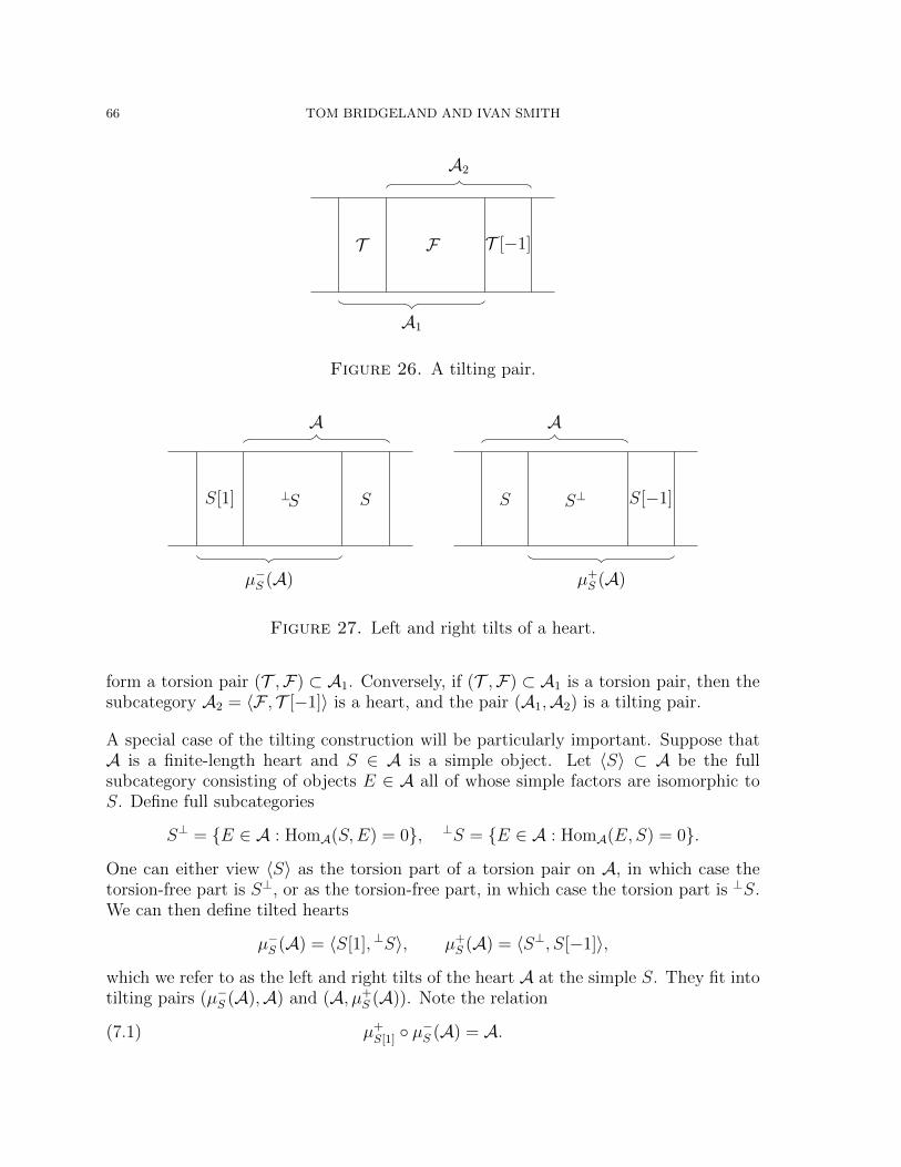
66 TOM BRIDGELAND AND IVAN SMITH
T F T [−1]
A2
A1
Figure 26. A tilting pair.
S[1] ⊥S S
A
µ−S (A)
S S⊥ S[−1]
A
µ+S (A)
Figure 27. Left and right tilts of a heart.
form a torsion pair (T ,F) ⊂ A1. Conversely, if (T ,F) ⊂ A1 is a torsion pair, then thesubcategory A2 = 〈F , T [−1]〉 is a heart, and the pair (A1,A2) is a tilting pair.
A special case of the tilting construction will be particularly important. Suppose thatA is a finite-length heart and S ∈ A is a simple object. Let 〈S〉 ⊂ A be the fullsubcategory consisting of objects E ∈ A all of whose simple factors are isomorphic toS. Define full subcategories
S⊥ = {E ∈ A : HomA(S,E) = 0}, ⊥S = {E ∈ A : HomA(E, S) = 0}.
One can either view 〈S〉 as the torsion part of a torsion pair on A, in which case thetorsion-free part is S⊥, or as the torsion-free part, in which case the torsion part is ⊥S.We can then define tilted hearts
µ−S (A) = 〈S[1], ⊥S〉, µ+S (A) = 〈S⊥, S[−1]〉,
which we refer to as the left and right tilts of the heart A at the simple S. They fit intotilting pairs (µ−S (A),A) and (A, µ+
S (A)). Note the relation
(7.1) µ+S[1] ◦ µ
−S (A) = A.

QUADRATIC DIFFERENTIALS AS STABILITY CONDITIONS 67
The tilting graph of D is the graph Tilt(D) whose vertices are finite-length hearts, andin which two vertices are joined by an edge if the corresponding hearts are relatedby a tilt in a simple object. There is a natural action of the group of triangulatedautoequivalences Aut(D) on this graph.
If A ⊂ D is a finite-length heart we denote by TiltA(D) ⊂ Tilt(D) the connectedcomponent containing A. We say that the hearts in TiltA(D) are reachable from A. Wesay that an autoequivalence Φ ∈ Aut(D) is reachable from A if its action on Tilt(D)preserves the connected component TiltA(D). These autoequivalences form a subgroupAutA(D) ⊂ Aut(D).
We say that a finite-length heart A ⊂ D is infinitely tiltable if the graph TiltA(D) is2n-regular, where n is the rank of K(D). This means that the tilting process can becontinued indefinitely at all simple objects, and in both directions, without leaving theclass of finite-length hearts.
7.3. Tilting in the CY3 case. Suppose now that D is a triangulated category withthe CY3 property. To ensure the existence of the twist functors appearing below weshould also assume that D is algebraic in the sense of Keller [19, Section 3.6].
Associated to a finite-length heart A ⊂ D there is a quiver Q(A), whose vertices areindexed by the isomorphism classes of simple objects Si ∈ A and which has
nij = dimk Ext1A(Si, Sj)
arrows connecting vertex i to vertex j. We call a finite-length heart A ⊂ D non-degenerate if it is infinitely-tiltable and if, for every heart B ⊂ D reachable from A, thequiver Q(B) has no loops or oriented 2-cycles.
The quiver Q(A) associated to a finite-length heart A ⊂ D has no loops precisely if thesimple objects of A are all spherical in the sense of [31]. Any spherical object S ∈ Ddefines an autoequivalence TwS ∈ Aut(D) called a spherical twist. It has the propertythat for any object E ∈ D there is a triangle
Hom•D(S,E)⊗ S −→ E −→ TwS(E).
Suppose now that A ⊂ D is a non-degenerate finite-length heart with n simple objectsup to isomorphism. Taken together, the spherical twists in these simple objects generatea subgroup
SphA(D) = 〈TwS1 , . . . ,TwSn〉 ⊂ Aut(D).
The following result is well-known, but for the reader’s convenience we include a sketchproof. A more careful treatment can be found for example in [23].
Proposition 7.1. (a) for every simple object S ∈ A there is a relation
TwS(µ−S (A)) = µ+S (A) ⊂ D;
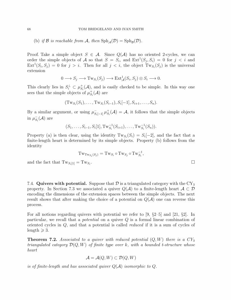
68 TOM BRIDGELAND AND IVAN SMITH
(b) if B is reachable from A, then SphA(D) = SphB(D).
Proof. Take a simple object S ∈ A. Since Q(A) has no oriented 2-cycles, we canorder the simple objects of A so that S = Si, and Ext1(Sj, Si) = 0 for j < i andExt1(Si, Sj) = 0 for j > i. Then for all j < i, the object TwSi
(Sj) is the universalextension
0 −→ Sj −→ TwSi(Sj) −→ Ext1
A(Si, Sj)⊗ Si −→ 0.
This clearly lies in S⊥i ⊂ µ+Si
(A), and is easily checked to be simple. In this way one
sees that the simple objects of µ+Si
(A) are
(TwSi(S1), . . . ,TwSi
(Si−1), Si[−1], Si+1, . . . , Sn).
By a similar argument, or using µ−Si[−1] µ+Si
(A) = A, it follows that the simple objects
in µ−Si(A) are
(S1, . . . , Si−1, Si[1],Tw−1Si
(Si+1), . . . ,Tw−1Si
(Sn)).
Property (a) is then clear, using the identity TwSi(Si) = Si[−2], and the fact that a
finite-length heart is determined by its simple objects. Property (b) follows from theidentity
TwTwSi(Sj) = TwSi
◦TwSj◦Tw−1
Si,
and the fact that TwSi[1] = TwSi. �
7.4. Quivers with potential. Suppose that D is a triangulated category with the CY3
property. In Section 7.3 we associated a quiver Q(A) to a finite-length heart A ⊂ Dencoding the dimensions of the extension spaces between the simple objects. The nextresult shows that after making the choice of a potential on Q(A) one can reverse thisprocess.
For all notions regarding quivers with potential we refer to [9, §2–5] and [21, §2]. Inparticular, we recall that a potential on a quiver Q is a formal linear combination oforiented cycles in Q, and that a potential is called reduced if it is a sum of cycles oflength > 3.
Theorem 7.2. Associated to a quiver with reduced potential (Q,W ) there is a CY3
triangulated category D(Q,W ) of finite type over k, with a bounded t-structure whoseheart
A = A(Q,W ) ⊂ D(Q,W )
is of finite-length and has associated quiver Q(A) isomorphic to Q.
QUADRATIC DIFFERENTIALS AS STABILITY CONDITIONS 69
Proof. Define the category D(Q,W ) to be the subcategory of the derived category ofthe complete Ginzburg algebra Π(Q,W ) consisting of objects with finite-dimensionalcohomology. It has the CY3 property by [21, Lemma 7.16, Theorem 7.17].
The category D(Q,W ) has a standard bounded t-structure [21, Lemma 5.2] whose heartA(Q,W ) is equivalent to the category of finite-dimensional modules for the completeJacobi algebra J(Q,W ) = H0(Π(Q,W )). The algebra J(Q,W ) is the quotient of thecomplete path algebra of Q by the relations obtained by cyclically differentiating thepotential W . In particular, its simple modules are naturally in bijection with the verticesof Q, and the spaces of extensions between them are based by the arrows in Q. �
The combinatorial incarnation of the process of tilting at a simple module is called mu-tation. It acts on right-equivalence classes of quivers with potential. Roughly speaking,two potentials on a quiver Q are said to be right-equivalent if they differ by an auto-morphism of the completed path algebra which fixes the zero length paths; for the fulldefinition see [9, §4] or [21, §2.1]. Right-equivalent potentials give rise to isomorphiccomplete Ginzburg algebras [21, Lemma 2.9], and hence equivalent categories D(Q,W ).
Suppose that (Q,W ) is a reduced quiver with potential, and fix a vertex i of Q. Themutation (Q′,W ′) = µi(Q,W ) is another reduced quiver with potential, well-defined upto right-equivalence, and depending only on the right-equivalence class of (Q,W ). Thevertex sets of Q and Q′ are naturally identified, and the operation µi is an involution.We refer the reader to [9, §5] or [21, §2.4] for the relevant definitions.
For our purposes, the importance of mutations of quivers with potential is the followingresult of Keller and Yang [21, Thm. 3.2, Cor. 5.5].
Theorem 7.3. Let (Q,W ) be a quiver with reduced potential, such that Q has no loopsor oriented 2-cycles. Let i be a vertex of Q and set
(Q′,W ′) = µi(Q,W ).
Then there is a canonical pair of k-linear triangulated equivalences
Φ± : D(Q′,W ′) −→ D(Q,W )
which induce tilts in the simple object Si ∈ A(Q,W ) in the sense that
Φ±(A(Q′,W ′)) = µ±Si(A(Q,W )) ⊂ D(Q,W ),
and which moreover induce the natural bijections on simple objects.
For the last part of this statement, recall that there is a natural bijection betweenthe simple objects of A and those of µ±Si
(A) which was made explicit in the proof ofProposition 7.1. There is also a natural bijection between the vertices of the quivers(Q,W ) and µi(Q,W ). The claim is that these bijections are compatible with the canon-ical bijections between the vertices of the quivers Q,Q′ and the simple objects in thecorresponding standard hearts.

70 TOM BRIDGELAND AND IVAN SMITH
A quiver with potential (Q,W ) is called non-degenerate [9, §7] if any sequence of muta-tions of (Q,W ) results in a quiver with potential having no loops or oriented 2-cycles.Theorem 7.3 shows that this condition is equivalent to the statement that the standardheart A(Q,W ) ⊂ D(Q,W ) is non-degenerate in the sense of Section 7.3.
7.5. Stability conditions. Here we summarize the basic properties of spaces of sta-bility conditions. We refer the reader to [2, 3] for more details on this material. Let usfix a triangulated category D, and assume for simplicity that the Grothendieck groupK(D) ∼= Z⊕n is free of finite rank.
A stability condition σ = (Z,P) on D consists of a group homomorphism Z : K(D)→ Ccalled the central charge, and full additive subcategories P(φ) ⊂ D for each φ ∈ R,which together satisfy the following axioms:
(a) if E ∈ P(φ) then Z(E) ∈ R>0 · eiπφ ⊂ C,(b) for all φ ∈ R, P(φ+ 1) = P(φ)[1],
(c) if φ1 > φ2 and Aj ∈ P(φj) then HomD(A1, A2) = 0,
(d) for each nonzero object E ∈ D there is a finite sequence of real numbers
φ1 > φ2 > · · · > φk
and a collection of triangles
0 E0// E1
//
���������E2
//
���������. . . // Ek−1
// Ek
���������E
A1
^^==
==
A2
^^==
==
Ak
``BB
BB
with Aj ∈ P(φj) for all j.
The semistable objects Aj appearing in the filtration of axiom (d) are unique up toisomorphism, and are called the semistable factors of E. We set
φ+(E) = φ1, φ−(E) = φk, m(E) =∑i
|Z(Ai)| ∈ R>0.
The real number m(E) is called the mass of E. It follows from the definition thatthe subcategories P(φ) ⊂ D are abelian categories; the objects of P(φ) are said to besemistable of phase φ, and the simple objects of P(φ) are said to be stable of phase φ.For any interval I ⊂ R there is a full subcategory P(I) ⊂ D consisting of objects whosesemistable factors have phases in I.
We shall always assume that our stability conditions σ = (Z,P) satisfy the supportproperty of [24], namely that for some norm ‖ ·‖ on K(D)⊗R there is a constant C > 0such that
(7.2) ‖γ‖ < C · |Z(γ)|

QUADRATIC DIFFERENTIALS AS STABILITY CONDITIONS 71
for all classes γ ∈ K(D) represented by σ-semistable objects in D. As explained in [1,Prop. B.4], this is equivalent to assuming that they are full and locally-finite in theterminology of [2, 4]. We let Stab(D) denote the set of all such stability conditions onD.
There is a natural topology on Stab(D) induced by the metric(7.3)
d(σ1, σ2) = sup06=E∈D
{|φ−σ2(E)− φ−σ1(E)|, |φ+
σ2(E)− φ+
σ1(E)|,
∣∣∣∣logmσ2(E)
mσ1(E)
∣∣∣∣} ∈ [0,∞].
The following result is proved in [2].
Theorem 7.4. The space Stab(D) has the structure of a complex manifold, such thatthe forgetful map
π : Stab(D) −→ HomZ(K(D),C)
taking a stability condition to its central charge, is a local isomorphism.
There are two commuting group actions on Stab(D) that will be important later. Thegroup of triangulated autoequivalences Aut(D) acts on Stab(D) in a rather obviousway: an autoequivalence Φ ∈ Aut(D) acts by
Φ: (Z,P) 7→ (Z ′,P ′), Z ′(E) = Z(Φ−1(E)), P ′ = Φ(P).
There is also an action of the universal cover of the group GL+(2,R) of orientation-preserving linear automorphisms of R2. This action does not change the subcategoryP , but acts by post-composition on the central charge, viewed as a map to C = R2,with a corresponding adjustment of the grading on P . This action is not free in general,but there is a subgroup isomorphic to C which does act freely: an element t ∈ C actsby
t : (Z, P ) 7→ (Z ′,P ′), Z ′(E) = e−iπt · Z(E), P ′(φ) = P(φ+ Re(t)).
Note that for any integer n ∈ Z, the action of the multiple shift functor [n] coincideswith the action of n ∈ C.
Later we will need the following more precise version of Theorem 7.4.
Proposition 7.5. Fix a real number 0 < ε � 1. Given a stability condition σ =(Z,P) ∈ Stab(D), and a group homomorphism W : K(D)→ C satisfying
|W (E)− Z(E)| < ε · |Z(E)|for all σ-stable objects E ∈ D, there is a unique stability condition σ′ ∈ Stab(D) withcentral charge W such that d(σ, σ′) < 1
2.
Proof. In fact we can take any 0 < ε < 18. The support property implies that for
any interval I ⊂ R of length < 1, the quasi-abelian categories P(I) have finite-length.The existence part then follows from the results of [2, Section 7]. The uniqueness is aconsequence of [2, Lemma 6.4]. �

72 TOM BRIDGELAND AND IVAN SMITH
7.6. Walls and chambers. In this section we give some basic results on the wall-and-chamber decomposition of the space of stability conditions. These are well-known, butthe proofs in the general setting are not available in the literature. As in the last section,we fix a triangulated category D and assume that K(D) ∼= Z⊕n is free of finite rank.
Proposition 7.6. Fix an object E ∈ D. Then
(a) the set of σ ∈ Stab(D) for which E is σ-stable is open.(b) the set of σ ∈ Stab(D) for which E is σ-semistable is closed.
Proof. For part (a), take a stability condition σ = (Z,P) and an object E ∈ P(φ) whichis σ-stable. Choose 0 < r � 1 and consider the open ball Br(σ) of radius r centered atσ, with respect to the metric (7.3). By definition of this metric, for σ′ = (Z ′,P ′) ∈ Br(σ)there are inclusions
P(φ) ⊂ P ′(φ− r, φ+ r) ⊂ P(φ− 2r, φ+ 2r).
Thus E fails to be stable in σ′ precisely if there is a triangle A→ E → B whose objectsall lie in P(φ− 2r, φ+ 2r) and for which φ′(A) > φ′(E).
The support property implies that for any M > 0 there are only finitely many classesα ∈ K(D) satisfying |Z(α)| < M for which there exist σ-semistable objects of classα. It follows that the set of classes α ∈ K(D) of objects A as above is finite. SinceE is stable in σ we must have φ(A) < φ(E) for each such subobject, and so, reducingr if necessary, we can assume that these phase inequalities continue to hold for allσ′ ∈ Br(σ). It follows that E is stable for all stability conditions in Br(σ).
Part (b) is immediate: the object E is semistable in σ precisely if φ+σ (E) = φ−σ (E). By
the definition of the metric (7.3) this is a closed condition. �
Let us now fix a class γ ∈ K(D) and consider stability for objects of this class. Letα ∈ K(D) be another class which is not proportional to γ. We define
Wγ(α) ⊂ Stab(D)
to be the subset of stability conditions σ = (Z,P) satisfying the following condition:for some φ ∈ R there is an inclusion A ⊂ E in the category P(φ) such that A and Ehave classes α and γ respectively. Locally, the subset Wγ(α) is contained in the realcodimension one submanifold of Stab(D) defined by the condition Z(α)/Z(γ) ∈ R>0.
Lemma 7.7. If B ⊂ Stab(D) is a compact subset then the set of classes α for whichthe subset Wγ(α) intersects B is finite.
Proof. The support property for a fixed stability condition σ implies that for any givenM > 0 there are only finitely many classes α ∈ K(D) represented by objects of mass< M in σ. On the other hand, the definition of the metric (7.3) shows that the masses ofobjects of D vary by a uniformly bounded amount in B, so the same is true if we allow

QUADRATIC DIFFERENTIALS AS STABILITY CONDITIONS 73
σ to vary in B. Using compactness again we can assume that M is large enough that|Z(γ)| < M for all points in B. But if σ ∈ Wγ(α)∩B then there is an inclusion A ⊂ Ein some P(φ), and it follows that A has mass < M , and hence has one of finitely-manyclasses. �
Consider the complement of the closures
Cγ = Stab(D) \⋃α 6∼γ
Wγ(α)
where the union is over classes α which are not proportional to γ. This is the complementof a locally-finite union of closed subsets, hence is open.
We refer to the subsets Wγ(α) as walls for the class γ, and the connected componentsof Cγ will be called chambers. The following result shows that the question of whether agiven object E ∈ D of class γ is stable or semistable has a constant answer for stabilityconditions in a fixed chamber.
Proposition 7.8. Let U ⊂ Cγ be a chamber. If an object E of class γ is (semi)stablefor some stability condition σ ∈ U then the same is true for all σ ∈ U .
Proof. We say that an object E ∈ D is pseudostable in a stability condition σ if itis semistable and the classes in K(D) of its stable factors are all proportional. Theset of points σ ∈ Stab(D) for which a given object E ∈ D is pseudostable is open:indeed, by Lemma 7.6(a), if E is pseudostable for σ then the stable factors of E remainstable in some open neighbourhood of σ, and their phases remain equal since they haveproportional classes. The set of points where E is unstable is also open, by Lemma7.6(b), since it is the complement of the points where E is semistable.
Suppose now that E ∈ D has class γ. If E is semistable but not pseudostable then σmust lie on a wall Wγ(α). Thus, the subset of points of the chamber U for which E issemistable is both open and closed. Since U is connected, this subset must be eitherempty or the whole of U .
Assume now that E is semistable for all σ ∈ U . As above this implies that E ispseudostable at each σ ∈ U . The set of σ ∈ U for which E is stable is then open, byLemma 7.6(a), and its complement, the set of points for which E is strictly pseudostableis also open, by the argument given above. Hence, if E is stable for some stabilitycondition in U , then it is stable for all of them. �
7.7. Stability conditions from t-structures. Let D be a triangulated category. Anystability condition σ = (Z,P) on D has an associated heart
A = P((0, 1]) ⊂ D.

74 TOM BRIDGELAND AND IVAN SMITH
It is the extension closure of the subcategories P(φ) for 0 < φ 6 1. All nonzero objectsof A are mapped by Z into the semi-closed upper half plane
H = {r exp(iπφ) : r ∈ R>0 and 0 < φ 6 1} ⊂ C.
Conversely, given a heart A ⊂ D, and a group homomorphism Z : K(A) → C withthis property, then providing some finiteness conditions are satisfied, there is a uniquestability condition on D with heart A and central charge Z.
In particular, if A ⊂ D is a finite-length heart with n simple objects Si up to isomor-phism, the subset Stab(A) ⊂ Stab(D) consisting of stability conditions with heart A ismapped bijectively by π onto the subset
{Z ∈ HomZ(K(D),C) : Z(Si) ∈ H},
and is therefore homeomorphic to Hn.
The following result shows that tilting controls the way the subsets Stab(A), for differenthearts A ⊂ D, are glued together in Stab(D).
Lemma 7.9. Let A ⊂ D be a finite-length heart, and suppose that
σ = (Z,P) ∈ Stab(D)
lies on a unique boundary component of the region Stab(A) ⊂ Stab(D), so that ImZ(Si) =0 for a unique simple object Si. Assume that the tilted hearts µ±Si
(A) are also finite-length. Then there is a neighbourhood σ ∈ U ⊂ Stab(D) such that one of the followingholds
(i) Z(Si) ∈ R<0, and U ⊂ Stab(A) t Stab(µ+Si
(A)),
(ii) Z(Si) ∈ R>0, and U ⊂ Stab(A) t Stab(µ−Si(A)).
Proof. This is stated without proof in [3, Lemma 5.5]. A special case is proved in [5,Proposition 2.4], and the general case is proved in exactly the same way. �
The subsets Stab(A) ⊂ Stab(D) form a different system of walls and chambers inStab(D). The walls consist of points where the subcategory P(0) contains nonzeroobjects. To distinguish them from the walls considered in the last subsection they areoften referred to as walls of type II. Note that they do not depend on a choice of classα ∈ K(D).
Suppose that A ⊂ D is a finite-length heart. It follows from Lemma 7.9 that there isa single connected component StabA(D) ⊂ Stab(D) containing all stability conditionswhose hearts lie in the connected component TiltA(D) ⊂ Tilt(D). Note however that itis not usually the case that StabA(D) is the union of the chambers Stab(B) for heartsB reachable from A (see [37] for a detailed discussion of this point).

QUADRATIC DIFFERENTIALS AS STABILITY CONDITIONS 75
An autoequivalence of D lying in the subgroup AutA(D) ⊂ Aut(D) of autoequivalencesreachable from A necessarily preserves the connected component StabA(D). The con-verse is false: the existence of the C-action shows that the shift functor [1] fixes allconnected components of Stab(D), but it is not generally true that [1] is reachable.
It is easy to see that a triangulated autoequivalence Φ acts trivially on StabA(D) pre-cisely if it fixes a heart A ⊂ D and furthermore fixes pointwise the isomorphism classesof its simple objects. This is equivalent to the condition that Φ acts trivially on theconnected component TiltA(D). We say that such autoequivalences are negligible withrespect to the heart A.
8. Surfaces and triangulations
The particular examples of CY3 categories considered in this paper will be definedusing quivers with potential associated to triangulations of marked bordered surfaces.Unfortunately, the non-degenerate ideal triangulations appearing in Section 1.2 will notbe sufficient for our purposes. Indeed, to understand the space of stability conditions onour categories, we will need to understand all hearts that are reachable from the standardheart; whilst some of these hearts correspond to non-degenerate ideal triangulations,others correspond to more exotic objects introduced in [11] called tagged triangulations.
8.1. Ideal triangulations. Here we give a brief summary of the relevant definitionsconcerning triangulations of marked bordered surfaces. The reader can find a morecareful treatment in the paper of Fomin, Shapiro and Thurston [11].
A marked bordered surface is defined to be a pair (S,M) consisting of a compact, con-nected oriented surface with boundary, and a finite non-empty set M ⊂ S of markedpoints such that each boundary component of S contains at least one marked point.Marked points in the interior of S are called punctures ; the set of punctures is denotedP ⊂M.
An arc in (S,M) is a smooth path γ in S connecting points of M, whose interior lies inthe open subsurface S \ (M∪∂S), and which has no self-intersections in its interior. Wemoreover insist that γ should not be homotopic, relative to its endpoints, to a singlepoint, or to a path in ∂S whose interior contains no points of M. Two arcs are consideredto be equivalent if they are related by a homotopy through such arcs.
An ideal triangulation of (S,M) is defined to be a maximal collection of equivalenceclasses of arcs for which it is possible to find representatives whose interiors are pairwisedisjoint. We refer to the arcs as the edges of the triangulation. An example of an idealtriangulation of a disc with 5 marked points on its boundary is depicted in Figure28; note that it has just two edges. To get something more closely approximating the

76 TOM BRIDGELAND AND IVAN SMITH
intuitive notion of a triangulation of the surface one should add arcs in ∂S connectingthe points of M.
Figure 28. A triangulation of a disc with 5 marked points.
A face or triangle of an ideal triangulation T is the closure in S of a connected componentof the complement of all arcs of T . A triangle is called interior if its intersection with∂S is contained in M. Each interior triangle is topologically a disc, containing eithertwo or three distinct edges of the triangulation.
Figure 29. A self-folded triangle.
An interior triangle with just two distinct edges is called a self-folded triangle; such atriangle has a self-folded edge and an encircling edge. The valency of a puncture p ∈ Pwith respect to a triangulation T is the number of half-edges of T that are incident withit; a puncture has valency 1 precisely if it is contained in a self-folded triangle.
For various technical reasons, when dealing with triangulations of marked borderedsurfaces (S,M), we shall always make the following
Assumption 8.1. We assume that (S,M) is not one of the following surfaces
(a) a sphere with 6 5 marked points;(b) an unpunctured disc with 6 3 marked points on the boundary;(c) a disc with a single puncture and one marked point on its boundary.
In the cases of a sphere with 6 2 punctures, or an unpunctured disc with 6 2 markedpoints, there are no ideal triangulations, and so the theory described below is vacuous.In the cases of an unpunctured disc with 3 marked points, and the surface of case (c),there is a unique ideal triangulation and the theory is trivial and rather degenerate; seeExamples 12.1 and 12.3.
The case of a three-punctured sphere is special in that there is an ideal triangulationconsisting of two self-folded triangles meeting along a common edge; this plays havoc

QUADRATIC DIFFERENTIALS AS STABILITY CONDITIONS 77
with the definition of a tagged triangulation below and for this reason it is better todeal with this case directly: see Section 12.4. Finally, the cases of spheres with 4 or 5punctures are definitely interesting, but we have to exclude them because the crucialresults of Section 9.1 have not been established for these surfaces.
A marked bordered surface (S,M) is determined up to diffeomorphism by its genus g,the number of punctures p, and a collection of integers ki > 1 encoding the number ofmarked points on each boundary component. Any ideal triangulation of such a surfacehas the same number of edges, namely
n = 6g − 6 + 3p+∑i
(ki + 3).
8.2. Flips and pops. Let (S,M) be a marked bordered surface satisfying Assumption8.1. A signed triangulation of (S,M) is a pair (T, ε) consisting of an ideal triangulationT , and a function
ε : P→ {±1}.By a pop of a signed triangulation (T, ε) we mean the operation of changing the signε(p) associated to a puncture p ∈ P of valency one. Note that any such puncture lies inthe centre of a self-folded triangle of T .
The popping operation generates an equivalence relation on signed triangulations, inwhich two signed triangulations (Ti, εi) are equivalent precisely if the underlying trian-gulations Ti are the same, and the signings εi differ only at punctures p ∈ P of valencyone.
It turns out that the equivalence classes for this relation can be explicitly representedby a combinatorial gadget called a tagged triangulation. We will explain this in Section8.3 below, but for now we simply define a tagged triangulation to be an equivalenceclass of signed triangulations.
Let us introduce notation Tri(S,M),Tri±(S,M),Tri./(S,M) for the sets of ideal, signedand tagged triangulations of (S,M) respectively. There is a diagram of maps
(8.1) Tri±(S,M)
q
��
Tri(S,M)i//
j77ppppppppppp
Tri./(S,M)
where q is the obvious quotient map, and the arrows i and j are embeddings obtained byconsidering an ideal triangulation as a signed, and hence a tagged triangulation, usingthe signing ε ≡ +1.
Two ideal triangulations T1 and T2 are related by a flip if they are distinct, and there areedges ei ∈ Ti such that T1\{e1} = T2\{e2}. Note that the edges e1 and e2 are necessarily

78 TOM BRIDGELAND AND IVAN SMITH
non-self-folded. Conversely, if e is a non-self-folded edge of an ideal triangulation T ,it is contained in exactly two triangles of T , and there is a unique ideal triangulationwhich is the flip of T along e. The flipping operation extends to signed triangulations
Figure 30. Flip of a triangulation.
in the obvious way: we flip the underlying triangulation, keeping the signs constant.We say that two tagged triangulations are related by a flip if they can be representedby signed triangulations which differ by a flip.
The sets appearing in the diagram (8.1) can be considered as graphs, with two (ideal,signed, tagged) triangulations being connected by an edge if they differ by a flip. Themaps in the diagram then become maps of graphs. The important point is that, unlikethe graph Tri(S,M) of ideal triangulations, the graph Tri./(S,M) of tagged triangula-tions is n-regular.
The basic explanation for this regularity is as follows. When a triangulation T1 containsa self-folded triangle ∆, we cannot flip the self-folded edge f of ∆, so the number offlips that can be performed on T1 is less than the total number of edges n. On theother hand, if we choose a signing ε : P→ {±1}, and consider the signed triangulation(T1, ε1) up to the above equivalence relation, then when we flip the encircling edge eof ∆, the puncture p contained in ∆ has valency 2 in the new triangulation T2, and sothere are two inequivalent possible choices for the sign ε2(p).
It is well-known that any two ideal triangulations of (S,M) are related by a finitechain of flips; thus the graph Tri(S,M) is always connected [11, Prop. 3.8]. Thegraph Tri./(S,M) is also connected, except for the case when (S,M) is a closed surfacewith a single puncture p ∈ P: in that case Tri./(S,M) has two connected componentscorresponding to the two possible choice of signs ε(p) [11, Prop. 7.10].
8.3. Tagged triangulations. We now explain why the set Tri./(S,M) of tagged tri-angulations we defined above coincides with the standard version as defined by Fomin,Shapiro and Thurston [11]. This material will not be used in the rest of the paper, andis only logically necessary to justify the above assertions that the graph Tri./(S,M) isconnected and n-regular.
Let (S,M) be a marked, bordered surface (S,M) satisfying Assumption 8.1. A taggedarc in (S,M) is an arc as defined above, each end of which has been labelled by one

QUADRATIC DIFFERENTIALS AS STABILITY CONDITIONS 79
of two labels: plain or tagged. Fix a function ε : P → {±1}. Given an ordinary arc e,there is a corresponding tagged arc tε(e) defined by the following rule:
(a) If e is not a loop enclosing a once-punctured disc, the underlying arc of tε(e) isjust e, and an end of e is labelled tagged precisely if it lies at a puncture p ∈ Pwith ε(p) = −1.
(b) If e is a loop based at m ∈M, enclosing a disc which contains a single puncturep ∈ P, then the underlying arc of tε(e) is the arc connnecting p to m inside thedisc. We label the edge adjacent to m tagged precisely if m is a puncture withε(m) = −1, and the edge adjacent to p tagged precisely if ε(p) = +1.
By [11, Lemma 9.3], a tagged triangulation in the standard sense considered there isprecisely a set of tagged arcs of the form tε(T ) for some signed triangulation (T, ε).The following result shows that these tagged triangulations are in bijection with theequivalence classes of signed triangulations considered in the last section.
Lemma 8.2. Suppose that (T1, ε1) and (T2, ε2) are signed triangulations. Then tε1(T1) =tε2(T2) if and only if T1 = T2, and the signings ε1, ε2 differ only at punctures of valencyone.
Proof. Any vertex of valency one lies in the interior of a self-folded triangle, and it isclear from the definition of tε(T ) that the resulting collection of tagged arcs does notdistinguish between the two choices of sign at such a vertex (the enclosing and foldededge of the self-folded triangle get mapped to two taggings of the same arc; changingthe sign just exchanges these two).
The converse follows easily from the following observations. Suppose that η ∈ tε(T ) isa tagged arc, with underlying arc f . Consider tagged arcs ζ ∈ tε(T ) which have thesame underlying arc f . If there is no such ζ then we must have η = tε(f), and thearc f is not contained in a self-folded triangle of T . If there is such a ζ, then thereis a self-folded triangle ∆ in T with self-folded edge f , and encircling edge e, suchthat {η, ζ} = {tε(e), tε(f)}. Moreover, the encircling edge e is completely determined,because the puncture inside ∆ is the one at which η and ζ have different markings. �
We should also check that our definition of when two tagged triangulations differ by aflip coincides with the standard one. Namely, in [11], two tagged triangulations τ1 andτ2 are said to be related by a flip if they are distinct, and there are tagged arcs ηi ∈ τisuch that τ1 \ {η1} = τ2 \ {η2}.
Lemma 8.3. Two tagged triangulations differ by a flip in the above sense, precisely ifthey can be represented by signed triangulations differing by a flip.

80 TOM BRIDGELAND AND IVAN SMITH
Proof. One implication is clear, since if two signed triangulations differ by a flip thenby Lemma 8.2, so do the associated tagged triangulations. For the converse, supposethat τ1 \ {η1} = τ2 \ {η2}. Then we can write τ1 = tε(T1) for some signed triangulation(T1, ε) in such a way that η1 = tε(e1) for some non-self-folded edge e1. Flipping thisedge gives a different signed triangulation T2 satisfying T1 \ {e1} = T2 \ {e2}. It followsthat τ1 \ {η1} = tε(T2) \ tε(e2). But the flip of a tagged triangulation in a tagged arc isunique [11, Theorem 7.9]. Thus we have τ2 = tε(T2) and η2 = tε(e2). �
8.4. Edge lattice and quiver. Let (S,M) be a marked bordered surface satisfyingAssumption 8.1. The edge lattice of an ideal triangulation T of (S,M) is defined tobe the free abelian group Γ(T ) on the edges of T . We denote by [e] the basis elementcorresponding to the edge e ∈ T ; thus
Γ(T ) =⊕e∈T
Z · [e].
For distinct edges e, f ∈ T , we define c(e, f) to be the number of internal triangles of Tin which e and f appear as adjacent edges in clockwise order. There is a skew-symmetricform
〈−,−〉 : Γ(T )× Γ(T )→ Zgiven by the formula
〈[e], [f ]〉 = c(f, e)− c(e, f).
Note that if e and f are the encircling and self-folded edges of a self-folded triangle then
(8.2) c(e, f) = 1 = c(f, e), 〈[e], [f ]〉 = 0.
It will be convenient for later purposes to define c(e, e) = −2 for all edges e, althoughof course this has no effect on the form 〈−,−〉.
We will also need a modified basis {e} for the group Γ(T ) defined as follows:
(a) if e ∈ T is not an edge of a self-folded triangle then {e} = [e];
(b) if e and f are respectively the encircling and self-folded edges of a self-foldedtriangle, then {e} = [e] and {f} = [e] + [f ].
We will see some more intrinsic interpretations of the edge lattice Γ(T ) later: as aGrothendieck group with its Euler form (Lemma 9.10), and as a homology group withan intersection form (Lemma 10.3). We will also give some explanation for the strange-looking definition of the basis {e} (Section 10.2).
Define a map κ : T → T by setting κ(f) = f unless f is a self-folded edge of a self-foldedtriangle, in which case κ(f) = e is the encircling edge of the same triangle. For distinctedges e and f define
n(e, f) = max(0, 〈[κ(f)], [κ(e)]〉
)> 0.

QUADRATIC DIFFERENTIALS AS STABILITY CONDITIONS 81
Note that there is a relation
(8.3) 〈{e}, {f}〉 = 〈[κ(e)], [κ(f)]〉 = n(f, e)− n(e, f)
for all e, f ∈ T . This is easily checked by noting that when f is a self-folded edge, thebasis element [f ] lies in the kernel of the form 〈−,−〉.
To any ideal triangulation T we can now associate a quiver Q(T ) whose vertices arethe edges of T , and with n(e, f) arrows from vertex e to vertex f . By its definition ithas no loops or 2-cycles. In the case of a non-degenerate ideal triangulation of a closedsurface it reduces to the quiver considered in Section 1.2.
Remarks 8.4. (a) If T has a self-folded triangle with edges e and f , then sinceκ(e) = κ(f), there is an involution of the quiver Q(T ) exchanging the verticescorresponding to these two edges.
(b) If e and f are distinct non-self-folded edges, then it is easily checked that c(e, f)and c(f, e) are both nonzero precisely if e and f meet at a puncture of valency2. Thus if a pair of edges e, f are such that κ(e) are κ(f) are distinct, and donot meet at a vertex of valency 2, then n(e, f) = c(κ(e), κ(f)).
8.5. Ordered versions. Sometimes in what follows it will be clearer to work withordered versions of our basic combinatorial objects: triangulations, quivers, t-structuresetc. In this section we gather the necessary definitions; these mostly proceed along theobvious lines.
An ordered ideal triangulation is an ideal triangulation equipped with an ordering of itsedges. Similarly, one can consider ordered signed triangulations. By a pop of an orderedsigned triangulation we mean the operation which changes the sign ε(p) associated to apuncture p ∈ P of valency 1, and which also changes the ordering of the triangulation bytransposing the two edges of the self-folded triangle containing p. Two ordered signedtriangulations are considered equivalent if they differ by a finite sequence of such pops.By an ordered tagged triangulation we mean an equivalence class of ordered signedtagged triangulations. The map tε of Section 8.3 respects this equivalence relation, andit follows that we can realise ordered tagged triangulations as ordered collections oftagged arcs.
Two ordered triangulations are related by a flip if the underlying triangulations arerelated by a flip, and if the orderings of their edges are compatible with the obviousbijection between the edges of the two triangulations. Similarly, one can consider flipsof ordered signed triangulations. Two ordered tagged triangulations are related by aflip if they can be represented by ordered signed triangulations that are related by aflip.
An ordered quiver is a quiver equipped with a fixed ordering of its vertices. An orderedtriangulation T has an associated ordered quiver Q(T ). Remark 8.4(a) shows that the

82 TOM BRIDGELAND AND IVAN SMITH
ordered quiver associated to an ordered triangulation is invariant under transposing theorder of the two edges of a self-folded triangle, and it follows that every ordered taggedtriangulation also has an associated ordered quiver.
Finally, suppose that D is a CY3 triangulated category. By an ordering of a finite-length heart A ⊂ D we mean an ordering of the simple objects of A. The associatedquiver Q(A) is then also ordered in the obvious way. As we explained in the proof ofProposition 7.1, for any simple object S ∈ A, there is a canonical bijection between thesimple objects of the heart A and those of the tilted heart µ±S (A). We say that twoordered hearts A,B ⊂ D are related by a tilt in a simple object, if the hearts A,B arerelated by such a tilt, and if the orderings on A,B are compatible with this canonicalbijection.
We denote the graphs of ordered ideal, signed, tagged triangulations by
Tri�(S,M), Tri�±(S,M), Tri�./(S,M)
respectively. The maps in (8.1) induce maps of the ordered versions in the obvious way.Similarly, given a non-degenerate heart A ⊂ D we use the notation
Tilt�A(D), Exch�A(D)
for the graphs of ordered reachable finite-length hearts, and the quotient of this graphby the group SphA(D). We note that these graphs will not be connected in general.
8.6. Mapping class group. By a diffeomorphism of a marked bordered surface (S,M)we mean a diffeomorphism of S which fixes the subset M, although possibly permutingits elements. The mapping class group MCG(S,M) is the group of all orientation-preserving diffeomorphisms of (S,M) modulo those which are homotopic to the identitythrough diffeomorphisms of (S,M).
The mapping class group clearly acts on the graphs of (ideal, signed, tagged) triangu-lations of the surface (S,M), since the edges of such triangulations consist of homotopyclasses of arcs.
Proposition 8.5. Suppose that (S,M) is a marked bordered surface which satisfiesAssumption 8.1 and which is not one of the following 3 surfaces
(a) a once-punctured disc with 2 or 4 marked points on the boundary;
(b) a twice-punctured disc with 2 marked points on the boundary.
Then two ideal triangulations of (S,M) differ by an element of MCG(S,M) precisely ifthe associated quivers are isomorphic.
Proof. One implication is clear: if two triangulations differ by an orientation-preservingdiffeomorphism then they have the same combinatorics and hence the same associatedquivers.

QUADRATIC DIFFERENTIALS AS STABILITY CONDITIONS 83
For the converse, suppose that two surfaces (Si,Mi) have ideal triangulations Ti. In [11,Section 13] it is explained how to decompose the quivers Q(Ti) into certain blocks. Inthe proof of [11, Proposition 14.1] it is shown that if each quiver Q(Ti) has a uniqueblock decomposition, then the quivers Q(Ti) are isomorphic precisely if there is anorientation-preserving diffeomorphism between the surfaces (Si,Mi) taking one trian-gulation Ti to the other. Weiwen Gu [17] has classified all quivers which have more thanone block decomposition. The only examples corresponding to combinatorially-distincttriangulations of the same surface occur when (S,M) is one of the three cases listed inthe statement of the Proposition, or a sphere with 3 or 4 punctures. These last twocases are already excluded by Assumption 8.1. �
The mapping class group of (S,M) acts on the set P ⊂ M of punctures in the obviousway, and we define the signed mapping class group to be the corresponding semi-directproduct
(8.4) MCG±(S,M) = MCG(S,M) n ZP2 .
This group acts on the set of signed triangulations, with the ZP2 part acting by changing
the signs ε(p) ∈ {±1} associated to the punctures. This action clearly descends to anaction on tagged triangulations. It is an immediate consequence of Proposition 8.5 thatthe quivers associated to two signed or tagged triangulations of (S,M) are isomorphicprecisely if they differ by an element of the signed mapping class group.
8.7. Free action on ordered triangulations. One reason to introduce ordered tri-angulations is the following result.
Proposition 8.6. Suppose that (S,M) satisfies Assumption 8.1 and is not one of thefollowing 3 surfaces:
(i) an unpunctured disc with 4 points on its boundary;
(ii) an annulus with one marked point on each boundary component;
(iii) a closed torus with a single puncture.
Then the action of the mapping class group MCG(S,M) on the set Tri�(S,M) of orderedideal triangulations is free. Similarly, the actions of the signed mapping class groupMCG±(S,M) on the sets Tri�±(S,M) and Tri�./(S,M) are free.
Proof. For the case of ideal triangulations, we must show that an orientation-preservingdiffeomorphism g of (S,M) which fixes the edges of such a triangulation T is homotopicto the identity, through diffeomorphisms of (S,M).
Suppose first that g fixes every triangle of T . Since g then induces an orientation-preserving diffeomorphism of each triangle, it follows that g preserves the orientation ofeach edge of T . Moreover, since every triangle contains at least one edge, we see that gpreserves each connected component of ∂S\M. Now Diff(I, ∂I) is contractible, and the

84 TOM BRIDGELAND AND IVAN SMITH
edges are disjoint in their interiors, so we can isotope g so that it fixes all edges of T ,and all components of ∂S pointwise. The result then follows from the fact [32, TheoremB] that the group Diff(D2, ∂D2) is contractible.
Suppose instead that there is some triangle ∆ such that g(∆) 6= ∆. Then the edges of∆ coincide with those of gi(∆) for all i ∈ Z. Since any edge occurs in the boundary ofat most 2 triangles, it follows that g2(∆) = ∆. Moreover, the surface S is completelycovered by the two triangles ∆ and g(∆), since passing through an edge of ∆ takes usinto g(∆) and vice versa. We then obtain the three possibilities listed, according towhether the closures of the triangles ∆ and g(∆) meet in 1,2 or 3 edges.
The extension to signed triangulations is obvious. For the case of tagged triangulations,suppose that an element of g ∈ MCG±(S,M) fixes an ordered tagged triangulation τ ,which we view as an equivalence-class of signed triangulations (T, ε). Note that theaction of g on Tri�±(S,M) commutes with the flipping operation. Thus we can reduce tothe case when T has no self-folded triangles. Then g must fix the signed triangulation(T, ε), since this is the only signed triangulation in the equivalence-class τ . Hence g isthe identity. �
We note that the excluded cases in Proposition 8.6 are essentially the same as thosein Proposition 6.6 (the case of an unpunctured disc with 3 marked points would ap-pear above were it not already excluded by Assumption 8.1). This is not a coincidence:generic automorphisms of the space Quad(S,M) correspond to automorphisms of (S,M)which preserve a horizontal strip decomposition together with an ordering of the hori-zontal strips. Any such automorphism will also preserve an ordered version of the WKBtriangulation of Section 10.1.
9. The category associated to a surface
In this section we introduce the particular examples of CY3 categories that appear inour main Theorems. They are indexed by diffeomorphism classes of marked borderedsurfaces (S,M). We also provide the combinatorial underpinning of our main theo-rems, by giving a precise correspondence between tagged triangulations of (S,M) andt-structures on the corresponding category D(S,M). Throughout this section we relyheavily on the work of D. Labardini-Fragoso.
9.1. Some results of Labardini-Fragoso. Let (S,M) be a marked bordered surfacesatisfying Assumption 8.1. Let T be an ideal triangulation of (S,M). Labardini-Fragoso[25] defined a reduced potential W (T ) on the quiver Q(T ) introduced in Section 8.4,depending also on some nonzero scalar constants xp ∈ k \ {0}, one for each puncturep ∈ P. We shall always take these scalars to be defined by a signing; thus we take

QUADRATIC DIFFERENTIALS AS STABILITY CONDITIONS 85
a signed triangulation (T, ε) and consider the quiver with potential (Q(T ),W (T, ε))obtained by setting xp = ε(p).
In the case when T is non-degenerate, the resulting potential reads
(9.1) W (T, ε) =∑f
T (f)−∑p
ε(p)C(p),
where T (f) and C(p) are the cycles in Q(T ) defined in Section 1.2. In the presenceof punctures of valency 6 2 the recipe becomes more complicated. The explicit formof the potential will not be important for what follows, and we refer to [25, Section 3]for details. What will be important are the invariance properties under flips and popswhich we now describe.
The case of flips is dealt with by the following result of Labardini-Fragoso [25, Theorem30]. To be absolutely clear we state it for ordered triangulations.
Theorem 9.1. Let (S,M) be a marked bordered surface satisfying Assumption 8.1.Suppose that two ordered signed triangulations (Ti, εi) of (S,M) are related by a flip in anon-self-folded edge e. Then, up to right-equivalence, the ordered quivers with potential(Q(Ti),W (Ti, εi)) are related by a mutation at the corresponding vertex.
We now move on to the case of pops. As we remarked in Section 8.5, the popping sym-metry of Remark 8.4(a) implies that an ordered tagged triangulation has an associatedordered quiver. The following result [8, Theorem 6.1] extends this statement to quiverswith potential.
Theorem 9.2. Let (S,M) be a marked bordered surface satisfying Assumption 8.1.Suppose that two ordered signed triangulations (T, εi) of (S,M) are related by a pop.Then the associated ordered quivers with potential (Q(T ),W (T, εi) are right-equivalent.
We conclude that every ordered tagged triangulation has an associated ordered quiverwith potential, well-defined up to right-equivalence. If we think of a tagged triangu-lation τ as a collection of tagged arcs as in Section 8.3, then we can say that there isan associated quiver with potential (Q(τ),W (τ)), well-defined up to right-equivalence,whose vertices are in natural bijection with these tagged arcs.
To avoid all technical difficulties we shall mostly work with the following class of surfaces.We return to some of the exceptional cases in Section 11.6.
Definition 9.3. We say that a marked bordered surface (S,M) is amenable if
(a) (S,M) satisfies Assumption 8.1;
(b) (S,M) is not one of the 3 surfaces listed in Proposition 8.5;
(c) (S,M) is not one of the 3 surfaces listed in Proposition 8.6;
(d) (S,M) is not a closed surface with a single puncture.

86 TOM BRIDGELAND AND IVAN SMITH
Note for example that (S,M) is amenable if g(S) > 0 and |M| > 1.
Recall from Section 7.4 the definition of a non-degenerate quiver with potential.
Theorem 9.4. Suppose that the marked bordered surface (S,M) is amenable. Then thequiver with potential (Q(T ),W (T, ε)) associated to any signed triangulation of (S,M) isnon-degenerate.
Proof. Up to right-equivalence the quiver with potential (Q(T ),W (T, ε)) associated toa signed triangulation depends only on the corresponding tagged triangulation. Sincetagged triangulations can be flipped in any edge, and such flips can be expressed as flipsof signed triangulations to which Theorem 9.1 applies, we conclude that every mutationof (Q(T ),W (T, ε)) is of the same type. The result follows, since by definition, none ofthe quivers Q(T ) has loops or oriented 2-cycles. �
9.2. Definition of the category. Let (S,M) be an amenable marked bordered surface.In this section we introduce the associated CY3 triangulated category D(S,M), well-defined up to k-linear triangulated equivalence.
Given a signed triangulation (T, ε) of (S,M), let us write
D(T, ε) = D(Q(T ),W (T, ε))
for the CY3 category defined by the quiver with potential considered in the last subsec-tion. This category comes equipped with a standard heart
A(T, ε) ⊂ D(T, ε),
whose simple objects Se are indexed by the edges e of the triangulation T .
Combining Theorem 7.3 and Theorem 9.1 immediately gives
Theorem 9.5. Suppose that two signed triangulations (Ti, εi) of (S,M) differ by a flipin an edge e. Then there is a canonical pair of k-linear triangulated equivalences
Φ± : D(T1, ε1)→ D(T2, ε2),
satisfying Φ±(A(T1, ε1)) = µ±Se(A(T2, ε2)) and inducing the natural bijection on simple
objects.
Similarly, Conjecture ??, which holds by the assumption that (S,M) is amenable, implies
Theorem 9.6. Suppose that two signed triangulations (T, εi) of (S,M) are related by apop at a puncture p ∈ P. Then there is a k-linear triangulated equivalence
Ψ: D(T, ε1)→ D(T, ε2)
which identifies the standard hearts, and exchanges the two simple objects Se and Sfcorresponding to the two edges of the self-folded triangle containing p.

QUADRATIC DIFFERENTIALS AS STABILITY CONDITIONS 87
Since the graph Tri./(S,M) is connected, these two results show that, up to k-lineartriangulated equivalence, the category D(T, ε) depends only on the surface (S,M) andnot on the chosen signed triangulation. Thus we can associate to the surface (S,M) aCY3 triangulated category
D = D(S,M).
In fact it will be important to make a slightly stronger statement, as we now explain.Each category D(T, ε) comes with a distinguished connected component of its tiltinggraph, namely the one containing the standard heart. Moreover, if (Ti, εi) are two signedtriangulations of (S,M) then by composing the equivalences of Theorems 9.5 and 9.6 weobtain equivalences D(T1, ε1) ∼= D(T2, ε2) which identify these connected components.Thus the category D comes equipped with a distinguished connected component
Tilt4(D) ⊂ Tilt(D).
Adapting the general notation from Section 7, we write
Aut4(D) ⊂ Aut(D)
for the group of autoequivalences of D which preserve this connected component; suchautoequivalences will be called reachable. We write
Nil4(D) ⊂ Aut4(D)
for the autoequivalences which act trivially on Tilt4(D); we call these autoequivalencesnegligible.
Negligible autoequivalences fix the simple objects of all the hearts in our distinguishedcomponent Tilt4(D). They will also act trivially on the corresponding distinguishedconnected component Stab4(D). For this reason, it is useful to consider the quotientgroup
Aut4(D) = Aut4(D)/Nil4(D)
which acts effectively on these spaces.
Remark 9.7. We could instead consider defining a category D†(S,M) by using uncom-pleted Ginzburg algebras, rather than the complete ones we are using here. It seemslikely that if (S,M) is amenable the resulting category would be equivalent to D(S,M).As evidence for this, note that in the case when S has non-empty boundary the naturalmap J†(Q,W )→ J(Q,W ) from the uncompleted Jacobi algebra to the complete versionis an isomorphism [8, Theorem 5.7]. When the surface is not amenable this statementcan definitely fail. For example, when (S,M) is a closed torus with a single puncturethe algebra J†(Q,W ) is infinite-dimensional, whereas J(Q,W ) is finite-dimensional [26,Example 8.2]. See also Example 12.4 below for the case of the three-punctured sphere.
9.3. T-structures and autoequivalences. Let (S,M) be an amenable marked bor-dered surface, and let D = D(S,M) be the associated CY3 triangulated category. Inthis section we study the distinguished connected component Tilt4(D) of the tiltinggraph of D, and the corresponding group Aut4(D) of reachable autoequivalences.

88 TOM BRIDGELAND AND IVAN SMITH
Recall from Section 7.3 that there is a subgroup
Sph4(D) ⊂ Aut4(D),
generated by the twist functors TwSiin the simple objects of any heart A ∈ Tilt4(D).
We write
Sph4(D) ⊂ Aut4(D),
for the corresponding subgroup of Aut4(D). The group Sph4(D) acts on the tiltinggraph Tilt(D), and Proposition 7.1 implies that this action preserves the connectedcomponent Tilt4(D). We call the quotient graph
Exch4(D) = Tilt4(D)/ Sph4(D)
the heart exchange graph of (S,M). There is also an ordered version Exch�4(D) definedin the obvious way.
The following result gives the basic link between triangulations of the surface (S,M)and t-structures in the corresponding category D(S,M).
Theorem 9.8. There are isomorphisms of graphs
Tri./(S,M) ∼= Exch4(D), Tri�./(S,M) ∼= Exch�4(D).
Proof. Corollary 3.6 of [7] and Theorem 5.6 of [20] together imply that the heart ex-change graph Exch4(D) is isomorphic to the cluster exchange graph. On the otherhand, the cluster exchange graph was shown to be isomorphic to the tagged triangula-tion graph Tri./(S,M) in [11, Theorem 7.11] and [12]. Both of these isomorphisms areconstructed in such a way that they lift to maps of the corresponding ordered graphs,and it follows that these maps are also isomorphisms. �
We note that the isomorphisms of Theorem 9.8 have the property that if a taggedtriangulation is represented by a signed triangulation (T, ε), then the correspondingheart A ⊂ D is the image of the standard heart A(T, ε) under an equivalence
D(T, ε) ∼= D.
The obvious generalization to the ordered versions also holds. We can use this result toprove9 a result on the structure of the group Aut4(D).
Theorem 9.9. Assume that (S,M) is amenable. Then there is a short exact sequence
1 −→ Sph4(D) −→ Aut4(D) −→ MCG±(S,M) −→ 1.
9The method of proof was explained to us by Alastair King.

QUADRATIC DIFFERENTIALS AS STABILITY CONDITIONS 89
Proof. Consider the n-fold free product group
Fn = Z2 ∗ · · · ∗ Z2 = 〈µ1, · · · , µn : µ2i = 1〉.
There is an obvious action of the symmetric group Symn permuting the generators µi,and we also consider the semi-direct product
Gn = SymnnFn.
The set Tri�./(S,M) of ordered, tagged triangulations has a natural action of the groupGn: the generator µi acts by flipping the ith edge of an ordered triangulation, andthe group Symn acts by permuting the ordering of the edges. This action is transitive,because, with our assumptions on S, the graph of unordered tagged triangulationsTri./(S,M) is connected.
In a similar way, the set Exch�4(D) of ordered reachable hearts has a transitive actionof the group Gn. This time the generator µi acts by tilting an ordered heart at theith simple object. Note that the left and right tilts co-incide on the exchange graph byProposition 7.1(a), and the relation µ2
i = 1 follows from the relation (7.1).
Consider the set Qn of right-equivalence classes of ordered quivers with n vertices. Itcarries an action of the group Gn, where the generator µi acts by mutation at the ithvertex. We now have a commutative diagram of Gn-equivariant maps of sets
(9.2) Tri�./(S,M)
p$$HHHHHHHHH
θ// Exch�4(D)
q{{vvvvvvvvv
Qn
where p sends an ordered tagged triangulation (T, ε) to the associated ordered quiverQ(T ), the map q sends an ordered heart A ⊂ D to the associated quiver Q(A), and θis the bijection of Theorem 9.8.
The signed mapping class group MCG±(S,M) acts freely on Tri�./(S,M) by Proposition8.6 and obviously commutes with the Gn-action. Proposition 8.5 shows that the orbitsfor this action are precisely the fibres of p. It then follows from the transitivity of theGn-action that MCG±(S,M) can be identified with the group of automorphisms of theset Tri�./(S,M) which commute with the Gn-action and preserve the map p.
By the definition of a negligible autoequivalence, the group Aut4(D) acts freely onthe graph Tilt�4(D) of ordered reachable hearts. Quotienting Aut4(D) by the normalsubgroup Sph4(D), we therefore obtain a free action of the group
(9.3) Aut4(D)/Sph4(D)
on the set Exch�4(D), commuting with the Gn-action. To complete the proof we mustshow that the orbits of Aut4(D) are precisely the fibres of the map q.

90 TOM BRIDGELAND AND IVAN SMITH
Suppose that two ordered hearts Ai ⊂ D lie in the same fibre of q. Under the bijectionθ, these hearts correspond to ordered tagged triangulations (Ti, εi) lying in the samefibre of p. It follows that they differ by an element g ∈ MCG±(S,M). We claim thatthe ordered quivers with potential (Q(Ti),W (Ti, εi)) are right-equivalent up to scale,meaning that there is a nonzero scalar λ ∈ k∗ and a right-equivalence
(Q(T1, ),W (T1, ε1)) ∼ (Q(T2), λW (T2, ε2)).
In particular it follows that there are equivalences
D(T1, ε1) ∼= D(T2, ε2)
preserving the standard hearts. The remark following Theorem 9.8 then shows that thehearts Ai differ by an autoequivalence of D, and the result then follows.
When g ∈ MCG(S,M) the claim is obvious since the quiver with potential associated toa signed triangulation depends only on the combinatorial structure of the triangulation.For general g ∈ MCG±(S,M) the claim follows from the statement that the quiverwith potential (Q(T ),W (T, ε)) is independent of the signing ε, up to scaling and right-equivalence. A proof of this statement will appear in [13] (see [8, Prop. 10.4]). When Shas non-empty boundary, no scaling is necessary, and the claim follows from [8, Prop.10.2]. �
9.4. Grothendieck group. Let (S,M) be an amenable marked bordered surface. Re-call from Section 8.4 the definition of the edge lattice Γ(T ) associated to an idealtriangulation of (S,M).
Lemma 9.10. Let (T, ε) be a signed triangulation of (S,M). Then there is an isomor-phism of abelian groups
λ : Γ(T )→ K(D(T, ε)),
such that for each edge e, the basis element {e} is mapped to the class of the corre-sponding simple object Se. This map takes the form 〈−,−〉 on Γ(T ) to the Euler formon K(D(T, ε)).
Proof. For any reduced quiver with potential (Q,W ), the Grothendieck group of thecategory D(Q,W ) is identified with that of its canonical heart A = A(Q,W ), and istherefore the free abelian group on the vertices of Q. The CY3 condition implies thatthe Euler form is given by skew-symmetrising the adjacency matrix of the quiver. Theresult is then immediate from (8.3). �
Suppose that (Ti, εi) are signed triangulations of (S,M) differing by a flip in an edge e.We then use the natural bijection between the edges of T1 and T2 to identify these twosets. Theorem 9.5 gives equivalences
Φ± : D(T1, ε1) ∼= D(T2, ε2),

QUADRATIC DIFFERENTIALS AS STABILITY CONDITIONS 91
which induce isomorphisms φ± on the Grothendieck groups. We have the followingexplicit formulae for these maps.
Lemma 9.11. Define maps F± by the commutative diagram
Γ(T1)
λ1��
F±// Γ(T2)
λ2��
K(D(T1, ε1))φ±
// K(D(T2, ε2))
where the λi are the maps of Lemma 9.10. Then for all edges f we have
(9.4) F+({f}) = {f}+ n(e, f) {e}, F−({f}) = {f}+ n(f, e) {e},
where n(−,−) is computed in the triangulation T2, and we set n(e, e) = −2.
Proof. According to Theorem 9.5, the simple objects of the canonical heart A(T1, ε1) aremapped by the functor Φ± to the simple objects of the tilted heart µ±Se
(A(T2, ε2)). The
simple objects of the mutated heart µ+Se
(A(T2, ε2)) were listed in the proof of Proposition7.1. The first formula of (9.4) then follows because the extension groups between thesimple objects in A(T2, ε2) are based by the arrows in the quiver Q(T2).
To prove the second formula in (9.4) note that by (8.3) it differs from the first by areflection in the element {e} with respect to the form 〈−,−〉. By Lemma 9.10 this cor-responds under the isometry λ2 to the action of the twist functor TwSe on K(D(T2, ε2)).The result therefore follows from Proposition 7.1(a). �
We have a similar result for pops. Suppose that (T, εi) are signed triangulations of(S,M) differing by a pop at a puncture p ∈ P. Theorem 9.6 gives an equivalence
Ψ: D(T, ε1) ∼= D(T, ε2),
which induces an isomorphism ψ on the Grothendieck groups.
Lemma 9.12. Define a map F by the commutative diagram
Γ(T )
λ1��
F// Γ(T )
λ2��
K(D(T, ε1))ψ
// K(D(T, ε2))
where the λi are the maps of Lemma 9.10. Then the map F exchanges the two elements{e} and {f} corresponding to the edges of the self-folded triangle containing p, and fixesall other elements of this basis.
Proof. Immediate from Theorem 9.6. �

92 TOM BRIDGELAND AND IVAN SMITH
9.5. An unpleasant Lemma. Let (S,M) be an amenable marked bordered surface.Suppose that (Ti, ε) are two signed triangulations related by a flip in an edge e. Thepurpose of this section is to write the maps F± of Lemma 9.11 in terms of the originalbasis elements [e] of the lattices Γ(Ti). As before, we use the natural bijection betweenthe edges of T1 and T2 to identify these two sets.
Lemma 9.13. The maps F± of Lemma 9.11 satisfy
(9.5) F+([f ]) = [f ] + c(e, f) [e], F−([f ]) = [f ] + c(f, e) [e],
where c(−,−) is computed in the triangulation T2, and we set c(e, e) = −2.
Proof. As in the proof of Lemma 9.11, it is enough to check the result for F+ since thetwo formulae differ by a reflection in the element [e] = {e}. Recall from Section 8.4 themap κ, which sends an edge to itself, unless it is self-folded, in which case it sends it tothe corresponding encircling edge. We have the relations
(9.6) {f} = [f ] + ρi(f) [κi(f)], i = 1, 2,
where ρi(f) = 0 unless edge f is self-folded in the triangulation Ti, in which case itis equal to 1. By definition, the edge e is not self-folded in either triangulation, soρi(e) = 0 and κi(e) = e.
We note two basic facts which we will use in the proof. Firstly, if f is self-folded inT1 then f fails to be self-folded in T2 if and only if e = κ1(f). Secondly, if f is notself-folded in T1 then it is self-folded in T2 precisely if e and f meet in T1 at a punctureof valency 2.
The formula of the statement certainly defines some isomorphism; we must just checkthat it agrees with the formula of Lemma 9.11. Substituting (9.6) into (9.5) gives
F+({f}) = [f ] + ρ1(f)[κ1(f)] + (c(e, f) + ρ1(f)c(e, κ1(f))) [e].
= {f} − ρ2(f)[κ2(f)] + ρ1(f)[κ1(f)] + (c(e, f) + ρ1(f)c(e, κ1(f))) {e}.We now claim that
−ρ2(f)[κ2(f)] + ρ1(f)[κ1(f)] = (ρ1(f)δe,κ1(f) − ρ2(f)δe,κ2(f)) {e}.To see this, note that both sides are zero unless f is self-folded in one of the Ti. If f isself-folded in both, then e is not equal to κ1(f) or κ2(f), and since κ1(f) = κ2(f), bothsides are still zero. If f is self-folded in T1 but not in T2 then necessarily e = κ1(f), andboth sides return {e}. Similarly, if f is self-folded in T2 but not in T1 then e = κ2(f)and both sides return −{e}.
Thus it remains to show that
n(e, f) = c(e, f) + ρ1(f)c(e, κ1(f)) + ρ1(f)δe,κ1(f) − ρ2(f)δe,κ2(f),
where c(−,−) and n(−,−) are always computed in the triangulation T2. Write m(e, f)for the expression on the right. If e = f then since e is not self-folded in either trian-gulation we have m(e, e) = c(e, e) = n(e, e) = −2. Thus we assume that e 6= f . We

QUADRATIC DIFFERENTIALS AS STABILITY CONDITIONS 93
proceed by a case-by-case analysis according to whether f is self-folded in each of thetwo triangulations Ti.
Case (a). ρ1(f) = 0, ρ2(f) = 0. In this case we have n(e, f) = c(e, f) = m(e, f).
Case (b). ρ1(f) = 0, ρ2(f) = 1. Then e = κ2(f) so n(e, f) = 0 and m(e, f) = 1− 1 = 0.
Case (c). ρ1(f) = 1, ρ2(f) = 0. Then e and f must meet at a vertex of valency 2 in T2,so c(e, f) = c(f, e) = 1 and n(e, f) = 0. But then κ1(f) = e, so m(e, f) = 1− 2 + 1 = 0.
Case (d). ρ1(f) = 1, ρ2(f) = 1. Then κ1(f) = κ2(f) and e 6= κ2(f), so using Remark8.4(b) we have m(e, f) = c(e, κ2(f)) = n(e, f). �
10. From differentials to stability conditions
In this last part of the paper we shall prove our main theorems, by combining thegeometry of Sections 2–6 with the algebra and combinatorics of Sections 7–9. In this firstsection we explain the basic link between quadratic differentials and stability conditions,following the ideas of Gaiotto, Moore and Neitzke [15, Section 6].
Our starting point is the observation that a complete and saddle-free differential φ ∈Quad(S,M) determines an ideal triangulation T (φ) of the surface (S,M) up to theaction of the mapping class group MCG(S,M). We then go on to study how thistriangulation changes as we cross between different connected components of the opensubset of saddle-free differentials.
10.1. WKB triangulation. Let (S,M) be a marked bordered surface. Take a completeand saddle-free GMN differential φ on a Riemann surface S which defines a point of thespace Quad(S,M)0. The basic link with the combinatorics of ideal triangulations is thefollowing.
Lemma 10.1. Taking one generic trajectory from each horizontal strip of φ definesan ideal triangulation T (φ) of the surface (S,M), well-defined up to the action ofMCG(S,M).
Proof. Let us identify (S,M) with the marked bordered surface associated to (S, φ).This identification is unique up to the action of the group of orientation-preservingdiffeomorphisms of (S,M). In each horizontal strip h for φ choose a correspondinggeneric trajectory gh. Note that if gh tends to a pole p of order m+2, then it approachesp along one of the m distinguished tangent vectors at p. It therefore defines a path δhin the surface S connecting two (not necessarily distinct) points of M, which we denoteδh.
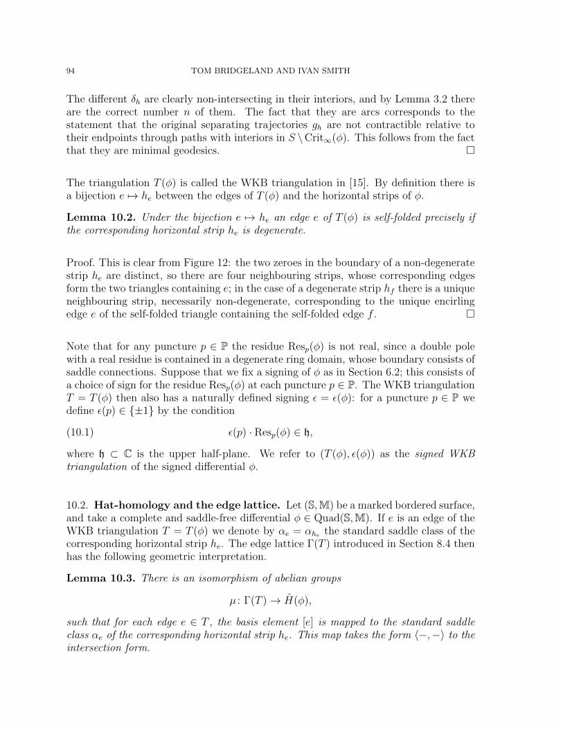
94 TOM BRIDGELAND AND IVAN SMITH
The different δh are clearly non-intersecting in their interiors, and by Lemma 3.2 thereare the correct number n of them. The fact that they are arcs corresponds to thestatement that the original separating trajectories gh are not contractible relative totheir endpoints through paths with interiors in S \Crit∞(φ). This follows from the factthat they are minimal geodesics. �
The triangulation T (φ) is called the WKB triangulation in [15]. By definition there isa bijection e 7→ he between the edges of T (φ) and the horizontal strips of φ.
Lemma 10.2. Under the bijection e 7→ he an edge e of T (φ) is self-folded precisely ifthe corresponding horizontal strip he is degenerate.
Proof. This is clear from Figure 12: the two zeroes in the boundary of a non-degeneratestrip he are distinct, so there are four neighbouring strips, whose corresponding edgesform the two triangles containing e; in the case of a degenerate strip hf there is a uniqueneighbouring strip, necessarily non-degenerate, corresponding to the unique encirlingedge e of the self-folded triangle containing the self-folded edge f . �
Note that for any puncture p ∈ P the residue Resp(φ) is not real, since a double polewith a real residue is contained in a degenerate ring domain, whose boundary consists ofsaddle connections. Suppose that we fix a signing of φ as in Section 6.2; this consists ofa choice of sign for the residue Resp(φ) at each puncture p ∈ P. The WKB triangulationT = T (φ) then also has a naturally defined signing ε = ε(φ): for a puncture p ∈ P wedefine ε(p) ∈ {±1} by the condition
(10.1) ε(p) · Resp(φ) ∈ h,
where h ⊂ C is the upper half-plane. We refer to (T (φ), ε(φ)) as the signed WKBtriangulation of the signed differential φ.
10.2. Hat-homology and the edge lattice. Let (S,M) be a marked bordered surface,and take a complete and saddle-free differential φ ∈ Quad(S,M). If e is an edge of theWKB triangulation T = T (φ) we denote by αe = αhe the standard saddle class of thecorresponding horizontal strip he. The edge lattice Γ(T ) introduced in Section 8.4 thenhas the following geometric interpretation.
Lemma 10.3. There is an isomorphism of abelian groups
µ : Γ(T )→ H(φ),
such that for each edge e ∈ T , the basis element [e] is mapped to the standard saddleclass αe of the corresponding horizontal strip he. This map takes the form 〈−,−〉 to theintersection form.

QUADRATIC DIFFERENTIALS AS STABILITY CONDITIONS 95
Proof. The map µ is an isomorphism by Lemma 3.2, since it takes a basis to a basis.We must just check the relation
αe · αf = c(f, e)− c(e, f)
for all edges e and f of the triangulation T . Examining Figure 11 it is clear that αemeets αf precisely if e and f are two sides of the same face of T . The intersection thenoccurs at the unique point of the spectral cover lying over the zero of the differentialcontained in this face.
Figure 31. The oriented foliation on the spectral cover above a simple zero.
In the case when e and f are not self-folded, a glance at Figure 31 shows that theintersection of two such cycles is ±1 depending on whether e and f occur in clockwise oranticlockwise order. If f is self-folded and e is the encircling edge of the correspondingself-folded triangle, then αe · αf = 0, since αe meets αf twice with opposite signs.Comparing with (8.2) we see that the claimed relation holds also in this case. �
In Section 8.4 we also considered a modified basis {e} of the edge lattice Γ(T ), indexedby the edges of T . Let us define classes
γe = µ({e}) ∈ H(φ),
where µ is the map of Lemma 10.3. We can now give some geometric justification forthese classes γe, and hence also the basis {e}.
As explained in the proof of Lemma 10.2, any degenerate horizontal strip hf is enclosedby a non-degenerate strip he, and taking a generic trajectory from each strip then gives aself-folded triangle, with self-folded edge f and enclosing edge e. Note that the standardsaddle connection in the strip hf is closed and lifts to a singular curve in S which is abouquet of two circles. By definition of the basis {e} ∈ Γ(T ), we have
(γe, γf ) = (αe, αe + αf ).
These classes are both represented by simple closed curves in S obtained by lifting thepaths illustrated by dotted arcs in the two sides of Figure 33.

96 TOM BRIDGELAND AND IVAN SMITH
10.3. Flips and pops. We can lift the stratification of Section 5.2 to the etale coverof complete, signed differentials
Quad±(S,M)0 → Quad(S,M)0.
We call the connected components of B0 chambers. The signed WKB triangulation isconstant in each chamber.
The points of the locally-closed subset F2 = B2 \ B0 consist of complete, signed differ-entials with a single saddle trajectory γ. We think of the connected components of F2
as walls. Let us now consider the behaviour of the signed WKB triangulation as wecross such a wall.
Suppose then that φ0 ∈ F2 ⊂ Quad±(S,M)0 is a complete signed GMN differential lyingon a wall, with a unique saddle trajectory γ. By Proposition 5.5 we can find r > 0 suchthat for all 0 < t 6 r the signed differentials
φ±(t) = e±it · φ0
are saddle-free and complete. Consider the WKB triangulations T± = T (φ±(r)) withtheir signings ε±. Note that the wall has a natural orientation to it: we make theconvention that as we cross from φ− to φ+ the period Zφ(γ) moves in a clockwisedirection around the origin.
There is an isomorphism F : Γ(T−) → Γ(T+) defined by the following commutativediagram
(10.2) Γ(T−)
µ−��
F// Γ(T+)
µ+��
H(φ−)GM
// H(φ+)
where the bottom arrow is given by the Gauss-Manin connection.
Proposition 10.4. Take a complete signed GMN differential φ0 ∈ F2 with a uniquesaddle trajectory γ. There are two possible cases.
(a) The ends of the saddle trajectory γ are distinct. Then the signed triangulations(T±, ε±) are related by a flip in a non-self-folded edge e. Identifying the edges ofthese triangulations in the standard way, the map F is given by
F ([f ]) = [f ] + c(e, f) [e],
for all edges f , where c(−,−) is computed in the triangulation T+, and we setc(e, e) = −2.
(b) The saddle trajectory γ is closed and forms the boundary of a degenerate ringdomain centered on a double pole p with real residue. The triangulations T− = T+
are equal, and the pole p is the centre of a self-folded triangle with encircling andself-folded edges e and f respectively. The signed triangulations (T±, ε±) are related

QUADRATIC DIFFERENTIALS AS STABILITY CONDITIONS 97
by a pop at p, and the map F exchanges the basis elements {e} and {f}, leavingall other elements of the basis fixed.
Proof. Case (a) is illustrated in Figure 32 (the four poles represented by the black dotsneed not be distinct on the surface, however). The central picture represents φ0 with
Figure 32. The separating trajectories on either side of a flip wall.
a single saddle trajectory appearing in the boundary of two neighbouring horizontalstrips or half-planes. The wall-crossing is effected by rotating φ0. Thus to find outwhat happens to the saddle trajectory, we just need to consider trajectories of smallnonzero phase in the two horizontal strips or half-planes. The result is as illustrated onthe two sides of the figure. The associated triangulations T± are related by a flip in anon-self-folded edge e, exactly as shown in Figure 30.
Identifying the edges of the two triangulations T± via the obvious bijection, we see fromthe picture that the Gauss-Manin connection satisfies
GM(αf ) = αf + c(e, f)αe
for all edges f , where c(−,−) is computed in the triangulation T+, and we set c(e, e) =−2.
Figure 33. The separating trajectories on either side of a pop wall. Thehat-homology classes γe are represented by the lifts of the dotted arcs.
For (b) note that if γ is closed then it is necessarily the boundary of a ring domain,which must be degenerate because there is only one saddle trajectory. This case isillustrated in Figure 33. The central picture again represents φ0 with its degenerate

98 TOM BRIDGELAND AND IVAN SMITH
ring domain encased in a horizontal strip. The wall-crossing is effected by rotating thedifferential, so to find the separating trajectories on either side of the wall it is enoughto consider trajectories of small nonzero phase. The result on either side of the wall isa degenerate horizontal strip hf , encased in a non-degenerate horizontal strip he.
The WKB triangulations T± are the same, with a self-folded triangle with self-foldededge f and encircling edge e. The hat-homology class γ = αf is equal to the residueclass βp, where p is the double pole at the centre of the degenerate ring domain. SinceZφ(γ) crosses the real axis as φ crosses the wall, the signing ε(p) given by (10.1) changes,and the two signed WKB triangulations on either side of the wall are related by a pop.The two classes {γe, γf} = {αe, αe+αf} are the same on both sides of the wall, but theirlabelling by the edges e, f is exchanged (see the dotted arcs in Figure 33). It followsthat F exchanges the two basis elements {e} and {f} as claimed. �
10.4. Stability conditions from saddle-free differentials. Let us now assume thatour marked bordered surface (S,M) is amenable, and take a saddle-free, complete,signed differential
φ ∈ B0 ⊂ Quad±(S,M)0.
Let (T, ε) denote the signed WKB triangulation of φ, and consider the category D(T, ε)with its canonical heart A(T, ε). The simple objects Se ∈ A(T, ε) are naturally indexedby the edges of the triangulation T , and so too are the classes γe.
Lemma 10.5. There is an isomorphism of abelian groups
ν : K(D(T, ε))→ H(φ),
taking the class of a simple object Se to the corresponding class γe, and taking the Eulerform to the intersection form.
Proof. This is immediate by combining Lemma 9.10 and Lemma 10.3. �
The following result gives the basic link between quadratic differentials and stabilityconditions.
Lemma 10.6. There is a unique stability condition σ(φ) ∈ StabD(T, ε) whose heart isthe standard heart A(T, ε) ⊂ D(T, ε), and whose central charge
Z : K(D(T, ε))→ C
corresponds to the period of φ under the isomorphism of Lemma 10.5.
Proof. Define Z via the isomorphism ν of Lemma 10.5. Then for each edge e thecorresponding central charge Z(Se) = Zφ(γe) lies in the upper half-plane. Indeed, bythe definition of the basis {e} in Section 8.4, the classes γe = µ({e}) are positive linearcombinations of the classes αe = µ([e]), whose periods lie in the upper half-plane by

QUADRATIC DIFFERENTIALS AS STABILITY CONDITIONS 99
definition. Since the standard heart A(T, ε) is of finite length, this is enough to give astability condition. �
10.5. Wall-crossing. We now describe how the stability conditions σ(φ) defined inthe last section behave as the differential φ crosses walls in Quad±(S,M)0 of the sortconsidered in Section 10.3. Consider a complete, signed GMN differential
φ0 ∈ F2 ⊂ Quad±(S,M)0
with a unique saddle trajectory γ. Take r > 0 such that for all 0 < t 6 r the signeddifferentials
φ±(t) = e±it · φ0
are saddle-free and complete. Consider the corresponding signed WKB triangulations(T±, ε±) = (T (φ±(r), ε(φ±(r)) and their associated categories
D± = D(T±, ε±)
with their standard hearts A± = A(T±, ε±). For 0 < t < r we set
σ±(t) = σ(φ±(t)) ∈ Stab(D±).
The following result shows that these different stability conditions glue together in theappropriate way.
Proposition 10.7. There is a canonical equivalence Ψ: D− ∼= D+ with the followingtwo properties
(a) the diagram of isomorphisms
K(D−)
ν−��
Ψ// K(D+)
ν+��
H(φ−)GM
// H(φ+)
commutes, where the bottom arrow is given by the Gauss-Manin connection, andthe vertical arrows are the isomorphisms of Lemma 10.5;
(b) the stability conditions Ψ(σ−(t)) and σ+(t) on D+ become arbitrarily close as t→ 0.
Proof. According to Proposition 10.4 there are two cases, the flip and the pop.
In the first case, the signed triangulations (T±, ε±) are related by a flip in an edge e, andwe take Ψ to be the equivalence Φ+ of Theorem 9.5. Part (a) then follows by comparingthe formulae of Lemma 9.11 and Proposition 10.4 using Lemma 9.13. To prove (b), notethat Theorem 9.5 shows that the heart of the stability condition Ψ(σ−(t)) is the tiltedheart µ+
Se(A+). By Lemma 7.9 the regions in Stab(D+) consisting of stability conditions
with hearts A+ and µ+Se
(A+) are glued together along a common boundary componentto make a larger region on which the period map is still injective. Since part (a) shows

100 TOM BRIDGELAND AND IVAN SMITH
that the central charges of the two given stability conditions approach one another, theresult follows.
In the case of the pop, the signed triangulations (T±, ε±) differ by a pop, and we takeΨ to be equivalence of Theorem 9.6. Part (a) then follows by comparing the formulaeof Lemma 9.12 and Proposition 10.4. To prove (b) note that since Ψ preserves thecanonical hearts, all the stability conditions σ±(t) have the same heart, and since theircentral charges approach each other, they become arbitrarily close. �
11. Proofs of the main results
In this section we prove our main results. Throughout (S,M) is a fixed marked borderedsurface. For the first five sections we shall assume that (S,M) is amenable. In Section11.6 we shall examine what can be said without this assumption.
11.1. General set-up. Let us fix a free abelian group Γ of rank n. We consider thespace of framed differentials QuadΓ(S,M). A point of this space corresponds to a GMNdifferential φ on a Riemann surface S, equipped with a framing of the extended hat-homology group
θ : Γ ∼= He(φ)
as in Section 6.5. By abuse of notation, we will simply write φ ∈ QuadΓ(S,M).
Let us fix a base-point
φ0 ∈ QuadΓ(S,M),
which we may as well assume is complete, saddle-free and generic. Recall that the spaceof framed differentials on (S,M) is not usually connected, so we define
QuadΓ∗ (S,M) ⊂ QuadΓ(S,M)
to be the connected component containing φ0.
Let us choose a signing for the differential φ0, as in Section 6.2. We claim that any pointin QuadΓ
∗ (S,M) then also has a canonical signing. To see this, note that to specify a
signing of a differential φ is to specify a choice of sign for the residue class βp ∈ H(φ) ateach double pole p of φ. Given a framing of such a differential, the classes βp correspondto fixed classes in Γ. It follows that if we choose a sign for the βp at the base-point φ0,then this sign propagates throughout QuadΓ
∗ (S,M).
We want to study stability conditions on the CY3 triangulated category D(S,M). Moreprecisely, let
(T0, ε0) = (T (φ0), ε(φ0))

QUADRATIC DIFFERENTIALS AS STABILITY CONDITIONS 101
be the signed WKB triangulation associated to the signed differential φ0, and defineD = D(T0, ε0). We identify the Grothendieck group K(D) with Γ using the isomorphism
(11.1) ν−10 ◦ θ0 : Γ→ K(D),
obtained by composing the framing θ0 with the inverse of the map of Lemma 10.5.
The distinguished connected component Tilt4(D) ⊂ Tilt(D) of the tilting graph of Dis the one containing the standard heart A(T0, ε0). As explained in Section 7.7, there isa corresponding distinguished connected component
Stab4(D) ⊂ Stab(D)
of the space of stability conditions on D. The group of reachable autoequivalencesAut4(D) ⊂ Aut(D) preserves this connected component. We define
Aut04(D) ⊂ Aut4(D)
to be the subgroup of reachable autoequivalences which act by the identity on K(D).
Remark 11.1. Later, as a consequence of Corollary 11.12, we will see that
(a) the group Aut4(D) is precisely the group of autoequivalences preserving the con-nected component Stab4(D),
(b) the group Aut04(D) is non-trivial, and in fact contains all even powers of the shift
functor.
The subgroup Nil4(D) ⊂ Aut4(D) of negligible autoequivalences is precisely the sub-group of elements acting trivially on Stab4(D). The quotient group
Aut4(D) = Aut4(D)/Nil4(D)
therefore acts effectively. Negligible autoequivalences fix the simple objects of heartsA ∈ Tilt4(D), and hence act trivially on K(D), so we can also form the quotient
Aut 04(D) = Aut0
4(D)/Nil4(D).
In the next five sections we shall prove the following result.
Theorem 11.2. There is an isomorphism of complex orbifolds
Quad♥(S,M) ∼= Stab4(D)/Aut4(D).
This result implies Theorems 1.2 and 1.3 from the Introduction, except that it doesn’tcover the non-amenable cases (a)–(d) listed after the statement of Theorem 1.3. Theseexceptional cases will be discussed in Section 11.6 below, and some of them are workedout explicitly in Section 12.

102 TOM BRIDGELAND AND IVAN SMITH
11.2. Construction of the map. In this section we construct a map from framedquadratic differentials to stability conditions.
Proposition 11.3. There is a holomorphic map of complex manifolds K fitting into acommutative diagram
(11.2) QuadΓ∗ (S,M)
K//
π''OOOOOOOOOOO
Stab4(D)/Aut 04(D)
πvvlllllllllllll
HomZ(Γ,C)
and which commutes with the C-actions on both sides.
Proof. The space on the left of the diagram (11.2) is a manifold by Proposition 6.6(note that the surfaces listed for which this result fails are not amenable). The spaceon the right is a manifold because the action of the group Aut 0
4(D) on the connectedcomponent Stab4(D) is free. To see this, note that if an autoequivalence Φ fixes astability condition σ ∈ Stab4(D) and acts trivially on K(D), then, because the periodmap π is a local isomorphism, it must act trivially on a neighbourhood of σ, and henceon the whole connected component Stab4(D). But then it is negligible and hencedefines the identity in Aut 0
4(D).
The action of C on the right of (11.2) is the standard one of Section 7.5; the elementt ∈ C acts at the level of central charges by Z(E) 7→ eiπt · Z(E). After the event it willfollow from Corollary 11.12 that 2 ∈ C acts trivially, so that this factors via a C∗ action,but we don’t know this yet. The action of C on the left is the pullback of the standardC∗ action rescaling the quadratic differential, via the map C→ C∗ defined by t 7→ e2πit.This action lifts to framed differentials by continuity; note that 1 ∈ C acts trivially onthe underlying quadratic differential, but multiplies the framing isomorphism by −1.
The maps π in the diagram (11.2) are both local isomorphisms. The map on the left isthe standard period map on framed differentials. The map on the right sends a stabilitycondition to its central charge, which we consider as a group homomorphism Z : Γ→ Cby composing it with the isomorphism (11.1). Let t ∈ C act on the space of centralcharges HomZ(Γ,C) via the map Z(E) 7→ eiπt ·Z(E) as above. Then because periods ofquadratic differentials are given by integrals of
√φ, both the maps π are C-equivariant.
As soon as we know that K is continuous it is automatically holomorphic, and in fact, alocal isomorphism. The C-equivariance is also automatic, just because each of the twomaps π is a local isomorphism. We first define a map
K0 : B0 → Stab4(D)/Aut 04(D).
The key point is to then use the stratification
B0 ⊂ B1 ⊂ B2 ⊂ · · · ⊂ Bk ⊂ · · · ⊂ QuadΓ∗ (S,M)0 ⊂ QuadΓ
∗ (S,M)
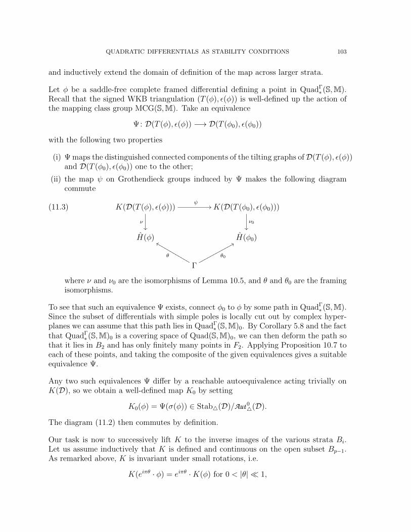
QUADRATIC DIFFERENTIALS AS STABILITY CONDITIONS 103
and inductively extend the domain of definition of the map across larger strata.
Let φ be a saddle-free complete framed differential defining a point in QuadΓ∗ (S,M).
Recall that the signed WKB triangulation (T (φ), ε(φ)) is well-defined up the action ofthe mapping class group MCG(S,M). Take an equivalence
Ψ: D(T (φ), ε(φ)) −→ D(T (φ0), ε(φ0))
with the following two properties
(i) Ψ maps the distinguished connected components of the tilting graphs ofD(T (φ), ε(φ))and D(T (φ0), ε(φ0)) one to the other;
(ii) the map ψ on Grothendieck groups induced by Ψ makes the following diagramcommute
(11.3) K(D(T (φ), ε(φ)))
�
ψ// K(D(T (φ0), ε(φ0)))
ν0��
H(φ) H(φ0)
Γ
θ
ffLLLLLLLLLLLLθ0
88pppppppppppp
where ν and ν0 are the isomorphisms of Lemma 10.5, and θ and θ0 are the framingisomorphisms.
To see that such an equivalence Ψ exists, connect φ0 to φ by some path in QuadΓ∗ (S,M).
Since the subset of differentials with simple poles is locally cut out by complex hyper-planes we can assume that this path lies in QuadΓ
∗ (S,M)0. By Corollary 5.8 and the factthat QuadΓ
∗ (S,M)0 is a covering space of Quad(S,M)0, we can then deform the path sothat it lies in B2 and has only finitely many points in F2. Applying Proposition 10.7 toeach of these points, and taking the composite of the given equivalences gives a suitableequivalence Ψ.
Any two such equivalences Ψ differ by a reachable autoequivalence acting trivially onK(D), so we obtain a well-defined map K0 by setting
K0(φ) = Ψ(σ(φ)) ∈ Stab4(D)/Aut 04(D).
The diagram (11.2) then commutes by definition.
Our task is now to successively lift K to the inverse images of the various strata Bi.Let us assume inductively that K is defined and continuous on the open subset Bp−1.As remarked above, K is invariant under small rotations, i.e.
K(eiπθ · φ) = eiπθ ·K(φ) for 0 < |θ| � 1,

104 TOM BRIDGELAND AND IVAN SMITH
because both maps π of (11.2) are local isomorphisms. Take a point φ0 ∈ Fp. ByProposition 5.5 there is some r > 0 such that
(11.4) 0 < |t| < r =⇒ eit · φ0 ∈ Bp−1.
By the C-equivariance property, the limits
σ±(φ0) = limt→0+
K(e±it · φ0)
both exist, and the diagram (11.2) shows that they have the same central charge. Thepoint is to show that they are equal.
When p = 2 this involves extending from saddle-free differentials to differentials lyingon a single wall, and the result follows from Proposition 10.7. Thus we can assume thatp > 2. Note that the stability conditions σ±(φ0) vary continuously on Fp, by the factthat their central charges do, and using the remark following Proposition 5.5. Thus thequestion of whether they are equal has a constant answer on each connected componentof Fp. The result then follows from Proposition 5.7.
The final step is to extendK across the incomplete locus. Suppose that φ ∈ QuadΓ∗ (S,M)
has simple poles, and fix 0 < ε < 18. Using Proposition 6.7 we can find complete, generic
differentials ψ arbitrarily close to φ , and such that
|Zφ(γ)− Zψ(γ)| < ε |Zψ(γ)|,
for all classes γ ∈ Γ represented by a non-closed saddle connection in ψ. Lemma 11.4below then shows that this inequality holds for all classes represented by stable objectsin the stability condition K(ψ). The deformation result Proposition 7.5 then shows thatK extends uniquely over φ. �
11.3. Saddle trajectories and stable objects. In this section and the next we relatesaddle trajectories for a generic GMN differential to the existence of stable objects inthe corresponding stability condition. Let
φ ∈ QuadΓ∗ (S,M)0
is a complete, framed differential, and let σ = K(φ) be the corresponding stabilitycondition on D, well-defined up to the action of the group Aut0
4(D). Note that any
saddle connection γ for φ has a well-defined hat-homology class in H(φ), which we canview as an element of Γ using the framing isomorphism. Similarly, every object E ∈ Dhas a well-defined class in Γ using the identification (11.1).
We shall start with the following simple result which was used in the final step of theproof of Proposition 11.3 above.
Lemma 11.4. If σ has a stable object E of class α ∈ Γ then φ has a saddle trajectoryof class proportional to α.

QUADRATIC DIFFERENTIALS AS STABILITY CONDITIONS 105
Proof. Rotating we can assume that E is of phase 1. Consider a generic differential ψclose to φ such that Zψ(α) remains real. Proposition 7.6(a) shows that the object Eremains stable in the corresponding stability condition K(ψ). By construction thereforeψ cannot be saddle-free, and has at least one saddle trajectory C, which by genericitymust have class proportional to α. Since the class of a saddle connection has divisibilityat most 2, the length of this saddle is at most |Zψ(2α)|.
Applying Theorem 4.1, we can now find a sequence of such differentials ψi, convergingto φ, such that the corresponding curves Ci limit to some curve C. Then C is a geodesicin φ which must be a union of saddle trajectories. �
For each class α ∈ Γ we can consider the moduli spaceMσ(α) of σ-stable objects in Dwhich have class α ∈ Γ and phase in the interval (0, 1]. It is necessary to constrain thephase, since otherwise all shifts of a given stable object would have to be parameterized.
Lemma 11.5. The moduli space Mσ(α) is represented by a quasi-projective scheme.
Proof. By rotation, we can assume that φ is saddle-free and therefore defines somesigned triangulation (T, ε). The heart of the stability condition σ is then equivalent tothe category of finite-dimensional modules for the complete Jacobi algebra of the corre-sponding quiver with potential. This algebra J(T, ε) is known to be finite-dimensional10
[27, Corollary 12.6]. The moduli spaceMσ(α) can therefore be identified with the mod-uli space of θ-stable representations of J(T, ε) with fixed dimension vector. The claimthen follows from the results of King [22]. �
Recall the notion of a 0-generic differential from Section 5.2. Note that any such dif-ferential is, in particular, complete. In this and the next section we shall prove thefollowing precise correspondence, which implies Theorem 1.4 from the Introduction.
Theorem 11.6. Assume that φ is 0-generic and take a class α ∈ Γ satisfying Zφ(α) ∈R. Then each connected component of the moduli scheme Mσ(α) is either a point or acopy of P1. Moreover
(a) the zero-dimensional components of Mσ(α) are in bijection with the non-closedsaddle trajectories for φ of class α;
(b) the one-dimensional components ofMσ(α) are in bijection with the non-degeneratering domains for φ of class α.
We first prove the result under an additional assumption; the general case will be dealtwith in the next section.
10This could also be deduced from Corollary 11.12 below together with an argument of Nagao [20,Theorem 5.4].

106 TOM BRIDGELAND AND IVAN SMITH
Proposition 11.7. Take assumptions as in Theorem 11.6. Suppose moreover that φhas at most one saddle trajectory. Then the conclusion of Theorem 11.6 holds.
Proof. Suppose that φ has a unique saddle trajectory γ of some class α ∈ Γ. Sincethe surface (S,M) is assumed to be amenable, it is not a closed surface with a singlepuncture, and it follows that there can be no spiral domains. Thus φ ∈ F2 and we arein the situation of Proposition 10.4.
Assume first that γ has distinct ends, as in Proposition 10.4(a). Small rotations of φ aresaddle-free, and γ is represented by a standard saddle class. The corresponding stabilityconditions have a unique simple object S of class α. This is, in particular, stable andspherical, and all semistable objects of class proportional to α are of the form S⊕k, andhence strictly semistable for all k > 1.
Suppose instead that γ is a closed saddle trajectory. This is the situation of Proposition10.4(b). By Proposition 10.7, stability conditions on either side of the wall obtained bysmall rotations of σ have the same heart. This implies that P(0) = (0) and so there areno semistable objects with class a multiple of α.
For the converse, suppose that the stability condition σ has a stable object of class α.Then, by construction of the map K, the differential φ cannot be saddle-free. Thus φhas a saddle trajectory γ of some class β proportional to α. Applying what we haveproved in the first part, it follows that σ has at most one stable object of class β, andno stable objects of any other class proportional to β. We conclude that α = β and soφ has a (necessarily unique) saddle trajectory of class α. �
11.4. Ring-shrinking again. In this section we complete the proof of Theorem 11.6.It will be convenient to denote the differential and corresponding stability conditionof the statement by φ+ and σ+ respectively. Thus we consider a complete, framed,0-generic differential
φ+ ∈ QuadΓ(S,M)0,
and let σ+ = K(φ+) be the corresponding stability condition on D, well-defined up tothe action of the group Aut0
4(D). We may assume that φ+ has more than one saddletrajectory, since otherwise we are in the situation of Proposition 11.7.
The surface (S,M) is amenable, hence not a once-punctured torus, so according toSection 5.9 there are two possible cases, labelled (J1) and (J2). Shrinking the uniquering domain A as in Section 5.9 gives a smooth path in QuadΓ(S,M)0 ending at anon-generic point
φ ∈ QuadΓ(S,M)0
with either 2 or 3 saddle trajectories γi. Label the saddle trajectories γi exactly as inSection 5.9, and write αi ∈ Γ for the corresponding hat-homology classes. We recall

QUADRATIC DIFFERENTIALS AS STABILITY CONDITIONS 107
that there is a linear relationα3 = α1 + α2.
Our stategy will be to first understand the stable objects of phase 1 in the stabilitycondition σ = K(φ) by applying Proposition 11.7 to nearby points on the other side ofthe wall
ImZφ−(α1)/Zφ−(α2) = 0.
We will then follow this information back through the ring-shrinking operation.
•1
a1**
a2
44 •2 •1
b��
:::::::a
// •2
•3
c
BB�������
Figure 34. The quivers relevant to the two cases (J1) and (J2).
Let A = P(1) denote the abelian category of semistable objects of phase 1 in thestability conditon σ = K(φ). This category has finite-length, so we can model it bythe category of representations of the Jacobi algebra of a quiver with potential (Q,W ).The relevant quivers Q in the two cases (J1) and (J2) are as shown in Figure 34; inboth cases the potential is necessarily zero.
Proposition 11.8. The category A is equivalent to the category of finite-dimensionalrepresentations of the corresponding quiver Q.
Proof. For definiteness we consider the more difficult case (J2).
Let nij denote the number of arrows in the quiver Q connecting vertex i to vertex j.To prove the Lemma we must show
(a) the category A has exactly 3 stable objects Si;
(b) these objects have classes [Si] = αi respectively;
(c) For all i, j we have dimk Ext1A(Si, Sj) = nij.
It is easy to see that after contracting the ring domain in Figure 18 the intersectionmultiplicities αi · αj coincide with the expressions nji − nij. So for the last part it willbe enough to show that each object Si is spherical, and for each pair i 6= j, we haveeither
Ext1A(Si, Sj) = 0 or Ext1
A(Sj, Si) = 0.
Take a class β ∈ Γ and consider the wall-and-chamber decomposition of Stab(D) withrespect to the class β. Take a chamber containing σ in its closure, and containing points

108 TOM BRIDGELAND AND IVAN SMITH
σ− = K(φ−) which satisfy
ImZφ−(α1)/Zφ−(α2) < 0, ImZφ−(β) = 0.
Let us choose such a point σ− in this chamber, and assume further that the correspond-ing differential φ− is generic, and that it lies in the open subset U of Proposition 5.10.Of course, our choice of φ− = φ−(β) will depend on the class β we started with.
The genericity condition implies that all saddle trajectories for φ− have classes whichare multiples of β. Proposition 5.10 then implies that any such saddle trajectory is oneof the γi. Since the classes αi are pairwise non-proportional, it follows in particular thatφ− has at most one saddle trajectory. Thus Proposition 11.7 applies to φ−, and showsthat φ− has a saddle trajectory of class β precisely if σ− has a stable object of class β.
In the case when β = αi for some i, Proposition 11.7 implies that σ− = σ−(αi) has aunique stable object Si of class β, which is moreover spherical. By Proposition 7.8, theobject Si is then semistable in σ, and hence lies in the category A = P(1).
Conversely, suppose that an object E ∈ A is stable in σ of phase 1. Proposition 7.6(a)shows that E is stable in all nearby stability conditions, and in particular we can assumethat this is the case for σ− = σ−(β). Then φ− must have a saddle trajectory of classβ, and by Proposition 5.10 it follows that β = αi for some i. Since Si was the uniquestable object in σ−(αi) of class αi it follows that E = Si.
Thus the set of stable objects in P(1) is some subset of the objects {S1, S2, S3}. It followsfrom this that the objects S1 and S2 must actually be stable in σ. For example, if S2
was unstable, it would have a filtration by the objects S1 and S3, which is impossiblebecause α2 is not a positive linear combination of the classes α1 and α3 = α1 + α2.
Suppose there are extensions in two directions between S1 and S2. Then on both sidesof the wall ImZφ(α1)/Zφ(α2) = 0 there would be stable objects of class [S1]+[S2], whichis not the case for σ−. It follows that the object S3 must also be stable, since the onlyother possibility is that there is a sequence
0 −→ S2 −→ S3 −→ S1 −→ 0,
which is impossible since S3 is stable on the σ− side of the wall. Using the same argumentas before, we can now check that nonzero extensions between one of the objects S1 orS2 and S3 only go in one direction. This completes the proof. �
Consider stability conditions W : K(A) → C on the abelian category A satisfying theconditions
(11.5) Z(S1) + Z(S2) ∈ iR, ImZ(S1)/Z(S2) > 0.
In the case (J2), assume also that Z(S3) ∈ iR. Then
Lemma 11.9. The set of stable objects satisfying Z(E) ∈ iR is independent of theparticular choice of stability condition satisfying (11.5), and is as follows:

QUADRATIC DIFFERENTIALS AS STABILITY CONDITIONS 109
(J1) a single P1 family of objects of dimension vector (1, 1);
(J2) a single P1 family of objects of dimension vector (1, 1, 1), and unique objects ofdimension vectors (1, 1, 0) and (0, 0, 1).
Proof. In the case (a) we are considering representations of the Kronecker quiver andthe result is well-known. In case (b) we are considering the affine A2 quiver, and sinceindecomposable representations are completely understood in terms of the real andimaginary roots, the result is again easy. �
Note the precise correspondence with the finite-length trajectories of φ+ listed in Section5.9. The following result then completes the proof of Theorem 11.6.
Proposition 11.10. An object E ∈ D is stable of phase 1 in σ+ precisely if it lies inthe abelian subcategory A and is stable with respect to stability conditions W as above.
Proof. As the ring domain A shrinks we move along a path of differentials φ+(t) for0 6 t 6 1 with φ+(0) = φ+ and φ+(1) = φ. Let σ+(t) = K(φ+(t)) be the correspondingstability conditions. The first claim is that the class of stable objects of phase 1 in thestability condition σ+(t) is constant for 0 6 t < 1. To prove this it will be enough toshow that if E is a stable object of phase 1 in some differential σ+(t), then the class βof E is a multiple of the class α of the ring domain, and hence remains of phase 1 forall t. This follows immediately from Lemma 11.4 and the list of saddle trajectories forσ+ given in Section 5.9.
Suppose that E ∈ D is stable in σ+ of phase 1. Then by the above, the class of E isproportional to α, and moreover E is stable in σ+(t) for 0 6 t < 1. It follows that Eis at least semistable in σ, and hence that E ∈ A = P(1). Thus we are reduced tounderstanding which objects E ∈ A whose classes are proportional to α are stable inthe stability conditions σ+(t) for 0 6 t < 1.
Consider the central charge of σ+(t) and rotate it by an angle of π/2. It then inducesa stability function W on A satisfying the conditions (11.5). It follows that an objectE ∈ A of class proportional to α is stable in σ+(t) precisely if it is stable with respectto the stability conditions W of Lemma 11.9. �
11.5. Completion of the proof. The following result will be enough to complete theproof of Theorem 11.2.
Proposition 11.11. The map K of Proposition 11.3 is an isomorphism of complexmanifolds.

110 TOM BRIDGELAND AND IVAN SMITH
Proof. We begin by showing that K is injective; it then follows that it is an openembedding because it commutes with the period maps, which are local isomorphisms.Suppose we have two distinct framed differentials
φ1, φ2 ∈ QuadΓ∗ (S,M)
such that K(φ2) = Φ(K(φ1)) for some autoequivalence Φ ∈ Aut04(D). Since the period
maps are local isomorphisms, and K commutes with these maps, if we deform boththe φi maintaining the condition that their periods are equal, we will also preserve thecondition K(φ2) = Φ(K(φ1)). Thus we can assume that the φi are saddle-free. Let(Ti, εi) be the associated signed WKB triangulations.
By definition, K(φi) = Ψi(σ(φi)), where the Ψi are equivalences
Ψi : D(Ti, εi)→ D(T0, ε0)
satisfying the conditions (i) and (ii) of the proof of Proposition 11.3. It follows that Ψ−12 ◦
Φ◦Ψ1 takes the canonical heart A(T1, ε1) ⊂ D(T1, ε1) to the canonical heart A(T2, ε2) ⊂D(T2, ε2). In particular, the quivers Q(Ti) are isomorphic. Thus by Proposition 8.5, theWKB triangulations Ti differ by an orientation-preserving diffeomorphism.
Examining Figure 5 it is easy to see that this implies that the differentials φi havethe same horizontal strip decomposition in the sense of Section 4.5. The fact thatthe equivalences Ψi satisfy the condition (ii) of the proof of Proposition 11.3 impliesfurther that the horizontal strips of the φi have the same labellings by elements of Γ.Proposition 4.9 then shows that φ1 = φ2 ∈ QuadΓ(S,M).
The fact that the image of K is closed follows from Proposition 6.8. Indeed, supposeσn → σ ∈ Stab4(D) with σn = K(φn). We can assume that each φn is complete andgeneric since these points are dense. Theorem 11.6 implies that the lengths of non-degenerate saddle connections in φn correspond to the masses of stable objects in σn.Thus it will be sufficient to show that the masses of objects in the σn are uniformlybounded below. By continuity it is enough to check that the masses of objects in σ arebounded below, and this follows from the support property (7.2). �
To prove Theorem 11.2 it remains to show that K descends to give an isomorphism ofcomplex orbifolds fitting into the commutative diagram
(11.6) QuadΓ∗ (S,M)
��
K// Stab4(D)/Aut 0
4(D)
��
Quad♥(S,M)J
// Stab4(D)/Aut4(D)
Since the map on the left is a covering map, to prove that K descends it is enough tocheck that all framings of the differential φ0 give the same stability condition up to theaction of Aut4(D). This is immediate from the definition of K0.

QUADRATIC DIFFERENTIALS AS STABILITY CONDITIONS 111
To prove that the resulting map J is injective, hence an isomorphism, we follow thesame argument used above to show that K is injective. Suppose that J(φ1) = J(φ2).By deforming the differentials φi as before, it is enough to deal with the case when the φiare complete and saddle-free. As above we conclude that the φi have the same horizontalstrip decomposition. Since they also have the same periods, they are equal. �
Corollary 11.12. An autoequivalence of D preserves the connected component Stab4(D)precisely if it is reachable. In particular, the shift functor [1] lies in the group Aut4(D)of reachable autoequivalences.
Proof. One implication is always true, by Lemma 7.9. Conversely, suppose that Φ ∈Aut(D) preserves Stab4(D). Take a smooth path connecting σ0 and Φ(σ0) in Stab4(D).Applying K−1 this defines a smooth path of framed quadratic differentials. As inthe proof of Proposition 11.3, we can use Proposition 5.7 to find a homotopic pathconsisting entirely of tame differentials, and crossing only finitely many walls. ApplyingProposition 10.7 at each of these walls shows that Φ is reachable. �
11.6. Non-amenable cases. Suppose now that (S,M) is a marked bordered surfacewhich fails to be amenable because it violates one of the first four conditions of Definition9.3. We shall make some brief comments about what can be said in these various cases.
Case (a). Suppose that (S,M) does not satisfy Assumption 8.1. We refer the readerto the comments made following Assumption 8.1. We cannot deal with the case of a4-punctured sphere, but the other cases are all described explicitly in Section 12.
Case (b). Suppose that (S,M) is one of the three surfaces listed in Proposition 8.5having distinct triangulations with the same associated quiver. The isomorphism ofTheorem 9.8 still holds and induces an action of the group Aut4(D) on the set oftagged triangulations. We say that a reachable autoequivalence is allowable if theinduced action on the quotient set
Tri./(S,M)/MCG±(S,M)
is trivial. If we replace the group Aut4(D) of reachable autoequivalences by the subgroupAut allow
4 (D) of allowable ones then Proposition 9.9 holds for (S,M) with the same proof.
In these cases Theorem 11.2 still holds, with the group Aut4(D) replaced by Aut allow4 (D).
The proof is the same, one just needs to check at several places that certain autoequiv-alences are allowable. This is easily done, and we omit the details. The case of aonce-punctured disc with two points on the boundary is described in detail in Example12.4 below.
Case (c). Consider the two non-closed surfaces listed in Proposition 8.6, for which theaction of the mapping class group on ordered ideal triangulations is not free. Proposi-tion 9.9 also fails in these two cases. These surfaces are dealt with explicitly in Examples

112 TOM BRIDGELAND AND IVAN SMITH
12.2 and 12.5 below. Note that the orbifold Quad♥(S,M) has non-trivial generic au-tomorphism group Z2, and Theorem 11.2 continues to hold if we rigidify the orbifoldQuad♥(S,M) by killing this group.
Case (d). We leave the case of a closed surface with a single puncture for futureresearch, and restrict ourselves here to some sketchy comments about some of the specialfeatures of these surfaces.
The first new feature is that the graph Tri./(S,M) has two connected components. Thismeans that we have two potentially distinct categories D(S,M), depending on the choiceof sign ε = ε(p). But by the result [8, Prop. 10.4] referred to in the proof of Theorem9.9, the two potentials W (T,±1) are right-equivalent up to scale, so in fact there is awell-defined category D = D(S,M).
As stated, Theorem 9.8 is false for these examples, again because the graph Tri./(S,M)is disconnected. A related issue is that Corollary 11.12 fails, and the shift functor [1] isnot reachable11. It might therefore be best to replace the notion of a reachable heart bya shift-reachable heart: one for which A[i] lies in Tilt4(D) for some i ∈ Z. Of course, inthe case of an amenable surface, the notions of reachable and shift-reachable coincideby Corollary 11.12.
One more feature in this case is that the complete Ginzburg algebra definitely does notcoincide with the uncompleted version in general, see Remark 9.7. It may well be thatit is more natural to consider the uncompleted Ginzburg algebra in this context.
12. Examples
In this section we consider some special cases of Theorem 1.3 corresponding to surfaces(S,M) of genus g = 0. This leads to descriptions of spaces of stability conditions onCY3 categories associated to certain simple quivers familiar in representation theory.We adopt a less formal approach in this section, and some of the details are left for thereader.
12.1. Unpunctured discs: An type. Fix an integer n > 2 and let (S,M) be anunpunctured disc with n+3 points on its boundary. This corresponds to differentials onP1 with a single pole of order n+5. The space Quad♥(S,M) coincides with Quad(S,M)and parameterizes differentials of the form
ϕ(z) = pn+1(z) dz⊗2
11To see this, note that because there are no self-folded triangles, the residue class βp is alwayseither a strictly positive or strictly negative linear combination of the classes of the simple objects ofany heart, and this sign is constant under mutation.

QUADRATIC DIFFERENTIALS AS STABILITY CONDITIONS 113
where pn+1(z) is a polynomial of degree n + 1 having simple roots, considered modulothe automorphisms of P1 which fix infinity. Taking the sum of the roots to be 0 we canreduce to differentials of the form
φ(z) =n+1∏i=1
(z − ai) dz⊗2,
n+1∑i=1
ai = 0, ai 6= aj,
modulo a residual action of Zn+3 acting by rescaling z by an (n + 3)rd root of unity.Thus
Quad(S,M) ∼= Confn+10 (C)/Zn+3,
where Confn+10 (C) denotes the configuration space of n + 1 distinct points in C with
centre of mass at the origin, and the group Zn+3 acts by multiplication by (n + 3)rdroots of unity.
Figure 35. Triangulation of a 5-gon.
The mapping class group of the surface is
MCG(S,M) = Zn+3
and coincides with the signed mapping class group. Ideal triangulations of (S,M) cor-respond to triangulations of an (n+ 3)-gon. The resulting quivers are orientations of aDynkin diagram of An type and necessarily have zero potential.
Our main Theorem gives an isomorphism of complex orbifolds
Confn+10 (C)/Zn+3
∼= Stab4(D)/Aut4(D).
Note that there is a short exact sequence
1 −→ Br(An) −→ π1 Quad(S,M) −→ Zn+3 −→ 1,
where the Artin braid group Br(An) is the fundamental group of the configuration spaceConfn+1
0 (C). On the other hand, the group Sph(D) ⊂ Aut(D) is isomorphic to Br(An)by [31, Theorem 1.3]. The sequence of Lemma 9.9 therefore becomes
1 −→ Br(An) −→ Aut4(D) −→ Zn+3 −→ 1.
The fact that these two sequences coincide suggests that Stab4(D) is simply-connected.

114 TOM BRIDGELAND AND IVAN SMITH
Example 12.1. The non-amenable case n = 0 corresponding to an unpunctured discwith 3 marked points on its boundary is very degenerate. The space Quad(S,M) isa single point with automorphism group Z3, corresponding to the unique differentialφ(z) = z dz⊗2. The mapping class group is MCG(S,M) = Z3. There is a unique idealtriangulation, but it contains no edges, and the associated quiver is empty.
Example 12.2. Consider the non-amenable case n = 1 corresponding to an unpunc-tured disc with four marked points on its boundary. The space Quad(S,M) consists ofdifferentials of the form
φ(z) = (z2 + c) dz⊗2, c ∈ C∗,modulo the action of Z4 acting on z by multiplication by i. Thus
Quad(S,M) ∼= C∗/Z4
with the generator of Z4 acting by change of sign. Note that the generic stabilizer groupis Z2.
There are two ideal triangulations of (S,M), each with a single edge. These are relatedby the action of the mapping class group Z4. Note that Proposition 8.6 breaks down inthis case: the element of Z4 of order 2 fixes all triangulations.
The quiver corresponding to either triangulation has a single vertex and no arrows.The category D is generated by a single spherical object S, and the group Aut4(D) isgenerated by the shift functor [1]. Proposition 9.9 also breaks down in this case, sinceSph(D) ∼= Z is generated by the second shift [2].
The quotient space Stab(D)/〈[2]〉 is isomorphic to C∗ with co-ordinate Z(S). Thus
Stab(D)/Aut4(D) ∼= C∗/Z2,
with the generator of Z2 acting by change of sign. There is a morphism
Quad(S,M)→ Stab(D)/Aut4(D)
given by setting Z(S) = πic, but it is not an isomorphism of orbifolds, since the genericautomorphism groups are different.
12.2. Punctured discs: Dn type. Fix an integer n > 2 and let (S,M) be a once-punctured disc with n points on its boundary. This corresponds to differentials on P1
with polar type (2, n+ 2).
The space Quad(S,M) consists of differentials of the form
φ(z) =n∏i=1
(z − ai)dz⊗2
z2, ai 6= aj,
modulo the action of C∗ rescaling z. Thus
Quad(S,M) ∼= Confn(C)/Zn,

QUADRATIC DIFFERENTIALS AS STABILITY CONDITIONS 115
where Confn(C) denotes the configuration space of n distinct points in C, and the groupZn acts by multiplication by nth roots of unity.
Note that the product a =∏n
i=1 ai is invariant under the Zn action, and hence definesa map
a : Quad(S,M)→ C.The cover Quad±(S,M) corresponds to choosing a square-root of a.
When n > 3 the obvious rotationally-symmetric triangulation of (S,M) has an associ-ated quiver with potential which consists of a cycle of n arrows, equipped with a nonzerosuperpotential of degree n. This is known [11, Example 6.7] to be mutation-equivalentto any orientation of the Dynkin diagram of Dn type, necessarily with zero potential.
Example 12.3. In the non-amenable case n = 1 the space Quad(S,M) consists ofdifferentials of the form
φ(z) = (z + c)dz⊗2
z2, c ∈ C.
The residue at 0 is Res0(φ) = 4πi√c. The cover Quad±(S,M) corresponds to choosing
a square-root s =√c. Thus
Quad♥(S,M) ∼= C/Z2
with Z2 acting on C by s 7→ −s.
There is only one triangulation, and the resulting quiver is a single vertex with noarrows. The category D is generated by a single spherical object. The mapping classgroup is trivial, and MCG±(S,M) = Z2. The group Aut4(D) is generated by the shift[1], and the subgroup Sph(D) by the second shift [2]. The quotient Stab4(D)/ Sph(D)is isomorphic to C with co-ordinate Z(S). Thus the relation
Quad♥(S,M) ∼= Stab4(D)/Aut4(D),
also holds in this case.
Example 12.4. In the non-amenable case n = 2 the space Quad(S,M) consists ofdifferentials of the form
φ(z) = (az2 + bz + c)dz⊗2
z2, a ∈ C∗, b, c ∈ C, b2 − 4ac 6= 0,
modulo the rescaling action of C∗. Using this we can take a = 1; there is then a residualaction of Z2 acting by z 7→ −z. These differentials have a double pole at z = 0 and afourth order pole at infinity. The respective residues are
Res0(φ) = 4πi√c, Res∞(φ) = 2πib.
The cover Quad±(S,M) corresponds to choosing a square-root of c. Writing the differ-ential as
φ(z) = (z2 + 2sz + t2)dz⊗2
z2, s, t ∈ C, s2 6= t2,
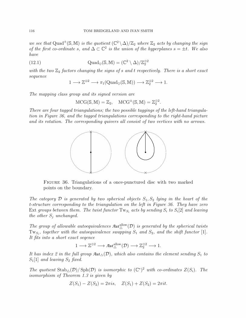
116 TOM BRIDGELAND AND IVAN SMITH
we see that Quad±(S,M) is the quotient (C2 \∆)/Z2 where Z2 acts by changing the signof the first co-ordinate s, and ∆ ⊂ C2 is the union of the hyperplanes s = ±t. We alsohave
(12.1) Quad♥(S,M) = (C2 \∆)/Z⊕22
with the two Z2 factors changing the signs of s and t respectively. There is a short exactsequence
1 −→ Z⊕2 −→ π1(Quad♥(S,M)) −→ Z⊕22 −→ 1.
The mapping class group and its signed version are
MCG(S,M) = Z2, MCG±(S,M) = Z⊕22 .
There are four tagged triangulations; the two possible taggings of the left-hand triangula-tion in Figure 36, and the tagged triangulations corresponding to the right-hand pictureand its rotation. The corresponding quivers all consist of two vertices with no arrows.
Figure 36. Triangulations of a once-punctured disc with two markedpoints on the boundary.
The category D is generated by two spherical objects S1, S2 lying in the heart of thet-structure corresponding to the triangulation on the left in Figure 36. They have zeroExt groups between them. The twist functor TwSi
acts by sending Si to Si[2] and leavingthe other Sj unchanged.
The group of allowable autoequivalences Aut allow4 (D) is generated by the spherical twists
TwSi, together with the autoequivalence swapping S1 and S2, and the shift functor [1].
It fits into a short exact seqence
1 −→ Z⊕2 −→ Aut allow4 (D) −→ Z⊕2
2 −→ 1.
It has index 2 in the full group Aut4(D), which also contains the element sending S1 toS1[1] and leaving S2 fixed.
The quotient Stab4(D)/ Sph(D) is isomorphic to (C∗)2 with co-ordinates Z(Si). Theisomorphism of Theorem 1.3 is given by
Z(S1)− Z(S2) = 2πis, Z(S1) + Z(S2) = 2πit.

QUADRATIC DIFFERENTIALS AS STABILITY CONDITIONS 117
In the Z(Si) co-ordinates the discriminant ∆ of (12.1) is given by Z(S1)Z(S2) = 0.One of the Z2 factors acts by exchanging the Z(Si), and the other acts by changing thesigns of the Z(Si).
12.3. Unpunctured annuli: affine An type. Fix integers p, q > 1 and let (S,M) bean annulus whose boundary components contain p and q marked points respectively.This corresponds to differentials on P1 with polar type (p+ 2, q + 2). Let n = p+ q.
The space Quad±(S,M) = Quad(S,M) consists of differentials of the form
φ(z) =n∏i=1
(z − ai)dz⊗2
zp+2, ai ∈ C∗, ai 6= aj.
These are considered modulo the action of C∗ rescaling z, so if p 6= q we have
Quad(S,M) ∼= Confn(C∗)/Zq,
where Confn(C∗) denotes the configuration space of n distinct points in C∗, and thegroup Zq acts by multiplication by a qth root of unity. In the case p = q one shouldquotient by an extra factor of Z2 acting by z ↔ 1/z.
For any triangulation of (S,M) the resulting quiver Q is a cycle of n arrows but witha non-cyclic orientation. Thus Q is a non-cyclic orientation of the affine An−1 Dynkindiagram, necessarily with zero potential.
Example 12.5. Consider the non-amenable case p = q = 1. The space Quad(S,M)parameterizes differentials of the form
φ(z) = (tz + 2s+ tz−1)dz⊗2
z2, s ∈ C, t ∈ C∗, t2 6= s2
modulo an action of Z⊕22 , with one generator acting by changing the sign of t, and the
other acting trivially, via the automorphism z 7→ 1/z of P1. Writing a = s ∈ C andb = t2 ∈ C∗ we obtain
Quad(S,M) ∼= (C× C∗ \∆)/Z2,
where ∆ is the hypersurface b = a2 and Z2 acts trivially. Write Quad′(S,M) for therigidified moduli space obtained by forgetting about the trivial Z2 action. There is ashort exact sequence
1 −→ Z ∗ Z −→ π1 Quad′(S,M) −→ Z −→ 1
obtained from the obvious projection to C∗ whose fibre over b ∈ C∗ is C \ {±√b}.
The mapping class group is MCG(S,M) = Z2 nZ with the Z2 acting by exchanging thetwo boundary components, and Z acting by a Dehn twist around an equatorial curve.There is a single triangulation of (S,M) up to diffeomorphism, and the associated quiveris the Kronecker quiver.
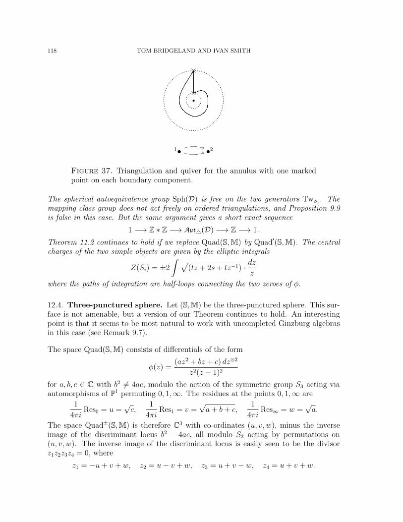
118 TOM BRIDGELAND AND IVAN SMITH
1•**44 •2
Figure 37. Triangulation and quiver for the annulus with one markedpoint on each boundary component.
The spherical autoequivalence group Sph(D) is free on the two generators TwSi. The
mapping class group does not act freely on ordered triangulations, and Proposition 9.9is false in this case. But the same argument gives a short exact sequence
1 −→ Z ∗ Z −→ Aut4(D) −→ Z −→ 1.
Theorem 11.2 continues to hold if we replace Quad(S,M) by Quad′(S,M). The centralcharges of the two simple objects are given by the elliptic integrals
Z(Si) = ±2
∫ √(tz + 2s+ tz−1) · dz
z
where the paths of integration are half-loops connecting the two zeroes of φ.
12.4. Three-punctured sphere. Let (S,M) be the three-punctured sphere. This sur-face is not amenable, but a version of our Theorem continues to hold. An interestingpoint is that it seems to be most natural to work with uncompleted Ginzburg algebrasin this case (see Remark 9.7).
The space Quad(S,M) consists of differentials of the form
φ(z) =(az2 + bz + c) dz⊗2
z2(z − 1)2
for a, b, c ∈ C with b2 6= 4ac, modulo the action of the symmetric group S3 acting viaautomorphisms of P1 permuting 0, 1,∞. The residues at the points 0, 1,∞ are
1
4πiRes0 = u =
√c,
1
4πiRes1 = v =
√a+ b+ c,
1
4πiRes∞ = w =
√a.
The space Quad±(S,M) is therefore C3 with co-ordinates (u, v, w), minus the inverseimage of the discriminant locus b2 − 4ac, all modulo S3 acting by permutations on(u, v, w). The inverse image of the discriminant locus is easily seen to be the divisorz1z2z3z4 = 0, where
z1 = −u+ v + w, z2 = u− v + w, z3 = u+ v − w, z4 = u+ v + w.

QUADRATIC DIFFERENTIALS AS STABILITY CONDITIONS 119
Thus we conclude that
Quad±(S,M) ∼= ((C∗)3 \∆)/S3
where the discriminant ∆ is given by z1 + z2 + z3 = 0 and the symmetric group Sym3
acts by permuting (z1, z2, z3). Hence
Quad♥(S,M) ∼= ((C∗)3 \∆)/(Sym3 n(Z2)⊕3),
where the Z2 factors change the signs of u, v, w respectively. The fundamental groupthen sits in a sequence
1 −→ π1((C∗)3 \∆) −→ π1(Quad♥(S,M)) −→ Sym3 nZ⊕32 −→ 1.
The space (C∗)3 \∆ is a trivial C∗-bundle over its projectivisation, which is the comple-ment of four hyperplanes in CP2. A theorem due to Zariski [38, Lemma, p. 317] assertsthat π1((C∗)3 \∆) is abelian, hence isomorphic to H1((C∗)3 \∆) ∼= Z⊕4.
The mapping class group is MCG(S,M) = S3 and permutes the punctures in the obviousway. The signed mapping class group is MCG±(S,M) = S3 n Z⊕3
2 . There are twotriangulations up to the mapping class group action: one has two triangles meetingalong three common edges, and the other consists of two self-folded triangles gluedalong their encircling edges. We claim that the relevant quiver with potential in bothcases is the one depicted in Figure 38.
•1a
,,
c′
��
•2
b
��
a′
ll
•3
cc
UU
b′
??
W = aa′ + bb′ + cc′ − abc− c′b′a′.
Figure 38. The quiver with potential for the 3-punctured sphere.
Note that the associated reduced quiver with potential has three verices and no ar-rows. Let A′ be the category of finite-dimensional representations of the ordinary (in-complete) Jacobi algebra of the above quiver with potential, and A the category offinite-dimensional representations of the completed version. Then A ⊂ A′ is the fullsubcategory of nilpotent representations.
Lemma 12.6. The category A′ has exactly four indecomposable objects, all of themsimple, namely the three vertex simple objects S1, S2, S3 together with the representationS4 of dimension vector (1, 1, 1) obtained by taking all arrows to be the identity. Thesubcategory A is the subcategory consisting of direct sums of the objects S1, S2, S3.

120 TOM BRIDGELAND AND IVAN SMITH
Proof. Differentiating the potential we see that the Jacobi algebra has relations
a′ = bc, b′ = ca, c′ = ab,
which allow us to eliminate a′, b′, c′. The remaining relations are then
(12.2) a = abca, b = bcab, c = cabc.
Given a representation of the Jacobi algebra we can split the vector space associatedto vertex 1 as Im(abc)⊕Ker(abc). Indeed, by the relations (12.2), if v = (w)abc lies inthe kernel of the map abc then (w)a = (w)abca = (v)a = (v)abca = 0 and hence v = 0.Similar splittings exist at the other vertices and it follows easily from the relations (12.2)that all arrows preserve these splittings. Hence, if E is an indecomposable object of A′we either have abc = bca = cba = 0 or each of these maps is injective.
In the first case it follows from the relations (12.2) that all arrows are 0, and hence,since E is indecomposable it must be one of the vertex simples. In the second case,each of a, b, c is injective, hence they are all isomorphisms, and (12.2) implies that abcis the identity, and similarly for bca and cab. We can then choose the gauge so thata, b, c are identity maps, and since E is indecomposable it follows that the dimensionvector must be (1, 1, 1). This unique extra indecomposable S4 is simple, since there areno maps between it and the vertex simples. �
It follows from the Lemma that the objects Si are all spherical and have no extensionsbetween them, since otherwise there would be more indecomposable objects in the cate-gory. Consider now the the derived category of the uncompleted Ginzburg algebra of theabove quiver with potential, and the subcategory D′ of objects with finite-dimensionalcohomology. It is a CY3 triangulated category with a heart A′ ⊂ D containing 4 simple,spherical objects, with zero Ext-groups between them.
The Grothendieck group is K(D′) ∼= Z⊕4 and the dimension vector defines a grouphomomorphism
d : K(D′)→ Z⊕3.
Consider the space Stab′(D′) ⊂ Stab(D′) consisting of those stability conditions whosecentral charge factors via d. This is acted on by the group of autoequivalences Aut′(D′)whose action on K(D′) preserves the kernel of d.
The group of all exact autoequivalences of D′ is Aut(D′) ∼= Sym4 nZ⊕4, with the fourgenerators ρi shifting the four simples Si respectively, and the symmetric group Sym4
permuting them. The subgroup Aut′(D′) contains a subgroup Sph(D′) ∼= Z⊕4 generatedby the 4 elements ρ2
i .
Lemma 12.7. There is a short exact sequence
1 −→ Sph(D′) −→ Aut′(D′) −→ Sym3 nZ⊕32 −→ 1.

QUADRATIC DIFFERENTIALS AS STABILITY CONDITIONS 121
Proof. An element of Aut′(D′) is determined by its action on the objects Si, and, upto the action of Sph(D′), each of these is taken to an object of the form Sj or Sj[1].Consider the transformation
τ(12)(34) : (S1, S2, S3, S4) 7→ (S2, S1, S4[1], S3[1])
along with its two conjugates by permutations of (S1, S2, S3). There is a relation
τ(12)(34) ◦ τ(13)(24) ◦ τ(23)(14) = [1] ∈ Aut′(D′)/ Sph(D′).
Consider an element σ of the quotient group Aut′(D′)/ Sph(D′). Composing with theabove transformations we can asssume that σ takes S4 to itself. The relation [S4] =[S1] + [S2] + [S3] then forces σ to be a permutation of the objects (S1, S2, S3). �
The space Stab′(D′)/ Sph(D′) is equal to (C∗)3 \∆ with co-ordinates zi = Z(Si), wherethe discriminant locus ∆ is given by z1 + z2 + z3 = 0 as before. Thus we obtain anisomorphism
Quad♥(S,M) ∼= Stab′(D′)/Aut′(D′)which can be thought of as a modifed version of Theorem 1.2.
References
1. A. Bayer and E. Macri. The space of stability conditions on the local projective plane. Duke Math.J. 160: 263–322, (2011).
2. T. Bridgeland. Stability conditions on triangulated categories. Ann. of Math. 166:317-345, (2007).3. T. Bridgeland. Spaces of stability conditions. Algebraic Geometry – Seattle 2005. Part I, 1–21.
Proc. Sympos. Pure Math. 80, Part 1, Amer. Math. Soc., (2009).4. T. Bridgeland. Stability conditions on K3 surfaces. Duke Math. J. 141 (2008), no. 2, 241291. Duke
Math. J. (2009).5. T. Bridgeland. Stability conditions on a non-compact Calabi-Yau threefold. Comm. Math. Phys.
266:715–33, (2006).6. T. Bridgeland and I. Smith. Quiver algebras as Fukaya categories. Preprint in preparation, 2013.7. G. Cerulli Irelli, B. Keller, D. Labardini-Fragoso and P.-G. Plamondon. Linear independence of
cluster monomials for skew-symmetric cluster algebras. Preprint, available at arxiv:1203.1307.8. G. Cerulli Irelli and D. Labardini Fragoso. Quivers with potential associated to triangulated
surfaces, Part III: Tagged triangulations and cluster monomials. Preprint, to appear in CompositioMath., available at arXiv:1108.1774.
9. H. Derkson, J. Weyman and A. Zelevinsky. Quivers with potential and their representations, I:Mutations Selecta Math. (N.S.) 14:59–119, (2008).
10. A. Fletcher and V. Markovich, Quasiconformal maps and Teichmuller theory. Oxford GraduateTexts in Mathematics, 11. Oxford University Press, Oxford, 2007. viii+189 pp.
11. S. Fomin, M. Shapiro and D. Thurston. Cluster algebras and triangulated surfaces, Part I: clustercomplexes. Acta Math. 201:83-146, (2008).
12. S. Fomin and D. Thurston. Cluster algebras and triangulated surfaces part II: Lambda lengths.Preprint, available at arXiv:1210.5569.
13. C. Geiss, D. Labardini-Fragoso and J. Schroer. Preprint in preparation.14. D. Gaiotto, G. Moore and A. Neitzke. Four-dimensional wall-crossing via three-dimensional field
theory. Comm. Math. Phys. 299:163–224, (2010).

122 TOM BRIDGELAND AND IVAN SMITH
15. D. Gaiotto, G. Moore and A. Neitzke. Wall-crossing, Hitchin systems and the WKB approxima-tion. Preprint, available at arXiv:0907.3987.
16. V. Ginzburg. Calabi-Yau algebras. Preprint, available at arXiv:math/0612139.17. Weiwen Gu. Graphs with non-unique decomposition and their associated surfaces. Preprint, avail-
able at arXiv:1112.1008.18. D. Happel, I. Reiten and S. Smalo. Tilting in abelian categories and quasitilted algebras. Mem.
Amer. Math. Soc. 120, no. 575, (1996).19. B. Keller. On differential graded categories. International Congress of Mathematicians. Vol. II,
151190, Eur. Math. Soc., Zrich, (2006).20. B. Keller. On cluster theory and quantum dilogarithm identities. Preprint, available at
arxiv:1102.4148.21. B. Keller and D. Yang. Derived equivalences from mutations of quivers with potential. Adv. Math.
226:2118-2168, (2011).22. A. D. King. Moduli of representations of finite-dimensional algebras. Quart. J. Math. 45:515–530,
(1994).23. A. D. King and Yu Qiu. Exchange graphs of acyclic Calabi-Yau categories. Preprint, available at
arxiv 1109.2924v2.24. M. Kontsevich and Y. Soibelman. Stability structures, motivic Donaldson-Thomas invariants and
cluster transformations. Preprint, available at arXiv:0811.2435.25. D. Labardini-Fragoso. Quivers with potentials associated to triangulated surfaces. Proc. Lond.
Math. Soc. 98:797-839, (2009).26. D. Labardini-Fragoso. Quivers with potentials associated to triangulated surfaces, Part II: Arc
Representations. Preprint, available at arXiv:0909.4100.27. D. Labardini-Fragoso. Quivers with potentials associated to triangulated surfaces, part IV: Re-
moving boundary assumptions. Preprint, available at arXiv:1206.1798.28. H. Masur. Closed trajectories for quadratic differentials with an application to billiards. Duke
Math. J. 53:307-314, (1986).29. H. Masur and A. Zorich. Multiple saddle trajectories on flat surfaces and the principal boundary
of the moduli spaces of quadratic differentials. Geom. Funct. Anal. 18:919–987, (2008).30. A. Papadopoulos. Metric Spaces, Convexity and Nonpositive Curvature. European Mathematical
Society, (2005).31. P. Seidel, R.P. Thomas. Braid group actions on derived categories of coherent sheaves. Duke Math.
J. 108:37–108, (2001).32. S. Smale. Diffeomorphisms of the 2-sphere. Proc. Amer. Math. Soc. 10:621–626, (1959).33. K. Strebel. Quadratic differentials. Ergebnisse der Mathematik und ihrer Grenzgebiete, Springer-
Verlag, Berlin, 1984.34. T. Sutherland. The modular curve as the space of stability conditions of a CY3 algebra. Preprint,
available at arXiv:1111.4184.35. T. Sutherland. Stability conditions and Seiberg-Witten curves, Ph.D. Thesis, University of
Sheffield. To appear, 2013.36. W. Veech. Moduli spaces of quadratic differentials. J. Analyse Math. 55:117-171, (1990).37. J. Woolf. Stability conditions, torsion theories and tilting. J. Lond. Math. Soc. 82:663–682, (2010).38. O. Zariski. On the Problem of Existence of Algebraic Functions of Two Variables Possessing a
Given Branch Curve. Amer. J. Math. 51: 305328, (1929).
Tom Bridgeland, All Souls College, Oxford, OX1 4AL, England.
Ivan Smith, Centre for Mathematical Sciences, Cambridge, CB3 0WB, England.