qspr of n-octanol/water partition coefficient of nonionic organic compounds using extended...

QSPR of n-Octanol/Water Partition Coefficient of NonionicOrganic Compounds Using Extended Topochemical Atom (ETA)IndicesKunal Roy*, Indrani Sanyal and Gopinath Ghosh

Drug Theoretics and Cheminformatics Laboratory, Division of Medicinal and Pharmaceutical Chemistry, Department ofPharmaceutical Technology, Faculty of Engineering and Technology, Jadavpur University, Kolkata 700032, India,E-mail: [email protected]; [email protected]; URL: http://www.geocities.com/kunalroy_in

Keywords: ETA – Partition coefficient – QSAR – QSPR – QSTR– Topological index

Received: August 14, 2006; Accepted: November 7, 2006

DOI: 10.1002/qsar.200610112

AbstractConsidering n-octanol/water partition coefficient as an important chemical property inmodeling the fate and persistence of chemicals, recently introduced ExtendedTopochemical Atom (ETA) indices have been used to model n-octanol/water partitioncoefficient data of 122 nonionic organic compounds which are highly persistent in theenvironment and reported to bioconcentrate considerably in lipid tissues. In deriving themodels, principal component Factor Analysis (FA) followed by Multiple LinearRegression (MLR), stepwise regression, Partial Least Squares (PLS), and PrincipalComponent Regression Analyses (PCRA) were applied as the statistical tools. The modeldevelopment process was repeated with non-ETA (topological and physicochemical)descriptors and a combination set comprising both the ETA and non-ETA descriptors.The models with ETA indices suggested negative contributions of groups capable ofhydrogen bonding and/or polar interactions and positive contributions of volume anddegree of halogen substitution to the partition coefficient. Finally, we discuss validation ofQSPR models by dividing the dataset into training and test sets based on differentstrategies, e.g., random division, sorted log Kow data and K-means clusters for the factorscores of the original variable (ETA) matrix without the response property values. TheETA (FA-MLR and stepwise regression) models were also applied on a purely externaldataset (n¼35) and acceptable predictive r2 values (0.582 and 0.651 respectively) wereobtained. The results suggest that ETA parameters are sufficiently rich in chemicalinformation to encode the structural features contributing to the n-octanol/water partitioncoefficient of nonionic organic compounds and thus these merit further assessment toexplore their potential in QSAR/QSPR/QSTR modeling.

1 Introduction

A considerable amount of halogenated organic com-pounds such as Polychlorinated Biphenyls (PCBs), Poly-brominated Biphenyls (PBBs), chlorinated aliphatic hy-drocarbons, polychlorinated benzenes, polybrominatedbenzenes, polychlorinated anilines, polychlorinated nitro-benzenes, and phenols are found in our environment,many of which move through food chains and accumulateat sizeable levels in the tissues of animals and man [1 – 6].The fate of these chemicals is controlled by their biologi-cal, physical, and chemical properties. A partition coeffi-cient is a measure of differential solubility of a compoundin two solvents. The log ratio of the concentrations of thesolute in the solvents is designated as log P. The best

known of these partition coefficients is the one based onthe solvents octanol and water (Kow). The octanol –waterpartition coefficient is a measure of the hydrophobicityand hydrophilicity of a substance. Many chemical com-pounds, especially those with a hydrophobic componentpartition easily into the lipids and lipid membranes of or-ganisms and bioaccumulate.The octanol –water partition coefficient (log Kow) repre-

senting the overall lipophilicity of a molecule has been ex-tensively used in Quantitative Structure –Activity/Proper-ty/Toxicity Relationship (QSAR/QSPR/QSTR) models ashydrophobicity parameter [7]. Since experimental deter-mination of partition coefficient values of a large set ofcompounds is a tedious job, there are many approaches forcalculating log P values, e.g., Ghose and CrippenEs atom

QSAR Comb. Sci. 26, 2007, No. 5, 629 – 646 G 2007 WILEY-VCH Verlag GmbH&Co. KGaA, Weinheim 629

Full Papers

contribution method [8], BodorEs quantum chemical meth-od [9], KlopmanEs Multi-CASE method [10], MoriguchiEsmethod [11] etc. Recently, several attempts have beenmade to model partition coefficients using different de-scriptors and statistical tools [12 – 18].In the present paper, we have modeled the log Kow data

of 122 nonionic organic compounds [19] using the recentlyintroduced Extended Topochemical Atom (ETA) indices[20 – 28], which were developed in the Valence ElectronMobile (VEM) environment as an extension of the TAUconcept [29 – 32]. These compounds were reported previ-ously to have considerably high bioconcentration factorswhen studied in fish tissues [19]. We have used the Multi-ple Linear Regression (MLR) technique, stepwise regres-sion analysis, Partial Least Squares (PLS) analysis andPrinciple Component Regression Analysis (PCRA) as thestatistical tools. The best relations obtained with ETA indi-ces have been compared to those derived from some se-lected topological and physicochemical descriptors (non-ETA indices). Attempt was also made to use both ETAand non-ETA descriptors in combination to model the par-tition coefficient data. Finally all the models were validat-ed by dividing the dataset into training and test sets basedon different strategies, e.g., random division (three trials),sorted response property data and K-means clusters forthe factor scores of the original variable (ETA) matrixwithout the log Kow values. Selected ETA models werealso applied on a purely external dataset (n¼35) to cross-check the predictive potential of the ETA models.

2 Materials and Methods

2.1 The Dataset

The log Kow data for 122 nonionic organic compounds (Ta-ble 1) were taken from the literature [19]. The compoundsunder the present study include halogenated benzenes,halogenated biphenyls, chlorinated aliphatic hydrocar-bons, polychlorinated anilines, polychlorinated nitroben-zenes and polychlorinated phenols, alkyl benzenes, and al-kyl phenols. These chemicals are ubiquitous contaminantsin the environment due to their wide use in industry andagriculture.

2.2 Descriptors

Definitions of some of the basic parameters used in theETA scheme are given below:

2.2.1 The Core Count (a)

The core count [a] for a nonhydrogen vertex is defined as[20]

a ¼ Z� Zv

Zv1

PN� 1 ð1Þ

In Equation 1, Z and Zv represent the atomic and valenceelectron-numbers respectively, and PN stands for periodnumber. Hydrogen atom being considered as reference, afor hydrogen is taken to be zero. The a values of differentatoms (which are commonly found in organic compounds)have high correlation (r¼0.946) with (uncorrected) vander Waals volume. Thus, Sa values of all nonhydrogenatoms of a molecule (instead of vertex count NV) may betaken as a gross measurement of molecular bulk.

2.2.2 The Electronegativity Measure (e)

We defined a term e as a measure of electronegativity inthe following manner [20]:

e¼�aþ0.3 Zv (2)

It was found [20] that e has good correlation (r¼0.937)with PaulingEs electronegativity scale.

2.2.3 The VEM Count b

The VEM count b of the ETA scheme was defined as [20]

b¼S xsþS ypþd (3)

In the above equation, x is the contribution of a sigmabond (s) having values of 0.5 for two bonded atoms of sim-ilar electronegativity (De�0.3) and 0.75 for two bondedatoms of different electronegativity (De>0.3). Again, inthe case of p bonds, contributions (y) are considered de-pending on the type of the double bond: (i) for p bond be-tween two atoms of similar electronegativity (De�0.3), yis taken to be 1; (ii) for p bond between two atoms of dif-ferent electronegativity (De>0.3) or for a conjugated(nonaromatic) p system, y is considered to be 1.5; and (iii)for an aromatic system, y is taken as 2. d is a correctionfactor of value 0.5 per atom with lone pair of electrons ca-pable of resonance with aromatic ring (e.g., nitrogen ofaniline, oxygen of phenol, etc.). For a given part (substruc-ture) of a molecular graph, Sbs and Sbns may be calculatedconsidering all bonds (sigma bonds for the former and p

bonds and lone pair of electrons for the latter) in the sub-structure. Sb’s (defined as [Sbs]/NV, NV being the vertexcount) may be taken as a relative measure of number ofelectronegative atoms in the substructure while Sb’ns (de-fined as [Sbns]/NV) may be taken as a relative measure ofelectron-richness (unsaturation) of the substructure.

2.2.4 The VEM Vertex Count g

The VEM vertex count gi of the ith vertex in a moleculargraph was defined as [20]

630 G 2007 WILEY-VCH Verlag GmbH&Co. KGaA, Weinheim www.qcs.wiley-vch.de QSAR Comb. Sci. 26, 2007, No. 5, 629 – 646

Full Papers Kunal Roy et al.

www.qcs.wiley-vch.de

QSAR Comb. Sci. 26, 2007, No. 5, 629 – 646 www.qcs.wiley-vch.de G 2007 WILEY-VCH Verlag GmbH&Co. KGaA, Weinheim 631

Table 1. Partition coefficient (log Kow) values for 122 nonionic organic chemicals.

Serial no. Compounds log Kowa log Kow calculated by Eq. 10

1 1,1,1-Trichloroethane 2.49 2.242 1,1,2,2-Tetrachloroethane 2.39 2.623 1,1,2,3,4,4-Hexachloro-1,3-butadiene 4.78 4.324 Trichloroethylene 2.42 2.265 1,2-Dichloroethane 1.48 1.186 Tetrachloromethane 2.83 2.457 Trichloromethane 1.97 1.928 Hexachloroethane 4.14 3.619 Pentachloroethane 3.22 3.1310 Tetrachloroethylene 3.4 2.7911 Benzene 2.19 1.7212 Toluene 2.73 2.0413 Ethyl benzene 3.15 2.3314 o-Xylene 3.12 2.3915 m-Xylene 3.2 2.3916 p-Xylene 3.15 2.3917 Isopropylbenzene 3.72 2.6518 Biphenyl 4.09 3.4919 1,2,3,4-Tetrachlorobenzene 4.64 4.0720 1,2,3,5-Tetrachlorobenzene 4.92 4.0721 1,2,3-Trichlorobenzene 4.05 3.5322 1,2,4,5-Tetrachlorobenzene 4.82 4.0723 1,2,4-Trichlorobenzene 4.02 3.5824 1,2-Dichlorobenzene 3.43 3.0225 1,3,5-Trichlorobenzene 4.19 3.5826 1,3-Dichlorobenzene 3.6 3.0227 1,4-Dichlorobenzene 3.52 3.0228 Hexachlorobenzene 5.31 5.0229 2,4,5-Trichlorotoluene 4.56 3.7930 Chlorobenzene 2.84 2.3931 Pentachlorobenzene 5.18 4.5732 1,2,4,5-Tetrabromobenzene 5.13 4.9433 1,2,4-Tribromobenzene 4.66 4.1634 1,3,5-Tribromobenzene 4.51 4.1635 1,3-Dibromobenzene 3.75 3.3636 1,4-Dibromobenzene 3.79 3.3637 Bromobenzene 2.99 2.5238 1,2-Dibromobenzene 3.64 3.3639 2,2’,4,5-Tetrachlorobiphenyl 5.69 5.7340 2,2’,5,5’-Tetrachlorobiphenyl 5.79 5.7341 2,2’,5-Trichlorobiphenyl 5.55 5.2242 2,2’,4,4’-Tetrachlorobiphenyl 6.29 5.7343 2,2’-Dichlorobiphenyl 4.9 4.6644 2,3’,4’,5-Tetrachlorobipenyl 6.07 5.7345 2,3-Dichlorobiphenyl 5.02 4.6646 2,4,4’-Trichlorobiphenyl 5.58 5.1947 2,4’,5-Trichlorobiphenyl 5.68 5.2248 2,4,5-Trichlorobiphenyl 5.9 5.2049 2,4’-Dichlorobiphenyl 5.1 4.6650 2,5-Dichlorobiphenyl 5.16 4.6651 3,3’,4,4’-Tetrachlorobiphenyl 6.63 5.7152 3,5-Dichlorobiphenyl 5.41 4.6453 4-Chlorobiphenyl 4.63 4.0954 4,4’-Dichlorobiphenyl 5.58 4.6455 2,2’,3,3’-Tetrachlorobiphenyl 5.67 5.7356 2,2’,4,5,5’-Pentachlorobiphenyl 6.65 6.2557 2,2’,4,4’,5,5’-Hexachlorobiphenyl 7.75 6.7458 2,2’,4,4’,6,6’-Hexachlorobiphenyl 7.55 6.7459 2,2’,3,3’,4,4’,5,5’-Octachlorobiphenyl 8.68 7.6860 2,2’,3,5’-Tetrachlorobiphenyl 5.73 5.7361 2,2’,4,5’-Tetrachlorobiphenyl 5.87 5.7362 2,2’,6,6’-Tetrachlorobiphenyl 5.94 5.75

QSPR of n-Octanol/Water Partition Coefficient of Nonionic Organic Compounds



Table 1. (cont.)

Serial no. Compounds log Kowa log Kow calculated by Eq. 10

63 2,2’,3,4,5’-Pentachlorobiphenyl 6.23 6.2564 2,2’,3’,4,5-Pentachlorobiphenyl 6.67 6.2565 3,3’,4,4’,5-Pentachlorobiphenyl 6.98 6.2366 2,2’,3,3’,4,4’-Hexachlorobiphenyl 6.96 6.7267 2,2’,3,3’,6,6’-Hexachlorobiphenyl 7.03 6.7468 2,2’,3,4,4’,5-Hexachlorobiphenyl 6.82 6.7269 2,2’,3,4,5,5’-Hexachlorobiphenyl 6.75 6.7270 2,2’,3,4,4’,5’,6-Heptachlorobiphenyl 7.04 7.2271 2,2’,3,3’4,4’,5,6-Octachlorobiphenyl 7.35 7.7072 2,2’,3,3’,4,5,5’,6-Octachlorobiphenyl 8.91 7.7073 2,2’,3,3’,5,5’,6,6’-Octachlorobiphenyl 7.73 7.7274 2,2’,3,3’,4,4’,5,5’,6-Nonachlorobiphenyl 9.14 8.1575 2,2’,5,5’-Tetrabromobiphenyl 7.31 6.6576 2,4,6-Tribromobiphenyl 6.42 5.8877 4,4’-Dibromobiphenyl 5.72 5.0778 2,4-Dichlorophenol 5.53 2.8379 Pentachlorophenol 5.12 4.4380 2,4,6-Trichlorophenol 3.69 3.3981 2-Chlorophenol 2.15 2.4282 3-Chlorophenol 2.5 2.2183 2-Methylphenol 1.95 1.8784 Phenol 1.46 1.4785 4-t-Butylphenol 3.31 2.8986 2,4-Dimethylphenol 2.3 2.2287 4-Bromophenol 2.59 2.3888 p-sec-Butylphenol 3.08 2.8389 2-Chloroaniline 1.9 1.7890 3-Chloroaniline 1.88 1.7891 Diphenylamine 3.5 2.9792 Pentachloroaniline 4.82 4.0993 2,3,4,5-Tetrachloroaniline 4.27 3.6094 2,3,5,6-Tetrachloroaniline 4.1 3.5295 2,3,4-Trichloroaniline 3.68 3.0196 2,4,5-Trichloroaniline 3.45 3.0197 2,4,6-Trichloroaniline 3.52 3.0398 3,4,5-Trichloroaniline 3.32 3.0199 4-Chloroaniline 1.88 1.57100 2,4-Dichloroaniline 2.78 2.44101 3,4-Dichloroaniline 2.78 2.42102 Aniline 0.9 0.97103 2-Nitrophenol 1.79 1.21104 2-Chloronitrobenzene 2.24 2.09105 3-Chloronitrobenzene 2.46 2.09106 4-Chloronitrobenzene 2.39 2.07107 2,3-Dichloronitrobenzene 3.05 2.71108 2,4-Dichloronitrobenzene 3.07 2.73109 2,5-Dichloronitrobenzene 3.09 2.73110 3,4-Dichloronitrobenzene 3.12 2.73111 3,5-Dichloronitrobenzene 3.09 2.73112 2-Methyl-4,6-dinitrophenol 2.12 1.61113 3-Nitrophenol 2 1.26114 Pentachloronitrobenzene 4.77 4.42115 2,3,4,5-Tetrachloronitrobenzene 4.57 3.90116 2,3,5,6-Tetrachloronitrobenzene 3.89 3.87117 2,3,4-Trichloronitrobenzene 3.68 3.31118 2,4,5-Trichloronitrobenzene 3.48 3.34119 4-Nitroaniline 1.39 0.86120 3-Nitroaniline 1.37 0.86121 2-Nitroaniline 1.85 0.80122 2,4,6-Tribromophenol 4.13 4.08

aFrom Ref. [19].



gi ¼ai

bi

ð4Þ

In the equation above, ai stands for a value for the ith ver-tex and bi stands for the VEM count considering all bondsconnected to the atom and a lone pair of electrons (if any).

2.2.5 The Composite Index h

The composite index h was defined in the following man-ner [20]:

h ¼Xi<j

gigj

r2ij

" #0:5ð5Þ

In Equation 5, rij stands for the topological distance be-tween the ith and the jth atom. Again, when all heteroa-toms in the molecular graph are replaced by carbon andmultiple bonds are replaced by single bond, the corre-sponding molecular graph is considered as the referencealkane and the corresponding composite index value isdesignated as hR [20].

2.2.6 The Functionality Index hF

Considering functionality as the presence of heteroatoms(atoms other than carbon or hydrogen) and multiplebonds, functionality index hF was calculated [20] as hR – h.To avoid dependence of functionality on vertex count orbulk, another term h’F was defined as hF/NV.

2.2.7 The Atom Level Index

The contribution of a particular position or vertex to thefunctionality can be determined in the following manner[20]:

h½ �i¼Xi=j

gigj

r2ij

" #0:5ð6Þ

In Equation 6, [h]i stands for the contribution of the ithvertex to h. Similarly, contribution of the ith vertex [hR]i tohR can be computed. Contribution of the ith vertex [hF]i tofunctionality was defined [20] as [hR]i – [h]i. To avoid de-pendence of this value on NV, a related term [h’F]i was de-fined [20] as [hF]i/NV.

2.2.8 The Local Index hlocal

When only bonded interactions are considered (rij¼1), thecorresponding composite index may be written as hlocal.

hlocal¼X

i < j;rij ¼ 1

(gigj)0.5 (7)

In a similar way, hlocalR for the corresponding reference al-kane may also be calculated. Local functionality contribu-tion (without considering global topology), hlocalF , may becalculated as hlocalR �hlocal.

2.2.9 The Branching Index hB

Branching is calculated with respect to h value of the cor-responding normal alkane (straight chain compound ofsame vertex count obtained from the reference alkane),hlocalN , which may be conveniently calculated as (for com-pounds having nonhydrogen vertex count NV3) [20]:

hlocal¼1.414þ (Nv�3)0.5 (8)

Branching index hB can be calculated as hlocalN �hlocalR þ0.086NR, where NR stands for the number of rings in themolecular graph of the reference alkane. The NR term inthe branching index expression represents a correction fac-tor for cyclicity. To calculate branching contribution incomparison to the molecular size, another term h’B was de-fined [20] as hB/NV.

2.2.10 The Shape Indices

The terms like (Sa)p/Sa, (Sa)Y/Sa, and (Sa)X/Sa can beused as the shape parameters. (Sa)p, (Sa)Y, and (Sa)Xstand for summation of a values of the vertices that arejoined to one, three and four other nonhydrogen vertices,respectively in the molecular graph. Calculation of differ-ent indices is illustrated in Table 2 taking the example of4-chloroaniline. The definitions of important ETA param-eters are given in Table 3.

2.3 Model Development

For the model development we have used MLR with FactorAnalysis (FA-MLR) as the data-preprocessing step, step-wise regression analysis, PLS analysis and principle compo-nent regression analysis (PCRA) as the statistical tools.In the case of FA-MLR, FA has been performed as the

data-preprocessing step for the identification of importantdescriptors [33 – 35] for the subsequent multiple regressionanalysis [36]. For this purpose the data matrix consisting ofthe descriptors has been subjected to principal componentFA using SPSS software [37]. The objective of FA is to re-duce the number of variables of possible importance incharacterizing an array of numbers. The details of FA-MLR have been described in previous communications[26, 27].In stepwise regression [38], a multiple term linear equa-

tion was built step-by-step. The basic procedures involve(1) identifying an initial model, (2) iteratively “stepping”,that is, repeatedly altering the model at the previous stepby adding or removing a predictor variable in accordancewith the “stepping criteria” (partial F-statistic; F¼4 for in-





Table 2. Calculations of ETA parameters: example of 4-chloroaniline.

4-Chloroaniline Reference alkane

Vertex no. 1 2 3 4 5 6 7 8 1 2 3 4 5 6 7 8ai 0.5 0.5 0.5 0.5 0.5 0.5 0.4 0.72 0.5 0.5 0.5 0.5 0.5 0.5 0.5 0.5[bs]i 1.75 1.00 1.00 1.75 1.00 1.00 0.75 0.75 1.50 1.00 1.00 1.50 1.00 1.00 0.50 0.50[bns]i 2.00 2.00 2.00 2.00 2.00 2.00 0.50 0.50 0.00 0.00 0.00 0.00 0.00 0.00 0.00 0.00bI 3.75 3.00 3.00 3.75 3.00 3.00 1.25 1.25 1.50 1.00 1.00 1.50 1.00 1.00 0.50 0.50gI 0.13 0.17 0.17 0.13 0.17 0.17 0.32 0.58 0.33 0.50 0.50 0.33 0.50 0.50 1.00 1.00[h]i 0.77 .075 0.76 0.82 0.76 0.75 0.73 0.95 – – – – – – – –[hR]i – – – – – – – – 2.05 2.12 2.12 2.05 2.12 2.12 2.10 2.10[h’F]i 0.16 0.17 0.17 0.16 0.17 0.17 0.17 0.14 – – – – – – – –h 3.141 –hR – 8.392

h’F 0.656 –hlocal 1.413 –hlocalR – 3.786

hlocalF 2.373 –hlocalN – 3.914

h’B 0.016a –Sa 4.115 –[Sa]p 1.115 –

aWithout ring correction.

Table 3. Definitions of the different ETA parameters used in exploring QSAR of the bioconcentration factors of nonionic organiccompounds.

Variables Definition

Sa Sum of a values of all nonhydrogen vertices of a molecule[Sa]p Sum of a values of all nonhydrogen vertices, each of which is joined to only one other nonhydrogen vertex

of the moleculeh The composite ETA indexhR The composite index for the reference alkaneNV Vertex count (excluding hydrogen)N Total number of atoms (including hydrogen)Sbs Sum of bs values of all nonhydrogen vertices of a moleculeSbns Sum of values of all nonhydrogen vertices of a moleculeSb’s Sum of b’s values of all nonhydrogen vertices of a molecule; Sb’s is defined as [Sbs]/NV

Sb’ns Sum of b’ns values of all nonhydrogen vertices of a molecule; Sb’ns is defined as [Sbns]/NV

Se/N Sum of e/N values of all atoms including hydrogen[Sa]2 Square of the sum of a values of all nonhydrogen vertices of a molecule[h’F]Cl Functionality for the chlorine atom[h’F]NO2

Functionality for the nitro group[h’F]Br Functionality for the bromine atom[h’F]NH2 Functionality for the amino group[h’F]COOH Functionality for the carboxylic group[h’F]OH Functionality for the hydroxyl group



clusion; F¼3.5 for exclusion) and (3) terminating thesearch when stepping is no longer possible given the step-ping criteria, or when a specified maximum number ofsteps has been reached [26, 27].In the PLS regression [39], the prediction functions are

represented by latent variables extracted as linear combi-nations of the original predictor variables, so that there isno correlation among the latent variables used in the pre-dictive regression model. Initially, variables for PLS wereselected based on the factor loading tables and PLS regres-sion was repeated, each time eliminating the variable withthe minimum standardized regression coefficient value,until the model giving the maximum Q2 value was ob-tained [26, 27]. The stepwise regression and PLS analyseswere performed using MINITAB software [40].Attempt was also made to perform PCRA [35] taking

factor scores derived from the descriptor matrix excludingthe response variable as the predictor variables and adopt-ing linear regression method. In this case the principalcomponents serve as latent variables. PCRA has an ad-vantage that collinearities among X variables are not a dis-turbing factor and that the number of variables included inthe analysis may exceed the number of observations [35].The calculations of h, hR, hF, hB and contributions of dif-

ferent vertices to hF were done, using distance matrix andVEM vertex counts as inputs, by the GW-BASIC pro-grams KRETA1 and KRETA2 developed by one of theauthors [41]. We have also modeled the partition coeffi-cient data using other selected topological and physico-chemical variables and compared the ETA models withnon-ETA ones. The values for the topological descriptorsand physicochemical variables for the compounds havebeen generated by QSARþand Descriptorþmodules ofthe Cerius 2 version 4.8 software [42]. The various topolog-ical indices calculated are (Balaban [43]) connectivity indi-ces (0c, 1c, 2c, 3cp,

3cc,0cv, 1cv, 2cv, 3cvp,

3ccv) [44], kappa shape

indices (1k, 2k, 3k, 1ka,2ka,

3ka) [45], E-state index [46] andWiener index (W) [47]. Among the physicochemical varia-bles, molar refractivity (MolRef) and hydrophobicity(A logP98), and the number of hydrogen bond donor andacceptors (H_bond_donor and H_bond_acceptor) [48]were considered.

2.4 Equation Statistics and Robustness Test

The statistical quality of the equations [36, 49] was judgedby the parameters as explained: variance (R2a, i.e., adjustedR2), correlation coefficient (r or R), standard error of esti-mate (s), and variance ratio (F) at specified degrees offreedom (df). The models were validated internally usingthe MINITAB software, and Leave-One-Out (LOO) sta-tistics [50, 51] such as LOO crossvalidation R2 (Q2) andPredicted Residual Sum of Squares (PRESS) were ob-tained. All the accepted MLR equations have regressionconstants and F ratios significant at 95 and 99% levels, re-spectively, if not stated otherwise. A compound was con-

sidered as an outlier if the residual is more than twice thestandard error of estimate for a particular equation. Se-lected equations were subjected to leave-10%-out andleave-25%-out crossvalidation using GW-BASIC pro-grams KRPRES1 and KRPRES2 developed by one of theauthors [41].Additionally, QSPR models were also developed by di-

viding the dataset into training (75% of the total dataset)and test (25% of the total dataset) sets using three differ-ent algorithms namely random division, sorted log Kow

data and K-means clusters for the factor scores of the orig-inal variable (ETA) matrix without log Kow values and ex-ternal validation statistics were reported for FA-MLR,stepwise and PLS models developed from the correspond-ing training sets. QSPR models were developed using thetraining set compounds (optimized by Q2), and then thedeveloped models were validated (externally) using thetest set compounds. We have used three algorithms for thedivision of the dataset into training and test sets. Initiallythe dataset was divided into training and test sets in a ran-dom manner [52] for three trials. Then the whole range ofcompounds was sorted through ascending order of re-sponse variable, and every fourth compound was assignedto the test set. Finally, an attempt was made to rationalizethe division process in which the division was performedso that points representing both training and test sets weredistributed within the whole descriptor space occupied bythe entire dataset, and each point of the test set was closeto at least one point of the training set. For this, we haveclassified the dataset into clusters using the K-means clus-ter based on the factor scores of the ETA descriptors with-out log Kow values. The original variables were convertedto the latent variables (factor scores) only to reduce thenumber of descriptors. This approach (clustering) ensuresthat the similarity principle can be employed for the log -Kow prediction of the test set. Cluster Analysis (CA) is acollection of statistical methods that is used to assign cases(or descriptors) to groups (clusters) [50]. In K-means clus-tering, there is no hierarchy and the data are partitioned.It expresses the final cluster membership for each caseonly. This procedure ensures that any chemical classes (asdetermined by the clusters derived form the K-means clus-tering technique) will be represented in both series ofcompounds (i.e., training and test sets) [53, 54]. Again, thepredictive ability of the best models was estimated accord-ing to the method reported earlier [55] for each of thethree different sets of descriptors. In this method log Kow

was plotted against log Kow_pred to get the regression lineswith and without the intercepts (with the intercept set tozero) and the corresponding R2 and the R0

2 values wereobtained. Finally, the criteria for acceptance of the modelswere checked such that [(R2�R0

2)/R2]<0.1 and 0.85�k�1.15, where k is the slope of the line passing through origin(intercept set to zero).Finally, selected ETA models were also applied on a

purely external dataset (n¼35) to crosscheck the predic-




tive potential of the ETA models. The external datasetwas taken from reference [56] and the compounds thatwere common with the original dataset were excluded.ETA descriptors were computed for the new dataset andpartition coefficient values were predicted from the select-ed ETA models and predictive potential of the models wasjudged from predictive R2 (R2

Pred) statistic.

3 Results and Discussion

3.1 ETA Indices

Table 4 shows the results of FA of the data matrix com-posed of the ETA descriptors and log Kow. It is observedthat seven factors could explain 98.1% of the variance ofthe data matrix. Factor loading pattern after VARIMAXrotation shows that log Kow of the nonionic organic com-pounds is highly loaded with factor 1 which is in turn high-ly loaded in h, hR, NV, Sa, [Sa]p and [Sa]

2. The log Kow

shows low loading in the rest of the factors: factor 4 (highlyloaded in h0

F½ �NO2), factor 5 (highly loaded in [h’F]OH), fac-tor 6 (highly loaded in h0

F½ �NH2).Based on the results of FA, a number of equations were

generated taking the descriptors showing high loading indifferent factors and the best model is noted below:

logK0w ¼ 0:655 �0:017ð ÞX

aþ 0:674 �0:228ð Þ

�X

ah i

p=X

aþ 2:173 �0:527ð Þ h0F

� �Br�2:432

� �0:252ð Þ h0F

� �NO2

�3:050 �0:854ð Þ h0F

� �OH

�6:105

� �0:863ð Þ h0F

� �NH2

þ0:145 �0:159ð Þ

n¼122, R2a¼0.952, R2¼0.954, R¼0.977, F¼400.563(df

6,115), s¼0.398, Q2¼0.948, PRESS¼20.8 (9)

The standard errors of the regression coefficients are givenwithin parentheses. Equation 9 with six predictor variablescould predict and explain 94.8 and 95.2% of the variance,respectively. The standard error of this equation is 0.398and all the coefficients (except the intercept) are signifi-cant at 95% level. The parameter Sa being a measure ofthe steric bulk, the positive coefficient of the parameter inEquation 9 indicates that the partition coefficient (log -Kow) increases with molecular size. Again, most of thecompounds of the dataset being aromatic in nature, the pa-rameter [Sa]p/Sa actually signifies the number of aromaticsubstitution positions and the positive coefficient of [Sa]p/Sa in Equation 9 indicates that the partition coefficient in-creases with the degree of (halogen) substitutions of thearomatic rings (as most of the polysubstituted aromaticcompounds of the dataset are polyhalogenated com-pounds). Again, the positive coefficient of [h’F]Br indicatesthat the partition coefficient increases with the presence ofhalogen and the negative coefficients of [h’F]OH, h0

F

� �NH2,

and h0F

� �NO2

indicate that log Kow decreases in the presenceof groups capable of hydrogen bonding and/or polar inter-actions.Next, another model-building attempt was made from

the ETA descriptors using the stepwise regression method.The best model obtained is as follows:

logK0w ¼ 0:582 �0:019ð ÞX

a� 2:36 �0:237ð Þ h0F

� �NO2

�6:33

� �0:798ð Þ h0F

� �NH2

þ1:90 �0:332ð Þ h0F

� �Cl�2:77

� �0:808ð Þ h0F

� �OH

þ2:9 �1:124ð Þh0B þ 0:437

� �0:118ð Þ

n¼122, R2a¼0.958, R2¼0.960, R¼0.980, Q2¼0.953,

PRESS¼18.8 (10)


Table 4. Factor loadings of the variables (ETA) and log Kow after VARIMAX rotation.

Variables Factor 1 Factor 2 Factor 3 Factor 4 Factor 5 Factor 6 Factor 7 Communality

log Kow 0.910 0.072 0.034 �0.263 �0.149 �0.201 0.065 0.970h 0.966* 0.195 �0.032 �0.003 �0.031 �0.052 0.074 0.981hR 0.978* �0.059 0.153 0.060 �0.032 �0.036 0.032 0.991h’F 0.481 �0.630 0.509 0.245 0.060 0.107 �0.137 0.981NV 0.967* �0.180 0.128 0.063 �0.042 �0.036 0.044 0.992h’B 0.134 0.189 0.007 0.045 0.025 0.019 0.969 0.995Sa 0.986* �0.006 �0.056 �0.068 �0.087 �0.065 0.045 0.993[Sa]P 0.753* 0.613 �0.142 �0.033 �0.055 �0.032 0.132 0.986[Sa]P/Sa 0.046 0.970 �0.071 �0.019 �0.073 �0.051 0.154 0.980[Sa]2 0.980* 0.024 �0.044 �0.090 �0.072 �0.066 0.013 0.981[h’F]Cl 0.624 0.411 0.571 �0.094 �0.154 0.006 �0.070 0.922[h’F]Br �0.101 �0.192 0.945 0.040 0.009 0.026 0.037 0.945[h’F]OH �0.176 �0.094 �0.013 0.039 0.974* �0.097 0.024 0.999[h’F]NH2 �0.186 �0.073 0.038 0.007 �0.097 0.973* 0.019 0.999[h’F]NO2 �0.113 �0.067 0.041 0.988* 0.035 0.005 0.045 0.998%variance 0.459 0.137 0.104 0.076 0.069 0.068 0.068 0.981



Equation 10 shows that using six predictor variables,95.3% of the predicted variance and 95.8% of the ex-plained variance can be achieved. The positive coefficientof h’B in Eq. 10 indicates that the partition coefficient in-creases with the number of halogen substitutions of thecompounds (as most of the polysubstituted compounds ofthe dataset are polyhalogenated compounds and degree ofsubstitution increases branching of the compounds). Thisis further corroborated by the positive coefficient of [h’F]Cl.This is followed by the application of PLS analysis on

the ETA descriptors and the best model obtained (fourPLS components selected by crossvalidation) is reportedbelow:

logKow ¼ 1:044h0F þ 0:129Nv þ 0:245

Xaþ 0:318

�X

ah i

P�4:486 h0

F

� �OH

�7:292 h0F

� �NH2

�3:286

� h0F

� �NO2

þ0:212

n¼122, R2a¼0.956, R2¼0.957, R¼0.978, F¼686.60

(df 4,117), Q2¼0.952, PRESS¼19.2 (11)

Equation 11 shows that by using seven predictor variables,95.2% predicted variance and 95.6% explained variancecan be achieved. The positive coefficient of Nv in Eq. 11indicates that the partition coefficient increases with mo-lecular bulk.Attempt was also made to use factor scores as the pre-

dictor variables to avoid loss of information on the selec-tion of relevant molecular descriptors from the set of de-scriptors and significant increase in statistical qualities wasobtained.

logKow ¼ 1:624 �0:037ð Þf1þ 0:147 �0:037ð Þf2� 0:498� �0:037ð Þf4� 0:283 �0:037ð Þf5þ 0:121� �0:037ð Þ f6� 0:382 �0:037ð Þf7þ 4:278� �0:036ð Þ

n¼122, R2a¼0.951, R2¼0.953, R¼0.976, F¼390.958

(df 6,115), s¼0.403, Q2¼0.940, PRESS¼24.2 (12)

Equation 12 could predict and explain 94 and 95.1% re-spectively of the variance of the toxicity. The factor scoresas mentioned in Eq. 12 signify the importance of differentvariables as shown in asterisks in Table 4.

3.2 Non-ETA Indices

Table 5 shows the rotated loading matrix obtained fromFA of the data matrix composed of the log Kow values andselected topological and physicochemical descriptors.Eleven factors could explain 95.2% of the variance of thedata matrix. The log Kow data of the nonionic organic com-pounds were found to be highly loaded with factor 1

(which is in turn highly loaded in 1k, 2k, 1ka,2ka, f, SC0,

SC1, SC2, SC3_P, SC3_C, 0c, 1c, 2c, 3cp,2cv, 3cc,

3cvp,0cv, 1cv,

2cv, Wiener, log Z, Zagreb, H_bond_acc, S_sCl, A log P98and MolRef).The best formulated relation from these descriptors was

the following:

logKow ¼ 0:533 �0:018ð Þ0c� 0:163 �0:028ð ÞS sNH2� 0:078 �0:006ð ÞS dOþ 0:023 �0:167ð Þ

n¼122, R2a¼0.908, R2¼0.912, R¼0.954, F¼401.4

(df 3,118), s¼0.550, Q2¼0.906, PRESS¼37.7 (13)

Equation 13 is a three-variable relation predicting 90.6and explaining 90.8% of the variance of the responseproperty. All the regression coefficients are significant at95% level. In order to explore the possibility of improvingthe quality of the relation for all compounds using thenon-ETA descriptors [Eq. 13], stepwise regression wasperformed and the best model obtained is noted below:

logKow ¼ 0:853 �0:023ð ÞA logP98þ 0:126 �0:028ð ÞS aasC� 2:34 �0:749ð ÞS dssCþ 0:571 �0:083ð Þ

n¼122, R2a¼0.954, R2¼0.955, R¼0.977, F¼835.5

(df 3,118), s¼0.390, Q2¼0.952, PRESS¼19.1 (14)

Equation 14 is a three-variable relation predicting 95.2and explaining 95.4% of the variance of the responseproperty. Subsequently, PLS analysis was performed andthe following equation (two PLS components selected bycrossvalidation) was obtained:

logKow ¼ 0:1412cv þ 0:1403cvp þ 0:014S sClþ 0:0863cpþ 0:112S aasCþ 0:0680cv þ 0:1261cv� 0:298H bond don� 0:024S dOþ 0:129�A logP98þ 0:011MolRef þ 0:708

n¼122, R2a¼0.969, R2¼0.953, R¼0.976, F¼1205.1

(df 2,119), Q2¼0.949, PRESS¼20.2 (15)

Equation 15 shows that using 11 predictor variables,94.9% of the predicted variance and 96.9% of the ex-plained variance can be achieved.When factor scores were used as predictor variables, the

following equation was obtained:

logKow ¼ 1:613 �0:039ð Þf1þ 0:185 �0:039ð Þf2þ 0:523� �0:039ð Þf3þ 0:364 �0:039ð Þf4� 0:091� �0:039ð Þf5� 0:143 �0:039ð Þf þ 70:157� �0:039ð Þf9� 0:080 �0:039ð Þf10� 0:175� �0:039ð Þf11þ 4:278 �0:039ð Þ

n¼122, R2a¼0.945, R2¼0.949, R¼0.974, s¼0.428,

F¼230.0(df 9,112), Q2¼0.912, PRESS¼35.0 (16)




Equation 16 could predict and explain 91.2 and 94.5 % re-spectively of the variance of the response variable. Thefactor loadings as mentioned in Table 5 signify the impor-tance of different variables as shown in asterisks in Ta-ble 5. Next, attempt was made to use non-ETA descriptorsalong with ETA ones to further improve the ETA models.

3.3 ETA and Non-ETA Indices

Table 6 shows FA results of the data matrix composed ofETA and non-ETA descriptors. Eleven factors could ex-plain 95.04% of the variance. The partition coefficient ofthe modeled compounds was found to be highly loadedwith factor 1 (which is in turn highly loaded in h, hR, NV,Sa, [Sa]p, [Sa]

2, 1k, 2k, 1ka,2ka, f, SC0, SC1, SC2, SC3_P,

SC3_C, 0c, 1c, 2c, 3cp,3cc,

0cv, 1cv, 2cv, 3cvp, Wiener, log Z, Za-


Table 5. Factor loadings of the variables (non-ETA) and log Kow after VARIMAX rotation.

Variables Factor 1 Factor 2 Factor 3 Factor 4 Factor 5 Factor 6 Factor 7 Factor 8 Factor 9 Factor 10 Factor 11 Com-munality

log Kow 0.893 0.097 0.288 0.201 �0.049 �0.025 �0.078 0.030 0.085 �0.045 �0.097 0.958JX �0.295 0.120 �0.264 �0.246 �0.586 0.134 �0.355 0.032 0.032 �0.358 0.176 0.8801k 0.991* 0.053 �0.082 0.039 �0.018 �0.003 0.029 0.021 �0.049 0.020 �0.019 0.9982k 0.943* �0.166 �0.069 0.090 0.031 0.051 0.185 0.029 �0.019 0.136 �0.083 0.9943k 0.567 – 0.129 �0.091 0.138 �0.127 �0.032 0.296 0.474 0.036 0.467 �0.063 0.9191ka 0.970* 0.170 0.010 0.059 �0.087 �0.090 �0.066 0.058 �0.019 0.018 �0.015 0.9982ka 0.952* 0.037 0.086 0.130 �0.098 �0.118 0.010 0.107 0.028 0.140 �0.075 0.9933ka 0.513 0.139 0.097 0.168 �0.300 �0.247 0.078 0.529 0.104 0.395 �0.055 0.926f 0.821* 0.221 0.117 0.144 �0.251 �0.262 �0.110 0.196 0.014 0.190 �0.048 0.978SC0 0.990* �0.040 �0.032 0.042 0.057 0.042 0.080 �0.019 �0.019 �0.003 �0.041 0.998SC1 0.982* �0.076 �0.008 0.046 0.087 0.058 0.103 �0.034 �0.008 �0.011 �0.053 0.997SC2 0.994* 0.009 �0.015 0.026 0.063 0.031 0.038 �0.026 �0.023 �0.031 �0.027 0.999SC3P 0.992* �0.055 �0.006 0.013 0.059 0.015 0.008 �0.019 �0.037 �0.031 �0.026 0.995SC3C 0.912* 0.352 �0.064 �0.019 �0.040 �0.049 �0.139 0.017 �0.082 �0.056 0.054 0.9960c 0.996* 0.023 �0.059 0.030 0.015 0.014 0.027 0.000 �0.037 �0.003 �0.020 0.9991c 0.980* �0.089 �0.019 0.050 0.077 0.057 0.110 �0.027 �0.011 0.002 �0.055 0.9972c 0.988* 0.066 �0.035 0.042 0.060 0.039 0.060 �0.029 �0.018 �0.025 �0.029 0.9943cp 0.989* �0.067 0.003 �0.008 0.027 0.014 0.007 �0.012 �0.039 �0.039 �0.016 0.9873cC 0.701* 0.655 �0.084 0.016 �0.029 �0.032 �0.128 �0.004 �0.076 �0.065 0.067 0.9610cv 0.955* 0.127 0.136 0.082 �0.044 �0.059 �0.062 0.033 0.170 �0.007 �0.046 0.9951cv 0.960* 0.065 0.164 0.099 0.008 �0.036 �0.002 0.012 0.168 0.022 �0.065 0.9972cv 0.880* 0.342 0.201 0.121 �0.023 �0.080 �0.053 0.010 0.195 �0.004 �0.049 0.9953cvp 0.926* 0.106 0.139 0.030 �0.086 �0.095 �0.127 0.047 0.136 �0.027 �0.031 0.9443cvC 0.316 0.893 0.159 0.121 �0.028 �0.099 �0.100 �0.018 0.095 �0.046 �0.009 0.969Wiener 0.968* 0.017 0.055 0.087 0.081 �0.029 0.052 0.023 �0.068 0.051 �0.043 0.967Log Z 0.975* �0.110 �0.005 0.049 0.090 0.063 0.119 �0.034 �0.007 �0.003 �0.059 0.997Zagreb 0.991* �0.024 �0.012 0.034 0.072 0.042 0.063 �0.029 �0.017 �0.023 �0.037 0.998H_bond_acc 0.710* 0.355 �0.203 0.040 �0.237 �0.340 �0.320 0.129 �0.079 �0.063 0.056 0.977H_bond_don �0.233 �0.094 �0.031 �0.924* 0.015 0.038 0.070 �0.056 �0.043 �0.033 0.245 0.991S_sCH3 �0.209 0.055 0.128 0.162 0.033 0.640 �0.015 �0.060 �0.129 0.163 0.368 0.683S_ssCH2 �0.153 �0.038 0.048 0.022 0.032 0.160 �0.093 �0.033 �0.049 0.907 0.059 0.893S_dsCH �0.146 �0.024 0.032 0.038 0.148 0.027 �0.046 0.940 �0.043 �0.069 �0.029 0.939S_aaCH 0.158 �0.401 0.248 0.200 0.316 0.296 0.567 �0.178 0.178 0.005 �0.236 0.915S_sssCH 0.154 �0.126 �0.059 �0.116 �0.058 0.846 �0.035 0.030 0.053 0.038 �0.026 0.782S_dssC 0.024 0.027 �0.046 �0.073 0.928 �0.005 �0.074 0.103 0.021 �0.052 0.073 0.894S_aasC 0.531 �0.152 0.520 0.118 0.219 0.174 0.195 �0.065 0.399 0.024 �0.207 0.912S_ssssC 0.184 �0.901 �0.005 �0.045 �0.029 0.010 �0.088 0.014 0.035 �0.007 0.107 0.869S_sNH2 �0.164 �0.058 0.015 �0.949* 0.008 �0.005 �0.053 �0.042 �0.053 �0.038 �0.197 0.978S_ssNH �0.004 0.030 0.016 �0.053 �0.058 �0.073 0.836 0.031 �0.061 �0.056 0.067 0.725S_ddsN 0.024 0.046 0.985* �0.013 �0.002 �0.005 0.029 0.022 0.032 0.028 �0.054 0.980S_sOH �0.158 �0.088 �0.097 �0.029 0.028 0.114 0.026 �0.042 0.033 0.023 0.919 0.906S_dO �0.053 �0.061 �0.988* �0.007 0.012 0.002 �0.021 �0.027 �0.037 �0.026 0.003 0.987S_sCl 0.722* 0.297 0.148 0.013 �0.188 �0.278 �0.251 0.118 �0.395 �0.034 �0.089 0.987S_sBr �0.020 0.026 0.095 0.071 �0.006 �0.034 �0.054 �0.007 0.976 �0.042 0.025 0.973A log P98 0.920* 0.113 0.243 0.201 �0.009 �0.046 �0.106 0.010 0.014 �0.031 �0.078 0.980MolRef 0.980* 0.029 0.123 0.057 0.015 0.009 0.045 0.001 0.097 0.003 �0.082 0.999%variance 0.540 0.065 0.061 0.047 0.038 0.037 0.036 0.034 0.033 0.032 0.029 0.952




Table 6. Factor loadings of the variables (ETA and non-ETA) and log Kow after VARIMAX rotation.

Variables Factor 1 Factor 2 Factor 3 Factor 4 Factor 5 Factor 6 Factor 7 Factor 8 Factor 9 Factor 10 Factor 11 Communality

log Kow 0.895 0.288 0.055 0.087 �0.204 �0.065 �0.126 0.052 �0.022 0.033 0.010 0.961h 0.948 0.035 0.172 0.166 �0.050 �0.129 �0.018 �0.005 �0.042 0.052 0.037 0.983hR 0.992 �0.030 0.015 0.006 �0.040 0.082 �0.021 �0.002 �0.008 �0.025 0.008 0.995h’F 0.553 �0.235 �0.451 �0.284 0.103 0.520 0.038 �0.005 0.144 �0.140 �0.109 0.980NV 0.988 �0.037 �0.055 �0.094 �0.041 0.065 �0.029 0.026 0.030 �0.035 �0.010 0.999h’B 0.152 �0.066 0.403 0.138 0.041 �0.006 0.067 0.788 0.041 0.093 0.000 0.847Sa 0.976 0.099 0.020 0.000 �0.074 �0.149 �0.071 0.031 �0.040 �0.002 0.007 0.998[Sa]P 0.703 0.072 0.338 0.469 �0.023 �0.295 �0.051 0.045 �0.175 0.160 0.071 0.988[Sa]P/Sa �0.002 0.048 0.583 0.617 �0.033 �0.214 �0.070 �0.001 �0.306 0.184 0.152 0.925[Sa]2 0.964 0.126 0.045 0.029 �0.079 �0.128 �0.060 �0.009 �0.056 �0.027 0.023 0.978[h’F]Cl 0.634 0.138 0.053 0.460 0.006 0.423 �0.169 �0.037 �0.268 0.098 0.059 0.929[h’F]Br �0.006 �0.057 �0.019 �0.057 0.040 0.954 0.003 �0.016 0.022 �0.004 0.012 0.920[h’F]OH �0.177 �0.060 �0.077 �0.004 �0.036 0.017 0.965 0.012 0.091 �0.021 �0.037 0.983h0F

� �NH2

�0.175 �0.004 �0.048 �0.112 0.959 0.055 �0.150 0.031 �0.039 0.000 �0.028 0.994h0F

� �NO2

�0.076 �0.984 �0.062 0.008 0.018 0.046 0.020 0.034 �0.006 �0.020 �0.018 0.984JX �0.304 �0.247 0.049 0.465 0.221 �0.073 0.125 0.390 0.161 0.495 �0.020 0.8651k 0.989 �0.087 0.041 �0.012 �0.039 0.081 �0.021 0.013 �0.001 0.030 0.028 0.9982k 0.942 �0.078 �0.158 �0.208 �0.080 0.076 �0.051 �0.119 0.029 0.016 0.054 0.9943k 0.572 �0.100 �0.073 �0.293 �0.127 0.051 �0.026 �0.396 �0.027 0.208 0.536 0.9351ka 0.971 0.009 0.149 0.115 �0.063 0.030 �0.039 0.011 �0.073 0.076 0.051 0.9992ka 0.955 0.082 0.032 0.025 �0.127 �0.008 �0.084 �0.127 �0.110 0.107 0.109 0.9953ka 0.522 0.097 0.172 �0.010 �0.168 �0.059 �0.065 �0.318 �0.206 0.331 0.561 0.916f 0.826 0.116 0.219 0.204 �0.145 �0.030 �0.088 �0.172 �0.227 0.234 0.187 0.987SC0 0.988 �0.037 �0.055 �0.094 �0.041 0.065 �0.029 0.026 0.030 �0.035 �0.010 0.999SC1 0.980 �0.014 �0.091 �0.130 �0.043 0.059 �0.034 0.029 0.041 �0.061 �0.023 0.999SC2 0.993 �0.019 �0.013 �0.044 �0.027 0.064 �0.022 0.049 0.024 �0.052 �0.024 0.999SC3P 0.989 �0.009 �0.080 �0.011 �0.015 0.070 �0.023 0.031 0.006 �0.054 �0.024 0.995SC3C 0.913 �0.062 0.317 0.202 0.008 0.085 0.016 0.089 �0.021 0.011 �0.002 0.9940c 0.994 �0.063 0.006 �0.020 �0.030 0.072 �0.019 0.029 0.012 �0.005 0.005 0.9991c 0.978 �0.025 �0.102 �0.137 �0.047 0.062 �0.035 0.016 0.039 �0.050 �0.014 0.9992c 0.987 �0.040 0.048 �0.068 �0.042 0.062 �0.023 0.060 0.034 �0.043 �0.020 0.9963cp 0.985 0.000 �0.094 �0.003 0.006 0.071 �0.014 0.040 0.006 �0.023 �0.017 0.9873cC 0.707 �0.081 0.627 0.199 �0.027 0.077 0.021 0.142 0.008 0.000 �0.013 0.9670cv 0.962 0.131 0.097 0.076 �0.083 �0.157 �0.076 0.021 �0.044 0.032 0.024 0.9991cv 0.967 0.158 0.042 �0.007 �0.097 �0.143 �0.082 �0.008 �0.028 �0.005 0.011 0.9992cv 0.891 0.196 0.316 0.066 �0.122 �0.182 �0.085 0.046 �0.053 0.012 0.006 0.9973cvp 0.931 0.135 0.065 0.160 �0.034 �0.144 �0.071 0.022 �0.073 0.058 0.022 0.9513cvC 0.335 0.163 0.868 0.158 �0.127 �0.111 �0.062 0.126 �0.051 �0.005 �0.031 0.969Wiener 0.968 0.048 0.012 �0.059 �0.081 0.092 �0.038 �0.038 �0.028 �0.064 0.031 0.967Log Z 0.973 �0.011 �0.123 �0.151 �0.046 0.060 �0.037 0.019 0.043 �0.060 �0.021 0.998Zagreb 0.989 �0.017 �0.044 �0.078 �0.034 0.062 �0.027 0.041 0.031 �0.055 �0.023 0.999H_bond_acc 0.709 �0.188 0.310 0.469 �0.066 0.044 0.013 0.062 �0.308 0.162 0.078 0.992H_bond_don �0.234 �0.028 �0.076 �0.016 0.912 0.046 0.304 0.035 0.034 �0.017 �0.045 0.992S_sCH3 �0.213 0.095 0.118 �0.060 �0.131 0.067 0.222 �0.067 0.732 0.012 0.008 0.683S_ssCH2 �0.141 0.044 0.038 0.064 �0.037 0.026 0.056 �0.876 0.233 0.003 0.000 0.854S_dsCH �0.147 0.040 �0.036 0.110 �0.037 0.024 �0.043 0.089 0.012 �0.177 0.923 0.931S_aaCH 0.162 0.236 �0.374 �0.765 �0.168 �0.059 �0.132 0.011 0.214 �0.199 �0.114 0.954S_sssCH 0.157 �0.047 �0.214 0.034 0.107 �0.023 0.019 �0.106 0.760 0.020 �0.033 0.677S_dssC 0.029 �0.042 0.002 �0.017 0.059 �0.023 0.047 �0.027 �0.003 �0.942 0.076 0.904S_aasC 0.542 0.498 �0.159 �0.349 �0.103 �0.324 �0.189 0.007 0.161 �0.165 �0.025 0.894S_ssssC 0.165 �0.023 �0.871 0.051 0.059 �0.073 0.074 �0.060 0.010 0.040 0.032 0.809S_sNH2 �0.166 0.006 �0.065 0.068 0.951 0.051 �0.158 0.043 0.004 �0.029 �0.040 0.974S_ssNH 0.005 0.006 0.094 �0.637 0.139 0.029 0.035 �0.033 �0.189 0.142 0.050 0.496S_ddsN 0.032 0.980 0.037 �0.047 0.017 �0.041 �0.064 �0.037 0.000 0.004 0.014 0.972S_sOH �0.158 �0.070 �0.051 0.009 �0.027 �0.016 0.970 �0.004 0.119 �0.013 �0.027 0.989S_dO �0.060 �0.992 �0.054 0.028 0.003 0.046 0.019 0.036 �0.005 �0.013 �0.018 0.996S_sCl 0.713 0.161 0.258 0.390 �0.025 0.362 �0.128 0.032 �0.256 0.132 0.071 0.989S_sBr 0.012 0.082 0.000 �0.023 �0.071 �0.979 �0.006 0.016 �0.017 �0.018 �0.014 0.972A log P98 0.922 0.243 0.072 0.126 �0.202 �0.012 �0.118 0.025 �0.038 �0.012 �0.015 0.987MolRef 0.984 0.115 0.009 �0.059 �0.052 �0.061 �0.086 0.019 0.008 �0.003 0.006 0.999% Variance 0.516 0.064 0.060 0.052 0.052 0.050 0.039 0.033 0.031 0.028 0.027 0.950



greb, H_bond_acc, S_sCl, A log P98 and MolRef). Basedon the results of FA, the following equation was obtainedusing the combined set of descriptors:

logKow ¼ 0:512 �0:016ð Þ0c� 0:075 �0:005ð ÞS dO� 8:480� �0:993ð Þ h0

F

� �NH2

�0:086 �0:015ð ÞS sOH

þ 0:328 �0:151ð Þ

n¼122, R2a¼0.933, R2¼0.935, R¼0.976, F¼420.0

(df 4,117), s¼0.471, Q2¼0.928, PRESS¼28.7 (17)

Equation 17 is a four-variable relation predicting 92.8%and explaining 93.3% of the variance of the partition coef-ficient. All the regression coefficients are significant at95% level.An attempt was made to improve the relation for the

whole dataset obtained from the combined set of descrip-tors [Eq. 17] using stepwise regression and the best modelis found to be identical to Eq. 14.This is followed by the application of PLS analysis on

the combined set of descriptors and the best model ob-tained (3 PLS components selected by crossvalidation) isreported below:

logKow ¼ 0:135X

a� 1:845 h0F

� �NO2

þ0:0881ka þ 0:1320cv

� 0:001Wienerþ 0:249A logP98þ 0:011MolRef þ 0:0813cp � 0:363H bond don

þ 0:163

n¼122, R2a¼0.956, R2¼0.957, R¼0.978, F¼874.4

(df 3,118), Q2¼0.953, PRESS¼18.9 (18)

Equation 18 shows that using nine predictor variables,95.3% of predicted variance and 95.6% of explained var-iance can be achieved. Subsequently, PCRA was repeatedwith the combined set of descriptors using the factorscores as the predictor variables. The equation thus ob-tained was of the following statistical quality:

logKow ¼ 1:619 �0:037ð Þf1þ 0:524 �0:037ð Þf2þ 0:107� �0:037ð Þf3þ 0:160 �0:037ð Þf4� 0:371� �0:037ð Þf5� 0:121 �0:037ð Þf6� 0:230� �0:037ð Þf7þ 0:092 �0:037ð Þf8þ 4:278� �0:037ð Þ

n¼122, R2a¼0.951, R2¼0.954, R¼0.978, s¼0.404,

F¼291.6(df 8,113), Q2¼0.942, PRESS¼23.0 (19)

Equation 19 could predict and explain 94.2 and 95.1 % re-spectively of the variance of response variable. The factorscores as mentioned in Eq. 19 signify the importance ofdifferent variables having high loading values in such fac-tors (Table 6).

3.4 Validation of the Models

3.4.1 Leave-many-out Crossvalidation

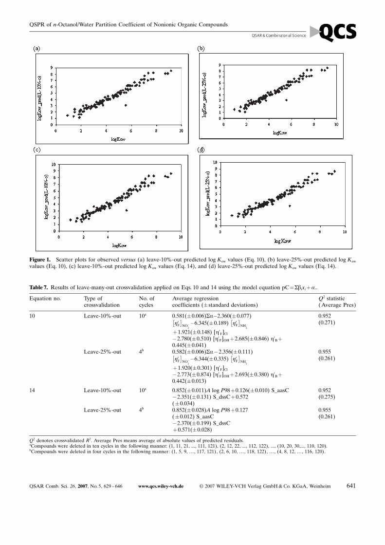
Based on LOO Q2 values, Eq. 10 is the best ETA modeland Eq. 14 is the best non-ETA model, which were furthervalidated using leave-10%-out and leave-25%-out crossva-lidation and the results are shown in Table 7. It is foundthat the average values of the regression coefficients of dif-ferent terms in different cycles of iterations do not varysignificantly from the corresponding original regressioncoefficient values of Eq. 10 or 14. Scatter plots of observedversus leave-10%-out and leave-25%-out predicted log -Kow values according to Eqs. 10 and 14 are shown in Fig-ure 1.

3.4.2 Splitting of the Dataset into Training and Test Sets

For the validation process, the dataset was divided intotraining and test sets. The log Kow data of the training setcompounds were modeled and the developed models wereused to predict the responses of the test sets. 25% (n¼30)of the total number of compounds in the dataset was usedas the test set and the remaining 75% (n¼92) as the train-ing set. The selection of the training and the test sets werebased upon three different algorithms [57]: random selec-tion, selection based on sorted response data, and selec-tion based on K-means clustering based upon the factorscores of the data matrix without the response variable.We have applied the combined set of descriptors for thefirst two methods while for the third method, ETA, non-ETA and combined set of descriptors were tried separate-ly.

3.4.2.1 Random Division

Initially the dataset was divided into training (n¼92) andtest (n¼30) sets in a random manner (three trials). TheQSPR models were generated using three different statis-tical methods (FA-MLR, stepwise regression, and PLS)and then validated using the test sets. We have selectedthe models based on the Q2 value and then validated theselected models through external validation to comparethe quality of internal validation (Q2) with that of externalvalidation (R2

Pred) for all the models. However, it was foundthat all the test sets selected through random trials pro-duced good external validation statistics, i.e., R2

Pred>0.9.For the first trial, Q2 and R2

Pred values are identical for FA-MLR and PLS and a bit higher for stepwise regression. Onthe contrary, for the second trial, the R2

Pred value exceedsQ2 in FA-MLR and PLS, and is almost similar to R2

Pred inthe case of stepwise regression. In the third trial, R2

Pred isinferior to Q2 in FA-MLR, whereas in stepwise regressionand PLS, the reverse happens. In all the three trials, the ex-ternal validation statistics (R2

Pred) of stepwise regressionwere found to be superior compared to those of the other





Table 7. Results of leave-many-out crossvalidation applied on Eqs. 10 and 14 using the model equation pC¼Sbixiþa..

Equation no. Type ofcrossvalidation

No. ofcycles

Average regressioncoefficients (� standard deviations)

Q2 statistic(Average Pres)

10 Leave-10%-out 10a 0.581(�0.006)Sa�2.360(�0.077)h0F

� �NO�

2

�6.345(�0.189) h0F

� �NH�

2

þ1.921(�0.148) [h’F]Cl�2.780(�0.510) [h’F]OHþ2.685(�0.846) h’Bþ0.445(�0.041)

0.952(0.271)

Leave-25%-out 4b 0.582(�0.006)Sa�2.356(�0.111)h0F

� �NO�

2

�6.344(�0.335) h0F

� �NH�

2

þ1.920(�0.301) [h’F]Cl�2.773(�0.874) [h’F]OHþ2.693(�0.380) h’Bþ0.442(�0.013)

0.955(0.261)

14 Leave-10%-out 10a 0.852(�0.011)A log P98þ0.126(�0.010) S_aasC�2.351(�0.131) S_dssCþ0.572(�0.034)

0.952(0.275)

Leave-25%-out 4b 0.852(�0.028)A log P98þ0.127(�0.012) S_aasC�2.370(�0.199) S_dssCþ0.571(�0.028)

0.955(0.261)

Q2 denotes crossvalidated R2. Average Pres means average of absolute values of predicted residuals.aCompounds were deleted in ten cycles in the following manner: (1, 11, 21, ..., 111, 121), (2, 12, 22, ..., 112, 122), ..., (10, 20, 30,..., 110, 120).bCompounds were deleted in four cycles in the following manner: (1, 5, 9, . . . , 117, 121), (2, 6, 10, . . . , 118, 122), . . . , (4, 8, 12, . . . , 116, 120).

Figure 1. Scatter plots for observed versus (a) leave-10%-out predicted log Kow values (Eq. 10), (b) leave-25%-out predicted log Kow

values (Eq. 10), (c) leave-10%-out predicted log Kow values (Eq. 14), and (d) leave-25%-out predicted log Kow values (Eq. 14).



techniques (FA-MLR and PLS). The compounds selectedas test compounds are listed in Table 8 and the R2, Q2, andthe R2

Pred for different trials are presented in Table 9.

3.4.2.2 Selection Based on Sorted log Kow Data

The dataset was sorted in an ascending manner based onlog Kow values, and then every fourth compound was as-signed as a test set compound (trial four). The test setcompounds are presented in Table 8. In this method the in-ternal validation statistics were better than the externalvalidation statistics. The statistics of the models based onthe sorted log Kow data are presented in Table 9.

3.4.2.3 Selection Based on K-means Clustering Techniqueusing Factor Scores of the Data Matrix Withoutlog Kow Values

Finally, we classified the dataset into clusters using the K-means cluster technique and the factor scores of the data-set without the log Kow values based only on the ETA de-scriptor space (trial five). Three factors could explain96.8% of the variance of the original data matrix. Consid-ering all the compounds, five clusters were derived usingthe SPSS software and the division of the compounds ac-cording to the clusters is presented in Table 10. About25% of compounds of each cluster were chosen as mem-bers of the test set. This has been applied for all the threesets of descriptors.


Table 8. Compounds selected for the test sets in random validation and based on sorted log Kow data.

Trial Test set (n¼30)

Selection based on random method1 5 8 12 13 16 18 25 29 32 34 37 45 53 55 59 63 76 79 80 81 88 90 93 96 97 98 100 107 108 1122 3 5 6 12 15 19 25 30 35 36 37 39 40 49 52 55 62 63 65 66 68 69 81 82 84 87 98 99 114 1173 2 6 10 15 16 17 24 26 30 31 35 36 37 43 63 64 69 72 74 76 83 84 85 108 110 113 115 116 117 121

Selection based on sorted log Kow data4 3 10 11 13 16 20 23 25 28 33 35 38 39 44 50 57 62 64 65 68 83 88 91 96 99 105 106 110 114 117

Table 9. Statistical quality of the developed models using various combinations of training and test sets and combined set of descrip-tors.

Modeling type FA-MLR Stepwise regression PLS

Trial R2 Q2 R2Pred R2 Q2 R2

Pred R2 Q2 R2Pred

Test set selection based on random method1 0.929 0.918 0.918 0.953 0.949 0.964 0.914 0.910 0.9122 0.919 0.907 0.922 0.952 0.949 0.945 0.912 0.908 0.9413 0.920 0.914 0.906 0.952 0.915 0.963 0.902 0.897 0.944Test set selection based on sorted log Kow data4 0.940 0.930 0.957 0.951 0.948 0.945 0.909 0.906 0.930

Table 10. K- means clustering using ETA descriptors space.

Clusterno.

Compounds present in each cluster Number of compounds in the cluster Number of compounds in test set

1 59 71 72 73 74 75 6 22 3 18 19 20 22 28 29 31 33 34 35 36 38 43 45 49 50 52 53 54 79 80 85 88 91 92 93 94 95 96 57 10

97 98 107 108 109 110 111 112 115 116 118 94 95 96 97 98 107 108 109 110 111 112 115 116 117 118 1223 32 39 40 41 42 44 46 47 48 51 55 56 60 61 62 63 64 65 77 114 20 54 57 58 66 67 68 69 70 76 8 25 1 2 4 5 6 7 8 9 10 11 12 13 14 15 16 17 21 23 24 25 26 27 30 37 78 81 82 83 84 86 45 11

87 89 90 99 100 101 102 103 104 105 106 113 119 120 121



3.4.2.3.1 ETA Indices

The R2Pred statistics obtained are excellent although inferior

compared to the Q2 values. However, the R2Pred obtained

from stepwise regression and PLS are identical, i.e.,(R2

Pred¼0.906). The statistics of the models based on theK-means clustering technique are presented in Table 11.Again, the predictive ability of the QSPR model devel-oped using stepwise regression was estimated according tothe method reported earlier [55]. The model was found tosatisfy both the conditions with [(R2�R0

2)/R2] and k beingequal to 0.000 and 1.024, respectively. The plots of ob-served versus predicted log Kow values with and without in-tercept are given in Figures 2a and 2b, respectively.

3.4.2.3.2 Non-ETA Indices

The R2Pred statistics are excellent but inferior to the Q

2 val-ues. The best R2

Pred value (0.914) is obtained from stepwiseregression. The statistics of the models based on the K-means clustering technique are presented in Table 11.Again, the predictive ability of the QSPR model devel-oped using stepwise regression was estimated according tothe method reported earlier [55]. The model was found tosatisfy both the conditions with [(R2�R0

2)/R2] and k beingequal to 0.001 and 1.031, respectively. The plots of ob-served versus predicted log Kow values with and without in-tercept are given in Figures 2c and 2d, respectively.


Figure 2. Plots of regression equations from observed versus predicted values for the cluster based test set compounds using modelsderived from stepwise regression: (a) with ETA descriptors (with intercept), (b) with ETA descriptors (without intercept), (c) withnon-ETA descriptors (with intercept), and (d) with non-ETA descriptors (without intercept).



3.4.2.3.3 ETA and Non-ETA Indices

Following the previous trend, the R2Pred statistics are excel-

lent but inferior compared to the Q2 values and once

again, the best statistics is obtained from stepwise regres-sion (R2

Pred¼0.914). The statistics of the models based onthe K-means clustering technique are presented in Ta-ble 11.


Table 11. Statistical quality of different models based on test set selected from clustering of data points using descriptor matrix with-out log Kow data.

Model FA-MLR Stepwise regression PLS

R2 Q2 R2Pred R2 Q2 R2Pred R2 Q2 R2Pred

ETA 0.966 0.961 0.887 0.974 0.970 0.906 0.966 0.961 0.906Non-ETA 0.946 0.939 0.834 0.971 0.965 0.914 0.968 0.965 0.902Combined 0.954 0.948 0.875 0.971 0.965 0.914 0.936 0.932 0.876

Table 12. Application of Eqs. 9 and 10 for prediction of log Kow values of external set of compounds.

Serial no. Compound name log Kow

Obs.a Calculated (Eq 9) Calculated (Eq 10)

01 4-Nitrophenol 1.91 3.03 2.9202 4-Chloro-2-nitrophenol 1.67 3.59 3.3903 2,4-Dintrophenol 2.46 3.72 3.5104 2-Nitroresorcinol 1.56 3.25 3.0905 4-Fluoro-2-nitrophenol 2.11 3.07 2.9306 4-Chlorophenol 2.39 2.97 2.8707 2,4-Dichlorophenol 3.06 3.51 3.3408 2-Bromo-4-methylphenol 2.95 3.83 3.5109 2-Hydroxy-5-chlorobenzoic acid 2.89 3.78 3.5710 4-Fluorophenol 1.91 2.63 2.5911 4-Methoxyphenol 1.58 3.00 2.8912 2-Methoxyphenol 1.32 3.00 2.8813 4-Methylphenol 1.94 2.8 2.7114 2,6-Dimethylphenol 2.36 3.19 3.0215 Salicylaldehyde 1.81 2.98 2.8816 4-Hydroxybenzaldehyde 1.35 2.98 2.8917 Salicylic acid 2.26 3.23 3.1118 4-Hydroxybenzoic acid 2.55 3.23 3.1119 Methyl 2-hydroxybenzoate 1.96 3.57 3.3820 Methyl 4-hydroxybenzoate 1.96 3.57 3.3921 Bisphenol A 1.65 5.62 5.2522 Bisphenol S 3.19 5.59 5.2523 Resorcinol 0.59 2.59 2.5524 Hydroquinone 0.88 2.59 2.5525 Pyrocatechol 0.16 2.59 2.5426 Pyrogallol 0.21 2.8 2.7127 3-Aminophenol 0.62 2.59 2.5128 2-Aminophenol 1.35 2.58 2.529 4-Hydroxyacetophenone 3.31 3.37 3.2130 4-tert-Butylphenone 3.35 3.87 3.6531 4-Phenoxyphenol 2.27 4.54 4.3332 3-Hydroxybenzoic acid 1.50 3.23 3.1133 2,6-Dihydroxyacetophenone 2.27 3.57 3.3734 2-Naphthol 2.70 3.68 3.5535 1-Naphthol 2.85 3.68 3.55Prediction statisticsb R2

Pred¼0.582 (Eq. 9) R2Pred¼0.651 (Eq. 10)

a From Ref. [56].

bR2Pr ed ¼ 1�P

Ypred Testð Þ�Y Testð Þð Þ2PY Testð Þ�Y trainingð Þð Þ2, Ypred(Test) and Y(Test) indicate predicted and observed log Kow values respectively of the test set compounds (n¼35) and

Ytraining indicate mean log Kow value (4.278) of the training set (n¼122).



3.4.3 Application of ETA Models on Purely External Da-taset

Equations 9 and 10 [FA-MLR and stepwise regressionmodels] obtained from ETA descriptors were used to pre-dict log Kow values of a purely external dataset [56] andthe predicted values along with predictive R2 statistics areshown in Table 12. The acceptable R2

Pred values indicate ap-plicability of the ETA models for calculation of log Kow

values for compounds of structural classes listed in Section2.1.

3.5 Overview of the Models

Of all the models developed using the entire dataset, wesuggest Eq. 10 (the stepwise regression model obtained us-ing ETA descriptors) to be the best with excellent statistics(R2¼0.960, R2

a¼0.958, Q2¼0.953, PRESS¼18.8). The se-lection has been made based on LOO Q2 values. There-fore, we have used Eq. 10 for calculating log Kow of all the122 compounds (Table 1). The ETA models suggest thatthe partition coefficient increases with molecular bulk anddegree of halogen substitution and decreases in the pres-ence of groups capable of hydrogen bonding and/or polarinteractions.A comparative study (Table 13) has been made on the

basis of the statistical qualities obtained from the three dif-ferent models (ETA, non-ETA and the combined set in-cluding both ETA and non-ETA descriptors) using FA-MLR, stepwise regression, PLS and PCRA as the statisti-cal tools. For each set of descriptors, the best equation sta-tistics were obtained using stepwise regression method(n¼122): ETA: R2¼0.960, R2

a¼0.958, Q2¼0.953, andPRESS¼18.8; non-ETA and combined : R2¼0.955, R2

a¼0.954, Q2¼0.952 and, PRESS¼19.1). The models ob-tained from non-ETA and combined descriptors usingstepwise regression method were identical. This may bedue to the inherent problem of stepwise regression, which

presumes that there is a single “best” subset of X variablesand seeks to identify it. However, there is often no uniquebest subset, and all possible regression models with a simi-lar number of X variables as in the stepwise regression so-lution should be fitted subsequently to study whethersome other subsets of X variables might be better. In othermethods (FA-MLR, PLS, and PCRA), the combined mod-els were better in statistical quality than the non-ETAmodels. However, in all statistical techniques, ETA modelswere better than or comparable to the non-ETA models(Table 13).We have also made an attempt to validate the models

externally based upon three different algorithms (randomselection, sorted response data and K- means CA) for se-lection of the training and test sets. The R2

Pred statisticswere found to be robust for all the three methods. This isbecause the test sets constructed using all the three algo-rithms contained data points which were representative ofthe training sets. Selected ETA models were also appliedon a purely external dataset (n¼35) to crosscheck the pre-dictive potential of the ETA models and acceptable pre-dictive R2 values were obtained.The log Kow values for all the studied compounds ranged

from 0.90 to 9.14, and 17% of the dataset have log Kow>6.We have correlated log Kow with log BCF (bioconcentra-tion factor) of the studied compounds (obtained from ref-erence [19]) and the R2 value was found to be 0.865 (n¼122), which indicates the dependence of bioconcentrationfactor on the partition coefficient.

Conclusions

The information presented in this paper shows that usingETA indices reliable prediction models were developedfor the n-octanol/water partition coefficient of aliphaticand aromatic compounds containing varied groups such as�CH3,�NO2,�Cl,�Br,�OH, and�NH2. This QSPR mod-el can be used to predict the log Kow values for compoundsthat have similar structural characteristics with the modelcompounds. This study suggests that ETA parameters aresufficiently rich in chemical information to encode thestructural features contributing significantly to the n-octa-nol/water partition coefficient of nonionic organic com-pounds. This indicates that ETA indices merit further as-sessment to explore their potential in QSAR/QSPR/QSTR modeling.

Acknowledgements

One of the authors (KR) thanks the All India Council forTechnical Education (AICTE), New Delhi, for financialassistance under the Career Award for Young Teachersscheme and Department of Science and Technology


Table 13. Comparison of statistical quality of different models(n¼122).

Model Statistical tools log Kow

R2 R2a Q2 PRESS

ETA FA-MLR 0.946 0.944 0.940 23.9Stepwise 0.960 0.958 0.953 18.8PLS 0.957 0.956 0.952 19.2PCRA 0.953 0.951 0.940 24.2

Non-ETA FA-MLR 0.911 0.908 0.906 37.7Stepwise 0.955 0.954 0.952 19.1PLS 0.953 0.969 0.949 20.2PCRA 0.949 0.945 0.912 35.0

Combined FA-MLR 0.935 0.933 0.928 28.7Stepwise 0.955 0.954 0.952 19.1PLS 0.950 0.859 0.947 21.1PCRA 0.957 0.956 0.953 18.9



(DST), Government of India, for awarding Fast TrackScheme for Young Scientists.

References

[1] G. Schuurmann, W. Klein, Chemosphere 1988, 17, 1551 –1574.

[2] T. Feijtel, P. Kloepper-Sams, K. Den Hann, R. Van Egmond,M. Comber, R. Heusel, P. Wierich, W. Ten Berge, A. Gard,W. Wolf, H. Niessen, Chemosphere 1997, 34, 2337 – 2350.

[3] C. Franke, G. Studinger, G. Berger, S. Bohling, U. Bruk-mann, D. Cohors-Fresenborg, U. Johncke, Chemosphere1994, 29, 1501 – 1514.

[4] L. Turne, F. Choplin, P. Dugard, J. Hermens, R. Jaeckh, M.Marsmann, D. Roberts, Toxicol. in vitro. 1987, 1, 143 – 171.

[5] L. Carlsen, J. D. Walker, QSAR Comb. Sci. 2003, 22, 49 – 57.[6] G. M. Swanson, H. E. Ratcliffe, L. J. Fisher, Regul. Toxicol.

Pharmacol. 1995, 21, 136 – 150.[7] H. Kubinyi, The quantitative analysis of structure-activityrelationships, in: M. E. Wolff (Ed.), Burger?s MedicinalChemistry and Drug Discovery, 5th Edn., Vol. I, John Wiley& Sons, New York, 1995, pp. 497 – 571.

[8] A. K. Ghose, V. N. Viswanadhan, J. J. Wendoloski, J. Phys.Chem. 1998, 102, 3762 – 3772.

[9] N. Bodor, Z. Gabanyi, C.-K. Wong, J. Am. Chem. Soc. 1989,111, 3783 – 3786.

[10] G. Klopman, S. Wang, J. Comput. Chem. 1991, 12, 1025 –1032.

[11] I. Moriguchi, S. Hirono, Q. Liu, I. Nakagome, Y. Matsushi-ta, Chem. Pharm. Bull. (Tokyo) 1992, 40, 127 – 130.

[12] A. Y. Sedykh, G. Klopman, J. Chem. Inf. Model. 2006, 46,1598 – 1603.

[13] M. Soskic, D. Plavsic, J. Chem. Inf. Model. 2005, 45, 930 –938.

[14] Y. In, H. H. Chai, K. T. No, J. Chem. Inf. Model. 2005, 45,254 – 263.

[15] A. A. Toropov, K. Roy, J. Chem. Inf. Comput. Sci. 2004, 44,179 – 186.

[16] E. A. Tehrany, F. Fournier, S. Desobry, J. Food Eng. 2004,64, 315 – 320.

[17] R. Mannhold, H. van de Waterbeemd, J. Comput. AidedMol. Des. 2001, 15, 337 – 354.

[18] B. Beck, A. Breindl, T. Clark, J. Chem. Inf. Comput. Sci.2000, 40, 1046 – 1051.

[19] M. T. Sacan, S. S. Erdem, G. A. Ozpinar, I. A. Balcioglu, J.Chem. Inf. Comput. Sci. 2004, 44, 985 – 992.

[20] K. Roy, G. Ghosh, Internet Electron. J. Mol. Des. 2003, 2,599 – 620, http://www.biochempress.com.

[21] K. Roy, G. Ghosh, J. Chem. Inf. Comput. Sci. 2004, 44,559 – 567.

[22] K. Roy, G. Ghosh, QSAR Comb. Sci. 2004, 23, 99 – 108.[23] K. Roy, G. Ghosh, QSAR Comb. Sci. 2004, 23, 526 – 535.[24] K. Roy, G. Ghosh, Bioorg. Med. Chem. 2004, 13, 1185 –

1194.[25] K. Roy, G. Ghosh, J. Mol. Model. 2006, 12, 306 – 316.[26] K. Roy, I. Sanyal, QSAR Comb Sci. 2006, 25, 359 – 371.[27] K. Roy, G. Ghosh, QSAR Comb. Sci. 2006, 25, 846 – 859.[28] K. Roy, I. Sanyal, P. P. Roy, SAR QSAR Environ. Res. 2006,

17, 563 – 582.[29] D. K. Pal, C. Sengupta, A. U. De, Indian J. Chem. 1988,

27B, 734 – 739.

[30] D. K. Pal, C. Sengupta, A. U. De, Indian J. Chem. 1989,28B, 261 – 267.

[31] D. K. Pal, M. Sengupta, C. Sengupta, A. U. De, Indian J.Chem. 1990, 29B, 451 – 454.

[32] D. K. Pal, S. K. Purkayastha, C. Sengupta, A. U. De, IndianJ. Chem. 1992, 31B, 109 – 114.

[33] R. Franke, Theoretical Aspects of Rational Drug Design,Elsevier, Amsterdam, 1984, 184 – 193.

[34] P. J. Lewi, Drug Design, Vol. 10, in: E. J. Ariens (Ed.), Aca-demic Press, New York, 1980, pp. 307 – 342.

[35] R. Franke, A. Gruska, Principal component and factor anal-ysis, in: H. van de Waterbeemd, (Ed.), Chemometric Meth-ods in Molecular Design, VCH, Weinheim, 1995, pp. 113 –163.

[36] G. W. Snedecor, W. G. Cochran, Statistical Methods, Oxfordand IBH Publishing Co. Pvt. Ltd., New Delhi, 1967.

[37] SPSS is statistical software of SPSS Inc., USA.[38] R. B. Darlington, Regression and Linear Models, McGraw-

Hill, New York, 1990.[39] S. Wold, in: H. van de Waterbeemd, (Ed.), Chemometric

Methods in Molecular Design, VCH, Weinheim 1995,pp. 195 – 218.

[40] MINITAB is statistical software of MINITAB Inc., USA.[41] The GW-BASIC programs KRETA1, KRETA2, KRPRES1

and KRPRES2 were developed by Kunal Roy and standar-dized using known datasets.

[42] Cerius 2 version 4.8 is a product of Accelrys Inc., San Die-go, CA.

[43] A. T. Balaban, C. Catana, M. Dawson, I. Niculescu –Duvaz,Rev. Roum. Chim. 1990, 35, 997 – 1003.

[44] L. B. Kier, L. H. Hall, Molecular Connectivity in Structure –Activity Analysis, Research Studies Press, Letchworth, Eng-land, 1986.

[45] L. B. Kier, Prog. Clin. Biol. Res. 1989, 291, 105 – 109.[46] L. B. Kier, L. H. Hall, Pharm. Res. 1990, 7, 801 – 807.[47] H. Wiener, J. Am. Chem. Soc. 1947, 69, 17 – 20.[48] C. Hansch, P. G. Sammes, J. B. Taylor, (Eds.), Comprehen-

sive Medicinal Chemistry, Pergamon, Oxford, 1990, Vol. 4.[49] J. Fox, Applied Regression Analysis, Linear Models, and Re-

lated Methods, Sage Publications, Thousand Oaks, CA,1997.

[50] S. Wold, L. Eriksson, Statistical Validation of QSAR Re-sults, in: H. van de Waterbeemd (Ed.), Chemometric Meth-ods in Molecular Design, VCH, Weinheim, 1995, pp. 312 –317.

[51] A. K. Debnath, Quantitative Structure-Activity Relationship(QSAR): A Versatile tool in Drug Design, in: A. K. Ghose,V. N. Viswanadhan (Eds.), Combinatorial Library Designand Evaluation, Marcel Dekker, Inc., New York, 2001,pp. 73 – 129.

[52] http://www.random.org/.[53] B. S. Everitt, S. Landau, M. Leese, Cluster Analysis, in: H.

van de Waterbeemd (Ed.), Chemometric Methods, EdwardArnold, London, 2001.

[54] R. B. Kowalski, S. Wold. Handbook of Statistics, North Hol-land Publishing Company, Amsterdam, 1982.

[55] A. Golbraikh, A. Tropsha, J. Mol. Graphics Model. 2002,20, 269 – 276.

[56] X. Wang, J. Yu, Y. Wang, L. Wang, Chemosphere 2002, 46,241 – 250.

[57] K. Roy, J. T. Leonard, QSAR Comb. Sci. 2006, 25, 235 – 251.




qspr of n-octanol/water partition coefficient of nonionic organic compounds using extended...

Documents