Modeling of QCM Data

Diethelm Johannsmann Institute of Physical Chemistry, Clausthal University of Technology Arnold-Sommerfeld-Str. 4, D-38678 Clausthal-Zellerfeld johannsmann@pc.tu-clausthal.de www.pc.tu-clausthal.de Table of Contents 1 Introduction ........................................................................................................................ 2 2 Complex Resonance Frequencies....................................................................................... 4 3 Assumptions of the Standard Model .................................................................................. 9 4 Wave Equations and Continuity Conditions: The Mathematical Approach .................... 10 5 The QCM as an Acoustic Reflectometer: The Optical Approach.................................... 13 6 Equivalent Circuits: The Electrical Approach ................................................................. 16 7 Relation Between the Frequency Shift and the Load Impedance .................................... 21 8 Layered Systems within the Small-Load-Approximation................................................ 23

8.1 Semi-Infinite Viscoelastic Medium ......................................................................... 23 8.1.1 Roughness ........................................................................................................ 25 8.1.2 The Sheet-Contact Model................................................................................. 25 8.1.3 Nematic Liquid Crystals................................................................................... 26 8.1.4 Colloidal Dispersions ....................................................................................... 26

8.2 Viscoelastic Film in Air ........................................................................................... 27 8.2.1 Purely Inertial Loading..................................................................................... 27 8.2.2 Viscoelastic Film.............................................................................................. 27 8.2.3 Derivation of Viscoelastic Constants ............................................................... 28

8.3 Viscoelastic Film in Liquid ...................................................................................... 30 8.3.1 Physical Interpretation of the Sauerbrey Thickness ......................................... 31 8.3.2 Comparison of Optical and Acoustic Reflectometry ....................................... 32 8.3.3 Information Contained in the D-f-ratio ............................................................ 33 8.3.4 Slip ................................................................................................................... 35 8.3.5 Roughness at the Film–Air Interface ............................................................... 35

8.4 Two Viscoelastic Films in Air ................................................................................. 36 8.5 Two Viscoelastic Films in Liquid ............................................................................ 36

9 Perturbation Analysis ....................................................................................................... 36 10 Contact Mechanics ....................................................................................................... 42

10.1 Mass Loading ........................................................................................................... 42 10.2 Loading with a Spring Attached to a Solid Wall ..................................................... 43 10.3 The Mass-Spring-Model .......................................................................................... 44 10.4 The Mass-Dashpot-Model........................................................................................ 45 10.5 Mass-Spring-Dashpot-Models ................................................................................. 46 10.6 Nonlinear Mechanics and Memory Effects.............................................................. 47

11 Concluding Remarks .................................................................................................... 47 12 Appendices ................................................................................................................... 49

12.1 Equivalent Circuit of a Viscoelastic Layer .............................................................. 49 12.2 Derivation of the Butterworth-van-Dyke Equivalent Circuit................................... 51 12.3 The Amplitude of Oscillation................................................................................... 54 12.4 The Effective Area ................................................................................................... 55 12.5 Piezoelectric Stiffening ............................................................................................ 56 12.6 The Parameter ff and the Fundamental Frequency................................................... 58

– 2 –

viscoelastic multilayers

QCM & SPRacoustic and optical thickness of adsorbates

colloidal dispersions

acoustic second- harmonic-generation

sphere−plate contactdry granular media

AFM / colloidal probeadhesion under HFshear excitation

Fig. 1: Different uses of the QCM

1 Introduction

The quartz crystal microbalance (QCM) is a well-known tool to measure film thicknesses in the nanometer range.1,2,3 It is difficult to imagine a device which is simpler than a quartz crystal resonator, and simplicity is one of the principle advantages of the QCM. A QCM is a disk of crystalline quartz. The disk displays acoustic resonances like any other three-dimensional body. As a resonator, it distinguishes itself from other resonators by a number of features:

- Since crystalline quartz is weakly piezoelectric, the acoustic resonances can be probed by electrical means. Otherwise, piezoelectricity is of minor importance.

- There are a number of acoustic modes, which can be well approximated by standing plain waves with the k-vector perpendicular to the crystal surface. For these plain-wave-modes, the crystal can be considered as laterally infinite. The only dimension of interest is the dimension perpendicular to the surface. One-dimensional models apply.4

- For certain crystal cuts the motion is of the thickness-shear type. Since the motion at the crystal surface then is in the surface plain, these modes do not emit longitudinal sound (or at least not very much of it). The weak acoustic coupling to the environment increases the Q-factor of the resonances to rather exceptional levels. The bandwidth is orders of magnitude smaller than the resonance frequency, which much simplifies the data analysis.

The classical sensing application of quartz crystal resonators is microgravimetry.1,5 Many commercial instruments are around. These devices exploit the “Sauerbrey relation”. For thin films, the resonance frequency is – by-and-large – inversely proportional to the total thickness of the plate. The latter increases when a film is deposited onto the crystal surface. Monolayer sensitivity is easily reached. However, when the film thickness increases, viscoelastic effects come into play, as was for instance recognized by Lu and Lewis, who derived a refined version of the Sauerbrey equation.6 These authors mainly intended to improve the micro-weighing procedure. Actually measuring viscoelastic properties with the QCM was not a major issue at the time. In the late 80’s, it was recognized that the QCM can also be operated in liquids, if proper measures are taken to overcome the consequences of the large damping.7,8 The ensuing problems and questions contributed much to the increased interest in non-gravimetric applications of the QCM.

Today, microweighing is only one out of many uses of the QCM (Fig. 1). The QCM can be viewed as an acoustic reflectometer, as a high-frequency interfacial rheometer, or as a micromechanical probe. In view of this diverse set of applications, it is helpful to describe the acoustic interaction between the crystal and the sample in a general way. This entails a certain mathematical effort. However, there are intuitive views for most cases. Regard-less of the complexity occurring in the intermediate steps of the calculation, simple relations are eventually found, which can be readily programmed in any of the standard software packages for data analysis. For instance, if the sample is a thin films in air, an advanced analysis (Eq. 8.14) can yield the viscous compliance of the film, Jf ''(ω). If the film is in a liquid environment, the elastic compliance of the film, Jf '(ω), is derived (Eq. 8.29). Eq. 8.14 and Eq. 8.29 are limiting cases to a viscoelastic model,

– 3 –

which today is well-established. Note that the “non-gravimetric” QCM by no means is an alternative to the conventional QCM. Viscoelastic modeling deepens our understanding of the conventional QCM and enhances the information derived from physical, chemical, or biological sensors based on quartz crystal resonators.

Although this chapter is mainly concerned with modeling, we briefly address a few experimental issues:

- Impedance analysis (Fig. 2), whereby the resonance curves are passively mapped out with a network analyzer, has in many ways laid the experimental ground for the viscoelastic modeling.9,10 With impedance analysis, both the frequency and the bandwidth of the resonance are accessible on a number of different overtones. Ring-down has been recently introduced as an alternative to impedance analysis.11 This technique (see section 2) also provides frequency and bandwidth and can do so on a number of harmonics.

- Oscillator circuits are a cost-efficient alternative to impedance analysis and ring-down.12,13 Naturally, most sensors run on oscillator circuits. Some advanced circuits provide a measure of the dissipation (such as the peak resistance, R1, see section 6) in addition to the frequency. Most oscillators operate on one harmonic only. Oscillators can be more stable then ring-down and impedance analysis because the latter two techniques periodically turn the crystal on and off in one way or another, whereas oscillators just run quietly on one fixed frequency. If the signal-to-noise ratio is the primary concern, no technique can beat oscillators. There is one pitfall with the use of oscillators worth mentioning: The theory below pertains to the series resonance frequency (simply called resonance frequency). The output frequency of an oscillator circuit, on the other hand, usually is not the series resonance frequency (Fig. 2). For instance, phase-locked-loop oscillators keep the phase constant. Many oscillators run at the zero-phase frequency (B ª 0, Fig. 2). Importantly, the difference between the zero-phase frequency and the series resonance frequency changes if the bandwidth or the parallel capacitance (section 6) change. The latter may happen as a consequence of fluctuating stray capacitances. Changes in bandwidth or parallel capacitance therefore induce a change in the frequency of oscillation which is not related to a shift of the (series) resonant frequency, which leads to artifacts.

- Because the QCM is so tremendously sensitive, factors of influence come into play, which can safely be ignored in other fields of physics. The correct interpretation of an experiment often is a challenge and supplemental information in addition to the frequency shift is helpful. Such information can, for instance, come from the comparison of the shifts of frequency and bandwidth at the different harmonics. The combination of the QCM with other surface-analytical techniques like electrochemical cyclovoltammetry,14,15,16 optical reflectometry,17 atomic force microscopy,18,19 or the colloidal probe20,21 has been pursued for the same reason. Particularly advanced is the electrochemical QCM (EQCM).

- While a stability of 10-9 and better is achieved with sealed resonators as they are usually employed in timing and frequency-control applications, a typical stability for resonators exposed to the environment is in the range of 10-8 – 10-7.

- The best agreement between theory and experiment is reached with planar, optically polished crystals for overtone orders between n = 5 and n = 13. On low harmonics, energy trapping22 is insufficient, while on high harmonics, anharmonic side bands interfere with the main resonance.23

- Admittedly, some of the amazing simplicity of quartz crystal resonators is lost, once the surfaces are covered with electrodes and the crystal is inserted into a holder. In this

– 4 –

chapter, we stick to an idealistic view and describe the modeling as if there were none of these complications. We do not touch upon compressional waves,24,25 effects of varying temperature or stress,26, 27 anharmonic side bands,23 roughness,28,29 bubbles and slip,30 and effects of a variable dielectric environment.31,32 Many of these effects are rather interesting. Some are, in fact, exploited for sensing. Still, they are outside the scope of this text.

Although this chapter is concerned with bulk acoustic wave (BAW) devices, some of the concepts apply to shear horizontal surface acoustic wave (SH-SAW) devices in a similar way.33,34 When modeling SH-SAW devices, one usually decomposes the wave vector into a vertical and a lateral component. The vertical component obeys similar laws as the shear wave in a BAW resonator. This being said, we confine the discussion to BAW devices (also termed thickness-shear resonators) in the following.

The most popular of BAW resonator is the quartz crystal microbalance (QCM). The name QCM correctly suggests that the main use of the QCM is microgravimetry. However, many researchers who use quartz resonators for other purposes, have continued to call the quartz crystal resonator “QCM”. We will follow this usage and call all quartz crystal resonators QCM. Actually, the term "balance" makes sense even for non-gravimetric applications if it is understood in the sense of a force balance. At resonance, the force exerted onto the crystal by the sample is balanced by a force originating from the shear gradient inside the crystal. This is the essence of the small-load-approximation (Eq. 7.3). Crystalline α–quartz is by far the most important material for thickness-shear resonators. Langasite (La3Ga5SiO14, “LGS”) and gallium-orthophosphate (GaPO4) are investigated as alternatives to quartz, mainly (but not only) for use at high temperatures.35,36 We also call these devices “QCM”, even though they are not made out of quartz (and may or may not be used for gravimetry).

2 Complex Resonance Frequencies

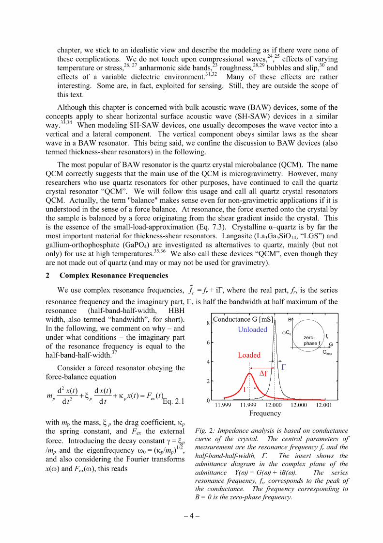
We use complex resonance frequencies, rf = fr + iΓ, where the real part, fr, is the series resonance frequency and the imaginary part, Γ, is half the bandwidth at half maximum of the resonance (half-band-half-width, HBH width, also termed “bandwidth”, for short). In the following, we comment on why – and under what conditions – the imaginary part of the resonance frequency is equal to the half-band-half-width.37

Consider a forced resonator obeying the force-balance equation

Eq. 2.1

with mp the mass, ξ p the drag coefficient, κp the spring constant, and Fex the external force. Introducing the decay constant γ = ξp /mp and the eigenfrequency ω0 = (κp/mp)1/2, and also considering the Fourier transforms x(ω) and Fex(ω), this reads

2

2

d ( ) d ( ) ( ) ( )d dp p p ex

x t x tm x t F tt t

+ ξ + κ =

Frequency 11.999 11.999 12.000 12.000 12.001

0

2

4

6

8

Γ ∆f

Unloaded

Loaded

Γ

Conductance G [mS]

frzero-phase f G

B

ωC0

Gmax

Fig. 2: Impedance analysis is based on conductance curve of the crystal. The central parameters of measurement are the resonance frequency fr and the half-band-half-width, Γ. The insert shows the admittance diagram in the complex plane of the admittance Y(ω) = G(ω) + iB(ω). The series resonance frequency, fr, corresponds to the peak of the conductance. The frequency corresponding to B = 0 is the zero-phase frequency.

– 5 –

Eq. 2.2

We now introduce the variables f = ω/(2π), fr = ω0/2π and Γ = 1/2 γ/(2π). The factor of 1/2 in the latter definition is essential. Assuming that the resonance is narrow (Γ á fr) one may approximate 2iΓf by 2iΓfr and write

Eq. 2.3

The small term Γ2 has been added to the denominator in step 3. As Eq. 2.3 shows, the bandwidth can been absorbed into a complex resonance frequency, rf , if one chooses the real part as fr and the imaginary part as Γ. Since the crystal cannot be excited with a complex frequency, the denominator always remains nonzero and the amplitude x(f) remains finite. Allowing for complex resonance frequencies is a convenient way to include the bandwidth into all equations.

It is instructive to go through a similar set of equations in the time domain. Assume that the excitation of the resonance is carried out with a sharp radio frequency pulse (rather than a continuous sine wave). After the excitation has been turned off, the resonator rings down according to a decaying complex exponential:

Eq. 2.4

Since Fex = 0, Eq. 2.1 requires that

Eq. 2.5

and further, since x0 ≠ 0:

Eq. 2.6

which, for γ á ω0, is solved by

Eq. 2.7

Again, the imaginary part of rω is one half of the decay constant, γ, provided that the resonance is sharp. Sharp resonances are always found for the QCM. A quick estimate shows that the error caused by neglecting γ2/4 in comparison to ω0

2 in Eq. 2.7 is negligible in all cases of practical interest. The complex resonance frequency, rf , also describes the ring-down of a freely oscillating resonator. Since the decay time τ is equal to (2πΓ)−1, Γ can be determined by ring-down experiments just as well as by mapping out the resonance curve with an impedance analyzer.

2 20

( ) 1( ) i

p

ex

m xF

ω=

ω ω − ω + γω

( )

2

2 2 2 2 2 2 2

2 2 22

4 ( ) 1 1 1( ) 2i 2i 2i

1 1i

p

ex r r r r r

rr

m x fF f f f f f f f f f f

f ff f

π≈ ≈ ≈

− + Γ − + Γ − + Γ − Γ

= =−+ Γ −

( ) ( ) ( )0 0( ) exp i exp 2 i exp 2r rx t x t x f t t= ω = π − πΓ

( ) ( )( )20i exp 2 i 0p r p r p rm x t− ω + ξ ω + κ π ω =

2 20i 0r rω − γω − ω =

220 0

i i2 4 2rγ −γ γ

ω = ± + ω ≈ ±ω +

– 6 –

The time-domain description and the frequency-domain description are connected via the Greens-function formalism. For an arbitrary functional form of the excitation, Fex(t), one has

Eq. 2.8

where the Greens function G(t–t') obeys the relation

Eq. 2.9

δ(t–t') is the Dirac δ-function. Requiring that the left-hand-side of Eq. 2.9 is zero for t ≠ t' yields:

Eq. 2.10

where G0 is prefactor to be determined below and θ(t–t') is the step function (θ(t-t') = 0 for t<t' and θ(t–t')=1 otherwise. The use of the step function ensure causality. For t = t' we find

Eq. 2.11

The second line of Eq. 2.11 makes use of the fact that only the derivative of θ(t-t')' = δ(t-t') contributes to the integral. The step function itself as well as its second derivative vanish after integration and taking the limit εØ0. Eq. 2.11 shows that

Eq. 2.12

We now assume a sinusoidal excitation Fex(t') = F0 exp(iωt'). Inserting this excitation into Eq. 2.8 we find

( ) ( ) ( )' ' 'exx t G t t F t dt∞

−∞

= −∫

( )2

2

d ( ') d ( ') ( ') 'd dp p p

G t t G t tm G t t t tt t

− −+ ξ + κ − = δ −

( ) ( )( ) ( )0' exp i ' 'rG t t G t t t t− = ω − θ −

{ }

( )

2

20

0 0

0

d ( ') d ( ')1 lim ' ( ')d ' d '

lim ' 2i ( ') ( ')

2i

p p p

p r p

p r p

G t t G t tdt m G t tt t

G dt m t t t t

G m

ε

ε→−ε

ε

ε→−ε

− −= + ξ + κ −

≈ ω δ − + ξ δ −

= ω + ξ

∫

∫

01

2i p r p

Gm

=ω + ξ

– 7 –

Eq. 2.13

where x0 is the amplitude of motion. Using γ ≈ 2Γ, expanding the denominator, neglecting terms quadratic in Γ, and using f ≈ fr yields

Eq. 2.14

which reproduces Eq. 2.3.

The Greens-function formalism is of importance in the context of advanced pulse sequences for driving the crystal. It shows that the response of the crystal to a change of driving conditions will occur on a time scale of about 1/(2πΓ). Note, however, that a response to a change in the crystal properties (for example a change in κp caused by a contact with an external object, cf. section 10) is instantaneous. The parameters G0, mp, rω , and ξp in Eq. 2.10 and Eq. 2.12 then acquire an explicit time dependence.

In this chapter, the half-band-half-width, Γ, is used to quantify dissipation. Other common parameters are the quality factor, Q, and the dissipation11 D = Q-1. Q is defined as

Eq. 2.15

which implies that

Eq. 2.16

These other measures of dissipation are completely equivalent to the bandwidth. It is entirely a matter of taste which variable to use.

2

r

DfΓ

=

2rfQ =Γ

( ) ( )( ) ( ) ( )

( ) ( )( )

( ) ( ) ( )( )

( ) ( ) ( )

( )( ) ( ) ( )

0

0

0

0

02

1 exp i ' ' exp i ' '2i

exp i exp i ' '2i

1 exp i exp i '2i i

exp i2 +i

1 exp i4 2 i i +i i

rr p p

t

r rr p p

t

r rr p p r

p r r p r

p r r r

x t t t t t F t dtm

F t t dtm

F t tm

F tm

F tm f f f f f

∞

−∞

−∞

−∞

= ω − θ − ωω + ξ

= ω ω− ωω + ξ

= ω ω− ω ω + ξ ω− ω

= ω− ω ω− ω ξ ω− ω

≈ ωπ − + Γ − − Γ γ − − Γ

∫

∫

( )0: exp ix t= ω

( )( ) ( ) ( ) ( )

( )( )

( )

2

0

2 2

4 12 2i 2i +2i

12i

12i

p

r r r r r

r r

r

m x fF f f f f f f f f

f f f f f

f f f

π≈

ω − − − Γ − + Γ Γ −

≈− + − + Γ

=− + Γ

– 8 –

The motional resistance, R1, (section 6) is also used as a measure of dissipation. R1 is an output parameter of some instruments based on advanced oscillator circuits. However, experiments based on impedance analysis show that R1 usually is not strictly proportional to the bandwidth (although it should, according to BvD circuit, cf. section 12.4). Also, in absolute terms, R1 – being an electrical quantity and not a frequency – is affected by calibration problems much more than the bandwidth. In the author’s opinion, Γ or D are better measures of dissipation than R1.

Even though getting used to a complex resonance frequency takes some exercise, one is rewarded later on with a reduction in the number of equations by a factor of two. Just about every single equation below (concerning load, impedance, speed of sound, wave vector, resonance frequency, shear modulus, or shear compliance) can be formulated with complex parameters, where the imaginary part quantifies a loss of energy. Consistently using complex variables (including complex resonance frequencies) much simplifies the algebra.

At this point, we introduce a convention: A traveling wave u(z, t) shall be of the form

Eq. 2.17

where “c.c.” denotes the complex conjugate and is usually omitted. We could have equally well written ( )( ),0( , ) exp i c.c.u z t u t kz± ±= − ω ± + because after adding the complex

conjugate, it does not matter whether the time dependence has the form exp(iωt) or exp(–iωt). However, it is helpful to stick to exp(+iωt) and to certain other sign conventions, as well, in order ensure that dissipative processes always increase the entropy and never decrease it. These sign conventions are: G = G’ + iG’’ for the shear modulus, J = J’ – i J’’ for the shear compliance, Z = Z’ + iZ’’ for the acoustic impedance, ε = ε’ – i ε’’ for the dielectric constant, k = ± k’ – i k’’ for the wave vector, c = c’ + ic’’ for the speed of sound, and η = η’ – iη’’ for the viscosity. Using the above conventions, all quantities with two primes are positive as long as the corresponding processes comply with the second law of thermodynamics.38

In the following, all variables which are connected to viscoelasticity in one way or another (such as G, J, k, c, or Z) are considered complex. An exception are the parameters Gq, kq, cq, and Zq which pertain to the quartz crystal. These parameters, as well as the frequency of the fundamental, ff, are considered to be real in order to conform with the current usage in the literature. One can also define them as complex (which they are, in principle, although the imaginary parts are much smaller than the real parts). When any of the parameters Gq, kq, cq, and Zq are meant to be complex, they attain a tilde (~). Even when they are complex, the ratios ( )/ 2q fc f and ( )/ 2q fZ f (leading to the thickness of the crystal dq and the mass per

unit area of the crystal, mq) will be real. Frequencies and spring constants are real, unless they have a tilde ( rf , 0f , rω , f∆ , pκ ). The overtone order, n, never is complex. The overtone

order is meant to be the nearest integer to rf /ff . In some cases, it makes sense to define n as

the real part of rf / ff . Since overtones are always slightly displaced from the exact integer

multiples of the fundamental, rf / ff is not exactly an integer. The deviation is small and, further, the context will make it clear whether accuracy can be gained by considering n a real number (close to an integer), rather than an integer.

( )( ),0( , ) exp +i c.c.u z t u t kz± ±= ω ± +

– 9 –

3 Assumptions of the Standard Model A standard model has emerged for the calculation of the resonance frequencies of quartz

crystal resonators coated with planar layers.39,37,40,41,42 We first summarize the assumptions entering the model:

i) The resonator and all cover layers are laterally homogeneous and laterally infinite.

ii) The distortion of the crystal is given by a transverse plain wave with the k-vector perpendicular to the surface normal (thickness-shear mode). There are neither compressional waves24 nor flexural contributions to the displacement pattern.43 There are no nodal lines in the plane of the resonator. The standard model ignores anharmonic side bands (spurious modes).23

iii) All stresses are proportional to strain. Linear viscoelasticity holds.44

iv) The voltage across the crystal is a boundary condition controlled by the experimentalist. The current through the electrodes is the primary parameter of the measurement.

These assumptions deserve a few comments. Assumptions i) and ii) are interrelated and not fulfilled in practice. In order to be able to mount the crystal in a holder touching its rim, “energy trapping”22 is employed. One confines the oscillating region to the center of the plate by making the crystal slightly thicker in the center than at the rim. The resonator then acts as a small acoustic lens, which focuses the acoustic beam to the center of the plate. An increased thickness at the center can, for instance, be achieved with key-hole shaped back electrodes or, alternatively, with plane-convex crystals. There is an analytical treatment of energy trapping with plane–convex crystals by Stevens and Tiersten.45 Finite element calculations are being done,46 but their routine use at this point seems difficult. Importantly, energy trapping induces flexural contributions to the pattern of motion as well as compressional waves,47,48 which is a problem with the use of the QCM in liquids. Because laterally heterogeneous samples are of tremendous importance in the practice, we treat them briefly in sections 8.1.2 and 10.

Assumptions i and ii constitute a practical requirement for the construction of resonators in the sense that resonators perform poorly if the width-to-thickness ratio is less than about 30. This condition severely restricts the design options when it comes to miniaturization and array sensors. Violations of assumptions i and ii are tolerable only to a certain extent.

Linear viscoelasticity (assumption iii) is obeyed as long as the driving voltage is small enough. In air, a drive level of –5 dBm (170 mVrms) usually is safe.49 In liquids, higher drive levels (resulting in a better signal-to-noise ratio) can be tolerated because the motion is more strongly damped and the peak amplitude is not as high as in air. The main source of a drive-level-dependence of the resonance parameters is an elastic anharmonicity of the crystal.44,50 Heating also plays a role. Linear viscoelasticity is often violated in contact mechanics experiments (section 10) because interfacial friction is a strongly nonlinear phenomenon.

Assumption iv is not fulfilled in practice, either, because the electrical circuitry probing the crystal has finite output and input impedance. Nevertheless, since the calculations provide the electrical impedance of the crystal, the electrical circuitry can be accounted for by using the appropriately extended electrical circuit in the analysis. When using impedance analysis, proper calibration of the impedance analyzer takes care of the additional electric circuit elements to a large extent.51

It turns out to be advantageous to interface the crystal to an electronic circuitry with low impedance. Because of piezoelectric stiffening (section 12.5) the crystal responds rather sensitively to stray capacitances between the electrodes. The influence of stray capacitances can be lowered by connecting the two electrodes across a small resistor (typically 14.2 ohms).

– 10 –

The resistor short-circuits the stray capacitances. Such an electrical separation from the environment is achieved by means of a π-network.52 However, the π-network also short-circuits the connection between the crystal and the driving electronics to some extent (effectively acting as a 15 dB attenuator), thereby decreasing the signal-to-noise ratio.

4 Wave Equations and Continuity Conditions: The Mathematical Approach The chapter describes the canonical

mathematical way of finding the resonance frequencies of coated quartz crystals. It is described in detail in Ref. 53. The wave equations for the different layers and the boundary conditions at the interfaces between the layers form a homogeneous system of linear equations, which can only be solved if the determinant of the system is zero. Since the determinant depends on frequency, the zeros of the determinant lead to the resonance frequencies.

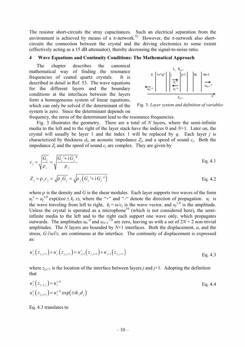
Fig. 3 illustrates the geometry. There are a total of N layers, where the semi-infinite media to the left and to the right of the layer stack have the indices 0 and N+1. Later on, the crystal will usually be layer 1 and the index 1 will be replaced by q. Each layer j is characterized by thickness dj, an acoustic impedance Zj, and a speed of sound cj. Both the impedance Zj and the speed of sound cj are complex. They are given by

Eq. 4.1

Eq. 4.2

where ρ is the density and G is the shear modules. Each layer supports two waves of the form uj

± = uj±,0 exp(i(ωt ± kj x), where the “+” and “–“ denote the direction of propagation. uj

– is the wave traveling from left to right, kj = ω/cj is the wave vector, and uj

±,0 is the amplitude. Unless the crystal is operated as a microphone54 (which is not considered here), the semi-infinite media to the left and to the right each support one wave only, which propagates outwards. The amplitudes u0

-,0 and uN+1+,0 are zero, leaving us with a set of 2N + 2 non-trivial

amplitudes. The N layers are bounded by N+1 interfaces. Both the displacement, u, and the stress, G ∂u/∂z, are continuous at the interface. The continuity of displacement is expressed as:

Eq. 4.3

where zj,j+1 is the location of the interface between layers j and j+1. Adopting the definition that

Eq. 4.4

Eq. 4.3 translates to

' i ''j j jj

j j

G G Gc

+= =

ρ ρ

( )' i ' 'j j j j j j j jZ c G G G= ρ = ρ = ρ +

( ) ( ) ( ) ( ), 1 , 1 1 , 1 1 , 1j j j j j j j j j j j ju z u z u z u z+ − + −+ + + + + ++ = +

( )( ) ( )

,01,

,0, 1 exp i

j j j j

j j j j j j

u z u

u z u k d

± ±−

± ±+

=

= ±

0 1="q" j j+1 N+1N

u0+,0 uj

+,0uN+1

-,0uj

-,0

zzj,j+1

Sj,j+1Lj

Fig. 3: Layer system and definition of variables

– 11 –

Eq. 4.5

The continuity of stress is expressed as

Eq. 4.6

Using relations Eq. 4.4 and Eq. 4.5 as well as k = ω/c = ω (ρ/G)1/2 = ω Z/G, Eq. 4.6 can also be written as

Eq. 4.7

Eq. 4.7 illustrates why the acoustic impedance is of such fundamental importance in the physics of the QCM. The acoustic impedance governs the condition of stress continuity, and thereby the reflectivity at acoustic interfaces.

Eq. 4.5 and Eq. 4.7 constitute a homogenous system of 2N+2 linear equations. A non-trivial solution for the set of amplitudes {uj

±,0} only exists if the determinant of this equation system vanishes. The search for the zeros of the determinant as a function of frequency will in general be carried out numerically. The zeros define the resonance frequencies. Since, for a real material, the shear modulus always contains a dissipative component, G’’, the resonance frequencies are complex (where the imaginary part is the half-band-half-width, Γ).

Let’s consider a simple example. For the bare crystal in air, the number of layers is equal to 1 and the adjacent bulk media have vanishing impedance (Z0=0, Z2=0). Here and in the following, we neglect the impedance of air and treat air and vacuum as the same. Comparing measurements in air and vacuum, one in fact does find a slight difference (which we neglect).55 We use the index "q" instead of "1" because the first layer is the quartz crystal. The resulting set of equations is

Eq. 4.8

Eq. 4.9

Eq. 4.10

Eq. 4.11

In matrix notation this reads as

Eq. 4.12

Requiring that the determinant of this system be zero amounts to

( ) ( ),0 ,0 ,0 ,01 1exp i exp ij j j j j j j ju k d u k d u u+ − + −

+ ++ − = +

( ) ( ) ( ) ( ), 1 , 1 1 1 1 , 1 1 , 1i ij j j j j j j j j j j j j j j jG k u z u z G k u z u z+ − + −+ + + + + + + +

− = −

( ) ( ),0 ,0 ,0 ,01 1 1exp i exp ij j j j j j j j j jZ u k d u k d Z u u+ − + −

+ + + − − = −

,0 ,0 ,00 q qu u u+ + −= +

,0 ,00 q q qZ u u+ − = −

( ) ( ),0 ,0 ,02exp i exp iq q q q q qu k d u k d u+ − −+ − =

( ) ( ),0 ,0exp i exp i 0q q q q q q qZ u k d u k d+ − − − =

( ) ( )( ) ( )

,00

,0

,0

,02

1 1 1 00 0

00 exp i exp i 1

0 exp i exp i 0

q qq

q q q q q

q q q q q q

uZ Z u

k d k d uuZ k d Z k d

+

+

−

−

− − = − − − −

– 12 –

Eq. 4.13

or equivalently

Eq. 4.14

where the overtone order, n, is an integer.56 Eq. 4.14 is the well-known resonance condition for a bare plate in vacuum. The displacement pattern is given by a standing wave with antinodes at the surfaces. For the fundamental, the wavelength is twice the crystal thickness. The surfaces are stress-free with vanishing gradients ∂u/∂z. The overtone order may be even or odd. However, only odd harmonics can be excited electrically.57

For later use, we rewrite Eq. 4.14 in two different ways. Calling the frequency of the fundamental ff, (n = 1, see section 12.6) we find:

Eq. 4.15

Eq. 4.16

where mq is the mass per unit area of the crystal, and ρq is the density.

Let’s assume that a thin film of thickness df á dq has been coated onto the crystal surface. Let the film have the same acoustic properties as the crystal. Adding a film of identical properties amounts to a thickening of the plate. This system may still be modeled as a single layer. If the properties of the film were to be different from the properties of the crystal, we would need to repeat the full analysis with two layers instead of one. The discussion of the viscoelastic film with arbitrary properties is the deferred to section 8.2.

For a film which has the exact same acoustic properties as the crystal, the shift in resonance frequency is predicted as

Eq. 4.17

Here and in the following 0f is the resonance frequency of the crystal in the reference state (which usually is the uncoated state). mf and mq are the areal mass densities (mass per unit area) of the film and the crystal, respectively. The relation df /dq = mf /mq evidently requires that the density of the film and the crystal are the same. It will turn out that the normalized frequency shift is the same as the ratio of the areal mass densities for all thin films regardless of their acoustic properties. Therefore one may memorize the relation 0/f f∆ = -mf /mq right here. Note that this “Sauerbrey limit” only holds for films much thinner than the wavelength of sound, λ.

Using Eq. 4.16 for the parameter mq, we arrive at the famous Sauerbrey equation:

( ) ( )2 2exp i exp i 0q q q q q qZ k d Z k d− − =

rq

q q

nkc dω π

= =

0

f f

q q

d mfd mf

∆≈ − = −

12

qq

f

cd

f=

1 12 2

q q qq q q

f f

c Zm d

f fρ

= ρ = =

– 13 –

Eq. 4.18

Zq is the acoustic impedance of AT-cut quartz. Its value is 8.8 µ 106 kg m-2 s-1. Strictly speaking, Zq is a complex quantity Zq' + iZq'', where Zq'' accounts for internal friction. Zq is often considered to be real. When this happens, the fundamental frequency ff must also be a real number (see end of section 2 as well as section 12.6). The Sauerbrey equation fails to account for viscoelasticity and also, when applied in liquids, cannot distinguish between the adsorbed material itself and solvent trapped inside the adsorbed film. When a mass is derived by means of the Sauerbrey equation, the interpretation of this mass parameter is sometimes difficult. The terms “Sauerbrey mass” and “Sauerbrey thickness” are used in order to indicate that the respective parameters have been calculated by means of the simple Sauerbrey equation.

The derivation above ignores piezoelectricity (section 12.5). The theory of the piezoelectric plate has been worked out by Tiersten.58 Kanazawa has applied this theory rigorously to the case of a crystal loaded with a liquid or a viscoelastic film.53 These treatments are equivalent to the treatment with equivalent circuits (section 6), and we therefore defer the discussion of piezoelectricity to this chapter.

5 The QCM as an Acoustic Reflectometer: The Optical Approach The procedure described in section 4 is mathematically straight-forward, but – on the

other hand – it is somewhat technical. Applying the formalism to multilayers leads to awkwardly large determinants (cf. Eq. 4.12). Searching the zeros of these determinants certainly is possible, but the procedure is tedious and the physics is somewhat obscured by these numerical calculations. Two other formulations are around. These make use of analogies to the theory of optical reflectivities and to equivalent electrical circuits. With regard to the outcome, these theories are completely equivalent to the strictly mathematical formulation. It is just a matter of language and graphical representation. The alternative formulations provide an intuitive insight and we therefore discuss them both.

Within an optics-type approach, one considers the resonator as an acoustic cavity. The term "acoustic" in this context always pertains to shear waves, never to longitudinal waves. This distinction is important: in liquids, shear waves are evanescent because the elastic part of the shear modulus is zero. Shear waves therefore provide for surface specificity. Longitudinal waves, on the contrary, propagate because the elastic component of the compressional modulus is nonzero.

Resonances occur if the time required for one round-trip is an integer multiple of the period of oscillation. In this case, there is constructive interference and the amplitude becomes large. In order to calculate the time needed for one round-trip we need to know the set of layer thicknesses, {dj}, wave vectors, {kj}, and reflectivities at the interfaces (Fig. 3). Let’s calculate the reflectivity ra,b = ua

+,0 / ua-,0 of a single interface between media termed “a”

and “b”. We have ua-,0 = 1 and ub

+,0 = 0. The analog of Eq. 4.3 and Eq. 4.7 is

Eq. 5.1

Eq. 5.2

Eliminating ub-,0, one finds

02f

f q

ff mf Z∆

≈ −

,0 ,0 ,0a a bu u u+ − −+ =

,0 ,0 ,0a a a b bZ u u Z u+ − − − =

– 14 –

Eq. 5.3

This relation is reminiscent of the reflectivity of optical waves impinging vertically onto a dielectric interface. The optical reflectivity r is given by r = (na–nb)/(na+nb), where na and nb are the indices of refraction. In acoustics, the acoustic impedance, Z = (ρG)1/2, takes the role of the refractive index. Note, however, that this analogy has its limitations. In optics, the refractive index governs both the reflectivity at interfaces and the speed of light. This happens because the magnetic permeability (the analog of the density) is about equal to unity at optical frequencies. In acoustics, it is not quite as easy. Also, strictly speaking, n is not the optical impedance, but the inverse ratio of the optical impedances of the medium and air. Finally, refractive indices typically vary by a few percent. Typical optical reflectivities (of – let’s say – the water surface) therefore also are in the range of a few percent. The acoustic shear impedance, on the other hand, can easily vary by a factor of 10 or more because the shear modulus may vary by orders of magnitude. As a consequence, acoustic reflectivities easily approach unity even for rather similar materials (section 8.3.2).

Let’s apply the optical approach to a single plate in vacuum. The amplitude of the wave after one round trip, u(1), is given by

Eq. 5.4

where u(0) is the initial amplitude, and r is the reflectivity. Since both Z0 and Z2 vanish, we have rq,2 = rq,0 = 1 and the condition of constructive interference is

Eq. 5.5

The argument of the exponential must be an integer multiple of 2πi, leading to

Eq. 5.6

which is the familiar resonance condition.

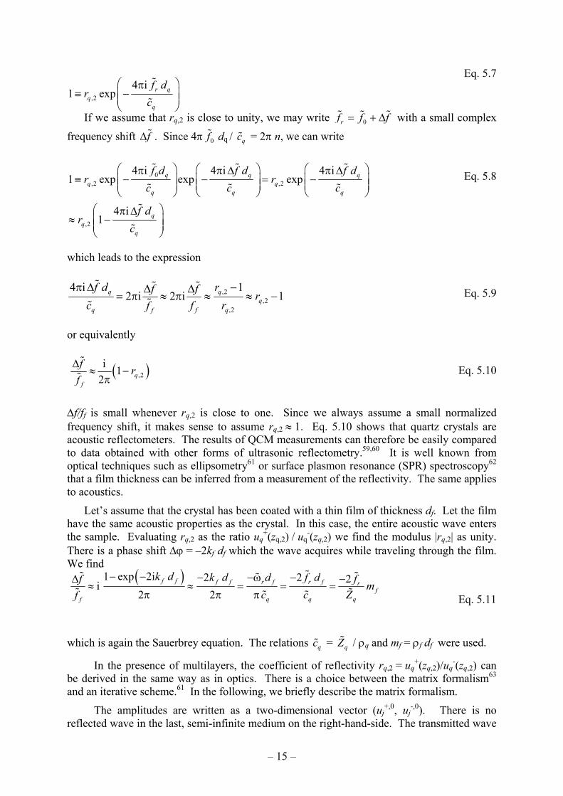
Now let’s assume that the reflectivity at the front surface, rq,2 is slightly different from unity. The absolute value may be smaller than unity because some energy may be dissipated inside the sample. Also, there may be a phase shift because a certain part of the wave enters the sample, returns, and superimposes itself onto the wave reflected at the crystal surface (Fig. 4). The resonance condition then is

,0

, ,0a a b

a ba a b

u Z Zru Z Z

+

−

−= =

+

( ) ( )(1) (0),2 ,0exp i exp iq q q q q qu u k d r k d r= − −

( )(0) (1) (0) (0)

(0) (0)

(0)

2iexp 2i exp

4 i4 iexp exp

4 iexp

rq q q

q

r qrq q

q q

r qq

q

u u u k d u dc

ffu d u dc G

fu d

Z

− ω≡ = − = =

− π ρ − π = =

− π ρ=

12 2 2 2

q q q qr

q q q q q q

nc G n Z n Znfd d d m

= = = =ρ ρ

resonance condition :∆φ =2 π n

bare crystal

loaded crystal

Fig. 4: The frequency shift depends on the acoustic reflectivity at the quartz–sample interface.

– 15 –

Eq. 5.7

If we assume that rq,2 is close to unity, we may write 0rf f f= + ∆ with a small complex

frequency shift f∆ . Since 4π 0f dq / qc = 2π n, we can write

Eq. 5.8

which leads to the expression

Eq. 5.9

or equivalently

Eq. 5.10

∆f/ff is small whenever rq,2 is close to one. Since we always assume a small normalized frequency shift, it makes sense to assume rq,2 ≈ 1. Eq. 5.10 shows that quartz crystals are acoustic reflectometers. The results of QCM measurements can therefore be easily compared to data obtained with other forms of ultrasonic reflectometry.59,60 It is well known from optical techniques such as ellipsometry61 or surface plasmon resonance (SPR) spectroscopy62 that a film thickness can be inferred from a measurement of the reflectivity. The same applies to acoustics.

Let’s assume that the crystal has been coated with a thin film of thickness df. Let the film have the same acoustic properties as the crystal. In this case, the entire acoustic wave enters the sample. Evaluating rq,2 as the ratio uq

+(zq,2) / uq-(zq,2) we find the modulus |rq,2| as unity.

There is a phase shift ∆ϕ = –2kf df which the wave acquires while traveling through the film. We find

Eq. 5.11

which is again the Sauerbrey equation. The relations qc = qZ / ρq and mf = ρf df were used.

In the presence of multilayers, the coefficient of reflectivity rq,2 = uq+(zq,2)/uq

-(zq,2) can be derived in the same way as in optics. There is a choice between the matrix formalism63 and an iterative scheme.61 In the following, we briefly describe the matrix formalism.

The amplitudes are written as a two-dimensional vector (uj+,0, uj

-,0). There is no reflected wave in the last, semi-infinite medium on the right-hand-side. The transmitted wave

,2

4 i1 exp r q

qq

f dr

c π

≡ −

0,2 ,2

,2

4 i 4 i 4 i1 exp exp exp

4 i1

q q qq q

q q q

qq

q

f d f d f dr r

c c c

f dr

c

π π ∆ π ∆≡ − − = −

π ∆

≈ −

,2,2

,2

4 i 12 i 2 i 1q q

qq f qf

f d rf f rc f rf

π ∆ −∆ ∆= π ≈ π ≈ ≈ −

( ),2i 1

2 qf

f rf

∆≈ −

π

( )1 exp 2i 2 2 2i2 2

f f f f r f r f rf

q q qf

k d k d d f d ff mc c Zf

− − − −ω − −∆≈ ≈ = = =

π π π

– 16 –

in this medium uN+1-,0 is normalized to unity. The vector of amplitudes in this medium

therefore is (0, 1). The vector (uj+,0, uj

-,0) at any other location is related to the wave amplitudes at the right end of the layer system via transfer matrices (Fig. 3). There are transfer matrices for the layers ( jL ) and for the interfaces ( , 1j jS + ). The amplitudes are calculated as

Eq. 5.12

For the matrix jL , one has

Eq. 5.13

where kj is the wave vector and dj is the thickness. , 1j jS + takes care of reflection at interfaces. One has

Eq. 5.14

where Zj = (ρjGj)1/2 is the acoustic impedance of the respective medium. Applying , 1j jS + to the vector (uj+1

+,0, uj+1-,0), one reproduces Eq. 4.3 and Eq. 4.7. The vector (uq

+(zq,2),uq-(zq,2)) is

computed as

Eq. 5.15

Finally, using rq,2 = uq+(zq,2) / u1

-(zq,2), the reflectivity of an arbitrary layer system can be obtained.

6 Equivalent Circuits: The Electromechanical Approach

Electrical engineers also deal with waves. In electrical engineering, the waves are usually confined to cables and different cables are interconnected to form networks. When calculating the properties of such networks, one makes use of a the Kirchhoff laws. The first Kirchhoff law states that the sum of all the currents entering a junction is equal to the sum of all the currents leaving the same junction. The second law states that the sum of voltages encountered in a complete traversal of any closed loop is zero. With a little exercise, one can get an intuitive feeling for a network by just looking at its graphical representation. For instance, when a capacitance, C, and an inductance, L, are placed in series, the total impedance of the two vanishes at a resonance frequency equal to (LC)-1/2.

Naturally, electrical engineers have designed “equivalent circuits” for non-electrical wave phenomena. The waves may or may not be confined to cables. For simple propagating waves, the equivalent circuits are often called transmission line models. The transmission line has two ports representing input and output. The input-output relation can be predicted by applying the Kirchhoff laws to the set of elements located in-between.64 The circuit elements

,0

, 1 , 1,0

01

jj j j N N

j

uL S S

u

+

+ +−

= ⋅ ⋅ ⋅ ⋅

…

( )( )

exp i 0

0 exp i

j j

j

j j

k dL

k d

− =

+1 +1, 1

+1 +1

1 111 12

j j j jj j

j j j j

Z Z Z ZS

Z Z Z Z+

+ − = − +

,2,2 2 , 1

,2

( ) 0( ) 1

q qq N N

q q

u zS L S

u z

+

+−

= ⋅ ⋅ ⋅ ⋅

…

– 17 –

may be simple resistors or capacitors, but their electrical impedance may also be a more complicated function of frequency (see, for instance, Fig. 6).

Can acoustic phenomena be described by electrical circuits? Yes, they can by means of the electro-mechanical analogy. The electromechanical analogy maps forces onto voltages and speeds onto currents. The ratio of force and speed is termed “mechanical impedance”. Nota bene: Speed here means the derivative of a displacement, not the speed of sound. There also is an electro-acoustic analogy, within which stresses (rather than forces) are mapped onto voltages. In acoustics, forces are normalized to area. With regard to the terminology, there is a complication: the ratio of stress and speed cannot be called "acoustic impedance" (in analogy to the mechanical impedance) because this term is already in use for the material property Z (which only under certain conditions is equal to the stress–speed ratio, see below). We call the stress–speed ratio "load impedance". It is called also called "surface impedance"30 and "acoustic load."65

The electro-mechanical analogy provides for simple equivalents of a resistor, an inductance, and a capacitance, which are the dashpot (quantified by the drag coefficient, ξp), the point mass (quantified by the mass, mp), and the spring (quantified by the spring constant, κp). The ratio of force and speed is the mechanical impedance, Zm. For a dashpot, the impedance by definition is Zm = F/u = ξp (with F the force and u the speed). For a point mass undergoing oscillatory motion u(t) = u0 exp(iωt) we have Zm = iωmp. Finally, the spring obeys Zm = κp/(iω).

Piezoelectric coupling is depicted as a transformer. It is characterized by a “ratio of the number of loops”, φ. While φ is dimensionless for usual transformers, it has the dimension of current/speed here. The transformer separates the electrical and the acoustic branch of the network. The following equations hold4

Eq. 6.1

The parameter A is the effective area of the crystal, σ is the stress, dq is the thickness of the quartz plate, and e26 is the piezoelectric stress coefficient.66 Its value is 9.65 µ 10-2 C/m2 for AT-cut quartz. Actually, putting down a number for the effective area of a quartz crystal, A,

2 2

26

1 1

1 1

el

el

elel m

el

q

I u

U F A

U AZ ZI u

Aed

= φ

= = σφ φ

σ= = =

φ φ

φ =

physical situation

equivalent circuit

Fig. 5: When representing mechanical elements with equivalent circuits, elements which are placed in series to each other, physically, have to be drawn as parallel elements in the circuit representation because currents (speeds) are additive for parallel elements. Conversely, mechanical elements which are physically placed in parallel, have to represented in series because the voltage (force) is additive for electrical elements placed in series.

In the literature on polymer rheology, springs and dashpots are drawn as on the right-hand-side, but they are connected to each other like shown on the left-and-side. This convention differs from the convention chosen here.

– 18 –

is not an easy task (section 12.4). The effective area is less than the total area of the plate because of energy trapping.22

There is a pitfall with the application of the electro-mechanical analogy, which has to do with how we draw networks. When a spring pulls onto a dashpot, we would usually draw the two elements in series. However, when applying the electro-mechanical analogy, we have to draw the two elements in parallel. For two parallel electrical elements the currents are additive. Since the speeds (= currents) add when placing a spring behind a dashpot, this assembly has to be represented by a parallel network (Fig. 5).

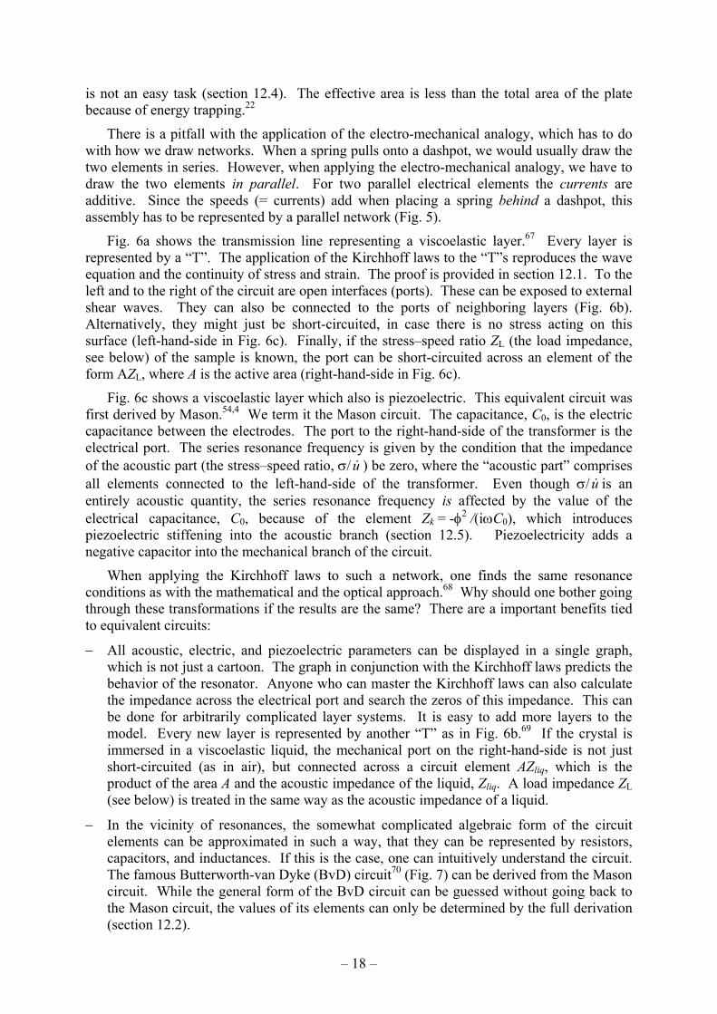
Fig. 6a shows the transmission line representing a viscoelastic layer.67 Every layer is represented by a “T”. The application of the Kirchhoff laws to the “T”s reproduces the wave equation and the continuity of stress and strain. The proof is provided in section 12.1. To the left and to the right of the circuit are open interfaces (ports). These can be exposed to external shear waves. They can also be connected to the ports of neighboring layers (Fig. 6b). Alternatively, they might just be short-circuited, in case there is no stress acting on this surface (left-hand-side in Fig. 6c). Finally, if the stress–speed ratio ZL (the load impedance, see below) of the sample is known, the port can be short-circuited across an element of the form AZL, where A is the active area (right-hand-side in Fig. 6c).

Fig. 6c shows a viscoelastic layer which also is piezoelectric. This equivalent circuit was first derived by Mason.54,4 We term it the Mason circuit. The capacitance, C0, is the electric capacitance between the electrodes. The port to the right-hand-side of the transformer is the electrical port. The series resonance frequency is given by the condition that the impedance of the acoustic part (the stress–speed ratio, σ/u ) be zero, where the “acoustic part” comprises all elements connected to the left-hand-side of the transformer. Even though σ/u is an entirely acoustic quantity, the series resonance frequency is affected by the value of the electrical capacitance, C0, because of the element Zk = -φ2 /(iωC0), which introduces piezoelectric stiffening into the acoustic branch (section 12.5). Piezoelectricity adds a negative capacitor into the mechanical branch of the circuit.

When applying the Kirchhoff laws to such a network, one finds the same resonance conditions as with the mathematical and the optical approach.68 Why should one bother going through these transformations if the results are the same? There are a important benefits tied to equivalent circuits:

− All acoustic, electric, and piezoelectric parameters can be displayed in a single graph, which is not just a cartoon. The graph in conjunction with the Kirchhoff laws predicts the behavior of the resonator. Anyone who can master the Kirchhoff laws can also calculate the impedance across the electrical port and search the zeros of this impedance. This can be done for arbitrarily complicated layer systems. It is easy to add more layers to the model. Every new layer is represented by another “T” as in Fig. 6b.69 If the crystal is immersed in a viscoelastic liquid, the mechanical port on the right-hand-side is not just short-circuited (as in air), but connected across a circuit element AZliq, which is the product of the area A and the acoustic impedance of the liquid, Zliq. A load impedance ZL (see below) is treated in the same way as the acoustic impedance of a liquid.

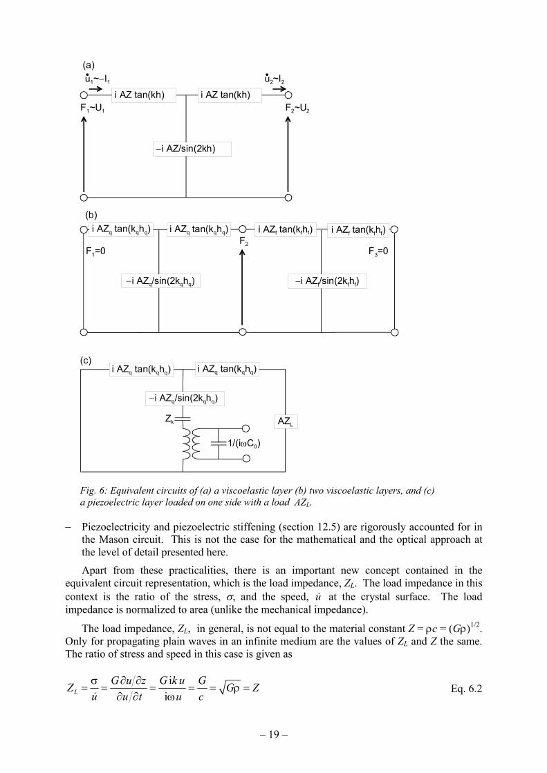
− In the vicinity of resonances, the somewhat complicated algebraic form of the circuit elements can be approximated in such a way, that they can be represented by resistors, capacitors, and inductances. If this is the case, one can intuitively understand the circuit. The famous Butterworth-van Dyke (BvD) circuit70 (Fig. 7) can be derived from the Mason circuit. While the general form of the BvD circuit can be guessed without going back to the Mason circuit, the values of its elements can only be determined by the full derivation (section 12.2).

– 19 –

− Piezoelectricity and piezoelectric stiffening (section 12.5) are rigorously accounted for in the Mason circuit. This is not the case for the mathematical and the optical approach at the level of detail presented here.

Apart from these practicalities, there is an important new concept contained in the equivalent circuit representation, which is the load impedance, ZL. The load impedance in this context is the ratio of the stress, σ, and the speed, u at the crystal surface. The load impedance is normalized to area (unlike the mechanical impedance).

The load impedance, ZL, in general, is not equal to the material constant Z = ρc = (Gρ)1/2. Only for propagating plain waves in an infinite medium are the values of ZL and Z the same. The ratio of stress and speed in this case is given as

Eq. 6.2 i

iLG u z G k u GZ G Z

u u t u cσ ∂ ∂

= = = = = ρ =∂ ∂ ω

u1~−I1 u2~I2

F1~ U1 F2~ U2

i AZ tan(kh) i AZ tan(kh)

−i AZ/sin(2kh)

(a)

i AZq tan(kqhq)i AZq tan(kqhq)

−i AZq/sin(2kqhq)

F1=0F2

i AZf tan(kfhf)i AZf tan(kfhf)

−i AZf/sin(2kfhf)

F3=0

(b)

i AZq tan(kqhq)i AZq tan(kqhq)

−i AZq/sin(2kqhq)

1/(iωC0)

Zk AZL

(c)

Fig. 6: Equivalent circuits of (a) a viscoelastic layer (b) two viscoelastic layers, and (c) a piezoelectric layer loaded on one side with a load AZL.

– 20 –

1/(iωC1)

1/(iωC0)

iωL1 R1 AZL

acoustic branch

electrical branch

Fig. 7: Butterworth-van-Dyke equivalent circuit.

For a propagating wave in an infinite medium the stress−speed ratio is the same everywhere and equal to the acoustic impedance. This is not true for more complicated displacement patterns. For instance, if two waves u+ and u- travel into opposite directions, the analog of Eq. 6.2 reads

Eq. 6.3

and there is no way to further specify ZL without knowledge about the amplitudes and the relative phase of the two waves.

One can show that the fractional frequency shift of a quartz crystal resonator is proportional to the load impedance. This important result is further elaborated on in section 7.

The Mason circuit is a necessary level of complication (and a safe ground, as well) if any of the following conditions are encountered:

− Both sides of the crystal are loaded.

− The behavior of the crystal far away from the resonances matters.

− The linearizations used in the derivation of the Butterworth-van-Dyke circuit (Fig. 7) are not accurate enough (section 9).

− The amplitude of shear oscillation motion is of interest (section 12.3).

A word of caution is in place with regard to an over-interpretation of the Mason circuit: In principle, one might attempt to calculate the complete admittance spectrum of a crystal directly from the Mason circuit. However, this possibility is of little practical use, because the electrical admittance cannot be measured accurately enough in experiment. In order to allow for a comparison with the prediction from the Mason circuit, the admittance would have to be measured as precisely as the resonance frequency (relative error of 10-7), which is impossible. The strength of the QCM is in its tremendous accuracy with regard to frequency measurements. Unfortunately, this extreme accuracy is limited to the frequency of the peak conductance; it does not extend to the conductance (or, more generally, the complex admittance) itself.

For frequencies close to the resonance, the Mason circuit can be simplified to the Butterworth-van-Dyke (BvD) circuit shown in Fig. 7. The values of its elements are:

Eq. 6.4

( ) ( )( )( ) ( )( )

i

iL

G k u z u zZ

u u z u z

+ −

+ −

−σ= =

ω +

( )

( ) ( )

22 26

1 2

3

1 2 226

22

1 2 2 226 26

814

14 8

1 tan4 8 8

p q q

q qp

q qp q q

AeCd n G

dL m

Ae

d dR Z n n

Ae Ae

= φ =κ π

ρ= =

φ

= ξ = π δ = π ηφ

– 21 –

The derivation is provided in section 12.2. κp, mp, and ξp represent a spring, a mass, and a dashpot. The BvD circuit is frequently referred to. For instance, the admittance diagram of a quartz crystal (insert in Fig. 2) can be easily understood from the BvD circuit. Given that the width of any given resonance is small, the susceptance of the parallel capacitance, ωC0, can be considered constant over the frequency range of an individual resonance. It adds to the susceptance of the motional branch and therefore just displaces the admittance curve along the vertical scale. The conductance (the real part of the admittance) is unaffected by C0. The admittance curve of the motional branch is a circle, where the series resonance frequency corresponds to the point with the largest conductance.

We will use the BvD circuit to derive the small-load-approximation in section 7. The BvD circuit captures piezoelectric stiffening. A few other comments on the Mason circuit are provided in the appendix. Here, we move on and discuss the role of the load impedance in data analysis.

7 Relation Between the Frequency Shift and the Load Impedance The load impedance is the ratio of stress and speed at the crystal surface. Here and in the

following, the terms “load impedance”, “load”, and “stress−speed ratio” are used synonymously. From the BvD circuit, one can read how the resonance frequency responds to the load. Below we derive a relation between the frequency shift and the stress−speed ratio. We use a complex spring constant pκ = κp + iωξp and a complex eigenfrequency of the bare

crystal 0ω = ( pκ /mp)1/2 for computational convenience. Also, we neglect the term Zk in Fig. 6c (section 12.5). From Fig. 17b one reads the resonance condition as

Eq. 7.1

where the relation ( pκ mp)1/2 = ((κp + iωξ)mp)1/2 = Α qZ nπ/2 was used (Eq. 12.18). Eq. 7.1 made also use of the approximation ω0 + ωr ≈ 2ω0, which requires ∆f/f0 á 1. Further using

0f = n ff we obtain

Eq. 7.2

Since the phase angles of qZ and ff are the same, one has / /q f q fZ f Z f= and one can also write

Eq. 7.3

Using qZ = 2mq / ff , this can be further rewritten as

( )( ) ( )

0

0

0 0 0

0 0

0

0 i ii

2i i

2iA2

p rr p L p p L

r r

r r rp p L p p L

r

q L

m AZ m AZ

m AZ m AZ

n fZ AZf

κ ωω= ω + + = κ − + ω ω ω

ω + ω ω − ω ω − ω= κ + ≈ κ +

ω ω ω

π ∆≈ +

i iL

q qf

f ZuZ Zf

∆ σ≈ =

π π

i iL

f q q

f Zf Z Z u∆ σ

= =π π

– 22 –

Eq. 7.4

Eq. 7.4 shows that the mass of the crystal is the only parameter entering the frequency shift, as long as the latter is small. The stiffness of the crystal (and piezoelectric stiffening, in particular) is of no influence at this level of approximation. Comparing Eq. 7.3 and Eq. 5.10, we find

Eq. 7.5

which provides the link between the optical and the equivalent circuit formulation.

We briefly convince ourselves that the same result is found without recurrence to equivalent circuits in case the sample is a semi-infinite liquid (ZL = Zliq with Zliq a materials constant). For such a situation we have (Eq. 5.3):

Eq. 7.6

which is equivalent to Eq. 7.5.

Since Eq. 7.3 is of such fundamental importance, we briefly re-derive it in the frame of the mathematical approach. According to Eq. 4.3 and Eq. 4.6, the displacement and the stress must both be continuous at the crystal surface. The equation for displacement is given as

Eq. 7.7

where zq,2 is the location of the crystal surface and totsampleu is the total displacement at the

crystal surface. Note that uj±(z) was always defined to be equal to uj

±,0 on the left-hand-side of each layer j (Eq. 4.4). The condition that the stress at the back of the crystal (the left-hand-side in Fig. 3) vanishes, reads

Eq. 7.8

where zq,0 is the location of the back of the crystal. The stress continuity at the front surface is expressed as

Eq. 7.9

From Eq. 7.8 we know that uq+,0 = uq

–,0. Using this result, Eq. 7.9 can be simplified to read

i2 L

q

f Zm

∆ =π

( ) ( ) ( ) ( ),0 ,0,2 ,2 exp i exp i tot

q q q q q q q q q q sampleu z u z k d u k d u u+ − + −+ = + − =

( ) ( ) ,0 ,0,0 ,0i i 0q q q q q q q q qG k u z u z Z u u+ − + − − = ω − =

( ) ( )( ) ( )

( ) ( )

,2 ,2

,0 ,0

,0 ,0

i

i exp i exp i

i i exp i exp i

q q q q q

q q q q q q q

sampkeL tot L q q q q q q

Z u z u z

Z k d u k d u

Z u Z k d u k d u

+ −

+ −

+ −

ω − = ω − − =

= ω = ω + −

,21 2 Lq

q

ZrZ

− ≈

,2

21 1 q liq liq

qq liq q

Z Z Zr

Z Z Z−

− = − ≈+

– 23 –

Eq. 7.10

or, equivalently

Eq. 7.11

Eq. 4.15 as well as the relation tan(nπ+ε) = tan(ε) have been used. Taylor-expanding tan(x) as tan(x) ≈ x we find Eq. 7.2 confirmed. The perturbation analysis (section 9) will start out from Eq. 7.11.

When using the small-load-approximation below, the load will always be evaluated at the reference frequency, f0. For instance, for the load given by a Sauerbrey film, one uses iωm = 2πif0 m (as opposed to 2πi(f0 +∆f) m). Using the latter expression would turn Eq. 7.3 into an implicit equation in ∆f and that is exactly what is to be avoided at this level of approximation. Within the perturbation analysis, one makes peace with implicit equations and therefore also evaluates the load at the true frequency of oscillation, rather than the reference frequency. The perturbation analysis cures both the problems resulting from approximating tan(x) as x and the problems resulting from evaluating the load at f0 rather than f.

Eq. 7.3 is the most important equation of the physics of the QCM. As long as the frequency shift is small compared to the frequency, the complex frequency shift is proportional to the load impedance at the crystal surface. We term Eq. 7.3 the small-load-approximation. At this point, we have not made any statement on the nature of the sample. We have only stated how the frequency shift depends of the stress–speed ratio at the crystal surface. Under certain conditions, this statement can also be applied in an average sense.71,72 Assume that the sample does not consist of planar layers, but instead of a sand pile, a froth, an AFM tip, an assembly of spheres or vesicles, a cell culture, a droplet, or any other kind of heterogeneous material. There are many interesting samples of this kind. The frequency shift induced by such objects can be estimated from the average ratio of stress and speed at the crystal–sample interface. The latter is the load impedance of the sample. The concept of the load impedance tremendously broadens the range of applicability of the QCM. The load impedance is the conceptual link between the QCM and complex samples. If we want to predict the frequency shift induced by any kind of sample, we must ask for the average stress–speed ratio. If this ratio can be estimated in one way or another, a quantitative analysis of the QCM experiment is in reach. Otherwise, the analysis will have to remain qualitative.

8 Layered Systems within the Small-Load-Approximation

In the previous chapters, we have assembled the tools needed to calculate the frequency shifts based on acoustic modeling. In following, we apply these equations to calculate the complex frequency shift for a number of different planar geometries.

8.1 Semi-Infinite Viscoelastic Medium

For the semi-infinite medium, there is only one wave traveling outwards with an amplitude u-,0. The stress exerted onto the crystal surface is

Eq. 8.1

( ) ( ) ( ) ( )exp i exp i exp i exp iq q q q q L q q q qZ k d k d Z k d k d − − = + −

( ) ( )0i tan i tan 2 i tan 2 i tanq qLq q

q q q f

d dZ fk d f f fZ c c f

∆= = π + ∆ = π∆ = π

( ) ,0 ,0 ,0 ,0i i iliqliq liq liq liq liq

liq liq

uG G ik u G u G u Z uz c G

− − − −ρ∂ ωσ = − = − − = = ω = ω

∂

– 24 –

where the index liq denotes the liquid. For the frequency shift, f∆ , one finds

Eq. 8.2

Eq. 8.2 was independently derived by Borovikov73 and Kanazawa.74 A related version of this equation was derived for torsional resonators by Mason.75 For Newtonian liquids (η’ = const, η’’ = 0) ∆f and ∆Γ are equal and opposite. They scale as the square root of the overtone order, n1/2. For non-Newtonian liquids (η’ = η(ω), η’’≠ 0), the complex viscosity can be obtained by inversion of Eq. 8.2 as

Eq. 8.3

Note that viscoelasticity always entails viscoelastic dispersion in the sense that η’ and η’’ are themselves a function of frequency. The n1/2-scaling therefore no longer holds. Contrary to intuition, a finite elastic component increases the bandwidth more than the negative frequency shift. An ideally elastic medium leads to ∆f = 0 and to a non-zero ∆Γ, because energy is withdrawn from the crystal in the form of elastic waves.

Compressional waves, surface roughness, and slip cause systematic errors in the determination of the viscosity on the order of about 10%. For reasons which are not entirely understood, the imaginary part of the viscosity, η’’, often is derived as slightly negative when applying Eq. 8.3 to the experimental data. This clearly contradicts the second law of thermodynamics and points to a systematic short-coming of Eq. 8.3. Roughness and slip may play a role. The values for η’ found by application of Eq. 8.3 to the experimental data tend to be larger than the literature values, which may be related to compressional waves.24

Importantly, the QCM only probes the region close to the interface. The shear wave evanescently decays into the liquid according to

Eq. 8.4

For Newtonian liquids (η'' = 0), this amounts to

Eq. 8.5

with ( )2 '/ liqδ = η ρ ω the penetration depth. Using ω = 2π · 5 MHz and the viscosity of

water (η ≈ 10-3 Pa s) the penetration depth is found to be about 250 nm. For the general case of viscoelastic materials, on writes

( )' ''i i i 1 1 ii 2 i2liq liq f liq

f q q q q

f Z nff Z u Z Z Z∆ σ − +

= = = ρ ωη = π ρ η − ηπ π π π

( )

2'

2

2 22''

2

12

q

liq f

q

liq f

Z f ff

fZ ff

π ∆ ∆Γη = −

ρ

∆Γ − ∆πη =

ρ

( )( )( )0

i( ) iexp i ' i '' exp exp' ''

liqu z k k z z zu c i

ρ ωω = − − = − = − η − η

( )0

( ) exp 1 iu x zu

= − + δ

– 25 –

Eq. 8.6

8.1.1 Roughness

Urbakh and Daikhin have included small-scale roughness into Eq. 8.2 by writing28

Eq. 8.7

where lr is the lateral correlation length of roughness (where the spectrum of spatial frequencies is assumed to be Gaussian), hr is the root-mean-square roughness, and δ = (2η/(ρω))1/2 is the penetration depth. Both lr and hr must be much smaller than δ for Eq. 8.7 to hold. Also, hr must much muss less than lr (shallow roughness). For strong roughness (hràlr) the same authors provide a more complicated formula based on the Brinkman equation and Darcy flow.28,76

Note that in the limit leading to Eq. 8.7, roughness affects the frequency shift much more than the shift in bandwidth. For a fixed aspect ratio hr/lr, roughness looks like a Sauerbrey term, where the Sauerbrey mass is given by the term in curly brackets. The effect on bandwidth remains quadratic in hr. Such a behavior is typical for scattering phenomena.79

8.1.2 The Sheet-Contact Model

Eq. 8.3 is very attractive for the study of adhesion between polymers and solid surfaces, since it allows for the determination of the viscoelastic constants of the adhesive in the immediate vicinity of the contact. Unfortunately, the QCM does not work well with semi-infinite media when the viscosity, η, is larger than about 50 cP. The acoustic load in this case is too large. Most polymers exceed this limit. If, however, the contact area can be confined to a small spot in the center of the crystal the measurement becomes feasible again.77 Such a small contact area can be, for instance, established with a JKR–tester.78 The area of contact can be determined by optical microscopy. Of course, this kind of sample is laterally heterogeneous and the applicability of simple models may be questioned. Experiment shows that the finite contact area can be reasonably well be accounted for by modifying Eq. 8.3 as:

Eq. 8.8

where Ac is the contact area and KA is a “sensitivity factor”. Eq. 8.8 assumes a contact area much larger than the decay length of the shear wave. Also, energy trapping is assumed to be unaffected by the contact.

The sensitivity factor, KA, accounts for the non-trivial amplitude distribution over the area of the crystal. For small contact areas, KA is about constant and equal to 2. Since, the

( ) ( )

1

1'' Imi ' i ''

liqk−

− ρ ωδ = = − η − η

i cA L

f q

Af K Zf Z A∆

=π

2 2

2

2

2 2

2

1 1 3 22

1 1 32

1 2 32 2

1 11 22 2

liq r r

f q r

liq r

q r

liq rliq r

q q r

liq liq liqr r

f q q q q

h hff Z l

hZ l

hf hZ Z l

h hnf Z Z d

ρ ωη ∆ −≈ + π − π δ δ

ρ ωη −≈ + π π δ

ρ ωη − π = − ρ π

ρ ωη ρ ωη ρ ∆Γ= + = + π δ π ρ δ

– 26 –

efficiency of energy trapping depends on overtone order, the parameter KA depends on overtone order, as well. The KA-factor can be determined independently by placing drops of water with known contact radius onto the center of the crystal. Eq. 8.8 has been tested in that way and found to be a good approximation to the data for a large range of experimental conditions.77 There are small deviations in the limit of small contact radius.79

8.1.3 Nematic Liquid Crystals

In nematic liquid crystals, the viscosity depends on the relative orientation between the shear gradient and the orientation of the nematic phase. Close to a surface, the orientation usually is governed by surface orientational anchoring.80 Anchoring transitions, for instance induced by the adsorption of an analyte molecule to the surface,81 can therefore be easily detected with the QCM.82,83 This reorientation induced by adsorption amounts to an amplification scheme: the expected shift in the resonance frequency and bandwidth due to reorientation is much larger than the frequency shift induced by the adsorption in the Sauerbrey sense.

The physics of shear waves in nematic liquid crystals is rather complicated. Because shear couples to reorientation, there are two separate modes – termed “hydrodynamic” and “orientational” – emanating from the oscillating crystal surface. The hydrodynamic mode mainly transports vorticity. This mode is known from simple liquids. The orientational modes mainly transports rotation of the director with regard to the background fluid. The penetration depth of the orientational mode is much smaller than the penetration depth of the hydrodynamic mode. While the amplitude of the orientational mode strongly depends on the strength of surface anchoring, the amplitude of the hydrodynamic mode does not.84

The quantitative description has been worked out by Kiry and Martinoty.85 They discuss the director orientations perpendicular to the surface (“c”), along the direction of shear (“b”) and in-plane and perpendicular to the direction of shear (“a”). Tilted orientation is not covered. Their experiments were based on ultrasonic reflectometry86 rather than quartz crystal resonators. Generally speaking, the topic is somewhat academic because the theory involves no less than 5 independent parameters, which are usually unknown. Interestingly, Kiry and Martinoty predict the effective viscosities ηb and ηc to be the same, which was confirmed by their experiments on the liquid crystal 4-n-pentyl-4’cyanobiphenyl (5CB). This finding as gotten some attention because it constitutes the only experimental proof of the Parodi relation.87 Parodi has used the Onsager theorem to reduce the number of independent parameters of nematodynamics from 6 to 5. Somewhat loosely spoken, the LC-orientation does not matter as long as it is in the shear plane (true for geometries b and c), because the shear stress at the surface is calculated from the symmetrized velocity gradient tensor.

8.1.4 Colloidal Dispersions

The flow behavior of colloidal dispersions at interfaces is of paramount importance in many branches of industry.88 The effective high frequency viscosity of such materials is of considerable interest in this context because there are qualitative differences between the low-frequency and the high-frequency rheology.89,90,91 Three different time scales come into play, which are the Brownian diffusion time τR ~ a2/D0 (a a characteristic length such as the particle radius and D0 the self diffusion coefficient), the hydrodynamic retardation time τH ~ d2/ν (d the interparticle distance and ν the kinematic viscosity), and the momentum relaxation time τB ~ m/ξ (m the mass and ξ = 6πηR the drag coefficient).92 Time-temperature superposition93 does not hold for colloidal dispersions. Theories exist for excitation frequencies larger than τR

-1, but smaller than τH-1 and τB

-1.92,90 Inputting numbers, one finds that the particle size must be in the range of 10 nm or less in order for these conditions to hold in the MHz range.

– 27 –

8.2 Viscoelastic Film in Air

8.2.1 Purely Inertial Loading

Before going into the details of the calculation for thin films, we briefly come back to a statement made earlier with regard to the proportionality of frequency shift and added mass (as opposed to film thickness). This proportionality is the essence of the Sauerbrey relation. The frequency shift − mass proportionality holds for all thin films, regardless of their viscoelastic properties. It even applies to laterally heterogeneous samples as long as these are so thin that viscoelasticity can be ignored. In the latter case, the areal mass density of course is an average density.

We now prove the Sauerbrey equation (Eq. 4.18) based on the small-load-approximation (Eq. 7.3): the stress induced by a very thin film is caused by inertia only and is given as σ = -ω2u0mf, where u0 is the amplitude of oscillation and mf is the (average) mass per unit area. Inserting this result into the small-load-approximation (Eq. 7.3), one finds

Eq. 8.9

which is the Sauerbrey relation.

8.2.2 Viscoelastic Film

If we now drop the thin-film-condition and instead consider viscoelastic films of arbitrary thickness, we find

Eq. 8.10

where u-,0 and u+,0 are the amplitudes of the waves traveling away from the crystal and towards the crystal, respectively. Since the reflectivity at the film–air interface is r = 1, the parameter u+,0 is given by

Eq. 8.11

where kf is the wave number and df is the film thickness. The frequency shift induced by the film is

Eq. 8.12

( )( )

( )

( )

,0 ,00

,0 ,00

,0 ,00

i

i

i

f f f

ff

f

uG G k u uz

G u uc

Z u u

− +

− +

− +

∂σ = − = − ⋅ − −

∂ω

= −

= ω −

( ),0 ,0exp 2i f fu k d u+ −= −

( )( )

( )( )

( ) ( )( ) ( )

( )

,0 ,0

,0 ,0

i 1 exp 2ii i1 exp 2ii

exp i exp iiexp i exp i

1 tan

f f ff

f q q f f

f f f ff

q f f f f

f f fq

Z u u k df Zf Z Z k du u

k d k dZ

Z k d k d

Z k dZ

− +

− +

ω − − −∆= =

π π + −ω +

− −=

π +

−=

π

20

0

i 2i

ff

f q q

u mf f mf Z u Z

−ω∆≈ = −

π ω

– 28 –

The first pole of the tangent (kf df = π/2) defines the film resonances. 94,37,6 Higher order film resonances corresponding to kf df = mπ/2 with m an odd integer should exist, in principle, but have rarely been observed in experiment. At the film resonance one has df = λ/4. Note that the frequency shift is not small right at the film resonance and that the small-load-approximation used in the derivation of Eq. 8.12 breaks down. Cernosek et al. have developed an equivalent circuit for the film resonance which also holds right at the film resonance.95 According to this circuit (and also to a more rigorous numerical calculations based on the Mason circuit) the frequency shift does not go to infinity at the film resonance. Rather, there are two resonances in parallel, which correspond to a symmetric and an antisymmetric motion of the crystal and the film, respectively. The quantitative agreement between the experimental data and this more rigorous theory still is not impressive. This is one manifestation of the general rule that the QCM does not work well when the frequency shifts become large.

It instructive to write Eq. 8.12 in a slightly different form:

Eq. 8.13

Eq. 8.13 shows that the acoustic properties of a film are fully specified by two parameters, which are its acoustic impedance, Z, and its mass per unit area, m. Eq. 8.12 misleadingly suggests that there might be three parameters (Z, k, and d), but these three parameters are not independent. As a consequence, one can never hope to independently derive the thickness, the viscoelastic parameters, and the density of a film from acoustic measurements alone. A transformation of the form (ρf Ø α ρf, df Ø 1/α df, Gf Ø 1/α Gf) with α some numerical coefficient leaves the left-hand-side of Eq. 8.13 unchanged. This statement holds for multilayers and films in contact with a liquid in the same way.

8.2.3 Derivation of Viscoelastic Constants

In principle, viscoelastic constants can extracted from the experimental data by fitting Eq. 8.12 (or any of the more complicated equations below) to the data. For small film thickness, certain approximations hold which make the derivation more transparent. If kf df is much less than unity, the tangent in Eq. 8.12 can be Taylor-expanded to third order as tan(x) ≈ x + 1/3 x3, resulting in:

Eq. 8.14 ( ) ( )3

22 22

2

22

2

1 1 1tan3

1 1 1 11 13 3

1 113

f f f f f f f ff q q

f f q ff f f f f

q f f q f q

q ff

q f q

f Z k d Z k d k df Z Z

m Z mZ k d m J n

Z G Z m

Z mm n

Z Z m

∆ − − = ≈ + π π

ρ− − = + ω = ω + π π ρ π ρ − = ω + π π

( )1 tan

tan tan tan

tan

f f ff q

ff f ff f f f

q f q q ff

ff

q f

f Z k df Z

Z Z Zd d d

Z c Z Z ZG

Zm

Z Z

∆ −=

π

ω ρ − − −ω ω = = = ρ π π π − ω

= π

– 29 –

where the relation ω = 2πn ff = πnZq/mq has been used. For small mf (neglecting the second term inside the brackets) this expansion reproduces the Sauerbrey equation. For slightly larger film thickness, there is a viscoelastic correction proportional to n2. A large elastic compliance Jf’ tends to decrease the frequency, whereas a large viscous compliance, Jf’’, increases the bandwidth. In principle, both Jf’ and Jf’’ can be extracted from the dependence of the frequency shift on the overtone order. However, there are certain caveats to be kept in mind:

− Unless the film is very soft, Eq. 8.14 should be replaced by the corresponding equation derived from perturbation theory (Eq. 9.6) for the reasons stated in section 9. The difference is noticeable if the compliance of the film is of the same order of magnitude as the compliance of the crystal.

− Jf’ and Jf’’ often depend on frequency f. Since the experimentally accessible range of frequencies is narrow (usually less than a decade), it is fair to assume that Jf ' and Jf '' depend on f according to a power law with power law exponents β' and β'':

Eq. 8.15

In standard polymer rheology, there are no inertial effects and β’ is always negative for that reason.93 The choice of the exponents β' and β'' does affect the derived values of the compliance. Generally speaking, viscoelastic dispersion applies to all viscoelastic parameters, not just the compliance of the film. However, for the crystal and the electrodes, the viscoelastic dispersion is often weaker than for polymer films.

− Jf’ and Jf’’ and interrelated by the Kramers-Kronig relations93

Eq. 8.16

where P is the principal value in the Cauchy sense. Eq. 8.16 is not of immediate practical use because it requires an integration over an infinite frequency range. Still, certain values of J’, J’’, β’, and β’’ are more plausible than others. For instance, if the rates of relaxation are much above the resonance frequency of the crystal, the material should behave according to the three element network shown in the inset of Fig. 9. If the spring on the left-hand-side is small, the material behaves a Maxwell fluid (J’’ à J’, β’ ≈ –2, β’’ ≈ –1, cf. Fig. 14). The other extreme is given by the viscoelastic material in the Voigt sense (J’ á J’’, β’ ≈ 0, β’’ ≈ -1, cf. Fig. 14). Voigt-based modeling97 with frequency-independent parameters G’ and η makes sense if the low-frequency limit is indeed fulfilled. Note that the relaxation time, τ,

( ) ( )

( ) ( )

'

' '

' '

' ' ' '

f f ff

f f ff

fJ f J ff

fJ f J ff

β

β

≈

≈

( ) ( )

( ) ( )

2 20

2 20

' '' '2' d ''

' '2'' d ''

ff

ff

JJ P

JJ P

∞

∞

ω ωω = ω

π ω − ω

ωωω = − ω

π ω − ω

∫

∫

G' (3-element)

G' (Maxwell)

G'' (Maxwell)

slope > 0

slope 2

slope 1

log

G',

log

G''

log ω Fig. 9 Three-element network describing a viscoelastic solid

– 30 –

cannot possibly be below 0.1 ns and often is much longer. Most of the times (but not strictly always) G’ will be larger than ωη(ωτ) in the low frequency limit.

− Electrode effects are very important in the derivation of Jf' from experimental data (Fig. 11). Unless the electrode thickness is precisely known, the derivation of Jf ' is difficult. The viscous compliance Jf '' can be derived much more reliably. Even the frequency-dependence of Jf '' can be determined. This applies to experiments in air.

8.3 Viscoelastic Film in Liquid

As usual, we start the calculation from the small-load-approximation. Eq. 8.10 still applies, but the coefficient of reflection at the outer interface of the film now is not unity but (Zf –Zliq)/(Zf +Zliq), instead. The amplitude u+,0 is given by

Eq. 8.17

Inserting Eq. 8.17 into Eq. 8.10, we arrive at

Eq. 8.18

leading to96,97

Eq. 8.19

At the pole of the tangent one again has a film resonance.96 The Chalmers group has derived an equivalent equation, which they term "Voigt model".97 Expanding Eq. 8.19 to first order in df, one finds

( )( )q

tan i

i tanf f f liqf

f f liq f f

Z k d ZZff Z Z Z k d

−−∆=

π +

( ),0 exp 2i f liqf f

f liq

Z Zu k d

Z Z+ −

= −+

( )

( )

( ) ( ) ( ) ( )( ) ( ) ( ) ( )

( ) ( )( ) ( ) ( )( )( )

1 exp 2ii

1 exp 2i

exp i exp iiexp i exp i

exp i exp i exp i exp iiexp i exp

f liqf f

f liqf

f liqf qf f

f liq

f liq f f f liq f ff

q f liq f f f liq f f

f f f f f liq f f f ff

q f f f

Z Zk d

Z Zf Z Z Zf Z k dZ Z

Z Z k d Z Z k dZ

Z Z Z k d Z Z k d

Z k d k d Z k d k dZ

Z Z k d

−− −

+∆=

−π + −+

+ − − −=

π + + − −

− − + + −=

π + −( )( ) ( ) ( )( )( ) ( )( ) ( )( )

( )

i exp i exp i

2i sin 2cosi2cos 2isin

i tanii tan

f f liq f f f f

f f f liq f ff

q f f f liq f f

f f f liqf

q f liq f f

k d Z k d k d

Z k d Z k dZ

Z Z k d Z k d

Z k d ZZ

Z Z Z k d

+ − −

+=

π +

+=

π +

– 31 –

Eq. 8.20

The frequency shift is usually determined with respect to a reference state, where the quartz is already immersed in liquid. When the film is absent, one has ZL = Zliq. Referencing the measurement to the bare quartz in liquid, one therefore obtains98,99,100

Eq. 8.21

Apart from the term in brackets, Eq. 8.21 is equivalent to the Sauerbrey equation. The term in brackets is a viscoelastic correction, dealing with the fact that highly dilute and soft layers lead to a smaller Sauerbrey thickness than rigid layers. See the discussion following Eq. 9.17 with regard to implications of Eq. 8.21 for viscoelastic modeling.

Because Eq. 8.21 is linear in mass, it also holds in an integral sense:101

Eq. 8.22

where ρ(z) was assumed to be about constant and equal to ρ. The integral formulation would be used when the viscoelastic properties vary with distance from the crystal surface.

8.3.1 Physical Interpretation of the Sauerbrey Thickness

The correct interpretation of the frequency shift from QCM experiments in liquids is a challenge. Practitioners often just apply the Sauerbrey equation (Eq. 4.18) to their data and term the resulting areal mass density "Sauerbrey mass" and the corresponding thickness "Sauerbrey thickness". Even though the Sauerbrey thickness can certainly serve to compare different experiments, it must not be naively identified with the geometric thickness. Here is a list of worthwhile considerations:

a) The QCM always measures an areal mass density, never a geometric thickness. The conversion from areal mass density to thickness usually requires the physical density as an independent input. A density of 1 g/cm3 is often assumed in soft matter experiments. Given the other uncertainties (see below) this is in many cases a fair approximation.

b) It is difficult to infer the viscoelastic correction factor (brackets in Eq. 8.21) from QCM data. However, if the correction factor is significantly different from unity, it may be expected that it also affects the bandwidth ∆Γ and, also, that it depends on overtone order. If, conversely, such effects are absent (∆Γ á ∆f, Sauerbrey thickness same on all overtone orders) one may assume (1–Zliq

2/Zf2) ≈ 1.

c) When the viscoelastic correction as discussed in (b) is insignificant, this does by no means imply that the film is not swollen in the solvent. It only means that the (swollen) film is much more rigid than the ambient liquid. The amount of swelling can only be inferred from the comparison of the wet and the dry thickness. QCM data taken on the wet sample alone do not allow to infer the degree of swelling (cf. section 8.3.2).

2

2

i i 1 liqliq f f f

f q f

Zf Z Z d kf Z Z

∆≈ + − π

2 2

2 2

2 2

2

i 1( ) 1 1liq f liqtot liq f f f

f q q f q f

f f liq

q f

Z m Zf Z Z Z k df Z Z Z Z Z

m Z ZZ Z

−ω∆ −≈ − = − = − π π π

−ω −= π

2 2

20 0

( ) ( )( )d d

( ) ( )f liq f liq

f q f q f

Z z Z G z Gf z z zf Z Z z Z G z

∞ ∞ − −∆ −ω ρω≈ − ρ ≈ −

π π ∫ ∫

– 32 –

d) Complex samples are often laterally heterogeneous. Needless to say, the QCM cannot capture lateral heterogeneity (cf. section 8.1.1 for attempts to model roughness).

e) Complex samples often have fuzzy interfaces. Again, the QCM can never quantitatively determine such a fuzziness. However, a "fluffy" interface will lead to a viscoelastic correction and, as a consequence, to a non-zero ∆Γ as well as an overtone-dependent Sauerbrey mass. In the absence of such effects, one may conclude that the outer interface of film is sharp.

f) Last not least, let it be mentioned that the competing techniques for thickness determination in liquids have their own problems. For AFM measurements, one worries about the influence of the tip on the film. Neutron reflectometry102 certainly is very accurate, but not easily available on a routine basis. With optical measurements, there is the unknown refractive index of the film. The output of SPR measurements is often reported in terms of the shift of the coupling angle (rather than in terms of thickness) for that reason. The conversion from the shift in coupling angle (or from “RUs”103) to percent-coverage must be done for every adsorbate separately, based on a calibration to be carried out on this particular system.

8.3.2 Comparison of Optical and Acoustic Reflectometry

It is instructive of compare Eq. 8.22 with the corresponding equation applied in the context of surface plasmon resonance (SPR) spectroscopy. For the shift of the coupling angle θc we have104,17 ,105

Eq. 8.23

where nr is the refractive index, λ is the wavelength, and ε = nr2 is the dielectric permittivity

( )2

0

( )2 1sin( )

q liq f liqc

r q liq fq liq

zdz

n z

∞ ε ε ε − επ∆ θ ≈ λ ε + ε ε−ε ε

∫

polymer volume fraction

optical contrast (εf−εL) / εf

0 1

acoustic contrast (Gf−GL) / Gf

0

1

Fig. 8: The acoustic contrast easily saturates. The figure shows a sketch of the contrast function (integrands in Eq. 8.22 and Eq. 8.23) as a function of the polymer volume fraction of an adsorbed polymer film. It is implicitly assumed that both the shear modulus Gf and the dielectric constant εfare roughly proportional to the polymer concentration. However, Gf increases much stronger than εf. If, for instance, a swollen polymer film contains 50% of water, this will not appreciably decrease the apparent acoustic thickness because the modulus of the film is still much larger than the modulus of water and (Gf–Gliq)/Gf remains about unity. This is different in optics because the contrast is roughly proportional to the concentration. As a consequence, the apparent optical film thickness is proportional to the product of concentration and thickness, which is the adsorbed amount. In acoustics, the apparent thickness is close to the geometric thickness. Trapped water appears as part of the film in acoustics.

– 33 –

of the medium. The index q in this case denotes the substrate, rather than the quartz crystal. The structure of Eq. 8.22 and Eq. 8.23 is very similar. Since both techniques are based on reflectometry, this is not at all a coincidence.

Comparing Eq. 8.22 and Eq. 8.23, and one might assume that the information contained in surface plasmon resonances and quartz crystal resonances is essentially the same. However, this is very often not the case, which has to do with the fact that the contrast obtained with acoustic shear waves is usually much larger than the contrast in optics. While refractive indices typically vary in the range of a few percent, shear moduli may easily vary by orders of magnitude even for rather dilute adsorbates. In optics the weight function (the integrand in Eq. 8.23) is much smaller than unity and roughly proportional to the concentration. Therefore, the shift of the coupling angle is approximately proportional to the adsorbed amount. In acoustics, on the contrary, the weight function (integrand in Eq. 8.22) easily saturates to a value of unity even for dilute adsorbates if the shear modulus of the adsorbate is much higher than the shear modulus of the liquid.96 As a consequence, the Sauerbrey thickness (also termed acoustic thickness) approaches the geometric thickness even for rather dilute polymer layers. If the adsorbate drags some solvent along in its shear movement, the trapped solvent appears as part of the film, as far as the acoustic properties are concerned. However, the trapped solvent does not increase the optical thickness (Fig. 8). Swelling therefore effectively increases the acoustic thickness, while it affects the optical thickness to a much lesser extent.106 The ratio of acoustic and optical thickness gives an estimate of the degree of swelling. For adsorbed proteins, this amounts to an estimate of the degree of hydration.

Evidently, the fact that the acoustic contrast is much higher than the optical contrast is beneficial for sensing. The advantage which the QCM has over the competing optical techniques is most strongly felt for dilute adsorbates. The QCM responds very sensitively to these because − pictorially speaking − a few polymer strands suffice to turn the film into a solid-like object..

8.3.3 Information Contained in the D-f-ratio

The term in brackets in Eq. 8.21 is a viscoelastic correction to the Sauerbrey equation. The viscoelastic correction is independent of film thickness in a liquid environment. This contrasts to films in air or vacuum, where the viscoelastic correction scales as the square of the mass (Eq. 8.14). In air, the film surface is stress-free. The film only shears under its own inertia and in the limit of vanishing film thickness, the shear strain goes to zero. As a consequence, the shear compliance drops out of the equations in the thin-film limit. This is different in liquids: here the film is “clamped” by the liquid on its outer side, regardless of how thin it is.

In most cases, the viscoelastic correction cannot be directly extracted from the frequency shift because the mass, mf, is usually not known independently. The frequency shift contains the product of the mass and the real part of the term in brackets in Eq. 8.21. The two contributions cannot be disentangled. Note, however, that the mass can be eliminated by considering the ratio of the shift in half-band-half-width ∆Γ, and the negative frequency shift, –∆f (the “D-f-ratio”). One has

– 34 –

Eq. 8.24

In the following, we assume that the liquid is Newtonian with a density ρliq and a viscosity η. The acoustic impedance then is

Eq. 8.25

For the film we use

Eq. 8.26

Inserting Eq. 8.25 and Eq. 8.26 into Eq. 8.24, we find

Eq. 8.27

Eq. 8.27 is exact to first order in df. Further simplifying assumptions can be made with regard to the right-hand-side. Firstly, the densities in soft-matter experiments usually are similar. Assuming ρf ≈ ρliq yields

Eq. 8.28

Secondly, most films of interest are substantially more rigid than the ambient liquid. Even films which are statically soft, will often appear rigid at MHz frequencies. The denominator in Eq. 8.27 can be rewritten as 1 – Jf” / Jliq” where Jliq” = (ωη)-1 is the viscous compliance of the liquid. The elastic compliance of the liquid is infinite. If the film is much more rigid than the liquid, the denominator is close to unity and one has101

Eq. 8.29

If the density of the film and the liquid are not the same, can still neglect the second term in the denominator in Eq. 8.27, leading to

Eq. 8.30

The detailed investigation shows that Eq. 8.29 and Eq. 8.30 require films with a thickness of not more than a few nm in order to yield fair agreement with the full equation. Still, it holds quite generally that the shift in bandwidth is mostly affected by the elastic compliance of the

( )( )

2 2

2 2

Im 1 /

Re 1 /liq f

liq f

Z Z

f Z Z

− −∆Γ=

−∆ −

iliq liqZ = ωρ η

ff f f

f

Z GJρ

= ρ =

( )( )

'

' '

Im 1 i

Re 1 iliq f f liq f

f liq fliq f f

J Jf JJ

− − ωρ η ρ ωρ η∆Γ= =

−∆ ρ − ωρ η− ωρ η ρ

'

' '1f

f

Jf J

ωη∆Γ≅

−∆ − ωη

' '2f f fJ nf Jf

∆Γ≈ ηω = π η

−∆

z

v(z)

bs df Fig. 10: Flow profile above a solid surface with slip. Dashed line: The viscosity η(z) increases continuously from a small value at the surface to a somewhat higher value in the bulk. At the surface, the shear gradient is correspondingly increased. Solid line: the viscosity is reduced inside a hypothetical discrete layer of thickness df.

2' '

22 Re liqliq liqf f f

f f f

ZJ nf J

f Z

ρ ρ∆Γ ≈ ηω = π η = −∆ ρ ρ

– 35 –

film, rather than its viscous compliance. This contrasts to the situation in air, where ∆Γ is dominated by the viscous compliance of the film.

8.3.4 Slip

Slip at the quartz surface can be introduced into the model by using the equations for a film in a liquid, where the “film” is a liquid layer with reduced viscosity. Inside this layer, the shear gradient is increased, leading to the flow profile as indicated in Fig. 10. The slope of the profile dv(z)/dz is proportional to η-1(z). The slip length, bs, is the difference between the location of the surface and the extrapolated plane-of-zero-shear. One can show that the slip length, bs, is given by

Eq. 8.31

where ηf is the viscosity inside the film and df is the thickness of the layer with reduced viscosity (solid line in Fig. 10). Since this relation is linear in df, it also holds for continuous profiles η(z) (dashed line in Fig. 10) in an integral sense:

Eq. 8.32

For quantitative analysis, we may treat the layer with reduced viscosity like a thin film. As in Eq. 8.22, we can use an integral formulation:

Eq. 8.33

where ρ(z) ≈ ρliq has been used.

To the experimentalist, slip looks like a negative Sauerbrey mass, where the slip length is equal to the negative Sauerbrey thickness. This model ignores roughness and lateral heterogeneities, which presumably play a role in most practical situations where slip is observed.

8.3.5 Roughness at the Film–Air Interface

Roughness, generally speaking, is not easily incorporated into the multilayer formalism because it violates the assumption of lateral heterogeneity. On the other hand, it is certainly essential. Roughness may very well occur not only at a quartz–liquid interface, but at a film–liquid interface, as well. There is a logical extension of the formalism treated in section 8.1.1 to the case of multilayers. One assigns a load impedance of the form

Eq. 8.34

1liqs f

f

b d η

= − η

2

2q q0 0

sq q0

i2 21 ( ) 1 ( )i ( ) ( )( )

2 21( )

liq liq liq

f f

liqliq liq

Zf f fz dz z dzf Z Z z zZ z

f fdz bZ z Z

∞ ∞

∞

ωρ η ∆=− − ρ = − − ρ ωρ η

η ≈ ρ − = ρ η

∫ ∫

∫

( )0

1liqsb dz

z

∞ η = − η

∫

2 2 2

2 21 2 +i 1 3 22

liq r r rL

r

h h hZl

ρ ωη ≈ + + π − δ δ δ

– 36 –

to the liquid and uses this impedance instead of Zliq. whenever the latter occurs Eq. 8.34 is subject to the same approximations as Eq. 8.7. Furthermore, it is assumed that the vertical scale of roughness is much less than the film thickness. Otherwise, effects of roughness and viscoelasticity cannot be separated.

8.4 Two Viscoelastic Films in Air

For two films in air, the matrix formalism yields

Eq. 8.35

The indices e and f denote the electrode (the lower film, in general) and the film (the upper film, in general), respectively. Electrode effects can be very noticeable, particular when Eq. 8.35 is used to derive elastic properties of a film. For thin films (tan(x) ≈ x), the effects of both films are additive in the sense that

Eq. 8.36

8.5 Two Viscoelastic Films in Liquid

For two films in a semi-infinite medium (liquid) the matrix formalism yields

Eq. 8.37

The indices e, f, and liq denote the electrode (the lower film, in general), the film (the upper film, in general), and the liquid, respectively. While Eq. 8.37 seems long and complicated, it definitely is of practical relevance. It has to be used when films in liquids are investigated and electrode effects shall not be neglected.

9 Perturbation Analysis In section 8 we have used the small-load-approximation in order to derive frequency shifts

for various geometries. Evidently, the linearization in ∆f, which was applied in order to derive the small-load-approximation, has its limits of validity. These limits are felt not only when large frequency shifts are encountered, but also when one looks into the details of the dependence of the frequency shift on the overtone order n. This, one would do in order to derive viscoelastic parameters such as the compliances J’ and J’’. These viscoelastic effects are typical second-order effects in the sense that a linearization of the equations can easily produce wrong results.

For an illustration of this short-coming, assume that the film has the exact same acoustic properties as the quartz crystal. In this case the fractional frequency shift must be the strictly the same on all overtone orders:

Eq. 9.1

( ) ( )( ) ( )

e

q

tan tan11 / tan tan

f f f e e

f f e f f e e

Z k d Z k dff Z Z Z k d k d

+∆ −=

π −

( ) ( )( ) ( ) ( )( )( ) ( )( ) ( ) ( )( )

tan tan i tan tan

tan tan i tan tanf e e e f f f liq e f f e e fe

f q f e f f f e e liq e f f f e e

Z Z k d Z k d Z Z k d k d ZZff Z Z Z Z k d k d Z Z k d Z k d

+ + −−∆=

π − + +

( )q

e ff

f m mf Z∆ −ω

= +π

0

f f

q q

d mff d m

∆≡ − ≡ −

– 37 –

-580

-560

-540

-520

0 100 200 300 4000.0

0.2

0.4

0.6

0.8

J'

∆f /

n [H

z]

surface impedance 3rd order pert. 5th order pert.

J''

∆Γ

/ n [H

z]

n2

Fig. 11: Illustration of the effects of electrodes: The figure shows the frequency shift scaled by overtone order ∆f/n induced by 100 nm polymer film (ρ = 1 g/cm3, G ' = 1 GPa, G '' = 0) as a function of the square of the overtone order (cf. Eq. 9.6 and Eq. 9.17). : load-impedance calculation, no electrode effects. : 200 nm gold electrodes (ρe = 19 g/cm3, Ge' = 29 GPa), 3rd

order perturbation ó: same as , 5th order perturbation. The slope in the upper panel strongly depends on the electrode thickness.

0 5 10 15 200

50

100

150

200

250

300

-1500

-1000

-500

0

∆Γ

[Hz]

overtone order n

∆f [

Hz]

Experimental Surface Impedance 3rd order perturbation

Fig. 12: Illustration of the difference between the load-impedance formalism and the perturbation analysis. : Experimental data obtained with an adsorbed protein layer in buffer. Dashed line: Fit with 3rd order perturbation analysis (Eq. 9.18). Fit parameters: df = 14 nm, Jf’ = 13300 GPa-1, and β’ = –1, gold electrodes as in Fig. 11. The viscosity of the buffer was 0.96 cP. Solid line: Simulation with the load-impedance-approximation and the same model parameters as the input to the dashed line. There is a systematic difference.

Eq. 9.1 holds regardless of the overtone order and is a simple result. However, Eq. 9.1 is not reproduced when applying the small-load-approximation (Eq. 7.3) and using the load impedance of a viscoelastic film as expressed in Eq. 8.14:

Eq. 9.2

Unless the compliance of the film, Jf, is zero (which is physically impossible) there is a non-trivial dependence of f∆ on overtone order, contradicting Eq. 9.1. This error occurs because the term ( )2i cotAZ kh− in Eq. 12.15 was linearized in f∆ (section 12.2), whereas the impedance of the load was expanded to third order in thickness (section 8.2). In order to do the derivation consistently, we have to omit the linearization in f∆ . Requiring that the mechanical impedance on resonance, Zm, be zero, amounts to an implicit equation in f∆ . The entire equation has to be Taylor expanded in f∆ /f and solved iteratively. In the following, we sketch the argument. The full derivation is given in Ref. 107.

2 22 2

2

1 1 11 13 3

q f f q ff f

f q f q q f q

Z m m Z mf m n J nf Z Z m m m

∆ − ≈ ω + π = − + π π ρ

– 38 –

We neglect piezoelectric stiffening and base the analysis on Eq. 7.11:

Eq. 9.3

where the second identity only serves to define the parameter Zcr. Both sides of Eq. 9.3 can be Taylor expanded in the small perturbation parameter f∆ /f0 as

Eq. 9.4

Superscripts in brackets (“(n)”) denote the respective coefficient of the Taylor-expansion. Importantly, the 0-th order term on the right-hand-side vanishes. Solving Eq. 9.4 to first order in f∆ /f , we find

Eq. 9.5

In the next step we write f∆ /f0 as ( f∆ /f0 )[1] + ( f∆ /f0 )[2], insert this expression into Eq. 9.4, linearize in ( f∆ /f0 )[2], and solve for( f∆ /f0 )[2]. Superscripts in square brackets denote the perturbation order. This step is iterated until the desired accuracy is reached. This procedure cures, for instance, the problem outlined below Eq. 9.2. After going through the perturbation analysis to third order, one finds

Eq. 9.6

Clearly, the viscoelastic correction (second term in brackets) vanishes if the film and the crystal have identical properties (Zf = Zq).

Below, we quote the results of the perturbation analysis without going through the calculation. We introduce the following new variables

Eq. 9.7

The parameter µ is a dimensionless measure of the film thickness. The parameter ζ is a dimensionless measure of the shear compliance, and the parameter ξliq is a dimensionless measure of the viscosity of the liquid. Strictly speaking, the parameters ζe, ζf, and ξliq of course are measures of the acoustic impedances of these materials. In soft matter experiments, the density often cases is about constant and the impedance is governed by the viscoelastic parameters. The parameters µe, µf, and ξliq are considered small in the perturbation calculation. The perturbation therefore can only cover the thin-film limit. We provide results for 3rd order and 5th order perturbation. The only difference between the two

0

i tan i tanL q q crf

f fZ Z Z n Zf f

∆ ∆= − π = − π ≡

2 2

(0) (1) (2) (1) (2)

0 0 0 0

... ....L L L cr crf f f fZ Z Z Z Z

f f f f ∆ ∆ ∆ ∆

+ + + ≈ + +

[1] (0)

(1)0

L

cr

f Zf Z

∆≈

2 22 20 0

2

2 21 11 1 1 13 3

q f q ff f

f q f q q f q

Z m Z mf ff m n m J nf Z Z m Z m

∆ = − + − π ≈ − + − π ρ

2 22 2

2 2

,

( ) ( )( )( ) 1 1, ( ) 1 1, ( )( ) ( )

fee f

q q

q q f liqee q f q liq

e e f f q

mmm m

Z Z J ZJ Z ZZ Z Z

µ = µ =

ω ωωζ ω = − = − ζ ω = − = − ξ ω =

ω ρ ω ρ

– 39 –

is in the trade-off between complexity and accuracy. Note that the equations below (Eq. 9.8 to Eq. 9.18) have the quantity ∆ f /f0 on the left-hand-side, not ∆ f /ff . f0 is the frequency of the unloaded crystal, as opposed to the frequency of the fundamental. Also, note that the reference state always is the bare crystal. Should the crystal in the reference state already have a load (such as an electrode or a buffer solution) the proper subtractions have to be carried out.

Semi-infinite viscoelastic medium 3rd order :

Eq. 9.8

5th order:

Eq. 9.9

Viscoelastic film in air 3rd order:

Eq. 9.10

5th order

Eq. 9.11

Viscoelastic film in liquid 3rd order

Eq. 9.12

( ) ( )

( ) ( ) ( )

2 22 3 4

f f f f f f0

2 45

f f f f

41 1

3 3

101 1 2

3 15

n nff

n n

π π∆≈ −µ + µ − + ζ µ + + ζ µ

π π− + ζ + − ζ ζ µ

( )

3 2 2f f f

0

23

f f

ii 1 i1 1 i3

13

liqliq liq f liq liq

f nf n n n

n

ξ ∆ ≈ ξ + ξ − + − ζ ξ µ + + + πζ ξ µ π π π π

− + ζ µ

3

0

i 13liq liq

ff n

∆ ≈ ξ + ξ π

3 5

0

i 1 13 5liq liq liq

ff n

∆ ≈ ξ + ξ + ξ π

( )22 3f f f f

0

113

f nf

∆ ≈ −µ + µ − + π ζ µ

– 40 –

5th order

Eq. 9.13

Eq. 9.12 clarifies which viscoelastic parameters are easily determined from experiments, and which are not. A typical situation, where Eq. 9.12 would be employed is adsorption from solution, such as it typically occurs in biosensing. In this case, the reference state usually corresponds to the QCM inserted in the buffer. Also, the films are usually so thin, that only the first-order term in µf is of importance. Subtracting the contribution from the pure liquid and omitting terms proportional to µf

2 and µf3 one arrives at:

Eq. 9.14

In order to make the comparison with Eq. 8.21, we normalize to the frequency of the fundamental ff, rather than to f0. Also, we assume a Newtonian liquid (η' = const, η'' = 0) and separate the real and the imaginary parts:

Eq. 9.15

Eq. 9.15 contains a non-trivial contribution from the liquid to the complex frequency shift when a film is adsorbed. Note, however, that this contribution will usually be small since the parameter Zq in the denominator is large. More importantly, Eq. 9.15 shows that – at this level of approximation – only the quantity J'' (the viscous compliance) enters the frequency shift, whereas only the quantity J’ (the elastic compliance) enters the bandwidth. This has far-reaching consequences in the data analysis. Because both the thickness and the viscous compliance enter the frequency shift, it is difficult to derive the viscous compliance without independent knowledge of the thickness. The matter is further complicated by the fact that the compliance will usually be frequency-dependent. The elastic compliance, on the other

( )

( ) ( )

3 5 3f2 4

0

2 2 22 3 2

2 2

i i i i 5i 15i1

3 5 15

15i 15i5i 45ii1 i 415 15

1 i1 4i3

liq liq liq liq liqf liq f liq f

f fff liq f liq liq f

f f

ff n n n n n

nn n n

n nn

ξ ξ ξ ξ − + ζ ξ∆≈ + + + − − + ζ ξ + + ζ ξ µ + π π π π π π ζ − π ζ− ζ + + πζ ξ − ζ ξ + + ξ µ + π π π

− − π ζ + − − πζ π

( )

( )

( )

2 3 22 3

3 4 4 22 2 3

2 2 4 4 5

10 2010

15

5 104 i1 10i3 15

10 11 1 23 15

f fliq f liq f

f ff f liq f

f f f f

n

nn n

n

n n

− π ζ + ζ ξ + ζ + ξ µ +

π − π ζ + π ζ − π ζ + + πζ + ξ µ +

π π − − π ζ − π ζ − + ζ µ

2 22

2 20

i ii1 1 liqliq f liq liq

f liq fq f q q

m Z Zff n m Z Z n Z

ωρ ηξ ∆ ≈ − + − ζ ξ µ = − − + + π π

0

02

2 1 ''2

2 '2

liqliqf f

f q f q

liqliq liqf f

f q f q q

ff m Jf Z n Z

f m Jf Z Z n Z

ωρ ηωρ η∆ ≈ − − + ρ π

ωρ ηωρ η ωρ η∆Γ ≈ − − ρ π

– 41 –

hand, can be derived with fair accuracy, because the mass does not enter the bandwidth. Even its frequency dependence (cf. Eq. 8.15) is obtained.

The situation becomes much more complicated when moduli (or a viscosity) are used for the analysis, rather than compliances. Moduli and compliances are interrelated in the following way:

Eq. 9.16

When using moduli (or an elastic modulus and a Newtonian viscosity) one has parameters which are combinations of J’ and J’’. Since only J’ is well determined, the solutions found in the fitting procedure will not be unique. However, it will be difficult to find the cross correlations, because J’ and J’’ both contribute. Again, the frequency dependence makes matters even more difficult. Fitting with J' and J'' is more transparent.

Two viscoelastic films in air 3rd order

Eq. 9.17

5th order: see Ref. 108

Eq. 9.17 shows that it is essential to include electrodes into the analysis when deriving viscoelastic parameters of a film. This is also demonstrated in Fig. 11. Only when the electrodes have an acoustic impedance close to the acoustic impedance of AT-cut quartz (which is the case for aluminum) may electrode effects be ignored. Another option is to use electrode-less crystals.109

( ) ( )

( ) ( )

2 22 3 2

e e e e e e e f0

2 22 3

e e f f f

1 1 2 3 13 3

1 3 1 13 3

n nff

n n

π π∆ ≈ −µ + µ − + ζ µ − − µ + + ζ µ µ

π π + − + ζ µ µ − + ζ µ

( ) ( )( )

( ) ( )

( ) ( )( )

( ) ( )

( ) ( ) ( )( ) ( )

2 2

2 2

2 2

'1' Re' ''

''1'' Im' ''

''1 1' ''' ''

JG

J J J

JG

J J J

JG

J J

ωω = = ω ω + ω

ωω = = ω ω + ω

ωη ω = ω =

ω ω ω + ω

– 42 –

Two viscoelastic films in liquid 3rd order

Eq. 9.18

5th order: see Ref. 108

The importance of including electrodes into the analysis even in liquids is illustrated in Fig. 12. The data were acquired during adsorption of a protein layer to the crystal. The fit quality much improves when including electrode effects and using the full perturbation theory.

Note that electrode effects can also be accounted for without the perturbation analysis. One can use Eq. 8.35 or Eq. 8.37 and subtract the result found for the reference state from the result found for the entire sample. This is preferable for thick, soft films. The perturbation calculation does not describe thick films well and the systematic errors removed by the perturbation analysis are only felt for stiff samples (Zf ≈ Zq).

10 Contact Mechanics The previous two sections have dealt with planar layer systems. In the following

paragraphs, we briefly touch upon the interaction of a quartz crystal with discrete objects. Clearly, these are non-planar samples and the standard model cannot be applied. Discrete objects touching the crystal surface are often encountered in contact mechanics experiments. The modeling starts out from the assumption that the stress–speed ratio may be replaced by an average stress–speed ratio, where the average stress just is the lateral force divided by the active area of the crystal.17 Replacing the stress by an average stress certainly is an approximation. However, it can to some extent be justified by an argument based on the scattering of acoustic waves.79

Once one has accepted this simple picture, the change of resonance frequency in response to the contact with discrete objects can be easily understood on the basis of the BvD-circuit. In the following, we use the version of the BvD circuit, where electrical and mechanical entities are separated as shown in Fig. 17b.

10.1 Mass Loading Consider an assembly of small spheres rigidly attached to the crystal. Let the total mass

of the spheres be mpf. If the spheres are small enough, they can be treated like a Sauerbrey film. mpf then is equal to the product of the areal mass density of the film, mf, and the active area of the crystal, A. The frequency of the composite resonator then is

( )

( )

3 2e e

0

22 3e e e e

22 2f e e e e f

f

i 1 i13

i 11 i 13

i i 11 2 1 i 3 13

i1 i

liq liq liq liq

liq

liq liq liq

l

ff n n

n nn

n nn n

nn

∆ ≈ ξ + ξ − + ξ − ξ ξ µ π π

+ + + πζ ξ µ − + π ζ µ π − + ξ − ζ ξ − + + πζ ξ µ + + π ζ µ µ π π

+ + + πζ ξ π ( ) ( )2 22 3

e e f f f1 13 1 13 3iq n n − + π ζ µ µ − + π ζ µ

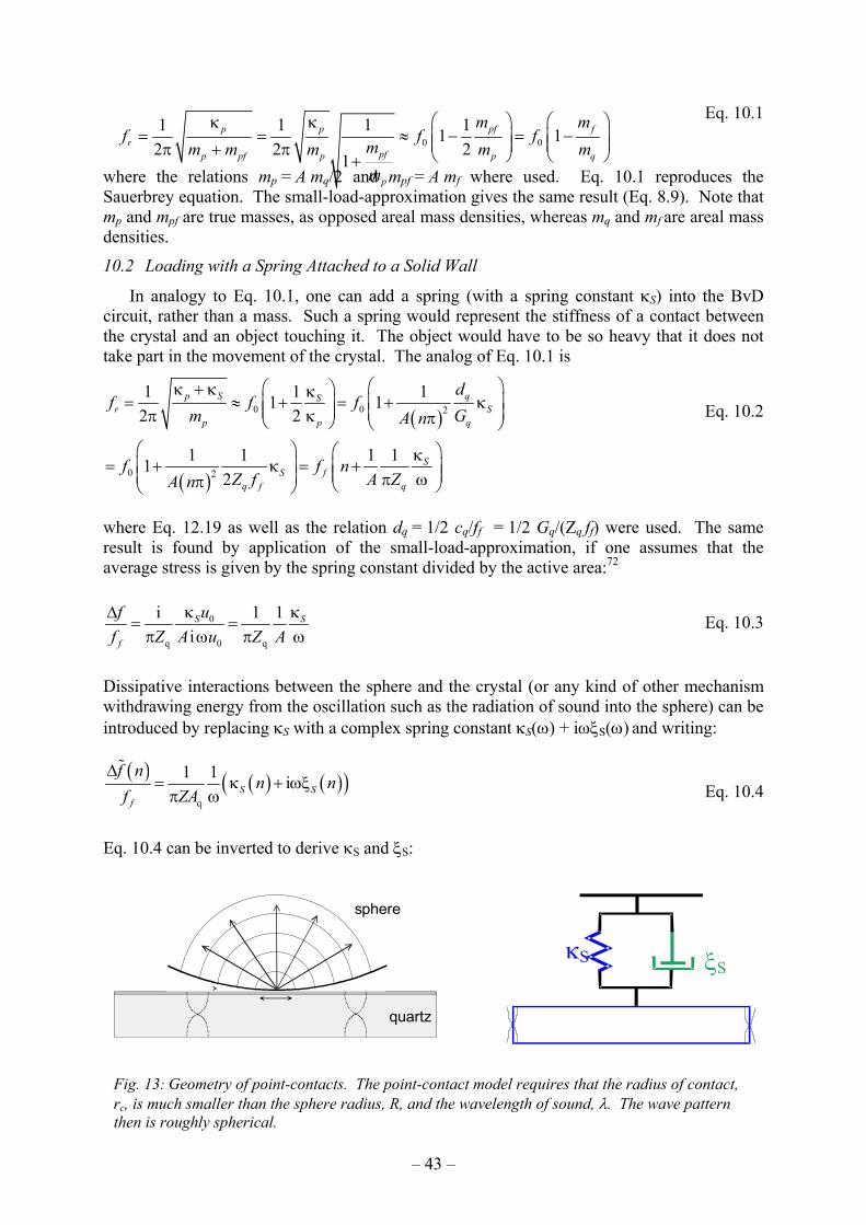
– 43 –

Eq. 10.1

where the relations mp = A mq/2 and mpf = A mf where used. Eq. 10.1 reproduces the Sauerbrey equation. The small-load-approximation gives the same result (Eq. 8.9). Note that mp and mpf are true masses, as opposed areal mass densities, whereas mq and mf are areal mass densities.

10.2 Loading with a Spring Attached to a Solid Wall

In analogy to Eq. 10.1, one can add a spring (with a spring constant κS) into the BvD circuit, rather than a mass. Such a spring would represent the stiffness of a contact between the crystal and an object touching it. The object would have to be so heavy that it does not take part in the movement of the crystal. The analog of Eq. 10.1 is

Eq. 10.2

where Eq. 12.19 as well as the relation dq = 1/2 cq/ff = 1/2 Gq/(Zq ff) were used. The same result is found by application of the small-load-approximation, if one assumes that the average stress is given by the spring constant divided by the active area:72

Eq. 10.3

Dissipative interactions between the sphere and the crystal (or any kind of other mechanism withdrawing energy from the oscillation such as the radiation of sound into the sphere) can be introduced by replacing κS with a complex spring constant κS(ω) + iωξS(ω) and writing:

Eq. 10.4

Eq. 10.4 can be inverted to derive κS and ξS:

0 01 1 1 11 1

2 2 21

p p pf fr

pfp pf p p q

p

m mf f f

mm m m m mm

κ κ= = ≈ − = − π + π +

( )

( )

0 0 2

0 2

1 1 11 12 2

1 1 1 112

p S qSr S

p p q

SS f

q f q

df f f

m GA n

f f nZ f A ZA n

κ + κ κ= ≈ + = + κ π κ π

κ= + κ = + π ωπ

0

q 0 q

i 1 1iS S

f

uff Z A u Z A

κ κ∆= =

π ω π ω

( ) ( ) ( )( )q

1 1 iS Sf

f nn n

f ZA∆

= κ + ωξπ ω

κS ξS

quartz

sphere

Fig. 13: Geometry of point-contacts. The point-contact model requires that the radius of contact, rc, is much smaller than the sphere radius, R, and the wavelength of sound, λ. The wave pattern then is roughly spherical.

– 44 –

( )1

11 1

22

2

1 ii

i 1i1

L mass springS S

S S

S S

S

Z Z Zm

m mm

−−− − ω

= + = + ω κ ω κ

= = ωω−ω + κ −ω

2

20

1

1

S

f q

N mff Z

− ω∆=

ωπ −ω

Eq. 10.5

Eq. 10.6

For Hertzian sphere–plate contacts having a contact diameter much smaller than the wavelength of sound, the Mindlin model110 predicts the spring constant to be

Eq. 10.7

where K is a modulus of the order of the shear modulus and rc is the radius of contact. Mindlin emphasizes that there is a stress concentration at the rim of the contact, which leads to partial slip and, consequently, to a nonlinear stress–speed relation even at small amplitudes.

If the dashpot, ξS, is dominated by the radiation of acoustic waves into the crystal,72 one can approximate the parameter ξS as

Eq. 10.8

where k is the wave number of sound. Eq. 10.7 and Eq. 10.8 constitute the "point-contact model".17,111

10.3 The Mass-Spring-Model In the spring-model the contact was made with an immobile external object (like a wall). Such an object could be either a real wall or an object which is too heavy to take part in the MHz oscillation. The model can be extended to cover situations, where the object takes part in the oscillation to some extent. Typical objects like this would be small spheres. Fig. 14 depicts the physical situation and the equivalent circuit representation. Note the motion occurs into the lateral direction even though the spring is depicted as vertical. Fig. 14 shows a single sphere. Real crystals might be in contact with many such spheres, which is accounted for by including the number density of these spheres, NS, as a prefactor into Eq. 10.14 below. From Fig. 14, we infer the load to be

Eq. 10.9

where the parameter ωS = (κS/mS)1/2 denotes the resonance frequency of the mass–spring system. Using the small-load-approximation, we find112

Eq. 10.10

In the limits of ω02 à ω and ω0

2 á ω, Eq. 10.10 reproduces the Sauerbrey equation (Eq. 4.18) and the point-contact model (Eq. 10.3), respectively. Eq. 10.10 can also be derived from Eq. 8.35 by expanding all tangents to first order. This amounts to a continuum model of the same experimental situation.

2q( ) 2 ( )S n Z n A f nκ = π ∆

( ) ( )qS

f

Zn A n

fπ

ξ = ∆Γ

S cK rκ =

S S ckrξ = κ

– 45 –

( )1

11 1

2 2

1 1i

i 1 1 ii ii 1 i 1

L mass dashpotS S

S SS S

S S

Z Z Zm

m m mm

−−− −

= + = + ω ξ ω ξ − ωτ

= = ω = ωω + ξ + ωτ + ω τ

10.4 The Mass-Dashpot-Model

The connection between the sphere and the crystal can also be made across a dashpot. This model assumes sliding of the sphere on the surface. Note that this sliding is sliding in a liquid-like sense, also called creep. Interfacial sliding in the Coulomb sense would be nonlinear in the force. From Fig. 14 we read:

Eq. 10.11

where the slip time τ = mS/ξS was introduced. The slip time (also termed “momentum relaxation time” in the colloid science) is the time needed for deceleration of the sphere after a lateral motion of the substrate has abruptly stopped. Using the small-load-approximation, we

1/(iωC0)

1 to 4φ24Zk mp κp ξp

ξS mSmSκS

ξS

κS

ZL

ξS κS

mass-spring mass-dashpot

Maxwell Voigt Fig. 14: Equivalent circuit representations of various models. The lower four circuits are inserted for the load ZL in the Mason circuit (top). For the Maxwell and the Voigt model, the mass is assumed to be so heavy that it may be represented by a wall. The conversion from the physical situation to the equivalent circuits is nontrivial for two reasons: Firstly, elements which are physically placed in series are represented as parallel circuit elements and vice versa (cf. Fig. 5). Secondly, an open (stress-free) end in the physical situation corresponds to a connection to ground (lower line in the equivalent circuits), because the latter has a voltage of zero. In the literature on polymer rheology, springs and dashpots are drawn as on the left-hand-side, but they are connected to each other like shown on the right-and-side of each graph. This convention differs from the convention chosen here.

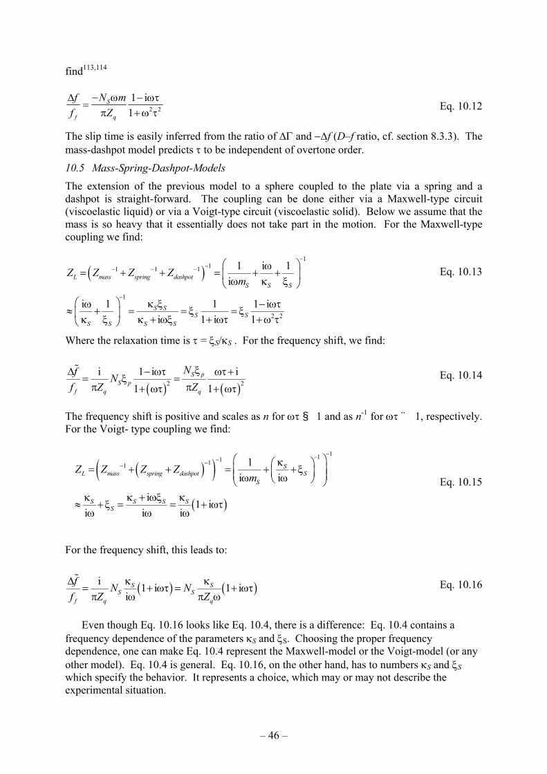
– 46 –

( )1

11 1 1

1

2 2

1 i 1i

i 1 1 1 ii 1 i 1

L mass spring dashpotS S S

S SS S

S S S S

Z Z Z Zm

−−− − −

−

ω= + + = + + ω κ ξ

κ ξω − ωτ≈ + = = ξ = ξ κ ξ κ + ωξ + ωτ + ω τ

( ) ( )2 2i 1 i i

1 1S p

S pf q q

Nf Nf Z Z

ξ∆ − ωτ ωτ+= ξ =

π π+ ωτ + ωτ

( )( )( )

11111 1i i

i 1 ii i i

SL mass spring dashpot S

S

S S S SS

Z Z Z Zm

−−−−− κ = + + = + + ξ ω ω

κ κ + ωξ κ≈ + ξ = = + ωτ

ω ω ω

( ) ( )i 1 i 1 ii

S SS S

f q q

f N Nf Z Z

κ κ∆= + ωτ = + ωτ

π ω π ω

find113,114

Eq. 10.12

The slip time is easily inferred from the ratio of ∆Γ and −∆f (D–f ratio, cf. section 8.3.3). The mass-dashpot model predicts τ to be independent of overtone order.

10.5 Mass-Spring-Dashpot-Models

The extension of the previous model to a sphere coupled to the plate via a spring and a dashpot is straight-forward. The coupling can be done either via a Maxwell-type circuit (viscoelastic liquid) or via a Voigt-type circuit (viscoelastic solid). Below we assume that the mass is so heavy that it essentially does not take part in the motion. For the Maxwell-type coupling we find:

Eq. 10.13

Where the relaxation time is τ = ξS/κS . For the frequency shift, we find:

Eq. 10.14

The frequency shift is positive and scales as n for ωτ á 1 and as n-1 for ωτ à 1, respectively. For the Voigt- type coupling we find:

Eq. 10.15

For the frequency shift, this leads to:

Eq. 10.16

Even though Eq. 10.16 looks like Eq. 10.4, there is a difference: Eq. 10.4 contains a frequency dependence of the parameters κS and ξS. Choosing the proper frequency dependence, one can make Eq. 10.4 represent the Maxwell-model or the Voigt-model (or any other model). Eq. 10.4 is general. Eq. 10.16, on the other hand, has to numbers κS and ξS which specify the behavior. It represents a choice, which may or may not describe the experimental situation.

2 2

1 i1

S

f q

N mff Z

− ω∆ − ωτ=

π + ω τ

– 47 –

( ) ( )

( ) ( )

0

0

1 1 2 cos

1 1 2 sin

tf q

tf q

f F t tf Z Au

F t tf Z Au

∆= ω

π ω

∆Γ= ω

π ω

( )

( )

2

2

1 1 2 1 1 1cos

1 1 2 1 1sin

S Sf q q

S Sf q q

f tf Z A Z A

tf Z A Z A

∆= κ ω = κ

π ω π ω

∆Γ= ωξ ω = ξ

π ω π

10.6 Nonlinear Mechanics and Memory Effects

The above analysis assumes linear force–displacement relations. However, when interfacial friction enters the game, the mechanical behavior may easily become nonlinear.115 Memory effects are ubiquitous. Equivalent circuits then no longer hold, since they assume linear mechanics. However, as long as the interaction between the crystal and its environments can be considered a small perturbation to the forces governing the oscillation (which comes down to the condition of a small fractional frequency shift fff /∆ ), there still is room for quantitative modeling. For a small perturbation, the two-timing approximation116 holds. Within the two-timing approximation, the motion of the crystal is essentially sinusoidal. The consequence of the small external forces is captured by a slowly varying amplitude A(t) and a slowly varying phase ϕ(t). The excess damping, 2π∆Γ, is the negative normalized time derivative of the amplitude /A A− , whereas the frequency shift, 2π∆f, is the time derivative of the phase ϕ .117,118 This formalism is also used in the context of non-contact atomic force microscopy. It links the force-distance curve to the shifts of frequency and dissipation of the cantilever.119 The detailed calculation shows that:

Eq. 10.17

where the angular brackets denote a time average and F(t) is the (small) force exerted by the sample. When linear force laws hold, one as F(t) = κSu(t) + ξS u (t) which leads to

Eq. 10.18

Eq. 10.17 then reduces to Eq. 10.3 and Eq. 10.4. If memory effects are absent and the nonlinearities are small, a nonlinear stress–strain and a stress–speed relation can be inferred from the amplitude dependence of the ∆f and ∆Γ.117,118

If there are memory effects, the time-dependence of the force F(t) must be inserted directly into Eq. 10.17. The machine cannot run backwards, that is, the force F(t) cannot be explicitly inferred from the frequency shift and the bandwidth in the same way as the spring constant and the drag coefficient are inferred from ∆f and ∆Γ in Eq. 10.5 and Eq. 10.6. Still, the relation between force F(t) and frequency shift f∆ is strictly quantitative. By means of Eq. 10.17, any given hypothesis about the force F(t) (including stick-slip, memory, and nonlinearities) can be checked against the experiment.

11 Concluding Remarks This chapter has focused on applications of the QCM which go beyond microweighing.

The analysis has relied on the small-load-approximation and has lead to a comprehensive picture covering a wide variety of configurations. From an practical point of view, the main benefits of this analysis can be summarized as follows:

− The frequency-dependent viscous compliance J’’(ω) can be determined for thin films in air.

– 48 –

− The frequency-dependent elastic compliance J’(ω) can be estimated for thin films in a liquid environment.

− Interfacial viscoelastic spectroscopy on soft elastomers is possible be virtue of the sheet-contact model.

− The strength of particle–sphere contacts can be estimated on the basis of the point-contact model.

On the other hand, there are numerous samples and experiments, which cannot easily be interpreted within this frame. Here are some examples:

− Electrical fringe fields often do penetrate into the sample. The sample's dielectric properties affect the parallel capacitance C0, and thereby the frequency shift. The QCM can probe dielectric properties and viscoelastic properties at the same time.

− The laws of linear acoustics are violated at high amplitudes of oscillation. Studying nonlinear interactions between the crystal and the sample should be useful in the context of tribology and adhesion.

− Many interesting samples are not laterally homogeneous. The calculation of the average shear-induced stress is not an easy task, but it seems feasible in some cases. High-frequency fluid dynamics should be able to solve some of the problems.

It is to be hoped that the established models describing the QCM can be extended to cover these more complicated – but also more interesting – samples, as well.

Acknowledgements The author is indebted to I. Reviakine and R. Lucklum for critical reading of the manuscript.

– 49 –

12 Appendices

12.1 Equivalent Circuit of a Viscoelastic Layer

The displacement inside the layer u(z) is of the form4

Eq. 12.1

where k is the wave vector, and A0 and B0 are amplitudes to be specified by the boundary conditions. The origin of the z-axis is in the center of the plate. The width of the plate is 2h. We then have for the speeds at the edge of the plate, 1u and 2u :

Eq. 12.2

For the forces F = AG ∂u/∂z (A the area, G the shear modulus) we find

Eq. 12.3

where Gk = ωZ has been used. This leads to the relations

Eq. 12.4

When making the transformation to the electrical circuit ( 1u → – I1, 2u →I2, F1→U1, F2→U2), we need to account for the fact that there is a sign reversal between 1u and I1 (Fig. 15). We want to achieve an equation system in matrix form:

Eq. 12.5

For reasons of symmetry, we have Z12 = Z21 and Z11 = Z22. Such an equation system is graphically represented by

, if the coefficients Z11 and Z12 are the impedances as shown in the figure. Inserting Eq. 12.4 and taking care of the sign reversal between

1u and I1, we find Z22 − Z12

− 1~ I1 2~ I2

F1~ U1 F2~ U2

Z22 − Z12

Z12

u u

Fig. 15: Equivalent circuit representing a viscoelastic layer (transmission line model).

( ) ( ) ( )0 0sin cosu z A kz B kz= +

( )( )

1 2 0

1 2 0

2i sin

2i cos

u u A kh

u u B kh

− = − ω

+ = ω

( ) ( )( ) ( )

1 2 0 0

1 2 0 0

2 sin 2 sin

2 cos 2 cos

F F AG k B kh A Z B kh

F F AG k A kh A Z A kh

− = = ω

+ = = ω

( ) ( )( ) ( )

1 2 1 2

1 2 1 2

i tan

i cot

F F u u A Z kh

F F u u A Z kh

− = − +

+ = −

1 11 1 12 2

2 21 1 22 2

U Z I Z IU Z I Z I

= += +

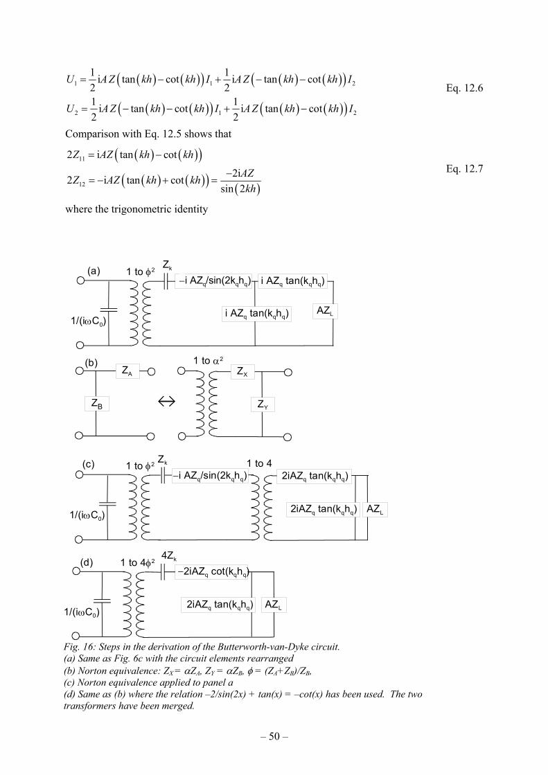
– 50 –

Eq. 12.6

Comparison with Eq. 12.5 shows that

Eq. 12.7

where the trigonometric identity

( ) ( )( ) ( ) ( )( )

( ) ( )( ) ( ) ( )( )

1 1 2

2 1 2

1 1i tan cot i tan cot2 21 1i tan cot i tan cot2 2

U A Z kh kh I A Z kh kh I

U A Z kh kh I A Z kh kh I

= − + − −

= − − + −

( ) ( )( )( ) ( )( ) ( )

11

12

2 i tan cot

2i2 i tan cotsin 2

Z AZ kh kh

AZZ AZ kh khkh

= −

−= − + =

i AZq tan(kqhq)

i AZq tan(kqhq)−i AZq/sin(2kqhq)

1/(iωC0)

Zk

AZL

1 to φ2(a)

(b)ZX

ZY

1 to α2

ZXZX

ZB

ZA

2iAZq tan(kqhq)

2iAZq tan(kqhq)

1/(iωC0)AZL

−i AZq/sin(2kqhq)1 to φ2 1 to 4Zk(c)

1/(iωC0)

1 to 4φ2

2iAZq tan(kqhq)

4Zk

AZL

−2iAZq cot(kqhq)(d)

Fig. 16: Steps in the derivation of the Butterworth-van-Dyke circuit. (a) Same as Fig. 6c with the circuit elements rearranged (b) Norton equivalence: ZX = αZA, ZY = αZB, φ = (ZA+ZB)/ZB, (c) Norton equivalence applied to panel a (d) Same as (b) where the relation –2/sin(2x) + tan(x) = –cot(x) has been used. The two transformers have been merged.

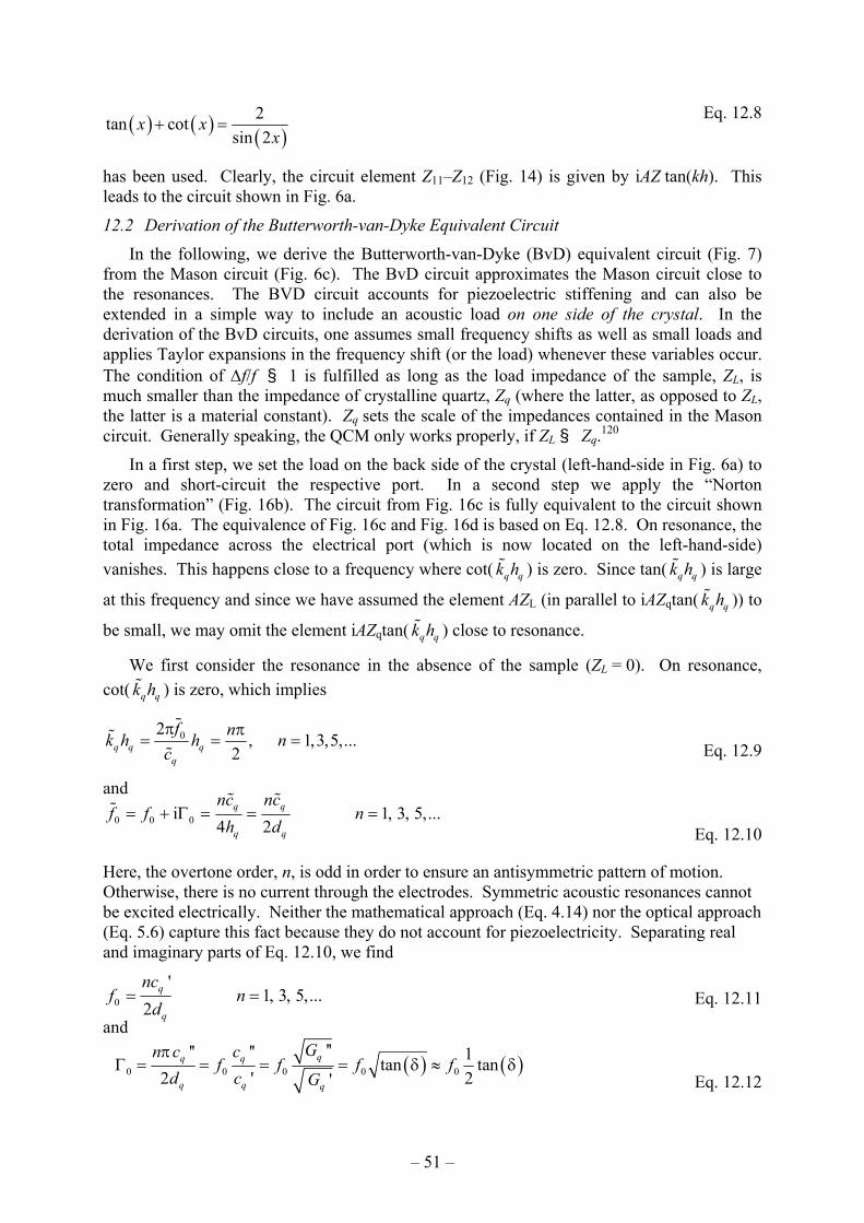
– 51 –

Eq. 12.8

has been used. Clearly, the circuit element Z11–Z12 (Fig. 14) is given by iAZ tan(kh). This leads to the circuit shown in Fig. 6a.

12.2 Derivation of the Butterworth-van-Dyke Equivalent Circuit

In the following, we derive the Butterworth-van-Dyke (BvD) equivalent circuit (Fig. 7) from the Mason circuit (Fig. 6c). The BvD circuit approximates the Mason circuit close to the resonances. The BVD circuit accounts for piezoelectric stiffening and can also be extended in a simple way to include an acoustic load on one side of the crystal. In the derivation of the BvD circuits, one assumes small frequency shifts as well as small loads and applies Taylor expansions in the frequency shift (or the load) whenever these variables occur. The condition of ∆f/f á 1 is fulfilled as long as the load impedance of the sample, ZL, is much smaller than the impedance of crystalline quartz, Zq (where the latter, as opposed to ZL, the latter is a material constant). Zq sets the scale of the impedances contained in the Mason circuit. Generally speaking, the QCM only works properly, if ZL á Zq.120

In a first step, we set the load on the back side of the crystal (left-hand-side in Fig. 6a) to zero and short-circuit the respective port. In a second step we apply the “Norton transformation” (Fig. 16b). The circuit from Fig. 16c is fully equivalent to the circuit shown in Fig. 16a. The equivalence of Fig. 16c and Fig. 16d is based on Eq. 12.8. On resonance, the total impedance across the electrical port (which is now located on the left-hand-side) vanishes. This happens close to a frequency where cot( q qk h ) is zero. Since tan( q qk h ) is large

at this frequency and since we have assumed the element AZL (in parallel to iAZqtan( q qk h )) to

be small, we may omit the element iAZqtan( q qk h ) close to resonance.

We first consider the resonance in the absence of the sample (ZL = 0). On resonance, cot( q qk h ) is zero, which implies

Eq. 12.9

and

Eq. 12.10

Here, the overtone order, n, is odd in order to ensure an antisymmetric pattern of motion. Otherwise, there is no current through the electrodes. Symmetric acoustic resonances cannot be excited electrically. Neither the mathematical approach (Eq. 4.14) nor the optical approach (Eq. 5.6) capture this fact because they do not account for piezoelectricity. Separating real and imaginary parts of Eq. 12.10, we find

Eq. 12.11

and

Eq. 12.12

02, 1,3,5,...

2q q qq

f nk h h ncπ π

= = =

0 0 0i 1, 3, 5,...4 2

q q

q q

nc ncf f n

h d= + Γ = = =

0

'1, 3, 5,...

2q

q

ncf n

d= =

( ) ( )0 0 0 0 0

'''' '' 1tan tan2 ' 2'

qq q

q q q

Gn c cf f f f

d c Gπ

Γ = = = = δ ≈ δ

( ) ( ) ( )2tan cot

sin 2x x

x+ =

– 52 –

where tan(δ) = Gq’’/Gq’ is the loss tangent. Note that the approximation (tan(δ))1/2 ≈ tan(δ)/2 requires tan(δ) á 1, which is certainly fulfilled for quartz.

For the Q-factor, we find

Eq. 12.13

We now consider a frequency close to the resonance frequency and frequencies close to the resonance f = fr + df rather than the resonance frequency itself. Here df is a small difference between the driving frequency and the resonance frequency (as apposed to a shift of the resonance frequency). We write

Eq. 12.14

Separation of cot( q qk h ) into its real and imaginary part yields

Eq. 12.15

Using Eq. 12.14 and Taylor-expanding Eq. 12.15 to first order in the small terms df/f0 and tan(δ), we find

Eq. 12.16

In order to find the equivalent mass, mp, the equivalent spring constant, κp, and the equivalent dashpot, ξp, we need to write down the impedance of such an equivalent circuit (Fig. 17b). By comparing the coefficients with the coefficients in Eq. 12.16, we determine the values of mp, κp, and ξp. When placing a mass, a spring, and a dashpot in series (in the electrical sense, Fig. 5) the total impedance is

Eq. 12.17

where the relations ω0 = (κp/mp)1/2 and ω + ω0 ≈ 2ω have been used. Comparison with Eq. 12.16 shows that

Eq. 12.18

( )0

0

12 tan

fQ = =

Γ δ

( )tann d' i '' 1 i2 2q q q q q q

r

fk h k h k hf

δπ= + ≈ + +

( )( ) ( )( ) ( )

( )( ) ( )

sin 2 ' sinh 2 ''cot ' i '' i

cos 2 ' cosh 2 '' cos 2 ' cosh 2 ''q q q q

q q qq q q q q q q q

k h k hk k h

k h k h k h k h− = − −

− −

( ) ( )tan d2i cot i2q q q q

r

fAZ k h n AZf

δ− ≈ π +

( )( )

( )

0

0

0 0

0

0

0

i ii

i

2i

2di

pp p p p

p p p

p p p

p p pr

m m

m

m

fmf

κ ωωω + + ξ = κ − + ξ ω ω ω

ω + ω ω− ω= κ + ξ ω ω

ω− ω≈ κ + ξ

ω

≈ κ + ξ

( )

2

tan2

p p q

p pp q

nm AZ

mnAZQ

πκ =

κπξ = δ =

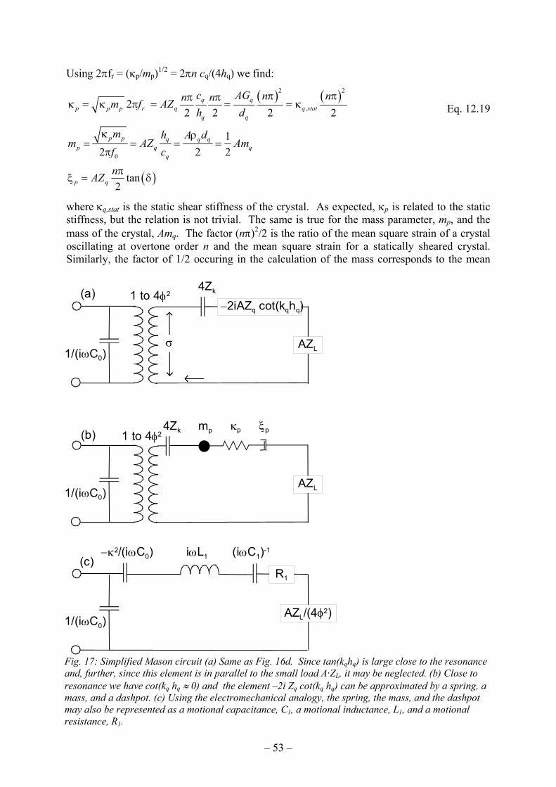
– 53 –

1/(iωC0)

1 to 4φ2

−2iAZq cot(kqhq)4Zk

AZLσ

1/(iωC0)

R1

( iωC1)-1

AZL/(4φ2)

iωL1−κ2/(iωC0)

(a)

(c)

1/(iωC0)

1 to 4φ24Zk

AZL

(b)mp κp ξp

Fig. 17: Simplified Mason circuit (a) Same as Fig. 16d. Since tan(kqhq) is large close to the resonance and, further, since this element is in parallel to the small load A·ZL, it may be neglected. (b) Close to resonance we have cot(kq hq ≈ 0) and the element –2i Zq cot(kq hq) can be approximated by a spring, a mass, and a dashpot. (c) Using the electromechanical analogy, the spring, the mass, and the dashpot may also be represented as a motional capacitance, C1, a motional inductance, L1, and a motional resistance, R1.

Using 2πfr = (κp/mp)1/2 = 2πn cq/(4hq) we find:

Eq. 12.19

where κq,stat is the static shear stiffness of the crystal. As expected, κp is related to the static stiffness, but the relation is not trivial. The same is true for the mass parameter, mp, and the mass of the crystal, Amq. The factor (nπ)2/2 is the ratio of the mean square strain of a crystal oscillating at overtone order n and the mean square strain for a statically sheared crystal. Similarly, the factor of 1/2 occuring in the calculation of the mass corresponds to the mean

( ) ( )

( )

2 2

,

0

22 2 2 2

12 2 2

tan2

q qp p p r q q stat

q q

p p q q qp q q

q

p q

c AG n nn nm f AZh d

m h A dm AZ Am

f c

nAZ

π ππ πκ = κ π = = = κ

κ ρ= = = =

π

πξ = δ

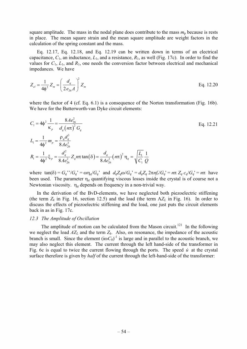
– 54 –

square amplitude. The mass in the nodal plane does contribute to the mass mp because is rests in place. The mean square strain and the mean square amplitude are weight factors in the calculation of the spring constant and the mass.

Eq. 12.17, Eq. 12.18, and Eq. 12.19 can be written down in terms of an electrical capacitance, C1, an inductance, L1, and a resistance, R1, as well (Fig. 17c). In order to find the values for C1, L1, and R1, one needs the conversion factor between electrical and mechanical impedances. We have

Eq. 12.20

where the factor of 4 (cf. Eq. 6.1) is a consequence of the Norton transformation (Fig. 16b). We have for the Butterworth-van Dyke circuit elements:

Eq. 12.21

where tan(δ) = Gq’’/Gq’ = ωηq/Gq’ and dqZqω/Gq’ = dqZq 2πnfr/Gq' = nπ Zq cq/Gq' = nπ have been used. The parameter ηq quantifying viscous losses inside the crystal is of course not a Newtonian viscosity. ηq depends on frequency in a non-trivial way.

In the derivation of the BvD-elements, we have neglected both piezoelectric stiffening (the term Zk in Fig. 16, section 12.5) and the load (the term AZL in Fig. 16). In order to discuss the effects of piezoelectric stiffening and the load, one just puts the circuit elements back in as in Fig. 17c.

12.3 The Amplitude of Oscillation

The amplitude of motion can be calculated from the Mason circuit.121 In the following we neglect the load AZL and the term Zk. Also, on resonance, the impedance of the acoustic branch is small. Since the element (iωC0)-1 is large and in parallel to the acoustic branch, we may also neglect this element. The current through the left hand-side of the transformer in Fig. 6c is equal to twice the current flowing through the ports. The speed u at the crystal surface therefore is given by half of the current through the left-hand-side of the transformer:

2

226

14 2

qel m m

dZ Z Z

e A

= = φ

( )

( ) ( )

22 26

1 2

3

1 2 226

22 1

1 2 2 226 26 1

814

14 8

1 1tan4 8 8

p q q

q qp

q qp q q

AeCd n G

dL m

Ae

d d LR Z n nAe Ae C Q

= φ =κ π

ρ= =

φ

= ξ = π δ = π η =φ

– 55 –

Eq. 12.22

where Eq. 12.8 and Eq. 12.14 were used. Converting to the amplitude a yields

Eq. 12.22

Here d26 = e26/Gq = 3.1µ10–12 m/V is the piezoelectric strain coefficient. Note that the derivation assumes laterally infinite resonators; it does not account for energy trapping. Eq. 12.22 is therefore expected to miss a numerical factor of order unity. Inputting values (d26 = 3.1 pm/V), we arrive at

Eq. 12.23

This compares well with the experimental value of 1.4 pm/V, where the latter has been determined from the wear induced by an STM tip on a oscillating quartz surface.122 Kanazawa finds a similar value by numerically solving the full Mason circuit.123

The direction of oscillation can be experimentally determined with a polarizing microscope in the conoscopic mode.121 Colored rings are observed. The direction of curvature points perpendicular to the x-axis of the crystal, that is, perpendicular to the direction of oscillation.

The drive level is often quoted in dBm, where 0 dBm corresponds to a power of 1 mW. The conversion is

Eq. 12.24

where Uel is amplitude (1/2 of the peak-to-peak voltage).

12.4 The Effective Area

We can also infer an estimate of the active area, A, from the value of R1 (Eq. 12.21) and Q. The effective area is needed in the application of the sheet contact model (section 8.1.2). Using the relation between the Q-factor and the loss tangent (Eq. 12.13), we have:

Eq. 12.25

which, by inversion, yields

Eq. 12.26

( ) ( ) ( )26 26

el 26 el el 26 el2 2 21 1 4 4 4 4

2 f q q qq q

e ea u QU e QU QU d QUnf n Z d Gn Z c n n

= = = = =ω π π π π π

( ) ( )

( )

( )

1

1

126

26

i1 1 i tan2 2sin 2

1 1 i cot2 2

1 tan2 8

4

qq q q el

q q

q q q el

q elq

elq q

AZu AZ k h U

k h

AZ k h U

AenAZ Ud

eQ Un Z d

−

−

−

− = + φ

= − φ

π ≈ δ

≈π

( )2 2

1 2 226 26

tan8 8

q q qq

d d Z nR Z n

Ae Ae Qπ

= π δ =

2 2 2

2 2 2 2 2 2 2 226 1 26 1 26 1 26 1

18 8 32 32

q q q q q q

q q f f q

d Z d Z c Zn n n nAe R Q G d R Q G f d R Q f Z d R Q

π π π π= = = =

( ) 262 2el

4 1.25 pmV

a dQU nn

= =π

( )power[dBm]/ 200.317 10elU = ×

– 56 –

When the resonance parameters are probed via impedance analysis, the parameter R1 is routinely determined as the inverse of the peak conductance, Gmax. The effective area is proportional to the peak conductance, Gmax = R1

-1. because a large active area draws a large current. Being an electric quantity, the parameter R1 is susceptible to calibration problems and electrical imperfections. Also, Eq. 12.26 does not account for energy trapping and is therefore expected to miss a factor of the order unity. The correction factor may vary with energy overtone order.

12.5 Piezoelectric Stiffening

For the most part, piezoelectricity can just be considered as a convenient effect allowing for detection of acoustic resonances by electrical means. Actually, the piezoelectric coefficients of α-quartz (which is the room-temperature modification of crystalline quartz) are rather small. This can be viewed as a benefit for the purpose of sensing. If the electro-mechanical coupling were stronger, electrical disturbances would have a stronger influence on the acoustic resonance than they have (see below). On the other hand, a stronger coupling would make it easier to pick up resonances with simple oscillator circuits. Gallium-orthophosphate (GaPO4) has a coupling constant about four times larger than quartz, which makes it attractive in this respect (in addition to the high-temperature stability).

If one looks at the resonance behavior a little closer, one finds that piezoelectricity does more than serving as an electro-mechanical coupler. It introduces “piezoelectric stiffening”. The elastic energy contained in a strained crystal depends on whether or not the strain-induced polarization on the crystal surfaces is compensated by a charge (supplied by the electric circuit). If the polarization is not compensated, then there is an electrical contribution to the strain energy and the restoring force pushing the crystal back into its original shape is stronger than in the case of short-circuited electrodes. This stiffening is one out of two reasons, why the resonance frequencies of the various overtone orders do not strictly scale as the overtone order, n (section 12.6). In the context of timing applications, one actually takes advantage of piezoelectric stiffening in order to electrically pull the resonance frequency of a crystal. Inserting a capacitor in series with the crystal, one can shift the resonance frequency within certain limits. Stray capacitances between the electrodes and the housing also pull the frequency, which is an undesired perturbance. One way to diminish the influence of stray capacitances is to connect the two electrodes across a small resistor (see section 3).

In the context of sensing, one does not rely on absolute frequencies, but rather on frequency shifts. The calculation below shows that the frequency shifts are only weakly affected by piezoelectricity unless the electrical boundary conditions vary. Such electric effects can be avoided by grounding the front electrode well, and in the following we assume that this is the case. If not, piezoelectricity opens a box of interesting phenomena,31,32 which are, however, outside of the scope of this chapter.

Before discussing piezoelectric stiffening in mathematical detail, we explain on a qualitative basis, why piezoelectric stiffening is more effective on higher harmonics than on

elec

trica

l pot

entia

l [a.

u.]

z [a.u.]

Fig. 18: Distribution of electrical potential inside the crystal for the fundamental and the 5th overtone. For the fundamental, the piezoelectrically induced electrical potential is to a large extent compensated by the external potential. This compensation is less effective on higher overtones, leading to piezoelectric stiffening. Dashed: potential in the absence of external compensation. Full: partially compensated potential. Dotted: external potential.

– 57 –

lower ones. The electric energy density is proportional to the square of the dielectric displacement Del, which in turn is proportional to the gradient of the electric potential ϕ. The potential ϕ has an internal component which is proportional to the local displacement (and therefore given by a sine wave) as well as an external component produced by the charge on the electrodes (which is given by a straight line). As Fig. 18 shows, these two component compensate each other rather well on the fundamental, but to a lesser extent on the higher harmonics. The current into the electrodes can only compensate the surface polarization, not the polarization generated inside the crystal.

With regard to the more rigorous mathematics, the theory of the piezoelectric plate has been worked out by Tiersten58 and put into a graphical form by Mason.54 Kanazawa has applied this theory rigorously to the case of a crystal loaded with a liquid and with a viscoelastic film.53 We do not reproduce this calculation here. A rather general statement can be made on the basis of the BvD circuit shown in Fig. 16c: Given the functional form of the term related to piezoelectric stiffening, one can define a knew complex spring constant, pκ , taking piezoelectric stiffening into account. One finds

Eq. 12.27

where the definitions of all variables other than κ is given in section 12.2. κ = [e26

2 / (εε0Gq)]1/2 is a dimensionless coefficient of piezoelectric coupling. Its value is κ=0.089 for AT-cut quartz. With this new definition of the spring constant, the relation between the frequency shift, f∆ , and the load impedance, ZL, comes out be the same as in Eq. 7.3. The resonance condition is (cf. Eq. 12.17)

Eq. 12.28

The spring constant drops out from the resonance conditions when the latter is linearized in /f f∆ . Within the linearized theory, piezoelectric stiffening may be ignored. This is not true

in the same way for the perturbation analysis (section 9). Neglecting piezoelectric stiffening in the perturbation theory amounts to an approximation which does change the outcome of the calculation to some extent.

The new definition of the spring constant as pκ can be carried over into a corresponding

definition of the BvD parameter C1. A new parameter 1C can be defined which takes piezoelectric stiffening into account.

Eq. 12.29

( )

( )( ) ( )

2 2 22 26

20 0

2 2226

2 20

414 i i2

8 1 81 i 1 i2

q qp p p p

q q

qp p p

q q

AG dn A eC d d A

AG n ed G n n

πκ = κ − φ + ωξ = − + ωξ

εε

π = − + ωξ = κ − κ + ωξ εε π π

1 0

0

20 i ii

4i i 4

pp L p p L

p p L p L

fm AZ m AZC f

fm AZ m f AZ

κ ∆= ω + + ≈ κ + ω

π∆= κ + = π∆ + ω

( )

2

21 1 0 1

1 1 1 1 81C C C C n

κ = − = − π

– 58 –

The first expression in Eq. 12.29 is more useful than the second because the parallel capacitance, C0, may include stray capacitances which are not captured by the piezoelectric coupling coefficient. These stray capacitances do affect the series resonance frequency and necessitate the use of a π-network if the electrical boundary conditions are not well controlled.

12.6 The Parameter ff and the Fundamental Frequency

Neglecting piezoelectricity and energy trapping, the standard model predicts that the overtones should appear at odd multiples of the fundamental. In experiment, however, one finds that the parameter f0/n decreases with overtone order124 (Fig. 19). For high overtone orders, an asymptotic value is approached. As we show below, the asymptotic value of f0/n is the best choice for the parameter ff, where the latter is denoted “the frequency of the fundamental”. The difference between the asymptotic value and the true frequency of the fundamental is of the order of 0.05%.

There are two reasons, why the ratio f0/n is not constant, which are piezoelectric stiffening and energy trapping. Piezoelectric stiffening has been treated in section 12.5. The correction due to piezoelectric stiffening scales as n-2 and therefore levels off at high overtone orders. Piezoelectricity causes and increase of f0/n with increasing overtone order. 125

A second reason for a dependence of f0/n on overtone order is the finite lateral width of the resonator. For the sake of simplicity, let’s the assume a quadratic plate of with L with an amplitude distribution be given by

Eq. 12.30

where kx, ky, and kz are wave vectors, x and y are the distance from the center of the plate in the lateral direction, z is the distance from the center of the plate in the vertical direction, and dq is the thickness of the plate. m, l, and n are mode indices. In reality, the amplitude profile in the lateral direction is not given by a cosine function, but rather by function close to a Gaussian. We choose the cosine function in order to qualitatively demonstrate an argument. The lowest nontrivial mode indices in the lateral direction are m = 1 and l = 1. Higher indices correspond to anharmonic sidebands. Assuming an isotropic material (which is unrealistic) the resonance frequency corresponding to this mode is

Eq. 12.31

In this case, the lower harmonics have a frequency above the value predicted by the standard model. The parameter f0/n decreases with overtone order and again, the effect vanishes in the limit of high overtone orders.

Going back to the derivation of the frequency shifts, one finds that the frequency of the fundamental ff is always inserted for the combination of parameters cq/(2dq). Therefore the limiting value of f0/n for high overtones is the best choice for this parameter.

( ) ( ) ( )0 0( , , ) cos cos sin cos cos sinx y zq

m x l y n zu x y z u k x k y k z uL L d

π π π = =

( )1 1

2 222 2 212 2 2 2 1 2

2 2 2q q q q

r x y zq q

c c c dnf k k k nL L d d nL

π π π = + + = + + = + π π

0 2 4 6 8 10 124.9405

4.9410

4.9415

4.9420

4.9425

f 0 / n

[MH

z]

Frequency [MHz] Fig. 19: Scaled resonance frequency fr/n versus overtone order for a typical crystal. The limiting value at high frequencies is a good choice for the parameter ff.

– 59 –

Glossary of Abbreviations A area section 12.4 a amplitude of oscillation at the crystal surface section 12.3 bs slip length section 8.3 c speed of sound c = (G/ρ)1/2 C1 motional capacitance section 6 C0 electrical (parallel) capacitance section 6 D dissipation D = Q–1 d thickness de thickness of the electrode df thickness of the film dq thickness of the crystal dq = cq / (2ff) d26 piezoelectric strain coefficient d26 = 3.1 × 10–12 m/V e26 piezoelectric stress coefficient e26 = d26 · Gq = 9.65 × 10–2 C/m2 e as an index: electrode F force Fex external force f as an index: film (exception: ff) f frequency fr resonance frequency (real part) f0 resonance frequency in reference state

rf resonance frequency rf = fr + i Γ

0f resonance frequency in reference state ff a parameter close to the resonance section 12.6 frequency of the fundamental G shear modulus G = G ' +iG '' Gq shear modulus of AT-cut quartz Gq ≈ 29.3 × 109 Pa hq half of the thickness of the crystal hq = dq/2 Iel electrical current J shear compliance J = 1/G, J = J ' − i J '' k wave vector k = ω/c = ω(ρ/G)1/2

,

k = k ' − i k '' liq as an index: liquid L1 motional inductance section 6 L width of a plate me areal mass density of the electrode mf areal mass density of the film mp mass of resonating system mp is not an area mass density, it is a mass mq areal mass density of the crystal mq = ρqdq = ρqcq / (2ff) = Zq / (2ff) n overtone order n = fr / ff q as an index: quartz Q Q-factor Q = fr/(2Γ) R1 motional resistance section 6 t time u lateral displacement u lateral speed u =iωu u± wave traveling to the left (+) or to the right (–) Fig. 3

– 60 –

u±,0 amplitudes of waves Uel electrical voltage x spatial coordinate in the surface plane y spatial coordinate in the surface plane z spatial coordinate perpendicular the surface plane zj,j+1 location of interface between layers j and j+1 Z acoustic impedance Z = ρc = (ρG)1/2, Z = Z ' + i Z '' Zel electric impedance Zk circuit element related piezoelectric stiffening section 12.5 Zliq acoustic impedance of a liquid Zliq = (iωηρ)1/2 Zm mechanical impedance Zm = F/u = Aσ/u Zq acoustic impedance of AT-cut quartz Zq = 8.8 µ 106 kg m–2 s–1 ZL load impedance ZL = σ/ u β' power law exponent of viscoelastic dispersion J '(f) = J'(ff) · (f/ff)β' β'' power law exponent of viscoelastic dispersion J ''(f) = J ''(ff) · (f/ff)β''

f∆ complex frequency shift ∆f frequency shift ∆Γ shift of half-band-half-width γ decay constant γ = ξ/mp Γ half-band-half-width of a resonance, HBH width, “bandwidth” for short φ factor for conversion between current and speed φ = A e26 / dq, Iel = φ u η viscosity η = G/(–iω) κp spring constant κS spring constant of a sphere–plate contact section 10

pκ spring constant including piezoelectric stiffening κ piezoelectric coupling coefficient κ2 = e26

2 / (εε0 Gq) λ wavelength µe dimensionless parameter describing the mass µe = me / mq of the electrode µf dimensionless parameter describing the mass µf = mf / mq of the film ρ density σ stress ω radial frequency ωr radial frequency on resonance ω0 radial frequency on resonance in reference state or eigenfrequency of a resonator ω0 = (κp/mp)1/2 ξp drag coefficient ξp = F / u ξS dissipative part of the interaction section 10 of a sphere–plate contact ξliq dimensionless parameter describing the viscosity section 9 of liquid ζe dimensionless parameter describing the compliance section 9 of the electrode ζf dimensionless parameter describing the compliance section 9 of the film

– 61 –

References 1 C. Lu, A. W. Czanderna (edts.), Applications of Piezoelectric Quartz Crystal

Microbalances, Elsevier, Amsterdam 1984. 2 A. Arnau, (edt.), Piezoelectric Transducers and Applications, Springer, Heidelberg 2004. 3 J.W. Grate, Chem. Rev. 100, 2627 (2000) . 4 R.N. Thurston, in C. Truesdell (edt.) "Mechanics of Solids", vol. 4, chap. 36, p. 257,

Springer, Heidelberg 1984. 5 G. Sauerbrey, Z. Phys. 155, 206 (1959). 6 C.S. Lu, O. Lewis, J. Appl. Phys. 43, 4385 (1972). 7 S. Bruckenstein, M. Shay, Electrochim. Acta 30, 1295 (1985). 8 M.D. Ward, D.A. Buttry, Science 249, 1000 (1990). 9 R. Beck, U. Pittermann, K.G. Weil, Ber. Bunsen-Ges. Phys. Chem. 92, 1363 (1988). 10 The frequency-modulation approach put forward by L. Bruschi, G. Delfitto, and G.

Mistura (Rev. Sci. Instr. 70, 153 (1999)) in essence is a very fast version of impedance analysis.

11 M. Rodahl M, B. Kasemo, Rev. Sci. Instr. 67, 3238 (1996). 12 See, e.g., P. Horowitz and W. Hill, The Art of Electronics, 2nd. ed. Cambridge University

Press, New York, 1989. 13 A. Arnau, T. Sogorb, Y. Jimenez, Rev. Sci. Instr. 73, 2724 (2002). 14 R. Schumacher, Angew. Chem., Int. Ed. Engl. 29, 329 (1990). 15 S. Bruckenstein, M. Shay, J. Electroanal. Chem. Interfacial Electrochem. 188, 131 (1985) 16 D.A. Buttry, M.D. Ward, Chem. Rev. 92 1335 (1992). 17 A. Laschitsch, B. Menges, D. Johannsmann, Appl. Phys. Lett. 77, 2252 (2000). 18 J. M. Kim, S. M. Chang, H. Muramatsu, Appl. Phys. Lett. 74, 466 (1999). 19 A. Bund, O. Schneider, V. Dehnke, Phys. Chem. Chem. Phys. 4, 3552 (2002). 20 W.A. Ducker, T.J. Senden, R.M. Pashley, Nature 353, 239 (1991). 21 H.J. Butt, Biophys. J. 60, 1438 (1991). 22 V.E. Bottom, Introduction to Quartz Crystal Unit Design, Van Nostrand Reinhold, New

York, 1982. 23 S. Goka, K. Okabe, Y. Watanabe, H. Sekimoto, Jpn. J. Appl. Phys. PART 1 39, 3073

(2000). 24 Z.X. Lin, M.D. Ward, Anal. Chem. 67, 685 (1995) 25 F. Eggers, Th. Funck, J. Phys. E: Sci. Instrumen. 20, 523 (1987). 26 E.P. EerNisse, Jap. J. Appl. Phys. PART 1 40, 3479 (2001). 27 K.E. Heusler, A. Grzegozewski, L. Jäckel, J. Pietrucha, Ber. Bunsenges. Phys. Chem.

1218, 92, (1988) 28 L. Daikhin, E. Gileadi, G. Katz, V. Tsionsky, M. Urbakh, Anal. Chem. 74, 554 (2002). 29 S.J. Martin, G.C. Frye, A.J. Ricco, Anal. Chem. 65, 2910 (1993). 30 See, for example, G. McHale, R. Lucklum, M.I. Newton, J.A. Cowen, J. Appl. Phys. 88,

7304 (2000). 31 C. Zhang, J.F. Vetelino, Sens. Actuators B 91, 320 (2003). 32 Z.A: Shana, F. Josse, Anal. Chem. 66, 1955 (1994). 33 F. Martin, M.I. Newton, G. McHale, Ka.A. Melzak, E. Gizeli, Biosensors and Bioelectr.

19, 627 (2004). 34 Y.V. Gulyaev, IEEE Trans. Ultrason. Ferroelectr. Freq. Control 45, 935 (1998).

– 62 –

35 H. Fritze, H.L. Tuller, Appl. Phys. Lett. 78, 976 (2001). 36 J.W. Elam, M.J. Pellin, Anal. Chem. 77, 3531 (2005). 37 D. Johannsmann, K. Mathauer, G. Wegner, and W. Knoll, Phys. Rev. B 46, 7808 (1992). 38 For the viscosity, the primed quantity (η’) is related to dissipation rather than the quantity

with double primes. 39 T. Nakamoto, T. Moriizumi, Jpn. J. Appl. Phys. 29, 963 (1990). 40 H.L. Bandey, S.J. Martin. R.W. Cernosek A.R. Hillman, Anal. Chem. 71, 2205 (1999). 41 R. Lucklum, C. Behling, P. Hauptmann, Anal. Chem. 71, 2488 (1999). 42 E. Benes J. Appl. Phys. 56 608 (1984). 43 J.M. Friedt, K.H. Choi, L. Francis, A. Campitelli, Jpn. J. Appl. Phys. PART 1 41, 3974

(2002). 44 V.V. Borovikov, R.A. Dialnyan, I.M. Shmyt’ko, Sov. Phys. Tech. Phys. 32, 325 (1987). 45 S.D. Stevens, H.F. Tiersten,. J. Acoust. Soc. Am. 79, 1811 (1986). 46 See, for instance: D.H. Wu W.T. Chien, Y.J. Tsai, IEEE Trans. Ultrason. Ferroelectr.

Freq. Control 52, 480 (2005). 47 Z.X. Lin, M.D. Ward, Anal. Chem. 67, 685 (1995). 48 T.W. Schneider, S.J. Martin, Anal. Chem. 67, 3324 (1995). 49 A drive level DL = 0 dBm corresponds to a power of P = 1 mW. With an impedance of

the cable of R = 50 ohms, this translates to a voltage Uel = (RP)1/2=(50 ×10-3)1/2 Volt(rms) × exp(DL/(20 dBm)) = 223.6 mV(rms) × exp(DL/(20 dBm)).

50 R.N. Thurston, H.J. McSkimin, C.P. Andrea, J. Appl. Phys. 37, 267 (1966). 51 Most network analyzer use three-term calibration, which is good enough in the sense that

the resonance curves look correct after calibration. Evidently, three-term calibration only account for sufficiently simple electrical elements between the analyzer and the crystal. Three-term calibration is described in the EIA Standard 512.

52 IEC standard 60444-1 53 C.E. Reed, K.K. Kanazawa, J.H. Kaufmann, J. Appl. Phys. 68, 1993 (1990). 54 W.P. Mason, "Piezoelectric Crystals and their Applications to Ultrasonics", Van

Nostrand, Princeton 1948. 55 C. D. Stockbridge, Vacuum Microbalance Techniques, vol. 5, Plenum, New York, 1966. 56 The overtone order may turn into a non-integer number if piezoelectric stiffening and

energy trapping are taken into account (sections 12.5 and 12.6). This does not change the structure of the equations.

57 A resonance can be excited electrically, if there is a difference between the displacement of the two electrodes (inducing a polarization and a current). Harmonics with even overtone order can under certain conditions also be electrically excited. The displacement pattern has to be slightly asymmetric. This may be the case if one side of the crystal is heavily loaded whereas the other side is empty.

58 H.F. Tiersten, J. Acoust. Soc. Amer. 35, 234 (1963). 59 I. Alig I, D. Lellinger J. Sulimma, S. Tadjbakhsch, Rev. Scient. Instr. 68, 1536 (1997). 60 W.P. Mason, W.O. Baker, H.J. McSkimin, J.H. Heiss, Phys. Rev. 75 936 (1949). 61 R.M.A. Azzam, N.M. Bashara, "Ellipsometry and Polarized Light", Elsevier, Amsterdam

1987. 62 See, for example: W. Knoll, in: Handbook of Optical Properties, R. E. Hummel,

P. Wißmann (eds.) Vol II, 373 (1997).

– 63 –

63 M. Salomaki, K. Loikas, J. Kankare, Anal. Chem. 75, 5895 (2003).

64 While a certain equivalent circuit uniquely predicts the input-output relation, the same input-output relation can be represented by more than one equivalent circuit. It is a bit of an art to find the simplest one. For example, the Norton transformation (Fig. 16b) links two networks which are equivalent to each other with regard to the input-output relation.

65 R. Lucklum, P. Hauptmann, Meas. Sci. Techn. 14, 1854 (2003). 66 R.W. Munn, J. Phys. C: Solid State Phys. 6, 3213 (1973). 67 J.F. Rosenbaum, Bulk Acoustic Wave Theory and Devices, Artech House 1988, p.376. 68 In this chapter, only the Mason circuits accounts for piezoelectric stiffening, whereas

piezoelectric stiffening is neglected in chapters 4 and 5. In order to find exact equivalence between the three models, the element Zk (dealing with piezoelectric stiffening) must be deleted from the Mason circuit.

69 H.L. Bandey, S.J. Martin, R.W. Cernosek, A.R. Hillman, Anal. Chem. 71, 2205 (1999). 70 John Henderson, Electronic Devices. Concepts and Applications, Prentice Hall, NJ,

(1991) p. 357. 71 Heterogeneous samples will, in general, lead to scattering of acoustic waves, which is not

captured by just calculating the average stress. 72 A. Laschitsch, D. Johannsmann, J. Appl. Phys. 85, 3759 (1999). 73 A.P. Borovikov, Instruments and Experimental Techniques, 1976, 19, 223.

This reference misses a factor of 2 in eqs. 1, 2, and 3. Otherwise, Borovikov's result is the same Kananazawa-Gordon result (ref. 74).

74 K.K. Kanazawa, J.G. Gordon II, Anal. Chim. Acta 99, 175 (1985). 75 W.P. Mason, J. Colloid Sci. 3, 147 (1948). 76 A. Bund, M. Schneider, J.Eelectrochem. Soc. 149, E331 (2002). 77 C.M. Flanigan, M. Desai, K.R.Shull, Langmuir 16, 9825, (2000). 78 K.R. Shull, Materials Science and Engineering R 36, 1 (2002). 79 A.M. König, M. Düwel, M. Kunze, B. Du, D. Johannsmann, Langmuir, in press. 80 B. Jérôme, Rep. Prog. Phys. 54, 391 (1991). 81 V.K. Gupta, J.J. Skaife T.B. Dubrovsky, N.L. Abbott, Science 279, 2077 (1998). 82 H. Muramatsu, F. Iwasaki, Mol. Cryst. Liq. Cryst. 258, 153 (1995). 83 A. Domack, D. Johannsmann, Appl. Phys. Lett. 80, 4750 (2002), 84 J.P. de Gennes, J. Prost, The Physics of Liquid Crystals, Oxford University Press, Oxford,

1993, ch. 5.2.2 85 F. Kiry, P. Martinoty, Journ. Phys. (Paris) 38, 153 (1977). 86 P. Martinoty, S. Candau, Mol. Cryst. Liq. Cryst. 14, 243 (1971). 87 O. Parodi, Journ. Phys. (Paris) 31, 581 (1970). 88 See for example: J.S Huang, R. Varadaraj, Current Opinion in Colloid & Interface Science

1, 535 (1996). 89 J. Bell, T. Köhler, D. Woermann, Ber. Bunsenges. Phys. Chem. 101, 879 (1997). 90 R. Lionberger, W.B. Russel, J. Rheol. 38, 1885 (1994). 91 G. Fritz, W. Pechhold, N. Willenbacher, N.J. Wagner, J. Rheol. 47, 303 (2003). 92 N.J. Wagner, J. Coll. Interf. Sci. 161, 169 (1993). 93 J.D. Ferry, "Viscoelastic Properties of Polymers", Wiley, New York 1980. 94 V.E. Granstaff, S.J. Martin, J. Appl. Phys. 75, 1319 (1994).

– 64 –

95 S.J. Martin, H.L. Bandey, R.W. Cernosek, A.R. Hillman, M.J. Brown, Anal. Chem. 72,

141 (2000). 96 A. Domack, O. Prucker, J. Rühe, D. Johannsmann, Phys. Rev. E 56, 680 (1997). 97 M.V. Voinova, M. Rodahl, M. Jonson, B. Kasemo, Physica Scripta 59, 391 (1999). 98 D. Johannsmann, Macromol. Chem. Phys. 200, 501 (1999), eq. 13. 99 M.V. Voinova, M. Jonson, B. Kasemo, Biosens. Bioelectr. 17, 835 (2002). 100 J. Kankare, Langmuir 18, 7092 (2002). 101 B. Du, D. Johannsmann, Langmuir 20, 2809 (2004). 102 T.P. Russell, Material Science Reports 5, 171 (1990). 103 D.G. Myszka, Methods in Enzymology 323, 325 (2000). 104 I. Pockrand, Surf. Sci. 72, 577 (1978). 105 M.A. Plunkett, Z. Wang, M.W. Rutland, D. Johannsmann, Langmuir 19, 6837 (2003). 106 M.V. Voinova, M. Jonson, B. Kasemo, Biosens. Bioelectron. 17, 835 (2002). 107 D. Johannsmann, J. Appl. Phys. 89, 6356 (2001). 108 D. Johannsmann, in preparation. 109 O. Wolff, D. Johannsmann, J. Appl. Phys. 87, 4182 (2000). 110 R.D. Mindlin, H. Deresiewicz, J. Appl. Mech. 20, 327 (1953). 111 S. Berg, D. Johannsmann, M. Ruths, J. Appl. Phys. 92, 6905 (2002). 112 G.L. Dybwad, J. Appl. Phys. 58, 2789 (1985). 113 J. Krim, D. H. Solina, R. Chiarello, Phys. Rev. Lett. 66, 181 (1991). 114 E. T. Watts, J. Krim, A. Widom, Phys. Rev. B 41, 3466 (1990). 115 M. Müser, M. Urbakh, M.O. Robbins, Adv. Chem. Phys. 126, 187 (2003). 116 S. Strogatz: Nonlinear Dynamics and Chaos, chapter 7.6, Addison-Wesley 1996. 117 S. Berg, T. Prellberg, D. Johannsmann, Rev. Sci. Instr. 74, 118 (2003). 118 S. Berg, D. Johannsmann, Phys. Rev. Lett. 91, 145505 (2003). 119 F.J. Giessibl, Appl. Phys. Lett. 78, 123 (2001). 120 That is a statement based on practical experience. The theory itself is not limited to small

loads. However, the agreement between theory and experiment is unsatisfactory for large loads.

121 L. Heim, G. Glaser, M. Stemmler, D. Johannsmann, in preparation. 122 B. Borovski, B.L. Mason, J. Krim, J. Appl. Phys. 88, 4017 (2000). 123 K.K. Kanazawa, Faraday Disc. 107, 77 (1997). 124 I. Reviakine I, A.N. Morozov, F.F. Rossetti, J. Appl. Phys. 95, 7712 (2004). 125 W.G. Cady, Piezoelectricity, McGraw Hill, New York 1946.