python introduction note
DESCRIPTION
Python Introduction NoteTRANSCRIPT

Introduction to Python for Econometrics, Statistics and Data Analysis
Kevin SheppardUniversity of Oxford
Thursday 22nd March, 2012

-
©2012 Kevin Sheppard

Notes
These notes are not yet complete. Missing include:
1. Some of the more esoteric chapters
2. Solutions
I hope to have the addressed by the end of March 2012.
3


Contents
1 Introduction 13
1.1 Background . . . . . . . . . . . . . . . . . . . . . . . . . . . . . . . . . . . . . . . . . . . . . 13
1.2 Conventions . . . . . . . . . . . . . . . . . . . . . . . . . . . . . . . . . . . . . . . . . . . . . 14
1.3 Required Components . . . . . . . . . . . . . . . . . . . . . . . . . . . . . . . . . . . . . . . . 14
1.4 Setup . . . . . . . . . . . . . . . . . . . . . . . . . . . . . . . . . . . . . . . . . . . . . . . . 16
1.5 Testing the Environment . . . . . . . . . . . . . . . . . . . . . . . . . . . . . . . . . . . . . . . 20
1.6 Python Programming . . . . . . . . . . . . . . . . . . . . . . . . . . . . . . . . . . . . . . . . . 21
1.7 Exercises . . . . . . . . . . . . . . . . . . . . . . . . . . . . . . . . . . . . . . . . . . . . . . 24
2 Python 2.7 vs. 3.2 (and the rest) 25
2.1 Python 2.7 vs. 3.2 . . . . . . . . . . . . . . . . . . . . . . . . . . . . . . . . . . . . . . . . . . 25
2.2 Intel Math Kernel Library and AMD Core Math Library . . . . . . . . . . . . . . . . . . . . . . . . 25
2.3 Other Variants . . . . . . . . . . . . . . . . . . . . . . . . . . . . . . . . . . . . . . . . . . . . 26
2.A Relevant Differences between Python 2.7 and 3.2 . . . . . . . . . . . . . . . . . . . . . . . . . . 26
3 Built-in Data Types 29
3.1 Variable Names . . . . . . . . . . . . . . . . . . . . . . . . . . . . . . . . . . . . . . . . . . . 29
3.2 Core Native Data Types . . . . . . . . . . . . . . . . . . . . . . . . . . . . . . . . . . . . . . . 30
3.3 Python and Memory Management . . . . . . . . . . . . . . . . . . . . . . . . . . . . . . . . . . 40
3.4 Exercises . . . . . . . . . . . . . . . . . . . . . . . . . . . . . . . . . . . . . . . . . . . . . . 41
4 Arrays and Matrices 45
4.1 Array . . . . . . . . . . . . . . . . . . . . . . . . . . . . . . . . . . . . . . . . . . . . . . . . . 45
4.2 Matrix . . . . . . . . . . . . . . . . . . . . . . . . . . . . . . . . . . . . . . . . . . . . . . . . 47
4.3 Arrays, Matrices and Memory Management . . . . . . . . . . . . . . . . . . . . . . . . . . . . . 48
4.4 Entering Data . . . . . . . . . . . . . . . . . . . . . . . . . . . . . . . . . . . . . . . . . . . . 50
4.5 Entering Matrices . . . . . . . . . . . . . . . . . . . . . . . . . . . . . . . . . . . . . . . . . . 50
4.6 Higher Dimension Arrays . . . . . . . . . . . . . . . . . . . . . . . . . . . . . . . . . . . . . . . 51
4.7 Concatenation . . . . . . . . . . . . . . . . . . . . . . . . . . . . . . . . . . . . . . . . . . . . 51
4.8 Accessing Elements of Array (Slicing) . . . . . . . . . . . . . . . . . . . . . . . . . . . . . . . . 52
4.9 import and Modules . . . . . . . . . . . . . . . . . . . . . . . . . . . . . . . . . . . . . . . . 53
4.10 Calling Functions . . . . . . . . . . . . . . . . . . . . . . . . . . . . . . . . . . . . . . . . . . . 54
5

4.11 Exercises . . . . . . . . . . . . . . . . . . . . . . . . . . . . . . . . . . . . . . . . . . . . . . 56
5 Basic Math 59
5.1 Operators . . . . . . . . . . . . . . . . . . . . . . . . . . . . . . . . . . . . . . . . . . . . . . 59
5.2 Broadcasting . . . . . . . . . . . . . . . . . . . . . . . . . . . . . . . . . . . . . . . . . . . . . 60
5.3 Array and Matrix Addition (+) and Subtraction (-) . . . . . . . . . . . . . . . . . . . . . . . . . . 61
5.4 Array Multiplication (*) . . . . . . . . . . . . . . . . . . . . . . . . . . . . . . . . . . . . . . . . 61
5.5 Matrix Multiplication (*) . . . . . . . . . . . . . . . . . . . . . . . . . . . . . . . . . . . . . . . 62
5.6 Array and Matrix Division (/) . . . . . . . . . . . . . . . . . . . . . . . . . . . . . . . . . . . . . 62
5.7 Array Exponentiation (**) . . . . . . . . . . . . . . . . . . . . . . . . . . . . . . . . . . . . . . . 62
5.8 Matrix Exponentiation (**) . . . . . . . . . . . . . . . . . . . . . . . . . . . . . . . . . . . . . . 62
5.9 Parentheses . . . . . . . . . . . . . . . . . . . . . . . . . . . . . . . . . . . . . . . . . . . . . 63
5.10 Transpose . . . . . . . . . . . . . . . . . . . . . . . . . . . . . . . . . . . . . . . . . . . . . . 63
5.11 Operator Precedence . . . . . . . . . . . . . . . . . . . . . . . . . . . . . . . . . . . . . . . . 63
5.12 Exercises . . . . . . . . . . . . . . . . . . . . . . . . . . . . . . . . . . . . . . . . . . . . . . 64
6 Basic Functions 65
6.1 Generating Arrays and Matrices . . . . . . . . . . . . . . . . . . . . . . . . . . . . . . . . . . . 65
6.2 Rounding . . . . . . . . . . . . . . . . . . . . . . . . . . . . . . . . . . . . . . . . . . . . . . 68
6.3 Mathematics . . . . . . . . . . . . . . . . . . . . . . . . . . . . . . . . . . . . . . . . . . . . . 69
6.4 Complex Values . . . . . . . . . . . . . . . . . . . . . . . . . . . . . . . . . . . . . . . . . . . 70
6.5 Set Functions . . . . . . . . . . . . . . . . . . . . . . . . . . . . . . . . . . . . . . . . . . . . 71
6.6 Sorting and Extreme Values . . . . . . . . . . . . . . . . . . . . . . . . . . . . . . . . . . . . . 72
6.7 Nan Functions . . . . . . . . . . . . . . . . . . . . . . . . . . . . . . . . . . . . . . . . . . . . 74
6.8 Exercises . . . . . . . . . . . . . . . . . . . . . . . . . . . . . . . . . . . . . . . . . . . . . . 75
7 Special Matrices 77
7.1 Exercises . . . . . . . . . . . . . . . . . . . . . . . . . . . . . . . . . . . . . . . . . . . . . . 78
8 Array and Matrix Functions 79
8.1 Views . . . . . . . . . . . . . . . . . . . . . . . . . . . . . . . . . . . . . . . . . . . . . . . . 79
8.2 Shape Information and Transformation . . . . . . . . . . . . . . . . . . . . . . . . . . . . . . . . 80
8.3 Linear Algebra Functions . . . . . . . . . . . . . . . . . . . . . . . . . . . . . . . . . . . . . . . 86
8.4 Exercises . . . . . . . . . . . . . . . . . . . . . . . . . . . . . . . . . . . . . . . . . . . . . . 89
9 Importing and Exporting Data 91
9.1 Importing Data . . . . . . . . . . . . . . . . . . . . . . . . . . . . . . . . . . . . . . . . . . . . 91
9.2 CSV and other formatted text files . . . . . . . . . . . . . . . . . . . . . . . . . . . . . . . . . . 91
9.3 Reading 97-2003 Excel Files . . . . . . . . . . . . . . . . . . . . . . . . . . . . . . . . . . . . . 92
9.4 Reading 2007 & 2010 Excel Files . . . . . . . . . . . . . . . . . . . . . . . . . . . . . . . . . . 93
9.5 Reading MATLAB Data Files (.mat) . . . . . . . . . . . . . . . . . . . . . . . . . . . . . . . . . 94
9.6 Manually Reading Poorly Formatted Text . . . . . . . . . . . . . . . . . . . . . . . . . . . . . . . 94

9.7 Stat Transfer . . . . . . . . . . . . . . . . . . . . . . . . . . . . . . . . . . . . . . . . . . . . . 95
9.8 Saving and Exporting Data . . . . . . . . . . . . . . . . . . . . . . . . . . . . . . . . . . . . . . 95
9.9 Exercises . . . . . . . . . . . . . . . . . . . . . . . . . . . . . . . . . . . . . . . . . . . . . . 97
10 Inf, NaN and Numeric Limits 99
10.1 Exercises . . . . . . . . . . . . . . . . . . . . . . . . . . . . . . . . . . . . . . . . . . . . . . 100
11 Logical Operators and Find 101
11.1 >, >=, <, <=, ==, != . . . . . . . . . . . . . . . . . . . . . . . . . . . . . . . . . . . . . . . . . 101
11.2 and, or, not and xor . . . . . . . . . . . . . . . . . . . . . . . . . . . . . . . . . . . . . . . . . 102
11.3 Multiple tests . . . . . . . . . . . . . . . . . . . . . . . . . . . . . . . . . . . . . . . . . . . . . 102
11.4 Logical Indexing . . . . . . . . . . . . . . . . . . . . . . . . . . . . . . . . . . . . . . . . . . . 104
11.5 is* . . . . . . . . . . . . . . . . . . . . . . . . . . . . . . . . . . . . . . . . . . . . . . . . . 105
11.6 Exercises . . . . . . . . . . . . . . . . . . . . . . . . . . . . . . . . . . . . . . . . . . . . . . 106
12 Flow Control, Loops and Exception Handling 107
12.1 if . . . elif . . . else . . . . . . . . . . . . . . . . . . . . . . . . . . . . . . . . . . . . . . . . 107
12.2 for . . . . . . . . . . . . . . . . . . . . . . . . . . . . . . . . . . . . . . . . . . . . . . . . . 108
12.3 while . . . . . . . . . . . . . . . . . . . . . . . . . . . . . . . . . . . . . . . . . . . . . . . . 111
12.4 try . . . except . . . . . . . . . . . . . . . . . . . . . . . . . . . . . . . . . . . . . . . . . . . 112
12.5 List Comprehensions . . . . . . . . . . . . . . . . . . . . . . . . . . . . . . . . . . . . . . . . . 113
12.6 Exercises . . . . . . . . . . . . . . . . . . . . . . . . . . . . . . . . . . . . . . . . . . . . . . 114
13 Custom Function and Modules 117
13.1 Functions . . . . . . . . . . . . . . . . . . . . . . . . . . . . . . . . . . . . . . . . . . . . . . 117
13.2 Variable Scope . . . . . . . . . . . . . . . . . . . . . . . . . . . . . . . . . . . . . . . . . . . . 124
13.3 Example: Least Squares with Newey-West Covariance . . . . . . . . . . . . . . . . . . . . . . . 125
13.4 Modules . . . . . . . . . . . . . . . . . . . . . . . . . . . . . . . . . . . . . . . . . . . . . . . 126
13.5 PYTHONPATH . . . . . . . . . . . . . . . . . . . . . . . . . . . . . . . . . . . . . . . . . . . . 127
13.6 Packages . . . . . . . . . . . . . . . . . . . . . . . . . . . . . . . . . . . . . . . . . . . . . . 128
13.7 Python Coding Conventions . . . . . . . . . . . . . . . . . . . . . . . . . . . . . . . . . . . . . 128
13.8 Exercises . . . . . . . . . . . . . . . . . . . . . . . . . . . . . . . . . . . . . . . . . . . . . . 129
13.A Listing of econometrics.py . . . . . . . . . . . . . . . . . . . . . . . . . . . . . . . . . . . . . . 129
14 Probability and Statistics Functions 133
14.1 Simulating Random Variables . . . . . . . . . . . . . . . . . . . . . . . . . . . . . . . . . . . . 133
14.2 Simulation and Random Number Generation . . . . . . . . . . . . . . . . . . . . . . . . . . . . . 136
14.3 Statistics Functions . . . . . . . . . . . . . . . . . . . . . . . . . . . . . . . . . . . . . . . . . 139
14.4 Continuous Random Variables . . . . . . . . . . . . . . . . . . . . . . . . . . . . . . . . . . . . 141
14.5 Select Statistics Functions . . . . . . . . . . . . . . . . . . . . . . . . . . . . . . . . . . . . . . 144
14.6 Select Statistical Tests . . . . . . . . . . . . . . . . . . . . . . . . . . . . . . . . . . . . . . . . 147
14.7 Exercises . . . . . . . . . . . . . . . . . . . . . . . . . . . . . . . . . . . . . . . . . . . . . . 148

15 Optimization 151
15.1 Unconstrained Optimization . . . . . . . . . . . . . . . . . . . . . . . . . . . . . . . . . . . . . 152
15.2 Derivative-free Optimization . . . . . . . . . . . . . . . . . . . . . . . . . . . . . . . . . . . . . 155
15.3 Constrained Optimization . . . . . . . . . . . . . . . . . . . . . . . . . . . . . . . . . . . . . . 156
15.4 Scalar Function Minimization . . . . . . . . . . . . . . . . . . . . . . . . . . . . . . . . . . . . . 160
15.5 Nonlinear Least Squares . . . . . . . . . . . . . . . . . . . . . . . . . . . . . . . . . . . . . . . 161
15.6 Exercises . . . . . . . . . . . . . . . . . . . . . . . . . . . . . . . . . . . . . . . . . . . . . . 162
16 Dates and Times 163
16.1 Creating Dates and Times . . . . . . . . . . . . . . . . . . . . . . . . . . . . . . . . . . . . . . 163
16.2 Dates Mathematics . . . . . . . . . . . . . . . . . . . . . . . . . . . . . . . . . . . . . . . . . . 163
17 Graphics 165
17.1 2D Plotting . . . . . . . . . . . . . . . . . . . . . . . . . . . . . . . . . . . . . . . . . . . . . . 165
17.2 Advanced 2D Plotting . . . . . . . . . . . . . . . . . . . . . . . . . . . . . . . . . . . . . . . . 172
17.3 3D Plotting . . . . . . . . . . . . . . . . . . . . . . . . . . . . . . . . . . . . . . . . . . . . . . 180
17.4 General Plotting Functions . . . . . . . . . . . . . . . . . . . . . . . . . . . . . . . . . . . . . . 183
17.5 Exporting Plots . . . . . . . . . . . . . . . . . . . . . . . . . . . . . . . . . . . . . . . . . . . . 184
17.6 Exercises . . . . . . . . . . . . . . . . . . . . . . . . . . . . . . . . . . . . . . . . . . . . . . 184
18 String Manipulation 187
18.1 String Building . . . . . . . . . . . . . . . . . . . . . . . . . . . . . . . . . . . . . . . . . . . . 187
18.2 String Functions . . . . . . . . . . . . . . . . . . . . . . . . . . . . . . . . . . . . . . . . . . . 188
18.3 Formatting Numbers . . . . . . . . . . . . . . . . . . . . . . . . . . . . . . . . . . . . . . . . . 191
18.4 Regular Expressions . . . . . . . . . . . . . . . . . . . . . . . . . . . . . . . . . . . . . . . . . 195
18.5 Conversion of Strings . . . . . . . . . . . . . . . . . . . . . . . . . . . . . . . . . . . . . . . . 196
19 File System and Navigation 199
19.1 Changing the Working Directory . . . . . . . . . . . . . . . . . . . . . . . . . . . . . . . . . . . 199
19.2 Creating and Deleting Directories . . . . . . . . . . . . . . . . . . . . . . . . . . . . . . . . . . 199
19.3 Listing the Contents of a Directory . . . . . . . . . . . . . . . . . . . . . . . . . . . . . . . . . . 200
19.4 Copying, Moving and Deleting Files . . . . . . . . . . . . . . . . . . . . . . . . . . . . . . . . . 200
19.5 Executing Other Programs . . . . . . . . . . . . . . . . . . . . . . . . . . . . . . . . . . . . . . 201
19.6 Creating and Opening Archives . . . . . . . . . . . . . . . . . . . . . . . . . . . . . . . . . . . 201
19.7 Reading and Writing Files . . . . . . . . . . . . . . . . . . . . . . . . . . . . . . . . . . . . . . 202
19.8 Exercises . . . . . . . . . . . . . . . . . . . . . . . . . . . . . . . . . . . . . . . . . . . . . . 204
20 Structured Arrays 205
20.1 Mixed Arrays with Column Names . . . . . . . . . . . . . . . . . . . . . . . . . . . . . . . . . . 205
20.2 Record Arrays . . . . . . . . . . . . . . . . . . . . . . . . . . . . . . . . . . . . . . . . . . . . 207

21 Performance and Code Optimization 209
21.1 Getting Started . . . . . . . . . . . . . . . . . . . . . . . . . . . . . . . . . . . . . . . . . . . . 209
21.2 Timing Code . . . . . . . . . . . . . . . . . . . . . . . . . . . . . . . . . . . . . . . . . . . . . 209
21.3 Vectorize to Avoid Unnecessary Loops . . . . . . . . . . . . . . . . . . . . . . . . . . . . . . . . 210
21.4 Alter the loop dimensions . . . . . . . . . . . . . . . . . . . . . . . . . . . . . . . . . . . . . . 211
21.5 Utilize Broadcasting . . . . . . . . . . . . . . . . . . . . . . . . . . . . . . . . . . . . . . . . . 212
21.6 Avoid Allocating Memory . . . . . . . . . . . . . . . . . . . . . . . . . . . . . . . . . . . . . . . 212
21.7 Inline Frequent Function Calls . . . . . . . . . . . . . . . . . . . . . . . . . . . . . . . . . . . . 212
21.8 Think about data storage . . . . . . . . . . . . . . . . . . . . . . . . . . . . . . . . . . . . . . . 212
21.9 Cython . . . . . . . . . . . . . . . . . . . . . . . . . . . . . . . . . . . . . . . . . . . . . . . . 213
21.10 Exercises . . . . . . . . . . . . . . . . . . . . . . . . . . . . . . . . . . . . . . . . . . . . . . 217
22 Examples 219
22.1 Estimating the Parameters of a GARCH Model . . . . . . . . . . . . . . . . . . . . . . . . . . . . 219
22.2 Estimating the Risk Premia using Fama-MacBeth Regressions . . . . . . . . . . . . . . . . . . . 223
22.3 Estimating the Risk Premia using GMM . . . . . . . . . . . . . . . . . . . . . . . . . . . . . . . 227
22.4 Outputting LATEX . . . . . . . . . . . . . . . . . . . . . . . . . . . . . . . . . . . . . . . . . . . 230
23 Quick Reference 233
23.1 Built-ins . . . . . . . . . . . . . . . . . . . . . . . . . . . . . . . . . . . . . . . . . . . . . . . 233
23.2 NumPy (numpy) . . . . . . . . . . . . . . . . . . . . . . . . . . . . . . . . . . . . . . . . . . . 240
23.3 SciPy . . . . . . . . . . . . . . . . . . . . . . . . . . . . . . . . . . . . . . . . . . . . . . . . 255
23.4 Matplotlib . . . . . . . . . . . . . . . . . . . . . . . . . . . . . . . . . . . . . . . . . . . . . . 258
23.5 IPython . . . . . . . . . . . . . . . . . . . . . . . . . . . . . . . . . . . . . . . . . . . . . . . 260
24 Parallel 267
24.1 map and related functions . . . . . . . . . . . . . . . . . . . . . . . . . . . . . . . . . . . . . . 267
24.2 Multiprocess module . . . . . . . . . . . . . . . . . . . . . . . . . . . . . . . . . . . . . . . . . 268
24.3 Python Parallel . . . . . . . . . . . . . . . . . . . . . . . . . . . . . . . . . . . . . . . . . . . . 269
25 Other Python Packages 271
25.1 scikits.statsmodels . . . . . . . . . . . . . . . . . . . . . . . . . . . . . . . . . . . . . . . . . . 271
25.2 pandas . . . . . . . . . . . . . . . . . . . . . . . . . . . . . . . . . . . . . . . . . . . . . . . . 271
25.3 rpy and rpy2 . . . . . . . . . . . . . . . . . . . . . . . . . . . . . . . . . . . . . . . . . . . . . 271
25.4 PyTables and h5py . . . . . . . . . . . . . . . . . . . . . . . . . . . . . . . . . . . . . . . . . . 271


Completed
11


Chapter 1
Introduction
1.1 Background
These notes are designed for someone new to statistical computing wishing to develop a set of skills neces-
sary to perform original research using Python.
Python is a popular language which is well suited to a wide range of problems. Recent progress has
extended Python’s range of applicability to econometrics, statistics and numerical analysis. Python – with
the right set of add-ons – is comparable to MATLAB and R, among other languages. If you are wondering
whether you should bother with Python (or another language), a very incomplete list of considerations
includes:
You might want to consider R if:
• You want to apply statistical methods. The statistics library of R is second to none, and R is clearly
at the forefront in new statistical algorithm development – meaning you are most likely to find that
new(ish) procedure in R.
• Performance is of secondary importance.
• Free is important.
You might want to consider MATLAB if:
• Commercial support, and a clean channel to report issues, is important.
• Documentation and organization of modules is more important than raw routine availability.
• Performance is more important than scope of available packages. MATLAB has optimizations, such
as Just-in-Time (JIT) compiling of loops, which are not available in most (possibly all) other packages.
Having read the reasons to choose another package, you may wonder why you should consider Python.
• You need a language which can act as a end-to-end solution so that everything from accessing web-
based services and database servers, data management and processing and statistical computation
can be accomplished in a single language.
• Performance is a concern, but not at the top of the list.
• Free is an important consideration. Python can be freely deployed, even to 100s of servers in a com-
pute cluster.
13

1.2 Conventions
These notes will follow two conventions.
1. Code blocks will be used throughout.
"""A docstring
"""
# Comments appear in a diferent color
# Reserved keywords are highlighted
and as assert break class continue def del elif else
except exec finally for from global if import in is
lambda not or pass print raise return try while with yield
# Common functions and classes are highlighted in a
# different color. Note that these are not reserved,
# and can be used although best practice would be
# to avoid them if possible
array matrix xrange list True False None
2. Then a code block contains >>>, this indicates that the command is running an interactive IPython
session. Output will often appear after the console command, and will not be preceded by a com-
mand indicator.
>>> x = 1.0
>>> x + 2
3.0
If the code block does not contain the console session indicator, the code contained in the block is
designed to be in a standalone Python file.
from __future__ import print_function
import numpy as np
x = np.array([1,2,3,4])
y = np.sum(x)
print(x)
print(y)
1.3 Required Components
1.3.1 Python
Python 2.7.2 (or later, but Python 2.7.x) is required. It provides the core Python interpreter.
1.3.2 NumPy
NumPy provides a set of array and matrix data types which are essential for econometrics and data analysis.
1.3.3 SciPy
SciPy contains a large number of routines needed for analysis of data. The most important include a wide
range of random number generators, linear algebra and optimizers. SciPy depends on NumPy.
1.3.4 IPython
IPython provides an interactive Python environment. It is the main environment for entering commands
and getting instant results, and is a very useful tool when learning Python.
1.3.5 Distribute
Distribute provides a variety of tools which make installing other packages easy.
1.3.6 PyQt4
PyQt4 provides a set of libraries used in the Qt console mode of IPython. This component is optional, but
recommended.
1.3.7 matplotlib
matplotlib provides a plotting environment for 2D plots, with limited support for 3D plotting.
1.3.8 Windows Specific
Pyreadline Pyreadline is required for windows to provide syntax highlighting in IPython.
Console2 Optional component that provides an enhanced console.
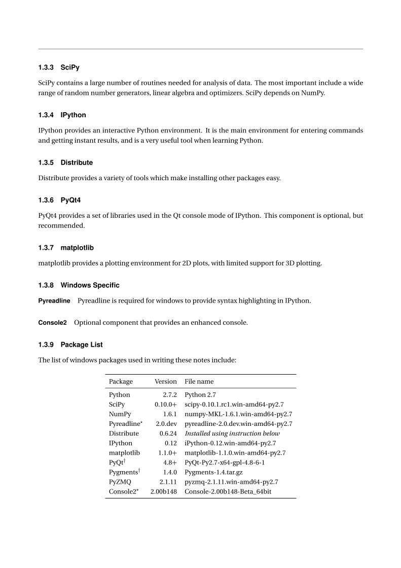
1.3.9 Package List
The list of windows packages used in writing these notes include:
Package Version File name
Python 2.7.2 Python 2.7
SciPy 0.10.0+ scipy-0.10.1.rc1.win-amd64-py2.7
NumPy 1.6.1 numpy-MKL-1.6.1.win-amd64-py2.7
Pyreadline? 2.0.dev pyreadline-2.0.dev.win-amd64-py2.7
Distribute 0.6.24 Installed using instruction below
IPython 0.12 iPython-0.12.win-amd64-py2.7
matplotlib 1.1.0+ matplotlib-1.1.0.win-amd64-py2.7
PyQt† 4.8+ PyQt-Py2.7-x64-gpl-4.8-6-1
Pygments† 1.4.0 Pygments-1.4.tar.gz
PyZMQ 2.1.11 pyzmq-2.1.11.win-amd64-py2.7
Console2? 2.00b148 Console-2.00b148-Beta_64bit

Figure 1.1: The basic IPython environment running pylab inside cmd, Windows command interpreter.† needed for IPython QtConsole, ? Windows only
1.4 Setup
Setup of the required packages is straightforward. A video demonstration of the setup on Windows 7 and
Fedora 16 is available on the website for these notes.
1.4.1 Windows
Begin by installing Python, NumPy, SciPy, Pyreadline, Distribute, IPython and matplotlib. These are all
standard windows installers (msi or exe), and the order is not important aside from installing Python first.
You should create a shortcut containing c:\Python27\Scripts\iPython.exe --pylab. The icon will
be generic, and if you want a nice icon, select the properties of the shortcut, and then Change Icon, and
navigate to c:\Python27\DLLs and select pyc.ico.
Opening the icon should produce a command window similar to that in figure
1.4.1.1 Better: Console2
The Windows command interpreter (cmd.exe) is very limited compared to other platforms. Fortunately,
cmd.exe can be replaced with Console2. To use Console2, extract the contents of the zip file Console-
2.00b148-Beta_64bit.zip (assumed to be C:\Python27\Console2\). Launch Console.exe, and select Edit
> Settings > Tabs. Click on Add, and input the following:
Title IPython(Pylab)
Icon Navigate to c:\Python27\DLLs and select py.ico.
Shell cmd.exe /k "c:\Python27\Scripts\iPython-script.py --pylab"

Figure 1.2: IPython environment running pylab inside Console2. Console2 provides a more productive environmentthan cmd.
Startup dir Where data and work are stored, e.g. c:\Users\username\Documents\
Finally, create a shortcut to Console with the command:
c:\Python27\Console2\Console.exe -t IPython(Pylab)
1.4.1.2 Best: QtConsole
IPython comes with its own environment build using the Qt Toolkit. To use this version, it is necessary
to install PyQt, PyZMQ and Pygments. Both PyQt and PyZMQ come with installers and so installation is
simple.
Pygments must be manually installed. Begin by extracting Pygments-1.4.tar.gz to c:\Python27\. Open a
command prompt (cmd.exe), and enter the following two commands:
cd c:\Python27\Pygments-1.4
c:\Python27\Python.exe setup.py install
Finally, create a shortcut to c:\Python27\Scripts\iPython-qtconsole.exe --pylab. The font and
colors of the QtConsole can be customized using command line switches such as:
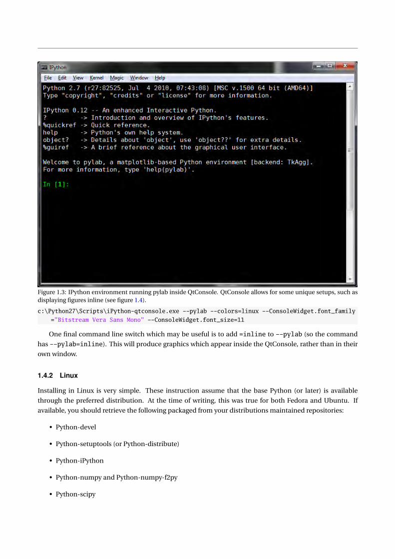
Figure 1.3: IPython environment running pylab inside QtConsole. QtConsole allows for some unique setups, such asdisplaying figures inline (see figure 1.4).
c:\Python27\Scripts\iPython-qtconsole.exe --pylab --colors=linux --ConsoleWidget.font_family
="Bitstream Vera Sans Mono" --ConsoleWidget.font_size=11
One final command line switch which may be useful is to add =inline to --pylab (so the command
has --pylab=inline). This will produce graphics which appear inside the QtConsole, rather than in their
own window.
1.4.2 Linux
Installing in Linux is very simple. These instruction assume that the base Python (or later) is available
through the preferred distribution. At the time of writing, this was true for both Fedora and Ubuntu. If
available, you should retrieve the following packaged from your distributions maintained repositories:
• Python-devel
• Python-setuptools (or Python-distribute)
• Python-iPython
• Python-numpy and Python-numpy-f2py
• Python-scipy

Figure 1.4: An example of the IPython QtConsole using the command line switch –pylab=inline, which produces plotsinside the console.

• Python-matplotlib
• Python-PyQt4
• Python-zmq
• Python-pygments
• Python-tk
1.4.2.1 Missing or Outdated components
If a component is badly outdated, you should manually install the current version (after uninstalling using
package manager in your distribution).
IPython, PyZMQ and Pygments IPython, PyZMQ and Pygments can all be installed using easy_install.
Run the following commands in a terminal window, omitting any which have maintained versions for your
distribution of Linux:
sudo easy_install iPython
sudo easy_install pyzmq
sudo easy_install pygments
If you have followed the instructions, these should all complete without issue.
Notes:
• If the install of PyZMQ fails, you may need to install or build zeromq and zeromq-devel (see below).
matplotlib Begin by heading to the matplotlib github repository in your browser. There you will find a link
which says zip. Click on the link and download the file. Extract the contents of the file, and navigate in the
terminal to the directory which contains the extracted files. Build and install matplotlib by running
unzip matplotlib-matplotlib-v.1.1.0.411-glcd07a6.zip
cd matplotlib-matplotlib-v.1.1.0.411-glcd07a6
Python setup.py build
sudo Python setup.py install
Note: The file name for the matplotlib source will change as it is further developed.
1.4.3 OS X
OS X is similar to Linux. I do not have access to an OS X computer for testing the installation procedure, and
so no instructions are included. Instructions for installing Python (or Python 3) on OS X are readily available
on the internet, and, once available, the remainder of the install should be similar to that of Linux.
1.5 Testing the Environment
To make sure that you have successfully installed the required components, run IPython using the shortcut
previously created on windows, or by running iPython --pylab or iPython-qtconsole --pylab in a
Linux terminal window. Enter the following commands, one at a time (Don’t worry about what these mean).

Figure 1.5: A successful test that matplotlib, IPython, NumPy and SciPy were all correctly installed.
>>> x = randn(100,100)
>>> y = mean(x,0)
>>> plot(y)
>>> import scipy as sp
If everything was successfully installed, you should see something similar to figure 1.5.
1.6 Python Programming
Python can be programmed using an interactive session, preferably using IPython, or by executing Python
scripts, which are simply test files which normally end with the extension .py.
1.6.1 Python and IPython
Most of this introduction focuses on interactive programming, which has some distinct advantages when
learning a language. Interactive Python can be initiated using either the Python interpreter directly, by
launching Python.exe (Windows) or Python (Linux). The standard Python interactive console is very ba-
sic, and does not support useful features such as tab completion. IPython, and especially the QtConsole
version of IPython, transforms the console into a highly productive environment which supports a number
of useful features:
• Tab completion - After entering 1 or more characters, pressing the tab button will bring up a list of
functions, packages and variables which match have the same beginning. If the list of matches is
long, a pager is used. Press ’q’ to exit the pager.
• “Magic” function which make tasks such as navigating the local file system (using %cd ~/directory/)
or running other Python programs (using %run program.py) simple. Entering %magic inside and
IPython session will provide a detailed description of the available functions. Alternatively, %lsmagic
provides a succinct list of available magic commands.
• Integrated help - When using the QtConsole, calling a function provides a view of the top of the help
function. For example, mean computes the mean of an array of data. When using the QtConsole,
entering mean( will produce a view of the top 15 lines or so of the help available for mean.
• Inline figures - The QtConsole can also display figure inline (when using the --pylab=inline switch
when starting), which produces a neat environment. In some cases this may be desirable.
• The special variable _ contains the last result in the console. This results can be saved to a new variable
(in this case, named x) using x = _.
1.6.2 Getting Help
Help is available in IPython sessions using help(function). Some functions (and modules) have very long
help files. These can be paged using the command ?function or function?, and the text can be scrolled using
page up and down, and q to quit. ??function or function?? can be used to type the function in the interactive
console.
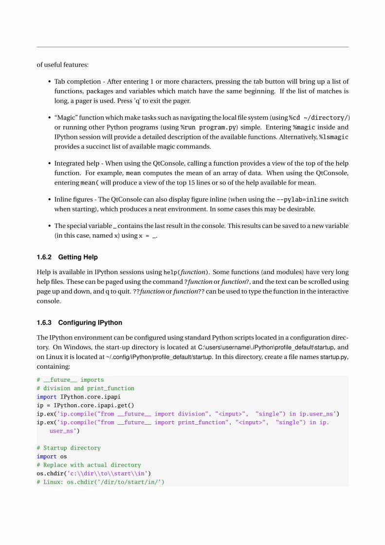
1.6.3 Configuring IPython
The IPython environment can be configured using standard Python scripts located in a configuration direc-
tory. On Windows, the start-up directory is located at C:\users\username\.iPython\profile_default\startup, and
on Linux it is located at ~/.config/iPython/profile_default/startup. In this directory, create a file names startup.py,
containing:
# __future__ imports
# division and print_function
import IPython.core.ipapi
ip = IPython.core.ipapi.get()
ip.ex(’ip.compile("from __future__ import division", "<input>", "single") in ip.user_ns’)
ip.ex(’ip.compile("from __future__ import print_function", "<input>", "single") in ip.
user_ns’)
# Startup directory
import os
# Replace with actual directory
os.chdir(’c:\\dir\\to\\start\\in’)
# Linux: os.chdir(’/dir/to/start/in/’)

This code does 2 things. First, it imports 2 “future” features, the print function division, which are useful for
numerical programming.
• In Python 2.7, print is not standard function and is used like print ’string to print’. Python 3.x
changes this behavior to be a standard function call, print(’string to print’). I prefer the latter
since it will make the move to 3.x easier, and is more coherent.
• In Python 2.7, division of integers always produces an integer, and the result is truncated, so 9/5=1. In
Python 3.x, division of integers does not produce an integer if the integers are not even multiples, so
9/5=1.8. Additionally, Python 3.x uses the syntax 9//5 to force integer division with truncation (e.g.
11/5=2.2, while 11//5=2).
Second, startup.py sets the startup directory to a location of your choosing.
1.6.4 Running Python programs
While interactive programing is useful for learning a language or quickly developing some simple code,
more complex projects require the use of more complete programs. Programs can be run either using the
IPython magic work %run program.py or by directly launching the Python program using the standard
interpreter using Python program.py (Windows). The advantage of using the IPython environment is that
the variables used in the program can be inspected after the end of the program run, while directly calling
Python will run the program and then terminate – and so it is necessary to output any important results to
a file so that they can be viewed later.1
To test that you can successfully execute a Python program, input the the code in the block below into a
text file and save it as firstprogram.py.
# First Python program
from __future__ import print_function
from __future__ import division
import time
print(’Welcome to your first Python program.’)
raw_input(’Press enter to exit the program.’)
print(’Bye!’)
time.sleep(2)
Once you have saved this file, open the console, navigate to the directory you saved the file and run Python
firstprogram.py. If the program does not run on Windows with an error that states Python cannot be
found, you need to add the Python root directory to your path. The path can be located in the Control
Panel, under Environment Variables. Finally, run the program in IPython by first launching IPython, and
the using %cd to change to the location of the program, and finally executing the program using %run
firstprogram.py.
1.6.4.1 Integrated Development Environments
As you progress in Python, and begin writing more sophisticated programs, you will find that using an In-
tegrated Development Environment (IDE) will increase your productivity. Most contain productivity en-
1Programs can also be run in the standard Python interpreter using the command:exec(compile(open(’filename.py’).read(),’filename.py’,’exec’))

hancements such as built-in consoles, intellisense (for completing function names) and integrated de-
bugging. Discussion of IDEs is beyond the scope of this text, although I recommend Spyder (free, cross-
platform).
1.7 Exercises
1. Install Python.
2. Test the installation using the code in section 1.5.
3. Configure IPython using the start-up script in section 1.6.3.
4. Customize IPython-QtConsole using a font or color scheme. More customizations can be found by
running ipyton-qtconsole -h.
5. Explore tab completion in IPython by entering a<TAB> to see the list of functions which start with a
and are loaded by pylab. Next try i<TAB>, which will produce a list longer than the screen – press q
to exit the pager.
6. Install Spyder. For optimal performance, Spyder requires a number of additional packages. These are
all available using easy_install packageName. The additional packages are:
• pyflakes
• rope
• sphinx
• pylint
• pep8

Chapter 2
Python 2.7 vs. 3.2 (and the rest)
Python comes in a number of varieties which may be suitable for econometrics, statistics and numerical
analysis. This chapter explains why, ultimately 2.7 was chosen for these notes, and highlights some alterna-
tives.
2.1 Python 2.7 vs. 3.2
Python 2.7 is the final version of the Python 2.x line – all future development work will focus on Python 3.2.
It may seem strange to learn an “old” language. The reasons for using 2.7 are:
• There are more modules available for Python 2.7. While all of the core python modules are available
for both Python 2.7 and 3.2, some relevant modules are only available in 2.7, for example, modules
which allow Excel files to be read and written to. Over time, many of these modules will be available
for Python 3.2+, but they aren’t today.
• The language changes relevant for numerical computing are very small – and these notes explicitly
minimize these so that there should few changes needed to run against Python 3.2+ in the future
(ideally none).
• Configuring and installing 2.7 is much easier, especially on Linux.
Learning Python 3.2 has some advantages:
• No need to update in the future
• Some improved out-of-box behavior for numerical applications.
2.2 Intel Math Kernel Library and AMD Core Math Library
Intel’s MKL and AMD’s CML provide optimized linear algebra routines. They are much faster then simple
implementations and are, by default, multithreaded so that a matrix inversion can use all of the processors
on your system. They are used by NumPy, although most pre-compiled code does not use them. The ex-
ception for Windows are the pre-built NumPy binaries made available by Christoph Gohlke. Directions for
building NumPy on Linux with Intel’s MKL are available online. It is strongly recommended that you use a
25
NumPy built using these highly tuned linear algebra routines if performance on matrix algebra operations
is important. Alternatively, Enthought Python Distribution (see below) is built with MKL and is available for
all Intel platforms (Windows, Linux and OS X).
2.3 Other Variants
Some other variants are worth mentioning.
2.3.1 Enthought Python Distribution
Enthought Python Distribution (EPD) is a collection of a large number of modules for scientific computing
(including core Python). It is available for Windows, Linux and OS X. EPD is regularly updated and is cur-
rently available for free to members of academic institutions. EPD is also built using MKL, and so matrix
algebra performance is very fast.
2.3.2 IronPython
IronPython is a variant which runs on the CLR (Windows .NET). The core modules – NumPy and SciPy –
are available for IronPython, and so it is a viable alternative for numerical computing, especially if already
familiar with the C# or another .NET language. Other libraries, for example, matplotlib (plotting) are not
available, so there are some important caveats.
2.3.3 PyPy
PyPy is a new implementation of Python which uses Just-in-time compilation to accelerate code, especially
loops (which are common in numerical computing). It may be anywhere between 2 - 5 times faster than
standard Python. Unfortunately, at the time of writing, the core library, NumPy is only partially imple-
mented, and so it is not ready for use. Current plans are to have a version ready by the end of 2012, and if
so, PyPy may quickly become the preferred version of Python for numerical computing.
2.A Relevant Differences between Python 2.7 and 3.2
Most difference significant between Python 2.7 and 3.2 are not important for using Python in econometrics,
statistics and numerical analysis. I will make three common assumptions which will allow 2.7 and 3.2 to be
used interchangeable. These differences are important in stand-alone Python programs. The configuration
instructions for IPython will produce similar behavior when run interactively.
2.A.1 print
print is a function used to display test in the console when running programs. In Python 2.7, print is a
keyword which behaves differently from other functions. In Python 3.2, print behaves like most functions.
The standard use in Python 2.7 is
print ’String to Print’
while in Python 3.2, the standard use is
print(’String to Print’)
which resembles calling a function. Python 2.7 contains a version of the Python 3.2 print, which can be
used in any program by including
from __future__ import print_function
at the top of the file. I prefer the 3.2 version of print, and so I assume that all programs will include this
statement.
2.A.2 division
Python 3.2 changes the way integers are divided. In Python 2.7, the ratio of two integers was always an
integer, and was truncated towards 0 if the result was fractional. For example, in Python 2.7, 9/5 is 1. Python
3.2 gracefully converts the result to a floating point number, and so in Python 3.2, 9/5 is 1.8. When working
with numerical data, automatically converting ratios avoids some rare errors. Python 2.7 can use the 3.2
behavior by including
from __future__ import division
at the top of the program. I assume that all programs will include this statement.
2.A.3 range and xrange
It is often useful to generate a sequence of number for use when iterating over the some data. In Python
2.7, the best practice is to use the keyword xrange to do this, while in Python 3.2, this keyword has been
renamed range. Fortunately Python 2.7 contains a function range which is inefficient but compatible with
the range function in Python 3.2, and so I will always use range, even where best practices indicate that
xrange should be used. No changes are needed in code for use range in both Python 2.7 and 3.2.

Chapter 3
Built-in Data Types
Before diving into Python for analyzing data to running Monte Carlos, it is necessary to understand some
basic concepts about the available data types in Python and NumPy. In many ways, this description is
necessary since Python is a general purpose programming language which is also well suited to data anal-
ysis, econometrics and statistics. This differs from environments such as MATLAB and R which are statisti-
cal/numerical packages first, and general purpose programming languages second. For example, the basic
numeric type in MATLAB is an array (using double precision, which is useful for floating point mathemat-
ics), while the numeric basic data type in Python is a 1-dimensional scalar which may be either integer or a
double-precision floating point, depending on how the number is formatted when entered.
3.1 Variable Names
Variable names can take many forms, although they can only contain numbers, letters (both upper and
lower), and underscores (_). They must begin with a letter or an underscore and are CaSe SeNsItIve. Addi-
tionally, some words are reserved in Python and so cannot be used for variable names (e.g. import or for).
For example,
x = 1.0
X = 1.0
X1 = 1.0
X1 = 1.0
x1 = 1.0
dell = 1.0
dellreturns = 1.0
dellReturns = 1.0
_x = 1.0
x_ = 1.0
are all legal and distinct variable names. Note that names which begin or end with an underscore are convey
special meaning in Python, and so should be avoided in general. Illegal names do not follow these rules.
# Not allowed
x: = 1.0
1X = 1
_x = 1
X-1 = 1
29

for = 1
Multiple variables can be assigned on the same line using
x, y, z = 1, 3.1415, ’a’
3.2 Core Native Data Types
3.2.1 Numeric
Simple numbers in Python can be either integers, floats or complex. Integers correspond to either 32 bit or
64-bit integers, depending on whether the python interpreter was compiled 32-bit or 64-bit, and floats are
always 64-bit (corresponding to doubles in C/C++). Long integers, on the other hand, do not have a fixed
size and so can accommodate numbers which are larger than maximum the basic integer type can handle.
Note: This chapter does not cover all Python data types, only those which are most relevant for numerical
analysis, econometrics and statistics. The following built-in data types are not described: bytes, bytearray
and memoryview.
3.2.1.1 Floating Point (float)
The most important (scalar) data type for numerical analysis is the float. Unfortunately, not all non-complex
numeric data types are floats. To input a floating data type, it is necessary to include a . (period, dot) in the
expression. This example uses the function type() to determine the data type of a variable.
>>> x = 1
>>> type(x)
int
>>> x = 1.0
>>> type(x)
float
>>> x = float(1)
>>> type(x)
float
This example shows that using the expression that x = 1 produces an integer while x = 1.0 produces a
float. Using integers can produce unexpected results and so it is important to ensure values entered manu-
ally are floats (e.g. include “.0” when needed).1
3.2.1.2 Complex (complex)
Complex numbers are also important for numerical analysis. Complex numbers are created in Python using
j or the function complex().
>>> x = 1.0
>>> type(x)
float
1Programs which contain from __future__ import division will automatically convert integers to floats when dividing.
>>> x = 1j
>>> type(x)
complex
>>> x = 2 + 3j
>>> x
(2+3j)
>>> x = complex(1)
>>> x
(1+0j)
Note that a+bj is the same as complex(a,b), while complex(a) is the same as a+0j.
3.2.1.3 Integers (int and long)
Floats use an approximation to represent numbers which may contain a decimal portion. The integer data
type stores numbers using an exact representation, so that no approximation is needed. The cost of the
exact representation is that the integer data type cannot (naturally) express anything that isn’t an integer.
This renders integers of limited use in most numerical analysis work.
Basic integers can be entered either by excluding the decimal (see float), or explicitly using the int()
function. The int() function can also be used to find the smallest integer (in absolute value) to a floating
point number.
>>> x = 1
>>> type(x)
int
>>> x = 1.0
>>> type(x)
float
>>> x = int(x)
>>> type(x)
int
Integers can range from −231 to 231 − 1. Python contains another type of integer known as a long
integers which has essentially no range. Long integers are entered using the syntax x = 1L or by calling
long(). Additionally python will automatically convert integers outside of the standard integer range to
long integers.
>>> x = 1
>>> x
1
>>> type(x)
int
>>> x = 1L
>>> x

1L
>>> type(x)
long
>>> x = long(2)
>>> type(x)
long
>>> x = 2 ** 64
>>> x
18446744073709551616L
The trailing L after the number indicates that it is a long integer, rather than a standard integer.
3.2.2 Boolean (bool)
The Boolean data type is used to represent true and false, using the reserved keywords True and False.
Boolean variables are important for program flow control (see Chapter 12) and are typically created as a
result of logical operations (see Chapter 11), although they can be entered directly.
>>> x = True
>>> type(x)
bool
>>> x = bool(1)
>>> x
True
>>> x = bool(0)
>>> x
False
Non-zero values, in general, evaluate to true when evaluated by bool(), although bool(0), bool(0.0), and
bool(None) are all false.
3.2.3 Strings (str)
Strings are not usually important for numerical analysis, although they are frequently encountered when
dealing with data files, especially when importing, or when formatting output for human readability (e.g.
nice, readable tables of results). Strings are delimited using ’’ or "". While either single or double quotes
are valid for declaring strings, they cannot be mixed (e.g. do not try ’") in a single string, except when used
to express a quotation.
>>> x = ’abc’
>>> type(x)
str
>>> y = ’"A quotation!"’
>>> print(y)
"A quotation!"
String manipulation is further discussed in Chapter 18.
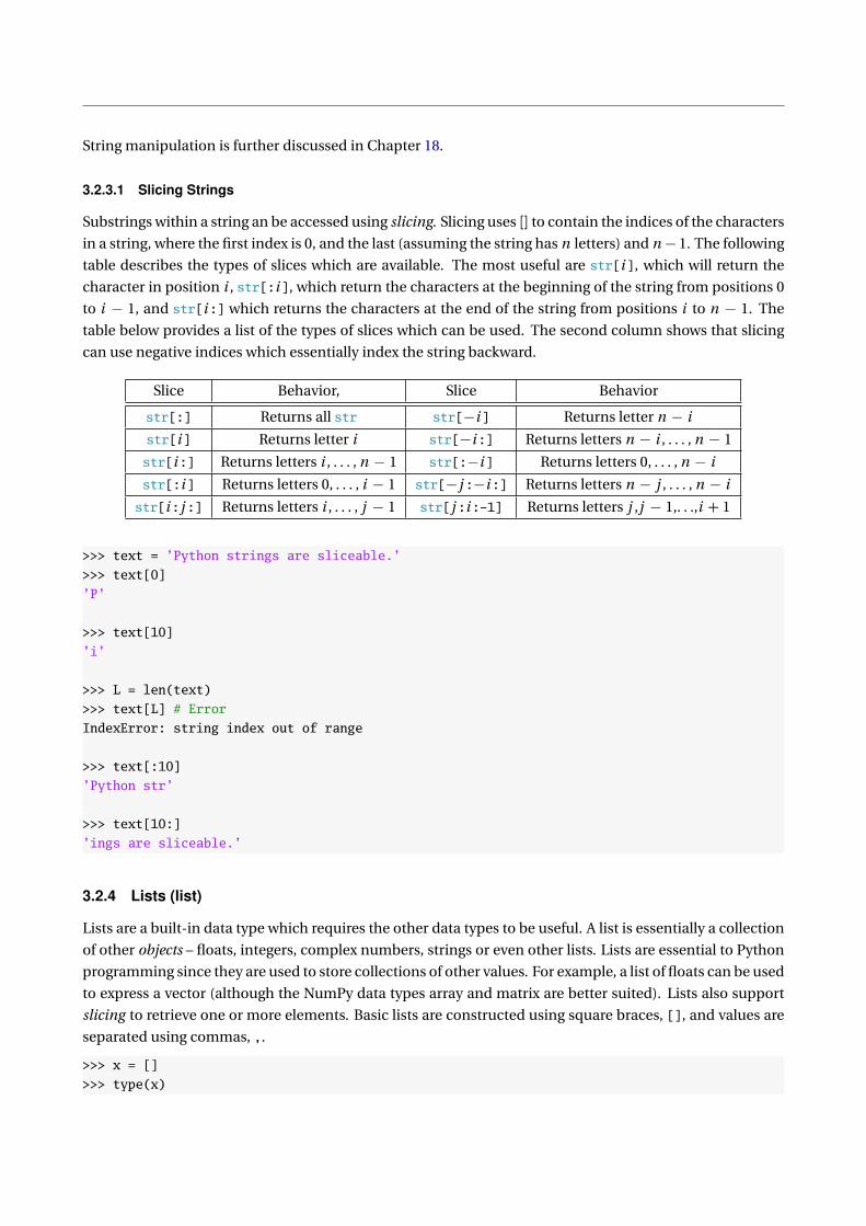
3.2.3.1 Slicing Strings
Substrings within a string an be accessed using slicing. Slicing uses [] to contain the indices of the characters
in a string, where the first index is 0, and the last (assuming the string has n letters) and n−1. The following
table describes the types of slices which are available. The most useful are str[i], which will return the
character in position i , str[:i], which return the characters at the beginning of the string from positions 0
to i − 1, and str[i:] which returns the characters at the end of the string from positions i to n − 1. The
table below provides a list of the types of slices which can be used. The second column shows that slicing
can use negative indices which essentially index the string backward.
Slice Behavior, Slice Behavior
str[:] Returns all str str[−i] Returns letter n − i
str[i] Returns letter i str[−i:] Returns letters n − i , . . . , n − 1
str[i:] Returns letters i , . . . , n − 1 str[:−i] Returns letters 0, . . . , n − i
str[:i] Returns letters 0, . . . , i − 1 str[−j :−i:] Returns letters n − j , . . . , n − i
str[i:j :] Returns letters i , . . . , j − 1 str[j :i:-1] Returns letters j ,j − 1,. . .,i + 1
>>> text = ’Python strings are sliceable.’
>>> text[0]
’P’
>>> text[10]
’i’
>>> L = len(text)
>>> text[L] # Error
IndexError: string index out of range
>>> text[:10]
’Python str’
>>> text[10:]
’ings are sliceable.’
3.2.4 Lists (list)
Lists are a built-in data type which requires the other data types to be useful. A list is essentially a collection
of other objects – floats, integers, complex numbers, strings or even other lists. Lists are essential to Python
programming since they are used to store collections of other values. For example, a list of floats can be used
to express a vector (although the NumPy data types array and matrix are better suited). Lists also support
slicing to retrieve one or more elements. Basic lists are constructed using square braces, [], and values are
separated using commas, ,.
>>> x = []
>>> type(x)

builtins.list
>>> x=[1,2,3,4]
>>> x
[1,2,3,4]
# 2-dimensional list (list of lists)
>>> x = [[1,2,3,4], [5,6,7,8]]
>>> x
[[1, 2, 3, 4], [5, 6, 7, 8]]
# Jagged list, not rectangular
>>> x = [[1,2,3,4] , [5,6,7]]
>>> x
[[1, 2, 3, 4], [5, 6, 7]]
# Mixed data types
>>> x = [1,1.0,1+0j,’one’,None,True]
>>> x
[1, 1.0, (1+0j), ’one’, None, True]
These examples show that lists can be regular, nested and can contain any mix of data types. x = [[1,2,3,4],
[5,6,7,8]] is a 2-dimensional list, where the main elements of x are lists, and the elements of these lists
are integers.
3.2.4.1 Slicing Lists
Lists, like strings, can be sliced. Slicing is similar, although lists can be sliced in more ways than strings.
The difference arises since lists can be multi-dimensional while strings are always 1 × n . Basic list slicing
is identical to strings, and operations such as x[:], x[1:], x[:1] and x[-3:] can all be used. To understand
slicing, assume x is a 1-dimensioanl list with n elements and i ≥ 0, j > 0, i < j . Python using 0-based
indices, and so the n elements of x can be thought of as x0, x1, . . . , xn−1.
Slice Behavior, Slice Behavior
x[:] Return all x x[i] Return x i
x[i] Return x i x[−i] Return xn−i
x[i:] Return x i , . . . xn−1 x[−i:] Return xn−i , . . . , xn−1
x[:i] Return x0, . . . , x i−1 x[:−i] Return x0, . . . , xn−i
x[i:j :] Return x i , x i+1, . . . x j−1 x[−j :−i:] Return xn−j , . . . , xn−i
Examples of accessing elements of 1-dimensional lists are presented in the code block below.
>>> x = [0,1,2,3,4,5,6,7,8,9]
>>> x[0]
0
>>> x[5]
5
>>> x[10] # Error
IndexError: list index out of range
>>> x[4:]
[4, 5, 6, 7, 8, 9]
>>> x[:4]
[0, 1, 2, 3]
>>> x[1:4]
[1, 2, 3]
>>> x[-0]
0
>>> x[-1]
9
>>> x[-10:-1]
[0, 1, 2, 3, 4, 5, 6, 7, 8]
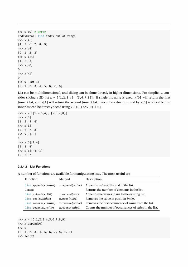
List can be multidimensional, and slicing can be done directly in higher dimensions. For simplicity, con-
sider slicing a 2D list x = [[1,2,3,4], [5,6,7,8]]. If single indexing is used, x[0] will return the first
(inner) list, and x[1] will return the second (inner) list. Since the value returned by x[0] is sliceable, the
inner list can be directly sliced using x[0][0] or x[0][1:4].
>>> x = [[1,2,3,4], [5,6,7,8]]
>>> x[0]
[1, 2, 3, 4]
>>> x[1]
[5, 6, 7, 8]
>>> x[0][0]
1
>>> x[0][1:4]
[2, 3, 4]
>>> x[1][-4:-1]
[5, 6, 7]
3.2.4.2 List Functions
A number of functions are available for manipulating lists. The most useful are
Function Method Description
list.append(x,value) x.append(value) Appends value to the end of the list.
len(x) – Returns the number of elements in the list.
list.extend(x,list) x.extend(list) Appends the values in list to the existing list.
list.pop(x,index) x.pop(index) Removes the value in position index.
list.remove(x,value) x.remove(value) Removes the first occurrence of value from the list.
list.count(x,value) x.count(value) Counts the number of occurrences of value in the list.
>>> x = [0,1,2,3,4,5,6,7,8,9]
>>> x.append(0)
>>> x
[0, 1, 2, 3, 4, 5, 6, 7, 8, 9, 0]
>>> len(x)

11
>>> x.extend([11,12,13])
>>> x
[0, 1, 2, 3, 4, 5, 6, 7, 8, 9, 0, 11, 12, 13]
>>> x.pop(1)
>>> x
[0, 2, 3, 4, 5, 6, 7, 8, 9, 0, 11, 12, 13]
>>> x.remove(0)
>>> x
[2, 3, 4, 5, 6, 7, 8, 9, 0, 11, 12, 13]
3.2.4.3 del
Elements can also be deleted from lists using the keyword del in combination with a slice.
>>> x = [0,1,2,3,4,5,6,7,8,9]
>>> del x[0]
>>> x
[1, 2, 3, 4, 5, 6, 7, 8, 9]
>>> x[:3]
[1, 2, 3]
>>> del x[:3]
>>> x
[4, 5, 6, 7, 8, 9]
>>> del x[1:3]
>>> x
[4, 7, 8, 9]
>>> del x[:]
>>> x
[]
3.2.5 Tuples (tuple)
A tuple is in many ways like a list. A tuple contains multiple pieces of data which comprised of a variety of
data types. Aside from using a different syntax to construct a tuple, they are close enough to lists to ignore
the difference except that tuples are immutable. Immutability means that the elements of tuple cannot
change, and so once a tuple is constructed, it is not possible to change an element without reconstructing a
new tuple.
Tuples are constructed using parentheses (()), rather than square braces ([]) of lists. Tuples can be
sliced in an identical manner as lists. A list can be converted into a tuple using tuple() (Similarly, a tuple
can be converted to list using list()).
>>> x =(0,1,2,3,4,5,6,7,8,9)
>>> type(x)
tuple

>>> x[0]
0
>>> x[-10:-5]
(0, 1, 2, 3, 4)
>>> x = list(x)
>>> type(x)
list
>>> x = tuple(x)
>>> type(x)
tuple
Note that tuples must have a comma when created, so that x = (2,) is assign a tuple to x, while x=(2) will
assign 2 to x. The latter interprets the parentheses as if they are part of a mathematical formula, rather than
being used to construct a tuple. x = tuple([2]) can also be used to create a single element tuple. Lists do
not have this issue since square brackets are reserved.
>>> x =(2)
>>> type(x)
int
>>> x = (2,)
>>> type(x)
tuple
>>> x = tuple([2])
>>> type(x)
tuple
3.2.5.1 Tuple Functions
Tuples are immutable, and so only have the functions index and count, which behave in an identical man-
ner to their list counterparts.
3.2.6 Xrange (xrange)
A xrange is a useful data type which is most commonly encountered when using a for loop. Range are
essentially lists of numbers. xrange(a,b,i) creates the sequences that follows the pattern a , a + i , a +2i , . . . , a + (m − 1)i where m = db−a
i e. In other words, it find all integers x starting with a such a ≤ x < b
and where two consecutive values are separated by i . Range can also be called with 1 or two parameters.
xrange(a,b) is the same as xrange(a,b,1) and xrange(b) is the same as xrange(0,b,1).
>>> x = xrange(10)
>>> type(x)
xrange
>>> print(x)
xrange(0, 10)
>>> list(x)
[0, 1, 2, 3, 4, 5, 6, 7, 8, 9]
>>> x = xrange(3,10)
>>> list(x)
[3, 4, 5, 6, 7, 8, 9]
>>> x = xrange(3,10,3)
>>> list(x)
[3, 6, 9]
>>> y = range(10)
>>> type(y)
list
>>> y
[0, 1, 2, 3, 4, 5, 6, 7, 8, 9]
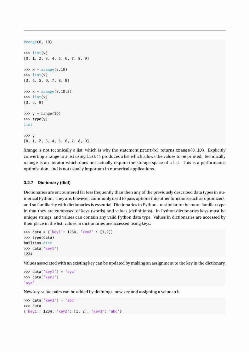
Xrange is not technically a list, which is why the statement print(x) returns xrange(0,10). Explicitly
converting a range to a list using list() produces a list which allows the values to be printed. Technically
xrange is an iterator which does not actually require the storage space of a list. This is a performance
optimization, and is not usually important in numerical applications.
3.2.7 Dictionary (dict)
Dictionaries are encountered far less frequently than then any of the previously described data types in nu-
merical Python. They are, however, commonly used to pass options into other functions such as optimizers,
and so familiarity with dictionaries is essential. Dictionaries in Python are similar to the more familiar type
in that they are composed of keys (words) and values (definitions). In Python dictionaries keys must be
unique strings, and values can contain any valid Python data type. Values in dictionaries are accessed by
their place in the list; values in dictionaries are accessed using keys.
>>> data = ’key1’: 1234, ’key2’ : [1,2]
>>> type(data)
builtins.dict
>>> data[’key1’]
1234
Values associated with an existing key can be updated by making an assignment to the key in the dictionary.
>>> data[’key1’] = ’xyz’
>>> data[’key1’]
’xyz’
New key-value pairs can be added by defining a new key and assigning a value to it.
>>> data[’key3’] = ’abc’
>>> data
’key1’: 1234, ’key2’: [1, 2], ’key3’: ’abc’
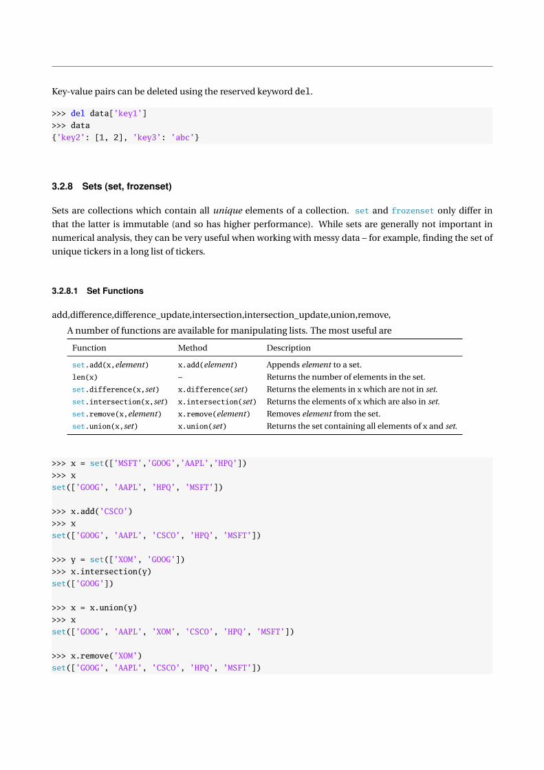
Key-value pairs can be deleted using the reserved keyword del.
>>> del data[’key1’]
>>> data
’key2’: [1, 2], ’key3’: ’abc’
3.2.8 Sets (set, frozenset)
Sets are collections which contain all unique elements of a collection. set and frozenset only differ in
that the latter is immutable (and so has higher performance). While sets are generally not important in
numerical analysis, they can be very useful when working with messy data – for example, finding the set of
unique tickers in a long list of tickers.
3.2.8.1 Set Functions
add,difference,difference_update,intersection,intersection_update,union,remove,
A number of functions are available for manipulating lists. The most useful are
Function Method Description
set.add(x,element) x.add(element) Appends element to a set.
len(x) – Returns the number of elements in the set.
set.difference(x,set) x.difference(set) Returns the elements in x which are not in set.
set.intersection(x,set) x.intersection(set) Returns the elements of x which are also in set.
set.remove(x,element) x.remove(element) Removes element from the set.
set.union(x,set) x.union(set) Returns the set containing all elements of x and set.
>>> x = set([’MSFT’,’GOOG’,’AAPL’,’HPQ’])
>>> x
set([’GOOG’, ’AAPL’, ’HPQ’, ’MSFT’])
>>> x.add(’CSCO’)
>>> x
set([’GOOG’, ’AAPL’, ’CSCO’, ’HPQ’, ’MSFT’])
>>> y = set([’XOM’, ’GOOG’])
>>> x.intersection(y)
set([’GOOG’])
>>> x = x.union(y)
>>> x
set([’GOOG’, ’AAPL’, ’XOM’, ’CSCO’, ’HPQ’, ’MSFT’])
>>> x.remove(’XOM’)
set([’GOOG’, ’AAPL’, ’CSCO’, ’HPQ’, ’MSFT’])

3.3 Python and Memory Management
Python uses a highly optimized memory allocation system which attempts to avoid allocating unnecessary
memory. As a result, when one variable is assigned to another (e.g. to y = x), these will actually point to the
same data in the computer’s memory. To verify this, id() can be used to determine the unique identification
number of a piece of data.2
>>> x = 1
>>> y = x
>>> id(x)
82970264L
>>> id(y)
82970264L
>>> x = 2.0
>>> id(x)
82970144L
>>> id(y)
82970264L
In the above example, the initial assignment of y = xproduced two variables with the same ID. However,
once x was changed, its ID changed while the ID of y did not, indicating that the data in each variable was
stored in different locations. This behavior is very safe yet very efficient, and is common to the basic Python
types: int, long, float, complex, string, xrange and tuple.
3.3.1 Example: Lists
Lists are mutable and so assignment does not create a copy – changes to either variable affect both.
>>> x = [1, 2, 3]
>>> y = x
>>> y[0] = -10
>>> y
[-10, 2, 3]
>>> x
[-10, 2, 3]
Slicing a list creates a copy of the list and any immutable types in the list – but not mutable elements in the
list.
>>> x = [1, 2, 3]
>>> y = x[:]
>>> id(x)
86245960L
>>> id(y)
86240776L
2The ID numbers on your system will likely differ from those in the code listing.

For example, consider slicing a list of lists.
>>> x=[[0,1],[2,3]]
>>> y = x[:]
>>> y
[[0, 1], [2, 3]]
>>> id(x[0])
117011656L
>>> id(y[0])
117011656L
>>> x[0][0]
0.0
>>> y[0][0] = -10.0
>>> y
[[-10.0, 1], [2, 3]]
>>> x
[[-10.0, 1], [2, 3]]
When lists are nested or contain other mutable objects (which do not copy), slicing copies the outermost list
to a new ID, but the inner lists (or other objects) are still linked. In order to copy nested lists, it is necessary
to explicitly call deepcopy(), which is in the module copy.
>>> import copy as cp
>>> x=[[0,1],[2,3]]
>>> y = cp.deepcopy(x)
>>> y[0][0] = -10.0
>>> y
[[-10.0, 1], [2, 3]]
>>> x
[[0, 1], [2, 3]]
3.4 Exercises
1. Enter the following into Python, assigning each to a unique variable name:
(a) 4
(b) 3.1415
(c) 1.0
(d) 2+4j
(e) ’Hello’
(f) ’World’
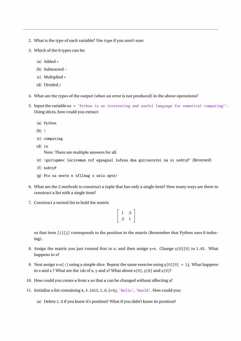
2. What is the type of each variable? Use type if you aren’t sure.
3. Which of the 6 types can be:
(a) Added +
(b) Subtracted -
(c) Multiplied *
(d) Divided /
4. What are the types of the output (when an error is not produced) in the above operations?
5. Input the variable ex = ’Python is an interesting and useful language for numerical computing!’.
Using slices, how could you extract:
(a) Python
(b) !
(c) computing
(d) in
Note: There are multiple answers for all.
(e) !gnitupmoc laciremun rof egaugnal lufesu dna gnitseretni na si nohtyP’ (Reversed)
(f) nohtyP
(g) Pto sa neetn n sfllnug o ueia optn!
6. What are the 2 methods to construct a tuple that has only a single item? How many ways are there to
construct a list with a single item?
7. Construct a nested list to hold the matrix [1 .5
.5 1
]
so that item [i][j] corresponds to the position in the matrix (Remember that Python uses 0 index-
ing).
8. Assign the matrix you just created first to x, and then assign y=x. Change y[0][0] to 1.61. What
happens to x?
9. Next assign z=x[:] using a simple slice. Repeat the same exercise using y[0][0] = 1j. What happens
to x and z ? What are the ids of x, y and z? What about x[0], y[0] and z[0]?
10. How could you create w from x so that w can be changed without affecting x?
11. Initialize a list containing 4, 3.1415, 1.0, 2+4j, ’Hello’, ’World’. How could you:
(a) Delete 1.0 if you knew it’s position? What if you didn’t know its position?
(b) How can the list [1.0, 2+4j, ’Hello’] be added to the existing list?
(c) How can the list be reversed?
(d) In the extended list, how can you count the occurrence of ’Hello’?
12. Construct a dictionary with the keyword-value pairs: alpha and 1.0, beta and 3.1415, gamma and -99.
How can the value of alpha be retrieved?
13. Convert the final list at the end of problem 11 to a set. How is the set different from the list?

Chapter 4
Arrays and Matrices
NumPy provides the most important data types for econometrics, statistics and numerical analysis. The
two data types provided by NumPy are the arrays and matrices. Arrays and matrices are closely related,
and matrices are essentially a special case of arrays – 2 (and only 2)-dimensional arrays. The differences
between arrays and matrices can be summarized as:
• Arrays can have 1, 2, 3 or more dimensions. Matrices always have 2 dimensions. This means that a
1 by n vector stored as an array has 1 dimension and 5 elements, while the same vector stored as a
matrix has 2-dimensions where the sizes of the dimensions are 1 and n (in either order).
• Standard mathematical operators on arrays operate element-by-element. This is not the case for ma-
trices, where multiplication (*) follows the rules of linear algebra. 2-dimensional arrays can be multi-
plied using the rules of linear algebra using dot(). Similarly, the function multiply() can be used on
two matrices for element-by-element multiplication.
• Arrays are more common than matrices, and so all functions work and are tested with arrays (they
should also work with matrices, but an occasional strange result may be encountered).
• Arrays can be quickly treated as a matrix using either asmatrix() or mat() without copying the un-
derlying data.
4.1 Array
Arrays are the base data type in NumPy, and are the most important data type for numerical analysis in
Python. In many ways, arrays are similar to lists in that they can be used to help collections of elements.
The focus of this section is on arrays which only hold 1 type of data – whether it is float or int – and so all
elements must have the same type (See Chapter 20). Additionally, arrays are always rectangular – in other
words, if the first row has 10 elements, all other rows must have 10 elements.
Arrays are initialized using lists (or tuples), and calling array(). 2-dimensional arrays are initialized
using lists of lists (or tuples of tuples, or lists of tuples, etc.), and higher dimensional arrays can be initialized
by further nesting lists or tuples.
>>> x = [0.0, 1, 2, 3, 4]
>>> y = array(x)
>>> y
45

array([0, 1, 2, 3, 4])
>>> type(y)
NumPy.ndarray
2 (or higher) dimensional arrays are initialized using nested lists.
>>> y = array([[0.0, 1, 2, 3, 4], [5, 6, 7, 8, 9]])
>>> y
array([[ 0., 1., 2., 3., 4.],
[ 5., 6., 7., 8., 9.]])
>>> shape(y)
(2L, 5L)
>>> y = array([[[1,2],[3,4]],[[5,6],[7,8]]])
>>> y
array([[[1, 2],
[3, 4]],
[[5, 6],
[7, 8]]])
>>> shape(y)
(2L, 2L, 2L)
4.1.1 Array dtypes
Arrays can contain a variety to data types. The most useful is ’float64’, which corresponds to the python
built-in data type of float (and C/C+ double). By default, calls to array() will preserve the type of the input,
if possible. If an input contains all integers, it will have a dtype of ’int32’ (the built in data type ’int’). If
an input contains integers, floats, or a mix of the two, the array’s dtype will be float. It is contains a mix of
integers, floats and complex types, the array will be complex.
>>> x = [0, 1, 2, 3, 4] # Integers
>>> y = array(x)
>>> y.dtype
dtype(’int32’)
>>> x = [0.0, 1, 2, 3, 4] # 0.0 is a float
>>> y = array(x)
>>> y.dtype
dtype(’float64’)
>>> x = [0.0 + 1j, 1, 2, 3, 4] # (0.0 + 1j) is a complex
>>> y = array(x)
>>> y
array([ 0.+1.j, 1.+0.j, 2.+0.j, 3.+0.j, 4.+0.j])
>>> y.dtype
dtype(’complex128’)
NumPy attempts to find the smallest data type which can represent the data when constructing an array. It is
possible to force NumPy to use a particular dtype by passing another argument, dtype=datetype to array().
>>> x = [0, 1, 2, 3, 4] # Integers
>>> y = array(x)
>>> y.dtype
dtype(’int32’)
>>> y = array(x, dtype=’float64’)
>>> y.dtype
dtype(’float64’)
Important: If an array has an integer dtype, trying to place a float into the array results in the float being
truncated and stored as an integer. This is dangerous, and so in most cases, arrays should be initialized to
contain floats unless a conscious decision is taken to have them contain a different data type.
>>> x = [0, 1, 2, 3, 4] # Integers
>>> y = array(x)
>>> y.dtype
dtype(’int32’)
>>> y[0] = 3.141592
>>> y
array([3, 1, 2, 3, 4])
>>> x = [0.0,1, 2, 3, 4] # 1 Float makes all float
>>> y = array(x)
>>> y.dtype
dtype(’float64’)
>>> y[0] = 3.141592
>>> y
array([ 3.141592, 1. , 2. , 3. , 4. ])
4.2 Matrix
Matrices are essentially a subset of arrays, and behave in a virtually identical manner. The two important
differences are:
• Matrices always have 2 dimensions
• Matrices follow the rules of linear algebra for *
1- and 2-dimensional arrays can be copied to a matrix by calling matrix() on an array. Alternatively, call-
ing mat() or asmatrix() provides a faster method where an array can behave like a matrix (without being
explicitly converted).

4.3 Arrays, Matrices and Memory Management
Arrays and matrices do not behave like lists – slicing an array does not create a copy. In general, when
an array, matrix or list is sliced, the slice will refer to the same memory as original variable – this means
changing an element in the slice also changes an element in the original variable.
>>> x = array([0.0, 1.0, 2.0])
>>> y = x
>>> x
array([ 0., 1., 2.])
>>> y
array([ 0., 1., 2.])
>>> id(x)
130165568L
>>> id(y)
130165568L
>>> y[0] = -1.0
>>> y
array([-1., 1., 2.])
>>> x
array([-1., 1., 2.])
y = x sets x and y to the same data, and so changing one changes the other. Next, consider what happens
when y is a slice of x.
>>> x = array([[0.0, 1.0],[2.0,3.0]])
>>> y = x[0]
>>> y
array([ 0., 1.])
>>> y[0] = -1.0
>>> y
array([ -1., 1.])
>>> x # x changes too
array([[-1., 1.],
[ 2., 3.]])
In order to get a new variable when slicing or assigning an array or a matrix, it is necessary to explicitly
copy the data. Arrays or matrices can be copied by calling copy. Alternatively, they can also be copied by by
calling array() on arrays, or matrix() on matrices.
>>> x = array([[0.0, 1.0],[2.0,3.0]])
>>> y = copy(x)
>>> id(x)
130166048L
>>> id(y)
130165952L
>>> y[0,0] = -10.0
>>> y
array([[-10., 1.],
[ 2., 3.]])
>>> x # No change in x
array([[ 0., 1.],
[ 2., 3.]])
>>> z = x.copy()
>>> id(z)
130166432L
>>> w = array(x)
>>> id(w)
130166144L
w, x, y and z all have unique IDs are distinct. Changes to one will not affect any of the others.
Finally, assignments from functions which change the value automatically create a copy.
>>> x = array([[0.0, 1.0],[2.0,3.0]])
>>> y = x
>>> id(x)
130166816L
>>> id(y)
130166816L
>>> y = x + 1.0
>>> y
array([[ 1., 2.],
[ 3., 4.]])
>>> id(y)
130167008L
>>> y = exp(x)
>>> y
array([[ 1. , 2.71828183],
[ 7.3890561 , 20.08553692]])
>>> id(y)
130166912L
Even trivial function such as y = x + 0.0 create a copy of x, and so the only cases where explicit copying is
required is when y is directly assigned a slice of x, y is changed, but x should not be.

4.4 Entering Data
Almost all of the data used in are matrices by construction, even if they are 1 by 1 (scalar), K by 1 or 1 by
K (vectors). Vectors, both row (1 by K ) and column (K by 1), can be entered directly into the command
window. The mathematical notation
x = [1 2 3 4 5]
is entered as
>>> x=array([1.0,2.0,3.0,4.0,5.0])
array([ 1., 2., 3., 4., 5.])
when an array is needed or
>>> x=matrix([1.0,2.0,3.0,4.0,5.0])
>>> x
matrix([[ 1., 2., 3., 4., 5.]])
for a matrix. 1-dimensional arrays do not have row or column forms, but matrices do. The column
vector,
x =
1
2
3
4
5
is entered using a set of nested lists
>>> x=matrix([[1.0],[2.0],[3.0],[4.0],[5.0]])
>>> x
matrix([[ 1.],
[ 2.],
[ 3.],
[ 4.],
[ 5.]])
>>> x = array(x)
>>> array([[ 1., 2., 3., 4., 5.]])
The final two line show that converting a column matrix to an array eliminates any notion row and column.
4.5 Entering Matrices
Matrices are just rows of columns. For instance, to input
x =
1 2 3
4 5 6
7 8 9
,
enter the matrix one row at a time, each in a list, and then surround the row lists with another list.
>>> x = array([[1.0,2.0,3.0],[4.0,5.0,6.0],[7.0,8.0,9.0]])
>>> x
array([[ 1., 2., 3.],
[ 4., 5., 6.],
[ 7., 8., 9.]])
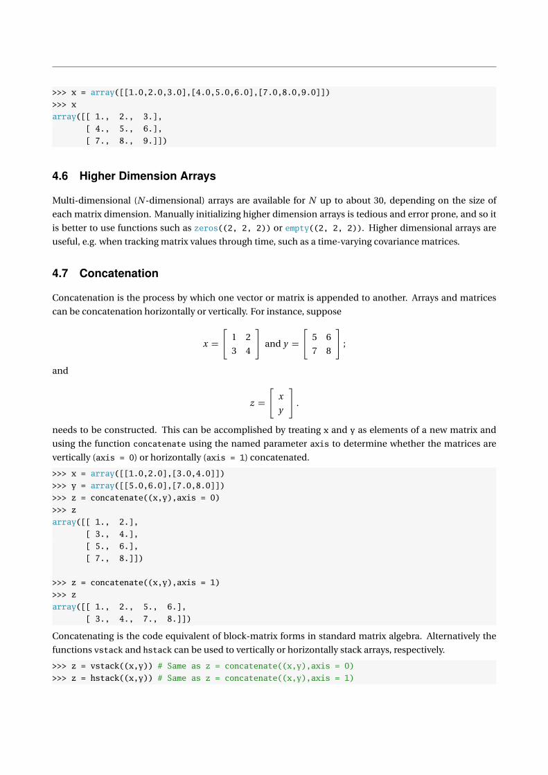
4.6 Higher Dimension Arrays
Multi-dimensional (N -dimensional) arrays are available for N up to about 30, depending on the size of
each matrix dimension. Manually initializing higher dimension arrays is tedious and error prone, and so it
is better to use functions such as zeros((2, 2, 2)) or empty((2, 2, 2)). Higher dimensional arrays are
useful, e.g. when tracking matrix values through time, such as a time-varying covariance matrices.
4.7 Concatenation
Concatenation is the process by which one vector or matrix is appended to another. Arrays and matrices
can be concatenation horizontally or vertically. For instance, suppose
x =
[1 2
3 4
]and y =
[5 6
7 8
];
and
z =
[x
y
].
needs to be constructed. This can be accomplished by treating x and y as elements of a new matrix and
using the function concatenate using the named parameter axis to determine whether the matrices are
vertically (axis = 0) or horizontally (axis = 1) concatenated.
>>> x = array([[1.0,2.0],[3.0,4.0]])
>>> y = array([[5.0,6.0],[7.0,8.0]])
>>> z = concatenate((x,y),axis = 0)
>>> z
array([[ 1., 2.],
[ 3., 4.],
[ 5., 6.],
[ 7., 8.]])
>>> z = concatenate((x,y),axis = 1)
>>> z
array([[ 1., 2., 5., 6.],
[ 3., 4., 7., 8.]])
Concatenating is the code equivalent of block-matrix forms in standard matrix algebra. Alternatively the
functions vstack and hstack can be used to vertically or horizontally stack arrays, respectively.
>>> z = vstack((x,y)) # Same as z = concatenate((x,y),axis = 0)
>>> z = hstack((x,y)) # Same as z = concatenate((x,y),axis = 1)

4.8 Accessing Elements of Array (Slicing)
Arrays, like lists and tuples, can be sliced. Slicing in arrays is virtually identical to slicing in lists, except
that since arrays are explicitly multidimensional and rectangular, slicing in more than 1-dimension is im-
plemented using a different syntax. 1-dimensional arrays can be sliced in an identical manner as lists or
tuples. 2 (or higher)-dimensional arrays are sliced using the syntax [:,:,. . .,:] (where the number of di-
mensions of the arrays determines the size of the slice). The 2-dimensions, first dimension is always the
row, and the second is the column.
>>> y = array([[0.0, 1, 2, 3, 4],[5, 6, 7, 8, 9]])
>>> y
array([[ 0., 1., 2., 3., 4.],
[ 5., 6., 7., 8., 9.]])
>>> y[0,:] # Row 0, all columns
array([ 0., 1., 2., 3., 4.])
>>> y[:,0] # all rows, column 0
array([ 0., 5.])
>>> y[0,0:3] # Row 0, columns 0 to 3
array([ 0., 1., 2.])
>>> y[0:,3:] # Row 0 and 1, columns 3 and 4
array([[ 3., 4.],
[ 8., 9.]])
>>> y = array([[[1.0,2],[3,4]],[[5,6],[7,8]]])
>>> y[0,:,:] # Panel 0 of 3D y
array([[1, 2],
[3, 4]])
>>> y[0] # Same as y[0,:,:]
array([[1., 2.],
[3., 4.]])
>>> y[0,0,:] # Row 0 of panel 0
array([1., 2.])
>>> y[0,1,0] # Panel 0, row 1, column 0
3.0
4.8.1 Linear Slicing using flat
k -dimensional arrays can be sliced using the [:,:,. . .,:] syntax, or they can be linear sliced. Linear slicing
assigns an index to each element of the array, starting with the first (0), the second (1), and so on up to the
last (n − 1). In 2-dimensions, linear slicing works be first counting across rows, and then down columns. To
use linear slicing, the method or function flat must first be used
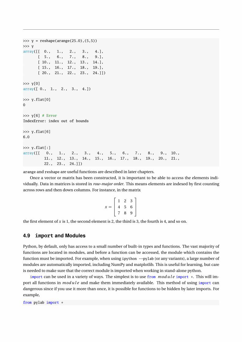
>>> y = reshape(arange(25.0),(5,5))
>>> y
array([[ 0., 1., 2., 3., 4.],
[ 5., 6., 7., 8., 9.],
[ 10., 11., 12., 13., 14.],
[ 15., 16., 17., 18., 19.],
[ 20., 21., 22., 23., 24.]])
>>> y[0]
array([ 0., 1., 2., 3., 4.])
>>> y.flat[0]
0
>>> y[6] # Error
IndexError: index out of bounds
>>> y.flat[6]
6.0
>>> y.flat[:]
array([[ 0., 1., 2., 3., 4., 5., 6., 7., 8., 9., 10.,
11., 12., 13., 14., 15., 16., 17., 18., 19., 20., 21.,
22., 23., 24.]])
arange and reshape are useful functions are described in later chapters.
Once a vector or matrix has been constructed, it is important to be able to access the elements indi-
vidually. Data in matrices is stored in row-major order. This means elements are indexed by first counting
across rows and then down columns. For instance, in the matrix
x =
1 2 3
4 5 6
7 8 9
the first element of x is 1, the second element is 2, the third is 3, the fourth is 4, and so on.
4.9 import and Modules
Python, by default, only has access to a small number of built-in types and functions. The vast majority of
functions are located in modules, and before a function can be accessed, the module which contains the
function must be imported. For example, when using ipython --pylab (or any variants), a large number of
modules are automatically imported, including NumPy and matplotlib. This is useful for learning, but care
is needed to make sure that the correct module is imported when working in stand-alone python.
import can be used in a variety of ways. The simplest is to use from mod u l e import *. This will im-
port all functions in mod u l e and make them immediately available. This method of using import can
dangerous since if you use it more than once, it is possible for functions to be hidden by later imports. For
example,
from pylab import *

from numpy import *
creates a conflict for load which is first imported by pylab (from matplotlib.pylab.load), and then im-
ported by NumPy (from numpy.lib.npyio.load). A better method is to just import the required functions.
This still places functions at the top level of the namespace, but can be used to avoid conflicts.
from pylab import load # Will import load only
from numpy import array, matrix # Will not import the load from NumPy
The functions load, array and matrix can be directly called. An alternative, and more common, method is
to use import in the form
import pylab
import scipy
import numpy
or the closely related alternative
import pylab as pl
import scipy as sp
import numpy as np
The only difference between these two is that import numpy is equivalent to import numpy as numpy. When
this form of import is used, function will be located below the “as” name. For example, the load provided
by NumPy, is located at np.load, while the pylab load is pl.load – and both can be used where appropriate.
While this method is the most general, it does require slightly more typing.
4.10 Calling Functions
Functions calls have different conventions other expressions. The most important difference is that func-
tions can take more than one input and return more than one output. The generic structure of a function
call is out1, out2, out3, . . . = functionname(in1, in2, in3, . . .). The important aspects of this structure are
• If multiple outputs are returned, but only one output variable is provided, the output will (generally)
be a tuple.
• The number of output variables determines how many outputs will be returned. Asking for more
outputs than the function provides will result in an error.
• Both inputs and outputs must be separated by commas (,)
• Inputs can be the result of other functions as long only one output is returned. For example, the
following are equivalent,
>>> y = var(x)
>>> mean(y)
and
>>> mean(var(x))
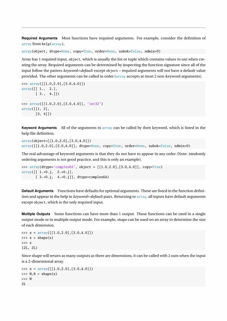
Required Arguments Most functions have required arguments. For example, consider the definition of
array from help(array),
array(object, dtype=None, copy=True, order=None, subok=False, ndmin=0)
Array has 1 required input, object, which is usually the list or tuple which contains values to use when cre-
ating the array. Required arguments can be determined by inspecting the function signature since all of the
input follow the patters keyword=default except object – required arguments will not have a default value
provided. The other arguments can be called in order (array accepts at most 2 non-keyword arguments).
>>> array([[1.0,2.0],[3.0,4.0]])
array([[ 1., 2.],
[ 3., 4.]])
>>> array([[1.0,2.0],[3.0,4.0]], ’int32’)
array([[1, 2],
[3, 4]])
Keyword Arguments All of the arguments to array can be called by their keyword, which is listed in the
help file definition.
array(object=[[1.0,2.0],[3.0,4.0]])
array([[1.0,2.0],[3.0,4.0]], dtype=None, copy=True, order=None, subok=False, ndmin=0)
The real advantage of keyword arguments is that they do not have to appear in any order (Note: randomly
ordering arguments is not good practice, and this is only an example).
>>> array(dtype=’complex64’, object = [[1.0,2.0],[3.0,4.0]], copy=True)
array([[ 1.+0.j, 2.+0.j],
[ 3.+0.j, 4.+0.j]], dtype=complex64)
Default Arguments Functions have defaults for optional arguments. These are listed in the function defini-
tion and appear in the help in keyword=default pairs. Returning to array, all inputs have default arguments
except object, which is the only required input.
Multiple Outputs Some functions can have more than 1 output. These functions can be used in a single
output mode or in multiple output mode. For example, shape can be used on an array to determine the size
of each dimension.
>>> x = array([[1.0,2.0],[3.0,4.0]])
>>> s = shape(x)
>>> s
(2L, 2L)
Since shape will return as many outputs as there are dimensions, it can be called with 2 outs when the input
is a 2-dimensional array.
>>> x = array([[1.0,2.0],[3.0,4.0]])
>>> M,N = shape(x)
>>> M
2L
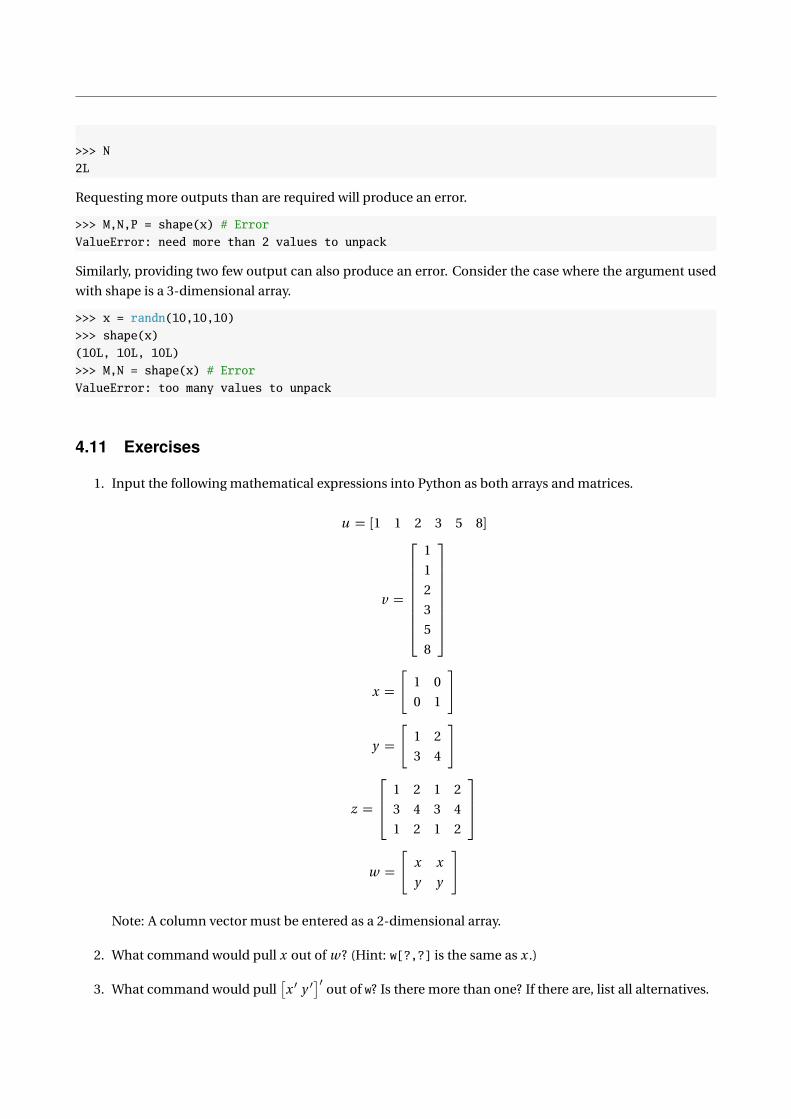
>>> N
2L
Requesting more outputs than are required will produce an error.
>>> M,N,P = shape(x) # Error
ValueError: need more than 2 values to unpack
Similarly, providing two few output can also produce an error. Consider the case where the argument used
with shape is a 3-dimensional array.
>>> x = randn(10,10,10)
>>> shape(x)
(10L, 10L, 10L)
>>> M,N = shape(x) # Error
ValueError: too many values to unpack
4.11 Exercises
1. Input the following mathematical expressions into Python as both arrays and matrices.
u = [1 1 2 3 5 8]
v =
1
1
2
3
5
8
x =
[1 0
0 1
]
y =
[1 2
3 4
]
z =
1 2 1 2
3 4 3 4
1 2 1 2
w =
[x x
y y
]
Note: A column vector must be entered as a 2-dimensional array.
2. What command would pull x out of w ? (Hint: w[?,?] is the same as x .)
3. What command would pull[x ′ y ′
]′out of w? Is there more than one? If there are, list all alternatives.
4. What command would pull y out of z ? List all alternatives.
5. Explore the options for creating an array using keyword arguments. Create an array containing
y =
[1 −2
−3 4
]
with combination of keyword arguments in:
(a) dtype in float, float64, int32 (32-bit integers), uint32 (32-bit unsigned integers) and complex128
(double precision complex numbers).
(b) copy either True or False.
(c) ndim either 3 or 4. Use shape(y) to see the effect of this argument.
6. Enter y = [1.6180 2.7182 3.1415] as an array. Define x = mat(y). How is x different from y ?


Chapter 5
Basic Math
Note: Python contains a math module that contains functions which operate on built-in scalar data types
(e.g. float and complex). This and subsequent chapters assume mathematical functions must operate on
arrays and matrices, and so are imported from NumPy.
5.1 Operators
These standard operators are available:
Operator Meaning Example Algebraic
+ Addition x + y x + y
- Subtraction x - y x − y
* Multiplication x * y x y
/ Division (Left divide) x/y xy
** Exponentiation x**y x y
When x and y are scalars, the behavior of these operators is obvious. The only exception occurs when
both x and y are integers for division, where x/y returns the smallest integer less than the ratio (e.g. b xy c). The
simplest method to avoid this problem is to explicitly avoid integers by using 5.0 rather than 5. Alternatively,
integers can be explicitly cast to floats before the division.
>>> x = 9
>>> y = 5
>>> (type(x), type(y))
(int, int)
>>> x/y
1
>>> float(x)/y
1.8
When x and y are arrays or matrices, things are a bit more complex. The examples usually refer to arrays,
and except where explicit differences are noted, it is safe to assume that the behavior is identical for 2-
dimensional arrays and matrices.
59
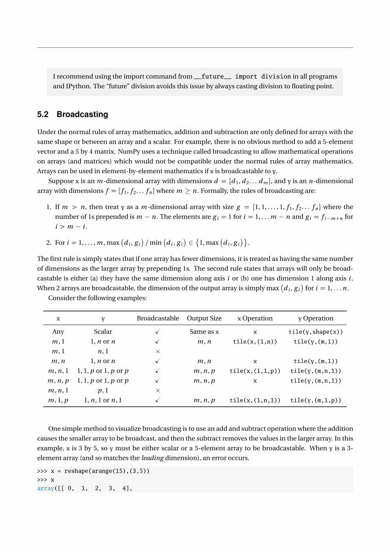
I recommend using the import command from __future__ import division in all programs
and IPython. The “future” division avoids this issue by always casting division to floating point.
5.2 Broadcasting
Under the normal rules of array mathematics, addition and subtraction are only defined for arrays with the
same shape or between an array and a scalar. For example, there is no obvious method to add a 5-element
vector and a 5 by 4 matrix. NumPy uses a technique called broadcasting to allow mathematical operations
on arrays (and matrices) which would not be compatible under the normal rules of array mathematics.
Arrays can be used in element-by-element mathematics if x is broadcastable to y.
Suppose x is an m -dimensional array with dimensions d = [d 1, d 2. . . d m ], and y is an n-dimensional
array with dimensions f = [ f 1, f 2. . . f n ]where m ≥ n . Formally, the rules of broadcasting are:
1. If m > n , then treat y as a m -dimensional array with size g = [1, 1, . . . , 1, f 1, f 2. . . f n ] where the
number of 1s prepended is m − n . The elements are g i = 1 for i = 1, . . . m − n and g i = f i−m+n for
i > m − i .
2. For i = 1, . . . , m , max(
d i , g i
)/min
(d i , g i
)∈
1, max(
d i , g i
).
The first rule is simply states that if one array has fewer dimensions, it is treated as having the same number
of dimensions as the larger array by prepending 1s. The second rule states that arrays will only be broad-
castable is either (a) they have the same dimension along axis i or (b) one has dimension 1 along axis i .
When 2 arrays are broadcastable, the dimension of the output array is simply max(
d i , g i
)for i = 1, . . . n .
Consider the following examples:
x y Broadcastable Output Size x Operation y Operation
Any Scalar Ø Same as x x tile(y,shape(x))
m , 1 1, n or n Ø m , n tile(x,(1,n)) tile(y,(m,1))
m , 1 n , 1 ×m , n 1, n or n Ø m , n x tile(y,(m,1))
m , n , 1 1, 1, p or 1, p or p Ø m , n , p tile(x,(1,1,p)) tile(y,(m,n,1))
m , n , p 1, 1, p or 1, p or p Ø m , n , p x tile(y,(m,n,1))
m , n , 1 p , 1 ×m , 1, p 1, n , 1 or n , 1 Ø m , n , p tile(x,(1,n,1)) tile(y,(m,1,p))
One simple method to visualize broadcasting is to use an add and subtract operation where the addition
causes the smaller array to be broadcast, and then the subtract removes the values in the larger array. In this
example, x is 3 by 5, so y must be either scalar or a 5-element array to be broadcastable. When y is a 3-
element array (and so matches the leading dimension), an error occurs.
>>> x = reshape(arange(15),(3,5))
>>> x
array([[ 0, 1, 2, 3, 4],
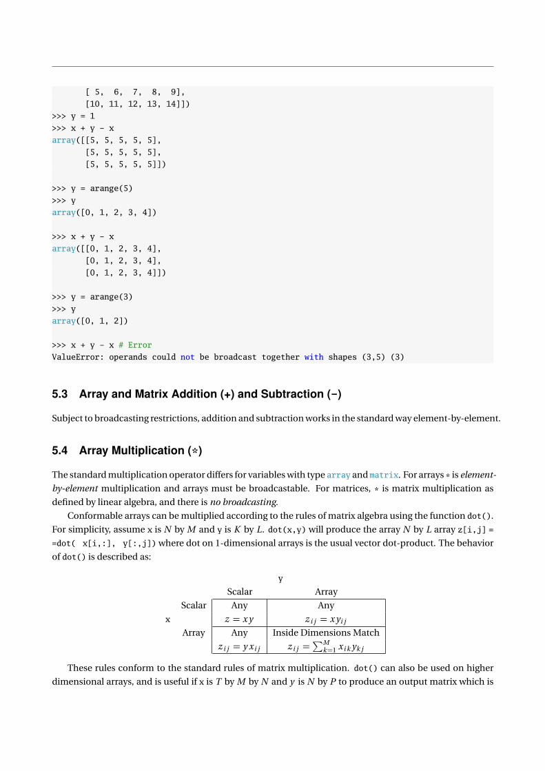
[ 5, 6, 7, 8, 9],
[10, 11, 12, 13, 14]])
>>> y = 1
>>> x + y - x
array([[5, 5, 5, 5, 5],
[5, 5, 5, 5, 5],
[5, 5, 5, 5, 5]])
>>> y = arange(5)
>>> y
array([0, 1, 2, 3, 4])
>>> x + y - x
array([[0, 1, 2, 3, 4],
[0, 1, 2, 3, 4],
[0, 1, 2, 3, 4]])
>>> y = arange(3)
>>> y
array([0, 1, 2])
>>> x + y - x # Error
ValueError: operands could not be broadcast together with shapes (3,5) (3)
5.3 Array and Matrix Addition (+) and Subtraction (-)
Subject to broadcasting restrictions, addition and subtraction works in the standard way element-by-element.
5.4 Array Multiplication (*)
The standard multiplication operator differs for variables with type array and matrix. For arrays * is element-
by-element multiplication and arrays must be broadcastable. For matrices, * is matrix multiplication as
defined by linear algebra, and there is no broadcasting.
Conformable arrays can be multiplied according to the rules of matrix algebra using the function dot().
For simplicity, assume x is N by M and y is K by L. dot(x,y) will produce the array N by L array z[i,j] =
=dot( x[i,:], y[:,j]) where dot on 1-dimensional arrays is the usual vector dot-product. The behavior
of dot() is described as:
y
Scalar Array
Scalar Any Any
x z = x y z i j = x yi j
Array Any Inside Dimensions Match
z i j = y x i j z i j =∑M
k=1 x i k yk j
These rules conform to the standard rules of matrix multiplication. dot() can also be used on higher
dimensional arrays, and is useful if x is T by M by N and y is N by P to produce an output matrix which is

T by M by P , where each of the M by P (T in total) have the form dot(x[i],y).
5.5 Matrix Multiplication (*)
If x is N by M and y is K by L and both are non-scalar matrices, x*y requires M = K . Similarly, y*x requires
L = N . If x is scalar and y is a matrix, then z=x*y produces z(i,j)=x*y(i,j).
Suppose z=x * y where both x and y are matrices:
y
Scalar Matrix
Scalar Any Any
x z = x y z i j = x yi j
Matrix Any Inside Dimensions Match
z i j = y x i j z i j =∑M
k=1 x i k yk j
Note: These conform to the standard rules of matrix multiplication.
multiply() provides element-by-element multiplication of matrices. Suppose z=multiply(x,y) where
x and y are matrices:
y
Scalar Array
Scalar Any Any
x z = x y z i j = x yi j
Array Any Both Dimensions Match
z i j = y x i j z i j = x i j yi j
Multiply will use broadcasting if necessary, and so matrices are effectively treated as 2-dimensional ar-
rays.
5.6 Array and Matrix Division (/)
Division is always element-by-element, and the rules of broadcasting are used.
5.7 Array Exponentiation (**)
Array exponentiation operates element-by-element, and the rules of broadcasting are used.
5.8 Matrix Exponentiation (**)
Matrix exponentiation differs from array exponentiation, and can only be used on square matrices. When
x is a square matrix and y is an integer, and z=x*x*...*x (y times). Python does not support non-integer
values for y, although x p can be defined (in linear algebra) using eigenvalues and eigenvectors for a subset
of all matrices.

5.9 Parentheses
Parentheses can be used in the usual way to control the order in which mathematical expressions are eval-
uated, and can be nested to create complex expressions. See section 5.11 on Operator Precedence for more
information on the order mathematical expressions are evaluated.
5.10 Transpose
Matrix transpose is expressed using either the transpose() function, or the shortcut .T. For instance, if x is
an M by N matrix, transpose(x), x.transpose() and x.T are all its transpose with dimensions N by M . In
practice, using the .T will improve readability of code. Consider
>>> x = randn(2,2)
>>> xpx1 = x.T * x
>>> xpx2 = x.transpose() * x
>>> xpx3 = transpose(x) * x
Transpose has no effect on 1-dimensaional arrays. In 2-dimensions, transpose switches indices so that
if z=x.T, z[j,i] is that same as x[i,j]. In higher dimensions, transpose reverses the order or the indices.
For example, if x has 3 dimensions and z=x.T, then x[i,j,k] is the same as z[k,j,i]. Transpose takes
an optional second argument, which can be used to manually determine the order of the axes after the
transposition.
5.11 Operator Precedence
Computer math, like standard math, has operator precedence which determined how mathematical ex-
pressions such as
2**3+3**2/7*13
are evaluated. Best practice is to always use parentheses to avoid ambiguity in the order or operations.
The order of evaluation is:
Operator Name Rank
( ) Parentheses 1
** Exponentiation 2
+,- Unary Plus, Unary Minus 3
*, /, % Multiply, Divide, Modulo 3
+,- Addition and Subtraction 4
<, <=, >, >= Comparison operators 5
==, != Equality operators 6
=,+=,-=,/=,*=,**= Assignment Operators 7
is, is not Identity Operators 8
in, not in Membership Operators 9
and , or, not Logical Operators 10

In the case of a tie, operations are executed left-to-right. For example, x**y**z is interpreted as (x**y)**z.
This table has omitted some operators available in Python (bit-wise) which are not useful (in general) in
numerical analysis.
Note: Unary operators are + or - operations that apply to a single element. For example, consider the
expression (-4). This is an instance of a unary - since there is only 1 operation. (-4)**2 produces 16.
-4**2 produces -16 since ∗∗ has higher precedence than unary negation and so is interpreted as -(4**2).
-4 * -4 produces 16 since it is interpreted as (-4) * (-4), since unary negation has higher precedence
than multiplication.
5.12 Exercises
1. Using the arrays entered in exercise 1 of chapter 4, compute the values of u + v ′, v + u ′, v u , u v and
x y (where the multiplication is as defined as linear algebra).
2. Repeat exercise 1 treating the inputs as matrices.
3. Which of the arrays in exercise 1 are broadcastable with:
a = [3 2],
b =
[3
2
],
c = [3 2 1 0] ,
d =
3
2
1
0
.
4. Is x/1 legal? If not, why not. What about 1/x?
5. Compute the values (x+y)**2 and x**2+x*y+y*x+y**2. Are they the same when x and y are arrays?
What if they are matrices?
6. Is x**2+2*x*y+y**2 the same as any of the above?
7. When will x**y for matrices be the same as x**y for vectors?
8. For conformable arrays, is a*b+a*c the same as a*b+c? If so, show it, if not, how can the second be
changed so they are equal.
9. Suppose a command x**y*w+z was entered. What restrictions on the dimensions of w, x, y and z must
be true for this to be a valid statement?
10. What is the value of -2**4? What about (-2)**4? What about -2*-2*-2*-2?

Chapter 6
Basic Functions
6.1 Generating Arrays and Matrices
linspace
linspace(l,u,n) generates a set of n points uniformly spaced between l, a lower bound (inclusive) and u,
an upper bound (inclusive).
>>> x = linspace(0, 10, 11)
>>> x
array([ 0., 1., 2., 3., 4., 5., 6., 7., 8., 9., 10.])
logspace
logspace(l,u,n) produces a set of logarithmically spaced points between 10l and 10u . It is identical to
10**linspace(l,u,n).
arange
arange(l,u,s) a set of points spaced by s between l, a lower bound (inclusive) and u, an upper bound
(exclusive). arange can be used with a single parameter, so that arange(n) is equivalent to arange(0,n,1).
arange will return integer data type if all inputs are integer.
>>> x = arange(11)
array([ 0, 1, 2, 3, 4, 5, 6, 7, 8, 9, 10])
>>> x = arange(11.0)
array([ 0., 1., 2., 3., 4., 5., 6., 7., 8., 9., 10.])
>>> x = arange(4, 10, 1.25)
array([ 4. , 5.25, 6.5 , 7.75, 9. ])
meshgrid
meshgrid is a useful function for broadcasting two vectors into grids when plotting functions in 3 dimen-
sions.
65
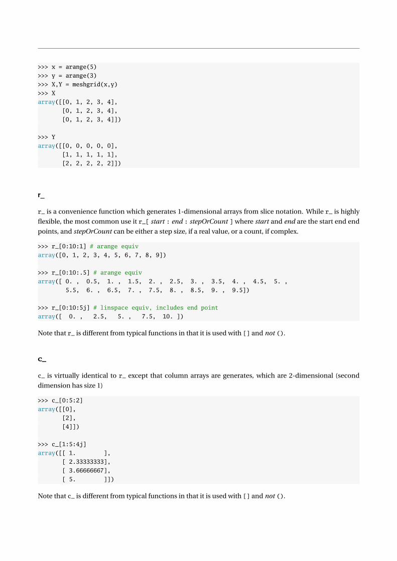
>>> x = arange(5)
>>> y = arange(3)
>>> X,Y = meshgrid(x,y)
>>> X
array([[0, 1, 2, 3, 4],
[0, 1, 2, 3, 4],
[0, 1, 2, 3, 4]])
>>> Y
array([[0, 0, 0, 0, 0],
[1, 1, 1, 1, 1],
[2, 2, 2, 2, 2]])
r_
r_ is a convenience function which generates 1-dimensional arrays from slice notation. While r_ is highly
flexible, the most common use it r_[ start : end : stepOrCount ] where start and end are the start end end
points, and stepOrCount can be either a step size, if a real value, or a count, if complex.
>>> r_[0:10:1] # arange equiv
array([0, 1, 2, 3, 4, 5, 6, 7, 8, 9])
>>> r_[0:10:.5] # arange equiv
array([ 0. , 0.5, 1. , 1.5, 2. , 2.5, 3. , 3.5, 4. , 4.5, 5. ,
5.5, 6. , 6.5, 7. , 7.5, 8. , 8.5, 9. , 9.5])
>>> r_[0:10:5j] # linspace equiv, includes end point
array([ 0. , 2.5, 5. , 7.5, 10. ])
Note that r_ is different from typical functions in that it is used with [] and not ().
c_
c_ is virtually identical to r_ except that column arrays are generates, which are 2-dimensional (second
dimension has size 1)
>>> c_[0:5:2]
array([[0],
[2],
[4]])
>>> c_[1:5:4j]
array([[ 1. ],
[ 2.33333333],
[ 3.66666667],
[ 5. ]])
Note that c_ is different from typical functions in that it is used with [] and not ().
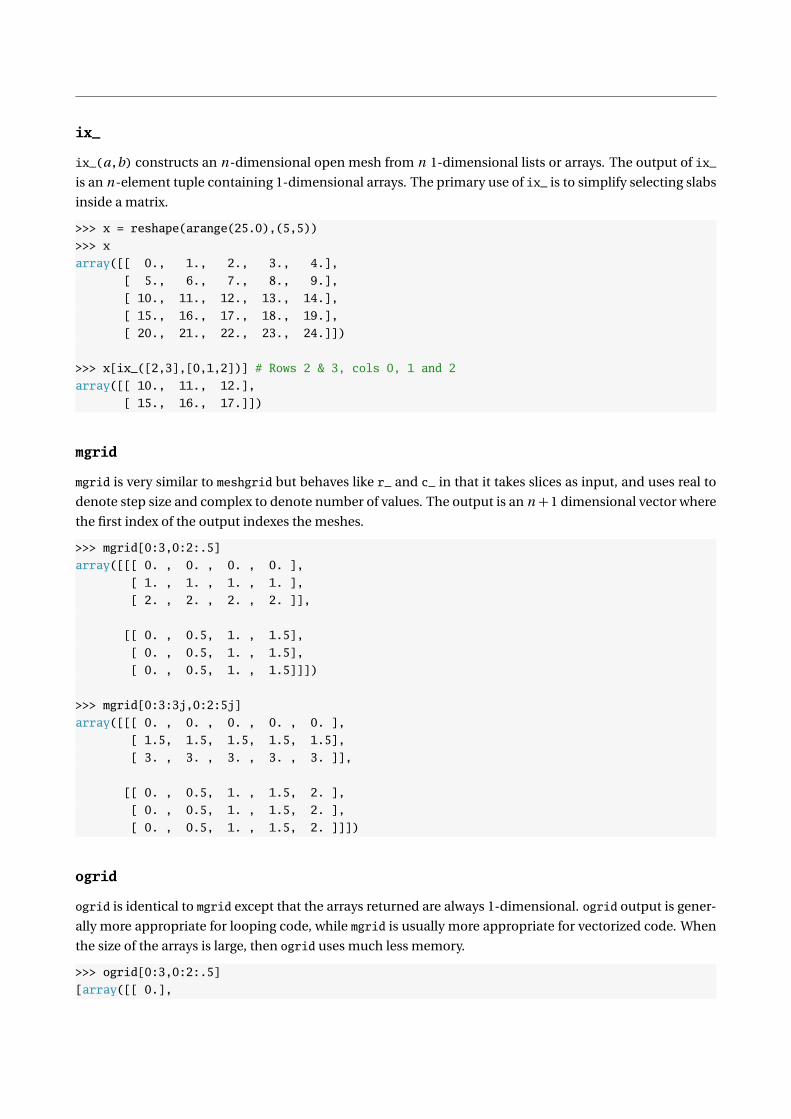
ix_
ix_(a,b) constructs an n-dimensional open mesh from n 1-dimensional lists or arrays. The output of ix_
is an n-element tuple containing 1-dimensional arrays. The primary use of ix_ is to simplify selecting slabs
inside a matrix.
>>> x = reshape(arange(25.0),(5,5))
>>> x
array([[ 0., 1., 2., 3., 4.],
[ 5., 6., 7., 8., 9.],
[ 10., 11., 12., 13., 14.],
[ 15., 16., 17., 18., 19.],
[ 20., 21., 22., 23., 24.]])
>>> x[ix_([2,3],[0,1,2])] # Rows 2 & 3, cols 0, 1 and 2
array([[ 10., 11., 12.],
[ 15., 16., 17.]])
mgrid
mgrid is very similar to meshgrid but behaves like r_ and c_ in that it takes slices as input, and uses real to
denote step size and complex to denote number of values. The output is an n + 1 dimensional vector where
the first index of the output indexes the meshes.
>>> mgrid[0:3,0:2:.5]
array([[[ 0. , 0. , 0. , 0. ],
[ 1. , 1. , 1. , 1. ],
[ 2. , 2. , 2. , 2. ]],
[[ 0. , 0.5, 1. , 1.5],
[ 0. , 0.5, 1. , 1.5],
[ 0. , 0.5, 1. , 1.5]]])
>>> mgrid[0:3:3j,0:2:5j]
array([[[ 0. , 0. , 0. , 0. , 0. ],
[ 1.5, 1.5, 1.5, 1.5, 1.5],
[ 3. , 3. , 3. , 3. , 3. ]],
[[ 0. , 0.5, 1. , 1.5, 2. ],
[ 0. , 0.5, 1. , 1.5, 2. ],
[ 0. , 0.5, 1. , 1.5, 2. ]]])
ogrid
ogrid is identical to mgrid except that the arrays returned are always 1-dimensional. ogrid output is gener-
ally more appropriate for looping code, while mgrid is usually more appropriate for vectorized code. When
the size of the arrays is large, then ogrid uses much less memory.
>>> ogrid[0:3,0:2:.5]
[array([[ 0.],

[ 1.],
[ 2.]]), array([[ 0. , 0.5, 1. , 1.5]])]
>>> ogrid[0:3:3j,0:2:5j]
[array([[ 0. ],
[ 1.5],
[ 3. ]]),
array([[ 0. , 0.5, 1. , 1.5, 2. ]])]
6.2 Rounding
around, round
around rounds to the nearest integer, or to a particular decimal place when called with two arguments.
>>> x= randn(3)
array([ 0.60675173, -0.3361189 , -0.56688485])
>>> around(x)
array([ 1., 0., -1.])
>>> around(x, 2)
array([ 0.61, -0.34, -0.57])
around can also be used as a method on an ndarray – except that the method is named round. For example,
x.round(2) is identical to around(x, 2). The change of names is needed since there is a built-in function
round which is not aware of arrays.
floor
floor rounds to the next smallest integer (negative values are rounded away from 0).
>>> x= randn(3)
array([ 0.60675173, -0.3361189 , -0.56688485])
>>> floor(x)
array([ 0., -1., -1.])
ceil
ceil rounds to the next largest integer (negative values are rounded towards 0).
>>> x= randn(3)
array([ 0.60675173, -0.3361189 , -0.56688485])
>>> ceil(x)
array([ 1., -0., -0.])
Note that the values returned are still floating points and so -0. is the same as 0..
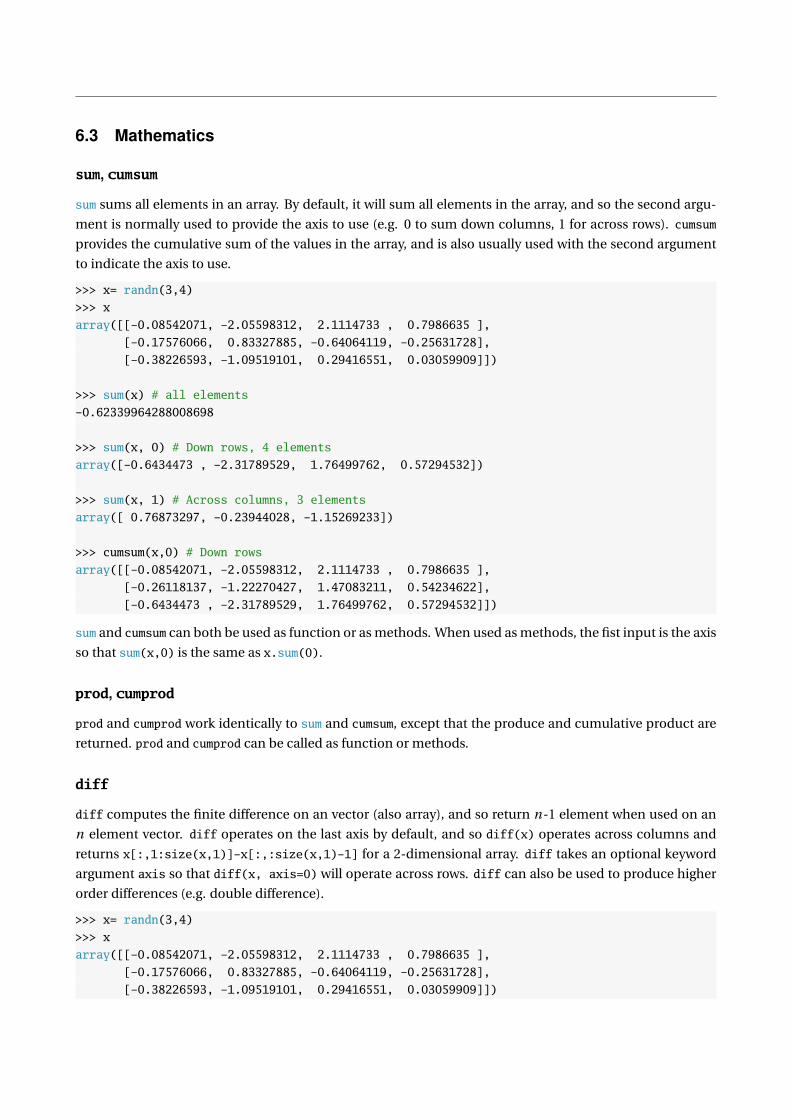
6.3 Mathematics
sum, cumsum
sum sums all elements in an array. By default, it will sum all elements in the array, and so the second argu-
ment is normally used to provide the axis to use (e.g. 0 to sum down columns, 1 for across rows). cumsum
provides the cumulative sum of the values in the array, and is also usually used with the second argument
to indicate the axis to use.
>>> x= randn(3,4)
>>> x
array([[-0.08542071, -2.05598312, 2.1114733 , 0.7986635 ],
[-0.17576066, 0.83327885, -0.64064119, -0.25631728],
[-0.38226593, -1.09519101, 0.29416551, 0.03059909]])
>>> sum(x) # all elements
-0.62339964288008698
>>> sum(x, 0) # Down rows, 4 elements
array([-0.6434473 , -2.31789529, 1.76499762, 0.57294532])
>>> sum(x, 1) # Across columns, 3 elements
array([ 0.76873297, -0.23944028, -1.15269233])
>>> cumsum(x,0) # Down rows
array([[-0.08542071, -2.05598312, 2.1114733 , 0.7986635 ],
[-0.26118137, -1.22270427, 1.47083211, 0.54234622],
[-0.6434473 , -2.31789529, 1.76499762, 0.57294532]])
sum and cumsum can both be used as function or as methods. When used as methods, the fist input is the axis
so that sum(x,0) is the same as x.sum(0).
prod, cumprod
prod and cumprod work identically to sum and cumsum, except that the produce and cumulative product are
returned. prod and cumprod can be called as function or methods.
diff
diff computes the finite difference on an vector (also array), and so return n-1 element when used on an
n element vector. diff operates on the last axis by default, and so diff(x) operates across columns and
returns x[:,1:size(x,1)]-x[:,:size(x,1)-1] for a 2-dimensional array. diff takes an optional keyword
argument axis so that diff(x, axis=0) will operate across rows. diff can also be used to produce higher
order differences (e.g. double difference).
>>> x= randn(3,4)
>>> x
array([[-0.08542071, -2.05598312, 2.1114733 , 0.7986635 ],
[-0.17576066, 0.83327885, -0.64064119, -0.25631728],
[-0.38226593, -1.09519101, 0.29416551, 0.03059909]])

>>> diff(x) # Same as diff(x,1)
-0.62339964288008698
>>> diff(x, axis=0)
array([[-0.09033996, 2.88926197, -2.75211449, -1.05498078],
[-0.20650526, -1.92846986, 0.9348067 , 0.28691637]])
>>> diff(x, 2, axis=0) # Double difference, collumn-by-column
array([[-0.11616531, -4.81773183, 3.68692119, 1.34189715]])
exp
exp returns the element-by-element exponential (e x ) for an array.
log
log returns the element-by-element natural logarithm (ln(x )) for an array.
log10
log10 returns the element-by-element base-10 logarithm (log10 (x )) for an array.
sqrt
sqrt returns the element-by-element square root (√
x ) for an array.
square
square returns the element-by-element square (x 2) for an array.
absolute
absolute returns the element-by-element absolute value for an array. For complex values inputs, |a + b i |=√
a 2 + b 2.
sign
sign returns the element-by-element sign function which is defined as 0 if x = 0, and x/|x | otherwise.
6.4 Complex Values
real
real returns the real elements of a complex array. real can be called either as a function real(x) or as an
attribute x.real.
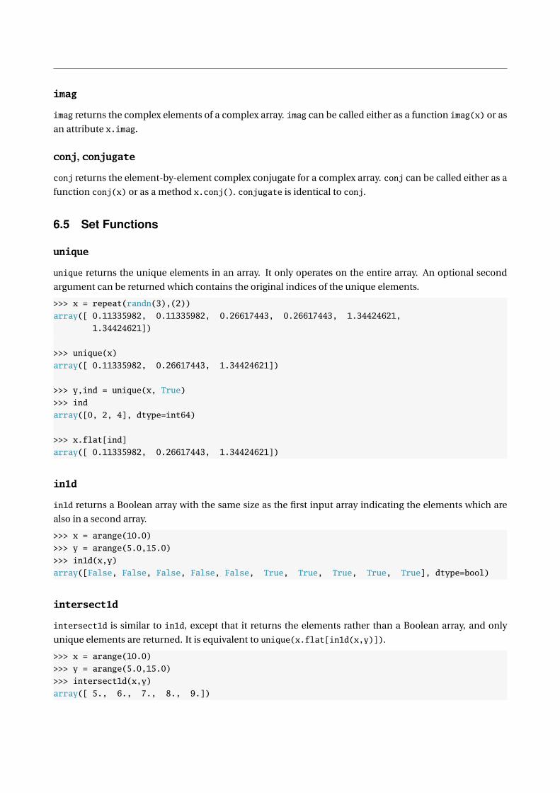
imag
imag returns the complex elements of a complex array. imag can be called either as a function imag(x) or as
an attribute x.imag.
conj, conjugate
conj returns the element-by-element complex conjugate for a complex array. conj can be called either as a
function conj(x) or as a method x.conj(). conjugate is identical to conj.
6.5 Set Functions
unique
unique returns the unique elements in an array. It only operates on the entire array. An optional second
argument can be returned which contains the original indices of the unique elements.
>>> x = repeat(randn(3),(2))
array([ 0.11335982, 0.11335982, 0.26617443, 0.26617443, 1.34424621,
1.34424621])
>>> unique(x)
array([ 0.11335982, 0.26617443, 1.34424621])
>>> y,ind = unique(x, True)
>>> ind
array([0, 2, 4], dtype=int64)
>>> x.flat[ind]
array([ 0.11335982, 0.26617443, 1.34424621])
in1d
in1d returns a Boolean array with the same size as the first input array indicating the elements which are
also in a second array.
>>> x = arange(10.0)
>>> y = arange(5.0,15.0)
>>> in1d(x,y)
array([False, False, False, False, False, True, True, True, True, True], dtype=bool)
intersect1d
intersect1d is similar to in1d, except that it returns the elements rather than a Boolean array, and only
unique elements are returned. It is equivalent to unique(x.flat[in1d(x,y)]).
>>> x = arange(10.0)
>>> y = arange(5.0,15.0)
>>> intersect1d(x,y)
array([ 5., 6., 7., 8., 9.])
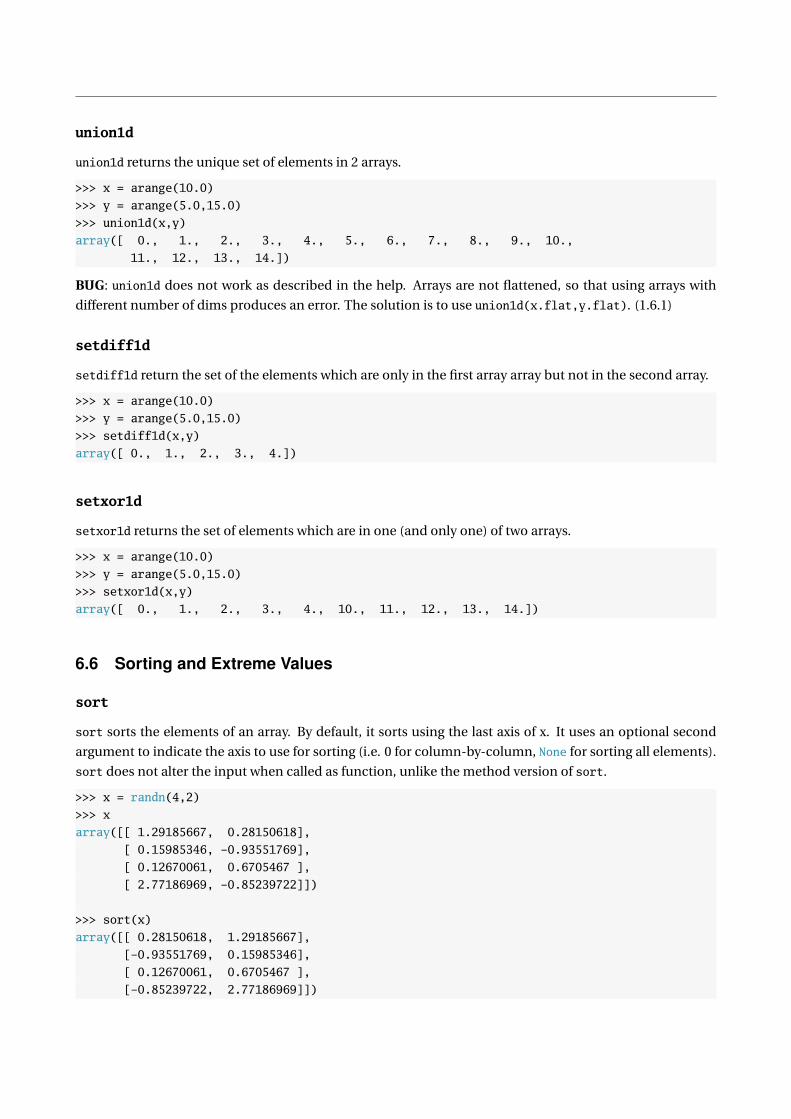
union1d
union1d returns the unique set of elements in 2 arrays.
>>> x = arange(10.0)
>>> y = arange(5.0,15.0)
>>> union1d(x,y)
array([ 0., 1., 2., 3., 4., 5., 6., 7., 8., 9., 10.,
11., 12., 13., 14.])
BUG: union1d does not work as described in the help. Arrays are not flattened, so that using arrays with
different number of dims produces an error. The solution is to use union1d(x.flat,y.flat). (1.6.1)
setdiff1d
setdiff1d return the set of the elements which are only in the first array array but not in the second array.
>>> x = arange(10.0)
>>> y = arange(5.0,15.0)
>>> setdiff1d(x,y)
array([ 0., 1., 2., 3., 4.])
setxor1d
setxor1d returns the set of elements which are in one (and only one) of two arrays.
>>> x = arange(10.0)
>>> y = arange(5.0,15.0)
>>> setxor1d(x,y)
array([ 0., 1., 2., 3., 4., 10., 11., 12., 13., 14.])
6.6 Sorting and Extreme Values
sort
sort sorts the elements of an array. By default, it sorts using the last axis of x. It uses an optional second
argument to indicate the axis to use for sorting (i.e. 0 for column-by-column, None for sorting all elements).
sort does not alter the input when called as function, unlike the method version of sort.
>>> x = randn(4,2)
>>> x
array([[ 1.29185667, 0.28150618],
[ 0.15985346, -0.93551769],
[ 0.12670061, 0.6705467 ],
[ 2.77186969, -0.85239722]])
>>> sort(x)
array([[ 0.28150618, 1.29185667],
[-0.93551769, 0.15985346],
[ 0.12670061, 0.6705467 ],
[-0.85239722, 2.77186969]])
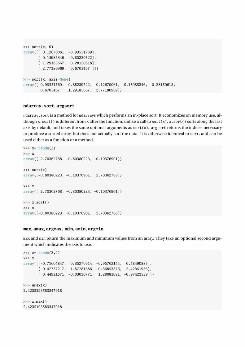
>>> sort(x, 0)
array([[ 0.12670061, -0.93551769],
[ 0.15985346, -0.85239722],
[ 1.29185667, 0.28150618],
[ 2.77186969, 0.6705467 ]])
>>> sort(x, axis=None)
array([-0.93551769, -0.85239722, 0.12670061, 0.15985346, 0.28150618,
0.6705467 , 1.29185667, 2.77186969])
ndarray.sort, argsort
ndarray.sort is a method for ndarrays which performs an in-place sort. It economizes on memory use, al-
though x.sort() is different from x after the function, unlike a call to sort(x). x.sort() sorts along the last
axis by default, and takes the same optional arguments as sort(x). argsort returns the indices necessary
to produce a sorted array, but does not actually sort the data. It is otherwise identical to sort, and can be
used either as a function or a method.
>>> x= randn(3)
>>> x
array([ 2.70362768, -0.80380223, -0.10376901])
>>> sort(x)
array([-0.80380223, -0.10376901, 2.70362768])
>>> x
array([ 2.70362768, -0.80380223, -0.10376901])
>>> x.sort()
>>> x
array([-0.80380223, -0.10376901, 2.70362768])
max, amax, argmax, min, amin, argmin
max and min return the maximum and minimum values from an array. They take an optional second argu-
ment which indicates the axis to use.
>>> x= randn(3,4)
>>> x
array([[-0.71604847, 0.35276614, -0.95762144, 0.48490885],
[-0.47737217, 1.57781686, -0.36853876, 2.42351936],
[ 0.44921571, -0.03030771, 1.28081091, -0.97422539]])
>>> amax(x)
2.4235193583347918
>>> x.max()
2.4235193583347918

>>> x.max(0)
array([ 0.44921571, 1.57781686, 1.28081091, 2.42351936])
>>> x.max(1)
array([ 0.48490885, 2.42351936, 1.28081091])
max and min can only be used on arrays as methods. When used as a function, amax and amin must be used
to avoid conflicts with the built-in functions max and min. This behavior is also seen in around and round.
argmax and argmin return the index or indices of the maximum or minimum element(s). They are used in
an identical manner to max and min, and can be used either as a function or method.
minimum, maximum
maximum and minimum can be used to compute the maximum and minimum of two arrays which are broad-
castable.
>>> x = randn(4)
>>> x
array([-0.00672734, 0.16735647, 0.00154181, -0.98676201])
>>> y = randn(4)
array([-0.69137963, -2.03640622, 0.71255975, -0.60003157])
>>> maximum(x,y)
array([-0.00672734, 0.16735647, 0.71255975, -0.60003157])
6.7 Nan Functions
NaN function are convenience function which act similarly to their non-NaN versions, only ignoring NaN
values (rather than propagating) when computing the function.
nansum
nansum is identical sum, except that NaNs are ignored. nansum can be used to easily generate other NaN-
functions, such as nanstd (standard deviation, ignoring nans) since variance can be implemented using 2
sums.
>>> x = randn(4)
>>> x[1] = np.nan
>>> x
array([-0.00672734, nan, 0.00154181, -0.98676201])
>>> sum(x)
nan
>>> nansum(x)
-0.99194753275859726
>>> nansum(x) / sum(logical_not(isnan(x)))

nanmax, nanargmax, nanmin, nanargmin
nanmax, nanmin, nanargmax and nanargmin are identical to their non-NaN counterparts, except that NaNs are
ignored.
6.8 Exercises
1. Construct each of the following sequences using linspace, arange and r_:
0, 1, . . . , 10
4, 5, 6, . . . , 13
0, .25, .5, .75, 1
0,−1,−2, . . . ,−5
2. Show that logspace(0,2,21) can be constructed using linspace and 10 (and **). Similarly, show how
linsapce(2,10,51) can be constructed with logspace and log10.
3. Determine the differences between the rounding by applying round (or around), ceil and floor to
y = [0, 0.5, 1.5, 2.5, 1.0, 1.0001,−0.5,−1,−1.5,−2.5]
4. Prove the relationship that∑n
j=1 j = n (n + 1)/2 for 0 ≤ n ≤ 10 using cumsum and directly using math
on an array.
5. randn(20)will generate an array containing draws from a standard normal random variable. If x=randn(20),
which element of y=cumsum(x) is the same as sum(x)?
6. cumsum computes the cumulative sum while diff computes the difference. Is diff(cumsum(x)) the
same as x? If not, how can a small modification be made to the this statement to recover x?
7. Compute the exp of
y = [ln 0.5 ln 1 ln e ]
Note: You should use log and the constant numpy.e to construct y.
8. What is absolute of 0.0, -3.14, and 3+4j?
9. Suppose x = [−4 2 − 9 − 8 10]. What is the difference between y = sort(x) and x.sort()?
10. Using the same x as in the previous problem, find the max. Also, using argmax and a slice, retrieve the
same value.
11. Show that setdiff1d could be replaced with in1d and intersect1d using x = [1 2 3 4 5] and y =[1 2 4 6]? How could setxor1d be replaced with union1d, intersect1d and in1d?
12. Suppose y = [nan 2.2 3.9 4.6 nan 2.4 6.1 1.8] . How can nansum be used to compute the variance or the
data? Note: sum(1-isnan(y)) will return the count of non-NaN values.

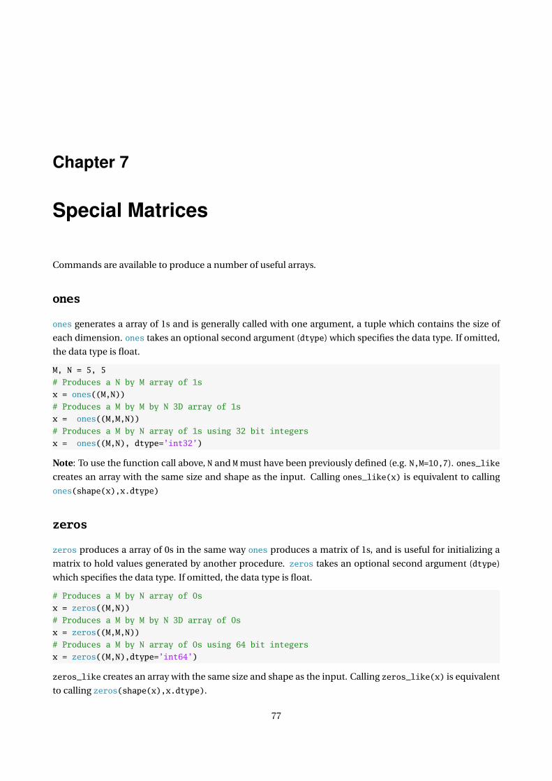
Chapter 7
Special Matrices
Commands are available to produce a number of useful arrays.
ones
ones generates a array of 1s and is generally called with one argument, a tuple which contains the size of
each dimension. ones takes an optional second argument (dtype) which specifies the data type. If omitted,
the data type is float.
M, N = 5, 5
# Produces a N by M array of 1s
x = ones((M,N))
# Produces a M by M by N 3D array of 1s
x = ones((M,M,N))
# Produces a M by N array of 1s using 32 bit integers
x = ones((M,N), dtype=’int32’)
Note: To use the function call above, N and M must have been previously defined (e.g. N,M=10,7). ones_like
creates an array with the same size and shape as the input. Calling ones_like(x) is equivalent to calling
ones(shape(x),x.dtype)
zeros
zeros produces a array of 0s in the same way ones produces a matrix of 1s, and is useful for initializing a
matrix to hold values generated by another procedure. zeros takes an optional second argument (dtype)
which specifies the data type. If omitted, the data type is float.
# Produces a M by N array of 0s
x = zeros((M,N))
# Produces a M by M by N 3D array of 0s
x = zeros((M,M,N))
# Produces a M by N array of 0s using 64 bit integers
x = zeros((M,N),dtype=’int64’)
zeros_like creates an array with the same size and shape as the input. Calling zeros_like(x) is equivalent
to calling zeros(shape(x),x.dtype).
77

empty
empty produces an empty (uninitialized) array to hold values generated by another procedure. empty takes
an optional second argument (dtype) which specifies the data type. If omitted, the data type is float.
# Produces a M by N empty array
x = empty((M,N))
# Produces a 4D empty array
x = empty((N,N,N,N))
# Produces a M by N empty array using 32-bit floats (single precision)
x = empty((M,N),dtype=’float32’)
Using empty is slightly faster than calling zeros since it does not assign 0 to all elements of the array – the
“empty” array created will be populated with (essential random) values. empty_like creates an array with
the same size and shape as the input. Calling empty_like(x) is equivalent to calling empty(shape(x),x.dtype).
eye, identity
eye generates an identity matrix (an array with ones on the diagonal, zeros every where else). An identity
matrix is square and so usually only 1 input is needed.
In = eye(N)
identity is a virtually identical function with similar use, In = identity(N).
7.1 Exercises
1. Produce two arrays, one containing all zeros and one containing only ones, of size 10× 5.
2. Multiply (linear algebra) these two arrays in both possible ways.
3. Produce an identity matrix of size 5. Take the exponential of this matrix, element-by-element.
4. How could ones and zeros be replaced with tile?
5. How could eye be replaced with diag and ones?
6. What is the value of y=empty((1,))? Is it the same as any element in y=empty((10,))?

Chapter 8
Array and Matrix Functions
Some functions operate exclusively on array inputs. Some are mathematical in nature, for instance com-
puting the eigenvalues and eigenvectors, while other are functions for manipulating the elements of an
array.
8.1 Views
Views are computationally efficient methods to produce objects which behave as other objects without
copying data. For example, an array x can always be converted to a matrix using matrix(x), which will copy
the elements in x. View “fakes” the call to matrix and only inserts a thin layer so that x viewed as a matrix
behaves like a matrix.
view
view can be used to produce a representation of an array, matrix or recarray as another type without copying
the data. Using view is faster than copying data into a new class.
>>> x = arange(5)
>>> type(x)
numpy.ndarray
>>> x.view(np.matrix)
matrix([[0, 1, 2, 3, 4]])
>>> x.view(np.recarray)
rec.array([0, 1, 2, 3, 4])
asmatrix, mat
asmatrix and mat can be used to view an array as a matrix. This view is useful since matrix views will use
matrix multiplication by default.
>>> x = array([[1,2],[3,4]])
>>> x * x # Element-by-element
array([[ 1, 4],
[ 9, 16]])
79
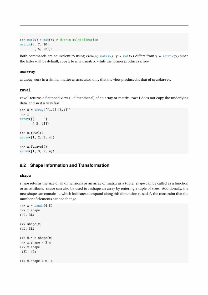
>>> mat(x) * mat(x) # Matrix multiplication
matrix([[ 7, 10],
[15, 22]])
Both commands are equivalent to using view(np.matrix). y = mat(x) differs from y = matrix(x) since
the latter will, by default, copy x to a new matrix, while the former produces a view.
asarray
asarray work in a similar matter as asmatrix, only that the view produced is that of np.ndarray.
ravel
ravel returns a flattened view (1-dimensional) of an array or matrix. ravel does not copy the underlying
data, and so it is very fast.
>>> x = array([[1,2],[3,4]])
>>> x
array([[ 1, 2],
[ 3, 4]])
>>> x.ravel()
array([1, 2, 3, 4])
>>> x.T.ravel()
array([1, 3, 2, 4])
8.2 Shape Information and Transformation
shape
shape returns the size of all dimensions or an array or matrix as a tuple. shape can be called as a function
or an attribute. shape can also be used to reshape an array by entering a tuple of sizes. Additionally, the
new shape can contain -1 which indicates to expand along this dimension to satisfy the constraint that the
number of elements cannot change.
>>> x = randn(4,3)
>>> x.shape
(4L, 3L)
>>> shape(x)
(4L, 3L)
>>> M,N = shape(x)
>>> x.shape = 3,4
>>> x.shape
(3L, 4L)
>>> x.shape = 6,-1

>>> x.shape
(6L, 2L)
reshape
reshape transforms an array with one set of dimensions and to one with a different set, preserving the
number of elements. reshape can transform an M by N array x into an K by L array y as long as M N = K L.
Note that the number of elements cannot change. The most useful call to reshape switches an array into a
vector or vice versa. For example
>>> x = array([[1,2],[3,4]])
>>> y = reshape(x,(4,1))
>>> y
array([[1],
[2],
[3],
[4]])
>>> z=reshape(y,(1,4))
>>> z
array([[1, 2, 3, 4]])
>>> w = reshape(z,(2,2))
array([[1, 2],
[3, 4]])
The crucial implementation detail of reshape is that matrices are stored using row-major notation. Ele-
ments in matrices are counted first across and then then down rows. reshape will place elements of the old
array into the same position in the new array and so after calling reshape, x (1) = y (1), x (2) = y (2), and so
on.
size
size returns the total number of elements in an array or matrix. size can be used as a function or an
attribute.
>>> x = randn(4,3)
>>> size(x)
2
>>> x.size
12
ndim
ndim returns the size of all dimensions or an array or matrix as a tuple. ndim can be used as a function or an
attribute .
>>> x = randn(4,3)
>>> ndim(x)

2
>>> x.ndim
2
tile
tile, along with reshape, are two of the most useful non-mathematical functions. tile replicates an ar-
ray according to a specified size vector. To understand how repmat functions, imagine forming an array-
composed of blocks. The generic form of tile is tile(X , (M , N ) ) where X is the matrix to be replicated,
M is the number of rows in the new block matrix, and N is the number of columns in the new block matrix.
For example, suppose X was a matrix
X =
[1 2
3 4
]and the block matrix
Y =
[X X X
X X X
]was needed. This could be accomplished by manually constructing y using concatenate
x = array([[1,2],[3,4]])
z = concatenate((x,x,x))
y = concatenate((z.T,z.T),axis=0)
However, tile provides a much easier method to construct y
y = tile(x,(2,3))
tile has two clear advantages over manual allocation: First, tile can be executed using parameters deter-
mined at run-time, such as the number of explanatory variables in a model and second tile can be used for
arbitrary dimensions. Manual matrix construction becomes tedious and error prone with as few as 3 rows
and columns. repeat is a related function which copies data is a less useful manner.
flatten
flatten works much like ravel, only that is copies the array when producing the flattened version.
flat
flat produces a numpy.flatiter object which is an iterator over a flattened view of an array. Because it is
an iterator, it is especially fast.
>>> x = array([[1,2],[3,4]])
>>> x.flat
<numpy.flatiter at 0x6f569d0>
>>> x.flat[2]
3
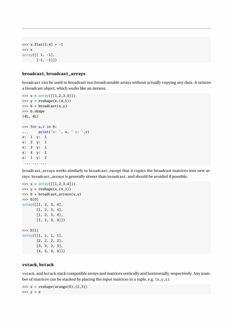
>>> x.flat[1:4] = -1
>>> x
array([[ 1, -1],
[-1, -1]])
broadcast, broadcast_arrays
broadcast can be used to broadcast two broadcastable arrays without actually copying any data. It returns
a broadcast object, which works like an iterator.
>>> x = array([[1,2,3,4]])
>>> y = reshape(x,(4,1))
>>> b = broadcast(x,y)
>>> b.shape
(4L, 4L)
>>> for u,v in b:
... print(’x: ’, u, ’ y: ’,v)
x: 1 y: 1
x: 2 y: 1
x: 3 y: 1
x: 4 y: 1
x: 1 y: 2
... ... ...
broadcast_arrays works similarly to broadcast, except that it copies the broadcast matrices into new ar-
rays. broadcast_arrays is generally slower than broadcast, and should be avoided if possible.
>>> x = array([[1,2,3,4]])
>>> y = reshape(x,(4,1))
>>> b = broadcast_arrays(x,y)
>>> b[0]
array([[1, 2, 3, 4],
[1, 2, 3, 4],
[1, 2, 3, 4],
[1, 2, 3, 4]])
>>> b[1]
array([[1, 1, 1, 1],
[2, 2, 2, 2],
[3, 3, 3, 3],
[4, 4, 4, 4]])
vstack, hstack
vstack, and hstack stack compatible arrays and matrices vertically and horizontally, respectively. Any num-
ber of matrices can be stacked by placing the input matrices in a tuple, e.g. (x,y,z).
>>> x = reshape(arange(6),(2,3))
>>> y = x

>>> vstack((x,y))
array([[0, 1, 2],
[3, 4, 5],
[0, 1, 2],
[3, 4, 5]])
>>> hstack((x,y))
array([[0, 1, 2, 0, 1, 2],
[3, 4, 5, 3, 4, 5]])
concatenate
concatenate generalizes vstack and hsplit to allow concatenation along any axis.
split, vsplit, hsplit
vsplit and hsplit split arrays and matrices vertically and horizontally, respectively. Both can be used to
split an array into n equal parts or into arbitrary segments, depending on the second argument. If scalar,
the matrix is split into n equal sized parts. If a 1 dimensional array, the matrix is split using the elements
of the array as break points. For example, if the array was [2,5,8], the matrix would be split into 4 pieces
using [:2] , [2:5], [5:8] and [8:]. Both vsplit and hsplit are special cases of split.
>>> x = reshape(arange(20),(4,5))
>>> y = vsplit(x,2)
>>> len(y)
2
>>> y[0]
array([[0, 1, 2, 3, 4],
[5, 6, 7, 8, 9]])
>>> y = hsplit(x,[1,3])
>>> len(y)
3
>>> y[0]
array([[ 0],
[ 5],
[10],
[15]])
>>> y[1]
array([[ 1, 2],
[ 6, 7],
[11, 12],
[16, 17]])

delete
delete removes values from an array, and is similar to splitting an array, and then concatenating the values
which are not deleted. The form of delete is delete(x,rc, axis) where rc are the row or column indices to
delete, and axis is the axis to use (0 or 1 for a 2-dimensional array). If axis is omitted, delete operated on
the flattened array.
>>> x = reshape(arange(20),(4,5))
>>> delete(x,1,0) # Same as x[[0,2,3]]
array([[ 0, 1, 2, 3, 4],
[10, 11, 12, 13, 14],
[15, 16, 17, 18, 19]])
>>> delete(x,[2,3],1) # Same as x[:,[0,1,4]]
array([[ 0, 1, 4],
[ 5, 6, 9],
[10, 11, 14],
[15, 16, 19]])
>>> delete(x,[2,3]) # Same as hstack((x.flat[:2],x.flat[4:]))
array([ 0, 1, 4, 5, 6, 7, 8, 9, 10, 11, 12, 13, 14, 15, 16, 17, 18,
19])
squeeze
squeeze removes singleton dimensions from an array. squeeze can be called as a function or a method.
>>> x = ones((5,1,5,1))
>>> shape(x)
(5L, 1L, 5L, 1L)
>>> y = x.squeeze()
>>> shape(y)
(5L, 5L)
>>> y = squeeze(x)
fliplr, flipud
fliplr and flipud flip arrays in a left-to-right and up-to-down directions, respectively. Since 1-dimensional
arrays are neither column nor row vectors, these two functions are only applicable on 2-dimensional (or
higher) arrays.
>>> x = reshape(arange(4),(2,2))
>>> x
array([[0, 1],
[2, 3]])
>>> fliplr(x)
array([[1, 0],

[3, 2]])
>>> flipud(x)
array([[2, 3],
[0, 1]])
diag
diag can produce one of two results depending on the form of the input. If the input is a square matrix, it
will return a column vector containing the elements of the diagonal. If the input is a vector, it will return a
matrix containing the elements of the diagonal along the vector. Consider the following example:
>>> x = matrix([[1,2],[3,4]])
>>> x
matrix([[1, 2],
[3, 4]])
>>> y = diag(x)
>>> y
array([1, 4])
>>> z = diag(y)
>>> z
array([[1, 0],
[0, 4]])
triu, tril
triu and tril produce upper and lower triangular, respectively.
>>> x = matrix([[1,2],[3,4]])
>>> triu(x)
matrix([[1, 2],
[0, 4]])
>>> tril(x)
matrix([[1, 0],
[3, 4]])
8.3 Linear Algebra Functions
matrix_power
matrix_power raises a square array or matrix to an integer power, and matrix_power(x,n) is identical to
x**n.

svd
svd computed the singular value decomposition of a matrix. A singular value decomposition of a matrix X
is
X = UΣV ′
where Σ is a diagonal elements, and U and V are unitary matrices (orthonormal if real valued). SVDs are
closely related to eigenvalue decompositions when X is a real, positive definite matrix.
cond
cond computes the condition number of a matrix, which measures how close to singular a matrix is. Lower
numbers are better conditioned (and further from singular).
>>> x = matrix([[1.0,0.5],[.5,1]])
>>> cond(x)
3
>>> x = matrix([[1.0,2.0],[1.0,2.0]]) # Singular
>>> cond(x)
inf
slogdet
slogdet computes the sign and log of the absolute value of the determinant. slogdet is useful for computing
determinants which may be very large or small to avoid overflow or underflow.
solve
solve solves the system Xβ = y when X is square and invertible so that the solution is exact.
>>> X = array([[1.0,2.0,3.0],[3.0,3.0,4.0],[1.0,1.0,4.0]])
>>> y = array([[1.0],[2.0],[3.0]])
>>> solve(X,y)
array([[ 0.625],
[-1.125],
[ 0.875]])
lstsq
lstsq solves the system Xβ = y when X is n by k , n > k by finding the least squares solution. lstsq returns
a 4-element tuple where the first element is β and the second element is the sum of squared residuals. The
final two outputs are diagnostic – the third is the rank of X and the fourth contains the singular values of X .
>>> X = randn(100,2)
>>> y = randn(100)
>>> lstsq(X,y)
(array([ 0.03414346, 0.02881763]),
array([ 3.59331858]),
2,
array([ 3.045516 , 1.99327863]))array([[ 0.625],
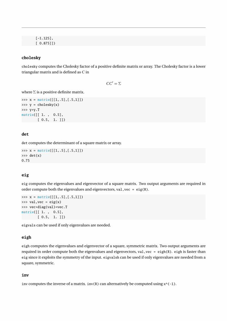
[-1.125],
[ 0.875]])
cholesky
cholesky computes the Cholesky factor of a positive definite matrix or array. The Cholesky factor is a lower
triangular matrix and is defined as C in
CC ′ = Σ
where Σ is a positive definite matrix.
>>> x = matrix([[1,.5],[.5,1]])
>>> y = cholesky(x)
>>> y*y.T
matrix([[ 1. , 0.5],
[ 0.5, 1. ]])
det
det computes the determinant of a square matrix or array.
>>> x = matrix([[1,.5],[.5,1]])
>>> det(x)
0.75
eig
eig computes the eigenvalues and eigenvector of a square matrix. Two output arguments are required in
order compute both the eigenvalues and eigenvectors, val,vec = eig(R).
>>> x = matrix([[1,.5],[.5,1]])
>>> val,vec = eig(x)
>>> vec*diag(val)*vec.T
matrix([[ 1. , 0.5],
[ 0.5, 1. ]])
eigvals can be used if only eigenvalues are needed.
eigh
eigh computes the eigenvalues and eigenvector of a square, symmetric matrix. Two output arguments are
required in order compute both the eigenvalues and eigenvectors, val,vec = eigh(R). eigh is faster than
eig since it exploits the symmetry of the input. eigvalsh can be used if only eigenvalues are needed from a
square, symmetric.
inv
inv computes the inverse of a matrix. inv(R) can alternatively be computed using x^(-1).

>>> x = matrix([[1,.5],[.5,1]])
>>> xInv = inv(x)
>>> x*xInv
matrix([[ 1., 0.],
[ 0., 1.]])
kron
kron computes the Kronecker product of two matrices,
z = x ⊗ y
and is written as z = kron(x,y).
trace
trace computes the trace of a square matrix (sum of diagonal elements) and so trace(x) equals sum(diag(x)).
matrix_rank
matrix_rank computes the rank of a matrix using a SVD.
>>> x = matrix([[1,.5],[1,.5]])
>>> x
matrix([[ 1. , 0.5],
[ 1. , 0.5]])
>>> matrix_rank(x)
1
8.4 Exercises
1. Let x = arange(12.0). Use both shape and reshape to produce 1 × 12, 2 × 6, 3 × 4,4 × 3, 6 × 2 and
2× 2× 3 versions or the array. Finally, return x to its original size.
2. Let x = reshape(arange(12.0),(4,3)). Use ravel, flatten and flat to extract elements 1, 3, . . ., 11
from the array (using a 0 index).
3. Let x be 2 by 2 array, y be a 1 by 1 array, and z be a 3 by 2 array. Construct
w =
x
y y y
y y y
zz ′
y y y
using hstack, vstack, and tile.
4. Let x = reshape(arange(12.0),(2,2,3)). What does squeeze do to x ?

5. How can a diagonal matrix containing the diagonal elements of
y =
[2 .5
.5 4
]
be constructed using diag?
6. Using the y array from the previous problem, verify that cholesky work by computing the Cholesky
factor, and then multiplying to get y again.
7. Using the y array from the previous problem, verify that the sum of the eigenvalues is the same as the
trace, and the product of the eigenvalues is the determinant.
8. Using the y array from the previous problem, verify that the inverse of y is equal to V D−1V ′ where V
is the array containing the eigenvectros, and D is a diagonal array containing the eigenvalues.
9. Simulate some data where x = randn(100,2), e = randn(100,1), B = array([[1],[0.5]]) and y =xβ + ε. Use lstsq to estimate β from x and y .
10. Suppose
y =
5 −1.5 −3.5
−1.5 2 −0.5
−3.5 −0.5 4
use matrix_rank to determine the rank of this array. Verify the results by inspecting the eigenvalues
using eig and check that the determinant is 0 using det.
11. Let x = randn(100,2). Use kron to compute
I2 ⊗ ΣX
where ΣX is the 2 by 2 covariance matrix of x .

Chapter 9
Importing and Exporting Data
9.1 Importing Data
Importing data ranges from easy for files which contain only numbers difficult, depending on the data size
and format. A few principles can simplify this task:
• The file imported should contain numbers only, with the exception of the first row which may contain
the variable names.
• Use another program, such as Microsoft Excel, to manipulate data before importing.
• Each column of the spreadsheet should contain a single variable.
• Dates should be converted to YYYYMMDD, a numeric format, before importing. This can be done in
Excel using the formula:
=10000*YEAR(A1)+100*MONTH(A1)+DAY(A1)+(A1-FLOOR(A1,1))
9.2 CSV and other formatted text files
A number of importers are available for regular (e.g. all rows have the same number of columns) comma-
separated value (CSV) data. The choice of which importer to use depends on the complexity and size of the
file. Purely numeric files are the simplest to import, although most files which have a repeated structure can
be imported (unless they are very large).
9.2.1 loadtxt
loadtxt (numpy.lib.npyio.loadtxt)is a simple, but fast, text importer. The basic use is loadtxt( f i l e na m e),
which will attempt to load the data in file name as floats. Other useful named arguments include delim,
which allow the file delimiter to be specified, and skiprows which allows one or more rows to be skipped.
loadtxt requires the data to be numeric and so is only useful for the simplest files.
>>> data = loadtxt(’FTSE_1984_2012.csv’,delimiter=’,’) # Error
ValueError: could not convert string to float: Date
# Fails since csv has a header
>>> data = loadtxt(’FTSE_1984_2012_numeric.csv’,delimiter=’,’) # Error
91

ValueError: could not convert string to float: Date
>>> data = loadtxt(’FTSE_1984_2012_numeric.csv’,delimiter=’,’,skiprows=1)
>>> data[0]
array([ 4.09540000e+04, 5.89990000e+03, 5.92380000e+03, 5.88060000e+03, 5.89220000e+03,
8.01550000e+08, 5.89220000e+03])
9.2.2 genfromtxt
genfromtxt (numpy.lib.npyio.genfromtxt ) is a slower, but more robust, importer than loadtxt. genfromtxt
is called in an identical matter as loadtxt, but will not fail if a non-numeric type is encountered. Instead,
genfromtxt will return a NaN (not-a-number) for fields in the file it cannot read.
>>> data = genfromtxt(’FTSE_1984_2012.csv’,delimiter=’,’)
>>> data[0]
array([ nan, nan, nan, nan, nan, nan, nan])
>>> data[1]
array([ nan, 5.89990000e+03, 5.92380000e+03, 5.88060000e+03, 5.89220000e+03, 8.01550000e+08,
5.89220000e+03])
Tab delimited data can be read in a similar manner using delimiter=’\t’.
>>> data = genfromtxt(’FTSE_1984_2012_numeric_tab.txt’,delimiter=’\t’)
9.2.2.1 csv2rec
csv2rec (matplotlib.mlab.csv2rec) is an even more robust – and slower – csv importer which allows for
non-numeric data such as dates. It also attempts to find the best data type using for each row.
>>> data = csv2rec(’FTSE_1984_2012.csv’,delimiter=’,’)
>>> data[0]
(datetime.date(2012, 2, 15), 5899.9, 5923.8, 5880.6, 5892.2, 801550000L, 5892.2)
Unlike loadtxt and genfromtxt, which both return an array, csv2rec returns a recarray (numpy.core.
.records .recarray, see Chapter 20) which is, in many ways, like a list. csv2rec converted each row of the
input file into a datetime (see Chapter 16), followed by 4 floats for open, high, low and close, then a long
integer for volume, and finally a float for the adjusted close.
Because the values returned are not an array, it is normally necessary to create an array to store the array.
>>> open = data[’open’]
>>> open
array([ 5899.9, 5905.7, 5852.4, ..., 1095.4, 1095.4, 1108.1])
9.3 Reading 97-2003 Excel Files
Reading Excel files in Python is more involved, so unless essential, it is probably simpler to convert the xls
to csv. Reading 97-2003 Excel files requires a python package which is not in the core, xlutils, which can be
installed using easy_install xlutils.

from __future__ import print_function
import xlrd
wb = xlrd.open_workbook(’FTSE_1984_2012.xls’)
sheetNames = wb.sheet_names()
# Assumes 1 sheet name
sheet = wb.sheet_by_name(sheetNames[0])
excelData = []
for i in xrange(sheet.nrows):
excelData.append(sheet.row_values(i))
# - 1 since excelData has the header row
open = empty(len(excelData) - 1)
for i in xrange(len(excelData) - 1):
open[i] = excelData[i+1][1]
The listing does a few things. First, it opens the workbook for reading (xlrd. open_workbook( ’FTSE_1984_
_2012.xls’)), then it gets the sheet names (wb.sheet_names()) and opens a sheet (wb.sheet_by_name(sheetNames[0])).
From the sheet, it gets the number of rows (sheet.nrows), and fills a list with the values, row-by-row. Once
the data has been read-in, the final block fills an array from the data from opening prices in the list. This
is substantially more complicated than converting to a CSV file, although reading Excel files is useful for
automated work (e.g. you have no choice but to import from an Excel file since it is produced by some other
software).
Python 2.7 vs. 3.2
xlrd is not available for Python 3.
9.4 Reading 2007 & 2010 Excel Files
xlrd only reads 97-2003 files, and so a different package, openpyxl, is needed to read xlsx files created in
Office 2007 or later. Unfortunately openpyxl has a different syntax to xlrd, and so a modified reader is needed
for xlsx files.
from __future__ import print_function
import openpyxl
wb = openpyxl.load_workbook(’FTSE_1984_2012.xlsx’)
sheetNames = wb.get_sheet_names()
# Assumes 1 sheet name
sheet = wb.get_sheet_by_name(sheetNames[0])
excelData = []
rows = sheet.rows
# - 1 since excelData has the header row
open = empty(len(rows) - 1)
for i in xrange(len(excelData) - 1):
open[i] = rows[i+1][1].value
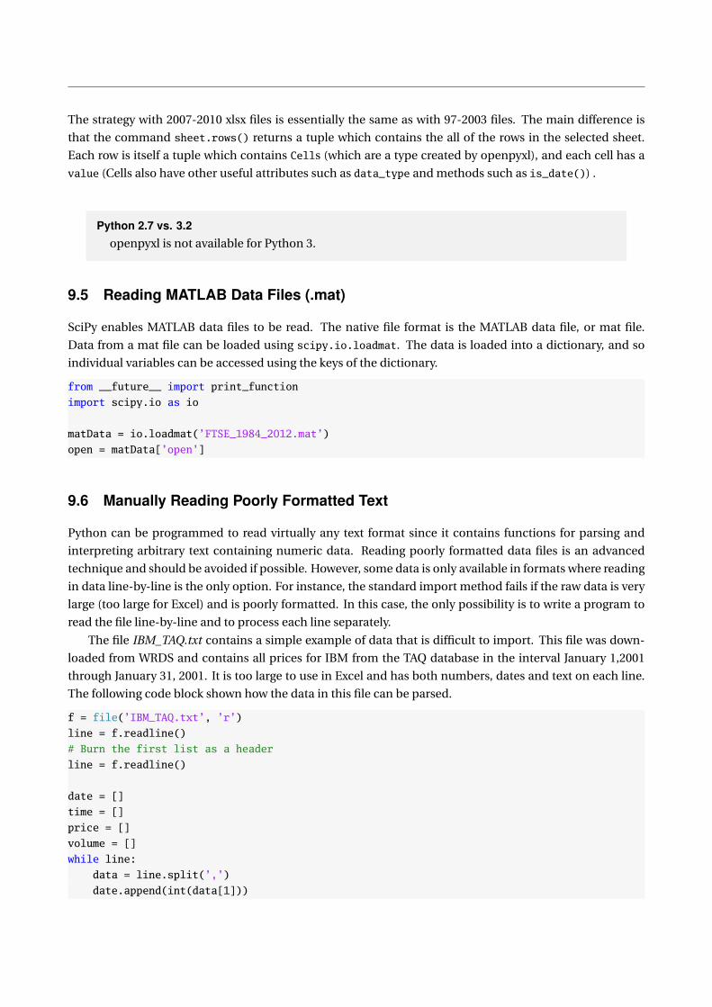
The strategy with 2007-2010 xlsx files is essentially the same as with 97-2003 files. The main difference is
that the command sheet.rows() returns a tuple which contains the all of the rows in the selected sheet.
Each row is itself a tuple which contains Cells (which are a type created by openpyxl), and each cell has a
value (Cells also have other useful attributes such as data_type and methods such as is_date()) .
Python 2.7 vs. 3.2
openpyxl is not available for Python 3.
9.5 Reading MATLAB Data Files (.mat)
SciPy enables MATLAB data files to be read. The native file format is the MATLAB data file, or mat file.
Data from a mat file can be loaded using scipy.io.loadmat. The data is loaded into a dictionary, and so
individual variables can be accessed using the keys of the dictionary.
from __future__ import print_function
import scipy.io as io
matData = io.loadmat(’FTSE_1984_2012.mat’)
open = matData[’open’]
9.6 Manually Reading Poorly Formatted Text
Python can be programmed to read virtually any text format since it contains functions for parsing and
interpreting arbitrary text containing numeric data. Reading poorly formatted data files is an advanced
technique and should be avoided if possible. However, some data is only available in formats where reading
in data line-by-line is the only option. For instance, the standard import method fails if the raw data is very
large (too large for Excel) and is poorly formatted. In this case, the only possibility is to write a program to
read the file line-by-line and to process each line separately.
The file IBM_TAQ.txt contains a simple example of data that is difficult to import. This file was down-
loaded from WRDS and contains all prices for IBM from the TAQ database in the interval January 1,2001
through January 31, 2001. It is too large to use in Excel and has both numbers, dates and text on each line.
The following code block shown how the data in this file can be parsed.
f = file(’IBM_TAQ.txt’, ’r’)
line = f.readline()
# Burn the first list as a header
line = f.readline()
date = []
time = []
price = []
volume = []
while line:
data = line.split(’,’)
date.append(int(data[1]))

price.append(float(data[3]))
volume.append(int(data[4]))
t = data[2]
time.append(int(t.replace(’:’,’’)))
line = f.readline()
# Convert to arrays, which are more useful than lists
# for numeric data
date = array(date)
price = array(price)
volume = array(volume)
time = array(time)
allData = array([date,price,volume,time])
f.close()
This block of code does a few thing:
• Open the file directly using file
• Reads the file line by line using readline
• Initializes lists for all of the data
• Rereads the file parsing each line by the location of the commas using split(’,’) to split the line at
each comma into a list
• Uses replace(’:’,’’) to remove colons from the times
• Uses int() and float() to convert strings to numbers
• Closes the file directly using close()
9.7 Stat Transfer
StatTransfer is available on the servers and is capable of reading and writing approximately 20 different
formats, including MATLAB, GAUSS, Stata, SAS, Excel, CSV and text files. It allow users to load data in
one format and output some or all of the data in another. StatTransfer can make some hard-to-manage
situations (e.g. poorly formatted data) substantially easier. StatTransfer has a comprehensive help file to
provide assistance.
9.8 Saving and Exporting Data
Native NumPy Format
A number of options are available for saving data. These include using native npz data files, MATLAB data
files, csv or plain text. Multiple numpy arrays can be saved using savez (numpy.savez).

x = arange(10)
y = zeros((100,100))
savez(’test’,x,y)
data = load(’test.npz’)
# If no name is given, arrays are generic names arr_1, arr_2, etc
x = data[’arr_1’]
savez(’test’,x=x,otherData=y)
data = load(’test.npz’)
# x=x provides the name x for the data in x
x = data[’x’]
# otherDate = y saves the data in y as otherData
y = data[’otherData’]
A version which compresses data but is otherwise identical is savez_compressed. Compression is very help-
ful for arrays which have repeated values or are very large.
x = arange(10)
y = zeros((100,100))
savez_compressed(’test’,x=x,otherData=y)
data = load(’test.npz’)
# x=x provides the name x for the data in x
x = data[’x’]
# otherDate = y saves the data in y as otherData
y = data[’otherData’]
9.8.1 Writing MATLAB Data Files (.mat)
SciPy enables MATLAB data files to be written. Data can be written using scipy.io.savemat, which takes
two inputs, a file name and a dictionary containing data, in its simplest form.
from __future__ import print_function
import scipy.io
x = array([1.0,2.0,3.0])
y = zeros((10,10))
# Set up the dictionary
saveData = ’x’:x, ’y’:y
io.savemat(’test’,saveData,do_compression=True)
# Read the data back
matData = io.loadmat(’test.mat’)
savemat uses the optional argument do_compression = True, which compresses the data, and is generally
a good idea on modern computers and/or for large datasets.
9.8.2 Exporting Data
Data can be exported to a tab-delimited text files using savetxt. By default, savetxt produces tab delimited
files, although then can be changed using the names argument delimiter.
x = randn(10,10)

# Save using tabs
savetxt(’tabs.txt’,x)
# Save to CSV
savetxt(’commas.csv’,x,delimiter=’,’)
# Reread the data
xData = loadtxt(’commas.csv’,delimiter=’,’)
9.9 Exercises
1. The file exercise3.xls contains three columns of data, the date, the return on the S&P 500, and the
return on XOM (ExxonMobil). Using Excel, convert the date to YYYYMMDD format and save the file.
2. Save the file as both CSV and tab delimited. Use the three text readers to read the file, and compare
the arrays returned.
3. Parse loaded data into three variables, dates, SP500 and XOM.
4. Save NumPy, compressed NumPy and MATLAB data files with all three variables. Which files is the
smallest?
5. Construct a new variable, sumreturns as the sum of SP500 and XOM. Create another new variable,
outputdata as a horizontal concatenation of dates and sumreturns.
6. Export the variable outputdata to a new CSV file using savetxt.
7. (Difficult) Read in exercise3.xls directly using xlrd.
8. (Difficult) Save exercise3.xls as exercise3.xlsx and read in directly using openpyxl.

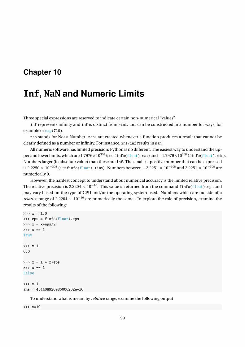
Chapter 10
Inf, NaN and Numeric Limits
Three special expressions are reserved to indicate certain non-numerical “values”.
inf represents infinity and inf is distinct from -inf. inf can be constructed in a number for ways, for
example or exp(710).
nan stands for Not a Number. nans are created whenever a function produces a result that cannot be
clearly defined as a number or infinity. For instance, inf/inf results in nan.
All numeric software has limited precision; Python is no different. The easiest way to understand the up-
per and lower limits, which are 1.7976×10308 (see finfo(float).max) and−1.7976×10308 (finfo(float).min).
Numbers larger (in absolute value) than these are inf. The smallest positive number that can be expressed
is 2.2250 × 10−308 (see finfo(float).tiny). Numbers between−2.2251 × 10−308 and 2.2251 × 10−308 are
numerically 0.
However, the hardest concept to understand about numerical accuracy is the limited relative precision.
The relative precision is 2.2204 × 10⁻¹⁶. This value is returned from the command finfo(float).eps and
may vary based on the type of CPU and/or the operating system used. Numbers which are outside of a
relative range of 2.2204 × 10⁻¹⁶ are numerically the same. To explore the role of precision, examine the
results of the following:
>>> x = 1.0
>>> eps = finfo(float).eps
>>> x = x+eps/2
>>> x == 1
True
>>> x-1
0.0
>>> x = 1 + 2*eps
>>> x == 1
False
>>> x-1
ans = 4.4408920985006262e-16
To understand what is meant by relative range, examine the following output
>>> x=10
99
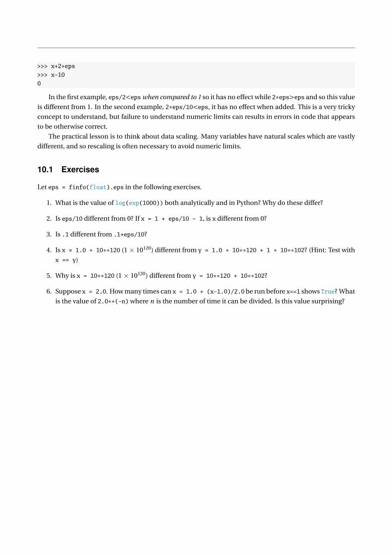
>>> x+2*eps
>>> x-10
0
In the first example, eps/2<eps when compared to 1 so it has no effect while 2*eps>eps and so this value
is different from 1. In the second example, 2*eps/10<eps, it has no effect when added. This is a very tricky
concept to understand, but failure to understand numeric limits can results in errors in code that appears
to be otherwise correct.
The practical lesson is to think about data scaling. Many variables have natural scales which are vastly
different, and so rescaling is often necessary to avoid numeric limits.
10.1 Exercises
Let eps = finfo(float).eps in the following exercises.
1. What is the value of log(exp(1000)) both analytically and in Python? Why do these differ?
2. Is eps/10 different from 0? If x = 1 + eps/10 - 1, is x different from 0?
3. Is .1 different from .1+eps/10?
4. Is x = 1.0 * 10**120 (1× 10120) different from y = 1.0 * 10**120 + 1 * 10**102? (Hint: Test with
x == y)
5. Why is x = 10**120 (1× 10120) different from y = 10**120 + 10**102?
6. Suppose x = 2.0. How many times can x = 1.0 + (x-1.0)/2.0be run before x==1 shows True? What
is the value of 2.0**(-n) where n is the number of time it can be divided. Is this value surprising?

Chapter 11
Logical Operators and Find
Logical operators are useful when writing batch files or custom functions. Logical operators, when com-
bined with flow control, allow for complex choices to be compactly expressed.
11.1 >, >=, <, <=, ==, !=
The core logical operators are
Symbol Function Definition
> greater Greater than
>= greater_equal Greater than or equal to
< less Less than
<= less_equal Less then or equal to
== equal Equal to
!= not_equal Not equal to
Logical operators can be used on scalars, arrays or matrices. All comparisons are done element-by-
element and return either True or False. For instance, suppose x and y are matrices. z= x < y will be a
matrix of the same size as x and y composed of True and False. Alternatively, if one is scalar, say y, then
the elements of z are z[i,j] = x[i,j] < y. Logical operators can be used to access elements of a vector or
matrix. For instance, suppose z = xLy where L is one of the logical operators above such as < or ==. The
following table examines the behavior when x and/or y are scalars or matrices. Suppose z = x < y:
y
Scalar Matrix
Scalar Any Any
x z = x < y z i j = x < yi j
Matrix Any Same Dimensions
z i j = x i j < y z i j = x i j < yi j
Logical operators are used in portions of programs known as flow control (e.g. if ... else ... blocks)
which will be discussed later. It is important to remember that vector or matrix logical operations return
vector or matrix output and that flow control blocks require scalar logical expressions.
101

11.2 and, or, not and xor
Logical expressions can be combined using four logical devices,
Keyword Function True if . . .
and logical_and Both True
or logical_or Either or Both True
not logical_not Not True
logical_xor One True and One False
and and logical_and() both return true if both arguments are true. The keyword and can only be used
on scalars, and so is called a short-circuit operator. logical_and() can be used on matrices. The same is
true
>>> x=matrix([[1,2],[-3,-4]])
>>> y = x > 0
>>> z = x < 0
>>> logical_and(y, z)
matrix([[False, False],
[False, False]], dtype=bool)
>>> y[0,0] and z[0,0]
Out: False
These operators follow the same rules as other logical operators. If used on two matrices, the dimen-
sions must be the same. If used on a scalar and a matrix, the effect is the same as calling the logical device
on the scalar and each element of the matrix.
Suppose x and y are logical variables (1s or 0s). and define z=logical_and(x,y):
y
Scalar Matrix
Scalar Any Any
x z = x & y z i j = x & yi j
Matrix Any Same Dimensions
z i j = x i j & y z i j = x i j & yi j
11.3 Multiple tests
all and any
The commands all and any take logical data input and are self descriptive. all returns True if all logical
elements in an array are 1. If all is called without any additional arguments on an array, it returns True if all
elements of the array are logical true and 0 otherwise. any returns logical(True) if any element of an array
is True. Both all and any can be also be used along the dimensions of the array using a second argument (or
the named argument axis ) which indicates the axis of operation, where 0 is column-wise (e.g. is examines
all elements in a single row), 1 is row-wise, and so on. When used column- or row-wise, the output is an
array with one less dimension than the input, where each element of the output contains the truth value of
the operation on the column or row.

>>> x = matrix([[1,2][3,4]])
>>> y = x <= 2
>>> y
matrix([[ True, True],
[False, False]], dtype=bool)
>>> any(y)
True
>>> any(y,0)
matrix([[ True, True]], dtype=bool)
>>> any(y,1)
matrix([[ True],
[False]], dtype=bool)
allclose
allclose can be used to compare two arrays, while allowing for a tolerance. This type of function is impor-
tant when comparing floating point values which may be effectively the same, but not identical.
>>> eps = np.finfo(np.float64).eps
>>> eps
2.2204460492503131e-16
>>> x = randn(2)
>>> y = x + eps
>>> x == y
array([False, False], dtype=bool)
>>> allclose(x,y)
True
array_equal
array_equal tests if two arrays have the same shape and elements. It is safer than comparing arrays directly
since comparing arrays which are not broadcastable produces an error.
array_equiv
array_equiv tests if two arrays are equivalent, even if they do not have the exact same shape. Equivalence
is defined as one array being broadcastable to produce the other.
>>> x = randn(10,1)
>>> y = tile(x,2)
>>> array_equal(x,y)
False
>>> array_equiv(x,y)
True
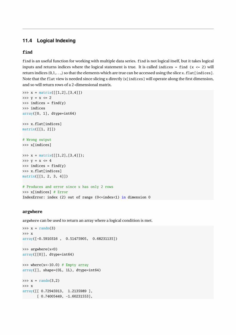
11.4 Logical Indexing
find
find is an useful function for working with multiple data series. find is not logical itself, but it takes logical
inputs and returns indices where the logical statement is true. It is called indices = find (x <= 2) will
return indices (0,1,. . .,) so that the elements which are true can be accessed using the slice x.flat[indices].
Note that the flat view is needed since slicing x directly (x[indices] will operate along the first dimension,
and so will return rows of a 2-dimensional matrix.
>>> x = matrix([[1,2],[3,4]])
>>> y = x <= 2
>>> indices = find(y)
>>> indices
array([0, 1], dtype=int64)
>>> x.flat[indices]
matrix([[1, 2]])
# Wrong output
>>> x[indices]
>>> x = matrix([[1,2],[3,4]]);
>>> y = x <= 4
>>> indices = find(y)
>>> x.flat[indices]
matrix([[1, 2, 3, 4]])
# Produces and error since x has only 2 rows
>>> x[indices] # Error
IndexError: index (2) out of range (0<=index<1) in dimension 0
argwhere
argwhere can be used to return an array where a logical condition is met.
>>> x = randn(3)
>>> x
array([-0.5910316 , 0.51475905, 0.68231135])
>>> argwhere(x<0)
array([[0]], dtype=int64)
>>> where(x<-10.0) # Empty array
array([], shape=(0L, 1L), dtype=int64)
>>> x = randn(3,2)
>>> x
array([[ 0.72945913, 1.2135989 ],
[ 0.74005449, -1.60231553],
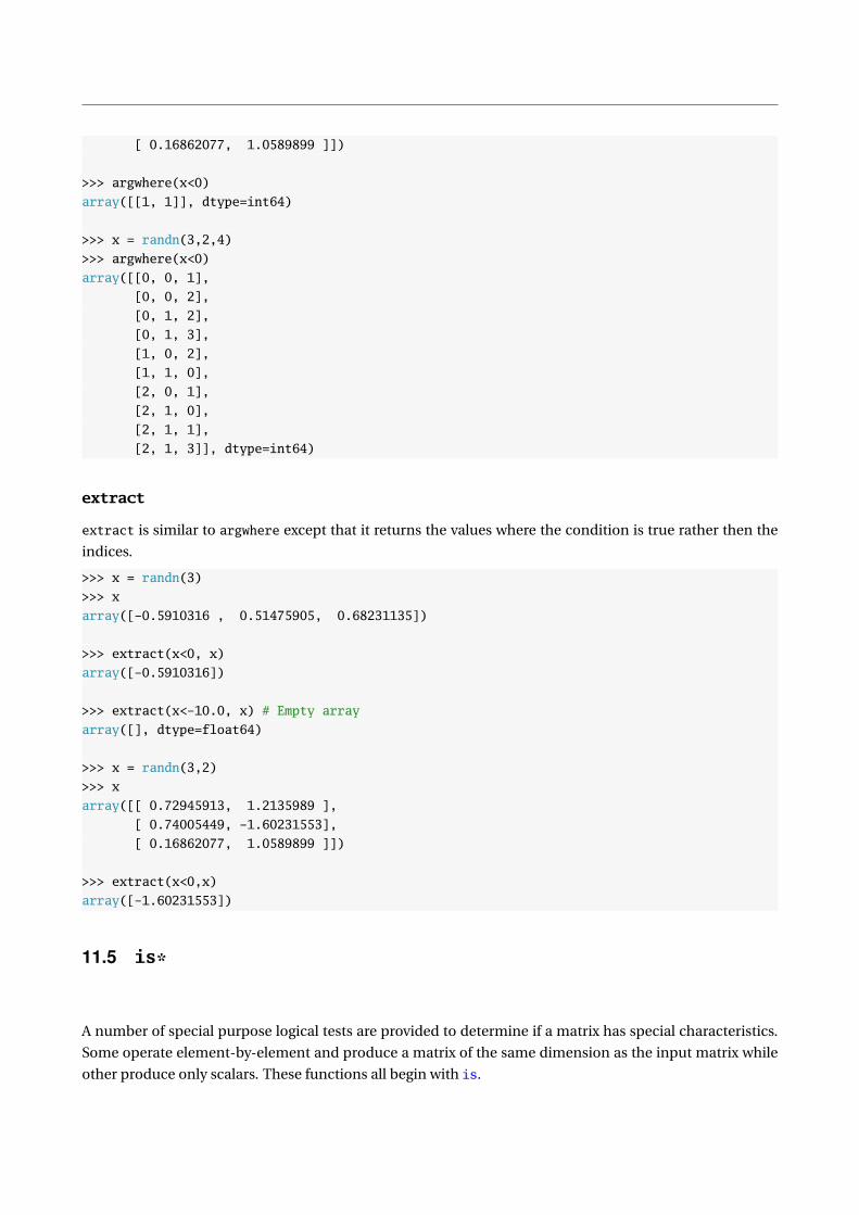
[ 0.16862077, 1.0589899 ]])
>>> argwhere(x<0)
array([[1, 1]], dtype=int64)
>>> x = randn(3,2,4)
>>> argwhere(x<0)
array([[0, 0, 1],
[0, 0, 2],
[0, 1, 2],
[0, 1, 3],
[1, 0, 2],
[1, 1, 0],
[2, 0, 1],
[2, 1, 0],
[2, 1, 1],
[2, 1, 3]], dtype=int64)
extract
extract is similar to argwhere except that it returns the values where the condition is true rather then the
indices.
>>> x = randn(3)
>>> x
array([-0.5910316 , 0.51475905, 0.68231135])
>>> extract(x<0, x)
array([-0.5910316])
>>> extract(x<-10.0, x) # Empty array
array([], dtype=float64)
>>> x = randn(3,2)
>>> x
array([[ 0.72945913, 1.2135989 ],
[ 0.74005449, -1.60231553],
[ 0.16862077, 1.0589899 ]])
>>> extract(x<0,x)
array([-1.60231553])
11.5 is*
A number of special purpose logical tests are provided to determine if a matrix has special characteristics.
Some operate element-by-element and produce a matrix of the same dimension as the input matrix while
other produce only scalars. These functions all begin with is.
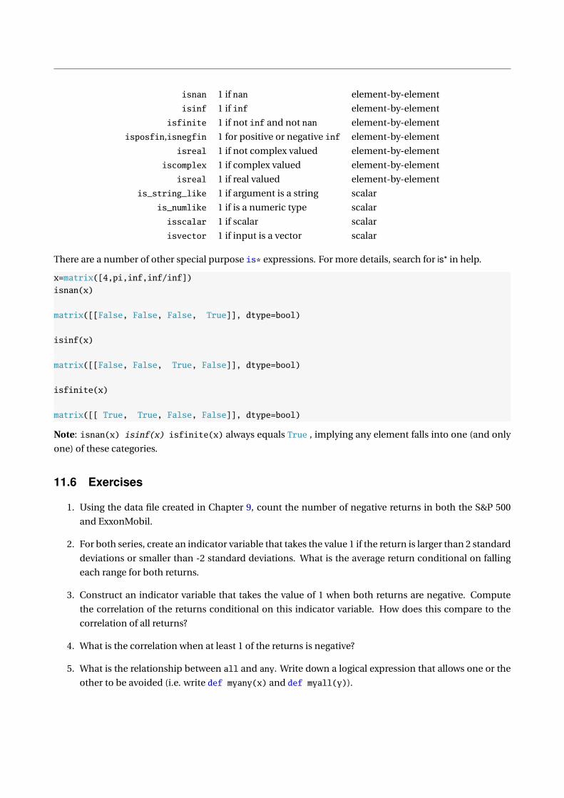
isnan 1 if nan element-by-element
isinf 1 if inf element-by-element
isfinite 1 if not inf and not nan element-by-element
isposfin,isnegfin 1 for positive or negative inf element-by-element
isreal 1 if not complex valued element-by-element
iscomplex 1 if complex valued element-by-element
isreal 1 if real valued element-by-element
is_string_like 1 if argument is a string scalar
is_numlike 1 if is a numeric type scalar
isscalar 1 if scalar scalar
isvector 1 if input is a vector scalar
There are a number of other special purpose is* expressions. For more details, search for is* in help.
x=matrix([4,pi,inf,inf/inf])
isnan(x)
matrix([[False, False, False, True]], dtype=bool)
isinf(x)
matrix([[False, False, True, False]], dtype=bool)
isfinite(x)
matrix([[ True, True, False, False]], dtype=bool)
Note: isnan(x) isinf(x) isfinite(x) always equals True , implying any element falls into one (and only
one) of these categories.
11.6 Exercises
1. Using the data file created in Chapter 9, count the number of negative returns in both the S&P 500
and ExxonMobil.
2. For both series, create an indicator variable that takes the value 1 if the return is larger than 2 standard
deviations or smaller than -2 standard deviations. What is the average return conditional on falling
each range for both returns.
3. Construct an indicator variable that takes the value of 1 when both returns are negative. Compute
the correlation of the returns conditional on this indicator variable. How does this compare to the
correlation of all returns?
4. What is the correlation when at least 1 of the returns is negative?
5. What is the relationship between all and any. Write down a logical expression that allows one or the
other to be avoided (i.e. write def myany(x) and def myall(y)).
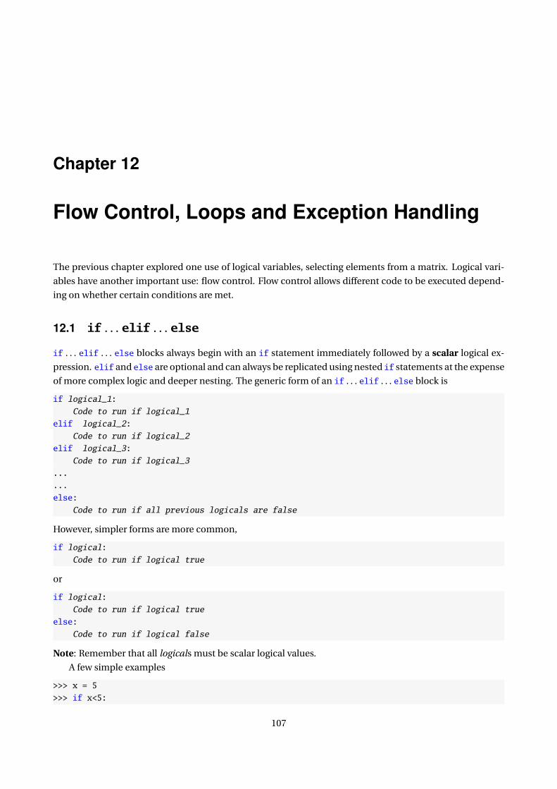
Chapter 12
Flow Control, Loops and Exception Handling
The previous chapter explored one use of logical variables, selecting elements from a matrix. Logical vari-
ables have another important use: flow control. Flow control allows different code to be executed depend-
ing on whether certain conditions are met.
12.1 if . . . elif . . . else
if . . . elif . . . else blocks always begin with an if statement immediately followed by a scalar logical ex-
pression. elif and else are optional and can always be replicated using nested if statements at the expense
of more complex logic and deeper nesting. The generic form of an if . . . elif . . . else block is
if logical_1:
Code to run if logical_1
elif logical_2:
Code to run if logical_2
elif logical_3:
Code to run if logical_3
...
...
else:
Code to run if all previous logicals are false
However, simpler forms are more common,
if logical:
Code to run if logical true
or
if logical:
Code to run if logical true
else:
Code to run if logical false
Note: Remember that all logicals must be scalar logical values.
A few simple examples
>>> x = 5
>>> if x<5:
107

... x += 1
... else:
... x -= 1
>>> x
4
and
>>> x = 5;
>>> if x<5:
... x = x + 1
... elif x>5:
... x = x - 1
... else:
... x = x * 2
>>> x
10
These examples have all used simple logical expressions. However, any scalar logical expressions, such
as (x<0 or x>1) and (y<0 or y>1) (y<0 or y>1) or isinf(x) or isnan(x), can be used in if . . . elif . . .
else blocks.
12.2 for
for loops begin with for item in iterable: . The generic structure of a for loop is
for item in iterable:
Code to run
item is an element from iterable, and iterable can be anything that is iterable in Python. The most common
examples are xrange or range, lists, tuples, arrays or matrices. The for loop will iterate across all items in
iterable, beginning with item 0 and continuing until the final item.
count = 0
for i in range(100):
count += i
count = 0
x = linspace(0,500,50)
for i in x: # Python 3: for i in range(0,500,5)
count += i
count = 0
x = list(arange(-20,21))
for i in x:
count += i
The first loop will iterate over i = 0, 1, 2,. . . , 99. The second loops over the values produced by the
function linspace, which returns an array, which creates 50 uniform points between 0 and 500, inclusive.
The final loops over x, a vector constructed from a call to list(arange(-20,21)), which produces a list

containing the series −20,−19,. . . , 0, . . .19,20. All three – range, arrays, and lists – are iterable. The key to
understanding for loop behavior is that for always iterates over the elements of the iterable in the order
they are presented (i.e. iterable[0], iterable[1], . . .).
Python 2.7 vs. 3.2 Note: This chapter exclusively uses range in loops (instead of xrange). This
is a simplification used so that the same code will run in Python 2.7 and 3.2, although the best
practice is to use xrange in Python 2.7 loops.
Loops can also be nested:
count = 0
for i in range(10):
for j in range(10):
count += j
and can contain flow control variables:
returns = randn(100)
count = 0
for ret in returns:
if ret<0:
count += 1
This for expression can be equivalently expressed using range, by using len to get the number of items in
the iterable:
returns = randn(100)
count = 0
for i in range(len(returns)):
if returns[i]<0:
count += 1
Finally, these ideas can be combined to produce nested loops with flow control.
x = zeros((10,10))
for i in range(size(x,0)):
for j in range(size(x,1)):
if i<j:
x[i,j]=i+j;
else:
x[i,j]=i-j
or loops containing nested loops that are executed based on a flow control statement.
x = zeros((10,10))
for i in range(size(x,0)):
if (i % 2) == 1:
for j in range(size(x,1)):
x[i,j] = i+j
else:
for j in range(int(i/2)):
x[i,j] = i-j

Note: The iterable variable cannot be changed once inside the loop. Consider, for example,
x = range(10) # Python 3: x = range(10)
for i in x:
print(i)
print(’Length of x:’, len(x))
x = range(5)
Produces the output
# Output
0
Length of x: 10
1
Length of x: 5
2
Length of x: 5
3
...
8
Length of x: 5
9
Length of x: 5
Note that it is not safe to modify the sequence of the iterable when looping over it. The means that the
iterable should not change size, which can occur when using a list and the functions pop(), insert() or
append() or the keyword del. The loop below would never terminate (except for the break) since L is being
extended each iteration.
L = [1, 2]
for i in L:
print(i)
L.append(i+2)
if i>5:
break
Finally, for loops can be used with 2 items when the iterable is wrapped in enumerate, which allows the
elements of the iterable to be directly accessed, as well as their index in the iterable.
x = linspace(0,100,11)
for i,y in enumerate(x):
print(’i is :’, i)
print(’y is :’, y)
12.2.1 Whitespace
Like if . . . elif . . . else flow control blocks, for loops are whitespace sensitive. The indentation of the
line immediately below the for statement determines the indentation that all statements in the block must
have. The convention is 4 spaces.

12.2.2 break
A loop can be terminated early using break. break is usually used after an if statement to terminate the
loop prematurely if some condition has been met.
x = randn(1000)
for i in x:
print(i)
if i > 2:
break
break is more useful in while loops.
12.2.3 continue
continue can be used to skip an iteration of a loop, immediately returning to the top of the loop using
the next item in iterable. continue is usually used to avoid a level of nesting, such as in the following two
examples.
x = randn(10)
for i in x:
if i < 0:
print(i)
for i in x:
if i >= 0:
continue
print(i)
Avoiding excessive levels of indentation is essential in Python programming – 4 is usually considered the
maximum – and continue can be used to in a for loop to avoid one level of indentation.
12.3 while
while loops are useful when the number of iterations needed depends on the outcome of the loop contents.
while loops are commonly used when a loop should only stop if a certain condition is met, such as the
change in some parameter is small. The generic structure of a while loop is
while logical:
Code to run
Two things are crucial when using a while loop: first, the logical expression should evaluate to true
when the loop begins (or the loop will be ignored) and second the inputs to the logical expression must
be updated inside the loop. If they are not, the loop will continue indefinitely (hit CTRL+C to break an
interminable loop). The simplest while loops are (verbose) drop-in replacements for for loops:
count = 0
i = 1
while i<=10:
count += i
i += 1
which produces the same results as
count=0;
for i in range(0,11):
count += i
while loops should generally be avoided when for loops will do. However, there are situations where no for
loop equivalent exists.
mu = 1.0
index = 1
while abs(mu) > .0001:
mu = (mu+randn(1))/index
index=index+1
In the block above, the number of iterations required is not known in advance and since randn is a standard
normal pseudo-random number, it may take many iterations until this criteria is met – any finite for loop
cannot be guaranteed to meet the criteria.
12.3.1 break
break can be used in a while loop to immediately terminate execution. In general, break should not be used
in a while loop – instead the logical condition should be set to False to terminate the loop.
condition = True
i = 0
x = randn(1000)
while condition:
print(x[i])
i += 1
if x[i] > 2:
break
It is better to update the logical statement which determines whether the while loop should execute.
i = 0
while x[i] <= 2:
print(x[i])
i += 1
12.3.2 continue
continue can be used in a while loop to skip an iteration of a loop, immediately returning to the top of the
loop, which then checks the while condition, and executes the loop if it still true. Use of continue in while
loops is also rare.
12.4 try . . . except
Exception handling is an advanced programming technique which can be used to make code more resilient
(often at the code of speed). try . . . except blocks are useful for running code which may be dangerous. In
most numerical applications, code should be deterministic and so dangerous code can usually be avoided.

When it can’t, for example, if reading data from a data source which isn’t always available (e.g. a website),
then try . . . except can be used to attempt the code, and then do something helpful if the code fails to
execute. The generic structure of a try . . . except block is
try:
Dangerous Code
except ExceptionType1:
Code to run if ExceptionType1 is raised
except ExceptionType2:
Code to run if ExceptionType1 is raised
...
...
except:
Code to run if an unlisted exception type is raised
12.5 List Comprehensions
List comprehensions are a form of syntactic sugar which may simplify code when an iterable object is looped
across and the results are saved to a list, possibly conditional on some logical test. Simple list can be used
to convert a for loop which includes an append into a single line statement.
>>> x = arange(5.0)
>>> y = []
>>> for i in xrange(len(x)):
... y.append(exp(x[i]))
>>> y
[1.0,
2.7182818284590451,
7.3890560989306504,
20.085536923187668,
54.598150033144236]
>>> z = [exp(x[i]) for i in xrange(len(x))]
>>> z
[1.0,
2.7182818284590451,
7.3890560989306504,
20.085536923187668,
54.598150033144236]
This simple list comprehension saves 2 lines of typing. List comprehensions can also be extended to include
a logical test.
>>> x = arange(5.0)
>>> y = []
>>> for i in xrange(len(x)):
... if floor(i/2)==i/2:
... y.append(x[i]**2)
>>> y
[0.0, 4.0, 16.0]

>>> z = [x[i]**2 for i in xrange(len(x)) if floor(i/2)==i/2]
>>> z
[0.0, 4.0, 16.0]
List comprehensions can also be used to loop over multiple iterable input.
>>> x1 = arange(5.0)
>>> x2 = arange(3.0)
>>> y = []
>>> for i in xrange(len(x1)):
... for j in xrange(len(x2)):
... y.append(x1[i]*x2[j])
>>> y
[0.0, 0.0, 0.0, 0.0, 1.0, 2.0, 0.0, 2.0, 4.0, 0.0, 3.0, 6.0, 0.0, 4.0, 8.0]
>>> z = [x1[i]*x2[j] for i in xrange(len(x1)) for j in xrange(len(x2))]
[0.0, 0.0, 0.0, 0.0, 1.0, 2.0, 0.0, 2.0, 4.0, 0.0, 3.0, 6.0, 0.0, 4.0, 8.0]
>>> # Only when i==j
>>> z = [x1[i]*x2[j] for i in xrange(len(x1)) for j in xrange(len(x2)) if i==j]
[0.0, 1.0, 4.0]
While list comprehensions are powerful methods to compactly express complex operations, they are never
essential to Python programming.
Loops make many problems, particularly when combined with flow control blocks, simple and in many
cases, possible. Two types of loop blocks are available: for and while. for blocks iterate over a predeter-
mined set of values and while blocks loop as long as some logical expression is satisfied. All for loops can
be expressed as while loops although the opposite is not quite true. They are nearly equivalent when break
is used, although it is generally preferable to use a while loop than a for loop and a break statement.
12.6 Exercises
1. Write a code block that would take a different path depending on whether the returns on two series
are simultaneously positive, both are negative, or they have different signs using an if . . . elif . . .
else block.
2. Simulate 1000 observations from an ARMA(2,2) where εt are independent standard normal innova-
tions. The process of an ARMA(2,2) is given by
yt = φ1yt−1 + φ2yt−2 + θ1εt−1 + θ2εt−2 + εt
Use the values φ1 = 1.4, φ2 = −.8, θ1 = .4 and θ2 = .8. Note: A T vector containing standard normal
random variables can be simulated using e = randn(T). When simulating a process, always simulate
more data then needed and throw away the first block of observations to avoid start-up biases. This
process is fairly persistent, at least 100 extra observations should be computed.
3. Simulate a GARCH(1,1) process where εt are independent standard normal innovations. A GARCH(1,1)

process is given by
yt = σt εt
σ2t = ω + αy 2
t−1 + βσ2t−1
Use the valuesω = 0.05, α = 0.05 and β = 0.9, and set h0 = ω/(
1− α− β)
.
4. Simulate a GJR-GARCH(1,1,1) process where εt are independent standard normal innovations. A GJR-
GARCH(1,1) process is given by
yt = σt εt
σ2t = ω + αy 2
t−1 + γy 2t−1I [yt−1<0] + βσ2
t−1
Use the valuesω = 0.05, α = 0.02 γ = 0.07 and β = 0.9 and set h0 = ω/(
1− α− 12γ− β
). Note that
some form of logical expression is needed in the loop. I [εt−1<0] is an indicator variable that takes the
value 1 if the expression inside the [ ] is true.
5. Simulate a ARMA(1,1)-GJR-GARCH(1,1)-in-mean process,
yt = φ1yt−1 + θ1σt−1εt−1 + λσ2t + σt εt
σ2t = ω + ασ
2t−1ε
2t−1 + γσ
2t−1ε
2t−1I [εt−1<0] + βσ2
t−1
Use the values from Exercise 3 for the GJR-GARCH model and use the φ1 = −0.1, θ1 = 0.4 and
λ = 0.03.
6. Find two different methods to use a for loop to fill a 5 × 5 array with i × j where i is the row index,
and j is the column index. One will use xrange as the iterable, and the other should directly iterate on
the rows, and then the columns of the matrix.
7. Using a while loop, write a bit of code that will do a bisection search to invert a normal CDF. A bisec-
tion search cuts the interval in half repeatedly, only keeping the sub interval with the target in it. Hint:
keep track of the upper and lower bounds of the random variable value and use flow control. This
problem requires stats.norm.cdf.
8. Test out the loop using by finding the inverse CDF of 0.01, 0.5 and 0.975. Verify it is working by taking
the absolute value of the difference between the final value and the value produced by stats.norm.ppf.
9. Write a list comprehension that will iterate over a 1-dimensional array and extract the negative ele-
ments to a list. How can this be done using only logical functions (no explicit loop), without the list
comprehension (and returning an array)?


Chapter 13
Custom Function and Modules
Python supports a wide range of programming styles including procedural (imperative), object oriented and
functional. While object oriented programming and functional programming are powerful programming
paradigms, especially in large, complex software, procedural is often much easier to understand, and is
often a direct representation of a mathematical formula. The basic idea of procedural programming is to
produce a function or set of function (generically) of the form
y = f (x ).
That is, the functions take inputs, and produce outputs – there can be more than one of either.
13.1 Functions
Python functions are very simple to declare and can occur in a variety of locations, including in the same
file as the main program or in a standalone module. Functions are declared using the def keyword, and the
value produced is returned using the return keyword. Consider a simple function which returns the square
of the input,
y = x 2.
from __future__ import print_function
from __future__ import division
def square(x):
return x**2
# Call the function
x = 2
y = square(x)
print(x,y)
In this example, the same Python file contains the main program – the bottom 3 lines – as well as the func-
tion. More complex function can be crafted with multiple inputs.
from __future__ import print_function
from __future__ import division
117

def l2distance(x,y):
return (x-y)**2
# Call the function
x = 3
y = 10
z = l2distance(x,y)
print(x,y,z)
They can also be defined using NumPy arrays and matrices.
from __future__ import print_function
from __future__ import division
import numpy as np
def l2_norm(x,y):
d = x - y
return np.sqrt(np.dot(d,d))
# Call the function
x = np.random.randn(10)
y = np.random.randn(10)
z = l2_norm(x,y)
print(x-y)
print("The L2 distance is ",z)
Similarly, multiple outputs can be returned, usually as a tuple.
from __future__ import print_function
from __future__ import division
import numpy as np
def l1_l2_norm(x,y):
d = x - y
return sum(np.abs(d)),np.sqrt(np.dot(d,d))
# Call the function
x = np.random.randn(10)
y = np.random.randn(10)
# Using 1 output returns a tuple
z = l1_l2_norm(x,y)
print(x-y)
print("The L1 distance is ",z[0])
print("The L2 distance is ",z[1])
# Using 2 output returns the values
l1,l2 = l1_l2_norm(x,y)
print("The L1 distance is ",l1)
print("The L2 distance is ",l2)

All of these functions have been placed in the same file as the main program. While this is a simple method,
it limits reuse. Placing functions in modules allows for reuse in multiple programs, and will be discussed
later in this chapter.
13.1.1 Keyword Arguments
Input values in functions are automatically keyword arguments, so that the function can be accessed either
by placing the inputs in the order they appear in the function (positional arguments), or by calling the input
by their name using keyword=value.
from __future__ import print_function
from __future__ import division
import numpy as np
def lp_norm(x,y,p):
d = x - y
return sum(abs(d)**p)**(1/p)
# Call the function
x = np.random.randn(10)
y = np.random.randn(10)
z1 = lp_norm(x,y,2)
z2 = lp_norm(p=2,x=x,y=y)
print("The Lp distances are ",z1,z2)
Because variable names are automatically keywords, it is important to use meaningful variable names when
possible, rather than generic variables such as a, b, c or x, y and z. In some cases, x may be a reasonable
default, but in the previous example which computed the L p norm, calling the third input z would be bad
idea.
13.1.2 Default Values
Default values are set in the function declaration using the syntax input=default.
from __future__ import print_function
from __future__ import division
import numpy as np
def lp_norm(x,y,p = 2):
d = x - y
return sum(abs(d)**p)**(1/p)
# Call the function
x = np.random.randn(10)
y = np.random.randn(10)
# Inputs with default values can be ignored
l2 = lp_norm(x,y)
l1 = lp_norm(x,y,1)

print("The l1 and l2 distances are ",l1,l2)
print("Is the default value overridden?", sum(abs(x-y))==l1)
Default values should not normally be mutable (e.g. lists or arrays) since they are only initialized the first
time the function is called. Subsequent calls will use the same value, which means that the default value
could change every time the function is called.
from __future__ import print_function
from __future__ import division
import numpy as np
def bad_function(x = zeros(1)):
print(x)
x[0] = np.random.randn(1)
# Call the function
bad_function()
bad_function()
bad_function()
Each call to bad_function() shows that x has a different value – despite the default being 0. The solution
to this problem is to initialize mutable objects to None, and then the use an if to check and initialize.
from __future__ import print_function
from __future__ import division
import numpy as np
def good_function(x = None):
if x == None:
x = zeros(1)
print(x)
x[0] = np.random.randn(1)
# Call the function
good_function()
good_function()
Repeated calls to good_function() all show x as 0.
13.1.3 Variable Inputs
Most function written as an “end user” have a deterministic number of inputs. However, functions which
evaluate other functions often must accept variable numbers of input. Variable inputs can be handled using
the *arguments or **keywords syntax. The *arguments syntax will generate a containing all inputs past the
specified input list. For example, consider extending the L p function so that it can accept a set of p values
as extra inputs (Note: in practice it would make more sense to accept an array for p ).
from __future__ import print_function

from __future__ import division
import numpy as np
def lp_norm(x,y,p = 2, *arguments):
d = x - y
print(’The L’ + str(p) + ’ distance is :’, sum(abs(d)**p)**(1/p))
out = [sum(abs(d)**p)**(1/p)]
for p in arguments:
print(’The L’ + str(p) + ’ distance is :’, sum(abs(d)**p)**(1/p))
out.append(sum(abs(d)**p)**(1/p))
return tuple(out)
# Call the function
x = np.random.randn(10)
y = np.random.randn(10)
# Inputs with default values can be ignored
lp = lp_norm(x,y,1,2,3,4,1.5,2.5,0.5)
The alternative syntax, **keywords, generates a dictionary with all keyword inputs which are not in the
function signature. One reason for using **keywords is to allow a long list of optional inputs without having
to have an excessively long function definition, and is how this input mechanism is often encountered when
using other code, for example plot().
from __future__ import print_function
from __future__ import division
import numpy as np
def lp_norm(x,y,p = 2, **keywords):
d = x - y
for key in keywords:
print(’Key :’, key, ’ Value:’, keywords[key])
return sum(abs(d)**p)
# Call the function
x = np.random.randn(10)
y = np.random.randn(10)
# Inputs with default values can be ignored
lp = lp_norm(x,y,kword1=1,kword2=3.2)
# The p keyword is in the function def, so not in **keywords
lp = lp_norm(x,y,kword1=1,kword2=3.2,p=0)
It is possible to use both *arguments and **keywords in a function definition and their role does not
change – *arguments is a tuple which contains all extraneous non-keyword inputs, and **keywords will con-
tain all extra keyword arguments. Function with both often have the simple signature y = f(*arguments,
**keywords)which allows for a wide range of configuration.
13.1.4 The Docstring
The docstring is one of the most important elements of any function – especially a function written by
consumption by others. The docstring is a special string, enclose using triple-quotation marks, either ’’’
or """, which is available using help(). When help(fun) is called, Python looks for the docstring which is
placed immediately below the function definition.
from __future__ import print_function
from __future__ import division
import numpy as np
def lp_norm(x,y,p = 2):
’’’ The docstring contains any available help for
the function. A good docstring should explain the
inputs and the outputs, provide an example and a list
of any other related function.
’’’
d = x - y
return sum(abs(d)**p)
Calling help(lp_norm) produces
>>> help(lp_norm)
Help on function lp_norm in module __main__:
lp_norm(x, y, p=2)
The docstring contains any available help for
the function. A good docstring should explain the
inputs and the outputs, provide an example and a list
of any other related function.
Note that the docstring is not a good example. I suggest following the the NumPy guidelines, currently avail-
able atNumPy source repository (or search for numpy docstring). Also see NumPy example.py These differ
from and are more specialized than the standard Python docstring guidelines, and so are more appropriate
for numerical code. A better docstring for lp_norm would be
from __future__ import print_function
from __future__ import division
import numpy as np
def lp_norm(x,y,p = 2):
r""" Compute the distance between vectors.
The Lp normed distance is sum(abs(x-y)**p)**(1/p)
Parameters
----------

x : ndarray
First argument
y : ndarray
Second argument
p : float, optional
Power used in distance calcualtion, >=0
Returns
-------
output : scalar
Returns the Lp normed distance between x and y
Notes
-----
For p>=1, returns the Lp norm described above. For 0<=p<1,
returns sum(abs(x-y)**p). If p<0, p is set to 0.
Examples
--------
>>> x=[0,1,2]
>>> y=[1,2,3]
L2 norm is the default
>>> lp_norm(x,y)
Lp can be computed using the optional third input
>>> lp_norm(x,y,1)
"""
if p<0: p=0
d = x - y
dist = sum(abs(d)**p)
if p<1:
return dist
else:
return dist**(1/p)
Convention is to use triple double-quotes in docstrings, with r""" used to indicate “raw” strings, which will
ignore backslash, rather than treating it like an escape character (use u""" if the docstring contains unicode
text, which is not usually necessary). A complete docstring may contain, in order:
• Parameters - a description of key inputs
• Returns - a description of outputs
• Other Parameters - a description of seldom used inputs

• Raises - an explanation of any exceptions raised. See Section 12.4.
• See also - a list of related functions
• Notes - details of the algorithms or assumptions used
• References - any bibliographic information
• Examples - demonstrates use form console
13.2 Variable Scope
Variable scope determines which function can access, and possibly modify a variable. Python determines
variable scope using two principles: where the variable appears in the file, and whether the variable is inside
a function or in the main program. Variables declared inside a function are local variables and are only
available to that function. Variables declared outside a function are global variables, and can be accessed
but normally not modified. Consider the example which shows that variables at the root of the program
which have been declared before a function can be printed by that function.
from __future__ import print_function
from __future__ import division
import numpy as np
a, b, c = 1, 3.1415, ’Python’
def scope():
print(a)
print(b)
print(c)
# print(d) #Error, d has not be declared yet
scope()
d = np.array(1)
def scope2():
print(a)
print(b)
print(c)
print(d) # Ok now
scope2()
def scope3():
a = ’Not a number’ # Local variable
print(’Inside scope3, a is ’, a)
print(’a is ’,a)
scope3()
print(’a is now ’,a)

Using the name of a global variable inside a function does not cause any issues outside of the function. In
scope3, a is given a different value. That value is specific to the function scope3 and outside of the function,
a will have its global value. Generally, global variables can be accessed, but not modified inside a function.
The only exception is when a variable is first declared using the keyword global.
from __future__ import print_function
from __future__ import division
import numpy as np
a = 1
def scope_local():
a = -1
print(’Inside scope_local, a is ’,a)
def scope_global():
global a
a = -10
print(’Inside scope_global, a is ’,a)
print(’a is ’,a)
scope_local()
print(’a is now ’,a)
scope_global()
print(’a is now ’,a)
One word of caution: a variable name cannot be used as a local and global variable in the same function.
Attempting to access the variable as a global (e.g. for printing) and then locally assign the variable produces
an error.
13.3 Example: Least Squares with Newey-West Covariance
Estimating cross-section regressions using time-series data is common practice. When regressors are per-
sistent, and errors may not be white noise, standard inference, including White standard errors, are no
longer consistent. The most common solution is to use a long-run covariance estimator, and the most
common long-run covariance estimator is known as the Newey-West covariance estimator, which uses a
Bartlett kernel applied to the autocovariances of the scores. This example produces a function which re-
turns parameter estimates, the estimated asymptotic covariance matrix of the parameters, the variance of
the regression error, the R2, and adjusted R2 and the fit values (or errors, since actual is equal to fit plus er-
rors). These be computed using a T -vector for the regressand (dependent variable), a T by k matrix for the
regressors, an indicator for whether to include a constant in the model (default True), and the number of
lags to include in the long-run covariance (default behavior is to automatically determine based on sample
size). The steps required to produce the function are:
1. Determine the size of the variables

2. Append a constant, if needed
3. Compute the regression coefficients
4. Compute the errors
5. Compute the covariance or the errors
6. Compute the covariance of the parameters
7. Compute the R2 and R2
The function definition is simple and allows for up to 4 inputs, where 2 have default values: def olsnw(y,
X, constant=True, lags=None):. The size of the variables is then determined using size and the constant is
prepended to the regressors, if needed, using hstack. The regression coefficients are computed using lstsq,
and then the Newey-West covariance is computed for both the errors and and scores. The covariance of the
parameters is then computed using the NW covariance of the scores. Finally the R2 and R2 are computed.
A complete code listing is presented in the appendix to this chapter.
13.4 Modules
The previous examples all included the function in inside the Python file that contained the main program.
While this is convenient, especially for writing the function, it hinders use in other code. Modules allow
multiple functions to be combined in a single Python file and accessed using import module and then mod-
ule.function syntax. Suppose a file named core.py contains the following code:
r"""Demonstration module
"""
def square(x):
r"""Returns the square of a scalar input
"""
return x*x
def cube(x):
r"""Returns the cube of a scalar input
"""
return x*x*x
The functions square and cube can be accessed by other files in the same directory using
from __future__ import division
from __future__ import print_function
import core
y = -3
print(core.square(y))
print(core.cube(y))
The functions in core.py can be imported using any of the standard import methods such as
from core import square, cube
or
from core import *
in which case both functions could be directly accessed.
13.4.1 __main__
Normally modules should only have code required for the module to run, and other code should reside
in a different function. However, it is possible that a module could be both directly important and also
directly runnable. If this is the case, it is important that the directly runnable code should not be exe-
cuted when the module is imported by other code. This can be accomplished using a special construct
if __name__=="__main__":before any code that should execute when run as a standalone program. Con-
sider the following simple example in a module namedtest.py.
from __future__ import division
from __future__ import print_function
def square(x):
return x**2
if __name__=="__main__":
print(’Program called directly.’)
else:
print(’Program called indirectly using name: ’, __name__)
Running and importing test cause the different paths to be executed.
>>> %run test.py
Program called directly.
>>> import test
Program called indirectly using name: test
13.5 PYTHONPATH
While it is simple to reference files in the same current working directory, this behavior is undesirable for
code shared between multiple projects. Fortunately the PYTHONPATH allows directories to be added so
that they are automatically searched if a matching module cannot be found in the current directory. The
current path can be checked by running
>>> import sys
>>> sys.path
Additional directories can be added at runtime using
import sys
# New directory is first to be searched
sys.path.insert(0, ’c:\\path\\to\add’)
# New directory is last to be searched
sys.path.append

Directories can also be added permanently by adding or modifying the environment variable PYTHON-
PATH.
On Windows, the System environment variables can be found in My Computer> Properties>Advanced
System Settings> Environment Variables. PYTHONPATH should be a System Variable. If it is present, it can
be edited, and if not, added. The format of PYTHONPATH is
c:\dir1;c:\dir2;c:\dir2\dir3;
which will add 3 directories to the path. On Linux, PYTHONPATH is stored in .bash_profile, and it should
resemble
PYTHONPATH="$PYTHONPATH:/dir1/:/dir2/:/dir2/dir3/"
export PYTHONPATH
after three directories have been added, using : as a separator between directories.
13.6 Packages
Packages are the next level beyond modules, and allow, for example, nested module names (e.g. numpy.random
which contains randn). Packages are also installed in the local package library, and can be compiled into
optimized Python byte code, which makes loading modules faster (but does not make code run faster).
Building a package is beyond the scope of these notes, but there are many resources on the internet with
instructions for building packages.
13.7 Python Coding Conventions
There are a number of common practices which can be adopted to produce Python code which looks more
like code found in other modules:
1. Use 4 spaces to indent blocks – avoid using tab, except when an editor automatically converts tabs to
4 spaces
2. Avoid more than 4 levels of nesting, if possible
3. Limit lines to 79 characters. The \ symbol can be used to break long lines
4. Use blank lines to separate functions or logical sections in a function.
5. Use ASCII model in text editors, not UTF-8
6. One import per line
7. Avoid from module import * (for any module). Use either from module import func1, func2 or
import module as shortname.
8. Follow the NumPy guidelines for documenting functions
More suggestions can be found in PEP8.

13.8 Exercises
1. Write a function which takes an array with T elements contains categorical data (e.g. 1,2,3), and
returns a T by C array of indicator variables where C is the number of unique values of the categorical
variable, and each column of the output is a indicator variable (0 or 1) for whether the input data
belonged to that category. For example, if x = [1 2 1 1 2], then the the output is1 0
0 1
1 0
1 0
0 1
The function should provide a second output containing the categories (e.g. [1 2] in the example).
2. Write a function which takes a T by K array X , a T by 1 array y , and a T by T arrayΩ are computes the
GLS parameter estimates. The function definition should be
def gls(X, y, Omega = None
and if Ω is not provided, an identity matrix should be used.
3. Write a function which will compute the partial correlation. Lower partial correlation is defined as∑S(
ri ,1 − r1,S) (
ri ,2 − r2,S)∑
S(
rj ,1 − r1,S)2∑
S(
rk ,2 − r2,S)2
whereS is the set where r1,i and r2,i are both less than their (own) quantile q . Upper partial correlation
uses returns greater than quantile q . The function definition should have definition
def partial_corr(x, y=None, quantile = 0.5, tail = ’Lower’)
and should take either a T by K array for x , or T by 1 arrays for x and y . If x is T by K , then y is ignored
and the partial correlation should be computed pairwise. quantile determines the quantile to use for
the cut off. Note: if S is empty or has 1 element, nan should be returned. tail is either ’Lower’ or
’Upper’, and determined whether the lower or upper tail is used. The function should return both the
partial correlation matrix (K by K ), and the number of observations used in computing the partial
correlation.
13.A Listing of econometrics.py
The complete code listing of econometrics, which contains the function olsnw, is presented below.
from __future__ import print_function
from __future__ import division
from numpy import dot, mat, asarray, mean, size, shape, hstack, ones, ceil, \
zeros, arange
from numpy.linalg import inv, lstsq
def olsnw(y, X, constant=True, lags=None):
r""" Estimation of a linear regression with Newey-West covariance
Parameters
----------
y : array_like
The dependant variable (regressand). 1-dimensional with T elements.
X : array_like
The independant variables (regressors). 2-dimensional with sizes T
and K. Should not include a constant.
constant: bool, optional
If true (default) includes model includes a constant.
lags: int or None, optional
If None, the number of lags is set to 1.2*T**(1/3), otherwise the
number of lags used in the covariance estimation is set to the value
provided.
Returns
-------
b : ndarray, shape (K,) or (K+1,)
Parameter estimates. If constant=True, the first value is the
intercept.
vcv : ndarray, shape (K,K) or (K+1,K+1)
Asymptotic covariance matrix of estimated parameters
s2 : float
Asymptotic variance of residuals, computed using Newey-West variance
estimator.
R2 : float
Model R-square
R2bar : float
Adjusted R-square
e : ndarray, shape (T,)
Array containing the model errors
Notes
-----
The Newey-West covariance estimator applies a Bartlett kernel to estimate
the long-run covariance of the scores. Setting lags=0 produces White’s
Heteroskedasticity Robust covariance matrix.
See also
--------
np.linalg.lstsq
Example
-------
>>> X = randn(1000,3)
>>> y = randn(1000,1)

>>> b,vcv,s2,R2,R2bar = olsnw(y, X)
Exclude constant:
>>> b,vcv,s2,R2,R2bar = olsnw(y, X, False)
Specify number of lags to use:
>>> b,vcv,s2,R2,R2bar = olsnw(y, X, lags = 4)
"""
T = y.size
if size(X, 0) != T:
X = X.T
T,K = shape(X)
if constant:
X = copy(X)
X = hstack((ones((T,1)),X))
K = size(X,1)
if lags==None:
lags = int(ceil(1.2 * float(T)**(1.0/3)))
# Parameter estimates and errors
out = lstsq(X,y)
b = out[0]
e = y - dot(X,b)
# Covariance of errors
gamma = zeros((lags+1))
for lag in xrange(lags+1):
gamma[lag] = dot(e[:T-lag],e[lag:]) / T
w = 1 - arange(0,lags+1)/(lags+1)
w[0] = 0.5
s2 = dot(gamma,2*w)
# Covariance of parameters
Xe = mat(zeros(shape(X)))
for i in xrange(T):
Xe[i] = X[i] * float(e[i])
Gamma = zeros((lags+1,K,K))
for lag in xrange(lags+1):
Gamma[lag] = Xe[lag:].T*Xe[:T-lag]

Gamma = Gamma/T
S = Gamma[0].copy()
for i in xrange(1,lags+1):
S = S + w[i]*(Gamma[i]+Gamma[i].T)
XpX = dot(X.T,X)/T
XpXi = inv(XpX)
vcv = mat(XpXi)*S*mat(XpXi)/T
vcv = asarray(vcv)
# R2, centered or uncentered
if constant:
R2 = dot(e,e)/dot(y-mean(y),y-mean(y))
else:
R2 = dot(e,e)/dot(y,y)
R2bar = 1-R2*(T-1)/(T-K)
R2 = 1 - R2
return b,vcv,s2,R2,R2bar,e
Chapter 14
Probability and Statistics Functions
This chapter is divided into two main parts, one for NumPy and one for SciPy. Both packages contain
important functions for simulation, probability distributions and statistics.
NumPy
14.1 Simulating Random Variables
14.1.1 Core Random Number Generators
NumPy random number generators are all stored in the module numpy.random. These can be imported
with using import numpy as np and then calling np.random.rand(), for example, or by importing import
numpy.random as rnd and using rnd.rand().1
rand, random_sample
rand and random_sample are uniform random number generators which are identical except that rand takes
a variable number of integer inputs – one for each dimension – while random_sample takes a n-element
tuple. rand is a convenience function for random_sample.
>>> x = rand(3,4,5)
>>> y = random_sample((3,4,5))
randn, standard_normal
randn and standard_normal are standard normal random number generators. randn, like rand, takes a vari-
able number of integer inputs, and standard_normal takes an n-element tuple. Both can be called with
no arguments to generate a single standard normal (e.g. randn()). randn is a convenience function for
standard_normal.
>>> x = randn(3,4,5)
>>> y = standard_normal((3,4,5))
1Other import methods can also be used, such as from numpy.random import rand and then calling rand()
133

randint, random_integers
randint and random_integers are uniform integer random number generators which take 3 inputs, low,
high and size. Low is the lower bound of the integers generated, high is the upper and size is an n-element
tuple. randint and random_integers differ in that randint generates integers exclusive of the value in high
(as most Python functions), while random_integers includes the value in high.
>>> x = randint(0,10,(100))
>>> x.max() # Is 9 since range is [0,10)
9
>>> y = random_integers(0,10,(100))
>>> y.max() # Is 10 since range is [0,10]
10
14.1.2 Random Array Functions
shuffle
shuffle randomly reorders the elements of an array in place.
>>> x = arange(10)
>>> shuffle(x)
>>> x
array([4, 6, 3, 7, 9, 0, 2, 1, 8, 5])
permutation
permutation returns randomly reordered elements of an array.
>>> x = arange(10)
>>> permutation(x)
array([2, 5, 3, 0, 6, 1, 9, 8, 4, 7])
>>> x
array([0, 1, 2, 3, 4, 5, 6, 7, 8, 9])
14.1.3 Select Random Number Generators
NumPy provides a large selection of random number generators for specific distribution. All take between 0
and 2 required input which are parameters of the distribution, plus a tuple containing the size of the output.
All random number generators are in the module numpy.random.
Bernoulli
There is no Bernoulli generator. Instead use 1 - (rand()>p) to generate a single draw or 1 - (rand(10,10)>p)
to generate an array.
beta
beta(a,b) generates a draw from the Beta(a , b ) distribution. beta(a,b,(10,10)) generates a 10 by 10 array
of draws from a Beta(a , b ) distribution.
binomial
binomial(n,p) generates a draw from the Binomial(n , p ) distribution. binomial(n,p,(10,10)) generates a
10 by 10 array of draws from the Binomial(n , p ) distribution.
chisquare
chisquare(nu) generates a draw from theχ2ν distribution, where ν is the degree of freedom. chisquare(nu,(10,10))
generates a 10 by 10 array of draws from the χ2ν distribution.
exponential
exponential() generates a draw from the Exponential distribution with scale parameterλ = 1. exponential(
lambda, (10,10)) generates a 10 by 10 array of draws from the Exponential distribution with scale parame-
ter λ.
f
f(v1,v2) generates a draw from the distribution Fν1,ν2 distribution where ν1 is the numerator degree of free-
dom and ν2 is the denominator degree of freedom. f(v1,v2,(10,10)) generates a 10 by 10 array of draws
from the Fν1,ν2 distribution.
gamma
gamma(a) generates a draw from the Gamma(α, 1) distribution, where α is the shape parameter. gamma(a,
theta, (10,10)) generates a 10 by 10 array of draws from the Gamma(α, θ ) distribution where θ is the scale
parameter.
laplace
laplace() generates a draw from the Laplace (Double Exponential) distribution with centered at 0 and unit
scale. laplace(loc, scale, (10,10)) generates a 10 by 10 array of Laplace distributed data with location
loc and scale scale. Using laplace(loc, scale) is equivalent to calling loc + scale*laplace().
lognormal
lognormal() generates a draw from a Log-Normal distribution with µ = 0 and σ = 1. lognormal(mu,
sigma, (10,10)) generates a 10 by 10 array or Log-Normally distributed data where the underlying Normal
distribution has mean parameter µ and scale parameterσ.
multinomial
multinomial(n, p) generates a draw from a multinomial distribution using n trials and where each out-
come has probability p , a k -element array where Σki=1p = 1. The output is a k -element array containing
the number of successes in each category. multinomial(n, p, (10,10)) generates a 10 by 10 by k array of
multinomially distributed data with n trials and probabilities p .
multivariate_normal
multivariate_normal(mu, Sigma) generates a draw from a multivariate Normal distribution with mean µ
(k -element array) and covariance Σ (k by k array). multivariate_normal(mu, Sigma, (10,10)) generates
a 10 by 10 by k array of draws from a multivariate Normal distribution with mean µ and covariance Σ.
negative_binomial
negative_binomial(n, p) generates a draw from the Negative Binomial distribution where n is the number
of failures before stopping and p is the success rate. negative_binomial(n, p, (10, 10)) generates a 10 by
10 array of draws from the Negative Binomial distribution where n is the number of failures before stopping
and p is the success rate.
normal
normal() generates draws from a standard Normal (Gaussian). normal(mu, sigma) generates draws from
a Normal with mean µ and standard deviation σ. normal(mu, sigma, (10,10)) generates a 10 by 10 ar-
ray of draws from a Normal with mean µ and standard deviation σ. normal(mu, sigma) is equivalent to
mu + sigma * rand() or mu + sigma * standard_normal().
poisson
poisson() generates a draw from a Poisson distribution with λ = 1. poisson(lambda) generates a draw
from a Poisson distribution with expectation λ. poisson(lambda, (10,10)) generates a 10 by 10 array of
draws from a Poisson distribution with expectation λ.
standard_t
standard_t(nu) generates a draw from a Student’s t with shape parameter ν . standard_t(nu, (10,10))
generates a 10 by 10 array of draws from a Student’s t with shape parameter ν .
uniform
uniform() generates a uniform random variable on (0, 1). uniform(low, high) generates a uniform on
(l , h). uniform(low, high, (10,10)) generates a 10 by 10 array of uniforms on (l , h).
14.2 Simulation and Random Number Generation
Computer simulated random numbers are usually constructed from very complex, but ultimately deter-
ministic functions. Because they are not actually random, simulated random numbers are generally de-
scribed to as pseudo-random. All pseudo-random numbers in NumPy use one core random number gen-
erator based on the Mersenne Twister, a generator which can produce a very long series of pseudo-random
data before repeating (up to 219937 − 1 non-repeating values).

RandomState
RandomState is the class used to control the random number generators. Multiple generators can be initial-
ized by RandomState.
>>> gen1 = np.random.RandomState()
>>> gen2 = np.random.RandomState()
>>> gen1.uniform() # Generate a uniform
0.6767614077579269
>>> state1 = gen1.get_state()
>>> gen1.uniform()
0.6046087317893271
>>> gen2.uniform() # Different, since gen2 has different seed
0.04519705909244154
>>> gen2.set_state(state1)
>>> gen2.uniform() # Same uniform as gen1 produces after assigning state
0.6046087317893271
14.2.1 State
Pseudo-random number generators track a set of values known as the state. The state is usually a vector
which has the property that if two instances of the same pseudo-random number generator have the same
state, the sequence of pseudo-random numbers generated will be identical. The state in NumPy can be read
using numpy.random.get_state and can be restored using numpy.random.set_state.
>>> st = get_state()
>>> randn(4)
array([ 0.37283499, 0.63661908, -1.51588209, -1.36540624])
>>> set_state(st)
>>> randn(4)
array([ 0.37283499, 0.63661908, -1.51588209, -1.36540624])
The two sequences are identical since they the state is the same when randn is called. The state is a 5-
element tuple where the second element is a 625 by 1 vector of unsigned 32-bit integers. In practice the
state should only be stored using get_state and restored using set_state.
get_state
get_state() gets the current state of the random number generator, which is a 5-element tuple. It can be
called as a function, in which case it gets the state of the default random number generator, or as a method
on a particular instance of RandomState().
set_state
set_state(state) sets the state of the random number generator. It can be called as a function, in which
case it sets the state of the default random number generator, or as a method on a particular instance of
RandomState(). set_state should generally only be called using a state tuple returned by get_state.
14.2.2 Seed
numpy.random.seed is a more useful function for initializing the random number generator, and can be used
in one of two ways. seed() will initialize (or reinitialize) the random number generator using some actual
random data provided by the operating system.2 seed( s) takes a vector of values (can be scalar) to initialize
the random number generator at particular state. seed( s) is particularly useful for producing simulation
studies which are reproducible. In the following example, calls to seed() produce different random num-
bers, since these reinitialize using random data from the computer, while calls to seed(0) produce the same
(sequence) of random numbers.
>>> seed()
>>> randn(1)
array([ 0.62968838])
>>> seed()
>>> randn(1)
array([ 2.230155])
>>> seed(0)
>>> randn(1)
array([ 1.76405235])
>>> seed(0)
>>> randn(1)
array([ 1.76405235])
NumPy always calls seed() when the first random number is generated. As a result. calling randn(1) across
two “fresh” sessions will not produce the same random number.
seed
seed(value) uses value to seed the random number generator. seed() takes actual random data from the
operating system (e.g. /dev/random on Linux, or CryptGenRandom in Windows).
14.2.3 Replicating Simulation Data
It is important to have reproducible results when conducting a simulation study. There are two methods to
accomplish this:
1. Call seed() and then st = get_state(), and save st to a file which can then be loaded in the future
when running the simulation study.
2. Call seed(s) at the start of the program (where s is a constant).
Either of these will allow the same sequence of random numbers to be used.
2All modern operating systems collect data that is effectively random by collecting noise from device drivers and other systemmonitors.

Warning: Do not over-initialize the pseudo-random number generators. The generators should be initial-
ized once per session and then allowed to produce the pseudo-random sequence. Repeatedly re-initializing
the pseudo-random number generators will produce a sequence that is decidedly less random than the gen-
erator was designed to provide.
14.2.3.1 Considerations when Running Simulations on Multiple Computers
Simulation studies are ideally suited to parallelization. Parallel code does make reproducibility more diffi-
cult. There are 2 methods which can ensure that a parallel study is reproducible.
1. Have a single process produce all of the random numbers, where this process has been initialized us-
ing one of the two methods discussed in the previous section. Formally this can be accomplished by
pre-generating all random numbers, and then passing these into the simulation code as a parameter,
or equivalently by pre-generating the data and passing the state into the function. Inside the simula-
tion function, the random number generator will be set to the state which was passed as a parameter.
The latter is a better option if the amount of data per simulation is large.
2. Seed each parallel worker independently, and then return then save the state inside the simulation
function. The state should be returned and saved along with the simulation results. Since the state
is saved for each simulation, it is possible to use the same state if repeating the simulation using, for
example, a different estimator.
14.3 Statistics Functions
mean
mean computes the average of an array. An optional second argument provides the axis to use (default is to
use entire array). mean can be used either as a function or as a method on an array.
>>> x = arange(10.0)
>>> x.mean()
4.5
>>> mean(x)
4.5
>>> x= reshape(arange(20.0),(4,5))
>>> mean(x,0)
array([ 7.5, 8.5, 9.5, 10.5, 11.5])
>>> x.mean(1)
array([ 2., 7., 12., 17.])
median
median computed the median value in an array. An optional second argument provides the axis to use
(default is to use entire array).
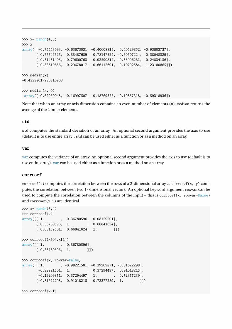
>>> x= randn(4,5)
>>> x
array([[-0.74448693, -0.63673031, -0.40608815, 0.40529852, -0.93803737],
[ 0.77746525, 0.33487689, 0.78147524, -0.5050722 , 0.58048329],
[-0.51451403, -0.79600763, 0.92590814, -0.53996231, -0.24834136],
[-0.83610656, 0.29678017, -0.66112691, 0.10792584, -1.23180865]])
>>> median(x)
-0.45558017286810903
>>> median(x, 0)
array([-0.62950048, -0.16997507, 0.18769355, -0.19857318, -0.59318936])
Note that when an array or axis dimension contains an even number of elements (n), median returns the
average of the 2 inner elements.
std
std computes the standard deviation of an array. An optional second argument provides the axis to use
(default is to use entire array). std can be used either as a function or as a method on an array.
var
var computes the variance of an array. An optional second argument provides the axis to use (default is to
use entire array). var can be used either as a function or as a method on an array.
corrcoef
corrcoef(x) computes the correlation between the rows of a 2-dimensional array x . corrcoef(x, y) com-
putes the correlation between two 1- dimensional vectors. An optional keyword argument rowvar can be
used to compute the correlation between the columns of the input – this is corrcoef(x, rowvar=False)
and corrcoef(x.T) are identical.
>>> x= randn(3,4)
>>> corrcoef(x)
array([[ 1. , 0.36780596, 0.08159501],
[ 0.36780596, 1. , 0.66841624],
[ 0.08159501, 0.66841624, 1. ]])
>>> corrcoef(x[0],x[1])
array([[ 1. , 0.36780596],
[ 0.36780596, 1. ]])
>>> corrcoef(x, rowvar=False)
array([[ 1. , -0.98221501, -0.19209871, -0.81622298],
[-0.98221501, 1. , 0.37294497, 0.91018215],
[-0.19209871, 0.37294497, 1. , 0.72377239],
[-0.81622298, 0.91018215, 0.72377239, 1. ]])
>>> corrcoef(x.T)
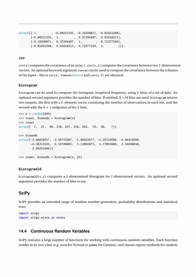
array([[ 1. , -0.98221501, -0.19209871, -0.81622298],
[-0.98221501, 1. , 0.37294497, 0.91018215],
[-0.19209871, 0.37294497, 1. , 0.72377239],
[-0.81622298, 0.91018215, 0.72377239, 1. ]])
cov
cov(x) computes the covariance of an array x . cov(x,y) computes the covariance between two 1-dimensional
vectors. An optional keyword argument rowvar can be used to compute the covariance between the columns
of the input – this is cov(x, rowvar=False) and cov(x.T) are identical.
histogram
histogram can be used to compute the histogram (empirical frequency, using k bins) of a set of data. An
optional second argument provides the number of bins. If omitted, k =10 bins are used. histogram returns
two outputs, the first with a k -element vector containing the number of observations in each bin, and the
second with the k + 1 endpoints of the k bins.
>>> x = randn(1000)
>>> count, binends = histogram(x)
>>> count
array([ 7, 27, 68, 158, 237, 218, 163, 79, 36, 7])
>>> binends
array([-3.06828057, -2.46725067, -1.86622077, -1.26519086, -0.66416096,
-0.06313105, 0.53789885, 1.13892875, 1.73995866, 2.34098856,
2.94201846])
>>> count, binends = histogram(x, 25)
histogram2d
histogram2d(x,y) computes a 2-dimensional histogram for 1-dimensional vectors. An optional second
argument provides the number of bins to use.
SciPy
SciPy provides an extended range of random number generators, probability distributions and statistical
tests.
import scipy
import scipy.stats as stats
14.4 Continuous Random Variables
SciPy contains a large number of functions for working with continuous random variables. Each function
resides in its own class (e.g. norm for Normal or gamma for Gamma), and classes expose methods for random
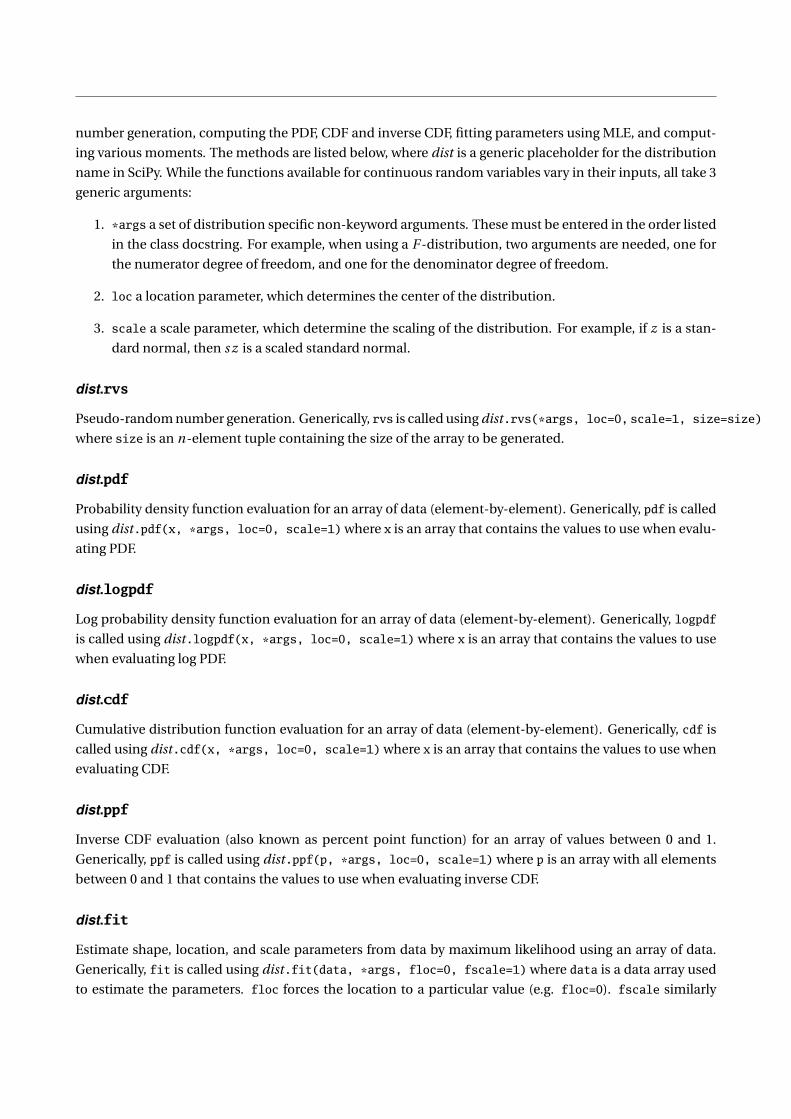
number generation, computing the PDF, CDF and inverse CDF, fitting parameters using MLE, and comput-
ing various moments. The methods are listed below, where dist is a generic placeholder for the distribution
name in SciPy. While the functions available for continuous random variables vary in their inputs, all take 3
generic arguments:
1. *args a set of distribution specific non-keyword arguments. These must be entered in the order listed
in the class docstring. For example, when using a F -distribution, two arguments are needed, one for
the numerator degree of freedom, and one for the denominator degree of freedom.
2. loc a location parameter, which determines the center of the distribution.
3. scale a scale parameter, which determine the scaling of the distribution. For example, if z is a stan-
dard normal, then s z is a scaled standard normal.
dist.rvs
Pseudo-random number generation. Generically, rvs is called using dist.rvs(*args, loc=0, scale=1, size=size)
where size is an n-element tuple containing the size of the array to be generated.
dist.pdf
Probability density function evaluation for an array of data (element-by-element). Generically, pdf is called
using dist.pdf(x, *args, loc=0, scale=1) where x is an array that contains the values to use when evalu-
ating PDF.
dist.logpdf
Log probability density function evaluation for an array of data (element-by-element). Generically, logpdf
is called using dist.logpdf(x, *args, loc=0, scale=1) where x is an array that contains the values to use
when evaluating log PDF.
dist.cdf
Cumulative distribution function evaluation for an array of data (element-by-element). Generically, cdf is
called using dist.cdf(x, *args, loc=0, scale=1) where x is an array that contains the values to use when
evaluating CDF.
dist.ppf
Inverse CDF evaluation (also known as percent point function) for an array of values between 0 and 1.
Generically, ppf is called using dist.ppf(p, *args, loc=0, scale=1) where p is an array with all elements
between 0 and 1 that contains the values to use when evaluating inverse CDF.
dist.fit
Estimate shape, location, and scale parameters from data by maximum likelihood using an array of data.
Generically, fit is called using dist.fit(data, *args, floc=0, fscale=1) where data is a data array used
to estimate the parameters. floc forces the location to a particular value (e.g. floc=0). fscale similarly

forces the scale to a particular value (e.g. fscale=1) . It is necessary to use floc and/or fscale when com-
puting MLEs if the distribution does not have a location and/or scale. For example, the gamma distribution
is defined using 2 parameters, often referred to as shape and scale. In order to use ML to estimate parame-
ters from a gamma, floc=0 must be used.
dist.median
Returns the median of the distribution. Generically, median is called using dist.median(*args, loc=0, scale=1).
dist.mean
Returns the mean of the distribution. Generically, mean is called using dist.mean(*args, loc=0, scale=1).
dist.moment
nth non-central moment evaluation of the distribution. Generically, moment is called using dist.moment(r, *args,
loc=0, scale=1) where r is the order of the moment to compute.
dist.varr
Returns the variance of the distribution. Generically, var is called using dist.var(*args, loc=0, scale=1).
dist.std
Returns the standard deviation of the distribution. Generically, std is called using dist.std(*args, loc=0, scale=1).
14.4.1 Example: gamma
The gamma distribution is used as an example. The gamma distribution takes 1 shape parameter a (a is
the only element of *args), which is set to 2 in all examples.
>>> gamma = stats.gamma
>>> gamma.mean(2), gamma.median(2), gamma.std(2), gamma.var(2)
(2.0, 1.6783469900166608, 1.4142135623730951, 2.0)
>>> gamma.moment(2,2) - gamma.moment(1,2)**2 # Variance
2
>>> gamma.cdf(5, 2), gamma.pdf(5, 2)
(0.95957231800548726, 0.033689734995427337)
>>> gamma.ppf(.95957232, 2)
5.0000000592023914
>>> log(gamma.pdf(5, 2)) - gamma.logpdf(5, 2)
0.0
>>> gamma.rvs(5, size=(2,2))
array([[ 2.60426534, 3.28844939],
[ 1.2592476 , 2.29415338]])

>>> gamma.fit(gamma.rvs(5, size=(1000)), floc = 0) # a, 0, shape
(5.614220461484499, -0.13375877842240613, 0.92353448409408001)
14.4.2 Important Distributions
SciPy provides classes for a large number of distribution. The most important in econometrics are listed
in the table below, along with any required arguments (shapeq parameters). All classes can be used with
the keyword arguments loc and scale to set the location and scale, respectively. The default location is 0
and the default scale is 1. Setting loc to something other than 0 is equivalent to adding loc to the random
variable. Similarly setting scale to something other than 0 is equivalent to multiplying the variable by scale.
Distribution Name SciPy Name Required Arguments Notes
Normal norm Use loc to set mean (µ), scale to set std. dev. (σ)
Beta(a , b ) beta a : a, b : b
Cauchy cauchy
χ2ν chi2 ν : df
Exponential(λ) expon Use scale to set shape parameter (λ)
Exponential Power exponpow shape: b Nests normal when b=2, Laplace when b=1
F(ν1, ν2) f ν1: dfn, ν2: dfd
Gamma(a , b ) gamma a : a Use scale to set scale parameter (b )
Laplace, Double Exponential laplace Use loc to set mean (µ), scale to set std. dev. (σ)
Log Normal(µ,σ2) lognorm σ: s Use scale to set µ, as scale=exp(mu)
Student’s-tν t ν : df
14.4.3 Frozen Random Variable Object
Random variable objects can be used in one of two ways:
1. Calling the class along with any shape, location and scale parameters, simultaneously with the method.
For example gamma(1, scale=2).cdf(1).
2. Initializing the class with any shape, location and scale arguments and assigning a variable name.
Using the assigned variable name with the method. For example:
>>> g = scipy.stats.gamma(1, scale=2)
>>> g.cdf(1)
0.39346934028736652
The second method is known as using a frozen random variable object. If the same distribution (with fixed
parameters) is repeatedly used, frozen objects can be used to save typing, and potentially improve speed
since frozen objects avoid re-initializing the class.
14.5 Select Statistics Functions
mode
mode computes the mode of an array. An optional second argument provides the axis to use (default is to
use entire array). Returns two outputs: the first contains the values of the mode, the second contains the
number of occurrences.

>>> x=randint(1,11,1000)
>>> stats.mode(x)
(array([ 4.]), array([ 112.]))
moment
moment computed the rth central moment for an array. An optional second argument provides the axis to
use (default is to use entire array).
>>> x = randn(1000)
>>> moment = stats.moment
>>> moment(x,2) - moment(x,1)**2
0.94668836546169166
>>> var(x)
0.94668836546169166
>>> x = randn(1000,2)
>>> moment(x,2,0) # axis 0
array([ 0.97029259, 1.03384203])
skew
skew computes the skewness of an array. An optional second argument provides the axis to use (default is
to use entire array).
>>> x = randn(1000)
>>> skew = stats.skew
>>> skew(x)
0.027187705042705772
>>> x = randn(1000,2)
>>> skew(x,0)
array([ 0.05790773, -0.00482564])
kurtosis
kurtosis computes the excess kurtosis (actual kurtosis minus 3) of an array. An optional second argument
provides the axis to use (default is to use entire array). Setting the keyword argument fisher=False will
compute the actual kurtosis.
>>> x = randn(1000)
>>> kurtosis = stats.kurtosis
>>> kurtosis(x)
-0.2112381820194531
>>> kurtosis(x, fisher=False)
2.788761817980547
>>> kurtosis(x, fisher=False) - kurtosis(x) # Must be 3

3.0
>>> x = randn(1000,2)
>>> kurtosis(x,0)
array([-0.13813704, -0.08395426])
pearsonr
pearsonr computes the Pearson correlation between two 1-dimensional vectors. It also returns the 2-tailed
p-value for the null hypothesis that the correlation is 0.
>>> x = randn(10)
>>> y = x + randn(10)
>>> pearsonr = stats.pearsonr
>>> corr, pval = pearsonr(x, y)
>>> corr
0.40806165708698366
>>> pval
0.24174029858660467
spearmanr
spearmanr computes the Spearman correlation (rank correlation). It can be used with a single 2-dimensional
array input, or 2 1-dimensional arrays. Takes an optional keyword argument axis indicating whether to treat
columns (0) or rows (1) as variables. If the input array has more than 2 variables, returns the correlation ma-
trix. If the input array as 2 variables, returns only the correlation between the variables.
>>> x = randn(10,3)
>>> spearmanr = stats.spearmanr
>>> rho, pval = spearmanr(x)
>>> rho
array([[ 1. , -0.02087009, -0.05867387],
[-0.02087009, 1. , 0.21258926],
[-0.05867387, 0.21258926, 1. ]])
>>> pval
array([[ 0. , 0.83671325, 0.56200781],
[ 0.83671325, 0. , 0.03371181],
[ 0.56200781, 0.03371181, 0. ]])
>>> rho, pval = spearmanr(x[:,1],x[:,2])
>>> corr
-0.020870087008700869
>>> pval
0.83671325461864643

kendalltau
kendalltau computed Kendall’s τ between 2 1-dimensonal arrays.
>>> x = randn(10)
>>> y = x + randn(10)
>>> kendalltau = stats.kendalltau
>>> tau, pval = kendalltau(x,y)
>>> tau
0.46666666666666673
>>> pval
0.06034053974834707
linregress
linregress estimates a linear regression between 2 1-dimensional arrays. It takes two inputs, the indepen-
dent variables (regressors) and the dependent variable (regressand). Models always include a constant.
>>> x = randn(10)
>>> y = x + randn(10)
>>> linregress = stats.linregress
>>> slope, intercept, rvalue, pvalue, stderr = linregress(x,y)
>>> slope
1.6976690163576993
>>> rsquare = rvalue**2
>>> rsquare
0.59144988449163494
>>> x.shape = 10,1
>>> y.shape = 10,1
>>> z = hstack((x,y))
>>> linregress(z) # Alternative form, [x y]
(1.6976690163576993,
-0.79983724584931648,
0.76905779008578734,
0.0093169560056056751,
0.4988520051409559)
14.6 Select Statistical Tests
normaltest
normaltest tests for normality in an array of data. An optional second argument provides the axis to use
(default is to use entire array). Returns the test statistic and the p-value of the test. This test is a small sample
modified version of the Jarque-Bera test statistic.

kstest
kstest implements the Kolmogorov-Smirnov test. Requires two inputs, the data to use in the test and the
distribution, which can be a string or a frozen random variable object. If the distribution is provided as a
string, and if it requires shape parameters, these are passed in the third argument using a tuple containing
all parameters, in order.
>>> x = randn(100)
>>> kstest = stats.kstest
>>> stat, pval = kstest(x, ’norm’)
>>> stat
0.11526423481470172
>>> pval
0.12963296757465059
>>> ncdf = stats.norm().cdf # No () on cdf to get the function
>>> kstest(x, ncdf)
(0.11526423481470172, 0.12963296757465059)
>>> x = gamma.rvs(2, size = 100)
>>> kstest(x, ’gamma’, (2,)) # (2,) contains the shape parameter
(0.079237623453142447, 0.54096739528138205)
>>> gcdf = gamma(2).cdf
>>> kstest(x, gcdf)
(0.079237623453142447, 0.54096739528138205)
ks_2samp
ks_2samp implements a 2-sample version of the Kolmogorov-Smirnov test. It is called ks_2samp(x,y) where
both inputs are 1-dimensonal arrays, and returns the test statistic and p-value for he null that the distribu-
tion of x is the same as that of y .
shapiro
shapiro implements the Shapiro-Wilk test for normality on a 1-dimensional array of data. It returns the test
statistic and p-value for the null of normality.
14.7 Exercises
1. For each of the following distributions, simulate 1000 pseudo-random numbers:
(a) N (0, 12)
(b) N(
3, 32)
(c) Uni f (0, 1)
(d) Uni f (−1, 1)

(e) G a m m a (1, 2)
(f) Lo g N(
.08, .22)
2. Use kstest to compute the p-value for each set of simulated data.
3. Use seed to re-initialize the random number generator.
4. Use get_state and set_state to to produce the same set of pseudo-random numbers.
5. Write a custom function that will take a T vector of data and returns the mean, standard deviation,
skewness and kurtosis (not excess) as a 4-element array.
6. Generate a 100 by 2 array of normal data with covariance matrix
1 −.5
−.5 1
and compute the Pearson and Spearman correlation and Kendall’s τ.
7. Compare the analytical median of a Gamma(1, 2) with that of 10,000 simulated data points. (You will
need a hist , which is discussed in the graphics chapter to finish this problem.)
8. For each of the sets of simulated data in exercise 1, plot the sorted CDF values to verify that these lie
on a 45o line. (You will need plot , which is discussed in the graphics chapter to finish this problem.)


Chapter 15
Optimization
The optimization toolbox contains a number of routines to the find extremum of a user-supplied objective
function. Most of these implement a form of the Newton-Raphson algorithm which uses the gradient to
find the minimum of a function. Note: The optimization routines can only find minima. However, if f is a
function to be maximized, − f is a function with the minimum at located the same point as the maximum
of f .
A custom function that returns the function value at a set of parameters – for example a log-likelihood
or a GMM quadratic form – is required use one of the optimizers must be constructed. All optimization
targets must have the parameters as the first argument. For example consider finding the minimum of x 2.
A function which allows the optimizer to work correctly has the form
def optim_target1(x):
return x**2
When multiple parameters (a parameter vector) are used, the objective function must take the form
def optim_target2(params):
x, y = params
return x**2-3*x+3+y*x-3*y+y**2
Optimization targets can have additional inputs that are not parameters of interest such as data or hyper-
parameters.
def optim_target3(params,hyperparams):
x, y = params
c1, c2, c3=hyperparams
return x**2+c1*x+c2+y*x+c3*y+y**2
This form is useful when optimization targets require at least two inputs: parameters and data. Once an
optimization target has been specified, the next step is to use one of the optimizers find the minimum.
SciPy contains a large number of optimizers.
import scipy.optimize as opt
151

15.1 Unconstrained Optimization
A number of functions are available for unconstrained optimization using derivative information. Each uses
a different algorithm to determine the best direction to move and the best step size to take in the direction.
The basic structure of all of the unconstrained optimizers is
optimizer(f, x0)
where optimizer is one of fmin_bfgs, fmin_cg, fmin_ncg or fmin_powell, f is a callable function and x0 is
an initial value used to start the algorithm. All of the unconstrained optimizers take the following keyword
arguments, except where noted:
Keyword Description Note
fprime Function returning derivative of f. Must take same inputs as f (1)
args Tuple containing extra parameters to pass to f
gtol Gradient norm for terminating optimization (1)
norm Order of norm (e.g. inf or 2) (1)
epsilon Step size to use when approximating f ′ (1)
maxiter Integer containing the maximum number of iterations
disp Boolean indicating whether to print convergence message
full_output Boolean indicating whether to return additional output
retall Boolean indicating whether to return results for each iteration.
callback User supplied function to call after each iteration.
(1) Except fmin, fmin_powell.
fmin_bfgs
fmin_bfgs is a classic optimizer which uses derivative information in the 1st derivative to estimate the sec-
ond derivative, which is known as the BFGS algorithm (after the initials of the creators). This is probably
the first choice when trying an optimization problem. A function which returns the first derivative of the
problem can be provided. if not provided, it is numerically approximated. The basic use of fmin_bfgs for
optimizing optim_target1 is shown below.
>>> opt.fmin_bfgs(optim_target1, 2)
Optimization terminated successfully.
Current function value: 0.000000
Iterations: 2
Function evaluations: 12
Gradient evaluations: 4
array([ -7.45132576e-09])
This is a very simple function to minimize and the solution is accurate to 8 decimal places. fmin_bfgs can
also use first derivative information, which is provided using a function which must have the same inputs
are the optimization target. In this simple example, f ′ (x ) = 2x .
def optim_target1_grad(x):
return 2*x

The derivative information is used through the keyword argument fprime. Using analytic derivatives may
improve accuracy of the solution is will require fewer function evaluations to find the solution.
>>> opt.fmin_bfgs(optim_target1, 2, fprime = optim_target1_grad)
Optimization terminated successfully.
Current function value: 0.000000
Iterations: 2
Function evaluations: 4
Gradient evaluations: 4
array([ 2.71050543e-20])
Multivariate optimization problems are defined using an array for the starting values, but are otherwise
identical.
>>> opt.fmin_bfgs(optim_target2, array([1.0,2.0]))
Optimization terminated successfully.
Current function value: 0.000000
Iterations: 3
Function evaluations: 20
Gradient evaluations: 5
array([ 1. , 0.99999999])
Additional inputs are padded through to the optimization target using the keyword argument args and a
tuple containing the input arguments in the correct order. Note that since there is a single additional input,
the comma is necessary in (hyperp,) to let Python know that this is a tuple.
>>> hyperp = array([1.0,2.0,3.0])
>>> opt.fmin_bfgs(optim_target3, array([1.0,2.0]), args=(hyperp ,))
Optimization terminated successfully.
Current function value: -0.333333
Iterations: 3
Function evaluations: 20
Gradient evaluations: 5
array([ 0.33333332, -1.66666667])
Derivative functions can be produced in a similar manner, although the derivative of a scalar function with
respect to an n-element vector is an n-element vector. It is important that the derivative (or gradient)
returned has the same order as the input parameters. Note that the inputs must have both be present, even
if not needed, and in the same order.
def optim_target3_grad(params,hyperparams):
x, y = params
c1, c2, c3=hyperparams
return array([2*x+c1+y,x+c3+2*y])
Using the analytical derivative reduces the number of function evaluations and produces the same result.
>>> opt.fmin_bfgs(optim_target3, array([1.0,2.0]), fprime=optim_target3_grad, args=(hyperp ,))
Optimization terminated successfully.
Current function value: -0.333333
Iterations: 3
Function evaluations: 5

Gradient evaluations: 5
array([ 0.33333333, -1.66666667])
fmin_cg
fmin_cg uses a nonlinear conjugate gradient method to minimize a function. A function which returns the
first derivative of the problem can be provided. if not provided, it is numerically approximated.
>>> opt.fmin_cg(optim_target3, array([1.0,2.0]), args=(hyperp ,))
Optimization terminated successfully.
Current function value: -0.333333
Iterations: 7
Function evaluations: 59
Gradient evaluations: 12
array([ 0.33333334, -1.66666666])
fmin_ncg
fmin_ncg use a Newton conjugate gradient method. fmin_ncg also requires a function which can compute
the first derivative of the optimization target, and can also take a function which returns the second deriva-
tive of the optimization target. It not provided, the hessian will be numerically approximated.
>>> opt.fmin_ncg(optim_target3, array([1.0,2.0]), optim_target3_grad, args=(hyperp,))
Optimization terminated successfully.
Current function value: -0.333333
Iterations: 5
Function evaluations: 6
Gradient evaluations: 21
Hessian evaluations: 0
array([ 0.33333333, -1.66666666])
The hessian can optionally be provided to fmin_ncg using the keyword argument fhess. The hessian returns
∂ 2 f /∂ x∂ x ′, which is an n by n array of derivatives. In this simple problem, the hessian does not depend
on the hyper-parameters, although the Hessian function must take the same inputs are the optimization
target.
def optim_target3_hess(params,hyperparams):
x, y = params
c1, c2, c3=hyperparams
return(array([[2, 1],[1, 2]]))
Using an analytical Hessian can reduce the number of function evaluations. While in theory an analytical
Hessian should produce better results, it may not improve convergence, especially is for some parameter
values the Hessian is nearly singular (for example, near a saddle point which is not a minimum).
>>> opt.fmin_ncg(optim_target3, array([1.0,2.0]), optim_target3_grad, \
... fhess = optim_target3_hess, args=(hyperp ,))
Optimization terminated successfully.
Current function value: -0.333333
Iterations: 5
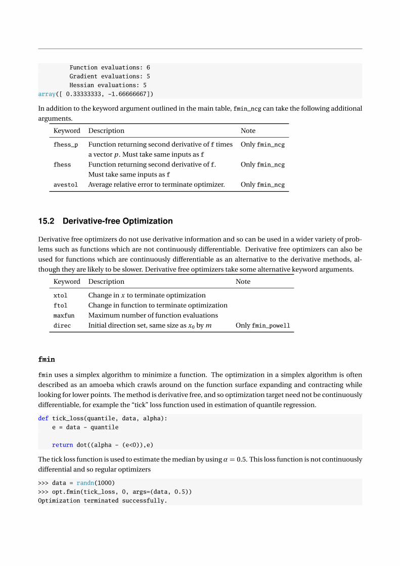
Function evaluations: 6
Gradient evaluations: 5
Hessian evaluations: 5
array([ 0.33333333, -1.66666667])
In addition to the keyword argument outlined in the main table, fmin_ncg can take the following additional
arguments.
Keyword Description Note
fhess_p Function returning second derivative of f times Only fmin_ncg
a vector p . Must take same inputs as f
fhess Function returning second derivative of f. Only fmin_ncg
Must take same inputs as f
avestol Average relative error to terminate optimizer. Only fmin_ncg
15.2 Derivative-free Optimization
Derivative free optimizers do not use derivative information and so can be used in a wider variety of prob-
lems such as functions which are not continuously differentiable. Derivative free optimizers can also be
used for functions which are continuously differentiable as an alternative to the derivative methods, al-
though they are likely to be slower. Derivative free optimizers take some alternative keyword arguments.
Keyword Description Note
xtol Change in x to terminate optimization
ftol Change in function to terminate optimization
maxfun Maximum number of function evaluations
direc Initial direction set, same size as x0 by m Only fmin_powell
fmin
fmin uses a simplex algorithm to minimize a function. The optimization in a simplex algorithm is often
described as an amoeba which crawls around on the function surface expanding and contracting while
looking for lower points. The method is derivative free, and so optimization target need not be continuously
differentiable, for example the “tick” loss function used in estimation of quantile regression.
def tick_loss(quantile, data, alpha):
e = data - quantile
return dot((alpha - (e<0)),e)
The tick loss function is used to estimate the median by usingα = 0.5. This loss function is not continuously
differential and so regular optimizers
>>> data = randn(1000)
>>> opt.fmin(tick_loss, 0, args=(data, 0.5))
Optimization terminated successfully.

Current function value: -0.333333
Iterations: 48
Function evaluations: 91
array([ 0.33332751, -1.66668794])
>>> median(data)
-0.0053901030307567602
The estimate is close to the sample median as expected.
fmin_powell
fmin_powell used Powell’s method, which is derivative free, to minimize a function. It is an alternative to
fmin which uses a different algorithm.
>>> data = randn(1000)
>>> opt.fmin_powell(tick_loss, 0, args=(data, 0.5))
Optimization terminated successfully.
Current function value: 396.760642
Iterations: 1
Function evaluations: 17
array(-0.004659496638722056)
fmin_powell converged quickly and requires far fewer function calls.
15.3 Constrained Optimization
Constrained optimization is frequently encountered in economic problems where parameters are only mean-
ingful in some particular range – for example, a variance must be weakly positive. The relevant class con-
strained optimization problems can be formulated
minθ f (θ ) subject to
g (θ ) = 0 (equality)
h (θ ) ≥ 0 (inequality)
θL ≤ θ ≤ θH (bounds)
where the bounds constraints are redundant if the optimizer allows for general inequality constraints since
if a scalar x satisfies xL ≤ x ≤ xH , then x − xL ≥ 0 and xH − x ≥ 0. The optimizers in SciPy allow for
different subsets of these configurations.
fmin_slsqp
fmin_slsqp is the most general constrained optimizer and allows for equality, inequality and bounds con-
straints. While bounds are redundant, constraints which take the form of bounds should be implemented
using bounds since this provides more information directly to the optimizer. Constraints are provided ei-
ther as list of callable functions or as a single function which returns an array. The latter is simpler if there
are multiple constraints, especially if the constraints can be easily calculated using linear algebra. Func-
tions which compute the derivative of the optimization target, the derivative of the equality constraints,

and the the derivative of the inequality constraints can be optionally provided. If not provided, these are
numerically approximated.
As an example, consider the problem of optimizing a CRS Cobb-Douglas utility function of the form
U (x1, x2) = xλ1 x 1−λ2 subject to a budget constraint p1x1+p2x2 ≤ 1. This is a nonlinear function subject to a
linear constraint (note that is must also be that case that x1 ≥ 0 and x2 ≥ 0). First, specify the optimization
target
def utility(x, p, alpha):
# Minimization, not maximization so -1 needed
return -1.0 * (x[0]**alpha)*(x[1]**(1-alpha))
There are three constraints, x1 ≥ 0, x2 ≥ 0 and the budget line. All constraints must take the form of ≥ 0
constraint, to that the budget line can be reformulated as 1 − p1x1 − p2x2 ≥ 0 . Note that the arguments
in the constraint must be identical to those of the optimization target, which is why in this case the utility
function takes prices as an input, which are not needed, and the constraint takes α which does not affect
the budget line.
def utility_constraints(x, p, alpha):
return array([x[0], x[1], 1 - p[0]*x[0] - p[1]*x[1]])
The optimal combination of good can be computed using fmin_slsqp once the starting values and other
inputs for the utility function and budget constraint are constructed.
>>> p = array([1.0,1.0])
>>> alpha = 1.0/3
>>> x0 = array([.4,.4])
>>> opt.fmin_slsqp(utility, x0, f_ieqcons=utility_constraints, args=(p, alpha))
Optimization terminated successfully. (Exit mode 0)
Current function value: -0.529133683989
Iterations: 2
Function evaluations: 8
Gradient evaluations: 2
array([ 0.33333333, 0.66666667])
fmin_slsqp can also take functions which compute the gradient of the optimization target, as well as
the gradients of the constraint functions (both inequality and equality). The gradient of the optimization
function should return a n-element vector, one for each parameter of the problem.
def utility_grad(x, p, alpha):
grad = zeros(2)
grad[0] = -1.0 * alpha * (x[0]**(alpha-1))*(x[1]**(1-alpha))
grad[1] = -1.0 * (1-alpha) * (x[0]**(alpha))*(x[1]**(-alpha))
return grad
The gradient of the constraint function returns a m by n array where m is the number of constraints. When
both equality and inequality constraints are used, the number of constraints will me me q and m i n which
will generally not be the same.
def utility_constraint_grad(x, p, alpha):
grad = zeros((3,2)) # 3 constraints, 2 variables
grad[0,0] = 1.0
grad[0,1] = 0.0
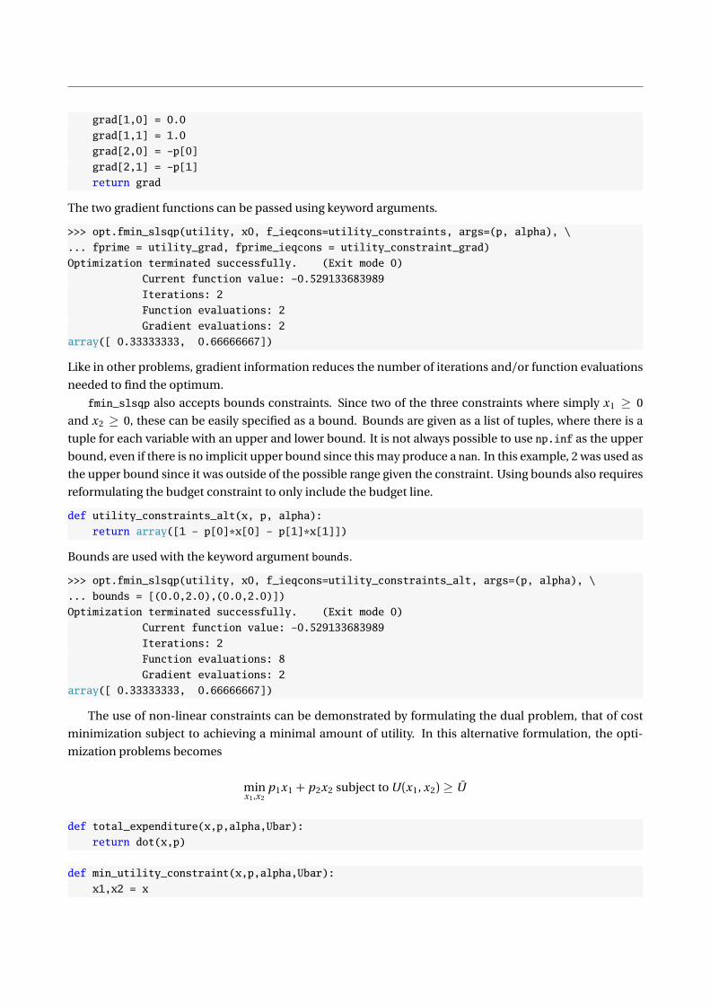
grad[1,0] = 0.0
grad[1,1] = 1.0
grad[2,0] = -p[0]
grad[2,1] = -p[1]
return grad
The two gradient functions can be passed using keyword arguments.
>>> opt.fmin_slsqp(utility, x0, f_ieqcons=utility_constraints, args=(p, alpha), \
... fprime = utility_grad, fprime_ieqcons = utility_constraint_grad)
Optimization terminated successfully. (Exit mode 0)
Current function value: -0.529133683989
Iterations: 2
Function evaluations: 2
Gradient evaluations: 2
array([ 0.33333333, 0.66666667])
Like in other problems, gradient information reduces the number of iterations and/or function evaluations
needed to find the optimum.
fmin_slsqp also accepts bounds constraints. Since two of the three constraints where simply x1 ≥ 0
and x2 ≥ 0, these can be easily specified as a bound. Bounds are given as a list of tuples, where there is a
tuple for each variable with an upper and lower bound. It is not always possible to use np.inf as the upper
bound, even if there is no implicit upper bound since this may produce a nan. In this example, 2 was used as
the upper bound since it was outside of the possible range given the constraint. Using bounds also requires
reformulating the budget constraint to only include the budget line.
def utility_constraints_alt(x, p, alpha):
return array([1 - p[0]*x[0] - p[1]*x[1]])
Bounds are used with the keyword argument bounds.
>>> opt.fmin_slsqp(utility, x0, f_ieqcons=utility_constraints_alt, args=(p, alpha), \
... bounds = [(0.0,2.0),(0.0,2.0)])
Optimization terminated successfully. (Exit mode 0)
Current function value: -0.529133683989
Iterations: 2
Function evaluations: 8
Gradient evaluations: 2
array([ 0.33333333, 0.66666667])
The use of non-linear constraints can be demonstrated by formulating the dual problem, that of cost
minimization subject to achieving a minimal amount of utility. In this alternative formulation, the opti-
mization problems becomes
minx1,x2
p1x1 + p2x2 subject to U (x1, x2) ≥ U
def total_expenditure(x,p,alpha,Ubar):
return dot(x,p)
def min_utility_constraint(x,p,alpha,Ubar):
x1,x2 = x
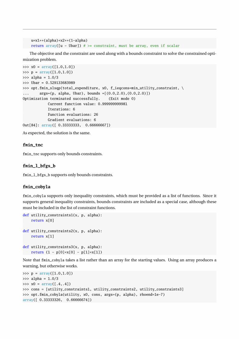
u=x1**(alpha)*x2**(1-alpha)
return array([u - Ubar]) # >= constraint, must be array, even if scalar
The objective and the constraint are used along with a bounds constraint to solve the constrained opti-
mization problem.
>>> x0 = array([1.0,1.0])
>>> p = array([1.0,1.0])
>>> alpha = 1.0/3
>>> Ubar = 0.529133683989
>>> opt.fmin_slsqp(total_expenditure, x0, f_ieqcons=min_utility_constraint, \
... args=(p, alpha, Ubar), bounds =[(0.0,2.0),(0.0,2.0)])
Optimization terminated successfully. (Exit mode 0)
Current function value: 0.999999999981
Iterations: 6
Function evaluations: 26
Gradient evaluations: 6
Out[84]: array([ 0.33333333, 0.66666667])
As expected, the solution is the same.
fmin_tnc
fmin_tnc supports only bounds constraints.
fmin_l_bfgs_b
fmin_l_bfgs_b supports only bounds constraints.
fmin_cobyla
fmin_cobyla supports only inequality constraints, which must be provided as a list of functions. Since it
supports general inequality constraints, bounds constraints are included as a special case, although these
must be included in the list of constraint functions.
def utility_constraints1(x, p, alpha):
return x[0]
def utility_constraints2(x, p, alpha):
return x[1]
def utility_constraints3(x, p, alpha):
return (1 - p[0]*x[0] - p[1]*x[1])
Note that fmin_cobyla takes a list rather than an array for the starting values. Using an array produces a
warning, but otherwise works.
>>> p = array([1.0,1.0])
>>> alpha = 1.0/3
>>> x0 = array([.4,.4])
>>> cons = [utility_constraints1, utility_constraints2, utility_constraints3]
>>> opt.fmin_cobyla(utility, x0, cons, args=(p, alpha), rhoend=1e-7)
array([ 0.33333326, 0.66666674])

15.3.1 Reparameterization
Many constrained optimization problems can be converted into an unconstrained program by reparame-
terizing from the space of unconstrained variables into the space where parameters must reside. For exam-
ple, the constraints in the utility function optimization problem require 0 ≤ x1 ≤ 1/p1 and 0 ≤ x2 ≤ 1/p2.
Additionally the budget constrain must be satisfied so that if x1 ∈ [0, 1/p1], x2 ∈ [0, (1 − p1x1)/p2]. These
constraints can be implemented using a “squasher” function which maps x1 into its domain, and x2 into its
domain and is one-to-one and onto (i.e. a bijeciton). For example,
x1 =1
p1
e z 1
1 + e z 1, x2 =
1− p1x1
p2
e z 2
1 + e z 2
will always satisfy the constraints, and so the constrained utility function can be mapped to an uncon-
strained problem, which can then be optimized using an unconstrained optimizer.
def reparam_utility(z,p,alpha,printX = False):
x = exp(z)/(1+exp(z))
x[0] = (1.0/p[0]) * x[0]
x[1] = (1-p[0]*x[0])/p[1] * x[1]
if printX:
print(x)
return -1.0 * (x[0]**alpha)*(x[1]**(1-alpha))
The unconstrained utility function can be minimized using fmin_bfgs. Note that the solution returned
is in the transformed space, and so a special call to reparam_utility is used to print the actual values of x
at the solution (which are virtually identical to those found using the constrained optimizer).
>>> x0 = array([.4,.4])
>>> optX = opt.fmin_bfgs(reparam_utility, x0, args=(p,alpha))
Optimization terminated successfully.
Current function value: -0.529134
Iterations: 24
Function evaluations: 104
Gradient evaluations: 26
>>> reparam_utility(optX, p, alpha, printX=True)
[ 0.33334741 0.66665244]
15.4 Scalar Function Minimization
SciPy provides a number of scalar function minimizers. These are very fast since additional techniques are
available for solving scalar problems which are not applicable when the parameter vector has more than 1
element. A simple quadratic function will be used to illustrate the scalar solvers. Scalar function minimizers
do not require starting values, but may require bounds for the search.
def optim_target5(x, hyperparams):
c1,c2,c3 = hyperparams
return c1*x**2 + c2*x + c3
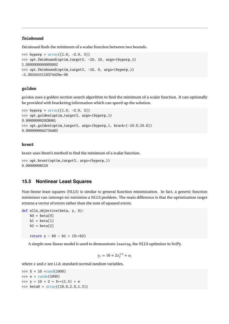
fminbound
fminbound finds the minimum of a scalar function between two bounds.
>>> hyperp = array([1.0, -2.0, 3])
>>> opt.fminbound(optim_target5, -10, 10, args=(hyperp,))
1.0000000000000002
>>> opt.fminbound(optim_target5, -10, 0, args=(hyperp,))
-5.3634455116374429e-06
golden
golden uses a golden section search algorithm to find the minimum of a scalar function. It can optionally
be provided with bracketing information which can speed up the solution.
>>> hyperp = array([1.0, -2.0, 3])
>>> opt.golden(optim_target5, args=(hyperp,))
0.999999992928981
>>> opt.golden(optim_target5, args=(hyperp,), brack=[-10.0,10.0])
0.9999999942734483
brent
brent uses Brent’s method to find the minimum of a scalar function.
>>> opt.brent(optim_target5, args=(hyperp,))
0.99999998519
15.5 Nonlinear Least Squares
Non-linear least squares (NLLS) is similar to general function minimization. In fact, a generic function
minimizer can (attempt to) minimize a NLLS problem. The main difference is that the optimization target
returns a vector of errors rather than the sum of squared errors.
def nlls_objective(beta, y, X):
b0 = beta[0]
b1 = beta[1]
b2 = beta[2]
return y - b0 - b1 * (X**b2)
A simple non-linear model is used to demonstrate leastsq, the NLLS optimizer in SciPy.
yi = 10 + 2x 1.5i + e i
where x and e are i.i.d. standard normal random variables.
>>> X = 10 *rand(1000)
>>> e = randn(1000)
>>> y = 10 + 2 * X**(1.5) + e
>>> beta0 = array([10.0,2.0,1.5])

>>> opt.leastsq(nlls_objective, beta0, args = (y, X))
(array([ 10.08885711, 1.9874906 , 1.50231838]), 1)
leastsq returns a tuple containing the solution, which is very close to the true values, as well as a flag indi-
cating whether convergence was achieved. leastsq takes many of the same additional keyword arguments
as other optimizers, including full_output, ftol, xtol, gtol, maxfev (same as maxfun). It has the additional
keyword argument:
Keyword Description Note
Ddun Function to compute the Jacobian of the problem.
Element i , j should be ∂ e i /∂ βj
col_deriv Direction to use when computing Jacobian numerically
epsfcn Step to use in numerical Jacobian calculation.
diag Scalar factors for the parameters.
Used to rescale if scale is very different.
factor used to determine the initial step size. Only fmin_powell
15.6 Exercises
1. The MLE for µ in a normal random variable is the sample mean. Write a function which takes a scalar
parameter µ (1st argument) and a T vector of data and computes the negative of the log-likelihood,
assuming the data is random and the variance is 1. Minimize the function (starting from something
other than the same mean) using fmin_bfgs and fmin.
2. Extend to previous example where the first input is a 2-element vector containing µ and σ2, and
compute the negative log-likelihood. Use fmin_slsqp along with a a lower bound of 0 forσ2.
3. Repeat the exercise in problem 2, except using reparameterization so thatσ is input (and then squared).
4. Verify that the OLS β is the MLE by writing a function which takes 3 inputs: K vector β ,T by K array X
and T by 1 array y , and computes the negative log-likelihood for these values. Minimize the function
using fmin_bfgs starting at the OLS estimates of β .

Chapter 16
Dates and Times
Date and time manipulation is provided by a built-in Python module datetime. This chapter assumes that
datetime has been imported using import datetime.
16.1 Creating Dates and Times
Dates are created using date using years, months and days and times are created using time using hours,
minutes, seconds and microseconds.
>>> import datetime as dt
>>> yr = 2012; mo = 12; dd = 21
>>> dt.date(yr, mo, dd)
datetime.date(2012, 12, 21)
>>> hr = 12; mm = 21; ss = 12; ms = 21
>>> dt.time(hr, mm, ss, ms)
dt.time(12,21,12,21)
Dates created using date no not allow times, and dates which require a time stamp can be created using
datetime, which borrow the inputs from date and time , in order.
>>> dt.datetime(yr, mo, dd, hr, mm, ss, ms)
datetime.datetime(2012, 12, 21, 12, 21, 12, 21)
16.2 Dates Mathematics
Date-times and dates (but not times, and only with the same type) can be subtracted to produce a timedelta,
which consists of three values, days, seconds and microseconds. Time deltas can also be added to dates and
times compute different dates – although date types will ignore any information in the time delta hour or
millisecond fields.
>>> d1 = dt.datetime(yr, mo, dd, hr, mm, ss, ms)
>>> d2 = dt.datetime(yr + 1, mo, dd, hr, mm, ss, ms)
>>> d2-d1
datetime.timedelta(365)
163

>>> d2 + dt.timedelta(30,0,0)
datetime.datetime(2014, 1, 20, 12, 21, 12, 20)
>>> dt.date(2012,12,21) + dt.timedelta(30,12,0)
datetime.date(2013, 1, 20)
If accurately times stamps is important, date types can be promoted to datetime using combine.
>>> d3 = dt.date(2012,12,21)
>>> dt.datetime.combine(d3, dt.time(0))
datetime.datetime(2012, 12, 21, 0, 0)
Values in dates, times and datetimes can be modified using replace, which takes keyword arguments.
>>> d3 = dt.datetime(2012,12,21,12,21,12,21)
>>> d3.replace(month=11,day=10,hour=9,minute=8,second=7,microsecond=6)
datetime.datetime(2012, 11, 10, 9, 8, 7, 6)
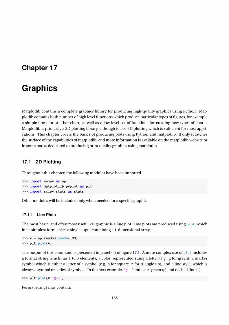
Chapter 17
Graphics
Matplotlib contains a complete graphics library for producing high-quality graphics using Python. Mat-
plotlib contains both number of high level functions which produce particular types of figures, for example
a simple line plot or a bar chart, as well as a low level set of functions for creating new types of charts.
Matplotlib is primarily a 2D plotting library, although it also 3D plotting which is sufficient for most appli-
cations. This chapter covers the basics of producing plots using Python and matplotlib. It only scratches
the surface of the capabilities of matplotlib, and more information is available on the matplotlib website or
in some books dedicated to producing print quality graphics using matplotlib.
17.1 2D Plotting
Throughout this chapter, the following modules have been imported.
>>> import numpy as np
>>> import matplotlib.pyplot as plt
>>> import scipy.stats as stats
Other modules will be included only when needed for a specific graphic.
17.1.1 Line Plots
The most basic, and often most useful 2D graphic is a line plot. Line plots are produced using plot, which
in its simplest form, takes a single input containing a 1-dimensional array.
>>> y = np.random.randn(100)
>>> plt.plot(y)
The output of this command is presented in panel (a) of figure 17.1. A more complex use of plot includes
a format string which has 1 to 3 elements, a color, represented suing a letter (e.g. g for green), a marker
symbol which is either a letter of a symbol (e.g. s for square, ^ for triangle up), and a line style, which is
always a symbol or series of symbols. In the next example, ’g--’ indicates green (g) and dashed line (–).
>>> plt.plot(y,’g--’)
Format strings may contain:
165
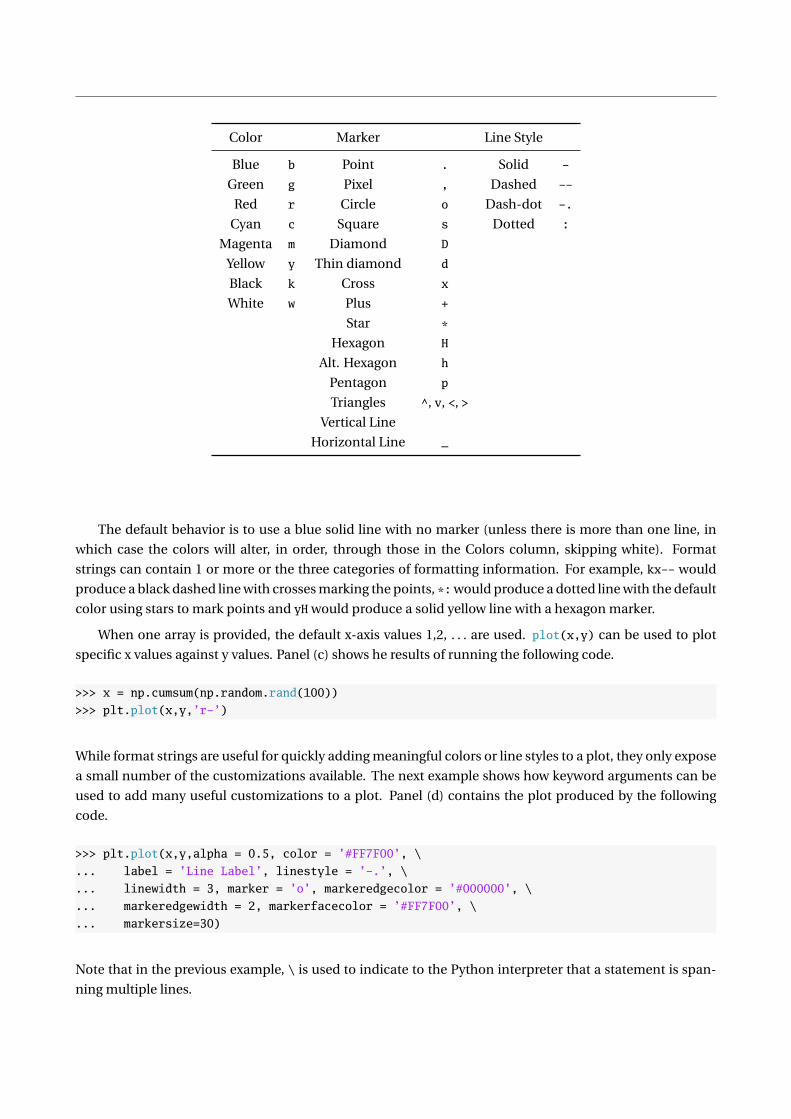
Color Marker Line Style
Blue b Point . Solid -
Green g Pixel , Dashed --
Red r Circle o Dash-dot -.
Cyan c Square s Dotted :
Magenta m Diamond D
Yellow y Thin diamond d
Black k Cross x
White w Plus +
Star *
Hexagon H
Alt. Hexagon h
Pentagon p
Triangles ^, v, <, >
Vertical Line
Horizontal Line _
The default behavior is to use a blue solid line with no marker (unless there is more than one line, in
which case the colors will alter, in order, through those in the Colors column, skipping white). Format
strings can contain 1 or more or the three categories of formatting information. For example, kx-- would
produce a black dashed line with crosses marking the points, *:would produce a dotted line with the default
color using stars to mark points and yH would produce a solid yellow line with a hexagon marker.
When one array is provided, the default x-axis values 1,2, . . . are used. plot(x,y) can be used to plot
specific x values against y values. Panel (c) shows he results of running the following code.
>>> x = np.cumsum(np.random.rand(100))
>>> plt.plot(x,y,’r-’)
While format strings are useful for quickly adding meaningful colors or line styles to a plot, they only expose
a small number of the customizations available. The next example shows how keyword arguments can be
used to add many useful customizations to a plot. Panel (d) contains the plot produced by the following
code.
>>> plt.plot(x,y,alpha = 0.5, color = ’#FF7F00’, \
... label = ’Line Label’, linestyle = ’-.’, \
... linewidth = 3, marker = ’o’, markeredgecolor = ’#000000’, \
... markeredgewidth = 2, markerfacecolor = ’#FF7F00’, \
... markersize=30)
Note that in the previous example, \ is used to indicate to the Python interpreter that a statement is span-
ning multiple lines.

Keyword Description
alpha Alpha (transparency) of the plot. Default is 1 (no transparency)
color Color description for the line.1
label Label for the line. Used when creating legends
linestyle A line style symbol
linewidth A positive integer indicating the width of the line
marker A marker shape symbol or character
markeredgecolor Color of the edge (a line) around the marker
markeredgewidth Width of the edge (a line) around the marker
markerfacecolor Face color of the marker
markersize A positive integer indicating the size of the marker
Many more keyword arguments are available for a plot. The full list can be found in the docstring or by
running the following code. The functions getp and setp can be used to get the list of properties for a line
(or any matplotlib object). setp can also be used to set a particular property.
>>> h = plot(randn(10))
>>> matplotlib.artist.getp(h)
agg_filter = None
alpha = None
animated = False
antialiased or aa = True
axes = Axes(0.125,0.1;0.775x0.8)
children = []
clip_box = TransformedBbox(Bbox(array([[ 0., 0.], [ 1...
clip_on = True
clip_path = None
color or c = b
contains = None
dash_capstyle = butt
dash_joinstyle = round
data = (array([ 0., 1., 2., 3., 4., 5., 6., 7., 8...
drawstyle = default
figure = Figure(652x492)
fillstyle = full
gid = None
label = _line0
linestyle or ls = -
linewidth or lw = 1.0
marker = None
markeredgecolor or mec = b
markeredgewidth or mew = 0.5
markerfacecolor or mfc = b
markerfacecoloralt or mfcalt = none
markersize or ms = 6
markevery = None
path = Path([[ 0. -0.27752688] [ 1. 0.3...
picker = None
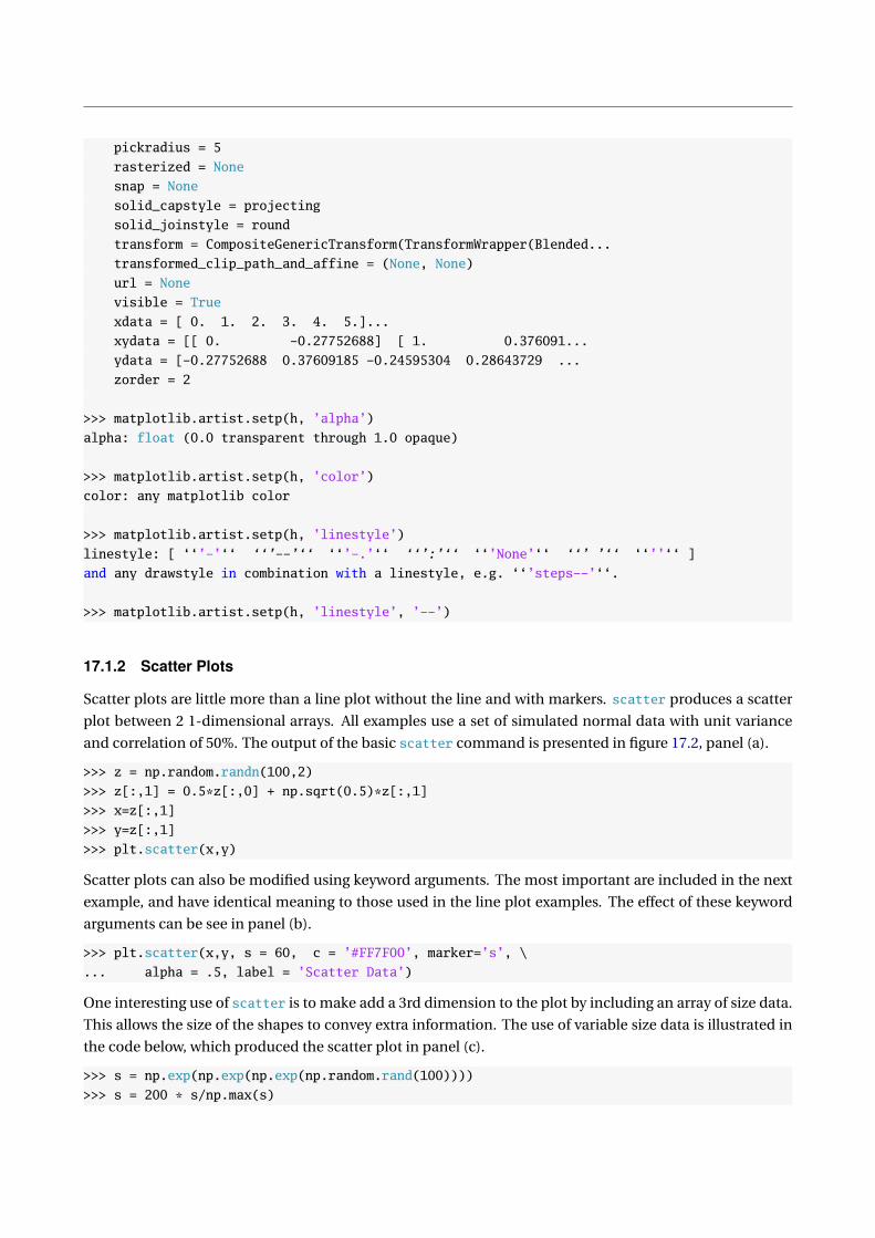
pickradius = 5
rasterized = None
snap = None
solid_capstyle = projecting
solid_joinstyle = round
transform = CompositeGenericTransform(TransformWrapper(Blended...
transformed_clip_path_and_affine = (None, None)
url = None
visible = True
xdata = [ 0. 1. 2. 3. 4. 5.]...
xydata = [[ 0. -0.27752688] [ 1. 0.376091...
ydata = [-0.27752688 0.37609185 -0.24595304 0.28643729 ...
zorder = 2
>>> matplotlib.artist.setp(h, ’alpha’)
alpha: float (0.0 transparent through 1.0 opaque)
>>> matplotlib.artist.setp(h, ’color’)
color: any matplotlib color
>>> matplotlib.artist.setp(h, ’linestyle’)
linestyle: [ ‘‘’-’‘‘ ‘‘’--’‘‘ ‘‘’-.’‘‘ ‘‘’:’‘‘ ‘‘’None’‘‘ ‘‘’ ’‘‘ ‘‘’’‘‘ ]
and any drawstyle in combination with a linestyle, e.g. ‘‘’steps--’‘‘.
>>> matplotlib.artist.setp(h, ’linestyle’, ’--’)
17.1.2 Scatter Plots
Scatter plots are little more than a line plot without the line and with markers. scatter produces a scatter
plot between 2 1-dimensional arrays. All examples use a set of simulated normal data with unit variance
and correlation of 50%. The output of the basic scatter command is presented in figure 17.2, panel (a).
>>> z = np.random.randn(100,2)
>>> z[:,1] = 0.5*z[:,0] + np.sqrt(0.5)*z[:,1]
>>> x=z[:,1]
>>> y=z[:,1]
>>> plt.scatter(x,y)
Scatter plots can also be modified using keyword arguments. The most important are included in the next
example, and have identical meaning to those used in the line plot examples. The effect of these keyword
arguments can be see in panel (b).
>>> plt.scatter(x,y, s = 60, c = ’#FF7F00’, marker=’s’, \
... alpha = .5, label = ’Scatter Data’)
One interesting use of scatter is to make add a 3rd dimension to the plot by including an array of size data.
This allows the size of the shapes to convey extra information. The use of variable size data is illustrated in
the code below, which produced the scatter plot in panel (c).
>>> s = np.exp(np.exp(np.exp(np.random.rand(100))))
>>> s = 200 * s/np.max(s)
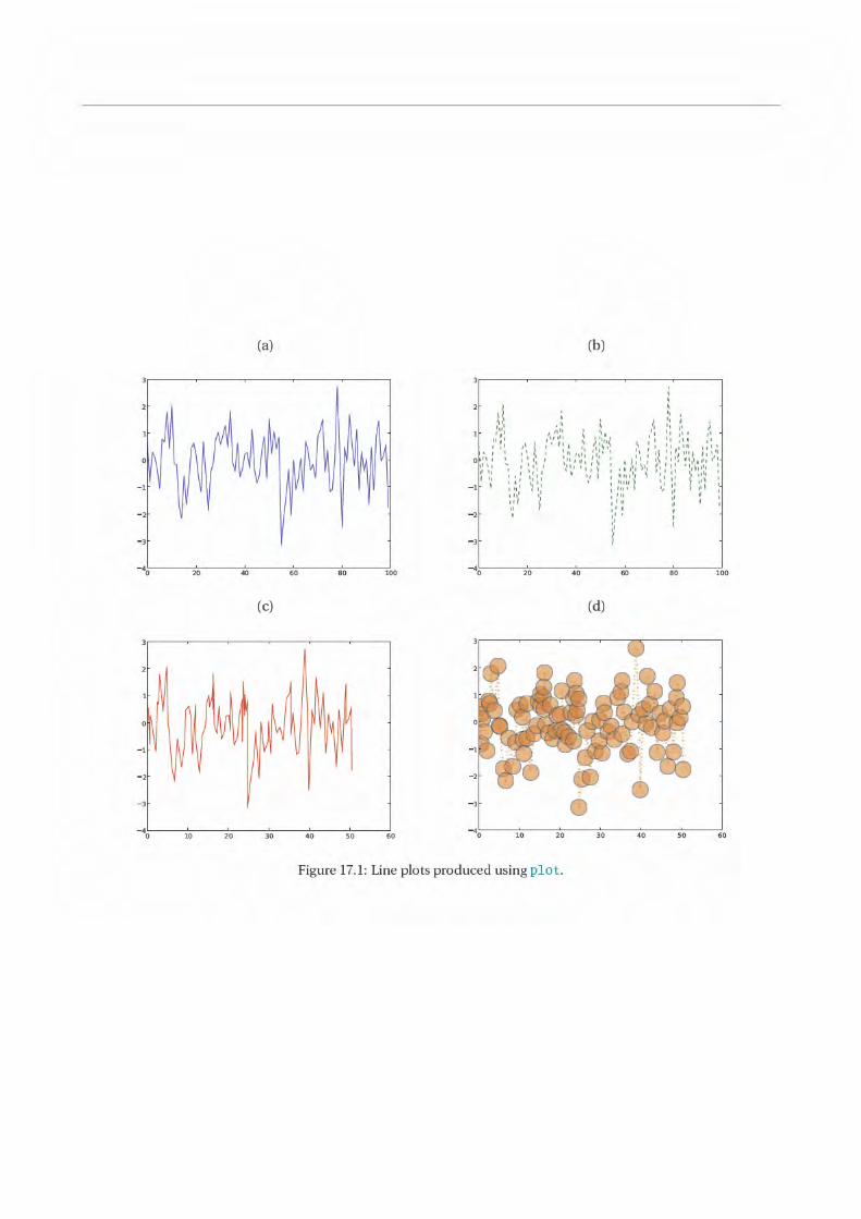
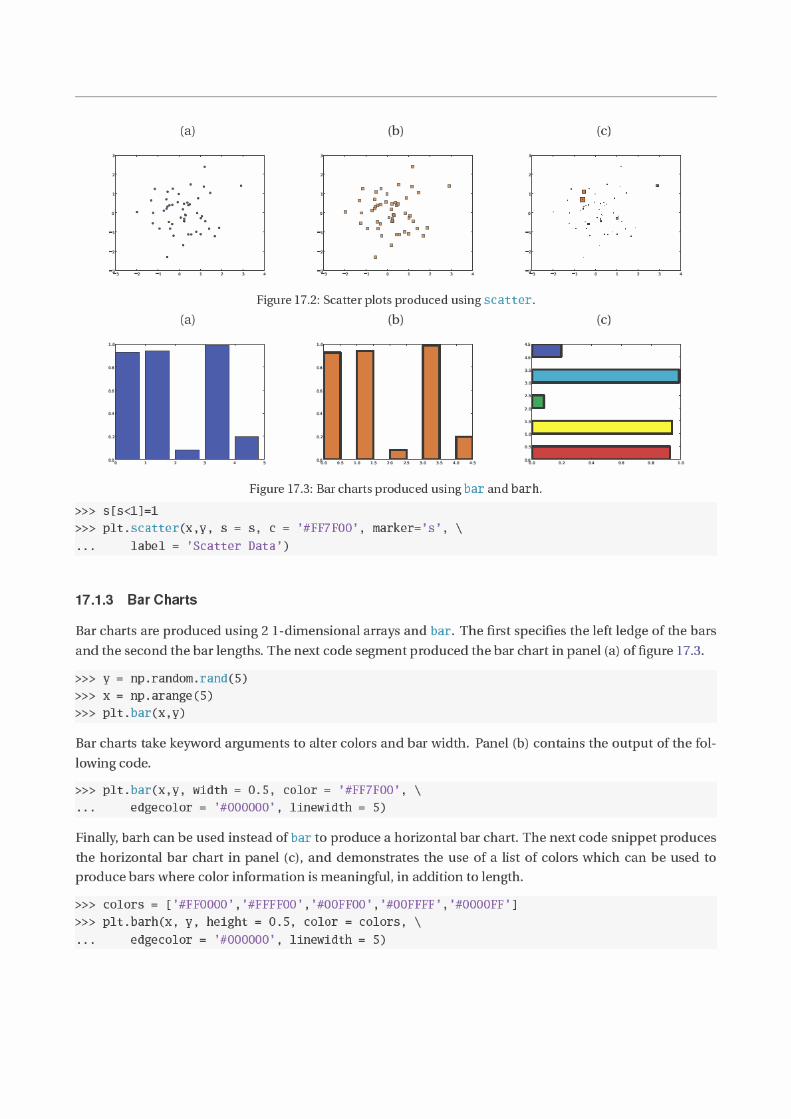


(a) (b)
3 2 1 0 1 2 3 40
20
40
60
80
100
3 2 1 0 1 2 3 40
200
400
600
800
1000
Figure 17.5: Histograms produced using hist.
17.2 Advanced 2D Plotting
17.2.1 Multiple Plots
In some scenarios it is advantageous to have multiple plots or charts in a single figure. Implementing this
is simple using figure and then add_subplot. Figure is used to initialize the figure window. Subplots can
then be added the the figure using a grid notation with m rows and n columns 1 is the upper left, 2 is the
the right of 1, and so on until the end of a row, where the next element is below 1. For example, the plots in
a 3 by 2 subplot have indices 1 2
3 4
5 6
.
add_subplot is called using the notation add_subplot(mni) or add_subplot(m,n,i) where m is the number
of rows, n is the number of columns and i is the index of the subplot. Note that subplots require the subplot
axes to be called as a method from figure. Figure XX contains the output of the code below. Note that the
next code block is sufficient long that it isn’t practical to run interactively. Also note that plt.show() is used
to force an update to the window to ensure that all plots and charts are visible. Figure 17.6 contains the
result running the code below.
fig = plt.figure()
# Add the subplot to the figure
# Panel 1
ax = fig.add_subplot(2,2,1)
y = np.random.randn(100)
plt.plot(y)
ax.set_title(’1’)
# Panel 2
y = np.random.rand(5)
x = np.arange(5)
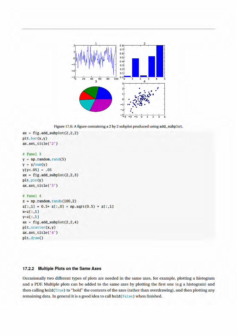

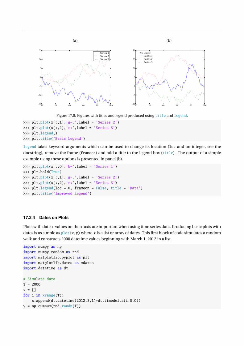
(a) (b)
0 20 40 60 80 10015
10
5
0
5
10
15
Series 1Series 2Series 3
0 20 40 60 80 10010
5
0
5
10
15
20
The Legend
Series 1Series 2Series 3
Figure 17.8: Figures with titles and legend produced using title and legend.
>>> plt.plot(x[:,1],’g-.’,label = ’Series 2’)
>>> plt.plot(x[:,2],’r:’,label = ’Series 3’)
>>> plt.legend()
>>> plt.title(’Basic Legend’)
legend takes keyword arguments which can be used to change its location (loc and an integer, see the
docstring), remove the frame (frameon) and add a title to the legend box (title). The output of a simple
example using these options is presented in panel (b).
>>> plt.plot(x[:,0],’b-’,label = ’Series 1’)
>>> plt.hold(True)
>>> plt.plot(x[:,1],’g-.’,label = ’Series 2’)
>>> plt.plot(x[:,2],’r:’,label = ’Series 3’)
>>> plt.legend(loc = 0, frameon = False, title = ’Data’)
>>> plt.title(’Improved Legend’)
17.2.4 Dates on Plots
Plots with date x-values on the x-axis are important when using time series data. Producing basic plots with
dates is as simple as plot(x,y) where x is a list or array of dates. This first block of code simulates a random
walk and constructs 2000 datetime values beginning with March 1, 2012 in a list.
import numpy as np
import numpy.random as rnd
import matplotlib.pyplot as plt
import matplotlib.dates as mdates
import datetime as dt
# Simulate data
T = 2000
x = []
for i in xrange(T):
x.append(dt.datetime(2012,3,1)+dt.timedelta(i,0,0))
y = np.cumsum(rnd.randn(T))

A basic plot with dates only requires calling plot(x,y) on the x and y data. The output of this code is in
panel (a) of figure 17.9.
fig = plt.figure()
ax = fig.add_subplot(111)
ax.plot(x,y)
plt.draw()
Once the plot has been produced autofmt_xdate() is usually called to rotate and format the labels on the
x-axis. The figure produced by running this command on the existing figure is in panel (b).
fig.autofmt_xdate()
plt.draw()
Sometime, depending on the length of the sample plotted, automatic labels will not be adequate. To
show a case where this issue arises, a shorted sample with only 100 values is simulated.
T = 100
x = []
for i in xrange(T):
x.append(dt.datetime(2012,3,1)+dt.timedelta(i,0,0))
y = np.cumsum(rnd.randn(T))
A basic plot is produced in the same manner, and is depicted in panel (c). Note the labels overlap and so
this figure is not acceptable.
fig = plt.figure()
ax = fig.add_subplot(111)
ax.plot(x,y)
plt.draw()
A call to autofmt_xdate() can be used to address the issue of overlapping labels. This is shown in panel (d).
fig.autofmt_xdate()
plt.draw()
While the formatted x dates are are an improvement, they are still unsatisfactory in that the date labels
have too much information (month, day and year) and are not at the start of the month. The next piece
of code shows how markers can be placed at the start of the month using MonthLocator which is in the
matplotlib.dates module. This idea is to construct a MonthLocator instance (which is a class), and then to
pass this axes using xaxis.set_major_locator which determines the location of major tick marks (minor
tick marks can be set using xaxis.set_mijor_locator). This will automatically place ticks on the 1st of every
month. Other locators are available, including YearLocator and WeekdayLocator, which place ticks on the
first day of the year and on week days, respectively. The second change is to format the labels on the x-axis
to have the short month name and year. This is done using DateFormatter which takes a custom format
string containing the desired text format. Options for formatting include:
• %Y - 4 digit numeric year
• %m - Numeric month
• %d - Numeric day
• %b - Short month name

• %H - Hour
• %M - Minute
• %D - Named day
These can be combined along with other characters to produce format strings. For example, %b %d, %Y
would produce a string with the format Mar 1, 2012. The format is used by calling DateFormatter. Finally
autofmt_xdate is used to rotate the labels. The result of running this code is in panel (e).
months = mdates.MonthLocator()
ax.xaxis.set_major_locator(months)
fmt = mdates.DateFormatter(’%b %Y’)
ax.xaxis.set_major_formatter(fmt)
fig.autofmt_xdate()
plt.draw()
Note that March 1 is not present in the figure in panel (e). This is because the plot doesn’t actually
include the date March 1 12:00:00 AM, but starts slightly later. To address this, simply change the axis limits
using first calling get_xlim to get the 2-element tuple containing the limits, change the it to include March
1 12:00:00 AM using set_xlim. The line between these call is actually constructing the correctly formatted
date. Internally, matplotlib uses serial dates which are simply the number of days past some initial date.
For example March 1, 2012 12:00:00 AM is 734563.0, March 2, 2012 12:00:00 AM is 734564.0 and March 2,
2012 12:00:00 PM is 734563.5. The function date2num can be used to convert datetimes to serial dates. The
output of running this final price of code on the existing figure is presented in panel (f)
xlim = list(ax.get_xlim())
xlim[0] = mdates.date2num(dt.datetime(2012,3,1))
ax.set_xlim(xlim)
plt.draw()
17.2.5 Shading Areas
For a simple demonstration of the range of matplotlib and Python graphics, consider the problem of pro-
ducing a plot of Macroeconomic time series which has business cycle fluctuations. Capacity utilization data
from FRED has been used to illustrate the steps needed to produce a plot with the time series, dates and
shaded regions representing periods where the NBER has decided were recessions.
The code has been split into two parts. The first is the code needed to read the data, find the common
dates, and finally format the data so that only the common sample is retained.
# Reading the data
import matplotlib.pyplot as plt
import matplotlib.mlab as mlab
# csv2rec for simplicity
recessionDates = mlab.csv2rec(’USREC.csv’,skiprows=0)
capacityUtilization = mlab.csv2rec(’TCU.csv’)
d1 = set(recessionDates[’date’])
d2 = set(capacityUtilization[’date’])
# Find the common dates
commonDates = d1.intersection(d2)

(a) (b)
2013 2014 2015 2016 201740
30
20
10
0
10
20
20132014
20152016
201740
30
20
10
0
10
20
(c) (d)
Mar 01 2012Mar 15 2012Mar 29 2012Apr 12 2012Apr 26 2012May 10 2012May 24 2012Jun 07 201225
20
15
10
5
0
5
10
Mar 01 2012
Mar 15 2012
Mar 29 2012
Apr 12 2012
Apr 26 2012
May 10 2012
May 24 2012
Jun 07 201225
20
15
10
5
0
5
10
(e) (f)
Mar 2012
Apr 2012
May 2012
Jun 201225
20
15
10
5
0
5
10
Mar
20
12
Apr
20
12
May 2
01
2
Jun 2
01
225
20
15
10
5
0
5
10
Figure 17.9: Figures with dates and additional formatting.

commonDates = list(commonDates)
commonDates.sort()
# And the first date
firstDate = min(commonDates)
# Find the data after the first date
plotData = capacityUtilization[capacityUtilization[’date’]>firstDate]
shadeData = recessionDates[recessionDates[’date’]>firstDate]
The second part of the code produces the plot. Most of the code is very simple. It begins by constructing
a figure, then add_subplot to the figure, and the plotting the data using plot. fill_between is only one of
many useful functions in matplotlib – it fills an area whenever a variable is 1, which is the structure of the
recession indicator. The final part of the code adds a title with a custom font (set using a dictionary), and
then changes the font and rotation of the axis labels. The output of this code is figure 17.10.
# The shaded plot
x = plotData[’date’]
y = plotData[’value’]
# z is the shading values, 1 or 0
z = shadeData[’value’]!=0
# Figure
fig = plt.figure()
ax = fig.add_subplot(111)
plt.plot_date(x,y,’r-’)
limits = plt.axis()
font = ’fontname’:’Times New Roman’, ’fontsize’:14
ax.fill_between(x, limits[2], limits[3], where=z, edgecolor=’#BBBBBB’, \
facecolor=’#BBBBBB’, alpha=0.5)
ax.set_title(’Capacity Utilization’,font)
xl = ax.get_xticklabels()
for label in xl:
label.set_fontname(’Times New Roman’)
label.set_fontsize(14)
label.set_rotation(45)
yl = ax.get_yticklabels()
for label in yl:
label.set_fontname(’Times New Roman’)
label.set_fontsize(14)
plt.draw()
17.2.6 TEX in plots
Matplotlib supports using TEX in plots. The only steps needed are the first three lines in the code below,
which configure some settings. the labels use raw mode to avoid needing to escape the \ in the TEX string.
The final plot with TEX in the labels is presented in figure 17.11.
>>> from matplotlib import rc
>>> rc(’text’, usetex=True)

1970
1974
1978
1982
1986
1990
1994
1998
2002
2006
2010
65
70
75
80
85
90Capacity Utilization
Figure 17.10: A plot of capacity utilization (US) with shaded regions indicating NBER recession dates.
>>> rc(’font’, family=’serif’)
>>> y = 50*np.exp(.0004 + np.cumsum(.01*np.random.randn(100)))
>>> plt.plot(y)
>>> plt.xlabel(r’\textbftime ($\tau$)’)
>>> plt.ylabel(r’\textitPrice’,fontsize=16)
>>> plt.title(r’Geometric Random Walk: $d\ln p_t = \mu dt + \sigma dW_t$’,fontsize=16)
>>> rc(’text’, usetex=False)
17.3 3D Plotting
The 3D plotting capabilities of matplotlib are decidedly weaker than the 2D plotting facilities. Despite this
warning, the 3D capabilities are still more than adequate for most application – especially since 3D graphics
are rarely necessary, and often not even useful when used.
17.3.1 Line Plots
Line plot in 3D are virtually identical to plotting in 2D, except that 3 1-dimensional vectors are needed, x , y
and z (height). The simple example demonstrates how how plot can be used with the keyword argument
zs to construct a 3D line plot. The line that sets up the axis using Axed3D(fig) is essential when producing
3D graphics. The other new command, view_init, is used to rotate the view using code (the view can be
interactive rotated in the figure window). The result of running the code below is presented in figure 17.12.
>>> from mpl_toolkits.mplot3d import Axes3D
>>> x = np.linspace(0,6*np.pi,600)
>>> z = x.copy()
>>> y = np.sin(x)
>>> x= np.cos(x)
>>> fig = plt.figure()
>>> ax = Axes3D(fig) # Different usage
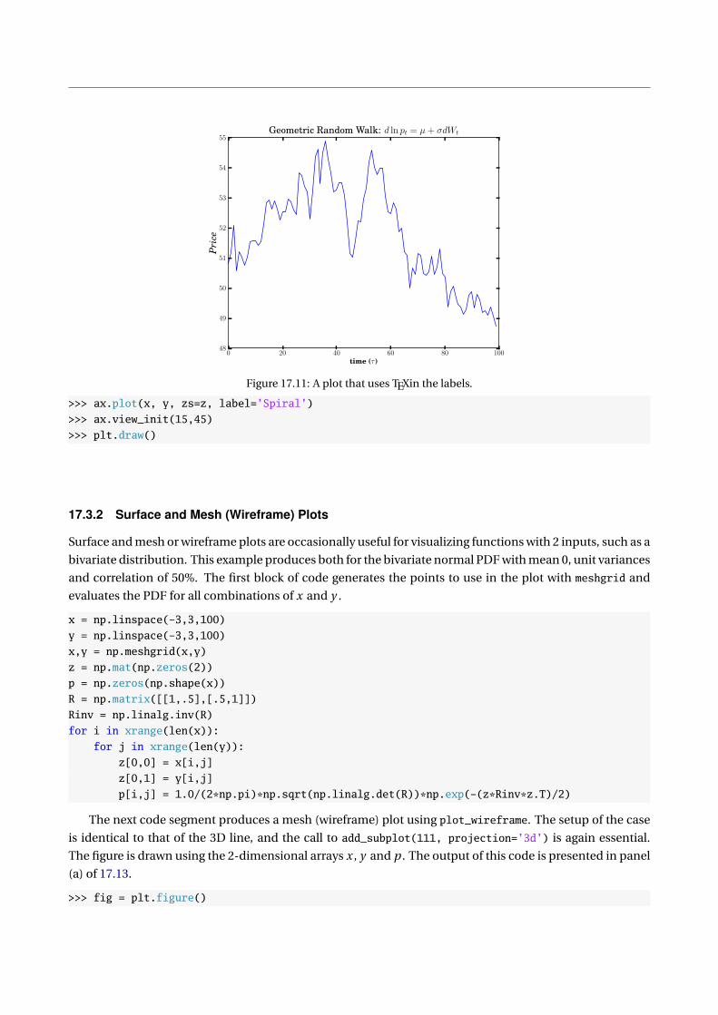
0 20 40 60 80 100time (τ)
48
49
50
51
52
53
54
55
Pri
ce
Geometric Random Walk: d ln pt = µ+ σdWt
Figure 17.11: A plot that uses TEXin the labels.
>>> ax.plot(x, y, zs=z, label=’Spiral’)
>>> ax.view_init(15,45)
>>> plt.draw()
17.3.2 Surface and Mesh (Wireframe) Plots
Surface and mesh or wireframe plots are occasionally useful for visualizing functions with 2 inputs, such as a
bivariate distribution. This example produces both for the bivariate normal PDF with mean 0, unit variances
and correlation of 50%. The first block of code generates the points to use in the plot with meshgrid and
evaluates the PDF for all combinations of x and y .
x = np.linspace(-3,3,100)
y = np.linspace(-3,3,100)
x,y = np.meshgrid(x,y)
z = np.mat(np.zeros(2))
p = np.zeros(np.shape(x))
R = np.matrix([[1,.5],[.5,1]])
Rinv = np.linalg.inv(R)
for i in xrange(len(x)):
for j in xrange(len(y)):
z[0,0] = x[i,j]
z[0,1] = y[i,j]
p[i,j] = 1.0/(2*np.pi)*np.sqrt(np.linalg.det(R))*np.exp(-(z*Rinv*z.T)/2)
The next code segment produces a mesh (wireframe) plot using plot_wireframe. The setup of the case
is identical to that of the 3D line, and the call to add_subplot(111, projection=’3d’) is again essential.
The figure is drawn using the 2-dimensional arrays x , y and p . The output of this code is presented in panel
(a) of 17.13.
>>> fig = plt.figure()
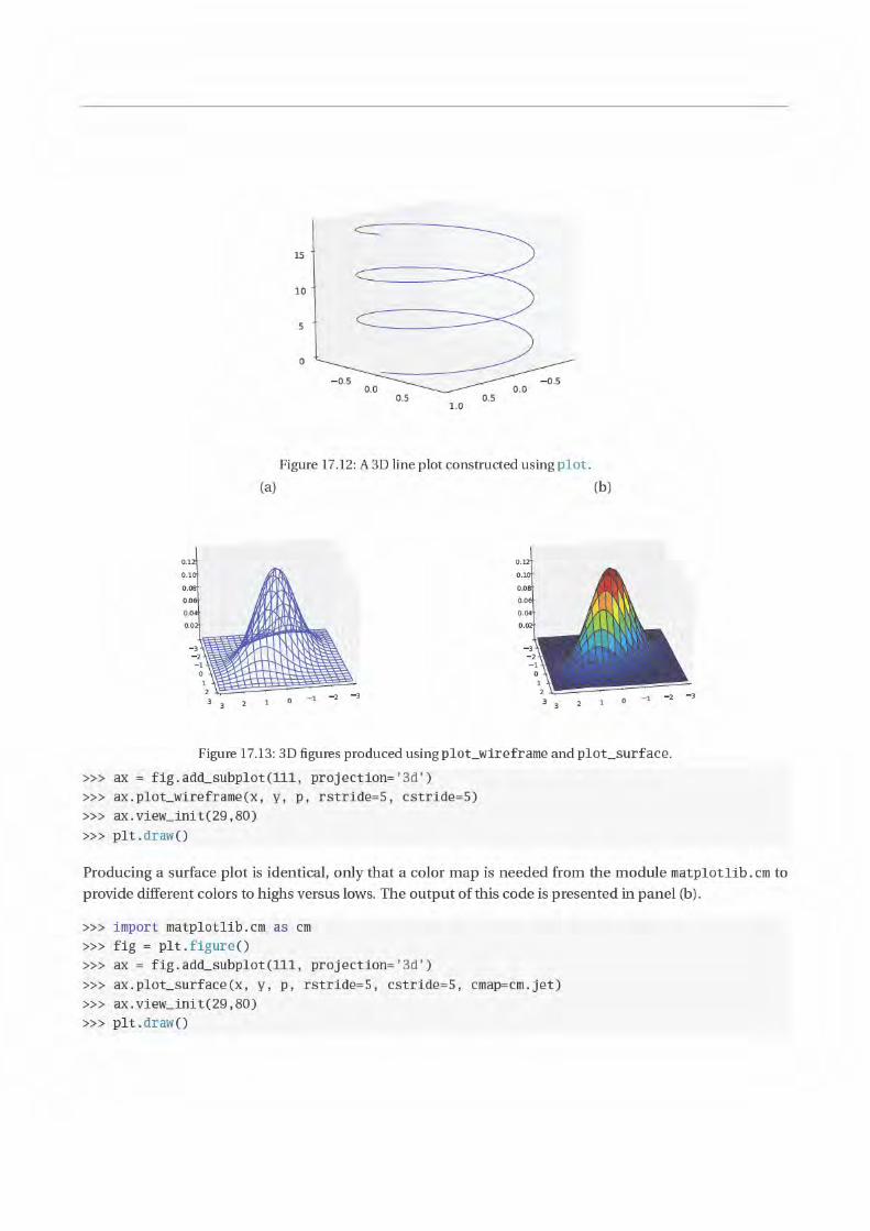

3 2 1 0 1 2 33
2
1
0
1
2
3
Figure 17.14: Contour plot produced using contour.
17.3.3 Contour Plots
Contour plots are not technically 3D, although they are used as a 2D representation of 3D data. Since they
are ultimately 2D, little setup is needed, aside form a call to contour using the same inputs as plot_surface
and plot_wireframe. The output of the code below is in figure 17.14.
>>> fig = plt.figure()
>>> ax = fig.gca()
>>> ax.contour(x,y,p)
>>> plt.draw()
17.4 General Plotting Functions
figure
figure is used to open a figure window, and can be used to generate axes. fig = figure(n) produces a
figure object with id n , and assigns the object to fig.
add_subplot
add_subplot is used to add axes to a figure. ax = fig.add_subplot(111) can be used to add a basic axes to
a figure. ax = fig.add_subplot(m,n,i) can be used to add an axes to a non-trivial figure with a m by n grid
of plots.
close
close closes figures. close(n) closes the figure with id n , and close(’all’) closes all figure windows.
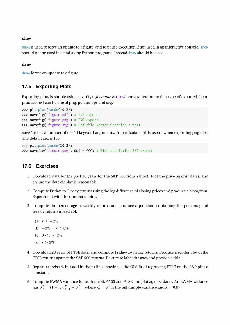
show
show is used to force an update to a figure, and to pause execution if not used in an interactive console. show
should not be used in stand along Python programs. Instead draw should be used.
draw
draw forces an update to a figure.
17.5 Exporting Plots
Exporting plots is simple using savefig(’filename.ext’) where ext determine that type of exported file to
produce. ext can be one of png, pdf, ps, eps and svg.
>>> plt.plot(randn(10,2))
>>> savefig(’figure.pdf’) # PDF export
>>> savefig(’figure.png’) # PNG export
>>> savefig(’figure.svg’) # Scalable Vector Graphics export
savefig has a number of useful keyword arguments. In particular, dpi is useful when exporting png files.
The default dpi is 100.
>>> plt.plot(randn(10,2))
>>> savefig(’figure.png’, dpi = 600) # High resolution PNG export
17.6 Exercises
1. Download data for the past 20 years for the S&P 500 from Yahoo!. Plot the price against dates, and
ensure the date display is reasonable.
2. Compute Friday-to-Friday returns using the log difference of closing prices and produce a histogram.
Experiment with the number of bins.
3. Compute the percentage of weekly returns and produce a pie chart containing the percentage of
weekly returns in each of:
(a) r ≤ −2%
(b) −2% < r ≤ 0%
(c) 0 < r ≤ 2%
(d) r > 2%
4. Download 20 years of FTSE data, and compute Friday-to-Friday returns. Produce a scatter plot of the
FTSE returns against the S&P 500 returns. Be sure to label the axes and provide a title.
5. Repeat exercise 4, but add in the fit line showing is the OLS fit of regressing FTSE on the S&P plus a
constant.
6. Compute EWMA variance for both the S&P 500 and FTSE and plot against dates. An EWMA variance
hasσ2t ‘ = (1− λ) r 2
t−1 + σ2t−1 where r 2
0 = σ20 is the full sample variance and λ = 0.97.


Chapter 18
String Manipulation
Strings are usually less interesting than numerical values in econometrics and statistics. There are, however,
some important uses for strings:
• Reading complex data formats
• Outputting formatted results to screen or file
Recall that strings are sliceable, but unlike arrays, are immutable, and so it is not possible to replace part of
a string.
18.1 String Building
18.1.1 Adding Strings (+)
Strings can be concatenated using +.
>>> a = ’Python is’
>>> b = ’a rewarding language.’
>>> a + ’ ’ + b
’Python is a rewarding language.’
While + is a simple method to joint strings, the modern method is to use join. join is a string method
which joins a list of strings (the input) using the object calling the string as the separator.
>>> a = ’Python is’
>>> b = ’a rewarding language.’
>>> ’ ’.join([a,b])
’Python is a rewarding language.’
Alternatively, the same output can be constructed using an empty string ’’.
>>> a = ’Python is’
>>> b = ’a rewarding language.’
>>> ’’.join([a,’ ’,b])
’Python is a rewarding language.’
187

18.1.2 Multiplying Strings (*)
Strings can be repeated using *.
>>> a = ’Python is’
>>> 2*a
’Python isPython is’
18.2 String Functions
18.2.1 split and rsplit
split splits a string into a list based on a character, for example a comma. Takes an optional third argument
maxsplit which limits the number of outs in the list. rsplit works identically to split, only scanning from
the end of the string – split and rsplit only differ when maxsplit is used.
>>> s = ’Python is a rewarding language.’
>>> s.split(’ ’)
[’Python’, ’is’, ’a’, ’rewarding’, ’language.’]
>>> s.split(’ ’,3)
[’Python’, ’is’, ’a’, ’rewarding language.’]
>>> s.rsplit(’ ’,3)
[’Python is’, ’a’, ’rewarding’, ’language.’]
18.2.2 join
join concatenates a list or tuple of strings, using an optional argument sep which specified a separator
(default is space).
>>> import string
>>> a = ’Python is’
>>> b = ’a rewarding language.’
>>> string.join((a,b))
’Python is a rewarding language.’
>>> string.join((a,b),’:’)
’Python is:a rewarding language.’
18.2.3 strip, lstrip, and rstrip
strip removes leading and trailing whitespace from a string. An optional input char removes leading and
trailing occurrences of the input value (instead of space). lstrip and rstrip work identically, only stripping
from the left and right, respectively.
>>> s = ’ Python is a rewarding language. ’
>>> s=s.strip()
’Python is a rewarding language.’

>>> s.strip(’P’)
’ython is a rewarding language.’
18.2.4 find and rfind
find locates the lowest index of a substring, and returns -1 if not found. Optional arguments limit the range
of the search, and s.find(’i’,10,20) is identical to s[10:20].find(’i’). rfind works identically, only
returning the highest index of the substring.
>>> s = ’Python is a rewarding language.’
>>> s.find(’i’)
7
>>> s.find(’i’,10,20)
18
>>> s.rfind(’i’)
18
18.2.5 index and rindex
index returns the lowest index of a substring, and is identical to find except that an error is raised if the
substring does not exist. As a result, index is only safe to use in a try . . . except block.
>>> s = ’Python is a rewarding language.’
>>> s.index(’i’)
7
>>> s.index(’q’) # Error
ValueError: substring not found
18.2.6 count
count counts the number of occurrences of a substring. It takes optional arguments which limit the search
range.
>>> s = ’Python is a rewarding language.’
>>> s.count(’i’)
2
>>> s.count(’i’, 10, 20)
1
18.2.7 lower and upper
lower and upper convert strings to lower and upper case, respectively. They are useful to remove case am-
biguity when comparing string to known constants.

>>> s = ’Python is a rewarding language.’
>>> s.upper()
’PYTHON IS A REWARDING LANGUAGE.’
>>> s.lower()
’python is a rewarding language.’
18.2.8 ljust, rjust and center
ljust, rjust and center left justify, right justify and center, respectively, a string while expanding its size to
a given length. If the desired length is smaller than the string, the unchanged string is returned.
>>> s = ’Python is a rewarding language.’
>>> s.ljust(40)
’Python is a rewarding language. ’
>>> s.rjust(40)
’ Python is a rewarding language.’
>>> s.center(40)
’ Python is a rewarding language. ’
18.2.9 replace
replace replaces a substring with an alternative string, which can have different size. An optional argument
limits the number of replacement.
>>> s = ’Python is a rewarding language.’
>>> s.replace(’g’,’Q’)
’Python is a rewardinQ lanQuaQe.’
>>> s.replace(’is’,’Q’)
’Python Q a rewarding language.’
>>> s.replace(’g’,’Q’,2)
’Python is a rewardinQ lanQuage.’
18.2.10 textwrap.wrap
The module textwrap contains a function wrap which reformats a long string into a fixed width paragraph,
stored line-by-line in a list. An optional argument changes the width of the output paragraph form the
default of 70 characters.
>>> import textwrap
>>> s = ’Python is a rewarding language. ’
>>> s = 10*s
>>> textwrap.wrap(s)
[’Python is a rewarding language. Python is a rewarding language. Python’,
’is a rewarding language. Python is a rewarding language. Python is a’,
’rewarding language. Python is a rewarding language. Python is a’,
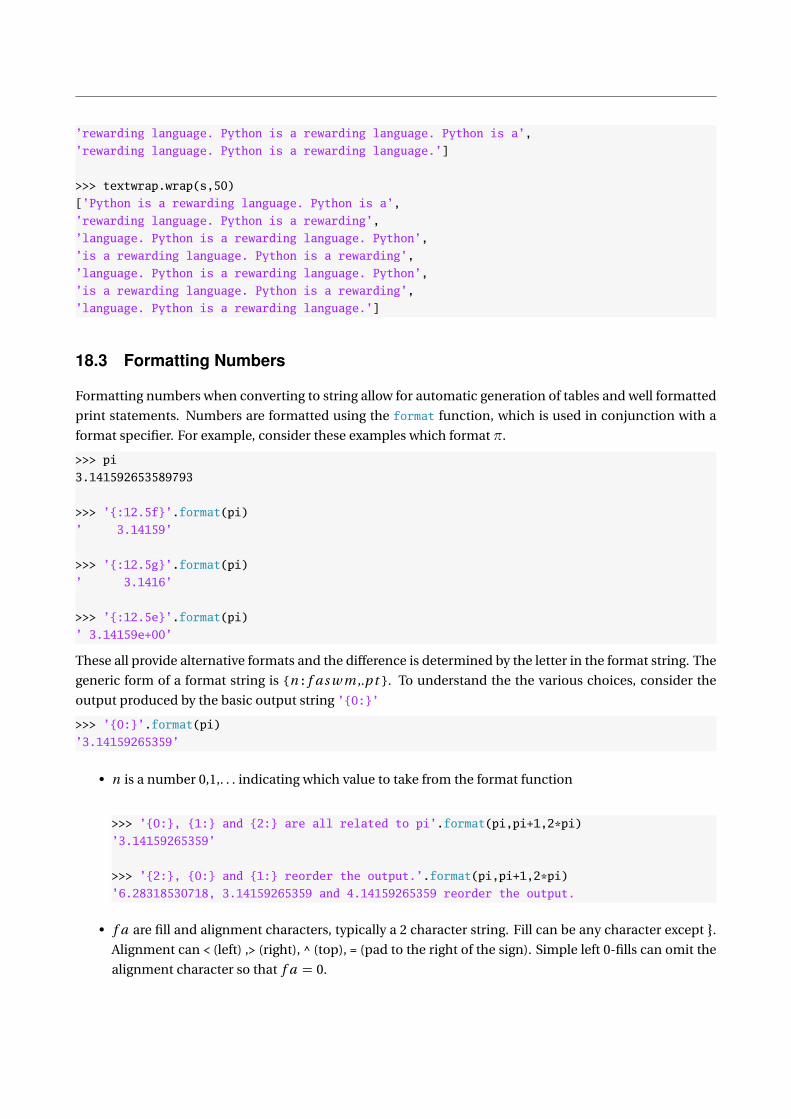
’rewarding language. Python is a rewarding language. Python is a’,
’rewarding language. Python is a rewarding language.’]
>>> textwrap.wrap(s,50)
[’Python is a rewarding language. Python is a’,
’rewarding language. Python is a rewarding’,
’language. Python is a rewarding language. Python’,
’is a rewarding language. Python is a rewarding’,
’language. Python is a rewarding language. Python’,
’is a rewarding language. Python is a rewarding’,
’language. Python is a rewarding language.’]
18.3 Formatting Numbers
Formatting numbers when converting to string allow for automatic generation of tables and well formatted
print statements. Numbers are formatted using the format function, which is used in conjunction with a
format specifier. For example, consider these examples which format π.
>>> pi
3.141592653589793
>>> ’:12.5f’.format(pi)
’ 3.14159’
>>> ’:12.5g’.format(pi)
’ 3.1416’
>>> ’:12.5e’.format(pi)
’ 3.14159e+00’
These all provide alternative formats and the difference is determined by the letter in the format string. The
generic form of a format string is n: f a s w m ,.p t . To understand the the various choices, consider the
output produced by the basic output string ’0:’
>>> ’0:’.format(pi)
’3.14159265359’
• n is a number 0,1,. . . indicating which value to take from the format function
>>> ’0:, 1: and 2: are all related to pi’.format(pi,pi+1,2*pi)
’3.14159265359’
>>> ’2:, 0: and 1: reorder the output.’.format(pi,pi+1,2*pi)
’6.28318530718, 3.14159265359 and 4.14159265359 reorder the output.
• f a are fill and alignment characters, typically a 2 character string. Fill can be any character except .Alignment can < (left) ,> (right), ^ (top), = (pad to the right of the sign). Simple left 0-fills can omit the
alignment character so that f a = 0.

>>> ’0:0<20’.format(pi) # Left, 0 padding, precion 20
’3.141592653590000000’
>>> ’0:0>20’.format(pi) # Right, 0 padding, precion 20
’00000003.14159265359’
>>> ’0: >20’.format(pi) # Right, space padding, precion 20
’ 3.14159265359’
>>> ’0:$^20’.format(pi) # Center, dollar sign padding, precion 20
’$$$3.14159265359$$$$’
• s indicates whether a sign should be included. + indicates always include sign, - indicates only in-
clude if needed, and a blank space indicates to use a blank space for positive numbers, and a− sign
for negative numbers – this format is useful for producing aligned tables.
>>> ’0:+’.format(pi)
’+3.14159265359’
>>> ’0:-’.format(pi)
’3.14159265359’
>>> ’0: ’.format(pi)
’ 3.14159265359’
>>> ’0: ’.format(-1 * pi)
’-3.14159265359’
• m is the minimum total size of the formatted string. If the formatted string is shorter than m , charac-
ter w is prepended.
>>> ’0:10’.format(pi)
’3.14159265359’
>>> ’0:20’.format(pi)
’ 3.14159265359’
>>> ’0:30’.format(pi)
’ 3.14159265359’
• c can be , or omitted. , produces numbers with 1000s separated using a ,. In order to use c it is
necessary to include the . before the precision.
>>> ’0:.10’.format(1000000 * pi)
’3141592.654’
>>> ’0:,.10’.format(1000000 * pi)
’3,141,592.654’
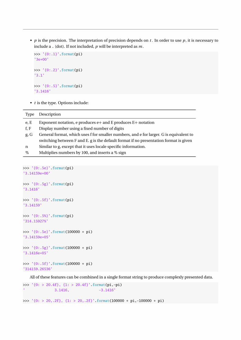
• p is the precision. The interpretation of precision depends on t . In order to use p , it is necessary to
include a . (dot). If not included, p will be interpreted as m .
>>> ’0:.1’.format(pi)
’3e+00’
>>> ’0:.2’.format(pi)
’3.1’
>>> ’0:.5’.format(pi)
’3.1416’
• t is the type. Options include:
Type Description
e, E Exponent notation, e produces e+ and E produces E+ notation
f, F Display number using a fixed number of digits
g, G General format, which uses f for smaller numbers, and e for larger. G is equivalent to
switching between F and E. g is the default format if no presentation format is given
n Similar to g, except that it uses locale specific information.
% Multiplies numbers by 100, and inserts a % sign
>>> ’0:.5e’.format(pi)
’3.14159e+00’
>>> ’0:.5g’.format(pi)
’3.1416’
>>> ’0:.5f’.format(pi)
’3.14159’
>>> ’0:.5%’.format(pi)
’314.15927%’
>>> ’0:.5e’.format(100000 * pi)
’3.14159e+05’
>>> ’0:.5g’.format(100000 * pi)
’3.1416e+05’
>>> ’0:.5f’.format(100000 * pi)
’314159.26536’
All of these features can be combined in a single format string to produce complexly presented data.
>>> ’0: > 20.4f, 1: > 20.4f’.format(pi,-pi)
’ 3.1416, -3.1416’
>>> ’0: > 20,.2f, 1: > 20,.2f’.format(100000 * pi,-100000 * pi)
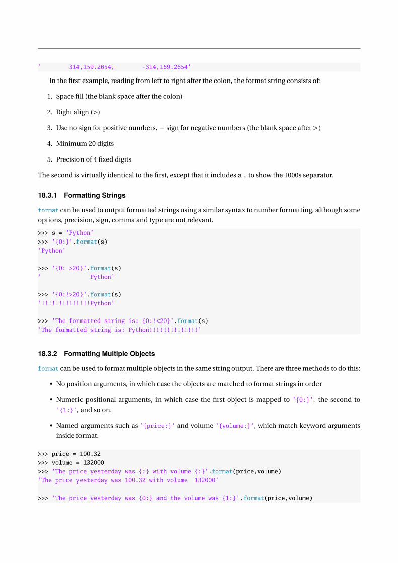
’ 314,159.2654, -314,159.2654’
In the first example, reading from left to right after the colon, the format string consists of:
1. Space fill (the blank space after the colon)
2. Right align (>)
3. Use no sign for positive numbers,− sign for negative numbers (the blank space after >)
4. Minimum 20 digits
5. Precision of 4 fixed digits
The second is virtually identical to the first, except that it includes a , to show the 1000s separator.
18.3.1 Formatting Strings
format can be used to output formatted strings using a similar syntax to number formatting, although some
options, precision, sign, comma and type are not relevant.
>>> s = ’Python’
>>> ’0:’.format(s)
’Python’
>>> ’0: >20’.format(s)
’ Python’
>>> ’0:!>20’.format(s)
’!!!!!!!!!!!!!!Python’
>>> ’The formatted string is: 0:!<20’.format(s)
’The formatted string is: Python!!!!!!!!!!!!!!’
18.3.2 Formatting Multiple Objects
format can be used to format multiple objects in the same string output. There are three methods to do this:
• No position arguments, in which case the objects are matched to format strings in order
• Numeric positional arguments, in which case the first object is mapped to ’0:’, the second to
’1:’, and so on.
• Named arguments such as ’price:’ and volume ’volume:’, which match keyword arguments
inside format.
>>> price = 100.32
>>> volume = 132000
>>> ’The price yesterday was : with volume :’.format(price,volume)
’The price yesterday was 100.32 with volume 132000’
>>> ’The price yesterday was 0: and the volume was 1:’.format(price,volume)
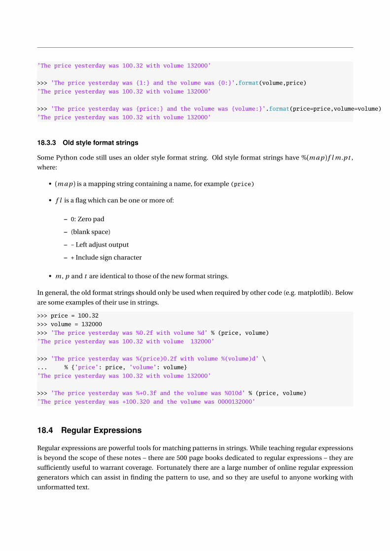
’The price yesterday was 100.32 with volume 132000’
>>> ’The price yesterday was 1: and the volume was 0:’.format(volume,price)
’The price yesterday was 100.32 with volume 132000’
>>> ’The price yesterday was price: and the volume was volume:’.format(price=price,volume=volume)
’The price yesterday was 100.32 with volume 132000’
18.3.3 Old style format strings
Some Python code still uses an older style format string. Old style format strings have %(m a p ) f l m .p t ,
where:
• (m a p ) is a mapping string containing a name, for example (price)
• f l is a flag which can be one or more of:
– 0: Zero pad
– (blank space)
– - Left adjust output
– + Include sign character
• m , p and t are identical to those of the new format strings.
In general, the old format strings should only be used when required by other code (e.g. matplotlib). Below
are some examples of their use in strings.
>>> price = 100.32
>>> volume = 132000
>>> ’The price yesterday was %0.2f with volume %d’ % (price, volume)
’The price yesterday was 100.32 with volume 132000’
>>> ’The price yesterday was %(price)0.2f with volume %(volume)d’ \
... % ’price’: price, ’volume’: volume
’The price yesterday was 100.32 with volume 132000’
>>> ’The price yesterday was %+0.3f and the volume was %010d’ % (price, volume)
’The price yesterday was +100.320 and the volume was 0000132000’
18.4 Regular Expressions
Regular expressions are powerful tools for matching patterns in strings. While teaching regular expressions
is beyond the scope of these notes – there are 500 page books dedicated to regular expressions – they are
sufficiently useful to warrant coverage. Fortunately there are a large number of online regular expression
generators which can assist in finding the pattern to use, and so they are useful to anyone working with
unformatted text.
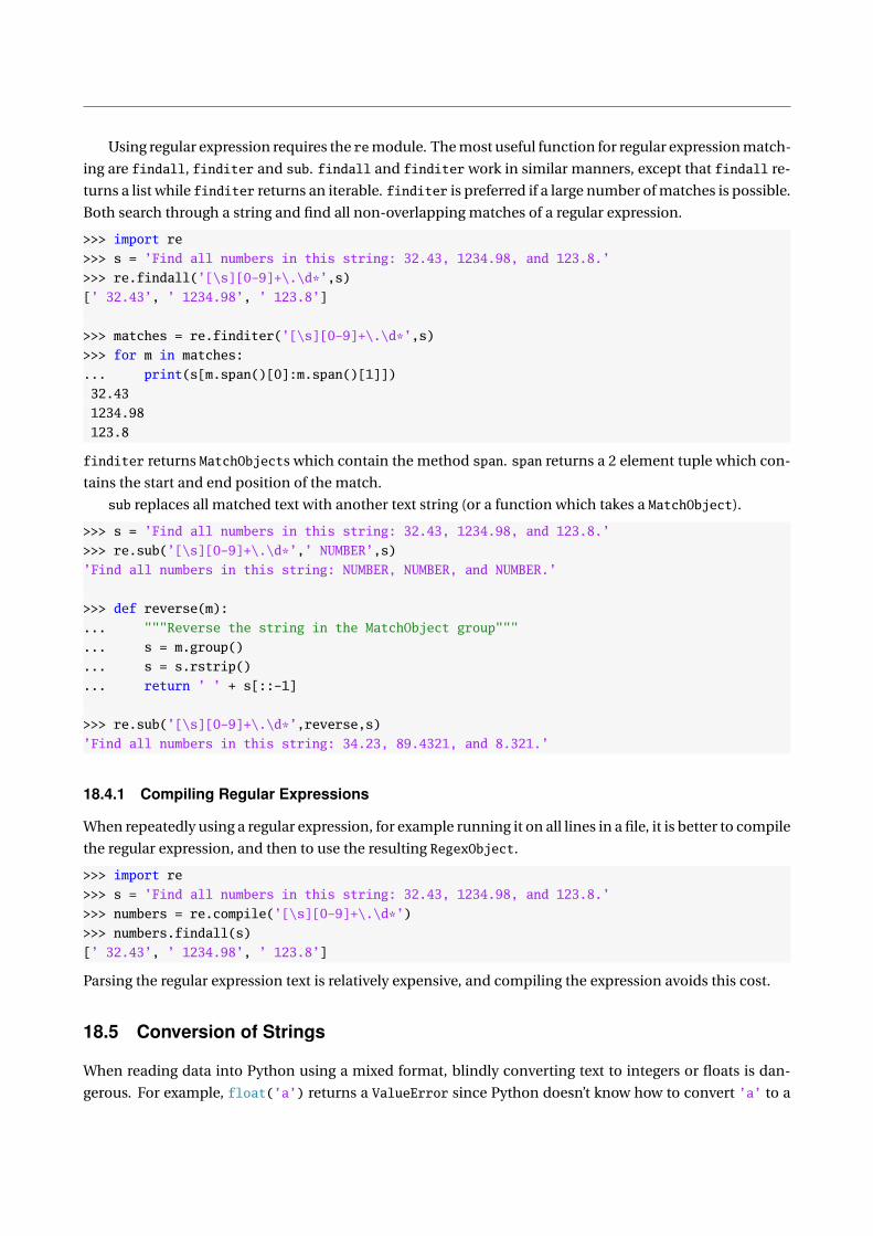
Using regular expression requires the remodule. The most useful function for regular expression match-
ing are findall, finditer and sub. findall and finditer work in similar manners, except that findall re-
turns a list while finditer returns an iterable. finditer is preferred if a large number of matches is possible.
Both search through a string and find all non-overlapping matches of a regular expression.
>>> import re
>>> s = ’Find all numbers in this string: 32.43, 1234.98, and 123.8.’
>>> re.findall(’[\s][0-9]+\.\d*’,s)
[’ 32.43’, ’ 1234.98’, ’ 123.8’]
>>> matches = re.finditer(’[\s][0-9]+\.\d*’,s)
>>> for m in matches:
... print(s[m.span()[0]:m.span()[1]])
32.43
1234.98
123.8
finditer returns MatchObjects which contain the method span. span returns a 2 element tuple which con-
tains the start and end position of the match.
sub replaces all matched text with another text string (or a function which takes a MatchObject).
>>> s = ’Find all numbers in this string: 32.43, 1234.98, and 123.8.’
>>> re.sub(’[\s][0-9]+\.\d*’,’ NUMBER’,s)
’Find all numbers in this string: NUMBER, NUMBER, and NUMBER.’
>>> def reverse(m):
... """Reverse the string in the MatchObject group"""
... s = m.group()
... s = s.rstrip()
... return ’ ’ + s[::-1]
>>> re.sub(’[\s][0-9]+\.\d*’,reverse,s)
’Find all numbers in this string: 34.23, 89.4321, and 8.321.’
18.4.1 Compiling Regular Expressions
When repeatedly using a regular expression, for example running it on all lines in a file, it is better to compile
the regular expression, and then to use the resulting RegexObject.
>>> import re
>>> s = ’Find all numbers in this string: 32.43, 1234.98, and 123.8.’
>>> numbers = re.compile(’[\s][0-9]+\.\d*’)
>>> numbers.findall(s)
[’ 32.43’, ’ 1234.98’, ’ 123.8’]
Parsing the regular expression text is relatively expensive, and compiling the expression avoids this cost.
18.5 Conversion of Strings
When reading data into Python using a mixed format, blindly converting text to integers or floats is dan-
gerous. For example, float(’a’) returns a ValueError since Python doesn’t know how to convert ’a’ to a

string. The simplest method to safely convert potentially non-numeric data is to use a try . . . except block.
from __future__ import print_function
from __future__ import division
S = [’1234’,’1234.567’,’a’,’1234.a34’,’1.0’,’a123’]
for s in S:
try:
int(s)
print(s, ’is an integer.’)
except:
try:
float(s)
print(s, ’is a float.’)
except:
print(’Unable to convert’, s)


Chapter 19
File System and Navigation
Manipulating the file system is surprising useful when working with data. The most important file system
commands are located in the modules os and shutil. This chapter assumes that
import os
import shutil
have been included.
19.1 Changing the Working Directory
The working directory is where files can be created and accessed without any path information. os.getcwd()
can be used to determine the current working directory, and os.chdir(path) can be used to change the
working directory, where path is a directory, such as /temp or c:\\temp.1 Alternatively, path can can be .. to
more up the directory tree.
pwd = os.getcwd()
os.chdir(’c:\\temp’)
os.chdir(’c:/temp’) # Identical
os.chdir(’..’)
os.getcwd() # Now in ’c:\\’
19.2 Creating and Deleting Directories
Directories can be created using os.mkdir(dirname), although it must be the case that the higher level di-
rectories exist (e.g. to create /home/username/ Python/temp, it must be the case that /home/username/Python
already exists). os.makedirs(dirname) works similar to os.mkdir(dirname), except that is will create any
higher level directories needed to create the target directory.
Empty directories can be deleted using os.rmdir(dirname) – if the directory is not empty, an error oc-
curs. shutil.rmtree(dirname) works similarly to os.rmdir(dirname), except that it will delete the direc-
tory, and any files or other directories contained in the directory.
1On Windows, directories use the backslash, which is used to escape characters in Python, and so an escaped backslash – \\ – isneeded when writing Windows’ paths. Alternatively, the forward slash can be substituted, so that c:\\temp and c:/temp are equivalent.
199
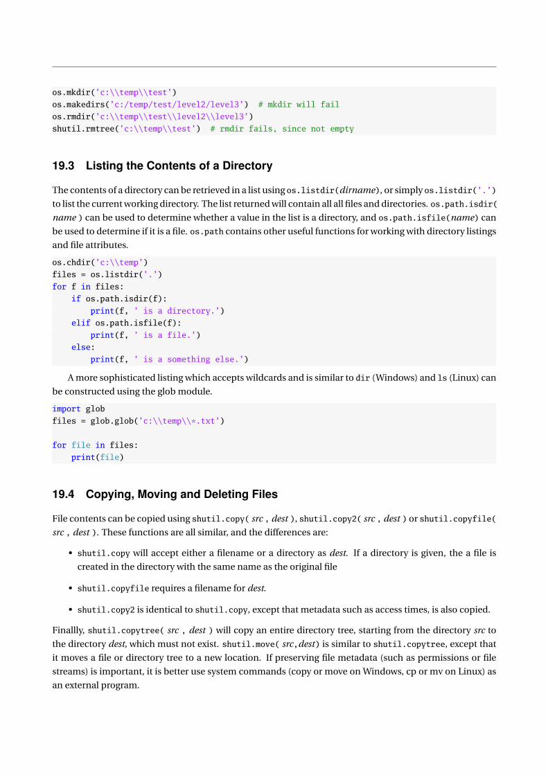
os.mkdir(’c:\\temp\\test’)
os.makedirs(’c:/temp/test/level2/level3’) # mkdir will fail
os.rmdir(’c:\\temp\\test\\level2\\level3’)
shutil.rmtree(’c:\\temp\\test’) # rmdir fails, since not empty
19.3 Listing the Contents of a Directory
The contents of a directory can be retrieved in a list using os.listdir(dirname), or simply os.listdir(’.’)
to list the current working directory. The list returned will contain all all files and directories. os.path.isdir(
name ) can be used to determine whether a value in the list is a directory, and os.path.isfile(name) can
be used to determine if it is a file. os.path contains other useful functions for working with directory listings
and file attributes.
os.chdir(’c:\\temp’)
files = os.listdir(’.’)
for f in files:
if os.path.isdir(f):
print(f, ’ is a directory.’)
elif os.path.isfile(f):
print(f, ’ is a file.’)
else:
print(f, ’ is a something else.’)
A more sophisticated listing which accepts wildcards and is similar to dir (Windows) and ls (Linux) can
be constructed using the glob module.
import glob
files = glob.glob(’c:\\temp\\*.txt’)
for file in files:
print(file)
19.4 Copying, Moving and Deleting Files
File contents can be copied using shutil.copy( src , dest ), shutil.copy2( src , dest ) or shutil.copyfile(
src , dest ). These functions are all similar, and the differences are:
• shutil.copy will accept either a filename or a directory as dest. If a directory is given, the a file is
created in the directory with the same name as the original file
• shutil.copyfile requires a filename for dest.
• shutil.copy2 is identical to shutil.copy, except that metadata such as access times, is also copied.
Finallly, shutil.copytree( src , dest ) will copy an entire directory tree, starting from the directory src to
the directory dest, which must not exist. shutil.move( src,dest) is similar to shutil.copytree, except that
it moves a file or directory tree to a new location. If preserving file metadata (such as permissions or file
streams) is important, it is better use system commands (copy or move on Windows, cp or mv on Linux) as
an external program.
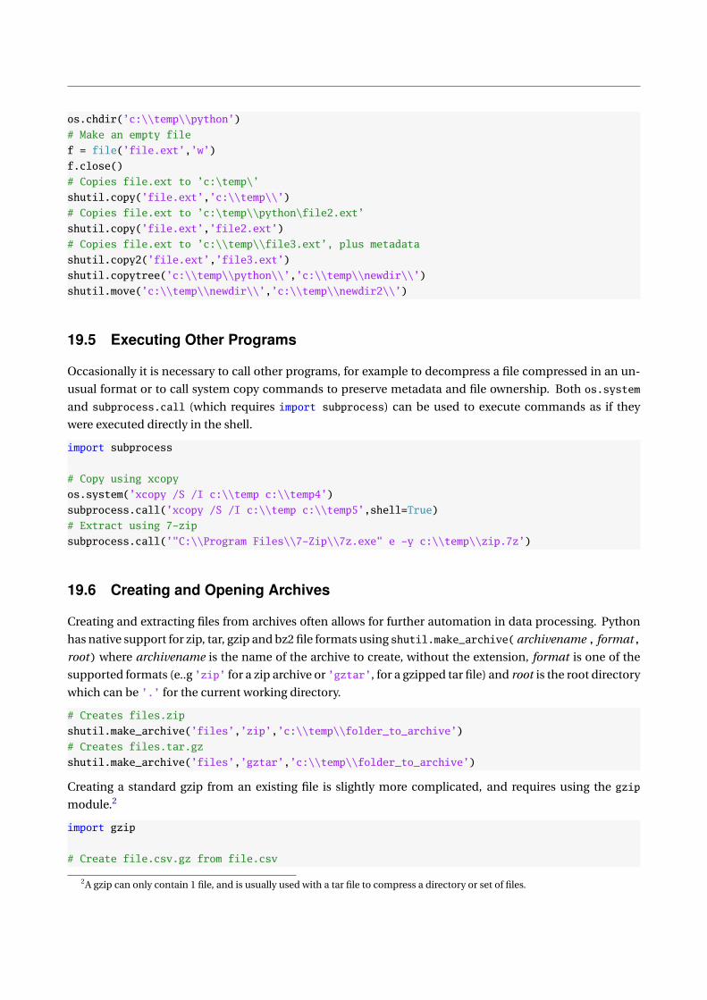
os.chdir(’c:\\temp\\python’)
# Make an empty file
f = file(’file.ext’,’w’)
f.close()
# Copies file.ext to ’c:\temp\’
shutil.copy(’file.ext’,’c:\\temp\\’)
# Copies file.ext to ’c:\temp\\python\file2.ext’
shutil.copy(’file.ext’,’file2.ext’)
# Copies file.ext to ’c:\\temp\\file3.ext’, plus metadata
shutil.copy2(’file.ext’,’file3.ext’)
shutil.copytree(’c:\\temp\\python\\’,’c:\\temp\\newdir\\’)
shutil.move(’c:\\temp\\newdir\\’,’c:\\temp\\newdir2\\’)
19.5 Executing Other Programs
Occasionally it is necessary to call other programs, for example to decompress a file compressed in an un-
usual format or to call system copy commands to preserve metadata and file ownership. Both os.system
and subprocess.call (which requires import subprocess) can be used to execute commands as if they
were executed directly in the shell.
import subprocess
# Copy using xcopy
os.system(’xcopy /S /I c:\\temp c:\\temp4’)
subprocess.call(’xcopy /S /I c:\\temp c:\\temp5’,shell=True)
# Extract using 7-zip
subprocess.call(’"C:\\Program Files\\7-Zip\\7z.exe" e -y c:\\temp\\zip.7z’)
19.6 Creating and Opening Archives
Creating and extracting files from archives often allows for further automation in data processing. Python
has native support for zip, tar, gzip and bz2 file formats using shutil.make_archive( archivename , format,
root) where archivename is the name of the archive to create, without the extension, format is one of the
supported formats (e..g ’zip’ for a zip archive or ’gztar’, for a gzipped tar file) and root is the root directory
which can be ’.’ for the current working directory.
# Creates files.zip
shutil.make_archive(’files’,’zip’,’c:\\temp\\folder_to_archive’)
# Creates files.tar.gz
shutil.make_archive(’files’,’gztar’,’c:\\temp\\folder_to_archive’)
Creating a standard gzip from an existing file is slightly more complicated, and requires using the gzip
module.2
import gzip
# Create file.csv.gz from file.csv
2A gzip can only contain 1 file, and is usually used with a tar file to compress a directory or set of files.

csvin = file(’file.csv’,’rb’)
gz = gzip.GzipFile(’file.csv.gz’,’wb’)
gz.writelines(csvin.read())
gz.close()
csvin.close()
Zip files can be extracted using the module zipfile, and gzip files can be extracted using gzip, and
gzipped tar files can be extracted using tarfile.
import zipfile
import gzip
import tarfile
# Extract zip
zip = zipfile.ZipFile(’files.zip’)
zip.extractall(’c:\\temp\\zip\\’)
zip.close()
# Extract gzip tar ’r:gz’ indicates read gzipped
gztar = tarfile.open(’file.tar.gz’, ’r:gz’)
gztar.extractall(’c:\\temp\\gztar\\’)
gztar.close()
# Extract csv from gzipped csv
gz = gzip.GzipFile(’file.csv.gz’,’rb’)
csvout = file(’file.csv’,’wb’)
csvout.writelines(gz.read())
csvout.close()
gz.close()
19.7 Reading and Writing Files
Occasionally it may be necessary to read or write a file, for example to output a formatted LATEX table. Python
contains low level file access tools which can be used to to generate files with any structure. Custom files all
begin by using file to create a new or open an existing file. Files can be opened in different modes, ’r’ for
reading, ’w’ for writing, and ’a’ for appending (’w’ will overwrite an existing file). An additional modifier ’b’
can be be used if the file is binary (not text), so that ’rb’, ’wb’ and ’ab’ allow reading, writing and appending
binary files.
Reading text files is usually implemented using readline() to read a single line, readlines( n) to read
at most n lines or readlines() to read all lines in a file. readline() and readlines( n) are usually used
inside a while loop which terminates if teh value retured is an empty string (’’).
# Read all lines using readlines()
f = file(’file.csv’,’r’)
lines = f.readlines()
for line in lines:
print(line)
f.close()

# Using readline(n)
f = file(’file.csv’,’r’)
line = f.readline()
while line != ’’:
print(line)
line = f.readline()
f.close()
# Using readlines(n)
f = file(’file.csv’,’r’)
lines = f.readlines(2)
while lines != ’’:
for line in lines:
print(line)
lines = f.readline(2)
f.close()
In practice, the information from the file is usually transformed in a more meaningful way than using print.
Writing text files is similar, and begins by using file to create a file, and then fwrite to output informa-
tion. frwite is conceptually similar to using print, except that the output will be written to a file rather than
printed on screen. The next example show how to create a LATEXtable from an array.
import numpy as np
import scipy.stats as stats
x = np.random.randn(100,4)
mu = np.mean(x,0)
sig = np.std(x,0)
sk = stats.skew(x,0)
ku = stats.kurtosis(x,0)
summaryStats = np.vstack((mu,sig,sk,ku))
rowHeadings = [’Var 1’,’Var 2’,’Var 3’,’Var 4’]
colHeadings = [’Mean’,’Std Dev’,’Skewness’,’Kurtosis’]
# Build table, then print
latex = []
latex.append(’\\begintabularr|rrrr’)
line = ’ ’
for i in xrange(len(colHeadings)):
line += ’ & ’ + rowHeadings[i]
line += ’ \\ \hline’
latex.append(line)
for i in xrange(size(summaryStats,0)):
line = rowHeadings[i]
for j in xrange(size(summaryStats,1)):

line += ’ & ’ + str(summaryStats[i,j])
latex.append(line)
latex.append(’\\endtabular’)
# Output using write()
f = file(’latex_table.tex’,’w’)
for line in latex:
f.write(line + ’\n’)
f.close()
19.8 Exercises
1. Create a new directory, chapter19.
2. Change into this directory.
3. Create a new file names tobedeleted.py a text editor in this new directory (It can be empty).
4. Create a zip file tobedeleted.zip containing tobedeleted.py.
5. Get and print the directory listing.
6. Delete the newly created file, and then delete this directory.
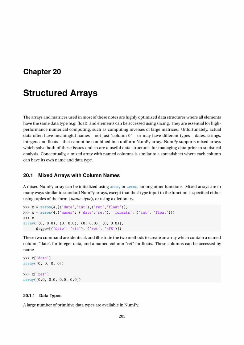
Chapter 20
Structured Arrays
The arrays and matrices used in most of these notes are highly optimized data structures where all elements
have the same data type (e.g. float), and elements can be accessed using slicing. They are essential for high-
performance numerical computing, such as computing inverses of large matrices. Unfortunately, actual
data often have meaningful names – not just “column 0” – or may have different types – dates, strings,
integers and floats – that cannot be combined in a uniform NumPy array. NumPy supports mixed arrays
which solve both of these issues and so are a useful data structures for managing data prior to statistical
analysis. Conceptually, a mixed array with named columns is similar to a spreadsheet where each column
can have its own name and data type.
20.1 Mixed Arrays with Column Names
A mixed NumPy array can be initialized using array or zeros, among other functions. Mixed arrays are in
many ways similar to standard NumPy arrays, except that the dtype input to the function is specified either
using tuples of the form (name,type), or using a dictionary.
>>> x = zeros(4,[(’date’,’int’),(’ret’,’float’)])
>>> x = zeros(4,’names’: (’date’,’ret’), ’formats’: (’int’, ’float’))
>>> x
array([(0, 0.0), (0, 0.0), (0, 0.0), (0, 0.0)],
dtype=[(’date’, ’<i4’), (’ret’, ’<f8’)])
These two command are identical, and illustrate the two methods to create an array which contain a named
column “date”, for integer data, and a named column “ret” for floats. These columns can be accessed by
name.
>>> x[’date’]
array([0, 0, 0, 0])
>>> x[’ret’]
array([0.0, 0.0, 0.0, 0.0])
20.1.1 Data Types
A large number of primitive data types are available in NumPy.
205
Type Syntax Description
Boolean b True/False
Integers i1,i2,i4,i8 1 to 8 byte signed integers (−2B−1, . . . 2B−1 − 1)
Unsigned Integers u1,u2,u4,u8 1 to 8 byte signed integers (0, . . . 2B )
Floating Point f4,f8 Single (4) and double (8) precision float
Complex c8,c16 Single (8) and double (16) precision complex
Object On Generic n-byte object
String Sn , an n-letter string
Unicode String Un n-letter unicode string
The majority of data types are for numeric data, and are simple to understand. The n in the string data
type indicates the maximum length of a string. Attempting to insert a stringer with more than n characters
will truncate the string. The object data type is somewhat abstract, but allows for storing Python objects
such as datetimes.
Custom data types can be built using dtype. The constructed data type can then be used in the con-
struction of a mixed array.
t = dtype([(’var1’,’f8’), (’var2’,’i8’), (’var3’,’u8’)])
Data types can even be nested to create a structured environment where one of the “variables” has multiple
values. Consider this example which uses a nested data type to contain the bid and ask price or a stock,
along with the time of the transaction.
ba = dtype([(’bid’,’f8’), (’ask’,’f8’)])
t = dtype([(’date’, ’O8’), (’prices’, ba)])
data = zeros(2,t)
In this example, data is an array where each item has 2 elements, the date and the price. Price is also an array
with 2 elements. Names can also be used to access values in nested arrays (e.g. data[’prices’][’bid’]
returns an array containing all bid prices). In practice nested arrays can almost always be expressed as a
non-nested array without loss of fidelity.
Determining the size of object NumPy arrays can store objects which are anything which fall outside of the
usual data types. One example of a useful, but abstract, data type is datetime. One method to determine
the size of an object is to create a plain array containing the object – which will automatically determine the
data type – and then to query the size from the array.
import datetime as dt
x = array([dt.datetime.now()])
# The size in bytes
print(x.dtype.itemsize)
# The name and description
print(x.dtype.descr)
20.1.2 Example: TAQ Data
TAQ is the NYSE Trade and Quote database which contains all trades and quotes of US listed equities which
trade on major US markets (not just the NYSE). A record from a trade contains a number of fields:

• Date - The Date in YYYYMMDD format stored as a 4-byte unsigned integer
• Time - Time in HHMMSS format, stored as a 4-byte unsigned integer
• Size - Number of shares trades, stores as a 4 byte unsigned integer
• G127 rule indicator - Numeric value, stored as a 2 byte unsigned integer
• Correction - Numeric indicator of a correction, stored as a 2 byte unsigned integer
• Condition - Market condition, a 2 character string
• Exchange - The exchange where the trade occurred, a 1-character string
First consider a data type which stores the data in an identical format.
t = dtype([(’date’, ’u4’), (’time’, ’u4’),
(’size’, ’u4’), (’price’, ’f8’),
(’g127’, ’u2’), (’corr’, ’u2’),
(’cond’, ’S2’), (’ex’, ’S2’)])
taqData = zeros(10, dtype=t)
taqData[0] = (20120201,120139,1,53.21,0,0,’’,’N’)
An alternative is to store the date and time as a datetime, which is an 8-byte object.
import datetime as dt
t = dtype([(’datetime’, ’O8’), (’size’, ’u4’), (’price’, ’f8’),
(’g127’, ’u2’), (’corr’, ’u2’), (’cond’, ’S2’), (’ex’, ’S2’)])
taqData = zeros(10, dtype=t)
taqData[0] = (dt.datetime(2012,2,1,12,01,39),1,53.21,0,0,’’,’N’)
20.2 Record Arrays
Record arrays are closely related to mixed arrays with names. The primary difference is that elements record
arrays can be accessed using variable.name format.
>>> x = zeros((4,1),[(’date’,’int’),(’ret’,’float’)])
>>> y = rec.array(x)
>>> y.date
array([[0],
[0],
[0],
[0]])
>>> y.date[0]
array([0])
In practice record arrays may be slower than standard arrays, and unless the variable.name is really impor-
tant, record arrays are not compelling.

Chapter 21
Performance and Code Optimization
We should forget about small efficiencies, say about 97% of the time: premature optimization
is the root of all evil.
Donald Knuth
21.1 Getting Started
Occasionally a direct implementation of a statistical algorithm will not be fast enough to be applied to in-
teresting data sets. When this happens, there are a number of alternatives. Before starting to optimize code,
it is essential that a clean, working implementation has been coded. This allows for both benchmarking
improvements and to ensure that optimizations have not introduced bugs to code. The famous quote of
Donald Knuth should also be heeded. Code optimization is only needed for a very small amount of code
which is repeatedly used. Most code, on modern computers, is sufficiently fast and/or infrequently used
that optimization is a wasted effort.
21.2 Timing Code
Timing code is an important step in performance tuning. IPython contains the magic keywords %timeit and
%time which can be used to determine the performance of code. %time simply runs the code and reports
the time needed. %timeit is smarter in that it will loop very fast code which will increase the accuracy of the
timing measurements. Both are used in the same manner, %timeit code to time.
>>> x = randn(1000,1000)
>>> %timeit inv(dot(x.T,x))
1 loops, best of 3: 387 ms per loop
>>> %time inv(dot(x.T,x))
CPU times: user 0.52 s, sys: 0.00 s, total: 0.52 s
Wall time: 0.52 s
>>> x = randn(100,100)
209

>>> %timeit inv(dot(x.T,x))
1000 loops, best of 3: 797 us per loop
21.3 Vectorize to Avoid Unnecessary Loops
Vectorization is the key to getting top performance out of NumPy code. Code that is vectorized run inside
NumPy and so executes as quickly as possible (with some small technical caveats, see NumExpr). Consider
the difference between manually multiplying two matrices and using dot.
def pydot(a, b):
M,N = shape(a)
P,Q = shape(b)
assert N==P
c = zeros((M,Q))
for i in xrange(M):
for j in xrange(Q):
for k in xrange(N):
c[i,j] = c[i,j] + a[i,k] * b[k,j]
return c
Timing the difference shows that in this extreme case, NumPy is about 10000x faster than looping Python.
>>> a = randn(100,100)
>>> b = randn(100,100)
>>> %timeit c = pydot(a,b)
1 loops, best of 3: 1.27 s per loop
>>> %timeit d = dot(a,b)
10000 loops, best of 3: 165 us per loop
>>> absolute(c-d).max()
0.0
>>> 1.72/0.000165
10424.242424
A less absurd example is to consider computing a weighted moving average across m consecutive values of
a vector.
def naive_weighted_avg(x, w):
T = x.shape[0]
m = len(w)
m12 = int(ceil(m/2))
y = zeros(T)
for i in xrange(len(x)-m+1):
y[i+m12] = dot(x[i:i+m].T,w)
return y

>>> w = r_[1:11,9:0:-1]
>>> w = w/sum(w)
>>> x = randn(10000,1)
>>> %timeit naive_weighted_avg(x,w)
100 loops, best of 3: 22.6 ms per loop
def clever_weighted_avg(x,w):
T = x.shape[0]
m = len(w)
wc = copy(w)
wc.shape = m,1
T = x.size
xc = copy(x)
xc.shape=T,1
y = vstack((xc,zeros((m,1))))
y = tile(y,(m,1))
y = reshape(y[:len(y)-m],(m,T+m-1))
y = y.T
y = y[m-1:T,:]
return dot(y,flipud(wc))
>>> %timeit clever_weighted_avg(x,w)
1000 loops, best of 3: 1.31 ms per loop
The loop-free method which uses copying and slicing is about 20 times faster than the simple looping
specification.
21.4 Alter the loop dimensions
In many applications, it may be natural to loop over the long dimension in a time series. This is especially
common if the mathematical formula underlying the program has a sum of t = 1 to T . In some cases, it
is possible to replace a loop over time, which is assumed to be the larger dimension, with an alternative
loop across another iterable. For example, in the moving average, it is possible to loop over the weights
rather than the data, and if the moving windows length is much smaller than the length of the data, the
code should run much faster.
def sideways_weighted_avg(x, w):
T = x.shape[0]
m = len(w)
y = zeros(T)
m12 = int(ceil(m/2))
y = zeros(x.shape)
for i in xrange(m):
y[m12:T-m+m12] = x[i:T+i-m] * w[i]
return y
>>> %timeit sideways_weighted_avg(x,w)
1000 loops, best of 3: 574 us per loop
In this example, the “sideways” loop is much faster than fully vectorized version since it avoids allocating a
large amount of memory, and the loop dimension is very small.
21.5 Utilize Broadcasting
NumPy uses broadcasting for virtually all primitive mathematical operations (and for some more compli-
cated functions). Broadcasting avoids unnecessary multiplication of matrix repetition, and so improves
performance.
>>> x = randn(1000,1)
>>> y = randn(1,1000)
>>> %timeit x*y
100 loops, best of 3: 8.77 ms per loop
>>> %timeit dot(x,ones((1,1000))) * dot(ones((1000,1)),y)
10 loops, best of 3: 36.7 ms per loop
Broadcasting is about 4 times as fast as manually expanding the arrays.
21.6 Avoid Allocating Memory
Memory allocation is expensive, especially if it occurs inside a for loop. It is often better to pre-allocate
storage space for computed values, and also to reuse existing space.
21.7 Inline Frequent Function Calls
Function calls are fast but not completely free. Simple functions, especially inside loops, should be in-lined
to avoid the cost of calling functions.
21.8 Think about data storage
Arrays are stored using row major format, which means that data is stored across a row first, and then down
columns second. This means that in an m by n array, element i , j is stored next to elements i , j + 1 and
i , j − 1 (except when j is the first (previous is i − 1, n) or last element in a row (next is i + 1, 1)). Spatial
location matters for performance, and it is much faster to access data which is physically adjacent than it is
to access data adjacent in the array (i + 1, j ), but not as the array is stored in the computer’s memory. The
simplest method to understand array storage is to use:
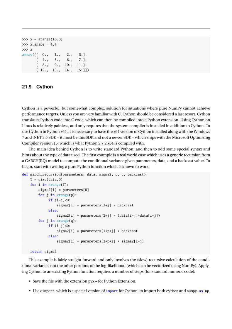
>>> x = arange(16.0)
>>> x.shape = 4,4
>>> x
array([[ 0., 1., 2., 3.],
[ 4., 5., 6., 7.],
[ 8., 9., 10., 11.],
[ 12., 13., 14., 15.]])
21.9 Cython
Cython is a powerful, but somewhat complex, solution for situations where pure NumPy cannot achieve
performance targets. Unless you are very familiar with C, Cython should be considered a last resort. Cython
translates Python code into C code, which can then be compiled into a Python extension. Using Cython on
Linux is relatively painless, and only requires that the system compiler is installed in addition to Cython. To
use Cython in Python x64, it is necessary to have the x64 version of Cython installed along with the Windows
7 and .NET 3.5 SDK – it must be this SDK and not a newer SDK – which ships with the Microsoft Optimizing
Compiler version 15, which is what Python 2.7.2 x64 is compiled with.
The main idea behind Cython is to write standard Python, and then to add some special syntax and
hints about the type of data used. The first example is a real world case which uses a generic recursion from
a GARCH(P,Q) model to compute the conditional variance given parameters, data, and a backcast value. To
begin, start with writing a pure Python function which is known to work.
def garch_recursion(parameters, data, sigma2, p, q, backcast):
T = size(data,0)
for i in xrange(T):
sigma2[i] = parameters[0]
for j in xrange(p):
if (i-j)<0:
sigma2[i] = parameters[1+j] * backcast
else:
sigma2[i] = parameters[1+j] * (data[i-j]*data[i-j])
for j in xrange(q):
if (i-j)<0:
sigma2[i] = parameters[1+p+j] * backcast
else:
sigma2[i] = parameters[1+p+j] * sigma2[i-j]
return sigma2
This example is fairly straight forward and only involves the (slow) recursive calculation of the condi-
tional variance, not the other portions of the log-likelihood (which can be vectorized using NumPy). Apply-
ing Cython to an existing Python function requires a number of steps (for standard numeric code):
• Save the file with the extension pyx – for Python Extension.
• Use cimport, which is a special version of import for Cython, to import both cython and numpy as np.
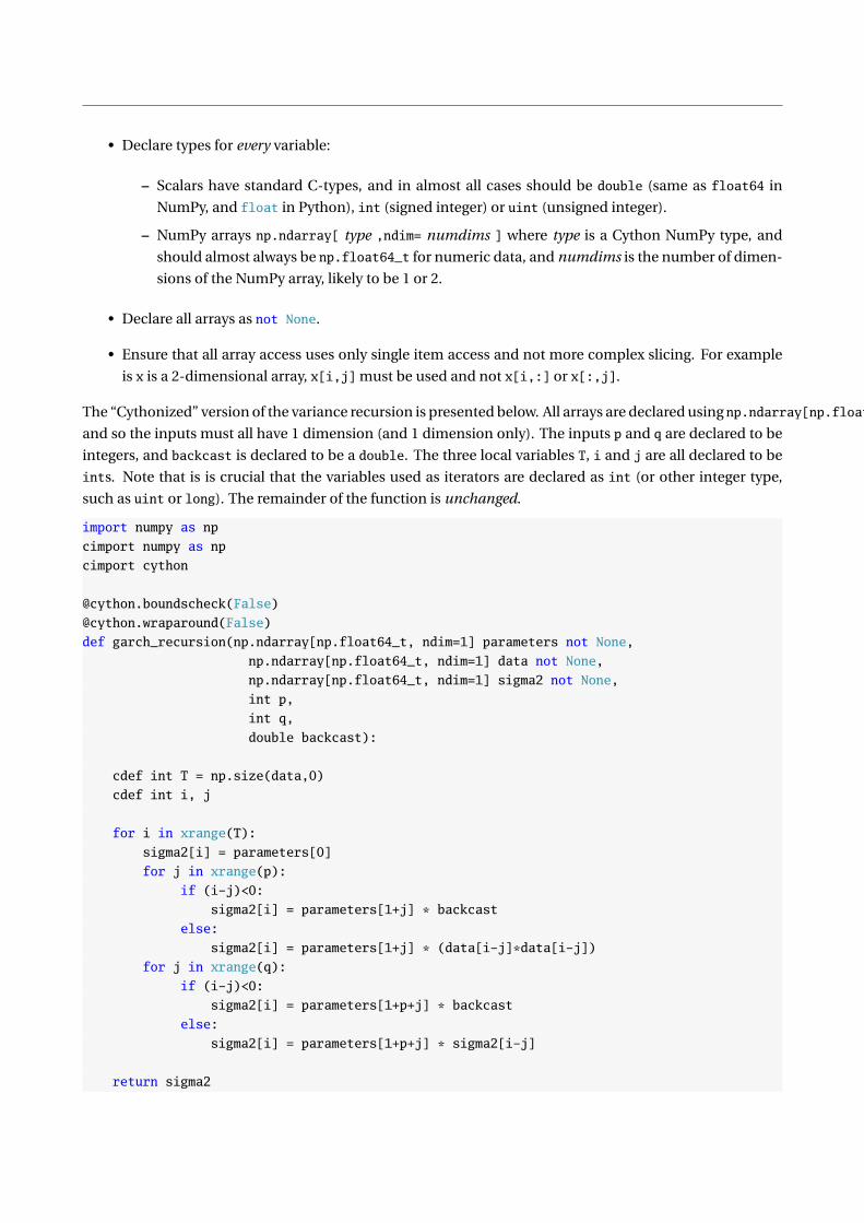
• Declare types for every variable:
– Scalars have standard C-types, and in almost all cases should be double (same as float64 in
NumPy, and float in Python), int (signed integer) or uint (unsigned integer).
– NumPy arrays np.ndarray[ type ,ndim= numdims ] where type is a Cython NumPy type, and
should almost always be np.float64_t for numeric data, and numdims is the number of dimen-
sions of the NumPy array, likely to be 1 or 2.
• Declare all arrays as not None.
• Ensure that all array access uses only single item access and not more complex slicing. For example
is x is a 2-dimensional array, x[i,j] must be used and not x[i,:] or x[:,j].
The “Cythonized” version of the variance recursion is presented below. All arrays are declared using np.ndarray[np.float64_t, ndim=1]
and so the inputs must all have 1 dimension (and 1 dimension only). The inputs p and q are declared to be
integers, and backcast is declared to be a double. The three local variables T, i and j are all declared to be
ints. Note that is is crucial that the variables used as iterators are declared as int (or other integer type,
such as uint or long). The remainder of the function is unchanged.
import numpy as np
cimport numpy as np
cimport cython
@cython.boundscheck(False)
@cython.wraparound(False)
def garch_recursion(np.ndarray[np.float64_t, ndim=1] parameters not None,
np.ndarray[np.float64_t, ndim=1] data not None,
np.ndarray[np.float64_t, ndim=1] sigma2 not None,
int p,
int q,
double backcast):
cdef int T = np.size(data,0)
cdef int i, j
for i in xrange(T):
sigma2[i] = parameters[0]
for j in xrange(p):
if (i-j)<0:
sigma2[i] = parameters[1+j] * backcast
else:
sigma2[i] = parameters[1+j] * (data[i-j]*data[i-j])
for j in xrange(q):
if (i-j)<0:
sigma2[i] = parameters[1+p+j] * backcast
else:
sigma2[i] = parameters[1+p+j] * sigma2[i-j]
return sigma2

Two additional lines were included in the Cython version of the function, @cython.boundscheck(False)
and @cython.wraparound(False). The first disables bounds checking which speeds up the final code, but is
dangerous if the loop has the wrong ending point. The second rules out the use of negative indices, which
is simple to verify and enforce. The @cython syntax means that these are only set for the next function and
wouldn’t affect any other code in the extension.
The next step is to code up a setup.py file which is used to build the actual extension. The code is
located in a file named garch_ext.pyx, which will be the name of the extension. The setup code is standard,
and is unlikely to require altering (aside from the extension and file name).
from distutils.core import setup
from distutils.extension import Extension
from Cython.Distutils import build_ext
import numpy
setup(
cmdclass = ’build_ext’: build_ext,
ext_modules = [Extension("garch_ext", ["garch_ext.pyx"])],
include_dirs = [numpy.get_include()]
)
The final step is to build the extension by running python setup.py build_ext --inplace from the termi-
nal. This will produce garch_ext.pyd which contains the compiled code.
>>> parameters = array([.1,.1,.8])
>>> data = randn(10000)
>>> sigma2 = zeros(shape(data))
>>> p,q = 1,1
>>> backcast = 1.0
>>> %timeit -n 100 garch_recursion(parameters, data, sigma2, p, q, backcast)
100 loops, best of 3: 27.7 ms per loop
>>> import garch_ext
>>> %timeit garch_ext.garch_recursion(parameters, data, sigma2, p, q, backcast)
10000 loops, best of 3: 134 us per loop
>>> .0277/.000134
The Cythonized version is about 200 times faster than the standard Python version, and only required about
3 minutes to write (after the main Python function has been written).
The function pydot was similarly Cythonized. This Cython program demonstrates how arrays should
be allocated within the function. Not that the Cython type for an array is np.float64_t which corresponds
to the usual NumPy data type of np.float64 (other _t types are available for different NumPy data types).
Again, it only required a couple of minutes to Cythonize the original Python function.
import numpy as np
cimport numpy as np
cimport cython
@cython.boundscheck(False)
@cython.wraparound(False)
def pydot(np.ndarray[np.float64_t, ndim=2] a not None,
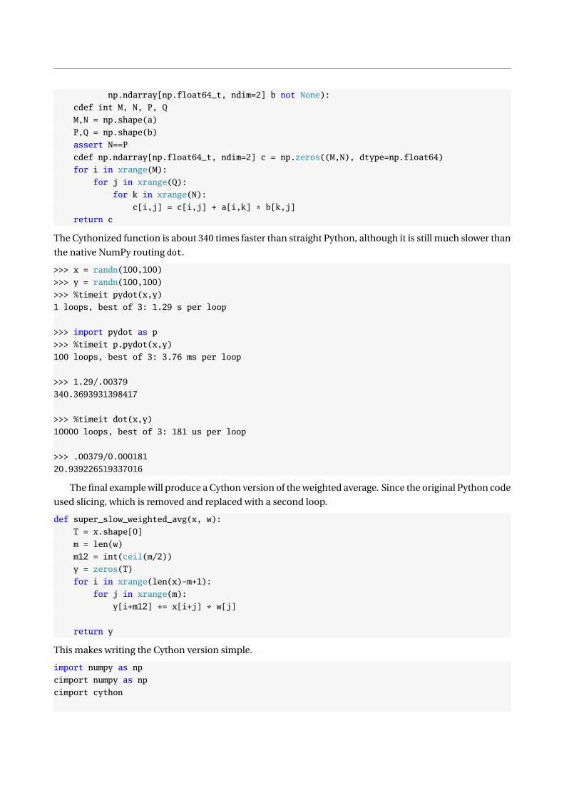
np.ndarray[np.float64_t, ndim=2] b not None):
cdef int M, N, P, Q
M,N = np.shape(a)
P,Q = np.shape(b)
assert N==P
cdef np.ndarray[np.float64_t, ndim=2] c = np.zeros((M,N), dtype=np.float64)
for i in xrange(M):
for j in xrange(Q):
for k in xrange(N):
c[i,j] = c[i,j] + a[i,k] * b[k,j]
return c
The Cythonized function is about 340 times faster than straight Python, although it is still much slower than
the native NumPy routing dot.
>>> x = randn(100,100)
>>> y = randn(100,100)
>>> %timeit pydot(x,y)
1 loops, best of 3: 1.29 s per loop
>>> import pydot as p
>>> %timeit p.pydot(x,y)
100 loops, best of 3: 3.76 ms per loop
>>> 1.29/.00379
340.3693931398417
>>> %timeit dot(x,y)
10000 loops, best of 3: 181 us per loop
>>> .00379/0.000181
20.939226519337016
The final example will produce a Cython version of the weighted average. Since the original Python code
used slicing, which is removed and replaced with a second loop.
def super_slow_weighted_avg(x, w):
T = x.shape[0]
m = len(w)
m12 = int(ceil(m/2))
y = zeros(T)
for i in xrange(len(x)-m+1):
for j in xrange(m):
y[i+m12] += x[i+j] * w[j]
return y
This makes writing the Cython version simple.
import numpy as np
cimport numpy as np
cimport cython

@cython.boundscheck(False)
@cython.wraparound(False)
def cython_weighted_avg(np.ndarray[np.float64_t, ndim=1] x,
np.ndarray[np.float64_t, ndim=1] w):
cdef int T, m, m12, i, j
T = x.shape[0]
m = len(w)
m12 = int(np.ceil(float(m)/2))
cdef np.ndarray[np.float64_t, ndim=1] y = np.zeros(T, dtype=np.float64)
for i in xrange(T-m+1):
for j in xrange(m):
y[i+m12] += x[i+j] * w[j]
return y
The Cython version can be compiled using a setup function in the same way that the GARCH recursion
was compiled.
>>> %timeit super_slow_weighted_avg(x,w)
1 loops, best of 3: 195 ms per loop
>>> import cython_weighted_avg as c
>>> %timeit c.cython_weighted_avg(x,w)
1000 loops, best of 3: 688 us per loop
The gains are unsurprisingly large (about 300×) – however, the Cython code is no faster than the sideways
version. This shows that Cython is not a magic bullet and that good vectorized code, even with a small
amount of looping, can be very fast.
21.10 Exercises
1. Write a Python function which will accept a p+q+1 vector of parameters, a T vector of data, and p and
q (integers, AR and MA order, respectively) and recursively computes the the ARMA error beginning
with observation p + 1. If an MA index is negative it should be backcast to 0.
2. [Only for the brave] Convert the function written in the previous function to Cython, compile it, and
compare the pure Python implementation to Cython.


Chapter 22
Examples
These examples are all actual econometric problems chosen to demonstrate the use of Python in an end-
to-end manner, form importing data to presenting estimates. A reasonable familiarity with the underlying
econometric models and methods is assumed so that the focus can be on the translation of mathematics to
Python.
22.1 Estimating the Parameters of a GARCH Model
This example will highlight the steps needed to estimate the parameters of a GJR-GARCH(1,1,1) model with
a constant mean. The volatility dynamics in a GJR-GARCH model are given by
σ2t = ω +
p∑i=1
αi r 2t−i +
o∑j=1
γj r 2t−j I [rt−j<0] +
q∑k=1
βkσ2t−k .
Returns are assumed to be conditionally normal, rt |Ft−1 ∼ N(µ,σ2
t
), and parameters are estimated by
maximum likelihood. To estimate the parameters, it is necessary to:
1. Produce some starting values
2. Estimate the parameters using (quasi) maximum likelihood
3. Compute standard errors using a “sandwich” covariance estimator (also known as the Bollerslev &
Wooldridge (1992) covariance estimator)
The first task is to write the log-likelihood which can be used in an optimizer. The log-likelihood function
will compute the recursion and the log-likelihood. It will also, optionally, return the T by 1 vector of indi-
vidual log-likelihoods which are useful for numerically computing the scores.
First, I will discuss the imports needed for this. I prefer to use the import form frommodule import func1,
func2 for commonly used functions. This both saves typing and increases code readability. For functions
which are used less, I use import module as shortname. This is a personal choice, and any combination is
acceptable, although from module import * should be avoided.
import numpy as np
import matplotlib.pyplot as plt
from numpy import size, log, pi, sum, diff, array, zeros, diag, dot, mat, asarray, sqrt
219

from numpy.linalg import inv
from scipy.optimize import fmin_slsqp
from matplotlib.mlab import csv2rec
The log-likelihood can be defined using the normal log-likelihood
ln f(
rt |µ,σ2t
)= −1
2
(ln 2π + lnσ2
t +
(rt − µ
)2
σ2t
),
which is negated in the code since the optimizers all minimize.
def gjr_garch_likelihood(parameters, data, sigma2, out=None):
’’’ Returns likelihood for GJR-GARCH(1,1,1) model.’’’
mu = parameters[0]
omega = parameters[1]
alpha = parameters[2]
gamma = parameters[3]
beta = parameters[4]
T = size(data,0)
eps = data - mu
# Data and sigma2 are T by 1 vectors
for t in xrange(1,T):
sigma2[t] = (omega + alpha * eps[t-1]**2
+ gamma * eps[t-1]**2 * (eps[t-1]<0) + beta * sigma2[t-1])
logliks = 0.5*(log(2*pi) + log(sigma2) + eps**2/sigma2)
loglik = sum(logliks)
if out is None:
return loglik
else:
return loglik, logliks, copy(sigma2)
The keyword argument out has a default value of None, and is used to determine whether to return 1 output
or 3. This is common practice since the optimizer requires a single output – the log-likelihood function
value, but it is also useful to be able to output other useful quantities, such asσ2
t
.
The optimization is constrained so that α + γ/2 + β ≤ 1, which constraint function.
def gjr_constraint(parameters, data, sigma2, out=None):
’’’ Constraint that alpha+gamma/2+beta<=1’’’
alpha = parameters[2]
gamma = parameters[3]
beta = parameters[4]
return array([1-alpha-gamma/2-beta])
The constraint function takes the same inputs as the negative of the log-likelihood function.
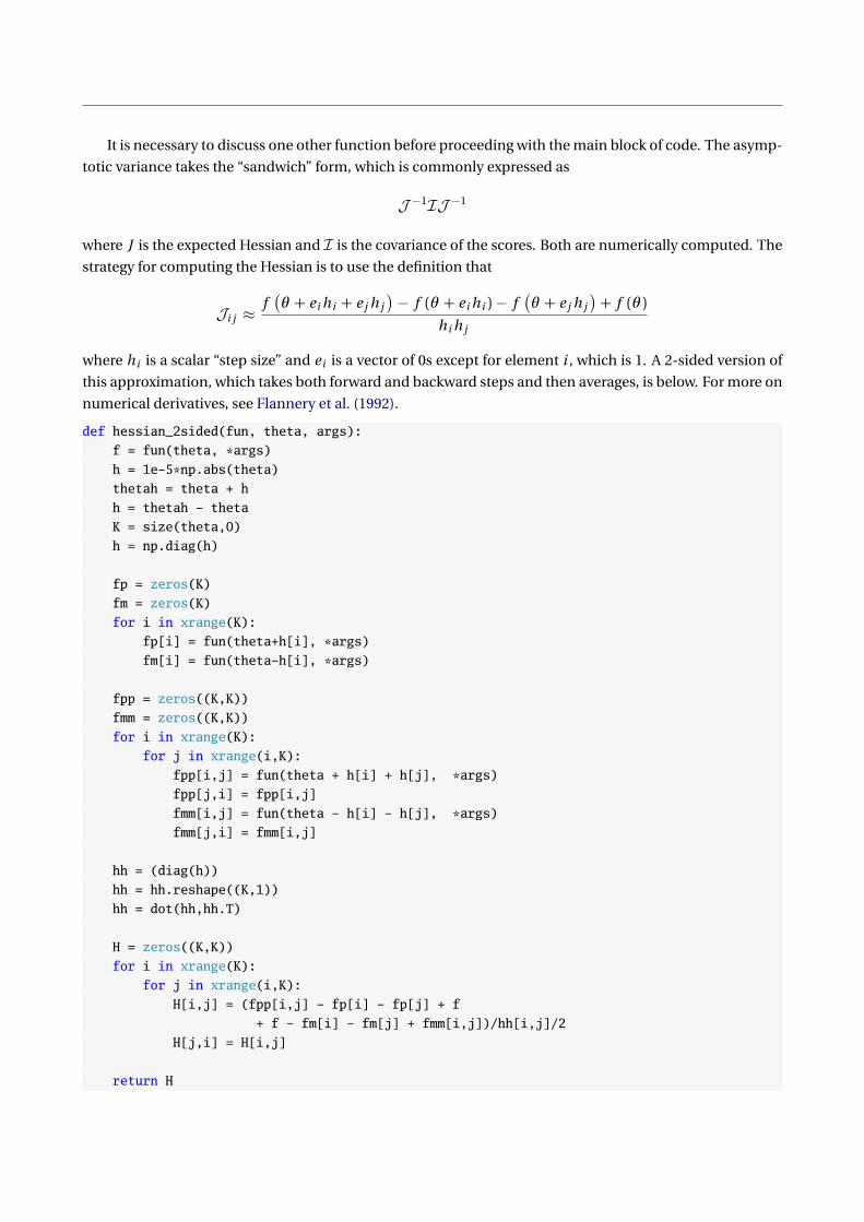
It is necessary to discuss one other function before proceeding with the main block of code. The asymp-
totic variance takes the “sandwich” form, which is commonly expressed as
J −1IJ −1
where J is the expected Hessian and I is the covariance of the scores. Both are numerically computed. The
strategy for computing the Hessian is to use the definition that
Ji j ≈f(θ + e i h i + e j h j
)− f (θ + e i h i )− f
(θ + e j h j
)+ f (θ )
h i h j
where h i is a scalar “step size” and e i is a vector of 0s except for element i , which is 1. A 2-sided version of
this approximation, which takes both forward and backward steps and then averages, is below. For more on
numerical derivatives, see Flannery et al. (1992).
def hessian_2sided(fun, theta, args):
f = fun(theta, *args)
h = 1e-5*np.abs(theta)
thetah = theta + h
h = thetah - theta
K = size(theta,0)
h = np.diag(h)
fp = zeros(K)
fm = zeros(K)
for i in xrange(K):
fp[i] = fun(theta+h[i], *args)
fm[i] = fun(theta-h[i], *args)
fpp = zeros((K,K))
fmm = zeros((K,K))
for i in xrange(K):
for j in xrange(i,K):
fpp[i,j] = fun(theta + h[i] + h[j], *args)
fpp[j,i] = fpp[i,j]
fmm[i,j] = fun(theta - h[i] - h[j], *args)
fmm[j,i] = fmm[i,j]
hh = (diag(h))
hh = hh.reshape((K,1))
hh = dot(hh,hh.T)
H = zeros((K,K))
for i in xrange(K):
for j in xrange(i,K):
H[i,j] = (fpp[i,j] - fp[i] - fp[j] + f
+ f - fm[i] - fm[j] + fmm[i,j])/hh[i,j]/2
H[j,i] = H[i,j]
return H
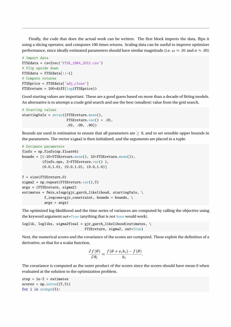
Finally, the code that does the actual work can be written. The first block imports the data, flips it
using a slicing operator, and computes 100 times returns. Scaling data can be useful to improve optimizer
performance, since ideally estimated parameters should have similar magnitude (i.e. ω ≈ .01 and α ≈ .05)
# Import data
FTSEdata = csv2rec(’FTSE_1984_2012.csv’)
# Flip upside down
FTSEdata = FTSEdata[::-1]
# Compute returns
FTSEprice = FTSEdata[’adj_close’]
FTSEreturn = 100*diff(log(FTSEprice))
Good starting values are important. These are a good guess based on more than a decade of fitting models.
An alternative is to attempt a crude grid search and use the best (smallest) value from the grid search.
# Starting values
startingVals = array([FTSEreturn.mean(),
FTSEreturn.var() * .01,
.03, .09, .90])
Bounds are used in estimation to ensure that all parameters are ≥ 0, and to set sensible upper bounds in
the parameters. The vector sigma2 is then initialized, and the arguments are placed in a tuple.
# Estimate parameters
finfo = np.finfo(np.float64)
bounds = [(-10*FTSEreturn.mean(), 10*FTSEreturn.mean()),
(finfo.eps, 2*FTSEreturn.var() ),
(0.0,1.0), (0.0,1.0), (0.0,1.0)]
T = size(FTSEreturn,0)
sigma2 = np.repeat(FTSEreturn.var(),T)
args = (FTSEreturn, sigma2)
estimates = fmin_slsqp(gjr_garch_likelihood, startingVals, \
f_ieqcons=gjr_constraint, bounds = bounds, \
args = args)
The optimized log-likelihood and the time series of variances are computed by calling the objective using
the keyword argument out=True (anything that is not None would work).
loglik, logliks, sigma2final = gjr_garch_likelihood(estimates, \
FTSEreturn, sigma2, out=True)
Next, the numerical scores and the covariance of the scores are computed. These exploit the definition of a
derivative, so that for a scalar function,
∂ f (θ )∂ θi
≈ f (θ + e i h i )− f (θ )h i
.
The covariance is computed as the outer product of the scores since the scores should have mean 0 when
evaluated at the solution to the optimization problem.
step = 1e-5 * estimates
scores = np.zeros((T,5))
for i in xrange(5):

h = step[i]
delta = np.zeros(5)
delta[i] = h
loglik, logliksplus, sigma2 = gjr_garch_likelihood(estimates + delta, \
FTSEreturn, sigma2, out=True)
loglik, logliksminus, sigma2 = gjr_garch_likelihood(estimates - delta, \
FTSEreturn, sigma2, out=True)
scores[:,i] = (logliksplus - logliksminus)/(2*h)
B = np.dot(scores.T,scores)/T
The final block of the numerical code calls hessian_2sided to estimate the Hessian, and finally computes
the asymptotic covariance.
A = hessian_2sided(gjr_garch_likelihood, estimates, args)
A = A/T
Ainv = mat(inv(A))
vcv = Ainv*mat(B)*Ainv/T
vcv = asarray(vcv)
The final steps are to pretty print the results and to produce a plot of the conditional variances,
output = np.vstack((estimates,sqrt(diag(vcv)),estimates/sqrt(diag(vcv)))).T
print(’Parameter Estimate Std. Err. T-stat’)
param = [’mu’,’omega’,’alpha’,’gamma’,’beta’]
for i in xrange(len(param)):
print(’0:<11 1:>0.6f 2:0.6f 3: 0.5f’.format(param[i],output[i,0],output[i,1],output[i,2]))
This final code block produce a plot of the annualized conditional standard deviations.
# Produce a plot
dates = FTSEdata[’date’][1:]
fig = plt.figure()
ax = fig.add_subplot(111)
ax.plot(dates,np.sqrt(252*sigma2))
fig.autofmt_xdate()
ax.set_ylabel(’Volatility’)
ax.set_title(’FTSE Volatility (GJR GARCH(1,1,1))’)
plt.show()
22.2 Estimating the Risk Premia using Fama-MacBeth Regressions
This example highlights how to implement a Fama-MacBeth 2-stage regression to estimate factor risk pre-
mia, make inference on the risk premia, and test whether a linear factor model can explain a cross-section
of portfolio returns. This example closely follows Cochrane (2001) (See also Jagannathan et al. (2010)). As in
the previous example, the first segment contains the imports.
from __future__ import print_function
from numpy import mat, dot, cov, mean, hstack, multiply,sqrt,diag, genfromtxt, \
squeeze, ones, array
from numpy.linalg import lstsq, inv

from scipy.stats import chi2
Next, the data are imported. I formatted the data downloaded from Ken French’s website into an easy-
to-import CSV which can be read by genfromtxt. The data is split using slicing, and the dimensions are
determined using shape. Finally the risk free rate is forces to have 2 dimensions so that it will be broad-
castable with the portfolio returns in order to construct the excess returns to the Size and Value-weighted
portfolios. Fama-MacBeth makes heavy use of matrix algebra, and so mat is used in the import statement to
ensure the imported data is a matrix. Since all other series are slices of a matrix, they are also matrices.
# Import data
data = mat(genfromtxt(’famafrench.csv’,delimiter=’,’))
# Split using slices
data = data[1:]
dates = data[:,0]
factors = data[:,1:4]
riskfree = data[:,4]
portfolios = data[:,5:]
# Shape information
T,K = factors.shape
T,N = portfolios.shape
# Reshape rf and compute excess returns
riskfree.shape = T,1
excessReturns = portfolios - riskfree
The next block does 2 things:
1. Compute the time-series βs. This is done be regressing the full array of excess returns on the factors
(augmented with a constant) using lstsq.
2. Compute the risk premia using a cross-sectional regression of average excess returns on the estimates
βs. This is a standard regression where the step 1 β estimates are used as regressors, and the depen-
dent variable is the average excess return.
# Time series regressions
X = hstack((ones((T,1)),factors))
out = lstsq(X,excessReturns)
alpha = out[0][0]
beta = out[0][1:]
avgExcessReturns = mean(excessReturns,0)
# Cross-section regression
out = lstsq(beta.T,avgExcessReturns.T)
lam = out[0]

The asymptotic variance requires computing the covariance of the demeaned returns and the weighted
pricing errors. The problem is formulated as a 2-step GMM estimation where the moment conditions are
g t (θ ) =
ε1t
ε1t f t
ε2t
ε2t f t...
εN t
εN t f t
βu t
where εi t = r e
i t − αi − β ′i f t , βi is a K by 1 vector of factor loadings, f t is a K by 1 set of factors, β =[β1 β2 . . .βN
]is a K by N matrix of all factor loadings, u t = r e
t − β ′λ are the N by 1 vector of pricing errors
and λ is a K by 1 vector of risk premia. θ =[α1 β
′1 α2 β
′2 . . . αN β
′N λ′]′To make inference on this problem,
the derivative of the moments with respect to the parameters, ∂ g t (θ ) /∂ θ ′ is needed. With some work, the
estimator of this matrix can be seen to be
G = E
[∂ g t (θ )∂ θ ′
]=
[−In ⊗ ΣX 0
G21 −ββ ′
].
where X t =[
1 f ′t]′
and ΣX = E[
X t X ′t]
. G21 is a matrix with the structure
G21 =[G21,1 G21,2 . . . G21,N
]where
G21,i =[
0K ,1 diag(
E [u i ]− βi λ) ]
and where E [u i ] is the expected pricing error. In estimation, all expectations are replaced with their sample
analogues.
# Moment conditions
X = hstack((ones((T,1)),factors))
p = vstack((alpha,beta))
epsilon = excessReturns - X*p
moments1 = kron(epsilon,ones((1,K+1)))
moments1 = multiply(moments1, kron(ones((1,N)),X))
u = excessReturns - lam.T*beta
moments2 = u*beta.T
# Score covariance
S = mat(cov(hstack((moments1,moments2)).T))
# Jacobian
G = mat(zeros((N*K+N+K,N*K+N+K)))
SigmaX = X.T*X/T
G[:N*K+N,:N*K+N] = kron(eye(N),SigmaX)
G[N*K+N:,N*K+N:] = -beta*beta.T
for i in xrange(N):
temp = zeros((K,K+1))
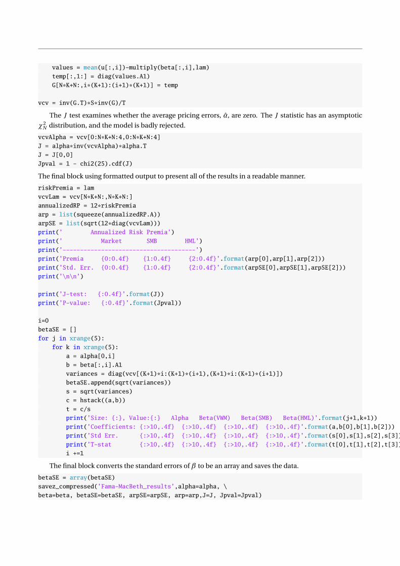
values = mean(u[:,i])-multiply(beta[:,i],lam)
temp[:,1:] = diag(values.A1)
G[N*K+N:,i*(K+1):(i+1)*(K+1)] = temp
vcv = inv(G.T)*S*inv(G)/T
The J test examines whether the average pricing errors, α, are zero. The J statistic has an asymptotic
χ2N distribution, and the model is badly rejected.
vcvAlpha = vcv[0:N*K+N:4,0:N*K+N:4]
J = alpha*inv(vcvAlpha)*alpha.T
J = J[0,0]
Jpval = 1 - chi2(25).cdf(J)
The final block using formatted output to present all of the results in a readable manner.
riskPremia = lam
vcvLam = vcv[N*K+N:,N*K+N:]
annualizedRP = 12*riskPremia
arp = list(squeeze(annualizedRP.A))
arpSE = list(sqrt(12*diag(vcvLam)))
print(’ Annualized Risk Premia’)
print(’ Market SMB HML’)
print(’--------------------------------------’)
print(’Premia 0:0.4f 1:0.4f 2:0.4f’.format(arp[0],arp[1],arp[2]))
print(’Std. Err. 0:0.4f 1:0.4f 2:0.4f’.format(arpSE[0],arpSE[1],arpSE[2]))
print(’\n\n’)
print(’J-test: :0.4f’.format(J))
print(’P-value: :0.4f’.format(Jpval))
i=0
betaSE = []
for j in xrange(5):
for k in xrange(5):
a = alpha[0,i]
b = beta[:,i].A1
variances = diag(vcv[(K+1)*i:(K+1)*(i+1),(K+1)*i:(K+1)*(i+1)])
betaSE.append(sqrt(variances))
s = sqrt(variances)
c = hstack((a,b))
t = c/s
print(’Size: :, Value:: Alpha Beta(VWM) Beta(SMB) Beta(HML)’.format(j+1,k+1))
print(’Coefficients: :>10,.4f :>10,.4f :>10,.4f :>10,.4f’.format(a,b[0],b[1],b[2]))
print(’Std Err. :>10,.4f :>10,.4f :>10,.4f :>10,.4f’.format(s[0],s[1],s[2],s[3]))
print(’T-stat :>10,.4f :>10,.4f :>10,.4f :>10,.4f’.format(t[0],t[1],t[2],t[3]))
i +=1
The final block converts the standard errors of β to be an array and saves the data.
betaSE = array(betaSE)
savez_compressed(’Fama-MacBeth_results’,alpha=alpha, \
beta=beta, betaSE=betaSE, arpSE=arpSE, arp=arp,J=J, Jpval=Jpval)

22.3 Estimating the Risk Premia using GMM
The final numeric example estimates examines the same problem, only using GMM rather than 2-stage
regression. The first block imports relevant modules and functions. GMM requires non-linear optimization,
and fmin_bfgs will be used.
from __future__ import print_function
from numpy import hstack, ones, array, mat, tile, dot, reshape, squeeze, eye
from numpy.linalg import lstsq, inv
from scipy.linalg import kron
from scipy.optimize import fmin_bfgs
import numpy as np
Before defining the problem, the next code block contains a callback function which is called after each
iteration of the minimizer. This function will be used to display information about the progress of the op-
timizer: the current function value, the iteration and the number of function calls. Because the callback
only gets 1 input, the current value of the parameters used by the optimizer, it is necessary to use global
variables to pass information between functions. Three variables have been declared as global, iteration,
lastValue and functionCount. iteration is updated only by the callback function since it should report the
number of completed iterations of the optimizer, and the callback is called once per iteration. lastValue
is updated each time the main GMM objective function is called, and functionCount is incremented by 1
each time the main GMM objective is called.
global iteration, lastValue, functionCount
iteration = 0
lastValue = 0
functionCount = 0
def iter_print(params):
global iteration, lastValue, functionCount
iteration += 1
print(’Func value: 0:, Iteration: 1:, Function Count: 2:’.format(lastValue, iteration, functionCount))
The GMM objective takes the parameters, portfolio returns, factor returns and the weighting matrix and
computes the moments, average moments and the objective value. The moments used can be described as(r 2
i t − βi f t
)f t ∀i = 1, . . . N
and
ri t − βiλ ∀i = 1, . . . N .
def gmm_objective(params, pRets, fRets, Winv, out=False):
global lastValue, functionCount
T,N = pRets.shape
T,K = fRets.shape
beta = squeeze(array(params[:(N*K)]))
lam = squeeze(array(params[(N*K):]))
beta = reshape(beta,(N,K))
lam = reshape(lam,(K,1))
betalam = dot(beta,lam)
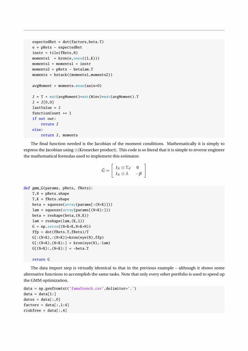
expectedRet = dot(factors,beta.T)
e = pRets - expectedRet
instr = tile(fRets,N)
moments1 = kron(e,ones((1,K)))
moments1 = moments1 * instr
moments2 = pRets - betalam.T
moments = hstack((moments1,moments2))
avgMoment = moments.mean(axis=0)
J = T * mat(avgMoment)*mat(Winv)*mat(avgMoment).T
J = J[0,0]
lastValue = J
functionCount += 1
if not out:
return J
else:
return J, moments
The final function needed is the Jacobian of the moment conditions. Mathematically it is simply to
express the Jacobian using⊗(Kronecker product). This code is so literal that it is simple to reverse engineer
the mathematical formulas used to implement this estimator.
G =
[IN ⊗ ΣF 0
IN ⊗ λ −β
]
def gmm_G(params, pRets, fRets):
T,N = pRets.shape
T,K = fRets.shape
beta = squeeze(array(params[:(N*K)]))
lam = squeeze(array(params[(N*K):]))
beta = reshape(beta,(N,K))
lam = reshape(lam,(K,1))
G = np.zeros((N*K+K,N*K+N))
ffp = dot(fRets.T,fRets)/T
G[:(N*K),:(N*K)]=kron(eye(N),ffp)
G[:(N*K),(N*K):] = kron(eye(N),-lam)
G[(N*K):,(N*K):] = -beta.T
return G
The data import step is virtually identical to that in the previous example – although it shows some
alternative functions to accomplish the same tasks. Note that only every other portfolio is used to speed up
the GMM optimization.
data = np.genfromtxt(’famafrench.csv’,delimiter=’,’)
data = data[1:]
dates = data[:,0]
factors = data[:,1:4]
riskfree = data[:,4]
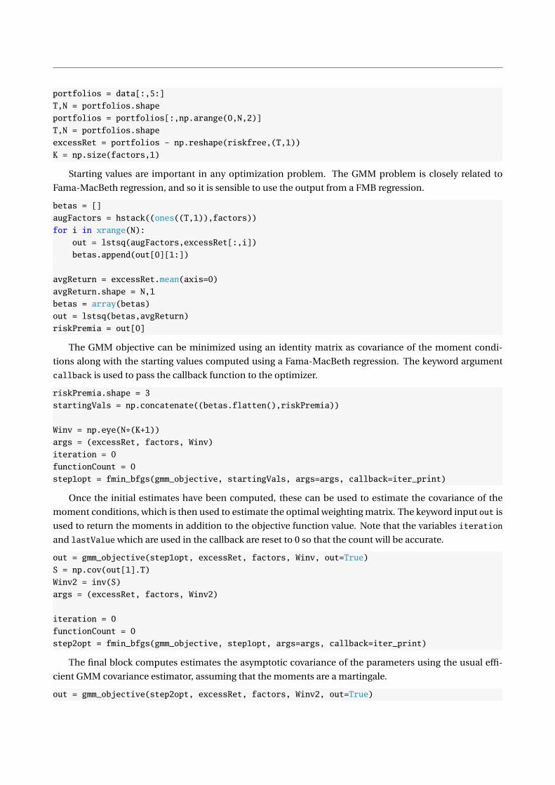
portfolios = data[:,5:]
T,N = portfolios.shape
portfolios = portfolios[:,np.arange(0,N,2)]
T,N = portfolios.shape
excessRet = portfolios - np.reshape(riskfree,(T,1))
K = np.size(factors,1)
Starting values are important in any optimization problem. The GMM problem is closely related to
Fama-MacBeth regression, and so it is sensible to use the output from a FMB regression.
betas = []
augFactors = hstack((ones((T,1)),factors))
for i in xrange(N):
out = lstsq(augFactors,excessRet[:,i])
betas.append(out[0][1:])
avgReturn = excessRet.mean(axis=0)
avgReturn.shape = N,1
betas = array(betas)
out = lstsq(betas,avgReturn)
riskPremia = out[0]
The GMM objective can be minimized using an identity matrix as covariance of the moment condi-
tions along with the starting values computed using a Fama-MacBeth regression. The keyword argument
callback is used to pass the callback function to the optimizer.
riskPremia.shape = 3
startingVals = np.concatenate((betas.flatten(),riskPremia))
Winv = np.eye(N*(K+1))
args = (excessRet, factors, Winv)
iteration = 0
functionCount = 0
step1opt = fmin_bfgs(gmm_objective, startingVals, args=args, callback=iter_print)
Once the initial estimates have been computed, these can be used to estimate the covariance of the
moment conditions, which is then used to estimate the optimal weighting matrix. The keyword input out is
used to return the moments in addition to the objective function value. Note that the variables iteration
and lastValue which are used in the callback are reset to 0 so that the count will be accurate.
out = gmm_objective(step1opt, excessRet, factors, Winv, out=True)
S = np.cov(out[1].T)
Winv2 = inv(S)
args = (excessRet, factors, Winv2)
iteration = 0
functionCount = 0
step2opt = fmin_bfgs(gmm_objective, step1opt, args=args, callback=iter_print)
The final block computes estimates the asymptotic covariance of the parameters using the usual effi-
cient GMM covariance estimator, assuming that the moments are a martingale.
out = gmm_objective(step2opt, excessRet, factors, Winv2, out=True)
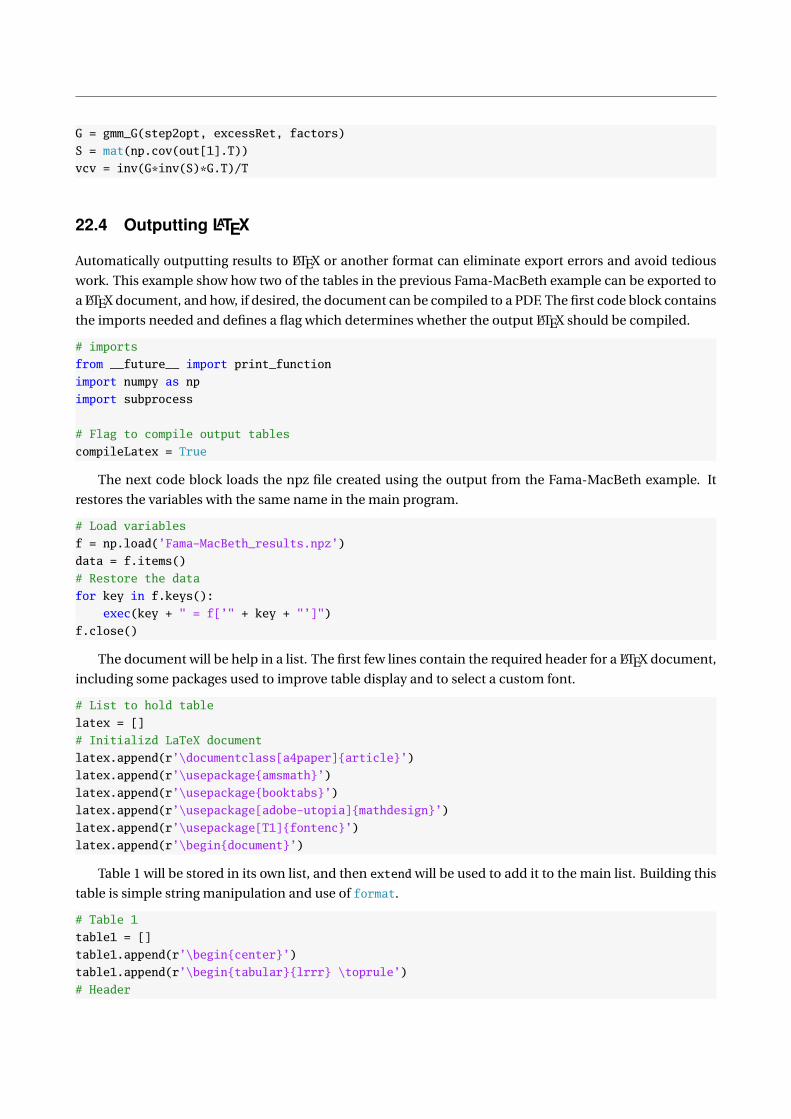
G = gmm_G(step2opt, excessRet, factors)
S = mat(np.cov(out[1].T))
vcv = inv(G*inv(S)*G.T)/T
22.4 Outputting LATEX
Automatically outputting results to LATEX or another format can eliminate export errors and avoid tedious
work. This example show how two of the tables in the previous Fama-MacBeth example can be exported to
a LATEX document, and how, if desired, the document can be compiled to a PDF. The first code block contains
the imports needed and defines a flag which determines whether the output LATEX should be compiled.
# imports
from __future__ import print_function
import numpy as np
import subprocess
# Flag to compile output tables
compileLatex = True
The next code block loads the npz file created using the output from the Fama-MacBeth example. It
restores the variables with the same name in the main program.
# Load variables
f = np.load(’Fama-MacBeth_results.npz’)
data = f.items()
# Restore the data
for key in f.keys():
exec(key + " = f[’" + key + "’]")
f.close()
The document will be help in a list. The first few lines contain the required header for a LATEX document,
including some packages used to improve table display and to select a custom font.
# List to hold table
latex = []
# Initializd LaTeX document
latex.append(r’\documentclass[a4paper]article’)
latex.append(r’\usepackageamsmath’)
latex.append(r’\usepackagebooktabs’)
latex.append(r’\usepackage[adobe-utopia]mathdesign’)
latex.append(r’\usepackage[T1]fontenc’)
latex.append(r’\begindocument’)
Table 1 will be stored in its own list, and then extend will be used to add it to the main list. Building this
table is simple string manipulation and use of format.
# Table 1
table1 = []
table1.append(r’\begincenter’)
table1.append(r’\begintabularlrrr \toprule’)
# Header

colNames = [r’VWM$^e$’,’SMB’,’HML’]
header = ’’
for cName in colNames:
header += ’ & ’ + cName
header += r’\\ \cmidrule2-4’
table1.append(header)
# Main row
row = ’’
for a,se in zip(arp,arpSE):
row += r’ & $\underset(0:0.3f)1:0.3f$’.format(se,a)
table1.append(row)
# Blank row
row = r’\\’
table1.append(row)
# J-stat row
row = r’J-stat: $\underset(0:0.3f)1:0.1f$ \\’.format(float(Jpval),float(J))
table1.append(row)
table1.append(r’\bottomrule \endtabular’)
table1.append(r’\endcenter’)
# Extend latex with table 1
latex.extend(table1)
latex.append(r’\newpage’)
Table 2 is a bit more complex, and uses loops to iterate over the rows of the arrays containing the βs and
their standard errors.
# Format information for table 2
sizes = [’S’,’2’,’3’,’4’,’B’]
values = [’L’,’2’,’3’,’4’,’H’]
# Table 2 has the same header as table 1, copy with a slice
table2 = table1[:3]
m = 0
for i in xrange(len(sizes)):
for j in xrange(len(values)):
row = ’Size: :, Value: : ’.format(sizes[i],values[j])
b = beta[:,m]
s = betaSE[m,1:]
for k in xrange(len(b)):
row += r’ & $\underset(0:0.3f)1: .3f$’.format(s[k],b[k])
row += r’\\ ’
table2.append(row)
m += 1
if i<(len(sizes)-1):
table2.append(r’\cmidrule2-4’)
table2.append(r’\bottomrule \endtabular’)
table2.append(r’\endcenter’)
# Extend with table 2
latex.extend(table2)

The penultimate block finished the document, and uses write to write the lines to the LATEX file. write
does not break lines, so the new line character is added to each (\n).
# Finish document
latex.append(r’\enddocument’)
# Write to table
fid = file(’latex.tex’,’w’)
for line in latex:
fid.write(line + ’\n’)
fid.close()
Finally, if the flag is set, subprocess is used to compile the LATEX. This assumes that pdflatex is on the
system path.
# Compile if needed
if compileLatex:
exitStatus = subprocess.call(r’pdflatex latex.tex’, shell=True)
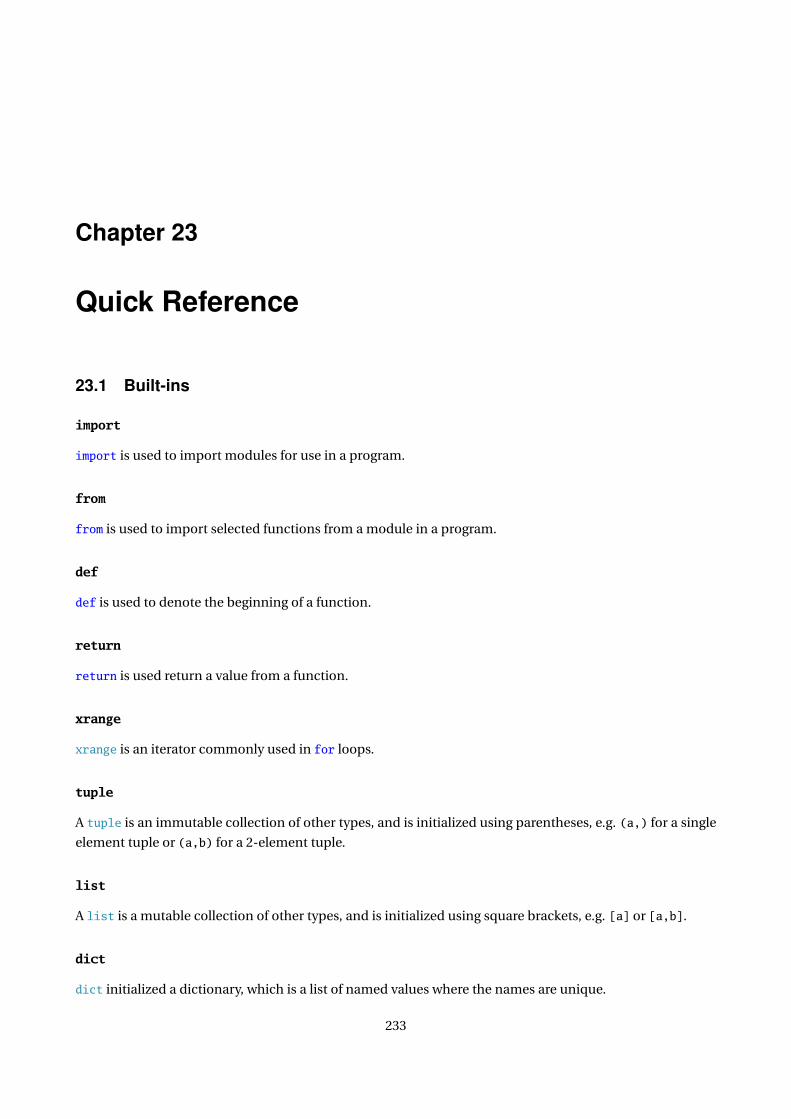
Chapter 23
Quick Reference
23.1 Built-ins
import
import is used to import modules for use in a program.
from
from is used to import selected functions from a module in a program.
def
def is used to denote the beginning of a function.
return
return is used return a value from a function.
xrange
xrange is an iterator commonly used in for loops.
tuple
A tuple is an immutable collection of other types, and is initialized using parentheses, e.g. (a,) for a single
element tuple or (a,b) for a 2-element tuple.
list
A list is a mutable collection of other types, and is initialized using square brackets, e.g. [a] or [a,b].
dict
dict initialized a dictionary, which is a list of named values where the names are unique.
233

set, frozenset
set initializes a set which is a unique, mutable collection. frozenset is an immutable counterpart.
for
for being a for loop, and should have the structure for var in iterable: .
while
while begins a while loop, and should have the structure while logical :
break
break terminates a loop prematurely.
continue
continue continues a loop without processing any code below the continue statement.
try
try begin a block which can handle code which may not succeed. It must be followed by an except state-
ment.
except
except catches errors generated in a try statement.
if
if begins an if . . . elif . . . else, and should have the structure if logical :
elif
elif stands for else if, and can be used after an if statement to refine the expression. It should have the
structure elif logical :
else
else finalizes an if block and executes if no previous path was taken.
print outputs information to the console. If used with from __future__ import print_function, print
behaves like a function.
file
file opens a file for low-level file reading and writing.

23.1.1 file Methods
File methods operate on a file object, which is initialized using file. For example, f = file(’text.txt’,’r’)
opens the file text.txt for reading, and close is used as f.close().
close
close closes an open file handle, and flushes any unwritten data to disk.
flush
flush flushes any unwritten data to disk without closing the file.
read
read reads data from an open file.
readline
readline reads a single line from an open file.
readlines
readlines reads one or more lines from an open file.
write
write writes a single line to a file without appending the new line character.
writelines
writelines writes the contents of an iterable (e.g. a list) to a file without appending the new line character
to each line.
23.1.2 String (str) Methods
String methods operate on strings. For example, strip can be used on a string x = ’abc ’ as x.strip(), or
can be directly used as ’ abc ’.strip().
split
split splits a string at every occurrence of another string, left to right.
rsplit
rsplit splits a string at every occurrence of another string, right to left.
join
join combines an iterable of strings using a given string to combine.
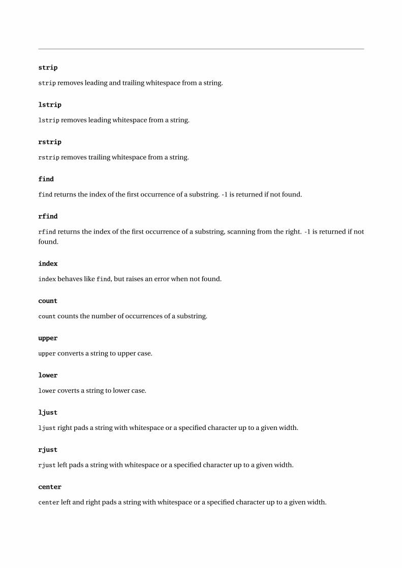
strip
strip removes leading and trailing whitespace from a string.
lstrip
lstrip removes leading whitespace from a string.
rstrip
rstrip removes trailing whitespace from a string.
find
find returns the index of the first occurrence of a substring. -1 is returned if not found.
rfind
rfind returns the index of the first occurrence of a substring, scanning from the right. -1 is returned if not
found.
index
index behaves like find, but raises an error when not found.
count
count counts the number of occurrences of a substring.
upper
upper converts a string to upper case.
lower
lower coverts a string to lower case.
ljust
ljust right pads a string with whitespace or a specified character up to a given width.
rjust
rjust left pads a string with whitespace or a specified character up to a given width.
center
center left and right pads a string with whitespace or a specified character up to a given width.
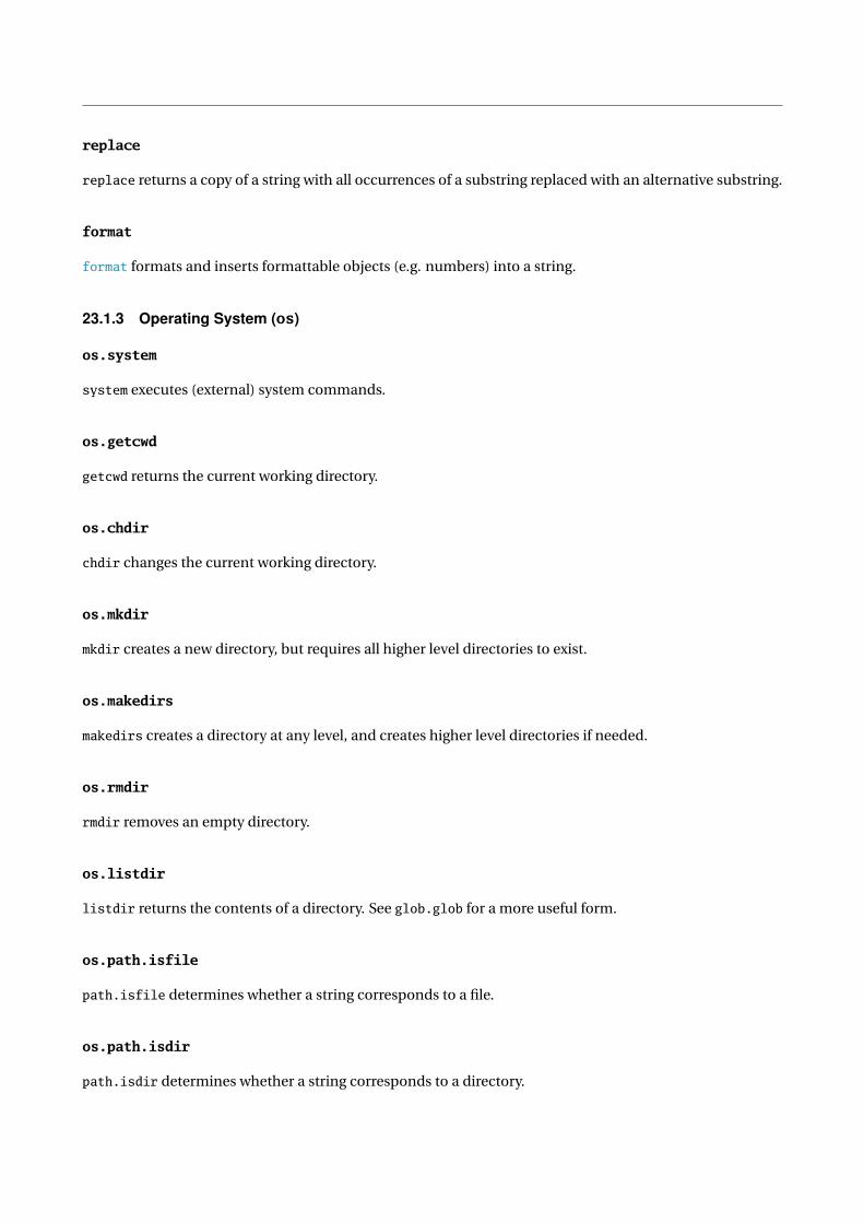
replace
replace returns a copy of a string with all occurrences of a substring replaced with an alternative substring.
format
format formats and inserts formattable objects (e.g. numbers) into a string.
23.1.3 Operating System (os)
os.system
system executes (external) system commands.
os.getcwd
getcwd returns the current working directory.
os.chdir
chdir changes the current working directory.
os.mkdir
mkdir creates a new directory, but requires all higher level directories to exist.
os.makedirs
makedirs creates a directory at any level, and creates higher level directories if needed.
os.rmdir
rmdir removes an empty directory.
os.listdir
listdir returns the contents of a directory. See glob.glob for a more useful form.
os.path.isfile
path.isfile determines whether a string corresponds to a file.
os.path.isdir
path.isdir determines whether a string corresponds to a directory.
23.1.4 Shell Utilities (shutil)
shutil.copy
copy copies a files using either a file name to use for the copy or a directory to use as a destination, in which
case the current file name is used.
shutil.copyfile
copyfile copies a file using a file name.
shutil.copy2
copy2 is identical to copy only that (some) file meta-data is also copied.
shutil.copytree
copytree copies an entire directory tree to a destination that must not exist.
shutil.move
move moves a directory tree to a destination which must not exist.
shutil.make_archive
make_archive creates zip, gztar and bztar archives.
shutil.rmtree
rmtree recursively removes a directory tree.
23.1.5 Regular Expressions (re)
re.findall
findall returns all occurrences of a regular expression in a string as a list.
re.split
split splits a string on occurrences of a regular expression.
re.sub
sub substitutes a string of each occurrence of a regular expression.
re.finditer
finditer works similarly to findall, only returning an iterable object rather than a list.

re.compile
compile compiles a regular expression for repeated use.
23.1.6 Dates and Times (datetime)
datetime.datetime
datetime initializes a date-time object.
datetime.date
date initializes a date object.
datetime.time
time initializes a time object.
datetime.timedelta
timedelta represents the difference between two datetimes.
datetime.datetime.replace
replace replaces fields in a date-time object. replace is a method of a date-time, date or time object.
datetime.datetime.combine
combine combines a date object and a time object and returns a date-time object. combine is a method of a
date-time, date or time object.
23.1.7 Other
These function all are contained in other modules, as listed to the left of the dot.
glob.glob
glob.glob returns a directory listing allowing for wildcards.
subprocess.call
subprocess.call can be used to run external commands.
textwrap.wrap
textwrap.wrap wraps a long block of text at a fixed width.

23.2 NumPy (numpy)
The functions listed in this section are all provided by NumPy. When a function is listed using only the
function name, this function appears in the NumPy module, and so can be accessed as numpy.function,
assuming that NumPy was imported using import numpy. When a function name contains a dot, for exam-
ple linalg.eig, then the function eig is in the linalg module of numpy, and so the function is accessed as
numpy.linalg.eig.
23.2.1 Core NumPy Types
dtype
dtype is used for constructing data types for use in arrays.
array
array is the primary method for constructing arrays from iterables (e.g. list or matrix). Variables created
using array have type numpy.ndarray.
matrix
matrix constructs a matrix from an iterable (e.g. list or array) that directly supports matrix mathemat-
ics. Variables created using matrix have type numpy.matrixlib.defmatrix.matrix, which is a subclass of
numpy.ndarray. Since matrix is a subclass of numpy.ndarray, it inherits the methods of numpy.ndarray.
23.2.2 ndarray
ndarray is the core array data type provided by NumPy. Both array (numpy.ndarray) and matrix (numpy.matrixlib.defmatrix.matrix)
offer a large number of attributes and methods. Attributes are accessed directly from an array, e.g. x.dtype,
and methods are calls to functions which operate on an array, e.g. x.sum().
Attributes
T
T returns the transpose of an array.
dtype
dtype returns the data type of an array.
flat
flat returns a 1-dimensional iterator for an array.
imag
imag returns the imaginary portion of an array.

real
real returns the real portion of an array.
size
size returns the total number of elements of an array.
ndim
ndim returns the number of dimensions of an array.
shape
shape returns the shape of an array as a tuple with ndim elements. shape can also be used to set the shape
using a tuple, e.g. x.shape=(10,5) as long as the number of elements does not change.
Methods
all
all returns True if all elements evaluate to True (i.e. not False, None or 0). axis can be used to compute
along a particular axis.
any
any returns True if any element evaluates to True. axis can be used to compute along a particular axis.
argmax
argmax returns the index of the maximum of an array. axis can be used to compute along a particular axis.
argmin
argmin returns the index of the minimum of an array. axis can be used to compute along a particular axis.
argsort
argsort returns the indices needed to sort an array. axis can be used to compute along a particular axis.
astype
astype allows an array to be viewed as another type (e.g. matrix or recarray) and copies the underlying.
conj, conjugate
conj and conjugate both return the complex-conjugate element-by-element.
copy
copy returns a copy of an array.
cumprod
cumprod returns the cumulative product of an array. axis can be used to compute along a particular axis.
cumsum
cumsum return the cumulative sum of an array. axis can be used to compute along a particular axis.
dot
dot computes the dot-product (standard matrix multiplication) or an array with another array.
flatten
flatten returns a copy of an array flattened into a 1-dimensional array.
max
max returns the maximum value of an array. axis can be used to compute along a particular axis.
mean
mean returns the average of an array. axis can be used to compute along a particular axis.
min
min returns the minimum of an array. axis can be used to compute along a particular axis.
nonzero
nonzero returns the indices of the non-zero elements of an array.
prod
prod computes the produce of all elements of an array. axis can be used to compute along a particular axis.
ravel
ravel returns a flattened view of an array without copying data.
repeat
repeat returns an array repeated, element-by-element.
reshape
reshape returns returns an array with a different shape. The number of elements must not change.

resize
resize changes the size shape of an array in-place. If the new size is larger then new entries are 0 filled. If
the new size is smaller, then the elements selected are ordered according too their order in ravel.
round
round returns an array with each element rounded to a provided number of decimals.
sort
sort sorts an array (in-place). axis can be used to compute along a particular axis.
squeeze
squeeze returns an array with any singleton dimensions removed.
std
std returns the standard deviation of an array. axis can be used to compute along a particular axis.
sum
sum returns the sum of an array. axis can be used to compute along a particular axis.
tolist
tolist returns a list of an array. If the array has more than 1 dimension, the list will be nested.
trace
trace returns the sum of the diagonal elements.
transpose
transpose returns a view of the array transposed. x.transpose() is the same as x.T.
var
var returns the variance of an array. axis can be used to compute along a particular axis.
view
view returns a view of an array without copying data.
Methods and Attributes as functions
Many of the ndarray methods can be called as functions and behave identically, aside from taking the array
as the first input. For example, sum(x, 1) is identical to x.sum(1), and x.dot(y) is identical to dot(x,y). The
following list of functions are identical to their method: all, any, argmax, argmin, argsort, conj, cumprod,
cumsum, diagonal, dot, imag, real, mean, std, var, prod, ravel, repeat, squeeze, reshape, std, var, trace,
ndim, and squeeze.
Functions with different behavior
round
around is the function name for round. around is preferred as a function name since round is also the name
of a built-in function which does not operate on arrays.
resize
Using resize as a function returns the resized array. Using resize as a method performs the resizing in-
place.
sort
Using sort as a function returns the sorted array. Using sort as a method performs the sorting in-place.
size
Using size as a function can take an additional argument axis specifying the axis to use. When used without
an argument size(x) is identical to x.size.
shape
Using shape as a function only returns the shape of an array. The attribute use of shape also allows the shape
to be directly set, e.g. x.shape=3,3.
max
amax is the function name for the method max. amax is preferred as a function name since max is also the
name of a built-in function which does not operate on arrays.
min
amin is the function name for the method min. amin is preferred as a function name since min is also the
name of a built-in function which does not operate on arrays.
23.2.3 matrix
matrix is a derived class of ndarray and so inherits its attributes and methods. Members of the matrix class
have additional attributes.
Attributes
I
I returns the inverse of the matrix. This command is equivalent to inv(x) for an invertible matrix x.
A
A returns a view of the matrix as a 2-dimensional array.
A1
A1 returns a view of the matrix as a flattened array.
H
H returns the Hermetian (conjugate-transpose) of a matrix. For real matrices, x.H and x.T are identical.
Attributes
23.2.4 Array Construction and Manipulation
linspace
linspace creates an n-element linearly spaced vector between a lower and upper bound.
logspace
logspace creates a logarithmically spaced (base-10) vector between a lower and upper (log-10) bound.
arange
arange creates an equally spaced vector between a lower and upper bound using a fixed step size.
ones
ones creates an array of 1s.
zeros
zeros creates an array of 0s.
empty
empty creates an array without initializing the values.
eye
eye creates an identity array.

identity
identify creates an identity array.
meshgrid
meshgrid creates 2-dimensional arrays from 2 1-dimensional arrays which contain all combinations of the
original arrays.
tile
tile block repeats an array.
broadcast_arrays
broadcast_arrays produces the broadcasted version of 2 broadcastable arrays.
vstack
vstack vertically stacks 2 or more size compatible arrays.
hstack
hstack horizontally stacks 2 or more size compatible arrays.
vsplit
vsplit splits an array into 2 or more arrays vertically.
hsplit
hsplit splits an array into 2 or more arrays horizontally.
split
split splits an array into 2 or more arrays along an arbitrary axis.
concatenate
concetenate combines 2 or more arrays along an arbitrary axis.
delete
delete deletes elements from an array. axis can be used to delete along a particular axis.
flipud
flipud flips an array top-to-bottom.
fliplr
fliplrud flips an array left-to-right.
diag
diag returns the diagonal from a 2-dimensional matrix, or returns a diagonal 2-dimensional matrix when
used with a 1-dimensional input.
triu
triu returns the upper triangular array from an array.
tril
tril returns the lower triangular array from an array.
23.2.5 Array Functions
kron
kron returns the Kronecker product of 2 arrays.
trace
trace returns the sum of the diagonal elements of an array.
diff
diff returns the 1st difference of an array. An optional second input allows for higher order differencing.
axis can be used to compute the difference along a particular axis.
23.2.6 Input/Output
loadtxt
loadtxt loads a rectangular array from a text file. No missing values are allowed. Automatically decom-
presses gzipped or bzipped text files.
genfromtxt
genfromtxt loads text from a data file and can accept missing values.
load
load loads a npy or npz file.
save
save saves a single array a NumPy data file (npy).

savez
savez saves an array or set of arrays to a NumPy data file (npz).
savez_compressed
savez_compressed saves an array or set of arrays to a NumPy data file (npz) using compression.
savetxt
savetxt saves a single array to a text file.
23.2.7 nan Functions
nansum
nansum returns the sum of an array, ignoring NaN values. axis can be used to compute along a particular
axis.
nanmax
nanmax returns the maximum of an array, ignoring NaN values. axis can be used to compute along a partic-
ular axis.
nanargmax
nanargmax returns the index of the maximum of an array, ignoring NaN values. axis can be used to compute
along a particular axis.
nanmin
nanmin returns the minimum of an array, ignoring NaN values. axis can be used to compute along a partic-
ular axis.
nanargmin
nanargmin returns the index of the minimum of an array, ignoring NaN values. axis can be used to compute
along a particular axis.
23.2.8 Set Functions
unique
unique returns the set of unique elements of an array.
in1d
in1d returns an Boolean array indicating which elements of one array are in another.

intersect1d
intersect1d returns the set of elements of one array which are in another.
union1d
union1d returns the set of elements which are in either of 2 arrays, or both.
setdiff1d
setdiff1d returns the set of elements on one array which are not in another.
setxor1d
setxor1d returns the set of elements which are in either or 2 arrays, but not both.
23.2.9 Logical and Indexing Functions
logical_and
logical_and compute the value of applying and to the elements of two broadcastable arrays.
logical_or
logical_or compute the value of applying or to the elements of two broadcastable arrays.
logical_xor
logical_xor compute the value of applying xor to the elements of two broadcastable arrays.
logical_not
logical_not compute the value of applying not to the elements of an array.
allclose
allclose returns True if all elements of two arrays differ by less than some tolerance.
array_equal
array_equal returns True if two arrays have the same shape and elements.
array_equiv
array_equiv returns True if two arrays are equivalent int eh sense that one array can be broadcast to become
the other.
find
find returns the indices of an array where a logical statement is true. The indices returned correspond to
the flattened array.
argwhere
argwhere returns the indices from an array where a logical condition is True.
extract
extract returns the elements from an array where a logical condition is True.
isnan
isnan returns a Boolean array indicating whether the elements of the input are nan .
isinf
isinf returns a Boolean array indicating whether the elements of the input are inf .
isfinite
isfinite returns a Boolean array indicating whether the elements of the input are not inf and not nan.
isposinf
isposinf returns a Boolean array indicating whether the elements of the input are inf.
isneginf
isneginf returns a Boolean array indicating whether the elements of the input are -inf
isreal
isreal returns a Boolean array indicating whether the elements of the input are either real or have 0j com-
plex component.
iscomplex
iscomplex returns a Boolean array indicating whether the elements of the input are either have non-zero
complex component.
is_string_like
is_string_like returns True if the input is a string or similar to a string.
isscalar
isscalr returns True if the input is not an array or matrix.
is_numlike
is_numlike returns True if the input is numeric.

isvector
isvector returns True if the input has at most 1 dimension which is not unity.
23.2.10 Numerics
nan
nan represents Not a Number.
inf
inf represents infinity.
finfo
finfo can be used along with a data type to return machine specific information about numerical limits
and precision.
23.2.11 Mathematics
log
log returns the natural logarithm of the elements of an array.
log10
log10 returns the bast-10 logarithm of the elements of an array.
sqrt
sqrt returns the square root of the elements of an array.
exp
exp returns the exponential of the elements of an array.
absolute
absolute returns the absolute value of the elements of an array.
sign
sign returns the sign of the elements of an array.
23.2.12 Rounding
floor
floor rounds to next smallest integer.

ceil
ceil round to next largest integer
23.2.13 Views
asmatrix
asmatrix returns a view of an array as a matrix.
mat
mat is identical to asmatrix.
asarray
asarray returns a view of a matrix as an ndarray.
23.2.14 rec
rec.array
rec.array construct record arrays.
23.2.15 linalg
linalg.matrix_power
matrix_power raises a square array to an integer power.
linalg.cholesky
cholesky computes the Cholesky factor of a positive definite array.
linalg.qr
qr computes the QR factorization of an array.
linalg.svd
svd computes the singular value decomposition of an array.
linalg.eig
eig computes the eigenvalues and eigenvectors of an array.
linalg.eigh
eigh computes the eigenvalues and eigenvectors of a Hermitian (symmetric) array.

linalg.cond
cond computes the conditioning number of an array.
linalg.det
det computes the determinant of an array.
linalg.slogdet
slogdet computes the log determinant and the sign of the determinant of an array.
linalg.solve
solve solves a just-identified set of linear equations.
linalg.lstsq
lstsq finds the least squares solutions of an over-identified set of equations.
linalg.inv
inv computes the inverse a of a square array.
23.2.16 random
random.rand
rand returns standard uniform pseudo-random numbers. Uses n inputs to produce an n-dimensional array.
random.randn
randn returns standard normal pseudo-random numbers. Uses n inputs to produce an n-dimensional ar-
ray.
random.randint
randing returns uniform integers on a specified range, exclusive of end point. Uses an n-element tuple to
produce an n-dimensional array.
random.random_integers
random_integers returns uniform integers on a specified range, inclusive of end point. Uses an n-element
tuple to produce an n-dimensional array.
random.random_sample
random_sample returns standard Uniform pseudo-random numbers. Uses an n-element tuple to produce
an n-dimensional array.

random.random
random returns standard Uniform pseudo-random numbers. Uses an n-element tuple to produce an n-
dimensional array.
random.standard_normal
standard_normal returns standard normal pseudo-random numbers. Uses an n-element tuple to produce
an n-dimensional array.
random.sample
sample returns standard Uniform pseudo-random numbers. Uses an n-element tuple to produce an n-
dimensional array.
random.shuffle
shuffle shuffles the elements of an array in-place.
random.permutation
permutation returns a random permutation of an array.
random.RandomState
RandomState is a container for the core random generator. RandomState is used to initialize and control
additional random number generators.
random.seed
seed seeds the core random number generator.
random.get_state
get_state gets the state of the core random number generator.
random.set_state
set_state sets the state of the core random number generator.
Random Number Generators
Random number generators are available for distribution in the following list: beta , binomial, chisquare,
exponential, f, gamma, geometric, laplace, logistic, lognormal, multinomial, multivariate_normal, negative_binomial,
normal, poisson, uniform.

23.3 SciPy
23.3.1 Statistics (stats)
23.3.1.1 Continuous Random Variables
Normal (norm), Beta (beta), Cauchy (cauchy), χ2 (chi2), Exponential (expon), Exponential Power (exponpow),
F (f), Gamma (gamma), Laplace/Double Exponential (laplace), Log-Normal (lognorm), Student’s t (t)
stats.dist.rvs
rvs generates pseudo-random variables.
stats.dist.pdf
pdf returns the value of the PDF at a point in the support.
stats.dist.logpdf
logpdf returns the log of the PDF value at a point in the support.
stats.dist.cdf
cdf returns the value of the CDF at a point in the support.
stats.dist.ppf
ppf returns the value of the random variable from a point in (0,1). PPF is the same as the inverse CDF.
stats.dist.fit
fit estimates parameters by MLE.
stats.dist.median
median returns the median of random variables which follow the distribution.
stats.dist.mean
mean returns the mean of random variables which follow the distribution.
stats.dist.moment
moment returns non-central moments of random variables which follow the distribution.
stats.dist.var
var returns the variance of random variables which follow the distribution.
stats.dist.std
std returns the standard deviation of random variables which follow the distribution.
23.3.1.2 Statistical Functions
stats.mode
mode returns the empirical mode of an array.
stats.moment
moment computes non-central moments of an array.
stats.skew
skew computes the skewness of an array.
stats.kurtosis
kurtosis computes the excess kurtosis of an array.
stats.pearsonr
pearsonr computes the correlation of an array.
stats.spearmanr
spearmanr computes the rank correlation of an array.
stats.kendalltau
kendalltau computed Kendall’s τ, which is similar to a correlation, from an array.
stats.normaltest
normaltest computes a Jarque-Bera like test for normality.
stats.kstest
kstest computes a Kolmogorov-Smirnov test for a specific distribution.
stats.ks_2samp
ks_2samp computes a Kolmogorov-Smirnov test from directly from two samples.
stats.shapiro
shapire computes the Shapiro-Wilks test of normality.

23.3.2 Optimization (optimize)
23.3.2.1 Unconstrained Function Minimization
optimize.fmin_bfgs
fmin_bfgs minimizes functions using the BFGS algorithm.
optimize.fmin_cg
fmin_cg minimizes functions using a Conjugate Gradient algorithm.
optimize.fmin_ncg
fmin_ncg minimizes functions using a Newton-Conjugate Gradient algorithm.
23.3.2.2 Derivative Free Unconstrained Function Minimization
optimize.fmin
fmin minimizes a function using a simplex algorithm.
optimize.fmin_powell
fmin_powell minimizes a function using Powell’s algorithm.
23.3.2.3 Constrained Function Minimization
optimize.fmin_slsqp
fmin_slsqp minimizes a function subject to inequality, equality and bounds constraints.
optimize.fmin_tnc
fmin_tnc minimizes a function subject to bounds constraints.
optimize.fmin_l_bfgs_s
fmin_l_bfgs_s minimizes a function subject to bounds constraints.
optimize.fmin_colyba
fmin_colyba minimizes a function subject to inequality and equality constraints.
23.3.2.4 Scalar Function Minimization
optimize.fmin_bound
fmin_bound minimizes a function in a bounded region.

optimize.golden
golden uses a golden section search to minimize minimize a scalar function.
optimize.brent
brent uses Brent’s method to minimize a scalar function.
23.3.2.5 Nonlinear Least Squares
optimize.lstsq
lstsq performs non-linear least squares minimization of a function which returns a 1-dimensional array of
errors.
23.3.3 Input/Output (io)
io.loadmat
loadmat loads a MATLAB data file.
io.savemat
savemat saves an array or set of arrays to a MATLAB data file.
23.4 Matplotlib
23.4.1 2D plotting
plot
plot plots a 2-dimensional line or set of lines.
pie
pie produces a pie chart.
hist
hist computes and plots a histogram.
scatter
scatter produces a scatter plot.
bar
bar produces a vertical bar chart.
barh
barh produces a horizontal bar chart.
contour
contour produces a 2-dimensional contour representation of 3-dimensional data.
23.4.2 3D plotting
plot
plot using the optional keyword argument zs produces 3-dimensional plots.
plot_wireframe
plot_wireframe plots a 3-dimensional wire-frame surface.
plot_surface
plot_surface plots a 3-dimensional solid surface.
23.4.3 Utility Commands
figure
figure opens a new figure or changes the current figure to an existing figure.
add_axes
add_axes adds a single axes to a figure.
add_subplot
add_subplot adds a subplot to a figure.
show
show updates a figure and pauses the running of a non-interactive program until the figure is closed.
draw
draw updates a figure.
close
close closes figures. close(’all’) closes all figures.
legend
legend adds a legend to a plot or chart using the information in label keyword arguments.
title
title adds a title to a plot or chart.
savefig
savefig exports figures to common file formats including PDF, EPS, PNG and SVG.
23.4.4 Input/Output
csv2rec
csv2rec reads data in a CSV file and returns a NumPy record array. Columns are automatically types based
on the first few rows of the input array, and importing dates is supported.
23.5 IPython
?*partial*, ?module.*partial*
?*partial* list any known objects – variables, functions or modules – which match the wild card expression
*partial* where partial can be any string.
function?, magic?
?function, ?magic, ?module, function?, magic? and module? all pretty print the docstring for a function,
magic word or module.
function??, magic??
??function, ??magic, ??module, function??, magic?? and module?? all pretty print the entire function,
magic word or module, including both the docstring and the code inside the function.
!command
!command is used to run a system command as if executed in the terminal. For example, !copy file.py backup.py
will copy file.by to backup.py. An output can be used to capture the command window text printed by the
command to a local variable. Foe example, dirListing = !dir *.py will capture the contents to running a
directory listing for all py files. This can then be parsed or used for error checking.
%bookmark
%bookmark allows bookmarks to be created to directories. Manage IPython’s bookmark system. For exam-
ple, the current directory can be bookmarked using %bookmark currentDir, and can be returned to using
%cd currentDir (assuming the current directory doesn’t contain a directory named currentDir).

%cd
%cd changes the current working directory. In Windows, \, \\ or / can be used as directory separators. In
Linux, / should be used to separate directories. %cd support tab completion, so that only a few letters are
needed before hitting the tab key to complete the directory name.
%clear, %cls
%clear and %cls both clear the terminal window (but do not remove any variables, functions or modules).
%edit
%edit opens the editor for py files, and is usually used %edit filename.py.
%hist
%hist lists command history. %hist -g searchterm can be used to search for a specific term or wildcard
expression.
%lsmagic
%lsmagic lists all defined magic functions.
%magic
%magic prints detailed information about all magic functions.
%pdb
%pdb controls the use of the Python debugger.
%pdef
%pdef prints only the definition header (the line beginning with def) for functions.
%precision
%precision sets the display precision. For example %precision 3 will show 3 decimal places.
%prun
%prun runs a statement in the profiler, and returns timing and function call information. Use %run -p file-
name.py to profile a standalone file.
%psearch
%psearch searches for variables, functions and loaded modules using wildcards.
%pwd
%pwd shows the current working directory.
%pycat, %more, %less
%pycat, %more and %less all show the contents of a file in the IPython window.
%pylab
%pylab initializes pylab if not initialized from the command line.
%quickref
%quickref shows a reference sheet for magic commands.
%reset
%reset resets the session by removing all variables, functions and imports defined by the user.
%reset_selective
%reset_selective re resets all names which match the regular expression re.
%run
%run filename.py executes a file containing Python code in the IPython environment.
%time
%time code provides the time needed to run the code once. %timeit is often more useful.
%timeit
%timeit code times a segment of code, and is useful for finding bottlenecks and improving algorithms. If
code is very fast, multiple runs are used to improve timing accuracy.
>>> %timeit x=randn(100,100);dot(x.T,x)
1000 loops, best of 3: 758 us per loop
%who
%who lists all variables in memory.
%who_ls
%who_ls returns a sorted list containing the names of all variables in memory.
%whos
%whos provides a detailed list of all variables in memory.

%xdel
%xdel variable deletes the variable from memory.


Incomplete
265


Chapter 24
Parallel
To be completed
24.1 map and related functions
map is a built-in function which is used to apply a function to a generic iterable. It is used as map( function
, iterable ), and returns a list containing the results of applying the function to each item of iterable. Note
that the list returned can be either a simple list if the function returns a single item, or a list of tuples if the
function returns more than 1 value.
def powers(x):
return x**2, x**3, x**4
This function can be called on any iterable, for example a list.
>>> y = [1.0, 2.0, 3.0, 4.0]
>>> map(powers, y)
[(1.0, 1.0, 1.0), (4.0, 8.0, 16.0), (9.0, 27.0, 81.0), (16.0, 64.0, 256.0)]
The output is a list of tuples where each tuple contains the result of calling the function on a single input.
Note that the same result could be achieved using a list comprehension. In general usage, list comprehen-
sions are preferrable to using map.
>>> [powers(i) for i in y]
[(1.0, 1.0, 1.0), (4.0, 8.0, 16.0), (9.0, 27.0, 81.0), (16.0, 64.0, 256.0)]
map can be used with more than 1 iterable, in which case it iterates along the longest iterable. If one of
the iterable is shorter than the other(s), then it is extended with None. It is usually best practice to ensure
that all iterables have the same length before using map.
def powers(x,y):
if x is None or y is None:
return None
else:
return x**2, x*y, y**2
>>> x = [10.0, 20.0, 30.0]
>>> y = [1.0, 2.0, 3.0, 4.0]
>>> map(powers, x, y)
267

[(100.0, 10.0, 1.0), (400.0, 40.0, 4.0), (900.0, 90.0, 9.0), None]
A related function is zip. While zip does not apply a function to data, it can be used to combine two
or more lists into a single list of tuples. It is similar to calling map except that it will stop at the end of the
shortest iterable, rather than extending using None.
>>> x = [10.0, 20.0, 30.0]
>>> y = [1.0, 2.0, 3.0, 4.0]
>>> zip(x, y)
[(10.0, 1.0), (20.0, 2.0), (30.0, 3.0)]
24.2 Multiprocess module
The real advantage of map over list comprehensions is that it can be combined with the multiprocess mod-
ule to run code on more than 1 (local) processor. multiprocess module does not work correctly in IPython,
and so it is necessary to use stand-alone Python programs.
from __future__ import print_function
import multiprocessing as mp
import numpy as np
import matplotlib.pyplot as plt
def compute_eig(arg):
n = arg[0]
state = arg[1]
print(arg[2])
np.random.set_state(state)
x = np.random.standard_normal((n))
m = int(np.round(np.sqrt(n)))
x.shape=m,m
w = np.linalg.eigvalsh(np.dot(x.T,x)/m)
return w
if __name__ == ’__main__’:
states = []
np.random.seed()
for i in xrange(1000):
n = 1000000
states.append((n,np.random.get_state(),i))
temp = np.random.standard_normal((n))
# Non parallel map
# res = map(compute_eig,states)
# Parallem map
po = mp.Pool(processes=2)
res = po.map(compute_eig,states)
print(len(res))
po.close()

maxEig = [r.max() for r in res]
maxEig = np.array(maxEig)
plt.hist(maxEig)
plt.show()
Note: You must have a __name__==’__main__ ’ when using multiprocessing.
24.3 Python Parallel


Chapter 25
Other Python Packages
To be completed
25.1 scikits.statsmodels
25.2 pandas
25.3 rpy and rpy2
25.4 PyTables and h5py
271

Bibliography
Bollerslev, T. & Wooldridge, J. M. (1992), ‘Quasi-maximum likelihood estimation and inference in dynamic
models with time-varying covariances’, Econometric Reviews 11(2), 143–172.
Cochrane, J. H. (2001), Asset Pricing, Princeton University Press, Princeton, N. J.
Flannery, B., Press, W., Teukolsky, S. & c, W. (1992), Numerical recipes in C, Press Syndicate of the University
of Cambridge, New York.
Jagannathan, R., Skoulakis, G. & Wang, Z. (2010), The analysis of the cross section of security returns, in
Y. Aït-Sahalia & L. P. Hansen, eds, ‘Handbook of financial econometrics’, Vol. 2, Elsevier B.V., pp. 73–134.
273
Index
(, 63
), 63
+, 187
+, 59
-, 59
/, 59
<, 101
<=, 101
==, 101
>, 101
>=, 101
%time, 209
%timeit, 209
*, 59
*, 188
**, 59
absolute, 70
all, 102
and, 102
any, 102
arange, 65
argmax, 73
argmin, 73
argsort, 73
around, 68
array, 45
Arrays, 45–47
Broadcasting, 60–61
Complex Values, 70–71
conj, 71
conjugate, 71
imag, 71
real, 70
Extreme Values, 73–74
argmax, 73
argmin, 73
max, 73
maximum, 74
min, 73
minimum, 74
Inputting, 50–51
Manipulation, 80–86
broadcast, 83
concatenate, 84
delete, 85
diag, 86
dsplit, 84
flat, 82
flatten, 82
fliplr, 85
flipud, 85
hsplit, 84
hstack, 83
ndim, 81
ravel, 80
reshape, 81
shape, 80
size, 81
squeeze, 85
tile, 82
tril, 86
triu, 86
vsplit, 84
vstack, 83
Mathematics, 61–62, 69–70
absolute, 70
cumprod, 69
cumsum, 69
diff, 69
exp, 70
log, 70
log10, 70
prod, 69
274

sign, 70
sqrt, 70
square, 70
sum, 69
NaN Functions, 74–75
nanargmax, 75
nanargmin, 75
nanmax, 75
nanmin, 75
nansum, 74
Set Functions, 71–72
in1d, 71
intersect1d, 71
setdiff1d, 72
setxor1d, 72
union1d, 72
unique, 71
Slicing, 52–53
Sorting, 72–73
argsort, 73
sort, 72, 73
Special
empty, 78
eye, 78
identity, 78
ones, 77
zeros, 77
Views
asarray, 80
asmatrix, 79
view, 79
as, 53
asarray, 80
asmatrix, 79
beta, 134
binomial, 135
break, 111, 112
brent, 161
broadcast, 83
broadcast_arrays, 83
Broadcasting, 212
c_, 66
ceil, 68
center, 190
chisquare, 135
cholesky, 88
close, 95
concatenate, 84
cond, 87
conj, 71
conjugate, 71
continue, 111, 112
corrcoef, 140
count, 189
cov, 141
cumprod, 69
cumsum, 69
Cython, 213–217
date, 163
Dates and Times, 163–164
date, 163
datetime, 163
Mathematics, 163
time, 163
timedelta, 163
datetime, 163
def, 117
del, 36
delete, 85
det, 88
diag, 86
diff, 69
docstring, 122
dsplit, 84
eig, 88
eigh, 88
elif, 107
else, 107
empty, 78
empty_like, 78
equal, 101
except, 112
exp, 70
exponential, 135
eye, 78
f, 135
file, 95
find, 189
finfo, 99
flat, 82
flatten, 82
fliplr, 85
flipud, 85
float, 95
float, 196
floor, 68
Flow Control
elif, 107
else, 107
except, 112
if, 107
try, 112
fmin, 155
fmin_1_bfgs_b, 159
fmin_bfgs, 152
fmin_cg, 154
fmin_cobyla, 159
fmin_ncg, 154
fmin_powell, 156
fmin_slsqp, 156
fmin_tnc, 159
fminbound, 161
for, 108
from, 53
Functions
Custom, 117–128
Default Values, 119
docstring, 122
Keyword Arguments, 119
Variable Inputs, 120
Variable Scope, 124
Custom Modules, 126
def, 117
PYTHONPATH, 127
gamma, 135
Generating Arrays, 65–68
arange, 65
c_, 66
ix_, 67
linspace, 65
logspace, 65
meshgrid, 65
mgrid, 67
ogrid, 67
r_, 66
get_state, 137
golden, 161
greater, 101
greater_equal, 101
histogram, 141
histogram2d, 141
hsplit, 84
hstack, 83
identity, 78
if, 107
imag, 71
import, 53
Importing Data, 91–95
loadtxt, 91
in1d, 71
index, 189
inf, 99
int, 95
int, 196
intersect1d, 71
inv, 88
ix_, 67
join, 187, 188
kendalltau, 147
kron, 89
ks_2samp, 148
kstest, 148
kurtosis, 145
laplace, 135
leastsq, 161
less, 101
less_equal, 101
Linear Algebra
cholesky, 88

cond, 87
det, 88
eig, 88
eigh, 88
inv, 88
kron, 89
lstsq, 87
matrix_power, 86
matrix_rank, 89
slogdet, 87
solve, 87
svd, 87
trace, 89
linregress, 147
linspace, 65
List comprehensions, 113
ljust, 190
loadtxt, 91
log, 70
log10, 70
Logical
<, 101
<=, 101
==, 101
>, 101
>=, 101
all, 102
and, 102
any, 102
equal, 101
greater, 101
greater_equal, 101
less, 101
less_equal, 101
logical_and, 102
logical_not, 102
logical_or, 102
logical_xor, 102
not, 102
not_equal, 101
or, 102
logical_and, 102
logical_not, 102
logical_or, 102
logical_xor, 102
lognormal, 135
logspace, 65
Looping, 108–112
break, 111, 112
continue, 111, 112
for, 108
while, 111Looping
Whitespace, 110
lower, 189
lstrip, 188
lstsq, 87
mat, 79
Mathematics
+, 59
-, 59
/, 59
*, 59
**, 59
Array, 61
Arrays
), 62
Matrix, 61–62
Operator Precedence, 63
Matrix, 47
Inputting, 50–51
Mathematics, 61–62
matrix, 47
matrix_power, 86
matrix_rank, 89
max, 73
maximum, 74
mean, 139
median, 139
meshgrid, 65
mgrid, 67
min, 73
minimum, 74
mode, 144
moment, 145
multinomial, 135
multivariate_normal, 136

nan, 99
nanargmax, 75
nanargmin, 75
nanmax, 75
nanmin, 75
nansum, 74
ndaray
mean, 139
std, 140
var, 140
ndarray
argmax, 73
argmin, 73
argsort, 73
conj, 71
cumprod, 69
cumsum, 69
flat, 82
flatten, 82
imag, 71
max, 73
min, 73
ndim, 81
prod, 69
ravel, 80
real, 70
reshape, 81
round, 68
shape, 80
size, 81
sort, 73
squeeze, 85
sum, 69
T, 63
transpose, 63
view, 79
ndim, 81
negative_binomial, 136
normal, 136
normaltest, 147
not, 102
not_equal, 101
Numerics
eps, 99
Limits, 99
Precision, 99
numpy
array, 45
matrix, 47
ndarray, 45
ogrid, 67
ones, 77
ones_like, 77
Optimization
Constrained, 156–160
fmin_1_bfgs_b, 159
fmin_cobyla, 159
fmin_slsqp, 156
fmin_tnc, 159
Least Squares, 161–162
leastsq, 161
Scalar, 160–161
brent, 161
fminbound, 161
golden, 161
Unconstrained, 151–156
fmin, 155
fmin_bfgs, 152
fmin_cg, 154
fmin_ncg, 154
fmin_powell, 156
or, 102
pearsonr, 146
Performance and Optimization, 209–217
Broadcasting, 212
Cython, 213–217
Loop Order, 211
Memory Management, 212
Timing, 209
Vectorization, 210
permutation, 134
poisson, 136
prod, 69
Python
2 vs. 3, 25–27
as, 53
Built-in Data Types, 30–41

bool, 32
Boolean Values, 32
complex, 30
Complex Numbers, 30
dict, 38
Dictionaries, 38
float, 30
Floating Point Numbers, 30
frozenset, 39
int, 31
Integers, 31
list, 33
Lists, 33
long, 31
Range Iteration, 37
Real Numbers, 30
set, 39
Sets, 39
str, 32
Strings, 32
tuple, 36
Tuples, 36
xrange, 37
Coding Conventions, 128
from, 53
Functions
Calling, 54–56
import, 53
Importing Modules, 53
Memory Management, 40, 48–49, 212
Performance, 25–26
Setup, 14–20
Linux, 18
OS X, 20
Windows, 16
Slicing, 33, 34, 52–53
Variable Names, 29–30
Variable Scope, 124
Variants, 26
r_, 66
rand, 133
randint, 134
randn, 133
Random Numbers, 133–138
beta, 134
binomial, 135
chisquare, 135
exponential, 135
f, 135
gamma, 135
get_state, 137
laplace, 135
lognormal, 135
multinomial, 135
multivariate_normal, 136
negative_binomial, 136
normal, 136
permutation, 134
poisson, 136
rand, 133
randint, 134
randn, 133
random_integers, 134
random_sample, 133
RandomState, 137
seed, 138
set_state, 137
shuffle, 134
Simulation, 136–139
standard_normal, 133
standard_t, 136
uniform, 136
random_integers, 134
random_sample, 133
RandomState, 137
ravel, 80
readline, 95
real, 70
Regular Expressions, 195
compile, 196
findall, 195
finditer, 195
sub, 195
replace, 95
replace, 190
reshape, 81
rfind, 189
rindex, 189
rjust, 190
round, 68
Rounding, 68
around, 68
ceil, 68
floor, 68
round, 68
rsplit, 188
rstrip, 188
savetxt, 96
SciPy, 141–148
stats
beta, 144
cauchy, 144
cdf, 142
chi2, 144
Continuous Random Variables, 141
expon, 144
f, 144
fit, 142
gamma, 144
kendalltau, 147
ks_2samp, 148
kstest, 148
kurtosis, 145
laplace, 144
linregress, 147
lognorm, 144
logpdf, 142
mean, 143
median, 143
mode, 144
moment, 143, 145
norm, 144
normaltest, 147
pdf, 142
pearsonr, 146
ppf, 142
rvs, 142
shapiro, 148
skew, 145
spearmanr, 146
std, 143
t, 144
var, 143
seed, 138
set_state, 137
setdiff1d, 72
setxor1d, 72
shape, 80
shapiro, 148
shuffle, 134
sign, 70
Simulation, 136–139
get_state, 137
seed, 138
set_state, 137
size, 81
skew, 145
slogdet, 87
solve, 87
sort, 72, 73
spearmanr, 146
split, 95
split, 188
sqrt, 70
square, 70
squeeze, 85
standard_normal, 133
standard_t, 136
Statistics, 139–141
corrcoef, 140
cov, 141
histogram, 141
histogram2d, 141
mean, 139
median, 139
std, 140
var, 140
std, 140
Strings, 187–197
+, 187
*, 188
Building, 187
center, 190
Conversion, 196
count, 189
find, 189
format, 191–195
Formatting, 191–195
Formatting (Legacy), 195
Functions, 188–191
index, 189
join, 187, 188
ljust, 190
lower, 189
lstrip, 188
Regular Expressions, 195–196
replace, 190
rfind, 189
rindex, 189
rjust, 190
rsplit, 188
rstrip, 188
split, 188
strip, 188
upper, 189
wrap, 190
strip, 188
Structured Data, 205–207
Mixed Arrays, 205
Named Arrays, 205
Record Arrays, 207
sum, 69
svd, 87
T, 63
tile, 82
time, 163
Timing Code, 209
trace, 89
transpose, 63
tril, 86
triu, 86
try, 112
uniform, 136
union1d, 72
unique, 71
upper, 189
var, 140
Vectorization, 210
view, 79
vsplit, 84
vstack, 83
while, 111
wrap, 190
zeros, 77
zeros_like, 77