python for unified research in econometrics and...
TRANSCRIPT
Econometric Reviews, 31(5):558–591, 2012Copyright © Taylor & Francis Group, LLCISSN: 0747-4938 print/1532-4168 onlineDOI: 10.1080/07474938.2011.553573
PYTHON FOR UNIFIED RESEARCH IN ECONOMETRICSAND STATISTICS
Roseline Bilina1 and Steve Lawford2
1School of Operations Research and Information Engineering, Cornell University,Ithaca, New York, USA2Department of Economics and Econometrics (LH/ECO), ENAC, Toulouse, France
� Python is a powerful high-level open source programming language that is available formultiple platforms. It supports object-oriented programming and has recently become a seriousalternative to low-level compiled languages such as C++. It is easy to learn and use, and isrecognized for very fast development times, which makes it suitable for rapid software prototypingas well as teaching purposes. We motivate the use of Python and its free extension modulesfor high performance stand-alone applications in econometrics and statistics, and as a toolfor gluing different applications together. (It is in this sense that Python forms a “unified”environment for statistical research.) We give details on the core language features, which willenable a user to immediately begin work, and then provide practical examples of advanced usesof Python. Finally, we compare the run-time performance of extended Python against a numberof commonly-used statistical packages and programming environments.
Supplemental materials are available for this article. Go to the publisher’s onlineedition of Econometric Reviews to view the free supplemental file.
Keywords Object-oriented programming; Open source software; Programming language;Python; Rapid prototyping.
JEL Classification C6; C87; C88.
1. INTRODUCTION
“And now for something completely different.”(catch phrase from Monty Python’s Flying Circus.)
Python is a powerful high-level programming language, with object-oriented capability, that was designed in the early 1990s by Guido van
Address correspondence to Steve Lawford, Department of Economics and Econometrics(LH/ECO), ENAC, 7 avenue Edouard Belin, BP 54005, 31055 Toulouse, Cedex 4, France; E-mail:[email protected]

Python for Unified Research 559
Rossum, then a programmer at the Dutch National Research Institutefor Mathematics and Computer Science (CWI) in Amsterdam. The corePython distribution is open source and is available for multiple platforms,including Windows, Linux/Unix, and Mac OS X. The default CPythonimplementation, as well as the standard libraries and documentation,are available free of charge from www.python.org, and are managedby the Python Software Foundation, a nonprofit body.1 van Rossum stilloversees the language development, which has ensured a strong continuityof features, design, and philosophy. Python is easy to learn and use, and isrecognized for its very clear, concise, and logical syntax. This feature alonemakes it particularly suitable for rapid software prototyping, and greatlyeases subsequent program maintenance and debugging, and extension bythe author or another user.
In software development, there is often a trade-off betweencomputational efficiency and final performance, and programmingefficiency, productivity, and readability. For both applied and theoreticaleconometricians and statisticians, this frequently leads to a choice betweenlow-level languages such as C++, and high-level languages or software suchas PcGive, GAUSS, or Matlab (e.g., Ooms and Doornik, 2006; Renfro,2004). A typical academic study might involve development of asymptotictheory for a new procedure with use of symbolic manipulation softwaresuch as Mathematica, assessment of the finite-sample properties throughMonte Carlo simulation using C++ or Ox, treatment of a very largemicroeconometric database in MySQL, preliminary data analysis in EViewsor Stata, production of high quality graphics in R, and finally creation of awritten report using LATEX. An industrial application will often add to thissome degree of automation (of data treatment or updating, or of reportgeneration), and frequently a user-friendly front-end, perhaps in Excel.
We will motivate the use of Python as a particularly appropriatelanguage for high performance stand-alone research applications ineconometrics and statistics, as well as its more commonly known purpose asa scripting language for gluing different applications together. In industryand academia, Python has become an alternative to low-level compiledlanguages such as C++. Recent examples in large-scale computationalapplications include Bröker et al. (2005), Lucks (2008), Meinke et al.(2008), Nilsen (2007a), and Nilsen (2007b)—the latter explicitly referringto faster development times—and indicate comparable run times withC++ implementations in some situations (although we would generallyexpect some overhead from using an interpreted language). The PythonWiki lists Google, Industrial Light and Magic, and Yahoo! among majororganizations with applications written in Python.2 Furthermore, Python
1For brevity, we will omit the prefix http:// from internet URL references throughout the paper.2See wiki.python.org/moin/OrganizationsUsingPython.
560 R. Bilina and S. Lawford
can be rapidly mastered, which also makes it suitable for training purposes(Borcherds, 2007, discusses physics teaching).
The paper is organized as follows. Section 2 explains how Python andvarious important additional components can be installed on a Windowsmachine. Section 3 introduces the core features of Python, which arestraightforward, even for users with little programming experience. Whilewe do not attempt to replace the excellent book length introductions toPython such as Beazley (2001), a comprehensive treatment of standardmodules, Downey (2008), with good case studies and exercises, Hetland(2005), with detailed examples, and Langtangen (2005), more orientedtowards computational science, we provide enough detail to enable auser to immediately start serious work. Shorter introductions to the corelanguage include the Python tutorial (van Rossum, 2010b), which isregularly updated.3 Python comes into its own as a general programminglanguage when some of the many free external modules are imported. InSection 4, we detail some more advanced uses of Python and show how itcan be extended with scientific modules (in particular, NumPy and SciPy),and used to link different parts of a research project. We illustrate practicalissues such as data input and output, access to the graphical capabilities ofR (through the rpy module), automatic creation of a LATEX code (programsegment) from within Python (with numerical results computed usingscipy), object-oriented programming in a rapid prototype of a copulaestimation, incorporation of C++ code within a Python program, andnumerical optimization and plotting (using matplotlib). In Section 5,we compare the speed of extended Python to a number of otherscientific software packages and programming environments, in a seriesof tests. We find comparable performance to languages such as Ox, fora variety of mathematical operations. Section 6 concludes the paper, andmentions additional useful modules. Supplementary material is containedin Appendix A.
2. INSTALLATION OF PACKAGES
Here, we describe the procedure for installation of Python andsome important additional packages, on a Windows machine. We useWindows for illustration only, and discussion of installation for otheroperating systems is found in Hetland (2005) and van Rossum (2010c),and is generally straightforward. We use Python 2.6.5 (March 2010),which is the most recent production version for which compatibleversions of the scientific packages NumPy and SciPy are available.Python 2.6.5 includes the core language and standard libraries, and is
3For additional documentation, see Pilgrim (2004), and references in, e.g., Langtangen (2005)and www.python.org/doc/.
Python for Unified Research 561
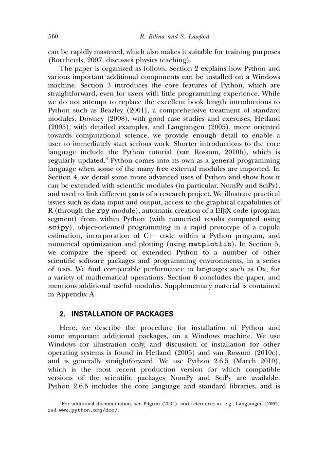
FIGURE 1 The Python 2.6.5 Integrated Development Environment (IDLE). (Figure available incolor online.)
installed automatically from www.python.org/download, by followingthe download instructions.4 After installation, the Python IntegratedDevelopment Environment (IDLE), or “shell window” (interactiveinterpreter) becomes available (see Fig. 1). The compatible Pywin32should also be installed. This provides extension modules for access tomany Windows API (Application Programming Interface) functions, andis available from sourceforge.net.
Two open source packages provide advanced functionality for scientificcomputing. The first of these, NumPy (numpy.scipy.org), enablesMatlab-like multidimensional arrays and array methods, linear algebra,Fourier transforms, random number generation, and tools for integratingC++ and Fortran code into Python programs (see Oliphant, 2006,for a comprehensive manual, and Langtangen, 2005, Chapter 4, forapplications). NumPy version 1.4.1 is stable with Python 2.6.5 and Pywin32(build 210), and is available from sourceforge.net (follow the link fromnumpy.scipy.org). The second package, SciPy (www.scipy.org),which requires NumPy, provides further mathematical libraries, includingstatistics, numerical integration and optimization, genetic algorithms,and special functions. SciPy version 0.8.0 is stable with the abovepackages, and is available from sourceforge.net (follow the link from
4The Windows Installer file for Python 2.6.5 is python-2.6.5.msi. The latest versionof Python, 3.0, is less well-tested, and we do not use it in this paper. The Pywin32 file (build210) is pywin32-210.win32-py2.6.exe. The NumPy 1.4.1 file is numpy-1.4.1-win32-superpack-python2.6.exe. The SciPy 0.8.0 file is scipy-0.8.0rc2-win32-superpack-python2.6.exe. The R-2.9.1 file is R-2.9.1-win32.exe. The RPy 1.0.3 file isrpy-1.0.3-R-2.9.0-R-2.9.1-win32-py2.6.exe. The MDP file is MDP-2.6.win32.exe.The Matplotlib 1.0.0 file is matplotlib-1.0.0.win32-py2.6.exe. The automatic MinGW 5.1.6installer file is MinGW-5.1.6.exe. We have tested the installations on a 1.73GHz Celeron M machinewith 2GB RAM running Windows Vista, and a 1.66MHz Centrino Duo machine with 1GB RAM runningWindows XP. Further information on IDLE is available at docs.python.org/library/idle.html,while some alternative environments are listed in Hetland (2005, Table 1-1); also see IPython(ipython.scipy.org/moin/Documentation).
562 R. Bilina and S. Lawford
www.scipy.org); see SciPy Community (2010) for a reference. We useNumPy and SciPy extensively below.
For statistical computing and an excellent graphical interface, Pythoncan be linked to the R language (www.r-project.org) via the RPyinterface (rpy.sourceforge.net). The strengths of R are discussedat length in Cribari-Neto and Zarkos (1999), Kleiber and Zeileis (2008),Racine and Hyndman (2002), and Zeileis and Koenker (2008). An Rjournal exists (journal.r-project.org). Release R 2.9.1 (June 2009;follow the download links on rpy.sourceforge.net, and choose “fullinstallation”) and RPy 1.0.3, available from sourceforge.net, are stablewith Python 2.6.5.
An additional third-party module that is useful for data-processingis MDP 2.6: Modular Toolkit for Data Processing (see Zito et al.,2009 for details). It contains a number of learning algorithms and,in particular, user-friendly routines for principal components analysis.It is available from mdp-toolkit.sourceforge.net. We also useMatplotlib 1.0.0, a comprehensive and Matlab-like advanced plottingtool, available from sourceforge.net/projects/matplotlib.Documentation (Dale et al., 2010) and examples can be found atmatplotlib.sourceforge.net. A C++ compiler is also needed torun Python programs that contain C++ code segments, and a good freeoption is a full MinGW 5.1.6 (Minimalist GNU for Windows) installation.An automatic Windows installer is available from www.mingw.org(which links to sourceforge.net), and contains the GCC (GNUCompiler System), which supports C++. We refer to the above installationas “extended Python”, and use it throughout the paper, and especiallyin Sections 4 and 5. We have installed the individual packagesfor illustration, but bundled scientific distributions of Python andadditional packages are available. These include pythonxy for Windows(code.google.com/p/pythonxy/) and the Enthought PythonDistribution (www.enthought.com/products/epd.php), which isfree for academic use.
Python is well supported by a dynamic community, with helpful onlinemailing lists, discussion forums, and archives. A number of Python-relatedconferences are held annually. A general discussion list is available at mail.python.org/mailman/listinfo/python-list, and the Pythonforum is at www.python-forum.org/pythonforum/index.php. It isalways advisable to check the archives before posting new requests.5
5A full listing of mailing lists is available from mail.python.org/mailman/listinfo.The www.python.org helpdesk can be contacted at [email protected]. SciPy andNumPy mailing lists are available at mail.scipy.org/mailman/listinfo/scipy-userand mail.scipy.org/mailman/listinfo/numpy-discussion. An RPy mailing list isat lists.sourceforge.net/lists/listinfo/rpy-list. Conference announcements areposted at www.python.org/community/workshops.
Python for Unified Research 563
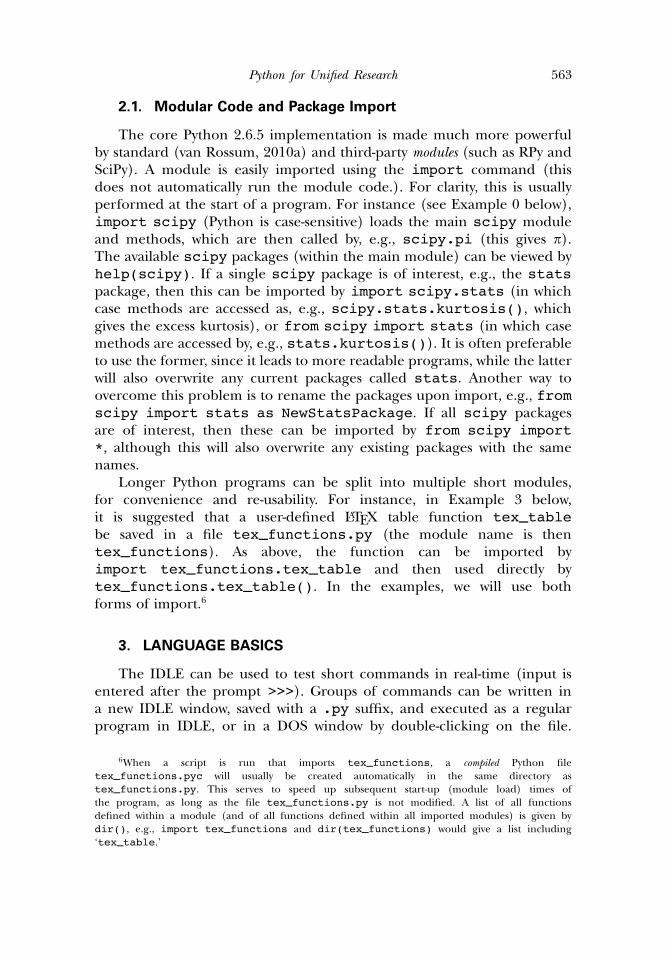
2.1. Modular Code and Package Import
The core Python 2.6.5 implementation is made much more powerfulby standard (van Rossum, 2010a) and third-party modules (such as RPy andSciPy). A module is easily imported using the import command (thisdoes not automatically run the module code.). For clarity, this is usuallyperformed at the start of a program. For instance (see Example 0 below),import scipy (Python is case-sensitive) loads the main scipy moduleand methods, which are then called by, e.g., scipy.pi (this gives �).The available scipy packages (within the main module) can be viewed byhelp(scipy). If a single scipy package is of interest, e.g., the statspackage, then this can be imported by import scipy.stats (in whichcase methods are accessed as, e.g., scipy.stats.kurtosis(), whichgives the excess kurtosis), or from scipy import stats (in which casemethods are accessed by, e.g., stats.kurtosis()). It is often preferableto use the former, since it leads to more readable programs, while the latterwill also overwrite any current packages called stats. Another way toovercome this problem is to rename the packages upon import, e.g., fromscipy import stats as NewStatsPackage. If all scipy packagesare of interest, then these can be imported by from scipy import*, although this will also overwrite any existing packages with the samenames.
Longer Python programs can be split into multiple short modules,for convenience and re-usability. For instance, in Example 3 below,it is suggested that a user-defined LATEX table function tex_tablebe saved in a file tex_functions.py (the module name is thentex_functions). As above, the function can be imported byimport tex_functions.tex_table and then used directly bytex_functions.tex_table(). In the examples, we will use bothforms of import.6
3. LANGUAGE BASICS
The IDLE can be used to test short commands in real-time (input isentered after the prompt >>>). Groups of commands can be written ina new IDLE window, saved with a .py suffix, and executed as a regularprogram in IDLE, or in a DOS window by double-clicking on the file.
6When a script is run that imports tex_functions, a compiled Python filetex_functions.pyc will usually be created automatically in the same directory astex_functions.py. This serves to speed up subsequent start-up (module load) times ofthe program, as long as the file tex_functions.py is not modified. A list of all functionsdefined within a module (and of all functions defined within all imported modules) is given bydir(), e.g., import tex_functions and dir(tex_functions) would give a list including‘tex_table.’
564 R. Bilina and S. Lawford
Single-line comments are preceded by a hash #, and multi-line commentsare enclosed within multiple quotes """. Multiple commands can beincluded on one line if separated by a semi-colon, and long commands canbe enclosed within parentheses () and split over several lines (a backslashcan also be used at the end of each line to be split). A general Pythonobject a (e.g., a variable, function, class instance) can be used as a functionargument f(a), or can have methods (functions) applied to it, with dotsyntax a.f(). There is no need to declare variables in Python since theyare created at the moment of initialization. Objects can be printed to thescreen by entering the object name at the prompt (i.e., >>> a) or fromwithin a program with print a.
3.1. Basic Types: Numbers and Strings
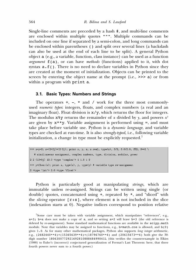
The operators +, -, * and / work for the three most commonly-used numeric types: integers, floats, and complex numbers (a real and animaginary float). Float division is x/y, which returns the floor for integers.The modulus x%y returns the remainder of x divided by y, and powers xy
are given by x**y. Variable assignment is performed using =, and musttake place before variable use. Python is a dynamic language, and variabletypes are checked at run-time. It is also strongly-typed, i.e., following variableinitialization, a change in type must be explicitly requested.7
Python is particularly good at manipulating strings, which areimmutable unless re-assigned. Strings can be written using single (ordouble) quotes, concatenated using +, repeated by *, and “sliced” withthe slicing operator [r:s], where element s is not included in the slice(indexation starts at 0). Negative indices correspond to position relative
7Some care must be taken with variable assignment, which manipulates “references”, e.g.,a=3; b=a does not make a copy of a, and so setting a=2 will leave b=3 (the old reference isdeleted by re-assignment). Some standard mathematical functions are available in the scipy.mathmodule. Note that variables may be assigned to functions, e.g., b=math.cos is allowed, and b(0)gives 1.0. As for many other mathematical packages, Python also supports long integer arithmetic,e.g., (2682440**4)+(15365639**4)+(18796760**4) and (20615673**4) both give the 30-digit number 180630077292169281088848499041L (this verifies the counterexample in Elkies(1988) to Euler’s (incorrect) conjectured generalization of Fermat’s Last Theorem: here, that threefourth powers never sum to a fourth power.)
Python for Unified Research 565
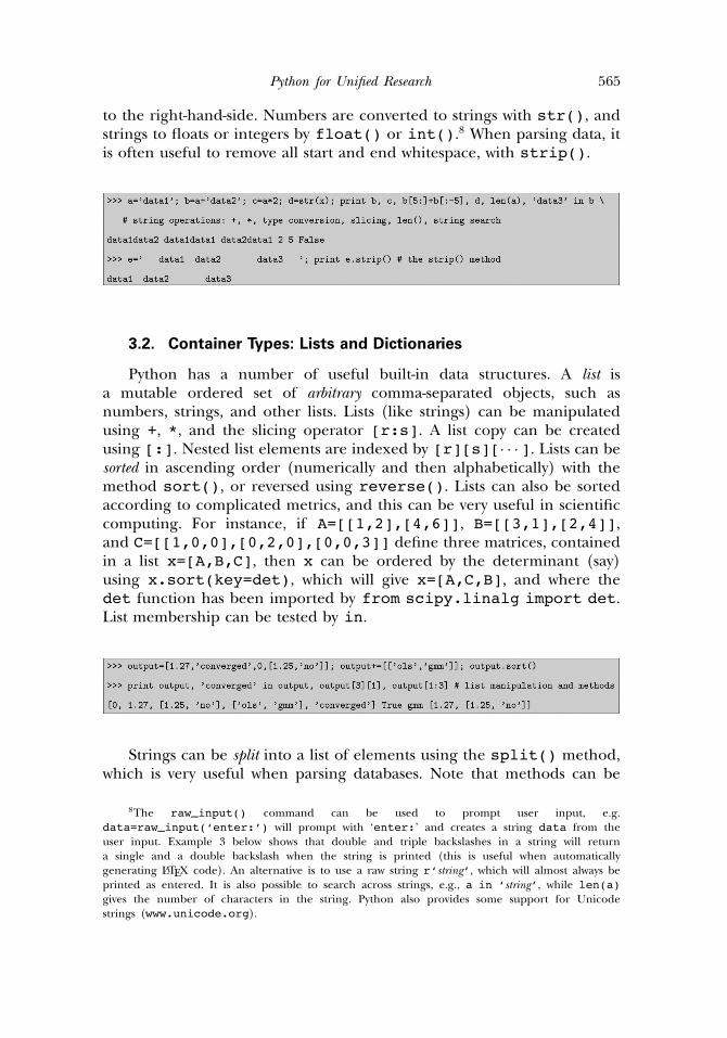
to the right-hand-side. Numbers are converted to strings with str(), andstrings to floats or integers by float() or int().8 When parsing data, itis often useful to remove all start and end whitespace, with strip().
3.2. Container Types: Lists and Dictionaries
Python has a number of useful built-in data structures. A list isa mutable ordered set of arbitrary comma-separated objects, such asnumbers, strings, and other lists. Lists (like strings) can be manipulatedusing +, *, and the slicing operator [r:s]. A list copy can be createdusing [:]. Nested list elements are indexed by [r][s][· · ·]. Lists can besorted in ascending order (numerically and then alphabetically) with themethod sort(), or reversed using reverse(). Lists can also be sortedaccording to complicated metrics, and this can be very useful in scientificcomputing. For instance, if A=[[1,2],[4,6]], B=[[3,1],[2,4]],and C=[[1,0,0],[0,2,0],[0,0,3]] define three matrices, containedin a list x=[A,B,C], then x can be ordered by the determinant (say)using x.sort(key=det), which will give x=[A,C,B], and where thedet function has been imported by from scipy.linalg import det.List membership can be tested by in.
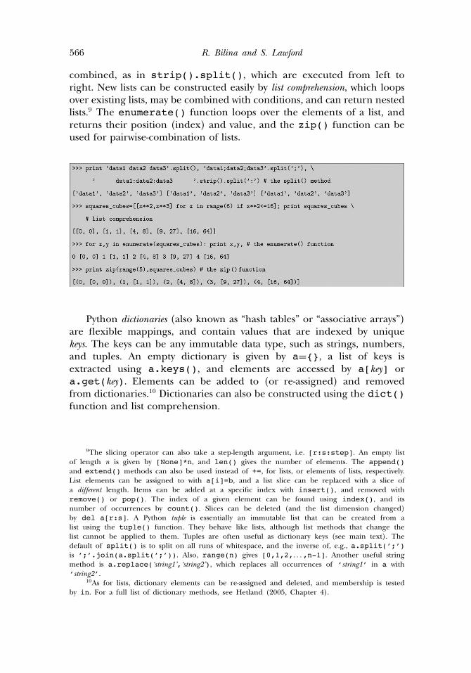
Strings can be split into a list of elements using the split() method,which is very useful when parsing databases. Note that methods can be
8The raw_input() command can be used to prompt user input, e.g.data=raw_input(‘enter:’) will prompt with ‘enter:’ and creates a string data from theuser input. Example 3 below shows that double and triple backslashes in a string will returna single and a double backslash when the string is printed (this is useful when automaticallygenerating LATEX code). An alternative is to use a raw string r‘string’, which will almost always beprinted as entered. It is also possible to search across strings, e.g., a in ‘string’, while len(a)gives the number of characters in the string. Python also provides some support for Unicodestrings (www.unicode.org).
566 R. Bilina and S. Lawford
combined, as in strip().split(), which are executed from left toright. New lists can be constructed easily by list comprehension, which loopsover existing lists, may be combined with conditions, and can return nestedlists.9 The enumerate() function loops over the elements of a list, andreturns their position (index) and value, and the zip() function can beused for pairwise-combination of lists.
Python dictionaries (also known as “hash tables” or “associative arrays”)are flexible mappings, and contain values that are indexed by uniquekeys. The keys can be any immutable data type, such as strings, numbers,and tuples. An empty dictionary is given by a={}, a list of keys isextracted using a.keys(), and elements are accessed by a[key] ora.get(key). Elements can be added to (or re-assigned) and removedfrom dictionaries.10 Dictionaries can also be constructed using the dict()function and list comprehension.
9The slicing operator can also take a step-length argument, i.e. [r:s:step]. An empty listof length n is given by [None]*n, and len() gives the number of elements. The append()and extend() methods can also be used instead of +=, for lists, or elements of lists, respectively.List elements can be assigned to with a[i]=b, and a list slice can be replaced with a slice ofa different length. Items can be added at a specific index with insert(), and removed withremove() or pop(). The index of a given element can be found using index(), and itsnumber of occurrences by count(). Slices can be deleted (and the list dimension changed)by del a[r:s]. A Python tuple is essentially an immutable list that can be created from alist using the tuple() function. They behave like lists, although list methods that change thelist cannot be applied to them. Tuples are often useful as dictionary keys (see main text). Thedefault of split() is to split on all runs of whitespace, and the inverse of, e.g., a.split(’;’)is ’;’.join(a.split(’;’)). Also, range(n) gives [0,1,2,� � �,n-1]. Another useful stringmethod is a.replace(‘string1’,‘string2’), which replaces all occurrences of ‘string1’ in a with‘string2’.
10As for lists, dictionary elements can be re-assigned and deleted, and membership is testedby in. For a full list of dictionary methods, see Hetland (2005, Chapter 4).
Python for Unified Research 567
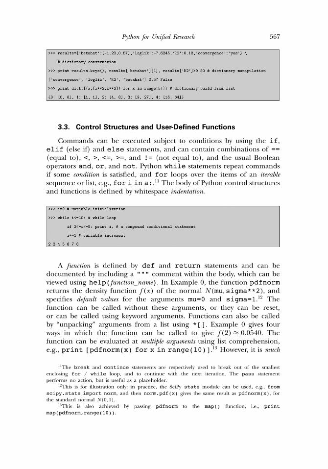
3.3. Control Structures and User-Defined Functions
Commands can be executed subject to conditions by using the if,elif (else if) and else statements, and can contain combinations of ==(equal to), <, >, <=, >=, and != (not equal to), and the usual Booleanoperators and, or, and not. Python while statements repeat commandsif some condition is satisfied, and for loops over the items of an iterablesequence or list, e.g., for i in a:.11 The body of Python control structuresand functions is defined by whitespace indentation.
A function is defined by def and return statements and can bedocumented by including a """ comment within the body, which can beviewed using help(function_name). In Example 0, the function pdfnormreturns the density function f (x) of the normal N (mu,sigma**2), andspecifies default values for the arguments mu=0 and sigma=1.12 Thefunction can be called without these arguments, or they can be reset,or can be called using keyword arguments. Functions can also be calledby “unpacking” arguments from a list using *[]. Example 0 gives fourways in which the function can be called to give f (2) ≈ 0�0540. Thefunction can be evaluated at multiple arguments using list comprehension,e.g., print [pdfnorm(x) for x in range(10)].13 However, it is much
11The break and continue statements are respectively used to break out of the smallestenclosing for / while loop, and to continue with the next iteration. The pass statementperforms no action, but is useful as a placeholder.
12This is for illustration only: in practice, the SciPy stats module can be used, e.g., fromscipy.stats import norm, and then norm.pdf(x) gives the same result as pdfnorm(x), forthe standard normal N (0, 1).
13This is also achieved by passing pdfnorm to the map() function, i.e., printmap(pdfnorm,range(10)).

568 R. Bilina and S. Lawford
faster to call the function with a vector array argument by from scipyimport arange and print pdfnorm(arange(10)).14 Python can alsodeal naturally with composite functions, e.g., scipy.log(pdfnorm(0)) willreturn ln(f (x)) at x = 0.15
Python uses call by assignment, which enables implementation offunction calls by value and by reference. Essentially, the call by value effect canbe obtained by appropriate use of immutable objects (such as numbers,strings or tuples), or by manipulating but not re-assigning mutable objects(such as lists, dictionaries or class instances). The call by reference effectcan be obtained by re-assigning mutable objects; see, e.g., Langtangen(2005, Sections 3.2.10, 3.3.4) for discussion.
4. LONGER EXAMPLES
4.1. Example 1: Reading and Writing Data
It is straightforward to import data of various forms into Pythonobjects. We illustrate using 100 cross-sectional observations on income andexpenditure data in a text file, from Greene (2008, Table F.8.1).16
14Array computations are very efficient. In a simple speed test (using the machine described inSection 5), we compute pdfnorm(x) once only, where x ∈ �0, 1, � � � , 999999�, by (a) [pdfnorm(x)for x in range(1000000)], (b) map(pdfnorm,range(1000000)), (c) from scipy importarange and pdfnorm(arange(1000000)), and also (d) from scipy.stats import norm andnorm.pdf(arange(1000000)). Tests (a) and (b) both run in roughly 58 seconds, while (c) and(d) take about 0.5 seconds, i.e., the array function is more than 100 times faster. It is encouragingthat the user-defined pdfnorm() is comparable in speed terms to the SciPy stats.norm.pdf().
15Given two functions f : X → Y and g : Y → Z , where the range of f is the same set as thedomain of g (otherwise, the composition is undefined), then the composite function g ◦ f : X → Zis defined as (g ◦ f )(x) := g (f (x)).
16The dataset is freely available at www.stern.nyu.edu/∼wgreene/Text/Edition6/TableF8-1.txt. The variable names (‘MDR,’ ‘Acc,’ ‘Age,’ ‘Income,’ ‘Avgexp,’ ‘Ownrent,’ and‘Selfempl’) are given in a single header line. Data is reported in space-separated columns, whichcontain integers or floats. See Examples 2, 3, and 6 for analysis.

Python for Unified Research 569
In Example 1a, a file object f is opened with open(). A list of variablenames, header, is created from the first line of the file: readline()leaves a new line character at the end of the string, which is removedby strip(), and the string is split into list elements by split().A dictionary data_dict is initialized by list comprehension with keystaken from header, and corresponding values [] (an empty list). Thedictionary is then filled with data (by iterating across the remaining linesof f), after which the file object is closed by close().17 The commandeval() ‘evaluates’ the data into Python expressions, and the dictionaryelements corresponding to the variables ‘Acc,’ ‘Age,’ ‘MDR,’ ‘Ownrent,’and ‘Selfempl’ are automatically created as integers, while ‘Avgexp’ and‘Income’ are floats. The formatted data dictionary is then ready for use inapplied work.
The cPickle module provides a powerful means of saving arbitraryPython objects to file, and for retrieving them.18 The ‘pickling’ (save)can be applied to, e.g., numbers and strings, lists and dictionaries, top-level module functions and classes, and creates a byte stream (stringrepresentation) without losing the original object structure. The originalobject can be reconstructed by ‘unpickling’ (load). The technique is veryuseful when storing the results of a large dataset parse to file, for lateruse, avoiding the need to parse the data more than once. It encouragesshort modular code, since objects can easily be passed from one code (oruser) to another, or sent across a network. The speed of cPickle also
17Valid arguments for open() are the filename (including the path if this is not the currentlocation) and the mode of use of the file: useful are ‘r’ read only (default) and ‘w’ write only(‘r+’ is read and write). While f.readlines() reads f into a list of strings, f.read() wouldread f into a single string. The iteration for j in f.readlines(): in this example could alsobe replaced by for j in f:.
18cPickle is an optimized C implementation of the standard pickle module, andis reported to be faster for data save and load (Beazley, 2001; van Rossum, 2010a,Section 12.2), although some of the pickle functionality is missing. The default cPickle save‘serializes’ the Python object into a printable ASCII format (other protocols are available). Seedocs.python.org/library/pickle.html for further details. In Example 1b, the raw datafile is 3.37 k, and the Python .bin, which contains additional structural information, is 5.77 k.The present authors have made frequent use of cPickle in parsing and manipulating the U.S.Department of Transportation Origin and Destination databases.
570 R. Bilina and S. Lawford
makes Python a natural choice for application checkpointing, a techniquewhich stores the current state of an application, and that is used torestart the execution should the system fail. Applications in econometricsinclude treatment of massive microeconometric datasets, and intensiveMonte Carlo simulation (e.g., a bootstrap simulation, or one with a heavynumerical computation in each of a large number of replications).
In Example 1b, a file object g is created, and the dictionarydata_dict is pickled to the file python_data.bin, before beingimmediately unpickled to a new dictionary data_dict2.
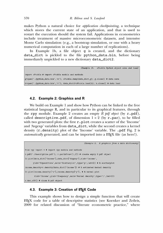
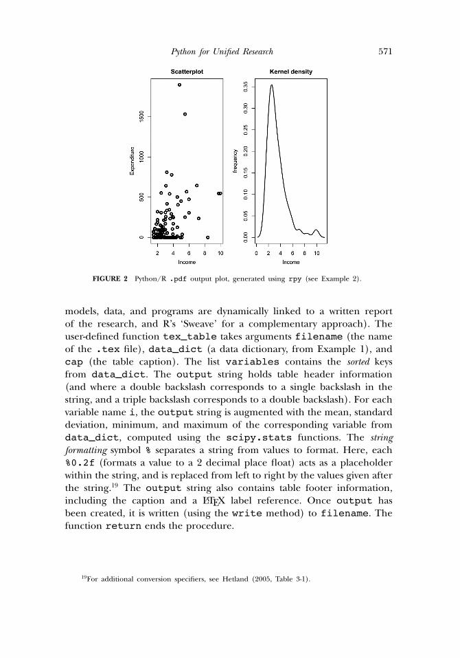
4.2. Example 2: Graphics and R
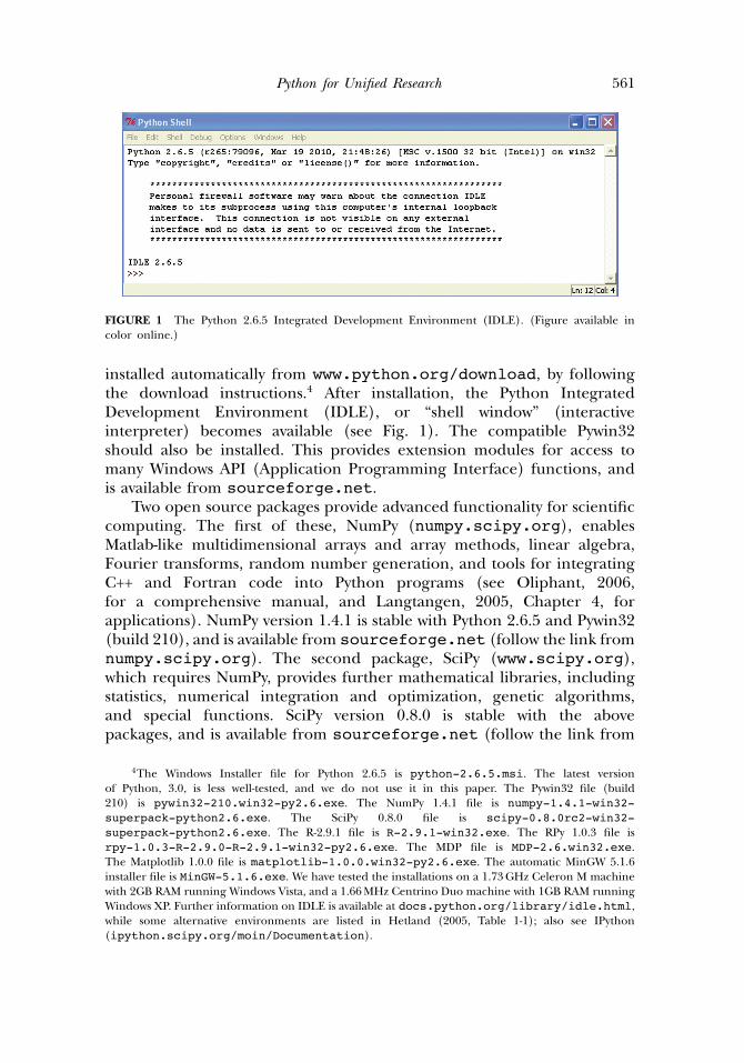
We build on Example 1 and show how Python can be linked to the freestatistical language R, and in particular to its graphical features, throughthe rpy module. Example 2 creates an empty R pdf object (by r.pdf),called descriptive.pdf, of dimension 1 × 2 (by r.par), to be filledwith two generated plots: the first r.plot creates a scatter of the ‘Income’and ‘Avgexp’ variables from data_dict, while the second creates a kerneldensity (r.density) plot of the ‘Income’ variable. The .pdf Fig. 2 isautomatically generated, and can be imported into a LATEX file (as here!).
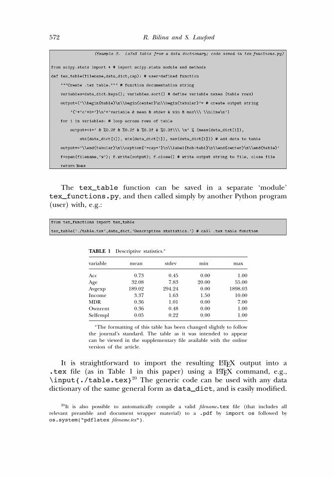
4.3. Example 3: Creation of LATEX Code
This example shows how to design a simple function that will createLATEX code for a table of descriptive statistics (see Koenker and Zeileis,2009 for related discussion of “literate econometric practice,” where
Python for Unified Research 571
FIGURE 2 Python/R .pdf output plot, generated using rpy (see Example 2).
models, data, and programs are dynamically linked to a written reportof the research, and R’s ‘Sweave’ for a complementary approach). Theuser-defined function tex_table takes arguments filename (the nameof the .tex file), data_dict (a data dictionary, from Example 1), andcap (the table caption). The list variables contains the sorted keysfrom data_dict. The output string holds table header information(and where a double backslash corresponds to a single backslash in thestring, and a triple backslash corresponds to a double backslash). For eachvariable name i, the output string is augmented with the mean, standarddeviation, minimum, and maximum of the corresponding variable fromdata_dict, computed using the scipy.stats functions. The stringformatting symbol % separates a string from values to format. Here, each%0.2f (formats a value to a 2 decimal place float) acts as a placeholderwithin the string, and is replaced from left to right by the values given afterthe string.19 The output string also contains table footer information,including the caption and a LATEX label reference. Once output hasbeen created, it is written (using the write method) to filename. Thefunction return ends the procedure.
19For additional conversion specifiers, see Hetland (2005, Table 3-1).
572 R. Bilina and S. Lawford
The tex_table function can be saved in a separate ‘module’tex_functions.py, and then called simply by another Python program(user) with, e.g.:
TABLE 1 Descriptive statistics.∗
variable mean stdev min max
Acc 0�73 0�45 0�00 1�00Age 32�08 7�83 20�00 55�00Avgexp 189�02 294�24 0�00 1898�03Income 3�37 1�63 1�50 10�00MDR 0�36 1�01 0�00 7�00Ownrent 0�36 0�48 0�00 1�00Selfempl 0�05 0�22 0�00 1�00
∗The formatting of this table has been changed slightly to followthe journal’s standard. The table as it was intended to appearcan be viewed in the supplementary file available with the onlineversion of the article.
It is straightforward to import the resulting LATEX output into a.tex file (as in Table 1 in this paper) using a LATEX command, e.g.,\input{./table.tex}20 The generic code can be used with any datadictionary of the same general form as data_dict, and is easily modified.
20It is also possible to automatically compile a valid filename.tex file (that includes allrelevant preamble and document wrapper material) to a .pdf by import os followed byos.system("pdflatex filename.tex").

Python for Unified Research 573
4.4. Example 4: Classes and Object-Oriented Programming
The following example illustrates rapid prototyping and object-orientedPython, with a simple bivariate copula estimation. Appendix A.1 containsa short discussion of the relevant copula theory. We use 5042 timeseries observations on the daily closing prices of the Dow JonesIndustrial Average and the S&P500 over June 9, 1989 to June 9,2009.21 The raw data is parsed in Python, and log returns arecreated, as x and y (not shown). There are two classes: a base classCopula, and a derived class NormalCopula. The methods availablein each class, and the class inheritance structure, can be viewed by,e.g., help(Copula). A Copula instance (conventionally referred to byself) is initialized by a=Copula(x,y), where the initialization takes thedata as arguments (and __init__ is the “constructor”). The instancevariables a.x and a.y (SciPy data arrays) and a.n (sample size)become available. The method a.empirical_cdf(), with no argument,returns an empirical distribution function F (x) = (n + 1)−1
∑ni=1 1Xi≤x ,
for both a.x and a.y, evaluated at the observed datapoints (sumreturns the sum). The Copula method a.rhat() will return an “indevelopment” message, and illustrates how code segments can be clearlyreserved for future development (perhaps a general maximum-likelihoodestimation procedure for multiple copula types). The Copula methoda.invert_cdf() is again reserved for future development and willreturn a user-defined error message, since this operation requires theestimated copula parameters, which have not yet been computed (and soa does not have a simulate attribute; this is tested with hasattr).22
A NormalCopula instance can now be created byb=NormalCopula(x,y). The derived class NormalCopula(Copula)inherits the methods of Copula (i.e., __init__, empirical_cdfas well as invert_cdf), replacing them by methods defined in theNormalCopula class if necessary (i.e., rhat), and adding any newmethods (i.e., simulate). The first time that the method b.rhat() iscalled, it will compute the estimated copula parameters R = n−1
∑ni=1 �i�
′i ,
where �i = (�−1(ui1),�
−1(ui2)) (b.test), �−1 is the inverse standard
normal distribution (norm.ppf from scipy.stats), u1 and u2 arethe empirical distributions of b.x and b.y, respectively, and i indexes
21The dataset is available from the authors as djia_sp500.csv. The data was downloadedfrom finance.yahoo.com (under tickers ∧DJI for Dow Jones and ∧GSPC for S&P500). It is easyto iterate over the lines of a .csv file with f=open(’filename.csv’,’r’) and for i in f:, andit is not necessary to use the csv module for this. This example is not intended to represent aserious copula model (there is no dynamic aspect, for instance).
22Python has flexible built-in exception handling features, which we do not explore here (e.g.,Beazley, 2001, Chapter 5).
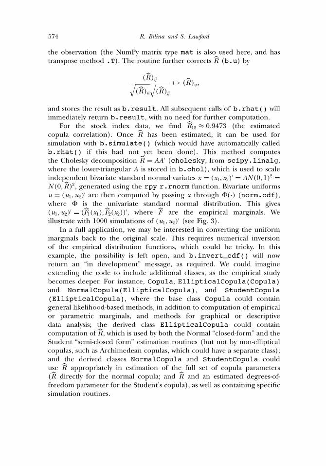
574 R. Bilina and S. Lawford
the observation (the NumPy matrix type mat is also used here, and hastranspose method .T). The routine further corrects R (b.u) by
(R)ij√(R)ii
√(R)jj
→ (R)ij ,
and stores the result as b.result. All subsequent calls of b.rhat() willimmediately return b.result, with no need for further computation.
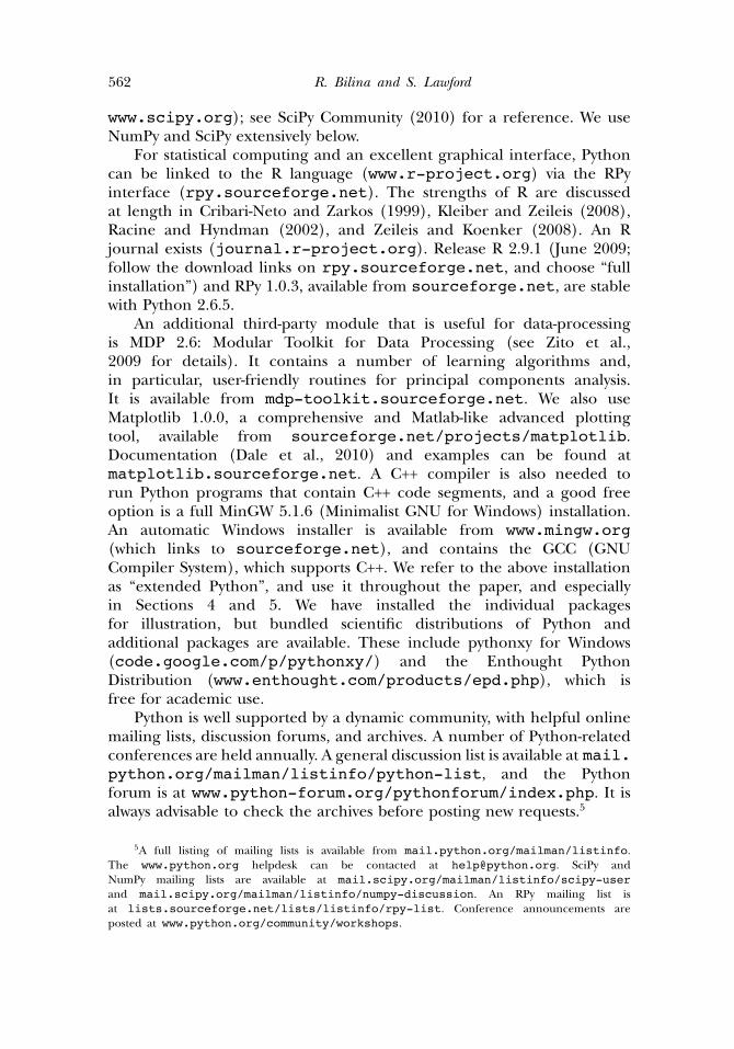
For the stock index data, we find R12 ≈ 0�9473 (the estimatedcopula correlation). Once R has been estimated, it can be used forsimulation with b.simulate() (which would have automatically calledb.rhat() if this had not yet been done). This method computesthe Cholesky decomposition R = AA′ (cholesky, from scipy.linalg,where the lower-triangular A is stored in b.chol), which is used to scaleindependent bivariate standard normal variates x = (x1, x2)′ = AN (0, 1)2 =N (0, R)2, generated using the rpy r.rnorm function. Bivariate uniformsu = (u1,u2)
′ are then computed by passing x through �(·) (norm.cdf),where � is the univariate standard normal distribution. This gives(u1,u2)
′ = (F1(x1), F2(x2))′, where F are the empirical marginals. Weillustrate with 1000 simulations of (u1,u2)
′ (see Fig. 3).In a full application, we may be interested in converting the uniform
marginals back to the original scale. This requires numerical inversionof the empirical distribution functions, which could be tricky. In thisexample, the possibility is left open, and b.invert_cdf() will nowreturn an “in development” message, as required. We could imagineextending the code to include additional classes, as the empirical studybecomes deeper. For instance, Copula, EllipticalCopula(Copula)and NormalCopula(EllipticalCopula), and StudentCopula(EllipticalCopula), where the base class Copula could containgeneral likelihood-based methods, in addition to computation of empiricalor parametric marginals, and methods for graphical or descriptivedata analysis; the derived class EllipticalCopula could containcomputation of R , which is used by both the Normal “closed-form” and theStudent “semi-closed form” estimation routines (but not by non-ellipticalcopulas, such as Archimedean copulas, which could have a separate class);and the derived classes NormalCopula and StudentCopula coulduse R appropriately in estimation of the full set of copula parameters(R directly for the normal copula; and R and an estimated degrees-of-freedom parameter for the Student’s copula), as well as containing specificsimulation routines.

Python for Unified Research 575
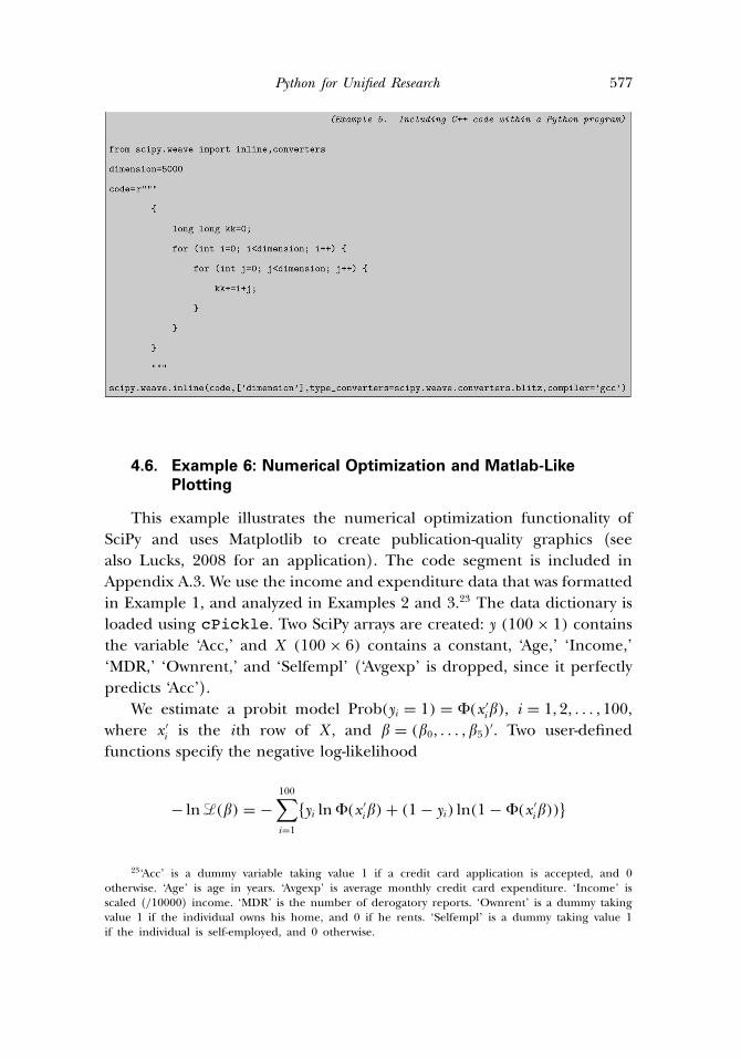
4.5. Example 5: Using C++ from Python for IntensiveComputations
This example shows how to include C++ code directly within a Pythonprogram, using the scipy.weave module. We are motivated by thenested speed test result in Section 5, which shows that Python nested loopsare quite inefficient compared to some software packages. Specifically, a5000 × 5000 nested loop that only keeps track of the cumulative sum ofthe loop indexes runs in about 9 seconds in Python 2.5.4, compared to 5seconds in Ox Professional 5.00, for instance (see Table 2). Generally, wewould not advise use of Python nested loops for numerical computations,

576 R. Bilina and S. Lawford
FIGURE 3 1000 simulations from a simple bivariate copula model (see Example 4).
and the problem worsens rapidly as the number of loops increases.However, it is easy to optimize Python programs by writing the heaviestcomputations in C++ (or Fortran). To illustrate, Example 5 solves theproblem of the slow nested loop in the speed test. The C++ code that willperform the computation is simply included in the Python program as araw string r"""string""", exactly as it would be written in a C++ editor(but without the C++ preamble statements). The scipy.weave.inlinemodule is called with the string that contains the C++ commands (code),the variables that are to be passed to and (although not in this example)from the C++ code (dimension), the method of variable type conversion(performed automatically using the scipy.weave.converters.blitzmodule), and optionally the compiler to be used (here, gcc, the GNUCompiler Collection). There will be a short compile time, when the Pythonprogram is first run, and we would expect some small overhead comparedto the same code running directly in C++. However, we find over 1000replications that the loop test now runs in a mean time of 0.02 seconds,or about 600 times faster than in Python! (roughly 300 times fasterthan Ox).
Python for Unified Research 577
4.6. Example 6: Numerical Optimization and Matlab-LikePlotting
This example illustrates the numerical optimization functionality ofSciPy and uses Matplotlib to create publication-quality graphics (seealso Lucks, 2008 for an application). The code segment is included inAppendix A.3. We use the income and expenditure data that was formattedin Example 1, and analyzed in Examples 2 and 3.23 The data dictionary isloaded using cPickle. Two SciPy arrays are created: y (100 × 1) containsthe variable ‘Acc,’ and X (100 × 6) contains a constant, ‘Age,’ ‘Income,’‘MDR,’ ‘Ownrent,’ and ‘Selfempl’ (‘Avgexp’ is dropped, since it perfectlypredicts ‘Acc’).
We estimate a probit model Prob(yi = 1) = �(x ′i�), i = 1, 2, � � � , 100,
where x ′i is the ith row of X , and � = (�0, � � � , �5)
′. Two user-definedfunctions specify the negative log-likelihood
− ln�(�) = −100∑i=1
�yi ln�(x ′i�) + (1 − yi) ln(1 − �(x ′
i�))�
23‘Acc’ is a dummy variable taking value 1 if a credit card application is accepted, and 0otherwise. ‘Age’ is age in years. ‘Avgexp’ is average monthly credit card expenditure. ‘Income’ isscaled (/10000) income. ‘MDR’ is the number of derogatory reports. ‘Ownrent’ is a dummy takingvalue 1 if the individual owns his home, and 0 if he rents. ‘Selfempl’ is a dummy taking value 1if the individual is self-employed, and 0 otherwise.
578 R. Bilina and S. Lawford
and the gradient function
�(− ln�(�))
��= −
100∑i=1
((x ′
i�)(yi − �(x ′i�))
�(x ′i�)(1 − �(x ′
i�))
)xi ,
where () is the density function of the standard normal(scipy.stats.norm, scipy.log, and numpy.dot are usedin the expressions). The unconstrained optimization � =argmin(− ln�(�)) is solved using the SciPy Newton-conjugate-gradient(scipy.optimize.fmin_ncg) method, with the least squares estimateof � used as starting value (scipy.linalg.inv is used in thecalculation), and making use of the analytical gradient. The methodconverges rapidly, and the accuracy of the maximum-likelihood estimate� was checked using EViews 6.0 (which uses different start values).24
It could be useful in a teaching environment to explain the estimationprocedure in more detail. Here, we use Matplotlib to design a figurefor this purpose (Fig. 4). We create a contour plot of − ln�(�) in the(�1, �2)-space, using numpy.meshgrid, as well as matplotlib.pyplot.The plot settings can all be user-defined (e.g., line widths, colours, axislimits, labels, grid-lines, contour labels). We use LATEX commands directlywithin Matplotlib to give mathematical axis labels, add a text box withinformation on the optimization, and annotate the figure with the positionof the least squares starting values (in (�1, �2)-space), and the maximum-likelihood estimate. Matplotlib creates a .png graphic, which can be savedin various formats (here, as a .pdf file).
5. SPEED COMPARISONS
In this section, we compare the speed performance of extendedPython 2.6.5 with Gauss 8.0, Mathematica 6.0, Ox Professional 5.00, R2.11.1, and Scilab 5.1.1. We run 15 mathematical benchmark tests on a1.66MHz Centrino Duo machine with 1GB RAM running Windows XP.The algorithms are adapted from Steinhaus (2008, Section 8), and aredescribed in Appendix A.2. They include a series of general mathematical,statistical, and linear algebra operations that occur frequently in appliedwork, as well as routines for nested loops and data import and analysis.
24Other numerical optimization routines are available. For instance, BFGS, with numerical oranalytical gradient, is available from scipy.optimize, as fmin_bfgs(f,x0,fprime=fp), wheref is the function to be minimized, x0 is the starting value, and fp is the derivative function(if fprime=None, a numerical derivative is used instead). Optional arguments control step-size,tolerance, display and execution parameters. Other optimization routines include a Nelder–Meadsimplex algorithm (fmin), a modified level set method due to Powell (fmin_powell), a Polak–Ribière conjugate gradient algorithm (fmin_cg), constrained optimizers, and global optimizersincluding simulated annealing.

Python for Unified Research 579
FIGURE 4 Annotated contour plot from probit estimation (see Example 6). (Figure available incolor online.)
The tests are generally performed on large dimension random vectors ormatrices, which are implemented as SciPy arrays.25 We summarize the testsand report the extended Python functions that are used:
1) Fast Fourier Transform over vector (scipy.fftpack.fft()).2) Linear solve of Xw = y for w (scipy.linalg.solve()).3) Vector numerical sort (scipy.sort()).4) Gaussian error function over matrix (scipy.special.erf()).5) Random Fibonacci numbers using closed-form (uses SciPy array).6) Cholesky decomposition (scipy.linalg.cholesky()).7) Data import and descriptive statistics (uses numpy.mat() and
numpy.loadtxt()).8) Gamma function over matrix (scipy.special.gamma()).9) Matrix element-wise exponentiation (**).
10) Matrix determinant (scipy.linalg.det()).11) Matrix dot product (numpy.dot()).12) Matrix inverse (scipy.linalg.inv()).
25All of the Python speed tests discussed in Section 5 and Appendix A.2 that require pseudo-random uniform numbers (13 of the 15 tests) use the well-known Mersenne Twister (MT19937).See Section 10.3 in Oliphant (2006) and Section 9.6 in van Rossum (2010a) for details. Pythonsupports random number generation from many discrete and continuous distributions. For instance,the continuous generators include the beta, Cauchy, 2, exponential, Fisher’s F , gamma, Gumbel,Laplace, logistic, lognormal, noncentral 2, normal, Pareto, Student’s t , and Weibull.
580 R. Bilina and S. Lawford
13) Two nested loops (core Python loops; fast Python/C++ routineimplemented).
14) Principal components analysis (mdp.pca()).15) Computation of eigenvalues (scipy.linalg.eigvals()).
For each software environment, the 15 tests were run over 10(sometimes 5) replications. The code for the benchmark tests,implemented in Gauss, Mathematica, Ox, R, and Scilab, and thedataset that is required for the data import test, are availablefrom www.scientificweb.com/ncrunch. We have made minormodifications to the timing (using the time module) and dimensionsof some of the tests, but have not attempted to further optimize thecode developed by Steinhaus (2008), although we have looked for thefastest Python and R implementations in each case. Our results cannot bedirectly compared to those in Steinhaus (2008) or Laurent and Urbain(2005), who run a previous version of these speed tests.
Full results are reported in Table 2, which gives the mean time(in seconds) across all replications for each of the tests. The testshave been ordered by increasing run-time for the extended Pythonimplementation. The “overall performance” of each software is calculatedfollowing Steinhaus (2008), as(
n−1∑i
minj(tij)tij
)× 100%,
where i = 1, 2, � � � ,n are the tests, j is the software, and tij is the speed(seconds) of test i with software j . Higher overall performance valuescorrespond to higher overall speed (maximum 100%).
We remark briefly on the results. Extended Python is comparable in“overall performance” to the econometric and statistical programmingenvironments Ox and Scilab. For the first 12 tests, the Pythonimplementation is either the fastest, or close to this, and displays somesubstantial speed gains over GAUSS, Mathematica, and R. While thedata test imports directly into a NumPy array, Python is also able toparse complicated and heterogeneous data structures (see Example 1for a simple illustration). The loop test takes almost twice as long asin GAUSS and Ox, but is considerably faster than Mathematica, Scilab,and R. It is well-known that Python loops are inefficient, and mostsuch computations can usually be made much faster either by usingvectorized algorithms (Langtangen, 2005, Section 4.2), or by optimizing oneof the loops (often the inner loop). We would certainly not suggest thatPython nested loops be used for heavy numerical work. In Section 4,Example 5, we show that it is straightforward to write the loop test as a

Python for Unified Research 581
TABLE 2 Speed test results. The mean time (seconds) across 10 replications is reported to 1decimal place, for each of the 15 tests detailed in Appendix A.2. The GAUSS and R nested loopsand the GAUSS, R, and Scilab principal components tests were run over 5 replications. TheScilab principal components test code (Steinhaus, 2008) uses a third-party routine. The testswere performed in ‘Python’ (extended Python 2.6.5), ‘GAUSS’ (GAUSS 8.0), ‘Mathematica’(Mathematica 6.0), ‘Ox’ (Ox Professional 5.00), ‘R’ (R 2.11.1), and ‘Scilab’ (Scilab 5.1.1),on a 1.66MHz Centrino Duo machine with 1GB RAM running Windows XP. The fastestimplementation of each individual test is highlighted. ‘Overall performance’ is calculated asin Steinhaus (2008): (n−1 ∑
i minj (tij )/tij ) × 100%, where i = 1, 2, � � � ,n are the tests, j is thesoftware used, and tij is the speed (seconds) of test i with software j . The speed test codes arepython_speed_tests.py, benchga5.e, benchmath5.nb, benchox5.ox,r_speed_tests.r, and benchsc5.sce, and are available from the authors (code for thePython and R tests was written by the authors). There is no principal components test in theSteinhaus (2008) Ox code, and that result is not considered in the overall performance for Ox.�For a much faster (Python/C++) implementation of the Python nested loop test, see Section 4,Example 5, and the discussion in Section 5.
Test Python GAUSS Mathematica Ox R Scilab
Fast Fourier Transform over vector 0.2 2.2 0.2 0.2 0.6 0.7Linear solve of Xw = y for w 0.2 2.4 0.2 0.7 0.8 0.2Vector numerical sort 0.2 0.9 0.5 0.2 0.4 0.3Gaussian error function over matrix 0.3 0.9 3.6 0.1 1.0 0.3Random Fibonacci numbers 0.3 0.4 2.3 0.3 0.6 0.5Cholesky decomposition 0.4 1.6 0.3 0.6 1.3 0.2Data import and statistics 0.4 0.2 0.5 0.3 0.8 0.3Gamma function over matrix 0.5 0.7 3.3 0.2 0.7 0.2Matrix element-wise exponentiation 0.5 0.7 0.2 0.2 0.8 0.6Matrix determinant 0.7 7.3 0.5 3.4 2.1 0.4Matrix dot product 1.4 8.9 1.0 1.7 7.8 1.0Matrix inverse 2.0 7.3 1.9 6.4 9.0 1.4Two nested loops� 8.1 4.3 84.7 4.8 58.0 295.9Principal components analysis 11.1 359.0 141.7 n/a 55.9 88.3Computation of eigenvalues 32.3 90.2 24.2 21.7 13.6 17.3
Overall performance 67% 30% 53% 70% 29% 65%
Note. The fastest implementation of each individual test is in bold.
Python/C++ routine, and that this implementation runs about 600 timesfaster than core Python. Code optimization is generally advisable, and notjust for Python (see, e.g., www.scipy.org/PerformancePython). Theprincipal components routine is the fastest implementation. The speed ofthe eigenvalue computation is roughly comparable to Mathematica.
Given the limited number of replications, and the difficulty ofsuppressing background processes, the values in Table 2 are only indicative(and especially for the heavier tests, which can sometimes be observedto have mean run-times that increase in the number of replications),although we do not expect the qualitative results to change dramaticallywith increased replications. In any given application, Python is likely to becomparably fast to some purpose-built mathematical software, and any slowtime-critical code components can always be optimized by using C++ orFortran.

582 R. Bilina and S. Lawford
6. CONCLUDING REMARKS
Knowledge of computer programming is indispensable for muchapplied and theoretical research. Although Python is now used in otherscientific fields (e.g., physics), and as a teaching tool, it is much lesswell-known to econometricians and statisticians (exceptions are Choiratand Seri, 2009, which briefly introduces Python and contains some niceexamples; and Almiron et al., 2009). We have tried to motivate Pythonas a powerful alternative for advanced econometric and statistical projectwork, but in particular as a means of linking different environments usedin applied work.
Python is easy to learn, use, and extend, and has a large standardlibrary and extensive third-party modules. The language has a supportivecommunity, and excellent tutorials, resources, and references. The“pythonic” language structure leads to readable (and manageable)programs, fast development times, and facilitates reproducible research.We agree with Koenker and Zeileis (2009) that reproducibility is important(they also note the desirability of a single environment that can beused to manage multiple parts of a research project; consider also thesurvey paper [Ooms, 2009]). Extended Python offers the possibility ofdirect programming of large-scale applications or, for users with high-performance software written in other languages, it can be useful as astrong “glue” between different applications.
We have used the following packages here: (1) cPickle fordata import and export, (2) matplotlib (pyplot) for graphics, (3)mdp for principal components analysis, (4) numpy for efficient arrayoperations, (5) rpy for graphics and random number generation, (6)scipy for scientific computation (especially arange for array sequences,constants for built-in mathematical constants, fftpack for FastFourier transforms, linalg for matrix operations, math for standardmathematical functions, optimize for numerical optimization, specialfor special functions, stats for statistical functions, and weave for linkingC++ and Python), and (7) time for timing the speed tests.
Many other Python modules can be useful in econometrics (seeBeazley, 2001 and van Rossum, 2010a for coverage of standard modules).These include csv (.csv file import and export), os (commonoperating-system tools), random (pseudo-random number generation),sets (set-theoretic operations), sys (interpreter tools), Tkinter (seewiki.python.org/moin/TkInter; for building application front-ends), urllib and urllib2 (for internet support, e.g. automatedparsing of data from websites and creation of internet bots andweb spiders), and zipfile (for manipulation of .zip compresseddata files). For third-party modules, see Langtangen (2005) (and alsowiki.python.org/moin/NumericAndScientific). Also useful are
Python for Unified Research 583
the ‘Sage’ mathematics system (www.sagemath.org), the statsmodelsPython statistics package (statsmodels.sourceforge.net), and the‘SciPy Stats Project,’ a blog that developed out of the ‘Google Summer ofCode 2009’ (www.scipystats.blogspot.com).
Of additional interest are the Psyco just-in-time compiler, whichis reported to give substantial speed gains in some applications(see Langtangen, 2005, Section 8 and Rigo, 2007, for a manual),and ScientificPython (not to be confused with SciPy), whichprovides further open source scientific tools for Python (seedirac.cnrs-orleans.fr/plone/software/scientificpython).The f2py module can be used to link Fortran and Python(cens.ioc.ee/projects/f2py2e), and the SWIG (SimplifiedWrapper and Interface Generator) interface compiler (www.swig.org)provides advanced linking for C++ and Python. The ‘Cython’ languagecan be used to write C extensions for Python (www.cython.org). Forcompleteness, we note that some commercial Python libraries are alsoavailable, e.g., the PyIMSL wrapper (to the IMSL C Numeric library).Python is also appropriate for network applications, animations, andapplication front-end management (e.g., it can be linked to Excel withthe xlwt module, available from pypi.python.org/pypi/xlwt).
Parallel processing is possible in Python, with the multiprocessingpackage. Python is implemented so that only one simple thread caninteract with the interpreter at a time (the Global Interpreter Lock: GIL).However, NumPy can release the GIL, leading to significant speed gainswhen arrays are used. Unlike threads, full processes each have their ownGIL, and do not interfere with one another. In general, achieving optimaluse of a multiprocessor machine or cluster is nontrivial. However, Pythontools are also available for sophisticated parallelization.
We hope that this paper will encourage the reader to join the Pythoncommunity!
A. APPENDIX
A.1. A Short Introduction to Bivariate Copulas
Excellent references to copula theory and applications include Nelsen(2006) and Patton (2009). Let X and Y be random variables such that
X ∼ F , Y ∼ G , (X ,Y ) ∼ H ,
where F and G are marginal distribution functions, and H is a jointdistribution function. Sklar’s Theorem states that
H (x , y) = C�(F (x),G(y)),
584 R. Bilina and S. Lawford
where C�(u, v) is (in this paper) a parametric copula function that mapsC(u, v) : [0, 1]2 → [0, 1] and describes the dependence between u := F (x)and v := G(y), and “binds” the marginals F and G together, to give avalid joint distribution H ; and � is a set of parameters that characterizethe copula. The probability integral transform X ∼ F �⇒ F (x) ∼ U [0, 1],where U is a uniform distribution, implies that the copula arguments uand v are uniform.
Elliptical copulas (notably Normal and Student’s t) are derivedfrom elliptical distributions. They model symmetric dependence and arerelatively easy to estimate and simulate. Copulas are generally estimatedusing maximum likelihood, although for elliptical copulas some of theparameters in � can often be estimated using efficient (semi)closed formformulae.
Here, we assume that the marginals are known, so that
H (x , y) = C�(F (x), G(y)),
and F (x) and G(x) are empirical marginal distributions, e.g., F (x) :=(n + 1)−1
∑ni=1 1Xi≤x , where Xi is an observed datapoint, 1· is the indicator
function, and n is the sample size.The 2-dimensional Normal copula is given by
CR(u) = �R(�−1(u1),�−1(u2))
=∫ �−1(u1)
−∞
∫ �−1(u2)
−∞(2�)−1|R |−1/2 exp(−x ′R−1x/2)dx1dx2,
where � := R is a 2 × 2 correlation matrix, uj = Fj(xj), �R is a 2-dimensional Normal distribution, and �−1 (�) is the univariate (inverse)standard Normal distribution. We further define a bivariate copula density�2C�(u)/�u1�u2, which for the Normal gives cR(�) := |R |−1/2 exp(−�′(R−1 −I2)�/2), where � = (�−1(u1),�−1(u2))
′. Maximum-likelihood estimation ofR solves
R = argmaxR
n−1n∑
i=1
ln cR(u)�
Numerical optimization of the log-likelihood surface is usually slow andcan lead to numerical errors. Fortunately, there is a closed-form for theNormal R ,
R = n−1n∑
i=1
�i�′i ,

Python for Unified Research 585
where �i = (�−1(ui1),�
−1(ui2))
′. Due to numerical errors, we correct to avalid correlation matrix by
(R)ij√(R)ii
√(R)jj
→ (R)ij �
Once we have estimated the copula parameters we have, in thebivariate case, H (x , y) = C�(F (x), G(y)) := C�(u, v). Simulation from acopula involves generation of (ur , vr ), which can subsequently betransformed to the original data scale (not considered here). Forthe bivariate Normal, we simulate by: (1) computing the Choleskydecomposition R = AA′, (2) simulating a 2-vector of standard Normalsz ∼ N (0, 1)2, (3) scaling the standard Normals: x = Az ∼ N (0, R)2, (4)simulating the uniforms uj by uj = �(xj), j = 1, 2; this gives (u1,u2) =(F1(x1), F2(x2)).
A.2. Speed Test Algorithms
We detail the algorithms that are used for the speed tests discussedin Section 5 (adapted from Steinhaus, 2008), and reported in Table 2.We assume that all required Python modules have been imported.Matrices and vectors have representative elements X = (Xrs) and x = (xr )respectively. Further, we let I = �1, 2, � � � , 10�. We give brief details on theextended Python implementations.
1) Fast Fourier Transform over vector[Replication i] Generate a 220 × 1 random uniform vector x =
(U (0, 1)). [Start timer] Compute the Fast Fourier Transform of x .[End timer] [End replication i] Repeat for i ∈ I . Random numbers aregenerated with x=scipy.random.random(2**20). The Fast Fouriertransform is performed using scipy.fftpack.fft(x).
2) Linear solve of Xw = y for w[Replication i] Generate a 1000 × 1000 random uniform matrix
X = (U (0, 1)). Generate a 1000 × 1 vector y = (j), j = 1, 2, � � � , 1000.[Start timer] Solve Xw = y for w. [End timer] [End replication i]Repeat for i ∈ I . Random numbers are generated using the commandx=scipy.random.random((1000,1000)). The array sequence isy=scipy.arange(1,1001). The linear solve is performed by thecommand scipy.linalg.solve(x,y).
3) Vector numerical sort[Replication i] Generate a 1000000 × 1 random uniform vector x =
(U (0, 1)). [Start timer] Sort the elements of x in ascending order.[End timer] [End replication i] Repeat for i ∈ I . Random numbers are
586 R. Bilina and S. Lawford
generated using x=scipy.random.random(1000000). The array sortmethod is scipy.sort(x).
4) Gaussian error function over matrix[Replication i] Generate a 1500 × 1500 random uniform matrix X =
(U (0, 1)). [Start timer] Compute the Gaussian error function erf(x).[End timer] [End replication i] Repeat for i ∈ I . The random array isgenerated with x=scipy.random.random((1500,1500)). The errorfunction implementation is scipy.special.erf(x).
5) Random Fibonacci numbers[Replication i] Generate a 1000000 × 1 random uniform vector x =
(�1000 × U (0, 1)�), where �·� returns the integer part. The Fibonaccinumbers yn are defined by the recurrence relation yn = yn−1 + yn−2, wherey0 = 0 and y1 = 1 initialize the sequence. [Start timer] Compute theFibonacci numbers yn for x = (n) (i.e., n ∈ �0, 1, � � � , 999� will give 1million random drawings from the first 1000 Fibonacci numbers), usingthe closed-form Binet formula
yn = n − (−)−n
√5
,
where = (1 + √5)/2 is the golden ratio.26 [End timer] [End
replication i] Repeat for i ∈ I . The random vector is x=scipy.floor(1000*scipy.random.random((1000000,1))). The Binet formulais implemented as ((golden**x)-(-golden)**(-x))/scipy.sqrt(5), where golden is taken from scipy.constants.
6) Cholesky decomposition[Replication i] Generate a 1500 × 1500 random uniform matrix
X = (U (0, 1)). Compute the dot product X ′X . [Start timer] Computethe upper-triangular Cholesky decomposition X ′X = U ′U , i.e., solvefor square U . [End timer] [End replication i] Repeat for i ∈ I .The random array is x=scipy.random.random((1500,1500)).The dot product is computed by y=numpy.dot(x.T,x). TheCholesky decomposition computation is performed by the commandscipy.linalg.cholesky(y,lower=False).
7) Data import and statistics[Replication i] [Start timer] Import the datafile Currency2.txt.
This contains 3160 rows and 38 columns of data, on 34 daily exchangerates over the period January 2, 1990 to February 8, 2002. There is a
26A faster closed-form formula is yn = �(n/√5) + (1/2)�, although we do not use it here.
For extended Python, the faster formula takes roughly 0.2 seconds across 10 replications. We alsocorrect for a typo in the Steinhaus (2008) Mathematica code: RandomInteger[{100,1000},� � �]is replaced by RandomInteger[{0,999},� � �].
Python for Unified Research 587
single header line. For each currency-year, compute the mean, minimumand maximum of the data, and the percentage change over the year.27
[End timer] [End replication i] Repeat for i ∈ I . We import the data withnumpy.mat(numpy.loadtxt("filename")).
8) Gamma function over matrix[Replication i] Generate a 1500 × 1500 random uniform matrix
X = (U (0, 1)). [Start timer] Compute the gamma function (x). [Endtimer] [End replication i] Repeat for i ∈ I . The random array isx=scipy.random.random((1500,1500)). The gamma functioncommand is scipy.special.gamma(x).28
9) Matrix element-wise exponentiation[Replication i] Generate a 2000 × 2000 random uniform matrix
X = (U (1, 1�01)) := (Xrs). [Start timer] Compute the matrix Y =(X 1000
rs ). [End timer] [End replication i] Repeat for i ∈ I . The randomarray is x=1+(scipy.random.random((2000,2000))/100). Theexponentiation is x**1000.
10) Matrix determinant[Replication i] Generate a 1500 × 1500 random uniform matrix X =
(U (0, 1)). [Start timer] Compute the determinant det(X ). [End timer][End replication i] Repeat for i ∈ I . The random array is generatedby x=scipy.random.random((1500,1500)). The determinant iscomputed by scipy.linalg.det(x).
11) Matrix dot product[Replication i] Generate a 1500 × 1500 random uniform matrix
X = (U (0, 1)). [Start timer] Compute the dot product X ′X . [Endtimer] [End replication i] Repeat for i ∈ I . The random array isx=scipy.random.random((1500,1500)). The dot product iscomputed by numpy.dot(x.T,x).
12) Matrix inverse[Replication i] Generate a 1500 × 1500 random uniform matrix
X = (U (0, 1)). [Start timer] Compute the inverse X −1. [Endtimer] [End replication i] Repeat for i ∈ I . The random arrayis x=scipy.random.random((1500,1500)). The inverse isscipy.linalg.inv(x).
27The file Currency2.txt is available from www.scientificweb.com/ncrunch. Wemodify the Steinhaus (2008) GAUSS code to import data into a matrix using loaddata[]=∧"filename"; and datmat=reshape(data,3159,38);. For the GAUSS and Pythonimplementations, we first removed the header line from the data file, before importing the data.
28We correct for a typo in the Steinhaus (2008) Mathematica code: we useRandomReal[{0,1},{1000,1000}] instead of RandomReal[NormalDistribution[],{1000,1000}].

588 R. Bilina and S. Lawford
13) Two nested loops[Replication i] Set a = 1. [Start timer] (Loop across l =
1, 2, � � � , 5000). (Loop across m = 1, 2, � � � , 5000). Set a = a + l + m. (Closeinner loop). (Close outer loop). [End timer] [End replication i] Repeatfor i ∈ I . Routine written in core Python. See Section 4 (Example 5) andSection 5 for further discussion.
14) Principal components analysis[Replication i] Generate a 10000 × 1000 random uniform matrix X =
(U (0, 1)). [Start timer] Transform X into principal components usingthe covariance method. [End timer] [End replication i] Repeat for i ∈ I .The random array is x=scipy.random.random((10000,1000)). Theprincipal components are computed using mdp.pca(x).
15) Computation of eigenvalues[Replication i] Generate a 1200 × 1200 random uniform matrix
X = (U (0, 1)). [Start timer] Compute the eigenvalues of X . [Endtimer] [End replication i] Repeat for i ∈ I . The random array isx=scipy.random.random((1200,1200)). The eigenvalues arecomputed using the command scipy.linalg.eigvals(x).
A.3. Python Code Segment for Probit Example

Python for Unified Research 589

590 R. Bilina and S. Lawford
ACKNOWLEDGMENTS
R.B. and S.L. thank the editor, Esfandiar Maasoumi, and twoanonymous referees, for comments that improved the paper, and aregrateful to Christophe Bontemps, Christine Choirat, David Joyner, MarkoLoparic, Sébastien de Menten, Marius Ooms, Skipper Seabold, andMichalis Stamatogiannis for helpful suggestions, Mehrdad Farzinpour forproviding access to a Mac OS X machine, and John Muckstadt and EricJohnson for providing access to a DualCore machine. R.B. thanks ENACand Farid Zizi for providing partial research funding. R.B. was affiliatedto ENAC when the first draft of this paper was completed. S.L. thanksNathalie Lenoir for supporting this project, and Sébastien de Menten,who had the foresight to promote Python at Electrabel (which involvedS.L. in the first place). This paper was typed by the authors in MiKTEX2.8 and WinEdt 5, and numerical results were derived using extendedPython 2.6.5 (described in Section 2), as well as C++, EViews 6.0, Gauss 8.0,Mathematica 6.0, Ox Professional 5.00, R 2.9.1 and R 2.11.1, and Scilab5.1.1. The results in Table 2 depend upon our machine configuration, thenumber of replications, and our modification of the original Steinhaus(2008) benchmark routines. They are not intended to be a definitivestatement on the speed of the other software, most of which we have usedproductively at some time in our work. The authors are solely responsiblefor any views made in this paper, and for any errors that remain. Allextended Python, C++, and R code for the examples and speed tests waswritten by the authors. Code and data are available on request.
REFERENCES
Almiron, M., Almeida, E., Miranda, M. (2009). The reliability of statistical functions in four softwarepackages freely used in numerical computation. Brazilian Journal of Probability and Statistics23:107–119.
Beazley, D. (2001). Python Essential Reference. 2nd ed. Indianapolis, IN: New Riders.Borcherds, P. (2007). Python: A language for computational physics. Computer Physics Communications
177:199–201.Bröker, O., Chinellato, O., Geus, R. (2005). Using Python for large scale linear algebra applications.
Future Generation Computer Systems 21:969–979.Choirat, C., Seri, R. (2009). Econometrics with Python. Journal of Applied Econometrics 24:698–704.Cribari-Neto, F., Zarkos, S. (1999). R: Yet another econometric programming environment. Journal
of Applied Econometrics 14:319–329.Dale, D., Droettboom, M., Firing, E., Hunter, J. (2010). Matplotlib Release 0.99.3.
matplotlib.sf.net/Matplotlib.pdf Accessed 18 April 2011.Downey, A. (2008). Think Python: How to think like a computer scientist – Version 1.1.22.
www.greenteapress.com/thinkpython/thinkpython.pdf Accessed 18 April 2011.Elkies, N. (1988). On A4 + B4 + C 4 = D4. Mathematics of Computation 51:825–835.Greene, W. (2008). Econometric Analysis. 6th ed. Upper Saddle River, NJ: Prentice-Hall.Hetland, M. (2005). Beginning Python: From Novice to Professional. Berkeley, CA: Apress.Kleiber, C., Zeileis, A. (2008). Applied Econometrics with R. New York, NY: Springer.Koenker, R., Zeileis, A. (2009). On reproducible econometric research. Journal of Applied Econometrics
24:833–847.

Python for Unified Research 591
Langtangen, H. (2005). Python Scripting for Computational Science. 2nd ed. Berlin: Springer.Laurent, S., Urbain, J.-P. (2005). Bridging the gap between Gauss and Ox using OXGAUSS. Journal
of Applied Econometrics 20:131–139.Lucks, J. (2008). Python – All a Scientist Needs. arxiv.org/pdf/0803.1838. Accessed 18 April 2011.Meinke, J., Mohanty, S., Eisenmenger, F., Hansmann, U. (2008). SMMP v. 3.0 – Simulating proteins
and protein interactions in Python and Fortran. Computer Physics Communications 178:459–470.Nelsen, R. (2006). An Introduction to Copulas. 2nd ed. New York, NY: Springer.Nilsen, J. (2007a). MontePython: Implementing Quantum Monte Carlo using Python. Computer
Physics Communications 177:799–814.Nilsen, J. (2007b). Python in scientific computing: Applications to Bose–Einstein condensates.
Computer Physics Communications 177:45.Oliphant, T. (2006). Guide to NumPy. www.tramy.us/numpybook.pdf Accessed 18 April 2011.Ooms, M. (2009). Trends in applied econometrics software development 1985–2008. In: Mills, T.,
Patterson, K., eds. Palgrave Handbook of Econometrics. Vol. 2. Basingstoke, Hampshire, UK:Palgrave MacMillan.
Ooms, M., Doornik, J. (2006). Econometric software development: Past, present and future. StatisticaNeerlandica 60:206–224.
Patton, A. (2009). Copula-based models for financial time series. In: Andersen, T., Davis, R., Kreiß,J.-P., Mikosch, T., eds. Handbook of Financial Time Series. Berlin: Springer.
Pilgrim, M. (2004). Dive into Python. www.diveintopython.org/download/diveintopython-pdf-5.4.zipAccessed 18 April 2011.
Racine, J., Hyndman, R. (2002). Using R to teach econometrics. Journal of Applied Econometrics17:175–189.
Renfro, C. (2004). A compendium of existing econometric software packages. Journal of Economicand Social Measurement 29:359–409.
Rigo, A. (2007). The Ultimate Psyco Guide – Release 1.6. psyco.sourceforge.net/psycoguide.ps.gzAccessed 18 April 2011.
SciPy Community. (2010). SciPy Reference Guide – Release 0.9.0.dev6597. docs.scipy.org/doc/scipy/scipy-ref.pdf Accessed 18 April 2011.
Steinhaus, S. (2008). Comparison of mathematical programs for data analysis (Edition 5.04).www.scientificweb.com/ncrunch/ncrunch5.pdf Accessed 18 April 2011.
van Rossum, G. (2010a). The Python Library Reference: Release 2.6.2. docs.python.org/archives/python-2.7-docs-pdf-a4.zip Accessed 18 April 2011. Drake, F. J. Jr. ed.
van Rossum, G. (2010b). Python Tutorial: Release 2.6.2. docs.python.org/archives/python-2.7-docs-pdf-a4.zip Accessed 18 April 2011. Drake, F. J. Jr., ed.
van Rossum, G. (2010c). Using Python: Release 2.6.2. docs.python.org/archives/python-2.7-docs-pdf-a4.zip Accessed 18 April 2011. Drake, F. J. Jr., ed.
Zeileis, A., Koenker, R. (2008). Econometrics in R: Past, present, and future. Journal of StatisticalSoftware 27(1).
Zito, T., Wilbert, N., Wiskott, L., Berkes, P. (2009). Modular toolkit for Data Processing (MDP):A Python data processing framework. Frontiers in Neuroinformatics Vol. 2.