Amplitude AnalysisAn Experimentalists View

Part II

Kinematics and More

1

K. Peters

Overview

Kinematics and More

2

Phasespace

Dalitz-Plots

Observables

Spin in a nutshell

Examples

Goal

For whatever you need the parameterization of the n-Particle phase space

It contains the static properties of the unstable (resonant) particles within the decay chain like

masswidthspin and parities

as well as properties of the initial stateand some constraints from the experimental setup/measurement

The main problem is, you don‘t need just a good description,you need the right one

Many solutions may look alike, but only one is right

3

n-Particle Phase space, n=3 4

Dalitz plot

Phase Space Plot - Dalitz Plot 5

dN ~ (E1dE1) (E2dE2) (E3dE3)/(E1E2E3)Energy conservation E3 = Etot-E1-E2

Phase space density ρ = dN/dEtot ~ dE1 dE2

Kinetic energies Q=T1+T2+T3

Plot x=(T2-T1)/√3y=T3-Q/3

Flat, if no dynamics is involved

Q smallQ large

The first plots τ/θ-Puzzle 6

Dalitz applied it first to KL-decaysThe former τ/θ puzzle with only a few eventsgoal was to determine spin and parity

And he never called them Dalitz plots

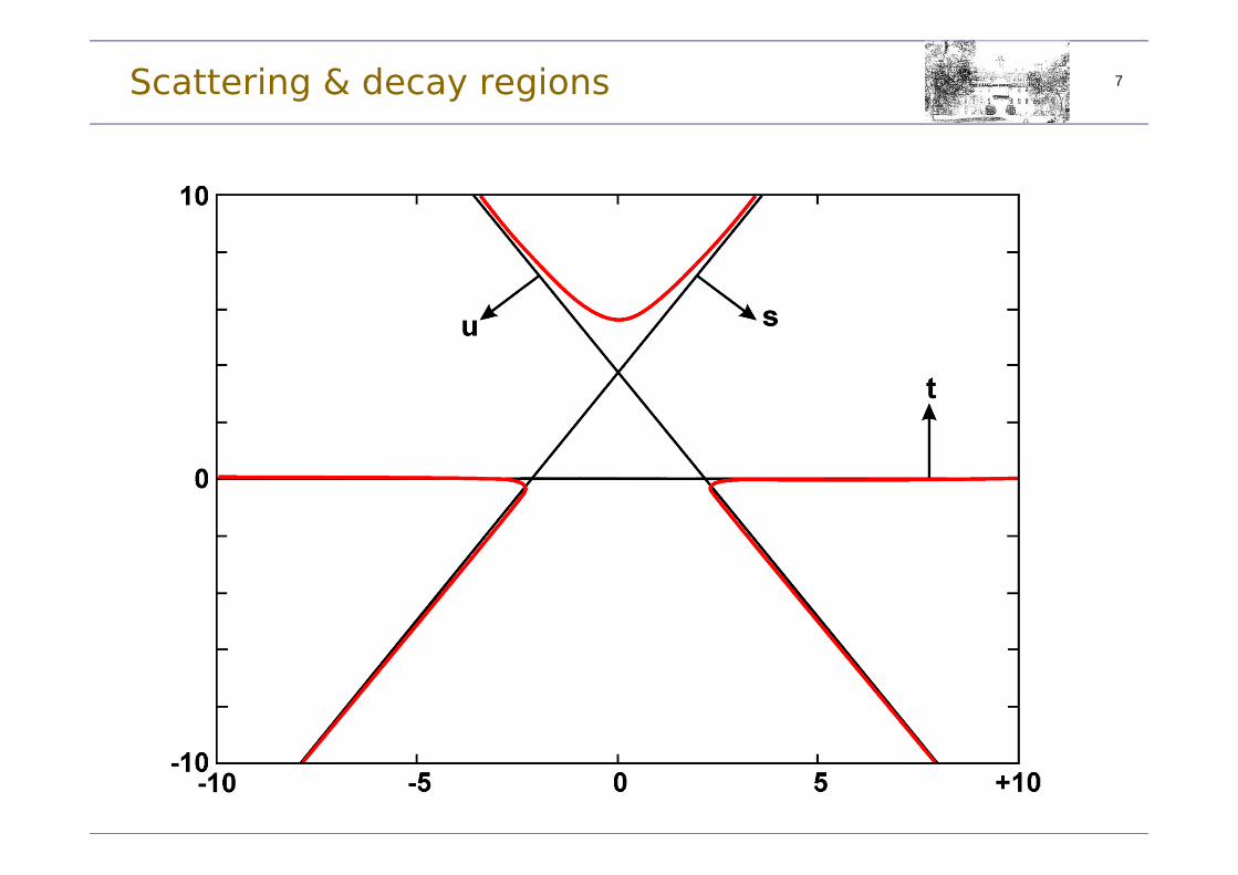
Scattering & decay regions 7

A

B

C

Ds

A

B

D

C

u

A

B

C

D

tScattering regions 8

Decay region

A C

D

B

9

A C

D

B

Decay region 10

A C

D

B

Decay region 11

D

K

Decay region

D0 K0S π+π-

12

π+π-

K0S π+ (GeV)2

(GeV

)2 K0S π-

Dalitz plot 13

D0 K0S π+π-

Phase space

visual inspection of the phase space distributionare the structures?structures from signal or background?are there strong interferences, threshold effects, potential resonances?

14

K*(892) → K-π+

ф → K+K-

Dalitz Plot – 2D Phase Space

How can resonances be studied in multi-body decays?Consider 3 body decay M → m1m2m3 (all spin 0)

Degrees of freedom

Complete dynamics describedby two variables!

Usual choice

15

3 Lorentz-vectors 123 Masses -3

Energy conserv. -1Momentum conserv. -3

3 Euler angles -3Remaining d.o.f 2

available phase space

Dalitz-Plot

1. s3,max

2. s3,min

3. s1,max

4. s1,min

5. s2,max

6. s2,min

Kinematics in the Dalitz-Plot 16

3.

1.

2. 6.

5.4.

3

1

2M

Kinematics in the Dalitz-Plot

Phasespace limits (example: s1):Pos 3: M rest system:

s1 maximum, if E1 is at minimum

Pos 4: m23 rest system (= Jackson-Frame R23), p2=-p3

full picture

17

but: not the wholecube is accessible!

Kinematics in the Dalitz-Plot

Example: need s2,±(s1); calculate in Restsystem R23 (p2=-p3, p1=p)

with and

18

kinematical function

Properties of Dalitz-Plots

Density distribution in the Dalitz Plot given by

for Spin-0 Particles M, m1, m2, m3

Dynamics is contained by the matrix element M

non-resonant processes ⇒M=const., uniform distribution

resonant processes ⇒ bands (horizontal, vertical, diagonal)

spins ⇒ Density distribution along the bands

19

Dalitz Plot – 2D Phase space

Possible decay patterns:

Non-Resonant (or background)flat (homogeneous) distribution

Resonance R in m12, m13, m23Band Structures

Position: Mass of RDensity: Spin of R

20

available phase space

Dalitz-Plot Tool (Root) Examples…. 21

Properties of Dalitz Plots

For the process M → Rm3, R→ m1m2 the matrix element can be expressed like

22

Winkelverteilung(Legendre Polyn.)

Formfaktor(Blatt-Weisskopf-F.)

Resonanz-Fkt.(z.B. Breit Wigner)

decay angular distribution of R

Form-(Blatt-Weisskopf)-Factor forM Rm3, p=p3 in R12

Form-(Blatt-Weisskopf)-Factor forR m1m2, q=p1 in R12

Dynamical Function (Breit-Wigner, K-Matrix, Flatté)

J L+l Z0 0 + 0 10 1 + 1 cos2θ0 2 + 2 [cos2θ – 1/3]2

Angular Distributions

density distribution along the band = decay angular distribution of R

results from Spin of R, the spin configuration and polarization of initial and final state(s)

Compare R=ρ and ф (both 1--) angular distributions are different !!

23

Dalitz-Plot-Analysis

Simultaneous fit of all resonant structures in a Dalitz-PlotTakes into account interference between resonances!

24

The Dalitz Plot

Reco Efficiency

The Ingredients

Fit Results

It’s All a Question of Statistics ...

p → 3π0 with

100 events

25

It’s All a Question of Statistics ... ...

p → 3π0 with

100 events1000 events

26

It’s All a Question of Statistics ... ... ...

p → 3π0 with

100 events1000 events10000 events

27

It’s All a Question of Statistics ... ... ... ...

p → 3π0 with

100 events1000 events10000 events100000 events

28

Observables, cont’d

are there symmetries in the phase space?unique assignment of phase space coordinates is important to avoid double countingtransformation necessary?

Most Dalitz plots are symmetric:Problem: sharing of eventsPossible solution: transform DP

29

r

f

f(r)

f

Spin Part in a nutshell

just a few words…

usually this is not part of your job

there are very many formalisms and packages

finally it‘s just a decomposition of the phase space which obeys all the necessary symmetries of the reaction

thus (in principle) straigth forward

and usually done by other people

30

Formalisms – an overview (very limited)

Non-relativistic Tensor formalismsin non-relativistic (Zemach) or covariant flavorFast computation, simple for small L and S

Spin-projection formalismswhere a quantization axis is chosen and proper rotations are used to define a two-body decayEfficient formalisms, even large L and S easy to handle

Relativistic Tensor Formalisms based on Lorentz invariants (Rarita-Schwinger)

where each operator is constructed from Mandelstam variables onlyElegant, but extremely difficult for large L and S

31

Spin-Projection Formalisms

Differ in choice of quantization axis

Helicity Formalismparallel to its own direction of motion

Transversity Formalismthe component normal to the scattering plane is used

Canonical (Orbital) Formalismthe component m in the incident z-direction is diagonal

32

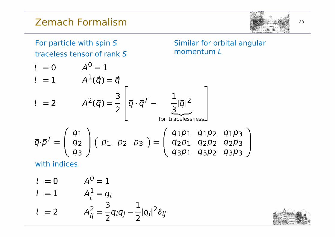
Zemach Formalism

For particle with spin Straceless tensor of rank S

with indices

Similar for orbital angular momentum L

33

The Original Zemach Paper 34

Tensors revisited

The Zemach amplitudes are only valid in the rest frame of the resonance.

Thus they are not covariantRetain covariance by adding the time component and use 4-vectorsBehavior under spatial rotations dictates that the time component of the decay momentum vanishes in the rest frame This condition is called Rarita Schwinger condition

For Spin-1 it readswith p = (pa+pb)/m the 4-momentum of the resonance

The vector Sμμ is orthogonal to the timelike vector pμ and is therefore spacelike, thus S2 < 0

35

0μμSu S p

Covariant Tensor Formalism

The most simple spin-1 covariant tensor with above properties isSμ=qμ-(qp)pμwith q = (pa - pb)

The negative norm is assured by the equation

where qR is the break-up three-momentum

the general approach and recipe is a lecture of its own and you should refer to the primary literature for more information

to calculate the amplitudes and intensities you may use qft++

36

2 2 2 2( ) | |RS q qp q

qft++ Package

qft++ = Numerical Object Oriented Quantum Field Theory(by Mike Williams, Carnegie Mellon Univ.)Calculation of the matrices, tensors, spinors, angular momentum tensors etc. with C++ classes

37

37

qft++ Package

Example:Amplitude and Intensity given by

qft++: Declaration and Calculation

38

38

and

Inte

nsity

Angular distributionof

Helicity Decay Amplitudes

HelicityFrom two-particle state

Helicity amplitude

39

f2 → ππ (Ansatz)

Initial: f2(1270) IG(JPC) = 0+(2++)Final: π0 IG(JPC) = 1-(0-+)

Only even angular momenta, since ηf = ηπ2(-1)l

Total spin s =2sπ =0

Ansatz

40

1 2 1 2

*

1 2

2 2 2*00 2 00 0

22 00 20 20

1 12 2*00 20 0

,0

2,

5 20 00 20 00 00 00 5

5 ,

JM J Jλ λ J λ λ Mλ

MM

MM

A N F D φ θλ λ λJ

A N F D φ θ

N F a a

A a D φ θ

f2 → ππ (Rates)

Amplitude has to be symmetrized because of the final state particles

41

2 22 0

21 0

1 200 20 00

2102 220

1 1 '*00 ' 00

, '

5

11

2 1 1

iφ

iφ

M

iφ

iφ

M MMM

M M

d θ e

d θ eA a d θ

d θ ed θ e

I θ A ρ A

ρJ

4 2 2 4 2

22 4 2 2 2

20

1 3 1 115 sin sin cos cos cos4 4 2 12

2

20

15 3 1sin 15sin cos 5 cos4 2 2

θ θ θ θ θ

I θ a θ θ θ θ

a const

2 22 0

21 0

2 200

6 sin4

3 sin cos2

3 1cos2 2

d θ θ

d θ θ θ

d θ θ

THANK YOUfor today

42