pulse vs. optimal stationary fishing: the northern
TRANSCRIPT

ISSN 1988-088X
Department of Foundations of Economic Analysis II University of the Basque Country Avda. Lehendakari Aguirre 83 48015 Bilbao (SPAIN) http://www.dfaeii.ehu.es
DFAE-II WP Series
José María Da Rocha, María-José Gutiérrez,
Luis T. Antelo
Pulse vs. Optimal Stationary Fishing: The Northern Stock of hake
2011-04
Pulse vs. Optimal Stationary Fishing: The Northern Stock of hake
José-María Da-Rochaa,1 , María-José Gutiérrez∗,b , Luís T. Anteloc,2
aUniversidade de Vigo, Facultad CC. Económicas, Campus Universitario Lagoas-Marcosende, C.P. 36200 Vigo, SpainbFAEII and MacLab - University of the Basque Country, Avda. Lehendakari Aguirre, 83, 48015 Bilbao, Spain.
cProcess Engineering Group. Instituto de Investigaciones Marinas (IIM) CSIC. C/ Eduardo Cabello, 6. 36208 Vigo, Spain.
Abstract
Pulse fishing may be a global optimal strategy in multicohort fisheries. In this article we compare the pulse
fishing solutions obtained by using global numerical methods with the analytical stationary optimal solution.
This allows us to quantify the potential benefits associated with the use of periodic fishing in the Northern
Stock of hake. Results show that: first, management plans based exclusively on traditional reference targets
as Fmsy may drive fishery economic results far from the optimal; second, global optimal solutions would
imply, in a cyclical manner, the closure of the fishery for some periods and third, second best stationary
policies with stable employment only reduce optimal present value of discounted profit in a 2%.
Key words:
optimal fisheries, management optimization in age-structured models, pulse fishing
1. Introduction
Since Beverton and Holt (1957) target reference points have been one of the main tools used by fishery
managers to make decisions about future catch options. Among the classical target reference points Fmsy
(the fishing mortality rate) stands out. If applied constantly it results in the maximum sustainable yield,
MSY (Caddy and Mahon, 1995).
There are two major shortcomings in this classical reference point approach. First, Fmsy is time inde-
pendent and fishery management strategies are evaluated using time dependent indicators, usually the net
present values of profits. Second, Fmsy is a stationary concept and optimal harvesting in a multi-cohort
model may take the form of periodic fishing (Clark, 1976; Spulber, 1983; McCallum, 1988; Tahvonen, 2009).
In order to overcome these drawbacks, numerical methods have been implemented to find the optimal
fishing mortality trajectory that maximises the net present profits of the fishery using the Beverton-Holt
multi-cohort models (Hannesson, 1975; Horwood, 1987; Björndal et al., 2004a, 2004b and 2006). In all these
cases, the optimal solution of the problem is non stationary but consists of pulse fishing, i.e. periodic cycles
of fishing followed by fallow periods for stock to recover. This means that periodic fishing leads to higher
profits than those implied by fishing at a constant stationary rate. It is worth mentioning that pulse fishing
may be optimal in this context because it mitigates the consequences of imperfect gear selectivity.
∗Corresponding author. Phone: 34-94-6013786, Fax: 34-94-6017123, e-mail: [email protected] e-mail: [email protected] e-mail: [email protected]
Preprint submitted to Elsevier October 19, 2011
Pulse fishing has some advantages in live product fisheries (Graham, 2001) and it has been applied for
years, under spatial rotation, in location-specific areas with marine invertebrates and sedentary reef fishes
(Caddy, 1993; Botsford et al., 1993; Hart, 2003; Hart and Rago, 2006; Cinner et al., 2006). Nevertheless,
fishery agencies do not consider periodic fishing as a feasible management tool, mainly because if rotation
is not possible its application may imply high financial and social costs. If rotation is not possible, periodic
fishing means the cyclical closure of the fishery for some periods with no alternative use of the fleet. As a
result, most fishery agencies consider that fishery management must be stationary.
Optimal stationary solutions have recently been assessed for different fisheries (Dichmont et al., 2010;
Grafton et al., 2006, 2007, 2010; Kompas et al., 2010; Kulmala et al., 2008; Da Rocha et al., 2010; Da
Rocha and Gutiérrez, 2011). In a seminal paper Grafton et al. (2007) analyse the biomass associated with
yield maximisation and discounted profit maximisation for Western and Central Pacific big eye tuna and
yellowfin tuna, the Australian northern prawn fishery and the Australian orange roughly fishery. They find
that stationary fishing mortality maximising net present profit is a win-win strategy compared to the usual
reference point policy, achieving higher profits and safer biomass. As a result of this study, the Australian
federal government started to manage 26 species based on profit maximisation as from the beginning of 2008
(Black, 2007).
However, we know that the Beverton-Holt multi-cohort models used to assess the stock is not globally
concave, so it is possible that constrained stationary solutions may be locally but not globally optimal. If
this is the case, what is the relative advantage of pulse fishing with respect to optimal stationary fishing
mortalities in a Beverton-Holt multi-cohort model?
In this paper we quantify the potential benefits associated with the use of periodic fishing in the Northern
Stock of hake. In particular, we compare the solutions obtained by using global numerical methods with the
analytical stationary optimal solution. This allows us to measure the potential benefits of periodic fishing
relative to the optimal institutional constrained solution. We find that when periodic fishing is compared
with optimal stationary solutions rather than with time independent classical reference points (Fmsy), the
potential disadvantage of stationary fishing is much lower than shown in previous articles.
2. The model
Age-structured models are the common population structure used in Virtual Population Analysis for fish
stock assessment (Lassen and Medley, 2000). The population structure is applied to a group of fish that has
the same life cycle, similar growth rates and can be considered a single biological unit. This unit stock is
broken down into cohorts, i.e. into groups of fish that have the same age and probably the same size and
weight, and that will mature at the same time.
Assume that the fish stock is broken into A cohorts. That is in each period t there are A− 1 initial old
cohorts and a new cohort is born. Let zat be the mortality rate that affects to the population of fish of the
ath age during the tth period. This mortality rate can be decomposed into fishing mortality, F at , and natural
mortality (non-human predation, disease and old age), ma,
zat = F at +ma.
2

While the fishing mortality rate may vary from one periods and one age to another, natural mortality is
constant across all periods. Moreover, it is assumed that the fishing mortality at each age is given by
stationary selection patterns, pa, i.e.
F at = paFt.
Assume that the fish population is continuous and the mortality rate acts on the fish stock continuously
throughout the period. Then the size of a cohort varies according to
Na+1t+1 = e−z
atNa
t , (1)
where Nat is the number of fish of the a
th age at the beginning of the tth period.
It is worth mentioning that by backwards substitution Nat , can be expressed as a function of the past
mortality rates and initial recruitment,
Nat = e−z
a−1t−1 (Ft−1)Na−1
t−1 = e−za−1t−1 (Ft−1)e−z
a−2t−2 (Ft−2)Na−2
t−2 = .... = Πa−1i=1 e
−za−it−i (Ft−i)N1t−(a−1).
Therefore we can express Nat as
Nat = φatN
1t−(a−1), for a = 1, ...A, (2)
where
φat = φ(Ft−1, Ft−2, ...Ft−(a−1)) =
1 for a = 1,
Πa−1i=1 e
−za−it−i (Ft−i) for a = 2, .....A,
can be understood as the survival function that shows the probability of a recruit born in period t− (a− 1)
reaching age a > 1 for a given fishing mortality path{Ft−1, Ft−2, ...Ft−(a−1)
}.
The size of a new cohort (recruitment), N1t+1 , depends on the spawning stock biomass of the previous
year, SSBt,
N1t+1 = Ψ(SSBt), (3)
where Ψ denotes the stock/recruits (S-R) relationship. Moreover, the spawning stock biomass, SSB, is a
function of the stock weight distribution, ω, and the maturity fraction, µ, of each age,
SSBt =
A∑a=1
µaωaNat . (4)
Let Dat and Cat denote the number of fish that dye from natural causes and from fishing (catches),
respectively. Then the dynamics of the cohort can be expressed as
Nat −Na+1
t+1 = Dat + Cat .
Taking into account equation (1) and the definitions of natural and fishing mortality, Dat and C
at can be
expressed as
Dat =
ma
zat
(Nat −Na+1
t+1
)=ma
zat
(1− e−z
at
)Nat ,
Cat =F atzat
(Nat −Na+1
t+1
)=F atzat
(1− e−z
at
)Nat . (5)
This last equation is known as the Baranov catch equation (Baranov, 1918).
3

3. Optimal Management
The profits of the fishery for any period t are given by the difference between revenues and fishing cost.
That is
πt =
A∑a=1
praCat (Ft)− TC(Ft), (6)
where pra is the selling price for a unit of fish of age a and TC represents the total fishing cost which depend
on the fishing rate. For the shake of simplicity, prices are assumed to be constant over time and total cost to
be a convex function. In the Discussion in Section 5 we discuss the implications of these assumptions based
on the sensitivity analysis carried out.
Note that πt can be interpreted in several ways from the economic point of view (Da Rocha et al., 2011).
For instance, if the cost is zero πt represents the discounted revenues of the fishery. Alternatively, if the
price is one and the cost is zero, πt represents the discounted yield of the fishery.
Assume that the objective of the fishery manager is to find the fishing mortality that maximises the
present value of the future profits of the fishery. Formally, the present value of future profits is given by
J =∑∞t=0 β
tπt. The parameter β ∈ [0, 1] is the discount factor which represents how much the manager is
willing to pay to trade-off the value of fishing today against the benefits of increased profits in the future,
measured by higher biomass and recruitment. Considering β = 1 implies that managers care about future
changes as much as if they occurred in the current year. By contrast, considering β = 0 implies not caring
about the future at all.
Therefore, the objective for the managers of the fishery should be to find the fishing rate trajectory that
maximises the present value of the fishery, J, taking into account that the spawning stock biomass is always
greater than the precautionary level, SSBpa, and the dynamics described by equations (1) to (5). Formally,
the maximisation problem consists of solving
max{Ft,N1
t+2}∞t=0J =
∞∑t=0
βt
{A∑a=1
praya(Ft)φatN
1t+1−a − TC(Ft)
},
s.t.
N1t+1 = Ψ
(∑Aa=1 µ
aωaφatN1t+1−a
)∀t,
SSBpa ≤∑Aa=1 µ
aωaφatN1t+1−a ∀t,
Na0 given, ∀a,
(7)
where ya(Ft) = ωa FtpaFt+m
(1− e−paFt−ma)
.
In the appendix we show how to find the first order conditions that solve this problem. Formally, the
4

optimal paths can be characterised by the following set of dynamic equations
A∑a=1
pra∂ya(Ft)
∂FtNat −
1
Nat
∂TCt∂Ft
=
A−1∑a=1
pa
A−a∑j=1
βj[praya+j(Ft+j) + (Ψ′t+jλt+j + θt+j)µ
a+jωa+j]Na+jt+j
,
(8)
A∑a=1
βapraya(Ft+1+a)φat+1+a = λt+1 − EtA∑a=1
βa(Ψ′t+1+aλt+1+a + θt+1+a)µaωaφat+1+a, (9)
Na+1t+1 = e−z
a(Ft)Nat , ∀t ∀a = 1, ...A− 1, (10)
N1t+2 = Ψ
(A∑a=1
µaωaNat+1
), ∀t, (11)
θt+1
[A∑a=1
µaωaNat+1 − SSBpa
]= 0, ∀t, (12)
where λt and θt are the Lagrange multipliers associated with the first and second restrictions of the max-
imisation problem (7), respectively.
Condition (8) shows how the mortality rate, Ft, is selected. The insight is the following. In the optimal
path, an increase in current mortality rate leads to an increase in current fishery profits (left-hand side)
that is offset by a decrease in future profits derived from reductions in future stock (right-hand side). In
particular, the left-hand side represents the effects of changes in fishing mortality on the current profit of
the fishery. However, the right-hand side shows the effect on the future size of the living cohorts, t + 1 to
t+A−1 (first sum) and on the future stock recruitments from periods t+2 to t+A (second sum). This can
also be visualised by looking at age structure in Table 1. The left-hand side represents the effects of Ft on
the structure of the fishery in period t (column t). The first sum on the right-hand side shows the effects of
Ft on the structure of future size of the living cohorts (lower triangle matrix) and the second sum illustrates
the effects of Ft on future stock recruitments (row a = 1). Note that β affects the future net present value
(right side). Note that making β = 1 implies caring about future changes as much as if they occurred in the
current year. By contrast, considering β = 0 implies not caring about the future at all.
[Insert Table 1]
Equation (9) indicates that the optimal path recognises that the effect of an increase in the stock recruit-
ment, N1t+2, is two-fold. On the one hand, the abundance in periods t + 2 to t + 2 + A − 1 goes up, which
leads to an increase in catches (left-hand side). On the other hand, the SSB for periods t+3 to t+3+A−1
also increases, (right-hand side).
Equations (10) and (11) show the dynamics of the population cohorts. Finally, equation (12) indicates
whether SSB is below the precautionary level, SSBpa. The Lagrange multiplier θt shows the effects on
mortality when the precautionary principle is not binding. If at a period t, the SSB is below the precaution-
ary level, SSBpa, then θt indicates how much the fishing mortality rate should be modified between periods
t−A and t− 1.
5

3.1. Optimal Stationary Solution
The optimal trajectories derived from maximization problem (7) are the optimal paths for {Ft}∞t=1,
{λt}∞t=2, and{Nat+2
}∞t=1
which satisfy the infinity set of equations that characterises the first order conditions
(8) to (12). In this section we focus on solutions that solve the manager maximisation problem leading the
fishery to a stationary situation. Our strategy to find these optimal stationary trajectories follows two steps.
First, we algebraically characterises the stationary solution, i.e. the solution that determines a unique value
for the long-term fishing rate which if applied, will generate a stationary recruitment leading to the maximum
long-term profits of the fishery. Second, the optimal path of fishing mortality that drives the fishery from
the initial conditions to the stationary solution is found using numerical methods.
Assume that the precautionary restriction is not binding, θt = 0. In this context, a stationary solution is
defined as an optimal solution characterised by a vector (Fss, N1ss, N
2ss, ...N
Ass, λss) such that for any future
period t
Fss = Ft = Ft+1,
Nass = Na
t = Nat+1, ∀a = 1, .., A,
λss = λt = βjλt+j , ∀j = 1, .., A+ 1.
The first order conditions (8)-(11) valued at the stationary solution can be reduced to the following 3−equation
system,
A∑a=1
pra∂ya(Fss)
∂FssφatN
1ss −
∂TC
∂Fss=
A−1∑a=1
pa
A−a∑j=1
[βjpraya+j(Fss) + Ψ′λssµ
a+jωa+j]φa+jt N1
ss
, (13)
A∑a=1
β1+apraya(Fss)φa(Fss) = λss
[1−Ψ′
A∑a=1
µaωaφa(Fss)
], (14)
N1ss = Ψ
(A∑a=1
µaωaφatN1ss
), (15)
which can be solved for (Fss, N1ss, λss). Once N
1ss is known the cohort size of any age can be calculated using
the survival function valued in the stationary solution, i.e. Nass = φa(Fss)N
1ss.
Now, to make the computation of the optimal trajectories that drives the fishery from the initial conditions
to the stationary solution described above tractable, we assume that convergence is reached in a finite number
of periods, T . In other words we truncate the first order conditions using that FT = Fss, N1T+2 = N1
ss, and
λT+1 = λss. Taking this into account, the model is solving by choosing F1,F1, F2, ....., FT = Fss such
that the system of equations implied by the first order condition (8)-(9) is satisfied. This system of (T − 1)
nonlinear equations with (T−1) unknowns can be solved relatively quickly using standard numerical methods
following the algorithm bellow:
1. Collect all the exogenous parameters describing biological and economic characteristics of the fishery.
This includes the biological parameters (ωj , µj , pj ,mj), the initial population distribution (N j0 ), the
precautionary limit reference point (SSBjpa), the economic parameters (prj , TC) and the discount
factor used to calculate variables in present terms, β.
6

2. Using outside information, select the S−R relationship to be used. With this relationship, it is possible
to find the recruitment for any fishing rate from optimal condition (15). Some examples:
• If the S −R relationship is defined as the Shepherd relationship3 (1982),
N1t =
αSSBt
1 +(SSBt
K
)b ,then recruitment is determined by
N1t = K
(α∑Aa=1 µ
aωaφat − 1)1/b
∑Aa=1 µ
aωaφat.
So, α,K and b have to be reported.
• If the S−R relationship is not well defined then recruitment may be considered as a fixed variable
that does not depend on fishing rate, that is N1t = N1.
3. Assume that the fishery is above the precautionary level. That is SSBt > SSBpa ∀t, and therefore
θt = 0, t = 2, .., T . Compute the stationary solution,(Fss, N
1ss, λss
)implied by (13)-(15).
4. Guess a trajectory for the fishing mortality rate path, {Ft}T−1t=1 , and assume that in period T the steady
state has been reached, i.e. FT = ... = FT+A+1 = Fss.
5. Project the future age cohort structure for periods 1, ..., T + A + 1, {Nat }
T+A+1t=1 using the initial age
structure, Na0 , and the S-R relationship. To do this, we use the cohort dynamic population (1), and
the recruitment relationship, (3) and (4).
6. Compute Ψ′t using the recruitment relationship, (3) and (4), associated with {Nat }
T+A+1t=1 .
7. Using λss compute λT from equation (9) valued at t = T − 1,
λT =
A∑a=1
βapraya(Fss)φass(Fss) +
A∑a=1
Ψ′T+aλssµaωaφass(Fss).
Note that Ψ′T+a is a function of N1T+a which depends on the guess {Ft}
T+a−2t=1 .
8. Given λT , compute {λt+1}T−1t=1 backwards recursively using equation (9).
9. Using the values of {λt+1}T−1t=1 , the guess of {Ft}T−1t=1 and the cohort projections {Na
t }T+A+1t=1 , it is
now possible to compute how far we are from the first order condition (8). Formally the following is
calculated: ∀t = 1, ....T,
ft =
A∑a=1
pra∂ya(Ft)
∂FtNat −
∂TCt∂Ft
−A−1∑a=1
pa
A−a∑j=1
βj[praya+j(Ft+j) + (Ψ′t+jλt+j + θt+j)µ
a+jωa+j]Na+jt+j
.
Using an appropriate algorithm, a new guess for the mortality rate path is selected.
3Parameter α is the maximum recruitment attainable when the SSB is very low, K > 0 is a threshold of SSB below which
the likelihood of population collapse is increased and b > 0 measures the power of the density-dependent effects.
7

10. Repeat the procedure for step 4 to 9 until ft is low enough.
11. Finally check that{∑A
a=1 µaωaNat
}Tt=1
> SSBpa. If the restriction is not satisfied, we should guess
a new set of positives values for 4 {θt}Tt=2.
3.2. Optimal Global Solutions: Pulse Fishing
It is well known that the Beverton-Holt multi-cohort models used to assess the stock are not globally
concave. Therefore the constrained stationary solution described in Section 3.1 may be a local rather than
a global optimum (Tahvonen 2009).
In order to find the global solution, we start by transforming the original dynamic optimisation problem
of infinite dimension, (7), into a low dimension non-linear optimisation problem. This transformation is
carried out using the control vector parameterisation approach (Vassiliadis, 1993; Vassiliadis et al., 1994)
which consists of dividing the considered time horizon into ρ constant (equidistant or not) or variable time
intervals.
In order to implement this, the management problem (7) must first be rewritten in continuous time. Let
n(a, t) be the number of fishes of age a at time t. In age structured models, the conservation law is described
by the following McKendrick-Von Foerster equation (Von Forester, 1959; McKendrick, 1926)
∂n(a, t)
∂t+∂n(a, t)
∂a= −[m(a) + p(a)F (t)]n(a, t).
The Stock Recruitment relationship occurs as a boundary condition at age zero.
n(0, t) =αSSB(t)
1 +(SSB(t)K
)β ,where, the SSB is given by
SSB(t) =
∫ A
0
µ(a)ω(a)n(a, t)da.
Profits in period t (6) can be written in continuos time as
π(t) =
∫ A
0
[pr(a)C(a, F (t))− TC(F (t))] da,
where C(a, F (t)) = p(a)F (t)m(a)+p(a)F (t)
(1− e−m(a)−p(a)F (t)
)n(a, t). Therefore, the objective function to be max-
imised can be rewritten as
J =
∫ ∞0
(∫ A
0
[pr(a)C(a, F (t))− TC(F (t))] da
)e−rtdt,
where r is the instantaneous interest rate and it is related with the discount factor in such a way that
4 In long-run management plans, the stock is usually far from SSBpa. So for those cases the best initial guess is θt = 0.
8

β = (1 + r)−1. Therefore, the maximisation problem (7) can be expressed in continuous time as
maxF (t)
J =
∫ ∞0
([pr(a)C(a, F (t))− TC(F (t))] da) e−rtdt,
s.t.
∂n(a, t)
∂t+∂n(a, t)
∂a= −[m(a) + p(a)F (t)]n(a, t). ∀t, a
n(0, t) =αSSB(t)
1 +
(SSB(t)
K
)β ∀t,
n(A, t) = 0 ∀t,
SSBpa ≤∫ A
0
µ(a)ω(a)n(a, t)da. ∀t,
n(a, 0) given, ∀a,
(16)
Second, the controls are approximated in each interval by using different base functions, generally low
order polynomials (zero order - steps, and order one - ramps, as depicted in Figure ??). The coeffi cients of
the polynomials considered constitute a vector ω (that also includes the lengths of the intervals when these
are variable) so that u = u(ω).
[Insert Figure 1]
This parametrisation transforms the original dynamic optimisation problem of infinite dimension into a
non-linear optimisation problem (NLP) of finite dimension where p=[µ,ω] (time invariant parameters and
control parametrisation coeffi cients, respectively) is the new vector of decision variables. As a consequence,
this new problem can be solved by employing different optimisation algorithms considering that in each
internal iteration the process dynamics need to be integrated in order to evaluate both the objective function
and the constraints.
For the most general case, the control approximation can be defined by employing Lagrange polynomials
of the form (Vassiliadis, 1993):
u(i)j (t) =
Mj∑k=1
σijkΘ(Mj)k (τ (i)),
where j = 1, 2, ..., ν; i = 1, 2, ..., ρ; t ∈ [ti−1, ti] and τ (i) is the normalised time on each interval i, which is
given by the following expression
τ (i) =t− ti−1ti − ti−1
=t− ti−1qi−1
,
9

and the M-order Lagrande polynomials (Θ(M)k ) are defined as
Θ(M)k (τ) ≡
1 if M = 1,
M∏k′=1,k 6=1
τ − τk′τk − τk′
if M ≥ 2.
The parameters σijk of these polynomials are directly related with the vector of new decision variables ω.
For the case of fixed final time problems and one control variable, the approximation of this variable is
given by
u(t) = ωi ∀i ti−1 ≤ t < ti−1 + qi.
So the vector of decision variables is formed by both the value of the steps as well as by the time interval
lengths: ω = [ω1, ..., ωρ, q1, ..., qρ−1] ∈ R2ρ−1. For the same case, but considering ν control variables with
constant time interval lengths, it is verified that ω ∈ R(ν+1)·(ρ−1).
In our application, to transform of the infinite dynamic optimization problem (16) into the NLP of finite
dimension, the time horizon is divided into ρ = 80 constant time intervals and the controls in each interval
are approximated using ramps.
Once the NLP of finite dimension is set, stochastic optimisation algorithms are used to solve it. In
particular two global stochastic optimisation algorithms plus one hybrid strategies are considered to solve
the transformed optimisation problem. We describe briefly the main characteristics of each method:
• DE: Differential Evolution. It is a metaheuristics algorithm for global optimisation of nonlinear and
(possibly) non-differentiable continuous functions presented by Storn and Price (1997). This is a
population-based method which, starting with a randomly generated population, computes new candi-
date solutions by calculating differences between population members. It handles stochastic variables
by means of a direct search method which outperforms other popular global optimisation algorithms,
and it is widely used by the evolutionary computation community.
• eSS-SSm: Enhanced Scatter Search. As presented in Egea et al. (2009), Scatter Search is a population-
based metaheuristic method which combines a global phase with an intensification method (i.e., a local
search). This methodology is very flexible, since each of its elements can be implemented in a variety
of ways and degrees of sophistication. A basic design to implement scatter-search is given on the well-
known “five-method template” (Laguna and Martí, 2003): (1) A Diversification Generation Method
to generate a collection of diverse trial solutions. (2) An Improvement Method to transform a trial
solution into one or more enhanced trial solutions. (3) A Reference Set Update Method to build and
maintain a reference set consisting of the b “best” solutions found, where the value of b is typically
small compared to the population size of other evolutionary algorithms. Solutions gain membership
to the reference set according to their quality or their diversity. (4) A Subset Generation Method to
operate on the reference set, to produce several subsets of its solutions as a basis for creating combined
solutions. (5) A Solution Combination Method to transform a given subset of solutions produced by
the Subset Generation Method into one or more combined solution vectors.
10

eSS-SSm is an advanced scatter search method developed by the IIM-CSIC Process Engineering Group
for chemical and bioprocess optimisation problems providing excellent results.
• Hybrid strategies: The key concept of hybrid methods is synergy. A hybrid method tries to exploit
the best properties of different methodologies. They combine global stochastic and local optimisation
algorithms. The global ones cover the whole search space to find the global optimum, but they are
slow in finding the exact location of this global solution. A promising strategy consists of obtaining a
good initial guess with one of these global methods and then fine tuning employing local optimisation.
These strategies take advantage of both the robustness of stochastic solvers and the effi ciency of local
methods when started in the optimum neighbourhoods. In this article, the hybrid strategy considered
is SSm+DHC.
The DHC algorithm (Dynamic Hill Climbind; De la Maza and Yuret, 1994) draws on ideas from
genetic algorithms, hill climbing and conjugate gradient methods. It is a direct search algorithm wich
explores every dimension of the search space using dynamic steps. It is formed by an inner and an
outer loop. The first one contains a very effi cient technique for locating local optima while the outer
loop ensures that the entire search space has been explored. In this work, only the local phase of the
algorithm has been used.
In order to select the algorithm that leads to the best results, it is necessary to perform an effi ciency
analysis. To that purpose, the convergences curves, which show the evolution of the best value obtained
by each solver over the CPU time , are constructed. With these representations, both the robustness (the
capability of the solver to attain consistently good final solutions) and the effi ciency (the speed of convergence
to the final solution) can be evaluated, allowing the user to select an appropriate algorithm to solve a given
optimisation problem.
4. The Northern Stock of Hake
In order to compare the optimal stationary and pulse fishing solutions, we apply the methods described
above to the Northern Stock of Hake (NSH). The NSH is a fishery managed with the advice of the Interna-
tional Council for the Exploitation of the Sea (ICES) and includes all fisheries in subareas VII and VIII and
also some fisheries in Subareas IV and VI (see Figure 2). Hake (merluccius merluccius) is caught throughout
the year, though the peak landings are made in the spring-summer months. It spawns from March to July at
depths of 120-160 m., mainly to the south and west of Ireland and moves to shallower water by September.
The two major nursery areas are the Bay of Biscay and off southern Ireland. As they become mature, the
fish disperse to offshore regions of the Bay of Biscay and Celtic Sea. Male hake mature at 3-4 years old
(27-35 cm) and females at 5-7 years old (50-70 cm).
[Insert Figure 2]
Hake has been the main species supporting trawling fleets off the Atlantic coasts of France and Spain since
the 1930s. The three main gear types used by vessels fishing for hake as a target species are lines (Spain),
11

fixed-nets and other trawls (all countries). Landings in 2008 were 47, 800 tonnes, below the regulated TAC
of 54, 000 tonnes. Spain accounts for most of the landings with 53% of the total captures. France takes
30% of the total, the UK 7%, Denmark 3%, Ireland 3% and other countries (Norway, Belgium, Netherlands,
Germany, and Sweden) take smaller amounts (ICES 2009). Tables 2 and 3 display the main characteristics
of the Spanish and French fleets according to the European Data Collection Regulation, respectively.
[Insert Table 2]
[Insert Table 3]
After the collapse of spawning SSB in the 1990s, an emergency plan was implemented for the NSH in
2001 and 2002 (EC 1162/2001, EC 2602/2001 and EC 494/2002). After this emergency plan, a recovery
plan was implemented in 2004 (EC 811/2004). Its aim was to achieve a SSB of 140, 000 tonnes (Bpa) by
limiting fishing mortality to 0.25 and by allowing a maximum change in harvest between consecutive years
of 15%. The recovery plan was to be replaced by a management plan when the target level for the stock
had been reached in two consecutive years,. This objective was achieved in 2004, 2005 and 2006. So in 2007,
an Expert Working Group from the Scientific, Technical and Economic Committee for Fisheries (STECF,
2008a) was convened in Lisbon from 18-22 June to evaluate the potential biological consequences of the long
term management plan. The working group proposed as objective of this plan a shift from the current fishing
rate Fsq = 0.25 to Fmsy = 0.17 assuming gradual changes to avoid drastic season closures.
In order to calibrate the age structured model for this fishery two data sources are used. First, the infor-
mation regarding the biological parameters of the fishery comes from the Expert Working Group (STECF,
2008a). Most of the parameters result from the summary of Extended Survivor Analysis (XSA) results
from the 2006 update (ICES, 2007). Secondly, economic data on the fishery come from expert working
group meeting on Northern Hake Long-Term Management Plan Impact Assessment (STECF, 2008b) held
in Brussels on December 3-6 2007.
Table 4 shows, for each age, the number of fishes at the initial conditions, the parameters of the population
dynamics (selection pattern, weight and maturity) and the prices.5
[Insert Table 4]
As the S-R relationship we use the Shepherd relationship (1982) described by
N1 =αSSB
1 +(SSBK
)b . (17)
To calibrate this recruitment function and SSB data for the period 1978-2006 are used. Since parameter α
represents the slope of the S-R relationship at the origin, it is calibrated as the maximum value of N1t /SSBt.
This calibration implies α = 2.4879, K = 168, 270 and b = 1.7602. The upper left panel in Figure 3 shows
this calibration and the data. We also use the values of the STECF groups for SSBpa = 140, 000 tonnes.
For calibrating the costs, we use data on the cost structure and the degree of dependency of hake for the
different FUs for the Spanish fleet in 2004 and for the French fleet in 2006 (See Table 5).
5To calculate prices as a function of ages we use data on 2007 daily sales for the Galician trawl, gill nets and long lines fleets.
12

[Insert Table 5]
In the numerical simulations we assume that the cost of effort is proportional to the mortality rate,
TC = cF, where c = TC/F represents the average and the marginal cost. Once the total costs are known,
c is calibrated as this amount divided by the current mortality rate, F = 0.25.
In order to calibrate the total costs, we start by determining the running costs per day. First we calculate
fuel costs, other costs, depreciation and interest divided by the days at sea of each segment (see Table 6).
Second, the average costs weighted by the sea days for each segment are calculated (last column in Table
6). Third, the fuel costs are adjusted taking into account the increase suffered by the fuel price during 2007.
Since fuel prices rose from 0.346 Euros in late 2006 to 0.52 in early 2008, fuel costs have been multiplied by
1.5. These calculations imply a cost of the fishery of 1, 919.14 Euros per day. Since the hake dependency of
the fleet is 0.28, the costs per day imputed to hake are 542.50 Euros per day.
[Insert Table 6]
We assume that 543.17 Euros per day and 135, 635 days at sea are good proxies for the marginal cost and
total effort, respectively, so the total cost can be considered as C(F ) = 543.17 × 135, 635 = 73.57 millions
Euros.
We define three different scenarios for the problem proposed:
• Scenario 1: The smooth trajectory that drives the fishery from the initial conditions to Fmsy using a
constant annual reduction in fishing mortality of 15%.6
• Scenario 2: The trajectory that drives the fishery smoothly from the initial conditions to the optimal
stationary solution.
• Scenario 3: The trajectory that drives the fishery from the initial conditions to the global optimal
solution.
Scenario 1 is simulated calculating Fmsy as the fishing rate that maximises the stationary yield. For
the NSH this results in Fmsy = 0.172. In Scenario 2 the optimal stationary trajectory is obtained using the
algorithm described in Section 3.1. As a result for the NSH we obtain Fss = 0.119.
In relation to the Scenario 3, the three global methods described in Section 3.2 are applied to the NSH
considering a time horizon of 80 periods for the transformed problem. Several runs (n = 5) have been
performed on a Intel Core2 Quad 2.40 GHz. for the algorithms considered to solve the NLP problem
associated with the maximisation problem (3) to attain an average function J . The maximum CPUtime
was set to 8 hours. The effi ciency analysis of the results for three global methods leads to the selection of
the hybrid strategy. This method converges to high quality solutions faster than the other global stochastic
optimization algorithms considered. With this hybrid strategy, the global optimal solution for the NSH
6This scenario is similar to the management strategy proposed by the Expert Working Group in the Long Term Plan for
this fishery (STECF/SGBRE-07-03).
13

consists of fishing every four years applying a fishing rate of Fperiodic = 0.489 in the harvesting years and
three consecutive fallow years.
Figure 3 shows the changes over time in F , SSB and the yield under the three scenarios. Notice that
even for the optimal pulse trajectory the SSB levels implied are safe over the time (higher than 140,000
kgT). However, the SSB cycle is not in the rank of the historical data. The maximum SSB recorded is lower
than the 354,760 kgT implied by the four-year period predicted by the model, because the optimal pulse
that maximises the present value of profits would imply, in a cyclical manner, the closure of the fishery for
three years and then allowing harvesting once the stock has recovered. This policy would require alternative
employment for the fleet for the three fallow years of the cycle; otherwise the costs associated with this
management rule would be very high from the social point of view.
[Insert Figure 3]
Table 7 summarises the quantitative results for the three trajectories. The long run values for each
scenario are shown for F , SSB, yield and the net present value of profits. The net present value of the
profits associated with each trajectory is calculated using for β = 0.95.
[Insert Table 7]
It is worth comparing how far in terms of present value of profits the pulse fishing solution (Scenario 3)
is from the optimal stationary solution (Scenario 2). We observe that the stationary trajectory represents
2% less present value of profits than the optimal periodic pulse trajectory. Furthermore, the stationary
trajectory implies a higher net present profit and higher SSB in the long term than the Fmsy trajectory.
In particular, for the NSH the stationary trajectory represents 19% more present value of profits than the
Fmsy trajectory. This result is along in the same lines as that of Grafton et al. (2007).
The analysis has been repeated without considering costs in the objective function to be maximised. We
draw two conclusions. First, the optimal stationary fishing mortality is almost the same as that the reference
target set in the long term management plan for this fishery, Fmsy. This implies similar a present value of
profits associated with the both smooth trajectories. Second, when costs are not considered the potential
benefit from a periodic trajectory is lower.
[Insert Table 8]
5. Discussion and policy recommendation
In this study we have shown how the advantages of pulse fishing are lower when compared to stationary
trajectories than to reference points. The results of numerical simulations show that pulse fishing entails far
lower benefits than indicated previously in the relevant literature.
These results were obtained using constant prices and linear costs in fishing mortality. These assumptions
are very similar to those in Hanneson (1975). However, the advantages of pulse fishing are closely related to
them.
14

Is it reasonable to assume that hake prices will remain constant over time? When it is possible to alternate
between different stocks of hake and/or to freeze catches from one year for the next, it can be assumed that
pulse fishing solutions can be implemented while maintaining a constant supply over time. In this case, the
constant price assumption seems reasonable.
But the NSH is a fresh fishery. Vessels may be at sea for 10-15 days, and the prices of their landings
— which depend on size — are higher than those of frozen hake imported from other fisheries (Namibia,
Argentina).
Price changes could be introduced into the model in two ways. If it is assumed that there are no
differences in the price per kg of fish of different sizes, it suffi ces to assume that prices are isoelastic functions
of quantities, . In this case, revenues can be written as[A∑a=1
pya(Ft)Nat
](1−ε).
This assumption is used to assess the economic impact of management plans. The value considered for this
assessment was ε = 0.2.
If it is assumed that the price per kg varies for fish of different sizes, price elasticities can be introduced
via age in a way very similar to the above case. If pra = pa Y a−ε, then revenues can be written as
A∑a=1
[paya(Ft)Nat ](1−εa)
.
Another assumption used in our work is that fishing mortality costs are linear. This results from the
assumption of closely homogenous fleets, which enables a linear relationship to be established (the catchability
coeffi cient) between fishing days and fishing mortality. This is the most neutral assumption in regard to the
assessment of the advantages of pulse fishing over stationary solutions. However, other cost configurations
are also possible.
For instance it is well known that if fisheries showed increasing yields then costs would not be convex
and the benefits from pulse fishing would be greater. Hake as a species does not appear suitable for school
fishing along the lines of North Sea Herring.
However it is possible to assume that yields are decreasing, and that fishing costs are convex. For example
van Oostenbrugge et al. (2008) show that when the number of days on which fleets may fish is limited, as is
the case here, a more than proportional reduction in days is required to reduce fishing mortality, i.e. fishing
mortality costs are convex.
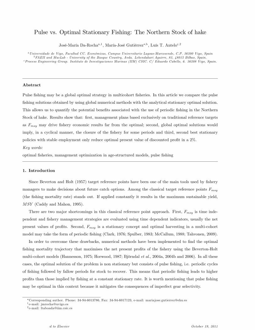
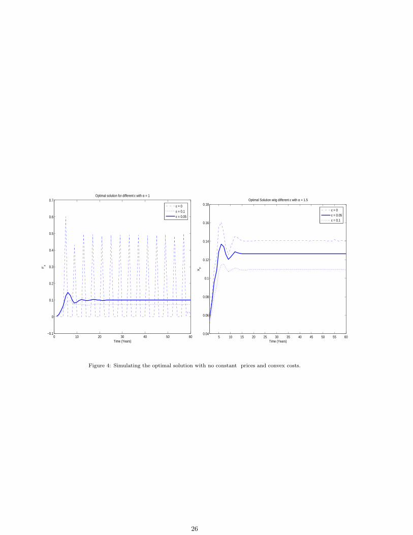
What would be the implications for our model of abandoning the assumption of constant fishing mortality
unit costs and prices? Under this new assumption the analytical solution could be characterised and the
numerical solution found. Figure 4 shows the results of seeking the numerical solution using control vector
parameterisation if the following is used as the objective function
A∑a=1
[paya(Ft)Nat ](1−εa) − cFα.
[Insert Figure 4]
15

When ε = 0, the solution is similar to that for constant prices. If ε > 0, the price function introduces a
mechanism that reduces the advantages of pulse fishing solutions: the more sensitive prices are to variations
in catches, the more desirable stationary solutions become. Cost convexity also has a considerable impact.
When α = 1.5, the stationary solution is optimal even with constant prices.
Concave and convex costs can be considered as reduced forms of more complex relationships that can be
incorporated into the model. For instance Da Rocha, Cerviño and Gutiérrez (2010) show that it is possible
to introduce fleet dynamics into an age-structured model, with forward-looking firms that make decisions
discounting the sum of future profits. Another possible extension of the model would be to consider that
the catchability coeffi cient is not constant but dependent on time, horsepower and tonnage (see Da Rocha
and Gutiérrez, 2011). Of course, these changes might influence the results. And our guess is that in a richer
environment, periodic solutions would prove inferior to stationary ones.
As mentioned in the Introduction, there are cases of fisheries which are exploited on a pulse basis.
However, in general the fact that stocks are exploited jointly by several countries, the non malleable nature
of capital and employment, the impossibility of storing catches and the possibility of losing market access all
make it inadvisable to use pulse solutions that would entail the closure of fisheries for some seasons. In other
words stationary solutions are implemented because there are numerous effects not considered explicitly in
the model that make pulse fishing inadvisable.
This study should be seen as measuring the institutional constraints faced by regulators. A comparison
of the stationary and pulse solutions reveals a shadow price of all the implicit constraints not included in
the model (non linear prices, convex costs, fleet dynamics, effort indices, etc). The numerical simulation run
shows that when all these effects are ignored the stationary solution gives results only 2% below those of
the pulse solution. This gives a measure in terms of discounted present value of all the factors not included
in the model. If regulators, resorting to their experience and expertise, consider that reducing the sum
total of discounted benefits by 2% is a low price to pay for keeping the fleet at work continuously, then out
simulations show that the stationary solution is optimal.
Acknowledgements
Special thanks are extended to all participants in the 2007 Lisbon and Brussels North Hake Working
Group Meetings. Financial aid from the Spanish Ministry of Education and Science (ECO2009-14697-C02-
01 and 02), the Basque Government (HM-2009-1-21) and the Xunta de Galicia (Anxeles Alvariño programme)
is gratefully acknowledged.
References
Baranov, F.I., 1918. On the question of the biological basis of fisheries . Institute for Scientific Ichthy-
ological Investigations, Proceedings 1(1), 81-128.
Beverton, R.J.H., Holt, S.J., 1957. On the Dynamics of Exploited Fish Populations. Fish. Invest., II,
19. Republished by Chapman and Hall, 1993, London.
16

Bjørndal, T., Brasão, A., 2006. The East Atlantic Bluefin Tuna Fisheries: Stock Collapse or Recovery?
Marin. Resour. Econ. 21, 193:210.
Bjørndal, T., Gordon D., Kaitala, V., Lindroos, M., 2004a. International Management Strategies for
a Straddling Fish Stock: A Bio-Economic Simulation Model of the Norwegian Spring-Spawning Herring
Fishery. Environ. Resour. Econ. 29, 435:457.
Bjørndal, T., Ussif, A., Sumaila, R., 2004b. A bioeconomic analysis of the Norwegian spring spawning
herring (NSSH) stock. Marin. Resour. Econ. 19, 353:365.
Black, R., 2007. Catch cuts ‘bring bigger profits”. In: BBC News. Available at: http://news.bbc.co.uk/2
/hi/science/nature/7127761.stm.
Botsford, L.W., Quinn, J.F., Wing, S.R., Britmacher, J.G., 1993. Rotating spatial harvest of a benthic
invertebrate, the red sea urchin, Strongylocentrotus franciscanus. In: Proceedings of the International
Symposium on Management Strategies for Exploited Fish Populations. Alaska Sea Grant College Program
AK-93-02, pp. 409—428.
Caddy, J.F., 1993. Background concepts for a rotating harvesting strategy with particular reference to
the Mediterranean Red Coral, Corallium rubrum. Mar. Fish. Rev. 55, 10—18.
Caddy, J.F., Mahon, R., 1995. Reference Points for Fisheries Management. FAO Fish. Tech. Pap., 347.
Clark, C.W., 1976. Mathematical Bioeconomics. John Wiley, New York.
Cinner, J., Marnane. M.J., McClanahan, T.R., Almany, G.R., 2006. Periodic Closures as Adaptive Coral
Reef Management in the Indo-Pacific. Ecol. Soc. 11, 31.
Da Rocha, J. M., Gutiérrez, M. J., Cerviño, S., 2010. Reference points as the steady-state solution for
mixed fisheries management with bio-economic age-structured models. Mimeo.
Da Rocha, J. M., Cerviño, S., Gutiérrez, M. J., 2010. An endogenous bioeconomic optimization algorithm
to evaluate recovery plans: an application to southern hake. ICES J. Mar. Sci., 67:1957-1962.
Da Rocha, J. M., Gutiérrez, M. J., 2011. Lessons from the long-term management plan for northern
hake: Could the economic assessment have accepted it?. ICES J. Mar. Sci., doi:10.1093/icesjms/fsr105.
De la Maza, M., Yuret, D. ,1994. Dynamic hill climbing. AI Expert, 9(3): 26-31.
Dichmont, C. M., Pascoe, S., Kompas, T., Punt, A. E., Deng, R., 2010. On implementing maximum
economic yield in commercial fisheries. PNAS 107, 16-21.
Commission Regulation (EC) No 1162/2001 of 14 June 2001 Establishing Measures for the Recovery of
the Stock of Hake in ICES sub-areas III, IV, V, VI and VII and ICES Divisions VIII a, b, d, e and Associated
Conditions for the Control of Activities of Fishing Vessels
Commission Regulation (EC) No 2602/2001 of 27 December 2001 Establishing Additional Technical
Measures for the Recovery of the Stock of Hake in ICES subareas III, IV, V, VI and VII and ICES Divisions
VIIIa,b,d,e.
Commission Regulation (EC) No 492/2002 of 19 March 2002 Derogating from Regulation (EC) No
562/2000 Laying down Detailed Rules for the Application of Council Regulation (EC) No 1254/1999 as
Regards the Buying-in of Beef and Amending Regulation (EEC) No 1627/89 on the Buying-in of Beef by
Invitation to Tender
17

Council Regulation (EC) No 811/2004 of 21 April 2004 Establishing measures for the recovery of the
Northern Hake Stock.
Egea, J.A., Balsa-Canto, E., García, M.S.G., Banga, J.R., 2009. Dynamic optimization of nonlinear
processes with an enhanced scatter search method. Ind. Eng. Chem. Res 48(9), 4388-4401.
Grafton, R. Q., Kirkley, J., Kompas, T., Squires, D., 2006. Economics for fisheries management. Ashgat,
London.
Grafton, R. Q., Kompas, T., Chu, L., Che, N., 2010. Maximum economic yield. Aust. J. Agric. Resour.
Econ. 54, 273-280.
Grafton, R. Q., Kompas, T. and Hilborn, R.W., 2007. Economics of overexploitation revisited. Science,
318:1601.
Graham, T.R., 2001. Advantages of pulse fishing in live product fisheries. Live Reef Fish Inf. Bull. 9,
5-10.
Gröger, J. P., Rountree, R. A., Missong, M., and Rätz, H. J., 2007. A stock rebuilding algorithm
featuring risk assessment and an optimization strategy of single or multispecies fisheries. ICES J. Mar. Sci.
64, 1101-1115.
Hannesson, R., 1975. Fishery dynamics: a North Atlantic cod fishery. Can. J. Econ. 8, 151-173.
Hart, D.R. (2003). Yield-and biomass-per-recruit analysis for rotational fisheries, with an application to
the Atlantic sea scallop (Placopecten magellanicus). Fish. B.-NOAA, 101, 44—57.
Hart, D.R., Rago, P.J., (2006). Long-term dynamics of U.S. Atlantic sea scallop Placopecten magellanicus
populations. N. Am. J. Fish. Manage. 26, 490—501.
Horwood, J.W., 1987. A Calculation of Optimal Fishing Mortalities. ICES J. Mar. Sci. 43, 199-208.
Horwood, J.W., Whittle, P., 1986. The optimal harvest from a multicohort stock. IMA J. Math. Appl.
Med. Biol. 3, 143-155.
ICES (2007). Report of the Working Group on the Assessment of Southern Shelf Stocks of Hake, Monk
and Megrim (WGHMM), 8-17 May 2007, Vigo, Spain. ICES CM 2007\ACFM:21, 700 pp.
ICES, 2009. Report of the Working Group on the Assessment of Southern Shelf Stocks of Hake, Monk
and Megrim (WGHMM), 5-11 May 2009, Copenhagen, Denmark. ICES CM 2009\ACOM:08, 537 pp.
Kompas, T., Dichmont, C. M., Punt, A. E., Dent, A., Che, T. N., Bishop, J., Gooday, P., Ye, Y., Zhou,
S., 2010, Maximizing profits and conserving stocks in the Australian Northern Prawn Fishery. Aust. J.
Agric. Resour. Econ. 54, 281-299.
Kulmala, S., Laukkanen, M., Michielsens, C., 2008. Reconciling economic and biological modeling of
migratory fish stocks: optimal management of the atlantic salmon fishery in the Baltic Sea. Ecol. Econ. 64,
716-728.
Laguna, M. Martí, R., 2003. Scatter Search: Methodology and Implementations in C. Kluwer Academic
Publishers: Norwell, MA.
Lassen, H., Medley, P., 2000. Virtual Population Analysis. A Practical Manual for Stock Assessment.
FAO Fish. Tech. Pap., 400.
Mayne, D.Q., Rawlings, J.B, Rao, C.V. and J.O. Scokaert, 2000. Constrained Model Predictive Control:
18

Optimality and Stability. Automatica. 36(6), 789-814.
McCallum, H.I., 1988. Pulse fishing may be superior to selective fishing. Math. Biosci. 89, 177-181.
McKendrick, A.G., 1926. Applications of mathematics to medical problems. Proceedings of the Edin-
burgh Mathematical Society 44, 98-130.
Shepherd, J.G., 1982. A versatile new stock-recruitment relationship for fisheries, and the construction
of sustainable yield curves. ICES J. Mar. Sci. 40(1), 67-75.
Spulber, D.F., 1983. Pulse-fishing and stochastic equilibrium in the multicohort fishery. J. Econ. Dyn.
Control. 6, 309-332.
Scientific, Technical and Economic Committee for Fisheries (STECF). 2008a. Report of the sub-group
on balance between resources and their exploitation (SGBRE). Northern hake long-term management plans
(SGRE-07-03). (eds. Jardim E & Hölker, F). 2008. Publication Offi ce of the European Union, Luxemburg,
ISBN 978-92-79-11044-3, JRC49104, 133pp.
Scientific, Technical and Economic Committee for Fisheries (STECF). 2008b. Report of the sub-group
on balance between resources and their exploitation (SGBRE). Northern hake long-term management plans
(SGRE-07-05). (eds. Van Hoof L & Hölker, F). 2008. Publication Offi ce of the European Union, Luxemburg,
ISBN 978-92-79-11044-6, JRC49103, 106pp.
Storn, R., Price, K., 1997. Differential evolution. A simple and effi cient heuristic for global optimization
over continuous spaces. J. glob. optim. 11, 341—359.
Tahvonen, O., 2009. Economics of Harvesting Age-Structured Fish Populations . J. Environ. Econ.
Manage. 58, 281—299.
Vassiliadis, V.S., 1993. Computational Solution of Dynamic Optimization Problems with General Differential-
Algebraic Constraints. PhD Thesis. Imperial College. London.
Vassiliadis, V.S., Pantelides, C.C., Sargent, R.W.H., 1994. Solution of a class of multistage dynamic
optimization problems. 1. Problems without path constraints. Ind. Eng. Chem. Res. 33(9), 2111-2122.
Von Foerster, H., (1959. Some remarks on changing populations. In The Kinetics of Cell Prolifeeration,
382-407.
Van Oostenbrugge, J.A.E., Powell, J.P., Smit. J.P.G., Poos, J.J., Kraak, S.B.M. and Buisman, F.C.
(2008). Linking catchability and fisher behaviour under effort management. Aquatic Living Resources, 21,
265-273.
19

Table 1: Age Structure and the Intertemporal Maximization Problem
t t+1 t+2 ... t+A-2 t+A-1 t+A t+A+1
a=1 N1t N1
t+2 ...
a=2 N2t N2
t+1 ... N2t+A−2
... ... ... ... ... ... ... ...
a=A-1 NA−1t NA−1
t+1 NA−1t+2 ... NA−1
t+A−2 NA−1t+A
a=A NAt NA
t+1 NAt+2 ... NA
t+A−2 NAt+A−1 NA
t+A+1
Table 2: Characteristics of the Spanish Fleet (2004)
Segment Fleet Length Class Number of vessels Total employment Gross Value Added (m€)
Demersal Trawlers 24-40m 93 1,023 56.8
Pair Demersal Trawlers 24-40m 20 239 9.6
Longliners 24-40m 84 1,176 59.8
Total 197 2,438 126.2
Source: STECF, 2008b. Tables 6.1.5, 6.1.6, 6.1.8 y 6.1.9
20

Table 3: Characteristics of the French Fleet (2006)
Segment Fleet Length Class Number of vessels Total employment Gross Value Added (me)
DTS-Targeted Nephrops 12-24m 204 759 45.4
DTS-Targeted Fish 12-24m 106 490 35.9
DTS 24-40m 55 389 28.9
Hook 24-40m 5 62 2.3
Netters 12-24m 60 351 22.2
Netters 24-40m 18 223 11.3
Others - 210 803 -
Total 658 3,077 -
Source: STECF, 2008b. Tables 6.2.5, 6.2.8-6.2.13
Table 4: Parameters by age
Initial conditions
Age 0 Age 1 Age 2 Age 3 Age 4 Age 5 Age 6 Age 7 Age 8 Age 9 Age 10
Na (1) 186, 213 152, 458 123, 457 100, 213 67, 409 35, 551 19, 674 10, 206 9, 147 4, 078 1, 819
Population dynamics
Age 0 Age 1 Age 2 Age 3 Age 4 Age 5 Age 6 Age 7 Age 8 Age 9 Age 10
pa 0.00 0.06 0.54 1.15 1.03 1.52 2.09 2.43 2.43 2.43 2.43
ωa (2) 0.06 0.13 0.22 0.34 0.60 0.98 1.44 1.83 2.68 2.68 2.68
µa 0.00 0.00 0.00 0.23 0.60 0.90 1.00 1.00 1.00 1.00 1.00
Prices
Age 0 Age 1 Age 2 Age 3 Age 4 Age 5 Age 6 Age 7 Age 8 Age 9 Age 10
pra (3) 2.36 2.93 3.42 3.85 4.55 5.22 5.81 6.22 6.92 6.92 6.92
Source: Meeting on Northern Hake Long-Term Management Plans (STECF/SGBRE-07-03) and ICES (2007)
(1) Thousand;(2) kg ; (3) Euros/kg
21

Table
5:Economic
Indicators
forSegmen
t
Segmen
tS1(2004)
S2(2004)
S3(2004)
F1(2006)
F2(2006)
F3(2006)
F4(2006)
F5(2006)
F6(2006)
Valueoflandings
101,914,422
19,172,000
90,970,320
98.1
77.6
67.5
3.9
37.9
18.3
Fuel
costs
21,182,889
3,141,640
7,300,860
20.2
15.9
15.4
0.5
3.0
1.7
Other
runningcosts
12,071,121
3,867,258
20,030,640
9.7
7.7
7.1
0.4
3.1
1.5
Dep
reciation
12,938,904
2,551,888
10,711,260
8.8
7.0
8.1
0.3
2.8
1.4
Interest
879,594
194,053
859,236
1.6
1.3
1.6
0.2
0.6
0.4
Day
satthesea
25,389
4,112
21,924
32,300.0
21,500.0
14,500.0
11,00.0
10,300.0
4500.0
Crew
share
40,876,476
7,221,568
44,804,508
32.1
25.4
20.1
1.5
15.0
7.3
S1=Longliners(24-40m);S2=Dem
ersaltraw
lers
(24-40m);S3=
Pairdem
ersaltraw
lers
(24-40m);F1=Dem
ersaltraw
lsseiners-Targetingnep
hrops,(12-24m);
F2=
Dem
ersaltraw
lsseiners,-Targetingfish,(12-24m);F3=Dem
ersaltraw
lsseiners-Targetingnep
hropsorfish,(24-40m);F4=
Hook(24-40m);F5=
Netters
(12-24m)andF6=Netters
(24-40m).
S1,S2andS3in
Euros;F1.F2.F3.F4.F5andF6in
millionsofEuros.
Source:
Tables6.1.7-6.1.9,6.2.8-6.2.13and7-2-3
(STECF,2008b). Table
6:Costsper
Day
andFU
Segmen
tS1(2004)
S2(2004)
S3(2004)
F1(2006)
F2(2006)
F3(2006)
F4(2006)
F5(2006)
F6(2006)
mean
Fuel
per
day
834.3
764.0
333.0
625.4
739.5
1062.1
454.5
291.3
377.8
651
Other
costsper
day
475.4
940.5
913.6
300.3
358.1
489.7
363.6
301.0
333.3
483
Dep
reciation/day
509.6
620.6
488.6
272.4
325.6
558.6
272.7
271.8
311.1
403
Iinterest/day
34.6
47.2
39.2
49.5
60.5
110.3
181.8
58.3
88.9
56
Totalcost
per
day
1,854.1
2,372.3
1,774.4
1,247.7
1,483.7
2,220.7
1,272.7
922.3
1,111.1
1593
Hakedep
enden
cy24%
36%
98%
4%
2%
6%
77%
20%
84%
0.47%
Crew
share
0.40
0.38
0.49
0.33
0.33
0.30
0.38
0.40
0.40
0.37
S1=Longliners(24-40m);S2=Dem
ersaltraw
lers
(24-40m);S3=
Pairdem
ersaltraw
lers
(24-40m);F1=Dem
ersaltraw
lsseiners-Targetingnep
hrops,(12-24m);
F2=
Dem
ersaltraw
lsseiners,-Targetingfish,(12-24m);F3=Dem
ersaltraw
lsseiners-Targetingnep
hropsorfish,(24-40m);F4=
Hook(24-40m);F5=
Netters
(12-24m)andF6=Netters
(24-40m).
S1,S2andS3in
Euros;F1.F2.F3.F4.F5andF6in
millionsofEuros.
Source:
Owncalculations
22

Table 7: Comparison of the three scenarios with positive costs
Long Run Values Net Present Profits
F SSB Yield J ∆J
Scenario 1: Fmsy 0.172 1.9807e+ 005 3.395e+ 005 3.5752e+ 006 100.00
Scenario 2: Fss 0.119 2.5414e+ 005 3.314e+ 005 4.2736e+ 006 119.53
Scenario 3: Fperiodic 4.3562e+ 006 121.85
year 1 0 1.6719e+005 0
year 2 0 2.1240e+005 0
year 3 0 2.6985e+005 0
year 4 0.489 3.5476e+ 005 13.500e+ 005
Table 8: Comparison of the three scenarios with zero costs
Long Run Net Present Profits
F J ∆J
scenario 1: Fmsy 0.172 6.2946e+ 006 100.00
scenario 2: Fss 0.172 6.3363e+ 006 100.66
scenario 3: Fperiodic 0.170 6.3906e+ 006 101.53
Figure 1: Control Vector Parametrization (CVP) scheme
23

Figure 2: ICES Fishing Areas
24

0 0.5 1 1.5 2 2.5 3 3.5
x 105
0
0.5
1
1.5
2
2.5
3
3.5
4x 10
5
Spawning stock biomass (M tonne)
Re
cru
itm
en
t a
t 1
ye
ar
old
(1
0 e
−9
)
78
79
80
81
8283
84
85
86
8788
89
90
91
92
93
94
9596
9798
9900
01
02
03 04
05 06
2009 2014 2022 2029 2037 2045 2053 20611
1.5
2
2.5
3
3.5
4
4.5x 10
5
Sp
aw
nin
g s
tock b
iom
ass
Fmax
pulse
stationary
2009 2013 2017 2022 2029 2037 2045 2053 20610
0.1
0.2
0.3
0.4
0.5
0.6
0.7
Fis
hin
g m
ort
alit
y
Fmax
pulse
stationary
2009 2013 20222017 2029 2037 2045 2053 20610
2
4
6
8
10
12
14
16
18x 10
5
Yie
ld (
’00
0 �)
Fmax
pulse
stationary
Figure 3: Trajectories under the three scenarios: optimal (Fperiodic), the stationary solution (Fss) and smooth driven to the
reference point (Fmsy). Stock recruitment relationship (upper left panel); SSB (upper right panel); fishing mortality (lower
left panel) and yield (lower right panel)
25
0 10 20 30 40 50 60−0.1
0
0.1
0.2
0.3
0.4
0.5
0.6
0.7
Time (Years)
Fx
Optimal solution for different ε with α = 1
ε = 0ε = 0.1ε = 0.05
5 10 15 20 25 30 35 40 45 50 55 600.04
0.06
0.08
0.1
0.12
0.14
0.16
0.18
Time (Years)
XF
Optimal Solution witg different ε with α = 1.5
ε = 0ε = 0.05ε = 0.1
Figure 4: Simulating the optimal solution with no constant prices and convex costs.
26

Appendix
A.Tech
nicalreport:Solvingth
emaxim
ization
pro
blem
488
Inthis
report
weshow
indetailhow
tosolveoptimalmanagem
entproblem
forthecase
ofA
=3.7
max
{F
t,N
1 t+
2}
∞ t=
0
∞∑
t=0
βt
{
3∑ a=1
praya(F
t)N
a t
}
s.t.
Na+1
t+1=
e−za(F
t)N
a t∀t
∀a=
1,2
N1 t+
1=
Ψ(
∑
3 a=1µaωaN
a t
)
∀t
∑
3 a=1µaωaN
a t≥
SSB
pa
∀t
Inthis
context,thefunctionto
bemaxim
ized
canbeexpressed
as
L=
∞∑
t=0
βt
pr1y1 t(F
t)φ
1 tN
1 t+pr2y2 t(F
t)φ
2 tN
1 t−1+pr3y3 t(F
t)φ
3 tN
1 t−2−TC(F
t)
+λt
[
Ψ1 t
(
µ1ω1φ1 tN
1 t+µ2ω2φ2 tN
1 t−1+µ3ω3φ3 tN
1 t−2
)
−N
1 t+1
]
+θ t[
µ1ω1φ1 tN
1 t+µ2ω2φ2 tN
1 t−1+µ3ω3φ3 tN
1 t−2−SSB
1 pa
]
,(A
.1)
wherethesurvivalfunctionsare
given
by
489
φ1 t=
1,
φ2 t=
φ(F
t−1)=
e−p1F
t−
1−m
1
,
φ3 t=
φ(F
t−1,F
t−2)=
e−p2F
t−
1−m
2
e−p1F
t−
2−m
1
,
Itis
easy
toseethatFtappears
in(A
.1)only
inthesumsmultiply
byβt ,βt+
1andβt+
2.Thatis
490
7Themathem
aticaldevelopmen
tssh
ownin
this
Appen
dix
could
beconsidered
atech
nicalreport.Weletto
theed
itors’decisionthereleva
nce
ofbeingpublish
edorkep
tastech
nical
report
available
from
theauthors.
27

......+βt
pr1y1 t(F
t)N
1 t+pr2y2 t(F
t)e
−p1F
t−
1−m
1
N1 t−
1+pr3y3 t(F
t)e−
p2F
t−
1−m
2
e−p1F
t−
2−m
1
N1 t−
2−TC(F
t)
+λt
[
Ψ1 t
(
µ1ω1N
1 t+µ2ω2e−
p1F
t−
1−m
1
N1 t−
1+µ3ω3e−
p2F
t−
1−m
2
e−p1F
t−
2−m
1
N1 t−
2
)
−N
1 t+1
]
+θ t
[
µ1ω1N
1 t+µ2ω2e−
p1F
t−
1−m
1
N1 t−
1+
µ3ω3e−
p2F
t−
1−m
2
e−p1F
t−
2−m
1
N1 t−
2−SSB
1 pa
]
+βt+
1
pr1y1 t+
1(F
t+1)N
1 t+1+pr2y2 t+
1(F
t+1)e
−p1F
t−m
1
N1 t+pr3
.1y3 t+
1(F
t+1)e
−p2F
t−m
2
e−p1F
t−
1−m
1
N1 t−
1−TC(F
t+1)
+λt+
1
[
Ψ1 t+
1
(
µ1ω1N
1 t+1+µ2ω2e−
p1F
t−m
1
N1 t+µ3ω3e−
p2F
t−m
2
e−p1F
t−
1−m
1
N1 t−
1
)
−N
1 t+2
]
+θ t
+1
[
µ1ω1N
1 t+1+µ2ω2e−
p1F
t−m
1
N1 t+µ3ω3e−
p2F
t−m
2
e−p1F
t−
1−m
1
N1 t−
1−SSB
1 pa
]
+βt+
2
pr1y1 t+
2(F
t+2)N
1 t+2+pr2y2 t+
2(F
t+2)e
−p1F
t+
1−m
1
N1 t+
1+pr3
.1y3 t+
2(F
t+2)e
−p2F
t+
1−m
2
e−p1F
t−m
1
N1 t−TC(F
t+2)
+λt+
2
[
Ψ1 t+
2
(
µ1ω1N
1 t+2+µ2ω2e−
p1F
t+
1−m
1
N1 t+
1+µ3ω3e−
p2F
t+
1−m
2
e−p1F
t−m
1
N1 t
)
−N
1 t+3
]
+θ t
+2
[
µ1ω1N
1 t+2+µ2ω2e−
p1F
t+
1−m
1
N1 t+
1+µ3ω3e−
p2F
t+
1−m
2
e−p1F
t−m
1
N1 t−SSB
1 pa
]
+....
Therefore,thefirstorder
conditionsfrom
∂L/∂Ft=
0is
given
by
491
∂L
∂Ft
=βt{
pr1
∂y1 t(F
t)
∂F
tN
1 t+pr2
∂y2 t(F
t)
∂F
t)φ
2 tN
1 t−1+
pr3
∂y3 t(F
t)
∂F
tφ3 tN
1 t−2−
∂TC(F
t)
∂F
t
}
+
+βt+
1
pr2y2 t+
1(F
t+1)(
−p1)
φ2 t+
1N
1 t+pr3y3 t+
1(F
t+1)(
−p2)
φ3 t+
1N
1 t−1
+λt+
1
(
Ψ1 t+
1
)
′[
µ2ω2(
−p1)
φ2 t+
1N
1 t+µ3ω3(
−p2)
φ3 t+
1N
1 t−1
]
+θ t
+1
[
µ2ω2(
−p1)
φ2 t+
1N
1 t+µ3ω3(
−p2)
φ3 t+
1N
1 t
]
+
+βt+
2
pr3y3 t+
2(F
t+2)(
−p1)
φ3 t+
2N
1 t
+λt+
2
(
Ψ1 t+
2
)
′[
µ3ω3(
−p1)
φ3 t+
2N
1 t
]
+θ t
+2
[
µ3ω3(
−p1)
φ3 t+
2N
1 t
]
=0
28
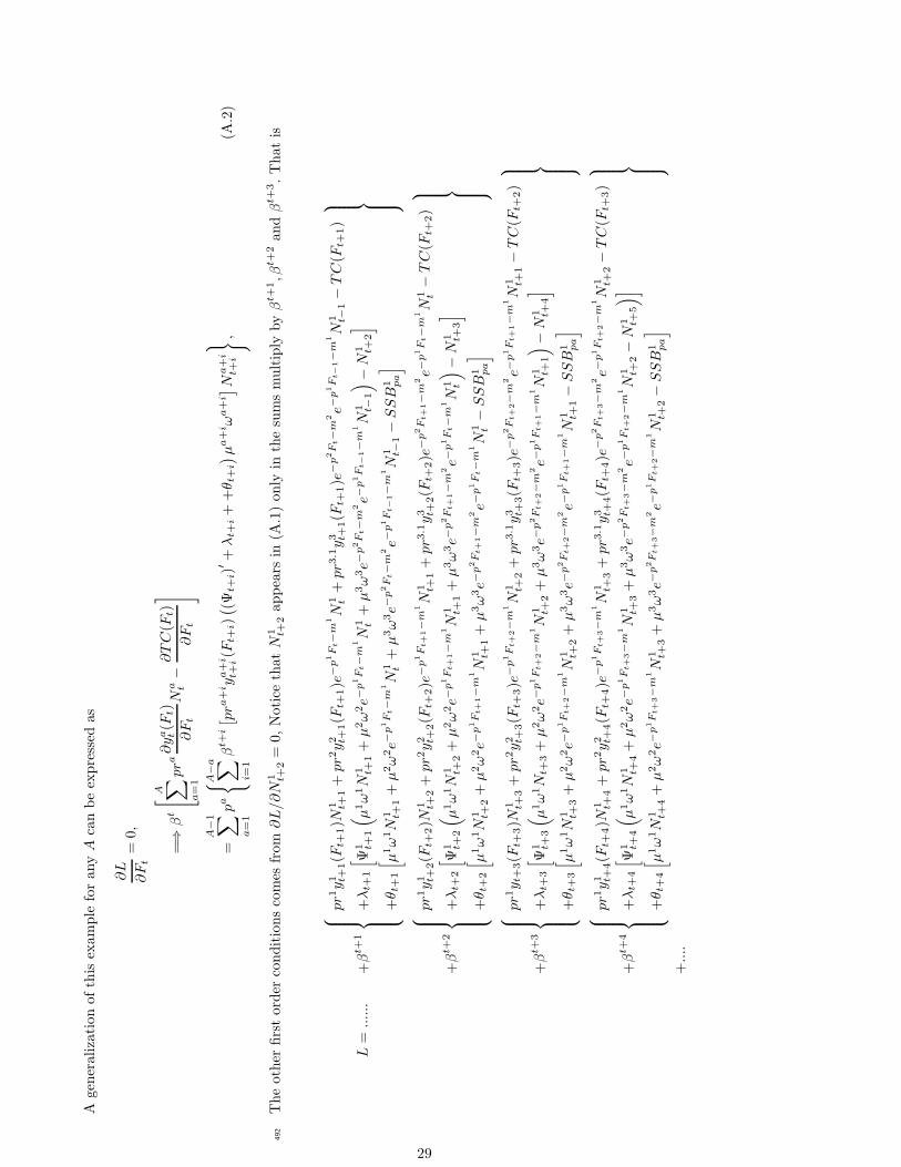
Ageneralizationofthis
example
foranyA
canbeexpressed
as
∂L
∂Ft=
0,
=⇒
βt
[
A∑ a=1
pra
∂ya t(F
t)
∂Ft
Na t−
∂TC(F
t)
∂Ft
]
=
A−1
∑ a=1
pa
{
A−a
∑
i=1
βt+
i[
pra
+i y
a+i
t+i(F
t+i)(
(Ψt+
i)′+λt+
i++θ t
+i)µa+i ω
a+i]N
a+i
t+i
}
,(A
.2)
Theother
firstorder
conditionscomes
from
∂L/∂N
1 t+2=
0,Notice
thatN
1 t+2appears
in(A
.1)only
inthesumsmultiply
byβt+
1,β
t+2andβt+
3.Thatis
492
L=
......
+βt+
1
pr1y1 t+
1(F
t+1)N
1 t+1+pr2y2 t+
1(F
t+1)e
−p1F
t−m
1
N1 t+pr3
.1y3 t+
1(F
t+1)e
−p2F
t−m
2
e−p1F
t−
1−m
1
N1 t−
1−TC(F
t+1)
+λt+
1
[
Ψ1 t+
1
(
µ1ω1N
1 t+1+µ2ω2e−
p1F
t−m
1
N1 t+µ3ω3e−
p2F
t−m
2
e−p1F
t−
1−m
1
N1 t−
1
)
−N
1 t+2
]
+θ t
+1
[
µ1ω1N
1 t+1+µ2ω2e−
p1F
t−m
1
N1 t+µ3ω3e−
p2F
t−m
2
e−p1F
t−
1−m
1
N1 t−
1−SSB
1 pa
]
+βt+
2
pr1y1 t+
2(F
t+2)N
1 t+2+pr2y2 t+
2(F
t+2)e
−p1F
t+
1−m
1
N1 t+
1+pr3
.1y3 t+
2(F
t+2)e
−p2F
t+
1−m
2
e−p1F
t−m
1
N1 t−
TC(F
t+2)
+λt+
2
[
Ψ1 t+
2
(
µ1ω1N
1 t+2+µ2ω2e−
p1F
t+
1−m
1
N1 t+
1+µ3ω3e−
p2F
t+
1−m
2
e−p1F
t−m
1
N1 t
)
−N
1 t+3
]
+θ t
+2
[
µ1ω1N
1 t+2+µ2ω2e−
p1F
t+
1−m
1
N1 t+
1+µ3ω3e−
p2F
t+
1−m
2
e−p1F
t−m
1
N1 t−SSB
1 pa
]
+βt+
3
pr1y t
+3(F
t+3)N
1 t+3+pr2y2 t+
3(F
t+3)e
−p1F
t+
2−m
1
N1 t+
2+pr3
.1y3 t+
3(F
t+3)e
−p2F
t+
2−m
2
e−p1F
t+
1−m
1
N1 t+
1−TC(F
t+2)
+λt+
3
[
Ψ1 t+
3
(
µ1ω1N
t+3+µ2ω2e−
p1F
t+
2−m
1
N1 t+
2+µ3ω3e−
p2F
t+
2−m
2
e−p1F
t+
1−m
1
N1 t+
1
)
−N
1 t+4
]
+θ t
+3
[
µ1ω1N
1 t+3+µ2ω2e−
p1F
t+
2−m
1
N1 t+
2+µ3ω3e−
p2F
t+
2−m
2
e−p1F
t+
1−m
1
N1 t+
1−SSB
1 pa
]
+βt+
4
pr1y1 t+
4(F
t+4)N
1 t+4+pr2y2 t+
4(F
t+4)e
−p1F
t+
3−m
1
N1 t+
3+pr3
.1y3 t+
4(F
t+4)e
−p2F
t+
3−m
2
e−p1F
t+
2−m
1
N1 t+
2−TC(F
t+3)
+λt+
4
[
Ψ1 t+
4
(
µ1ω1N
1 t+4+µ2ω2e−
p1F
t+
3−m
1
N1 t+
3+µ3ω3e−
p2F
t+
3−m
2
e−p1F
t+
2−m
1
N1 t+
2−N
1 t+5
)]
+θ t
+4
[
µ1ω1N
1 t+4+µ2ω2e−
p1F
t+
3−m
1
N1 t+
3+µ3ω3e−
p2F
t+
3−m
2
e−p1F
t+
2−m
1
N1 t+
2−SSB
1 pa
]
+....
29

Therefore,thefirstorder
conditionsfrom
∂L/∂N
1 t+2=
0is
given
by
493
∂L
∂N
1 t+2
=−βt+
2+
λt+
1+βt+
2{
pr1y1 t+
2(F
t+2)[
+λt+
2(Ψ
t+2)′++θ t
+2
]
µ1ω1}
+βt+
3{
pr2y2 t+
3(F
t+3)φ
2 t+3+[
+λt+
3(Ψ
t+3)′++θ t
+3
]
µ2ω2φ2 t+
3
}
+βt+
4{
pr3y3 t+
4(F
t+4)φ
2 t+4+[
+λt+
4(Ψ
t+4)′++θ t
+4
]
µ3ω3φ2 t+
4
}
=0
Ageneralizationofthis
example
foranya=
1,...A
canbeexpressed
as
A∑ a=1
βt+
1+apraya t+
1+a(F
t+1+a)φ
a t+1+a=
βt+
1+λt+
1−
A∑ a=1
βt+
1+a(
(Ψt+
1+a)′+λt+
1+a+
+θ t
+1+a
)
µaωaφa t+
1+a,
(A.3)
30