pulse techniques. off-resonance effects initial magnetization along z x-pulse ( = 0) on-resonance:...
TRANSCRIPT

Pulse Techniques

Off-Resonance Effects
Initial magnetization along z x-pulse ( = 0) On-resonance:
Mz -> -My
Off-resonance: phase
sin
cos)cos1(tan
sintan
)sincos(cos
sinsin
cossin)cos1(
01
220
0
0
y
x
z
y
x
M
M
MM
MM
MM
x
y
Mxy
z
y
x
B1
Br
Bo

Off-Resonance Effects – 90º Pulse
90º hard pulse works well for < 1
Phase shift is approximately linear
Effective flip angle increases 0 1 3 4
-0.5
0.5
1.0
/1
-1.0
Mxy
0 1 3 40
50
100
150
200
250
300
350
/1
Off-Resonance Effects – 90º Pulse
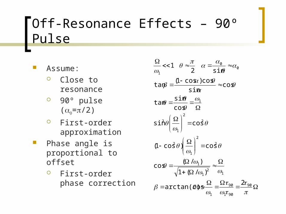
Assume: Close to resonance 90º pulse (=/2) First-order
approximation Phase angle is
proportional to offset First-order phase
correction
90
901
90
1
12
1
1
2
2
1
2
2
2
1
2
1
00
1
2)arctan(cos
)/(1
)/(cos
cos)cos1(
cossin
cos
sintan
cossin
cos)cos1(tan
sin21

Off-Resonance Effects – 90º Pulse
Initial magnetization state is irrelevant
Result: z-x-z
)()()(
)()()2/()(
)()()()2/(
)()()()2/(
)()()2/()(
)()2/()()2/()2/()(
),(
1sin
1
2,
2sin
2/
,2
)()()(),(
1
zxz
zxxz
zxyx
yxzx
yxxy
yyzzyy
x
yzyx
z
y
x
B1
Br
Bo

Off-Resonance Effects - Compensation
Not constant-time Subtract 290/ for each
90º pulse, or Add a short echo
Constant-time No compensation
needed if 90º pulses are identical
Shaped 90º pulses?
t1 - 4/
T - T +
t1 +
t12
t12

Pulse calibration – 180º or 360º?
180º pulse: Poor off-resonance
performance Mxy ~
Linear phase twist Saturation in repeated
experiments 360º pulse
Better off-resonance performance < 0.1 1
Uniform phase Minimal saturation
0.0 0.1 0.2 0.3 0.4 0.50.0
0.2
0.6
0.8180o
360o
/1
Mxy
0.0 0.1 0.2 0.3 0.4 0.50
5
15
20 180o
360o
/1

Off-Resonance Effects – 180º Pulse
Inversion: Poor off-resonance
performance Refocusing:
Orthogonal better than parallel
Phase twist is the same Both work only for
< 0.2 1
0.0 0.2 0.6 0.8
0.2
0.4
0.6
0.8
1.0
0.0
-Mz (inv.)
Mxy (x/x)
Mxy (y/x)
/1
0.0 0.2 0.6 0.80
5
10
15
25
30
35
/1
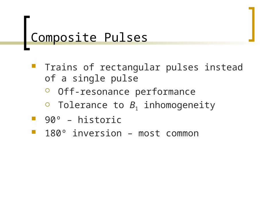
Composite Pulses
Trains of rectangular pulses instead of a single pulse Off-resonance performance Tolerance to B1 inhomogeneity
90º – historic 180º inversion – most common

90x-180y-90x Composite Pulse
90x-180y-90x replaces 180x
for inversion The middle 180º
compensates for off-resonance behavior of the outer 90º pulses

x-2y-x Composite Pulse
90x-180y-90x has better broadband inversion performance < 1
90x-225y-90x has smoother, but narrower profile < 0.7 1
x-2y-x composite pulse is less sensitive to mis-calibration of 90º pulse
Cannot be used for refocusing 80 85 95 100
-0.998
-0.996
-0.994
-0.992
-0.990
-1.000
Mz
2x
x2.5yxx2yx
0.0 0.5 1.5 2.0-1.0
-0.5
0.5
1.0
Mz
/1
180x
90x1
80y9
0x
90x2
25y9
0x

Selective Pulses
Requirements: Uniform excitation (inversion) profile Minimal perturbation outside the target
frequency range Uniform resulting phase (for excitation) Short pulse length Low peak power Easy to implement shape

Soft Rectangular Pulses
Find 1, which produces a null in the excitation (inversion) profile at a certain offset off-resonance
33
1tan
2
3cos
2
1sin
1515
1tan
4
15cos
4
1sin
2
2sin2
sin
...,2...,,4,2,01cos
1sincoscos
)sincos(cos
)180(1
1
0
)90(1
1
0
00
22
022
0
n
MMM z
0 1 2 3 4 5
-0.75
-0.50
-0.25
0.25
0.50
0.75
1.00
-1.00
180
90
Mz
/1
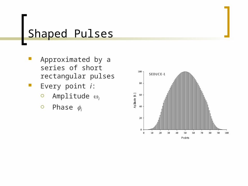
Shaped Pulses
Approximated by a series of short rectangular pulses
Every point i: Amplitude i
Phase i
SEDUCE-1
Points
0 10 20 30 40 50 60 70 80 90 100A
plit
ud
e [
%]
0
20
40
60
80
100

Examples - Gaussian Pulse
Truncated at 1% of max amplitude
Excitation profile - gaussian

Examples - Sinc Pulse
One-lobe of the sinc function
Needs less power for the same length
Similar excitation profile
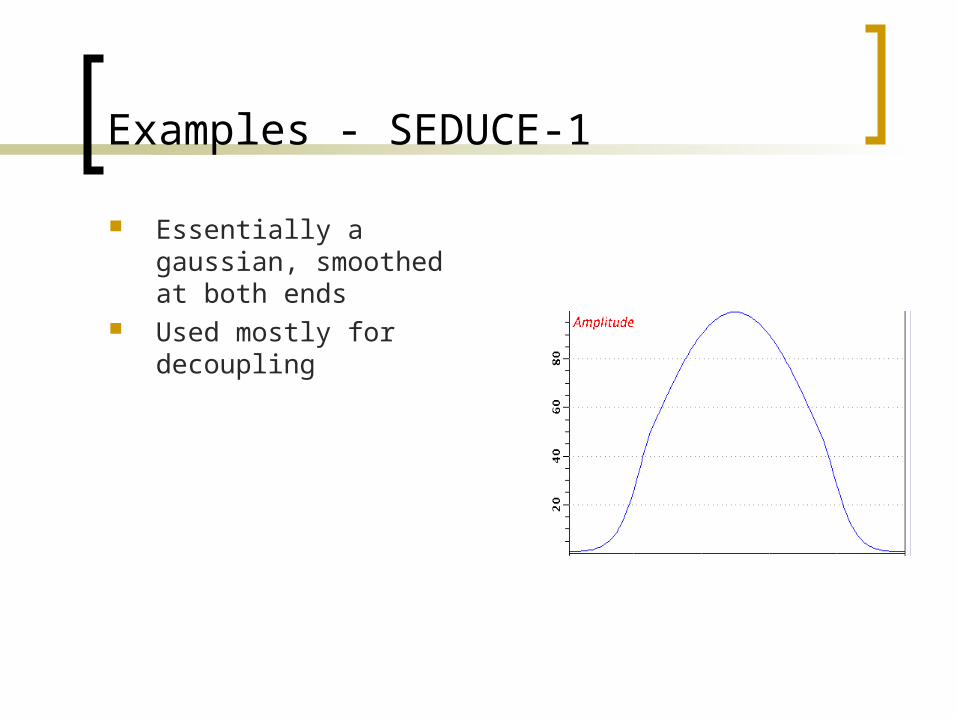
Examples - SEDUCE-1
Essentially a gaussian, smoothed at both ends
Used mostly for decoupling

Examples - Q5 Gaussian Cascade
~300 s pulse used as 90º 13C excitation pulse in Bruker pulse sequences
Better than a soft rectangular 90º pulse
For Iy -> Iz application needs to be time-reversed

Q5 Gaussian Cascade – Excitation Profile

Examples - Q3 Gaussian Cascade
~200 s pulse used as 180º 13C refocusing pulse in Bruker pulse sequences

Q3 Gaussian Cascade – Refocusing Profile

Q3 Gaussian Cascade – Inversion Profile
It also provides good inversion

Examples - E-BURP2
Used in L-optimized experiments

E-BURP2 – Excitation Profile

Phase-Modulated Pulses – Frequency shifting
Linear phase ramp 0 controls the phase of the
resulting pulse: 90º (Iz -> Iy): N = 0
90º (Iy -> Iz): 0 = 0
180º (Iy -> -Iy): N/2 = 0
180º (Iz -> -Iz): arbitrary
Nii
f
i ,...1),(
2
21
0
Phase-Modulated Pulses – Resolution Issues
Time resolution More points = better shape approximation Minimal pulse delay
Phase resolution More points = smaller phase steps Minimal phase step
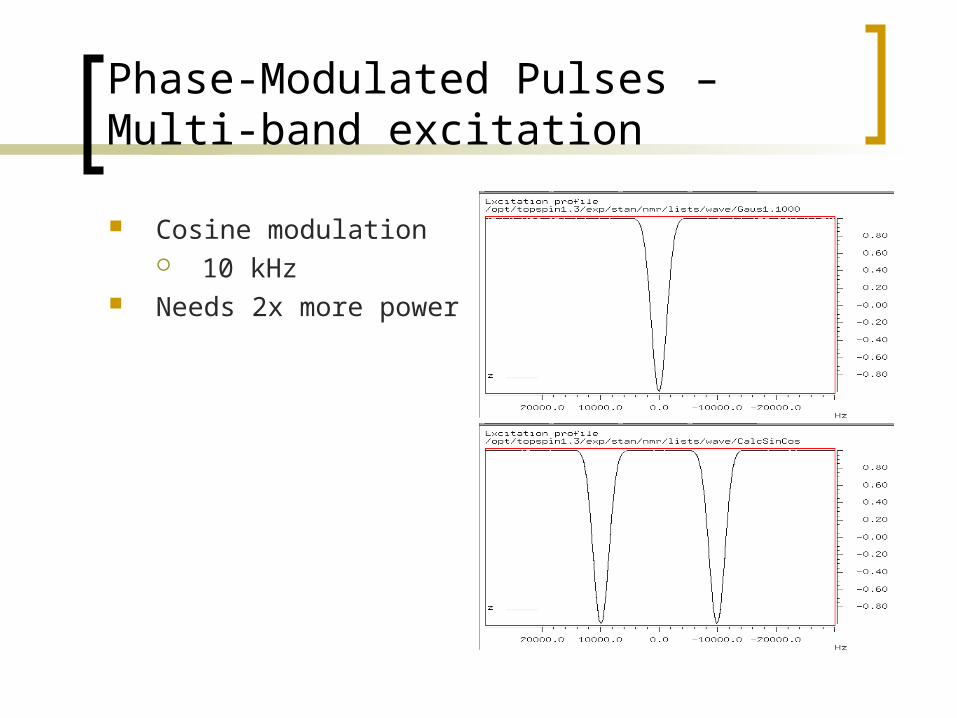
Phase-Modulated Pulses – Multi-band excitation
Cosine modulation 10 kHz
Needs 2x more power

Adiabatic Pulses
“Conventional” pulses: Stationary Beff
orientation Magnitude may be
variable Precession around Beff
Adiabatic pulses: Non-stationary Beff
orientation Magnetization follows
Beff, while precessing around it
z
y
xB1
Beff
Bo
xr
yr
zr
1
ddt

Adiabatic Pulses –Performance Conditions
Beff magnitude should be changed gradually
dt
BdMBBM
dt
BdMB
dt
Md
dt
Md
BMdt
Md
effeffeff
effeff
eff
2
2
2
2
2
2
,
effeff
effeffeffeff
effeffeff
effeff
effeffeff
dt
d
BBdt
Bd
BMBBM
dt
BdM
dt
BdM
BBMdt
BdM

Adiabatic Pulses –Performance Conditions
A second rotating frame {xr, yr, zr} within the first rotating frame
Beff magnitude should be tilted slowly
rreff
reff j
dt
diBB
1
z
y
xB1
Beff
Bo
xr
yr
zr
1
ddt

Adiabatic Pulses –Performance Conditions
Adiabatic condition
Adiabaticity factor
00 /
/
1
dtdQ
dtdQ
dt
d
Bdt
d
eff
eff
eff
eff
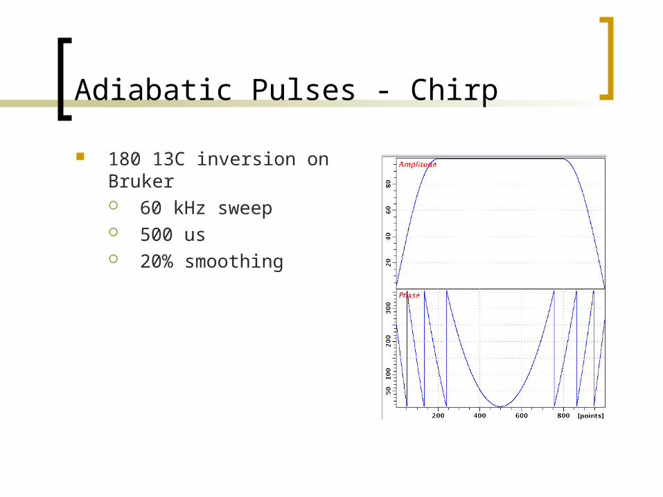
Adiabatic Pulses - Chirp
180 13C inversion on Bruker 60 kHz sweep 500 us 20% smoothing

Chirp – Inversion Profile
Very broad inversion profile Low peak power
~50% of high power

Adiabatic Pulses – Tolerance B1 Inhomogeneity
Power 3 dB higher than calibrated
Power 3 dB lower than calibrated

Adiabatic Pulses - Wurst
Smoothed ramp-up and ramp-down

Adiabatic Pulses - sech

Pseudo Bloch-Siegert Shifts
Assume: x-pulse ( = 0) Very far off-resonance Magnetization along y Third order
approximation
z
y
x
B1
Br
Bo
Pseudo Bloch-Siegert Shifts
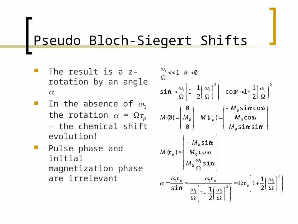
The result is a z-rotation by an angle
In the absence of 1 the rotation = p – the chemical shift evolution!
Pulse phase and initial magnetization phase are irrelevant
2
12
11
11
10
0
0
0
0
0
0
2
1
2
11
1
2
11
21
1sin
sin
cos
sin
)(
sinsin
cos
cossin
)(
0
0
)0(
2
11cos
2
11sin
01
ppp
p
p
M
M
M
M
M
M
M
MMM
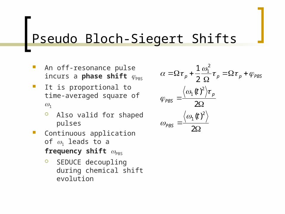
Pseudo Bloch-Siegert Shifts
An off-resonance pulse incurs a phase shift PBS
It is proportional to time-averaged square of 1
Also valid for shaped pulses
Continuous application of 1 leads to a frequency shift PBS
SEDUCE decoupling during chemical shift evolution
2
)(
2
)(
2
1
21
21
21
t
t
PBS
p
PBS
PBSppp

PBS Phase Shifts - Compensation
Small-phase adjustment of a 90º pulse or phase correction in the frequency domain Depends on whether
there is chemical shift evolution
Works only for a narrow range of resonances far off-resonance
Partial compensation Used in BioPack
t12
t12

PBS Phase Shifts - Compensation
Using a second identical pulse and an echo Perfect compensation
over a broad spectral range
Limited by the broadband performance of refocusing 180º pulse
Default for Bruker sequences
T - Tt12
t12

PBS Phase Shifts - Compensation
A second pulse with opposite offset Must be far off-
resonance Imperfect
compensation – first-order phase correction required
Not widely used Cosine modulation
Requires twice the power
t12
t12
2mod
21 )(t
PBS

PBS Frequency Shifts – SEDUCE decoupling
Train of cosine modulated SEDUCE-1 shaped pulses Modulation frequency
mod
Signals of interest are near the carrier
Decoupling is very far off resonance
The result is a scaling of the spectrum by a factor Compression around
the center2mod
21
2mod
21
2mod
21
2mod
22
1
mod
21
mod
21
mod
)(1
)(1
)()(
)(2
)(
)(2
)(
t
t
tt
tt
PBSobs
PBS
rf
rf rfmodrf mod
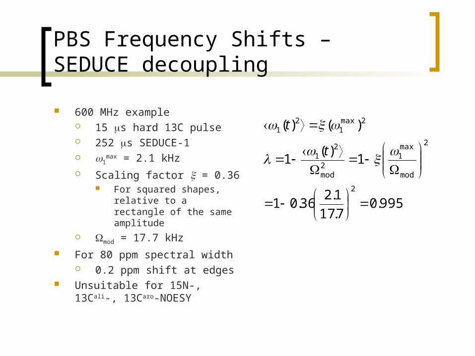
PBS Frequency Shifts – SEDUCE decoupling
600 MHz example 15 s hard 13C pulse 252 s SEDUCE-1 1
max = 2.1 kHz Scaling factor = 0.36
For squared shapes, relative to a rectangle of the same amplitude
mod = 17.7 kHz For 80 ppm spectral width
0.2 ppm shift at edges Unsuitable for 15N-, 13Cali-,
13Caro-NOESY
995.07.17
1.236.01
1)(
1
)()(
2
2
mod
max1
2mod
21
2max1
21
t
t