Principles and Practice of Data Analysis

for Reproducible Research in R

Publication Quality Reports with knitr

Heather Turner

Department of Statistics, University of Warwick

2016�09�29

Markdown

Markdown is a lightweight markup language.

This means it is relatively easy to learn and use, but inevitably haslimitations

I lack of control over page layout: page breaks, columns, �gureplacement

I markup may be insu�cient for complex tables, nested elements, etc

I it can be hard to meet journal style requirements

The rmarkdown Package

RStudio uses the rmarkdown package to convert .Rmd �les to HTML,PDF or Word docx.

There are two steps to this process

I use the knitr package to create a .md �le with the R chunksreplaced by their output

I use the pandoc software to convert the .md �le to HTML, PDF (viaLaTeX) or docx.

Beyond Markdown

The limitations of markdown can be overcome in a number of ways

I using markup language of the intermediate/�nal output, e.g. HTMLfor HTML output, LaTeX for PDF output

I adding metadata to specify parameters used in theintermediate/�nal output, e.g. add header HTML, use an add-onLaTeX package

I using a custom template for the intermediate/�nal output

These all require knowledge of how to produce the intermediate/�naloutput directly.

HTML, LaTeX or Word?

Word document templates can control the general layout e.g. pagemargins, fonts. But some aspects cannot be controlled from markdown(e.g. centering �gures) and converting to word does not o�er richermarkup.

HTML o�ers more control over layout, but is not commonly used byjournals.

LaTeX o�ers full control over layout and style �les are often provided byjournals. More options available to annotate PDFs vs HTML forcollaborators that don't want to edit source code.

Structure of a LaTeX Document

% preamble

\documentclass[12pt]{article}

% document

\begin{document}

Content of article goes here.

\end{document}

Content of article goes here.

1

Document Classes

The document classes available by default are article, report, bookand letter.

A report can have chapters and the title page and abstract take awhole page each. Therefore article is most suited to journalarticles/simple reports. This has options:

Option article

Papersize a4paper/letterpaperFont size 10pt/11pt/12ptNumber of columns onecolumn/two columnMargins oneside/twosideTitle page notitlepage

Orientation portrait/landscapeFormula options center; right label

Draft or �nal �nal/draft

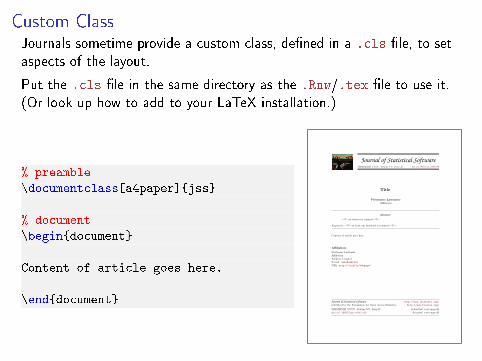
Custom ClassJournals sometime provide a custom class, de�ned in a .cls �le, to setaspects of the layout.

Put the .cls �le in the same directory as the .Rnw/.tex �le to use it.(Or look up how to add to your LaTeX installation.)

% preamble

\documentclass[a4paper]{jss}

% document

\begin{document}

Content of article goes here.

\end{document}

JSS Journal of Statistical SoftwareMMMMMM YYYY, Volume VV, Issue II. doi: 10.18637/jss.v000.i00

Title

Firstname LastnameAffiliation

Abstract

—!!!—an abstract is required—!!!—

Keywords: —!!!—at least one keyword is required—!!!—.

Content of article goes here.

Affiliation:

Firstname LastnameAffiliationAddress, CountryE-mail: name@addressURL: http://link/to/webpage/

Journal of Statistical Software http://www.jstatsoft.org/

published by the Foundation for Open Access Statistics http://www.foastat.org/

MMMMMM YYYY, Volume VV, Issue II Submitted: yyyy-mm-dddoi:10.18637/jss.v000.i00 Accepted: yyyy-mm-dd

Preamble

The preamble (before \begin{document}) is for all the set up codebefore we can start writing the document. Apart from setting thedocument class this includes

I de�ning parameters used by the document class, e.g. title, author

I loading addition packages and setting package options

I de�ning custom commands

Document Parameters

In the standard classes, the document parameters relate to the titlesection which is created in the body using \maketitle.

\documentclass[12pt]{article}

\title{A Small Article \\

Template\thanks{Thanks/footnote}}

\author{Your Name \\

Your Affiliation \\

\and

Your Collaborator \\

Their Affiliation \\

}

\date{\today}

\begin{document}

\maketitle

\end{document}

A Small ArticleTemplate∗

Your NameYour Affiliation

Your CollaboratorTheir Affiliation

September 23, 2016

∗Thanks/footnote

1

Add-on Packages

Like R, LaTeX has thousands of add-on packages. Important ones include

amsmath for typsetting mathematical formulae

graphicx include PNG or PDF graphics (needed for R graphics!)

hyperref for de�ning hyperlinks within documents/for urls

booktabs for publication quality tables

natbib for including citations from a bibliography

Package Example

\documentclass[12pt]{article}

\usepackage[margin = 0cm]{geometry}

\title{A Small Article \\

Template\thanks{Thanks/footnote}}

\author{Your Name \\

Your Affiliation \\

\and

Your Collaborator \\

Their Affiliation \\

}

\date{\today}

\begin{document}

\maketitle

\end{document}

A Small ArticleTemplate∗

Your NameYour Affiliation

Your CollaboratorTheir Affiliation

September 23, 2016

∗Thanks/footnote

1

Abstract

After beginning the document with \maketitle, the next part of thebody will typically be the abstract. This can be added using the the\abstract{} command or the abstract environment:

\begin{abstract}

My first LaTeX paper.

\end{abstract}

Abstract

My first LaTeX paper.

Sectioning

The remainder of the paper will be organised by sections. The starredversions will be unnumbered.

\section{First Section}

The first section.

\subsection{A Subsection}

Text.

\subsection{Another Subsection}

Text.

\subsubsection{A Subsubsection}

Text.

\paragraph{A Labelled Paragraph}

Text.

\section{Second Section}

\subsection*{Unnumbered Subsection}

1 First Section

The first section.

1.1 A Subsection

Text.

1.2 Another Subsection

Text.

1.2.1 A Subsubsection

Text.

A Labelled Paragraph Text.

2 Second Section

Unnumbered Subsection

Text Markup

\textbf{bold} \\

\textit{italic} \\

\texttt{monospace}\\

Non-breaking space: A.~Author \\

"quote" ``double quotes'' \\

inter-word \\

page range, 1--10 \\

punctuation dash---like this \\

\href{http://r-project.org/}{

R Project} \\

\url{http://r-project.org/}

bold

italic

monospace

Non-breaking space: A. Author"quote" �double quotes�inter-wordpage range, 1�10punctuation dash�like thisR Projecthttp://r-project.org/

Special Characters

Some characters are reserved for LaTeX commands:

# $ % _ & { }

They must be escaped to use show the character itself, e.g. \#.

The underscore package enables _ to be typed without escaping.

For extended character support, including

| < >

use \usepackage[T1]{fontenc}

For Unicode character support, e.g. for characters such as

á ä © ¿

use \usepackage[utf8]{inputenc}

Mark up for Mathematics

Inline math $(x + y)^2$.

Displayed math:

\[

\left( \frac{3 + x}{5} \right)

\]

$$ x_1, x_2, \ldots, x_n $$

Numbered equation:

\begin{equation}

\label{model}

y_i = \beta_0 + \beta_1 x_1 +

\epsilon_i

\end{equation}

The model is given in Equation

\ref{model}.

Inline math (x+ y)2.Displayed math:(

3 + x

5

)x1, x2, . . . , xn

Numbered equation:

yi = β0 + β1x1 + εi (1)

The model is given in Equation 1.

Lists

\begin{itemize}

\item A bullet point

\end{itemize}

\begin{enumerate}

\item The first item

\end{enumerate}

\begin{description}

\item[cats] a example of a mammal.

\end{description}

• A bullet point

1. The first item

cats a example of a mammal.

Including Graphics

\begin{figure}[tb]

\centering

\caption{\label{fig:boxplot} Example of a boxplot}

\includegraphics[height=3cm]{boxplot}

\end{figure}

Figure \ref{fig:boxplot} shows an example of a boxplot.

Figure 1: Example of a boxplot

●

−2 −1 0 1 2x

Figure 1 shows an example of a boxplot.

Floats

The �gure environment is a �oating environment. The �gure will be�oated to a suitable position in the document. The options give somecontrol over placement

Option Allowed placement

h will be placed approximately where code appearst top of pageb bottom of pagep separate page for �oats onlyH will be placed exactly where code appears, requires �oat package

Graphic Format

includegraphics can include PNG or PDF graphics - the PNG will beused if there are two �les with the same extension.

PNG is a raster format, i.e. composed of coloured pixels. This generallya poor choice for publications as the graphics can look "fuzzy" and lookworse when zoomed in.

PDF is a vector format, i.e. composed of coloured shapes. This isgenerally the best choice for statistical graphics. Exceptions include

I The graph has 1000s of points

I The graph has large blocks of colour, e.g. a heatmap

In these cases, the PDF �le can be very large and the graph can take along time to "load".

Saving Base Graphics as PDF in R

A base graphic can be saved as PDF in an R script as follows

pdf("plot.pdf", width = 5, height = 5)

plot(y ~ x)

dev.off()

The width and height are speci�ed in inches.

Setting the width and height controls the aspect ratio. Increasing thewidth and/or height makes the text appear smaller as it has a �xed size.

Saving ggplot Graphics as PDF in R

A ggplot can be saved as PDF in an R script as follows

library(ggplot2)

p <- ggplot(data, aes(x = x, y = y)) + geom_point()

ggsave("plot.pdf", p, width = 10, height = 10,

units = "cm")

The width and height are speci�ed in inches by default, di�erent unitswith the units argument.

If the width and height are unspeci�ed, the dimensions of the plotwindow are used.

If p is unspeci�ed, the last plot displayed in the plot window is saved.

Saving Base Graphics as PNG in R

A base graphic can be saved as PNG in an R script as follows

png("plot.png", width = 5, height = 5, units = "in",

res = 600)

plot(y ~ x)

dev.off()

The width and height are speci�ed in pixels by default, so units must bespec�ed to use in or cm.

Here the resolution is set to 600 ppi (pixels per inch) which is a highresolution for publication. 300 ppi is generally �ne for self-printing. Thedefault is 72 ppi, which is suitable for on-screen viewing.

Saving ggplot2 Graphics as PNG in R

A ggplot2 graphic can be saved as PNG in an R script as follows

ggsave("plot.png", p, width = 10, height = 10,

units = "cm", dpi = 600)

The dpi argument is used to set the resolution.

The knitr Package

The knitr package is a general purpose package for dynamic reportingwith R. Supported formats include the following:

I .Rmd to .md

I .Rhtml to .html

I .Rtex or .Rnw to .tex

It is conventional to use .Rnw �R no web� for R + LaTeX, as this wasused by an earlier package, Sweave.

.Rnw Code Chunks

As in R markdown documents, R code can be included inline or as acode chunk.

Inline R expressions are written as \Sexpr{1+1}.

R chunks are written as<<"label", echo = TRUE, eval=TRUE>>=

sample(1:9)

@

sample(1:9)

## [1] 7 9 2 5 3 1 4 6 8

Code Chunks producing Graphics

knitr provides several chunk options to control graphical output,including

Option Setting

dev e.g. "pdf", "png"; "pdf" by defaultdpi e.g. 300; 72 by default�g.width, �g.height e.g. 5, the dimensions of the image �le al-

ways in inches; 7 by defaultout.width, out.height e.g. "5in", "40%", the dimensions of the

image in the document, line width by default�g.align e.g "center", alignment; default none (left)�g.cap e.g. "A caption." a caption for the �gure�g.pos e.g. "H" the position of the �gure �oat�g.show "asis", "hold", "hide"; show as soon as

produced, hold till end of chunk or hide.�g.lp e.g. "fig:", pre�x for the �gure label,

"fig:" by default

Boxplot Example

The following chunk saves the plot produced by the R code as a PDF �le(by default in a figures/ sub-directory), then creates a LaTeX chunk toinclude the graphic as in our earlier example.<<"boxplot", fig.height = 2, fig.width = 5,

¬ out.height = "3cm", fig.cap = "Example of a boxplot",

¬ fig.align = "center", fig.pos = "tb">>=

ggHorizBoxplot(data.frame(x = rnorm(100)), ~x)

@

Adding fig.cap makes knit put the \includegraphics command in a�gure environment, labelled as fig:label.

Side-by-side Plots

Multiple plots can be created in a chunk. If the width is set so there isspace, plots will be placed side by side with fig.show = "hold"

<<"side-by-side", fig.height = 2, fig.width = 5,

¬ out.width = "50%", fig.cap = "Side-by-side boxplots",

¬ fig.show = "hold", echo = FALSE>>=

ggHorizBoxplot(data.frame(x = rnorm(100)), ~x)

ggHorizBoxplot(data.frame(x = rnorm(100)), ~x)

@

−2 −1 0 1 2x

−2 −1 0 1 2x

Figure 1: Side-by-side boxplots

Multiple Figures

Without fig.show = "hold", i.e. with fig.show = "asis", separate�gures are produced<<"multiple", fig.height = 2, fig.width = 5,

¬ out.width = "50%", fig.align = "center", fig.cap = c("Boxplot 1",

¬ "Boxplot 2"), echo = FALSE>>=

ggHorizBoxplot(data.frame(x = rnorm(100)), ~x)

ggHorizBoxplot(data.frame(x = rnorm(100)), ~x)

@

−2 0 2x

Figure 1: Boxplot 1

−3 −2 −1 0 1 2x

Figure 2: Boxplot 2

Subcaptions

Subcaptions can be added, this requires the sub�g package<<"subcaption", fig.height = 2, fig.width = 5,

¬ out.width = "50%", fig.align = "center", fig.cap = "Boxplots",

¬ fig.subcap = c("Boxplot 1", "Boxplot 2"), echo = FALSE>>=

ggHorizBoxplot(data.frame(x = rnorm(100)), ~x)

ggHorizBoxplot(data.frame(x = rnorm(100)), ~x)

@

−2 0 2x

(a) Boxplot 1

−2 −1 0 1 2x

(b) Boxplot 2

Figure 1: Boxplots

Setting Default Chunk Options

Default chunk options can be set by including a chunk at the start ofyour document like the following<<"setup", echo = FALSE>>=

library(knitr)

opts_chunk$set(fig.align = 'center', fig.show = 'hold',

out.width = "5cm")

@

Colours in Statistical Graphics

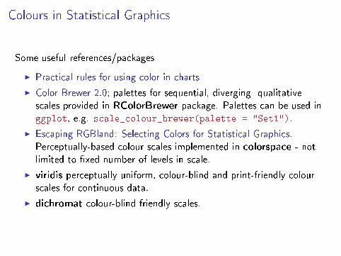
Some useful references/packages

I Practical rules for using color in charts

I Color Brewer 2.0; palettes for sequential, diverging qualitativescales provided in RColorBrewer package. Palettes can be used inggplot, e.g. scale_colour_brewer(palette = "Set1").

I Escaping RGBland: Selecting Colors for Statistical Graphics.Perceptually-based colour scales implemented in colorspace - notlimited to �xed number of levels in scale.

I viridis perceptually uniform, colour-blind and print-friendly colourscales for continuous data.

I dichromat colour-blind friendly scales.

Including Tables in LaTeX

\begin{table}[tb]

\centering

\caption{\label{tab:table}

Example of a table}

\begin{tabular}{lc}

\toprule

Col 1 & Col 2 \\

\midrule

Text 1 & 1 \\

Text 2 & 2 \\

\bottomrule

\end{tabular}

\end{table}

Table \ref{tab:table} shows

an example of a table.

Table 1: Example of a table

Col 1 Col 2

Text 1 1Text 2 2

Table 1 shows an example of a table.

Including Tables in Knitr

We can use kable in the .Rnw �le, to generate LaTeX code for the table:<<"kable">>=

library(knitr)

library(tibble) # use tibble to keep spaces in column names

dat <- data_frame(`Col 1` = paste("Text", 1:2), `Col 2` = 1:2)

kable(dat, "latex", align = "lc", booktabs = TRUE,

caption = "\\label{tab:table} Example of a table")

@

Table : Example of a table

Col 1 Col 2

Text 1 1

Text 2 2

When the .Rnw �le is converted to .tex, the chunk will be replaced bythe LaTeX code, so the �nal PDF contains the desired table.

LaTex Code Generated by kable

\begin{table}

\caption{\label{tab:table} Example of a table}

\centering

\begin{tabular}[t]{lclc}

\toprule

Col 1 & Col 2\\

\midrule

Text 1 & 1\\

Text 2 & 2\\

\bottomrule

\end{tabular}

\end{table}

Table 1: Example of a table

Col 1 Col 2

Text 1 1Text 2 2

Almost the same as before, but table won't �oat (no �oat options).

Including Floating Tables in Knitr

For a �oating table, we can create an xtable object:<<"xtable-code">>=

library(xtable)

tab <- xtable(dat, caption = "Example of a table",

label = "tab:table", align = "llc")

@

xtable adds the rownames as a column by default so we align 3 columns.

Then we print the xtable in a chunk with the argument results ="asis", so the generated LaTeX code gets printed �as is� in the .tex�le.

<<"xtable-print", results = "asis">>=

print(tab, include.rownames = FALSE, table.placement = "tb",

booktabs = TRUE, comment = FALSE)

@

The print method has > 30 (!) arguments allowing us to control exactlywhat gets printed in the LaTeX document.

xtable output

The LaTeX code generated by xtable is as follows

\begin{table}[tb]

\centering

\begin{tabular}{lc}

\toprule

Col 1 & Col 2 \\

\midrule

Text 1 & 1 \\

Text 2 & 2 \\

\bottomrule

\end{tabular}

\caption{Example of a table}

\label{tab:table}

\end{table}

Table 1: Example of a table

Col 1 Col 2

Text 1 1Text 2 2

Now this is the same as our original LaTeX code (in a slightly di�erentorder).

More Complex Table

Here we add a custom header to the printed table

<<"xtable-more", results = "asis", eval = TRUE>>=

add2row <- list(pos = list(0, 0, 0),

command = c("\\multicolumn{2}{c}{Columns} \\\\",

"\\cmidrule{1-2}",

"Col 1 & Col 2 \\\\"))

print(tab, add.to.row = add2row, include.colnames = FALSE,

include.rownames = FALSE, table.placement = "tb",

booktabs = TRUE, comment = FALSE)

@

More Complex Table Output\begin{table}[tb]

\centering

\begin{tabular}{lc}

\toprule

\multicolumn{2}{c}{Columns} \\ \cmidrule{1-2} Col 1 & Col 2 \\ \midrule

Text 1 & 1 \\

Text 2 & 2 \\

\bottomrule

\end{tabular}

\caption{Example of a table}

\label{tab:table}

\end{table}

Columns

Col 1 Col 2

Text 1 1Text 2 2

Table 1: Example of a table

Tables

kable and xtable assume you have a data frame ready to output as atable. There are other R package that help you create the contents ofthe table, including

tables for computing and tabulating (multiple) summarystatistics, cross-classi�ed by di�erent variables, withoptional total rows/columns.

texreg for summarizing statistical models, e.g. tables ofcoe�cients with con�dence intervals and optional modelsummaries, e.g. R2

Both of these packages can be used to produce HTML or LaTeX tables,look at the package vignettes for help and examples.

References

LaTeX can be used in combination with BibTeX to generating thebibilography or references section of your document. BibTeX will beincluded as part of your LaTeX installation.

You need to create a separate .bib �le which is a plain text databasewith an entry for each reference. Such �les can be created from manyreference managers e.g. JabRef, Zotero, Mendeley, . . .. AlternativelyBibTeX entries for individual papers can often be downloaded fromjournal websites.

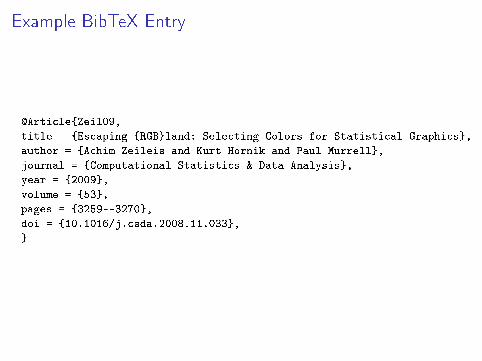
Example BibTeX Entry

@Article{Zeil09,

title = {Escaping {RGB}land: Selecting Colors for Statistical Graphics},

author = {Achim Zeileis and Kurt Hornik and Paul Murrell},

journal = {Computational Statistics & Data Analysis},

year = {2009},

volume = {53},

pages = {3259--3270},

doi = {10.1016/j.csda.2008.11.033},

}

Using the Bibliography

Put the .bib �le in the same directory as your .tex (or .Rnw) �le.

In your preamble, add \usepackage{natbib}.

Then references are cited in the body of the document using their key,e.g.

I \citet{Zeil09}, produces Zeileis et al. (2009).

I \citep{Zeil09}, produces (Zeileis et al., 2009).

I \citep[See][p.~22]{Zeil09}, produces (See Zeileis et al., 2009,p. 22).

Creating the References Section

Finally at the end of your document, add the following lines

\bibliographystyle{chicago}

\bibliography{paper}

References

Zeileis, A., K. Hornik, and P. Murrell (2009). Escaping RGBland: Selectingcolors for statistical graphics. Computational Statistics & Data Analysis 53,3259–3270.

where paper.bib is the name of your .bib �le.

Sometimes journals will require a custom bibliography style de�ned in a.bst �le. Put that in the same directory as the .tex �le and use the �lename instead of chicago.

Alternatively, look up where to install .bst �les for use across di�erentdocuments.

Back to R Markdown

When compiling .md to PDF, we can use some of the extra features ofLaTeX by cutomising the YAML header to modify the preamble of theintermediate .tex document, e.g.---

title: "My Title"

output:

pdf_document:

citation_package: "natbib"

documentclass: "article"

fontsize: 11pt

geometry: margin=1in

bibliography: paper.bib

---

Testing natbib \citep{Zeil09}.

# References

R Markdown/LaTeX Output

My Title

Testing natbib [Zeileis et al., 2009].

ReferencesAchim Zeileis, Kurt Hornik, and Paul Murrell. Escaping RGBland: Selecting colors for statisticalgraphics. Computational Statistics & Data Analysis, 53:3259–3270, 2009. doi: 10.1016/j.csda.2008.11.033.

1

Getting Styles Right

Although we can change the document class in the YAML header, acustom .cls �le may not work, e.g. jss.cls. In this case a template.tex �le, or a customised output format is required.

The rticles package provides special R markdown templates for

I JSS articles

I R Journal articles

I CTeX documents

I ACM articles

I ACS articles

I Elsevier journal submissions

I AEA journal submissions

These templates can be accessed in the dialog found via File > New File> R Markdown...From Template in RStudio.

See R Markdown help for custom bib styles.