PUBLIC PREFERENCES AND ECONOMICVALUES FOR RESTORATION OF THE

EVERGLADES/SOUTH FLORIDA ECOSYSTEM

by

J. Walter Milon, ProfessorAlan W. Hodges, Coordinator of Economic Analysis

Arbindra Rimal, Post-Doctoral AssociateClyde F. Kiker, Professor

Frank Casey, Post-Doctoral Associate

August, 1999

Economics Report 99-1Food & Resource Economics Department

University of FloridaGainesville, FL 32611

ii

PUBLIC PREFERENCES AND ECONOMIC VALUES FORRESTORATION OF THE EVERGLADES/SOUTH FLORIDA

ECOSYSTEM

J. Walter Milon, Alan W. Hodges, Arbindra Rimal, Clyde F. Kiker, and Frank Casey

ABSTRACT

The Everglades/South Florida region is a unique, globally significant ecosystem that has been altered bydrainage and water control structures. These alterations have changed the overall quantity, quality, andtemporal distribution of freshwater flows and impacted wildlife species throughout the region. Under state andfederal legislative directives, restoration of the ecosystem is being planned yet little research has beenconducted to identify public preferences and economic values for alternative restoration plans. This reportdescribes the application of a multiattribute utility survey of nearly 500 South and Central Florida residents toevaluate tradeoffs between natural and social system dimensions of the restoration problem. Both hydrologicaland wildlife species attributes were used to represent alternative states of the ecosystem along with possibleeffects on municipal water supplies, farmland, and annual household taxes. Statistical results show thatrespondents indicated strong preferences for Everglades restoration but the responses varied depending onhow the alternative states of the ecosystem were represented. Also, these preferences were tempered byconcern for the consequences of restoration decisions on municipal water users and farmland acreage.Willingness to pay measures derived from the sample indicate a maximum annual benefit from "full restoration"of approximately $60 - $70 per household per year over a ten-year period. Extrapolating these results to theFlorida population yields annual benefits of $342.2 - $406.5 million or $3.42 - $4.07 billion over a ten yearperiod. These benefits, however, decline rapidly and turn negative if restoration imposes high costs in the formof water supply restrictions, losses in farmland acreage, and annual household taxes. This survey representsan initial effort to document Floridians' preferences and economic values for restoration of theEverglades/South Florida ecosystem. Multiattribute utility analysis provides a flexible research tool to framethe decision problem, evaluate public preferences for alternative plans, and develop measures of economicvalue. This type of social science research is an essential part of an adaptive management approach torestoration planning and can be used to objectively evaluate how the perceptions and economic values ofFloridians and others change as new information becomes available about the effects of restoration actions.

KEY WORDS: Multiattribute utility, decision analysis, economic valuation, ecosystem restoration planning,survey research, Everglades/South Florida.

iii

ACKNOWLEDGMENTS

This research was conducted under Cooperative Agreement No. 43-3AEL-6-80078 between the Universityof Florida and the Economic Research Service, U.S. Department of Agriculture and the U.S. Fish and WildlifeService. The authors thank Dr. Mary Ahearn, Economic Research Service, U.S. Department of Agricultureand Dr. Jon Charbonneau, U.S. Fish and Wildlife Service for their support and insights over the course of thisproject. We also thank Drs. Peter Feather and Daniel Mullarkey, Economic Research Service, for reviewand comment on the survey design and statistical results reported in this paper. Dr. Andrew Laughland, U.S.Fish and Wildlife Service, also offered helpful comments on the survey design.

A number of other individuals also made valuable contributions to this project. Stu Applebaum, U.S. ArmyCorps of Engineers, and Agnes McLean and Carl Woehlcke, South Florida Water Management District,offered helpful comments on the overall design of the survey and technical comments on the development ofhydrological attributes for the analysis. Drs. Lance Gunderson, Ronald Labisky, and Peter Frederick,University of Florida, provided guidance and assistance on historical wildlife populations and possible levelsof these populations as a result of Everglades restoration efforts. Dr. Ken Portier, Statistics Department,University of Florida provided guidance on the statistical design for the field interviews. Dr. Donna Lee, Foodand Resource Economics Department, University of Florida, critiqued the multiattribute design and surveyelicitation methods. Ron Thomas and Cindy Spence from Educational Media and Services, Institute of Foodand Agricultural Sciences, University of Florida, provided excellent technical assistance and guidance duringthe development and production of the video used in the field interviews. Mary Rife, Sandi Palmer and KariMadison of Rife Market Research, Inc., Miami, FL, provide invaluable services in conducting the focus groupsessions, administering the field interviews, and delivering high quality data sets. Dr. Elaine Lyons-Lepke ofPerceptive Market Research, Inc., Gainesville, FL, assisted in pretests of the survey instruments. Drs. MarkHarwell and John Gentile, University of Miami, and participants in the U.S. Man and the Biosphere Human-Dominated Ecosystems Directorate meetings provided many helpful insights on analytical concerns relating toEverglades/South Florida ecosystem restoration. Finally, Dr. Bonnie Kranzer, Executive Director, Governor'sCommission for a Sustainable South Florida, was a valuable source of information and encouragementthroughout the project. To all these individuals and many others, too numerous to mention, who havegraciously assisted us in this project over the past three years we offer our very sincere thanks.

The views and opinions expressed are solely those of the authors and do not represent the opinions of otherindividuals or sponsoring agencies. Any errors or omissions are the responsibility of the authors.

iv

PUBLIC PREFERENCES AND ECONOMIC VALUES FORRESTORATION OF THE EVERGLADES/SOUTH FLORIDA

ECOSYSTEM

TABLE OF CONTENTS

ABSTRACT . . . . . . . . . . . . . . . . . . . . . . . . . . . . . . . . . . . . . . . . . . . . . . . . . . . . . . . . . . . . . . . . . . . . ii

ACKNOWLEDGMENTS . . . . . . . . . . . . . . . . . . . . . . . . . . . . . . . . . . . . . . . . . . . . . . . . . . . . . . . . . iii

EXECUTIVE SUMMARY . . . . . . . . . . . . . . . . . . . . . . . . . . . . . . . . . . . . . . . . . . . . . . . . . . . . . . . . vii

SECTION 1. INTRODUCTION . . . . . . . . . . . . . . . . . . . . . . . . . . . . . . . . . . . . . . . . . . . . . . . . . . 1-11.1 The Study Area and Problem Setting . . . . . . . . . . . . . . . . . . . . . . . . . . . . . . . . . . . . 1-11.2 Study Purpose and Objectives . . . . . . . . . . . . . . . . . . . . . . . . . . . . . . . . . . . . . . . . . 1-41.3 Overview of the Report . . . . . . . . . . . . . . . . . . . . . . . . . . . . . . . . . . . . . . . . . . . . . . 1-6

SECTION 2. MULTIATTRIBUTE UTILITY THEORY AS A PLANNING TOOL . . . . . . . . . . . 2-12.1 Multiattribute Utility Theory . . . . . . . . . . . . . . . . . . . . . . . . . . . . . . . . . . . . . . . . . . . 2-12.2 Multiattribute Utility Preference Elicitation Methods . . . . . . . . . . . . . . . . . . . . . . . . . . 2-22.3 Scoring and Ranking Alternatives with Multiattribute Utility Theory . . . . . . . . . . . . . . 2-42.4 Design of Multiattribute Utility Studies . . . . . . . . . . . . . . . . . . . . . . . . . . . . . . . . . . . . 2-4

SECTION 3. ATTRIBUTES AND TRADEOFFS FOR EVERGLADES RESTORATION . . . . . . 3-13.1 Endpoints, Attributes and Ecosystem Restoration . . . . . . . . . . . . . . . . . . . . . . . . . . . 3-1

3.1.1 Public Perceptions and Focus Groups . . . . . . . . . . . . . . . . . . . . . . . . . . . . . . 3-23.2 Functional/Hydrological Attributes and Levels . . . . . . . . . . . . . . . . . . . . . . . . . . . . . . 3-33.3 Structural/Species Attributes and Levels . . . . . . . . . . . . . . . . . . . . . . . . . . . . . . . . . . 3-63.4 Annual Cost, Farmland and Water Use Restriction Attributes . . . . . . . . . . . . . . . . . . 3-83.5 Attribute Combinations and Plan Alternatives . . . . . . . . . . . . . . . . . . . . . . . . . . . . . 3-103.6 Other Attributes Not Included . . . . . . . . . . . . . . . . . . . . . . . . . . . . . . . . . . . . . . . . 3-12

SECTION 4. SURVEY DESIGN AND RESPONDENT PROFILE . . . . . . . . . . . . . . . . . . . . . . . . 4-14.1 Description of the Interview Process . . . . . . . . . . . . . . . . . . . . . . . . . . . . . . . . . . . . . 4-14.2 Respondent Selection . . . . . . . . . . . . . . . . . . . . . . . . . . . . . . . . . . . . . . . . . . . . . . . . 4-24.3 Respondent Socio-Demographic Profiles . . . . . . . . . . . . . . . . . . . . . . . . . . . . . . . . . 4-2

SECTION 5. STATISTICAL RESULTS . . . . . . . . . . . . . . . . . . . . . . . . . . . . . . . . . . . . . . . . . . . . 5-15.1 Statistical Modeling of Pairwise Choices . . . . . . . . . . . . . . . . . . . . . . . . . . . . . . . . . . 5-15.2 Sample Data . . . . . . . . . . . . . . . . . . . . . . . . . . . . . . . . . . . . . . . . . . . . . . . . . . . . . . 5-25.3 Statistical Results for the Multiattribute Models . . . . . . . . . . . . . . . . . . . . . . . . . . . . . 5-4

5.3.1 Basic Hydrological Multiattribute Model Results . . . . . . . . . . . . . . . . . . . . . . 5-55.3.2 Basic Species Multiattribute Model Results . . . . . . . . . . . . . . . . . . . . . . . . . . 5-7

v

5.4 Statistical Results for Models with Socioeconomic Characteristics Interactions . . . . . . 5-9

SECTION 6. EVALUATION OF ALTERNATIVE RESTORATION PLANS . . . . . . . . . . . . . . . 6-16.1 Voting, Ranking and Net Willingness to Pay Measures from

Multiattribute Models . . . . . . . . . . . . . . . . . . . . . . . . . . . . . . . . . . . . . . . . . . . . . . . . 6-16.2 Overall Evaluation of Alternative Restoration Plans . . . . . . . . . . . . . . . . . . . . . . . . . . 6-2

6.2.1 Evaluation with the Hydrological Multiattribute Model . . . . . . . . . . . . . . . . . . 6-26.2.2 Evaluation with the Species Multiattribute Model . . . . . . . . . . . . . . . . . . . . . . 6-5

6.3 Effects of Socioeconomic Characteristics on Evaluations of Alternative Restoration Plans6-76.3.1 Evaluations of Alternative Plans with the Hydrological Multiattribute Model by

Respondents’ Location and Environmental Donation Status . . . . . . . . . . . . . . 6-76.3.2 Evaluations of Alternative Plans with the Species Multiattribute Model by

Respondents’ Location and Environmental Donation Status . . . . . . . . . . . . . 6-13

SECTION 7. SUMMARY AND EXTENSIONS . . . . . . . . . . . . . . . . . . . . . . . . . . . . . . . . . . . . . . 7-17.1 Study Objectives and Methods . . . . . . . . . . . . . . . . . . . . . . . . . . . . . . . . . . . . . . . . . 7-17.2 Survey Results and Alternative Restoration Plan Evaluations . . . . . . . . . . . . . . . . . . . 7-27.3 Extending the Economic Valuation Results to the Florida Population . . . . . . . . . . . . . 7-47.4 Limitations of the Study and Suggestions for Future Research . . . . . . . . . . . . . . . . . . 7-5

SECTION 8. REFERENCES . . . . . . . . . . . . . . . . . . . . . . . . . . . . . . . . . . . . . . . . . . . . . . . . . . . . 8-1

APPENDIX A. QUESTIONNAIRE AND INTERVIEWER GUIDE . . . . . . . . . . . . . . . . . . . . . . . A-1

APPENDIX D. INFORMATIONAL VIDEO SCRIPT . . . . . . . . . . . . . . . . . . . . . . . . . . . . . . . . . . D-1

APPENDIX E. SUMMARY OF INTERVIEWER EVALUATIONS OF RESPONDENTS . . . . . . E-1

vi

LIST OF TABLES

Table 2-1. Example of a Multiattribute Decision Problem for Purchase of an Automobile. . . . . . . . . . 2-2Table 3-1. Description of Attributes and Levels for the Hydrological Multiattribute Model . . . . . . . . . 3-5Table 3-2. Description and Results for the Species Multiattribute Model . . . . . . . . . . . . . . . . . . . . . . 3-7Table 3-3. Description of Attributes and Levels for Cost, Farmland and Water Use

Restrictions . . . . . . . . . . . . . . . . . . . . . . . . . . . . . . . . . . . . . . . . . . . . . . . . . . . . . . . . . . . . . 3-9Table 3-4. Example of Pairwise Choice for the Hydrological Multiattribute Model . . . . . . . . . . . . . . 3-11Table 3-5. Example of Pairwise Choice for the Wildlife Multiattribute Model . . . . . . . . . . . . . . . . . . 3-11Table 4-1. Socioeconomic Characteristics for the Survey Sample and Comparisons to the

Florida Population . . . . . . . . . . . . . . . . . . . . . . . . . . . . . . . . . . . . . . . . . . . . . . . . . . . . . . . . 4-4Table 4-2. Race/Ethnicity and Median Household Income for the Survey Sample, by County, and

Comparisons to the County Population . . . . . . . . . . . . . . . . . . . . . . . . . . . . . . . . . . . . . . . . . 4-5Table 4-3. Priorities for State of Florida Expenditures by Program Area by Survey Sample

Respondents and Comparisons to the Florida Population . . . . . . . . . . . . . . . . . . . . . . . . . . . 4-6Table 4-4. Survey Respondent Attitudes about the Environment and Water Supply . . . . . . . . . . . . . 4-7Table 5-1. Variable Definitions and Summary Statistics for the Hydrological and Species Attribute

Models. . . . . . . . . . . . . . . . . . . . . . . . . . . . . . . . . . . . . . . . . . . . . . . . . . . . . . . . . . . . . . . . . 5-3Table 5-2. Coefficient Estimates for the Hydrological Multiattribute Models . . . . . . . . . . . . . . . . . . . 5-6Table 5-3. Coefficient Estimates for the Species Multiattribute Model. . . . . . . . . . . . . . . . . . . . . . . . 5-8Table 5-4. Coefficient Estimates for the Hydrological Multiattribute Model with Socioeconomic

Characteristics Interactions . . . . . . . . . . . . . . . . . . . . . . . . . . . . . . . . . . . . . . . . . . . . . . . . . 5-10Table 5-5. Coefficient Estimates for the Species Multiattribute Model with Socioeconomic Characteristics

Interactions . . . . . . . . . . . . . . . . . . . . . . . . . . . . . . . . . . . . . . . . . . . . . . . . . . . . . . . . . . . . 5-11Table 6-1 Evaluation of Selected Restoration Plans with the Hydrological Multiattribute

Model . . . . . . . . . . . . . . . . . . . . . . . . . . . . . . . . . . . . . . . . . . . . . . . . . . . . . . . . . . . . . . . . . 6-3Table 6-2 Evaluation of Restoration Plans with the Species Multiattribute Model . . . . . . . . . . . . . . . 6-6Table 6-3. Evaluation of Selected Restoration Plans with the Hydrological Multiattribute Model by

Respondent Location . . . . . . . . . . . . . . . . . . . . . . . . . . . . . . . . . . . . . . . . . . . . . . . . . . . . . . 6-9Table 6-4. Evaluation of Selected Restoration Plans with the Hydrological Multiattribute Model by

Respondent Past Donations . . . . . . . . . . . . . . . . . . . . . . . . . . . . . . . . . . . . . . . . . . . . . . . . 6-11Table 6-5. Evaluation of Selected Restoration Plans with the Species Multiattribute Model by Respondent

Location . . . . . . . . . . . . . . . . . . . . . . . . . . . . . . . . . . . . . . . . . . . . . . . . . . . . . . . . . . . . . . 6-15Table 6-6. Evaluation of Restoration Plans with the Species Multiattribute Model by Respondent Past

Donations . . . . . . . . . . . . . . . . . . . . . . . . . . . . . . . . . . . . . . . . . . . . . . . . . . . . . . . . . . . . . 6-17

LIST OF FIGURES

Figure 1.2. The South Florida Ecosystem and Its Components . . . . . . . . . . . . . . . . . . . . . . . . . . 1-2Figure 7.1. Relative Weightings of Attributes in the Multiattribute Models . . . . . . . . . . . . . . . . . . 7-3

vii

viii

PUBLIC PREFERENCES AND ECONOMIC VALUES FORRESTORATION OF THE EVERGLADES/SOUTH FLORIDA

ECOSYSTEM

EXECUTIVE SUMMARY

The Everglades/South Florida region is a unique, globally significant ecosystem encompassing over 69,000square kilometers. For more than 100 years, the natural flow of water through the Everglades has been alteredby drainage and water control structures, in order to provide flood control and water supplies for the rapidlygrowing human population and large agricultural industry in the South Florida region. These alterations havelead to harmful changes in the overall quantity, quality, and temporal distribution of freshwater inflows to theEverglades, saltwater intrusion into aquifers in coastal areas, invasion by exotic plant species causing changesin plant community structure, and dramatic declines in certain wildlife species typical of the Everglades.

Under state and federal legislative directives, restoration of the Everglades/South Florida ecosystem is nowin progress under the leadership of the US Army Corps of Engineers and the South Florida WaterManagement District. Proposed plans for restoration are expected to require decades to complete with costsin excess of $6 billion. Despite considerable efforts to base restoration decisions on sound science, there hasbeen relatively little formal research to inform the decision-making process about public expectations for therestoration, or willingness to pay for restoration costs. The purpose of the present study was to quantitativelyevaluate the perceptions and preferences of the general public in Florida regarding alternative possibleoutcomes for restoration of the Everglades/South Florida ecosystem, and to use these results to estimateeconomic values associated with alternative restoration plans.

Multiattribute utility theory has been widely applied to problems involving tradeoffs between multiple conflictingelements. This study was designed as an application of multiattribute utility theory in order to accommodatethe inherent tradeoffs between natural and social system dimensions of the restoration problem. Afterextensive consultation with agency staffs and two focus group sessions with the public, the many differentaspects of Everglades restoration were represented in terms of nine independent attributes, as shown in thefollowing table. A group of three hydrologic attributes represented water levels and timing in differentgeographic portions of the Everglades: Lake Okeechobee, the Water Conservation Areas, and EvergladesNational Park. Another set of three attributes represented different groups of species and habitat types:wetland species, dryland species, and estuarine species. Finally, three attributes were used to represent thesocial services and costs associated with restoration: restrictions on water use by households, changes infarmland acreage in South Florida, and the annual cost to households. Each of the attributes had three levelsassociated with complete restoration, intermediate restoration, and no restoration as a baseline case. Thevalues for each level of the attributes corresponded to expected outcomes based on various hydrologic orbiological models, agency planning documents, or consensus views of experts consulted. The hydrologic andwildlife species attribute levels were specified in relation to "historic" levels.

ix

Attribute Names, Descriptions and Alternative Levels for Multiattribute Analysis of EvergladesRestoration.

Attributes/DescriptionAttribute

Levels

HydrologicModelAttributes

Lake Okeechobee. Percentage of time that water levels and timing in Lake Okeechobee aresimilar to historic, predrainage conditions

60%* 75% 90%

Everglades Water Conservation Areas. Percentage of area in the Everglades Water ConservationArea having water levels and timing similar to historic, predrainage conditions

50%*75%90%

Everglades National Park and Florida Bay. Percentage of the area in Everglades National Parkand Florida Bay that has water levels and timing similar to historic, predrainage conditions

50%*75%90%

SpeciesModelAttributes

Wetland Dependent Species. Percentage of historic, predrainage population levels of wetland

dependent species such as wading birds and alligators

20%*

50%80%

Dry Land Dependent Species. Percentage of historic, predrainage population levels of dry landdependent species such as deer, hawks and songbirds

50%*60%70%

Florida Bay Dependent Species. Percentage of historic, predrainage population levels of FloridaBay dependent species such as pink shrimp, mullet and sea trout

60%*75%

90%

Socio-EconomicAttributes(bothHydrologicand SpeciesModels)

Annual cost per household. Additional annual cost per household for water utilities $0*$25$50

Restrictions on Household Water Use. Number of days per week that outdoor water useallowed during dry years, and percentage reduction in indoor water use

3/10%*2/25%1/40%

Farm land Reduction. Area (acres) of farm land that would be reduced in the EvergladesAgricultural Area and western portions of Palm Beach, Broward and Dade counties

0*100,000200,000

* Denotes baseline condition currently

Primary information in this study was collected through personal interview surveys of 480 randomly selectedhouseholds in five south and central Florida metropolitan areas (Miami, West Palm Beach, Fort Meyers,Tampa and Orlando). Interviews were conducted in respondent’s homes by an independent market researchfirm. The survey samples were representative of their respective county populations and the state as a wholein terms of sociodemographic characteristics such as income, race, age, education, household size and politicalaffiliation. The interview included presentation of an 11 minute informational video about the Everglades/SouthFlorida ecosystem in order to orient respondents to key issues addressed in the survey. Survey respondentswere given a pairwise choice task in which pairs of systematically-generated combinations of six attributeswere presented, and the respondent was asked to choose the preferred attribute set. Either the hydrologicalor species attribute specifications were presented to half of the respondents in each county, in order tocompare preferences for alternative restoration plans based on different representations of the ecologicaldimensions of the problem. Responses from the pairwise choice tasks were used to statistically estimatemultiattribute utility functions for the hydrological and species attribute sets. Results of the statistical analysisand evaluation are summarized in the figure below.

x

Relative Weightings of Attributes in the Multiattribute Models

5.8

6.2

2.4

-3

-0.1

-2.3

-1.9

Lake Okeechobee

Water Conservation Areas

Everglades National Park

Cost Per Household

HH Water Use I

HH Water Use II

Farm Land in EAA

0 2 4 6 8-2-4

2.9

-7

8.1

-2.4

-0.4

-1.7

-0.9

Wetland Species

Dryland Species

Estuarine Species

Cost Per Household

HH Water Use I

HH Water Use II

Farm Land in EAA

0 2 4 6 8 10-2-4-6-8

Hydrological Model Species Model

! The hydrological multiattribute utility model indicated that respondents gave positive weights to allthree hydrological attributes and preferred potential restoration plans that would lead to water levelsand timing more similar to historical conditions in all three of the South Florida hydrologic regions.However, the social service and cost attributes in the model revealed that higher levels of annual cost,water restrictions, or reductions in farmland acreage were negatively weighted.

! The species multiattribute utility model showed positive weightings for wetland and estuarine speciesattributes indicating that restoring these species populations to be more comparable to historical levelswas preferred. However, a significant negative weighting on the dryland species attribute indicatedthat restoration of these species was not preferred. Also, the preferences for restoring wetland andestuarine species were tempered by negative weightings for the annual cost, water restrictions, andfarmland reduction attributes.

! The negative sign and magnitude of weightings assigned to the annual cost, water restriction, andfarmland reduction attributes in both the hydrological and species multiattribute models were generallysimilar indicating that respondents expressed consistent preferences regardless of the type of attributeused to represent the ecological dimensions.

! Higher levels of the wetland and estuarine species attributes were consistently preferred across thesample indicating that the general public would more readily identify with a restoration program thatemphasizes species restoration rather than hydrological management.

Weightings for the multiattribute utility models were used to evaluate various hypothetical full and partialrestoration plans, both with and without social service and cost components. ! The results presented in the following table showed that Floridians expressed strong preferences for

plans that fully restore the hydrological conditions and wetland/estuarine species populations of SouthFlorida. Net willingness to pay amounts for the full restoration plans of $59 and $70 annually for the

xi

hydrological and species multiattribute models, respectively, provide measures of the maximum annualbenefits per household.

! While the results for the hypothetical restoration plans indicated generally strong support forrestoration, respondents would not support a restoration plan that imposed high costs on Floridians.Hypothetical restoration plans that included annual costs of $50 per household (or $500 over 10years) coupled with either farmland reductions of 100,000 or more acres or severe restrictions onmunicipal water use during dry years received poor rankings and less than majority support.Moreover, the net willingness to pay values for these high cost plans were negative suggesting apotential loss in economic welfare. On the other hand, intermediate cost levels were clearly notviewed as too overbearing, such as moderate restrictions on water use, or annual costs of $25 perhousehold.

! When the results were extrapolated to estimate the aggregate benefits of alternative Everglades/SouthFlorida restoration plans for the Florida population, the net willingness to pay for full hydrologicalrestoration without costs was $342.2 million annually, or $3.42 billion over a ten-year period.Similarly, for full wetland/estuarine species restoration without costs the aggregate willingness to paywas $406.5 million annually, or $4.07 billion over ten years. A more realistic restoration plan whichprovided full hydrological restoration with annual costs of $25 per household, a 100,000 acrereduction in farmland, and moderate water restrictions had a net willingness to pay of $15.60 perhousehold annually, or $907.9 million for the Florida population over ten years.

This survey represents an initial effort to document Floridians’ preferences and economic values for restorationof the Everglades/South Florida ecosystem. This type of social science research is an essential part of anadaptive management approach to restoration decisions in which scientists and the public learn about theeffects of management actions. Future surveys of Floridians are necessary to objectively evaluate how publicperceptions and economic values may change over time. In light of the national significance of theEverglades/South Florida ecosystem, additional surveys are necessary to quantify the preferences andeconomic values of citizens in other regions of the U.S.

Evaluation of Selected Restoration Plans for the Hydrological and Species Multiattribute Models.

Plan DescriptionPercent of

Respondentsin Favor

NetWillingness

to Pay

Hydrological Multiattribute Model

Partial Hydrologic Restoration without Costs 71.7 $34.32

Full Hydrologic Restoration without Costs 71.7 $58.79

Partial Hydrologic Restoration with Minimized Costs 44.3 $9.32

Full Hydrologic Restoration with Minimized Costs 54.3 $15.60

Full Hydrologic Restoration with Full Costs 31.1 -$61.09

Species Multiattribute Model

Partial Wetland Wildlife Restoration without Costs 92.7 $34.93

Full Wetland Wildlife Restoration without Costs 92.7 $69.86

Partial Dryland Wildlife Restoration without Costs 17.9 -$11.95

Full Dryland Wildlife Restoration without Costs 17.9 -$23.90

1-1

Full Wetland Wildlife Restoration with Minimized Costs 67.9 $26.63

SECTION 1. INTRODUCTION

1.1 The Study Area and Problem Setting

The southern portion of Florida is a complex mosaic of hydrologically interrelated terrestrial, freshwater, andmarine ecosystems. The entire regional ecosystem is linked through surface and ground hydrology from theKissimmee River watershed, through Lake Okeechobee, through water conservation areas, the Big CypressSwamp, and the Everglades, and out through Florida Bay and the passes between the Florida Keys to theoffshore corals reefs (Figure 1). The uniqueness of the region has been recognized through the designationof a number of state and federal parks and sanctuaries including Big Cypress National Preserve, Biscayne BayNational Park, Everglades National Park, Pennekamp Coral Reef State Park, and the Florida Keys NationalMarine Sanctuary. Also, Everglades National Park has been designated an international Biosphere Reserve,a World Heritage ecosystem, and a Wetland of International Importance (Maltby and Dugan 1994). Theentire area covers more than 69,000 square kilometers and is larger than nine states. More than one-third ofthe land area is in public ownership.

For more than 100 years, the flow of water through this network of habitats and ecosystems has been modifiedfrom its natural conditions to satisfy the demands of a growing human population within the region. More thanhalf of the original Everglades system has been drained and water management structures now channel morethan four times as much freshwater to the Atlantic Ocean as natural drainage flows (Davis and Ogden 1994).While many warned of the consequences of these interventions (e.g. Beard 1938; Douglas 1947), a series ofecological and institutional crises over the past two decades has focused scientific and public attention on theproblems of the region and efforts to restore the ecosystems (Light et al. 1995).

Restoration efforts for the Everglades/South Florida ecosystem have been proceeding under state and federallegislative directives. The Everglades Forever Act of 1994 (Chapter 373.4592, Florida Statutes) outlined ageneral plan to restore the ecosystem by improving the quantity and distribution of freshwater, reducing theamount of phosphorus enriched agricultural storm water entering the system (from agricultural production areassouth of Lake Okeechobee), removing exotic plant species, and setting time deadlines. The South FloridaWater Management District is responsible for overall coordination and administration of these efforts and hasdeveloped a planning document that describes restoration projects over the next two decades (South FloridaWater Management District 1994).

The Water Resources Development Act of 1992 (Public Law 580, 102nd Congress) authorized the U.S.Army Corps of Engineers to initiate a study to determine whether the existing Corps' Central and SouthernFlorida Project (and the water control structures built by the Corps) should be modified to improve the qualityof the environment, improve protection of the aquifer, and improve conservation of urban water supplies. TheCentral and Southern Florida Project (C&SFP) dates back to the Flood Control Act of 1948 and has beenthe focal point of federal efforts to provide flood control, drainage, water control, navigation, water supply forEverglades National Park, and other purposes (U.S. Army Corps of Engineers 1994, Appendix J). Theobjectives and accomplishments from the earlier years of this Project have been cited by scientists as thesource of many of the environmental problems throughout the region (e.g. Light and Dineen 1994).

1-2

1-3

Figure 1-1 The South Florida Ecosystem and Its Components

1-4

The first phase of the Corps' study was a Reconnaissance Report that identified problems and opportunities,described alternative plans, and recommended further studies (U.S. Army Corps of Engineers 1994). Thereport presented ten basic restoration plans that ranged from changes in operating procedures with existingphysical structures to major redesign of canals, levees, and flowways throughout the system. No specificrestoration plan was recommended. At about the same time, other restoration plans were proposed including:The Greater Everglades Ecosystem Restoration Plan by the Everglades Coalition (1994), the Action Plan,South Florida Ecosystem Restoration by the U.S. Fish and Wildlife Service (1993), and the FederalObjectives for The South Florida Restoration by the Science Sub-Group of the South Florida Managementand Coordination Working Group (1993).

The Water Resources Development Act of 1996 (Public Law 303, 104th Congress) directed the Corps toproceed from the reconnaissance phase to the development of a comprehensive plan for the purpose ofrestoring, preserving and protecting the Everglades/South Florida ecosystem. The plan also would addressother water related needs of the region such as water supplies and flood control (Section 309(1)). The Corpsand the South Florida Water Management District (as local sponsor) must present the plan to Congress byJuly 1999. Under the Act, cost sharing would be 50/50 between state and local government.

As this planning effort (commonly referred to as “the Restudy”) proceeds, it is useful to describe the majorplanning problem as the choice of restoration goals. While a great deal has been written about the need torestore the ecosystem, little has been offered to help the public understand what would be achieved withrestoration (Vogel 1998). In this regard, it is helpful to understand that the choice of goals for a restorationproject is equivalent to a choice of ecological endpoints. Ecological endpoints are defined as thosecharacteristics of the ecosystem that if changed, would constitute a change in the health of the ecosystem(Harwell and Long 1992; Harwell et al. 1992). These endpoints represent vectors of functions and servicesfrom the ecosystem that have both biological and social importance (Russell 1995). The dilemma arises fromthe fact that choosing endpoints is in part an ecological issue and in part a social issue. The essence of theproblem is clearly identified in the Corps' Reconnaissance Report:

The vision of the future wetlands in south Florida is influenced by different views of how wedetermine restoration goals for the system. The future Kissimmee River, Lake Okeechobee,Everglades, Big Cypress, and Florida Bay ecosystems can be, to some extent, what we wantthem to be, based on our value systems, and our decisions about what conditions andcomponents constitute a restored ecosystem (U.S. Army Corps of Engineers 1994, p. 109).

This dilemma might be resolved solely at an administrative level by agencies participating in the planningprocess. But as Russell (1993) points out, public preferences and economic values for alternative endpointsmust be considered since restoration projects compete with other public projects for funds. And, economicvalues for alternative endpoints cannot be easily measured since many of the possible endpoints involveenvironmental goods that are not valued in traditional markets or directly related to observable humanbehavior. Hence, any complete feasibility analysis of alternative restoration plans must consider publicpreferences and values for alternative ecological endpoints.

Recognizing the need for information about public preferences and values for alternative ecological endpointsdoes not, however, readily translate into a well-defined research program. Most economic studies ofenvironmental goods have focused on a single dimension or endpoint while assuming (most often implicitly)

1-5

that other endpoints were fixed in time or irrelevant (Russell 1993). Studies that have considered multiplealternative endpoints (e.g. Crocker 1985; Hoehn and Loomis 1993; Loomis et al. 1990; Opaluch et al. 1993)encountered the well-known principle that individuals ability to make consistent choices decreases as thenumber of options increases (Miller 1956). Professionals from both the natural and social sciences who haveconsidered the current state of affairs have concluded that research should focus on identifying the ways thatindividuals (nonscientists) think about environmental problems and begin to evaluate the effectiveness ofalternative value elicitation procedures involving multiple ecological endpoints (Green and Tunstall 1991;Harwell et al. 1992; Russell 1993).

While there are many ways to characterize ecological endpoints for ecosystem restoration (Bratton 1992;Cairns 1988; Harwell and Long 1992), two broad classifications are "structural" endpoints and "functional"endpoints. Structural endpoints focus on the number and diversity of individual species, and may includekeystone species or other distinctions to differentiate the species (Paine 1980, Westman 1985, Wilson 1992).For the Everglades/South Florida ecosystem, these species indicators might include bird populations, fishpopulations, and/or populations of endangered species such as the Snail Kite and Wood Stork. On the otherhand, functional endpoints emphasize broad ecosystem processes and dynamic properties (Holling 1987,Westman 1985, 1991). In an uplands/wetlands ecotone such as the Everglades, these endpoints might includehydroperiod levels and timing, salinity fluctuations, spatial extent, and fire frequency (Harwell and Long 1992,Holling et al. 1994). While the exact linkages between these alternative endpoint classifications are not wellknown, in general the two sets of endpoints represent different dimensions of an ecosystem. Ecosystemmanagement based on one set of endpoints may lead to different restoration decisions than for the alternateendpoints (May 1973, McNaughton 1988, Westman 1985, 1991).

1.2 Study Purpose and Objectives

The purpose of this study was to develop and implement a public survey elicitation procedure that could beused to evaluate public perceptions of alternative ecological endpoints for what may well be the ‘granddaddy’of all ecosystem restoration efforts, the Everglades/South Florida region. The elicitation procedure would alsoprovide estimates of individual's economic value (willingness to pay) for bundles of environmental goods thatcould result from alternative restoration plans. Results from the survey could then be used to rank alternativerestoration plans and provide measures of the economic benefits (net willingness to pay) associated withalternative ecological endpoints. This study also contributes to the state-of-the-art in ecosystem valuationmethodology by evaluating respondents' perceptions of alternative representations of environmental functions.Specifically, this will involve a test of the hypothesis that sets of wildlife species population levels (speciesendpoints) elicit the same preferences for ecosystem restoration as functional endpoints such as the level andtiming of water flows in different areas within the region. Specific objectives for this study were:

1) To develop a public survey instrument for eliciting preferences for alternative restoration plans using amultiattribute utility framework.

Rationale: Management of a complex ecosystem such as the Everglades/South Florida ecosysteminvolves hydrologic, vegetative, and faunal processes that imply multiple objectives and multiple alternativesfor human decision making. Multiattribute utility theory (MAUT) provides a well-known analytical frameworkin which the attributes of decision alternatives can be arrayed and statistical procedures can be used to

1-6

measure respondents' preferences for different alternatives (Keeney and Raiffa 1976; von Winterfeldt andEdwards 1986). MAUT can be implemented in a discrete choice framework (McFadden 1986) to evaluatealternatives using several different response formats such as paired comparisons (e.g. Opaluch et al. 1993)or multiple rankings (e.g. Beggs et al. 1981). For example, Opaluch et al. (1993) evaluated public preferencesfor alternative landfill locations based on site attributes such as acreage of the landfill and adjacent land usesand location attributes such as proximity to residential areas, access roads, and hauling costs. In addition, theMAUT approach can be used to derive estimates of economic value for changes in attribute levels (Louviere1988; Swallow et al. 1994).

2) To develop two representative sets of ecological attributes based on functional and structural endpointconcepts for use in a multiattribute utility survey instrument.

Rationale: Ecosystem management has often focused on the levels of individual species within an areaas an indicator of ecosystem health (Wilson 1984, 1992; Bratton). Laws such as the Endangered Species Actdirect wildlife management efforts to species level protection and these laws focus public perceptions onchanges in specific ecosystems. In fact, declines in the number of nesting colonies for the endangered WoodStork and Snail Kite have been one of the primary factors driving current efforts for South FloridaEcosystem/Florida Bay restoration (Odgen 1994). An alternative, though not necessarily conflicting approachto ecosystem management is to focus on broad ecosystem functions (Holling 1987). In this approach,individual species endpoints are less important than overall functional endpoints such as the periodicity ofwetland flooding and drying or the diversity of micro and meso habitats within the overall ecosystem (Hollinget al. 1994). With this approach, species levels may be less stable (although potentially more productive) thanwith a structural endpoint focus. The significance of these two approaches to endpoint indicators is that theyconvey different conceptual models of ecosystems that may influence individuals' perceptions of restorationand the choice of actions that would be undertaken as part of an actual restoration.

3) To implement the multiattribute utility theory (MAUT) survey to measure Floridians’ preferences for SouthFlorida Ecosystem/Florida Bay restoration; to test whether structural endpoints or functional endpointsinfluence individuals' preferences for restoration; and, to determine whether there are geographical or othersociodemographic differences in preferences.

Rationale: Hypothesis tests based on multiattribute utility survey responses can be used to understandFloridians’ preferences for restoration initiatives. This information may influence the choice of specificrestoration plans. A primary hypothesis for this research is that individuals' preferences for restorationalternatives will not be influenced by the use of structural or functional endpoints to represent alternativerestoration plans. This hypothesis can be tested using a split sample survey design whereby different groupsof respondents are presented with either structural or functional endpoint choice sets. The results from thisanalysis will provide information about the structure of public preferences for restoration and the specificattributes of restoration plans that are most important to the public. A secondary hypothesis is that individuals'preferences are the same regardless of where they live in Florida or their sociodemographic characteristics(e.g. age, income). This hypothesis can be tested using a representative sample of respondents in differentregions of Florida.

4) To use the results of the multiattribute utility survey of Floridians to rank alternative restoration plans andto estimate economic values associated with these restoration plan alternatives.

1-7

Rationale: With the multiattribute utility survey results it is possible to rank alternative plans based onthe type and degree of change in endpoints provided by a specific ecosystem restoration plan. These rankingscan provide guidance to restoration planners and elected officials about the relative merits of alternative plans.Differences in rankings can also be identified for various sociodemographic groups. Survey results alsoprovide measures of willingness to pay for specific restoration plans and the marginal economic valueindividuals assign to attribute endpoints. These values can be used to measure the economic benefits ofalternative restoration plans to Floridians. Also, the marginal value of endpoint attributes can provideinformation about the economic benefits of individual components of a restoration plan.

1.3 Overview of the Report

This report is organized as follows. Section 2 provides an overview and description of multiattribute utilitytheory and how it can be used as a tool for ecosystem restoration planning. Section 3 describes the selectionof functional attributes based on hydrological properties of the ecosystem and structural attributes based onspecies populations. This section explains the basis for selecting these attributes and how alternative levels forthese attributes were specified based on a variety of information sources including the U.S. Army Corps ofEngineers, the South Florida Water Management District, and scientists from various agencies and universitiesaround the state of Florida. Also, this section provides a description of the procedures used to combine theselected functional and structural attributes into alternative "plans" to be used in personal household interviewswith Florida residents. In Section 4, the interview process and the materials used in the interviews aredescribed. Procedures followed to identify a stratified, random sample of residents in three South Floridacounties (Dade, Lee, and Palm Beach) and two Central Florida counties (Hillsborough and Orange) are alsodescribed. This is followed by a summary of results from the interview surveys for sociodemographic andother descriptive information about the respondents. More detailed information about statistical modeling of the multiattribute choice process used in this survey ispresented in Section 5. This section also provides statistical results for various analytical models estimatedfrom the survey data along with an interpretation of the results of the statistical analysis. Section 6 extends thestatistical results presented in the previous chapter to develop rankings and willingness to pay measures foralternative restoration plans based on relative scores from the multiattribute utility models. Rankings arepresented for the functional (hydrological) attribute models and the structural (species) attribute models basedon results for all survey respondents and for various sociodemographic subgroups within the sample. Section7 concludes the report with a summary of the survey design and results of the analysis. This section alsoprovides a discussion of possible uses of this information in Everglades/South Florida restoration planning alongwith a discussion of the limitations of the survey and results. Appendices to this report provide completecopies of the questions and materials used in the interviews along with other detailed information to supportresults provided in the main sections of the report.

2-1

SECTION 2. MULTIATTRIBUTE UTILITY THEORY AS A PLANNINGTOOL

2.1 Multiattribute Utility Theory

Multiattribute utility theory (MAUT) is a method among a class of procedures known as "multi-criteria decisionmaking" which are used for analysis of problems that have a number of disparate dimensions that must beconsidered simultaneously. Basically, a multiattribute problem consists of one or more decision alternatives thatare evaluated by a decision maker(s) based on a set of attributes that are deemed essential to the problem.The decision maker’s choices reflect an implicit weighting assigned to each attribute that reflects the importanceof each attribute to the decision maker.

A primary strength of MAUT is in evaluating alternatives where there are tradeoffs, i.e. where one or morealternatives are superior in one respect while inferior in another. Such tradeoffs are involved in many, perhapsmost, real world decisions. MAUT may be used to identify a single "best" option, to rank the options in orderof preference, or to identify a subset of acceptable or nondominated options for further analysis. A virtue ofthe methodology is that attributes may be either quantitative or qualitative in nature, and it is able toaccommodate important but ill-defined or subjective dimensions of a problem. MAUT is suitable for problems in which there is uncertainty about the realization of different alternatives. Incases where there is not any consideration of uncertainty, the methodology is known as "multiattributevaluation" (MAV). MAUT and MAV techniques have been applied in numerous settings, including technologyselection, energy and transportation planning, strategic business planning, product marketing and environmentalmanagement (Giocoechea, Hansen and Duckstein, 1982; Hwang and Yoon, 1981; Keeney, 1980; Keeneyand Raiffa, 1976; Mollaghasemi and Pet-Edwards; Nijkamp, Rietveld and Voogd, 1990; Saaty, 1980;Szidarovsky, Gershon and Duckstein, 1986; von Winterfeldt and Edwards, 1986).

To illustrate the basic principles of MAUT, consider the decision by a consumer to purchase an automobile.Two possible models (A,B) may differ in terms of a number of attributes such as price, fuel economy (milesper gallon), passenger seating capacity, performance (horsepower, maximum speed, acceleration), safety,handling characteristics, appearance, and so forth. These attributes can be arrayed to provide a directcomparison between attributes as in Table 2.1. A vehicle which has a lower price may have fewer safetyfeatures while a vehicle that has superior performance may have lower fuel economy. The decision as towhich vehicle to purchase depends upon the relative weightings the individual gives to the different attributesand the cumulative value or “score” assigned to each alternative. If an individual attribute is strongly weighted,the choice may be determined in favor of the vehicle that is rated most highly on this attribute. Alternatively,if there are only weak differences in weightings among attributes, several or all attributes may influence the decision.

2-2

Table 2-1. Example of a Multiattribute Decision Problem for Purchase of an Automobile.

Attribute Model A Model B

Price (new) $25,000 $15,000

Safety Has air bags No air bags

Performance (Horsepower) 250 Hp 200 Hp

Fuel Economy 20 miles per gallon 30 miles per gallon

Seating Capacity 6 persons 4 persons

Solution of a MAU or MAV problem typically involves the following steps (von Winterfeldt and Edwards,1986):

• Respondents assign relative weights to the attributes.• Develop utility or value functions for individual attributes.• Respondents evaluate each alternative separately against each attribute.• Aggregate the weighted evaluations to obtain an overall evaluation of each alternative by

means of an appropriate aggregation rule.

The selection of meaningful, appropriate attributes for the decision is one of the most critical and difficult stepsfor solving multiattribute problems. The attributes must be essential to the decision problem, but each attributeshould reflect independent dimensions to the degree possible to avoid redundancy (Keeney and Raiffa 1976;Louviere 1988). The attributes must be measurable and must also be understood by decision makers.Theoretically, any number of attributes may be used in a multiattribute decision problem. The literature,however, indicates that in practice only seven to nine attributes can be meaningfully evaluated by decisionmakers due to limited cognitive skills and memory capacity of most individuals (Saaty 1980; Miller 1956; dePalma et al. 1994).

2.2 Multiattribute Utility Preference Elicitation Methods

Elicitation of the preferences of decision makers involves weighting the relative importance of the attributes andan assessment of the utilities of different levels of the attributes. Because of the subtlety and complexity of thisinformation, it is typically gathered through extended personal interviews with individual decision makers. Thepreference elicitation procedure is repeated for several choices in order to assure consistency of thepreferences expressed. There is much experimental evidence to indicate that as the complexity of the decision increases, the reliability and consistencyof respondent judgements decreases (Borcherding, Eppel and von Winterfeldt 1991; Boxall et al 1996; DePalma et al. 1994; Mazzotta and Opaluch, 1997). Therefore, properly designed multiattribute surveys presentthe task to the decision maker in clear and simple terms and provide opportunities to learn about the taskthrough practice decisions before the actual decision choices are presented. Also, the total number of timesthe decision task is repeated is limited to avoid respondent fatigue.

2-3

A variety of techniques have been used to assess multiattribute utility or value functions. These techniquesdiffer in the degree of difficulty and the nature of the preference information expressed (Keeney and Raiffa1976; Giocoechea Hansen and Duckstein 1982). Perhaps the simplest technique is the pairwise choice, i.e.to choose the preferred alternative or attribute from a set of two choices given. A slightly more difficult taskis to rank-order a set of three or more alternatives in order of preference. These techniques provideinformation on the order of preferences among a set of alternatives but do not indicate the strength or intensityof preferences.

To assess the strength of preferences among alternatives or attributes, different techniques are used. In thesimple rating method, the respondent is asked to estimate a numerical value that represents his value or utilityat various levels of the attribute based upon some arbitrarily chosen scale. These values are then normalizedso that the sum of all weights equals unity. For example, the respondent may be asked to first choose the mostimportant attribute which is assigned a value of 100. Then all other attributes are rated on a scale of 1 to 100. Another class of techniques involves establishing equally preferred conditions to which the respondent isindifferent. In a technique known as "value splitting" or "bisection", the decision maker is first asked todetermine the upper and lower bounds for the value of an attribute which are assigned utilities of 1 and 0,respectively. Then the respondent is asked to identify a value for the attribute which represents the utilitymidpoint, i.e. a value that represents a utility exactly halfway between the upper and lower bound, and thisvalue is assigned a utility of 0.5. The procedure can be continued to further split intervals of the utility function,until a reasonable approximation of the utility curve is obtained. A similar approach, known as the differencestandard sequence, involves asking the respondent to construct a series of equal marginal value intervals.These methods may be used to assess utility or value functions that are suspected to be non-linear, since aminimum of three points are sufficient to define a simple utility curve that may be linear, convex or concave inshape. A convex or concave utility function represents a risk-averse or risk-seeking strategy, respectively. Inthe more sophisticated cross-attribute strength method, the attribute weightings are determined by matchingthe strength of preference in one attribute to a strength of preference in another. Similarly, the cross-attributeindifference method involves systematically varying alternatives in two attributes to generate simple equationsthat can be solved for the attribute weights.

For estimating individual utility functions that explicitly consider uncertainty, various types of lottery scenariosare used. For example, in the variable probability method, respondents are asked to choose between twoalternatives, one with a certain given value, the other with specified probabilities for either a higher or lowervalue. The values of the specified probabilities are adjusted until the respondent is indifferent, i.e. the utility isequal, then a set of equations can be solved to determine the utilities at different levels of the attribute. Arelated approach is the variable certainty equivalent technique in which respondents are asked to select acertain payoff value for which they would be indifferent to a lottery with a 50% chance of a higher payoffamount and 50% chance of zero payoff. Then, by adjusting the value of the higher payoff amount andobserving the change in the respondent's certainty equivalent, the utility function can be derived.

Conjoint analysis is a multiattribute decision technique that combines the elicitation of preferences among bothattributes and alternatives into a single step (Louviere, 1988). A series of multiple attribute alternatives arepresented to the decision maker in which specified levels are given for all attributes. The respondent thenchooses or rank-orders the preferred alternative(s). The advantage of this approach is that the choice task isset in the more realistic context of choosing directly among alternatives with the complete set of associated

2-4

attributes. A drawback is that the most important attributes used by decision makers to select the preferredalternative are not revealed directly. A relatively large number of choices must be made with carefullyconstructed combinations of attribute levels to determine the attribute weightings that were implicitly used bythe respondent.

2.3 Scoring and Ranking Alternatives with Multiattribute Utility Theory

Once a set of individual choice decisions have been made involving a small number or a large sample ofdecision makers, the individual evaluations are aggregated to give an overall value or score for each alternative.The simplest general form of a utility aggregation function is described mathematically as follows:

U(xj) = nG I=1 Wi Ui(xij), for j = 1, 2, 3, ..., n,

where U(xj) is the utility of the jth alternative, Wi is the weight of the ith attribute, Ui is the utility function forattribute I, and xij is the score given to the jth alternative on the ith attribute. The alternative with the highestvalue would be the most preferred option. The above function is additive with a linear combination of theweighted values of each attribute. This functional form is valid when there is mutual preferential independenceamong the attributes, i.e. when the preference for different values of any pair of attributes does not depend onthe level of other attributes. In cases where this does not hold, a more complex multiplicative model may beused. However, in practice the additive form is generally used for convenience because it reduces the numberof choice repetitions required to derive acceptable statistical results.

The output of a MAU or MAV procedure may be a cardinal (ratio scale) or ordinal ranking of the alternatives.In the cardinal ranking, specific numerical values are given to each alternative that permits a quantitativecomparison of how much better or worse one alternative is versus another. With an ordinal ranking, the utilitymodel results only indicate that a particular alternative is more or less preferred than another, but not by howmuch. In economic valuation studies, the marginal willingness to pay (MWTP) for changes in a nonmonetaryattribute can be estimated from the marginal utility coefficient. The marginal utility coefficient for an attributerepresents the change in utility corresponding to a unit change in the level of the attribute. The MWTP iscalculated by dividing the marginal utility coefficient for an attribute by the marginal utility coefficient of amonetary attribute as follows:

MWTP(I) = (MUi/MI) / (MUm /Mm)

where MWTP(I) is the marginal willingness to pay for changes in attribute I, MUi/MI is the marginal utilitycoefficient of attribute I, and MUm /Mm is the marginal utility coefficient of the monetary attribute. The neteconomic value of various alternatives can then be calculated by summing the MWTPs for changes in theattributes for each alternative.

2.4 Design of Multiattribute Utility Studies

When multiattribute utility studies are conducted to characterize the preferences of a large group orpopulation, it is important that the set of attribute choice combinations is presented in a statisticallyrepresentative manner. This assures that the maximum amount of information is revealed by the study and theinformation is unbiased. A variety of orthogonal factorial experimental design procedures are available to assist

2-5

in this task (Addelman, 1962). In a full factorial experimental design, all possible combinations of attributesand levels are used. For example, in a study with 6 attributes (factors) with three levels for each attribute,there are 36 or 729 possible attribute combinations. With a full factorial design, all factor-level combinationscan be tested and all possible main effects and nth-order interactive effects can be evaluated in a statisticalmodel. But, with a pairwise choice technique, a full factorial design study with six attributes and three levelswould require more than 360 choice decisions. Such a large number of choices is impractical for mostmultiattribute studies.

Limitations in time, resources, and respondent attentiveness lead to the use of fractional factorial designs tocreate a balanced sample of possible attribute combinations with some loss of information. For example, aone-half fractional design for a study with 6 attributes and 3 levels for each attribute would require only 33 or27 choice decisions. This design provides a significant savings in time and research costs yet still allows theestimation of all main effects and first-order interactive effects. Several software packages are available forconstruction of optimized fractional factorial experimental designs such as the SAS "Factex" procedure (SASInstitute).

3-1

SECTION 3. ATTRIBUTES AND TRADEOFFS FOR EVERGLADESRESTORATION

3.1 Endpoints, Attributes and Ecosystem Restoration

Restoration of ecosystems presents one of the most difficult challenges in contemporary science andenvironmental decision-making. Numerous technical questions arise over methods and procedures to improvethe ecological health of ecosystems that have been impacted by anthropogenic stresses. Moreover, there isconsiderable uncertainty about what the recovery path of these systems will be in response to existing, andpotentially new, stressors (Cairns, 1988).

Equally, if not more, vexing is the problem of deciding what the objectives of restoration will be. Severalalternative points of view may exist about the services of the ecosystem that are most important and whatconstitutes a ‘restored’ ecosystem (Bratton, 1992). The decision process to deal with these problems requiresnatural science models of ecosystem processes and responses as well as social science research to identifythe importance of different ecosystem services to society and the public’s preferences for different levels ofrestoration (Milon et al 1997).

One way to consider the goals of ecosystem restoration is to describe ecological endpoints. The endpointsrepresent characteristics of the ecosystem that, if changed, would indicate a change in the health of theecosystem (Harwell and Long 1992; Suter and Barnthouse 1993). These endpoints are not fixed points butreflect multiple possible states of an ecosystem that can be observed and monitored through one or moreperformance measures. In this sense, ecological endpoints are comparable to the concept of attributes inmultiattribute utility theory. One possible ecological endpoint such as population levels of a species within anecosystem can be conceptually related to the attributes of a consumer product such as a car’s safety orperformance. While some may question the comparison of nature with manufactured products, the decisionof what and how much ecological restoration is desirable is ultimately a social decision. And, the public’sability to understand ecosystem attributes as well as the meaning of changes in these attributes can play a majorrole in determining the type and level of restoration.

While there are many ways to characterize ecological endpoints for ecosystem restoration (Bratton 1992;Cairns 1988; Harwell and Long 1992), two broad classifications are "structural" endpoints and "functional"endpoints. Structural endpoints focus on the number and diversity of individual species, and may includekeystone species or other distinctions to differentiate the species (Paine 1980, Westman 1985, Wilson 1992).For the Everglades/South Florida ecosystem, these species indicators might include bird populations, fishpopulations, and/or populations of endangered species such as the Snail Kite and Wood Stork. On the otherhand, functional endpoints emphasize broad ecosystem processes and dynamic properties (Holling 1987,Westman 1985, 1991). In an uplands/wetlands ecotone such as the Everglades, these endpoints might includehydroperiod levels and timing, salinity fluctuations, spatial extent, and fire frequency (Harwell and Long 1992,Holling et al. 1994). While the exact linkages between these alternative endpoint classifications are not wellknown, in general the two sets of endpoints represent different dimensions of an ecosystem. Ecosystemmanagement based on one set of endpoints may lead to different restoration decisions than for the alternateendpoints (May 1973, McNaughton 1988, Westman 1985, 1991).

3-2

An additional consideration in this discussion of defining attributes to represent different types and levels ofecosystem restoration is the distinction between endpoints and the means to achieve them. Changinghydrological conditions may require a number of engineering projects and/or management regulations. Theexact combination of these projects and regulations is not directly related to the consideration of endpoints.While decisions about these projects and regulations do influence the cost and even the technical feasibility ofvarious endpoints, the details of these relationships are usually not part of the process of describing attributesin a multiattribute study.

3.1.1 Public Perceptions and Focus Groups

To help understand how the general public perceived the Everglades and the idea of ecosystem restorationof this region, focus group sessions were conducted in Miami and West Palm Beach. Both sessions wereadministered by a private marketing firm using a trained focus group facilitator (Rife Market Research, Inc.1998). Participants were recruited by the firm to represent a diverse cross-section of the respectivecommunities. As part of the sessions, participants were asked to explain what they thought of when someonementioned the term ‘Everglades’ and what personal experiences they had in visiting places they identified withthe Everglades. To facilitate this exercise, participants were asked to draw a picture to show how they woulddescribe the Everglades to someone who had never been to Florida. They also were asked to describe whatthey thought of when someone talked about the concept of Everglades ‘restoration.’

The focus groups were helpful in establishing several points to consider about the selection of attributes torepresent the Everglades ecosystem. First, the participants' knowledge of the region varied from those whoknew little more than that the Everglades were located in South Florida (but not quite sure where) to otherswho had closely followed events surrounding the Everglades over the years and had personal recreationalexperiences (fishing, hunting, etc.) throughout the Everglades region. This variety of backgrounds implied thatthe geographic dimensions of the problem and any attribute descriptions used in a survey of the general publicwould need to be simple and clearly defined to provide a common basis. Second, some participants hadrelatively strong opinions. A few thought of the Everglades as little more than a “mosquito infested swamp”while others talked about the unique flora and fauna and endangered species. Third, the picture drawingexercise revealed that most participants thought of the Everglades in terms of both water and wildlife. Mostdrew pictures of relatively flat, watery landscapes with different animals such as alligators, birds, and snakes.Very few included open prairies or vegetation other than trees (mostly palms) in their drawings. Finally, someparticipants expressed an understanding of the linkages between water levels in different areas of theEverglades and various wildlife species. In general most participants were only loosely aware of this linkage.These differences in knowledge once again indicated that some basic level of information about the functioningof the ecosystem would be necessary to provide a common basis for the general public to understand howthe water management system was related to the ecology of the region.

Finally, the focus groups revealed that the term “restoration” was confusing and often misunderstood. Manyfocus group participants expressed concerns that they thought this meant areas that had been developed wouldbe converted to wetlands. Others thought it would not be possible to “restore” a system that had been alteredso extensively as South Florida. Still others associated restoration with the controversial constitutionalamendment campaign to impose a tax on sugar produced in the Everglades Agricultural Area. Theseparticipants thought that water quality was the principal problem in the Everglades and the system would be

3-3

healthy if this problem was corrected. These varied perceptions of the term restoration indicated that this wasnot a useful word to describe changes in the system and might potentially bias the results of a public survey.

3.2 Functional/Hydrological Attributes and Levels

To develop a set of functional attributes to represent different hydrological endpoints for Everglades/SouthFlorida restoration in this study, a number of planning documents from the Restudy process were considered.For example, the Reconnaissance Report (U.S. Army Corps of Engineers 1994) described the use ofdifferent hydrological and ecological performance measures to evaluate the effects of alternative restorationplans. These plans were combinations of engineering structures and drainage system design modifications tothe existing C&SFP infrastructure.

One of the most important hydrological performance measures was a comparison between the effects of a planas measured by the South Florida Water Management Model (SFWMM) and the Natural Systems Model(NSM). The SFWMM is a mathematical engineering model that represents current hydrological conditionsthroughout the area of South Florida from Lake Okeechobee south to Florida Bay (see Figure 1). The modelincludes existing engineering structures such as canals, pump stations, well fields, etc. and can be modified torepresent new structures or the removal of existing structures (U.S. Army Corps of Engineers 1999, AppendixB). The NSM is also a mathematical engineering model for a comparable area that was developed to depicthydrological conditions of “predrainage” South Florida based on rainfall patterns from 1965 to 1995. TheNSM includes none of the existing engineering structures. Estimates of overland flow rates and water levelsthat would have occurred in a predrainage Everglades are based on assumptions about topography, rainfall,and evapotranspiration (Fennema et al. 1994). Since neither accurate hydrological or rainfall data exist forearlier periods, there is no way to know with any degree of precision how well the NSM actually representspredrainage conditions (U.S. Army Corps of Engineers 1999, Summary pp. xv). Also, since the SFWMMand the NSM only consider hydrological conditions, no information is provided about predrainage or currentecological conditions in the region (Fennema et al. 1994).

Performance measures based on a comparison between existing/projected conditions and “historical”conditions provide a convenient way to describe ecosystem restoration endpoints and are consistent withgeneral concepts of ecosystem restoration (Bratton 1992). Moreover, this type of comparison provides astrong linkage between attributes that can be understood by the public and the hydrological performancemeasures used in the Restudy planning process. The difficulty with the use of this type of information in amultiattribute study is knowing what existing levels of the attribute might be and how these might change underpossible restoration scenarios. Fortunately, the South Florida Water Management District had conductedstudies to characterize hydrological conditions in key subregions of South Florida as part of the Lower EastCoast water supply planning process (South Florida Water Management District 1997). This information canbe used to characterize baseline conditions with existing (1990) hydrological conditions and expected near-term (2010) conditions given expected water demands and water system infrastructure. Unfortunately, sincethe Restudy process was developing and evaluating alternative restoration plans up through early 1999 (U.S.Army Corps of Engineers 1999), there was no way to know with any precision how future (beyond 2010)hydrological conditions resulting from these plans might change in relation to historical conditions (asrepresented by the NSM).

1 As discussed in Section 4, the term ‘restoration’ may have caused a bias against the status quo.

3-4

Therefore, to represent possible future hydrological conditions, hydrological attribute descriptions weredeveloped and three levels for each attribute were selected based on available information about near-termand possible future conditions. The hydrological attributes were developed for three subregions: LakeOkeechobee, the Water Conservation Areas, and Everglades National Park including Florida Bay (Figure 1).These three subregions were selected because the current management system had identified them as distinctareas within the overall Everglades/South Florida region. And, the Restudy planning process has identifiedhydrological problems and restoration alternatives that were unique to each subregion (U.S. Army Corps ofEngineers 1994). Also, information was available about hydrological conditions in these regions based oncomparisons between the SFWMM and the NSM (South Florida Water Management District 1997).

Other areas that are part of the Everglades/South Florida region such as the Caloosahatchee River andestuary, the St. Lucie River and estuary, and the Big Cypress National Preserve were not included for tworeasons. First, relatively little information was available about “predrainage” conditions in these areas.Therefore, planning objectives have not been based on the same types of comparisons between the SFWMMand the NSM that were used for the three subregions selected for this study. Second, the addition of moreareas into the multiattribute problem would have significantly increased the dimension of the tradeoffs to beevaluated and required increases in the number of pairwise choices made by each respondent and/or increasesin sample size (see Section 2.4). The relative loss of comprehensiveness in this study relative to the broaderRestudy planning process was necessary given the available information and budget.

The actual hydrological attribute descriptions for the three subregions along with the levels selected for eachattribute are presented in Table 3-1. The attribute for each subregion was described in terms of how toomuch or too little water impacts the primary habitats that characterize each subregion. Then, the role thata plan to change the South Florida water management system was introduced as a mechanism to controlwater levels and fluctuations in each subregion to be similar to historic, predrainage conditions. Thisdescription of the attribute allowed the concept of “ecosystem restoration” to be introduced through changesin hydrological conditions without actually using the term restoration.1 Respondents could then considerchanges in the level of each attribute based on their own understanding and evaluation of the merits of historic,predrainage conditions. To provide a common reference point for all respondents about the role of waterlevels and timing in the Everglades ecosystem, an informational video about the Everglades/South Floridaregion was presented prior to the description of the attributes (see Section 4.1; Appendix D provides the fullscript for the video). Note that no specific state or federal agency was mentioned in the attribute descriptionsor in the video. This was done to avoid any feelings, either positive or negative, individuals might have towardspecific agencies that would influence their judgment about the merits of the attribute alternatives.

2 It is important to note that this definition of the baseline for the hydrological attributes differs fromthe concept of a baseline in the Restudy planning process. In the Restudy, the baseline is service areademands projected for the year 2050.

3-5

Table 3-1. Description of Attributes and Levels for the Hydrological Multiattribute Model

Attribute Descriptions Levels

Water Levels in Lake Okeechobee -- The water management systemcontrols the water levels and fluctuations in Lake Okeechobee. Too much water in thelake causes flooding of the shoreline and marsh areas. Too little water causes these areasto dry out. Part of a plan to change the South Florida water management system couldinclude ways to control the levels of the lake and timing of fluctuations to be similar tohistoric, predrainage conditions. The possible water level controls that could be includedin the plan are:

60%, 75%, and 90% of thetime, lake levels are similar tohistoric, predrainageconditions

Water Levels in Water Conservation Area -- The water managementsystem controls the water levels and fluctuations in Water Conservation Areas. Toomuch water in these Areas causes flooding of wetlands, upland areas and tree islands. Too little water causes these areas to dry out. Part of a plan to change the South Florida

water management system could include ways to control water levels and fluctuations inthe Water Conservation Area to be similar to historic, predrainage conditions. Thepossible water level controls that could be included in the plan are:

50%, 75%, and 90% of thetime, water levels in theWater Conservation Area aresimilar to historic, predrainage

conditions

Water Levels in Everglades National Park -- The water managementsystem controls the water levels and fluctuations in Everglades National Park and the flowof fresh water to the Florida Bay. Too much water causes flooding of wetlands, uplandareas and tree islands. Too little water causes these areas to dry out and increase thesalinity in Florida Bay. Part of a plan to change the South Florida water managementsystem could include ways to control the water levels and fluctuations in the Park to besimilar to historic, predrainage conditions. The possible water level controls that could beincluded in the plan are:

50%, 75%, and 90% of thetime, water levels inEverglades National Park aresimilar to historic, predrainageconditions

The attribute levels presented in Table 3-1 denote the baseline and possible alternative levels of each attribute.The baseline levels for each attribute are based on information presented in the Lower East Coast WaterSupply Plan (South Florida Water Management District 1997). As discussed above, performance criteriain the Plan were based on the percent of time the current water levels and hydroperiods (as represented bythe SFWMM) would be comparable to predrainage conditions (as represented by the NSM). Baselinesrepresent the current system given expected service area demands in the year 20102 and the completion ofongoing habitat restoration (e.g. Kissimmee River restoration) and water quality improvement projects asmandated by the Everglades Forever Act (Florida Statutes 373.4592) of 1994 (South Florida WaterManagement District 1997, pp. III-3–III-5). Alternative levels of the attributes were based on hypotheticalchanges in the water management system so that the subregions would approximate predrainage water levelsand hydroperiods 75 or 90 percent of the time. These endpoints were selected because: a) they representclear differences from the baseline for each area, b) they represent ‘partial’ and ‘full’ changes in the currentsystem relative to predrainage conditions, and c) they avoid the notion that ‘100 percent’ restoration of theecosystem is possible given the land use and engineering modifications that have occurred in the region overthe past century. These attribute levels were not intended to represent any specific restoration plan and, as

3 As of April 1999, detailed results from ATLSS were available only for a few of the speciesmodels; these models apparently were not a primary evaluation tool in the Restudy planning process (U.S.Army Corps of Engineers 1999, Section 7).

4 Based in part of focus group discussions conducted as part of this study.

3-6

discussed in Section 3.1, the means by which the endpoints would be achieved were not considered as partof the attribute description or in the multiattribute decision process.

3.3 Structural/Species Attributes and Levels

The problem of developing a set of structural attributes to represent animal and fish endpoints forEverglades/South Florida restoration was complicated by a number of factors. First is the sheer magnitudeof the potential candidates. Due to the tropical and subtropical climate, the region includes habitats for morethan 350 bird species, 50 reptile species, 35 mammals, and more than 500 fish species (U.S. Army Corps ofEngineers 1994). Of these, more than 62 have been listed as endangered or threatened under the EndangeredSpecies Act. Second, information on historic and existing population levels for many species is limited.Changes in populations of some species such as wading birds have been well-documented (e.g. Ogden 1994)yet there is little consensus on how drainage over the past century has impacted other populations such asdeer, raptors and marine fishes. Third, one of the most critical elements of uncertainty in the entireEverglades/South Florida restoration process is the linkage between hydrological changes and ecosystemresponse (U.S. Army Corps of Engineers 1999, pp. O-13–O-17). This problem was recognized early in theRestudy planning process and led to efforts to develop the Across Trophic Level Simulation System (ATLSS)to predict the effects of hydrological changes on species and species groups (U.S. Army Corps of Engineers1994). Unfortunately, output from ATLSS was not available during the attribute development stage of thisstudy.3 Therefore it was necessary to rely on the limited published literature and discussions with various fishand wildlife professionals from universities and agencies around Florida to develop a set of structural/speciesattributes for this analysis. Table 3-2 presents the three species groupings that were selected as speciesattributes and the levels associated with each attribute.

The wetland species group, which included wading birds and alligators, was selected since it represented abroad, yet clearly defined, assemblage that most people would associate with wetlands in South Florida.4 Thedryland species group was similarly easy to associate with upland and prairie habitats with different foragingand nesting requirements than wetland species. The third group, Florida Bay and estuarine species, represented marine crustaceans and fishes that would most likelybe impacted by changes in hydrology in the lower Everglades region. Note that none of these groupingsexplicitly identify endangered or threatened species such as the Florida Panther that many people mayassociate with Everglades/South Florida fauna. This was done to avoid excessive concern that an individualmay place on a particular species in the overall consideration of each attribute.

5 The primary nursery area for juvenile spiny lobster in the Florida Keys is Florida Bay. While theBay provides important habitat during the life cycle, spiny lobster larvae in Florida Bay may recruit froma variety of locations throughout the Caribbean (Ehrhard 1994; Hunt 1994).

3-7

Table 3-2. Description and Results for the Species Multiattribute Model

Attribute Descriptions Levels

Wetland Species-- The water management system affects the food supplies and nesting

areas available for animals and birds that live wetlands, marshes and tree islands. Part of a planto change the South Florida water management system could include ways to influence wetlandhabitat quality to increase populations of birds such as herons, spoonbills and wood storks andother animals such as alligators to levels similar to historic, predrainage conditions. Thepopulation levels that are possible to include in the plan are:

20%, 50%, and 80% ofhistoric, predrainagepopulation levels

Dryland Species -- The water management system affects the amount of dry land and thefood supplies available for animals and birds that live in pine forests, hardwood hammocks, andprairies. Part of a plan to change the South Florida water management system could includeways to influence dry land habitat quality to increase the populations of species such as deer andracoons and birds such hawks, mockingbirds and jays to levels similar to historic, predrainageconditions. The population levels that are possible to include in the plan are:

50%, 60%, and 70% ofhistoric, predrainagepopulation levels

Florida Bay Species -- The water management system affects the flow of fresh water into

Florida Bay and fishes that are dependent on mangrove swamps and sea grasses in the Bay. Part

of a plan to change the South Florida water management system could include ways to influencethe habitat quality of Florida Bay to improve the populations of pink shrimp and fishes such asmullet, sea trout and redfish to be similar to historic, predrainage populations levels. Thepopulation levels that are possible to include in the plan are:

60%, 75%, and 90% ofhistoric, predrainage

population levels

Baseline and possible future levels for the wetland species attribute group in Table 3-2 were based on Ogden’s(1994) studies of wading bird nesting in the Everglades. The reductions in wading bird nesting have beenfrequently cited as a primary indicator of Everglades ecosystem health (e.g. U.S. Army Corps of Engineers1999, Summary, pp. iii). Possible future population levels for this attribute, such as the 80 percent of historic,predrainage populations, were based on experts’ opinions and the assumption that land use and hydrologicalconditions in areas surrounding the remaining undeveloped parts of the Everglades ecosystem would notsignificantly impair the recovery of wetland species populations. If these changes, such as the loss of wetlandsand mangroves around Biscayne Bay, do constrain wetland species populations in the Everglades, the 80percent level would be unrealistic.

In contrast to wading birds and wetland species, historical data on fish and marine life populations in FloridaBay are limited. Available time series data do suggest some overall decline, particularly for pink shrimppopulations during periods of low rainfall when salinity levels in the Bay increase (Bohnsack et al. 1994).While it is difficult to use these fishery-dependent data to compare to historic, predrainage conditions, they dosuggest that fish and marine life populations have not declined as dramatically as wading bird populations. Thisis certainly the case for spiny lobster populations (as measured by commercial harvests) which have remainedrelatively stable since the 1950s (Labiskey et al. 1980; Milon et al. 1998).5 Moreover, the loss of mangrove

6 A commonly used payment vehicle in public surveys is an income tax (Mitchell and Carson 1989).The Florida Constitution prohibits income taxes.

3-8

and seagrass habitat in and around Florida Bay has been significantly less than the loss of wetland habitat inother areas (U.S. Army Corps of Engineers 1999, Sections 2 and 3). Therefore, levels for the Florida Bayspecies attribute in Table 3-2 have a higher baseline level than wetland species (60 percent of historic,predrainage conditons compared to 20 percent) and it is assumed that overall Florida Bay species populationscould recover to 90 percent of historic levels.

The dryland species attribute in Table 3-2, which includes deer, racoons, and a variety of songbirds, is themost difficult to characterize in terms of historic population levels. Large areas of pine forests and hardwoodhammocks along the eastern coastal ridge of South Florida have been converted to farm land and urbandevelopment. Yet, some prairie areas are much drier now than they were prior to drainage in the 1940s and‘50s (Light and Dineen 1994). Therefore, it was assumed that the current baseline level for dryland specieswas 50 percent of historic levels. This reduction roughly matches the area of upland habitat converted to otheruses. The highest possible level for this attribute was set at 70 percent of historic levels to reflect the loss ofhabitat.

In evaluating the species attributes in Table 3-2, it is important to note that simultaneous increases in the levelsof all three attributes are not likely under any restoration plan. Changes in hydrology and habitat quality thatfavor wetland species in the Everglades/South Florida region are not likely to also benefit dryland speciesexcept in isolated areas. This aspect of the species attribute combinations is different than the hydrologyattributes which could all increase to higher levels relative to the baseline. The significance of this differencewill be more obvious when the multiattribute survey results are applied to the evaluation of hypotheticalrestoration plans in Section 6.

3.4 Annual Cost, Farmland and Water Use Restriction Attributes

Restoration of hydrological and/or ecological conditions in the Everglades/South Florida region cannot beconsidered in isolation from competing uses for water supplies and the costs of restoration plans. While thereis a broad range of alternative ways to describe these considerations, the attribute descriptions and levelspresented in Table 3-3 were selected for this study. These attributes were considered to be important to theplanning problem regardless of the way ecological endpoints were described. Therefore, the attributesdescribed in Table 3-3 were used in combination with both the hydrological and species attributes presentedabove in Tables 3-1 and 3-2.

The annual cost per household attribute in Table 3-3 establishes that all Floridians could have to pay for anEverglades/South Florida restoration plan. As with the hydrological and species attributes, these costs arepresented in the context of a plan to change the South Florida water management system. A generalutility tax was used as the ‘payment vehicle’ (Mitchell and Carson 1989) for a plan since this type of tax is themost broadly based tax that could be assessed under Florida’s tax system.6 A broad based tax is importantin this study because it helps to avoid respondent ‘free-riding’ in which respondents express preferences forpublic programs knowing that they will not have to pay for these programs. Moreover, since one of the

7 The initial Reconnaissance Report (U.S. Army Corps of Engineers, 1994) estimated restorationcosts could vary between $3 – $6 billion depending on the extent of restoration. Cost-sharing betweenFlorida and the federal government for Everglades restoration under the Water Resources DevelopmentAct of 1996 would be 50/50. Using an estimate of 5.7 million households in Florida, annual payments of$25 or $50 per household for a ten year period would amount to approximately $1.5 – $3.0 billion.

3-9

objectives of this survey was to measure Floridians' preferences and economic values for Everglades/SouthFlorida restoration (Section 1.2), a broad based tax applicable to all Floridians was necessary. Also, in orderto estimate economic values from multiattribute survey results, a measure of the tradeoff between personalcosts and other attributes was necessary (see Section 2.3).

Table 3-3. Description of Attributes and Levels for Cost, Farmland and Water Use Restrictions

Attribute Descriptions Levels

Annual Cost per Household --All Florida residents pay utility taxes as part of theirwater, electric and telephone bills. Part of a plan to change the South Florida watermanagement system could include additional taxes and all Floridians would pay forthese changes over the next 10 years. Proceeds from these taxes would go into aspecial trust fund that would be used only to change to South Florida watermanagement system. Possible tax payments that could be included in the plan are:

No change in utility taxes; $25increase per year; $50 increase peryear.

Farmland -- Farmland acreage can be converted to water storage to increase theflexibility of the water management system, increase the extent of natural areas, andreduce irrigation demand for water. Part of a plan to change South Florida watermanagement system could include reductions in existing farmland acreage in theEverglades Agricultural Area in western portions of Broward and Dade counties that

are adjacent to the Water Conservation Areas and Everglades National Park. Thepossible levels of farm land reductions that could be included in the plan are:

No change in farm land acreage;100,000 acre reduction; 200,000acre reduction.

Restrictions on Water Use -- Changes in the water management system can affect theavailability of water for households in South Florida. The primary effect would occurduring years with low rainfall. These dry years occur, on average, in 1 out of every 5years. Possible levels of restrictions on outdoor and indoor water use that could beincluded in the plan are:

3 days per week outdoor use and 10% reduction in indoor use;2 days per week outdoor use and 25% reduction in indoor use;1 day per week outdoor use and 40% reduction in indoor use.

The levels for the annual cost per household attribute in Table 3-3 were based on a no-cost ($0), low-cost($25), and high-cost ($50) hierarchy. All annual costs apply over ten years, the planning horizon used in thissurvey. The full attribute descriptions provided to survey respondents emphasized that the tax payments wouldapply over ten years (see Appendices B and C). The $25 and $50 levels were selected because they arereadily understandable intervals and they roughly correspond to initial estimates of Floridians’ per capita costsfor Everglades restoration.7

The farmland attribute description and attribute levels presented in Table 3-3 reflect the possibility that farmlandcould be converted to meet the objectives of a plan to change the South Florida water managementsystem. The specific areas where farmland acreage could be reduced were identified as the EvergladesAgricultural Area (see Figure 1-1) and western portions of Broward and Dade counties. The acreagesidentified as possible levels for the attribute (0, 100,000 acres and 200,000 acres) reflect plan alternatives

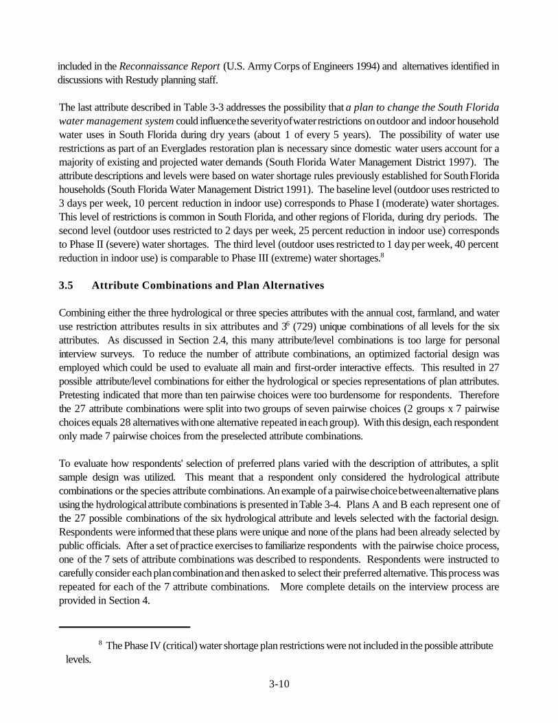
8 The Phase IV (critical) water shortage plan restrictions were not included in the possible attributelevels.

3-10

included in the Reconnaissance Report (U.S. Army Corps of Engineers 1994) and alternatives identified indiscussions with Restudy planning staff.

The last attribute described in Table 3-3 addresses the possibility that a plan to change the South Floridawater management system could influence the severity of water restrictions on outdoor and indoor householdwater uses in South Florida during dry years (about 1 of every 5 years). The possibility of water userestrictions as part of an Everglades restoration plan is necessary since domestic water users account for amajority of existing and projected water demands (South Florida Water Management District 1997). Theattribute descriptions and levels were based on water shortage rules previously established for South Floridahouseholds (South Florida Water Management District 1991). The baseline level (outdoor uses restricted to3 days per week, 10 percent reduction in indoor use) corresponds to Phase I (moderate) water shortages.This level of restrictions is common in South Florida, and other regions of Florida, during dry periods. Thesecond level (outdoor uses restricted to 2 days per week, 25 percent reduction in indoor use) correspondsto Phase II (severe) water shortages. The third level (outdoor uses restricted to 1 day per week, 40 percentreduction in indoor use) is comparable to Phase III (extreme) water shortages.8

3.5 Attribute Combinations and Plan Alternatives

Combining either the three hydrological or three species attributes with the annual cost, farmland, and wateruse restriction attributes results in six attributes and 36 (729) unique combinations of all levels for the sixattributes. As discussed in Section 2.4, this many attribute/level combinations is too large for personalinterview surveys. To reduce the number of attribute combinations, an optimized factorial design wasemployed which could be used to evaluate all main and first-order interactive effects. This resulted in 27possible attribute/level combinations for either the hydrological or species representations of plan attributes.Pretesting indicated that more than ten pairwise choices were too burdensome for respondents. Thereforethe 27 attribute combinations were split into two groups of seven pairwise choices (2 groups x 7 pairwisechoices equals 28 alternatives with one alternative repeated in each group). With this design, each respondentonly made 7 pairwise choices from the preselected attribute combinations.

To evaluate how respondents' selection of preferred plans varied with the description of attributes, a splitsample design was utilized. This meant that a respondent only considered the hydrological attributecombinations or the species attribute combinations. An example of a pairwise choice between alternative plansusing the hydrological attribute combinations is presented in Table 3-4. Plans A and B each represent one ofthe 27 possible combinations of the six hydrological attribute and levels selected with the factorial design.Respondents were informed that these plans were unique and none of the plans had been already selected bypublic officials. After a set of practice exercises to familiarize respondents with the pairwise choice process,one of the 7 sets of attribute combinations was described to respondents. Respondents were instructed tocarefully consider each plan combination and then asked to select their preferred alternative. This process wasrepeated for each of the 7 attribute combinations. More complete details on the interview process areprovided in Section 4.

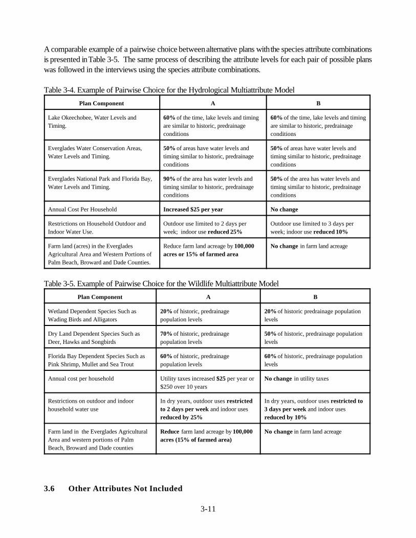
3-11

A comparable example of a pairwise choice between alternative plans with the species attribute combinationsis presented in Table 3-5. The same process of describing the attribute levels for each pair of possible planswas followed in the interviews using the species attribute combinations.

Table 3-4. Example of Pairwise Choice for the Hydrological Multiattribute Model

Plan Component A B

Lake Okeechobee, Water Levels andTiming.

60% of the time, lake levels and timingare similar to historic, predrainageconditions

60% of the time, lake levels and timingare similar to historic, predrainageconditions

Everglades Water Conservation Areas,Water Levels and Timing.

50% of areas have water levels andtiming similar to historic, predrainageconditions

50% of areas have water levels andtiming similar to historic, predrainageconditions

Everglades National Park and Florida Bay,Water Levels and Timing.

90% of the area has water levels andtiming similar to historic, predrainageconditions

50% of the area has water levels andtiming similar to historic, predrainageconditions

Annual Cost Per Household Increased $25 per year No change

Restrictions on Household Outdoor andIndoor Water Use.

Outdoor use limited to 2 days perweek; indoor use reduced 25%

Outdoor use limited to 3 days perweek; indoor use reduced 10%

Farm land (acres) in the EvergladesAgricultural Area and Western Portions ofPalm Beach, Broward and Dade Counties.

Reduce farm land acreage by 100,000acres or 15% of farmed area

No change in farm land acreage

Table 3-5. Example of Pairwise Choice for the Wildlife Multiattribute Model

Plan Component A B

Wetland Dependent Species Such asWading Birds and Alligators

20% of historic, predrainagepopulation levels

20% of historic predrainage populationlevels

Dry Land Dependent Species Such asDeer, Hawks and Songbirds

70% of historic, predrainagepopulation levels

50% of historic, predrainage populationlevels

Florida Bay Dependent Species Such asPink Shrimp, Mullet and Sea Trout

60% of historic, predrainagepopulation levels

60% of historic, predrainage populationlevels

Annual cost per household Utility taxes increased $25 per year or$250 over 10 years

No change in utility taxes

Restrictions on outdoor and indoorhousehold water use

In dry years, outdoor uses restrictedto 2 days per week and indoor usesreduced by 25%

In dry years, outdoor uses restricted to3 days per week and indoor usesreduced by 10%

Farm land in the Everglades AgriculturalArea and western portions of PalmBeach, Broward and Dade counties

Reduce farm land acreage by 100,000acres (15% of farmed area)

No change in farm land acreage

3.6 Other Attributes Not Included

9 Although not explained to respondents, the plan being referred to is the Everglades Forever Act(EFA) of 1994 which established water quality targets and timetables for the Everglades Protection Area.It is assumed for the purposes of this survey that these targets and timetables will be achieved and thatfuture modifications to the C&SFP would conform to the requirements of the EFA.

3-12

The multiattribute survey process provides a flexible tool to simultaneously consider a number of importantattributes of a decision. The design of attributes for this survey was intended to incorporate as many of thekey issues and tradeoffs in the choice combinations as was feasible given limits on respondent’s time andability to consider complex choices. But, other key issues being considered in the context of Everglades/SouthFlorida restoration were excluded.

First, water quality issues were not included in the attribute set due to the variety of existing and potentialproblems in different subregions. This issue was particularly troubling since a highly contentious and well-publicized campaign to amend the Florida Constitution had occurred in 1996 to assess a 1 cent per pound taxon sugar produced in the Everglades Agricultural Area (EAA). Proceeds from the proposed tax, which failedto get a statewide majority, would have been used to pay for improved water quality for water flowing fromthe EAA into the Everglades. Initial focus groups conducted in 1997 indicated that many people in SouthFlorida considered water quality as the major environmental problem in the Everglades.

Since the attribute combinations used to represent restoration plans in this survey focused only on changes inthe water management system to enhance hydrological (water levels and timing) or structural (species)attributes, it was necessary to deal with the water quality issue if respondents asked about how it would beaddressed under the plans described in the pairwise choice process. If this issue was raised, interviewerswere instructed to inform respondents that water quality problems were being addressed under a different planthat had already been established by the State of Florida.9 The plans each respondent was asked considerwould not interfere with this plan. Therefore respondents were asked to not consider water quality issues intheir selection of preferred alternatives.

A second issue that was not considered in the multiattribute survey was the potential effects of structuralmodifications in the C&SFP on local areas and communities in South Florida. Given the focus on endpoints,the external effects of achieving these endpoints were not considered. These effects, such as the impacts ofwater storage reservoirs or water tables on community development patterns, may be a strong influence onthe selection of projects to achieve restoration objectives. Due to the potentially large number of local concernsand the lack of a specific restoration plan to consider, this issue was excluded.

4-1

SECTION 4. SURVEY DESIGN AND RESPONDENT PROFILE

4.1 Description of the Interview Process

This survey was designed to be conducted through household personal interviews because of the large amountof detailed information to be presented and gathered. Interviews consisted of five parts in the following order:1) explanation of the nature and purpose of the survey; 2) questions about the respondents’ general attitudestoward environmental and public policy issues; 3) presentation of an informational video about the Evergladesand water management in South Florida; 4) a paired choice task to select preferred water management plansto change ecosystem attributes; and, 5) questions about respondent’s socio-economic characteristics.

Respondents who were selected to participate in the survey (see Section 4.2 below) were told that thepurpose was to determine public opinions about proposed changes in the water management system forSouth Florida. The term “restoration” was not used in the interview process because focus groups conductedin the early stages of the study indicated that the public had many different definitions of the term and ideasabout what it meant for South Florida. Also, there was concern that use of the term “restoration” might imparta negative image to the status quo and thereby bias the plan choice process.

Questions about public policy issues and environmental attitudes included a series of questions about spendingpriorities for State of Florida programs, questions about drinking water, and a series of statements about theenvironment that the respondents were asked to either agree or disagree with. Questions about socio-demographic characteristics included political party affiliation and voting history, educational attainment, placeof birth and years residency in Florida, age, household size, racial/ethnic background, donations toenvironmental groups, and household income. The paired choice task to select conjoint sets for watermanagement plans in South Florida consisted of 3 practice choices and 7 test choices for either the watermanagement or wildlife management multiattribute sets described in the previous section. The complete set ofinterview questions is provided in Appendix A.

The informational video, approximately 11 minutes in length, was a key part of the survey. The video wasdesigned to provide a common frame of reference about the issues surrounding the Everglades and SouthFlorida water management, and to enable respondents to clearly understand and answer survey questions. Thevideo was displayed either on the respondent’s video player or on a portable player provided by theinterviewer. Major sections of the video included the history of the Everglades, its hydrology and wildlife,alteration of the natural hydrologic patterns, the current water management system, uses of water in the region,and modern environmental problems. The narrative script for the video is presented in Appendix D.

Interviews were conducted by an independent market research firm (Rife Market Research, Inc. Miami, FL)subcontracted by the University of Florida to implement the survey. Bilingual interviewers were used insampling areas of South Florida with a high percentage of Hispanic residents. An incentive of $10 was paidto respondents as compensation for their time and cooperation to encourage participation in the survey. Surveyrespondents were screened to be at least 18 years of age and a legal Florida resident for at least 6 months.All respondents signed a consent form describing the conditions of the interview and their rights in the interviewprocess prior to the start of the formal interview.

4-2

The interviews averaged 57 minutes in duration and ranged from 20 minutes to nearly 2 hours. All interviewmaterials were organized in a set of notebooks that contained graphic representations of response possibilitiesand were color-coded for the two multiattribute choice protocols (Appendices B and C). Interviewers askedthe respondent questions and recorded his or her answers on a separate coding sheet. Interviewers also ratedthe respondents in terms of their seriousness about the survey, level of distraction or attentiveness to the task,and understanding of the material, as well as recording any general comments that were made about thesurvey.

4.2 Respondent Selection

A total of 480 randomly selected households were interviewed for the survey. Respondents were drawn fromselected Census tracts in 5 metropolitan areas: Miami (Dade County), West Palm Beach (Palm BeachCounty), Ft. Meyers (Lee County), Tampa (Hillsborough Co.) and Orlando (Orange Co.). The first threecounties were chosen to represent the opinions of citizens most directly affected by the restoration projectsince they were located within the South Florida Water Management District. The other areas represented theopinions of urban residents outside South Florida. The margin of error was ± 4.5 percent for estimation ofa binomial variable within the overall sample with a 95 percent level of confidence and ± 10 percent withineach county.

In each of the target sample areas, 96 households were sampled from 6 or 7 selected U.S. Census tracts. TheCensus tracts in the study area were stratified by median household income and racial/ethnic composition. Thethree strata for median annual household income were: less than $25,000, $25,000 to $39,999, and $40,000or greater. The two strata for racial/ethnic composition were based on the population of non-white andHispanic minorities as a percentage of the county population: less than 25 percent and greater than or equalto 25 percent. These stratifications gave a total of 6 (3x2) strata combinations. Each stratum was representedin the sample for each county by random selection from the universe of Census tracts for that county.

The final selection of households for the survey was made by interviewers in the field following a prescribedprocedure to assure randomness. In each targeted Census tract, a typical street was selected from twodifferent Census blocks. A listing of all addresses on the street was made and numbered consecutively. Thena random number table was consulted to randomly select 8 of the addresses as primary target households forinterviews and 4 as alternate households. At least two attempts were made to contact the residents of theselected primary households at different times of day before accepting an alternate address to avoid systematicbias in the selection based on daily work-activity patterns. Additional sets of alternate households weregenerated as needed to complete the sample of 8 from each block group. Approximately 10 percent ofhouseholds contacted refused to participate.

4.3 Respondent Socio-Demographic Profiles

Socio-demographic characteristics of the respondents interviewed for the survey are summarized in Tables4.1 and 4.2. Comparable figures are also provided for the state population based on official Census statisticsand the Florida Annual Policy Survey (FAPS) conducted by Florida State University. While this surveysample was not designed to be representative of the Florida population, the target areas represent a majorshare of the total resident population in Florida.

4-3

In general, the characteristics of the survey sample closely matched the Florida population. Table 1 shows thatrespondent gender was 48.5 percent male and 51.5 percent female. Respondent ages were: 18 to 24 years -6.6 percent, 25 to 44 years - 43.0 percent, 45 to 64 years - 25.0 percent, and 65 years or older - 25.4percent. The highest level of education attained by survey respondents was: primary school (no high schooldiploma) - 12.2 percent, high school - 30.3 percent, some college - 27.8 percent, college graduates - 19.6percent, and post-graduate work - 9.9 percent. This represented a slightly higher share of sample respondentswith advanced education, and a correspondingly lower share with only primary education than the statepopulation (Table 4.1). The number of respondents who indicated they were not born in Florida (79 percent)was slightly greater than the state population (71 percent). Also, respondents who had lived in Florida lessthan 5 years (31 percent) were somewhat more frequent than the state population (17.5 percent), while thosewho had been residents over 21 years (30 percent) were less frequent (37 percent).

The racial/ethnic composition of sample respondents was: white - 82.9 percent, black - 11.9 percent,Hispanic (included in either white or black) - 22.9 percent, and other - 4.3 percent. Racial composition ofthe sample in each county surveyed closely matched that of the county as a whole (Table 4.2). Political partyaffiliation of respondents was: Republican - 24.6 percent, Democrat - 37.4 percent, Independent or otherparty - 16.7 percent, and no preference - 21.3 percent. The proportion of respondents who indicated thatthey voted in the last 3 years (62.6 percent) was slightly less than the population (72.7 percent). In terms ofdonations made annually to environmental groups, 53.1 percent of respondents did not make any, 33.3 percentdonated less than $100, 9.0 percent donated $100 to $500, and 1.5 percent reported donating more than$500. Annual household income was less than $20,000 for 23.3 percent of respondents, $20,000 to $50,000for 42.9 percent, over $50,000 for 23.1 percent; 10.6 percent refused to disclose household income levels(Table 4.1). The estimated median household income for the survey sample in each county ranged from$25,000 in Hillsborough County to $46,250 in Palm Beach County, but were similar to the county populationin toto (Table 4.2). The mean household size reported by respondents was 2.7 persons as compared to 2.46for the state population (Table 4.1).

As part of the interview, respondents were asked to indicate their support for state expenditures in 12 majorprogram areas. These questions were identical to those contained in the FAPS in 1996 and provide a usefulbenchmark for comparison. The results are summarized in Table 4.3.

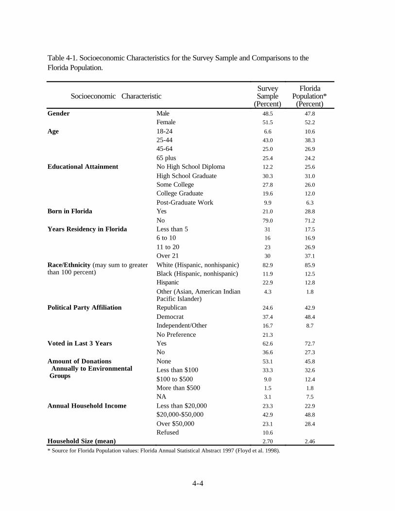
4-4

Table 4-1. Socioeconomic Characteristics for the Survey Sample and Comparisons to theFlorida Population.

Socioeconomic CharacteristicSurveySample

(Percent)

FloridaPopulation*(Percent)

Gender Male 48.5 47.8

Female 51.5 52.2

Age 18-24 6.6 10.6

25-44 43.0 38.3

45-64 25.0 26.9

65 plus 25.4 24.2

Educational Attainment No High School Diploma 12.2 25.6

High School Graduate 30.3 31.0

Some College 27.8 26.0

College Graduate 19.6 12.0

Post-Graduate Work 9.9 6.3

Born in Florida Yes 21.0 28.8

No 79.0 71.2

Years Residency in Florida Less than 5 31 17.5

6 to 10 16 16.9

11 to 20 23 26.9

Over 21 30 37.1

Race/Ethnicity (may sum to greaterthan 100 percent)

White (Hispanic, nonhispanic) 82.9 85.9

Black (Hispanic, nonhispanic) 11.9 12.5

Hispanic 22.9 12.8

Other (Asian, American IndianPacific Islander)

4.3 1.8

Political Party Affiliation Republican 24.6 42.9

Democrat 37.4 48.4

Independent/Other 16.7 8.7

No Preference 21.3

Voted in Last 3 Years Yes 62.6 72.7

No 36.6 27.3

Amount of Donations Annually to Environmental Groups

None 53.1 45.8

Less than $100 33.3 32.6

$100 to $500 9.0 12.4

More than $500 1.5 1.8

NA 3.1 7.5

Annual Household Income Less than $20,000 23.3 22.9

$20,000-$50,000 42.9 48.8

Over $50,000 23.1 28.4

Refused 10.6

Household Size (mean) 2.70 2.46

* Source for Florida Population values: Florida Annual Statistical Abstract 1997 (Floyd et al. 1998).

4-5

4-6

Table 4-2. Race/Ethnicity and Median Household Income for the Survey Sample, by County, andComparisons to the County Population.

County

Race/Ethnicity

(Percentage of Survey Sample or Population) Median HouseholdIncomeWhite, non-Hispanic Minority, other

Sample Population* Sample Population* Sample Population*

Dade 35.4 30.4 64.6 69.6 $40,625 $33,117

Lee 87.5 88.4 12.5 11.6 $32,273 $29,734

Palm Beach 77.1 79.4 22.9 20.6 $46,250 $36,013

Hillsborough 81.3 72.9 18.8 27.1 $25,000 $27,466

Orange 72.9 73.4 27.1 26.6 $34,444 $31,277

All Counties 70.8 58.5 29.2 41.5 $33,942 $31,628

* County population characteristics from 1990 US Census.

Public schools were rated as the top priority by 31.7 percent of respondents, followed by crime (18.5percent), health care (11.9 percent), the environment (11.0 percent), the elderly (7.9 percent), low incomefamilies (5.2 percent), endangered species (3.5 percent), highways (3.1 percent), colleges/universities (2.5percent), industrial development (2.3 percent), prisons (1.5 percent) and tourism (0.6 percent). Theserankings were very similar to those of the Florida population as measured by the 1996 FAPS. For publicschools, 79.4 percent of respondents indicated that public funding should be increased in this area, 16.5percent said it should remain the same and 3.8 percent wanted it decreased. Again these results closelymatched the Florida population. For programs for the environment, a somewhat higher percentage of surveyrespondents (66.7 percent) desired an increase in funding as compared to the state population (57.6 percent).A lower percentage wished it to remain the same or to decrease. A similar pattern of results was foundconcerning priorities for funding programs for endangered species. The percentage of survey respondents whosupported increased funding was also greater than the population for health care, highways, low incomefamilies, the elderly, and tourism, but were lower for prisons and colleges/universities.

Respondents were also read statements about the environment and water supply issues and asked whetherthey (strongly or somewhat) agreed or disagreed with each statement. Table 4.4 shows that generally therewas a very high level of concern and support expressed for statements about the environment. Over 90percent of respondents either “strongly agreed” or “somewhat agreed” with the statements “the environmentis easily upset” and “interference with the environment often causes disaster.” These results are highlyconsistent with other statewide surveys of Floridians attitudes about the environment (Milon et al. 1998). Respondents also expressed strong support for water conservation as in the statement “water conservationpractices are a good idea.” Conversely, nearly two thirds of respondents disagreed with the statement“humans have the right to change the environment to suit their needs.” There was a somewhat lower level ofagreement with statements regarding water supply: “water will always be available for my community,” “waterwill always be available for anybody who wishes to move to Florida,” or “water supply needs are a toppriority.” A majority of respondents disagreed with the statement “protection from flooding is adequate in mycommunity.”

4-7

Table 4-3. Priorities for State of Florida Expenditures by Program Area by Survey Sample Respondents and Comparisons to the Florida Population.

Program Area Sample orPopulation*

Top RatedPriority (Percent)

Funding Change Indicated(Percent of Respondents)

IncreaseRemainSame

DecreaseNo

Answer

Crime Sample 18.5 71.3 23.3 4.4 1.0Population 16.4 70.5 21.8 4.5 3.2

Public schools Sample 31.7 79.4 16.5 3.8 0.4Population 35.4 78.5 15.0 3.0 3.5

The Environment Sample 11.0 66.7 29.2 3.1 1.0Population 8.6 57.6 33.0 6.3 3.1

Industrial development Sample 2.3 26.3 45.2 26.5 2.1Population 4.3 24.4 43.0 27.4 5.2

Endangered Species Sample 3.5 57.7 32.3 8.3 1.7Population na 51.1 36.3 9.3 3.4

Health care Sample 11.9 65.8 28.5 5.4 0.2Population 7.6 55.0 32.1 8.6 4.3

Colleges/universities Sample 2.5 50.0 42.3 7.1 0.6Population 3.9 55.3 34.3 5.8 4.6

Highways Sample 3.1 43.3 45.6 10.2 0.8Population 3.7 35.5 52.9 9.4 2.2

Low income families Sample 5.2 48.5 40.0 10.8 0.6Population 6.0 36.5 40.9 16.2 6.4

Elderly Sample 7.9 64.2 31.5 4.0 0.4Population 9.6 49.7 38.8 6.6 4.9

Prisons Sample 1.5 31.5 42.3 24.8 1.5Population 2.9 33.7 39.5 21.5 5.2

Tourism Sample 0.6 23.3 47.1 28.5 1.0Population 1.0 20.8 53.6 23.5 2.1

* Population estimates are from the 1996 Florida Annual Policy Survey (Florida State University).

4-8

Table 4-4. Survey Respondent Attitudes about the Environment and Water Supply.Percent of Respondents Choosing

Statement Strongly Agree Somewhat

Agree

Somewhat

Disagree

Strongly

Disagree

No Answer

Water will always be available for anyone who comes to my community.

38.3 32.5 18.8 6.3 4.2

Water will always be available for anyone who comes to Florida.

40.4 32.1 15.8 7.7 4.0

Water supply needs are a top priority.

38.5 27.3 20.4 12.9 0.8

The environment is delicate and easily upset.

63.1 28.3 5.6 1.5 1.5

Interference with the environment often causes disaster.

60.8 32.3 4.2 1.9 0.8

Protection from flooding in my community is adequate.

9.6 25.8 19.6 38.3 6.7

Humans have the right to change environment to suit their needs.

6.0 21.0 24.0 46.9 2.1

Water conservation practices are a good idea.

66.3 27.3 3.3 2.7 0.4

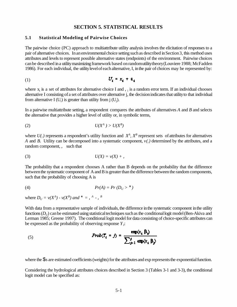
5-1

(1)

(5)

SECTION 5. STATISTICAL RESULTS

5.1 Statistical Modeling of Pairwise Choices

The pairwise choice (PC) approach to multiattribute utility analysis involves the elicitation of responses to apair of alternative choices. In an environmental choice setting such as described in Section 3, this method usesattributes and levels to represent possible alternative states (endpoints) of the environment. Pairwise choicescan be described in a utility maximizing framework based on random utility theory (Louviere 1988; McFadden1986). For each individual, the utility level of each alternative, I, in the pair of choices may be represented by:

where xi is a set of attributes for alternative choice I and ,i is a random error term. If an individual choosesalternative I consisting of a set of attributes over alternative j, the decision indicates that utility to that individualfrom alternative I (Ui) is greater than utility from j (Uj). In a pairwise multiattribute setting, a respondent compares the attributes of alternatives A and B and selectsthe alternative that provides a higher level of utility or, in symbolic terms,

(2) U(XA ) > U(XB)

where U(.) represents a respondent’s utility function and XA, XB represent sets of attributes for alternativesA and B. Utility can be decomposed into a systematic component, v(.) determined by the attributes, and arandom component, , such that

(3) U(X) = v(X) + ,

The probability that a respondent chooses A rather than B depends on the probability that the differencebetween the systematic component of A and B is greater than the difference between the random components,such that the probability of choosing A is

(4) Pr(A) = Pr (DU > *)

where DU = v(XA) - v(XB) and * = ,A - ,B

With data from a representative sample of individuals, the difference in the systematic component in the utilityfunctions (DU) can be estimated using statistical techniques such as the conditional logit model (Ben-Akiva andLerman 1985; Greene 1997). The conditional logit model for data consisting of choice-specific attributes canbe expressed as the probability of observing response Y I:

where the $s are estimated coefficients (weights) for the attributes and exp represents the exponential function.

Considering the hydrological attributes choices described in Section 3 (Tables 3-1 and 3-3), the conditionallogit model can be specified as:

5-2

(6)

(7)

(8)

where $i are the estimated coefficients and Xi are the attributes of the alternatives in the choice sets with X1

the Lake Okeechobee attribute, X2 the Water Conservation Areas attribute, X3 the Everglades National Parkattribute, X4 the Annual Cost attribute, X5 the Water Use Restrictions attribute, and X6 the Farmland attribute.

Similarly, the species attributes choices (Tables 3-2 and 3-3) can be specified as:

where X1 is the Wetland Species attribute, X2 is the Dryland Species attribute, X3 is the Estuarine Speciesattribute, X4 is the Annual Cost Attribute, X5 is the Water Use Restrictions attribute, and X6 is the Farmlandattribute.

In addition to identifying respondents' weighting of different attributes, it may also be desirable to evaluatewhether socioeconomic characteristics such as age, income, or geographic location influence the attributeweights. The conditional logit model can be used to evaluate socioeconomic interactions with the attributesvariables (Swallow et al. 1994). A comparable specification for either the hydrological attributes or speciesattributes models that includes socioeconomic variables interacting with the attributes can be expressed as:

where Xi denotes the ith attribute, $i are estimated coefficients for the main effects of each attribute, "mi areestimated coefficients for interactive variables with attributes and eight socioeconomic characteristics, Smi, thatinclude political party affiliation, region of the state, donations to environmental causes, gender, years living inFlorida, income, and two ethnic groupings.

5.2 Sample Data

Using the survey design and split sample process described in Sections 3 and 4 resulted in 480 completedinterviews which were divided evenly between the hydrological attributes and species attributes formats. The480 completed interviews provided 1,680 choices for each attribute set (7 choices times 240 respondents).Based upon the interviewer’s appraisal that some respondents lacked attentiveness and seriousness during theinterview, 21 respondents were removed from the hydrological attributes respondent sample and 6respondents were removed from the species attributes sample. This resulted in a total of 1,533 observations(choices) for the hydrological attributes model and 1,638 observations for the species attributes model. SeeAppendix E for complete data on interviewer evaluations of respondents.

Table 5-1 reports descriptive statistics for the attributes and socioeconomic variables for the hydrological andspecies sample groups used in the analysis. As discussed in detail in Section 3, the attribute variables areexpressed in terms of the percentage of historic levels. The mean, minimum, and maximum values for theattributes reflect the statistical design.

5-3

Table 5-1. Variable Definitions and Summary Statistics for the Hydrological and Species Attribute Models.

Attribute/Variable Definition

Hydrological Attribute Models Species Attribute Models

Mean S. D. Min Max Mean S.D Min Max

Lake Okeechobee Percentage of historic level 0.74 0.12 0.6 0.9

Water Conservation Area Percentage of historic level 0.72 0.17 0.5 0.9

Everglades National Park Percentage of historic level 0.71 0.17 0.5 0.9

Wetland Species Percentage of historic level 0.49 0.25 0.2 0.8

Dryland Species Percentage of historic level 0.60 0.08 0.5 0.7

Estuarine Species Percentage of historic level 0.76 0.12 0.6 0.9

Annual Cost Annual increase in utilities tax for 10 years 25 20.02 0 50 25 20.03 0 50

Water Restriction 1 Outdoor uses restricted to 2 days per week and

25% reduction in indoor consumption

0.36 0.48 0 1 0.36 0.48 0 1

Water Restriction 2 Outdoor uses restricted to 1 day per week and

40% reduction in indoor consumption

0.32 0.47 0 1 0.32 0.46 0 1

Farmland Farm land acreage in EAA and South Florida

(‘000 acres)

99.84 80.19 0 200 99.88 80.19 0 200

Political Party 1 if Republican, 0 all others 0.25 0.44 0 1 0.27 0.44 0 1

Region 1 if Central Florida, 0 South Florida 0.41 0.49 0 1 0.39 0.49 0 1

Donations 1 if donated to environmental groups, 0 otherwise 0.42 0.49 0 1 0.49 0.50 0 1

Gender 1 if male, 0 female 0.48 0.50 0 1 0.48 0.50 0 1

Years in Florida Number of years as resident 20.24 14.09 1 73 18.71 12.69 1 71

Income 1 to 9 by $10,000 increments (i.e. 1=less than

$10,000, 2=$10,000 to $19,999, etc.)

4.07 2.06 1 9 4.26 2.08 1 9

Ethnic 1 1 if White-Hispanic or Black-Hispanic, 0

otherwise

0.14 0.35 0 1 0.12 0.33 0 1

Ethnic 2 1 if White-Non-Hispanic, 0 otherwise 0.74 0.44 0 1 0.73 0.45 0 1

5-4

Since the choice combinations were randomly distributed across the sample groups, the means for eachattribute are approximately the midpoint of the upper and lower levels.

For the purpose of this statistical analysis, the three levels for the water use restrictions attribute (see Table3-3) were converted into two dummy variables. The variable “ Water Restriction 1" was defined as thesecond level of the attribute that would restrict outdoor uses to two days per week with a 25 percent reductionin indoor use during dry periods. The variable “Water Restriction 2" was defined as the third level of theattribute that would restrict outdoor uses to one day per week with a 40 percent reduction in indoorconsumption. The first level of the attribute was defined as the base and included in the estimated interceptsof the statistical models. As indicated in Table 5.1, Water Restriction 1 was included in approximately onethird of the choices in each sample group and Water Restriction 2 was also included in about one third of thechoices. These proportions are as expected given the sample design.

Table 5-1 also presents the socioeconomic variables that were included in the statistical models. Several ofthe socioeconomic variables (originally described in Table 4-1) were redefined as 0,1 variables as presentedin Table 5-1. A comparison of the means for the socioeconomic variables in the two sample groups showsthat the two groups were very similar. This indicates that the alternative attribute formats (hydrological andspecies) were randomly distributed across the total sample.

5.3 Statistical Results for the Multiattribute Models

The first multiattribute models estimated with the survey data were basic models that included only the choiceattributes as defined previously in this section in Equations (6) and (7). The basic model was specified withand without an intercept term to test whether there was an order bias in respondents’ choices betweenalternative plans. The null hypothesis that the intercept ($0 ) equals zero indicates whether respondents basedtheir choices on whether a plan was on the left- or right-hand side of the page (see Table 3-5) when they wereasked to choose between alternative plans. If the order of presentation did influence respondents’ decisions,then any information about the relative weighting given to different attributes would be questionable. This isbecause multiattribute analysis assumes that responses as based solely on the levels of the attributes.

The estimated coefficients and related statistics for the hydrological and species multiattribute models arepresented in Tables 5-2 and 5-3, respectively. The tables also include estimates of the marginal willingnessto pay (WTP) for changes in each attributes. The WTP for each attribute was calculated with the formula:

($i (Ai1) - $i (Ai2)) /$c

where $i is the estimated coefficient for attribute I, Ai1 is the base level of attribute I, Ai2 is the next level ofthe attribute, and $c is the estimated coefficient for the annual cost attribute. By dividing the marginal changefor each attribute by the cost attribute, the estimated WTPs provide a measure of the relative weightingassigned to each attribute. This weighting is a monetary measure of the utility derived from each attribute. TheWTP measure is appropriate for benefit-cost analysis of alternative plans (Johnson and Desvousges 1997; Roeet al. 1996). Because the basic utility function specification is additive, the marginal WTPs are constant (linear)for each attribute with the exception of the water restrictions attribute that was decomposed into two separateeffects. Given the description of the annual cost attribute in the analysis (see Table 3-3), the annual WTPswould apply over a ten year period. A comparable approach can be used to estimate WTP values in themultiattribute model with socioeconomic interactions (Equation (8). The basic difference is that marginal valuesmust be calculated for each individual in the sample because the coefficients ($i ) for each attribute vary acrosssocioeconomic characteristics.

5.3.1 Basic Hydrological Multiattribute Model Results

5-5

Table 5-2 presents statistical results for the hydrological multiattribute model. The coefficient for the modelestimated with an intercept term was statistically insignificant indicating that this subsample of respondents’choices were not influenced by the order of presentation of the plan alternatives. Several other coefficients,however, were statistically significant in the model estimated without an intercept. The Lake Okeechobee andWater Conservation Areas attributes were both positive and statistically significant indicating that respondentspreferred plans that had higher levels of these attributes. The Everglades National Park attribute was alsopositive but not statistically significant.

The Annual Cost and Farmland attributes were also statistically significant but had a negative sign indicatingthat respondents preferred plans that had lower levels of these attributes. The water supply restrictionattributes provided interesting results. The Water Restriction 1 attribute was negative but not statisticallysignificant. The Water Restriction 2 attribute, however, was highly significant and the estimated coefficientindicates that respondents placed a large negative weight on this attribute.

These statistical results indicate that higher levels of the hydrological attributes increased the likelihood thatrespondents would select a plan that included higher levels of those attributes. On the other hand, higher levelsof the Annual Cost and Farmland attributes and the Water Restriction 2 attribute decreased the likelihood ofselecting a plan. The full effects of respondents’ preferences for each attribute across the sample are reflectedin the marginal WTP values. The Water Conservation Areas attribute had the highest positive WTP ($17.63)indicating that respondents derived the most satisfaction (utility) from an increase (e.g. 50 percent to 75percent) in this attribute. The Lake Okeechobee and Everglades National Park attribute WTPs were alsopositive but relatively smaller.

The relatively large negative marginal WTP (-$37.10) associated with the Water Restriction 2 attributeindicates the strong aversion respondents had to this component of a plan. On the other hand, the WaterRestriction 1 attribute had a relatively small negative WTP indicating that respondents would be willing toexperience some restrictions on water use for desirable changes in hydrological conditions in the Evergladesareas. The relatively large negative WTP associated with the Farmland attribute (-$16.39), however, indicatesthat respondents would not prefer that these desirable changes in hydrological conditions were accompaniedby large reductions (100,000 or more acres) in farmland acreage in South Florida.

5-6

Table 5-2. Coefficient Estimates for the Hydrological Multiattribute Models.

Attribute/VariableModel with Intercept Model without Intercept

Coefficient Standard Error

Coefficient Standard ErrorMarginal

Willingness to Pay (WTP)

Intercept -0.1066 0.0756 - - -

Lake Okeechobee 0.3639 0.4724 0.7876* 0.3675 $9.68

Water Conservation Areas 0.9797* 0.2808 0.8606* 0.2666 $17.63

Everglades National Park 0.4445 0.3383 0.3419 0.3310 $7.01

Annual Cost -0.0136* 0.0031 -0.0122* 0.0029 -

Water Restriction 1 0.0354 0.1143 -0.0220 0.1063 -$1.80

Water Restriction 2 -0.4048* 0.1030 -0.4539* 0.0973 -$37.10

Farmland -0.0001* 0.0001 -0.0001* 0.0001 -$16.39

Log Likelihood Function for the Model -999.36 -1000.36

Unrestricted Log Likelihood Function -1162.59 -1162.59

Chi-squared (7 degrees of freedom) 326.32* 324.46*

* Indicates significance at the 0.05 level

5-7

5.3.2 Basic Species Multiattribute Model Results

Table 5-3 presents statistical results for the species multiattribute model estimated with and without an interceptterm. The intercept in this model was also statistically insignificant indicating that this subsample of respondentswas not influenced by the order of presentation of the choice alternatives. Most of the other coefficients,however, were statistically significant. The Wetland and Estuarine Species attributes were positive andsignificant while the Dryland Species attribute was negative. The marginal WTPs associated with theseattributes indicates that respondents placed the most value on higher levels of Estuarine Species ($27.34) andthe least value on higher levels of Dryland Species (-$29.87). Clearly respondents were expressing strongpreferences for plans that would improve habitat for wading birds and various marine fishes in the Evergladesand Florida Bay.

As in the hydrological multiattribute models, higher levels of the Annual Cost and Farmland attributes and theWater Restriction 2 attribute decreased the likelihood of selecting a plan. The coefficients for all three of theseattributes were negative and statistically significant. Moreover, it is also interesting to note the similarity in theestimated WTPs for the Water Restriction 2 attribute in the hydrological attributes model (Table 5-2) and thespecies attributes model. The relatively small difference (-$37.10 vs -$34.96) indicates that both subsamplesresponded in approximately the same way to the potential of severe water restrictions despite the presenceof other quite different attributes in the choice set.

5-8

Table 5-3. Coefficient Estimates for the Species Multiattribute Model.

Attribute/VariableModel with Intercept Model without Intercept

Coefficient StandardError

Coefficient Standard Error

Marginal Willingness to Pay (WTP)

Intercept 0.0930 0.0715 - - -

Wetland Species 0.7736* 0.2239 0.5991* 0.1780 $9.26

Dryland Species -1.3915* 0.6420 -1.1593* 0.6154 -$29.87

Estuarine Species 0.9589* 0.3594 1.0606* 0.3518 $27.34

Annual Cost -0.0084* 0.0029 -0.0097* 0.0027 -

Water Restriction 1 -0.1289 0.1075 -0.0869 0.1027 -$8.95

Water Restriction 2 -0.3815* 0.0995 -0.3391* 0.0934 -$34.96

Farmland -0.0001* 0.0001 -0.0001* 0.0001 -$9.27

Log Likelihood Function for the Model -1078.12 -1078.96

Unrestricted Log Likelihood Function -1135.38 -1135.37

Chi-squared (7 degrees of freedom) 114.39* 112.82*

* Indicates significance at the 0.05 level

5-9

5.4 Statistical Results for Models with Socioeconomic Characteristics Interactions

The hydrological multiattribute and species multiattribute models were also estimated using interactivesocioeconomic variables as described in Section 5.1 (Equation (8)). Tables 5.4 and 5.5 present results forthe hydrological and species multiattribute models, respectively. These coefficient estimates are more difficultto interpret because of the large number of interactions. Moreover, WTP measures for individual attributeinteractions with socioeconomic characteristics can be misleading if not considered along with other relatedinteractions. Therefore, WTP values for the attributes are not presented in these tables.

The statistical results indicate several significant interaction effects but the effects differ in each model. In thehydrological multiattribute model, gender, region, income and ethnic variables had statistically significant effects.On the other hand, only income and ethnic status had significant effects in the species multiattribute model.While there were a number of insignificant interactions in both models, the overall statistical results (i.e. loglikelihood functions) indicate that the multiattribute models with socioeconomic interactions provide importantinformation to assess differences in respondent preferences.

The primary importance of these results is that they provide the basis for disaggregating overall scoring andranking results for possible plans that can be constructed with alternative combinations of the attribute. Thisapplication of the results will be discussed in greater detail in Section 6.

5-10

Table 5-4. Coefficient Estimates for the Hydrological Multiattribute Model with Socioeconomic CharacteristicsInteractions.

Variable Coefficient Standard ErrorLake Okeechobee -0.0222 1.5309

Water Conservation Areas 1.0656 1.0944

Everglades National Park -3.6539* 1.1832

Annual Cost -0.0130* 0.0030

Water Restriction 1 -0.3111 0.4345

Water Restriction 2 -1.2725* 0.3992

Farmland -0.0001 0.0001

Political Party/Lake Okeechobee 0.1995 0.9244

Political Party/Water Conservation Areas 0.3207 0.6757

Political Party/Everglades National Park 0.5636 0.7257

Political Party/Water Restriction 1 -0.1225 0.2773

Political Party/Water Restriction 2 0.1598 0.2305

Political Party/Farmland 0.0001 0.0001

Region/Lake Okeechobee 0.4523 0.7936

Region/Water Conservation Areas -0.3920 0.5723

Region/Everglades National Park -1.9221* 0.6081

Region/Water Restriction 1 0.1474 0.2304

Region/Water Restriction 2 -0.0674 0.1997

Region/Farmland -0.0001 0.0001

Donations/Lake Okeechobee 1.4508 0.7962

Donations/Water Conservation Areas -0.1894 0.5829

Donations/Everglades National Park -0.2004 0.6128

Donations/Water Restriction 1 0.2569 0.2298

Donations/Water Restriction 2 0.2534 0.2006

Donations/Farmland 0.0001 0.0001

Gender/Lake Okeechobee -1.6513* 0.7763

Gender/Water Conservation Areas -0.1156 0.5600

Gender/Everglades National Park 0.8863 0.6018

Gender/Water Restriction 1 0.4791* 0.2283

Gender/Water Restriction 2 0.5932* 0.1975

Gender/Farmland 0.0001 0.0001

Years in Florida/Lake Okeechobee -0.0103 0.0285

Years in Florida/Water Conservation Areas -0.0281 0.0201

Years in Florida/Everglades National Park -0.0013 0.0218

Years in Florida/Water Restriction 1 -0.0144 0.0083

Years in Florida/Water Restriction 2 -0.0115 0.0073

Years in Florida/Farmland 0.0001 0.0001

Income/Lake Okeechobee 0.2408 0.1982

Income/Water Conservation Areas 0.1756 0.1440

Income/Everglades National Park 0.5424* 0.1540

Income/Water Restriction 1 0.0703 0.0578

Income/Water Restriction 2 0.0741 0.0502

Income/Farmland -0.0001 0.0001

Ethnic1/Lake Okeechobee 0.7024 1.5441

Ethnic1/Water Conservation Areas 0.2611 1.1123

Ethnic1/Everglades National Park 0.9575 1.1794

Ethnic1/Water Restriction 1 -0.2855 0.4435

Ethnic1/Water Restriction 2 0.4555 0.3942

Ethnic1/Farmland 0.0001 0.0001

Ethnic2/Lake Okeechobee 0.0234 1.2438

Ethnic2/Water Conservation Areas -0.2963 0.8771

Ethnic2/Everglades National Park 2.6056* 0.9424

Ethnic2/Water Restriction 1 -0.1129 0.3604

Ethnic2/Water Restriction 2 0.2937 0.3170

Ethnic2/Farmland 0.0001 0.0001

Log Likelihood Function for the Model -951.91

Unrestricted Log Likelihood Function -1162.59

Chi-squared (55 degrees of freedom) 421.36*

* Indicates significance at the 0.05 level

5-11

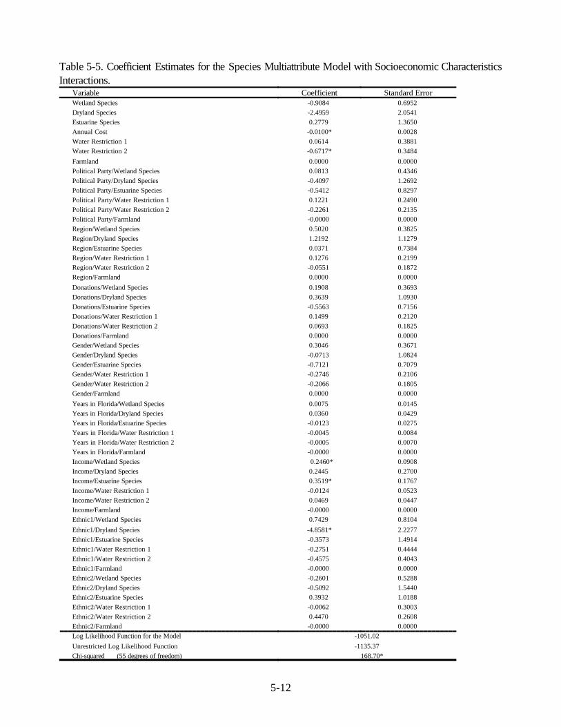
5-12

Table 5-5. Coefficient Estimates for the Species Multiattribute Model with Socioeconomic CharacteristicsInteractions.

Variable Coefficient Standard ErrorWetland Species -0.9084 0.6952

Dryland Species -2.4959 2.0541

Estuarine Species 0.2779 1.3650

Annual Cost -0.0100* 0.0028

Water Restriction 1 0.0614 0.3881

Water Restriction 2 -0.6717* 0.3484

Farmland 0.0000 0.0000

Political Party/Wetland Species 0.0813 0.4346

Political Party/Dryland Species -0.4097 1.2692

Political Party/Estuarine Species -0.5412 0.8297

Political Party/Water Restriction 1 0.1221 0.2490

Political Party/Water Restriction 2 -0.2261 0.2135

Political Party/Farmland -0.0000 0.0000

Region/Wetland Species 0.5020 0.3825

Region/Dryland Species 1.2192 1.1279

Region/Estuarine Species 0.0371 0.7384

Region/Water Restriction 1 0.1276 0.2199

Region/Water Restriction 2 -0.0551 0.1872

Region/Farmland 0.0000 0.0000

Donations/Wetland Species 0.1908 0.3693

Donations/Dryland Species 0.3639 1.0930

Donations/Estuarine Species -0.5563 0.7156

Donations/Water Restriction 1 0.1499 0.2120

Donations/Water Restriction 2 0.0693 0.1825

Donations/Farmland 0.0000 0.0000

Gender/Wetland Species 0.3046 0.3671

Gender/Dryland Species -0.0713 1.0824

Gender/Estuarine Species -0.7121 0.7079

Gender/Water Restriction 1 -0.2746 0.2106

Gender/Water Restriction 2 -0.2066 0.1805

Gender/Farmland 0.0000 0.0000

Years in Florida/Wetland Species 0.0075 0.0145

Years in Florida/Dryland Species 0.0360 0.0429

Years in Florida/Estuarine Species -0.0123 0.0275

Years in Florida/Water Restriction 1 -0.0045 0.0084

Years in Florida/Water Restriction 2 -0.0005 0.0070

Years in Florida/Farmland -0.0000 0.0000

Income/Wetland Species 0.2460* 0.0908

Income/Dryland Species 0.2445 0.2700

Income/Estuarine Species 0.3519* 0.1767

Income/Water Restriction 1 -0.0124 0.0523

Income/Water Restriction 2 0.0469 0.0447

Income/Farmland -0.0000 0.0000

Ethnic1/Wetland Species 0.7429 0.8104

Ethnic1/Dryland Species -4.8581* 2.2277

Ethnic1/Estuarine Species -0.3573 1.4914

Ethnic1/Water Restriction 1 -0.2751 0.4444

Ethnic1/Water Restriction 2 -0.4575 0.4043

Ethnic1/Farmland -0.0000 0.0000

Ethnic2/Wetland Species -0.2601 0.5288

Ethnic2/Dryland Species -0.5092 1.5440

Ethnic2/Estuarine Species 0.3932 1.0188

Ethnic2/Water Restriction 1 -0.0062 0.3003

Ethnic2/Water Restriction 2 0.4470 0.2608

Ethnic2/Farmland -0.0000 0.0000

Log Likelihood Function for the Model -1051.02

Unrestricted Log Likelihood Function -1135.37

Chi-squared (55 degrees of freedom) 168.70*

5-13

* Indicates significance at the 0.05 level

6-1

SECTION 6. EVALUATION OF ALTERNATIVE RESTORATION PLANS

6.1 Voting, Ranking and Net Willingness to Pay Measures from Multiattribute Models

The paired comparison, multiattribute utility approach is one method to derive quantitative measures ofrespondents’ preferences for alternative levels of choice attributes based on statistically reliable procedures.The results reported in Section 5 provide multiattribute utility functions for both representative andsocioeconomic-specific preferences using hydrological and species attributes of the Everglades/South Floridaecosystem. These utility functions can be used to evaluate how respondents would respond to hypotheticalalternative combinations of the attributes based on the overall score assigned to an alternative (see Section2.3). The scoring information can be summarized in three ways: 1) as rankings of alternatives based onoverall scores, 2) as the percent in favor of an alternative relative to the status quo, and 3) as the netwillingness to pay for an alternative. Because each summary measure aggregates the scoring results in adifferent way, the ordering of alternatives may vary with these measures.

A ranking evaluation of alternatives can be derived directly from the multiattribute utility function. Using thebasic model described in Equations (5) and (6) in Section 5, the net score (S) for the jth alternative would becomputed as:

Sj = ($1X1j + $2X2j + $3X3j + $4X4j + $5X5j + $6X6j + $7X7j )

where the $i s are the estimated coefficients and Xij is the level of the ith attribute in alternative j. This netscore can be calculated for as many hypothetical alternatives as are feasible with the attribute combinationsor are applicable to the overall problem setting. Once the net scores have been calculated for all alternatives,the alternatives can then be arrayed in order of the net score to provide a unique, ordinal ranking. The topranked alternative would have the highest overall utility to respondents. This same computational approachcould be used with the socioeconomic interactive variable models described in Equation (8) in Section 5 toprovide rankings of alternatives according to respondents' location (e.g. South Florida vs Central Florida) orother socioeconomic characteristics.

The net scores for each alternative could also be used as measures of whether respondents would vote in favorof an alternative if it were presented as a referendum. If the status quo (i.e. a plan with no change frombaseline attribute levels) has a net score defined as S0 , then a voter would vote in favor of the jth alternativeplan if Sj , S0 or against the alternative if Sj + S0 . By adding up the votes of all respondents, the percent infavor of the alternative can be calculated. Note that this calculation only requires a comparison of two netscores for each individual. Therefore two alternatives with similar net scores may have the same percent infavor relative to the status quo.

The third way that the scoring information can be used is to calculate net willingness to pay (WTP) for eachalternative. The net WTP is a measure of the economic benefits (value) each respondent would derive fromall attributes included in the alternative. Following the basic approach to calculate the marginal WTP for eachattribute described in Section 5.3, the net WTP can be defined as:

10 The reader should note that none of the plans were intended to fully represent the components

being considered as part of the Everglades/South Florida Restudy. Also, the definition of the status quo(baseline) differs from that used in the Restudy. For a further discussion of the differences between thisevaluation and the Restudy process, see Section 3.

6-2

Net WTPj = [(($1X1j - $1X10 )/$4 )+ (($2X2j - $2X20 )/$4 ) + (($3X3j - $3X30 )/$4 ) +(($5X5j - $5X50 )/$4 ) + (($6X6j - $6X60 )/$4 ) + (($7X7j - $7X70 )/$4 ) ) ! X4j ]

where the $i s are the estimated coefficients, Xij is the level of the ith attribute in alternative j, Xi0 is the levelof the ith attribute in the status quo (baseline) alternative, and $4 is the coefficient for the annual cost attribute.Dividing the net score for the jth alternative (relative to the baseline) by the annual cost coefficient converts thenet score (measured in units of utility) into a money metric of individual benefits (Johnson and Desvousges1997; Roe et al. 1996). In contrast to the other two evaluation measures, the net WTP measure providessome indication of the intensity of preferences. WTP measures can be used in benefit-cost analysis ofalternative plans by aggregating across the sample and extrapolating the sample results to the population. 6.2 Overall Evaluation of Alternative Restoration Plans

6.2.1 Evaluation with the Hydrological Multiattribute Model

A set of alternative Everglades/South Florida ecosystem restoration plans were constructed with differentlevels of the attributes in the hydrological multiattribute model.10 These plans were designed to represent avariety of possible scenarios: full and partial restoration with no direct costs to Floridians, full and partialrestoration with varying levels of costs to Floridians, and the status quo. Each plan was then evaluated for theaverage survey respondent using the three measures described in the previous section. Not all of these plansare intended to be technically or administratively feasible. For example, any restoration plan conducted underthe Water Resources Development Act of 1996 (see Section 1) would require 50/50 cost-sharing betweenfederal and state government. While a restoration plan scenario involving no direct costs to Floridians is notlikely, the no cost scenarios are useful as indicators of Floridians’ preferences for Everglades/South Floridaecosystem restoration. The WTPs for the no cost scenarios can be interpreted as measures of the maximumbenefits the average respondent would receive from restoration.

Descriptions of 13 alternative restoration plans, the attribute levels included in each plan, and results for theplan with the three evaluation measures are presented in Table 6-1. The baseline plan was represented as thestatus quo levels of the three hydrological attributes. Since no changes in water management attributes occurunder the status quo, the annual cost, farmland and water restriction attributes would not change from their

11 The annual cost attribute would be $0 since no additional money would be paid by Floridiansto finance restoration plans; the farmland attribute would be 0 since no farmland would be converted forwater management purposes; and water use would be restricted to 3 days per week with 10 percentreductions in indoor use during dry years. These are essentially the 2010 conditions as described in theLower East Coast Water Supply Plan (South Florida Water Management District 1997).

6-3

baseline levels.11 The baseline ranked 8th overall. Since the ‘percent in favor’ and net WTP measures arecalculated relative to the baseline, there is no result for the baseline with these measures.

Table 6-1 Evaluation of Selected Restoration Plans with the Hydrological Multiattribute Model.

Plan Description Percent inFavor

RankingNet

Willingnessto Pay

H1-Baseline (no change) Hydrology.Lake Okeechobee: 60% Costs: 0Water Conservation: 50% Farmland Reduction: 0Everglades National Park: 50% Water Restriction: 3 days/10%

NA 8 NA

H2-Partial Everglades Park Restoration.Lake Okeechobee: 60% Costs: 0Water Conservation: 50% Farmland Reduction: 0Everglades National Park: 75% Water Restriction: 3 days/10%

54.3 6 $7.01

H3-Full Everglades Park Restoration.Lake Okeechobee: 60% Costs: 0Water Conservation: 50% Farmland Reduction: 0Everglades National Park: 90% Water Restriction: 3 days/10%

54.3 4 $11.21

H4-Partial Hydrologic Restoration without Costs.Lake Okeechobee: 75% Costs: 0Water Conservation: 75% Farmland Reduction: 0Everglades National Park: 75% Water Restriction: 3 days/10%

71.7 2 $34.32

H5-Full Hydrologic Restoration without Costs.Lake Okeechobee: 90% Costs: 0Water Conservation: 90% Farmland Reduction: 0Everglades National Park: 90% Water Restriction: 3 days/10%

71.7 1 $58.79

H6-Partial Everglades Park Restoration and WaterConservation Area with no costs, minimum restrictions.Lake Okeechobee: 60% Costs: 0Water Conservation: 75% Farmland Reduction: 100,000 acresEverglades National Park: 75% Water Restriction: 2 days/25%

54.3 7 $6.45

H7-Partial Hydrologic Restoration with Minimized Taxes.Lake Okeechobee: 75% Costs: $25Water Conservation: 75% Farmland Reduction: 100,000 acresEverglades National Park: 75% Water Restriction: 2 days/25%

54.3 5 -$8.87

H8-Partial Hydrologic Restoration, No Water Supply Restrictions.Lake Okeechobee: 75% Costs: $25Water Conservation: 75% Farmland Reduction: 100,000 acresEverglades National Park: 75% Water Restriction: 3 days/10%

44.7 9 -$7.07

6-4

H9-Partial Hydrologic Restoration with MinimizedCostsLake Okeechobee: 75% Costs: $25Water Conservation: 75% Farmland Reduction: 100,000 acresEverglades National Park: 75% Water Restriction: 3 days/10%

44.3 10 $9.32

H10-Full Hydrologic Restoration with Minimized Costs.Lake Okeechobee: 90% Costs: $25Water Conservation: 90% Farmland Reduction: 100,000 acresEverglades National Park: 90% Water Restriction: 2 days/25%

54.3 3 $15.60

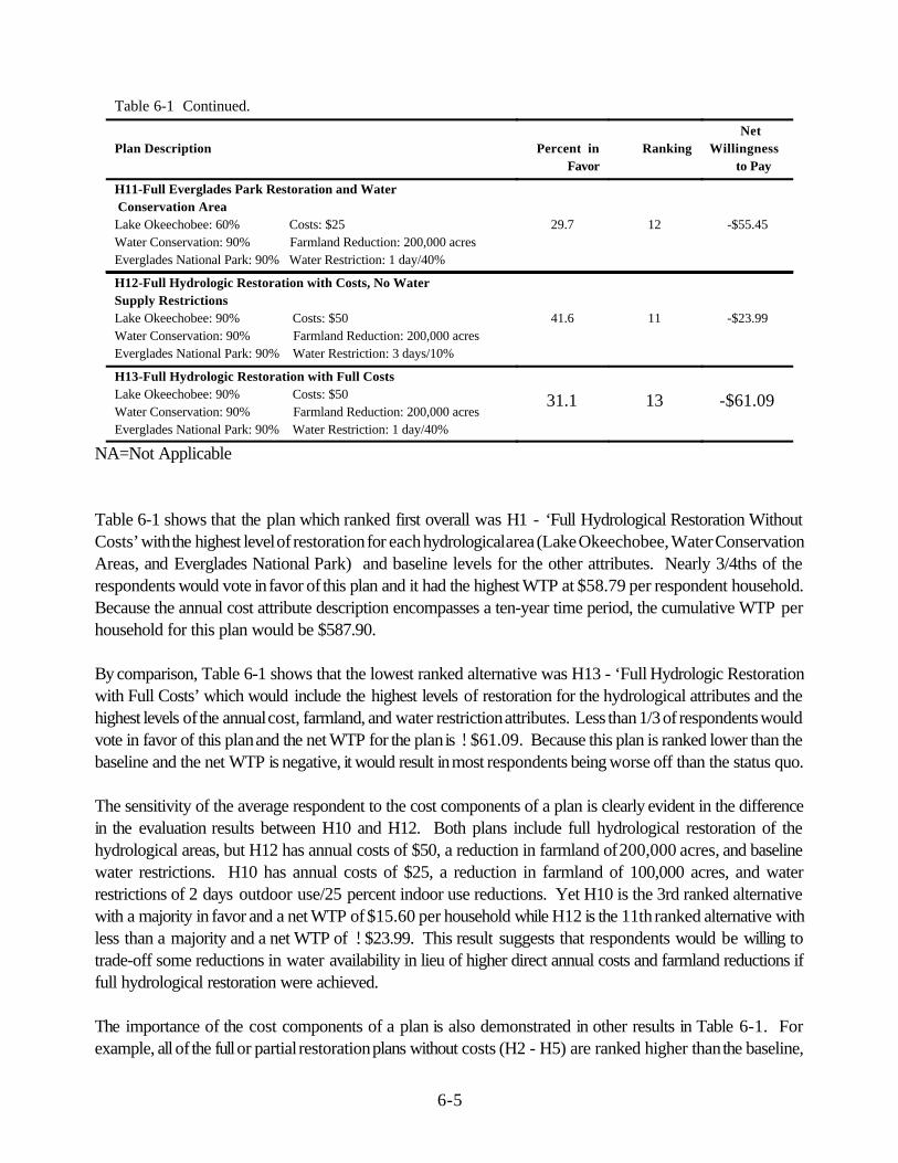
6-5

Table 6-1 Continued.

Plan Description Percent inFavor

RankingNet

Willingness to Pay

H11-Full Everglades Park Restoration and Water Conservation AreaLake Okeechobee: 60% Costs: $25Water Conservation: 90% Farmland Reduction: 200,000 acresEverglades National Park: 90% Water Restriction: 1 day/40%

29.7 12 -$55.45

H12-Full Hydrologic Restoration with Costs, No WaterSupply RestrictionsLake Okeechobee: 90% Costs: $50Water Conservation: 90% Farmland Reduction: 200,000 acresEverglades National Park: 90% Water Restriction: 3 days/10%

41.6 11 -$23.99

H13-Full Hydrologic Restoration with Full CostsLake Okeechobee: 90% Costs: $50Water Conservation: 90% Farmland Reduction: 200,000 acresEverglades National Park: 90% Water Restriction: 1 day/40%

31.1 13 -$61.09

NA=Not Applicable

Table 6-1 shows that the plan which ranked first overall was H1 - ‘Full Hydrological Restoration WithoutCosts’ with the highest level of restoration for each hydrological area (Lake Okeechobee, Water ConservationAreas, and Everglades National Park) and baseline levels for the other attributes. Nearly 3/4ths of therespondents would vote in favor of this plan and it had the highest WTP at $58.79 per respondent household.Because the annual cost attribute description encompasses a ten-year time period, the cumulative WTP perhousehold for this plan would be $587.90.

By comparison, Table 6-1 shows that the lowest ranked alternative was H13 - ‘Full Hydrologic Restorationwith Full Costs’ which would include the highest levels of restoration for the hydrological attributes and thehighest levels of the annual cost, farmland, and water restriction attributes. Less than 1/3 of respondents wouldvote in favor of this plan and the net WTP for the plan is !$61.09. Because this plan is ranked lower than thebaseline and the net WTP is negative, it would result in most respondents being worse off than the status quo.

The sensitivity of the average respondent to the cost components of a plan is clearly evident in the differencein the evaluation results between H10 and H12. Both plans include full hydrological restoration of thehydrological areas, but H12 has annual costs of $50, a reduction in farmland of 200,000 acres, and baselinewater restrictions. H10 has annual costs of $25, a reduction in farmland of 100,000 acres, and waterrestrictions of 2 days outdoor use/25 percent indoor use reductions. Yet H10 is the 3rd ranked alternativewith a majority in favor and a net WTP of $15.60 per household while H12 is the 11th ranked alternative withless than a majority and a net WTP of !$23.99. This result suggests that respondents would be willing totrade-off some reductions in water availability in lieu of higher direct annual costs and farmland reductions iffull hydrological restoration were achieved.

The importance of the cost components of a plan is also demonstrated in other results in Table 6-1. Forexample, all of the full or partial restoration plans without costs (H2 - H5) are ranked higher than the baseline,

6-6

have majorities in favor, and positive net WTPs. When direct costs are minimized such as in H6 and H7, evenpartial hydrological restoration plans are favored by a majority of respondents and have positive net WTPs. In summary, these evaluations of alternative hydrological restoration plans with the multiattribute model resultsindicate that the average respondent has a strong desire for restoration of the Everglades/South Floridaecosystem. But, these preferences to restore the ecosystem are tempered by other preferences to minimizethe direct costs of restoration to households and to avoid severe water use restrictions.

6.2.2 Evaluation with the Species Multiattribute Model

A comparable set of alternative Everglades/South Florida restoration plan scenarios were constructed for theattributes in the species multiattribute model. As with the hydrological model scenarios, these plans weredesigned to represent a variety of possible attribute combinations and were not intended to represent actualrestoration plans or to be technically or administratively feasible. The variety of plan scenarios helps toillustrate the preferences of the average survey respondent who was interviewed using the species attributepairwise choice process.

Descriptions of 11 alternative restoration plans, the attribute levels included in each plan, and results for theplan with the three evaluation measures are presented in Table 6-2. The baseline plan was again defined asthe status quo levels of the three species attributes with all other attributes at their baseline levels. The baselineranked 7th of the 11 plans considered indicating some plans were preferred to the baseline while others wouldleave respondents worse off.

The top ranked alternative in Table 6-2 was S3 ! ‘Full Wetland Wildlife Restoration Without Costs.” Thisplan had a very large majority in favor and a net WTP of $69.86 indicating significant potential economicbenefits would accrue from this restoration scenario. The similarity in this net WTP value with the net WTPvalue for H1 ! ‘Full Hydrological Restoration Without Costs’ suggests that respondents were expressing arelatively consistent set of preferences regardless of the survey instrument used in the interview.

The effects of the large negative weighting given to dryland species restoration in the species multiattributemodel (Table 5-3) are evident in the plan rankings in Table 6-2. Both partial and full dryland speciesrestoration plans without costs (S4 and S5) were ranked below the baseline scenario and have negative netWTPs. Clearly the average respondent did not view restoring dryland species populations as a desirableoutcome.

As in the hydrological restoration scenario evaluations, however, the cost components of a plan had a majorimpact on the overall evaluation. The full wetland wildlife restoration scenario S11 ! ‘Full Wetland WildlifeRestoration With Full Costs’ was the lowest ranked alternative and had a net WTP of !$33.64. Other fulland partial wetland wildlife restoration plans illustrate the sensitivity of the average respondent to the costcomponents. But, the species model evaluations did not change as dramatically in response to costs as in thehydrological model evaluations. Plans S6 and S9 in Table 6-2 would yield either full or partial wetland wildlifespecies restoration with annual costs at $25, farmland reductions of 100,000 or less, and no severe waterrestrictions. These plans were ranked 3rd and 4th, respectively, had majorities in favor, and had positive netWTPs. Even plan S10 with full wetland wildlife species restoration and annual costs of $50 and farmland

6-7

reductions of 200,000 acres had a majority in favor and a positive, yet small, positive net WTP. Only whenpartial wetland species restoration was coupled with annual costs of $25, farmland reductions of 100,000acres, and water use restrictions of 2 days/25 percent as in plan S8 did the percent in favor fall below amajority and the net WTP become negative.Table 6-2 Evaluation of Restoration Plans with the Species Multiattribute Model.

Plan DescriptionPercent in

Favor RankingNet

Willingness toPay

S-1 Baseline (no change) Wildlife.Wetland Species: 20% Costs: 0Dryland Species: 50% Farmland Reduction: 0Estuarine Species: 60% Water Restriction: 3 days/10%

NA 7 NA

S-2 Partial Wetland Wildlife Restoration without Costs.Wetland Species: 50% Costs: 0Dryland Species: 50% Farmland Reduction: 0Estuarine Species: 75% Water Restriction: 3 days/10%

92.7 2 $34.93

S-3 Full Wetland Wildlife Restoration without Costs.Wetland Species: 80% Costs: 0Dryland Species: 50% Farmland Reduction: 0Estuarine Species: 90% Water Restriction: 3 days/10%

92.7 1 $69.86

S-4 Partial Dryland Wildlife Restoration without Costs.Wetland Species: 20% Costs: 0Dryland Species: 60% Farmland Reduction: 0Estuarine Species: 60% Water Restriction: 3 days/10%

17.9 9 -11.95

S-5 Full Dryland Wildlife Restoration without Costs.Wetland Species: 20% Costs: 0Dryland Species: 70% Farmland Reduction: 0Estuarine Species: 60% Water Restriction: 3 days/10%

17.9 10 -23.90

S-6 Partial Wetland Wildlife Restoration with Minimized Taxes.Wetland Species: 50% Costs: $25Dryland Species: 50% Farmland Reduction: 0Estuarine Species: 75% Water Restriction: 3 days/10%

61.5 4 $9.93

S-7 Partial Wetland Wildlife Restoration, No Water Use Restrictions.Wetland Species: 50% Costs: $25Dryland Species: 50% Farmland Reduction:100,000 acresEstuarine Species: 75% Water Restriction: 3 days/10%

52.1 6 $0.66

S-8 Partial Wetland Wildlife Restoration with Costs.Wetland Species: 50% Costs: $25Dryland Species: 50% Farmland Reduction:100,000 acresEstuarine Species: 75% Water Restriction: 2 days/25%

42.7 8 -$8.3

S-9 Full Wetland Wildlife Restoration with Minimized Costs.Wetland Species: 80% Costs: $25Dryland Species: 50% Farmland Reduction:100,000 acresEstuarine Species: 90% Water Restriction: 2 days/25%

67.9 3 $26.63

S-10 Full Wetland Wildlife Restoration with Costs and NoWater Use Restrictions.Wetland Species: 80% Costs: $50Dryland Species: 50% Farmland Reduction:200,000 acresEstuarine Species: 90% Water Restriction: 3 days/10%

52.1 5 $1.32

6-8

S-11 Full Wetland Wildlife Restoration with Full CostsWetland Species: 80% Costs: $50Dryland Species: 50% Farmland Reduction:200,000 acresEstuarine Species: 90% Water Restriction: 1 day/40%

29.9 11 -33.64

In summary, the evaluations of alternative species restoration plans support the proposition that the averagerespondent had strong desires for restoration of the Everglades/South Florida ecosystem. Responses with thespecies multiattribute model were generally less sensitive to the cost components and resulted in favorableevaluations of several wetland wildlife species restoration plans. Respondents, however, showed no inclinationto restore dryland species populations.

6.3 Effects of Socioeconomic Characteristics on Evaluations of Alternative Restoration Plans

6.3.1 Evaluations of Alternative Plans with the Hydrological Multiattribute Model byRespondents’ Location and Environmental Donation Status

The same set of 13 alternative restoration plans constructed for the hydrological multiattribute model presentedin Table 6-1 were evaluated using the socioeconomic characteristics interactive model coefficients reportedpreviously in Table 5-4. This analysis was conducted using the same three evaluation measures. Theinteractive model allows the evaluation results to be disaggregated according to specific socioeconomiccharacteristics of the respondents.

Evaluation results for the 13 hydrological restoration plans for respondents in South Florida and CentralFlorida are reported in Table 6-3. The results reveal some rather striking differences in the preferences ofSouth vs Central Floridians. While both rank H5 ! ‘Full Hydrological Restoration Without Costs’ as the mostpreferred alternative, a large majority (87.6 percent) of South Floridians would vote in favor of this plan whileless than a majority (48.9 percent) of Central Floridians would vote in favor. Moreover, South Floridians’net WTP for H5 is $86.42 as compared to a net WTP of $8.24 for Central Floridians. In fact, only two plans(H4 and H5), which both include restoration with no costs to Floridians, are preferred by Central Floridiansto the status quo and have positive net WTPs. All the other alternative plans evaluated for Central Floridarespondents would be ranked lower than the baseline and have negative net WTPs. For some plans thesenegative values were quite large (e.g. !$131.65 for H13) indicating a strong aversion to any restoration planthat would impose costs on Floridians.

On the other hand, the percent of South Floridians who would vote in favor of a number of restoration plansand the positive net WTPs for these plans indicates strong preferences for these alternatives. The only plansnot preferred to the status quo and with negative net WTPs (i.e. H11 and H13) would impose high direct costsand severe water use restrictions. These results suggest that most South Floridians would be willing to incursignificant personal costs and experience at least moderate water use restrictions to achieve hydrologicalrestoration of the Everglades/South Florida ecosystem.

A similar evaluation of the 13 hydrological plans is reported by respondent’s environmental donation statusin Table 6-4. Prior research has shown that respondents who donated to environmental causes in the past

6-9

generally express higher levels of concern about the environment and are more supportive of policies to protectand enhance the environment (Milon et al. 1998). It would be expected that respondents who donated toenvironmental causes would be more likely to have stronger preferences for environmental restoration plans.The results reported in Table 6-4 confirm these expectations. Respondents who donated ranked a significantlylarger number of alternative plans as superior to the status quo and the percent voting in favor across all of theplans was consistently higher for the donations group. Moreover, the net WTPs for the donations group inTable 6-4 were negative for only two plans (H11 and H13). Compared with the average respondent’s netWTPs for the same plans (Table 6-1), the donations group expressed consistently stronger preferences forEverglades/South Florida ecosystem restoration.

The differences in preferences between respondents who donated to environmental groups compared to thosewho did not are important given that approximately 50 percent of the sample respondents had donated (seeTable 4-1). This is very similar to the percentage reporting environmental donations in other statewide surveys(e.g. Milon et al. 1998). The results suggest that Floridians who express high levels of concern about theenvironment are likely to strongly support Everglades/South Florida ecosystem restoration.

6-10

Table 6-3. Evaluation of Selected Restoration Plans with the Hydrological Multiattribute Model by Respondent Location.

Plan Description Percent in Favor Ranking Net Willingness to Pay

South Florida

CentralFlorida

South Florida

CentralFlorida

South Florida

CentralFlorida

H-1 Baseline (no change) Hydrology.Lake Okeechobee: 60% Costs: 0Water Conservation: 50% Farmland Reduction: 0Everglades National Park: 50% Water Restriction: 3 days/10%

NA NA 11 3 NA NA

H-2 Partial Everglades Park Restoration.Lake Okeechobee: 60% Costs: 0Water Conservation: 50% Farmland Reduction: 0Everglades National Park: 75% Water Restriction: 3 days/10%

72.9 27.8 7 4 $21.55 -$18.10

H-3 Full Everglades Park Restoration.Lake Okeechobee: 60% Costs: 0Water Conservation: 50% Farmland Reduction: 0Everglades National Park: 90% Water Restriction: 3 days/10%

72.9 27.8 4 6 $34.47 -$28.96

H-4 Partial Hydrologic Restoration without Costs.Lake Okeechobee: 75% Costs: 0Water Conservation: 75% Farmland Reduction: 0Everglades National Park: 75% Water Restriction: 3 days/10%

87.6 48.9 2 2 $51.55 $2.37

H-5 Full Hydrologic Restoration without Costs.Lake Okeechobee: 90% Costs: 0Water Conservation: 90% Farmland Reduction: 0Everglades National Park: 90% Water Restriction: 3 days/10%

87.6 48.9 1 1 $86.42 $8.24

H-6 Partial Everglades Park Restoration and Water Conservation Area with no costs, minimum restrictions

Lake Okeechobee: 60% Costs: 0Water Conservation: 75% Farmland Reduction: 100,000 acresEverglades National Park: 75% Water Restriction: 2 days/25%

66.7 36.7 6 7 $21.61 -$31.37

H- 7 Partial Hydrologic Restoration with Minimized Taxes.Lake Okeechobee: 75% Costs: $25Water Conservation: 75% Farmland Reduction: 100,000 acresEverglades National Park: 75% Water Restriction: 2 days/25%

72.9 27.8 5 5 $6.56 -$45.28

6-11

Table 6-3 Continued.

Plan DescriptionPercent in Favor Ranking Net Willingness to

Pay

SouthFlorida

CentralFlorida

SouthFlorida

CentralFlorida

SouthFlorida

CentralFlorida

H-8 Partial Hydrologic Restoration, No Water Supply Restrictions.

Lake Okeechobee: 75% Costs: $25Water Conservation: 75% Farmland Reduction: 100,000 acresEverglades National Park: 75% Water Restriction: 3 days/10%

64.3 16.7 8 9 $14.29 -$43.26

H-9 Partial Hydrologic Restoration with Minimized Costs.Lake Okeechobee: 75% Costs: $25Water Conservation: 75% Farmland Reduction: 0Everglades National Park: 75% Water Restriction:3 days/10%

58.1 24.4 10 10 $26.55 -$22.63

H-10 Full Hydrologic Restoration with Minimized Costs.Lake Okeechobee: 90% Costs: $25Water Conservation: 90% Farmland Reduction: 100,000 acresEverglades National Park: 90% Water Restriction: 2 days/25%

69.0 33.3 3 8 $41.43 -$39.41

H-11 Full Everglades Park and Water Conservation Area Restoration

Lake Okeechobee: 60% Costs: $25Water Conservation: 90% Farmland Reduction: 200,000 acresEverglades National Park: 90% Water Restriction: 1 day/40%

45.7 6.7 12 12 -$16.97 -$128.83

H-12 Full Hydrologic Restoration with Costs, No Water SupplyRestrictions

Lake Okeechobee: 90% Costs: $50Water Conservation: 90% Farmland Reduction: 200,000 acresEverglades National Park: 90% Water Restriction: 3 days/10%

58.9 16.7 9 11 $11.90 -$83.01

H-13 Full HydrologicRestoration with Full CostsLake Okeechobee: 90% Costs: $50Water Conservation: 90% Farmland Reduction: 200,000 acresEverglades National Park: 90% Water Restriction: 1 day/40%

43.4 13.3 13 13 -$22.11 -$131.65

NA=Not Applicable

6-12

Table 6-4. Evaluation of Selected Restoration Plans with the Hydrological Multiattribute Model by Respondent Past Donations.

Plan DescriptionPercent in Favor Ranking Net Willingness to Pay

DONATIONS DONATIONS DONATIONS

NO YES NO YES NO YES

H-1 Baseline (no change) Hydrology.Lake Okeechobee: 60% Costs: 0Water Conservation: 50% Farmland Reduction: 0Everglades National Park: 50% Water Restriction: 3 days/10%

NA NA 3 11 NA NA

H-2 Partial Everglades Park Restoration.Lake Okeechobee: 60% Costs: 0Water Conservation: 50% Farmland Reduction: 0Everglades National Park: 75% Water Restriction: 3 days/10%

48.4 62.6 4 8 -$2.18 $15.71

H-3 Full Everglades Park Restoration.Lake Okeechobee: 60% Costs: 0Water Conservation: 50% Farmland Reduction: 0Everglades National Park: 90% Water Restriction: 3 days/10%

48.4 62.6 5 6 -$3.49 $25.15

H-4 Partial Hydrologic Restoration without Costs.Lake Okeechobee: 75% Costs: 0Water Conservation: 75% Farmland Reduction: 0Everglades National Park: 75% Water Restriction: 3 days/10%

58.6 90.1 2 3 $16.29 $52.52

H-5 Full Hydrologic Restoration without Costs.Lake Okeechobee: 90% Costs: 0Water Conservation: 90% Farmland Reduction: 0Everglades National Park: 90% Water Restriction: 3 days/10%

58.6 90.1 1 1 $27.35 $92.26

H-6 Partial Everglades Park Restoration and Water ConservationArea with No Costs, Minimum Restrictions

Lake Okeechobee: 60% Costs: 0Water Conservation: 75% Farmland Reduction: 100,000 acresEverglades National Park: 75% Water Restriction: 2 days/25%

40.6 73.6 7 4 $20.22 $6.51

H-7 Partial Hydrologic Restoration with Minimized Taxes.Lake Okeechobee: 75% Costs: $25Water Conservation: 75% Farmland Reduction:100,000 acresEverglades National Park: 75% Water Restriction: 2 days/25%

43.0 70.3 6 5 $41.99 $2.04

6-13

Table 6-4 Continued.

Plan DescriptionPercent in Favor Ranking Net Willingness to Pay

DONATIONS DONATIONS DONATIONS

NO YES NO YES NO YES

H-8 Partial Hydrologic Restoration, No Water Supply Restrictions.Lake Okeechobee: 75% Costs: $25Water Conservation: 75% Farmland Reduction: 100,000 acresEverglades National Park: 75% Water Restriction: 3 days/10%

32.8

61.5 8 10 -$25.12 $12.82

H-9 Partial Hydrologic Restoration with Minimized Costs. Lake Okeechobee: 75% Costs: $25 Water Conservation: 75% Farmland Reduction: 0 Everglades National Park: 75% Water Restriction: 3 days/10%

27.3 68.1 10 7 -$8.71 $27.52

H-10 Full Hydrologic Restoration with Minimized Costs.Lake Okeechobee: 90% Costs: $25Water Conservation: 90% Farmland Reduction: 100,000 acresEverglades National Park: 90% Water Restriction: 2 days/25%

39.1 75.8 9 2 -$30.93 $41.78

H-11 Full Everglades Park and Water Conservation Area Restoration.

Lake Okeechobee: 60% Costs: $25Water Conservation: 90% Farmland Reduction: 200,000 acresEverglades National Park: 90% Water Restriction: 1 day/40%

20.3 42.9 12 13 -$90.81 -$23.75

H-12 Full Hydrologic Restoration with Costs, No Water SupplyRestrictions.

Lake Okeechobee: 90% Costs: $50Water Conservation: 90% Farmland Reduction: 200,000 acresEverglades National Park: 90% Water Restriction: 3 das/10%

28.1 60.4 11 9 -$55.47 $12.86

H-13 Full Hydrologic Restoration with Full Costs.Lake Okeechobee: 90% Costs: $50Water Conservation: 90% Farmland: 200,000 acresEverglades National Park: 90% Water Restriction: 1 day/40%

15.6 52.7 13

12 -$109.35 -$7.68

NA=Not Applicable

6-14

6.3.2 Evaluations of Alternative Plans with the Species Multiattribute Model by Respondents’Location and Environmental Donation Status

The set of 11 alternative restoration plans constructed for the species multiattribute model presented in Table6-2 was evaluated using the socioeconomic characteristics interactive model coefficients reported previouslyin Table 5-5. And, the same three evaluation measures were used as in the preceding analyses. Theinteractive model was used to disaggregate the species restoration plan evaluations into responses based onrespondent location (South and Central Florida) and past donations to environmental groups.

Evaluation results for the 11 species restoration plans for respondents in South Florida and Central Floridaare reported in Table 6-5. In contrast to the hydrological attributes evaluation, the results in Table 6-5 showrelatively few differences in the preferences of South vs Central Floridians. Both rank S3 ! ‘Full WetlandWildlife Restoration Without Costs’ as the most preferred alternative. And, a large majority of both SouthFloridians (88.7 percent) and Central Floridians (98.9 percent) would vote in favor of this plan. Both groups’net WTP for this plan are very similar ($68.82 and $72.42) and are also comparable to South Floridians’ netWTP of $86.42 for their highest ranked hydrological restoration plan. Of the 11 species restoration plans,South Floridians prefer 4 of the plans to the status quo while Central Floridians prefer 7 of the plans to thestatus quo. Neither group favored the full or partial dryland species restoration plans (S4 and S5).

While the cost components clearly influenced the relative desirability of the plans, Central Floridians weregenerally less sensitive to the cost and water restriction attributes of the plans. Both S7 and S8, partial wetlandwildlife species restoration plans with different cost attribute levels, were favored by a majority of CentralFloridians but not by South Floridians. The net WTPs for both plans were positive for Central Floridians($12.25 and $14.37, respectively) but negative for South Floridians (!$6.31 and !$22.39, respectively).Indeed, the only wetland wildlife restoration plan Central Floridians did not have a majority in favor or apositive net WTP was the full wetland wildlife restoration plan with full costs (S11).

A similar evaluation of the 11 species restoration plans is reported by respondent’s environmental donationstatus in Table 6-6. As in the earlier evaluation of the hydrological restoration plans by environmental donationstatus (Table 6.4), respondents who donated to environmental causes in the past were more likely to favor therestoration plans. Seven of the plans were ranked higher than the status quo by those who donated comparedwith only 4 plans that were ranked higher by those who had not donated. But, in contrast to the hydrologicalrestoration plan results, the overall differences between the donation status groups were not large. The overallpercent in favor and net WTPs were relatively similar for partial wetland wildlife restoration with a $25 annualhousehold cost (S6). The differences grew larger only when additional cost components were added suchas in S8 and S9 which added 100,000 acre reductions in farmland and severe water use restrictions. Thedifferences in net WTPs for S9 for those who donated ($39.81) versus those who did not ($15.00) suggestthat the former were less averse to the prospect of severe water use restrictions as a tradeoff for full wetlandwildlife restoration.

In general, the socioeconomic interaction evaluation results in Tables 6-5 and 6-6 indicate that the speciesmultiattribute format tended to elicit fewer differences in preferences across socioeconomic groups than thehydrological multiattribute format (Tables 6-3 and 6-4). This result may have occurred because morerespondents were able to understand the concept of restoring species population levels as compared to

6-15

restoring historic water levels and timing. Respondents in Central Florida and those who had not contributedto environmental groups were the least likely to have strong preferences for hydrological restoration plans.These results suggest that building support for Everglades/South Florida ecosystem restoration on the basisof hydrological restoration endpoints may be difficult outside of South Florida.

6-16

Table 6-5. Evaluation of Selected Restoration Plans with the Species Mulitattribute Model by Respondent Location.

Plan DescriptionPercent in Favor Ranking Net Willingness to Pay

SouthFlorida

CentralFlorida

SouthFlorida

CentralFlorida

SouthFlorida

CentralFlorida

S-1 Baseline (no change) Wildlife.Wetland Species: 20% Costs: 0Dryland Species: 50% Farmland Reduction: 0Estuarine Species: 60% Water Restriction: 3 days/10%

NA NA 5 8 NA NA

S-2 Partial Wetland Wildlife Restoration without Costs.Wetland Species: 50% Costs: 0Dryland Species: 50% Farmland Reduction: 0Estuarine Species: 75% Water Restriction: 3 days/10%

88.7 98.9 2 3 $34.41 $36.21

S-3 Full Wetland Wildlife Restoration without Costs.Wetland Species: 80% Costs: 0Dryland Species: 50% Farmland Reduction: 0Estuarine Species: 90% Water Restriction: 3 days/10%

88.7 98.9 1 1 $68.82 $72.42

S-4 Partial Dryland Wildlife Restoration without Costs.Wetland Species: 20% Costs: 0Dryland Species: 60% Farmland Reduction: 0Estuarine Species: 60% Water Restriction: 3 days/10%

7.0 34.8 8 9 -$17.62 -$3.87

S-5 Full Dryland Wildlife Restoration without Costs.Wetland Species: 20% Costs: 0Dryland Species: 70% Farmland Reduction: 0Estuarine Species: 60% Water Restriction: 3 days/10%

7.0 34.8 10 10 -$35.23 -$7.74

S-6 Partial Wetland Wildlife Restoration with Minimized Taxes.

Wetland Species: 50% Costs: $25Dryland Species: 50% Farmland Reduction: 0Estuarine Species: 75% Water Restriction: 3 days/10%

59.9 64.1 4 7 $9.41 $11.21

S-7 Partial Wetland Wildlife Restoration, No Water Supply Restrictions.

Wetland Species: 50% Costs: $25Dryland Species: 50% Farmland Reduction: 100,000 acresEstuarine Species: 75% Water Restriction: 3 days/10%

43.7 65.2 6 6 -$6.31 $12.25

6-17

Table 6-5. Continued.

Plan DescriptionPercent in Favor Ranking Net Willingness to Pay

SouthFlorida

CentralFlorida

SouthFlorida

CentralFlorida

SouthFlorida

CentralFlorida

S-8 Partial Wetland Wildlife Restoration with Minimized Costs.

Wetland Species: 50% Costs: $25Dryland Species: 50% Farmland Reduction: 100,000 acresEstuarine Species: 75% Water Restriction: 2 days/25%

21.8 75.0 9 5 -$22.39 $14.37

S-9 Full Wetland Wildlife Restoration with Minimized CostsWetland Species: 80% Costs: $25Dryland Species: 50% Farmland Reduction: 100,000 acresEstuarine Species: 90% Water Restriction: 2 days/25%

54.9 88.0 3 2 $12.02 $50.58

S-10 Full Wetland Wildlife Restoration with Costs, No Water Supply Restrictions

Wetland Species: 80% Costs: $50Dryland Species: 50% Farmland Reduction: 200,000 acresEstuarine Species: 90% Water Restriction: 3 days/10%

43.7 65.2 7 4 -$12.62 $24.50

S-11 Full Wetland Wildlife Restoration with Full CostsWetland Species: 80% Costs: $50Dryland Species: 50% Farmland Reduction:200,000 acresEstuarine Species: 90% Water Restriction: 1 day/40%

26.1 35.9 11 11 -$47.85 -$12.63

NA=Not Applicable

6-18

Table 6-6. Evaluation of Restoration Plans with the Species Multiattribute Model by Respondent Past Donations.

Plan DescriptionPercent in Favor Ranking Net Willingness to Pay

DONATIONS DONATIONS DONATIONS

NO YES NO YES NO YES

S-1 Baseline (no change) Wildlife.Wetland Species: 20% Costs: 0Dryland Species: 50% Farmland Reduction: 0Estuarine Species: 60% Water Restriction: 3 days/10%

NA NA 5 8 NA NA

S-2 Partial Wetland Wildlife Restoration without Costs.Wetland Species: 50% Costs: 0Dryland Species: 50% Farmland Reduction: 0Estuarine Species: 75% Water Restriction: 3 days/10%

92.4 93.0 2 3 $33.61 $36.68

S-3 Full Wetland Wildlife Restoration without Costs.Wetland Species: 80% Costs: 0Dryland Species: 50% Farmland Reduction: 0Estuarine Species: 90% Water Restriction: 3 days/10%

92.4 93.0 1 1 $67.23 $73.37

S-4 Partial Dryland Wildlife Restoration without Costs.Wetland Species: 20% Costs: 0Dryland Species: 60% Farmland Reduction: 0Estuarine Species: 60% Water Restriction: 3 days/10%

10.1 26.1 8 9 -$15.65 -$8.65

S-5 Full Dryland Wildlife Restoration without Costs.Wetland Species: 20% Costs: 0Dryland Species: 70% Farmland Reduction: 0Estuarine Species: 60% Water Restriction: 3 days/10%

10.1 26.1 10 10 -$31.31 -$17.30

S-6 Partial Wetland Wildlife Restoration with Minimized Taxes.Wetland Species: 50% Costs: $25

Dryland Species: 50% Farmland Reduction: 0Estuarine Species: 75% Water Restriction: 3 days/10%

63.0 60.0 4 4 $8.61 $11.68

6-19

Table 6-6 Continued.

Plan DescriptionPercent in Favor Ranking Net Willingness to Pay

DONATIONS DONATIONS DONATIONS

NO YES NO YES NO YES

S-7 Partial Wetland Wildlife Restoration, No Water SupplyRestrictions.

Wetland Species: 50% Costs: $25Dryland Species: 50% Farmland Reduction: 100,000 acresEstuarine Species: 75% Water Restriction: 3 days/10%

50.4 53.9 6 6 -$2.26 $4.35

S-8 Partial Wetland Wildlife Restoration with Costs.Wetland Species: 50% Costs: $25Dryland Species: 50% Farmland Reduction: 100,000 acresEstuarine Species: 75% Water Restriction: 2 days/25%

27.7 58.3 9 7 -$18.62 $3.12

S-9 Full Wetland Wildlife Restoration with Minimized Costs. Wetland Species: 80% Costs: $25Dryland Species: 50% Farmland Reduction: 100,000 acresEstuarine Species: 90% Water Restriction: 2 days/25%

59.7 76.5 3 2 $15.00 $39.81

S-10 Full Wetland Wildlife Restoration with Costs with No WaterSupply Restrictions.

Wetland Species: 80% Costs: $50Dryland Species: 50% Farmland Reduction: 200,000 acresEstuarine Species: 90% Water Restriction: 3 days/10%

50.4 53.9 7 5 -$4.52 $8.71

S-11 Full Wetland Wildlife Restoration with Full Costs.Wetland Species: 80% Costs: $50Dryland Species: 50% Farmland Reduction: 200,000 acresEstuarine Species: 90% Water Restriction: 1 day/40%

24.4 35.7 11 11 -$47.59 -$19.93

NA=Not Applicable

7-1

SECTION 7. SUMMARY AND EXTENSIONS

7.1 Study Objectives and Methods

Efforts to restore the Everglades/South Florida ecosystem represent one of the most difficult challenges incontemporary science and environmental decision-making. Numerous scientific questions exist over thecurrent state of the ecosystem and how the components of the system will respond to management initiatives.Present and future scientific studies will help to address these uncertainties. Equally, if not more, difficultquestions arise over the choice of objectives for restoration. These questions involve both scientific and publicpreference issues that require both natural and social science research. This report has attempted to answersome of these questions by presenting the results from a survey of Florida residents to identify their preferencesand economic values for different levels of ecosystem restoration. These results provide baseline informationabout Floridians’ preferences that can be used in contemporary assessments of alternative restoration plansand for comparisons with future social science studies of public preferences.

The survey was designed as an application of multiattribute utility (MAU) theory because the Everglades/SouthFlorida ecosystem restoration problem requires the consideration of multiple dimensions as well as tradeoffsbetween natural and social system considerations. Given the geographic scale and ecological complexity ofthe region, a large number of attributes could possibly be considered. The range of possibilities was limited,however, by the need to develop a survey instrument that could be readily understood by the public and couldbe administered under normal field conditions. To represent ecological dimensions of the problem, functionalendpoints were expressed as hydrological attributes that represented water levels and timing in three criticalgeographic areas: Lake Okeechobee, the Water Conservation Areas, and Everglades National Park. Analternative characterization of the ecological dimensions of the problem was expressed as species attributesthat represented three broad species groupings: wetland species, dryland species, and estuarine species.These alternative attribute specifications were both measured in terms of ‘percentages of historical levels’ todescribe how current and possible future conditions would change under alternative management plans. Otherattributes used in the analysis captured the possible effects of restoration plans on water availability tomunicipal users, changes in farmland acreage in South Florida, and the annual cost to households.

Field interviews were conducted by an independent market research firm during the first half of 1998 basedon a stratified, random sampling design of households in five Florida counties: Dade, Hillsborough, Lee,Orange and Palm Beach. Approximately 100 interviews were conducted in each county. The interviews wereconducted in respondents' homes and consisted of five parts: 1) a general introduction, 2) questions to elicitrespondents' attitudes about public expenditures and environmental issues, 3) an informational video about theEverglades/South Florida ecosystem, 4) description of the choice attributes and a pairwise choice taskinvolving preselected attribute combinations, and 5) additional questions to elicit socioeconomic characteristics.Copies of all questions and supporting materials for the interviews are provided in the appendices to thisreport.

A pairwise choice response procedure was used in the interviews because pretesting indicated this was thesimplest and most easily understood procedure for respondents to deal with the large number of attributes andattribute combinations. A split sample design was used so that the hydrological and species attributespecifications were divided evenly across respondents in each county. This design provided a basis to

12The normalized weights were computed by multiplying each attribute coefficient times the meanlevel of the attribute and then multiplying the product times ten.

7-2

compare respondents’ preferences for alternative restoration plans based on different representations of theecological dimensions of the problem. While the interview procedure used in this study required more timeand was more difficult than a typical public opinion survey, it was clear that respondents were able tounderstand the choices and express their preferences. Moreover, the survey framework provides detailedinformation about respondents’ preferences that could be used to address specific components of proposedrestoration plans.

7.2 Survey Results and Alternative Restoration Plan Evaluations

Responses from the pairwise choice tasks were used to estimate MAU functions for the hydrological andspecies attribute sets. The MAU functions were estimated using specifications that included only the basicattributes and with interactive variables to identify the effects of socioeconomic characteristics on respondentpreferences. The results reported in Section 5 showed that both specifications resulted in strong statisticalresults indicating that respondents evaluated the attribute combination options and expressed their preferencesfor different levels of the attributes.

The MAU functions for the hydrological and species models can be compared through the use of normalizedweights12 for each attribute such as those presented in Figure 7-1. The figure shows that respondents gavea positive weight to all three hydrological attributes. The results indicate respondents preferred potentialrestoration plans that would lead to water levels and timing throughout the South Florida region that would bemore similar to historical conditions. Other attributes in the model, however, revealed that higher levels ofannual cost, water restrictions, or reductions in farmland acreage were negatively weighted. The negativeweights assigned to these attributes would temper the positive weights given to higher levels of the hydrologicalattributes.

Weights for the species attributes from the species multiattribute model in Figure 7-1 show that respondentsgave a positive weight to wetland and estuarine species attributes. But, they also gave a significantly negativeweighting to the dryland species attribute indicating that restoring these species populations to be morecomparable to historical levels was not preferred. The results for restoring wetland/estuarine species were alsotempered by negative weights assigned to the annual cost, water restrictions, and farmland attributes. Figure7-1 also shows that the weightings assigned to these three attributes in the hydrological and speciesmultiattribute models were generally similar suggesting that respondents expressed consistent preferences inthe two choice settings despite the presence of other attributes.

The statistically derived weights for the hydrological and species multiattribute models were used to evaluatealternative hypothetical restoration plans. The evaluation results reported in Section 6 indicated that Floridiansexpressed strong preferences for restoration plans that restore the hydrological conditions or wetland/estuarinespecies populations of South Florida. For example, Tables 6-1 and 6-2 showed that a large majority ofrespondents would be in favor of full restoration plans that imposed no or low costs on Floridians. In addition,the highest net willingness to pay (WTP) amounts for the full restoration plans were $58.79 annually with the

13 It is interesting to note that the U.S. Fish and Wildlife Service recently announced a “SouthFlorida Multi-Species Recovery Plan” that U.S. Department of the Interior Secretary Bruce Babbittdescribes as “an integral component in meeting the Administration’s restoration plan for South Florida”(1999, pp. I). This recovery plan is distinct from the Restudy yet many of the species identified in the plan“are dependent upon implementation of the Restudy for survival and recovery, and many others will benefitsignificantly as a result of this restoration effort” (1999, pp. ix). The perspective of the Plan’s sponsors is

7-3

Figure 7-1. Relative Weightings of Attributes in the Multiattribute Models

5.8

6.2

2.4

-3

-0.1

-2.3

-1.9

Lake Okeechobee

Water Conservation Areas

Everglades National Park

Cost Per Household

HH Water Use I

HH Water Use II

Farm Land in EAA

0 2 4 6 8-2-4

2.9

-7

8.1

-2.4

-0.4

-1.7

-0.9

Wetland Species

Dryland Species

Estuarine Species

Cost Per Household

HH Water Use I

HH Water Use II

Farm Land in EAA

0 2 4 6 8 10-2-4-6-8

Hydrological Model Species Model

hydrological multiattribute model and $69.86 annually with the species multiattribute model. These economicvalues measure the maximum annual benefits the average resident would receive if full restoration wereaccomplished with no costs to Floridians.

Costs imposed by a plan would reduce these maximum amounts and vary with the specifics of each plan. Thetables in Section 6 showed how these amounts would change with different plans for the sample as a wholeand for various socioeconomic groups. There were differences in preferences for restoration between socioeconomic groups. Respondents in CentralFlorida and those who had not donated to environmental groups were much less supportive of restorationplans when these respondents expressed their preferences with the hydrological multiattribute choice set. Thesame results, however, did not occur in responses with the species multiattribute set. The differences for thesegroups may be that they did not relate the hydrological attributes to ecosystem restoration and therefore gaveless weight to these attributes. These results suggest that it may be more difficult to explain and build supportfor an Everglades/South Florida restoration program if the emphasis is primarily hydrological management.The fact that higher levels of the wetland/estuarine species attributes were consistently preferred across thesample indicates that the general public would more readily identify with a restoration program that emphasizesspecies restoration.13

clearly revealed in the statement:“South Florida cannot be considered ‘restored’ if the song of the Cape Sable seasidesparrow has been silenced from the marl prairies of the Everglades, if clouds of woodstorks no longer cover the skies of the mangrove forests of southernmost Florida, if thefootprints of marsh rabbits no longer occur in the Lower Keys, or if there are no Floridascrub-jay families defending their territories on the Central Florida Ridge” (1999, pp. 1-2).

7-4

While the hypothetical restoration plan evaluation results indicated generally strong support for restoration, theresults in Section 6 made it evident that respondents would not support a restoration plan that imposed highcosts on Floridians. With either the hydrological or species multiattribute models, hypothetical restorationplans that included annual costs of $50 per household ($500 over 10 years) coupled with either farmlandreductions of 100,000 or more acres or severe restrictions on municipal water use during dry years receivedpoor rankings and less than majority support. Moreover, the net WTPs for these ‘high cost’ plans werenegative suggesting a potential loss in economic welfare. Even socioeconomic groups such as those who hadmade environmental donations and typically revealed the strongest support for most plans had unfavorableevaluations of the high cost plans.

Overall the results of both the hydrological and species multiattribute models indicate that the likelihood ofsupport for a restoration plan will depend on the balancing of restoration objectives with costs imposed onFloridians. The level of restoration will have to be considered in relation to the costs imposed. Some costswere clearly not viewed as too overbearing such as moderate restrictions on water use. But, it is clear thatother costs associated with possible restoration plans such as severe water restrictions (outdoor uses restrictedto 1 day per week and indoor uses reduced 40 percent) or annual costs greater than $25 per household wouldencounter significant opposition from the general public. Thus, the task of developing an actual plan for theEverglades/South Florida region that achieves meaningful ecosystem restoration, satisfies Floridians’ obligationfor cost sharing under the Water Resources Development Act of 1996, and is supported by the public maybe a daunting endeavor.

7.3 Extending the Economic Valuation Results to the Florida Population

The results presented in Section 6 for the survey sample could also be extrapolated to the Florida populationto estimate the aggregate benefits of alternative Everglades/South Florida restoration plans. Although thesampling design for this study was selected to represent the population of five counties (Dade, Hillsborough,Lee, Orange and Palm Beach), the comparison of the socioeconomic characteristics of the sample and theFlorida resident population in Section 4 (Tables 4-1and 4-3) indicated a strong similarity between the sampleand the population. This is not surprising since each county is located in the major population centers of thestate and the five counties account for more than one-third of the total state population. The primary areas thatwere not represented in the sample are the urban and rural areas of North Florida. With these limitations of

14 Population estimates are presented for households rather than individuals because onlyrespondents over 18 years of age who participated in household financial decisions were selected. Also,the cost attributes used in the multiattribute models were expressed in terms of annual household costs.

15 Growth in the number of households in Florida or changes in preferences over the ten-yearperiod are not considered in this calculation. Also, this calculation assumes that no additional benefitsaccrue beyond the ten-year period.

16 An alternative approach to aggregating the benefits over time is to assume that the annualbenefits would continue into perpetuity. Then the capitalized value of the benefits could be calculated bydividing the annual benefits by a capitalization (discount) rate. Assuming a real discount rate of 3 percent,the capitalized value of the economic benefits for full restoration without costs from the hydrological andspecies multiattribute models would be $11.4 and $13.5 billion, respectively.

7-5

the sample data in mind, population estimates can be calculated for the 5.82 million households14 in Floridain 1997 (Floyd et al., 1998).

Using the net WTP estimates reported in Section 6, aggregate measures of the economic benefits to Floridaresidents can be calculated by multiplying the average WTP for a specific plan by the number of households.For example, using the net WTP value of $58.79 per household per year for full hydrological restorationwithout costs (Plan H-5 in Table 6-1) from the hydrological multiattribute model would result in an aggregateannual WTP of $342.2 million for this plan. Over the ten-year period indicated in the cost attribute description(see Table 3-3), the aggregate WTP would be $3.42 billion in 1998 dollars.15 Similarly, the WTP value of$69.86 per household for full wetland/estuarine species restoration without costs (Plan S-3 in Table 6-2) fromthe species multiattribute model would result in an annual WTP of $406.5 million for this plan or $4.07 billionover ten years.16 These are aggregate measures of the maximum economic benefits Floridians would derivefrom a full restoration plan with no costs to Floridians.

A plan with direct costs to Floridians would obviously result in lower aggregate benefits for Floridians. Forexample, the restoration plan H10 developed from the hydrological multiattribute model would provide fullhydrological restoration with annual costs of $25 per household, a 100,000 acre reduction in farmland, andmoderate water restrictions. This plan yielded a net WTP of $15.60 for the sample (Table 6-1). Aggregatingthis economic benefit measure to the population would result in annual benefits of $90.8 million or $907.9million over ten years. The same approach can be used to aggregate any of the net WTP results reported inTables 6-1 and 6-2.

7.4 Limitations of the Study and Suggestions for Future Research

This research study was intended to provide an understanding of the preferences of Floridians forEverglades/South Florida ecosystem restoration. In any effort to identify public preferences, especially forcomplex issues such as ecosystem restoration, simplifying assumptions are always necessary. In the survey,it was necessary to limit the dimensions of the problem to make the multiattribute tradeoffs easily understoodand consistent with the limited information that was available about different attributes of the ecosystem. Whilethese constraints on the choices provided to respondents may have influenced the results, the extent and

7-6

direction of this influence cannot be known until a different survey is conducted using more extensive andcomplete information on the ecosystem and social attributes influenced by restoration decisions. Similarly,other multiattribute elicitation procedures such as direct rating and ranking of plan alternatives by respondentsmay influence the results. As with any social or natural science research, replication is necessary to validateresults.

Also, the geographic coverage for this survey was constrained to large population centers of Florida due tothe project budget. While the survey design resulted in a representative sample, certainly the preferences ofrural Floridians and those who live in North Florida were not included. Whether the preferences of theseFlorida residents differ from the sample in this study cannot be known without further research.

Perhaps more importantly, this research provided no information about the preferences of people who live inother states or the millions of domestic and international visitors who come to Florida each year. Certainly theEverglades/South Florida region has a unique place among the U.S.’s national treasures (see Section 1), yetno information exists about the preferences of U.S. citizens for restoration of the region’s ecosystem. Thisinformation is particularly important in light of the 50/50 state and federal cost sharing relationship establishedfor Everglades/South Florida ecosystem restoration in the Water Resources Development Act of 1996.

Finally, it is important to recognize that social science research on public preferences is an integral part of anadaptive management approach to Everglades/South Florida ecosystem restoration (Milon et al. 1997).Uncertainty about the responses of natural systems to human intervention means that both scientists and thepublic will learn about the effects of restoration as a selected plan proceeds. As scientists update theirinformation, so too will the public update their perceptions of the ecosystem and the restoration plan.Therefore, the results from this study should be viewed as a benchmark for future surveys to objectivelyevaluate how public perceptions and economic values may change over time. This integration of natural andsocial science research in an adaptive management framework offers the promise of continually improving theinformation available for both resource managers and the public.

8-1

SECTION 8. REFERENCES

Adamowicz, V., J. Louviere, and M. Williams. "Combining Revealed and Stated Preference Methods forValuing Environmental Amenities." Journal of Environmental Economics and Management 26(1994): 271-292.

Addelman, S. "Orthogonal Main-Effect Plans for Asymmetrical Factorial Experiments." Technometrics4(1962): 21-46.

Beard, D.B. Wildlife Reconnaissance: Everglades National Park Project. National Park Service, U.S.Department of the Interior, 1938.

Beggs, S., S. Cardell, and J. Hausman. "Assessing the Potential Demand for Electric Cars." Journal ofEconometrics 17(1981): 1-20.

Ben-Akiva, M. and S. Lerman. Discrete Choice Analysis. Cambridge: MIT Press, 1985.

Ben-Akiva, M., T. Morikawa, and F. Shiroishi. "Analysis of the Reliability of Preference Ranking Data."Journal of Business Research 24(1992): 149-164.

Borcherding, K., T. Eppel and D. vonWinterfeldt. “Comparison of Weighting Judgments in MultiattributeUtility Measurement. Management Science 37(1991): 1603-19.

Boxall, P.C., W.L. Adamowitz, J. Swait, M. Williams and J. Louviere. “A Comparison of Stated PreferenceMethods for Environmental Valuation.”Ecological Economics 18(1996):243-53.

Bratton, S.P. "Alternative Models of Ecosystem Restoration." In Ecosystem Health: New Goals forEnvironmental Management, R. Costanza, B. Norton, and B. Haskell, eds. Washington, D.C.: Island Press,1992.

Cairns, J. “Restoration Ecology: The New Frontier.” In Rehabilitating Damaged Ecosystems, J. Cairns, ed.Boca Raton, FL: CRC Press, 1988.

Davis, S.M. and J.C. Ogden, eds. Everglades - The Ecosystem and Its Restoration. Delray Beach, FL: St.Lucie Press, 1994.

De Palma, A., G. Myers, and Y. Papageorgiou. "Rational Choice Under an Imperfect Ability to Choose."American Economic Review 84(1994):419-440.

Douglas, M.S. The Everglades: River of Grass. Sarasota, FL: Pineapple Press, 1947 (revised ed., 1988).

Ehrhardt, N.M. "The Lobster Fisheries off the Caribbean Coast of Central America." In Spiny LobsterManagement, B. Phillips. J. Cobb and J. Kittaka, eds., pp. 133-143. Cambridge, MA: Blackwell, 1994

8-2

Everglades Coalition. The Greater Everglades Ecosystem Restoration Plan. Washington, DC, 1994.

Fennema, R.J., C.J. Neidrauer, R.A. Johnson, T.K. MacVicar, and W.A. Perkins. "A Computer Model toSimulate Natural Everglades Hydrology." In Everglades - The Ecosystem and Its Restoration. S.M. Davisand J.C. Ogden, eds., pp. 249-289. Delray Beach, FL: St. Lucie Press, 1994.

Floyd, S., E. Irwin, and D. Evans. 1998 Florida Statistical Abstract. Gainesville, FL: Bureau of Economicand Business Research, University of Florida, 1998.

Giocoechea, A, D.R. Hansen and L. Duckstein. Multiobjective Decision Analysis With Engineering andBusiness Applications. John Wiley, New York, 1982.

Greene, W. Econometric Analysis, Third Edition. Englewood Cliffs: Prentice Hall, 1997

Green, C.H. and S.M. Tunstall. "Is the Economic Evaluation of Environmental Resources Possible?" Journalof Environmental Management 33(1991): 123-141.

Harwell, M.A., W. Cooper, and R. Flaak. "Prioritizing Ecological and Human Welfare Risks fromEnvironmental Stresses." Environmental Management 16(1992): 451-464.

Harwell, M.A. and J.F. Long. US MAB Human-Dominated Systems Directorate Workshop on EcologicalEndpoints and Sustainability Goals. United States Man and the Biosphere Program. Rosensteil Schoolof Marine and Atmospheric Science, University of Miami, May 1992.

Hausman, J. and P. Ruud. "Specifying and Testing Econometric Models for Rank-Ordered Data." Journalof Econometrics 34(1987): 83-104.

Hoehn, J.P. and J.B. Loomis. "Substitution Effects in the Valuation of Multiple Environmental Programs."Journal of Environmental Economics and Management 25(1993): 56-75.

Holling, C.S. "Simplifying the Complex: The Paradigms of Ecological Function and Structure." EuropeanJournal of Operational Research 30(1987): 139-146.

Holling, C.S., L.H. Gunderson, and C.J. Walters. "The Structure and Dynamics of the Everglades System:Guidelines for Ecosystem Restoration." In Everglades - The Ecosystem and Its Restoration. S.M. Davisand J.C. Ogden, eds. Delray Beach, FL: St. Lucie Press, 1994.

Hunt, J. "Status of the Spiny Lobster Fishery in Florida." In Spiny Lobster Management, B. Phillips. J. Cobband J. Kittaka, eds., pp. 158-168. Cambridge, MA: Blackwell, 1994

Hwang, C. and K. Yoon, 1981. Multiple Attribute Decision Making. Springer-Verlag, Berlin.

8-3

Johnson, F.R. and W.H. Desvousges. “Estimating Stated Preferences with Rated-Pair Data: Environmental,Health, and Employment Effects of Energy Programs.” Journal of Environmental Economics andManagement 34(1997):79-99.

Keeney, R.L., 1980. Siting Energy Facilities. Academic Press, New York, 413 p.

Keeney, R.L. and H. Raiffa. Decisions with Multiple Objectives: Preferences and Value Tradeoffs. NewYork, Wiley, 1976.

Labisky, R., D. Gregory, and J. Conti. "Florida's Spiny Lobster Fishery: An Historical Perspective." In SpinyLobster Series, G. Davis, ed., pp. 28-37. Bethesda, MD: American Fisheries Society, 1980.

Light, S.S. and J.W. Dineen. "Water Control in the Everglades: A Historical Perspective." In Everglades -The Ecosystem and Its Restoration. S.M. Davis and J.C. Ogden, eds. Delray Beach, FL: St. Lucie Press,1994.

Light, S.S., L.H. Gunderson, and C.S. Holling. "The Everglades: Evolution of Management in a TurbulentEcosystem." In Barriers and Bridges to the Renewal of Ecosystems and Institutions. L.H. Gunderson, C.S.Holling, and S.S. Light, eds. New York: Columbia University Press, 1995.

Louviere, J. Analyzing Decision Making: Metric Conjoint Analysis. Newbury Park, CA: SagePublications, 1988.

Louviere, J. "Experimental Choice Analysis: Introduction and Overview." Journal of Business Research24(1992): 89-96.

Mackenzie, J. "A Comparison of Contingent Preference Models." American Journal of AgriculturalEconomics 75(1993): 593-603.

Maltby, E. and P.J. Dugan. "Wetland Ecosystem Protection, Management, and Restoration: An InternationalPerspective." In Everglades - The Ecosystem and Its Restoration, S.M. Davis and J.C. Ogden, eds. DelrayBeach, FL: St. Lucie Press, 1994.

May, R. Stability and Complexity in Model Ecosystems. Princeton: Princeton University Press, 1973.

Mazzotta, M. and J. Opaluch. "Decision Making When Choices are Complex: A Test of Heiner's Hypothesis."Land Economics 71(1995):500-515.

McFadden, D. "The Choice Theory Approach to Market Research." Marketing Science 5(1986): 275-297.

McIvor, C.C., J.A. Ley, and R.D. Bjork. "Changes in Freshwater Inflow from the Everglades to Florida BayIncluding Effects on Biota and Biotic Processes: A Review." In Everglades - The Ecosystem and ItsRestoration, S.M. Davis and J.C. Ogden, eds. Delray Beach, FL: St. Lucie Press, 1994.

8-4

McNaughton, S. "Diversity and Stability." Nature 333(1988): 204-205.

Miller, G.A. "The Magical Number Seven, Plus or Minus Two: Some Limits on our Capacity for ProcessingInformation." Psychological Review 62(1956): 81-97.

Milon, J. W., C.M. Adams, and D.W. Carter. Floridian’s Attitudes About the Environment and CoastalMarine Resources. Florida Sea Grant Technical Paper No. 95. Gainesville, FL: Florida Sea Grant CollegeProgram, August 1998.

Milon, J.W., C.F. Kiker, and D.J. Lee. "Ecosystems and Social Conflict: Lessons from the FloridaEverglades." In Conflict and Cooperation on Trans-Boundary Water Resources, R. Just and S. Netanyahu,eds., pp. 231-247. New York: Kluwer Academic Publishers, 1998.

Milon, J.W., C.F. Kiker, and D.J. Lee. "Adaptive Ecosystem Management and the Florida Everglades: TheRole of Social Scientists." Journal of Agricultural and Applied Economics 29(1997):99-107.

Milon, J.W., C.F. Kiker, and D.J. Lee. "Adaptive Ecosystem Management and the Florida Everglades: MoreThan Trial-and-Error?" Water Resources Update, Issue No. 113, Autumn 1998:37-46.

Milon, J.W., S. Larkin, D.J. Lee, K.J. Quigley, and C.M. Adams. The Performance of Florida's SpinyLobster Trap Certificate Program. Florida Sea Grant Report No. 116. Gainesville, FL: Florida Sea GrantCollege Program, December 1998.

Mitchell, R. and R. Carson. Using Surveys to Value Public Goods: The Contingent Valuation Method.Washington, D.C.: Resources for the Future, 1989.

Mollaghasemi, M. and J. Pet-Edwards, Making Multiple-Objective Decisions, IEEE Computer SocietyTechnical Briefing, Inst. Electrical and Electronics Engineers.

Moore, W. and M. Holbrook. “Conjoint Analysis on Objects with Environmentally Correlated Attributes: TheQuestionable Importance of Representative Design.” Journal of Consumer Research 16(1990):490-497.

Nijkamp, P., P. Rietveld and H. Voogd. Multicriteria Evaluation in Physical Planning, North-Holland,Amsterdam, 1990.

National Research Council. Restoring and Protecting Marine Habitat - The Role of Engineering andTechnology. Washington, DC, 1994.

Nash, S. "What Price Nature." BioScience 41(1991): 677-680.

Ogden, J.C. "A Comparison of Wading Bird Nesting Colony Dynamics (1931-1946 and 1974-1989) as anIndication of Ecosystem Conditions in the Southern Everglades." In Everglades - The Ecosystem and ItsRestoration, S.M. Davis and J.C. Ogden, eds. Delray Beach, FL: St. Lucie Press, 1994.

8-5

Opaluch, J.J., S.K. Swallow, T. Weaver, C.W. Wessells, and D. Wichelns. "Evaluating Impacts from NoxiousFacilities: Including Public Preferences in Current Siting Mechanisms." Journal of Environmental Economicsand Management 24(1993): 41-59.

Payne, J.W., J.R. Bettman, and E.J. Johnson. "Adaptive Strategy Selection in Decision Making." Journal ofExperimental Psychology: Learning, Memory, and Cognition 14(1988): 534-552.

Rife Market Research, Inc. "Focus Group Sessions on Public Preferences for Restoration of the FloridaEverglades: Summary Report." Miami, FL, January 1997.

Roe, B., K. Boyle, and M. Teisl. “Using Conjoint Analysis to Derive Estimates of Compensating Variation.”Journal of Environmental Economics and Management 31(1996):145-159.

Russell, C.S. "Moving from 'Principle' to 'Practical' in the Valuation of Changes in Ecological Systems."Research and Exploration 9(1993): 272-273.

Russel. C.S.. "Old Lessons and New Contexts in Economic-Ecological Modeling." In Integrating Economicand Ecological Indicators, J.W. Milon and J.F. Shogren, eds., pp. 9-25. New York: Praeger Publishers,1995.

Saaty, T.L., 1980. The Analytic Hierarchy Process. McGraw-Hill, New York.

SAS Institute. The FACTEX Procedure, SAS Procedures Guide, ch. 4, pp. 209-35, Cary, NC.

Science Sub-Group. Report of Federal Objectives for the South Florida Restoration. J. Weaver and B.Brown, eds. Report of the Science Sub-Group to the South Florida Management and Coordination WorkingGroup, November 15, 1993.

South Florida Water Management District. Water Shortage Plan. West Palm Beach, FL, February 1991.

South Florida Water Management District and Florida Department of Environmental Protection. EvergladesProgram Implementation - Program Management Plan, Preliminary Draft. West Palm Beach, FL,September 13, 1994.

South Florida Water Management District. Lower East Coast Regional Water Supply Plan. West PalmBeach, FL, March 1997.

Stewart, D.W. Focus Groups: Theory and Practice. Newbury Park, CA: Sage, 1992.

Suter, G. and L. Barnthouse. "Assessment Concepts." In Ecological Risk Assessment, G.W. Suter, ed. , pp.21-47. Boca Raton, FL: Lewis Publishers, 1993.

8-6

Swallow, S., T. Weaver, J. Opaluch, and T. Michelman. "Heterogeneous Preferences and Aggregation inEnvironmental Policy Analysis: A Landfill Siting Case." American Journal of Agricultural Economics76(1994): 431-443.

Szidarovszky, F., M.E. Gershon and L. Duckstein, 1986. Techniques for Multiobjective Decision Makingin Systems Management. Elsevier, Amsterdam, 506 p.

U.S. Army Corps of Engineers. Comprehensive Review Study: Reconnaissance Report, Volumes I andII. Central and South Florida Project, Jacksonville District, 1994.

U.S. Army Corps of Engineers. Final Integrated Feasibility Report and Programatic EnvironmentalImpact Statement. Central and South Florida Project Comprehensive Review Study, Jacksonville District,April 1999.

U.S. Fish and Wildlife Service. Action Plan, South Florida Ecosystem Restoration. Draft. 1993.

U.S. Fish and Wildlife Service. South Florida Multi-Species Recovery Plan. Atlanta, GA: May 1999.

Vogel, C.C. "Central & Southern Florida Project Comprehensive Review Study: Road Map or Roadblockfor the Future? A Case Study in Water Resource Planning in the Age of Ecosystem Management." WaterResources Update Issue No. 111(Spring 1998):83-97.

von Winterfeldt, D. and W. Edwards. Decision Analysis and Behavioral Research. Cambridge: CambridgeUniversity Press, 1986.

Westman, W. Ecology, Impact Assessment, and Environmental Planning. New York: John Wiley andSons, 1985.

Westman, W. "Ecological Restoration Projects: Measuring Their Performance." The EnvironmentalProfessional 13(1991):207-215.

Wilson, E.O. Biophilia. Cambridge: Harvard University Press, 1984.

Wilson, E.O. The Diversity of Life. Cambridge: Harvard University Press, 1992.

A-1

APPENDIX A

QUESTIONNAIRE AND INTERVIEWER GUIDE

A-2

PUBLIC PREFERENCES FOR CHANGES IN THE SOUTH FLORIDA

WATER MANAGEMENT SYSTEM

QUESTIONNAIREAND

INTERVIEWER GUIDE

I. RESPONDENT SCREENING

S-1. READ: Are you 18 years of age or older? If NO, may I speak with someone in the householdwho is?

Age of respondent:

Yes 1No 2Refused 88

S-2. READ: Are you currently a resident of the State of Florida?

Yes 1No 2Refused 88

S-3. READ: Are you usually involved in the financial decision making for this household?

Yes 1No 2Refused 88

S-4. READ: This interview is being conducted as part of a research project by the University ofFlorida. You will not have to answer any questions you do not wish to answer and youmay discontinue your participation at any time. The interview will take about 45 minutesand you will be paid $10 for your time.

In order to proceed with the interview, I need you to read this consent form and agree to participate in thisinterview. (IF RESPONDENT AGREES, CODE S-5 AND S-6)

S-5. CODE: Gender of Respondent

Male 1Female 2

S-6. CODE: Type of Household Structure

Single-Family Detached Home 1Townhouse, Row House 2Attached Apartment or Condominium 3Mobile Home 4

A-3

Duplex 5Other (Specify)___________________ 6

II. BASE SURVEY QUESTIONS

II-A. SPENDING PRIORITIES AND ENVIRONMENTAL ATTITUDES

II-B. VIDEO VIEWING

II-C. DESCRIPTION OF WATER/WILDLIFE MANAGEMENT PLAN ATTRIBUTES ANDATTRIBUTE LEVELS.

II-D. SELECTION OF EXAMPLE WATER/WILDLIFE MANAGEMENT PLANS

II-E. SELECTION OF SURVEY WATER MANAGEMENT PLANS.

II-F. SOCIO-DEMOGRAPHIC QUESTIONS

II-G. INTERVIEW EVALUATION

SECTION II-A.SPENDING PRIORITIES AND ENVIRONMENTALATTITUDES

READ: Thank you again for participating in this survey. I am going to start this survey by asking you somegeneral questions about spending on programs by the State of Florida. Please bear in mind thateventually all government spending comes out of the taxes you and other Floridians pay. Thereare no right or wrong answers.

SHOW CARD A THAT LISTS STATE PROGRAMS.

READ: As I mention each program, tell me whether the amount now being spent should be increased alot, increased somewhat, kept at the present level, decreased somewhat or decreased a lot.

SHOW CARD B THAT LISTS RESPONSES TO SPENDING ON STATE PROGRAMS.

CIRCLE ONE CODE FOR EACH QUESTION. RE-READ EACH QUESTION AS NECESSARY.

A-1. READ: Do you think that state spending should increase, be kept at the present level, or decreasefor programs to combat crime?

Increase A Lot 1Increase Somewhat 2Same 3Decrease Somewhat 4Decrease A Lot 5Don't know 88

A-2. How about for public schools (K-12)?

Increase A Lot 1Increase Somewhat 2

A-4

Same 3Decrease Somewhat 4Decrease A Lot 5Don't know 88

A-3. To protect the environment?

Increase A Lot 1Increase Somewhat 2Same 3Decrease Somewhat 4Decrease A Lot 5Don't know 88

A-4. How about state spending for industrial development and to attract new industry?

Increase A Lot 1Increase Somewhat 2Same 3Decrease Somewhat 4Decrease A Lot 5Don't know 88

A-5. To acquire land to protect endangered species?

Increase A Lot 1Increase Somewhat 2Same 3Decrease Somewhat 4Decrease A Lot 5Don't know 88

A-6. For health care services?

Increase A Lot 1Increase Somewhat 2Same 3Decrease Somewhat 4Decrease A Lot 5Don't know 88

A-7. How about spending for colleges and universities?

Increase A Lot 1Increase Somewhat 2Same 3Decrease Somewhat 4Decrease A Lot 5Don't know 88

A-8. For state highways and road systems?

Increase A Lot 1Increase Somewhat 2Same 3Decrease Somewhat 4

A-5

Decrease A Lot 5Don't know 88

A-9. For low income families with children?

Increase A Lot 1Increase Somewhat 2Same 3Decrease Somewhat 4Decrease A Lot 5Don't know 88

A-10. How about state spending for the elderly?

Increase A Lot 1Increase Somewhat 2Same 3Decrease Somewhat 4Decrease A Lot 5Don't know 88

A-11. For state prisons and correctional facilities?

Increase A Lot 1Increase Somewhat 2Same 3Decrease Somewhat 4Decrease A Lot 5Don't know 88

A-12. How about state spending to promote tourism?

Increase A Lot 1Increase Somewhat 2Same 3Decrease Somewhat 4Decrease A Lot 5Don't know 88

WITHDRAW CARD B.

A-13. Of those program areas which you feel should receive increased spending, which one would yougive as your top priority for an increase?

REFER TO CARD A AGAIN : PRIORITY SPENDING PROGRAM

Programs to combat crime 1Public schools (K-12) 2Protect the environment 3Industrial development and to attract new industry 4Acquire land to protect endangered species 5Health care service 6State colleges and universities 7State highways and road systems 8Low income families with children 9Elderly 10

A-6

Prisons and correctional facilities 11Promote tourism 12No increased spending on anything 13Don't know 88

WITHDRAW CARD A.

READ: Now on want to ask you a few questions about your household water use.

A-14. Do you currently get your water for household uses such as drinking water and washing froma water utility or do you have a private well?

Water Utility 1Private Well 2Don’t Know 88

A-15. How about water for watering the yard? Do you use water from a water utility or do you havea private well?

Water Utility 1Private Well 2Don’t Know 88

A-16. Do you currently use water filters in your home?

Yes 1No 2Don’t Know 88

A-17. Do you buy bottled drinking water from places such as the grocery store or a water companyto use in your home?

Yes 1No 2Don’t Know 88

IF RESPONDENT ANSWERS "YES" TO A-17, GO TO QUESTION A-17a. IF NOT, GO TOQUESTION A-18.

A-17a. IF YES, about what percentage of your total water uses for things like drinking, cooking, ormaking coffee and tea comes from bottled water? (ASSIGN RESPONSE TO CLOSESTCATEGORY)

100% 1 75% 2 50% 3 25% or less 4 Don’t Know 88

A-18. Now I want to read you some statements and I’d like you to tell me whether you agree ordisagree with each statement. Please indicate whether you Strongly Agree, Somewhat Agree,Somewhat Disagree or Strongly Disagree.

SHOW CARD C. AGREE/DISAGREE STATEMENTS

A-7

READ QUESTIONS AND CHOICES FIRST TIME, CIRCLE ONE RESPONSE FOR EACH; RE-READ QUESTIONS ASNECESSARY.

READ: The first statement is: In 10 years, there will not be enough water available for everyone whowants to move into my community. Do you ...

Strongly Agree 1Somewhat Agree 2Somewhat Disagree 3Strongly Disagree 4Don’t Know 88

A-19. In 10 years, there will not be enough water available for everyone who wants to move intoFlorida.

Strongly Agree 1Somewhat Agree 2Somewhat Disagree 3Strongly Disagree 4Don’t Know 88

A-20. Public officials should give first priority to the water supply needs of communities and economicdevelopment before they consider other water uses such as maintaining wetlands and protectingwildlife.

Strongly Agree 1Somewhat Agree 2Somewhat Disagree 3Strongly Disagree 4Don’t Know 88

A-21. The environment is very delicate and easily upset.

Strongly Agree 1Somewhat Agree 2Somewhat Disagree 3Strongly Disagree 4Don’t Know 88

A-22. When people interfere with the environment it often produces disastrous results.

IF NECESSARY, Do you strongly agree, somewhat agree, somewhat disagree, or stronglydisagree?

Strongly Agree 1Somewhat Agree 2Somewhat Disagree 3Strongly Disagree 4Don’t Know 88

A-23. Public officials have done all they can do to protect the people and buildings in my communityfrom flooding caused by heavy rains and hurricanes.

Strongly Agree 1Somewhat Agree 2Somewhat Disagree 3

A-8

Strongly Disagree 4Don’t Know 88

A-24. People have the right to change the natural environment to suit their needs.

Strongly Agree 1Somewhat Agree 2Somewhat Disagree 3Strongly Disagree 4Don’t Know 88

A-25. Everyone should use water conservation practices such as low-flow showers and toilets andlandscaping their yards with plants that need little or no irrigation.

Strongly Agree 1Somewhat Agree 2Somewhat Disagree 3Strongly Disagree 4Don’t Know 88

GO TO SECTION II-B.

SECTION II-B. VIDEO VIEWING

READ: In this part of the survey I am going to show you a video that will give you some information onthe historical and present water management system in South Florida. Included in the video isa description of the various uses for water in South Florida and how those uses compete forwater resources in South Florida. After the showing, I am going to ask you some questionsabout some of the issues raised in the video. The video will take about 10 minutes to show.

SHOW THE VIDEO.

AFTER THE VIDEO IS OVER GO TO SECTION II-C.

SECTION II-C. DESCRIPTION OFWATER MANAGEMENT/WILDLIFE MANAGEMENT

PLAN ATTRIBUTES AND ATTRIBUTE LEVELS

INTERVIEWER NOTE:There are two types of attributes that describe the water management plans thatthe respondent will be asked to choose from. SET I Attributes are comprised of HYDROLOGICALattributes and these are listed and described in Appendix III-B. SET II Attributes are comprised ofWILDLIFE attributes and a listing and description of these attributes are given in Appendix III-C.

READ: As you heard in the video, several water management plans are now under consideration. Eachpossible water management plan has six attributes. In this part of the interview I am going to

A-9

describe to you the various attributes of a water management plan. These attributes can be bestdescribed as representing the types of features one would compare between 2 automobilemakes or models. For example, when buying a car, features to compare would include the priceof the car, safety, horsepower or engine size, fuel economy, and seating capacity.

SHOW CARD D. ATTRIBUTES OF TWO CAR MODELS

READ: Each car has these same features or attributes, but the amount or level of each of these attributeswill differ according to the make of car. For example, some cars will cost less than others, butmay have fewer safety features as well. Or, one car may get great gas mileage, but has lessseating capacity than another make. People choose the model of the car they want based onthe amount or level of the attributes they value most. The choice process involves makingtradeoffs.

I am now going to describe each attribute of a water management plan, and the corresponding attributelevels, to you in detail.

INTERVIEWER NOTE: If you are describing SET I HYDROLOGICAL attributes, see (Appendix III-B).If describing SET II WILDLIFE attributes, see Appendix III-C). The listing of the respective attributes,as well as a written and graphical description of the attributes and their levels are provided in NOTEBOOKform.

READ THE ATTRIBUTE LISTING AND EACH OF THE ATTRIBUTE DESCRIPTIONS WITH THE RESPONDENT,HOLDING THE NOTEBOOK SO THAT BOTH THE RESPONDENT AND YOU CAN EASILY SEE IT . EACHATTRIBUTE DESCRIPTION CONSISTS OF TWO PARTS: A VERBAL DESCRIPTION AND A GRAPHICDESCRIPTION IN THE FORM OF A BAR CHART. READ THE WRITTEN DESCRIPTION OF EACH ATTRIBUTEALOUD, ALONG WITH THE CORRESPONDING ATTRIBUTE LEVELS GIVEN BELOW THE WRITTEN DESCRIPTION.NEXT, REFER TO THE BAR CHART THAT GIVES A GRAPHICAL REPRESENTATION OF THE LEVELS FOR THEATTRIBUTE.

AFTER READING THE ATTRIBUTE DESCRIPTION AND SHOWING THE BAR CHART FOR EACH ATTRIBUTE,ASK THE RESPONDENT IF HE OR SHE HAS ANY QUESTIONS.

AFTER COMPLETING THE SET OF ATTRIBUTE DESCRIPTIONS, GIVE THE RESPONDENT COPIES OF THE BARCHARTS (LAST PAGE OF NOTEBOOK) FOR EACH ATTRIBUTE TO REFER TO DURING THE REMAINDER OFWATER MANAGEMENT PLAN SELECTION EXERCISE.

GO TO SECTION II-D.

SECTION II-D. EXAMPLE WATER MANAGEMENT PLAN PAIRS

INTERVIEWER NOTE: THE EXAMPLE PAIRS OF WATER MANAGEMENT PLANS WHICHWILL BE USED FOR PRACTICE EXERCISES ARE DIVIDED INTO TWO SECTIONS.SECTION 1 HAS THE SET I HYDROLOGICAL ATTRIBUTES AND THREE PAIRS OFEXAMPLE PLANS TO CHOOSE FROM ARE SHOWN IN THE NOTEBOOK.

SECTION 2 INCLUDES SET II WILDLIFE ATTRIBUTES AND THREE PAIRS OF EXAMPLEPLANS TO CHOOSE FROM ARE SHOWN IN THE NOTEBOOK.

THE THREE PAIRS OF EXAMPLE PLANS TO CHOOSE FROM FOR SET I AND SET IIATTRIBUTES ARE PROVIDED IN THE NOTEBOOK.

A-10

WHETHER YOU ARE ADMINISTERING A QUESTIONNAIRE USING SET I HYDROLOGICALATTRIBUTES OR SET II WILDLIFE ATTRIBUTES, START WITH PRACTICE 1.

READ: We are now going to go through an example of a way of choosing between two alternative watermanagement plans. Recall what I said earlier that, like automobiles, two management plans willdiffer according the effects each one will have on the levels of the attributes. Each managementplans has six attributes, as earlier described.

SHOW PRACTICE 1: CHOOSE BETWEEN MANAGEMENT PLANS 1 AND 2.

READ: As you can see, Column 1 lists the six attributes for each of the two management plans.

READ THE LIST OF ATTRIBUTES TO THE RESPONDENT.

READ: Column 2 shows the attribute level achieved with Management Plan 1, and Column 3 showsthe attribute level achieved with Water Management Plan 2.

POINT OUT TO THE RESPONDENT THE SIMILARITIES AND DIFFERENCES IN THEATTRIBUTE LEVELS BETWEEN THE TWO MANAGEMENT PLANS. INDICATE WHICHATTRIBUTES ARE AT THEIR "PRESENT LEVELS" AND REMIND THE RESPONDENT THATHE/SHE CAN REFER TO THE BAR CHART GIVEN TO HIM/HER INDICATING THE POSSIBLELEVELS THE SIX ATTRIBUTES.

ASK THE RESPONDENT IF HE/SHE HAS ANY QUESTIONS.

READ: Please read the levels of the attributes that Plan 1 and Plan 2 can achieve and select the Plan youmost prefer. Take your time to make a selection. Tell me the number of the Plan you mostprefer.

AFTER THE RESPONDENT HAS SELECTED ONE OF THE PLANS CIRCLE THE RESPONSEON THE EXAMPLE PLAN ANSWER SHEET.

DEBRIEFING: ASK THE RESPONDENT WHY HE/SHE SELECTED A PARTICULAR PLAN?WHAT ATTRIBUTES WERE IMPORTANT? THE PURPOSE OF THE DEBRIEFING IS TOMAKE SURE THE RESPONDENT UNDERSTANDS WHAT THE DIFFERENT LEVELS OF THEPLAN ATTRIBUTES REALLY MEAN (e.g. that restrictions on water use become increasingly severe).

IF A RESPONDENT SELECTS A PLAN WHICH IMPLIES A HIGH LEVEL OF TAXATION,LOSS OF AGRICULTURAL LAND, OR SEVERE RESTRICTIONS ON INDOOR ANDOUTDOOR WATER USE, ASK IF THIS IS THE CHOICE THE RESPONDENT REALLY WANTS.READ: We are now going to do a second example exercise.

SHOW EXAMPLE PLAN'S 3 AND 4.

READ: The format for Management Plans 3 and 4 are the same as the previous example. However,there are now four attributes with different levels in Plans 3 and Plan 4.

INDICATE HOW THE ATTRIBUTES OF THE PLANS 3 AND 4 DIFFER. REMIND THERESPONDENT THAT HE/SHE CAN REFER TO THE BAR CHART HANDOUTS DESCRIBINGTHE DIFFERENT POSSIBLE LEVELS OF ATTRIBUTES.

READ: Plans 3 and 4 are different from Plans 1 and 2. You are not to compare Plan 3 or Plan 4 witheither Plan 1 or Plan 2. The only choice to make is between Plans 3 and 4. Please read the

A-11

levels of the attributes of each plan carefully and select the one you most prefer. Tell me thenumber of the plan you most prefer. Please ask if you have any questions.

AFTER THE RESPONDENT HAS SELECTED ONE OF THE PLANS MARK THE CHOICE ONTHE EXAMPLE PLAN ANSWER SHEET.

DEBRIEFING: ASK THE RESPONDENT WHY HE/SHE SELECTED A PARTICULAR PLAN?WHAT ATTRIBUTES WERE IMPORTANT? THE PURPOSE OF THE DEBRIEFING IS TOMAKE SURE THE RESPONDENT UNDERSTANDS WHAT THE DIFFERENT LEVELS OF THEPLAN ATTRIBUTES REALLY MEAN (e.g. that restrictions on water use become increasingly severe).

IF A RESPONDENT SELECTS A PLAN WHICH IMPLIES A HIGH LEVEL OF TAXATION,LOSS OF AGRICULTURAL LAND, OR SEVERE RESTRICTIONS ON INDOOR ANDOUTDOOR WATER USE, ASK IF THIS IS THE CHOICE THE RESPONDENT REALLY WANTS.

STOP HERE AND PROCEED TO THE ACTUAL CHOICES (A thru N IF THE RESPONDENTSHOWS THAT HE/SHE UNDERSTANDS THE TASKS AND TRADEOFFS FOR CHOOSING AMANAGEMENT PLAN. IF NOT, CONTINUE ON AND DO THIRD EXAMPLE 3.

READ: We will now do a third example selection.

SHOW EXAMPLE PLANS 5 AND 6

READ: The format for the presented plans is the same as the previous two examples. Plan 5 and Plan6 are different from one another because some of the levels for some attributes are different. Donot compare these plans with the previous example plans. Choose only between Plans 5 and6. In this example, the levels of four attributes are different, but the differences are not the sameas in the previous example.

INDICATE TO THE RESPONDENT HOW THE ATTRIBUTE LEVELS DIFFER BETWEEN THETWO PLANS. REMIND THE READER THAT HE/SHE CAN REFER TO THE BAR CHARTHANDOUTS IN MAKING A CHOICE.

READ: Please read the levels for each of the components of each Plan carefully and select the Plan youmost prefer. Tell me the number of the Plan you most prefer. Please ask if you have anyquestions.

AFTER THE RESPONDENT HAS SELECTED ONE OF THE PLANS MARK THE ANSWER ONTHE EXAMPLE ANSWER SHEET.

GO TO SECTION II-E.

SECTION II-E. SELECTION OFWATER/WILDLIFE MANAGEMENT PLANS

INTERVIEWER NOTE: THERE ARE TWO BASIC SETS OF WATER MANAGEMENT PLANSELECTION EXERCISES, CORRESPONDING TO THE HYDROLOGICAL AND WILDLIFEATTRIBUTES. EACH SET IS COMPOSED OF TWO FORMS, EACH FORM HAS SEVEN PAIRSOF MANAGEMENT PLANS. THE DIFFERENCE IN THE TWO FORMS FOR EACH SET IS THEATTRIBUTE LEVELS. ONLY ONE FORM WILL BE ADMINISTERED FOR AN INDIVIDUALRESPONDENT. THE FORM TO BE ADMINISTERED WILL BE DETERMINED PRIOR TO THEINTERVIEW. THE TWO SETS AND FOUR FORMS INCLUDE:

A-12

SET I: HYDROLOGICAL FORM 1 PLANS SET II: WILDLIFE FORM 1 PLANS.SET I: HYDROLOGICAL FORM 2 PLANS SET II: WILDLIFE FORM 2 PLANS.

WITHIN EACH FORM THERE ARE SEVEN PAIRS OF WATER MANAGEMENT PLANS, STARTING WITH PAIR A-B AND GOING THROUGH M-N. AS IN THE PRACTICE EXERCISE, YOU ARE TO ASK RESPONDENTS TO CHOOSEONE OF TWO PRESENTED PLANS.

READ: I am now going to ask you to choose between two alternative Management Plans. Each Planis a unique combination of the levels for each of the six attributes described earlier. The first setis made up of Plans A and B.

SHOW PLANS A AND B.

READ: Please read the levels of each of the levels of the Plan A and B carefully, and tell me the letterof the Plan you most prefer. Take your time and refer to the bar charts as necessary. Pleaseask if you have any questions.

WAIT UNTIL RESPONDENT HAS SELECTED ONE OF THE PLANS AND CIRCLE THE PLAN INDICATED BY THERESPONDENT ON THE PLAN ANSWER SHEET. INDICATE THE SET NUMBER ADMINISTERED AT THE TOP OFTHE ANSWER SHEET.

READ: I am now going to give you the second set of management plans to consider. These are PlansC and D.

SHOW PLANS C AND D.

READ: These are plans C and D, and the levels for each of these plans also differ. Plans C and D aredifferent from Plans A and B. You are choosing only between Plans C and D and are not tocompare them to Plans A and B. Please consider each plan carefully and go at your own pace.Tell me the letter of the Plan you most prefer. If you have any questions, please ask.

WAIT UNTIL THE RESPONDENT HAS SELECTED ONE OF THE PLANS AND CIRCLE THE PLAN INDICATED BYTHE RESPONDENT ON THE CODING ANSWER SHEET.

READ: I am now going to ask you to select a management Plan from a few more sets of Plans, startingwith E and F. Remember, you are selecting only between these two Plans and are not tocompare them with previous Plans. Once you have selected a Plan, tell me the letter of the Planyou most prefer. As you go along, please ask me any questions you may have.

SHOW PLANS E AND F. AFTER RESPONDENT HAS CHOSEN PLAN E OR F AND CIRCLE THE PLAN INDICATEDBY THE RESPONDENT ON THE PLAN ANSWER SHEET. CONTINUE WITH ALL REMAINING PLANS THRU MAND N. CIRCLE THE PLAN INDICATED BY THE RESPONDENT ON THE PLAN ANSWER SHEET.

PROCEED TO SECTION II-F.

SECTION II-F. SOCIO-DEMOGRAPHICS

F-1. READ: I have a few final questions for you so that can analyze your answers along with the answersof others.

Have you voted in a state or local election within the past 3 years?

Yes 1No 2

A-13

Don't know 88

F-2 What was the highest grade or year in school you completed?

0-8 years 1Some high school 2Completed high school 3Some college 4Completed college 5Graduate or professional school 6Don't Know 88

F-3 Were you born in Florida

Yes 1 No 2 ± Go to F-3a

F-3a How many years have you lived in Florida?

0-99 -88 Refused

F-4 What year were you born? (CODE LAST TWO YEARS ONLY e.g. 1950 is 50)

0-8088 Refused

F-5 Including yourself, how many people live in your household?

1-2088 Refused

F-6 How many children under age 18 do you have living with you?

0-1088 Refused

SHOW RESPONDENT CARD E. F-7 Please indicate how you would you describe your racial or ethnic background?

White (Non-Hispanic) 1Black (Non-Hispanic) 2White (Hispanic) 3Black (Hispanic) 4American Indian 5Asian 6Pacific Islander 7Other 8Refused 88

F-8 Generally speaking, do you usually think of yourself as a Republican, a Democrat, an Independent,or what?

A-14

Republican 1 ± Go to F-9Democrat 2 ± Go to F-10Independent 3 ± Go to F-11Other party 4 ± Go to F-11No preference 5 ± Go to F-11

F-9 Would you consider yourself a strong, moderate or a not very strong Republican?

Strong 1 Moderate 2

Not very strong 3Refused 88

F-10 Would you consider yourself a strong, moderate or a not very strong Democrat?

Strong 1 Moderate 2 Not very strong 3

Refused 88

F-11 Do you make donations to environmental groups?

Yes 1 ± Go to F-12No 2 ± Go to F-13Refused 88 ± Go to F-13

F-12 On average how much do you donate annually?

Less than $100 1Between $100 and $500 2More than $500 3Refused 88

F-13 Now consider your family's household income from all sources. Here is a card that lists variouscategories of income.

SHOW CARD F . CATEGORIES OF INCOME.

Please indicate the number of the category that best describes your total household income in 1996.

Less than $10,000 1$10,000 to $20,000 2$20,000 to $30,000 3$30,000 to $40,000 4$40,000 to $50,000 5$50,000 to $60,000 6$60,000 to $80,000 7$80,000 to $100,000 8over $100,000 9Refused 88

THIS IS THE END OF THE SURVEY. THANK THE RESPONDENT FOR HIS/HER TIME ANDCOOPERATION.

A-15

SECTION II-G. INTERVIEW EVALUATION QUESTIONS

INTERVIEWER NOTE: PLEASE ANSWER QUESTIONS G-1 THROUGH G-4.

G-1. What was the reaction of the respondent as you read through the attribute descriptions (this includesthe descriptive material, including the bar charts).

EXTREMELY VERY SOMEWHAT SLIGHTLY NOT AT NOTSURE ALL

a. How distracted was 1 2 3 4 5 8 the respondent

b. How attentive was 1 2 3 4 5 8 the respondent c. How well did the 1 2 3 4 5 8 respondent understand the material

G-2. Did the respondent say anything suggesting that he or she had any difficulty understanding either theattributes or the attribute levels?

1 YES (if YES, go to question G-2a).

2 NO

G-2a. Describe the difficulties.

G-3. Did the respondent have any difficulty understanding the process of choosing a water managementor wildlife plan?

1 YES (if YES, go to question G-3a).

2 NO

G-3a. Describe the difficulties.

A-16

G-4. How serious was the consideration the respondent gave to the decision about what watermanagement or wildlife plan to choose?

1 Extremely Serious2 Very Serious3 Somewhat Serious4 Slightly Serious5 Not At All Serious6 Not Sure

A-17

INTERVIEW CONSENT

I have received a copy of the interview consentform and I agree to participate in this interview.

NAME DATE

A-18

CARD A

Programs to Combat Crime

Public Schools (K-12)

Protect the Environment

Industrial Development and Attract NewIndustry

Acquire land to Protect EndangeredSpecies

Health Care Services

Spending for Colleges and Universities

Highways and Road Systems

Low Income Families with Children

State Spending for the Elderly

State Prisons and Correctional Facilities

State Spending to Promote Tourism

A-19

CARD B

Increase A Lot

Increase Somewhat

Same

Decrease Somewhat

Decrease A Lot

A-20

CARD C

Strongly Agree

Somewhat Agree

Somewhat Disagree

Strongly Disagree

A-21

CARD D

Attribute Model A Model B

Price (new) $25,000 $15,000

Safety Has air bags No air bags

Horsepower 250 200

Fuel Economy 20 milesper gallon

25 milesper gallon

SeatingCapacity

6 persons 4 persons

A-22

CARD E

White-Non-Hispanic

Black-Non-Hispanic

White-Hispanic

Black-Hispanic

American Indian

Asian

Pacific Islander

Other

A-23

CARD F

Less than $10,000 1

$10,000 to $20,000 2

$20,000 to $30,000 3

$30,000 to $40,000 4

$40,000 to $50,000 5

$50,000 to $60,000 6

$60,000 to $80,000 7

$80,000 to $100,000 8

over $100,000 9

A-24

MAIN ATTRIBUTES OFSOUTH FLORIDA WATER

MANAGEMENT PLANS

! Water Levels and Timing in Lake Okeechobee

! Water Levels and Timing in Water ConservationAreas

! Water Levels and Timing in Everglades NationalPark and Florida Bay

! Annual Cost Per Household

! Restrictions on Outdoor and Indoor HouseholdWater Use

! Acres of Farm Land in the Everglades AgriculturalArea and Western Portions of Broward and DadeCounties

A-25

WATER LEVELS AND TIMINGIN LAKE OKEECHOBEE

The water management system controls the waterlevels and fluctuations in Lake Okeechobee. Toomuch water in the Lake causes flooding of theshoreline and marsh areas. Too little water causesthese areas to dry out. Part of a plan to change theSouth Florida water management system couldinclude ways to control the levels of the Lake and thetiming of fluctuatios to be similar to historic,predrainage conditions. The possible water levelcontrols that could be included in the plan are:

! 60% of the Time Lake Levels and Timing areSimilar to Historic, Predrainage Conditions.

! 75% of the Time Lake Levels and Timing are Similarto Historic, Predrainage Conditions.

! 90% of the Time Lake Levels and Timing are Similarto Historic, Predrainage Conditions.

A-26

WATER LEVELS AND TIMING INWATER CONSERVATION AREAS

The water management system controls the waterlevels and fluctuations in the Water ConservationAreas. Too much water in these Areas causes floodingof wetlands, upland areas, and tree islands. Too littlewater causes these areas to dry out. Part of a plan tochange the South Florida water management systemcould include ways to control the water levels andfluctuations in the Water Conservation Areas to besimilar to historic, predrainage conditions. Thepossible water level controls that could be included inthe plan are:

! 50% of the Areas has Water Levels and TimingSimilar to Historic, Predrainage Conditions.

! 75% of the Areas has Water Levels and TimingSimilar to Historic, Predrainage Conditions.

! 90% of the Areas has Water Levels and TimingSimilar to Historic, Predrainage Conditions.

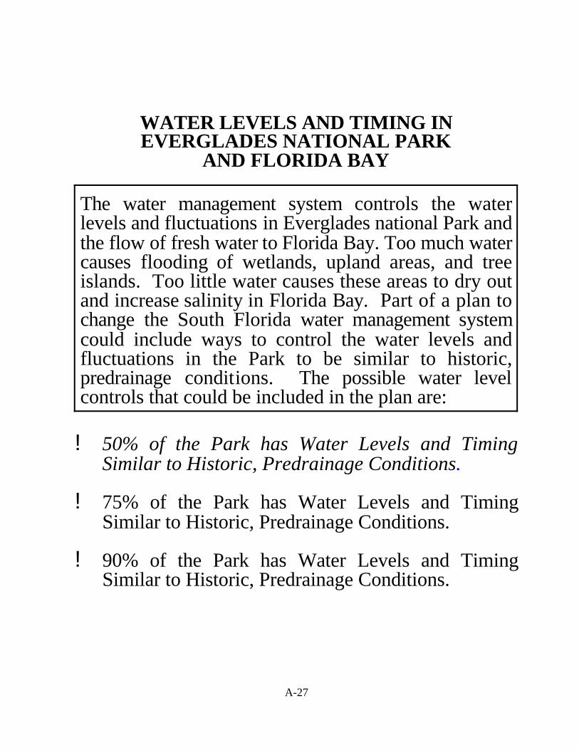
A-27

WATER LEVELS AND TIMING INEVERGLADES NATIONAL PARK

AND FLORIDA BAY

The water management system controls the waterlevels and fluctuations in Everglades national Park andthe flow of fresh water to Florida Bay. Too much watercauses flooding of wetlands, upland areas, and treeislands. Too little water causes these areas to dry outand increase salinity in Florida Bay. Part of a plan tochange the South Florida water management systemcould include ways to control the water levels andfluctuations in the Park to be similar to historic,predrainage conditions. The possible water levelcontrols that could be included in the plan are:

! 50% of the Park has Water Levels and TimingSimilar to Historic, Predrainage Conditions.

! 75% of the Park has Water Levels and TimingSimilar to Historic, Predrainage Conditions.

! 90% of the Park has Water Levels and TimingSimilar to Historic, Predrainage Conditions.

A-28

ANNUAL COST PER HOUSEHOLD

All Florida residents pay utility taxes as part oftheir water, electric, and telephone bills. Part ofa plan to change the South Florida watermanagement system could include additionaltaxes and all Floridians would pay for thesechanges over the next 10 years. Proceeds fromthese taxes would go into a special trust fund thatwould be used only to change the South Floridawater management system. The possible taxpayments that could be included in the plan are:

! No Change in Utility Taxes

! Utility Taxes Would Increase $25 per Year(Adding up to $250 over 10 years)

! Utility Taxes Would Increase $50 per Year(Adding up to $500 over 10 Years)

A-29

RESTRICTIONS ON OUTDOOR ANDINDOOR HOUSEHOLD WATER USE

Changes in the water management system can affect theavailability of water for households in South Florida.The primary effect would occur during years with lowrainfall. These dry years occur, on average, in 1 out ofevery 5 years. The possible levels of restrictions onoutdoor and indoor water use that could be included inthe plan are:

! In Dry Years, Outdoor Uses Restricted to 3 DaysPer Week and Indoor Uses Reduced by 10%

! In Dry Years, Outdoor Uses Restricted to 2 Days PerWeek and Indoor Uses Reduced by 25%

! In Dry Years, Outdoor Uses Restricted to 1 Day PerWeek and Indoor Uses Reduced by 40%

A-30

FARM LAND IN THE EVERGLADESAGRICULTURAL AREA AND WESTERN

PORTIONS OF BROWARDAND DADE COUNTIES

Farm land acreage can be converted to water storageareas or wetlands to increase the flexibility of the watermanagement system, increase the extent of naturalareas, and reduce irrigation demand for water. Part ofa plan to change the South Florida water managementsystem could include reductions in existing farm landacreage in the Everglades Agricultural Area and inwestern portions of Broward and Dade counties that areadjacent to the Water Conservation Areas andEverglades National Park. The possible levels off farmland reductions that could be included in the plan are:

! No Change in Farm Land Acreage

! Reduce Farm Land Acreage by 100,000 Acres (15%of all Farm Acreage)

! Reduce Farm Land Acreage by 200,000 acres (30%of All Farm Acreage)

D-1

APPENDIX D

INFORMATIONAL VIDEO SCRIPT

Topic SlideNum Slide Description Narrative Text

SECTION I INTRODUCTION AND HISTORIC EVERGLADES: ESTABLISHING AN ECOLOGICAL BASELINE

Introduction Satellite Video of South Florida

Viewed from high above, South Florida is rich in water resources. Waterpractically defines South Florida with its lakes, estuaries, and the Everglades.The purpose of this video is to provide you with information about the historicnature of the South Florida ecosystem and how that ecosystem has been changedto provide water-related services to the people of South Florida. After the video,we will ask you some questions to get your opinions about future changes in thewater management system for the region.

GeographicBoundaries

1 Historic EvergladesBasin: Uplands,Lowlands,Open Water.

Before the Twentieth Century, the defining feature of South Florida was theEverglades ecosystem. This system stretched from north of Lake Okeechobee tothe Florida Keys in the south and covered an area 130 miles long and 50 mileswide. The system was made up of wetlands, upland areas, and open water.

Water Flow 2 Schematic map showingpre-drainage wet seasonhigh water surfaceflows through EG andto tide .

Surface water flow, which made the Everglades one of the largest freshwatermarshes in the world, started at Lake Okeechobee and flowed like a river of grassto Florida Bay at the southern end of the state.

3 Photo of saw grassmarsh.

Flow from the Lake into the river of grass varied over the seasons and from year-to-year depending on rainfall.

ClimaticConditions

4 Schematic diagram ofthe hydrologic cycle.

This rainfall filled up surrounding marshes and recharged underground aquifers.Seasonal changes in rainfall affected the timing and flow of water and determinedwater levels in the Everglades.

5 Chart showing annualrainfall, 1966-1990.

Rainfall in South Florida varies widely from less than 40 inches in dry years tomore than 60 inches in wet years. Rainfall occurs during a wet season from Mayto October, and a dry season from November to April.

6 Photo of hurricanewinds and flooding.

During the wet season, hurricanes often produced heavy rains and floodingthroughout South Florida.

7 Photo of alligator holehabitat.

During the dry season alligator holes provided habitat for small fish and frogs andfeeding areas for wading birds.

8 Photo of Evergladesfire.

When saw grass marshes dried out, fires caused by lightning were a natural partof the Everglade's ecosystem.

Topic SlideNum

Slide Description Narrative Text

D-2

EvergladesFlora andFauna

9 Photo of saw grassmarsh

The variability in weather, and its effect on water flow, was the most importantfactor in creating a wide variety of natural habitats. Wetlands included saw grassmarshes and tree islands which established themselves on higher ground withinthe marshes. There were also cypress swamps....

tidal creeks and bays....

mangroves....

and sea grass beds in Florida Bay.

The Everglades ecosystem also included dry land habitats such as hardwoodhammocks....

10 Tree islands

11 Photo of cypressswamp.

12 Aerial photo of tidalcreeks.

13 Photo of mangroveswith roosting birds andshallow marine coastalwaters.

14 Photo of sea grass bedin Florida Bay

15 Photo of hardwoodhammock

16 Photo of pine forest pine forests....

17 Photo of dry landprairie

and prairies.

18 Photo of a spoonbill. This blend of wetland and dry land habitat created one of the most diversewildlife communities of any ecosystem in the world. Wetland areas supportedmore than 35 species of water birds and 50 reptile species.

Dry land areas supported more than 35 species of mammals and a wide varietyof land birds.

19 Photo of an egret

20 Photo of alligator.

21 Photo of a deer

22 Photo of a scrub jay

SECTION II PRESENT WATER MANAGEMENT SYSTEM and Infrastructure

Geography23 Slide with The Present

Water ManagementSystem

In the past fifty years, the historic South Florida ecosystem has been changedto provide for a variety of water uses.

24 Satellite photo of So.Fla./E.G. showingagriculture and urbandevelopment, withoriginal area of E.G.outlined.

As shown by the dark line on the map, more than 50% of the historicEverglades has been drained to reclaim land for urban development andagricultural use. The white area to the right shows urban development alongthe Atlantic coast. The red area directly beneath Lake Okeechobee is farmland.

25 Schematic map showingagriculture, storagewca’s, and park lands.

The present water management system divides the historic Everglades intofour separate regions: Lake Okeechobee, the Everglade's Agricultural Area,Water Conservation Areas, and Everglade's National Park. Water levels andflows in each region can be managed separately from the others.

26 Map showing waterflow in the presentwater managementsystem

During the wet season, water levels in Lake Okeechobee and the WaterConservation Areas are controlled by releases to the Atlantic Ocean andEverglades National Park. During the dry season, releases are made to meet theagricultural, industrial, and household water needs of South Florida.

Topic SlideNum

Slide Description Narrative Text

D-3

Infrastructure 27 Aerial photo of LakeOkeechobee, dike andflood gates.

The present water management system consists of levees, canals, and waterstorage areas. Lake Okeechobee in the north is the beginning of the system.

28 Aerial photo of canalsand pumping station.

Water is pumped in a southward direction from the Lake through a managedsystem of six primary canals, an extensive network of secondary canals, andseven major pump stations.

29 Aerial photo of leveeand WCA

Water pumped from the Lake is stored in the Water Conservation Areas whereit seeps into underground aquifers and well fields for urban and agricultural use.

Services Provided by Infrastructure

ServicesUrban

30 Aerial photo of housingdevelopment adjacentto marsh.

Today's water management system provides services to urban, agricultural,and recreational users.

31 Photo of floodedhomes.

It serves to prevent seasonal flooding of residential areas although in very wetyears some areas still experience problems.

32 Slide of glass of water. The Water Conservation Areas feed underground aquifers that are the primarywater supply for South Florida's urban population of five million people andmillions of tourists. By the year 2020, the population of South Florida isexpected to increase by 40% to seven million people.

33 Slide of lawn watering. Also, water is supplied for outdoor uses such as watering lawns and washingcars.

AgriculturalServices

34 Aerial photo showingag. fields and adjacentcanal.

The water management system provides services to agriculture in the form ofdrainage and irrigation, depending on the time of year. In the wet season,runoff from fields is pumped into large canals to prevent flooding. In the dryseason, water is pumped from canals for crop irrigation.

35 Photo of a sugarcaneharvesting operation.

There are about a half million acres of crop land in the Everglades AgriculturalArea just south of Lake Okeechobee, of which 85% is sugar cane.

36 Photo of field andtractor.

Other crops produced in Palm Beach, Broward and Dade counties include sodfor yards and golf courses, and vegetables such as radishes.....

37 Photo of vegetable field celery, corn, tomatoes and lettuce.

38 Photo of fishing from apier

The water management system also provides water for the environment so thatresidents and tourists can fish on freshwater lakes and rivers....

39 Photo of men fishing ina boat

and on coastal bays.

40 Aerial photo of boat incanal.

People can also enjoy boating ....

41 Ranger with group tour and observe wildlife.

B. Consequences of Controlling Water Flow in the Everglades

42 Map showing change inwater flows direction.

Unfortunately, the present water management system has result ed in manyunexpected consequences. Changes in water levels in Lake Okeechobee havedamaged shore line habitat for fish and wildlife.

Topic SlideNum

Slide Description Narrative Text

D-4

43 Schematic Mapshowing change inwater flows

A significantly greater amount of water is now drained to the Atlantic Oceanrather than flowing through the Everglades to Florida Bay.

44 Chart showing flows totide and to ENP, pre-and post-drainage.

More than four times as much water flows to the Atlantic Ocean, causing damageto coastal estuaries. A 60% reduction in fresh water flows to Florida Bay hascaused increased salinity in the Bay.

45 Chart showing changein timing of flows.

The timing of water flows has also changed. Compared to historical flows, thecurrent pattern of water flows are more uneven and move faster through thesystem.

46 Map showing change inwater levels in wetyears

In these maps, wet areas are shown in green and blue, with dark blue indicatingthe highest water levels. In the historic system, water levels during the wetseason were evenly distributed across the region and these areas were wet mostof the year. In the present system, higher water levels are concentrated in a fewareas. Some areas are much drier, even during the wet season.

47 Map showing change inwater levels in dryyears

During the driest years, water levels in the historic system were lower thanduring the wet years, but were still evenly distributed across the region. In thepresent system, most of the region is dry in the driest years, including the WaterConservation Areas.

Wildlife 48 Slide of deer or othermammal in water

Changes in water depth, and the direction and timing of water flow, changed thepattern of wet and dry periods and adversely affected several Everglade'shabitats. For example, storing water for long periods of time has resulted inunusually high water levels in some areas.

49 Photo of heron inwater

Wetland habitats for wading birds have been harmed by decreased water flows tothe lower Everglades.

50 Chart of wading birdpopulation decline

As this chart shows, there has been about a 90% reduction in the number ofwading birds in the lower Everglades in the last fifty years. Loss of habitat hasresulted in the listing of 17 species of animals and birds as either endangered orthreatened in South Florida.

51 Aerial photo of FloridaBay.

Changes in the timing and flow of freshwater have also contributed to unusuallyhigh levels of salinity in Florida Bay.

52 Photo of a damagedmangrove stand.

Once healthy mangroves along the coast have been damaged by high salinitylevels and....

53 Photo of a damaged seagrass bed.

during a recent dry period, about 100,000 acres of sea grass died back in FloridaBay.

54 Shrimp boat in the bay. These changes in the Bay have also harmed recreational fishing and the pinkshrimp industry in the Florida Keys.

Groundwater/UrbanConsequence

55 Schematic of increasingsalt water intrusion,1904 and 1982.

The present water management system has also had consequences for drinkingwater supplies. Low water levels in wetlands, which replenish freshwateraquifers, have resulted in increased salt water intrusion into these aquifers. Inthe Miami area, for example, salt water intrusion has forced drinking water wellfields to be located further inland.

56 Aerial photo ofsuburban Coral Springsadjacent to Everglades

The growing population in South Florida requires more water for householduses. The increased demand puts pressure on groundwater supplies and may leadto future water shortages.

57 Photo of water userestrictions placard.

Reduced rainfall and low levels of groundwater storage have sometimes led torestrictions on household water use.

Topic SlideNum

Slide Description Narrative Text

D-5

SECTION III : PLANNING FOR THE FUTURE

58 Slide with text:Planning For the Future

Public officials are now considering possible changes in the water managementsystem in South Florida.

59 Schematic map showingAlternative plans forrestoration

A range of alternatives to change the mix of services provided by the presentwater management system are being considered. Many of these alternativeswould take a decade or more to implement.

60-65 Two-part slide of theEverglades and urbanarea (IFAS), and singleslides of Evergladespark, wildlife, sea grassbed, agriculture, andurban area.

The choice of which alternative to select will depend upon public opinion aboutthe types of services to provide and the costs associated with a change in thewater management system. Any decision will require tradeoffs between thevarious services described in this video and will have an impact on all Floridians.

66 Four part video ofvarious uses.

The purpose of the survey you are about to participate in is to ask your opinionabout alternative water management plans for South Florida. Your opinion, alongwith those of other Florida citizens, is vital to this process and your participationis greatly appreciated.

67 Slide with UF LOGO. Thank you for your cooperation.

E-1

APPENDIX E

SUMMARY OF INTERVIWER EVALUATIONS OF RESPONDENTS

Respondent Distraction

Rating by Interviewer Number ofRespondents

Percentage ofRespondents

Extremely distracted 12 2.5

Very distracted 11 2.3

Somewhat distracted 51 10.6

Slightly distracted 86 17.9

Not at all distracted 316 65.8

Not sure 4 0.8

Respondent Attentiveness

Rating by Interviewer Number ofRespondents

Percentage ofRespondents

Extremely attentive 140 29.2

Very attentive 250 52.1

Somewhat attentive 75 15.6

Slightly attentive 10 2.1

Not at all attentive 5 1.0

Respondent Understanding of Material

Rating by Interviewer Number ofRespondents

Percentage ofRespondents

Extremely well undestood 116 24.2

Very well understood 236 49.2

Somewhat understood 103 21.5

Slightly understood 17 3.5

E-2

Not at all understood 3 0.6

Not sure 5 1.0

Respondent Difficulty With Attributes

Rating by Interviewer Number ofRespondents

Percentage ofRespondents

Yes (had difficulty) 36 7.5

No (had no difficulty) 444 92.5

Respondent Difficulty With Choosing Plans

Rating by Interviewer Number ofRespondents

Percentage ofRespondents

Yes (had difficulty) 43 9.0

No (had no difficulty) 434 90.4

Respondent Seriousness

Rating by Interviewer Number ofRespondents

Percentage ofRespondents

Extremely serious 153 31.9

Very serious 167 34.8

Somewhat serious 127 26.5

Slightly serious 16 3.3

Not at all serious 3 0.6

Missing 14 2.9