Public Goods, Transferable Utilityand

Divorce Laws∗

Pierre-Andre Chiappori†, Murat Iyigun‡and Yoram Weiss§

April 2007

Abstract

We reconsider the well known Becker-Coase (BC ) argument, according towhich changes in divorce laws should not affect divorce rates, in the contextof households which consume public goods in addition to private goods. Forthis result to hold, utility must be transferable both within marriage and upondivorce, and the marginal rate of substitution between public and private con-sumption needs to be invariant in marital status. We develop a model in whichcouples consume public goods and show that if divorce alters the way somegoods are consumed (either because some goods that are public in marriagebecome private in divorce or because divorce affects the marginal rate of sub-stitution between public and private goods), then the Becker-Coase theoremholds only under strict quasi-linearity. We conclude that, in general, divorcelaws will influence the divorce rate, although the impact of a change in divorcelaws can go in either direction.

1 Introduction

A highly pertinent question in the economics of the family is whether changes in

divorce laws would impact divorce rates. In the words of Becker (1993, p. 331), “A

husband and wife would both consent to a divorce if, and only if, they both expected

to be better off divorced. Although divorce might seem more difficult when mutual

∗Corresponding author: Pierre-Andre Chiappori, Economics Department, Columbia University,1009A International Affairs Building, MC 3308, 420 West 118th Street, New York, NY 10027. E-Mail: pc2167@columbia.edu. Phone: (212) 854-6369. Fax: (212) 854-8059.

†Columbia University.‡University of Colorado and IZA.§Tel Aviv University and IZA.

1

consent is required than when either alone can divorce at will, the frequency and inci-

dence of divorce should be similar with these and other rules if couples contemplating

divorce can easily bargain with each other. This assertion is a special case of the

Coase theorem (1960) and is a natural extension of the argument [...] that persons

marry each other if, and only if, they both expect to better off compared to their best

alternatives.”1 Thus, according to the Becker-Coase theorem, the move from mutual

consent to unilateral divorce laws ought to have no impact on the rates of marriage

dissolution, although it would affect the division of family resources within marriage

and in the aftermath of divorce.2 Given, this result one can go further and show that

divorce laws have no effect on the joint expected utility from marriage and therefore

the entry into marriage, implying that any laws that determine divisions of property

rights conditioned on marital status can be undone by individual recontracting and

therefore have no effect on either marriage or divorce. However, empirical studies on

this topic which exploit the cross-state variation in the adoption of the no-fault, uni-

lateral divorce laws in the United States show that unilateral divorce laws did raise

divorce rates in the short run, although longer term effects are harder to establish

(see, for example, Peters, 1986, Friedberg, 1998, Stevenson and Wolfers, 2006 and

Wolfers, 2006). There is also some evidence that the change in divorce laws have

reduced marriage rates (see Rasul 2005, and Matouschek and Rasul, 2006).

The goal of this paper is to reassess the theoretical validity of the Becker-Coase

argument. We do so by assuming the same basic environment as in Becker (1993).

In particular, we assume away inefficiencies generated by frictions or asymmetric

information between the spouses. In such an environment there are three specific re-

quirements for the Becker-Coase theorem: (a) transferable utility between the spouses

within marriage (TUM ); (b) transferable utility between the spouses upon divorce

(TUD); and (c) invariance of the ”exchange rate” of the utilities of the two part-

ners to changes in marital status (IER). Together, these requirements imply that the

decision to divorce is determined by the aggregate ‘real income’ of the two partners

(including non-monetary benefits). If the couple’s real income is higher upon divorce,

the partners will choose to split. But if it is lower in divorce, they will stay married.

This holds true irrespective of the individual incomes (utilities) of the partners in the

1The generalized Becker-Coase theorem as it applies to couples and intra-household allocationswas originally formulated in Becker (1981).

2By definition, mutual consent divorce laws require both spouses to agree to a divorce whereasunder unilateral divorce legislation divorce occurs when one spouse files for it.

2

two situations and the type of the divorce legislation in effect.

Recent analysis such as Zelder (1993), Clark (1999) and Fella et al. (2004) demon-

strate that, in the absence of transferable utility, divorce rates can–and typically

will be–influenced by changes in the divorce legislation. The question, however, is

whether TUM, TUD and IER, taken together, are reasonable. To address this issue,

we consider the implications of these conditions for household behavior. We apply

a collective approach which presumes that partners to marriage reach an efficient

outcome and consider a situation in which couples may consume both private and

public goods. The presence of public goods generates economic marital gains. In

addition, marriage generates non-pecuniary benefits which are revealed with some

lag and may be different for the two spouses. A poor realization of these benefits can

trigger divorce, although the economic surplus generated by marriage can mitigate

the likelihood of this outcome. Having an explicit household model with endogenous

divorce allows us to go beyond the implications of the three requirements listed above

for divorce and explore their implications for other observable features of household

behavior, such as household demand functions.

We begin by identifying spousal preferences that enable transferability of utility

between spouses within marriage and characterizing their implications for household

demand. A standard sufficient condition for TUM is quasi-linearity of spousal utili-

ties, which implies that all goods, but one, have zero income elasticity. However, in an

important contribution, Bergstrom and Cornes (1981, 1983) show that transferable

utility within marriage does not require quasi-linearity, because the marginal utility

of private consumption of the partners can depend on their common consumption of

the public good; in particular, all commodities can have positive income elasticity.

They provide a simple characterization of the preferences of the two spouses that

maintain TUM. Basically, spouses’ preferences are such that one good (at least) can

be used to transfer utility between the partners. For both partners, this good gener-

ates a positive and identical level of marginal utility that depends only on the goods

that are publicly consumed. We refer to such preferences as ‘generalized quasi-linear

(GQL). We note, however, that from the perspective of the collective approach, the

assumption of GQL is quite restrictive because it implies that couples behave in

a ‘unitary’ way. When GQL holds, couples act as if they maximize a single util-

ity function and household demand satisfies income pooling as well as the Slutsky

conditions. Accordingly, holding total family income fixed, transferring income from

3

the husband to the wife should have no impact on household consumption except

on those goods that are used to transfer utility. This prediction is often rejected by

empirical evidence.

We argue that even if GQL holds, structural changes in the domains of public and

private consumption following divorce will cause violations of TUD or IER (unless

quasi-linearity of spousal utility representations is imposed). There are two basic

reasons for this. First, some commodities that are public in marriage become private

in divorce (e.g. housing). In this case, GQL preferences imply that the Pareto frontier

upon divorce is convex (rather than linear). Second, even for those goods that remain

public after divorce (e.g., children), the marginal rate of substitution between public

and private consumption is likely to change (for instance, due to the distance of non-

custodial parents to their offspring), implying different slopes for the linear frontiers

in marriage and divorce. Due to either of these two reasons, the utility frontiers

facing a couple upon marriage and divorce, respectively, can intersect. Consequently,

the divorce outcome will depend on the initial sharing rule, the realization of match-

specific qualities and the distribution of property rights as they are defined by the

prevailing divorce legislation.

In sum, we find that the violations of Becker-Coase may be more complex than

usually assumed. If divorce settlements are characterized by an uneven allocation

of income and wealth, say because one spouse is much richer than the other and

divorce laws allows the wealthier spouse to keep most of his/her wealth, then there are

realizations of the shocks to match quality such that the marriage will dissolve under

unilateral divorce laws but will remain intact under mutual consent. In contrast, when

divorce laws produce more even divorce settlements in terms of income and wealth,

there are realizations of the shocks to match quality such that the marriage will remain

intact under unilateral divorce laws but not under mutual consent–a possibility

already identified by Clark (1999). In general, couples who experience different match-

quality shocks can react differently to changes in divorce legislation and, without

further information on the prevailing divorce settlement laws, it is impossible to

predict whether or not a switch from mutual consent divorce laws to no-fault divorce

would lead to higher or lower aggregate divorce rates.

4

2 The Basic Ingredients

We consider a static model in which individuals live for two periods. Each person

has preferences over commodities and marital status. Commodities are classified into

two types; private goods, denoted by x and public goods denoted X that can be

consumed jointly when two individuals are married. Preferences are represented by a

pair of state dependent utility functions, v (x,X) if a person is single and u (x,X)+θ,

if a person is married. The additive component θ represents non-economic benefits

from marriage, such as love and companionship, that are assumed to be separable

from the preferences over goods and are match specific. We do not consider altruism

between spouses for now; the extension to an altruistic context is discussed in the last

section. We view children as one of the public goods and in this manner allow for the

possibility that both parents, whether married or divorced, care about the welfare of

their child(ren).

We assume that the quality of the match is not observable at the date of marriage

but that it is fully revealed after one period. At the date of marriage, the partners

agree upon the consumption levels of all goods, public and private. We assume

that this allocation is Pareto efficient and not contingent on future realizations of the

quality of the match.3 We do not restrict the mechanism that determines the outcome

within marriage in any particular way (such as Nash Bargaining) but recognize that

it can depend on the spouses’ incomes and on marriage market conditions. At the end

of the period, the individual marital match qualities of the two partners are drawn

from some given distribution and each spouse obtains a utility payoff derived from

the predetermined levels of consumption, as well as the realized values of θh for the

husband and θw for the wife. On that basis, and given the laws governing divorce, the

spouses decide either to dissolve their marriage or remain married. If the partners

split, their incomes can be modified by some redistribution determined by law but

the partners can renegotiate around this stipulation and, if both partners agree, the

courts will “rubber-stamp” the agreement. If they choose to continue the marriage,

the partners can also renegotiate the intra-household allocation defined by the initial

sharing rule. In this regard, couples bargain in the “shadow of the law” (see Mnookin

and Kornhauser, 1979).

In what follows, we do not consider the possibility of remarriage and whenever

3Contingent contracts would raise complex implementation issues, insofar as the realization ofmatch qualities are not verifiable by a third party.

5

a marriage dissolves, the partners remain single. This assumption is made for ex-

positional simplicity and could easily be relaxed. However, the ex-spouses remain

connected in the sense that they transfer resources to each other, if forced by law.4

3 A benchmark case without public goods

To reiterate Becker’s results, consider a model with only one private good, x, and

strictly quasi linear preferences given by

u(xm) = xm + θm, (1)

v(xm) = xm, m = w, h,

where h denotes the husband and w denotes the wife. This specification satisfies

TUM, TUD and IER, which implies that the utility frontiers upon continued marriage

and divorce are parallel straight lines. Then, for any allocation of the property

rights upon marriage and divorce and irrespective of whether consent is required,

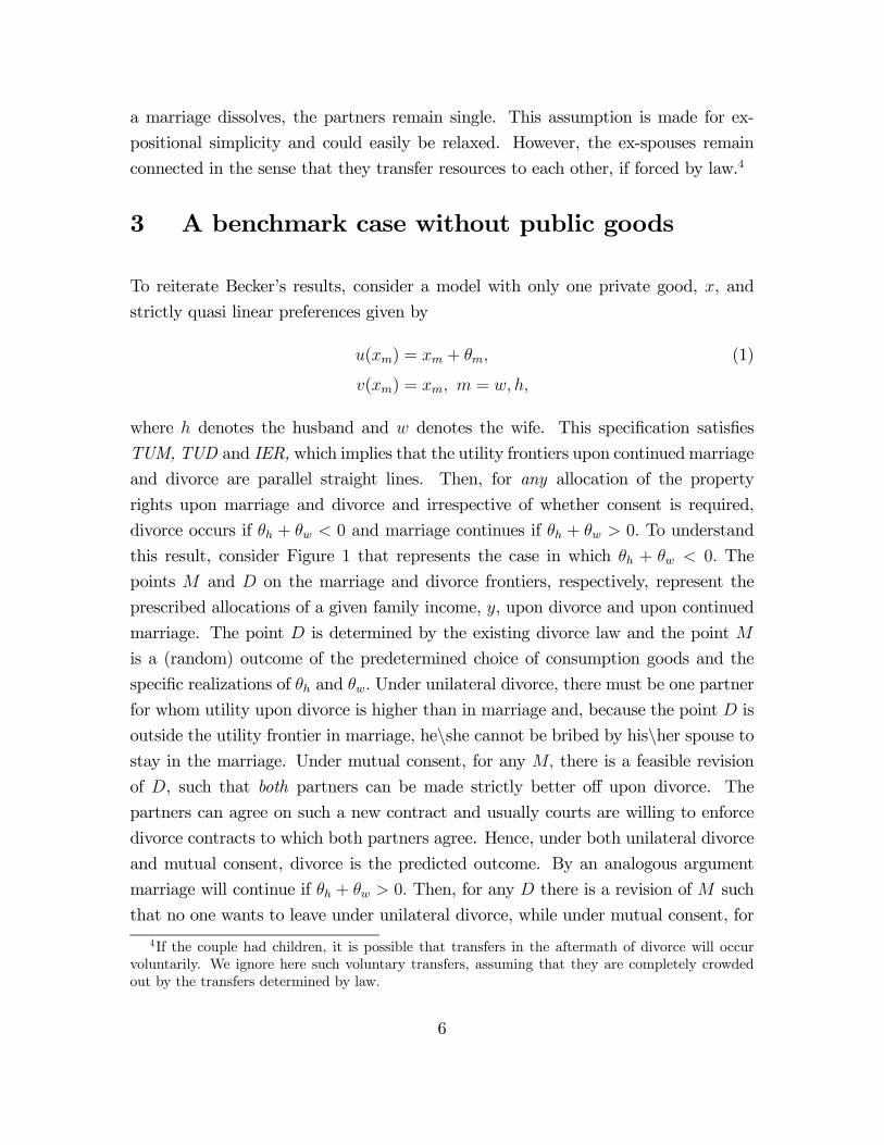
divorce occurs if θh + θw < 0 and marriage continues if θh + θw > 0. To understand

this result, consider Figure 1 that represents the case in which θh + θw < 0. The

points M and D on the marriage and divorce frontiers, respectively, represent the

prescribed allocations of a given family income, y, upon divorce and upon continued

marriage. The point D is determined by the existing divorce law and the point M

is a (random) outcome of the predetermined choice of consumption goods and the

specific realizations of θh and θw. Under unilateral divorce, there must be one partner

for whom utility upon divorce is higher than in marriage and, because the point D is

outside the utility frontier in marriage, he\she cannot be bribed by his\her spouse tostay in the marriage. Under mutual consent, for any M, there is a feasible revision

of D, such that both partners can be made strictly better off upon divorce. The

partners can agree on such a new contract and usually courts are willing to enforce

divorce contracts to which both partners agree. Hence, under both unilateral divorce

and mutual consent, divorce is the predicted outcome. By an analogous argument

marriage will continue if θh + θw > 0. Then, for any D there is a revision of M such

that no one wants to leave under unilateral divorce, while under mutual consent, for

4If the couple had children, it is possible that transfers in the aftermath of divorce will occurvoluntarily. We ignore here such voluntary transfers, assuming that they are completely crowdedout by the transfers determined by law.

6

anyM , the party who wants to leave cannot compensate his ex-spouse upon divorce,

without becoming worse off.

Moving backward in time, we see that the expected utilities of the partners, con-

ditioned on marriage in the first period, are

Um = xm + p(xm +Eθm p θh + θw ≥ 0) + (1− p)uDm, (2)

where p = prob(θh + θw ≥ 0) and uDm is the utility outcome upon divorce which

depends on the division of income between the two spouses upon divorce that he law

prescribes and on whether mutual consent is required. Adding the utilities of the two

partners, we see that the Pareto frontier upon marriage is linear and given by

Uh + Uw = 2y + pEθh p θh + θw ≥ 0+ pEθw p θh + θw ≥ 0 (3)

Due to the assumed transferable utility, marriage occurs whenever the RHS of (3)

exceeds 2y which is what the partners obtain together as singles. Under plausible

assumptions on the distributions of θh and θw, the expected non monetary gains from

marriage are positive. Hence, if all individuals are identical and there are no frictions

all matched couples will choose to marry. The important conclusion here is that the

joint gains from marriage are independent of the divorce laws.5

4 A simple example with public goods

Consider now a case with 2 commodities; one that is purely private (the price of which

is normalized to 1) and another that can be publicly consumed if two individuals

marry. Assume that spouses’ respective preferences regarding the private and the

public good can be represented by the utility function:

vm (xm,X) = X + xmX ,

when single and by

um (xm, X) = X + xmX + θm , m = w, h, (4)

5Note further that if law specifies a particular division upon divorce, the partners are still freeto choose any division of life time utilities upon this expected utilities frontier. in particular, apartner with high entitlement upon divorce may be "punished" upon marriage by lower level ofconsumption. .

7

hU

wU

Utility Frontier in Divorce

Utility Frontier in Marriage 0h wθ θ+ <

0

D

M

Figure 1: Pareto frontiers in marriage and divorce, no public goods

if they are married. This specification imposes some complementarity between public

and private goods and, in particular, the marginal utility from private good is given

by X for both spouses. By construction, it then follows that it is possible to transfer

utility within marriage on a one-to-one basis between the spouses, using the private

consumption good. Initially, we assume that preferences over commodities are the

same for the two spouses and independent of marital status so that um (xm,X) =

vm (xm, X) for m = w, h. Alternative scenarios will be discussed shortly.

4.1 Consumption and utility if marriage continues

For the preferences described here, the efficient level of X in an interior solution with

xh > 0 and xw > 0 depends only on its price P and on the aggregate family income

y. It is given by

X = min

µy

P,y + 2

2P

¶, (5)

8

where y is the pooled income of the two spouses (see Bergstrom and Cornes, 1983).

We shall assume hereafter that y > 2. Then household demand takes the LES form:

X =y + 2

2P, x = xh + xw =

y − 22

. (6)

Note that the consumption of the public good and the aggregate consumption of

the private goods both rise with family income. Furthermore, any pair of private

consumption levels that satisfies

xh > 0, xw > 0, xh + xw =y − 22

(7)

is efficient.6

The implied utility levels of the two partners, conditioned on the efficient and

interior level of the public good, are

UMm = (1 + xm)

2 + y

2P+ θm , m = w, h . (8)

Hence, the Pareto frontier is given by

UMh + UM

w =1

4

(2 + y)2

P+ θh + θw , (9)

which defines a straight line with slope −1. This indicates transferable utility. Thatis, by shifting the amount of private consumption goods between the two partners, it

is possible to transfer utility at a fixed ‘rate of exchange’ that can be normalized to

unity.

The significance of this feature is that the new Pareto set generated by any change

in circumstances, such as a rise in family income or shocks to marital match quality

of either spouse, either includes or is included in the initial Pareto set. In this respect,

there is no conflict between the partners in their evaluations of the overall situation

that they face–they always prefer the context in which the Pareto set is largest.7

Note, however, that this is true only on the segment of the Pareto frontier which

corresponds to 0 < xh + xw < (y− 2) / 2. There are also other regions of the Paretofrontier in which the non-negativity constraints on consumption bind and the Pareto

6To determine the division of private consumption goods between the two spouses, one must gobeyond the principle of efficiency and specify a ‘sharing rule’ that selects (implements) a particu-lar point on the Pareto frontier as a function of the individual incomes of the spouses and other‘distribution factors’. See Browning et al. (2006, ch. 3).

7This idea of potential compensation plays an important role in the early literature on welfareeconomics, especially the evaluation of national income (see Samuelson, 1950).

9

frontier is no longer linear. One such region covers xh = 0 and xw = y − PX. Then,

UMh = X + θh and UM

w = X (1 + y −PX) + θw, which represents a concave segment

of the Pareto frontier given by

UMw =

¡UMh − θh

¢[1 + y − P

¡UMh − θh

¢] + θw . (10)

Another concave segment exists when xw = 0, and xh = y −X. Then,

UMw =

1

2P

∙1 + y +

q(1 + y)2 − 4P (UM

h − θh)

¸+ θw . (11)

When either of these ‘corner’ solutions arises, utility is no longer transferable at a

fixed rate of exchange between the spouses even in marriage. But the higher is family

income, the wider is the range in which utility is transferable.

4.2 Consumption and Utility in Divorce

Consider, now, the case in which agents decide to divorce. The utilities actually

achieved depend on two features. One is the division of income following divorce, as

determined either by law or a private contract between the parties. Without making

explicit which of those mechanisms determine the post-divorce allocations, we simply

assume that the husband gets βy and the wife gets (1− β) y for some parameter

1 ≥ β ≥ 0.The other determinant of intra-household welfare is the technology of consump-

tion that prevails after divorce. Specifically, while the private good certainly remains

private, the impact of divorce on consumption of the other (previously public) com-

modity is less clear. One possibility is that good X is privately consumed after

divorce. This would be the case, for instance, of housing assuming that the spouses

quit cohabiting after divorce. Alternatively, the consumption of good X may remain

public. For instance, we may think of ‘child quality’ as such a good, since parents gen-

erally care about their children’s wellbeing regardless of the state of their marriage.

However, divorce may still influence the allocations for this ‘consumption’. A plausi-

ble reason for this is that loss of custody or shared custody arrangements reduce the

interaction time between at least one of the parents and the child(ren). In essence,

this ‘distance’ effect reduces the marginal benefit of child-quality investments.

To capture these ideas in our simple framework, we consider two alternative set-

tings: In one, the public good becomes purely private upon divorce. In the other,

10

the good remains public but the consumption utility of one of the ex-spouses is ‘dis-

counted’ in the sense that the person’s marginal willingness to pay for this public

consumption is smaller than it was in marriage.

4.2.1 Public Good Become Private

We start with the private consumption case. The ex-husband solves

maxxh,Xh

Xh + (βy − PXh)Xh, (12)

which yields the consumption levels and the utility

Xh =1 + βy

2P, xh = βy − PXh =

βy − 12

,

(13)

UDh = uDh =

(1 + βy)2

4P.

Similarly, the ex-wife solves

maxxw,Xw

Xw + ((1− β) y − PXw)Xw, (14)

which gives

Xw =(1− β) y + 1

2P, xw = (1− β) y − PXw =

(1− β) y − 12

,

(15)

UDw = uDw =

(1 + (1− β) y)2

4P.

Using transfers, that is, by changing β, it is possible to move along the Pareto

frontier in the aftermath of divorce. Hence, the Pareto frontier in divorce is given by

UDw =

(2 + y − 2pPUD

h )2

4P, (16)

which is decreasing and convex with a slope given by

dUDw

dUDh

= − 1 + (1− β)y

1 + βy. (17)

In Figure 2, we compare the Pareto frontiers in marriage and divorce, assuming

that p = 1. The location of the marriage frontier depends on the realization of the θ0s.

11

More precisely, while the location of the linear segment depends on the sum θh + θw,

those of the ‘corner’ portions depend on the specific values of each marital match-

quality shock.In the special case in which θh = θw = 0, the utility frontier in marriage

is completely outside the utility frontier in divorce, because of the economic gains

resulting from the joint consumption of public goods when partners live together.

Variation in θh and θw shift the utility frontier in marriage upwards and downwards.

However, when θh + θw < 0 the two utility frontiers can intersect, as indicated by

the broken blue line. Having assumed that consumption is determined before the

values of θh and θw are realized, different realizations are associated with different

utility outcomes for the two partners in marriage, as indicated by the points M and

M 0. In contrast, the utility outcomes upon divorce, represented by the point D are

independent of θh and θw.

12

It is important to note that in comparing the two Pareto frontiers in the case

of marriage and divorce, we maintain the same cardinal representation of individual

preferences. That is, if there exists a representation such that utility is transferable

in marriage but it is not fully transferable in divorce, then the two Pareto frontiers

can intersect. For this example, there will be two intersections provided that

0 > θh + θw > −(2 + y)2

8P. (18)

If monotone transformations are applied to individual preferences in marriage and

divorce, the shapes of the two Pareto frontiers will change but the pattern of inter-

sections will remain the same.8

4.2.2 ‘Distance’ in Public Consumption

Assume, alternatively, that the marital public goods remain public upon divorce (e.g.,

ex-spouses still care about the welfare of their offspring after divorce). However, the

‘distance’ created by divorce between the non-custodial parent and the child(ren)

affects preferences in terms of the relative importance of public and private goods

and the evaluation of the marital state compared to being single.

Suppose, for instance, that the mother’s preferences are unaffected by divorce be-

cause she maintains custody over the child(ren), but the father’s utility upon divorce

becomes

vh (xh,X) = γ

µX +

1

δxhX

¶, (19)

with γ < δ < 1.

In words, divorce has two effects. First, the public good is discounted by some

factor γ, compared to its value in marriage. Second, the marginal willingness to pay

for the public good, which is equal to (1+xh) / X within marriage, drops to (δ+xh)

/ X after divorce. Both of these changes reflect the reduction in the interaction

between the father and the child(ren) when the mother is the custodial parent.

8At an intersection, we have

UMh = uMh + θh = uDh = UD

h ,

UMw = uMw + θw = uDw = UD

w .

Thus, any monotone transformation Hm(U) will maintain the equality (as well as an inequality).

13

hU

wU

( )214

y +

( )214

y +

( )22

y +

( )22

y +

( ) ( )2 24

y y+ −

( )224

y +

( )224

y +

( ) ( )2 24

y y+ −

Utility Frontier in Marriage 0h wθ θ= =

Utility Frontier in Divorce

Utility Frontier in Marriage 0h wθ θ+ <

D

0

M

'M

Figure 2: Pareto frontiers in marriage and divorce, with public goods

14

Following divorce, the Pareto frontier remains linear with a constant (income-

independent) slope. In particular, one can easily check that, for any interior solution,

we haveδ

γUDh + UD

w = maxX[(δ + 1)X + (y − PX)X] . (20)

The slope is no longer equal to −1. Instead, it is now −γ/δ > −1, reflecting thefather’s ‘discount’ factor in divorce.9

Figure 3 compares the divorce and marriage frontier in this case. Again, in the

special case in which θh = θw = 0, the utility frontier in marriage is completely

outside the utility frontier in divorce and the divorce frontier upon divorce is steeper

because of the husband suffers a larger utility loss upon separation. Variation in

θh and θw shift the utility frontier in marriage upwards and downwards. However,

when θh + θw < 0 the two utility frontiers can intersect, as indicated by the broken

blue line. Under unilateral divorce, the couple will divorce if and only if the division

prescribed upon divorce D falls outside the utility frontier in marriage. Under mutual

consent, divorce will occur if and only if the (random) divisionM implied by choice of

consumption prior to the realization of θh and θw falls inside the utility frontier upon

divorce. The points M and D in Figure 3 illustrates a case in which divorce occurs

under mutual consent but marriage continues under divorce at will. It is important to

note, however that under mutual consent the points M and D are not independent,

because commitment made at marriage affect the range of renegotiated outcomes if

marriage continues and, therefore, the probability of divorce. Taking D as given and

looking forward, a couple may choose an initial allocation of the private consumption

goods such that, on the average, M is close to D, thereby making divorce less likely.

The partner who is hurt by this shift in the first period, may be compensated in

term of life time utility by higher gains from joint consumption if marriage continues.

Nevertheless, with sufficient variation in θh and θw, there will be ex-post realizations

such that M and D are as drawn in Figure 3, implying that for such couples divorce

laws matters.

9By the same token, the optimal level of public consumption is still identical for all efficientallocations, but it is smaller than before divorce; namely,

XD =y + δ + 1

2P<

y + 2

2P.

15

hU

wU

Utility Frontier in Divorce

Utility Frontier in Marriage 0h wθ θ+ <

0

D

M

Figure 3: Pareto frontiers in marriage and divorce with "distance" in public goods

16

4.3 Becker-Coase Theorem Revisited

Our key result is that in both cases described above, regarding the nature of marital

public goods and how they might be altered in divorce, the strong version of the

Becker-Coase theorem does not hold. Indeed, for some realization of the match-

quality shocks, the divorce decision depends on the legal framework. In particular, we

provide below two examples in which different divorce laws lead to opposite outcomes.

The first one is somewhat standard, in the sense that the couple in question would

split under unilateral divorce, but would remain married if mutual consent is required.

The second example is more counter-intuitive, because the same couple would divorce

if mutual consent is required but they would remain married under unilateral divorce.

The reason for this is that unilateral divorce would trigger a renegotiation of the intra-

household allocations and enable the couple to find efficient reallocations they can

agree upon within marriage.

We present both examples utilizing the ‘public-good-becomes-private’ framework

we worked out above. Moreover, we ignore the possibility of corner solutions for the

Pareto frontier when married. None of these choices is important, as these examples

can easily be transposed into a different context. The key condition is that the

realizations of match quality generate a Pareto frontier under marriage that intersects

the utility frontier under divorce.10 In addition, we require that the match-quality

shocks apply at the individual level and for them not be identical for the husband

and the wife, so that any distribution of the marital gains upon marriage is possible.

Counter-example 1 (Mutual Consent Reduces Divorce) Consider the case

depicted in Figure 2 and suppose that

1. Divorce legislation is rather favorable to men (i.e. β is large; for instance,

property is mostly private and the husband is much wealthier than his wife);

2. The realization of the shocks is such that marriage is more valuable to the wife,

θw > 0 > θh.

Figure 4 depicts the corresponding points on the Pareto frontiers as M if married

and as D if divorced.11 One can readily see from the diagram that the couple will

10In the case under consideration, this condition is met whenever equation (15) is satisfied.11For simplicity, we ignore here the non linear segments of the utility frontiers in marriage.

17

hU

wU

Utility Frontier in Divorce

Utility Frontier in Marriage 0h wθ θ+ <

0

D

MMwU

DhU

MhU

DwU

Figure 4: Mutual consent redueces divorce

remain married mutual consent is required for divorce. Because of the veto power

conferred to either spouse, the wife can guarantee a utility level that is at least equal

to what she gets when she is married, namely UMw and because no point on the divorce

frontier can offer the wife a similar level of welfare without making the husband worse

off. Assume, on the contrary, that the husband can unilaterally decide to divorce.

Then, he can reach the utility level UDh . This is more than what he can achieve when

married and the wife is unable to bribe him to stay. Therefore, the couple will split.12

The general intuition is clear: whenever the two Pareto frontiers intersect, one

can find two utility levels—one for the couple when they are married and another for

12Note that this case is similar to Figure 2 in Clark (1999). Our model can thus be seen asproviding an explicit foundation for Clark’s discussion.

18

when they are divorced–such that the wife cannot, under unilateral divorce, ‘bribe’

the husband into staying married and the husband cannot, under mutual consent,

pay off his wife to accept a separation.

Counter-example 2 (Mutual Consent Raises Divorce) We now reverse the

two assumptions introduced above. In particular, consider the following scenario:

1. Divorce legislation is not too favorable to men (say, it splits household wealth

equally between the spouses, β = 1/2);

2. The realization of the shocks favors the husband, θh > 0 > θw.

This situation is represented by the Pareto frontiers in Figure 5, where M is

the division when the couple remains married and D is the division if the couple

divorces. This case is similar to Figure 3 in Clark (1999) and the argument goes

as follows: When mutual consent divorce laws apply, the husband will use his veto

power to make sure that his utility is at least as much as what he gets when he

stays married, namely UMh . Therefore, the final outcome must be located to the

northeast of pointM . Actually, there exist achievable outcomes that Pareto improve

upon the current situation. However, they are all located on the divorce frontier.

From a straightforward efficiency argument, the partners will renegotiate the divorce

contract, allowing them to reach upon divorce a point such as D0, which is preferred

by both of them to remaining married.

Now consider the case of unilateral divorce. The wife may, by divorcing, achieve

the utility level UDw that exceeds her payoff within marriage UM

w . Hence, the initial

allocation within marriage, M, is no longer implementable and will be renegotiated.

The outcome of the renegotiation must provide the wife with a payoff within marriage

that exceeds UDw and there is a continuum of points on the Pareto frontier when

married that are located to the northeast of pointD and Pareto dominate the outcome

in the case of divorce. Therefore, the couple will remain married and the private

consumption goods will be redistributed in favor of the wife to yield an allocation

such as M 0.

19

hU

wU

Utility Frontier in Divorce

Utility Frontier in Marriage 0h wθ θ+ <

0

D

M

MwU

DhU M

hU

DwU

'M

'D

Figure 5: Mutual consent raises divorce

20

In the first example, the outcomes within marriage and upon divorce that were

agreed upon ex-ante (at the time of marriage) are efficient ex-post (after the shocks

to the match quality have been realized) and, therefore, are executed. In the sec-

ond example, these agreements are ex-post inefficient and, therefore, are renegoti-

ated. However, in both cases, the decision ultimately taken is efficient (regardless of

whether it is divorce or not) in the conventional sense that no alternative could make

both spouses better off. Therefore, a weaker version of the Becker-Coase theorem

still holds; outcomes are efficient irrespective of the distribution of property rights.

However, it is not generally true that efficiency arguments are sufficient to select a

specific decision. On the contrary, there may exist a continuum of different Pareto

efficient allocations which correspond to different decisions and outcomes. Efficiency

alone cannot determine one particular divorce decision, except in the very peculiar

case in which utility remains fully transferable after divorce (i.e., TUD holds, which

requires the X commodity to remain public) and the slope of the Pareto frontier is

unchanged (i.e., IER holds so that there are no ‘distance’ effects).

In general, whenever one spouse could lose in divorce while the other one could

gain, there may exist efficient outcomes with and without divorce. And whether

or not the marriage continues depends on the initial sharing rule, the realization

of match-specific qualities and the distribution of property rights as defined by the

prevailing divorce legislation.

5 A General Model

We now study the robustness of the insights we sketched out above. We consider a

general model of household behavior with an arbitrary number of private and public

consumption goods. We provide necessary and sufficient conditions for the Becker-

Coase conclusion to hold and then argue that they are unduly restrictive. Specifically,

we show that the requirements for transferable utility within marriage imply that

utility cannot be transferable in the aftermath of divorce, unless the preferences of

the two partners can be represented by quasi-linear utility functions. As is well

known, quasi-linear preferences imply that the income elasticity of demand for all

goods but one be zero–an assumption that can hardly be maintained as a basis for

the empirical analysis of family behavior. In practice, while the Bergstrom conditions

for transferable utility within marriage provide a possibly realistic framework for

21

the economic analysis of married couples, they also imply that utility cannot be

transferable upon divorce. This suggests that, in general, divorce laws would impact

divorce rates.

5.1 Goods and Preferences

There are n private and N public commodities.13 Let xm = (x1i , ..., xni ), where

m = h,w, denote member m’s private consumption and p = (p1 = 1, ..., pn) the

corresponding price vector where p1 is normalized to 1. Similarly, X =¡X1, ...,XN

¢denotes the household’s public consumption purchased at price P =

¡P 1, ..., PN

¢.

Finally, let ym denote member m’s income, and let y = yh + yw be the household’s

total (pooled) income.

We assume that utility is transferable betweenmarried spouses; clearly, the Becker-

Coase intuition cannot apply if this condition is not satisfied. Technically, the trans-

ferable utility (TUM ) property is satisfied if, for each agent m, there exists a cardinal

representation um of m’s utility such that, for each (p, P ) , the Pareto set defined by

the budget constraint is the hyperplaneP

m um = 1.

Necessary and sufficient conditions for transferability have been known for some

time. Specifically, define the notion of generalized quasi-linearity as follows:

Definition 1 The utility functions um is generalized quasi linear (GQL) if there existincreasing functions Fm, Am and bm such that:

um (xm,X) = Fm

£Am

¡x2m, ..., x

nm, X

¢+ x1mbm (X)

¤, m = h, w. (21)

Obviously, whenever we are interested in the properties of individual or household

demands generated by such utilities, we may assume that both Fh and Fw are the

identity transform (Fh = Fw = Id). Note that the requirement that Ah, Aw and b be

each increasing is needed for consistency. Indeed, if b could be decreasing, then um

would also be decreasing for sufficiently large values of x1m. And similarly, if Ai could

be decreasing in its arguments, then um would also be decreasing for sufficiently small

values of x1m.

In a seminal contribution, Bergstrom (1989) has shown that transferable utility

(TUM ) requires three properties for utility functions:

13The goods are public within the household only; they are privately purchased on the market.One may think of housing or expenditures on children as typical examples.

22

1. individual utilities are of the GQL form;

2. the bm (X) functions are identical across agents: bh (X) = bw (X) = b (X) ;

3. the allocation of resources between members is such that each member has a

positive consumption of commodity 1, x1h, x1w > 0.

We maintain these assumptions throughout the paper. In addition, it is natural

to assume the following:14

Assumption N: Preferences are such that all public goods are normal, in thesense that for any efficient household, the demand for each public good weakly in-

creases with income.

A consequence of this setting is that, for the particular cardinal representation of

preferences corresponding to Fh = Fw = Id, the marginal utility of private commodity

1 that serves to transfer utility increases with the consumption of the public goods,

hence with income. The imposition of this restriction is fairly benign, however, be-

cause our results–and, in particular, the examples of violations of the Becker-Coase

theorem–are ordinal. Thus, they remain valid for any choice of Fh and Fw.

Finally, except for the increase in the number of goods, we maintain all other

assumptions on preferences and timing of events of the simple example presented in

Section 2.

5.2 Consumption and Utility in Marriage

Following the standard collective approach (see Chiappori, 1988, 1992), we assume

that household decisions are Pareto efficient. As demonstrated elsewhere (for ex-

ample, Chiappori and Ekeland, 2006), the decision can be analyzed as a two-stage

process. At stage one, the spouses jointly decide the vector of public consumptions,

X, and how to split the remaining amount between them. If ρi denotes the amount re-

ceived by member i (the ‘conditional sharing rule’ in Chiappori and Ekeland’s terms),

14An interesting implication of this framework is in terms of spousal matching. Assume thatagents with preferences of this type are respectively endowed with individual incomes and thatmarriage is the outcome of a standard matching process. Assuming public goods are normal, allstable equilibria exhibit positive assortative matching on income if and only if b(X) is increasing inX.

23

we have

ρh + ρw +Xi

P iX i = yh + yw = y . (22)

At the second stage, individuals choose their private consumption vector by max-

imizing their utility subject to the budget constraint and taking the public consump-

tion vector X as given. They solve

vm (xm,X) = maxxm

Am

¡x2m, ..., x

nm, X

¢+ x1mb (X) , (23)

under the constraint Xi

pixim = ρm (24)

for m = h,w.

Now the key remark is that, conditional on X, the utility vm is quasi-linear in xm.

It follows that, if ρm is ‘large enough’ (which we assume to be the case throughout

the paper), then the optimal consumption of commodities 2, ..., n does not depend on

ρm:

x−1m =¡x2m, ..., x

nm

¢= ξ−1m (p,X) and x1m = ρm −

Xi≥2

piξim (p,X) . (25)

The utility of member m is thus

vm (xm, X) = Am

¡ξ−1m (p,X) ,X

¢+

Ãρm −

Xi≥2

piξim (p,X)

!b (X) , (26)

and we may define a reduced-form utility um as

um (ρm,X, p) = am (p,X) + ρmb (X) , (27)

where

am (p,X) = Am

¡ξ−1m (p,X) ,X

¢−Xi≥2

piξim (p,X) b (X) . (28)

Regarding the first-stage, Pareto efficiency implies that the household solves

maxρh,ρw,X

ah (p,X) + ρhb (X) (29)

under the constraints

aw (p,X) + ρwb (X) ≥ uw ,

(30)

ρh + ρw +Xi

P iX i = y .

24

This program satisfies the transferable utility properties. Therefore, the optimal

vector X does not depend on the parameter uw, and it solves

maxX

Xi

ai (p,X) +

Ãy −

Xi

P iX i

!b (X) . (31)

Let X (p, P, y) denote the solution and η(p, P, y) the value of the maximum. Since

we do not consider price variations in what follows, we simply write X (y) and η (y).

A particular Pareto efficient allocation is defined by the choice of the private good

consumptions ρm. Individual utilities are thus

Vm (p, P, y, ρm) = am¡p, X (p, P, y)

¢+ ρmb

¡X (p, P, y)

¢+ θm , (32)

where the shares ρm satisfy

ρh + ρw +Xi

P iXi (p, P, y) = y . (33)

The Pareto frontier is the set of couples¡UhM , Uw

M

¢satisfying the condition

UhM + Uw

M = η (y, p, P ) = maxX

Xi

ai (p,X) +

Ãy −

Xi

P iX i

!b (X) . (34)

Defining the function A by

A¡x2, ..., xn, X

¢= max(x1,x2h,...,xnh ,x2w,...,xnw)

⎧⎨⎩ Ah (x2h, ..., x

nh, X) +Aw (x

2w, ..., x

nw, X)

s.t. xih + xiw = xi, i = 2, ..., n

⎫⎬⎭ ,

(35)

we see that household demand can be derived from the maximization, subject to

the family budget constraint, of a single utility function UH which is also of the

generalized quasi-linear form:

UH¡x1, x2, ..., xn,X

¢= A

¡x2, ..., xn, X

¢+ x1b (X) (36)

Conversely, if a household demand stems from the maximization of a unique utility

of the form (36), then it can always be derived as the Pareto efficient aggregate

demand of a household satisfying the TUM property. We now study the properties

of such demand functions.

25

5.3 Testable implications of the TUM Assumption

Since the TUM assumption plays a key role in the theoretical analysis, it is natural

to investigate its empirical implications (if any). We thus address the following

questions:

• What testable restrictions does the form under consideration imply for observ-able behavior - i.e. demand functions?

• If such restrictions exist, are they ‘likely’ to be empirically fulfilled? In otherwords, how easy is it to empirically falsify the TUM property?

Unitary restrictions We know that the TUM assumption is satisfied if and only if

household demand can be derived from the maximization of a single utility function,

namely UH . Therefore, the resulting household demand must satisfy the standard,

’unitary’ restrictions reflecting this fact. Specifically:

Proposition 2 If the TUM assumption is satisfied, household demand must satisfy

• Income pooling: it only depends on total income y = yh + yw,

• Slutsky symmetry and negativity: if ξ = (x,X) and π = (p, P ) then

∂ξi

∂πj+ ξj

∂ξi

∂y=

∂ξj

∂πi+ ξi

∂ξj

∂y

In practice, a large literature has been devoted to testing these restrictions. Most

recent works concentrate on the income pooling property (see, for instance, Thomas

(1990), Schultz (1990), Bourguignon et al (1993), Browning et al (1994), Lundberg,

Pollak and Wales (1997), Thomas et al. (1997) and Duflo (2003) to mention just

a few). All these papers reject the income pooling assumption. The few contribu-

tions testing Slutsky symmetry also reject the property for couples, although, quite

interestingly, they fail to reject it for singles (Browning and Chiappori 1998, Kapan

2006). These findings suggest that the unitary representation of household behavior,

a necessary consequence of the TUM assumption, is far from being an innocuous

property, and that it may fail to be supported by the data.

26

Generalized quasi-linearity Additional restrictions come from the specific form

of the household utility. Indeed, the TUM property requires aggregate demand be

generated by a generalized quasi-linear (GQL) utility.

We are thus looking for conditions on the resulting demand function that fully

characterize GQL utilities. Chiappori (2007) provides a comprehensive answer to

that question. Specifically, he proves the following result: Take some specific demand

(x, X), expressed as a function of¡p2, ..., pn, P 1, ..., PN , y

¢, and consider some open

set O0 on which its Jacobian determinant does not vanish. Then, one can invert it,

thus defining the inverse demand function

pi = πi (x,X) , i = 2, ..., n (37)

P k = Πk (x,X) , k = 1, ..., N

y = θ (x,X)

On this basis, we can state the following:

Proposition 3 Assume that (x, X), as functions of (p, P, y), stems from the max-imization of some generalized quasi-linear utility UH under the budget constraint.

Consider some open set O on which its Jacobian determinant does not vanish, and

such that x1 (p, P, y) > 0 over O. Then:

1. Each xi, i = 2, ..., n, can be written as a function of (p, X) alone. In particular,

the vector DP,yxi =

³∂xi

∂P 1, ..., ∂xi

∂PN ,∂xi

∂y

´0can be written as a linear combination

of DP,yXj, j = 1, ..., N.

2. The inverse demand function (π,Π, θ) satisfies the following conditions:

• For any 1 ≤ k ≤ N , Πk (x,X) has the affine (in x1) form:

Πk (x,X) = αk

¡x−1, X

¢+ x1βk (X) (38)

for some functions αk and βk (where x−1 = (x2, ..., xn)). In particular,

∂2Πk

∂x1∂xi= 0, i = 1, ..., n (39)

• For any 1 ≤ k ≤ N , 1 ≤ j ≤ N ,

∂βk∂Xj

=∂βj∂Xk

(40)

27

• If b (X) is such that βk (X) = ∂ log b(X)∂Xk , k = 1, ..., N , the matrix M of

general term

Mk,j =∂ [αk (x

−1, X) b (X)]

∂Xj(41)

is symmetric:

∂ [αk (x−1, X) b (X)]

∂Xj=

∂ [αj (x−1, X) b (X)]

∂Xk(42)

Proof. See Chiappori (2007). Note that condition (40) guarantees the existence andthe uniqueness (up to a multiplicative constant) of the function b (X) used in condition

(42). Indeed, from (40), the vector (β1, ..., βN)0 is the gradient of some function B (X)

and we may then define b (X) = exp (β (X)).

Intuitively, property 1 generalizes the standard characteristic of quasi-linear func-

tions. Indeed, in the absence of public goods, it implies that ∂xi/∂y = 0 for all i ≥ 2,a property characteristic of strict quasi-linearity. Clearly, the condition above is much

less restrictive than quasi-linearity; it simply requires that there be a link between the

income effects of private and public goods. On the other hand, the presence of public

goods, while it relaxes the quasi-linearity requirement, generates additional condi-

tions, which happen to be easily expressed in terms of the inverse demand function.

These constitute the second set of restrictions. 15

Finally, Chiappori (2007) shows that these conditions are also sufficient, at least

locally. If a demand function satisfies Slustky and the conditions of Proposition 3,

then it is possible to construct a household utility of the GQL family from which

demand can be derived.

We can thus conclude that the TUM assumption generates strong testable pre-

dictions on behavior. These predictions are of two types. First, the TUM assumption

leads to a unitary representation of household behavior. A second set of conditions

characterizes the specific form the household utility must take in a TUM context.

While the latter are indeed restrictive, it is important to note that they can be em-

pirically tested only to the extent that variations in the prices of public goods can be15Household’s demand prices for public goods equal the sum of the willingness to pay of the

household members for each public goods (see Samuelson, 1954). Under GQL, this sum equals

Xm

∂Am(x2m,...,xnm,X)∂Xk + x1m

∂b(X)∂Xk

b (X),

which is affine in x1.

28

observed. If not, as is often the case with cross-sectional data, then the restrictions

stemming from the generalized quasi-linear form of household utility cannot be em-

pirically rejected: any household behavior that is compatible with (unitary) utility

maximization can be derived from a TUM framework. In other words, in the absence

of public-good price variations, the testable implications of the TUM framework

boil down to those of the unitary model–namely, the existence of a ‘representative’

household utility.

5.4 Consumption and Utility in Divorce

The previous results fully characterize the conditions under which utility is trans-

ferable between the married spouses. However, a crucial remark suggested by the

example above is that even if the transferable utility (TUM ) property is satisfied

when agents are married, it need not hold after divorce (TUD). Even if it does, the

slope of the Pareto frontier need not–and, in general, will not–be the same as within

marriage. We now formally investigate the robustness of this claim.

We first make a regularity assumption:

Assumption R: The function b (X) is not constant and the function Am (x2, ..., xn,X)

is not itself of the generalized quasi-linear form (36).

In words, demand for public goods increases with income and household utility is

neither quasi-linear (which it would be if b (X) was constant) nor ‘twice generalized

quasi-linear’ (if the function Am (x2, ..., xn,X) was itself of the generalized quasi-

linear form, UH would be of the form (36) for two different commodities, x1 and xi

for i ≥ 2).The first assumption is uncontroversial. Clearly, quasi-linear utilities exhibit de-

mand properties (zero income elasticity for all goods but one) that are grossly counter-

factual. As for the second, the assumption is in fact very mild. Indeed, consider a

utility of the GQL form (36), and assume that, furthermore, A is GQL, say in x2:

A¡x2, ..., xn,X

¢= α

¡x3, ..., xn, X

¢+ x2β (X) (43)

Then

UH¡x1, x2, ..., xn, X

¢= α

¡x3, ..., xn,X

¢+ x2β (X) + x1b (X) . (44)

29

When this function is maximized under a budget constraint, generically prices are

such that β (X) / p2 6= b (X) / p1. Assume, for instance, that we are considering

a price-income bundle such that β (X) / p2 < b (X) / p1. Then x2 = 0 in a neigh-

borhood of that price-income bundle, and we may simply ignore (locally) commodity

2; therefore A is not GQL in the relevant neighborhood. In practice, a function is

almost never ‘twice generalized quasi-linear’: A form like (44) is in fact GQL ‘only

once’ almost everywhere, although the specific good with respect to which generalized

quasi-linearity obtains may vary with prices and income.

Our main result is then the following:

Proposition 4 Assume that Assumptions N and R are satisfied. Then:

• If at least one marital public commodity j such that ∂b (X) /∂Xj 6= 0 becomesprivate, TUD is violated. If all public goods become private, the Pareto frontier

after divorce is actually strictly convex.

• If all commodities j such that ∂b (X) /∂Xj 6= 0 remain public, but utilities

functions are altered so that, after divorce,

vh (xh,X) = ADh

¡x2h, ..., x

nh, X

¢+ x1hb

Dh (X)

and (45)

vw (xw,X) = ADw

¡x2w, ..., x

nw,X

¢+ x1wb

Dw (X)

with bDh (X) 6= bDw (X), TUD is violated unless bDw (X) = ΩbDh (X) for some

scalar Ω. Even if TUD is not violated, the slope of the Pareto frontier after

divorce is not equal to −1 unless Ω = 1.

Proof. We first show the second statement. Consider the post-divorce equivalent ofprogram (29); with obvious notations, post-divorce Pareto efficient allocations solve:

maxρh,ρw,X

aDh (p,X) + ρhbDh (X) (46)

under the constraints

aDw (p,X) + ρwbDw (X) ≥ uw ,

(47)

ρh + ρw +Xi

P iX i = y .

30

where ρm is now the amount member m can spend on private consumption after

divorce. Let µ and λ be the Lagrange multiplier of the first and the second constraint

respectively. Equivalently, µ is the Pareto weight of the wife when the husband’s weight

is normalized to 1. In the (vh, vw) plane, therefore, the slope of the Pareto frontier at

the particular solution of this program is −µ. But first-order conditions give

bDh (X) = λ and µbDw (X) = λ, therefore µ =bDh (X)

bDw (X). (48)

Assume the ratio bDh (X) / bDw (X) is not constant. By the Bergstrom-Cornes result

mentioned above, X is not constant across the various Pareto efficient outcomes. But

then slope of the Pareto frontier is not constant either, and TUD is violated. Assume,

now, that bDh (X) / bDw (X) is constant and equal to some scalar Ω. Then the slope of

the Pareto frontier is constant and equal to −Ω, hence the conclusion.Let us now consider the alternative case in which some of the public goods - say,

goods 1 to K - become private after divorce. The previous construct must be modified

to account for the fact that the set of public commodities has been reduced. Specifically,

we now define the post-divorce conditional sharing rule as:

ρh = x1h +Xi≥2

pixih +X

j=1,...,K

P jXjh, ρw = x1w +

Xi≥2

pixiw +X

j=1,...,K

P jXjw (49)

Also, let the husband’s conditional utility, vh¡p, P 1, ..., PK ,XK+1, ...,XN , ρh

¢, be de-

fined as the value of the program

maxxh,X

1h,...,X

Kh

Ah

¡x−1h ,X1

h, ...,XKh , XK+1, ...,XN

¢+ x1hb

¡X1

h, ...,XKh ,XK+1, ...,XN

¢(50)

under the constraint

x1h +Xi≥2

pixih +X

j=1,...,K

P jXjh ≤ ρh . (51)

Note that, from the envelope theorem,

∂vh∂ρh

= b¡X1

h, ..., XKh ,XK+1, ...,XN

¢. (52)

Similarly, we define the wife’s conditional utility vw¡p, P 1, ..., PK ,XK+1, ...,XN , ρw

¢,

which is such that∂vw∂ρw

= b¡X1

w, ..., XKw ,XK+1, ...,XN

¢. (53)

31

Now, the couple solves:

maxXK+1,...,XN ,ρh,ρw

vh¡p, P 1, ..., PK ,XK+1, ...,XN , ρh

¢(54)

under the constraints

vw¡p, P 1, ..., PK ,XK+1, ...,XN , ρw

¢≥ uw

(55)Xj≥K+1

P jXj + ρh + ρw = y

With the same notations as above, the slope of the Pareto frontier at the particular

solution of this program is:

−µ = − ∂vh/∂ρh∂vw/∂ρw

= −b¡X1

h, ..., XKh ,XK+1, ...,XN

¢b (X1

w, ...,XKw , XK+1, ..., XN)

(56)

The end of the proof is as before: by Bergstrom-Cornes, the Xkm are not constant

across the various Pareto efficient outcomes, nor is slope of the Pareto frontier.

Hence, TUD is violated. Finally, if K = N (so that all goods become private),

the slope becomes

−µ = −b¡X1

h, ..., XNh

¢b (X1

w, ..., XNw )

(57)

Consider two Pareto efficient outcomes (x,X) and¡x, X

¢, and assume the second is

more favorable to the wife (hence the corresponding point is located to the southeast of

the first on the Pareto frontier if her utility is on the horizontal axis). By normality,

we get that

X jw ≥ X j

w and Xjh ≤ X j

h for all j. (58)

Thereforeb¡X1

h, ..., XNh

¢b¡X1

w, ..., XNw

¢ ≤ b¡X1

h, ...,XNh

¢b (X1

w, ...,XNw )

(59)

and the slope is flatter, which describes a convex frontier.

This proposition generalizes the results in the previous section. They imply, in-

deed, that for some values of the shocks the Pareto frontiers in marriage and upon

divorce may intersect, provided that (i) Assumptions N and R hold; (ii) the marital

match qualities differ at the individual level; and (iii) either the sets of public goods

and private commodities change depending on marital status or spousal utility from

32

marital public goods is altered in divorce. We conclude that the situations depicted

in Figure 4a and 4b are fully general; they obtain in the general setting considered in

this section as well.

5.5 Extensions

In our framework, a number of generalizations can be introduced at little or no cost.

We list the main possible extensions below:

1. Altruism

Although our model assumes ‘egoistic’ preferences, in which individual care

exclusively about their own (public and private) consumption, the extension to

more altruistic preferences is straightforward. The key remark, here, is that,

as argued for instance by Browning and Chiappori (2002), an allocation that

is Pareto efficient for altruistic preferences of the form Wm (uw, uh) , h = m,w

is Pareto efficient for the egoistic preferences uw, uh; therefore the collective

approach, which only assumes efficiency, readily applies. Assume, furthermore,

that the W are linear:

Wm (uw, uh) = um + kmun, n 6= m (60)

Then:

1− kw1− kwkh

Wh +1− kh1− kwkh

Ww = uh + uw

(61)

= Ah

¡x−1h ,X

¢+Aw

¡x−1w ,X

¢+¡x1h + x1w

¢b (X)

and the analysis goes through, the slope of the Pareto frontier now being now

equal to − (1− kh) / (1− kw).

Our results are therefore extended in the following way: if, after divorce, either

(i) some public commodities become private, or (ii) the MRS between private

and public consumptions are modified, or (iii) the ‘altruism coefficients kh, kwchange in such a way that the ratio (1 − kh) / (1 − kw) is modified, then the

Becker-Coase theorem does not apply. In particular, (iii) is quite realistic: it is

hard to believe that divorce will leave altruistic feelings unchanged within the

33

couple. We conclude that the introduction of altruism (if anything) strengthens

our negative conclusions.

2. Externalities

Our model assumes away consumption externalities, whereby a person’s pri-

vate consumption directly affects the spouse’s well being. One issue raised by

externalities is the nature of the decision process; some authors have argued

that non-cooperative decision processes should be considered (in which case the

Becker-Coase theorem cannot apply). If, on the other hand, one sticks to a

cooperative framework (thus assuming that the agents manage to internalize

the interaction), then each member’s private consumption of the externality-

generating good can be considered as publicly consumed, and the analysis can

readily be extended to that case.

3. Household production

Assume, now, that some of the commodities are produced within the household,

according to some general technology described by

φ¡x−1h , x−1w ,X

¢= 0 (62)

where x−1m = (x2m, ..., xnm) ,m = h,w. Note that commodity 1 is not used in the

production process. Define household utility by

UH (x,X) = maxx−1h ,x−1w

Ah

¡x−1h ,X

¢+Aw

¡x−1w ,X

¢+ x1b (X)

(63)

under the constraint (62) .

By the envelope theorem, ∂UH / ∂x1 = b (X), so that UH is again GQL and

the previous analysis applies. Note, however, that a change in the production

technology upon divorce is not sufficient, in general, to generate a violation of

Becker-Coase, at least as long as b (X) remains unchanged.

4. Non-additive shocks

34

The exposition of our model is considerably simplified by the separability prop-

erty of the ‘marriage quality’ shocks; indeed, the MRS between various com-

modities are not affected by their realization. Note, however, that non-separability

can only make the three basic properties (TUM, TUD and IER) more difficult to

fulfill (for instance, TUM should hold for any realization of the shocks). Hence,

if marital shocks are non-additive, our negative result can only be strengthened.

5. Investment

The model presented here contained only consumption activities. Investment

activities in schooling or on the job and match-specific investment, such as

fertility choices, should be included in any realistic model of the household.

The main added element is that the risk of divorce and the type of divorce

settlement can affect the shape of the Pareto frontier as well as the sharing

rule within marriage. Risk aversion and risk sharing may also become an issue.

An analysis of these important issues require a dynamic setup that we have

not considered here, but see Rasul (2006), Matuschek and Rasul (2006) and

Wickelgren (2006) for their treatment.

6 Concluding Remarks

The Becker-Coase theorem, which posits that changes in divorce laws should have no

impact on marriage dissolution rates relies on two main insights. One is that couples

will be able, by bargaining in the shadow of the law, to reach Pareto efficient agree-

ments; changes in divorce laws may therefore affect the distribution of the surplus

between the spouses, but not the efficiency of the outcome. This intuition remains

fully valid in our context. A second, and more fragile, ingredient is that only one

marital status is compatible with efficiency - so that efficiency considerations de facto

dictate the divorce decision.

Our maim claim is that the TU assumption is unlikely to hold in both marriage

and divorce. As a consequence, the utility frontiers facing a couple upon marriage and

divorce can intersect. Then, the divorce outcome depends on the initial sharing rule,

the realization of match-specific qualities and the distribution of property rights as

they are defined by the prevailing divorce legislation. A switch from mutual consent

35

to unilateral may, as expected, increase divorce probability. This effect is more likely

to be observed when divorce results in an unequal distribution of income or wealth

welfare between spouses. We show, however, that the opposite effect is also possible.

In some circumstances a couple may be more likely to divorce under mutual consent

than under a unilateral rule. This counter intuitive situation may stem from the

conjunction of a very unbalanced allocation of welfare when the couple is married

and a relatively equal distribution of income and wealth after divorce. Then the

spouse who becomes (relatively) unhappy in marriage would trigger a renegotiation

that would raise his\her share within marriage, as compared to the share agreed uponat marriage when the quality of match was still unknown.

Using an explicit model of household consumption and divorce decisions allowed

us to derive the testable restrictions implied by transferability in terms of household

demand functions. Hence, the choice of a modeling strategy for the analysis of the

household (and the marriage market in general) such as transferable utility vs. non-

transferable utility can be based on evidence on household behavior rather than on

considerations of tractability or faith alone. The available evidence suggests some

caution in applying transferable utility, but it is hard to say whether or not we err

much by maintaining it as a simplifying assumption for our analysis. In the end, the

Becker-Coase theorem, although technically debatable, may remain an acceptable

approximation.

36

References

[1] Becker, G. S. (1992). “Fertility and the Economy,” Journal of PopulationEconomics, 5, 158-201.

[2] Becker G. (1993). Treatise on the Family, paperback edition, Harvard Univer-sity Press.

[3] Browning, M., P. A. Chiappori, and Y. Weiss. (in progress). Family Eco-nomics, Tel Aviv University, unpublished textbook manuscript.

[4] Bergstrom, T. (1989). “A Fresh Look at the Rotten Kid Theorem—and OtherHousehold Mysteries”, The Journal of Political Economy Vol. 97, No. 5, pp.

1138-1159

[5] Bergstrom, T. (1999). “Systems of Benevolent Utility Functions,” Journal ofPublic Economic Theory, 1(1), 71-100.

[6] Bergstrom, T. and R. Cornes. (1983). “Independence of Allocative Efficiencyfrom Distribution in the Theory of Public Goods,” Econometrica, 51, 1753-1765.

[7] Bourguignon, F., M. Browning, P.-A. Chiappori and V. Lechene (1993),“Intra—Household Allocation of Consumption: a Model and some Evidence from

French Data”, Annales d’Économie et de Statistique , 29, 137—156.

[8] Browning, M., F. Bourguignon, P.-A. Chiappori and V. Lechene (1994),“Incomes and Outcomes: A Structural Model of Intra—Household Allocation”,

Journal of Political Economy, 102, 1067—1096.

[9] Browning M. and P.-A. Chiappori (1998), “ Efficient Intra-Household Al-locations: a General Characterization and Empirical Tests”, Econometrica, 66,

1241-1278.

[10] Chiappori, P. A. (1988). “Rational Household Labor Supply,” Econometrica,56, 63-90.

[11] Chiappori, P. A. (1992). “Collective Labor Supply and Welfare,” Journal ofPolitical Economy, 100 (3), 437—67.

37

[12] Chiappori, P. A. (2007). “Characterizing the Properties of the GeneralizedQuasi-linear Utilities,” Columbia University, mimeo.

[13] Chiappori, P. and Y. Weiss. (2007), “Divorce, Remarriage and Child Sup-port,” Journal of Labor Economics, 25, 37-74.

[14] Chiappori, P. A., M. Iyigun, and Y. Weiss. (2006). “Spousal Matching,Marriage Contracts and Property Division in Divorce,” Tel Aviv University, un-

published manuscript.

[15] Chiappori, P. A. and I. Ekeland (2006). “The Microeconomics of GroupBehavior: General Characterization,” Journal of Economic Theory, 130 (1) 1-26

[16] Chiappori, P. A. and I. Ekeland (2007). “The Microeconomics of GroupBehavior: Identification,” Mimeo, Columbia University.

[17] Clark, S. (1999) , ”Law, Property, and Marital Dissolution,” The EconomicJournal, 109, c41-c54.

[18] Coase, R. H. (1960). “The Problem of Social Cost,” Journal of Law and Eco-

nomics, 3, 1-23.

[19] Diamond, P. and E. Maskin. (1979). “An Equilibrium Analysis of Search andBreach of Contract, I: Steady States,” Bell Journal of Economics, 10, 282-316.

[20] Duflo, E. (2003),“Grandmothers and Granddaughters: Old Age Pension andIntra-household Allocation in South Africa”,World Bank Economic Review, vol.

17, no. 1, pp. 1-25

[21] Fella, G., Mariotti, M. and P. Manzini. (2004), “Does Divorce Law Mat-ter?” Journal of the European Economic Association, 2, 607-633.

[22] Friedberg, L. (1998). “Did Unilateral Divorce Raise Divorce Rates? Evidencefrom Panel Data,” American Economic Review, 88 (3), 608-627, June 1998.

[23] Kapan, T. (2006), “Collective Tests of Household Behavior: New Results”,

Mimeo, Columbia University.

[24] Lundberg, S., Pollak R. and T. Wales (1997). “Do Husbands and WivesPool Resources?: Evidence from the UK Child Benefit,” Journal of Human Re-

sources, 32, 463-480.

38

[25] Matouschek, N. and I. Rasul. (2006), “The Economics of the Marriage Con-tract: Theories and Evidence,” Journal of Law and Economics, forthcoming.

[26] Mnookin, R. and L. Kornhauser (1979). " Bargaining in the shadow of thelaw," Yale Law Journal, 88, 950-997

[27] Peters, E. (1986). “Marriage and Divorce: Informal Constraints and PrivateContracting,” American Economic Review, 76 (3), June, 437-54.

[28] Rasul, I. (2006), “Marriage Markets and Divorce Laws,” Journal of Law, Eco-nomics, and Organization, 22, 30-69.

[29] Samuelson, P. (1950), “Evaluation of Real National Income,”Oxford EconomicPapers, 2, 1-29.

[30] Samuelson, P. (1954), “The Pure Theory of Private Expenditures,” Review ofEconomics and Statistics, 36, 387-389.

[31] Schultz, T. Paul (1990), ”Testing the Neoclassical Model of Family LaborSupply and Fertility”, Journal of Human Resources, 25(4), 599-634.

[32] Stevenson, B. and J. Wolfers (2006). “Bargaining in the Shadow of the Law:Divorce Laws and Family Distress,” Quarterly Journal of Economics, 121 (1),

February.

[33] Thomas, D. (1990), “Intra—Household Resource Allocation: An Inferential Ap-proach”, Journal of Human Resources, 25, 635—664.

[34] Thomas, D., Contreras, D. and E. Frankenberg (1997). ”Child Health andthe Distribution of Household Resources at Marriage.” Mimeo RAND, UCLA.

[35] Wickelgren, A. (2006). “Why Divorce Laws Matter: Incentives for non Con-tractible Marital Investments under Unilateral and Consent Divorce,” unpub-

lished manuscript, University of Texas at Austin.

[36] Wolfers, J. (2006). “Did Unilateral Divorce Raise Divorce Rates? A Reconcil-iation and New Results,”American Economic Review, December.

[37] Zelder, M. (1993) ”Inefficient Dissolution as a Consequence of Public Goods:The Case of Non-Fault Divorce,” Journal of Legal Studies, 22, 503-520.

39