public and private spending for environmental protection
TRANSCRIPT
Fiscal Studies (2001) vol. 22, no. 4, pp. 403–456
© Institute for Fiscal Studies, 2001
This is the ninth in a commissioned series of survey articles from distinguished academics covering the economic issues in public spending.
Public and Private Spending for Environmental Protection: A Cross-Country Policy Analysis
DAVID PEARCE and CHARLES PALMER*
Abstract
OECD data are used to investigate public and private environmental expenditures and, although they are more complete and consistent than other datasets, they are still poor. This is important in the context of measuring the benefits of environmental protection, when little is really known about its actual costs. Despite these limitations, this study demonstrates that there has been no shift towards an increasing private sector burden relative to the public sector over time. The paper also finds little evidence to show that environmental expenditures negatively impact on economic growth, although there is inconsistency between the ‘no effects’ finding of the competitiveness literature and the ‘negative effects’ finding of most of the productivity literature. Finally, the elasticity of expenditure with respect to income is found to be 1.2, lower than would be expected if the ‘environmental demand effect’ is significant in explaining the downward slope of the environmental Kuznets curve.
JEL classification: Q28.
*Department of Economics and Centre for Social and Economic Research on the Global Environment (CSERGE), University College London.
Fiscal Studies
404
I. INTRODUCTION: THE GROWTH OF PUBLIC SPENDING
The increase in public spending in advanced economies has been well documented (Peacock and Wiseman, 1961; Maddison, 1984, 1991 and 1995; Tanzi and Schuknecht, 2000). Traditionally, interest in public spending has been driven by the debate about the relative merits of the role of the state in the modern economy. Crudely put, those who favour less intervention call for less public spending, and those who favour more intervention call for more spending. In turn, the degree of intervention is thought to be linked to the driving forces of economic growth and, by implication, the prospects for increasing per capita human well-being. Few now argue,1 as they might have done in the latter part of the nineteenth century, that the bigger the share of GNP absorbed by government spending, the better the prospects for growth or, if not growth, the better the prospect for social well-being.
Public expenditure growth has, of course, been dominated by the major components of state provision: pensions, social security, education and health. In this paper, we focus on a neglected element of expenditure, environmental protection. Environmental protection appears to be a classic case of a public good: expenditure generates improvements that benefit large numbers of people simultaneously (joint consumption) and there are few prospects for exclusion.2 The jurisdiction of the publicness also varies: measures to control local air pollution, for example, will have local public good characteristics. Measures to control transboundary air pollution (usually, acidifying and eutrophying emissions such as sulphur and nitrogen) will have regional jurisdictions. Measures to control global pollutants such as carbon dioxide have global jurisdictions. Traditional public finance theory suggests that public goods will be underprovided in a market-oriented economy. Hence there is a clear role for the state in providing those goods. Tanzi and Schuknecht (2000) note some of the more recent reactions to this popular economic notion of state provision. Few believe any longer that governments are altruistic social welfare maximisers. Forms of government control are often found to be inefficient as public good providers. Public expenditure cannot be reversed as easily as it can be expanded, and the instruments ostensibly under the control of government are not in fact in their full control, nor is there full understanding of the effects of policy choices. The move away from the presumption that state provision is best suggests that there should be more private provision of public goods. In terms of
1For an exception, see Ng (2001), who argues that economists’ efforts to estimate the marginal social cost of public spending are flawed. Attention has been focused on the ‘true’ cost of taxation, deadweight losses adding considerably to the cost of raising revenue, but little attention has been paid to any offsetting gains on the spending side. Once the focus shifts to what makes people happy, as opposed to income- or consumption-based surrogates for utility, public spending may secure net gains in happiness. 2The exceptions generally relate to land- or water-based assets — for example, nature reserves.
Public and Private Spending for Environmental Protection
405
environmental expenditures, we would expect to see some shift away from the public provision of environmental goods to their private provision.
The first issue to be investigated, then, is the public/private mix of environmental protection expenditure. Environmental policy has always been characterised by substantial private expenditures, simply because of the nature of the regulations — for example, standard-setting. But there has been an attempt to shift the burdens of protection further away from the public purse to the private sector, usually by experimenting with new forms of regulation that involve self-regulation by corporations. Additionally, trends towards privatisation of utilities such as water and energy should result in significant reclassification of public expenditures as private expenditures. Unfortunately, as we shall see, this is not a trend that can be discerned from the published data. In general, the quality of the recorded data on environmental expenditures is extremely bad and this permits only limited policy analysis to be carried out.
A second policy issue that has been much debated in the environmental economics literature is the extent to which environmental policy has been a ‘drag’ on economic growth and competitiveness. The focus here has generally not been on the public spending aspect of environmental control — which could conceivably affect competitiveness through the crowding-out of private investment — so much as on the burdens borne by the private sector through environmental standard-setting. We therefore review the extent to which the evidence supports the regulatory burden hypothesis.
Third, we investigate the hypothesis of an ‘environmental Kuznets curve’ (EKC) for environmental protection expenditures. The EKC hypothesis suggests that economies at an early stage of economic transition tend to deteriorate their environments. After some point, however, environmental quality increases. Part of this change is due to structural transformations within the economy (for example, from heavy industry to light industry or from dirty to clean fuels — both of which have an effect in terms of reducing environmental expenditures compared with the counterfactual situation in which these transformations do not occur). But, in most explanations of the EKC, part of the downward turn is also thought to be due to the demand for environmental quality growing as per capita income rises. The literature has extensively investigated the relationship between per capita income and various pollutants, but there has been a general neglect of environmental protection expenditures and their relationship to income. On the other hand, there is a modest political economy literature that asks why environmental concerns are apparently stronger in some countries than in others. Hence we can ask what the links are between environmental expenditures and potential determining factors.
Overall, then, the paper sets out to investigate three issues:
• the relationship between public and private protective expenditures;
Fiscal Studies
406
• the evidence for or against ‘regulatory drag’ due to environmental expenditures;
• the environmental Kuznets curve hypothesis and the determinants of environmental demand.
Before turning to these issues, it is important to set out what we know about environmental expenditures.
II. PUBLIC EXPENDITURE GROWTH
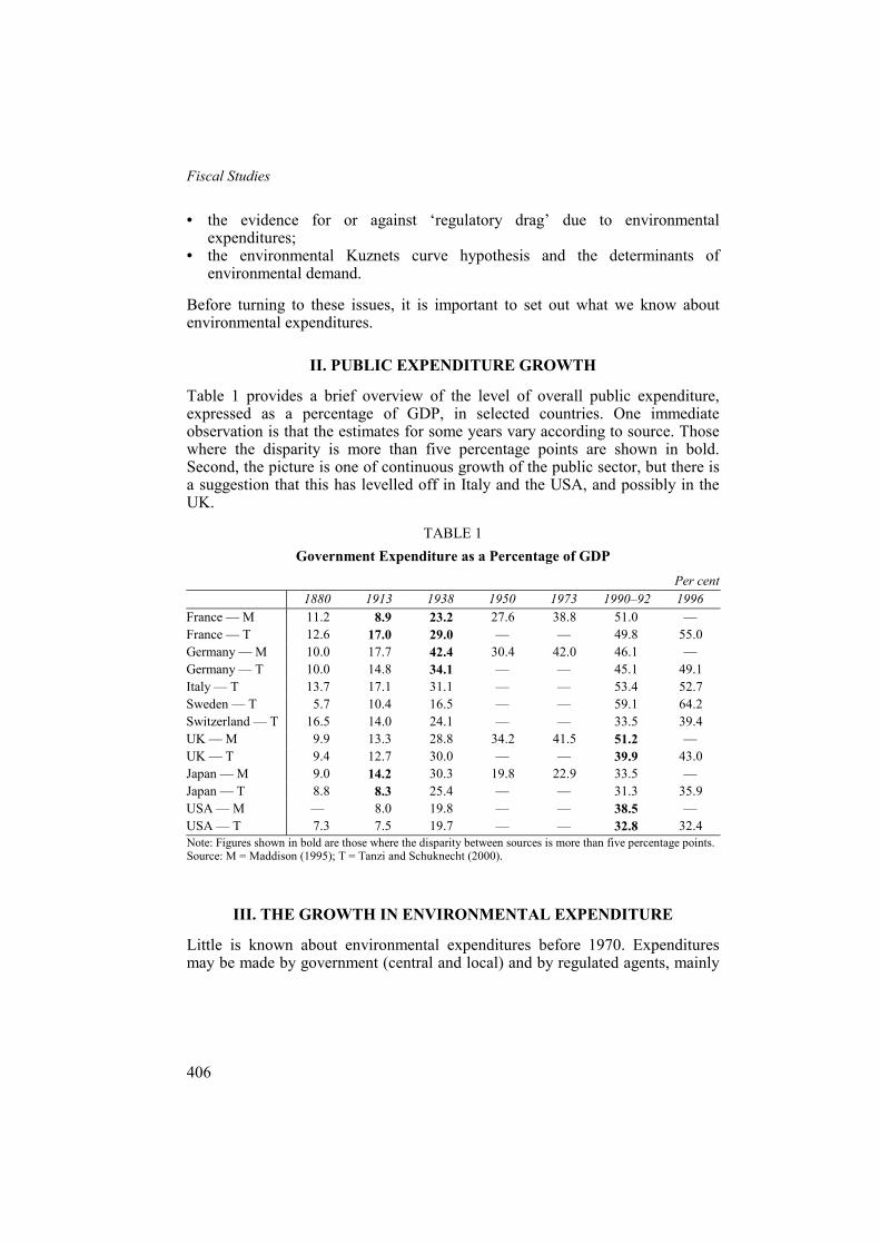
Table 1 provides a brief overview of the level of overall public expenditure, expressed as a percentage of GDP, in selected countries. One immediate observation is that the estimates for some years vary according to source. Those where the disparity is more than five percentage points are shown in bold. Second, the picture is one of continuous growth of the public sector, but there is a suggestion that this has levelled off in Italy and the USA, and possibly in the UK.
TABLE 1 Government Expenditure as a Percentage of GDP
Per cent 1880 1913 1938 1950 1973 1990–92 1996 France — M 11.2 8.9 23.2 27.6 38.8 51.0 — France — T 12.6 17.0 29.0 — — 49.8 55.0 Germany — M 10.0 17.7 42.4 30.4 42.0 46.1 — Germany — T 10.0 14.8 34.1 — — 45.1 49.1 Italy — T 13.7 17.1 31.1 — — 53.4 52.7 Sweden — T 5.7 10.4 16.5 — — 59.1 64.2 Switzerland — T 16.5 14.0 24.1 — — 33.5 39.4 UK — M 9.9 13.3 28.8 34.2 41.5 51.2 — UK — T 9.4 12.7 30.0 — — 39.9 43.0 Japan — M 9.0 14.2 30.3 19.8 22.9 33.5 — Japan — T 8.8 8.3 25.4 — — 31.3 35.9 USA — M — 8.0 19.8 — — 38.5 — USA — T 7.3 7.5 19.7 — — 32.8 32.4 Note: Figures shown in bold are those where the disparity between sources is more than five percentage points. Source: M = Maddison (1995); T = Tanzi and Schuknecht (2000).
III. THE GROWTH IN ENVIRONMENTAL EXPENDITURE
Little is known about environmental expenditures before 1970. Expenditures may be made by government (central and local) and by regulated agents, mainly
Public and Private Spending for Environmental Protection
407
corporations. The private component tends to reflect the expenditures that arise because of regulations, especially regulations that establish environmental standards. Depending on the country, standards may be set on the basis of allowable emissions, ambient concentrations of pollutants in the receiving environment or permitted technology. Technology-based standards are very common and usually centre on the notion of ‘best available technology’ (BAT) or some variant of this (Pearce, 2000). ‘Best’ here refers to technology that is regarded as suitable in terms of its environmental performance. Clearly, determining what expenditure borne by the private sector is due to the standard is complex. Strictly, it would be the difference in cost between the BAT and the technology that otherwise would have been adopted. Such cost differences are hard to estimate without knowledge of the counterfactual technology. Added complications are that there will be differential running costs and potential effects on output. In practice, very crude estimates of technology costs are used to estimate actual expenditures.
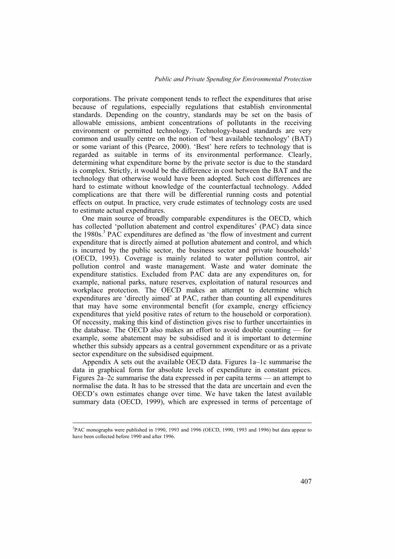
One main source of broadly comparable expenditures is the OECD, which has collected ‘pollution abatement and control expenditures’ (PAC) data since the 1980s.3 PAC expenditures are defined as ‘the flow of investment and current expenditure that is directly aimed at pollution abatement and control, and which is incurred by the public sector, the business sector and private households’ (OECD, 1993). Coverage is mainly related to water pollution control, air pollution control and waste management. Waste and water dominate the expenditure statistics. Excluded from PAC data are any expenditures on, for example, national parks, nature reserves, exploitation of natural resources and workplace protection. The OECD makes an attempt to determine which expenditures are ‘directly aimed’ at PAC, rather than counting all expenditures that may have some environmental benefit (for example, energy efficiency expenditures that yield positive rates of return to the household or corporation). Of necessity, making this kind of distinction gives rise to further uncertainties in the database. The OECD also makes an effort to avoid double counting — for example, some abatement may be subsidised and it is important to determine whether this subsidy appears as a central government expenditure or as a private sector expenditure on the subsidised equipment.
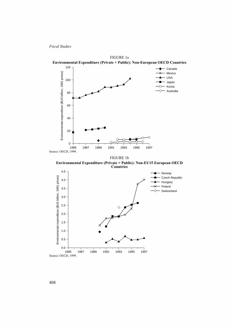
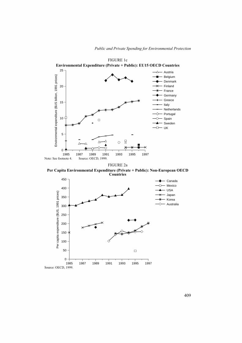
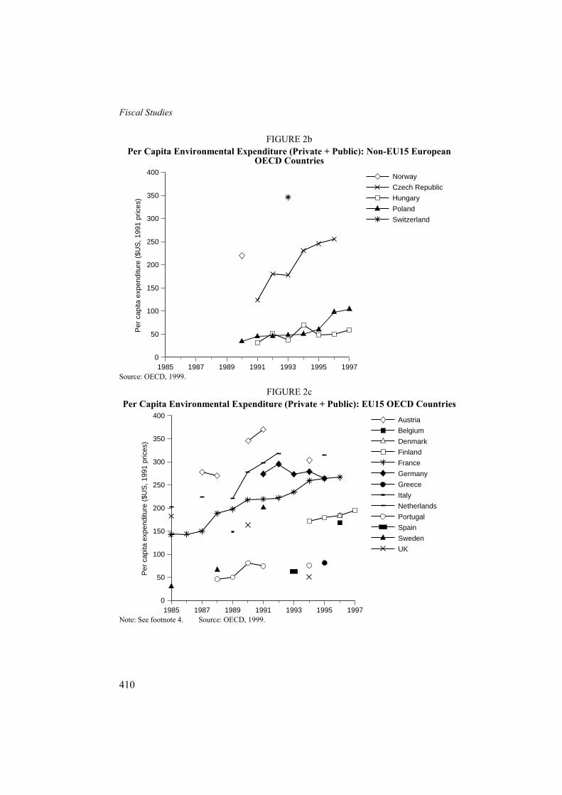
Appendix A sets out the available OECD data. Figures 1a–1c summarise the data in graphical form for absolute levels of expenditure in constant prices. Figures 2a–2c summarise the data expressed in per capita terms — an attempt to normalise the data. It has to be stressed that the data are uncertain and even the OECD’s own estimates change over time. We have taken the latest available summary data (OECD, 1999), which are expressed in terms of percentage of
3PAC monographs were published in 1990, 1993 and 1996 (OECD, 1990, 1993 and 1996) but data appear to have been collected before 1990 and after 1996.
Fiscal Studies
408
FIGURE 1a Environmental Expenditure (Private + Public): Non-European OECD Countries
Canada
Mexico
USA
Japan
Korea
Australia
Env
ironm
enta
l exp
endi
ture
($U
S b
illio
n, 1
991
pric
es)
1985
120
100
80
60
40
20
1989 1991 1995 19970
19931987 Source: OECD, 1999.
FIGURE 1b Environmental Expenditure (Private + Public): Non-EU15 European OECD
Countries Norway
Czech Republic
Hungary
Poland
Switzerland
Env
ironm
enta
l exp
endi
ture
($U
S b
illio
n, 1
991
pric
es)
1985
4.5
3.5
2.5
1.5
0.5
1989 1991 1995 19970.0
19931987
4.0
3.0
2.0
1.0
Source: OECD, 1999.
Public and Private Spending for Environmental Protection
409
FIGURE 1c Environmental Expenditure (Private + Public): EU15 OECD Countries
Austria
Belgium
Denmark
Finland
France
Germany
Greece
Italy
Netherlands
Portugal
Spain
Sweden
UK
Env
ironm
enta
l exp
endi
ture
($U
S b
illio
n, 1
991
pric
es)
1985
25
20
15
10
5
1989 1991 1995 19970
19931987 Note: See footnote 4. Source: OECD, 1999.
FIGURE 2a Per Capita Environmental Expenditure (Private + Public): Non-European OECD
Countries Canada
Mexico
USA
Japan
Korea
Australia
Per
cap
ita e
xpen
ditu
re (
$US
, 199
1 pr
ices
)
1985
450
400
300
200
150
50
1989 1991 1995 19970
19931987
350
250
100
Source: OECD, 1999.
Fiscal Studies
410
FIGURE 2b Per Capita Environmental Expenditure (Private + Public): Non-EU15 European
OECD Countries Norway
Czech Republic
Hungary
Poland
Switzerland
Per
cap
ita e
xpen
ditu
re (
$US
, 199
1 pr
ices
)
1985
400
250
150
50
1989 1991 1995 19970
19931987
350
300
200
100
Source: OECD, 1999.
FIGURE 2c Per Capita Environmental Expenditure (Private + Public): EU15 OECD Countries
Austria
Belgium
Denmark
Finland
France
Germany
Greece
Italy
Netherlands
Portugal
Spain
Sweden
UK
Per
cap
ita e
xpen
ditu
re (
$US
, 199
1 pr
ices
)
1985
400
300
200
100
50
1989 1991 1995 19970
19931987
350
250
150
Note: See footnote 4. Source: OECD, 1999.
Public and Private Spending for Environmental Protection
411
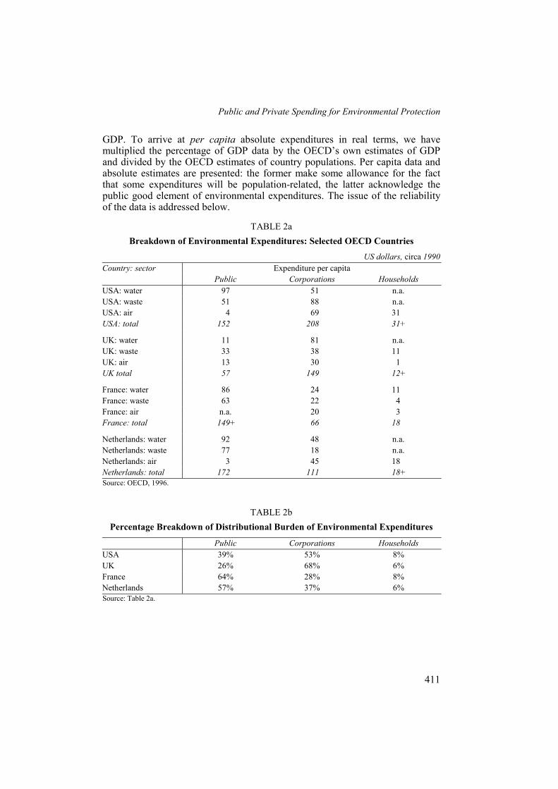
GDP. To arrive at per capita absolute expenditures in real terms, we have multiplied the percentage of GDP data by the OECD’s own estimates of GDP and divided by the OECD estimates of country populations. Per capita data and absolute estimates are presented: the former make some allowance for the fact that some expenditures will be population-related, the latter acknowledge the public good element of environmental expenditures. The issue of the reliability of the data is addressed below.
TABLE 2a Breakdown of Environmental Expenditures: Selected OECD Countries
US dollars, circa 1990 Expenditure per capita Country: sector
Public Corporations Households USA: water 97 51 n.a. USA: waste 51 88 n.a. USA: air 4 69 31 USA: total 152 208 31+
UK: water 11 81 n.a. UK: waste 33 38 11 UK: air 13 30 1 UK total 57 149 12+
France: water 86 24 11 France: waste 63 22 4 France: air n.a. 20 3 France: total 149+ 66 18
Netherlands: water 92 48 n.a. Netherlands: waste 77 18 n.a. Netherlands: air 3 45 18 Netherlands: total 172 111 18+ Source: OECD, 1996.
TABLE 2b Percentage Breakdown of Distributional Burden of Environmental Expenditures
Public Corporations Households USA 39% 53% 8% UK 26% 68% 6% France 64% 28% 8% Netherlands 57% 37% 6% Source: Table 2a.
Fiscal Studies
412
The OECD data are largely confined to water pollution control, air pollution control and waste management.4 Table 2 gives approximate orders of magnitude for the sectoral breakdown of expenditures for selected OECD countries. Some patterns are discernible. First, the household sector typically bears a small cost burden relative to the corporate and government sectors, ignoring, of course, the role of household taxation in financing government expenditure. The US household sector bears a much higher burden than that in the European countries shown, due to the US procedure of allocating vehicle emission abatement to vehicle purchasers, i.e. including households. Otherwise, household burdens appear fairly consistent across the different countries.
Second, corporate expenditures are higher in the USA and the UK, but lower in the Netherlands and France. The OECD offers no clues as to why this is the case.
Third, the US expenditures total around $400 per capita, the Netherlands totals around $300 per capita, and France and the UK total around $200 per capita each. Arguably, this pattern reflects popular perceptions of the relative strengths of environmental concern in the different countries, an issue to which we return.
Fourth, there are some environmental sectoral rankings. Water pollution is ranked first in terms of public expenditure in three of the four countries, and again (just) for three of the four countries in terms of corporate expenditure. Waste tends to be the next most important category, with the exception of the Dutch corporate burden.
European Union data are assembled by EUROSTAT5 for the period 1988 to 1996. Prior to 1988, some estimates are available in ERECO (1993). Appendix B summarises the relevant information. Unfortunately, the quality of the EUROSTAT data is very poor, and the database has not been used in what follows.6 We have also investigated UK data, and Appendix C summarises what is known about that information. UK estimates of environmental expenditure exist for only a few years and are biased towards expenditure by the corporate sector. Only one attempt appears to have been made to collect estimates for overall levels of expenditure beyond pollution abatement and embracing all sectors (UK Department of the Environment, 1992). Again, therefore, we make use of these data only to the extent that they help illuminate issues arising as we proceed.7
4The figures for the UK (Figures 1c and 2c) show a marked downturn in environmental expenditure in the 1990s. We consider this to be the result of a misprint in the original OECD documents: 0.3 per cent of GDP should read 1.3 per cent. We have not changed the figure here. 5At www.europa.eu.int/comm/eurostat. 6Not only are the data poor, but the presentation of the data is poor: columns in tables are mislabelled, no indication is given as to whether estimates are in current or constant prices, and terminology is not explained. EUROSTAT’s website simply adds to the confusion. 7Data on environmental expenditure in developing countries are sparse — see Appendix D.
Public and Private Spending for Environmental Protection
413
IV. HOW RELIABLE ARE ENVIRONMENTAL EXPENDITURE DATA?
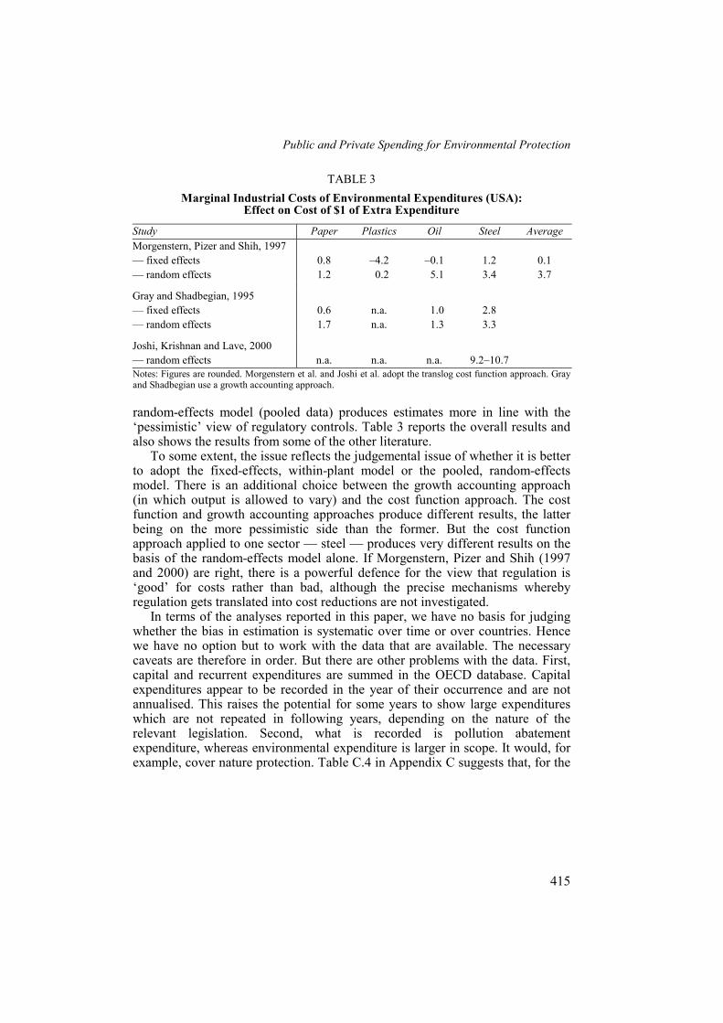
One reason for the comparative absence of econometric exercises involving environmental expenditures could be that analysts have judged the data to be unreliable. There appear to be no exercises testing for data reliability outside of the USA. The US studies are enabled by the collection of reasonably consistent and regular data using the PACE system (pollution abatement and control expenditures) by the US Census Bureau. The US studies relate only to private, corporate expenditures and produce ambiguous answers. Joshi, Krishnan and Lave (2000) suggest that environmental expenditures in the US steel industry are grossly underestimated by a factor of around 10. On the other hand, Morgenstern, Pizer and Shih (1997 and 2000) suggest that, for a wide range of manufacturing industries, reported costs are overestimates of true costs.
The obvious starting point for an analysis is to compare the ‘correct’ notion of cost with what is reported in the statistics. What get reported tend to be expenditures that industry regards as being due to environmental legislation. But these can obviously differ from true economic costs for various reasons. Economic cost would be measured by the change in the combined sum of producers’ and consumers’ surplus. Any lost consumer surplus element is obviously omitted by industrial reporting. Changes in producers’ surplus may also be problematic. If the expenditure takes the form of capital equipment, there may be some negative effect on other capital investments. Public capital expenditure could crowd out private investment generally, and private environmental expenditure could compete for limited capital funds at the corporate level. Hence some analysts regard the true cost of environmental expenditure as involving forgone long-run profitability and economic growth due to these crowding-out effects. There may also be ‘new source bias’ whereby mandated standards relate to new plant but perversely exempt old plant, discouraging investment in new, more efficient technology. Conventional operational costs may also rise due to the impact of the abatement measure on operating efficiency (for example, sulphur emission controls may lower energy conversion efficiency). Clearly, there are a fair number of ways in which environmental expenditures may have negative impacts on cost structures. This has been the presumption in the literature that tries to assess ‘true’ control costs, and has also been instrumental in the literature on the relationship between environmental policy and economic growth and productivity.
There are reasons for supposing that there may be offsetting factors that lower rather than raise costs. First, mandated expenditures may raise awareness within the corporation about ways of saving costs on energy and materials. This is more likely to be the case when regulations permit process changes rather than add-on abatement equipment (Morgenstern, Pizer and Shih, 1997 and 2000). Potentially more significant, and emphasised in the literature on corporate environmental management, is the complementarity between profit and
Fiscal Studies
414
environmental expenditure in contexts where firms are not operating on the production possibility frontier. The most famous example of this view is attributed to Porter (1990 and 1991) and Porter and van der Linde (1995a and 1995b). The ‘Porter hypothesis’ is not clear-cut, but is generally taken to imply that firms are not operating at full efficiency and that some form of regulation acts as a catalyst that makes firms realise more productive potential through resource efficiency. This is the familiar ‘win–win’ argument in the corporate environmental literature. The corporate environmental accounting literature has tended to suggest some balance of effects, i.e. a proper reporting of the wider costs and the offsetting gains that may accrue (Schaltegger and Burritt, 2000).
Morgenstern, Pizer and Shih (1997 and 2000) estimate translog cost functions (Heathfield and Wibe, 1987) for selected US manufacturing industries based on 800 separate plants. Inputs include capital, labour, energy, materials and environmental abatement effort. Abatement effort is assumed to be fixed in the sense that expenditures are determined exogenously by regulation, and output is also assumed to be fixed, i.e. varying output in response to environmental regulation is not an option. The full effects of regulation should then show up in raised costs. Morgenstern et al. stress the need to allow for differences in productivity between plants — differences that, in their view, are unlikely to be caused by environmental regulations (inter-plant variation is affected by factors such as location). Hence they opt for models that involve not pooling the data but separately estimating within-plant effects. They find that pooled effects produce larger estimates of regulatory impacts on costs, whereas the expectation should be that the longer-run effects would be smaller. The authors focus on the marginal cost of regulation rather than the overall cost impact, i.e. on
[ ]C CR R
α β∂ = +∂
X ,
where C is cost, R is regulatory expenditure, X is a vector of log output, regulatory expenditure and input prices, and α and β are the parameters to be estimated.
Based on Morgenstern et al.’s fixed-effects model (i.e. the non-pooled data), the results suggest that the industry average effect of a dollar of regulatory expenditure is to raise costs by just $0.13, i.e. there are $0.87 of offsetting gains. For steel, there is a net increase in costs of $1.16, but this is far lower than the effect found in other studies — for example, Joshi, Krishnan and Lave (2000). For plastics, there are net reductions in costs — a $4 saving — i.e. something like the Porter hypothesis is at work on this industry. For petroleum, environmental expenditures are fairly neutral, i.e. each dollar of regulatory expenditure is associated with an offsetting dollar of savings. Finally, for pulp and paper, the additional cost is $0.82. Note, however, that Morgenstern et al.’s
Public and Private Spending for Environmental Protection
415
TABLE 3 Marginal Industrial Costs of Environmental Expenditures (USA):
Effect on Cost of $1 of Extra Expenditure
Study Paper Plastics Oil Steel Average Morgenstern, Pizer and Shih, 1997 — fixed effects — random effects
0.8 1.2
–4.2
0.2
–0.1
5.1
1.2 3.4
0.1 3.7
Gray and Shadbegian, 1995 — fixed effects — random effects
0.6 1.7
n.a. n.a.
1.0 1.3
2.8 3.3
Joshi, Krishnan and Lave, 2000 — random effects
n.a.
n.a.
n.a.
9.2–10.7
Notes: Figures are rounded. Morgenstern et al. and Joshi et al. adopt the translog cost function approach. Gray and Shadbegian use a growth accounting approach.
random-effects model (pooled data) produces estimates more in line with the ‘pessimistic’ view of regulatory controls. Table 3 reports the overall results and also shows the results from some of the other literature.
To some extent, the issue reflects the judgemental issue of whether it is better to adopt the fixed-effects, within-plant model or the pooled, random-effects model. There is an additional choice between the growth accounting approach (in which output is allowed to vary) and the cost function approach. The cost function and growth accounting approaches produce different results, the latter being on the more pessimistic side than the former. But the cost function approach applied to one sector — steel — produces very different results on the basis of the random-effects model alone. If Morgenstern, Pizer and Shih (1997 and 2000) are right, there is a powerful defence for the view that regulation is ‘good’ for costs rather than bad, although the precise mechanisms whereby regulation gets translated into cost reductions are not investigated.
In terms of the analyses reported in this paper, we have no basis for judging whether the bias in estimation is systematic over time or over countries. Hence we have no option but to work with the data that are available. The necessary caveats are therefore in order. But there are other problems with the data. First, capital and recurrent expenditures are summed in the OECD database. Capital expenditures appear to be recorded in the year of their occurrence and are not annualised. This raises the potential for some years to show large expenditures which are not repeated in following years, depending on the nature of the relevant legislation. Second, what is recorded is pollution abatement expenditure, whereas environmental expenditure is larger in scope. It would, for example, cover nature protection. Table C.4 in Appendix C suggests that, for the
TAB
LE 4
Pr
ivat
e En
viro
nmen
tal E
xpen
ditu
re a
s a P
erce
ntag
e of
Tot
al E
nvir
onm
enta
l Exp
endi
ture
: Sel
ecte
d O
ECD
Cou
ntri
es
19
85
1986
19
87
1988
19
89
1990
19
91
1992
19
93
1994
19
95
1996
19
97
Aus
tralia
33
.3
50.0
44
.4
37.5
37
.5
37.5
Aus
tria
44.4
41
.2
45
.0
42.9
41
.2
C
anad
a
33
.3
36.4
45
.5
Cze
ch R
epub
lic
73.7
66
.7
66.7
66
.7
Fi
nlan
d
45.5
54
.5
45.5
45
.5
Fran
ce
33.3
33
.3
33.3
27
.3
27.3
41
.7
33.3
33
.3
30.8
35
.7
28.6
28
.6
G
erm
any
43.8
41
.2
43.8
43
.8
46.7
W
est G
erm
any
53.3
50
.0
50.0
50
.0
50.0
50
.0
43.8
43
.8
40.0
46
.7
42.9
H
unga
ry
71
.4
40.0
33
.3
33.3
50
.0
Ja
pan
10.0
9.1
9.1
9.1
18.2
Kor
ea
50
.0
46.7
46
.7
46.7
50
.0
41.2
N
ethe
rland
s 28
.6
40
.0
35
.7
47.1
38
.9
36.8
27
.8
Pola
nd
71
.4
80.0
60
.0
60.0
70
.0
72.7
64
.7
64.7
Po
rtuga
l
20.0
20
.0
12.5
14
.3
14.3
UK
46
.2
60.0
USA
64
.3
57.1
57
.1
57.1
57
.1
60.0
53
.3
53.3
60
.0
56.3
Sour
ce: O
ECD
, 199
9.

Public and Private Spending for Environmental Protection
417
UK, pollution control expenditures constitute around 60 per cent of the total of environmental expenditures. Third, the focus in the OECD data is on government and corporations and it is unclear how far household expenditures are adequately covered. Appendix C looks at this issue in the context of UK data.
V. IS THERE A SHIFT TO PRIVATE CONTROL EXPENDITURE?
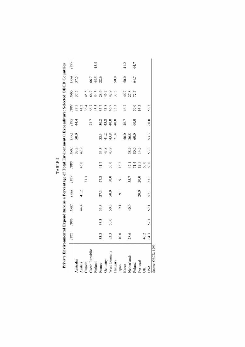
The first question we raised was the extent to which environmental public goods originally provided by the public sector were now provided by the private sector, albeit on an ‘involuntary’ basis through regulation. We hypothesised that this shift would occur because of the concerns in recent decades to reduce the size of public expenditure generally and to shift regulation towards ‘voluntary and negotiated agreements’ and because of privatisation. However, the OECD data do not readily support the idea that there has been a significant shift away from the public provision of environmental goods to their private provision. Table 4 summarises the public/private mix of environmental protection expenditure between 1985 and 1997 for those OECD countries with data covering two or more years. Japan and Portugal have by far the lowest levels of private environmental expenditure as a proportion of total environmental expenditure. Perhaps surprisingly, the former communist countries of Eastern Europe, such as Poland and the Czech Republic, have the highest relative levels of private environmental expenditure. From the mid-1980s to the mid-1990s, France, Germany,8 the Netherlands and the USA all experienced declines in private environmental expenditure as a proportion of total environmental spending. Hence, during this period, public environmental expenditure increased at a faster rate than private expenditure, which suggests that the burden of environmental protection is not shifting away from the public to the private sector as expected. Equally, we are unable to say if this is a genuine trend, because of the poor quality of the data.
VI. ARE ENVIRONMENTAL EXPENDITURES A DRAG ON ECONOMIC GROWTH?
A common argument that may help to mobilise lobbies against environmental expenditures is that they act as a ‘drag’ on industrial competitiveness and hence economic growth. The argument is potentially most powerful in the context of legislation that imposes costs on the private sector, but there is also a weaker link in terms of public expenditures as a means of ‘crowding out’ private investment and hence productivity.
While it is not always clear what is meant by competitiveness, it has at least two components: ‘macro’-competitiveness (i.e. the competitiveness generally of 8West Germany until 1991, and then Germany including the former East Germany.
Fiscal Studies
418
any nation vis-à-vis other countries and trading blocs) and sectoral competitiveness (i.e. competition between sectors within a nation). Macro-competitiveness is frequently invoked in discussions about environmental policy. However, it is not clear how this form of competitiveness can be damaged by environmental regulation so long as the relevant competition is between countries with flexible exchange rates. The effect of any cost changes in one country, even assuming they were significant, would feed through changes in exchange rates, not through loss of market share.
There are several comprehensive surveys of the effects of environmental regulation generally on macro-competitiveness. Various tests of the proposition that environmental expenditures affect competitiveness negatively have been considered:
• the extent to which net exports of environmentally regulated goods change with regulations, or the extent to which net exports of environmentally regulated goods perform less well than those of less regulated goods;
• the extent to which firms facing heavy regulation locate outside the regulating country (the ‘pollution haven hypothesis’);
• the extent to which investment occurs away from strictly regulating countries; and
• the extent to which productivity is affected by regulation.
Net exports have not been found to be significantly affected by regulations (Jaffe et al., 1995; Sorsa, 1994). Corporations’ location decisions are generally unaffected by environmental costs, primarily because they tend to be a small fraction of total costs (Jaffe et al., 1995; Eskeland and Harrison, 1997). There is no evidence that firms invest more abroad in pollution-intensive industries to compensate for higher environmental costs at home (Eskeland and Harrison, 1997; World Bank, 1999).
1. The ‘Porter Hypothesis’ The idea that regulation may improve competitiveness is associated with Michael Porter and the ‘Porter hypothesis’ (Porter, 1990a, 1990b and 1991; Porter and van der Linde, 1995a and 1995b). There is some doubt as to what the Porter hypothesis is meant to be. For example, it seems fairly clear that Porter does not think that any form of environmental regulation will induce cost reductions and competitiveness gains. Seemingly, only regulations that focus on prevention rather than amelioration or end-of-pipe technology will have this effect. Also there is the suggestion that the regulations should be market-based rather than in the traditional command-and-control mode. If so, then the hypothesis may not differ much from the traditional advocacy of most
Public and Private Spending for Environmental Protection
419
environmental economists in favour of market-based instruments such as taxes and tradable quotas.
What are the mechanisms through which the Porter hypothesis is supposed to operate? The general context is clearly intended to be bounded rationality: firms simply do not operate like neo-classical optimisers with perfect information. Accordingly, somehow illuminating an area where the ‘mental account’ of resource efficiency is located should induce some sort of ‘win–win’ solution whereby costs are reduced and environmental quality improved. Jaffe, Newell and Stavins (2000) suggest that Porter has five mechanisms in mind: (a) regulation forces attention to be paid to wastefulness; (b) regulation requires information to be generated and information has public good characteristics that mean it is likely to be undersupplied; (c) regulation reduces uncertainty about the returns that can be secured from innovations in environmental technology; (d) there is a first mover advantage in having high standards and responding to them, since other countries are likely to develop such standards later on; and (e) most generally, regulation creates a climate of thinking about innovation. As Jaffe et al. (2000) note, none of these mechanisms is uncontroversial. For example, regulation may create information but it is unclear if governments have better claims to know about the missing information than firms. (Indeed, most modern approaches resting on asymmetric information assume the opposite.) More to the point, adopting cost-reducing technologies does not necessarily mean that the adoption process has passed a cost–benefit test from the firm’s point of view. Finally, a point not made in the literature but that seems worth stating is that ‘win–win’ theorems are undeniably popular and are not confined to this aspect of corporate behaviour. Win–win solutions may be illusory but politically attractive because they hold out the prospect of facing real and potentially painful trade-offs.
One can imagine other mechanisms being at work that could provide indirect support for the Porter view. More regulation benefits firms manufacturing environmental compliance equipment. This is important because markets for pollution control technology and services are projected to rise well into the hundreds of billions of dollars in the next decade. Or it may be that firms finding it easy to comply with regulations squeeze out those that find it less easy to comply, increasing the market share of the lower-cost firms. Those who anticipate market changes — for example, to smaller more-fuel-efficient vehicles — might gain. There may be other benefits — as environmental concerns become ‘globalised’, so the green image of corporations is becoming internationally important. This raises the possibility that market share can be increased through environmental credentials, a benefit likely to accrue to first movers only, as Porter surmises. Similarly, environmental standards in the so-called ‘lax environmental standard’ countries are in fact rising rapidly, which is one of the reasons why the pollution haven hypothesis is not fulfilled. Again, those making first moves in strict environmental compliance could secure export
Fiscal Studies
420
market share because they are already locked into clean technology suitable for the expanding markets in comparison with their competitors.
Overall, however, most economists have been very sceptical of the Porter hypothesis. If it were true, it would imply that corporations are very ignorant of the potential for cost reductions and that they require the stimulus of regulation to recognise such opportunities. This seems fairly unlikely (Jaffe et al., 1995; Oates, Palmer and Portney, 1994). Sorsa (1994) finds no evidence to suggest that rising standards improve competitiveness. Whereas Porter and van der Linde (1995a) cite case studies to support their propositions, Oates et al. survey the same corporations, and others, and find that they generally regarded the adopted clean technology as imposing a net cost on them, not a net benefit.9
2. Productivity Effects Most studies find that US productivity has been negatively affected by environmental regulation. The rate of growth of total factor productivity (i.e. output per unit of all inputs) has been lower in the USA than in other major countries such as Japan and Europe. Considerable efforts have therefore gone into trying to explain this comparatively poor performance. The comparatively strict environmental legislative regime in the USA has often been cited as a major, and sometimes the major, factor in explaining this difference. The issue can be addressed in three phases:
• Stage 1: Assess the evidence that conventionally measured output per unit input is adversely affected by environmental regulation as historically practised.
• Stage 2: Assess what the effect would have been had the environmental regulation taken a different form, especially through more widespread adoption of market-based approaches. The USA has made extensive use of strict command-and-control regulations combined with an excessively bureaucratic and litigious liability system (Stewart, 1993). The US experience of negative productivity effects may not therefore be generalisable.
• Stage 3: Assess whether the measure of productivity used in the literature is in fact the right measure. In particular, what happens when the negative economic impacts of environmental degradation are taken into account?
As Repetto et al. (1996) note, the effect of environmental regulation on productivity must be negative, almost by definition. Most environmental regulation in advanced economies has been based on technological standards such as ‘best available technology’. Hence any regulation forces firms to
9Albrecht (1999) does find some support for the Porter hypothesis in the context of the chlorofluorocarbon industry (CFCs). CFCs have been severely regulated via national implementation of the Montreal Protocol. Du Pont was an early mover in switching out of CFCs into substitutes and gained market share.

Public and Private Spending for Environmental Protection
421
purchase abatement technology, which is not productive in the sense of contributing to the firm’s output. Hence output must be less than it otherwise would have been if the resources used for abatement were allocated to productive uses. Costs rise and there is no offsetting increase in output. This conclusion need not follow if the measures used to reduce pollution themselves contribute to productivity, an issue addressed earlier in the context of the reliability of environmental expenditure data.
Table 5 lists the more recent studies on the links between regulation and productivity (the literature goes back to the 1970s). Notably, most of the studies again relate to the USA. Most also use a specific dataset on pollution control expenditures. As noted earlier, one study, by Morgenstern, Pizer and Shih (1997
TABLE 5 Studies of the Effects of Environmental Regulation on (Conventionally Measured)
Productivity
Study Country Effect of environmental regulation Barbera and McConnell, 1990
USA 10–30 per cent of reduced productivity growth 1970–80 compared with 1960–70 due to environmental regulation
Jorgensen and Wilcoxen, 1990
USA GNP growth lower than would have been 1973–85, by 0.07 of a percentage point due to mandated environmental investments and by 0.3 of a percentage point due to environmental operating costs
Conrad and Morrison, 1989
Canada, Germany
Negative effects
Nestor and Pasurka, 1994
Japan, Germany
Negative effects
Joshi, Krishnan and Lave, 2000
USA steel-making
For 1995, each $1 of environmental expenditures raises (marginal) cost of production by $7–12
Gray and Shadbegian, 1993 and 1995
USA pulp/paper, oil refineries, steel
Each $1 of environmental expenditures raises (marginal) cost of production by $3–4; less effect found in the later paper
Robinson, 1995
USA manufacturing
‘Significant negative effect’
Morgenstern, Pizer and Shih, 1997 and 2000
USA Each $1 of environmental expenditure raises (marginal) cost of production by $0.13 (note the contrast with previous studies); range is minus $1 to plus $1.25
Bruvoll, Glomsrod and Vennemo, 1995
Norway Negligible impact on economic growth rates (less than 0.1 of a percentage point)
Fiscal Studies
422
and 2000), produces markedly different results from the other studies. It suggests that each dollar of environmental expenditure raises production costs by only 13 cents. This may be compared with up to $12 in previous studies. Indeed, the Morgenstern et al. (1997) study has a lower limit of –$1, i.e. each dollar of expenditure saves $1 of cost. Morgenstern et al. suggest their result arises because the other studies assume that plants are homogeneous, i.e. that the effects on productivity will be the same regardless of plant age, location and management. Once heterogeneity is assumed, the negative productivity effects fall dramatically.
As far as the Stage 1 question goes, then, the literature seems overwhelmingly to support the view that conventional productivity measures are negatively affected by environmental expenditures. But this result could be peculiar to the USA and could arise from a highly restrictive assumption about the nature of the factors affecting productivity at the plant level.
The next stage asks whether a different configuration of environmental policy would have the same negative effects on productivity as might be suggested by the conventional literature. In particular, if policy had been driven by market-based approaches, would the effects have been the same? Surprisingly, little analysis seems to have been carried out on this question. This raises the possibility that, if there are negative productivity effects, they arise because policy has simply been inefficient. The reasons for supposing that market-based instruments (MBIs) would produce markedly lower impacts on productivity are now well known. First, the flexibility introduced by MBIs means that firms can adopt cost-minimising strategies to comply with regulations. Tietenberg (2000) suggests that traditional policies range from being 2 to 22 times more expensive than MBI-based policies. Even a modest ‘multiplier’ of 2 would have a dramatic effect on the analysis of productivity effects. Second, MBIs probably have a dynamic effect on abatement technology, markedly reducing its cost due to the incentive to avoid taxes or buy tradable permits. Thus abatement technology itself would be cheaper under an MBI system.
A further feature of prevailing policy is that it might not pass a cost–benefit test, i.e. it might be inefficient anyway. Hahn (1996) finds that only 18 per cent of 92 US regulations pass a cost–benefit test. Only 19 per cent of the US Environmental Protection Agency’s regulations pass such a test. Unfortunately, there is no comparable information for other countries. But it can be conjectured that the result may not be very different. If so, any negative productivity effects of environmental regulation may reflect the inefficiency of the way policy is implemented, rather than policy per se.
Even if negative productivity effects are an issue, the final concern is whether productivity is being correctly measured. Repetto et al. (1996) measure the damages of the environmental impacts arising from economic activity and then deduct them from the output measure. Viewed from another standpoint, regulation will have environmental benefits which should be added to the
Public and Private Spending for Environmental Protection
423
conventional productivity measure. Undertaking studies of the US electricity industry, pulp and paper industry and farming, Repetto et al. find that conventional measures of the change in productivity for the period from 1970 to the early 1990s were –0.35 per cent, +0.16 per cent and +2.3 per cent respectively. But the revised productivity measures allowing for the benefits of environmental improvement are +0.68 per cent, +0.44 per cent and +2.41 per cent. For electricity and paper, then, the proper measurement of productivity makes a stark difference. There is a general lesson here for the current concern to focus on ‘resource productivity’ (i.e. increases in the ratio of output to resource inputs). An unduly narrow focus on, say, GDP as the output measure tends to miss the central point that the main importance of resource productivity lies in its bilateral environmental effects — reducing the rate of use of resources and the corresponding reduction in emissions from producing the output.10 It is these effects, valued at the relevant shadow environmental prices, that are likely to justify the focus on resource productivity policies.
VII. IS THERE EVIDENCE OF AN ENVIRONMENTAL KUZNETS CURVE FOR ENVIRONMENTAL EXPENDITURE?
The environmental Kuznets curve (EKC) hypothesis suggests that there is an inverted U-shaped curve for environmental quality when measured against income per capita. In economies at the beginning of an economic development process, one might expect the resources allocated to environmental conservation to be limited. Essentially, environment is sacrificed in the name of economic growth or, put another way, natural capital is depleted and substituted by other factors of production, especially man-made capital. After a point, however, the demand for environmental quality grows and this eventually results in the pollution–income curve peaking and then turning down; further increases in per capita income are associated with reductions in pollution. There is an extensive literature testing for the presence of EKCs. Early analyses suggested strong relationships between income and pollution (for example, Grossman and Krueger (1995)) but more recent work (for example, Harbaugh, Levinson and Wilson (2000)) has questioned the early findings. EKCs appear to be less obviously present once attention focuses away from ‘conventional’ pollutants towards various natural resources and more ‘modern’ pollutants such as carbon dioxide.
Explanations for the shape of the EKC abound. Generally, the following features of the growth process might be expected:
10Indeed, the contribution of resource productivity to overall productivity is likely to be small. Growth accounting approaches based on generalised production functions would make the contribution dependent on (a) the rate of change in resource productivity and (b) the share of natural resources in GDP. For other than resource-rich countries, the latter will tend to be small.
Fiscal Studies
424
(a) Rising per capita income will ‘drag through’ more materials and energy consumption and hence more waste — environmental quality will, without policy action, decline as income grows.
(b) A change in the structure of output will, after a point at least, reduce impacts per unit GNP. Additionally, pollution-intensive processes may be exported from rich to poor countries (Suri and Chapman, 1998) — pollution could effectively be ‘exported’.
(c) A change in the demand for the environment will, if the environment is income-elastic, translate into policy measures. Such policy measures require advanced institutions and, in turn, these institutions tend to evolve only in richer countries.
(d) A change in technology will occur as growth induces capital replacement that embodies technologies with lower environmental impact.
On this analysis, the question is how far (c) and (d) and the benign aspects of (b) offset the effects of (a) and the damaging effects of (b). The EKC literature does not, in fact, resolve this issue, since most of it contents itself with a straightforward link between income and environmental degradation. Only limited efforts have been made to ‘decompose’ the relationship in terms of factors (a)–(d) above. What is tested tends to have the general form
2
it it it
it it it
E Y Ya b cPOP POP POP
ε
= + + +
or
2
it itit
it it
Y YE a b cPOP POP
ε
= + + +
,
where E is the environmental change variable (emissions, change in land cover of forests etc.), Y is GNP, POP is population, t is time, i is location, a, b and c are parameters to be estimated and ε is an error term. The squared term reflects the expected shape of the EKC. Note that the first equation has the dependent variable as per capita environmental change and the second equation has absolute environmental change. Differentiating either equation with respect to Y/POP gives
*
2Y b
POP c = −
,
Public and Private Spending for Environmental Protection
425
where (Y/POP)* is the turning-point of the inverted U, i.e. the point at which environmental impact per capita or absolute environmental degradation declines with income per capita.11
Some authors provide other explanations of inverted U-shaped curves. Andreoni and Levinson (2001) show that the EKC can result from a simple model in which individual well-being is a positive function of consumption and a negative linear function of pollution, and in which pollution is a linear function of consumption and a negative function of abatement. The essence of the model is that the abatement function has increasing returns to scale. The authors suggest that this is typical of abatement expenditures and that their model embraces other models, including those that posit ‘political economy’ relationships involving various stakeholders in society, some demanding more abatement, some demanding less.
While the competing explanations for the shape of the EKC are interesting, implicit in the EKC is the notion that one of the factors producing the downturn in the curve, if the curve itself is identifiable, is the rise in the demand for environmental goods as income goes beyond the peak. This holds whether the explanatory model is a simple evolutionary model of how economies behave over time or a political economy model involving interest groups. This suggests that the demand for the environment is income-elastic. Due to data limitations — namely, the general absence of expenditure data for poorer countries — we cannot identify a ‘full’ EKC. But we can investigate the relationship between environmental expenditure and income for richer countries. More specifically, we can look at the elasticity of expenditure with respect to income. It is important to note that the conventional notion of an income elasticity of demand relates to private goods, while the relevant notion in the current context is that of a quantity-rationed public good. Essentially, public goods are exogenous to household and corporate decisions. Hence the relevant income elasticity is what has been called in the literature the ‘price flexibility of income’ (Randall and Stoll, 1980) or the ‘income elasticity of virtual price’ (Hanemann, 1991), the ‘income elasticity of willingness to pay’ (Flores and Carson, 1997), the ‘income elasticity of environmental value’ and the ‘income elasticity of environmental improvement’ (Kristrom and Riera, 1996). Appendix E sets out the basic relationships. The main point of relevance is that the elasticity of willingness to pay with respect to income is equal to the ratio of the conventional income elasticity of demand to the (negative) of the price elasticity of demand. In other words,
11There is a debate as to the functional form of the EKC. Some authors argue that cubic equations fit rich-country data better so that the declining section of the inverted U is followed by a further rising section — see, for example, Magnani (2000).

Fiscal Studies
426
YW
P
εεε
=−
,
where ε is elasticity and the subscripts denote willingness to pay with respect to income (W), quantity with respect to income (Y) and quantity with respect to price (P).
There are several views about the expected size of εW. Garrod and Willis (1999) argue that short-run price elasticities for environmental goods are less than one and income elasticities are positive and often greater than one. The latter finding is consistent with the intuition that ‘the environment’ is a luxury good (i.e. a normal good with conventional income elasticity greater than unity). Hence εW will be significantly greater than one in the short run and, arguably, smaller in the long run as price elasticities rise. Flores and Carson (1997) show that the size of εW cannot be determined from the size of εY (as is clear from the equation above) and offer no empirical support for small or large values. Kristrom and Riera (1996) analyse contingent valuation studies of environmental change12 and conclude that εW is less than one, i.e. the ‘consumption’ of environmental goods accounts for a higher proportion of income of the poor than of the rich. If they are right, then ‘environment’ is a normal good but not a luxury good, contradicting the usual intuition about the demand for environmental quality.
We seek to offer some further evidence of relevance to this debate by estimating the income elasticity of environmental expenditure using the OECD database. To our knowledge, this is the first time that environmental expenditure data have been used for this purpose. Magnani (2000) purports to carry out such an exercise but has mistakenly used OECD data on environmental research and development (R&D) expenditures rather than the aggregate expenditure on environmental protection. Even if the data for R&D expenditures were reliable (what constitutes R&D expenditure is open to considerable interpretation), these expenditures add up to a few tens of millions of dollars in most OECD countries, and a few hundred millions in France, the UK, Japan and the USA. In the UK, for example, OECD-recorded R&D expenditures are around $180 million, compared with total environmental protection expenditures of over $12,000 million. In other words, Magnani’s analysis relates to expenditures that constitute between 1 and 2 per cent of total pollution abatement expenditures (and even less if the total relates to environmental protection generally).
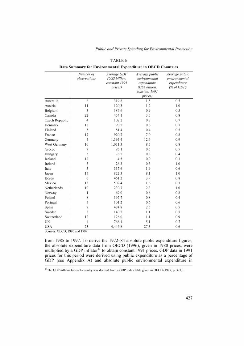
Table 6 summarises the available GDP and public environmental expenditure data. The data are derived from two OECD papers (OECD, 1996 and 1999). The earlier one contains data from 1972 to 1984, while the later one contains data 12Contingent valuation studies elicit measures of willingness to pay directly via questionnaires, so that the resulting values can be related to socio-economic characteristics of respondents, such as income.
Public and Private Spending for Environmental Protection
427
TABLE 6 Data Summary for Environmental Expenditure in OECD Countries
Number of observations
Average GDP (US$ billion,
constant 1991 prices)
Average public environmental
expenditure (US$ billion,
constant 1991 prices)
Average public environmental
expenditure (% of GDP)
Australia 6 319.8 1.5 0.5 Austria 11 120.3 1.2 1.0 Belgium 3 187.6 0.9 0.5 Canada 22 454.1 3.5 0.8 Czech Republic 4 102.2 0.7 0.7 Denmark 18 90.5 0.6 0.7 Finland 5 81.4 0.4 0.5 France 17 920.7 7.0 0.8 Germany 5 1,395.4 12.6 0.9 West Germany 10 1,031.3 8.5 0.8 Greece 7 93.1 0.5 0.5 Hungary 5 76.5 0.3 0.4 Iceland 12 4.5 0.0 0.3 Ireland 3 26.3 0.3 1.0 Italy 3 337.6 1.9 0.6 Japan 15 822.3 8.1 1.0 Korea 6 461.2 3.9 0.8 Mexico 13 502.4 1.6 0.3 Netherlands 10 230.7 2.3 1.0 Norway 1 69.0 0.6 0.8 Poland 8 197.7 0.8 0.4 Portugal 7 101.2 0.6 0.6 Spain 7 474.8 2.5 0.5 Sweden 3 140.5 1.1 0.7 Switzerland 12 126.0 1.1 0.9 UK 4 766.4 5.1 0.7 USA 23 4,446.8 27.3 0.6 Sources: OECD, 1996 and 1999.
from 1985 to 1997. To derive the 1972–84 absolute public expenditure figures, the absolute expenditure data from OECD (1996), given in 1980 prices, were multiplied by a GDP inflator13 to obtain constant 1991 prices. GDP data in 1991 prices for this period were derived using public expenditure as a percentage of GDP (see Appendix A) and absolute public environmental expenditure in 13The GDP inflator for each country was derived from a GDP index table given in OECD (1999, p. 321).
Fiscal Studies
428
constant 1991 prices. For the period 1985–97, absolute public environmental expenditure was derived in the same way as described in Section III to get Figures 1a–1c, except that the percentage of GDP for public environmental expenditure was used only. GDP data for this period were also obtained from OECD (1999) using a GDP index. Thus data from two OECD papers were amalgamated, resulting in a cross-sectional time-series (or panel) dataset of 240 observations covering the period 1972–97, with all data in constant 1991 prices.
The USA spends by far the most in absolute terms, followed by Germany, France and Japan. As a percentage of GDP, the USA is behind a number of countries with regards to public environmental expenditure, with Japan, Austria, the Netherlands and Ireland spending around 1 per cent of GDP on environmental goods. However, this dataset is limited by the large number of missing observations over the 1972–97 period, although the inclusion of even more limited private expenditure data would increase the number of missing observations. In addition, there were problems with amalgamating the two sets of OECD data, with some data anomalies occurring in the earlier paper as a result of its general unreliability.
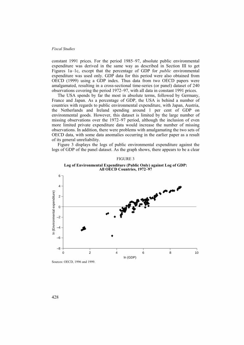
Figure 3 displays the logs of public environmental expenditure against the logs of GDP of the panel dataset. As the graph shows, there appears to be a clear
FIGURE 3 Log of Environmental Expenditure (Public Only) against Log of GDP:
All OECD Countries, 1972–97
0
–6
10
6
4
2
0
–2
–4
–8
ln (
Env
ironm
enta
l exp
endi
ture
)
2 4 6 8
ln (GDP) Sources: OECD, 1996 and 1999.

Public and Private Spending for Environmental Protection
429
relationship between GDP and public environmental expenditure: as GDP increases, so does public environmental expenditure. However, this relationship does not control for any country-specific effects, i.e. different countries having different levels of public environmental expenditure that are independent of time and GDP. Furthermore, the plot does not control for any time trend in that there may be growing environmental expenditure due to increasing pollution, population or environmental awareness over time that may be independent of country-specific effects or GDP.
Using the data from OECD (1996 and 1999), a fixed-effects model,14 which estimates a constant for each country and takes account of missing observations, was fitted to test the effects of a change in GDP on changes in absolute public environmental expenditure over the period 1972–97:
0 1it it i itY Xβ β ν ε= + + + , t = 0, 1, 2, …, T (0 = 1972, 1 = 1973, …) i = 1, 2, 3, …, N (1 = Australia, 2 = Austria, …),
where T = 26 time periods covering 1972 to 1997, N = 27 countries covered by the OECD data, Yit denotes public environmental expenditure for country i in year t in 1991 prices (US$ billion) and Xit denotes absolute GDP for country i in year t in 1991 prices (US$ billion). In this model, νi+εit is the residual.
Next, a time-trend variable (t) is incorporated into the model to control for any increases in environmental expenditure that occur independently of country-specific effects and GDP, where an observation taken in 1972 is coded as 0, an observation in 1975 is coded as 3 and so on. In addition, the data were transformed. Natural logs were taken of both absolute public environmental expenditure and GDP since a log-log specification is the most readily interpretable, although the most general model would be to Box-Cox-transform15 both variables.
This produces the final model:
0 1 2ln lnit it i itY X tβ β β ν ε= + + + + , t = 0, 1, 2, …, T (0 = 1972, …) i = 1, 2, 3, …, N (1 = Australia, …).
The results in Table 7 show that the time-trend variable is not a significant determinant of public environmental expenditure, i.e. β2 is not significantly different from 0 (p = 0.113 > 0.005). Hence there is no evidence for growth in public environmental expenditure over time independent of growth in GDP.
14This is equivalent to an ordinary least squares (OLS) regression model with country-specific dummies. 15Box-Cox transformations were attempted (results available from the authors on request) and showed that the log-log transformation was favoured to the linear model, semi-log model or reciprocal model.

Fiscal Studies
430
TABLE 7 Results from the Regression Analysis
Coefficient Standard error t statistic p>|t| ln GDP 1.194958 0.0655344 18.234 0.000 Time trend –0.008117 0.0050999 –1.592 0.113 Constant –6.048623 0.3343025 –18.093 0.000 Notes: Number of observations = 240 R-squared = 0.6693 Country-specific constants are available from the authors on request.
GDP16 is a very significant determinant of public environmental expenditure, i.e. β1 is significantly different from both 0 and 1 (p < 0.05). The coefficient of GDP is greater than 1 and is also statistically significantly greater than 1. The results of this log-log model, where the coefficient can be interpreted as an elasticity, appear to show that the income elasticity of willingness to pay for the environment is just higher than unity, i.e. a 1 per cent increase in GDP leads to an average 1.2 per cent increase in public environmental expenditure. Finally, the R-squared from this model is relatively high, with around two-thirds of the variation in environmental expenditure being explained by the model.
VIII. WHAT DETERMINES ENVIRONMENTAL EXPENDITURE?
The links between environmental expenditure and GDP are clearly very strong. However, a more general theory of what explains environmental expenditures has, to date, been missing. The link to income could be interpreted in two ways. First, as incomes grow, the demand for environmental quality grows, as predicted in most versions of the EKC hypothesis. The evidence in the previous section can be interpreted as suggesting that the income elasticity of willingness to pay is just above unity.
Second, higher incomes are associated with a higher ability to pay and, once the EKC ‘peak’ has been achieved, countries begin to devote more of their resources to environmental protection in order to ‘undo’ past damage as the nation climbs up the upwards portion of the EKC. On this view, high expenditures reflect high (cumulative) damage. To some extent, the contrast between these two positions is artificial in that any decision to spend more resources on environmental protection must still reflect a shift in social preferences. Such preference shifts could come about because of greater 16We recognise that GDP per capita is a better indicator of wealth than absolute GDP and ran a similar model, regressing GDP per capita on public environmental expenditure per capita. The results are almost the same (i.e. the coefficient of GDP per head is equal to 1.2, and significantly different from 0 and 1), which is due to OECD countries all being relatively similar to one another. The result would almost certainly differ if developing countries were included in the model as well.
Public and Private Spending for Environmental Protection
431
awareness of environmental problems after the early stages of growth. In other words, preference shifts precisely because what were largely invisible problems become visible as the assimilative capacity of natural environments begins to be exhausted. Casual empiricism does not support this view, however, since environmental problems in poor countries are more than visible and there is a high potential demand for their solution — for example, safe water supply, sanitation and soil quality. Overall, then, we prefer to see the expenditure–income link as reflecting a more general change in social preferences as income rises. We therefore surmise that εW <1 in poor countries.
If our hypothesis is correct, environmental expenditures reflect underlying social concerns about the environment, concerns that grow with income. As such, we would expect to see expenditures being correlated with some indicator or indicators of environmental concern. In turn, environmental concern may reflect other socio-economic influences such as education. Linking expenditures to some measures of social concern suggests analysing the issue in terms of a ‘political economy’ model of policy outcomes. Political economy models seek to explain policy outcomes in terms of the political forces that generate a political-economic equilibrium, i.e. an equilibrium in which the amount of a public good is determined by governments facing differing demands from various stakeholders. The models are rooted in the early literature on public choice (for example, Buchanan and Tullock (1975)) and bargaining solutions along the lines of the Coase theorem (Coase, 1960). While Aidt (1998) characterises the governmental implementation of policy as a Pigouvian feature of the models, in fact most environmental policy does not proceed along Pigouvian lines (essentially, environmental taxes) but through standard-setting.
In the current case, environmental expenditures would be the outcome of policy decisions made by government. Those decisions are, in turn, the outcome of some political compromise between the amount of environmental quality that households and corporations are willing to supply (through their taxes and forgone income) and what lobby groups, including the government itself, demand. Several attempts have been made to explain environmental preferences and to develop political economy models of environmental policy (Black, Guppy and Urmetzer, 1997; Aidt, 1998; Marsiliani and Renström, 2000). One significant feature of some of these models is the inclusion of income distribution as an explanatory variable (Magnani, 2000; Marsiliani and Renström, 2000). The essential argument here is that poorer individuals will have a lower preference for environmental goods relative to private goods and that the poor’s demand for redistribution of income will lower production due to production inefficiencies.17 Evidence that the poor care less about the
17This second element of the argument is contentious, however, since lower production means lower throughput of materials and energy via the materials balance principle. This production effect appears to be ignored in the Marsiliani–Renström paper, for instance.
Fiscal Studies
432
environment than the rich is, however, not strong — see, among others, Jones and Dunlap (1992). For the USA, Elliott, Seldon and Regens (1997) find that public support for environmental spending varies positively with education, gender, the degree to which the individual is ‘urbanised’, ‘liberalism’ of the individual’s viewpoint, and race (non-whites expressing more support). They also find that income is significant but less so than the previous factors. Age influences spending support negatively, i.e. older people show less support for environmental spending.
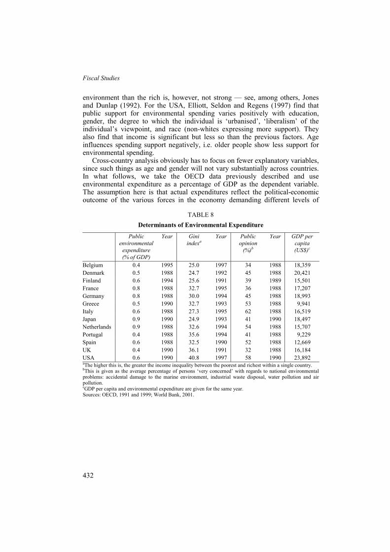
Cross-country analysis obviously has to focus on fewer explanatory variables, since such things as age and gender will not vary substantially across countries. In what follows, we take the OECD data previously described and use environmental expenditure as a percentage of GDP as the dependent variable. The assumption here is that actual expenditures reflect the political-economic outcome of the various forces in the economy demanding different levels of
TABLE 8 Determinants of Environmental Expenditure
Public environmental
expenditure (% of GDP)
Year Gini indexa
Year Public opinion
(%)b
Year GDP per capita (US$)c
Belgium 0.4 1995 25.0 1997 34 1988 18,359 Denmark 0.5 1988 24.7 1992 45 1988 20,421 Finland 0.6 1994 25.6 1991 39 1989 15,501 France 0.8 1988 32.7 1995 36 1988 17,207 Germany 0.8 1988 30.0 1994 45 1988 18,993 Greece 0.5 1990 32.7 1993 53 1988 9,941 Italy 0.6 1988 27.3 1995 62 1988 16,519 Japan 0.9 1990 24.9 1993 41 1990 18,497 Netherlands 0.9 1988 32.6 1994 54 1988 15,707 Portugal 0.4 1988 35.6 1994 41 1988 9,229 Spain 0.6 1988 32.5 1990 52 1988 12,669 UK 0.4 1990 36.1 1991 32 1988 16,184 USA 0.6 1990 40.8 1997 58 1990 23,892 aThe higher this is, the greater the income inequality between the poorest and richest within a single country. bThis is given as the average percentage of persons ‘very concerned’ with regards to national environmental problems: accidental damage to the marine environment, industrial waste disposal, water pollution and air pollution. cGDP per capita and environmental expenditure are given for the same year. Sources: OECD, 1991 and 1999; World Bank, 2001.
Public and Private Spending for Environmental Protection
433
environmental protection.18 The independent variables are GDP per capita, an index of income inequality (the Gini index) and the strength of public opinion on environmental problems. These data are given in Table 8.
The data for this cross-country analysis are fully available for only 13 countries. Furthermore, while the index for income inequality for a particular country changes very little from one year to the next, changes in public concern for the environment are not so well known. Hence this analysis uses public opinion data collected between 1988 and 1990,19 while some environmental expenditure data only become available in the mid-1990s — for example, for Belgium and Finland. Therefore, given the obvious data limitations where not all the data are collected for the same year, any conclusions drawn from this analysis should be treated with caution.
Consider the following model:
0 1 1 2 2 3 3lni i i i iY X X Xβ β β β ε= + + + + , i = 1, 2, …, N,
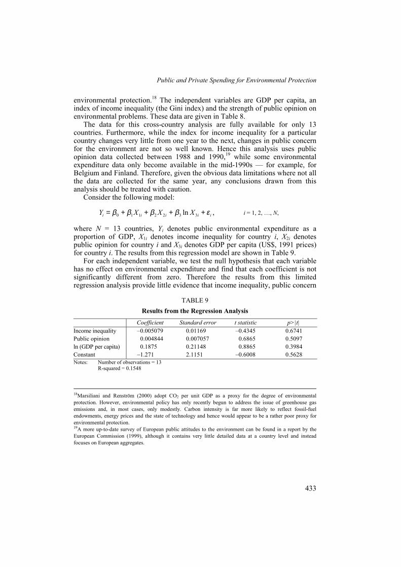
where N = 13 countries, Yi denotes public environmental expenditure as a proportion of GDP, X1i denotes income inequality for country i, X2i denotes public opinion for country i and X3i denotes GDP per capita (US$, 1991 prices) for country i. The results from this regression model are shown in Table 9.
For each independent variable, we test the null hypothesis that each variable has no effect on environmental expenditure and find that each coefficient is not significantly different from zero. Therefore the results from this limited regression analysis provide little evidence that income inequality, public concern
TABLE 9 Results from the Regression Analysis
Coefficient Standard error t statistic p>|t| Income inequality –0.005079 0.01169 –0.4345 0.6741 Public opinion 0.004844 0.007057 0.6865 0.5097 ln (GDP per capita) 0.1875 0.21148 0.8865 0.3984 Constant –1.271 2.1151 –0.6008 0.5628 Notes: Number of observations = 13 R-squared = 0.1548
18Marsiliani and Renström (2000) adopt CO2 per unit GDP as a proxy for the degree of environmental protection. However, environmental policy has only recently begun to address the issue of greenhouse gas emissions and, in most cases, only modestly. Carbon intensity is far more likely to reflect fossil-fuel endowments, energy prices and the state of technology and hence would appear to be a rather poor proxy for environmental protection. 19A more up-to-date survey of European public attitudes to the environment can be found in a report by the European Commission (1999), although it contains very little detailed data at a country level and instead focuses on European aggregates.
Fiscal Studies
434
for the environment or GDP per head has an effect on public environmental expenditure (as a proportion of GDP). Nonetheless, we acknowledge that the model has a very small sample and the results cannot be afforded firm credibility.
IX. CONCLUSIONS
Perhaps the overriding conclusion we would draw is that the data on environmental expenditure outside the USA, and probably Norway, are so poor that it is very much open to question whether econometric exercises are currently worthwhile. From a policy standpoint, this conclusion is somewhat startling. While there are several exercises in the USA whereby some idea can be obtained about the relative costs and benefits of environmental regulation generally (Freeman, 1982, 1990 and 2000; Hahn, 1996; Portney, 1990 and 2000), there are no such exercises outside the USA, nor do we see how they could take place. Ironically, while most of the controversy in cost–benefit procedures applied to the environment takes place in the context of the valuation of benefits, it turns out that we have little real idea of the budgetary costs of environmental protection, let alone the wide general equilibrium costs. In an era of renewed attention to efficiency in government, this finding is disturbing.
Despite the limitations of the data, we set out to see what the limited data could tell us about three questions:
• whether there has been a shift in the relative burdens of environmental expenditure borne by the state (national and local government) and the private sector (corporations and households);
• whether environmental expenditure acts as a ‘drag’ on economic growth; and • how environmental expenditure might vary as economic development occurs
and, a related issue, what determines environmental expenditure.
1. Inspecting the Data Before addressing the three questions directly, we asked how reliable the data were. No tests of reliability have been carried out outside the USA, where the ‘raw’ data are far more detailed. Somewhat oddly, the assessments of reliability of US data provide contradictory results, several studies suggesting substantial understatements of true cost and one recent study suggesting significant overstatement of costs!
Inspection of the raw OECD data (Figures 2a–2c) suggests that, in per capita terms and for private and public expenditures combined, countries might be ‘banded’ as follows:
Public and Private Spending for Environmental Protection
435
Per capita expenditure Above $300 Austria, Netherlands, Switzerland, USA $200–299 Canada, Czech Republic, France, Germany, Japan, Norway,
Sweden $100–199 Australia, Belgium, Denmark, Finland, Italy, Korea, UK <$100 Greece, Hungary, Mexico, Poland, Portugal, Spain
By and large, the banding is as one would expect but for the Czech Republic. Also, Korea appears to be highly placed. Inspection of the data shows that Korea significantly increased its expenditures in only six years, whilst the Czech Republic has more than doubled its per capita expenditure in the same period. The Netherlands, France and Sweden show substantial increases since the mid-1980s, and Poland has shown a big increase during the 1990s.
We turn now to the three questions.
2. The Public/Private Split in Environmental Expenditure We hypothesised that we would expect to see a rise in the relative burden of expenditure being borne by the private sector because of (a) increased private spending due to regulation based on standard-setting, (b) growth of fiscal ideologies favouring the reduction in public spending generally and (c), related to (b), increased privatisation. Taking the OECD data at face value, Table 4 suggested that there has been no such rise in the share of expenditure borne by the private sector. The general trends are either fairly constant or slightly declining. There are no obvious reasons for these trends. Coverage of the data varies by country, but this should not affect time trends for single countries. It is possible that coverage of individual country data varies with time as data collection changes (we hesitate to say it improves), but the detail in the original sources is not sufficient to judge. At best, then, we can say that the available data do not show the expected shift towards an increasing private sector burden.
3. Environmental Drag An important question concerns the role that increasing environmental expenditures have in economic growth. This has been addressed in a fairly large literature, although much of it is centred on the USA, historically arising because of the concern there to explain periods of low overall factor productivity growth. Cross-country generalisations may therefore be difficult. Various forms of the ‘drag’ hypothesis can be identified: the first concerns the export performance of environmentally heavily regulated industries relative to less regulated ones; the second concerns the notion that firms move out of national jurisdictions because of environmental regulation; the third suggests that inward investment will be less in heavily regulating countries; and the fourth concerns the impact of regulation on productivity. For all of the effects other than the impact on
Fiscal Studies
436
productivity, the literature finds little or no support for the drag hypothesis. This finding is consistent regardless of the methodologies used to identify impacts, ranging from case studies through to general equilibrium models. For those who espouse environmental concerns, this finding is important since the ‘threat’ that competitiveness and employment will suffer because of additional regulation is widely used by industry to lobby against regulations. Moreover, the regulations in question are dominated by traditional command-and-control measures. If environmental economists are right in arguing that market-based approaches are less costly, we would expect the drag hypothesis to be weakened even further.
The productivity literature is generally confined to the USA and nearly all of the studies find a negative effect of regulation on productivity. At one extreme, however, one study raises the possibility of positive impacts and, at the other, the negative impacts are said to be significantly negative (Table 5). However, the extent to which this literature should be used to cast doubt on the wisdom of regulatory policies is open to question. First, for the periods in which the studies were carried out, the USA was heavily reliant upon command-and-control measures. A market-based approach might not show the same productivity effects due to (a) initially lower compliance costs and (b) dynamic effects of inducing technological change. Second, the productivity literature adopts a highly partial view of the effects of environmental policies. By focusing on measured outputs, non-market effects are ignored entirely. This neglect has two effects. First, the beneficial effects of environmental policy on human well-being are not allowed to offset any of the negative output effects that are identified. The correct numeraire is not output but a welfare-adjusted measure of output such as output minus externalities. As the study by Repetto et al. (1996) shows, this can have a dramatic effect on the results. Second, it is unclear if the approaches account for any of the indirect but positive effects of environmental policy on output. One obvious link is from reduced pollution to improved human health and from health improvements to productivity impacts. Available but very limited evidence suggests that this indirect linkage could be important.
Overall, then, we doubt if the ‘productivity’ literature has significant implications for environmental policy, at least outside the USA and, we suspect, within the USA also. Nonetheless, it is important to keep such studies under review and to ensure that non-US experience is expanded by research in this area. A related issue concerns the potential contrast between the ‘no effects’ finding of the competitiveness literature and the ‘negative effects’ finding of most of the productivity literature since, a priori, one would expect these findings to be consistent.
We also investigated the view that, far from having negative impacts on economic growth, environmental policy might actually increase growth or, at least, increase competitiveness. This ‘win–win’ view is primarily associated with Michael Porter. It has strong similarities with the corporate environmental literature that argues that environmentally and socially responsible corporations
Public and Private Spending for Environmental Protection
437
are likely to fare better financially than those that neglect these social dimensions. But the Porter hypothesis has proved to be difficult to verify. Reassessments of the industries Porter claims do support the hypothesis have not been able to reproduce his results. We surmise that win–win arguments are likely to attract a degree of public and political attention out of proportion to the likelihood that they are correct. Win–win solutions avoid the necessity of facing up to real-world trade-offs. We do not reject the idea of win–win possibilities out of hand: few decision-makers are completely informed and few are completely economically rational. But for the Porter hypothesis to be right, bounded rationality and incomplete information must be pervasive, and we doubt if that is the case.
4. Environmental Expenditure and Economic Development A large literature has developed that argues that the process of economic development will at first worsen environmental quality and then improve it. There is, it is argued, an inverted U-shaped curve linking environmental degradation to income per capita. How far these ‘environmental Kuznets curves’ actually prevail is open to question. Rather like the win–win hypothesis, the early literature was seized upon as supporting the notion that ‘natural progress’ will guarantee environmental sustainability. In practice, more and more empirical research is casting doubt on the robustness of the early findings. Nonetheless, if we take a crude indicator such as the ratio of primary energy use to GDP, it is well known that this exhibits a time trend of an inverted U-shaped curve. Energy per unit GDP rises at first and then declines. Structural economic change, changing energy mixes and technological change that improves energy efficiency all account for the change in the relationship. But it is also suggested that higher incomes induce a demand for environmental quality, a demand that should translate into increased environmental expenditure. To play a significant role, we would expect this linkage to show up in a high income elasticity of demand for the environment. As noted in the main text, what can actually be measured is the income elasticity of willingness to pay or expenditure, not income elasticities of demand in the conventional sense. Appendix E shows the relationship between the two elasticities. We therefore investigate the elasticity of expenditure with respect to income using the available OECD data. These suggest an elasticity of 1.2, which is perhaps less than we would have expected if the ‘environmental demand effect’ is to play a significant role in explaining the downward slope of the environmental Kuznets curve.
Finally, we made an attempt to ‘explain’ environmental expenditure in terms of a political economy model. We regressed environmental expenditure as a percentage share of GDP on a measure of inequality, GDP itself and public opinion. We found no statistically significant relationship but accept that the sample is probably too small to detect true relationships.
Fiscal Studies
438
APPENDIX A OECD ENVIRONMENTAL EXPENDITURES
Tables A.1 and A.2 set out the available OECD data for environmental expenditure in OECD countries, both private and public, as a percentage of each country’s GDP. At best, the data are spotty, particularly those derived from OECD (1989). For each table, the data for 1972 up until 1984 originate from OECD (1989), while the data from 1985 to 1997 originate from OECD (1999). Data for public expenditures are better than those for total expenditures since private expenditures — i.e. what corporations and households spend — are often not known.
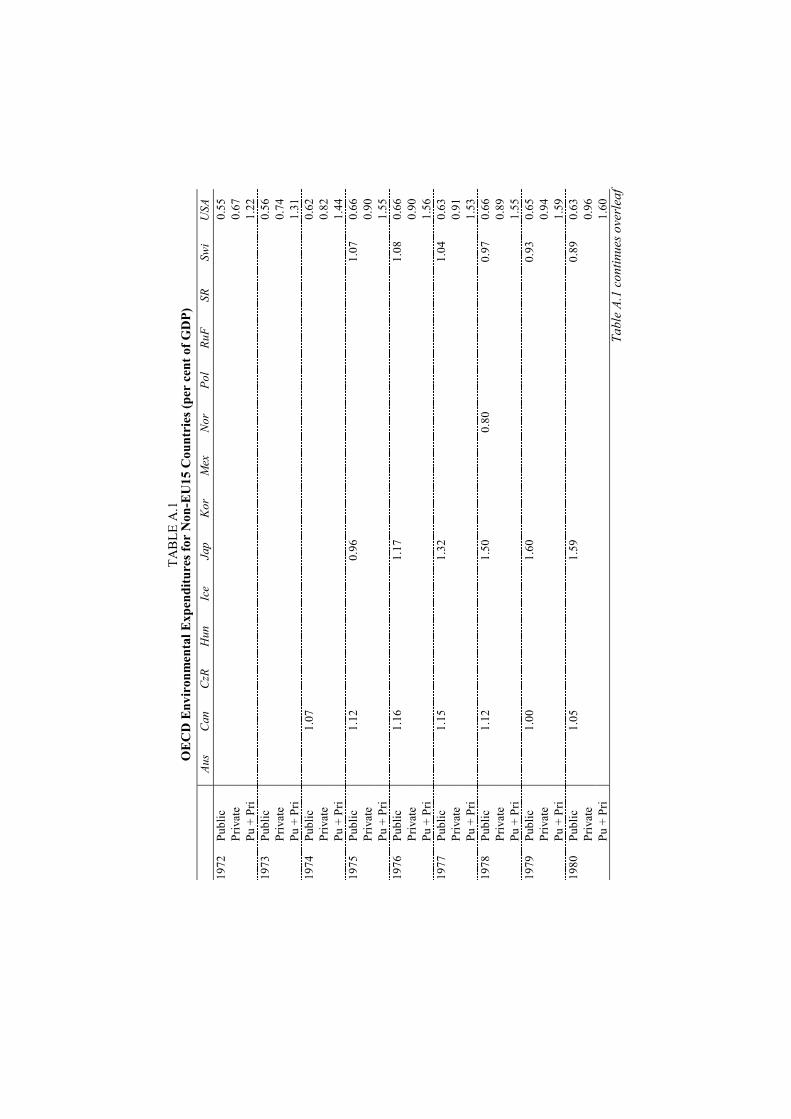
TAB
LE A
.1
OEC
D E
nvir
onm
enta
l Exp
endi
ture
s for
Non
-EU
15 C
ount
ries
(per
cen
t of G
DP)
Au
s C
an
CzR
H
un
Ice
Jap
Kor
M
ex
Nor
Po
l Ru
F SR
Sw
i U
SA
Publ
ic
0.
55
Priv
ate
0.
67
1972
Pu +
Pri
1.
22
Publ
ic
0.
56
Priv
ate
0.
74
1973
Pu +
Pri
1.
31
Publ
ic
1.
07
0.
62
Priv
ate
0.
82
1974
Pu +
Pri
1.
44
Publ
ic
1.
12
0.
96
1.07
0.
66
Priv
ate
0.
90
1975
Pu +
Pri
1.
55
Publ
ic
1.
16
1.
17
1.08
0.
66
Priv
ate
0.
90
1976
Pu +
Pri
1.
56
Publ
ic
1.
15
1.
32
1.04
0.
63
Priv
ate
0.
91
1977
Pu +
Pri
1.
53
Publ
ic
1.
12
1.
50
0.80
0.97
0.
66
Priv
ate
0.
89
1978
Pu +
Pri
1.
55
Publ
ic
1.
00
1.
60
0.93
0.
65
Priv
ate
0.
94
1979
Pu +
Pri
1.
59
Publ
ic
1.
05
1.
59
0.89
0.
63
Priv
ate
0.
96
1980
Pu +
Pri
1.
60
Tabl
e A.
1 co
ntin
ues o
verle
af
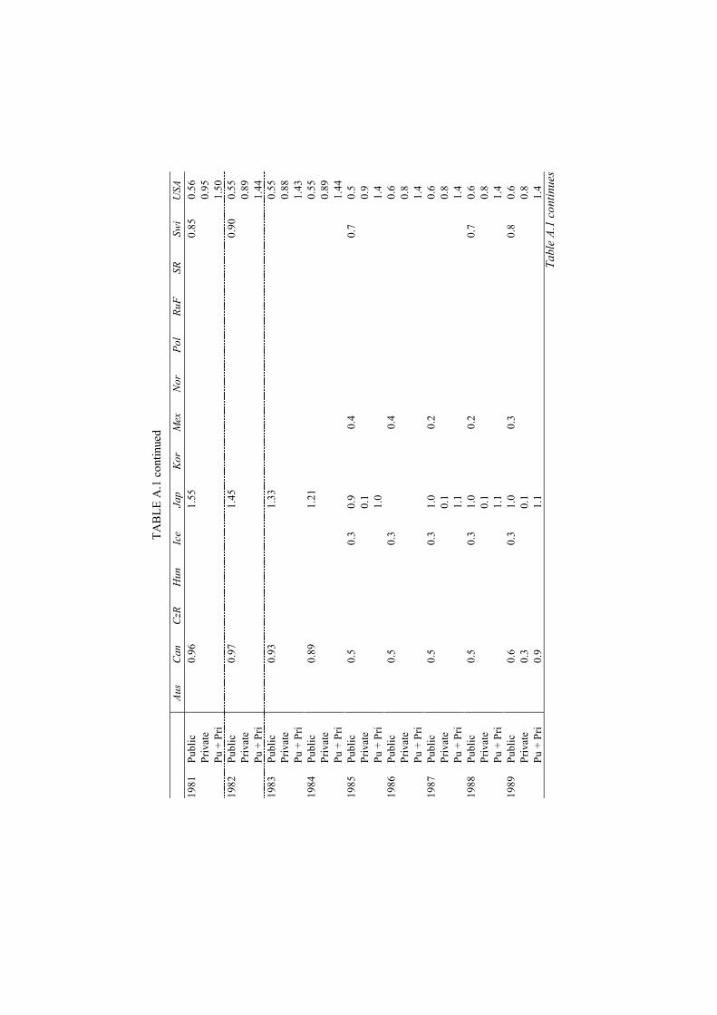
TAB
LE A
.1 c
ontin
ued
Aus
Can
C
zR
Hun
Ic
e Ja
p K
or
Mex
N
or
Pol
RuF
SR
Swi
USA
Pu
blic
0.96
1.55
0.
85
0.56
Pr
ivat
e
0.95
19
81
Pu +
Pri
1.
50
Publ
ic
0.
97
1.
45
0.90
0.
55
Priv
ate
0.
89
1982
Pu +
Pri
1.
44
Publ
ic
0.
93
1.
33
0.
55
Priv
ate
0.
88
1983
Pu +
Pri
1.
43
Publ
ic
0.
89
1.
21
0.
55
Priv
ate
0.
89
1984
Pu +
Pri
1.
44
Publ
ic
0.
5
0.
3 0.
9
0.4
0.7
0.5
Priv
ate
0.
1
0.9
1985
Pu +
Pri
1.
0
1.4
Publ
ic
0.
5
0.
3
0.
4
0.6
Priv
ate
0.
8 19
86
Pu +
Pri
1.
4 Pu
blic
0.5
0.3
1.0
0.
2
0.6
Priv
ate
0.
1
0.8
1987
Pu +
Pri
1.
1
1.4
Publ
ic
0.
5
0.
3 1.
0
0.2
0.7
0.6
Priv
ate
0.
1
0.8
1988
Pu +
Pri
1.
1
1.4
Publ
ic
0.
6
0.
3 1.
0
0.3
0.8
0.6
Priv
ate
0.
3
0.1
0.
8 19
89
Pu +
Pri
0.
9
1.1
1.
4 Ta
ble
A.1
cont
inue
s
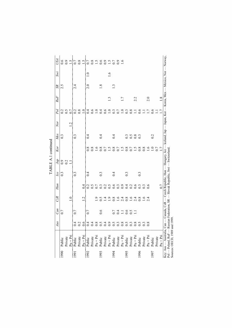
TAB
LE A
.1 c
ontin
ued
Aus
Can
C
zR
Hun
Ic
e Ja
p K
or
Mex
N
or
Pol
RuF
SR
Swi
USA
Pu
blic
0.7
0.3
0.9
0.
3
0.2
2.
5
0.6
Priv
ate
0.
2
0.5
0.
9 19
90
Pu +
Pri
1.0
1.1
1.2
0.7
1.
5 Pu
blic
0.
4 0.
7
0.
3
0.
3
0.2
2.
4
0.7
Priv
ate
0.2
0.8
0.
8 19
91
Pu +
Pri
0.6
1.
2 0.
4
1.0
1.
5 Pu
blic
0.
4 0.
7
0.2
0.4
0.
8 0.
4
0.4
2.
0 1.
0 0.
7 Pr
ivat
e 0.
4
0.
5
0.
8
0.
6
0.8
1992
Pu +
Pri
0.8
1.
9 0.
7
1.
6
1.
0
1.5
Publ
ic
0.5
0.6
0.5
0.3
0.3
0.
8 0.
4
0.4
1.
8
0.6
Priv
ate
0.4
1.
4 0.
2
0.
7
0.
6
0.9
1993
Pu +
Pri
0.9
1.
9 0.
5
1.
5
1.
0 1.
3
1.6
1.5
Publ
ic
0.5
0.7
0.8
0.6
0.4
0.
8 0.
4
0.3
1.
3
0.7
Priv
ate
0.3
0.4
1.6
0.3
0.7
0.7
0.
9 19
94
Pu +
Pri
0.8
1.1
2.4
0.9
1.5
1.0
1.7
1.6
Publ
ic
0.5
0.6
0.8
0.4
0.3
0.
8 0.
3
0.3
Priv
ate
0.3
0.5
1.6
0.2
0.7
0.5
0.
8
19
95
Pu +
Pri
0.8
1.1
2.4
0.6
1.5
0.8
1.
1 2.
2
Publ
ic
0.5
0.
8 0.
3 0.
3
0.8
0.3
0.
6
Pr
ivat
e 0.
3
1.6
0.3
0.8
1.1
1996
Pu +
Pri
0.8
2.
4 0.
6
1.
6
1.
7 2.
0
Publ
ic
1.0
0.2
0.
6
Pr
ivat
e
0.
7
1.
1
19
97
Pu +
Pri
0.
7
1.
7
1.
7 1.
8
Key
: Aus
— A
ustra
lia, C
an —
Can
ada,
CzR
— C
zech
Rep
ublic
, Hun
— H
unga
ry, I
ce —
Icel
and,
Jap
— Ja
pan,
Kor
— K
orea
, Mex
— M
exic
o, N
or —
Nor
way
, Po
l — P
olan
d, R
uF —
Rus
sian
Fed
erat
ion,
SR
— S
lova
k R
epub
lic, S
wi —
Sw
itzer
land
. So
urce
s: O
ECD
, 198
9 an
d 19
99.
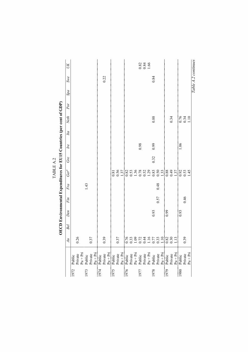
TAB
LE A
.2
OEC
D E
nvir
onm
enta
l Exp
endi
ture
s for
EU
15 C
ount
ries
(per
cen
t of G
DP)
Au
Bel
Den
Fi
n Fr
a G
era
Gre
Ir
e Ita
N
eth
Por
Spa
Swe
UK
Pu
blic
Pr
ivat
e 0.
26
19
72
Pu +
Pri
Publ
ic
1.43
Priv
ate
0.37
1973
Pu +
Pri
Publ
ic
Priv
ate
0.39
0.22
1974
Pu +
Pri
Publ
ic
0.
81
Priv
ate
0.37
0.
56
1975
Pu +
Pri
1.
37
Publ
ic
0.76
0.
82
Priv
ate
0.33
0.
53
1976
Pu +
Pri
1.09
1.
36
Publ
ic
0.72
0.
78
0.
98
0.
82
Priv
ate
0.44
0.
52
0.
84
1977
Pu +
Pri
1.16
1.
29
1.
66
Publ
ic
0.77
0.93
0.
83
0.32
0.
99
0.
88
0.84
Priv
ate
0.33
0.
57
0.48
0.
50
1978
Pu +
Pri
1.10
1.
33
Publ
ic
0.82
0.99
0.
88
Priv
ate
0.30
0.
49
0.
34
1979
Pu +
Pri
1.13
1.
37
Publ
ic
0.93
0.
92
1.
06
0.
76
Priv
ate
0.39
0.
46
0.
53
0.
34
1980
Pu +
Pri
1.
45
1.
10
Tabl
e A.
2 co
ntin
ues
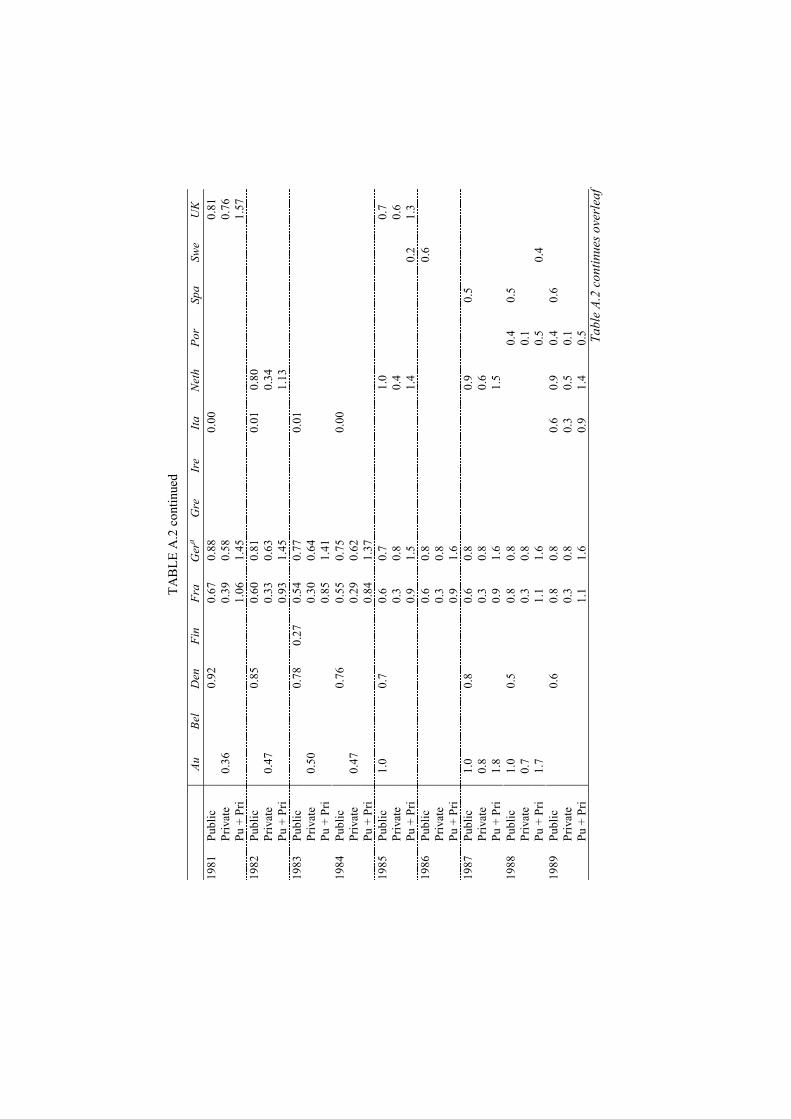
TAB
LE A
.2 c
ontin
ued
Au
Bel
Den
Fi
n Fr
a G
era
Gre
Ir
e Ita
N
eth
Por
Spa
Swe
UK
Pu
blic
0.
92
0.
67
0.88
0.
00
0.81
Pr
ivat
e 0.
36
0.
39
0.58
0.76
19
81
Pu +
Pri
1.06
1.
45
1.
57
Publ
ic
0.85
0.60
0.
81
0.01
0.
80
Priv
ate
0.47
0.33
0.
63
0.
34
1982
Pu +
Pri
0.93
1.
45
1.
13
Publ
ic
0.78
0.
27
0.54
0.
77
0.01
Priv
ate
0.50
0.30
0.
64
1983
Pu +
Pri
0.85
1.
41
Publ
ic
0.76
0.55
0.
75
0.00
Priv
ate
0.47
0.29
0.
62
1984
Pu +
Pri
0.84
1.
37
Publ
ic
1.0
0.
7
0.6
0.7
1.
0
0.7
Priv
ate
0.3
0.8
0.
4
0.6
1985
Pu +
Pri
0.9
1.5
1.
4
0.
2 1.
3 Pu
blic
0.
6 0.
8
0.
6
Priv
ate
0.3
0.8
1986
Pu +
Pri
0.9
1.6
Publ
ic
1.0
0.
8
0.6
0.8
0.
9
0.5
Priv
ate
0.8
0.
3 0.
8
0.6
1987
Pu +
Pri
1.8
0.
9 1.
6
1.5
Publ
ic
1.0
0.
5
0.8
0.8
0.4
0.5
Priv
ate
0.7
0.
3 0.
8
0.
1
1988
Pu +
Pri
1.7
1.
1 1.
6
0.
5
0.4
Pu
blic
0.
6
0.8
0.8
0.6
0.9
0.4
0.6
Priv
ate
0.3
0.8
0.3
0.5
0.1
19
89
Pu +
Pri
1.1
1.6
0.9
1.4
0.5
Ta
ble
A.2
cont
inue
s ove
rleaf
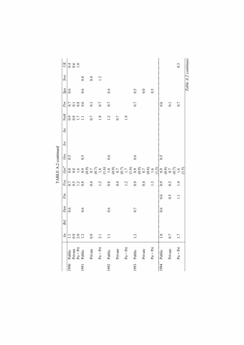
TAB
LE A
.2 c
ontin
ued
Au
Bel
Den
Fi
n Fr
a G
era
Gre
Ir
e Ita
N
eth
Por
Spa
Swe
UK
Pu
blic
1.
1
0.6
0.
7 0.
8 0.
5
0.
9 0.
7 0.
6
0.4
Priv
ate
0.9
0.
5 0.
8
0.8
0.1
0.6
1990
Pu +
Pri
2.0
1.
2 1.
6
1.7
0.8
1.0
Publ
ic
1.2
0.
6
0.8
0.9
(0.9
) 0.
5
1.
1 0.
6 0.
6 0.
8
Priv
ate
0.9
0.
4 0.
7 (0
.7)
0.
7 0.
1
0.4
1991
Pu +
Pri
2.1
1.
2 1.
6 (1
.6)
1.
8 0.
7
1.2
Publ
ic
1.1
0.
6
0.8
1.0
(0.9
) 0.
6
1.
2 0.
7 0.
4
Priv
ate
0.4
0.7
(0.7
)
0.7
1992
Pu +
Pri
1.2
1.7
(1.6
)
1.9
Publ
ic
1.2
0.
7
0.9
0.9
(0.9
) 0.
6
0.7
0.5
Priv
ate
0.4
0.7
(0.6
)
0.0
1993
Pu +
Pri
1.3
1.6
(1.5
)
0.5
Publ
ic
1.0
0.
6 0.
6 0.
9 0.
9 (0
.8)
0.5
0.
6
Priv
ate
0.7
0.5
0.5
0.7
(0.7
)
0.
1
1994
Pu +
Pri
1.7
1.1
1.4
1.6
(1.5
)
0.
7
0.
3
Tabl
e A.
2 co
ntin
ues
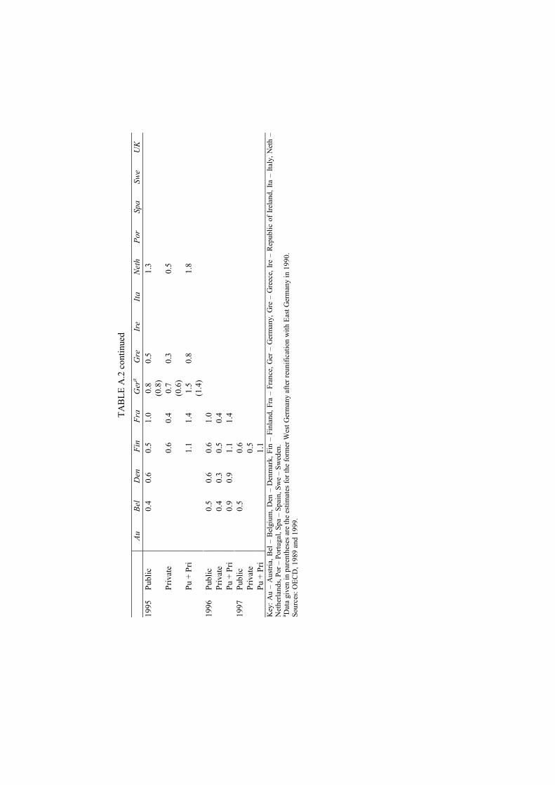
TAB
LE A
.2 c
ontin
ued
Au
Bel
Den
Fi
n Fr
a G
era
Gre
Ir
e Ita
N
eth
Por
Spa
Swe
UK
Pu
blic
0.4
0.6
0.5
1.0
0.8
(0.8
) 0.
5
1.
3
Priv
ate
0.
6 0.
4 0.
7 (0
.6)
0.3
0.5
1995
Pu +
Pri
1.
1 1.
4 1.
5 (1
.4)
0.8
1.8
Publ
ic
0.
5 0.
6 0.
6 1.
0
Priv
ate
0.
4 0.
3 0.
5 0.
4
1996
Pu +
Pri
0.
9 0.
9 1.
1 1.
4
Publ
ic
0.
5
0.6
Priv
ate
0.
5
19
97
Pu +
Pri
1.
1
K
ey: A
u –
Aus
tria,
Bel
– B
elgi
um, D
en –
Den
mar
k, F
in –
Fin
land
, Fra
– F
ranc
e, G
er –
Ger
man
y, G
re –
Gre
ece,
Ire
– R
epub
lic o
f Ire
land
, Ita
– It
aly,
Net
h –
Net
herla
nds,
Por –
Por
tuga
l, Sp
a –
Spai
n, S
we
– Sw
eden
. a D
ata
give
n in
par
enth
eses
are
the
estim
ates
for t
he fo
rmer
Wes
t Ger
man
y af
ter r
euni
ficat
ion
with
Eas
t Ger
man
y in
199
0.
Sour
ces:
OEC
D, 1
989
and
1999
.
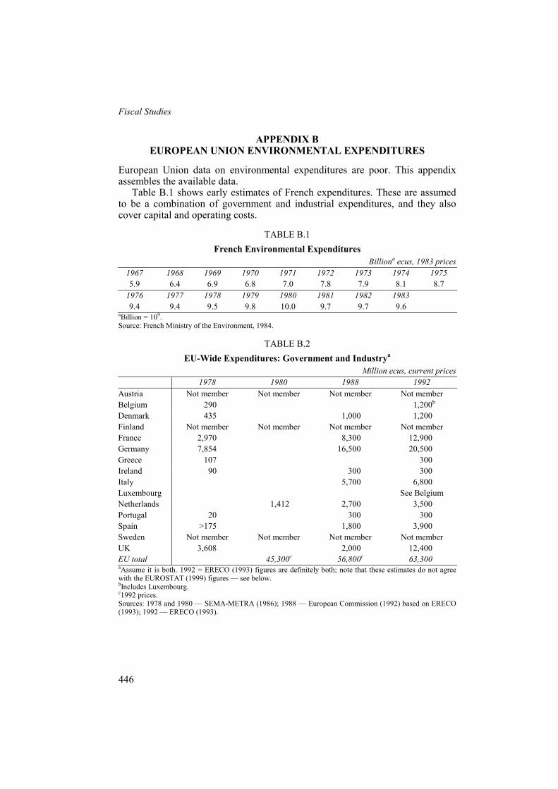
Fiscal Studies
446
APPENDIX B EUROPEAN UNION ENVIRONMENTAL EXPENDITURES
European Union data on environmental expenditures are poor. This appendix assembles the available data.
Table B.1 shows early estimates of French expenditures. These are assumed to be a combination of government and industrial expenditures, and they also cover capital and operating costs.
TABLE B.1 French Environmental Expenditures
Billiona ecus, 1983 prices 1967 1968 1969 1970 1971 1972 1973 1974 1975 5.9 6.4 6.9 6.8 7.0 7.8 7.9 8.1 8.7
1976 1977 1978 1979 1980 1981 1982 1983 9.4 9.4 9.5 9.8 10.0 9.7 9.7 9.6
aBillion = 109. Source: French Ministry of the Environment, 1984.
TABLE B.2 EU-Wide Expenditures: Government and Industrya
Million ecus, current prices 1978 1980 1988 1992 Austria Not member Not member Not member Not member Belgium 290 1,200b Denmark 435 1,000 1,200 Finland Not member Not member Not member Not member France 2,970 8,300 12,900 Germany 7,854 16,500 20,500 Greece 107 300 Ireland 90 300 300 Italy 5,700 6,800 Luxembourg See Belgium Netherlands 1,412 2,700 3,500 Portugal 20 300 300 Spain >175 1,800 3,900 Sweden Not member Not member Not member Not member UK 3,608 2,000 12,400 EU total 45,300c 56,800c 63,300 aAssume it is both. 1992 = ERECO (1993) figures are definitely both; note that these estimates do not agree with the EUROSTAT (1999) figures — see below. bIncludes Luxembourg. c1992 prices. Sources: 1978 and 1980 — SEMA-METRA (1986); 1988 — European Commission (1992) based on ERECO (1993); 1992 — ERECO (1993).
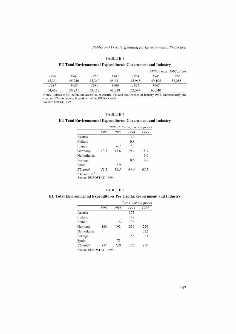
Public and Private Spending for Environmental Protection
447
TABLE B.3 EU Total Environmental Expenditures: Government and Industry
Million ecus, 1992 prices 1980 1981 1982 1983 1984 1985 1986
45,314 45,240 45,340 45,641 45,948 49,105 52,285 1987 1988 1989 1990 1991 1992
54,458 56,831 59,150 61,618 62,544 63,340 Notes: Relates to EU before the accession of Austria, Finland and Sweden in January 1995. Unfortunately, the sources offer no country breakdown of the ERECO totals. Source: ERECO, 1993.
TABLE B.4 EU Total Environmental Expenditures: Government and Industry
Billiona Euros, current prices 1992 1993 1994 1995
Austria 3.0 Finland 0.8 France 6.7 7.7 Germany 13.5 15.6 19.4 18.7 Netherlands 5.0 Portugal 0.6 0.6 Spain 2.9 EU total 53.2 56.2 64.6 65.5 aBillion = 109. Source: EUROSTAT, 1999.
TABLE B.5 EU Total Environmental Expenditures Per Capita: Government and Industry
Euros, current prices 1992 1993 1994 1995
Austria 373 Finland 149 France 116 133 Germany 168 192 239 229 Netherlands 322 Portugal 58 63 Spain 73 EU total 137 150 170 186 Source: EUROSTAT, 1999.

Fiscal Studies
448
Tables B.2 and B.3 report on early estimates of EU-wide expenditure. Table B.4 gives data in current prices, based on EUROSTAT (1999). Note
that the cell figures are the only independent figures, i.e. based on country returns. The EU totals are artefacts based on EUROSTAT’s assumption that expenditures vary directly with GNP.
Table B.5 repeats Table B.4 but in per capita terms. Again, note that the cell figures are the only independent figures and that the EU totals are artefacts, as in Table B.4.
Table B.6 provides estimates of government expenditure only. These are not summarised in EUROSTAT (1999) and have therefore been taken from the country tables.
Table B.7 shows EUROSTAT’s estimates of industry expenditure, again taken from country tables.
TABLE B.6 EU Environmental Expenditures: Government Only
Million Euros, current prices 1988 1989 1990 1991 1992 1993 1994 1995 1996
Austria 1,745 Denmark 282 248 279 339 372 393 432 507 509 Finland 420 France 3,702 4,070 4,579 5,184 6,082 6,574 Germany 4,518 4,413 4,788 5,441 6,694 8,457 8,938 9,672 Netherlands 2,642 3,215 Portugal 94 171 159 189 213 255 264 Spain 1,399 1,662 1,994 1,376 1,719 1,795 Sweden 1,300 Source: EUROSTAT, 1999.
TABLE B.7 EU Environmental Expenditures: Industry Only
Million Euros, current prices 1992 1993 1994 1995
Austria 1,240 Finland 506 457 396 Netherlands 1,825 1,573 Portugal 109 109 Spain 1,210 EU total 3,009 Source: EUROSTAT, 1999.
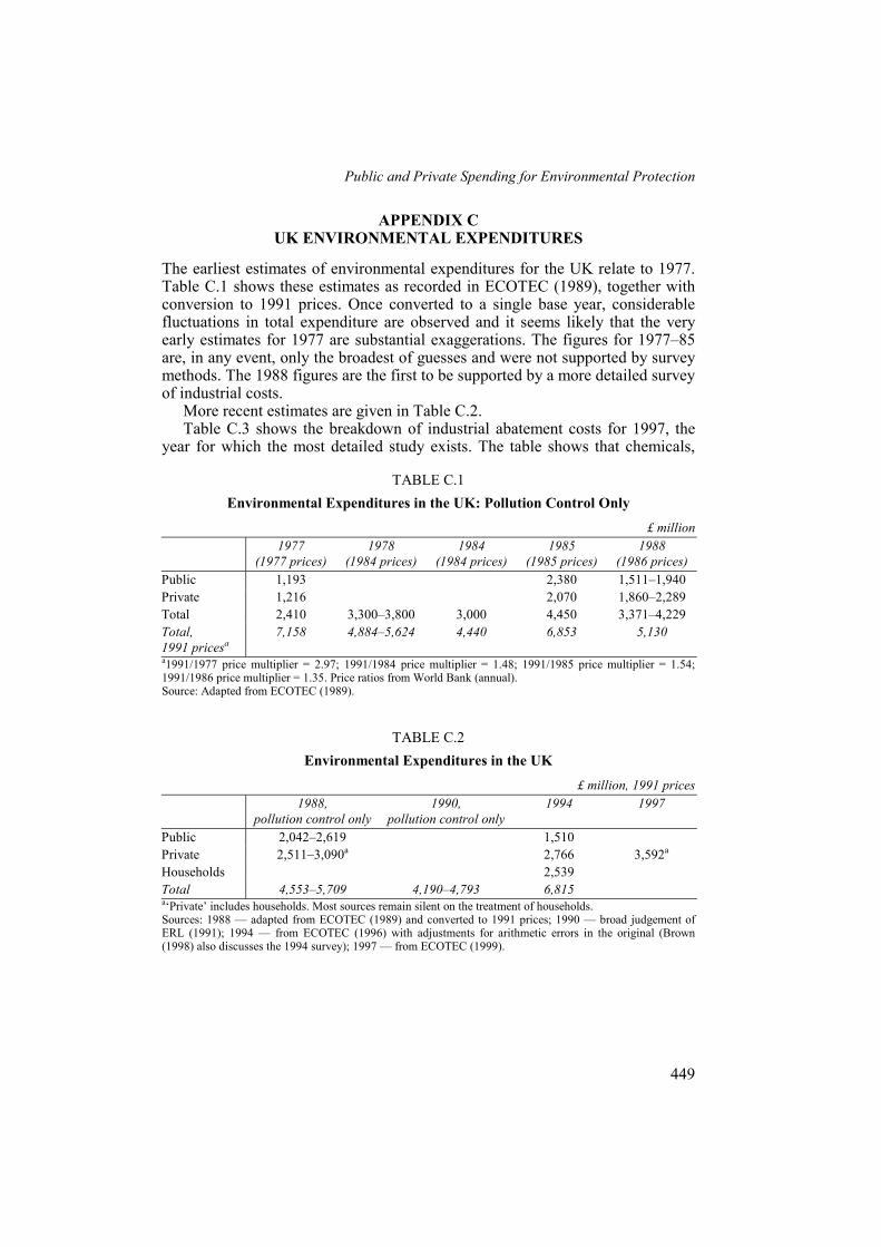
Public and Private Spending for Environmental Protection
449
APPENDIX C UK ENVIRONMENTAL EXPENDITURES
The earliest estimates of environmental expenditures for the UK relate to 1977. Table C.1 shows these estimates as recorded in ECOTEC (1989), together with conversion to 1991 prices. Once converted to a single base year, considerable fluctuations in total expenditure are observed and it seems likely that the very early estimates for 1977 are substantial exaggerations. The figures for 1977–85 are, in any event, only the broadest of guesses and were not supported by survey methods. The 1988 figures are the first to be supported by a more detailed survey of industrial costs.
More recent estimates are given in Table C.2. Table C.3 shows the breakdown of industrial abatement costs for 1997, the
year for which the most detailed study exists. The table shows that chemicals,
TABLE C.1 Environmental Expenditures in the UK: Pollution Control Only
£ million 1977
(1977 prices) 1978
(1984 prices) 1984
(1984 prices) 1985
(1985 prices) 1988
(1986 prices) Public 1,193 2,380 1,511–1,940 Private 1,216 2,070 1,860–2,289 Total 2,410 3,300–3,800 3,000 4,450 3,371–4,229 Total, 1991 pricesa
7,158 4,884–5,624 4,440 6,853 5,130
a1991/1977 price multiplier = 2.97; 1991/1984 price multiplier = 1.48; 1991/1985 price multiplier = 1.54; 1991/1986 price multiplier = 1.35. Price ratios from World Bank (annual). Source: Adapted from ECOTEC (1989).
TABLE C.2 Environmental Expenditures in the UK
£ million, 1991 prices 1988,
pollution control only 1990,
pollution control only 1994 1997
Public 2,042–2,619 1,510 Private 2,511–3,090a 2,766 3,592a Households 2,539 Total 4,553–5,709 4,190–4,793 6,815 a‘Private’ includes households. Most sources remain silent on the treatment of households. Sources: 1988 — adapted from ECOTEC (1989) and converted to 1991 prices; 1990 — broad judgement of ERL (1991); 1994 — from ECOTEC (1996) with adjustments for arithmetic errors in the original (Brown (1998) also discusses the 1994 survey); 1997 — from ECOTEC (1999).
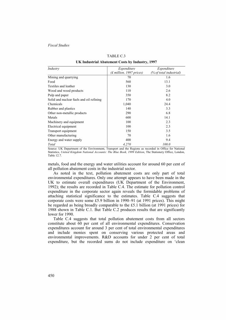
Fiscal Studies
450
TABLE C.3 UK Industrial Abatement Costs by Industry, 1997
Industry Expenditure (£ million, 1997 prices)
Expenditure (% of total industrial)
Mining and quarrying 70 1.6 Food 560 13.1 Textiles and leather 130 3.0 Wood and wood products 110 2.6 Pulp and paper 350 8.2 Solid and nuclear fuels and oil refining 170 4.0 Chemicals 1,040 24.4 Rubber and plastics 140 3.3 Other non-metallic products 290 6.8 Metals 600 14.1 Machinery and equipment 100 2.3 Electrical equipment 100 2.3 Transport equipment 150 3.5 Other manufacturing 70 1.6 Energy and water supply 400 9.4 Total 4,270 100.0 Source: UK Department of the Environment, Transport and the Regions as recorded in Office for National Statistics, United Kingdom National Accounts: The Blue Book, 1999 Edition, The Stationery Office, London, Table 12.7.
metals, food and the energy and water utilities account for around 60 per cent of all pollution abatement costs in the industrial sector.
As noted in the text, pollution abatement costs are only part of total environmental expenditures. Only one attempt appears to have been made in the UK to estimate overall expenditures (UK Department of the Environment, 1992); the results are recorded in Table C.4. The estimate for pollution control expenditure in the corporate sector again reveals the formidable problems of attaching statistical significance to the estimates. Table C.4 suggests that corporate costs were some £5.9 billion in 1990–91 (at 1991 prices). This might be regarded as being broadly comparable to the £5.1 billion (at 1991 prices) for 1988 shown in Table C.1. But Table C.2 produces results that are significantly lower for 1990.
Table C.4 suggests that total pollution abatement costs from all sectors constitute about 60 per cent of all environmental expenditures. Conservation expenditures account for around 3 per cent of total environmental expenditures and include monies spent on conserving various protected areas and environmental improvements. R&D accounts for under 2 per cent of total expenditure, but the recorded sums do not include expenditure on ‘clean

Public and Private Spending for Environmental Protection
451
TABLE C.4 Total Environmental Expenditures in the UK, 1990–91
£ million, 1991 prices Activity Government Firms Households Nature
protection organisations
Total
Pollution abatement 2,200 5,900 680 — 8,780 Environmental conservation
290 — — 160 450
R&D 250 — — — 250 Education and training
90 60 — — 150
Sub-total 2,830 5,960 680 160 9,630 Management of natural resources
630 2,800 — — 3,430
Amenity improvement
1,200 — — — 1,200
Total 4,660 8,760 680 160 14,260 Per cent 33 61 5 1 100 Source: Brown, 1998.
technology’ and hence R&D expenditures are understated. Education and training relates mainly to expenditures on university courses in environmental sciences. Management of natural resources constitutes a significant portion of expenditure — around 25 per cent — and includes water company expenditures, flood defences and fisheries management; energy conservation is excluded. Finally, amenity improvement covers activities such as road cleaning and local park maintenance. Total expenditures of £14 billion in 1990 would have been some 2.5 per cent of UK GDP.
APPENDIX D ENVIRONMENTAL EXPENDITURES IN DEVELOPING COUNTRIES
Little is known about environmental expenditure in developing countries. The World Bank and the Asian Development Bank have sponsored studies of expenditure in Malaysia and Indonesia (personal communication with J. Vincent, 2001) but neither study appears to be publicly available. Hansen (1994) reports estimates produced by Phantumvanit and Panayotou (1990) for selected countries, as shown in Table D.1. Coverage of the data is unclear but the figures do suggest expenditures well below 1 per cent of GDP for poorer countries.

Fiscal Studies
452
TABLE D.1 Environmental Expenditures in Selected Developing Countries, 1987
As % of GDP Per capita (US$)
Singapore 1.09 107 Republic of Korea 0.40 11 Thailand 0.24 2 China 0.70 2 Indonesia 0.38 1.7 Source: Authors’ estimates.
APPENDIX E THE ‘INCOME ELASTICITY’ OF DEMAND FOR ENVIRONMENTAL
QUALITY
For a given demand function of the form
q p yα β γ= + + ,
where q = quantity, y = income and p = price, derive the inverse demand function
q yp α γβ
− −= .
The ‘conventional’ income and price elasticities are then
yq
yEq
γ=
and
pq
pEq
β= .
From the inverse demand function, the elasticity of price with respect to income is
yp
yEp
γβ
= − .
Public and Private Spending for Environmental Protection
453
But yqy E qγ = and p
qp E qβ = , so
yqy
p pq
EE
E=
−.
REFERENCES
Aidt, T. (1998), ‘Political internalization of economic externalities and environmental policy’, Journal of Public Economics, vol. 69, pp. 1–16.
Albrecht, J. (1999), ‘Environmental regulation, comparative advantage and the Porter hypothesis’, University of Ghent, Faculty of Economics, mimeo.
Andreoni, J. and Levinson, A. (2001), ‘The simple analytics of the environmental Kuznets curve’, Journal of Public Economics, vol. 80, pp. 269–86.
Barbera, A. and McConnell, V. (1990), ‘The impact of environmental regulations on industry productivity: direct and indirect effects’, Journal of Environmental Economics and Management, vol. 18, pp. 50–65.
Black, D., Guppy, N. and Urmetzer, P. (1997), ‘Canadian public opinion and environmental action: evidence from British Columbia’, Canadian Journal of Political Science, vol. 30, pp. 451–71.
Brown, A. (1998), ‘UK experience in collecting environmental expenditure information by industry’, in P. Vaze (ed.), UK Environmental Accounts 1998, London: Office for National Statistics.
Bruvoll, A., Glomsrod, S. and Vennemo, H. (1995), ‘The environmental drag on long-term economic performance: evidence from Norway’, Statistics Norway, Discussion Paper no. 143.
Buchanan, J. and Tullock, G. (1975), ‘Polluters’ profit and political response: direct controls versus taxes’, American Economic Review, vol. 65, pp. 139–47.
Coase, R. (1960), ‘The problem of social cost’, Journal of Law and Economics, vol. 3, pp. 1–44. Conrad, K. and Morrison, C. (1989), ‘The impact of pollution abatement investment on
productivity change: an empirical comparison of the US, Germany and Canada’, Southern Economic Journal, vol. 55, pp. 684–98.
ECOTEC (1989), Industry Costs of Pollution Control, Report to the UK Department of the Environment, London.
— (1996), Environmental Protection Expenditure by Industry, Report to the UK Department of the Environment, London.
— (1999), Environmental Protection Expenditure by UK Industry: A Survey of 1997 Expenditure, Report to the UK Department of the Environment, Transport and the Regions, London.
Elliott, E., Seldon, B. and Regens, L. (1997), ‘Political and economic determinants of individuals’ support for environmental spending’, Journal of Environmental Management, vol. 51, pp. 15–27.
ERECO (1993), Environmental Expenditure in the European Community, Final Report to DG XI, Brussels: European Commission.
ERL (1991), Pollution Abatement Cost Evaluation, March, London: Environmental Resources Ltd. Eskeland, G. and Harrison, A. (1997), ‘Moving to greener pastures? Multinationals and the
pollution haven hypothesis’, World Bank, Policy Research Working Paper no. 1744.
Fiscal Studies
454
European Commission (1992), The State of the Environment in the European Community, three volumes, COM(92) 23 Final, Brussels.
— (1999), What Do Europeans Think about the Environment?, the main results of the survey carried out in the context of Eurobarometer 51.1, DG XI Environment, Nuclear Safety and Civil Protection in conjunction with DG X Information, Communication, Culture and Audiovisual Media, Brussels.
EUROSTAT (1999), Environmental Protection Expenditure in Member States: First Edition — 1988–1996, Luxembourg: Eurostat. See also Eurostat web page: www.europa.eu.int/comm/ eurostat.
Flores, N. and Carson, R. (1997), ‘The relationship between the income elasticities of demand and willingness to pay’, Journal of Environmental Economics and Management, vol. 33, pp. 287–95.
Freeman, A. M. (1982), Air and Water Pollution Control: A Benefit–Cost Assessment, New York: Wiley.
— (1990), ‘Water pollution policy’, in P. Portney (ed.), Public Policies for Environmental Protection, Washington, DC: Resources for the Future.
— (2000), ‘Water pollution policy’, in P. Portney (ed.), Public Policies for Environmental Protection, Washington, DC: Resources for the Future.
French Ministry of the Environment (1984), Données Economiques de l’Environnement, Paris: Documentation Française.
Garrod, G. and Willis, K. (1999), Economic Valuation of the Environment: Methods and Case Studies, Cheltenham: Edward Elgar.
Gray, W. and Shadbegian, R. (1993), ‘Environmental regulation and manufacturing productivity at the plant level’, US Department of Commerce, Occasional Paper no. 93-6.
— and — (1995), ‘Pollution abatement costs, regulation and plant-level productivity’, National Bureau of Economic Research, Working Paper no. 4944.
Grossman, G. and Krueger, A. (1995), ‘Economic growth and the environment’, Quarterly Journal of Economics, May, vol. 110, pp. 353–77.
Hahn, R. (1996), ‘Regulatory reform: what the government’s numbers tell us’, in R. Hahn (ed.), Risks, Costs and Lives Saved: Getting Better Results from Regulation, Oxford: Oxford University Press.
Hanemann, M. (1991), ‘Willingness to pay and willingness to accept: how much can they differ?’, American Economic Review, vol. 81, pp. 635–47.
Hansen, S. (1994), ‘The market for environmental goods and services’, in Asian Development Bank, Financing Environmentally Sound Development, Manila: Asian Development Bank.
Harbaugh, W., Levinson, A. and Wilson, D. (2000), ‘Re-examining the empirical evidence for an environmental Kuznets curve’, National Bureau of Economic Research, Working Paper no. 7711.
Heathfield, D. and Wibe, S. (1987), Production Functions, Houndmills: Macmillan. Jaffe, A., Newell, R. and Stavins, R. (2000), ‘Technological change and the environment’,
Washington DC, Resources for the Future, Discussion Paper no. 00-47. —, Peterson, S., Portney, P. and Stavins, R. (1995), ‘Environmental regulation and the
competitiveness of US manufacturing: what does the evidence tell us?’, Journal of Economic Literature, vol. 33, pp. 132–63.
Jones, R. and Dunlap, R. (1992), ‘The social bases of environmental concern: have they changed over time?’, Rural Sociology, vol. 57, pp. 28–47.
Public and Private Spending for Environmental Protection
455
Jorgensen, D. and Wilcoxen, P. (1990), ‘Environmental regulation and US economic growth’, RAND Journal of Economics, vol. 21, pp. 314–40.
Joshi, J., Krishnan, R. and Lave, L. (2000), ‘Estimating the hidden costs of environmental regulation’, The Accounting Review, vol. 76, April.
Kristrom, B. and Riera, P. (1996), ‘Is the income elasticity of environmental improvements less than one?’, Environmental and Resource Economics, vol. 7, pp. 45–55.
Maddison, A. (1984), ‘Origins and impacts of the Welfare State, 1883–1983’, Banca Nazionale del Lavoro Quarterly Review, March.
— (1991), Dynamic Forces in Capitalist Development, Oxford: Oxford University Press. — (1995), Monitoring the World Economy 1820–1992, Paris: Organisation for Economic Co-
operation and Development. Magnani, A. (2000), ‘The environmental Kuznets curve, environmental protection policy and
income distribution’, Ecological Economics, vol. 32, pp. 431–43. Marsiliani, L. and Renström, T. (2000), ‘Inequality, environmental protection and growth’, Milan,
Fondazione Eni Enrico Mattei, Discussion Paper. Morgenstern, R., Pizer, W. and Shih, J-S. (1997), ‘Are we overstating the real economic costs of
environmental protection?’, Washington DC, Resources for the Future, Discussion Paper no. 97-36REV.
—, — and — (2000), ‘The cost of environmental protection’, Review of Economics and Statistics, forthcoming. (Revised and shortened version of Morgenstern et al. (1997).)
Nestor, D. and Pasurka, C. (1994), Productivity Measurement and Undesirable Outputs: A Distance Function Approach, Washington, DC: Economic Analysis and Research Branch, US Environmental Protection Agency.
Ng, Y-K. (2001), ‘Is public spending good for you?’, World Economics, vol. 2, no. 2, pp. 1–17. Oates, W., Palmer, K. and Portney, P. (1994), ‘Environmental regulation and international
competitiveness: thinking about the Porter hypothesis’, Washington DC, Resources for the Future, Discussion Paper no. 94-02.
OECD (1989), Pollution Control Expenditure in OECD Countries: Statistical Compendium, Paris: Organisation for Economic Co-operation and Development.
— (1990), Pollution Abatement and Control Expenditure in OECD Countries, Paris: Organisation for Economic Co-operation and Development.
— (1991), OECD Environmental Data, Compendium 1991, Paris: Organisation for Economic Co-operation and Development.
— (1993), Pollution Abatement and Control Expenditure in OECD Countries, Paris: Organisation for Economic Co-operation and Development.
— (1996), Pollution Abatement and Control Expenditure in OECD Countries, Paris: Organisation for Economic Co-operation and Development.
— (1999), OECD Environmental Data, Compendium 1999, Paris: Organisation for Economic Co-operation and Development.
Peacock, A. and Wiseman, J. (1961), The Growth of Public Expenditure in the United Kingdom, Oxford: Oxford University Press.
Pearce, D. W. (2000), ‘The economics of technology-based environmental standards’, in D. Helm (ed.), Environmental Policy: Objectives, Instruments and Implementation, Oxford: Oxford University Press.
Phantumvanit, D. and Panayotou, T. (1990), ‘Industrialisation and environmental quality: paying the price’, paper to Thailand Development Research Institute conference on industrialising Thailand and its impact on the environment, Chonburi, Thailand.
Fiscal Studies
456
Porter, M. (1990a), ‘The competitive advantage of nations’, Harvard Business Review, March/April, pp. 73–95.
— (1990b), The Competitive Advantage of Nations, New York: Free Press. — (1991), ‘America’s green strategy’, Scientific American, April, p. 168. — and van der Linde, C. (1995a), ‘Toward a new conception of the environment–competitiveness
relationship’, Journal of Economic Perspectives, vol. 9, no. 4, pp. 119–32. — and — (1995b), ‘Green and competitive: ending the stalemate’, Harvard Business Review, vol.
73, September/October, pp. 120–33. Portney, P. (1990), ‘Air pollution policy’, in P. Portney (ed.), Public Policies for Environmental
Protection, Washington DC: Resources for the Future. — (2000), ‘Air pollution policy’, in P. Portney (ed.), Public Policies for Environmental Protection,
Washington DC: Resources for the Future. Randall, A. and Stoll, J. (1980), ‘Consumer’s surplus in commodity space’, American Economic
Review, vol. 70, pp. 949–1024. Repetto, R., Rothman, D., Faeth, P. and Austin, D. (1996), Has Environmental Protection Really
Reduced Productivity Growth? We Need New Measures, Washington, DC: World Resources Institute.
Robinson, J. (1995), ‘The impact of environmental and occupational health regulation on productivity growth in US manufacturing’, Yale Journal of Regulation, vol. 12, pp. 346–87.
Schaltegger, S. and Burritt, R. (2000), Contemporary Environmental Accounting: Issues, Concepts and Practice, Sheffield: Greenleaf Publishing.
SEMA-METRA (1986), ‘Les flux économiques associés à la protection de l’environnement’, paper to DG XI, European Commission, Brussels.
Sorsa, P. (1994), ‘Competitiveness and environmental standards’, World Bank, Policy Research Working Paper no. 1249.
Stewart, R. (1993), ‘Environmental regulation and international competitiveness’, The Yale Law Journal, vol. 102, pp. 2039–106.
Suri, V. and Chapman, D. (1998), ‘Economic growth, trade and energy: implications for the environmental Kuznets curve’, Ecological Economics, vol. 25, pp. 195–208.
Tanzi, V. and Schuknecht, L. (2000), Public Spending in the Twentieth Century: A Global Perspective, Cambridge: Cambridge University Press.
Tietenberg, T. (2000), Environmental and Natural Resource Economics, 5th edition, Reading, MA: Addison Wesley Longman.
UK Department of the Environment (1992), The UK Environment, London: HMSO. World Bank (annual), World Tables, Washington, DC: World Bank. — (1999), Greening Industry: New Roles for Communities, Markets and Governments,
Washington, DC: World Bank. — (2001), World Development Report 2000–1, Oxford: Oxford University Press.