psychological physiological

HearingAn Introduction to Psychological and Physiological Acoustics

5th Edition

He

aring 5th

Editio

nG

elfa

nd

www.informahealthcare.com

Telephone House, 69-77 Paul Street, London EC2A 4LQ, UK

52 Vanderbilt Avenue, New York, NY 10017, USA

Stanley A Gelfand

About the bookHearing science is an exciting area of study due to its dynamic, broad and interdisciplinary scope. This new edition has been updated and expanded, and provides the reader a friendly unified approach to the anatomical, physiological, and perceptual aspects of audition.

Hearing, 5th edition will provide graduate students in audiology and hearing science with an integrated introduction to the sciences of hearing, as well as provide an overview of the field for the more experienced reader. Practicing audiologists, psychologists, speech-language pathologists, physicians, deaf educators, industrial hygienists, and engineers, will also find this as a useful reference.

Table of contentsPhysical Concepts • Anatomy • Conductive Mechanism • Cochlear Mechanisms and Processes • Auditory Nerve • Auditory Pathways • Psychoacoustic Methods • Theory of Signal Detection • Auditory Sensitivity • Masking • Loudness • Pitch • Binaural and Spatial Hearing • Speech and its Perception

About the authorStanley A Gelfand PhD is Professor at the Department of Linguistics and Communication Disorders, Queens College of the City University of New York, Flushing, NY, as well as the PhD Program in Speech-Language-Hearing Sciences, and the AuD Program, Graduate School of the City University of New York, USA. Previously, Professor Gelfand served as Chief of the Audiology and Speech Pathology Service, Veterans Administration Medical Center, East Orange, New Jersey, USA, and Clinical Professor, Department of Neurosciences, New Jersey Medical School, University of Medicine and Dentistry of New Jersey, Newark, USA. He has authored numerous publications on a wide range of topics including acoustic immitance, speech perception, hearing aids, auditory deprivation, and reverberation, including Essentials of Audiology, now in its third edition. Professor Gelfand is a Fellow of the American Speech-Language-Hearing Association and the American Academy of Audiology, and a member of the Acoustical Society of America and the American Auditory Society. He received his BA and MA degrees from the City College of New York, USA, and his PhD degree from the City University of New York, USA.

Hearing: An Introduction to Psychological and Physiological Acoustics5th edition

SPH SPH

IHBK034-FM IHBK034-Gelfand November 12, 2009 19:21 Char Count=

Hearing: An Introduction toPsychological and

Physiological Acoustics

5th Edition

Stanley A. GelfandDepartment of Linguistics and Communication Disorders

Queens College of the City University of New YorkFlushing, New York

Ph.D. Program in Speech-Language-Hearing Sciences, and Au.D. ProgramGraduate School of the City University of New York

New York, New York, USA

SPH SPH


C© 2010 Informa UK

First published in 2010 by Informa Healthcare, Telephone House, 69-77 Paul Street, London EC2A 4LQ. InformaHealthcare is a trading division of Informa UK Ltd. Registered Office: 37/41 Mortimer Street, London W1T 3JH.Registered in England and Wales number 1072954.

All rights reserved. No part of this publication may be reproduced, stored in a retrieval system, or transmitted, in anyform or by any means, electronic, mechanical, photocopying, recording, or otherwise, without the prior permissionof the publisher or in accordance with the provisions of the Copyright, Designs and Patents Act 1988 or under theterms of any licence permitting limited copying issued by the Copyright Licensing Agency, 90 Tottenham CourtRoad, London W1P 0LP.

Although every effort has been made to ensure that all owners of copyright material have been acknowledged inthis publication, we would be glad to acknowledge in subsequent reprints or editions any omissions brought to ourattention.

A CIP record for this book is available from the British Library.Library of Congress Cataloging-in-Publication Data

Data available on application

ISBN-13: 978-1-4200-8865-6 (Hardcover)

Orders in the rest of the world

Informa HealthcareSheepen PlaceColchesterEssex CO3 3LPUK

Telephone: +44 (0)20 7017 5540Email: [email protected]

Typeset by Aptara R©, Inc.Printed and bound in Great Britain by CPI, Antony Rowe, Chippenham, Wiltshire

SPH SPH


To JaniceIn Loving Memory

SPH SPH


SPH SPH


Contents

Preface . . . . vii

1. Physical Concepts 1

2. Anatomy 20

3. Conductive Mechanism 51

4. Cochlear Mechanisms and Processes 72

5. Auditory Nerve 103

6. Auditory Pathways 122

7. Psychoacoustic Methods 146

8. Theory of Signal Detection 160

9. Auditory Sensitivity 166

10. Masking 187

11. Loudness 207

12. Pitch 218

13. Binaural and Spatial Hearing 231

14. Speech and Its Perception 257

Author Index . . . . 282Subject Index . . . . 301

v

SPH SPH


SPH SPH


Preface

This is the fifth edition of a textbook intended to provide begin-ning graduate students with an introduction to the sciencesof hearing, as well as to provide an overview of the field formore experienced readers. The need for a current text has beenexpanded by the advent and wide acceptance of the professionaldoctorate in audiology, the Au.D. However, an interest in hear-ing is by no means limited to audiologists and includes readerswith widely diverse academic backgrounds. Among them onefinds psychologists, speech-language pathologists, physicians,deaf educators, industrial hygienists, and engineers, among oth-ers. The result is a frustrating dilemma in which a text will likelybe too basic for some of its intended readers and too advancedfor others. Thus, the idea is to provide a volume sufficientlydetailed to serve as a core text for graduate students with a pri-mary interest in hearing, at the same time avoiding a relianceon scientific or mathematical backgrounds not shared by thosewith different kinds of academic experiences.

Hearing science is an exciting area of study because of itsbroad, interdisciplinary scope, and even more because it is vitaland dynamic. Research continuously provides new informationto expand on the old and also causes us to rethink what was oncewell established. The reader (particularly the beginning student)is reminded that new findings occasionally disprove the “laws”of the past. Thus, this textbook should be treated as a first step;it is by no means the final word.

This edition of Hearing was strongly influenced by exten-sive comments and suggestions from colleagues and graduatestudents. As a result of their input, material has been updatedand added, and a number of new and revised figures have beenincluded; however, the fundamental characteristics of the prioreditions have been maintained wherever possible. These includethe basic approach, structure, format, and the general (and oftenirregular) depth of coverage, the provision of references at theend of each chapter, and liberal references to other sourcesfor further study. As one might expect, the hardest decisionsinvolved choosing material that could be streamlined, replaced,or omitted, keeping the original orientation and flavor of thebook, and avoiding a “state-of-the-art” treatise.

It is doubtful that all of the material covered in this textwould be addressed in a single, one semester course. It is more

likely that this book might be used as a core text for a two-course sequence dealing with psychological and physiologicalacoustics, along with appropriately selected readings from theresearch literature and state-of-the-art books. Suggested read-ings are provided in context throughout the text to provide afirm foundation for further study.

My sincerest thanks are expressed to the numerous col-leagues and students who provided me with valuable sugges-tions that have been incorporated into this and prior editions.I am especially indebted to my current and former colleaguesand students in the Department of Linguistics and Commu-nication Disorders at Queens College, the Ph.D. Program inSpeech-Language-Hearing Sciences and the Au.D. Program atthe City University of New York Graduate Center, and at theEast Orange Veterans Affairs Medical Center. Thank you all forbeing continuous examples of excellence and for your valuedfriendships. I am also grateful to the talented and dedicated staffof Informa Healthcare, who contributed so much to this bookand graciously arranged for the preparation of the indices andthe proofreading of the final page proofs.

At the risk of inadvertently omitting several, I would liketo thank the following people for their advice, inspiration, influ-ence, and support, which have taken forms too numerous tomention: Sandra Beberman, Moe Bergman, Arthur Boothroyd,Helen Cairns, Joseph Danto, Daniel Falatko, Lillian and SolGelfand, Irving Hochberg, Gertrude and Oscar Katzen, ArleneKraat, Aimee Laussen, John Lutolf, Harriet Marshall-Arnold,Maurice Miller, Neil Piper, Teresa Schwander, Stanley Schwartz,Shlomo Silman, Carol Silverman, Harris, Helen and Gabe Topel,Robert Vago, Barbara Weinstein, and Mark Weiss. Very specialgratitude is expressed to Harry Levitt, who will always be myprofessor.

Finally, my deepest gratitude goes to Janice, the love ofmy life, whose memory will always be a blessing and inspira-tion; and to my wonderful children, Michael, Jessica, Joshua,and Erin, for their love, support, confidence, and unparalleledpatience.

Stan Gelfand

vii

SPH SPH


SFK SFK

IHBK034-01 IHBK034-Gelfand October 20, 2009 16:48 Char Count=

1 Physical Concepts

This book is concerned with hearing, and what we hear is sound.Thus, both intuition and reason make it clear that a basic under-standing of the nature of sound is prerequisite to an understand-ing of audition. The study of sound is acoustics. An understand-ing of acoustics, in turn, rests upon knowing several funda-mental physical principles. This is so because acoustics is, afterall, the physics of sound. We will therefore begin by reviewing anumber of physical principles so that the following chapters canproceed without the constant need for the distracting insertionsof basic definitions and concepts. The material in this chapteris intended to be a review of principles that were previouslylearned. Therefore, the review will be rapid and somewhat cur-sory, and the reader may wish to consult the American NationalStandard addressing acoustical terminology and a physics oracoustics textbook for a broader coverage of these topics (e.g.,Pearce and David, 1958; van Bergeijk et al., 1960; Peterson andGross, 1972; Beranek, 1986; Everest, 2000; Kinsler et al., 1999;Speaks, 1960; Rossing et al., 2002; Hewitt, 2005; Young andFreedman, 2007),1 as well as the American National Standardaddressing acoustical terminology (ANSI, 2004).

physical quantities

Physical quantities may be thought of as being basic or derived,and as either scalars or vectors. The basic quantities of concernhere are time, length (distance), and mass. The derived quan-tities are the results of various combinations of the basic quan-tities (and other derived quantities), and include such phenom-ena as velocity, force, and work. If a quantity can be describedcompletely in terms of just its magnitude (size), then it is ascalar. Length is a good example of a scalar. On the other hand,a quantity is a vector if it needs to be described by both itsmagnitude and its direction. For example, if a body moves 1 mfrom point x1 to point x2, then we say that it has been displaced.Here, the scalar quantity of length becomes the vector quan-tity of displacement when both magnitude and direction areinvolved. A derived quantity is a vector if any of its componentsis a vector. For example, force is a vector because it involves thecomponents of mass (a scalar) and acceleration (a vector). Thedistinction between scalars and vectors is not just some esotericconcept. One must be able to distinguish between scalars andvectors because they are manipulated differently in calculations.

The basic quantities may be more or less appreciated in termsof one’s personal experience and are expressed in terms of con-ventionally agreed upon units. These units are values that are

1 Although no longer in print, the interested student may be able tofind the classical books by Pearce and David (1958), van Bergeijk et al.(1960), and Peterson and Gross (1972) in some libraries.

measurable and repeatable. The unit of time (t) is the second(s), the unit of length (L) is the meter (m), and the unit of mass(M) is the kilogram (kg). There is a common misconceptionthat mass and weight are synonymous. This is actually untrue.Mass is related to the density of a body, which is the same forthat body no matter where it is located. On the other hand, anobject’s weight is related to the force of gravity upon it so thatweight changes as a function of gravitational attraction. It is acommon knowledge that an object weighs more on the earththan it would on the moon, and that it weighs more at sea levelthan it would in a high-flying airplane. In each of these cases,the mass of the body is the same despite the fact that its weightis different.

A brief word is appropriate at this stage regarding the avail-ability of several different systems of units. When we expresslength in meters and mass in kilograms, we are using the unitsof the Systeme International d’Unites, referred to as the SI or theMKS system. Here, MKS stands for meters, kilograms, and sec-onds. An alternative scheme using smaller metric units coexistswith MKS, which is the cgs system (for centimeters, grams, andseconds), as does the English system of weights and measures.Table 1.1 presents a number of the major basic and derived phys-ical quantities we will deal with, their units, and their conversionfactors.2

Velocity (v) is the speed at which an object is moving andis derived from the basic quantities of displacement (which wehave seen is a vector form of length) and time. On average,velocity is the distance traveled divided by the amount of timeit takes to get from the starting point to the destination. Thus,if an object leaves point x1 at time t1 and arrives at x2 at time t2,then we can compute the average velocity as

v = (x2 − x1)

(t2 − t1). (1.1)

If we call (x2 − x1) displacement (x) and (t2 − t1) time (t), then,in general we have

v = x

t. (1.2)

Because displacement (x) is measured in meters and time (t)in seconds, velocity is expressed in meters per second (m/s).

2 The student with a penchant for trivia will be delighted to know thefollowing details: (1) The reference value for 1 kg of mass is that of acylinder of platinum–iridium alloy kept in the International Bureau ofWeights and Measures in France. (2) One second is the time needed tocomplete 9,192,631,700 cycles of the microwave radiation that causes achange between the two lowest energy states in a cesium atom. (3) Onemeter is 1,650,763.73 times the wavelength of orange-red light emittedby krypton-86 under certain conditions.

1

SFK SFK


chapter 1

Table 1.1 Principal Physical Quantities

Quantity Formula SI (MKS) units cgs units Equivalent values

Time (t) t Second (s) sMass (M) M Kilogram (kg) Gram (g) 1 kg = 1000 gDisplacement (x) x Meter (m) Centimeter (cm) 1 m = 100 cmArea (A) A m2 cm2 1 m2 = 104 cm2

Velocity (v) v = x/t m/s cm/s 1 m/s = 100 cm/sAcceleration (a) a = v/t = x/t2 m/s2 cm/s2 1 m/s2 = 100 cm/s2

Force (F) F = Ma = Mv/t Newton (N), kg·m/s2 Dyne (d), g·cm/s2 1 N = 105 dWork (w) w = Fx Joule (J), N·m erg, d·cm 1 J = 107 ergPower (P) P = w/t = Fx/t = Fv Watt (W) Watt (W) 1 W = 1 J/s = 107 erg/sIntensity (I) I = P/A W/m2 W/cm2 Reference values: 10−12 W/m2 or 10−16 W/cm2

Pressure (p) p = F/A Pascal (Pa), N/m2 Microbar (bar) d/cm2 Reference values:2 × 10−5 N/m2 (Pa) or 2 × 10−4 d/cm2 (bar)a

aThe reference value for sound pressure in cgs units is often written as 0.0002 dynes/cm2.

In contrast to average velocity, as just defined, instantaneousvelocity is used when we are concerned with the speed of a mov-ing body at a specific moment in time. Instantaneous velocityreflects the speed at some point in time when the displacementand time between that point and the next one approaches zero.Thus, students with a background in mathematics will recog-nize that instantaneous velocity is equal to the derivative ofdisplacement with respect to time, or

v = dx

dt. (1.3)

As common experience verifies, a fixed speed is rarely main-tained over time. Rather, an object may speed up or slow downover time. Such a change of velocity over time is acceleration(a). Suppose we are concerned with the average acceleration ofa body moving between two points. The velocity of the bodyat the first point is v1 and the time as it passes that point is t1.Similarly, its velocity at the second point and the time when itpasses this point are, respectively, v2 and t2. The average accel-eration is the difference between these two velocities divided bythe time interval involved:

a = (v2 − v1)

(t2 − t1)(1.4)

or, in general:

a = v

t. (1.5)

If we recall that velocity corresponds to displacement dividedby time (Eq. 1.2), we can substitute x/t for v so that

a =xt

t= x

t2. (1.6)

Therefore, acceleration is expressed in units of meters per secondsquared (m/s2) or centimeters per second squared (cm/s2).

The acceleration of a body at a given moment is called itsinstantaneous acceleration, which is the derivative of velocity

with respect to time, or

a = dv

dt. (1.7)

Recalling that velocity is the first derivative of displacement(Eq. 1.3), and substituting, we find that acceleration is the sec-ond derivative of displacement:

a = d2x

dt2 . (1.8)

Common experience and Newton’s first law of motion tell usthat if an object is not moving (is at rest), then it will tend toremain at rest, and that if an object is moving in some directionat a given speed, then it will tend to continue doing so. This phe-nomenon is inertia, which is the property of mass to continuedoing what it is already doing. An outside influence is neededto make a stationary object move, or to change the speed orthe direction of a moving object. That is, a force (F) is neededto overcome the body’s inertia. Because a change in speed isacceleration, we may say that force is that which causes a massto be accelerated, that is, to change its speed or direction. Theamount of force is equal to the product of mass and acceleration(Newton’s second law of motion):

F = Ma. (1.9)

Recall that acceleration corresponds to velocity over time(Eq. 1.5). Substituting v/t for a (acceleration) reveals that forcecan also be defined in the form:

F = Mv

t, (1.10)

where Mv is the property of momentum. Stated in this manner,force is equal to momentum over time.

Because force is the product of mass and acceleration, theamount of force is measured in kg·m/s2. The unit of force is thenewton (N), which is the force needed to cause a 1-kg mass to

2

SFK SFK


physical concepts

be accelerated by 1 kg·m/s2 (i.e., 1 N = 1 kg·m/s2). It wouldthus take a 2-N force to cause a 2-kg mass to be accelerated by1 m/s2, or a 1-kg mass to be accelerated by 2 kg·m/s2. Similarly,the force required to accelerate a 6-kg mass by 3 m/s2 would be18 N. The unit of force in cgs units is the dyne, where 1 dyne =1 g·cm/s2 and 105 dynes = 1 N.

Actually, many forces tend to act upon a given body at thesame time. Therefore, the force referred to in Eqs. 1.9 and 1.10is actually the resultant or the net force, which is the net effectof all forces acting upon the object. The concept of net force isclarified by a few simple examples: If two forces are both pushingon a body in the same direction, then the net force would be thesum of these two forces. (For example, consider a force of 2 Nthat is pushing an object toward the north, and a second forceof 5 N that is also pushing that object in the same direction.The net force would be 2 N + 5 N, or 7 N and the direction ofacceleration would be to the north.) Alternatively, if two forcesare pushing on the same body but in opposite directions, thenthe net force is the difference between the two, and the objectwill be accelerated in the direction of the greater force. (Suppose,for example, that a 2-N force is pushing an object toward theeast and a 5-N force is simultaneously pushing it toward thewest. Then the net force would be 5 N − 2 N, or 3 N, whichwould cause the body to accelerate toward the west.)

If two equal forces push in opposite directions, then the netforce would be zero, in which case there would be no change inthe motion of the object. This situation is called equilibrium.Thus, under conditions of equilibrium, if a body is alreadymoving, it will continue in motion, and if it is already at rest, itwill remain still. That is, of course, what Newton’s first law ofmotion tells us.

Experience, however, tells us that a moving object in the realworld tends to slow down and will eventually come to a halt.This occurs, for example, when a driver shifts to “neutral” andallows his car to coast on a level roadway. Is this a violation ofthe laws of physics? Clearly, the answer is no. The reason is thatin the real world a moving body is constantly in contact withother objects or mediums. The sliding of one body against theother constitutes a force opposing the motion, called friction orresistance. For example, the coasting automobile is in contactwith the surrounding air and the roadway; moreover, its internalparts are also moving one upon the other.

The opposing force of friction depends on two factors. Differ-ing amounts of friction occur depending upon what is slidingon what. The magnitude of friction between two given materialsis called the coefficient of friction. Although the details of thisquantity are beyond current interest, it is easily understood thatthe coefficient of friction is greater for “rough” materials thanfor “smooth” or “slick” ones.

The second factor affecting the force of friction is easilydemonstrated by an experiment the reader can do by rubbingthe palms of his hands back and forth on one another. Firstrub slowly and then rapidly. Not surprisingly, the rubbing willproduce heat. The temperature rise is due to the conversion of

the mechanical energy into heat as a result of the friction, andwill be addressed again in another context. For the moment, wewill accept the amount of heat as an indicator of the amountof friction. Note that the hands become hotter when they arerubbed together more rapidly. Thus, the amount of frictionis due not only to the coefficient of friction (R) between thematerials involved (here, the palms of the hands), but also tothe velocity (v) of the motion. Stated as a formula, the force offriction (F) is thus

F = Rv. (1.11)

A compressed spring will bounce back to its original shapeonce released. This property of a deformed object to return toits original form is called elasticity. The more elastic or stiff anobject, the more readily it returns to its original form after beingdeformed. Suppose one is trying to compress a coil spring. Itbecomes increasingly more difficult to continue squeezing thespring as it becomes more and more compressed. Stated differ-ently, the more the spring is being deformed, the more it opposesthe applied force. The force that opposes the deformation of aspring-like material is called the restoring force.

As the example just cited suggests, the restoring force dependson two factors: the elastic modulus of the object’s material andthe degree to which the object is displaced. An elastic modulusis the ratio of stress to strain. Stress (s) is the ratio of the appliedforce (F) to the area (A) of an elastic object over which it isexerted, or

s = F

A(1.12)

The resulting relative displacement or change in dimensionsof the material subjected to the stress is called strain. Of particu-lar interest is Young’s modulus, which is the ratio of compressivestress to compressive strain. Hooke’s law states that stress andstrain are proportional within the elastic limits of the material,which is equivalent to stating that a material’s elastic modulusis a constant within these limits. Thus, the restoring force (F) ofan elastic material that opposes an applied force is

F = Sx (1.13)

where S is the stiffness constant of the material and x is theamount of displacement.

The concept of “work” in physics is decidedly more specificthan its general meaning in daily life. In the physical sense, work(w) is done when the application of a force to a body results inits displacement. The amount of work is therefore the productof the force applied and the resultant displacement, or

w = Fx (1.14)

Thus, work can be accomplished only when there is displace-ment: If the displacement is zero, then the product of force anddisplacement will also be zero no matter how great the force.Work is quantified in newton-meters (N·m), and the unit ofwork is the joule (J). Specifically, one joule (1 J) is equal to

3

SFK SFK


chapter 1

1 N·m. In the cgs system, work is expressed in ergs, where 1 ergcorresponds to 1 dyne-centimeter (1 d·cm).

The capability to do work is called energy. The energy of anobject in motion is called kinetic energy, and the energy of abody at rest is its potential energy. Total energy is the body’skinetic energy plus its potential energy. Work corresponds to thechange in the body’s kinetic energy. The energy is not consumed,but rather is converted from one form to the other. Consider,for example, a pendulum that is swinging back and forth. Itskinetic energy is greatest when it is moving the fastest, which iswhen it passes through the midpoint of its swing. On the otherhand, its potential energy is greatest at the instant that it reachesthe extreme of its swing, when its speed is zero.

We are concerned not only with the amount of work, but alsowith how fast it is being accomplished. The rate at which workis done is power (P) and is equal to work divided by time,

P = w

t(1.15)

in joules per second (J/s). The watt (W) is the unit of power,and 1 W is equal to 1 J/s. In the cgs system, the watt is equal to107 ergs/s.

Recalling that w = Fx, Eq. 1.15 may be rewritten as

P = Fx

t(1.16)

If we now substitute v for x/t (based on Eq. 1.2), we find that

P = Fv (1.17)

Thus, power is equal to the product of force and velocity.The amount of power per unit of area is called intensity (I).

In formal terms,

I = P

A(1.18)

where I is intensity, P is power, and A is area. Therefore, intensityis measured in watts per square meter (W/m2) in SI units, orin watts per square centimeter (W/cm2) in cgs units. Becauseof the difference in the scale of the area units in the MKS andcgs systems, we find that 10−12 W/m2 corresponds to 10−16

W/cm2. This apparently peculiar choice of equivalent values isbeing provided because they represent the amount of intensityrequired to just barely hear a sound.

An understanding of intensity will be better appreciated if oneconsiders the following. Using for the moment the common-knowledge idea of what sound is, imagine that a sound sourceis a tiny pulsating sphere. This point source of sound will pro-duce a sound wave that will radiate outward in every directionso that the propagating wave may be conceived of as a sphereof ever-increasing size. Thus, as distance from the point sourceincreases, the power of the sound will have to be divided overthe ever-expanding surface. Suppose now that we measure howmuch power registers on a one-unit area of this surface at variousdistances from the source. As the overall size of the sphere is get-ting larger with distance from the source, so this one-unit sam-

ple must represent an ever-decreasing proportion of the totalsurface area. Therefore, less power “falls” onto the same area asthe distance from the source increases. It follows that the mag-nitude of the sound appreciated by a listener would become lessand less with increasing distance from a sound source.

The intensity of a sound decreases with distance from thesource according to an orderly rule as long as there are noreflections, in which case a free field is said to exist. Under theseconditions, increasing the distance (D) from a sound sourcecauses the intensity to decrease to an amount equal to 1 overthe square of the change in distance (1/D2). This principle isknown as the inverse-square law. In effect, the inverse squarelaw says that doubling the distance from the sound source (e.g.,from 1 to 2 m) causes the intensity to drop to 1/22 or 1/4 ofthe original intensity. Similarly, tripling the distance causes theintensity to fall to 1/32, or 1/9, of the prior value; four times thedistance results in 1/42, or 1/16, of the intensity; and a 10-foldincrease in distance causes the intensity to fall 1/102, or 1/100,of the starting value.

Just as power divided by area yields intensity, so force (F)divided by area yields a value called pressure (p):

p = F

A(1.19)

so that pressure is measured in N/m2 or in dynes/cm2. The unitof pressure is called the pascal (Pa), where 1 Pa = 1 N/m2. Asfor intensity, the softest audible sound can also be expressed interms of its pressure, for which 2 × 10−5 N/m2 and 2 × 10−4

dynes/cm2 are equivalent values.

decibel notation

The range of magnitudes we concern ourselves with in hearing isenormous. As we shall discuss in Chapter 9, the sound pressureof the loudest sound that we can tolerate is on the order of10 million times greater than that of the softest audible sound.One can immediately imagine the cumbersome task that wouldbe involved if we were to deal with such an immense rangeof numbers on a linear scale. The problems involved with andrelated to such a wide range of values make it desirable totransform the absolute physical magnitudes into another form,called decibels (dB), which make the values both palatable andrationally meaningful.

One may conceive of the decibel as basically involving twocharacteristics, namely, ratios and logarithms. First, the value ofa quantity is expressed in relation to some meaningful baselinevalue in the form of a ratio. Because it makes sense to use thesoftest sound one can hear as our baseline, we use the intensityor pressure of the softest audible sound as our reference value.

As introduced earlier, the reference sound intensity is 10−12

W/m2, and the equivalent reference sound pressure is 2 × 10−5

N/m2. Also, recall that the equivalent corresponding values incgs units are 10−16 W/cm2 for sound intensity and 2 × 10−4

4

SFK SFK


physical concepts

dynes/cm2 for sound pressure. The appropriate reference valuebecomes the denominator of our ratio, and the absolute inten-sity or pressure of the sound in question becomes the numerator.Thus, instead of talking about a sound having an absolute inten-sity of 10−10 W/m2, we express its intensity relatively in termsof how it relates to our reference, as the ratio:

(10−10 W/m2

)

(10−12 W/m2),

which reduces to simply 102. This intensity ratio is then replacedwith its common logarithm. The reason is that the linear dis-tance between numbers having the same ratio relationshipbetween them (say, 2:1) becomes wider when the absolute mag-nitudes of the numbers become larger. For example, the distancebetween the numbers in each of the following pairs increasesappreciably as the size of the numbers becomes larger, eventhough they all involve the same 2:1 ratio: 1:2, 10:20, 100:200,and 1000:2000. The logarithmic conversion is used becauseequal ratios are represented as equal distances on a logarith-mic scale.

The decibel is a relative entity. This means that the decibelin and of itself is a dimensionless quantity, and is meaninglesswithout knowledge of the reference value, which constitutesthe denominator of the ratio. Because of this, it is necessaryto make the reference value explicit when the magnitude of asound is expressed in decibel form. This is accomplished bystating that the magnitude of the sound is whatever numberof decibels with respect to the reference quantity. Moreover, itis a common practice to add the word “level” to the originalquantity when dealing with decibel values. Intensity expressedin decibels is called intensity level (IL), and sound pressurein decibels is called sound pressure level (SPL). The referencevalues indicated above are generally assumed when decibels areexpressed as dB IL or dB SPL. For example, one might say thatthe intensity level of a sound is “50 dB re: 10−12 W/m2” or “50dB IL.”

The general formula for the decibel is expressed in terms ofpower as

PLdB = 10 · log

(P

P0

)(1.20)

where P is the power of the sound being measured, P0 is thereference power to which the former is being compared, andPL is the power level. Acoustical measurements are, however,typically made in terms of intensity or sound pressure. Theapplicable formula for decibels of intensity level is thus:

ILdB = 10 · log

(I

I0

)(1.21)

where I is the intensity (in W/m2) of the sound in question, andI0 is the reference intensity, or 10−12 W/m2. Continuing with theexample introduced above, where the value of I is 10−10 W/m2,

we thus find that

ILdB = 10 · log

(10−10 W/m2

10−12 W/m2

)

= 10 · log 102

= 10 × 2

= 20dB r e : 10−12 W/m2

In other words, an intensity of 10−10 W/m2 corresponds toan intensity level of 20 dB re: 10−12 W/m2, or 20 dB IL.

Sound intensity measurements are important and useful, andare preferred in certain situations. [See Rassmussen (1989) fora review of this topic.] However, most acoustical measurementsinvolved in hearing are made in terms of sound pressure, andare thus expressed in decibels of sound pressure level. Here, wemust be aware that intensity is proportional to pressure squared:

I ∝ p2 (1.22)

and

p ∝√

I (1.23)

As a result, converting the dB IL formula into the equivalentequation for dB SPL involves replacing the intensity values withthe squares of the corresponding pressure values. Therefore

SPLdB = 10 · log

(p2

p20

)(1.24)

where p is the measured sound pressure and p0 is the refer-ence sound pressure (2 × 10−5 N/m2). This formula may besimplified to

SPLdB = 10 · log

(p

p0

)2

(1.25)

Because the logarithm of a number squared corresponds totwo times the logarithm of that number (log x = 2·log x), thesquare may be removed to result in

SPLdB = 10 · 2 · log

(p

p0

)(1.26)

Therefore, the simplified formula for decibels of SPL becomes

SPLdB = 20 · log

(p

p0

)(1.27)

where the value of 20 (instead of 10) is due to having removedthe square from the earlier described version of the formula.(One cannot take the intensity ratio from the IL formula andsimply insert it into the SPL formula, or vice versa. The squareroot of the intensity ratio yields the corresponding pressure ratio,which must be then placed into the SPL equation. Failure to usethe proper terms will result in an erroneous doubling of thevalue in dB SPL.

By way of an example, a sound pressure of 2 × 10−4 N/m2

corresponds to a SPL of 20 dB (re: 2 × 10−5 N/m2), which may

5

SFK SFK


chapter 1

be calculated as follows:

SPLdB = 20 · log

(2 × 10−4 N/m2

2 × 10−5 N/m2

)

= 20 · log 101

= 20 × 1

= 20dB re : 10−5 N/m2

What would happen if the intensity (or pressure) in questionwere the same as the reference intensity (or pressure)? In otherwords, what is the dB value of the reference itself? In terms ofintensity, the answer to this question may be found by simplyusing 10−12 W/m2 as both the numerator (I) and denominator(I0) in the dB formula; thus

ILdB = 10 · log

(10−12 W/m2

10−12 W/m2

)(1.28)

Because anything divided by itself equals 1, and the logarithmof 1 is 0, this equation reduces to:

ILdB = 10 · log 1

= 10 × 0

= 0dB re : 10−12 W/m2

Hence, 0 dB IL is the intensity level of the reference intensity.Just as 0 dB IL indicates the intensity level of the referenceintensity, so 0 dB SPL similarly implies that the measured soundpressure corresponds to that of the reference

SPLdB = 20 · log

(2 × 10−5 N/m2

2 × 10−5 N/m2

)(1.29)

Just as we saw in the previous example, this equation is solvedsimply as follows:

SPLdB = 20 · log 1

= 20 × 0

= 0dB re : 10−5 N/m2

In other words, 0 dB SPL indicates that the pressure of thesound in question corresponds to the reference sound pressureof 2 × 10−5 N/m2. Notice that 0 dB does not mean “no sound.”Rather, 0 dB implies that the quantity being measured is equalto the reference quantity. Negative decibel values indicate thatthe measured magnitude is smaller than the reference quantity.

Recall that sound intensity drops with distance from thesound source according to the inverse-square law. However,we want to know the effect of the inverse-square law in terms ofdecibels of sound pressure level because sound is usually expressedin these terms. To address this, we must first remember that pres-sure is proportional to the square root of intensity. Hence, pres-sure decreases according to the inverse of the distance change(1/D) instead of the inverse of the square of the distance change(1/D2). In effect, the inverse-square law for intensity becomesan inverse-distance law when we are dealing with pressure. Letus assume a doubling as the distance change, because this is themost useful relationship. We can now calculate the size of the

decrease in decibels between a point at some distance from thesound source (D1, e.g., 1 m) and a point at twice the distance(D2, e.g., 2 m) as follows:

Level drop in SPL = 20 · log(D2/D1)

= 20 · log(2/1)

= 20 · log 2

= 20 × 0.3

= 6dB

In other words, the inverse-square law causes the sound pres-sure level to decrease by 6 dB whenever the distance from thesound source is doubled. For example, if the sound pressurelevel is 60 dB at 1 m from the source, then it will be 60−6 =54 dB when the distance is doubled to 2 m, and 54−6 = 48 dBwhen the distance is doubled again from 2 to 4 m.

harmonic motion and sound

What is sound? It is convenient to answer this question witha formally stated sweeping generality. For example, one mightsay that sound is a form of vibration that propagates througha medium (such as air) in the form of a wave. Although thisstatement is correct and straightforward, it can also be uncom-fortably vague and perplexing. This is so because it assumes aknowledge of definitions and concepts that are used in a veryprecise way, but which are familiar to most people only as “gut-level” generalities. As a result, we must address the underlyingconcepts and develop a functional vocabulary of physical termsthat will not only make the general definition of sound mean-ingful, but will also allow the reader to appreciate its nature.

Vibration is the to-and-fro motion of a body, which couldbe anything from a guitar string to the floorboards under thefamily refrigerator, or a molecule of air. Moreover, the motionmay have a very simple pattern as produced by a tuning fork,or an extremely complex one such as what one might hear atlunchtime in an elementary school cafeteria. Even though fewsounds are as simple as that produced by a vibrating tuningfork, such an example provides what is needed to understandthe nature of sound.

Figure 1.1 shows an artist’s conceptualization of a vibratingtuning fork at different moments of its vibration pattern. Theheavy arrow facing the prong to the reader’s right in Fig. 1.1arepresents the effect of applying an initial force to the fork,such as by striking it against a hard surface. The progression ofthe pictures in the figures from (a) through (e) represents themovements of the prongs as time proceeds from the momentthat the outside force is applied.

Even though both prongs vibrate as mirror images of oneanother, it is convenient to consider just one of them for thetime being. Figure 1.2 highlights the right prong’s motion afterbeing struck. Point C (center) is simply the position of the prongat rest. Upon being hit (as in Fig. 1.1a) the prong is pushed, as

6

SFK SFK


physical concepts

(a) (b) (c) (d) (e)

Figure 1.1 Striking a tuning fork (indicated by the heavy arrow) results ina pattern of movement that repeats itself over time. One complete cycle ofthese movements is represented from frames (a) through (e). Note that thetwo prongs move as mirror images of one another.

shown by arrow 1, to point L (left). The prong then bounces back(arrow 2), picking up speed along the way. Instead of stopping atthe center (C), the rapidly moving prong overshoots this point.It now continues rightward (arrow 3), slowing down along theway until it comes to a halt at point R (right). It now reversesdirection and begins moving leftward (arrow 4) at an ever-increasing speed so that it again overshoots the center. Now,again following arrow 1, the prong slows down until it reachesa halt at L, where it reverses direction and repeats the process.

The course of events just described is the result of applying aforce to an object having the properties of elasticity and inertia(mass). The initial force to the tuning fork displaces the prong.Because the tuning fork possesses the property of elasticity,the deformation caused by the applied force is opposed by arestoring force in the opposite direction. In the case of the singleprong in Fig. 1.2, the initial force toward the left is opposed by arestoring force toward the right. As the prong is pushed fartherto the left, the magnitude of the restoring force increases relativeto the initially applied force. As a result, the prong’s movementis slowed down, brought to a halt at point L, and reversed indirection. Now, under the influence of its elasticity, the prongstarts moving rightward. Here, we must consider the mass ofthe prong.

As the restoring force brings the prong back toward its restingposition (C), the inertial force of its mass causes it to increase inspeed, or accelerate. When the prong passes through the restingposition, it is actually moving fastest. Here, inertia does notpermit the moving mass (prong) to simply stop, so instead it

Figure 1.2 Movements toward the right (R) and left (L) of the center (C)resting position of a single tuning fork prong. The numbers and arrows aredescribed in the text.

overshoots the center and continues its rightward movementunder the force of its inertia. However, the prong’s movement isnow resulting in deformation of the metal again once it passesthrough the resting position. Elasticity therefore comes into playwith the buildup of an opposing (now leftward) restoring force.As before, the restoring force eventually equals the applied (nowinertial) force, thus halting the fork’s displacement at point Rand reversing the direction of its movement. Here, the courseof events described above again comes into play (except that thedirection is leftward), with the prong building up speed againand overshooting the center (C) position as a result of inertia.The process will continue over and over again until it dies outover time, seemingly “of its own accord.”

Clearly, the dying out of the tuning fork’s vibrations does notoccur by some mystical influence. On the contrary, it is due toresistance. The vibrating prong is always in contact with theair around it. As a result, there will be friction between thevibrating metal and the surrounding air particles. The frictioncauses some of the mechanical energy involved in the movementof the tuning fork to be converted into heat. The energy thathas been converted into heat by friction is no longer available tosupport the to-and-fro movements of the tuning fork. Hence,the oscillations die out, as continuing friction causes more andmore of the energy to be converted into heat. This reduction inthe size of the oscillations due to resistance is called damping.

The events and forces just described are summarized in Fig.1.3, where the tuning fork’s motion is represented by the curve.This curve represents the displacement to the right and left ofthe center (resting) position as the distance above and belowthe horizontal line, respectively. Horizontal distance from leftto right represents the progression of time. The initial dottedline represents its initial displacement due to the applied force.The elastic restoring forces and inertial forces of the prong’smass are represented by arrows. Finally, damping is shown bythe reduction in the displacement of the curve from center astime goes on.

The type of vibration just described is called simple harmonicmotion (SHM) because the to-and-fro movements repeat them-selves at the same rate over and over again. We will discuss thenature of SHM in greater detail below with respect to the motionof air particles in the sound wave.

The tuning fork serves as a sound source by transferring itsvibration to the motion of the surrounding air particles (Fig.1.4). (We will again concentrate on the activity to the right of thefork, remembering that a mirror image of this pattern occursto the left.) The rightward motion of the tuning fork prongdisplaces air molecules to its right in the same direction as theprong’s motion. These molecules are thus displaced to the rightof their resting positions, thereby being forced closer and closerto the particles to their own right. In other words, the air pressurehas been increased above its resting (ambient or atmospheric)pressure because the molecules are being compressed. This stateis clearly identified by the term “compression.” The amount ofcompression (increased air pressure) becomes greater as the

7

SFK SFK


chapter 1

TIMELEFT

RIGHT

INERTIAAP

PLIE

D F

OR

CE

RESTORINGFORCE ELASTICITY

MASS

DAMPING DUE TO FRICTIOND

ISP

LAC

EM

EN

T F

RO

M C

EN

TE

R (

C)

RE

ST

ING

PO

SIT

ION

C

Figure 1.3 Conceptualized diagram graphing the to-and-fro movements of the tuning fork prong in Fig. 2. Vertical distance represents the displacement ofthe prong from its center (C) or resting position. The dotted line represents the initial displacement of the prong as a result of some applied force. Arrowsindicate the effects of restoring forces due to the fork’s elasticity, and the effects of inertia due to its mass. The damping effect due to resistance (or friction)is shown by the decreasing displacement of the curve as time progresses and is highlighted by the shaded triangles (and double-headed arrows) above andbelow the curve.

tuning fork continues displacing the air molecules rightward; itreaches a maximum positive pressure when the prong and airmolecules attain their greatest rightward amplitude.

The prong will now reverse direction, overshoot its restingposition, and then proceed to its extreme leftward position.The compressed air molecules will also reverse direction alongwith the prong. The reversal occurs because air is an elasticmedium, so the rightwardly compressed particles undergo aleftward restoring force. The rebounding air molecules accel-erate due to mass effects, overshoot their resting position, andcontinue to an extreme leftward position. The amount of com-

Figure 1.4 Transmittal of the vibratory pattern from a tuning fork to thesurrounding air particles. Frames represent various phases of the tuningfork’s vibratory cycle. In each frame, the filled circle represents an air parti-cle next to the prong as well as its position, and the unfilled circle shows anair molecule adjacent to the first one. The latter particle is shown only in itsresting position for illustrative purposes. Letters above the filled circle high-light the relative positions of the oscillating air particle [C, center (resting);L, leftward; R, rightward]. The line connecting the particle’s positions goingfrom frames (a) through (e) reveals a cycle of simple harmonic motion.

pression decreases as the molecules travel leftward, and fallsto zero at the moment when the molecules pass through theirresting positions.

As the air molecules move left of their ambient positions, theyare now at an increasingly greater distance from the moleculesto their right than when they were in their resting positions.Consequently, the air pressure is reduced below atmosphericpressure. This state is the opposite of compression and is calledrarefaction. The air particles are maximally rarefied so thatthe pressure is maximally negative when the molecules reachthe leftmost position. Now, the restoring force yields a right-ward movement of the air molecules, enhanced by the pushof the tuning fork prong that has also reversed direction. Theair molecules now accelerate rightward, overshoot their restingpositions (when rarefaction and negative pressure are zero), andcontinue rightward. Hence, the SHM of the tuning fork has beentransmitted to the surrounding air so that the air molecules arenow also under SHM.

Consider now one of the air molecules set into SHM by theinfluence of the tuning fork. This air molecule will vibrate backand forth in the same direction as that of the vibrating prong.When this molecule moves rightward, it will cause a similardisplacement of the particle to its own right. Thus, the SHM ofthe first air molecule is transmitted to the one next to it. Thesecond one similarly initiates vibration of the one to its right,and so forth down the line.

In other words, each molecule moves to and fro around itsown resting point, and causes successive molecules to vibrateback and forth around their own resting points, as shownschematically by the arrows marked “individual particles” inFig. 1.5 Notice in the figure that each molecule stays in itsown general location and moves to and fro about this aver-age position, and that it is the vibratory pattern, which istransmitted.

8

SFK SFK


physical concepts

Figure 1.5 Transverse and longitudinal representations of a sinusoidal wave(illustrating points made in the text).

This propagation of vibratory motion from particle to parti-cle constitutes the sound wave. This wave appears as alternatingcompressions and rarefactions radiating from the sound sourceas the particles transmit their motions outward and is repre-sented in Fig. 1.5

The distance covered by one cycle of a propagating wave iscalled its wavelength (). If we begin where a given molecule isat the point of maximum positive displacement (compression),then the wavelength would be the distance to the next molecule,which is also at its point of maximum compression. This isthe distance between any two successive positive peaks in thefigure. (Needless to say, such a measurement would be equallycorrect if made between identical points on any two successivereplications of the wave.) The wavelength of a sound is inverselyproportional to its frequency, as follows:

= c

f(1.30)

where f is frequency and c is a constant representing the speedof sound. (The speed of sound in air approximates 344 m/s ata temperature of 20C.) Similarly, frequency can be derived ifone knows the wavelength, as:

f = c

(1.31)

Figure 1.5 reveals that the to-and-fro motions of each airmolecule is in the same direction as that in which the overallwave is propagating. This kind of wave, which characterizessound, is a longitudinal wave. In contrast to longitudinal waves,most people are more familiar with transverse waves, suchas those that develop on the water’s surface when a pebble isdropped into a still pool. The latter are called transverse wavesbecause the water particles vibrate up and down around theirresting positions at right angles (transverse) to the horizontalpropagation of the surface waves out from the spot where thepebble hit the water.

Even though sound waves are longitudinal, it is more con-venient to show them diagrammatically as though they weretransverse, as in upper part of Fig. 1.5 Here, the dashed hori-zontal baseline represents the particle’s resting position (ambi-ent pressure), distance above the baseline denotes compression(positive pressure), and distance below the baseline shows rar-efaction (negative pressure). The passage of time is representedby the distance from left to right. Beginning at the resting posi-tion, the air molecule is represented as having gone throughone cycle (or complete repetition) of SHM at point 1, two cyclesat point 2, three complete cycles at point 3, and four cycles atpoint 4.

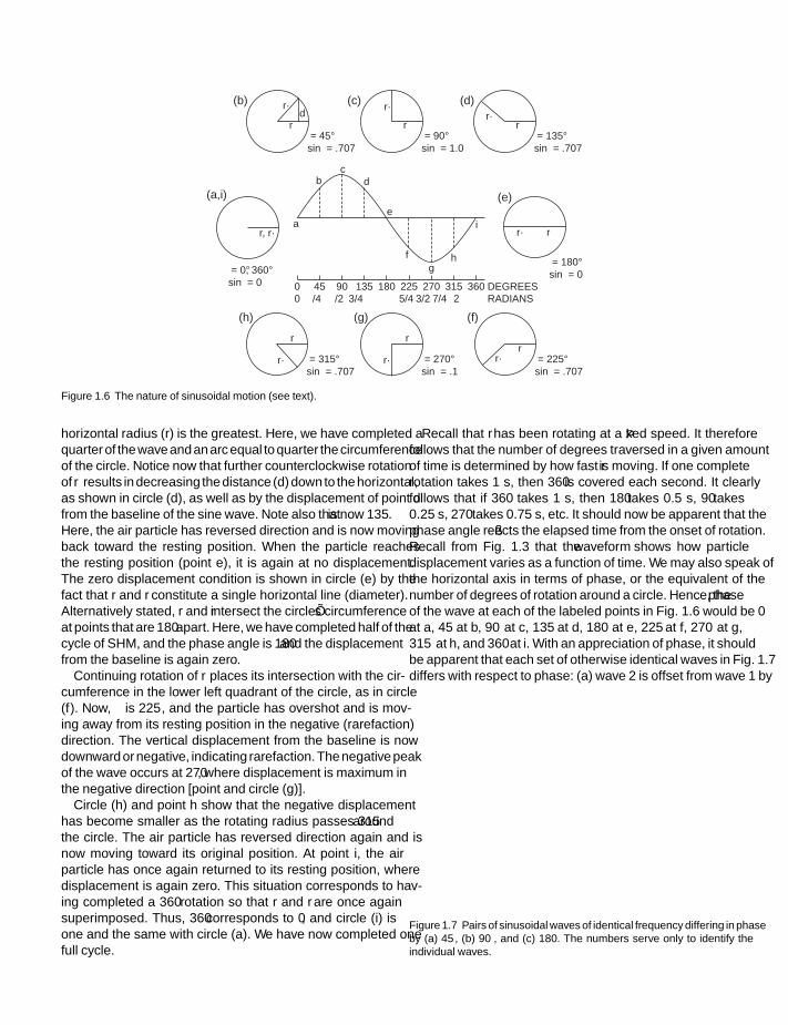
The curves in Fig. 1.5 reveal that the waveform of SHM is asinusoidal function and is thus called a sinusoidal wave, alsoknown as a sine wave or a sinusoid. Figure 1.6 elucidates thisconcept and also indicates a number of the characteristics ofsine waves. The center of the figure shows one complete cycle ofSHM, going from points a through i. The circles around the sinewave correspond to the various points on the wave, as indicatedby corresponding letters. Circle (a) corresponds to point a onthe curve, which falls on the baseline. This point correspondsto the particle’s resting position.

Circle (a) shows a horizontal radius (r) drawn from the centerto the circumference on the right. Imagine as well a secondradius (r′) that will rotate around the circle in a counterclockwisedirection. The two radii are superimposed in circle (a) so that theangle between them is 0. There is clearly no distance betweenthese two superimposed lines. This situation corresponds topoint a on the sine wave at the center of the figure. Hence, pointa may be said to have an angle of 0, and no displacement fromthe origin. This concept may appear quite vague at first, but itwill become clear as the second radius (r′) rotates around thecircle.

Let us assume that radius r′ is rotating counterclockwise at afixed speed. When r′ has rotated 45, it arrives in the positionshown in circle (b). Here, r′ is at an angle of 45 to r. We willcall this angle as the phase angle (), which simply reflects thedegree of rotation around the circle, or the number of degreesinto the sine wave at the corresponding point b. We now drop avertical line from the point where r′ intersects the circle down tor. We label this line d, representing the vertical distance betweenr and the point where r′ intersects the circle. The length ofthis line corresponds to the displacement of point b from thebaseline of the sine wave (dotted line at b). We now see thatpoint b on the sine wave is 45 into the cycle of SHM, at whichthe displacement of the air particle from its resting positionis represented by the height of the point above the baseline. Itshould now be clear that the sine wave is related to the degrees ofrotation around a circle. The shape of the sine wave correspondsto the sine of as r′ rotates around the circle, which is simplyequal to d/r′.

The positive peak of the sine wave at point c corresponds tocircle (c), in which r′ has rotated to the straight up position.It is now at a 90 angle to r, and the distance (d) down to the

9

SFK SFK


chapter 1

(b) r´

rθ = 45°sin θ = .707

dθ

(a,i)

r, r´

θ = 0°, 360°sin θ = 0

(c) r´

rθ = 90°sin θ = 1.0

θ

(h)

r´

r

θ = 315°sin θ = –.707

θ

(f)

r´r

θ = 225°sin θ = –.707

θ

(e)

r´ r

θ = 180°sin θ = 0

θ

(g)

r´

r

θ = 270°sin θ = –.1

θ

(d)r´

rθ = 135°sin θ = .707

θ

a

0 45 90 135 180 225 270 315 360 DEGREES0 π/4 π/2 3π/4 π 5π/4 3π/2 7π/4 2π RADIANS

bc

d

e

fg

h

i

Figure 1.6 The nature of sinusoidal motion (see text).

horizontal radius (r) is the greatest. Here, we have completed aquarter of the wave and an arc equal to quarter the circumferenceof the circle. Notice now that further counterclockwise rotationof r′ results in decreasing the distance (d) down to the horizontal,as shown in circle (d), as well as by the displacement of point dfrom the baseline of the sine wave. Note also that is now 135.Here, the air particle has reversed direction and is now movingback toward the resting position. When the particle reachesthe resting position (point e), it is again at no displacement.The zero displacement condition is shown in circle (e) by thefact that r and r′ constitute a single horizontal line (diameter).Alternatively stated, r and r′ intersect the circle’s circumferenceat points that are 180 apart. Here, we have completed half of thecycle of SHM, and the phase angle is 180 and the displacementfrom the baseline is again zero.

Continuing rotation of r′ places its intersection with the cir-cumference in the lower left quadrant of the circle, as in circle(f). Now, is 225, and the particle has overshot and is mov-ing away from its resting position in the negative (rarefaction)direction. The vertical displacement from the baseline is nowdownward or negative, indicating rarefaction. The negative peakof the wave occurs at 270, where displacement is maximum inthe negative direction [point and circle (g)].

Circle (h) and point h show that the negative displacementhas become smaller as the rotating radius passes 315 aroundthe circle. The air particle has reversed direction again and isnow moving toward its original position. At point i, the airparticle has once again returned to its resting position, wheredisplacement is again zero. This situation corresponds to hav-ing completed a 360 rotation so that r and r′ are once againsuperimposed. Thus, 360 corresponds to 0, and circle (i) isone and the same with circle (a). We have now completed onefull cycle.

Recall that r′ has been rotating at a fixed speed. It thereforefollows that the number of degrees traversed in a given amountof time is determined by how fast r′ is moving. If one completerotation takes 1 s, then 360 is covered each second. It clearlyfollows that if 360 takes 1 s, then 180 takes 0.5 s, 90 takes0.25 s, 270 takes 0.75 s, etc. It should now be apparent that thephase angle reflects the elapsed time from the onset of rotation.Recall from Fig. 1.3 that the waveform shows how particledisplacement varies as a function of time. We may also speak ofthe horizontal axis in terms of phase, or the equivalent of thenumber of degrees of rotation around a circle. Hence, the phaseof the wave at each of the labeled points in Fig. 1.6 would be 0

at a, 45 at b, 90 at c, 135 at d, 180 at e, 225 at f, 270 at g,315 at h, and 360 at i. With an appreciation of phase, it shouldbe apparent that each set of otherwise identical waves in Fig. 1.7differs with respect to phase: (a) wave 2 is offset from wave 1 by

Figure 1.7 Pairs of sinusoidal waves of identical frequency differing in phaseby (a) 45, (b) 90, and (c) 180. The numbers serve only to identify theindividual waves.

10

SFK SFK


physical concepts

45, (b) waves 3 and 4 are apart in phase by 90, and (c) waves5 and 6 are 180 out of phase.

We may now proceed to define a number of other funda-mental aspects of sound waves. A cycle has already been definedas one complete repetition of the wave. Thus, four cycles of asinusoidal wave were shown in Fig. 1.5 because it depicts fourcomplete repetitions of the waveform. Because the waveform isrepeated over time, this sound is said to be periodic. In contrast,a waveform that does not repeat itself over time would be calledaperiodic.

The amount of time that it takes to complete one cycle iscalled its period, denoted by the symbol t (for time). For exam-ple, a periodic wave that repeats itself every millisecond is said tohave a period of 1 ms, or t = 1 ms or 0.001 s. The periods of thewaveforms considered in hearing science are overwhelminglyless than 1 s, typically in the milliseconds and even microsec-onds. However, there are instances when longer periods areencountered.

The number of times a waveform repeats itself per unit of timeis its frequency (f). The standard unit of time is the second; thus,frequency is the number of times a wave repeats itself in a second,or the number of cycles per second (cps). By convention, theunit of cycles per second is the hertz (Hz). Thus, a wave that isrepeated 1000 times per second has a frequency of 1000 Hz, andthe frequency of a wave that repeats at 2500 cycles per second is2500 Hz.

If period is the time it takes to complete one cycle, and fre-quency is the number of cycles that occur each second, then itfollows that period and frequency are intimately related. Con-sider a sine wave that is repeated 1000 times per second. Bydefinition it has a frequency of 1000 Hz. Now, if exactly 1000cycles take exactly 1 s, then each cycle must clearly have a dura-tion of 1 ms, or 1/1000 s. Similarly, each cycle of a 250-Hztone must last 1/250 s, or a period of 4 ms. Formally, then, fre-quency is the reciprocal of period, and period is the reciprocalof frequency:

f = 1

t(1.32)

and

t = 1

f(1.33)

It has already been noted that the oscillating air particle ismoving back and forth around its resting or average position.In other words, the air particle’s displacement changes over thecourse of each cycle. The magnitude of the air particle’s displace-ment is called amplitude. Figure 1.8 illustrates a difference inthe amplitude of a sinusoid, and contrasts this with a change inits frequency. In both frames of the figure, the tone representedby the finer curve has greater amplitude than the one portrayedby the heavier line. This is shown by the greater vertical distancefrom the baseline (amplitude) at any point along the horizontalaxis (time). (Obviously, exceptions occur at those times whenboth curves have zero amplitudes.)

Figure 1.8 Within each frame (a and b), both sinusoidal waves have thesame frequency, but the one depicted by the lighter curves has a greateramplitude than the one represented by the heavier curves. The curves inframe (b) have twice the frequency as those shown in frame (a).

At any given moment, the particle may be at its extremepositive or negative displacement from the resting position inone direction or the other, or it may be somewhere between thesetwo extremes (including being at the resting position, wheredisplacement is zero). Because each of these displacements isa momentary glimpse that holds true only for that instant,the magnitude of a signal at a given instant is aptly called itsinstantaneous amplitude.

Because the instantaneous amplitude changes from momentto moment, we also need to be able to describe the magnitudeof a wave in more general terms. The overall displacement fromthe negative to positive peak yields the signal’s peak-to-peakamplitude, while the magnitude from baseline to a peak is calledthe wave’s peak amplitude. Of course, the actual magnitude isno more often at the peak than it is at any other phase of thesine wave. Thus, although peak amplitudes do have uses, wemost often are interested in a kind of “average” amplitude thatmore reasonably reflects the magnitude of a wave throughoutits cycles. The simple average of the sinusoid’s positive andnegative instantaneous amplitudes cannot be used because thisnumber will always be equal to zero. The practical alternativeis to use the root-mean-square (rms) amplitude. This valueis generally and simply provided by measuring equipment, butit conceptually involves the following calculations: First, thevalues of all positive and negative displacements are squared sothat all resulting values are positive numbers (and zero for thosevalues that fall right on the resting position). Then the mean ofall these values is obtained, and the rms value is finally obtainedby taking the square root of this mean. The rms amplitude ofa sinusoidal signal is numerically equal to 0.707 times the peakamplitude, or 0.354 times the peak-to-peak amplitude. Figure1.9 illustrates the relationships among peak, peak-to-peak, andrms amplitudes.

11

SFK SFK


chapter 1

Figure 1.9 The relationships among the root-mean-square (rms), peak, and peak-to-peak amplitudes.

combining waves

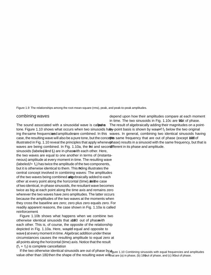
The sound associated with a sinusoidal wave is called a puretone. Figure 1.10 shows what occurs when two sinusoids hav-ing the same frequencies and amplitudes are combined. In thiscase, the resulting wave will also be a pure tone, but the conceptsillustrated in Fig. 1.10 reveal the principles that apply wheneverwaves are being combined. In Fig. 1.10a, the first and secondsinusoids (labeled fl and f2) are in-phase with each other. Here,the two waves are equal to one another in terms of (instanta-neous) amplitude at every moment in time. The resulting wave(labeled fl + f2) has twice the amplitude of the two components,but it is otherwise identical to them. This finding illustrates thecentral concept involved in combining waves: The amplitudesof the two waves being combined are algebraically added to eachother at every point along the horizontal (time) axis. In the caseof two identical, in-phase sinusoids, the resultant wave becomestwice as big at each point along the time axis and remains zerowherever the two waves have zero amplitudes. The latter occursbecause the amplitudes of the two waves at the moments whenthey cross the baseline are zero; zero plus zero equals zero. Forreadily apparent reasons, the case shown in Fig. 1.10a is calledreinforcement.

Figure 1.10b shows what happens when we combine twootherwise identical sinusoids that are 180 out of phase witheach other. This is, of course, the opposite of the relationshipdepicted in Fig. 1.10a. Here, wave f1 is equal and opposite towave f2 at every moment in time. Algebraic addition under thesecircumstances causes the resulting amplitude to equal zero atall points along the horizontal (time) axis. Notice that the result(f1 + f2) is complete cancellation.

If the two otherwise identical sinusoids are out of phase by avalue other than 180, then the shape of the resulting wave will

depend upon how their amplitudes compare at each momentin time. The two sinusoids in Fig. 1.10c are 90 out of phase.The result of algebraically adding their magnitudes on a point-by-point basis is shown by wave fl + f2 below the two originalwaves. In general, combining two identical sinusoids havingthe same frequency that are out of phase (except 180 out ofphase) results in a sinusoid with the same frequency, but that isdifferent in its phase and amplitude.

Figure 1.10 Combining sinusoids with equal frequencies and amplitudesthat are (a) in phase, (b) 180 out of phase, and (c) 90 out of phase.

12

SFK SFK


physical concepts

complex waves

Thus far, we have dealt only with the combination of sinusoidshaving the same frequency. What happens when we combinedsinusoids that differ in frequency? When two or more pure tonesare combined, the result is called a complex wave or a complexsound. The mechanism for combining waves of dissimilar fre-quencies is the same as what applies for those having the samefrequency: Any two or more waves are combined by algebraicallysumming their instantaneous displacements on a point-by-point basis along the horizontal (time) axis, regardless of theirindividual frequencies and amplitudes or their phase relation-ships. However, the combination of waves having unequal fre-quencies will not yield a sinusoidal result. Instead, the resultwill depend upon the specifics of the sounds being combined.

Consider the three sinusoids at the top in Fig. 1.11, labeled f1,f2, and f3. Note that the two cycles of f1 are completed in the sametime as four cycles of f2 or six cycles of f3. Thus, frequency of f2

is exactly two times that of f1, and the frequency of f3 is exactlythree times f1. The actual frequencies of f1, f2, and f3 could beany values meeting the described conditions; for example, 100,200, and 300 Hz; 1000, 2000, and 3000 Hz, or 20, 40, and 60 Hz,etc. Because f2 and f3 are integral multiples of f1, we say that theyare harmonics of f1. Hence, f1, f2, and f3 constitute a harmonicseries. The lowest frequency of this series is the fundamen-tal frequency. Otherwise stated, harmonics are whole-numbermultiples of the fundamental frequency; the fundamental is thelargest whole-number common denominator of its harmonics.Notice that the fundamental frequency (often written as f0) isalso the first harmonic because its frequency is the value ofthe first harmonic, or 1 × f0. Clearly, the harmonics are sepa-rated from one another by amounts equal to the fundamentalfrequency.

The lower three waves in Fig. 1.11 show what happens whenf1, f2, and f3 are combined in various ways. Notice that the com-bining of two or more sinusoidal waves differing in frequencygenerates a resultant wave that is no longer sinusoidal in charac-ter. Note, however, that the combined waveforms shown in thisfigure are still periodic. In other words, even though these com-bined waveforms are no longer sinusoidal, they still retain thecharacteristic of repeating themselves at regular intervals overtime. Moreover, notice that all three waves (f1 + f2, f1 + f3, and f1

+ f2 + f3) repeat themselves with the same period as f1, which isthe lowest component in each case. These are examples of com-plex periodic waves, so called because (1) they are composedof more than one component and (2) they repeat themselvesat regular time intervals. The lowest-frequency component of acomplex periodic wave is its fundamental frequency. Hence, f1

is the fundamental frequency of each of the complex periodicwaves in Fig. 1.11 The period of the fundamental frequencyconstitutes the rate at which the complex periodic wave repeatsitself. In other words, the time needed for one cycle of a com-plex periodic wave is the same as the period of its fundamentalfrequency.

Figure 1.11 The in-phase addition of sinusoidal waves f1, f2, and f3 intocomplex periodic waves, f1 + f2, f1 + f3, and f1 + f2 + f3. The frequency of f2

is twice that of f1, and f3 is three times the frequency of f1. The frequency off1 is the fundamental frequency of each of the three complex periodic waves.

The example shown in Fig. 1.12 involves combining onlyodd harmonics of 1000 Hz (1000, 3000, 5000, and 7000 Hz)whose amplitudes become smaller with increasing frequency.The resulting complex periodic waveform becomes progres-sively squared off as the number of odd harmonics is increased,eventually resulting in the aptly named square wave. The com-plex periodic waveform at the bottom of the figure depicts theextent to which a square wave is approximated by the combina-tion of the four odd harmonics shown above it.

The combination of components that are not harmonicallyrelated results in a complex waveform that does not repeatitself over time. Such sounds are thus called aperiodic. In theextreme case, consider a wave that is completely random. Anartist’s conceptualization of two separate glimpses of a randomwaveform is shown in Figs. 1.13 1.13a and 1.13b. The point ofthe two pictures is that the waveform is quite different frommoment to moment. Over the long run, such a wave wouldcontain all possible frequencies, and all of them would havethe same average amplitudes. The sound described by suchwaveforms is often called random noise or Gaussian noise.Because all possible frequencies are equally represented, theyare more commonly called white noise on analogy to whitelight. Abrupt sounds that are extremely short in duration mustalso be aperiodic because they are not repeated over time. Suchsounds are called transients. The waveform of a transient isshown in Fig. 1.13c.

Because the waveform shows amplitude as a function of time,the frequency of a pure tone and the fundamental frequency ofa complex periodic tone can be determined only indirectly by

13

SFK SFK


chapter 1

Figure 1.12 The addition of odd harmonics of 1000 Hz to produce a square wave. Waveforms (amplitude as a function of time) are shown in the left panelsand corresponding spectra (amplitude as a function of frequency) are shown in the right panels.

examining such a representation, and then only if the time scaleis explicit. Moreover, one cannot determine the frequency con-tent of a complex sound by looking at its waveform. In fact,dramatically different waveforms result from the combinationof the same component frequencies if their phase relationshipsare changed. Another means of presenting the material is there-fore needed when one is primarily interested in informationabout frequency. This information is portrayed by the spec-trum, which shows amplitude as a function of frequency. Ineffect, we are involved here with the issue of going betweenthe time domain (shown by the waveform) and the frequencydomain (shown by the spectrum). The underlying mathemat-ical relationships are provided by Fourier’s theorem, whichbasically says that a complex sound can be analyzed into itsconstituent sinusoidal components. The process by which onemay break down the complex sound into its component partsis called Fourier analysis. Fourier analysis enables one to plotthe spectrum of a complex sound.

The spectra of several periodic waves are shown in the rightside of Fig. 1.12, and the spectrum of white noise is shown in

Fig. 1.13d. The upper four spectra in Fig. 1.12 corresponds,respectively, to the waveforms of the sinusoids to their left. Thetop wave is that of a 1000-Hz tone. This information is shownon the associated spectrum as a single (discrete) vertical linedrawn at the point along the abscissa corresponding to 1000Hz. The height of the line indicates the amplitude of the wave.The second waveform in Fig. 1.12 is for a 3000-Hz tone thathas a lower amplitude than does the 1000-Hz tone shown aboveit. The corresponding spectrum shows this as a single verticalline drawn at the 3000-Hz location along the abscissa. Similarly,the spectra of the 5000- and 7000-Hz tones are discrete verticallines corresponding to their respective frequencies. Notice thatthe heights of the lines become successively smaller going fromthe spectrum of the 1000-Hz tone to that of the 7000-Hz tone,revealing that their amplitudes are progressively lower.

The lowest spectrum in Fig. 1.12 depicts the complex peri-odic wave produced by the combination of the four pure tonesshown above it. It has four discrete vertical lines, one each atthe 1000-, 3000-, 5000-, and 7000-Hz locations. This spectrumapproximates that of a square wave. The spectrum of a square

14

SFK SFK


physical concepts

Figure 1.13 Artist’s conceptualizations of the waveform of white noise as itmight appear at two different times (a and b), and of a transient (c), alongwith the spectrum of white noise or a transient (d).

wave is composed of many discrete vertical lines, one each at thefrequencies corresponding to odd multiples of its lowest (funda-mental) component, with their heights decreasing as frequencyincreases.

To summarize, the spectrum of a periodic wave shows a ver-tical line at the frequency of each sinusoidal component of thatwave, and the amplitude of each component is shown by theheight of its corresponding line. Consequently, the spectrumof a periodic sound is referred to as a discrete spectrum. Asshould be apparent, the phase relationships among the vari-ous components are lost when a sound is represented by itsspectrum.

Figure 1.13d shows the spectrum of white noise. Becausewhite noise contains all conceivable frequencies, it would bea fruitless exercise to even try to draw individual (discrete)vertical lines at each of its component frequencies. The samepoint applies to the three spectra depicted in Fig. 1.14 shows thecontinuous spectra of aperiodic sounds that contain (1) greateramplitude in the higher frequencies, (2) greater amplitude inthe lower frequencies, and (3) a concentration of energy withina particular range band (range) of frequencies.

filters

The three spectra depicted in Fig. 1.14 may also be used todescribe the manner in which a system transfers energy as afunction of frequency. Filters are described according to therange of frequencies that they allow to pass as opposed to thosethat they stop or reject . Thus, Fig. 1.15a depicts a high-pass

Figure 1.14 Continuous spectra of aperiodic sounds with (a) greater ampli-tude in the high frequencies, (b) greater amplitude in the lower frequencies,and (c) a concentration of energy within a given band of frequencies.

filter because the frequencies higher than a certain cutoff fre-quency are passed, whereas those below that cutoff frequencyare stopped or rejected. On the other hand, Fig. 1.15b showsa low-pass filter because the frequencies lower than its cutofffrequency are passed whereas higher ones are rejected. A cutofffrequency is usually defined as the frequency where the powerfalls to half of its peak value. This location is called the half-power point. In decibels, the half-power point is 3 dB belowthat level of the peak, and is therefore also known as the 3-dBdown point.

Figure 1.15c illustrates a band-pass filter because the fre-quencies within the designated range are passed, whereas thosebelow and above its lower and upper cutoff frequencies arerejected. A band-pass filter is usually described in terms of itscenter frequency, which is self-explanatory, and its bandwidth,which is how wide the filter is between its upper and lower cutofffrequencies. A filter that passes the frequencies above and belowa certain band, but rejects the frequencies within that band iscalled a band-reject filter (Fig. 1.15d).

The sharpness with which a filter de-emphasizes the rejectband is given by its slope, also know as its rolloff, attenuation,or rejection rate. The slope is usually expressed in decibels peroctave. For example, a slope of 24 dB/octave means that themagnitude of the sound outside of the pass band is reduced ata rate of 24 dB for each doubling of frequency. Beginning at1000 Hz, a 24-dB/octave rolloff rate would cause the signal tobe reduced by 24 dB by 2000 Hz (an octave above 1000 Hz)and by an additional 24 dB by 4000 Hz (an octave above 2000Hz). Besides using its slope, it is often convenient to describethe sharpness of tuning for a band-pass filter in terms of avalue called Q, especially when comparing the characteristics ofdifferent filters. The Q of a filter is simply the ratio of its centerfrequency to its bandwidth.

15

SFK SFK


chapter 1

Cut-offFrequency

3 dB

RejectBand

RejectBand

RejectBand

PassBand

PassBand

PassBand

PassBand

3 dB

3 dB

Cut-offFrequency

Frequency

Am

plitu

de

Center Frequency

Slope

Slope

Slop

e Cut-off frequency

(a) High-pass filter

(b) Low-pass filter

(c) Band-pass filter

(d) Band-reject filter

Bandwidth

Figure 1.15 Examples of filters and some of their parameters: (a) high-passfilter, (b) low-pass filter, (c) band-pass filter, and (d) band-reject filter.

standing waves

Let us consider two situations. In the first situation, imaginethe sound waves propagating rightward and leftward from avibrating tuning fork placed in the center of a small room. Thesesound waves will hit and be reflected from the walls so that nowthere will also be reflected waves propagating in the oppositedirections in addition to the original waves. (Considering forthe moment only the right wall for simplicity, we can envisiona rightward-going original wave and a leftward-going reflectedwave.) The other situation involves plucking the center of aguitar string that is tied tautly at both ends. Here, the wavesinitiated by the pluck move outward toward each fixed endof the string, from which a reflected wave propagates in theopposite direction.

To reiterate, in both cases, just described, there are continu-ous original and continuous reflected waves moving toward oneanother. The reflected waves are equal in frequency to the origi-nal ones, and both the reflected and original waves are of coursepropagating at the same speed. Now, recall from prior discus-sion that two waves will interact with one another such that

their instantaneous displacements add algebraically. Thus, thenet displacement (of the air particles in the room or of the string)at any moment that occurs at any point (in the room or alongthe string) will be due to how the superimposed waves interact.It turns out that the resultant wave produced by this interactionconstitutes a pattern that f1, f2, and f3 actually stands still eventhough it is derived from component waves which themselvesare propagating. Hence, the points of maximum displacement(peaks of the waves) and no displacement (baseline crossings ofthe waves) will always occur at fixed locations in the room oralong the string. This phenomenon is quite descriptively calleda standing wave.

Because the vibration pattern of the string is easily visualized,we will refer only to the string as example for the remainderof the discussion, although these points apply similarly to theroom example as well. The locations of no (zero) displacementin the standing wave pattern are called nodes, and the placesof maximum displacement are thus called antinodes. Evenbrief consideration will reveal that the displacement must bezero at the two ends of the string, where they are tied and thuscannot move. (This corresponds to the hard walls of the room,which prevent the air molecules from being displaced.) Hence,nodes must occur at the two ends of the string. It follows thatif there is a node at each end of the string, then there mustbe an antinode at the center of the string, halfway betweenthe two nodes. This notion should not be surprising, becausewe already know that the zero displacements (at 0 and 180

phase) and maximum displacements (at 90 and 270 phase)alternate for any cycle of a sinusoid.

This standing wave pattern is depicted in Fig. 1.16a. Somethought will confirm that the arrangement just described (anode at each end an antinode at the center) constitutes the

Figure 1.16 The (a) first, (b) second, and (c) third modes of a vibratingstring.

16

SFK SFK


physical concepts

longest possible standing wave pattern that can occur for anygiven string. We will call it the first mode of vibration. The figurealso highlights the fact that this standing wave pattern comprisesexactly one-half of a cycle (from 0 to 180). Consequently, itslength (L) corresponds to exactly one-half of a wavelength (),or L = /2. Its length therefore is equal to one-half of a wave-length (/2) of some frequency. This frequency, in turn, maybe determined by applying the formula, f = c/ (Eq. 1.31). Bysubstitution, the frequency of the string’s first mode of vibrationwould be c/2L (where L is the length of the string and c is theappropriate speed of the wave for that string3). It should nowbe apparent that the first mode of vibration corresponds to thefundamental frequency.

The standing wave just described is not the only one thatcan occur for the string, but rather is the longest one. Otherstanding waves may develop as well as long as they meet therequirement that nodes occur at the two tied ends of the string.Several other examples are shown in Fig. 1.16, which revealsthat each of these standing wave patterns must divide the stringinto parts that are exactly equal in length to one another. Thus,there will be standing wave patterns that divide the string intoexact halves, thirds, fourths, fifths, etc. These are the second,third, fourth, fifth, etc., modes of vibration. In turn, they pro-duce frequencies, which are exact multiples (harmonics) of thefundamental frequency.

Suppose we were to set the air inside of a tube into vibrationby, for example, blowing across the open end of the tube. If wewere to do this experiment for several tubes, we would find thatthe shorter tubes make higher-pitch sounds than do the longerones. We would also find that the same tube would produce ahigher pitch when it is open at both ends than when it is openat only one end. The frequency(ies) at which a body or mediumvibrates is referred to as its natural or resonant frequency(ies).

In the case of a column of air vibrating in a tube open at bothends, the greatest pressure and the least particle displacementcan occur in the center of the tube, while the greatest displace-ment and thus lowest pressure can occur at the two open ends(Fig. 1.17a). This is analogous to the vibration of the string. Onemay understand this in the sense that going from one end ofthe tube to the other involves going from a pressure node to anantinode to a node (or from displacement antinode to node toantinode), or 180 of a cycle. This pattern is related to the out-of-phase reflection of the wave at the two ends of the tubeso that the pattern is duplicated when the length of the tubeis covered twice. Hence, the lowest (fundamental) frequencycapable of covering the tube exactly twice in one cycle musthave a wavelength twice the length of the tube. Thus, the lowest

3 The speed of a wave along a vibrating string is not the same as for air.Instead, we would be dealing with the speed of a transverse wave alonga string, which is the square root of the ratio of the string’s tension (T)to its mass per unit area (M). Hence, the formula for the string’s lowestresonant frequency actually would be f = (1/2L)

√T/M.

Figure 1.17 Standing waves in (a) a tube which is open at both ends (a half-wavelength resonator) and (b) a tube which is closed at one end and openat the other end (a quarter-wavelength resonator). Source: From Gelfand SA(2001). Essentials of Audiology, Second Edition. New York: Thieme MedicalPublishers, with permission.

resonant frequency (f1) of a tube open at both ends is the fre-quency whose wavelength is twice the length of the tube, or f1 =c/2L. Harmonics will occur at each multiple of this fundamentalfrequency.

Air vibration in a tube closed at one end is most restrictedat the closed end, where pressure must thus be greatest anddisplacement the least (Fig. 1.17b). (Reflections at the closed endoccur without phase reversal.) Thus, in terms of displacement,there must be a node at the closed end and an antinode at theopen end. This means that the length of the tube corresponds toa quarter of a wavelength so that the lowest resonant frequency(f1) of a tube closed at one end and open at the other is theone whose wavelength is four times the length of the tube,or f1 = c/4L. Since a node can occur at only one end, sucha tube produces only the fundamental frequency and its oddharmonics (e.g., f1, f3, f5, f7, etc.).

impedance

Impedance is the opposition to the flow of energy througha system. Some knowledge of impedance thus helps one tounderstand how a system transmits energy, and why it is moreresponsive to some frequencies than it is to others. We maygenerally define impedance (Z), in ohms, as the ratio of force

17

SFK SFK


chapter 1

to velocity:

Z = F

v(1.34)

Therefore, the greater the amount of force needed to resultin a given amount of velocity, the greater the impedance of thesystem.

We may also consider impedance in terms of its components.These are shown in the form of a mechanical representation ofimpedance in Fig. 1.18 Here, we see that impedance (Z) is theinteraction between resistance (R) and two kinds of reactance(X), known as positive or mass reactance (Xm) and negativeor stiffness reactance (Xs). These components are, respectively,related to friction, mass, and stiffness. In the figure, mass isrepresented by the block, and stiffness is provided by the spring.Friction is represented in the figure by the irregular surfaceacross which the mass (represented by a solid block) is moved.

Let us imagine that a sinusoidal force (represented by thearrow) is being applied to the system depicted in the illustration.Friction causes a portion of the energy applied to the systemto be converted into heat. This dissipation of energy into heatis termed resistance. Resistance is not related to frequency andoccurs in phase with the applied force. In contrast, reactanceis the storage (as opposed to the dissipation) of energy by thesystem. Mass reactance is, of course, associated with the massof the system (the block in Fig. 1.18). Since mass is associatedwith the property of inertia, the application of a force causesthe mass to accelerate according to the familiar formula F =Ma (where F is force, M is mass, and a is acceleration). If theforce is applied sinusoidally, then the mass reactance is relatedto frequency as

Xm = M · 2f (1.35)

where f is frequency. Thus, the magnitude of the mass reactanceis directly proportional to frequency; that is, the higher thefrequency, the greater the mass reactance. Since accelerationprecedes force by a quarter-cycle, Xm will lead the applied forcein phase by 90. This is why Xm is termed positive reactance,

Figure 1.18 The components of impedance (Z) are friction or resistance(R), represented by the rough surface, mass (positive) reactance (Xm), rep-resented by the block, and stiffness (negative) reactance (Xs), represented bythe spring.

Positive (mass)Reactance (Xm)

Negative (stiffness)Reactance (Xs)

Resistance(R)

Impedance(Z)

(–θ) PhaseAngle

Xnet = Xs – Xm

Z = √ R2 – (Xs – Xm)2

Figure 1.19 The relationships between impedance and its components.

and its value is shown in the positive direction on the y-axis inFig. 1.19

Stiffness reactance is represented by the spring in Fig. 1.18We will represent the stiffness as S. Applying a force compresses(displaces) the spring according to the formula F = Sx, wherex is the amount of displacement. When the force is appliedsinusoidally, then stiffness reactance is related to frequency as

X = S

2f(1.36)

In other words, the amount of stiffness reactance is inverselyproportional to frequency; that is, stiffness reactance goes downas frequency goes up. Since displacement follows force by aquarter-cycle, Xs lags behind the applied force in phase by 90.It is thus called negative reactance and is plotted downward onthe y-axis in Fig. 1.19 It should be apparent at this point thatXm and Xs are 180 out of phase with each other.

Because stiffness and mass reactance are 180 out of phase, asystem’s net reactance is equal to the difference between them(Xm − Xs). This relationship is illustrated in Fig. 1.19 for thecondition where Xs exceeds Xm, which is the case for lowerfrequencies in the normal ear (see Chap. 3). Notice that theimpedance (Z) is a vector, which results from the interactionbetween the resistance (R) and the net reactance (Xnet). The neg-ative phase angle (−) in Fig. 1.19 shows that the net reactanceis negative. The relationship among impedance, resistance, andreactance may now be summarized as follows:

Z =√

R2 + (Xs − Xm)2 (1.37)

Looking at the effect of frequency, we find that

Z =√

R2 +(

S

2f− M · 2f

)2

(1.38)

The implication is that frequency counts. Because Xm is pro-portional to frequency, while Xs is inversely proportional to

18

SFK SFK


physical concepts

Figure 1.20 Artist’s conceptualizations of the relationship between theamount of damping (left panels) and the sharpness of tuning around theresonant frequency (right panels).

frequency, they should be equal at some frequency. This is thesystem’s resonant frequency, at which the reactance compo-nents cancel each other out, leaving only the resistance compo-nent.

The amount of resistance is associated with how rapidlydamping occurs, and it determines the sharpness of the tuningaround the resonant frequency. This relationship is illustratedin Fig. 1.20 The less the resistance (i.e., the slower the damp-ing), the more narrowly tuned the resonance is; the more theresistance (i.e., the faster the damping), the broader the respon-siveness of the system around the resonant frequency.

referencesAmerican National Standards Institute, ANSI S1−1994

(R2004). 2004. American National Standard Acoustical Ter-minology. New York: ANSI.

Beranek LL. 1986. Acoustics. New York: American Institute ofPhysics.

Everest FA. 2000. The Master Handbook of Acoustics, 4th ed. NewYork: McGraw-Hill.

Gelfand SA. 2001. Essentials of Audiology, 2nd ed. New York:Thieme Medical Publishers.

Hewitt, PG 2005. Conceptual Physics, 10th ed. Boston, MA: Pear-son Addison-Wesley.

Kinsler LE, Frey AR, Coopens AB, and Sanders JB. 1999. Fun-damentals of Acoustics, 4th ed. New York, NY: Wiley.

Pearce JR, David EE Jr. 1958. Man’s World of Sound. GardenCity, New York, NY: Doubleday.

Peterson APG, Gross EE. 1972. Handbook of Noise Measurement,7th ed. Concord, MA: General Radio.

Rassmussen G. Intensity—Its measurement and uses. SoundVibr 1989; 23(3):12–21.

Rossing TD, Moore RF, Wheeler PA. 2002. The Science of Sound,3rd ed. Boston, MA: Pearson Addison-Wesley.

Speaks CE. 1999. Introduction to Sound: Acoustics for Hearingand Speech Sciences, 3rd ed. San Diego, CA: Singular.

van Bergeijk WA, Pearce JR, David EE Jr. 1960. Waves and theEar. Garden City, New York, NY: Doubleday.

Young HD, Freedman RA. 2007. Sears and Zemansky’s UniversityPhysics with Modern Physics, 12th ed. Boston, MA: PearsonAddison-Wesley.

19

SFK SFK


2 Anatomy

gross anatomy and overview

The auditory system comprises the ears and their connectionsto and within the central nervous system. From the standpointof physical layout, the auditory system may be divided intothe outer, middle, and inner ears; the auditory nerve; and thecentral auditory pathways. This section provides a very briefand simplified overview of the auditory system, in the hope thata brief glance at the forest will help the student avoid beingblinded by the trees. Before proceeding, those not familiar withanatomical terminology should review the pictures in Fig. 2.1and the definitions in Table 2.1, which summarize some of theterms used to describe the orientation of anatomical structuresand the relationships among them.

The major divisions of the ear are shown in Fig. 2.2, and theirrelative positions within the head are given in Fig. 2.3. The outerear is made up of the pinna (auricle) and ear canal (externalauditory meatus). The eardrum (tympanic membrane) sepa-rates the outer and middle ears and is generally considered tobe part of the latter. The middle ear also includes the tym-panic (middle ear) cavity; the ossicular chain with its associatedmuscles, tendons, and ligaments; and the eustachian (auditory)tube. The inner ear begins at the oval window. It includes thesensory organs of hearing (the cochlea) and of balance (thesemicircular canals, utricle, and saccule). While the balance sys-tem is certainly important, the concern here is hearing, andaccordingly the balance apparatus is mentioned only insofar asit is directly associated with the auditory system.

The inner ear, beyond the oval window, is composed of thevestibule, the cochlea, and the vestibular apparatus. A mem-branous duct is continuous throughout these. In the cochlea,it separates the perilymph-filled scala vestibuli and scala tym-pani above and below from the endolymph-filled scala mediabetween them. The scala media contains the organ of Corti,whose hair cells are the sensory receptors for hearing. Whenstimulated, the hair cells initiate activity in the auditory nervefibers with which they are in contact. The auditory nerve leavesthe inner ear through the internal auditory canal (internal audi-tory meatus), enters the brain at the angle of the pons and cere-bellum, and terminates in the brainstem at the cochlear nuclei.We are now in the central auditory system.

temporal bone

The ear is contained within the temporal bone. Knowledge ofthe major landmarks of this bone is thus important in under-standing the anatomy and spatial orientation of the ear. Theright and left temporal bones are two of the 22 bones that makeup the skull. Eight of these bones (including the two temporalbones) contribute to the cranium, and the remaining 14 bones

form the facial skeleton. Figure 2.4 gives a lateral (side) view ofthe skull, emphasizing the temporal bone. The temporal boneforms the inferior portion of the side of the skull. It is borderedby the mandible, zygomatic parietal, sphenoid, and occipitalbones. The temporal bone itself is divided into five anatomicaldivisions: the squamous, mastoid, petrous, and tympanic por-tions, and the anteroinferiorly protruding styloid process. Theseparts of the temporal bone, as well as its major landmarks, areshown in Fig. 2.5.

The squamous portion is the fan-shaped part of the temporalbone. It is quite thin, often to the point of being translucent. Itsinferior surface forms the roof and part of the posterior wall ofthe ear canal. The zygomatic process protrudes forward fromthe squamous portion to meet the zygomatic bone. The fan-shaped squamous plate is also in contact with the sphenoid boneanteriorly and with the parietal bone superiorly and posteriorly.The mandible attaches to the temporal bone just anterior to theear canal, near the base of the zygomatic process, forming thetemporomandibular joint.

The mastoid portion lies behind and below the squamousand forms the posterior aspect of the temporal bone. The mas-toid portion attaches to the parietal bone superiorly and to theoccipital bone posteriorly. It projects downward to form themastoid process, which appears as a somewhat cone-shapedextension below the base of the skull. The mastoid processcontains interconnecting air cells of variable size, shape, andnumber. Continuous with these air cells is a cavity known asthe tympanic antrum, which lies anterosuperior to the mastoidprocess. The antrum also connects with the epitympanic recess(attic) of the middle ear via the aditus ad antrum. The antrumis bordered inferiorly by the mastoid process, superiorly by thethin bony plate called the tegmen tympani, medially by the wallof the lateral semicircular canal, and laterally by the squamouspart.

The tympanic portion of the temporal bone forms the flooras well as the anterior and inferoposterior walls of the ear canal.It is bordered superiorly by the squamous and petrous portionsand by the mastoid process posteriorly. The lower part of thetympanic portion partially covers the styloid process, which is athin, cylinder-like anteroinferior projection from the base of thetemporal bone. The styloid process, which varies in length fromas little as 5 mm to as much as 50 mm, is generally consideredto be a separate portion of the temporal bone. Although it doesnot contribute to the hearing mechanism, per se, the styloidprocess is important as a connecting point for several musclesinvolved in speech production.

The petrous portion houses the sensory organs of hearingand balance and contains the internal auditory canal. It ismedially directed and is fused at its base to the tympanic andsquamous portions. The mastoid lies posterior to the petrousportion, and in fact develops from it postnatally. The details

20

SFK SFK


anatomy

Figure 2.1 Commonly used anatomical orientations and directions. Source: From Gelfand (2001), Essentials of Audiology, Second Edition, by permission ofThieme Medical Publishers.

of the petrous portion are equivalent to those of the inner ear,discussed below.

outer and middle ear

PinnaThe pinna (auricle) is the external appendage of the ear. It is anirregularly shaped ovoid of highly variable size, which folds over

the side of the head posteriorly, superiorly, and inferiorly. It isbasically composed of skin-covered elastic cartilage, althoughit contains some grossly undifferentiated muscles that are of acompletely vestigial nature in humans. The pinna has a numberof extrinsic muscles as well, which are also essentially vestigialin humans.

The landmarks of the pinna are shown in Fig. 2.6. Most ofits perimeter is demarcated by a ridge-like rim called the helix.

Table 2.1 Summary of Commonly Used Terms Describing Anatomical Planes, Orientations, and Directions

Term Definition

Anterior FrontCaudal Toward the tailCephalad Toward the headContralateral Opposite side of the bodyCoronal plane Vertical plane separating the structure into front and back; frontal planeCranial Toward the headDextral RightDistal Away or further from a reference point (e.g., midline of the body)Dorsal Toward the spine (posterior in humans)Homolateral Same side of the bodyInferior BelowIpsilateral Same side of the bodyLateral Away from the midline (toward the side)Medial Toward the midlineMidsagittal plane Sagittal plane at the midlinePosterior BackProximal Toward, closer to a reference point (e.g., midline of the body)Rostral Toward the head (toward the beak)Sagittal plane Vertical plane separating the structure into right and leftSinistral LeftSuperior AboveTransverse plane Horizontal plane separating the structure into top and bottom; axial planeVentral Toward the sternum (anterior in humans)

21

SFK SFK


chapter 2

Figure 2.2 Cross-sectional view of the human ear.

Figure 2.3 Structures of the ear in relation to the head. Source: Courtesy of Abbott Laboratories.

22

SFK SFK


anatomy

Figure 2.4 Lateral view of the skull emphasizing the position of the temporal bone. Source: From Anson and Donaldson (1967). The Surgical Anatomy ofthe Temporal Bone and Ear, Copyright c© 1967 by W.B. Saunders, with permission.

If we first follow the helix posteriorly from the top of the ear, wesee that it curves widely back and down to end in the earlobe(lobule) at the bottom of the pinna. Unlike the rest of the pinna,the lobe does not have any cartilage. Starting again from the apexof the helix, we see that it proceeds anteriorly and downward,and then turns posteriorly in a rather sharp angle to form thecrus of the helix, which is an almost horizontal shelf at aboutthe center of the pinna. The scaphoid fossa is a depression lyingbetween the posterior portion of the helix posteriorly and aridge called the antihelix anteriorly.

The antihelix is a ridge that runs essentially parallel to theposterior helix. Its upper end bifurcates to form two crura, arather wide superoposterior crus and a narrower anterior crus,which ends under the angle where the helix curves backward.A triangular depression is thus formed by the two crura of theantihelix and the anterior part of the helix, and is called thetriangular fossa. From the crura, the antihelix curves down-ward and then forward, and ends in a mound-like widening,the antitragus. Opposite and anterior to the antitragus is abackward-folding ridge called the tragus. The inferoanterioracute angle formed by the tragus and antitragus is called theintertragal incisure. The tragus, the antitragus, and the crus ofthe helix border a relatively large and cup-shaped depressioncalled the concha. Sebaceous glands are present in the skin of

the concha as well as in the ear canal. At the bottom of theconcha, protected by the tragus, is the entrance to the ear canal.

Ear CanalThe ear canal (external auditory meatus) leads from the con-cha to the eardrum and varies in both size and shape. Theouter portion of the canal, about one-third of its length, iscartilaginous; the remaining two-thirds is bony. The canal isby no means straight; rather it is quite irregular in its course.It takes on a somewhat S-shaped form medially. It curves firstanterosuperiorly, then posterosuperiorly, and finally anteroin-feriorly. It is for this reason that the pinna must be pulled upand back in order for one to see the eardrum.

The ear canal has a diameter of about 0.7 cm at its entrance,with an average horizontal diameter of 0.65 cm and a mean ver-tical diameter of 0.9 cm (Wever and Lawrence, 1954). As wouldbe expected from its irregular course, the length of the canal isnot uniform. Instead, it is approximately 2.6 cm long postero-superiorly and about 3.1 cm long inferoanteriorly (Donaldsonand Miller, 1973). Also contributing to the greater length ofthe lower part of the ear canal is the oblique orientation of theeardrum as it sits in its annulus at the end of the canal.

The canal is lined with tight-fitting skin that is thicker in thecartilaginous segment than in the bony part. Ceruminous (wax)

23

SFK SFK


chapter 2

Figure 2.5 Lateral (a) and medial (b) aspects of view of the temporal bone. Source: From Anson and Donaldson (1967). The Surgical Anatomy of theTemporal Bone and Ear, Copyright c© 1967 by W.B. Saunders, with permission.

and sebaceous (oil) glands are plentiful in the cartilaginoussegment and are also found on the posterior and superior wallsof the bony canal. The wax and oil lubricate the canal and helpto keep it free of debris and foreign objects. Tiny hairs similarlycontribute to the protection of the ear from invasion.

EardrumThe canal terminates at the eardrum (tympanic membrane),which tilts laterally at the top, so as to sit in its annulus at an angleof about 55 to the ear canal (see Fig. 2.1). The membrane is quitethin and translucent, with an average thickness of approximately

24

SFK SFK


anatomy

Helix

Triangularfossa

Auriculartubercle

Scaphoidfossa

Concha

Anthelix

Posteriorauricular sulcus

Lobule

Antitragus

Intertragicincisure

Externalacoustic meatus

Tragus

Supratragictubercle

Anteriorincisure

Crus ofhelix

Crura ofanthelix

Figure 2.6 Landmarks of the pinna. Source: From Anson and Donaldson(1967). The Surgical Anatomy of the Temporal Bone and Ear, Copyright c©1967 by W.B. Saunders, with permission.

0.074 mm (Donaldson and Miller, 1973). It is elliptical in shape,with a vertical diameter of about 0.9 to 1.0 cm and a horizontalcross section of approximately 0.8 to 0.9 cm. The eardrum isconcave outward, and the peak of this broad cone is known as theumbo. This inward displacement is associated with the drum’sattachment to the manubrium of the malleus, the tip of whichcorresponds to the umbo (Fig. 2.7). In contact with the drum,the malleus continues upward in a direction correspondingto the 1-o’clock position in the right ear and the 11-o’clockposition in the left. The malleal prominence of the malleus isformed by the lateral process of the malleus, from which runthe malleal folds, which divide the drum into the pars flaccidaabove and the pars tensa below.

The eardrum is made up of four layers. The outermost layer iscontinuous with the skin of the ear canal, and the most mediallayer is continuous with the mucous membrane of the middleear. The pars flaccida is composed solely of these two layers. Thepars tensa has two additional layers: a layer of radial fibers justmedial to the skin layer, and a layer of nonradial fibers betweenthe radial and mucous membrane layers.

Tympanic CavityThe middle ear cavity or tympanum may be thought ofschematically as a six-sided box or room. The lateral wall isthe eardrum, and opposite to it the promontory of the basalcochlear turn forms the medial wall. Figure 2.8 shows such aschematic conceptualization of the right middle ear. The view isas though the lateral wall of the room (the eardrum, shown withthe malleus attached to it) had been folded downward to revealits contents. The front of the head would be toward the right inthe drawing and the back of the head would be toward the left.

Figure 2.7 Lateral (a) and medial (b) aspects of the tympanic membraneand its connections to the ossicular chain. Source: From Anson and Donald-son (1967). The Surgical Anatomy of the Temporal Bore and Ear, Copyrightc© 1967 by W.B. Saunders, with permission.)

The roof of the middle ear is formed by the tegmen tympani,which separates the middle ear from the middle cranial fossaabove. The floor of the tympanum separates it from the jugularbulb. In the anterior wall is the opening to the eustachian tube,and above it the canal for the tensor tympani muscle. The canal

25

SFK SFK


chapter 2

Figure 2.8 Schematic representation of the middle ear as though it were a room with its lateral wall (including the tympanic membrane with the malleusattached) folded downward. Source: Adapted from Proctor (1989), Surgical Anatomy of the Temporal Bone, by permission of Thieme Medical Publishers.

of the internal carotid artery lies behind the anterior wall, pos-teroinferior to the tubal opening. The posterior wall containsthe aditus ad antrum, through which the upper portion of themiddle ear called the epitympanic recess or attic communicateswith the mastoid antrum. The posterior wall also contains thefossa incudis, a recess that receives the short process of theincus, and the pyramidal eminence, which houses the stape-dial muscle. The stapedial tendon exits from the pyramidalprominence at its apex.

Returning to the medial wall, we see that the oval window islocated posterosuperiorly to the promontory, while the roundwindow is posteroinferior to the latter. Superior to the ovalwindow lies the facial canal prominence with the cochleari-form process on its anterior aspect. The tendon of the tensortympani muscle bends around the cochleariform process toproceed laterally to the malleus.

The eustachian tube, also known as the auditory tube, servesto equalize the air pressure on both sides of the eardrum as well asallow for drainage of the middle ear by serving as a portal into thenasopharynx. Its principal features are highlighted in relationto the structures of the ear in Fig. 2.9. From its opening in themiddle ear, the eustachian tube courses medially, downwardat an angle of approximately 45, and forward to exit into thenasopharynx via a prominence called the torus tubarius. Theoverall length of the tube is about 3.5 cm. The lateral first third ofthe eustachian tube beginning at the middle ear is surrounded bybone, whereas the remainder is enclosed within an incompletering of hook-shaped elastic cartilage, as illustrated in Fig. 2.9.The meeting of the bony and cartilaginous portions is called

the isthmus. At this point, the lumen of the tube may be as littleas 1.0 to 1.5 mm compared to a diameter of about 3.0 to 6.0mm at its opening into the middle ear. The cartilaginous partof the eustachian tube is normally closed (Fig. 2.10a), and itopens reflexively by action of the tensor palatini muscle, which

Bone

Isthmus

Cartilage

EustachianTube

Figure 2.9 Orientation of the eustachian tube with respect to the ear. Source:Adapted from Hughes (1985), Textbook of Otology, by permission of ThiemeMedical Publishers.

26

SFK SFK


anatomy

Figure 2.10 (a) Cross-section of the hook-shaped cartilage in the normallyclosed state of the tube. (b) Opening of the tube by action of the tensorpalatini muscles, which uncurls the hook-shaped cartilage. Source: Adaptedfrom Gelfand (2001), Essentials of Audiology, Second Edition, by permissionof Thieme Medical Publishers.

uncurls the normally hook-shaped cartilages (Fig. 2.10b) inresponse to swallowing, yawning, sneezing, or shouting.

Ossicular ChainSound energy impinging upon the eardrum is conducted tothe inner ear by way of the ossicles, which are the smallestbones in the body. There are three ossicles in each ear, themalleus, incus, and stapes; they are collectively referred to asthe ossicular chain. Schematic illustrations of these bones areshown with the ossicular chain in place in Fig. 2.11. (Differentand somewhat more life-like perspectives of the ossicles may also

be seen in Fig. 2.7.) Instead of being attached to the other bonesof the skull, the ossicular chain is suspended in the middle ear bya series of ligaments, by the tendons of the two intratympanicmuscles, and by the attachments of the malleus to the eardrumand of the stapes to the oval window.

The malleus is commonly called the hammer, although itmore closely resembles a mace. It is the largest of the ossicles,being about 8 to 9 mm long and weighing approximately 25 mg.The head of the malleus is located in the epitympanic space, towhich it is connected by its superior ligament. Laterally, themanubrium (handle) is embedded between the mucous mem-brane and fibrous layers of the eardrum. The anterior process ofthe malleus projects anteriorly from the top of the manubriumjust below the neck. It attaches to the tympanic notch by itsanterior ligament, which forms the axis of mallear movement.The malleus is connected to the tensor tympani muscle via atendon, which inserts at the top of the manubrium.

The incus bears a closer resemblance to a tooth with tworoots than to the more commonly associated anvil. It weighsapproximately 30 mg and has a length of about 5 mm alongits short process and about 7 mm along its long process. Itsbody is connected to the posteromedial aspect of the mallearhead within the epitympanic recess. The connection is by asaddle joint, which was originally thought to move by a cog-like mechanism when the malleus was displaced (Helmholtz,1868). However, subsequent research demonstrated that these

Superior MallealLigament

Anterior MallealLigament

AnteriorCrus

MalleoincudalJoint

Head

Head

Body

INCUS

STAPES

MALLEUS

Superior IncudalLigament

Short Process

Incudostapedial Joint

Stapedial Tendon

Obturator Foramen

LongProcess

Neck

Neck

Manubrium

Chorda Tympani Nerve

LenticularProcess

LateralProcess

TensorTympaniTendon

PosteriorIncudalLigament

Posterior Crus

Footplate

Figure 2.11 Schematic representation of the ossicular chain. Source: Adapted from Tos (1995), Manual of Middle Ear Surgery, Vol 2, by permission ofThieme Medical Publishers.

27

SFK SFK


chapter 2

two bones move as a unit rather than relative to one another(Wever and Lawrence, 1954). The short process of the incusconnects via its posterior ligaments to the fossa incudis on theposterior wall of the tympanic cavity. Its long process runs infe-riorly, parallel to the manubrium. The end of the long processthen bends medially to articulate with the head of the stapes ina true ball-and-socket joint.

The stapes (stirrup) is the smallest of the ossicles. It isabout 3.5 mm high, and the footplate is about 3 mm long by1.4 mm wide. It weighs on the order of 3 to 4 mg. The head ofthe stapes connects to the footplate via two crura. The anteriorcrus is straighter, thinner, and shorter than the posterior crus.The footplate, which encases the very fine stapedial membrane,is attached to the oval window by the annular ligament. Thestapedius tendon inserts on the posterior surface of the neck ofthe stapes and connects the bone to the stapedius muscle.

Intratympanic MusclesThe middle ear contains two muscles, the tensor tympani andthe stapedius (Figs. 2.7 and 2.8). The stapedius muscle isthe smallest muscle in the body, with an average length of6.3 mm and a mean cross-sectional area of 4.9 mm2 (Weverand Lawrence, 1954). This muscle is completely encased withinthe pyramidal eminence on the posterior wall of the tympaniccavity and takes origin from the wall of its own canal. Its tendonexits through the apex of the pyramid and courses horizon-tally to insert on the posterior aspect of the neck of the stapes.Contraction of the stapedius muscle thus pulls the stapes pos-teriorly. The stapedius is innervated by the stapedial branch ofthe seventh cranial (facial) nerve.

The tensor tympani muscle has an average length of 25 mmand a mean cross-sectional area of approximately 5.85 mm2

(Wever and Lawrence, 1954). The tensor tympani occupies anosseous semicanal on the anterior wall of the tympanum, justsuperior to the eustachian tube, from which it is separated bya thin bony shelf. The muscle takes origin from the cartilageof the auditory tube, from the walls of its own canal, and fromthe part of the sphenoid bone adjacent to the canal. Emerg-ing from the canal, the tendon of the tensor tympani hooksaround the cochleariform process, and inserts on the top ofthe manubrium of the malleus. Contraction of the tensor tym-pani thus pulls the malleus anteromedially, at a right angle tothe uninterrupted motion of the ossicles. The tensor tympanimuscle is innervated by the tensor tympani branch of the oticganglion of the fifth cranial (trigeminal) nerve.

Both intratympanic muscles are completely encased withinbony canals and attach to the ossicular chain by way of theirrespective tendons. Bekesy (1936) pointed out that this situa-tion reduces the effects that muscular contractions might haveupon the transmission of sound through the middle ear sys-tem. Contraction of either muscle increases the stiffness of theossicular chain as well as of the eardrum. The stapedius musclepulls posteriorly whereas the tensor tympani pulls anterome-dially so that they might initially be thought to be antagonists.

However, the effect of these muscles is to lessen the amount ofenergy conducted by the ossicular chain, and they thus functionas synergists with respect to hearing.

Of particular interest in this context is the acoustic reflex,which is the response of the intratympanic muscles to intensesound stimulation. It is generally accepted that the acousticreflex in humans is due mainly, if not exclusively, to contractionof the stapedius muscle. In contrast, auditory activation of thetensor tympani muscle in humans occurs only for extremelyintense sounds, as part of a startle response. The acoustic reflexarc is described in the context of the auditory pathways later inthis chapter.

inner ear

Osseous and Membranous LabyrinthsThe inner ear structures are contained within a system of spacesand canals, the osseous or bony labyrinth, in the petrousportion of the temporal bone. As shown in Fig. 2.12, thesespaces and canals are grossly divided into three sections: thevestibule, the cochlea, and the semicircular canals. The ovalwindow accepts the footplate of stapes and opens medially intothe vestibule, which is about 4 mm in diameter and is some-what ovoid in shape. The snail-shaped cochlea lies anteriorand slightly inferior to the vestibule and is approximately 5mm high and 9 mm in diameter at its base. Posterior to thevestibule are the three semicircular canals, lying at right anglesto one another, each about 1 mm in diameter. The general shapeof the bony labyrinth is followed by the enclosed membra-nous labyrinth, which contains the end organs of hearing andbalance. The membranous labyrinth and its principal structuresare illustrated in Fig. 2.13.

Figure 2.12 The osseous (bony) labyrinth.

28

SFK SFK


anatomy

Cupular caecum

Cristae

Crista

Utricle

Acoustic

macula

Superior

Ampullae

Ampulla

Semicircularducts

Endolymphaticsac

Posterior

Lateral

Saccule

Reuniting duct

Cochlea:basal coil

Vestibular caecum

Saccular duct

Figure 2.13 The membranous labyrinth. Source: From Donaldson and Miller (1973), Anatomy of the ear, in Otolaryngology, Vol. 1, Paparella and Schurnrick(eds.), Copyright c© 1973 by W.B. Saunders (with permission).

Inner Ear FluidsThe spaces between the bony walls of the osseous labyrinth andthe membranous labyrinth are filled with a fluid called peri-lymph or perilymphatic fluid, and the membranous labyrinthitself is mostly filled with endolymph or endolymphatic fluid.1

Because they are located outside of any cells, perilymph andendolymph are referred to as extracellular fluids. In contrast,fluids contained within cells are called intracellular fluids.Smith Lowry, and Wu (1954) found that perilymph is chem-ically similar to other extracellular fluids (e.g., cerebrospinalfluid and blood serum) in the sense that it has a very high con-centration of sodium and a very low concentration of potas-sium. Oddly, they found that endolymph has just the oppositeconcentrations—it is high in potassium but low in sodium. Infact, endolymph has the distinction of being the only extra-cellular fluid in the body with this characteristic. Subsequentresearch has not only confirmed the different compositions ofperilymph and endolymph, but has also richly expanded ourknowledge about their composition and properties, relation-

1 A third inner ear fluid called intrastrial fluid is found in the striavascularis (see, e.g., Wangemann and Schacht, 1996).

ships to other fluids and structures, as well as their roles in thecochlea.

The spaces within the organ of Corti itself are filled withperilymph-like fluid that diffuses across the basilar membranefrom the scala tympani.2 As a result, the cochlear hair cellsand other structures within the organ of Corti are bathed in asodium-rich fluid (Slepecky, 1996; Wangemann and Schacht,1996). Tight junctions among the cells forming the reticularlamina (discussed below) isolate the endolymph above fromthe organ of Corti below.

The origins of perilymph and endolymph have been the sub-ject of controversy. Perilymph appears to be a derivative of thecerebrospinal fluid and/or the cochlear blood supply, and severallines of evidence have suggested that endolymph componentsmay be derived from perilymph rather than from the blood.Overall, modern experiments disproved early ideas that thesefluids are secreted at one site and flow longitudinally to anotherlocation, replacing them with the concept that the composi-tions of the inner ear fluids are maintained locally within the

2 It was previously thought that the organ of Corti contained a distinctsodium-rich fluid called “cortilymph.”

29

SFK SFK


chapter 2

Figure 2.14 The modiolus. Source: Adapted from Proctor (1989), Surgical Anatomy of the Ear and Temporal Bone, by permission of Thieme MedicalPublishers.

cochlea (e.g., Ohyama et al., 1998; Salt, 2001; Salt et al., 1986).Informative reviews are provided by Wangemann and Schacht(1996), Salt (2001), and Rask-Andersen, Schrott-Fisher, Pfaller,and Glueckert (2006).

The cochlear aqueduct leads from the vicinity of the roundwindow in the scala tympani to the subarachnoid space medialto the dura of the cranium. Although the aqueduct leads fromthe perilymph-filled scala to the cerebrospinal fluid-filled sub-arachnoid space, it is not patent in many humans. Thus, it isdoubtful that there is any real interchange between these twofluid systems. The endolymphatic duct leads from the mem-branous labyrinth within the vestibule to the endolymphaticsac. The sac is located partially between the layers of the dura inthe posterior cranial fossa and partly in a niche in the posterioraspect of the petrous portion of the temporal bone.

Vestibular OrgansReturning to the structures of the inner ear, the vestibule con-tains two vestibular or balance organs, which are concernedwith linear acceleration and gravity effects. These organs are theutricle and saccule. The semicircular canals, located behind thevestibule, widen anteriorly into five sac-like structures, whichopen into the somewhat elongated utricle. These widenings arethe ampullae, and they contain the sensory receptors for rota-tional acceleration. (The interested reader is referred to any ofthe fine books listed in the References section for a detaileddiscussion of the balance system.) The most important con-nection between the areas of hearing and balance is the ductusreuniens, which joins the membranous labyrinth between thecochlea and the utricle.

CochleaThe cochlea is the part of the inner ear concerned with hearing.An extensive albeit rather advanced review of cochlear anatomy

and physiology may be found in Dallos, Popper, and Fay (1996).The human cochlea is about 35 mm long and forms a somewhatcone-shaped spiral with about 2 3/4 turns. It is widest at thebase, where the diameter is approximately 9 mm, and taperstoward the apex. It is about 5 mm high. The modiolus is thecore, which forms the axis of the cochlear spiral, as illustratedin Fig. 2.14. Through the modiolus course the auditory nerveand the blood vessels that supply the cochlea. The osseous spirallamina is a bony ramp-like shelf that goes up the cochlea aroundthe modiolus much like the spiral staircase of a lighthouse, asillustrated in Fig. 2.15. Notice how the basilar membrane isattached to the osseous spiral lamina medially, as it proceeds upthe cochlea. Figure 2.16 illustrates how the osseous spiral lamina

Figure 2.15 The osseous spiral lamina coils around the modiolus like thespiral staircase of a lighthouse. Notice how the basilar membrane is attachedto osseous spiral lamina. Source: Adapted from Proctor (1989), SurgicalAnatomy of the Ear and Temporal Bone, by permission of Thieme MedicalPublishers.

30

SFK SFK


anatomy

Figure 2.16 The osseous spiral lamina, scala vestibuli, scala tympani, and helicotrema. Source: From Anson and Donaldson (1967), The Surgical Anatomyof the Temporal Bone and Ear, Copyright c© 1967, by W.B. Saunders with permission.

separates the scala vestibuli above from the scala tympani below.It also shows the orientation of the helicotrema at the apical turn,and the relationship between the round window and the scalatympani at the base of the cochlea.

It is easier to visualize the cochlea by imagining that the spi-ral has been uncoiled, as in Fig. 2.17. In this figure, the baseof the cochlea is shown at the left and the apex at the right.We see three chambers: the scala media, scala vestibuli, andscala tympani. The scala media is self-contained and sepa-rates the other two. The scalae vestibuli and tympani, on theother hand, communicate with one another at the apex of thecochlea, through an opening called the helicotrema. The scalamedia is enclosed within the membranous labyrinth and con-tains endolymph, while the other two contain perilymph. Thescala vestibuli is in contact with the stapes at the oval window,while the scala tympani has a membrane-covered contact withthe middle ear at the round window. The scala media is sepa-rated from the scala vestibuli above by Reissner’s membrane,

and from the scala tympani below by the basilar membrane.Reissner’s membrane is only two cells thick and separates per-ilymph above from endolymph below without influencing themechanical properties of the cochlea. In contrast, the basilarmembrane plays a major role in cochlear functioning. Bekesy(1960/1989) reported that the basilar membrane is approxi-mately 32 mm long, and that it tapers from about 0.5 mm wideat the apex to about 0.1 mm wide near the stapes at its base.Figures 2.15 and 2.17 illustrate how the basilar membrane getsprogressively wider going from the base to the apex. Further-more, it is thicker at the base than at the apex. Central to itsrole in cochlear functioning, the basilar membrane is stiffestat its base and becomes progressively less stiff toward the apex(Bekesy, 1960/1989).

The structures and orientation of the scala media are shownschematically in Fig. 2.18. The scala media is attached mediallyto the osseous spiral lamina, just described, and laterally tothe outer wall of the cochlea by a fibrous connective tissue

Figure 2.17 Schematic representations of the uncoiled cochlea. (a) Side view showing the three chambers. (b) Top view looking down on the basilarmembrane (cochlear partition).

31

SFK SFK


chapter 2

Hair Cells

Bone

Scala Vestibuli(Perilymph)

Scala Tympani(Perilymph)

Scala Media(Endolymph)

LimbusInternal External Tectorial Membrane

ReticularLaminaHansen’sClaudius Cells

Basilar MembraneDeiters’ Cells

Spiral Ligament

Nerve Fibers

Rods and Tunnelof Corti

IntraganglionicSpiral Bundle

Cochlear Neurons

Reissner’s Membrane

Stria Vascularis

Figure 2.18 Cross-section of the organ of Corti. Source: From Davis (1962), with permission.

called the spiral ligament. Looking first at the osseous spirallamina (toward the left in the figure), we see that this bonyshelf is actually composed of two plates, separated by a spacethrough which fibers of the auditory nerve pass. These fibersenter via openings called the habenula perforata. Resting onthe osseous spiral lamina is a thickened band of periosteum, thelimbus. Reissner’s membrane extends from the top of the inneraspect of the limbus to the outer wall of the canal. The side ofthe limbus facing the organ of Corti is concave outward. Thetectorial membrane is attached to the limbus at the upper lipof this concave part, forming a space called the internal spiralsulcus. The basilar membrane extends from the lower lip of thelimbus to the spiral ligament at the outer wall of the duct. Thespiral ligament itself has been described in considerable detail(Henson et al., 1984; Morera et al., 1980; Takahashi and Kimura,1970); it is involved in the metabolic activities of the inner earin addition to its role as a crucial supporting structure.

The basilar membrane has two sections. The inner sectionextends from the osseous spiral lamina to the outer pillars and isrelatively thin. The remainder is thicker and extends to the spiralligament. These two sections are called the zona arcuata and thezona pectinata, respectively. Sitting on the basilar membraneis the end organ of hearing—the organ of Corti. The width,

thickness, and orientation of the basilar membrane and theorgan of Corti on it vary along the course of the cochlear duct(Lim, 1980).

The organ of Corti runs longitudinally along the basilarmembrane. Grossly, it is made up of a single row of inner haircells (IHCs), three rows of outer hair cells (OHCs) (thoughas many as four or five rows have been reported in the apicalturn), the pillar cells forming the tunnel of Corti, and varioussupporting cells (see Slepecky, 1996, for a detailed review). Thetunnel pillars contribute considerably to the rigidity of the zonaarcuata of the basilar membrane (Miller, 1985).

This tunnel separates the IHCs from the OHCs. Each of theapproximately 3500 IHCs is supported by a phalangeal cell thatholds the rounded base of the IHC as in a cup. There are about12,000 OHCs, shaped like test tubes, which are supported byDeiters’ cells. The closeup drawing of the organ of Corti in Fig.2.19 shows that the IHCs are surrounded by supporting cells.In contrast, the OHCs are attached to the Deiters’ cells belowand the reticular lamina above, but their sides are not in contactwith other cells.

Between the inner and outer hair cells are the tilted andrather conspicuous pillars (rods) of Corti, which come togetherat their tops to enclose the triangular tunnel of Corti. Fibers of

32

SFK SFK


anatomy

InterdentalCell

LimbalZone

Middle Zone

TECTORIAL MEMBRANEMarginal

Zone

MarginalNet

Marginal Band

Kimura’s

MembraneHensen’s

Stripe

TrabecularRemnant

Inner Sulcus Cell

Nerve Fiber

Spiral Vessel

Osseous Spiral Lamina

Inner Spiral Bundle

Tunnel Spiral Bundle

Inner Hair Cell Outer Hair Cell

Hensen’s Cell

Deiter’s Cell

Zona Arcuata (BasilarMembrane)

Zona Pactinata(Basilar Membrane)

Tunnel Radial Bundle

Corti’s Tunnel

Outer TunnelSchuknecht’s Canaliculae

Perforantes

Fibrous Layer

Covering Net

Figure 2.19 Schematic drawing of the organ of Corti and the tectorial membrane. The inner hair cells are surrounded by supporting cells. The outer haircells attach to the Deiters’ cells below and the reticular lamina above, but their lateral aspects do not make contact with other cells. Source: From Lim (1980)with permission of J Acoust Soc Am.

the eighth cranial (auditory) nerve traverse the tunnel to contactthe OHCs. Just lateral to Deiters’ cells are several rows of tall,supporting cells called Hensen’s cells. Lateral to these are thecolumnar Claudius cells, which continue laterally to the spiralligament and the stria vascularis.

The reticular lamina is made up of the tops of the hair cells(cuticular plates; see below) along with the upward-extendingprocesses of the phalangeal and Deiters’ cells. Tight junctionsbetween the apical parts of these cells provide a barrier thatisolates the endolymph-filled portions of the scala media fromthe structures and spaces of the organ of Corti. The distinctivesurface pattern of the reticular lamina is shown in Fig. 2.20. Thepillar cells maintain a strong structural attachment between thereticular lamina above and the basilar membrane below, andthus the reticular lamina provides a source of support for the

hair cells at their upper surfaces. This relationship is exemplifiedin Fig. 2.21, showing the OHCs and Deiters’ cells in the reticularlamina, as well as the stereocilia of the hair cells protrudingthrough the lamina.

The tectorial membrane (Fig. 2.19) extends from its medialconnection to the upper lip of the limbus, courses over the haircells, and then connects laterally to the Hensen’s (and perhapsto the most lateral Deiters’) cells by a border or marginal net.Its connection to the limbus is a strong and robust one; how-ever, the attachment of the tectorial membrane to the Hensenscells is quite fragile. The undersurface of the main body ofthe tectorial membrane (fibrous layer) is marked by Hensen’sstripe located above the inner hair cells. Informative reviews ofthe tectorial membrane are provided by Steel (1983, 1985) andLim (1986a).

33

SFK SFK


chapter 2

Figure 2.20 The upper surface of the organ of Corti (chinchilla) showing thestereocilia of the inner and outer hair cells protruding through the reticularlamina. The outside aspect (toward the spiral ligament) is at the left, and themedial side (toward the modiolus) is at the right. Landmarks indicated arethe Hensen’s cells (H), three rows of Deiters’ cells (D1, D2, D3), and outerhair cells (OH1, OH2, OH3), outer (OP) and inner (UP) pillar cells, innerhair cells (UH), and inner phalangeal cells (UPh). Source: From HearingResearch 22, Lim (Functional structure of the organ of Corti: a review, 117–146, c© 1986) with kind permission from Elsevier Science Publishers-NL,Sara Burgerhartstraat 25, 1055 KV Amsterdam, The Netherlands.

The tectorial membrane is frequently described as beingribbon-like in appearance, although Fig. 2.19 shows that thisis really not the case. Instead, the tectorial membrane has agelatinous consistency containing various proteins, mainly col-lagen II, which is arranged in fibers going across the tectorial

Figure 2.21 Scanning electron micrograph (a) and schematic diagram (b)of Deiters’ cells, outer hair cells, and the reticular lamina. Abbreviations: DC,Deiters’ cell; DCP, phalange of Deiters’ cell; SC, sensory (outer hair) cell;SH, sensory hairs (stereocilia). Source: From Engstrom and Wersall (1958)by permission of Academic Press.

membrane (Thalmann et al., 1987, 1993). Notice also that it istopped by a covering net. The collagen II provides the tecorialmembrane with tensile strength (Zwislocki et al., 1988). Thecollagen fibers in the part of the tectorial membrane overlyingthe OHCs become increasingly tightly packed going from theapex toward the base of the cochlea, and its stiffness changesgoing up the length of the cochlea from stiffest at the base toleast stiff at the apex (Gueta et al., 2006, 2007).

The stria vascularis contains a rich network of capillariesand is attached to the spiral ligament on the lateral wall ofthe scala media. Structurally, the stria vascularis is composedof three layers having characteristic cell types (e.g., Slepecky,1996). The hexagonal marginal cells face into the scala media.Next are irregular intermediate cells, which have projectionsinto the marginal layer. Finally, there are rather flat basal cells,which are in contact with the spiral ligament. The stria vascularismaintains the electrochemical characteristics of the endolymph,and in particular is viewed as the source of its high concentrationof potassium as well as the endocochlear potential discussed inChapter 4 (see Wangemann and Schacht, 1996, for an in-depthdiscussion).

The blood supply to the cochlea is well described (see, e.g.,Axelsson and Ryan, 2001; Slepecky, 1996). It follows a courseof successive arterial branches, going from the basilar arteryto the anterior inferior cerebellar artery, to the labyrinthine(internal auditory) artery, to the common cochlear artery,and finally to the spiral modiolar artery. As its name implies,the spiral modiolar artery follows a corkscrew-like course up themodiolus from the base to the apex of the cochlea, as shown inFig. 2.22a. The distribution of the blood supply to the structuresin the cochlear duct is illustrated in Fig. 2.22b. Notice that thesystem involves one branch supplying the spiral ligament abovethe point of attachment of Reissner’s membrane, the capillarynetwork within the stria vascularis, and the spiral prominence,as well as a second branch feeding the limbus and a plexus underthe basilar membrane. Venous drainage of the cochlea is intothe internal auditory vein.

Hair CellsThere are roughly 12,000 outer hair cells (OHC) and 3500inner hair cells (IHC) in each ear, averaging (with considerablevariability among people) about 86 IHCs and 343 OHCs permillimeter of cochlear length (Ulehlova et al., 1987; Wright,1981; Wright et al., 1987).

The inner and outer hair cells were shown in relation to thecross-section of the organ of Corti in Fig. 2.17. A closer look atthese cells is provided in Fig. 2.23. The hair cells are so-namedbecause of the presence of cilia on their upper surfaces. Noticein Fig. 2.23 that the upper surface of each hair cell contains athickening called the cuticular plate, which is topped by threerows of stereocilia, as well as a noncuticular area that containsthe basal body of a rudimentary kinocilium.

The structures and interrelationships of the cuticular plateand stereocilia have been described by many researchers

34

SFK SFK


anatomy

Figure 2.22 Cochlear blood supply: (a) Modiolar view emphasizing thespiral modiolar artery (crosshatched) and the spiral modiolar vein (black).Source: Adapted from Axelsson A and Ryan AF (2001), with permission.(b) Cross-sectional view of the cochlear duct emphasizing distribution ofblood supply to the spiral ligament above Reissner’s membrane (1), striavascularis (2), spiral prominence (3), limbus (5), and (6) basilar mem-brane. Also shown are terminal branches to collecting venules (4). Source:Adapted from Lawrence (1973), Inner ear physiology, in Otolaryngology, Vol.1, Paparella and Schumrick (eds.), Copyright c© 1973 by W.B. Saunders withpermission.

(e.g., Crawford and Fettiplace, 1985; Flock and Cheung, 1977;Flock et al., 1981; Hirokawa and Tilney, 1982; Tilney et al.,1980; Tilney and Tilney, 1986). The stereocilia are composedof bundles of actin filaments and are encased in plasma mem-branes. The actin filaments are extensively cross-linked, and thecuticular plate into which the stereocilia rootlets are planted issimilarly made up of a mosaic of cross-linked actin filaments.The filaments of the stereocilia rootlets extend into the cuticularplate, where fine cross bridges also interconnect the rootlet andcuticular plate filaments.

The stereocilia are arranged in a W-shaped pattern on theOHCs and a very wide “U” or “W” shape on the IHCs, as shownin Fig. 2.20. The base of the “W” faces away from the modiolus(or toward the outer wall of the duct). The stereocilia themselvestaper toward the base. When the stereocilia are displaced, theyremain stiff, bending at the tapered base in response to physicalstimulation (Flock et al., 1977; Flock and Strelioff, 1984; Strelioffand Flock, 1984).

Figure 2.23 Schematic representation of (a) an inner hair cell and (b) anouter hair cell (see text). Source: Used with permission from Lim D J (1986b),Effects of noise and ototoxic drugs at the cellular level in the cochlea: A review.Am J Otolaryngol 7, 73–99.

Figure 2.24 shows closeup views of the stereocilia bundlesfrom all three rows of OHCs and also for IHCs. The figurehighlights the tapering of stereocilia heights from row to rowon each hair cell, with the tallest row toward the outer wallof the duct (or away from the modiolus). At least the talleststereocilia of the OHCs are firmly attached to the undersurfaceof the tectorial membrane; however, the IHC stereocilia are notattached to Hensen’s stripe, or their attachment is tenuous if itdoes exist (see, e.g., Slepecky, 1996; Steel, 1983, 1985).

The height (length) of the stereocilia increases going from thebase (high-frequency end) to the apex (low-frequency end) ofthe cochlea in many species (Fettiplace and Fuchs, 1999; Lim,1986b; Saunders et al., 1985; Tilney and Saunders, 1983; Weisset al., 1976; Wright, 1984). In humans, Wright (1984) foundthat the longest IHC stereocilia increased linearly from about 4to 5 m near the base to about 7 to 8 m near the apex. Thelength of the OHC stereocilia also increased with distance upthe cochlear duct, although there was more variability and therelationship was not linear.

A particularly interesting aspect of the hair cell stereociliamay be seen in Fig. 2.23. Looking back to this figure, one maynotice that the stereocilia are joined by tiny lines. These linesrepresent filaments that serve as cross-links among the stere-ocilia. These cross-links occur in both inner and outer haircells (Flock et al., 1977; Flock and Strelioff, 1984; Furness andHackney, 1986; Osborne et al., 1988; Pickles et al., 1984; RhysEvans et al., 1985; Strelioff and Flock, 1984; Vollrath, Kwan,and Corey, 2007). Different types of cross-links occur betweenthe stereocilia of both inner and outer hair cells and are var-iously named according to their locations and configurations(Figs. 2.25–2.28). Thus, shaft connectors go between the main

35

SFK SFK


chapter 2

Figure 2.24 Close-up views of the stereocilia bundles of inner (a) and outer (b–d) hair cells demonstrating the decreasing cilia heights from row to row(numbered 1 to 3). Source: From Hearing Research 22, Lim (Functional structure of the organ of Corti: A review, 117–146, c© 1986) with kind permissionfrom Elsevier Science Publishers-NL, Sara Burgerhartstraat 25, 1055 KV Amsterdam, The Netherlands.

Figure 2.25 Side-to-side (arrows) and tip-links (tip-to-side) cross-links onOHCs. Source: From Hearing Research 21, Furness and Hackney (High-resolution scanning-electron microscopy of stereocilia using the osmium-thiocarbohydrazide coating technique, c© 1986) with kind permission fromElsevier Science Publishers-NL, Sara Burgerhartstraat 25, 1055 KV Amster-dam, The Netherlands.

Figure 2.26 Row-to-row cross-links (RR) on OHCs. Source: From Hear-ing Research 21, Furness and Hackney (High-resolution scanning-electronmicroscopy of stereocilia using the osmium-thiocarbohydrazide coatingtechnique, c© 1986) with kind permission from Elsevier Science Publishers-NL, Sara Burcrerhartstraat 25, 1055 KV Amsterdam, The Netherlands.

36

SFK SFK


anatomy

Figure 2.27 Inner hair cell stereocilia showing examples of side-to-sidecross links (arrows) and tip-links (arrowheads), which may be relativelylong (L) or short (S). Source: From Hearing Research 21, Furness and Hack-ney (High-resolution scanning-electron microscopy of stereocilia using theosmium-thiocarbohydrazide coating technique, 1986) with kind permis-sion from Elsevier Science Publishers-NL, Sara Burgerhartstraat 25, 1055KV Amsterdam, The Netherlands.

shafts of the stereocilia; ankle connectors are links between thetapered bottoms of the stereocilia; side-to-side cross-links joinstereocilia that are juxtaposed within the same row; row-to-rowcross-links go from stereocilia in one row to adjacent ones inthe next row.3 Finally, tip links (also known as tip-to-side orupward-pointing cross-links) go from the tips of stereociliain a shorter row upward to the sides of the stereocilia in theadjacent taller row and plays a central role in the functioningof the hair cells. As we shall see in Chapter 4, bending of thestereocilia toward the outer wall of the duct stretches thesetip links, which in turn open mechanoelectrical transductionpores at the tops of the shorter stereocilia, triggering the haircell’s response (Fettiplace and Hackney, 2006; Vollrath et al.,2007; Beurg et al., 2009).

The structures of the hair cells and their orientation in theorgan of Corti reflect their function as sensory receptors, whichtransduce the mechanical signal carried to them into electro-chemical activity. Yet, the contrasting structures and associa-tions of the inner and outer hair cells reflect functional dif-ferences between them. Even a casual look at Fig. 2.23 revealsthat the test tube–shaped OHCs are very different from theflask-shaped IHCs. Many of these characteristics are associatedwith the unique property of OHC electromotility, their abilityto contract and expand, which is central to the active cochlearprocesses discussed in Chapter 4. For example, OHCs containcontractile proteins (e.g., actin, fibrin, myosin, tropomyosin,tubulin) in their cell bodies and cell membranes, stereocilia,

3 Horizontal top connectors going between the apical ends of the ciliahave been described in the mouse cochlea (Goodyear, Marcotti, Kros,and Richardson, 2005).

Figure 2.28 Tip-links (arrows) on an outer hair cell. The white arrowheadshows a row-to-row link. Inset : close-up of a tip-link. Source: From HearingResearch 15, Pickles, Comis, and Osborne (Cross links between stereocilia inthe guinea pig organ of Corti, and their possible relation to sensory trans-duction, 103–112, c© 1984) with kind permission from Elsevier SciencePublishers-NL Sara Burgerhartstraat 25, 1055 KV Amsterdam, The Nether-lands.

and cuticular plates (e.g., Flock, 1980; Flock et al., 1982, 1986;Slepecky, 1996; Slepecky et al., 1988). A more apparent differ-ence pertains to the arrangement of their intracellular struc-tures. Notice that the intracellular structures are distributedthroughout the IHC, which is the typical arrangement. In con-trast, the nucleus and many organelles in the OHC tend to beconcentrated toward the bottom and top of the cell, leaving thecytoplasm between these areas relatively free of cellular struc-tures (Brownell, 1990).

The lateral walls of the OHCs are particularly interesting.They are composed of three layers, as illustrated in Fig. 2.29 (e.g.,Brownell and Popel, 1998; Dallos, 1992; Holley, 1996; Slepecky,1996). The outside layer is the cell’s plasma membrane, andthe inside layer comprises the subsurface cisternae. Betweenthem is the cortical lattice, which is a matrix composed ofparallel rows of actin filaments going circumferentially aroundthe tube-shaped cell, with spectrin cross-links between them.The actin filaments appear to be attached to the outer surface

37

SFK SFK


chapter 2

PlasmaMembrane

CorticalLattice

SSCECiS

Pillar

Actin Spectrin

Cuticular Plate

Ax

Figure 2.29 The lateral wall of the outer hair cell is composed of thesubsurface cisternae on the inside, the plasma membrane on the outside,and a filamentous matrix between them (see text). Abbreviations: Ax, axialcore of the hair cell; ECiS, extra-cisternal space; SSC, subsurface cisternae.Source: Adapted from Brownell and Popel (1998), Electrical and mechanicalanatomy of the outer hair cell, in Psychophysical and Physiological Advances inHearing , Palmer et al. (eds.), copyright c© 1998 by Whurr, with permission.

of the subsurface cisternae, and they are attached to the plasmamembrane by pillars. The actin filaments are slanted at about15 (instead of horizontal) so that they go around the cell inthe form of a helix (Fig. 2.30). The OHC’s cytoplasm providespositive hydrostatic pressure (turgor) within the cell, and its testtube–like shape is maintained by the tension of the matrix ofstructures in its lateral walls (Fig. 2.30).

innervation

The sensory hair cells of the cochlea interact with the ner-vous system by way of the auditory (cochlear) branch ofthe eighth cranial (vestibulocochlear or statoacoustic) nerve.The auditory nerve was probably first described in the 1500sby Falloppia. However, its structure and connections havebecome well defined only during the 20th century. A com-

Figure 2.30 Schematic illustration of the hydrostatic pressure (or turgor)of the cytoplasm of an OHC and the matrix of circumferential tensileelements of its lateral walls. Source: Adapted from Brownell (1990), withpermission.

prehensive discussion of the auditory nerve, its relationshipto the cochlea, and its central projections are provided byRyugo (1992).

There are approximately 30,000 neurons in the human audi-tory nerve, and approximately 50,000 or more cochlear neuronsin the cat (Engstrom and Wersall, 1958; Furness and Hackney,1986). These neurons are primarily afferents, which carry sen-sory information up from the hair cells, but they also includeefferents, which descend from the brainstem to the cochlea. Theefferent fibers of the auditory nerve represent the terminal por-tion of the olivocochlear bundle, described later in this chapter.The cell bodies of the afferent auditory neurons constitute thespiral ganglia, residing in Rosenthal’s canal in the modiolus.These neurons may be myelinated or unmyelinated before exit-ing through the habenula perforata, but all auditory nerve fibersare unmyelinated once they enter the organ of Corti. Figure 2.31shows how the auditory nerve and spiral ganglia relate to a crosssection of the cochlear duct.

Most sensory neurons are bipolar, so called because the cellbody is located part way along the axon, as illustrated in Fig.2.32. Auditory neurons are of this general type. More specifi-cally, the cells of the spiral ganglia are composed of at least twodistinctive types. Spoendlin (1969, 1971, 1978) demonstratedthat approximately 95% of these cells are relatively large, myeli-nated, bipolar neurons. Spoendlin classified these cells as typeI auditory neurons. In contrast, he found that roughly 5% ofthe spiral ganglion cells were relatively small, unmyelinated, andtended to be pseudo-monopolar in structure. These spiral gan-glion cells were classified as type II auditory neurons. These twotypes of auditory neurons are illustrated in the lower left handportion in Fig. 2.33.

Upon exiting the habenula perforata into the organ of Corti,the now unmyelinated neural fibers follow different routes todistribute themselves asymmetrically between the inner andouter hair cells, as shown schematically in Figs. 2.33 and 2.34.About 95% of these fibers are inner radial fibers, which coursedirectly out to innervate the inner hair cells. The remaining 5%,consist of 2500 to 3000 outer spiral fibers that cross the tunnelof Corti as basal fibers, and then turn to follow a route of about0.6 mm toward the base as the outer spiral bundle. These outerspiral fibers then make their way up between the Deiters’ cellsto synapse with the outer hair cells.

Innervation patterns are very different for inner and outerhair cells. Each inner hair cell receives a fairly large number ofradial fibers. Each IHC in the cat cochlea receives an exclusivesupply of 10 to 30 afferent fibers, with fewer toward the apexand more toward the base (Liberman, Dodds, and Pierce, 1990;Spoendlin, 1978). In contrast, outer spiral bundle gives off col-laterals so that each neural fiber innervates several outer haircells (up to 10 toward the base, and about 10–20 toward theapex), and each OHC receives collaterals from roughly 10 neu-rons. In humans, IHCs receive about 10 afferents throughoutthe cochlea, and some fibers branch at their ends to synapsewith two or three IHCs instead of to just one (Nadol, 1983a).

38

SFK SFK


anatomy

Figure 2.31 Relationship of the auditory nerve to a cross-section of the cochlear duct (cat). Abbreviations: AN, auditory nerve; SG, spiral ganglion; IGSB,intraganglionic spiral bundle primarily composed of efferents; TM, tectorial membrane; BM, basilar membrane; SV, SM, ST, scalae vestibuli, media, andtympani, respectively. Source: From Hearing Research 22, Kiang, Liberman, Sewell, and Guinan (Single unit clues to cochlear mechanisms, 171–182, c©1984) with kind permission from Elsevier Science Publishers-NL, Sara Burgerhartstraat 25, 1055 KV Amsterdam, The Netherlands.

Human OHCs typically receive 4 to 6 afferent fibers (Nadol,1983b).

Liberman (1982) traced the courses of single auditory neu-rons by marking them with horseradish peroxidase (HRP). Allof the type I auditory neurons he labeled with intracellularinjections of HRP could be traced to radial fibers going to IHCs.Kiang et al. (1982) injected HRP into the auditory nerve within

the internal auditory canal. They were then able to trace thecourses of 50 radial and 11 outer spiral fibers. Their HRP label-ing studies confirmed earlier conjectures by Spoendlin (1971,1978) that the large caliber (over 2 m), bipolar type I cellscontinue as radial fibers in the organ of Corti; and that thesmall caliber (under 1 m), pseudomonopolar type II cells cor-respond to the outer spiral fibers (see Figs. 2.32 and 2.33).

Figure 2.32 Schematic drawing of a typical bipolar sensory neuron.

39

SFK SFK


chapter 2

Figure 2.33 The afferent innervation of the organ of Corti. Notice how Type I auditory neurons in the spiral ganglion continue in the organ of Corti asinner radial fibers to inner hair cells, and Type II auditory neurons continue as outer spiral fibers to outer hair cells. Examples of Type I and Type II neuronsare illustrated in the lower left-hand section of the drawing. Source: Adapted from drawings by Spoendlin H. The afferent innervation of the cochlea, inElectrical Activity of the Auditory Nervous System, R.F. Naunton and C. Fernandez (eds.), Copyright c© 1978 by Academic Press, with permission.

As illustrated in Fig. 2.35, Liberman and Simmons (1985)demonstrated that a given inner hair cell makes contact withthree types of radial fibers, differing in terms of their aver-age diameters, cellular characteristics, and spontaneous firingrates (see Chap. 5). Moreover, these three types of radial fibersattach to the IHC at characteristic locations. The thickest fibers(having the highest spontaneous rates) always attach on thesurface of the IHC, which is toward the OHCs. The thinnestand medium thickness fibers (having low and medium sponta-neous rates, respectively) attach to the IHC on the surface facingtoward the modiolus.

Efferent Innervation of the Hair CellsOther kinds of neurons are also found in the organ of Corti.Figures 2.34 and 2.36 show that two different types of fiberscan be identified with respect to their nerve endings (Engstrom,1958; Smith and Sjostrand, 1961). One group of cells has smallernonvesiculated endings. These are afferent (ascending sensory)neurons.

The second group of cells has larger vesiculated endings andis derived from the efferent (descending) neurons of the olivo-cochlear bundle (see below). The vesiculated endings containacetylcholine. Various studies found degeneration of these vesic-ulated units when parts of the descending olivocochlear bundle

were cut (Smith and Rasmussen, 1963; Spoendlin and Gacek,1963). However, no degeneration was found to occur for thenonvesiculated afferent neurons. The endings of the efferentfibers are in direct contact with the OHCs, whereas they termi-nate on the afferent neural fibers of the IHCs rather than onthese sensor cells themselves (Fig. 2.36). This suggests that theefferents act directly upon the OHCs (presynaptically), but thatthey act upon the associated afferent fibers of the IHCs (postsy-naptically). The density of efferent fibers is substantially greaterfor the OHCs than for the IHCs. Furthermore, there is greaterefferent innervation for the OHCs at the base of the cochleathan at the apex, and this innervation of the OHCs also tapersfrom the first row through the third.

central auditory pathways

The auditory (or cochlear) nerve appears as a twisted trunk—itscore is made up of fibers derived from the apex of the cochlea,and its outer layers come from more basal regions. The nerveleaves the inner ear via the internal auditory meatus and entersthe brainstem at the lateral aspect of the lower pons. We arenow in the central auditory nervous system, or the centralauditory pathways, the major aspects of which are outlined in

40

SFK SFK


anatomy

Figure 2.34 (a) Afferent and efferent innervation of the organ of Corti.Source: Adapated from Spoendlin (1975) with permission. Efferent fibersare shown in black. (b) Arrangement of Type I and Type II afferent auditorynerve fibers to inner and outer hair cells [based on findings of Spoendlin(1975) and Nadol (1983a)].

Figure 2.35 The thickest radial fibers attach to the IHC surface facing theOHCs, whereas the thinnest and medium thickness fibers attach on thesurface toward the modiolus. Source: From Liberman and Simmons (1985),with permission of J Acoust Soc Am.

Figure 2.36 Relationship between afferent and efferent neural fibers andthe inner and outer hair cells. Source: Adapted from Spoendlin (1975), withpermission.

this section. Although not addressed here, interested studentswill find a summary of the neurotransmitters associated withthe auditory system in Table 2.2. In addition, many sources areavailable to those wishing to pursue a more detailed coverageof the anatomy and physiology of the auditory pathways (e.g.,Ehret and Romand, 1997; Møller, 2000; Musiek and Baran,2007; Popper and Fay, 1992; Webster, Popper and Fay, 1992;Altschuler, Bobbin, Clopton, and Hoffman, 1991; Winer, 1992).

Afferent PathwaysThe major aspects of the ascending central auditory pathwaysare shown schematically in Fig. 2.37. The fibers of the audi-tory nerve constitute the first-order neurons of the ascendingcentral auditory pathways. The number of nerve fibers asso-ciated with the auditory system increases dramatically goingfrom the auditory nerve to the cortex. For example, the rhesusmonkey has roughly 30,000 cells in its auditory nerve, com-pared to approximately 10 million at the auditory cortex (Chow,1951).

Upon entering the brainstem, the auditory nerve fiberssynapse with cells in the cochlear nuclei, constituting the firstlevel of way stations in the central auditory nervous system.Comprehensive discussions of the cochlear nuclei and theirsynaptic connections may be found in Cant (1992) and Ryugo(1992). The cochlear nuclei are composed of three main sec-tions: the anterior ventral cochlear nucleus (AVCN), the poste-rior ventral cochlear nucleus (PVCN), and the dorsal cochlearnucleus (DCN). The incoming type I auditory neurons (orig-inating from the inner hair cells) bifurcate into ascendingbranches to the AVCN and descending branches to the PVCNand DCN. [Type II auditory neurons also project to the cochlearnuclei, following paths parallel to the type I fibers, but theyterminate in different cellular regions (Leak-Jones and Sny-der, 1982; Ruggero et al., 1982; Ryugo, 1992).] Auditory neu-rons arising from the more basal (higher frequency) areas ofthe cochlea terminate in the dorsomedial parts of the cochlearnuclei, and fibers from the more apical (lower frequency) partsof the cochlea go to the ventrolateral parts of these nuclei.Frequency–place relationships extend throughout the central

41

SFK SFK


chapter 2

Table 2.2 Likely/Possible Neurotransmitters in the Auditory Nervous System

Location Neurotransmitter(s) Reference examples

Auditory nerve Aspartate, glutamate Wenthold (1978), Romand and Avan (1997)Cochlear nucleus Ach, aspartate, GABA, glutamate, glycine Godfrey et al. (1990), Wenthold et al. (1993), Romand and Avan

(1997)Superior olivary complex Aspartate (in MSO), GABA, glutamate (in MSO),

glutamate decarboxylase, glycine (in LSO)Wenthold (1991), Helfert and Aschoff (1997)

Lateral lemniscus GABA, glycine Helfert and Aschoff (1997)Inferior colliculus GABA, glutamate decarboxylase, glycine Faingold et al. (1989), Wynne et al. (1995)Medial geniculate GABA, glutamate Li et al. (1995), Schwartz et al. (2000)Auditory cortex Ach, GABA, glutamate, noradrenoline, serotonin Metherate and Ashe (1995), Metherate and Hsieh (2003)Medial olivocochlear bundle Ach, CGRP, GABA Sahley et al. (1997)Lateral olivocochlear bundle Ach, CGRP, dopamine, dynorphin, enkephalin,

GABA, urocortinFex and Altschuler (1981), Sahley et al. (1997), Gil-Loyzaga et al.

(2000)

Abbreviations: Ach, acetylcholine; CGRP, calcitonin gene-related peptide; GABA, -aminobutyric acid; LSO, lateral superior olive; MSO, medial superiorolive.

auditory nervous system and are covered in the discussion oftonotopic organization in Chapter 6.

Second-order neurons arise from the cochlear nuclei to pro-ceed up the auditory pathways. Some fibers ascend ipsilaterally,but most cross the midline and ascend along the contralat-eral pathway. The ventral acoustic stria arises from the AVCN,forming the trapezoid body. The fibers of the trapezoid bodydecussate [cross to the opposite side to synapse with the nuclei ofthe contralateral superior olivary complex (SOC) or to ascend

Figure 2.37 Schematic representation of the major aspects of the ascend-ing central auditory pathways. Abbreviations: A, anterior ventral cochlearnucleus; P, posterior ventral cochlear nucleus; D, dorsal cochlear nucleus;CIC, commissure of the inferior colliculus; CLL, commissure of the laterallemniscus; das, dorsal acoustic stria; ias, intermediate acoustic stria; vas,ventral acoustic stria.

in the lateral lemniscus]. Other fibers of the trapezoid bodyterminate at the SOC on the ipsilateral side and at the trape-zoid nuclei. The PVCN gives rise to the intermediate acousticstria (of Held), which contralateralizes to ascend in the lat-eral lemniscus of the opposite side. The dorsal acoustic stria(of Monakow) is made up of fibers projecting from the DCN,which cross to the opposite side and ascend in the contralaterallateral lemniscus.

The superior olivary complex constitutes the next way sta-tion in the auditory pathway and is distinguished as the first(lowest) level that receives information originating from bothsides of the head (bilateral representation). The SOC is made upof the medial superior olive (MSO), the lateral superior olive(LSO), and the medial nucleus of the trapezoid body (MNTB),as well as rather diffuse accumulations of cell bodies known asthe periolivary nuclei (Helfert and Aschoff, 1997; Moore, 1987,2000; Schwartz, 1992). Each MSO receives bilateral inputs fromthe right and left AVCNs, and then projects to the ipsilateralinferior colliculus via the lateral lemniscus on its own side. TheLSO also receives inputs directly from the AVCN on the sameside as well as from the opposite AVCN via the ipsilateral MNTB.In turn, the LSO projects bilaterally to the inferior colliculi viathe lateral lemnisci on both sides. As just implied, the MNTBreceives its input from the opposite AVCN and then projectsto the LSO on its own side. Although similar to the SOCsof lower mammals, the human SOC has a relatively smallerLSO, more prominent periolovary cell groups, and the TB doesnot appear to be organized into a identifiable nucleus (Moore,2000).

The lateral lemniscus (LL) is the pathway from the lowernuclei of the auditory pathway just described to the level of theinferior colliculus and has been described in some detail (e.g.,Brunso-Bechtold, Thompson, and Masterton, 1981; Ferraroand Minckler, 1977a; Glendenning, Brunso-Bechtold, Thomp-son, and Masterton, 1981; Helfert and Aschoff, 1997; Moore,1987; Schwartz, 1992). Each lateral lemniscus includes neural

42

SFK SFK


anatomy

fibers originating from the cochlear nuclei and superior olivarycomplexes on both sides, as well as fibers arising from the nucleiof the LL itself. The LL principally includes a ventral nucleus(VNLL) and a dorsal nucleus (DNLL), which have typicallybeen described, although an intermediate nucleus has also beendescribed. However, Ferraro and Minckler (1977a) reportedthat the nuclei of the human LL are somewhat dispersed intoscattered cell clusters among the lemniscal fibers, and that aclear-cut demarcation between them could not be found. Com-munication between the lateral lemnisci of the two sides occursvia the commissural fibers of Probst.

The majority of the ascending fibers from the LL project tothe inferior colliculi (IC), which are large nuclei on the rightand left sides of the midbrain (see, e.g., Ehret and Romand,1997; Oliver and Huerta, 1992; Oliver and Morest, 1984). Thedivisions of the IC have been variously described based on dif-ferent anatomical and physiological methods (e.g., Morest andOlivers, 1984; Rockel and Jones, 1973a, 1973b). The centralnucleus of the IC is the principal way station for auditory sig-nals arising from the LL, while its dorsal cortex and pericentraland external (lateral) nuclei interact with the central nucleusas well as being involved in many interconnections with otherneural systems. Hence, the IC plays a role in multisensory inte-gration. Communication between the inferior colliculi of thetwo sides occurs via the commissure of the inferior collicu-lus. The auditory pathway continues from the IC to the medialgeniculate body (MGB) of the thalamus by way of the brachiumof the inferior colliculus, which also includes ascending fibersthat bypass the IC (Ferraro and Minckler, 1977b). See Oliverand Huerta (1992) for a comprehensive review of the anatomyof the inferior colliculus.

The medial geniculate body is the highest subcortical waystation of the auditory pathway, which has been described ingreat detail by Winer (1984, 1985, 1991, 1992). Unlike other waystations along the ascending auditory pathway, all fibers reach-ing the MGB will synapse here. Moreover, the right and leftMGBs are not connected by commissural pathways. Each MGBis composed of ventral, dorsal, and medial divisions, whichare relatively similar in humans and other mammals. The ven-tral division receives auditory signals from the central nucleusof the IC (and nonauditory inputs from the reticular nucleusof the thalamus and the ventrolateral medullary nucleus). Itprojects mainly to the primary auditory cortex, as well as tosome other cortical auditory areas. The dorsal division receivesauditory signals from the IC and nonauditory information froma variety of brainstem and thalamic inputs and projects mainlyto the auditory association cortex as well as to a wide vari-ety of other cortical sites. The medial division receives a widerange of both auditory inputs (from the IC, perolivary nuclei ofthe SOC, and the ventral nucleus of the LL) and multisensorynonauditory inputs (from the spinal cord, superior collicu-lus, vestibular nuclei, and spinal cord), and projects to diverseareas of the cortex, including the somatosensory and prefrontalcortices. The auditory (geniculocortical or thalamocortical)

(a)

(b)

Lateral Fissure

Central Fissure

SuperiorTemporalGyrus

Superior

Anterior Posterior

Inferior

Area 41

Area 42

TransverseTemporal(Heschl's)Gyrus

SuperiorTemporal

Gyrus

LateralFissureInsula

Superior

Lateral Lateral

Inferior

Figure 2.38 Lateral (a) and coronal (b) representations of the human brainillustrating the locations of the primary and secondary auditory areas.

radiations project ipsilaterally from the MGB to the auditorycortex, which is located in the temporal lobe.

The auditory cortex occupies a band of tissue along the supe-rior border of the temporal lobe just below the lateral (Sylvian)fissure, largely involving the transverse temporal (Heschl’s)gyrus and the posterior two-thirds of the superior temporalgyrus (Fig. 2.38) The traditional view of the auditory cortexdistinguishes between the primary auditory and auditory asso-ciation cortices. The primary auditory cortex (koniocortex),or area AI, mainly involves Heschl’s gyrus located within thelateral fissure, and roughly corresponds to area 41 in the classicBrodmann classification system. Area AI is largely surroundedby the auditory association cortex (parakoniocortex), or areaAII, which is mainly situated on parts of the posterior trans-verse and superior temporal gyri, more-or-less correspondingto Brodmann area 42. A more precise description of the audi-tory cortex is still evolving, with current descriptions of theanatomy expressed in terms of core regions and secondary beltregions (e.g., Galaburda and Sanides, 1980; Hackett, Preuss,and Kaas, 2001; Rivier and Clark, 1997; Wallace, Johnson, andPalmer, 2002). For example, Wallace et al. (2002) integratedtheir findings with those of Rivier and Clark (1997) to delineatethe anatomical regions in the human auditory cortex illustratedin Fig. 2.39. The figure identifies two core regions surroundedby six belt regions. The core regions are (filled with dots inthe figure) include (a) the primary auditory area (AI) involv-ing the posteriomedial two-thirds of Heschl’s gyrus, and (b)a narrow lateroposterior area (LP) adjacent to it and abuttingHeschl’s sulcus. The surrounding belt regions (filled with lines

43

SFK SFK


chapter 2

Anterior

MedialLateral

Posterior

Core Regions

Belt Regions

AI (Primary auditory area)

LP (Lateroposterior area)

ALA (Anterolateral area)

AA (Anterior area)

MA (Medial area)

STA (Superior temporal area)

PA (Posterior area)

LP (Lateroposterior area)

Figure 2.39 The core and belt regions of the human auditory cortex based on the combined findings of Rivier and Clarke (1997) and Wallace et al.(2002). Dots represent core regions; lines and cross-hatching represent belt regions. Abbreviations: AI, primary auditory area; LP, lateroposterior area; ALA,anterolateral area; AA, anterior area; MA, medial area; LA, lateral area (lateral to LP); PA, posterior area; STA, superior temporal area; L, responsive tolow frequencies; H, responsive to high frequencies. Source: From Wallace et al. (2002), Histochemical identification of cortical areas, Experimental BrainResearch, Vol 143, p. 506, Fig. 6A, c©2002, used with kind permission of Springer Science+Business Media.

and cross-hatching in the figure) include the (a) anterolateral(ALA) area on the posterior third of Heschl’s gyrus, (b) anteriorarea (AA) anterior to area AI, (c) medial area (MA) anterome-dial to AI, (d) lateral area (LA) lateral to LP, (e) posterior area(PA) posterior to LP, and (f) a superior temporal area (STA).

The fiber connections between the medial geniculate bodyand auditory cortex have been described based on findings invarious animals and humans (e.g., Diamond et al., 1958; Mesu-lam and Pandya, 1973; Niimi and Matsuoka, 1979; Ravizza andBelmore, 1978; Rose and Woolsey, 1949, 1958; Winer et al.,1977). The principal connections are from the ventral divisionof the MGB to area AI; however, there are also connections fromother parts of the MGB to many of the areas that respond toauditory stimulation, such as areas AII and Ep, among others.

As suggested in the previous paragraph, areas AI and AII areby no means the only cortical locations that respond to sound.Additional cortical auditory areas have been known for sometime (e.g., Reale and Imig, 1980; Rose, 1949; Rose and Woolsey,1958), and are discussed further in Chapter 6. Communicationbetween right and left auditory cortices occurs via the corpuscallosum (e.g., Karol and Pandya, 1971; Musiek and Baran,2007; Pandya et al., 1969).

In contrast to the principal afferent auditory pathway fromthe cochlea to the primary auditory cortex (AI), as in Fig. 2.37,those involving more diverse connections and leading to otherareas have been identified as the nonclassical (adjunct) audi-tory pathways (see, Aitkin, 1986; Ehret and Romand, 1997;Møller, 2000). This include the diffuse system from IC tothe dorsal division of the MGB, and then to auditory associ-ation cortex (AII); and the polysensory system, which goesfrom the IC (including visual and somatosensory inputs) to themedial division of the MGB, and then projecting to sites such as

the anterior auditory field of the cortex, the thalamic reticularnucleus, and the limbic system.

Acoustic Reflex ArcThe acoustic reflex was mentioned earlier in this chapter and isaddressed in some detail in Chapter 3. The acoustic reflex archas been described in detail (Borg, 1973; Lyons, 1978) and isshown schematically in Fig. 2.40. The afferent (sensory) leg ofthe reflex arc is the auditory nerve, and the efferent (motor) legsare the seventh cranial (facial) nerve to the stapedius muscleand the fifth cranial (trigeminal) nerve to the tensor tympani.We will trace the pathways for just the stapedius reflex, whichconstitutes the acoustic reflex in humans (see Chap. 3).

The afferent leg of the reflex goes from the stimulatedcochlea via the auditory nerve to the ipsilateral VCN. From

Figure 2.40 Schematic diagram of the crossed and uncrossed acous-tic (stapedius) reflex pathways. Abbreviations: FNN, facial nerve nucleus;SOC, superior olivary complex; TB, trapezoid body; VCN, ventral cochlearnucleus.

44

SFK SFK


anatomy

there, second-order neurons pass through the trapezoid bodyleading to two uncrossed and two crossed pathways. One ofthe uncrossed pathways goes from the VCN to the facialnerve nucleus, from which motor neurons go to the stapediusmuscle on the same side. The other uncrossed pathway goesfrom the VCN to the ipsilateral SOC, from which third-orderneurons go to the facial nerve nucleus. From there, motor neu-rons proceed to the ipsilateral stapedius muscle.

One of the crossed pathways goes from the ipsilateral VCN tothe ipsilateral SOC, from which third-order neurons cross themidline to the facial nerve nucleus on the opposite side. Fromthere, the facial nerve goes to the stapedius muscle on the sideopposite the stimulated ear. The other crossed pathway goesfrom the ipsilateral VCN to the contralateral SOC, and then tothe facial nerve nucleus on that side (opposite to the stimulatedcochlea). The facial nerve then proceeds to the stapedius musclecontralateral to the stimulated cochlea.

Efferent PathwaysAs described above, descending efferent fibers enter the innerear and make contact with the OHCs directly and with theIHCs indirectly via synapses with their associated afferent fibers.These fibers are the cochlear terminations of the olivocochlearbundle (OCB). The OCB is sometimes referred to as Ras-mussen’s bundle because it was originally characterized in 1946by Rasmussen. Since then, the OCB has been described in con-siderable detail (e.g., DeVenecia, Liberman, Guinan, and Brown,2005; Guinan, 1996, 2006; Guinan et al., 1983, 1984; Libermanand Brown, 1986; Luk et al., 1974; Robertson, 1985; Strutz andSpatz, 1980; Warr, 1978, 1992).

The general organization of the olivocochlear pathway systemis depicted in Fig. 2.41. It is made up of neurons derived fromthe regions of the medial superior olive (MSO) and the lateralsuperior olive (LSO) on both sides. The neurons of the OCBenter the inner ear along with the vestibular branch of the audi-tory nerve, and then enter the cochlea to distribute themselvesto the inner and outer hair cells.

Figure 2.40 shows that we are really dealing with two efferentsystems rather than one. The lateral olivocochlear (LOC) sys-tem, or uncrossed olivocochlear bundle (UOCB), is made upof efferent fibers derived from the vicinity of the lateral supe-rior olive. These unmyelinated, small diameter fibers project tothe ipsilateral cochlea, where they synapse with the afferents ofthe inner hair cells. A comparably small number of myelinatedfibers from the ipsilateral medial superior olive go to outer haircells on the same side.

The medial olivocochlear (MOC) system or crossed olivo-cochlear bundle (COCB) involves large-diameter, myelinatedneurons originating from the vicinity of the medial superiorolive. These cross the midline of the brainstem at the level ofthe fourth ventricle and eventually terminate directly upon theouter hair cells on the opposite side. (A few unmyelinated fibersfrom the lateral superior olivary area also cross the midline,going to the contralateral inner hair cells.)

Figure 2.41 Schematic representation of the crossed and uncrossed olivo-cochlear bundles. As suggested by the wider lines, the crossed OCB goesmainly from the MSO to the contralateral OHCs, and the uncrossed OCBgoes mainly from the LSO to the ipsilateral IHCs. Abbreviations: OCB, olivo-cochlear bundle; LSO, lateral superior olive; MSO, medial superior olive;DMPO, dorsal periolivary nucleus; MNTB, medial nucleus of trapezoidbody; VNTB, ventral nucleus of trapezoid body; triangles, large OCB neu-rons; crosses, small OCB neurons. Source: Adapted from Warr (1978), Theolivocochlear bundle: Its origins and terminations in the cat, in Evoked Elec-trical Activity in the Auditory Nervous System, R.E Naunton and C. Fernandez(eds.), Copyright c© 1978 by Academic Press.

In addition to the olivocochlear systems, other efferent con-nections have been demonstrated coming from the inferior col-liculus, the nuclei of the lateral lemniscus, and possibly thecerebellum (e.g., Harrison and Howe, 1974; Huffman and Hen-son, 1990; Rasmussen, 1967), as well as descending fibers thatmay also provide cortical feedback and/or control over lowercenters including, for example, corticofugal pathways to theinferior colliculus and to the medial geniculate (e.g., Andersonet al., 1980; Diamond et al., 1969; Oliver and Huerta, 1992;Rockel and Jones, 1973a, 1973b; Winer, 1992; Winer et al.,1977).

referencesAitkin, J. 1986. The Auditory Midbrain. Clifton, NJ: Humana

Press.Anderson, RA, Snyder, RL, Merzenich, MM. 1980. The tono-

topic organization of corticocollicular projections from phys-iologically identified loci in AI, AII, and anterior cortical fieldsof the cat. J Comp Neurol 191, 479–494.

Anson, BJ, Donaldson, JA. 1967. The Surgical Anatomy of theTemporal Bone and the Ear. Philadelphia, PA: Saunders.

45

SFK SFK


chapter 2

Axelsson, A, Ryan, AF. 2001. Circulation of the inner ear: I.Comparative study of the vascular anatomy in the mallaliancochlea. In: AF Jahn, J Santos-Sacchi (eds.), Physiology of theEar, 2nd ed. San Diego: Singular, 301–320.

Bekesy, G. 1936. Zur Physik des Mittelohres und uber das Horenbei fehlerhaftem Trommelfell. Akust Zeitschr i, 13–23.

Bekesy, G. 1960/1989. Experiments in Hearing . New York:McGraw-Hill. [Republished by the Acoustical Society ofAmerica].

Beurg, M, Fettiplace, R, Nam, J-H, Ricci, AJ. 2009. Localizationof inner hair cell mechanotransducer channels using high-speed calcium imaging. Nature Neurosci 12, 553–558.

Borg, E. 1973. On the neuronal organization of the acousticmiddle ear reflex: A physiological and anatomical study. BrainRes 49, 101–123.

Brodmann, K. 1909. Vergleichende Lokalisantionlehre derGrosshirnrinde in ihren Preinzipien dargestellt auf Grunddes Zellenbaues. Leipzig: Barth.

Brownell, WE. 1990. Outer hair cell electromotility and otoa-coustic emissions. Ear Hear 11, 82–92.

Brownell, WE, Popel, AS. 1998. Electrical and mechanicalanatomy of the outer hair cell. In: AR Palmer, A Rees, AQSummerfield, R Meddis (eds.), Psychophysical and Physiolog-ical Advances in Hearing . London: Whurr, 89–96.

Brunso-Bechtold, JK, Thompson, GC, Masterton, RB. 1981.HRP study of the organization of the auditory afferentsascending to central nucleus of inferior colliculus in cat. JComp Neurol 197, 705–722.

Cant, NB. 1992. The cochlear nucleus: Neuronal types and theirsynaptic organization. In: WB Webster, AN Popper, RF Fay(eds.), The Mammalian Auditory Pathway: Neuroanatomy.New York: Springer-Verlag, 66–116.

Chow, K. 1951. Numerical estimates of the auditory centralnervous system of the monkey. J Comp Neurol 95,159–175.

Crawford, AC, Fettiplace, R. 1985. The mechanical propertiesof ciliary bundles of turtle cochlear hair cells. J Physiol 364,359–379.

Dallos, P. 1992. The active cochlea. J Neurosci 12, 4575–4585.Dallos, P, Popper, AN, Fay, RR (eds.) (1996). The Cochlea. New

York, NY: Springer-Verlag.Davis, H. 1962. Advances in the neurophysiology and neu-

roanatomy of the cochlea. J Acoust Soc Am 34, 1377–1385.DeVenecia, RK, Liberman, MC, Guinan, JJ Jr, Brown, MC. 2005.

Medial olivocochlear reflex interneurons are located in theposteroventral cochlear nucleus: A kainic acid lesion study inguinea pigs. J Comp Neurol 487, 345–360.

Diamond, IT, Chow, KL, Neff, WD. 1958. Degeneration of cau-dal medial geniculate body following cortical lesion ventralto auditory area II in the cat. J Comp Neurol 109, 349–362.

Diamond, IT, Jones, EG, Powell, TPS. 1969. The projection ofthe auditory cortex upon the diencephalon and brain stemin the cat. Brain Res 15, 305–340.

Donaldson, JA, Miller, JM. 1973. Anatomy of the ear. In: MMPaparella, DA Shumrick (eds.), Otolaryngology Vol. 1: Basic

Sciences and Related Disciplines. Philadelphia, PA: Saunders,75–110.

Ehret, G, Romand, R, eds. 1997. The Central Auditory Pathway.New York, NY: Oxford University Press.

Engstrom, H. 1958. On the double innervation of the inner earsensory epithelia. Acta Otol 49, 109–118.

Engstrom, H, Wersall, J. 1953. Structure and innervation of theinner ear sensory epithelia. Int Rev Cytol 7, 535–585.

Engstrom, H, Wersall, J. 1958. Structure and innervation of theinner ear sensory epithelia. Int Rev Cytol 7, 535–585.

Faingold, CL, Gehlbach, G, Caspary, DM. 1989. On the role ofGABA as an inhibitory neurotransmitter in inferior colliculusneurons: iontophoretic studies. Brain Res 500, 302–312.

Ferraro, JA, Minckler, J. 1977a. The human auditory pathways:A quantitative study: The human lateral lemniscus and itsnuclei. Brain Lang 4, 277–294.

Ferraro, JA, Minckler, J. 1977b. The human auditory pathways:A quantitative study: The brachium of the inferior colliculus.Brain Lang 4, 156–164.

Fettiplace, R, Fuchs, PA. 1999. Mechanisms of hair cell tuning.Ann Rev Physiol 61, 809–834.

Fettiplace, R, Hackney, CM. 2006. The sensory and motor rolesof auditory hair cells. Nat Rev Neurosci 7(1), 19–29.

Fex, J, Altschuler, RA. 1981. Enkephalin-like immuno reactivityof olivocochlear nerve fibers in cochlea of guinea pig and cat.Proc Natl Acad Sci U S A 78, 1255–1259.

Flock, A. 1980. Contractile proteins in hair cells. Hear Res 2,411–412.

Flock, A, Bretscher, A, Weber, K. 1982. Immunohistochemi-cal localization of several cytoskeletal proteins in inner earsensory and supporting cells. Hear Res 7, 75–89.

Flock, A, Cheung, HC. 1977. Actin filaments in sensory hairs ofinner ear receptor cells. J Cell Biol 75, 339–343.

Flock, A, Cheung, HC, Utter, G. 1981. Three sets of actin fil-aments in sensory hairs of the inner ear: Identification andfunctional organization determined by gel electrophoresis,immunofluorescence, and electron microscopy. J Neurocytol10, 133–147.

Flock, A, Flock, B, Murray, E. 1977. Studies on the sensory hairsof receptor cells in the inner ear. Acta Otol 83, 85–91.

Flock, A, Flock, B, Ulfendahl, M. 1986. Mechanisms of move-ment in outer hair cells and a possible structural basis. ArchOtoryhinolaryngol 243, 83–90.

Flock, A, Strelioff, D. 1984. Studies on hair cells in isolated coilsfrom the guinea pig cochlea. Hear Res 15, 11–18.

Frommer, GH. 1982. Observations of the organ of Corti underin vivo-like conditions. Acta Otol 94, 451–460.

Furness, DN, Hackney, CM. 1985. Cross links between stere-ocilia in the guinea pig cochlea. Hear Res 18, 177–188.

Furness, DN, Hackney, CM. 1986. High-resolution scanning-electron microscopy of stereocilia using the osmium-thiocarbohydrazide coating technique. Hear Res 21, 243–249.

Galaburda, A, Sanides, F. 1980. Cytoarchitectonic organizationof the human auditory cortex. J Comp Neurol 190, 597–610.

46

SFK SFK


anatomy

Gelfand, SA. 2001. Essentials of Audiology, 2nd ed. New York,NY: Thieme Medical Publishers.

Gil-Loyzaga, P, Bartolome, V, Vicente-Torres, A, Carricondo, F.2000. Serotonergic innervation of the organ of Corti. ActaOtolaryngol 120, 128–132.

Glendenning, KK, Brunso-Bechtold, JK, Thompson, GC, Mas-terton, RB. 1981. Ascending afferents to the nuclei of thelateral lemniscus. J Comp Neurol 197, 673–703.

Godfrey, D, Beranek, K, Carlson, L, Parli, J, Dunn, J, and Ross,C. 1990. Contribution of centrifugal innervation to cholineacetyltransferase activity in the cat cochlear nucleus. Hear Res49, 259–280.

Goodyear, RJ, Marcotti, W, Kros, CJ, Richardson, GP. 2005.Development and properties of stereociliary link typesin hair cells of the mouse cochlea. J Comp Neurol 485,75–85.

Gueta, R, Barlam, D, Shneck, RZ, Rousso, I. 2006. Measurementof the mechanical properties of isolated tectorial membraneusing atomic force microscopy. Proc Natl Acad Sci USA 103,14790–14795.

Gueta, R, Tal, E, Silberberg, Y, Rousso, I. 2007. The 3D structureof the tectorial membrane determined by second-harmonicimaging microscopy. J Struct Biol 159, 103–110

Guinan, JJ Jr. 1996. Physiology of olivocochlear efferents. In: PDallos, AN Popper, RR Fay (eds.), The Cochlea. New York,NY: Springer-Verlag, 435–502.

Guinan, JJ Jr. 2006. Olivocochlear efferents: Anatomy, physi-ology, function, and the measurement of efferent effects inhumans. Ear Hear 27, 589–607.

Guinan, JJ, Warr, WB, Norris, BE. 1983. Differential olivo-cochlear projections from lateral vs medial zones of the supe-rior olivary complex. J Comp Neurol 221, 358–370.

Guinan, JJ, Warr, WB, Norris, BE. 1984. Topographic organi-zation of the olivocochlear projections from the lateral andmedial zones of the superior olivary complex. J Comp Neurol226, 21–27.

Hackett, TA, Preuss, TM, Kaas, JH. 2001. Architectonic identi-fication of the core region in auditory cortex of macaques,chimpanzees, and humans. J Comp Neurol 441, 197–222.

Harrison, JM, Howe, ME. 1974. Anatomy of the descendingauditory system (mammalian). In: WD Keidel, WD Neff(eds.), Handbook of Sensory Physiology, V5/1. Berlin, Ger-many: Springer, 363–388.

Helfert, RH, Aschoff, A. 1997. Superior olivary complex andnuclei of the lateral lemniscus. In: G Ehret, R Romand (eds.),The Central Auditory System. New York, NY: Oxford Univer-sity Press, 193–258.

Helmholtz, H. 1868. Die Mechanik der Gehorknochelchen unddes Trommelfells. Pflugers Arch Physiol 1, 1–60.

Henson, MM, Henson, OW Jr, Jenkins, DB. 1984. The attach-ment of the spiral ligament to the cochlear wall: Anchoringcells and the creation of tension. Hear Res 16, 231–242.

Hirokawa, N, Tilney, LG. 1982. Interactions between actin fila-ments and between actin filaments and membranes in quick-

frozen and deeply etched hair cells of the chick ear. J Cell Biol95, 249–261.

Holley, MC. 1996. Cochlear mechanics and micromechanics.In: P Dallos, AN Popper, RR Fay (eds.), The Cochlea. NewYork, NY: Springer-Verlag, 386–434.

Holton, T, Hudspeth, AJ. 1983. A micromechanical contributionto cochlear tuning and tonotopic organization. Science 222,508–510.

Huffman, RF, Henson, OW Jr. 1990. The descending auditorypathway and acousticomotor systems: Connections with theinferior colliculus. Brain Res Rev 15, 295–323.

Hughes, GB. 1985. Textbook of Otology. New York, NY: ThiemeMedical Publishers.

Jepsen, O. 1963. Middle-ear muscle reflexes in man. In: J Jerger(ed). Modern Developments in Audiology. New York, NY: Aca-demic Press, 194–239.

Karol, EA, Pandya, DN. 1971. The distribution of the corpuscallosum in the rhesus monkey. Brain 94, 471–486.

Kiang, NYS, Rho, JM, Northrop, CC, Liberman, MC, Ryugo,DK. 1982. Hair-cell innervation by spiral ganglion cells inadult cats. Science 217, 175–177.

Lawrence, M. 1966. Effects of interference with terminalblood supply on the organ of Corti. Laryngoscope 76,1318–1337.

Lawrence, M. 1973. Inner ear physiology. In: MM Paparella, DAShumrick (eds.), Otolaryngology Vol. 1: Basic Sciences andRelated Disciplines. Philadelphia, PA: Saunders, 275–298.

Leak-Jones, PA, Synder, RL. 1982. Uptake transport ofhorseradish peroxidase by cochlear spiral ganglion neurons.Hearing Res 8, 199–223.

Li, XF, Phillips, R, LeDouz, JE. 1995. NMDA and non-MNDAreceptors contribue to synaptic transmission between themedial geniculate body and the lateral nucleus of the amyg-dala. Exp Brain Res 105, 87–100.

Liberman, MC. 1982. Single-neuron labeling in the cat auditorynerve. Science 216, 1239–1241.

Liberman, MC, Brown, MC. 1986. Physiology and anatomyof single olivocochlear neurons in the cat. Hear Res 24,17–36.

Liberman, MC, Dodds, LW, Pierce, S. 1990. Afferent and efferentinnervation of the cat cochlea: Quantitative analysis with lightand electron microscopy. J Comp Neurol 301, 443–460.

Liberman, MC, Simmons, DD. 1985. Applications of neurallabeling to the study of the peripheral auditory system. JAcoust Soc Am 78, 312–319.

Lim, DJ. 1980. Cochlear anatomy related to cochlear micro-phonics. A review. J Acoust Soc Am 67, 1686–1695.

Lim, DJ. 1986a. Functional structure of the organ of corti: Areview. Hear Res 22, 117–146.

Lim, DJ. 1986b. Effects of noise and ototoxic drugs at the cellularlevel in cochlea: A review. Am J Otol 7, 73–99.

Lim, DJ, Melnick, W. 1971. Acoustic damage of the cochlea: Ascanning and transmission electron microscope observation.Arch Otol 94, 294–305.

47

SFK SFK


chapter 2

Luk, GD, Morest, DK, McKenna, NM. 1974. Origins of thecrossed olivocochlear bundle shown by an acid phophatasemethod in the cat. Ann Otol 83, 382–392.

Lyons, MJ. 1978. The central location of the motor neurons tothe stapedius muscle in the cat. Brain Res 143, 437–444.

Mesulam, MM, Pandya, DN. 1973. The projections of the medialgeniculate complex within the Sylvian fissure of the rhesusmonkey. Brain Res 60, 315–333.

Metherate, R, Ashe, JH. 1995. Synaptic interactions involvingacetylcholine, glutamate, and GABA in rat auditory cortex.Exp Brain Res 107, 59–72.

Metherate, R, Hsieh, CY. (2003). Regulation of glutamatesynapses by nicotinic acetylcholine receptors in auditory cor-tex. Neurobiol Learn Mem 80, 285–290.

Miller, CE. 1985. Structural implications of basilar membranecompliance measurements. J Acoust Soc Am 77, 1465–1474.

Møller, AR. 2000. Hearing: Its Physiology and Pathophysiology.San Diego, CA: Academic Press.

Moore, JK. 1987. The human auditory brain stem: A compara-tive review. Hear Res 29, 33–43.

Moore, JK. 2000. Organization of the human superior olivarycomplex. Microsc Res Tech 51, 403–412.

Morera, C, DalSasso, A, Iurato, S. 1980. Submicroscopic struc-ture of the spiral ligament in man. Rev Laryngol 101,73–85.

Morest, DK, Oliver, DL. 1984. The neuronal architecture of theinferior colliculus in the cat: Defining the functional anatomyof the auditory midbrain. J Comp Neurol 222, 209–236.

Musiek, FE, Baran, JA. 2007. The Auditory System: Anatomy,Physiology, and Clinical Correlates. Boston: Allyn & Bacon.

Nadol, JB Jr. 1983a. Serial section reconstruction of the neuralpoles of hair cells in the human organ of Corti. I. Inner haircells. Laryngoscope 93, 599–614.

Nadol, JB Jr. 1983b. Serial section reconstruction of the neuralpoles of hair cells in the human organ of Corti. II. Outer haircells. Laryngoscope 93, 780–791.

Niimi, K, Matsuoka, H. 1979. Thalamocortical organization ofthe auditory system in the cat studied by retrograde axonaltransport of horseradish peroxidase. Adv Anat Embryol CellBiol 57, 1–56.

Ohyama, K, Salt, AN, Thalmann, R. 1998. Volume flow rate ofperilymph in the guinea-pig cochlea. Hear Res 35, 119–129.

Oliver, DL, Huerta, MF. 1992. Inferior and superior colliculi.In: WB Webster, AN Popper, RF Fay (eds.), The MammalianAuditory Pathway: Neuroanatomy. New York, NY: Springer-Verlag, 168–221.

Oliver, DL, Morest, DK. 1984. The central nucleus of the inferiorcolliculus in the cat. J Comp Neurol 222, 237–264.

Osborne, M, Comis, SD, Pickles, JO. 1988. Further observationson the fine structure of tip links between stereocilia of theguinea pig cochlea. Hear Res 35, 99–108.

Pandya, DN, Hallett, M, Mukherjee, S. 1969. Intra- and inter-hemispheric connections of neocortical auditory system inthe rhesus monkey. Brain Res 14, 49–65.

Pickles, JO, Comis, SD, Osborne, MR. 1984. Cross linksbetween stereocilia in the guinea-pig organ of Corti, andtheir possible relation to sensory transduction. Hear Res 15,103–112.

Popper, AN, Fay RF, (eds). 1992. The Mammalian AuditoryPathway: Neurophysiology. New York, NY: Springer-Verlag.

Proctor, B. 1989. Surgical Anatomy of the Ear and Temporal Bone.New York, NY: Thieme Medical Publishers.

Rask-Andersen, H, Schrott-Fisher, A, Pfaller, K, Glueckert, R.2006. Perlilymph/modiolar communication routes in thehuman cochlea. Ear Hear 27, 457–465.

Rasmussen, GL. 1946. The olivary peduncle and other fiberprojections of the superior olivary complex. J Comp Neurol84, 141–219.

Rasmussen, GL. 1967. Efferent connections of the cochlearnucleus. In: AB Graham (ed.), Sensorineural Hearing Pro-cesses and Disorders. Boston, MA: Little, Brown.

Ravizza, RJ, Belmore, SM. 1978. Auditory forebrain: Evi-dence from anatomical and behavioral experiments involv-ing human and animal subjects. In: RB Masterson (ed.),Handbook of Behavioral Neurobiology. New York, NY: PlenumPress, 459–501.

Reale, RA, Imig, TJ. 1980. Tonotopic organization in the audi-tory cortex of the cat. J Comp Neurol 192, 265–291.

Rhys Evans, RH, Comis, SD, Osborne, MR, Pickles, JO, Jefferies,DJR. 1985. Cross links between stereocilia in the humanorgan of Corti. J Laryngol Otol 99, 11–20.

Rivier, F, Clarke, S. 1997. Cytochrome oxidase, acetyl-cholinesterase, and NADPH-diaphorase staining in humansupratemporal and insular cortex: Evidence for multiple audi-tory areas. Neuroimage 6, 288–304.

Robertson, D. 1985. Brainstem localization of efferent neuronsprojecting to the guinea pig cochlea. Hear Res 20, 79–84.

Rockel, AJ, Jones, EG. 1973a. The neuronal organization of theinferior colliculus of the adult cat. I. The central nucleus. JComp Neurol 147, 22–60.

Rockel, AJ, Jones, EG. 1973b. The neuronal organization of theinferior colliculus of the adult cat: II. The pericentral nucleus.J Comp Neurol 147, 301–334.

Romand, R, Avan, P. 1997. Anatomical and functional aspectsof the cochlear nucleus. In: G Ehret, R Romand (eds.), TheCentral Auditory System. New York, NY: Oxford UniversityPress, 97–192.

Rose, JE. 1949. The cellular structure of the auditory region ofthe cat. J Comp Neurol 91, 409–439.

Rose, JE, Woolsey, CN. 1949. The relations of thalamic con-nections, cellular structure and evokable electrical activ-ity in the auditory region of the cat. J Comp Neurol 91,441–466.

Rose, JE, Woolsey, CN. 1958. Cortical connections and func-tional organization of the thalamic auditory system of the cat.In: HF Harlow, CN Woolsey (eds.), Biological and Biochemi-cal Bases of Behavior. Madison, WI: University of WisconsinPress, 127–150.

48

SFK SFK


anatomy

Ruggero, MA, Santi, PA, Rich NC. 1982. Type II cochlear gan-glion cells in the chinchilla. Hearing Res 8, 339–356.

Ryugo, DK. 1992. The auditory nerve: Peripheral innervation,cell body morphology, and central projections. In: WB Web-ster, AN Popper, RF Fay (eds.), The Mammalian AuditoryPathway: Neuroanatomy. New York, NY: Springer-Verlag, 23–65.

Sahley, SL, Nodar, RH, Musiek, FE. 1997. Efferent Auditory Sys-tem. San Diego, CA: Singular.

Salt, AN. 2001. Dynamics of the inner ear fluids. In: AF. Jahn, JSantos-Sacchi (eds.), Physiology of the Ear, 2nd ed. San Diego,CA: Singular, 333–355.

Salt, AN, Thalmann, R, Marcus, DC, Bohne, BA. 1986. Directmeasurement of longitudinal endolymph flow rate in theguinea pig cochlea. Hear Res 23, 141–151.

Saunders, JC, Schneider, ME, Dear, SR. 1985. The structure andfunction of actin in hair cells. J Acoust Soc Am 78, 299–311.

Schwartz, DW, Tennigkeit, F, Puil, E. 2000. Metabotropic trans-mitter actions in auditory thalamus. Acta Otolaryngol 120,251–254.

Schwartz, IR. 1992. The superior olivary complex and lat-eral lemniscal nuclei. In: WB Webster, AN Popper, RF Fay(eds.), The Mammalian Auditory Pathway: Neuroanatomy.New York, NY: Springer-Verlag, 117–167.

Slepecky, NB. 1996. Structure of the mammalian cochlea. In: PDallos, AN Popper, RR Fay (eds.), The Cochlea. New York,NY: Springer-Verlag, 44–129.

Slepecky, NB, Ulfendahl, M, Flock, A. 1988. Effects of caffeineand tetracaine on outer hair cell shortening suggest intracel-lular calcium involvement. Hear Res 32, 11–32.

Smith, CA, Lowry, OH, Wu, M-L. 1954. The electrolytes of thelabyrinthine fluids. Laryngoscope 64, 141–153.

Smith, CA, Rasmussen, GL. 1963. Recent observations on theolivocochlear bundle. Ann Otol 72, 489–506.

Smith, CA, Sjostrand, F. 1961. Structure of the nerve endings ofthe guinea pig cochlea by serial sections. J Ultrasound Res 5,523–556.

Spoendlin, H. 1969. Innervation of the organ of Corti of thecat. Acta Otol 67, 239–254.

Spoendlin, H. 1971. Degeneration behavior in the cochlearnerve. Arch Klin Exp Ohren Nasen KehlkopfFeilkd 200, 275–291.

Spoendlin, H. 1975. Neuroanatomical basis of cochlear codingmechanisms. Audiology 14, 383–407.

Spoendlin, H. 1978. The afferent innervation of the cochlea. In:RF Naunton, C Fernandez (eds.), Evoked Electrical Activity inthe Auditory Nervous System. London, UK: Academic Press,21–41.

Spoendlin, H. 1979. Neural connection of the outer hair-cellsystem. Acta Otol 87, 381–387.

Spoendlin, H. 1981. Differentiation of cochlear afferent neu-rons. Acta Otol 91, 451–456.

Spoendlin, H. 1982. Innervation of the outer hair cell system.Am J Otol 3, 274–278.

Spoendlin, H, Gacek, RR. 1963. Electromicroscopic study of theefferent and afferent innervation of the organ of Corti. AnnOtol 72, 660–686.

Steel, KR. 1983. The tectorial membrane of mammals. Hear Res9, 327–359.

Steel, KR. 1985. Composition and properties of mam-malian tectorial membrane. In: DG Drescher (ed.), Audi-tory Biochemistry. Springfield, IL: Charles C. Thomas,351–365.

Strelioff, D, Flock, A. 1984. Stiffness of sensory-cell hair bundlesin the isolated guinea pig cochlea. Hear Res 15, 19–28.

Strutz, J, Spatz, W. 1980. Superior olivary and extraolivary originof centrifugal innervation of the cochlea in guinea pig: Ahorseradish peroxadase studys. Neurosci Lett 17, 227.

Takahashi, T, Kimura, RS. 1970. The ultrastructure of the spiralligament in the Rhesus monkey. Acta Otol 69, 46–60.

Thalmann, I, Machiki, K, Calabro, A, Hascall, VC, Thalmann,R. 1993. Uronic acid-containing glycosaminoglycans and ker-atan sulfate are present in the tectorial membrane of the innerear: Functional implications. Arch Biochem Biophys 307, 391–393.

Thalmann, I, Thallinger, G, Comegys, TH, Crouch, EC, Barret,N, Thalmann, R. 1987. Composition and supramolecularorganization of the tectorial membrane. Laryngoscope 97,357–367.

Tilney, LG, DeRosier, DJ, Mulroy, MJ. 1980. The organizationof actin filaments in the skeleton of cochlear hair cells. J CellBiol 86. 244–259.

Tilney, LG, Saunders, JC. 1983. Actin filaments, stereocilia, andhair cells of bird cochlea. I. Length, number, width, and distri-bution of stereocilia of each hair cell are related to the positionof the hair cell on the cochlea. J Cell Biol 96, 807–821.

Tilney, LG, Tilney, MS. 1986. Functional Organization of theCytoskeleton. Hear Res 22, 55–77.

Tos, M. 1995. Manual of Middle Ear Surgery: Vol. 2, MastoidSurgery and Reconstructive Procedures. New York, NY: ThiemeMedical Publishers.

Ulehlova, J, Voldrich, L, Janisch, R. 1987. Correlative study ofsensory cell density and cochlear length in humans. Hear Res28, 149–151.

Vollrath, MA, Kwan, KY, Corey, DP. 2007. The micromachineryof mechanotransduction in hair cells. Ann Rev Neurosci 30,339–365.

Wallace, MN, Johnson, PW, Palmer, AR. 2002. Histochemicalidentification of cortical areas in the auditory region of thehuman brain. Exp Brain Res 143, 499–508.

Wangemann, P, Schacht, J. 1996. Cochlear homeostasis. In: PDallos, AN Popper, RR Fay (eds.), The Cochlea: Handbook ofAuditory Research. Vol. 8. New York: Springer Verlag, 130–185.

Warr, WB. 1978. The olivocochlear bundle: Its origins and ter-minations in the cat. In: RF Naunton, C Fernandez (eds.),Evoked Electrical Activity in the Auditory Nervous System. NewYork, NY: Academic Press, 43–65.

49

SFK SFK


chapter 2

Warr, WB. 1992. Organization of the olivocochlear efferent sys-tems in mammals. In: WB Webster, AN Popper, RF Fay(eds.), The Mammalian Auditory Pathway: Neuroanatomy.New York, NY: Springer-Verlag, 410–448.

Wbarnes, WT, Magoun, HW, Ranson, SW. 1943. The ascendingauditory projection in the brainstem of the monkey. J CompNeurol 79, 129–152.

Webster, WB, Popper, AN, Fay, RF, (eds.). 1992. The MammalianAuditory Pathway: Neuroanatomy. New York, NY: Springer-Verlag.

Weiss, TE, Mulroy, MJ, Turner, RG, Pike, CL. 1976. Tuning ofsingle fibers in the cochlear nerve of the alligator lizards:Relation to receptor morphology. Brain Res 115, 71–90.

Wenthold, RJ. 1978. Glutamic acid and apartic acid in subdi-visions of the cochlear nucleus after auditory nerve lesion.Brain Res 143, 544–548.

Wenthold, RJ. 1991. Neurotransmitters of the brainstem audi-tory nuclei. In: RA Altschuler, RP Bobbin, BM Clopton, DWHoffman (eds.), Neurobiology of Hearing: The Central Audi-tory System. New York, NY: Raven, 121–140.

Wenthold, R, Hunter, C, Petralia, R. 1993. Excitatory aminoacid in the rat cochlear nucleus. In: M Murchan, J Juis,D Godfrey, F Mugnaina (eds.), The Mammalian CochlearNuclei: Organization and Function. New York, NY: Plenum,179–194.

Wever, EG, Lawrence, M. 1954. Physiological Acoustics. Prince-ton, NJ: Princeton University Press.

Winer, JA. 1984. The human medial geniculate body. Hear Res15, 225–247.

Winer, JA. 1985. The medial geniculate body of the cat. AdvAnat Embryol Cell Biol 86, 1–98.

Winer, JA. 1991. Anatomy of the medial geniculate body. In: RAAltschuler, RP Bobbin, BM Clopton, DW Hoffman (eds.),Neurobiology of Hearing, Vol. 2. The Central Auditory System.New York, NY: Springer-Verlag.

Winer, JA. 1992. The functional architecture of the medial genic-ulate body and the primary auditory cortex. In: WB Webster,AN Popper, RF Fay (eds.), The Mammalian Auditory Pathway:Neuroanatomy. New York, NY: Springer-Verlag, 222–409.

Winer, JA, Diamond, IT, Raczkowski, D. 1977. Subdivisions ofthe auditory cortex of the cat: The retrograde transport ofhorseradish peroxidase to the medial geniculate body andposterior thalamic nuclei. J Comp Neurol 176, 387–417.

Wright, A. 1981. Scanning electron microscopy of the humancochlea—The organ of Corti. Arch Otorhinolaryngol 230,11–19.

Wright, A. 1984. Dimensions of the cochlear stereocilia in manand the guinea pig. Hear Res 13, 89–98.

Wright, A, Davis, A, Bredberg, G, Ulehlova, L, Spencer, H. 1987.Hair cell distributions in the normal human cochlea. ActaOtol Suppl 444, 1–48.

Wynne, B, Harvey, AR, Robertson, D, and Sirinathsinghji, DJ1995. Neurotransmitter and neuromodulator systems of therat inferior colliculus and auditory brainstem studied by insitu hybridization. J Chem Neuroanat 9, 289–300.

Zwislocki, JJ, Chamberlain, SC, Slepecky, NB. 1988. Tectorialmembrane 1: Static mechanical properties in vivo. Hear Res33, 207–222.

50

SFK SFK


3 Conductive Mechanism

This chapter deals with the routes over which sound is con-ducted to the inner ear. The first section is concerned with theusual air conduction path through the outer and middle ear.The second section briefly discusses the bone conduction route.In the last section, we shall address the acoustic reflex.

outer ear

We cannot discuss the contributions of the outer ear per sewithout being aware that the sounds we hear are affected bythe entire acoustical path from the sound source to our ears.This path includes the effects of the listener him- or herself. Forexample, the head casts an acoustical shadow (analogous to aneclipse) when it is between the sound source and the ear beingtested. This head shadow is significant for frequencies overabout 1500 Hz because their wavelengths are small compared tothe size of the head. Moreover, the sound entering the ear canalis affected by reflections and diffractions associated with thehead, pinna, and torso. Hence, the issue of spatial orientationcomes into play, and with it the need for a way to describethe direction of a sound source. Many of these matters arediscussed in Chapter 13. For now, it should suffice to know thatthe horizontal direction of a source is given as an angle calledazimuth, where 0 is straight ahead, 180 is straight back, and90 is off to one side; and that the vertical direction (along themedial plane from front to back) is given by an angle calledelevation, where 0 is straight ahead, 180 is straight back, and90 is directly above.

PinnaThe pinna has traditionally been credited with funneling soundsinto the ear canal and enhancing localization. It has beendemonstrated, however, that hearing sensitivity is not affectedwhen the pinna is excluded from sound conduction by bypass-ing it with tubes into the canal and by filling its depres-sions (Bekesy and Rosenblith, 1958). Thus, the sound collect-ing/funneling function is not significant for the human pinna.The pinna’s greatest contribution to hearing is actually in therealm of sound source localization (see Chap. 13).

The pinna influences localization because its depressions andridges filter the high-frequency aspects of the signal (over about4000 Hz) in a way that depends on the direction of the sound(e.g., Shaw, 1997). The spectral variations introduced by thepinna are important directional cues for determining the ele-vation of a sound source and front/back distinctions, and con-tribute to extracranialization, or the perception that a soundsource is outside of the head (Plenge, 1974 ; Blauert, 1997).Pinna effects are particularly important when one must localizesounds while listening with only one ear (monaurally), becausemonaural hearing precludes the use of the interaural differences

available during binaural hearing, and when the sound sourceis in the medial plane of the head, where interaural differencesare minimized because the sound source is equidistant fromboth ears. These effects are readily shown by increases in thenumber of localization errors that are made when the variousdepressions of the pinna are filled (e.g., Gardner and Gardner,1973 ; Oldfield and Parker, 1984).

Ear CanalThe tympanic membrane is located at the end of the ear canalrather than flush with the surface of the skull. Sounds reachingthe eardrum are thus affected by the acoustic characteristics ofthe ear canal. The ear canal may be conceived of as a tube openat one end and closed at the other. Such a tube resonates at thefrequency with a wavelength four times the length of the tube.Because the human ear canal is about 2.3 cm long, its resonanceshould occur at the frequency corresponding to a wavelength of9.2 cm, that is, at about 3800 Hz. One could test this hypothesisby directing a known sound into a sound field, and then mon-itoring the sound pressure at the eardrum of a subject sittingin that sound field. This test has been done in various waysin many studies. Figure 3.1 shows the results of three classicstudies in the form of head-related transfer functions (Wienerand Ross, 1946 ; Shaw, 1974 ; Mehrgardt and Mellert, 1977).A transfer function shows the relationship between the inputto a system and its output. The head-related transfer function(HRTF) shows how sounds presented from a particular direc-tion are affected by the entire path from the loudspeaker to theeardrum. The HRTFs in the figure show how sounds presentedfrom a speaker directly in front of the subject (0 azimuth) areaffected by the ear canal. The common finding of these func-tions is a wide resonance peak in from roughly 2000 to 5000 Hz,which is due to the resonance of the ear canal. It does not resem-ble the sharp resonance of a rigid tube. However, the ear canal isan irregular rather than a simple tube, and the drum and canalwalls are absorptive rather than rigid. These factors introducedamping. Group (averaged) data are also shown in the figure.Because resonant frequency depends on canal length, variationsin ear canal length among subjects will widen and smooth theaveraged function. The important point, however, is that theresonance characteristics of the canal serve to boost the levelof sounds in the mid-to-high frequencies by as much as about15 dB at the eardrum compared to the sound field.

Stinton and Lawton (1989) reported very accurate geometricspecifications of the human ear canal based upon impressionstaken from cadavers. They found considerable diversity fromcanal to canal, resulting in differences greater than 20 dB for thehigher frequencies, particularly over 10,000 Hz. Considerablevariability in the dimensions of the skull, dimensions of pinnastructures, etc., which influence HRTFs, has also been reportedby Middlebrooks (1999) .

51

SFK SFK


chapter 3

Figure 3.1 Head-related transfer functions for sounds presented fromdirectly in front of the listener (0 azimuth) from three studies [Wiener andRoss (1946), dotted line; Shaw (1974), dashed line; Mehrgardt and Mellert(1977), solid line]. Source: From Mehrgardt and Mellert (1977), with per-mission of J Acoust. Soc. Am.

Head-related transfer functions depend on the direction ofthe sound source. The fundamental nature of this azimuth effectis illustrated for two representative directions in Fig. 3.2. Here,we are concerned with the sound reaching the right eardrumwhen it is presented from a loudspeaker at an azimuth of45 to the right compared to being presented from a speakerat 45 to the left. The right ear is the near ear when the soundcomes from the right (same side of the head), and it is the farear when the sound comes from the left (the opposite side ofthe head). Note that the sound level increases going from thefar ear, and that there are differences in the details of the shapes

of the two curves. Physical factors of this type provide the basisfor sound localization in space (see Chap. 13).

Middle EarSound reaches the ear by way of the air, a gas. On the otherhand, the organ of Corti is contained within the cochlear fluids,which are physically comparable to seawater. The differencebetween these media is of considerable import to hearing, asthe following example will show. Suppose you and a friend arestanding in water at the beach. He is speaking, and in the middleof his sentence you dunk your head under the water. Howeverloud and clear your friend’s voice was a moment ago, it will bebarely, if at all, audible while your head is submerged. Why?

The answer to this question is really quite straightforward.Air offers less opposition, or impedance, to the flow of soundenergy than does seawater. Because the water’s impedance isgreater than that of the air, there is an impedance mismatchat the boundary between them. Airborne sound thus meets asubstantial increase in the opposition to its flow at the water’ssurface, and much of the energy is reflected back rather thanbeing transmitted through the water. The impedance mismatchbetween the air and cochlear fluids has the same effect. The mid-dle ear system serves as an impedance-matching transformerthat makes it possible for the sound energy to be efficientlytransmitted from the air to the cochlea.

As with any other system, the impedance of the conductivesystem is due to its stiffness, mass, and resistance. Figure 3.3is a block diagram of the conductive mechanism with respectto its impedance components, based on conceptualizations by

Loudspeaker Arrangement

45° Left 45° Right25

20

15

10

5

–5

–10

–15100 1000

Far Ear

Near Ear

10000

Frequency (Hz)

Gai

n at

the

Ear

drum

(dB

)

0

Figure 3.2 Head-related transfer functions resulting from the presentation of sound from loudspeakers located on the same (“near ear”) and opposite (“farear”) sides of the head. Insert: loudspeaker arrangement associated with the transfer functions. Source: Based on data derived from Shaw (1974) and Shawand Vaillancourt (1985).

52

SFK SFK


conductive mechanism

Figure 3.3 Block diagram of the components contributing to the impedance of the ear, based on various diagrams by Zwislocki (1962, 1976) and Bennett(1984).

Zwislocki (1962 , 1976) and Bennett (1984) . The leftmost box,labeled “external ear canal,” represents the stiffness reactancecontributed by the external auditory meatus. One may thinkof the upper row of boxes as the line of energy flow from theeardrum to the cochlea, and of the boxes coming down fromthem via dotted lines as the ways in which energy is shuntedfrom the system. The first box represents the middle ear cav-ities, which contribute significantly to the stiffness of the sys-tem. Actually, the impedance of the middle ear space (includingthe mastoid air cells) is controlled by compliance up to about500 Hz, but becomes complicated at higher frequencies (Steppand Voss, 2005). The next two boxes, “eardrum/malleus” and“eardrum (decoupled),” should be thought of together. Theformer represents the proportion of sound energy transmittedfrom the drum to the malleus. It includes the inertia of themalleus; the elasticity of the drum, tensor tympani muscle, andmallear ligaments; and the friction caused by the strain on thesestructures. “Eardrum (decoupled)” is the proportion of energydiverted from the system when the drum vibrates independently(decoupled from) the malleus, which occurs particularly at highfrequencies. The box labeled “incus” is the effective mass of theincus and the stiffness of its supporting ligaments. The energylost at the two ossicular joints is represented by the boxes labeled“malleoincudal joint” and “incudostapedial joint,” which shuntenergy off the main line of the diagram. The last box showsthe effects of the stapes, cochlea, and round window in series.The attachments of the stapes as well as the round windowmembrane contribute to the stiffness component. Most of theear’s resistance is attributable to the cochlea. Zwislocki (1975)pointed out that a major effect of this resistance is to smooth outthe response of the middle ear by damping the free oscillationsof the ossicular chain.

Middle Ear Transformer MechanismThe ratio between the impedances of the cochlear fluids andthe air is approximately 4000:1. To find out how much energywould be transmitted from the air to the cochlea without themiddle ear, we apply the simple formula T = 4r/(r + 1)2, whereT is transmission and r is the ratio of the impedances. Theresult is approximately 0.001. In other words, only about 0.1%

of the airborne energy would be transmitted to the cochlea,while about 99.9% would be reflected back. This correspondsto a 40-dB drop going from the air to the cochlea.

The middle ear “steps up” the level of airborne sound to over-come the impedance mismatch between the air and cochlearfluids. As we shall see in the next chapter, early place theoryheld that the middle ear transformer mechanism was the sourceof various nonlinearities in hearing, such as the perception ofcombination tones (Helmholtz, 1868). These distortion prod-ucts of the middle ear’s hypothetical nonlinear response wereostensibly transmitted to the cochlea, where the nonlineari-ties were analyzed according to the place principle as thoughthey were present in the original signal. However, Wever andLawrence (1954) demonstrated that the middle ear mecha-nism actually performs its function with elegant linearity, andwe must accordingly regard it as a linear transformer, andlook elsewhere (to the cochlea) for the sources of nonlineardistortions.

Several factors, discussed below, contribute to the trans-former function of the middle ear. They include the area ratio ofthe eardrum to the oval window, the curved-membrane mech-anism of the eardrum, and the lever action of the ossicularchain.

Area RatioWe know that pressure (p) is equal to force (F) per unit area(A), or p = F/A. If we therefore exert the same pressure overtwo areas, one of which is five times larger than the other, thenthe pressure on the smaller surface will be five times greater.Examples of the fundamental principle are shown in Fig. 3.4a.

Wever and Lawrence (1954) reported that the area of thehuman eardrum is roughly 64.3 mm2, whereas Bekesy (1941)estimated its area to be about 85 mm2. Regardless of which esti-mate is used, it is clear that the area of the eardrum is substan-tially larger than that of the oval window, which is commonlyaccepted to be only 3.2 mm2. Using the values by Wever andLawrence for purposes of illustration, the ratio of the area ofthe eardrum to that of the oval window area would be 64.3/3.2= 20.1 to 1, as shown in Fig. 3.4b. If we assume that the ossiclesact as a simple rigid connection between the two membranes,

53

SFK SFK


chapter 3

Figure 3.4 (a) Conceptual representation of the area ratio. (b) Determina-tion of the overall area ration using values by Wever and Lawrence (1954),using Bekesy’s (1941) values and applying the effective area result in differentestimates of the area ratio (see text).

then this area ratio would cause the pressure to be amplified bya factor of 20.1 going from the tympanic membrane to the ovalwindow.

Curved-Membrane MechanismHelmholtz (1868) suggested that the eardrum contributes to theeffectiveness of the middle ear transformer by a form of leveraction, according to the curved-membrane principle (Fig. 3.5).The eardrum’s rim is firmly attached to the annulus and curvesdown to the attachment of the malleus, which is mobile, as inthe figure. A given force increment z thus displaces the mem-brane with greater amplitude than it displaces the manubrium.Because the products of force and distance (amplitude of dis-placement) on both legs of the lever are equal (F1D1 = F2D2),the smaller distance traveled by the manubrium is accompaniedby a much greater force. In this way, Helmholtz proposed thatlever action of the eardrum would result in an amplification offorce to the ossicles.

Figure 3.5 The curved-membrane principle (see text). Source: Adaptedfrom Tonndorf and Khanna (1970), with permission of Ann. Otol.

Figure 3.6 (a) Equal relative eardrum displacement contours for a 2000-Hz stimulus. Numbers indicate the relative amplitudes. (b) Cross-section ofthe tympanic membrane showing a loose-fitting inferior edge. Source: FromBekesy (1941).

Subsequent experiments led to the abandonment of this prin-ciple, since studies of drum movement were inconsistent withit, and since Helmholtz’s results were not replicated (Wever andLawrence, 1954). Bekesy (1941) used a capacitance probe tomeasure human eardrum displacement at various frequencies.The capacitance probe used a very fine wire as one plate of acapacitor and the drum surface as the other plate. Sound causesthe drum to vibrate, which in turn varies its distance from thewire. If a current is passed through this capacitor, the movementof the drum will affect current flow. Monitoring the current flowat different spots on the drum enabled Bekesy to determine itsdisplacement with considerable accuracy.

Figure 3.6a shows Bekesy’s results for a 2000-Hz tone in theform of equal displacement contours. For frequencies up toapproximately 2000 Hz, the eardrum moved as a stiff plate orpiston, hinged superiorly at the axis of the ossicles. The greatestdisplacement occurred inferiorly. Bekesy attributed the drum’sability to move in this manner, without significant deformation,to a highly elastic or loose-fitting fold at its inferior edge (Fig.3.6b). Above about 2000 Hz the tympanic membrane’s stiffnessbroke down, and movement of the manubrium lagged behindthat of the membrane rather than being synchronized with it.The stiffly moving portion of the drum had an area of 55 mm2

out of a total area of 85 mm2. This area constitutes an effectivearea for the eardrum of about 55 mm2/85 mm2 = 65% of itstotal area. Using Bekesy’s values, the ratio of the area of theentire eardrum to the area of the oval window would be 85mm2/3.2 mm2 = 26.6 to 1. However, applying the eardrum’s65% effective area to the overall ratio results in an effective arearatio of 26.6 × 0.65 = 17.3 to 1.

The role of the eardrum was reevaluated by Tonndorf andKhanna (1970), who used time-averaged holography to studyeardrum movement in the cat. Time-averaged holography is anoptical method that reveals equal-amplitude (or isoamplitude)contours as alternating bright and dark lines on a vibrating

54

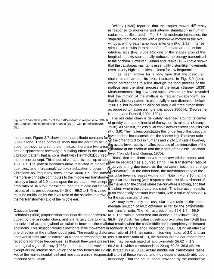
SFK SFK



Figure 3.7 Vibration patterns of the cat’s eardrum in response to 600-Hztone. Source: From Tonndorf and Khanna (1970), with permission of Ann.Otol.

membrane. Figure 3.7 shows the isoamplitude contours for a600-Hz tone. These contours show that the eardrum actuallydoes not move as a stiff plate. Instead, there are two areas ofpeak displacement revealing a buckling effect in the eardrumvibration pattern that is consistent with Helmholtz’s curved-membrane concept. This mode of vibration is seen up to about1500 Hz. The pattern becomes more restricted at higher fre-quencies, and increasingly complex subpatterns occur in thevibrations as frequency rises above 3000 Hz. The curved-membrane principle contributes to the middle ear transformerratio by a factor of 2.0 based upon the cat data. If we accept anarea ratio of 34.6 to 1 for the cat, then the middle ear transferratio as of this point becomes 34.6 × 2.0 = 69.2 to 1. This valuemust be multiplied by the level ratio of the ossicles to arrive atthe final transformer ratio of the middle ear.

Ossicular LeverHelmholtz (1868) proposed that nonlinear distortions are intro-duced by the ossicular chain, and are largely due to what heconceived of as a cogwheel articulation between the malleusand incus. This situation would allow for relative movement inone direction at the malleoincudal joint. The resulting distor-tions would stimulate the cochlea at places corresponding to thereceptors for those frequencies, as though they were present inthe original signal. Barany (1938) demonstrated, however, thatexcept during intense stimulation these two bones are rigidlyfixed at the malleoincudal joint and move as a unit in responseto sound stimulation.

Bekesy (1936) reported that the stapes moves differentlyin response to moderate and intense stimulation in humancadavers, as illustrated in Fig. 3.8. At moderate intensities, thestapedial footplate rocks with a piston-like motion in the ovalwindow, with greater amplitude anteriorly (Fig. 3.8a). Intensestimulation results in rotation of the footplate around its lon-gitudinal axis (Fig. 3.8b). Rocking of the stapes around thelongitudinal axis substantially reduces the energy transmittedto the cochlea. However, Guinan and Peake (1967) have shownthat the cat stapes maintains essentially piston-like movementseven at very high intensities, at least for low frequencies.

It has been known for a long time that the ossicularchain rotates around its axis, illustrated in Fig. 3.9 (top),which corresponds to a line through the long process of themalleus and the short process of the incus (Barany, 1938).Measurements using advanced optical techniques have revealedthat the motion of the malleus is frequency-dependent, sothat its vibratory pattern is essentially in one dimension below2500 Hz, but involves an elliptical path in all three dimensions,as opposed to having a single axis above 2500 Hz (Decraemer,Khanna, and Funnell, 1991, 1994).

The ossicular chain is delicately balanced around its centerof gravity so that the inertia of the system is minimal (Barany,1938). As a result, the ossicular chain acts as a lever about its axis(Fig. 3.9). The malleus constitutes the longer leg of this ossicularlever and the incus constitutes the shorter leg. The lever ratio ison the order of 1.3 to 1 in humans and 2.2 to 1 in cats. However,the actual lever ratio is smaller, because of the interaction of thecurvature of the eardrum and the length of the ossicular chainlever (Tonndorf and Khanna, 1970).

Recall that the drum curves more toward the umbo, andmay be regarded as a curved string. The transformer ratio ofa curved string decreases as the curvature becomes stronger(1/curvature). On the other hand, the transformer ratio of theossicular lever increases with length. Note in Fig. 3.10 that theossicular lever is long (with respect to the point of attachment ofthe malleus on the drum) where the curvature is strong, and thatit is short where the curvature is small. This interaction resultsin an essentially constant lever ratio, with a value of about 1.4for the cat ossicular chain.

We may now apply the ossicular lever ratio to the inter-mediate solution of 69.2 obtained so far for the cat’s middleear transfer ratio. The final ratio becomes 69.2 × 1.4 = 96.9to 1. The ratio is converted into decibels as follows: 20 × log96.9 = 39.7 dB. This value closely approximates the 40-dB lossthat results when the cat’s middle ear is completely obliterated(Tonndorf, Khanna, and Fingerhood, 1966). Using an effectivearea ratio of 26.6, an eardrum bucking factor of 2.0 and anossicular lever ratio of 1.3, the human middle ear transformerratio may be estimated at approximately 26.6 × 2 × 1.3 =69.2 to 1, which corresponds to 20 × log 69.2 = 36.8 dB. Asillustrated in Fig. 3.11, actual middle ear transformer ratiosfall short of these values, and they depend considerably uponfrequency. That the actual boost provided by the conductive

55

SFK SFK


chapter 3

Figure 3.8 The nature of stapes movement in cadavers in response to stimuli presented at (a) moderate levels and (b) very intense levels. Source: FromBekesy (1936).

system does not achieve the values based on the calculations isprobably due to transmission losses. Rosowski (1991) estimatedthat the efficiency of the human middle ear system peaks atabout 0.4 in the vicinity of 900 Hz, and then decreases forhigher frequencies, and averages approximately 0.2 in the cat.

Middle Ear ResponseFigure 3.11, based on Nedzelnitsky’s (1980) data from cats,provides an example of a middle ear transfer function. Themiddle ear transfer function makes a substantial contributionto the shapes of minimal audibility curves (see Chap. 9). Thesecurves show the amount of sound energy needed to reach thethreshold of hearing as a function of frequency.

Bekesy (1941) reported that the resonant frequency of themiddle ear is in the 800 to 1500 Hz region. Recall that resonanceoccurs when mass and stiffness reactance are equal, cancelingout. Impedance is then entirely composed of resistance, andaccordingly the opposition to energy flow is minimal at the res-onant frequencies. Mller (1960)Møller (1960) found the major

Figure 3.9 The axis of rotation of the ossicular chain and the ossicular levermechanism. Based in part on drawings by Barany (1938) and Bekesy (1941).

resonance peak of the middle ear to be about 1200 Hz, with asmaller resonance peak around 800 Hz. Normal ear reactanceand resistance values based on 20 studies are summarized in Fig.3.12 (Margolis, VanCamp, Wilson, and Creten, 1985). Note thatthe ear’s impedance results primarily from negative reactanceup to about 800 Hz. This effect is due to the middle ear mecha-nism itself, which is stiffness controlled below the resonant fre-quency. There is virtually no reactance between about 800 Hzand roughly 5000–6000 Hz, indicating that energy transmissionfrom the eardrum to the cochlea is maximal in this range. Pos-itive reactance takes over at higher frequencies as a result of theeffective mass of the drum and ossicles. We thus expect soundtransmission through the middle ear to be frequency-dependentwith emphasis on the midfrequencies; and the minimal audi-bility curves of the ear should reflect this relation.

The cat’s middle ear transfer function and behavioral thresh-olds are compared in Fig. 3.13. The open circles in Fig. 3.13show the middle ear transfer function based on data from anes-thetized cats (Dallos, 1973). The filled circles are the behavioral

Figure 3.10 The interaction between the length of the ossicular chain andthe inverse of the eardrum curvature. Source: From Tonndorf and Khanna(1970), with permission of Ann. Otol.

56

SFK SFK



Figure 3.11 The middle ear transfer function from the tympanic membraneto the cochlear fluids as a function of frequency. Source: Adapted fromNedzelnitsky (1980), with permission of J. Acoust. Soc. Am.

thresholds of waking cats in a sound field (Miller et al., 1963).The binaural threshold and transfer function are generally sim-ilar, but the threshold curve is steeper at low frequencies andflatter at high. This may reflect several factors (Simmons, 1964;Wiener et al., 1966; Dallos, 1970, 1973): First, since the thresh-olds show mean group data, the curve is probably somewhat

flattened by the averaging among subjects; the transfer functionis from a single representative animal. In addition, there is a peakat around 4000 Hz in the middle ear response of anesthetizedanimals, which is much smaller when they are awake due todamping of the system by the tonus of the stapedius muscle. Asecond factor has to do with the effects of head diffraction, thepinna, and the ear canal, as discussed in the section on the outerear in this chapter. These effects are accounted for by viewing thebehavioral thresholds in terms of the sound pressure level (SPL)near the eardrum at threshold, as is shown by the filled trian-gles in Fig. 3.13. The relationship of the threshold curve to thetransfer function is closer when considered in these terms. Thedisparity between the transfer function and thresholds belowabout 1000 Hz is reconciled by correcting the transfer functionfor the input impedance of the cochlea (open triangles).

These factors show a considerable degree of correspondencebetween the middle ear transfer function and the thresholdcurve, at least for the cat. Reasonable agreement between thetransfer function based upon a model of the middle ear and thethreshold curve has also been shown for humans (Zwislocki,1975). Thus we find that the impedance-matching job of themiddle ear is accomplished quite well for the midfrequencies,although the frequency-dependent nature of the middle earreduces its efficiency at higher and lower frequencies.

Resistance Rd

Reactance Xd

1200

1000

800

600

400

200

0800

600

400

200

–200

–400–600

–1000

–2000

–3000

–40000.02 0.05 0.1 0.2 0.5 1 2 5 10

Frequency (kHz)

Impe

danc

e at

ear

drum

, c.g

.s. a

cous

tic (

Ω)

0

Figure 3.12 Acoustic resistance and reactance as a function of frequency based on 20 studies (see text). Source: From Margolis, Van Camp, Wilson, andCreten (1985), with permission.

57

SFK SFK


chapter 3

Figure 3.13 Middle ear transfer function (open circles) compared to behavioral thresholds (closed circles) and sound pressure level (SPL) at the eardrum(closed triangles) in cats. Source: From Dallos (1973), The Auditory Periphery, copyright c© 1973 by Academic Press.

bone conduction

Until now we have dealt with the usual route from the air to thecochlea. The discussion would be incomplete, however, withoutat least a brief consideration of bone conduction—the transmis-sion of sound to the cochlea by the bones of the skull. For thisto occur, a sound must be strong enough to cause the bonesto vibrate, or else the stimulus must be delivered by way of avibrator applied to the skull. The impedance mismatch betweenair and bone is even greater than between air and cochlear fluid:An airborne sound must exceed the air conduction thresholdby at least 50 to 60 dB before the bone conduction thresholdis reached (Bekesy, 1948). Direct stimulation with a vibratoris routinely employed in audiological evaluations to separatehearing losses attributable to the outer and/or middle ear fromthose due to impairments of the sensorineural mechanisms.

Two classic experiments proved that both air conductionand bone conduction initiate the same traveling waves in thecochlea (see Chap. 4). Bekesy (1932) showed that air- and bone-conduction signals cancel one another when their phases andamplitudes are appropriately adjusted. Lowy (1942) demon-strated that this cancellation occurs in the cochlea, since rep-etition of the Bekesy experiment on guinea pigs resulted incancellation of the cochlear microphonic. (The cochlear micro-phonic is an electrical potential that reflects the activity of thehair cells; see Chap 4.) The implications of these experimentsare monumental, since they demonstrate that the final activity

in the cochlea is the same regardless of the mode of entry of thesound. Furthermore, this result gives support to the use of boneconduction as an audiological tool, and the results of which canvalidly be compared with those of air conduction in determin-ing the locus of a lesion (assuming appropriate calibration ofboth signals).

Bekesy (1932) found that below 200 Hz the human skullvibrates as a unit (Fig. 3.14a). At about 800 Hz, the mode ofvibration changes (Fig. 3.14b), and the front and back of thehead vibrate in opposite phase to one another, with a nodalline of compression between them. At about 1600 Hz, the headbegins to vibrate in four segments (Fig. 3.14c).

Tonndorf and colleagues (1966, 1968) demonstrated that themechanism of bone conduction includes contributions fromthe outer, middle, and inner ear. For clarity, let us look at thesecomponents, beginning with the inner ear.

Compressional bone conduction is illustrated in Fig. 3.15.Vibration of the temporal bone results in alternate compressionand expansion of the cochlear capsule. Because the cochlearfluids are incompressible, there should be bulging at compliantpoints. Bulging would occur at the oval and round windowswithout displacement of the cochlear partition if both windowswere equally compliant (Fig. 3.15a). However, since the roundwindow is much more compliant than the oval window, com-pression of the cochlear capsule pushes the fluid in the scalavestibuli downward, displacing the basilar membrane as shownin Fig. 3.15b. This effect is reinforced, since the sum of the

58

SFK SFK



Figure 3.14 Patterns of skull vibration at (a) 200 Hz, (b) 800 Hz, and (c)1600 Hz, in response to a bone conduction stimulus being applied to theforehead. Source: Adapted from Bekesy (1932).

surface area of the vestibule (V in the figure) and the surfacearea of the scala vestibuli is greater than that of the scala tympani(Fig. 3.15c). The possibility of a “third window” for the releaseof this pressure is provided by the cochlear aqueduct.

Tonndorf (1962), however, found that the primary mecha-nism of bone conduction in the inner ear involves distortionalvibrations of the cochlear capsule, which are synchronouswith the signal (Fig. 3.16). Distortional bone conductionoccurs because the volume of the scala vestibuli is greater thanthat of the scala tympani, so that distortions of the cochlearcapsule result in compensatory displacements of the cochlear

Figure 3.15 Compressional bone conduction (see text). Source: Adaptedfrom Bekesy (1932).

Figure 3.16 Effects of distortional vibrations on displacement of thecochlear partition. Source: Adapted from Tonndorf (1962), with permissionof J. Acoust. Soc. Am.

partition even in the absence of compliant windows. Theabove-mentioned “windows effects” modify the distortionalcomponent.

The contribution of the middle ear to bone conduction isoften known as inertial or ossicular-lag bone conduction, andwas demonstrated by Barany (1938). Recall that the ossiclesmove from side to side rather than front to back. Barany foundthat for low frequencies bone conduction was maximal when avibrator was applied to the side of the head and was minimalwhen it was applied to the forehead. This occurs because thelateral placement vibrates the skull in the direction of ossicularmovement (Fig. 3.17a), whereas frontal placement vibrates theskull perpendicular to their movement (Fig. 3.17b). In otherwords, the signal was transmitted best when it was applied inthe direction of rotation of the ossicular chain about its axis.The mechanism is as follows: Because the ossicles are suspendedanalogously to pendulums, as shown in Fig. 3.17, their inertiacauses them to move relative to the skull when the latter isvibrated. Inertial bone conduction, then, stimulates the cochleaby the relative movement of the skull and ossicles, and the effectof which is a rocking motion of the stapes at the oval window.

The middle ear component of bone conduction is of partic-ular interest in otosclerosis, a disorder in which hearing loss

Figure 3.17 Inertial (ossicular lag) bone conduction: (a) lateral placementof the bone vibrator; (b) forehead placement. Source: Abstracted from Barany(1938).

59

SFK SFK


chapter 3

results from fixation of the stapes in the oval window. A hearingloss results because the fixated stapedial footplate cannot effec-tively transmit energy to the cochlea. Although one might expectbone conduction to be impaired at low frequencies, the elevatedbone-conduction threshold occurs at about 2000 Hz. This phe-nomenon is called Carhart’s notch (Carhart, 1950). Bone con-duction is impaired at 2000 Hz, because this is the resonantfrequency of the ossicular chain in humans (Tonndorf, 1966).1

The contribution of the outer ear to bone conduction is oftencalled osseotympanic bone conduction. It occurs because thevibration of the skull leads to the radiation of sound energy intothe ear canal from its walls, and is principally due to vibrationsof the cartilaginous portion of the canal (Naunton, 1963; Sten-felt et al., 2003). These radiations then stimulate the eardrumand finally the cochlea along the familiar air-conduction route.The outer ear component is emphasized at low frequencies dur-ing occlusion of the cartilaginous part of the ear canal, called theocclusion effect. According to Tonndorf (1966), this enhance-ment of the low frequencies is not appreciated when the ear isunoccluded because the open ear canal acts as a high-pass (low-cut) filter. However, closing off the canal removes the high-passfilter so that the lows are not lost. Another explanation attributesthe occlusion effect to differences in the resonances of the earcanal when it is open and closed (Huizing, 1960).

In summary, the bone-conduction mechanism appears tobe primarily due to distortion of the inner ear capsule, to therelative movements of the skull and ossicles due to the inertial lagof the latter, and to the sound radiated into the ear canal from itswalls. Tonndorf (1966) found in cats that the outer and middleear components are dominant below about 1000 Hz, but that allthree mechanisms are about equally important in the range of1000 to 6000 Hz, as illustrated in Fig. 3.18. However, findings inhuman cadavers have suggested that the outer ear componentis not significant when the ears are open, although it becomesdominant when the ears are occluded (Stenfelt et al., 2003).

the acoustic reflex

The contraction of the middle ear muscles in response torelatively intense sound stimulation is known as the acousticreflex. Early experiments on dogs revealed bilateral tensortympani contractions when either ear was stimulated by intensesound (Hensen, 1878; Pollack, 1886). It was later demonstratedthat the stapedius muscles also respond bilaterally to soundstimulation in cats and rabbits (Kato, 1913). However, whetherthe acoustic reflex in humans is due to contractions of oneor both of the intratympanic muscles has been the subject ofsome controversy.

1 The resonant frequency was about 1500 Hz in temporal bones fromcadavers of individuals averaging 74 years old (Stenfelt et al., 2002).

Figure 3.18 The relative contributions of the inner, middle, and outer earcomponents of bone conduction. Source: Adapted from Tonndorf et al.(1966).

Direct observation through perforated eardrums revealedstapedius muscle contractions in humans as a consequence ofintense sound stimulation (Luscher, 1929; Lindsay et al., 1936;Potter, 1936). Terkildsen (1957, 1960) indirectly examined mid-dle ear muscle activity by monitoring changes in air pressure inthe ear canal in response to sound stimulation. Stapedius con-traction would result in an outward movement of the drum,while tensor concentration would pull the drum inward (seeChap. 2). The drum movement, in turn, results in changes inear canal pressure. Terkildsen could thus infer the nature ofmuscle activity by monitoring the air pressure in the ear canalduring sound stimulation. Most of his subjects manifested anoutward deflection of the drum, suggesting that the stapediusmuscle was active. There were, however, some cases showingtensor activity as well (inward drum displacement). Similarfindings were reported by Mendelson (1957, 1961).

Perhaps the greatest contribution to what is known aboutthe acoustic reflex comes from measurements of acousticimpedance at the plane of the eardrum using impedancebridges and subsequent instruments. The mechanical acous-tic impedance bridge was first applied to the study of theacoustic reflex by Metz (1946) and was improved upon andmade clinically efficient by Zwislocki (1963). An electroacous-tic impedance bridge was introduced by Terkildsen and Nielsen(1960). Almost all acoustic reflex research since the introductionof the electroacoustic device has used this method or variationsof it. The main principle is straightforward: Because contrac-tions of the intratympanic muscles stiffen the middle ear system(including the drum), the impedance is increased. (The reflexprimarily affects the compliance component of impedancerather than resistance, because the system is stiffened.) It is thischange in acoustic impedance that is measured by the device.

Let us now consider how the ear’s impedance can be usedto infer information about the activities of one intratympanicmuscle versus the other. In the normal ear, we really cannottell whether the acoustic reflex is due to contractions of thestapedius and/or of the tensor. However, if the reflex is present

60

SFK SFK



when the stapedius muscle is intact but not when the muscle (orits reflex arc or attachment) is impaired, then we may concludethat the stapedius muscle contributes to the acoustic reflex inhumans. The same argument applies to the tensor tympani.

Several studies have demonstrated that the acoustic reflex isabsent when there is pathology affecting the stapedius muscle(Jepsen, 1955; Klockhoff, 1961; Feldman, 1967). However, theacoustic reflex was still obtained in two cases of tensor tympanipathology (Jepsen, 1955). It might be added at this point that ameasurable tensor tympani reflex is known to occur as part of astartle reaction to very intense sound (Djupesland, 1964), or inresponse to a jet of air directed into the eye (Klockhoff, 1961).Based on these observations, one is drawn to conclude that inhumans the acoustic reflex is a stapedius reflex.

Reflex ParametersSeveral parameters of the acoustic reflex should be discussedbefore describing its effect upon energy transmission throughthe ear, or its suggested roles within the auditory system. Thepossible relationship between the acoustic reflex and loudnesswill also be considered.

We have been referring to the acoustic reflex as occurring inresponse to “intense” sound stimulation. Let us now examinejust how intense a sound is needed. With a reasonable amountof variation among studies, the acoustic reflex thresholds inresponse to pure-tone signals from 250 to 4000 Hz range from85- to 100-dB SPL (Metz, 1952; Møller, 1962; Jepsen, 1963,Jerger, 1970; Margolis and Popelka, 1975; Wilson and McBride,1978; Silman, Popelka, and Gelfand, 1978; Gelfand, 1984). Thereflex threshold is approximately 20 dB lower (better) whenthe eliciting stimulus is broadband noise (Peterson and Liden,1972; Margolis and Popelka, 1975; Silman et al., 1978; Gelfand,1984). In general, the reflex response is obtained at a lowerintensity when it is monitored in the ear being stimulated(the ipsilateral or uncrossed acoustic reflex) instead of inthe opposite ear (the contralateral or crossed acoustic reflex)(Møller, 1961; Green and Margolis, 1984). For an extensivediscussion of the acoustic reflex threshold and its parameters,see the review by Gelfand (1984).

The lower reflex threshold for broadband noise than for tonessuggests that the acoustic reflex is related to the bandwidth ofthe stimulus. Flottrop et al. (1971) studied this relationshipby measuring acoustic reflex thresholds elicited by successivelywider bands of noise and complex tones. They found that theincreasing bandwidth did not cause the threshold to differ fromits value for a pure-tone activator until a certain bandwidth wasexceeded. At this point there was a clear-cut break, after whichincreasing the bandwidth resulted in successively lower reflexthresholds. Similar results were found by Popelka, Karlovich,and Wiley (1974). In addition, Djupesland and Zwislocki (1973)found that increasing the separation in frequency between thetwo tones in a two-tone complex caused a lowering of the reflexthreshold once a particular bandwidth was exceeded. Thesefindings suggest that there is a critical band for the acoustic

Figure 3.19 Critical bandwidths for acoustic reflex thresholds at centerfrequencies of 250 to 4000 Hz. Dots to the left of the functions show the cor-responding pure-tone reflex thresholds. Source: From Popelka et al. (1976),with permission of J. Acoust. Soc. Am.

reflex, beyond which widening of the bandwidth results in lowerthresholds.

Although the existence of a critical bandwidth was a con-sistent finding in the noise and two-tone studies, the thresh-olds were lower for noise. Popelka, Margolis, and Wiley (1976)replicated this work using tone complexes made up of manycomponents that were equally spaced (on a logarithmic scale)in frequency. Their findings, which are shown in Fig. 3.19, con-firm the critical band phenomenon. The width of the criticalband (shown by the break from the horizontal on each functionin Fig. 3.19) increases with center frequency. It is important tonote that the critical bandwidth for the acoustic reflex is sub-stantially wider than the psychoacoustic critical bands discussedin chapters that follow. However, Hellmann and Scharf (1984)pointed out that the differences between acoustic reflex andpsychoacoustic critical bands may not be as substantial as hasbeen supposed.

The acoustic reflex does not occur instantaneously uponthe presentation of the activating signal. Instead, a measur-able impedance change is observed after a latency, the lengthof which depends on both the intensity and frequency of the

61

SFK SFK


chapter 3

stimulus. Metz (1951) found that this latency decreased fromabout 150 ms at 80 dB above the threshold of hearing [dB sen-sation level (SL)] to 40 m at 100-dB SL in response to a 1000-Hzactivating signal. Møller (1958) reported latencies of 25 to 130ms for 500-Hz and 1500-Hz pure-tones. As a rule, latencieswere shorter for 1500 Hz than for 500-Hz tones. Dallos (1964)found a similar inverse relationship between activator inten-sity and reflex latency for white noise. Hung and Dallos (1972)found that acoustic reflex latencies were shorter for noise signalsthan for pure-tones, with the longest latencies for tones below300 Hz. The shortest latencies, on the order of 20 ms, were inresponse to noise activators.

These measurements were based upon changes in acous-tic impedance. However, the latency of the impedance changereflects the mechanical response of the middle ear rather thanof the neural transport time for the reflex arc alone (Borg, 1976).Zakrisson, Borg, and Blom (1974) found that the electromyo-graphic (EMG) response of the stapedius muscle in humans isas short as 12 ms. They also reported that the EMG thresholdis about 6 dB lower than that for the impedance change mea-sured as the lowest stimulus level needed to yield 10% of themaximum response. Because we are concerned with the effectof the acoustic reflex on the transmission of energy through themiddle ear (at least in this context), we are most interested inthe mechanical-response latency. However, one should be awarethat changes in muscle potentials occur in the stapedius priorto the measured impedance change.

We have already seen that acoustic reflex latency shortenswith increasing stimulus intensity. Similarly, increasing stimuluslevel also causes an increase in reflex magnitude, which is theamount of impedance change associated with the reflex (Metz,1951; Møller, 1958; Silman et al., 1978; Gelfand et al., 1981;Silman and Gelfand, 1981; Silman, 1984) and a faster rise timeof the reflex response (Dallos, 1964; Hung and Dallos, 1972).The relationship between stimulus level and the resulting reflexmagnitude is called the acoustic reflex growth function.

The acoustic reflex growth function has been studied inresponse to pure-tones and wide- and narrowband noiseactivating signals (Møller, 1962; Dallos, 1964; Hung and Dallos,1972; Wilson and McBride, 1978; Silman et al., 1978; Gelfandet al., 1981; Silman and Gelfand, 1981; Silman, 1984). Thereflex growth functions of four subjects studied by Hung andDallos (1972) are presented in Fig. 3.20. It illustrates thatthe growth of acoustic reflex magnitude is essentially linearfor pure-tones as high as about 120-dB SPL. The functionsfor wideband noise are essentially linear up to approximately110-dB SPL. These data are substantially supported by theother studies cited. Thus, acoustic reflex magnitude tends toincrease linearly with a stimulus intensity of 85- to 120-dB SPLfor tones and roughly 70- to 110-dB SPL for wideband noise.Saturation occurs at higher levels.

Møller (1961, 1962) reported steeper reflex growth functionswith increasing frequency in the 300- to 1500-Hz range. Flottropet al. (1971) found greater impedance changes at 250 Hz than

at 4000 Hz. They also reported that although signals at 1000and 2000 Hz elicited the same maximum reflex magnitude asat 250 Hz, about 10 dB more (re: reflex threshold) was neededfor the two higher frequencies. Furthermore, while some havesuggested that a 2000-Hz tone elicits the greatest impedancechange (e.g., Kaplan, Gilman, and Dirks, 1977), others suggestthat 1000-Hz and wideband stimuli produce maximal responses(Cunningham, 1976; Wilson and McBride, 1978). On the otherhand, Borg and Møller (1968) found no significant differencesin the slopes of acoustic reflex growth functions in the rangefrom 500 to 3000 Hz in laboratory animals. It thus appears thata clear-cut relationship between activator frequency and reflexmagnitude is not fully established.

Temporal summation deals with the relationship betweenstimulus duration and intensity when the time frame is lessthan about 1 s (see Chap. 9). It is most easily understood byexample. Suppose a subject’s threshold for a tone that lasts200 ms happens to be 18 dB. Will the threshold remain at 18dB when the same tone is presented for only 20 ms? It is foundthat when the 20-ms tone is used the threshold changes to28 dB. (A similar trade-off is needed to maintain the stimulusat a constant loudness. This illustrates the general psychoacous-tic observation that when a signal is shortened by a factor of10 (e.g., from 200 to 20 ms), the signal level must be increased byas much as 10 dB to offset the decade decrease in duration. Thisrelationship is understandably called a time-intensity trade.

Temporal summation also occurs for the acoustic reflex(Djupesland and Zwislocki, 1971; Djupesland et al., 1973;Woodford et al., 1975; Jerger et al., 1977; Gelfand et al., 1981).However, it appears that the amount of intensity change neededto counteract a given decrease in stimulus duration is greaterfor the acoustic reflex than for psychoacoustic phenomena. Fig-ure 3.21 summarizes the general nature of temporal summationfor the acoustic reflex (Woodford et al., 1975). Unfortunately,there are rather large differences between the results of var-ious studies reporting the intensity needed to offset a givenduration change. For example, decreasing the duration of a2000-Hz tone from 100 to 10 ms was offset by an increasein stimulus level by about 25 dB in one study (Djupeslandand Zwislocki, 1971) as opposed to roughly 15 dB in another(Woodford et al., 1975). In the 500- to 4000-Hz range, Dju-pesland et al. (1973) studied the time-intensity trade-off rela-tion for the acoustic reflex with one-octave wide noise bands.They used as their comparison point the stimulus level/durationneeded to maintain the reflex magnitude at half the maxi-mum impedance change. Djupesland et al. found that a 10-fold decrease in duration was offset by a 20- to 25-dB increasein signal level. In contrast, Gnewikow [1974, cited by Jergeret al. (1977)] found that a 12- to 23-dB intensity increase wasneeded to offset decade reductions in duration for 500- and4000-Hz pure-tones. Jerger et al. (1977) found less tempo-ral summation than the other studies, as shown in Fig. 3.22for 500-, 1000-, 2000-, and 4000-Hz stimuli. Note that theamount of temporal integration increases with frequency, which

62

SFK SFK



Figure 3.20 Reflex growth functions for wideband noise (open circles) and pure-tones (250 Hz, open squares; 300 Hz, filled squares; 500 Hz, filled triangles;600 Hz, open tri angles; 1000 Hz, crosses; 1500 Hz, filled circles). Source: From Hung and Dallos (1972), with permission of J. Acoust. Soc. Am.

is a common finding among studies. Jerger et al. (1977) sug-gested that at least some of the differences are due to problemsassociated with the “visual detection threshold” (the smallestnoticeable impedance change on a meter or oscilloscope), andwith “constant percentage of maximum impedance change”methods (Djupesland et al., 1973) of obtaining the data.

Early studies on laboratory animals showed that the degreeof muscle contraction due to the acoustic reflex decreases asstimulation is prolonged (Kato, 1913; Lorente de No, 1935).This decrease in acoustic reflex magnitude over time is referredto as reflex decay or adaptation, and it has been found inhumans (Dallos, 1964; Borg, 1968; Tietze, 1969a,1969b; Wileyand Karlovich, 1975; Kaplan, Gilman, and Dirks, 1977; Wilson,McCollough, and Lilly, 1984a; Wilson, Shanks, and Lilly 1984b).An extensive review of this topic is provided by Wilson et al.(1984b). In spite of differences among studies, the commonfinding is that reflex adaptation increases as the frequency of apure-tone stimulus is raised.

Figure 3.21 Temporal summation for the acoustic reflex threshold. Thisfigure shows the trade-off between activator signal duration and level at500 Hz (crosses), 1000 Hz (circles), 2000 Hz (triangles), 3000 Hz (squares),and 4000 Hz (inverted triangles). A typical psychoacoustic temporal summa-tion function is represented by the solid line for comparison. Source: FromWoodford, Henderson, Hamernick, and Feldman (1975), with permission.

63

SFK SFK


chapter 3

Figure 3.22 Temporal summation for the acoustic reflex at four frequenciesobtained by Jerger et al. (1977) (open circles), Gnewikow (1974) (filled circles),and Woodford et al. (1975) (crosses). Source: From Jerger, Mauldin, and Lewis(1977). Temporal summation of the acoustic reflex, Audiology 16, 177–200, with permission.

Particular attention should be given to the findings ofKaplan et al. (1977), who studied acoustic reflex adaptation topure-tones of 500 to 4000 Hz, which were presented at levelsof 6, 12, and 18 dB above the reflex threshold. Figure 3.23summarizes their median data at three sensation levels re:reflex threshold, with stimulus frequency as the parameter.[Sensation level (SL) more properly refers to the number ofdB above one’s threshold of hearing . However, in the contextof the acoustic reflex, SL is also used to refer to the numberof dB above the reflex threshold.] There is greater reflexadaptation as frequency increases. Also, adaptation tends tobegin sooner after stimulus onset for higher frequencies. Thesedata are normalized in Fig. 3.24, in which the point of greatestimpedance change is given a value of 100% and the other pointsare shown as percentages of the maximum impedance change.In this plot, the data are shown separately at each frequency,with the suprathreshold level as the parameter. In addition toclearly showing the frequency effect, Fig. 3.24 demonstratesthat the course of the adaptation function is similar at variouslevels above reflex threshold, at least up to +18 dB.

Tietze (1969a,1969b) proposed that the course of acousticreflex adaptation could be described by the time constantsof reflex rise time and adaptation. These time constants refer

Figure 3.23 Median absolute impedance change (in acoustic ohms) as a function of time for three levels above the acoustic reflex threshold. Source: FromKaplan et al. (1977), with permission of Ann. Otol.

64

SFK SFK



Figure 3.24 Median normalized impedance change (in percent) as a function of time for each frequency. Source: From Kaplan et al. (1977), with permissionof Ann. Otol.

respectively to how long it takes for reflex magnitude to attain63% of the maximum value (rise) and then to decrease to 63% ofit (adaptation); both are measured from the moment of acous-tic reflex onset. The time constants are functions of frequency.Tietz’s model describes reflex adaptation by the formula

Zn = 1

1 − an/ab

[exp (−t/ab) − exp (−t/an)

](3.1)

where Zn is the normalized maximum impedance change; an

and ab are the time constants of reflex rise and adaptation,respectively; and t is the time (in seconds) of reflex rise fromonset. Kaplan et al. (1977) applied this formula to their data,using the ratio an/ ab to generate the dotted lines in Fig. 3.24.

(Note that, except at high frequencies where rapid adaptationreduces the maximum impedance change, an is generally quitesmall relative to ab.) As Fig. 3.24 shows, the data of Kaplanet al. support the exponential adaptation predicted by Tietze’smodel.

Loudness is the perceptual correlate of the intensity of theacoustic stimulus (see Chap. 11); other things being equal,loudness increases as stimulus level is increased. An aberra-tion of the intensity–loudness relationship is found in patientswith cochlear disorders. Once the signal is increased above theimpaired threshold of such an ear, the loudness grows at a fasterrate than normal in response to increasing stimulus level. Thisis called loudness recruitment. What has the acoustic reflex to

65

SFK SFK


chapter 3

do with loudness and recruitment? Because both loudness andthe acoustic reflex are related to stimulus intensity, at least someassociation between them is understandable. The question iswhether the acoustic reflex is a function of loudness.

Metz (1952) obtained acoustic reflex thresholds at lower SLsfrom patients with presumably cochlear sensorineural hearingloss than from normal subjects. In other words, the spreadbetween the threshold of hearing and the acoustic reflex thresh-old was smaller for those with the hearing losses. Because theimpaired subjects also had loudness recruitment, Metz pro-posed that the lower SL of the reflex reflected recruitment. Inother words, it was argued that the acoustic reflex was elicited bythe loudness of the signal. Jepsen (1963) also attributed acousticreflex findings in patients with sensorineural hearing losses tobe the result of recruitment.

The relationship between loudness and the acoustic reflex,however, is not nearly as clear-cut as these early findings sug-gest. Ross (1968) compared the equal-loudness and equal-reflexcontours of four subjects. The contours were similar for two,while the others had systematic differences between the loud-ness and acoustic reflex contours (the loudness curves were flat-ter). Ross suggested that the latter two equal-loudness contoursmight have been aberrant, but in fact they were quite similar tothose reported by Fletcher and Munson (1933), among others.

Margolis and Popelka (1975) compared the loudness of a vari-ety of stimuli set to the acoustic reflex threshold level. There wasa range of about 17 dB in the loudness levels, suggesting that theacoustic reflex is not a manifestation of a critical loudness level.Block and Wightman (1977) suggested that the loudness–reflexrelationship is supported by their finding of similarly shapedequal-loudness and equal-reflex contours. However, they oftenfound that the same reflex magnitude was elicited by stimu-lus levels as much as 10 dB apart. Such a spread correspondsto a doubling of loudness (Stevens, 1956); in this light, theirfindings appear to support rather than refute those of Margo-lis and Popelka. The substantially wider critical bands for theacoustic reflex than for loudness discussed previously provide afurther basis for questioning the concept that the acoustic reflexis loudness-based.

Returning to patient data, Beedle and Harford (1973) foundsteeper acoustic reflex growth functions for normal ears thanfor ears with cochlear dysfunction. This result is, of course,inconsistent with a loudness basis for the reflex. The impact oftheir data, however, was impaired by the fact that their normalsubjects averaged 24 years old, compared to 47 years old for thepathological group. The reflex growth functions of age-matchednormal and hearing-impaired subjects were studied by Silman,Popelka, and Gelfand (1978). Examples of their findings areshown in Fig. 3.25. If the reflex were loudness-determined, thenthe function for the impaired groups, although displaced alongthe intensity axis, would be expected to approach the normalcurves at higher stimulus levels. This expectation is based onthe notion that loudness recruitment should result in equalloudness for both groups at equal suprathreshold levels. Equal

loudness would in turn elicit equal reflex magnitudes at thoselevels. As Fig. 3.25 shows, this was not the case.

Hellman and Scharf (1984) argued that the case against aloudness–reflex relationship is not as convincing as it mightseem. Just two examples will be briefly mentioned. Considerfirst the material in Fig. 3.25, just discussed. These data couldbe explained by the fact that both loudness and reflex magni-tude increase as power functions of the stimulus level at the SPLswhere these functions are obtained. Second, they demonstratedthat for given subjects, equally loud sounds elicited equal reflexmagnitudes when the criteria were defined precisely. Given thatboth loudness and the acoustic reflex reflect the neural codingof the stimulus level at the periphery, it is thus understandablethat the two phenomena should be related. The controversialand unresolved issue is whether one is dependent upon theother. It is apparent that the acoustic reflex is largely stimulus-dependent. Furthermore, it should not be surprising that theparameters of the reflex response reflect the sensory (and neu-ral) processing of relatively intense stimulation. It is equallyapparent that the acoustic reflex is a feedback or control mech-anism, although its exact purpose(s) remains unclear. Giventhese points, what effect does the acoustic reflex have on energytransmission through the conductive mechanism?

Recall that the acoustic reflex stiffens the conductive mecha-nism so that sound is reflected at the eardrum (Dallos, 1964).Because the effect of stiffness is inversely related to frequency,we would expect the acoustic reflex to affect middle ear trans-mission most strongly at lower frequencies.

Smith (1943) and Reger (1960) compared the pure-tonethresholds of human subjects to the thresholds during volun-tary contractions of the middle ear muscles. Thresholds wereshifted by about 20 to 40 dB at 125 to 500 Hz, and by 15 dB at1000 Hz, and there was little or no change at higher frequencies.While the expected frequency relation is maintained, voluntarycontractions may not yield the same transmission loss as theacoustic reflex (Reger, 1960). Perhaps the most impressive dataon how the acoustic reflex affects middle ear transmission comefrom animal studies.

The transmission loss produced by the acoustic reflex hasbeen studied in animals by monitoring the resulting changesin the magnitude of the cochlear microphonic (e.g., Simmons,1959; Møller, 1964, 1965; Nuttall, 1974). (The cochlear micro-phonic is an electrical potential of the cochlea, which is propor-tional to the intensity of the stimulus over a wide dynamic range;it is discussed in the next chapter.) Figure 3.26 shows the changesin the cochlear microphonic magnitude as a function of fre-quency due to stapedius muscle contraction in the cat, obtainedby Møller (1965). He found that impedance change data andcochlear microphonic findings in response to the acoustic reflexwere within 5 dB over a substantial portion of the frequencyrange. The figure shows that the acoustic reflex affects primarilythe frequencies below about 2000 Hz. Low-frequency changeshave also been reported in response to contractions of the tensortympani muscle (e.g., Starr, 1969; Nuttall, 1974).

66

SFK SFK



Figure 3.25 Reflex growth as a function of activator level in dB SPL for (a) a 1000-Hz tone and (b) a broadband noise. Open symbols, normal ears; closedsymbols, impaired ears. Source: Adapted from Silman, Popelka, and Gelfand (1978).

Several studies have addressed the effects of middle ear musclecontractions on absolute thresholds and loudness in humans(Smith, 1946; Loeb and Riopelle, 1960; Morgan and Dirks, 1975;Morgan, Dirks, and Kamm, 1978; Rabinowitz, 1976), albeit withmixed results. For example, Rabinowitz (1976) reported a 10-dBchange in the low-frequency transmission characteristics of themiddle ear due to the acoustic reflex, but Morgan et al. (1978)found that absolute thresholds were not affected by the acousticreflex. Morgan and Dirks (1975) found that the acoustic reflexcaused a change in the loudness of a test tone presented to theopposite ear when the reflex-eliciting stimulus was greater than100-dB SPL, but not for lower activator levels.

Middle Ear Muscle TheoriesThere are many theories and speculations about the purposeof the middle ear muscles and the acoustic reflex. Space andscope preclude more than a cursory review here; and the reader

Figure 3.26 Effect of the acoustic reflex on transmission in the cat’s middleear. Source: Adapted from Møller (1965), with permission.

should see the discussions by Simmons (1964); Jepsen (1963);and Borg, Counter, and Rosler (1984).

Because the reflex is elicited by relatively high stimulus levelsand its magnitude grows with increasing stimulus level, onewould expect that a primary purpose of the acoustic reflex wouldbe protection of the cochlea from damaging stimulation. Thisprotection theory is limited by the latency and adaptation of thereflex, causing it to respond too slowly to sudden sounds, andmaking it inefficient against prolonged sounds. Nevertheless,protection against injury to hearing is still a beneficial effect ofthe acoustic reflex, even if it is not the main purpose.

The accommodation theory states that the action of the twomiddle ear muscles modifies the conductive mechanism so asto optimize the absorption of sound energy. According to theossicular fixation theory, the intratympanic muscles help keepthe ossicles in proper position and appropriately rigid, partic-ularly at high frequencies, where acceleration is great. Othertheories have asserted that these muscles contribute to changesin labyrinthine pressure and to the formation of aural overtones.

Simmons (1964) found a sharp antiresonance peak around4000 Hz in the middle ear transmission function of cats whoseintratympanic muscles were removed, as well as in normal catsunder anesthesia. Normal, waking cats whose intratympanicmuscles have normal tonus showed greatly reduced dips in thisregion. In his perceptual theory, Simmons reasoned that tonusof the middle ear muscles smoothes the frequency response ofthe conductive system. He suggested that modulation of muscletonus would have the effect of enhancing attention by chang-ing the intensity and frequency characteristics of environmentalsounds. This modulation would be analogous to the constantmotion of the extraocular muscles in vision. Also, several skele-tal movements as well as unexpected and novel environmen-tal sounds elicit the acoustic reflex. Because the reflex mainlyattenuates low frequencies, and most of an organism’s own

67

SFK SFK


chapter 3

physiological noises are low in frequency, such a reflex responsewould have the effect of reducing the animal’s internal noise.A better signal-to-noise ratio would result, which is of obvi-ous importance to the survival of any species, whether preda-tor or prey. This idea agrees with Borg’s (1976) position thatthe qualitative purpose of the acoustic reflex is to attenuatelow-frequency sounds, thereby improving the auditory system’sdynamic range.

The desensitization–interference–injury protection theoryproposed by Borg et al. (1984) explained that the middle earmuscles and the acoustic reflex have multiple purposes: (1)Contractions of the intratympanic muscles are elicited byeating, talking, yelling, and other vocalizations. The musclecontractions alleviate desensitization because they reduce thenoises produced by these activities, which would have otherwisecompromised the alertness and the sensitivity to salient aspectsof the acoustical environment. (2) Interference is reducedbecause contractions of the middle ear muscles cause the lowfrequencies to be attenuated, thereby reducing the extent towhich they mask the higher frequencies (e.g., reducing themasking produced by one’s own speech). (3) Finally, middle earmuscle contractions provide injury protection by attenuatingintense sounds reaching the inner ear.

referencesBarany, E. 1938. A contribution to the physiology of bone con-

duction. Acta Otol Suppl 26, 1–223.Beedle, RK, Harford, ER. 1973. A comparison of acoustic reflex

growth in normal and pathological ears. J Speech Hear Res16, 271–280.

Bekesy, G. 1932. Zur Theorie des Horen bei der Schallaufnahmedurch Knochenleitung. Ann Physik 13, 111–136.

Bekesy, G. 1936. Zur Physik des Mittelohres und uber dasHoren bei fehlerhaftem Trommelfell. Akust Zeitschr 1,13–23.

Bekesy, G. 1941. Uber die Messung der Schwingungsamplitudeder Gehorknochelchen mittels einer kapazitiven Sonde. AkustZeitschr 6, 1–16.

Bekesy, G. 1948. Vibrations of the head in a sound field andits role in hearing by bone conduction. J Acoust Soc Am 20,749–760.

Bekesy, G. 1960/1989. Experiments in Hearing . New York, NY:McGraw-Hill. [Republished by the Acoustical Society ofAmerica].

Bekesy, G, Rosenblith, WA. 1958. The mechanical propertiesof the ear. In: SS Stevens (ed.), Handbook of ExperimentalPsychology. New York, NY: Wiley, 1075–1115.

Bennett, M. 1984. Impedance concepts relating to the acousticreflex. In: S Silman (ed.), The Acoustic Reflex. New York, NY:Academic Press, 35–61.

Blauert, J. 1997. Special Hearing: The Psychophysics of HumanSound Localization. Revised Edition. Cambridge, MA: MITPress.

Block, MG, Wightman, FL. 1977. A statistically based measureof the acoustic reflex and its relation to stimulus loudness. JAcoust Soc Am 61, 120–125.

Borg, E. 1968. A quantitative study of the effects of the acousticstapedius reflex on sound transmission through the middleear. Acta Otol 66, 461–472.

Borg, E. 1976. Dynamic characteristics of the intra-auralmuscle reflex. In: AS Feldman, LA Wilber (eds.), AcousticImpedance and Admittance. Baltimore: Williams Wilkins,236–299.

Borg, E, Counter, SA, Rosler, G. 1984. Theories of middle-earmuscle function. In: S Silman (ed.), The Acoustic Reflex. NewYork, NY: Academic Press, 63–99.

Borg, E, Møller, A. 1968. The acoustic middle ear reflex in manand in anesthetized rabbits. Acta Otol 65, 575–585.

Bosatra, A, Russolo, M, Silverman, CA. 1984. Acoustic—reflexlatency: State of the art. In: S Silman (ed.), The Acoustic Reflex.New York, NY: Academic Press, 301–328.

Carhart, R. 1950. Clinical application of bone conductionaudiometry. Arch Otol 51, 798–808.

Cunningham, D. 1976. Admittance values associated withacoustic reflex decay. J Acoust Soc Am 1, 197–205.

Dallos, P. 1964. Dynamics of the acoustic reflex: Phenomeno-logical aspects. J Acoust Soc Am 36, 2175–2183.

Dallos, P. 1970. Low-frequency auditory characteristics: Speciesdependencies. J Acoust Soc Am 48, 489–499.

Dallos, P. 1973. The Auditory Periphery. New York, NY: Aca-demic Press.

Decraemer, WF, Khanna, SM, Funnell, WRL. 1991. Malleusvibration mode changes with frequency. Hear Res 54, 305–318.

Decraemer, WF, Khanna, SM, Funnell, WRL. 1994. A methodfor determining three-dimensional vibration in the ear. HearRes 77, 19–37.

Djupesland, G. 1964. Middle ear muscle reflexes elicited byacoustic and nonacoustic stimulation. Acta Otol Suppl 188,287–292.

Djupesland, G, Sundby, A, Flottrop, G. 1973. Temporal sum-mation in the acoustic stapedius reflex mechanism. Acta Otol76, 305–312.

Djupesland, G, Zwislocki, J. 1971. Effect on temporal summa-tion on the human stapedius reflex. Acta Otol 71, 262–265.

Djupesland, G, Zwislocki, J. 1973. On the critical band in theacoustic stapedius reflex. J Acoust Soc Am 54, 1157–1159.

Dutsch, L. 1972. The threshold of the stapedius reflex for pure-tone and noise stimuli. Acta Otol 74, 248–251.

Feldman, A. 1967. A report of further impedance studies of theacoustic reflex. J Speech Hear Res 10, 616–622.

Fletcher, H, Munson, WA. 1933. Loudness: Its definition, mea-surement and calculation. J Acoust Soc Am 5, 82–108.

Flottrop, G, Djupesland, G, Winther, F. 1971. The acousticstapedius reflex in relation to critical bandwidth. J Acoust SocAm 49, 457–461.

68

SFK SFK



Gardner, MB, Gardner, RS. 1973. Problems of localization inthe medial plane: Effect of pinnae cavity occlusion. J AcoustSoc Am 53, 400–408.

Gelfand, SA. 1984. The contralateral acoustic—reflex thresh-old. In: S Silman (ed.), The Acoustic Reflex. New York, NY:Academic Press, 137–186.

Gelfand, SA, Silman, S, Silverman, CA. 1981. Temporal sum-mation in acoustic reflex growth functions. Acta Otol 91,177–182.

Green, KW, Margolis, RH. 1984. The ipsilateral acoustic reflex.In: S Silman (ed.), The Acoustic Reflex. New York, NY: Aca-demic Press, 275–299.

Guinan, J, Peake, WT. 1967. Middle ear characteristics of anes-thetized cats. J Acoust Soc Am 41, 1237–1261.

Hellman, R, Scharf, B. 1984. Acoustic reflex and loudness. In: SSilman (ed.), The Acoustic Reflex. New York, NY: AcademicPress, 469–516.

Helmholtz, H. 1868. Die Mechanik der Gehorknochelchen unddes Trommelfells. Pflugers Arch Ges Physiol I , 1–60.

Hensen, V. 1878. Beobachtungen uber die Thatigkeit des Trom-mellspanners bei Hund und Katze. Arch Anat Physiol II , 312–319.

Huizing, EH. 1960. Bone conduction—The influence of themiddle ear. Acta Otol Suppl 155, 1–99.

Hung, I, Dallos, P. 1972. Study of the acoustic reflex in humanbeings: I. Dynamic characteristics. J Acoust Soc Am 52, 1168–1180.

Jepsen, O. 1955. Studies on the acoustic stapedius reflex in man:Measurements of the acoustic impedance of the tympanic mem-brane in normal individuals and in patients with peripheralfacial palsy [Thesis], Universitetsforlaget, Aarhus, Denmark.

Jepsen, O. 1963. The middle ear muscle reflexes in man. In: JJerger (ed.), Modern Developments in Audiology. New York,NY: Academic Press, 194–239.

Jerger, J. 1970. Clinical experience with impedance audiometry.Arch Otol 92, 311–321.

Jerger, J, Mauldin, L, Lewis, N. 1977. Temporal summation ofthe acoustic reflex. Audiology 16, 177–200.

Kaplan, H, Gilman, S, Dirks, D. 1977. Properties of acousticreflex adaptation. Ann Otol 86, 348–356.

Kato, T. 1913. Zur Physiologie der Binnenmuskeln des Ohres.Pflugers Arch Physiol 150, 569–625.

Klockhoff, I. 1961. Middle-ear muscle reflexes in man. Acta OtolSuppl. 164.

Lindsay, JR, Kobrack, H, Perlman, HB. 1936. Relation of thestapedius reflex to hearing sensitivity in man. Arch Otol 23,671–678.

Loeb, M, Riopelle, AJ. 1960. Influence of loud contralateralstimulation on the threshold and perceived loudness of low-frequency tones. J Acoust Soc Am 32, 602–610.

Lorente de No, R. 1935. The function of the central acousticnuclei examined by means of the acoustic reflexes. Laryngo-scope 45, 573–595.

Lowy, K. 1942. Cancellation of the electrical cochlear responsewith air- and bone-conduction. J Acoust Soc Am 14, 156–158.

Luscher, E. 1929. Die Function des Musculus stapedius beimMenschen. Zeitschr Hals Nasen Ohrenheilk 23, 105–132.

Margolis, R, Popelka, G. 1975. Loudness and the acoustic reflex.J Acoust Soc Am 58, 1330–1332.

Margolis, RH, Van Camp, J, Wilson, RH, Creten, WL. 1985.Multifrequency tympanometry in normal ears. Audiology 24,44–53.

Mehrgardt, S, Mellert, V. 1977. Transformation character-istics of the external human ear. J Acoust Soc Am 61,1567–1576.

Mendelson, ES. 1957. A sensitive method for registration ofhuman intratympanic muscle reflexes. J Appl Physiol 11, 499–502.

Mendelson, ES. 1961. Improved method for studying tympanicreflexes in man. J Acoust Soc Am 33, 146–152.

Metz, O. 1946. The acoustic impedance measured on normaland pathological ears. Acta Otol 63(Suppl), 3–254.

Metz, O. 1951. Studies on the contraction of the tympanic mus-cles as indicated by changes in impedance of the ear. ActaOtol 39, 397–405.

Metz, O. 1952. Threshold of reflex contractions of muscles ofthe middle ear and recruitment of loudness. Arch Otol 55,536–593.

Middlebrooks, JC. 1999. Individual differences in external eartransfer functions reduced by scaling in frequency. J AcoustSoc Am 106, 1480–1492.

Miller, JD, Watson, CS, Covell, WP. 1963. Deafening effects ofnoise on the cat. Acta Otol 176(Suppl), 1–91.

Møller, A. 1958. Intra-aural muscle contraction in man exam-ined by measuring acoustic impedance of the ear. Laryngo-scope 68, 48–62.

Møller, A. 1961. Bilateral contraction of the tympanic musclesin man examined by measuring acoustic impedance-change.Ann Otol 70, 735–753.

Møller, AR. 1960. Improved technique for detailed measure-ments of the middle ear impedance. J Acoust Soc Am 32,250–257.

Møller, AR. 1962. The sensitivity of contraction of tympanicmuscle in man. Ann Otol 71, 86–95.

Møller, AR. 1964. Effects of tympanic muscle activity on move-ment of the ear drum, acoustic impedance, and cochlearmicrophonics. Acta Otol 58, 525–534.

Møller, AR. 1965. An experimental study of the acousticimpedance and its transmission properties Acta Otol 60, 129–149.

Morgan, DE, Dirks, DD. 1975. Influence of middle ear mus-cle contraction on pure-tone suprathreshold loudness judg-ments. J Acoust Soc Am 57, 411–420.

Morgan, D.E, Dirks, DD, Kamm, C. 1978. The influence ofmiddle-ear contraction on auditory threshold for selectedpure-tones. J Acoust Soc Am 63,1896–1903.

69

SFK SFK


chapter 3

Nedzelnitsky, V. 1980. Sound pressures in the basal turn of thecat cochlea. J Acoust Soc Am 68, 1676–1689.

Naunton, R. 1963. The measurement of hearing by bone con-duction. In: J Jerger (ed.), Modern Developments in Audiology.New York, NY: Academic Press, 1–29.

Nuttall, AL. 1974. Tympanic muscle effects on middle-ear trans-fer characteristic. J Acoust Soc Am 56, 1239–1247.

Oldfield, SR, Parker, PA. 1984. Acuity of sound localization: Atopography of auditory space. II. Pinna cues absent. Percep-tion 13, 601–617.

Peterson, JL, Liden, G. 1972. Some static characteristics of thestapedial muscle reflex. Audiology 11, 97–114.

Plenge, G. 1974. On the difference between localization andlateralization. J Acoust Soc Am 56, 944–951.

Pollack, J. 1886. Uber die Function des Musculus tensor tym-pani. Med Jahrbuch 82, 555–582.

Popelka, G, Karlovich, R, Wiley, T. 1974. Acoustic reflex andcritical bandwidth. J Acoust Soc Am 55, 883–885.

Popelka, G, Margolis, R, Wiley, T. 1976. Effects of activatingsignal bandwidth on acoustic-reflex thresholds. J Acoust SocAm 59, 153–159.

Potter, AB 1936. Function of the stapedius muscle. Ann Otol 45,639–643.

Rabinowitz, WM. 1976. Acoustic-Reflex Effects on the InputAdmittance and Transfer Characteristics of the Human Middle-Ear [unpublished Ph.D. Dissertation]. Cambridge, MA: MITPress.

Reger, SN. 1960. Effect of middle ear muscle actionon certain psycho-physical measurements. Ann Otol 69,1179–1198.

Rosowski, JJ. 1991. The effects of external- and middle-ear fil-tering on auditory threshold and noise-induced hearing loss.J Acoust Soc Am 90, 124–135.

Ross, S. 1968. On the relation between the acoustic reflex andloudness. J Acoust Soc Am 43, 768–779.

Shaw, EAG. 1974. Transformation of sound pressure level fromthe free field to the eardrum in the horizontal plane. J AcoustSoc Am 56, 1848–1861.

Shaw, EAG. 1997. Acoustical features of the external ear. In:R Gilkey, T Anderson (eds.), Binaural and Spacial Hearingin Real and Virtual Environments. Hillsdale, NJ: Erlbaum,25–47.

Shaw, EAG, Vaillancourt, MM. 1985. Transformation of sound-pressure level from the free field to the eardrum presented innumerical form. J Acoust Soc Am 78, 1120–1123.

Silman, S. 1984. Magnitude and growth of the acoustic reflex. In:S Silman (ed.), The Acoustic Reflex. New York, NY: AcademicPress, 225–274.

Silman, S, Gelfand, SA. 1981. Effect of sensorineural hearingloss on the stapedius reflex growth function in the elderly. JAcoust Soc Am 69, 1099–1106.

Silman, S, Popelka, S, Gelfand, SA. 1978. Effect of sensorineuralhearing loss on acoustic stapedius reflex growth functions. JAcoust Soc Am 64, 1406–1411.

Simmons, FB 1959. Middle ear muscle activity at moderatesound levels. Ann Otol 68, 1126–1143.

Simmons, FB. 1964. Perceptual theories of middle ear function.Ann Otol 73, 724–740.

Smith, HD. 1943. Audiometric effects of voluntary contractionof the tensor tympani muscle. Arch Otol 38, 369–373.

Smith, HD. 1946. Audiometric effects of voluntary contractionof the tensor tympani muscles. Arch Otol 38, 369–372.

Starr, A. 1969. Regulatory mechanisms of the auditory pathway.In: S Locke (ed.), Modern Neurology. Boston, MA: Little,Brown.

Stenfelt, S, Hato, N, Goode, RL. 2002. Factors contributing tobone conduction: The middle ear. J Acoust Soc Am 111, 947–959.

Stenfelt, S, Wild, T, Hato, N, Goode, RL. 2003. Factors con-tributing to bone conduction: The outer ear. J Acoust Soc Am113, 902–913.

Stepp, CE, Voss, SE. (2005). Acoustics of the human middle-earair space. J Acoust Soc Am 118, 861–871.

Stevens, SS. 1956. The direct estimation of sensory magnitude—Loudness. Am J Psychol 69, 1–25.

Stinton, MR, Lawton, DW. 1989. Specification of the geometryof the human ear canal for the prediction of sound-pressurelevel distribution. J Acoust Soc Am 85, 2492–2530.

Terkildsen, K. 1957. Movements of the eardrum following inter-aural muscle reflexes. Arch Otol 66, 484–488.

Terkildsen, K. 1960. Acoustic reflexes of the human musculustensor tympani. Acta Otol Suppl. 158, 230–236.

Terkildsen, K, Nielsen, SS. 1960. An electroacoustic measuringbridge for clinical use. Arch Otol 72, 339–346.

Tietze, G. 1969a. Zum zeitverhalten des akustischen reflexesbei reizung mit dauertonen. Arch Klin Exp Ohren NasenKehlkoopfheilkd 193, 43–52.

Tietze, G. 1969b. Einge eigenschaften des akustischen reflexesbei reizung mit tonimpulsen. Arch Klin Exp Ohren NasenKehlkopfFeilkd 193, 53–69.

Tonndorf, J. 1962. Compressional bone conduction in cochlearmodels. J Acoust Soc Am 34, 1127–1132.

Tonndorf, J. 1966. Bone conduction: Studies in experimentalanimals—A collection of papers. Acta Otol Suppl 213, 1–32.

Tonndorf, J. 1968. A new concepts of bone conduction. ArchOtol 87, 49–54.

Tonndorf, J, Khanna, SM. 1970. The role of the tympanic mem-brane in middle ear transmission. Ann Otol 79, 743–753.

Tonndorf, J, Khanna, SM, Fingerhood, BJ. 1966. The inputimpedance of the inner ear in cats. Ann Otol 75, 752–763.


Wiener, FN, Pfeiffer, RR, Backus, ASN. 1966. On the pressuretransformation by the head and auditory meatus of the cat.Acta Otol 61, 255–269.

Wiener, FM, Ross, DA. 1946. The pressure distribution in theauditory canal in a progressive sound field. J Acoust Soc Am18, 401–408.

70

SFK SFK



Wiley, TL, Karlovich, TS. 1975. Acoustic reflex response to sus-tained signals. J Speech Hear Res 18, 148–157.

Wilson, RH, McBride, LM. 1978. Threshold and growth of theacoustic reflex. J Acoust Soc Am 63, 147–154.

Wilson, RH, McCollough, JK, Lilly, DJ. 1984a. Acoustic reflexadaptation: Morphology and half-life data for subjects withnormal hearing. J Speech Hear Res 27, 586–595.

Wilson, RH, Shanks, JE, Lilly, DJ. 1984b. Acoustic-reflex adap-tation. In: S Silman (ed.), The Acoustic Reflex. New York, NY:Academic Press, 329–386.

Woodford, C, Henderson, D, Hamernick, R, Feldman, A. 1975.Threshold duration function of the acoustic reflex in man.Audiology 14, 53–62.

Zakrisson, JE, Borg, E, Blom, S. 1974. The acoustic impedancechange as a measure of stapedius muscle activity in man: A

methodological study with electromyography. Acta Otol 78,357–364.

Zwislocki, J. 1962. Analysis of the middle-ear function. Part I:Input impedance. J Acoust Soc Am 34, 1514–1523.

Zwislocki, J. 1963. An acoustic method for clinical examinationof the ear. J Speech Hear Res 6, 303–314.

Zwislocki, J. 1975. The role of the external and middle ear insound transmission. In: DB Tower, EL. Eagles (eds.), The Ner-vous System. Vol. 3: Human Communication and Its Disorders.New York, NY: Raven Press, 45–55.

Zwislocki, J. 1976. The acoustic middle ear function. In: ASFeldman, LA, Wilber (eds.), Acoustic Impedance and Admit-tance—The Measurement of Middle Ear Function. Baltimore,MD: Williams & Wilkins. 66–77.

71

SFK SFK


4 Cochlear Mechanisms and Processes

We have already discussed the manner in which the conduc-tive mechanism influences the signal and transmits it to theinner ear. In this chapter we will concentrate upon the sensorymechanism. The cochlea may be conceived of as a transducerthat converts the vibratory stimulus into a form usable by thenervous system. However, this is far from the whole picture. Weshall see that the cochlea performs a considerable amount ofanalysis, that it is the major source of aural distortion, and thatit is involved in processes that are active as well as passive.

Before proceeding to examine the processes of the cochlea, itis desirable to briefly review the traditional theories of hearingas well as some principles of sensory receptor action. Thesetwo topics provide a useful general framework as well as animportant historical perspective within which the student canconsider the material that follows.

classical theories of hearing

The study of the auditory system is practically and historicallyintertwined with the traditional theories of hearing. Broadlyspeaking, these theories fall into two general categories—place(resonance) theories and frequency (temporal, periodicity)theories—as well as the combined place-frequency theory. Adetailed review of these theories goes beyond the current scopeor intent; the student is referred to Wever’s classical work The-ory of Hearing Hearing (1949) for an excellent review of thesetheories.

Classical Resonance TheoryAlthough place or resonance theories existed since the begin-ning of the 1600s, modern versions began with the resonancetheory proposed by Helmholtz (1870). Helmholtz relied to alarge extent upon Ohm’s auditory law and Muller’s doctrine ofspecific nerve energies. Ohm’s auditory law states that the earperforms a Fourier analysis upon complex periodic sounds; thatis, that it breaks the complex wave down into its componentsregardless of their phase relationships. A major problem withOhm’s auditory law is that it precludes temporal analysis. Weshall see, however, that the auditory system is sensitive to tem-poral as well as frequency parameters. Muller’s doctrine refersto the specificity of the different senses. It state that the neuralsignal coming from the ear is interpreted as sound whether theactual stimulus was a tone or a blow to the head; the eye elic-its a visual image whether the stimulus is light or pressure onthe eyeball, etc. The doctrine appears to hold on the periphery,although there are dramatic commonalities among the varioussenses in terms of their fundamental principles of operation(see section “Action of Sensory Receptors,” below) and centralmechanisms.

The resonance place theory proposed by Helmholtz assumesthat the basilar membrane is composed of a series of tunedsegments, each of which resonates in response to a particularfrequency. Thus, an incoming stimulus results in the vibrationof those parts of the basilar membrane whose natural frequen-cies correspond to the components of the stimulus. Since theseresonators are arranged by place along the cochlear partition,the precise place of the vibrating segment would signal the exis-tence of a component at the natural frequency of that location.Nonlinear distortions introduced by the ear (such as combi-nation tones due to the interaction of two stimulus tones, orharmonics of the stimulus tone) were viewed as being generatedby a nonlinear response of the middle ear mechanism. Thesedistortion products are then transmitted to the cochlea, wherethey cause vibrations at the places whose resonant frequenciescorrespond to the frequency of the combination tone (or har-monic). The distortion product is thus perceived as though itwere present in the original signal.

Such a strict resonance theory is faced with several seriousproblems. To begin with, in order to account for the sharp fre-quency tuning of the inner ear, the theory demands that thebasilar membrane contains segments that are under differingamounts of tension in a manner analogous to the tension onvariously tuned piano strings. However, Bekesy (1948)1 demon-strated that the basilar membrane is under no tension at all.

A second problem is that resonance theory cannot account forthe perception of the “missing fundamental,” the phenomenonin which the presence of only the harmonics of tone (e.g., 1100,1200, and 1300 Hz) results in the perception of the fundamentalfrequency (100 Hz), even though the latter is not physicallypresent. (The missing fundamental is discussed in Chap. 12.)

Resonance theory is also plagued by the relationship betweenthe sharpness of a system’s tuning and the persistence of itsresponse. In order for the ear to achieve the required fine fre-quency discriminations, the various segments of the basilarmembrane must be sharply tuned. In other words, they couldeach respond only to a very narrow range of frequencies. Asegment could not respond to higher or lower frequencies, orelse the necessary discriminations would be impossible. Theproblem is that such a narrowly tuned system must have verylow damping—its response will take a relatively long time todie away after the stimulus stops. In other words, if there weresharp tuning of the resonators along the basilar membrane,then their responses would persist long after the stimulus hadceased. This situation would cause an interminable echo in ourears, precluding any functional hearing. On the other hand, ifthe resonators were less sharply tuned, they would not have the

1 The student will find much of Bekesy’s work is conveniently repro-duced in his book, Experiments in Hearing (1960/1989).

72

SFK SFK


cochlear mechanisms and processes

persistence problem, but they would be unable to support thenecessary fine frequency discriminations.

The resonance theory ascribed the perception aural distor-tions to nonlinear processes taking place in the middle ear.However, as we saw in the last chapter, it is now known thatthe middle ear operates in a manner that is astoundingly linear.Moreover, we shall see later in this chapter that the inner ear isthe site of active processes, and that most nonlinear distortionsare attributable to the cochlea.

Traveling Wave TheoryA variety of other place theories followed that of Helmholtz. Ofparticular interest is the traveling wave theory of Nobel laure-ate Georg von Bekesy. The traveling wave theory has been con-firmed by many investigators using a multiplicity of approachesand is discussed later in this chapter.

Classical Temporal TheoriesThe classical temporal (frequency) theories proposed that theperipheral hearing mechanism does not perform a frequencyanalysis, but rather that it transmits the signal to the centralauditory nervous system for processing. Such theories have beenreferred to as “telephone theories” by analogy with the mannerin which a telephone signal is transmitted. Although there areseveral such theories, Rutherford’s (1886) telephone theory,proposed not long after Helmholtz described the resonancetheory, has been the best known. It proposed that the cochleais not frequency-sensitive along its length, but rather that allparts respond to all frequencies. The job of the hair cells issimply to transmit all parameters of the stimulus waveform tothe auditory nerve, and analysis is performed at higher levels.

Because a neuron can respond only in an all-or-none manner,the only way in which it can of itself transmit frequency infor-mation is to discharge the same number of times per secondas there are cycles in the stimulus (e.g., it must fire 720 timesper second to transmit 720-Hz tone). Classical temporal theorythus presumes that auditory nerve fibers can fire fast enough torepresent this information. There is no problem at low frequen-cies; however, an upper limit on the number of discharges persecond is imposed by the absolute refractory period of the neu-ron. The absolute refractory period is the time required afterdischarging for the cell to re-establish the polarization it needsto fire again; it lasts about 1 ms. The fiber cannot fire during theabsolute refractory period, no matter how intensely stimulated.This period is followed by a relative refractory period duringwhich the neuron will respond provided the stimulus is strongenough. The 1-ms absolute refractory period corresponds to amaximum firing rate of 1000 times per second. Thus, simplefrequency theory is hard pressed to explain how sounds higherin frequency than about 1000 Hz can be transmitted by theauditory nerve and perceived by the listener.

A second problem of the telephone theories is that damage tothe basal part of the cochlea results in high-frequency hearingloss. This is contradictory to frequency theory, which states that

Figure 4.1 Diagrammatic representation of the volley principle (see text).Source: Based on various drawings by Wever and colleagues.

the different parts of the cochlea are not differentially sensitiveto frequency. Furthermore, we shall see that there is actually aremarkable degree of frequency selectivity along the cochlearpartition.

We shall see in Chapter 5 that the discharges of auditorynerve fibers do appear to follow the periodicity of the stimulusfor frequencies as high as about 4000 to 5000 Hz. However,these responses are probabilistic rather than one-to-one.

Place-Volley TheoryInstead of suggesting that any one neuron must carry the entireinformation burden, Wever’s (1949) volley principle states thatgroups of fibers cooperate to represent the stimulus frequencyin the auditory nerve. This is shown in Fig. 4.1. The sinusoid(sound wave) at the top of the figure has a frequency too highto be represented by a series of spike discharges from a singleauditory nerve fiber. Instead, fibers work in groups so that inthe total response of the group there is a spike correspondingto each cycle of the stimulus. This cooperation is accomplishedby having each individual neuron respond to cycles separatedby some interval. In Fig. 4.1 this interval is every 5 cycles. Thus,fiber a discharges in response to cycles 1, 6, and 11; fiber b tocycles 2, 7, and 12; fiber c to 3, 8, and 13; etc. The result is thateach cycle is represented by a spike in the combined response ofthe fiber group (bottom line in the figure).

Even at this early point it should be apparent that neitherthe place nor temporal theory alone can explain the selec-tivity of the ear. Instead, both mechanisms are operative. Aperiodicity mechanism is most important for low frequen-cies, while a place mechanism is paramount for high-frequency

73

SFK SFK


chapter 4

representation (Wever, 1949; Wever and Lawrence, 1954). Thequestion is not one of where the “cutoff points” are, becausethese do not exist. As we shall see in the following chapters,place coding below approximately 300 to 400 Hz is too broadto reasonably account for frequency discrimination, and peri-odicity coding is not supported for frequencies above roughly4000 to 5000 Hz. Frequency coding in the wide range betweenthese two extremes appears to involve the interaction of bothmechanisms.

action of sensory receptors

The auditory system is one of several specialized sensory sys-tems. Although there is specificity of the senses at the periphery,there are nevertheless remarkable similarities among them. Thefollowing is a brief overview of sensory receptor action, withparticular reference to the ear (Davis, 1961; Grundfest, 1971;Tonndorf, 1975).

Davis (1961) proposed a general plan of sensory action, whichis outlined schematically in Fig. 4.2. This model describes howexternal stimulus energy is transmitted and coded into a form,which is usable by the central nervous system. The sensoryneuron is common to all sensory systems, although specializedreceptor cells (sense organs) and accessory structures may ormay not be present, and are different for the various senses. Inthe ear, the conductive mechanisms and the parts of the cochlea

Figure 4.2 General plan of sensory receptor action (efferent feedback notshown) as described by Davis (1961).

other than the hair cells constitute the accessory structures. Thehair cells are the specialized receptors for hearing.

The accessory structures assist in the action of the sense organ,but do not actually enter directly into the sensory transductionprocess per se. In other words, the conductive and cochlearstructures help the hair cell to do its job, but are not themselvesreceptors. In the ear, the accessory structures carry out a largevariety of vital functions. They receive, amplify, and analyze thestimulus, and convert it into a form usable by the hair cells. Theymay also perform feedback and inhibitory functions (under thecontrol of efferent neurons), and protect the sensory receptorsfrom external damage.

The sensory receptor cell transduces the stimulus and trans-mits it to the afferent neuron, which is an electrochemical event.Electrical potentials associated with this process can be detectedwithin the hair cells and outside of them as receptor potentials.These receptor potentials are graded, meaning that their mag-nitudes depend upon the intensity of the stimulus. The receptorcell also emits a chemical mediator that is transmitted acrossthe synapse between the hair cell and the afferent neuron. It isthis chemical mediator that excites the neuron.

Exactly what substance constitutes the neurotransmitterfrom the hair cells to the afferent auditory neurons is still notfirmly established. However, the amino acid glutamate is themost likely candidate. Acetylcholine is accepted as the princi-pal efferent mediator in the cochlea, although others have alsobeen identified [-aminobutyric acid (GABA), calcium gene-related peptide, dynorphin, and enkephalins]. Detailed discus-sion of neurotransmitters in the cochlea may be found in severalinformative reviews (Klink, 1986; Eybalin, 1993; Sewell, 1996;Wangemann and Schacht, 1996).

The neuron’s dendrite receives an amount of chemical media-tor from the hair cell, which elicits a graded postsynaptic poten-tial. The postsynaptic potential is called a generator potentialbecause it provides the electrical stimulus that triggers the all-or-none spike discharges from the axon. When the magnitudeof the generator potential is great enough, it activates the axon,which in turn produces the spike potential (nerve impulse). Thematerial in Chapter 5 on the activity of the auditory nerve isbased upon these action potentials. This impulse travels downthe axon to its terminus, where the presynaptic endings emit achemical mediator. This chemical mediator crosses the synap-tic junction to excite the dendrites of the next neuron, and theprocess is repeated.

the traveling wave

Classical resonance theory envisioned the basilar membrane tobe under varying degrees of tension along its length to accountfor frequency tuning by place. However, Bekesy (1948) demon-strated that the basilar membrane is not under tension at all.Instead, its elasticity per unit area is essentially uniform, whilethere is a widening of the basilar membrane with distance along

74

SFK SFK



Figure 4.3 Pendulum analogy of traveling wave motion. Source: Based on various drawings by Bekesy.

the cochlea from base to apex (see Chap. 2). This wideningof the basilar membrane results in a gradation of stiffness alongthe cochlear partition such that the membrane is about 100times stiffer near the stapes than at the helicotrema (Naidu andMountain, 1998). Because of this stiffness gradient, stimula-tion of the cochlea results in the formation of a pressure wavethat travels from the base to the apex. In fact, this travelingwave proceeds toward the helicotrema regardless of where thestimulus is applied.

Before examining the details of the traveling wave, let usexplore why it occurs. To begin with, the wavelengths of allaudible sounds are much larger than the length of the out-stretched cochlea. The result is that the pressure exerted onthe cochlear partition is uniform over its length. The stiffnessgradient of the basilar membrane causes it to act as a seriesof low-pass filters. Thus, no matter where applied, successivelyhigher frequencies can only initiate vibrations of the cochlearpartition closer and closer to the base, where they fall withinthe pass-band. Because the partition’s impedance is composedof both stiffness and resistive components toward the base, andvirtually only resistance toward the apex, the traveling wave ispropagated up the partition from places of greater impedanceto places of lesser impedance. The speed of the traveling wavedecreases with distance from the stapes as it proceeds up thecochlear duct (Bekesy, 1960/1989).

The pendulum analogy suggested by Bekesy (1960/1989)should make the nature of the traveling wave clear. Supposethere is a rod to which a series of progressively longer pendu-lums are attached (Fig. 4.3). Each pendulum has its own naturalfrequency: the shorter the string, the higher the resonant fre-quency. We may think of each pendulum as representing a placealong the basilar membrane, with the lengths of the pendulumstrings corresponding to the stiffness gradient. A driving forceis supplied by swinging the heavy pendulum rigidly attachedto the rod. If the rod is rotated back and forth at a particularfrequency, the resulting stimulus is applied over the entire rodjust as the pressure from a sound stimulus is exerted over the

entire cochlear duct. The motion of the rod will cause eachpendulum to swing at the stimulus frequency. Of course, thecloser the natural frequency of a particular pendulum is to thefrequency being applied to the rod, the larger will be its ampli-tude of swing. There will thus be a particular pendulum thatswings with maximum amplitude for each frequency appliedto the rod, and changing the frequency at which the rod rockswill move the location of maximum swing to the pendulumwhose resonant frequency corresponds to the new stimulus fre-quency. Note at this point that each pendulum is connected toits neighbor so that the vibrations of the pendulums interact.The different string lengths cause phase differences between thependulums, which produces waves. The result is that a sinu-soidal motion applied to the rod causes a wave that travels fromshorter (higher frequency) to longer (lower frequency) pendu-lums, with the maximum of the wave occurring at the pendulumthat resonates at the frequency of the stimulus.

Let us now proceed to the vibration pattern of the basilarmembrane in response to sinusoidal stimulation. The abscissain Fig. 4.4 is distance (in mm) from the stapes along the basilarmembrane, and the ordinate is amplitude of membrane dis-placement. Two types of information are shown in this figure.

Figure 4.4 Traveling wave pattern for a 200-Hz tone. Source: From Bekesy(1947) with permission of J. Acoust. Soc. Am.

75

SFK SFK


chapter 4

Figure 4.5 Traveling wave envelopes (a) and phase curves (b) for severallow frequencies. Source: From Bekesy (1947) with permission of J. Acoust.Soc. Am.

The outer dashed lines represent the envelope of the travelingwave as a whole. This envelope outlines the displacement of thecochlear partition during an entire cycle of the wave. Note thatthe displacement pattern builds gradually with distance fromthe stapes, reaches a maximum in the vicinity of 28 to 29 mm,and then decays rapidly beyond the point of maximal displace-ment. The peak of the traveling wave envelope occurs at theplace along the basilar membrane where vibration is greatest inresponse to the stimulus frequency (200 Hz in this case). Thetraveling wave envelopes for several low frequencies are shownin Fig. 4.5. Observe that these low frequencies result in displace-ment patterns covering most of the basilar membrane, althoughthe places of maximum vibration move toward the base withincreasing frequency. Standing waves do not arise because thereare virtually no reflections from the apical end of the cochlearduct. For very low frequencies (50 Hz), the entire membranevibrates in phase so that no traveling wave arises. For higherfrequencies, however, notice that there is an increasing phaselag with distance from the stapes; this lag reflects the increas-ing propagation time and shortening wavelength as the waveproceeds toward the apex. Bekesy also used cochlear modelslike the one illustrated in Fig. 4.6 to observe the nature of thetraveling wave. Models of this type were based on the known

Figure 4.6 An example of a cochlear model used by Bekesy (1928).

properties of the cochlear duct and greatly facilitated experi-mental manipulations and measurements.

Figure 4.4 also shows the peak-to-peak amplitudes of mem-brane displacement at two discrete phases of the wave cycle. Forsimplicity, assume that the solid line a occurs at 0 (time zero)and that the dashed line b occurs at 90 (1/4-cycle later). The dif-ference between the two instantaneous displacements dependson what phase of the cycle the wave is in. A full cycle wouldinclude a complex set of instantaneous displacement patternsback and forth within the traveling wave envelope, which wouldbegin and end at the solid curve a we have designated as our ref-erence for 0 phase. If one imagines this series of instantaneousdisplacement curves in rapid succession (as in a motion picturewith a successive phase in each frame), then the resulting imagewould be a traveling wave with a maximum at the place shownby the peak of the envelope.

hair cell activation

A primary task is to determine exactly what it is that stim-ulates the hair cells of the organ of Corti. It is firmly estab-lished that hair cells transduce mechanical into electrochem-ical activity when their stereocilia are bent (e.g., Hudspethand Corey, 1977; Hudspeth and Jacobs, 1979; Hudspeth, 1982,1985; Roberts et al., 1988; Pickles and Corey, 1992). Flock(1971) demonstrated that sensory hair cells like those in thecochlea are activated (excited) when their stereocilia are bent ina particular direction, whereas inhibition occurs when they arebent in the opposite direction. Excitation is associated with anincrease in the firing rate of the auditory neurons connected tothe hair cell, and inhibition is associated with a decrease in theirfiring rates (these concepts will become clearer in Chap. 5). Theeffects of the direction of stereocilia bending are illustrated inFig. 4.7. Here we see that bending of the stereocilia toward thetallest row results in excitation, while bending away from thetallest row is inhibitory. Recall that the tall row of stereocilia (aswell as the base of their W- or U-shaped arrangement on the

ExcitationInhibition

(Modiolus) (Outer wall)

Figure 4.7 Bending of the stereocilia toward the tall row of stereocilia(toward the outer wall of the duct) causes excitation, and bending of thestereocilia away from the tall row (toward the modiolus) causes inhibition.

76

SFK SFK



Figure 4.8 Schematic diagram showing radial and longitudinal shearingobserved by Bekesy in the vicinity of the traveling wave peak. Source: FromBekesy (1953) with permission of J. Acoust. Soc. Am.

hair cells) is toward the outside of the cochlear duct, away fromthe modiolus. Therefore, from the standpoint of orientationwithin the cochlea, the process of hair cell activation involvesthe bending of the stereocilia toward the outer wall or awayfrom the modiolus.

Having established that the mechanical stimulus to the sen-sory cells is to bend their stereocilia away from the modiolus,we are left with two key questions. First, how does the mechani-cal activity along the cochlear partition get translated into suchbending forces upon the sensory hairs? Second, what is it aboutthe bending of these cilia, which causes the hair cells to becomeactivated?

Bending of the hair cell stereocilia toward and away from themodiolus involves a motion that is across the cochlear duct, thatis, in the radial direction. Yet, the traveling wave runs longi-tudinally in the direction of the cochlear duct. Bekesy (1953)demonstrated that such radial motion is actually achieved in thevicinity of the traveling wave peak. Specifically, he observed thatthe nature of the shearing force changes at different locationsalong the traveling wave envelope. As shown in Fig. 4.8, theshearing vibrations basal to the point of maximal displacement(toward the stapes) were found to be in the radial direction,as required to eventuate the properly oriented stimulation ofthe stereocilia. The shearing forces apical to the peak of thetraveling wave (toward the helicotrema) were in the longitudi-nal direction, that is, in the direction followed by the cochlearduct.

Tonndorf (1960) explained how this change from longitudi-nal to radial shearing can come about. Figure 4.9a shows how thebasilar membrane might move if it were like a freely vibratingribbon. Note how the pattern is all in the longitudinal direction.However, this is not the case. Instead, the membrane is actu-ally constrained on both sides by its attachments to the walls

Figure 4.9 Vibration patterns of the basilar membrane that would beexpected if it vibrated (a) like an unconstrained ribbon, and (b) when itis constrained by its lateral attachments. Source: From Tonndorf (1960) withpermission of J. Acoust. Soc. Am.

of the cochlea. The result is a vibration pattern more like theone depicted in Fig. 4.10b, which is based upon observationsof the instantaneous pattern in a cochlear model. Notice thatthe vibrations under these lateral constraints induce radiallydirected forces on the basal (high frequency) side of the travel-

Figure 4.10 Relative positions of the basilar membrane and tectorial mem-brane (a) at rest, and (b) duration elevation toward the scala vestibuli. Source:Based on Davis, 1958. Davis’ (1958) model calls for upward deflection toresult in outward bending of the stereocilia, as shown in frame (b).

77

SFK SFK


chapter 4

ing wave peak. In the cochlea, these forces would be across thedirection of the duct.

Having established a mechanism to generate radial forces, wemay focus on how these forces are caused to act upon the haircells. It has long been established that the bending of the haircell stereocilia in the proper direction (away from the modiolus)occurs when the cilia are sheared between the tectorial mem-brane above and the reticular lamina below. Recall here that thehair cells are seated in a complex system of supporting cells onthe basilar membrane with the reticular lamina on top and withtheir cilia associated in various ways with the tectorial mem-brane (Chap. 2). The shearing effect takes place because thetectorial and basilar membranes are hinged at different points.Specifically, although the basilar membrane extends from thebottom of the osseous spiral lamina, the tectorial membraneis hinged at the upper lip of the limbus. As a result, the axesof rotation are different for these two membranes so that theirdisplacement causes them to move relative to one another. Theresult is a shearing force upon the stereocilia between them.

The essence of the notion just described appears to have beenintroduced by Kuile in 1900. The most widely accepted mech-anism for this concept was proposed by Davis (1958) and isrepresented schematically in Fig. 4.10. Frame (a) in the fig-ure shows the relative positions of the basilar membrane andtectorial membrane at rest, and frame (b) shows their relativepositions when the scala media is deflected upward toward thescala vestibuli. Notice that the membranes are viewed as oper-ating as stiff boards that pivot around the hinge points. Theresulting motions shear the cilia so that they bend outward(away from the modiolus) when the membranes are deflectedupward (toward scala vestibuli), resulting in depolarizationof the hair cell. Interestingly, Manoussaki, Dimitriadis, andChadwick (2006) recently found that the increasing curvature ofthe spiral-shaped cochlea acts to concentrate vibrations towardthe outer wall of the duct, especially for the low frequencies.

Recall from Chapter 2 that the stereocilia of the outer haircells (OHCs) are firmly attached to the overlying tectorial mem-brane, whereas the inner hair cell (IHC) stereocilia are incontact with the tectorial membrane but are not attached toit (e.g., Steel, 1983). This difference implies alternative meansof communicating the movements of the membranes to thestereocilia of the two types of hair cells. To study this, Dallosand associates (1972a) compared the cochlear microphonicsgenerated by the IHCs and OHCs in the guinea pig. (Cochlearmicrophonics are electrical potentials that reflect cochlear activ-ity and are explained later in this chapter.) It is possible todifferentiate the responses of the two cell groups because thenormal cochlear microphonic is derived chiefly from the OHCs,and ototoxic drugs tend to obliterate these same cells. Thus, thecochlear microphonic responses of the two cell groups were sep-arated by measuring the responses before and after the animalswere injected with an ototoxic drug (kanamycin). The outputof the OHCs was found to be proportional to the basilar mem-brane displacement . In contrast, the response of the IHCs was

proportional to the velocity of basilar membrane displacement.Subsequent studies have confirmed that the IHCs are activatedby the velocity of basilar membrane movement (Sellick andRussell, 1980; Nuttall et al., 1981; Russell and Sellick, 1983;Dallos, 1984). In other words, the OHCs respond to the amountof basilar membrane displacement and the IHCs respond to therate at which the displacement changes.

This difference in the mode of activation is consistent withthe different relationships of the inner and outer hair cell stere-ocilia to the tectorial membrane. Since the OHC cilia attachto the tectorial membrane, an effective stimulus is providedby the relative movement of the reticular and tectorial mem-branes, which depends on basilar membrane displacement. TheIHCs, on the other hand, stand free of the tectorial membrane.Their stimulus is thus provided by the drag imposed by thesurrounding viscous fluid as the basilar membrane is displaced;the greater the velocity of basilar membrane displacement, thegreater the drag exerted upon the cilia.

Suppose that all the necessary events have brought the sig-nal to the relevant location along the organ of Corti, and thatwhatever relative appropriate movements of the reticular andtectorial membranes have operated in order to impart outwardshearing forces upon the hair cells. We already know that thehair cells are activated by the ensuing deflections of their stere-ocilia away from the modiolus. How does this occur? In otherwords, what is the process by which the bending of the stereociliatranslates into sensory transduction?

mechanoelectrical transduction

The transduction process has been described by Pickles and byHudspeth and their collaborators (Hudspeth and Corey, 1977;Hudspeth and Jacobs, 1979; Hudspeth, 1982, 1985; Pickles et al.,1984; Roberts et al., 1988; Pickles and Corey, 1992). In addition,the interested student will find several detailed reviews (e.g.,Dallos et al., 1996; Geisler, 1998; Robles and Ruggero, 2001;Corey, 2006; Fettiplace and Hackney, 2006; Vollrath, Kwan, andCorey, 2007). Recall from Chapter 2 that the stereocilia bundlesare composed of rows of stiff cilia that are cross-linked by finefilaments. One general class of cross-linking fibers connects thestereocilia laterally within and between rows. The other generalcategory involves tip links, which are filaments that go upwardfrom the tip of a shorter stereocilium to the side of the adjacenttaller stereocilium in the next row (Fig. 4.11).2 Bending of thestereocilia toward their tallest row (i.e., toward the outer wall of

2 Tip links are formed by the interaction of cadherin 23 and protocad-herin 15 (Kazmierczak, Sakaguchi, Tokita, et al., 2007), but the proper-ties of the transduction channels themselves are still being investigated(Corey, 2006; Vollrath et al., 2007). For a review of the molecular con-stituents involved in mechanoelectrical transduction, see Vollrath et al.(2007).

78

SFK SFK



Figure 4.11 Tip links (identified as transduction links), which are upward-pointing (or tip-to-side) filaments between hair cell stereocilia, are shown inrelation to the sensory transduction process (see text). Source: From HearingResearch 15, Pickles, Comis and Osborne (Cross-links between stereociliain the guinea pig organ of Corti, and their possible relation to sensorytransduction, 103–112, c© 1984), with kind permission of from ElsevierScience Publishers—NL, Sara Burgerhartstraat 25, 1055 KV Amsterdam,The Netherlands.

the duct) is associated with excitation. This motion is illustratedin left frame of Fig. 4.11, where we see that it stretches the tiplinks. Bending of the stereocilia in the opposite direction asin the right frame of the figure compresses the tip links and isassociated with inhibition.

Stretching of the tip links causes pores known as mechano-electrical transduction (MET) channels to open on the tops ofthe shorter stereocilia, where the links are attached. In contrast,the pores would be closed when opposite bending of the stere-ocilia compresses the rows together. By analogy, the bending ofthe stereocilia in one direction or the other in effect pulls orpushes upon the tip link, which in turn opens or closes a “trapdoor” on the stereocilium. This opening of the MET channelgrants access to a channel through which ions may flow. Thismechanism may be thought of as being springy so that the porealternates between being open and closed even when there isno stimulation. When stimulation deflects the stereocilia in theappropriate direction, the filaments are stretched so that theMET channel stays open for a longer proportion of the time,which in turn causes the ion current flow be greater and causesthe hair cell to be activated. This mechanism constitutes themechanoelectrical transduction process at the hair cells.

Figure 4.12 illustrates some of the basic electrochemicalevents associated with the electromechanical transduction pro-cess (see, e.g., Kros, 1996; Patuzzi, 1996; Wangemann andSchacht, 1996; Geisler, 1998; Fettiplace and Hackney, 2006;Vollrath et al., 2007). Notice that the endolymph is electricallypositive (+80 mV) and the inside of the hair cell is electricallynegative (−40 mV), constituting a polarity (voltage difference)of about 120 mV. (Cochlear electrical potentials are discussedfurther in the next section.) The mechanically gated opening of

Ca2+

K+

Ca2+

Neurotransmitter

Auditory Neuron

Perilymph

EndolymphReticular Lamina

Intracellularpotential –40mV

K+

Nucleus

Endocochlear potential +80mV

K+, Ca2+

Figure 4.12 Bending of the stereocilia opens their transduction pores, lead-ing to an inflow of potassium (K+) and calcium (Ca2+) ions. Changes in thereceptor potential trigger the inflow of calcium ions (Ca2+), which in turnactivate the release of neurotransmitter to the afferent neurons attached tothe hair cell.

the transduction channels at the apex of the hair cell leads toan inflow of potassium and calcium ions, constituting a trans-duction current. As a result, the hair cell becomes partiallydepolarized, and the transmembrane voltage triggers the inflowof calcium ions. In turn, the calcium ions trigger the release ofa neurotransmitter from the hair cell to its associated auditoryneurons. Thus, sound stimulation is transformed into basilarmembrane vibrations, which lead to the opening and closingof MET channels on the stereocilia, and result in electrochemi-cal responses, leading to the representation of the sound in theauditory nerve.

cochlear electrical potentials

Several electrical potentials may be recorded from various partsof the cochlea and its environs. References have already beenmade to the cochlear microphonic, which is one of these, andto the general conceptualization of the action of sensory recep-tors. Resting potentials are the positive and negative directcurrent (DC) polarizations of the various tissues and their sur-rounding fluids. Receptor potentials are electrical responsesfrom a receptor cell (e.g., a cochlear hair cell) that result whenthe cell is stimulated. These may involve alternating current(AC) or DC. Note that the presence of a receptor potential doesnot necessarily mean that the nervous system is aware of the

79

SFK SFK


chapter 4

stimulus: it reflects the fact that the hair cell itself has responded.It is the transmission of a chemical mediator across the synapseand the resulting neural firing that indicate that the signal hasnow activated the nervous system. We may conceive of thesepotentials in terms of whether they are derived from a singlecell or from many cells. Compound potentials include the con-tributions of many cells at various distances from the electrodeand may include responses to different phases of the same stim-ulus (or to different stimuli) at different times and in differentways. Thus, the electrode “sees” a much different picture thanit would if it were recording from a single cell.

The method of measurement chosen determines whethersingle-cell or compound (gross) potentials are recorded. Thedifferences among methods boil down to a dichotomy betweenmicroelectrodes and gross electrodes. Basically, microelectrodesare electrodes small enough to impale an individual cell so thatits activity can be monitored in relative isolation from othercells. Microelectrodes often have diameters much smaller thanone micrometer. Gross electrodes, on the other hand, are notsmall enough to enter a cell. They include electrodes ranging insize from those that can be inserted into a nerve bundle (whichare sometimes themselves called microelectrodes) to the largesurface electrodes used in electroencephalography and otherclinical applications. Electrodes are used in two general ways.One method uses a single active electrode to measure the elec-trical activity in an area (relative to a ground electrode). On theother hand, differential electrodes use two active electrodes, thesignals of which are added, subtracted, or averaged, dependingupon the specific need.

Resting PotentialsThe unusual chemical situation in the cochlear duct was dis-cussed in Chapter 2. Recall that endolymph is high in potassium,and that the proper ionic balance of the cochlear fluids has aprofound effect upon the functioning of the organ of Corti.

Bekesy (1952) measured the cochlear resting potentials of theguinea pig by inserting an electrode into the perilymph of thescala vestibuli (which he set as a 0 mV reference), and thenadvancing it down through the scala media and the organ ofCorti, and into the scala tympani. He found a positive 50 to 80mV resting potential within the scala media. As the electrodewas advanced through the organ of Corti, the voltage droppedfrom about +50 mV to about −50 mV, and then returned tonear zero as the electrode passed through the basilar membraneinto the perilymph of the scala tympani. Peake, Sohmer, andWeiss (1969) found the scala media potential to be about +100mV. This positive resting potential is called the endocochlearpotential (EP), illustrated above the reticular lamina in Fig. 4.12.The stria vascularis is the source of the endocochlear potential(e.g., Tasaki et al., 1954; Tasaki and Spiropoulos, 1959; Konishiet al., 1961; Wangemann and Schacht, 1996).

Tasaki et al. (1954) measured a negative resting potential ofabout −60 to −70 mV in the organ of Corti, which is the intra-cellular potential (IP) of the hair cells (Dallos, 1973). Advances

in measurement techniques enabled subsequent studies to pro-vide a more accurate picture of the resting potentials of theinner and outer hair cells (Russell and Sellick, 1978a, 1983; Dal-los et al., 1982; Dallos, 1985, 1986; Wangemann and Schacht,1996). For example, Dallos and colleagues measured the elec-trical potentials in the upper turns of the guinea pig cochlea byusing a precisely controlled microelectrode that was advancedacross the organ of Corti below and parallel to the reticularlamina (Dallos et al., 1982; Dallos, 1985, 1986). This approachenabled them to accurately establish intracellular potentials forboth inner and outer hair cells, as well as to describe the detailsof both AC and DC intracellular receptor potentials, addressedbelow. Based on their data, it would appear that representativevalues are approximately −40 mV for the IHCs (as in Fig. 4.12)and −70 mV for the OHCs (Dallos, 1985, 1986). The net resultof the positive endocochlear potential and negative intracellularpotential is an electrical polarity difference of 120 mV or moreacross the reticular lamina.

Receptor PotentialsThe measurement of electrical potentials that depend on thestimulation of the ear has impacted upon virtually all aspects ofour understanding of auditory physiology. In this section, wewill explore several aspects of the cochlear receptor potentials.The parameters of these potentials to a large extent also describemany other aspects of cochlear physiology, as well.

Cochlear MicrophonicsIn 1930, Wever and Bray reported that if the electrical activ-ity picked up from the cat’s auditory nerve is amplified anddirected to a loudspeaker, then one can talk into the animal’sear and simultaneously hear himself over the speaker. Thisresult demonstrated that the electrical potentials being mon-itored were a faithful representation of the stimulus waveform.

Wever and Bray originally thought that they were monitor-ing the auditory nerve alone. However, it was soon shown thatthe auditory nerve action potential was not the only signalbeing recorded. Instead, the Wever–Bray effect is actually due toan AC electrical potential being picked up by the electrodesplaced near the nerve (Adrian, 1931; Davis et al., 1934). Itwas found, for example, that the response was stronger at theround window than at the nerve, and that it was still foundeven if the nerve was destroyed or anesthetized. Such findingsdemonstrated that the AC potential which reflects the stimuluswith such remarkable fidelity is generated by the cochlea, andAdrian (1931) coined the term cochlear microphonic (CM) todescribe it.

The relationship between the hair cells and the CM is firmlyestablished (Wever, 1966; Dallos, 1973). Bekesy (1950) demon-strated that CMs are elicited by basilar membrane deflections. Aclassic study by Tasaki, Davis, and Eldridge (1954) revealed thatthe CM is generated at the cilia-bearing ends of the hair cells.To locate the generator of the CM, the polarity of the poten-tial was monitored by an electrode that was advanced through

80

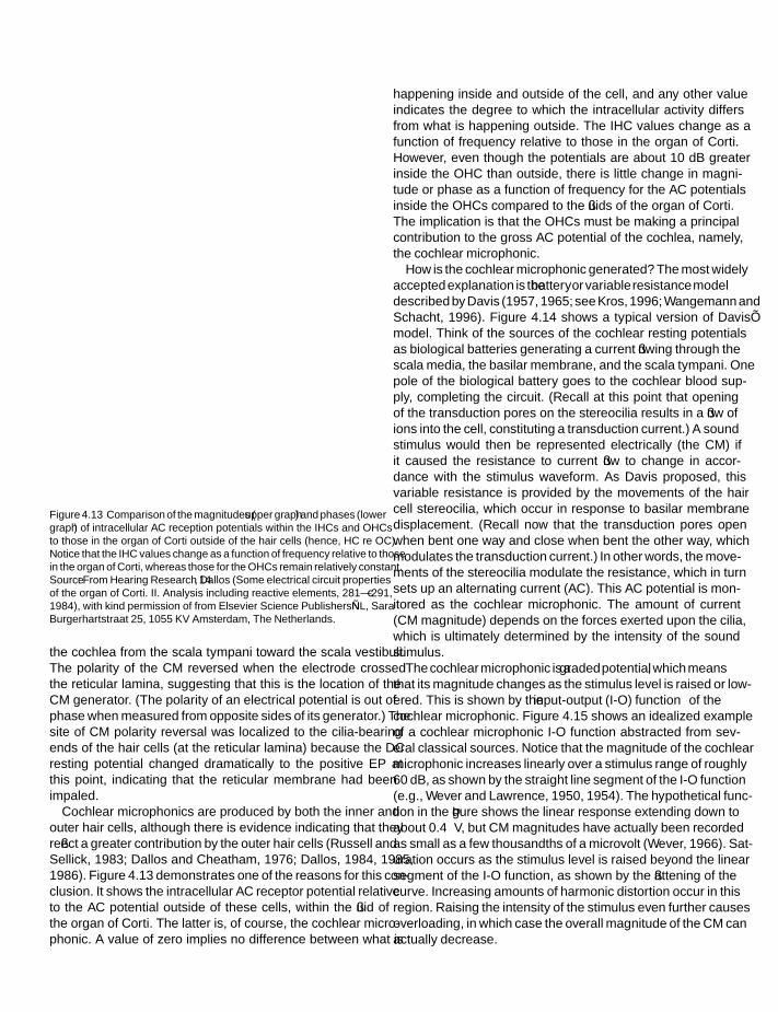
SFK SFK



Figure 4.13 Comparison of the magnitudes (upper graph) and phases (lowergraph) of intracellular AC reception potentials within the IHCs and OHCsto those in the organ of Corti outside of the hair cells (hence, HC re OC).Notice that the IHC values change as a function of frequency relative to thosein the organ of Corti, whereas those for the OHCs remain relatively constant.Source: From Hearing Research 14, Dallos (Some electrical circuit propertiesof the organ of Corti. II. Analysis including reactive elements, 281–291, c©1984), with kind permission of from Elsevier Science Publishers—NL, SaraBurgerhartstraat 25, 1055 KV Amsterdam, The Netherlands.

the cochlea from the scala tympani toward the scala vestibuli.The polarity of the CM reversed when the electrode crossedthe reticular lamina, suggesting that this is the location of theCM generator. (The polarity of an electrical potential is out ofphase when measured from opposite sides of its generator.) Thesite of CM polarity reversal was localized to the cilia-bearingends of the hair cells (at the reticular lamina) because the DCresting potential changed dramatically to the positive EP atthis point, indicating that the reticular membrane had beenimpaled.

Cochlear microphonics are produced by both the inner andouter hair cells, although there is evidence indicating that theyreflect a greater contribution by the outer hair cells (Russell andSellick, 1983; Dallos and Cheatham, 1976; Dallos, 1984, 1985,1986). Figure 4.13 demonstrates one of the reasons for this con-clusion. It shows the intracellular AC receptor potential relativeto the AC potential outside of these cells, within the fluid ofthe organ of Corti. The latter is, of course, the cochlear micro-phonic. A value of zero implies no difference between what is

happening inside and outside of the cell, and any other valueindicates the degree to which the intracellular activity differsfrom what is happening outside. The IHC values change as afunction of frequency relative to those in the organ of Corti.However, even though the potentials are about 10 dB greaterinside the OHC than outside, there is little change in magni-tude or phase as a function of frequency for the AC potentialsinside the OHCs compared to the fluids of the organ of Corti.The implication is that the OHCs must be making a principalcontribution to the gross AC potential of the cochlea, namely,the cochlear microphonic.

How is the cochlear microphonic generated? The most widelyaccepted explanation is the battery or variable resistance modeldescribed by Davis (1957, 1965; see Kros, 1996; Wangemann andSchacht, 1996). Figure 4.14 shows a typical version of Davis’model. Think of the sources of the cochlear resting potentialsas biological batteries generating a current flowing through thescala media, the basilar membrane, and the scala tympani. Onepole of the biological battery goes to the cochlear blood sup-ply, completing the circuit. (Recall at this point that openingof the transduction pores on the stereocilia results in a flow ofions into the cell, constituting a transduction current.) A soundstimulus would then be represented electrically (the CM) ifit caused the resistance to current flow to change in accor-dance with the stimulus waveform. As Davis proposed, thisvariable resistance is provided by the movements of the haircell stereocilia, which occur in response to basilar membranedisplacement. (Recall now that the transduction pores openwhen bent one way and close when bent the other way, whichmodulates the transduction current.) In other words, the move-ments of the stereocilia modulate the resistance, which in turnsets up an alternating current (AC). This AC potential is mon-itored as the cochlear microphonic. The amount of current(CM magnitude) depends on the forces exerted upon the cilia,which is ultimately determined by the intensity of the soundstimulus.

The cochlear microphonic is a graded potential, which meansthat its magnitude changes as the stimulus level is raised or low-ered. This is shown by the input-output (I-O) function of thecochlear microphonic. Figure 4.15 shows an idealized exampleof a cochlear microphonic I-O function abstracted from sev-eral classical sources. Notice that the magnitude of the cochlearmicrophonic increases linearly over a stimulus range of roughly60 dB, as shown by the straight line segment of the I-O function(e.g., Wever and Lawrence, 1950, 1954). The hypothetical func-tion in the figure shows the linear response extending down toabout 0.4 V, but CM magnitudes have actually been recordedas small as a few thousandths of a microvolt (Wever, 1966). Sat-uration occurs as the stimulus level is raised beyond the linearsegment of the I-O function, as shown by the flattening of thecurve. Increasing amounts of harmonic distortion occur in thisregion. Raising the intensity of the stimulus even further causesoverloading, in which case the overall magnitude of the CM canactually decrease.

81

SFK SFK


chapter 4

Figure 4.14 An electrical circuit representing the variable resistance model in relation to the major structures of the cochlea. Source: From Davis (1965),with permission.

Figure 4.15 An idealized input-output function for cochlear microphonicsin response to pure tone stimuli presented at increasing levels. The sinewaves represent the cochlear microphonic responses at various points on thefunction (notice the distortion at high levels). Source: Based on various dataand figures by Wever and Lawrence (1950, 1954) and Davis and Eldridge(1959).

The graded nature of the cochlear microphonic is alsoobserved in terms of the intracellular AC reception potential,which is its equivalent measured within the hair cells. In fact,because these potentials are recorded within a given cell, theyenable one to compare the relative thresholds of the inner versusouter hair cells. Using this approach, Dallos (1985) showed thatthe inner hair cells are on the order of 12 dB more sensitive thanthe outer hair cells. (This demonstration negated the previouslyheld notion that the OHCs are more sensitive than the IHCs,which was largely based upon studies that measured thresholdsfollowing the destruction of OHCs with ototoxic drugs [Daviset al., 1958; Dallos et al., 1972a, 1972b].)

Figure 4.16 shows how the intracellular AC receptor potentialchanges in magnitude as a function of frequency in response tostimuli that are increased in 20-dB steps. The IHC–OHC sensi-tivity difference is marked by the comparison of their responsemagnitudes at the best frequency for the lowest stimulus level (0dB). (The best, or characteristic, frequency is the one for whichthe hair cell has the lowest thresholds or the greatest magnitudeof response.) The graded nature of the response is revealed bythe increasing magnitude of the potential as the stimulus levelincreases. The slowing down of response growth at higher lev-els is easily seen in the figure: Even though any two successivestimuli are 20 dB apart, the resulting curves become closer andcloser for the higher stimulus levels.

82

SFK SFK



Figure 4.16 Effects of stimulus levels on the magnitude of the intracellular AC receptor potential as a function of frequency for an outer hair cell (left frame)and an inner hair cell (right frame). Source: From Hearing Research 22, Dallos (Neurobiology of cochlear inner and outer hair cells: Intracellular recordings,185–198, c© 1986), with kind permission of from Elsevier Science Publishers—NL, Sara Burgerhartstraat 25, 1055 KV Amsterdam, The Netherlands.

Distribution of the Cochlear MicrophonicRecall that large cochlear microphonic responses are recordedfrom the round window (Wever and Bray, 1930; Wever andLawrence, 1954; Eggermont et al., 1974). In order to deter-mine what contributes to the round window response, Misrahyet al. (1958) successively destroyed sections of the guinea pig’scochlea, beginning at the apex and working downward, whilemonitoring the CM in the basal turn. They found that the upperturns did not make significant contributions to the CM in thebasal turn. It may thus be concluded that the CM recorded atthe round window is for the most part derived from the activityof the basal turn.

Another approach to studying the distribution of the CMis to place electrodes along the cochlea to obtain CMs frommore or less restricted locations. The distribution of the CMalong the cochlear spiral was first reported with this methodby Tasaki, Davis, and Legouix (1952). They inserted pairs ofdifferential electrodes into the scalae tympani and vestibuli ofthe guinea pig. One electrode pair was placed in each of the fourturns. This method allowed them to separate the CM, which isof opposite polarity in the two scalae, from the auditory nerveaction potential (AP), which is always negative. (Addition ofthe out-of-phase signals cancels the CM and enhances the AP,whereas subtraction removes the AP and enhances the CM.)They found that the distribution of the CM was consistent withthe propagation pattern of the traveling wave. Low-frequencysignals had large CMs at the apical turn and minimal responsesat the base, while high frequencies had maximal CMs at the base

and no response at the apex (Fig. 4.17). They also found thatthe velocity of the signal was very high in the first turn of thecochlea and smaller toward the apex.

Honrubia and Ward (1968) used microelectrodes in the scalamedia to measure the distribution of CM responses along thecochlear duct. The electrodes were precisely placed at intervalsdetermined from place-frequency maps of the cochlear par-tition. Tones were then presented at fixed intensities, and CMmagnitude was measured at various distances along the cochlearduct. For example, the CM was measured at each electrode sitein response to a 1200-Hz tone at 78 dB, a 2500-Hz tone at 101dB, etc. Figure 4.18 shows typical results, with stimulus level asthe parameter. Consider first the distribution of CMs at the low-est stimulus levels (most sensitive curves). Consistent with thetraveling wave envelope, the peaks of these curves occur closerto the apex as frequency decreases. However, the CM curvesdo not line up exactly with the basilar membrane displacementcurve. This discrepancy is shown clearly in Fig. 4.19, in whichthe CM curve is wider and less peaked than the basilar mem-brane tuning curve. The difference occurs because the electrode“sees” CMs generated by thousands of hair cells in its generalvicinity rather than by just those at its precise point of insertion(Dallos et al., 1974). In other words, the electrode really mon-itors a weighted average of many CMs, which has the effect offlattening the curve somewhat.

As shown in Fig. 4.15, CM magnitude increases with stimuluslevel for each frequency. Also, the place of maximum CM mag-nitude shifts downward toward the base as intensity increases.

83

SFK SFK


chapter 4

Figure 4.17 Artist’s representation of the cochlear microphonics recordedwith differential electrodes in the first and third turns of the guinea pigcochlea (right) in response to stimuli of various frequencies (left).

This may at first seem inconsistent with the place principle.However, the basal shift of maximum CM response is proba-bly due to the wider range over which the more basal genera-tors respond linearly (Dallos, 1973). In other words, as stimu-lus intensity increases, the CMs from the most sensitive placealong the basilar membrane become saturated sooner than dothe responses from more basal regions. Thus, CMs generatedtoward the base continue to increase in magnitude when thosefrom the most sensitive place have already become saturated.The place of maximal CM response therefore shifts downwardalong the cochlear partition (upward in frequency).

The intracellular AC receptor potential also reveals a chang-ing distribution with respect to frequency when the stimuluslevel increases, as shown in Fig. 4.16. Here, we see that the tun-ing of the AC potential is reasonably restricted around the bestfrequency when the stimulus level is low, and that it becomeswider, extending toward the low frequencies, when the stimu-lus level becomes greater. In other words, the intracellular ACreceptor potential resembles a band-pass filter around the bestfrequency at low levels of stimulation and a low-pass filter athigher levels (Dallos, 1985).

Summating PotentialsThe summating potential (SP) was first described by Davis,Fernandez, and McAuliffe (1950) and by Bekesy (1950). Unlike

Figure 4.18 Cochlear microphonic magnitude as a function of distance along the basilar membrane for four frequencies presented at various intensities.Source: From Honrubia and Ward (1968), with permission of J. Acoust. Soc. Am.

84

SFK SFK



Figure 4.19 Comparison of basilar membrane tuning curves (based onWilson and Johnstone, 1972) and the CM curve at similar locations in theguinea pig cochlea. Source: From Dallos et al. (1974), with permission ofJ. Acoust. Soc. Am.

the CM, which is an AC potential, the SP is a shift in the DCbaseline in response to sound stimulation. In other words, the SPis a DC potential. Bekesy originally called this shift the “DC fall.”Subsequent research revealed that it may be either a positive ora negative baseline shift (Davis et al., 1958). We will see that SPpolarity is associated with the traveling wave envelope and howthe potential is recorded. Like the cochlear microphonic, the SPis a graded potential that increases in magnitude as the stimuluslevel is raised (Davis et al., 1958). Although the origin of the SPwas once a matter of debate, it is now well established that it is areceptor potential of the hair cells (Dallos and Cheatham 1976;Russell and Sellick, 1977a, 1977b, 1978a, 1978b, 1983; Dallos,1985, 1986).

Honrubia and Ward (1969b) measured the SP and CM simul-taneously in each turn of the guinea pig cochlea using electrodeslocated in scala media. We have already seen that the envelopeof the distribution of CM amplitude along the length of thecochlear duct is a reasonable representation of the travelingwave envelope. Honrubia and Ward found that the SP was pos-itive on the basal side of the CM envelope and negative on itsapical side. This suggests that the SP is positive on the basalside of the traveling wave and becomes negative apical to thetraveling wave peak.

Dallos and colleagues used a somewhat different recordingapproach (Dallos, 1973; Dallos et al., 1970, 1972b; Cheathamand Dallos, 1984). This method distinguishes between the aver-age potential of both the scala vestibuli and the scala tympanion the one hand and the potential gradient (difference) across

Figure 4.20 (a) Electrode arrangement and calculations used to obtain theDIF and AVE components of the summating potential. (b) Spatial relation-ships of the AVE SP and the DIF SP to the traveling wave envelope. Source:Modified from various drawings by Dallos, with permission.

the cochlear partition on the other. This at first complicateddistinction is clarified in Fig. 4.20a. One electrode is in the scalavestibuli and the other is in the scala tympani. Each one registersthe SP at the same cross-sectional plane along the cochlea, butfrom opposite sides of the scala media. Subtracting the SP inthe scala tympani (ST) from the SP in the scala vestibuli (SV),(SV − ST), gives the potential difference of the SP across thecochlear partition. This difference is called the DIF component.The average (AVE) component is obtained by simply averagingthe SPs from both scalae [(SV + ST)/2]. The AVE componentthus expresses the common properties (common mode) of theSP on both sides of scala media.

The spatial arrangements of the DIF SP and AVE SP are shownsuperimposed upon the traveling wave envelope in Fig. 4.20b.Note that the DIF component becomes negative in the vicinity ofthe peak of the traveling wave envelope, a situation that resem-bles the spatial distribution of SP+ and SP− discussed above.The polarity of the AVE component is essentially the reverse,being positive around the traveling wave peak and negative

85

SFK SFK


chapter 4

Figure 4.21 Intracellular AC and DC receptor potentials as a function offrequency at low levels of stimulation from an inner hair cell (left frame) andan outer hair cell (right frame) with comparable characteristic frequencies.Source: From Hearing Research 22, Dallos (Neurobiology of cochlear innerand outer hair cells: Intracellular recordings, 185–198, c© 1986), with kindpermission of from Elsevier Science Publishers—NL, Sara Burgerhartstraat25, 1055 KV Amsterdam, The Netherlands.

elsewhere. The AVE SP and DIF SP components of the sum-mating potential are probably produced by the same underlyingprocesses (Cheatham and Dallos, 1984).

As we have seen for the cochlear microphonic, intracellularrecordings also reveal that the summating potential is derivedfrom the hair cells, with the principal contribution coming fromthe OHCs (Russell and Sellick, 1983; Dallos, 1985, 1986). Fig-ure 4.21 provides insight into this relationship. It shows tuningcurves obtained at low levels of stimulation for the AC andDC intracellular receptor potentials (the intracellular versionsof the CM and SP, respectively) of an IHC and an OHC havingcomparable best frequencies. The figure reveals that the polarityof the outer hair cell’s DC receptor potential changes in both thepositive and negative directions. In contrast, the DC receptorpotential of the inner hair cell is positive only. Thus, the distri-bution of the SP is consistent with that of the OHCs as opposedto the IHCs.

This negative–positive distribution of the intracellular DCreceptor potential is in agreement with what we have just seenfor the SP, which is the gross extracellular potential representingthe contribution of many cells. (The negative–positive shape ofthe DC receptor potential as a function of frequency at lowstimulus levels becomes positive only at higher levels.)

The effects of increasing stimulus level upon the intracellularDC potential are largely similar to those observed above for

the AC potential. Specifically, the magnitude of the potentialincreases with stimulus level, compressing once moderate levelsare achieved, and as a function of frequency, the response issharply tuned and the band-pass around the best frequency atlow levels of stimulation becomes wider and low-pass at higherlevels.

Several other observations might be made from Fig. 4.21.The data were obtained using the lowest stimulus levels, whichallowed complete tuning curves to be generated. Note that thiswas 15 dB for the IHC and 30 dB for the OHC. This differenceshould not be surprising if one recalls that the IHCs are roughly12 dB more sensitive than the OHCs. Second, notice that thetuning curves for the DC receptor potentials are sharper thanthose for the AC potentials. Finally, notice that these tuningcurves obtained at low levels of stimulation are very sharp—much sharper than what we have seen for the traveling waveenvelope.

cochlear tuning and frequency selectivity

Basilar membrane displacement reaches a peak near the apexof the cochlea in response to low frequencies and near the basefor higher frequencies. That is, the traveling wave causes a dis-placement pattern, which is tuned as a function of distancealong the basilar membrane. One may say that the cochlea istuned to frequency as a function of distance along the cochlearpartition. This relationship between the tuning of a locationalong the cochlear partition and the distance from the base toapex is depicted in Liberman’s (1982) cochlear frequency mapshown in Fig. 4.22. This map was derived by determining thecharacteristic or best frequencies of auditory neurons labeledwith horseradish peroxidase (HRP), and then tracing theseneurons back to their respective hair cells along the cochlear

Figure 4.22 This cochlear map shows the relationship between frequencyand distance in percent along the cochlear partition in the cat. Source: FromLiberman (1982), with permission of J. Acoust. Soc. Am.

86

SFK SFK



Figure 4.23 Upper curves: Neural tuning curves (guinea pig). Lower curves:Mechanical tuning (guinea pig) based on (a) Wilson and Johnstone, 1972,(b) Bekesy (1960/1989), and (c) Johnstone et al. (1970). Source: From Evans(1975), The sharpening of cochlear frequency selectivity. Audiology, 14, 419–442.

duct (see Chap. 5). This method made it possible to preciselylocate the places along the cochlea that correspond to particu-lar frequencies. This cochlear map expresses distance along thecochlea in terms of percentage, thereby accounting for differ-ences in cochlear length across specimens.

In the following chapters, we shall see that fine frequency dis-criminations are made in psychoacoustic experiments, and thatauditory nerve fibers are very sharply tuned. Can the mechanicaldisplacement pattern in the cochlea account for this remarkabledegree of frequency selectivity?

A key question is whether the sharpness of cochlear tuningapproaches that of the auditory nerve. The upper curves inFig. 4.23 show a set of response areas or tuning curves forauditory nerve fibers in the guinea pig. Neural tuning curveswill be discussed in Chapter 5. For now, note their sharp peaks,which indicate that auditory nerve fibers respond best to alimited range of frequencies around a characteristic frequency.The low-frequency slopes of the neural tuning curves range fromabout 100 to 300 dB per octave, and the high-frequency slopesare approximately −100 to −600 dB per octave in a variety ofspecies (e.g., Kiang, 1965; Evans and Wilson, 1971, 1973; Evans,1972a, 1972b; Geisler et al., 1974).

The sharpness of tuning can be described by a value Q, whichis the ratio of the center frequency to the bandwidth. For aparticular center (characteristic) frequency, the narrower thebandwidth, the larger is the Q value. This relationship is illus-trated in Fig. 4.24. Recall that the half-power points are theusual cutoff values used to define a bandwidth. Since it is diffi-cult to determine the half-power points of physiological tuningcurves, it has become standard practice to use the points on thecurve that are 10 dB down from the peak. For this reason, weuse the value Q10dB to summarize the sharpness of physiologi-

Figure 4.24 Q10dB for three idealized “tuning curves” centered at 1000 Hz.These Q10dB values were obtained as follows: (a) 1000/140=7.1, (b) 1000/600= 1.7, and (c) 1000/1000 = 1.0.

cal tuning curves. Auditory neurons have Q10dB values of about2 to 10 for the midfrequencies (Evans and Wilson, 1973). Withthis in mind, let us proceed to examine the nature of frequencyselectivity in the cochlea.

Bekesy (1949) was the first to describe mechanical tuning inthe cochlea. He used a binocular microscope to observe basilarmembrane displacement patterns in response to high-intensitysignals. Figure 4.25 shows some of the basilar membrane tuningcurves obtained by Bekesy. These curves are in terms of relativeamplitude so that the peak is assigned a value of 1.0 and thedisplacements at other points along the curves are in propor-tions of the peak amplitude. The tuning curves tend to becomesharper with increasing frequency, but the low-frequency slopesof about 6 dB per octave are far from the sharpness of neuraltuning. This is illustrated in Fig. 4.23, in which Bekesy’s curves(labeled b) are compared with neural tuning curves having sim-ilar characteristic frequencies.

Figure 4.25 Basilar membrane tuning curves obtained in (a) cadaver (afterBeksey, 1943/1949) and (b) guinea pig (after Bekesy, 1944).

87

SFK SFK


chapter 4

Although Bekesy’s data were of monumental significance,several experimental limitations make it difficult to comparethese early findings with neural tuning data: Access to thecochlear partition was limited to the apical areas so that Bekesy’sobservations were restricted to relatively low frequencies. Theobservations were obtained visually. Absolute displacementswere not specified (although they were in other contexts). Veryhigh stimulus levels (roughly 120 dB SPL) were used, whileneural data are available at much lower, including threshold,levels.

Subsequent studies investigated basilar membrane tuningusing methods made possible by technological advances in the1960s and 1970s (e.g., Johnstone et al., 1970; Rhode, 1971,1978; Kohllofel, 1972; Wilson and Johnstone, 1972, 1975; John-stone and Yates, 1974; Rhode and Robles, 1974). For example,Johnstone and Boyle (1967) measured tuning in the guinea pigcochlea by using the Mossbauer technique, which made it pos-sible to use stimulus levels as low as 60 to 70 dB SPL. In thismethod, a radioactive source is placed on the basilar membraneand an absorber of the radiation is situated nearby. Vibrationof the basilar membrane causes the amount of gamma raysabsorbed to be modulated in a manner related to the vibration.Basilar membrane displacement is calculated based on thesedata. Mechanical tuning curves obtained with the Mossbauermethod (e.g., curve c at the bottom of Fig. 4.23) were consid-erably sharper than what Bekesy found at low frequencies (e.g.,curves labeled b in the figure).

Wilson and Johnstone (1972, 1975) measured basilar mem-brane tuning with a capacitance probe, which was a minia-ture version of the one used by Bekesy (1960/1989) (seeChap. 3). Their findings are of interest because they confirmedthe Mossbauer data with another technique and also because thecapacitance probe enabled them to measure basilar membranevibrations for stimuli as low as 40 dB SPL (which is closer to thelevels used to obtain neural tuning curves). Curve a in lowerpart of Fig. 4.23 shows an example. Comparing the upper andlower sections of Fig. 4.23 makes it clear that these measure-ments cannot account for the sharpness of the neural tuningdata.

It was once thought that a “second filter” existing between thebasilar membrane and neural responses might account for thesharpness of neural tuning. The main evidence for this idea wasthat neural tuning curves become wider when the metabolism ofthe cochlea is disturbed by interference with its oxygen supply orby chemical influences (Evans, 1972a, 1972b, 1974, 1975; Evansand Wilson, 1971, 1973). The appeal of the second filter con-cept to bridge the gap from broad mechanical to sharp neuraltuning led to the proposal of several theories about its loca-tion and mechanism. One example involved lateral inhibition,which involves the suppression of activity in weakly stimulatedneural units by more intense stimulation of adjoining units(e.g., Bekesy, 1960/1989), although other possible mechanismswere also proposed (e.g., Khanna et al., 1968; Duifhuis, 1976;Zwislocki, 1974, 1975, 1985; Manley, 1978; Crawford and

Fettiplace, 1981). An example of lateral inhibition from com-mon experience is the sharply defined border that is seenbetween adjoining black and white bars known as Mach bands.However, we shall see that active processes are at work that pro-vide for mechanical tuning just as sharp as neural tuning. Thus,a “second filter” is not necessary. Interested readers should referto Pickles (1982) and Gelfand (1981) for reviews of second filtertheories.

That sharp tuning already exists prior to the neural responsewas demonstrated by Russell and Sellick (1977a, 1977b, 1978a,1978b). They measured the intracellular DC receptor potential(summating potential) in guinea pig IHCs as a function of stim-ulus frequency and level. Typical findings are shown in Fig. 4.26.Each curve shows the sound pressure level needed to reach acertain magnitude of DC potential within the IHC as a func-tion of frequency. These curves are called isoamplitude contoursbecause each point on a given curve represents the SPL neededto achieve the same amplitude of SP. The smallest intracellularSP response that could elicit a response from the auditory nervewas about 2.0 mV. At high stimulus levels (SPLs that result inlarger SP amplitudes), the SP tuning is more or less like thatof the mechanical data we have previously reviewed. However,as the stimulus level decreases, the reduction in SP amplitude(A in mV) comes with a clear increase in the frequency selec-tivity of IHC intracellular tuning curves. For example, whenSP amplitude is 2.7 mV (within 10 dB of threshold), Q10dB is9.2. This is as sharp as neural tuning. Similarly sharp tuningof intracellular potentials has also been reported for the OHCs(e.g., Dallos et al., 1982). One might note in this context thatCheatham and Dallos (1984) showed that tuning curves for theSP are consistent with those of the basilar membrane and theauditory nerve action potential.

These findings demonstrate that frequency selectivity as sharpas what is found in the auditory neuron already exists withinthe hair cell and before it transmits to the nerve fiber. Clearly,the acuity of neural tuning does not require an intervening filterbetween the hair cell and the neuron.

What (and where), then, is the origin of the sharp tuning thatis already seen in the hair cell? The answer comes from studiesof the in vivo mechanical responses of virtually undamagedcochleas at stimulus levels as low as those used to generateneural tuning curves.

In 1982, Khanna and Leonard demonstrated sharp basilarmembrane tuning in the cat by using laser inferometry. Adetailed discussion of this technique and its applications maybe found in an informative series of papers by Khanna andcolleagues (Khanna and Leonard, 1982, 1986a, 1986b; Khanna,1986; Khanna et al., 1986). The sharpness of mechanical tuningin the cochlea has been repeatedly corroborated (e.g., Sellick etal., 1982a; Robles et al., 1986; Ruggero et al., 1997).

Figure 4.27a shows three cat basilar membrane tuning curves.These curves show the sound pressure levels needed to yield acertain threshold amplitude of basilar membrane vibration asa function of frequency. The sharpest of these three curves is

88

SFK SFK



Figure 4.26 Intracellular DC receptor potentials (summating potentials)from guinea pig inner hair cells as a function of frequency: (a) Receptorpotential amplitude (A in mV) is shown with corresponding values of Q10dB.Source: From Russell and Sellick (1977a), courtesy of Nature. (b) Isoampli-tude curves are shown for 2, 5, and 10 mV intracellular potentials. Source:From Russell and Sellick, Intracellular studies of cochlear hair cells: Fill-ing the gap between basilar membrane mechanics and neural excitation,in Evoked Electrical Activity in the Auditory Nervous System (Naunton andFernandez, eds.), c© 1978 by Academic Press.

Figure 4.27 (a) The SPL necessary to achieve equal amplitudes of basilarmembrane movements in three cats. (b) Comparison of the sharpest basilarmembrane curve (3/26/81) with a neural tuning curve. Source: From Khannaand Leonard, Basilar membrane tuning in the cat cochlea, Science, 215, 305–306 (1982). Copyright c© 1982. Reprinted with permission from AmericanAssociation for the Advancement of Science.

89

SFK SFK


chapter 4

shown redrawn in Fig. 4.27b along with a neural tuning curve.The basilar membrane curve is strikingly similar to that ofthe neuron in the sharply tuned tip of the tuning curve, butdeviates from the neural response at lower frequencies. Thesegraphs reveal that the basilar membrane’s mechanical responseis as sharp as that of the neural tuning curve in the region ofthe most sensitive response (where Q10dB is 5.9 for both curvesin this example).

Similar findings for the guinea pig cochlea were obtained bySellick et al. (1982a, 1982b). Recall that the IHCs are activated bythe velocity rather than the displacement of basilar membranemovement. As a consequence, they expressed the mechanicalresponse of the basilar membrane in terms of the velocity of itsmotion. Figure 4.28a shows that the basilar membrane isove-locity curve (crosses) is remarkably similar to a representativeneural tuning curve. Figure 4.28b shows the SPLs needed toyield an isoamplitude response of the basilar membrane. Asin the previous figure, the isoamplitude response is similar tothe neural response in the sharply tuned tip of the curve, butdeviates at lower frequencies.

Sellick, Pauzzi, and Johnstone (1982a, 1982b) used the stimu-lus SPL needed to evoke an auditory nerve action potential (seeChap. 5) as a measure of the health of the cochlea over the courseof their measurements. Examples of their results are shown inFig. 4.29. They found that these thresholds worsened as timepassed, revealing that the experimental invasion of the innerear itself caused progressive damage to the cochlea. Khannaand Leonard (1982) also reported that trauma to the cochleadue to the experimental manipulations caused a loss of sharpmechanical tuning.

It is now clear that the mechanical tuning within the cochleaaccounts for the sharpness of neural tuning; but what is thenature of this mechanical tuning process? We must recall atthis juncture that the real concern is with the sharpness ofthe mechanical stimulus actually transmitted to the hair cells.The tuning of the cochlea involves more than just the passivetraveling wave response of the basilar membrane. There also areactive processes associated with the outer hair cells and theirconnections to surrounding structures.

Let us view the tuning curve somewhat differently in orderto appreciate why the mechanical tuning of the cochlea involvesactive processes. The cochlea’s mechanical response may bedescribed as having two components (Khanna and Leonard,1982, Leonard and Khanna, 1984; Kelly and Khanna, 1984a):One of these components has a broad low-pass response. Theother is a sharply tuned band-pass filter. Together, the two com-ponents reveal the neural tuning curve’s familiar sharp tip andbroad tail. Injuries that affect the tip do not particularly affectthe broad, low-pass component. In particular, injuries affect-ing the OHCs have been shown to affect the tip componentbut not the tail of the tuning curve, and the condition of theOHCs is correlated with the affect upon the tip of the tun-ing curve (Khanna and Leonard, 1986b; Leonard and Khanna,1984; Liberman and Dodds, 1984). These changes in the tip of

Figure 4.28 (a) The SPL necessary to achieve equal velocities (crosses) andamplitudes (circles) of basilar membrane vibration, and a comparable neuraltuning curve (dotted line) in the guinea pig. (b) The SPL needed to achievethree velocities of basilar membrane vibration in the same guinea pig. Source:From Sellick et al. (1982), with permission of J. Acoust. Soc. Am.

the tuning curve are found in the absence of basilar membraneabnormalities (Kelly and Khanna, 1984a, 1984b). The tip com-ponent of the cochlea’s mechanical tuning curve is associatedwith the outer hair cells.

One might note in this context the classic observation thatthresholds become about 30 to 40 dB poorer when ototoxic

90

SFK SFK



Figure 4.29 The loss of sharp mechanical tuning of the basilar membraneis observed as thresholds become elevated, revealing progressive damage tothe cochlea over the course of the measurements, and post mortem, for twoguinea pigs (a and b). From Sellick et al. (1982a, 1982b), with permission ofJ. Acoust. Soc. Am.

drugs have destroyed the outer hair cells (Dallos et al., 1972a,1972b). The long-held interpretation of this observation wasthat the inner hair cells, which survived the ototoxic assault,are not as sensitive as the outer hair cells. However, we nowknow that the drop in thresholds is due to the loss of thesensitizing effects of the OHCs (Dallos and Harris, 1978). Infact, as previously noted and in contrast to previously heldnotions, intracellular recordings have established that the IHCs

are on the order of 12 dB more sensitive than the OHCs(Dallos, 1985).

The two-component nature of cochlear tuning has also beendemonstrated by Liberman and colleagues, who determinedhow various cochlear manipulations affected the associatedauditory neurons’ responses (Liberman, 1984; Liberman andDodds, 1984; Liberman and Kiang, 1984; Kiang et al., 1986).They demonstrated that while both the IHCs and OHCs areneeded to yield a normal neural tuning curve, the presence ofthe sharply tuned component of the response depends upon thepresence and condition of the outer hair cells.

Smith et al. (1987) provided behavioral support for the con-tribution of the OHCs to the sensitivity and fine-tuning of thecochlea. They obtained psychoacoustic tuning curves (PTCs),a behavioral measure of frequency selectivity (see Chap. 10),from patas monkeys before and after producing OHC damagewith the drug dihydrostreptomycin. The drug caused elevationsof threshold sensitivity of 50 dB or more, and the sharp tipsof the PTCs to be obliterated, leaving only the broad, low-passfilter characteristic of the curves. Histological examination ofthe cochleas revealed that there was complete loss of OHCs butcomplete retention of the IHCs in the regions corresponding tothe changes of the PTCs.

cochlear nonlinearity

One of the seminal contributions to our knowledge ofcochlear functioning was Rhode’s (1971) demonstration thatthe mechanical response of the basilar membrane is nonlinear.The nonlinearity is seen in Fig. 4.30 as a lack of overlappingof the tuning curve peaks obtained at different stimulus levels.The three curves in the figure would have overlapped exactly ifthe basilar membrane’s vibration was linear because the ampli-tude (in dB) is derived from the ratio of basilar membrane-to-malleus displacement. In a linear system, this ratio would staythe same for different stimulus levels. This nonlinearity, origi-nally observed in the squirrel monkey, used to be the subject ofcontroversy because other researchers at that time did not findit in the guinea pig. However, as we have seen for the sharpnessof cochlear tuning, nonlinearity in the vicinity of the peak is thenormal response (e.g., Rhode, 1971, 1978; Rhode and Robles,1974; Sellick et al., 1982a, 1982b; Robles et al., 1986; Ruggeroet al., 1997) (see Figs. 4.26, 4.28b, and 4.31).

Figure 4.31 provides a detailed illustration of this nonlin-earity. Here, we see a set of tuning curves obtained from ahealthy chinchilla cochlea by Ruggero et al. (1997), who used awide range of stimulus levels and modern measurement tech-niques (a form of laser inferometry). Notice that the mechanicalresponse is nonlinear around the characteristic frequency (tun-ing curve peak) and at higher frequencies, again indicated bythe lack of overlapping). However, this does not occur at lowerfrequencies, where the curves are superimposed.

91

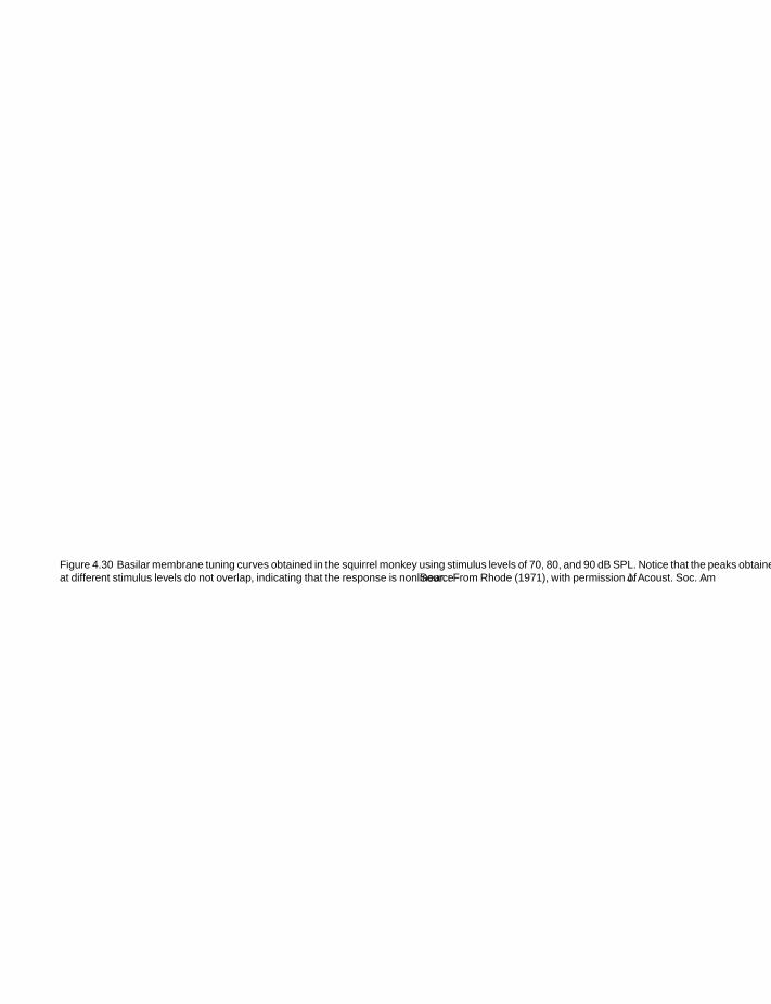
SFK SFK


chapter 4

Figure 4.30 Basilar membrane tuning curves obtained in the squirrel monkey using stimulus levels of 70, 80, and 90 dB SPL. Notice that the peaks obtainedat different stimulus levels do not overlap, indicating that the response is nonlinear. Source: From Rhode (1971), with permission of J. Acoust. Soc. Am.

Frequency (kHz)

Vel

ocity

(µm

/s)

47.9 dB

5 & 10 dB20

3040

50

60

7080

Stapes

103

102

101

100

10-1

2 3 4 5 6 7 8 910 20

Figure 4.31 Basilar membrane tuning curves (gain in response velocitydivided by stimulus level as a function of frequency) in the chinchilla cochlea,using a wide range of stimulus levels (indicated by the numbers next to eachcurve). The response is nonlinear for frequencies in the vicinity of the peakand above (revealed by the lack of overlapping), but is linear for lowerfrequencies (where the curves overlap). Source: Adapted from Ruggero et al.(1997), by permission of J. Acoust. Soc. Am.

The compressive nature of the nonlinear response of the basi-lar membrane is clearly seen in Fig. 4.32, which shows data fromsix essentially healthy chinchilla cochleas. Each curve shows howthe magnitude of the basilar membrane response at the tuningcurve peak is related to the sound pressure level of the stimu-lus. The straight line in the graph illustrates linear growth. Thetipping-over of these curves shows that the growth of responsemagnitude slows down as the stimulus level rises. The nonlinearnature of these curves is highlighted by comparing them withthe straight line representing linear growth.

As for sharp tuning, the sensitivity and nonlinear nature of thebasilar membrane response depend on the health and integrityof the cochlea (e.g., LePage and Johnstone, 1980; Sellick et al.,1982a, 1982b; Yates et al., 1990). For example, Sellick et al.(1982a, 1982b) showed that sharp turning and the nonlinearresponse deteriorated as thresholds worsened, and that theywere present early during experimental testing when the cochleawas still reasonably healthy, but were lost as the experimentproceeded and at postmortem (Fig. 4.29).

The nonlinearity of the cochlea also can be observed in theproduction of distortion products and by two-tone suppression.

92

SFK SFK


cochlear mechanisms and processesV

eloc

ity (

µm/s

)

Dis

plac

emen

t (nm

)

Sound Pressure Level (dB)

0 20 40 60 80 100

104

103

102

101

Line

ar G

rowth 101

100

102

Figure 4.32 Magnitude of the basilar membrane response at the character-istic frequency (tuning curve peak) as a function of stimulus level from sixchinchillas with essentially healthy cochleas. The compressive nature of thebasilar membrane response is seen by comparing these curved lines with thestraight line representing linear growth. (Filled circles indicate the functionfor the animal whose tuning curves are shown in Fig. 4.31.) Source: Adaptedfrom Ruggero et al. (1997), by permission of J. Acoust. Soc. Am.

Distortion products occur when the output of a system includescomponents that were not present at the input. For example,if two tones with frequencies f1 and f2 are presented to the ear(input), the basilar membrane’s vibratory response (output)might include the primaries f1 and f2 plus distortion productssuch as f2-f1 and 2f1-f2 (e.g., Nuttall et al., 1990; Nuttall andDolan, 1993; Robles et al., 1991, 1997; Rhode and Cooper, 1993;Cooper and Rhode, 1997; Robles and Ruggero, 2001). The firstexample, f2-f1, is sometimes called the quadratic differencetone and is produced when f1 and f2 are presented at high levels.On the other hand, the cubic difference tone 2f1-f2 occurs whenf1 and f2 are presented at low levels and is rather sensitive to theproximity of the primary tones. We will return to f2-f1 and 2f1-f2

in the context of otoacoustic emissions below, and will discusstheir perception in Chapter 12.

Two-tone suppression in the cochlea occurs when theresponse of the basilar membrane produced by one tone (atthe characteristic frequency) is weakened by the presence ofa second (suppressor) tone at a different frequency, and is themost likely origin of two-tone suppression in the auditory nerve,discussed in Chapter 6 (see, e.g., Ruggero et al., 1992; Cooper,1996; Geisler, 1998; Robles and Ruggero, 2001). The effect isgreatest when the characteristic frequency and suppressor tonesare very close in frequency and decreases as their frequenciesbecome further apart.

otoacoustic emissions

Kemp (1978, 1979) demonstrated that the cochlea can producesounds as well as receive them. He found that when a click isdirected into the ear, it is followed by an echo that is emitted backfrom the cochlea. This cochlear echo can be detected roughly 5 msor more after the click, typically peaking at latencies in the vicin-

Figure 4.33 Example of a spontaneous otoacoustic emission at approxi-mately 1500 Hz (arrow) detected above the noise floor in an occluded earcanal. Its level corresponds to about 11 dB SPL. Source: From Zurek, 1985,with permission of J. Acoust. Soc. Am.

ity of approximately 5 to 15 ms. This phenomenon was origi-nally referred to as the Kemp echo and has come to be know asthe evoked or stimulated otoacoustic emission. Spontaneousotoacoustic emissions occur as well (Kemp, 1979; Zurek, 1981;Strickland et al., 1985). These signals generated in the cochleaare measurable with a probe microphone in the ear canal. Figure4.33 shows an example of a spontaneous otoacoustic emissionat about 1500 Hz. However, we will concentrate upon evokedotoacoustic emissions here. The interested student will find agrowing number of informative reviews and discussions aboutthe nature, parameters, and applications of otoacoustic emis-sions in the literature (e.g., McFadden and Wightman, 1983;Zurek, 1985; Lonsbury-Martin et al., 1991; Probst et al., 1991;Dekker, 1992; Berlin, 1998; Robinette and Glattke, 2002).

It is worthwhile to review how the stimulated or evoked otoa-coustic emission is obtained. Suppose a probe device like theone represented in Fig. 4.34a is inserted into someone’s ear.This probe contains both a sound source (an earphone) and amicrophone, and it occludes the ear when inserted. A click ispresented to the ear and the sound pressure in the occluded earis measured over time.

Before putting the probe into a human ear, let’s first see whathappens when it is inserted into a Zwislocki coupler, which is ametal cavity that has the same impedance characteristics as thehuman ear. In this case, there would be a damped oscillationlike the one shown in the upper tracing of Fig. 4.34b. Now let’sput the coupler into a human ear. In this case, the resultingwaveform will resemble the middle tracing in Fig. 4.34b. Herewe see an initial damped oscillation lasting about 6 ms and alsoa much smaller oscillation occurring after a latency of roughly6 to 7 ms. The initial oscillations are the impulse response of theear and are similar to what we just saw in the metal coupler. Thelater and smaller oscillations constitute the cochlear echo, or theevoked otoacoustic emission. The lower tracing in Fig. 4.34bshows just the evoked otoacoustic emission after the responsehas been amplified and displaced by 5 ms to remove the initialpart of the response.

93

SFK SFK


chapter 4

Figure 4.34 (a) The probe for eliciting and measuring otoacoustic emissions is inserted into the ear canal. The sound source is provided by the earphoneand the microphone measures the sound pressure in the ear canal, which is occluded by the ear tip. (b) Responses to a click stimulus: Upper tracing : Dampedoscillation in a metal cavity (Zwislocki coupler). Middle tracing : Responses in a human ear consisting of initial damped oscillations followed by the evokedotoacoustic emission (echo). Lower tracing : Amplified echo response displaced by 5 ms. Source: From Johnsen and Elberling (1982), with permission ofScandinavian Audiology.

Many studies of evoked otoacoustic emissions were under-taken within a short period after its original description and itcontinues to be the topic of extensive investigation (see, e.g.,reviews by Wit and Ritsma, 1979, 1980; McFadden and Wight-man, 1983; Zurek, 1985; Lonsbury-Martin et al., 1991; Probst etal., 1991; Dekker, 1992; Robinette and Glattke, 2002). A numberof generalities have been derived from these and other studies.To begin with, virtually all normal hearing humans appear tohave a stimulated acoustic emission in response to clicks and/ortone bursts. A given ear’s emission is extraordinarily repro-ducible; however, the details of evoked emissions differ widelyfrom ear to ear, just as we have seen with respect to the sharpnessand nonlinearity of the cochlea’s mechanical tuning. The evokedacoustic emission is also vulnerable to such insults as ototoxicity

and noise exposure and is obliterated by any substantive degreeof sensorineural hearing loss.

The latency and magnitude of the echo depend on the levelof the stimulus. Latency tends to decrease as the stimulus levelsbecome greater. Although the magnitude of the evoked emis-sion gets larger with increasing stimulus level, this relationshipis linear only for low stimulus levels, above which the input-output curve becomes compressed, and saturates by the timethe emission reaches about 20 dB SPL.

The latency of the emission decreases with increasing fre-quency. This association is important because it is consistentwith the idea that the location within the cochlea from whichthe echo originates moves closer to the base with increasingfrequency, as one would expect. An apparent problem with this

94

SFK SFK



Figure 4.35 Effect of frequency from 500 to 2000 Hz on the evoked otoacoustic emission for one subject. Columns (a) and (b) show evoked otoacousticemission waveforms before and after processing. Column (c) compares the spectra of the stimuli (smoother curves) to those of the otoacoustic emissions.Source: From Norton and Neeley (1987), by permission of J. Acoust. Soc. Am.

point has been the observation that the actual latencies of theecho seem to be two or three times longer than the estimatedtime it would take for the signal to reach and then return froma given place along the cochlear duct. However, it has beenpointed out that otoacoustic emission latencies fall within theexpected round-trip travel time when the latter is based upondata obtained at low stimulus levels, similar to those employedin acoustic emissions work (e.g., Neeley et al., 1986; Norton andNeeley, 1987).

The spectral characteristics of click-evoked otoacoustic emis-sions do not exactly match those of the click used to elicit them.Instead, they tend to show energy concentrations in fairly nar-row frequency ranges. Norton and Neeley (1987) using tone-bursts showed that the frequency concentrations in the spectraof otoacoustic emissions follow those of the stimuli, as exem-plified in Fig. 4.35. The third column of the figure comparesthe spectra of the otoacoustic emissions to those of the stim-uli (represented by the smooth lines). Notice that there is anorderly change in the spectra of the otoacoustic emissions withthe changes in the stimulus spectra.

Distortion product otoacoustic emissions (DPOAEs) occurat frequencies corresponding to the f2-f1 difference tone and the2fl-f2 cubic difference tone. Here f1 and f2 are the frequenciesof the lower and higher primary tones, respectively. The levelof f1 is L1, and L2 is the level of f2. The cubic difference toneotoacoustic emission is the most interesting and widely studiedof the DPOAEs. Its level tends to be about 60 dB weaker thanthe levels of the primary tones. Several examples of DPOAEs areprovided in Fig. 4.36 from an experiment by Bums et al. (1984).In the lower tracing, we see spontaneous otoacoustic emissions(SOAEs) at 1723 and 2049 Hz. These behave as primary tonesto produce a cubic difference tone (2f1-f2) SOAE of 1397 Hz. Inthe upper tracing of the figure, we see that the introduction ofan external tone masks (see Chap. 10) the higher primary. As aresult, this leaves only the lower primary SOAE, and the cubicdifference tone, which previously resulted from the interactionof f1 and f2, is now obliterated. These findings provide furtherevidence of active processes in the cochlea.

It is generally accepted that DPOAEs are best observed when(1) the primaries are in the 1000- to 4000-Hz region with an f2/fl

95

SFK SFK


chapter 4

Figure 4.36 Lower tracing : Primary (1, 2) spontaneous otoacoustic emis-sions (SOAEs) at 1723 and 2049 Hz yield a cubic difference tone SOAEat 1397 Hz (CDT1,2). Upper tracing : Adding an external tone (ET) maskstone 2, leaving only tone 1, thus obliterating the distortion product. Source:From Hearing Research 24, Burns, Strickland, Tubis, and Jones (Interac-tions among spontaneous otoacoustic emissions. I. Distortion products andlinked emissions, 271–278, c©1984), with kind permission of from ElsevierScience Publishers—NL, Sara Burgerhartstraat 25, 1055 KV Amsterdam,The Netherlands.

frequency ratio approximating 1.2, and (2) the L1 is the same asL2 for low stimulus levels, and L1 is 10 to 15 dB greater than L2 forhigh stimulus levels. However, more complicated relationshipsamong the frequencies and levels of the primaries have beenshown to optimize DPOAE levels (e.g., Johnson, Neely, Garner,and Gorga, 2006).3

When continuous tones are presented to the ear, the acousticemission has the same frequency as the stimulus but is delayedby its latency. The stimulus and emission will interact, resultingin peaks and valleys at frequencies where they are in andout of phase. This effect is seen at low levels of the stimulus,becoming less apparent and finally disappearing when thestimulus level exceeds 40 to 50 dB SPL. This level dependencyis expected because of the emission’s very low amplitude. Thatis, interference between the stimulus and emission can onlyoccur when their levels are relatively similar; the low level of theemission means that this condition can only be met at lowerlevels of the stimulus.

These phenomena are consistent with the concept that theevoked acoustic emissions monitored in the ear canal arecochlear in origin. It is apparent that active processes enablethe cochlea to produce as well as receive acoustical signals.

active processes and the cochlear amplifier

We have seen that the outer hair cells have an significantimpact upon the sharpness and nonlinearity of cochlear pro-

3 Specifically, Johnson et al. (2006) found that, on average, normalDPOAEs were largest when

(a) f2/f1 = 1.22 + log2(9.6/f2) · (L2/415)2, and

(b) L1 = 80 + 0.137 · log2(18/f2) · (L2 − 80).

Figure 4.37 The electromotile response of an outer hair cell (changinglength over time) acts as a positive-feedback mechanism, providing the forcefor active cochlear processes. The magnitude of the length, which is actuallyon the order of about 1% to 4%, is highly exaggerated in the drawing forillustrative purposes.

cesses. This influence involves active processes that contributeto the cochlear response above and beyond the passive vibra-tory response of the basilar membrane (the traveling wave) andtransmission of the transduced signals to the nervous system.This cochlear amplifier enhances the vibratory stimulus deliv-ered to the inner hair cells, results in the cochlea’s sharply tunedand nonlinear response, and generates otoacoustic emissions.The active mechanism relies on outer hair cell electromotility,which is the unique ability of the OHCs to rapidly contract andexpand (by up to about 4%) in response to the sound stimulus,and thereby to affect cochlear micromechanics (e.g., Brownellet al., 1985; Brownell, 1990; Kalinec and Kachar, 1995; Holley,1996; Patuzzi, 1996; Brownell and Popel, 1998; Geisler, 1998;Santos-Sacchi, 2003).

The prevalent explanation of OHC electromotility may besummarized as follows: Recall from Chapter 2 that there is pos-itive hydrostatic pressure (turgor) within the OHC due to itscytoplasm, while its test tube–like shape is maintained by thetension of the matrix of structures in its lateral “walls” (seeFigs. 2.29 and 2.30). The arrangement of these forces is suchthat changing the cell’s surface area will change its length andgirth. The surface area of the OHC is altered by conformationalchanges of components in the cell membrane, which, in turn,is controlled by the cell’s polarization. Depolarization causesthe OHCs to contract and hyperpolarization causes them toexpand. As we have already seen, sound stimulation eventu-ates the bending of the OHC stereocilia, varying the ion cur-rents through the opening and closing transduction channels,and thus varying the receptor potential. The changing polar-ization activates the cycle-by-cycle electromotile responses ofthe OHCs, which is able to occur fast enough to operate at allaudible frequencies. Recalling that the OHCs are “mounted”between the Deiter’s cells below and the reticular lamina above,this pushing-and-pulling motile response (Fig. 4.37) operateslike a positive-feedback mechanism, which provides the forcesthat drive the cochlear amplifier.

Outer hair cell electromotility, which drives the cochlearamplifier, appears to be generated by the interaction of two

96

SFK SFK



mechanisms or “motors” (Dallos, Zheng, and Cheatham, 2006;Kennedy, Evans, Crawford, and Fettiplace, 2006; Fettiplace andHackney, 2006). The somatic motor relies on prestin, whichhas been identified as the motor protein of the OHC (Zhenget al., 2000; Oliver et al., 2001; Santos-Sacchi et al., 2001; Dallosand Fakler, 2002; Liberman et al., 2002; Dallos et al., 2006).The prestin motor is believed to operate by shuttling chlo-ride ions back and forth between the inner and outer partsof the cell membrane (Fig. 4.38). Shortening is triggered bydepolarization, which causes the prestin molecule to trans-port the chloride ion toward its inner side (Fig. 4.38a), andlengthening is triggered by hyperpolarization, which causes theprestin molecule to move the chloride ion toward its outer side(Fig. 4.38b). The hair bundle motor relies on the force gen-erated by the changing compliance of the stereocilia bundlethat occurs with the opening and closing of the transductionpores (Fettiplace, 2006; Fettiplace and Hackney, 2006; Kennedyet al., 2006).

In addition to the fast electromotile response just dis-cussed, slower motile responses are also produced when OHCsare exposed to chemical agents and efferent neurotransmitteracetylcholine and electrical stimulation (e.g., Brownell et al.,1985; Zenner et al., 1985; Flock et al., 1986; Kachar et al., 1986;Ashmore, 1987; Ulfendahl, 1987; Slepecky et al., 1988a, 1988b;Zajic and Schacht, 1991; Holley, 1996). Figure 4.39 shows anexample for a guinea pig OHC, which was removed from the

Figure 4.38 Artist’s conceptualization of the somatic (prestin) motor ofOHC electromotility. (a) Depolarization causes the prestin molecule totransport the chloride ion toward the inner side (shortening). (b) Hyperpo-larization causes the prestin molecule to transport the chloride ion towardthe outer side (lengthening).

cochlea and exposed to potassium gluconate (Slepecky et al.,1988b).

The central nervous system influences the active processesof the cochlea via the efferent innervation of the OHCs fromthe medial efferent (olivocochlear) system (e.g., Guinan, 1996,2006; Robles and Ruggero, 2001; see Chaps. 2 and 6). For exam-ple, activation of the medial efferent system has been found toreduce the magnitude and nonlinearity of basilar membranevibrations in the vicinity of the characteristic frequency (e.g.,Murugasu and Russell, 1996; Dolan et al., 1997; Russell andMurugasu, 1997; see Chap. 6).

Figure 4.39 Effects of potassium gluconate on an isolated outer hair cell. (a) Original length of the hair cell. (b) The cell is shortened when exposed topotassium gluconate for 1 minute. (c) Cell returned to its original length after 4 minutes of contact. (d) The cell became swollen and shorter when thechemical medium was diluted with water (indicating that the cell membrane stayed intact during the experiment because it retained its normal osmoticcharacteristics). Arrows shown original length of the cell for comparison. Source: From Hearing Research 24, Slepecky, Ulfendahl, and Flock (Shortening andelongation of isolated outer hair cells in response to application of potassium glucomate, acetylcholine, and cationed ferritin, 119–126, c©1988), with kindpermission of from Elsevier Science Publishers—NL, Sara Burgerhartstraat 25, 1055 KV Amsterdam, The Netherlands. Photograph courtesy of Dr. NormaSlepecky.

97

SFK SFK


chapter 4

referencesAdrian, ED. 1931. The microphonic action of the cochlea: An

interpretation of Wever and Bray’s experiments. J Physiol 71,28–29.

Ashmore, JE. 1987. A fast motile response in guinea-pig outerhair cells: The cellular basis of the cochlear amplifier. J Physiol388, 323–347.

Bekesy, G. 1928. Zur Theorie des Horens: Die Schwingungsformder Basilarmembran. Physik Zeitschrchr 29, 793–810.

Bekesy, G. 1944. Uber die mechanische Frequenzanalyse in derSchnecke verschiedener Tiere. Akust Zeitschr 9, 3–11.

Bekesy, G. 1947. The variations of phase along the basilar mem-brane with sinusoidal vibrations. J Acoust Soc Am 19, 452–460.

Bekesy, G. 1948. On the elasticity of the cochlear partition.J Acoust Soc Am 20, 227–241. [Original in German: AkustZeitschr 6: 265–278, 1941.]

Bekesy, G. 1949. On the resonance curve and the decay periodat various points on the cochlear partition. J Acoust Soc Am21, 245–254. [Original in German: Akust Zeitschr, 8: 66–76,1943.]

Bekesy, G. 1950. D-C potentials and energy balance of thecochlear partition. J Acoust Soc Am 22, 576–582.

Bekesy, G. 1952. D-C resting potentials inside the cochlear par-tition. J Acoust Soc Am 24, 72–76.

Bekesy, G. 1953. Description of some mechanical properties ofthe organ of Corti. J Acoust Soc Am 25, 770–785.


Berlin, CI (ed). 1998. Otoacoustic Emissions: Basic Science andClinical Applications. San Diego, CA: Singular.

Brownell, WE. 1990. Outer hair cell electromotility and otoa-coustic emissions. Ear Hear 11, 82–92.

Brownell, WE, Bader, CR, Bertrand, D, deRibaupierre, Y. 1985.Evoked mechanical response of isolated cochlear outer haircells. Science 227, 194–196.

Brownell, WE, Popel, AS. 1998. Electrical and mechanicalanatomy of the outer hair cell. In: AR Palmer, A Rees, AQSummerfield, R Meddis (eds.), Psychophysical and Physiolog-ical Advances in Hearing . London, UK: Whurr, 89–96.

Burns, EM, Strickland, EA, Tubis, A, Jones, K. 1984. Inter-actions among spontaneous otoacoustic emissions. I. Dis-tortion products and linked emissions. Hear Res 16, 271–278.

Cheatham, MA, Dallos, P. 1984. Summating potential (SP) tun-ing curves. Hear Res 16, 189–200.

Cooper, NP. 1996. Two-tone suppression in cochlear mechanics.J Acoust Soc Am 99, 3087—3098.

Cooper, NP, Rhode, WS. 1997. Mechanical responses to two-tone distortion products in the apical and basal turns of themammalian cochlea. J Neurophysiol 78, 261–270.

Corey, DP. 2006. What is the hair cell transduction channel? JPhysiol 576, 23–28.

Crawford, AC, Fettiplace, R. 1981. An electrical tuning mech-anism in turtle cochlear hair cells. J Laryngol 312, 377–422.

Dallos, P. 1973. The Auditory Periphery. New York, NY: Aca-demic Press.

Dallos, P. 1984. Some electrical circuit properties of the organof Corti. II. Analysis including reactive elements. Hear Res14, 281–291.

Dallos, P. 1985. Response characteristics of mammalian cochlearhair cells. J Neurosci 5, 1591–1608.

Dallos, P. 1986. Neurobiology of cochlear inner and outer haircells: Intracellular recordings. Hear Res 22, 185–198.

Dallos, P, Billone, MC, Durrant, JD, Wang, C-Y, Raynor, S.1972a. Cochlear inner and outer hair cells: Functional differ-ences. Science 177, 356–358.

Dallos, P, Cheatham, MA. 1976. Production of cochlear poten-tials by inner and outer hair cells. J Acoust Soc Am 60, 510–512.

Dallos, P, Cheathan, MS, Ferraro, J. 1974. Cochlear mechanics,nonlinearities, and cochlear potentials. J Acoust Soc Am 55,597–605.

Dallos, P, Fakler, B. 2002. Prestin, a new type of motor protein.Nat Rev Mol Cell Biol 3, 104–111.

Dallos, P, Harris, D. 1978. Properties of auditory-nerveresponses in the absence of outer hair cells. J Neurophys 41,365–383.

Dallos, P, Popper, AN, Fay, RR. (eds.), 1996. The Cochlea. NewYork, NY: Springer-Verlag.

Dallos, PJ, Santos-Sacchi, J, Flock, A. 1982. Intracellular record-ings from cochlear outer hair cells. Science 218, 582–584.

Dallos, P, Shoeny, ZG, Cheatham, MA. 1970. Cochlear summat-ing potentials: Composition. Science 170, 641–644.

Dallos, P, Shoeny, ZG, Cheatham, MA. 1972b. Cochlear sum-mating potentials: Descriptive aspects. Acta Otol Suppl 302,1–46.

Dallos, D, Zheng, J, Cheatham, MA. 2006. Prestin and thecochlear implifier. J Physiol 576(1), 37–42.

Davis, H. 1957. Biophysics and physiology of the inner ear.Physiol Rev 37, 1–49.

Davis, H. 1958. A mechano-electrical theory of cochlear action.Ann Otol 67, 789–801.

Davis, H. 1961. Some principles of sensory receptor action.Physiol Rev 4, 391–416.

Davis, H. 1965. A model for transducer action in the cochlea.Cold Spring Harb Symp Quant Biol 30, 181–190.

Davis, H, Deatherage, BH, Eldredge, DH, Smith, CA. 1958.Summating potentials of the cochlea. Am J Physiol 195, 251–261.

Davis, H, Deatherage, B, Rosenblut, B, Fernandez, C, Kimura,R, Smith, CA. 1958. Modificatiaon of cochlear potentials bystreptomycin poisoning and by extensive venous obstruction.Laryngoscope 68, 596–627.

Davis, H, Derbyshire, A, Lurie, M, Saul, L. 1934. The electricresponse of the cochlea. Ann Otol 68, 665–674.

98

SFK SFK



Davis, H, Eldridge, DH. 1959. An interpretation of the mechan-ical detector action of the cochlea. Ann Otol Rhinol Laryngol68, 665–674.

Davis, H, Fernandez, C, McAuliffe, DR. 1950. The excitatoryprocess in the cochlea. Proc Natl Acad Sci U S A 36, 580–587.

Dekker, TN, (ed). 1992. Otoacoustic emissions. Sem Hear 13(1),1–104.

Dolan, DF, Guo, MH, Nuttall, AL. 1997. Frequency-dependentenhancement of basilar membrane velocity during olivo-cochlear bundle stimulation. J Acoust Soc Am 102, 3587–3596.

Duifhuis, H. 1976. Cochlear nonlinearity and second filter: Pos-sible mechanisms and implications. J Acoust Soc Am 59, 408–423.

Eggermont, JJ, Odenthal, DW, Schmidt, PN, Spoor, A. 1974.Electrocochleography: Basic principles and clinical applica-tion. Acta Otol Suppl 316, 1–84.

Evans, EF. 1972a. The frequency response and other propertiesof single nerve fibers in the guinea pig cochlea. J Physiol 226,263–287.

Evans, EF. 1972b. Does frequency sharpening occur in the cochlea?In: Symposium on Hearing Theory. Eindhoven, The Nether-lands: Institute for Perception Research.

Evans, EF. 1974. The effects of hypoxia on tuning of single fibersin the cochlear nerve. J Physiol 238, 65–67.

Evans, EF. 1975. The sharpening of cochlear frequency selec-tivity in the normal and abnormal cochlea. Audiology 14,419–442.

Evans, EF, Wilson, JP. 1971. Frequency resolving power of thecochlea: The effective bandwidth of cochlear nerve fibers. In:Proceedings of the 7th International Congress on Acoustics,Vol. 3. Budapest, Hungary: Akademiai Kiado, 453–456.

Evans, EF, Wilson, JP. 1973. Frequency selectivity of the cochlea.In: AR Møller (ed.), Basic Mechanisms in Hearing . New York,NY: Academic Press, 519–554.

Eybalin, M. 1993. Neurotransmitters and neuromodulators ofthe mammalian cochlea. Physiol Rev 73, 309–373.

Fettiplace, R. 2006. Active hair bundle movements in auditoryhair cells. J Physiol 576 (1), 29–36.

Fettiplace, R, Hackney, CM. 2006. The sensory and motor rolesof auditory hair cells. Nat Rev Neurosci 7(1), 19–29.

Flock, A. 1971. Sensory transduction in hair cells. In: WRLowenstein (ed.), Principles of Receptor Physiology, Vol. I.New York, NY: Springer-Verlag, 396–441.

Flock, A, Flock, B, Ulfendahl, M. 1986. Mechanisms of move-ment in outer hair cells and a possible structural basis. ArchOtorhinolaryugol 243, 83–90.

Geisler, CD. 1998. From Sound to Synapse: Physiology of theMammalian Ear. New York, NY: Oxford University Press.

Geisler, CD, Rhode, WS, Kenedy, DT. 1974. Responses to tonalstimuli of single auditory nerve fibers and their relationshipto basilar membrane motion in the squirrel monkey. J Neu-rophysiol 37, 1156–1172.

Gelfand, SA. 1981. Hearing: An Introduction to Phychologicaland Physiological Acoustics. New York, NY: Marcel Dekker.

Grundfest, H. 1971. The general electrophysiology of inputmembrane in electrogenic excitable cells. In: WR Lowen-stein (ed.), Handbook of Sensory Physiology. Vol. 1: Principlesof Receptor Physiology. New York, NY: Springer-Verlag, 136–165.

Guinan, JJ Jr. 1996. Physiology of olivocochlear efferents. In: PDallos, AN Popper, RR Fay (eds.), The Cochlea. New York,NY: Springer-Verlag, 435–502.


Helmholtz, H. von. 1870. Die Lehre von den Tonempfindungenals physiologische Grundlage fur die Theorie der Musik. Dritteumgearbeitete Ausgabe. Braunschweig: Vieweg.

Holley, MC. 1996. Cochlear mechanics and micromechanics.In: P Dallos, AN Popper, RR Fay (eds.), The Cochlea. NewYork, NY: Springer-Verlag, 386–434.

Honrubia, V, Ward, PH. 1968. Longitudinal distribution of thecochlear microphonics inside the cochlear duct (guinea pig).J Acoust Soc Am 44, 951–958.

Honrubia, V, Ward, PH. 1969a. Dependence of the cochlearmicrophonic and summating potential on the endocochlearpotential. J Acoust Soc Am 46, 388–392.

Honrubia, V, Ward, PH. 1969b. Properties of the summatingpotential of the guinea pig’s cochlea. J Acoust Soc Am 45,1443–1449.

Hudspeth, AJ. 1982. Extracellular current flow and the site oftransduction by vertibrate hair cells. J Neurosci 2, 1–10.

Hudspeth, AJ. 1985. The cellular basis of hearing: The biophysicsof hair cells. Science 230, 745–752.

Hudspeth, AJ, Corey, DP. 1977. Sensitivity, polarity, and con-ductance change in the response of vertibrate hair cells tocontrolled mechanical stimulation. Proc Natl Acad Sci U S A74, 2407–2411.

Hudspeth, AJ, Jacobs, R 1979. Stereocilia mediate transduc-tion in vertibrate cells. Proc Natl Acad Sci U S A 76, 1506–1509.

Johnsen, NJ, Elberling, C. 1982b. Evoked acoustic emissionsfrom the human ear I. Equipment and response parameters.Scand Audiol 11, 3–12.

Johnson, TA, Neely, ST, Garner, CA, Gorga, MP. 2006. Influenceof primary-level and primary-frequency ratios on humandistortion product otoacoustic emissions. J Acoust Soc Am119, 418–428.

Johnstone, BM, Boyle, JE. 1967. Basilar membrane vibrationexamined with the Mossbauer technique. Science 15S, 389–390.

Johnstone, BM, Taylor, KJ, Boyle, AJ. 1970. Mechanics of theguinea pig cochlea. J Acoust Soc Am 47, 504–509.

Johnstone, BM, Yates, GK 1974. Basilar membrane tuningcurves in the guinea pig. J Acoust Soc Am 55, 584–587.

Kachar, B, Brownell, WE, Altschuler, R, Fex, J. 1986. Electroki-netic shape changes of cochlear outer hair cells. Nature 322,365–368.

99

SFK SFK


chapter 4

Kalinec, F, Kachar, B. 1995. Structure of the electromechanicaltransduction mechanism in mammalian outer hair cells. In:A Flock, D Ottoson, M Ulfendahl (eds.), Active Hearing .Kidlington, UK: Pergamon, 181–193.

Kazmierczak, P, Sakaguchi, H, Tokita, J, Wilson-Kubalek, EM,Ronald, A, Milligan, RA, Muller, U, Bechara Kachar, B.2007. Cadherin 23 and protocadherin 15 interact to formtip-link filaments in sensory hair cells. Nature 449(7158),87–92.

Kelly, JP, Khanna, SM. 1984a. Ultrastructural damage incochleae used for studies of basilar membrane mechanics.Hear Res 14, 59–78.

Kelly, JP, Khanna, SM. 1984b. The distribution of darnage inthe cochlea after removal of the round window membrane.Hear Res 16, 109–126.

Kemp, DT. 1978. Stimulated acoustic emissions from withinthe human auditory system. J Acoust Soc Am 64, 1386–1391.

Kemp, DT. 1979. Evidence of mechanical nonlinearity and fre-quency selective wave amplification in the cochlea. Arch OtolRhinol Laryngol 224, 37–45.

Kennedy, HJ, Evans, MG, Crawford, AC, Fettiplace, R. 2006.Depolarization of cochlear outer hair cells evoked active hairbundle motion by two mechanisms. J Neurosci 26, 2757–2766.

Khanna, SM. 1986. Homodyne interferometer for basilar mem-brane measurements. Hear Res 23, 9–26.

Khanna, SM, Johnson, GW, Jacobs, J. 1986. Homodyne inter-ferometer for basilar membrane vibration measurements. II.Hardware and techniques. Hear Res 23, 27–36.

Khanna, SM, Leonard, DGB. 1982. Basilar membrane tuning inthe cat cochlea. Science 215, 305–306.

Khanna, SM, Leonard, DGB. 1986a. Measurement of basilarmembrane vibrations and evaluation of the cochlear condi-tion. Hear Res 23, 37–53.

Khanna, SM, Leonard, DGB. 1986b. Relationship between basi-lar membrane tuning and hair cell condition. Hear Res 23,55–70.

Khanna, SM, Sears, RE, Tonndorf, J. 1968. Some properties oflongitudinal shear waves: A study by computer simulation. JAcoust Soc Am 43, 1077–1084.

Kiang, NYS. 1965. Discharge Patterns of Single Nerve Fibers inthe Cat’s Auditory Nerve. Cambridge, MA: MIT Press.

Kiang, NYS, Liberman, NC, Sewell, WF, Guinan, JJ. 1986. Singleunit clues to cochlear mechanisms. Hear Res 22, 171–182.

Kim, DO. 1986. Active and nonlinear cochlear biomechanicsand the role of outer-hair-cell subsystem in the mammalianauditory system. Hear Res 22, 105–114.

Klink, R. 1986. Neurotransmission in the inner ear. Hear Res22, 235–243.

Kohllofel, LUE. 1972. A study of basilar membrane vibrations.Acustica 27, 49–89.

Konishi, T, Butler, RA, Fernandez, C. 1961. Effect of anoxia oncochlear potentials. J Acoust Soc Am 33, 349–356.

Kros, CJ. 1996. Physiology of mammalian cochlear hair cells. In:P Dallos, AN Popper, RR Fay (eds.), The Cochlea. New York,NY: Springer-Verlag, 318–385.

Leonard, DGB, Khanna, SM. 1984. Histological evaluation ofdamage m cat cochleae used for measurement of basilarmembrane mechanics. J Acoust Soc Am 75, 515–527.

LePage, EL, Johnstone, BM. 1980. Nonlinear mechanical behav-ior of the basilar membrane in the basal turn of the guineapig cochlea. Hear Res 2, 183–192.

Liberman, MC. 1982. The cochlear frequency map for the cat:Labeling auditory-nerve fibers of known characteristic fre-quency. J Acoust Soc Am 72, 1441–1449.

Liberman, MC. 1984. Single-neuron labeling and chroniccochlear pathology. I. Threshold shift and characteristic-frequency shift. Hear Res 16, 33–41.

Liberman, MC, Dodds, LW. 1984. Single-neuron labeling andchronic cochlear pathology. II. Stereocilia damage and alter-ations of spontaneous discharge rates. Hear Res 16, 43–53.

Liberman, MC, Gao, J, He, DZZ, Wu, X, Jia, S, Zuo, J. 2002.Prestin is required for electromotility of the outer hair celland for the cochlear amplifier. Nature 419, 300–304.

Liberman, MC, Kiang, NYS. 1984. Single-neuron labeling andchronic cochlear pathology. IV. Stereocilia damage and alter-ations in rate- and phase-level functions. Hear Res 16, 75–90.

Lim, DJ. 1986. Cochlear micromechanics in understandingotoacoustic emission. Scand Audiol 25, 17–25.

Lonsbury-Martin, BL, Whitehead, ML, Martin, GK. 1991. Clin-ical applications of otoacoustic emissions. J Speech Hear Res,34, 964–981.

Manley, GA. 1978. Cochlear frequency sharpening—A new syn-thesis. Acta Otol 85, 167–176.

Manoussaki, D, Dimitriadis, EK, Chadwick, RS. 2006. Cochlea’sgraded curvature effect on low frequency waves. Phys Rev Lett96, 088701.

McFadden, D, Wightman, EL. 1983. Audition: Some relationsbetween normal and pathological hearing. Ann Rev Psychol34, 95–128.

Misrahy, GS, Hildreth, KM, Shinabarger, EW, Gannon, WJ.1958. Electrical properties of the wall of endolymphatic spaceof the cochlea (guinea pig). Am J Physiol 194, 396–402.

Murugasu, E, Russell, IJ. 1996. The effect of basilar membranedisplacement in the basal cochlea. J Neurosci 16, 325–332.

Naidu, RC, Mountain, DC. 1998. Measurements of the stiffnessmap challenge a basic tenet of cochlear theories. Hear Res124, 124–31.

Neeley, ST, Norton, SJ, Gorga, MP, Jesteadt, W. 1986. Latencyof otoacoustic emissions and ABR wave V using tone-burststimuli. J Acoust Soc Am 79(suppl. 1), S5.

Norton, SJ, Neeley, ST. 1987. Tone-burst-evoked otoacousticemissions from normal-hearing subjects. J Acoust Soc Am 81,1860–1872.

Nuttall, AL, Brown, MC, Masta, RI, Lawrence, M. 1981. Innerhair-cell responses to velocity of basilar membrane motionin the guinea pig. Brain Res 211, 171–174.

100

SFK SFK



Nuttall, AL, Dolan, DF. 1993. Intermodulation distortion (f2-f1) in inner hair cell and basilar membrane responses. J AcoustSoc Am 93, 2061–2068.

Nuttall, AL, Dolan, DF, Avinash, G. 1990. Measurements ofbasilar membrane tuning and distortion with laser velocime-try. In: P Dallos, JW Matthews, CD Geisler, MA Ruggero,CR Steele, (eds.), The Mechanics and Biophysics of Hearing .Berlin, Germany: Springer-Verlag, 288–295.

Oliver, D, He, DZZ, Klocker, N, Ludwig, J, Schulte, U, Waldegger,S, Ruppersberg, JP, Dallos, P, Fakler, B. 2001. Intracellularanions as the voltage sensor of prestin, the outer hair cellmotor protein. Science 292, 2340–2343.

Patuzzi, R. 1996. Cochlear mechanics and micromechanics. In:P Dallos, AN Popper, RR Fay (eds.), The Cochlea. New York,NY: Springer-Verlag, 186–257.

Peake, WT, Sohmer, HS, Weiss, TE. 1969. Microelectroderecordings of intracochlear potentials. MlT Res Lab ElectronQuart Prog Rep 94, 293–304.

Pickles, JO. 1982. An Introduction to the Physiology of Hearing .London, U.K.: Academic Press.

Pickles, JO, Corey, DP. 1992. Microelectrical transduction byhair cells. Trends Neurosci 15(7), 254–259.

Pickles, JO, Comis, SD, Osborne, MP. 1984. Cross-links betweenstereocilia in the guinea pig organ of Corti, and their possiblerelation to sensory transduction. Hear Res 15, 103–112.

Probst, R, Lonsbury-Martin, BL, Martin, GK. 1991. A review ofotoacoustic emissions. J Acoust Soc Am 89, 2027–2067.

Rhode, WS. 1971. Observations of the vibration of the basilarmembrane in squirrel monkey using the Mossbauer tech-nique. J Acoust Soc Am 49, 1218–1231.

Rhode, WS. 1978. Some observations on cochlear mechanics. JAcoust Soc Am 64, 158–176.

Rhode, WS, Cooper, NP. 1993. Two-tone suppression anddistortion production on the basilar membrane in thehook region of cat and guinea pig cochleae. Hear Res 66,31–45.

Rhode, WS, Robles, L. 1974. Evidence from Mossbauer experi-ments for nonlinear vibration in the cochlea. J Acoust Soc Am55, 588–596.

Roberts, WM, Howard, J, Hudspeth, AJ. 1988. Hair cells: Trans-duction, tuning, and transmission in the inner ear. Ann RevCell Biol 4, 63–92.

Robinette, MS, Glattke, TJ, (eds.). 2002. Otoacoustic Emissions:Clinical Applications, 2nd ed. New York, NY: Thieme MedicalPublishers.

Robles, L, Ruggero, MA. 2001. Mechanics of the mammaliancochlea. Physiol Rev 81, 1305–1352.

Robles, L, Ruggero, MA, Rich, NC. 1986. Basilar membranemechanics at the base of the chinchilla cochlea: I. Input-output functions, tuning curves, and response phase. J AcoustSoc Am 80, 1363–1374.

Robles, L, Ruggero, MA, Rich, NC. 1991. Two-tone distor-tion in the basilar membrane of the cochlea. Nature 349,413–414.

Robles, L, Ruggero, MA, Rich, NC. 1997. Two-tone distortion onthe basilar membrane of the chinchilla cochlea. J Neurophysiol77, 2385–2399.

Ruggero, MA, Rich, NC, Recio, A, Narayan, SS, Robles, L. 1997.Basilar membrane responses to tones at the base of the chin-chilla cochlea. J Acoust Soc Am 101, 2151–2163.

Ruggero, MA, Robles, L, Rich, NC. 1992. Two-tone suppressionin the basilar membrane of the cochlea: Mechanical basis ofauditory nerve rate suppression. J Neurophysiol 68, 1087–1099.

Russell, IJ, Murugasu, E. 1997. Medial efferent inhibition sup-presses basilar membrane responses to near characteristicfrequency tones of moderate to high intensities. J Acoust SocAm 102, 1734–1738.

Russell, IJ, Sellick, PM. 1977a. Tuning properties of cochlearhair cells. Nature 267, 858–860.

Russell, IJ, Sellick, PM. 1977b. The tuning properties of cochlearhair cells. In: EF Evans, JP Wilson (eds.), Psychophysics andPhysiology of Hearing . London, UK: Academic Press, 71–87.

Russell, IJ, Sellick, PM. 1978a. Intracellular studies of hair cellsin the mammalian cochlea. J Physiol 284, 261–290.

Russell, IJ, Sellick, PM. 1978b. Intracellular studies of cochlearhair cells: Filling the gap between basilar membrane mechan-ics and neural excitation. In: RF Naunton, C Fernandez (eds.),Evoked Electrical Activity in the Auditory Nervous System. Lon-don, UK: Academic Press, 113–139.

Russell, IJ, Sellick, PM. 1983. Low frequency characteristics ofintracellularly recorded potentials in guinea pig cochlear haircells. J Physiol 338, 179–206.

Rutherford, W. 1886. A new theory of hearing. J Anat Physiol21, 166–168.

Santos-Sacchi, J. 2003. New tunes from Corti’s organ: The outerhair cell boogie rules. Cur Opin Neurobiol 13, 1–10.

Santos-Sacchi, J, Shen, W, Zheng, J, Dallos, P. 2001. Effects ofmembrane potential and tension on prestin, the outer haircell lateral membrane motor protein. J Physiol 531, 661–666.

Sellick, PM, Patuzzi, R, Johnstone, BM. 1982a. Measurementof basilar membrane motion in the guinea pig using theMossbauer technique. J Acoust Soc Am 72, 131–141.

Sellick, PM, Patuzzi, R, Johnstone, BM. 1982b. Modulation ofresponses of spiral ganglion cells in the guinea pig by lowfrequency sound. Hear Res 7, 199–221.

Sellick, PM, Russell, IJ. 1980. The responses of inner hair cellsto basilar membrane velocity during low frequency audi-tory stimulation in the guinea pig cochlea. Hear Res 2, 439–445.

Sewell, WF. 1996. Neurotransmitters and synaptic transmission.In: P Dallos, AN Popper, RR Fay (eds.), The Cochlea. NewYork, NY: Springer-Verlag, 503–533.

Slepecky, N, Ulfendahl, M, Flock, A. 1988a. Effects of caffeineand tetracaine on outer hair cell shortening suggest intracel-lular calcium involvement. Hear Res 32, 11–32.

Slepecky, N, Ulfendahl, M, Flock, A. 1988b. Shortening andelongation of isolated outer hair cells in response to

101

SFK SFK


chapter 4

application of potassium gluconate, acetylcholine and cation-ized ferritin. Hear Res 34, 119–126.

Smith, DW, Moody, DB, Stebbins, WC, Norat, MA. 1987. Effectsof outer hair cell loss on the frequency selectivity of the patasmonkey auditory system. Hear Res 29, 125–138.

Steel, KR. 1983. The tectorial membrane of mammals. Hear Res9, 327–359.

Strickland, EA, Burns, EM, Tubis, A. 1985. Incidence of sponta-neous otoacoustic emissions in children and infants. J AcoustSoc Am 78, 931–935.

Tasaki, I, Davis, H, Eldredge, DH. 1954. Exploration of cochlearpotentials in guinea pig with a microelectrode. J Acoust SocAm 26, 765–773.

Tasaki, I, Davis, H, Legouix, JP. 1952. The space–time patternof the cochlear microphonic (guinea pig) as recorded by dif-ferential electrodes. J Acoust Soc Am 24, 502–518.

Tasaki, I, Spiropoulos, CS. 1959. Stria vascularis as a source ofendocochlear potential. J Neurophysiol 22, 149–155.

Tonndorf, J. 1960. Shearing motion in scale media of cochlearmodels. J Acoust Soc Am 32, 238–244.

Tonndorf, J. 1975. Davis-1961 revisited: Signal transmission inthe cochlear hair cell-nerve junction. Arch Otol 101, 528–535.

Ulfendahl, M. 1987. Motility in auditory sensory cells. ActaPhysiol Scand 13Q, 521–527.

Vollrath, MA, Kwan, KY, Corey, DP. 2007. The micromachineryof mechanotransduction in hair cells. Ann Rev Neurosci 30,339–365.

von Helmholtz, H. 1870. Die Lehre von den Tonempfindugen alsphysiologische Grundlage fur die Theorie der Musik. Dritteumgearbeitete Ausgabe. Braunschweig, Germany: Vieweg.

Wangemann, P, Schacht, J. 1996. Homeostatic mechanisms inthe cochlea. In: P Dallos, AN Popper, RR Fay (eds.), TheCochlea. New York, NY: Springer-Verlag, 130–185.

Wever, EG. 1949. Theory of Hearing . New York. NY: Dover.Wever, EG. 1966. Electrical potentials of the cochlea. Physiol Rev

46, 102–126.Wever, EG, Bray, CW. 1930. Action currents in the auditory

nerve in response to acoustic stimulation. Proc Natl Acad SciU S A 16, 344–350.

Wever, EG, Lawrence, M. 1950. The acoustic pathways to thecochlea. J Acoust Soc Am 22, 460–467.


Wilson, JP, Johnstone, JR. 1972. Capacitive probe measures ofbasilar membrane vibration. In: Symposium on Hearing The-ory. Eindhoven, The Netherlands: Institute for PerceptionResearch, 172–181.

Wilson, JP, Johnstone, JR. 1975. Basilar membrane and middleear vibration in guinea pig measured by capacitive probe. JAcoust Soc Am 57, 705–723.

Wit, HP, Ritsma, RJ. 1979. Stimulated acoustic emissions fromthe human ear. J Acoust Soc Am 66, 911–913.

Wit, HP, Ritsma, RJ. 1980. Evoked acoustical emissions fromthe human ear: Some experimental results. Hear Res 2,253–261.

Yates, GK, Winter, IM, Robertson, D. 1990. Basilar membranenonlinearity determines auditory nerve rate-intensity func-tions and cochlear dynamic range. Hear Res 45, 203–220.

Zajic, G, Schacht, J. 1991. Shape changes in isolated outer haircells: Measurements with attached microspheres. Hear Res407–411.

Zenner, HP, Zimmerman, U, Schmitt, U. 1985. Reversible con-traction of isolated mammalian cochlear hair cells. Hear Res18, 127–133.

Zheng, J, Shen, W, He, DZZ, Long, K, Madison, LD, Dallos, P.2000. Prestin is the motor protein of cochlear outer hair cells.Nature 405, 149–155.

Zurek, PM. 1981. Spontaneous narrow-band acoustic signalsemitted by human ears. J Acoust Soc Am 69, 514–523.

Zurek, PM. 1985. Acoustic emissions from the ear: A summaryof results from humans and animals. J Acoust Soc Am 78,340–344.

Zwislocki, J. 1974. A possible neuro-mechanical sound analysisin the cochlea. Acustica 31, 354–359.

Zwislocki, J. 1975. Phase opposition between inner and outerhair cells and auditory sound analysis. Audiology 14, 443–455.

Zwislocki, J. 1985. Cochlear function—An analysis. Acta Otol100, 201–209.

102

SFK SFK


5 Auditory Nerve

This chapter deals with the coding of information in the audi-tory nerve. This is usually measured by monitoring the electricalresponses of individual neurons or the compound output of thenerve “as a whole” during the presentation of various (usu-ally acoustic) stimuli. The resulting observations suggest howvarious parameters of sound are represented in this primarystage of the auditory nervous system. Moreover, as we havealready seen in previous chapters, responses from the auditorynerve have also been used as a window for observing cochlearprocesses.

Major advances in this area have been made possible by theuse of intracellular recordings from individual auditory neu-rons labeled with horseradish peroxidase (HRP), which wasintroduced by Liberman (1982a). This approach makes it pos-sible to definitively identify the neuron from which record-ings have been made, as well as to trace its course to otherneurons or to the hair cells. Two fundamental and interre-lated findings based upon this method must of necessity behighlighted at the outset of this chapter. First, recall fromChapter 2 that Kiang et al. (1982) established the correspon-dence of the type I auditory neurons (marked intracellularly)and inner radial fibers, which synapse with the inner haircells, and that the type II auditory neurons (marked extra-cellularly) continue as the outer spiral fibers to the outer haircells. Second, it is now accepted that all individual auditorynerve fiber responses of the type discussed here have actuallybeen derived from the type I auditory neurons that innervatethe inner hair cells (Liberman and Simmons, 1985; Kiang et al.,1986).

Let us briefly review a number of simple definitions and con-cepts about neural activity before we proceed. Nerve fibers elicitall-or-none electrical discharges called action potentials, whichare picked up by electrodes and typically appear on record-ing devices as “spikes” at certain points in time (Fig. 5.1). Forobvious reasons, action potentials are often called spikes orspike potentials and the discharging of a spike potential is alsocalled firing. Similarly, the number of action potentials dis-charged per second is known as the firing rate or dischargerate, and the manner in which spikes are elicited over time isknown as the discharge pattern or firing pattern. Figure 5.1shows a number of idealized auditory nerve firing patterns.The rate at which a neuron fires “on its own” when there isno stimulation is called its spontaneous rate and is illustratedin frame a of the figure. Activation of the neuron by a stim-ulus is associated with an increase in its firing rate above itsspontaneous rate (frames b and c). Finally, an increase in thelevel of a stimulus is typically associated with an increase inthe firing rate (frame b vs. frame c), at least within certainlimits.

frequency coding

Tuning CurvesThe responses of single auditory nerve fibers to acoustic stim-ulation at various frequencies were reported by Galambos andDavis (1943), and their results were confirmed and expandedupon by many others. The response areas of single neuronsas a function of frequency are shown by their tuning curves,as illustrated in Fig. 5.2. A narrowly tuned cell responds to avery limited range of frequencies, whereas a broadly tuned cellresponds to a much wider frequency range. Since an unstimu-lated neuron maintains an ongoing spontaneous discharge rateeven in the absence of any apparent stimulation, its thresholdmay be determined by varying the stimulus level until the low-est intensity is reached, at which the neuron responds aboveits spontaneous rate. An alternative approach is to present thestimulus at a fixed intensity and to measure the number of spikepotentials with which the unit responds at different stimulusfrequencies. The former method measures the neuron’s sensi-tivity, and the latter its firing rate, as functions of frequency. Thefrequency with the lowest threshold (or the greatest firing rate)is the characteristic frequency (CF) or best frequency of theneuron.

The tuning curves of various single fibers in the auditorynerve of the cat are shown in Fig. 5.2. Frequency is along thex-axis and the level needed to reach the neuron’s threshold ison the y-axis. Notice that each fiber will respond to a range offrequencies if the stimulus level is high enough. This frequencyrange extends considerably below the CF, but is quite restrictedabove it. In other words, a fiber responds readily to intensestimulation below its CF, but is only minimally responsive tostimulation above it. At lower intensity levels, the fibers arequite narrowly tuned to a particular frequency, as is shownby the V-shaped troughs around each characteristic frequency(Kiang, 1965, 1968; Kiang et al., 1967; Kiang and Moxon, 1972,1974).

The sensitivity of a particular neuron generally falls at a rateof more than 25 dB per octave below the CF and well over100 dB per octave above it. The low-frequency “tails” of higher-CF fibers actually extend very far below the CF, and phase-locked responses for low-frequency stimuli at high levels havebeen demonstrated for these fibers (Kiang and Moxon, 1974).Phase locking refers to a clear and fixed relationship betweensome aspect of the response and the phase (or time) of someaspect of the stimulus. The importance of this phenomenonwill become clear in the following sections dealing with firingpatterns. (The low-frequency tails in the figure should not besurprising, since we know that much of the cochlear partitionis affected at high intensities.)

103

SFK SFK


chapter 5

Figure 5.1 Idealized all-or-none action potentials or “spikes” generated byauditory nerve fibers (a) in the absence of a stimulus (the spontaneous firingrate), (b) in response to a relatively low intensity stimulus, and (c) in responseto a relatively high intensity stimulus.

The tuning of the auditory nerve fibers thus appears to reflectthe frequency analysis of the cochlea. Figure 5.2 also showsthat there tends to be a gradation in the sharpness of neuraltuning with increasing frequency. In other words, the high-frequency neural tuning curves tend to have sharper tips (aswell as the above-noted low-frequency tails) than do the lower-frequency tuning curves (which do not possess low-frequencytails). The same general relationships occur in the cochlea andare demonstrated by comparing the tuning curves for the intra-cellular receptor potentials of the hair cells in the first (higher-frequency) and third (lower-frequency) turns (Dallos, 1985).

One might recall here that the characteristic frequencies ofindividual auditory nerve fibers are related to distance along thelength of the cochlea by Liberman’s (1982b) cochlear frequencymap (see Fig. 4.22). This relationship was developed by deter-mining the CFs of individual auditory neurons, which werelabeled with HRP, and then tracing these fibers back to wherethey innervated various inner hair cells along the cochlear parti-tion. Keithley and Schreiber (1987) developed a spiral ganglionfrequency map for the cat in which CF is related to percentagedistance from the base of Rosenthal’s canal.

Firing PatternsThe firing patterns of fibers can suggest how information iscoded and transmitted in the auditory nervous system. The fir-ing patterns of auditory nerve fibers also provide corroborativeinformation about cochlear mechanics.

Various stimuli are used to provide different kinds of informa-tion about neural coding. Clicks (at least ideally) are discrete and

Figure 5.2 Tuning curves showing the response areas of single auditory nerve fibers in the cat. Source: Reprinted from Discharge Patterns of Single Fibers inthe Cat’s Auditory Nerve by NYS Kiang with permission of the M.I.T. Press, Cambridge, MA, Copyright c© 1965, p. 87.

104

SFK SFK


auditory nerve

instantaneous in time, with energy distributed equally through-out the frequency range. On the other hand, pure tones (alsoideally) extend indefinitely in time, but are discrete in frequency.Thus, click stimuli lend themselves to the study of the tempo-ral characteristics of the discharge pattern, while sinusoids canbe used to study frequency-related aspects. Tone bursts can beused to investigate both frequency and temporal characteris-tics, as they are similar to clicks in their duration and to tones intheir frequency specificity (Kiang, 1975). One should remem-ber, however, that a tone burst is a compromise between the twoextremes so that it is really less discrete in time than a click andless discrete in frequency than a pure tone.

Responses to ClicksOne way to study the response of an auditory nerve fiber is todetermine the probability that it will discharge under given cir-cumstances. This is not as complicated as it sounds. Assume thatwe have placed a microelectrode into an auditory nerve fiber.We then present a click to the animal’s ear and record the timebetween the click onset and the discharge of any spike potentialthat it may elicit. In other words, we record the time delay orlatency of each spike from the start of the click. This proce-dure is repeated many times for the same fiber, and the numberof spikes that occurred after each latency is counted. Thesedata are plotted on a graph called a post-stimulus time (PST)histogram, in which the latencies are shown on the abscissaand the number of spikes on the ordinate (Fig. 5.3). If manyspikes occurred at a latency of 2 ms, for example, then we cansay that there is a high probability that the fiber will respondat 2 ms. If concentrations of spikes (modes) also occur at otherlatencies, we can say that there is a good probability that thefiber will respond at these other latencies as well as at thefirst one.

Figure 5.3 shows the PST histograms obtained by Kiang(1965) for 18 auditory nerve fibers in one cat. The CF of eachfiber is given to the left of its histogram. Note that fibers withlower CFs have multiple peaks, while those with higher CFs havesingle peaks. Three other observations are important. First, thelatency to the first peak decreases as the CF increases. Second,the interpeak intervals (the time between successive modes)get smaller as the CF increases. Closer scrutiny reveals that theinterpeak interval corresponds to the period of the character-istic frequency of a fiber (i.e., to 1/CF) in a relationship thatconstitutes a linear function. Lastly, baseline activity is actuallyreduced between the peaks. Kiang found that these time-lockedmultiple peaks and the reduced baseline activity were main-tained even at very low levels of stimulation. Decreased baselineactivity was, in fact, the initial response noted at the loweststimulus levels.

If the PST histograms are compared for clicks of oppositepolarity, the peaks resulting from rarefaction clicks are found tooccur between those in response to condensation clicks (Kiang,1965). That is, when the click’s polarity is reversed (whichmeans that drum, and eventually basilar membrane, deflec-

tion is reversed; see Chap. 4), then so are the times at whichthe peaks and dips occur in the PST histogram. Furthermore,the rarefaction phase is related to increased neural activity, inagreement with the earlier findings of Davis et al. (1950) forstimuli up to 2000 Hz.

The traveling wave response to an impulsive stimulus such as aclick travels up the cochlea at a speed that is quite fast at the basalend and slows down toward the apex (Bekesy, 1960/1989). Wewould therefore expect the PST histogram to reflect rapid andsynchronous discharges of higher-frequency fibers originatingfrom the basal turn. This effect is shown by the short latencies ofthe first peak for higher CFs. The longer latencies for successivelylower CFs reflect the propagation time of the traveling wave upthe cochlear partition to the places from which the fiber arise.Thus, the latency to the first peak represents a neural coding ofthe mechanical activity in the cochlea.

The interpeak interval also reflects the activity of the cochlea,as it is a function of the period of the frequency (1/f) in the clickstimulus to which the fiber responds. Because the latencies ofthe peaks do not change with click level, Kiang suggested thatdeflections of the cochlear partition in one direction result inincreased neural activity, while neural activity is reduced rela-tive to the baseline rate when the basilar membrane is deflectedin the opposite direction. This interpretation is further sup-ported by the reversal of peaks and dips for clicks of oppositepolarity.

Responses to Tones and Tonal ComplexesThe PST histograms in Fig. 5.4 illustrate the typical firing pat-terns of auditory neurons in response to tone bursts (e.g., Kiang,1965; Westerman and Smith, 1984). Notice that each firing pat-tern has an initial peak (onset response), which is followed bya decline in the firing rate (adaptation) over a period of about10 to 20 ms. The size of this peak is a function of the toneburst level. The peak is followed by a gradual decrease in thedischarge rate (adaptation) over a period of about 10 to 20 ms,beyond which a stable level is attained. The stable rate contin-ues until the tone burst is turned off, at which time activitydrops sharply to a level below the spontaneous discharge rate.The spontaneous rate is then gradually reattained. The neuraldischarges are time-locked to individual cycles of the tone burstfor fibers up to about 5000 Hz. (This effect is not seen in thefigure because of the restricted time scale.)

Kiang (1965) found that the discharges of auditory nervefibers are time-locked to tonal stimuli up to 4000 to 5000 Hz.This relationship was demonstrated by the presence on the PSThistogram of single peaks corresponding to individual cyclesof the stimulus, and it is consistent with other evidence thatauditory nerve fibers respond to the particular phase of thestimulus within this frequency range (Hind et al., 1967; Roseet al., 1967). Furthermore, there is impressive evidence thatauditory nerve fibers respond only to deflections of the basilarmembrane in one direction (which is consistent with the clickdata), and that the timing of the firings corresponds to unilateral

105

SFK SFK


chapter 5

Figure 5.3 PST histograms for 18 auditory nerve fibers of a single cat in response to clicks. Source: Reprinted from Discharge Patterns of Single Fibers in theCat’s Auditory Nerve by NYS. Kiang with permission of the M.I.T. Press, Cambridge, MA, Copyright c© 1965, p. 28.

elevations of the partition (Brugge et al., 1969; Rose et al., 1969;see Chap. 4).

The relationship of the responses of single auditory nervefibers to stimulus phase is illustrated in Fig. 5.5. These graphsare not PST histograms, instead they show the number of spikesdischarged at various time intervals in response to 1-s pure tonesfrom 412 to 1600 Hz. The tones were presented at 80 dB SPL. Asingle fiber was monitored. It responded to frequencies between412 and 1800 Hz, with its best responses between 1000 and1200 Hz.

The dots under each histogram correspond to integral mul-tiples of the period of the stimulus tone. Thus, in the upper

left-hand graph of Fig. 5.5, with a frequency of 412 Hz anda period of 2427 s, the dots indicated 2427 s time inter-vals (2427, 4854, 7281 s, etc.). The spikes in each histogramcluster at a number of relatively discrete latencies, with fewerspikes at successively higher multiples of the period. Of pri-mary significance is that the locations of the peaks closely cor-respond to integral multiples of the period for each stimulusfrequency up to and including 1100 Hz. At higher frequencies,the period of the peaks become as low as 625 s (for 1600 Hz),although the latencies of the first peak stay in the range of 800to 900 s. This minimum period reflects the fiber’s refractoryperiod.

106

SFK SFK


auditory nerve

Figure 5.4 PST histograms in response to tone burst for fibers of different CFs. Source: Reprinted from Discharge Patterns of Single Fibers in the Cat’sAuditory Nerve by NYS Kiang with permission of the M.I.T. Press, Cambridge, MA, Copyright c© 1965, p. 69.

These findings suggest that, at least for pure tones, a period-time code is used to transmit frequency information in auditorynerve fibers: The discharge pattern of the neuron is in cadencewith the period of the stimulus. The locking of the responsepattern to the period of the sinusoid is maintained even if thestimulus frequency is not the CF of the fiber, and regardless ofstimulus intensity. When the spike discharges were studied rel-ative to a fixed point on the stimulus cycle, phase locking of thedischarge pattern was found for frequencies as high as 5000 Hz.This result is not to suggest that place coding is unfounded. Onthe contrary, the importance of place coding is demonstratedby the tuning curves in Fig. 5.2. Both mechanisms contributeto frequency coding.

When an auditory nerve fiber is stimulated simultaneously bytwo relatively low-frequency tones, the resulting firing patternwill be phase-locked to either (1) the cycles of the first sinusoid,(2) the cycles of the second sinusoid, or (3) the cycles of both

stimuli (Hind et al., 1967). When the response pattern is to onlyone of the two original tones, the phase-locked response is thesame as it would have been if that tone were presented alone.Which of the three response modes occurs is determined by theintensities of the two tones and by whether their frequencies liewithin the fiber’s response area.

Brugge et al. (1969) reported the discharge patterns inresponse to complex periodic sounds. Their stimuli were madeup of two relatively low-frequency primary tones combined invarious ways, as shown in Fig. 5.6. The firing patterns are shownin period histograms, in which discharges are represented as afunction of the period of the stimulus (i.e., as though they alloccurred during one period of the complex wave). Again, wesee clear-cut phase locking of the discharge pattern to the stim-ulus, reflecting neural coding of the mechanical activity alongthe cochlear partition in a straightforward manner. Note thatthe neural activity shown by the period histogram follows the

107

SFK SFK


chapter 5

Figure 5.5 Interspike intervals for a single auditory neuron of a squirrel monkey in response to 1 s tones at 80 dB SPL. Stimulus frequency is shown aboveeach graph. The dots below the abscissa are integral multiples of the period of the stimulus. (N is the number of intervals plotted plus the number of intervalswith values greater than shown on the abscissa.) Source: From Rose, Brugge, Anderson, and Hind (1969) with permission of J. Neurophysiol.

108

SFK SFK


auditory nerve

Figure 5.6 Complex tonal stimuli and period histograms of resulting discharge patterns: (a) and (b), primary tones; (c) to (l), complex tones; is the phaseshift between the primaries; upper right-hand graph shows the response areas for various SPLs. Source: From Rose, Brugge, Anderson, and Hind (1969) withpermission of J. Neurophysiol.)

shape of the stimulus waveform above and below the origin ofthe y-axis. These observations were associated with the conceptthat nerve fiber activation is linked to the upward deflectionsof the basilar membrane (Brugge et al., 1969). However, severalstudies have revealed that neural activation is also associatedwith downward deflections of the cochlear partition (Konishiand Nielsen, 1973; Sokolich et al., 1976; Sellick et al., 1982;Ruggero and Rich, 1983; Zwislocki, 1984, 1985, 1986). Thisreflects a more complicated state of affairs and has been thesubject of some controversy.

The neural firing patterns reported by Brugge et al. were cor-roborated by Rose et al. (1969). They found that when two tonesresulted in a complex wave whose peaks are not equidistant, thenthe spikes cluster about integral multiples of the period of thecomplex wave. The complex wave’s period corresponds to itsfundamental frequency, which, in turn, is the greatest commondenominator of the two original tones. Note in this regard thatwhen the ratio of the low to the high primary has a numera-tor of 1 less than the denominator, as for 1000 and 1100 Hz

(1000/1100 = 10/11), the fundamental is the difference tone(1100 − 1000 = 100 Hz). In this case, the spike discharges cor-respond to a period of 100 Hz, and the listener would perceivea tone corresponding to a pitch of 100 Hz. This provides onebasis for the missing fundamental phenomenon discussed inChapter 12.

Two-Tone SuppressionTwo-tone suppression (or inhibition) occurs when theresponse of an auditory neuron produced by one tone is reducedby the presence of a second tone (the suppressor) at a differentfrequency (e.g., Nomoto et al., 1964; Kiang, 1965; Hind et al.,1967; Sachs and Kiang, 1968). Assume that an auditory nervefiber is firing in response to a continuous tone presented at itscharacteristic frequency (Fig. 5.7a). A second tone at a slightlydifferent frequency is then added to the first. The presence ofthe second tone will actually cause a decrease in the firing rate(Fig. 5.7b)—this is two-tone suppression. Many studies of two-tone suppression have used tone bursts to inhibit a unit’s

109

SFK SFK


chapter 5

Figure 5.7 Idealized example of two-tone suppression (see text).

response to a continuous tone at its CF, as shown schemati-cally in Fig. 5.7b.

Two-tone suppression can be produced by suppressor tonefrequencies that are higher or lower than the CF. The formeris often called high-side suppression and the latter is known aslow-side suppression. It would be very cumbersome to “mapout” the inhibitory area(s) of a neuron using discrete tonebursts because of the enormous number of frequencies andintensities that would have to be tested one at a time. Insteadof tone bursts, Sachs and Kiang (1968) used a sweep-frequencytone to suppress the fiber’s response to a continuous tone atits characteristic frequency (CTCF). (A sweep-frequency toneis one that changes frequency continuously over time.) Figure5.8 shows a series of PST histograms for a fiber with a CFof 22.2 kHz. The left column shows the firing patterns (as afunction of log frequency) for the sweep-frequency (inhibiting)tone alone. The frequency of the sweep-frequency tone waschanged from 6 to 60 kHz and then back down to 6 kHz.Thus, the sweep-frequency tone approached the CF first frombelow and then from above. The histograms in the right-handcolumn of the figure are for the ongoing CTCF combined withthe sweep-frequency tone. Observe that the sweep-frequencytone causes a reduction in the firing rate at frequencies near theCF. Comparing the histograms in the right-hand column showsthat a wider range of frequencies suppressed the discharge rateas the level of the sweep-frequency tone increased from −75 to−20 dB.

The results obtained using various sweep-frequency tone fre-quencies and levels can be compiled and then plotted in a man-ner similar to a tuning curve. An idealized representation isgiven in Fig. 5.9, where the cross-hatched areas show the com-binations of frequencies and intensities that inhibit the firingof a fiber for a CTCF. This figure illustrates several aspects oftwo-tone suppression.

Two-tone suppression can be elicited by a suppressing (sweep-frequency) tone either higher or lower than the CF, as long as itsintensity and frequency are appropriate. In general, the greatest

Figure 5.8 Discharge rates for (a) a sweep frequency (SF) tone presentedalone and (b) the SF tone added to a continuous tone at its character-istic frequency (CTCF) at various levels of the SF tone. The CTCF is22.2 kHz at −75 dB. Duration is 72 s going from 6 to 60 kHz and backto 6 kHz. Abscissa: log frequency for the SF tone; ordinate: spike rate.Source: Adapted from Sachs and Kiang (1968), with permission of J. Acoust.Soc. Am.

110

SFK SFK


auditory nerve

Figure 5.9 Idealized response and inhibitory areas in a two-tone suppres-sion experiment. Source: Adapted from Sachs and Kiang (1968), with per-mission of J. Acoust. Soc. Am.

amount of suppression occurs when the suppressor tone isclose to the CF, and less suppression occurs as the frequencydifference widens. In Fig. 5.9, the high-frequency inhibitoryarea (high-side suppression) extends to within 10 dB of thelevel of the CTCF, whereas the low-frequency inhibitory area(low-side suppression) does not. In other words, inhibitory toneshigher in frequency than the CF are effective at lower intensitiesthan tones whose frequencies are below the CF. Other inten-sity and frequency dependencies in two-tone suppression havebeen described, but are beyond the current scope (see Geisler,1998 for a review). One might also note in this context thattwo-tone inhibition can affect auditory neuron tuning curves,although these effects are different depending upon whether theinhibitory tone is in close proximity to the CF or considerablybelow it (Kiang and Moxon, 1974; Javell et al., 1983; Patuzzi andSellick, 1984). For example, the sharpness of tuning is hardlyaffected in the former case, whereas broader tuning results fromthe latter.

A considerable body of evidence reveals that two-tone sup-pression is the result of nonlinear processes in the cochlea (e.g.,Geisler, 1998; Robles and Ruggero, 2001) (see Chap. 4). Forexample, two-tone suppression has been shown to occur forthe vibratory response of the basilar membrane (Rhode, 1977;Ruggero et al., 1992; Cooper, 1996), cochlear microphonicsand intracellular receptor potentials (e.g., Pfeiffer and Molnar,1970; Legouix et al., 1973; Dallos and Cheatham, 1974; Sellickand Russell, 1979) and otoacoustic emissions (e. g., Kemp andChum, 1980).

intensity coding

Determining how intensity is coded by the auditory neural sys-tem is a formidable problem. The most difficult aspect is to

explain how the auditory nerve is able to subserve an inten-sity continuum covering 120+ dB. Although there are severalways in which intensity information might be coded, the precisemechanism is still unresolved.

The first neural responses at barely threshold intensitiesappear to be a decrease in spontaneous activity (Kiang, 1965),and phase locking of spike discharges to the stimulus cycle (Roseet al., 1967). This is not to say that the fiber will fire in responseto every cycle of a near-threshold stimulus. Rather, even thoughthe overall discharge rate may not be significantly greater thanthe spontaneous level, those spikes that do occur will tend tobe locked in phase with the stimulus cycle (Hind, 1972). Effectssuch as this might provide some degree of intensity coding, sinceit has been known for some time that fibers with higher spon-taneous rates have lower thresholds (Kiang, 1965; Salvi et al.,1983). We will return to the latter relationship below.

While threshold differences are unquestionably important,it makes sense to also consider the neuron’s dynamic range,which is the intensity range over which the auditory nerve fibercontinues to respond with increasing magnitude. Saturation issaid to have occurred when the neuron’s response no longerincreases as the stimulus level is raised. In order to make thisconcept clear, Fig. 5.10 shows an example of the growth andsaturation of an auditory neuron’s firing pattern with increasingstimulus intensity. In their classic experiment, Galambos andDavis (1943) found that the dynamic range of auditory nervefibers is only about 20 to 40 dB. In other words, the dischargerate increases with stimulus intensity from threshold up to alevel 20 to 40 dB above it. At higher intensities the spike rateeither levels off or decreases. Obviously, a single fiber cannotaccommodate the 120+ dB range from minimal audibility tothe upper usable limits of hearing. However, if there were a set ofunits with graded thresholds, they could cooperate to producethe dynamic range of the ear (Rose et al., 1971). For example,if there were four fibers with similar CF having dynamic ranges0–40, 30–70, 60–100, and 90–130 dB, respectively, then theycould conceivably accommodate the ear’s dynamic range.

Subsequent findings reveal a wider dynamic range in fiberswith similar CFs than was previously thought, and it is nowestablished that auditory neurons can have dynamic ranges of asmuch as 40 dB or more (Davis, 1961; Rose et al., 1971; Evans andPalmer, 1980; Schalk and Sachs, 1980; Kiang, 1984; Libermanand Kiang, 1984; Liberman, 1988). The relationship betweenstimulus level and firing rate is shown by the rate-level function.Several examples of rate-level functions for various fibers withsimilar CFs in the same cat are shown in Fig. 5.11 from the studyby Sachs and Abbas (1974). In each case, the arrow indicatesthe fiber’s threshold. Notice that whereas the lower thresholdfibers tend to saturate about 20 dB above threshold, the unitswith higher thresholds tend to have dynamic ranges that can beroughly 40 dB wide.

Considerable insight into this area was provided by the iden-tification of three relatively distinct groups of auditory nervefibers with respect to their spontaneous rates and thresholds by

111

SFK SFK


chapter 5

Figure 5.10 The input-output (rate-level) function on the right shows the effect of stimulus intensity on the firing rate of an auditory nerve fiber. The PSThistograms on the left correspond to various points indicated on the input/output function. Source: From Salvi, Henderson, and Hamernik, Physiologicalbases of sensorineural hearing loss, in Hearing Research and Theory, Vol. 2, Tobias and Shuber (eds.), Copyright c© 1983 by Academic Press.

Figure 5.11 Discharge rate as a function of stimulus level for five auditorynerve fibers with similar CFs in the same cat. Arrows are fiber thresholds.Source: From Sachs and Abbas (1974), with permission of J. Acoust. Soc. Am.

Liberman (1978). The groups described by Liberman includedunits covering an overall threshold range as great as about 80dB for fibers with similar CFs in the same cat. The relationshipbetween auditory neuron thresholds and spontaneous rates hasalso been reported by Kim and Molnar (1979). Figure 5.12shows the three groups of auditory nerve fibers in terms of therelationship between their spontaneous firing rates and theirrelative threshold sensitivities. The fibers that had high spon-taneous rates (over 18 spikes/s) had the lowest thresholds ofthe three groups. These are indicated as group c in the figure.Within this high spontaneous rate (SR) group, the thresholdswere essentially the same regardless of the actual spontaneousrate. That is, thresholds were within 5 dB whether the SR was20 spikes/s or 100 spikes/s. These high-SR fibers made up about61% of those sampled.

The second group included fibers with medium spontaneousrates (between 0.5 and 18 spikes/s). These medium-SR unitscomprised approximately 23% of the fibers and are shown asgroup b in Fig. 5.12. The remaining 16% had low SRs (under0.5 spikes/s). Not only did these low-SR units have the highestthresholds of the three groups, but they also had a thresholdrange covering about 50 dB (group c).

It is now established that they are all inner radial unitsinnervating the inner hair cells, and that each inner hair cellreceives all three types of fibers (Liberman, 1982a). They arealso distinguished on the basis of size, morphology, and wherethey attach to the inner hair cells (Liberman, 1978, 1980a,1980b, 1982a, 1982b, 1988; Kim and Molnar, 1979; Kiang et al.,1982; Liberman and Oliver, 1984; Liberman and Brown, 1986).The high-SR fibers have the largest diameters and the greatest

112

SFK SFK


auditory nerve

Figure 5.12 Relationship between spontaneous rate and relative thresh-olds for fibers with (a) low, (b) medium, and (c) high spontaneous fir-ing rates. Source: From Liberman, 1978, with permission of J. Acoust.Soc. Am.

number of mitochondria. On the other hand, the low-SR unitshave the smallest diameters and relatively fewest mitochondria.Figure 2.35 shows the attachments of the three types of fibersto a typical inner hair cell. Notice that the thick, high-SR fibersynapses on the side of the hair cell, which faces toward thetunnel and outer hair cells (toward the right in the figure). Incontrast, low-SR and medium-SR fibers attach on the surfacesfacing the modiolus (toward the left). Of the three groups, thelow-SR fibers appear to have the greatest association with theefferent neurons.

The individual rate-level functions of a larger number ofhigh-, medium-, and low-SR fibers obtained by Liberman(1988) are shown in Fig. 5.13. Because these rate-level func-tions have been normalized in terms of both spike rates andstimulus levels, it is possible to directly compare the dynamicranges. These functions revealed that high-SR and medium-SRauditory nerve fibers reached saturation about 25 dB above theirthresholds; however, this did not occur for any of the fibers withlow SRs. Instead, the spike rates of the low-SR units continuedto increase with stimulus level through 40 dB above threshold,and some achieved continuing growth of magnitude as high as60 dB above threshold.

To recapitulate, it appears that type I auditory nerve fiberswith similar best frequencies have a considerable range ofthresholds and dynamic ranges, and both of these parametersare correlated with the SRs of the fibers. In turn, these SR char-acteristics tend to categorize themselves in three groups, whichare also distinguishable on the bases of their size, morphology,and the locations of their synapses. Moreover, each inner haircell synapses with all three types of fibers. It would thus appearthat there is a reasonable basis for the coding of intensity on the

basis of the auditory nerve fibers and their responses, at least toa first approximation.

A complementary if not alternative explanation that is basedon several things we already know is also consistent with thefactors already covered. For example, we know that auditorynerve fiber activity reflects the pattern of cochlear excitationin a rather straightforward manner. Figure 5.14 shows theeffect of stimulus intensity on the response area of a singleauditory neuron whose CF is 2100 Hz. Note that as intensityis increased, the number of spikes per second also increases,as does the frequency range to which the fiber responds.Also, the frequency range over which the fiber respondstends to increase more below than above the characteristicfrequency.

Keeping this in mind, also recall that the basilar membranemay be conceived of as an array of elements that are selec-tively responsive to successively lower frequencies going fromthe base to the apex. Now refer to Fig. 5.15 by Whitfield (1967).Here, frequency is represented along the horizontal axis fromleft to right, and the ordinate represents spike rate. The hypoth-esis for neural coding illustrated in this figure is as follows:Fig. 5.15a represents the response area resulting from stimula-tion at a given frequency and intensity. Figure 5.15b shows thedischarge pattern for an equivalent amount of stimulation ata higher frequency. The frequency change is represented by asimple displacement of the hypothetical response area (or exci-tation pattern) along the frequency axis and is analogous tothe movement of the traveling wave envelope along the basi-lar membrane. Figure 5.15c represents the effect of increasingthe stimulus level at the same frequency as in Fig. 5.15a. Asthe stimulus level increases, the fibers increase their spike rates(until saturation is reached). Although some fibers saturate,other fibers with similar CFs but different thresholds continueto increase their discharge rates as the level increases. As inten-sity continues to increase, the stimulus enters the excitatoryareas of other fibers, which respond to that frequency only athigher intensities. The overall effect, then, is for the intensityincrement to be coded by increased overall firing rates amongmore fibers and over a wider frequency range. We shall see inthe next section that increasing the stimulus level also results ingreater synchrony of the individual neural discharges, so that thewhole-nerve action potential has a shorter latency and greatermagnitude.

Such a model could employ all of the preceding factors inarriving at the overall change in the excitation pattern betweenFig. 5.15a and 5.15 5.15c, and could account for the widedynamic range of the ear. It does not, however, account for theobservation in Fig. 5.14 that the peak of a fiber’s response curveshifts in frequency as the stimulus level is increased (Rose et al.,1971). The implication is that phase-locking to the stimuluscycle would be particularly important in maintaining frequencycoding when the intensity increment is encoded by increases indensity of discharges per unit time and by widening of the arrayof active fibers.

113

SFK SFK


chapter 5

Figure 5.13 Normalized rate-level functions for various individual high-SR, medium-SR, and low-SR auditory nerve fibers (cat). Source: From HearingResearch 34, Liberman (Physiology of cochlear efferent and afferent neurons: Direct comparisons in the same animal, 179–192, c© 1988) with kindpermission from Elsevier Science Publishers, NL, Sara Burgerhartstraat 25, 1055 KV Amsterdam, The Netherlands.

speech coding

As is the case for other sounds, considerable attention has alsobeen given to representation of speech signals in the auditorynerve. The coding of vowels has received considerable attention.For example, it has been shown that auditory neurons phase-lock to formants (vocal tract resonances; see Chap. 14) close totheir characteristics frequencies and can represent the spectrumof a vowel (e.g., Sachs and Young, 1979, 1980; Young and Sachs,1979; Sachs, 1984; Delgutte and Kiang, 1984a; Palmer, Winter,and Darwin, 1986; Palmer, 1990). Although space and scope

limit our attention to the coding of vowels, one should be awarethat studies have also addressed the neural representation ofconsonant characteristics (e.g., Miller and Sachs, 1983; Sinexand Geisler, 1983; Carney and Geisler, 1986, Delgutte and Kiang,1984b; Deng and Geisler, 1987; Sinex, McDonald, and Mott,1991), as well as other issues, such as the neural coding ofspeech in noise (e.g., Delgutte and Kiang, 1984c; Geisler andGamble, 1989; Silkes and Geisler, 1991). The interested studentwill find several reviews that provide a nice starting point forfurther study (e.g., Delgutte, 1997; Geisler, 1998; Palmer andShamma, 2004).

114

SFK SFK


auditory nerve

Figure 5.14 Effect of stimulus intensity on the response area of a single auditory neuron (CF = 2100 Hz). Source: From Rose, Hind, Anderson, and Brugge(1971), with permission of J. Neurophysiol.

Figure 5.16a shows the spectrum of the synthesized vowel/ε/, which was one of the stimuli used in experiments by Sachsand Young (1979). The spectral peaks shown here are the for-mants that correspond to this vowel. The curves in Fig. 5.16bto 5.16d show examples of how the spectrum of the vowel wasrepresented by the firing rate (normalized rate) of a populationof neural fibers (rather than a single neuron) as a function ofthe characteristic frequencies of the neurons. In other words,these curves show the normalized firing rate produced by the

Figure 5.15 Hypothetical changes in the array of auditory nerve responses(Whitfield, 1967). See text. Source: Courtesy of IC Whitfield.

vowel /ε/ for each of many fibers having different characteristicfrequencies. (The arrows in Fig. 5.16b show the locations ofthe vowel formants with respect to the frequency scale used inframes b to d). The three curves show the patterns of firing ratesthat resulted when the vowel is presented at different intensities,indicated by the decibel values in each frame. Notice that theformants were clearly delineated when the vowel was presentedat relatively low and moderate levels (28 and 48 dB in frames band c), but that the details of the spectrum were lost when thevowel was presented at higher intensities (78 dB as in frame d).This is not surprising because neural firing rates saturate at highlevels. However, it does pose a problem because we can iden-tify and discriminate among vowels over a very wide range ofintensities, including the high levels where the discharge ratesfail to preserve the spectral peaks. Hence, the ability of theauditory nerve to represent the speech spectrum must rely onmore than just the firing rates. It appears that this goal may beaccomplished by combining the firing-rate information with ameasure of the phase-locking or synchrony of the neural firings,known as the averaged localized synchronized rate (ALSR). Asshown in Fig. 5.17, the ALSR is able to preserve the configura-tion of the vowel’s spectral peaks even at high intensities (Youngand Sachs, 1979).

whole-nerve action potentials

So far we have examined individual auditory nerve fibers. In thissection we shall review some aspects of the whole-nerve or com-pound action potential (AP) of the auditory nerve. The whole-nerve AP, as its name suggests, is a composite of many individualfiber discharges. These more or less synchronous discharges arerecorded by an extracellular electrode as a negative deflection.Recall from Chapter 4 that the AP must be separated from the

115

SFK SFK


chapter 5

Figure 5.16 (a) The spectrum of the vowel /ε/ stimulus. (b–d) Normalizedfiring rates as a function of characteristic frequency in a population ofauditory neurons in response to steady-state presentations of /ε/ at 28, 48,and 78 dB. Source: Adapted from Sachs and Young (1979), with permissionof J. Acoust. Soc. Am.

cochlear microphonic, which is generally accomplished by anaveraging procedure. (Recall that the cochlear microphonic isin opposite phase in the scalae vestibuli and tympani, whereasthe AP is always negative. Thus, averaging the responses fromthe two scalae cancels the cochlear microphonic and enhancesthe AP.)

The AP is also frequently recorded from locations other thanthe inside of the cochlea, for example, at the round window in

Figure 5.17 The degree of synchrony of neural discharges (averaged local-ized synchronized rate) as a function of frequency in response to steady-statepresentations of /ε/ at various levels. Stimulus levels are indicated next tothe curves. Source: Adapted from Young and Sachs (1979), with permissionof the J. Acoust. Soc. Am.

animals, and at the promontory and even from the ear canal inhumans. In these cases, averaging the responses has the impor-tant effect of enhancing the AP and reducing the random back-ground noise. (See Chap. 6 for a discussion of signal averaging.)

As shown in Fig. 5.18, the AP appears as a negative amplitudepeak identified as N1, at some latency following stimulus onset,which is followed by one or more smaller peaks, known as N2and N3. Whole-nerve APs are elicited by transient stimuli withfast rise times, such as clicks or tone bursts. It has been knownfor a long time that the transient stimulus leads to the syn-chronous firing of many fibers from the basal turn of the cochlea(Tasaki, 1954; Goldstein and Kiang, 1958). The AP is attributedto the basal turn because the high speed of the traveling wavein this part of the cochlea causes a large number of receptors tobe stimulated almost simultaneously, leading to the synchronyof the neural discharges. More apical parts of the cochlea arenot thought to contribute because the longer travel time up thepartition would cause firings from these regions to be nonsyn-chronous. However, there is some evidence that other parts ofthe cochlea may also contribute to the response (e.g., Legouixand Pierson, 1974).

The first peak of the compound AP is generated by thesynchronous firings of many auditory nerve fibers. This alsoappears to be the case for N2, although its origin has been

116

SFK SFK


auditory nerve

Figure 5.18 Hypothetical whole-nerve action potential (AP).

the subject of some controversy. Some of the suggested originsof N2 have included a diphasic waveform (a negative deflec-tion followed by a positive one) resulting in two peaks (Teaset al., 1962), discharges coming from the more apical areas ofthe cochlea (Pugh et al., 1973), repeated firings of the auditorynerve fibers (Tasaki, 1954), and discharges from second-orderneurons in the cochlear nucleus (Tasaki et al., 1952). Egger-mont (1975) found distinct N2 peaks in guinea pigs but notin the human response and suggested that N2 might be due tocochlear nucleus discharges which are more readily recorded inthe guinea pig than in humans. Experimental data, however,have shown that N2 is the positive deflection of the dipha-sic response that separates the AP into N1 and N2 peaks, andthat this separation occurs within the internal auditory meatus(Legouix and Pierson, 1974; Legouix et al., 1978). These studiesshowed that when the central end of the auditory nerve (in theinternal auditory canal) was deactivated chemically or mechan-ically, the result was a change in the AP wave so that the N2peak was absent. This loss is apparently due to the removal ofthe positive deflection of the diphasic response, which normallyseparates the N1 and N2 peaks.

Figure 5.19 shows that both the magnitude and latency ofthe AP depend on stimulus intensity (Goldstein et al., 1958;Yoshie, 1968). Increasing the level of the stimulus increasesthe amplitude of the response and decreases its latency. Thisrelationship is actually not a simple one-to-one correspondencebetween stimulus level and AP amplitude and latency. Noticethat the amplitude curve in Fig. 5.19 is made up of two ratherdistinct line segments rather than of a single straight line. Thereis a portion with a shallow or “low” slope at lower stimulus levels,and a segment that becomes abruptly steep or “high” in slopeas stimulus intensity continues to increase. Furthermore, thefunction is not necessarily monotonic, that is, the relationshipbetween stimulus level and AP amplitude is not always in thesame direction for all parts of the curve. A small dip in APamplitude has been reported to occur at about the place where

Figure 5.19 Amplitude and latency functions of the AP response basedon Yoshie’s (1968) data. Amplitude is in arbitrary units where 10 is theamplitude of the response to a click at 80 dB SPL.

the low and high segments meet, before the curve resumesincreasing with stimulus level (Kiang et al., 1962).

In the past, it has been proposed that the source of the two-part amplitude function might be the two populations of recep-tor cells in the cochlea (e.g., Davis, 1961; Eggermont, 1976a,1976b). That is, the low segment was interpreted as reflect-ing the output of the outer hair cells and the high portion wasseen as derived from the inner hair cells. This concept was basedupon contemporary interpretations of the different innervationpatterns of the two hair cell populations, and the subsequentlydisproven notion that the outer hair cells are more sensitivethan the inner hair cells. As discussed in Chapters 2 and 4, thesesuppositions are now known to be erroneous. There are otherexperimental data that also contradict the previously held ideathat the different sets of receptor cells cause the two segments ofthe AP amplitude function. In particular, the amplitude func-tion has been found to have a single slope over its entire lengthwhen the central end of the nerve within the internal auditorymeatus is deactivated (Legouix et al., 1978). Deactivation of thispart of the auditory nerve changes the shape of the AP wave-form by removing the positive deflection that separates the N1and N2 peaks.

Alternative models to explain the two segments of the APamplitude function, which have obvious implications for inten-sity coding in general, have been proposed by Evans (1975, 1976,1978) and by Ozdamar and Dallos (1976). These similar mod-els explain the shape of the amplitude function on the basis ofsingle-fiber tuning curves. Recall that the typical tuning curvehas two parts: a narrowly tuned area around the CF at lowlevels, and a more widely tuned area extending downward infrequency as stimulus intensity is raised. This shape is shown inFig. 5.19a. The important point is that the low-frequency tailsmake a neuron responsive to a wide frequency range providedthe intensity is great enough. Consider the responses of various

117

SFK SFK


chapter 5

Figure 5.20 (a) Auditory-nerve fiber tuning curves. (b) Across-fiber tuningcurves. Source: From Ozdamar and Dallos (1976), with permission of J.Acoust. Soc. Am.

fibers to a 1000-Hz tone, represented by the vertical line at 1000Hz in the figure. Point 1 represents the lowest level at which a1000-Hz CF fiber responds. The remaining points (2–8) showthe levels at which the 1000-Hz tone activates fibers with othercharacteristic frequencies.

The 1000-Hz tone primarily crosses the low-frequency tailsof the higher-CF tuning curves, but it also crosses the higher-frequency portions of some lower CF tuning curves (e.g., point6). Thus, a 1000-Hz tone activates more and more fibers withdifferent CFs as its level increases. This situation is plottedin Fig. 5.20b, which shows across-fiber tuning curves. Thenumbers correspond to those in Fig. 5.20a. Across-fiber tuningcurves show the levels at which fibers with various CFs respondto a particular frequency (1000 Hz here). The tip of the across-fiber tuning curve represents the lowest level at which any fiberresponds to that frequency. The width of the across-fiber tun-ing curve shows the range of neurons with different CFs thatrespond at a given stimulus level. For example, only the 1000-Hz CF fiber responds to 1000 Hz at 35 dB SPL, but fibers withCFs between about 500 and 10,000 Hz may respond when thesame tone is presented at 80 dB SPL (i.e., between points 6and 5).

Across-fiber tuning curves have high-frequency tails insteadof the low-frequency tails of individual fiber tuning curves. Thissituation occurs because the low-frequency tails of an increasingnumber of high-frequency fibers respond as the intensity israised (Fig. 5.20a).

How might this effect account for the two segments of theAP amplitude function? The left panel in Fig. 5.21 shows thewidth of a hypothetical across-fiber tuning curve. Line a showsthe width of the across-fiber tuning curve within the narrowly

Figure 5.21 Left panel: Across-fiber tuning curve. Right panel: Width of an across-fiber tuning curve (AFTC) as a function of SPL. Lines a and b correspondon both panels. Source: Adapted from Ozdamar and Dallos (1976), with permission of J. Acoust. Soc. Am.

118

SFK SFK


auditory nerve

tuned segment. The width of the tuning curve at 90 dB SPLis shown by line b, which is in the widely tuned part of thecurve. The right panel shows the width of the across-fiber tun-ing curve on the y-axis as a function of SPL. Lines a and bcorrespond in both panels. Only a small population of fiberswith CFs close to the stimulus frequency responds at low inten-sity levels. At higher levels there is a dramatic increase in thenumber of responding fibers, as the stimulus level reaches thelow-frequency tails of the other neurons. There is thus a slowincrease in the width of the across-fiber tuning curve followedby a sharp increase as intensity rises. Comparison of Fig. 5.21with Fig. 5.19 shows that this curve is remarkably similar to theAP amplitude function. The portion of the curve in the vicinityof line a corresponds to the low portion of the AP amplitudefunction, while the part around line b corresponds to the steeperhigh segment. This correspondence provides a mechanism thatmight underlie the two segments of the compound AP ampli-tude function. (One might also consider this mechanism withrespect to excitation models like the one in Fig. 5.15.) Physi-ological findings by Ozdamar and Dallos (1978) support thismechanism.

referencesAbbas, RJ, Sachs, MB. 1976. Two-tone suppression in auditory-

nerve fibers: Extension of a stimulus–response relationship.J Acoust Soc Am 59, 112–122.


Brugge, JE, Anderson, DJ, Hind, JE, Rose, JE. 1969. Time struc-ture of discharges in single auditory nerve fibers of the squirrelmonkey in response to complex periodic sounds. J Neuro-physiol 32, 386–401.

Carney, LH, Geisler, CD. 1986. A temporal analysis of auditory-nerve fiber responses to spoken stop-consonant syllables. JAcoust Soc Am 79, 1896–1914.

Cooper, NP. 1996. Two-tone suppression in cochlear mechanics.J Acoust Soc Am 99, 3087–3098.

Dallos, P. 1985. Response characteristics of mammalian cochlearhair cells. J Neurosci 5, 1591–1608.

Dallos, P, Cheatham, MA. 1974. Cochlear microphonic corre-lates of cubic difference tones. In: E Z wicker, E Terhardt(eds.), Facts and Models in Hearing . New York, NY: Springer-Verlag.

Davis, H. 1961. Peripheral coding of auditory information. In:WA Rosenblith (ed.), Sensory Communication. Cambridge,MA: M.I.T. Press, 119–141.

Davis, H, Fernandez, C, McAuliffe, DR. 1950. The excitatoryprocess in the cochlea. Proc Natl Acad Sci USA, 36, 580–587.

Delgutte, B. 1997. Auditory neural processing of speech. In: WJHardcastle, J Laver (eds.), The Handbook of Phonetic Sciences.Oxford, UK: Blackwell, 507–538.

Delgutte, B, Kiang, NYS. 1984a. Speech coding the auditorynerve: I. Vowel-like sounds. J Acoust Soc Am 75, 866–878.

Delgutte, B, Kiang, NYS. 1984b. Speech coding the auditorynerve: III. Voiceless fricative consonants. J Acoust Soc Am 75,887–896.

Delgutte, B, Kiang, NYS. 1984c. Speech coding the auditorynerve: V. Vowels in background noise. J Acoust Soc Am 75,908–918.

Deng, L, Geisler, CD. 1987. Responses of auditory-nerve fibersto nasal consonant-vowel syllables. J Acoust Soc Am 82, 1977–1988.

Eggermont, JJ. 1976a. Analysis of compound action potentialresponses to tone bursts in the human and guinea pig cochlea.J Acoust Soc Am 60, 1132–1139.

Eggermont, JJ. 1976b. Electrocochleography. In: WD Keidel,WD Neff (eds.), Handbook of Sensory Physiology, Vol. 3.Berlin, Germany: Springer-Verlag, 625–705.

Evans, EF. 1975. The sharpening of cochlear frequency selec-tivity in the normal and abnormal cochlea. Audiology 14,419–442.

Evans, EF. 1976. The effects of bandwidths of individual cochlearnerve fibers from pathological cochleae in the cat. In: SDGStephens (ed.), Disorders of Auditory Function. London, UK:Academic Press, 99–110.

Evans, EF. 1978. Peripheral auditory processing in normal andabnormal ears: Physiological considerations for attempts tocompensate for auditory deficits by acoustic or electricalprostheses. Scand Audiol Suppl 6, 9–47.

Evans, EE, Palmer, AA. 1980. Relationship between the dynamicrange of cochlear nerve fibers and their spontaneous activity.Exp Brain Res 240, 115–118.

Galambos, R, Davis, H. 1943. The response of single auditorynerve fibers to acoustic stimulation. J Neurophysiol 6, 39–57.

Geisler, CD. 1998. From Sound to Synapse: Physiology of theMammalian Ear. New York, NY: Oxford University Press.

Geisler, CD, Gamble, T. 1989. Responses of “high-spontaneous”auditory-nerve fibers to consonant–vowel syllables in noise.J Acoust Soc Am 85, 1639–1652.

Goldstein, MH, Kiang, NYS. 1958. Synchrony of neural activityin electrical responses evoked by transient acoustic clicks. JAcoust Soc Am 30, 107–114.

Hind, JE. 1972. Physiological correlates of auditory stimulusperiodicity. Audiology 11, 42–57.

Hind, JE, Anderson, DJ, Brugge, JE, Rose, JE. 1967. Codingof information pertaining to paired low-frequency tones insingle auditory nerve fibers of the squirrel monkey. J Neuro-physiol 30, 794–816.

Javell, E, McGee, J, Walsh, EJ, Farley, GR, Gorga, MR. 1983. Sup-pression of auditory nerve responses. II. Suppression thresh-old and growth, isosuppression contours. J Acoust Soc Am 74,801–813.

Keithley, EM, Schreiber, RC. 1987. Frequency map of the spiralganglion in the cat. J Acoust Soc Am 81, 1036–1042.

Kemp, DT, Chum, RA. 1980. Observations on the generatormechanism of stimulus frequency acoustic emissions-twotone suppression. In: G van den Brink, EA Bilsen (eds.),

119

SFK SFK


chapter 5

Physiological and Behavioral Studies in Hearing . Delft, TheNetherlands: Delft University Press, 34–42.

Kiang, NYS. 1965. Discharge Patterns of Single Fibers in the Cat’sAuditory Nerve. Cambridge, MA: M.I.T. Press.

Kiang, NYS. 1968. A survey of recent developments in the studyof auditory physiology. Ann Otol 77, 656–675.

Kiang, NYS. 1975. Stimulus representation in the discharge pat-terns of auditory neurons. In: DB Tower, EL Eagles (eds.), TheNervous System. Vol. 3: Human Communication and Its Dis-orders. New York, NY: Raven, 81–96.

Kiang, NYS. 1984. Peripheral neural processing of auditoryinformation. In: JM Brookhart, VB Mountcastle (eds.),Handbook of Physiology: The Nervous System, Vol. III,Part 2. Bethesda, MD: American Physiological Society,639–674.

Kiang, NYS, Goldstein, MH, Peake, WT. 1962. Temporal codingof neural responses to acoustic stimuli. Inst Radio Eng TransInform Theory IT-8, 113–119.

Kiang, NYS, Liberman, MC, Sewell, WE, Guinan, JJ. 1986. Singleunit clues to cochlear mechanisms. Hear Res 22, 171–182.

Kiang, NYS, Moxon, EC. 1972. Physiological considerations inartificial stimulation of the inner ear. Ann Otol 81, 714–731.

Kiang, NYS, Moxon, EC. 1974. Tails of tuning curves ofauditory-nerve fibers. J Acoust Soc Am 55, 620–630.

Kiang, NYS, Rho, JM, Northrop, CC, Liberman, MC, Ryugo,DK. 1982. Hair-cell innervation by spiral ganglion cells inadult cats. Science 217, 175–177.

Kiang, NYS, Sachs, MB, Peake, WT. 1967. Shapes of tuningcurves for single auditory-nerve fibers. J Acoust Soc Am 42,1341–1342.

Kim, DO, Molnar, CE. 1979. A population study of cochlearnerve fibers: Comparison of special distributions of average-rate and phase-locking measures of responses to single tones.J Neurophysiol 48, 16–30.

Konishi, T, Nielsen, DW. 1973. The temporal relationshipbetween basilar membrane motion and nerve impulse inhi-bition in auditory nerve fibers of guinea pigs. Jpn J Physiol28, 291–307.

Legouix, JP, Pierson, A. 1974. Investigations on the source ofwhole-nerve action potentials from various places in theguinea pig cochlea. J Acoust Soc Am 56, 1222–1225.

Legouix, JP, Remond, MC, Greenbaum, HB. 1973. Interferenceand two tone inhibition. J Acoust Soc Am 53, 409–419.

Legouix, JP, Teas, DC, Beagley, HC, Remond, MC. 1978. Rela-tion between the waveform of the cochlear whole nerve actionpotential and its intensity function. Acta Otol 85, 177–183.

Liberman, MC. 1978. Auditory-nerve response from cats raisedin a low-noise chamber. J Acoust Soc Am 63, 442–455.

Liberman, MC. 1980a. Morphological differences among radialafferent fibers in the cat cochlea: An electron microscopicstudy of serial sections. Hear Res 3, 45–63.

Liberman, MC. 1980b. Efferent synapses in the inner hair cellarea of the cat cochlea: An electron microscopic study of serialsections. Hear Res 3, 189–204.

Liberman, MC. 1982a. Single-neuron labeling in cat auditorynerve. Science 216, 1239–1241.

Liberman, MC. 1982b. The cochlear frequency map for thecat: Labeling auditory nerve fibers of known characteristicfrequency. J Acoust Soc Am 72, 1441–1449.

Liberman, MC. 1988. Physiology of cochlear efferent and affer-ent neurons: Direct comparisons in the same animal. HearRes 34, 179–192.

Liberman, MC, Brown, MC. 1986. Physiology and anatomy ofsingle olivocochlear neurons in the cat. Hear Res 24, 17–36.

Liberman, MC, Kiang, NYS. 1984. Single-neuron labeling andchronic cochlear pathology. IV. Stereocilia damage and alter-ations in rate- and phase-level functions. Hear Res 16,75–90.

Liberman, MC, Oliver, ME. 1984. Morphometry of intracellu-larly labeled neurons of the auditory nerve: Correlations withfunctional properties. J Comp Neurol 223, 163–176.

Liberman, MC, Simmons, DD. 1985. Applications of neuronallabeling techniques to the study of the peripheral auditorysystem. J Acoust Soc Am 78, 312–319.

Miller, MI, Sachs, MB 1983. Representation of stop consonantsin the discharge patterns of auditory-nerve fibers. J AcoustSoc Am 74, 502–517.

Nomoto, M, Suga, N, Katsuki, Y. 1964. Discharge pattern andinhibition of primary auditory nerve fibers in the monkey. JNeurophysiol 27, 768–787.

Ozdamar, O, Dallos, P. 1976. Input-output function of cochlearwhole-nerve action potentials: Interpretation in terms of onepopulation of neurons. J Acoust Soc Am 59, 143–147.

Ozdamar, O, Dallos, P. 1978. Synchronous responses of theprimary auditory fibers to the onset of tone burst and theirrelation to compound action potentials. Brain Res 155, 169–175.

Palmer, AR. 1990. The representation of the spectra and fun-damental frequencies of steady-state single and double vowelsounds in the temporal discharge patterns of guinea-pigcochlear nerve fibers. J Acoust Soc Am 88, 1412–1426.

Palmer, A, Shamma, S. 2004. Physiological representations ofspeech. In: S Greenberg, WA Ainsworth, AN Popper, RR Fay(eds.), Speech Processing in the Auditory System. New York,NY: Springer, 163–230.

Palmer, AR, Winter, IM, Darwin, CJ. 1986. The representa-tion steady-state vowel sounds in the temporal discharge pat-terns of guinea-pig cochlear nerve and primarylike cochlearnucleus neurones. J Acoust Soc Am 79, 100–113.

Patuzzi, R, Sellick, RM. 1984. The modulation of the sensitivityof mammalian cochlea by low frequency tones. II. Inner haircell receptor potentials. Hear Res 13, 9–18.

Pfeiffer, RR, Molnar, CE. 1970. Cochlear nerve fiber dischargepatterns: Relationship to cochlear microphonic. Science 167,1614–1616.

Pugh, JE Jr, Anderson, DJ, Burgio, PA. 1973. The origin of N2of the cochlear whole-nerve action potential. J Acoust Soc Am53, 325(A).

120

SFK SFK


auditory nerve

Rhode, WS. 1977. Some observations on two-tone interactionmeasured with the Mossbauer effect. In: EE Evans, JR Wilson(eds.), Psychophysics and Physiology of Hearing . London, UK:Academic Press, 27–38.

Robles, L, Ruggero, MA. 2001. Mechanics of the mammaliancochlea. Physiol Rev 81, 1305–1352.

Rose, JE, Brugge, JF, Anderson, DJ, Hind, JE. 1967. Phase-lockedresponse to low-frequency tones in single auditory nervefibers of the squirrel monkey. J Neurophysiol 30, 769–793.

Rose, JE, Brugge, JE, Anderson, DJ, Hind, JE. 1969. Some pos-sible neural correlates of combination tones. J Neurophysiol32, 402–423.

Rose, JE, Hind, JE, Anderson, DJ, Brugge, JF. 1971. Some effectsof stimulus intensity on response of auditory nerve fibers inthe squirrel monkey. J Neurophysiol 34, 685–699.

Ruggero, MA, Rich, NC. 1983. Chinchilla auditory-nerveresponses to low frequency tones. J Acoust Soc Am 73, 2096–2108.

Ruggero, MA, Robles, L, Rich, NC. 1992. Two-tone suppressionin the basilar membrane of the cochlea: Mechanical basis ofauditory nerve rate suppression. J Neurophysiol 68, 1087–1099.

Sachs, MB. 1984. Neural coding of complex sounds: Speech.Annu Rev Physiol 46, 261–273.

Sachs, MB, Abbas, PJ. 1974. Rate versus level functions forauditory-nerve fibers in cats: Tone-burst stimuli. J AcoustSoc Am 56, 1835–1847.

Sachs, MB, Abbas, PJ. 1976. Phenomenological model for two-tone inhibition. J Acoust Soc Am 60, 1157–1163.

Sachs, MB, Kiang, NYS. 1968. Two-tone inhibition in auditorynerve fibers. J Acoust Soc Am 43, 1120–1128.

Sachs, MB, Young, ED. 1979. Encoding of steady-state vowelsin the auditory nerve: Representation in terms of dischargerate. J Acoust Soc Am 66, 470–479.

Sachs, MB, Young, ED. 1980. Effects of nonlinearities on speechencoding in the auditory nerve. J Acoust Soc Am 68, 858–875.

Salvi, R, Henderson, D, Hamernick, R. 1983. Physiological basesof sensorineural hearing loss. In: JV Tobias, ED Schubert(eds.), Hearing Research and Theory, Vol. 2. New York, NY:Academic Press, 173–231.

Schalk, TB, Sachs, MB. 1980. Nonlinearities in auditory-nervefiber responses to bandlimited noise. J Acoust Soc Am 67,903–913.

Sellick, PM, Patuzzi, R, Johnstone, BM. 1982. Modulation ofresponses of spiral ganglion cells in the guinea pig by lowfrequency sound. Hear Res 7, 199–221.

Sellick, RM, Russell, IJ. 1979. Two-tone suppression in cochlearhair cells. Hear Res 1, 227–236.

Silkes, SM, Geisler, CD. 1991. Responses of lower-spontaneous-rate auditory-nerve fibers to speech syllables presented innoise. 1. General characteristics. J Acoust Soc Am 90, 3122–3139.

Sinex, DG, Geisler, CD. 1983. Responses of auditory-nervefibers to consonant-vowel syllables. J Acoust Soc Am 73,602–615.

Sinex, DG, McDonald, LP, Mott, JB. 1991. Neural correlated ofnonmonotonic temporal acuity for voice onset time. J AcoustSoc Am 90, 2441–2449.

Sokolich, WG, Hamernick, RP, Zwislocki, JJ, Schmiedt, RA.1976. Inferred response polarities of cochlear hair cells. JAcoust Soc Am 59, 963–974.

Tasaki, I. 1954. Nerve impulses in individual auditory nervefibers. J Neurophysiol 17, 97–122.

Tasaki, I, Davis, H, Goldstein, R. 1952. The peripheral organi-zation of activity, with reference to the ear. Cold Spring HarbSymp Quant Biol 17, 143–154.

Teas, DC, Eldridge, DH, Davis, H. 1962. Cochlear responses toacoustic transients: An interpretation of whole nerve actionpotentials. J Acoust Soc Am 34, 1438–1459.

Westerman, LA, Smith, RL. 1984. Rapid and short-termadaptation in auditory nerve responses. Hear Res 15,249–260.

Whitfield, IC. 1967. The Auditory Pathway. London, UK:Arnold.

Yoshie, N. 1968. Auditory nerve action potential responses toclicks in man. Laryngoscope 78, 198–213.

Young, ED, Sachs, MB. 1979. Representation of steady-statevowels in the temporal aspects of discharge patterns of pop-ulations of auditory-nerve fibers. J Acoust Soc Am 66, 1381–1403.

Zwislocki, J. 1984. How OHC lesions can lead to neural cochlearhypersensitivity. Acta Otol 97, 529–534.

Zwislocki, J. 1985. Cochlear function—An analysis. Acta Otol100, 201–209.

Zwislocki, J. 1986. Analysis of cochlear mechanics. Hear Res 22,155–169.

121

SFK SFK


6 Auditory Pathways

The previous chapter discussed the coding of information inthe auditory nerve, the peripheral segment of the auditory ner-vous system. This chapter continues our coverage by address-ing several fundamental topics pertaining to the representationof information at various levels in the central auditory ner-vous system, from the cochlear nuclei through the cortex. Stu-dents wishing to pursue their study of the central auditory ner-vous system and related issues will find many extensive reviewsthat will facilitate their efforts (e.g., Popper and Fay, 1992;Webster et al., 1992; Ehret and Romand, 1997; Irvine, 1986,1992; Møller, 2000; Palmer and Shamma, 2004; Musiek andBaran, 2007).

responses of the auditory nervous system

In this section, we will look at several examples of the typesof responses that occur at various levels in the central audi-tory nervous system, after which we will consider how binauralstimulation is represented.

Recall from Chapter 5 that the responses of auditory nervefibers (often referred to as primary auditory neurons) areexclusively excitatory. In other words, their mode of opera-tion is to fire in response to incoming signals. As we shallsee, this and other characteristics of the responses of audi-tory nerve fibers are not seen in all neurons at higher levels.In fact, discharge patterns are dramatically different from thoseof auditory nerve units that are seen as low as the cochlearnuclei.

The nature of stimulus coding in the cochlear nuclei hasbeen described in great detail for several animals, such asthe cat (e.g., Rose et al., 1959; Kiang et al., 1965; Godfreyet al., 1975a, 1975b; Rhode, 1985). A variety of discharge pat-terns occur, which are in turn associated with neurons dif-fering in terms of their morphologies, and which are vari-ously distributed within the cochlear nuclei. It is interestingto note in this context that greater degrees of phase-locking(Joris, Carney, Smith, and Yin, 1994a, 1994b) and synchronizedresponses to modulation (Frisina, Smith, and Chamberlain,1990; Wang and Sachs, 1994; Rhode and Greenberg, 1994) havebeen found in the cochlear nucleus compared to the auditorynerve.

Several examples of the descriptively named neural firingpatterns observed in central auditory pathways are illustratedin Fig. 6.1. These kinds of discharge patterns are often calledperi-stimulus time histograms (PSTHs) because they indicatespike rates (vertically) as a function of the time while a stimulusis on. Figure 6.2 shows examples of several of the cells associatedwith these firing patterns.

Primary-like units have firing patterns that are like thoseof auditory nerve fibers. This firing pattern is associated with

bushy cells found in the anterior ventral cochlear nucleus(AVCN) and in the posterior ventral cochlear nucleus (PVCN).

Onset units respond to the onset of a tone burst with amomentary discharge of spikes, but do not respond duringthe remainder of the tone burst or to continuous tones. Theseresponse patterns have been associated with octopus cells, aswell as with small stellate and large monopolar cells, and arefound in the PVCN and the dorsal cochlear nucleus (DCN), aswell as in the AVCN.

Choppers get their name from the chopped appearanceof their PSTHs, which look as though segments have beenchopped out. The chopping is probably due to the presenceof preferred discharge times, which are regularly spaced overtime; the rate of chopping is related to the tone burst’s level,duration, and rate. The response is greatest at onset of the toneburst and decreases over the time that the stimulus is left on.This firing pattern is associated with stellate cells found in theAVCN, PVCN, and DCN.

Pausers and buildup units are associated with fusiform cellsencountered in the DCN.

The pausers are so named because they respond after longerlatencies than the other cells. At higher stimulus levels pausershave an initial discharge peak, then a silent interval followedby discharges that last for the rest of the tone burst. Buildupunits are characterized by a graduated increase in their firingrates until they achieve a steady-state discharge rate for theremainder of the tone burst.

These five discharge patterns are by no means the only typesencountered, nor are they mutually exclusive. There are othertypes, such as discharge patterns that decay at an exponentialrate, as well as combined patterns. For example, some supe-rior olivary complex fibers respond to clicks with a single dis-charge, others with two, and still others with a train of firings(e.g., Galambos et al., 1959; Rupert et al., 1966). Moreover,onset units, pausers, and fibers responding to the duration arefound in the inferior colliculus (e.g., Rose et al., 1959; Faure,Fremouw, Casseday, and Covey, 2003). The central point is thatthe responses of neurons in the central auditory nervous systemare more diverse than the exclusively excitatory firing patternswe have seen in auditory nerve fibers. Informative reviews ofSOC functioning are provided by Helfert and Aschoff (1997)and Rouiller (1997).

Many fibers in the medial geniculate body (MGB) are onsetunits, while others are pausers, cells that fire upon stimulusoffset, and cells that respond as long as the stimulus is present(e.g., Galambos, 1952; Katsuki et al., 1959; Aitkin et al., 1966).Moreover, many cells in the MGB respond to trains of clicksby firing synchronously with the clicks, at the onset of the clicktrain, or through the duration of the train rather than syn-chronously with the clicks (Rouiller et al., 1981; Rouiller andde Ribaupierre, 1982). Responses are also elicited by frequency

122

SFK SFK


auditory pathways

Figure 6.1 Peristimulus time histograms (spike rate as a function of time from stimulus onset) showing representative firing patterns obtained fromneurons in the cochlear nuclei. Source: Adapted from Rhode (1985), with permission of J. Acoust. Soc. Am.

and/or amplitude modulation (e.g., Creutzfeldt et al., 1980;Allon et al., 1981; Mendelson and Cynader, 1985; Preuss andMuller-Preuss, 1990).

Neurons in the auditory cortex are more interested in stimu-lus novelty or change than in ongoing stimulation. Thus, whileauditory cortical neurons are not particularly responsive tosteady-state tones or continuous noises, they do respond to ahost of stimulus changes, such as onsets and offsets (e.g., Hind,1960; Katsuki et al., 1962) as well as frequency and amplitude

`

100 µm50 µm

50 µm

Bushy cell

Octopus cell

50 µm

Fusiformcell

Stellate cell

Figure 6.2 Examples of bushy, octopus, fusiform, and stellate cells. Source:Adapted from Rhode (1985), with permission of J. Acoust. Soc. Am.

modulation (e.g., Whitfield and Evans, 1965; Creutzfeldt et al.,1980; Mendelson and Cynader, 1985; Schreiner and Urbas, 1986;Phillips and Hall, 1987; Bieser and Muller-Preuss, 1996; Lianget al., 2002). Other examples include responses to click-trainsin a similar fashion as just described for MGB neurons (e.g.,de Ribaupierre et al., 1972), as well as to differences betweenthe ears and movements of a sound source around the head(discussed below).

binaural coding

A variety of auditory functions depend upon information fromboth ears, or binaural hearing. For example, the ability to local-ize a sound source depends on the differences in the time ofarrival and level of the sound at the two ears, known as inter-aural time differences (ITDs) and interaural level differences(ILDs), as well as monaural spectral cues introduced by thepinna. These issues are discussed further in Chapter 13. Thecurrent question deals with how this information from the twoears is represented within the auditory system.

Superior Olivary ComplexRecall from Chapter 2 that the superior olivary complex is thelowest level at which binaural information is available. Thisbinaural input is illustrated schematically in Fig. 6.3a, whichshows cells in the medial superior olive receiving inputs fromboth the ipsilateral and contralateral cochlear nuclei. Neuronsin the SOC code binaural information through an interactionof excitatory and inhibitory inputs, which are the results ofintensity and time (phase) differences in the stimuli at the

123

SFK SFK


chapter 6

Frequency

Inte

raur

al T

ime

Diff

eren

ce

(a)

(b)

MedialSuperior

Olive

Input fromIpsilateral

AVCN

Input fromContralateralAVCN

abcde

f

Figure 6.3 Artist’s conceptualizations of (a) the basic Jeffress (1948) model,and (b) the spatial mapping of ITDs across neurons with different charac-teristic frequencies.

two ears. The majority of SOC neurons are excited by eithercontralateral or ipsilateral stimulation, about one-quarterare excited by stimulation from one side and inhibited bystimulation from the other side, and about 10% respond toonly contralateral stimulation (see, e.g., Rouiller, 1997).

The lateral superior olive is principally receptive to higherfrequencies and interaural level differences, whereas the medialsuperior olive is predominantly responsive to lower frequenciesand interaural time differences. Lateral superior olivary neuronssensitive to ILDs tend to receive ipsilateral inputs that are exci-tatory and contralateral inputs that are inhibitory, and variouscells respond to different ILDs (e.g., Boudreau and Tsuchitani,1968; Caird and Klinke, 1983; Glendenning et al., 1985; Cantand Casseday, 1986; Tsuchitani, 1988a, 1988b; Smith et al., 1993,1998; Park, 1998). Moreover, several investigators have identi-fied neurons in the LSO that respond to ITDs in the envelopes ofhigh-frequency signals and the fine structures of low-frequencysounds (e.g. Caird and Kinlke, 1983; Finlayson and Caspary,1991; Joris and Yin, 1995; Joris, 1996).

Cells sensitive to ITDs in the MSO receive excitatory inputsfrom the cochlear nuclei on both sides (e.g., Warr, 1966;Goldberg and Brown, 1969; Yin and Chan, 1988, 1990). Medialsuperior olivary neurons fire maximally in response to a certain

Interaural Time Difference in Microseconds

-2000 -1000 200010000

Num

ber

of S

pike

s

0

500

400

300

200

100

100 µsec

(Contralateral delay) (Ipsilateral delay)

Figure 6.4 Firing rate as a function of interaural time difference for a neu-ron in the medial superior olive with a characteristic delay of 100 s. Thestimulus is a 1000-Hz tone presented to both ears, with a delay of 100 sat the ipsilateral ear compared to the contralateral ear. The periodic peaksindicate that the cell is phase-locked to the period of the 1000-Hz tone.Source: Adapted from Yin and Chan (1990), with permission of J. Neuro-physiol.

ITD, or characteristic delay (e.g., Goldberg and Brown, 1969;Yin and Chan, 1990). An example is shown in Fig. 6.4, whichshows firing rate as a function of ITD for an MSO neuron inresponse to a pure tone presented to both ears at its best fre-quency of 1000 Hz. Notice that this cell responds maximallywhen the ITD is 100 s (highlighted by the dashed line in thefigure), indicating that this is its characteristic delay. (Peaksoccur periodically because the cell’s response is phase-lockedto the period of the tone.) Neurons in the MSO appear to bearranged according to their characteristic delays along the ante-rioposterior axis of the nucleus (Yin and Chan, 1990).

The principal model explaining the coding of binaural signalsin the SOC was introduced by Jeffress (1948), although modifi-cations have been proposed over the years (see, e.g., Stern andTrahiotis, 1997; Joris et al., 1998). The fundamental concept isillustrated in Fig. 6.3a, which shows ipsilateral and contralat-eral inputs to neurons in the MSO. Recall that the directionof the sound source (azimuth) produces a certain ITD, whichis zero when the source is in the midline (equidistant betweenthe ears), and favors the closer ear when it is off to one side.Now, notice in the figure how the paths from the two sides arearranged so that they constitute neural delay lines, causing a sig-nal coming from the contralateral side to arrive soonest at cell a,and progressively later at cells b through f. In addition, a signalcoming from the ipsilateral side arrives soonest at cell f, andprogressively later at cells e through a. Because of these delaylines, there will be a set of neural delays that compensates forthe ITDs that are between the two ears, resulting in maximumexcitation of the MSO cell(s) receiving these coincident signals.The orderly arrangement of these cells receiving the coincident

124

SFK SFK


auditory pathways

Figure 6.5 Responses of a single neuron in the inferior colliculus with a characteristic delay of approximately 140 s to binaural stimulation at various lowfrequencies. Note that the peak occurs at the characteristic delay regardless of frequency. Source: From Rose et al. (1966), with permission of J. Neurophysiol.

signals causes a spatial mapping of ITDs, as suggested by thefigure. Figure 6.3b illustrates how this spatial mapping of ITDsis maintained across neurons with different characteristic fre-quencies, which we have seen are arranged tonotopically.

Responses to ILD and ITDs have also been found in the dorsalnucleus of the lateral lemniscus (DNLL) (Brugge et al., 1970),where the findings have been similar to those for the superiorolivary complex.

Inferior ColliculusThe inferior colliculus also responds to interaural differences,receiving its principal inputs for ITDs from the ipsilateral MSOand for ILDs from the contralateral LSO. In general, cells sen-sitive to ILDs in the central nucleus of the inferior colliculus(ICC) receive ipsilateral inputs that are inhibitory and con-tralateral inputs that are excitatory (Brugge et al., 1970; Rothet al., 1978; Semple and Aitkin, 1979; Semple and Kitzes, 1987;Caird and Klinke, 1987; Irvine and Gago, 1990). The change-over from ipsilateral-excitation/contralateral-inhibition in theLSO to the opposite arrangement in the ICC may occur becauseprojections from the LSO go to the opposite ICC (Glendenningand Masterson, 1983).

As in the MSO, cells in the ICC also respond to ITDs withcharacteristic delays (e.g., Rose et al., 1966; Geisler et al., 1969;Benevento and Coleman, 1970; Kuwada et al., 1979; Spitzer andSemple, 1993; Fitzpatrick et al., 1997). For example, Fig. 6.5shows spike counts as a function of ITD for an inferiorcolliculus neuron in response to various stimulus frequencies.Notice that the number of discharges is greatest when the ITDis about 140 s (the characteristic frequency) regardless of

the frequency. If the time scale were extended, one would seeadditional peaks repeated at intervals equal to the periods ofthe stimulus tones (e.g., at 476 s intervals for the 2100-Hztone and 715-s intervals for 1400 Hz). In addition to ILD-and ITD-sensitive cells, Benevento and Coleman (1970) foundinferior colliculus neurons sensitive to both ILD and ITD, aswell as units not sensitive to either one.

Medial Geniculate BodySensitivity to binaural information continues beyond the infe-rior colliculus to the auditory thalamus and cortex. Neuronsin the medial geniculate body respond to ILDs or ITDs, bothILDs and ITDs, and to the locations (azimuths) of soundsources (e.g., Aitkin and Dunlop, 1968; Aitkin and Webster,1972; Aitkin, 1973; Ivarsson et al., 1988; Stanford et al., 1992;Samson et al., 2000). It is interesting to note that the degreeof tuning to ITDs appears to become increasingly selective(i.e., tuned to narrower ranges of ITDs) going from the SOCto the inferior colliculus and then to the auditory thalamus(Fitzpatrick et al., 1997). This is clearly seen in Fig. 6.6, whichshows that normalized responses are narrower as a function ofITD for cells in the auditory thalamus compared to those inthe SOC.

Auditory CortexCells responsive to ILDS or ITDs are found in the auditorycortex (Brugge et al., 1969; Brugge and Merzenich, 1973; Realeand Kettner, 1986; Benson and Teas, 1976; Phillips and Irvine,1981; Reale and Brugge, 1990; Mendelson and Grasse, 2000),and some auditory cortical neurons are responsive to interaural

125

SFK SFK


chapter 6

differences in both level and time (Benson and Teas, 1976; Kitzeset al., 1980).1 While many auditory cortical cells respond tocharacteristic interaural delays, there are also others that donot (Benson and Teas, 1976). Auditory cortical neurons alsorespond to the locations (azimuths) of sound sources and to thedirection of sound source movement (Sovijari and Hyvarinen,1974; Rajan et al., 1990; Imig et al., 1990). For a comprehensivereview of auditory cortical responses to monaural and binauralstimulation, see Clarey et al. (1992).

In summary, the processing of binaural information exists atall levels for which binaural inputs are represented, from thesuperior olivary complex up to and including the cortex.

tonotopic organization

Tuning curves providing best or characteristic frequencies(CFs) have been reported for the all levels of the auditorysystem from the cochlear nuclei through the auditory cortex(e.g., Hind, 1960; Katsuki, 1961; Katsuki et al., 1962; Rose et al.,1963; Kiang, 1965; Boudreau and Tsuchitani, 1970; Guinanet al., 1972; Kiang et al., 1973).

One of the most interesting aspects of the auditory path-ways is the relatively systematic representation of frequency ateach level. That is, there is a virtual “mapping” of the audi-ble frequency range within each nuclear mass—neurons mostsensitive to high frequencies are in one area, those sensitiveto lows are in another part, and those sensitive to interme-diate frequencies are located successively between them. Thisorderly representation of frequency according to place is calledtonotopic organization. In addition, one should be aware thataccumulating evidence is revealing that the “what” (e.g., spec-tral) and “where” (spatial location) characteristics of a soundobject appear to be separately represented in different parts ofthe auditory cortex (e.g., Ahveninen, Jaaskelainen, Raij, et al.,2006; Hall and Barrett, 2006; Lomber and Malhotra, 2008).

High frequencies are represented basally in the cochlea, taper-ing down to low frequencies at the apex. This tonotopic arrange-ment is continued in the auditory nerve, where apical fibers arefound toward the core of the nerve trunk and basal fibers on theoutside and of the inferior margin (Sando, 1965), as shown inFig. 6.7. Moreover, as pointed out in Chapters 4 and 5, frequencymaps have been developed that relate auditory nerve fiber char-acteristic frequencies to distance along the cochlear duct and todistance from the base of Rosenthal’s canal (Liberman, 1982;Keithley and Schreiber, 1987). Keithley and Schreiber (1987)used these two sets of data to establish the relationship of therelative distances (from the base to apex) along the organ ofCorti and Rosenthal’s canal (Fig. 6.8).

1 We will not address echolocation in bats, but interested students willfind several informative reviews of this topic (e.g., Suga, 1990; Popperand Fay, 1995).

100

0–1.0 –0.5 0

(a) Superior Olivary Complex

0.5 1.0

100

0–1.0 –0.5 0

Internal Delay (ms)N

orm

aliz

ed R

espo

nse

(Per

cent

)

(b) Auditory Thalamus

0.5 1.0

Figure 6.6 Normalized responses of neurons, as a function of interau-ral time differences become narrower (more selective) going from the (a)superior olivary complex and (b) auditory thalamus. Source: Adapted fromFitzpatrick, Batra, Stanford, and Kuwada (1997) with permission of Nature.

Cochlear NucleiLewy and Kobrak (1936) found that basal axons enter the dorsalpart of the dorsal cochlear nucleus, and apical fibers enter theventral cochlear nucleus (VCN) as well as part of the DCN.As illustrated in Fig. 6.7, Sando (1965) found that eighth nerveaxons bifurcate into an anterior branch to the VCN and a pos-terior branch to the DCN. Fibers from the basal turn distributedorsomedially in the CN, while fibers with more apical originsin the cochlea distribute ventrolaterally. Furthermore, the apicalfibers of the posterior branch were found more inferiorly in theDCN than the corresponding fibers of the anterior branch of theVCN. On the other hand, the basally derived fibers in the pos-terior branch are distributed more superiorly in the DCN thanthe corresponding anterior branch fibers in the VCN. Overall,auditory nerve fibers originating from the more basal (high-frequency) areas of the cochlea terminate in the dorsomedialportions of the cochlear nuclei, and the ventrolateral portionsof the cochlear nuclei receive neurons originating from the moreapical (low-frequency) parts of the cochlea (Cant, 1992).

Rose and colleagues (Rose et al., 1959; Rose, 1960) advancedmicroelectrodes through the cochlear nuclei of anesthetizedcats to measure the number of neural discharges in response totone pips of various frequencies. At a given intensity, a neuronresponds with the greatest number of spikes at its characteristicfrequency. As illustrated in Fig. 6.9, they found that each of thenuclei of the cochlear nuclear complex has a complete frequencymapping in a dorsoventral direction; that is, low frequenciesmap ventrally and high frequencies dorsally in each division ofthe cat’s cochlear nuclei.

126

SFK SFK


auditory pathways

Figure 6.7 Tonotopic relations between the organ of Corti (OC), spiral ganglia (SG), auditory nerve, and cochlear nuclei based on degeneration observedafter selective lesions of the organ of Corti and spiral ganglia. Solid lines indicate the induced lesions; crosshatched and dotted areas are resulting degenerations:(a) basal, (b) middle, and (c) apical turns of different cats. Source: From Sando (1965), with permission of Acta Otol.

Superior Olivary ComplexTonotopic organization continues in the superior olivary com-plex (SOC), although the representation of frequency is dispro-portional, favoring the low frequencies in the medial superiorolive (MSO) and the highs in the lateral superior olive (LSO)(e.g., Tsuchitani and Boudreau, 1966; Guinan et al., 1972).

Tsuchitani and Boudreau (1966) studied the responses ofsingle neurons in the S-shaped LSO in cats. This structure

appears as a backward S, as shown in Fig. 6.10a. The higherCFs were found in the curve lying downward toward the dor-somedial curve of the S. Goldberg and Brown (1968) stud-ied the distribution of CFs in the MSO of dogs. By advancinga microelectrode through the U-shaped nucleus, they foundthat the neurons with higher CFs are in the ventral leg ofthe structure and those with lower CFs are in the dorsal leg(Fig. 6.10b).

Figure 6.8 Relationship of distances (in percent) along the organ of Corti and Rosenthal’s canal. Source: From Keithley and Schreiber (1987), withpermission of J. Acoust. Soc. Am.

127

SFK SFK


chapter 6

Figure 6.9 Tonotopic arrangement of anteroventral (AV), posteroventral (PV), and dorsal (DC) cochlear nuclei of a cat (saggital section on left side).Each nuclear group has its own sequence from low- to high-frequency representation. Source: Used with permission from Rose, Galambos, and Hughes.Microelectrode studies of the cochlear nuclear nuclei of the cat, Bull. Johns Hopkins Hosp. 104, 211–251, c© 1959. Johns Hopkins University Press.

MSO

LSO

00.6

0.5

0.30.80.7

0.4

5.7

7.37.4

10.59.0

11.8

0.40.30.2

14151617

1920

212326

2728

303132

353739

44

13

1211

10 9 8 75

4

3

MSO

LSO

NTB

cat dog

(a) (b)

Figure 6.10 Tonotopic arrangement of the cells in (a) the lateral superior olivary nucleus of the cat (Tsuchitani and Boudreau, 1966), and (b) the medialsuperior olivary nucleus of the dog (Goldberg and Brown, 1968). Numbers show characteristic frequencies in kHz. Abbreviations: LSO, lateral superiorolive; MSO, medial superior olive; NTB, nucleus of trapezoid body. Source: From Tsuchitani and Boudreau (1966) and Goldberg and Brown (1968), withpermission of J. Neurophsiol.

128

SFK SFK


auditory pathways

Figure 6.11 Tonotopic representation of characteristic frequencies in thecentral nucleus (C) and external nucleus (EX) of the inferior colliculus ofthe cat. Source: Based on Rose et al. (1963).

Lateral LemniscusEarly studies found tonotopic organization in the ventral anddorsal nuclei of the lateral lemniscus, with neurons having highCFs found ventrally and those with low CFs found dorsallyin both nuclei (Aitkin et al., 1970; Brugge and Geisler, 1978).This relationship has been confirmed for the dorsal nucleus,but it now appears that tonotonicity in the lateral nucleus isless clear or has a more complicated arrangement (see, e.g.,Helfert, Snead, and Altschuler, 1991; Merchan and Berbel, 1996;Glendenning and Hutson, 1998).

Inferior ColliculusThe tonotopic arrangement of the cat’s inferior colliculus wasstudied by Rose et al. (1963). They inserted a microelectrodeinto the dorsomedial surface of the inferior colliculus andadvanced it in a ventromedial direction (Fig. 6.11). Theelectrode thus passed through the external nucleus and intothe central nucleus. Within the central nucleus, cells withincreasing CFs were encountered as the electrode proceededventromedially into the nucleus. The opposite arrangementwas observed in the external nucleus, that is, the CFs went fromhigh to low as the electrode was advanced ventromedially. Ahigh-to-low frequency organization was found in the externalnucleus, but it was not as consistent as in the central nucleus ofthe inferior colliculus.

Medial Geniculate BodyThe existence of tonotopic organization in the medial genicu-late body (MGB) was confirmed by Aitkin and Webster (1971).

They found that lateral units in the pars principalis of thecat responded to low frequencies, while medial neurons wereresponsive to high. This was a significant finding because therewas little to support tonotonicity in the MGB prior to theirreport (Whitfield, 1967).

Tonotopic Organization of the CortexIn their classic study, Woolsey and Walzl (1942) found two audi-tory areas in each hemisphere of the cat, each with its own pro-jection of the auditory nerve. A primary auditory area (AI) wasidentified in the middle ectosylvian area, and a secondary audi-tory area (AII) was found just ventral to AI. Stimulating the basal(low-frequency) auditory nerve fibers resulted responses in therostral part of AI, and stimulating apical (low-frequency) fibersyielded responses from the caudal part. The opposite arrange-ment was observed in AII; that is, the basal fibers projectedcaudally and the apical fibers rostrally. A similar arrangementwas found in the dog by Tunturi (1944), who later reported athird auditory area (AIII) under the anterior part of the supra-sylvian gyrus. Working with cats, Abeles and Goldstein (1970)showed that tonotonicity in the auditory cortex is not orga-nized by depth; that is, cells in a given vertical column of cortexshow the same CFs as a microelectrode is advanced deeper intothe cortex. Thus, the tonotopic organization of AI has cellswith essentially similar CFs arranged in vertical columns and inbands horizontally. These isofrequency bands widen as stimulusintensity is increased (Brugge, 1975), that is, as a stimulus getsmore intense a wider band of cortex responds to it.

Figure 6.12 is a slightly modified version of Woolsey’s (1960)classical summary of the tonotopic organization of the animalcortex. It shows tonotopic organization in several areas, withlocations responsive to low frequencies labeled a, and areasresponsive to high frequencies labeled b. Area AI is arrangedfrom high frequencies rostrally to lows caudally. Area AII is orga-nized in the opposite direction, although other studies found awide range of CFs among the cells in the same part of AII (Realeand Imig, 1980; Schreiner and Cynader, 1984). Merzenich andBrugge (1973) found high frequencies represented caudome-dially and lows rostrally in the monkey AI, and a secondaryauditory belt around area AI. In the ectosylvian area, highs arerepresented above and lows are below. Separately identifiableareas have been found on the posterior margin of AII and inthe posterior ectosylvian sulcus on the anterior aspect of Ep(Knight, 1977; Reale and Imig, 1980). Tunturi’s area AIII is sit-uated in the head subdivision of somatic sensory area II (SII).Some degree of frequency representation has been identified inthe insular area (INS) (Loeffler, 1958; Desmedt and Michelse,1959). The sylvian fringe area (SF) has a high frequencies rep-resented posteriorly and lows anteriorly. The anterior auditoryfield (AAF) is a separate tonotopically organized area (Knight,1977; Reale and Imig, 1980) that was previously considered thelower-frequency section of SF.

Contemporary findings have revealed that there are sev-eral tonotopic arrangements in the human auditory cortex

129

SFK SFK


chapter 6

Figure 6.12 Composite summary of the tonotopic organization of the ani-mal cortex based on Woolsey (1960), with some modifications based onmore recent findings. Regions identified by Woolsey as responsive to lowerfrequencies are designated by the letter a, and those responsive to higher fre-quencies are labeled b. See text for details. Source: Adapted from Woolsey, CN(1960). Organization of the cortical auditory system: A review and synthesis.In: GL Rasmussen, WF Windle (eds.), Neural Mechanisms of the Auditoryand Vestibular Systems. Courtesy of Charles C. Thomas, Publisher.

(e.g., Thomas, Talavage, Ledden, et al., 2000; Talavage, Sereno,Melcher, et al., 2004). For example, Fig. 6.13 shows six tono-topic progressions identified by Talavage et al. (2004). Theseshown as arrows, with a circle indicating the high-frequencyend of each tonotopic arrangement and a square representingits low-frequency end.

It has been known for some time that most of the audi-tory areas are interconnected with each cerebral hemisphereand are connected via commissural pathways with theircounterparts on the other side in both cats and monkeys(Diamond et al., 1968a, 1968b; Hall and Goldstein, 1968; Pandyaet al., 1969). These findings have been extended by more recentanatomical studies in the cat, which demonstrated tonotopi-cally organized projections among the thalamus and cortex,and the auditory cortex and several frontal lobe areas on thesame side and between hemispheres via commissural connec-tions (e.g., Lee, Imaizumi, Schreiner, and Winer, 2004; Lee andWiner, 2005).

Before leaving the topic of frequency representation in theauditory system, it is interesting to be aware that functionalmagnetic resonance studies by Janata et al. (2002) have iden-tified cortically active areas related to tonality in listeners withmusical experience. Most notably, responses were obtainedfrom the superior temporal gyri on both sides, althoughmore extensively in the right hemisphere, and topographicalrepresentations related to musical tonality were identified inthe rostromedial prefrontal cortex. Their findings may providephysiological correlates to several aspects of musical perceptionlike those discussed in Chapter 12.

Postero-lateral

Antero-medial

Progression of Frequency Selectivity

Higher FrequencyEndpoint

Lower FrequencyEndpoint

Postero-lateral

Antero-medial

Posterolateral

Anteromedial

Progression of Frequency Selectivity

Higher FrequencyEndpoint

Lower FrequencyEndpoint

Figure 6.13 Tonotopic organization in the human auditory cortex showingsix numbered tonotopic progressions with frequencies represented from high(circles) to low (squares). Abbreviations: HG, Heschl’s gyrus; HS, Heschl’ssulcus; STG, superior temporal gyrus. The unfamiliar appearance of theanatomy is the result of projecting the folded, three-dimensional layout of theactual anatomy onto a flat, two-dimensional picture. Source: From Talavage,Sereno, Melcher, Ledden, Rosen, Dale (2004). Journal of Neurophysiology,Vol 91, used with permission from the American Physiological Society.

auditory evoked potentials

Until now we have been primarily concerned with the responsesof single cells, measured by inserting microelectrodes directlyinto the neural material. It is also possible to measure the neu-ral responses evoked by sound stimulation by using electrodesplaced on the surface of the brain or, more often, on the scalp.Although this approach does not allow one to focus upon theactivity of single neurons, it does permit the study of aggregateresponses of various nuclei. The major advantage is that sur-face electrodes allow noninvasive study, and hence may readilybe applied to diagnostic audiology as well as a wide range ofresearch applications. This section provides a brief descriptionof these evoked potentials.

Two problems need to be addressed when evoked responsesare measured. One is the very low intensity of any singleresponse, and the other is the excessive noise in the form ofongoing neural activity. Both problems are overcome by obtain-ing an averaged response from many stimulus repetitions.

Suppose we measure the ongoing electrical response of thebrain, or the electroencephalographic response (EEG). In theabsence of stimulation, the EEG will be random at any particularmoment. That is, if we randomly select and line up a large num-ber of segments from an ongoing EEG, there will be about asmany positive as negative values at the points being compared.The algebraic sum of these random values will be zero. Alterna-tively, suppose a group of cells fire at a given time (latency) after

130

SFK SFK


auditory pathways

Figure 6.14 Composite representation of the short, middle-, and long-latency auditory evoked potentials representation of the major auditoryevoked potentials (note the logarithmic time scale). Source: Adapted fromASHA (1987), with permission of American Speech-Language-HearingAssociation.

the onset of a click. If we always measure the activity at the samelatency, then we would find that the responses at that pointare always positive (or negative) going. Instead of averag-ing these responses out, algebraic summation will exaggeratethem, since positives are always added to positives and neg-atives to negatives. Thus, the averaging (or summation) pro-cess improves the signal-to-noise ratio by averaging out thebackground activity (noise) and summating the real responses,which are locked in time to the stimulus.

Auditory evoked potentials are described with regard to theirresponse latencies, as illustrated by the composite diagram inFig. 6.14. The earliest set of response waves were originallydescribed by Sohmer and Feinmesser (1967) and by Jewett,Romano, and Williston (1970). They are collectively known asthe short latency response, auditory brainstem response, orbrainstem auditory evoked response, and occasionally referredto as “Jewett bumps” in some of the earlier literature. The shortlatency response occurs within the first 8 ms of stimulus onset(e.g., Jewett, 1970; Jewett et al., 1970; Jewett and Williston,1971; Buchwald and Huang, 1975). They appear as about sevensuccessive peaks, the largest and most stable of which is the fifthone, known as wave V. A comprehensive reviews are providedby Hall (2007) and Burkhard and Don (2007).

On the basis of their latencies, there has been a tendency toassociate the various waves with successive nuclei in the audi-tory pathways. Waves I and II are generated by the auditorynerve, and correspond to the negative peaks (N1 and N2) ofthe auditory nerve compound action potential discussed in theprior chapter. Wave III has been attributed to the superior olive,wave IV with the lateral lemniscus and/or inferior colliculus,wave V with the inferior colliculus and possible higher centers,and wave VI with the medial geniculate. However, one shouldnot attribute specific peaks beyond waves I and II to individual

neural centers. On the contrary, they are actually due to the com-bined activity of multiple generators in the auditory brainstem(Jewett and Williston, 1971; Møller and Jannetta, 1985; Schergand vonCramon, 1985; Moore, 1987, 2000; Rudell, 1987; Hall,2007; Møller, 2007).

The middle latency response occurs at latencies of roughly 10to 60 ms (e.g., Geisler et al., 1958; Ruhm et al., 1967; Hall, 2007;Pratt, 2007), as is shown in Fig. 6.14 as a succession of positive(P) and negative (N) waves labeled Na, Pa, Nb, and Pb. WavePb is generally considered part of the middle latency response,but it is also identified as P1 in the figure because it is sometimesconsidered the first positive peak of the long latency response.The middle latency response appears to be produced by theneural activity of the auditory cortex, as well as subcortical sitesinvolving the midbrain, thalamocortical pathways, and reticularsystem.

Long latency responses, also known as auditory corticalevoked potentials, are observed at latencies between about 70and 300 ms (e.g., Davis, 1964; McCandless and Best, 1964, 1966;Hall, 2007; Martin, Tremblay, and Stapells, 2007; Martin, Trem-blay, and Korezak, 2008), and have been the subject of extensivestudy. Its components are identified as N1, P2, and N2 in Fig.6.14. The long latency response (particularly waves P2 and N2)is largely due to the activity in the temporal and frontal lobes ofthe cortex, as well as due to some contributions from the limbicsystem.

Another group of evoked auditory responses may be referredto as event-related potentials. A large positive wave called P300or P3 occurs at a latency of about 300 ms when the subject mustlisten for and make a cognitive response to infrequently occur-ring “oddball” stimuli that are randomly interspersed amonga much larger number of frequently occurring signals (Suttonet al., 1965; Hall, 2007; Starr and Golob, 2007). The frequent sig-nals are all the same, and the oddball signals differ from them insome way (e.g., frequency). When the listener ignores the stim-uli, the resulting long latency responses are similar regardlessof whether or not the oddball are included among the signalsused to obtain the averaged response (Fig. 6.15a). However, aP3 wave is generated when oddballs are included among thesignals and the subject listens for them (Fig. 6.15b).

The contingent negative variation is a slow shift in the DCbaseline after a latency of about 300 ms that occurs when thesubject is required to perform a mental or motor task in responseto a stimulus (Davis, 1964; McCandless and Best, 1964, 1966).

Mismatch negativity (Naatanen, 1995; Hall, 2007; Starr andGolob, 2007; Martin et al., 2008) is a negative deflection atlatencies of about 150 to 275 ms, which occurs when a subjectdetects a signal that differs from the ones that came before it.This electrophysiological discrimination measure occurs evenif the subject is not attending to the stimuli. It should not besurprising that the event-related potentials are reflecting corticalactivity that involves more than just the auditory areas.

A given potential, such as the P300 wave, can be monitoredsimultaneously at many different sites on the surface of the head.

131

SFK SFK


chapter 6

Figure 6.15 (a) The long latency response is not changed by the presenceof oddball signals when the listener ignores the stimuli. (b) The long latencyresponse includes a P3 wave (arrow) when the oddballs are present and thesubject listens for them. Source: Adapted from Squires and Hecox (1983),“Electrophysiological evaluation of higher level auditory function,” withpermission.

The amplitudes of the potentials picked up by the electrodeswill depend on their locations, being greatest where there is themost underlying neural activity, and least over inactive sites.These simultaneously recorded potentials can then be analyzedto generate a set of differently shaded (or colored) areas orcontour lines that indicate equally active locations on the head.Similar to the color coded weather maps commonly seen ontelevision weather reports, the resulting tonotopic brain mapreveals brain locations that are more or less active (“hot”) orinactive (“cold”) with respect to the neurological activity thatis associated with a particular perceptual event, response, oractivity.

Frequency-Following ResponseIn contrast to responses we have considered so far, thefrequency-following response and the auditory steady-stateresponse are evoked potentials that occur during a period ofongoing (albeit short duration) stimulation. The frequency-following response (FFR) is a steady-state evoked potentialthat is elicited by periodic signals. In the case of tonal signals,the FFR is synchronized (i.e., phase-locked) to the period ofthe stimulus. For example, Fig. 6.16 shows the FFR producedby 25-ms, 500-Hz tone bursts. Notice that the FFR waveformhas a 2-ms period, corresponding to the period of the 500-Hzstimulus (t = 1/f = 1/500 Hz = 0.002 s, or 2 ms). When mea-sured using surface electrodes on the scalp, the FFR is mostrobust in response to lower frequency tones like 500 Hz butcan elicited by tone bursts up to about 2000 Hz (Moushegian,Rupert, Stillman, 1973; Glaser, Suter, Dasheiff, and Goldberg,1976).

The FFR is likely the result of multiple generators, with var-ious lines of evidence implicating the brainstem nuclei (e.g.,Moushegian and Rupert, 1970; Huis in’t Veldt, Osterhammel,

Am

plitu

de (

0.01

V)

Time (ms)

FFROnset

2 ms

Figure 6.16 Frequency-following response (FFR) elicited by 500-Hz tonebursts. Source: From Ananthanarayan and Durrant (1992). The frequency-following response and the onset response. Ear Hear, Vol 13, p. 229, c©1992,used with permission from Lippincott Williams and Wilkins.

and Terkildsen, 1977; Sohmer and Pratt, 1977; Stillman, Crow,and Moushegian, 1978; Gardi and Merzenich, 1979; Galbraith,Bagasan, and Sulahian, 2001), the auditory nerve (e.g., Huisin’t Veld et al., 1977; Galbraith et al., 2001), and contributionsfrom the cochlear microphonic (e.g., Huis in’t Veld et al., 1977;Sohmer and Pratt, 1977; Gardi and Merzenich, 1979). For acomprehensive discussion of the FFR, see Krishnan (2007).

Auditory Steady-State ResponseThe auditory steady-state response (ASSR) is evoked by sig-nals that modulate periodically. As an example, we will assumethat the stimulus is a sinusoidally amplitude modulated (SAMor just AM) tone.2 Figure 6.17a shows the envelope of theamplitude-modulated waveform; the inset in the figure dis-tinguishes between the carrier frequency of the tone and themodulation rate (or frequency), which is the rate at which theamplitude of the carrier tone fluctuates over time. Let us supposethat the carrier frequency is 2000 Hz and that the modulationrate is 100 times per second, or 100 Hz. In this case, 2000 Hzis the carrier frequency and 80 Hz is the modulation rate or fre-quency. The spectrum of this stimulus is shown on the rightside of Fig. 6.17c. Notice that this kind of signal has consider-able frequency specificity, containing just the carrier frequency(2000 Hz) and components at frequencies equal to the carrierfrequency plus-and-minus the modulation rate (i.e., 2000−100= 1900 Hz and 2000 + 100 = 2100 Hz).

Modulated signals like the one in Fig. 6.17a elicit neural activ-ity that is phase-locked to the modulation pattern, as in Fig.6.17b. In other words, the period of the ASSR waveform cor-responds to the period of the modulating signal. Notice, too,

2 We are using an SAM tone for clarity and to highlight the frequency-specificity provided by this kind of stimulus. However, the ASSR can alsobe evoked by other kinds of modulation, such as frequency modulation(FM) or a combination of both AM and FM, as well as using noiseinstead of a tonal signal.

132

SFK SFK


auditory pathways

Frequency (Hz)

500 1000 2000 5000100 20010 5020

Stimulus ASSR

Stim

ulus

Lev

el (

dB)

Res

pons

e A

mpl

itude

(c)

Am

plitu

de

Time

(a)

(b)

StimulusWaveform

Delay

Carrier Frequency

Modulation Rate

ResponseWaveform

Figure 6.17 (a) Idealized envelope of a sinusoidally amplitude-modulated tonal stimulus (the inset distinguishes between the carrier frequency andmodulation rate). (b) ASSR (response) waveform [adapted from Grason-Stadler, Inc. (2001) with permission] synchronized to the stimulus modulationrate with slight delay indicated by arrows. (c) Idealized spectra of a 2000-Hz AM tone with a 100-Hz modulation rate (right) and the resulting 100-Hz ASSRresponse (left).

that the ASSR waveform is delayed (phase shifted) relative tothe stimulus (highlighted in the figure by the arrows marked“delay” between frames a and b). In the frequency domain,the spectrum of the ASSR has a distinct peak at the frequencycorresponding to the modulation rate (100 Hz in our exam-ple), illustrated on the left side of Fig. 6.17c. Unlike most EAPs,which are evaluated by inspection of the waveform, the presenceof an ASSR is determined by a statistical analysis of amplitudeand/or phase of the response (e.g., Rance, Rickards, Cohen,et al., 1995; Dimitrijevic, John, Van Roon, et al., 2002). Thisis typically accomplished by using automated procedures pro-grammed into the measurement instrumentation.

The ASSR has been studied in considerable detail and hasbeen incorporated into clinical practice (see Hall, 2007; Pic-ton, 2007). The ASSR can be elicited in infants, children, andadults (Lins, Picton, Boucher, et al., 1996; Cone-Wesson, Parker,Swiderski, and Richards, 2002; Rance, Tomlin, and Rickards,2006). On average, ASSR thresholds are found within about15 dB of behavioral thresholds (Lins et al., 1996; Herdman andStapells, 2001, 2003; Dimitrijevic et al., 2002; Picton, Dimitri-

jevic, Perez-Abalo, and Van Roon, 2005; Van der Werff andBrown, 2005). However, amplitudes are small in neonates, andASSR thresholds improve over the course of the infant’s first12 months (Savio, Cardenas, Perez Abalo, et al., 2001; John,Brown, Muir, and Picton, 2004; Rance and Tomlin, 2004).

The ASSR includes contributions from brainstem and theauditory cortex generators, with the brainstem contributiondominating the response at higher modulation rates and the cor-tical contribution dominating at lower modulation rates (e.g.,Herdman, Lins, Van Roon, et al., 2002; Szalda and Burkard,2005). Consistent with these contributions, state of arousal doesnot have a substantial effect on the ASSR when obtained withhigh (roughly ≥80 Hz) modulation rates (Cohen, Rickards,and Clark, 1991; Levi, Folsom, and Dobie, 1993; Aoyagi, Kiren,Kim, et al., 1993), similar to what we saw for the ABR. In con-trast, the ASSR obtained with lower modulation rates (e.g.,40 Hz) is greatly affected by sleep and anesthesia (Jerger,Chmiel, Frost, and Coker, 1986; Picton, John, Purcell, andPlourde, 2003), similar to what we saw for the longer-latencypotentials.

133

SFK SFK


chapter 6

effects of cortical ablation

Which auditory functions are subserved at a cortical level?Equivalent to this question is the more testable one of whichfunctions can still be accomplished (or relearned) after the audi-tory cortex has been removed, and which ones can be carriedout only when the cortex is intact. This question has been inves-tigated extensively in laboratory animals, particularly cats. Thefundamental approach has been fairly consistent. This approachhas been to bilaterally ablate the auditory cortex, and then totest the animal’s ability to perform (or relearn) various sounddiscrimination tasks. The assumption is that discriminationsunaffected by the ablations are subserved by subcortical and/ornonauditory cortical centers, whereas discriminations impairedafter ablation must require processing in the auditory cortices.

It is well established that certain sound discriminations canbe accomplished after bilateral ablation of the auditory cortices,while others cannot. The bilaterally ablated animal can discrim-inate: (1) the onset of a sound (Kryter and Ades, 1943; Meyerand Woolsey, 1952), (2) changes in tonal intensity (Raab andAdes, 1946; Rosenzweig, 1946; Neff, 1960), and (3) changes inthe frequency of a tonal stimulus (Meyer and Woolsey, 1952;Butler and Diamond, 1957; Goldberg and Neff, 1961). However,the type of frequency discrimination is critical, especially whenthe discrimination is between sequences of tones. Diamond etal. (1962) presented bilaterally ablated animals with discrimi-nation tasks between two sequences of three tones each. Onesequence contained three low-frequency tones (LO-LO-LO),and the other group had two low tones separated by a higherfrequency (LO-HI-LO). The LO-HI-LO sequence could be dis-criminated from the LO-LO-LO group, but the discriminationcould no longer be performed when the task was reversed (i.e.,when all low tones was the positive stimulus to be discriminatedfrom the LO-HI-LO sequence).

Bilaterally ablated animals cannot discriminate: (1) changesin tonal duration (Scharlock et al., 1965), (2) changes in the tem-poral pattern of a tonal sequence (Diamond and Neff, 1957),or (3) sound localizations in space (Neff et al., 1956). Surgi-cally induced lesions and ablation of the auditory cortex alsoaffect temporal resolution, revealed by lengthened gap detec-tion thresholds (GDTs) in rodents (Kelly, Rooney, and Phillips,1996; Syka, Rybalko, Mazelova, and Druga, 2002). However,Syka et al. (2002) found that GDTs did improve with time aftersurgery, eventually becoming slightly longer than those in nor-mal (control) animals.

Masterton and Diamond (1964) presented bilaterally ablatedcats with a series of pairs of clicks separated by 0.5 ms, in whichthe first click of each pair went to one ear and the second clickwent to the other ear. If the first click is directed to the rightear (R-L), then the clicks are lateralized to the right; if the firstclick goes to the left ear (L-R), they are lateralized left (seeChap. 13). These workers found that bilaterally ablated catscould not discriminate the change from a series of L-R clickpairs to R-L click pairs. In this regard, Neff (1967) suggested

that the auditory cortex plays an important role in the accuratelocalization of sounds in space.

Cats with bilateral ablations of the auditory cortex evidencea startle response to sound, but do not exhibit the orienta-tion response of reflexive head turning in the direction of thesound source found in normal cats (Neff, 1967). Also, bilaterallyablated animals do appear to be able to push a response leverindicating whether a sound came from the right or left, butcannot approach the sound source to get a reward (Heffner andMasterton, 1975; Neff et al., 1975). Neff and Casseday (1977)suggested that the right-left distinction may be based upondifferent perceptual cues than spatial location. However, theyexplained that the auditory cortex is essential if the animal isto perceive spatial orientations and the relationships of its ownbody to the environment. Heffner and Heffner (1990) foundthat monkeys with bilateral ablations of the auditory cortexexperienced deficits in a variety of tasks involving sound loca-tion in space, such as discriminating signals presented from thesame side, making right-left discriminations, and the ability toapproach the sound source.

There is evidence that localization ability is impaired by uni-lateral ablation of the auditory cortex (Whitfield et al., 1972).An experiment by Neff and Casseday (1977) is especially inter-esting in this regard. They surgically destroyed one cochlea eachin a group of cats, and then trained these unilaterally hearinganimals to make sound localizations. Following this procedure,half of the animals were subjected to unilateral ablations of theauditory cortex opposite the good ear, and half were ablatedipsilateral to the good ear (opposite the deaf ear). Those withcortical ablations on the same side as the hearing ear wereessentially unaffected in localization ability. The animals whosecortical ablations were contralateral to the good ear could notrelearn the localization task. These findings demonstrate thatlocalization behavior is affected by destruction of the auditorycortex opposite to a functioning ear. They also suggest thatexcitation of the auditory cortex on one side serves as a cuethat the opposite ear is stimulated. These results are consistentwith single-cell data suggesting that contralateral stimulation isexcitatory to cells in the auditory cortex.

Most studies on humans with central auditory lesions haveemployed speech tests. However, tests using nonverbal mate-rials are also valuable since they are directly comparable withthe results of animal studies (Neff, 1977). Bilateral temporallobe damage in humans has been shown to result in impairedability to make temporal pattern discriminations (Jerger et al.,1969; Lhermitte et al., 1971; Karaseva, 1972). Temporal lobedamage in humans has also been reported to result in impairedsound localization in space (Jerger et al., 1969; Neff et al., 1975).These results essentially confirm the animal studies. Clinicaldata also tend to support Neff and Casseday’s (1977) positionthat neural activity at the contralateral cortex provides a “sign”of the stimulated ear. For example, patients who underwentunilateral temporal lobectomies have reported localization dif-ficulties on the side opposite to the removed cortex (Penfield

134

SFK SFK


auditory pathways

and Evans, 1934), and electrical stimulation of the auditory cor-tex has resulted in hallucinations of sounds or hearing loss at theear opposite to the stimulated cortex (Penfield and Rasmussen,1950; Penfield and Jasper, 1954).

Neff (1960, 1967) has proposed that in order for sound dis-criminations to be accomplished after bilateral ablation of theauditory cortex, it is necessary for the positive stimulus to exciteneural units that were not excited by the previous (neutral) stim-ulus. Thus, stimulus onset, as well as intensity and frequencychanges, is discriminated because new neural units are excitedby the changes in each case. The same is true when the sequenceLO-HI-LO is discriminated from LO-LO-LO. However, LO-LO-LO is not discriminated from LO-HI-LO, because there isnothing new in the LO-LO-LO sequence that was not alreadypresent in LO-HI-LO, so no new neural units are excited by thechange. These functions may be processed below the level of theauditory cortex, or by other cortical areas. On the other hand,discriminations that involve the processing of serial orders ortime sequences (i.e., discriminations in the temporal domain)are subserved by the auditory cortex. Thus, they are obliteratedwhen the auditory cortex is bilaterally removed.

olivocochlear efferent system

Recall that the olivocochlear pathways are composed of both amedial system terminating directly on the outer hair cells anda lateral system terminating on the afferent nerve fibers of theinner hair cells rather than on the IHCs themselves (Chap. 2).However, this section concentrates on the medial olivocochlearsystem because little is currently known about effects of the lat-eral system (see, e.g., Guinan, 1996, 2006; Groff and Liberman,2003).

The medial olivocochlear system (MOC) is activated withelectricity or sound, its effects are generally studied by compar-ing measurements made with and without activation. Electri-cal stimulation is typically usually involves the crossed olivo-cochlear bundle (COCB) where it crosses the floor of the fourthventricle, and sound activation typically involves presenting anoise to the opposite ear. The effects of sound stimulation areoften called the medial efferent acoustic reflex or medial olivo-cochlear reflex that involves activating the medial olivocochlearsystem by sound stimulation, which reduces the gain of thecochlear amplifier, and provides a reduction of masking effects,suppression of otoacoustic emissions, and a degree of protec-tion to the cochlea from overstimulation due to loud sounds(e.g., Guinan, 1996, 2006; Brown, DeVenecia, and Guinan, 2003;DeVenecia, Liberman, Guinan, et al., 2005). Let us briefly lookat examples of a few of these effects.

Activation of the medial olivocochlear system results in alowering in the magnitude and nonlinearity of basilar mem-brane vibrations in the vicinity of the characteristic frequency,a reduction in auditory nerve action potentials, endocochlearpotentials and summating potentials, and increase in cochlear

microphonics (Fex, 1959, 1967; Galambos, 1959; Wiederholdand Peake, 1966; Konishi and Slepian, 1971; Gifford and Guinan,1987; Mountain et al., 1980; Gifford and Guinan, 1987; Guinan,1996, 2006; Dolan et al., 1997; Russell and Murugasu, 1997). Itappears that the efferent system evokes these effects by affectingthe outer hair cells (Guinan, 1996, 2006).

The resulting loss of sensitivity is seen in Fig. 6.18, whichshows basilar membrane displacement as a function of stimuluslevel with and without electrical activation of the medial olivo-cochlear system. The rightward shift of the curves indicates thathigher stimulus levels are needed to obtain a particular magni-tude of response when the MOC is activated. Also notice thatthe functions become more linear (especially in frames c, e, andf) with stimulation of the medial efferent system, indicatingits affect on the compressive nonlinearity of the basilar mem-brane response. (Dolan et al. (1997) also found that activationof the medial efferent system caused an increase in responsemagnitude for high stimulus levels.)

The inhibitory effect of medial olivocochlear system activa-tion is also seen as a reduction in the firing rate of the afferentauditory neurons (Kiang et al., 1970; Brown and Nuttall, 1984;Guinan and Gifford, 1988a; Warren and Liberman, 1989). Iffiring rate is expressed as a function of the sound pressure levelof the stimulus, then the inhibitory effect of MOC activationis observed as a shift to the right of this function, as illustratedin Fig. 6.19. The primary effects occur at the sharply tunedtip of the auditory neuron’s tuning curve. This phenomenonis depicted in Fig. 6.20, where we see that it is tantamountto a reduction in sensitivity in the vicinity of the tip of thetuning curve. Studies using various approaches to activate theMOC have suggested that auditory neuron firing rates are sup-pressed after latencies of about 15 ms or more, and it is oftenfound that there is a greater effect on the afferent responses tohigher-frequency sounds than to lower ones (e.g., Wiederhold,1970; Wiederhold and Kiang, 1970; Teas et al., 1972; Giffordand Guinan, 1987). The rightward movement of the rate-levelfunction and the sensitivity decrement at the tip of the tuningcurve are often on the order of approximately 20 dB. Consistentwith its effect on afferent auditory neurons are a reduction ofintracellular receptor potential magnitudes and a drop of sen-sitivity at the tip of the tuning curves for the inner hair cells(Brown et al., 1983; Brown and Nuttall, 1984).

Stimulating the medial efferent system also has an suppres-sive effect on click-evoked, tone-burst-evoked and distortionproduct otoacoustic emissions (e.g., Mountain, 1980; Siegeland Kim, 1982; Collet et al., 1990; Ryan et al., 1991; Moulinet al., 1993; Killan and Kapadia, 2006; Wagner, Heppelmann,Muller, et al., 2007), and also causes spontaneous OAEs to shiftupward in frequency (but up or down in amplitudes) (e.g., Mottet al., 1983; Harrison and Burns, 1993). These observations,along with those already mentioned, provide compelling evi-dence that the medial efferent system influences the active pro-cesses in the cochlear associated with its nonlinear responses,amplification, and tuning.

135

SFK SFK


chapter 6

Figure 6.18 Displacement of the basilar membrane as a function of stimulus level with (closed symbols) and without (open symbols) electrical activation ofthe medial olivocochlear system (guinea pig). The characteristic frequency (CF) for the basilar membrane location involved was 16 kHz, and the stimulusfrequencies are shown in each frame. Source: From Russell and Murugasu (1997), by permission of J. Acoust. Soc. Am.

Further insight into the nature and potential practical impli-cations of the efferent system is gained when one examinesthe effects of medial olivocochlear system stimulation in thepresence of masking noise (Nieder and Nieder, 1970a, 1970b;Winslow and Sachs, 1987; Dolan and Nuttall, 1988; Guinanand Gifford, 1988b; Kawase et al., 1993). For example, Dolan

and Nuttall (1988) studied how MOC stimulation affects theresponses to the different levels of a stimulus presented withand without various levels of masking noise. Their results areshown in Fig. 6.21. Notice first that the effect upon the magni-tude of the auditory nerve compound action potential (CAP) ofmedial olivocochlear system stimulation alone is very much like

Figure 6.19 Rate-level functions of individual cat auditory neurons showing the rightward shift of the functions during stimulation of the COCB. (Xs,without COCB stimulation; triangles, with COCB stimulation). Source: From Gifford and Guinan (1983), with permission of J. Acoust. Soc. Am.

136

SFK SFK


auditory pathways

Figure 6.20 Effect of COCB stimulation on the auditory neuron tuningcurve. Source: Based on the findings of Kiang, Moxon, and Levine (1970),used with the authors’ permission.

what we have already seen for individual neuron rate-level func-tions: The response magnitude is reduced considerably at lowerstimulus levels and less so (or not at all) at the highest levelsof the tone burst. This effect (seen by comparing the “control”and “COCB” curves) is the same in each frame of the figure.Also, see how CAP magnitude is reduced more and more as themasker is increased from 30 dB (frame a) to 42 dB (frame b) to53 dB (frame c).

The unmasking effect of medial olivocochlear system stimu-lation can be seen by comparing the curves for the masker alone(“BBN”) with those for MOC combined with the noise (“BBNand COCB”). Combining MOC stimulation with the low-levelmasker (frame a) causes a smaller response (compared to themasker alone) at low stimulus levels and a slight improvementat high levels. For the higher-level maskers (frames b and c),adding MOC stimulation to the masker increases the responsemagnitude over what it was for the masker alone for all condi-tions where the comparison is made.

referencesAbeles, M, Goldstein, MH. 1970. Functional architecture

in cat primary auditory cortex: Columnar organizationand organization according to depth. J Neurophysiol 33,172–187.

20 40 60 80

20 40 60 80

20 40 60 80

40

60

80

100

0

20

40

60

80

100

0

20

40

60

80

100

0

20

Control

BBN

COCB

BBN and COCB



Com

poun

d A

ctio

n P

oten

tial M

agni

tude

(P

erce

nt o

f Max

imum

) (a) (b)

(c)

BBN = 30 dB SPL

BBN = 53 dB SPL

BBN = 42 dB SPL

Figure 6.21 Effects of combining COCB stimulation with various masking noise (BBN) levels upon the compound action potential response to 10 kHztone bursts presented at low to high sound pressure levels. Source: Adapted from Dolan and Nuttall (1988), with permission of J. Acoust. Soc. Am.

137

SFK SFK


chapter 6

Ahveninen, J, Jaaskelainen, IP, Raij, T, Bonmassar, G,Devore, S, Hamalainen, M, Levanen, S, Lin, FH, Sams,M, shinn-Cunningham, BG, Witzel, T, Belliveau, JW.2006. Task-modulated “what” and “where” pathways inhuman auditory cortex. Proc Natl Acad Sci USA 103,14608–14613.

Aitkin, IM, Anderson, DJ, Brugge, JE. 1970. Tonotopic orga-nization and discharge characteristics of single neurons innuclei of the lateral lemniscus of the cat. J Neurophysiol 33,421–440.

Aitkin, IM, Dunlop, CW. 1968. Interplay of excitation and inhi-bition in the cat medial geniculate body. J Neurophysiol 31,44–61.

Aitkin, IM, Dunlop, CW, Webster, WR. 1966. Click evokedresponse patterns in single units in the medial geniculatebody of the cat. J Neurophysiol 29, 109–123.

Aitkin, IM, Webster, WR. 1971. Tonotopic organization in themedial geniculate body of the cat. Brain Res 26, 402–405.

Aitkin, LM, Webster, WR. 1972. Medial geniculate body of thecat: Organization and responses to tonal stimuli of neuronsin the ventral division. J Neurophysiol 35, 356–380.

Aitkin, LM. 1973. Medial geniculate body of the cat: Responsesto tonal stimuli of neurons in the medial division. J Neuro-physiol 36, 275–283.

Allon, N, Yeshurun, Y, Wolberg, Z. 1981. Responses of singlecells in the medial geniculate body of awake squirrel monkeys.Exp Brain Res 41, 222–232.

American Speech-Language-Hearing Association (ASHA).1987. The Short Latency Auditory Evoked Potentials. RockvillePike, MD: ASHA.

Ananthanarayan, AK, Durrant, JD. 1992. The frequency-following response and the onset response: Evaluation offrequency specificity using a forward-masking paradigm. EarHear 13, 228–232.

Aoyagi, M, Kiren, T, Kim, Y, Suzuki Y, Fuse, T, Koike, Y. 1993.Optimal modulation frequency for amplitude-modulationfollowing response in young children during sleep. Hear Res65, 253–261.

Benevento, LA, Coleman, PD. 1970. Responses of single cells incat inferior colliculus to binaural click stimuli: Combinationsof intensity levels, time differences and intensity differences.Brain Res 17, 387–405.

Benson, DA, Teas, DC. 1976. Single unit study of binaural inter-action in the auditory cortex of the chinchilla. Brain Res 103,313–338.

Bieser, A, Muller-Preuss, P. 1996. Auditory responsive cortexin the squirrel monkey: Neural responses to amplitude-modulated sounds. Exp Brain Res 108, 273–284.

Boudreau, JC, Tsuchitani, C. 1968. Binaural interaction in thecat superior olive S segment. J Neurophysiol 31, 442–454.

Boudreau, JD, Tsuchitani, CC. 1970. Cat superior olivary S seg-ment cell discharge to tonal stimulation. In: WD Neff (ed.),Contributions to Sensory Physiology. New York, NY: AcademicPress, 143–213.

Brown, MC, DeVenecia, RK, Guinan, JJ Jr. 2003. Responses ofmedial olivocochlear neurons. Specifying the central path-ways of the medial olivocochlear reflex. Exp Brain Res 153,491–498.

Brown, MC, Nuttall, AL. 1984. Efferent control of cochlear innerhair cell responses in the guinea pig. J Physiol 354, 625–646.

Brown, MC, Nuttall, AL, Masta, RI. 1983. Intracellular record-ings from cochlear inner hair cells: Effects of the crossedolivocochlear efferents. Science 222, 69–72.

Brugge, JF. 1975. Progress in neuroanatomy and neurophys-iology of auditory cortex. In: DB Tower (ed.), The NervousSystem. Vol. 3: Human Communication and Its Disorders. NewYork, NY: Raven, 97–111.

Brugge, JF, Anderson, DJ, Aitkin, LM. 1970. Responses of neu-rons in the dorsal nucleus of the lateral lemniscus of cat tobinaural tonal stimulation. J Neurophysiol 33, 441–458.

Brugge, JF, Dubrovsky, NA, Aitkin, LM, Anderson, DJ. 1969.Sensitivity of single neurons in auditory cortex of cat to bin-aural tonal stimulation: Effects of varying interaural time andintensity. J Neurophysiol 32, 1005–1024.

Brugge, JF, Geisler, CD. 1978. Auditory mechanisms of the lowerbrainstem. Annu Rev Neurosci l, 363–394

Brugge, JF, Merzenich, MM. 1973. Patterns of activity of singleneurons of the auditory cortex in monkey. In: AR Møller(ed.), Basic Mechanisms in Hearing . New York, NY: AcademicPress.

Buchwald, JS, Huang, CM. 1975. Far-field acoustic response:Origins in the cat. Science 189, 382–384.

Burkhard, RF, Don, M, Eggermont, JJ (eds.). 2007. AuditoryEvoked Potentials: Basic Principles and Clinical Applications.Philadelphia, PA: Lippincott Williams & Wilkins.

Burkhard, RF, Don, M. 2007. The auditory brainstem response.In: RF Burkhard, M Don, JJ Eggermont (eds.), AuditoryEvoked Potentials: Basic Principles and Clinical Applications.Philadelphia, PA: Lippincott Williams & Wilkins, 229–253.

Butler, RA, Diamond, IT, Neff, WD. 1957. Role of auditory cor-tex in discrimination of changes in frequency. J Neurophysiol20, 108–120.

Caird, D, Klinke, R. 1983. Processing of binaural stimuli by catsuperior olivary complex neurons. Exp Brain Res 52, 385–399.

Caird, D, Klinke, R. 1987. Processing of interaural time andintensity differences in the cat inferior colliculus. Exp BrainRes 68, 379–392.

Cant, NB. 1992. The cochlear nucleus: Neronal types and theirsynaptic organization. In: WB Webster, AN Popper, RR Fay(eds.), The Mammalian Auditory Pathway: Neuroanatomy.New York, NY: Springer-Verlag, 66–116.

Cant, NB, Casseday, JH. 1986. Projections from the anteroven-tral cochlear nucleus to the lateral and medial superior olivarynuclei. J Comp Neurol 247, 457–476.

Clarey, JC, Barone, P, Imig, TJ. 1992. Physiology of the thalamusand cortex. In: AN Popper, RR Fay (eds.), The MammalianAuditory Pathway: Neurophysiology. New York, NY: Springer-Verlag, 232–334.

138

SFK SFK


auditory pathways

Cohen, L, Rickards, F, Clark, G. 1991. A comparison of steady-state evoked potentials to modulated tones in awake andsleeping humans. J Acoust Soc Am 90, 2467–2479.

Collet, L, Kemp, DT, Veuillet, E, Duclaux, R, Moulin, A, Mor-gon, A. 1990. Effect of contralateral auditory stimuli on activecochlear micro-mechanical properties in human subjects.Hear Res 43, 251–262.

Cone-Wesson, B, Parker, J, Swiderski, N, Richards, F. 2002.The auditory steady-state response: Full-term and prematureneonates. J Am Acad Audiol 13, 260–269.

Creutzfeldt, O, Hellweg, FC, Schreiner, C. 1980. Thalamocorti-cal transformation of responses to complex auditory stimuli.Exp Brain Res 39, 87–104.

Davis, H. 1964. Some properties of the slow cortical responsein humans. Science 146, 434.

de Ribaupierre, F, Goldstein, MH Jr, Yeni-Komshian, GH. 1972.Cortical coding of repetitive acoustic pulses. Brain Res 48,205–225.

Desmedt, JE, Michelse, K. 1959. Corticofugal projections fromtemporal lobe in cat and their possible role in acoustic dis-crimination. J Physiol (London) 147, 17–18.

DeVenecia, RK, Liberman, MC, Guinan, JJ Jr, Brown,MC. 2005. Medial olivocochlear reflex interneurons arelocated in the posteroventral cochlear nucleus: A kainicacid lesion study in guinea pigs. J Comp Neurol 487,345–360.

Diamond, IT, Goldberg, JM, Neff, WD. 1962. Tonal discrimi-nation after ablation of auditory cortex. J Neurophysiol 25,223–235.

Diamond, IT, Jones, EG, Powell, TPS. 1968a. Interhemisphericfiber connections of the auditory cortex of the cat. Brain Res11, 177–193.

Diamond, IT, Jones, EG, Powell, TPS. 1968b. The associationconnections of the auditory cortex of the cat. Brain Res 11,560–579.

Diamond, IT, Neff, WD. 1957. Ablation of temporal cortex anddiscrimination of auditory patterns. J Neurophysiol 20, 300–315.

Dimitrijevic, A, John, M, Van Roon, P, Purcell, D, Adamonis, J,Ostroff, J, Nedzelski, J, Picton T. 2002. Estimating the audio-gram using multiple auditory steady-state responses. J AmAcad Audiol 13, 205–224.

Dolan, DF, Guo, MH, Nuttall, AL. 1997. Frequency-dependentenhancement of basilar membrane velocity during olivo-cochlear bundle stimulation. J Acoust Soc Am 102,3587–3596.

Dolan, DF, Nuttall, AL. 1988. Masked cochlear whole-nerveresponse intensity functions “altered by electrical stimulationof the crossed olivocochlear bundle. J Acoust Soc Am 83, 1081–1086.

Faure, PA, Fremouw, T, Casseday, JH, Covey, E. 2003. Temporalmasking reveals properties of sound-evoked inhibition induration-tuned neurons of the inferior colliculus. J Neurosci23, 3052–3065.

Fex, J. 1959. Augmentation of the cochlear microphonics bystimulation of efferent fibers to the cochlea. Acta Otolaryngol50, 540–541.

Fex, J. 1967. Efferent inhibition in the cochlea related tohair-cell dc activity: Study of postsynaptic activity of thecrossed olivocochlear fibers in the cat. J Acoust Soc Am 41,666–675.

Finlayson, PG, Caspary, DM. 1991. Low-frequency neuronsin the lateral superior olive exhibit phase-sensitive binauralinhibition. J Neurophysiol 65, 598–605.

Fitzpatrick, DC, Batra, R, Stanford, TR, Kuwada, S. 1997. Aneuronal population code for sound localization. Nature 388,871–874.

Frisina, RD, Smith, RL, Chamberlain, SC. 1990. Encoding ofamplitude modulation in the gerbil cochlear nucleus: I. Ahierarchy of enhancement. Hear Res 44, 99–122.

Galambos, R. 1952. Microelectrode studies on medial geniculatebody of cat. III. Response to pure tones. J Neurophysiol 15,381–400.

Galambos, R, Schwartzkopff, J, Rupert, AL. 1959. Microelec-trode study of superior olivary nuclei. Am J Physiol 197,527–536.

Galambos, R. 1959. Suppression of auditory activity by stimula-tion of efferent fibers to cochlea. J Neurophysiol 19, 424–437.

Galbraith, G, Bagasan, B, Sulahian, J. 2001. Brainstemfrequency-following response recorded from one vertical andthree horizontal electrode derivations. Percept Mot Skills 92,99–106.

Gardi, J, Merzenich, M. 1979. The effect of high-pass noise onthe scalp-recorded frequency-following response (FFR) inhumans and cats. J Acoust Soc Am 65, 1491–1500.

Geisler, C, Frishkopf, L, Rosenblith, W. 1958. Extracranialresponses to acoustic clicks in man. Science 128, 1210–1211.

Geisler, CD, Rhode, WS, Hazelton, DW. 1969. Responses ofinferior colliculus neurons in the cat to binaural acous-tic stimuli having wide-band spectra. J Neurophysiol 32,960–974.

Gifford, ML, Guinan, JJ. 1983. Effects of crossed-olivocochlear-bundle stimulation on cat auditory nerve fiber responses totones. J Acoust Soc Am 74, 115–123.

Gifford, ML, Guinan, JJ. 1987. Effects of cross-olivocochlear-bundle stimulation on cat auditory nerve fiber responses totone. J Acoust Soc Am 74, 115–123.

Glaser, EM, Suter, CM, Dasheiff, R, Goldberg, A. 1976. Thehuman frequency-following response: Its behavior duringcontinuous tone and tone burst stimulation. Electroen-cephalogr Clin Neurophysiol 40, 25–32.

Glendenning, KK, Hutson, KA. 1998. Lack of topography in theventral nucleus of the lateral lemniscus. Microsc Res Tech 41,298–312.

Glendenning, KK, Hutson, KA, Nudo, RJ, Masterton, RB.1985. Acoustic chiasm II: Anatomical basis of binaural-ity in lateral superior olive of cat. J Comp Neurol 232,261–285.

139

SFK SFK


chapter 6

Glendenning, KK, Masterson, RB. 1983. Acoustic chiasm: Effer-ent projections of the lateral superior olive. J Neurosci 3,1521–1537.

Godfrey, DA, Kiang, NYS, Norris, BE. 1975a. Single unit activityin the posteroventral cochlear nucleus of the cat. J CompNeurol 162, 247–268.

Godfrey, DA, Kiang, NYS, Norris, BE. 1975b. Single unit activityin the dorsal cochlear nucleus of the cat. J Comp Neurol 162,269–284.

Goldberg, JM, Brown, RB. 1968. Functional organization of thedog superior olivary complex: An anatomical and physiolog-ical study. J Neurophysiol 31, 639–656.

Goldberg, JM, Brown, RB. 1969. Response of binaural neu-rons of dog superior olivary complex to dichotic tonal stim-uli: Some physiological mechanisms of sound localization. JNeurophysiol 32, 613–636.

Goldberg, JM, Neff, WD. 1961. Frequency discrimination afterbilateral ablation of auditory cortical areas. J Neurophysiol 24,119–128.

Grason-Stadler, Inc. (GSI). 2001. Auditory Steady-state response:A new tool for frequency-specific hearing assessment in infantsand children. Madison, WI: Viasys NeuroCare/GSI.

Groff, JA, Liberman, MC. 2003. Modulation of the cochlearafferent response by the lateral olivocochlear system: Acti-vation via electrical stimulation of the inferior colliculus. JNeurophysiol 90, 3178–3200.

Guinan, JJ Jr. 1996. Physiology of the olivocochlear efferents. In:P Dallos, AN Popper, RR Fay (eds.). The Cochlea. New York,NY: Springer-Verlag, 435–502.


Guinan, JJ Jr, Gifford, ML. 1988a. Effects of electrical stimula-tion of efferent olivocochlear neurons on cat auditory-nervefibers. III. Tuning curves and thresholds at CF. Hear Res 37,29–46.

Guinan, JJ Jr, Gifford, ML. 1988b. Effects of electri-cal stimulation of efferent olivocochlear neurons on catauditory-nerve fibers. II. Spontaneous rate. Hear Res 33,115–128.

Guinan, JJ Jr, Norris, BE, Guinan, SS. 1972. Single auditoryunits in the superior olivary complex II. Locations of unitcategories and tonotopic organization. Int J Neurosci 4, 147–166.

Hall, DA, Barrett, DJK. 2006. Response preferences for ‘‘what’’and ‘‘where’’ in human. Neuroimage 32, 968–977.

Hall, JL, Goldstein, MH. 1968. Representation of binaural stim-uli by single units in primary auditory cortex of unanesthe-sized cats. J Acoust Soc Am 43, 456–461.

Hall, JW. 2007. New Handbook For Auditory Evoked Responses.Boston, MA: Allyn and Bacon.

Harrison, WA, Burns, EM. 1993. Effects of contralateral acousticstimulation on spontaneous otoacoustic emissions. J AcoustSoc Am 94, 2649–2658.

Heffner, HE, Heffner, RS. 1990. Effect of bilateral auditory cor-tex lesions on sound localization in Japanese macaques. JNeurophysiol 64, 915–931.

Heffner, HE, Masterton, RB. 1975. The contributions of audi-tory cortex to sound localization in the monkey. J Neurophys-iol 38, 1340–1358.

Helfert, RH, Aschoff, A. 1997. Superior olivary complex andnuclei of the lateral lemniscus. In: G Ehret, R Romand (eds.),The Central Auditory System. New York, NY: Oxford Univer-sity Press, 193–258.

Helfert, RH, Snead, CR, Altschuler, RA. 1991. The ascendingauditory pathways. In: RA Altschuler, RP Bobbin, DW Hoff-man, BM Clopton (eds.), Neurobiology of Hearing: The Audi-tory System. New York, NY: Raven Press, 1–21.

Herdman, AT, Lins, O, Van Roon, P, Stapells, DR, Scherg, M,Picton, TW. 2002. Intracerebral sources of human auditorysteady-state responses. Brain Topogr 15, 69–86

Herdman, AT, Stapells, DR. 2001. Thresholds determined usingthe monotic and dichotic multiple auditory steady-stateresponse technique in normal-hearing subjects. Scand Audiol30, 41–49.

Herdman, AT, Stapells, DR. 2003. Auditory steady-stateresponse thresholds of adults with sensorineural hearingimpairment. Int J Audiol 42, 237–248.

Hind, JE. 1960. Unit activity in the auditory cortex. In: GLRasmussen, WE Windle (eds.), Neural Mechanisms of theAuditory and Vestibular Systems. Springfield, IL: Charles C.Thomas, 201–210.

Huis in’t Veld, F, Osterhammel, P, Terkildsen, K. 1977. Fre-quency following auditory brain stem responses in man.Scand Audiol 6, 27–34.

Imig, TJ, Irons, WA, Samson, FR. 1990. Single-unit selectivity toazimuthal direction and sound pressure level of noise burstsin cat high-frequency primary auditory cortex. J Neurophysiol63, 1448–1466.

Irvine, DRF, Gago, G. 1990. Binaural interaction in high-frequency neurons in inferior colliculus of cat: Effects ofvariations in sound pressure level on sensitivity to interauralintensity differences. J Neurophysiol 63, 570–591.

Irvine, DRF. 1986. The auditory brainstem: A review of structureand function of auditory brainstem processing mechanisms.In: D Ottoson (ed.), Progress in Sensory Physiology, Vol. 7 .Berlin, Germany: Spriger-Verlag, 1–279.

Irvine, DRF. 1992. Physiology of the auditory brainstem. In: ANPopper, RR Fay (eds.), The Mammalian Auditory Pathway:Neurophysiology. New York, NY: Springer-Verlag, 153–231.

Ivarsson, C, DeRibaupierre, Y, DeRibaupierre, E. 1988. Influ-ence of auditory localization cues on neuronal activity in theauditory thalamus of the cat. J Neurophysiol 59, 586–606.

Janata, P, Birk, JL, Van Horn, JD, Leman, M, Tillmann, B,Bharucha, JJ. 2002. The cortical topography of tonal struc-tures underlying western music. Science 298, 2167–2170.

Jeffress, LA. 1948. A place code theory of sound localization. JComp Physiol Psychol 41, 35–39.

140

SFK SFK


auditory pathways

Jerger, J, Chmiel, R, Frost, J, Coker, N. 1986. Effect of sleepon the auditory steady state evoked potential. Ear Hear 7,240–245.

Jerger, J, Weikers, NJ, Sharbrough, F, Jerger, S. 1969. Bilaterallesions of the temporal lobe: A case study. Acta OtolaryngolSuppl 258, 1–51.

Jewett, DL. 1970. Volume-conducted potentials in response toauditory stimuli as detected by averaging in the cat. Electroen-cephalogr Clin Neurophysiol 28, 609–618.

Jewett, DL, Romano, MN, Williston, JS. 1970. Human auditoryevoked potentials: Possible brainstem components detectedon the scalp. Science 167, 1517–1518.

Jewett, DL, Williston, JS. 1971. Auditory-evoked far fields aver-aged from the scalp of humans. Brain 94, 681–696.

John, MS, Brown, DK, Muir, PJ, Picton, TW. 2004. Recordingauditory steady-state responses in young infants. Ear Hear25, 539–553.

Joris, PX. 1996. Envelope coding in the lateral superior olive. II.Characteristic delays and comparison with responses in themedial superior olive. J Neurophysiol 76, 2137–2156.

Joris, PX, Carney, LH, Smith, PH, Yin, TCT. 1994a. Enhance-ment of neural synchronation in the anteroventral cochlearnucleus. I. Responses to tones at the characteristic frequency.J Neurophysiol 71, 1022–1036.

Joris, PX, Smith, PH, Yin, TCT. 1994b. Enhancement of neu-ral synchronation in the anteroventral cochlear nucleus. II.Responses in the tuning curve tail. J Neurophysiol 71, 1037–1051.

Joris, PX, Smith, PH, Yin, TCT. 1998. Coincidence detectionin the auditory system: 50 years after Jeffress. Neuron 21,1235–1238.

Joris, PX, Yin, TCT. 1995. Envelope coding in the lateral superiorolive. I. Sensitivity to interaural time differences. J Neurophys-iol 73, 1043–1062.

Karaseva, TA. 1972. The role of the temporal lobe in humanauditory perception. Neuropsychology 10, 227–231.

Katsuki, Y. 1961. Neural mechanisms of auditory sensation incats. In: WA Rosenblith (ed.), Sensory Communication. Cam-bridge, MA: MIT Press, 561–583.

Katsuki, Y, Suga, N, Kanno, Y. 1962. Neural mechanisms of theperipheral and central auditory systems in monkeys. J AcoustSoc Am 32, 1396–1410.

Katsuki, Y, Watanabe, T, Maruyama, N. 1959. Activity of audi-tory neurons in upper levels of brain of cat. J Neurophysiol22, 343–359.

Kawase, T, Degutte, B, Liberman, MC. 1993. Anti-maskingeffects of the olivocochlear reflex, II. Enhancement ofauditory-nerve response to masked tones. J Neurophysiol 70,2533–2549.

Keithley, EM, Schreiber, RC. 1987. Frequency map of the spiralganglion in the cat. J Acoust Soc Am 81, 1036–1042.

Kelly, JB, Rooney, BJ, Phillips, DP. 1996. Effects of bilateralauditory cortical lesions on gap-detection thresholds in theferret (Mustela putorius). Behav Neurosci 110, 542–550.

Kiang, NYS, Morest, DK, Godfrey, DA, Guinan, JJ, Kane, EC.1973. Stimulus coding at caudal levels of the cat’s auditorynervous system: I. Response characteristics of single units.In: AR Møller (ed.), Basic Mechanisms in Hearing . New York,NY: Academic Press, 455–478.

Kiang, NYS, Moxon, EC, Levine, RA. 1970. Auditory-nerveactivity in cats with normal and abnormal cochleae. In:GEW Wolstenholme, J Knight (eds.), Sensorineural HearingLoss, (CIBA Foundation Symposium). London, UK: Churchill,241–273.

Kiang, NYS, Pfeiffer, RR, Warr, WB, Backus, AS. 1965. Stimuluscoding in the cochlear nucleus. Ann Otol 74, 463–485.

Killan, EC, Kapadia, S. 2006. Simultaneous suppression of toneburst-evoked otoacoustic emissions–Effect of level and pre-sentation paradigm. Hear Res 212(1–2), 65–73

Kitzes, LM, Wrege, KS, Cassady, M. 1980. Patterns of responsesof cortical cells to binaural stimulation. J Comp Neurol 192,455–472.

Knight, PL. 1977. Representation of the cochlea within the ante-rior field (AAF) of the cat. Brain Res 130, 447–467.

Konishi, T, Slepian, JZ. 1971. Effects of electrical stimulationof the crossed olivocochlear bundle on cochlear potentialsrecorded with intracochlear electrodes in guinea pigs. J AcoustSoc Am 49, 1762–1769.

Krishnan, A. 2007. Frequency-following response. In: RFBurkhard, M Don, JJ Eggermont (eds.), Auditory EvokedPotentials: Basic Principles and Clinical Applications. Philadel-phia, PA: Lippincott Williams & Wilkins, 313–333.

Kryter, KD, Ades, HW. 1943. Studies on the function of thehigher acoustic nerve centers. Am J Psychol 56, 501–536.

Kuwada, S, Yin, TCT, Wickesberg, RE. 1979. Response of catinferior colliculus to binaural best frequency: Possible mech-anisms for sound localization. Science 206, 586–588.

Lee, CC, Imaizumi, K, Schreiner, CE, Winer, JA. 2004. Princi-ples governing auditory cortex connections. Cereb Cortex 15,1804–1814.

Lee, CC, Winer, JA. 2005. Principles governing auditory cortexconnections. Cereb Cortex 15, 1804–1814.

Levi, E, Folsom, R, Dobie, R. 1993. Amplitude-modulated fol-lowing response (AMFR): Effects of modulation rate carrierfrequency age and state. Hear Res 68, 42–52.

Lewy, EH, Kobrak, H. 1936. The neural projection of thecochlear spirals of primary acoustic centers. Schweiz ArchNeurol Psychiat 35, 839–852.

Lhermitte F, Chain, F, Escourolle, R, Ducarne, B, Pillon, B,Chendru, F. 1971. Etude de troubles perceptifs auditifs dansles lesions temporales bilaterales. Rev Neurol 124, 329–351.

Liang, L, Lu, T, Wang, X. 2002. Neural representations of sinu-soidal amplitude and frequency modulations in the primaryauditory cortex of awake primates. J Neurophysiol 87, 2237–2261.

Liberman, MC. 1982. The cochlear frequency map for the cat:Labeling auditory nerve fibers of known characteristic fre-quency. J Acoust Soc Am 72, 1441–1449.

141

SFK SFK


chapter 6

Lins, OG, Picton, TW, Boucher, BL, Durieux-Smith, A, Cham-pagne, SC, Moran, LM, Perez-Abalo, MC, Martin, V, Savio,G. 1996. Frequency-specific audiometry using steady-stateresponses. Ear Hear 17, 81–96.

Loeffler, JD. 1958. An investigation of auditory responses in insularcortex of cat and dog . Unpublished Thesis. Madison, WI:University of Wisconsin.

Lomber, SG, Malhotra, S. 2008. Double dissociation of “what”and “where” processing in auditory cortex. Nat Neurosci11(5), 609–616.

Martin, BA, Tremblay, KL, Korezak, P. 2008. Speech evokedpotentials: From the laboratory to the clinic. Ear Hear 29,285–313

Martin, BA, Tremblay, KL, Stapells, DR. 2007. Principlesand applications of cortical auditory evoked potentials.In: RF Burkhard, M Don, JJ Eggermont (eds.), Audi-tory Evoked Potentials: Basic Principles and Clinical Appli-cations. Philadelphia, PA: Lippincott Williams & Wilkins,482–507.

Masterton, RB, Diamond, IT. 1964. Effects of auditory cortexablation on discrimination of small binaural time differences.J Neurophysiol 27, 15–36.

McCandless, G, Best, L. 1964. Evoked response to auditory stim-ulation in man using a summating computer. J Speech HearRes 7, 193–202.

McCandless, G, Best, L. 1966. Summed evoked responses usingpure tone stimuli. J Speech Hear Res 9, 266–272.

Mendelson, JR, Cynader, MS. 1985. Sensitivity of cat primaryauditory cortex (AI) neurons to direction and rate of fre-quency modulation. Brain Res 327, 331–335.

Mendelson, JR, Grasse, KL. 2000. Auditory cortical responses tothe interactive effects of interaural intensity disparities andfrequency. Cerebral Cortex 10, 32–39.

Merchan, MA, Berbel, P. 1996. Anatomy of the ventral nucleusof the lateral lemniscus in rats: A nucleus with a concentriclaminar organization. J Comp Neurol 372, 245–263.

Merzenich, MM, Brugge, JE. 1973. Representation of thecochlear partition on the superior temporal plane of themacaque monkey. Brain Res 50, 275–296.

Meyer, DR, Woolsey, CN. 1952. Effects of localized corticaldestruction on auditory discriminative conditioning in cat. JNeurophysiol 15, 149–162.

Møller, AR. 2000. Hearing: Its Physiology and Pathophysiology.San Diego, CA: Academic Press.

Møller, AR. 2007. Neural generators for auditory brainstemevoked potentials. In: RF Burkhard, M Don, JJ Eggermont(eds. ), Auditory Evoked Potentials: Basic Principles and Clin-ical Applications. Philadelphia, PA: Lippincott Williams &Wilkins, 336–354.

Møller, AR, Jannetta, PJ. 1985. Neural generators of the audi-tory brainstem response. In: JT Jacobson (ed.), The AuditoryBrainstem Response. San Diego, CA: College Hill, 13–31.

Moore, JK. 1987. The human auditory brainstem as a generatorof auditory evoked potentials. Hear Res 29, 33–43.

Moore, JK. 2000. Organization of the human superior olivarycomplex. Microsc Res Tech 51, 403–412.

Mott, JT, Norton, SJ, Neely, ST, Warr, WB. 1983. Changes inspontaneous otoacoustic emissions produced by acousticstimulation of the contralateral ear. Hear Res 38, 229–242.

Moulin, A, Collet, L, Duclaux, R. 1993. Contralateral auditorystimulation alters distortion products in humans. Hear Res65, 193–210.

Mountain, DC. 1980. Changes in endolymphatic potentialand crossed olivocochlear bundle stimulation alter cochlearmechanics. Science 210, 71–72.

Mountain, DC, Geisler, CD, Hubbard, AE. 1980. Stimulationof efferents alters the cochlear microphonic and the soundinduced resistance changes measured in scala media of theguinea pig. Hear Res 3, 231–240.

Moushegian, G, Rupert, AL, Stillman, RD. 1973. Scalp-recordedearly responses in man to frequencies in the speech range.Electroencephalogr Clin Neurophysiol 35, 665–667.

Moushegian, G, Rupert, AL. 1970. Response diversity of neuronsin ventral cochlear nucleus of kangaroo rat to low-frequencytones. Electroencephalogr Clin Neurophysiol 33, 351–364.

Musiek, FE, Baran, JA. 2007. The Auditory System: Anatomy,Physiology, and Clinical Correlates. Boston, MA: Allyn &Bacon.

Naatanen, R (ed.). 1995. Special issue: Mismatch negativity asan index of central auditory function. Ear Hear 16, 1–146.

Neff, WD. 1960. Role of the auditory cortex in sound discrimi-nation. In: GL Rasmussen, WE Windle (eds.), Neural Mech-anisms of the Auditory and Vestibular Systems. Springfield, IL:Charles C. Thomas, 221–216.

Neff, WD. 1967. Auditory discriminations affected by cor-tical ablation. In: AB Graham (ed.), Sensorineural Hear-ing Processes and Disorders. Boston, MA: Little, Brown,201–210.

Neff, WD. 1977. The brain and hearing: Auditory discrimina-tions affected by brain lesions. Ann Otol 86, 500–506.

Neff, WD, Casseday, JH. 1977. Effects of unilateral ablation ofauditory cortex on monaural cat’s ability to localize sounds.J Neurophysiol 40, 44–52.

Neff, WD, Diamond, IT, Casseday, JH. 1975. Behavioral studiesof auditory discrimination: Central nervous system. In: WDKeiday, WD Neff (eds.), Handbook of Sensory Physiology. Vol.5: Auditory System. New York, NY: Springer-Verlag, 307–400.

Neff, WD, Fisher, JF, Diamond, IT, Yela, M. 1956. Role of audi-tory cortex in discrimination requiring localization of soundin space. J Neurophysiol 19, 500–512.

Nieder, P, Nieder, I. 1970a. Antimasking effect of crossed olivo-cochlear bundle stimulation with loud clicks in guinea pig.Exp Neurol 28, 179–188.

Nieder, P, Nieder, I. 1970b. Stimulation of efferent olivocochlearbundle causes release from low level masking. Nature 227,184–185.

Palmer, A, Shamma, S. 2004. Physiological representations ofspeech. In: S Greenberg, WA Ainsworth, AN Popper, RR Fay

142

SFK SFK


auditory pathways

(eds.), Speech Processing in the Auditory System. New York,NY: Springer, 163–230.

Pandya, DN, Hallett, M, Mukherjee, SK. 1969. Intra- and inter-hemispheric connections of the neocortical auditory systemin the rhesus monkey. Brain Res 14, 49–65.

Park, TJ. 1998. IID sensitivity differs between two principalcenters in the interaural intensity difference pathway: theLSO and the IC. J Neurophysiol 79, 2416–2431.

Penfield, W, Evans, J. 1934. Functional deficits producedby cerebral lobectomies. A Res Nerv Ment Dis Proc 13,352–377.

Penfield, W, Jasper, H. 1954. Epilepsy and the FunctionalAnatomy of the Human Brain. Boston, MA: Little, Brown.

Penfield, W, Rasmussen, T. 1950. The Cerebral Cortex: A ClinicalStudy of Localization of Function. New York, NY: MacMillan.

Phillips, DP, Hall, SE. 1987. Responses of single neurons in catauditory cortex to time-varying stimuli: Linear amplitudemodulations. Exp Brain Res 67, 479–492.

Phillips, DP, Irvine, DRF. 1981. Responses of single neurons inphysiologically defined area AI of cat cerebral cortex: Sensi-tivity to interaural intensity differences. Hear Res 4, 299–307.

Picton, TW. 2007. Audiometry using auditory steady-stateresponses. In: RF Burkhard, M Don, JJ Eggermont (eds.),Auditory Evoked Potentials: Basic Principles and Clinical Appli-cations. Philadelphia, PA: Lippincott Williams & Wilkins,441–462.

Picton, TW, Dimitrijevic, A, Perez-Abalo, MC, Van Roon,P. 2005. Estimating audiometric thresholds using auditorysteady-state responses. J Am Acad Audiol 16, 140–156.

Picton, TW, John, MS, Purcell, DW, Plourde, G. 2003. Humanauditory steady-state responses: The effects of recording tech-nique and state of arousal. Anesth Analg 97, 1396–1402.

Popper, N, Fay, RR (eds.). 1992. The Mammalian Auditory Path-way: Neurophysiology. New York, NY: Springer-Verlag.

Popper, N, Fay, RR (eds.). 1995. Hearing by Bats. New York, NY:Springer-Verlag.

Pratt, H. 2007. Middle-latency responses. In: RF Burkhard, MDon, JJ Eggermont (eds.), Auditory Evoked Potentials: BasicPrinciples and Clinical Applications. Philadelphia, PA: Lippin-cott Williams & Wilkins, 463–481.

Preuss, AP, Muller-Preuss, P. 1990. Processing of amplitudemodulated sounds in the medial geniculate body of squir-rel monkeys. Exp Brain Res 79, 207–211.

Raab, DH, Ades, HW. 1946. Cortical and midbrain mediationof a conditioned discrimination of acoustic intensities. Am JPsychol 59, 59–83.

Rajan, R, Aitkin, LM, Irvine, DRF, McKay, J. 1990. Azimuthalsensitivity of neurons in primary auditory cortex of cats. I.Types of sensitivity and the effects of variations in stimulusparameters. J Neurophysiol 64, 872–887.

Rance, G, Rickards, F, Cohen, L, DeVidi S, Clark G. 1995. Theautomated prediction of hearing thresholds in sleeping sub-jects using auditory steady state evoked potentials. Ear Hear16, 499–507.

Rance, G, Tomlin, D. 2004. Maturation of auditory steady-stateresponses in normal babies. Ear Hear 27, 20–29.

Rance, G, Tomlin, D, Rickards, FW. 2006. Comparison of audi-tory steady-state responses and tone-burst auditory brain-stem responses in normal babies. Ear Hear 27, 751–762.

Reale, RA, Brugge, JF. 1990. Auditory cortical neurons are sen-sitive to static and continuously changing interaural phasecues. J Neurophysiol 64, 1247–1260.

Reale, RA, Imig, TJ. 1980. Tonotopic organization in cortex ofthe cat. J Comp Neurol 192, 265–291.

Reale, RA, Kettner, RE. 1986. Topograpy of binaural organiza-tion in primary auditory cortex of the cat: Effects of changinginteraural intensity. J Neurophysiol 56, 663–682.

Rhode, WS. 1985. The use of intracellular techniques inthe study of the cochlear nucleus. J Acoust Soc Am 78,320–327.

Rhode, WS, Greenberg, S. 1992. Physiology of the cochlearnuclei. In: AN Popper, RR Fay (eds.), The Mammalian Audi-tory Pathway: Neurophysiology. New York, NY: Springer-Verlag, 94–152.

Rhode, WS, Greenberg, S. 1994. Encoding of amplitude mod-ulation in the cochlear nucleus of the cat. J Neurophysiol 71,1797–1825.

Rhode, WS, Smith, RH, Oertel, D. 1983a. Physiological responseproperties of cells labeled intracellularly with horseradishperoxidase in cat dorsal cochlear nucleus. J Comp Neurol213, 426–447.

Rhode, WS, Smith, RH, Oertel, D. 1983b. Physiological responseproperties of cells labeled intracellularly with horseradishperoxidase in cat ventral cochlear nucleus. J Comp Neurol213, 448–463.

Romand, R, Avan, P. 1997. Anatomical and functional aspectsof the cochlear nucleus. In: G Ehret, R Romand (eds.), TheCentral Auditory System. New York, NY: Oxford UniversityPress, 97–192.

Rose, JE. 1960. Organization of frequency sensitive neurons inthe cochlear nuclear complex of the cat. In: GL Rasmussen,WE Windle (eds.), Neural Mechanisms of the Auditory andVestibular Systems. Springfield, IL: Charles C. Thomas, 116–136.

Rose, JE, Galambos, R, Hughes, JR. 1959. Microelectrode studiesof the cochlear nuclei of the cat. Bull Johns Hopkins Hosp 104,211–251.

Rose, JE, Greenwood, DD, Goldberg, JM, Hind. JE. 1963. Somedischarge characteristics of single neurons in the inferiorcolliculus of the cat. I. Tonotopical organization, relationof spike-counts to tone intensity, and firing patterns of singleelements. J Neurophysiol 26, 294–320.

Rose, JE, Gross, NB, Geisler, CD, Hind, JE. 1966. Some neuralmechanisms in the inferior colliculus of the cat which maybe relevant to localization of a sound source. J Neurophysiol29, 288–314.

Rosenzweig, MR. 1946. Discrimination of auditory intensitiesin the cat. Am J Psychol 59, 127–136.

143

SFK SFK


chapter 6

Roth, GL, Aitkin, LM, Andersen, RA, Merzenich, MM. 1978.Some features of the spatial organization of the centralnucleus of the inferior colliculus of the cat. J Comp Neurol182, 661–680.

Rouiller, E, de Ribaupierre, F. 1982. Neurons sensitive to narrowranges of repetitive acoustic transients in the medial genicu-late body of the cat. Exp Brain Res 48, 323–326.

Rouiller, E, de Ribaupierre, Y, Toros-Morel, A, de Ribaupierre,F. 1981. Neural coding of repetitive clicks in the medial genic-ulate body of cat. Hear Res 5, 81–100.

Rouiller, EM. 1997. Functional organization of the auditorypathways. In: G Ehret, R Romand (eds.), The Central AuditorySystem. New York, NY: Oxford University Press, 3–65.

Rudell, AP. 1987. A fiber tract model of auditory brain-stem responses. Electroencephalogr Clin Neurophysiol 62,53–62.

Ruhm, H, Walker, E, Flanigin, H. 1967. Acoustically evokedpotentials in man: Mediation of early components. Laryngo-scope 77, 806–822.

Rupert, AL, Moushegian, GM, Whitcomb, MA. 1966. Superiorolivary complex response patterns to monaural and binauralclicks. J Acoust Soc Am 39, 1069–1076.

Russell, IJ, Murugasu, E. 1997. Medial efferent inhibition sup-presses basilar membrane responses to near characteristicfrequency tones of moderate to high intensities. J Acoust SocAm 102, 1734–1738.

Ryan, S, Kemp, DT, Hinchcliffe, R. 1991. The influence of con-tralateral acoustic stimulation on click-evoked otoacousticemissions in humans. Br J Audiol 25, 391–397.

Samson, FK, Barone, P, Irons, WA, Clarey, JC, Poirier, P, Imig,TJ. 2000. Directionality derived from differential sensitivityto monaural and binaural cues in the cat’s medial geniculatebody. J Neurophysiol 84, 1330–1345.

Sando, I. 1965. The anatomical interrelationships of the cochlearnerve fibers. Acta Otolaryngol 59, 417–436.

Savio, G, Cardenas, J, Perez Abalo, M, Gonzalez, A, Valdes,J. 2001. The low and high frequency auditory steady stateresponses mature at different rates. Audiol Neurootol 6, 279–287.

Scharlock, DP, Neff, WD, Strominger, NL. 1965. Discriminationof tonal duration after ablation of cortical auditory areas. JNeurophysiol 28, 673–681.

Scherg, M, vonCramon, D. 1985. A new interpretation of gener-ators of BAEP waves I-V: Results of a spatio-temporal dipolemodel. Electroencephalogr Clin Neurophysiol 62, 290–299.

Schreiner, CE, Cynader, MS. 1984. Basic functional organizationof second auditory cortical field (AII) of the cat. J Neurophys-iol 51, 1284–1305.

Schreiner, CE, Urbas, JV. 1986. Representation of amplitudemodulation in the auditory cortex of the cat: I. The anteriorauditory field (AAF). Hear Res 21, 227–341.

Semple, MN, Aitkin, LM. 1979. Representation of sound fre-quency and laterality by units in central nucleus of cat inferiorcolliculus. J Neurophysiol 42, 1626–1639.

Semple, MN, Kitzes, LM. 1987. Binaural processing of soundpressure level in the inferior colliculus. J Neurophysiol 57,1130–1147.

Siegel, JH, Kim, DO. 1982. Efferent neural control ofcochlear mechanics? Olivocochlear bundle stimulationaffects cochlear biomechanical nonlinearity. Hear Res 6, 171–182.

Smith, PH, Joris, PX, Yin, TCT. 1993. Projections of physio-logically characterized spherical bushy cell axons from thecochlear nucleus of the cat: Evidence for delay lines to themedial superior olive. J Comp Neurol 331, 245–260.

Smith, PH, Joris, PX, Yin, TCT. 1998. Anatomy and physiologyof principal cells of the medial nucleus of the trapezoid body(MNTB) of the cat. J Neurophysiol 79, 3127–3142.

Sohmer, H, Feinmesser, M. 1967. Cochlear action potentialsrecorded from the external ear in man. Ann Otol RhinolLaryngol 76, 427–435.

Sohmer, H, Pratt, H. 1977. Identification and separation ofthe frequency following responses (FFR) in man. Electroen-cephalogr Clin Neurophysiol 42, 493–500.

Sovijarvi, ARA, Hyvarinen, J. 1974. Auditory cortical neurons inthe cat sensitive to the direction of sound source movement.Brain Res 73, 455–471.

Spitzer, MW, Semple, MN. 1993. Responses of inferior colliculusneurons to time-varying interaural phase disparity: Effects ofshifting the locus of virtual motion. J Neurophysiol 69, 1245–1263.

Squires, KC, Hecox, KE. 1983. Electrophysiological evaluationof higher level auditory processing. Sem Hear 4, 415–433.

Stanford, TR, Kuwada, S, Batra, R. 1992. A comparison of theinteraural time sensivitiy ofneurons in the inferior colliculusand thalamus of the unanesthetized rabbit. J Neurosci 12,3200–3216.

Starr, A, Golob, EJ. 2007. Cognitive factors modulating auditorycortical potentials. In: RF Burkhard, M Don, JJ Eggermont(eds.), Auditory Evoked Potentials: Basic Principles and Clin-ical Applications. Philadelphia, PA: Lippincott Williams &Wilkins, 508–524.

Stern, RM, Trahiotis, C. 1997. Models of binaural perception.In: R Gilkey, T Anderson (eds.), Binaural and Spatial Hearingin Real and Virtual Environments. Hillsdale, NJ: Erlbaum,499–531.

Stillman, RD, Crow, G, Moushegian, G. 1978. Components ofthe frequency-following potential in man. ElectroencephalogrClin Neurophysiol 44, 438–446.

Suga, N. 1990. Bisonar and neural computation in bats. Sci Am262, 60–68.

Sutton, S, Barren, M, Zubin, J, John, JE. 1965. Evoked-potentialcorrelates of stimulus uncertainty. Science 150, 1187–1188.

Syka, J, Rybalko, N, Mazelova, J, Druga, R. 2002. Gap detectionthreshold in the rat before and after auditory cortex ablation.Hear Res 172, 151–159.

Szalda, K, Burkard, R. 2005. The effects of nembutal anesthe-sia on the auditory steady-state response (ASSR) from the

144

SFK SFK


auditory pathways

inferior colliculus and auditory cortex of the chinchilla. HearRes 203, 32–44.

Talavage, TM, Sereno, MI, Melcher, JR, Ledden, PJ, Rosen, BR,Dale, AM. 2004. Tonotopic organization in human auditorycortex revealed by progressions of frequency sensitivity. JNeurophysiol 91, 1282–1996.

Teas, DC, Konishi, T, Neilsen, DW. 1972. Electrophysiologicalstudies on the special distribution of the crossed olivocochlearbundle along the guinea pig cochlea. J Acoust Soc Am 51,1256–1264.

Thomas, M, Talavage, TM, Ledden, PJ, Benson, RR, Rosen, BR,Melcher, JR. 2000. Frequency-dependent responses exhibitedby multiple regions in human auditory cortex. Hear Res 150,225–244.

Tsuchitani, C. 1988a. The inhibition of cat lateral superior oliveunit excitatory responses to binaural tone-bursts. I. The tran-sient chopper response. J Neurophysiol 59, 164–183.

Tsuchitani, C. 1988b. The inhibition of cat lateral superior oliveunit excitatory responses to binaural tone-bursts. II. The sus-tained discharges. J Neurophysiol 59, 184–211.

Tsuchitani, C, Boudreau, JC. 1966. Single unit analysis of stim-ulus frequency and intgensity by cat superior olive S-segmentcell discharge. J Neurophysiol 42, 794–805.

Tunturi, AR. 1944. Audio frequency localization in the acousticcortex of the dog. Am J Physiol 141, 397–403.

Van Der Werff, KR, Brown, CF. 2005. Effect of audiometric con-figuration on threshold and suprathreshold auditory steady-state responses. Ear Hear 26, 310–326.

Wagner, W, Heppelmann, G,Muller, J, Janssen, T, Zenner, H-P.2007. Olivocochlear reflex effect on human distortion prod-uct otoacoustic emissions is largest at frequencies with dis-tinct fine structure dips. Hear Res 223, 83–92.

Wang, XQ, Sachs, MB. 1994. Neural encoding of single-formantstimuli in the cat: II. Responses of anteroventral cochlearnucleus units. J Neurophysiol 71, 59–78.

Warr, WB. 1966. Fiber degeneration following lesions in theanteroventral cochlear nucleus of the cat. Exp Neurol 14,453–474.

Warren, ML, Liberman, MC. 1989. Effects of contralateral

sound on auditory-nerve response: I. Contributions ofcochlear efferents. Hear Res 37, 89–104.

Webster, DB, Popper, N, Fay, RR, (eds.). 1992. The MammalianAuditory Pathway: Neuroanatomy. New York, NY: Springer-Verlag.

Whitfield, IC. 1967. The Auditory Pathway. London, UK:Arnold.

Whitfield, IC, Cranford, J, Ravizza, R, Diamond, IT. 1972.Effects of unilateral ablation of auditory cortex in cat oncomplex sound localization. J Neurophysiol 35, 718–731.

Whitfield, IC, Evans, EE. 1965. Responses of auditory corticalneurons to stimuli of changing frequency. J Neurophysiol 28,655–672.

Wiederhold, ML. 1970. Variations in the effects of electricalstimulation of the crossed olivo-cochlear bundle on cat singleauditory nerve fiber responses to tone bursts. J Acoust Soc Am48, 966–977.

Wiederhold, ML, Kiang, NYS. 1970. Effects of electrical stimu-lation of the crossed olivo-cochlear bundle on single auditorynerve fibers in the cat. J Acoust Soc Am 48, 950–965.

Wiederhold, ML, Peake, WT. 1966. Efferent inhibition of audi-tory nerve responses: Dependence on acoustic stimulusparameters. J Acoust Soc Am 40, 1427–1430.

Winslow, RL, Sachs, MB. 1987. Effect of electrical stimulation ofthe crossed olivocochlear bundle on auditory nerve responsesto tones in noise. J Neurophysiol 57, 1002–1021.

Woolsey, CN. 1960. Organization of cortical auditory system: Areview and a synthesis. In: GL Rasmussen, WF Windle (eds.),Neural Mechanisms of the Auditory and Vestibular Systems.Springfield, IL: Charles C. Thomas, 165–180.

Woolsey, CN, Walzl, EM. 1942. Topical projection of nerve fibersfrom local regions of the cochlea to the cerebral cortex of thecat. Bull Johns Hopkins Hosp 71, 315–344.

Yin, TCT, Chan, JCK. 1988. Neural mechanisms underlyinginteraural time sensitivity to tones and noise. In: GM Edel-man,WE Gall, WM Cowan (eds.), Auditory Function. NewYork: Wiley, 385–430.

Yin, TCT, Chan, JC. 1990. Interaural time sensitivity in medialsuperior olive of cat. J Neurophysiol 64, 465–488.

145

SFK SFK


7 Psychoacoustic Methods

Psychophysics is concerned with how we perceive the phys-ical stimuli impinging upon our senses. The branch of psy-chophysics that deals with the perception of sound is psychoa-coustics. In defining this term we make a sharp distinctionbetween the physical stimulus and the psychological responseto it. We may think of the sound presented to our ears as thestimulus and of what we hear as the response. For example,what we hear as loudness is the perceptual correlate of intensity:Other things being equal, a rise in intensity is perceived as anincrease in loudness. Similarly, pitch is the perception related tosound frequency: Other things being equal, pitch gets higher asfrequency increases.

If there were a single one-to-one correspondence betweenthe physical parameters of sound and how they are perceived,then we could quantify what we hear directly in terms of theattributes of the sound. That would mean that all physicallyexisting sounds could be heard, that all changes in them wouldbe discriminable, and that any change in stimulus magnitudewould result in a perceptual change of the same magnitude. Thisis not the case. It is thus necessary to describe the manner inwhich sound is perceived, and to attempt to explain the under-lying mechanisms of the auditory system. This is the provinceof psychoacoustics.

scales of measurement

The study of auditory perception almost always involves mea-surements, the assignment of numbers that reflect the phenom-ena being investigated. Our ability to properly analyze what wefind and to arrive at valid interpretations depends on knowingthe properties of the measurements made and the qualities ofthe resulting data. Stevens’ (1951, 1958, 1961, 1975) four scalesof measurement provide us with this foundation.

Nominal scales are the least restrictive, in the sense that theobservations are simply assigned to groups. This is the low-est order of scaling because the nominal label does not tell usanything about the relationship among the groups other thanthat they are different with respect to some parameter. For exam-ple, the nominal scale “gender” enables us to separate peopleinto two categories, “male” and “female.” All we know is thatthe two categories are differentiable, and that we can count howmany cases fall into each one. The same would apply to thenumber of subcompact cars made by different manufacturers.We know that there are so many Fords, Toyotas, etc., but we haveno idea of their relative attributes. A nominal scale, then, makesno assumptions about the order among the classes; thus, it isthe least restrictive and least informative of the levels of scaling.

Ordinal scales imply that the observations have values, whichcan be rank-ordered so that one class is greater or lesser thananother with respect to the parameter of interest. However, anordinal scale does not tell us how far apart they are. Consider the

relative quality of artistic reproductions. Painter A may producea better reproduction of the Mona Lisa than painter B, who inturn makes a better copy than painter C, and so on. However,there may be one magnitude of distance between A and B, asecond distance between B and C, and still a third distancebetween C and D. An ordinal scale thus gives the rank order ofthe categories (A > B > C. . . ), but does not specify the distancesbetween them. Whereas the nominal scale allows us to expressthe mode of the data (which category contains more cases thanany other), ordinal scales permit the use of the median (thevalue with the same number of observations above and below it).However, the lack of equal distances between values precludesthe use of most mathematical operations. Sometimes the natureof the categories enables some of them to be rank-ordered, butnot others. This constitutes a partially ordered scale (Coomb,1953), which lies between the nominal and ordinal scales.

An interval scale specifies both the order among categoriesand the fixed distances among them. In other words, the distancebetween any two successive categories is equal to the distancebetween any other successive pair. Interval scales, however, donot imply a true zero reference point. Examples are temperature(in degrees Celsius or Fahrenheit) and the dates on a calendar. Incontrast to nominal and ordinal data, equal distances betweencategory values make it possible to use most mathematical oper-ations with interval data. For example, the central tendency ofinterval data may be expressed as a mean (average). However,interval data cannot be expressed as proportions (ratios) of oneanother, because a true zero point is not assumed. It is alsopossible to rank the categories in such a way that there is anordering of the distances between them. For example, the dis-tances between successive categories may become progressivelylonger, as follows:

A − B − − C − − − D − − − − E − − − − − F − − − − − − G . . .

This is an ordered metric scale (Coomb, 1953). An orderedmetric scale actually falls between the definitions of ordinal andinterval scales, but may be treated as an interval scale (Abelsonand Tukey, 1959).

Ratio scales include all the properties of interval scales aswell as an inherent zero point. The existence of a true zeropoint permits values to be expressed as ratios or in decibels, andthe use of all mathematical operations. As the most restrictivelevel, ratio scales give the most information about the data andtheir interrelationships. Examples are length, time intervals, andtemperature (in kelvins), as well as loudness (sone) and pitch(mel) scales.

measurement methods

Establishing relationships between the sound presented andhow the subject perceives it is a primary goal. To accomplishthis goal, the investigator contrives a special situation designed

146

SFK SFK


psychoacoustic methods

to home in on the relation of interest. An experimental situa-tion is used to avoid the ambiguities of presenting a stimulusand, in effect, asking the open-ended question “What did youhear?” Instead, the stimulus and response are clearly specified,and then some aspect of the stimulus (intensity, frequency, etc.)is manipulated. The subject’s task is to respond in a predeter-mined manner so that the investigator can get an unambiguousidea of what was heard. For example, one may vary the intensityof a tone and ask the subject whether it was heard during eachpresentation. The lowest level at which the sound is heard (thetransition between audibility and inaudibility) might be con-sidered an estimate of absolute sensitivity. Alternatively, twotones might be presented, one of which is varied in frequency.The subject is asked whether the varied tone is higher (or lower)in pitch, and the smallest perceivable frequency difference—thejust noticeable difference (jnd)—might be considered an esti-mate of differential sensitivity.

We must also distinguish between what the subject actuallyhears and the manner in which he responds. The former is sen-sory capability or sensitivity, and the latter is response procliv-ity. For the most part, we are interested in sensory capability.Response proclivity reflects not only the subject’s sensitivity,but also the biases and criteria that affect how he responds. Wetherefore try to select measurement methods and techniquesthat minimize the effects of response bias. An excellent dis-cussion of the many details to be considered in psychoacous-tic experiments is given in Robinson and Watson (1973). In

this chapter, we shall be concerned with classical psychophysi-cal methods, adaptive techniques, and some aspects of scaling.Chapter 8 covers the theory of signal detection.

classical methods of measurement

There are three classical psychophysical methods: limits, adjust-ment, and constant stimuli.

Method of LimitsIn the method of limits, the stimulus is under the investigator’scontrol and the subject simply responds after each presentation.Suppose we are interested in the absolute sensitivity or thresh-old for a particular sound. The sound is presented at a levelexpected to be well above threshold. Since it is clearly audible,the subject responds by saying that he heard the sound (+) inFig. 7.1. The level of the sound is then decreased by a discreteamount (2 dB in Fig. 7.1) and presented again. This process isrepeated until the subject no longer perceives the sound (−),at which point the series (or run) is terminated. This exampleinvolves a descending run. In an ascending series, the soundis first presented at a level known to be below the thresholdand is increased in magnitude until a positive (+) response isobtained. The odd-numbered runs in Fig. 7.1 are descendingseries and the even-numbered runs are ascending. Since thecrossover between “hearing” and “not hearing” lies somewhere

Stimulus (dB)

Threshold (dB) per run:

Mean Threshold: 16 dB

Run 1

+++++++++

++++++++

–––––––

+

––––––

+

–––––

–

+

–

– ––––

+ –

++

++

+++++

–

+++++

++

–

2 3 4

4

13 17 17 19 15 15 17 15

68

10121416182022242628303234

5 6 7 8

Figure 7.1 An example of the method of limits in hypothetical threshold experiments.

147

SFK SFK


chapter 7

between the lowest audible level and the highest inaudible one,the “threshold” for each series may be taken as the halfway pointbetween them. The subject’s threshold is obtained by averagingthe thresh old levels across runs. This average is 16 dB for thedata in Fig. 7.1.

Several forms of response bias are associated with the methodof limits. Since a series either ascends or descends, and is ter-minated by a change in response, the subject may anticipate thelevel at which his response should change from “no” to “yes” inan ascending run and from “yes” to “no” in a descending series.Anticipation thus results in a lower (better) ascending thresh-old because the subject anticipates hearing the stimulus, and ahigher (poorer) descending threshold since he anticipates nothearing it. An opposite affect is caused by habituation. Here,the subject does not change his response from “no” to “yes”during an ascending run until the actual threshold is exceededby a few trials (raising the measured threshold level), and hecontinues to respond “yes” for one or more descending trialsafter the sound has actually become inaudible (lowering themeasured threshold level). These biases may be minimized byusing an equal number of ascending and descending test runsin each threshold determination. These runs may be presentedalternatively (as in the figure) or randomly. A second way tominimize these biases is to vary the starting levels for the runs.Both tactics are illustrated in Fig. 7.1.

The method of limits is also limited in terms of step size andinefficiently placed trials. Too large a step size reduces accuracybecause the actual threshold may lie anywhere between twodiscrete stimulus levels. For example, a 10-dB step is far lessprecise than a 2-dB increment; and the larger the incrementbetween the steps, the more approximate the result. Too largea step size may place the highest inaudible presentation at alevel with a 0% probability of response, and the lowest audi-ble presentation at a level with a 100% probability of response.The 50% point (threshold) may be anywhere between them! Tomake this point clear, consider the psychometric functions inFig. 7.2. A psychometric function shows the probability (per-centage) of responses for different stimulus levels. Figure 7.2ashows the psychometric function for a particular sound. It isinaudible (0% responses) at 13 dB and is always heard (100%responses) at 21 dB. It is customary to define the thresholdas the level at which the sound is heard 50% of the time (0.5probability). The threshold in Fig. 7.2a is thus 17 dB. Supposewe try to find this threshold by using a 10-dB step size, withincrements corresponding to 14 dB, 24 dB, etc. Notice that thisstep size essentially includes the whole psychometric function,so that we do not know where the responses change from 0%to 100%, nor do we know whether they do so in a rapid jump(a step function) or along a function where gradual changesin the proportion of “yes” responses correspond to gradualchanges in stimulus level. The result is low precision in esti-mating the location of the 50% point. However, a large stepsize is convenient in that it involves fewer presentations (andthus shorter test time), since responses go from “yes” to “no” in

100

75

50

25

014 16 18 20 22 24

(a)

100

75

50

25

014 16 18 20 22 24

(b)

10 dB Steps

100

75

50

25

014 16 18 20

Stimulus Level (dB)

22 24

(c)

2 dB Steps

Per

cent

of “

Yes”

Res

pons

es

Figure 7.2 (a) Psychometric function showing the 50% threshold at 17 dB.(b) Responses obtained at near 0% at 14 dB and 100% at 24 dB with a 10-dBstep size. (c) Percent responses at various levels with a 2-dB step size. The50% threshold is shown on each graph. The 2-dB and 10-dB step sizes areillustrated at the top of the figure.

very few trials, each of which is either well above or well belowthreshold.

A smaller step size permits a more precise estimate of thresh-old because the reversals from “yes” to “no” (and vice versa) arebetter placed (closer) in relation to the 50% point. The relation-ship of a 2-dB step to the psychometric function is shown inFig. 7.2c, which gives the probability of a response in 2-B inter-vals. Notice that these points are better placed than those for the10 dB step size in Fig. 7.2b. For this reason, even though theremay be “wasted” presentations due to test levels well above orbelow the threshold, the method of limits with an appropriatestep size is still popular. This is particularly true in pilot experi-ments and in clinical evaluations, both of which take advantage

148

SFK SFK



StimulusLevel (dB)

6059585756555453525150

Run 1

LouderLouderLouderEqualEqualEqualEqualSofter

Run 3

LouderLouderLouderEqualEqualEqualSofter

Run 2

LouderEqualEqualEqualEqualSofterSofterSofter

Run 4

LouderEqualEqualEqualSofterSofterSofterSofter

Figure 7.3 An example of the method of limits in a hypothetical discrimi-nation experiment.

of the speed with which thresholds are estimated by the methodof limits. The clinical method of limits (e.g., ASHA, 2005), how-ever, is actually a hybrid technique with characteristics of thestaircase method, discussed below.

The method of limits may also be used to determine differ-ential thresholds. In this case, two stimuli are presented in eachtrial, and the subject is asked whether the second is greater than,less than, or equal to the first with respect to some parameter.The first stimulus is held constant, and the second is varied bythe investigator in discrete steps. The procedure is otherwise thesame as for determining thresholds, although the findings aredifferent. Suppose the subject is to make an equal loudness judg-ment. The method of limits would result in a range of intensitiesin which the second stimulus is louder than the first, a range inwhich the second is softer, and a range in which the two soundsappear equal. In Fig. 7.3, the average upper limen (halfwaybetween “higher” and “equal”) is 57 dB, and the average lowerlimen (halfway between “equal” and “lower”) is 53.5 dB. Therange between these values is the interval of uncertainty, whichis 57 − 53.5 = 3.5 dB wide in this example. Although there is arange of “equal” judgments, we may estimate the “equal level” tolie halfway between the upper and lower limens, at 55.25 dB inthis example. This point is commonly referred to as the point ofsubjective equality (PSE). The just noticeable difference (jnd)or difference limen (DL) is generally estimated as one-half ofthe uncertainty interval, or 1.75 dB for the data in Fig. 7.3.

Method of AdjustmentThe method of adjustment differs from the method of lim-its in two ways. First, the stimulus is controlled by the subjectinstead of by the investigator. In addition, the level of the stim-ulus is varied continuously rather than in discrete steps. Asin the method of limits, the level is adjusted downward fromabove threshold until it is just inaudible, or increased frombelow threshold until it is just audible. Threshold is taken as theaverage of the just audible and just inaudible levels. To obtainan estimate of differential sensitivity, the subject adjusts thelevel of one sound until it is as loud as a standard sound, or

adjusts the frequency of one sound until it has the same pitch asthe other.

The stimulus control (generally a continuous dial) must beunlabeled and should have no detents that might provide tactilecues that could bias the results. Furthermore, a second controlis sometimes inserted between the subject’s dial and the instru-mentation, allowing the investigator to vary the starting point ofa test series by an amount unknown to the subject. This strategyavoids biases based on the positioning of the response dial andto the use of dial settings as “anchors” from one series to thenext. Even with these precautions, however, it is difficult for theinvestigator to exercise the same degree of control over the pro-cedure as in the method of limits. Furthermore, the subject maychange his criterion of audibility during test runs, introducinganother hard-to-control bias into the method of adjustment.

Just as anticipation and habituation affect the results obtainedwith the method of limits, stimulus persistence (perseveration)biases the results from the method of adjustment. Persistenceof the stimulus means that a lower threshold is obtained on adescending run because the subject continues to turn the leveldown below threshold as though the sound were still audible.Thus, we may think of this phenomenon as persistence of thestimulus, or as perseveration of the response. In an ascendingtrial, the absence of audibility persists so that the subject keepsturning the level up until the true threshold is passed by someamount, which has the opposite effect of raising the measuredthreshold level. These biases may be minimized by using bothascending and descending series in each measurement. Anothervariation is to have the subject bracket his threshold by varyingthe level up and down until a just audible sound is perceived.After the ending point is recorded, the investigator may use thesecond stimulus control discussed above to change the startinglevel by an amount unknown to the subject, in preparation forthe next trial.

Method of Constant StimuliThe method of constant stimuli (or constants) involves thepresentation of various stimulus levels to the subject in ran-dom order. Unlike the methods of limits and adjustments, themethod of constants is a nonsequential procedure. In otherwords, the stimuli are not presented in an ascending or descend-ing manner. A range of intensities is selected which, based uponprevious experience or a pilot experiment, encompasses thethreshold level. A step size is selected, and the stimuli are thenpresented to the subject in random order. In an absolute sensi-tivity (threshold) experiment, an equal number of stimuli arepresented at each level. The subject indicates whether the stim-ulus presentation has been perceived during each test trial. In adifferential sensitivity (DL) experiment, the subject’s task wouldbe to say whether two items are the same or different.

In an experiment to determine the threshold for a tone byusing the method of constant stimuli, one might randomlypresent tones in 1-dB increments between 4 and 11 dB, fora total of 50 trials at each level. Sample results are tabulated

149

SFK SFK


chapter 7

Table 7.1 Threshold of a Tone Using the Method of ConstantStimuli

Stimulus level (dB) Number of responses Percent of responses

11 50 10010 50 1009 47 948 35 707 17 346 3 65 0 04 0 0

in Table 7.1. When these data are graphed in the form of apsychometric function (Fig. 7.4), the 50% point corresponds to7.5 dB, which is taken as the threshold.

Table 7.2 shows the results of an experiment using the methodof constants to find differential sensitivity for intensity. Twotones are presented and the subject is asked whether the secondtone is louder or softer than the first. The intensity of the secondtone is changed so that the various stimulus levels are presentedrandomly. Table 7.2 shows the percentage of presentations inwhich the subject judged the second tone to be louder than thefirst tone at each of the levels used. (The percentage of “softer”judgments is simply obtained by subtracting the percentage of“louder” judgments from 100%. Thus, the 60-dB presentationsof the second tone were “softer” 100% − 35% = 65% of thetime.) Figure 7.5 shows the psychometric function for thesedata. Because the intensity at which the second tone is judgedlouder 50% of the time is also the tone for which it was judgedsofter half of the time, the 50% point is where the two tones wereperceived as equal in loudness. This is the PSE. In experimentsof this kind, the 75% point is generally accepted as the thresh-old for “louder” judgments. (If we had also plotted “softer”judgments, then the 75% point on that psychometric function

Figure 7.4 Psychometric function based on data from Table 7.1 obtainedby using the method of constant stimuli. The threshold corresponds to7.5 dB.

Table 7.2 Data from an Experiment on DifferentialSensitivity for Intensity Using the Method of Constant Stimuli

Level of second tone (dB) Percentage of louder judgments

70 10068 9566 8564 7062 5560 3558 2056 1054 852 550 0

would constitute the “softer” threshold.) The DL is taken as thedifference in stimulus values between the PSE and the “louder”threshold. For the data in Fig. 7.5, this difference is 64.8 dB −61.5 dB = 3.3 dB.

The method of constant stimuli enables the investigator toinclude “catch” trials over the course of the experiment. Theseare intervals during which the subject is asked whether a tonewas heard, when no tone was really presented. Performanceon catch trials provides an estimate of guessing, and perfor-mance on real trials is often corrected to account for this effect(see Chap. 8). This correction reduces, but does not completelyremove, response biases from the results.

The method of constants has the advantage over the methodsof limits and adjustments of greater precision of measurement,and, as just mentioned, has the advantage of allowing direct esti-mation of guessing behavior. However, it has the disadvantageof inefficiency, because a very large number of trials are needed

Figure 7.5 Psychometric function for a differential sensitivity experimentshowing the point of subjective equality (PSE), “higher” threshold, anddifference limen (DL). The data are from Table 7.2.

150

SFK SFK



to obtain the data. Most of these trial points are poorly placedrelative to the points of interest (generally the 50% and 75%points), so that the method of constants costs heavily in timeand effort for its accuracy. The prolonged test time increasesthe effects of subject fatigue and the difficulty of maintainingmotivation to respond.

forced choice methods

Until now, we have focused for the most part on a “yes/no”testing approach. However, other formats are used as well andare actually more commonly employed in actual experiments.These approaches involve forced choice paradigms in whichthe subject is presented with two or more alternatives fromwhich he must choose a response. Suppose, for example, thatwe want to find out whether a subject can hear a tone in thepresence of a noise. In a “yes/no” experiment the subject hearsone stimulus presentation, which might be a just a tone, orperhaps a noise alone versus a tone-plus-noise combination. Ineither case, the subject’s task is to indicate whether the tone wasthere or not (“yes” or “no”). In a two-alternative forced choice(2AFC) method, the subject is presented with two stimuli insuccession, only one of which contains the tone. After listeningto both stimuli, he must decide whether the tone was present inthe first one or the second. Similarly, in a 4AFC experiment, thesubject must decide which of four successive stimuli includes thetone. Because the two or more presentations occur as successiveintervals, we could also say that the subject must decide whichinterval contained the stimulus. Therefore, these experimentsare often called 2- (or more) interval forced choice methods(hence, 2-IFC, 3-IFC, etc.). These topics are covered further inthe context of the theory of signal detection in the next chapter.

adaptive procedures

In an adaptive procedure, the level at which a particular stim-ulus is presented to the subject depends upon how the subject

responded to the previous stimuli (Wetherill and Levitt, 1965;Levitt, 1971; Bode and Carhart, 1973). Broadly defined, even theclassical method of limits can be considered an adaptive methodbecause of its sequential character and the rule that stimuli arepresented until there is a reversal in the subject’s responses from“yes” to “no” or vice versa. However, use of the term “adap-tive procedures” has come to be associated with methods thattend to converge upon the threshold level (or some other tar-get point), and then place most of the observations aroundit. This approach, of course, maximizes the efficiency of themethod because most of the test trials are close to the thresh-old rather than being “wasted” at some distance from it. It alsohas the advantage of not requiring prior knowledge of wherethe threshold level is located, since adaptive methods tend tohome in on the threshold regardless of the starting point, andoften include step sizes which are large at first and then becomesmaller as the threshold level is approached. As a result, bothefficiency and precision are maximized.

Bekesy’s Tracking MethodBekesy (1960/1989) devised a tracking method which sharesfeatures with both the classical methods of adjustment andlimits and with adaptive procedures. The level of the stimuluschanges at a fixed rate (e.g., 2.5 dB/s) under the control of amotor-driven attenuator, and the direction of level change iscontrolled by the subject via a pushbutton switch. The motoris also connected to a recorder, which shows the sound levelas a function of time (Fig. 7.6) or frequency. The pushbuttoncauses the motor to decrease the sound level when it is depressedand to increase the level when it is up. The subject is asked topress the button whenever he hears the tone and to releaseit whenever the tone is inaudible. Thus, the sound level isincreased toward threshold from below when the tone is inaudi-ble and decreased toward threshold from above when the soundis heard. The threshold is thus tracked by the subject, and itsvalue is the average of the midpoints of the excursions on therecording (once they are stabilized).

Figure 7.6 Bekesy’s tracking method. (a) Intensity decreases as the subject depresses the response button when he hears the sound. (b) Intensity increases asthe subject releases the button when he cannot hear the sound. The midpoints of the excursions correspond to the 50% point on the psychometric functionshown to the left of the tracing.

151

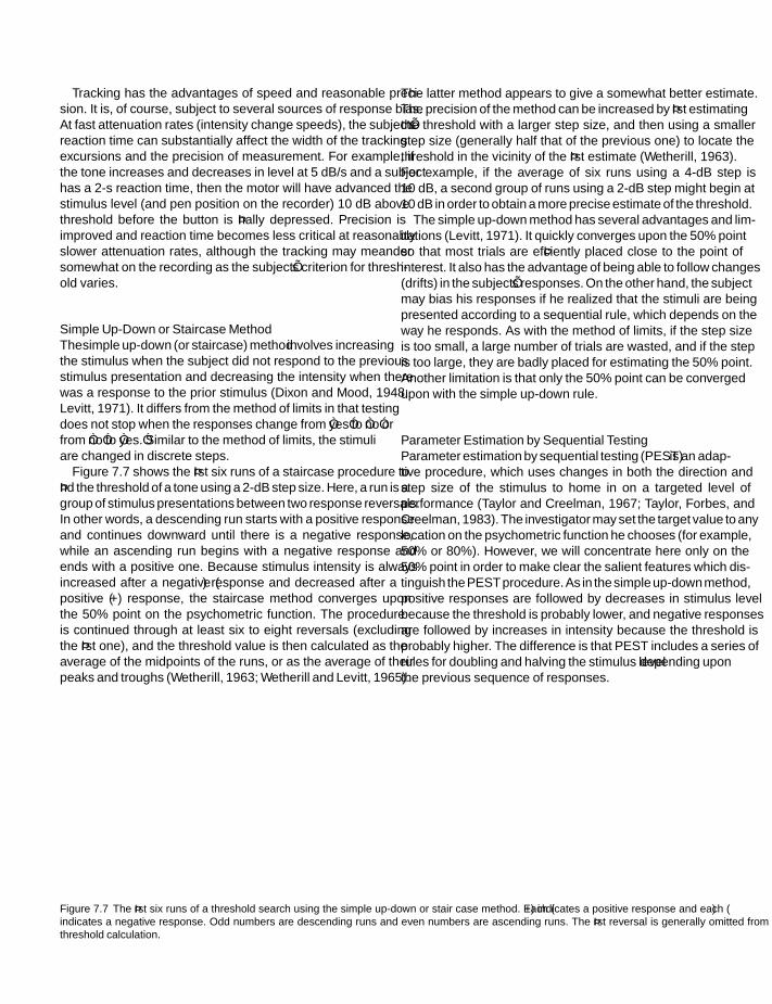
SFK SFK


chapter 7

Tracking has the advantages of speed and reasonable preci-sion. It is, of course, subject to several sources of response bias.At fast attenuation rates (intensity change speeds), the subject’sreaction time can substantially affect the width of the trackingexcursions and the precision of measurement. For example, ifthe tone increases and decreases in level at 5 dB/s and a subjecthas a 2-s reaction time, then the motor will have advanced thestimulus level (and pen position on the recorder) 10 dB abovethreshold before the button is finally depressed. Precision isimproved and reaction time becomes less critical at reasonablyslower attenuation rates, although the tracking may meandersomewhat on the recording as the subject’s criterion for thresh-old varies.

Simple Up-Down or Staircase MethodThe simple up-down (or staircase) method involves increasingthe stimulus when the subject did not respond to the previousstimulus presentation and decreasing the intensity when therewas a response to the prior stimulus (Dixon and Mood, 1948;Levitt, 1971). It differs from the method of limits in that testingdoes not stop when the responses change from “yes” to “no” orfrom “no” to “yes.” Similar to the method of limits, the stimuliare changed in discrete steps.

Figure 7.7 shows the first six runs of a staircase procedure tofind the threshold of a tone using a 2-dB step size. Here, a run is agroup of stimulus presentations between two response reversals.In other words, a descending run starts with a positive responseand continues downward until there is a negative response,while an ascending run begins with a negative response andends with a positive one. Because stimulus intensity is alwaysincreased after a negative (−) response and decreased after apositive (+) response, the staircase method converges uponthe 50% point on the psychometric function. The procedureis continued through at least six to eight reversals (excludingthe first one), and the threshold value is then calculated as theaverage of the midpoints of the runs, or as the average of theirpeaks and troughs (Wetherill, 1963; Wetherill and Levitt, 1965).

The latter method appears to give a somewhat better estimate.The precision of the method can be increased by first estimatingthe threshold with a larger step size, and then using a smallerstep size (generally half that of the previous one) to locate thethreshold in the vicinity of the first estimate (Wetherill, 1963).For example, if the average of six runs using a 4-dB step is10 dB, a second group of runs using a 2-dB step might begin at10 dB in order to obtain a more precise estimate of the threshold.

The simple up-down method has several advantages and lim-itations (Levitt, 1971). It quickly converges upon the 50% pointso that most trials are efficiently placed close to the point ofinterest. It also has the advantage of being able to follow changes(drifts) in the subject’s responses. On the other hand, the subjectmay bias his responses if he realized that the stimuli are beingpresented according to a sequential rule, which depends on theway he responds. As with the method of limits, if the step sizeis too small, a large number of trials are wasted, and if the stepis too large, they are badly placed for estimating the 50% point.Another limitation is that only the 50% point can be convergedupon with the simple up-down rule.

Parameter Estimation by Sequential TestingParameter estimation by sequential testing (PEST) is an adap-tive procedure, which uses changes in both the direction andstep size of the stimulus to home in on a targeted level ofperformance (Taylor and Creelman, 1967; Taylor, Forbes, andCreelman, 1983). The investigator may set the target value to anylocation on the psychometric function he chooses (for example,50% or 80%). However, we will concentrate here only on the50% point in order to make clear the salient features which dis-tinguish the PEST procedure. As in the simple up-down method,positive responses are followed by decreases in stimulus levelbecause the threshold is probably lower, and negative responsesare followed by increases in intensity because the threshold isprobably higher. The difference is that PEST includes a series ofrules for doubling and halving the stimulus level depending uponthe previous sequence of responses.

Figure 7.7 The first six runs of a threshold search using the simple up-down or stair case method. Each (+) indicates a positive response and each (−)indicates a negative response. Odd numbers are descending runs and even numbers are ascending runs. The first reversal is generally omitted from thethreshold calculation.

152

SFK SFK



Figure 7.8 An example of how the threshold is obtained with the PESTprocedure. Points identified by letters are discussed in the text. Point I is theestimate of threshold.

At each stimulus level, PEST in effect asks whether the thresh-old has been exceeded. The level is then changed so that themaximum amount of information is obtained from the nexttrial. To do this, the step size is varied in the manner specified inFig. 7.8. Although it is most efficient to know the approximatelocation of the threshold range in advance, it is not essential.Suppose we begin testing at some value below threshold corre-sponding to point A in Fig. 7.8. Since the subject gives a negativeresponse, the stimulus is presented at a higher level (B). Thislevel also produces no response and the stimulus is raised by thesame amount as previously and is presented again (C). Sincethere is still no response, the stimulus level is again increased.However, PEST has a rule, which states that if there is a negativeresponse on two successive presentations in the same direction,then the step size is doubled for the next presentation. Thus, thenext stimulus is presented at level D. The doubling rule ensuresthat a minimal number of trials are wasted in finding the rangeof interest.

A positive response at level D indicates that the thresholdhas been exceeded. As in the staircase method, the directionof the trials is changed after a response reversal. However,the PEST procedure also halves the step size at this point. Thehalving rule causes the stimuli to be presented closer to thethreshold value. Thus, precision is improved as the thresholdis converged upon. Since D is followed by another positive

response, the stimulus is then presented at a lower level (E). Anegative response at E causes the direction of stimulus changeto be changed again, and the step size is halved compared tothe previous one. The stimulus is heard again at the next higherlevel (F), so the direction is changed again and the step size isagain halved. Stimuli are now presented in a descending rununtil there is a negative response (G). Halving the step size andchanging direction results in a positive response at H, indicat-ing that the threshold lies somewhere between points G and H.Since this interval represents an acceptable degree of precision,the procedure is terminated. The level at which the next stim-ulus would have been presented is taken as the threshold. Thislevel is point I, which lies halfway between levels C and H. Noteon the scale for Fig. 7.8 that the step size between E and F is 2 dB,between F and G is 1 dB, and between G and H is 0.5 dB. Thisobservation highlights the rapidity with which PEST results ina precise threshold estimate.

Block Up-Down MethodsSuppose we are interested in the 75% point on the psychometricfunction. One way to converge upon the point is to modify thesimple up-down procedure by replacing the single trial perstimulus level with a block of several trials per level. Then,by adopting three out of four positive responses (75%) as thecriterion per level, the strategy will home in on the 75% point.If blocks of five were used with a four out of five criterion,then the 80% point would be converged upon. The proceduremay be further modified by changing the response from yes-noto a two-alternative (interval) forced choice. In other words, thesubject is presented with two stimulus intervals during each trialand must indicate which of the intervals contains the stimulus.This is the block up-down temporal interval forced-choice(BUDTIF) procedure (Campbell 1963). Using the two-intervalforced choice method allows the investigator to determine theproportion of responses to the no-stimulus interval—the “falsealarm” rate. We shall see when the theory of signal detection isdiscussed in the next chapter that this distinction is importantin separating sensitivity from bias effects.

The BUDTIF procedure is illustrated in Fig. 7.9. Note thateach block is treated as though it were one trial in a staircaseprocedure. Since the target point has been preselected as 75%,

Figure 7.9 An example of convergence upon the 75% point of the psychometric function using BUDTIF.

153

SFK SFK


chapter 7

stimulus intensity is raised whenever there are less than threeout of four correct responses in a block and is decreased whenall four are correct. Testing is terminated when three out of fourcorrect responses are obtained. The last level is the target level(75% in this case). Notice that since blocks of trials are presentedat each level, poor placement of the initial test level will causemany wasted trials in converging upon the target range.

A modification of BUDTIF replaces the two-alternativeforced-choice paradigm with the familiar yes-no response. Thisadaptation is called the block up-down yes-no (BUDYEN)method (Campbell and Counter, 1969). However, the BUDYENparadigm is less advantageous than its forced-choice prede-cessor because an estimate of false alarms is not obtained(Creelman and Taylor, 1969).

Transformed Up-Down or Staircase ProceduresThe simple up-down method converges on the 50% point of thepsychometric function because each positive response leads to adecrease in stimulus level and each negative response leads to anintensity increase. If the up-down rule is modified so that stim-ulus level is changed only after certain sequences have occurred,then the procedure will home in on other points on the psycho-metric function (Wetherill and Levitt, 1965; Levitt and Rabiner,1967; Levitt, 1971, 1978). These other target points dependupon the particular set of sequences chosen by the investigator.

We will go over the fundamental principles of transformedup-down methods because they are ubiquitous in hearing sci-ence research. When the target is 50% on the psychometricfunction, as in the simple up-down method, the chances of apositive response to stimuli well below the 50% point are verysmall. Similarly, it is likely that stimuli presented at levels wellabove the 50% point will frequently be heard. However, as theintensity corresponding to 50% is approached, the chances ofpositive and negative responses become closer and closer. At the50% point, the probability of a positive response is the same as ofa negative one. This is, of course, exactly what we mean by 50%.Now, suppose that the total probability of all responses is 1.00. Ifwe call the probability of a positive response (p), then the proba-bility of a negative response would be (1 − p). At the 50% point

p = (1 − p) = 0.5 (7.1)

In other words, the probability of a positive response at the50% point is 0.5, which is also the probability of a negativeresponse. In effect, the simple up-down rule forces the intensityto the point on the psychometric function where the probabil-ities of positive and negative responses are equal (0.5 each).

Other target levels can be converged upon by changing the up-down rule so that the probabilities of increasing and decreasingstimulus intensity are unequal. This is done by setting the cri-teria for increasing stimulus level (the “up rule”) to be a certainresponse sequence, and those for decreasing stimulus level (the“down rule”) to be other response sequences. An example willdemonstrate how the transformed up-down method works.

Suppose we are interested in estimating a point above 50%on the psychometric function, say 70%. To accomplish this,we would increase the stimulus level after a negative response(−) or a positive response followed by a negative one (+, −),and lower the stimulus level after two successive positives(+, +). In other words, we have established the following rulesfor changing stimulus level:

Up rule : (−) or (+, −)Down rule : (+, +)

(7.2)

As with the simple staircase rule, levels well above the targetwill often yield (+, +) responses, and those well below will tendto have (−) or (+, −) responses. However, at the target level,the probability of increasing the stimulus level will be

(1 − p) + p(1 − p) (7.3)

and the probability of two successive positive responses (+, +)will be

p × p or p2 (7.4)

The up-down strategy will converge on the point where theup and down rules have the same probabilities (0.5). In otherwords, the probability of the transformed positive response(+, +) at the target is

p2 = 0.5 (7.5)

Since we are interested in the probability (p) of a singlepositive response, which is the square root of p2, we simply findthe square root of p2 = 0.5, and we obtain

p = 0.707 (7.6)

Converting to percent, the transformed procedure just out-lined homes in on the 70.7% point of the psychometric function,which is a quite acceptable estimate of the 70% point.

To converge on the 29.3% of the psychometric function(which is a reasonable estimate of the 30% point), we mightchoose to increase the stimulus after a sequence of two succes-sive negative responses (−, −), and to decrease stimulus levelafter a positive response (+) or a negative response followed bya positive one (−, +).

The 70.7% and 29.3% transformed up-down strategies areillustrated in Fig. 7.10. As with the simple up-down method,each transformed strategy would be continued through six toeight reversals, and the average of the peaks and valleys wouldbe taken as the target level. Because these two points are on therising portion of the psychometric function and are equidistantfrom 50%, a reasonably good estimate of the 50% point canbe obtained by averaging the levels from 70.7% to 29.3%. Toincrease efficiency, one might start with a large step size, andthen halve it in the target range for increased precision.

Other target points can be converged upon by varioussequences of positive and negative responses, and differentsequences may be used to converge upon the same target points

154

SFK SFK



Figure 7.10 Examples of how the transformed up-down procedure converges upon the 70.7% point (upper frame) and the 29.3% point (lower frame) ofthe psychometric function.

(Levitt and Rabiner, 1967; Levitt, 1971, 1973). Transformed up-down procedures can also be used in the measurement of subjec-tive judgments, such as for loudness balances (Jesteadt, 1980).In addition, both simple and transformed up-down proceduresare particularly adaptable to testing various aspects of speechrecognition functions under a variety of conditions (e.g., Levitt,1971; Bode and Carhart, 1974; Plomp and Mimpen, 1979;Duquesnoy, 1983; Dubno, Morgan, and Dirks, 1984; Gelfand,Ross, and Miller, 1988).

A useful approach to minimizing biases is to interleave differ-ent testing strategies (Levitt, 1968). In other words, two pointson the psychometric function are converged upon during thesame test session. This is done by switching in an approximatelyrandom manner between the two test strategies. For example,two reversals on the 29.3% strategy might be followed by afew reversals on the 70.7% strategy, then the investigator wouldreturn to where he left off on the 29.3% sequence, and so forth.Such interleaving can also be applied to other psychoacousticmethods. Of course, greater flexibility and ease of measure-ment is made possible when the procedure is automated, and,almost needless to say, computerized administrations of theseprocedures are the norm.

Modifications, Other Procedures, and ComparisonsNumerous approaches have been introduced that modify themethods already discussed and/or combine adaptive proce-dures with maximum likelihood, Bayesian, or other techniques(Hall, 1968, 1981, 1983; Pentland, 1980; Watson and Pelli, 1983;Emmerson, 1984; Findlay, 1978; Simpson, 1989; Kaernbach,1991; King-Smith, Grigsby, Vingrys, et al., 1994; Kontsevich andTyler, 1999; Remus and Collins, 2008). The maximum likelihoodmethods use the history of the subject’s responses combinedwith certain assumptions about the nature of the psychometricfunction to estimate where the threshold (actually the mid-point of the function) lies after each response. This estimatedvalue then becomes the level of the next stimulus presentation.

For example, Hall’s (1981, 1983) hybrid procedure combinesaspects of maximum likelihood methods with features of PEST.In the Bayesian adaptive procedures, the step size is adaptiverather than fixed and each stimulus value is calculated based ona running update of the probability distribution.1

Many studies have compared the various adaptive meth-ods and between adaptive and more traditional approaches(Pentland, 1980; Shelton et al., 1983; Shelton and Scarrow(1984); Taylor et al., 1983; Hesse, 1986; Marshall and Jesteadt,1986; Madigan and Williams, 1987; Kollmeier, Gilkey andSieben, 1988; Simpson, 1988, 1989; Leek, 2001; Marvit, Floren-tine, and Buus, 2003; Amitay, Irwin, Hawkey, et al., 2006; Rowan,Hinton, and Mackenzie, 2006; Remus and Collins, 2008). Gen-erally speaking, thresholds obtained with the various adaptiveapproaches tend to be relatively close to each other. For exam-ple, Shelton et al. (1983) found that thresholds were nearly thesame when obtained using the transformed up-down, PEST, andmaximum likelihood procedures. However, it does appear thatsomewhat better performance is obtained with forced choicecompared to nonforced choice paradigms (Taylor et al., 1983;Hesse, 1986; Marshall and Jesteadt, 1986; Kollmeier et al., 1988),and with adaptive step sizes and Bayesian approaches than withfixed step size methods (Pentland, 1980; Leek, 2001; Marvitet al., 2003; Remus and Collins, 2008). One should consult thesepapers when deciding upon the most appropriate approach fora given experiment.

direct scaling

The methods discussed so far in this chapter, in which the sub-ject’s task is to detect the presence of or small differences between

1 For readily available explanations of Bayesian probabilities andmethods see, e.g., http://www.bayesian.org/bayesexp/bayesexp.html, orhttp://drambuie.lanl.gov/∼bayes/tutorial.htm.

155

SFK SFK


chapter 7

stimuli, are often referred to as discriminability or confusionscales. In contrast, direct scaling involves having the subjectestablish perceptual relationships among stimuli (magnitudeand ratio scales) or to divide a range of stimuli into equallyspaced or sized perceptual categories (category or partitionscales). In other words, the subject must specify a perceptualcontinuum that corresponds to a physical continuum. Two typesof continua may be defined (Stevens, 1961). Prothetic continua,such as loudness, have the characteristic of amount . They areadditive in that the excitation due to an increase in stimuluslevel is added to the excitation caused by the intensity whichwas already present. On the other hand, pitch has the charac-teristic of kind and azimuth has the characteristic of location.These are metathetic continua and are substantive rather thanadditive. In other words, a change in the pitch corresponds to asubstitution of one excitation pattern, as it were, for another.

Ratio Estimation and ProductionIn ratio estimation, the subject is presented with two stimulidiffering in terms of some parameter and is asked to expressthe subjective magnitude of one stimulus as a ratio of the other.Subjective values are thus scaled as a function of the physicalmagnitudes. Suppose two 1000-Hz tones with different inten-sities are presented to a subject, who must judge the loudnessof the second tone as a ratio of the first. He might report thatthe intensity of the second tone sounds one-half, one-quarter,twice, or five times as loud as the first tone.

Ratio production, or fractionalization, is the opposite ofratio estimation in that the subject’s task is to adjust the mag-nitude of a variable stimulus so that it sounds like a particularratio (or fraction) of the magnitude of a standard stimulus. Forexample, the subject might adjust the intensity of a comparisontone so that it sounds half as loud as the standard, twice asloud, etc. Fractionalization has been used in the developmentof scales relating loudness to intensity (Stevens, 1936) and pitchto frequency (Stevens, Volkmann, and Newman, 1937; Stevensand Volkmann, 1940).

Magnitude Estimation and ProductionIn magnitude estimation, the subject assigns to physical inten-sities numbers that correspond to their subjective magnitudes.This may be done in two general ways (Stevens, 1956, 1975).In the first method, the subject is given a standard or referencestimulus and is told that its intensity has a particular value. Thisreference point is called a modulus. He is then presented withother intensities and must assign numbers to these, which areratios of the modulus. Consider a loudness scaling experimentin which the subject compares the loudness of variable tonesto a standard tone of 80 dB. If the 80-dB standard is called 10(modulus), then a magnitude estimate of 1 would be assignedto the intensity 1/10 as loud, 60 would be assigned to the onethat is 6 times as loud, etc. The relationship between these mag-nitude estimates and intensity is shown by the closed circles inFig. 7.11.

Figure 7.11 Magnitude estimations of loudness obtained with a modulus(closed circles) and without a modulus (open squares) as a function of stimulusintensity based on data from Stevens (1956).

An alternative approach is to omit the modulus. Here, thesubject is presented with a series of stimuli and is asked toassign numbers to them reflecting their subjective levels. Theresults of such an experiment are shown by the open squaresin Fig. 7.11. As the figure shows, magnitude estimates obtainedwith and without a modulus result in similar findings.

The reverse of magnitude estimation is magnitude produc-tion. In this approach, the subject is presented with numbersrepresenting the perceptual values and must adjust the physicalmagnitude of the stimulus to correspond to the numbers.

Absolute magnitude estimation (AME) and absolute magni-tude production (AMP) involve the performance of magnitudeestimates (or productions) without any specified or impliedreference value, and with each estimate (or production) madewithout regard to the judgments made for previous stimuli(Hellman and Zwislocki, 1961, 1963, 1968; Hellman, 1976, 1981;Zwislocki and Goodman, 1980; Zwislocki, 1983a; Hellman andMeiselman, 1988). There has been some discussion regardingthis approach (e.g., Mellers, 1983a, 1983b; Zwislocki, 1983b).However, the convincing preponderance of evidence reveals thatit is valid, reliable, and efficient, and that AMEs and AMPs arereadily performed by naive clinical patients as well as laboratorysubjects (Hellman and Zwislocki, 1961, 1963, 1968; Hellman,1976, 1981; Zwislocki and Goodman, 1980; Zwislocki, 1983a;Hellman and Meiselman, 1988).

Subject bias causes magnitude estimation and productionto yield somewhat different results, especially at high and lowstimulus levels. Specifically, subjects tend not to assign extremevalues in magnitude estimation, or to make extreme leveladjustments in magnitude production. These bias effects arein opposite directions so that the “real” function lies some-where between the ones obtained from magnitude estima-tions and productions. This is illustrated in Fig. 7.12 by the

156

SFK SFK



Figure 7.12 Bias effects in magnitude estimation (ME) and magnitudeproduction (MP) are minimized by geometric averaging in the method ofpsychological magnitude balance (PMB). Source: Adapted from Hellmanand Zwislocki (1968) with permission of J. Acoust. Soc. Am.

divergence of the magnitude estimation and magnitude pro-duction functions. An unbiased function may be obtained byusing the method of psychological magnitude balance (Hell-man and Zwislocki, 1963, 1968). This is done by calculating thegeometric mean of the corresponding magnitude estimationsand magnitude productions along the intensity axis or the loud-ness axis. An example is illustrated by the curve labeled PMB inFig. 7.12.

Cross-Modality MatchesA scaling approach related to magnitude estimation and pro-duction is called cross-modality matching (Stevens and Guirao,1963; Stevens and Marks, 1965, 1980; Stevens, 1975; Hellmanand Meiselman, 1988, 1993). In this technique, the subject isasked to express the perceived magnitude for one sense in termsof another sensory modality. For example, loudness (an auditoryperception) might be expressed in terms of apparent line length(a visual perception). A very useful variation of this approachhas been developed and applied by Hellman and Meiselman(1988, 1993). In this method, the slope of the power functionfor loudness is derived from that for line length combined withthe cross-modality match between loudness and line length.

Category Rating of LoudnessCategory rating methods are often used in loudness measure-ments, particularly in clinical assessments related to hearingaids. These methods involve presenting sounds to the listenerat various levels, who gives a loudness rating to each of thembased on a list of descriptive loudness categories (e.g., Allen,Hall, Jeng, 1990; Hawkins, Walden, Montgomery, and Prosek,1987; Cox, Alexander, Taylor, and Gray, 1997). For example, inthe Contour Test developed by Cox et al. (1997), the listener

assigns numerical loudness ratings to pulsed warble tone stim-uli using a seven-point scale from 1 for “very soft,” to 7 for“uncomfortably loud.” Sherlock and Formby (2005) found nosignificant differences between sound levels rated “uncomfort-ably loud” using this approach and directly measured loudnessdiscomfort levels (Sherlock and Formby, 2005).

referencesAbelson, RP, Tukey, JW. 1959. Efficient conversion of non-

metric information into metric information. In: ER Tufte(ed.), The Quantitative Analysis of Social Problems. Reading,MA: Addison Wesley, 407–417.

Allen, JB, Hall, JL, Jeng, PS. 1990. Loudness growth in 1/2-octavebands (LGOB)—A procedure for the assessment of loudness.J Acoust Soc Am 88, 745–753.

American Speech-Language-Hearing Association (ASHA).2005. Guidelines for manual pure-tone threshold audiometry.Rockville, MD: ASHA.

Amitay, S, Irwin, A, Hawkey, DJC, Cowan, JA, Moore, DR. 2006.A comparison of adaptive procedures for rapid and reliablethreshold assessment and training in naive listeners. J AcoustSoc Am 119, 1616–1625.


Bode, DL, Carhart, R. 1973. Measurements of articulation func-tions using adaptive test procedures. IEEE Trans Audiol Elec-troacoust AU-21, 196–201.

Bode, DL, Carhart, R. 1974. Stability and accuracy of adaptivetests of speech discrimination. J Acoust Soc Am 56, 963–970.

Campbell, RA. 1963. Detection of a noise signal of varyingduration. J Acoust Soc Am 35, 1732–1737.

Campbell, R.A, Counter, SA. 1969. Temporal energy integrationand periodicity pitch. J Acoust Soc Am 45, 691–693.

Coomb, CH. 1953. Theory and methods of measurement. In: LFestinger, D Katz (eds.), Research Methods in the BehavioralSciences. New York, NY: Holt, Rinehart, and Winston, 471–535.

Cox, RM, Alexander, GC, Taylor, IM, Gray, GA. 1997. The Con-tour Test of loudness perception. Ear Hear 18, 388–400.

Creelman, CD, Taylor, MM. 1969. Some pitfalls in adaptivetesting: Comments on “Temporal integration and periodicitypitch”. J Acoust Soc Am 46, 1581–1582.

Dixon, WJ, Mood, AM. 1948. A method for obtaining andanalyzing sensitivity data. J Am Stat Assn 43, 109–126.

Dubno, JR, Dirks, DD, Morgan, DE. 1984. Effects of age andmild hearing loss on speech recognition in noise. J Acoust SocAm 76, 87–96.

Duquesnoy, AJ. 1983. Effect of a single interfering noise orspeech sound upon the binaural sentence intelligibility ofaged persons, J Acoust Soc Am 74, 739–743.

Emmerson, PL. 1984. Observations on a maximum likelihoodmethod of sequential threshold estimation and a simplifiedapproximation. Percept Psychophys 36, 199–203.

157

SFK SFK


chapter 7

Findlay, JM. 1978. Estimates on probability functions: A morevirulent PEST. Percept Psychophys 23, 181–185.

Gelfand, SA, Ross, L, Miller, S. 1988. Sentence reception in noisefrom one versus two sources: Effects of aging and hearing loss.J Acoust Soc Am 83, 248–256.

Hall, JL. 1968. Maximum-likelihood sequential procedure forestimation of psychometric functions. J Acoust Soc Am 44,370.

Hall, JL. 1981. Hybrid adaptive procedure for estimation ofpsychometric functions. J Acoust Soc Am 69, 1763–1769.

Hall, JL. 1983. A procedure for detecting variability of psy-chophysical thresholds. J Acoust Soc Am 73, 663–669.

Hawkins, DB, Walden, BE, Montgomery, A, Prosek, RA. 1987.Description and validation of an LDL procedure designed toselect SSPL-90. Ear Hear 8, 162–169.

Hellman, RP. 1976. Growth of loudness at 1000 and 3000 Hz. JAcoust Soc Am 60, 672–679.

Hellman, RP. 1981. Stability of individual loudness functionsobtained by magnitude estimation and production. PerceptPsychophys 29, 63–78.

Hellman, RP, Meiselman, CH. 1988. Prediction of individualloudness exponents from cross-modality matching. J SpeechHear Res 31, 605–615.

Hellman, RP, Meiselman, CH. 1993. Rate of loudness growthfor pure tones in normal and impaired hearing. J Acoust SocAm 93, 966–975.

Hellman, RP, Zwislocki, JJ. 1961. Some factors affecting theestimation of loudness. J Acoust Soc Am 33, 687–694.

Hellman, RP, Zwislocki, J. 1963. Monaural loudness function ofa 1000-cps tone and interaural summation. J Acoust Soc Am35, 856–865.

Hellman, R.P, Zwislocki, J. 1968. Loudness summation at lowsound frequencies. J Acoust Soc Am 43, 60–63.

Hesse, A. 1986. Comparison of several psychophysical proce-dures with respect to threshold estimates, reproducibility,and efficiency. Acustica 59, 263–266.

Jesteadt, W. 1980. An adaptive procedure for subjective judg-ments. Percept Psychophys 2S, 85–88.

Kaernbach, C. 1991. Simple adaptive testing with the weightedup-down method. Percept Psychophys 49, 227–229.

King-Smith, PE, Grigsby, SS, Vingrys, AJ, Benes, SC, Supowit,A. 1994. Efficient and unbiased modifications of theQUEST threshold method: Theory, simulations, experimen-tal evaluation and practical implementation. Vision Res 34,885–912.

Kollmeier, B, Gilkey, RH, Sieben, UK. 1988. Adaptive stair-case techniques in psychoacoustics: A comparison of humandata and a mathematical model. J Acoust Soc Am 83,1852–1862.

Kontsevich, LL, Tyler, CW. 1999. Bayesian adaptive estimationof psychometric slope and threshold. Vision Res 39, 2729–2737.

Leek, MR. 2001. Adaptive procedures in psychophysicalresearch. Percept Psychophys 63, 1279–1292.

Levitt, H. 1968. Testing for sequential dependencies. J AcoustSoc Am 43, 65–69.

Levitt, H. 1971. Transformed up-down methods in psychoa-coustics. J Acoust Soc Am 49, 467–477.

Levitt, H. 1978. Adaptive testing in audiology. Scand AudiolSuppl 6, 241–291.

Levitt, H, Rabiner, LR. 1967. Use of a sequential strategy inintelligibility testing. J Acoust Soc Am 42, 609–612.

Madigan, R, Williams, D. 1987. Maximum-likelihood proce-dures in two alternative forced-choice: evaluation and rec-ommendations. Percept Psychophys 42, 240–249.

Marshall, L, Jesteadt, W. 1986. Comparison of pure-tone audi-bility thresholds obtained with audiological and two-intervalforced-choice procedures. J Speech Hear Res 29, 82–91.

Marvit, P, Florentine, M, Buus, S. 2003. A comparison of psy-chophysical procedures for level-discrimination thresholds.J Acoust Soc Am 113, 3348–3361.

Mellers, BA. 1983a. Evidence against "absolute" scaling. PerceptPsychophys 33, 523–526.

Mellers, BA. 1983b. Reply to Zwislocki’s views on "absolute"scaling. Percept Psychophys 34, 405–408.

Pentland, A. 1980. Maximum likelihood estimation: The bestPEST. Percept Psychophys 28, 377–379.

Plomp, R, Mimpen, AM. 1979. Speech-reception threshold forsentences as a function of age and noise. J Acoust Soc Am 66,1333–1342.

Remus, JJ, Collins, LM. 2008. Comparison of adaptive psy-chometric procedures motivated by the Theory of OptimalExperiments: Simulated and experimental results. J AcoustSoc Am 123, 315–326.

Robinson, DE, Watson, CS. 1973. Psychophysical methods inmodern psychoacoustics. In: JV Tobias (ed.), Foundations ofModern Auditory Theory, Vol. 2. New York, NY: AcademicPress, 99–131.

Rowan, D, Hinton, K, Mackenzie, E. 2006. Comparison ofLevitt- and Zwislocki-type adaptive procedures for stimulusplacement in human listeners. J Acoust Soc Am 119, 3538–3541.

Shelton, BR, Scarrow, I. 1984. Two-alternative versus three-alternative procedures for threshold estimation. Percept Psy-chophys 35, 385–392.

Shelton, BR, Picardi, MC, Green, DM. 1983. Comparison ofthree adaptive psychophysical procedures. J Acoust Soc Am71, 1527–1532.

Sherlock, P, Formby, C. 2005. Estimates of loudness, Loudnessdiscomfort, and the auditory dynamic range: Normative esti-mates, comparison of procedures, and test-retest reliability. JAm Acad Audiol 16, 85–100.

Simpson, WA. 1988. The method of constant stimuli is efficient.Percept Psychophys 44, 433–436.

Simpson, WA. 1989. The step method: A new adaptive psy-chophysical procedure. Percept Psychophys 45, 572–576.

Stevens, SS. 1936. A scale for the measurement of a psychologicalmagnitude: Loudness. Psychol Rev 43, 405–416.

158

SFK SFK



Stevens, SS. 1951. Mathematics, measurement, and psy-chophysics. In: SS Stevens (ed.), Handbook of ExperimentalPsychology. New York, NY: Wiley.

Stevens, SS. 1958. Problems and methods in psychophysics.Psychol Bull 55, 177–196.

Stevens, SS. 1956. The direct estimation of sensorymagnitudes—loudness. Am J Psychol 69, 1–25.

Stevens, SS. 1961. The psychophysics of sensory function. In:WA Rosenblith (ed.), Sensory Communication. Cambridge,MA: MIT Press.

Stevens, SS. 1975. Psychophysics. New York, NY: Wiley.Stevens, SS, Guirao, M. 1963. Subjective scaling of length and

area and the matching of length to loudness and brightness.J Exp Psychol 66, 177–186.

Stevens, JC, Marks, LM. 1965. Cross-modality matching ofbrightness and loudness. Proc Natl Acad Sci U S A 54, 407–411.

Stevens, JC, Marks, LM. 1980. Cross-modality matching func-tions generated by magnitude estimation. Precept Psychophys27, 379–389.

Stevens, SS, Volkmann, J. 1940. The relation of pitch to fre-quency: A revised scale. Am J Psychol 53, 329–353.

Stevens, SS, Volkmann, J, Newman, EB. 1937. A scale for themeasurement of the psychological magnitude pitch. J AcoustSoc Am 8, 185–190.

Taylor, MM, Creelman, CD. 1967. PEST: Efficient estimates onprobability functions. J Acoust Soc Am 41, 782–787.

Taylor, MM, Forbes, SM, Creelman, CD. 1983. PEST reducesbias in forced choice psychophysics. J Acoust Soc Am 74, 1367–1374.

Watson, AB, Pelli, DG. 1983. QUEST: A Bayesian adaptive psy-chometric method. Percept Psychophys 33, 113–120.

Wetherill, GB. 1963. Sequential estimation of quantal responses.J R Stat Soc 25, 1–48.

Wetherill, GB, Levitt, H. 1965. Sequential estimation of pointson a psychometric function. Br J Math Stat Psychol 18, 1–10.

Zwislocki, JJ. 1983a. Group and individual relations betweensensation magnitudes and their numerical estimates. PerceptPsychophys 33, 460–468.

Zwislocki, JJ. 1983b. Absolute and other scales: The question ofvalidity views on "absolute" scaling. Percept Psychophys 33,593–594.

Zwislocki, JJ, Goodman, DA. 1980. Absolute scaling of sensorymagnitudes: A validation. Percept Psychophys 28, 28–38.

159

SFK SFK


8 Theory of Signal Detection

The previous chapter addressed itself to the classical and mod-ern psychoacoustical methods and the direct scaling of sensorymagnitudes with respect to hearing. It left essentially unre-solved, however, the problem of how to effectively separatesensitivity from response proclivity. In this chapter, we shallapproach this problem from the standpoint of the theory ofsignal detection.

factors affecting responses

The theory of signal detection (Swets, 1965; Greene and Swets,1974; Egan, 1975) provides the best approach to separate theeffects of sensitivity from those of response bias. We might thinkof the theory of signal detection (TSD) as asking the question,“what led to a “yes” (or “no”) decision?” as opposed to “whatdid the subject hear (or not hear)?”

Suppose a subject were asked to say “yes” when he hears atone during a test trial and “no” when a tone is not heard. Alarge number of trials are used for each of several stimulus levels,and half of those at each level are “catch trials” during whichsignals are not actually presented. There are thus four possibleoutcomes for each test trial. Two of them are correct:

1. A hit occurs when the signal is present and the subject says“yes.”

2. A correct rejection occurs when the signal is absent and thesubject says “no.” The other two alternatives are wrong:

3. The signal is present but the subject says “no.” This is calleda miss.

4. The signal is absent but the subject says “yes”. Here a falsealarm has occurred.

A convenient way to show these possible stimulus andresponse combinations is to tabulate them in a stimulus–response matrix, which is illustrated in Fig. 8.1.

The stimulus–response table is generally used to summarizethe results of all trials at a particular test level; there would thusbe such a table for each stimulus level used in an experiment.For example, Fig. 8.2 shows the results of 100 trials containinga signal and 100 catch trials. The subject responded to 78 of thesignal trials (so that the probability of a hit was 0.78), did notrespond to 22 signals (the probability of a miss is 0.22), said “yes”for 17 out of 100 catch trials (the probability of a false alarmis 0.17), and said “no” for the remaining absent-stimulus trials(the probability of a correct rejection is 0.83). One is tempted tosay that the percent correct at this stimulus level is 78% (the hitrate), but the fact that the subject also responded 17 times whenthere was no stimulus present tells us that even the 78% correctincludes some degree of chance success or guessing. One wayto account for this error is to use the proportion of false alarmsas an estimate of the overall guessing rate and to correct the hit

rate accordingly. The traditional formula to correct the hit ratefor chance success is

p(hit)corrected = p(hit) − p(false alarm)

1 − p(false alarm)

In other words, the probability p of a hit corrected for chancesuccess is obtained by dividing the difference between the hitrate and the false alarm rate by 1 minus the false alarm rate. [Ifthis seems odd, recall that the total probability of all catch trialsis 1.0, so that 1 − p(false alarm) is the same as the probabilityof a correct rejection.] Thus, for this example:

p(hit)corrected = 0.78 − 0.17

1.0 − 0.17= 0.61

0.83= 0.735

The original 78% correct thus falls to 73.5% when we accountfor the proportion of the “yes” responses due to chance.

Correcting for chance success is surely an improvement overapproaches that do not account for guessing, but it still doesnot really separate the effects of auditory factors (sensitivity)and nonauditory factors. In essence, this process highlights theimportance of nonauditory factors in determining the response,because the very fact that the subject said “yes” to catch trialsand “no” to stimulus trials indicates that his decision to respondwas affected by more than just sensitivity to the stimulus. Thetheory of signal detection is concerned with the factors thatenter into this decision.

Let us, at least for the moment, drop the assumption thatthere is some clear-cut threshold that separates audibility frominaudibility and replace it with the following assumptions ofTSD. First, we assume that there is always some degree of noisepresent. This may be noise in the environment, instrumenta-tion noise, or noise due to the subject’s moving around andfidgeting. Even if all of these noises were miraculously removed,there would still remain the subject’s unavoidable physiologi-cal noises (heartbeat, pulse, breathing, blood rushing throughvessels, stomach gurgles, etc.). Indeed, the noise is itself oftenpresented as part of the experiments. For example, the task maybe to detect a tone in the presence of a noise. Since there is alwaysnoise, which is by nature random, we also assume that the stim-ulation of the auditory system varies continuously. Finally, weshall assume that all of the stimulation occurs (or is at leastmeasurable) along a single continuum. In other words, the sub-ject must decide whether the stimulation in the auditory system(e.g., energy) is due to noise alone (N) or to signal-plus-noise(SN). This process may be represented by distributions along adecision axis like the one in Fig. 8.3. Here, the abscissa may beconceived of as representing the energy contained in the noiseand in the noise plus signal. The x-axis may also be conceivedof as representing the magnitude of sensory activation resultingfrom such stimulation. The ordinate denotes the probabilityof an event occurring. Hence, the N distribution shows the

160

SFK SFK


theory of signal detection

Figure 8.1 Stimulus–response matrix or table showing the four possibleoutcomes for any given test trial. Correct responses may be “hits” or “correctrejections,” whereas errors may also be of two possible types, “misses” or“false alarms.”

probability of occurrence of a noise alone as a function of x,and the SN curve shows the chances of a signal-plus-noise asa function of x. The convention is to use the term “probabilitydensity” (as opposed to “probability”) for the y-axis in order toreflect the fact that values of x change continuously rather thanin discrete steps. The subject’s response is a decision between“yes” (“I hear the signal as well as the noise”) and “no” (“I hearthe noise alone”).

The N and SN distributions in Fig. 8.3 show the probabilityfunctions of noise alone (N) and signal-plus-noise (SN). Wemight think of these curves as showing the chances (or like-lihood) of there being, respectively, a noise alone or a signal-plus-noise during a particular test trial. Obviously, there mustalways be more energy in SN than in N, due to the presence ofthe signal. The separation between the N and SN curves thusbecomes a measure of sensitivity. This is an unbiased measurebecause the separation between the two curves is not affectedby the subject’s criteria for responding (biases). The separationis determined solely by the energy in the signals and the sen-sitivity of the auditory system. This separation is measured interms of a parameter called d prime (d′). The value of d′ isequal to the difference between the means (x) and the N andSN distributions divided by their standard deviation ():

d′ = xSN − xN

Comparing Figs. 8.3 8.3a and 8.3b, we see that the greaterthe separation between N and SN distributions, the larger thevalue of d′. This value does not change even when differentexperimental methods are used (Swets, 1959).

Figure 8.2 Hypothetical results in the form of proportions for 100 testtrials actually containing stimuli and 100 test trials actually without stimuli(“catch trials”).

Figure 8.3 The separation between the distribution for the noise alone (N)and the distribution for the signal-plus-noise (SN) determines the valueof d′.

Several points will be of interest to the quantitatively orientedreader. It is assumed that SN and N are normally distributedwith equal variances. Since is the square root of the variance,and the variances of SN and N are assumed to be equal, thenonly one value of need be shown. The value of d′ is equal tothe square root of twice the energy in the signal (2E) divided bythe noise power (NO) in a band that is one cycle wide (Swets,Tanner, and Birdsall, 1961), or

d′ =√

2E

NO

Tables of d′ are available in the literature (Elliot, 1964); how-ever, a corrected value of d′ may be a more valid measure becausethe standard deviation of SN is actually larger than that of N insome cases (Theodore, 1972).

How, then, does a subject decide whether to say “yes” or“no” for a given separation between the N and SN curves?Consider the N and SN distributions in Fig. 8.4. A vertical linehas been drawn through the overlapping N and SN distributionin each frame of this figure. This line represents the subject’scriterion for responding. Whenever the energy is greater thanthat corresponding to the criterion the subject will say “yes.”This occurs to the right of the criterion along the x-axis. On theother hand, the subject will say “no” if the energy is less than(to the left of) the criterion value. The value (or placement) ofthis criterion depends on several factors, which we will examinenext.

161

SFK SFK


chapter 8

Figure 8.4 Criterion points (shown by vertical lines) for two degrees ofoverlapping of the noise alone (N) and signal-plus-noise (SN) distributions.The probabilities corresponding to the SN and N distributions at the criterionpoint are highlighted by brackets. Values of x below (to the left of) thecriterion result in “no” decisions and those greater than (to the right of) thecriterion yield “yes” decisions.

The first factor affecting the criterion may be expressed bythe question “What is the probability that there is a noise alonecompared to the probability that there is a signal-plus-noise fora given value of x?” For any point along the decision axis, thisquestion is the same as comparing the height of the N curvewith the height of the SN curve (Fig. 8.4). Otherwise stated, thisvalue is the ratio of the likelihoods that the observation is fromthe N versus SN distributions for the two overlapping curvesat any value of x. The ratio of these two probabilities is calledbeta (). The value of the criterion is affected by the amountof overlap between the N and SN distributions, and by whatthe subject knows about the relative chances of a signal actuallybeing presented.

Comparison of Figs. 8.4a and 8.4b shows how overlappingof the N and SN functions affects this ratio. At any point,the heights of the two curves becomes close as the separationbetween them decreases from that in Fig. 8.4a to that in Fig.8.4b. An ideal observer, which is actually a mathematical con-cept rather than a real individual, would place the criterion pointat the ratio which minimizes the chances of error, that is, at thepoint at which misses and false alarms are minimized. However,the placement of the criterion point will also be adjusted some-what by what the subject knows about the chances of occurrenceof a noise alone versus a signal-plus-noise. Let us now addressourselves to this factor.

Up to this point, it has been assumed that N and SN will bepresented on a fifty-fifty basis. However, if the subject knows thata signal will actually be presented one-third of the time, thenhe will of course adjust his criterion accordingly. In otherwords, he will adopt a stricter criterion. Alternatively, if thesubject knows that a signal will occur more often than the noisealone, then he will relax his criterion for responding, adjustingfor the greater chances of the signal actually being presented.The theoretical ideal observer always knows these probabilities;a real subject is often, but not always, told what they are.

The last factor that we will discuss which affects the finalvalue of the criterion has to do with how much a correctresponse is worth and how much a wrong response will cost. Weare therefore concerned with the chance of an error associatedwith a particular criterion for responding. These chances areshown in Fig. 8.5. The subject will say “no” whenever the actualpresentation falls to the left of the criterion, and will say “yes”when the presentation is to the right of the criterion. As a resultof the fact that the N and SN distributions are overlapping, itturns out that there will be both “yes” and “no” decisions for acertain proportion of both signal and no-signal presentations.With the criterion placed as shown in the figure, most of the“yes” decisions will be in response to actual SN presentations;that is, the subject will say “yes” when there actually was asignal present. Recall that such a correct identification of thepresence of the signal is called a hit . On the other hand, a certainpercentage of the N trials will fall to the right of the criterion,so the subject will say “yes” even though there was actuallyno signal presented. This incorrect decision that a signal waspresent even though it really was not there is a false alarm. Astimulus–response table similar to the one in Fig. 8.1a is shownnext to the N and SN distributions in Fig. 8.5 to illustrate how

“Yes”

“Yes!”

SN

SN

N

N

Hit

Hit

Miss

Misses(stripes)

CorrectRejection

CorrectRejection

FalseAlarm

False Alarm(solid)

“No”

“No!”

Figure 8.5 The four possible outcomes of a “yes” or “no” response basedupon a given criterion value (vertical line). The corresponding stimulus–response table is shown to the right.

162

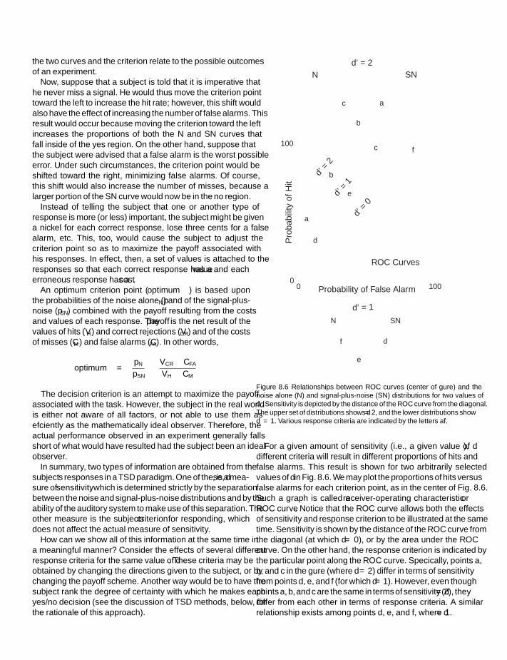
SFK SFK



the two curves and the criterion relate to the possible outcomesof an experiment.

Now, suppose that a subject is told that it is imperative thathe never miss a signal. He would thus move the criterion pointtoward the left to increase the hit rate; however, this shift wouldalso have the effect of increasing the number of false alarms. Thisresult would occur because moving the criterion toward the leftincreases the proportions of both the N and SN curves thatfall inside of the “yes” region. On the other hand, suppose thatthe subject were advised that a false alarm is the worst possibleerror. Under such circumstances, the criterion point would beshifted toward the right, minimizing false alarms. Of course,this shift would also increase the number of misses, because alarger portion of the SN curve would now be in the “no” region.

Instead of telling the subject that one or another type ofresponse is more (or less) important, the subject might be givena nickel for each correct response, lose three cents for a falsealarm, etc. This, too, would cause the subject to adjust thecriterion point so as to maximize the payoff associated withhis responses. In effect, then, a set of values is attached to theresponses so that each correct response has a value and eacherroneous response has a cost.

An optimum criterion point (optimum ) is based uponthe probabilities of the noise alone (pN) and of the signal-plus-noise (pSN) combined with the payoff resulting from the costsand values of each response. The payoff is the net result of thevalues of hits (VH) and correct rejections (VCR) and of the costsof misses (CM) and false alarms (CFA). In other words,

optimum =(

pN

pSN

) (VCR − CFA

VH − CM

)

The decision criterion is an attempt to maximize the payoffassociated with the task. However, the subject in the real worldis either not aware of all factors, or not able to use them asefficiently as the mathematically ideal observer. Therefore, theactual performance observed in an experiment generally fallsshort of what would have resulted had the subject been an idealobserver.

In summary, two types of information are obtained from thesubject’s responses in a TSD paradigm. One of these, d′, is a mea-sure of sensitivity, which is determined strictly by the separationbetween the noise and signal-plus-noise distributions and by theability of the auditory system to make use of this separation. Theother measure is the subject’s criterion for responding, whichdoes not affect the actual measure of sensitivity.

How can we show all of this information at the same time ina meaningful manner? Consider the effects of several differentresponse criteria for the same value of d′. These criteria may beobtained by changing the directions given to the subject, or bychanging the payoff scheme. Another way would be to have thesubject rank the degree of certainty with which he makes eachyes/no decision (see the discussion of TSD methods, below, forthe rationale of this approach).

N SN

c

c

b

b

e

e

d

d

f

f

100

0P

roba

bilit

y of

Hit

Probability of False Alarm

ROC Curves

0 100

N SN

a

a

d' = 2

d' =

2d'

= 1

d' = 1

d' =

0

Figure 8.6 Relationships between ROC curves (center of figure) and thenoise alone (N) and signal-plus-noise (SN) distributions for two values ofd′. Sensitivity is depicted by the distance of the ROC curve from the diagonal.The upper set of distributions shows d′ = 2, and the lower distributions showd′ = 1. Various response criteria are indicated by the letters a–f.

For a given amount of sensitivity (i.e., a given value of d′),different criteria will result in different proportions of hits andfalse alarms. This result is shown for two arbitrarily selectedvalues of d′ in Fig. 8.6. We may plot the proportions of hits versusfalse alarms for each criterion point, as in the center of Fig. 8.6.Such a graph is called a receiver-operating characteristic orROC curve. Notice that the ROC curve allows both the effectsof sensitivity and response criterion to be illustrated at the sametime. Sensitivity is shown by the distance of the ROC curve fromthe diagonal (at which d′ = 0), or by the area under the ROCcurve. On the other hand, the response criterion is indicated bythe particular point along the ROC curve. Specifically, points a,b, and c in the figure (where d′ = 2) differ in terms of sensitivityfrom points d, e, and f (for which d′ = 1). However, even thoughpoints a, b, and c are the same in terms of sensitivity (d′ =2), theydiffer from each other in terms of response criteria. A similarrelationship exists among points d, e, and f, where d′ = 1.

163

SFK SFK


chapter 8

psychophysical methods in tsd

Yes/No MethodsThis discussion of the theory of signal detection has dealt pri-marily with the yes/no method. To recapitulate: The subject ispresented with a large number of trials for each stimulus level,and a large proportion of these are actually catch trials. For eachtrial, the subject says “yes” when a signal is detected and “no”when a signal is not detected. Fundamentally, then, the yes/nomethod in TSD is somewhat akin to the classical method ofconstant stimuli, although there are obvious differences in thenumber of trials, the large proportion of catch trials, and themanner of data analysis.

As in the classical methods, the TSD experiment is easilymodified for use in a study of differential sensitivity. In thiscase, two signals are presented in a trial and the subject’s taskis to say “yes” (“they are different”) or “no” (“they are notdifferent”).

The yes/no method is actually a subcategory of a larger classof experiments in which each trial contains one or two alterna-tive signals. In this general case, the subject’s task is to indicatewhich of two possible signals was present during the trial. Forexample, in the differential sensitivity experiment mentionedin the last paragraph, the decision is “same” versus “different”,or else the subject might be asked to decide between two alter-native speech sounds (e.g., /p/ and /b/) while some parameter isvaried. In this light, the yes/no method might be thought of as asingle-interval forced-choice experiment. In other words, thesubject is presented with a stimulus interval during each trialand is required to choose between signal-plus-noise (one of thealternatives) and noise alone (the other alternative).

Two-Interval and N-Interval Forced-Choice MethodsJust as the subject may be asked to choose between two alter-natives in a single-interval trial, he might also be asked todecide which of two successive intervals contained a signal. Thisapproach is called the two-interval forced-choice (2IFC) ortwo-alternative forced-choice (2AFC) method. In this method,a test trial consists of two intervals, A and B, presented one afterthe other. One of the intervals (SN) contains the signal and theother one (N) does not. The subject must indicate whether thesignal was presented in interval A or in interval B.

Experiments involving a choice between more than twochoices are termed multiple or N-interval (or alternative)forced-choice, where N refers to the number of choices. Forexample, a 4IFC task would include four intervals (alternatives)in each test trial, among which the subject must choose the onethat contained the signal.

Confidence Rating MethodsRecall that various points along the same ROC curve representdifferent response criteria with the same sensitivity d′. We mightthink of the response criterion as a reflection of how much con-fidence a subject has in his decision. In other words, a strict

criterion means that the subject must have a great deal of confi-dence in his decision that the signal is present before he is willingto say “yes.” In this case, the criterion value 3 is pushed towardthe right along the decision axis. Alternatively, a lax criterionmeans that the subject does not require as much confidence inhis “yes” decision, which moves the criterion point toward theleft.

We might apply this relationship between the confidence inthe decision and the criterion point by asking the subject torate how much confidence he has in each of his responses.For example, the subject might be instructed to rate a “yes”response as “five” when he is absolutely positive that there wasa signal, and “four” when he thinks there was a signal. A ratingof “three” would mean “I’m not sure whether there was a signalor no signal.” “Two” would indicate that there probably wasno signal present, and a rating of “one” would suggest thatthe subject is positive that a signal was not presented. Thisprocedure is the same as adopting a series of criterion pointslocated successively from right to left along the decision axis.Thus, the use of confidence ratings enables the experimenter toobtain several points along the ROC curve simultaneously. Thisapproach results in data comparable to those obtained by thepreviously discussed methods (Egan, Schulman, and Greenberg,1959).

some implications of tsd

The theory of signal detection has importance in psychoacous-tics because its application allows the experimenter to ferretout the effects of sensitivity and response criterion. Further-more, TSD lends itself to experimental confirmation and canbe used to test theories and their underlying assumptions. Akey application of TSD has been the testing of the classical con-cept of threshold as an absolute boundary separating sensationfrom no sensation. It is implicit in this discussion that such aconcept of a clear-cut threshold is not supported by TSD. How-ever, the more general concept of threshold remains unresolved.Threshold theory is beyond the scope of this text. The interestedstudent is therefore referred to the very informative discussionsthat may be found in the papers by Swets (1961) and by Krantz(1969).

referencesEgan, JP. 1975. Signal Detection Theory and ROC Analysis. New

York, NY: Academic Press.Egan, JP, Schulman, AI, Greenberg, GZ. 1959. Operating char-

acteristics determined by binary decisions and by ratings. JAcoust Soc Am 31, 768–773.

Elliot, PB. 1964. Tables of d’. In: JA Swets (ed.), Signal Detectionand Recognition by Human Observers. New York, NY: Wiley,651—684.

Greene, DM, Swets, JA. 1974. Signal Detection Theory and Psy-chophysics. New York: Krieger.

164

SFK SFK



Krantz, DH. 1969. Threshold theories of signal detection. Psy-chol Rev 76, 308–324.

Swets, JA. 1959. Indices of signal delectability obtained withvarious psychophysical procedures. J Acoust Soc Am 31, 511–513.

Swets, JA. 1961. Is there a sensory threshold? Science 134, 168–177.

Swets, JA (ed.). 1965. Signal Detection and Recognition by HumanObservers. New York, NY: Wiley.

Swets, JA, Tanner, WP Jr, Birdsall, TG. 1961. Decision processesin perception. Psychol Rev 68, 301–340.

Theodore, LH. 1972. A neglected parameter: Some commentson “A table for calculation of d′ and ”. Psychol Bull 78 260–261.

165

SFK SFK


9 Auditory Sensitivity

The ear’s extremely wide range of sensitivity is one of the moststriking aspects of audition. The preceding chapters empha-sized that hearing measurements are affected by psychophysicalmethods and other nonauditory factors; nevertheless, a reliablepicture of auditory sensitivity has been provided by researchover the years. Briefly, the ear is sensitive to a range of inten-sities from about 0 dB SPL (which is an amplitude of vibra-tion of about the size of a hydrogen molecule) to roughly 140dB (at which pain and damage to the auditory mechanismensue). This dynamic range of the approximately 140 dB corre-sponds to a pressure ratio of 10 million to 1. In other words, themost intense sound pressure that is bearable is on the order of10 million times as great as the softest one that is perceivableunder optimum listening conditions. In terms of frequency,humans can hear tones as low as 2 Hz (although roughly20 Hz is required for a perception of “tonality”) and as highas about 20,000 Hz. Furthermore, the auditory system is capa-ble of resolving remarkably small temporal differences.

The frequency and intensity sensitivities of the ear interact,affecting each other to a greater or lesser degree. In addition,when the duration of a sound is less than about half of a sec-ond, it affects both frequency and intensity sensitivity. Longerdurations may be thought of as being infinitely long as far asauditory sensitivity is concerned.

Finally, the ear is able to discriminate small differences ina wide range of stimuli; that is, it has remarkable differentialsensitivity—the ability to detect very small differences betweensimilar sounds. This ability applies to all three parameters:intensity, frequency, and time.

So much for sweeping generalizations. Let us now look atsome of the details.

absolute sensitivity

Minimum Audible LevelsThe issue of absolute sensitivity is essentially one of describinghow much sound intensity is necessary for a typical, normallyhearing person to just detect the presence of a stimulus. Wemust realize at the outset that these values are actually mea-sures of central tendencies (means, medians, and/or modes)that describe a group of ostensibly normal subjects. In addition,it is essential to know how and where the minimum audiblesound intensity is measured.

Two fundamental methods have been used to measure theintensity of a minimum audible stimulus (Sivian and White,1933). The first involves testing a subject’s thresholds throughearphones, and then actually monitoring the sound pressuresin the ear canal (between the earphone and eardrum) that cor-respond to these thresholds. This procedure yields a measure ofminimum audible pressure (MAP). The alternative approach

is to seat the subject in a sound field and test his thresholds forsounds presented through a loudspeaker. The subject then leavesthe sound field and the threshold intensity is measured witha microphone placed where his head had been. This methodmeasures the minimum audible field (MAF). It is important todichotomize between the MAP and MAF methods because theyresult in different threshold values.

Ostensibly, MAP refers to the sound pressure at the eardrum.This quantity is monitored by placing a probe tube in the sub-ject’s ear canal. The probe tube passes through the earphoneenclosure and leads to a microphone, which measures the soundpressure at the tip of the probe tube. Because it is difficult toplace the probe right at the drum (as well as potentially painfuland dangerous), the probe is generally located somewhere inthe ear canal, as close to the drum as is practicable.

Minimum audible pressures are often stated in terms of thesound pressure generated by an earphone in a standardized 6-cc metal cavity (6-cc coupler), which approximates the volumeunder an earphone on the subject’s ear. Such coupler pressuresform the reference levels used in audiometric standards (seebelow). These coupler-referred MAP values are more appro-priately called MAPC to distinguish them from the probe-tubeMAP data obtained from actual ear canals (Killion, 1978).

Sivian and White reported the results of their classical MAPand MAF experiments in 1933. Their work was essentiallyconfirmed by Dadson and King (1952) and by Robinson andDadson (1956), whose data are shown in the lower portionof Fig. 9.1. These curves show monaural MAP and binauralMAF (from a loudspeaker located directly in front of the sub-ject, i.e., at 0 azimuth) as a function of frequency. MonauralMAP values extending to very low frequencies are also shown.The MAP values for frequencies between 10,000 and 18,000Hz are shown in the figure on an expanded frequency scale.As these MAP and MAF curves clearly show, human hearing ismost sensitive between about 2000 and 5000 Hz, and reasonablygood sensitivity is maintained in the 100 to 10,000 Hz range.Absolute sensitivity becomes poorer above and below thesefrequencies.

While the general relationship between auditory sensitivityand frequency is well established, one should be aware thatsubsequent experiments have provided detailed estimates ofabsolute sensitivity in the lower and upper frequency ranges.For example, one should refer to Berger (1981) for a detailedanalysis of hearing sensitivity in the low-frequency range (50–1000 Hz), and to Schechter et al. (1986) for a detailed analysisof thresholds for the high frequencies (8000–20,000 Hz).

Notice in Fig. 9.1 that the MAF curve falls consistently belowthe MAP curve. In other words, a lower intensity is needed toreach threshold in a sound field (MAF) than under earphones(MAP). This fact was first demonstrated by Sivian and White(1933), and the discrepancy of 6 to 10 dB is called the “missing

166

SFK SFK


auditory sensitivity

160

140

120

100

80

60

40

20

0

10

“TICKLE” (Bekesy, 1960)

“PRICKLING” (Bekesy, 1960)

MAP(Yeowart,

et al., 1967)

“FEELING” (Wegel, 1932)

Northernet al., 1972

Minimum Audible Pressure (MAP)(Dadson & King, 1952)

Minimum Audible Field (MAF)(Robinson & Dadson, 1956)

100 1000

Frequency (Hz)

Sou

nd P

ress

ure

Leve

l (dB

)

10K 10K 15K 20K

Figure 9.1 Minimal auditory field (MAF) after Robinson and Dadson (1956), and monaural minimal auditory pressure (MAP) after Dadson and King(1952) and Yeowart et al. (1967). The high-frequency MAP curve after Northern et al. (1972) is shown on the expanded scale to the right for clarity. Upperlimits of “usable” hearing after Bekesy (1960) and Wegel (1932).

6 dB” (Munson and Wiener, 1952). Sivian and White proposedthat the MAP/MAF discrepancy might be due to physiologicalnoises picked up by the ear when it is covered by an earphone.These physiological noises would partially mask (see Chap. 10)the signal presented by the earphone, so that more sound pres-sure would be needed to achieve MAP than for the unmaskedMAF. Although this explanation accounted for part of the miss-ing 6 dB problem, it fell short of accounting for the wholedifference.

Subsequent studies have formed the basis for resolving theMAP/MAF difference (Rudmose, 1963, 1982; Villchur, 1969,1970, 1972; Morgan and Dirks, 1974; Stream and Dirks, 1974;Killion, 1978). This explanation was presented in a cohesivemanner by Killion (1978). To begin with, recall from Chapter 3that diffraction and ear canal resonance enhance the pressure ofa free-field signal reaching the eardrum (Shaw, 1974). Thus, acorrected version of the international standard reference MAFcurve (ISO-1961) may be converted to eardrum pressure byapplying Shaw’s (1974) head-related transfer function data. Thecorrection accounts for an apparent error in the low-frequencyMAF levels (Killion, 1978). Since binaural thresholds are some-what better than monaural ones (see Chap. 13), a correction isalso made to account for the advantage of binaural MAF overmonaural MAP. By accounting for differences between real ear(MAP) and coupler (MAPC) values, the effects of impedancechanges and ear canal distortion due to the placement of theearphone, and the effects of physiological noises, the MAP/MAFdiscrepancy is essentially resolved.

Threshold MicrostructureThe MAP and MAF curves in Fig. 9.1 are drawn as smoothcurves. It is commonly (and generally implicitly) assumedthat an individual’s threshold curve is similarly representedby a smooth line. The ubiquitous nature of this assumptionis revealed by the fact that both clinicians and researchers makemost of their threshold measurements at frequencies that are anoctave apart, and very rarely sample at intervals that are less thana half-octave wide. However, this may not be the case (Elliot,1958; van den Brink, 1970; Cohen, 1982; Long, 1984; Long andTubis, 1988). Instead, a rippled or jagged configuration is oftenobtained when thresholds are sampled at numerous frequenciesthat are measured at very close intervals. Moreover, these pat-terns are highly repeatable. These irregularities in the thresholdmicrostructure are associated with (particularly spontaneous)otoacoustic emissions, and it is believed that they reflect activeprocesses in the cochlea (Wilson, 1980; Schloth, 1983; Zwickerand Schloth, 1983; Long, 1984; Long and Tubis, 1988; Talmadgeet al., 1998, 1999). Discussions of active cochlear processes andotoacoustic emissions may be found in Chapter 4.

Upper Limits of HearingJust as we may conceive of the minimum audibility (MAP andMAF) curves as the lower limit of hearing sensitivity, the upperlimits of hearing may be thought of as the sound pressure levels(SPLs) that are too loud or cause some kind of unpleasant sen-sation. These criteria are actually quite different. Uncomfortableloudness is usually what we mean by the upper limit of usable

167

SFK SFK


chapter 9

Table 9.1 Reference Equivalent Threshold Sound Pressure Levels (RETSPLs) for Various Earphones in Decibels of SoundPressure Level (dB SPL re: 20 Pa) in Appropriate Measurement Couplers

Supra-aural receivers in 6-cc[NBS-9A] coupler

Circumaural receiversin flat-plate coupler

Insert receivers (etymotic ER-3A& EARtone 3A) in:

Frequency(Hz)

TelephonicsTDH-49 & 50

TelephonicsTDH-39

SennheiserHDA200

KossHV/1A

HA-2coupler

HA-1coupler

Occludedear simulator

125 47.5 45.0 30.5 – 26.0 26.5 28.0250 26.5 25.5 18.0 – 14.0 14.5 17.5500 13.5 11.5 11.0 – 5.5 6.0 9.5750 8.5 8.0 6.0 – 2.0 2.0 6.01000 7.5 7.0 5.5 16.0 0.0 0.0 5.51500 7.5 6.5 5.5 – 2.0 0.0 9.52000 11.0 9.0 4.5 – 3.0 2.5 11.53000 9.5 10.0 2.5 – 3.5 2.5 13.04000 10.5 9.5 9.5 8.0 5.5 0.0 15.06000 13.5 15.5 17.0 – 2.0 −2.5 16.08000 13.0 13.0 17.5 16.5 0.0 −3.5 15.59000 – – 18.5 21.0 – – –10,000 – – 22.0 25.5 – – –11,200 – – 23.0 24.5 – – –12,500 – – 28.0 26.0 – – –14,000 – – 36.0 33.0 – – –16,000 – – 56.0 51.0 – – –

Source: Based on ANSI S3.6-2004.

hearing. It refers to the level at which a sound is too loud tolisten to for any appreciable period of time and is often referredto as the uncomfortable loudness level (UCL) or loudness dis-comfort level (LDL). The LDL is associated with sound pres-sure levels approximating 100 dB (Hood and Poole, 1966, 1970;Hood, 1968; Morgan, Wilson, and Dirks, 1974), with highermean LDLs of about 111 to 115 dB SPL reported by Sherlockand Formby (2005). On the other hand, the upper curves in Fig.9.1 show that SPLs of about 120 dB or more produce sensationsvariously described as feeling, tickle, touch, tolerance, discom-fort, or pain. Notice that these unpleasant sensations are actuallytactile rather than auditory. High levels can produce temporarychanges in hearing sensitivity and even permanent hearing lossand are discussed later in this chapter.

reference levels

One might now ask what constitutes a reasonable conception ofnormal hearing sensitivity for the population as a whole. Thatis, how much SPL does the average person who is apparentlyfree of pathology need to detect a particular sound? The answerpermits standardization of audiometric instruments so that wemay quantify hearing loss relative to “what normal people canhear.”

Prior to 1964, several countries had their own standards fornormal hearing and audiometer calibration based upon locallyobtained data. For example, the 1954 British Standard (1954)was based upon one group of studies (Wheeler and Dickson,

1952; Dadson and King, 1952, whereas the 1951 American Stan-dard (ASA-1951) reflected other findings (USPHS, 1935–1936;Steinberg et al., 1940). Unfortunately, these standards differedby about 10 dB, and the American Standard was too lax at250 and 500 Hz, and too strict at 4000 Hz (Davis and Kranz,1964). This situation was rectified in 1964 with the issuance ofRecommendation R389 by the International Organization forStandardization (ISO-1964). This standard is generally referredto as ISO-1964. It was based upon a round-robin of loudness-balance and threshold experiments involving American, British,French, Russian, and German laboratories, and as a result equiv-alent reference SPLs were obtained for the earphones used byeach country. These reference levels were subsequently incor-porated into the S3.6 standard disseminated by the AmericanNational Standards Institute (ANSI S3.6-1969; now ANSI S3.6-2004).

The reference values for pure tone signals presented fromvarious kinds of earphones are shown in Table 9.1.1 These val-ues are called reference-equivalent threshold sound pressurelevels (RETSPLs) and are based on the current versions of theAmerican National Standard Specification for Audiometers (ANSIS3.6-2004), essentially corresponding to the ISO 389 standards

1 The testing room must be very quiet in order to obtain auditorythresholds as low as those in Tables 9-1 to 9-3 (corresponding to0 dB HL in Fig. 9.2). The maximum permissible noise levels for thispurpose (ANSI S3.1−1999 [R2003]) are summarized in octave bandsin Appendix 9-1 and in third-octave bands in Appendix 9-2.

168

SFK SFK



Table 9.2 Sound Field Reference Equivalent Threshold Sound Pressure Levels (RETSPLs) inDecibels of Sound Pressure Level (dB SPL re: 20 Pa) at a Point Corresponding to the Listener’sHead When Narrow Bands of Noise or Frequency Modulated Tones are Presented fromLoudspeakers Located at Various Azimuths

Loudspeaker azimuth

0 (front) 45 (side) 90 (side)

Center frequencya (Hz) Monauralb Binauralc Monauralb Monauralb

125 24.0 22.0 23.5 23.0250 13.0 11.0 12.0 11.0500 6.0 4.0 3.0 1.5750 4.0 2.0 0.5 −1.01000 4.0 2.0 0.0 −1.51500 2.5 0.5 −1.0 −2.52000 0.5 −1.5 −2.5 −1.53000 −4.0 −6.0 −9.0 −6.54000 −4.5 −6.5 −8.5 −4.06000 4.5 2.5 −3.0 −5.08000 13.5 11.5 8.0 5.5

aCenter frequencies of the narrow bands of noise or frequency-modulated tones used as test signals.bListening with one ear.cListening with both ears.Source: Based on ANSI S3.6-2004.

(ISO-389-1-5,7, 1994a, 1994b, 1994c, 1998a, 1988b, 2005). Rep-resentative reference values for signals presented from loud-speakers are shown in Table 9.2 (ANSI S3.6-2004; ISO-389-7,2005). Notice that these signals are narrow bands of noise orfrequency modulated tones, which are employed because puretones are subject to problems due to standing waves when usedfor sound field testing. In addition, separate values are providedfor listening with one ear (monaurally) to sounds presentedfrom different loudspeaker directions, and for listening withtwo ears (binaurally) when the speaker is located in front of thelistener. Table 9.3 shows the reference values used when hearingis measured by bone conduction (ANSI S3.6-2004; ISO-389-3,1994b). These values are called reference-equivalent thresholdforce levels (RETFLs) because they express the equivalent force(in dB re: 1 N) on a measuring device known as a mechan-ical coupler or artificial mastoid, which corresponds to 0 dBHL when the bone-conduction vibrator is placed on a person’smastoid or forehead.

Hearing LevelBecause each of the SPLs in Table 9.1 corresponds to minimumaudibility, we may think of them as all representing the samehearing level. Thus, each RETSPL may also be referred to as 0dB hearing level (0 dB HL) for its respective frequency. Forexample, the reference level for a 1000-Hz tone (for TDH-49 earphones) is 7.5 dB SPL so that 0 dB HL corresponds to7.5 dB SPL at 1000 Hz. At 250 Hz, more sound pressure isrequired to reach the normal threshold so that 0 dB HL equals26.5 dB SPL at this frequency. The relationship between SPLand HL is illustrated in Fig. 9.2. Figure 9.2a shows the minimally

audible (threshold) values in dB SPL as a function of frequency.As in Fig. 9.1, intensity increases upward on the y-axis. Figure9.2b shows the same information in dB HL. Notice that theminimum audible values (0 dB HL) all lie along a straight linein terms of hearing level. In other words, the HL scale callseach zero reference SPL value “0 dB HL,” so that thresholdscan be measured in comparison to a straight line rather than acurved one.

The graph in Fig. 9.2b is the conventional audiogram used inaudiology. Actually, the term “audiogram” may legitimately beused to describe any graph of auditory sensitivity as a function offrequency. By convention, increasing intensity (which indicatesa hearing loss) is read downward on the y-axis when thresholdsare plotted in dB HL.

Table 9.3 Reference Equivalent Threshold Force Levels(RETFLs) for Bone-Conduction Vibrators, Expressed inDecibels (dB) re: 1 N Measured on a Mechanical Coupler(Artificial Mastoid)

Frequency (Hz) Vibrator at mastoid Vibrator at forehead

250 67.0 79.0500 58.0 72.0750 48.5 61.51000 42.5 51.01500 36.5 47.52000 31.0 42.53000 30.0 42.04000 35.5 43.5

Source: Based on ANSI S3.6-2004.

169

SFK SFK


chapter 9

110

100

90

80

70

60

50

40

30

20

10

0125

(a)

Sou

nd P

ress

ure

Leve

l (dB

SP

L)

250 500Frequency (Hz)

1000 2000 4000 8000

–100

102030405060708090

100110120

125

(b)

Hea

ring

Leve

l (dB

HL)

250 500Frequency (Hz)

1000 2000 4000 8000

Figure 9.2 Audiograms showing normal hearing (circles) and a hearing loss in the high frequencies (triangles), expressed in (a) dB SPL and (b) dB HL.Note that intensity is shown downward on the clinical audiogram in dB HL.

Now, suppose that we measure the thresholds of a personwhose cochlea has been partially damaged by excessive noiseexposure. This kind of trauma often appears as a hearing lossin the higher frequencies. The triangles in Fig. 9.2 show theimpaired thresholds in terms of both SPL and HL. The differencein dB between the impaired thresholds and the reference values(circles) is the amount of hearing loss at that frequency. Forexample, our hypothetical patient has a threshold of 5 dB HLat 1000 Hz. This means that he requires 5 dB HL to just detectthe tone, as opposed to only 0 dB HL for a normal person.In SPL, this corresponds to a threshold of 12 dB (i.e., the 7.5dB RETSPL) for 0 dB HL plus the 5 dB hearing loss. Hadthe threshold been 40 dB HL, the corresponding value wouldhave been 47.5 dB SPL. Similarly, the 70 dB HL threshold at4000 Hz is equivalent to 80.5 dB SPL (70 dB over the 10.5 dBRETSPL). As one might expect, audiometers are calibrated todB HL values by measuring the output of the earphone in SPLat each frequency and then converting to HL by subtracting theappropriate RETSPL shown in Table 9.1.

Effects of DurationThus far we have been considering tones lasting for about 1 s ormore. From the standpoint of audition, such durations may beviewed as infinite. Auditory sensitivity is altered, however, fordurations much shorter than 1 s. Extremely short durations, onthe order of 10 ms or less, result in transients that spread energyacross the frequency range. These transients will confound theresult of an experiment if they are audible (Wright, 1960, 1967),so that special care is needed in the design and interpretation ofstudies using short durations.

The perception of tonality appears to change in a somewhatorderly manner as the duration of a very short tone burst isincreased (Burck et al., 1935; Doughty and Garner, 1947). Aclick is heard at the shortest durations, then a click with tonalqualities (click pitch) at slightly longer durations. For frequen-

cies below about 1000 Hz, a tonal pitch is perceived when theduration of the tone burst is long enough for the subject tohear several cycles (periods) of the tone. Thus, the durationthreshold for tonality decreases from about 60 ms at 50 Hz toapproximately 15 ms at 500 Hz. Above 1000 Hz, the thresh-old for tonality is essentially constant and is on the order ofabout 10 ms.

Absolute sensitivity decreases when the duration of a stimu-lus becomes much shorter than 1 s, and the nature of this phe-nomenon reveals an interesting property of the auditory system.Two observations are routinely encountered (Hughes, 1946;Zwislocki, 1960; Small et al., 1962; Campbell and Counter, 1969;Watson and Gengel, 1969). First, for durations up to roughly200-300 ms, a 10-fold (decade) change in duration can offset anintensity change on the order of about 10 dB. In other words,reducing the duration of a tone burst at threshold from 200 to20 ms (a decade reduction) reduces sensitivity to the degree thatthe intensity must be increased by 10 dB to re-attain threshold.Alternatively, the threshold intensity decreases by about 10 dBwhen the duration of a tone burst is increased from 20 to 200 ms.Second, durations longer than about 1/3 s are treated by the earas though they are infinitely long. That is, increasing or decreas-ing durations that are longer than approximately 300 ms doesnot change the threshold level. These principles are shown inidealized form in Fig. 9.3.

The phenomenon under discussion is called temporal inte-gration or temporal summation. It demonstrates that the earoperates as an energy detector that samples the amount ofenergy present within a certain time frame (or window). A cer-tain amount of energy is needed within this time window for thethreshold to be attached. This energy may be obtained by usinga higher intensity for less time or a lower intensity for moretime. The ear integrates energy over time within an integra-tion time frame of roughly 200 ms. This interval might also beviewed as a period during which energy may be stored and can

170

SFK SFK



30

20

Inte

nsity

(dB

) (A

rbitr

ary

Leve

ls)

20

10 dB

10 times

Duration (ms)200 2000

10

Figure 9.3 Idealized temporal integration function showing that a 10-times(decade) change in duration is offset by an intensity change of about 10 dBfor stimulus durations up to about 200–300 ms.

be measured as a time constant (Plomp and Bouman, 1959).Energy available for longer periods of time is not integratedwith the energy inside the time window. This additional energythus does not contribute to the detection of the sound, sothat the threshold does not change durations longer than 200ms. Photographers might think of this situation as analogousto the interaction of a camera’s f-stop (intensity) and shutterspeed (duration) in summating the light energy for a certainfilm speed (integration time): The lens opening and shutterspeed may be traded against one another as long as the sameamount of light is concentrated upon the film. The trade-offbetween intensity and duration is illustrated conceptually inFig. 9.4.

Figure 9.5 shows the effect of frequency upon temporal inte-gration at threshold. Thresholds for shorter durations are shownrelative to the threshold levels obtained for 512 ms, which arerepresented by the horizontal line. Notice that although tempo-ral integration occurs for all frequencies shown, the functionsbecome flatter (i.e., the time constant for integration becomesshorter) as frequency increases from 250 to 4000 Hz.

Duration Represented by Width

Inte

nsity

Rep

rese

nted

by

Hei

ght Less

Duration

GreaterDuration

Gre

ater

Inte

nsity

Less

Inte

nsity

EnergyRepresented

by Area EnergyRepresented

by Area

Figure 9.4 Artist’s conceptualization of temporal integration depicting thetrade-off between stimulus intensity and duration.

0

8

1 kHzT=83 125 kHz

T=160

4 kHzT=52

16 32 64

Duration (ms)

128 256 512 1024

2

4

6

8

10

12

dB r

e: 5

12 &

102

4 m

s T

hres

hold

s

Figure 9.5 Effect of frequency on temporal integration. Source: Adaptedfrom Watson and Gengel (1969), with Permission of J. Acoust. Soc. Am.

Temporal integration is observed at higher levels as well asat absolute threshold. Temporal summation of loudness is dis-cussed in Chapter 11, and Chapter 3 covers this topic withrespect to the acoustic reflex.

differential sensitivity

Having examined the lower and upper bounds of hearing, wemay now ask what is the smallest perceivable difference betweentwo sounds. This quantity is called either the difference limen(DL) or the just noticeable difference (jnd). These terms willbe used interchangeably in this text. The DL is the smallestperceivable difference in dB between two intensities (I) or thesmallest perceivable change in hertz between two frequencies(f). We may think of the jnd in two ways. One is as theabsolute difference between two sounds, and the other is asthe relative difference between them. The latter is obtained bydividing the absolute DL by the value of the starting level. Thus,if the starting level I is 1000 units and the DL or I is 50 units,then the relative DL I/I is 50/1000 = 0.05. This ratio, I/I, iscalled the Weber fraction.

A point about absolute versus relative DLs should be clarifiedbefore proceeding. The frequency DL or f is an absolute differ-ence in hertz, as opposed to the relative frequency DL obtainedby dividing f by the starting frequency f. Suppose it is neces-sary to change a 1000-Hz tone (f) by a 3.6 Hz f in order fora particular subject to just detect the frequency difference. Hisabsolute frequency DL is thus 3.6 Hz, whereas his relative DLis 0.0036. However, the situation is different when the intensityDL is given in decibels, which is usually expressed as I in dB or10log 1+I

I. Since decibels are actually ratios, I in dB is really

a relative value. (This is why I and I were expressed as “units”in the above example.) Both I/I and I in dB are commonlyencountered in the literature. Let’s use two examples to illus-trate the relationship between I/I and I in dB or 10log I+I

I.

171

SFK SFK


chapter 9

If I/I = 1.0, then I in dB would be 10log 1+11

= 10log2, or3 dB. When I/I is 0.5, then I in dB = 10log 1+0.5

1= 1.76dB.

An important concept in psychophysics is known as Weber’slaw, which states that the value of I/I (the Weber fraction) isa constant (k) regardless of stimulus level, or

I

I= k

Similarly,I in dB or 10log I+II

would also be the same acrossstimulus levels. A classic conceptual illustration of Weber’s law isthe number of candles one must add to a number of candles thatare already lit in order to perceive a difference in the amount oflight (Hirsh, 1952). If 10 candles are lit, then only one more willproduce a jnd of light (DL = 1). However, if there are originally100 candles then 10 must be added to result in a perceptibledifference, and to notice an increase in the light provided by1000 candles, 100 must be added. Thus, the absolute value ofthe DL increases from 1 to 100, whereas the Weber fraction hasremained constant, at k = 0.1 (since 1/10 = 10/100 = l00/l000= 0.1), illustrating Weber’s law.

Intensity DiscriminationEarly differential sensitivity experiments (Knudsen, 1923) wereplagued by audible transient noises due to the abrupt switch-ing on and off of the stimuli, making it unclear whether sub-jects were responding to the stimulus or to the audible tran-sient. In his classical study, Riesz (1928) overcame the switchingnoise problem by using amplitude modulation (AM) to pro-duce intensity differences, as illustrated in Fig. 9.6a. Amplitudemodulation was produced by simultaneously presenting twotones of slightly different frequencies, resulting in a tone thatbeats (fluctuates in intensity) at a rate equal to the difference infrequency between the two original tones. For example, com-bining a 1000-Hz tone with a 1003-Hz tone results in threebeats per second, which Riesz found to be the optimal rate for

Figure 9.6 Artist’s conceptualizations of various methods used to obtainthe DL for intensity (see text): (a) amplitude modulation, (b) pulsed tonesor gated pedestal, and (c) continuous pedestal.

Figure 9.7 The intensity difference limen in decibels shown as a functionof stimulus level for white noise based on the data of Houtsma, Durlach, andBraida (1980). The horizontal dashed line has been drawn through the datato represent Weber’s law.

measuring intensity DLs in his study. To find the DL, Riesz’ssubjects adjusted the amplitude of one of the two beating tonesuntil the beats became minimally audible. The intensity differ-ence between the two tones was then taken as the measure of theDL. Technological advances made it possible for later studies tomeasure intensity DL by using pulsed pure tones, as illustratedin Fig. 9.6b.

The size of I in dB is shown as a function of stimulus levelfor white noise in Fig. 9.7 and for pure tones in Fig. 9.8. Weber’slaw predicts that I in dB should be the same at all stimuluslevels, represented by the dashed horizontal lines in these fig-ures. Weber’s law appears to hold for broadband stimuli likewhite noise (e.g., Houtsma et al., 1980; Wojtczak and Viemeis-ter, 2008). For example, Fig. 9.7 shows that the Weber fractionfor white noise (expressed as 10log I+I

I) is constant at about 0.6

to 0.8 dB except for the faintest stimulus level.The situation is different for narrow band signals like pure

tones, for which the Weber fraction decreases somewhat asthe stimulus level increases (Riesz, 1928; McGill and Gold-berg, 1968a, 1968b; Viemeister, 1972; Moore and Raab, 1974;

Figure 9.8 The intensity difference limen in decibels shown as a functionof stimulus level for pure tones based on the data of Jesteadt, Wier, andGreen (1977). The horizontal dashed line has been drawn through the datato represent Weber’s law.

172

SFK SFK



Jesteadt et al., 1977; Houtsma et al., 1980; Florentine et al.,1987; Viemeister and Bacon, 1988; Turner et al., 1989; Stell-mack, Viemeister, and Byrne, 2004; Wojtczak and Viemeister,2008). For example, Figure 9.8 shows that the Weber fractiondecreases with increasing intensity from about 1.7 dB at a sen-sation level (SL) of 5 dB to about 0.5 dB at 80 dB SL. This slightdeviation from Weber’s law has come to be known as the nearmiss to Weber’s law (McGill and Goldberg, 1968a, 1968b).2

Rabinowitz et al. (1976) combined and summarized theresults for differential sensitivity at 1000 Hz. Their analysis sug-gested that Weber’s law holds between 10 and 40 dB SL, althoughdifferential sensitivity changes with sensation level above andbelow this range. Viemeister and Bacon (1988) similarly sug-gested that the function relating the relative DL for intensity tosensation level can be approximated by a horizontal line seg-ment between about 20 and 50 dB SL and a sloping one forhigher levels. Informative discussions if Weber’s law and thenear miss are provided by, for example, Florentine et al. (1987),Viemeister and Bacon (1988), Green (1988), and Wojtczak andViemeister (2008).

Riesz (1928), using the amplitude modulation method,reported that the Weber fraction is frequency dependent,becoming smaller as frequency increased from 35 Hz up toabout 1000 Hz. The Weber fraction remained more or lessconstant for the frequencies above this, at least for SLs above20 dB. However, this result has not been confirmed by subse-quent studies (e.g., Harris, 1963; Schacknow and Raab, 1973;Penner et al., 1974; Jesteadt et al., 1977). For example, Jesteadtet al. (1977) found that I/I does not change with frequency sothat a single straight line could be used to show I/I as a func-tion of sensation level. The similarity of the functions relatingI in dB to sensation level at various frequencies can be seenFig. 9.8. Florentine et al. (1987) investigated intensity DLs overa wide frequency range from 250 to 12,000 Hz. They did finda frequency dependency for the high frequencies, but not forthe frequencies up to about 4000 Hz (similar to the findings byJesteadt et al.).

Some of the variability existing in the intensity DL data may bedue to the use of alternative methods of presenting the stimuli.Recall here that the DL experiment basically asks whether thesubject can hear a difference (which is equal to I) between abaseline signal presented at intensity of I and a more intensesignal presented at an intensity of (I + I). We might callthe baseline signal the pedestal. There are two general ways topresent the increment.

2 A “severe departure” from Weber’s law occurs under certain conditions(see Carlyon and Moore, 1984, 1986a, 1986b; Moore, 1984, 1986a,b).Here, a large increase in the Weber fraction is found at about 55-65dB SPL for very brief high-frequency signals presented under the gated(versus continuous) pedestal condition, and for the detection of a signalin a band-reject masker, expressed as the signal-to-noise ratio.

One approach involves leaving the pedestal (I) on all the timeand to add an intensity increment (I) on top of it at varioustimes. This is the continuous pedestal method and is shownschematically in lower frame (c) of Fig. 9.6. Alternatively, apedestal alone (I), which may be presented for some period oftime, and then be turned off, followed after a brief interval bythe presentation of the pedestal together with the increment ontop of it (I + I). This strategy may be called the gated pedestalmethod and is shown in the middle frame (b) of Fig. 9.6. Turner,Zwislocki, and Filion (1989) pointed out that the continuouspedestal method is analogous to the types of listening condi-tions used in early DL studies (e.g., Riesz, 1928; Luscher andZwislocki, 1949; Jerger, 1952), while the pulsed-tone methodsused by Jesteadt et al. (1977) and other more recent studies (e.g.,Florentine and Buus, 1981; Florentine et al., 1987; Viemeisterand Bacon, 1988; Turner et al., 1989) involve the gated pedestaltechnique.

Quite a few studies have directly or indirectly compared inten-sity DLs using the continuous and gated pedestal methods (e.g.,Campbell and Lasky, 1967; Green, 1969; Green et al., 1979; Car-lyon and Moore, 1986a; Viemeister and Bacon, 1988; Turneret al., 1989; Bacon and Viemeister, 1994). The general findinghas been that smaller intensity DLs are produced by the con-tinuous pedestal method than by the gated pedestal approach.Representative mean results from the study by Turner et al.are shown in Fig. 9.9 for stimuli presented at three frequen-cies. The reason(s) for the gated-continuous difference is not

Figure 9.9 Intensity DLs in decibels (as 10log 1+I1 ) as a function of sen-

sation level at three frequencies for the continuous (squares/solid lines)versus gated (circles/dashed lines) pedestal methods. Source: From Turneret al. (1989), with permission of J. Acoust. Soc. Am.

173

SFK SFK


chapter 9

clearly established. Turner et al. (1989) have suggested that itmight involve a short-term memory effect, and that (citing databy Gescheider et al.) it is probably not a specifically auditoryphenomenon because similar findings are also found for touch.

In summary, differential sensitivity for intensity followsWeber’s law for wide-band noise and becomes slightly moreacute with increasing sensation level in a manner that is a “nearmiss” to Weber’s law for narrow-band stimuli like pure tones.

Frequency DiscriminationThe early work (Knudsen, 1923) on differential sensitivity forfrequency, like that on intensity discrimination was plagued bytransient noise problems associated with the presentation of thestimuli. Shower and Biddulph (1931) circumvented this prob-lem by using frequency-modulated (FM) tones as the stimuli. Inother words, the test tone was varied continuously in frequencyat a rate of twice per second. The subject’s task was to detectthe presence of a modulated tone as opposed to a steady tone.The DL was taken as the smallest difference in frequency thatproduced a perceptible modulation of the original tone. SinceShower and Biddulph’s classic study included a very wide rangeof frequencies (62–11, 700 Hz) and sensation levels (5–80 dB),it has remained the most widely cited study of differential fre-quency sensitivity for many years. However, subsequent studiesusing pulsed tones have generally resulted in better (smaller)DLs at low frequencies and poorer (larger) DLs at higher fre-quencies than were found with the FM tones (Harris, 1952;Rosenblith and Stevens, 1953; Henning, 1967; Nordmark, 1968;Moore, 1973; Jesteadt and Wier, 1977; Wier et al., 1977; Nelsonet al., 1983). We shall return to this point below. The most likelyreason for the discrepancy is that frequency modulation resultsin a stimulus with a complex spectrum, so that we really cannotbe sure what serves as the basis for the subject’s responses.

Wier et al. (1977) reported the results of an extensivefrequency-discrimination study using pulsed pure tones from200 to 8000 Hz at sensation levels between 5 and 80 dB. Theytook the DL to be the smallest frequency difference f that thesubject could detect 71% of the time. Fig. 9.10 shows some oftheir results at four sensation levels. The important observationsare that f becomes larger as frequency increases, and that fbecomes smaller as sensation level increases. Sensation level isrelatively more important at low frequencies than at high ones,where the curves tend to converge. The best (smallest) valuesof f—on the order of 1 Hz—occur for low frequencies pre-sented at about 40 dB SL or more. The DL increases substantiallyabove about 1000 Hz so that f at 40 dB SL is roughly 16 Hz at4000 Hz and 68 Hz by 8000 Hz. Figure 9.10 also shows thatf is not simply a monotonic function of frequency; it doesnot always get larger as frequency increases. We see a departurefrom a monotonically rising function between 200 and 400 Hz.(There are also rather dramatic peaks in the vicinity of 800 Hz,although their origin is unclear.)

Other studies using pulsed tones at various frequencies andsensation levels are in essential agreement with the findings of

Figure 9.10 The frequency difference limen f is shown as a function offrequency at sensation levels of 5, 10, 20, and 40 dB, based the on data ofWier, Jesteadt, and Green (1977).

Wier et al. (Harris, 1952; Moore, 1973; Jesteadt and Wier, 1977;Nelson et al., 1983). Nordmark’s data (1968) are in agreementwith those of Wier et al. when the latter are corrected for differ-ences in experimental methodology (Wier et al., 1976). Nelsonet al. (1983) replicated the Wier et al. study using a somewhatdifferent methodology. On the basis of their data, they devel-oped a general equation to predict frequency discriminationgiven the frequency and level of the stimulus. This approachalso predicted the data of Weir et al. extremely well and was alsoable to successfully estimate earlier frequency DL data of Harris(1952).

Relative differential sensitivity for frequency is shown as theWeber fraction f/f for the data of Wier et al. (1977) in Fig. 9.11.Notice that f/f improves (becomes smaller) as SL increases and

Figure 9.11 Differential sensitivity f/f is shown as a function of frequencyat sensation levels of 5, 10, 20, and 40 dB, based on the data of Wier, Jesteadt,and Green (1977).

174

SFK SFK



is about 0.006 or less for frequencies as high as 4000 Hz when thetone level reaches 20 dB SL. The Weber fraction becomes as smallas approximately 0.002 for frequencies between 400 and 2000 Hzat 40 dB SL, which corresponds to a frequency difference ofjust 0.2%. The value of f/f is relatively constant for moderatesensation levels between about 400 and 2000 Hz, but becomeslarger at higher and lower frequencies. In summary, then, f/fis a somewhat complex function of both frequency and level,unlike I in dB, which appears to depend principally uponstimulus level alone for a reasonably wide range of frequencies.

Profile AnalysisThe discrimination of changes in spectral configuration is calledprofile analysis (Green, 1983, 1988). These differences in spec-tral shape are important factors contributing to the distinc-tion between sound qualities or timbers (Chap. 12) and amongspeech sounds (Chap. 14).

Profile analysis experiments involve asking subjects to listenfor a difference in the level of one component of a complexsound compared to the other components of the sound. Thisis a lot like an intensity DL, but instead of listening for a leveldifference between two sounds, the comparison is being madeacross frequencies within the same sound. The typical approachuses a two-alternative forced choice method, as illustrated inFig. 9.12. Both intervals contain complex sounds made up ofthe same component frequencies. All of the components areequal in level in the comparison sound, illustrated by the left(interval 1) spectrum for trial a in the figure. In the targetsound, all but one of the components are equal in level, but theremaining component is higher in level, as in the right (interval2) spectrum for trial a. The larger component (highlighted witha thicker line) is the signal and the equal-level componentsare called the background. The subject’s task is to choose theinterval containing the target signal (interval 2 in this case).In this context, the threshold is the smallest level incrementnecessary to detect the signal above the background.

A special technique is needed to induce the subject to listenfor a level difference across frequencies between the signal andthe background instead of a difference between the overall levelsof the two sounds. The approach is called roving levels, and itinvolves randomly varying the overall levels of both the compar-ison and target sounds over a large range (usually about 40 dB)from trial to trial. This concept is easily appreciated by seeinghow the amplitudes of the spectra change across the six trialsillustrated in Fig. 9.12. The ensuing jumble of levels preventsthe subject from choosing the target sound by comparing itslevel to that of the comparison sound. In addition, the listeneris given feedback (indicating which interval contained the targetsound) after each response. As a result, the subject learns to pickthe target sound based on the across-frequencies comparisonbetween the signal and background (i.e., the spectral profile).

Figure 9.12 illustrates the typical profile analysis experiment,in which the components are equally spaced logarithmically infrequency, the signal (usually about 1000 Hz) is the center fre-

quency, and the background frequencies all have the same level.Although our discussion focuses upon this basic arrangement,the student should be aware that others have also been used,such as multiple-component signals (e.g., Green and Kidd, 1983;Bernstein and Green, 1987; Green et al., 1987), jagged spectra(e.g., Kidd et al., 1991; Lenze and Richards, 1998), and signalsinvolving decrements in level (e.g., Heinz and Formby, 1999).

Let us summarize several of the principal features of profileanalysis. The interested student should refer to the papers citedand Green’s (1988) classical book, Profile Analysis. Discrimina-tions in profile analysis appear to be most sensitive (thresholdsare lowest) when the signal frequency is in the midrange ofthe sound’s spectrum, usually in the vicinity of about 500 to2000 Hz (Green and Mason, 1985; Green et al., 1987). Thresh-olds become lower as the range of frequencies in the sound(bandwidth) widens and as the number of components withinthat range (spectral density) gets larger (Green et al., 1983, 1984;Bernstein and Green, 1987). However, the threshold becomespoorer due to masking (Chap. 10) when adding componentsthat are close in frequency to the signal (Green et al., 1983; Bern-stein and Green, 1987). Thresholds do not appear to be affectedby the phase relationships among the components (Green et al.,1984; Green and Mason, 1985). In addition, Green and Mason(1985) found that the size of the increment (in dB) neededfor a 1000-Hz signal to be discriminated from the backgroundstayed the same for a range of background components from30 to 70 dB SPL (although the increment became smaller at80 dB). Thus, the intensity discrimination involved in profileanalysis appears to follow Weber’s law over a fairly wide range oflevels. This is similar to what we saw for I in dB for broadbandnoise earlier in the chapter.

Temporal ResolutionThe importance of being able to make fine temporal discrimi-nations should become obvious when one realizes that speech ismade up of signals that change rapidly over time. We will brieflylook at several general aspects of the temporal realm. The firstdeals with temporal resolution, the second with the nature ofsuccessiveness and temporal order, and the last is the differencelimen for duration.

Temporal resolution refers to the shortest period of time overwhich the ear can discriminate two signals. One way to measurethis period is by asking a subject to discriminate between signalsthat are exactly the same except for a phase difference. Green(1971, 1973a, 1973b) has referred to this quantity as tempo-ral auditory acuity or minimum integration time. The latterphrase suggests that the ear’s most sensitive temporal discrim-inations also provide an estimate of the shortest time periodwithin which the ear can integrate energy. We could think ofthis time period as the “low end” of the scale for temporalintegration, as discussed earlier in the chapter.

Temporal resolution has been studied using a variety ofapproaches, such as the temporal modulation transfer functionand gap detection (e.g., Patterson and Green, 1970; Ronken,

175

SFK SFK


chapter 9

Figure 9.12 The typical profile-analysis experiment employs a two-interval forced choice procedure with roving levels. The time course of the two intervalsis shown at the top of the figure, and the spectra of the sounds in intervals 1 and 2 are shown for six trials, labeled (a)–(f). The subject’s task is to indicatewhich interval contains a level difference between the signal frequency (indicated by the thicker line) and the background frequencies. Notice that the overalllevels of the comparison and target sounds are varied from trial to trial.

1970; Green, 1971, 1973a, 1973b, 1985; Viemeister, 1979; For-est and Green, 1987; Formby and Muir, 1988). The temporalmodulation transfer function (TMTF) addresses the abilityto detect the presence of amplitude modulation in a sound(e.g., Viemeister, 1979; Bacon and Viemeister, 1985; Formbyand Muir, 1988). The basic method is illustrated in Fig. 13a,which shows the envelopes of two noises presented one after theother in a two-interval forced-choice paradigm. One of thesesignals is a noise that has been subjected to sinusoidal ampli-tude modulation (SAM), and the other signal is the same noisewithout modulation. The subject’s task is to select the amplitude

modulated noise. This is a measure of temporal acuity becausethe amplitude fluctuations are occurring over time: the fasterthe modulation rate or frequency (the number of modulationsper second), the closer together in time are the fluctuations(Fig. 9.13b). The listener’s sensitivity for hearing the presenceof amplitude modulation is measured in terms of modulationdepth, or how deep the amplitude fluctuations must be in orderfor them to be detected (Fig. 9.13c).

Typical TMTFs are illustrated in Fig. 9.14 using data from tworepresentative studies and show how much modulation depth isneeded for modulation to be detected by the listener at different

176

SFK SFK



Figure 9.13 Artist’s conceptualizations of (a) amplitude-modulated ver-sus unmodulated noises, (b) different modulation rates, and (c) differentmodulation depths.

modulation frequencies. Modulation depth is usually expressedin percent or decibels. When expressed in decibels, 0 dB cor-responds to 100% and 0 dB, with smaller modulation depthsgiven in decibels below 0 dB. For example, −6 dB would be50%, −12 dB would be 25%, and −20 dB would be 10% mod-

Figure 9.14 Examples of temporal modulation transfer functions based onthe data of Bacon and Viemeister (1985; squares) and Formby and Muir(1988; circles). The inserts are artist’s conceptualizations of stimulus wave-forms to show that modulation frequency increases from left to right alongthe x-axis, and modulation depth decreases from bottom to top on the y-axis.

ulation. Moreover, TMTFs are plotted with maximum (100%or 0 dB) modulation depth and the bottom of the y-axis. Thefigure shows that the TMTF has a low-pass configuration. Theability to detect modulation is most sensitive for modulationfrequencies up to about 50 Hz, and then decreases considerablyabove about 100 Hz.

A lucid appreciation of temporal resolution is provided by thegap detection technique, which has been employed by numer-ous investigators since it was introduced by Plomp in 1964(e.g., Penner, 1977; Fitzgibbons, 1983; Shailer and Moore, 1983;Fitzgibbons and Gordon-Salant, 1987; Forest and Green, 1987;Formby and Muir, 1988; Moore et al., 1992; Schneider et al.,1994; Trehub et al., 1995; Phillips, Taylor, Hall, et al., 1997;Lister, Besing, and Koehnke, 2002; Phillips and Smith, 2004;Elangovan and Stuart, 2008). The basic strategy of the gap detec-tion experiment is actually quite straightforward. Suppose wehave a continuous burst of noise lasting 500 ms. We could “chopout” a short segment in the center of the noise lasting, say, 10ms. We now have a (leading) noise burst lasting 245 ms, fol-lowed by a 30 ms silent period, followed by a (trailing) 245 msnoise burst. Hence, we have a gap lasting 10 ms surrounded intime by leading and trailing noise bursts. Three different gapdurations are illustrated schematically in Fig. 9.15. The subjectis asked whether he hears the gap, hence, the paradigm is calledgap detection. The duration of the gap is varied according tosome psychophysical method (see Chaps. 7 and 8) in order tofind the shortest detectable gap between the two noise bursts,which is called the gap detection threshold (GDT). Thus, theGDT reflects the shortest time interval we can resolve, and it istaken as a measure of temporal resolution.

The essential finding of GDT experiments is that auditorytemporal resolution is on the order of 2 to 3 ms. Such GDTs areobtained when the noise signal contains the higher frequenciesand when these are presented at levels that are adequately audi-ble. That the ear can make temporal discriminations as small asabout 2 ms is a consistent finding for the various approaches thathave been used to study temporal auditory acuity, and is analo-gous to what Hirsh (1959) Hirsh and Sherrick (1961) describedas auditory successiveness (versus simultaneity). Interested stu-dents will find detailed discussions of gap detection parametersin many sources (e.g., Fitzgibbons, 1983; Shailer and Moore,1983; Buus and Florentine, 1985; Green, 1985; Forest and Green,1987; Phillips, 1999; Elangovan and Stuart, 2008).

GapNoise Burst Noise Burst

Time

Figure 9.15 Artist’s conceptualization of the gap detection paradigm withthree different gap durations.

177

SFK SFK


chapter 9

It is noteworthy, however, that 2 to 3 ms GDTs are found whenthe two sounds separated by the gap are the same, as in Fig.9.16a. In contrast, GDTs are much longer (typically exceeding20 ms) when the leading and following sounds differ in variousways, such as in terms of their spectra and/or durations (Phillipset al., 1997; Lister et al., 2002; Phillips and Smith, 2004; Elango-van and Stuart, 2008). Figure 9.16b shows an example, in whichthe two sounds differ in frequency. These examples reveal a dis-tinction between with-channel and across-channel processing(e.g., Phillips, 1999; Elangovan and Stuart, 2008): Hearing thegap simply involves detecting a discontinuity between the twosounds when the two sounds are the same (i.e., within the sameauditory filter channel), as in frame a, which can be accom-plished by the peripheral auditory system. In contrast, the com-parison is more complex when the two sounds are different (i.e.,in different auditory channels), which requires central process-ing across auditory channels. Similarly longer temporal intervalsare needed for perceived temporal order, which involves deter-mining which of two different sounds came first (e.g., “high”and “low”) as in Fig. 9.16b, and for detecting differences in theonset times of two otherwise simultaneous tones, as in Fig. 9.16c(e.g., Hirsh, 1959; Hirsh and Sherrick, 1961; Pisoni, 1977).

Temporal DiscriminationEarlier in this chapter, we saw that I depends mainly uponintensity and that f is appreciably affected by both intensityand frequency. Differential sensitivity for the duration of a sig-nal has also been investigated, although not as extensively as theother two parameters. The general finding is that the differencelimen for duration (T) becomes smaller as the overall dura-tion decreases (Small and Campbell, 1962; Abel, 1972; Sinnottet al., 1987; Dooley and Moore, 1988). Abel (1972) studied T

Freq

uenc

y

Time

Freq

uenc

yFr

eque

ncy

Time

Time

(a)

(c)

(b)

Figure 9.16 Examples of stimulus arrangements for tasks involving (a)gap detection when both signals are the same (within channel), (b) gapdetection when the two sounds differ in frequency (between channels), and(c) detection of temporal onset time between two otherwise simultaneoussignals differing in frequency. Arrangement (b) also shows the arrangementof a temporal order task, where the listener indicates whether the higher orlower signal came first.

for stimulus durations between 0.16 and 960 ms, using vari-ous bandwidths of noise from 200 to 300 Hz wide as well as1000 Hz tone bursts. She presented subjects with two intervals,one containing a standard stimulus duration (T) and the othercontaining a slightly longer duration (T + T). The subject lis-tened to the two intervals (which were presented randomly) andindicated the one with the longer-duration signal. The small-est time difference correctly detected that 75% of the time wastaken as the DL for duration T. As Figure 9.17 shows, Tdecreases from about 50 ms at durations of 960 ms to on the

Figure 9.17 Values of T as a function of duration from 0.16 to 960 ms. Source: From Abel (1972), with permission of J. Acoust. Soc. Am.

178

SFK SFK



order of 0.5 for durations of less than 0.5 ms. Differential sensi-tivity in terms of the Weber fraction T/T is not a constant, butchanges with duration so that T/T is about 1.0 at 0.5 to 1 ms,roughly 0.3 at 10 ms, and approximately 0.1 from 50 to 500 ms.The results were essentially independent of bandwidth andintensity. Observations by Sinnott et al. (1987) and Dooley andMoore (1988) were in essential agreement with these findings.

Stimulus UncertaintyFigure 9.18 illustrates a discrimination experiment in which thesubjects are presented with pairs of tonal sequences (Watsonet al., 1975, 1976; Watson and Kelly, 1981). Each sequenceinvolves 10 brief tones arranged in a certain pattern of fre-quencies, one after the other. The sequences are the same inboth intervals of each trial, except that the frequency of oneof the tones may be changed in the second interval. The lis-tener’s task is indicate whether the two sequences are the sameor different. The smallest frequency difference that allows thesubject to tell the two sequences apart constitutes a frequencyDL, but the outcome is clearly being affected by the complexityof the task as well as by the frequency difference itself. (It is alsopossible to change more than one of the frequencies, or to varythe amplitude or duration.)

The nature of the task can be altered in various ways. Theposition of the tone being changed (shown by arrows in thefigure) may be the same in every trial, such as always second(trial a) or always ninth (trial b), or it might occur in differentpositions from trial to trial. It is also possible for the overall pat-tern of the tones to be the same in every trial (e.g., a and b), or forthe patterns to change from trial to trial (e.g., b and c). Stimulusarrangements that keep changing from trial to trial present thelistener with considerably more uncertainty than trials that arealways the same. In fact, the general observation has been thatdiscrimination performance deteriorates when the listener mustdeal with greater amounts of stimulus uncertainty compared tolesser degrees of uncertainty about the stimuli (e.g., Watson etal., 1975, 1976; Watson and Kelly, 1981; Howard et al., 1984;Leek et al., 1991; Neff and Jesteadt, 1996; Kidd et al., 2002).

Figure 9.18 Schematic illustration of discrimination experiments in whichsubjects must determine whether pairs of 10-tone sequences are the same ordifferent based on a frequency difference affecting one tone in the sequence.The frequency changes are highlighted by arrows and occur for the 2nd tonein trial a, the 9th tone in trial b, and the 3rd tone in trial c. Notice that theoverall tonal patterns are similar in trials a and b, and is different in trial c.

Figure 9.19 illustrates the dramatic influence of stimulus uncer-tainty on the sizes of the DLs for frequency (f), intensity (I),and time (T), based on data reported by Watson and Kelly(1981). The term “informational masking” is used to describethe deterioration in perceptual performance due to uncertaintyabout the stimuli and will be revisited in Chapter 10.

temporary threshold shift

It is not uncommon to experience a period of decreased hearingsensitivity, which lasts for some time, after being exposed to

Figure 9.19 Increasing amounts of stimulus uncertainty [minimal (min), intermediate (int) and high] cause f, I, and T to increase considerably(informational masking). Source: Based on data by Watson and Kelly (1981).

179

SFK SFK


chapter 9

high sound intensities, for example, after leaving a rock concert.This temporary shift in auditory threshold may last as long asroughly 16 h or more, improving gradually. The phenomenonis quite descriptively called temporary threshold shift (TTS) orpoststimulatory fatigue.

Temporary threshold shift appears to be a manifestation oftemporary changes in the hair cells as a result of exposure to thefatiguing stimulus. As one might expect, excessive and/or long-standing exposures may result in permanent threshold shifts,reflecting pathological changes or destruction of the hair cellsand their associated structures. From the practical standpoint,the amount of TTS produced by exposure to a given fatiguingstimulus has been used as a predictor of individual susceptibilityfor noise-induced hearing loss. However, this approach is notunchallenged. Because space permits only brief coverage of TTS,the reader is referred to other sources for reviews of this topic and

related areas (e.g., Elliott and Fraser, 1970; Kryter, 1985; Ward,1973, 1991; Miller, 1974; Henderson et al., 1976; Melnick, 1991;Schmiedt, 1984; Saunders et al., 1985; Clark, 1991; Hamerniket al., 1991; Gelfand, 2001).

It has long been known that TTS is related to the stimu-lus intensity (Hirsh and Bilger, 1955; Ward et al., 1958, 1959a,1959b; Mills et al., 1970). Exposure levels below approximately80 dB SPL are often described as effective quiet because theydo not appear to produce any TTS. Above effective quiet, theamount of threshold shift increases as stimulus intensity israised, as illustrated in the upper frame of Fig. 9.20 (Mills, JH,Gengle, RW, Watson, CS, Miller, JD, 1970). For a given intensity,the amount of TTS increases with the duration of the fatigu-ing stimulus in a manner that is proportional to the logarithmof exposure time. In addition, higher exposure levels producegreater amounts of threshold shift. However, the amount of

Figure 9.20 Upper frame: development of temporary threshold shift as a function of exposure duration (parameter is exposure level). Lower frame: patternsof recovery from temporary threshold shift with time after exposure ends. See text.

180

SFK SFK



threshold shift eventually stops increasing after approximately8 to 16 hours of exposure, when a maximum amount of TTS isachieved, called asymptotic threshold shift (ATS).

It appears that higher frequency stimuli result in more TTSthan do lower frequency fatiguers (Ward, 1963). The amount ofTTS is smaller for intermittent sounds than for continuous stim-ulation (Ward et al., 1958, 1959a), and it appears to be relatedto the total or average time that the fatiguer is “on” during thecourse of stimulation (Ward, 1973). The frequency range overwhich TTS occurs becomes wider as the stimulus level is raised,and this affect is asymmetrical in that the higher frequencies(up to roughly 4000–6000 Hz) are the most severely affected.Temporary threshold shift reaches a maximum at a higher fre-quency than the fatiguer frequency, generally about one-half toone-octave above (Ward, 1962; Elliott and Fraser, 1970; Ward,1973; Miller, 1974; Schmiedt, 1984; Saunders et al., 1985). Phys-iological work has also revealed that the greatest amount of TTSmeasured for single auditory neurons occurs when the animalis exposed to high-level sounds a half-octave below the neu-ron’s characteristic frequency (Cody and Johnstone, 1981). Thebasis of this phenomenon appears to be that the location of themaximum basilar membrane vibration shifts in a basal (higherfrequency) direction by an amount equivalent to about a half-octave at high levels of stimulation (Johnstone et al., 1986).

The course of recovery from TTS may be measured at vari-ous times after the fatiguing stimulus has been turned off. Therecovery course is rather complicated within about 2 minutesfollowing the offset of the fatiguer, during which time it is non-monotonic with a “bounce” occurring in the vicinity of thetwo-minute point (Hirsh and Ward, 1952; Hirsh and Bilger,1955). This bounce is a reversal of the recovery after which theTTS begins to decrease again with time. For this reason, theamount of TTS produced by a given exposure is typically mea-sured at the two-minute point and is therefore called TTS2. Thecourse of recovery of temporary threshold shift is then measuredbeginning from TTS2. Three types of recovery are illustrated inthe lower panel of Fig. 9.20. The normal course of recovery isseen as a straight line and progresses at a rate that is propor-tional to the logarithm of the time since exposure (Ward et al.,1959a, 1959b). Greater amounts of TTS begin their recoveryafter some delay. Both of these recovery patterns are complete,meaning that hearing sensitivity eventually returns to its pre-exposure level. In contrast, it is possible that large amounts ofTTS may not resolve completely, leaving the person with a per-manent threshold shift (PTS) or noise-induced hearing loss.

referencesAbel, SM. 1972. Duration discrimination of noise and tone

bursts. J Acoust Soc Am 51, 1219–1223.American National Standards Institute, ANSI−S3.6−1969.

1970. Specifications for Audiometers. New York, NY: ANSI.American National Standards Institute, ANSI S3.1−1999

(R2003). 2003. Maximum Permissible Ambient Noise Levelsfor Audiometric Test Rooms. New York, NY: ANSI.

American National Standards Institute, ANSI−S3.6−2004.2004. American National Standard Specification for Audiome-ters. New York, NY: ANSI.

American Standards Association, ASA−Z24.5−1951. 1951.Specifications for Audiometers for General Diagnostic Purposes.New York: ANA

Bacon, SP, Viemeister, NF. 1985. Temporal modulation transferfunctions in normal-hearing and hearing-impaired listeners.Audiology 24, 117–134.

Bacon, SP, Viemeister, NF. 1994. Intensity discrimination andincrement detection at 16 kHz. J Acoust Soc Am 95, 2616–2621.

Bekesy, G. 1960. Experiments in Hearing . New York, NY:McGraw-Hill.

Berger, H. 1981. Re-examination of the low-frequency 50-1000Hz) normal threshold of hearing in free and diffuse soundfields. J Acoust Soc Am 70, 1635–1645.

Bernstein, LR, Green, DM. 1987. The profile-analysis band-width. J Acoust Soc Am 81, 1888–1895.

British Standards Institute, Standard 2497. 1954. The NormalThreshold of Hearing for Pure Tones by Earphone Listening .

Burck, W, Kotowski, P, Lichte, H. 1935. Die Lautstarke vonKnacken. Gerauchen und Tonen. Elek NachrTech 12, 278–288.

Buus, S, Florentine, M. 1985. Gap detection in normal andimpaired listeners: The effect of level and frequency. In: AMichelsen (ed.), Time Resolution in Auditory Systems. Berlin,Germany: Springer, 159–179.

Campbell, RS, Counter, SA. 1969. Temporal integration andperiodicity pitch. J Acoust Soc Am 45, 691–693.

Campbell, RA, Lasky, EZ. 1967. Masker level and sinusoidaldetection. J Acoust Soc Am 42, 972–976.

Carlyon, RR, Moore, BCJ. 1984. Intensity discrimination: A“severe departure” from Weber’s law. J Acoust Soc Am 76,1369–1376.

Carlyon, RR, Moore, BCJ. 1986a. Continuous versus gatedpedestals and the “severe departure” from Weber’s law. JAcoust Soc Am 79, 453–460.

Carlyon, RR, Moore, BCJ. 1986b. Detection of tones in noiseand the “severe departure” from Weber’s law. J Acoust Soc Am79, 461–464.

Clark, WW. 1991. Recent studies of temporary threshold shift(TTS) and permanent threshold shift (PTS) in animals. JAcoust Soc Am 90, 175–181.

Cody, AR, Johnstone, BM. 1981. Acoustic trauma: Single neuronbasis for the “half-octave shift”. J Acoust Soc Am 70, 707.

Cohen, MF. 1982. Detection threshold microstructure and itseffect on temporal integration data. J Acoust Soc Am 71, 405–409.

Dadson, RS, King, JH. 1952. A determination of the normalthreshold of hearing and its relation to the standardizationof audiometers. J Laryngol Otol 46, 366–378.

Davis, H, Krantz, FW. 1964. The international standard refer-ence zero for pure-tone audiometers and its relation to the

181

SFK SFK


chapter 9

evaluation of impairment of hearing. J Speech Hear Res 7,7–16.

Dooley, GJ, Moore, BCJ. 1988. Duration discrimination ofsteady and gliding tones: A new method for estimating sen-sitivity to rate of change. J Acoust Soc Am 84, 1332–1337.

Doughty, JM, Garner, WR. 1947. Pitch characteristics of shorttones. 1. Two kinds of pitch threshold. J Exp Psychol 37, 351–365.

Elangovan, S, Stuart, A. 2008. Natural boundaries in gap detec-tion are related to categorical perception of stop consonants.Ear Hear 29, 761–774.

Elliot, E. 1958. A ripple effect in the audiogram. Nature 181,1076.

Elliott, DN, Fraser, W. 1970. Fatigue and adaptation. In: JVTobias (ed.), Foundations of Modern Auditory Theory, Vol. 1.New York, NY: Academic Press, 115–155.

Fitzgibbons, PJ. 1983. Temporal gap detection in noise as afunction of frequency, bandwidth and level. J Acoust Soc Am74, 67–72.

Fitzgibbons, PJ, Gordon-Salant, S. 1987. Temporal gap resolu-tion in listeners with high-frequency sensorineural hearingloss. J Acoust Soc Am 81, 133–137.

Florentine, M, Buus, S. 1981. An excitation-pattern model forintensity discrimination. J Acoust Soc Am 70, 1646–1654.

Florentine, M, Buus, S, Mason, CR. 1987. Level discriminationas a function of level for tones from 0.25 to 16 kHz. J AcoustSoc Am 81, 1528–1541.

Forest, TG, Green, DM. 1987. Detection of partially filled gapsin noise and the temporal modulation transfer function. JAcoust Soc Am 82, 1933–1943.

Formby, C, Muir, K. 1988. Modulation and gap detection forbroadband and filtered noise signals. J Acoust Soc Am 84,545–550.

Gelfand, SA. 2001. Essentials of Audiology, 2nd ed. New York,NY: Thieme.

Green, DM. 1969. Masking with continuous and pulsed tones.J Acoust Soc Am 46, 939–946.

Green, DM. 1971. Temporal auditory acuity. Psychol Rev 78,540–551.

Green, DM. 1973a. Temporal acuity as a function of frequency.J Acoust Soc Am 54, 373–379.

Green, DM. 1973b. Temporal integration time. In: AR Møller(ed.), Basic Mechanisms in Hearing . New York, NY: AcademicPress, 829–846.

Green, DM. 1983. Profile analysis: A different view of auditoryintensity discrimination. Am Psychol 38, 133–142.

Green, DM. 1985. Temporal factors in psychoacoustics. In: AMichelsen (ed.), Time Resolution in Auditory Systems. NewYork, NY: Springer, 122–140.

Green, DM. 1988. Profile Analysis: Auditory Intensity Discrimi-nation. New York, NY: Oxford University Press.

Green, DM, Kidd, G Jr, 1983. Further studies in audi-tory profile analysis. J Acoust Soc Am 73, 1260–1265.

Green, DM, Kidd, G Jr, Picardi, MC. 1983. Successive versussimultaneous comparison in auditory intensity discrimina-tion. J Acoust Soc Am 73, 639–643.

Green, DM, Mason, CR. 1985. Auditory profile analysis: Fre-quency, phase, and Weber’s law. J Acoust Soc Am 77, 1155–1161.

Green, DM, Mason, CR, Kidd, G Jr. 1984. Profile analysis: Crit-ical bands and duration. J Acoust Soc Am 75, 1163–1167.

Green, DM, Nachmias, J, Kearny, JK, Jeffress, LA. 1979. Intensitydiscrimination with gated and continuous sinusoids. J AcoustSoc Am 66, 1051–1056.

Green, DM, Onsan, ZA, Forrest, TG. 1987. Frequency effectsin profile analysis and detecting complex spectral changes. JAcoust Soc Am 81, 692–699.

Hamernik, RP, Ahroon, WA, Hsueh, KD. 1991. The energy spec-trum of an impulse: Its relation to hearing loss. J Acoust SocAm 90, 197–208.

Harris, JD. 1952. Pitch discrimination. J Acoust Soc Am 24, 750–755.

Harris, JD. 1963. Loudness Discrimination. J Speech Hear DisMonogr Suppl 11, 1–63.

Heinz, MG, Formby, C. 1999. Detection of time- and bandlim-ited increments and decrements in a random-level noise. JAcoust Soc Am 106, 313–326.

Henderson, D, Hamernik, RP, Dosanjh, DS, Mills, JH. 1976.Effects of Noise on Hearing . New York, NY: Raven.

Henning, GB. 1967. Frequency discrimination in noise. J AcoustSoc Am 41, 774–777.

Hirsh, IJ. 1952. The Measurement of Hearing . New York, NY:McGraw-Hill.

Hirsh, IJ. 1959. Auditory perception of temporal order. J AcoustSoc Am 31, 759–767.

Hirsh, IJ, Bilger, RC. 1955. Auditory-threshold recovery afterexposures to pure tones. J Acoust Soc Am 27, 1186–1194.

Hirsh, IJ, Sherrick, CE Jr. 1961. Perceived order in different sensemodalities. J Exp Psychol 62, 423–432.

Hirsh, IJ, Ward, WD. 1952. Recovery of the auditory thresholdafter strong acoustic stimulation. J Acoust Soc Am 24, 131–141.

Hood, JD. 1968. Observations upon the relationship of loudnessdiscomfort level and auditory fatigue to sound-pressure-leveland sensation level. J Acoust Soc Am 44, 959–964.

Hood, JD, Poole, JD 1966. Tolerable limit of loudness: Its clinicaland physiological significance. J Acoust Soc Am 40, 47–53.

Hood, JD, Poole, JP. 1970. Investigations on hearing upon theupper physiological limit of normal hearing. Int Audiol 9,250–255.

Houtsma, AJM, Durlach, NI, Braida, LD. 1980. Intensity per-ception XI. Experimental results on the relation of intensityresolution to loudness matching. J Acoust Soc Am 68, 807–813.

Howard, JH, O’Toole, AJ, Parasuraman, R, Bennett, KB. 1984.Pattern-directed attention in uncertain-frequency detection.Percept Psychophys 35, 256–264.

182

SFK SFK



Hughes, JW. 1946. The threshold of audition for short periodsof stimulation. Proc R Soc B133, 486–490.

International Organization for Standardization, ISO 389-1.1998a. Acoustics—Reference Zero for Calibration of Audio-metric Equipment—Part 1: Reference Equivalent ThresholdSound Pressure Levels for Pure Tone and Supraaural Earphones.Geneva, Switzerland: ISO.

International Organization for Standardization, ISO 389-2.1994a. Acoustics—Reference Zero for Calibration of Audiomet-ric Equipment—Part 2: Reference Equivalent Threshold SoundPressure Levels for Pure Tone and Insert Earphones. Geneva,Switzerland: ISO.

International Organization for Standardization, ISO 389-3.1994b. Acoustics—Reference Zero for Calibration of Audiomet-ric Equipment–Part 3: Reference Equivalent Threshold ForceLevels for Pure Tones and Bone Vibrators. Geneva, Switzer-land: ISO.

International Organization for Standardization, ISO 389-4.1994c. Acoustics—Reference Zero for Calibration of Audio-metric Equipment—Part 4: Reference Levels for Narrow-BandMasking Noise. Geneva, Switzerland: ISO.

International Organization for Standardization, ISO 389-5.1998b. Acoustics—Reference Zero for Calibration of Audiomet-ric Equipment—Part 5: Reference Equivalent Threshold SoundPressure Levels for Pure Tones in the Frequency Range 8 kHz to16 kHz. Geneva, Switzerland: ISO.

International Organization for Standardization, ISO 389-7.2005. Acoustics—Reference Zero for Calibration of Audiomet-ric Equipment—Part 7: Reference Threshold of Hearing UnderFree-Field and Diffuse-Field Listening Conditions. Geneva,Switzerland: ISO.

Jerger, J. 1952. A difference limen recruitment test and its diag-nostic significance. Laryngoscope 62, 1316–1332.

Jesteadt, W, Wier, CC. 1977. Comparison of monaural and bin-aural discrimination of intensity and frequency. J Acoust SocAm 61, 1599–1603.

Jesteadt, W, Wier, CC, Green, DM. 1977. Intensity discrimina-tion as a function of frequency and sensation level. J AcoustSoc Am 61, 169–177.

Johnstone, BM, Patuzzi, R, Yates, GK. 1986. Basilar mem-brane measurements and the traveling wave. Hear Res 22,147–153.

Kidd, G Jr, Mason, CR, Arbogast, TL. 2002. Similarity, uncer-tainty, and masking in the identification of nonspeech audi-tory patterns. J Acoust Soc Am 111, 1367–1376.

Kidd, G Jr, Mason, CR, Uchanski, RM, Brantley, MA, Shah, P.1991. The effects of amplitude perturbation and increasingnumbers of components in profile analysis. J Acoust Soc Am103, 535–541.

Killion, MC. 1978. Revised estimate of minimum audible pres-sure: Where is the “missing 6 dB?”. J Acoust Soc Am 63, 1501–1508.

Knudsen, VO. 1923. The sensibility of the ear to small differencesin intensity and frequency. Physiol Rev 21, 84–103.

Kryter, KD. 1985. The Effects of Noise on Man, 2nd ed. Orlando,FL: Academic Press.

Leek, MR, Brown, ME, Dorman, MF. 1991. Informational mask-ing and auditory attention. Percept Psychophys 50, 205–214.

Lentz, JJ, Richards, VM. 1998. The effects of amplitude per-turbation and increasing numbers of components in profileanalysis. J Acoust Soc Am 103, 535–541.

Lister, J, Besing, J, Koehnke, J. 2002. Effects of age and frequencydisparity on gap discrimination. J Acoust Soc Am 111, 2793–2800.

Long, GR. 1984. The microstructure of quiet and maskedthresholds. Hear Res 15, 73–87.

Long, GR, Tubis, A. 1988. Modification of spontaneous andevoked otoacoustic emissions and associated psychoacousticmicrostructure by aspirin consumption. J Acoust Soc Am 84,1343–1353.

Luce, RD, Green, DW. 1974. Neural coding and physio-logical discrimination data. J Acoust Soc Am 56, 1554–1564.

Luscher, E, Zwislocki, J. 1949. A simple method for indi-rect monaural determination of the recruitment phenomena(Difference limen in intensity in different types of deafness).Acta Otol Suppl 78, 156–168.

McGill, WJ, Goldberg, JP. 1968a. Pure-tone intensity discrimi-nation as energy detection. J Acoust Soc Am 44, 576–581.

McGill, WJ, Goldberg, JP. 1968b. A study of the near-missinvolving Weber’s law and pure tone intensity discrimina-tion. Percept Psychophys 4, 105–109.

Melnick, W. 1991. Human temporary threshold shift and dam-age risk. J Acoust Soc Am 90, 147—154.

Miller, JD. 1974. Effects of noise on people. J Acoust Soc Am 56,729–764.

Mills, JH, Gengle, RW, Watson, CS, Miller, JD. 1970. Temporarychanges in the auditory system due to exposure to noise forone or two days. J Acoust Soc Am 48, 524–530.

Moore, BCJ. 1973. Frequency difference limens for short dura-tion tones. J Acoust Soc Am 54, 610–619.

Moore, BCJ, Peters, RW, Glassberg, BR. 1992. Detection of tem-poral gaps in sinusoids by elderly subjects with and withouthearing loss. J Acoust Soc Am 92, 1923–1932.

Moore, BJC, Raab, DH. 1974. Pure-tone intensity discrimina-tion: Some experiments relating to the “near-miss” to Weber’slaw. J Acoust Soc Am 55, 1049–1054.

Morgan, DW, Dirks, DD. 1974. Loudness discomfort level underearphone and in the free field: The effect of calibration. JAcoust Soc Am 56, 172–178.

Morgan, DW, Wilson, RH, Dirks, DD. 1974. Loudness discom-fort level under earphone and in the free field: The effect ofcalibration. J Acoust Soc Am 56, 577–581.

Munson, WA, Wiener, FM. 1952. In search of the missing 6 dB.J Acoust Soc Am 24, 498–501.

Neff, DL, Jesteadt, W. 1996. Intensity discrimination in the pres-ence of random-frequency, multicomponent maskers andbroadband noise. J Acoust Soc Am 100, 2289–2298.

183

SFK SFK


chapter 9

Nelson, DA, Stanton, ME, Freyman, RL. 1983. A general equa-tion describing frequency discrimination as a function offrequency and sensation level. J Acoust Soc Am 73, 2117–2123.

Nordmark, JO. 1968. Mechanisms of frequency discrimination.J Acoust Soc Am 44, 1533–1540.

Northern, JL, Downs, MR, Rudmose, W, Glorig, A, Fletcher, J.1972. Recommended high-frequency audiometric thresholdlevels 8000–18000 Hz. J Acoust Soc Am 52, 585–595.

Patterson, J, Green, DM. 1970. Discrimination of transient sig-nals having identical energy spectra. J Acoust Soc Am 48,894–905.

Penner, MJ. 1977. Detection of temporal gaps in noise as ameasure of the decay of auditory sensation. J Acoust Soc Am61, 552–557.

Penner, MJ, Leshowitz, B, Cudahy, E, Richard, G. 1974. Intensitydiscrimination for pulsed sinusoids of various frequencies.Percept Psychophys 15, 568–570.

Phillips, DP. 1999. Auditory gap detection, perceptual channels,and temporal resolution in speech perception. J Am AcadAudiol 10, 343–354.

Phillips, DP, Smith, JC. 2004. Correlations among within-channel and between-channel auditory gap-detection thresh-olds in normal listeners. Perception 33, 371–378.

Phillips, D, Taylor, T, Hall, S, Carr, M, Mossop, JE. 1997. Detec-tion of silent intervals between noises activating differentperceptual channels: Some properties of “central” auditorygap detection. J Acoust Soc Am 101, 3694–3705.

Pisoni, DB. 1977. Identification and discrimination of the rel-ative onset time of two component tones: Implications forvoicing perception in stops. J Acoust Soc Am 61, 1352–1361.

Plomp, R. 1964. Rate of decay auditory sensation. J Acoust SocAm 36, 277–282.

Plomp, R, Bouman, MA. 1959. Relation between hearing thresh-old and duration for pure tones. J Acoust Soc Am 31,749–758.

Rabinowitz, WM, Lim, LS, Braida, LD, Durlach, NI. 1976. Inten-sity perception: VI. Summary of recent data on deviationsfrom Weber’s law for 1000-Hz tone pulses. J Acoust Soc Am59, 1506–1509.

Riesz, RR. 1928. Differential intensity sensitivity of the ear forpure tones. Physiol Rev 31, 867–875.

Robinson, DW, Dadson, RS. 1956. A re-determination of theequal loudness relations for pure tones. Br J Appl Phys 7,166–181.

Ronken, DA. 1970. Monaural detection of a phase differencebetween clicks. J Acoust Soc Am 47, 1091–1099.

Rosenblith, WA, Stevens, KN. 1953. On the DL for frequency. JAcoust Soc Am 25, 980–985.

Rudmose, W. 1963. On the lack of agreement between earphonepressures and loudspeaker pressures for loudness balances atlow frequencies. J Acoust Soc Am 35, S1906.

Rudmose, W. 1982. The case of the missing 6 dB. J Acoust SocAm 71, 650–659.

Saunders, JC, Dear, SP, Schneider, ME. 1985. The anatomicalconsequences of hearing loss: A review and tutorial. J AcoustSoc Am 78, 833–860.

Schacknow, RN, Raab, DH. 1973. Intensity discrimination oftone bursts and the form of the Weber function. PerceptPsychophys 14, 449–450.

Schechter, MA, Fausti, SA, Rappaport, BZ, Frey, RH. 1986. Agecategorization of high-frequency auditory threshold data. JAcoust Soc Am 79, 767–771.

Schloth, E. 1983. Relation between spectral composition ofspontaneous otoacoustic emissions and fine-structure ofthresholds in quiet. Acustica 53, 250–256.

Schmiedt, RA. 1984. Acoustic injury and the physiology of hear-ing. J Acoust Soc Am 76, 1293–1317.

Schneider, BA, Pichora-Fuller, MK, Kowalchuk, D, Lamb, M.1994. Gap detection and the precedence effect in young andold adults. J Acoust Soc Am 95, 980–991.

Shailer, MJ, Moore, BCJ. 1983. Gap detection as a functionof frequency, bandwidth, and level. J Acoust Soc Am 74,467–473.


Sherlock, P, Formby, C. 2005. Estimates of loudness, loudnessdiscomfort, and the auditory dynamic range: Normative esti-mates, comparison of procedures, and test-retest reliability. JAm Acad Audiol 16, 85–100.

Shower, EG, Biddulph, R. 1931. Differential pitch sensitivity ofthe ear. J Acoust Soc Am 3, 275–287.

Sinnott, JM, Owren, MJ, Petersen, MR. 1987. Auditory durationdiscrimination in Old World monkeys (Macaca, Cercopithe-cus) and humans. J Acoust Soc Am 82, 465–470.

Sivian, LJ, White, SD. 1933. On minimum audible fields. J AcoustSoc Am 4, 288–321.

Small, AM, Brandt, JF, Cox, PG. 1962. Loudness as a functionof signal duration. J Acoust Soc Am 34, 513–514.

Small, AM Jr, Campbell, RA. 1962. Temporal differential sensi-tivity for auditory stimuli. Am J Psychol 75, 401–410.

Steinberg, JC, Montgomery, HC, Gardner, MB. 1940. Resultsof the World’s Fair hearing tests. J Acoust Soc Am 12,291–301.

Stellmack, MA, Viemeister, NF, Byrne, AJ. 2004. Monaural andinteraural intensity discrimination: Level effects and the “bin-aural advantage.” J Acoust Soc Am 116, 1149–1159.

Stream, RW, Dirks, DD. 1974. Effects of loudspeaker on differ-ence between earphone and free-field thresholds MAP andMAF. J Speech Hear Res 17, 549–568.

Talmadge, CL, Long, GR, Tubis, A, Dhar, S. 1999. Experimentalconfirmation of the two-source interference model for thefine structure of distortion product otoacoustic emissions. JAcoust Soc Am 105, 275–292.

Talmadge, CL, Tubis, A, Long, GR, Piskorski, P. 1998. Modelingotoacoustic and hearing threshold fine structure. J Acoust SocAm 104, 1517–1543.

184

SFK SFK



Trehub, SE, Schneider, BA, Henderson, JL. 1995. Gap detectionin infants, children, and adults. J Acoust Soc Am 98, 2532–2541.

Turner, CW, Zwislocki, JJ, Filion, PR. 1989. Intensity discrimina-tion determined with two paradigms in normal and hearing-impaired subjects. J Acoust Soc Am 86, 109–115.

U.S. Public Health Service. National Health Survey: PreliminaryReports, 1935–1936. Hearing Study Series Bulletins 1–7.

Van Den Brink, G. 1970. Experiments on binaural diplacusisand tone perception. In: R Plomp, GF Smoorenburg (eds.),Frequency Analysis and Periodicity Detection in Hearing . TheNetherlands: Sitjhoff, 64–67.

Viemeister, NF. 1972. Intensity discrimination of pulsed sinu-soids: The effects of filtered noise. J Acoust Soc Am 51, 1265–1269.

Viemeister, NF. 1979. Temporal modulation transfer functionsbased upon modulation thresholds. J Acoust Soc Am 66, 1364–1380.

Viemeister, NF, Bacon, SR. 1988. Intensity discrimination, andmagnitude estimation for 1-kHz tones. J Acoust Soc Am 84,172–178.

Villchur, E. 1969. Free-field calibration of earphones. J AcoustSoc Am 46, 1527–1534.

Villchur, E. 1970. Audiometer–earphone mounting to improveintersubject and cushion–fit reliability. J Acoust Soc Am 48,1387–1396.

Villchur, E. 1972. Comparison between objective andthreshold–shift methods of measuring real–ear attenuationof external sound by earphones. J Acoust Soc Am 51, 663–664.

Ward, WD. 1962. Damage–risk criteria for line spectra. J AcoustSoc Am 34, 1610–1619.

Ward, WD. 1963. Auditory fatigue and masking. In: J Jerger(ed.), Modern Developments in Audiology. New York, NY:Academic Press, 241–286.

Ward, WD. 1973. Adaptation and fatigue. In: J Jerger (ed.),Modern Developments In Audiology, 2nd ed. New York, NY:Academic Press, 301–344.

Ward, WD. 1991. The role of intermittence on PTS. J Acoust SocAm 90, 164–169.

Ward, WD, Glorig, A, Sklar, DL. 1958. Dependence of tempo-rary threshold shift at 4kc on intensity and time. J Acoust SocAm 30, 944–954.

Ward, WD, Glorig, A, Sklar, DL. 1959a. Temporary thresholdshift from octave-band noise: Applications to damage-riskcriteria. J Acoust Soc Am 31, 522–528.

Ward, WD, Glorig, A, Sklar, DL. 1959b. Temporary threshold

shift produced by intermittent exposure to noise. J Acoust SocAm 31, 791–794.

Watson, CS, Gengel, RW. 1969. Signal duration and signal fre-quency in relation to auditory sensitivity. J Acoust Soc Am 46,989–997.

Watson, CS, Kelly, WJ. 1981. The role of stimulus uncertaintyin the discrimination of auditory patterns. In: DJ Getty, JHHoward Jr. (eds.), Auditory and Visual Pattern Recognition.Hillsdale, NJ: Erlbaum, 37–59.

Watson, CS, Kelly, WJ, Wroton, HW. 1976. Factors in the dis-crimination of tonal patterns. II. Selective attention andlearning under various levels of uncertainty. J Acoust Soc Am60, 1176–1186.

Watson, CS, Wroton, HW, Kelly, WJ, Benbasset, CA. 1975. Fac-tors in the discrimination of tonal patterns. I. Componentfrequency, temporal position and silent intervals. J AcoustSoc Am 57, 1175–1185.

Wegel, RL. 1932. Physical data and physiology and excitation ofthe auditory nerve. Ann Otol 41, 740–779.

Wheeler, LJ, Dickson, EDD. 1952. The determination of thethreshold of hearing. J Laryngol Otol 46, 379–395.

Wier, CC, Jesteadt, W, Green, DM. 1976. A compari-son of method-of-adjustment and forced-choice proce-dures in frequency discrimination. Percept Psychophys 19,75–79.

Wier, CC, Jesteadt, W, Green, DM. 1977. Frequency discrimina-tion as a function of frequency and sensation level. J AcoustSoc Am 61, 178–184.

Wilson, JR. 1980. Evidence for a cochlear origin for acoustic re-emissions, threshold fine-structure and tonal tinnitus. HearRes 2, 233–252.

Wojtczak, M, Viemeister, NF. 2008. Perception of suprathresh-old amplitude modulation and intensity increments: Weber’slaw revisited. J Acoust Soc Am 123, 2220–2236.

Wright, HN. 1960. Audibility of switching transients. J AcoustSoc Am 32, 138.

Wright, HN. 1967. An artifact in the measurement of temporalsummation at the threshold of hearing. J Speech Hear Dis 32,354–359.

Yoewart, NS, Bryan, M, Tempest, W. 1967. The monaural MAPthreshold of hearing at frequencies from 1.5 to 100 c/s. JSound Vib 6, 335–342.

Zwicker, E, Schloth, E. 1983. Interrelation of different oto-acoustic emissions. J Acoust Soc Am 75, 1148–1154.

Zwislocki, J. 1960. Theory of auditory summation. J Acoust SocAm 32, 1046–1060.

185

SFK SFK


chapter 9

appendix 9.1

Maximum Permissible Room Noise Levelsa (As Octave Band Levels in dB)Required for the Measurement of Thresholds As Low As the Reference Levelsin Tables 9.1 to 9.3 and 0 dB HL in Fig. 9.2

Ears covered withOctave band centerfrequency (Hz) Supra-aural receivers Insert receivers Ears not covered

125 39b (35c) 67b (59c) 35b (29c)250 25 53 21500 21 50 161000 26 47 132000 34 49 144000 37 50 118000 37 56 14

aDifferent room noise levels apply when the ears are covered versus uncovered because theamount of noise entering the ear is reduced by earphone muffs and insert receivers.bApplies when 250 Hz is the lowest frequency tested.cApplies when 125 Hz is the lowest frequency tested.Source: Based on ANSI S3.1-1999 [R2003].

appendix 9.2

Maximum Permissible Room Noise Levelsa (As Third-Octave Band Levels in dB)Required for the Measurement of Thresholds As Low As the Reference Levels inTables 9.1 to 9.3 and 0 dB HL in Fig. 9.2

Ears covered withThird-octave band centerfrequency (Hz) Supra-aural receivers Insert receivers Ears not covered

125 34b (30c) 62b (54c) 30b (24c)250 20 48 16500 16 45 11800 19 44 101000 21 42 81600 25 43 92000 29 44 93150 33 46 84000 32 45 66300 32 48 88000 32 51 9

aDifferent room noise levels apply when the ears are covered versus uncovered because the amountof noise entering the ear is reduced by earphone muffs and insert receivers.bApplies when 250 Hz is the lowest frequency tested.cApplies when 125 Hz is the lowest frequency tested.Source: Based on ANSI S3.1-1999 [R2003].

186

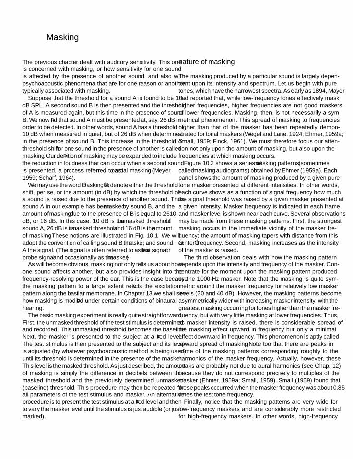
SFK SFK


10 Masking

The previous chapter dealt with auditory sensitivity. This oneis concerned with masking, or how sensitivity for one soundis affected by the presence of another sound, and also withpsychoacoustic phenomena that are for one reason or anothertypically associated with masking.

Suppose that the threshold for a sound A is found to be 10dB SPL. A second sound B is then presented and the thresholdof A is measured again, but this time in the presence of soundB. We now find that sound A must be presented at, say, 26 dB inorder to be detected. In other words, sound A has a threshold of10 dB when measured in quiet, but of 26 dB when determinedin the presence of sound B. This increase in the threshold orthreshold shift for one sound in the presence of another is calledmasking. Our definition of masking may be expanded to includethe reduction in loudness that can occur when a second soundis presented, a process referred to as partial masking (Meyer,1959; Scharf, 1964).

We may use the word “masking” to denote either the thresholdshift, per se, or the amount (in dB) by which the threshold ofa sound is raised due to the presence of another sound. Thus,sound A in our example has been masked by sound B, and theamount of masking due to the presence of B is equal to 26−10dB, or 16 dB. In this case, 10 dB is the unmasked threshold ofsound A, 26 dB is its masked threshold, and 16 dB is the amountof masking . These notions are illustrated in Fig. 10.1. We willadopt the convention of calling sound B the masker, and soundA the signal. (The signal is often referred to as the test signal orprobe signal, and occasionally as the maskee.)

As will become obvious, masking not only tells us about howone sound affects another, but also provides insight into thefrequency-resolving power of the ear. This is the case becausethe masking pattern to a large extent reflects the excitationpattern along the basilar membrane. In Chapter 13 we shall seehow masking is modified under certain conditions of binauralhearing.

The basic masking experiment is really quite straightforward.First, the unmasked threshold of the test stimulus is determinedand recorded. This unmasked threshold becomes the baseline.Next, the masker is presented to the subject at a fixed level.The test stimulus is then presented to the subject and its levelis adjusted (by whatever psychoacoustic method is being used)until its threshold is determined in the presence of the masker.This level is the masked threshold. As just described, the amountof masking is simply the difference in decibels between thismasked threshold and the previously determined unmasked(baseline) threshold. This procedure may then be repeated forall parameters of the test stimulus and masker. An alternativeprocedure is to present the test stimulus at a fixed level and thento vary the masker level until the stimulus is just audible (or justmarked).

nature of masking

The masking produced by a particular sound is largely depen-dent upon its intensity and spectrum. Let us begin with puretones, which have the narrowest spectra. As early as 1894, Mayerhad reported that, while low-frequency tones effectively maskhigher frequencies, higher frequencies are not good maskersof lower frequencies. Masking, then, is not necessarily a sym-metrical phenomenon. This spread of masking to frequencieshigher than that of the masker has been repeatedly demon-strated for tonal maskers (Wegel and Lane, 1924; Ehmer, 1959a;Small, 1959; Finck, 1961). We must therefore focus our atten-tion not only upon the amount of masking, but also upon thefrequencies at which masking occurs.

Figure 10.2 shows a series of masking patterns (sometimescalled masking audiograms) obtained by Ehmer (1959a). Eachpanel shows the amount of masking produced by a given puretone masker presented at different intensities. In other words,each curve shows as a function of signal frequency how muchthe signal threshold was raised by a given masker presented ata given intensity. Masker frequency is indicated in each frameand masker level is shown near each curve. Several observationsmay be made from these masking patterns. First, the strongestmasking occurs in the immediate vicinity of the masker fre-quency; the amount of masking tapers with distance from this“center” frequency. Second, masking increases as the intensityof the masker is raised.

The third observation deals with how the masking patterndepends upon the intensity and frequency of the masker. Con-centrate for the moment upon the masking pattern producedby the 1000-Hz masker. Note that the masking is quite sym-metric around the masker frequency for relatively low maskerlevels (20 and 40 dB). However, the masking patterns becomeasymmetrically wider with increasing masker intensity, with thegreatest masking occurring for tones higher than the masker fre-quency, but with very little masking at lower frequencies. Thus,as masker intensity is raised, there is considerable spread ofthe masking effect upward in frequency but only a minimaleffect downward in frequency. This phenomenon is aptly calledupward spread of masking. Note too that there are peaks insome of the masking patterns corresponding roughly to theharmonics of the masker frequency. Actually, however, thesepeaks are probably not due to aural harmonics (see Chap. 12)because they do not correspond precisely to multiples of themasker (Ehmer, 1959a; Small, 1959). Small (1959) found thatthese peaks occurred when the masker frequency was about 0.85times the test tone frequency.

Finally, notice that the masking patterns are very wide forlow-frequency maskers and are considerably more restrictedfor high-frequency maskers. In other words, high-frequency

187

SFK SFK


chapter 10

Figure 10.1 Hypothetical example in which a masker shifts the thresholdof a test signal by 16 dB from 10 dB SPL to 26 dB SPL.

maskers only are effective over a relatively narrow frequencyrange in the vicinity of the masker frequency, but low frequen-cies tend to be effective maskers over a very wide range offrequencies.

These masking patterns reflect the activity along the basilarmembrane, as illustrated in Fig. 10.3. Recall from Chapter 4 thatthe traveling wave envelope has a gradually increasing ampli-tude along its basal (high-frequency) slope, reaches a peak,and then decays rapidly with a steep apical (low-frequency)

slope. It is thus expected that higher (more basal) frequencieswould be most affected by the displacement pattern caused bylower-frequency stimuli. In addition, the high-frequency trav-eling wave peaks and “decays away” fairly close to the basalturn, so that its masking effect would be more restricted. Lowerfrequencies, on the other hand, produce basilar membrane dis-placements along most of the partition. In addition, the excita-tion pattern becomes wider as the signal level increases.

Although a great deal of information about masking has beenderived from studies using tonal maskers, difficulties becomereadily apparent when both the masker and test stimulus aretones. Two major problems are due to the effects of beats andcombination tones.

Beats are audible fluctuations that occur when a subject is pre-sented with two tones differing in frequency by only a few cyclesper second (e.g., 1000 and 1003 Hz) at the same time. Conse-quently, when the masker and test tones are very close in fre-quency, one cannot be sure whether the subject has respondedto the beats or to the test tone. These audible beats can result innotches at the peaks of the masking patterns when the maskerand signal are close in frequency (Wegel and Lane, 1924). Thesituation is further complicated because combination tones arealso produced when two tones are presented together. Com-bination tones are produced at frequencies equal to numericalcombinations of the two original tones (fl and f2), such as f2–fl

or 2fl–f2. Beats and combination tones are covered in Chapter12. Beats may be partially (though not totally) eliminated byreplacing the tonal maskers with narrow bands of noise cen-tered around given frequencies; however, the elimination ofcombination tones requires more sophisticated manipulations(Patterson and Moore, 1986). The results of narrow-band noise

Figure 10.2 Masking patterns produced various pure tone maskers (masker frequency indicated in each frame). Numbers on curves indicate masker level.Source: Adapted from Ehmer (1959a, 1959b, with permission of J. Acoust. Soc. Am.

188

SFK SFK


masking

Figure 10.3 Artist’s conceptualization of how upward spread of maskingis related to traveling wave excitation patterns along the basilar membrane:The excitation pattern of a lower-frequency masker envelops that of a higher-frequency test signal (a), but a higher-frequency masker does not envelopthe excitation pattern of a lower-frequency test signal (b).

masking experiments have essentially confirmed the maskingpatterns generated in the tonal masking studies (Egan and Hake,1950; Ehmer, 1959b; Greenwood, 1961).

We have seen that upward spread of masking is the ruleas masker level is increased. However, a very interesting phe-nomenon appears when the stimulus level is quite high, forexample, at spectrum levels of about 60 to 80 dB. Spectrumlevel refers to the power in a one-cycle-wide band. In otherwords, spectrum level is level per cycle. It may be computed bysubtracting 10 times the log of the bandwidth from the overallpower in the band. Thus:

dBspectrum level = dBoverall − 10 log (bandwidth)

If the bandwidth is 10,000 Hz and the overall power is 95 dB,then the spectrum level will be 95 − 101og (10,000), or 95 − 40= 55 dB.

Higher-frequency maskers presented at intense levels can alsoproduce masking at low frequencies (Bilger and Hirsh, 1956;Deatherage et al., 1957a, 1957b). This is called remote maskingbecause the threshold shifts occur at frequencies below andremote from the masker. In general, the amount of remotemasking increases when the bandwidth of the masking noise iswidened or its spectrum level is raised (Bilger, 1958). Althoughthe acoustic reflex can cause a threshold shift at low frequencies,it is unlikely that this is the cause of remote masking becauseremote masking has been shown to occur in the absence of

the acoustic reflex (Bilger, 1966). Instead, remote masking ismost likely due primarily to envelope detection of distortionproducts generated within the cochlea at high masker intensities(Spieth, 1957; Deatherage et al., 1957a, 1957b). (See Chap. 4 fora discussion of cochlear distortion.)

It is apparent from Fig. 10.2 that masking increases as thelevel of the masker is raised. We may now ask how the amountof masking relates to the intensity of the masker. In other words,how much of a threshold shift results when the masker level israised by a given amount? This question was addressed in theclassical studies of Fletcher (1937) and Hawkins and Stevens(1950). Since the essential findings of the two studies agreed, letus concentrate upon the data reported by Hawkins and Stevensin 1950. They measured the threshold shifts for pure tones andfor speech produced by various levels of a white noise masker.(It should be pointed out that although white noise connotesequal energy at all frequencies, the actual spectrum reachingthe subject is shaped by the frequency response of the earphoneor loudspeaker used to present the signal. Therefore, the exactmasking patterns produced by a white noise depend upon thetransducer employed, as well as on bandwidth effects that willbe discussed in the next section.)

Figure 10.4 shows Hawkins and Stevens’ data as maskedthreshold contours. These curves show the masked thresholdsproduced at each frequency by a white noise presented at vari-ous spectrum levels. The curves have been idealized in that theactual results were modified to reflect the masking producedby a true white noise. The actual data were a bit more irregu-lar, with peaks in the curves at around 7000 Hz, reflecting theeffects of the earphone used. The bottom contour is simply theunmasked threshold curve. The essential finding is that thesecurves are parallel and spaced at approximately 10-dB intervals,which is also the interval between the masker levels. This resultsuggests that a 10-dB increase in masker level produces a 10-dB

Figure 10.4 Masking contours showing masking as a function of frequencyfor various spectrum levels of an idealized white noise. Bottom curve isthreshold in quiet. Source: Adapted from Hawkins and Stevens (1950), withpermission of J. Acoust. Soc. Am.

189

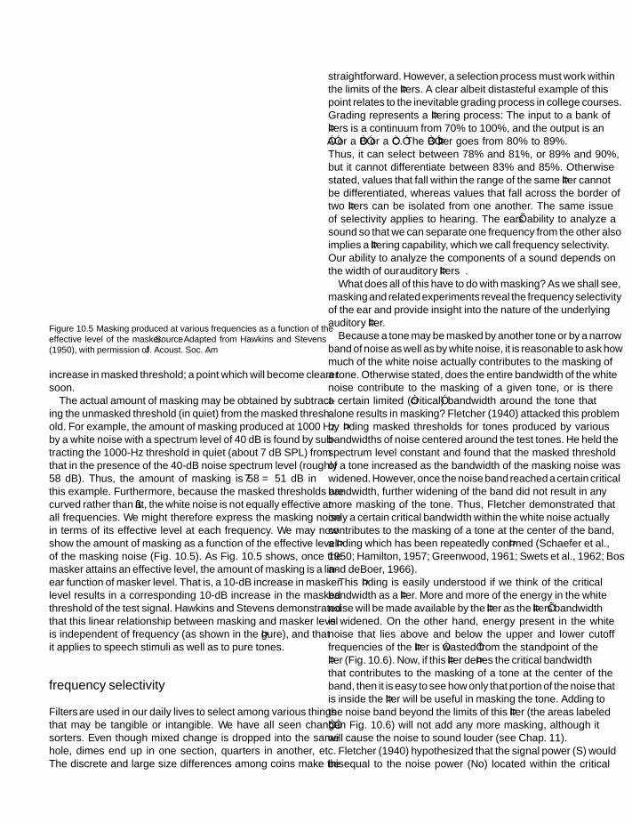
SFK SFK


chapter 10

Figure 10.5 Masking produced at various frequencies as a function of theeffective level of the masker. Source: Adapted from Hawkins and Stevens(1950), with permission of J. Acoust. Soc. Am.

increase in masked threshold; a point which will become clearersoon.

The actual amount of masking may be obtained by subtract-ing the unmasked threshold (in quiet) from the masked thresh-old. For example, the amount of masking produced at 1000 Hzby a white noise with a spectrum level of 40 dB is found by sub-tracting the 1000-Hz threshold in quiet (about 7 dB SPL) fromthat in the presence of the 40-dB noise spectrum level (roughly58 dB). Thus, the amount of masking is 58−7 = 51 dB inthis example. Furthermore, because the masked thresholds arecurved rather than flat, the white noise is not equally effective atall frequencies. We might therefore express the masking noisein terms of its effective level at each frequency. We may nowshow the amount of masking as a function of the effective levelof the masking noise (Fig. 10.5). As Fig. 10.5 shows, once themasker attains an effective level, the amount of masking is a lin-ear function of masker level. That is, a 10-dB increase in maskerlevel results in a corresponding 10-dB increase in the maskedthreshold of the test signal. Hawkins and Stevens demonstratedthat this linear relationship between masking and masker levelis independent of frequency (as shown in the figure), and thatit applies to speech stimuli as well as to pure tones.

frequency selectivity

Filters are used in our daily lives to select among various thingsthat may be tangible or intangible. We have all seen changesorters. Even though mixed change is dropped into the samehole, dimes end up in one section, quarters in another, etc.The discrete and large size differences among coins make this

straightforward. However, a selection process must work withinthe limits of the filters. A clear albeit distasteful example of thispoint relates to the inevitable grading process in college courses.Grading represents a filtering process: The input to a bank offilters is a continuum from 70% to 100%, and the output is an“A” or a “B” or a “C.” The “B” filter goes from 80% to 89%.Thus, it can select between 78% and 81%, or 89% and 90%,but it cannot differentiate between 83% and 85%. Otherwisestated, values that fall within the range of the same filter cannotbe differentiated, whereas values that fall across the border oftwo filters can be isolated from one another. The same issueof selectivity applies to hearing. The ear’s ability to analyze asound so that we can separate one frequency from the other alsoimplies a filtering capability, which we call frequency selectivity.Our ability to analyze the components of a sound depends onthe width of our auditory filters.

What does all of this have to do with masking? As we shall see,masking and related experiments reveal the frequency selectivityof the ear and provide insight into the nature of the underlyingauditory filter.

Because a tone may be masked by another tone or by a narrowband of noise as well as by white noise, it is reasonable to ask howmuch of the white noise actually contributes to the masking ofa tone. Otherwise stated, does the entire bandwidth of the whitenoise contribute to the masking of a given tone, or is therea certain limited (“critical”) bandwidth around the tone thatalone results in masking? Fletcher (1940) attacked this problemby finding masked thresholds for tones produced by variousbandwidths of noise centered around the test tones. He held thespectrum level constant and found that the masked thresholdof a tone increased as the bandwidth of the masking noise waswidened. However, once the noise band reached a certain criticalbandwidth, further widening of the band did not result in anymore masking of the tone. Thus, Fletcher demonstrated thatonly a certain critical bandwidth within the white noise actuallycontributes to the masking of a tone at the center of the band,a finding which has been repeatedly confirmed (Schaefer et al.,1950; Hamilton, 1957; Greenwood, 1961; Swets et al., 1962; Bosand deBoer, 1966).

This finding is easily understood if we think of the criticalbandwidth as a filter. More and more of the energy in the whitenoise will be made available by the filter as the filter’s bandwidthis widened. On the other hand, energy present in the whitenoise that lies above and below the upper and lower cutofffrequencies of the filter is “wasted” from the standpoint of thefilter (Fig. 10.6). Now, if this filter defines the critical bandwidththat contributes to the masking of a tone at the center of theband, then it is easy to see how only that portion of the noise thatis inside the filter will be useful in masking the tone. Adding tothe noise band beyond the limits of this filter (the areas labeled“b” in Fig. 10.6) will not add any more masking, although itwill cause the noise to sound louder (see Chap. 11).

Fletcher (1940) hypothesized that the signal power (S) wouldbe equal to the noise power (No) located within the critical

190

SFK SFK


masking

Figure 10.6 Energy within the critical band filter (a) contributes to themasking of the tone at the center, whereas energy outside of the filter (b)does not contribute to the masking (see text).

bandwidth (CB) when the tone was at its masked threshold:S = CB · No. Thus, the critical band would be equal to theratio of the signal power to the noise power, or CB = S/No. Indecibels, this corresponds to dBS − dBNo. Hawkins and Stevens(1950) found that the masked threshold of a 1000-Hz tone wasapproximately 58 dB in the presence of a white noise whosespectrum level was 40 dB. The resulting estimate of the criticalband is therefore 58 dB − 40 dB = 18 dB, which correspondsto a bandwidth of 63.1 Hz. This estimate of the critical band isshown by the X in Fig. 10.7. Notice that this indirect estimateof the critical bandwidth based upon the power ratio of signalto noise is actually quite a bit narrower than the other moredirect estimates of the critical band shown in the figure. Forthis reason, the indirect estimate based upon Fletcher’s formula

Figure 10.7 Critical bandwidth as a function of center frequency for variousstudies. The X is the critical ratio estimate of Hawkins and Stevens (1950) fora 1000-Hz tone. Source: Adapted from Scharf, Critical bands, in: Foundationsof Modern Auditory Theory (J. V. Tobias, ed.), Vol. 1, c©1970, Academic Press.

is referred to as critical ratios, as opposed to the critical bandsobtained by other, direct means. Good correspondence to thecritical band is obtained when the critical ratio is multipliedby a factor of 2.5 (Zwicker et al., 1957; Scharf, 1970). Thiscorrespondence is demonstrated by the open circles in Fig. 10.7,which are the values of the critical ratios multiplied by 2.5, basedupon Hawkins and Stevens’ (1950) data. Note that there is goodagreement with Greenwood’s (1961) masking data, as well aswith the critical bands directly derived from loudness studies(see Chap. 11).

Bilger (1976) proposed that the listener performs an intensitydiscrimination between the noise power in the critical bandand the combined power of the noise plus signal at the maskedthreshold; as a result the critical ratio is equated to the familiarWeber fraction (Chap. 9):

S

CB · N= I

I

This equation is solved for critical bandwidth by multiplyingS/N by the reciprocal of the Weber fraction

CB = S

N· I

I

Since the critical ratio is multiplied by 2.5 to obtain the criticalband, this leads to a Weber fraction of 1/2.5 = 0.4, or a differencelimen of 1.46 dB, a value that is in reasonable agreement withintensity DL data.

Figure 10.7 indicates that the critical band becomes wideras the center frequency increases. Scharf (1970) has provided atable of critical bandwidth estimates based upon the availabledata. Examples are a critical bandwidth of 100 Hz for a cen-ter frequency of 250 Hz, a 160-Hz band for 1000 Hz, and a700-Hz band for 4000 Hz. Similar data and formulas for cal-culation of the critical bandwidth and critical band rate (thebark scale) have been provided by Zwicker and Terhardt (1980).Actually, one should be careful not to conceive of a series ofdiscrete critical bands laid as it were end to end, but rather ofa bandwidth around any particular frequency that defines thephenomenon we have discussed with respect to that frequency.[One should remember in this context Scharf’s (1970, p. 159)elegant definition: “the critical band is that bandwidth at whichsubjective responses rather abruptly change.”] We should thusthink of critical bandwidths as overlapping filters rather than asdiscrete, contiguous filters.

It would appear that the original concept (Fletcher, 1940) ofthe critical bandwidth as defining an internal auditory filter isfundamentally correct. Its location is more than likely periph-eral, with critical bandwidths probably corresponding to 1 to2 mm distances along the human cochlear partition (Scharf,1970). Thus, the critical band presents itself as a fundamen-tal concept in the frequency-analysis capability of the cochlea,the physiological aspects of which are discussed in Chapter 4.

191

SFK SFK


chapter 10

Figure 10.8 Shape and bandwidth (ERB) of the auditory filter expressed in terms of increasing level in 10 dB steps from 20 to 90 dB SPL/ERB. (Note theopposite directions in which the left- and right-hand slope change as level increases from 20 to 90 dB. The left-hand slope shown on these filters determinesthe high frequency aspect of the excitation pattern.) Source: From Moore and Glasberg (1987), with permission of Hear Res.

Detailed reviews of the critical band concept may be found inthe work of Scharf (1970) and Bilger (1976).

The idea of the internal filter originally embodied in thecritical band concept, particularly in its conceptualization as arectangular filter around the center frequency (Fletcher, 1940),has been modified and updated by numerous investigators(Patterson, 1974, 1976; Houtgast, 1977; Weber, 1977; Mooreand Glassberg, 1981, 1987; Patterson et al., 1982; Shailer andMoore, 1983; Fidell et al., 1983; Glasberg et al., 1984a, 1984b).Figure 10.8 shows the shapes of the auditory filter over a widerange of intensities, as derived in a paper by Moore and Glasberg(1987). The curves were based on raw data from young, normalhearing subjects from variety of studies.1 The figure reveals thatthe filter becomes increasingly more asymmetric with increas-ing level. The major aspect of this asymmetry is that the slope ofthe low-frequency (left-hand) branch of the filter decreases withincreasing level. This widening of the left-hand branch of thefilter that corresponds to the phenomenon of upward spread ofmasking has been discussed earlier in this chapter. We saw thereason is that the left-hand branch of this filter determines thehigh-frequency aspect of the excitation pattern.

With an idea of the shape of the auditory filter, we mayask how it is related to frequency and to the critical band(cf. Fig. 10.7). To do this, we need to summarize the nature

1 The auditory filter tends to widen with age (Patterson and Moore,1986). See Patterson et al. (1982) for other findings, and Gelfand (2001)for a general discussion of factors relating to aging and hearing impair-ment.

of the filters in some valid and convenient way. This can bedone by using what is called the equivalent rectangular band-width (ERB) of the filter. An ERB is simply the rectangularfilter that passes the same amount of power as would passthrough the filter we are trying to specify. Thus, if a whitenoise is directed to the inputs of a filter of any given con-figuration and also through its ERB, then the power at theiroutputs (passed through them) would be the same. Using thisapproach, Moore and Glasberg (1983b) have shown how theauditory filter changes with frequency. Figure 10.9 shows theERB of the auditory filter as a function of its center frequency.Here we see that the width of the auditory filter widens asfrequency increases, and also that this relationship is quite con-sistent across several studies. Also shown in the figure is anequivalent line based upon the classical critical band. [The latterwas derived using a formula by Zwicker and Terhardt (1980).]Observe that the more recent measurements of auditory filterwidth are slightly narrower but generally parallel with the olderones based upon classical critical band data. The parallel rela-tionship breaks down below about 500 Hz, where unlike theearlier critical band data, the newer observations suggest thatthe auditory filter continues to be a function of frequency. Oneshould refer to Patterson and Moore (1986), whose extensivediscussion of this topic includes arguments addressing the dis-crepancy below 500 Hz in the light of differences in processingefficiency.

We have already seen that beats and combination tones canadversely affect tone-on-tone masking measurements. Now thatwe have an idea of the auditory filter, we may consider anotherfactor that can confound masking (among other) experiments.

192

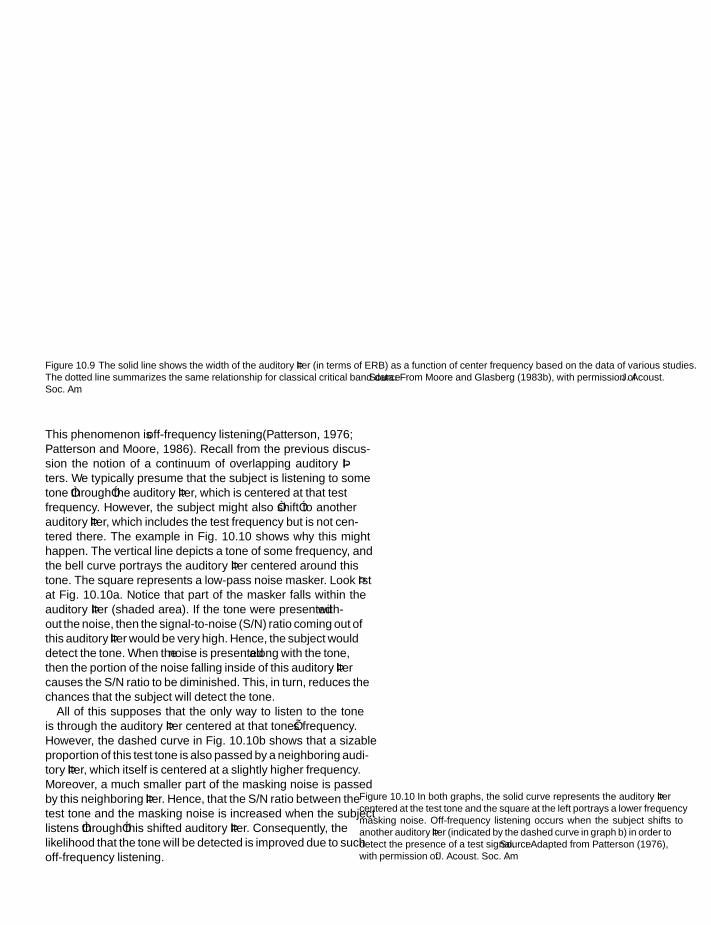
SFK SFK


masking

Figure 10.9 The solid line shows the width of the auditory filter (in terms of ERB) as a function of center frequency based on the data of various studies.The dotted line summarizes the same relationship for classical critical band data. Source: From Moore and Glasberg (1983b), with permission of J. Acoust.Soc. Am.

This phenomenon is off-frequency listening (Patterson, 1976;Patterson and Moore, 1986). Recall from the previous discus-sion the notion of a continuum of overlapping auditory fil-ters. We typically presume that the subject is listening to sometone “through” the auditory filter, which is centered at that testfrequency. However, the subject might also “shift” to anotherauditory filter, which includes the test frequency but is not cen-tered there. The example in Fig. 10.10 shows why this mighthappen. The vertical line depicts a tone of some frequency, andthe bell curve portrays the auditory filter centered around thistone. The square represents a low-pass noise masker. Look firstat Fig. 10.10a. Notice that part of the masker falls within theauditory filter (shaded area). If the tone were presented with-out the noise, then the signal-to-noise (S/N) ratio coming out ofthis auditory filter would be very high. Hence, the subject woulddetect the tone. When the noise is presented along with the tone,then the portion of the noise falling inside of this auditory filtercauses the S/N ratio to be diminished. This, in turn, reduces thechances that the subject will detect the tone.

All of this supposes that the only way to listen to the toneis through the auditory filter centered at that tone’s frequency.However, the dashed curve in Fig. 10.10b shows that a sizableproportion of this test tone is also passed by a neighboring audi-tory filter, which itself is centered at a slightly higher frequency.Moreover, a much smaller part of the masking noise is passedby this neighboring filter. Hence, that the S/N ratio between thetest tone and the masking noise is increased when the subjectlistens “through” this shifted auditory filter. Consequently, thelikelihood that the tone will be detected is improved due to suchoff-frequency listening.

Figure 10.10 In both graphs, the solid curve represents the auditory filtercentered at the test tone and the square at the left portrays a lower frequencymasking noise. Off-frequency listening occurs when the subject shifts toanother auditory filter (indicated by the dashed curve in graph b) in order todetect the presence of a test signal. Source: Adapted from Patterson (1976),with permission of J. Acoust. Soc. Am.

193

SFK SFK


chapter 10

Figure 10.11 (a) Thresholds of sweeping-frequency test tones (LT, dB) as a function of frequency (of the test tones, FT, Hz) in quiet (lower tracing) andin the presence of a fixed masker (upper tracing). The filled circle shows the level and frequency of the fixed masker (60 dB, 1000 Hz; LM, FM). (b) Thesetracings show the levels of sweeping-frequency masker tones (LM, dB) needed to just mask the fixed test tone of 1000 Hz at 15 dB (LT, FT). Source: FromZwicker and Schorn (1978), with permission of Audiology.

An effective approach to minimize the confounding effects ofoff-frequency listening is to present the signals involved in anexperiment (such as the test tone and masker tone) along withadditional noise(s) which will mask out the frequencies aboveand below the range of interest (O’Loughlin and Moore, 1981).

psychoacoustic tuning curves

So far, we have described masking in terms of the level of thetone (or other signal), which has been masked. Thus, the mask-ing patterns in Fig. 10.2 expressed the amount of masking pro-duced for various test tones as a function of frequency by a givenmasker (at some fixed level). That is, “30 dB of masking” on oneof these graphs means that the masker caused the threshold ofthe test signal to be increased by 30 dB above its unmaskedthreshold. If this experiment were done using the Bekesy track-ing method (Chap. 7), the “raw” results might look somethinglike the left panel in Fig. 10.11. Here, the lower tracing shows thethreshold of the test signal, which is a tone sweeping in frequencyfrom 500 to 4000 Hz. The upper tracing shows the maskedthreshold tracing in the presence of a fixed masker (which isa 1000-Hz tone at 60 dB). Subtracting the lower (unmasked)tracing from the upper (masked) threshold tracing would resultin a familiar masking pattern similar to those in Fig. 10.2.

Another way to look at masking was initiated by Chistovich(1957), Small (1959), and Zwicker (1974). This approach essen-tially asks the question, what levels of the masker are needed tomask the test signal? Now, the test tone (signal) is kept at a fixedlevel and frequency, and the level of the masker tone is adjusteduntil it just masks the test tone. This is done at many differentfrequencies of the masker, resulting in a curve very differentfrom the familiar masking audiogram seen above.

This approach is easily understood by referring to the rightpanel of Fig. 10.11. (A careful look at this graph will reveal

differences from the left panel not only in the tracing but alsoin the captions for the x- and y-axes.) The tonal signal (i.e., thesignal being masked) is a 1000-Hz tone at 15 dB (indicated by theX). Now it is the masker tone, which sweeps across the frequencyrange, and the subject uses the Bekesy tracking method to keepthe masker at a level that will just mask the fixed test tone. Theresulting diagram shows the level of the masker needed to keepthe test tone just masked as a function of the masker frequency.

It should be apparent to the reader that this tracing bearsa striking resemblance to the auditory neuron tuning curvesseen in earlier chapters. It is thus called a psychoacoustic (orpsychophysical) tuning curve (PTC). Psychophysical tuningcurves provide a very good representation of the ear’s frequencyselectivity. This occurs based on the notion that we are samplingthe output of just one auditory filter when a very low signal isused. As the masker gets closer and closer to the frequency ofthe test signal, less and less level will be required to mask it, andhence the function of masker level needed to just mask the toneprovides a picture of the filter.

However, one must avoid the temptation to think of the PTCas the psychoacoustic analogy of an individual neural tun-ing curve. It is clear that much more than a single neuronis being sampled, and that PTCs are wider than neural tun-ing curves. Moreover, the earlier discussions dealing with theimplications of beats, combination tones, and off-frequencylistening in masking are particularly applicable to PTCs. Forexample, PTCs become wider when off-frequency listening isminimized by the use of notched noise (Moore et al., 1984).A notched noise is simply a band-reject noise (see Chap. 1) inwhich the band being rejected is centered where we are mak-ing our measurement. Therefore, the notched noise masks thefrequency regions above and below the one of interest, so thatoff-frequency listening is reduced.

Figure 10.12 shows two sets of individual PTCs at fourtest-tone frequencies (500–4000 Hz) from a more recent

194

SFK SFK


masking

Figure 10.12 Individual psychoacoustic tuning curves at 500, 1000, 2000, and 4000 Hz for two listeners. Triangles are simultaneous masking data andsquares are forward masking data. Notice that the forward masking PTCs show sharper tuning. Source: From Moore et al. (1984), with permission of J.Acoust. Soc. Am.

195

SFK SFK


chapter 10

experiment. These PTCs were obtained by using simultane-ous masking (triangles) versus forward masking (squares). Asthe figure shows, PTCs generated under forward masking con-ditions generally show sharper tuning than those describedfor simultaneous masking conditions (e.g., Houtgast, 1972;Duifhuis, 1976; Wightman et al., 1977; Weber, 1983; Lufti, 1984;Moore et al., 1984). These differences go beyond the currentscope, but the interested reader will find several informativediscussions on this topic (e.g., Weber, 1983; Jesteadt and Nor-ton, 1985; Patterson and Moore, 1986; Lufti, 1988).

comodulation masking release

Recall that only a certain critical bandwidth of noise around asignal tone is involved in the masking of that tone: The maskedthreshold of the signal will not be changed by widening thenoise bandwidth beyond the CB or adding one or more otherbands outside of the CB. However, a different situation occurswhen the masking noise is amplitude modulated, as illustratedby the following example.

It will be convenient for the noise band centered on the testtone to be called the on-signal band, and for any other bandsof noise to be called flanking or off-frequency bands. We willbegin by masking a pure tone signal by an on-signal band of

noise that is being amplitude modulated, as illustrated by thewaveform in the panel labeled “on-signal band alone” in upperportion of Fig. 10.13. The graph in the lower part of the fig-ure shows that the masked threshold of the signal is 50 dB inpresence of this amplitude modulated on-signal noise. We willnow add another band of noise that is outside of the CB ofthe test tone. The off-signal band will be amplitude modulatedin exactly the same way as the on-signal band, as illustratedin the panel labeled “comodulated bands” in Fig. 10.13. Thesetwo noise bands are said to be comodulated bands because theenvelopes of their modulated waveforms follow the same pat-tern over time even though they contain different frequencies.We do not expect any change in masking with the comodu-lated bands because adding the off-frequency band is outsideof the signal’s critical band. However, we find that the maskedthreshold of the signal actually becomes better (lower) for thecomodulated bands compared to what it was for just the on-signal band alone. This improvement is called comodulationmasking release (CMR) (Hall, Haggard, and Fernandes, 1984).In the hypothetical example of Fig. 10.13, the masked thresholdof the tone improved from 50 dB in the presence of just theon-signal band (left bar) to 39 dB for the comodulated bands(middle bar), amounting to a CMR of 11 dB. Notice that themasked threshold does not improve (right bar) if the on-signaland off-signal noise bands are not comodulated (panel labeled

Figure 10.13 Hypothetical modulated noise band waveform envelopes (above) and masked threshold results (below) illustrating comodulation maskingrelease. See text.

196

SFK SFK


masking

“uncomodulated bands”). Comodulation masking release alsooccurs for complex signals (made up of, e.g., 804, 1200, 1747,and 2503 Hz) even if there is some spectral overlap between thesignal and the masker (Grose, Hall, Buss, and Hatch, 2005)

Comodulation masking release reveals that the auditory sys-tem is able to capitalize upon information provided across crit-ical band filters, although a cohesive model explaining CMRis not yet apparent. One type of explanation suggests that theinformation provided by the off-signal band(s) helps the subjectknow when the troughs or “dips” occur in the modulating noise.Listening for the signal during these dips would result in a lowerthreshold (less masking) compared to times when the noiselevel is higher. Another type of model suggests that the audi-tory system compares the modulation patterns derived from theoutputs of auditory filters in different frequency regions. Thispattern would be similar for the filters that do not contain a sig-nal but would be modified for the filter that contains a signal.Detecting a disparity between the outputs of the filters wouldthus indicate the presence of a signal. The interested studentshould see the informative review by Moore (1990) and themany contemporary discussions of CMR parameters, models,and related effects (e.g., Buus, 1985; Hatch et al., 1995; Hall andGrose, 1990; Moore et al., 1990; Hicks and Bacon, 1995; Baconet al., 1997; Grose et al., 2005).

overshoot

The masked threshold of a brief signal can be affected by thetemporal arrangement of the signal and a masking noise. Thetypical experiment involves a very brief signal and a longerduration masker, with various timing relationships betweenthem. For example, the signal onset might be presented withina few milliseconds of the masker onset (as in Fig. 10.14a), inthe middle of the masker (Fig. 10.14b), or the signal onsetmight trail the masker onset by various delays between theseextremes (as in Fig. 10.14c to d). Compared to the amountof masking that takes place when the signal is in the middleof the masker, as much as 10 to 15 dB more masking takesplace when the signal onset occurs at or within a few mil-liseconds of the masker onset. In other words, a brief signal issubjected to a much larger threshold shift at the leading edge ofa masker compared to when it is placed in the temporal mid-dle of the masker. This phenomenon was originally describedby Elliott (1965) and Zwicker (1965a, 1965b) and is known asovershoot.

The amount of masking overshoot decreases as the signaldelay gets longer, usually becoming nil by the time the delayreaches about 200 ms (e.g., Elliott, 1969; Zwicker, 1965a; Fastl,1976). Masking overshoot is maximized for signals with highfrequencies (above 2000 Hz) and short durations (under 30ms) (e.g., Elliott, 1967, 1969; Zwicker, 1965a; Fastl, 1976; Baconand Takahashi, 1992; Carlyon and White, 1992), and when themasker has a very wide bandwidth, much broader than the

Figure 10.14 Timing relationships between a masker and brief signal. Thesignal onset is within a few milliseconds of the masker onset in the firstframe and occurs at increasing delays in the subsequent frames. The signalis presented in the temporal middle of the masker in the last frame.

critical band (e.g., Zwicker, 1965b; Bacon and Smith, 1991).In addition, overshoot becomes greater as the masker increasesfrom low to moderate levels, but it declines again as the maskercontinues to increase toward high levels (Bacon, 1990).

The different amounts of overshoot produced by narrow ver-sus broad band maskers has been addressed by Scharf, Reeves,and Giovanetti (2008), who proposed that overshoot is caused(or at least affected) by the listener’s ability to focus on the testfrequency at the onset of the noise. This is disrupted by the widerange of frequencies in a broadband masker, but is focused by thenarrow band masker because its spectrum is close to the signalfrequency. Consistent with their explanation, they found thatnarrow band maskers caused little if any overshoot when the testtone always had the same frequency (stimulus certainty), as inthe typical overshoot experiment. In contrast, narrow maskersproduced more overshoot when the test frequency was changedrandomly between trials (stimulus uncertainty). The oppositeeffect occurred with wide band maskers, in which case stimulusuncertainty produced less overshoot.

Although the precise origin of overshoot is not definitivelyknown, the most common explanation is based on adaptation inauditory neurons (e.g., Green, 1969; Champlin and McFadden,1989; Bacon, 1990; McFadden and Champlin, 1990; Bacon andHealy, 2000). Recall from Chapter 5 that the initial responseof an auditory neuron involves a high discharge rate, whichdeclines over a period of roughly about 10 to 20 ms. The neuralresponse produced by the masker would thus be greatest atits leading edge and would weaker thereafter. As a result, moremasking would be produced at the beginning of the masker thanin the middle of it. Other hypotheses suggest that the basis formasking overshoot may be related to processes associated withthe basilar membrane input–output function (von Klitzing andKohlrausch, 1994; Strickland, 2001; Bacon and Savel, 2004),

197

SFK SFK


chapter 10

or a disruption in the listener’s ability to attend to the signalfrequency (Scharf et al., 2008).

Masking overshoot can also occur when the signal is veryclose to the offset of the masker, although it is considerablysmaller than the onset effect (e.g., Elliott, 1969; Bacon andViemeister, 1985; Bacon and Moore, 1986; Bacon et al., 1989;Formby et al., 2000). A peripheral origin for offset overshootis unlikely because the increased spike rate seen at the onset ofauditory neuron firing patterns does not also occur at offset.Hence, overshoot at masker offset has been attributed to centralprocesses (e.g., Bacon and Viemeister, 1985; Bacon and Moore,1986).

temporal masking

So far, we have been considering situations in which the maskerand test signal occur simultaneously. Let us now examine mask-ing that occurs when the test signal and masker do not overlapin time, referred to as temporal or nonsimultaneous masking.This phenomenon may be understood with reference to the dia-grams in Fig. 10.15, which show the basic arrangements usedin masking experiments. In Fig. 10.15a, the signal is presentedand terminated, and then the masker is presented after a brieftime delay following signal offset. Masking occurs in spite ofthe fact that the signal and masker are not presented together.This arrangement is called backward masking or pre-maskingbecause the masker is preceded by the signal, that is, the maskingeffect occurs backward in time (as shown by the arrow in the

Figure 10.15 Temporal masking paradigms: (a) in backward masking themasker follows the signal, (b) in forward masking the masker precedes thesignal, and (c) combined forward and backward masking. The heavy arrowsshow the direction of the masking effect.

Figure 10.16 Temporal masking in decibels as a function of the intervalbetween signal and masker. (Signal: 10 ms, 1000 Hz tone bursts; masker:50 ms broadband noise bursts at 70 dB SPL.) Source: Adapted from Elliott(1962a), with permission of J. Acoust. Soc. Am.

figure). Forward masking or post-masking is just the opposite(Fig. 10.15b). Here, the masker is presented first, and then thesignal is turned on after an interval following masker offset. Asthe arrow shows, the masking of the signal now occurs forwardin time.

The amount of masking of the test signal produced underbackward, forward, or combined forward/backward maskingconditions is determined while various parameters of the probeand masker are manipulated. These parameters may be thetime interval between signal and masker, masker level, maskerduration, etc.

Figure 10.16 shows some examples of temporal masking datafrom Elliott’s (1962a) classic paper. The ordinate is the amountof masking produced by 50-ms noise bursts presented at 70 dBSPL for a test signal of 1000 Hz lasting 10 ms. The abscissa is thetime interval between masker and test signal for the backwardand forward masking paradigms. Finally, the solid lines showthe amount of masking produced when the masker and signalare presented to the same ear (monotically), and the dottedlines reveal the masking that results when the noise goes toone ear and the signal goes to the other (dichotic masking).Notice that considerably more masking occurs monotically thandichotically.

The amount of temporal masking is related to the time gapbetween the signal and the masker. More masking occurs whenthe signal and masker are closer in time, and less masking occursas the time gap between them widens. However, the backwardand forward masking functions are not mirror images of eachother. As the figure shows, Elliott found greater threshold shiftsfor backward masking than for forward masking. Similar find-ings were reported by some investigators (Lynn and Small, 1977;Pastore et al., 1980), but others found the opposite to occur(Wilson and Carhart, 1971).

Backward masking decreases dramatically as the delaybetween the signal and masker increases from about 15 to 20ms, and then continues to decrease very slightly as the interval

198

SFK SFK


masking

Figure 10.17 Examples of the more or less linear decrease of forward mask-ing with the logarithm of the delay between the masker and the signal.Source: Based on data for various forward masking conditions from Wilsonand Carhart (1971; squares), Smiarowski and Carhart (1975; triangles), andWeber and Moore (1981; circles).

is lengthened further. Forward masking also decreases withincreasing delays, but more gradually. It declines linearly withthe logarithm of the masker-signal delay (Fig. 10.17) and existsfor intervals as long as about 200 ms depending on the study(e.g., Wilson and Carhart, 1971; Smiarowski and Carhart, 1975;Fastl, 1976, 1977, 1979; Widin and Viemeister, 1979; Weber andMoore, 1981; Jesteadt et al., 1982).

The amount of temporal masking increases as the level ofthe masker is increased, but not in the linear manner seenfor simultaneous masking (Elliott, 1962a; Babkoff and Sutton,1968; Jesteadt et al., 1981). Rather, with temporal masking,increasing the masker level by 10 dB may result in an additionalthreshold shift on the order of only about 3 dB.

The duration of the masker influences the amount of forwardmasking, but this does not appear to occur for backward mask-ing (Elliott, 1967). The amount of forward masking increases asthe masker duration gets longer up to about 200 ms (Zwicker,1984; Kidd and Feth, 1982).

As we might expect, temporal masking is influenced by thefrequency relationship between the signal and the masker (e.g.,Wright, 1964; Elliott, 1967) just as we have seen for simultane-ous masking. In other words, more masking occurs when thesignal and masker are close together in frequency than whenthey are far apart. Formby et al. (2000) found that a 2500-Hznoise band produced temporal masking for a 500-Hz signal,demonstrating that remote masking can occur under temporalmasking conditions.

The combined effects of forward and backward masking maybe found by placing the signal between the two maskers, asshown in Fig. 10.15c. More masking occurs when backward andforward masking are combined than would result if the indi-vidual contributions of backward and forward masking weresimply added together (Pollack, 1964; Elliott, 1969; Wilson and

Carhart, 1971; Robertson and Pollack, 1973; Penner, 1980; Pas-tore et al., 1980; Cokely and Humes, 1993; Oxenham and Moore,1994, 1995). Such findings suggest that forward and backwardmasking depend upon different underlying mechanisms.

The underlying mechanisms of temporal masking are notfully resolved. Duifhuis (1973) suggested that the steep seg-ments of the monotic temporal masking curves (Fig. 10.16) maybe associated with cochlear processes, while the shallower seg-ments at longer delays may be related to neural events. Severalfindings implicate some degree of central processing in tem-poral masking. For example, we have already seen that somedegree of temporal masking occurs under dichotic conditionsfor forward and backward masking. In addition, masking leveldifferences (a reduction in masking associated with binauralinteractions; see Chap. 13), have been shown to occur for for-ward, backward, and combined forward-backing masking (e.g.,Deatherage and Evans, 1969; Robertson and Pollack, 1973; Bergand Yost, 1976; Yost and Walton, 1977).

Although overlapping in time of the cochlear displacementpatterns is a reasonable explanation at very short masker-signaldelays, short-term neural adaptation caused by the masker isthe predominant explanation of forward masking (Smith, 1977;Harris and Dallos, 1979; Kidd and Feth, 1982). However, evenshort-term adaptation cannot fully account for the extent ofthe forward masking measured in psychoacoustic experiments(Relkin and Turner, 1988; Turner et al., 1994). Moreover, for-ward masking also occurs in cochlear implant users even thoughthe synapses between the hair cells and auditory neurons arebypassed in these patients (Chatterjee, 1999). Thus, the exist-ing evidence seems to suggest that both peripheral and centralprocesses are probably involved in forward masking.

Several lines of evidence in addition to the material describeabove suggest that central processes are the principal factorsin backward masking. Providing the listener with contralateraltiming cues supplies information that affects the uncertainty ofthe task and has been shown to influence backward maskingbut not forward masking (Pastore and Freda, 1980; Puleo andPastore, 1980). Moreover, performance decrements in backwardmasking (but not forward or simultaneous masking) have beenfound to be associated with disorders such as specific languageimpairment and dyslexia (Wright et al., 1997; Wright, 1998;Wright and Saberi, 1999; Rosen and Manganari, 2001).

central masking

The typical arrangement of a masking experiment involves pre-senting both the masker and the test stimulus to the same ear. Upto now, we have been discussing this ipsilateral type of masking.Another approach is to present the masker to one ear and thetest signal to the opposite ear. Raising the intensity of the maskerwill eventually cause the masker to become audible in the otherear, in which case it will mask the test stimulus (a process knownas cross-hearing or contralateralization of the masker). This is

199

SFK SFK


chapter 10

actually a case of ipsilateral masking as well, because it is theamount of masker that crosses the head, so to speak, that causesthe masking of the signal. However, it has been demonstratedthat a masker presented to one ear can cause a threshold shiftfor a signal at the other ear even when the masker level is toolow for it to cross over to the signal ear (Chocolle, 1957; Ing-ham, 1959; Sherrick and Mangabeira-Albarnaz, 1961; Dirks andMalmquist, 1964; Dirks and Norris, 1966; Zwislocki et al., 1967,1968). This contralateral effect of the masker is most likely dueto an interaction of the masker and test signal within the centralnervous system, probably at the level of the superior olivarycomplex where bilateral representation is available (Zwislocki,1972).

Central masking is in some ways similar to, yet in other waysquite different from, the monaural (direct, ipsilateral) maskingdiscussed earlier. In general, the amount of threshold shift pro-duced by central masking is far less than by monaural masking,and more central masking occurs for higher-frequency tonesthan for low. The amount of masking is greatest at masker onsetand decays to a steady-state value within about 200 ms. Of par-ticular interest is the frequency dependence of central masking.The greatest amount of central masking occurs when the maskerand test tones are close together in frequency. This frequencydependence is shown rather clearly in Fig. 10.18, in which themasker is a 1000-Hz tone presented at a sensation level of 60dB to the opposite ear. Note that the most masking occursin a small range of frequencies around the masker frequency.This frequency range is quite close to the critical bandwidth. Asthe figure also shows, more central masking results when themasker and test tones are pulsed on and off together (curve a)rather than when the masker is continuously on and the signalis pulsed in the other ear (curve b). This is a finding common

Figure 10.18 Central masking produced by a 1000-Hz tonal masker at 60dB SL for an individual subject. Curve a is for a masker and a test signalpulsed on and off together; curve b is for a continuously on masker and apulsed signal. Source: Adapted from Zwislocki et al. (1968), with permissionof J. Acoust. Soc. Am.

Figure 10.19 Relationship between actually obtained firing rates in theauditory (eighth cranial) nerve, ventral cochlear nucleus (VCN), and medialsuperior olive (MSO), and rates predicted from central masking data. Source:From Zwislocki, In search of physiological correlates of psychoacoustic char-acteristics, in: Basic Mechanisms in Hearing (A.R. Møller, ed.), c© 1973 byAcademic Press.

to most central masking experiments, although the amount ofmasking produced by a given masker level varies among studiesand between subjects in the same study. Furthermore, cen-tral masking increases as the level of the masker is raised onlyfor the pulsed masker/pulsed signal arrangement, whereas theamount of masking produced by the continuous masker/pulsedsignal paradigm remains between about 1 and 2 dB regardlessof masker level.

An excellent review of the relationships between the psy-chophysical and electrophysiological correlates of central mask-ing may be found in two papers by Zwislocki (1972,1973). Anexample is shown in Fig. 10.19, which demonstrates the firingrates of neurons at various levels of the lower auditory nervoussystem (see Chaps. 5 and 6), and those predicted on the basisof central masking data. With few exceptions, the agreementshown in the figure of the intensity parameter also holds for fre-quency and time. Thus, central masking is shown to be relatedto activity in the lower auditory pathways.

informational masking

The prior section dealt one type of central masking, in whichthe threshold for a signal presented to one ear is elevated bya masker in the opposite ear. This section addresses anotherkind of centrally mediated masking phenomenon, called infor-mational masking. Informational masking refers to maskingeffects due to higher-level (central) processes rather than theinteraction of the signal and masker in the cochlea. In thiscontext, the term energetic masking is often used to describeperipheral masking effects. Informational masking effects insound discrimination tasks are discussed in Chapter 9.

200

SFK SFK


masking

Figure 10.20 Informational masking experiments involve detecting a signal in the presence of a multiple-frequency masker. In each of these examples, thespectrum for interval 1 shows the signal and masker, and the spectrum for interval 2 shows the masker alone (no signal). The 1000-Hz signal is representedby a slightly taller line in each frame. No masker components occur within the critical band (protected range) around the signal frequency. (a) Spectrashowing the same 6-component masker in both intervals. (b) Spectra showing the 6-masker components randomized between intervals. (c) Spectra showingthe same 100-component masker in both intervals. (d) Spectra showing the 100 masker components randomized between intervals.

Informational masking has been studied in considerabledetail (e.g., Neff and Green, 1987; Neff and Callaghan, 1988;Neff and Dethlefs, 1995; Kidd et al., 1994; Neff, 1995; Wrightand Saberi, 1999; Richards et al., 2002; Arbogast, Mason, andKidd, 2002; Gallum, Mason, and Kidd, 2005; Hall, Buss, andGrose, 2005). In the typical experiment, the listener must detecta pure tone signal in the presence of a multiple-frequencymasker, although speech signals have also been used. The usualapproach involves raising and lowering the signal to find itsmasked threshold using a two-interval forced-choice method,where one interval contains the signal and masker and the otherinterval contains just the masker (no signal). The subject’s task isto indicate which interval contains the signal. Several examplesare shown in Fig. 10.20, where the signal is a 1000-Hz pure tone.It is represented in the figure by the slightly taller line in inter-val 1 of each frame for illustrative purposes. The signal wouldactually be presented randomly in both intervals in a real exper-iment. The masker is a sound composed of two or more puretone components within a certain frequency range (typicallyabout 300–3000 Hz). The examples in the figure have maskerscomposed of 6 components (frames a and b) and 100 compo-nents (frames c and d). Masked thresholds are obtained sepa-rately for each masking condition (for 2-component maskers,

4-component maskers, 8-component maskers, etc.). All of themaskers have the same overall level regardless of how manycomponents they contain or what the frequencies of the com-ponents happen to be. What is special about the informationalmasking situation is that the specific frequencies of the maskercomponents are randomized from trial to trial. In other words,the frequencies making up the masker in one trial are differentfrom what they are in another trial. In some conditions, themasker frequencies might also be randomized between the twointervals of the same trial.

In order to avoid or at least minimize the chances that theresults might be confounded by effects due to peripheral (ener-getic) masking, informational masking experiments use a crit-ical band-wide “protected region” around the signal frequencythat does not contain any masker components. (Recall that inperipheral masking, a tone is masked by the part of the maskerspectrum that is within a certain critical band around that tone.)All of the spectra in Fig. 10.20 have this protected range (mosteasily seen in frames c and d).

Figure 10.21 shows the amount of masking (for the 1000-Hz signal) produced by maskers with as few as 2 and as manyas 150 components under two conditions: (1) when maskercomponents are allowed to fall inside the critical band (as in the

201

SFK SFK


chapter 10

Figure 10.21 The graph shows amount of masking of a 1000-Hz signalproduced by maskers with different numbers of components when maskercomponents may fall within the critical band around the signal (filled sym-bols) compared to when none of the components are within the critical band(open symbols). Source: Adapted from Neff and Callaghan, 1988 with per-mission of J. Acoust. Soc. Am. Insets: The left spectrum shows some maskercomponents falling inside the critical band around the signal. The right spec-trum shows the same number of masker components, all falling outside thecritical band.

left inset), and (2) when all of the components are outside of thecritical band (as in the right inset). We see that more maskingoccurs when some of the masker components are within thecritical band (filled symbols) than when they are all outsideof the critical band (open symbols). However, there is still aconsiderable amount of masking even when all of the maskercomponents are outside the critical band, that is, where theyare too far from the signal to cause any appreciable energeticmasking. This is informational masking. It is attributed to theuncertainty introduced into the listening task by randomizingthe masker components, thereby interfering with the ability todetect the signal even though it has not be rendered inaudibleat the periphery.

The influence of the degree of masker uncertainty is illus-trated in Fig. 10.22. It shows the amount of masking (for the1000-Hz signal) produced by multitone maskers composed ofvarious numbers of components under two degrees of uncer-tainty. (1) The smaller degree of uncertainty occurs when thefrequencies of the masker components are randomized betweentrials, but are the same for both intervals within a given trial(e.g., Fig. 10.20a for a 6-component masker and Fig. 10.20c for a100-component masker). (2) Greater uncertainty occurs whenthe masker components are also randomized between the twointervals within each trial (e.g., Fig. 10.20b for 6 componentsand Fig. 10.20c for 100 components). The salient finding isthat more informational masking occurs when there is a greaterdegree of uncertainty (components randomized within trials,filled symbols) than when there is less uncertainty (componentsnot randomized within trials, open symbols). We also see thatinformational masking is greatest when the masker contains a

Figure 10.22 The amount of masking of a 1000-Hz signal produced bymaskers with different numbers of components. Open symbols show resultswhen the masker frequencies are the same for both intervals (as in Fig.10.20a and c). Closed symbols show results when the masker frequenciesare randomized between intervals (as in Fig. 10.20b and d). Source: Adaptedfrom Neff and Callaghan (1988) with permission of J. Acoust. Soc. Am.

smaller number of components and smallest when there are agreat many components.

It might seem odd that a smaller change in informationalmasking is produced by altering the degree of uncertainty whenthe masker contains a large number of components, but it makessense with a simple visual analogy: Look at the spectra in Fig.10.20, and notice that it is easier to see that the signal line is ininterval 1 in frame a (where the few masker lines are the samefor both intervals) than in frame b (where the few masker linesare different between the intervals). On the other hand, it is justas easy to see that the signal line is in interval 1 in frame d (wherethe many masker lines are different between the intervals) as itis in frame c (where they are the same for both intervals). Itis as if a small number of masker components face the listenerwith a sparse and irregular background where knowing thedetails is very important; thus random changes in these detailscreate a lot of uncertainty. On the other hand, a large numberof components make the background more uniform so thatknowing the details is relatively less important. Thus, randomchanges in its details do not cause as much uncertainty.

In summary, informational masking is the result of higher-level (central) processes related to uncertainty about the masker.The amount of informational masking is typically quite large,on the order of 40 to 50 dB or more, and the effect is greatestwhen the masker contains a relatively small number of compo-nents (generally about 20 or fewer). Before leaving this topic,it should be pointed out that informational masking is subjectto a considerable amount of variability among subjects and isaffected by a variety of factors (see, e.g., Neff and Callaghan,1988; Neff and Dethlefs, 1995; Neff, 1995; Wright and Saberi,1999; Richards et al., 2002).

202

SFK SFK


masking

referencesArbogast, TL, Mason, CR, Kidd, G. 2002. The effect of spatial

separation on informational and energetic masking of speech.J Acoust Soc Am 112, 2086–2098.

Babkoff, H, Sutton, S. 1968. Monaural temporal masking oftransients. J Acoust Soc Am 44, 1373–1378.

Bacon, SP. 1990. Effect of masked level on overshoot. J AcoustSoc Am 88, 698–702.

Bacon, SP, Healy, EW. 2000. Effects of ipsilateral and contralat-eral precursors on the temporal effect in simultaneous mask-ing with pure tones. J Acoust Soc Am 107, 589–1597.

Bacon, SP, Hendrick, MS, Grantham, DW. 1989. Temporaleffects in simultaneous pure-tone masking in subjects withhigh-frequency sensorineural hearing loss. Audiology 27,313–323.

Bacon, SP, Lee, J, Paterson, DN, Rainey, D.. 1997. Masking bymodulated and unmodulated noise: Effects of bandwidth,modulation rate, signal frequency, and masker level. J AcoustSoc Am 76, 50–56.

Bacon, SP, Moore, BCJ. 1986. Temporal effects in masking andtheir influence on psychophysical tuning curves. J Acoust SocAm 80, 1638–1645.

Bacon, SP, Savel, S. 2004. Temporal effects in simultaneousmasking with on- and off-frequency noise maskers: Effectsof signal frequency and masker level. J Acoust Soc Am 115,1674–1683.

Bacon, SP, Smith, MA. 1991. Spectral, intensive, and temporalfactors influencing overshoot. Quart J Exp Psychol 43A, 373–399.

Bacon, SP, Takahashi, GA. 1992. Overshoot in normal-hearingand hearing-impaired subjects. J Acoust Soc Am 91, 2865–2871.

Bacon, SP, Viemeister, NF. 1985. The temporal course ofsimultaneous pure-tone masking. J Acoust Soc Am 78,1231–1235.

Berg, K, Yost, WA. 1976. Temporal masking of a click by noise indiotic and dichotic conditions. J Acoust Soc Am 60, 173–177.

Bilger, RC. 1958. Intensive determinants of remote masking. JAcoust Soc Am 30, 817–824.

Bilger, RC. 1966. Remote masking in the absence of intra-auralmuscles. J Acoust Soc Am 39, 103–108.

Bilger, RC. 1976. A revised critical-band hypothesis. In: SKHirsh, DH Eldredge (eds.), Hearing and Davis: Essays Hon-oring Hallowell Davis. St. Louis. MO: Washington UniversityPress, 191–198.

Bilger, RC, Hirsh, IJ. 1956. Masking of tone by bands of noise.J Acoust Soc Am 28, 623–630.

Bos, CE, deBoer, E. 1966. Masking and discrimination. J AcoustSoc Am 39, 708–715.

Buus, S. 1985. Release from masking caused by envelope fluc-tuations. J Acoust Soc Am 78, 1958–1965.

Carlyon, RP, White, LJ. 1992. Effect of signal frequency andmasker level on the frequency regions responsible for theovershoot effect. J Acoust Soc Am 91, 1034–1041.

Champlin, CA, McFadden, D. 1989. Reductions in overshootfollowing intense sound exposures. J Acoust Soc Am 85, 2005–2011.

Chatterjee, M. 1999. Temporal mechanisms underlying recoveryfrom forward masking in multielectrode-implant listeners. JAcoust Soc Am 105, 1853–1863.

Chistovich, LA. 1957. Frequency characteristics of maskingeffect. Biophysics 2, 708–715.

Chocolle, R. 1957. La sensibility auditive differentielle dtinten-site en presence d’un son contralateral de meme frequence.Acustica 7, 75–83.

Cokely, CG, Humes, LE. 1993. Two experiments on the temporalboundaries for nonlinear additivity of masking. J Acoust SocAm 94, 2553–2559.

Deatherage, BH, Davis, H, Eldredge, DH. 1957a. Physiologicalevidence for the masking of low frequencies by high. J AcoustSoc Am 29, 132–137.

Deatherage, BH, Davis, H, Eldredge, DH. 1957b. Remote mask-ing in selected frequency regions. J Acoust Soc Am 29, 512–514.

Deatherage, BH, Evans, TR. 1969. Binaural and masking: Back-ward, forward and simultaneous effects. J Acoust Soc Am 46,362–371.

Dirks, DD, Malmquist, C. 1964. Changes in bone-conductionthresholds produced by masking of the non-test ear. J SpeechHear Res 7, 271–287.

Dirks, DD, Norris, JC. 1966. Shifts in auditory thresholds pro-duced by pulsed and continuous contralateral masking. JAcoust Soc Am 37, 631–637.

Duifhuis, H. 1973. Consequences of peripheral frequency selec-tivity for nonsimultaneous masking. J Acoust Soc Am 54,1471–1488.

Duifhuis, H. 1976. Cochlear nonlinearity and second filter. Pos-sible mechanisms and implications. J Acoust Soc Am 59, 408–423.

Egan, JP, Hake, HW. 1950. On the masking pattern of a simpleauditory stimulus. J Acoust Soc Am 22, 622–630.

Ehmer, RH. 1959a. Masking patterns of tones. J Acoust Soc Am31, 1115–1120.

Ehmer, RH. 1959b. Masking by tones vs. noise bands. J AcoustSoc Am 31, 1253–1256.

Elliott, LL. 1962a. Backward masking: Monotic and dichoticconditions. J Acoust Soc Am 34, 1108–1115.

Elliott, LL. 1962b. Backward and forward masking of probetones of different frequencies. J Acoust Soc Am 34,1116–1117.

Elliott, LL. 1964. Backward masking: Different durations of themasker stimulus. J Acoust Soc Am 36, 393.

Elliott, LL. 1965.Changes in the simultaneous masked thresholdof brief tones. J Acoust Soc Am 38, 738–756.

Elliott, LL. 1967. Development of auditory narrow-band fre-quency contours. J Acoust Soc Am 42, 143–153.

Elliott, LL. 1969. Masking of tones before, during, and after briefsilent periods in noise. J Acoust Soc Am 45, 1277–1279.

203

SFK SFK


chapter 10

Fastl, H. 1976. Temporal masking effects: I. Broad band noisemasker. Acustica 35, 287–302.

Fastl, H. 1977. Temporal masking effects: II. Critical band noisemasker. Acustica 36, 317–331.

Fastl, H. 1979. Temporal masking effects: III. Pure tone masker.Acustica 43, 283–294.

Fidell, S, Horonjeff, R, Teffeteller, S, Green, DM. 1983. Effectivemasking bandwidths at low frequencies. J Acoust Soc Am 73,628–638.

Finck, A. 1961. Low-frequency pure tone masking. J Acoust SocAm 33, 1140–1141.

Fletcher, H. 1937. Relation between loudness and masking. JAcoust Soc Am 9, 1–10.

Fletcher, H. 1940. Auditory patterns. J Acoust Soc Am 12, 47–65.Formby, C, Sherlock, LP, Ferguson, SH. 2000. Enhancement of

the edges of temporal masking functions by complex patternsof overshoot and undershoot. J Acoust Soc Am 107, 2169–2187.

Gallum, FJ, Mason, CR, Kidd, G. 2005. Binaural release frominformational masking in a speech identification task. JAcoust Soc Am 118, 1605–1613.

Gelfand, SA. 2001. Essentials of Audiology, 2nd edn. New York,NY: Thieme Medical Publishers.

Glasberg, BR, Moore, BCJ, Nimmo-Smith, I. 1984a. Compar-ison of auditory filter shapes derived with three differentmaskers. J Acoust Soc Am 75, 536–544.

Glasberg, BR, Moore, BCJ, Patterson, RD, Nimmo-Smith, I.1984b. Comparison of auditory filter. J Acoust Soc Am 76,419–427.

Green, DM. 1969. Masking with continuous and pulsed sinu-soids. J Acoust Soc Am 46, 939–946.

Greenwood, DD. 1961. Auditory masking and the critical band.J Acoust Soc Am 33, 484–502.

Grose, JH, Hall, JW, Buss, E, Hatch, DR. 2005. Detection ofspectrally complex signals in comodulated maskers: Effectsof temporal fringe. J Acoust Soc Am 118, 3774–3782.

Hall, JW, Buss, E, Grose, JH. 2005. Informational maskingrelease in children and adults. J Acoust Soc Am 118, 1605–1613.

Hall, JW, Grose, JH. 1990. Effects of flanking band proximity,number, and modulation pattern on comodulation maskingrelease. J Acoust Soc Am 87, 269–283.

Hall, JW, Haggard, MP, Fernandes, MA. 1984. Detection innoise by specto-temporal pattern analysis. J Acoust Soc Am76, 50–56.

Hamilton, PM. 1957. Noise masked thresholds as a function oftonal duration and masking noise band width. J Acoust SocAm 29, 506–511.

Harris, DM, Dallos, P. 1979. Forward masking of auditory nervefiber responses. J Neurophysiol 42, 1083–1107.

Hatch, DR, Arne, BC, Hall, JW. 1995. Comodulation maskingrelease (CMR): Effects of gating as a function of number offlanking bands and masker bandwidth. J Acoust Soc Am 97,3768–3774.

Hawkins, JE, Stevens, SS. 1950. The masking of pure tones andof speech by white noise. J Acoust Soc Am 22, 6–13.

Hicks, ML, Bacon, SP. 1995. Some factors influencing comodu-lation masking release and across-channel masking. J AcoustSoc Am 98, 2504–2514.

Houtgast, T. 1972. Psychophysical evidence for lateral inhibitionin hearing. J Acoust Soc Am 51, 1885–1894.

Houtgast, T. 1977. Auditory-filter characteristics derived fromdirect-masking data plus pulsation-threshold data with arippled-noise masker. J Acoust Soc Am 62, 409–415.

Ingham, JG. 1959. Variations in cross-making with frequency. JExp Psychol 58, 199–205.

Jesteadt, W, Bacon, SP, Lehman, JR. 1982. Forward maskingas a function of frequency, masker level, and signal delay. JAcoust Soc Am 71, 950–962.

Jesteadt, W, Norton, SJ. 1985. The role of suppression in psy-chophysical measures of frequency selectivity. J Acoust SocAm 78, 365–374.

Kidd, G, Feth, LL. 1982. Effect of masker duration on pure-toneforward masking. J Acoust Soc Am 72, 1384–1386.

Kidd, G Jr, Mason, CR, Deliwala, PS, Woods, WS, Colburn, HS.1994. Reducing informational masking by sound segregation.J Acoust Soc Am 95, 3475–3480.

Kryter, KD. 1973. Impairment to hearing from exposure tonoise. J Acoust Soc Am 53, 1211–1234. [Also: comments byA Cohen, H Davis, B Lempert, WD Ward, and reply by KDKryter. J Acoust Soc Am 53, 1235–1252 (1973)]

Kryter, KD. 1985. The Effects of Noise on Man, 2nd edn. NewYork, NY: Academic Press.

Lufti, RA. 1984. Predicting frequency selectivity in forwardmasking from simultaneous masking. J Acoust Soc Am 76,1045–1050.

Lufti, RA. 1988. Interpreting measures of frequency selectivity:Is forward masking special? J Acoust Soc Am 83, 163–177.

Lynn, G, Small, AM. 1977. Interactions of backward and forwardmasking. J Acoust Soc Am 61, 185–189.

Mayer, AM. 1894. Researches in acoustics. Philos Mag 37, 259–288.

McFadden, D, Champlin, CA. 1990. Reductions in overshootduring aspirin use. J Acoust Soc Am 87, 2634–2642.

Meyer, ME. 1959. Masking: Why restrict it to the thresholdlevel? J Acoust Soc Am 31, 243.

Mills, JH, Gengel, RW, Watson, CS, Miller, JD. 1970. Temporarychanges in the auditory system due to exposure to noise forone or two days. J Acoust Soc Am 48, 524–530.

Moore, BCJ. 1990. Co-modulation masking release: Spectro-temporal pattern analysis in hearing. Brit J Audiol 24, 131–137.

Moore, BCJ, Glasberg, BJ. 1983b. Suggested formulae for cal-culating auditory-filter bandwidths and excitation patterns.J Acoust Soc Am 74, 750–753.

Moore, BCJ, Glasberg, BR. 1981. Auditory filter shapes derivedin simultaneous and forward masking. J Acoust Soc Am 70,1003–1014.

204

SFK SFK


masking

Moore, BCJ, Glasberg, BR. 1987. Formulae describing fre-quency selectivity as a function of frequency and level, andtheir use in calculating excitation patterns. Hear Res 28,209–225.

Moore, BCJ, Glasberg, R, Roberts, B. 1984. Refining the mea-surement of psychophysical tuning curves. J Acoust Soc Am76, 1057–1066.

Moore, BCJ, Glasberg, BR, Schooneveldt, GP. 1990. Across-channel masking and across-channel masking. J Acoust SocAm 87, 1683–1694.

Neff, DL. 1995. Signal properties that reduce masking by simul-taneous random-frequency maskers. J Acoust Soc Am 98,1909–1920.

Neff, DL, Callaghan, BP. 1988. Effective properties of multicom-ponent simultaneous maskers under conditions of uncer-tainty. J Acoust Soc Am 83, 1833–1838.

Neff, DL, Dethlefs, DL. 1995. Individual differences in simul-taneous masking with random-frequency, multicomponentmaskers. J Acoust Soc Am 98, 125–134.

Neff, DL, Green, DM. 1987. Masking produced by spec-tral uncertainty with multicomponent maskers. Percept Psy-chophys 41, 409–415.

O’Loughlin, BJ, Moore, BCJ. 1981. Improving psychoacoustictuning curves. Hear Res 5, 343–346.

Oxenham, AJ, Moore, BCJ. 1994. Modeling the additivity ofnonsimultaneous masking. Hear Res 80, 105–118.

Oxenham, AJ, Moore, BCJ. 1995. Additivity of masking in nor-mally hearing and hearing-impaired subjects. J Acoust SocAm 98, 1921–1934.

Pastore, RE, Freda, JS. 1980. Contralateral cueing effects in for-ward masking. J Acoust Soc Am 67, 2104–2105.

Pastore, RE, Harris, LB, Goldstein, L. 1980. Auditory forwardand backward masking interaction. Percept Psychophys 28,547–549.

Patterson, RD. 1974. Auditory filter shape. J Acoust Soc Am 55,802–809.

Patterson, RD. 1976. Auditory filter shapes derived with noisestimuli. J Acoust Soc Am 59, 640–654.

Patterson, RD, Moore, BCJ. 1986. Auditory filters and excitationpatterns as representations of frequency resolution. In: BCJMoore (ed.), Frequency Selectivity in Hearing . London, UK:Academic Press, 123–177.

Patterson, RD, Nimmo-Smith, I, Webster, DL, Milroy, R. 1982.The deterioration of hearing with age: Frequency selectivity,the critical ratio, the audiogram, and speech threshold. JAcoust Soc Am 72, 1788–1803.

Penner, MJ. 1980. The coding of intensity and the interaction offorward and backward masking. J Acoust Soc Am 67, 608–616.

Pollack, I. 1964. Interaction of forward and backward masking.J Aud Res 4, 63–67.

Puleo, JS, Pastore, RE. 1980. Contralateral cueing effects in back-ward masking. J Acoust Soc Am 67, 947–951.

Relkin, EM, Turner, CW. 1988. A reexamination of forwardmasking in the auditory nerve. J Acoust Soc Am 84, 584–591.

Richards, VM, Tang, Z, Kidd G Jr. 2002. Informational maskingwith small set sizes. J Acoust Soc Am 111, 1359–1366.

Robertson, CE, Pollack, I. 1973. Interaction between for-ward and backward masking: A measure of the inte-grating period of the auditory system. J Acoust Soc Am1313–1316.

Rosen, S, Manganari, E. 2001. Is there a relationship betweenspeech and nonspeech auditory processing in children withdyslexia? J Speech Lang Hear Res 44, 720–736.

Schaefer, TH, Gales, RS, Shewaker, CA, Thompson, PO. 1950.The frequency selectivity of the ear as determined by maskingexperiments. J Acoust Soc Am 22, 490–497.

Scharf, B. 1964. Partial masking. Acoustica 14, 16–23.Scharf, B. 1970. Critical bands. In: JV Tobias (ed.), Foundations

of Modern Auditory Theory, Vol. 1. New York, NY: AcademicPress, 157–202.

Scharf, B, Reeves, A, Giovanetti, H. 2008. Role of attention inovershoot: Frequency certainty versus uncertainty. J AcoustSoc Am 123, 1555–1561.

Shailer, MJ, Moore, BCJ. 1983. Gap detection as a functionof frequency, bandwidth, and level. J Acoust Soc Am 74,467–473.

Sherrick, CE, Mangabeira-Albarnaz, PL. 1961. Auditory thresh-old shifts produced by simultaneous pulsed contralateralstimuli. J Acoust Soc Am 33, 1381–1385.

Small, AM. 1959. Pure tone masking. J Acoust Soc Am 31, 1619–1625.

Smiarowski, RA, Carhart, R. 1975. Relations among temporalresolution, forward masking, and simultaneous masking. JAcoust Soc Am 57, 1169–1174.

Smith, RL. 1977. Short-term adaptation in single auditory nervefibers: Some poststimulatory effects. J Neurophysiol 40, 1098–1112.

Spieth, W. 1957. Downward spread of masking. J Acoust Soc Am29, 502–505.

Stelmachowicz, PG, Jesteadt, W. 1984. Psychophysical tuningcurves in normal-hearing listeners: Test reliability and probelevel effects. J Speech Hear Res 27, 396–402.

Strickland, EA. 2001. The relationship between frequency selec-tivity and overshoot. J Acoust Soc Am 109, 2062–2073.

Swets, JA, Green, DM, Tanner, WP. 1962. On the width of thecritical bands. J Acoust Soc Am 34, 108–113.

Turner, CW, Relkin, EM, Doucet, J. 1994. Psychophysical andphysiological forward masking studies: Probe duration andrise-time effects. J Acoust Soc Am 96, 795–800.

von Klitzing, R, Kohlrausch, A. 1994. Effect of masker level onovershoot in running- and frozen-noise maskers. J Acoust SocAm 95, 2192–2201.

Weber, DL. 1977. Growth of masking and the auditory filter. JAcoust Soc Am 62, 424–429.

Weber, DL. 1983. Do off-frequency maskers suppress the signal?J Acoust Soc Am 73, 887–893.

Weber, DL, Moore, BCJ. 1981. Forward masking by sinusoidaland noise maskers. J Acoust Soc Am 69, 1402–1409.

205

SFK SFK


chapter 10

Wegel, RL, Lane, CE. 1924. The auditory masking of one puretone by another and its probable relation to the dynamics ofthe inner ear. Physiol Rev 23, 266–285.

Widin, GP, Viemeister, NF. 1979. Intensive and temporal effectsin pure-tone forward masking. J Acoust Soc Am 66, 388–395.

Wightman, FL, McGee, T, Kramer, M. 1977. Factors influenc-ing frequency selectivity in normal and hearing-impairedlisteners. In: EF Evans, JP Wilson (eds.), Psychophysics andPhysiology of Hearing . London. UK: Academic Press, 295–306.

Wilson, RH, Carhart, R. 1971. Forward and backward masking:Interactions and additivity. J Acoust Soc Am 49, 1254–1263.

Wright, HN. 1964. Backward masking for tones in narrow-bandnoise. J Acoust Soc Am 36, 2217–2221.

Wright, BA. 1998. Specific language impairment: Abnormalauditory masking and the potential for its remediationthrough training. In: AR Palmer, A Rees, AQ Summerfield,R Meddis (eds.), Psychophysical and Physiological Advances inHearing . London, UK: Whurr, 604–610.

Wright, BA, Lombardino, LJ, King, WM, Puranik, CS, Leonard,CM, Merzenich, MM. 1997. Deficits in auditory temporal andspectral resolution in language-impaired children. Nature387, 176–178.

Wright, BA, Saberi, K. 1999. Strategies used to detect auditorysignals in small sets of random maskers. J Acoust Soc Am 105,1765–1775.

Yost, WA, Walton, J. 1977. Hierarchy of masking-level differ-ences for temporal masking. J Acoust Soc Am 61, 1376–1379.

Zwicker, E. 1965a. Temporal effects in simultaneous maskingby white noise bursts. J Acoust Soc Am 37, 653–663.

Zwicker, E. 1965b. Temporal effects in simultaneous maskingand loudness. J Acoust Soc Am 132–141.

Zwicker, E. 1974. On a psychoacoustical equivalent of tuningcurves. In: E Zwicker, E Tehrhardt (eds.), Facts and Models inHearing . Berlin, Germany: Springer, 95–99.

Zwicker, E. 1984. Dependence of post-masking on masker dura-tion and its relation to temporal effects in loudness. J AcoustSoc Am 75, 219–223.

Zwicker, E, Flottrop, G, Stevens, SS. 1957. Critical bandwidthin loudness summation. J Acoust Soc Am 29, 548–557.

Zwicker, E, Schorn, K. 1978. Psychoacoustical tuning curves inaudiology. Audiology 17, 120–140.

Zwicker, E, Terhardt, E. 1980. Analytical expressions of critical-band rate and critical bandwidth as a function of frequency.J Acoust Soc Am 68, 1523–1525.

Zwislocki, J. 1972. A theory of central masking and its partialvalidation. J Acoust Soc Am 52, 644–659.

Zwislocki, J. 1973. In search of physiological correlates ofpsychoacoustic characteristics. In: AR Møller (ed.), BasicMechanisms in Hearing . New York, NY: Academic Press,787–808.

Zwislocki, J, Buining, E, Glantz, J. 1968. Frequency distributionof central masking. J Acoust Soc Am 43, 1267–1271.

Zwislocki, J, Damianopoulus, EN, Buining, E, Glantz J. 1967.Central masking: Some steady-state and transient effects. Per-cept Psychophys 2, 59–64.

206

SFK SFK


11 Loudness

The intensity of a sound refers to its physical magnitude, whichmay be expressed in such terms as its power or pressure. Turn-ing up the “volume” control on a stereo amplifier thus increasesthe intensity of the music coming out of the loudspeakers.This intensity is easily measured by placing the microphoneof a sound-level meter near the loudspeaker. The perception ofintensity is called loudness; generally speaking, low intensitiesare perceived as “soft” and high intensities as “loud.” In otherwords, intensity is the physical parameter of the stimulus andloudness is the percept associated with that parameter. How-ever, intensity and loudness are not one and the same; althoughincreasing intensity is associated with increasing loudness, thereis not a simple one-to-one correspondence between the two.Furthermore, loudness is also affected by factors other thanintensity. For example, it is a common experience to find thatloudness changes when the “bass” and “treble” controls of astereo amplifier are adjusted, even though the volume controlitself is untouched. (Bass and treble are the relative contribu-tions of the lower and higher frequency ranges, respectively.Thus, raising the bass emphasizes the low frequencies, and rais-ing the treble emphasizes the high.)

loudness level

We may begin our discussion of loudness by asking whetherthe same amount of intensity results in the same amount ofloudness for tones of different frequencies. For example, does a100-Hz tone at 40 dB SPL have the same loudness as a 1000-Hztone also presented at 40 dB? The answer is no. However, a moreuseful question is to ask how much intensity is needed in orderfor tones of different frequencies to sound equally loud. Thesevalues may be appropriately called equal loudness levels.

Although the exact procedures differ, the fundamentalapproach for determining equal loudness levels is quite sim-ple. One tone is presented at a fixed intensity level, and servesas the reference tone for the experiment. The other tone is thenvaried in level until its loudness is judged equal to that of thereference tone. Subsequent studies have employed adaptive test-ing strategies (see Chap. 7) to accomplish loudness matching(e.g., Jesteadt, 1980; Schlauch and Wier, 1987; Florentine et al.,1996; Buus et al., 1997). The traditional reference tone has been1000 Hz, but Stevens (1972) suggested the use of 3150 Hz, wherethreshold sensitivity is most acute. A third frequency tone maythen be balanced with the reference tone; then a fourth, a fifth,and so on. The result is a list of sound pressure levels at var-ious frequencies, all of which sound equal in loudness to thereference tone. We can then draw a curve showing these equallyloud sound pressure levels as a function of frequency. If theexperiment is repeated for different reference tone intensities,the result is a series of contours like the ones in Fig. 11.1.

The contour labeled “40 phons” shows the sound pressurelevels needed at each frequency for a tone to sound equal inloudness to a 1000-Hz reference tone presented at 40 dB SPL.Thus, any sound that is equal in loudness to a 1000-Hz tone at40 dB has a loudness level of 40 phons. A tone that is as loud as a1000-Hz tone at 50 dB has a loudness level of 50 phons, one thatis as loud as a 1000-Hz tone at 80 dB has a loudness level of 80phons, etc. We may now define the phon as the unit of loudnesslevel. All sounds that are equal in phons have the same loudnesslevel even though their physical magnitudes may be different.Since we are expressing loudness level in phons relative to thelevel of a 1000-Hz tone, phons and decibels of sound pressurelevel are necessarily equal at this frequency.

The earliest equal loudness data were reported by Kingsburyin 1927. However, the first well-accepted phon curves were pub-lished in 1933 by Fletcher and Munson, and as a result, equal-loudness contours have also come to be known as Fletcher–Munson curves. Subsequently, extensive equal loudness con-tours were also published by Churcher and King (1937) and byRobinson and Dadson (1956). Equal loudness contours havealso been reported for narrow bands of noise (Pollack, 1952).The curves shown in Fig. 11.1 reflect the values in the currentinternational standard (ISO 226–2003).

At low loudness levels, the phon curves are quite similarin shape to the minimum audible field (MAF) curve. Thus,considerably more intensity is needed to achieve equal loudnessfor lower frequencies than for higher ones. However, noticethat the phon curves tend to become flatter for higher loudnesslevels, indicating that the lower frequencies grow in loudnessat a faster rate than the higher frequencies, overcoming, so tospeak, their disadvantage at near-threshold levels. This effectcan be experienced in a simple, at-home experiment. We beginby playing music from a CD at a moderate level, with the bassand treble controls set so that the music is as “natural sounding”as possible. If we decrease the volume to a much softer level,the music will also sound as though the bass was decreased,demonstrating the de-emphasis of the low (bass) frequenciesat lower loudness levels. If we raise the volume to a quite loudlevel, then the music will sound as though the bass was turnedup as well. This “boomy” sound reflects the faster rate of growthfor the lower frequencies with increasing loudness levels.

Since the same sound pressure level will be associated withdifferent loudness levels as a function of frequency, it would beconvenient to have a frequency-weighting network that couldbe applied to the wide-band sounds encountered in the environ-ment. Such a weighting function would facilitate calculating theloudness of such sounds as highway noise, sonic booms, etc. Thishas been done to some extent in the construction of electronic-weighting networks for sound level meters. These networks arerough approximations to various phon curves. For example,the A-weighting network approximates the general shape of the

207

SFK SFK


chapter 11

100 1000 2000 10,00020,000

20 200505000

500

Frequency (Hz)

90

100

-10

0

10

20

30

40

50

60

70

80

90

100

110

120

130

Sou

nd P

ress

ure

Leve

l in

(dB

)

Loudness Level in Phons

Binaural free-fieldthreshold

at 0 azimutho

10

20

30

40

50

60

7080

Figure 11.1 Equal loudness-level or phon curves (based on values in ISO 226–2003) and binaural free-field auditory threshold curve (based on values inANSI S3.6–2004 and ISO 389–7-2005). Notice how the loudness level in phons corresponds to the number of decibels at 1000 Hz.

40-phon curve by de-emphasizing the low frequencies and moreefficiently passing the high. The B-weighting network roughlycorresponds to the 70-phon loudness level, and the C-weightingnetwork is designed to mimic the essentially flat response of theear at high loudness levels. These weightings are illustrated inFig. 11.2. Sound levels that reflect the A-weighting network areexpressed as dB-A, and dB-C refers to C-weighted sound levels(dB-B refers to B-weighted sound levels, but are rarely used).

The use of loudness levels represents a significant improve-ment over such vague concepts, as “more intense sounds are

Figure 11.2 Frequency response curves for the A, B, and C weightings.Notice how the lower frequencies are de-emphasized significantly by the Aweighting and less so by the B weighting, while the C-weighting network hasa frequency response that is almost flat.

louder.” However, the phon itself does not provide a directmeasure of loudness, per se. We must still seek an answer to thequestion of how the loudness percept is related to the level ofthe physical stimulus.

loudness scales

Loudness scales show how the loudness percept is related tothe level of the sound stimulus. Since we are interested not onlyin the loudness of a particular sound, but also in how muchlouder one sound is than another, the relationship betweenloudness and sound level is best determined with direct ratioscaling techniques (see Chap. 7). This approach was pioneeredand developed by Stevens (1955), 1956a, 1956b, 1957a, 1959,1975), whose earliest attempts to define a ratio scale of loud-ness used the fractionalization method (Stevens, 1936). Stevenslater adopted the use of magnitude estimation and magnitudeproduction (Stevens, 1956a, 1956b), and the preponderance ofsubsequent work has employed these techniques alone or incombination (e.g., Hellman and Zwislocki, 1963, 1964, 1968;Stevens and Guirao, 1964; Stevens and Greenbaum, 1966; Row-ley and Studebaker, 1969; Hellman, 1976).

The intensity difference limen (DLI), or just noticeable differ-ence (jnd), has also been proposed as a basis for loudness scal-ing, as has been the partitioning of the audible intensity rangeinto equal loudness categories. However, the consensus of datasupports ratio scaling. See Robinson’s (1957) review and study,and also Gardner (1958) and Stevens (1959) for summaries of

208

SFK SFK


loudness

the controversy, as well see Marks (1974a) and Stevens (1975)for informative treatments within the more general context ofpsychophysics.

The unit of loudness is called the sone (Stevens, 1936), suchthat one sone is the loudness of a 1000-Hz tone presented at40 dB SPL. Since sound pressure level in decibels and loudnesslevel in phons are equivalent at 1000 Hz, we may also defineone sone as the loudness corresponding to a loudness level of40 phons. We may therefore express loudness in sones as afunction of loudness level in phons (Robinson, 1957) as well asa function of stimulus level. Since loudness level does not varywith frequency (i.e., 40 phons represents the same loudnesslevel at any frequency even though the SPLs are different), wecan ignore frequency to at least some extent when assigningloudness in sones to a tone, as long as sones are expressed as afunction of phons.

The sone scale is illustrated in Fig. 11.3 and is easily under-stood. Having assigned a value of one sone to the referencesound, we assign a loudness of two sones to the intensitythat sounds twice as loud as the reference, 0.5 sones to thelevel that sounds half as loud, etc. For the most part, loudnessin sones is a straight line when plotted as a function of soundlevel on log–log coordinates, revealing a power function rela-tionship. In other words, the perception of loudness (L) maybe expressed as a power (e) of the physical stimulus level (I),according to the formula

L = kIe (11.1)

where k is a constant. (The value of the constant k dependsupon the units used to express the magnitudes.) The manner inwhich loudness is related to the intensity of a sound is usuallyconsidered to be a case of Stevens’ power law (1957b), whichstates that sensation grows as of stimulus level. Notice in thefigure, however, that the straight-line function actually appliesabove about 40 dB. The exponent indicates the rate at which thesensation grows with stimulus magnitude. Thus, an exponent of1.0 would mean that the magnitude of the sensation increases atthe same rate as the stimulus level (as is the case for line length).Exponents less than 1.0 indicate that the sensation grows at aslower rate than physical stimulus level (examples are loudnessand brightness), whereas exponents greater than 1.0 indicatethat the perceived magnitude grows faster than the physicallevel (examples are electric shock and heaviness). Conveniently,the exponent also corresponds to the slope of the function.

Early studies resulted in a median exponent of 0.6 for loud-ness as a function of sound pressure level so that a 10-dB levelincrease would correspond to a doubling of loudness (Stevens,1955); and Robinson (1957) reported that loudness increasedtwofold with a change in loudness level of 10 phons. Thisis essentially equivalent to saying that a doubling of loud-ness corresponds to a tripling of signal level. However, notall studies have reported this value. For example, Stevens andGuirao (1964) reported exponents averaging 0.77, and Stevens(1972) proposed an exponent of 0.67 (in which case a dou-

10 20 30 50 60 70 80 900.01

0.1

1

10

100

24

0.5

0.2

20

50

0 40 100

Stimulus Level in Phons or dB at 1000 Hz

Loud

ness

inS

ones

10

×2

Figure 11.3 The sone scale depicts the relationship between loudness andstimulus level, where 1 sone is the loudness of a 40-dB tone at 1000 Hz(or 40 phons at other frequencies). Loudness doubles (halves) when thestimulus increases (decreases) by 10 dB (phons). Instead of continuing as astraight line for lower stimulus levels (represented by the dashed segment),the solid curve (based on values in ANSI S3.4–2007, Table 7) shows that theactual function curves downward below 40 phons, revealing faster growthof loudness at lower stimulus levels.

bling of loudness would correspond to a 9-dB increase). Thereis a fair amount of variability in loudness function exponentsamong subjects, although the individual exponents are very reli-able (Logue, 1976; Walsh and Browman, 1978; Hellman, 1981;Hellman and Meiselman, 1988). Overall, the preponderance ofthe available data seems to point to an exponent of 0.6 as themost representative value (Marks, 1974b; Hellman, 1976, 1981;Scharf, 1978; Canevet et al., 1986; Hellman and Meiselman,1988, 1993).

The straight-line relationship between loudness in sones andstimulus level in phons (or dB at 1000 Hz), as just described,actually does not occur at stimulus levels below about 40 dB(e.g., Hellman and Zwislocki, 1961, 1963; Scharf, 1978; Canevetet al., 1986; Buus, Muesch, and Florentine, 1998; ANSI S3.4–2007). Instead, the loudness function actually becomes steeperat lower stimulus levels, indicating faster loudness growth. Thus,the function actually curves downward below 40 phons as in Fig.11.3. Moreover, instead of auditory threshold having a loudnesslevel of 0 phons and a loudness of 0 sone, the ANSI S3.4–2007incorporates the more correct actual values of 2 phons and 0003sones (see, e.g., Moore et al., 1997; Buus et al., 1998; Glasbergand Moore, 2006).

Various methods for calculating the loudness of a given actualsound have been developed over the years (e.g., Zwicker, 1958;Stevens, 1961, 1972; ISO 532–1975; ANSI S3.4–1980; Moore,Glasberg, and Baer, 1997; Zwicker and Fastl, 1999; Glasbergand Moore, 2006; ANSI S3.4–2007). The current approach isdescribed in ANSI S3.4–2007 and is based on a model by Mooreand colleagues (Moore et al., 1997; Glasberg and Moore, 2006).

209

SFK SFK


chapter 11

Figure 11.4 Effect of critical bandwidth upon loudness summation for a two-tone complex (open circles) and bands of noise (filled circles) for two subjects(SB and JP). Test level was 65 dB SPL and center frequency was 1000 Hz (see text). Source: From Florentine et al. (1978), with permission of J. Acoust.Soc. Am.

It can be used to calculate the loudness of any continuous soundcontaining noise and/or tonal components, presented eithermonaurally (to one ear) or binaurally (to both ears). The pro-cedure itself should be performed by using computer softwarethat is readily available (Glasberg and Moore, 2007; ANSI S3.4–2007) because it is quite laborious when done manually. We willnot attempt to outline the details, but the general frameworkis as follows. The spectrum reaching the cochlea is determinedby adjusting the stimulus spectrum to account for the transferfunctions (a) from the sound field 1 or the earphones to theeardrum, and (b) through the middle ear (see Chap. 3). Fromthis, the excitation level in the cochlea is determined for eachauditory filter, expressed as the equivalent rectangular band-width (ERBs; see Chap. 10),2 which is in turn converted intoloudness values in sones per ERB. The overall loudness of thesound in sones is then calculated by summing the values for allof the ERBs. Consistent with existing date (Fletcher and Mun-son, 1933; Hellman and Zwislocki, 1963; Marks, 1978, 1987),binaural loudness is calculated to be twice that of monauralloudness when the same sound is presented to both ears.

1 Different transfer functions are provided for free field and diffuse fieldmeasurements.2 The current approach employs ERBs instead of the critical bands usedin earlier methods (e.g., ANSI S3.4–1980; ), among other considerations.

loudness and bandwidth

The critical band concept was introduced with respect to mask-ing in the last chapter. As we shall see, loudness also bears anintimate relationship to the critical bandwidth, and loudnessexperiments provide a direct estimate of the width of the criticalband. As Scharf (1970) pointed out, it is convenient to think ofthe critical band as the bandwidth where abrupt changes occur.Consider the following experiment with this concept in mind.

Suppose pairs of simultaneous tones are presented to a sub-ject, both tones always at the same fixed level. The first pairof tones presented is very close together in frequency, and thesubject compares their loudness to the loudness of a standardtone. The frequency difference between the two tones is thenincreased, and the resulting loudness is again compared to thestandard. We find that the loudness of the two tones stays aboutthe same as long as the tones are separated by less than the criti-cal bandwidth, but that there is a dramatic increase in loudnesswhen the components are more than a critical bandwidth apart.The open circles in Fig. 11.4 show typical results for two subjects.In this figure, the amount of loudness summation is shown asthe level difference between the standard and comparison stim-uli (ordinate) as a function of bandwidth (abscissa). Notice thatthe loudness of the two-tone complex stays essentially the samefor frequency separations smaller than the critical bandwidth(roughly 200 Hz in this example), whereas loudness increases

210

SFK SFK


loudness

Figure 11.5 Loudness summation for tonal complexes and for noise (sym-bols show data for individual subjects). Source: From Florentine et al. (1978),with permission J. Acoust. Soc. Am.

when the frequency difference is greater than the width of thecritical band.

That loudness remains essentially the same for bandwidths(or frequency separations) smaller than the critical band, butincreases when the critical band is exceeded, has been demon-strated for two-tone and multitone complexes, and also forbands of noise (Zwicker and Feldtkeller, 1955; Zwicker andFeldtkeller, 1955; Feldtkeller and Zwicker, 1956; Zwicker et al.,1957; Scharf, 1959; Florentine et al., 1978). This loudness sum-mation effect is minimal at near-threshold levels, and the great-est loudness increases occur for moderate signal levels (Zwickerand Feldtkeller, 1955; Zwicker et al., 1957; Scharf, 1959). AsFigure 11.5 shows, loudness summation becomes greater as thenumber of components of a multitone complex is increased,with the most loudness summation occurring for bands of noisewider than the critical band (Florentine, Buus, and Bonding,1978). This relation is shown in Fig. 11.4, in which the sameloudness results from both two-tone complexes (open circles)and noise bands (filled circles) narrower than the critical band,but much greater loudness summation results for the noisewhen the critical bandwidth is exceeded.

temporal integration of loudness

Temporal integration (summation) at threshold was discussedin Chapter 9, where we found that sensitivity improves as sig-nal duration increases up to about 200 to 300 ms, after whichthresholds remain essentially constant. Temporal integrationwas also covered with respect to the acoustic reflex in Chapter3. A similar phenomenon is also observed for loudness (e.g.,Miller, 1948; Small et al., 1962; Creelman, 1963; Ekman et al.,1966; J.C. Stevens and Hall, 1966; Zwislocki, 1969; McFadden,

1975; Richards, 1977). Increasing the duration of a very briefsignal at a given level above threshold will, within the same gen-eral time frame as in the cases previously discussed, cause it tosound louder.

There are two basic techniques that may be used to study thetemporal integration of loudness. One method is similar to thatused in establishing phon curves. The subject is presented witha reference sound at a given intensity and is asked to adjust thelevel of a second sound until it is equal in loudness with the firstone (Miller, 1948; Small et al., 1962; Creelman, 1963; Richards,1977). In such cases, one of the sounds is “infinitely” long (i.e.,long enough so that we may be sure that temporal integrationis maximal, say 1 s), and the other is a brief tone burst (of aduration such as 10 ms, 20 ms, 50 ms, etc.). Either stimulus maybe used as the reference while the other is adjusted, and the resultis an equal loudness contour as a function of signal duration.The alternate method involves direct magnitude scaling fromwhich equal loudness curves can be derived (Ekman et al., 1966;J.C. Stevens and Hall, 1966; McFadden, 1975).

Figure 11.6 shows representative curves for the temporal inte-gration of loudness. These curves are based upon the findingsof Richards (1977). In his experiment, test tones of variousdurations were balanced in loudness to a 500-ms reference tonepresented at either 20, 50, or 80 dB SPL. The ordinate shows thetest tone levels (in dB SPL) needed to achieve equal loudnesswith the reference tone. This quantity is plotted as a func-tion of test-tone duration on the abscissa. Notice that loudnessincreases (less intensity is needed to achieve a loudness balancewith the reference tone) as test-tone duration increases. This

Figure 11.6 Temporal integration of loudness at 1000 Hz based upon loud-ness balances to a 500-ms tone presented at (a) 20 dB SPL, and (b) 50 dBSPL, and (c) 80 dB SPL. The steeper portions of the functions have slopes of(a) 10.5, (b) 12.5, and (c) 12.0 dB per decade duration change. Source: Basedupon data by Richards (1977).

211

SFK SFK


chapter 11

increase in loudness is greater for increases in duration up toabout 80 ms, and then tends to slow down. In other words,increases in duration from 10 to about 80 ms has a steeperloudness summation slope than increases in duration above 80ms. However, Richards did find that there was still some degreeof additional loudness integration at longer durations.

These data are basically typical of most findings on temporalintegration of loudness. That is, there is an increase of loudnessas duration is increased up to some “critical duration,” andloudness growth essentially stops (or slows down appreciably)with added duration. On the other hand, the critical durationis quite variable among studies and has generally been reportedto decrease as a function of sensation level (e.g., Miller,1948; Small et al., 1962), though not in every study (e.g.,J.C. Stevens and Hall, 1966). In addition, the rate at whichloudness has been found to increase with duration variesamong studies. McFadden (1975) found large differences alsoamong individual subjects. Richards (1977) fitted the steeperportions of the temporal integration functions with straightlines and found that their slopes were on the order of 10 to 12dB per decade change in duration. The mean values are shownin Fig. 11.6 and agree well with other studies (Small et al.,1962; J.C. Stevens and Hall, 1966). Temporal integration forloudness is also affected by the sensation level (SL) at which theloudness matches are made, with a greater amount of temporalintegration occurring at moderate levels (between roughly20–50 dB SL) compared to higher or lower sensation levels(Florentine et al., 1996; Buus et al., 1997). One might note atthis point that the results of loudness integration experimentshave been shown to be affected by the methodology used, andby the precise nature of the instructions given to the patients,and also by confusions on the part of subjects between loudnessand duration of the signal (Stephens, 1974).

induced loudness reduction(loudness recalibration)

Induced loudness reduction (ILR) or loudness recalibration isa commonly encountered phenomenon in which the loudnessof a test tone decreases when it follows the presentation ofa stronger tone (e.g., Mapes-Riordan and Yost, 1999; Ariehand Marks, 2003a, 2003b; Nieder, Buus, Florentine, and Scharf,2003; Arieh, Kelly, and Marks, 2005; Wagner and Scharf, 2006).For example, Wagner and Scharf (2006) asked listeners to makeloudness magnitude estimates for a series of 70-dB test-tonebursts presented either alone or following 80-dB SPL inducertone bursts at the same frequency. Figure 11.7 summarizes theirresults, which are averaged across frequencies because meanILRs did not differ with frequency between 500 and 8000 Hz.The average loudness magnitude estimate for the test tone alonewas 4.3, represented by the left-most filled symbol in the figure(labeled “without inducer”). In contrast, the loudness estimateswere lower when the test tones are preceded by the stronger

350300250200

5.0

3.5

5.5

4.5

6.0

4.0

1000 150503.0

Exposure Time (S)

Mea

n Lo

udne

ss M

agni

tude

Est

imat

ion

Development of ILR(with inducer)

Recovery of ILR(without inducer)

Without inducer

Figure 11.7 The development and recovery from induced loudness reduc-tion (ILR) or loudness recalibration. Loudness magnitude estimates for70-dB SPL test tone bursts presented alone (filled symbols) and following80-dB SPL inducer tone bursts (open symbols). See text. Source: Reprintedwith permission from Wagner and Scharf, 2006, Journal of Acoustical Societyof America, Vol 119, p. 1017, c© 2006, Acoustical Society of America.

inducer tones, shown by the open symbols. Notice that theamount of ILR increased with continued presentations of theinducer tones over time [labeled “development of ILR (withinducer)”] and began to decrease with time after the strongerinducer tones were discontinued [labeled “recovery of ILR (withinducer)”].

In general, induced loudness reduction occurs when the testtone and the stronger inducer tone are the same or relativelyclose in frequency, and the inducer ends at least several tenthsof a second before the test tone starts. Moreover, as we observedin the example, the amount of ILR increases as the strongerinducer tone is repeated over time, and then decreases overtime after the inducer is removed. The underlying mechanismof ILR is not known, but similarities between it and loudnessadaptation (discussed next) suggest that these phenomena mayinvolve a common mechanism (Nieder et al., 2003; Wagner andScharf, 2006).

loudness adaptation

Loudness adaptation refers to the apparent decrease in theloudness of a signal that is continuously presented at a fixedlevel for a reasonably long period of time. In other words, thesignal appears to become softer as time goes on even thoughthe sound pressure level is the same. Hood’s (1950) classicexperiment demonstrates this phenomenon rather clearly. A1000-Hz tone is presented to the subject’s right ear at 80 dB.

212

SFK SFK


loudness

Figure 11.8 Loudness adaptation as shown by the level of the comparisonstimulus. Source: Based on drawings by Hood (1950).

This adapting stimulus remains on continuously. At the start, asecond 1000-Hz tone is presented to the left ear, and the subjectadjusts the level of this second (comparison) tone to be equallyloud as the adapting tone in the right ear (part a in Fig. 11.8).Thus, the level of the comparison tone is used as an indicatorof the loudness of the adapting tone in the opposite ear. Thisfirst measurement represents the loudness prior to adaptation(the preadaptation balance).

The comparison tone is then turned off, while the adaptingtone continues to be applied to the right ear (adaptation periodb in Fig. 11.8). After several minutes of adaptation, the com-parison signal is reapplied to the opposite ear, and the subjectreadjusts it to be equally loud with the 80-dB adapting tone. Thistime, however, the comparison tone is adjusted by the subjectto only 50 dB in order to achieve a loudness balance with theadaptor (segment c in Fig. 11.8), indicating that the loudness ofthe adapting tone has decreased by an amount comparable to a30-dB drop in signal level. Thus, there has been 30 dB of adapta-tion due to the continuous presentation of the tone to the rightear. Because the loudness decrease occurs during stimulation,the phenomenon is also called perstimulatory adaptation. Thisphenomenon contrasts, of course, with the temporary thresholdshift (TTS) described in the previous chapter, which constitutespoststimulatory fatigue.

The method just described for the measurement of adapta-tion may be considered a simultaneous homophonic loudnessbalance. In other words, the subject must perform a loudnessbalance between two tones of the same frequency that are pre-sented, one to each ear, at the same time. Other studies employ-ing this approach have reported similar findings (Egan, 1955;Wright, 1960; ; Small and Minifie, 1961).

A problem inherent in these early studies of loudness adap-tation was their use of simultaneously presented adapting and

comparison tones of the same frequency. Although the pre-sumed task was a loudness balance between the ears, the exper-iments were confounded by the perception of a fused imagedue to the interaction of the identical stimuli at the two ears.As we shall see in Chapter 13, the relative levels at the two earswill determine whether the fused image is perceived centralizedwithin the skull or lateralized toward one side or the other. Itis therefore reasonable to question whether the loudness adap-tation observed in such studies is confounded by interactionsbetween the ears, such as lateralization.

One way around the problem is to use a comparison tonehaving a different frequency than the adapting tone. This pro-cedure would reduce the lateralization phenomenon becausethe stimuli would be different at each ear. In 1955, Egan foundno significant difference in the amount of loudness adapta-tion caused by this heterophonic method and the homophonicapproach described above. Subsequently, however, Egan andThwing (1955) reported that loudness balances involving lat-eralization cues did in fact result in greater adaptation thantechniques that kept the effects of lateralization to a minimum.

Other studies have shown that loudness adaptation is reducedor absent when binaural interactions (lateralization cues) areminimized (Stokinger and Studebaker, 1968; Fraser et al., 1970;Petty et al., 1970; Stokinger et al., 1972a, 1972b; Morgan andDirks, 1973). This may be accomplished by using adaptingand comparison tones of different frequencies (heterophonicloudness balances), or by a variety of other means. For exam-ple, Stokinger and colleagues (Stokinger et al., 1972a, 1972b)reduced or obliterated loudness adaptation by shortening theduration of the comparison tone and by delaying the onset ofthe comparison tone after the adapting tone was removed. Bothof these approaches had the effect of reducing or removing theinteraction of the two tones between the ears. Moreover, thepresentation of an intermittent tone to one ear induces adap-tation of a continuous tone in the other ear (Botte et al., 1982;Scharf, 1983). Thus, it appears that lateralization methods fos-ter misleading impressions about loudness adaptation effects,especially with regard to monaural adaptation (Scharf, 1983).

What, then, do we know about loudness adaptationbased upon experimentation which directly assesses the phe-nomenon? Scharf (1983) has provided a cohesive report of alarge number of loudness adaptation experiments using, forthe most part, magnitude estimations of loudness that wereobtained at various times during the stimulus. Several of hisfindings may be summarized for our purposes as follows. First,there appears to be a noticeable amount of variability amongpeople in terms of how much adaptation they experience. Sec-ond, the loudness of a pure tone adapts when it is presentedto a subject at levels up to approximately 30 dB sensation level(i.e., 30 dB above his threshold). This relationship is shown inFig. 11.9, although one might note that adaptation was foundto continue beyond the value of 70 s shown in the graph. Therelationship between sensation level and loudness adaptationwas subsequently qualified by Miskiewicz et al. (1993), who

213

SFK SFK


chapter 11

Figure 11.9 Adaptation (medians) for a 4000-Hz tone measured by successive magnitude estimations as a function of the duration of the tone. Theparameter is sensation level, or the number of decibels above the subjects’ thresholds. See text. Source: From Scharf, Loudness adaptation, in HearingResearch and Theory, Vol. 2 (J.V. Tobias and E.D. Schubert, eds.), Vol. 2, c©1983 by Academic Press.

found that loudness adaptation also occurs above 30 dB SL forhigh-frequency sounds (12,000, 14,000, and 16,000 Hz). Third,there is more adaptation for higher-frequency tones thanfor lower-frequencies tones or for noises. Fourth, adaptationappears to be the same whether the tones are presented to oneear or to both ears. In the latter case, the amount of adapta-tion that is measured seems to be primarily determined by theear with less adaptation. For example, if the right ear adaptsin 90 s and the left ear in 105 s, then the binaurally presentedtone would be expected to adapt in 105 s. Here, of course, weare assuming that both ears are receiving similar continuoustones. Clearly, these points represent only a brief sampling ofScharf ’s extensive findings and theoretical arguments. The stu-dent should consult his paper for greater elucidation as well asfor an excellent coverage of the overall topic.

noisiness and annoyance

It is interesting to at least briefly consider the “objectionabil-ity” of sounds before leaving the topic of loudness. After all,it is probably fair to say that louder sounds are often more

objectionable than softer ones. Some common examples includethe noises of airplane fly-overs, sirens, traffic, and constructionequipment, as well as somebody else’s loud music. On the otherhand, some sounds are quite objectionable regardless of theirintensities, such as the noise of squeaky floorboards and thescreech of fingernails on a blackboard. Thus, sounds (generallynoises) may be experienced as objectionable above and beyondtheir loudness, per se.

The term perceived noisiness (or just noisiness) is oftenused to describe the objectionability or unwantedness of a sound(Kryter, 1985). Specifically, noisiness is the unwantedness of asound that does not produce fear or pain and is neither unex-pected nor surprising. Moreover, noisiness is not related to themeaning or implications of the sound. In other words, noisinesshas to do with the physical parameters of the noise. The amountof noisiness is given in noys, analogous to loudness in sones,and equally objectionable sounds share the same number ofperceived noise decibels (PNdB) analogous to loudness levelin phons (Kryter, 1959; Kryter and Pearsons, 1963, 1964). Thus,if sound A has twice the noisiness of sound B, then A will havedouble the number of noys and it will be 10 PNdB higher. As wewould expect, the physical parameters that increase loudness

214

SFK SFK


loudness

also increase noisiness (e.g., noisiness increases as the soundlevel rises). Noisiness is also influenced by parameters of theoffending sound, such as its time course and spectrum: Length-ening the duration of a sound beyond 1 s increases the amountof noisiness. Sounds that rise in level over time are noisier thansounds that fall in level over the same amount of time, andnoisiness increases as the build-up gets longer. A noise whosespectrum has a lot of energy concentrated inside of a narrowrange of frequencies is noisier than a noise with a smootherspectrum.

In contrast to noisiness, the annoyance describes the objec-tionability of a sound involving such things as its meaning orinterpretation, implications for the listener, novelty, etc., aswell as its physical parameters, per se (Kryter, 1985). Hence,it is not surprising that in addition to its obvious dependenceon the level of the offending noise, annoyance is also relatedto a variety of other factors, such as the source of the noiseand the individual’s noise susceptibility. For example, residen-tial noise annoyance appears to be affected by concerns aboutthe dangers and other (including nonnoise) consequences ofthe noise source, attitudes about the importance of the noisesource, the amount of isolation from noise at home, beliefsabout noise prevention, and the person’s general noise sensi-tivity (Fields, 1993). Transportation noise annoyance appearsto be greatest for aircraft (followed by road traffic and thenby railroad noises) and is substantially affected by fears aboutthe noise source, concerns about how noise and pollution affecthealth, perceived disturbance from the noise, self-assessed noisesensitivity, coping capacity, and perceived ability to controlthe noise situation (Miedema and Vos, 1998, 1999; Kroesen,Molin, and van Wee, 2008). Several informative discussions ofnoise sensitivity and related matters are readily available for theinterested reader (e.g., Job, 1988; Fields, 1993; Miedema andVos, 2003).

referencesAmerican National Standards Institute, ANSI S3.4–1980. 1980.

American National Standard Procedure for the Computationof Loudness of Noise. New York, NY: ANSI.

American National Standards Institute, ANSI S3.4–2007. 2007.American National Standard Procedure for the Computationof Loudness of Steady Sounds. New York, NY: ANSI.

Arieh, Y, Kelly, K, Marks, LE. 2005. Tracking the time to recoveryafter induced loudness reduction. J Acoust Soc Am 117, 3381–3384.

Arieh, Y, Marks, LE. 2003a. Time course of loudness recalibra-tion: Implications for loudness enhancement. J Acoust SocAm 114, 1550–1556.

Arieh, Y, Marks, LE. 2003b. Recalibrating the auditory system: Aspeed-accuracy analysis of intensity perception. J Exp PsycholHum Percept Perform 29, 523–536.

Botte, MC, Canevet, G, Scharf, B. 1982. Loudness adapta-tion induced by an intermittent tone. J Acoust Soc Am 72,727–739.

Buus, S, Florentine, M, Poulsen, T. 1997. Temporal integrationof loudness, loudness discrimination and the form of theloudness function. J Acoust Soc Am 101, 669–680.

Buus, S, Muesch, H, Florentine, M. 1998. On loudness at thresh-old. J Acoust Soc Am 104, 399–410.

Canevet, G, Hellman, RP, Scharf, B. 1986. Group estimation ofloudness in sound fields. Acustica 277–282.

Churcher, BG, King, AJ. 1937. The performance of noise metersin terms of the primary standard. J Inst Elec Eng 81, 57–90.

Creelman, CD. 1963. Detection, discrimination, and the loud-ness of short tones. J Acoust Soc Am 35, 1201–1205.

Egan, JP. 1955. Perstimulatory fatigue as measured by hetero-phonic loudness balances. J Acoust Soc Am 27, 111–120.

Egan, JP, Thwing, EJ. 1955. Further studies on perstimulatoryfatigue. J Acoust Soc Am 27, 1225–1226.

Ekman, E, Berglund, G, Berglund, V. 1966. Loudness as a func-tion of duration of auditory stimulation. Scand J Psychol 7,201–208.

Feldtkeller, J, Zwicker, E. 1956. Das Ohr als Nachrichtenemp-fanger. Stuttgart, Germany: Hirzel.

Fields, JM. 1993. Effect of personal and situational variableson noise annoyance in residential areas. J Acoust Soc Am 93,2753–2763.

Fletcher, H, Munson, WA. 1933. Loudness, its definition, mea-surement, and calculation. J Acoust Soc Am 5, 82–105.

Florentine, M, Buus, S, Bonding, P. 1978. Loudness of complexsounds as a function of the standard stimulus and the numberof components. J Acoust Soc Am 64, 1036–1040.

Florentine, M, Buus, S, Poulsen, T. 1996. Temporal integrationof loudness as a function of level. J Acoust Soc Am 99, 1633–1644.

Fraser, WD, Petty, JW, Elliott, DN. 1970. Adaptation: Central orperipheral. J Acoust Soc Am 47, 1016–1021.

Gardner, WR. 1958. Advantages of the discriminability criteriafor a loudness scale. J Acoust Soc Am 30, 1005–1012.

Glasberg, BR, Moore, BCJ. 2006. Prediction of absolute thresh-olds and equal-loudness contours using a modified loudnessmodel. J Acoust Soc Am 120, 585–588.

Glasberg, BR, Moore, BCJ. 2007. Program for Calcu-lation of Loudness According to a Modified Ver-sion of ANSI S3.4–2007 “Procedure for the Compu-tation of Loudness of Steady Sounds.” Available athttp://hearing.psychol.cam.ac.uk/Demos/demos.html.

Hellman, RP. 1976. Growth of loudness at 1000 and 3000 Hz. JAcoust Soc Am 60, 672–679.

Hellman, RP. 1981. Stability of individual loudness functionsobtained by magnitude estimation and production. PerceptPsychophys 29, 63–70.

Hellman, RP, Meiselman, CH. 1988. Prediction of individualloudness exponents from cross-modality matching. J SpeechHear Res 31, 605–615.

Hellman, RP, Meiselman, CH. 1993. Rate of loudness growthfor pure tones in normal and impaired hearing. J Acoust SocAm 93, 966–975.

215

SFK SFK


chapter 11

Hellman, RP, Zwislocki, J. 1961. Some factors affecting the esti-mation of loudness. J Acoust Soc Am 33, 687–694.

Hellman, RP, Zwislocki, J. 1963. Monaural loudness functionat 1000 cps and interaural summation. J Acoust Soc Am 35,856–865.

Hellman, RP, Zwislocki, J. 1964. Loudness function of a 1000-cps tone in the presence of a masking noise. J Acoust Soc Am36, 1618–1627.

Hellman, RP, Zwislocki, J. 1968. Loudness determination at lowsound frequencies. J Acoust Soc Am 43, 60–64.

Hood, JD. 1950. Studies on auditory fatigue and adaptation.Acta Otolaryngol Suppl 92.

International Standards Organization, ISO 532–1975. 1975.Method for Calculating Loudness Level. Geneva, Switzerland:ISO.

International Standards Organization, ISO 226–2003. 2003.Acoustics—Normal Equal-Loudness-Level Contours. Geneva,Switzerland: ISO.

Jesteadt, W. 1980. An adaptive procedure for subjective judg-ments. Percept Psychophys 28, 85–88.

Job, RFS. 1988. Community response to noise: A review offactors influencing the relationship between noise exposureand reaction. J Acoust Soc Am 83, 991–1001.

Kingsbury, BA. 1927. A direct comparison of the loudness ofpure tones. Phys Rev 29, 588–600.

Kroesen, M, Molin, EJE, van Wee, B. 2008. Testing a theoryof aircraft noise annoyance: A structural equation analysis. JAcoust Soc Am 123, 4250–4260.

Kryter, KD. 1959. Scaling human reactions to sound from air-craft. J Acoust Soc Am 31, 1415–1429.

Kryter, KD. 1968. Concepts of perceived noisiness, theirimplementation and application. J Acoust Soc Am 43,344–361.

Kryter, KD. 1985. The Effects of Noise on Man, 2nd Ed. Orlando,FL: Academic Press.

Kryter, KD, Pearsons, KS. 1963. Some effects of spectral contentand duration on perceived noise level. J Acoust Soc Am 35,866–883.

Kryter, KD, Pearsons, KS. 1964. Modification of noy tables. JAcoust Soc Am 36, 394–397.

Logue, AW. 1976. Individual differences in magnitude estima-tion of loudness. Percept Psychophys 19, 279–280.

Mapes-Riordan, D, Yost, WA. 1999. Loudness recalibration as afunction of level. J Acoust Soc Am 106, 3506–3511.

Marks, LE. 1974a. Sensory Processes: The New Psychophysics.New York, NY: Academic Press.

Marks, LE. 1974b. On scales of sensation: Prolegomena to anyfuture psychophysics that will be able to come forth as science.Percept Psychophys 16, 358–376.

Marks, LE. 1978. Binaural summation of loudness of pure tones.J Acoust Soc Am 64, 107–113.

Marks, LE. 1987. Binaural versus monaural loudness: Super-summation of tone partially masked by noise. J Acoust SocAm 81, 122–128.

McFadden, D. 1975. Duration–intensity reciprocity for equal-loudness. J Acoust Soc Am 57, 701–704.

Miedema, HME, Vos, H. 1998. Exposure–response relationshipsfor transportation noise. J Acoust Soc Am 104, 3432–3445.

Miedema, HME, Vos, H. 1999. Demographic and attitudinalfactors that modify annoyance from transportation noise. JAcoust Soc Am 105, 3336–3344.

Miedema, HME, Vos, H. 2003. Noise sensitivity and reactionsto noise and other environmental conditions. J Acoust SocAm 113, 1492–1504.

Miller, GA. 1948. The perception of short bursts of noise. JAcoust Soc Am 20, 160–170.

Miskiewicz, A, Scharf, B, Hellman, R, Meiselman, C. 1993.Loudness adaptation at high frequencies. J Acoust Soc Am94, 1281–1286.

Moore, BCJ, Glasberg, BR, Baer, T. 1997. A model for the pre-diction of thresholds, loudness and partial loudness. J AudioEng Soc 45, 224–240.

Morgan, DE, Dirks, DD. 1973. Suprathreshold loudness adap-tation. J Acoust Soc Am 53, 1560–1564.

Nieder, B, Buus, S, Florentine, M, Scharf, B. 2003. Interactionsbetween test- and inducer-tone durations in induced loud-ness reduction. J Acoust Soc Am 114, 2846–2855.

Petty, JW, Fraser, WD, Elliott, DN. 1970. Adaptation and loud-ness decrement: A reconsideration. J Acoust Soc Am 47, 1074–1082.

Pollack, I. 1952. The loudness of bands of noise. J Acoust SocAm 24, 533–538.

Richards, AM. 1977. Loudness perception for short-durationtones in masking noise. J Speech Hear Res 20, 684–693.

Robinson, DW. 1957. The subjective loudness scale. Acustica 7,217–233.

Robinson, DW, Dadson, RS. 1956. A redetermination of theequal loudness relations for pure tones. Brit J Appl Phys 7,166–181.

Rowley, RR, Studebaker, GA. 1969. Monaural loudness–intensity relationships for a 1000–Hz tone. J Acoust Soc Am45, 1186–1192.

Scharf, B. 1959. Critical bands and the loudness of complexsounds near threshold. J Acoust Soc Am 31, 365–380.

Scharf, B. 1970. Critical bands. In: JV Tobias (ed.), Foundationsof Modern Auditory Theory. Vol. 1, New York, NY: AcademicPress, 157–202.

Scharf, B. 1978. Loudness. In: EC Carterette, MP Friedman(eds.), Handbook of Perception, Vol. IV, Hearing . New York,NY: Academic Press, 187–242.

Scharf, B. 1983. Loudness adaptation. In: JV Tobias, ED Schu-bert (eds.), Hearing Research and Theory, Vol. 2. New York,NY: Academic Press, 156.

Schlauch, RS, Wier, CC. 1987. A method for relating loudness-matching and intensity-discrimination data. J Speech HearRes 30, 13–20.

Small, AM, Brandt, JF, Cox, PG. 1962. Loudness as a functionof signal duration. J Acoust Soc Am 34, 513–514.

216

SFK SFK


loudness

Small, AM, Minifie, FD. 1961. Effect of matching time on per-stimulatory adaptation. J Acoust Soc Am 33, 1028–1033.

Stephens, SDG. 1974. Methodological factors influencing loud-ness of short duration tones. J Sound Vib 37, 235–246.

Stevens, SS. 1936. A scale for the measurement of a psychologicalmagnitude: Loudness. Psychol Rev 43, 405–416.

Stevens, SS. 1956a. Calculation of the loudness of complex noise.J Acoust Soc Am 28, 807–832.

Stevens, SS. 1956b. The direct estimation of sensorymagnitudes—Loudness. Am J Psychol 69, 1–25.

Stevens, SS. 1955. The measurement of loudness. J Acoust SocAm 27, 815–829.

Stevens, SS. 1957a. Concerning the form of the loudness func-tion. J Acoust Soc Am 29, 603–606.

Stevens, SS. 1957b. On the psychophysical law. Psychol Rev 54,153–181.

Stevens, SS. 1959. On the validity of the loudness scale. J AcoustSoc Am 31, 995–1003.

Stevens, SS. 1961. Procedure for calculating loudness: Mark VI.J Acoust Soc Am 33, 1577–1585.

Stevens, SS. 1972. Perceived level of noise by Mark VII anddecibels (E). J Acoust Soc Am 51, 575–601.

Stevens, SS. 1975. In: G Stevens (ed.), Psychophysics: Introductionto Its Perceptual, Neural and Social Prospects. New York, NY:Wiley.

Stevens, SS, Greenbaum, H. 1966. Regression effect in psy-chophysical judgment. Percept Psychophys 1, 439–446.

Stevens, JC, Guirao, M. 1964. Individual loudness functions. JAcoust Soc Am 36, 2210–2213.

Stevens, JC, Hall, JW. 1966. Brightness and loudness as a func-tion of stimulus duration. Percept Psychophys 1, 319–327.

Stokinger, TE, Cooper, WA, Meissner, WA, Jones, KO. 1972b.Intensity, frequency, and duration effects in the measurementof monaural perstimulatory loudness adaptation. J Acoust SocAm 51, 608–616.

Stokinger, TE, Cooper, WA, Meissner, WA. 1972a. Influence ofbinaural interaction on the measurement of perstimulatoryloudness adaptation. J Acoust Soc Am 51, 602–607.

Stokinger, TE, Studebaker, GA. 1968. Measurement of perstim-ulatory loudness adaptation. J Acoust Soc Am 44, 250–256.

Wagner, E, Scharf, B. 2006. Induced loudness reduction as afunction of exposure time and signal frequency. J Acoust SocAm 119, 1012–1020.

Walsh, JL, Browman, CP. 1978. Intraindividual consistency ona crossmodality matching task. Percept Psychophys 23, 210–214.

Wright, HN. 1960. Measurement of perstimulatory auditoryadaptation. J Acoust Soc Am 32, 1558–1567.

Zwicker, E. 1958. Uber psychologische and methodische Grund-lagen der Lautheit. Acustica 1, 237–258.

Zwislocki, J. 1969. Temporal summation of loudness: An anal-ysis. J Acoust Soc Am 46, 431–441.

Zwicker, E, Fastl, H. 1999. Psychoacoutics: Facts and Models, 2nded. Berlin, Germany: Springer.

Zwicker, E, Feldtkeller, J. 1955. Uber die Lautstarke von gleich-formigen Gerauschen. Acustica 5, 303–316.

Zwicker, E, Flottrop, G, Stevens, SS. 1957. Critical bandwidthin loudness summation. J Acoust Soc Am 29, 548–557.

217

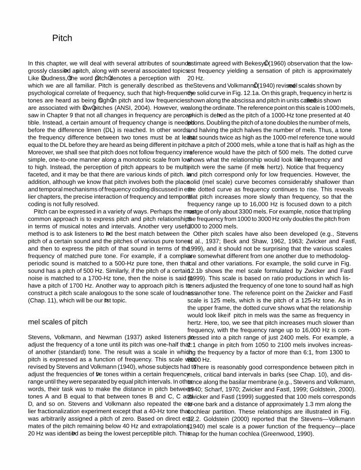
SFK SFK


12 Pitch

In this chapter, we will deal with several attributes of soundsgrossly classified as pitch, along with several associated topics.Like “loudness,” the word “pitch” denotes a perception withwhich we are all familiar. Pitch is generally described as thepsychological correlate of frequency, such that high-frequencytones are heard as being “high” in pitch and low frequenciesare associated with “low” pitches (ANSI, 2004). However, wesaw in Chapter 9 that not all changes in frequency are percep-tible. Instead, a certain amount of frequency change is neededbefore the difference limen (DL) is reached. In other words,the frequency difference between two tones must be at leastequal to the DL before they are heard as being different in pitch.Moreover, we shall see that pitch does not follow frequency in asimple, one-to-one manner along a monotonic scale from lowto high. Instead, the perception of pitch appears to be multi-faceted, and it may be that there are various kinds of pitch. Inaddition, although we know that pitch involves both the placeand temporal mechanisms of frequency coding discussed in ear-lier chapters, the precise interaction of frequency and temporalcoding is not fully resolved.

Pitch can be expressed in a variety of ways. Perhaps the mostcommon approach is to express pitch and pitch relationshipsin terms of musical notes and intervals. Another very usefulmethod is to ask listeners to find the best match between thepitch of a certain sound and the pitches of various pure tones,and then to express the pitch of that sound in terms of thefrequency of matched pure tone. For example, if a complexperiodic sound is matched to a 500-Hz pure tone, then thatsound has a pitch of 500 Hz. Similarly, if the pitch of a certainnoise is matched to a 1700-Hz tone, then the noise is said tohave a pitch of 1700 Hz. Another way to approach pitch is toconstruct a pitch scale analogous to the sone scale of loudness(Chap. 11), which will be our first topic.

mel scales of pitch

Stevens, Volkmann, and Newman (1937) asked listeners toadjust the frequency of a tone until its pitch was one-half thatof another (standard) tone. The result was a scale in whichpitch is expressed as a function of frequency. This scale wasrevised by Stevens and Volkmann (1940), whose subjects had toadjust the frequencies of five tones within a certain frequencyrange until they were separated by equal pitch intervals. In otherwords, their task was to make the distance in pitch betweentones A and B equal to that between tones B and C, C andD, and so on. Stevens and Volkmann also repeated the ear-lier fractionalization experiment except that a 40-Hz tone thatwas arbitrarily assigned a pitch of zero. Based on direct esti-mates of the pitch remaining below 40 Hz and extrapolations,20 Hz was identified as being the lowest perceptible pitch. This

estimate agreed with Bekesy’s (1960) observation that the low-est frequency yielding a sensation of pitch is approximately20 Hz.

Stevens and Volkmann’s (1940) revised mel scale is shown bythe solid curve in Fig. 12.1a. On this graph, frequency in hertz isshown along the abscissa and pitch in units called mels is shownalong the ordinate. The reference point on this scale is 1000 mels,which is defined as the pitch of a 1000-Hz tone presented at 40phons. Doubling the pitch of a tone doubles the number of mels,and halving the pitch halves the number of mels. Thus, a tonethat sounds twice as high as the 1000-mel reference tone wouldhave a pitch of 2000 mels, while a tone that is half as high as thereference would have the pitch of 500 mels. The dotted curveshows what the relationship would look like if frequency andpitch were the same (if mels = hertz). Notice that frequencyand pitch correspond only for low frequencies. However, thesolid (mel scale) curve becomes considerably shallower thanthe dotted curve as frequency continues to rise. This revealsthat pitch increases more slowly than frequency, so that thefrequency range up to 16,000 Hz is focused down to a pitchrange of only about 3300 mels. For example, notice that triplingthe frequency from 1000 to 3000 Hz only doubles the pitch from1000 to 2000 mels.

Other pitch scales have also been developed (e.g., Stevenset al., 1937; Beck and Shaw, 1962, 1963; Zwicker and Fastl,1999), and it should not be surprising that the various scalesare somewhat different from one another due to methodolog-ical and other variations. For example, the solid curve in Fig.12.1b shows the mel scale formulated by Zwicker and Fastl(1999). This scale is based on ratio productions in which lis-teners adjusted the frequency of one tone to sound half as highas another tone. The reference point on the Zwicker and Fastlscale is 125 mels, which is the pitch of a 125-Hz tone. As inthe upper frame, the dotted curve shows what the relationshipwould look like if pitch in mels was the same as frequency inhertz. Here, too, we see that pitch increases much slower thanfrequency, with the frequency range up to 16,000 Hz is com-pressed into a pitch range of just 2400 mels. For example, a2:1 change in pitch from 1050 to 2100 mels involves increas-ing the frequency by a factor of more than 6:1, from 1300 to8000 Hz.

There is reasonably good correspondence between pitch inmels, critical band intervals in barks (see Chap. 10), and dis-tance along the basilar membrane (e.g., Stevens and Volkmann,1940; Scharf, 1970; Zwicker and Fastl, 1999; Goldstein, 2000).Zwicker and Fastl (1999) suggested that 100 mels correspondsto one bark and a distance of approximately 1.3 mm along thecochlear partition. These relationships are illustrated in Fig.12.2. Goldstein (2000) reported that the Stevens–Volkmann(1940) mel scale is a power function of the frequency–placemap for the human cochlea (Greenwood, 1990).

218

SFK SFK


pitch

Figure 12.1 The relationship between frequency in hertz and pitch in melsbased on the findings of (a) Stevens and Volkmann (1940) and (b) Zwickerand Fastl (1999). The dotted curves labeled Mels = Hertz illustrate what therelationship would look like if pitch in mels was the same as frequency inhertz.

Figure 12.2 Illustration of the relationships between distance along thecochlear partition, pitch in mels, and critical band rate in barks. Notice theorientation of the basilar membrane. Based on scales by Zwicker and Fastl(1999).

beats, harmonics, and combination tones

The topics of audible beats, harmonics, and combination tonesare often discussed in the context of how we perceive frequency.We will divert our attention to these phenomena early in thischapter not only because they are topics of interest in their ownright, but also because they will be encountered as tools used tostudy various aspects of pitch perception in the discussion thatfollows.

We have seen in several contexts that a pure tone stimuluswill result in a region of maximal displacement along the basilarmembrane according to the place principle. Now, suppose thata second tone is added whose frequency (f2) is slightly higherthan that of the first sinusoid (f1), a in Fig. 12.3. If the frequencydifference between the two tones (f2 − f1) is small (say 3 Hz),then the two resulting excitation patterns along the cochlearpartition will overlap considerably so that the two stimuli willbe indistinguishable. However, the small frequency differencebetween the two tones will cause them to be in phase and out ofphase cyclically in a manner that repeats itself at a rate equal tothe frequency difference f2 − f1. Thus, a combination of a 1000-Hz tone and a 1003-Hz tone will be heard as a 1000-Hz tonethat beats, or waxes and wanes in level, at a rate of three timesper second. This perception of aural beats therefore reflects thelimited frequency-resolving ability of the ear.

If the two tones are equal in level, then the resulting beats willalternate between maxima that are twice the level of the originaltones and minima that are inaudible due to complete out-of-phase cancellation. Such beats are aptly called best beats. Tonesthat differ in level result in smaller maxima and incompletecancellation. As one would expect, the closer the levels of thetwo tones, the louder the beats will sound.

Figure 12.3 Tones of slightly different frequency, fl and f2, result in beatsthat fluctuate (wax and wane) at a rate equal to the difference between them(f2 − fl).

219

SFK SFK


chapter 12

As the frequency difference between the two tones widens,the beats become faster. These rapid amplitude fluctuationsare perceived as roughness rather than as discernible beats,as discussed earlier in the chapter. Further widening of thefrequency separation results in the perception of the two originaltones, in addition to which a variety of combination tones maybe heard. Combination tones, as well as aural harmonics, arethe result of nonlinear distortion in the ear.

Distortion products are those components at the output ofthe system that were not present at the input. A simple exampledemonstrates how nonlinear distortions produce outputs thatdiffer from the inputs. Consider two levers, one rigid and theother springy. The rigid lever represents a linear system. Ifone moves one arm of this lever up and down sinusoidally(the input), then the opposite arm will also move sinusoidally(the output). On the other hand, the springy lever illustratesthe response of a nonlinear system. A sinusoidal input to onearm will cause the other arm to move up and down, but therewill also be superimposed overshoots and undershoots in themotion, due to the “bounce” of the springy lever arms. Thus,the responding arm of the lever will move with a variety ofsuperimposed frequencies (distortion products) even thoughthe stimulus is being applied sinusoidally.

The simplest auditory distortion products are aural harmon-ics. As their name implies, these are distortion products, whichhave frequencies that are multiples of the stimulus frequency.For example, a stimulus frequency fl, when presented at a highenough level, will result in aural harmonics whose frequenciescorrespond to 2f1, 3f1, etc. Therefore, a 500-Hz primary tone(f1) will result in aural harmonics that are multiples of 500 Hz(2f1 = 1000 Hz, 3f1 = 1500 Hz, etc.). Two primary tones areillustrated in Fig. 12.4. The 800-Hz primary tone (f1) is associ-ated with an aural harmonic at 1600 Hz (2f1) and the 1000-Hzprimary (f2) is associated with the aural harmonic at 2000 Hz(2f2).

Figure 12.4 Examples of various auditory distortion products associatedwith stimulus (primary) tones of 800 Hz (f1) and 1000 Hz (f2).

If two primary tones f1 and f2 are presented together, nonlin-ear distortion will result in the production of various combi-nation tones due to the interactions among the primaries andthe harmonics of these tones. For convenience, we will call thelower-frequency primary tone f1 and the higher one f2. Thereare several frequently encountered combination tones that weshall touch upon. [See Boring (1942) and Plomp (1965) forinteresting historical perspectives, and Goldstein et al. (1978)for an classic review of the compatibility among physiologicaland psychoacoustic findings on combination tones.]

It is necessary to devise methods that enable us to quantifythe aspects of combination tones. A rather classical methodtakes advantage of the phenomenon of aural beats discussedabove. Recall that best beats occur when the beating tones areof equal amplitudes. Generally stated, this technique involvesthe presentation of a probe tone at a frequency close enoughto the combination tone of interest so that beats will occurbetween the combination and probe tones. Characteristics ofthe combination tone are inferred by varying the amplitude ofthe probe until the subject reports hearing best beats (i.e., max-imal amplitude variations). The best beats method, however,has been the subject of serious controversy (Lawrence and Yan-tis, 1956, 1957; Meyer, 1957; Chocolle and Legouix, 1957), andhas been largely replaced by a cancellation technique (Zwicker,1955; Goldstein, 1967; Hall, 1975). The cancellation methodalso employs a probe tone, but in this method, instead of ask-ing the subject to detect best beats, the probe tone is presentedat the frequency of the combination tone, and its phase andamplitude are adjusted until the combination tone is canceled.Cancellation occurs when the probe tone is equal in amplitudeand opposite in phase to the combination tone. The character-istics of the combination tone may then be inferred from thoseof the probe tone that cancels it. A lucid description of andcomparison among all of the major methods has been providedby Zwicker (1981).

Techniques such as these have resulted in various observationsabout the nature of combination tones. The simplest combina-tion tones result from adding or subtracting the two primarytones. The former is the summation tone (f1 + f2). As illus-trated in Fig. 12.4, primary tones of 800 Hz (f1) and 1000 Hz(f2) will result in the production of the summation tone 1000 +800 = 1800 Hz. We will say little about the summation toneexcept to point out that it is quite weak and not always audible.On the other hand, the difference tone (f2 − f1) is a significantcombination tone that is frequently encountered. For the 800-and 1000-Hz primaries in the figure, the difference tone wouldbe 1000 − 800 = 200 Hz. The difference tone is heard only whenthe primary tones are presented well above threshold. Plomp(1965) found, despite wide differences among his subjects, thatthe primaries had to exceed approximately 50 dB sensation levelin order for the difference tone to be detected.

The cubic difference tone (2f1 − f2) is another significantand frequently encountered combination tone. These distortionproducts appear to be generated by the active processes in the

220

SFK SFK


pitch

cochlea and have already been encountered when distortion-product otoacoustic emissions were discussed in Chapter 4. Forthe 800- and 1000-Hz primary tones in Fig. 12.4, the resultingcubic difference tone is 2(800) − 1000 = 600 Hz. A particularlyinteresting aspect of the cubic difference tone is that it is audibleeven when the primaries are presented at low sensation levels.For example, Smoorenburg (1972) demonstrated that 2f1 − f2

is detectable when the primaries are only 15 to 20 dB abovethreshold, although he did find variations among subjects.

When the primary tones exceed 1000 Hz, the level of thedifference tone f2 − f1 tends to be rather low (approximately50 dB below the level of the primaries); in contrast, the differ-ence tone may be as little as 10 dB below the primaries whenthey are presented below 1000 Hz (Zwicker, 1955; Goldstein,1967; Hall, 1972a, 1972b). On the other hand, the cubic differ-ence tone 2f1 − f2 appears to be limited to frequencies below thelower primary f1, and its level increases as the ratio f2/f1 becomessmaller (Goldstein, 1967; Hall, 1972a, 1972b, 1975; Smooren-burg, 1972). Furthermore, the cubic difference tone has beenshown to be within approximately 20 dB of the primaries whenthe frequency ratio of f2 and f1 is on the order of 1.2:1 (Hall,1972a; Smoorenburg, 1972). The student with an interest inthis topic should also refer to the work of Zwicker (1981) andHumes (1985a, 1985b) for insightful reviews and analyses of thenature of combination tones.

An interesting attribute of combination tones is theirstimulus-like nature. In other words, the combination tonesthemselves interact with primary (stimulus) tones as well as withother combination tones to generate beats and higher-order(secondary) combination tones, such as 3f1–2f2 and 4f1–2f2.Goldstein et al. (1978) have shown that such secondary com-bination tones have properties similar to those of combinationtones generated by the primaries.

musical pitch

As already mentioned, pitch is usually considered in musicalterms. Here, tones are separated by perceptually relevant inter-vals. The intervals themselves are based on ratios between thefrequencies of the tones (f2/f1) rather than on the differencesbetween them (f2 − f1). For example, the principal interval isthe octave, which is a 2:1 frequency ratio. It is helpful to discussmusical pitch scales with reference to Fig. 12.5, which depictsa standard piano keyboard with 88 keys.1The white keys aregrouped in sets of 7, which are labeled in the order

C, D, E , F , G, A, B, next C .

The frequency of a particular C is exactly twice the frequencyof the prior one so that each octave is divided into seven inter-vals. This order is called the major scale and is also associated

1 For an online application that provides the musical note correspond-ing to a given frequency, see Botros (2001).

Figure 12.5 The musical scaling of pitch intervals (equal temperament)with reference to the keys on the piano keyboard.

with the familiar singing scale (do, re, mi, fa, so, la, ti, do).Octaves can also be divided into 12 intervals, which are labeledin the order

C, C#2, D, D#, E , F , F #, G, G#, A, A#, B, next C .

2The symbol # is read as “sharp”; hence, C# is C-sharp, D# is D-sharp,etc.

221

SFK SFK


chapter 12

These 12-note groupings form the chromatic scale and corre-spond to the sets of 12 (7 white and 5 black) keys on the piano.Intervals within octaves are discussed below.

The musical scaling of pitch may be viewed in terms of twoattributes, height and chroma (Revesz, 1913; Bachem, 1948,1950; Shepard, 1964). Tone height pertains to the monotonicincrease from low to high pitch as frequency rises, and it is rep-resented by the vertical arrow in Fig. 12.6. It has been suggestedthat mel scales of pitch are related to the dimension of toneheight (Ward and Burns, 1982; Goldstein, 2000). In contrast,chroma is related to a perceptual similarity or sameness amongtones that are separated by 2:1 frequency intervals, called octaveequivalence. As a result, these tones have the same pitch class orchroma and share the same name. For example, every doublingof frequency beginning with 27.5 Hz in Fig. 12.5 produces anote called A, labeled A0 at 27.5 Hz through A7 at 3520 Hz.(The note called A4, which has a frequency of 440 Hz, is mostcommonly used standard or reference pitch for musical tuning.)Similarly, every doubling of frequency starting with 32.703 Hzin Fig. 12.5 is a note called C, from C1 at (32.703 Hz) to C8(4186 Hz). It should now be apparent that chroma changes fromC through B within each octave, and that this patterns recyclesat a higher frequency beginning at the next C. For example, C1,D1#, and F1 differ in terms of chroma, whereas A3, A5, and A6have the same chroma but different tone heights. Thus, chromais conceptualized in the form of the helix in Fig. 12.6.

Figure 12.6 Chroma changes going around the helix, and this pattern oftone classes is repeated every octave. Tone height increases monotonicallywith frequency, as suggested by vertical arrow. Notice that tones with thesame chroma and different tone heights appear above each other. Based onShepard’s (1964) conceptualization.

It is interesting to note in this context that Demany andArmand (1984) found that 3-month-old infants were less sen-sitive to frequency shifts of exactly one octave than to smaller orlarger shifts. These findings provide evidence of octave equiva-lence, supporting the existence of chroma perception in babies.Moreover, a typographically organized representation of musi-cal keys in the rostromedial prefrontal cortex was identifiedby functional magnetic resonance imaging (fMRI) in musi-cally experienced listeners performing musical perception tasks(Janata et al., 2002).

Just as there is a 2:1 frequency ratio between one C andthe next one, the intervals within an octave also take theform of frequency ratios; however, a variety of different scal-ing schemes are available. For example, the just (diatonic)scale is based on three-note groupings (triads) having fre-quency ratios of 4:5:6, in order to maximize the consonanceof thirds, fourths, and fifths. The Pythagorean scale concen-trates on fourths and fifths. In contrast, the equal temperamentscale employs logarithmically equal intervals. These scales arecompared in Table 12.1. Each scale has advantages and lim-itations in music, although we will concentrate on the equaltemperament scale. Several informative discussions of musicalscales are readily available (e.g., Campbell and Greated, 1987;Rossing, 1989).

The equal temperament scale divides the octave into logarith-mically equal semitone intervals corresponding to the group-ings of 12 (7 white and 5 black) keys on the piano (Fig. 12.5).In order to split the 2:1 frequency ratio of a whole octave into12 logarithmically equal intervals from C to the next C, eachinterval must be a frequency ratio of 21/12:1 or 1.0595:1 (anincrement of roughly 6%). For example, the semitone intervalfrom C to C# constitutes a frequency ratio of 21/12:1, which isthe equivalent to 1.0595:1; two semitones from C to D is (21/12 ×21/12):1 = 22/12:1 = 1.12246:1; and 12 semitones correspondingto one octave from one C to the next C is 212/12:1 = 2:1.

Each equal temperament semitone is further divided into 100logarithmically equal intervals called cents. The use of centsnotation often facilitates pitch scaling. For example, cents nota-tion makes it easier to compare the musical intervals involvedin the equal temperament, just, and Pythagorean scales (Table12.1). Since there are 100 cents per semitone and 12 semitonesper octave, there are 1200 cents per octave. Thus, 1 cent corre-sponds to a frequency ratio3 interval of 21/1200:1 or 1.00058:1,which is an increment of less than 0.06%. This is considerablysmaller than the relative difference limen for frequency (f/f)of about 0.002 encountered in Chapter 9, which corresponds to0.2%. In this sense, it takes more than a few cents to achieve aperceptible pitch change. In fact, a study of perceptible tuningchanges by Hill and Summers (2007) found that the difference

3 A frequency ratio (f2/f1) can be converted into cents (c) with theformula c = 1200 × log2(f2/f1); or c = 3986.31 × log10(f2/f1) if oneprefers to use common logarithms.

222

SFK SFK


pitch

Table 12.1 Frequency Ratios and Cents for Musical Intervals with the Equal Temperament, Just, and Pythagorean Scales

Interval Frequency ratio (f2/f1) Cents

From C Equal Equalto . . . Name temperament Just Pythagorean temperament Just Pythagorean

C (itself) Unison 20 = 1.0595 1/1 = 1.0000 1/1 = 1.0000 0 0 0C# Minor second 21/12 = 1.0595 16/15 = 1.0667 256/243 = 1.0535 100 112 90D Major second 22/12 = 1.1225 10/9 = 1.1111 9/8 = 1.1250 200 182 204D# Minor third 23/12 = 1.1892 6/5 = 1.2000 32/27 = 1.1852 300 316 294E Major third 24/12 = 1.2599 5/4 = 1.2500 81/64 = 1.2656 400 386 408F Fourth 25/12 = 1.3348 4/3 = 1.3333 4/3 = 1.3333 500 498 498F# Tritone 26/12 = 1.4142 45/32 = 1.4063 1024/729 = 1.4047 600 590 588G Fifth 27/12 = 1.4983 3/2 = 1.5000 3/2 = 1.5000 700 702 702G# Minor sixth 28/12 = 1.5874 8/5 = 1.6000 128/81 = 1.5802 800 814 792A Major sixth 29/12 = 1.6818 5/3 = 1.6667 27/16 = 1.6875 900 884 906A# Minor seventh 210/12 = 1.7818 7/4 = 1.7500 16/9 = 1.7778 1000 969 996B Major seventh 211/12 = 1.8877 15/8 = 1.8750 243/128 = 1.8984 1100 1088 1110(Next) C Octave 212/12 = 2.0000 2/1 = 2.0000 2/1 = 2.0000 1200 1200 1200

limen is about 10 cents and that category widths approximated70 cents.

Recall that frequency is coded by both temporal and placemechanisms, with the former taking on a more important rolefor lower frequencies and the latter predominating for higherfrequencies. Since auditory nerve firing patterns reflect phaselocking for stimulus frequencies as high as roughly 5000 Hz(Chap. 5), it would appear that the temporal mechanism isoperative up to about this frequency. With these points in mind,it is interesting to be aware of several lines of evidence indicatingthat the perception of pitch chroma is limited to the frequenciesbelow roughly 5000 Hz, although pitch height continues toincrease for higher frequencies.

The restriction of chroma perception to 5000 Hz and belowhas been shown in various ways. Bachem (1948) and Ohgushiand Hatoh (1989) found that listeners with absolute pitch couldidentify the chroma of pure tones was limited to the frequenciesup to about 4000 to 5000 Hz. Absolute (perfect) pitch is the veryrare ability to accurately identify or produce pitches in isolation,that is, without having to rely on a reference tone (Ward, 1963a,1963b). Ward (1954) found that musicians could adjust thefrequency of a (higher) tone to be an octave above another(lower) tone, providing both tones were less than 5500 Hz.In addition, Atteave and Olson (1971) found that the ability ofmusicians to transpose a familiar three-tone sequence (in effect,a simple melody) deteriorated above about 5000 Hz. Semal andDemany (1990) asked musicians to transpose a sequence of twopure tones until the higher tone in the pair was perceived to be“just above the upper limit of musical pitch.” On average, thislimit occurred at approximately 4700 Hz.

Consonance and DissonanceIn addition to their perceptual similarity, two simultaneouslypresented tones differing by octave intervals are also perceived

as being consonant. Such combinations of two or more simulta-neous tones are often referred to as chords. Consonance simplymeans that when two sounds are presented together they resultin a pleasant perception; in contrast, dissonance refers to soundsthat appear unpleasant when presented together. Consonanceversus dissonance for pairs of tones depends upon the differencebetween the two frequencies, and how well these frequenciescan be resolved by the ear (Plomp and Levelt, 1965; Plomp andSteeneken, 1968; Kameoka and Kuriyagawa, 1969; Schellenbergand Trehub, 1994). Dissonance occurs when two tones are closeenough in frequency to be less than a critical band apart. In thiscase, they are not completely resolved because their vibrationpatterns interact along the basilar membrane, leading to a sen-sation of roughness due to rapid beats between the two tones.This roughness is perceived as being unpleasant or dissonant. Incontrast, the two tones will not interact if they are separated bymore than a critical band, in which case there is no roughness,and if they are experienced as consonant.

Complex tones, such as musical notes, contain other fre-quencies in addition to their fundamentals. In music, the termspartials and overtones are used to refer these frequencies andare usually used as synonyms for harmonics. (However, oneshould be aware that many instruments, such as chimes andpianos, also produce “inharmonic” partials at frequencies thatare not exact multiples of the fundamental). Thus, dissonancecan be introduced by interactions among these partials, as wellas between the fundamentals. With these points in mind, conso-nance is associated with notes composed of frequencies that arerelated by simple (small) integer ratios, such as 2:1 (octave, e.g.,C4 and C5), 3:2 (perfect fifth, e.g., C4 and G4), and 4:3 (perfectfourth, C4 and F4). In contrast, dissonance occurs when theirfrequencies are related by complex (large) ratios such as 45:32(tritone, e.g., F3 and B3). In terms of the musical intervals,two tones will be consonant when they are separated by 0 and

223

SFK SFK


chapter 12

12 semitones (i.e., unison and octave), and dissonance occurswhen the two notes are separated by intervals of 1–2, 6, and10–11 semitones.

In contrast to two-tone combinations, the perception ofchords becomes more involved when three or more tones areinvolved. A consonant three-tone chord (triad) is perceived asbeing stable when the spacing between the low and middle tonesis different than the interval between the middle and high tones.However, tension is experienced when these two intervals areequal, in which case the chord is perceived as being unstable orambiguity even though there is no dissonance (Meyer, 1956).Cook and colleagues have shown that the harmonious percep-tion of triads depends on the effects of both dissonance andtension involving the fundamentals and partials of the notesthat make up the chord (Cook, 2001; Cook and Fujisawa, 2006;Cook and Hayashi, 2008).

pitch and intensity

In a classic study by Stevens (1935), subjects were asked to adjustthe intensity of a tone until it had the same pitch as a standardtone of slightly different frequency. Results for one subject whowas a “good responder” showed that increasing the intensity ofthe tone increased its pitch for frequencies 3000 Hz and above,and lowered its pitch for frequencies 1000 Hz and below. Thepitch stayed essentially constant as intensity was varied for tonesbetween 1000 and 3000 Hz.

Although Stevens’ study has frequently been cited to illustratehow intensity affects pitch, subsequent studies did not findlarge pitch changes associated with intensity increases (Morganet al., 1951; Ward, 1953; Cohen, 1961; Terhardt, 1979; Zwickerand Fastl, 1999). Figure 12.7 shows how the pitches of puretones change as the sound pressure level is increased abovea reference level of 40 dB (Terhardt, 1979; Zwicker and Fastl,1999). Increasing level does cause pitch to fall for low-frequencytones and to rise for high-frequency tones. However, the sizesof these pitch shifts are quite small, amounting to less than 2%to 3% as the level increases from 40 to 80 dB.

pitch of complex sounds

Pitch perception is not limited to pure tones. On the contrary,real-world sounds are complex, and common experience revealsthat pitch perceptions are associated with them. When dealingwith aperiodic sounds, the perceived pitch is related to the spec-trum of the noise (Small and Daniloff, 1967; Fastl, 1971). Ingeneral, the pitches of low- and high-pass noises are related totheir cut-off frequencies, and the pitches of band-pass noisesare associated with their center frequencies. Moreover, the dis-tinctiveness of the pitch sensation (pitch strength) elicited bynarrow bands of noise can be quite strong, but it lessens as thebandwidth gets wider and becomes quite weak when the criticalband is exceeded.

Figure 12.7 Change in pitch (pitch shift) compared to the pitch at 40 dBSPL for tones presented at sound pressure levels of 50, 60, 70, and 80 dB,at selected frequencies. Pitch shifts are upward for high frequencies anddownward for low frequencies by about 2% to 3% or less. Based on data byZwicker and Fastl (1999).

For complex periodic sounds, such as those produced bythe human voice and many musical instruments, consider, forexample, a woman’s voice that is composed of many harmonicsof 220 Hz (220, 440, 660, 880, 1100, 1320 Hz, etc.). Com-paring the pitch of her voice to various pure tones, a matchwould be made with a 220-Hz tone. Here, the pitch is thatof the fundamental frequency and is dominated by its lowerharmonics. Classical experiments emphasized the importanceof the first five harmonics in determining the pitch of com-plex tones (e.g., Plomp, 1964, 1967; Ritsma, 1967; Bilsen andRitsma, 1967). However, the dominant range does not appearto be a fixed, and it is affected by factors such as the frequencyof the fundamental, the levels of the harmonics, and duration(e.g., Patterson and Wightman, 1976; Moore et al., 1984, 1985;Gockel et al., 2005, 2007).

What is odd, however, is that woman just described wouldstill have a vocal pitch of 220 Hz even if the 220-Hz fundamentalfrequency is missing (in which case the lowest harmonic actuallypresent would be 440 Hz). Demonstrating this phenomenondoes not even require a trip to the laboratory—it is actuallyan every day occurrence because telephones do not provide anyfrequencies below about 300 Hz. This perception of the missingfundamental was first described by Seebeck in 1841, and wasreintroduced a century later by Schouten (1940).

The missing fundamental is perhaps the best-known exampleof what has descriptively been called periodicity pitch, virtualpitch, residue pitch, low pitch, and repetition pitch. Anothercase is provided by signals that are periodically interruptedor amplitude modulated (Thurlow and Small, 1955; Burnsand Viemeister, 1976, 1981). For example, Thurlow and Small(1955) found that if a high-frequency tone is interrupted peri-odically, then the subject will perceive a pitch corresponding to

224

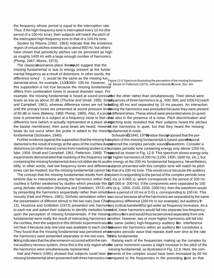
SFK SFK


pitch

the frequency whose period is equal to the interruption rate.Thus, if the high-frequency tone is interrupted every 10 ms (theperiod of a 100-Hz tone), then subjects will match the pitch ofthe interrupted high-frequency tone to that of a 100-Hz tone.

Studies by Ritsma (1962, 1963) indicate that the existenceregion of virtual pitches extends up to about 800 Hz, but othershave shown that periodicity pitches can be perceived as highas roughly 1400 Hz with a large enough number of harmonics(Plomp, 1967; Moore, 1973).

The classical resonance-place theory would suggest that themissing fundamental is due to energy present at the funda-mental frequency as a result of distortions. In other words, thedifference tone f2 − f1 would be the same as the missing fun-damental since, for example, 1100 − 1000 = 100 Hz. However,this supposition is not true because the missing fundamentaldiffers from combination tones in several dramatic ways. Forexample, the missing fundamental is heard at sound pressurelevels as low as about 20 dB (Thurlow and Small, 1955; Smalland Campbell, 1961), whereas difference tones are not hearduntil the primary tones are presented at sound pressure levelsof 60 dB or more (Bekesy, 1960; Plomp, 1965). Also, if a probetone is presented to a subject at a frequency close to that of adifference tone (which is actually represented at a place alongthe basilar membrane), then aural beats are heard. However,beats do not occur when the probe is added to the missingfundamental (Schouten, 1940).

Further evidence against the supposition that the missing fun-damental is the result of energy at the apex of the cochlea due todistortions (or other means) comes from masking studies (Lick-lider, 1954; Small and Campbell, 1961; Patterson, 1969). Theseexperiments demonstrated that masking of the frequency rangecontaining the missing fundamental does not obliterate its audi-bility. In other words, real low-frequency tones and differencetones can be masked, but the missing fundamental cannot be.

The concept that the missing fundamental results from dis-tortions due to interactions among the harmonics within thecochlea is further weakened by studies which preclude this byusing dichotic stimulation (Houtsma and Goldstein, 1972) orby presenting the harmonics sequentially rather than simulta-neously (Hall and Peters, 1981). Dichotic stimulation refers tothe presentation of different stimuli to the two ears (see Chap.13). Houtsma and Goldstein (1972) presented one harmonicto each ear and asked their subjects to identify melodies basedupon the perception of missing fundamentals. If the missingfundamental were really the result of interacting harmonics inthe cochlea, then the subjects in this dichotic experiment wouldnot hear it because only one tone was available to each cochlea.They found that the missing fundamental was perceived whenthe harmonics were presented separately to the two ears. Thisfinding indicates that the phenomenon occurred within the cen-tral auditory nervous system, since this is the only region wherethe harmonics were simultaneously represented.

Hall and Peters (1981) showed that subjects could hear themissing fundamental when presented with three harmonics one

Figure 12.8 Spectrum illustrating the perception of the missing fundamen-tal. Based on Patterson (1973), with permission of J. Acoust. Soc. Am.

after the other rather than simultaneously. Their stimuli weresequences of three harmonics (e.g., 600, 800, and 1000 Hz) eachlasting 40 ms and separated by 10 ms pauses. An interactionamong the harmonics was precluded because they were presentat different times. These stimuli were presented alone (in quiet)and also in the presence of a noise. Pitch discrimination andmatching tests revealed that their subjects heard the pitchesof the harmonics in quiet, but that they heard the missingfundamental in noise.

Schouten’s (1940, 1970) residue theory proposed that the per-ception of this missing fundamental is based upon the temporalpattern of the complex periodic sound’s waveform. Consider acomplex periodic tone containing energy only above 1200 Hz,spaced as shown in Fig. 12.8. This spectrum shows energy onlyfor higher harmonics of 200 Hz (1200, 1400, 1600 Hz, etc.), butno energy at the 200-Hz fundamental frequency. Nevertheless,subjects presented with this complex tone will match its pitchto that of a 200-Hz tone. This would occur because the auditorysystem is responding to the period of the complex periodic tone(5 ms or 0.005 s), which corresponds to the period of 200 Hz(1/0.005 s = 200 Hz). If the components were separated by 100Hz (e.g., 2000, 2100, 2200, 2300 Hz), then the waveform wouldhave a period of 10 ms or 0.01 s, corresponding to 100 Hz. Thiscan occur because all of the harmonics are separated by the samefrequency difference (200 Hz in our example), but auditory fil-ters (critical bandwidths) get wider as frequency increases. As aresult, lower harmonics would fall into separate low-frequencyauditory filters and would thus be perceived separately from oneanother. However, two or more higher harmonics will fall intothe same (wider) high-frequency auditory filter. Interferencebetween the harmonics within an auditory filter constitutes acomplex periodic wave that repeats itself over time at the rateof the fundamental.

Raising each of the frequencies making up the complex bythe same increment causes a slight increase in the pitch of themissing fundamental, as illustrated in Fig. 12.9. Here, the com-ponents of the complex sound have been increased by 60 Hzcompared to the frequencies in the preceding figure so that

225

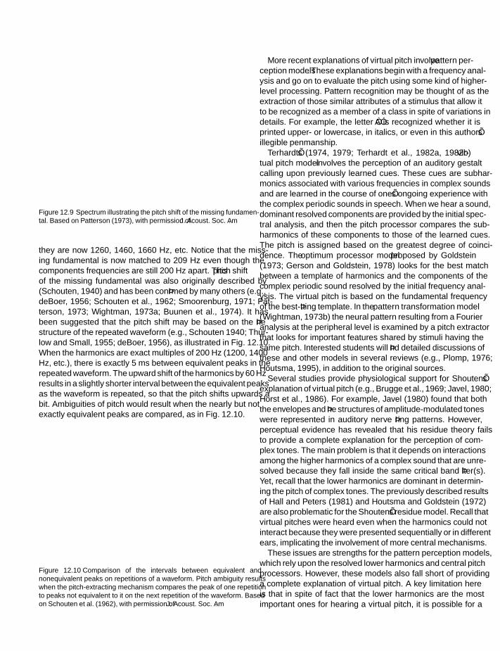
SFK SFK


chapter 12

Figure 12.9 Spectrum illustrating the pitch shift of the missing fundamen-tal. Based on Patterson (1973), with permission of J. Acoust. Soc. Am.

they are now 1260, 1460, 1660 Hz, etc. Notice that the miss-ing fundamental is now matched to 209 Hz even though thecomponents frequencies are still 200 Hz apart. This pitch shiftof the missing fundamental was also originally described by(Schouten, 1940) and has been confirmed by many others (e.g.,deBoer, 1956; Schouten et al., 1962; Smoorenburg, 1971; Pat-terson, 1973; Wightman, 1973a; Buunen et al., 1974). It hasbeen suggested that the pitch shift may be based on the finestructure of the repeated waveform (e.g., Schouten 1940; Thur-low and Small, 1955; deBoer, 1956), as illustrated in Fig. 12.10.When the harmonics are exact multiples of 200 Hz (1200, 1400Hz, etc.), there is exactly 5 ms between equivalent peaks in therepeated waveform. The upward shift of the harmonics by 60 Hzresults in a slightly shorter interval between the equivalent peaksas the waveform is repeated, so that the pitch shifts upwards abit. Ambiguities of pitch would result when the nearly but notexactly equivalent peaks are compared, as in Fig. 12.10.

Figure 12.10 Comparison of the intervals between equivalent andnonequivalent peaks on repetitions of a waveform. Pitch ambiguity resultswhen the pitch-extracting mechanism compares the peak of one repetitionto peaks not equivalent to it on the next repetition of the waveform. Basedon Schouten et al. (1962), with permission of J. Acoust. Soc. Am.

More recent explanations of virtual pitch involve pattern per-ception models. These explanations begin with a frequency anal-ysis and go on to evaluate the pitch using some kind of higher-level processing. Pattern recognition may be thought of as theextraction of those similar attributes of a stimulus that allow itto be recognized as a member of a class in spite of variations indetails. For example, the letter “A” is recognized whether it isprinted upper- or lowercase, in italics, or even in this author’sillegible penmanship.

Terhardt’s (1974, 1979; Terhardt et al., 1982a, 1982b) vir-tual pitch model involves the perception of an auditory gestaltcalling upon previously learned cues. These cues are subhar-monics associated with various frequencies in complex soundsand are learned in the course of one’s ongoing experience withthe complex periodic sounds in speech. When we hear a sound,dominant resolved components are provided by the initial spec-tral analysis, and then the pitch processor compares the sub-harmonics of these components to those of the learned cues.The pitch is assigned based on the greatest degree of coinci-dence. The optimum processor model proposed by Goldstein(1973; Gerson and Goldstein, 1978) looks for the best matchbetween a template of harmonics and the components of thecomplex periodic sound resolved by the initial frequency anal-ysis. The virtual pitch is based on the fundamental frequencyof the best-fitting template. In the pattern transformation model(Wightman, 1973b) the neural pattern resulting from a Fourieranalysis at the peripheral level is examined by a pitch extractorthat looks for important features shared by stimuli having thesame pitch. Interested students will find detailed discussions ofthese and other models in several reviews (e.g., Plomp, 1976;Houtsma, 1995), in addition to the original sources.

Several studies provide physiological support for Shouten’sexplanation of virtual pitch (e.g., Brugge et al., 1969; Javel, 1980;Horst et al., 1986). For example, Javel (1980) found that boththe envelopes and fine structures of amplitude-modulated toneswere represented in auditory nerve firing patterns. However,perceptual evidence has revealed that his residue theory failsto provide a complete explanation for the perception of com-plex tones. The main problem is that it depends on interactionsamong the higher harmonics of a complex sound that are unre-solved because they fall inside the same critical band filter(s).Yet, recall that the lower harmonics are dominant in determin-ing the pitch of complex tones. The previously described resultsof Hall and Peters (1981) and Houtsma and Goldstein (1972)are also problematic for the Shouten’s residue model. Recall thatvirtual pitches were heard even when the harmonics could notinteract because they were presented sequentially or in differentears, implicating the involvement of more central mechanisms.

These issues are strengths for the pattern perception models,which rely upon the resolved lower harmonics and central pitchprocessors. However, these models also fall short of providinga complete explanation of virtual pitch. A key limitation hereis that in spite of fact that the lower harmonics are the mostimportant ones for hearing a virtual pitch, it is possible for a

226

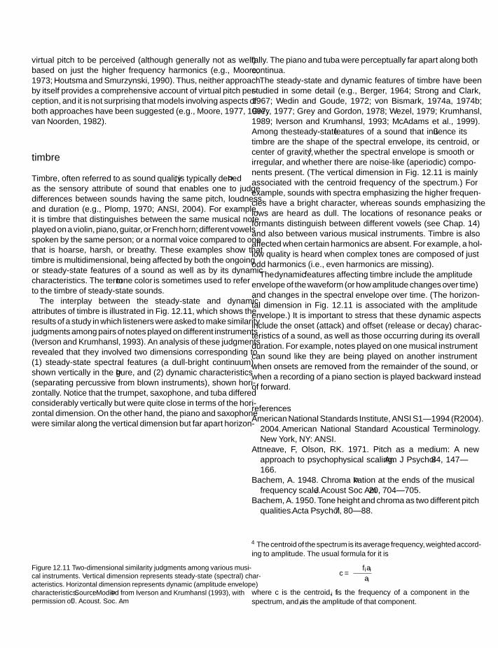
SFK SFK


pitch

virtual pitch to be perceived (although generally not as well)based on just the higher frequency harmonics (e.g., Moore,1973; Houtsma and Smurzynski, 1990). Thus, neither approachby itself provides a comprehensive account of virtual pitch per-ception, and it is not surprising that models involving aspects ofboth approaches have been suggested (e.g., Moore, 1977, 1997;van Noorden, 1982).

timbre

Timbre, often referred to as sound quality, is typically definedas the sensory attribute of sound that enables one to judgedifferences between sounds having the same pitch, loudness,and duration (e.g., Plomp, 1970; ANSI, 2004). For example,it is timbre that distinguishes between the same musical noteplayed on a violin, piano, guitar, or French horn; different vowelsspoken by the same person; or a normal voice compared to onethat is hoarse, harsh, or breathy. These examples show thattimbre is multidimensional, being affected by both the ongoingor steady-state features of a sound as well as by its dynamiccharacteristics. The term tone color is sometimes used to referto the timbre of steady-state sounds.

The interplay between the steady-state and dynamicattributes of timbre is illustrated in Fig. 12.11, which shows theresults of a study in which listeners were asked to make similarityjudgments among pairs of notes played on different instruments(Iverson and Krumhansl, 1993). An analysis of these judgmentsrevealed that they involved two dimensions corresponding to(1) steady-state spectral features (a dull-bright continuum),shown vertically in the figure, and (2) dynamic characteristics(separating percussive from blown instruments), shown hori-zontally. Notice that the trumpet, saxophone, and tuba differedconsiderably vertically but were quite close in terms of the hori-zontal dimension. On the other hand, the piano and saxophonewere similar along the vertical dimension but far apart horizon-

Figure 12.11 Two-dimensional similarity judgments among various musi-cal instruments. Vertical dimension represents steady-state (spectral) char-acteristics. Horizontal dimension represents dynamic (amplitude envelope)characteristics. Source: Modified from Iverson and Krumhansl (1993), withpermission of J. Acoust. Soc. Am.

tally. The piano and tuba were perceptually far apart along bothcontinua.

The steady-state and dynamic features of timbre have beenstudied in some detail (e.g., Berger, 1964; Strong and Clark,1967; Wedin and Goude, 1972; von Bismark, 1974a, 1974b;Grey, 1977; Grey and Gordon, 1978; Wezel, 1979; Krumhansl,1989; Iverson and Krumhansl, 1993; McAdams et al., 1999).Among the steady-state features of a sound that influence itstimbre are the shape of the spectral envelope, its centroid, orcenter of gravity,4 whether the spectral envelope is smooth orirregular, and whether there are noise-like (aperiodic) compo-nents present. (The vertical dimension in Fig. 12.11 is mainlyassociated with the centroid frequency of the spectrum.) Forexample, sounds with spectra emphasizing the higher frequen-cies have a bright character, whereas sounds emphasizing thelows are heard as dull. The locations of resonance peaks orformants distinguish between different vowels (see Chap. 14)and also between various musical instruments. Timbre is alsoaffected when certain harmonics are absent. For example, a hol-low quality is heard when complex tones are composed of justodd harmonics (i.e., even harmonics are missing).

The dynamic features affecting timbre include the amplitudeenvelope of the waveform (or how amplitude changes over time)and changes in the spectral envelope over time. (The horizon-tal dimension in Fig. 12.11 is associated with the amplitudeenvelope.) It is important to stress that these dynamic aspectsinclude the onset (attack) and offset (release or decay) charac-teristics of a sound, as well as those occurring during its overallduration. For example, notes played on one musical instrumentcan sound like they are being played on another instrumentwhen onsets are removed from the remainder of the sound, orwhen a recording of a piano section is played backward insteadof forward.

referencesAmerican National Standards Institute, ANSI S1–1994 (R2004).

2004. American National Standard Acoustical Terminology.New York, NY: ANSI.

Attneave, F, Olson, RK. 1971. Pitch as a medium: A newapproach to psychophysical scaling. Am J Psychol 84, 147–166.

Bachem, A. 1948. Chroma fixation at the ends of the musicalfrequency scale. J Acoust Soc Am 20, 704–705.

Bachem, A. 1950. Tone height and chroma as two different pitchqualities. Acta Psychol 7, 80–88.

4 The centroid of the spectrum is its average frequency, weighted accord-ing to amplitude. The usual formula for it is

c =∑

fiai∑ai

where c is the centroid, fi is the frequency of a component in thespectrum, and ai is the amplitude of that component.

227

SFK SFK


chapter 12

Beck, J, Shaw, WA. 1962. Magnitude estimations of pitch. JAcoust Soc Am 34, 92–98.

Beck, J, Shaw, WA. 1963. Single estimates of pitch magnitude. JAcoust Soc Am 35, 1722–1724.

Bekesy, G. 1960. Experiments in Hearing . New York, NY:McGraw-Hill.

Berger, KW. 1964. Some factors in the recognition of timbre. JAcoust Soc Am 36, 1888–1891.

Bilsen, FA, Ritsma, RJ. 1967. Repetition pitch mediated by tem-poral fine structure at dominant spectral regions. Acustica19, 114–116.

Boring, EG. 1942. Sensation and Perception in the History ofExperimental Psychology. New York, NY: Appleton-Century.

Botros, A. 2001. Frequency to Musical Note Converter. Availableat http://www.phys.unsw.edu.au/music/note/.

Brugge, JF, Anderson, DJ, Hind, JE, Rose, JE. 1969. Time struc-ture of discharges in singled auditory nerve fibers of thesquirrel monkey in response to complex periodic sounds. JNeurophysiol 32, 386–401.

Burns, EM, Viemeister, NF. 1976. Nonspectral pitch. J AcoustSoc Am 60, 863–869.

Burns, EM, Viemeister, NF. 1981. Played-again SAM: Furtherobservations on the pitch of amplitude-modulated noise. JAcoust Soc Am 70, 1655–1660.

Buunen, TJF, Festen, JM, Bilsen, FA, Van Den Brink, G. 1974.Phase effects in a three-component signal. J Acoust Soc Am55, 297–303.

Campbell, M, Greated, C. 1987. The Musician’s Guide to Acous-tics. New York, NY: Schirmer.

Chocolle, R, Legouix, JP. 1957. On the inadequacy of the methodof beats as a measure of aural harmonics. J Acoust Soc Am 29,749–750.

Cohen, A. 1961. Further investigations of the effects of intensityupon the pitch of pure tones. J Acoust Soc Am 33, 1363–1376.

Cook, ND. 2001. Explaining harmony. The roles of intervaldissonance and chordal tension. Ann N Y Acad Sci 930(1),382–385.

Cook, ND, Fujisawa, TX. 2006. The psychophysics of harmonyperception: Harmony is a three-tone phenomenon. EmperMus Rev 1, 106–126.

Cook, ND, Hayashi, T. 2008. The psychoacoustics of harmonyperception. Am Sci 96, 311–319.

deBoer, E. 1956. On the residue in hearing . Ph.D. Dissertation.Amsterdam, The Netherlands: University of Amsterdam.

Demany, L, Armand, F. 1984. The perceptual reality of tonechroma in early infancy. J Acoust Soc Am 76, 57–66.

Fastl, H. 1971. Uber Tonhohenempfindungen bei Rauschen.Acustica 25, 350–354.

Gerson, A, Goldstein, JL. 1978. Evidence for a general templatein central optimal processing for pitch of complex tones. JAcoust Soc Am 63, 498–510.

Gockel, HE, Carlyon, RP, Plack, CJ. 2005. Dominance region forpitch: Effects of duration and dichotic presentation. J AcoustSoc Am 117, 1326–1336.

Gockel, HE, Moore, BCJ, Carlyon, RP, Plack, CJ. 2007. Effectsof duration on the frequency discrimination of individualpartials in a complex tone and on the discrimination of fun-damental frequency. J Acoust Soc Am 121, 373–382.

Goldstein, JL. 1967. Auditory nonlinearity. J Acoust Soc Am 41,676–689.

Goldstein, JL. 1973. An optimum processor theory for the cen-tral formation of the pitch of complex tones. J Acoust Soc Am54, 1496–1516.

Goldstein, JL. 2000. Pitch perception. In: AE Kazdin (ed.), Ency-clopedia of Psychology, Vol. 6. Oxford, UK: Oxford UniversityPress, 201–210.

Goldstein, JL, Buchsbaum, G, Furst, M. 1978. Compatibilitybetween psychophysical and physiological measurements ofaural combination tones. J Acoust Soc Am 63, 474–485.

Greenwood, DD. 1990. A cochlear frequency-position functionfor several species—29 years later. J Acoust Soc Am 87, 2592–2605.

Grey, JM. 1977. Multidimensional perceptual scaling of musicaltimbres. J Acoust Soc Am 61, 1270–1277.

Grey, JM, Gordon, JW. 1978. Perceptual effects of spectralmodifications of musical timbres. J Acoust Soc Am 63,1493–1500.

Hall, JL. 1972a. Auditory distortion products f2–fl and 2f1–f2. JAcoust Soc Am 51, 1863–1871.

Hall, JL. 1972b. Monaural phase effect: Cancellation and rein-forcement of distortion products f2–fl and 2f1–f2. J Acoust SocAm 51, 1872–1881.

Hall, JL. 1975. Nonmonotonic behavior of distortion prod-uct 2f1–f2; Psychophysical observations. J Acoust Soc Am 58,1046–1050.

Hall, JW, Peters, RW. 1981. Pitch for nonsimultaneous successiveharmonics in quiet and noise. J Acoust Soc Am 69, 509–513.

Hill, TJW, Summers, IR. 2007. Discrimination of interval sizein short tone sequences. J Acoust Soc Am 121, 2376–2383.

Horst, JW, Javel, E, Farley, GR. 1986. Coding of fine structure inthe auditory nerve. I. Fourier analysis of period and interspikehistograms. J Acoust Soc Am 79, 398–416.

Houtsma, AJM. 1995. Pitch perception. In: BCJ Moore(ed.), Hearing . 2nd ed. San Diego, CA: Academic Press,267–297.

Houtsma, AJM, Goldstein, JL. 1972. The central origin of thepitch of complex tones: Evidence from musical interval recog-nition. J Acoust Soc Am 51, 520–529.

Houtsma, AJM, Smurzynski, J. 1990. Pitch identification anddiscrimination for complex tones with many harmonics. JAcoust Soc Am 87, 304–310.

Humes, LR. 1985a. Cancellation level and phase of the (f2–fl)distortion product. J Acoust Soc Am 78, 1245–1251.

Humes, LR. 1985b. An excitation-pattern algorithm for the esti-mation of (2fl–f2) and (f2–fl) cancellation level and phase. JAcoust Soc Am 78, 1252–1260.

Iverson, P, Krumhansl, C. 1993. Isolating the dynamic attributesof musical timbre. J Acoust Soc Am 94, 2595–2563.

228

SFK SFK


pitch

Janata, P, Birk, JL, van Horn, JD, Leman, M, Tillmann, B,Bharucha, JJ. 2002. The cortical topography of tonal struc-tures underlying western music. Science 298, 2167–2170.

Javel, E. 1980. Coding of AM tones in the chinchilla auditorynerve: Implications for the pitch of complex tones. J AcoustSoc Am 68, 133–146.

Kameoka, A, Kuriyagawa, M. 1969. Consonance theory. Part I:Consonance of dyads. J Acoust Soc Am 45, 1451–1459.

Krumhansl, CL. 1989. Why is musical timbre so hard to under-stand? In: J Nielzen, O Olsson (eds.), Structure and Elec-troacoustic Sound and Music. Amsterdam, The Netherlands:Elsevier (Excerpta Medica), 43–53.

Lawrence, M, Yantis, PJ. 1956. Onset and growth of auralharmonics in the overloaded ear. J Acoust Soc Am 28,852–858.

Lawrence, M, Yantis, PJ. 1957. In support of an “inadequate”method for detecting “fictitious” aural harmonics. J AcoustSoc Am 29, 750–751.

Licklider, JCR. 1954. Periodicity pitch and place pitch. J AcoustSoc Am 26, 945.

McAdams, S, Beauchamp, JW, Meneguzzi, S. 1999. Discrimina-tion of musical instrument sounds resynthesized with sim-plified spectrotemporal parameters. J Acoust Soc Am 105,882–897.

Meyer, LB. 1956. Emotion and Meaning in Music. Chicago, IL:University of Chicago Press.

Meyer, MF. 1957. Aural harmonics are fictitious. J Acoust SocAm 29, 749.

Moore, BCJ. 1973. Some experiments relating to the perceptionof complex tones. Q J Exp Psychol 25, 451–475.

Moore, BCJ. 1977. An Introduction to the Psychology of Hearing.London, UK: Academic.

Moore, BCJ. 1997. An Introduction to the Psychology of Hearing ,4th ed. London, UK: Academic Press.

Moore, BCJ, Glasberg, BR, Peters, RW. 1985. Relative domi-nance of individual partials in determining the pitch of com-plex tones. J Acoust Soc Am 77, 1853–1860.

Moore, BCJ, Glasberg, BR, Shailer, MJ. 1984. Frequency andintensity limens for harmonics within complex tones. J AcoustSoc Am 75, 550–561.

Morgan, CT, Garner, WR, Galambos, R. 1951. Pitch and inten-sity. J Acoust Soc Am 23, 658–663.

Ohgushi, K, Hatoh, T. 1989. On the perception of the musicalpitch of high frequency tones. Proceedings of the 13th Inter-national Congress on Acoustics (Belgrade), 3, 27–30

Patterson, RD. 1969. Noise masking of a change in residue pitch.J Acoust Soc Am 45, 1520–1524.

Patterson, RD. 1973. The effects of relative phase and the num-ber of components on residue pitch. J Acoust Soc Am 53,1565–1572.

Patterson, RD, Wightman, FL. 1976. Residue pitch as a functionof component spacing. J Acoust Soc Am 59, 1450–1459.

Plomp, R. 1964. The ear as a frequency analyzer. J Acoust SocAm 36, 1628–1636.

Plomp, R. 1965. Detect ability threshold for combination tones.J Acoust Soc Am 37, 1110–1123.

Plomp, R. 1967. Pitch of complex tones. J Acoust Soc Am 41,1526–1533.

Plomp, R. 1970. Timbre as a multidimensional attribute of com-plex tones. In: R Plomp, GF Smoorenburg (eds.), FrequencyAnalysis and Periodicity Detection in Hearing . Leiden, TheNetherlands: Sijtthoff, 397–414.

Plomp, R. 1976. Aspects of Tone Sensation. London, UK:Academic.

Plomp, R, Levelt, WJM. 1965. Tonal consonance and criticalbandwidth. J Acoust Soc Am 38, 548–560.

Plomp, R, Steeneken, HJM. 1968. Interference between twosimple tones. J Acoust Soc Am 43, 883–884.

Revesz, G. 1913. Zur Grundlegung der Tonspchologie. Leipzig:Veit. [English translation: de Courcy, G. 1954. Introductionto the Psychology of Music. Norman, France: University ofOklahoma Press.]

Ritsma, R. 1962. Existence region of the tonal residue. I. J AcoustSoc Am 34, 1224–1229.

Ritsma, R. 1963. Existence region of the tonal residue. II. J AcoustSoc Am 35, 1241–1245.

Ritsma, RJ. 1967. Frequencies dominant in the perception ofthe pitch of complex tones. J Acoust Soc Am 42,191–198.

Rossing, TD. 1989. The Science of Sound. Reading, MA: Addison-Wesley.

Scharf, B. 1970. Critical bands. In: JV Tobias (ed.), Foundationsof Modern Auditory Theory, Vol. I. New York, NY: AcademicPress, 157–202.

Schellenberg, EG, Trehub, SE. 1994. Frequency ratios andthe perception of tone patterns. Psychon Bull Rev 1,191–201.

Schouten, JF. 1940. The residue, a new concept in subjectivesound analysis. Proc K Ned Akad 43, 356–365.

Schouten, JF. 1970. The residue revisited. In: R Plomp, GFSmoorenburg (eds.), Frequency Analysis and PeriodicityDetection in Hearing . Leiden, The Netherlands: Sijtthoff, 41–58

Schouten, JF, Ritsma, R, Cardozo, B. 1962. Pitch of the residue.J Acoust Soc Am 34, 1418–1424.

Seebeck, A. 1841. Beohachtungen uber einige Bedingungen derEntstehung von Tonen. Ann Phys Chem 53, 417–436.

Semal, C, Demany, L. 1990. The upper limit of “musical” pitch.Music Perception 8, 165–176.

Shepard, RN. 1964. Circularity of judgments of relative pitch. JAcoust Soc Am 36, 2346–2353.

Small, A, Campbell, RA. 1961. Masking of pulsed tones by bandsof noise. J Acoust Soc Am 33, 1570–1576.

Small, A, Daniloff, TG. 1967. Pitch of noise bands. J Acoust SocAm 41, 506–512.

Smoorenburg, G. 1971. Pitch perception of two-frequency stim-uli. J Acoust Soc Am 48, 924–942.

Smoorenburg, GF. 1972. Audibility region of combinationtones. J Acoust Soc Am 52, 603–614.

229

SFK SFK


chapter 12

Stevens, SS. 1935. The relation of pitch to intensity. J Acoust SocAm 6, 150–154.

Stevens, SS, Volkmann, J, Newman, EB. 1937. A scale for themeasurement of the psychological magnitude pitch. J AcoustSoc Am 8, 185–190.

Stevens, SS, Volkmann, J. 1940. The relation of pitch to fre-quency: A revised scale. Am J Psych 53, 329–353.

Strong, W, Clark, M. 1967. Perturbations of synthetic orchestralwind-instrument tones. J Acoust Soc Am 41, 277–285.

Terhardt, E. 1974. Pitch, consonance, and harmony. J Acoust SocAm 55, 1061–1069.

Terhardt, E. 1979. Calculating virtual pitch. Hear Res 1, 155–182.Terhardt, E, Stoll, G, Seewann, M. 1982a. Pitch of complex

signals according to virtual-pitch theory: Tests, examples,and predictions. J Acoust Soc Am 71, 671–678.

Terhardt, E, Stoll, G, Seewann, M. 1982b. Algorithm for extrac-tion of pitch and pitch salience from complex tonal signals. JAcoust Soc Am 71, 679–688.

Thurlow, WR, Small, AM. 1955. Pitch perception of certainperiodic auditory stimuli. J Acoust Soc Am 27, 132–137.

von Bismark, G. 1974a. Timbre of steady sounds: A factorialinvestigation of its verbal attributes. Acustica 30, 146–159.

von Bismark, G. 1974b. Sharpness as an attribute of timbre ofsteady sounds. Acustica 30, 159–172.

van Noorden, L. 1982. Two-channel pitch perception. In: MClynes (ed.), Music, Mind and Brain. New York, NY: Plenum,217–225.

Ward, WD. 1953. The subjective octave and the pitch of puretones. Ph.D. Dissertation. Cambridge, MA: Harvard Univer-sity.

Ward, WD. 1954. Subjective musical pitch. J Acoust Soc Am 26,369–380.

Ward, WD. 1963a. Absolute pitch. Part I. Sound 2(3), 14–21.Ward, WD. 1963b. Absolute pitch. Part II. Sound 2(4), 33–41.Ward, WD, Burns, EM. 1982. Absolute pitch. In: D Deutch

(ed.), The Psychology of Music. London, UK: Academic Press,431–451.

Wedin, L, Goude, G. 1972. Dimensional analysis of the percep-tion of instrumental timbre. Scand J Psychol 13, 228–240.

Wezel, DL. 1979. Timbre space as a musical control structure.Comput Music J 3, 45–52.

Wightman, FL. 1973a. Pitch and stimulus fine structure. J AcoustSoc Am 54, 397–406.

Wightman, FL. 1973b. The pattern-transformation model ofpitch. J Acoust Soc Am 54, 407–416.

Zwicker, E. 1955. Der Ungewohnliche Amplitudengangder Nichtilinearen Vertzerrungen des Ohres. Acustica 5,67–74.

Zwicker, E. 1981. Dependence of level and phase of the (2fl–f2)-cancellation tone on frequency range, frequency difference,and level of primaries, and subject. J Acoust Soc Am 70, 1277–1288.

Zwicker, E, Fastl, H. 1999. Psychoacoustics: Facts and Models,2nd ed. Berlin, Germany: Springer-Verlag.

230

SFK SFK


13 Binaural and Spatial Hearing

In this chapter, we explore several aspects of binaural hearing,that is, hearing with both ears instead of just one. We shallsee that binaural hearing offers a number of advantages overmonaural hearing, which have obvious implications for dailyliving. In particular, we will examine how we use hearing todetermine the locations of sounds in space, which relies upontime and level differences between the ears and spectral vari-ations caused by the pinna, head, and torso, all of which areaffected by the direction of the sound source.

binaural summation

Although Sivian and White (1933) did not find significant dif-ferences between the minimal audible field (MAF) for the betterear and binaural MAF, subsequent studies demonstrate that theintensity needed to reach threshold is lower when listening withtwo ears than with one. The essential finding is that, if onefirst corrects for any difference in monaural threshold betweenthe two ears so that they are equal in terms of sensation level,then the binaural threshold will be approximately 3 dB better(lower) than the monaural thresholds (Causse and Chavasse,1941, 1942a; Keys, 1947; Shaw et al., 1947). For example, to cor-rect for the difference between monaural thresholds of 11 dB inthe right ear and 16 dB in the left, the binaural stimulus wouldbe presented 5 dB higher in the left ear. The resulting binauralthreshold would be about 3 dB below these equated monauralthresholds. Hirsh (1948a) refers to this threshold advantage thatoccurs when listening with two ears as binaural summation atthreshold. Similar binaural advantages have been demonstratedwhen the stimulus is white noise (Pollack, 1948) or speech (Keys,1947; Shaw et al., 1947).

Loudness is also enhanced by binaural hearing. Based uponloudness level measurements, Fletcher and Munson (1933) con-cluded that a stimulus presented at a given SPL will sound twiceas loud binaurally as monaurally. Binaural summation of loud-ness (Hirsh, 1948a) was shown as a function of sensation levelby Causse and Chavasse (1942b), who performed loudness bal-ances between binaurally and monaurally presented tones. Atsensation levels close to threshold, they found that a binauraltone had to be about 3 dB lower in intensity than a monauraltone in order to produce the same sensation of loudness. Thisbinaural advantage increased gradually with sensation level sothat equal loudness was produced by a binaural tone 6 dB softerthan the monaural stimulus at about 35 dB sensation level. Thisdifference remained essentially constant at approximately 6 dBfor higher sensation levels.

Perfect binaural summation means that a sound is twice asloud binaurally as it is monaurally. That loudness summationactually occurs at the two ears was questioned by Reynoldsand Stevens (1960), who found that rate of binaural loud-

ness growth had a slope of 0.6 compared to 0.54 for monauralloudness growth, and less than perfect binaural summationwas found by Scharf and Fishken (1970). However, most find-ings suggest that a sound is twice as loud binaurally as it ismonaurally (Fletcher and Munson, 1933; Hellman and Zwis-locki, 1963; Marks, 1978, 1987). For example, Marks (1978)reported on the binaural summation of loudness for tones usingmagnitude estimation (and also loudness matches for corrob-oration). His findings are summarized in Fig. 13.1 The circlesand squares show the loudness estimates for the left and rightears, respectively. The dotted lines show what the binaural esti-mates should be if summation is perfect. Notice that the actualbinaural loudness estimates (shown by the triangles) fall almostexactly along the predicted functions. This indicates essentiallyperfect binaural summation at each frequency. Marks (1987)subsequently demonstrated complete binaural summation ofloudness at 1000 Hz, as revealed by a 2:1 ratio of the loudness ofa binaural tone to the monaural one. Recall from Chapter 11, inthis context, that the calculated loudness of a binaural sound istaken to be twice that of a monaural sound (ANSI S3.4–2007).

differential sensitivity

Various studies suggest that differential sensitivity for bothintensity (Churcher et al., 1934; Harris, 1963; Rowland andTobias, 1967; Jesteadt et al., 1977a, 1977b) and frequency(Shower and Biddulph, 1931; Pickler and Harris, 1955; Jesteadtet al., 1977a, 1977b) is better binaurally than when listeningwith only one ear. A problem, however, has been that the smalldifferences detected between monaural and binaural differencelimens (DLs) may have been the result of loudness summation.Pickler and Harris (1955) highlighted this problem. They foundthat the frequency DL was better binaurally than monaurallyat low sensation levels. Recall from Chapter 9 that the effect ofintensity upon differential sensitivity is greatest at low sensationlevels, and that binaural hearing enhances sensitivity (or loud-ness) by roughly 3 to 6 dB. Thus, the smaller binaural DL maybe due to summation rather than to some binaural mechanismfor discrimination. To test this idea, Pickler and Harris adjustedthe binaural signal level to account for the loudness advantage,and also tested DLs at a high level where differential sensitivityshould not be affected by intensity. In both cases, the differencebetween monaural and binaural DLs disappeared. It was thusunclear whether the binaural DL is smaller than it is monaurally,or whether the difference just reflects a level difference.

This issue was essentially resolved in a study by Jesteadtet al. (1977a). They obtained intensity and frequency DLs at70 dB SPL for 2500-, 10,000-, and 4000-Hz tones by using atwo-interval forced-choice method. Their results are shown inFig. 13.2 Note that binaural differential sensitivity is uniformly

231

SFK SFK


chapter 13

Figure 13.1 Loudness magnitude estimates for each ear and binaurally at 100, 400, and 1000 Hz. The dotted lines are predicted values for perfect summation.(See text.) Source: From Marks (1978), with permission of J. Acoust. Soc. Am.

better (the DL is smaller) than monaural, and that the differ-ence is largely the same regardless of frequency. The ratio of themonaural to the binaural DL is on the order of 1.65 for inten-sity and 1.44 for frequency. The binaural–monaural differencesobtained by Jesteadt et al. are not attributable to a loudnessadvantage for binaural hearing, because a difference of about30 dB would have been needed to produce the observed binau-ral DL advantages (Shower and Biddulph, 1931; Jesteadt et al.,1977a, 1977b); and binaural summation is equivalent to onlyabout 3 to 6 dB. Stellmack, Viemeister, and Byrne (2004) foundthat average intensity DLs were about 2 dB better binaurally(interaural intensity differences) than monaurally, which wassignificant for broadband noise but not for 4000-Hz tones.

binaural fusion and beats

Even though the sounds of daily life reach the two ears some-what differently in terms of time, intensity, and spectrum, westill perceive a single image. As Cherry (1961) pointed out, weperceive one world with two ears. More precisely, the similar butnonidentical signals reaching the two ears are fused into a single,coherent image (gestalt). This process is called binaural fusion.

Binaural fusion experiments require earphone listeningbecause this allows us to precisely control the stimuli presented

to the two ears, as well as how these signals are related. Gener-ally, the experimenter is looking for a combination of stimulithat results in a fused image lateralized to the center (midline) ofthe head. The essential finding is that, although completely dis-similar signals are not fused, the auditory system does achievebinaural fusion as long as the signals presented to the two earsare similar in some way (Cherry, 1953; Cherry and Sayers, 1956;Sayers and Cherry, 1957; Broadbent, 1955; Leakey et al., 1958).The low frequencies, below roughly 1500 Hz, appear to be themost important. Thus, if each ear is presented with a 300-Hztone at the same time, the subject will perceive a fused image inthe center of his head.

A second example will demonstrate an important property ofbinaural fusion. If two different high-frequency tones are pre-sented one to each ear, they will be heard as two separate signals.However, if a single low-frequency tone is superimposed uponboth high frequencies so that they are caused to modulate at thefrequency of the low tone, the listener will report a fused image(Leakey et al., 1958). This result shows that the auditory systemuses the low-frequency envelopes of the complex signals (theirmacrostructures) for fusion even though the details of the sig-nals (their microstructures) are different. Fusion of speech canbe shown to occur, for example, when only the high-frequencycomponents of the speech waveform are directed to one ear andonly the lows are presented to the other (Broadbent, 1955). Even

232

SFK SFK


binaural and spatial hearing

Figure 13.2 (a) Mean values of binaural and monaural I//I. Dotted lineshows predicted monaural values from Jesteadt et al. (1977a). (b) Meanbinaural and monaural values of f. Dotted line shows predicted monauralDLs from Wier et al. (1977). Source: From Jesteadt et al. (1977b), withpermission of J. Acoust. Soc. Am.

though neither ear alone receives enough of the speech signalfor identification, the resulting fused image is readily identified.

The binaural fusion mechanism has been described in termsof a model by Cherry and Sayers (Cherry and Sayers, 1956;Sayers and Cherry, 1957) in which the central auditory ner-vous system carries out a running cross-correlation betweenthe inputs to the two ears. In other words, the signals enteringthe ears are viewed as statistical events, and the fusion mecha-nism operates by looking for commonalities between the inputscoming from the two ears on an ongoing basis.

A very interesting phenomenon occurs when one toneis presented to the right ear and a second tone of slightlydifferent frequency is presented to the left. The result is theperception of beats (see Chap. 12) in the fused image. Recallthat beats occur when one combines two tones slightly different

in frequency because phase differences between the tonesresult in alternating increases and decreases in amplitude. Theintriguing aspect of binaural beats is that they occur eventhough the two signals are acoustically completely isolatedfrom one another. Obviously, binaural beats must result fromsome interaction between the neural codings of the signalsfrom the two ears taking place within the central nervoussystem. [Cells have been identified in the superior olive thatare responsive to the envelope of binaural beats (e.g., Wernickand Starr, 1966). They are probably at least partially involvedin subserving the perception of binaural beats.]

Binaural beats differ from monaural beats in several ways(Licklider et al., 1950; Tobias, 1963; Groen, 1964). Whereasmonaural beats can be heard for interacting tones across theaudible frequency range, binaural beats are associated with thelower frequencies, and the best responses are for tones betweenabout 300 and 600 Hz. Binaural beats can still be heard evenif the frequency difference between the ears is relatively wide,although the perception of the image changes with frequencyseparation (see below). In addition, binaural beats can be per-ceived even if there is a substantial difference in sound levelbetween the ears. (Recall from Chap. 5 that phase locking tostimulus cycle occurs at the very lowest levels at which an audi-tory neuron responds.) There have also been reports that binau-ral beats can be detected if one of the tones is presented at a levelbelow the behavioral threshold for that ear (Lehnhardt, 1961;Groen, 1964); however, subsequent experiments have failed toconfirm these findings (Tobias, 1963; Gu et al., 1995).

Licklider et al. (1950) reported that perceptual differencesoccur as the frequency separation widens between the ears.When identical frequencies are presented to two ears, the lis-tener hears a fused image. When the frequencies are 2–10 Hzapart, the subject reports loudness fluctuations, which give wayto a perception of “roughness” when the frequency differencereaches about 20 Hz. As the frequency separation becomes widerand wider, the fused image appears first to split into two smoothtones, and these tones then migrate in perceived location to therespective ears.

auditory scene analysis

Before proceeding to the question of directional hearing, let usconsider the different but related issue of how we differentiateamong the many sounds that surround us at any particulartime. One very familiar experience of this kind is the aptlynamed cocktail party effect, which refers to our ability to followwhat one person is saying when one or more other peopleare talking at the same time (Cherry, 1953). Of course, thisis certainly not the only situation in which we separate onesound from the other. For example, we regularly separate thewords of a song from the accompanying music, and are ableto differentiate among the many sound sources in a busy workor home environment. This phenomenon has been described

233

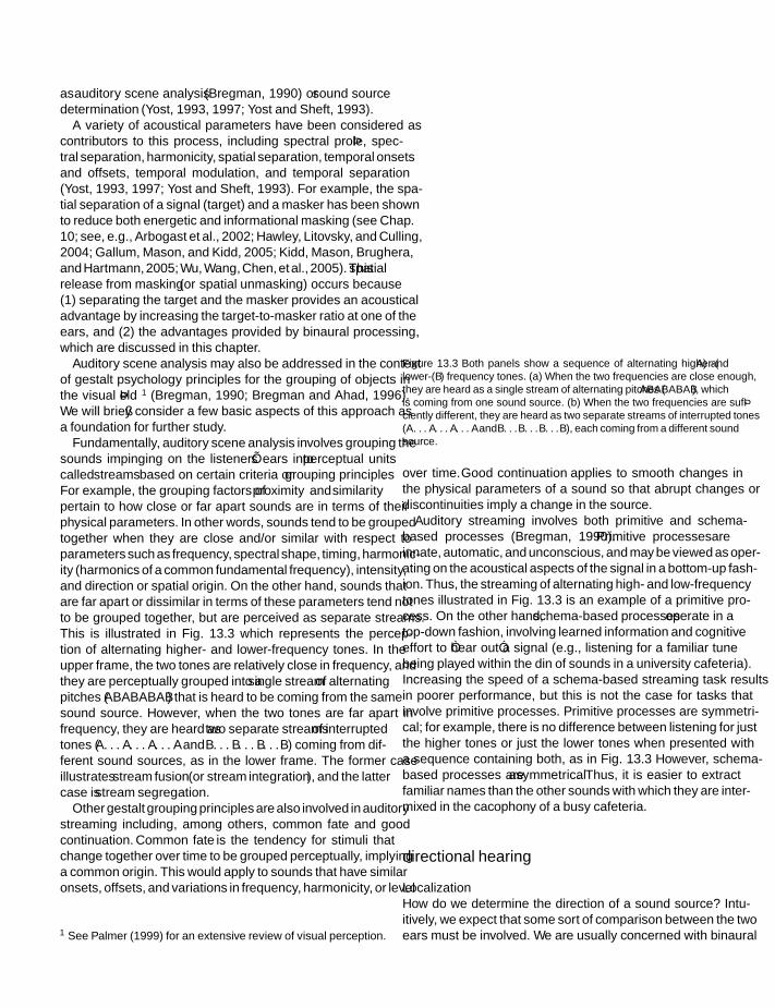
SFK SFK


chapter 13

as auditory scene analysis (Bregman, 1990) or sound sourcedetermination (Yost, 1993, 1997; Yost and Sheft, 1993).

A variety of acoustical parameters have been considered ascontributors to this process, including spectral profile, spec-tral separation, harmonicity, spatial separation, temporal onsetsand offsets, temporal modulation, and temporal separation(Yost, 1993, 1997; Yost and Sheft, 1993). For example, the spa-tial separation of a signal (target) and a masker has been shownto reduce both energetic and informational masking (see Chap.10; see, e.g., Arbogast et al., 2002; Hawley, Litovsky, and Culling,2004; Gallum, Mason, and Kidd, 2005; Kidd, Mason, Brughera,and Hartmann, 2005; Wu, Wang, Chen, et al., 2005). This spatialrelease from masking (or spatial unmasking) occurs because(1) separating the target and the masker provides an acousticaladvantage by increasing the target-to-masker ratio at one of theears, and (2) the advantages provided by binaural processing,which are discussed in this chapter.

Auditory scene analysis may also be addressed in the contextof gestalt psychology principles for the grouping of objects inthe visual field 1 (Bregman, 1990; Bregman and Ahad, 1996).We will briefly consider a few basic aspects of this approach asa foundation for further study.

Fundamentally, auditory scene analysis involves grouping thesounds impinging on the listener’s ears into perceptual unitscalled streams based on certain criteria or grouping principles.For example, the grouping factors of proximity and similaritypertain to how close or far apart sounds are in terms of theirphysical parameters. In other words, sounds tend to be groupedtogether when they are close and/or similar with respect toparameters such as frequency, spectral shape, timing, harmonic-ity (harmonics of a common fundamental frequency), intensity,and direction or spatial origin. On the other hand, sounds thatare far apart or dissimilar in terms of these parameters tend notto be grouped together, but are perceived as separate streams.This is illustrated in Fig. 13.3 which represents the percep-tion of alternating higher- and lower-frequency tones. In theupper frame, the two tones are relatively close in frequency, andthey are perceptually grouped into a single stream of alternatingpitches (ABABABAB) that is heard to be coming from the samesound source. However, when the two tones are far apart infrequency, they are heard as two separate streams of interruptedtones (A. . . A. . . A. . . A and B. . . B. . . B. . . B) coming from dif-ferent sound sources, as in the lower frame. The former caseillustrates stream fusion (or stream integration), and the lattercase is stream segregation.

Other gestalt grouping principles are also involved in auditorystreaming including, among others, common fate and goodcontinuation. Common fate is the tendency for stimuli thatchange together over time to be grouped perceptually, implyinga common origin. This would apply to sounds that have similaronsets, offsets, and variations in frequency, harmonicity, or level

1 See Palmer (1999) for an extensive review of visual perception.

Figure 13.3 Both panels show a sequence of alternating higher-(A) andlower-(B) frequency tones. (a) When the two frequencies are close enough,they are heard as a single stream of alternating pitches (ABABABAB), whichis coming from one sound source. (b) When the two frequencies are suffi-ciently different, they are heard as two separate streams of interrupted tones(A. . . A. . . A. . . A and B. . . B. . . B. . . B), each coming from a different soundsource.

over time. Good continuation applies to smooth changes inthe physical parameters of a sound so that abrupt changes ordiscontinuities imply a change in the source.

Auditory streaming involves both primitive and schema-based processes (Bregman, 1990). Primitive processes areinnate, automatic, and unconscious, and may be viewed as oper-ating on the acoustical aspects of the signal in a bottom-up fash-ion. Thus, the streaming of alternating high- and low-frequencytones illustrated in Fig. 13.3 is an example of a primitive pro-cess. On the other hand, schema-based processes operate in atop-down fashion, involving learned information and cognitiveeffort to “hear out” a signal (e.g., listening for a familiar tunebeing played within the din of sounds in a university cafeteria).Increasing the speed of a schema-based streaming task resultsin poorer performance, but this is not the case for tasks thatinvolve primitive processes. Primitive processes are symmetri-cal; for example, there is no difference between listening for justthe higher tones or just the lower tones when presented witha sequence containing both, as in Fig. 13.3 However, schema-based processes are asymmetrical. Thus, it is easier to extractfamiliar names than the other sounds with which they are inter-mixed in the cacophony of a busy cafeteria.

directional hearing

LocalizationHow do we determine the direction of a sound source? Intu-itively, we expect that some sort of comparison between the twoears must be involved. We are usually concerned with binaural

234

SFK SFK



listening in a sound field (stereophony), but we sometimesuse earphones for personal entertainment or to precisely con-trol experimental conditions, as described above. Interestingly,stereophonic and headphone listening can result in differentperceptions of space. Sounds presented from loudspeakers areperceived to be coming from outside the head (externalized)from a source that can be localized in the environment. Onthe other hand, sounds presented from earphones are gener-ally perceived to be inside the head (internalized), coming froman apparent source that is lateralized along a plane betweenthe two ears. This difference between extracranial localizationand intracranial lateralization is easily experienced by compar-ing the way music from the same compact disc album soundsthrough loudspeakers versus earphones. In general, identicalsounds impinging at the same time upon the two ears are local-ized directly in front of (or behind) the listener or, throughearphones, from an apparent source lateralized in the center ofthe head. However, one should be aware that externalization canbe a matter of degree, as opposed to being an all-or-none expe-rience (see Blauert, 1997; Hartmann and Wittenberg, 1996). Fora review of this topic, see Durlach et al. (1992).

Horizontal directions are expressed as angles of azimutharound the head, illustrated in Fig. 13.4a Sounds coming fromstraight ahead have an azimuth 0 and those coming fromdirectly behind have an azimuth of 180. Other azimuths areusually given as the number of degrees right (+) or left (−) ofcenter. For example, a loudspeaker that is off center toward theright by 45 has an azimuth of 45 right or +45, and a loud-speaker located 45 off center toward the left has an azimuth of45 left or −45. Azimuths are sometimes expressed in terms ofthe total number of degrees going around the head toward theright, in which case 45 right would be 45, and 45 left wouldbe 315. Vertical directions are expressed as angles of elevation(usually along the medial plane from front to back), as illus-trated in Fig. 13.4b. In this case, 0 elevation means straightahead, an elevation of 90 is directly above the head, and 180

is directly behind the head.The traditional duplex theory explains localization on the

basis of time differences between the ears at lower frequen-cies and level differences between the ears at higher frequencies(Lord Rayleigh, 1907).2 Consider the arrangement in Fig. 13.5a.The signal from the speaker, which is off to the right, must fol-low a longer path to the far (left) ear than to the near (right)ear. As Fig. 13.5b. shows, low frequencies have wavelengths thatare longer than the path around the head so that they “bendaround” the head to the far ear (diffraction). Thus, interauraltime differences (ITDs) are expected to provide localizationcues for the lower frequencies, where the wavelength of thetone is larger than the distance the signal must travel from thenear (right) ear to the far (left) ear. In contrast, higher frequen-cies have wavelengths smaller than the head so that they are

2 Lord Rayleigh was John William Strutt (1842–1919).

Figure 13.4 (a) Angles of azimuth horizontally around the head. Variousways of expressing azimuth angles are illustrated. (b) Angles of elevationvertically around the head in the medial plane.

“blocked” in the path to the far (left) ear (Fig. 13.5c). This headshadow causes a reduction in the intensity of the signal at the farear, producing sound level differences between the ears. Thus,interaural level differences (ILDs) or interaural intensity dif-ferences (IIDs) are expected to provide localization cues for thehigher frequencies. Our thresholds for interear differences areas small as approximately 10 s for ITDs (Klumpp and Eady,1956) and about 1 dB for ILDs (Mills, 1960; Blauert, 1997).

The traditional approach to interaural differences involvesmodeling the head as a solid sphere around which the ear-to-ear distance approximates 22 to 23 cm (Woodworth, 1938).This results in a time delay of roughly 660 s for the sound to getfrom the near ear to the far ear, which in turn corresponds to afrequency of 1500 Hz. Thus, the greatest time delay occurs whena sound source is directly to one side or the other (90 azimuth),for which the ITD would be 660 s, denoted by the peak of thecurve in Fig. 13.6 Below 1500 Hz, the wavelength is greater thanthe distance around the head, and the phase difference at thetwo ears provides an unambiguous localization cue. However,the phase discrepancy becomes ambiguous (except for the firstwavelength) as the frequency increases to 1500 Hz, where itswavelength approximates the distance around the head, result-ing in localization errors. At higher frequencies, the wavelength

235

SFK SFK


chapter 13

Figure 13.5 (a) Relationship between a loudspeaker and the two ears. (b)Low frequencies bend around the head due to their large wavelengths. (c)High frequencies have wavelengths smaller than head diameter so that anacoustic shadow results at the far ear.

is shorter than the size of the head so that the resulting headshadow produces ILDs. The ILDs thus provide localization cuesfor the higher frequencies.

Feddersen et al. (1957) measured the interaural time and leveldifferences for human heads as functions of angle around thehead (azimuth) and frequency. Figure 13.6 shows that their ITDmeasurements were in good agreement with the Woodworthmodel. Notice that there was no difference between the earswhen the signals (clicks) come from directly in front or behind(0 and 180), because the ears are equidistant from the soundsource in both cases. Interaural time differences developed asthe loudspeaker moved around the head, bringing it closer toone ear than the other. The ITD increased to a maximum ofabout 660 s when the loudspeaker was directly in front of oneear (90 azimuth), where the distance (and therefore the timedelay) between the ears is greatest. Feddersen et al. also foundthat ILDs depend on both frequency and azimuth. As expected,ILDs were negligible at 200 Hz and increased with frequency toas much as about 20 dB at 6000 Hz. The ILDs were 0 dB directlyin front and behind (at 0 and 180 azimuth), where the soundsource is equidistant between ears and increased to as muchas about 20 dB (depending on frequency), as the loudspeakermoved closer to side or the other, reaching a maximum wherethe loudspeaker directly in front of one ear (at 90).

Woodworth’s sphere model actually falls short of providingan accurate description of the interaural cues associated with thehuman head. This is not surprising because the configuration

Figure 13.6 Interaural time differences for different loudspeaker azimuths. Crosses are calculated differences based on Woodworth’s (1938) solid spheremodel. Circles are measurements by Feddersen et al. (1957). Source: From Feddersen et al. (1957), permission of J. Acoust. Soc. Am.

236

SFK SFK



of the head differs considerably from that of a sphere. Kuhn(1977) found that the ITDs for the higher frequencies cameclose to the 660 s value predicted by the sphere model, butthey do not change with frequency below 500 Hz or above3000 Hz. He also found that the ITDs below about 500 Hzwere about 800 to 820 s instead of 660 s. Middlebrooks(1999a) found that maximum interaural time delays amongadults ranged from 657 to 792 s. Taken together with otherfindings (e.g., Nordlund, 1962; Abbagnaro et al., 1975; Roth etal., 1980; Bronkhorst and Plomp, 1988), the implication is thatthe sphere model does not explain the nature of low-frequencyITDs, but applies principally to the higher frequencies and tothe leading edges of clicks and click-like signals, for whichthe major directional cues are not the phase-derived ITDs.Even directional hearing for high-frequency complex sounds,which is principally associated with ILDs, is also affected byinteraural time differences. Moreover, the duplex model alonefalls short of completely explaining directional hearing becauseit does not adequately explain front-back distinctions, direc-tionality above and below the horizontal plane, and monaurallocalization.

In addition to the effects of the ear canal resonance (Chap. 3),the spectrum of the sound arriving at the eardrum is affectedby the pinna, head, and torso. In particular, spectral cues (alsoknown as pinna cues and monaural spectral cues) at highfrequencies introduced by the pinnae are important for theperception of elevation, front-back distinctions, and monaurallocalization (Blauert, 1969/70, 1997; Hebrank and Wright, 1974;Weinrich, 1982; Musicant and Butler, 1984; Middlebrooks andGreen, 1991; Middlebrooks, 1992, 1997; Shaw, 1997; Wight-man and Kistler, 1997). These pinna cues also contribute tothe extracranialization of sound sources (Plenge, 1974; Blauert,1997). Low-frequency cues (below about 3000 Hz) associatedwith head diffraction and torso reflections appear to be involvedin vertical localization (e.g., Gardner, 1973; Algazi et al., 2001).

The manner in which the amplitude spectrum of a soundis modified going from a source in the environment to theeardrum is shown by the head-related transfer function(HRTF). Families of HRTFs are shown for sources located hor-izontally at many azimuths around the head in Fig. 13.7 (Shaw,1974),3 and vertically at many elevations around the medialplane of the head in Fig. 13.8

The curves in these figures make it clear that the spectrumof the sound that finally arrives at the eardrum depends on thedirection from which it came (see, e.g., Shaw, 1997). This is mosteasily seen for horizontal directions in Fig. 13.7 by comparingthe shapes of HRTFs for sounds coming from the front (toppanel), side (middle panel), and back (bottom panel) of thehead. Also notice that the sound level reaching the eardrumgets weaker as the source moves from the same side of the

3 This data may be found in tabular form in Shaw and Vaillancourt(1985).

head around to the opposite side of the head. Consider a soundsource located 45 to the right. In this case, the sound reachingthe right (near) eardrum is affected by the HRTF labeled 45,and the sound arriving at the left (far) eardrum is modified bythe HRTF labeled −45. (The 45 and −45 HRTFs are foundin the upper panel in Fig. 13.7, or refer back to Fig. 13.2 foran uncluttered view.) It is easy to realize how these differencestranslate into ILDs. The same 0 curve applies to both ears ifthe source is directly ahead, and the same 180 curve applies toboth ears if the sound is coming from directly behind (180), inwhich case the ILDs are 0 dB.

Changes in elevation cause changes in the high-frequencyaspects of the HRTF due to directionally dependent filtering bythe pinna (Hebrank and Wright, 1974; Shaw, 1997). This is seenin Fig. 13.8 as a “pinna notch” that shifts between about 5000and 11,000 Hz as the sound source moves up around the head.Scanning upward from the bottom of the figure, notice that thereis a notch at about 6000 Hz when the sound source is below thehead. The notch gets higher in frequency as the sound sourcemoves upward toward the front and then continues up towardthe top of the head (above), where the notch is essentially absent.Continuing around, the notch then gets lower in frequency asthe source moves downward toward the back of the head andthen below again.

Classical studies of localization were conducted by Stevensand Newman (1936) and Sandel, Teas, Feddersen, and Jeffress(1955). Stevens and Newman (1936) sat their subjects in a chairelevated about 12 f above the roof of the Harvard BiologicalLaboratories building to minimize the possible confoundingeffects of echoes and reverberation. The sound source was aloudspeaker mounted on a boom arm that extended 12 f fromthe listener. The loudspeaker was rotated around the subjectin 15 steps from 0 to 180, and the task was to listen for thesignal and report its apparent direction. It is important to pointout that their subjects regularly made front-back confusions. Forexample, sounds presented from 30 right of center in front ofthe subject (30 off center from 0 azimuth) were confused withsounds presented from 30 right of center behind (30 off centerfrom 180 azimuth). These front-back reversals were treated asequivalent, correct responses, and the location of the soundsource was judged relative to 0 or 180, whichever was closer.With this in mind, Stevens and Newman’s findings are shownas a function of frequency in Fig. 13.9 Localizations were mostaccurate below 1000 Hz and above 4000 Hz, with the greatesterrors between about 2000 and 4000 Hz.

Sandel et al. (1955) asked subjects to localize sounds in ananechoic (echo-free) room. Loudspeakers placed at 0 and at 40

right and left were used to generate “phantom” sound sourcesat various azimuths, depending upon the phases of the signals.The subject indicated the perceived location of the tone sourcewith an “acoustic pointer,” which was a speaker that rotatedon a boom around his or her head. A noise from this speakeralternated with the test tones, and the subject’s task was toplace the noise loudspeaker (pointer) at the apparent location

237

SFK SFK


chapter 13

Figure 13.7 Horizontal head-related transfer functions for sound sources located at many angles of azimuth () around the head based on data from 12studies. Source: From Shaw (1974) with permission of J. Acoust. Soc. Am.

of the test tone source. They found that ITDs accounted for thelocalization of tones below about 1500 Hz, and that these wereused to localize the high frequencies. Many random errors at1500 Hz suggested that interaural cues are ambiguous aroundthis frequency. These results were essentially consistent withthose of Stevens and Newman.

The sizable localization errors and front/back confusionsobserved in these early studies imply that the directional cuesprovided by tonal signals are limited and ambiguous. It is inter-esting to note in this context that Stevens and Newman foundbetter localization results for noises than for tones, which theyattributed to quality (spectral) differences and ILDs for the

high-frequency energy in these noises. In contrast, accuracyis substantially improved and front/back errors are reducedwhen localizing broad-band signals (e.g., Butler and Planert,1976; Oldfield and Parker, 1984; Butler, 1986; Makous andMiddlebrooks, 1990). Broad-brand stimuli provide the listenerwith multiple cues across frequencies, including both interau-ral differences and spectral shape information (Wightman andKistler, 1993, 1997). Recall, here, that the spectral shape cuesdue to pinna effects are found in the higher frequencies. Itis interesting to note, for example, that Musicant and Butler(1984) found that front/back distinctions were best when theirstimuli included high frequencies (above 4000 Hz), and that

238

SFK SFK



Figure 13.8 Vertical head-related transfer functions for sound sourceslocated at many angles of elevation along the medial plane around the headof a representative subject. Source: Figure provided courtesy of Dr. RichardO. Duda, used with permission.

performance dropped considerably when the various depres-sions of the pinnae were occluded.

We learn more about the contributions of the higher fre-quencies from a study by Middlebrooks (1992). In this study,subjects were asked to localize high-frequency narrow-bandnoises presented from loudspeaker locations corresponding to360 combinations of azimuth and elevation. The subject’s taskwas to point the subject’s nose at the perceived sound sourcelocation, and this response was in turn monitored by using spe-cial instrumentation to determine head orientation. The resultsdemonstrated that azimuth was accurately localized and relatedto ILDs, while front/back and elevation localizations were relatedto spectral cues.

Figure 13.9 Accuracy of localization in percent (left axis) and localizationerror in percent (right axis) as a function of frequency, based on data reportedby Stevens and Newman (1936).

Head MovementsThere has been some controversy about whether the dynamiccues provided by head movements can improve localizationaccuracy (see, e.g., Middlebrooks and Green, 1991; Wightmanand Kistler, 1993). Classical papers by Wallach (1939, 1940)presented findings and convincing arguments supporting therelevance of head movements as a means of reducing local-ization ambiguities, but some studies found that any benefitsprovided by head movements were either small or not signifi-cant (Pollack and Rose, 1967; Thurlow and Runge, 1967; Fisherand Freedman, 1968). However, questions about the impact ofhead movements on localization appear to have been resolved bycontemporary experiments using real and virtual sound meth-ods (e.g., Bronkhorst, 1995; Perrett and Noble, 1997a, 1997b;Wightman and Kistler, 1999; Macpherson and Middlebrooks,2002). Although there is considerable intersubject variability,localization is improved by head movements, especially in termsof reducing front/back and vertical confusions.

LateralizationLateralization experiments have helped clarify and expand uponwhat we know about directional cues, because the use of ear-phones allows us to precisely control and manipulate the signalspresented to the ears. Many studies have examined the effectsof ITD and ILD cues upon lateralization (e.g., Klumpp andEady, 1956; Zwislocki and Feldman, 1956; Mills, 1960; Yost etal., 1971; Yost, 1974; Grantham, 1984; Yost and Dye, 1988).While exact procedures vary, the general approach is to presenttwo stimuli to the subject that differ with respect to interauraltime (phase) or level, and to determine whether this interauraldisparity results in a perceptible change in lateralization. Theoverall findings essentially agree with the localization data. Thatis, ITDs are most important up to about 1500 Hz, and ILDs takeover as the primary lateralization cue for higher frequencies.

Yost (1974) performed a particularly interesting lateralizationexperiment addressing the discrimination of interaural time(actually phase) differences. He presented subjects with twostimuli. The first included a particular interaural time (actuallyphase) difference, . This difference, of course, resulted in alateralization toward one side of the head analogous to theazimuth position. The second stimulus was the same exceptthat the phase difference between the ears was larger by a slightamount . Thus, it was + . The subjects had to detectthe value of by discriminating between the two stimuli( vs. + ). For any value of , the smaller the value of needed for a change in apparent lateralization, the betterthe discrimination of interaural phase. We might think of asanalogous to the smallest perceptible change in azimuth (similarto the minimal audible angle discussed later in this chapter). Theresults are summarized in Fig. 13.10 Note that is smallest(best) when is 0 or 360. These values of are midlinelateralizations because 0 and 360 correspond to a zero phasedisparity between the ears. Thus, the most acute interaural phasediscriminations are made at the midline. On the other hand,

239

SFK SFK


chapter 13

Figure 13.10 Changes in interaural phase () required in order to detect adifference in lateralization from a standard (reference) phase difference ().Source: Adapted from Yost (1974), with permission of J. Acoust. Soc. Am.

interaural phase discrimination was poorest ( as largest)when was 180; that is, when the signals were lateralizeddirectly to one side.

Figure 13.10 also shows that was essentially the samefor the frequencies up to 900 Hz. In contrast, interaural phasediscrimination was substantially poorer at 2000 Hz, where itwas constant at about 30. Interaural phase had no effect atall for 4000 Hz (not shown on the graph). Thus, interauralphase was shown to be an important cue at low frequenciesbut unimportant for highs, in a manner consistent with thelocalization data.

Lateralization experiments have revealed that discriminationfor ILDs is constant as a function of frequency within a rangeof about 2 dB, but with a curious increase in the size of theILD at 1000 Hz (Mills, 1960; Grantham, 1984; Yost and Dye,1988). These findings are illustrated in Fig. 13.11 The excellentinteraural level discrimination at the high frequencies is, ofcourse, expected from the previous discussion. Three sets offindings are shown in Fig. 13.11 depending upon whether thestandard stimulus against which the discrimination was madewas itself perceived to be (lateralized) at the midline, halfwaybetween midline and the left ear, or at the left ear. These threelateralizations of the standards signal were achieved by usingILDs of 0, 9, and 15 dB, respectively (Yost, 1981). A comparisonof these three curves makes it clear that ILD discrimination ismost acute at midline, is least sensitive when the standard islateralized off to one side, and is at some intermediate valuewhen the discrimination is made between the midline and atthe left ear.

Interaural time differences come into play whenever the signalcontains low frequencies. For example, Yost et al. (1971) foundthat the lateralization of clicks is impaired by removing theirlow-frequency components, but not by eliminating the highs;others found that ITDs could result in lateralization differences

Figure 13.11 Thresholds for interaural differences in level (IDL) in decibelsas a function of frequency from 200 to 5000 Hz. (Note that the scale ofthe ordinate is from 0 to 2.5 dB.) These findings were obtained when thestandard stimulus itself was lateralized at midline (circles, marked 0 dB),halfway between midline and the left ear (squares, marked 15 dB), and atthe left ear (triangles, marked 15 dB). The 0-, 9-, and 15-dB values arethe interaural level differences needed to place the standard image at theselocations. Source: From Yost and Dye (1988), with permission of J. Acoust.Soc. Am.

for high-frequency noise bursts and clicks (Klumpp and Eady,1956; Hafter and DeMaio, 1975).

Lateralization has been used to study the relative salience ofILDs and ITDs by establishing the trade-off between the timeand intensity cues. This was done by asking the subject to adjustthe ILD (or ITD) until a midline image was perceived. Harris(1960) found trading ratios of 25 s/dB for clicks with energybelow 1500 Hz and 60 s/dB for clicks with energy above 1500Hz. These trading ratios imply that ITDs have greater saliencefor low frequencies (because a smaller ITD is needed to centerthe image) and ILDs are more salient for the highs (because alarger ITD is needed). However, these studies were marked byinconsistent results between subjects. For example, Moushegianand Jeffress (1959) found that the trading ratio for a 500-Hz tonewas about 20 to 25 s/dB for two subjects but only about 2.5s/dB for another subject.

Subjects in time-intensity trading studies often heard two lat-eralized images instead of one (Whitworth and Jeffress, 1961;Hafter and Jeffress, 1968; Jeffress and McFadden, 1971; Hafterand Carrier, 1972). One image was called the time image becauseit depended on ITDs (especially <1500 Hz) but was essentiallyunaffected by ILDs. The other was an intensity image and wasresponsive to both ILDs and ITDs at all frequencies. Typicaltrading ratios (for clicks) were on the order of 2 to 35 s/dBfor the time image and 85 to 150 s/dB for the intensity image(Hafter and Jeffress, 1968). It may be that the intersubject differ-ences reported by Harris (1960) and by Moushegian and Jeffress(1959) were due to responses to the time image by some subjectsand to the intensity image by others.

240

SFK SFK



Although high-frequency lateralization is typically associatedwith ILDs, it can be influenced by ITDs, such as when thehigh-frequency signal is amplitude-modulated at a low rate(e.g., Henning, 1974; Neutzel and Hafter, 1976, 1981). Let usborrow some examples from Henning (1974) to illustrate this.Consider three kinds of signals (each lasting 250 ms) presentedbinaurally to subjects with interaural time differences: (1) a lowfrequency (300 Hz), (2) a high frequency (3600 Hz), and (3)a high frequency (3900 Hz) that was sinusoidally amplitude-modulated (SAM) at 300 Hz. Listeners could lateralize the 300-Hz tone based on ITDs but could not do this for the 3600-Hztone, but the 3900-Hz SAM signal also could be lateralized onthe basis of ITDs (as well, in fact, as for the 300-Hz tone).

An interesting effect called binaural interference 4 occurswhen a listener’s experience of binaural phenomena for highfrequencies is affected by the simultaneous presence of lowfrequencies (e.g., McFadden and Pasanen, 1976; Trahiotis andBernstein, 1990; Buell and Hafter, 1991; Stellmack and Dye,1993; Bernstein and Trahiotis, 1995; Heller and Trahiotis,1995; Hill and Darwin, 1996; Best, Gallun, Carlile, and Shinn-Cunningham, 2007). This disruption is usually reported aspoorer sensitivity for ITDs or lateralization changes at a highfrequencies (signal) when the low frequency (interferer) arealso present compared to when the high frequency signal is pre-sented alone. Binaural interference appears to occur when thesignal and interferer are grouped into a single perceptual unit,such as when they turn on and off simultaneously; however,it is reduced or eliminated when cues are provided that allowthem to be segregated, such as when the signal and interfererfrequencies turn on and off at different times.

Virtual Auditory Space LocalizationThe ability to take advantage of earphone testing to study direc-tional hearing has been dramatically enhanced with the use ofvirtual auditory space (VAS) techniques. This approach usesan individual’s own HRTFs for both ears (based on many soundsource directions) to produce test signals that simulate naturallyoccurring free-field cues when they are presented to the sub-ject through earphones (Wightman and Kistler, 1989a). Thesevirtual stimuli have been found to accurately represent acous-tical cues for localization (Wightman and Kistler, 1989a), andresult in spatial position judgments similar to those found withreal free-field signals, although front/back and vertical errors aremore common (e.g., Wightman and Kistler, 1989b; Bronkhorst,1995).

Unlike the intracranially lateralized images produced by theearlier earphone methods, VAS techniques appear to pro-duce perceptions that are actually localized extracranially (e.g.,Macpherson and Middlebrooks, 2002). Subjects in these vir-

4 This term should not be confused with clinical binaural interference,in which some hearing-impaired patients have the atypical experienceof poorer performance binaurally than monaurally.

tual localization studies perceived a single apparent source asopposed to the split images often reported in the earlier lat-eralization studies (Wightman and Kistler, 1992; Macphersonand Middlebrooks, 2002). Wightman and Kistler (1992) com-pared the relative strengths of ITDs, ILDs, and spectral cues inestablishing the perceived location of a sound. This was doneby presenting broad-band noise signals containing conflictinglocalization cues. For example, the ITD would indicate thatthe sound source was at one location but the ILD and spectralcues would indicate that it was at a different location. In spiteof the conflicting cues, their subjects perceived a single soundsource at a location determined by the ITD. However, the dom-inance of the ITD cue was lost when the low frequencies wereremoved from the noise (by filtering), in which case the per-ceived location was determined by the ILD and spectral cues.More recently, Macpherson and Middlebrooks (2002) foundthat ITDs had greater salience than ILDs when localizing low-pass sounds, and that ILDs had greater salience than ITDs forhigh-pass sounds.

Considerable individual differences exist in the dimensions ofthe skull, pinna, etc., which are related to differences in HRTFs(Middlebrooks, 1999a). Testing with VAS techniques has madeit possible to determine whether these individual differencesaffect directional hearing. To do this involves comparing anindividual’s localization performance for virtual sources basedon his or her own ears versus virtual sources based on anotherperson’s ears (Wenzel et al., 1993; Møller et al., 1996; Middle-brooks, 1999b). Overall, it has been found that localizationbecomes less accurate when “listening through somebody else’sears” compared to “listening through your own ears,” prin-cipally involving front/back confusions and elevation errors.It is interesting to note that this kind of manipulation of VASsound sources has been found to produces changes in the spatialresponses of the primary auditory cortex in the ferret (Mrsic-Flogel et al., 2001).

Minimum Audible AngleAnother aspect of directional hearing involves determining thesmallest difference in location between two sound sources thatresults in a different perceived location. Since the two soundsources are viewed relative to the head, this is the same as ask-ing what is the smallest angle (or difference in azimuth) thata listener can discriminate. Mills (1958, 1963, 1972) studiedthis phenomenon in depth and called it the minimal audibleangle (MAA). Specifically, he tested the MAA as a function offrequency when the sound sources were located in front of thesubject (0), and when they were 30, 45, 60, and 75 off tothe side. The logistics of the basic task are illustrated in Fig.13.12 where we see that the listener must distinguish the differ-ence between two points in space. Notice that the figure actuallyshows two different conditions, one in which the MAA is beingdetermined when both sound sources are directly in front ofthe listener (at 0 azimuth) and another one in which the twosound sources are off to one side (at 45 azimuth).

241

SFK SFK


chapter 13

Figure 13.12 The minimal audible angle (MAA) is the smallest angular difference that can be perceived between two sound sources. This illustration showsthe arrangement when the MAA is being measured under two different conditions. In one case, the MAA is being measured for loudspeakers directly infront of the listener (at 0 azimuth); in the other case, the loudspeakers are located at 45 azimuth.

In his classical studies, Mills found that the MAA was small-est (best) for the frequencies below about 1500 Hz and aboveapproximately 2000 Hz, and was largest (poorest) between thesefrequencies. This result reflects the ambiguity of localizationcues in the vicinity of 1500 Hz, thus confirming the previ-ously mentioned findings. Mills also found that MAAs weremost acute (approximately 1–2) when the sound sources weredirectly in front of the head, and that they increased dramat-ically to very high values when the sources were at the side ofthe head. This result occurs because small changes in locationin front of the head result in large interaural differences (espe-cially ITDs). However, when the sources are off to one side of thehead (facing one ear), the interaural differences remain largelythe same in spite of relatively large changes in angle between theloudspeakers. We might thus conceive of a cone of confusion(Fig. 13.13) to one side of the head, within which the interauraldifferences do not vary when the sound sources change loca-tion (Mills, 1972). This image demonstrates the importance ofhead movements in localization, since these movements keepchanging the position of the cone of confusion—the zone ofambiguity—thereby minimizing its detrimental effect.

The MAA described by Mills involved the discriminationof two stimuli presented sequentially. Perrott (1984) expandedupon the concept of the MAA using stimuli that were presentedat the same time, describing the concurrent minimum audibleangle (CMAA). As for the MAA, the CMAA is also most acutefor sounds presented directly in front of the subject and leastsensitive when the stimuli are presented off to one side. However,

the CMAA is also affected by spectral differences between thetwo sounds whose locations are to be discriminated. Subjectswere unable to distinguish a difference in the angular locationsof the stimuli when their frequencies differed by only 15 Hz.When the signals differed in frequency by 43 Hz, the size of theCMAA increased from 4.5 when the two signals were presentedfrom 0 azimuth to an angle of about 45 when they were

Figure 13.13 The cone of confusion (see text). Source: Modified after Mills(1972).

242

SFK SFK



presented from 67 off to the left. On the other hand, signals101 Hz apart had CMAAs of about 10 when the two sourceswere anywhere from straight ahead (0 azimuth) up to 55

off center. The CMAA then increased dramatically to about30 when these signals were presented from 67 to the left.(An intermediate relationship between CMAA and azimuth wasobtained for signals differing in frequency by 72 Hz.) As Perrotthas pointed out, the CMAA involves the issue of sound sourceidentification (“what”) as well as that of localization (“where”).

Minimum Audible Movement AngleThe MAA and CMAA describe the smallest perceptible differ-ence in location between two stationary sound sources, A andB. We may also ask a similar question with regard to the motionof a sound source. How far (in degrees) must B travel awayfrom A in order for us to know that B is moving? This smallestchange in location that is needed for us to detect motion iscalled the minimum audible movement angle (MAMA) andhas been the topic of considerable study (Harris and Sergeant,1971; Perrott and Musicant, 1977; Grantham, 1986; Perrott andTucker, 1988; Perrott et al., 1989; Saberi and Perrott, 1990a;Chandler and Grantham, 1992). Taken together, the evidencesuggests that minimum audible movement angles depend onthe same parameters that apply for stationary sources, plus theeffect of how fast the moving sound source is moving. Usingbroad-band noise sources presented from directly in front ofthe head (0 azimuth), Chandler and Grantham (1992) foundthat the mean MAMA was 5.2 when the moving loudspeakerhad a velocity of 10 per second (/s), and 5.7 at 20/s. How-ever, the mean MAMA increased to 8.2 at 45/s, 12 at 90/s,and 17.3 at 180/s. For noises presented from speakers at 60

azimuth, mean MAMAs increased from 8.3 at 10/s to 28.4 at180/s. Notice that binaural sensitivity for motion becomes lesssensitive for faster velocities. Saberi and Perrott (1990a) foundthat the minimum audible movement angle was most acute forvelocities between 1.8/s and 11/s, and that it increased forslower velocities as well as for faster ones. Within this range,they were able to measure mean MAMAs as small as about 2

(approaching the size of the stationary MAA).

DistanceHow do we judge distance with hearing? The answer to thisquestion is not clear, although there has been renewed inter-est in this area. This section will outline several of the factorsthat have been considered as potential cues for perceiving thedistance from a sound source. The interested student will findinformative reviews in Coleman (1963), Blauert (1997), andZahorik (1996). We will begin with sound level and the ratio ofdirect-to-reverberant energy. It appears that both can be salientdistance cues, and that there is flexibility in their relative promi-nence in making distance judgments, depending on the natureof the sound (Zahorik, 2002a).

Sound level in a free field drops by 6 dB for each doublingof distance from the source (Chap. 1). Thus, sound level pro-

vides the listener with a distance cue. However, more than theexpected decrease of 6 dB is required to perceive a doubling ofdistance so that apparent distance underestimates actual dis-tance (Bekesy, 1938; Cochran, Throop, and Simpson, 1968;Gardner, 1969; Blauert, 1997; Petersen, 1990; Begault, 1991).For example, Blauert (1997) demonstrated that a doubling ofperceived distance requires sound level reduction of about 20dB instead of the expected value of 6 dB. Perceptual underes-timates of actual distances appear to be ubiquitous findings indistance perception studies (Zahorik, 2002a).

Sounds reaching a listener in a real room involve both thedirect sound from the source and reverberation, composed ofmultiple reflections from the walls, ceiling, floors, and variousobjects within the room. Under these conditions, the directenergy decreases with distance from the source (due to theinverse square law), but the reverberant energy remains prettymuch uniform. As a result, the ratio of direct-to-reverberantenergy changes with distance, enabling it to provide a distanceperception cue for the listener (Blauert, 1997). The salience ofthe direct-to-reverberant energy ratio is fairly well established,and it is commonly found that distance performance is betterin reverberant settings than in anechoic (echo-free) situations(Mershon and King, 1975; Mershon and Bowers 1979; Mershonet al., 1989; Wagenaars, 1990; Nielsen, 1993; Bronkhorst andHoutgast, 1999; Zahorik, 2002a, 2002b). Moreover, Zahorik(2002a) found that the direct-to-reverberant ratio had greaterperceptual weight as a distance cue than sound level for noisesignals. However, it appears to provide a coarsely graineddistance cue because the threshold for discriminating direct-to-reverberant ratios is about 5 to 6 dB, roughly correspondingto a 2.5-fold change in distance (Zahorik, 2002b).

Spectral shape is another potential acoustical cue for dis-tance perception when dealing with relatively long distances(Coleman, 1968; Butler et al., 1980; Little, Mershon, Cox, 1992;Blauert, 1997). The spectrum of a sound changes with dis-tance from the sound source due to absorption as sound travelsthrough the air, which causes the high frequencies to be atten-uated with distance a great deal more than the lows.

Brungart (1999) showed that binaural cues, specifically ILDsfor relatively low frequencies ( <3000 Hz), contribute to dis-tance perception when the sound source is less than 1 m fromthe head. This might seem odd because ILDs are generally asso-ciated with the high frequencies. However, low-frequency ILDsbecome significant when the source is close to the head andincrease with proximity (Brungart and Rabinowitz, 1999; Dudaand Martens, 1998).

There is at least some evidence which suggests that famil-iarity or experience with the sound source has some influenceon distance perception. For example, experience with speechmay provide the listener with a frame of reference that would behelpful in making distance judgments based on sound level, andit has been found that sound level is a salient cue for judging dis-tance for speech (Gardner, 1969; Brungart and Scott, 2001). Inaddition, the accuracy of distance judgments is better for speech

243

SFK SFK


chapter 13

played forward compared to backward (McGregor et al., 1985).Also suggesting that familiarity improves auditory distance per-ception, Coleman (1962) found that the accuracy of distancejudgments for unfamiliar sounds (1-s noise bursts) improvedas experience with the stimulus accumulated over the course ofrepeated test trials. (The accuracy of azimuth localizations didnot change with repeated trials.) Interestingly, Zahorik (2002a)found that sound level has a greater perceptual weight than thedirect-to-reverberant ratio when making distance judgmentsfor speech signals (a familiar sound), whereas the opposite istrue for noise bursts (an unfamiliar sound). On the other hand,Nielsen (1991) did not find differences in judged distances forspeech, noise, and two kinds of musical signals.

precedence effect

Consider two apparently unrelated situations. The first involveslistening to a radio news broadcast through both speakers ofa home sound system. (We are not using a stereo music CDbecause we want identical signals from both speakers.) Sittingequidistant from the speakers causes us to perceive a phan-tom sound source between them. However, sitting close to onespeaker (so that the signal reaches our ears sooner from thatdirection than from the other speaker) gives us the impressionthat all of the sound is coming from the closer speaker. Thisoccurs even though the other speaker is still on.

The second situation involves listening to someone talking ina hard-walled room. In this case, the sounds reaching our earsinclude the direct sound from the talker’s lips plus reflections ofthese sounds from the walls. Because the reflected sounds takean indirect route (via the walls), they reach our ears later thanthe direct sound and also from different directions. Yet, we heara single sound coming from the direction of the earlier-arrivingdirect sound (although the reflections will “color” the qualityof what we hear).

These situations illustrate a phenomenon known as the prece-dence effect, Haas effect, or the first wavefront principle(Gardner, 1968; Blauert, 1997). In general terms, when a soundcoming from one direction is very quickly followed by a secondsound (the echo) from another direction, then the perceivedsound will be dominated by the earlier-arriving signal. In otherwords, we could say that echo suppression has occurred.

The precedence effect may be described in terms of howlisteners perceive a sequence of four clicks presented throughearphones, as in the classic experiment by Wallach, Newman,and Rosenzweig (1949). Figure 13.14 shows that the first click(A) went to the left ear followed by click B to the right ear aftera very short delay (1). If presented alone, this pair of clickswas heard as a fused image coming from the left . Click C wentto the right ear followed after another very short delay (2)by click D to the left ear, and by itself this pair was heard as afused image from the right . The composite four-click sequencewas heard as a fused image from the left ; that is, its perception

Figure 13.14 Arrangement of clicks presented through earphones todemonstrate the precedence effect, as used by Wallach, Newman, and Rosen-zweig (1949).

was dominated by the left-leading onset rather than the rightleading at its offset. Thus, the first-arriving signal determinedthe perceived location of the fused sound. Wallach et al. foundthat this precedence effect occurred for intervals between thetwo click pairs (3) up to 40 ms. However, longer durations of 3caused the listener to hear two separate signals, one at each ear.

Haas’ (1949, 1951) classic demonstration of the precedenceeffect involved presenting speech from two loudspeakers, witha delay in the onset of the signal from one speaker comparedto the other. These delays are analogous to interval 3 in theWallach et al. study. A fused image coming from the leadingloudspeaker was heard for delays up to 35 ms. Longer delayscaused listeners to detect the presence of the second (delayed)sound, although the signal was still localized toward the leadingside. Delays longer than about 50 ms caused listeners to hear onesound from the leading speaker and a distinct echo coming fromthe delayed speaker. It is interesting to note that the precedenceeffect can is robust with regard to some modifications of thetemporal, spectral, and interear characteristics of the stimuli(Dixon and Colburn, 2006).

Various studies have expanded on the classical descrip-tions of the precedence effect, revealing that the general phe-nomenon encompasses several identifiable aspects (for reviews,see Blauert, 1997; Litovsky et al., 1999). Fusion is the percep-tion of the leading and trailing signals as a single, unified image,and occurs for delays up to about 5 to 10 ms for clicks (e.g.,Ebata et al., 1968; Freyman et al., 1991; Yang and Grantham,1997; Litovsky and Shinn-Cunningham, 2001) and roughly 40to 50 ms for speech (e.g., Haas, 1951; Lochner and Burger, 1958).Longer delays cause two separate images to be heard. The delayat which the perception splits into two images is called the echothreshold.

The perceived location of the fused image is affected by thesize of the delay between the two signals. Summing localizationoccurs for delays shorter than 1 ms, in which case the perceivedlocation of the fused image is affected by both the leading andlagging clicks (Blauert, 1997), as illustrated in Fig. 13.15a. Local-ization dominance occurs when the location of the fused image

244

SFK SFK



Figure 13.15 Aspects of the precedence effect shown in terms of signals presented from two loudspeakers, located 45 right and left of the listener. The leftsignal leads and the right signal(s) lags. In frames a to c, the filled circles indicate the locations of the perceived images, and the delay between the onsets ofthe two signals is shown along the top of each frame. In frame d, the task is to discriminate between the signals from the array of speakers on the (lagging)right side.

is determined by the leading signal (Fig. 13.15b). This occurswhen the delay between the first and second clicks is betweenabout 1 and 5 ms. Localization dominance breaks down as thedelay lengthens, with the image splitting in two at the echothreshold, beyond which two images are heard, each comingfrom its own side (Fig. 13.15c).

Another aspect of the precedence effect is illustrated in Fig.13.15d. Here, the listener is asked to discriminate between theazimuth locations of clicks on the lagging side (i.e., betweenspeakers 1, 2, 3, etc.). Discrimination is poorer when the lead-ing signal is present compared to what it is without the leadingsignal (e.g., Perrott et al., 1989; Freyman et al., 1991; Litovskyand Macmillan, 1994). An analogous effect occurs with ear-phones, where the presence of the leading signal affects thedifference limens for ITDs or ILDs for the delayed signal (e.g.,Zurek, 1980; Saberi and Perrott, 1990b; Shinn-Cunninghamet al., 1993; Tollin and Henning, 1998). This effect occurs fordelays up to about 5 ms and is aptly called discriminationsuppression.

As suggested by the examples at the beginning of this sec-tion, the precedence effect suppresses the effects of reflectionswhich would otherwise interfere with our perception of thedirect sound, including speech. For example, Lochner andBurger (1964) found that speech discrimination was unaffectedby reflections arriving up to 30 ms after the direct sound,although later-arriving reflections resulted in reduced intel-ligibility. Reflections that arrive beyond the time when theprecedence effect is operative result in distortions and mask-ing of the speech signal (e.g., Bolt and MacDonald, 1949;Kurtovic, 1975; Nabelek, 1976; Nabelek and Robinette, 1978;Gelfand and Silman, 1979; Nabelek and Dagenais, 1986; seeChap. 14).

Several interesting phenomena are encountered when theprecedence effect is viewed in the context of the listener’s imme-diate experience with the listening situation. Suppose we mea-sure a listener’s echo threshold several times: immediately afterhearing leading/lagging click trains of various lengths (e.g., 3,6, 9, 12, and 15 click pairs), and also without any precedingclick pairs. [The upper left part of Fig. 13.16 (labeled a) showsan example of a train of 12 leading/lagging click pairs pre-sented from right and left loudspeakers.] We would find that theecho threshold increases, as the preceding click train gets longer(reaching a maximum at 12 pairs). Thus, there is a build up ofecho suppression that is dependent upon the listener’s imme-diate experience with the listening task (Clifton and Freyman,1989; Freyman et al., 1991; Clifton et al., 1994). What’s more,this build up of echo suppression appears to be asymmetrical,being greater when the right click leads than when the left clickis leads (Clifton and Freyman, 1989; Grantham, 1996).

A breakdown of echo suppression called the Clifton effectoccurs when the leading and lagging clicks switch directions(Clifton, 1987; Clifton and Freyman, 1989). The basic demon-stration of the Clifton effect involves presenting the listener witha train of click pairs coming from right and left loudspeakers(Fig. 13.16). The leading click in each pair is from the left and thelagging click is from the right, so that each click pair is heard asa fused image coming from the left side (labeled a in the figure).After 12 pairs, the order of the clicks is switched so that now theright click leads and the left one lags. At this point, we wouldexpect to hear a fused image from the now-leading right side,but this does not happen. Instead, the precedence effect breaksdown and the listener hears both clicks, each coming from itsown side (b in the figure). Then, after several right/left clickpairs are presented, the listener again hears a fused image from

245

SFK SFK


chapter 13

Figure 13.16 The Clifton effect. (a) Left-leading click pairs are heard as a fused image coming from the left (represented by the filled circle in the lowerdrawing). (b) Switching to right-leading click pairs causes the precedence effect to break down, and both clicks are heard coming from their respective sides(represented by the two filled circles). (c) The precedence effect is then re-established, with a fused signal heard from the now-leading right side (representedby the filled circle).

the now-leading right side, which indicates that the precedenceeffect has been re-established (c in the figure).

A fascinating illusion called the Franssen effect (Franssen,1960, 1962) is illustrated in Fig. 13.17 Here, a low-frequencytone (e.g., 500 Hz) is presented from two loudspeakers. Thetone from the left speaker has an abrupt onset and then fadesaway over the course of, say, 100 ms. The tone from the rightspeaker builds up, while the left tone is fading away and may stayon for a few seconds. The amplitude envelopes of the two tonesover time are represented in Fig. 13.17a. As expected, the listenerinitially localizes a fused image coming from the left speaker,attributable to the abrupt onset (Fig. 13.17b). What is odd,however, is that the listener continues localizing the tone to theleft even after the left signal is off and the only signal is comingfrom the right speaker (Fig. 13.17c). This illusion can actually

persist for quite some time (Berkley, 1983, 1987). Interestingly,Hartmann and Rakerd (1989) showed that the Franssen effectfails to occur when the environment is anechoic (echo-free), andexplained the illusion based on the plausibility hypothesis: TheFranssen effect occurs in typical rooms, where reflections causethe ITDs for the steady-state tone from the right speaker (asin Fig. 13.17) to become so atypical that they are implausibleas localization cues. The listener discounts these implausiblecues and attributes the tone’s direction to the unambiguous cueprovided by the abrupt onset of the tone burst from the leftspeaker. The illusion does not occur in anechoic rooms becausethe ITDs are not distorted by reflections, and therefore providethe listener with plausible localization cues.

The build-up effect (including its right-left asymmetry),Clifton effect, and Franssen illusion reveal that the precedence

Figure 13.17 The Franssen effect (illusion). (a) Amplitude envelopes over time of the tones coming from the left and right loudspeakers. (b) Fused (filledcircle) image initially localized to the leading left side. (c) Image (filled circle) continues being localized to the left side even after the left signal is off.

246

SFK SFK



effect is influenced by, for example, experiences with andexpectations about the listening task and environment, andthe plausibility of the cues. Thus, higher-level central processesare involved in the precedence effect (e.g., Hafter et al.,1988; Hartmann and Rakerd, 1989; Freyman et al., 1991;Clifton et al., 1994; Grantham, 1996; Clifton and Freyman,1997; Hartmann, 1997; Litovsky et al., 1999). There is alsoconsiderable physiological evidence of central involvementin the precedence effect (e.g., Litovsky, 1998; Litovsky et al.,1999; Litovsky and Delgutte, 2002). For example, in theircomprehensive review, Litovsky et al. (1999) used physiologicaldata from several studies in the literature to compare the timeframes over which evidence of echo suppression occurredat various levels in the nervous system of cats. Suppressionincreased going from lower to higher levels of the auditorypathway from the auditory nerve to the auditory cortex.

masking level differences

The term masking level difference (MLD) may be a bit confus-ing at first glance. Obviously it refers to some sort of differencein masking. Consider a typical masking experiment (Chap. 10)in which a signal S is barely masked by a noise N. This can bedone in one ear (monotically), as in Fig. 13.18a, or by presentingan identical signal and noise to both ears (diotically), as in Fig.13.18b. (Identical stimuli are obtained by simply directing theoutput of the same signal and noise sources to both earphonesin phase.) For brevity and clarity, we will adopt a shorthand toshow the relationships among the stimuli and ears. The letterm will denote a monotic stimulus and o will refer to a dioticstimulus. Thus, SmNm indicates that the signal and noise arepresented to one ear, and SoNo means that the same signal andthe same noise are simultaneously presented to both ears. Eitherof these conditions can be used as our starting point.

Suppose that we add an identical noise to the unstimulatedear of Fig. 13.18a, so that the signal is still monotic but the noiseis now diotic (SmNo), as in Fig. 13.18c. Oddly enough, thepreviously masked signal now becomes audible again! Startingthis time from the masked situation in Fig. 13.18b (SoNo),we can make the signal audible again by reversing the phaseof (inverting) the noise between the ears (Fig. 13.18d) or byreversing the phase of the signal between the ears (Fig. 13.18e).The phase reversal is indicated by the Greek letter , since thestimuli are now 180 (or one radian, ) out of phase between theears. (The phase reversal is accomplished by simply reversing thepositive and negative poles at one of the earphones.) These newconditions are thus called SoN and SNo, respectively. Notethat the binaural advantage occurs only when the stimuli are insome way different at the two ears (dichotic). These fascinatingobservations were first reported in 1948 by Hirsh (1948b) fortonal signals and by Licklider (1948) for speech.

We may now define the MLD as the difference (advantage) inmasked threshold between dichotically presented stimuli and

Figure 13.18 Masking level differences (MLDs) for various conditions(see text).

signals that are presented monotically (or diotically). It is notsurprising to find that the MLD is also referred to as binau-ral unmasking, binaural release from masking, or the bin-aural masking level difference (BMLD). We shall express themagnitude of the MLD as the difference in decibels betweena particular dichotic arrangement and either the SmNmor SoNo conditions. Other MLD conditions are discussedbelow.

The size of the MLD varies from as large as about 15 dB forthe SNo condition (Green and Henning, 1969) to as little as0 dB, depending upon a variety of parameters. Typical MLDmagnitudes associated with various dichotic arrangements areshown in Fig. 13.18 The MLD becomes larger as the spectrumlevel of the masking noise is increased, especially when the noiseis presented to both ears (No) at the same level (Hirsh, 1948a,1948b; Blodgett et al., 1962; Dolan and Robinson, 1967; Dolan,1968; McFadden, 1968).

The largest MLDs are obtained when either the signal (SNo)or the noise (SoN) is opposite in phase at the two ears. Thelarge MLDs obtained from these antiphasic conditions havebeen known since it was first described (Hirsh, 1948b) and havebeen repeatedly confirmed (e.g., Jeffress et al., 1952; Colburnand Durlach, 1965). Recall from Chapter 5 that the firing pat-terns of auditory nerve fibers are phase-locked to the stimulus,particularly at low frequencies. Thus, the large MLDs associatedwith antiphasic conditions may be related to this phase-lockingin the neural coding of the stimuli (Green and Henning, 1969).Furthermore, since the degree of phase-locking is greatest atlow frequencies, and decreases as frequency becomes higher,

247

SFK SFK


chapter 13

Figure 13.19 Magnitude of the MLD (SNo–SoNo) as a function of frequency for many studies. Source: Adapted from Durlach, Binaural signal detection:equalization and cancellation theory, in Foundations of Modern Auditory Theory 2 (J.V. Tobias, ed.), c© 1972 by Academic Press.

we would expect the size of the MLD to be related to stimulusfrequency as well.

Figure 13.19 shows the relationship between MLD size andstimulus frequency from several studies, as summarized byDurlach (1972). As expected, the MLD is largest for lowfrequencies—about 15 dB for 250 Hz—and decreases for higherfrequencies until a constant of about 3 dB is maintained byabout 1500 to 2000 Hz. (Look at the individual data points inFig. 13.19 rather than at the smooth line, which is a statisticalapproximation of the actual results.) Note that the MLD (at leastfor SNo) does not fall to zero above 1500 Hz, and recall in thiscontext that statistically significant phase-locking is maintainedas high as 5000 Hz (Chap. 5).

There is very good agreement about the size of the MLD forthe frequencies above 250 Hz. At lower frequencies, there isa great deal of variation in the MLD sizes reported by differ-ent studies (e.g., Hirsh, 1948b; Webster, 1951; Durlach, 1963;Rabiner et al., 1966; Dolan, 1968). This is shown in Fig. 13.19by the substantial spread among the data points for the lowerfrequencies. Much of this variation in the lower frequencies maybe explained on the basis of differences in noise level. In par-ticular, Dolan (1968) showed that the MLDs at 150 and 300 Hzincrease with the spectrum level of the masker, attaining a valueof approximately 15 dB when the noise spectrum level is 50 dBor more. Thus, the MLD becomes rather stable once moderatelevels of presentation are reached.

We have been assuming that the noises at the two ears (SoNo)are derived from the same noise source, insuring that the wave-forms are exactly the same at both ears. Another way to indicateidentical waveforms is to say that the noises are perfectly cor-related. Had we used two separate noise generators, then thenoises would no longer be perfectly correlated. We would thensay that the noises are uncorrelated (Nu). Robinson and Jeffress(1963) added noises from the same (correlated) and different(uncorrelated) generators to study how noise correlation affects

the size of the MLD. They found that the MLD resulting fromuncorrelated noises is on the order of 3 to 4 dB, and that theMLD becomes larger as the degree of correlation decreases.The MLD resulting from uncorrelated noise may contribute toour ability to overcome the effects of reverberation. This rela-tion was demonstrated by Koenig et al. (1977), who found thatroom reverberation decorrelates the noise reaching the two ears,resulting in an MLD of about 3 dB.

As only a certain critical bandwidth contributes to the mask-ing of a tone (Chap. 10), it is not surprising that the MLD alsodepends upon the critical band (Sondhi and Guttman, 1966;Mulligan et al., 1967) around a tone. In fact, the MLD actuallyincreases as the noise band narrows (Metz et al., 1967; Wight-man, 1971). As it turns out, a very narrow band of noise looksmuch like a sinusoid that is being slowly modulated in frequencyand amplitude. If we present such a narrow band noise to bothears and delay the wavefront at one ear relative to the other,then the degree to which the noises are correlated will changeperiodically as a function of the interaural time delay.

With this in mind, consider the arrangement in Fig. 13.18f.The noises presented to the two ears are from the same generator,but the noise is delayed at one ear relative to the other (N).The interaural time delay decorrelates the noises in a mannerdependent upon the time delay. This situation (SoN ) resultsin MLDs, which are maximal when the time delay correspondsto half-periods of the signal and minimal when the time delayscorrespond to the period of the signal (Rabiner et al., 1966;Langford and Jeffress, 1964). Figure 13.20 shows example atseveral frequencies. The effect is clearest at 500 Hz. The periodof 500 Hz is 2 ms, and the half-period is thus 1 ms. As the figureshows, the MLDs are largest at multiples of the half-period (inthe vicinity of 1 ms and 3 ms for 500 Hz) and are smallest atmultiples of the full period (about 2 ms and 4 ms for 500 Hz).Also notice that successive peaks tend to become smaller andsmaller.

248

SFK SFK



Figure 13.20 The MLD as a function of interaural time delay. Source:Adapted from Rabiner et al. (1966), with permission of J. Acoust. Soc. Am.

Licklider (1948) reported MLDs for speech about the sametime that the phenomenon was described for tones (Hirsh,1948a, 1948b). Interestingly enough, the unmasking of speechis associated with the MLDs for pure tones within the spectralrange critical for speech perception (Carhart et al., 1967, 1968;Levitt and Rabiner, 1967a). This was shown quite clearly in astudy by Levitt and Rabiner (1967a) that used monosyllabicwords as the signal and white noise as the masker. The subjectswere asked to indicate whether the test words were detectablein the presence of the noise while different parts of the speechspectrum were reversed in phase between the ears. They foundMLDs (SNo) on the order of 13 dB when the frequenciesbelow 500 Hz were reversed in phase, indicating that the MLDfor speech detection is primarily determined by the lower fre-quencies in the speech spectrum.

The MLD for speech detection obviously occurs at a mini-mal level of intelligibility. That is, a signal whose intelligibility

is zero (see Chap. 14) may still be barely detectable. Increas-ing the presentation level of the words would result in higherintelligibility, that is, a larger proportion of the words wouldbe correctly repeated. The level at which half of the words arecorrectly repeated may be called the 50% intelligibility level;the 100% intelligibility level is the test level at which all of thewords are repeated correctly. The speech MLD is quite large atnear-detection levels. However, MLDs for speech are smallestat higher presentation levels where overall intelligibility is good(Schubert and Schultz, 1962; Green and Yost, 1975; Carhart etal., 1967, 1968; Levitt and Rabiner, 1967a).

Levitt and Rabiner (1967a, 1967b) suggested the term bin-aural intelligibility level difference (BILD or ILD)5 to indicatethe amount of unmasking for speech intelligibility. The BILDis the difference between the levels at which a particular per-centage of the test words are correctly repeated for a dichoticcondition and for SoNo. Levitt and Rabiner (1967a) found thatthe BILD was on the order of only 3 to 6 dB for an intelligi-bility level of 50%. Thus, the release from masking increasesfrom about 3 to 13 dB as the intelligibility level goes downtoward bare detection. At the lowest intelligibility level, whereone can detect but not repeat the words, the BILD and MLDfor speech are synonymous. In this light, we may consider theMLD as the limiting case of the BILD (Levitt and Rabiner,1967b).

Although the speech MLD depends on frequencies below 500Hz, Levitt and Rabiner (1967a) found that the entire speechspectrum makes a significant contribution to the BILD. In alater paper they presented a numerical method for predictingthe BILD (Levitt and Rabiner, 1967b). The procedure assumesthat the SNo condition reduces the noise level in a mannerthat depends upon frequency and signal-to-noise ratio. That is,the lower frequencies are given greater relative importance atlow signal-to-noise ratios where overall intelligibility is poor.This technique makes predictions that are in close agreementwith the empirical data (Licklider, 1948; Schubert and Schultz,1962; Levitt and Rabiner, 1967a).

Some work has also been done on MLDs for differential sen-sitivity and loudness (Townsend and Goldstein, 1972; Henning,1973). We shall not go into detail in these areas, except to pointout that MLDs for loudness and discrimination of intensityoccur mainly at near-detection levels and become insignificantwell above threshold. This situation, of course, is analogous towhat we have seen for BILDs as opposed to MLDs for speechsignals. However, Marks (1987) reported that binaural loudnesssummation for a 1000 Hz tone under MLD-like masking condi-tions was substantially greater than a doubling of loudness overthe monaural condition.

Although a variety of models has been proposed to explainthe mechanism of MLDs, we will take a brief look at two of the

5 We will use BILD to avoid confusion because ILD also means interaurallevel difference.

249

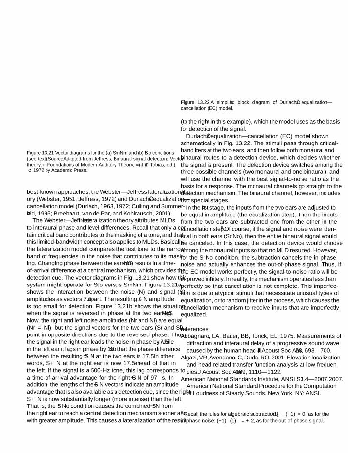
SFK SFK


chapter 13

Figure 13.21 Vector diagrams for the (a) SmNm and (b) SNo conditions(see text). Source: Adapted from Jeffress, Binaural signal detection: Vectortheory, in Foundations of Modern Auditory Theory, vol. 2 (J.V. Tobias, ed.),c© 1972 by Academic Press.

best-known approaches, the Webster–Jeffress lateralization the-ory (Webster, 1951; Jeffress, 1972) and Durlach’s equalization–cancellation model (Durlach, 1963, 1972; Culling and Summer-field, 1995; Breebaart, van de Par, and Kohlrausch, 2001).

The Webster–Jeffress lateralization theory attributes MLDsto interaural phase and level differences. Recall that only a cer-tain critical band contributes to the masking of a tone, and thatthis limited-bandwidth concept also applies to MLDs. Basically,the lateralization model compares the test tone to the narrowband of frequencies in the noise that contributes to its mask-ing. Changing phase between the ears (SNo) results in a time-of-arrival difference at a central mechanism, which provides thedetection cue. The vector diagrams in Fig. 13.21 show how thissystem might operate for SNo versus SmNm. Figure 13.21ashows the interaction between the noise (N) and signal (S)amplitudes as vectors 7.5 apart. The resulting S + N amplitudeis too small for detection. Figure 13.21b shows the situationwhen the signal is reversed in phase at the two ears (SNo).Now, the right and left noise amplitudes (Nr and Nl) are equal(Nr = Nl), but the signal vectors for the two ears (Sr and Sl)point in opposite directions due to the reversed phase. Thus,the signal in the right ear leads the noise in phase by 7.5, whilein the left ear it lags in phase by 10 so that the phase differencebetween the resulting S = N at the two ears is 17.5. In otherwords, S + N at the right ear is now 17.5 ahead of that inthe left. If the signal is a 500-Hz tone, this lag corresponds toa time-of-arrival advantage for the right S + N of 97 s. Inaddition, the lengths of the S + N vectors indicate an amplitudeadvantage that is also available as a detection cue, since the rightS + N is now substantially longer (more intense) than the left.That is, the SNo condition causes the combined S + N fromthe right ear to reach a central detection mechanism sooner andwith greater amplitude. This causes a lateralization of the result

Figure 13.22 A simplified block diagram of Durlach’s equalization–cancellation (EC) model.

(to the right in this example), which the model uses as the basisfor detection of the signal.

Durlach’s equalization–cancellation (EC) model is shownschematically in Fig. 13.22. The stimuli pass through critical-band filters at the two ears, and then follow both monaural andbinaural routes to a detection device, which decides whetherthe signal is present. The detection device switches among thethree possible channels (two monaural and one binaural), andwill use the channel with the best signal-to-noise ratio as thebasis for a response. The monaural channels go straight to thedetection mechanism. The binaural channel, however, includestwo special stages.

In the first stage, the inputs from the two ears are adjusted tobe equal in amplitude (the equalization step). Then the inputsfrom the two ears are subtracted one from the other in thecancellation step.6 Of course, if the signal and noise were iden-tical in both ears (SoNo), then the entire binaural signal wouldbe canceled. In this case, the detection device would chooseamong the monaural inputs so that no MLD resulted. However,for the SNo condition, the subtraction cancels the in-phasenoise and actually enhances the out-of-phase signal. Thus, ifthe EC model works perfectly, the signal-to-noise ratio will beimproved infinitely. In reality, the mechanism operates less thanperfectly so that cancellation is not complete. This imperfec-tion is due to atypical stimuli that necessitate unusual types ofequalization, or to random jitter in the process, which causes thecancellation mechanism to receive inputs that are imperfectlyequalized.

referencesAbbagnaro, LA, Bauer, BB, Torick, EL. 1975. Measurements of

diffraction and interaural delay of a progressive sound wavecaused by the human head-II. J Acoust Soc Am 58, 693–700.

Algazi, VR, Avendano, C, Duda, RO. 2001. Elevation localizationand head-related transfer function analysis at low frequen-cies. J Acoust Soc Am 109, 1110–1122.

American National Standards Institute, ANSI S3.4–2007.2007.American National Standard Procedure for the Computationof Loudness of Steady Sounds. New York, NY: ANSI.

6 Recall the rules for algebraic subtraction (+1) − (+1) = 0, as for thein-phase noise; (+1) − (−1) = +2, as for the out-of-phase signal.

250

SFK SFK



Arbogast, TL, Mason, CR, Kidd, G. 2002. The effect of spatialseparation on informational and energetic masking of speech.J Acoust Soc Am 112, 2086–2098.

Begault, DR. 1991. Preferred sound intensity increase for sen-sation of half distance. Percept Motor Skill 72, 1019–1029.

Bekesy, G. 1938. Uber die Entstehung der Entfernungsempfind-ung beim Horen. Akustiche Zeitschrif 3, 21–31.

Berkley, DA. 1983. Room acoustics and listening. J Acoust SocAm 44, S17.

Berkley, DA. 1987. Hearing in rooms. In: WA Yost, G Goure-vitch (eds.), Directional Hearing . New York, NY: Springer,249–260.

Bernstein, LR, Trahiotis, C. 1995. Binaural interference effectsmeasured with masking-level difference and with ITD- andIID-discrimination paradigms. J Acoust Soc Am 98, 155–163.

Best, V, Gallun, FJ, Carlile, S, Shinn-Cunningham, BG. 2007.Binaural interference and auditory grouping. J Acoust SocAm 121, 1070–1076.

Blauert, J. 1969/70. Sound localization in the median plane.Acustica 22, 205–213.

Blauert, J. 1997. Special Hearing: The Psychophysics of HumanSound Localization. Revised Edition. Cambridge, MA: MITPress.

Blodgett, HC, Jeffress, LA, Whitworth, RH. 1962. Effect of noiseat one ear on the masking threshold for tones at the other. JAcoust Soc Am 34, 979–981.

Bolt, RH, MacDonald, AD. 1949. Theory of speech masking byreverberation. J Acoust Soc Am 21, 577–580.

Breebaart, J, van de Par, S, Kohlrausch, A. 2001. Binaural pro-cessing model based on contralateral inhibition. I. Modelstructure. J Acoust Soc Am 110, 1074–1088.

Bregman, AS. 1990. Auditory Scene Analysis: The PerceptualOrganization of Sound. Cambridge, MA: Bradford Books,MIT Press.

Bregman, AS, Ahad, PA. 1996. Demonstrations of Auditory SceneAnalysis: The Perceptual Organization of Sound [CompactDisc]. Cambridge, MA: MIT Press.

Broadbent, DE. 1955. A note on binaural fusion. Q J Exp Psychol7, 46–47.

Bronkhorst, AW. 1995. Localization of real and virtual sources.J Acoust Soc Am 98, 2542–2553.

Bronkhorst, AW, Houtgast, T. 1999. Auditory distance percep-tion in rooms. Nature 397, 517–520.

Bronkhorst, AW, Plomp, R. 1988. The effect of head-inducedinteraural time and level differences on speech intelligibilityin noise. J Acoust Soc Am 83, 1508–1516.

Brungart, DS. 1999. Auditory localization of nearby sources. III.Stimulus effects. J Acoust Soc Am 106, 3589–3602.

Brungart, DS, Rabinowitz, WM. 1999. Auditory localization ofnearby sources. Head-related transfer functions. J Acoust SocAm 106, 1465–1479.

Brungart, DS, Scott, KR. 2001. The effects of production andpresentation level on the auditory distance perception ofspeech. J Acoust Soc Am 106, 1465–1479.

Buell, TN, Hafter, ER. 1991. Combination of binaural informa-tion across frequency bands. J Acoust Soc Am 90, 1894–1900.

Butler, RA. 1986. The bandwidth effect on monaural and bin-aural localization. Hear Res 21, 67–73.

Butler, RA, Levy, ET, Neff, WD. 1980. Apparent distance ofsounds recorded in echoic and anechoic chambers. J ExpPsychol Human Percept Perf 6, 745–750.

Butler, RA, Planert, N. 1976. The influence of stimulus band-width on localization of sound in space. Percept Psychophys19, 103–108.

Carhart, R, Tillman, T, Dallos, P. 1968. Unmasking for puretones and spondees: Interaural phase and time disparities. JSpeech Hear Res 11, 722–734.

Carhart, R, Tillman, T, Johnson, K. 1967. Release of maskingfor speech through interaural time delay. J Acoust Soc Am 42,124–138.

Causse, R, Chavasse, P. 1941. Recherches sur les seuil del’audition binauriculaire compare au seuil monauriculaire enfonction de la frequence. Comp R Soc Biol 135, 1272–1275.

Causse, R, Chavasse, P. 1942a. Difference entre le seuil del’audition binauriculaire et le seuil monauriculaire de la fre-quence. Comp R Soc Biol 136, 301.

Causse, R, Chavasse, P. 1942b. Difference entre l’ecoute binau-riculaire et monauriculaire por la perception des intensitiessupraliminaires. Comp R Soc Biol 139, 405.

Chandler, DW, Grantham, DW. 1992. Minimum audible move-ment angle in the horizontal plane as a function of frequencyand bandwidth, source azimuth, and velocity. J Acoust SocAm 91, 1625–1636.

Cherry, C. 1961. Two ears-but one world. In: WA Rosenblith(ed.), Sensory Communication. Cambridge, MA: MIT Press,99–117.

Cherry, EC. 1953. Some experiments on the recognition ofspeech, with one and with two ears. J Acoust Soc Am 25,975–979.

Cherry, EC, Sayers, BMcA. 1956. “Human cross-correlator”—Atechnique for measuring certain parameters of speech per-ception. J Acoust Soc Am 28, 889–896.

Churcher, BG, King, AJ, Davies, H. 1934. The minimal percepti-ble change of intensity of a pure tone. Phil Mag 18, 927–939.

Clifton, RK. 1987. Breakdown of echo suppression in the prece-dence effect. J Acoust Soc Am 82, 1834–1835.

Clifton, RK, Freyman, RL. 1989. Effect of click rate and delay onbreakdown of the precedence effect. Percept Psychophys 462,139–145.

Clifton, RK, Freyman, RL. 1997. The precedence effect: Beyondecho suppression. In: R Gilkey, T Anderson (eds.), Binau-ral and Spatial Hearing in Real and Virtual Environments.Hillsdale, NJ: Erlbaum, 233–255.

Clifton, RK, Freyman, RL, Litovsky, RY, McCall, D. 1994. Lis-teners’ expectations about echoes can raise or lower echothreshold. J Acoust Soc Am 95, 1525–1533.

Cochran, P, Throop, J, Simpson, WE. 1968. Estimation of dis-tance of a source of sound. Am J Psychol 81, 198–206.

251

SFK SFK


chapter 13

Colburn, HS, Durlach, NI. 1965. Time-intensity relations inbinaural unmasking. J Acoust Soc Am 38, 93–103.

Coleman, PD. 1962. Failure to localize the source distance of anunfamiliar sound. J Acoust Soc Am 34, 345–346.

Coleman, PD. 1963. Analysis of cues to auditory depth percep-tion in free space. Psychol Bull 60, 302–315.

Coleman, PD. 1968. Dual role of frequency spectrum in deter-mination of auditory distance. J Acoust Soc Am 44, 631–632.

Culling, JF, Summerfield, Q. 1995. Perceptual separation of con-current speech sounds: Absence of across-frequency group-ing by common interaural delay. J Acoust Soc Am 98, 785–797.

Dixon, RM, Colburn, HS. 2006. The influence of spectral, tem-poral and interaural stimulus variations on the precedenceeffect. J Acoust Soc Am 119, 2947–2964.

Dolan, TR. 1968. Effects of masker spectrum level on masking-level differences at low signal frequencies. J Acoust Soc Am 44,1507–1512.

Dolan, TR, Robinson, DE. 1967. An explanation of masking-level differences that result from interaural intensive dispar-ities of noise. J Acoust Soc Am 42, 977–981.

Duda, RO, Martens, WL. 1998. Range dependence of theresponse of a spherical head model. J Acoust Soc Am 104,3048–3058.

Durlach, NI. 1963. Equalization and cancellation theory of bin-aural masking level differences. J Acoust Soc Am 35, 1206–1218.

Durlach, NI. 1972. Binaural signal detection: Equalization andcancellation theory. In: JV Tobias (ed.), Foundations of Mod-ern Auditory Theory, Vol. 2. New York, NY: Academic Press,369–462.

Durlach, NI, Colburn, HS. 1978. Binaural phenomena. In: ECCarterette, MP Friedman (eds.), Handbook of Perception, Vol.I -Hearing . New York, NY: Academic Press, 365–466.

Durlach, NI, Rigopulos, A, Pang, XD, Woods, WS, Kulkarni, A,Colburn, HS, Wenzel, EM. 1992. On the externalization ofauditory images. Presence 1, 251–257.

Ebata, M, Sone, T, Nimura, T. 1968. On the perception of direc-tion of echo. J Acoust Soc Am 44, 542–547.

Feddersen, WE, Sandel, TT, Teas, DC, Jeffress, LA. 1957. Local-ization of high-frequency tones. J Acoust Soc Am 29, 988–991.

Fisher, HG, Freedman, SJ. 1968. The role of the pinna in auditorylocalization. J Aud Res 8, 15–26.

Fletcher, H, Munson, W. 1933. Loudness: Its definition, mea-surement and calculation. J Acoust Soc Am 5, 82–108.

Franssen, NV. 1960. Some considerations on the mechanism ofdirectional hearing. Ph.D. Dissertation. Delft, The Nether-lands: Technische Hogeschool.

Franssen, NV. 1962. Stereophony. Eindhoven, The Netherlands:Phillips Technical Library. [English translation, 1964.]

Freyman, RL, Clifton, RK, Litovsky, RY. 1991. Dynamic pro-cesses in the precedence effect. J Acoust Soc Am 90, 874–884.

Gallum, FJ, Mason, CR, Kidd, G. 2005. Binaural release frominformational masking in a speech identification task. JAcoust Soc Am 118, 1605–1613.

Gardner, MB. 1968. Historical background of the Haas and/orprecedence effect. J Acoust Soc Am 43, 1243–1248.

Gardner, MB. 1969. Distance estimation of 0 degrees or apparent0 degree-oriented speech signals in anechoic space. J AcoustSoc Am 45, 47–53.

Gardner, MB. 1973. Some monaural and binaural facets ofmedian plane localization. J Acoust Soc Am 54, 1489–1495.

Gelfand, SA, Silman, S. 1979. Effects of small room reverber-ation upon the recognition of some consonant features. JAcoust Soc Am 66, 22–29.

Grantham, DW. 1984. Interaural intensity discrimination:Insensitivity at 1000 Hz. J Acoust Soc Am 75, 1190–1194.

Grantham, DW. 1986. Detection and discrimination of simu-lated motion of auditory targets in the horizontal plane. JAcoust Soc Am 79, 1939–1949.

Grantham, DW. 1996. Left-right asymmetry in the buildup ofecho suppression in normal-hearing adults. J Acoust Soc Am99, 1118–1123.

Green, DM. 1966. Interaural phase effects in the masking ofsignals of different durations. J Acoust Soc Am 39, 720–724.

Green, DM, Henning, GR. 1969. Audition. Ann Rev Psychol 20,105–128.

Green, DM, Yost, WA. 1975. Binaural analysis. In: WD Keidel,WD Neff (eds.), Handbook of Sensory Physiology, Vol. V/2:Auditory System. New York, NY: Springer-Verlag, 461–480.

Groen, JJ. 1964. Super- and subliminate binaural beats. ActaOtol 57, 224–230.

Gu, X, Wright, BA, Green, DM. 1995. Failure to hear binauralbeats below threshold. J Acoust Soc Am 97, 701–703.

Haas, H. 1949. The influence of a single echo on the audibilityof speech. Library Com 363. Garston, Watford, UK: Dept. Sci.Indust. Rest.

Haas, H. 1951. Uber den Einfluss eines Einfachechos aud dieHorsamkeit von Sprache. Acustica 1, 49–58. [English trans-lation: J Audiol Eng Soc 20, 146–159 (1972).]

Hafter, ER, DeMaio, J. 1975. Difference thresholds for interauraldelay. J Acoust Soc Am 57, 181–187.

Hafter, ER, Bourbon, WT, Blocker, AS, Tucker, A. 1969. Directcomparison between lateralization and detection underantiphasic masking. J Acoust Soc Am 46, 1452–1457.

Hafter, ER, Buell, TN, Richards, V. 1988. Onset-coding in later-alization: Its form, site, and function. In: GM Edelman, WEGall, WM Cowan (eds.), Auditory Function: NeurobiologicalBases of Hearing . New York, NY: Wiley, 647–676.

Hafter, ER, Carrier, SC. 1970. Masking-level differencesobtained with a pulsed tonal masker. J Acoust Soc Am 47,1041–1048.

Hafter, ER, Carrier, SC. 1972. Binaural interaction in low-frequency stimuli: The inability to trade time and intensitycompletely. J Acoust Soc Am 51, 1852–1862.

Hafter, ER, Jeffress, LA. 1968. Two-image lateralization of tonesand clicks. J Acoust Soc Am 44, 563–569.

Harris, GG. 1960. Binaural interactions of impulsive stimuliand pure tones. J Acoust Soc Am 32, 685–692.

252

SFK SFK



Harris, JD. 1963. Loudness discrimination. J Speech Hear DisMonogr Suppl 11.

Harris, JD, Sergeant, RL. 1971. Monaural/binaural minimumaudible angle for a moving sound source. J Speech Hear Res14, 618–629.

Hartmann, WM. 1997. Listening in a room and the precedenceeffect. In: R Gilkey, T Anderson (eds.), Binaural and Spa-tial Hearing in Real and Virtual Environments. Hillsdale, NJ:Erlbaum, 191–210.

Hartmann, WM, Rakerd, B. 1989. Localization of sound inrooms. IV: The Franssen effect. J Acoust Soc Am 86, 1366–1373.

Hartmann, WM, Wittenberg, A. 1996. On the externalizationof sound images. J Acoust Soc Am 99, 3678–3688.

Hawley, ML, Litovsky, RY, Culling, JF. 2004. The benefits ofbinaural hearing in a cocktail party: Effect of location andtype of interferer. J Acoust Soc Am 115, 833–843.

Hebrank, J, Wright, D. 1974. Spectral cues used in the localiza-tion of sound sources on the median plane. J Acoust Soc Am56, 1829–1834.

Heller, LM, Trahiotis, C. 1995. Extents of laterality and binauralinterference effects. J Acoust Soc Am 99, 3632–3637.

Hellman, RP, Zwislocki, J. 1963. Monaural loudness functionat 1000 cps, and interaural summation. J Acoust Soc Am 35,856–865.

Henning, GB. 1973. Effect of interaural phase on frequency andamplitude discrimination. J Acoust Soc Am 54, 1160–1178.

Henning, GB. 1974. Delectability of interaural delay inhigh-frequency complex waveforms. J Acoust Soc Am 55,84–90.

Hill, NI, Darwin, CJ. 1996. Lateralization of a perturbed har-monic: Effects of onset asynchrony and mistuning. J AcoustSoc Am 100, 2352–2364.

Hirsh, IJ. 1948a. Binaural summation: A century of investiga-tion. Psychol Bull 45, 193–206.

Hirsh, IJ. 1948b. The influence of interaural phase on interauralsummation and inhibition. J Acoust Soc Am 20, 536–544.

Hirsh, IJ, Burgeat, M. 1958. Binaural effects in remote masking.J Acoust Soc Am 30, 827–832.

Jeffress, LA. 1972. Binaural signal detection: Vector theory. In:JV Tobias (ed.), Foundations of Modern Auditory Theory, Vol.2. New York, NY: Academic Press, 349–368.

Jeffress, LA, Blodgett, HC, Deatheredge, BH. 1952. The maskingof tones by white noise as a function of interaural phases ofboth components. J Acoust Soc Am 24, 523–527.

Jeffress, LA, McFadden, D. 1971. Differences of interaural phaseand level in detection and lateralization. J Acoust Soc Am 49,1169–1179.

Jesteadt, W, Wier, CC, Green, DM. 1977a. Comparison ofmonaural and binaural discrimination of intensity and fre-quency. J Acoust Soc Am 61, 1599–1603.

Jesteadt, W, Wier, CC, Green, DM. 1977b. Intensity discrimina-tion as a function of frequency and sensation level. J AcoustSoc Am 61, 169–177.

Keys, J. 1947. Binaural versus monaural hearing. J Acoust SocAm 19, 629–631.

Kidd, GK, Mason, CR, Brughera, A, Hartmann, WM. 2005.The role of reverberation in the release from masking due tospatial separation for speech intelligibility. Acta Acustica withAcustica 91, 526–536.

Klumpp, RG, Eady, HR. 1956. Some measurements of interauraltime difference thresholds. J Acoust Soc Am 28, 859–860.

Koenig, AH, Allen, JB, Berkley, DA, Curtis, TH. 1977. Determi-nation of masking-level differences in a reverberant environ-ment. J Acoust Soc Am 61, 1374–1376.

Kuhn, GF. 1977. Model for the interaural time differences inazimuthal plane. J Acoust Soc Am 62, 157–167.

Kurtovic, H. 1975. The influence of reflected sound upon speechintelligibility. Acustica 33, 32–39.

Langford, TL, Jeffress, LA. 1964. Effect of noise cross-correlation on binaural signal detection. J Acoust Soc Am 36,1455–1458.

Leakey, DM, Sayers, BMcA, Cherry, EC. 1958. Binaural fusionof low and high frequency sounds. J Acoust Soc Am 30,222–223.

Lehnhardt, E. 1961. Die akustische Korrelation. Arch OhrenNasen Kehlkopfheilk 178, 493–497.

Levitt, H, Rabiner, LR. 1967a. Binaural release from maskingfor speech and grain in intelligibility. J Acoust Soc Am 42,601–608.

Levitt, H, Rabiner, LR. 1967b. Predicting binaural gain in intel-ligibility and release from masking for speech. J Acoust SocAm 42, 820–829.

Licklider, JCR. 1948. The influence of interaural phase relationsupon the masking of speech by white noise. J Acoust Soc Am20, 150–159.

Licklider, JCR, Webster, JC, Hedlun, JM. 1950. On the frequencylimits of binaural beats. J Acoust Soc Am 22, 468–473.

Litovsky, RY. 1998. Physiological studies on the precedence effectin the inferior colliculus of the kitten. J Acoust Soc Am 103,3139–3152.

Litovsky, RY, Colburn, HS, Yost, WA, Guzman, SJ. 1999. Theprecedence effect. J Acoust Soc Am 106, 1633–1654.

Litovsky, RY, Delgutte, B. 2002. Neural correlates of the prece-dence effect in the inferior colliculus: Effect of localizationcues. J Neurophysiol 87, 976–994.

Litovsky, RY, Macmillan, NA. 1994. Sound localization precisionunder conditions of the precedence effect: Effects of azimuthand standard stimuli. J Acoust Soc Am 96, 752–758.

Litovsky, RY, Shinn-Cunningham, BG. 2001. Investigation ofthe relationship among three common measures of prece-dence: Fusion, localization dominance, and discriminationsuppression. J Acoust Soc Am 109, 346–358.

Little, AD, Mershon, DH, Cox, PH. 1992. Spectral content as acue to perceived auditory distance. Perception 21, 405–416.

Lochner, JPA, Burger, JF. 1958. The subjective masking of shorttime delayed echoes, their primary sounds, and their contri-bution to the intelligibility of speech. Acustica 8, 1–10.

253

SFK SFK


chapter 13

Lochner, JPA, Burger, JF. 1964. The influence of reflections onauditorium acoustics. J Sound Vib 1, 426–454.

Lord Rayleigh (Strutt, JW). 1907. Our perception of soundduration. Phil Mag 13, 214–232.

Macpherson, EA, Middlebrooks, JC. 2002. Listener weighting ofcues for lateral angle: The duplex theory of sound localizationrevisited. J Acoust Soc Am 111, 2219–2236.

Makous, JC, Middlebrooks, JC. 1990. Two-dimensional soundlocalization by human listeners. J Acoust Soc Am 87, 2188–2200.

Marks, LE. 1978. Binaural summation of loudness of pure tones.J Acoust Soc Am 64, 107–113.

Marks, LE. 1987. Binaural versus monaural loudness: Super-summation of tone partially masked by noise. J Acoust SocAm 81, 122–128.

McFadden, D. 1968. Masking-level differences determined withand without interaural disparities in masking intensity. JAcoust Soc Am 44, 212–223.

McFadden, D, Pasanen, EG. 1976. Lateralization at high fre-quencies based on interaural time differences. J Acoust SocAm 59, 634–639.

McGregor, P, Horn, AG, Todd, MA. 1985. Are familiar soundsranged more accurately? Percept Motor Skills 61, 1082.

Mershon, DH, Ballenger, WL, Little, AD, McMurtry, PL,Buchanan, JL. 1989. Effects of room reflectance and back-ground noise on perceived auditory distance. Perception 18,403–416.

Mershon, DH, Bowers, JN. 1979. Absolute and relative cues forthe auditory perception of egocentric distance. Perception 8,311–322.

Mershon, DH, King, LE. 1975. Intensity and reverberation asfactors in the auditory perception of echocentric distance.Percept Psychophys 18, 409–415.

Metz, PJ, von Bismark, G, Durlach, NI. 1967. I. Furtherresults on binaural unmasking and the EC model. II.Noise bandwidth and interaural phase. J Acoust Soc Am 43,1085–1091.

Middlebrooks, JC. 1992. Narrow-band sound localizationrelated to external ear acoustics. J Acoust Soc Am 92, 2607–2624.

Middlebrooks, JC. 1997. Spectral shape cues for sound local-ization. In: R Gilkey, T Anderson (eds.), Binaural and SpatialHearing in Real and Virtual Environments. Hillsdale, NJ: Erl-baum, 77–97.

Middlebrooks, JC. 1999a. Individual differences in external eartransfer functions reduced by scaling in frequency. J AcoustSoc Am 106, 1480–1492.

Middlebrooks, JC. 1999b. Virtual localization improved by scal-ing nonindividualized external-ear transfer functions in fre-quency. J Acoust Soc Am 106, 1493–1510.

Middlebrooks, JC, Green, DM. 1991. Sound localization byhuman listeners. Ann Rev Psychol 42, 135–159.

Mills, AW. 1958. On the minimal audible angle. J Acoust Soc Am30, 237–246.

Mills, AW. 1960. Lateralization of high-frequency tones. J AcoustSoc Am 32, 132–134.

Mills, AW. 1963. Auditory perception of spatial relations. ProcInt Cong Tech Blind,Vol. 2. New York, NY: American Foun-dation for the Blind.

Mills, AW. 1972. Auditory localization. In: JV Tobias (ed.), Foun-dations of Modern Auditory Theory, Vol. 2. New York, NY:Academic Press, 301–348.

Møller, H, Sorensen, MF, Jensen, CB, Hammershoi, D. 1996.Binaural technique: Do we need individual recordings? JAudio Eng Soc 44, 451–469.

Moushegian, G, Jeffress, LA. 1959. Role of interaural time andintensity differences in the lateralization of low-frequencytones. J Acoust Soc Am 31, 1441–1445.

Mrsic-Flogel, TD, King, AJ, Jenison, RL, Schnupp JWH. 2001.Listening through different ears alters special response fieldsin ferret primary auditory cortex. J Neurophysiol 86, 1043–1046.

Mulligan, BE, Mulligan, MJ, Stonecypher, JF. 1967. Critical bandin binaural detection. J Acoust Soc Am 41, 7–12.

Musicant, A, Butler, R. 1984. The influence of pinnae-basedspectral cues on sound localization. J Acoust Soc Am 75, 1195–1200.

Nabelek, AK. 1976. Reverberation effects for normal andhearing-impaired listeners. In: SK Hirsh, DH Eldridge, IJHirsh, SR Silverman (eds.), Hearing and Davis: Essays Hon-oring Hallowell Davis. St. Louis, MO: Washington UniversityPress, 333–341.

Nabelek, AK, Dagenais, PA. 1986. Vowel errors in noise and inreverberation by hearing impaired listeners. J Acoust Soc Am80, 741–748.

Nabelek, AK, Robinette, L. 1978. Influence of the precedenceeffect on word identification by normal hearing and hearing-impaired subjects. J Acoust Soc Am 63, 187–194.

Neutzel, JM, Hafter, ER. 1976. Lateralization of complex wave-forms: Effects of fine structure, amplitude, and duration. JAcoust Soc Am 60, 1339–1346.

Neutzel, JM, Hafter, ER. 1981. Discrimination of interauraldelays in complex waveforms: Spectral effects. J Acoust SocAm 69, 1112–1118.

Nielsen, SH. 1991. Distance perception in hearing. UnpublishedPh.D. Dissertation. Aalborg, Denmark: Aalborg University.

Nielsen, SH. 1993. Auditory distance perception in differentrooms. J Audio Eng Soc 41, 755–770.

Nordlund, B. 1962. Physical factors in angular localization. JAcoust Soc Am 54, 75–93.

Oldfield, SR, Parker, PA. 1984. Acuity of sound localisation: Atopography of auditory space. I. Normal hearing conditions.Perception 13, 581–600.

Palmer, SE. 1999. Vision Science: Photon to Phenomenology.Cambridge, MA: MIT Press.

Perrett, S, Noble, W. 1997a. The contribution of head motioncues to localization of low-pass noise. Percept Psychophys 59,1018–1026.

254

SFK SFK



Perrett, S, Noble, W. 1997b. The effect of head rotations onvertical plane sound localization. J Acoust Soc Am 102, 2325–2332.

Perrot, DR, Marlborough, K. 1989. Minimum audible move-ment angle: Marking the end points of a path traveledby a moving sound source. J Acoust Soc Am 85, 1773–1775.

Perrott, DR. 1984. Concurrent minimum audible angle: A re-examination of the concept of auditory special acuity. J AcoustSoc Am 75, 1201–1206.

Perrott, DR, Marlborough, K, Merrill, P, Strybel, TZ. 1989. Min-imum audible angle thresholds obtained under conditions inwhich the precedence effect is assumed to operate. J AcoustSoc Am 85, 282–288.

Perrott, DR, Musicant, A. 1977. Minimum audible movementangle: Binaural localization of moving sources. J Acoust SocAm 62, 1463–1466.

Perrott, DR, Tucker, J. 1988. Minimum audible movement angleas a function of signal frequency and the velocity of the source.J Acoust Soc Am 83, 1522–1527.

Petersen, J. 1990. Estimation of loudness and apparent distanceof pure tones in a free field. Acustica 70, 61–65.

Pickler, AG, Harris, JD. 1955. Channels of reception in pitchdiscrimination. J Acoust Soc Am 27, 124–131.

Plenge, G. 1974. On the difference between localization andlateralization. J Acoust Soc Am 56, 944–951.

Pollack, I. 1948. Monaural and binaural threshold sensitivityfor tones and white noise. J Acoust Soc Am 20, 52–58.

Pollack, I, Rose, M. 1967. Effects of head movements on thelocalization of sounds in the equatorial plane. Percept Psy-chophys 2, 591–596.

Rabiner, LR, Lawrence, CL, Durlach, NI. 1966. Further resultson binaural unmasking and the EC model. J Acoust Soc Am40, 62–70.

Reynolds, GS, Stevens, SS. 1960. Binaural summation of loud-ness. J Acoust Soc Am 32, 1337–1344.

Robinson, DE, Jeffress, LA. 1963. Effect of varying the interauralnoise correlation on the delectability of tonal signals. J AcoustSoc Am 35, 1947–1952.

Roth, RL, Kochhar, RK, Hind, JE. 1980. Interaural time differ-ences: Implications regarding the neurophysiology of soundlocalization. J Acoust Soc Am 68, 1643–1651.

Rowland, RC, Tobias, JV. 1967. Interaural intensity differencelimens. J Speech Hear Res 10, 745–756.

Saberi, K, Perrott, DR. 1990a. Minimum audible movementangles as a function of sound source trajectory. J Acoust SocAm 88, 2639–2644.

Saberi, K, Perrott, DR. 1990b. Lateralization thresholdsobtained under conditions in which the precedence effectis assumed to operate. J Acoust Soc Am 87, 1732–1737.

Sandel, TT, Teas, DC, Feddersen, WE, Jeffress, LA. 1955. Local-ization of sound from single and paired sources. J Acoust SocAm 27, 842–852.

Sayers, BMcA, Cherry, EC. 1957. Mechanism of binaural fusionin the hearing of speech. J Acoust Soc Am 29, 973–987.

Scharf, B, Fishken, D. 1970. Binaural summation of loudness:Reconsidered. J Exp Psychol 86, 374–379.

Schenkel, KD. 1964. Uber die Abhangigkeit derMithorschwellen von der interauralen Phasenlage desTestchalls. Acustica 14, 337–346.

Schubert, ED, Schultz, MC. 1962. Some aspects of binauralsignal selection. J Acoust Soc Am 34, 844–849.


Shaw, EAG. 1997. Acoustical features of the external ear. In:R Gilkey, T Anderson (eds.), Binaural and Spatial Hearingin Real and Virtual Environments. Hillsdale, NJ: Erlbaum,25–47.

Shaw, EAG, Vaillancourt, MM. 1985. Transformation of sound–pressure level from the free field to the eardrum presented innumerical form. J Acoust Soc Am 78, 1120–1123.

Shaw, WA, Newman, EB, Hirsh, IJ. 1947. The differencebetween monaural and binaural thresholds. J Exp Psycho 37,229–242.

Shinn-Cunningham, BG, Zurek, PM, Durlach, NI. 1993.Adjustment and discrimination measurements of the prece-dence effect. J Acoust Soc Am 93, 2923–2932.

Shower, EG, Biddulph, R. 1931. Differential pitch sensitivity ofthe ear. J Acoust Soc Am 3, 275–287.

Sivian, LJ, White, SD. 1933. On minimal audible fields. J AcoustSoc Am 4, 288–321.

Sondhi, MM, Guttman, N. 1966. Width of the spectrum effec-tive in the binaural release of masking. J Acoust Soc Am 40,600–606.

Stellmack, MA, Dye, RH. 1993. The combination of interauralinformation across frequencies: The effects of number andspacing of components, onset asynchrony, and harmonicity.J Acoust Soc Am 93, 2933–2947.

Stellmack, MA, Viemeister, NF, Byrne, AJ. 2004. Monaural andinteraural intensity discrimination: Level effects and the “binaural advantage.” J Acoust Soc Am 116, 1149–1159.

Stevens, SS, Newman, EB. 1936. The localization of actualsources of sound. Am J Psychol 48, 297–306.

Thurlow, WR, Runge, PS. 1967. Effect of induced head move-ments on localization of direction of sounds. J Acoust Soc Am42, 480–488.

Tobias, JV. 1963. Application of a “relative” procedure to thebinaural-beat problem. J Acoust Soc Am 35, 1442–1447.

Tollin, DJ, Henning, GB. 1998. Some aspects of the lateralizationof echoed sound in man. I: Classical interaural delay-basedprecedence. J Acoust Soc Am 104, 3030–3038.

Townsend, TH, Goldstein, DP. 1972. Suprathreshold binauralunmasking. J Acoust Soc Am 51, 621–624.

Trahiotis, C, Bernstein, LR. 1990. Detectability of interauraldelays over select spectral regions: Effects of flanking noise. JAcoust Soc Am 87, 810–813.

255

SFK SFK


chapter 13

Wagenaars, WM. 1990. Localization of sound in a room withreflecting walls. J Audio Eng Soc 38, 99–110.

Wallach, H. 1939. On sound localization. J Acoust Soc Am 10,270–274.

Wallach, H. 1940. The role of head movements and vestibularand visual cues in sound localization. J Exp Psychol 27, 339–368.

Wallach, H, Newman, EB, Rosenzweig, MR. 1949. The prece-dence effect in sound localization. Am J Psychol 62,315–336.

Webster, FA. 1951. The influence of interaural phase on maskedthresholds. I. The role of interaural time-duration. J AcoustSoc Am 23, 452–462.

Weinrich, S. 1982. The problem of front-back localization inbinaural hearing. Scand Audiol Suppl 15, 135–145.

Wenzel, EM, Arruda, M, Kistler, DJ, Wightman, FL. 1993. Local-ization using nonindividualized head-related transfer func-tions. J Acoust Soc Am 94, 111–123.

Wernick, JS, Starr, A. 1966. Electrophysiological correlates ofbinaural beats in superior-olivary complex of cat. J AcoustSoc Am 40, 1276.

Whitworth, RH, Jeffress, LA. 1961. Time vs. intensity on thelocalization of tones. J Acoust Soc Am 33, 925–929.

Wier, CC, Jesteadt, W, Green, DM. 1977. Frequency discrimina-tion as a function of frequency and sensation level. J AcoustSoc Am 61, 178–184.

Wightman, FL. 1971. Detection of binaural tones as a functionof masker bandwidth. J Acoust Soc Am 50, 623–636.

Wightman, FL, Kistler, DJ. 1989a. Headphone simulation offree-field listening. I: Stimulus synthesis. J Acoust Soc Am 85,858–867.

Wightman, FL, Kistler, DJ. 1989b. Headphone simulation offree-field listening. II: Psychophysical validation. J Acoust SocAm 85, 868–878.

Wightman, FL, Kistler, DJ. 1992. The dominant role of low-frequency interaural time differences in sound localization. JAcoust Soc Am 91, 1648–1661.

Wightman, FL, Kistler, DJ. 1993. Sound localization. In: WAYost, AN Popper, RR Fay (eds.), Human Psychoacoustics. NewYork, NY: Springer-Verlag, 155–192.

Wightman, FL, Kistler, DJ. 1997. Factors affecting the relativesalience of sound localization cues. In: R Gilkey, T Ander-son (eds.), Binaural and Spatial Hearing in Real and VirtualEnvironments. Hillsdale, NJ: Erlbaum, 1–23.

Wightman, FL, Kistler, DJ. 1999. Resolution of front-back ambi-guity in spatial hearing by listener and source movement. JAcoust Soc Am 105, 2841–2853.

Woodworth, RS. 1938. Experimental Psychology. New York, NY:Holt, Rhinehart, and Winston.

Wu, X, Wang, C, Chen, J, Qu, H, Li, W, Wu, Y, Schneider,BA., Li, L. 2005. The effect of perceived spatial separationon informational masking of Chinese speech. Hear Res 199,1–10.

Yang, X, Grantham, DW. 1997. Echo suppression and discrim-ination suppression aspects of the precedence effect. PerceptPsychophys 59, 1108–1117.

Yost, WA. 1974. Discriminations of interaural phase differences.J Acoust Soc Am 55, 1299–1303.

Yost, WA. 1981. Lateral position of sinusoids presented withinteraural intensive and temporal differences. J Acoust SocAm 70, 397–409.

Yost, WA. 1993 Overview: Psychoacoustics. In: WA Yost, ANPopper, RR Fay (eds.), Human Psychophysics. New York, NY:Springer-Verlag, 1–12.

Yost, WA. 1997. The cocktail party problem: Forty years later.In: R Gilkey, T Anderson (eds.), Binaural and Spatial Hearingin Real and Virtual Environments. Hillsdale, NJ: Erlbaum,329–347.

Yost, WA, Dye, RH Jr. 1988. Discrimination of interaural dif-ferences of level as a function of frequency. J Acoust Soc Am83, 1846–1851.

Yost, WA, Sheft, S. 1993. Auditory perception. In: WA Yost, ANPopper, RR Fay (eds.), Human Psychophysics. New York, NY:Springer-Verlag, 193–236.

Yost, WA, Wightman, FL, Green, DM. 1971. Lateralization offiltered clicks. J Acoust Soc Am 50, 1526–1531.

Zahorik, P. 1996. Auditory distance perception: A litera-ture review. Wisconsin: University of Wisconsin-Madison.http://www.waisman.wisc.edu/∼zahorik/papers/dist.html.

Zahorik, P. 2002a. Assessing auditory distance perception usingvirtual acoustics. J Acoust Soc Am 111, 1832–1846.

Zahorik, P. 2002b. Direct-to-reverberant energy ratio sensitivity.J Acoust Soc Am 112, 2110–2117.

Zurek, PM. 1980. The precedence effect and its possible role inthe avoidance of interaural ambiguities. J Acoust Soc Am 67,952–964.

Zwislocki, J, Feldman, RS. 1956. Just noticeable differences indichotic phase. J Acoust Soc Am 28, 860–864.

256

SFK SFK


14 Speech and Its Perception

Pure tones, clicks, and the like enable us to study specific aspectsof audition in a precise and controllable manner. On the otherhand, we communicate with each other by speech, which iscomposed of particularly complex and variable waveforms. Aknowledge of how we perceive simpler sounds is the foundationupon which an understanding of speech perception must bebuilt. As one might suppose, speech perception and intimatelyrelated areas constitute a voluminous subject encompassing farmore than hearing science, per se, and the interested studentwill find numerous sources addressing the topic at various levels(e.g., Miller, 1951; Fletcher, 1953; Fant, 1970; Flanagan, 1972;Massaro, 1987, 1998; Pickett, 1999; Miller et al., 1991; Kent andRead, 2002; Liberman, 1996; Ryalls, 1996; Jusczyk and Luce,2002; Diehl et al., 2004; Galantucci et al., 2006; Ferrand, 2007;Raphael et al., 2007; Massaro and Chen, 2008).

Speech perception and speech production are inherentlyinterrelated. We must be able to speak what we can perceive, andwe must have the ability to perceive the sounds that our speechmechanisms produce. Traditionally, the sounds of speech havebeen described in terms of the vocal and articulatory manipu-lations that produce them. We too shall begin with production.For the most part, our discussion will focus upon phonemes.

By a phoneme we mean a group of sounds that are classifiedas being the same by native speakers of a given language. Let ussee what the “sameness” refers to. Consider the phoneme /pi/ asit appears at the beginning and end of the word “pipe.” Thereare actually several differences between the two productions of/p/ in this word. For example, the initial /p/ is accompanied bya release of a puff of air (aspiration), whereas the final /p/ isnot. In other words, the actual sounds are different, or distinctphonetic elements. (By convention, phonemes are enclosedbetween slashes and phonetic elements between brackets.) Inspite of this, native speakers of English will classify both asbelonging to the family designated as the /p/ phoneme. Suchphonetically dissimilar members of the same phonemic class arecalled allophones of that phoneme. Consider a second example.The words “beet” and “bit” (/bit/ and /bIt/, respectively) sounddifferent to speakers of English but the same to speakers ofFrench. This happens because the phonetic elements [i] and [I]are different phonemes in English, but are allophones of thesame phoneme in French. Since the French person classifies [i]and [I] as members of the same phonemic family, he hears themas being the same, just as English speakers hear the aspiratedand unaspirated productions of /p/ to be the same.

This last example also demonstrates the second importantcharacteristic of phonemes. Changing a phoneme changes themeaning of a word. Thus, /i/ and /I/ are different phonemes inEnglish, because replacing one for the other changes the mean-ing of at least some words. However, [i] and [I] are not differ-ent phonemes in French; that is, they are allophones, becausereplacing one for the other does not change the meaning of

words. Implicit in the distinction of phonetic and phonemicelements is that even elementary speech sound classes are tosome extent learned. All babies the world over produce thesame wide range of sounds phonetically; it is through a processof learning that these phonetic elements become classified andgrouped into families of phonemes that are used in the languageof the community.

speech sounds: production and perception

Our discussion of speech sounds will be facilitated by refer-ence to the simplified schematic diagram of the vocal tractin Fig. 14.1 The power source is the air in the lungs, which isdirected up and out under the control of the respiratory muscu-lature. Voiced sounds are produced when the vocal folds (vocalcords) are vibrated. The result of this vibration is a periodiccomplex waveform made up of a fundamental frequency onthe order of 100 Hz in males and 200 Hz in females, with asmany as 40 harmonics of the fundamental represented in thewaveform (Flanagan, 1958) (Fig. 14.2a). Voiceless (unvoiced)sounds are produced by opening the airway between the vocalfolds so that they do not vibrate. Voiceless sounds are aperiodicand noise-like, being produced by turbulences due to partialor complete obstruction of the vocal tract. Regardless of thesource, the sound is then modified by the resonance character-istics of the vocal tract. In other words, the vocal tract constitutesa group of filters that are added together, and whose effect isto shape the spectrum of the waveform from the larynx. Theresonance characteristics of the vocal tract (Fig. 14.2b) are thusreflected in the speech spectrum (Fig. 14.2c). The vocal tractresonances are called formants and are generally labeled start-ing from the lowest as the first formant (F1), second formant(F2), third formant (F3), etc. This is the essence of the source-filter theory, or the acoustic theory of speech production(Fant, 1970).

VowelsSpeech sounds are generally classified broadly as vowels andconsonants. Vowels are voiced sounds whose spectral charac-teristics are determined by the size and shape of the vocal tract.(Certain exceptions are notable. For example, whispered speechis all voiceless, and vowels may also be voiceless in some con-texts of voiceless consonants in connected discourse. Also, thenasal cavity is generally excluded by action of the velum unlessthe vowel is in the environment of a nasal sound.) Changingthe shape of the vocal tract changes its filtering characteristics,which in turn change the formant structure, that is, the frequen-cies at which the speech signal is enhanced or de-emphasized(Fig. 14.2). Diphthongs such as /aI/ in “buy” and /oU/ in “toe”are heard when one vowel glides into another.

257

SFK SFK


chapter 14

Figure 14.1 Schematic representation of speech production.

In general, the formant frequencies depend upon where andto what extent the vocal tract is constricted (Peterson andBarney, 1952; Stevens and House, 1955, 1961; Flanagan, 1972).The locations and degrees of these constrictions control the sizesand locations of the volumes in the vocal tract. For example,elevation of the back of the tongue results in a larger volumebetween this point of constriction and the lips than does ele-vation of the tongue tip. We may thus describe a vowel fromfront to back in terms of the amount of tongue elevation. Liprounding is another important factor. In English, front vowels(/i, I, e, ε, æ/) are produced with retraction of the lips, whilethe lips are rounded when the back vowels (/u, U, o, ɔ, a/) areformed. Rounding the front vowel /i/ as in “tea” while keepingthe high-front tongue placement results in the French vowel /y/,as in “tu.” The degree of tenseness associated with the musclecontractions is also a factor in vowel production and perception,as in the differentiation of the tense /i/ (“peat”) from the lax /I/(“pit”). Tense vowels are generally more intense and longer induration than their lax counterparts.

The middle vowels (/,ə,,,/) are produced when tongueelevation is in the vicinity of the hard palate. These include theneutral vowel or schwa, /ə/, associated mainly with unstressedsyllables (e.g., “about” and “support”).

Without going into great detail, the frequency of the firstformat (F1) is largely dependent upon the size of the volumebehind the tongue elevation, that is, upon the larger of the vocaltract volumes. This volume must, of course, increase as the ele-vated part of the tongue moves forward. Thus, front tongueelevation produces a larger volume behind the point of con-striction, which in turn is associated with lower F1 frequencies,

Figure 14.2 The source-filter theory (acoustic theory) of speech produc-tion: Idealized spectra showing that when the glottal source spectrum (a) ispassed through the vocal tract filters (b) the resulting (output) spectrum (c)represents characteristics of the vocal tract. F1 and F2 indicate the first twoformants.

Figure 14.3 Spectrograms showing sustained production of the vowels /i/,/æ/, and /u/ (left to right). Timing marks along the top are 100 ms apart.

whereas back tongue elevations decrease the size of this volume,thereby raising the frequency of F1. The frequency of the secondformant (F2) depends largely upon the size of the volume infront of the point of tongue elevation, becoming higher whenthe cavity is made smaller (when the tongue is elevated closerto the front of the mouth). Lip rounding lowers the first twoformants by reducing the size of the mouth opening.

Figure 14.3 shows sustained productions of several vowels inthe form of sound spectrograms (Koenig et al., 1946; Potteret al., 1947). Frequency is shown up the ordinate, time alongthe abscissa, and intensity as relative blackness or gray-scale.Thus, blacker areas represent frequencies with higher energyconcentrations and lighter areas indicate frequency regions withless energy. The formants are indicated by frequency bandsmuch darker than the rest of the spectrogram. These horizontalbands represent frequency regions containing concentrationsof energy and thus reflect the resonance characteristics of thevocal tract. The vertical striations correspond to the period ofthe speaker’s fundamental frequency.

The relationship between tongue position and the frequenciesof F1 and F2 are shown for several vowels in Fig. 14.4. However,it should be noted that these formant frequencies are approxi-mations based on average male values from just one study. For-mant center frequencies and bandwidths tend to become highergoing from men to women to children, which reflects the effectof decreasing vocal tract length (Fig. 14.5). Formant parametersvary appreciably among talkers and even between studies (e.g.,Peterson and Barney, 1952; Hillenbrand et al., 1995); they areaffected by such factors as neighboring phonemes, by whetherthe syllable is stressed or unstressed, etc.

The lower formants (especially F1 and F2, as well as F3) areprimarily responsible for vowel recognition (Peterson, 1952;Peterson and Barney, 1952; Delattre et al., 1952; Hillenbrandet al., 1995). However, given the wide variations alluded toabove, it is doubtful that vowels are identified on the basis oftheir formant frequencies, per se. The relationships among the

258

SFK SFK


speech and its perception

Figure 14.4 Vowel quadrilateral showing the approximate values of thefirst (F1) and second (F2) formants of several vowels as they relate to tongueheight and place based on data for male talkers by Peterson and Barney(1952).

formants, as well as the environment of the vowel and its dura-tion, provide important cues (Tiffany, 1953; Stevens and House,1963; Lindblom and Studdert-Kennedy, 1967). It has been sug-gested that, for each individual speaker, the listener adjusts the“target” values of the formants according to the utterances ofthat speaker (e.g., Ladefoged and Broadbent, 1957; Lieberman,1973); however, this is certainly not the only explanation forvowel perception. A lucid review of vowel perception issuesand theories may be found in Kent and Read (2002), and moreadvanced students will find informative discussions in a series

3500

3000

2500

2000

1500

1000

Sec

ond

For

man

t (F

2) in

Her

tz

500200 400

uu

ua

aa

i

i

i

Men

Women

Children

600 800

First Formant (F1) in Hertz

1000 1200

Figure 14.5 Average formant frequencies increase going from men towomen to children, as illustrated here by the shifts in the average valuesof F1 and F2 for the vowels /i/, /a/, and /u/. Source: Based on data by Peter-son and Barney (1952).

of papers by Miller (1989), Nearey (1989), and Strange (1989a,1989b).

ConsonantsThe consonants are produced by either a partial or completeobstruction somewhere along the vocal tract. The ensuing tur-bulence causes the sound to be quasi-periodic or aperiodic andnoise-like. The consonants are differentiated on the basis ofmanner of articulation, place of articulation, and voicing; that is,on how and where the obstruction of the vocal tract occurs andon whether there is vocal cord vibration. Table 14.1 shows theEnglish consonants, arranged horizontally according to place ofarticulation and vertically by manner of articulation and voic-ing. Examples are given where the phonetic and orthographicsymbols differ.

The stops, fricatives, and affricates may be either voiced orvoiceless, whereas the nasals and semivowels are virtually alwaysvoiced. The nasal cavities are excluded from the production ofall consonants except the nasals by elevation of the velum. Weshall briefly discuss the consonants in order of the manner oftheir articulation.

The stops are produced by a transition (see below) from thepreceding vowel, a silent period on the order of roughly 30 msduring which air pressure is impounded behind a completeobstruction somewhere along the vocal tract, a release (burst) ofthe built-up pressure, and finally a transition into the followingvowel (Cooper et al., 1952; Fischer-Jorgensen, 1954; Libermanet al., 1956; Halle et al., 1957). Of course, whether there is atransition from the preceding vowel and/or into the followingvowel depends upon the environment of the stop consonant.Voiceless stops in the initial position are generally aspirated,or released with a puff of air. Initial voiced stops and all finalstops tend not to be aspirated, although this does not applyalways or to all speakers. The voiceless stops (/p,t,k/) and theirvoiced cognates (/b,d,g/) are articulated in the same way exceptfor the presence or absence of voicing and/or aspiration. Asa rule, the voiceless stops tend to have longer and strongerpressure buildups than do their voiced counterparts (Sharf,1962; Arkebauer et al., 1967).

The six stops are produced at three locations. The bilabials(/p,b/) are produced by an obstruction at the lips, the alve-olars (/t,d/) by the tongue tip against the upper gum ridge,and the velars (/k,g/) by the tongue dorsum against the softpalate. Whether the sound is heard as voiced or voiceless is, ofcourse, ultimately due to whether there is vocal cord vibration.However, cues differ according to the location of the stop inan utterance. The essential voicing cue for initial stops is voiceonset time (VOT), which is simply the time delay between theonset of the stop burst and commencement of vocal cord vibra-tion (Lisker and Abramson, 1964, 1967). In general, voicingonset precedes or accompanies stop burst onset for voiced stopsbut lags behind the stop burst for voiceless stops. For final stopsand those that occur medially within an utterance, the essen-tial voicing cue appears to be the duration of the preceding

259

SFK SFK


chapter 14

Table 14.1 Consonants of English.

Bilabial Labiodental Linguadental Alveolar Palatal Velar Glottal

StopsVoiceless p t kVoiced b d g

FricativesVoiceless (which) f (thing) s ʃ(shoe)Voiced v › (this) z (beige)

AffricatesVoiceless tʃ(catch) hVoiced (dodge)

Nasalsa m n ŋ (sing)Liquidsa r, lGlidesa w j (yes)

aThe nasals, liquids, and glides are voiced.

vowel (Raphael, 1972). Longer vowel durations are associatedwith the perception that the following stop is voiced. Voicelessstops are also associated with longer closure durations (Lisker,1957a, 1957b), faster formant transitions (Slis, 1970), greaterburst intensities (Halle et al., 1957), and somewhat higherfundamental frequencies (Haggard et al., 1970) than voicedstops.

Place of articulation (bilabial vs. alveolar vs. velar) for thestops has been related to the second formant (F2) transitionof the associated vowel (Liberman et al., 1954; Delattre et al.,1955), along with some contribution from the F3 transitions(Harris et al., 1958). By a formant transition we simply mean achange with time of the formant frequency in going from thesteady-state frequency of the vowel into the consonant (or viceversa). Formant transitions may be seen for several initial voicedstops in Fig. 14.6. The F2 transitions point in the directionof approximately 700 Hz for bilabial stops, 1800 Hz for thealveolars, and 3000 Hz for the velars (Liberman et al., 1954).The second formation transition locus principle is illustratedin Fig. 14.7 These directions relate to the location of vocal tractobstruction. That is, a larger volume is enclosed behind anobstruction at the lips (/p,b/) than at the alveolus (/t,d/) or the

Figure 14.6 Spectrograms of /ba/, /da/, and / ga/ (left to right). Note secondformant transitions.

velum (/k,g/) so that the resonant frequency associated withthat volume is lower for more frontal obstructions. Movingthe point of obstruction backward reduces the cavity volumeand thus increases the resonant frequency. Additional placeinformation is provided by the frequency spectrum of the stopburst. Stop bursts tend to have concentrations of energy atrelatively low frequencies (500–1500 Hz) for the bilabials, athigh frequencies (about 4000 Hz and higher) for the alveolars,and at intermediate frequencies (between around 1500 and 4000Hz) for the velars (Liberman et al., 1956).

There tends to be a considerable amount of variability (oftendescribed as a lack of invariance) in the formant cues because theconfigurations of the formant transitions change according tothe associated vowels. This variability is readily observed in Fig.14.7 and is especially apparent for the alveolars. For example,the second formant transition from /d/ into the following vowelis different for /di/ and /du/. An invariant place of articulationcue has been proposed on the basis of several acoustical andperceptual studies (e.g., Stevens and Blumstein, 1978; Blumsteinand Stevens, 1979, 1980; Blumstein, Isaacs, and Mertus, 1982;Kewley-Port, 1983; Kewley-Port and Luce, 1984; Furui, 1986).For example, Stevens, Blumstein, and colleagues demonstratedinvariant patterns in the gross configurations of the spectraintegrated over a period of roughly 20 ms in the vicinity of theconsonant release. Figure 14.8 shows the general configurationsof these onset spectra, which are (a) diffuse and falling forbilabials, /p,b/; (b) diffuse and rising for the alveolars, /t,d/; and(c) compact for the velars, /k,g/.

In addition to the perceptual findings, further support forthis concept comes from experiments using computer models(Searle, Jacobson, and Rayment, 1979) and auditory nerve dis-charge patterns (Miller and Sachs, 1983). There is theoreticaland experimental support for the notion that children use onsetspectra as the primary cues for place of articulation for stopsbefore they learn to use formant transitions as secondary per-ceptual cues (e.g., Blumstein and Stevens, 1979, 1980; Ohde etal., 1995), although there are contrary models and results, as

260

SFK SFK



Figure 14.7 Artist’s conceptualization of the second formant transition locus principle for stop consonant place of articulation. Stars indicate the locus(target frequency) toward which the second formant transitions point for bilabials, alveolars, and velars.

Figure 14.8 Invariant onset spectrum configurations associated with stop-consonant place of articulation: alveolars, diffuse, and rising; labials, diffuse,and falling; velars, compact. Source: Adapted from Blumstein and Stevens(1979), with permission of J. Acoust. Soc. Am.

well (e.g., Walley and Carrell, 1983; Nittrouer and Studdert-Kennedy, 1987; Nittrouer, 1992). Repp and Lin (1989) havesuggested that the onset spectrum may provide the listener witha very brief “acoustic snapshot of the vocal tract” that mightbe supplemented by the dynamic cues of formant transitions ifmore information is needed to accurately identify the sound.

The fricatives are produced by a partial obstruction of thevocal tract so that the air coming through becomes turbulent.The nature of the fricatives has been well described (Houseand Fairbanks, 1953; Huges and Halle, 1956; Harris, 1958;Strevens, 1960; Heinz and Stevens, 1961; Jassem, 1965; Guer-lekian, 1981; Jongman, 1985; Behrens and Blumstein, 1988).Several examples of the fricatives are shown in the spectrogramsin Fig. 14.9 Fricatives are distinguished from other manners ofarticulation by the continuing nature of their turbulent energy(generally lasting 100 ms or more); vowels preceding fricativestend to have greater power and duration, and somewhat longer

Figure 14.9 Spectrograms of /fa/, /sa/, and /ʃ,a/ (left to right).

261

SFK SFK


chapter 14

fundamental frequencies, than vowels preceding stops. As istrue for the stops, fricatives may be either voiced or voiceless.However, unlike the stops, the duration of the fricatives makes itpossible for voicing to be cued by the presence versus absence ofperiodic energy during frication. In addition, fricative voicingis also cued by VOT and by the nature of the preceding vowel.Moreover, voiceless fricatives tend to have longer durations thantheir voiced counterparts.

Spectral differences largely account for place distinctionsbetween the alveolar (/s,z/) and the palatal (/ʃ,/) sibilantfricatives. The palatals have energy concentrations extending tolower frequencies (about 1500–7000 Hz) than do the alveolars(roughly 4000–7000 Hz), most likely because of the largervolume in front of the point of vocal tract obstruction for/ʃ,/ than for /s,z/. On the other hand, /,›/, and /f, v/ aredifferentiated largely on the basis of formant transitions.Because of resonation of the entire vocal tract above the glottis,/h/ possesses more low frequencies than the more anteriorfricatives. The amplitudes of /s/ and /ʃ/ are considerably greaterthan those of /f/ and //. However, perceptual experimentsby Behrens and Blumstein (1988) have demonstrated thatthese amplitudes are less important than spectral propertiesin differentiating between these two groups of fricatives.The affricates are produced by the rapid release of their stopcomponents into their fricative components.

The nasals are produced by opening the port to the nasal cavi-ties at the velum. They are semivowels in that they are voiced andhave some of the formant characteristics of vowels. However,they differ from other sounds by the coupling of the nasal andoral cavities. The characteristics of nasals have been describedby Fujimura (1962) and others (Cooper et al., 1952; Malecot,1956; House, 1957; Kurowski and Blumstein, 1987a, 1987b).The coupling of the nasal cavities to the volume of oral cavitybehind the point of obstruction (the velum for /ŋ/, alveolus for/n/, and lips for /m/) constitutes a side-branch resonator. Thisresults in antiresonances at frequencies that become lower as thevolume of the side branch (oral cavity) becomes larger. Thus,we find that antiresonances appear in the frequency regions ofroughly 1000 Hz for /m/ (where the side branch is the largest),1700 Hz for /n/, and 3000 Hz for /ŋ/ (where the side branchis the shortest). Furthermore, overall intensity is reduced, andfor the first formant is lower than for the vowels, constitutinga characteristic low-frequency nasal murmur. Place of articu-lation is cued by differences in spectrum of the nasal murmur(e.g., Kurowski and Blumstein, 1993), and spectral and ampli-tude changes at the juncture between the nasal and the adjoin-ing vowel (e.g., Kurowski and Blumstein, 1987a, 1987b; Ohde,Haley, and Barnes, 2006).

The semivowels are /w,j/ and /r,l/. The former two are knownas the glides and the latter ones are liquids. The semivowelshave been described by O’Connor et al. (1957), Lisker (1957a,1957b), and Fant (1970). The bilabial glide /w/ is producedinitially in the same way as the vowel /u/, with a transition intothe following vowel over the course of about 100 ms. For the

glide /j/, /j/, the transition into the following vowel is from /i/and takes about the same amount of time as for /w/. The firstformants of both /w/ and /j/ are on the order of 240 Hz, with thesecond formant transitions beginning below about 600 Hz for/w/ and above 2300 Hz for /j /. Furthermore, there appears tobe relatively low-frequency frication-like noise associated with/w/ and higher-frequency noise with /j /, due to the degree ofvocal tract constriction in their production.

The liquids (/r,l/) have short-duration steady-state portionsof up to about 50 ms, followed by transitions into the followingvowel over the course of roughly 75 ms. The /r/ is producedwith some degree of lip rounding, and /l/ is produced withthe tongue tip at the upper gum ridge so that air is deflectedlaterally. The first formants of the liquids are on the order of500 Hz for /r/ and 350 Hz for /l/, which are relatively high,and the first and second formant transitions are roughly similarfor both liquids. The major difference appears to be associatedwith the presence of lip rounding for /r/ but not for /l /. Sincelip rounding causes the third formant to be lower in frequency,/r/ is associated with a rather dramatic third formant transitionupward in frequency, which is not seen for /l /, at least not fortransitions into unrounded vowels. The opposite would occurfor /r/ and /l / before a rounded vowel.

dichotic listening and cerebrallateralization

Dichotic listening studies involve asking listeners to respondto two different signals presented at the same time, one to theright ear and another to the left ear (see, e.g., Berlin and McNeil(1976). This approach was introduced to the study of speechperception by Broadbent (1954, 1956) as a vehicle for the studyof memory, and was extended to the study of hemispheric lat-eralization for speech by Kimura (1961, 1967). Kimura askedher subjects to respond to different digits presented to the twoears. The result was a small but significant advantage in the per-ception of the digits at the right ear—the right ear advantage(REA). On the other hand, there was a left ear advantage whenmusical material was presented dichotically (Kimura, 1964).

The study of dichotic listening was enhanced with the useof CV syllables by Shankweiler and Studdert-Kennedy (1967)and others (e.g., Studdert-Kennedy and Shankweiler, 1970;Studdert-Kennedy et al., 1970; Berlin et al., 1973; Cullen et al.,1974). The basic experiment is similar to Kimura’s, except thatthe dichotic digits are replaced by a pair of dichotic CV syllables.Most often, the syllables /pa, ka, ta, ba, da, ga/ are used. The CVstudies confirmed and expanded the earlier digit observations.For example, Studdert-Kennedy and Shankweiler (1970) founda significant REA for the CVs but not for vowels. They furtherfound that the REA was larger when the consonants differed inboth place of articulation and voicing (e.g., /pa/ vs. /ga/) thanwhen the contrast was one of place (e.g., /pa/ vs. /ta/) or voic-ing (e.g., /ta/ vs. /da/) alone. Similarly, Studdert-Kennedy and

262

SFK SFK



Shankweiler (1970) found that errors were less common whenthe dichotic pair had one feature (place or voicing) in commonthan when both place and voicing were different.

Since the primary and most efficient pathways are from theright ear to the left cerebral hemisphere and from the left ear tothe right hemisphere, these have been interpreted as revealingright-eared (left hemisphere) dominance for speech and left-eared (right hemisphere) dominance for melodic material. Thatthe left hemisphere is principally responsible for the processingof speech material is also supported by physiological findingsusing a variety of approaches (Wood et al., 1971; Wood, 1975;Makela et al., 2003, 2005; Josse et al., 2003; Tervaniemi andHugdahl, 2003; Price et al., 2005; Shtyrov et al., 2005).

The robustness of the REA was demonstrated by Cullen et al.(1974), who showed that the REA is maintained until the signalto the right ear is at quite a disadvantage relative to the onepresented to the left. Specifically, the REA was maintained until(1) the stimuli presented to the left ear were 20 dB strongerthan those to the right, (2) the signal-to-noise ratio (SNR) inthe right ear was 12 dB poorer than in the left, and (3) the CVspresented to the right ear were filtered above 3000 Hz while theleft ear received an unfiltered signal. Interestingly, Cullen et al.also demonstrated that when the right-ear score decreased, theleft ear score actually became proportionally better so that thetotal percent correct (right plus left) was essentially constant.This suggests that there is a finite amount of information thatcan be handled at one time by the speech-handling mechanismin the left hemisphere.

When the CV delivered to one ear is delayed relative to thepresentation of the CV to the other ear, then there is an advan-tage for the ear receiving the lagging stimulus, particularly fordelays on the order of 30 to 60 ms (Studdert-Kennedy et al.,1970; Berlin et al., 1973). This phenomenon is the dichotic lageffect. Since it also occurs for nonspeech (though speech-like)sounds, there is controversy over whether the lag effect is aspeech-specific event or a more general phenomenon such asbackward masking (Darwin, 1971; Pisoni and McNabb, 1974;Mirabile and Porter, 1975; Porter, 1975).

Since the primary and most efficient pathways are from theright ear to the left cerebral hemisphere and from the left ear tothe right hemisphere, the these have been interpreted as reveal-ing right-eared (left hemisphere) dominance for speech andleft-eared (right hemisphere) dominance for melodic material.That the left hemisphere is principally responsible for the pro-cessing of speech material is also supported by physiologicalfindings using a variety of approaches (Wood et al., 1971; Woodet al., 1971; Wood, 1975; Makela et al., 2003, 2005; Josse et al.,2003; Tervaniemi and Hugdahl, 2003;Price et al., 2005; Shtyrovet al., 2005).

categorical perception

Liberman et al. (1961) prepared synthetic consonant–vowel(CV) monosyllables composed of two formants each. They

asked their subjects to discriminate between these pairs of syn-thetic CVs, as the second formant transition was varied, andobtained a finding that has had a profound effect upon the studyof speech perception. Subjects’ ability to discriminate betweenthe two CVs in a pair was excellent when the consonants wereidentifiable as different phonemes, whereas discrimination waspoor when the consonants were identified as belonging to thesame phonemic category.

This phenomenon of categorical perception is illustratedin Fig. 14.10 which shows idealized results from a hypotheticalstudy of how VOT affects the perception of initial alveolar stops.Recall that VOT is the voicing cue for initial stops, so we aredealing with the perception of /t/ versus /d/. The stimuli are CVsyllables differing in VOT. For simplicity, we will identify VOTsby letters instead of actual durations in milliseconds. Two typesof perceptual tasks are involved. In the first test, the amount ofVOT is varied in 10 equal increments from A (the shortest) to J(the longest), and the subjects must identify the CVs as /ta/ or/da/. The upper frame of the figure shows that just about all ofthe shorter VOTs (A to E) were heard as /d/, whereas virtuallyall of the longer VOTs (F to J) were heard as /t/. In other words,there was an abrupt change in the categorization of the stimuli

A

0

PE

RC

EN

T O

F ID

EN

TIF

ICAT

ION

SD

ISC

RIM

INAT

ION

IN P

ER

CE

NT

20

40AB

STIMULUS PAIRS

Chance

BC CD DE EF FG GH HI IJ

50

60

70

80

100

90

40

60

80

100

B C D E F G

d

dddd

t t t tt

tt t t t

d d d d

H I JShorter LongerVOT INCREMENTS (ms)

Figure 14.10 Idealized results for in a categorical perception experiment(see text).

263

SFK SFK


chapter 14

as either voiced or voiceless between VOT increments E andF, constituting a category boundary. The second task is to dis-criminate between pairs of these stimuli; for example, betweenA–B, B–C, C–D, etc. Notice that the VOT difference (in mil-liseconds) is the same between the members of each pair. Theseresults are shown in the lower frame of the figure, where 50%is random guessing (chance). Notice that the subjects can easilydiscriminate between E and F, where one member of the pair(E) is identified as /da/ and the other member of the pair (F)is identified as /ta/. On the other hand, they cannot discrimi-nate between any of the other pairs, where both members wereidentified as /da/ (e.g., C vs. D) or as /ta/ (e.g., G vs. H). Thus,the CVs identified as belonging to the same category are poorlydiscriminated, whereas those identified as belonging to differentcategories are easily discriminated.

Categorical perception has been explored in many studiesusing a variety of speech and nonspeech (e.g., Fry et al., 1962;Lisker and Abramson, 1964, 1970; Liberman et al., 1961, 1967;Abramson and Lisker, 1970; Miller et al., 1976; Pisoni, 1977;Cutting and Rosner, 1974; Mitler et al., 1976; Stevens and Klatt,1974; Repp, 1984; Schouten and vanHessen, 1992; for reviews,see Repp, 1984; Diehl, Lotto, and Holt, 2004). Categorical per-ception was originally observed for speech sounds (especiallyfor consonants, and to a lesser extend for vowels), but not fornonspeech stimuli. Categorical perception has also been shownto occur in infants (Eimas et al., 1971; Eimas, 1974; Bertonciniet al., 1988). In addition, categorical perception is subject toselective adaptation, seen as changes in the boundary betweencategories (voiced–voiceless or different places of articulation)after hearing many repeated presentations of a prototype ofjust one of two opposing stimuli (e.g., Eimas and Corbit, 1973;Cooper and Blumstein, 1974). For example, hearing many rep-etitions of a /ba/ prototype (i.e., from the voiced end of the VOTcontinuum) will cause the listener’s voiced–voiceless boundarybetween /pa/ and /ba/ to shift toward /ba/, thus favoring theperception of /pa/.

Findings like the ones just described were originally inter-preted as suggesting that categorical perception reflects aninnate speech or phonetic module, that is, an underlying pro-cess that is phonetic or speech-specific in nature rather thaninvolving more general auditory mechanisms (e.g., Libermanet al., 1967; see below). However, the accumulated evidence hasshown that categorical perception involves more general audi-tory mechanisms rather than phonetic or speech-specific pro-cesses. In particular, categorical perception and selective adap-tation have been shown to occur for a variety of nonspeechmaterials, and an association of categorical perception with psy-choacoustic phenomena such as perceived temporal order andacross-channel gap detection (Miller et al., 1976; Pisoni, 1977;Cutting and Rosner, 1974; Tartter and Eimas, 1975; Mitler et al.,1976; Sawusch and Jusczyk, 1981; Formby et al., 1993; Nelsonet al., 1995; Phillips et al., 1997; Phillips, 1999; Elangovan andStuart, 2008). Experiments revealing categorical perception ina variety of animals provide even more impressive evidence for

an underlying auditory rather than phonetic mechanism (Kuhland Miller, 1975, 1978; Kuhl and Padden, 1982, 1983; Nelsonand Marler, 1989; Dooling et al., 1995).

the speech module

Whether speech perception actually involves a specialized pho-netic module as opposed to general auditory capabilities is anunresolved issue. We just considered this controversy whileaddressing categorical perception, which was originally con-sidered to be evidence of a specialized speech mode, but is nowunderstood to reflect underlying auditory capabilities. Otherphenomena have also been implicated in the fundamental issueof whether speech perception involves a specialized speech mod-ule or general auditory processes, such as duplex perception, theperception of sine wave speech, and the McGurk effect.

Duplex perception (e.g., Whalen and Liberman, 1987) refersto hearing separate speech and nonspeech sounds when the lis-tener is presented with certain kinds of stimuli. It can be demon-strated by splitting the acoustical characteristics of a syntheticconsonant–vowel syllable like /da/, and presenting them sepa-rately to the two ears as shown in the lower part of Fig. 14.11In this version of the duplex perception experiment, one earreceives only the syllable base, composed of F1 with its transi-tion and F2 without its transition. The other ear receives onlythe second formant transition. Neither of these sounds is heardas speech when presented alone. However, when they are pre-sented simultaneously, the listener hears both a speech sound(/da/) in one ear and a nonspeech sound (a chirp) in the otherear, as illustrated in the upper part of the figure. The abilityof the same stimuli to evoke separate speech and nonspeechperceptions implies the existence of separate auditory and pho-netic perceptual mechanisms. One should note, however, thatFowler and Rosenblum (1991) found duplex perception for adoor slamming sound, a non-speech stimulus that would notinvolve a specialized speech module.

The perception of sine wave speech has often been associatedwith a specialized speech mode because it reveals how the samesignal can be experienced as either speech or nonspeech (e.g.,Remez, Rubin, Pisoni, and Carrel, 1981; Remez, Rubin, Berns,et al., 1994).1 Sine wave speech is a synthetic signal composed ofthree or more pure tones that increase and decrease in frequencyover time to mimic the changing formants of naturally spokenspeech, but with all other aspects of the speech signal omit-ted. Naıve listeners experience these signals as peculiar complextonal patterns, but subjects will perceive them as speech whentold that they are listening to intelligible computer-generatedspeech.

1 On-line demonstrations of sine wave speech by Robert Remezmay be found at http://www.columbia.edu/∼remez/Site/Musical%20Sinewave%20Speech.html, and by Christopher Darwin athttp://www.lifesci.sussex.ac.uk/home/Chris Darwin/SWS/.

264

SFK SFK



chirp da

F2 Transition

Fre

quen

cy

Time

Syllable Base

Fre

quen

cy

Time

Stimuli

Perceptions

Figure 14.11 Idealized illustration of duplex perception. Presenting a sylla-ble base without the second formant transition to one ear and just the secondformant transition to other ear, causes the perception of both a speech sound(syllable /da/) in one ear and a nonspeech chirp-like sound in the other ear.

The McGurk (McGurk–MacDonald) effect illustrates theinteraction of auditory and visual information in speech percep-tion (McGurk and MacDonald, 1976; MacDonald and McGurk,1978), and has been proposed as evidence for a specializedspeech module and/or the perception of speech gestures forsome time (e.g., Liberman and Mattingly, 1985). To understandthis effect, remember that real face-to-face conversations involveauditory and visual signals that agree: the listener sees lip andfacial manipulations on the talker’s face that correspond withwhat he hears the talker saying. For example, when a talker says/ba/, the listener hears /ba/ and also sees /ba/ on the talker’s face,and, as expected, perceives /ba/. In contrast, the McGurk effectoccurs when the listener is presented with competing auditoryand visual representations of the speech. For example, the lis-tener might be presented with an audio recording of /ba/ fromearphones along with a video recording of a /ga/ on a screen.In this case, the listener perceives another syllable (e.g., /da/) orjust one of the two originals, constituting the McGurk effect.This illusion is so strong that the listener even experiences it if heknows that two different stimuli were presented. The McGurkeffect has been taken as evidence for a specialized speech mod-ule and/or the perception of speech gestures for some time(e.g., Liberman and Mattingly, 1985), but other interpretationsalso have been offered (e.g., Massaro, 1987, 1998). The accu-mulating physiological findings suggest that the McGurk effectinvolves mechanisms dealing with phonetic information, whichare located in cortical auditory areas and have left hemisphericdominance (Sams et al., 1991; Naatanen, 2001; Colin et al.,2002, 2004; Mottonen et al., 2002; Saint-Amour et al., 2007).

Additional physiological evidence for a speech module hasbeen provided by functional MRI (fMRI) studies (Benson,Whalen, Richardson, et al., 2001; Whalen, Benson, Richard-son, et al., 2006), which found that changes in the complex-ity of speech versus nonspeech signals during passive listeningresulted in different patterns of activation in the primary audi-tory and auditory association cortices.

power of speech sounds

Several points about the power of speech sounds are noteworthyprior to a discussion of speech intelligibility. From the foregoing,we would expect to find most of the power of speech in the vow-els, and since the vowels have a preponderance of low-frequencyenergy, we would expect the long-term average spectrum ofspeech to reflect this as well. This expectation is borne out bythe literature (Fletcher, 1953). The weakest sound in Englishis the voiceless fricative // and the strongest is the vowel /ɔ/(Sacia and Beck, 1926; Fletcher, 1953). If // is assigned a powerof one, then the relative power of /ɔ/ becomes 680 (Fletcher,1953). The relative power of the consonants range up to 80 for/ʃ/, are between 36 (/n/) and 73 (/ŋ/) for the nasals, are on theorder of 100 for the semivowels, and range upward from 220(/i/) for the vowels (Fletcher, 1953). As one would expect, themore powerful sounds are detected and are more intelligible atlower intensities than are the weaker ones.

The spectrograms shown earlier in this chapter show howthe speech spectrum changes from moment to moment. Incontrast, the spectrum of the speech signal over the long runis shown by the long-term average speech spectrum (LTASS).Two sets of LTASS values are illustrated in Fig. 14.12 Here,

100

Byrne, et al. (1994) at 45° azimuthCox & Moore(1988) at 0° azimuth

35

40

45

50

55

60

65

1000 10000

Frequency (Hz)

Sou

nd P

ress

ure

Leve

el (

dB)

Figure 14.12 Long-term average speech spectra for speech presented at anoverall level of 70 dB SPL. Filled symbols: composite of male and femalespeech samples from 12 languages at 45 azimuth (based on Byrne et al.(1994)). Open symbols: composite of male and female speech in English at0 azimuth (based on Cox and Moore, 1988).

265

SFK SFK


chapter 14

we see the sound pressure levels at each frequency (actuallyin third-octave bands) when the overall speech level is 70 dBSPL. (If the overall speech level is higher or lower, then thevalues shown on the y-axis would simply be scaled up or downproportionately.) The LTASS developed by Byrne et al. (1994) isidentified by the closed symbols. This is an overall composite formale and female speech across 12 languages and was measuredat an azimuth of 45. Notice that these values are very similarto the LTASS described by Cox and Moore (1988) for combinedmale and female speech by using English materials presentedfrom straight ahead of the listener (at 0 azimuth), which areidentified by the open symbols.

The essential and expected implication of the material in Fig.14.12 is that most of the energy in speech is found in the lowerfrequencies, particularly below about 1000 Hz, whereas inten-sity falls off as frequency increases above this range. It shouldbe kept in mind that these curves show the relative speech spec-trum averaged over time for male and female speakers com-bined. Although the LTASS tends to be similar for male andfemale speech in the 250 to 5000 Hz range, male levels are con-siderably higher at frequencies ≤160 Hz and female levels areslightly higher ≥6300 Hz (Byrne et al., 1994). The average over-all sound pressure level of male speech tends to be on the orderof 3 dB higher than that for females (e.g., Pearsons et al., 1977).

speech intelligibility

In general, speech intelligibility refers to how well the lis-tener receives and comprehends the speech signal. The basicapproach to studying speech intelligibility is quite simple anddirect. The subject is presented with a series of stimuli (syllables,words, phrases, etc.) and is asked to identify what he has heard.The results are typically reported as the percent correct, whichis called the speech recognition, discrimination, or articula-tion score (Campbell, 1910; Fletcher and Steinberg, 1929; Egan,1948). The approach may be further broken down into openset methods requiring the subject to repeat (or write) what washeard without prior knowledge of the corpus of test items (Egan,1948; Hirsh et al., 1952; Peterson and Lehiste, 1962), and closedset methods that provide a choice of response alternatives fromwhich the subject must choose (Fairbanks, 1958; House et al.,1965). These tests were originally devised in the development oftelephone communication systems. The factors that contributeto speech intelligibility (or interfere with it) may be examined byobtaining articulation scores under various stimulus conditionsand in the face of different kinds of distortions.

Audibility: Speech Level and Signal-to-Noise RatioIt is well established that speech intelligibility improves as thespeech signal becomes progressively more audible (Fletcher andSteinberg, 1929; French and Steinberg, 1947; Fletcher, 1953).The dependence of speech intelligibility on the audibility isseen as an increase in speech recognition performance with

Figure 14.13 Speech recognition performance for single-syllable wordsimproves with increasing (a) speech level and (b) speech-to-noise ratio.Source: Based on Gelfand (1998), used with permission.

increasing speech level (Fig. 14.13a) or signal-to-noise ratio(Fig. 14.13b). In other words, there are psychometric functionsfor speech intelligibility as well as for the other psychoacousticphenomena we have discussed. As a rule, recognition perfor-mance generally becomes asymptotic when maximum intelli-gibility is reached for a given type of speech material; however,speech intelligibility may actually decrease if the level is raisedto excessive levels.

FrequencyHow much information about the speech signal is contained invarious frequency ranges? The answer to this question is not onlyimportant in describing the frequencies necessary to carry thespeech signal (an important concept if communication channelsare to be used with maximal efficiency), but also may enable us topredict intelligibility. Egan and Wiener (1946) studied the effectsupon syllable intelligibility of varying the bandwidth around1500 Hz. They found that widening the bandwidth improvedintelligibility, which reached 85% when a 3000-Hz bandwidthwas available to the listener. Narrowing the passband resultedin progressively lower intelligibility; conversely, discriminationwas improved by raising the level of the stimuli. That is, thenarrower the band of frequencies, the higher the speech levelmust be in order to maintain the same degree of intelligibility.

266

SFK SFK



Figure 14.14 Syllable recognition as a function of high-pass and low-passfiltering. Source: Adapted from French and Steinberg (1947), with permissionof J. Acoust. Soc. Am.

French and Steinberg (1947) determined the intelligibility ofmale and female speakers under varying conditions of low- andhigh-pass filtering. Discrimination was measured while filter-ing out the high frequencies above certain cutoff points (low-pass), and while filtering out the lows below various cutoffs(high-pass). Increasing amounts of either high- or low-pass fil-tering reduced intelligibility, and performance fell to nil whenthe available frequencies (the passband) were limited to thosebelow about 200 Hz or above roughly 6000 Hz. As illustrated inFig. 14.14 the high- and low-pass curves intersected at approxi-mately 1900 Hz, where discrimination was about 68%. In otherwords, roughly equivalent contributions accounting for 68%intelligibility each were found for the frequencies above andbelow 1900 Hz. (That the frequency ranges above and below

1900 Hz each accounted for 68% intelligibility is but one ofmany demonstrations of the redundancy of the speech sig-nal.) One must be careful, however, not to attach any magi-cal significance to this frequency or percentage. For example,the crossover point dropped to about 1660 Hz only for maletalkers. Furthermore, Miller and Nicely (1955) showed that thecrossover point depends upon what aspect of speech (feature)is examined. Their high- and low-pass curves intersected at 450Hz for the identification of nasality, 500 Hz for voicing, 750 Hzfor frication, and 1900 Hz for place of articulation.

Amplitude DistortionIf the dynamic range of a system is exceeded, then there will bepeak-clipping of the waveform. In other words, the peaks ofthe wave will be “cut off,” as shown in Fig. 14.15 The resultingwaveform approaches the appearance of a square wave, as thefigure clearly demonstrates. The effects of clipping were studiedby Licklider and colleagues (Licklider, 1946; Licklider et al.,1948; Licklider and Pollack, 1948), and the essential thoughsurprising finding is that peak-clipping does not result in anyappreciable decrease in speech intelligibility even though thewaveform is quite distorted. On the other hand, if the peaksare maintained but the center portion of the wave is removed(center-clipping), then speech intelligibility quickly drops to nil.

Interruptions and Temporal DistortionThe effect of rapid interruptions upon word intelligibility wasexamined in a classical study by Miller and Licklider (1950).They electronically interrupted the speech waveform at ratesfrom 0.1 to 10,000 times per second, and with speech–timefractions between 6.25 and 75%. The speech–time fractionis simply the proportion of the time that the speech signal isactually on. Thus, a 50% speech–time fraction means that the

Figure 14.15 Effects of peak-clipping and center-clipping on the waveform. “Clipping level” indicates the amplitude above (or below) which clippingoccurs.

267

SFK SFK


chapter 14

Figure 14.16 Discrimination as a function of interruption rate with speech–time fraction as the parameter. Source: Adapted from Miller and Licklider(1950), with permission of J. Acoust. Soc. Am.

speech signal was on and off for equal amounts of time, while12.5% indicates that the speech signal was actually presented12.5% of the time.

For the lowest interruption rate, the signal was alternatelyon and off for several seconds at a time. Thus, the discrimina-tion score was roughly equal to the percent of the time that thesignal was actually presented. The results for faster interrup-tion rates are also shown in Fig. 14.16 When the speech–timefraction was 50%, performance was poorest when the signalwas interrupted about one time per second. This is an expectedfinding, because we would expect intelligibility to be minimalwhen the interruption is long enough to overlap roughly thewhole test word. At much faster interruption rates, the subjectsget many “glimpses” of the test word. That is, assuming a wordduration of 0.6 s and five interruptions per second, there wouldbe about three glimpses of each word, and so forth for higherinterruption rates. (The dip in the function between 200 and2000 interruptions per second may be due to an interactionbetween the speech signal and the square wave that was used tomodulate the speech signal to produce the interruptions.) Look-ing now at the remaining curves in Fig. 14.16 we find that themore the speech signal was actually on, the better the discrim-ination performance; whereas when the speech–time fractionfell well below 50%, intelligibility dropped substantially at allinterruption rates. Essentially similar findings were reportedby Powers and Speaks (1973). We see from such observationsthe remarkable facility with which we can “piece together” thespeech signal, as well as the considerable redundancy containedwithin the speech waveform.

Other forms of temporal distortion also substantially decreasespeech intelligibility, and this is particularly so for speedingor time compression of the speech signal (e.g., Calearo and

Lazzaroni, 1957; Fairbanks and Kodman, 1957; Beasley et al.,1972). Space and scope preclude any detailed discussion exceptto note that intelligibility decreases progressively with speeding(or time compression) of the speech signal. An excellent reviewmay be found in Beasley and Maki (1976).

Masking and ReverberationThe presentation of a noise has the effect of masking all orpart of a speech signal. The general relationship between theeffective level of the masker and the amount of masking fortones (Chap. 10) also holds true for the masking of speech bya broad-band noise (Hawkins and Stevens, 1950). That is, oncethe noise reaches an effective level, a given increment in noiselevel will result in an equivalent increase in speech threshold.Furthermore, this linear relationship between masker level andspeech masking holds true for both the detection of the speechsignal and intelligibility.

Recall from Chapter 10 that masking spreads upward infrequency, so that we would expect an intense low-frequencymasker to be more effective in masking the speech signal thanone whose energy is concentrated in the higher frequencies.This was confirmed by Stevens et al. (1946) and by Miller(1947). Miller also found that when noise bands were pre-sented at lower intensities, the higher-frequency noise bandsalso reduced speech discrimination. This effect reflects themasking of consonant information concentrated in the higherfrequencies.

Miller and Nicely (1955) demonstrated that the effect of awide-band noise upon speech intelligibility is similar to that oflow-pass filtering. This is expected, since a large proportion ofthe energy in the noise is concentrated in the higher frequen-cies. Both the noise and low-pass filtering resulted in rather

268

SFK SFK



systematic confusions among consonants, primarily affectingthe correct identification of place of articulation. On the otherhand, voicing and nasality, which rely heavily upon the lowerfrequencies, were minimally affected.

Reverberation is the persistence of acoustic energy in anenclosed space after the sound source has stopped; it is dueto multiple reflections from the walls, ceiling, and floor of theenclosure (normally a room). The amount of reverberation isexpressed in terms of reverberation time, which is simply howlong it takes for the reflections to decrease by 60 dB after thesound source has been turned off.

It is a common experience that intelligibility decreases in areverberant room, and this has been demonstrated in numer-ous studies, as well (e.g., Knudsen, 1929; Bolt and MacDon-ald, 1949; Nabelek and Pickett, 1974; Gelfand and Hochberg,1976; Nabelek, 1976; Nabelek and Robinette, 1978; Gelfandand Silman, 1979; Helfer, 1994). The amount of discrimina-tion impairment becomes greater as the reverberation timeincreases, particularly in small rooms where the reflections are“tightly packed” in time.

In one sense, reverberation appears to act as a maskingnoise in reducing speech intelligibility; however, this is an over-simplification. The reflected energy of reverberation overlapsthe direct (original) speech signal, so that perceptual cues aremasked, but there are at least two distinguishable maskingeffects: In overlap masking, a subsequent phoneme is maskedby energy derived from a preceding speech sound, whereasself-masking occurs when cues are masked within the samephoneme. In addition, reverberation distorts phoneme cuesby causing a smearing of the speech signal over time, therebyalso causing confusions that are not typical of masking. As aresult, we are not surprised to find that, for example, stops areespecially susceptible to the effects of reverberation, and finalconsonants are affected to a greater extent than are initial ones(e.g., Knudsen, 1929; Gelfand and Silman, 1979).

Different speech intelligibility outcomes have been asso-ciated with reverberation, masking, and the two combined:Lower percent-correct scores are obtained with noise-plus-reverberation than what would have been predicted from thescores obtained with masking alone and reverberation alone(e.g., Nabelek and Mason, 1981; Harris and Reitz, 1985; Helfer,1992); and differences have also been found between the pat-terns of the perceptual errors obtained with reverberation,masking, and the two combined (e.g., Nabelek et al., 1989;Tanaka and Nabelek, 1990; Helfer, 1994). In addition, reverber-ation and noise have been found to produce different errorsfor vowels, which were often associated with the time courseof the signal (Nabelek and Letowski, 1985; Nabelek and Dage-nais, 1986). The student will find several informative reviewsof reverberation effects in the literature (e.g., Nabelek, 1976;Helfer, 1994; Nabelek and Nabelek, 1994). With these and thepreceding points in mind, one should be aware that contem-porary standards for classroom acoustics call for unoccupiednoise levels of 35 dBA and reverberation times of 0.4 s (40 dBA

Figure 14.17 Psychometric functions showing the effects of test materials.Source: From Miller, Heise, and Lichten (1951), with permission of J. Exp.Psychol.

and 0.7 s for large rooms) and a SNR of +15 dB (ANSI S12.60,2002; ASHA,2004).

Nonacoustic ConsiderationsSpeech perception depends on more than just the acousticalparameters of the speech signal. In their classical study, Miller,Heise, and Lichten (1951) asked subjects to discriminate (1)words in sentences, (2) digits from 0 to 9, and (3) nonsense(meaningless) syllables. A psychometric function was gener-ated for each type of test material, showing percent correctperformance as a function of SNR (Fig. 14.17). Note that thedigits were audible at softer levels (lower SNRs) than were thewords in sentences, which were in turn more accurately per-ceived than the nonsense syllables. We observe this result inseveral ways. First, at each SNR in the figure, percent-correctperformance is best for the digits, less good for the words insentences, and poorest for the syllables. Conversely, the subjectswere able to repeat 50% of the digits at a level 17 dB softer thanthat needed to reach 50% correct for the monosyllables. Second,a small increase in SNR resulted in a substantial increase in digitdiscrimination but a much smaller improvement for the sylla-bles, with improvement for word identification lying betweenthese. Finally, notice that digit discrimination becomes asymp-totic at 100% correct at low levels. On the other hand, wordsin sentences do not approach 100% intelligibility until the SNRreaches 18 dB, and monosyllable discrimination fails to attaineven 70% at the highest SNR tested. Thus, we find that moreredundant materials are more intelligible than the less redun-dant ones. In other words, we need only get a small part ofthe signal to tell one digit from another, whereas there is lit-tle other information for the subject to call upon if part of anonsense syllable is unclear. For example, if one hears “-en”and knows in advance that the test item is a digit, the test isinordinately easier than when the initial sound might be anyof the 25 or so consonants of English. Word redundancy fallsbetween the exceptionally high redundancy of the digits and

269

SFK SFK


chapter 14

the rather minimal redundancy of the nonsense syllables. Asexpected, Miller and associates found that words were moreintelligible in a sentence than when presented alone, which alsoreflects redundancy afforded by the context of the test item.

In a related experiment, Miller et al. (1951) obtained intel-ligibility measures for test vocabularies made up of 2, 4, 8, 16,32, or 256 monosyllabic words, as well as for an “unrestricted”vocabulary of approximately 1000 monosyllables. The resultswere similar to those just described. The fewer the alternatives(i.e., the more redundant or predictable the message), the betterthe discrimination performance. As the number of alternativesincreases, greater intensity (a higher SNR) was needed in orderto obtain the same degree of intelligibility.

It should be clear from these classical examples that percep-tion of speech involves top-down processes as well as bottom-upprocesses are involved in the.

speech perception theories and approaches

Many theories and models explaining the nature of speech per-ception have been proposed over the years, and we will give anoverview of some of the key features of several of these theo-ries here. Students interested in pursuing these issues will find anumber of contemporary reviews which approach the topic andits issues from a variety of perspectives (e.g., Jusczyk and Luce,2002; Diehl et al., 2004; Remez, 2005; Galantucci et al., 2006;Pardo and Remez, 2006; Massaro and Chen, 2008). Notice whilereading this material that most approaches to speech perceptioninvolve the interplay of both the incoming signal (bottom-upprocessing) as well as higher level cognitive influences (top-downprocessing).

Models Implicating the Production SystemMotor TheoryPerhaps the most widely known speech perception theory isLiberman’s motor theory, the details of which have evolvedover the years (Liberman, 1996; Liberman et al., 1957, 1967;Liberman and Mattingly, 1985, 1989; Mattingly and Liberman,1988; Liberman and Whalen, 2000). Recall that coarticulationcauses a particular phonetic element to have different acousti-cal characteristics depending on its context (e.g., different for-mant transitions for /d/ in /di/ vs. /du/). Motor theory proposesthat speech perception involves identifying the intended speechgestures (effectively the neuromotor instructions to the artic-ulators) that resulted in the acoustical signal produced by thespeaker and heard by the listener. In other words, we perceive theinvariant intended phonetic gestures (e.g., release of the alveolarclosure in /di/ and /du/) that are encoded in the variable acousti-cal signals. This perceptual process involves biologically evolvedinteractions between the speech perception and production sys-tems, and is accomplished by a specialized speech or phoneticmodule (mode) in the central nervous system.

Direct Realist TheoryThe direct realist theory developed by Fowler and colleagues(e.g., Fowler, 1986, 1991, 1996; Galantucci et al., 2006) is relatedto motor theory but certainly distinct from it. It is similar tomotor theory in the sense that direct realist theory involvesthe perception of speech gestures and incorporates interactionswith the motor system in speech perception. However, it differsfrom motor theory by making use of the sound signal reach-ing the listener to recover the actual articulatory gestures thatproduced them (as opposed to intended gestures), and does notinvolve a biologically specialized phonetic module.

Analysis-by-SynthesisThe speech production system is also involved in the analysis-by-synthesis theory (e.g., Stevens and Halle, 1967; Stevens,1972), although the process is somewhat different from thoseof the motor and direct realist theories. Here, the perceptualdecision about the speech signal is influenced by consideringthe articulatory manipulations that the listener might use toproduce them, with the decision based on which of these givesthe best match to the signal.

General Auditory ApproachesThe general auditory approaches (Diehl et al., 2004) includea variety of descriptions and theories that address speech per-ception in terms of auditory capabilities and perceptual learn-ing rather than the gesture perception and related mechanismsinvolved in the motor and direct realist theories. Having alreadyaddressed some of the findings supporting the notion thatspeech perception makes use of general auditory capabilitiesrather than a speech-specific phonetic module, let us turn ourattention to the contribution of perceptual learning (for concisereviews see, e.g., Jusczyk and Luce, 2002; Diehl et al., 2004).

The effects of perceptual learning on speech perception isillustrated by comparing the speech sound discriminations ofyounger versus older infants. Recall that adults typically dis-criminate speech sound differences across the phoneme cat-egories of their language, but not within these categories.Infants less than about six months of age can discriminatespeech sounds within or across the phoneme categories oftheir language environment, but they become less respon-sive to differences falling within the phoneme categories oftheir language over the course of the next year or so (Werker,Gilbert, Humphrey, and Tees, 1981; Werker and Tees, 1984;Best, McRoberts, and Sithole, 1988; Pegg and Werker, 1997). Asconceptualized by Kuhl and colleagues (e.g., Kuhl, 1991; Kuhl,Williams, Lacerda, et al., 1992), infants over about six monthsof age begin to employ phoneme category prototypes, which actas perceptual magnets. Here, speech patterns relatively close tothe prototype are perceptually drawn to it and thus perceivedas the same, whereas speech patterns sufficiently far from theprototype are perceived as different.

270

SFK SFK



Fuzzy Logical Model of PerceptionThe fuzzy logical model of perception (FLMP; e.g., Ogden andMassaro, 1978; Massaro, 1987, 1998. Massaro and Chen, 2008)may be viewed as an example of a general auditory approach.Unlike the gesture perception approach of the motor and directrealist theories, the FLMP involves evaluating the auditory (andvisual) features 2 of the stimulus and comparing them to proto-types of alternative speech categories in the listener’s long termmemory. Speech perception in this model involves three pro-cesses. (1) The evaluation process involves analyzing the featuresof the signal. The term “fuzzy” is used because the features arevalued along a continuum from 0 to 1.0 instead being assessedan all-or-none (present/absent) basis. (2) The integration pro-cess involves comparing the features with possible prototypesin the listener’s long-term memory. (3) A decision is then made,which involves choosing the prototype with the best match tothe features.

Word Recognition ModelsLet us now briefly consider a number of speech perceptionmodels that concentrate on word recognition.

Prototype and Exemplar ModelsSome word recognition approaches involve comparing theacoustical characteristics of the speech signal (as opposedabstract representations like phonetic features) to internalizedperceptual references in the listener’s long-term memory. In theLexical Access from Spectra (LAFS) model (Klatt, 1989), theincoming speech spectra are compared to learned prototypesor templates. On the other hand, exemplar models involvecomparing the incoming signal to all existing instances of thecategory in the listener’s long-term memory. (Johnson, 1997).

Logogen ModelThe Logogen model (Morton, 1969) envisions the existenceof recognition units called logogens.3 The activation levels ofthe logogens increase as they accumulate acoustic, visual, andsemantic information from the incoming signal, and a givenlogogen is triggered once its activation level reaches a certainthreshold, at which point the corresponding word is recog-nized by the listener. Logogens associated with more commonlyencountered words have lower thresholds so that higher fre-quencies words are more likely to be recognized than lowerthresholds words.

Cohort ModelWord recognition in the Cohort model (Marslen-Wilson andWelsh, 1978; Marslen-Wilson and Tyler, 1980) involves progres-

2 Consideration of the auditory and visual features of the stimulusallows FLMP to account for the McGurk effect.3 The term logogen was coined by Hallowell Davis based on logos forword and genus for birth (Morton (1969).

sively reducing the viable alternatives in the listener’s lexiconuntil a decision can be reached and is based on both a bottom-up analysis of the sound pattern and top-down considerationssuch as syntactic and semantic constraints on the possible alter-natives. Consider the word remarkable. The /r/ activates a cohortof all words in the listener’s lexicon beginning with that sound.Then, the cohort is progressively narrowed with each succes-sive aspect of the word over time. For example, /ri/ limits thecohort to words beginning with /ri/ (read, real, recent , relax,remarkable, etc.); /rim/ narrows the cohort to words like ream,remember, remark, remarkable, etc.; /rimɑrk/ limits it to justremark, remarks, remarked, remarking , and remarkable; and/rimɑrkɘ/ finally reduces the cohort to remarkable (which isthus chosen). It is noteworthy that the various competing alter-natives do not inhibit each other at each stage of the analysis.For example, activation of remarkable by /rim/ does not affectactivation of remember, which falls out of the corpus whenthe stimulus analysis reaches /rimɑrk/. Bottom-down consid-erations are easily understood by considering how the cohortof possible alternatives is delimited by semantic and syntacticconsiderations when the word remarkable appears different sen-tences (e.g., That magic trick was remarkable. vs. The remarkableevent that I will describe is....).

Trace ModelThe Trace model of word recognition (Elman and McClel-land, 1986; McClelland and Elman, 1986; Elman, 1989) is aconnectionist model, which means that it involves intercon-nected elements that influence each other. The elements of aconnectionist model are called units, which can be activatedto a greater or lesser degree, and the connections between theunits are called links. Signals from excitatory links increase aunit’s activation level, and signals from inhibitory links decreasethe activation level. The recognition of a particular word in theTrace model involves three levels of units (features, phonemes,and word), with interactions both within and across these levels.Interactions within a particular level are inhibitory so that therepresentation of one unit (e.g., /t/ at the phoneme level, or biteat the word level) prevents activation of competing units (e.g.,/g/ or /m/ at the phoneme level, or sight at the word level). Onthe other hand, interactions across levels are excitatory (e.g., therepresentation of voicelessness at the feature level enhances therepresentation of voicelessness at other levels as well).

Shortlist ModelThe Shortlist model (Norris, 1994) is a bottom-up connection-ist approach to word recognition. In this two-stage model, theincoming speech signal activates a “short list” of viable wordchoices on a bottom-up basis (that is analogous to Cohort butunlike Trace), which are then subjected to inhibitory competi-tion (that is unlike Cohort but similar to Trace).

271

SFK SFK


chapter 14

Neighborhood Activation ModelThe neighborhood activation model (NAM; Luce, 1990; Kirket al., 1995; Luce and Pisoni, 1998) attempts to account forhow lexical neighborhoods and word frequency affect the iden-tification of a word. The lexical neighborhood of a word iscomprised of similar sounding alternatives. Words that havemany similar sounding alternatives have dense lexical neighbor-hoods, and words with few similar sounding alternatives havesparse lexical neighborhoods (Luce, 1990; Kirk et al., 1995; Luceand Pisoni, 1998). Confusions are more likely to occur whenthere are many viable (similar sounding) alternatives, so thatwords with denser lexical neighborhoods are more difficult torecognize than other words with sparser lexical neighborhoods.Word frequency comes into play because we are significantlybiased in favor of more frequently occurring words over those oflower frequency (e.g., Rosenzweig and Postman, 1957). Accord-ing to the NAM, the sound patterns of a word are comparedto acoustic–phonetic representations in the listener’s memory.The probability of a representation being activated depends thedegree to which it is similar to the stimulus. The next step is alexical selection process among the words in memory that arepotential matches to the stimulus, which is biased accordingto word frequency. A connectionist variation of NAM calledPARSYM (Luce, Stephen, Auer, and Vitevitch, 2000; Auer andLuce, 2005) also accounts probabilities of occurrence of differ-ent allophones in a various positions.

Speech Intelligibility and Acoustical MeasurementsSpeech intelligibility under given conditions can be estimatedor predicted using a number of acoustical methods, such asthe articulation index and the speech transmission index. Thearticulation index (AI) was introduced by French and Steinberg(1947). The AI estimates speech intelligibility by consideringhow much of the speech signal is audible above the listener’sthreshold as well as the signal-to-noise ratio. In its originalformulation, the basic concept of the AI involves the use of20 contiguous frequency bands, each of which contributes thesame proportion (0.05 or 5%) to the overall intelligibility of themessage. These bands are then combined into a single numberfrom 0 to 1.0, which is the articulation index.

In general, a given band is given full credit if all of the speechsignal it contains is above threshold and also has a high enoughsignal-to-noise ratio. Assuming that the speech level in a bandis well above threshold, then it would receive given full credit(0.05) if its SNR is at least +18 dB, and would receive partialcredit for poorer SNRs down to −12 dB, where that band’scontribution is zero. The resulting part of the band’s potentialvalue of 0.05 is its contribution; the sum of the 20 values (onefrom each band) becomes the AI, which therefore has a rangebetween 0 and 1.0. (The interested reader should consult thesources mentioned in this section for details of how to calculatethe various versions of the AI.)

French and Steinberg’s original AI, which employed 20equally weighted bandwidths, has been modified in various ways

Figure 14.18 Relationship between the articulation index and speech recog-nition scores for selected speech materials. Source: Based on Kryter (1962b,1985) and ANSI (1969, R1986).

since its original description (e.g., Beranek, 1947; Kryter, 1962a,1962b, 1985; ANSI S3.5-1969, [R1986]; Pavlovic, Studebaker,and Sherbecoe, 1986; Pavlovic, 1987; ANSI S3.5-1997[R2007];Rhebergen and Versfeld, 2005). The current version, known asthe speech intelligibility index (SII) involves the use of stan-dard third-octave and octave-bands, adjustments in importanceweightings given to each band, as well as other modifications(ANSI S3.5 1997[R2007]).

The articulation index and the speech intelligibility are rea-sonably good predictors of actual speech recognition perfor-mance for a variety of speech materials (e.g., Kryter, 1962a,1962b, 1985; Rhebergen and Versfeld, 2005). Figure 14.18 showssome examples of the way in which the AI is related to intelli-gibility scores for various kinds of speech materials. Notice thatan AI of 0.5 corresponds to speech recognition scores of about70% for nonsense syllables, 75% for phonetically balanced (PB)monosyllabic test words, 97% for sentences, and 100% when thetest vocabulary is limited to only 32 words. The student shouldconsider these differences in light of the discussion of the effectsof test materials (and Fig. 14.17) earlier in this chapter. Beranek(1954/1986) proposed that the conditions for speech commu-nication can be guesstimated as probably satisfactory when theAI is higher than 0.6 and most likely unsatisfactory when the AIis lower than 0.3. According to the material in Fig. 14.18 an AIof 0.6 is associated with speech recognition scores of approxi-mately 98% for sentences and 85% for words, whereas speechintelligibility falls to about 80% for sentences and 45% for wordswhen the AI is only 0.3.

The SII is based on the use a steady noise, but speech com-munication often occurs against a background of noise thatfluctuates over time. To address this limitation, Rhebergenand Versfeld (2005) developed a modification of the SII forthat can be used with fluctuating noises. Fundamentally, their

272

SFK SFK



modification involves obtaining individual SII values withinmany successive time frames, which are then averaged to arriveat the overall SII value. They found that their approach pro-duces more appropriate SII values for fluctuating noises andthe same results as the standard SII for steady noises. Withthis method, Rhebergen and Versfeld showed that 50% correctsentence reception in noise occurs when the SII is 0.35, corre-sponding to SNRs of about −4.5 dB for steady noises and −12dB for fluctuating noises.

The articulation index has been applied to the speech recog-nition of the hearing-impaired in a variety of ways. Althoughthis topic is outside of the current scope, the interested studentwill find numerous papers dealing with this topic throughoutthe current literature (e.g., Pavlovic et al., 1986; Steeneken andHoutgast, 1980; Kamm et al., 1985; Humes et al., 1986; Pavlovic,1988, 1991).

Beranek (1954/1986) introduced a simplified modification ofthe articulation index that estimates the amount of noise thatwill just allow speech communication to take place at variouslevels of vocal effort, and distances between the talker and lis-tener is known as the speech interference level (SIL). The SIL issimply the average of the noise levels that occur in three or fourselected bands. The 500, 1000, 2000, and 4000 Hz octave bandsare used in the current standard version of the SIL (ANSI, 1977,R1986). Several informative discussions of the SIL are avail-able to the interested reader (e.g., Beranek, 1954/1986; Webster,1978; ANSI-S3.14-1977 (R1997); Lazarus, 1987).

Another approach to estimate speech intelligibility fromacoustical measurements is the speech transmission index(STI), which is based upon the modulation transfer function(MTF). This technique was originated by Steeneken and Hout-gast (1980). In addition to their work, the interested readershould also refer to informative sources (e.g., Humes et al., 1986;Anderson and Kalb, 1987; Schmidt-Nielsen, 1987; Steeneken,2006; van Wijngaarden and Drullman, 2008). An importantadvantage of the STI is that it accounts for the effects of allkinds of noises and distortions that affect the speech signal,including reverberation and other aberrations that occur overtime.

Determining the STI begins by obtaining MTF results inthe octave-bands from 125 to 8000 Hz. These results are usedto produce a transmission index for each of the octave-bands,which are in turn adjusted by weighting factors that account forthe importance of each band for speech communication. Theweighted results are then combined to arrive at an STI, whichcan range in value from 0 to 1.0. Fig. 14.19 shows the STI andspeech recognition performance for reprehensive kinds of testmaterials.

The rapid speech transmission index (RASTI) is an efficientand relatively simple method for making STI measurementsusing special instrumentation designed for this purpose (e.g.,Bruel and Kjaer, 1985; IEC, 1987). A loudspeaker is placed inthe room or other environment being tested at the locationwhere a talker would be, and a microphone is placed at the

00

10

20

30

40

50

60

70

80

90

100

0.1 0.2 0.3 0.4 0.5 0.6 0.7

SPEECH TRANSMISSION INDEX

0.8 0.9 1.0

CNCNonsenseSyllables

PBWords

SP

EE

CH

RE

CO

GN

ITIO

N S

CO

RE

(P

ER

CE

NT

CO

RR

EC

T)

ModifiedRhyme

Test

Figure 14.19 Relationship between the speech transmission index andspeech recognition scores for selected speech materials. Source: Adaptedfrom Anderson and Kalb (1987) with permission of J. Acoust. Soc. Am.

listener’s location. The signal arriving at the microphone thusincorporates all of the ways in which the original signal hasbeen modified by the noise, reverberation, and other acousticalfeatures of the room. The RASTI equipment then provides theresults as a value ranging from 0 to 1.0. Orfield (1987) pro-posed that relative speech intelligibility may be inferred fromthe outcome of RASTI testing as follows: RASTI values of 0.75or higher may be considered excellent ; 0.6–0.74 are good; 0.45–0.59 are fair; 0.3–0.44 are poor; and values of 0.29 or lower areconsidered bad.

clear speech

We know from common experience that we sometimes modifythe way we talk when trying to maximize the clarity of ourspeech. This kind of speech is appropriately called clear speech(Picheny, Durlach, and Braida, 1985). Clear speech is used whenwe are trying to make our speech as intelligible as possible forthe benefit of a hearing-impaired listener, or perhaps whenspeaking under adverse acoustical conditions.

The acoustical characteristics and perceptual impact of clearspeech have been described in considerable detail (Picheny etal., 1985, 1986, 1989; Moon and Lindblom, 1994; Payton et al.,1994; Schum, 1996; Uchanski et al., 1996; Liu and Zeng, 2004,2006; Krause and Braida, 2002, 2004; Liu, Del Rio, Bradlow,and Zeng, 2004; Kain, Amano-Kusumoto, and Hosom, 2008).Several of the acoustical distinctions between clear and conver-sational speech may be seen by comparing the two spectrograms

273

SFK SFK


chapter 14

Figure 14.20 Spectrographic examples of conversational speech (above) and clear speech (below) produced by the same talker. Source: From Picheny,Durlach, and Braida (1986), with permission of the American Speech-Language-Hearing Association.

in Fig. 14.20. Clear speech involves a decrease in speaking rate sothat it is slower or longer in duration than conversational speech.However, the durational difference is more than simply a matterof talking slowly. The increased duration of clear speech is due toboth the insertion of more and longer pauses and increases in thedurations of many of the individual speech sounds. In addition,instead of a uniform lengthening of all speech sounds, dura-tion increases depend on the characteristics of the phonemesand their acoustical contexts. Moreover, there also tends to begreater variation in fundamental frequency and a greater degreeof temporal modulation. Differences in nature of the phonemesproduced during clear and conversational speech are seen, aswell. For example, all stop bursts and most final position con-sonants are released in clear speech, whereas this usually doesnot occur in conversational speech. Also, there are much lessvowel modifications (e.g., vowel reduction) in clear speech thanin conversational speech.

Another distinction is that clear speech involves greateramplitudes in the higher frequencies, with increased intensityfor obstruent sounds, especially for the stops, which can be asmuch as 10 dB higher than in conversational speech. Related tothis is the point that the relative power of consonants to vowels(consonant-to-vowel ratio) increases during clear speech. Thiscontrasts with what occurs during loud conversational speech,where the consonant-to-vowel ratio decreases.

Does clear speech successfully accomplish its goal of pro-viding improved intelligibility? The answer to this questionis clearly yes. Improved speech intelligibility for clear speechcompared to conversational speech has been a uniform findingunder a variety of listening situations, including such adverseconditions as noise and/or reverberation, and these advantagesare enjoyed by normal-hearing as well as those with hearing loss

and learning disabilities (Picheny et al., 1985, 1989; Payton etal., 1994; Schum, 1996; Uchanski et al., 1996; Helfer, 1997; Brad-low and Bent, 2002; Ferguson and Kewley-Port, 2002; Gagne etal., 1995; Krause and Braida, 2002; Bradlow, Kraus, and Hayes,2003; Liu et al., 2004).

referencesAbramson, AS, Lisker, L. 1970. Discriminability along the voic-

ing continuum: Cross-language tests. Proceedings of the SixthInternational Congress on Phonetic Science. Prague, CzechRepublic: Academia, 569–573.

American National Standards Institute (ANSI). 1986. S3.5-1969(R1986): American national standard methods for the calcula-tion of the articulation index. New York, NY: ANSI.

American National Standards Institute (ANSI). 1997. ANSI-S3.14-1977(R1997): American national standard for ratingnoise with respect to speech interference. New York, NY: ANSI.

American National Standards Institute (ANSI). 2002. S12.60-2002 Acoustical performance criteria, design requirements, andguidelines for schools. New York, NY: ANSI.

American National Standards Institute (ANSI). 2007. S3.5-1997(R2007) American national standard methods for calcu-lation of the speech intelligibility index. New York, NY: ANSI.

American Speech-Language-Hearing Association (ASHA).2004. Acoustics in educational settings: Position state-ment. Available at http://www.asha.org/about/leadershipprojects/LC/spring04/ LCAHS12004PS.htm.

Anderson, BW, Kalb, JT. 1987. English verification of the STImethod for estimating speech intelligibility of a communi-cations channel. J Acoust Soc Am 81, 1982–1985.

Arkebauer, JH, Hixon, TJ, Hardy, JC. 1967. Peak intraoral airpressure during speech. J Speech Hear Res 10, 196–208.

274

SFK SFK



Auer, ET Jr, Luce, PA. 2005. Probabilistic phonotactics in spokenword recognition. In: DB Pisoni, RE Remez (eds), The Hand-book of Speech Perception. Oxford, MA: Blackwell, 610–630.

Beasley, DS, Maki, JE. 1976. Time- and frequency-alteredspeech. In: EC Carterette, MP Friedman (eds.), Handbookof Perception. Vol. 7: Language and Speech. New York, NY:Academic Press, 419–458.

Beasley, DS, Schwimmer, S, Rintelmann, WF. 1972. Intelligibil-ity of time-compressed CNC monosyllables. J Speech HearRes 15, 340–350.

Behrens, S, Blumstein, SE. 1988. On the role of the amplitude ofthe fricative noise in the perception of place of articulation invoiceless fricative consonants. J Acoust Soc Am 84, 861–867.

Benson, R, Whalen, DH, Richardson, M, Swainson, B, Clark,VP, Lai, S, Liberman, AM. 2001. Parametrically dissociatingspeech and nonspeech perception in the brain using fMRI.Brain Lang 78, 364–396.

Beranek, LL. 1947. The design of communication systems. IREProc 35, 880–890.

Beranek, LL. 1954/1986. Acoustics. New York, NY: AcousticalSociety of America.

Berlin, CI, McNeil, MR. 1976. Dichotic listening. In: NJ Lass(ed.), Contemporary Issues in Experimental Phonetics. NewYork, NY: Academic Press, 327–387.

Berlin, CI, Lowe-Bell, SS, Cullen, JK, Thompson, CL, Loovis,CF. 1973. Dichotic speech perception: An interpretation ofright-ear advantage and temporal-offset effects. J Acoust SocAm 53, 699–709.

Bertoncini, J, Bijeljas-Babic, R, Jusczyk, P, Kennedy, L, Mehler,J. 1988. An investigation of young infants’ perceptual repre-sentations of speech sounds. J Exp Psychol: Gen 117, 21–33.

Best, CT, McRoberts, GW, Sithole, NM. 1988. Examination ofperceptual reorganization for nonnative speech contrasts:Zulu click discrimination by English-speaking adults andinfants. J Exp Psychol Hum Percept Perform 14, 345–360.

Blumstein, SE, Stevens, KN. 1979. Acoustic invariance in speechproduction: Evidence from measurements of the spectralcharacteristics of stop consonants. J Acoust Soc Am 66, 1001–1017.

Blumstein, SE, Stevens, KN. 1980. Perceptual invariance andonset spectra for stop consonants indifferent vowel environ-ments. J Acoust Soc Am 67, 648–662.

Blumstein, SE, Isaacs, E, Mertus, J. 1982. The role of grossspectral shape as a perceptual cue to place of articulation ininitial stop consonants. J Acoust Soc Am 72, 43–50.

Bolt, RH, MacDonald, AD. 1949. Theory of speech masking byreverberation. J Acoust Soc Am 21, 577–580.

Bradlow, AR, Bent, T. 2002. The clear speech effect for non-native listeners. J Acoust Soc Am 112, 272–284.

Bradlow, AR, Kraus, N, Hayes, E. 2003. Speaking clearly forchildren with learning disabilities: Sentence perception innoise. J Speech Lang Hear Res 46, 80–97.

Broadbent, DE. 1954. The role of auditory localization in atten-tion and memory span. J Exp Psychol 47,191–196.

Broadbent, DE. 1956. Successive responses to simultaneousstimuli. Q J Exp Psychol 8, 145–152.

Bruel and Kjaer. 1985. The modulation transfer function in roomacoustics. RASTI: A tool for evaluating auditoria. TechnicalReview No. 3-1985. Massachusetts: Bruel & Kjaer.

Byrne, D, Dillon, H, Tran, K, Arlinger, K, Cox, R, Hagerman,B, Hetu, R, Kei, J, Lui, C, Kiessling, J, Kotby, MN, Nasser, N,El Kholy, AH, Nakanishi, Y, Oyer, H, Powell, R, Stephens, D,Meredith, R, Sirimanna, T, Tavartkiladze, G, Frolenkov, GI,Westerman, S, Ludvigsen, C. 1994. An international compar-ison of long-term average speech spectra. J Acoust Soc Am 96,2108–2120.

Calearo, C, Lazzaroni, A. 1957. Speech intelligibility in relationto the speed of the message. Laryngoscope 67, 410–419.

Campbell, GA. 1910. Telephonic intelligibility. Philos Mag 19,152–159.

Colin, C, Radeau, M, Soquet, A, Demolin, D, Colin, F, Del-tenre, P. 2002. Mismatch negativity evoked by the McGurk–MacDonald effect: A phonetic representation within short-term memory. Clin Neurophysiol 113, 495–506.

Colin, C, Radeau, M, Soquet, A, Deltenre, P. 2004. General-ization of the generation of an MMN by illusory McGurkpercepts: Voiceless consonants. Clin Neurophysiol 115, 1989–2000.

Cooper, FS, Delattre, PC, Liberman, AM, Borst, JM, Gerstman,LJ. 1952. Some experiments on the perception of syntheticspeech sounds. J Acoust Soc Am 24, 597–617.

Cooper, WE, Blumstein, SA. 1974. A “labial” feature analyzerin speech perception. Percept Psychophys 15, 591–600.

Cox, RM, Moore, JN. 1988. Composite speech spectrum forhearing aid gain prescriptions. J Speech Hear Res 31, 102–107.

Cullen, JK, Thompsen, CL, Hughes, LF, Berlin, CI, Samson,DS. 1974. The effects of various acoustic parameters on per-formance in dichotic speech perception tasks. Brain Lang 1,307–322.

Cutting, JE, Rosner, BS. 1974. Categories and boundaries inspeech and music. Percept Psychophys 16, 564–570.

Darwin, CJ. 1971. Dichotic backward masking of complexsounds. Q J Exp Psychol 23, 386–392.

Delattre, PC, Liberman, AM, Cooper, FS. 1955. Acoustic lociand transitional cues for consonants. J Acoust Soc Am 27,769–773.

Delattre, PC, Liberman, AM, Cooper, FS, Gerstman, LJ. 1952.An experimental study of the acoustic determinants ofvowel color; Observations on one- and two-formant vow-els synthesized from spectrographic patterns. Word 8, 195–210.

Diehl, RL, Lotto, AJ, Holt, LL. 2004. Speech perception. AnnRev Psychol 55, 149–179.

Dooling, RJ, Best, CT, Brown, SD. 1995. Discrimination of syn-thetic full-formant and sinewave /ra-la/ continua by budgeri-gars (Melopsittacus undulatus) and zebra finches (Taeniopygiaguttata). J Acoust Soc Am 97, 1839–1846.

275

SFK SFK


chapter 14

Egan, JP. 1948. Articulation testing methods, Laryngoscope 58,955–981.

Egan, JP, Wiener, FM. 1946. On the intelligibility of bands ofspeech in noise. J Acoust Soc Am 18, 435–441.

Eimas, P. 1974. Auditory and linguistic processing of cues forplace of articulation by infants. Percept Psychophys 16, 513–521.

Eimas, P, Corbit, JD. 1973. Selective adaptation of linguisticfeature detectors. Cogn Psychol 4, 99–109.

Eimas, P, Siqueland, P, Jusczyk, P, Vigorito, J. 1971. Speechperception in infants. Science 171, 303–306.

Elangovan, S, Stuart, A. 2008. Natural boundaries in gap detec-tion are related to categorical perception of stop consonants.Ear Hear 29, 761–774.

Elman, JL. 1989. Connectionist approaches to acous-tic/phonetic processing. In: WD Marslen-Wilson (ed.), Lex-ical Representation and Process. Cambridge, MA: MIT Press,227–260

Elman, JL, McClelland, JL. 1986. Exploiting lawful variabilityin the speech wave. In: JS Perkell, DH Klatt (eds.), Invarianceand Variability in Speech Processes. Hillsdale, NJ: Erlbaum,360–380.

Fairbanks, G. 1958. Test of phonemic differentiation: The rhymetest. J Acoust Soc Am 30, 596–600.

Fairbanks, G, Kodman, F. 1957. Word intelligibility as a functionof time compression. J Acoust Soc Am 29, 636–641.

Fant, G. 1970. Acoustic Theory of Speech Perception. The Hague:Mouton.

Ferguson, SH, Kewley-Port, D. 2002. Vowel intelligibility in clearand conversational speech for normal-hearing and hearing-impaired listeners. J Acoust Soc Am 112, 259–271.

Ferrand, CT. 2007. Speech Science. 2nd ed. Boston, MA: Allynand Bacon.

Fischer-Jorgensen, E. 1954. Acoustic analysis of stop conso-nants. Misc Phonet 2, 42–59.

Flanagan, JL. 1958. Some properties of the glottal sound source.J Speech Hear Res 1, 99–116.

Flanagan, JL. 1972. Speech Analysis Synthesis and Perception.New York, NY: Springer-Verlag.

Fletcher, H. 1953. Speech and Hearing in Communication. NewYork, NY: Van Nostrand.

Fletcher, H, Steinberg, JC. 1929. Articulation testing methods.Bell Sys Tech J 8, 848–852.

Formby, C, Barker, C, Abbey, H, Raney, JJ. 1993. Detectionof silent temporal gaps between narrow-band noise markershaving second-formant like properties of voiceless stop/vowelcombinations. J Acoust Soc Am 93, 1023–1027.

Fowler, CA. 1986. An event approach to the study of speechperception from a direct realist perspective. J Phon 14, 3–28.

Fowler, CA. 1991. Auditory perception is not special: We see theworld, we feel the world, we hear the world. J Acoust Soc Am89, 2910–2915.

Fowler, CA. 1996. Listeners do hear sounds, not tongues. J AcoustSoc Am 99, 1730–1741.

Fowler, CA, Rosenblum, LD. 1991. Duplex perception: A com-parison of monosyllables and slamming doors. J Exp PsycholHum Percept Perform 16, 742–754.

French, NR, Steinberg, GC. 1947. Factors governing the intelli-gibility of speech. J Acoust Soc Am 19, 90–114.

Fry, D, Abramson, A, Eimas, P, Liberman, AM. 1962. The iden-tification and discrimination of synthetic vowels. Lang Speech5, 171–189

Fujimura, O. 1962. Analysis of nasal consonants. J Acoust SocAm 34, 1865–1875.

Furui, S. 1986. On the role of spectral transition for speechperception. J Acoust Soc Am 80, 1016–1025.

Gagne, J, Querengesser, C, Folkeard, P, Munhall, K, Mastern, V.1995. Auditory, visual and audiovisual speech intelligibilityfor sentence-length stimuli: An investigation of conversa-tional and clear speech. Volta Rev 97, 33–51.

Galantucci, B, Fowler, CA, Turvey, MT. 2006. The motor theoryof speech perception reviewed. Psychon Bull Rev 13, 361–377.

Gelfand, SA. 1998. Optimizing the reliability of speech recog-nition scores. J Speech Lang Hear Res 41, 1088–1102.

Gelfand, SA, Hochberg, I. 1976. Binaural and monaural speechdiscrimination under reverberation. Audiology 15, 72–84.

Gelfand, SA, Silman, S. 1979. Effects of small room reverber-ation upon the recognition of some consonant features. JAcoust Soc Am 66, 22–29.

Guerlekian, JA. 1981. Recognition of the Spanish fricatives /s/and /f/. J Acoust Soc Am 79 1624–1627.

Haggard, MP, Ambler, S, Callow, M. 1970. Pitch as a voicingcue. J Acoust Soc Am 47, 613–617.

Halle, M, Hughes, GW, Radley, JPA 1957. Acoustic propertiesof stop consonants. J Acoust Soc Am 29, 107–116.

Harris, KS. 1958. Cues for the discrimination of AmericanEnglish fricatives in spoken syllables. Lang Speech 1, 1–7.

Harris, KS, Hoffman, HS, Liberman, AM, Delattre, PC, Cooper,FS. 1958. Effect of third formant transitions on the perceptionof the voiced stop consonants. J Acoust Soc Am 30, 122–126.

Harris, RW, Reitz, ML. 1985. Effects of room reverberation andnoise on speech discrimination by the elderly. Audiology 24,319–324.

Hawkins, JE, Stevens, SS. 1950. The masking of pure tones andof speech by white noise. J Acoust Soc Am 22, 6–13.

Heinz, JM, Stevens, N. 1961. On the properties of voicelessfricative consonants. J Acoust Soc Am 33, 589–596.

Helfer, KS. 1992. Aging and the binaural advantage in reverber-ation and noise. J Speech Hear Res 35, 1394–1401.

Helfer, KS. 1994. Binaural cues and consonant perception inreverberation and noise. J Speech Hear Res 37, 429–438.

Helfer, KS. 1997. Auditory and auditory-visual perception ofclear and conversational speech. J Speech Lang Hear Res 40,432–443.

Hillenbrand, J, Getty, LA, Clark, MJ, Wheeler, K. 1995. Acousticcharacteristics of American English vowels. J Acoust Soc Am97, 3099–3111.

276

SFK SFK



Hirsh, IJ, Davis, H, Silverman, SR, Reynolds, ER, Eldert, E,Benson, RW. 1952. Development of materials for speechaudiometry. J Speech Hear Dis 17, 321–337.

House, AS. 1957. Analog studies of nasal consonants. J AcoustSoc Am 22, 190–204.

House, AS, Fairbanks, G. 1953. The influence of consonantenvironment upon the secondary characteristics of vowels. JAcoust Soc Am 25, 105–113.

House, A, Williams, C, Hecker, H, Kryter, A. 1965. Articulation-testing methods: Consonantal differentiations with a close-response set. J Acoust Soc Am 37,158–166.

Hughes, GW, Halle, M. 1956. Spectral properties of fricativeconsonants. J Acoust Soc Am 28, 303–310.

Humes, LE, Dirks, DD, Bell, TS, Ahlstrom, C, Kincaid, GE.1986. Application of the Articulation index and the speechtransmission index to the recognition of speech by normalhearing and hearing-impaired listeners. J Speech Hear Res 29,447–462.

International Electrotechnical Commission (IEC). 1987. Publ.268: Sound system equipment part 16: Report on theRASTI method for objective rating of speech intelligibility inauditoria.

Jassem, W. 1965. The formants of fricative consonants. LangSpeech 8, 1–16.

Johnson, K. 1997. Speech perception without speaker normal-ization: An exemplar model. In: K Johnson, JW Mullennix(eds.), Talker Variability in Speech Processing. San Diego,CA: Academic, 145–165.

Jongman, A. 1985. Duration of fricative noise as a perceptualcue to place and manner of articulation in English fricatives.J Acoust Soc Am 77(Suppl 1), S26.

Josse, G, Mazoyer, B, Crivello, F, Tzourio-Mazoyer, N. 2003. Leftplanum temporale: An anatomical marker of left hemisphericspecialization for language comprehension. Brain Res CognBrain Res 18, 1–14.

Jusczyk, PW, Luce, PA. 2002. Speech perception and spokenword recognition: Past and present. Ear Hear 23, 2–40.

Kain, A, Amano-Kusumoto, A, Hosom, JP. 2008. Hybridizingconversational and clear speech to determine the degree ofcontribution of acoustic features to intelligibility. J Acoust SocAm 124, 2308–2319.

Kamm, CA, Dirks, DD, Bell, TS. 1985. Speech recognition andthe articulation index for normal and hearing impaired lis-teners. J Acoust Soc Am 77, 281–288.

Kent, RD, Read, C. 2002. The Acoustic Analysis of Speech, 2nded. New York, NY: Delmar.

Kewley-Port, D. 1983. Time-varying features as correlates ofplace of articulation in stop consonants. J Acoust Soc Am 73,322–335.

Kewley-Port, D, Luce, PA. 1984. Time-varying features of stopconsonants in auditory running spectra: A first report. PerceptPsychophys 35, 353–360.

Kimura, D. 1961. Cerebral dominance and the perception ofverbal stimuli. Can J Psychol 15, 166–171.

Kimura, D. 1964. Left-right differences in the perception ofmelodies. Q J Exp Psychol 16, 355–358.

Kimura, D. 1967. Functional asymmetry of the brain in dichoticlistening. Cortex 3, 163–178.

Kirk, KI, Pisoni, DB, Osberger, MJ. 1995. Lexical effects onspoken word recognition by pediatric cochlear implant users.Ear Hear 16, 470–481.

Knudsen, VO. 1929. The hearing of speech in auditoriums. JAcoust Soc Am 1, 56–82.

Koenig, W, Dunn, HK, Lacy, LY. 1946. The sound spectrograph.J Acoust Soc Am 17, 19–49.

Krause, JC, Braida, LD. 2002. Investigating alternative forms ofclear speech: The effects of speaking rate and speaking modeon intelligibility. J Acoust Soc Am 112, 2165–2172.

Krause, JC, Braida, LD. 2004. Acoustic properties of naturallyproduced clear speech at normal speaking rates. J Acoust SocAm 115, 362–378.

Kryter, KD. 1962a. Methods for the calculation and use of thearticulation index. J Acoust Soc Am 34, 1689–1697.

Kryter, KD. 1962b. Validation of the articulation index. J AcoustSoc Am 34, 1698–1702.

Kryter, KD. 1985. The Effects of Noise on Man, 2nd ed. New York,NY: Academic Press.

Kuhl, PK. 1991. Human adults and human infants show a‘perceptual magnet effect’ for the prototypes of speechcategories, monkeys do not. Percept Psychophys 50, 93–107.

Kuhl, PK, Miller, JD. 1975. Speech perception by the chinchilla:Voice–voiceless distinctions in alveolar plosive consonants.Science 190, 69–72.

Kuhl, PK, Miller, JD. 1978. Speech perception by the chinchilla:Identification functions for synthetic VOT stimuli. J AcoustSoc Am 63, 905–917.

Kuhl, PK, Padden, DM. 1982. Enhanced discriminability at thephonetic boundaries for the voicing feature in macaques.Percept Psychophys 32, 542–550.

Kuhl, PK, Padden, DM. 1983. Enhanced discriminability at thephonetic boundaries for the place feature in macaques. JAcoust Soc Am 73, 1003–1010.

Kuhl, PK, Williams, KA, Lacerda, F, Stevens, KN, Lindblom,B. 1992. Linguistic experience alters phonetic perception ininfants by 6 months of age. Science 255, 606–608.

Kurowski, K, Blumstein, SE. 1987a. Acoustic properties for placeof articulation in nasal consonants. J Acoust Soc Am 81, 1917–1927.

Kurowski, KM, Blumstein, SE. 1987b. In: MK Huffman, RAKrakow (eds.), Nasals, Nasalization, and the Velum. New York,NY: Academic, 197–222.

Kurowski, K, Blumstein, SE. 1993. Acoustic properties for theperception of nasal consonants. In: MK Huffman, R Krakow(eds.), The Feature Nasal: Phonetic Bases and PhonologicalImplications. Academic Press, 197–222.

Ladefoged, P, Broadbent, DE. 1957. Information conveyed byvowels. J Acoust Soc Am 29, 98–104.

277

SFK SFK


chapter 14

Lazarus, H. 1987. Prediction of verbal communication in noise:A development of generalized SIL curves and the quality ofcommunication, Part 2. Appl Acoust 20, 245–261.

Liberman, AM. 1996. Speech: A Special Code. Cambridge, MA:MIT Press.

Liberman, AM, Cooper, FS, Shankweiler, DB, Studdert-Kennedy, M. 1967. Perception of the speech code. PsycholRev 74, 431–461.

Liberman, AM, Delattre, PC, Cooper, FS, Gerstman, LJ. 1954.The role of consonant–vowel transitions in the percep-tion of the stop and nasal consonants. Psychol Monogr 68,1–13.

Liberman, AM, Delattre, PC, Gerstman, LJ, Cooper, FS. 1956.Tempo of frequency as a cue for distinguishing classes ofspeech sounds. J Exp Psychol 52, 127–137.

Liberman, AM, Harris, KS, Hoffman, HS, Griffith, BC. 1957.The discrimination of speech sounds within and acrossphoneme boundaries. J Exp Psychol 54, 358–368.

Liberman, AM, Harris, KS, Kinney, KA, Lane, HL. 1961. Thediscrimination of relative onset of certain speech and non-speech patterns. J Exp Psychol 61, 379–388.

Liberman, AM, Mattingly, IG. 1985. The motor theory of speechperception revised. Cognition 21, 1–36.

Liberman, AM, Mattingly, IG. 1989. A specialization for speechperception. Science 243, 489–494.

Liberman, AM, Whalen, DH. 2000. On the relation of speechto language. Trends Cogn Sci 4, 187–196.

Licklider, JCR. 1946. Effects of amplitude distortion upon theintelligibility of speech. J Acoust Soc Am 18, 429–434.

Licklider, JCR, Bindra, D, Pollack, I. 1948. The intelligibility ofrectangular speech waves. Am J Psychol 61, 1–20.

Licklider, JCR, Pollack, I. 1948. Effects of differentiation, inte-gration, and infinite peak clipping upon the intelligibility ofspeech. J Acoust Soc Am 20, 42–51.

Lieberman, P. 1973. On the evaluation of language: A unifiedview. Cognition 2, 59–94.

Lindblom, B, Studdert-Kennedy, M. 1967. On the role of for-mant transitions in vowel recognition. J Acoust Soc Am 42,830–843.

Lisker, L. 1957a. Closure duration and the intervocalic voiced-voiceless distinction in English. Language 33, 42–49.

Lisker, L. 1957b. Minimal cues for separating /w,r,l,y/ in inter-vocalic position. Word 13, 256–267.

Lisker, L, Abramson, AS. 1964. Cross-language study of voic-ing in initial stops: Acoustical measurements. Word 20, 384–422.

Lisker, L, Abramson, AS. 1967. Some effects of context on voiceonset time in English stops. Lang Speech 10, 1–28.

Lisker, L, Abramson, AS. 1970. The voicing dimension: Someexperiments in comparative phonetics. Proceedings of theSixth International Congress on Phonetic Science. Prague,Czech Republic: Academia, 563–567.

Liu, S, Zeng, FG. 2006. Temporal properties in clear speechperception. J Acoust Soc Am 120, 424–432.

Liu, S, Rio, ED, Bradlow, AR, Zeng, F-G. 2004. Clear speechperception in acoustic and electric hearing. J Acoust Soc Am116, 2374–2383.

Luce, PA. 1990. Neighborhoods of Words in the Mental Lexicon.Research on Speech Perception Tech. Report 6. Bloomington,IL: Indiana University.

Luce, PA, Pisoni, DB. 1998. Recognizing spoken words: Theneighborhood activation model. Ear Hear 19, 1–36

Luce, PA, Stephen, DG, Auer, ET Jr, Vitevitch, MS. 2000. Pho-netic priming, neighborhood activation, and PARSYN. Per-cept Psychophys 62, 615–625.

MacDonald, J, McGurk, H. 1978. Visual influences onspeech perception processes. Percept Psychophys 24, 253–257.

Makela, AM, Alku, P, May, PJ, Makinen, V, Tiitinen, H. 2005.Left-hemispheric brain activity reflects formant transitionsin speech sounds. Neuroreport 16, 549–553.

Makela, AM, Alku, P, Tiitinen, H. 2003. The auditory N1mreveals the left-hemispheric representation of vowel identityin humans. Neurosci Lett 353, 111–114.

Malecot, A. 1956. Acoustic cues for nasal consonants. Language32, 274–284.

Marslen-Wilson, WD, Tyler, LK. 1980. The temporal structureof spoken language understanding. Cognition 8, 1–71.

Marslen-Wilson, WD, Welsh, A. 1978. Processing interactionsduring word-recognition in continuous speech. Cogn Psychol10, 29–63.

Massaro, DW. 1987. Speech Perception by Ear and Eye: AParadigm for Psychological Inquiry. Hillsdale, NJ: Erlbaum.

Massaro, DW. 1998. Perceiving Talking Faces: From Speech Per-ception to a Behavioral Principle. Cambridge, MA: MITPress.

Massaro, DW, Chen, TH. 2008. The motor theory of speechperception revisited. Psychon Bull Rev 15, 453–457.

Mattingly, IG, Liberman, AM. 1988. Specialized perceiving sys-tems for speech and other biologically significant sounds. In:GMG Edelman, WE Gall, WM Cowen (eds.), Auditory Func-tion: Neurological Bases of Hearing . New York, NY: Wiley,775–793.

McClelland, JL, Elman, JL. 1986. The TRACE model of speechperception. Cogn Psychol 18, 1–86.

McGurk, H, MacDonald, J. 1976. Hearing lips and seeing voices.Nature 264, 746–747.

Miller, GA. 1947. The masking of speech. Psychol Bull 44, 105–129.

Miller, GA. 1951. Language and Communication. New York, NY:McGraw-Hill.

Miller, JD. 1989. Auditory-perceptual interpretation of thevowel. J Acoust Soc Am 85, 2114–2134.

Miller, GA, Licklider, JCR. 1950. The intelligibility of inter-rupted speech. J Acoust Soc Am 22, 167–173.

Miller, GA, Heise, GA, Lichten, W. 1951. The intelligibility ofspeech as a function of the context of the test materials. J ExPsychol 41, 329–335.

278

SFK SFK



Miller, JL, Kent, RD, Atal, BS. (eds.) 1991. Papers in SpeechCommunication: Speech Perception. New York, NY: AcousticalSociety of America.

Miller, GA, Nicely, PA. 1955. An analysis of perceptual confu-sions among some English consonants. J Acoust Soc Am 27,338–352.

Miller, MI, Sachs, MB. 1983. Representation of stop consonantsin the discharge patterns of auditory-nerve fibers. J AcoustSoc Am 74, 502–517.

Miller, JD, Wier, CC, Pastore, RE, Kelly, WJ, and Dooling, RJ.1976. Discrimination and labeling of noise-buzz sequenceswith varying noise-lead times: An example of categoricalperception. J Acoust Soc Am 60, 410–417.

Mirabile, PJ, Porter, RJ. 1975. Dichotic and monotic interactionbetween speech and nonspeech sounds at different stimulus-onset-asynchronies. Paper at 89th Meeting of the AcousticalSociety of America, Austin, Texas.

Mitler, JD, Wier, CC, Pastore, R, Kelly, WJ, Dooling, RJ. 1976.Discrimination and labeling of noise-buzz sequences withvarying noise-lead times: An example of categorical percep-tion. J Acoust Soc Am 60, 410–417.

Moon, S, Lindblom, B. 1994. Interaction between duration,context, and speaking style in English stressed vowels. J AcoustSoc Am 96, 40–55.

Morton, J. 1969. Interaction of information in word recognition.Psychol Rev 76, 165–178.

Mottonen, R, Krause, CM, Tiippana, K, Sams, M. 2002. Pro-cessing of changes in visual speech in the human auditorycortex. Brain Res Cogn Brain Res 13, 417–425.

Naatanen, R. 2001. The perception of speech sounds by thehuman brain as reflected by the mismatch negativity (MMN)and its magnetic equivalent (MMNm). Psychophysiology 38,1–21.

Nabelek, AK. 1976. Reverberation effects for normal andhearing-impaired listeners. In: SK Hirsh, DH Eldredge, IJHirsh, SR Silverman (eds.), Hearing and Davis: Essays Hon-oring Hallowell Davis. St. Louis, MO: Washington UniversityPress, 333–341.

Nabelek, AK, Dagenais, PA. 1986. Vowel errors in noise and inreverberation by hearing impaired listeners. J Acoust Soc Am80, 741–748.

Nabelek, AK, Letowski, TR. 1985. Vowel confusions of hearing-impaired listeners under reverberant and nonreverberantconditions. J Speech Hear Dis 50,126–131.

Nabelek, AK, Letowski, TR, Tucker, FM. 1989. Reverberantoverlap- and self-masking in consonant identification. JAcoust Soc Am 86, 1259–1265.

Nabelek, AK, Mason, D. 1981. Effect of noise and reverbera-tion on binaural and monaural word identification by sub-jects with various audiograms. J Speech Hear Res 24, 375–383.

Nabelek, AK, Nabelek, IV. 1994. Room acoustics and speechperception. In: J Katz (ed.), Handbook of Clinical Audiology,4th ed. Baltimore, MD: Williams & Wilkins, 624–637.

Nabelek, AK, Pickett, JM. 1974. Reception of consonants in aclassroom as affected by monaural and binaural listening,noise, reverberation and hearing aids. J Acoust Soc Am 56,628–639.

Nabelek, AK, Robinette, LN. 1978. Reverberation as a parameterin clinical testing. Audiology 17, 239–259.

Nearey, TM. 1989. Static, dynamic, and relational properties invowel perception. J Acoust Soc Am 2088–2113.

Nelson, DA, Marler, P. 1989. Categorical perception of a naturalstimulus continuum: Birdsong. Science 244, 976–978.

Nelson, PB, Nittrouer, S, Norton, SJ. 1995. “Say-stay” identifi-cation and psychoacoustic performance of hearing-impairedlisteners. J Acoust Soc Am 97, 1830–1838.

Nittrouer, S,. 1992 Age-related difference in perceptual effectsof formant transitions with syllables and across phonemeboundaries. J Phonet 20, 351–382.

Nittrouer, S, Studdert-Kennedy, M. 1987. The role of coarticu-latory effects in the perception of fricatives by children andadults. J Acoust Soc Am 86, 1266–1276.

Norris, DG. 1994. SHORTLIST: A connectionist model of con-tinuous speech recognition. Cognition 52, 189–234.

O’Connor, JD, Gerstman, LJ, Liberman, AM, Delattre, PC, andCooper, FS. 1957. Acoustic cues for the perception of initial/w,j,r,l/ in English. Word 13, 24–43.

Ogden, GC, Massaro, DW. 1978. Integration of featural infor-mation in speech perception. Psychol Rev 85, 172–191.

Ohde, RN, Haley, KL, Barnes, CW. 2006. Perception of the[m]-[n] distinction in consonant–vowel (CV) and vowel–consonant (VC) syllables produced by child and adult talkers.J Acoust Soc Am 119, 1697–1711.

Ohde, RN, Haley, KL, Vorperian, HK, McMahon, C. 1995. Adevelopmental study of the perception of onset spectra forstop consonants in different vowel environments. J AcoustSoc Am 97, 3800–3812.

Orfield, SJ 1987. The RASTI method of testing relative intelli-gibility. Sound Vibr 21(12), 20–22.

Pardo, JS, Remez. 2006. The perception of speech. In: M Traxler,MA Gernsbacher (eds.), The Handbook of Psycholinguistics,2nd ed. New York, NY: Academic, 201–248.

Pavlovic, CV. 1987. Derivation of primary parameters and pro-cedures for use in speech intelligibility predictions. J AcoustSoc Am 82, 413–422.

Pavlovic, CV. 1988. Articulation index predictions of speechintelligibility in hearing aid selection. ASHA 30(6/7), 63–65.

Pavlovic, CV. 1991. Speech recognition and five articulationindexes. Hear Inst 42(9), 20–23.

Pavlovic, CV, Studebaker, GA, Sherbecoe, RL. 1986. An articu-lation index based procedure for predicting the speech recog-nition performance of hearing-impaired individuals. J AcoustSoc Am 80, 50–57.

Payton, KL, Uchanski, RM, Braida, LD. 1994. Intelligibility ofconversational and clear speech in noise and reverberationfor listeners with normal and impaired hearing. J Acoust SocAm 95(3), 1581–1592.

279

SFK SFK


chapter 14

Pearsons, KS, Bennett, RL, Fidell, S. 1977. Speech levels in variousnoise environments. EPA Report 600/1-77-025. Washington,D.C.: Environmental Protection Agency.

Pegg, JE, Werker, JF. 1997. Adult and infant perception of twoEnglish phones. J Acoust Soc Am 102, 3742–3753.

Peterson, GE. 1952. The information-bearing elements ofspeech. J Acoust Soc Am 24, 629–637.

Peterson, GE, Barney, HL. 1952. Control methods used in astudy of the vowels. J Acoust Soc Am 24, 175–184.

Peterson, GE, Lehiste, I. 1962. Revised CNC lists for auditorytests. J Speech Hear Dis 27, 62–70.

Phillips, DP. 1999. Auditory gap detection, perceptual channels,and temporal resolution in speech perception. J Am AcadAudiol 10, 343–354.

Phillips, DP, Taylor, T, Hass, SE, Carr, MM, Mossop, JE. 1997.Detection of silent intervals between noises activating dif-ferent perceptual channels: Some properties of “central” gapdetection. J Acoust Soc Am 101, 3694–3705.

Picheny, MA, Durlach, NI, Braida, LD. 1985. Speaking clearlyfor the hard of hearing I: Intelligibility differences betweenclear and conversational speech. J Speech Hear Res 28, 96–103.

Picheny, MA, Durlach, NI, Braida, LD. 1986. Speaking clearlyfor the hard of hearing II: Acoustic characteristics of clearand conversational speech. J Speech Hear Res 29, 434–446.

Picheny, MA, Durlach, NI, Braida, LD. 1989. Speaking clearlyfor the hard of hearing III: An attempt to determine thecontribution of speaking rate to differences in intelligibilityof clear and conversational speech. J Speech Hear Res 32,600–603.

Pickett, JM. 1999. The Acoustics of Speech Communication.Boston, MA: Allyn and Bacon.

Pisoni, DB. 1977. Identification and discrimination of the rel-ative onset time of two component tones: Implications forvoicing perception in stops. J Acoust Soc Am 61, 1352–1361.

Pisoni, DB, McNabb, SD. 1974. Dichotic interactions and pho-netic feature processing. Brain Lang 1, 351–362.

Porter, RJ. 1975. Effect of delayed channel on the perception ofdichotically presented speech and nonspeech sounds. J AcoustSoc Am 58, 884–892.

Potter, RK, Kopp, GA, Green, HC. 1947. Visible Speech. NewYork, NY: Van Nostrand.

Powers, GL, Speaks, C. 1973. Intelligibility of temporally inter-rupted speech. J Acoust Soc Am 54, 661–667.

Price, C, Thierry, G, Griffiths, T. 2005. Speech-specific auditoryprocessing: Where is it? Trends Cogn Sci 9, 271–276.

Raphael, LJ. 1972. Preceding vowel duration as a cue to theperception of the voicing characteristics of word-final conso-nants in American English. J Acoust Soc Am 51, 1296–1303.

Raphael, LJ, Borden, GJ, Harris, KS. 2007. Speech Science Primer,5th ed. Baltimore, MD: Lippincott Williams & Wilkins.

Remez, RE. 2005. Perceptual organization of speech. In: DBPisoni, RE Remez (eds.), The Handbook of Speech Perception.Oxford, MA: Blackwell, 28–50.

Remez, RE, Rubin, PE, Berns, SM, Pardo, JS, Lang, JM. 1994.On the perceptual organization of speech. Psychol Rev 101,129–156.

Remez, RE, Rubin, PE, Pisoni, DB, Carrell, TD. 1981. Speechperception without traditional speech cues. Science 212, 947–950.

Repp, BR. 1984. Categorical perception: Issues, methods, find-ings. In: N Lass (ed.), Speech and Language: Advances in BasicResearch and Practice, Vol. 10. New York, NY: Academic Press,243–335.

Repp, BR, Lin, HB. 1989. Acoustic properties and perception ofstop consonant release transients. J Acoust Soc Am 85, 379–396.

Rhebergen, KS, Versfeld, NJ. 2005. A Speech IntelligibilityIndex-based approach to predict the speech reception thresh-old for sentences in fluctuating noise for normal-hearing lis-teners. J Acoust Soc Am 117, 2181–2192.

Rosenzweig, MR, Postman, L. 1957. Intelligibility as a functionof frequency of usage. J Exp Psychol 54, 412–422.

Ryalls, J. 1996. A Basic Introduction to Speech Perception. SanDiego, CA: Singular.

Sacia, CE, Beck, CJ. 1926. The power of fundamental speechsounds. Bell Sys Tech J 5, 393–403.

Saint-Amour, D, DeSanctis, P, Molholm, S, Ritter, W, Foxe,JJ. 2007. Seeing voices: High-density electrical mappingand source-analysis of the multisensory mismatch negativityevoked during the McGurk illusion. Neuropsychologica 45,587–597.

Sams, M, Aulanko, R, Hamalainen, M, Hari, R, Lounasmaa, OV,Lu, ST, Simola, J. 1991. Seeing speech: Visual informationfrom lip movements modifies activity in the human auditorycortex. Neurosci Lett 127, 141–145.

Sawusch, JR, Jusczyk, PW. 1981. Adaptation and contrast in theperception of voicing. J Exp Psychol Hum Percept Perform 7,408–421.

Sawusch, JR, Pisoni, D. 1974. On the identification of placeand voicing features in synthetic stop consonants. J Phonet 2,181–194.

Schmidt-Nielsen, A. 1987. Comments on the use of physicalmeasures to assess speech intelligibility. J Acoust Soc Am 81,1985–1987.

Schouten, MEH, vanHessen, AJ. 1992. Modeling phoneme per-ception. I: Categorical perception. J Acoust Soc Am 92, 1841–1855.

Schum, DJ. 1996. Intelligibility of clear and conversationalspeech of young and elderly talkers. J Am Acad Audiol 7,212–218.

Searle, CL, Jacobson, JZ, Rayment, SG. 1979. Stop consonantdiscrimination based on human audition. J Acoust Soc Am79, 799–809.

Shankweiler, D, Studdert-Kennedy, M. 1967. Identification ofconsonants and vowels presented to the left and right ears. QJ Exp Psychol 19, 59–63.

280

SFK SFK



Sharf, DJ. 1962. Duration of post-stress intervocalic stops pre-ceding vowels. Lang Speech 5, 26–30.

Shtyrov, Y, Pihko, E, Pulvermuller, F. 2005. Determinants ofdominance: Is language laterality explained by physical orlinguistic features of speech? Neuroimage 27, 37–47.

Slis, IH. 1970. Articulatory measurements on voiced, voicelessand nasal consonants. Phonetica 24, 193–210.

Steeneken, HJM. 2006. Speech Transmission Index (STI):Objective Speech Intelligibility Assessment . Available athttp://www.steeneken.nl/sti.html (accessed April 29, 2008).

Steeneken, HJM, Houtgast, T. 1980. A physical method for mea-suring speech-transmission quality. J Acoust Soc Am 67, 318–326.

Stevens, KN. 1972. The quantal nature of speech: Evidence fromarticulatory-acoustic data. In: EE David, PB Denes (eds.),Human Communication: A Unified View. New York, NY:McGraw-Hill, 51–66.[check the surname]

Stevens, KN, Blumstein, SE. 1978. Invariant cues for place ofarticulation in stop consonants. J Acoust Soc Am 64, 1358–1368.

Stevens, KN, Halle, M. 1967. Remarks on analysis by synthesisand distinctive features. In: W Wathem-Dunn (ed.), Modelsfor the Perception of Speech and Visual Form. Cambridge, MA:MIT Press, 88–102.

Stevens, KN, House, AS. 1955. Development of a quantitativedescription of vowel articulation. J Acoust Soc Am 27, 484–493.

Stevens, KN, House, AS. 1961. An acoustical theory of vowelproductions and some of its implications. J Speech Hear Res4, 302–320.

Stevens, KN, House, AS. 1963. Perturbation of vowel articula-tions by consonantal context: An acoustical study. J SpeechHear Res 6, 111–128.

Stevens, KN, Klatt, DH. 1974. The role of formant transitionsin the voiced–voiceless distinctions for stops. J Acoust Soc Am55, 653–659.

Stevens, SS, Miller, J, Truscott, I. 1946. The masking of speech bysine waves, square waves, and regular and modulated pulses.J Acoust Soc Am 18, 418–424.

Strange, W. 1989a. Dynamic specification of coarticulated vow-els spoken in sentence context. J Acoust Soc Am 2135–2153.

Strange, W. 1989b. Evolving theories of vowel perception. JAcoust Soc Am 85, 2081–2087.

Strevens, P. 1960. Spectra of fricative noise in human speech.Lang Speech 3, 32–49.

Studdert-Kennedy, M, Shankweiler, D. 1970. Hemispheric spe-cialization for speech perception. J Acoust Soc Am 48, 579–594.

Studdert-Kennedy, M, Shankweiler, D, Schulman, S. 1970.Opposed effects of a delayed channel on perception of dichot-ically and monotically presented CV syllables. J Acoust Soc Am48, 599–602.

Takata, Y, Nabelek, AK. 1990. English consonant recognition innoise and in reverberation by Japanese and American listen-ers. J Acoust Soc Am 88, 663–666.

Tartter, VC, Eimas, PD. 1975. The role of auditory and pho-netic feature detectors in the perception of speech. PerceptPsychophys 18, 293–298.

Tervaniemi, M, Hugdahl, K. 2003. Lateralization of auditory-cortex functions. Brain Res Brain Res Rev 43, 231–246.

Tiffany, WR. 1953. Vowel recognition as a function of duration,frequency modulation and phonetic context. J Speech HearDisord 18, 289–301.

Uchanski, RM, Choi, SS, Braida, LD, Reed, CM, Durlach, NI.1996. Speaking clearly for the hard of hearing IV: Fur-ther studies of speaking rate. J Speech Hear Res 39, 494–509.

van Wijngaarden, SJ, Drullman, R. 2008. Binaural intelligibilityprediction based on the speech transmission index. J AcoustSoc Am 123, 4514–4523.

Walley, AC, Carrell, TD. 1983. Onset spectra and formanttransitions in the adult’s and child’s perception of place ofarticulation in stop consonants. J Acoust Soc Am 73, 1011–1022.

Webster, JC. 1978. Speech interference aspects of noise. In: DMLipscomb (ed.), Noise and Audiology. Baltimore, MD: Uni-versity of Park Press, 193–228.

Werker, JF, Gilbert, JHV, Humphrey, K, Tees, RC. 1981. Devel-opmental aspects of cross language speech perception. ChildDev 52, 349–53.

Werker, JF, Tees, RC. 1984. Cross-language speech perception:Evidence for perceptual reorganization during the first yearof life. Infant Behav Dev 7, 49–63.

Whalen, DH, Liberman, AM. 1987. Speech perception takesprecedence over nonspeech perception. Science 237, 169–171.

Whalen, DH, Benson, R, Richardson, M, Swainson, B, Clark,VP, Lai, S, Mencl, WE, Fulbright, RK, Constable, RT, Liber-man, AM. 2006. Differentiation of speech and nonspeechprocessing within primary auditory cortex. J Acoust Soc Am119, 575–581

Wood, CC. 1975. Auditory and phonetic levels of processingin speech perception: Neurophysiological and information-processing analyses. J Exp Psychol 104, 133.

Wood, CC, Goff, WR, Day, RS. 1971. Auditory evoked potentialsduring speech perception. Science 173, 1248–1251.

281

SFK SFK

IHBK034-IND IHBK034-Gelfand November 5, 2009 21:41 Char Count=

Author Index

Abbagnaro, LA, 237Abbas, PJ, 111, 112Abbey, H, 264Abel, SM, 178Abeles, M, 129Abelson, RP, 146Abramson, A, 264Abramson, AS, 259, 264Adamonis, J, 133Ades, HW, 134Adrian, ED, 80Ahad, PA, 234Ahlstrom, C, 273Ahroon, WA, 180Ahveninen, J, 126Aitkin, IM, 122, 125, 129Aitkin, J, 44Aitkin, LM, 125, 126Alexander, GC, 157Algazi, VR, 237Alku, P, 263Allen, JB, 157, 248Allon, N, 123Altschuler, R, 97Altschuler, RA, 42, 129Amano-Kusumoto, A, 273Ambler, S, 260Amitay, S, 155Ananthanarayan, AK, 132Andersen, RA, 125Anderson, BW, 273Anderson, DJ, 105, 106, 107, 108, 109, 111, 113, 115, 117, 125,

129, 226Anderson, RA, 45Anson, BJ, 31Aoyagi, M, 133Arbogast, TL, 179, 201, 234Arieh, Y, 212Arkebauer, JH, 259Arlinger, K, 265, 266Armand, F, 222Arne, BC, 197Arruda, M, 241Aschoff, A, 42, 122Ashe, JH, 42Ashmore, JE, 97Atal, BS, 257Atteave, F, 223Auer, ET, Jr, 272Aulanko, R, 265Avan, P, 42

Avendano, C, 237Avinash, G, 93Axelsson, A, 34, 35

Babkoff, H, 199Bachem, A, 222, 223Backus, AS, 122Backus, ASN, 57Bacon, SP, 173, 176, 177, 197, 198, 199Bacon, SR, 173Bader, CR, 96, 97Baer, T, 209Bagasan, B, 132Ballenger, WL, 243Baran, JA, 41, 44, 122Barany, E, 55, 56, 59Barker, C, 264Barlam, D, 34Barnes, CW, 262Barney, HL, 258, 259Barone, P, 125, 126Barren, M, 131Barret, N, 34Barrett, DJK, 126Bartolome, V, 42Batra, R, 125Bauer, BB, 237Beagley, HC, 117Beasley, DS, 268Beauchamp, JW, 227Bechara Kachar, B, 78Beck, CJ, 265Beck, J, 218Beedle, RK, 66Begault, DR, 243Behrens, S, 261, 262Bekesy, G, 28, 31, 51, 53, 54, 55, 56, 58, 59, 72, 74, 75, 76, 77,

80, 84, 87, 88, 105, 151, 167, 218, 225, 243Bell, TS, 273Belliveau, JW, 126Belmore, SM, 44Benbasset, CA, 179Benes, SC, 155Benevento, LA, 125Bennett, KB, 179Bennett, M, 53Bennett, RL, 266Benson, DA, 125, 126Benson, R, 265Benson, RR, 130Benson, RW, 266

282

SFK SFK


author index

Bent, T, 274Beranek, K, 42Beranek, LL, 1, 272, 273Berbel, P, 129Berg, K, 199Berger, H, 166Berger, KW, 227Berglund, G, 211Berglund, V, 211Berkley, DA, 246, 248Berlin, CI, 93, 262, 263Berns, SM, 264Bernstein, LR, 175, 241Bertoncini, J, 264Bertrand, D, 96, 97Besing, J, 177, 178Best, CT, 264, 270Best, L, 131Best, V, 241Beurg, M, 37Bharucha, JJ, 130, 222Biddulph, R, 174, 231, 232Bieser, A, 123Bijeljas-Babic, R, 264Bilger, RC, 180, 181, 189, 191, 192Billone, MC, 78, 82, 91Bilsen, FA, 224, 226Bindra, D, 267Birdsall, TG, 161Birk, JL, 130, 222Blauert, J, 51, 235, 237, 243, 244Block, MG, 66Blodgett, HC, 247Blom, S, 62Blumstein, SA, 264Blumstein, SE, 260, 261, 262Bode, DL, 151, 155Bohne, BA, 30Bolt, RH, 245, 269Bonding, P, 210, 211Bonmassar, G, 126Borden, GJ, 257Borg, E, 44, 62, 63, 67, 68Boring, EG, 220Borst, JM, 259, 262Bos, CE, 190Botros, A, 221Botte, MC, 213Boucher, BL, 133Boudreau, JC, 124, 127, 128Boudreau, JD, 126Bouman, MA, 171Bowers, JN, 243Boyle, AJ, 87, 88

Boyle, JE, 88Bradlow, AR, 273, 274Braida, LD, 172, 173, 273, 274Brandt, JF, 170, 211, 212Brantley, MA, 175Bray, CW, 83Bredberg, G, 34Breebaart, J, 250Bregman, AS, 234Bretscher, A, 37Broadbent, DE, 232, 259, 262Bronkhorst, AW, 237, 239, 241, 243Browman, CP, 209Brown, CF, 133Brown, DK, 133Brown, MC, 45, 78, 112, 135Brown, ME, 179Brown, RB, 124, 127, 128Brown, SD, 264Brownell, WE, 37, 38, 96, 97Bruel, 273Brugge, JE, 105, 106, 107, 108, 109, 129Brugge, JF, 105, 111, 113, 115, 125, 129, 226Brughera, A, 234Brungart, DS, 243Brunso-Bechtold, 42, JKBrunso-Bechtold, JK, 42Buchanan, JL, 243Buchsbaum, G, 220, 221Buchwald, JS, 131Buell, TN, 241, 247Buining, E, 200Burck, W, 170Burger, JF, 245Burgio, PA, 117Burkard, R, 133Burkhard, RF, 131Burns, EM, 93, 96, 135, 222, 224Buss, E, 197, 201Butler, R, 237, 238Butler, RA, 80, 134, 238, 243Buunen, TJF, 226Buus, S, 155, 173, 177, 207, 209, 210, 211, 212Byrne, AJ, 173, 232Byrne, D, 265, 266

Caird, D, 124, 125Calabro, A, 34Calearo, C, 268Callaghan, BP, 201, 202Callow, M, 260Campbell, GA, 266Campbell, M, 226Campbell, RA, 153, 154, 173, 178, 225

283

SFK SFK


author index

Campbell, RS, 170Canevet, G, 209, 213Cant, NB, 41, 124, 126Cardenas, J, 133Cardozo, B, 226Carhart, R, 60, 151, 155, 198, 199, 249Carlile, S, 241Carlson, L, 42Carlyon, RP, 197, 224Carlyon, RR, 173Carney, LH, 114, 122Carr, M, 177, 178Carr, MM, 264Carrell, TD, 261, 264Carricondo, F, 42Carrier, SC, 240Caspary, DM, 42, 124Cassady, M, 126Casseday, JH, 122, 124, 134Causse, R, 231Chadwick, RS, 78Chain, F, 134Chamberlain, SC, 34, 122Champagne, SC, 133Champlin, CA, 197Chan, JC, 124Chan, JCK, 124Chandler, DW, 243Chatterjee, M, 199Chavasse, P, 231Cheatham, MA, 9, 81, 82, 85, 86, 88,

91, 97Cheathan, MS, 83, 85Chen, J, 234Chen, TH, 257, 270, 271Chendru, F, 134Cherry, C, 232Cherry, EC, 232, 233Cheung, HC, 35Chistovich, LA, 194Chmiel, R, 133Chocolle, R, 200, 220Choi, SS, 273, 274Chow, K, 41Chow, KL, 44Chum, RA, 111Churcher, BG, 207, 231Clarey, JC, 125, 126Clark, G, 133Clark, M, 227Clark, MJ, 258Clark, VP, 265Clark, WW, 180Clarke, S, 43, 44

Clifton, RK, 244, 245, 247Cochran, P, 243Cody, AR, 181Cohen, A, 224Cohen, L, 133Cohen, MF, 167Cokely, CG, 199Coker, N, 133Colburn, HS, 201, 235, 244, 247Coleman, PD, 125, 243, 244Colin, C, 265Colin, F, 265Collet, L, 135Collins, LM, 155Comegys, TH, 34Comis, SD, 35, 78Cone-Wesson, B, 133Constable, RT, 265Cook, ND, 224Coomb, CH, 146Coopens, AB, 1Cooper, FS, 258, 259, 260, 262, 264, 270Cooper, NP, 93, 111Cooper, WA, 213Corbit, JD, 264Corey, DP, 35, 37, 76, 78, 79Counter, SA, 67, 68, 154, 170Covell, WP, 57Covey, E, 122Cowan, JA, 155Cox, PG, 170, 211, 212Cox, PH, 243Cox, R, 265, 266Cox, RM, 157, 265, 266Cranford, J, 134Crawford, AC, 35, 88, 97Creelman, CD, 152, 154, 155, 211Creten, WL, 56, 57Creutzfeldt, O, 123Crivello, F, 263Crouch, EC, 34Crow, G, 132Cudahy, E, 173Cullen, JK, 262, 263Culling, JF, 234, 250Cunningham, D, 62Curtis, TH, 248Cutting, JE, 264Cynader, MS, 123, 129

Dadson, RS, 166, 167, 168, 207Dagenais, PA, 245, 269Dale, AM, 130Dallos, D, 97

284

SFK SFK


author index

Dallos, P, 9, 30, 37, 56, 57, 58, 62, 63, 66, 78, 80, 81, 82, 83, 84,85, 86, 88, 91, 97, 104, 117, 118, 119, 199, 249

Dallos, PJ, 80, 88DalSasso, A, 32Damianopoulus, EN, 200Daniloff, TG, 224Darwin, CJ, 114, 241, 263Dasheiff, R, 132David, EE, Jr, 1Davies, H, 231Davis, A, 34Davis, H, 32, 74, 77, 78, 80, 81, 82, 83, 84, 85, 103, 105, 111,

117, 131, 168, 189, 266Day, RS, 263de Ribaupierre, F, 122, 123de Ribaupierre, Y, 122Dear, SP, 180, 181Dear, SR, 35Deatherage, B, 82, 85Deatherage, BH, 82, 85, 189, 199Deatheredge, BH, 247deBoer, E, 190, 226Decraemer, WF, 55Degutte, B, 136Dekker, TN, 93, 94Delattre, PC, 258, 259, 260, 262Delgutte, B, 114, 247Deliwala, PS, 201Deltenre, P, 265DeMaio, J, 240Demany, L, 222, 223Demolin, D, 265Deng, L, 114Derbyshire, A, 80DeRibaupierre, E, 125DeRibaupierre, Y, 125deRibaupierre, Y, 96, 97DeRosier, DJ, 35DeSanctis, P, 265Desmedt, JE, 129Dethlefs, DL, 201, 202DeVenecia, RK, 45, 135DeVidi S, 133Devore, S, 126Dhar, S, 167Diamond, IT, 44, 45, 130, 134Dickson, EDD, 168Diehl, RL, 257, 264, 270Dillon, H, 265, 266Dimitriadis, EK, 78Dimitrijevic, A, 133Dirks, D, 62, 63, 64, 65Dirks, DD, 67, 155, 167, 168, 200, 213, 273Dixon, RM, 244

Dixon, WJ, 152Djupesland, G, 61, 62, 63Dobie, R, 133Dodds, LW, 38, 90, 91Dolan, DF, 93, 97, 135, 136, 137Dolan, TR, 247, 248Don, M, 131Donaldson, JA, 29, 31Dooley, GJ, 178, 179Dooling, RJ, 264Dorman, MF, 179Dosanjh, DS, 180Doucet, J, 199Doughty, JM, 170Downs, MR, 167Druga, R, 134Drullman, R, 273Dubno, JR, 155Dubrovsky, NA, 125Ducarne, B, 134Duclaux, R, 135Duda, RO, 237, 243Duifhuis, H, 88, 196, 199Dunlop, CW, 122, 125, 129Dunn, HK, 258Dunn, J, 42Duquesnoy, AJ, 155Durieux-Smith, 133, ADurlach, NI, 172, 173, 235, 245, 247, 248, 249, 250, 273, 274Durrant, JD, 78, 82, 91, 132Dye, RH, 241Dye, RH, Jr, 239, 240

Eady, HR, 235, 239, 240Ebata, M, 244Egan, JP, 160, 164, 189, 213, 266Eggermont, JJ, 83, 117Ehmer, RH, 187, 188, 189Ehret, G, 41, 43, 44Eimas, P, 264Eimas, PD, 264Ekman, E, 211El Kholy, AH, 265, 266Elangovan, S, 177, 178, 264Elberling, C, 94Eldert, E, 266Eldredge, DH, 80, 82, 85, 189Eldridge, DH, 82, 117Elliot, E, 167Elliot, PB, 161Elliott, DN, 180, 181, 213Elliott, LL, 197, 198, 199Elman, J, 271, LEmmerson, PL, 155

285

SFK SFK


author index

Engstrom, H, 34, 38, 40Escourolle, R, 134Evans, EE, 111, 123Evans, EF, 87, 88, 117Evans, J, 134–135Evans, MG, 97Evans, TR, 199Everest, FA, 1Eybalin, M, 74

Faingold, CL, 42Fairbanks, G, 261, 266, 268Fakler, B, 97Fant, G, 257, 262Farley, GR, 111, 226Fastl, H, 197, 199, 209, 218, 219, 224Faure, PA, 122Fausti, SA, 166Fay, RF, 41Fay, RR, 30, 78, 122, 126Feddersen, WE, 236, 237Feinmesser, M, 131Feldman, A, 61, 62, 63Feldman, RS, 239Feldtkeller, J, 211Ferguson, SH, 198, 199, 274Fernandes, MA, 196Fernandez, C, 80, 82, 84, 85, 105Ferrand, CT, 257Ferraro, J, 83, 85Ferraro, JA, 43Festen, JM, 226Feth, LL, 199Fettiplace, R, 35, 37, 78, 79, 88, 97Fex, J, 42, 97, 135Fidell, S, 192, 266Fields, JM, 215Filion, PR, 173, 174Finck, A, 187Findlay, JM, 155Fingerhood, BJ, 55, 60Finlayson, PG, 124Fischer-Jorgensen, E, 259Fisher, HG, 239Fisher, JF, 134Fishken, D, 231Fitzgibbons, PJ, 177Fitzpatrick, DC, 125Flanagan, JL, 257, 258Flanigin, H, 131Fletcher, H, 66, 189, 190, 191, 192, 207, 210, 231, 257, 265, 266,

267Fletcher, J, 167Flock, A, 35, 37, 76, 80, 88, 97

Flock, B, 35, 37, 97Florentine, M, 155, 173, 177, 207, 209, 210, 211, 212Flottrop, G, 61, 62, 63, 191, 211Folkeard, P, 274Folsom, R, 133Forbes, SM, 152, 155Forest, TG, 176, 177Formby, C, 157, 198, 199, 264Formby, C, 168, 175, 176, 177Forrest, TG, 175Fowler, CA, 257, 264, 270Foxe, JJ, 265Franssen, NV, 246Fraser, W, 180, 181Fraser, WD, 213Freda, JS, 199Freedman, RA, 1Freedman, SJ, 239Fremouw, T, 122French, NR, 272Frey, AR, 1Frey, RH, 166Freyman, RL, 174, 244, 245, 247Frishkopf, L, 131Frisina, RD, 122Frolenkov, GI, 265, 266Frost, J, 133Fry, D, 264Fuchs, PA, 35Fujimura, O, 262Fujisawa, TX, 224Fulbright, RK, 265Funnell, WRL, 55Furness, DN, 35, 38Furst, M, 220, 221Furui, S, 260Fuse, T, 133

Gacek, RR, 40Gagne, J, 274Gago, G, 125Galaburda, A, 43Galambos, R, 103, 111, 122, 126, 128, 135, 224Galantucci, B, 257, 270Galbraith, G, 132Gales, RS, 190Gallum, FJ, 201, 234, 241Gamble, T, 114Gannon, WJ, 83Gao, J, 97Gardi, J, 132Gardner, MB, 51, 168, 237, 243, 244Gardner, RS, 51Gardner, WR, 208

286

SFK SFK


author index

Garner, CA, 96Garner, WR, 170, 224Gehlbach, G, 42Geisler, C, 131Geisler, CD, 78, 79, 87, 93, 96, 111, 114, 125, 129, 135Gelfand, SA, 17, 21, 27, 61, 62, 66, 67,.88, 155, 180, 192, 245,

266, 269Gengel, RW, 170, 171, 180Gerson, A, 226Gerstman, LJ, 258, 259, 260, 262Getty, LA, 258Gifford, M, 135, LGifford, ML, 135, 136Gil-Loyzaga, P, 42Gilbert, JHV, 270Gilkey, RH, 155Gilman, S, 62, 63, 64, 65Giovanetti, H, 197, 198Glantz, J, 200Glasberg, BJ, 192, 193Glasberg, BR, 192, 197, 209, 210, 224Glasberg, R, 194, 195, 196Glaser, EM, 132Glassberg, BR, 177Glattke, TJ, 93, 94Glendenning, KK, 42, 124, 125, 129Glorig, A, 167, 180, 181Glueckert, R, 30Gockel, HE, 224Godfrey, D, 42Godfrey, DA, 122, 126Goff, WR, 263Goldberg, A, 132Goldberg, JM, 124, 126, 127, 128, 129, 134Goldberg, JP, 172, 173Goldstein, DP, 249Goldstein, JL, 218, 220, 221, 222, 225, 226Goldstein, L, 198, 199Goldstein, MH, 116, 117, 129, 130Goldstein, MH, Jr, 123Goldstein, R, 117Golob, EJ, 131Gonzalez, A, 133Goode, RL, 60Goodman, DA, 156Goodyear, RJ, 37Gordon, JW, 227Gordon-Salant, S, 177Gorga, MP, 95, 96Gorga, MR, 111Goude, G, 227Grantham, DW, 198, 239, 240, 243, 244, 245, 247Grasse, KL, 125Gray, GA, 157

Greated, C, 222Green, DM, 155, 172, 173, 174, 175, 176, 177, 190, 192, 197,

201, 231, 232, 233, 237, 239, 240, 247, 249Green, HC, 258Green, KW, 61Greenbaum, H, 208Greenbaum, HB, 111Greenberg, GZ, 164Greenberg, S, 122Greene, DM, 160Greenwood, DD, 126, 129, 189, 190, 191, 218Grey, JM, 227Griffith, BC, 270Griffiths, T, 263Grigsby, SS, 155Groen, JJ, 233Groff, JA, 135Grose, JH, 197, 201Gross, EE, 1Gross, NB, 125Grundfest, H, 74Gu, X, 233Guerlekian, JA, 261Gueta, R, 34Guinan, J, 55Guinan, JJ, 45, 91, 103, 126, 135, 136Guinan, JJ, Jr, 45, 97, 126, 127, 135, 136Guinan, SS, 126, 127Guirao, M, 208, 209Guo, MH, 97, 135Guttman, N, 248Guzman, SJ, 244, 247

Haas, H, 244Hackett, TA, 43Hackney, CM, 35, 37, 38, 78, 79, 97Hafter, ER, 240, 241, 247Hagerman, B, 265Haggard, MP, 196, 260Hake, HW, 189Haley, KL, 260, 262Hall, DA, 126Hall, JL, 130, 155, 157, 220, 221Hall, JW, 131, 133, 196, 197, 201, 211, 212, 225, 226Hall, S, 177, 178Hall, SE, 123Halle, M, 259, 260, 261, 270Hallett, M, 44, 130Hamalainen, M, 126, 265Hamernick, R, 62, 63, 111, 112Hamernick, RP, 109Hamernik, RP, 180Hamilton, PM, 190Hammershoi, D, 241

287

SFK SFK


author index

Hardy, JC, 259Harford, ER, 66Hari, R, 265Harris, D, 91Harris, DM, 199Harris, GG, 240Harris, JD, 173, 174, 231, 243Harris, KS, 257, 260, 261, 263, 264, 270Harris, LB, 198, 199Harris, RW, 269Harrison, JM, 45Harrison, WA, 135Hartmann, WM, 234, 235, 246, 247Harvey, AR, 42Hascall, VC, 34Hass, SE, 264Hatch, DR, 197Hato, N, 60Hatoh, T, 223Hawkey, DJC, 155Hawkins, DB, 157Hawkins, JE, 189, 190, 191, 268Hawley, ML, 234Hayashi, T, 224Hayes, E, 274Hazelton, DW, 125He, DZZ, 97Healy, EW, 197Hebrank, J, 237Hecker, H, 266Hecox, KE, 132Hedlun, JM, 233Heffner, HE, 134Heffner, RS, 134Heinz, JM, 261Heinz, MG, 175Heise, GA, 269, 270Helfer, KS, 269, 274Helfert, RH, 42, 122, 129Heller, LM, 241Hellman, R, 61, 66, 213Hellman, RP, 156, 157, 208, 209, 210, 231Hellweg, FC, 123Helmholtz, H, 27, 53, 54, 55Henderson, D, 62, 63, 111, 112, 180Henderson, JL, 177Hendrick, MS, 198Henning, GB, 174, 241, 245, 249Henning, GR, 247Hensen, V, 60Henson, MM, 32Henson, OW, Jr, 32, 45Heppelmann, G, 135Herdman, AT, 133

Hesse, A, 155Hetu, R, 265, 266Hewitt, PG, 1Hicks, ML, 197Hildreth, KM, 83Hill, NI, 241Hill, TJW, 222Hillenbrand, J, 258Hinchcliffe, R, 135Hind, JE, 105, 106, 107, 108, 109, 111, 113, 115, 123, 125, 126,

129, 226, 237Hinton, K, 155Hirokawa, N, 35Hirsh, IJ, 172, 177, 178, 180, 181, 189, 231, 247, 248, 249, 266Hixon, TJ, 259Hochberg, I, 269Hoffman, HS, 260, 270Holley, MC, 37, 96, 97Holt, LL, 257, 264, 270Honrubia, V, 83, 84, 85Hood, JD, 168, 212, 213Horn, AG, 244Horonjeff, R, 192Horst, JW, 226Hosom, JP, 273House, A, 266House, AS, 258, 259, 261, 262Houtgast, T, 192, 196, 243, 273Houtsma, AJM, 172, 173, 225, 226, 227Howard, J, 76, 78Howard, JH, 179Howe, ME, 45Hsieh, CY, 42Hsueh, KD, 180Huang, CM, 131Hubbard, AE, 135Hudspeth, AJ, 76, 78Huerta, MF, 43, 45Huffman, RF, 45Hugdahl, K, 263Hughes, GB, 26Hughes, GW, 259, 260, 261Hughes, JR, 122, 126, 128Hughes, JW, 170Hughes, LF, 262, 263Huis in’t Veld, F, 132Huizing, EH, 60Humes, LE, 199, 273Humes, LR, 221Humphrey, K, 270Hung, I, 62, 63Hunter, C, 42Hutson, KA, 124, 129Hyvarinen, J, 126

288

SFK SFK


author index

Imaizumi, K, 130Imig, TJ, 44, 125, 126, 129Ingham, JG, 200Irons, WA, 125, 126Irvine, DRF, 122, 125, 126Irwin, A, 155Isaacs, E, 260Iurato, S, 32Ivarsson, C, 125Iverson, P, 227

Jaaskelainen, IP, 126Jacobs, J, 88Jacobs, R, 76, 78Jacobson, JZ, 260Janata, P, 130, 222Janisch, R, 34Jannetta, PJ, 131Janssen, T, 135Jasper, H, 135Jassem, W, 261Javel, E, 226Javell, E, 111Jefferies, DJR, 35Jeffress, LA, 124, 173, 236, 237, 240, 247,

248, 250Jeng, PS, 157Jenison, RL, 241Jenkins, DB, 32Jensen, CB, 241Jepsen, O, 61, 66, 67Jerger, J, 61, 62, 63, 64, 133, 134, 173Jerger, S, 134Jesteadt, W, 95, 155, 172, 173, 174, 179, 196, 199, 207, 231, 232,

233Jewett, DL, 131Jia, S, 97Job, RFS, 215John, JE, 131John, M, 133John, MS, 133Johnsen, NJ, 94Johnson, GW, 88Johnson, K, 249, 271Johnson, PW, 43, 44Johnson, TA, 96Johnstone, BM, 87, 88, 90, 91, 92, 109, 181Johnstone, JR, 85, 87, 88Jones, EG, 43, 45, 130Jones, K, 96Jones, KO, 213Jongman, A, 261Joris, PX, 122, 124Josse, G, 263

Jusczyk, P, 264Jusczyk, PW, 257, 264, 270

Kaas, JH, 43Kachar, B, 96, 97Kaernbach, C, 155Kain, A, 273Kalb, JT, 273Kalinec, F, 96Kameoka, A, 223Kamm, C, 67Kamm, CA, 273Kane, EC, 126Kanno, Y, 123, 126Kapadia, S, 135Kaplan, H, 62, 63, 64, 65Karaseva, TA, 134Karlovich, R, 61Karlovich, TS, 63Karol, EA, 44Kato, T, 60, 63Katsuki, Y, 109, 122, 123, 126Kawase, T, 136Kazmierczak, P, 78Kearny, JK, 173Kei, J, 265, 266Keithley, EM, 104, 126, 127Kelly, JB, 134Kelly, JP, 90Kelly, K, 212Kelly, WJ, 179, 264Kemp, DT, 93, 111, 135Kenedy, DT, 87Kennedy, HJ, 97Kennedy, L, 264Kent, RD, 257, 259Kettner, RE, 125Kewley-Port, D, 260, 274Keys, J, 231Khanna, SM, 54, 55, 56, 60, 88, 89, 90Kiang, NY, 103, SKiang, NYS, 39, 87, 91, 103, 105, 109, 110, 111, 112, 114, 116,

117, 122, 126, 135, 137Kidd, G, 199, 201, 202, 234Kidd, G, Jr, 175, 179Kidd, GK, 234Kiessling, J, 265, 266Killan, EC, 135Killion, MC, 166, 167Kim, DO, 112, 135Kim, Y, 133Kimura, D, 262Kimura, R, 82, 85Kimura, RS, 32

289

SFK SFK


author index

Kincaid, GE, 273King, AJ, 207, 231, 241King, JH, 166, 167, 168King, LE, 243King, WM, 199King-Smith, PE, 155Kingsbury, BA, 207Kinney, KA, 263, 264Kinsler, LE, 1Kiren, T, 133Kirk, KI, 272Kistler, DJ, 237, 238, 239, 241, 248Kitzes, LM, 125, 126Kjaer, 273Klocker, N, 97Klatt, DH, 264, 271Klink, R, 74Klinke, R, 124, 125Klockhoff, I, 61Klumpp, RG, 235, 239, 240Knight, PL, 129Knudsen, VO, 172, 174, 269Kobrack, H, 60Kobrak, H, 126Kochhar, RK, 237Kodman, F, 268Koehnke, J, 177, 178Koenig, AH, 248Koenig, W, 258Kohlrausch, A, 197, 250Koike, Y, 133Kollmeier, B, 155Konishi, T, 80, 109, 135Kontsevich, LL, 155Kopp, GA, 258Korezak, P, 131Kotby, MN, 265, 266Kotowski, P, 170Kowalchuk, D, 177Kramer, M, 196Krantz, DH, 164Krantz, FW, 168Kraus, N, 274Krause, CM, 265Krause, JC, 273, 274Krishnan, A, 132Kroesen, M, 215Kros, CJ, 37, 79, 80Krumhansl, C, 227Krumhansl, CL, 227Kryter, A, 266Kryter, KD, 134, 180, 214, 215, 272Kuhl, PK, 264, 270Kuhn, GF, 237

Kulkarni, A, 235Kuriyagawa, M, 223Kurowski, K, 262Kurtovic, H, 245Kuwada, S, 125Kwan, KY, 35, 37, 78, 79

Lacerda, F, 270Lacy, LY, 258Ladefoged, P, 259Lai, S, 265Lamb, M, 177Lane, CE, 187, 188Lane, HL, 263, 264Lang, JM, 264Langford, TL, 248Lasky, EZ, 173Lawrence, CL, 248, 249Lawrence, M, 23, 28, 35, 53, 54, 74, 78, 81, 82, 83, 220Lawton, DW, 51Lazarus, H, 273Lazzaroni, A, 268Leak-Jones, PA, 41Leakey, DM, 232Ledden, PJ, 130LeDouz, JE, 42Lee, CC, 130Lee, J, 197Leek, MR, 155, 179Legouix, JP, 83, 111, 116, 117, 220Lehiste, I, 266Lehman, JR, 199Lehnhardt, E, 233Leman, M, 130, 222Leonard, CM, 199Leonard, DGB, 88, 89, 90LePage, EL, 92Leshowitz, B, 173Letowski, TR, 269Levanen, S, 126Levelt, WJM, 223Levi, E, 133Levine, RA, 135, 137Levitt, H, 151, 152, 154, 155, 249Levy, ET, 243Lewis, N, 62, 63, 64Lewy, EH, 126Lhermitte F, 134Li, L, 234Li, W, 234Li, XF, 42Liang, L, 123Liberman, AM, 257, 258, 259, 260, 262, 263, 264,

265, 270

290

SFK SFK


author index

Liberman, MC, 38, 39, 40, 41, 45, 86, 90, 91, 97, 103, 104, 111,112, 113, 114, 126, 135, 136

Liberman, NC, 91Lichte, H, 170Lichten, W, 269, 270Licklider, JCR, 225, 233, 247, 249, 267, 268Liden, G, 61Lieberman, P, 259Lilly, DJ, 63Lim, DJ, 32, 33, 35Lim, LS, 173Lin, FH, 126Lin, HB, 261Lindblom, B, 259, 270, 273Lindsay, JR, 60Lins, O, 133Lins, OG, 133Lisker, L, 259, 260, 262, 264Lister, J, 177, 178Litovsky, RY, 234, 244, 245, 247Little, AD, 243Liu, S, 273, 274Lochner, JPA, 244, 245Loeb, M, 67Loeffler, JD, 129Logue, AW, 209Lombardino, LJ, 199Lomber, SG, 126Long, GR, 167Long, K, 97Lonsbury-Martin, BL, 93, 94Loovis, CF, 262, 263Lorente de No, R, 63Lotto, AJ, 257, 264, 270Lounasmaa, OV, 265Lowe-Bell, SS, 262, 263Lowry, OH, 29Lowy, K, 58Lu, ST, 265Lu, T, 123Luce, PA, 257, 260, 270, 272Ludvigsen, C, 265, 266Ludwig, J, 97Lufti, RA, 196Lui, C, 265, 266Luk, GD, 45Lurie, M, 80Luscher, E, 173Lynn, G, 198Lyons, MJ, 44

MacDonald, AD, 245, 269MacDonald, J, 265Machiki, K, 34

Mackenzie, E, 155Macmillan, NA, 245Macpherson, EA, 239, 241Madigan, R, 155Madison, LD, 97Makela, AM, 263Maki, JE, 268Makinen, V, 263Makous, JC, 238Malecot, A, 262Malhotra, S, 126Malmquist, C, 200Mangabeira-Albarnaz, PL, 200Manganari, E, 199Manley, GA, 88Manoussaki, D, 78Mapes-Riordan, D, 212Marcotti, W, 37Marcus, DC, 30Margolis, R, 61, 66Margolis, RH, 56, 57, 61Marks, LE, 209, 210, 212, 231, 232, 249Marks, LM, 157Marlborough, K, 243, 245Marler, P, 264Marshall, L, 155Marslen-Wilson, WD, 271Martens, WL, 243Martin, BA, 131Martin, GK, 93, 94Martin, V, 133Maruyama, N, 122Marvit, P, 155Mas-terton, RB, 42Mason, CR, 173, 175, 179, 201, 234Mason, D, 269Massaro, DW, 257, 265, 270, 271Masta, RI, 78, 135Mastern, V, 274Masterson, RB, 125Masterton, RB, 42, 124, 134Matsuoka, H, 44Mattingly, IG, 265, 270Mauldin, L, 62, 63, 64May, PJ, 263Mayer, AM, 187Mazelova, J, 134Mazoyer, B, 263McAdams, S, 227McAuliffe, DR, 84, 105McBride, LM, 61, 62McCall, D, 245, 247McCandless, G, 131McClelland, JL, 271

291

SFK SFK


author index

McCollough, JK, 63McDonald, LP, 114McFadden, D, 93, 94, 197, 211, 212, 240, 241, 247McGee, J, 111McGee, T, 196McGill, WJ, 172, 173McGregor, P, 244McGurk, H, 265McKay, J, 126McKenna, NM, 45McMahon, C, 260McMurtry, PL, 243McNabb, SD, 263McNeil, MR, 262McRoberts, GW, 270Mehler, J, 264Mehrgardt, S, 51, 52Meiselman, C, 213Meiselman, CH, 156, 157, 209Meissner, WA, 213Melcher, JR, 130Mellers, BA, 156Mellert, V, 51, 52Melnick, W, 180, 181Mencl, WE, 265Mendelson, ES, 60Mendelson, JR, 123, 125Meneguzzi, S, 227Merchan, MA, 129Meredith, R, 265, 266Merrill, P, 243, 245Mershon, DH, 243Mertus, J, 260Merzenich, M, 132Merzenich, MM, 45, 125, 129, 199Mesulam, MM, 44Metherate, R, 42Metz, O, 50, 61, 62, 66Metz, PJ, 248Meyer, DR, 134Meyer, LB, 224Meyer, ME, 187Meyer, MF, 220Michelse, K, 129Middlebrooks, JC, 51, 237, 238, 239, 241Miedema, HME, 215Miller, CE, 32Miller, GA, 211, 212, 257, 267, 268, 269, 270Miller, JD, 57, 180, 181, 259, 264, 268Miller, JL, 257Miller, JM, 29Miller, MI, 114, 260Miller, S, 155Milligan, RA, 78

Mills, AW, 235, 239, 240, 241, 242Mills, JH, 180Milroy, R, 192Mimpen, AM, 155Minckler, J, 42, 43Minifie, FD, 213Mirabile, PJ, 263Miskiewicz, A, 213Misrahy, GS, 83Mitler, JD, 264Molholm, S, 265Molin, EJE, 215Møller, A, 61, 62Møller, AR, 41, 44, 56, 61, 62, 66, 67, 122, 131Møller, H, 241Molnar, CE, 111, 112Montgomery, A, 157Montgomery, HC, 168Mood, AM, 152Moody, DB, 91Moon, S, 273Moore, BCJ, 172, 173, 174, 177, 178, 179, 188, 192, 193, 194,

195, 196, 197, 198, 199, 209, 210, 224, 225, 227Moore, DR,., 155Moore, JK, 42, 131Moore, JN, 265, 266Moore, RF, 1Moran, LM, 133Morera, C, 32Morest, DK, 43, 45, 126Morgan, CT, 224Morgan, DE, 67, 155, 213Morgan, DW, 167, 168Morgon, A, 135Morton, J, 271Mossop, JE, 177, 178, 264Mott, JB, 114Mott, JT, 135Mottonen, R, 265Moulin, A, 135Mountain, DC, 75, 135Moushegian, G, 132, 240Moushegian, GM, 122Moxon, EC, 103, 111, 135, 137Mrsic-Flogel, TD, 241Muesch, H, 209Muir, K, 176, 177Muir, PJ, 133Mukherjee, S, 44Mukherjee, SK, 130Muller, J, 135Muller, U, 78Muller-Preuss, P, 123Mulligan, BE, 248

292

SFK SFK


author index

Mulligan, MJ, 248Mulroy, MJ, 35Munhall, K, 274Munson, W, 231Munson, WA, 66, 167, 207, 210Murray, E, 35Murugasu, E, 97, 135, 136Musicant, A, 237, 238, 243Musiek, FE, 41, 42, 44, 122

Naatanen, R, 131, 265Nabelek, AK, 245, 269Nabelek, IV, 269Nachmias, J, 173Nadol, JB, Jr, 38, 39, 41Naidu, RC, 75Nakanishi, Y, 265, 266Nam, J-H, 37Narayan, SS, 88, 91, 92, 93Nasser, N, 265, 266Naunton, R, 60Nearey, TM, 259Nedzelnitsky, V, 56, 57Nedzelski, J, 133Neeley, ST, 95Neely, ST, 96, 135Neff, DL, 179, 201, 202Neff, WD, 44, 134, 135, 243Neilsen, DW, 135Nelson, DA, 174, 264Nelson, PB, 264Neutzel, JM, 241Newman, EB, 156, 218, 231, 237, 239, 244Nicely, PA, 267, 268Nieder, B, 212Nieder, I, 136Nieder, P, 136Nielsen, DW, 109Nielsen, SH, 243, 244Nielsen, SS, 60Niimi, K, 44Nimmo-Smith, I, 192Nimura, T, 244Nittrouer, S, 261, 264Noble, W, 239Nodar, RH, 42Nomoto, M, 109Norat, MA, 91Nordlund, B, 237Nordmark, JO, 174Norris, BE, 45, 122, 126, 127Norris, DG, 271Norris, JC, 200Northern, JL, 167

Northrop, CC, 39, 103, 112Norton, SJ, 95, 135, 196, 264Nudo, RJ, 124Nuttall, AL, 66, 78, 93, 97, 135, 136, 137

O’Connor, JD, 262O’Loughlin, BJ, 194O’Toole, AJ, 179Odenthal, DW, 83Ogden, GC, 271Ohde, RN, 260, 262Ohgushi, K, 223Ohyama, K, 30Old?eld, SR, 51Oldfield, SR, 238Oliver, D, 97Oliver, DL, 43, 45Oliver, ME, 112Olson, RK, 223Onsan, ZA, 175Orfield, SJ, 273Osberger, MJ, 272Osborne, M, 35Osborne, MP, 78Osborne, MR, 35Osterhammel, P, 132Ostroff, J, 133Owren, MJ, 178, 179Oxenham, AJ, 199Oyer, H, 265, 266Ozdamar, O, 117, 118, 119

Padden, DM, 264Palmer, A, 114, 122Palmer, AA, 111Palmer, AR, 43, 44, 114Palmer, SE, 234Pandya, DN, 44, 130Pang, XD, 235Parasuraman, R, 179Pardo, JS, 264, 270Park, TJ, 124Parker, J, 133Parker, PA, 51, 238Parli, J, 42Pasanen, EG, 241Pastore, R, 264Pastore, RE, 198, 199, 264Paterson, DN, 197Patterson, J, 175Patterson, RD, 188, 192, 193, 196, 224, 225, 226Patuzzi, R, 79, 88, 90, 91, 92, 96, 109, 111, 181Pavlovic, CV, 272, 273Payton, KL, 273, 274

293

SFK SFK


author index

Peake, WT, 55, 80, 103, 117, 135Pearce, JR, 1Pearsons, KS, 214, 266Pegg, JE, 270Pelli, DG, 155Penfield, W, 134–135, 135Penner, MJ, 173, 177, 199Pentland, A, 155Perez Abalo, M, 133Perez-Abalo, MC, 133Perlman, HB, 60Perrett, S, 239Perrott, DR, 242, 243, 245Peters, RW, 177, 224, 225, 226Petersen, J, 243Petersen, MR, 178, 179Peterson, APG, 1Peterson, GE, 258, 259, 266Peterson, JL, 61Petralia, R, 42Petty, JW, 213Pfaller, K, 30Pfeiffer, RR, 57, 111, 122Phillips, DP, 123, 125, 134, 177, 178, 264Phillips, R, 42Picardi, MC, 155, 175Picheny, MA, 273, 274Pichora-Fuller, MK, 177Pickett, JM, 257, 269Pickler, AG, 231Pickles, JO, 35, 76, 78, 88Picton T, 133Picton, TW, 133Pierce, S, 38Pierson, A, 116, 117Pihko, E, 263Pike, CL, 35Pillon, B, 134Piskorski, P, 167Pisoni, DB, 178, 263, 264, 272Plack, CJ, 224Planert, N, 238Plenge, G, 51, 237Plomp, R, 155, 171, 177, 220, 223, 224, 225, 226, 227, 237Plourde, G, 133Poirier, P, 125Pollack, I, 199, 207, 231, 239, 267Pollack, J, 60Poole, JD, 168Popel, AS, 37, 38, 96Popelka, G, 61, 66Popelka, S, 61, 62, 66, 67Popper, AN, 30, 41, 78Popper, N, 122, 126

Porter, RJ, 263Postman, L, 272Potter, AB, 60Potter, RK, 258Poulsen, T, 207, 212Powell, R, 265, 266Powell, TPS, 45, 130Powers, GL, 268Pratt, H, 131, 132Preuss, AP, 123Preuss, TM, 43Price, C, 263Probst, R, 93, 94Proctor, B, 26, 30Prosek, RA, 157Pugh, JE, Jr, 117Puil, E, 42Puleo, JS, 199Pulvermuller, F, 263Puranik, CS, 199Purcell, D, 133Purcell, DW, 133

Qu, H, 234Querengesser, C, 274

Raab, DH, 134, 172, 173Rabiner, LR, 154, 155, 248, 249Rabinowitz, WM, 67, 173, 243Raczkowski, D, 44, 45Radeau, M, 265Radley, JPA, 259, 260Raij, T, 126Rainey, D, 197Rajan, R, 126Rakerd, B, 246, 247Rance, G, 133Raney, JJ, 264Raphael, LJ, 257, 260Rappaport, BZ, 166Rask-Andersen, H, 30Rasmussen, GL, 5, 40, 45Rasmussen, T, 135Ravizza, R, 134Ravizza, RJ, 44Rayment, SG, 260Raynor, S, 78, 82, 91Read, C, 257, 259Reale, RA, 44, 125, 129Recio, A, 88, 91, 92, 93Reed, CM, 273, 274Reeves, A, 197, 198Reger, SN, 66Reitz, ML, 269

294

SFK SFK


author index

Relkin, EM, 199Remez, RE, 264, 270Remond, MC, 111, 117Remus, JJ, 155Repp, BR, 261, 264Revesz, G, 222Reynolds, ER, 266Reynolds, GS, 231Rhebergen, KS, 272Rho, JM, 39, 103, 112Rhode, WS, 87, 88, 91, 92, 93, 111, 122, 123, 125Rhys Evans, RH, 35Ricci, AJ, 37Rich NC, 41Rich, NC, 88, 91, 92, 93, 109, 111Richard, G, 173Richards, AM, 211, 212Richards, F, 133Richards, V, 247Richards, VM, 201, 202Richardson, GP, 37Richardson, M, 265Rickards, F, 133Rickards, FW, 133Riesz, RR, 172, 173Rigopulos, A, 235Rintelmann, WF, 268Rio, ED, 273, 274Riopelle, AJ, 67Ritsma, R, 225, 226Ritsma, RJ, 94, 224Ritter, W, 265Rivier, F, 43, 44Roberts, B, 194, 195, 196Roberts, WM, 76, 78Robertson, CE, 199Robertson, D, 42, 45, 92Robinette, LN, 245, 269Robinette, MS, 93, 94Robinson, DE, 147, 247, 248Robinson, DW, 166, 167, 207, 208, 209Robles, L, 78, 88, 91, 92, 93, 97, 111Rockel, AJ, 43, 45Romand, R, 41, 42, 43, 44Romano, MN, 131Ronald, A, 78Ronken, DA, 175–176Rooney, BJ, 134Rose, JE, 44, 105, 106, 107, 108, 109, 111, 113, 115, 122, 125,

126, 128, 129, 226Rose, M, 239Rosen, BR, 130Rosen, S, 199Rosenblith, W, 131

Rosenblith, WA, 51, 174Rosenblum, LD, 264Rosenblut, B, 82, 85Rosenzweig, MR, 134, 244, 272Rosler, G, 67, 68Rosner, BS, 264Rosowski, JJ, 56Ross, C, 42Ross, DA, 51, 52Ross, L, 155Ross, S, 66Rossing, TD, 1, 222Roth, GL, 125Roth, RL, 237Rouiller, E, 122Rouiller, EM, 122, 124Rousso, I, 34Rowan, D, 155Rowland, RC, 231Rowley, RR, 208Rubin, PE, 264Rudell, AP, 131Rudmose, W, 167Ruggero, MA, 41, 78, 88, 91, 92, 93, 97, 109, 111Ruhm, H, 131Runge, PS, 239Rupert, AL, 122, 132Ruppersberg, JP, 97Russell, IJ, 78, 80, 81, 85, 86, 88, 89, 97, 111, 135, 136Rutherford, 73, WRyalls, J, 257Ryan, AF, 34, 35Ryan, S, 135Rybalko, N, 134Ryugo, DK, 38, 39, 41, 103, 112

Saberi, K, 199, 201, 202, 243, 245Sachs, MB, 103, 109, 110, 111, 112, 114, 115, 116, 122, 136, 260Sacia, CE, 265Sahley, SL, 42Saint-Amour, D, 265Sakaguchi, H, 78Salt, AN, 30Salvi, R, 111, 112Sams, M, 126, 265Samson, DS, 262, 263Samson, FK, 125Samson, FR, 126Sandel, TT, 236, 237Sanders, JB, 1Sando, I, 126, 127Sanides, F, 43Santi, PA, 41Santos-Sacchi, J, 80, 88, 96, 97

295

SFK SFK


author index

Saul, L, 80Saunders, JC, 35, 180, 181Savel, S, 197Savio, G, 133Sawusch, JR, 264Sayers, BMcA, 232, 233Scarrow, I, 155Schacht, J, 29, 30, 34, 74, 79, 80, 81, 97Schacknow, RN, 173Schaefer, TH, 190Schalk, TB, 111Scharf, B, 22, 61, 66, 187, 191, 192, 197, 198, 209, 210, 212,

213, 218, 231Scharlock, DP, 134Schechter, MA, 166Schellenberg, EG, 223Scherg, M, 131, 133Schlauch, RS, 207Schloth, E, 167Schmidt, PN, 83Schmidt-Nielsen, 273, ASchmiedt, RA, 109, 180, 181Schmitt, U, 97Schneider, BA, 177, 234Schneider, ME, 35, 180, 181Schnupp JWH, 241Schooneveldt, GP, 197Schorn, K, 194Schouten, JF, 224, 225, 226Schouten, MEH, 264Schreiber, RC, 104, 126, 127Schreiner, C, 123Schreiner, CE, 123, 129, 130Schrott-Fisher, A, 30Schubert, ED, 249Schulman, AI, 164Schulman, S, 262, 263Schulte, U, 97Schultz, MC, 249Schum, DJ, 273Schwartz, DW, 42Schwartz, IR, 42Schwartzkopff, J, 122Schwimmer, S, 268Scott, KR, 243Searle, CL, 260Sears, RE, 88Seebeck, A, 224Seewann, M, 226Sellick, PM, 78, 80, 81, 85, 86, 88, 89, 90, 91, 92, 109Sellick, RM, 111Semal, C, 223Semple, MN, 125Sereno, MI, 130

Sergeant, RL, 243Sewell, WE, 103Sewell, WF, 74, 91Shah, P, 175Shailer, MJ, 177, 192, 224Shamma, S, 114, 122Shanks, JE, 63Shankweiler, D, 262, 263Shankweiler, DB, 264, 270Sharbrough, F, 134Sharf, DJ, 259Shaw, EAG, 51, 52, 167, 237, 238Shaw, WA, 218, 231Sheft, S, 234Shelton, BR, 155Shen, W, 97Shepard, RN, 222Sherbecoe, RL, 272, 273Sherlock, LP, 198, 199Sherlock, P, 157, 168Sherrick, CE, Jr, 177, 178, 200Shewaker, CA, 190Shinabarger, EW, 83Shinn-Cunningham, BG, 241, 244, 245shinn-Cunningham, BG, 126Shneck, RZ, 34Shoeny, ZG, 82, 85, 91Shower, EG, 174, 231, 232Shtyrov, Y, 263Sieben, UK, 155Siegel, JH, 135Silberberg, Y, 34Silkes, SM, 114Silman, S, 61, 62, 66, 67, 245, 269Silverman, CA, 62Silverman, SR, 266Simmons, DD, 40, 41, 103Simmons, FB, 57, 66, 67Simola, J, 265Simpson, WA, 155Simpson, WE, 243Sinex, DG, 114Sinnott, JM, 178, 179Siqueland, P, 264Sirimanna, T, 265, 266Sirinathsinghji, DJ, 42Sithole, NM, 270Sivian, LJ, 166, 167, 231Sjostrand, F, 40Sklar, DL, 180, 181Slepecky, N, 97Slepecky, NB, 29, 32, 34, 35, 37Slepian, JZ, 135Slis, IH, 260

296

SFK SFK


author index

Small, A, 224, 225Small, AM, 170, 178, 187, 194, 198, 211, 212, 213, 224, 225, 226Smiarowski, RA, 199Smith, CA, 29, 40, 82, 85Smith, DW, 91Smith, HD, 66, 67Smith, JC, 177, 178Smith, MA, 197Smith, PH, 122, 124Smith, RL, 105, 122, 199Smoorenburg, G, 226Smoorenburg, GF, 221Smurzynski, J, 227Snead, CR, 129Snyder, RL, 45Sohmer, HS, 80, 131, 132Sokolich, WG, 109Sondhi, MM, 248Sone, T, 244Soquet, A, 265Sorensen, MF, 241Sovijarvi, ARA, 126Spatz, W, 45Speaks, C, 268Speaks, CE, 1Spencer, H, 34Spieth, W, 189Spiropoulos, CS, 80Spitzer, MW, 125Spoendlin, H, 38, 39, 40, 41Spoor, A, 83Squires, KC, 132Stanford, TR, 125Stanton, ME, 174Stapells, DR, 131, 133Starr, A, 66, 131, 233Stebbins, W, 91, CSteel, KR, 33, 35, 78Steeneken, HJM, 223, 273Steinberg, GC, 272Steinberg, JC, 168, 266, 267Stellmack, MA, 173, 232, 241Stenfelt, S, 60Stephen, DG, 272Stephens, D, 265, 266Stephens, SDG, 212Stepp, CE, 53Stern, RM, 124Stevens, JC, 157, 208, 209, 211, 212Stevens, KN, 174, 258, 259, 260, 264, 270Stevens, N, 261Stevens, SS, 66, 146, 156, 157, 189, 190, 191, 207, 208, 209, 211,

218, 224, 231, 237, 239, 268Stillman, RD, 132

Stinton, MR, 51Stokinger, TE, 213Stoll, G, 226Stonecypher, JF, 248Strange, W, 259Stream, RW, 167Strelioff, D, 35Strevens, P, 261Strickland, EA, 93, 96, 197Strominger, NL, 134Strong, W, 227Strutz, J, 45Strybel, TZ, 243, 245Stuart, A, 177, 178, 264Studdert-Kennedy, M, 259, 261, 262, 263, 264,

270Studebaker, GA, 208, 213, 272, 273Suga, N, 109, 123, 126Sulahian, J, 132Summerfield, Q, 250Summers, IR, 222Sundby, A, 62, 63Supowit, A, 155Suter, CM, 132Sutton, S, 131, 199Suzuki Y, 133Swainson, B, 265Swets, JA, 160, 161, 164, 190Swiderski, N, 133Syka, J, 134Synder, RL, 41Szalda, K, 133

Takahashi, GA, 197Takahashi, T, 32Takata, Y, 269Tal, E, 34Talavage, TM, 130Talmadge, CL, 167Tang, Z, 201, 202Tanner, WP, Jr, 161, 190Tartter, VC, 264Tasaki, I, 80, 83, 116, 117Tavartkiladze, G, 265, 266Taylor, IM, 157Taylor, KJ, 87, 88Taylor, MM, 152, 154, 155Taylor, T, 177, 178, 264Teas, DC, 117, 125, 126, 135, 236, 237Tees, RC, 270Teffeteller, S, 192Tennigkeit, F, 42Terhardt, E, 191, 192, 224, 226Terkildsen, K, 60, 132

297

SFK SFK


author index

Tervaniemi, M, 263Thallinger, G, 34Thalmann, I, 34Thalmann, R, 30, 34Theodore, LH, 161Thierry, G, 263Thomas, M, 130Thompson, CL, 262, 263Thompson, GC, 42Thompson, PO, 190Throop, J, 243Thurlow, WR, 224, 225, 226, 239Thwing, EJ, 213Tietze, G, 63Tiffany, WR, 259Tiippana, K, 265Tiitinen, H, 263Tillman, T, 249Tillmann, B, 130, 222Tilney, LG, 35Tilney, MS, 35Tobias, JV, 231, 233Todd, MA, 244Tokita, J, 78Tollin, DJ, 245Tomlin, D, 133Tonndorf, J, 54, 55, 56, 58, 59, 60, 74, 77, 88Torick, EL, 237Toros-Morel, A, 122Tos, M, 27Townsend, TH, 249Trahiotis, C, 124, 241Tran, K, 265, 266Trehub, SE, 177, 223Tremblay, KL, 131Truscott, I, 268Tsuchitani, C, 124, 127, 128Tsuchitani, CC, 126Tubis, A, 93, 96, 167Tucker, FM, 269Tucker, J, 243Tukey, JW, 146Tunturi, AR, 129Turner, CW, 173, 174, 199Turner, RG, 35Turvey, MT, 257, 270Tyler, CW, 155Tyler, LK, 271Tzourio-Mazoyer, N, 263

Uchanski, RM, 175, 273, 274Ulehlova, J, 34Ulehlova, L, 34Ulfendahl, M, 37, 97

Urbas, JV, 123Utter, G, 35

Vaillancourt, MM, 52, 237Valdes, J, 133van Bergeijk, WA, 1van de Par, S, 250Van Den Brink, G, 167, 226Van Der Werff, KR, 133van Horn, JD, 130, 222van Noorden, 227, LVan Roon, P, 133van Wee, B, 215VanCamp, J, 56, 57vanHessen, AJ, 264vanWijngaarden, SJ, 273Versfeld, NJ, 272Veuillet, E, 135Vicente-Torres, A, 42Viemeister, NF, 172, 173, 176, 177, 198, 199, 224, 232Vigorito, J, 264Villchur, E, 167Vingrys, AJ, 155Vitevitch, MS, 272Voldrich, L, 34Volkmann, J, 156, 218Vollrath, MA, 35, 37, 78, 79von Bismark, G, 227, 248von Klitzing, R, 197vonCramon, D, 131vonHelmholtz, H, 72Vorperian, HK, 260Vos, H, 215Voss, SE, 53

Wagenaars, WM, 243Wagner, E, 212Wagner, W, 135Waldegger, S, 97Walden, BE, 157Walker, E, 131Wallace, MN, 43, 44Wallach, H, 239, 244Walley, AC, 261Walsh, EJ, 111Walsh, JL, 209Walton, J, 199Walzl, EM, 129Wang, C, 234Wang, C-Y, 78, 82, 91Wang, X, 123Wang, XQ, 122Wangemann, P, 29, 30, 74, 79, 80, 81Ward, PH, 83, 84, 85Ward, WD, 180, 181, 222, 223, 224

298

SFK SFK


author index

Warr, WB, 45, 122, 124, 135Warren, ML, 135Watanabe, T, 122Watson, AB, 155Watson, CS, 57, 147, 170, 171, 179, 180Weber, DL, 192, 196, 199Weber, K, 37Webster, DB, 122Webster, DL, 192Webster, FA, 248Webster, JC, 233, 250, 273Webster, WB, 41Webster, WR, 122, 125, 129Wedin, L, 227Wegel, RL, 167, 187, 188Weikers, NJ, 134Weinrich, S, 237Weiss, TE, 35, 80Wenthold, R, 42Wenthold, RJ, 42Wenzel, EM, 235, 241Werker, JF, 270Wernick, JS, 233Wersall, J, 34, 38Westerman, LA, 105Westerman, S, 265, 266Wetherill, GB, 151, 152, 154Wever, EG, 23, 28, 53, 54, 73, 74, 80, 81, 82, 83Wezel, DL, 227Whalen, DH, 264, 265, 270Wheeler, K, 258Wheeler, LJ, 168Wheeler, PA, 1Whitcomb, MA, 122White, LJ, 197White, SD, 166, 167, 231Whitehead, ML, 93, 94Whitfield, IC, 113, 115, 123, 129, 134Whitworth, RH, 240, 247Wickesberg, RE, 125Widin, GP, 199Wiederhold, ML, 135Wiener, FM, 51, 52, 167, 266Wiener, FN, 57Wier, CC, 172, 173, 174, 207, 231, 232, 233, 264Wightman, EL, 93, 94Wightman, FL, 66, 196, 224, 226, 237, 238, 239, 240, 241, 248Wild, T, 60Wiley, T, 61Wiley, TL, 63Williams, C, 266Williams, D, 155Williams, KA, 270Williston, JS, 131

Wilson, JP, 85, 87, 88Wilson, JR, 167Wilson, RH, 56, 57, 61, 62, 63, 168, 198, 199Wilson-Kubalek, EM, 78Winer, JA, 41, 43, 44, 45, 130Winslow, RL, 136Winter, IM, 92, 114Winther, F, 61, 62Wit, HP, 94Wittenberg, A, 235Witzel, T, 126Wojtczak, M, 172, 173Wolberg, Z, 123Wood, CC, 263Woodford, C, 62, 63Woods, WS, 201, 235Woodworth, RS, 235Woolsey, CN, 44, 129, 130, 134Wrege, KS, 126Wright, A, 34, 35Wright, BA, 199, 201, 202, 233Wright, D, 237Wright, HN, 170, 199, 213Wroton, HW, 179Wu, M-L, 29Wu, X, 97, 234Wu, Y, 234Wynne, B, 42

Yang, X, 244Yantis, PJ, 220Yates, GK, 88, 92, 181Yela, M, 134Yeni-Komshian, GH, 123Yeshurun, Y, 123Yin, TCT, 122, 124, 125Yoshie, N, 117Yost, WA, 199, 212, 234, 239, 240, 244, 247, 249Young, ED, 114, 115, 116Young, HD, 1Zahorik, P, 243, 244Zajic, G, 97Zakrisson, JE, 62Zeng, FG, 273, 274Zenner, HP,97, 135Zheng, J, 97Zimmerman, U, 97Zubin, J, 131Zuo, J, 97Zurek, PM, 93, 94, 245Zwicker, E, 167, 191, 192, 194, 197, 199, 209, 211, 218, 219,

220, 221, 224Zwislocki, JJ, 34, 53, 57, 60, 61, 62, 88, 109, 156, 157, 170, 173,

174, 200, 208, 209, 210, 211, 231, 239

299

SFK SFK


SFK SFK

IHBK034-IND IHBK034-Gelfand October 28, 2009 12:2 Char Count=

Subject Index

A-weighting network (see Weighting networks)Absolute (perfect) pitch, 223Absolute magnitude estimation, 156Absolute magnitude production, 156Absolute refractory period (see Refractory period)Absolute sensitivity, 147, 149, 166–168, 170 (see also

Threshold)Acceleration, 2, 18Accessory structures, 74Accommodation theory, 67Acoustic emissions (see Otoacoustic emissions)Acoustic reflex, 28, 44, 60–61, 62, 66, 67, 68Acoustic reflex arc, 44–45Acoustic stria, 42Acoustic theory of speech production, 257, 258Acoustics, 1Across-fiber tuning curves, 118, 119Action potential (AP), 74, 83, 103Active processes in cochlea, 90, 95, 96, 135 (see also Cochlear

micromechanics)Adaptation, 63, 64, 65, 105, 213, 214 (see also Loudness

adaptation)Adaptive procedures, 151–155Aditus ad antrum, 20, 26Afferent neurons and system (see Auditory neuron, Auditory

pathways)Affricates, 259, 262Air conduction, 58, 60All-or-none response, 73Allophones, 257, 272 (see also Phonemes)Alveolars, 259, 260, 262Amplitude, 11,12, 15, 117, 132, 133, 220, 246, 262Amplitude modulation (AM), 172, 173, 176Amplitude-latency function of action potential, 117Ampullae, 30Anechoic, 237, 243, 246Analysis-by-synthesis, 270Ankle connectors, 37Annulus, 23, 54Anterior auditory field (see Auditory cortex)Anteroventral cochlear nucleus (see Cochlear nucleus)Anticipation, 148Antihelix, 23Antinodes, 16Antitragus, 23Antrum, 20Aperiodic waves, 11, 13 (see also Complex waves, Noise,

Waves)Area (see Auditory cortex)Area AI (see Auditory cortex)Area AII (see Auditory cortex)

Area AIII (see Auditory cortex)Area ratio, 53–54Articulation index (AI), 272, 273Articulation score (see Speech recognition)Artificial mastoid, 169Ascending series (or run), 147Aspiration, 257, 259ASSR (see Auditory steady-state response)Asymptotic threshold shift (ATS), 180Attic (see Epitympanic recess)Audiogram, 169, 170Audiology, 130, 169Audiometer and Audiometry, 168, 170 (see also Audiology,

Hearing level, Hearing loss)Audiometric standards (see Hearing level)Auditory area (see Auditory cortex)Auditory brainstem response (see Short latency response)Auditory cortex, 43, 44, 123, 125–126, 130, 133, 134, 135Auditory evoked potentials, 130–133Auditory filter, 190, 192, 193, 225Auditory frequency analysis (see Auditory filter, Critical band,

Frequency selectivity, Pitch, Tuning)Auditory nerve, 20, 30, 38, 44, 74, 103–119Auditory neuron (see Auditory nerve)Auditory pathways, 122–137Auditory radiations, 43Auditory scene analysis, 233–234Auditory steady-state response (ASSR), 132–133Auditory streaming (see Auditory scene analysis)Auditory theories of speech perception (see General auditory

speech perception approaches)Aural beats (see Beats)Aural harmonics, 220 (see also Beats, Combination tones,

Distortion)Auricle (see Pinna)AVCN (see Cochlear nucleus)AVE SP (see Summating potential)Average acceleration, 2Average velocity, 1, 2Averaged localized synchronized rate (ALSR), 115, 116Averaging, 116, 131, 157Azimuth, 51, 52, 126, 156, 235, 239, 244Azimuth effect, 52

B-weighting network (see Weighting networks)Backward masking, 198, 199 (see also Forward masking,

Temporal masking)Balance system (see Vestibular system)Band-pass filter, 15, 16Band-reject filter, 15, 16Bandwidth, 15, 61, 87, 189, 190, 266

301

SFK SFK


subject index

Bark scale, 191Basic quantities, 1Basilar membrane (and Cochlear partition), 30, 31, 32, 72, 74,

75, 76, 78, 86, 90, 93, 113Bass, 207Beats, 172, 188, 192, 219–221, 232 (see also Binaural beats,

Best beats, Binaural fusion, Combination tones, Distortion)Best beats, 219, 220Best beats method, 220Best frequency (see Characteristic frequency)Beta (), 162Bias, 147, 152, 156, 157Bilabials, 259, 260BILD (see Masking level differences)Binaural beats, 233Binaural coding, 123–126Binaural fusion, 232–233Binaural hearing, 51, 231Binaural intelligibility level differences (BILD) (see MLD for

speech)Binaural interference, 241Binaural masking level differences (BMLD (see Masking level

differences)Binaural summation, 231, 232Binaural unmasking (see Masking level differences)Blood supply to cochlea, 34, 35, 81Bone conduction, 58–60Bony labyrinth, 28Bottom-up processing, 270Bounce effect (in TTS), 181Brachium of inferior colliculus, 43Bracketing method, 149Brainstem auditory evoked response (see Short latency

response)BUDTIF, 153–154BUDYEN, 154Build-up units, 246Bushy cells, 122

C-weighting network (see Weighting networks)Cancellation, 12, 58, 250Cancellation method, 220Capacitance probe, 54, 88Carhart’s notch, 60Catch trials, 150, 160, 161, 164Categorical perception, 263–264Category scales, 156Center clipping, 267Center frequency (of filter), 15, 192, 193Central auditory nervous system (CANS) (see Auditory

pathways)Central auditory system (see Auditory pathways)Central masking, 199–200Central nervous system (CNS) (see Auditory pathways)

Cents, 222Cerebellum, 20, 45Cerebral dominance (see Hemispheric lateralization)Ceruminous glands, 23–24cgs system/units (see also MKS system/units)Characteristic delay, 124, 125Characteristic frequency (CF) (see also Tuning)Chemical mediators, 74, 80Chopper units, 122Chorda tympani nerve, 27 (see also Facial nerve)Chords, 223, 224Chroma, 222, 223Cilia, 34, 78, 81 (see also Hair cells)Cilia cross-links (see Cross-links)Claudius cells, 33Clear speech, 273–274Click pitch, 170 (see also Pitch, Tonality)Clifton effect, 245, 246–247 (see also Precedence effect)Clinical method of limits, 149Closed set, 266CMR (see Comodulation masking release)CNV (see Contingent negative variation)Cochlea, 20, 28, 30–34, 38, 45, 53, 58, 72, 77, 83, 87, 90, 93, 97,

104, 105, 116, 126, 225Cochlear amplifier, 96–97, 135Cochlear aqueduct, 30Cochlear duct (see Scala media)Cochlear echo (see Otoacoustic emissions)Cochlear electrical potentials, 79–86Cochlear fluids, 52, 53, 58, 80 (see also Endolymph,

Perilymph)Cochlear frequency map, 86, 104Cochlear micromechanics, 96 (see also Active processes,

Cochlear frequency selectivity, Tuning)Cochlear microphonic (CM), 58, 66, 78, 80, 81, 82, 83, 84, 86,

111, 116, 135 (see also Receptor potentials)Cochlear models, 76Cochlear nerve (see Auditory nerve)Cochlear nucleus (CN), 42, 117, 122, 126Cochlear partition (see Basilar membrane)Cochlear tuning (see Cochlear frequency selectivity, Cochlear

micromechanics, Tuning)Cochleariform process, 26, 28Cocktail party effect, 233Coefficient of friction, 3Cognates, 259Cohort model, 271Combination tones, 72, 188, 192, 219–221Commissural fibers of Probst, 43Commissure of inferior colliculus, 42, 43Common fate (see Auditory scene analysis)Comodulated bands, 196Comodulation masking release (CMR), 196–197Complex waves, 13–15

302

SFK SFK


subject index

Compound action potential (CAP), 115, 131, 136 (see alsoWhole-nerve action potential)

Compression, 7, 9, 58Concha, 23Concurrent minimum audible angle (CMAA), 242 (see also

Minimal audible angle)Conductive mechanism, 51–68Cone of confusion, 242Confidence rating methods, 164Confusion scales (see Discriminability scales)Consonance, 223Consonants, 114, 223, 259–262, 265Consonant-to-vowel ratio, 274Context, 28, 64, 88, 90, 175, 200, 219, 222, 270Contingent negative variation (CNV), 131Continuous pedestal, 172, 173Contractile proteins, 37Conversational speech, 273–274 (see also Clear speech)Corpus callosum, 44Correct rejection, 160, 163Correction for guessing, 160Cortical ablation effects (see Cortical sound discrimination)Cortical evoked potentials (see Long latency response)Cortical sound discrimination, 134–135Corticofugal pathways, 45Cost, 163Coupler-referred MAP (MAPC), 166, 167Cristae, 29Criterion, 161, 162, 163, 164Critical band, 61, 191, 192, 202, 210, 223 (see also Auditory

filter, Critical ratio)Critical band rate scale (see Bark scale)Critical duration, 212Critical ratio, 191 (see also Critical band, Masking)Cross-hearing, 199Cross-links, 35Cross-modality matching, 157Crossed olivocochlear bundle (COCB) (see Olivocochlear

bundle)CTCF (Continuous tone at its characteristic frequency), 110,

111Cubic difference tone, 95, 220–221Curved-membrane mechanism, 54–55Curved membrane principle (see Curved-membrane

mechanism)Cut-off frequency (of filter), 15, 190Cuticular plate, 34, 35, 37Cycle, 11, 13, 73, 76, 113Cycles per second (cps), 11, 188 (see also Hertz)Cytoarchitecture of auditory cortex, 125–126d’ (d prime), 161, 163Damping, 7, 19, 72dB (see Decibels)dB-A (see Weighting networks)

dB-B (see Weighting networks)dB-C (see Weighting networks)dc fall (see Summating potential)

DCN (see Cochlear nucleus)Deafness (see Hearing loss)Decibels (dB), 4, 5, 15, 171, 177Decision axis, 160, 162, 164Deiters’ cells, 32, 33, 34, 38Descending series (or run), 147, 148, 149Desensitization-interference-injury protection theory (of

acoustic reflex), 168Dichotic listening, 262–263DIF SP (see Summating potential)Difference limen (DL), 149, 171, 218, 231 (see also Just

noticeable difference)Difference tones, 95, 220, 221, 225Differential sensitivity, 147, 149, 164, 171–179, 231–232Diphthongs, 257Direct scaling, 155–157Directional hearing, 234–244Direct Realist Theory, 270Discharge patterns (see Firing patterns)Discriminability scales, 156Discrimination score (see Speech recognition)Discrimination suppression (see Precedence effect)Displacement, 1, 2, 3, 10, 11, 16, 17, 18, 78, 136Dissonance, 223–224Distortion, 55, 60, 225, 245, 273Distortion product otoacoustic emissions (see Otoacoustic

emissions)Distortional bone conduction, 59Dorsal cochlear nucleus (see Cochlear nucleus)Doubling rule, 153Down rule, 154Ductus reuniens, 30Duplex perception, 264Duplex theory, 235Duration effects, 170–171 (see also Temporal discrimination,

Temporal summation)Dyne, 3

Ear canal, 20, 23–24Eardrum, 24–25 (see also Tympanic membrane)Earlobe, 23Earphones, 166, 210, 235, 239, 244, 247Echo suppression, 244, 247Echo suppression (see Precedence effect)Echo threshold (see Precedence effect)Echoes, 237Echolocation (in bats), 126Ectosylvian area (Ep) (see Auditory cortex)Ectosylvian sulcus (see Auditory cortex)Effective area of eardrum, 54

303

SFK SFK


subject index

Effective quiet, 180Efferent neurons and system, 40 (see also Olivocochlear

bundle)Eighth (cranial) nerve (see Auditory nerve)Elastic modulus, 3Elasticity, 3, 7Electrodes, 80, 83, 132Electroencephalographic response (EEG), 130Electromyographic response (EMG), 62Elevation, 51, 235, 237Endocochlear potential (EP), 80, 135Endolymph, 29, 31, 79, 80Endolymphatic duct, 30Endolymphatic fluid (see Endolymph)Endolymphatic sac, 30Energetic masking, 200, 201, 202Energy, 4, 161, 171Epitympanic recess, 20, 27Equal loudness contours, 66, 207, 211 (see also Phons)Equal loudness levels (see Phons)Equal noisiness contours, 207Equal pitch distances, 218Equal temperament, 221, 222Equalization-cancellation model of MLDs, 250Equilibrium, 3Equivalent rectangular filter, 192Erg, 4Eustachian tube, 25, 26, 28Event-related potentials, 131Evoked auditory potentials, 130–133Evoked otoacoustic emissions (see Otoacoustic emissions)Evoked potentials (see Evoked auditory potentials)Evoked responses (see Evoked auditory potentials)Excitation (see Excitatory responses)Excitation pattern, 113, 188 (see also Traveling wave)Excitatory responses, 122, 124Exemplar models, 271Expectation, 66, 265External auditory meatus (see Ear canal)

Facial nerve, 28, 44False alarm, 153, 160, 161, 162, 163Fatigue (see Post-stimulatory fatigue)Features, 271Feedback, 66, 96, 175Feeling, threshold of, 168FFR (see Frequency-following response)Fifth (cranial) nerve (see Trigeminal nerve)Figure-ground (see Auditory scene analysis)Filter, 15–16, 190 (see also Auditory filter)Filtered speech, 263Firing patterns, 103, 104–109, 122Firing rate, 103, 111, 115, 124, 135First wavefront principle (see Precedence effect)

Flanking bands (see Off-frequency bands)Fletcher-Munson curves (see Equal loudness contours, Phons)Force, 1, 2, 3, 54Formant transitions, 260Formants, 114, 257, 258Forward masking, 196, 198, 199 (see also Backward masking,

Temporal masking)Fossa incudis, 26, 28Fourier analysis, 14, 72, 226Fourier’s theorem, 14Fractionalization, 156 (see also Ratio production)Franssen effect, 246 (see also Precedence effect)Frequency, 9, 11, 13, 14, 17, 18, 166, 176, 181, 258Frequency coding, 74, 103–111 (see also Tuning)Frequency discrimination, 72, 87, 134, 174–175Frequency-following response (FFR), 132Frequency modulation, 132, 174Frequency selectivity, 86–91, 190–194Frequency theory (see Temporal theory)Frication, 262, 267Fricatives, 259, 261–262Friction, 3, 7, 18Fundamental frequency, 13, 72, 109, 224, 225, 226, 257, 274Fusiform cells, 122, 123Fuzzy logical model of perception (FLMP), 271

Gap detection, 177, 264Gap detection threshold, 134, 177Gated pedestal, 173Gaussian noise (see White noise)General auditory speech perception approaches, 264, 270Generator potential, 74Gestalt grouping factors (see Auditory scene analysis)Glides, 262 (see also Semivowels)Glottis, 262Good continuation (see Auditory scene analysis)

Haas effect (see Precedence effect)Habenula perforata, 32, 38Habituation, 148, 149Hair bundle motor, 97 (see also Somatic motor)Hair cell activation, 76–78Hair cell motility (see Cochlear micromechanics)Hair cells, 34–38Half-power point, 15, 87Halving rule, 153Harmonic distortion (see Distortion)Harmonic motion, 6–11 (see also Simple harmonic motion)Harmonicity (see Auditory scene analysis)Harmonics, 13, 219–221Head movement, 239, 242Head-related transfer function (HRTF), 51, 52, 237Head shadow, 51, 235, 236Hearing level, 169–170

304

SFK SFK


subject index

Hearing loss, 60, 135, 168, 170Helicotrema, 31, 75Helix, 21, 23, 222Hemispheric lateralization, 262Hensen’s body, 33, 35Hensen’s cells, 33Hensen’s stripe (see also Tectorial membrane)Hertz (Hz), 11Heschl’s gyrus (see Auditory cortex)Heterophonic loudness balance (see Loudness balance)High-pass filter, 15, 16, 60, 267Hit, 160Hooke’s law, 3Horseradish peroxidase (HRP), 39, 86, 103HRP (see Horseradish peroxidase)HRTF (see Head-related transfer function)Hybrid adaptive procedures, 155

IC (see Inferior colliculus)Ideal observer, 162, 163IHC (see Hair cells)IIDs (see Interaural intensity differences)ILDs (see Interaural level differences)Impedance, 17–18, 52Impedance matching transformer (see Middle ear transformer

mechanism)Incus, 27, 28, 53, 55Induced Loudness Reduction (ILR), 212 (see also Loudness

recalibration)Inertia, 2, 7, 53, 59Inertial bone conduction, 59 (see also Bone conduction)Inferior colliculus (IC), 42, 122, 125, 129Informational masking, 179, 200–202 (see also Stimulus

uncertainty)Inhibition (see Inhibitory responses)Inhibitory areas, 110, 111Inhibitory responses, 124, 135Inner ear, 20, 28–38, 45, 59, 72 (see also Cochlea)Inner hair cells (see Hair cells)Innervation of the cochlea, 40 (see also Auditory nerve)Input-output (I-O) function, 81, 82, 112, 197Insert receivers, 168, 186Instantaneous acceleration, 2Instantaneous amplitude, 11, 12Instantaneous velocity, 2Insular area (INS) (see Auditory cortex)Intensity, 4, 5Intensity coding, 111–114, 115Intensity discrimination, 172–174Intensity image, 240Intensity level (IL), 5, 6, 103, 207Interaural intensity differences (see Interaural level differences)Interaural intensity discrimination (see Interaural intensity

differences, Interaural level differences)

Interaural level differences (ILD), 123, 124, 235, 249Interaural phase differences (see Interaural time differences)Interaural phase discrimination (see Interaural time

differences)Interaural time differences (ITD), 123, 124, 235, 236, 237, 240,

241 (see also Interaural intensity differences)Internal auditory meatus (canal), 20, 40Internal spiral sulcus, 32Interruption rate, 225, 268Intertragal incisure, 23Interval of uncertainty, 149Interval scale, 146Intracellular potential (IP), 80, 88Intracellular receptor potentials (see Receptor potentials)Intrastrial fluid, 29Invariance in speech perception, 270 (see also Variance in

speech perception)Inverse square law, 4, 6, 243Iso-amplitude curves (see Tuning curves)Isofrequency bands, 129Iso-velocity curves (see Tuning curves)ITD (see Interaural time differences)

Jewett bumps (see Short latency response)Joule, 3Just (diatonic) scale, 222Just noticeable difference (jnd), 147, 149, 171, 208 (see also

Difference limen)

Kemp echo (see Otoacoustic emissions)Kinetic energy, 4Kinocilium, 34 (see also Cilia, Stereocilia)

Lag effect, 263Larynx, 257Laser inferometry, 88, 91Late auditory evoked response, 130Lateral inhibition, 88Lateral lemniscus (LL), 42–43, 129Lateral superior olive (LSO) (see Superior olivary complex)Lateralization (see Lateralization and localization)Lateralization and localization, 235, 239 (see also Directional

hearing)Lateralization model of MLDs, 250Length, 1Lexical Access from Spectra (LAFS) model, 271Limbic system, 44, 131Limbus, 32, 33Lip position and rounding, 258, 262Liquids, 262 (see also Semivowels)LL (see Lateral lemniscus)Lobe (see Earlobe)Lobule (see Earlobe)Localization (see Lateralization and localization)

305

SFK SFK


subject index

Localization dominance (see Precedence effect)Locus of second formant transition, 260, 261Logogens, 271Logogen model, 271Long latency response, 131, 132Longitudinal shear (see Shear)Longitudinal waves, 9Long-term average speech spectrum (LTASS), 265–266 (see

also Speech spectrum)Loudness, 65, 66, 146, 207–215Loudness adaptation, 212–214Loudness balance, 155, 211, 213, 231Loudness discomfort level (LDL) (see Uncomfortable loudness

levels)Loudness Level, 207–208, 209 (see also Phons)Loudness of complex sounds, 66, 146, 157, 207Loudness recalibration, 212 (see also Induced Loudness

Reduction)Loudness recruitment, 65, 66Loudness scaling, 156, 208 (see also Sones)Loudness summation, 210, 211, 231, 249Low pitch, 218, 224Lower limen, 149Low-pass filter, 15, 16, 91, 267, 268–269LSO (see Superior olivary complex)

MAA (see Minimal audible angle)Mach bands, 88MAF (see Minimal audible field)Magnitude estimation, 156–157, 208Magnitude production, 156–157, 208Magnitude scaling, 211 (see also Ratio scaling)Malleus, 25, 26, 27, 53, 55MAMA (see Minimum audible movement angleMandible, 20Manner of articulation, 259Manubrium (see Malleus)MAP (see Minimal audible pressure)MAPC (see Coupler-referred MAP)Marginal net (see Tectorial membrane)Masking, 187–202, 269Masking audiograms (see Masking patterns)Masking level differences (MLDs), 199, 247–250Masking patterns, 187, 188, 194Mass, 1, 7, 18Mass reactance, 18Mastoid air cells, 53Mastoid antrum (see Antrum)Mastoid portion (of temporal bone), 20Mastoid process, 20 (see also Mastoid portion)Maximum likelihood methods, 155McGurk effect (illusion), 264, 265, 271McGurk-MacDonald effect (see McGurk effect [illusion])Measurement methods, 146–147

Measurement scales, 146Mechanoelectrical transduction, 37, 78–79Mechanoelectrical transduction (MET) channels, 79Medial efferent acoustic reflex, 135Medial geniculate body (MGB), 43, 44, 122, 125, 129Medial plane, 51, 235Medial superior olive (MSO) (see Superior olivary

complex)Mels, 218 (see also Pitch scales)Membranous labyrinth, 28, 29, 30, 31Metathetic continua, 156MET channels (see Mechanoelectrical transduction [MET]

channels)Method of adjustment, 149Method of constants (constant stimuli), 149–151, 164Method of limits, 147–149MGB (see Medial geniculate body)Middle auditory evoked response (see Middle latency

response)Middle ear, 20, 23–28 (see also Tympanic cavity)Middle ear transformer mechanism, 53, 56, 72Middle ear response, 56–58Middle ear transformer (see Middle ear transformer

mechanism)Middle latency response, 131Midline lateralization, 239Minimal audible angle (MAA), 239, 241, 242Minimal audible field (MAF), 231Minimum audible pressure (MAP), 166, 167Minimum audible levels, 166–167 (see also Absolute

sensitivity, Threshold)Minimum audible movement angle (MAMA), 243Minimum integration time (see Temporal resolution)Mismatch negativity, 131Miss, 160Missing 6 dB, 167Missing fundamental, 72, 224, 225, 226MKS system/units, 1 (see also cgs system/units)MLD (see Masking level differences)Mode of vibration, 17Modiolus, 30, 77Modulation depth, 176, 177Modulation frequency (see Modulation rate)Modulation rate, 132, 133, 176Modulation transfer function (MTF), 273Modulus, 156Momentum, 2Monaural spectral cues (see Spectral cues)Monopolar cells, 122Mossbauer technique, 88Motor theory, 270MSO (see Superior olivary complex)Muller’s doctrine of specific nerve energies, 72Multiple generators, 131, 132

306

SFK SFK


subject index

Multiple-interval forced choice methods, 151, 164Music, 207, 223, 235

N-interval forced-choice, 164Nasal cavity, 257Nasal murmur, 262Nasality, 267, 269Nasals, 259, 262, 265Natural frequency, 72, 75 (see also Resonant frequency)Near miss to Weber’s law, 173, 174 (see also Weber’s law)Negative baseline shift (see Summating potential)Negative reactance (see Stiffness reactance)Neighborhood activation model, 272Net force, 3Net reactance, 18Neural coding, 66, 105, 113, 233, 247Newton, 2Nodes, 16Noise, 160, 192, 215, 237, 243, 247Noisiness, 214–215Nominal scale, 146Nonauditory factors, 160, 166Nonclassical auditory pathways, 44Nonlinear response of cochlea, 53, 72, 92, 96Nonlinearities (see Distortion)Nonsimultaneous masking (see Temporal masking)Normal hearing (see Hearing level)Normalized firing rate, 115, 116Notched noise, 194Noy(s), 214

Occlusion effect, 60Octave equivalence, 222Octopus cells, 122Off-frequency bands, 196Off-frequency listening, 193, 194Off-set time disparities (see Precedence effect)OHC (see Hair cells)Ohms, 17Ohm’s auditory law, 72Olivocochlear bundle (OCB), 38, 40, 45 (see also Efferent

neurons and system)On (onset) units, 122On-signal band, 196Onset spectra, 260Onset time disparities (see Precedence effect)Open set, 266Ordered metric scale, 146Ordinal scale, 146Organ of Corti, 20, 29, 32, 33, 37, 38, 40, 76, 80, 81Osseotympanic bone conduction, 60Osseous labyrinth (see Bony labyrinth)Osseous spiral lamina, 30–31, 32, 78Ossicles (see Ossicular chain)

Ossicular chain, 27–28, 55, 59, 60 (see also Incus, Malleus,Stapes)

Ossicular fixation theory, 67Ossicular lag bone conduction (see Inertial bone conduction)Ossicular lever mechanism, 56Otoacoustic emissions, 93–96, 135Otosclerosis, 59Ototoxic drugs and effects, 78, 82Outer ear, 20, 51–58, 60Outer hair cells (see Hair cells)Outer spiral bundle (see Innervation of the cochlea)Oval window, 20, 26, 28, 53, 55, 60Overlap masking, 269Overshoot, 7, 197–198, 220Overtones, 223

P3 response (see P300 response)P300 response, 131Pain threshold, 168Palatals, 262Pars flaccida, 25Pars principalis (see Medial geniculate body)PARSYM (see Neighborhood activation model)Pars tensa, 25Partial masking, 187Partials, 223Partially ordered scale, 146Partition scales (see Category scales)Pascal (Pa), 4Pattern recognition, 226Pausers units, 122Payoff, 163Peak amplitude, 11, 87 (see also Amplitude)Peak clipping, 267 (see also Distortion)Peak-to-peak amplitude, 11, 12, 76 (see also Amplitude)Pendulum analogy, 75 (see also Traveling wave)Perceived noise decibels (PNdB), 214Perceived noisiness (see Noisiness)Perceived temporal order, 178, 264Perceptual magnet (effect), 270Perceptual theory (of acoustic reflex), 67Perfect pitch (see Absolute pitch)Peri-stimulus time histogram (PSTH), 122, 123Perilymph, 29, 31Perilymphatic fluid (see Perilymph)Period, 11, 13Period histogram, 107, 109Periodic waves, 11, 14, 15 (see also Complex waves,

Waves)Periodicity pitch, 224, 225Periodicity theory (see Frequency theory)Permanent threshold shift (PTS), 180, 181Persistence, 149Perstimulatory adaptation (see Loudness adaptation)

307

SFK SFK


subject index

Parameter estimation by sequential testing (PEST), 152–153,155

Petrous portion (of temporal bone), 20, 28, 30Phalangeal cells, 34Phantom sound, 237, 244Phase, 10, 12, 247Phase angle, 9, 10Phase-locking, 103, 107, 113, 115, 247, 248 (see also

Time-locking)Phon curves (see Equal loudness contours)Phoneme boundaries (see Categorical perception)Phonemes, 257, 271, 274Phonetic elements, 257, 270Phonetic module (see Speech [or phonetic] module [mode])Phons, 207, 209 (see also Equal loudness contours)Physical quantities, 1–4Physiological noise, 68, 167Pillar cells (see Tunnel of Corti)Pillars of Corti (see Tunnel of Corti)Pilot experiments, 148Pinna, 21, 23, 25, 51Pinna cues (see Spectral cues)Pitch, 146, 156, 218–227

ambiguity, 226of complex sounds, 224–227

Pitch scales, 218 (see also Mels)Pitch shift, 224, 226Place of articulation, 259, 260, 262Place principle, 53, 84, 219 (see also Place theory)Place theory, 53 (see also Place principle)Place-volley theory, 73–74Plausibility hypothesis, 246PNdB (see Perceived noise decibels)Point of subjective equality (PSE), 149, 150Positive reactance (see Mass reactance)Posteroventral cochlear nucleus (see Cochlear nucleus)Post-masking (see Forward masking)Post-stimulatory fatigue (see Temporary threshold shift)Post-stimulus time (PST) histogram, 105Potential energy, 4Power, 4Power level, 5Power law (see Stevens’ power law)Precedence effect, 244–247Pregnance (see Auditory scene analysis)Pre-masking (see Backward masking)Pressure, 4, 6Prestin, 97 (see also Somatic motor)Prestin motor (see Somatic motor)Primary auditory area, AI (see Auditory cortex)Primary-like units, 122Primitive processes (see Auditory scene analysis)Profile analysis, 175, 176Promontory, 26, 116

Protection theory, 67Prothetic continua, 156Prototype models, 271Proximity (see Auditory scene analysis)PST (see Post-stimulus time histogram)PSTH (see Peri-stimulus time histogram)Psychoacoustic tuning curves (PTCs), 91, 194–196 (see also

Frequency selectivity, Tuning, Tuning curves)Psychoacoustics, 146Psychological magnitude balance (PMB), 157Psychometric functions, 148, 150, 152, 154, 155, 269Psychophysical tuning curves (see Psychoacoustic tuning

curves)Psychophysics, 146Pulsed tones, 172, 174Pure tone, 12, 62, 105, 172, 187, 201, 219 (see also Harmonic

motion, Simple harmonic motion)PVCN (see Cochlear nucleus)Pyramidal eminence, 26, 28Pythagorean scale, 222

Q, 15 (see also Q10dB , Tuning)Q10dB , 87, 88 (see also Q, Tuning)

Radial fibers (see Innervation of the cochlea)Radial shear (see Shear)Random noise (see White noise)Rapid speech transmission index (RASTI), 273Rarefaction, 8, 9, 10Rasmussen’s bundle (see Olivocochlear bundle)RASTI (see Rapid speech transmission index)Rate-level function, 111, 113, 114, 135, 136Ratio estimation, 156Ratio production, 156, 218 (see also Fractionalization)Ratio scale, 146, 156, 208Ratio scaling, 208REA (see Right ear advantage)Reactance, 18, 19, 56Receiver operating characteristic (ROC), 163Receptor potentials, 74, 79, 80, 85, (see also Cochlear

microphonic, Summating potential)Recognition score (see Speech recognition)Redundancy, 269–270Reference equivalent threshold force level (RETFL), 169Reference equivalent threshold sound pressure level

(RETSPL), 168, 169Reference values (for pressure, intensity), 1, 5, 168, 169, 170Refractory period, 73Reinforcement, 12Reissner’s membrane, 31, 32, 34Relative refractory period (see Refractory period)Remote masking, 189, 199Repetition pitch, 224Residue pitch, 224

308

SFK SFK


subject index

Resistance, 3, 7, 18, 19, 81Resonance theory, 72, 73 (see also Place theory)Resonant frequency, 17, 51, 56, 60, 75, 260 (see also Natural

frequency)Resonators, 72 (see also Filters)Response area (see Tuning curves)Response perseveration, 149Response proclivity, 147, 160Rest, 1Resting potentials, 79, 80Restoring force, 3, 7, 8RETFL (see Reference equivalent threshold force level)Reticular lamina, 33, 78, 81Reticular system, 131RETSPL (see Reference equivalent threshold sound pressure

level)Reverberation, 243, 269, 273Reverberation effects on speech, 269Reverberation time, 269Right ear advantage (REA), 262ROC curve (see Receiver operating characteristic)Rods of Corti (see Tunnel of Corti)Root-mean-square (RMS) amplitude, 11, 12Rosenthal’s canal, 38, 126, 127Roughness, 220, 223Round window, 26, 30, 31, 53, 58, 83Roving levels, 175Run, 147, 148, 149, 152

Saccule, 20, 30Scaphoid fossa, 23Scala media (and Cochlear duct), 20, 31, 80, 81, 83, 85Scala tympani, 29, 30, 31, 59, 80, 81, 85Scala vestibuli, 31, 59, 79, 81, 85Scalar quantities, 1Scaling, 157Schema-based processes (see Auditory scene analysis)Sebaceous glands, 23Second filter hypothesis, 88 (see also Tuning)Second formant transitions (see Formant transitions)Secondary auditory area AII (see Auditory cortex)Secondary combination tones, 221Selective adaptation, 264Self-masking, 269Semicircular canals, 20, 28, 30Semitones, 222, 224Semivowels (see also Glides, Liquids)Sensation level, 259, 262, 265Sensitivity, 103, 125, 160, 163 (see also Absolute sensitivity,

Differential sensitivity)Sensory capability, 147Sensory receptor action, 74Sensory transduction process (see Transduction process)Series (see Run)

Seventh (cranial) nerve (see Facial nerve)Shaft connectors, 36, 37Sharpening (see Tuning)Shear, 77 (see also Traveling wave)Short latency response, 131Shortlist model, 271SI system/units (see MKS system/units)Sibilants, 262Side-branch resonator, 262Signal averaging (see Averaging)Signal-to-noise ratio, 68, 131, 249, 250, 263, 266, 272SII (see Speech intelligibility index)Similarity (see Auditory scene analysis)Simple harmonic motion, 8 (see also Harmonic motion)Simple up-down method, 152, 154Sine wave, 9 (see also Harmonic motion, Simple harmonic

motion)Sine wave speech, 264Sinusoid (see Sine wave)Sinusoidal motion, 10, 75 (see also Simple harmonic motion,

Sine wave)Sinusoidal wave (see Sine Wave)Slope of filter, 15Smearing, 269 (see also Reverberation)SOC (see Superior olivary complex)Somatic motor, 97 (see also Hair bundle motor, Prestin)Sones, 209, 210 (see also Loudness, Loudness scaling)Sound field to eardrum transfer function, 51Sound pressure level (SPL), 5, 6, 57, 58, 88, 167, 207, 209Sound quality (see Timbre)Sound source determination (see Auditory scene analysis)Sound source identification, 243Source-filter theory, 258SP (see Summating potential)Spatial orientation, 51, 134Spatial release from masking, 234Spatial unmasking (see Spatial release from masking)Specificity of senses concept (see Mueller’s doctrine)Spectral cues, 123, 237, 241Spectral pitch, 226Spectrogram, 258, 260, 261, 265Spectrum, 14, 15, 115, 132, 226, 243Spectrum level, 189Speech bandwidth (see Filtered speech)Speech discrimination (see Speech recognition)Speech intelligibility, 266–270, 272–273, 274 (see also Speech

recognition)Speech intelligibility index (SII), 272–273Speech interference level (SIL), 273Speech interruption, 267Speech masking, 268Speech mechanism, 257 (see also Vocal tract)Speech (or phonetic) module (mode), 264, 270Speech perception, 257, 264, 269, 270, 271

309

SFK SFK


subject index

Speech power, 265Speech recognition, 266, 272, 273 (see also Speech

intelligibility)Speech sound confusions and errors, 269Speech sounds (see Phonemes, Phonetic elements)Speech spectrum, 115, 249, 265 (see also Long term average

speech spectrum, Spectrograms)Speech transmission index (STI), 273Speech, neural coding of, 114Speech-time fraction, 267–268Spike potential (see Action potential)Spiral fibers (see Innervation of the cochlea)Spiral ganglia, 38Spiral ganglion frequency map, 104Spiral ligament, 32, 34Spontaneous discharge rate (see Spontaneous rate)Spontaneous firing rate (see Spontaneous rate)Spontaneous otoacoustic emissions (see Otoacoustic

emissions)Spontaneous rate (SR), 103, 105, 112Squamous portion (of Temporal bone), 20Square waves, 13Staircase method (see Simple up-down method)Standing waves, 16–17, 76, 169Stapedius muscle and tendon, 28Stapedius reflex (see Acoustic reflex)Stapes, 27, 28, 53, 77Statoacoustic nerve (see Auditory nerve)Stellate cells, 122Step size, 148, 149, 152, 153Stereocilia, 34, 35, 37, 76, 77 (see also Cilia)Stereophony, 235Stevens’ power law, 209Stiffness, 66, 75Stiffness gradient, 75 (see also Basilar membrane, Traveling

wave)Stiffness reactance, 18, 53, 56Stimulated otoacoustic emissions (see Otoacoustic

emissions)Stimulus novelty, 123Stimulus persistence, 149Stimulus uncertainty, 179 (see also Informational masking)Stimulus-response matrix, 160, 161Stop burst spectrum, 260Stops, 259, 260, 262, 263, 269Strain, 3Stream fusion (see Auditory scene analysis)Stream integration (see Auditory scene analysis)Stream segregation (see Auditory scene analysis)Stress, 3Stria vascularis, 29, 34, 80Styloid process (of temporal bone), 20Subarachnoid space, 30Successiveness, 177

Summating potential (SP), 84–86, 135 (see also Receptorpotentials)

Summation tone, 220Summing localization (see Precedence effect)Superior olivary complex (SOC), 42, 43, 123–125, 127–128Suprasylvian gyrus (see Auditory cortex)Suprasylvian sulcus (see Auditory cortex)Sylvian fringe area SF (see Auditory cortex)Synchronous discharges, 105, 115Systeme International d’Unites (see MKS system/units)

Tectorial membrane, 32, 33, 34, 35, 78Tegmen tympani, 20, 25Telephone theory (see Temporal theory)Temporal auditory acuity, 175, 177 (see also Temporal

resolution)Temporal bone, 20–21, 28, 58, 60Temporal coding, 218Temporal discrimination, 175, 177, 178–179Temporal distortion, 267–268Temporal integration (see Temporal summation)Temporal lobe (see Auditory cortex)Temporal masking, 198–199 (see also Backward masking,

Forward masking)Temporal modulation transfer function (TMTF), 176, 177Temporal pattern discrimination, 134Temporal resolution, 175–178Temporal summation, 62–63, 64, 170, 171Temporal theory, 73Temporary threshold shift (TTS), 179–181, 213Temporomandibular joint, 20Tenseness, 258Tension, 224Tensor palatini muscle, 27Tensor tympani muscle and tendon, 26, 28Theories of hearing, 72–74Theory of signal detection (TSD), 153, 160–164Third formant transitions (see Formant transitions)Third window, 593-dB down pointThreshold (see Absolute sensitivity, Sensitivity)Threshold microstructure, 167Threshold shift, 180, 187, 189, 198, 200Tickle threshold, 168Timbre, 227Time image, 240Time-averaged holography, 54Time-compression (see Speeded speech)Time-intensity trade, 62Time-locking, 105 (see also Phase-locking)Tip-links, 36, 37, 78, 79Tolerance threshold, 168Tonality, 166, 170 (see also Pitch)Tone color (see Timbre)

310

SFK SFK


subject index

Tone height, 222Tongue position, 258Tonotonicity (see Tonotopic organization)Tonotopic brain map, 132Tonotopic organization, 126–130Top-down processing, 270Torus tubarius, 26Touch threshold, 168Trace model, 271Tracking method, 151, 194Tragus, 23Transduction links, 79 (see also Cross-Links)Transduction pores (see Mechanoelectrical transduction

[MET] channels)Transduction process, 74, 78Transfer function, 51, 56, 57, 58, 210Transformed up-down methods, 154Transients, 13, 170Transverse waves, 9Trapezoid body, 42, 45Traveling wave, 58, 74–76, 77, 83, 85, 86, 96, 113Treble, 207Triangular fossa, 23Trigeminal nerve, 28, 44TSD (see Theory of signal detection)TTS (see Temporary threshold shift)Tubes, vibratory responses of, 96Tuning, 19, 72, 87 (see also Frequency selectivity)Tuning curves, 86, 87, 91, 103, 104, 126Tuning fork, vibration of, 6, 7Tunnel of Corti, 32, 38Two-alternative forced-choice methods, 154, 164Two-interval forced-choice (2IFC) methods, 153, 176,

201, 231Two-tone inhibition (see Two-tone suppression)Two-tone suppression, 92, 93, 109–111Tympanic cavity, 25–27, 28 (see also Middle ear)Tympanic membrane, 20, 24, 51, 57 (see also Eardrum)Tympanic notch, 27Tympanic portion (of temporal bone), 20Tympanum (see Middle ear)Type I auditory neurons (see Auditory nerve)Type II auditory neurons (see Auditory nerve)

Umbo, 25, 55Uncertainty, 199, 202Uncomfortable loudness level (UCL) (see Uncomfortable

loudness levels)Uncomfortable loudness levels, 167, 168Uncrossed olivocochlear bundle (UOCB) (see Olivocochlear

bundle)Up rule, 154Upper limen, 149

Upward spread of masking, 187, 189, 192Utricle, 20, 30

Value, 163Variable resistance model, 82 (see also Cochlear microphonic)Variance in speech perception, 257 (see also Invariance in

speech perception)VAS (see Virtual auditory space)Vector model of MLDs (see Lateralization model of MLDs)Vector quantities, 1Vector theory (see Lateralization model of MLDs)Velars, 259, 260Velocity, 1, 2, 3Velum, 259, 260, 262Ventral cochlear nucleus (see Cochlear nucleus)Vestibular nerve, 30Vestibular system, 130Vestibule, 28, 30, 59Vestibulocochlear nerve (see Auditory nerve)Vibration, 6, 7Virtual auditory space (VAS), 241Virtual pitch, 224, 225, 226, 227Virtual sound (see Virtual auditory space)Vocal cords (see Vocal folds)Vocal folds, 257Vocal tract, 257, 258, 259, 260, 261262 (see also Speech

mechanism)Voice onset time (VOT), 259Voicing, 259, 262, 263, 269Volley principle (see Place-volley theory)VOT (see Voice onset time)Vowels, 114, 115, 257–259, 265

Watt, 4Waveform, 9, 10, 11, 13, 14Wavelength, 9, 17Waves, 11, 12, 13, 131Weber fraction, 171, 172, 173, 175, 179, 191Weber’s law, 172, 173, 174, 175Weighting networks, 207, 208Wever-Brey effect (see Cochlear microphonic)White noise, 13, 14, 15, 172, 189, 190, 192, 249Whole-nerve action potential, 113, 115–119 (see also

Compound action potential)Woodworth model, 236Work, 3, 4

Yes-no methods, 164Young’s modulus, 3Zona arcuata, 32Zona pectinata, 32Zwislocki coupler, 93Zygomatic process (of temporal bone), 20

311

SFK SFK


HearingAn Introduction to Psychological and Physiological Acoustics

5th Edition

He

aring 5th

Editio

nG

elfa

nd

www.informahealthcare.com

Telephone House, 69-77 Paul Street, London EC2A 4LQ, UK

52 Vanderbilt Avenue, New York, NY 10017, USA

Stanley A Gelfand

About the bookHearing science is an exciting area of study due to its dynamic, broad and interdisciplinary scope. This new edition has been updated and expanded, and provides the reader a friendly unified approach to the anatomical, physiological, and perceptual aspects of audition.

Hearing, 5th edition will provide graduate students in audiology and hearing science with an integrated introduction to the sciences of hearing, as well as provide an overview of the field for the more experienced reader. Practicing audiologists, psychologists, speech-language pathologists, physicians, deaf educators, industrial hygienists, and engineers, will also find this as a useful reference.

Table of contentsPhysical Concepts • Anatomy • Conductive Mechanism • Cochlear Mechanisms and Processes • Auditory Nerve • Auditory Pathways • Psychoacoustic Methods • Theory of Signal Detection • Auditory Sensitivity • Masking • Loudness • Pitch • Binaural and Spatial Hearing • Speech and its Perception

About the authorStanley A Gelfand PhD is Professor at the Department of Linguistics and Communication Disorders, Queens College of the City University of New York, Flushing, NY, as well as the PhD Program in Speech-Language-Hearing Sciences, and the AuD Program, Graduate School of the City University of New York, USA. Previously, Professor Gelfand served as Chief of the Audiology and Speech Pathology Service, Veterans Administration Medical Center, East Orange, New Jersey, USA, and Clinical Professor, Department of Neurosciences, New Jersey Medical School, University of Medicine and Dentistry of New Jersey, Newark, USA. He has authored numerous publications on a wide range of topics including acoustic immitance, speech perception, hearing aids, auditory deprivation, and reverberation, including Essentials of Audiology, now in its third edition. Professor Gelfand is a Fellow of the American Speech-Language-Hearing Association and the American Academy of Audiology, and a member of the Acoustical Society of America and the American Auditory Society. He received his BA and MA degrees from the City College of New York, USA, and his PhD degree from the City University of New York, USA.

Hearing: An Introduction to Psychological and Physiological Acoustics5th edition

psychological physiological

Documents