Pseudorandom Generators for Low Degree Polynomialsfrom Algebraic Geometry Codes

Gil Cohen∗ Amnon Ta-Shma†

November 10, 2013

Abstract

Constructing pseudorandom generators for low degree polynomials has receiveda considerable attention in the past decade. Viola [CC 2009], following an excitingline of research, constructed a pseudorandom generator for degree d polynomials inn variables, over any prime field. The seed length used is O(d log n + d2d), and thusthis construction yields a non-trivial result only for d = O(log n). Bogdanov [STOC2005] presented a pseudorandom generator with seed length O(d4 log n). However, itis promised to work only for fields of size Ω(d10 log2 n).

The main result of this paper is a construction of a pseudorandom generator for lowdegree polynomials based on algebraic geometry codes. Our pseudorandom generatorworks for fields of size Ω(d6) and has seed length O(d4 log n). The running time ofour construction is nO(d4). We postulate a conjecture concerning the explicitness ofa certain Riemann-Roch space in function fields. If true, the running time of ourpseudorandom generator would be reduced to nO(1). We also make a first step ataffirming the conjecture.

∗Department of Computer Science and Applied Mathematics, Weizmann Institute of Science, Rehovot76100, Israel. Email: gil.cohen@weizmann.ac.il. Supported by an ISF grant and by the I-COREProgram of the Planning and Budgeting Committee.†The Blavatnik School of Computer Science, Tel-Aviv University, Israel, 69978. Email:

amnon@cs.tau.ac.il. Supported by ISF grant no. 1090/10.

ISSN 1433-8092

Electronic Colloquium on Computational Complexity, Report No. 155 (2013)

Contents

1 Introduction 11.1 Our Results . . . . . . . . . . . . . . . . . . . . . . . . . . . . . . . . . . . . . . . . . 21.2 Proof Overview . . . . . . . . . . . . . . . . . . . . . . . . . . . . . . . . . . . . . . . 31.3 The Explicitness of L(r · P∞) in the Garcia-Stichtenoth Tower of Function Fields . . 6

2 Preliminaries 7

3 Fooling Sums with Bounded Coefficients over Prime Modulo 9

4 Hitting Set Generators for Relatively Small Fields 11

5 The More Efficient Hitting Set Generator 145.1 Proof of Theorem 1.5 . . . . . . . . . . . . . . . . . . . . . . . . . . . . . . . . . . . . 155.2 Finding a Prime in an Interval using Random Bits . . . . . . . . . . . . . . . . . . . 165.3 Proof of Theorem 5.1 . . . . . . . . . . . . . . . . . . . . . . . . . . . . . . . . . . . . 17

1 Introduction

A pseudorandom generator for degree d polynomials is a function G : 0, 1` → Fn that“fools” any degree d polynomial in n variables over a field F. 1 That is, a random outputof G is ε-close, in statistical distance, to a uniformly random element of Fn, from the pointof view of any degree d polynomial. The input for G is called the seed. Naturally, the goalis to devise an efficiently computable pseudorandom generator with seed length ` as smallas possible in terms of n, d and ε−1. In the introduction, for simplicity, we think of ε assome small fixed constant, say, 1/10. A probabilistic argument shows that, computationalaspects aside, there exists a pseudorandom generator for degree d polynomials with seedlength O(d log n), and this upper bound is optimal [BV10].2

Small-bias sets, introduced by Naor and Naor [NN93], are pseudorandom generatorsfor linear functions (that is, d = 1), and explicit constructions with optimal seed length` = O(log n) are known [NN93, ABN+92, AGHP92, BT09]. The first result to handlelarger degrees was obtained by Luby, Velickovic and Wigderson [LVW93] (simplified byViola [Vio07]), which yields a pseudorandom generator for constant degree polynomials overF2 with non-trivial, yet far from optimal, seed length 2O(

√logn). Over the last decade, the

problem of constructing pseudorandom generators for degree d polynomials, for any given d,has received considerable attention, and we briefly review this exciting line of research andthe techniques that were involved. See Table 1 for a summary of these results.

The first breakthrough in this line of research was obtained by Bogdanov [Bog05]. Byconsidering “large fields”, namely, fields with size that is allowed to depend on n, d, Bog-danov [Bog05] gave a pseudorandom generator that fools degree d polynomials for all d,assuming |F| ≥ Ω(d10 log2 n), having seed length O(d4 log n).3 Bogdanov applied classicalresults from algebraic geometry for his construction.

A key result in Bogdanov’s work is a novel black-box reduction from the constructionof pseudorandom generators for degree d polynomials to the construction of hitting setgenerators with density close to 1, for degree poly(d) polynomials. A hitting set generatorof density 1− δ for degree d polynomials in F[y1, . . . , yn] is a function H : 0, 1` → Fn suchthat for every degree d polynomial f ∈ F[y1, . . . , yn], it holds that Prx∼0,1` [f(H(x)) =0] ≤ δ. Bogdanov’s reduction can only yield pseudorandom generators for fields of sizepoly(d), regardless of the field size required by the hitting set generator. However, on thepositive side, if the hitting set generator works on fields of size independent of n, thenso does the resulting pseudorandom generator. Constructions of “standard” hitting setgenerators, namely, hitting set generators that are only promised to have non-zero density,were considered in the literature (see [Lu12] and references therein). Although these objectsare of interest by their own, they do not suffice for Bogdanov’s reduction.

In a subsequent work, Bogdanov and Viola [BV10] considered pseudorandom generators

1By “degree” we mean total degree.2By “optimal” we mean optimal up to a multiplicative constant factor.3Bogdanov gave a second construction that has the advantage of being “local” in the sense that every

output element depends on a small number of inputs (see [Bog05], Theorem 1.2). We give its parameters inTable 1.

1

over constant size fields (that is, fields with size independent of n, d), in particular, F2.The main idea in their work, which completely strays from the work [Bog05], is the elegantclaim stating that the sum of d independent samples of any small-bias set fools degreed polynomials. Bogdanov and Viola proved this claim assuming the d vs. d − 1 inverseconjecture for the Gowers norm. The resulting seed length is O(d log n) + f(d, |F|), wheref is some function of d, |F|. Bogdanov and Viola gave an unconditional proof for the caseof quadratic and cubic polynomials (i.e., d = 2, 3) over any prime field. Slightly afterwards,the above conjecture was proved for |F| > d by Green and Tao [GT07]. Together, these tworesults imply a pseudorandom generator for any degree d polynomial, with seed length asabove, assuming |F| > d, .

Somewhat surprisingly, the d vs. d − 1 inverse conjecture for the Gowers norm wasproved to be false for |F| ≤ d, as discovered independently by Green and Tao [GT07] andby Lovett, Meshulam and Samorodnitsky [LMS08]. Nevertheless, Lovett [Lov08] proved,unconditionally, that the sum of 2d independent samples from any small-bias set fools degreed polynomials, over any prime field. Moreover, Kaufman and Lovett [KL08] observed thatthe proof of Bogdanov and Viola can be conditioned on a weaker claim than the (false) d vs.d − 1 inverse conjecture for the Gowers norm, and this weaker claim was proved in [KL08]for all prime fields.

Finally, Viola [Vio09b] gave a surprisingly simple proof, based on basic Fourier analysis,for the claim that over any prime field, the sum of d independent samples from a small-bias set suffices to fool degree d polynomials. Viola’s analysis improved upon the resultsmentioned above in all aspects (i.e., seed length and field size), excluding Bogdanov’s pseu-dorandom generator, which has incomparable parameters. The only remaining caveat inViola’s construction is that the seed length has an exponential dependence on d (more pre-cisely, it is O(d log n + d · 2d)). Thus, it gives no meaningful pseudorandom generator fordegree d = Ω(log n) (see also [Vio09a]).

1.1 Our Results

In this paper we construct pseudorandom generators for low degree polynomials, based onalgebraic geometry codes, thus diverging from techniques used in previous works. Moreprecisely, we first construct a hitting set generator with density close to 1 and then applyBogdanov’s reduction to obtain a pseudorandom generator. In fact, our construction is moreof a meta construction, which we instantiate in two different ways to obtain two concreteconstructions of hitting set generators.

Theorem 1.1. Let p be a prime power, and let q = p2. Let d ∈ N and ε > 0 be suchthat q = Ω(d6/ε4). Then, there exists a pseudorandom generator for degree d polynomials inFq[y1, . . . , yn], with seed length O(d4 log(n) + log(1/ε)). The running-time of the pseudoran-dom generator is poly(nd

4, 1/ε). Moreover, assuming Conjecture 1.4,4 the running-time is

poly(n, d, log (1/ε)).

4We discuss this conjecture in Section 1.3.

2

seed lengthminimumfield size

remarks

optimal d log n 2

[LVW93] 2O(√n) 2 any constant degree

[Bog05] d4 log n d10 log2 n

[Bog05] c2d8n6/(c−2) cd6Each output element depends onc inputs.

[BV10] log n 2 d = 2, 3

[BV10]+[GT08] d log n+ f(d) d+ 1 f(d) exp(d)

[BV10]+[KL08] d log n+ f(d) 2 f(d) exp(d)

[Lov08] 2O(d) log n 2

[Vio09b] d log n+ d2d 2

Theorem 1.1 d4 log n d6Running time nO(d4), but nO(1) as-suming Conjecture 1.4.

Theorem 1.2 d4 log n d8 log2−o(1) n

Table 1: Explicit constructions of pseudorandom generators for low degree polynomials. Forsimplicity, we consider constant bias.

Our second construction is a pseudorandom generator with running-time poly(n, d, log (1/ε))and seed length O(d4 log(n) + log(1/ε)). However, it is promised to work only for fields ofsize depending also on n.

Theorem 1.2. Let p be a prime power, and let q = p2. Let n, d ∈ N and ε > 0 be such that

q = Ω

((d4

ε2· log (n/ε)

log log n

)2).

Then, there exists a pseudorandom generator for degree d polynomials in Fq[y1, . . . , yn], withseed length O(d4 log(n) + log(1/ε)). The running-time of the pseudorandom generator ispoly(n, d, log (1/ε)).

1.2 Proof Overview

As mentioned above, by Bogdanov’s reduction (see Theorem 2.3), to construct a pseudoran-dom generator for degree d polynomials, it is enough to construct a hitting set generator with

3

density close to 1 for degree poly(d) polynomials. In order to describe our hitting set gen-erator, we also consider the number of monomials a given polynomial has (i.e., its sparsity),which we denote by s. We do so as our proofs work naturally with respect to s. It shouldbe noted that constructing pseudorandom generators (and hitting set generators) for sparsepolynomials has also received attention in the literature (see, e.g., [KS01, Bog05, Lu12]).

Let F/Fq be an algebraic function field. Assume P∞ is a rational place of F/Fq. For aninteger r, consider the Riemann-Roch space L(r · P∞) with dimension n and basis vectorsf1, . . . , fn. We recall that the Riemann-Roch theorem implies that if r ≥ 2g(F ) − 1 thenn = r−g(F )+1. However, in this proof overview, we allow ourselves to assume for simplicitythat n = r, and that v∞(fi) = i for i = 1, . . . , n.

Influenced by the novel construction of algebraic geometry codes, introduced by Goppa [Gop81](see [Sti93], Chapter 2) and by the construction of small-bias sets based on algebraic geome-try codes by Ben-Aroya and Ta-Shma [BT09], a first attempt for a construction of a hittingset generator for degree d polynomials is the following.

The failing hitting set generator

1. Sample a rational place P 6= P∞ uniformly at random.

2. Output (f1(P ), . . . , fn(P )).

As in Goppa’s argument, we note that since P 6= P∞, each fi can be evaluated at P and thusthe output is well-defined. Moreover, the output is indeed a vector in Fnq since P is rational.

To analyze this attempt of a hitting set generator, consider a non-zero degree d polynomialh ∈ Fq[y1, . . . , yn] having s monomials. The hitting set generator above maps a basis functionfi, evaluated at a random rational place P , to each variable yi. This induces a mapping fromeach monomial yd11 · · · ydnn of h to the function fd11 · · · fdnn (which is then evaluated at P ). Wenote that the latter function is contained in L(nd · P∞) as it has no poles outside P∞, and

v∞(fd11 · · · fdnn ) =n∑i=1

div∞(fi) =n∑i=1

di(−i) ≥n∑i=1

di(−n) ≥ −nd.

Thus, h is mapped to a function f ∈ L(nd · P∞). If we knew f is a non-zero function thenan argument similar to that of Goppa would complete the proof. However, it could be thecase that the monomials of h induce functions that are linearly dependent over Fq. This mayresult in h being mapped to f = 0.

To overcome this obstacle, we recall that functions with different valuations are linearlyindependent over Fq. Thus, if we could guarantee that all monomials of h are mappedto functions with distinct valuations, then no cancelation can occur, and in particular, fwould be a non-zero function. We thus reduce the question of the linear independence ofthe induced functions to a question about avoiding collisions over the integers. How can weavoid these collisions? The answer is by using randomness!

The following is a hitting set generator that actually works, yet is extremely wasteful interms of random bits.

4

The working, yet wasteful, hitting set generator

1. Sample (Z1, . . . , Zn) uniformly at random from [m]n, where m is a parameter we fixlater on.

2. For each i ∈ [n], find a function fi ∈ L(Zi · P∞) \ L((Zi − 1) · P∞).

3. Sample a rational place P 6= P∞ uniformly at random.

4. Output (f1(P ), . . . , fn(P )).

To analyze this hitting set generator, consider two distinct monomials yd11 · · · ydnn , yd′11 · · · y

d′nn

of h. These monomials are mapped to the functions fd11 · · · fdnn , fd′11 · · · f

d′nn respectively. Note

that v∞(fd11 · · · fdnn ) =∑n

i=1 diZi and v∞(fd′11 · · · f

d′nn ) =

∑ni=1 d

′iZi. Thus, the valuation of

these two functions will collide if and only if

n∑i=1

(di − d′i)Zi = 0. (1.1)

Since the Zi’s are chosen uniformly and independently at random from [m], Equation (1.1)holds with probability at most 1/m. Thus, by union bound over all pairs of h’s monomials,except with probability

(s2

)· 1m

, the monomials of h are mapped to functions with distinctvaluations. By taking m = s2/δ, we have that f ∈ L(md ·P∞) is a non-zero function, exceptwith probability δ. Conditioned on this event, one can follow Goppa’s argument to showthat the algorithm above is indeed a hitting set generator with density close to 1.

Saving on randomness. Although the hitting set generator above works, it requiresΩ(n log s) random bits (while O(n log |F|) random bits are suffice to sample a uniform ntuple over F). One way to save on random bits is to exploit the locality of the “test” forthe Zi’s in Equation (1.1). Indeed, at most 2d of the n summands are non-zero. Takingadvantage of this locality can be done by using a 2d-wise independent family of hash functionsH = h : [n]→ [s2]. More precisely, Zi is obtained by sampling h ∼ H and setting Zi = h(i).This idea can be shown to work, and the number of random bits used is substantially lower– O(d log(ns)), which is O(d2 log n) under no assumption on the sparsity (i.e., s = O(nd),which follows by the bound on the degree).

In our constructions we sample the sequence (Z1, . . . , Zn) using even fewer random bits– O(log(sd log n)), by exploiting the fact that the test for the randomness of the Zi’s inEquation (1.1) is not only local but in fact a sparse linear function with bounded coefficients(see Section 3). Under no assumption on the sparsity, this boils down to O(d log n) randombits.

Computing a function with a given valuation. Another issue we point out is thatthe algorithm assumes it can find a function f ∈ L(r · P∞) \ L((r − 1) · P∞), given r.Finding a basis for L(r ·P∞) can be done in time poly(r), when F is the Garcia-Stichtenoth

5

tower [SAK+01] (and more generally using Heß’s algorithm [Heß02]). Thus, one can find fin time poly(r). However, r can be as large as Ω(nd). We conjecture that finding f can bedone in time polylog(r) (see Section 1.3). Unconditionally, we show how to find f as abovein time polylog(r) for large enough r (see Theorem 1.5). This allows us to construct a hittingset generator that runs in time poly(n), as apposed to npoly(d). However, this introduces adependency of the field size in n, s (see Theorem 1.2).

1.3 The Explicitness of L(r · P∞) in the Garcia-Stichtenoth Towerof Function Fields

Definition 1.3. Let F = Fk/Fq∞k=0 be a family of function fields. Let

G = G(k) | G(k) is a rational place of Fk.

We say L(r · G(k))r,k is fully explicit if there exists an algorithm that on input k, r suchthat r ≥ 2g(Fk)− 1, finds a function f ∈ L(r ·G(k)) \ L((r − 1) ·G(k)) in time polylog(r).

For concreteness we work with the Garcia-Stichtenoth tower of function fields over Fq, where

p is a prime power and q = p2 [GS96] (see Preliminaries). We consider G(k) = P(k)∞ . Our

conjecture states that L(r · P (k)∞ )r,k is fully explicit. Namely,

Conjecture 1.4. Let p be a prime power, and let q = p2. Consider the kth level, Fk, of theGarcia-Stichtenoth tower. Then, for any integer r ≥ 2g(Fk) − 1, one can find a function

f ∈ L(r · P (k)∞ ) \ L((r − 1) · P (k)

∞ ) in time polylog(r).

Shum et al. [SAK+01] devised an algorithm that given k, r as inputs, such that r ≥ 2g(Fk)−1,

runs in time poly(r) and computes a basis for L(r · P (k)∞ ). Therefore, one can find some

function f ∈ L(r ·P (k)∞ )\L((r−1) ·P (k)

∞ ) in time poly(r). The algorithm of Shum et al. seemsto be inherently “global”, in the sense that it heavily relies on finding all basis vectors in orderto find f . Heß’s algorithm [Heß02] also seems to rely on a global approach. Conjecture 1.4

asserts that a function with a given valuation r at P(k)∞ (having no poles elsewhere), can be

found “locally”, without resorting to the computation of all basis vectors. In fact, even anexp( 5√

log r)-time algorithm suffices for the pseudorandom generator from Theorem 1.1 torun in time poly(n), for d < log n.

It is worth noting that L(r · P (k)∞ )r,k in the Hermitian tower of function fields is fully

explicit. Indeed, a basis for L(r · P (k)∞ ) in this tower is given by

xi11 · · ·xikk

∣∣ i1, . . . , ik ≥ 0, i2, . . . , ik ≤ p− 1 andk∑j=1

ijpk−j(p+ 1)j−1 ≤ r

.

However, the algebraic geometry code that is based on this tower is not a good code. Instan-tiating our meta pseudorandom generator with this tower yields a pseudorandom generatorwith slightly better parameters than the one obtained by Bogdanov [Bog05], however, inTheorem 1.2 we obtain better parameters.

6

We make a first step at affirming Conjecture 1.4 by proving that the conjecture does holdfor many values of r.

Theorem 1.5. Let p be a prime power, and let q = p2. There exists an algorithm that givenintegers r, k, p such that

kpk+1 − pk − 1

p− 1− pk + 1 ≤ r ≤ kpk+1 − pk − 1

p− 1,

finds a function f ∈ L(r · P (k)∞ ) \ L((r − 1) · P (k)

∞ ) in the Garcia-Stichtenoth tower over Fq.The running time of the algorithm is polylog(r).

This weaker version of the conjecture enables us to prove Theorem 1.2. The proof of Theo-rem 1.5 follows straightforwardly from the work of Pellikaan, Stichtenoth and Torres [PST98],and we give it in Section 5.1.

2 Preliminaries

We denote by log (·) the logarithm to base 2. The set 1, . . . , n is denoted by [n]. Through-out the paper, for readability, we suppress flooring and ceiling.

Pseudorandom generators and hitting set generators for low degree polynomials

Definition 2.1. A function G : 0, 1` → Fn is called a pseudorandom generator with biasε for degree d polynomials, if for every degree d polynomial f ∈ F[y1, . . . , yn], the statisticaldistance between f(x) and f(G(y)), where x, y are sampled uniformly from Fn and 0, 1`respectively, is at most ε.

Definition 2.2. A function H : 0, 1` → Fn is called a hitting set generator of density1 − δ for degree d polynomials, if for every non-zero degree d polynomial f ∈ F[y1, . . . , yn],Prx∼0,1` [f(H(x)) = 0] ≤ δ.

Bogdanov [Bog05] gave a black-box reduction from the construction of pseudorandom gen-erators for low degree polynomials to the construction of hitting set generators with densityclose to 1 for low degree polynomials.

Theorem 2.3 ([Bog05], Theorem 3.1 restated). Let G1 : 0, 1`1 → F2n−1q be a hitting set

generator of density 1− δ for polynomials of degree 3d2. Let G2 : 0, 1`2 → Fn−1q be a hittingset generator of density 1− δ for polynomials of degree 3d4. Suppose that G1 maps a seed x1to (v1, . . . , vn, w2, . . . , wn) ∈ F2n−1

q and G2 maps a seed x2 to (z2, . . . , zn) ∈ Fn−1q . Then, themap G′ : 0, 1`1+`2 × F2

q → Fnq given by

G′(x1, x2, s, t) = (s+ v1, w2s+ z2t+ v2, . . . , wns+ znt+ vn)

is a pseudorandom generator for degree d polynomials, with bias O(√δd+ d2q−1/2 + d6q−1).

7

BCH codes

In this paper we use BCH codes over non-binary alphabets. More precisely, we are interestedin their parity check matrices. More information can be found in standard text books oncoding theory, such as [Rot06] (see also Appendix B in [Bog05]).

Theorem 2.4. Let p be a prime number and let `, d ∈ N. Then, there exists an `d×p` matrixA over Fp such that every d columns of A are linearly independent over Fp. Moreover, Acan be computed in time poly(d · p`).

Algebraic geometry

In this section we recall standard notions from the theory of algebraic function fields (see,e.g., [Sti93]). For a prime power q, we denote the field with q elements by Fq. The rationalfunction field is denoted by Fq(x), where x is some transcendental element over Fq. Analgebraic function field over Fq, denoted by F/Fq, is a finite algebraic extension of Fq(x). Adiscrete valuation of F/Fq is a function v : F → Z ∪ ∞ with the following properties:

1. v(f) = 0 for all non-zero f ∈ Fq.

2. v(f) =∞ if and only if f = 0.

3. v(fg) = v(f) + v(g) for all f, g ∈ F .

4. v(f + g) ≥ min(v(f), v(g)).

5. There exists f ∈ F such that v(f) = 1.

In fact, it follows that for f, g ∈ F with distinct valuations, v(f + g) = min(v(f), v(g)).In particular, elements f1, . . . , fs ∈ F with pairwise distinct valuations under some discretevaluation v are linearly independent over the base field Fq.

As its name suggests, one should think of the elements of a function field as functions.These functions are evaluated on places. Every discrete valuation induces a place P , f ∈F | v(f) > 0 and also a valuation ring O , f ∈ F | v(f) ≥ 0. P is a maximal ideal of Oand so FP , O/P is a field. For f ∈ O, the coset of f in FP is denoted by f(P ). This definesan embedding of Fq into FP . The degree of the place P , denoted by deg(P ), is defined as[FP : Fq]. A place is called rational if deg(P ) = 1. In such a case, FP is isomorphic to Fq.

The number of rational places of F/Fq is finite and is denoted by N(F ). If v(f) < 0then the place P induced by v is called a pole of f . If v(f) > 0 then P is called a zeroof f . A divisor is a formal sum of places D =

∑P nPP , where nP is non-zero only for

finitely many places P . We write vP (D) = nP . The degree of a divisor is defined bydeg(D) ,

∑P nP degP . For two divisors D,E, we write D ≥ E, if vP (D) ≥ vP (E) for all

places P . The principal divisor of a non-zero function f ∈ F , denoted by (f), is defined as(f) ,

∑P vP (f)P . It can be shown that this is indeed a divisor. Moreover, the degree of a

principal divisor is always 0. The pole divisor is defined by (f)∞ ,∑

P :vP (f)<0 vP (f)P .

8

With every divisor D one can associate a vector space called the Riemann-Roch space,denoted by L(D) , f | (f) ≥ −D ∪ 0. The following relation between the degree ofa divisor D and the dimension of L(D) is of central importance in the theory of algebraicfunction fields:

1 + deg(D)− g(F ) ≤ dim(L(D)) ≤ 1 + deg(D),

where g(F ) is independent of D and is an invariant of the function field F/Fq, called thegenus. Moreover, for any divisor D with deg(D) ≥ 2g(F ) − 1 it holds that dim(L(D)) =1 + deg(D)− g(F ).

The Garcia-Stichtenoth tower

Let p be a prime power, and q = p2. The Garcia-Stichtenoth tower F = (F0, F1, F2, . . .) isdefined as follows. F0 = Fq(x0), and for all k > 0, Fk = Fk−1(xk), where

xpk + xk =xpk−1

1 + xp−1k−1.

This tower was introduced and analyzed in [GS96]. Further analysis appears in [SAK+01]and [GS07, Chapter 1, Sec 5.1]. The material presented here is based on these two lattersources.

Let P∞ be the unique pole of x0 in F0 = Fq(x0). The place P∞ totally ramifies at all

levels, and P(k)∞ denotes the unique place above P∞ in Fk. The valuation associated with

the place P(k)∞ is denoted by v

(k)∞ . It holds that deg(P

(k)∞ ) = 1, moreover, xk is a simple pole

of v(k)∞ , i.e., v

(k)∞ (xk) = −1 and v

(k)∞ (xi) = −pk−i. The exact number of rational places in the

Garcia-Stichtenoth tower is known, and is given by the formula

N(Fk) =

(p− 1)pk+1 + 2p for odd p, k ≥ 2,(p− 1)pk+1 + 2q for even p, k ≥ 2.

The genus of Fk, denoted by g(Fk), is about pk+1. An exact formula for the genus is givenby

g(Fk) =

(p(k+1)/2 − 1)2 for odd k,(pk/2 − 1)(pk/2+1 − 1) for even k.

F is an asymptotically optimal tower as it achieves the Drinfeld-Vladut bound. In fact, forall k, N(Fk)/g(Fk) ≥ p− 1.

3 Fooling Sums with Bounded Coefficients over Prime

Modulo

In this section we introduce and construct a pseudorandom object that we use for the con-struction of our hitting set generators.

9

Definition 3.1. A sequence of integers (a1, . . . , an) is called d-bounded if each ai ∈ [−d, d]and there are at most d non-zero ai’s. Let n,m, d ∈ N. A sequence of random variables(Z1, . . . , Zn) supported on 0, 1, . . . ,m − 1n is called ε-biased for linear tests modulo mwith d-bounded coefficients, if for all non-zero d-bounded sequences (a1, . . . , an), it holdsthat

Pr

[n∑i=1

aiZi = 0 (mod m)

]≤ ε.

An explicit construction of ε-biased distribution (Z1, . . . , Zn) for linear tests modulo m withunbounded coefficients (i.e., d = m) is implicit in the work of Alon and Mansour [AM95] andAzar, Motwani and Naor [AMN98]. In particular, the bias obtained is ε = n/m and the seedlength used is O(logm). Based on ideas from [AM95] and [NN93], we obtain the following.

Theorem 3.2. There exists an algorithm that given n, d, and a prime number m > 2d3

as inputs, outputs (Z1, . . . , Zn) which is 2d log(n)/m-biased for linear tests modulo m withd-bounded coefficients. The algorithm uses logm random bits and outputs (Z1, . . . , Zn) intime poly(n, d, logm).

Proof. Let ε = 2d log (n)/m.

• Let D be the least prime number strictly larger than d. Note that D ≤ 2d. Let ` bethe least integer such that D` ≥ n. Consider the `D × D` matrix A over FD fromTheorem 2.4, and let B be the leftmost `D×n submatrix of A. Denote the ith columnof B by Bi, where we view it as a vector over the integers, Bi ∈ Z`D, with entriesbetween 0 and D − 1.

• Let f1, . . . , fεm be a basis for the [m, εm, (1− ε)m]m Reed Solomon code (e.g., fi(x) =xi−1 for i = 1, . . . , εm). Define the sequence of random variables (Y1, . . . , Yεm), whereeach Yi is supported on Fm, as follows. Pick r ∼ [m] uniformly at random, and letYi = fi(r). One can verify that `D ≤ εm and define Y = (Y1, . . . , Y`D) ∈ F`Dm .

We define the sequence of random variables (Z1, . . . , Zn) as follows. For i ∈ [n], Zi = 〈Bi, Y 〉,where we consider the entries of Bi, Y (which are taken from Z and Fm respectively) aselements of Fm, and perform addition and multiplication over Fm. In particular, each Zi issupported on 0, 1, . . . ,m− 1.

Let (a1, . . . , an) be a non-zero d-bounded sequence. Consider the random variable X =a1Z1+· · ·+anZn, where the sum is over Fm. Our goal is to show that Pr[X = 0 (mod m)] ≤ε. By the definition of the Zi’s,

X = a1〈B1, Y 〉+ · · ·+ an〈Bn, Y 〉 = 〈a1B1 + · · ·+ anBn, Y 〉.

Since at most d < D of the ai’s are non-zero integers, and since each ai is in [−d, d], it followsthat at mostD of the ai’s are non-zero over FD. Thus, by the definition of B, a1B1+· · ·+anBn

is a non-zero vector in F`DD . Hence, C = (c1, . . . , c`D) = a1B1+ · · ·+anBn ∈ Z`D is a non-zerovector over the integers. That is, for some j, cj =

∑i ai(Bi)j 6= 0 as an integer. However,

10

|cj| ≤ d · d ·D ≤ 2d3 < m. This is because there are at most d summands with non-zero ai,for each such summand |ai| ≤ d and |(Bi)j| ≤ D. Hence C (mod m) is a non-zero vector inF`Dm .

Thus, X = 〈a1B1 + · · ·+ anBn, Y 〉 =∑cifi(r) is an element of Fm obtained by sampling

uniformly a random entry r of the non-zero codeword∑cifi of a Reed Solomon code with

relative distance 1− ε. In particular, Pr[X = 0 (mod m)] ≤ ε.The randomness used by the algorithm is for sampling r ∼ [m] uniformly at random, and

so logm random bits are used. Computing D, the least prime number larger than d, can bedone deterministically in time poly(d). For computing the sequence (Z1, . . . , Zn) one needsto compute the matrix B, which by Theorem 2.4, can be done in time poly(D`) = poly(n, d).Also Y is a column of the Reed Solomon generating matrix. After fixing r, each entry of Ycan be computed by performing field operations over Fm, where m is a prime. In particular,powering field elements of F×m up to power bounded above by poly(m). This can be done intime polylog(m). Since there are O(d log n) entries in Y , the proof follows.

4 Hitting Set Generators for Relatively Small Fields

In this section we prove the following theorem which, together with Bogdanov’s reduction(Theorem 2.3), readily implies Theorem 1.1.

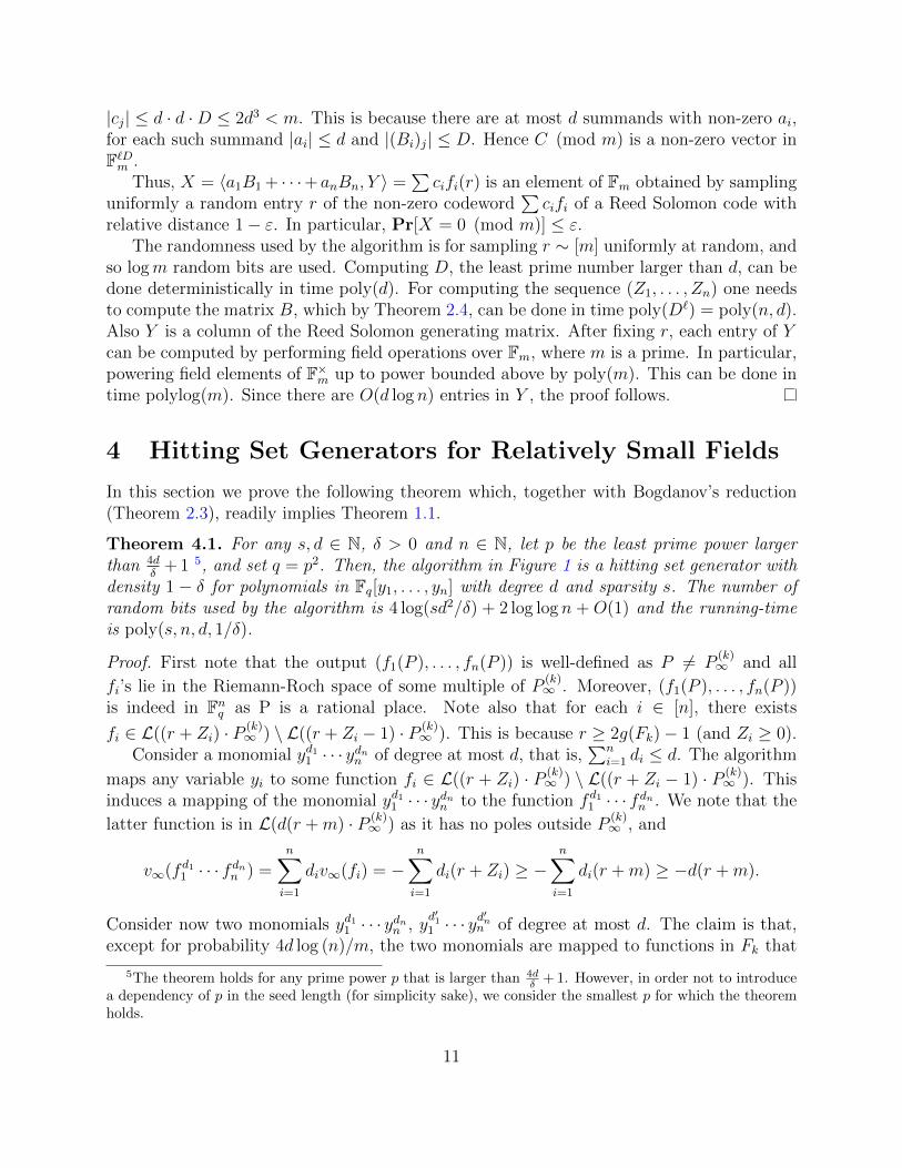
Theorem 4.1. For any s, d ∈ N, δ > 0 and n ∈ N, let p be the least prime power largerthan 4d

δ+ 1 5, and set q = p2. Then, the algorithm in Figure 1 is a hitting set generator with

density 1 − δ for polynomials in Fq[y1, . . . , yn] with degree d and sparsity s. The number ofrandom bits used by the algorithm is 4 log(sd2/δ) + 2 log log n + O(1) and the running-timeis poly(s, n, d, 1/δ).

Proof. First note that the output (f1(P ), . . . , fn(P )) is well-defined as P 6= P(k)∞ and all

fi’s lie in the Riemann-Roch space of some multiple of P(k)∞ . Moreover, (f1(P ), . . . , fn(P ))

is indeed in Fnq as P is a rational place. Note also that for each i ∈ [n], there exists

fi ∈ L((r + Zi) · P (k)∞ ) \ L((r + Zi − 1) · P (k)

∞ ). This is because r ≥ 2g(Fk)− 1 (and Zi ≥ 0).Consider a monomial yd11 · · · ydnn of degree at most d, that is,

∑ni=1 di ≤ d. The algorithm

maps any variable yi to some function fi ∈ L((r + Zi) · P (k)∞ ) \ L((r + Zi − 1) · P (k)

∞ ). Thisinduces a mapping of the monomial yd11 · · · ydnn to the function fd11 · · · fdnn . We note that the

latter function is in L(d(r +m) · P (k)∞ ) as it has no poles outside P

(k)∞ , and

v∞(fd11 · · · fdnn ) =n∑i=1

div∞(fi) = −n∑i=1

di(r + Zi) ≥ −n∑i=1

di(r +m) ≥ −d(r +m).

Consider now two monomials yd11 · · · ydnn , yd′11 · · · y

d′nn of degree at most d. The claim is that,

except for probability 4d log (n)/m, the two monomials are mapped to functions in Fk that

5The theorem holds for any prime power p that is larger than 4dδ + 1. However, in order not to introduce

a dependency of p in the seed length (for simplicity sake), we consider the smallest p for which the theoremholds.

11

Hitting Set Generator for Relatively Small Fields

Input. n, s, d ∈ N, δ > 0 and the least prime power p such that p ≥ 4d/δ + 1. Wedenote q = p2.

Output. A sample (Y1, . . . , Yn) ∈ Fnq such that for every non-zero polynomial h ∈Fq[y1, . . . , yn] with degree d and sparsity s, Pr[h(Y1, . . . , Yn) = 0] ≤ δ.

1. Find the smallest prime number m > 16s2d3 log (n)/δ, and let k be the lowestlevel in the Garcia-Stichtenoth tower such that N(Fk) ≥ 6md/δ.

2. Sample (Z1, . . . , Zn) from a (4d log (n)/m)-biased distribution for linear testsmodulo m with 2d-bounded coefficients.

3. Let r be the smallest integer divisible by m, such that r ≥ 2g(Fk)− 1.

4. For each i ∈ [n], find fi ∈ L((r + Zi) · P (k)∞ ) \ L((r + Zi − 1) · P (k)

∞ ).

5. Sample uniformly at random a rational place P 6= P(k)∞ of Fk.

6. Return (f1(P ), . . . , fn(P )).

Figure 1: A hitting set generator for relatively small fields.

have different valuations at P(k)∞ :

Pr[v∞(fd11 · · · fdnn

)= v∞

(fd′11 · · · fd

′n

n

)]= Pr

[n∑i=1

di(r + Zi) =n∑i=1

d′i(r + Zi)

]

≤ Pr

[n∑i=1

di(r + Zi) =n∑i=1

d′i(r + Zi) (mod m)

]

= Pr

[n∑i=1

diZi =n∑i=1

d′iZi (mod m)

]

= Pr

[n∑i=1

(di − d′i)Zi = 0 (mod m)

]

≤ 4d log (n)

m,

where the third inequality follows since m divides r, and the last inequality follows since(Z1, . . . , Zn) is sampled from a (4d log (n)/m)-biased distribution for linear tests modulo mwith 2d-bounded coefficients, and indeed, there are at most 2d indices i such that di − d′i is

12

not zero, and for such i, di − d′i ∈ [−d, d] ⊆ [−2d, 2d]. Moreover, note that m > 2 · (2d)3,and thus the hypothesis of Theorem 3.2 does indeed hold.

Consider a polynomial h ∈ Fq[y1, . . . , yn] with degree d and sparsity s. By the unionbound, the probability that there exist two monomials of h that are mapped to functionswith the same valuation at P

(k)∞ is at most

(s2

)· 4d log (n)/m, which is at most δ/8 by the

choice of m. Hence, except for probability δ/8, the polynomial h is mapped to a non-zero

function f ∈ L(d(r+m)·P (k)∞ ), as functions with different valuations are linearly independent.

We now restrict ourselves to the event where f 6= 0 and show that PrP [f(P ) = 0] ≤(7/8) · δ, where P 6= P

(k)∞ is a rational place of Fk sampled uniformly at random. This

will conclude the proof for the algorithm’s correctness. Assume there are z rational placesP1, . . . , Pz such that f(Pi) = 0 for all i ∈ [z]. LetD be the divisor d(r+m)P

(k)∞ −(P1+· · ·+Pz).

Since f(Pi) = 0 for all i ∈ [z], f ∈ L(D). Since f 6= 0, it follows that dim(L(D)) > 0 and sodeg(D) ≥ 0. However, deg(D) = d(r +m)− z, which implies z ≤ d(r +m). Thus,

PrP

[f(P ) = 0 | f 6= 0] =z

N(Fk)≤ d(r +m)

N(Fk)≤ 2d(g(Fk) +m)

N(Fk)≤ 2d

p− 1+

3

8· δ ≤ 7

8· δ,

where we used the fact that r ≤ 2g(Fk)+m, the choice ofm, p and the fact thatN(Fk)/g(Fk) ≥p− 1 for all k.

We now upper bound the number of random bits used. The algorithm performs tworandom steps. First there is the sampling of (Z1, . . . , Zn), which by Theorem 3.2, requireslogm random bits. Secondly, we sample a rational place uniformly out of N(Fk) places. Wechose k to be the least integer such that N(Fk) ≥ 6md/δ and so N(Fk−1) < 6md/δ. SinceN(Fk) ≤ p ·N(Fk−1), the number of random bits used is at most log(6mdp/δ). The assertionregarding the number of random bits used readily follows.

We turn to analyze the running-time of the algorithm. Computing the prime num-ber m can be carried out (deterministically) in time poly(m). By Theorem 3.2, sampling

(Z1, . . . , Zn) can be done in time poly(n, d, logm). In order to find fi ∈ L((r + Zi) · P (k)∞ ) \

L((r+Zi−1) ·P (k)∞ ), one can find a basis for L((r+Zi) ·P (k)

∞ ), in time poly(r) [SAK+01], and

find in this basis an element that has valuation r + Zi at P(k)∞ , also in time poly(r). Since

r ≤ 2g(Fk) +m = O(md/δ), this can be carried out in time poly(m). The last two steps ofthe algorithm can clearly be carried out in time poly(n, logm). The total running-time istherefore poly(s, n, d, 1/δ).

By examining the arguments above, one can see that the bottleneck in the running timeis determined by finding the prime number m ∼ s2/δ, and finding a function f with a givenvaluation. These are the only steps that cost us the poly(s/δ) in the running time. It turnsout that finding m can be done in time polylog(m) probabilistically (see Section 5.2), and wechose to present the simpler naive algorithm for finding a prime above, which runs in timepoly(m), for simplicity. Finding a function f with a given valuation is the real bottleneck inthe running time. In Section 5 we bypass this problem, however, our solution costs us in thefield size. Clearly, if Conjecture 1.4 holds, then finding f can be done in time polylog(s/δ),and the algorithm described above runs in time poly(n, d, log (1/δ)).

13

5 The More Efficient Hitting Set Generator

The More Efficient Hitting Set Generator

Input. n, s, d ∈ N, a prime power p and δ > 0 such that p = Ω(d·log (ds log (n)/δ)

δ·log log s

).

We denote q = p2.

Output. A sample (Y1, . . . , Yn) ∈ Fnq such that for every non-zero polynomial h ∈Fq[y1, . . . , yn] of degree d and sparsity s, Pr[h(Y1, . . . , Yn) = 0] ≤ δ.

1. Find some prime number m ∈ [16d3s2 log (n)/δ, 32d3s2 log (n)/δ] with failureprobability bounded by δ/2. Let k be the least integer such that pk ≥ 2m andFk the kth function field in Garcia-Stichtenoth tower.

2. Sample (Z1, . . . , Zn) from a (4d log (n)/m)-biased distribution for linear testsmodulo m with 2d-bounded coefficients.

3. Let r be the least integer divisible by m such that r > k · pk+1 − pk−1p−1 − p

k.

4. For each i ∈ [n], find fi ∈ L((r + Zi) · P (k)∞ ) \ L((r + Zi − 1) · P (k)

∞ ).

5. Sample uniformly at random a rational place P 6= P(k)∞ of Fk.

6. Return (f1(P ), . . . , fn(P )).

Figure 2: The more efficient hitting set generator.

In this section we prove the following theorem.

Theorem 5.1. Let p be a prime power, and let q = p2. For any s, d ∈ N, δ > 0 and n ∈ N,such that

p = Ω

(d · log (ds log (n)/δ)

δ · log log s

),

the following holds. The algorithm in Figure 2 is a hitting set generator with density 1−δ forpolynomials in Fq[y1, . . . , yn] with degree d and sparsity s. The number of random bits used bythe algorithm is 8 log(sd2/δ)+3 log log n+O(1) and the running-time is poly(n, d, log (s/δ)).

Theorem 1.2 readily follows by Theorem 5.1 and Bogdanov’s reduction (Theorem 2.3). Toprove Theorem 5.1, we prove two things:

• One can efficiently find elements fi ∈ L((r+Zi) ·P (k)∞ ) \L((r+Zi− 1) ·P (k)

∞ ) for manyi’s. This follows from Theorem 1.5 whose proof is given in Section 5.1.

14

• One can find appropriate primes efficiently using a randomized algorithm. This isstated in Lemma 5.3. This fact is known [pol09], and we give it an alternative proofin Section 5.2, with slightly improved randomness complexity.

We then complete the proof of Theorem 5.1 in Section 5.3.

5.1 Proof of Theorem 1.5

Let Fk be the kth level in the Garcia-Stichtenoth tower over Fq. For 0 ≤ i ≤ k, defineπi =

∏ij=0 (xp−1j + 1), and let

ui,e =

xei , if 0 ≤ e < p− 1;xei + 1, if e = p− 1.

In [PST98] (see their Lemma 3.4, ii), it is shown that each function in

πi−1 · ui,e | 0 ≤ i ≤ k , 0 ≤ e ≤ p− 1

has poles only at P(k)∞ in Fk. Moreover (see Table I in [SAK+01]), v

(k)∞ (πi) = −(pk+1 − pk−i)

and v(k)∞ (xi) = −pk−i. Thus, v

(k)∞ (ui,e) = −e · pk−i. Given that, we conclude the following

lemma, which readily implies Theorem 1.5.

Lemma 5.2. For every integer k ≥ 1 the following holds. Let 0 ≤ a ≤ pk−1 be some integerthat is written as a0 + a1 · p+ a2 · p2 + · · ·+ ak−1 · pk−1 in base p (namely, 0 ≤ ai ≤ p− 1 fori = 0, 1, . . . , k − 1). Define the function

fa =k∏i=1

πk−i · uk−i+1,p−1−ai−1.

Then, in Fk, fa has poles only at P(k)∞ , and

− v(k)∞ (fa) = k · pk+1 − pk − 1

p− 1− a. (5.1)

Moreover, given p, k and 0 ≤ a ≤ pk − 1, the function fa can be computed and evaluated ona given place in time polylog(pk).

Proof. First note that by the above discussion, the only poles fa has in Fk is at P(k)∞ . For

fixed 1 ≤ i ≤ k,

−v(k)∞ (πk−i · uk−i+1,p−1−ai−1) = pk+1 − pi + (p− 1− ai−1) · pi−1

= pk+1 − pi−1 − ai−1 · pi−1.

Equation (5.1) then follows by taking the sum, over i = 1, . . . , k, of the right hand side in theequation above. The assertion regarding the running-time for computing fa is trivial.

15

5.2 Finding a Prime in an Interval using Random Bits

The algorithm in Figure 2 involves finding a prime number m larger than Ω(s2), for theconstruction of the small-bias sequence that fools linear tests modulo m. Since we arewilling to run only for polylog(s) time, we cannot settle for known deterministic algorithms.However, we do have few random bits at our disposal, and it is known how to find mas above with success probability 1 − δ using O(log(s/δ)) random bits [pol09]. We givean alternative proof for this known fact in Lemma 5.3 below. Also, we slightly improveupon the randomness complexity of known techniques 6 (one uses the Nisan-Zuckermanpseudorandom generator [NZ96], and the other is based on an analysis of the moments ofthe indicator random variable for being a prime number in a given interval, via sieve theory).

Lemma 5.3 (Finding a prime in an interval). There exists a randomized algorithm thatgiven m and δ > 0 as inputs, outputs a prime number p ∈ [m, 2m] with probability at least1− δ. The running-time of the algorithm is polylog(m) · log (1/δ) and the number of randombits used by the algorithm is 0.525 · logm+ (2 + o(1)) · log(1/δ) +O(1).

Proof. It is well-known that in the range [m, 2m] there are Ω(m/ logm) prime numbers.However, better results are known. Define Γ(m) = m0.525. Baker et al. [BHP01] showed thatfor large enough m, in the interval [m,m + Γ(m)], at least 9/(100 · logm) fraction of thenumbers are primes. 7

Testing whether a given integer x is a prime can be done deterministically in timepolylog(x) [AKS04]. Thus, a first attempt to find a prime number in the interval [m,m +Γ(m)] would simply be to sample uniformly x ∼ [m,m+ Γ(m)] and test whether x is prime.Finding a prime in one iteration succeed with probability Ω(1/ logm). Thus, repeating thisprocess for O(log (m) · log (1/δ)) iterations reduces the failure probability to δ. Since we uselog Γ(m) random bits per iteration, the total number of random bits used by this algorithmis O(log2 (m) · log (1/δ)). Furthermore, the running-time is polylog(m) · log (1/δ) as we cantest the primality of each sample, deterministically, in time polylog(m).

One can reduce the number of random bits by using a hitter. Slightly deviating fromthe standard notation for our own needs, a hitter for density µ and error parameter δ is arandomized algorithm that gets as inputs m, k, δ, µ, and outputs a (random) set H ⊆ [m,m+k] with the following property. For every set B ⊆ [m,m + k] with density |B|/(k + 1) ≥ µ,it holds that PrH [H ∩B = ∅] ≤ δ. The maximum size of H that the hitter outputs is calledthe sample complexity of the hitter.

In [Gol97], Corollary C.5, a hitter with sample complexity O(log (1/δ)/µ) is presented.The number of random bits used by this hitter is log k + (2 + o(1)) · log (1/δ). By pluggingk = Γ(m) and µ = Ω(1/ logm) we get the desired parameters.

6We have not been able to find a formal proof for known techniques in the literature, and specifically wedo not know of an exact assertion regarding the number of random bits used, but doing some calculation, itseems our method does better in terms of randomness complexity.

7In fact, the main theorem of Baker et al. [BHP01] only states the existence of a prime in [m,m+ Γ(m)].Nevertheless, they actually proved the stronger claim we need.

16

5.3 Proof of Theorem 5.1

Proof. As in the proof of Theorem 4.1, we note that the output (f1(P ), . . . , fn(P )) is well-defined and is contained in Fnq . Moreover, since pk ≥ 2m and r is the least integer divisible by

m such that r > k ·pk+1− pk−1p−1 −p

k, there are at least m integers in the range [r, kpk+1− pk−1p−1 ].

This is necessary as the algorithm needs to find a function with a given valuation v at P(k)∞ ,

for v’s in r, r + 1, . . . , r + m − 1. Doing so efficiently we only know how to do inside the

interval [kpk+1 − pk−1p−1 − p

k + 1, kpk+1 − pk−1p−1 ].

Consider a monomial yd11 · · · ydnn of degree at most d. The algorithm maps every variable

yi to some function fi ∈ L((r + Zi) · P (k)∞ ) \ L((r + Zi − 1) · P (k)

∞ ). This induces a mappingof the monomial yd11 · · · ydnn to the function fd11 · · · fdnn . We note that the latter function is in

L(dkpk+1 · P (k)∞ ) as it has no poles outside P

(k)∞ , and

v∞(fd11 · · · fdnn ) =n∑i=1

div∞(fi) ≥ −n∑i=1

dikpk+1 ≥ −dkpk+1.

Consider now two monomials yd11 · · · ydnn , yd′11 · · · y

d′nn of degree at most d. The claim is that,

except with probability 4d log (n)/m, the two monomials are mapped to functions in Fk that

have different valuations at P(k)∞ . Thus, as in the proof of Theorem 4.1, the probability that

two distinct monomials of a polynomial h ∈ Fq[y1, . . . , yn] with degree d and sparsity s willbe mapped to functions with the same valuation is at most

(s2

)· 4d logn

m, which is at most δ/8

by the choice of m. We thus conclude that except with probability δ/8, the polynomial h is

mapped to a non-zero function f ∈ L(dkpk+1 · P (k)∞ ).

We now restrict ourselves to the event where f 6= 0. As before it is enough to showthat PrP [f(P ) = 0] ≤ δ/4, where P 6= P

(k)∞ is a rational place of Fk sampled uniformly at

random. This will conclude the proof for the algorithm’s correctness. By the same argumentused in the proof of Theorem 4.1, since 0 6= f ∈ L(dkpk+1 · P (k)

∞ ), it follows that

PrP

[f(P ) = 0 | f 6= 0] =dkpk+1

N(Fk)<

dk

p− 1≤ δ

4,

where the second inequality follows as N(Fk) > (p− 1)pk+1. The last inequality follows, forlarge enough n, by our choice of p and since k is chosen such that pk−1 < 2m.

We now upper bound the number of random bits used. The algorithm performs threerandom steps. First, by Lemma 5.3, finding the prime number m, with failure probability atmost δ/2, can be done using 0.525 · logm+(2+o(1)) · log (2/δ)+O(1) random bits. Secondly,by Theorem 3.2, sampling (Z1, . . . , Zn) requires logm random bits. Third, the number ofrational places N(Fk) is bounded above by pk+2 < 2p3m and so sampling a rational placecosts logm+ log(2p3) random bits. It can be easily verified that the assertion regarding thenumber of random bits used holds.

We now analyze the running-time of the algorithm. By Lemma 5.3, computing m can bedone in time polylog(m/δ). By Theorem 3.2, sampling (Z1, . . . , Zn) can be carried out

17

in poly(n, d, logm) time. By Lemma 5.2, finding a function fi with a given valuationcan be done in time polylog(m). Finally, sampling a place and evaluating the computedfunction on it, can be done in time polylog(m) as well. Thus, the total running-time ispoly(n, d, log (m/δ)) = poly(n, d, log (s/δ))

References

[ABN+92] N. Alon, J. Bruck, J. Naor, M. Naor, and R. Roth. Construction of asymptoti-cally good low-rate error-correcting codes through pseudo-random graphs. IEEETransactions on Information Theory, 38:509–516, 1992.

[AGHP92] N. Alon, O. Goldreich, J. Hastad, and R. Peralta. Simple construction of al-most k-wise independent random variables. Random Structures and Algorithms,3(3):289–304, 1992.

[AKS04] M. Agrawal, N. Kayal, and N. Saxena. Primes is in P. Annals of Mathematics,160(2):781–793, 2004.

[AM95] N. Alon and Y. Mansour. ε-discrepancy sets and their application for interpola-tion of sparse polynomials. Information Processing Letters, 54(6):337–342, 1995.

[AMN98] Y. Azar, R. Motwani, and J. Naor. Approximating probability distributions usingsmall sample spaces. Combinatorica, 18(2):151–171, 1998.

[BHP01] R. C. Baker, G. Harman, and J. Pintz. The difference between consecutive primes,II. Proceedings of the London Mathematical Society, 83:532–562, 2001.

[Bog05] A. Bogdanov. Pseudorandom generators for low degree polynomials. In Proceed-ings of the 37th annual STOC, pages 21–30, 2005.

[BT09] A. Ben-Aroya and A. Ta-Shma. Constructing small-bias sets from algebraic-geometric codes. In Proceedings of the 50th annual IEEE symposium on founda-tions of computer science (FOCS), pages 191–197, 2009.

[BV10] A. Bogdanov and E. Viola. Pseudorandom bits for polynomials. SIAM J. Com-put., 39(6):2464–2486, 2010.

[Gol97] O. Goldreich. A sample of samplers - a computational perspective on sampling(survey). Electronic Colloquium on Computational Complexity (ECCC), 4(20),1997.

[Gop81] V. D. Goppa. Codes on algebraic curves. In Soviet Math. Dokl, volume 24, pages170–172, 1981.

[GS96] A. Garcia and H. Stichtenoth. On the asymptotic behaviour of some towers offunction fields over finite fields. Journal of Number Theory, 61(2):248–273, 1996.

18

[GS07] A. Garcia and H. Stichtenoth. Topics in geometry, coding theory and cryptogra-phy, volume 6. Springer, 2007.

[GT07] B. Green and T. Tao. The distribution of polynomials over finite fields, withapplications to the Gowers norms. arXiv:0711.3191, 2007.

[GT08] B. Green and T. Tao. An inverse theorem for the Gowers U3-norm, with appli-cations. Proc. Edinburgh Math. Soc., 51(1):73–153, 2008.

[Heß02] F. Heß. Computing Riemann–Roch spaces in algebraic function fields and relatedtopics. Journal of Symbolic Computation, 33(4):425–445, 2002.

[KL08] T. Kaufman and S. Lovett. Worst case to average case reductions for polyno-mials. In Foundations of Computer Science (FOCS), 2008 49th Annual IEEESymposium on, pages 166–175. IEEE, 2008.

[KS01] A. Klivans and D. Spielman. Randomness efficient identity testing of multivariatepolynomials. In Proceedings of the 33rd Annual STOC, pages 216–223, 2001.

[LMS08] S. Lovett, R. Meshulam, and A. Samorodnitsky. Inverse conjecture for the Gowersnorm is false. In 40th Annual STOC, pages 547–556, 2008.

[Lov08] S. Lovett. Unconditional pseudorandom generators for low degree polynomials.In 40th Annual STOC, pages 557–562, 2008.

[Lu12] C. J. Lu. Hitting set generators for sparse polynomials over any finite fields. InComputational Complexity (CCC), 2012 IEEE 27th Annual Conference on, pages280–286. IEEE, 2012.

[LVW93] M. Luby, B. Velickovic, and A. Wigderson. Deterministic approximate countingof depth-2 circuits. In Theory and Computing Systems, 1993., Proceedings of the2nd Israel Symposium on the, pages 18–24. IEEE, 1993.

[NN93] J. Naor and M. Naor. Small-bias probability spaces: Efficient constructions andapplications. SIAM J. on Computing, 22(4):838–856, 1993.

[NZ96] N. Nisan and D. Zuckerman. Randomness is linear in space. J. of Computer andSystem Sciences, 52(1):43–52, 1996.

[pol09] Finding primes (polymath 4), 2009. http://michaelnielsen.org/polymath1/

index.php?title=Finding_primes_with_O(k)_random_bits.

[PST98] R. Pellikaan, H. Stichtenoth, and F. Torres. Weierstrass semigroups in anasymptotically good tower of function fields. Finite fields and their applications,4(4):381–392, 1998.

[Rot06] R. M. Roth. Introduction to coding theory. IET Communications, page 47, 2006.

19

[SAK+01] K. W. Shum, I. Aleshnikov, P. V. Kumar, H. Stichtenoth, and V. Deolalikar. Alow-complexity algorithm for the construction of algebraic-geometric codes betterthan the Gilbert-Varshamov bound. Information Theory, IEEE Transactions on,47(6):2225–2241, 2001.

[Sti93] H. Stichtenoth. Algebraic Function Fields and Codes. Universitext, Springer-Verlag, Berlin, 1993.

[Vio07] E. Viola. Pseudorandom bits for constant-depth circuits with few arbitrary sym-metric gates. SIAM Journal on Computing, 36(5):1387–1403, 2007.

[Vio09a] E. Viola. Guest column: correlation bounds for polynomials over 0,1. ACMSIGACT News, 40(1):27–44, 2009.

[Vio09b] E. Viola. The sum of d small-bias generators fools polynomials of degree d.Computational Complexity, 18(2):209–217, 2009.

20

ECCC ISSN 1433-8092

http://eccc.hpi-web.de