proxsarah: an e cient algorithmic framework for stochastic
TRANSCRIPT
Journal of Machine Learning Research 21 (2020) 1-48 Submitted 3/19; Revised 2/20; Published 5/20
ProxSARAH: An Efficient Algorithmic Framework forStochastic Composite Nonconvex Optimization
Nhan H. Pham† [email protected]
Lam M. Nguyen‡ [email protected]
Dzung T. Phan‡ [email protected]‡IBM Research, Thomas J. Watson Research CenterYorktown Heights, NY10598, USA
Quoc Tran-Dinh† [email protected]†Department of Statistics and Operations Research
The University of North Carolina at Chapel Hill, Chapel Hill, NC27599, USA.
Editor: Zaid Harchaoui
Abstract
We propose a new stochastic first-order algorithmic framework to solve stochastic compositenonconvex optimization problems that covers both finite-sum and expectation settings. Ouralgorithms rely on the SARAH estimator introduced in Nguyen et al. (2017a) and consist oftwo steps: a proximal gradient and an averaging step making them different from existingnonconvex proximal-type algorithms. The algorithms only require an average smoothnessassumption of the nonconvex objective term and additional bounded variance assumptionif applied to expectation problems. They work with both constant and dynamic step-sizes, while allowing single sample and mini-batches. In all these cases, we prove that ouralgorithms can achieve the best-known complexity bounds in terms of stochastic first-orderoracle. One key step of our methods is the new constant and dynamic step-sizes resultingin the desired complexity bounds while improving practical performance. Our constantstep-size is much larger than existing methods including proximal SVRG scheme in thesingle sample case. We also specify our framework to the non-composite case that coversexisting state-of-the-arts in terms of oracle complexity bounds. Our update also allowsone to trade-off between step-sizes and mini-batch sizes to improve performance. We testthe proposed algorithms on two composite nonconvex problems and neural networks usingseveral well-known data sets.
Keywords: Stochastic proximal gradient descent; variance reduction; composite noncon-vex optimization; finite-sum minimization; expectation minimization.
1. Introduction
In this paper, we consider the following stochastic composite, nonconvex, and possiblynonsmooth optimization problem:
minw∈Rd
F (w) := f(w) + ψ(w) ≡ E [f(w; ξ)] + ψ(w)
, (1)
c©2020 Nhan H. Pham, Lam M. Nguyen, Dzung T. Phan, and Quoc Tran-Dinh.
License: CC-BY 4.0, see https://creativecommons.org/licenses/by/4.0/. Attribution requirements are providedat http://jmlr.org/papers/v21/19-248.html.
Pham H., Nguyen M., Phan T., and Tran-Dinh
where f(w) := E [f(w; ξ)] is the expectation of a stochastic function f(w; ξ) depending on arandom vector ξ in a given probability space (Ω,P), and ψ : Rd → R ∪ +∞ is a proper,closed, and convex function.
As a special case of (1), if ξ is a random vector defined on a finite support set Ω :=ξ1, ξ2, · · · , ξn with a probability distribution p, then by defining fi(w) := npif(w; ξi), (1)can be written into the following composite finite-sum minimization problem:
minw∈Rd
F (w) := f(w) + ψ(w) ≡ 1
n
n∑i=1
fi(w) + ψ(w). (2)
We can also obtain (2) from (1) through a sample average approximation (SAA) (Nemirovskiet al., 2009). Note that problem (2) is often referred to as a regularized empirical riskminimization in machine learning and finance.
1.1. Motivation
Problems (1) and (2) cover a broad range of applications in machine learning and statistics,especially in neural networks (see Bottou, 1998, 2010; Bottou et al., 2018; Goodfellow et al.,2016; Sra et al., 2012). Hitherto, state-of-the-art numerical optimization methods for solvingthese problems rely on stochastic approaches (see Johnson and Zhang, 2013; Schmidt et al.,2017; Shapiro et al., 2009; Defazio et al., 2014; Frostig et al., 2015; Lei and Jordan, 2017;Lin et al., 2015). In the convex case, both non-composite and composite settings of (1)and (2) have been intensively studied with different schemes such as standard stochasticgradient (Robbins and Monro, 1951), proximal stochastic gradient (Ghadimi and Lan, 2013;Nemirovski et al., 2009), stochastic dual coordinate descent (Shalev-Shwartz and Zhang,2013), variance reduction methods (Allen-Zhu, 2017; Defazio et al., 2014; Johnson andZhang, 2013; Nitanda, 2014; Schmidt et al., 2017; Shalev-Shwartz and Zhang, 2014; Xiaoand Zhang, 2014), stochastic conditional gradient (Frank-Wolfe) methods (Reddi et al.,2016a), and stochastic primal-dual methods (Chambolle et al., 2018). The most popularvariance reduction methods in the literature are perhaps SAGA and SVRG. While SAGA(fast incremental gradient algorithm) is a successor of SAG (Stochastic Average Gradient)(Schmidt et al., 2017) and aims at solving finite-sum problems, SVRG (Stochastic VarianceReduced Gradient) (Johnson and Zhang, 2013) can solve both finite-sum and expectationproblems. Thanks to variance reduction techniques, several efficient methods with constantstep-sizes have been developed for convex settings that match the lower-bound worst-casecomplexity (Agarwal et al., 2010). However, variance reduction methods for nonconvexsettings are still limited and heavily focus on the non-composite form of (1) and (2), i.e.,ψ = 0, and the SVRG estimator.
Theory and stochastic methods for nonconvex problems are still in progress and requiresubstantial effort to obtain efficient algorithms with rigorous convergence guarantees. It isshown in Fang et al. (2018); Zhou and Gu (2019) that there is still a gap between the upper-bound complexity in state-of-the-art methods and the lower-bound worst-case complexityfor the nonconvex problem (2) under standard smoothness assumption. Motivated by thisfact, we attempt to develop a new algorithmic framework that can reduce and at leastnearly close this gap in the composite finite-sum setting (2). In addition to the best-knowncomplexity bounds, we expect to design practical algorithms advancing beyond existing
2
ProxSARAH Algorithms for Stochastic Composite Nonconvex Optimization
methods by providing a dynamic rule to update step-sizes with rigorous complexity analysis.Our algorithms rely on a recent biased stochastic estimator for the objective gradient, calledSARAH (StochAstic Recursive grAdient algoritHm), introduced in Nguyen et al. (2017a)for convex problems.
1.2. Related Work
In the nonconvex case, both problems (1) and (2) have been intensively studied in recentyears with a vast number of research papers. While numerical algorithms for solving the non-composite setting, i.e., ψ = 0, are well-developed and have received considerable attention(see Allen-Zhu, 2018; Allen-Zhu and Li, 2018; Allen-Zhu and Yuan, 2016; Fang et al., 2018;Lihua et al., 2017; Nguyen et al., 2017b, 2018b, 2019; Reddi et al., 2016b; Zhou et al., 2018),methods for composite setting remain limited (Reddi et al., 2016b; Wang et al., 2019). Interms of algorithms, Reddi et al. (2016b) study a non-composite finite-sum problem as aspecial case of (2) using SVRG estimator from Johnson and Zhang (2013). Additionally,they extend their method to the composite setting by simply applying the proximal operatorof ψ as in the well-known forward-backward scheme. Another related work using SVRGestimator can be found in Li and Li (2018). These algorithms have some limitation as willbe discussed later. The same technique is applied in Wang et al. (2019) to develop othervariants for both (1) and (2), but using the SARAH estimator from Nguyen et al. (2017a).The authors derive a large constant step-size, but at the same time control mini-batch sizeto achieve desired complexity bounds. Consequently, it has an essential limitation as willalso be discussed in Subsection 3.4. Both algorithms achieve the best-known complexitybounds for solving (1) and (2). In addition, Reddi et al. (2016a) propose a stochastic Frank-Wolfe method that can handle constraints as special cases of (2). Recently, a stochasticvariance reduction method with momentum was studied in Zhou et al. (2019) for solving(2) which can be viewed as a modification of SpiderBoost in Wang et al. (2019).
Our algorithm remains a variance reduction stochastic method, but it is different fromthese works at two major points: an additional averaging step and two different step-sizes(cf. Algorithm 1). Having two step-sizes allows us to flexibly trade-off them and develop adynamic update rule. Note that our averaging step looks similar to the robust stochasticgradient method in Nemirovski et al. (2009), but is fundamentally different since it evaluatesthe proximal step at the averaging point. In fact, it is closely related to averaged fixed-point schemes in the literature (see Bauschke and Combettes, 2017). While we only focus onstochastic gradient-type methods in this paper, some recent techniques such as Nesterov’smomentum, catalyst, and nonlinear acceleration (see Paquette et al., 2018) could also beinteresting to investigate for developing new variants of our methods.
In terms of theory, many researchers have focused on theoretical aspects of existingalgorithms. For example, Ghadimi and Lan (2013) appears to be one of the first pioneeringworks studying convergence rates of stochastic gradient descent-type methods for nonconvexand non-composite finite-sum problems. They later extend it to the composite setting inGhadimi et al. (2016). Wang et al. (2019) also investigate the gradient dominance case,and Karimi et al. (2016) consider both finite-sum and composite finite-sum under differentassumptions, including Polyak- Lojasiewicz condition.
3
Pham H., Nguyen M., Phan T., and Tran-Dinh
Whereas many researchers have been trying to improve complexity upper bounds ofstochastic first-order methods using different techniques (Allen-Zhu, 2018; Allen-Zhu andLi, 2018; Allen-Zhu and Yuan, 2016; Fang et al., 2018), other researchers attempt to con-struct examples for lower-bound complexity estimates. In the convex case, there existnumerous research papers including Agarwal et al. (2010); Nemirovskii and Yudin (1983);Nesterov (2004). In Fang et al. (2018); Zhou and Gu (2019), the authors have constructeda lower-bound complexity for nonconvex finite-sum problem covered by (2). They showedthat the lower-bound complexity for any stochastic gradient method using only smoothnessassumption to achieve an ε-stationary point in expectation is Ω
(n1/2ε−2
)given that the
number of objective components n does not exceed O(ε−4), where ε is a desired accuracy.
For the expectation problem (1), the best-known complexity bound to achieve an ε-stationary point in expectation is O
(σε−3 + σ2ε−2
)as shown in Fang et al. (2018); Wang
et al. (2019), where σ > 0 is an upper bound of the variance (see Assumption 2.3). Thiscomplexity matches the lower bound recently developed in Arjevani et al. (2019) up to agiven constant under the same assumptions for the non-composite setting of (1).
1.3. Our Approach and Contributions
We exploit the SARAH estimator, a biased stochastic recursive gradient estimator, inNguyen et al. (2017a), to design new proximal variance reduction stochastic gradient al-gorithms to solve both composite expectation and finite-sum problems (1) and (2). TheSARAH algorithm is simply a double-loop stochastic gradient method with a flavor ofSVRG (Johnson and Zhang, 2013), but using a novel biased estimator that is different fromSVRG. SARAH is a recursive method as SAGA (Defazio et al., 2014), but can avoid themajor issue of storing gradients as in SAGA. Our method will rely on the SARAH estimatoras in SPIDER and SpiderBoost combining with an averaging proximal-gradient scheme tosolve both (1) and (2).
The ultimate goal of this paper is to develop a new stochastic gradient-based algorithmicframework that covers different variants with constant and dynamic step-sizes, single sam-ple and mini-batch, and achieves best-known theoretical oracle complexity bounds. Morespecifically, our main contributions can be summarized as follows:
(a) Novel algorithms: We propose a new and general stochastic variance reductionframework (Algorithm 1) relying on the SARAH estimator to solve both expectationand finite-sum problems (1) and (2) in composite settings. As usual, the algorithmhas double loops, where the outer loop can either take full gradient or mini-batch toreduce computational burden in large-scale and expectation settings. The inner loopcan work with single sample or a broad range of mini-batch sizes. This frameworkhas two different step-sizes as opposed to existing methods. We also derive differentvariants of Algorithm 1 for using constant or dynamic step-sizes and for non-compositesettings of (1) and (2) (i.e., ψ = 0)
(b) Best-known complexity guarantees under constant step-sizes: We analyzeour framework and its variants to design appropriate constant step-sizes instead ofdiminishing step-sizes as in standard Stochastic Gradient Descent (SGD) methods.In the finite-sum setting (2), our methods achieve O
(n+ n1/2ε−2
)complexity bound
to attain an ε-stationary point in expectation under only the smoothness of fi. This
4
ProxSARAH Algorithms for Stochastic Composite Nonconvex Optimization
complexity matches the lower-bound worst-case complexity in Fang et al. (2018); Zhouand Gu (2019) up to a constant factor when n ≤ O
(ε−4). In the expectation setting
(1), our algorithms require O(σ2ε−2 + σε−3
)stochastic first-order oracle calls of f
to achieve an ε-stationary point in expectation under only the smoothness of f andbounded variance σ2 > 0. To the best of our knowledge, this is the best-knowncomplexity so far for (1) under standard assumptions in both the single sample andmini-batch cases. This complexity also matches the lower bound recently studied inArjevani et al. (2019) up to a constant.
(c) Best-known complexity guarantees under dynamic step-sizes: Apart fromconstant step-size algorithms, we also analyze variants of Algorithm 1 using dynamicstep-sizes for both composite and non-composite settings in both single sample andmini-batch cases. Our dynamic step-sizes are increasing along the inner iterationsrather than diminishing as usually used in standard SGDs.
Our result covers the non-composite setting in the finite-sum case (Nguyen et al., 2019),and matches the best-known complexity in Fang et al. (2018); Wang et al. (2019) for bothproblems (1) and (2). Since the composite setting covers a broader class of nonconvexproblems including convex constraints, we believe that our method has better chance tohandle new applications than non-composite methods. It also allows one to deal withcomposite problems under different type of regularizers such as sparsity or constraints onweights as in neural network training applications.
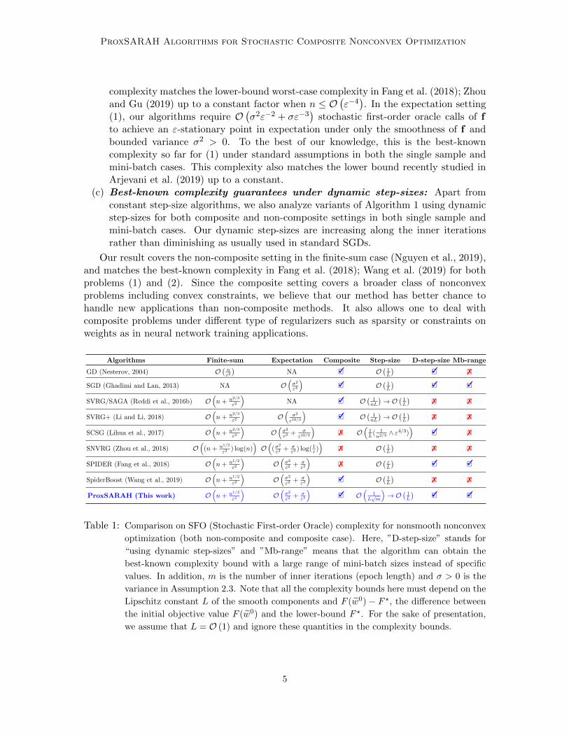
Algorithms Finite-sum Expectation Composite Step-size D-step-size Mb-range
GD (Nesterov, 2004) O(nε2
)NA 3 O
(1L
)3 7
SGD (Ghadimi and Lan, 2013) NA O(σ2
ε4
)3 O
(1L
)3 3
SVRG/SAGA (Reddi et al., 2016b) O(n+ n2/3
ε2
)NA 3 O
(1nL
)→ O
(1L
)7 7
SVRG+ (Li and Li, 2018) O(n+ n2/3
ε2
)O(
σ2
ε10/3
)3 O
(1nL
)→ O
(1L
)7 7
SCSG (Lihua et al., 2017) O(n+ n2/3
ε2
)O(σ2
ε2+ σ
ε10/3
)7 O
(1L( 1
n2/3 ∧ ε4/3))
3 7
SNVRG (Zhou et al., 2018) O(
(n+ n1/2
ε2) log(n)
)O(
(σ2
ε2+ σ
ε3) log(1
ε ))
7 O(
1L
)7 7
SPIDER (Fang et al., 2018) O(n+ n1/2
ε2
)O(σ2
ε2+ σ
ε3
)7 O
(εL
)3 3
SpiderBoost (Wang et al., 2019) O(n+ n1/2
ε2
)O(σ2
ε2+ σ
ε3
)3 O
(1L
)7 7
ProxSARAH (This work) O(n+ n1/2
ε2
)O(σ2
ε2+ σ
ε3
)3 O
(1
L√m
)→ O
(1L
)3 3
Table 1: Comparison on SFO (Stochastic First-order Oracle) complexity for nonsmooth nonconvex
optimization (both non-composite and composite case). Here, ”D-step-size” stands for
“using dynamic step-sizes” and ”Mb-range” means that the algorithm can obtain the
best-known complexity bound with a large range of mini-batch sizes instead of specific
values. In addition, m is the number of inner iterations (epoch length) and σ > 0 is the
variance in Assumption 2.3. Note that all the complexity bounds here must depend on the
Lipschitz constant L of the smooth components and F (w0) − F ?, the difference between
the initial objective value F (w0) and the lower-bound F ?. For the sake of presentation,
we assume that L = O (1) and ignore these quantities in the complexity bounds.
5

Pham H., Nguyen M., Phan T., and Tran-Dinh
1.4. Comparison Between Our Methods and Existing Work
Hitherto, we have found three different variance reduction algorithms of the stochastic prox-imal gradient method for nonconvex problems that are most related to our work: proximalSVRG (called ProxSVRG) in Reddi et al. (2016b), ProxSVRG+ in Li and Li (2018), andProxSpiderBoost in Wang et al. (2019). Other methods such as proximal stochastic gradientdescent (ProxSGD) scheme (Ghadimi et al., 2016), ProxSAGA in Reddi et al. (2016b), andNatasha variants in Allen-Zhu (2018) are quite different and already intensively comparedin previous works (see Li and Li, 2018; Reddi et al., 2016b; Wang et al., 2019), and we donot include them here.
In terms of theory, Table 1 compares different methods for solving (1) and (2) regardingthe stochastic first-order oracle calls (SFO), the applicability to finite-sum and/or expecta-tion and composite settings, step-sizes, and the use of dynamic step-sizes and mini-batches.
Now, let us compare in detail our algorithms and four methods: ProxSVRG, Prox-SVRG+, SPIDER, and ProxSpiderBoost for solving (1) and (2), or their special cases.
(a) Assumptions: In the finite-sum setting (2), ProxSVRG, ProxSVRG+, and Prox-SpiderBoost all use the smoothness of each component fi in (2), which is stronger thanthe average smoothness in Assumption 2.2 stated below. They did not consider (2) underAssumption 2.2. However, Assumption 2.2 is often stronger than the L-smoothness of f .
(b) Single sample for the finite-sum case: The performance of gradient descent-type algorithms crucially depends on the step-size (or learning rate). Let us make a com-parison between different methods in terms of step-size for single sample case, and thecorresponding complexity bound.
• As shown in Reddi et al. (2016b, Theorem 1), in the single sample case, i.e., themini-batch size of the inner loop b = 1, ProxSVRG for solving (2) has a small step-size η = 1
3Ln , and its corresponding complexity is O(nε−2
)(see Reddi et al., 2016b,
Corollary 1), which is the same as in standard proximal gradient methods.• ProxSVRG+ in Li and Li (2018, Theorem 3) is a variant of ProxSVRG, and in the
single sample case, it uses a different step-size η = min
16L ,
16mL
. This step-size is
only better than that of ProxSVRG if 2m < n. With this step-size, the complexity ofProxSVRG+ remains O
(n2/3ε−2
)as in ProxSVRG.
• In the non-composite case, SPIDER (Fang et al., 2018) relies on a dynamic step-size
ηt := min
εL‖vt‖
√n, 1
2L√n
, where vt is the SARAH stochastic estimator. Clearly, this
step-size is very small if the target accuracy ε is small, and/or ‖vt‖ is large. However,SPIDER achieves O
(n+ n1/2ε−2
)complexity bound, which is nearly optimal. Note
that this step-size is problem-dependent since it depends on vt. We also emphasizethat SPIDER did not consider the composite problems.• In our constant step-size ProxSARAH variants, we use two step-sizes: averaging step-
size γ =√
2√3mL
and proximal-gradient step-size η = 2√
3m4√
3m+√
2, and their product
presents a combined step-size, which is η := γη = 2L(4√
3m+√
2)(see (25) for our
definition of step-size). Clearly, our step-size η is much larger than that of bothProxSVRG and ProxSVRG+. It can be larger than that of SPIDER if ε is small and‖vt‖ is large. With these step-sizes, our complexity bound is O
(n+ n1/2ε−2
), and if
ε ≤ O(n−1/4
), then it reduces to O
(n1/2ε−2
), which is also nearly optimal.
6

ProxSARAH Algorithms for Stochastic Composite Nonconvex Optimization
• As we can observe from Algorithm 1 in the sequel, the number of proximal operatorcalls in our method remains the same as in ProxSVRG and ProxSVRG+.
(c) Mini-batch for the finite-sum case: Now, we consider the mini-batch case.
• As indicated in Reddi et al. (2016b, Theorem 2), if we choose the batch-size b = bn2/3cand m = bn1/3c, then the step-size η can be chosen as η = 1
3L , and its complexity is
improved up to O(n+ n2/3ε−2
)for ProxSVRG. However, the mini-batch size n2/3 is
close to the full data set n. Reddi et al. (2016b) do not consider a full range of b.• For ProxSVRG+ (Li and Li, 2018), based on Theorem 1, we need to set b = bn2/3c
and m = b√bc = bn1/3c to obtain the best complexity bound for this method, which
is O(n+ n2/3ε−2
). Nevertheless, its step-size is η = 1
6L , which is twice smaller thanthat of ProxSVRG. In addition, ProxSVRG requires the bounded variance assumptionfor (2), which can be avoided in our methods by using full batch for snapshot points.• For SPIDER, again in the non-composite setting, if we choose the batch-size b =
bn1/2c, then its step-size is ηt := min
εL‖vt‖ ,
12L
. In addition, SPIDER limits the
batch-size b in the range of [1, n1/2], and did not consider larger mini-batch sizes.• For SpiderBoost (Wang et al., 2019), it requires to properly set mini-batch size to
achieve O(n+ n1/2ε−2
)complexity for solving (2). More precisely, from Wang et al.
(2019, Theorem 1), we can see that one needs to set m = b√nc and b = b
√nc to
achieve such a complexity. This mini-batch size can be large if n is large, and lessflexible to adjust the performance of the algorithm. Unfortunately, ProxSpiderBoostdoes not have theoretical guarantee for the single sample case.• In our methods, it is flexible to choose the epoch length m and the batch-size b such
that we can obtain different step-sizes and complexity bounds. Our batch-size b can be
any value in [1, n−1] for (2). Given b ∈ [1,√n], we can properly choose m = O
(n/b)
to obtain the best-known complexity bound O(n+ n1/2ε−2
)when n > O
(ε−4)
and
O(n1/2ε−2
), otherwise. More details can be found in Subsection 3.4.
(d) Online or expectation problems: For online or expectation problems, a mini-batch is required to evaluate snapshot gradient estimators for the outer loop.
• In the online or expectation case (1), SPIDER (Fang et al., 2018, Theorem 1) achievesan O
(σε−3 + σ2ε−2
)complexity. In the single sample case, SPIDER’s step-size be-
comes ηt := min
ε2
2σL‖vt‖ ,ε
4σL
, which can be very small, and depends on vt and σ.
Note that σ is often unknown or hard to estimate. Moreover, in early iterations, ‖vt‖is often large potentially making this method slow.• ProxSpiderBoost (Wang et al., 2019) achieves the same complexity bound as SPIDER
for the composite problem (1), but requires to set the mini-batch for both outer andinner loops. The size of these mini-batches has to be fixed a priori in order to use aconstant step-size, which is certainly less flexible. The total complexity of this methodis O
(σε−3 + σ2ε−2
).
• As shown in Theorem 9, our complexity is O(σε−3
)given that σ ≤ O
(ε−1). Oth-
erwise, it is O(σε−3 + σ2ε−2
), which is the same as in ProxSpiderBoost. Note that
our complexity can be achieved for both single sample and a wide range of mini-batchsizes as opposed to a predefined mini-batch size of ProxSpiderBoost.
7

Pham H., Nguyen M., Phan T., and Tran-Dinh
From an algorithmic point of view, our method, Algorithm 1, is fundamentally different fromexisting methods due to its averaging step and large step-sizes in the composite settings.Moreover, our methods have more chance to improve the performance due to the use ofdynamic step-sizes and an additional damped step-size γt, and the flexibility to choose theepoch length m, the inner mini-batch size b, and the snapshot batch-size bs.
1.5. Paper Organization
The rest of this paper is organized as follows. Section 2 discusses the fundamental assump-tions and optimality conditions. Section 3 presents the main algorithmic framework andits convergence results for two settings. Section 4 considers extensions and special casesof our algorithms. Section 5 provides some numerical examples to verify our methods andcompare them with existing state-of-the-arts.
2. Mathematical Tools and Preliminary Results
Firstly, we recall some basic notation and concepts in optimization, which can be found inBauschke and Combettes (2017); Nesterov (2004). Next, we state our blanket assumptionsand discuss the optimality condition of (1) and (2). Finally, we provide preliminary resultsneeded in the sequel.
2.1. Basic Notation and Concepts
We work with finite dimensional spaces, Rd, equipped with standard inner product 〈·, ·〉and Euclidean norm ‖ · ‖. Given a function f : Rd → R ∪ +∞, we use dom(f) :=w ∈ Rd | f(w) < +∞
to denote its (effective) domain. If f is proper, closed, and convex,
∂f(w) :=v ∈ Rd | f(z) ≥ f(w) + 〈v, z − w〉, ∀z ∈ dom(f)
denotes its subdifferential at
w, and proxf (w) := arg minzf(z) + (1/2)‖z − w‖2
denotes its proximal operator. Note
that if f is the indicator of a nonempty, closed, and convex set X , i.e., f(w) = δX (w),then proxf (·) = projX (·), the projection of w onto X . Any element ∇f(w) of ∂f(w) iscalled a subgradient of f at w. If f is differentiable at w, then ∂f(w) = ∇f(w), thegradient of f at w. A continuous differentiable function f : Rd → R is said to be Lf -smooth if ∇f is Lipschitz continuous on its domain, i.e., ‖∇f(w) − ∇f(z)‖ ≤ Lf‖w − z‖for w, z ∈ dom(f). We use Up(S) to denote a finite set S := s1, s2, · · · , sn equipped witha probability distribution p over S. If p is uniform, then we simply use U(S). For any realnumber a, bac denotes the largest integer less than or equal to a. We use [n] to denote theset 1, 2, · · · , n. Finally, for the sake of clarity, Table 2 provides some notations commonlyused in this paper.
2.2. Fundamental Assumptions
To develop numerical methods for solving (1) and (2), we rely on some basic assumptionsusually used in stochastic optimization methods.
Assumption 2.1 (Bounded from below) Both problems (1) and (2) are bounded frombelow. That is F ? := infw∈Rd F (w) > −∞. Moreover, dom(F ) := dom(f) ∩ dom(ψ) 6= ∅.
8

ProxSARAH Algorithms for Stochastic Composite Nonconvex Optimization
Notation Meaning Type and range
ε The target accuracy for stochastic gradient mapping positive realm The epoch length (i.e., the number of iterations of the inner loop t) positive integerBs The mini-batch of the snapshot point ws−1 finite set of realizationsbs The size of the mini-batch Bs of the snapshot point ws−1 positive integer
B(s)t The mini-batch for evaluating SARAH estimator in the inner loop t finite set of realizations
b(s)t The size of the mini-batch B(s)
t positive integer
Table 2: Common quantities used in this paper.
This assumption usually holds in practice since f often represents a loss function which isnonnegative or bounded from below. In addition, the regularizer ψ is also nonnegative orbounded from below, and its domain intersects dom(f).
Our next assumption is the smoothness of f with respect to the argument w.
Assumption 2.2 (L-average smoothness) In the expectation setting (1), for any re-alization of ξ ∈ Ω, f(·; ξ) is L-smooth (on average), i.e., f(·; ξ) is continuously differen-tiable and its gradient ∇wf(·; ξ) is Lipschitz continuous with the same Lipschitz constantL ∈ (0,+∞), i.e.:
Eξ[‖∇wf(w; ξ)−∇wf(w; ξ)‖2
]≤ L2‖w − w‖2, w, w ∈ dom(f). (3)
In the finite-sum setting (2), the condition (3) reduces to
1
n
n∑i=1
‖∇fi(w)−∇fi(w)‖2 ≤ L2‖w − w‖2, w, w ∈ dom(f). (4)
We can write (4) as Ei[‖∇fi(w)−∇fi(w)‖2
]≤ L2‖w − w‖2. Note that (4) is weaker than
assuming that each component fi is Li-smooth, i.e., ‖∇fi(w) − ∇fi(w)‖ ≤ Li‖w − w‖ forall w, w ∈ dom(f) and i ∈ [n]. Indeed, the individual Li-smoothness implies (4) withL2 := 1
n
∑ni=1 L
2i . Conversely, if (4) holds, then ‖∇fi(w) − ∇fi(w)‖2 ≤
∑i=1 ‖∇fi(w) −
∇fi(w)‖2 ≤ nL2‖w − w‖2 for i ∈ [n]. Therefore, each component fi is√nL-smooth, which
is larger than (4) within a factor of√n in the worst-case. We emphasize that ProxSVRG,
ProxSVRG+, and ProxSpiderBoost all require the L-smoothness of each component fi in(2). However, the condition (3) is stronger than the L-smoothness of the expected functionf (i.e., ‖∇f(w) − ∇f(w)‖ ≤ Lf‖w − w‖ for w, w ∈ dom(f)) as used in standard SGDalgorithms (Ghadimi and Lan, 2013).
It is well-known that the L-smooth condition leads to the following bound
Eξ [f(w; ξ)] ≤ Eξ [f(w; ξ)] + Eξ [〈∇wf(w; ξ), w − w〉] +L
2‖w − w‖2, w, w ∈ dom(f). (5)
Indeed, from (3), we have
‖∇f(w)−∇f(w)‖2 = ‖Eξ [∇wf(w; ξ)−∇wf(w; ξ)] ‖2
≤ Eξ[‖∇wf(w; ξ)−∇wf(w; ξ)‖2
]≤ L2‖w − w‖2,
9

Pham H., Nguyen M., Phan T., and Tran-Dinh
which shows that ‖∇f(w)−∇f(w)‖ ≤ L‖w − w‖. Hence, using either (3) or (4), we get
f(w) ≤ f(w) + 〈∇f(w), w − w〉+L
2‖w − w‖2, w, w ∈ dom(f). (6)
The L-smooth condition also leads to the L-almost convexity of f (see Zhou and Gu, 2019)since f(·) + L
2 ‖ · ‖2 is convex.
In the expectation setting (1), we need the following bounded variance condition:
Assumption 2.3 (Bounded variance) For the expectation problem (1), there exists auniform constant σ ∈ (0,+∞) such that
Eξ[‖∇wf(w; ξ)−∇f(w)‖2
]≤ σ2, ∀w ∈ dom(f). (7)
For the finite-sum problem (2), there exists a uniform constant σ ∈ (0,+∞) such that
1
n
n∑i=1
‖∇fi(w)−∇f(w)‖2 ≤ σ2, ∀w ∈ dom(f). (8)
This assumption is standard in stochastic optimization and often required in almost anysolution method for solving (1) (see Ghadimi and Lan, 2013). For problem (2), if n isextremely large, passing over n data points is exhaustive or impossible. We refer to this caseas the online case mentioned in Fang et al. (2018), and can be cast into Assumption 2.3.Therefore, we do not consider this case separately. However, our theory and algorithmsdeveloped in this paper do apply to such a setting. In addition, for the finite-sum problem(2), if we define σ2
n(w) := 1n
∑ni=1
[‖∇fi(w)‖2 − ‖∇f(w)‖2
], then (8) becomes σ2
n(w) ≤ σ2
for all w ∈ dom(f), which is consistent to (7). We only use the condition (8) in Remark 7.
2.3. Optimality Conditions
Under Assumption 2.1, we have dom(f)∩dom(ψ) 6= ∅. When f(·; ξ) is nonconvex in w, thefirst order optimality condition of (1) can be stated as
0 ∈ ∂F (w?) ≡ ∇f(w?) + ∂ψ(w?) ≡ Eξ [∇wf(w?; ξ)] + ∂ψ(w?). (9)
Here, w? is called a stationary point of F . We denote S? the set of all stationary points.The condition (9) is called the first-order optimality condition, and also holds for (2).
Since ψ is proper, closed, and convex, its proximal operator proxηψ satisfies the nonex-
pansiveness, i.e., ‖proxηψ(w)− proxηψ(z)‖ ≤ ‖w − z‖ for all w, z ∈ Rd.Now, for any fixed η > 0, we define the following quantity
Gη(w) :=1
η
(w − proxηψ(w − η∇f(w))
). (10)
This quantity is called the gradient mapping of F (Nesterov, 2004). Indeed, if ψ ≡ 0,then Gη(w) ≡ ∇f(w), which is exactly the gradient of f . By using Gη(·), the optimalitycondition (9) can be equivalently written as
‖Gη(w?)‖2 = 0. (11)
10
ProxSARAH Algorithms for Stochastic Composite Nonconvex Optimization
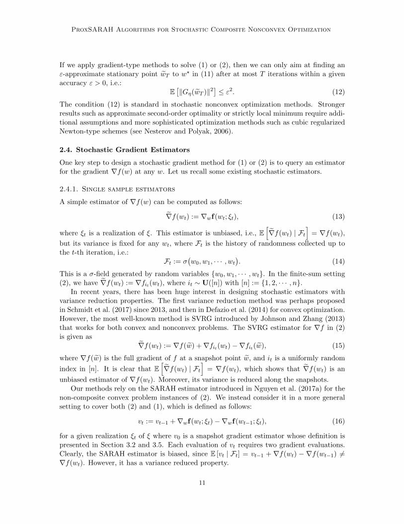
If we apply gradient-type methods to solve (1) or (2), then we can only aim at finding anε-approximate stationary point wT to w? in (11) after at most T iterations within a givenaccuracy ε > 0, i.e.:
E[‖Gη(wT )‖2
]≤ ε2. (12)
The condition (12) is standard in stochastic nonconvex optimization methods. Strongerresults such as approximate second-order optimality or strictly local minimum require addi-tional assumptions and more sophisticated optimization methods such as cubic regularizedNewton-type schemes (see Nesterov and Polyak, 2006).
2.4. Stochastic Gradient Estimators
One key step to design a stochastic gradient method for (1) or (2) is to query an estimatorfor the gradient ∇f(w) at any w. Let us recall some existing stochastic estimators.
2.4.1. Single sample estimators
A simple estimator of ∇f(w) can be computed as follows:
∇f(wt) := ∇wf(wt; ξt), (13)
where ξt is a realization of ξ. This estimator is unbiased, i.e., E[∇f(wt) | Ft
]= ∇f(wt),
but its variance is fixed for any wt, where Ft is the history of randomness collected up tothe t-th iteration, i.e.:
Ft := σ(w0, w1, · · · , wt
). (14)
This is a σ-field generated by random variables w0, w1, · · · , wt. In the finite-sum setting(2), we have ∇f(wt) := ∇fit(wt), where it ∼ U([n]) with [n] := 1, 2, · · · , n.
In recent years, there has been huge interest in designing stochastic estimators withvariance reduction properties. The first variance reduction method was perhaps proposedin Schmidt et al. (2017) since 2013, and then in Defazio et al. (2014) for convex optimization.However, the most well-known method is SVRG introduced by Johnson and Zhang (2013)that works for both convex and nonconvex problems. The SVRG estimator for ∇f in (2)is given as
∇f(wt) := ∇f(w) +∇fit(wt)−∇fit(w), (15)
where ∇f(w) is the full gradient of f at a snapshot point w, and it is a uniformly random
index in [n]. It is clear that E[∇f(wt) | Ft
]= ∇f(wt), which shows that ∇f(wt) is an
unbiased estimator of ∇f(wt). Moreover, its variance is reduced along the snapshots.Our methods rely on the SARAH estimator introduced in Nguyen et al. (2017a) for the
non-composite convex problem instances of (2). We instead consider it in a more generalsetting to cover both (2) and (1), which is defined as follows:
vt := vt−1 +∇wf(wt; ξt)−∇wf(wt−1; ξt), (16)
for a given realization ξt of ξ where v0 is a snapshot gradient estimator whose definition ispresented in Section 3.2 and 3.5. Each evaluation of vt requires two gradient evaluations.Clearly, the SARAH estimator is biased, since E [vt | Ft] = vt−1 + ∇f(wt) − ∇f(wt−1) 6=∇f(wt). However, it has a variance reduced property.
11

Pham H., Nguyen M., Phan T., and Tran-Dinh
2.4.2. Mini-batch estimators
We consider a mini-batch estimator of the gradient ∇f in (13) and of the SARAH estimator(16) respectively as follows:
∇fBt(wt) :=1
bt
∑ξi∈Bt
∇wf(wt; ξi),
and vt := vt−1 +1
bt
∑ξi∈Bt
(∇wf(wt; ξi)−∇wf(wt−1; ξi)) ,
(17)
where Bt is a mini-batch of the size bt := |Bt| ≥ 1. For the finite-sum problem (2), wereplace f(·; ξi) by fi(·). In this case, Bt is a uniformly random subset of [n]. Clearly, ifbt = n, then we take the full gradient ∇f as the exact estimator.
2.5. Basic Properties of Stochastic and SARAH Estimators
We recall some basic properties of the standard stochastic and SARAH estimators for (1)and (2). The following result was proved in Nguyen et al. (2017a).
Lemma 1 Let vtt≥0 be defined by (16) and Ft be defined by (14). Then
E [vt | Ft] = ∇f(wt) + εt 6= ∇f(wt), where εt := vt−1 −∇f(wt−1).
E[‖vt −∇f(wt)‖2 | Ft
]= ‖vt−1 −∇f(wt−1)‖2 + E
[‖vt − vt−1‖2 | Ft
]− ‖∇f(wt)−∇f(wt−1)‖2.
(18)
Consequently, for any t ≥ 0, we have
E[‖vt −∇f(wt)‖2
]= E
[‖v0 −∇f(w0)‖2
]+∑t
j=1 E[‖vj − vj−1‖2
]−∑t
j=1 E[‖∇f(wj)−∇f(wj−1)‖2
].
(19)
Our next result is some properties of the mini-batch estimators in (17). Most of the proofhave been presented in Harikandeh et al. (2015); Lohr (2009); Nguyen et al. (2017b, 2018a),and we only provide the missing proof of (23) and (24) in Appendix A.
Lemma 2 If ∇fBt(wt) is generated by (17), then, under Assumption 2.3, we have
E[∇fBt(wt) | Ft
]= ∇f(wt)
and E[‖∇fBt(wt)−∇f(wt)‖2 | Ft
]=
1
btE[‖∇wf(wt; ξ)−∇f(wt)‖2 | Ft
]≤ σ2
bt.
(20)
If ∇fBt(wt) is generated by (17) for the finite-sum problem (2), then
E[∇fBt(wt) | Ft
]= ∇f(wt)
and E[‖∇fBt(wt)−∇f(wt)‖2 | Ft
]≤ 1
bt
(n−btn−1
)σ2n(wt),
(21)
12

ProxSARAH Algorithms for Stochastic Composite Nonconvex Optimization
where σ2n(w) is defined as
σ2n(w) :=
1
n
n∑i=1
[‖∇fi(w)‖2 − ‖∇f(w)‖2
]. (22)
If vt is generated by (17) for the finite-sum problem (2), then
E[‖vt − vt−1‖2 | Ft
]= n(bt−1)
bt(n−1)‖∇f(wt)−∇f(wt−1)‖2
+ (n−bt)bt(n−1) ·
1n
∑ni=1 ‖∇fi(wt)−∇fi(wt−1)‖2.
(23)
If vt is generated by (17) for the expectation problem (1), then
E[‖vt − vt−1‖2 | Ft
]=
(1− 1
bt
)‖∇f(wt)−∇f(wt−1)‖2
+ 1btE[‖∇wf(wt; ξ)−∇wf(wt−1; ξ)‖2 | Ft
].
(24)
Note that if bt = n, i.e., we take a full gradient estimate, then the second estimate of (21)is vanished and independent of σn(·). The second term of (23) is also vanished.
3. ProxSARAH Framework and Convergence Analysis
We describe our unified algorithmic framework and then specify it to solve different in-stances of (1) and (2) under appropriate structures. The general algorithm is described inAlgorithm 1, which is abbreviated by ProxSARAH.
Algorithm 1 (Proximal SARAH with stochastic recursive gradient estimators)
1: Initialization: An initial point w0 and necessary parameters ηt > 0 and γt ∈ (0, 1](will be specified in the sequel).
2: Outer Loop: For s := 1, 2, · · · , S do
3: Generate a snapshot v(s)0 at w
(s)0 := ws−1 using (37) for (1) and (29) for (2).
4: Update w(s)1 := proxη0ψ(w
(s)0 − η0v
(s)0 ) and w
(s)1 := (1− γ0)w
(s)0 + γ0w
(0)1 .
5: Inner Loop: For t := 1, · · · ,m do
6: Generate a proper single random sample or mini-batch B(s)t .
7: Evaluate v(s)t := v
(s)t−1 + 1
|B(s)t |
∑ξ(s)t ∈B
(s)t
[∇wf(w
(s)t ; ξ
(s)t )−∇wf(w
(s)t−1; ξ
(s)t )].
8: Update w(s)t+1 := proxηtψ(w
(s)t − ηtv
(s)t ) and w
(s)t+1 := (1− γt)w(s)
t + γtw(s)t+1.
9: End For
10: Set ws := w(s)m+1
11: End For
In terms of algorithm, ProxSARAH is different from SARAH where it has one proximalstep followed by an additional averaging step, Step 8. However, using an approximation Gηof the gradient mapping Gη defined by (10), we can view Step 8 as:
w(s)t+1 := w
(s)t − ηtγtGηt(w
(s)t ), (25)
13

Pham H., Nguyen M., Phan T., and Tran-Dinh
where Gηt(w(s)t ) := 1
ηt
(w
(s)t −proxηtψ(w
(s)t − ηtv
(s)t ))
can be considered as an approximation
of Gηt(w(s)t ) and ηt := ηtγt can be viewed as a combined step-size. Hence, the update (25)
is similar to the gradient step applying to the approximate gradient mapping Gηt(w(s)t ) of
F . In particular, if we set γt = 1, then we obtain a vanilla proximal SARAH variant whichis similar to ProxSVRG, ProxSVRG+, and ProxSpiderBoost discussed above. ProxSVRG,ProxSVRG+, and ProxSpiderBoost are simply vanilla proximal gradient-type methods in
stochastic setttings. If ψ = 0, then Gηt(w(s)t ) ≡ v(s)
t and ProxSARAH is reduced to SARAHin Nguyen et al. (2017a,b, 2018b) with a step-size ηt := γtηt. Note that Step 8 can be
represented as a weighted averaging step with given weights τ (s)j mj=0:
w(s)t+1 :=
1
Σ(s)t
t∑j=0
τ(s)j w
(s)j+1, where Σ
(s)t :=
t∑j=0
τ(s)j and γ
(s)j :=
τ(s)j
Σ(s)t
.
Compared to Ghadimi and Lan (2012); Nemirovski et al. (2009), ProxSARAH evaluates vt
at the averaged point w(s)t instead of w
(s)t . Therefore, it can be written as
w(s)t+1 := (1− γt)w(s)
t + γtproxηtψ(w(s)t − ηtv
(s)t ),
which is similar to averaged fixed-point schemes (e.g., the Krasnosel’skii—Mann scheme) inthe literature (see Bauschke and Combettes, 2017).
In addition, we will show in our analysis a key difference in terms of step-sizes ηt andγt, mini-batch, and epoch length between ProxSARAH and existing methods, includingSPIDER (Fang et al., 2018) and SpiderBoost (Wang et al., 2019).
3.1. Analysis of The Inner-Loop: Key Estimates
This subsection proves two key estimates of the inner loop for t = 1 to m. We breakour analysis into two different lemmas, which provide key estimates for our convergence
analysis. We assume that the mini-batch size b := |B(s)t | in the inner loop is fixed.
Lemma 3 Let (wt, wt) be generated by the inner-loop of Algorithm 1 with |B(s)t | = b ∈
[n− 1] fixed. Then, under Assumption 2.2, we have
E[F (w
(s)m+1)
]≤ E
[F (w
(s)0 )]
+ρL2
2
m∑t=0
γt(1 + 2η2
t
) t∑j=1
γ2j−1E
[‖w(s)
j − w(s)j−1‖
2]
− 1
2
m∑t=0
γt
(2
ηt− Lγt − 3
)E[‖w(s)
t+1 − w(s)t ‖2
]+
1
2σ(s)
( m∑t=0
βt
)−
m∑t=0
γtη2t
2E[‖Gηt(w
(s)t )‖2
],
(26)
where σ(s) := E[‖v(s)
0 −∇f(w(s)0 )‖2
]≥ 0, ρ := 1
bif Algorithm 1 solves (1), and ρ := (n−b)
b(n−1)
if Algorithm 1 solves (2).
14

ProxSARAH Algorithms for Stochastic Composite Nonconvex Optimization
The proof of Lemma 3 is deferred to Appendix B.1. The next lemma shows how tochoose constant step-sizes γ and η by fixing other parameters in Lemma 3 to obtain adescent property. The proof of this lemma is given in Appendix B.2.
Lemma 4 Under Assumption 2.2 and b := |B(s)t | ∈ [n − 1], let us choose ηt = η > 0 and
γt = γ > 0 in Algorithm 1 such that
γt = γ :=1
L√ωm
and ηt = η :=2√ωm
4√ωm+ 1
, (27)
where ω := 32b
if Algorithm 1 solves (1) and ω := 3(n−b)2b(n−1)
if Algorithm 1 solves (2). Then
E[F (w
(s)m+1)
]≤ E
[F (w
(s)0 )]− γη2
2
m∑t=0
E[‖Gη(w(s)
t )‖2]
+γθ
2(m+ 1)σ(s), (28)
where θ := 1 + 2η2 ≤ 32 .
Remark 5 As mentioned in (25), the main update at Step 8 of Algorithm 1 can be written
as w(s)t+1 := w
(s)t − ηtγtGηt(w
(s)t ), where ηt := ηtγt can be viewed as a combined step-size.
Using (27), we have ηt = 2L(4√ωm+1)
= O(
1L
). This step-size is proportional to 1
L as
commonly seen in gradient-based methods (Nesterov, 2004).
3.2. Convergence Analysis for The Composite Finite-Sum Problem (2)
In this subsection, we specify Algorithm 1 to solve the composite finite-sum problem (2).
We replace v(s)0 at Step 3 and v
(s)t at Step 7 of Algorithm 1 by the following ones:
v(s)0 :=
1
bs
∑j∈Bs
∇fj(w(s)0 ), and v
(s)t := v
(s)t−1 +
1
b(s)t
∑i∈B(s)t
(∇fi(w(s)
t )−∇fi(w(s)t−1)
), (29)
where Bs is an outer mini-batch of a fixed size bs := |Bs| = b, and B(s)t is an inner mini-batch
of a fixed size b(s)t := |B(s)
t | = b. Moreover, Bs is independent of B(s)t .
We consider two separate cases of this algorithmic variant: dynamic1 step-sizes andconstant step-sizes, but with fixed inner mini-batch size b ∈ [n− 1]. The following theoremproves the convergence of the dynamic step-size variant, whose proof is in Appendix B.3.
Theorem 6 Assume that we apply Algorithm 1 to solve (2), where the estimators v(s)0 and
v(s)t are defined by (29) such that bs = b ∈ [n] and b
(s)t = b ∈ [n − 1], respectively. Let
ηt := η ∈ (0, 23) be fixed, ωη := (1+2η2)(n−b)
b(n−1), and δ := 2
η − 3 > 0. Let γtmt=0 be the sequence
of step-sizes updated in a backward mode as
γm :=δ
L, and γt :=
δ
L[η + ωηL
∑mj=t+1 γj
] , t = 0, · · · ,m− 1, (30)
Then, the following statements hold:
1. We call γt defined by (30) a dynamic step-size since γt is computed based on its previously computedcandidates γt+1, γt+2, · · · , γm.
15

Pham H., Nguyen M., Phan T., and Tran-Dinh
(a) The sequence of step-sizes γtmt=0 satisfies
δ
L(1 + δωηm)≤ γ0 < γ1 < · · · < γm,
and Σm :=
m∑t=0
γt ≥ 2δ(m+1)
L(√
2δωηm+1+1).
(31)
(b) Under Assumptions 2.1 and 2.2, and σ2n(w) defined by (22) (σ2
n(w) can be unbounded),the following bound holds:
1
SΣm
S∑s=1
m∑t=0
γtE[‖Gη(w(s)
t )‖2]≤ 2
η2SΣm
[F (w0)− F ?
]+
3
2η2S
S∑s=1
(n− bs)σ2n(ws−1)
nbs.
(32)
(c) Under Assumptions 2.1 and 2.2, if we choose η := 12 , m :=
⌊nb
⌋, bs := n, and
b ∈ [1,√n], then for wT ∼ Up
(w(s)
t s=1→St=0→m
)such that
Prob(wT = w
(s)t
)= p(s−1)m+t :=
γtSΣm
,
we have
E[‖Gη(wT )‖2
]≤ 4√
6L [F (w0)− F ?]S√n
. (33)
Consequently, the number of outer iterations S needed to obtain an output wT of
Algorithm 1 such that E[‖Gη(wT )‖2
]≤ ε2 is at most S := 4
√6L[F (w0)−F ?]√
nε2. Moreover,
if 1 ≤ n ≤ 96L2[F (w0)−F ?]2
ε4, then S ≥ 1.
The number of individual stochastic gradient evaluations ∇fi does not exceed
Tgrad :=20√
6L√n [F (w0)− F ?]ε2
= O(L√n
ε2[F (w0)− F ?]
).
The number of proxηψ operations does not exceed Tprox := 4√
6(√n+1)L[F (w0)−F ?]
bε2.
Remark 7 When n is sufficiently large, if we choose bs < n, then to guarantee con-vergence of Algorithm 1 for solving (2), we need to impose Assumption 2.3 and choosebs := O
(n ∧ ε−2
). Then we can derive similar conclusions as in Theorem 6(c).
Alternatively, Theorem 8 below shows the convergence of Algorithm 1 for the constantstep-size case, whose proof is given in Appendix B.4.
Theorem 8 Assume that we apply Algorithm 1 to solve (2), where the estimators v(s)0 and
v(s)t are defined by (29) such that bs = b ∈ [n] and b
(s)t = b ∈ [n− 1].
16
ProxSARAH Algorithms for Stochastic Composite Nonconvex Optimization
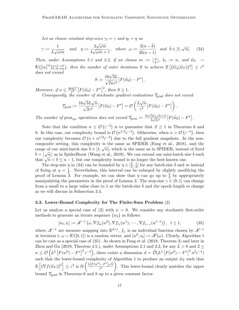
Let us choose constant step-sizes γt = γ and ηt = η as
γ :=1
L√ωm
and η :=2√ωm
4√ωm+ 1
, where ω :=3(n− b)2b(n− 1)
and b ∈ [1,√n]. (34)
Then, under Assumptions 2.1 and 2.2, if we choose m :=⌊nb
⌋, bs := n, and wT ∼
U(w(s)
t s=1→St=0→m
), then the number of outer iterations S to achieve E
[‖Gη(wT )‖2
]≤ ε2
does not exceed
S :=16√
3L√2nε2
[F (w0)− F ?
].
Moreover, if n ≤ 384L2
ε4
[F (w0)− F ?
]2, then S ≥ 1.
Consequently, the number of stochastic gradient evaluations Tgrad does not exceed
Tgrad :=16√
3L√n√
2ε2
[F (w0)− F ?
]= O
(L√n
ε2
[F (w0)− F ?
]).
The number of proxηψ operations does not exceed Tprox := 16√
3L(√n+1)
b√
2ε2
[F (w0)− F ?
].
Note that the condition n ≤ O(ε−4)
is to guarantee that S ≥ 1 in Theorems 6 and
8. In this case, our complexity bound is O(n1/2ε−2
). Otherwise, when n > O
(ε−4), then
our complexity becomes O(n+ n1/2ε−2
)due to the full gradient snapshots. In the non-
composite setting, this complexity is the same as SPIDER (Fang et al., 2018), and therange of our mini-batch size b ∈ [1,
√n], which is the same as in SPIDER, instead of fixed
b = b√nc as in SpiderBoost (Wang et al., 2019). We can extend our mini-batch size b such
that√n < b ≤ n− 1, but our complexity bound is no longer the best-known one.
The step-size η in (34) can be bounded by η ∈ [25 ,
12 ] for any batch-size b and m instead
of fixing at η = 12 . Nevertheless, this interval can be enlarged by slightly modifying the
proof of Lemma 3. For example, we can show that η can go up to 23 by appropriately
manipulating the parameters in the proof of Lemma 3. The step-size γ ∈ (0, 1] can changefrom a small to a large value close to 1 as the batch-size b and the epoch length m changeas we will discuss in Subsection 3.4.
3.3. Lower-Bound Complexity for The Finite-Sum Problem (2)
Let us analyze a special case of (2) with ψ = 0. We consider any stochastic first-ordermethods to generate an iterate sequence wt as follows:
[wt, it] := At−1(ω,∇fi0(w0),∇fi1(w1), · · · ,∇fit−1(wt−1)
), t ≥ 1, (35)
where At−1 are measure mapping into Rd+1, fit is an individual function chosen by At−1
at iteration t, ω ∼ U([0, 1]) is a random vector, and [w0, i0] := A0(ω). Clearly, Algorithm 1can be cast as a special case of (35). As shown in Fang et al. (2018, Theorem 3) and later inZhou and Gu (2019, Theorem 4.5.), under Assumptions 2.1 and 2.2, for any L > 0 and 2 ≤n ≤ O
(L2[F (w0)− F ?
]2ε−4)
, there exists a dimension d = O(L2[F (w0)− F ?
]2n2ε−4)
such that the lower-bound complexity of Algorithm 1 to produce an output wT such that
E[‖∇f(wT )‖2
]≤ ε2 is Ω
(L[F (w0)−F ?]
√n
ε2
). This lower-bound clearly matches the upper
bound Tgrad in Theorems 6 and 8 up to a given constant factor.
17

Pham H., Nguyen M., Phan T., and Tran-Dinh
3.4. Mini-Batch Size and Learning Rate Trade-offs
Although our step-size defined by (34) in the single sample case is much larger than that ofProxSVRG (Reddi et al., 2016b, Theorem 1), it still depends on
√m, where m is the epoch
length. To obtain larger step-sizes, we can choose m and the mini-batch size b using thesame trick as in Reddi et al. (2016b, Theorem 2). Let us first fix γ := γ ∈ (0, 1]. From (34),we have ωm = 1
L2γ2. It makes sense to choose γ close to 1 in order to use new information
from w(s)t+1 instead of the old one in w
(s)t .
Our goal is to choose m and b such that ωm = 3(n−b)m2b(n−1)
= 1L2γ2
. If we define C := 23L2γ2
,
then the last condition implies that b := mnCn+m−C ≤
mC provided that m ≥ C. Our
suggestion is to choose
γ := γ ∈ (0, 1], b :=⌊ mn
Cn+m− C
⌋, and η :=
2
4 + Lγ. (36)
If we choose m = bn1/3c, then b = O(n1/3
)≤ n1/3
C . This mini-batch size is much smaller
than bn2/3c in ProxSVRG. Note that, in ProxSVRG, they set γ := 1 and η := 13L .
In ProxSpiderBoost (Wang et al., 2019), m and the mini-batch size b were chosen as m =b = bn1/2c so that they can use constant step-sizes γ = 1 and η = 1
2L . In our case, if γ = 1,then η = 2
4+L . Hence, if L = 1, then ηProxSpiderBoost = 12 > ηProxSARAH = 2
5 > ηProxSVRG =13 . But if L > 4, then our step-size ηProxSARAH dominates ηProxSpiderBoost. However, bymanipulating some parameters in the proof of Lemma 3, we can obtain ηProxSARAH = 2
3 ,which shows that ηProxSARAH > ηProxSpiderBoost = 1
2 when L = 1.
If we choose m = O(n1/2
)and b = O
(n1/2
), then we maintain the same complexity
bound O(n1/2ε−2
)as in Theorems 6 and 8. Nevertheless, if we choose m = O
(n1/3
)and
b = O(n1/3
), then the complexity bound becomes O
((n2/3 + n1/3)ε−2
), which is similar to
ProxSVRG. The choice of m in Theorem 6 affects the values of γtmt=0. Hence, a reasonablysmall value of m is recommended in the dynamic step-size case.
3.5. Convergence Analysis for The Composite Expectation Problem (1)
In this subsection, we apply Algorithm 1 to solve the general expectation setting (1). Inthis case, we generate the snapshot at Step 3 of Algorithm 1 as follows:
v(s)0 :=
1
bs
∑ζ(s)i ∈Bs
∇wf(w(s)0 ; ζ
(s)i ), (37)
where Bs :=ζ
(s)1 , · · · , ζ(s)
bs
is a mini-batch of i.i.d. realizations of ξ at the s-th outer
iteration and independent of ξt from the inner loop, and bs := |Bs| = b ≥ 1 is fixed.
Now, we analyze the convergence of Algorithm 1 for solving (1) using (37) above. Forsimplicity of discussion, we only consider the constant step-size case. The dynamic step-sizevariant can be derived similarly as in Theorem 6 and we omit the details. The proof of thefollowing theorem can be found in Appendix B.5.
18

ProxSARAH Algorithms for Stochastic Composite Nonconvex Optimization
Theorem 9 Let us apply Algorithm 1 to solve (1) using (37) for v(s)0 at Step 3 of Algo-
rithm 1 with fixed outer loop batch-size bs = b ≥ 1 and inner loop batch-size b := |B(s)t | ≥ 1.
If we choose fixed step-sizes γ and η as
γ :=1
L√ωm
and η :=2√ωm
4√ωm+ 1
, with ω :=3
2b, (38)
then, under Assumptions 2.1, 2.2, and 2.3, we have the following estimate:
1
(m+ 1)S
S∑s=1
m∑t=0
E[‖Gη(w(s)
t )‖2]≤ 2
γη2(m+ 1)S
[F (w0)− F ?
]+
3σ2
2η2b. (39)
In particular, if we choose b :=⌊
75σ2
ε2
⌋and m :=
⌊σ2
bε2
⌋for b ≤ σ2
ε2, then after at most
S :=32L[F (w0)− F ?]
σε
outer iterations, we obtain E[‖Gη(wT )‖2
]≤ ε2, where wT ∼ U
(w(s)
t s=1→St=0→m
).
Consequently, the number of individual stochastic gradient evaluations ∇wf(w(s)t ; ξt) and
the number of proximal operations proxηψ, respectively do not exceed:
Tgrad :=2464σL[F (w0)− F ?]
ε3, and Tprox :=
32σL[F (w0)− F ?]bε2
.
If σ = 0, i.e., no stochasticity involved in our problem (1), then (39) reduces to
1
(m+ 1)S
S∑s=1
m∑t=0
E[‖Gη(w(s)
t )‖2]≤ 2
γη2(m+ 1)S
[F (w0)− F ?
],
where the expectation is taken over all the randomness generated by the algorithm. Fromthis bound, we can derive the well-known O
(ε−2)
oracle complexity bound for gradient-based methods in the deterministic case as often seen in the literature.
If σ > 0, then Theorem 9 achieves the best-known complexity O(σLε−3
)for the com-
posite expectation problem (1) as long as σ ≤ 32L[F (w0)−F ?]ε2
. Otherwise, our complexity
is O(σε−3 + σ2ε−2
)due to the snapshot gradient for evaluating v
(s)0 . This complexity is
the same as SPIDER (Fang et al., 2018) in the non-composite setting and ProxSpiderBoost(Wang et al., 2019) in the mini-batch setting. It also matches the lower bound complexity re-cently studied in Arjevani et al. (2019) up to a constant under the same set of assumptions,but only for the non-composite setting of (1). Hence, our complexity is nearly optimal.Note that our method does not require to perform mini-batch in the inner loop, i.e., it is
independent of B(s)t , and the mini-batch is independent of the number of iterations m of
the inner loop, while in (Wang et al., 2019), the mini-batch size |B(s)t | must be proportional
to√|Bs| = O
(ε−1), where Bs is the mini-batch of the outer loop. This is perhaps the
reason why ProxSpiderBoost can take a large constant step-size η = 12L as discussed in
Subsection 3.4.
Remark 10 We have not attempted to optimize the constants in the complexity bounds ofall theorems above, Theorems 6, 8, and 9. Our analysis can be refined to possibly obtainsmaller constants in these complexity bounds by manipulating different parameters.
19

Pham H., Nguyen M., Phan T., and Tran-Dinh
4. Dynamic Step-size Variants for Non-Composite Problems
In this section, we consider the non-composite settings of (1) and (2) as special cases ofAlgorithm 1. Note that if we solely apply Algorithm 1 with constant step-sizes to solvethe non-composite case of (1) and (2) when ψ ≡ 0, then by using the same step-size as inTheorems 6, 8, and 9, we can obtain the same complexity as stated in Theorems 6, 8, and9, respectively. However, we will modify our proof of Theorem 6 to take advantage of the
extra term∑m
t=0γt2 E[‖∇f(w
(s)t )− v(s)
t − (w(s)t+1 − w
(s)t )‖2
]in the proof of Lemma 3. The
proof of this theorem is given in Appendix C.
Theorem 11 Let w(s)t be generated by a variant of Algorithm 1 to solve the non-composite
instance of (1) or (2) using the following update for both Step 4 and Step 8:
w(s)t+1 := w
(s)t − ηtv
(s)t . (40)
Let ρ := 1b
for (1) and ρ := n−bb(n−1)
for (2), and ηt is computed recursively as:
ηm =1
Land ηt :=
1
L(1 + ρL
∑mj=t+1 ηj
) , ∀t = 0, · · · ,m− 1. (41)
Then, we have Σm :=∑m
t=0 ηt ≥2(m+1)
(√
2ρm+1+1)L.
Suppose that Assumptions 2.1 and 2.2 hold. Then, we have
1
SΣm
S∑s=1
m∑t=0
ηtE[‖∇f(w
(s)t )‖2
]≤ (√
2νm+ 1 + 1)L
S(m+ 1)
[f(w0)− f?
]+
1
S
S∑s=1
σs, (42)
where σs := E[‖∇f(w
(s)0 )− v(s)
0 ‖2].
Let wT ∼ Up
(w(s)
t s=1→St=0→m
)such that Prob
(wT = w
(s)t
)= p(s−1)m+t := ηt
SΣmfor all
s = 1, · · · , S and t = 0, · · · ,m, be the output of Algorithm 1. Then:(a) The finite-sum case: If we apply this variant of Algorithm 1 to solve (2) with ψ = 0
using bs := n, m := bnbc, and b ∈ [1,
√n], then under Assumptions 2.1 and 2.2:
E[‖∇f(wT )‖2
]≤ 2L
S√n
[f(w0)− f?]. (43)
Consequently, the total of outer iterations S to achieve E[‖∇f(wT )‖2
]≤ ε2 does not
exceed S := 2L[f(w0)−f?]√nε2
. The number of individual stochastic gradient evaluations
∇fi does not exceed Tgrad := 10√nL[f(w0)−f?]
ε2.
(b) The expectation case: If we apply this variant of Algorithm 1 to solve (1) with
ψ = 0 using bs = b := 2σ2
ε2for the outer-loop, m := σ2
bε2, and b ≤ σ2
ε2, then under
Assumptions 2.1, 2.2, and 2.3:
E[‖∇f(wT )‖2
]≤ 2L
S√bm
[f(w0)− f?
]+σ2
b. (44)
20
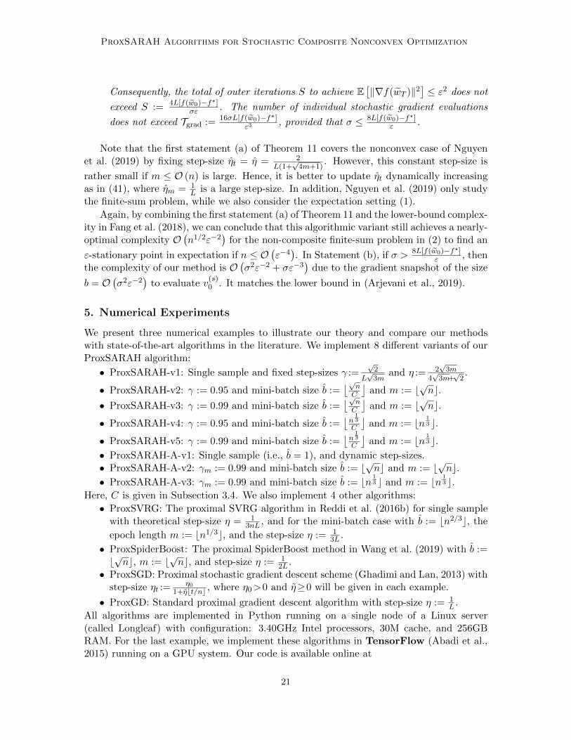
ProxSARAH Algorithms for Stochastic Composite Nonconvex Optimization
Consequently, the total of outer iterations S to achieve E[‖∇f(wT )‖2
]≤ ε2 does not
exceed S := 4L[f(w0)−f?]σε . The number of individual stochastic gradient evaluations
does not exceed Tgrad := 16σL[f(w0)−f?]ε3
, provided that σ ≤ 8L[f(w0)−f?]ε .
Note that the first statement (a) of Theorem 11 covers the nonconvex case of Nguyenet al. (2019) by fixing step-size ηt = η = 2
L(1+√
4m+1). However, this constant step-size is
rather small if m ≤ O (n) is large. Hence, it is better to update ηt dynamically increasingas in (41), where ηm = 1
L is a large step-size. In addition, Nguyen et al. (2019) only studythe finite-sum problem, while we also consider the expectation setting (1).
Again, by combining the first statement (a) of Theorem 11 and the lower-bound complex-ity in Fang et al. (2018), we can conclude that this algorithmic variant still achieves a nearly-optimal complexity O
(n1/2ε−2
)for the non-composite finite-sum problem in (2) to find an
ε-stationary point in expectation if n ≤ O(ε−4). In Statement (b), if σ > 8L[f(w0)−f?]
ε , thenthe complexity of our method is O
(σ2ε−2 + σε−3
)due to the gradient snapshot of the size
b = O(σ2ε−2
)to evaluate v
(s)0 . It matches the lower bound in (Arjevani et al., 2019).
5. Numerical Experiments
We present three numerical examples to illustrate our theory and compare our methodswith state-of-the-art algorithms in the literature. We implement 8 different variants of ourProxSARAH algorithm:
• ProxSARAH-v1: Single sample and fixed step-sizes γ :=√
2L√
3mand η := 2
√3m
4√
3m+√
2.
• ProxSARAH-v2: γ := 0.95 and mini-batch size b :=⌊√nC
⌋and m := b
√nc.
• ProxSARAH-v3: γ := 0.99 and mini-batch size b :=⌊√nC
⌋and m := b
√nc.
• ProxSARAH-v4: γ := 0.95 and mini-batch size b :=⌊n
13
C
⌋and m := bn
13 c.
• ProxSARAH-v5: γ := 0.99 and mini-batch size b :=⌊n
13
C
⌋and m := bn
13 c.
• ProxSARAH-A-v1: Single sample (i.e., b = 1), and dynamic step-sizes.• ProxSARAH-A-v2: γm := 0.99 and mini-batch size b := b
√nc and m := b
√nc.
• ProxSARAH-A-v3: γm := 0.99 and mini-batch size b := bn13 c and m := bn
13 c.
Here, C is given in Subsection 3.4. We also implement 4 other algorithms:
• ProxSVRG: The proximal SVRG algorithm in Reddi et al. (2016b) for single samplewith theoretical step-size η = 1
3nL , and for the mini-batch case with b := bn2/3c, the
epoch length m := bn1/3c, and the step-size η := 13L .
• ProxSpiderBoost: The proximal SpiderBoost method in Wang et al. (2019) with b :=b√nc, m := b
√nc, and step-size η := 1
2L .• ProxSGD: Proximal stochastic gradient descent scheme (Ghadimi and Lan, 2013) with
step-size ηt :=η0
1+ηbt/nc , where η0>0 and η≥0 will be given in each example.
• ProxGD: Standard proximal gradient descent algorithm with step-size η := 1L .
All algorithms are implemented in Python running on a single node of a Linux server(called Longleaf) with configuration: 3.40GHz Intel processors, 30M cache, and 256GBRAM. For the last example, we implement these algorithms in TensorFlow (Abadi et al.,2015) running on a GPU system. Our code is available online at
21

Pham H., Nguyen M., Phan T., and Tran-Dinh
https://github.com/unc-optimization/StochasticProximalMethods.
To be fair for comparison, we compute the norm of gradient mapping ‖Gη(w(s)t )‖ for visu-
alization at the same value η := 0.5 in all methods. To compute the relative loss residualsF (wT )−F ∗
|F ∗| , we use F ∗ := minF ∗j | j
as the minimum loss values F ∗j generated by all
algorithms. To increase the readability of figures, we only plot the performance of somerepresentative variants among the 8 instead of reporting them all. We run the first andsecond examples for 20 and 30 epochs, respectively whereas we increase it up to 150 and300 epochs in the last example. Several data sets used in this paper are from (Chang andLin, 2011)2. Two other well-known data sets are mnist3 and fashion mnist4.
5.1. Nonnegative Principal Component Analysis
We reconsider the problem of non-negative principal component analysis (NN-PCA) studiedin Reddi et al. (2016b). More precisely, for a given set of samples zini=1 in Rd, we solvethe following constrained nonconvex problem:
f? := minw∈Rd
f(w) := − 1
2n
n∑i=1
w>(ziz>i )w | ‖w‖ ≤ 1, w ≥ 0
. (45)
By defining fi(w) := −12w>(ziz
>i )w for i = 1, · · · , n, and ψ(w) := δX (w), the indicator
of X :=w ∈ Rd | ‖w‖ ≤ 1, w ≥ 0
, we can formulate (45) into (2). Moreover, since zi
is normalized, the Lipschitz constant of ∇fi is L = 1 for i = 1, · · · , n. Since (45) isnonconvex, it may have different stationary points. For a given algorithm to approximatea good stationary point of (45), it crucially depends on initial point. Following Reddi et al.(2016b), we use ProxSGD to generate an initial point and use it for all algorithms.
(a) Small and medium data sets: We test all the algorithms on three different well-known data sets: mnist (n = 60000, d = 784), rcv1-binary (n = 20242, d = 47236), andreal-sim (n = 72309, d = 20958). In ProxSGD, after manipulating different values, we setη0 := 0.1 and η := 1.0 that allow us to obtain good performance.
Experiment 1 (Single sample comparison): We first verify our theory by running 5algorithms with single sample (i.e., b = 1). The relative objective residuals and the absolutenorm of gradient mappings of these algorithms after 20 epochs are plotted in Figure 1.
Figure 1 shows that both ProxSARAH-v1 and its dynamic variant work really welland dominate all other methods. ProxSARAH-A-v1 is still better than ProxSARAH-v1.ProxSVRG is slow since its theoretical step-size 1
3nL is too small.
Experiment 2 (The effect o mini-batch sizes on ProxSARAH): In this experiment, weevaluate the effect of mini-batch sizes on the performance of ProxSARAH by running Prox-SARAH on these data sets with different mini-batch sizes. We choose b among 6 valuesn1/2, 0.75n1/2, 0.5n1/2, 0.25n1/2, 0.1n1/2, 0.05n1/2. The results are shown in Figure 2.
As we can see from Figure 2 that the performance of each particular batch-size varies be-tween data sets. Variants with larger mini-batch sizes work well in the mnist data set while
2. Available online at https://www.csie.ntu.edu.tw/∼cjlin/libsvm/3. Available online at http://yann.lecun.com/exdb/mnist/4. Available online at https://github.com/zalandoresearch/fashion-mnist
22

ProxSARAH Algorithms for Stochastic Composite Nonconvex Optimization
Number of effective passes0 5 10 15 20
TrainingLoss:
F(w
T)−
F⋆
|F⋆|
10-8
10-7
10-6
10-5
10-4
10-3
10-2
Training Loss: mnist
ProxSARAH-v1ProxSARAH-A-v1ProxSVRGProxSGDProxGD
Number of effective passes0 5 10 15 20
TrainingLoss:
F(w
T)−
F⋆
|F⋆|
10-8
10-7
10-6
10-5
10-4
10-3
Training Loss: rcv1_train.binary
ProxSARAH-v1ProxSARAH-A-v1ProxSVRGProxSGDProxGD
Number of effective passes0 5 10 15 20
TrainingLoss:
F(w
T)−
F⋆
|F⋆|
10-8
10-7
10-6
10-5
10-4
10-3
Training Loss: real-sim
ProxSARAH-v1ProxSARAH-A-v1ProxSVRGProxSGDProxGD
Number of effective passes0 5 10 15 20
Norm
ofGradientMap
ping‖G
η(w
T)‖
10-15
10-10
10-5
Norm of Gradient Mapping: mnist
ProxSARAH-v1ProxSARAH-A-v1ProxSVRGProxSGDProxGD
Number of effective passes0 5 10 15 20
Norm
ofGradientMapping‖G
η(w
T)‖
10-8
10-7
10-6
10-5
10-4
10-3
10-2
Norm of Gradient Mapping: rcv1_train.binary
ProxSARAH-v1ProxSARAH-A-v1ProxSVRGProxSGDProxGD
Number of effective passes0 5 10 15 20
Norm
ofGradientMap
ping‖G
η(w
T)‖
10-9
10-8
10-7
10-6
10-5
10-4
10-3
10-2
Norm of Gradient Mapping: real-sim
ProxSARAH-v1ProxSARAH-A-v1ProxSVRGProxSGDProxGD
Figure 1: The objective value residuals and gradient mapping norms of (45) on three datasets: mnist, rcv1-binary, and real-sim.
variants with smaller mini-batch sizes are better in rcv1 train.binary and real-sim. It isunclear for our methods to show that a larger mini-batch size leads to a better performanceor vice versa. Therefore, to achieve the best performance, a search over mini-batch size isrecommended for each particular data set.
Experiment 3 (Mini-batch comparison): Next, we run all the mini-batch variants of themethods described above to solve (45). The relative objective residuals and the norms ofgradient mapping are plotted in Figure 3.
From Figure 3, we observe that ProxSpiderBoost works well since it has a large step-size
η = 12L , and it is comparable with ProxSARAH-A-v2. The variants with b = O
(n
13
)of
ProxSARAH and ProxSARAH-A perform well for mnist data set while the variants with b =
O(n
12
)are better for the other two data sets. Although ProxSVRG takes η = 1
3L , its choice
of batch-size and epoch length also affects the performance resulting in a slower convergence.ProxSGD has good progress at early stage but then its relative objective residual is saturatedaround 10−5 accuracy. Also, its gradient mapping norms do not significantly decrease asin ProxSARAH variants or ProxSpiderBoost. Note that ProxSARAH variants with largestep-size γ (e.g., γ = 0.99) are very similar to ProxSpiderBoost which results in resemblancein their performance.
(b) Large data sets: Now, we test these algorithms on larger data sets: url combined
(n = 2, 396, 130; d = 3, 231, 961), news20.binary (n = 19, 996; d = 1, 355, 191), and
23

Pham H., Nguyen M., Phan T., and Tran-Dinh
0 5 10 15 20
10-15
10-10
10-5
Training Loss: mnist
0 5 10 15 20
10-15
10-10
10-5
Training Loss: rcv1_train.binary
0 5 10 15 20
10-15
10-10
10-5
Training Loss: real-sim
0 5 10 15 20
10-15
10-10
10-5
100
Norm of Gradient Mapping: mnist
0 5 10 15 20
10-10
10-5
Norm of Gradient Mapping: rcv1_train.binary
0 5 10 15 2010
-15
10-10
10-5
Norm of Gradient Mapping: real-sim
Figure 2: The relative objective residuals and the norms of gradient mappings of Prox-SARAH algorithms with different mini-batch sizes for solving (45) on three datasets: mnist, rcv1-binary, and real-sim.
0 5 10 15 20
10-15
10-10
10-5
Training Loss: mnist
0 5 10 15 20
10-10
10-8
10-6
10-4
Training Loss: rcv1_train.binary
0 5 10 15 20
10-10
10-5
Training Loss: real-sim
0 5 10 15 20
10-15
10-10
10-5
100
Norm of Gradient Mapping: mnist
0 5 10 15 20
10-6
10-5
10-4
10-3
10-2
Norm of Gradient Mapping: rcv1_train.binary
0 5 10 15 20
10-6
10-4
Norm of Gradient Mapping: real-sim
Figure 3: The relative objective residuals and the norms of gradient mappings of 5 algo-rithms for solving (45) on three data sets: mnist, rcv1-binary, and real-sim.
avazu-app (n = 14, 596, 137; d = 999, 990). The relative objective residuals and the ab-solute norms of gradient mapping of this experiment are depicted in Figure 4.
24

ProxSARAH Algorithms for Stochastic Composite Nonconvex Optimization
0 5 10 15 20
1e-15
1e-12
1e-9
1e-6
Training Loss: url_combined
0 5 10 15 20
1e-15
1e-12
1e-9
1e-6
1e-3
Training Loss: news20.binary
0 5 10 15 20
1e-15
1e-12
1e-9
1e-6
Training Loss: avazu-app
0 5 10 15 20
1e-15
1e-12
1e-9
1e-6
1e-3
Norm of Gradient Mapping: url_combined
0 5 10 15 20
1e-12
1e-9
1e-6
1e-3
1e-2
Norm of Gradient Mapping: news20.binary
0 5 10 15 20
1e-15
1e-12
1e-9
1e-6
1e-3
Norm of Gradient Mapping: avazu-app
Figure 4: The relative objective residuals and the absolute gradient mapping norms of 4algorithms for solving (45) on three data sets: url combined, news20.binary,and avazu-app.
Experiment 4 (Mini-batch comparison on large data sets): Figure 4 shows that Prox-SARAH variants still work well and depend on the data set in which ProxSARAH-A-v2 orthe variants with b = O(n
13 ) dominates other algorithms. In this experiment, ProxSpider-
Boost gives smaller gradient mapping norms for url combined and avazu-app in the lastepochs than the others. However, these algorithms have achieved up to 10−13 accuracy inabsolute values, the improvement of ProxSpiderBoost may not be necessary. With the samestep-size as in the previous test, ProxSGD performs quite poorly on these three data sets,and we did not report its performance here.
5.2. Sparse Binary Classification with Nonconvex Losses
We consider the following sparse binary classification involving nonconvex loss function:
minw∈Rd
F (w) :=
1
n
n∑i=1
`(a>i w, bi) + λ‖w‖1
, (46)
where (ai, bi)ni=1 ⊂ Rd × −1, 1n is a given training data set, λ > 0 is a regularizationparameter, and `(·, ·) is a given smooth and nonconvex loss function as studied in Zhaoet al. (2010). By setting fi(w) := `(a>i w, bi) and ψ(w) := λ‖w‖1 for i ∈ [n], we obtain (2).
The loss function ` is chosen from one of the following three cases (Zhao et al., 2010):• Normalized sigmoid loss: `1(s, τ) := 1 − tanh(ωτs) for a given ω > 0. Since∣∣∣d2`1(s,τ)
ds2
∣∣∣ ≤ 8(2+√
3)(1+√
3)ω2τ2
(3+√
3)2and |τ | = 1, we can show that `1(·, τ) is L-smooth with
respect to s, where L := 8(2+√
3)(1+√
3)ω2
(3+√
3)2≈ 0.7698ω2.
25

Pham H., Nguyen M., Phan T., and Tran-Dinh
• Nonconvex loss in 2-layer neural networks: `2(s, τ) :=(
1− 11+exp(−τs)
)2. For
this function, we have∣∣∣d2`2(s,τ)
ds2
∣∣∣ ≤ 0.15405τ2. If |τ | = 1, then this function is also
L-smooth with L = 0.15405.• Logistic difference loss: `3(s, τ) := ln(1 + exp(−τs)) − ln(1 + exp(−τs − ω)) for
some ω > 0. With ω = 1, we have |d2`3(s,τ)ds2
| ≤ 0.092372τ2. Therefore, if |τ | = 1, thenthis function is also L-smooth with L = 0.092372.
We set the regularization parameter λ := 1n in all the tests, which gives us relatively sparse
solutions. We test the above algorithms on different scenarios ranging from small to largedata sets, where we use 6 different data sets from LIBSVM.
(a) Small and medium data sets: We consider three small to medium data sets:rcv1.binary (n = 20, 242, d = 47, 236), real-sim (n = 72, 309, d = 20, 958), and epsilon
(n = 400, 000, d = 2, 000).
Number of effective passes0 5 10 15 20 25 30
TrainingLoss:
F(w
T)−
F⋆
|F⋆|
10-2
10-1
100
Training Loss: rcv1_train.binary
ProxSARAH-v1ProxSARAH-A-v1ProxSVRGProxSGDProxGD
Number of effective passes0 5 10 15 20 25 30
TrainingLoss:
F(w
T)−
F⋆
|F⋆|
10-2
10-1
100
Training Loss: real-sim
ProxSARAH-v1ProxSARAH-A-v1ProxSVRGProxSGDProxGD
Number of effective passes0 5 10 15 20 25 30
TrainingLoss:
F(w
T)−
F⋆
|F⋆|
10-2
10-1
100
Training Loss: epsilon
ProxSARAH-v1ProxSARAH-A-v1ProxSVRGProxSGDProxGD
Number of effective passes0 5 10 15 20 25 30
Norm
ofGradientMap
ping‖G
η(w
T)‖
10-3
10-2
Norm of Gradient Mapping: rcv1_train.binary
ProxSARAH-v1ProxSARAH-A-v1ProxSVRGProxSGDProxGD
Number of effective passes0 5 10 15 20 25 30
Norm
ofGradientMap
ping‖G
η(w
T)‖
10-3
10-2
Norm of Gradient Mapping: real-sim
ProxSARAH-v1ProxSARAH-A-v1ProxSVRGProxSGDProxGD
Number of effective passes0 5 10 15 20 25 30
Norm
ofGradientMap
ping‖G
η(w
T)‖
10-3
10-2
Norm of Gradient Mapping: epsilon
ProxSARAH-v1
ProxSARAH-A-v1
ProxSVRG
ProxSGD
ProxGD
Figure 5: The relative objective residuals and gradient mapping norms of (46) on threedata sets using the loss `2(s, τ) - The single sample case.
Experiment 5 (Singe sample comparison on (46)): Figure 5 shows the relative objectiveresiduals and the gradient mapping norms on these three data sets for the loss function `2(·)in the single sample case. Similar to the first example, ProxSARAH-v1 and its dynamicvariant work well, whereas ProxSARAH-A-v1 is better. ProxSVRG is still slow due to smallstep-size. ProxSGD appears to be better than ProxSVRG and ProxGD within 30 epochs.
Now, we test the loss function `2(·) with the mini-batch variants using the same threedata sets. Figure 6 shows the results on these data sets.
26
ProxSARAH Algorithms for Stochastic Composite Nonconvex Optimization
0 5 10 15 20 25 30
1e-2
1e-1
Training Loss: rcv1_train.binary
0 5 10 15 20 25 30
10-2
10-1
Training Loss: real-sim
0 5 10 15 20 25 30
10-2
10-1
Training Loss: epsilon
0 5 10 15 20 25 30
2e-3
5e-3
1e-2
Norm of Gradient Mapping: rcv1_train.binary
0 5 10 15 20 25 30
1e-3
5e-3
1e-2
Norm of Gradient Mapping: real-sim
0 5 10 15 20 25 30
1e-3
5e-3
1e-2Norm of Gradient Mapping: epsilon
Figure 6: The relative objective residuals and gradient mapping norms of (46) on threedata sets using the loss `2(s, τ) - The mini-batch case.
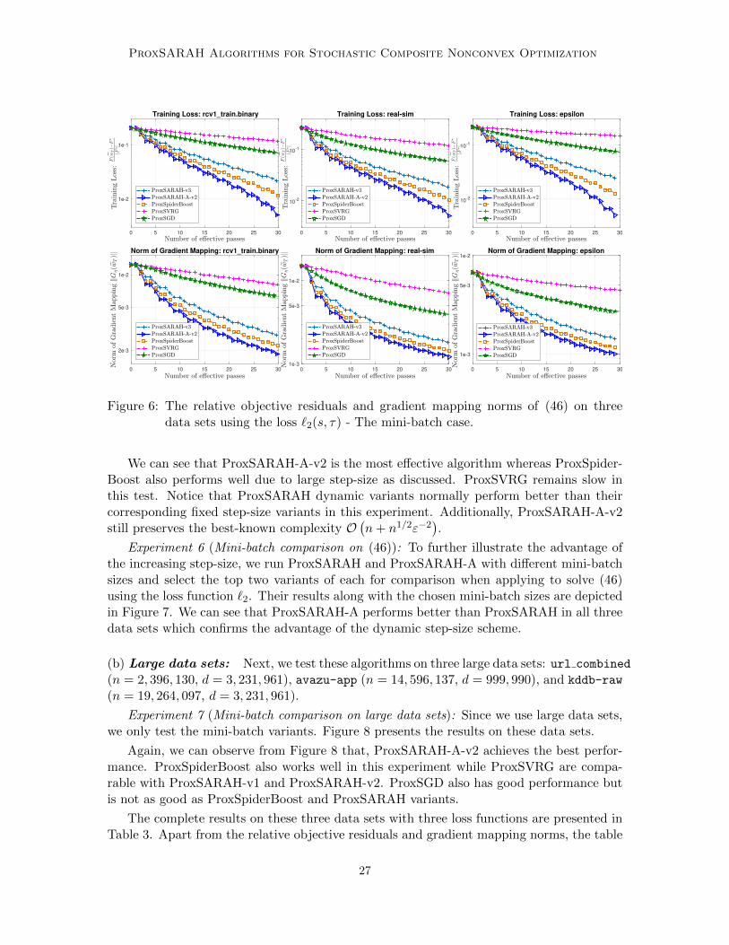
We can see that ProxSARAH-A-v2 is the most effective algorithm whereas ProxSpider-Boost also performs well due to large step-size as discussed. ProxSVRG remains slow inthis test. Notice that ProxSARAH dynamic variants normally perform better than theircorresponding fixed step-size variants in this experiment. Additionally, ProxSARAH-A-v2still preserves the best-known complexity O
(n+ n1/2ε−2
).
Experiment 6 (Mini-batch comparison on (46)): To further illustrate the advantage ofthe increasing step-size, we run ProxSARAH and ProxSARAH-A with different mini-batchsizes and select the top two variants of each for comparison when applying to solve (46)using the loss function `2. Their results along with the chosen mini-batch sizes are depictedin Figure 7. We can see that ProxSARAH-A performs better than ProxSARAH in all threedata sets which confirms the advantage of the dynamic step-size scheme.
(b) Large data sets: Next, we test these algorithms on three large data sets: url combined
(n = 2, 396, 130, d = 3, 231, 961), avazu-app (n = 14, 596, 137, d = 999, 990), and kddb-raw
(n = 19, 264, 097, d = 3, 231, 961).
Experiment 7 (Mini-batch comparison on large data sets): Since we use large data sets,we only test the mini-batch variants. Figure 8 presents the results on these data sets.
Again, we can observe from Figure 8 that, ProxSARAH-A-v2 achieves the best perfor-mance. ProxSpiderBoost also works well in this experiment while ProxSVRG are compa-rable with ProxSARAH-v1 and ProxSARAH-v2. ProxSGD also has good performance butis not as good as ProxSpiderBoost and ProxSARAH variants.
The complete results on these three data sets with three loss functions are presented inTable 3. Apart from the relative objective residuals and gradient mapping norms, the table
27

Pham H., Nguyen M., Phan T., and Tran-Dinh
0 5 10 15 2010
-3
10-2
10-1
Training Loss: w8a
0 5 10 15 2010
-2
10-1
Training Loss: rcv1_train.binary
0 5 10 15 20
10-2
10-1
Training Loss: real-sim
0 5 10 15 20
10-3
10-2
10-1
Norm of Gradient Mapping: w8a
0 5 10 15 20
0.004
0.006
0.008
0.01
0.012
0.014
0.016
0.018Norm of Gradient Mapping: rcv1_train.binary
0 5 10 15 20
10-2
Norm of Gradient Mapping: real-sim
Figure 7: The relative objective residuals and gradient mapping norms of (46) on threedata sets using the loss `2(s, τ).
0 5 10 15 20 25 30
10-3
10-2
10-1
Training Loss: url_combined
0 5 10 15 20 25 30
10-2
10-1
Training Loss: kddb-raw
0 5 10 15 20 25 30
10-5
10-4
10-3
10-2
10-1
Training Loss: avazu-app
0 5 10 15 20 25 30
10-3
10-2
10-1
Norm of Gradient Mapping: url_combined
0 5 10 15 20 25 30
10-4
10-3
10-2
10-1
Norm of Gradient Mapping: kddb-raw
0 5 10 15 20 25 3010
-5
10-4
10-3
10-2
10-1
Norm of Gradient Mapping: avazu-app
Figure 8: The relative objective residuals and gradient mapping norms of (46) on threelarge data sets using the loss `2(s, τ) - The mini-batch case.
28
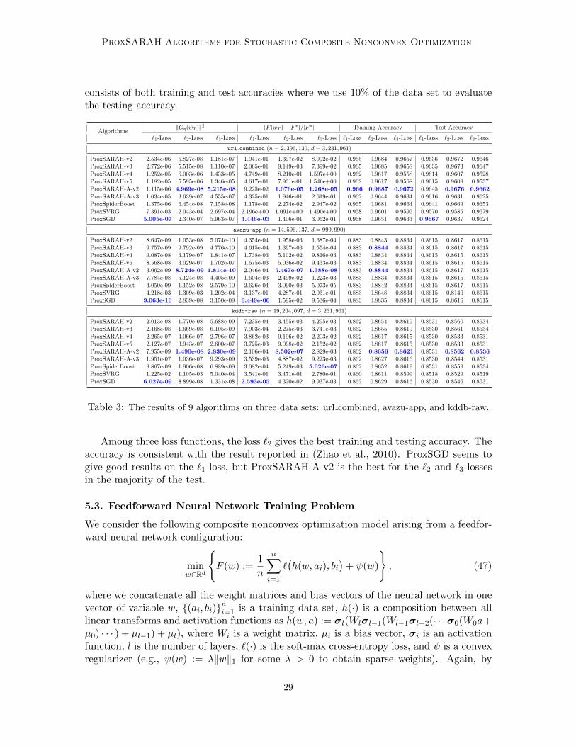
ProxSARAH Algorithms for Stochastic Composite Nonconvex Optimization
consists of both training and test accuracies where we use 10% of the data set to evaluatethe testing accuracy.
Algorithms‖Gη(wT )‖2 (F (wT )− F ∗)/|F ∗| Training Accuracy Test Accuracy
`1-Loss `2-Loss `3-Loss `1-Loss `2-Loss `3-Loss `1-Loss `2-Loss `3-Loss `1-Loss `2-Loss `3-Loss
url combined (n = 2, 396, 130, d = 3, 231, 961)
ProxSARAH-v2 2.534e-06 5.827e-08 1.181e-07 1.941e-01 1.397e-02 8.092e-02 0.965 0.9684 0.9657 0.9636 0.9672 0.9646ProxSARAH-v3 2.772e-06 5.515e-08 1.110e-07 2.065e-01 9.149e-03 7.399e-02 0.965 0.9685 0.9658 0.9635 0.9673 0.9647ProxSARAH-v4 1.252e-05 6.003e-06 1.433e-05 4.749e-01 8.210e-01 1.597e+00 0.962 0.9617 0.9558 0.9614 0.9607 0.9528ProxSARAH-v5 1.182e-05 5.595e-06 1.346e-05 4.617e-01 7.931e-01 1.546e+00 0.962 0.9617 0.9568 0.9615 0.9609 0.9537ProxSARAH-A-v2 1.115e-06 4.969e-08 5.215e-08 9.225e-02 1.076e-05 1.268e-05 0.966 0.9687 0.9672 0.9645 0.9676 0.9662ProxSARAH-A-v3 1.034e-05 3.639e-07 4.555e-07 4.325e-01 1.946e-01 2.619e-01 0.962 0.9644 0.9634 0.9616 0.9631 0.9625ProxSpiderBoost 1.375e-06 6.454e-08 7.158e-08 1.178e-01 2.274e-02 2.947e-02 0.965 0.9681 0.9664 0.9641 0.9669 0.9653ProxSVRG 7.391e-03 2.043e-04 2.697e-04 2.196e+00 1.091e+00 1.490e+00 0.958 0.9601 0.9595 0.9570 0.9585 0.9579ProxSGD 5.005e-07 2.340e-07 5.963e-07 4.446e-03 1.406e-01 3.062e-01 0.968 0.9651 0.9633 0.9667 0.9637 0.9624
avazu-app (n = 14, 596, 137, d = 999, 990)
ProxSARAH-v2 8.647e-09 1.053e-08 5.074e-10 4.354e-04 1.958e-03 1.687e-04 0.883 0.8843 0.8834 0.8615 0.8617 0.8615ProxSARAH-v3 9.757e-09 9.792e-09 4.776e-10 4.615e-04 1.397e-03 1.554e-04 0.883 0.8844 0.8834 0.8615 0.8617 0.8615ProxSARAH-v4 9.087e-08 3.179e-07 1.841e-07 1.738e-03 5.102e-02 9.816e-03 0.883 0.8834 0.8834 0.8615 0.8615 0.8615ProxSARAH-v5 8.568e-08 3.029e-07 1.702e-07 1.675e-03 5.036e-02 9.433e-03 0.883 0.8834 0.8834 0.8615 0.8615 0.8615ProxSARAH-A-v2 3.062e-09 8.724e-09 1.814e-10 2.046e-04 5.467e-07 1.388e-08 0.883 0.8844 0.8834 0.8615 0.8617 0.8615ProxSARAH-A-v3 7.784e-08 5.124e-08 4.405e-09 1.604e-03 2.499e-02 1.223e-03 0.883 0.8834 0.8834 0.8615 0.8615 0.8615ProxSpiderBoost 4.050e-09 1.152e-08 2.579e-10 2.626e-04 3.090e-03 5.073e-05 0.883 0.8842 0.8834 0.8615 0.8617 0.8615ProxSVRG 4.218e-03 1.309e-03 1.202e-04 3.137e-01 4.287e-01 2.031e-01 0.883 0.8648 0.8834 0.8615 0.8146 0.8615ProxSGD 9.063e-10 2.839e-08 3.150e-09 6.449e-06 1.595e-02 9.536e-04 0.883 0.8835 0.8834 0.8615 0.8616 0.8615
kddb-raw (n = 19, 264, 097, d = 3, 231, 961)
ProxSARAH-v2 2.013e-08 1.770e-08 5.688e-09 7.235e-04 3.455e-03 4.295e-03 0.862 0.8654 0.8619 0.8531 0.8560 0.8534ProxSARAH-v3 2.168e-08 1.669e-08 6.105e-09 7.903e-04 2.275e-03 3.741e-03 0.862 0.8655 0.8619 0.8530 0.8561 0.8534ProxSARAH-v4 2.265e-07 4.066e-07 2.796e-07 3.862e-03 9.196e-02 2.203e-02 0.862 0.8617 0.8615 0.8530 0.8533 0.8531ProxSARAH-v5 2.127e-07 3.943e-07 2.600e-07 3.725e-03 9.098e-02 2.152e-02 0.862 0.8617 0.8615 0.8530 0.8533 0.8531ProxSARAH-A-v2 7.955e-09 1.490e-08 2.830e-09 2.106e-04 8.502e-07 2.829e-03 0.862 0.8656 0.8621 0.8531 0.8562 0.8536ProxSARAH-A-v3 1.951e-07 1.036e-07 9.293e-09 3.539e-03 4.887e-02 9.223e-03 0.862 0.8627 0.8616 0.8530 0.8544 0.8531ProxSpiderBoost 9.867e-09 1.906e-08 6.889e-09 3.082e-04 5.249e-03 5.026e-07 0.862 0.8652 0.8619 0.8531 0.8559 0.8534ProxSVRG 1.225e-02 1.105e-03 5.040e-04 3.541e-01 3.471e-01 2.780e-01 0.860 0.8611 0.8599 0.8518 0.8529 0.8519ProxSGD 6.027e-09 8.899e-08 1.331e-08 2.593e-05 4.320e-02 9.937e-03 0.862 0.8629 0.8616 0.8530 0.8546 0.8531
Table 3: The results of 9 algorithms on three data sets: url combined, avazu-app, and kddb-raw.
Among three loss functions, the loss `2 gives the best training and testing accuracy. Theaccuracy is consistent with the result reported in (Zhao et al., 2010). ProxSGD seems togive good results on the `1-loss, but ProxSARAH-A-v2 is the best for the `2 and `3-lossesin the majority of the test.
5.3. Feedforward Neural Network Training Problem
We consider the following composite nonconvex optimization model arising from a feedfor-ward neural network configuration:
minw∈Rd
F (w) :=
1
n
n∑i=1
`(h(w, ai), bi
)+ ψ(w)
, (47)
where we concatenate all the weight matrices and bias vectors of the neural network in onevector of variable w, (ai, bi)ni=1 is a training data set, h(·) is a composition between alllinear transforms and activation functions as h(w, a) := σl(Wlσl−1(Wl−1σl−2(· · ·σ0(W0a+µ0) · · · ) + µl−1) + µl), where Wi is a weight matrix, µi is a bias vector, σi is an activationfunction, l is the number of layers, `(·) is the soft-max cross-entropy loss, and ψ is a convexregularizer (e.g., ψ(w) := λ‖w‖1 for some λ > 0 to obtain sparse weights). Again, by
29
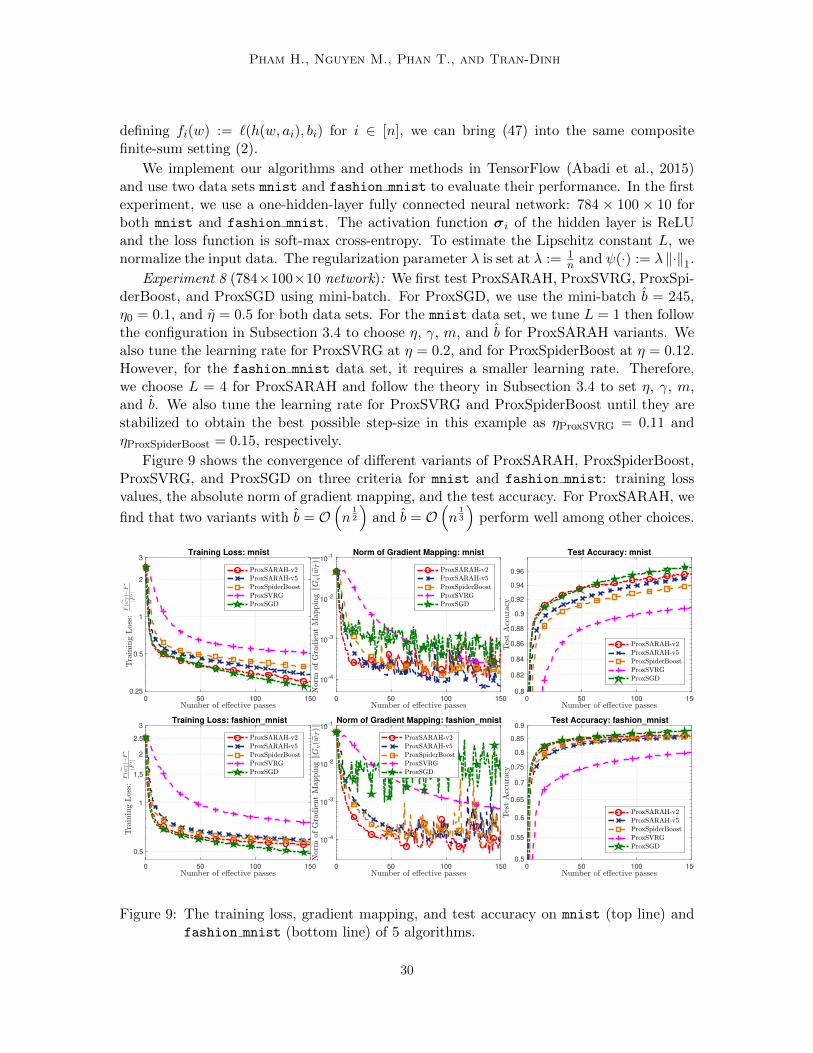
Pham H., Nguyen M., Phan T., and Tran-Dinh
defining fi(w) := `(h(w, ai), bi) for i ∈ [n], we can bring (47) into the same compositefinite-sum setting (2).
We implement our algorithms and other methods in TensorFlow (Abadi et al., 2015)and use two data sets mnist and fashion mnist to evaluate their performance. In the firstexperiment, we use a one-hidden-layer fully connected neural network: 784 × 100 × 10 forboth mnist and fashion mnist. The activation function σi of the hidden layer is ReLUand the loss function is soft-max cross-entropy. To estimate the Lipschitz constant L, wenormalize the input data. The regularization parameter λ is set at λ := 1
n and ψ(·) := λ ‖·‖1.
Experiment 8 (784×100×10 network): We first test ProxSARAH, ProxSVRG, ProxSpi-derBoost, and ProxSGD using mini-batch. For ProxSGD, we use the mini-batch b = 245,η0 = 0.1, and η = 0.5 for both data sets. For the mnist data set, we tune L = 1 then followthe configuration in Subsection 3.4 to choose η, γ, m, and b for ProxSARAH variants. Wealso tune the learning rate for ProxSVRG at η = 0.2, and for ProxSpiderBoost at η = 0.12.However, for the fashion mnist data set, it requires a smaller learning rate. Therefore,we choose L = 4 for ProxSARAH and follow the theory in Subsection 3.4 to set η, γ, m,and b. We also tune the learning rate for ProxSVRG and ProxSpiderBoost until they arestabilized to obtain the best possible step-size in this example as ηProxSVRG = 0.11 andηProxSpiderBoost = 0.15, respectively.
Figure 9 shows the convergence of different variants of ProxSARAH, ProxSpiderBoost,ProxSVRG, and ProxSGD on three criteria for mnist and fashion mnist: training lossvalues, the absolute norm of gradient mapping, and the test accuracy. For ProxSARAH, we
find that two variants with b = O(n
12
)and b = O
(n
13
)perform well among other choices.
0 50 100 150
0.25
0.5
1
2
3Training Loss: mnist
0 50 100 150
10-4
10-3
10-2
10-1
Norm of Gradient Mapping: mnist
0 50 100 150
0.8
0.82
0.84
0.86
0.88
0.9
0.92
0.94
0.96
Test Accuracy: mnist
0 50 100 150
0.5
1
1.5
2
2.5
3Training Loss: fashion_mnist
0 50 100 150
10-4
10-3
10-2
10-1
Norm of Gradient Mapping: fashion_mnist
0 50 100 150
0.5
0.55
0.6
0.65
0.7
0.75
0.8
0.85
0.9Test Accuracy: fashion_mnist
Figure 9: The training loss, gradient mapping, and test accuracy on mnist (top line) andfashion mnist (bottom line) of 5 algorithms.
30
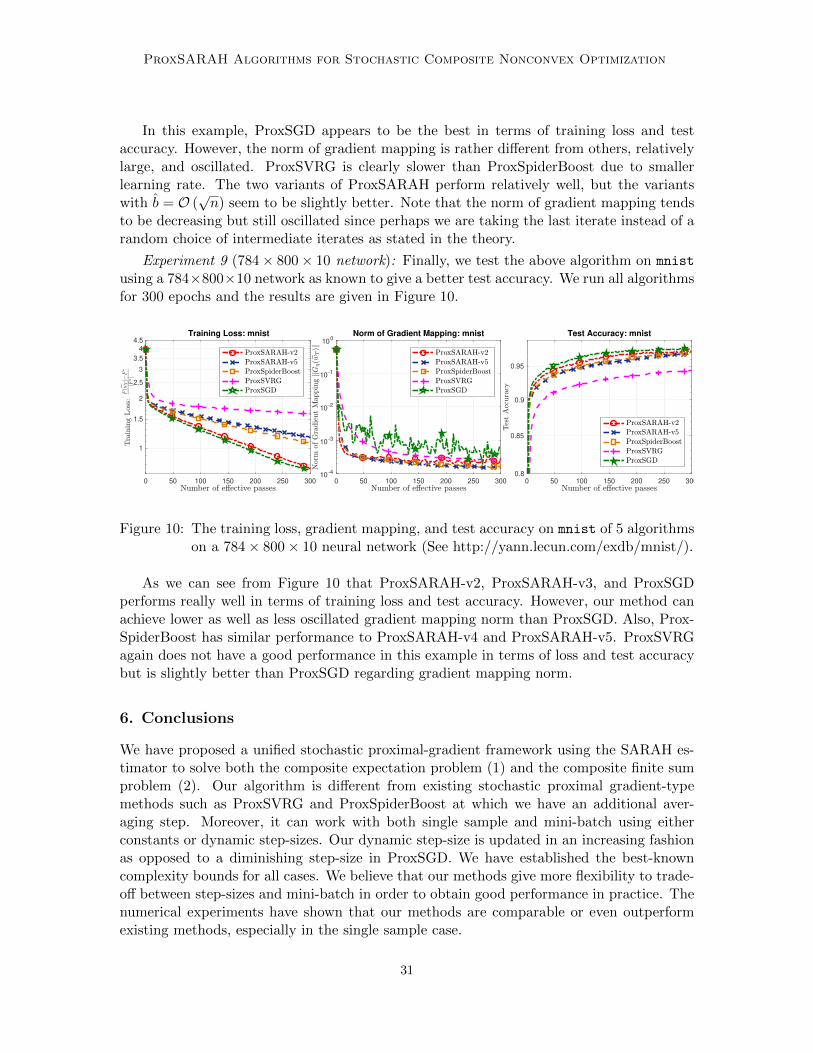
ProxSARAH Algorithms for Stochastic Composite Nonconvex Optimization
In this example, ProxSGD appears to be the best in terms of training loss and testaccuracy. However, the norm of gradient mapping is rather different from others, relativelylarge, and oscillated. ProxSVRG is clearly slower than ProxSpiderBoost due to smallerlearning rate. The two variants of ProxSARAH perform relatively well, but the variantswith b = O (
√n) seem to be slightly better. Note that the norm of gradient mapping tends
to be decreasing but still oscillated since perhaps we are taking the last iterate instead of arandom choice of intermediate iterates as stated in the theory.
Experiment 9 (784× 800× 10 network): Finally, we test the above algorithm on mnist
using a 784×800×10 network as known to give a better test accuracy. We run all algorithmsfor 300 epochs and the results are given in Figure 10.
0 50 100 150 200 250 300
1
1.5
2
2.5
3
3.5
4
4.5
Training Loss: mnist
0 50 100 150 200 250 30010
-4
10-3
10-2
10-1
100
Norm of Gradient Mapping: mnist
0 50 100 150 200 250 300
0.8
0.85
0.9
0.95
Test Accuracy: mnist
Figure 10: The training loss, gradient mapping, and test accuracy on mnist of 5 algorithmson a 784× 800× 10 neural network (See http://yann.lecun.com/exdb/mnist/).
As we can see from Figure 10 that ProxSARAH-v2, ProxSARAH-v3, and ProxSGDperforms really well in terms of training loss and test accuracy. However, our method canachieve lower as well as less oscillated gradient mapping norm than ProxSGD. Also, Prox-SpiderBoost has similar performance to ProxSARAH-v4 and ProxSARAH-v5. ProxSVRGagain does not have a good performance in this example in terms of loss and test accuracybut is slightly better than ProxSGD regarding gradient mapping norm.
6. Conclusions
We have proposed a unified stochastic proximal-gradient framework using the SARAH es-timator to solve both the composite expectation problem (1) and the composite finite sumproblem (2). Our algorithm is different from existing stochastic proximal gradient-typemethods such as ProxSVRG and ProxSpiderBoost at which we have an additional aver-aging step. Moreover, it can work with both single sample and mini-batch using eitherconstants or dynamic step-sizes. Our dynamic step-size is updated in an increasing fashionas opposed to a diminishing step-size in ProxSGD. We have established the best-knowncomplexity bounds for all cases. We believe that our methods give more flexibility to trade-off between step-sizes and mini-batch in order to obtain good performance in practice. Thenumerical experiments have shown that our methods are comparable or even outperformexisting methods, especially in the single sample case.
31
Pham H., Nguyen M., Phan T., and Tran-Dinh
Acknowledgements
The work of Q. Tran-Dinh has partly been supported by the National Science Foundation(NSF), grant no. DMS-1619884, and the Office of Naval Research (ONR), grant no. N00014-20-1-2088 (2020-2023).
Appendix A. Technical Lemmas
This appendix provides the missing proofs of Lemma 2 and one elementary result, Lemma 12,used in our analysis in the sequel.
Lemma 12 Given three positive constants ν, δ, and L, let γtmt=0 be a positive sequencesatisfying the following conditions:
Lγm − δ ≤ 0,
νL2γt∑m
j=t+1 γj − δ + Lγt ≤ 0, t = 0, · · · ,m− 1.(48)
Then, the following statements hold:(a) The sequence γtmt=0 computed recursively in a backward mode as
γm :=δ
L, and γt :=
δ
L[1 + νL
∑mj=t+1 γj
] , t = 0, · · · ,m− 1, (49)
tightly satisfies (48). Moreover, we have δL(1+δνm) < γ0 < γ1 < · · · < γm and
Σm :=m∑t=0
γt ≥2δ(m+ 1)
L[√
1 + 2δνm+ 1] . (50)
(b) The constant sequence γtmt=0 with γt := 2δL(√
1+4δνm+1)satisfies (48).
Proof (a) The sequence γtmt=0 given by (49) is in fact computed from (48) by setting allthe inequalities “≤” to equalities “=”. Hence, it automatically satisfies (48). Moreover, itis obvious that γ0 < γ1 < · · · < γm. Since
∑mt=1 γt < mγm = mδ
L , we have γ0 >δ
L(1+δνm) .
Let Σm :=∑m
t=0 γt. Using Σm into (48) with all equalities, we can rewrite it as
νL2γmΣm = δ − Lγm + νL2(γ2m + γmγm−1 + γmγm−2 + · · ·+ γmγ0)
νL2γm−1Σm = δ − Lγm−1 + νL2(γ2m−1 + γm−1γm−2 + γm−1γm−3 + · · ·+ γm−1γ0)
· · · · · · · · ·νL2γ1Σm = δ − Lγ1 + νL2(γ2
1 + γ1γ0)
νL2γ0Σm = δ − Lγ0 + νL2γ20 .
Summing up both sides of these equations, and using the definition of Σm and S2m :=∑m
t=0 η2t , we obtain
νL2Σ2m = (m+ 1)δ − LΣm +
νL2
2(Σ2
m + S2m).
32

ProxSARAH Algorithms for Stochastic Composite Nonconvex Optimization
Since (m+ 1)S2m ≥ Σ2
m by the Cauchy-Schwarz inequality, the last expression leads to
νL2Σ2m + 2LΣm − 2δ(m+ 1) = νL2S2
m ≥νL2Σ2
m
m+ 1.
Therefore, by solving the quadratic inequation νmL2Σ2m + 2(m+ 1)LΣm − 2δ(m+ 1)2 ≥ 0
in Σm with Σm > 0, we obtain
Σm ≥2δ(m+ 1)
L[1 +√
1 + 2δνm] ,
which is exactly (50).
(b) Let γt := γ > 0 for t = 0, · · · ,m. Then (48) holds if νL2γ2m− δ+Lγ = 0. Solving thisquadratic equation in γ and noting that γ > 0, we obtain γ = 2δ
L(√
1+4δνm+1).
Proof (The proof of Lemma 2: Properties of stochastic estimators): We onlyprove (23), since other statements were proved in Harikandeh et al. (2015); Lohr (2009);Nguyen et al. (2017b, 2018a). The proof of (23) for the finite-sum case (2) was also givenin Nguyen et al. (2018a) but under the L-smoothness of each fi, we conduct this proof hereby following the same path as in Nguyen et al. (2018a) for completeness.
Our goal is to prove (24) by upper bounding the following quantity:
At := E[‖vt − vt−1‖2 | Ft
]− ‖∇f(wt)−∇f(wt−1)‖2. (51)
Let Ft := σ(w(s)0 ,B1, · · · ,Bt−1) be the σ-field generated by w
(s)0 and mini-batches B1, · · · ,Bt−1,
and F0 = F1 = σ(w(s)0 ). If we define Ξi := ∇fi(wt)−∇fi(wt−1), then using the update rule
(17), we can upper bound At in (51) as
At = E[‖ 1bt
∑i∈Bt Ξi‖2 | Ft
]− ‖ 1
n
∑ni=1 Ξi‖2
= 1b2tE[∑
i∈Bt∑
j∈Bt〈Ξi,Ξj〉 | Ft]− 1
n2
∑ni=1
∑nj=1〈Ξi,Ξj〉
= 1b2tE[∑
i,j∈Bt,i 6=j〈Ξi,Ξj〉+∑
i∈Bt ‖Ξi‖2 | Ft
]− 1
n2
∑ni=1
∑nj=1〈Ξi,Ξj〉
= 1b2t
[bt(bt−1)n(n−1)
∑ni,j=1,i 6=j〈Ξi,Ξj〉+ bt
n
∑ni=1 ‖Ξi‖2
]− 1
n2
∑ni=1
∑nj=1〈Ξi,Ξj〉
= (bt−1)btn(n−1)
∑ni,j=1〈Ξi,Ξj〉+ (n−bt)
btn(n−1)
∑ni=1 ‖Ξi‖2 −
1n2
∑ni=1
∑nj=1〈Ξi,Ξj〉
= (n−bt)btn(n−1)
∑ni=1 ‖Ξi‖2 −
(n−bt)(n−1)bt
‖ 1n
∑ni=1 Ξi‖2
= (n−bt)bt(n−1)
1n
∑ni=1 ‖∇fi(wt)−∇fi(wt−1)‖2 − (n−bt)
(n−1)bt‖∇f(wt)−∇f(wt−1)‖2,
where we use the facts that
E[∑
i,j∈Bt,i 6=j〈Ξi,Ξj〉 | Ft]
= bt(bt−1)n(n−1)
∑ni,j=1,i 6=j〈Ξi,Ξj〉
and E[∑
i∈Bt ‖Ξi‖2 | Ft
]= bt
n
∑ni=1 ‖Ξi‖2
in the third line of the above derivation. Rearranging the estimate At, we obtain (23).
33

Pham H., Nguyen M., Phan T., and Tran-Dinh
To prove (24), we define Ξi := ∇wf(wt; ξi) − ∇wf(wt−1; ξi). Clearly, E [Ξi | Ft] =∇f(wt)−∇f(wt−1) and vt − vt−1 = 1
bt
∑i∈Bt Ξi. Similar to (20), we have
E[‖(vt − vt−1)− E [Ξi | Ft] ‖2 | Ft
]= 1
btE[‖Ξi − E [Ξi | Ft] ‖2 | Ft
].
Using the fact that E[‖X − E [X] ‖2
]= E
[‖X‖2
]− ‖E [X] ‖2, after rearranging, we obtain
from the last expression that
E[‖vt − vt−1‖2 | Ft
]=(
1− 1bt
)‖∇f(wt)−∇f(wt−1)‖2
+ 1btE[‖∇wf(wt; ξ)−∇wf(wt−1; ξ)‖2 | Ft
],
which is indeed (24).
Appendix B. The Proof of Technical Results in Section 3
We provide the full proof of the results in Section 3.
B.1. The Proof of Lemma 3: The Analysis of The Inner Loop
Proof From the update w(s)t+1 := (1−γt)w(s)
t +γtw(s)t+1, we have w
(s)t+1−w
(s)t = γt(w
(s)t+1−w
(s)t ).
Firstly, using the L-smoothness of f from (6) of Assumption 2.2, we can derive
f(w(s)t+1) ≤ f(w
(s)t ) + 〈∇f(w
(s)t ), w
(s)t+1 − w
(s)t 〉+ L
2 ‖w(s)t+1 − w
(s)t ‖2
= f(w(s)t ) + γt〈∇f(w
(s)t ), w
(s)t+1 − w
(s)t 〉+
Lγ2t2 ‖w
(s)t+1 − w
(s)t ‖2.
(52)
Next, using the convexity of ψ, one can show that
ψ(w(s)t+1) ≤ (1− γt)ψ(w
(s)t ) + γtψ(w
(s)t+1) ≤ ψ(w
(s)t ) + γt〈∇ψ(w
(s)t+1), w
(s)t+1 − w
(s)t 〉, (53)
where ∇ψ(w(s)t+1) ∈ ∂ψ(w
(s)t+1).
By the optimality condition of w(s)t+1 := proxηtψ(w
(s)t − ηtv
(s)t ), we have ∇ψ(w
(s)t+1) =
−v(s)t − 1
ηt(w
(s)t+1 − w
(s)t ) for some ∇ψ(w
(s)t+1) ∈ ∂ψ(w
(s)t+1). Substituting this expression into
(53), we obtain
ψ(w(s)t+1) ≤ ψ(w
(s)t ) + γt〈v(s)
t , w(s)t − w
(s)t+1〉 −
γtηt‖w(s)
t+1 − w(s)t ‖2. (54)
Combining (52) and (54), and then using F (w) := f(w) + ψ(w) yields
F (w(s)t+1) ≤ F (w
(s)t ) + γt〈∇f(w
(s)t )− v(s)
t , w(s)t+1 − w
(s)t 〉 −
(γtηt− Lγ2
t
2
)‖w(s)
t+1 − w(s)t ‖2. (55)
Also, the following expression holds
〈∇f(w(s)t )− v(s)
t , w(s)t+1 − w
(s)t 〉 = 1
2‖∇f(w(s)t )− v(s)
t ‖2 + 12‖w
(s)t+1 − w
(s)t ‖2
− 12‖∇f(w
(s)t )− v(s)
t − (w(s)t+1 − w
(s)t )‖2.
34
ProxSARAH Algorithms for Stochastic Composite Nonconvex Optimization
From this expression, we can rewrite (55) as
F (w(s)t+1) ≤ F (w
(s)t ) +
γt2‖∇f(w
(s)t )− v(s)
t ‖2 −(γtηt− Lγ2
t
2− γt
2
)‖w(s)
t+1 − w(s)t ‖2 − σ
(s)t ,
where σ(s)t := γt
2 ‖∇f(w(s)t )− v(s)
t − (w(s)t+1 − w
(s)t )‖2 ≥ 0.
Taking expectation both sides of this inequality over the entire history, we obtain
E[F (w
(s)t+1)
]≤ E
[F (w
(s)t )]
+ γt2 E[‖∇f(w
(s)t )− v(s)
t ‖2]
−(γtηt− Lγ2t
2 −γt2
)E[‖w(s)
t+1 − w(s)t ‖2
]− E
[σ
(s)t
].
(56)
Next, recall from (10) that Gη(w) := 1η
(w− proxηψ(w− η∇f(w))
)is the gradient mapping
of F . In this case, it is obvious that
ηt‖Gηt(w(s)t )‖ = ‖w(s)
t − proxηtψ(w(s)t − ηt∇f(w
(s)t ))‖.
Using this definition, the triangle inequality, and the nonexpansive property ‖proxηψ(z) −proxηψ(w)‖ ≤ ‖z − w‖ of proxηψ, we can derive that
ηt‖Gηt(w(s)t )‖ ≤ ‖w(s)
t+1 − w(s)t ‖+ ‖proxηtψ(w
(s)t − ηt∇f(w
(s)t ))− w(s)
t+1‖
= ‖w(s)t+1 − w
(s)t ‖+ ‖proxηtψ(w
(s)t − ηt∇f(w
(s)t ))− proxηtψ(w
(s)t − ηtv
(s)t )‖
≤ ‖w(s)t+1 − w
(s)t ‖+ ηt‖∇f(w
(s)t )− v(s)
t ‖.
Now, the last estimate leads to
η2tE[‖Gηt(w
(s)t )‖2
]≤ 2E
[‖w(s)
t+1 − w(s)t ‖2
]+ 2η2
tE[‖∇f(w
(s)t )− v(s)
t ‖2].
Multiplying this inequality by γt2 > 0 and adding the result to (56), we finally get
E[F (w
(s)t+1)
]≤ E
[F (w
(s)t )]− γtη2t
2 E[‖Gηt(w
(s)t )‖2
]+ γt
2
(1 + 2η2
t
)E[‖∇f(w
(s)t )− v(s)
t ‖2]
− γt2
(2ηt− Lγt − 3
)E[‖w(s)
t+1 − w(s)t ‖2
]− E
[σ
(s)t
].
Summing up this inequality from t = 0 to t = m, we obtain
E[F (w
(s)m+1)
]≤ E
[F (w
(s)0 )]
+1
2
m∑t=0
γt(1 + 2η2
t
)E[‖∇f(w
(s)t )− v(s)
t ‖2]
− 1
2
m∑t=0
γt
( 2
ηt− Lγt − 3
)E[‖w(s)
t+1 − w(s)t ‖2
]−
m∑t=0
γtη2t
2E[‖Gηt(w
(s)t )‖2
]−
m∑t=0
E[σ
(s)t
].
(57)
35

Pham H., Nguyen M., Phan T., and Tran-Dinh
We consider two cases:Case 1: In the finite-sum setting (2), i.e., Algorithm 1 solves (2), then from (23) of
Lemma 2, the L-smoothness condition (4) in Assumption 2.2, the choice b(s)t = b ≥ 1,
and w(s)j − w
(s)j−1 = γj−1(w
(s)j − w
(s)j−1), we can estimate
E[‖v(s)j − v
(s)j−1‖2 | Fj
](23)= n(b−1)
b(n−1)‖∇f(wj)−∇f(wj−1)‖2
+ n−bb(n−1)
1n
∑ni=1 ‖∇fi(w
(s)j )−∇fi(w(s)
j−1)‖2
(4)
≤ ‖∇f(wj)−∇f(wj−1)‖2 + (n−b)L2
b(n−1)‖w(s)
j − w(s)j−1‖2
= ‖∇f(wj)−∇f(wj−1)‖2 +(n−b)L2γ2j−1
b(n−1)‖w(s)
j − w(s)j−1‖2.
Case 2: In the expectation setting (1), i.e., Algorithm 1 solves (1), then from (24) ofLemma 2, we have
E[‖v(s)j − v
(s)j−1‖2 | Fj
](24)=(
1− 1b
)‖∇f(wj)−∇f(wj−1)‖2
+ 1bE[‖∇wf(wj ; ξ)−∇wf(wj−1; ξ)‖2 | Fj
](3)
≤ ‖∇f(wj)−∇f(wj−1)‖2 + L2
b‖w(s)
j − w(s)j−1‖2
= ‖∇f(wj)−∇f(wj−1)‖2 +L2γ2j−1
b‖w(s)
j − w(s)j−1‖2.
Using either one of the two last inequalities and (19), then taking the full expectation, wecan derive
E[‖∇f(w
(s)t )− v(s)
t ‖2]
= E[‖∇f(w
(s)0 )− v(s)
0 ‖2]∑t
j=1 E[‖v(s)j − v
(s)j−1‖2
]−∑t
j=1 E[‖∇f(wj)−∇f(wj−1)‖2
]≤ E
[‖∇f(w
(s)0 )− v(s)
0 ‖2]
+ ρL2∑t
j=1 γ2j−1E
[‖w(s)
j − w(s)j−1‖2
]= σ(s) + ρL2
∑tj=1 γ
2j−1E
[‖w(s)
j − w(s)j−1‖2
],
(58)
where σ(s) := E[‖∇f(w
(s)0 )− v(s)
0 ‖2]≥ 0, and ρ := 1
bif Algorithm 1 solves (1), and
ρ := n−bb(n−1)
if Algorithm 1 solves (2).
Substituting (58) into (57) and dropping the term −m∑t=0
E[σ
(s)t
](≤ 0), we finally arrive at
E[F (w
(s)m+1)
]≤ E
[F (w
(s)0 )]
+ ρL2
2
m∑t=0
γt(1 + 2η2
t
) t∑j=1
γ2j−1E
[‖w(s)
j − w(s)j−1‖
2]
− 1
2
m∑t=0
γt
(2
ηt− Lγt − 3
)E[‖w(s)
t+1 − w(s)t ‖2
]−
m∑t=0
γtη2t
2E[‖Gηt(w
(s)t )‖2
]+
1
2
m∑t=0
γt(1 + 2η2
t
)σ(s),
36
ProxSARAH Algorithms for Stochastic Composite Nonconvex Optimization
which is exactly (26).
B.2. The Proof of Lemma 4: The Selection of Constant Step-sizes
Proof Let us first fix all the step-sizes of Algorithm 1 as constants as follows:
γt := γ ∈ (0, 1] and ηt := η > 0.
We also denote a(s)t := E
[‖w(s)
t+1 − w(s)t ‖2
]≥ 0.
Let ρ := 1b
if Algorithm 1 solves (1) and ρ := n−bb(n−1)
if Algorithm 1 solves (2). Using these
expressions into (26), we can easily show that
E[F (w
(s)m+1)
]≤ E
[F (w
(s)0 )]
+ ρL2γ3
2
(1 + 2η2
) m∑t=0
t∑j=1
a(s)j−1
− γ2
(2η − Lγ − 3
) m∑t=0
a(s)t −
γη2
2
m∑t=0
E[‖Gηt(w
(s)t )‖2
]+ γ
2
(1 + 2η2
)(m+ 1)σ(s)
= E[F (w
(s)0 )]− γη2
2
m∑t=0
E[‖Gηt(w
(s)t )‖2
]+ γ
2
(1 + 2η2
)(m+ 1)σ(s) + Tm,
(59)
where Tm is defined as
Tm :=ρL2γ3
(1 + 2η2
)2
m∑t=0
t∑j=1
a(s)j−1 −
γ
2
(2
η− Lγ − 3
) m∑t=0
a(s)t .
Our goal is to choose η > 0, and γ ∈ (0, 1] such that Tm ≤ 0. We first rewrite Tm as follows:
Tm =ρL2γ3(1+2η2)
2
[ma
(s)0 + (m− 1)a
(s)1 + · · ·+ 2a
(s)m−2 + a
(s)m−1
]− γ
2
(2η − Lγ − 3
) [a
(s)0 + a
(s)1 + · · ·+ a
(s)m
].
By synchronizing the coefficients of the terms a(s)0 , a
(s)1 , · · · , a(s)
m , to guarantee Tm ≤ 0, weneed to satisfy ρ
(1 + 2η2
)L2γ2m−
(2η − Lγ − 3
)≤ 0,
2η − Lγ − 3 ≥ 0.
(60)
Assume that 2η −Lγ− 3 = 1 > 0. This implies that η = 2
Lγ+4 . Next, since Lγ > 0, we have
η ≤ 12 . Therefore, we can upper bound
ρL2γ2m(1 + 2η2)−(
2
η− Lγ − 3
)≤ 3ρL2γ2m
2− 1 = 0.
37

Pham H., Nguyen M., Phan T., and Tran-Dinh
The last equation and η = 2Lγ+4 lead to
γ :=1
L√ωm
and η :=2√ωm
4√ωm+ 1
,
which is exactly (27), where ω := 3(n−b)2b(n−1)
for (2) and ω := 32b
for (1).
Finally, using this choice (27) of the step-sizes, we can derive that
E[F (w
(s)m+1
]≤ E
[F (w
(s)0 )]− γη2
2
m∑t=0
E[‖Gη(w(s)
t )‖2]
+γθ
2(m+ 1)σ(s), (61)
which is exactly (28), where θ := 1 + 2η2 ≤ 32 .
B.3. The Proof of Theorem 6: The Dynamic Step-size Case
Proof Let βt := γt(1 + 2η2
t
)and κt := γt
(2ηt− Lγt − 3
). From (26) of Lemma 3 we have
E[F (w
(s)m+1)
]≤ E
[F (w
(s)0 )]−
m∑t=0
γtη2t
2E[‖Gηt(w
(s)t )‖2
]+
1
2σ(s)
( m∑t=0
βt
)+ Tm, (62)
where
Tm :=L2(n− b)2b(n− 1)
m∑t=0
βt
t∑j=1
γ2j−1E
[‖w(s)
j − w(s)j−1‖
2]− 1
2
m∑t=0
κtE[‖w(s)
t+1 − w(s)t ‖2
].
Now, to guarantee Tm ≤ 0, let us choose all the parameters such that κm = 0,
(n−b)b(n−1)
L2γ2t
∑mj=t+1 βj − κt = 0, t = 0, · · · ,m− 1.
(63)
Then, (62) becomes
E[F (w
(s)m+1)
]≤ E
[F (w
(s)0 )]−
m∑t=0
stη2t
2E[‖Gηt(w
(s)t )‖2
]+
1
2
m∑t=0
βtσ(s). (64)
If we fix ηt = η ∈ (0, 23), and define δ := 2
η − 3 > 0, then (63) reduces to δ − Lγm = 0,
L2(n−b)(1+2η2)
b(n−1)γt∑m
j=t+1 γj − δ + Lγt = 0, t = 0, · · · ,m− 1.(65)
Applying Lemma 12(a) with ν = ωη := (n−b)(1+2η2)
b(n−1), we obtain from (65) that
γm :=δ
L, and γt :=
δ
L[1 + ωηL
∑mj=t+1 γj
] , t = 0, · · · ,m− 1. (66)
38

ProxSARAH Algorithms for Stochastic Composite Nonconvex Optimization
Moreover, we have
δ
L(1 + ωηδm)< γ0 < γ1 < · · · < γm, and Σm :=
m∑t=0
γt ≥2δ(m+ 1)
L(√
2ωηδm+ 1 + 1),
which proves (31).
On the other hand, since σ(s) := E[‖∇f(w
(s)0 )− v(s)
0 ‖2]
= E[‖∇fBs(ws−1)−∇f(ws−1)‖2
],
by using (21), we have σ(s) ≤(n−bsnbs
)σ2n(ws−1). Using this upper bound and βt :=
γt(1 + 2η2) ≤ 3γt2 ≤
32 (since γt ∈ [0, 1]), into the estimate (64), we can arrive at
1
SΣm
S∑s=1
m∑t=0
γtE[‖Gη(w(s)
t )‖2]≤ 2
η2SΣm
[F (w0)− F ?
]+
3
2η2S
S∑s=1
(n− bs)σ2n(ws−1)
nbs,
which is exactly (32).
Now, let us choose η := 12 ∈ (0, 2
3). Then, we have δ = 1, ωη = 3(n−b)2b(n−1)
, and Σm ≥2δ(m+1)
L(√
2ωηm+1+1). Using these facts, wT ∼ Up
(w(s)
t s=1→St=0→m
)with Prob
(wT = w
(s)t
)=
p(s−1)m+t := γtSΣm
, and bs = n, we obtain from (32) that
E[‖Gη(wT )‖2
]=
1
SΣm
S∑s=1
m∑t=0
γtE[‖Gη(w(s)
t )‖2]≤ 4L(
√2ωm+ 1 + 1)
S(m+ 1)
[F (w0)− F ?
].
Next, using m = bnbc and ω := ωη = 3(n−b)
2b(n−1), if b ≤
√n, then we can bound
√2ωm+ 1 + 1
m+ 1≤ 2
√ω√
m+ 1≤√
6√n.
Using this bound, we can further bound the above estimate obtained from (32) as
E[‖Gη(wT )‖2
]≤ 4√
6L [F (w0)− F ?]S√n
,
which is (33).
To achieve E[‖Gη(wT )‖2
]≤ ε2, we impose 4
√6L[F (w0)−F ?]
S√n
= ε2, which shows that
the number of outer iterations S := 4√
6L[F (w0)−F ?]√nε2
. To guarantee S ≥ 1, we need n ≤96L2[F (w0)−F ?]2
ε4.
Hence, we can estimate the number of gradient evaluations Tgrad by
Tgrad = Sn+ 2S(m+ 1)b ≤ 5Sn =20√
6L√n [F (w0)− F ?]ε2
.
We can conclude that the number of stochastic gradient evaluations does not exceed Tgrad =
O(L√n[F (w0)−F ?]
ε2
). The number of proximal operations proxηψ does not exceed Tprox :=
S(m+ 1) ≤ 4√
6(√n+1)L[F (w0)−F ?]
bε2.
39

Pham H., Nguyen M., Phan T., and Tran-Dinh
B.4. The Proof of Theorem 8: The Constant Step-size Case
Proof If we choose (γt, ηt) = (γ, η) > 0 for all t = 0, · · · ,m, then, by applying Lemma 4,we can update
γ :=1
L√ωm
and η :=2√ωm
4√ωm+ 1
,
which is exactly (34), where ω := 3(n−b)2(n−1)b
. With this update, we can simplify (28) as
E[F (w
(s)m+1)
]≤ E
[F (w
(s)0 )]− γη2
2
m∑t=0
E[‖Gη(w(s)
t )‖2]
+3γ
4(m+ 1)σ(s).
With the same argument as above, we obtain
1
(m+ 1)S
S∑s=1
m∑t=0
E[‖Gη(w(s)
t )‖2]≤ 2
γη2(m+ 1)S
[F (w0)−F ?
]+
3
2η2S
S∑s=1
(n− bs)σ2n(ws−1)
nbs.
For wT ∼ U(w(s)
t s=1→St=0→m
)with T := (m+ 1)S and bs = n, the last estimate implies
E[‖Gη(wT )‖2
]=
1
(m+ 1)S
S∑s=1
m∑t=0
E[‖Gη(w(s)
t )‖2]≤ 2
γη2(m+ 1)S
[F (w0)− F ?
].
By the update rule of η and γ, we can easily show that γη2 ≥ 4√ωm
L(4√ωm+1)2
. Therefore, using
m := bnbc, we can overestimate
1
γη2(m+ 1)≤ L(4
√ωm+ 1)2
4√ωm(m+ 1)
≤ 8L√ω√
m≤ 8√
3L√2n
.
Using this upper bound, to guarantee E[‖Gη(wT )‖2
]≤ ε2, we choose S and m such that
16√
3LS√
2n
[F (w0) − F ?
]= ε2, which leads to S := 16
√3L√
2nε2
[F (w0) − F ?
]as the number of outer
iterations. To guarantee S ≥ 1, we need to choose n ≤ 384L2
ε4
[F (w0)− F ?
]2.
Finally, we can estimate the number of stochastic gradient evaluations Tgrad as
Tgrad = Sn+ 2S(m+ 1) ≤ 5Sn =16√
3L√n√
2ε2
[F (w0)− F ?
]= O
(L√n
ε2
[F (w0)− F ?
]).
The number of proxηψ is Tprox = S(m+ 1) ≤ 16√
3L(√n+1)
b√
2ε2
[F (w0)− F ?
].
B.5. The Proof of Theorem 9: The Expectation Problem
Proof Summing up (28) from s = 1 to s = S, and then using w(0)0 = w0, we obtain
γη2
2
S∑s=1
m∑t=0
E[‖Gη(w(s)
t )‖2]≤ F (w0)− E
[F (w
(S)m+1)
]+γθ(m+ 1)
2
S∑s=1
σ(s). (67)
40
ProxSARAH Algorithms for Stochastic Composite Nonconvex Optimization
Note that E[F (w
(S)m+1)
]≥ F ? by Assumption 2.1. Moreover, by (20), we have
σ(s) := E[‖v(s)
0 −∇f(w(s)0 )‖2
]= E
[‖∇fBs(w
(s)0 )−∇f(w
(s)0 )‖2
]≤ σ2
bs=σ2
b.
Recall that ρ := 1b
for (1). Therefore, we have θ = 1+ 8ωm(1+4
√ωm)2
< 32 , where ω := 3
2b. Using
these estimates into (67), we obtain (39).
Now, since wT ∼ U(w(s)
t s=1→St=0→m
)for T := S(m+ 1), we have
E[‖Gη(wT )‖2
]=
1
(m+ 1)S
S∑s=1
m∑t=0
E[‖Gη(w(s)
t )‖2]
≤ 2
γη2(m+ 1)S[F (w0)− F ?] +
3σ2
2η2b.
Since η = 2√ωm
4√ωm+1
≥ 25 and 1
γη2(m+1)≤ 25L
√ωm
4(m+1) ≤8L√bm
as proved above, to guarantee
E[‖Gη(wT )‖2
]≤ ε2, we need to set
16L
S√bm
[F (w0)− F ?] +75σ2
8b= ε2.
Let us choose b such that 75σ2
8b = ε2
2 , which leads to b := 75σ2
8ε2. We also choose m := σ2
bε2. To
guarantee m ≥ 1, we have b ≤ σ2
ε2. Then, since 1√
bm= ε
σ , the above condition is equivalent
to 16LεSσ [F (w0)− F ?] = ε2
2 , which leads to
S :=32L
σε[F (w0)− F ?].
To guarantee S ≥ 1, we need to choose ε ≤ 32Lσ [F (w0)− F ?] if σ is sufficiently large.
Now, we estimate the total number of stochastic gradient evaluations as
Tgrad =∑S
s=1 bs + 2mbS = (b+ 2mb)S = 32Lσε [F (w0)− F ?]
(75σ2
ε2+ 2σ2
bε2b)
= 2464Lσε3
[F (w0)− F ?].
Hence, the number of gradient evaluations is O(Lσ[F (w0)−F ?]
ε3
), and the number of proximal
operator calls is also Tprox := S(m+ 1) = 32σLbε2
[F (w0)− F ?].
Appendix C. The Proof of Theorem 11: The Non-Composite Cases
Proof Since ψ = 0, we have w(s)t+1 = w
(s)t − ηtv
(s)t . Therefore, w
(s)t+1 − w
(s)t = −ηtv(s)
t and
w(s)t+1 = (1− γt)w(s)
t + γtw(s)t+1 = w
(s)t − γtηtv
(s)t = w
(s)t − ηtv
(s)t , where ηt := γtηt. Using these
relations and choose ct = 1ηt
, we can easily show that E[‖w(s)
t+1 − w(s)t ‖2
]= η2
tE[‖v(s)t ‖2
],
σ(s)t := γt
2ct‖∇f(w
(s)t )− v(s)
t − ct(w(s)t+1 − w
(s)t )‖2 = ηt
2 ‖∇f(w(s)t )‖2.
41

Pham H., Nguyen M., Phan T., and Tran-Dinh
Substituting these estimates into (56) and noting that f = F and ηt := γtηt, we obtain
E[f(w
(s)t+1)
]≤ E
[f(w
(s)t )]
+ ηt2 E[‖∇f(w
(s)t )− v(s)
t ‖2]
− ηt2
(1− Lηt
)E[‖v(s)t ‖2
]− ηt
2 E[‖∇f(w
(s)t )‖2
].
(68)
On the other hand, from (19), by Assumption 2.2, (16), and w(s)t+1 := w
(s)t − ηtv
(s)t , we can
derive
E[‖∇f(w
(s)t )− v(s)
t ‖2]≤ E
[‖∇f(w
(s)0 )− v(s)
0 ‖2]
+∑t
j=1 E[‖v(s)j − v
(s)j−1‖2
]≤ E
[‖∇f(w
(s)0 )− v(s)
0 ‖2]
+ ρ∑t
j=1 E[‖∇wf(w
(s)j ; ξ
(s)j )−∇wf(w
(s)j−1; ξ
(s)j )‖2
]≤ E
[‖∇f(w
(s)0 )− v(s)
0 ‖2]
+ ρL2∑t
j=1 E[‖w(s)
j − w(s)j−1‖2
]≤ E
[‖∇f(w
(s)0 )− v(s)
0 ‖2]
+ ρL2∑t
j=1 η2j−1E
[‖v(s)j−1‖2
],
where ρ := 1b
if Algorithm 1 solves (1) and ρ := n−bb(n−1)
if Algorithm 1 solves (2).
Substituting this estimate into (68), and summing up the result from t = 0 to t = m,we eventually get
E[f(w
(s)m+1)
]≤ E
[f(w
(s)0 )]−
m∑t=0
ηt2E[‖∇f(w
(s)t )‖2
]+
1
2
( m∑t=0
ηt
)E[‖∇f(w
(s)0 )− v(s)
0 ‖2]
+ρL2
2
m∑t=0
ηt
t∑j=1
η2j−1E
[‖v(s)j−1‖
2]−
m∑t=0
ηt(1− Lηt)2
E[‖v(s)t ‖2
]. (69)
Our next step is to choose ηt such that
ρL2m∑t=0
ηt
t∑j=1
η2j−1E
[‖v(s)j−1‖
2]−
m∑t=0
ηt(1− Lηt)E[‖v(s)t ‖2
]≤ 0.
This condition can be rewritten explicitly as[ρL2η2
0(η1 + · · ·+ ηm)− η0(1− Lη0)]E[‖v(s)
0 ‖2]
+[ρL2η2
1(η2 + · · ·+ ηm)− η1(1− Lη1)]E[‖v(s)
1 ‖2]
+ · · ·
+[ρL2η2
m−1ηm − ηm−1(1− Lηm−1)]E[‖v(s)m−1‖2
]− ηm(1− Lηm)E
[‖v(s)m ‖2
]≤ 0.
Similar to (48), to guarantee the last inequality, we impose the following conditions−ηm(1− Lηm) ≤ 0,
ρL2η2t
∑mj=t+1 ηj − η0(1− Lη0) ≤ 0.
(70)
42

ProxSARAH Algorithms for Stochastic Composite Nonconvex Optimization
Applying Lemma 48 (a) with ν = ρ and δ = 1, we obtain
ηm =1
L, and ηm−t :=
1
L(1 + ρL
∑tj=1 ηm−j+1
) , ∀t = 1, · · · ,m,
which is exactly (41). With this update, we have 1L(1+ρm) < η0 < η1 < · · · < ηm and
Σm ≥ 2(m+1)L(√
2ρm+1+1).
Using the update (41), we can simplify (69) as follows:
E[f(w
(s)m+1)
]≤ E
[f(w
(s)0 )]−
m∑t=0
ηt2E[‖∇f(w
(s)t )‖2
]+
∑mt=0 ηt2
E[‖∇f(w
(s)0 )− v(s)
0 ‖2].
Let us define σs := E[‖∇f(w
(s)0 )− v(s)
0 ‖2]
and noting that f? := F ? ≤ E[f(w
(S)m+1)
]and
w0 := w(0)0 . Summing up the last inequality from s = 1 to S and using these relations, we
can further derive
S∑s=1
m∑t=0
ηtE[‖∇f(w
(s)t )‖2
]≤ 2[f(w0)− f?
]+( m∑t=0
ηt
) S∑s=1
σs.
Using the lower bound of Σm as Σm ≥ 2(m+1)L(√
2ρm+1+1), the above inequality leads to
1
SΣm
S∑s=1
m∑t=0
ηtE[‖∇f(w
(s)t )‖2
]≤ (√
2ρm+ 1 + 1)L
S(m+ 1)
[f(w0)− f?
]+
1
S
S∑s=1
σs. (71)
Since Prob(wT = w
(s)t
)= p(s−1)m+t with p(s−1)m+t = ηt
SΣmfor s = 1, · · · , S and t =
0, · · · ,m, we have
E[‖∇f(wT )‖2
]=
1
SΣm
S∑s=1
m∑t=0
ηtE[‖∇f(w
(s)t )‖2
].
Substituting this estimate into (71), we obtain (42).Now, we consider two cases:
Case (a): If we apply this algorithm variant to solve the non-composite finite-sum problemof (2) (i.e., ψ = 0) using the full-gradient snapshot for the outer-loop with bs = n, then
v(s)0 = ∇f(w
(s)0 ), which leads to σs = 0. By the choice of epoch length m = bn
bc and b ≤
√n,
we have√
2ρm+1+1m+1 ≤ 2√
n. Using these facts into (42), we obtain
E[‖∇f(wT )‖2
]≤ 2L
S√n
[f(w0)− f?
],
which is exactly (43).To achieve E
[‖∇f(wT )‖2
]≤ ε2, we impose 2L
S√n
[f(w0)−f?
]= ε2. Hence, the maximum
number of outer iterations is at most S = 2L√nε2
[f(w0) − f?]. The number of gradient
evaluations ∇fi is at most Tgrad := nS + 2(m+ 1)bS ≤ 5nS = 10L√n
ε2[f(w0)− f?].
43
Pham H., Nguyen M., Phan T., and Tran-Dinh
Case (b): Let us apply this algorithm variant to solve the non-composite expectation
problem of (1) (i.e., ψ = 0). Then, by using ρ := 1b
and σs := E[‖∇f(w
(s)0 )− v(s)
0 ‖2]≤
σ2
bs= σ2
b , we have from (42) that
E[‖∇f(wT )‖2
]≤ 2L
S√bm
[f(w0)− f?
]+σ2
b.
This is exactly (44). Using the mini-batch b := 2σ2
ε2for the outer-loop and m := σ2
bε2, we can
show that the number of outer iterations S := 4Lσε
[f(w0) − f?
]. The number of stochastic
gradient evaluations is at most Tgrad := Sb+ 2S(m+ 1)b = 4Sσ2
ε2= 16Lσ
ε3
[f(w0)− f?
]. This
holds if 2σ2
ε2≤ 4Sσ2
ε2= 16Lσ
ε3
[f(w0)− f?
]leading to σ ≤ 8L
ε
[f(w0)− f?
].
References
M. Abadi, A. Agarwal, P. Barham, E. Brevdo, Z. Chen, C. Citro, G. S. Corrado, A. Davis,J. Dean, M. Devin, S. Ghemawat, I. Goodfellow, A. Harp, G. Irving, M. Isard, Y. Jia,R. Jozefowicz, L. Kaiser, M. Kudlur, J. Levenberg, D. Mane, R. Monga, S. Moore, D.Murray, C. Olah, M. Schuster, J. Shlens, B. Steiner, I. Sutskever, K. Talwar, P. Tucker,V. Vanhoucke, V. Vasudevan, F. Viegas, O. Vinyals, P. Warden, M. Wattenberg, M.Wicke, Y. Yu, and X. Zheng. TensorFlow: Large-scale machine learning on heteroge-neous systems, 2015. URL https://www.tensorflow.org/. Software available fromtensorflow.org.
A. Agarwal, P. L. Bartlett, P. Ravikumar, and M. J. Wainwright. Information-theoreticlower bounds on the oracle complexity of stochastic convex optimization. IEEE Trans-actions on Information Theory, 99:1–1, 2010.
Z. Allen-Zhu. Katyusha: The first direct acceleration of stochastic gradient methods. AnnualACM SIGACT Symposium on Theory of Computing (STOC), pages 1200–1205, Montreal,Canada, 2017.
Z. Allen-Zhu. Natasha 2: Faster non-convex optimization than SGD. In Advances in NeuralInformation Processing Systems (NIPS), pages 2675–26860, Montreal, Canada, 2018.
Z. Allen-Zhu and Y. Li. NEON2: Finding local minima via first-order oracles. In Advancesin Neural Information Processing Systems (NIPS), pages 3720–3730, Montreal, Canada,2018.
Z. Allen-Zhu and Y. Yuan. Improved SVRG for non-strongly-convex or sum-of-non-convexobjectives. In International Conference on Machine Learning (ICML), pages 1080–1089,New York, USA, 2016.
Y. Arjevani, Y. Carmon, J. C. Duchi, D. J. Foster, N. Srebro, and B. Woodworth. Lowerbounds for non-convex stochastic optimization. arXiv:1912.02365, 2019.
44

ProxSARAH Algorithms for Stochastic Composite Nonconvex Optimization
H. H. Bauschke and P. Combettes. Convex Analysis and Monotone Operators Theory inHilbert Spaces. Springer-Verlag, 2nd edition, 2017.
L. Bottou. Large-scale machine learning with stochastic gradient descent. In InternationalConference on Computational Statistics (COMPSTAT), pages 177–186, Paris, France,2010.
L. Bottou, F. E. Curtis, and J. Nocedal. Optimization methods for large-scale machinelearning. SIAM Review (SIREV), 60(2):223–311, 2018.
L. Bottou. Online learning and stochastic approximations. In David Saad, editor, OnlineLearning in Neural Networks, pages 9–42. Cambridge University Press, Cambridge, UK,1998.
A. Chambolle, M. J. Ehrhardt, P. Richtarik, and C.-B. Schonlieb. Stochastic primal-dualhybrid gradient algorithm with arbitrary sampling and imaging applications. SIAM Jour-nal on Optimization (SIOPT), 28(4):2783–2808, 2018.
C.-C. Chang and C.-J. Lin. LIBSVM: A library for support vector machines. ACM Trans-actions on Intelligent Systems and Technology, 2:27:1–27:27, 2011.
A. Defazio, F. Bach, and S. Lacoste-Julien. SAGA: A fast incremental gradient method withsupport for non-strongly convex composite objectives. In Advances in Neural InformationProcessing Systems (NIPS), pages 1646–1654, Montreal, Canada, 2014.
C. Fang, C. J. Li, Z. Lin, and T. Zhang. SPIDER: Near-optimal non-convex optimizationvia stochastic path integrated differential estimator. In Advances in Neural InformationProcessing Systems (NIPS), pages 689–699, Montreal, Canada, 2018.
R. Frostig, R. Ge, S. M. Kakade, and A. Sidford. Competing with the empirical riskminimizer in a single pass. In Conference on Learning Theory (COLT), pages 728–763,Paris, France 2015.
S. Ghadimi and G. Lan. Optimal stochastic approximation algorithms for strongly convexstochastic composite optimization: A generic algorithmic framework. SIAM Journal onOptimization (SIOPT), 22(4):1469–1492, 2012.
S. Ghadimi and G. Lan. Stochastic first-and zeroth-order methods for nonconvex stochasticprogramming. SIAM Journal on Optimization (SIOPT), 23(4):2341–2368, 2013.
S. Ghadimi, G. Lan, and H. Zhang. Mini-batch stochastic approximation methods fornonconvex stochastic composite optimization. Mathematical Programming, 155(1-2):267–305, 2016.
I. Goodfellow, Y. Bengio, and A. Courville. Deep learning, volume 1. MIT Press, 2016.
R. Harikandeh, M. O. Ahmed, A. Virani, M. Schmidt, J. Konecny, and S. Sallinen. Stop-wasting my gradients: Practical SVRG. In Advances in Neural Information ProcessingSystems (NIPS), pages 2251–2259, Montreal, Canada, 2015.
45

Pham H., Nguyen M., Phan T., and Tran-Dinh
R. Johnson and T. Zhang. Accelerating stochastic gradient descent using predictive variancereduction. In Advances in Neural Information Processing Systems (NIPS), pages 315–323,Lake Tahoe, NV, USA, 2013.
H. Karimi, J. Nutini, and M. Schmidt. Linear convergence of gradient and proximal-gradient methods under the Polyak- lojasiewicz condition. In Joint European Conferenceon Machine Learning and Knowledge Discovery in Databases, pages 795–811, Riva delGarda, Italy, 2016.
L. Lei and M. Jordan. Less than a single pass: Stochastically controlled stochastic gradient.In Aarti Singh and Jerry Zhu, editors, International Conference on Artificial Intelligenceand Statistics (AISTATS), PMLR 54:148–156, Fort Lauderdale, FL, USA, 2017.
Z. Li and J. Li. A simple proximal stochastic gradient method for nonsmooth nonconvexoptimization. In Advances in Neural Information Processing Systems (NIPS), pages 5564–5574, Montreal, Canada, 2018.
L. Lihua, C. Ju, J. Chen, and M. Jordan. Non-convex finite-sum optimization via SCSGmethods. In Advances in Neural Information Processing Systems (NIPS), pages 2348–2358, Long Beach, CA, USA 2017.
H. Lin, J. Mairal, and Z. Harchaoui. A universal catalyst for first-order optimization. InAdvances in Neural Information Processing Systems (NIPS), pages 3384–3392, Montreal,Canada, 2015.
S. L. Lohr. Sampling: Design and Analysis. Nelson Education, 2009.
A. Nemirovski, A. Juditsky, G. Lan, and A. Shapiro. Robust stochastic approximationapproach to stochastic programming. SIAM Journal on Optimization (SIOPT), 19(4):1574–1609, 2009.
A. Nemirovskii and D. Yudin. Problem Complexity and Method Efficiency in Optimization.Wiley Interscience, 1983.
Y. Nesterov. Introductory lectures on convex optimization: A basic course, volume 87 ofApplied Optimization. Kluwer Academic Publishers, 2004.
Y. Nesterov and B.T. Polyak. Cubic regularization of Newton method and its global per-formance. Mathematical Programming, 108(1):177–205, 2006.
L. M. Nguyen, J. Liu, K. Scheinberg, and M. Takac. SARAH: A novel method for machinelearning problems using stochastic recursive gradient. In International Conference onMachine Learning (ICML), PMLR 70:2613–2621, Sydney, Australia, 2017a.
L. M. Nguyen, N. H. Nguyen, D. T. Phan, J. R. Kalagnanam, and K. Scheinberg. Whendoes stochastic gradient algorithm work well? arXiv:1801.06159, 2018a.
L. M. Nguyen, K. Scheinberg, and M. Takac. Inexact SARAH algorithm for stochasticoptimization. arXiv:1811.10105, 2018b.
46

ProxSARAH Algorithms for Stochastic Composite Nonconvex Optimization
L. M. Nguyen, M. van Dijk, D. T. Phan, P. H. Nguyen, T.-W. Weng, and J. R. Kalagnanam.Optimal finite-sum smooth non-convex optimization with SARAH. arXiv:1901.07648,2019.
L. M. Nguyen, J. Liu, K. Scheinberg, and M. Takac. Stochastic recursive gradient algorithmfor nonconvex optimization. arXiv:1705.07261, 2017b.
A. Nitanda. Stochastic proximal gradient descent with acceleration techniques. In Advancesin Neural Information Processing Systems (NIPS), pages 1574–1582, Montreal, Canada,2014.
C. Paquette, H. Lin, , D. Drusvyatskiy, J. Mairal, and Z. Harchaoui. Catalyst for gradient-based nonconvex optimization. In International Conference on Artificial Intelligence andStatistics (AISTATS), PMLR 84:613–622, Lanzarote, Canary Islands, 2018.
S. J. Reddi, S. Sra, B. Poczos, and A. Smola. Stochastic Frank-Wolfe methods for non-convex optimization. In Annual Allerton Conference on Communication, Control, andComputing (Allerton), pages 1244–1251, Monticello, IL, USA, 2016a.
S. J. Reddi, S. Sra, B. Poczos, and A. J. Smola. Proximal stochastic methods for nons-mooth nonconvex finite-sum optimization. In Advances in Neural Information ProcessingSystems (NIPS), pages 1145–1153, Barcelona, Spain, 2016b.
H. Robbins and S. Monro. A stochastic approximation method. The Annals of MathematicalStatistics, 22(3):400–407, 1951.
M. Schmidt, N. Le Roux, and F. Bach. Minimizing finite sums with the stochastic averagegradient. Mathematical Programming, 162(1-2):83–112, 2017.
S. Shalev-Shwartz and T. Zhang. Stochastic dual coordinate ascent methods for regularizedloss minimization. Journal of Machine Learning Research (JMLR), 14:567–599, 2013.
S. Shalev-Shwartz and T. Zhang. Accelerated proximal stochastic dual coordinate ascent forregularized loss minimization. In International Conference on Machine Learning (ICML),PMLR 32(1):64–72, Beijing, China, 2014.
A. Shapiro, D. Dentcheva, and A. Ruszczynski. Lectures on Stochastic Programming: Mod-elling and Theory. SIAM, 2009.
S. Sra, S. Nowozin, and S. J. Wright. Optimization for Machine Learning. MIT Press, 2012.
Z. Wang, K. Ji, Y. Zhou, Y. Liang, and V. Tarokh. SpiderBoost and momentum: Faster vari-ance reduction algorithms. Advances in Neural Information Processing Systems (NIPS),pages 2406–2416, Vancouver, Canada, 2019.
L. Xiao and T. Zhang. A proximal stochastic gradient method with progressive variancereduction. SIAM Journal on Optimization, 24(4):2057–2075, 2014.
L. Zhao, M. Mammadov, and J. Yearwood. From convex to nonconvex: a loss functionanalysis for binary classification. In IEEE International Conference on Data MiningWorkshops (ICDMW), pages 1281–1288, Sydney Australia, 2010.
47

Pham H., Nguyen M., Phan T., and Tran-Dinh
D. Zhou and Q. Gu. Lower bounds for smooth nonconvex finite-sum optimization. Interna-tional Conference on Machine Learning (ICML), PMLR 97:7574–7583, Long Beach, CA,USA, 2019.
D. Zhou, P. Xu, and Q. Gu. Stochastic nested variance reduction for nonconvex optimiza-tion. In Advances in Neural Information Processing Systems (NIPS), pages 3925–3936,Montreal, Canada, 2018.
Y. Zhou, Z. Wang, K. Ji, Y. Liang, and V. Tarokh. Momentum schemes with stochasticvariance reduction for nonconvex composite optimization. arXiv:1902.02715, 2019.
48