IOP PUBLISHING MEASUREMENT SCIENCE AND TECHNOLOGY

Meas. Sci. Technol. 24 (2013) 085601 (12pp) doi:10.1088/0957-0233/24/8/085601

Protocols for the high temperaturemeasurement of the Seebeck coefficient inthermoelectric materialsJoshua Martin

Material Measurement Laboratory, National Institute of Standards and Technology, Gaithersburg,MD 20899, USA

E-mail: joshua.martin@nist.gov

Received 30 January 2013, in final form 10 April 2013Published 2 July 2013Online at stacks.iop.org/MST/24/085601

AbstractIn Seebeck coefficient metrology, the present diversity in apparatus design, acquisitionmethodology and contact geometry has resulted in conflicting materials data that complicatethe interlaboratory confirmation of reported high efficiency thermoelectric materials. Toelucidate the influence of these factors in the measurement of the Seebeck coefficient at hightemperature and to identify optimal metrology protocols, we measure the Seebeck coefficientas a function of contact geometry under both steady-state and transient thermal conditions ofthe differential method, using a custom developed apparatus capable of in situ comparativemeasurement. The thermal gradient formation and data acquisition methodology, under idealconditions, have little effect on the measured Seebeck coefficient value. However, the off-axis4-probe contact geometry, as compared to the 2-probe, results in a greater local temperaturemeasurement error that increases with temperature. For surface temperature measurement, thedominant thermal errors arise from a parasitic heat flux that is dependent on the temperaturedifference between the sample and the external thermal environment, and on the variousthermal resistances. Due to higher macroconstriction and contact resistance in the 4-probearrangement, the measurement of surface temperature for this contact geometry exhibitsgreater error, thereby overestimating the Seebeck coefficient.

Keywords: Seebeck coefficient, thermoelectric, metrology

(Some figures may appear in colour only in the online journal)

Introduction

The Seebeck coefficient is the constant of proportionalitythat quantifies the thermoelectric conversion of an appliedtemperature difference into an electric potential. Materialsthat exhibit large absolute Seebeck coefficients (S ≈ 100–200 µV K–1 at their target operation temperature), in additionto other optimal transport properties, are considered candidatesfor use in thermoelectric applications [1–5]. These applicationsinclude automotive engine waste heat recovery, remotepower generation, integrated circuit cooling, and solid-staterefrigeration. Due to its intrinsic sensitivity to the electronicstructure, the Seebeck coefficient is an essential physical

parameter that is routinely measured to identify the potentialthermoelectric performance of a material.

The diversity in apparatus design, data acquisitionmethodology, and contact geometry, has resulted in conflictingmaterials data that complicate the meaningful interlaboratorycomparison of data [6–11]. To elucidate the influence ofthese factors in the measurement of the Seebeck coefficientat high temperature and to identify standard testing protocols,we measure the Seebeck coefficient as a function of contactgeometry under both steady-state and transient thermalconditions of the differential method. The measurement ofsurface temperature by direct contact is not trivial, as thermaloffsets are ubiquitous. Therefore, each system’s unique contactinterfaces, between the external environment, the probe, and

0957-0233/13/085601+12$33.00 1 © 2013 IOP Publishing Ltd Printed in the UK & the USA

Meas. Sci. Technol. 24 (2013) 085601 J Martin

the sample, each with distinct thermal properties, engendersa parasitic thermal transfer with the local environment thatperturbs the actual measured surface temperature. Followingan overview of Seebeck coefficient measurement techniques,we detail the influence of interstitial media, including lowpressure gases and graphitic foil, on the thermal contactresistance and thereby the measured Seebeck coefficient. Next,we discuss the influence of data acquisition methods. Finally,we report the measurement of the Seebeck coefficient as afunction of probe arrangement under both steady-state andquasi-steady-state thermal conditions at high temperature.

Seebeck coefficient metrology

Measurement of the relative Seebeck coefficient, especially athigh temperature (>300 K) where thermocouples are common,requires a minimum of three voltage measurements: one forthe thermoelectric voltage !V and one each for the hotand cold thermocouple voltage for T2 and T1, respectively,that determine the temperature difference !T. Acquisitionprotocols for these parameters must adhere to the followingcriteria, defined previously [6] as (1) the measurement of thevoltage and temperature at the same locations and at the sametime; (2) contact interfaces with the sample that are Ohmicand isothermal; and (3) the acquisition of small voltages withminimal extraneous contributions. Under these conditions, theelectric potential emergent under an applied thermal gradientis given by [6]:

Vab(T1, T2) =∫ T2

T1

Sab(T ) dT

=∫ T2

T1

[Sb(T ) − Sa(T )] dT , (1)

where Sa(T) is the absolute Seebeck coefficient of the samplebeing measured and Sb(T) is the known Seebeck coefficientof the reference wires. It is assumed that materials a and bare chemically and physically homogeneous and isotropic,such that Vab is a function of (T1, T2) and is independentof the temperature distribution between the interfaces [12].According to this definition, the measured Seebeck coefficientSab is explicitly relative and requires the correction Sab =Sb − Sa, where Sb is the contribution of the second conductor,to obtain Sa, the Seebeck coefficient of the sample (hereafterreferred to as S). In n-type (p-type) semiconductors the electricpotential establishes in the opposite direction (same direction)of the thermal gradient resulting in a negative (positive)Seebeck coefficient. This convention ensures agreementbetween the Seebeck coefficient and the sign of the chargecarriers.

There are two techniques used to measure the relativeSeebeck coefficient: the integral and the differential. In theintegral technique (or large !T), one end of the specimenis maintained at a fixed temperature T1 while the oppositeend is varied through the temperature range of interest, T2 =T1 + !T [6]. An analytic approximation is applied to theentire data set Vab(T1, T2), then differentiated with respect toT2. The integral method approximates thermoelectric deviceoperating conditions and can often minimize the influence of

voltage offsets due to the large temperature differences andsubsequently larger voltage signals. However, it is difficultto maintain a constant T1 throughout the large !T at hightemperatures, requiring additional corrections. It is thereforemost useful for longer samples, wires, metallic ribbons, andsemimetals.

In the more preferred differential method, a small thermalgradient !T is applied to the sample at an average temperatureof interest To = (T1 + T2)/2, where T1 = To − !T/2, andT2 = To + !T/2. By expanding the Seebeck coefficient Sab(T)in a Taylor series with center To and integrating, equation (1)becomes

!Vab

!T= Sab(To) +

∞∑

n=1

1(2n + 1)!

d2nSab(T )

dT (2n)0

(!T2

)2n

= Sab(To) + !Sab(To). (2)

The Seebeck coefficient can then be obtained by the ratioof the electric potential and the temperature difference: S =!V/!T, where !V is the electric potential, and !T =T2 − T1 is the applied temperature difference, provided !T/To

$ 1, and !S/S $ 1, when V ∝ To and the latter term inequation (2) can be neglected. Differential methods can becategorized into three conditions according to the behaviorof the thermal gradient: steady-state (DC), quasi-steady-state(qDC), and transient (AC), with respect to the observationtime scale, i.e., the time interval required to measure onevoltage channel. Under steady-state conditions, the Seebeckcoefficient is often calculated from the linear fit of multipleelectric potential/temperature difference data points to avoidthe assumption that the experimental data are collinear with theordinate (V = 0, !T = 0), effectively eliminating extraneousvoltage offsets (≈1–100 µV). Thermal offsets cannot beeliminated using this technique. To overcome the time burdenrequired to stabilize multiple steady-state !Ts, the qDCcondition employs an increasing heat flux where the voltageand temperature difference are continuously recorded.

In addition to these thermal conditions of the differentialmethod, there exist two primary contact geometries (or probearrangements). In the axial-flow arrangement (2-probe), thetemperature difference and the electric potential are measuredon the probes which are in direct contact with the ends of thesample. This is the arrangement preferred by Goldsmid andTritt for improved thermal and electrical contact [9]. However,many Seebeck coefficient apparatus also concurrently measureresistivity, requiring additional voltage contacts away from theends of the sample. In the potentiometric arrangement (or 4-probe), the temperature difference and the electric potentialare measured between two locations on the sample (or insertedwithin the sample) equidistant from the hot and cold probes.

There is little comparative research to substantiatewhich contact geometry, if any, provides the more accuratedetermination of temperature and voltage. In 1959, Bowers[13] compared the Seebeck coefficient as measured usingchromel–alumel thermocouples, inserted within nickel probespressed at the ends of the sample for the 2-probe geometry, andinserted within 0.8 mm holes drilled halfway within the samplefor the 4-probe geometry. The absolute Seebeck coefficientsmeasured using the 4-probe arrangement were ≈ 10% larger

2

Meas. Sci. Technol. 24 (2013) 085601 J Martin

than those obtained using the 2-probe arrangement up to500 ◦C. There was considerable scatter in the data obtainedusing the 4-probe arrangement and data obtained using the 2-probe arrangement above 500 ◦C were corrected for betteragreement but no further details on that procedure wereprovided. In addition, there was no estimation made of theoverall measurement uncertainty so comparison of the twogeometries is challenging. Wood [14] also compared the resultsobtained by using niobium–tungsten thermocouples pressedon the ends of a sample with those obtained by inserting thesame type of thermocouple in holes drilled into the sample. Theresults were consistent within the measurement uncertainty;however, data for only one temperature were included andthe actual temperature was not specified. Finally, neither ofthese reports measured the Seebeck coefficient using surfacecontact temperature probes, a prevalent design of modernthermoelectric apparatus.

Instrumentation

Measurements were conducted in a custom developedapparatus capable of in situ evaluation and comparison ofthe Seebeck coefficient as measured under multiple thermalconditions and surface-mounted probe arrangements. Thesalient features are restated below for completeness. Reference[15] describes the primary components in more detail.

The local temperature is maintained using a 7.2 kWULVAC RHL-P65C tube furnace1, consisting of a concentricseries of six infrared emitting tungsten elements, each mountedat the focal point of a parabolic gold reflector. This geometryprovides axial and radial thermal profiles that are temporallyand spatially consistent. The furnace temperature is monitoredthrough a custom spark welded 0.125 mm Pt–Pt + 13% Rhbare wire thermocouple mounted in an extruded alumina twinbore tube and wrapped in a molybdenum radiation shield. Oncethe setpoint has stabilized, the thermal oscillations as observedfrom the furnace thermocouple are below 50 mK throughoutthe stated temperature range.

The furnace encloses a 100 mm DIA (diameter) singleended quartz tube that mates to the vacuum chamber through aseries of water cooled O-ring connecting flanges. The sampleprobe is centered within this quartz tube and supported throughan opening in the vacuum chamber. To maintain an inertand contaminant free environment, the sample chamber isevacuated below 10−2 Pa (10−4 Torr) using a magnetic bearingPfeiffer TMH 071P turbomolecular drag pump, roughed inline by an oil-free Pfeiffer MVP 015 diaphragm pump.

The sample probe is uniquely machined with relieffeatures to accommodate multiple sample configurations,including parallelepiped (2–18 mm height) and discgeometries (6.35 mm radius), both in transverse andlongitudinal orientation. In addition, the probe design enablesmeasurement of the Seebeck coefficient in both 2- and 4-probe arrangements. This allows for routine comparison1 Certain commercial equipment, instruments, or materials are identifiedin this document. Such identification does not imply recommendation orendorsement by the National Institute of Standards and Technology, nor doesit imply that the products identified are necessarily the best available for thepurpose.

of both arrangements and expands the practical range ofsample size and geometry. For the 2-probe arrangement,thermocouples are spark welded to the upper and lowerelectrodes and encapsulated within an aluminum nitride(AIN) coating; 4-probe measurements are accomplished bymeans of two small diameter thermocouples pressed onto thesample between the top and bottom probes used in the 2-probe arrangement. The upper and lower probes are inverseconfigurations.

Tungsten was selected for the electrode probematerial due to its low electrical resistivity (52.8 n" m),high thermal conductivity (174 W m−1 K−1) and desirablephysical properties. Each tungsten electrode (19.05 mmDIA) features a corresponding raised alignment notch toenable straightforward sample mounting (centered for a2.5 mm × 2.5 mm cross section area sample and perpendicularto the 4-probe thermocouples) and to maintain a consistentfurnace immersion depth for the 4-probe thermocouplesthat press onto the sample. In this way, any chemicalinhomogeneity signature that develops in the thermocouples asa function of thermal profiles will remain consistent betweenmeasurements.

Each tungsten electrode is precisely fitted withinelectrically insulating support sleeves. These are fabricatedfrom AlN ceramic cylinders (25.4 mm DIA × 28.58 mmtall) and bonded to the tungsten using AlN-based adhesive(Aremco 865C). AlN has a high thermal conductivity≈180 W m−1 K−1 with an average thermal expansioncoefficient identical to tungsten. Controlled thermal gradientsfor Seebeck coefficient measurements are formed by passingcurrent through either of two heater coils, each bondedto the upper and lower AIN probe sleeves using a thinlayer of AIN adhesive. These coils are comprised ofcustom bifilar wound (non-inductive) tungsten–rhenium alloywires electrophoretically coated with alumina for electricalisolation. Bipolar heating allows for zero-gradient resistivitymeasurements as well as toggled Seebeck coefficientmeasurements to conduct thermal offset checks.

The probe assembly features simultaneous multi-axismovement for adjustment to the upper and lower probedistance (for variation in sample height), and for movement ofthe 4-probe thermocouples to and from the sample. A magneticspring-balanced, linear bearing assembly performs automaticadjustment of the 4-probe thermocouples’ vertical spacing in acontinuum, optimally selected for various sample heights. Theratio of the probe spacing to sample height is also adjustable.Vertical movement of both the upper and lower probes andthe 4-probe thermocouples is accomplished using a twin leadscrew slider for dual opposing motion connected. The upperand lower SIALON tubes are mounted to either of the twocoaxial dovetail slider mounts. A NEMA 23, 1.8◦ bipolar stepmotor with a resolution up to 1/256 step is used to adjust thetwin slider positions, where the pressing force is modulatedby adjusting the motor current and velocity (along the torquecurve). The 4-probe thermocouple alumina tubes are mountedexternal to the furnace using independent sliders fitted withcompression springs (k = 1.91) to maintain the pressure ofthe thermocouple interface. These sliders are mated through

3

Meas. Sci. Technol. 24 (2013) 085601 J Martin

a series of vacuum compatible linear bearings to a rotary-to-linear vacuum feedthrough, also fitted with a bipolar stepmotor for horizontal positioning.

Temperature measurement for each of the 2- and 4-probelocation pairs is accomplished using 0.125 mm Pt–Pt + 13%Rh thermocouples (Omega Engineering), with the entire lengthembedded in a twin bore alumina sheathing to avoid strainand contamination. This wire diameter can reduce parasiticheat sinking without significantly increasing contaminationsusceptibility or drift. Bentley [16] provides a thoroughdiscussion of thermocouple theory, error reduction, andmethods to estimate the total uncertainty. The thermocoupleswere cleaned with ethanol prior to assembly, then annealedtogether in air at 1100 ◦C in a tube furnace and cooled over2 h to 300 ◦C [16, 17] to ensure calibration. A thermocouplethat is not in calibration can contribute an additional errorof 0.3 K [16]. The thermocouple tips are shielded fromthermal radiation using two polished molybdenum radiationshields. One shield rests between the lower and upper probeto trace the temperature along the sample, while the secondshield encloses the entire probe along the axis of the furnace.Individual thermal fluctuation for each thermocouple at 295 Kis below 10 mK and the deviation between each thermocoupletemperature is less than 60 mK [15]. The thermal stability istypically between 20 and 40 mK at higher temperatures. Thisis better than the overall furnace stability due to the thermalmass of the probe.

In this embodiment, measurement of the Seebeckcoefficient is explicitly relative (equation (1)). The measuredvalue is proportional to the difference between the Seebeckcoefficient for the material of interest and that for thereference wires. Therefore the Seebeck coefficient of thereference material must be determined in a separate experimentthroughout the temperature range of interest. The mostaccurate reference data have been obtained by Roberts forPt between 273 and 1600 K by measuring the Thomsonheat µT (or Thompson coefficient) directly [18]. Burkov[19] provides an empirical interpolation function for theSeebeck coefficient of Pt between 70 and 1500 K andestimates the uncertainty for this absolute thermoelectric scaleas ± 0.1 µV K–1 at temperatures between 70 and 900 K,increasing to ± 0.5 µV K–1 at 1500 K.

Thermocouples provide a relative measurement oftemperature that requires accurate knowledge of areference temperature. Inaccurate measurement of thisreference temperature increases the uncertainty in themeasurement of a thermocouple temperature by ≈0.05 K[16]. The terminal block functions as the interface for eachthermocouple lead wire to the voltage measurement device.The temperature of the interface between these thermocouplewires and the voltmeter is the reference temperature. Toachieve uniform temperature distribution between all terminalswith respect to this single reference temperature, a customisothermal terminal block was constructed. This is composedof a high thermal conductivity AlN substrate with metalizedsurfaces, stack soldered to an oxygen free (OF) copper baseplate on the bottom and to individual OF copper screw terminalblocks on the top. Complete design and assembly details

are provided in [15]. The reference temperature is measuredusing a calibrated (NIST traceable) platinum resistor (LakeShore Cryotronics, Inc. Model PT-103-AM-70H) soldered andscrewed to the surface of the center copper terminal blocks tobest represent the temperature at each contact location. Themanufacturer’s quoted measurement uncertainty at 295 K is22 mK.

The series of connections between the thermocouple wiresand the nanovoltmeters are formed using copper to copperpressure interfaces to minimize thermoelectric voltage offsetsbelow 0.2 µV. All copper interfaces are polished and thencleaned prior to assembly using a Deoxit brand solution.The thermocouple voltage, thermoelectric voltage, resistancevoltage, and platinum resistor voltage are all measured usingthree Keithley 2182A nanovoltmeters. At any given time, twoof the meters are dedicated to the T2 and T1 thermocouples(2- or 4-probe) and the third is connected to an eight-channel7168 nV scanner card inserted within a Keithley 7001 switchmainframe to scan between the thermoelectric voltage andother signals. The nanovolt scanner card does not degradethe noise and drift performance of the 2182A, nor does itincrease the uncertainty. All nanovoltmeters are fitted withinan air-cooled and temperature stable enclosure. The quoteduncertainty for the 2182A under optimal settings and duringthe standard calibration period is 40 nV (under a squaredistribution).

Type B uncertainties are systematic in origin andprimarily derive from instrumentation, data acquisition,and/or calibration errors. Only those systematic uncertaintiesarising from the measurement of the hot and coldthermocouples and the electric potential are considered. At295 K, the voltage reading for an R-type thermocouple is≈ 10 µV and the standard uncertainty is 0.4%. In addition,the thermocouple manufacturer’s quoted accuracy is 0.25 K.Therefore, the combined standard measurement uncertaintyfor each thermocouple is 0.48% T. The uncertainty in !Tis (0.482 + 0.482)1/2% = 0.68%. Consequently, the Seebeckcoefficient, computed as the least square estimate of the slopebased on the data {(!T, !V)}, at each temperature point T,has the same 0.68% uncertainty. There is also an uncertaintyarising from the average sample temperature measurement,T, given by the compound average of the collection ofsample temperature values obtained for each !T and !V pair,where each sample temperature is calculated as the simpleaverage using the hot and cold thermometer measurements.The uncertainty for the average of two temperatures canbe computed easily in terms of uncertainties for individualtemperatures, i.e., ((0.48/2)2 + (0.48/2)2)1/2% = 0.34%. Theseare combined for a total uncertainty of 0.76%. The typeB expanded uncertainty for the Seebeck coefficient is then± 1.5% (with a coverage factor k = 2 for a 95% confidencelevel).

Identifying error arising from nonisothermalcontact

In this embodiment, the method of forming good electricaland thermal interfaces between the probes and the sample at

4

Meas. Sci. Technol. 24 (2013) 085601 J Martin

(a) (b)

Figure 1. (a) Comparison of voltage versus temperature difference plots obtained under the qDC condition for three different heat pulses:2, 8 and −3 mK s−1 with similar average sample temperatures Tavg. (b) Voltage versus temperature difference plot obtained under the DCcondition for a positive and negative thermal flux.

high temperature is using pressure modulated surface contacts,since this temperature range limits the practical use of soldersand epoxies. There are many references that describe thechallenges of forming Ohmic contacts between metal andsemiconductor interfaces [20, 21]. One diagnostic test isto conduct current–voltage (IV) sweeps at each measuredtemperature. In this apparatus, the linear regression typicallyapproximates the I and V data better than 4σ (99.993%),indicating Ohmic behavior. The typical zero current–voltageoffset is between 0.2 and 5 µV. Assuming the data are notcollinear with the ordinate (V = 0, !T = 0), these extraneousvoltage offsets can be effectively eliminated by calculatingthe Seebeck coefficient from the linear fit of multiple electricpotential/temperature difference data points.

However, thermal offsets are inherently ubiquitous andcannot be eliminated using this technique. The nature ofeach system’s unique contact interfaces, between the externalenvironment, the probe and the sample, each with distinctthermal properties, engenders a parasitic thermal transfer thatperturbs the actual measured surface temperature. Therefore,the challenge of forming good thermal contacts cannot beoverstated. Thermal interface quality can be evaluated byidentifying the degree of hysteretic behavior. For example,under the quasi-steady-state condition, a discrepancy betweenthe Seebeck coefficient measured under different heating ratesmay indicate a poor thermal contact. Figure 1(a) comparesvoltage versus temperature difference plots obtained on aBi2Te3 sample (SRM 3451) under three different heat pulses: 2,8 mK s−1, and one inverted heat pulse, −3 mK s−1. These datawere recorded for a temperature difference between 0.5 and1.5 K and for similar average sample temperatures (compoundaverage). The linear regressions approximate the voltage andtemperature difference data better than 4σ . The Seebeckcoefficients for all three data sets agree within 0.5 µV K–1,including the value obtained under a negative heat pulse. A

similar diagnostic can be performed under the steady-statecondition, by measuring the Seebeck coefficient with thermalgradients stabilized by heating from the bottom probe and withinverted gradients by heating from the top probe. Figure 1(b)plots a representative example of this diagnostic measuredon a polycrystalline Si80Ge20 sample by stabilizing sevenincremental !Ts between 0.25 and 4 K and between –0.25 and–4 K. The Seebeck coefficient obtained for the positive thermalflux is 117.19 µV K–1 and is 117.17 µV K–1 for the negativethermal flux. The linear regression approximating both positiveand negative voltage and temperature difference data setsis better than 4.5σ (99.9993%). The absence of thermalhysteresis in the Seebeck coefficient is one reliable indicationof an isothermal contact interface. It is therefore prudent toperform these diagnostic tests periodically throughout themeasurement cycle.

Low pressure gases are often introduced to enhance thethermal contact between the thermocouple and the sample. Forexample, many commercial apparatus require back filling ofhelium gas between 25 and 30 kPa (≈200 Torr) to achievereliable thermal contact. There are reports suggesting lowpressure gases such as helium and nitrogen may affect themeasured Seebeck coefficient value [15, 22, 23]. The presenceof high thermal conductivity gases will introduce additionalparasitic heat losses and consequently error in the Seebeckcoefficient. Without sufficient measurements on standardizedreference materials, it is a challenge to select the optimalgas pressure. The evacuation of the sample chamber cansignificantly affect the Seebeck coefficient value for a materialmeasured under a poor thermal contact. Figure 2 plots theSeebeck coefficient measured as a function of pressure fornitrogen (open squares) and for helium gas (open circles)measured in the 2-probe arrangement with a poor thermalcontact under the qDC condition at 295 K. Data at the highestand lowest pressures were also confirmed by measuring under

5

Meas. Sci. Technol. 24 (2013) 085601 J Martin

Figure 2. Seebeck coefficient as a function of helium (circles) andnitrogen (squares) gas pressure at 295 K for Bi2Te3 SRM 3451measured under a poor thermal contact (unfilled circles) and theSeebeck coefficient using a graphite-based foil interface (filledcircles). The error bars represent the ± 1.5 expanded uncertaintydescribed in the text. The lines are a guide for the eye.

the DC condition to preclude any influence of measurementtechnique. The data obtained under high vacuum are noticeablylower than those obtained under ambient pressure and to thereference value [24]. The standard deviation for all the averagesample temperatures is 0.25 K. The Seebeck coefficientvalue normalizes above 25 kPa for nitrogen gas and above5 kPa for helium gas, since helium has a comparativelylarge heat capacity and thermal conductivity. In addition, theabsolute Seebeck coefficients measured under helium gas aremarginally larger than those under nitrogen gas. This disparitymay suggest a larger convective cooling of the thermocouples,and hence a surface temperature measurement error. However,the data measured at these higher pressures agree withinthe measurement uncertainty, so it is prudent to avoid broadconclusions.

A tacit assumption is that a linear voltage versustemperature difference plot is indicative of an isothermalcontact. However, the linear relationship for these data (r2 =0.999 98) suggest the better assumption is that while anonlinear relationship may imply a poor thermal contact, alinear relationship does not imply a good thermal contact.Fortunately, the thermal contact can be modified using athermal interface material. The closed symbols in figure 2 arethe Seebeck coefficients for the same Bi2Te3 SRM material,measured in the 2-probe arrangement, but using graphiticinterface foil between the sample and each tungsten probe toreduce the thermal contact resistance (Graftech InternationaleGraf HT 1210). The data obtained under high vacuum areidentical to those obtained under all pressures measured,including ambient conditions. This interface material isroutinely used to enhance the thermal contact and does notincrease the contact voltage offset as measured using IVsweeps. In addition, the foil creates a barrier to preventchemical reaction of the test sample with the tungsten probes.Alternative diffusion barriers include nickel, tantalum orplatinum thin foils.

Figure 3. Experimental results of a Seebeck coefficientmeasurement on polycrystalline Si80Ge20 under simultaneousacquisition (filled circles), compared with the Seebeck coefficientsunder a 2.3 s staggered acquisition for a V:T2:T1 sequence (opensquares) and the inverse T1:T2:V sequence (open triangles). TheSeebeck coefficient for the simultaneous acquisition is117.26 µV K–1, compared with 106.53 µV K–1 (V:T2:T1) and128.24 µV K–1 (T1:T2:V) representing a 9.5% error. The inset showsthe nonlinear time dependence of the temperature difference.

Error arising from staggered acquisition

Some implementations using the quasi-steady-state conditionincorporate only one voltmeter and a voltage channelswitcher, and thereby stagger the acquisition of the !V, T2

and T1 parameters. As a result, the thermal drift betweeneach parameter acquisition introduces error in the measuredSeebeck coefficient by distorting the temperature–voltagecorrespondence. Consequently, the character of the distortionis dependent on the parameter acquisition sequence. Inthis embodiment, the three nanovoltmeters (two dedicatedto the T2 and T1 thermocouples and the third to measurethe thermoelectric voltage) simultaneously measure eachparameter to avoid staggered acquisition errors. This isaccomplished programmatically using a GPIB bus trigger.

One method to explore the effect of voltage/temperaturecorrespondence distortion under the qDC condition is toprogram the three nanovoltmeters to simultaneously acquirethe data, then combine the successive thermoelectric voltageand hot and cold thermocouple readings that model a specifictime delay. In this manner, it is possible to mimic theacquisition that would occur using only one nanovoltmeter anda switching card but retain the data obtained by simultaneousacquisition. Since the data used are from one measurementcycle, this process ensures both the thermal heating rate andthe average sample temperature are identical. The optimalaccuracy for the 2182A nanovoltmeters is obtained for anNPLC (number of power line cycles) setting of 5. Thiscorresponds to an aperture (analog to digital conversion) timeof 83.3 ms and a total measurement time of ≈ 2.3 s (obtainedexperimentally). As a demonstration of staggered acquisitionerror, figure 3 shows the Seebeck coefficient measurement ona doped polycrystalline Si80Ge20 material under simultaneous

6

Meas. Sci. Technol. 24 (2013) 085601 J Martin

Figure 4. Experimental results of a Seebeck coefficientmeasurement on polycrystalline Si80Ge20 under simultaneousacquisition (filled circles), compared with the Seebeck coefficientsunder a 2.3 s staggered acquisition for a V:T2:T1 sequence (opensquares) and the inverse T1:T2:V sequence (open triangles). TheSeebeck coefficient for the simultaneous acquisition is118.16 µV K–1, compared with 117.72 µV K–1 (V:T2:T1) and118.64 µV K–1 (T1:T2:V) representing only a 0.4% error. The insetshows the linear time dependence of the temperature difference.

acquisition (filled circles), compared with the Seebeckcoefficients measured under a 2.3 s staggered acquisition fora V:T2:T1 sequence (open squares) and the inverse T1:T2:Vsequence (open triangles). The Seebeck coefficient for thesimultaneous acquisition is 117.26 µV K–1, compared with106.53 µV K–1 (V:T2:T1) and 128.24 µV K–1 (T1:T2:V). Thisrepresents a 9.5% error for a nonlinear average heating rateof 29 mK s−1. Averaging the Seebeck coefficient obtained forone sequence and its inverse yields a value of 117.39 µV K–1,similar to that obtained under simultaneous acquisition.This is also consistent with the error model developed toquantitatively explore the effect of temporal perturbation to thevoltage and temperature correspondence using finite elementanalysis [25]. The error is proportional to the heating rateand the data acquisition delay. The error is also greaterfor a nonlinear heating rate than for a linear heating rate.Figure 4 shows the Seebeck coefficient measurement on thesame polycrystalline Si80Ge20 material under simultaneousacquisition (filled circles), compared with the Seebeckcoefficients measured under a 2.3 s staggered acquisition fora V:T2:T1 sequence (open squares) and the inverse T1:T2:Vsequence (open triangles). The Seebeck coefficient for thesimultaneous acquisition is 118.16 µV K–1, compared with117.72 µV K–1 (V:T2:T1) and 118.64 µV K–1 (T1:T2:V). Thisrepresents only a 0.4% error for a linear heating rate of56 mK s−1. Averaging the Seebeck coefficient obtained forone sequence and its inverse yields a value of 118.18 µV K–1,similar to that obtained under simultaneous acquisition. Analternative solution to minimize the correspondence distortionerror is to fit the time dependence of T2 and T1 andinterpolate the values corresponding in time to the electricpotentials. Therefore, errors arising from correspondencedistortion can be minimized by instrumentation and/or

Figure 5. Representative plot depicting the temporal stability of thetemperature difference (filled circles) and the voltage (unfilledcircles) for a period of 60 s at 400 K.

software modification without requiring a complete apparatusredesign. If additional voltage measurement instrumentationare not available, the heating rate should be slow and progresslinearly, with an increased data acquisition rate.

The Seebeck coefficient as a function of static andtransient thermal conditions

To meaningfully compare the Seebeck coefficient as a functionof steady-state and quasi-steady-state conditions of thedifferential method, all data were measured concurrently in thesame thermal cycle. The Seebeck coefficients were measuredon a p-type polycrystalline Si80Ge20 material between 300and 900 K. The maximum sample temperature was 900 K topreclude dopant precipitation [26]. For measurements underthe qDC condition, the maximum temperature differencewas between 0.001To and 0.02To with gradient heatingrates between 5 and 50 mK s−1. Data were recordedsimultaneously in 2.3 s intervals. The Seebeck coefficientswere then obtained from the unconstrained linear fit ofmultiple electric potential/temperature difference data points.For measurements under the DC condition, six incrementaltemperature differences between 0.001To and 0.02To wereallowed to stabilize for ≈ 30 min. The voltage and temperaturedifferences were recorded for 60 s and averaged. The temporalstability of the temperature difference is typically within10 mK and the voltage is within 100 nV. A representative plotis shown in figure 5 at 400 K. The Seebeck coefficients werethen similarly obtained from the unconstrained linear fit ofmultiple electric potential/temperature difference data points.To ensure similar thermal conditions and avoid potentialsample variability, the voltage and temperature difference datawere measured for both 2- and 4-probe arrangements usingthe same stabilized gradients. Consequently, the temperaturedifferences measured using the 2-probe arrangement werecomparatively larger than those measured for the 4-probe.Since the linear regressions approximate the voltage andtemperature difference data better than 4σ , and !S/S $ 1, therelative size of the temperature difference will have a negligibleeffect on the measured Seebeck coefficient value.

7

Meas. Sci. Technol. 24 (2013) 085601 J Martin

Figure 6. Room temperature voltage versus temperature differenceplots for the 2-probe and 4-probe arrangements, each comparingdata measured under both qDC and DC conditions. The obtainedSeebeck coefficients agree within the measurement uncertainty.

Figure 7. The temperature dependent Seebeck coefficient forSi80Ge20 measured under both qDC and DC conditions for the2-probe arrangement. The error bars represent the ± 1.5 expandeduncertainty described in the text.

Figure 6 shows the room temperature voltage versustemperature difference plots for the 2-probe and 4-probearrangements, each comparing data measured under both qDCand DC conditions. The obtained Seebeck coefficients agreewithin the measurement uncertainty. Figures 7 and 8 showthe temperature dependent Seebeck coefficient, comparingdata measured under both qDC and DC conditions for the 2-probe arrangement (figure 7) and for the 4-probe arrangement(figure 8). The Seebeck coefficients measured for each contactgeometry agree within the measurement uncertainty, althoughthe data measured using the DC technique are typically≈0.5 µV K–1 lower than the qDC data. These data indicateno dependence of the Seebeck coefficient on the measurementtechnique. Therefore, in the interest of measurement time, itshould be acceptable to employ the qDC technique, provided

Figure 8. The temperature dependent Seebeck coefficient forSi80Ge20 measured under both qDC and DC conditions for the4-probe arrangement. The error bars represent the ± 1.5 expandeduncertainty described in the text.

(a)

(b)

Figure 9. (a) The Seebeck coefficient measured as a function ofcontact geometry under both DC and qDC conditions. The data setsfor the 2- and 4-probe arrangement diverge monotonically as thetemperature increases. The dotted line is a fit to literature dataextrapolated from [32]. (b) The divergence value is a linear functionof the temperature difference between the sample and the externalenvironment. The error bars represent the ± 1.5 expandeduncertainty described in the text.

the sensors are in very good thermal contact with the sampleand the heating rate is slow.

The Seebeck coefficient as a function of contactgeometry

Figure 9(a) compares the Seebeck coefficient measured asa function of contact geometry under both steady-state

8

Meas. Sci. Technol. 24 (2013) 085601 J Martin

(a)

(b)

Figure 10. Steady-state error model for a homogenous semi-infinitesensor in non-perfect contact with a surface. (a) Diagram illustratingthe thermal transfer as a function of distance x. (b) Physicalillustration of the error model.

and transient thermal conditions. At room temperature, theSeebeck coefficients measured by the 2-probe arrangementand those measured by the 4-probe arrangement agreewithin the measurement uncertainty. However, the data setsdiverge monotonically as the temperature increases. Thedivergence value is a linear function of the temperature,or more specifically, the temperature difference betweenthe sample and the external environment (figure 9(b)). At900 K, the difference between the 2-probe Seebeck coefficientsand the 4-probe Seebeck coefficients approaches 14%. Datameasured under the DC condition were obtained for bothprobe arrangements using the same stabilized temperaturedifferences. However, the average sample temperaturesobtained in the 4-probe arrangement, as compared to thoseobtained in the 2-probe arrangement, decrease with increasingtemperature, reaching a difference of ≈ 0.9% at 900 K.The comparative differences in Seebeck coefficient can beunderstood in context of the error in measuring the surfacetemperature by contact.

The measurement of surface temperature by contactis influenced by intrinsic thermal errors. Application of asensor to the surface of the medium modifies the superficialconductive, convective, and radiative interaction of thecontacted surface with the environment, thereby inducing aparasitic thermal transfer between the sample and the sensor,and the sensor and the environment that perturbs the local

temperature field. This error depends on the unique geometricand thermophysical characteristics of the system, requiringsolutions of complex multidimensional heat transfer problemsto develop an accurate corrective error model. It is sufficientfor this discussion to consider a simplified error model andextract the relevant conceptual results.

The influence of geometric and thermal characteristics ofthe sensor and the environment on temperature measurementby direct contact has been studied by corroborating theoreticalmodels with experimental measurements [27–31]. The chosensteady-state model assumes a medium of thermal conductivityλ and internal temperature T, limited by an adiabatic planarsurface (except at the contact location) in non-perfect contactwith a homogeneous, semi-infinite sensor rod in a circle ofradius y (figure 10). The rod is perpendicular to the planarsurface with thermal conductivity λe and exchanges thermalenergy (positive or negative) with the ambient environmentthrough its lateral surface by convection and radiation. Thethermal exchanges between the medium and the thermometricsensor with the environment of temperature Te can berepresented by a heat transfer coefficient he. The temperaturemeasured is then an average of the rod face at x = 0 torepresent the average of a bead weld in a real thermocouple(non-intrinsic).

Under the condition T > Te, the parasitic thermaltransfer modifies the surface temperature due to thermal fluxconvergence toward the contact location:

T − Tp = rm% (3)

where Tp is the perturbed surface temperature, % is the parasiticthermal flux, and rm is termed the thermal macroconstrictionresistance. Under the model assumptions for an isothermalcontact circle, where the contact area and the size of the rodare equal, the macroconstriction resistance can be calculatedas [27, 30]:

rm = 14yλ

, (4)

where 94% of the temperature disturbance T − Tp occupiesa circle of radius 10y. The convergence effect is thereforeprominent in materials with low thermal conductivity and/orsmall contact area.

The sensor does not measure the modified surfacetemperature but one that is further offset by a thermal contactresistance, rc:

Tp − Tc = rc%, (5)

where Tc is the temperature of the sensor face. It ischallenging to experimentally or numerically determine thecontact resistance value, since the effective surface contact areais much lower than the apparent contact area, due micro andmacro surface texture. In addition, thermal contact resistanceis affected by surface roughness, asperity slope, waviness,interstitial media, the pressure between contacting surfaces,the elastic properties, and the temperature of the interface. Forthis discussion, the value can be assimilated to equal to thethermal resistance of an interstitial interface media [30], e.g.grafoil, helium gas:

rc = yint

λintπy2, (6)

9

Meas. Sci. Technol. 24 (2013) 085601 J Martin

where yint is the thickness of the thermal interface media,λint is its thermal conductivity, and y is the contact radius.The thermal contact resistance is therefore larger for sensorswith a small contact area and inversely proportional to thethermal conductivity of the interface media.

Finally, the fin effect determines the thermal transferbetween the face of the sensor at x = 0 and the externalenvironment. The change in temperature between Tc and Te

is related to the parasitic thermal flux by the constant ofproportionality re, the total thermal resistance between thesensor and the environment:

Tc − Te = re%. (7)

The total thermal resistance can be determined by the followingexpression [27, 29]:

re = 1πye

√2heλeye

, (8)

where he is the heat exchange coefficient, λe is the thermalconductivity of the rod, and ye is the radius of the rod (in thismodel y = ye).

Combining equations (3), (5) and (7), the error in themeasured temperature between T and Tc is given by:

δT = T − Tc = (rc + rm) %, (9)

with a heat flux:

% = T − Te

rc + rm + re. (10)

Rearranging equation (10) and dividing equation (9) byT – Te, the error can be expressed as:

δT = T − Te

1 + rerc+rm

. (11)

Therefore, the error in measuring temperature by contactwill increase with the difference in temperature between thesample and the environment. This error can be reduced byincreasing Te so that T ≈ Te, for example, by using a thermallycompensated temperature probe that maintains a low (orzero) heat flux through the sample–probe interface. However,practical implementation is challenging and may result ina positive heat flux into the sample. Additional mitigationstrategies include reducing rc and rm while maintaining alarge re. Even in the absence of a contact resistance, theratio of the total thermal resistance and the macroconstrictionresistance will dominate the error. The total thermal resistancecan be increased by using small diameter and low thermalconductivity probe wires and supports with low emissivity,and by decreasing h through the use of radiation shielding andby evacuation of the sample chamber to high vacuum. Thesemitigation strategies are then central in the design phase ofdeveloping a tool to measure the Seebeck coefficient at hightemperature.

We now apply the steady-state error model to elucidatethe influence of contact geometry in the measurement ofSeebeck coefficient. Low thermal conductivity is characteristicof thermoelectric materials, therefore macroconstrictionresistance dominates the surface temperature measurementerror. This error is larger for the 4-probe arrangement, sincethe contact area (i.e., y in the error model) is much smaller

than the contact area for the 2-probe arrangement and islimited by the thermocouple bead size. In our apparatus, the4-probe macroconstriction resistance is ≈10 times larger thanrm for the 2-probe, and the contact resistance is ≈125 timeslarger than rc for the 2-probe, assuming the bead (diameter= 0.25 mm) is in complete contact with the surface. Theseerrors can be mitigated by increasing the contact area torod area ratio (y ) ye), for example, by using a trumpetshaped probe, where the contact end is flared. This increasesy while maintaining a large re. The flare must also dilate inclose proximity to the sample as not to modify the thermalresponse of the sensor with excess mass. Alternatively, acontact disc may be inserted to increase y and increase re

by adding an additional rm term between the disc and thesensor. Unfortunately, since the 4-probe contact geometry isoff-axis to the direction of the thermal gradient, increasing thesize of the contact area averages parallel isothermal planesand introduces additional error. In addition, this significantlyincreases the error in concurrent resistivity measurementswherein the thermocouple probe is used to measure theresistive voltage. Inserting the sensor directly within thesample may further reduce the macroconstriction and contactresistance by increasing the contact area, s = 2πyL, whereL is the inserted sensor length. Here, the macroconstrictionresistance is given by [29]:

rm = 12πλL

log2yL

if L ) y. (12)

The distribution and homogeneity of the interstitial contactmaterial (e.g., colloidal graphite) may be quite complex andposes a challenge in calculating the actual resistance. Inpractice, this mounting technique is destructive to both thesample and the thermocouple.

In the 2-probe contact geometry, the thermocouplemeasures the temperature on the surface of a tungsten probe,which is in direct contact with the sample and thereforeintroduces two sets of interfacial thermal errors. However,the combination of these two error sets is likely to be muchless than the single interface thermal error for the 4-probearrangement by virtue of a design that optimally manages theerrors. For example, in the 2-probe contact geometry, y can beas large as the sample cross sectional area while remaining inplane. This significantly reduces both the macroconstrictionand contact resistance between the sample and the tungstenprobe. The thermal interface between the thermocouple and theprobe also has a very small convergence effect due to the highthermal conductivity of tungsten, even though y is small. Here,the thermal contact resistance dominates the error. Since thethermocouple is welded to the probe, a lower contact resistancecan be achieved than by simply pressing the thermocouple beaddirectly onto the sample’s surface. If welding is not possible,inserting the sensor within the probe may provide additionalreduction in rc. We note that the reduced macroconstriction andcontact resistance conferred by the 2-probe contact geometrydo not apply to situations wherein an isolated thermocouplebead is in direct contact with the end sample surface. Althoughthe surface temperature is measured in plane, rm and rc aresubstantially increased by the small contact area of the bead.

10

Meas. Sci. Technol. 24 (2013) 085601 J Martin

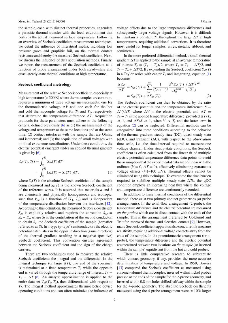
Figure 11. Diagram illustrating the error model applied to the2-probe arrangement along the z-axis (along the sample thermalgradient). The actual temperature difference across the sample isgiven by !TS = TH − TC and the measured temperature difference isgiven by !TM = T2 − T1.

Finally, the contact geometry determines the sign oferror in the Seebeck coefficient. According to the errormodel, the temperature measured by surface contact is lessthan the temperature of the sample medium. Therefore,the 4-probe contact geometry underestimates the surfacetemperature measurement by δT4P. This is further evidencedby the decrease in average sample temperatures for the4-probe arrangement as compared to the 2-probe whenmeasured under the identical stabilized thermal gradient. Inaddition, since there is a temperature difference betweenthe two probes, T2 and T1, the hotter probe will alwayshave a slightly greater error (equation (11)) than the coldprobe, underestimating the temperature difference and therebyoverestimating the Seebeck coefficient by δS4P. The diagramin figure 11 illustrates a similar error model applied to the2-probe arrangement but along the z-axis (along the samplethermal gradient). The actual temperature difference acrossthe sample is given by !TS = TH − TC and the measuredtemperature difference is given by !TM = T2 − T1 (ignoringfor this diagram the contact between the probes and thethermometric sensors). Accordingly, the 2-probe arrangement,by nature of the thermophysical properties and geometry, willoverestimate the temperature difference across the sample andthereby underestimate the Seebeck coefficient by δS2P. This issupported by the observed pressure dependence of the Seebeckcoefficient with a poor thermal contact (figure 2). Therefore,since δT4P ) δT2P and δS4P > 0 > δS2P, the absolute Seebeckcoefficient measured in the 4-probe arrangement increasesmonotonically as linear function of the temperature differencebetween the sample and the external environment, whencompared to the data measured in the 2-probe arrangement(figure 9). In addition, the data obtained under the 2-probe arrangement agree with data extrapolated from reliableliterature data [32].

Conclusions

The measurement of surface temperature by contact isinfluenced by intrinsic thermal errors. Application of asensor to the surface of the medium modifies the thermalinteraction of the contacted surface with the environment,thereby inducing a parasitic thermal transfer between thesample and the sensor, and the sensor and the environmentthat perturbs the local temperature field. This error dependson the unique geometric and thermophysical characteristicsof the system, the difference in temperature between thesample and the environment, and on the ratio of the totalthermal resistance to the sum of the macroconstriction andcontact resistance. For measurements of surface temperature inthermoelectric materials, the macroconstriction resistance willlikely dominate the error. In addition, the macroconstrictionand thermal contact resistances are larger in the 4-probearrangement as compared to the 2-probe due to the smallercontact area. The contact area for the 4-probe arrangementcannot be sufficiently increased due to the off-axis geometry.The thermal contact resistance can be modified by usinginterstitial interface materials. Finally, the 4-probe contactgeometry will tend to overestimate the absolute Seebeckcoefficient, while the 2-probe will underestimate the value.In the search for higher efficiency thermoelectric materials, itmay be prudent to implement the contact geometry that maymodestly underestimate the Seebeck coefficient rather thanone that may result in greater overestimation. Therefore,the contact geometry, dependent on the thermal interface, isthe primary limit to high accuracy, while the measurementtechnique, under ideal conditions, has little influence on themeasured Seebeck coefficient.

As a conservative measure, these results should notbe taken as quantitatively indicative of all measurementapparatus or as reflective upon their data quality.These results do serve to illustrate the likely outcomeof commonly adopted measurement practices currentlyemployed among both commercially available and customdeveloped instrumentation. As such, the stated conclusions areexpected to be qualitatively applicable to guide researchers indeveloping reasonable uncertainty limits.

References

[1] Wood C 1988 Materials for thermoelectric energy conversionRep. Prog. Phys. 51 459

[2] Mahan G D 1998 Good thermoelectrics Solid State Physicsvol 51 ed H Ehrenreich and F Spaepen (New York:Academic) p 81

[3] Nolas G S, Sharp J and Goldsmid H J 2001 Thermoelectrics:Basic Principles and New Materials Developments (NewYork: Springer)

[4] Rowe D M (ed) 1995 Thermoelectrics Handbook (BocaRaton, FL: CRC Press)

[5] Kanatzidis M G, Mahanti S D and Hogan T P (ed) 2003Chemistry, Physics, and Materials Science ofThermoelectric Materials: Beyond Bismuth Telluride (NewYork: Plenum)

[6] Martin J, Tritt T and Uher C 2010 High temperature Seebeckcoefficient metrology J. Appl. Phys. 108 121101

[7] Uher C 1996 TE materials Nav. Res. Rev. XLVIII 44

11

Meas. Sci. Technol. 24 (2013) 085601 J Martin

[8] Tritt T M 1997 Measurement and characterization techniquesfor thermoelectric materials Thermoelectric Materials—New Directions and Approaches: Materials ResearchSociety Symp. Proc. vol 478 ed T M Tritt, M Kanazidis,G Mahan and H B Lyons (Pittsburgh, PA: MRS) p 25

[9] Tritt T M and Browning V 2001 Recent Trends inThermoelectric Materials Research I: Semiconductors andSemimetals vol 69 ed T M Tritt (New York: Academic)pp 25–50

[10] Burkov T 2005 Thermoelectrics Handbook: Macro to Nano(Boca Raton, FL: CRC Press) p 22-1

[11] Tritt T M 2005 Thermoelectrics Handbook: Macro to Nano(Boca Raton, FL: CRC Press) p 23-1

[12] Magnus G 1851 Pogg. Ann. 83 469[13] Bowers R, Ure R W Jr, Bauerle J E and Cornish A J 1959

InAs and InSb as thermoelectric materials J. Appl. Phys.30 930

[14] Wood C, Zoltan D and Stapfer G 1985 Measurement ofSeebeck coefficient using a light pulse Rev. Sci. Instrum.56 719

[15] Martin J 2012 Apparatus for the high temperaturemeasurement of the Seebeck coefficient in thermoelectricmaterials Rev. Sci. Instrum. 83 065101

[16] Bentley R 1998 Theory and Practice of ThermoelectricThermometry (Singapore: Springer)

[17] Burns G W and Scroger M G 1989 NIST Special Publication250–35

[18] Roberts R B, Righini F and Compton R C 1985 The absolutescale of thermoelectricity: III Phil. Mag. 52 1147

[19] Burkov T, Heinrich A, Konstantinov P P, Nakama Tand Yagasaki K 2001 Apparatus for the high temperaturemeasurement of the Seebeck coefficient in thermoelectricmaterials Meas. Sci. Technol. 12 264

[20] Runyan W R and Shaffer T J 1997 SemiconductorMeasurements and Instrumentation 2nd edn (New York:McGraw-Hill)

[21] Streetman B G 1995 Solid State Electronic Devices(Englewood Cliffs, NJ: Prentice-Hall)

[22] Panagopoulos C, Fukami T and Aomine T 1993 The effects ofgaseous helium and nitrogen on the thermopower

measurements: a note of concern for the discrepancy of theresults observed in high temperature superconductorsJapan. J. Appl. Phys. 32 4684

[23] Villaflor B and de Luna L H 1994 Comments on the effects ofgaseous helium and nitrogen on the thermopowermeasurements: a note of concern for the discrepancy of theresults observed in high temperature superconductorsJapan. J. Appl. Phys. 33 4051

[24] Lowhorn N D, Wong-Ng W, Lu Z-Q, Martin J, Green M L,Bonevich J E and Thomas E L 2011 Development of aSeebeck coefficient standard reference material J. Mater.Res. 26 1983

[25] Martin J 2012 Error modeling of Seebeck coefficientmeasurements using finite-element analysis J. Electron.Mater. doi:10.1007/s11664-012-2212-5

[26] Nasby R D and Burgess E L 1972 Precipitation of dopants insilicon–germanium thermoelectric alloys J. Appl. Phys.43 2908

[27] Le Masson P and Dal M 2011 Analysis of errors inmeasurements and inversion Thermal Measurements andInverse Techniques ed H R B Orlande, O Fudym, D Mailletand R M Cotta (Boca Raton, FL: CRC Press) pp 565–98

[28] Cassagne B, Kirsch G and Bardon J P 1980 Analyse theoriquedes erreurs liees aux transferts de chaleur parasites lors de lamesure d’une temperature de surface par contact Int. J. HeatMass Transfer 23 1207

[29] Garnier B, Lanzetta F, Lemasson P and Virgone J 2011Lecture 5A: Measurements with contact in heat transfer:principles, implementation and pitfalls Metti 5 SpringSchool (Roscoff, June 13–18) pp 1–34

[30] Trombe A and Moreau J A 1995 Surface temperaturemeasurement of semitransparent material by thermocouplein a real site experimental approach and simulation Int. J.Heat Mass Transfer 38 2797

[31] Cassagne B and Leroy G 1982 Mesure de temperature desurface par contact en regime variable Rev. Phys. Appl.17 153

[32] Joshi G et al 2008 Enhanced thermoelectric figure-of-merit innanostructured p-type silicon germanium bulk alloys NanoLett. 8 4670

12