protocol design and performance issues in cognitive radio

Protocol Design and Performance Issuesin Cognitive Radio Networks

by

Yogesh R Kondareddy

A dissertation submitted to the Graduate Faculty ofAuburn University

in partial fulfillment of therequirements for the Degree of

Doctor of Philosophy

Auburn, AlabamaDecember 13, 2010

Keywords: Cognitive Radio Network, Ad-hoc Network

Copyright 2010 by Yogesh R Kondareddy

Approved by

Prathima Agrawal, Chair, Samuel Ginn Distinguished Professor of Electrical andComputer Engineering

Thaddeus A. Roppel, Associate Professor of Electrical and Computer EngineeringShiwen Mao, Assistant Professor of Electrical and Computer Engineering

Abstract

A cognitive radio is a frequency agile wireless communication device based on software

defined radio that enables dynamic spectrum access. cognitive radio represents a significant

paradigm change in spectrum regulation and usage, from exclusive use by licensed users (or,

primary users) to dynamic spectrum access by secondary users. While considerable progress

is made in understanding the physical layer aspects of cognitive radio and on developing

effective dynamic spectrum access schemes, it is now imperative to study how the enhanced

spectrum usage can effect or benefit the upper layers, such as medium access, network and

transport layers. In this dissertation, some of the important issues related to the implemen-

tation of Cognitive Radio Networks and their performance modeling are studied.

Firstly, the common control channel problem is discussed and three network setup mech-

anisms are proposed which do not require a common control channel. Secondly, selective

broadcasting technique is proposed to improve the communication efficiency of Multi-Hop

Cognitive Radio Networks, Thirdly, the capacity of secondary users in terms of blocking prob-

ability for varying dynamic spectrum access network parameters is studied. Based on the

study of the capacity of secondary users, the effect of dynamic spectrum access on Transport

Control Protocol Performance is modeled. Finally, to ensure cooperative spectrum sensing,

we design a cross-layer game to attain Nash Equilibrium at mutual cooperation. All of these

ideas have been either simulated or mathematically proven to have better performance than

the existing models.

ii

Acknowledgments

First and foremost, I would express my sincere gratitude to my advisor, Professor

Prathima Agrawal without whose encouragement I would not have pursued my Doctor-

ate degree. Her guidance and supervision has led me into the interesting research area of

cognitive radio networks and without her abundant support I wouldn’t have come this far.

I would like to thank Professors Thaddeus A. Roppel, Shiwen Mao and Alvin Lim for

serving on my advisory committee. My thanks also go out to my colleagues in the Wireless

Research Laboratory, Alireza Babaei, Pratap Simha, Santosh Kulkarini, Veneela Ammula,

Nirmal Andrews, Nida Bano, Indraneil Gokhale and Gopalakrishnan Iyer for the discussions

and valuable suggestions on our research. The Electrical and Computer Engineering staff

members; especially, Shelia Collis have made my work a lot easier by their prompt support

and help in many regards. Thanks to my friends for their kind presence whenever needed.

I am very grateful to my parents and sister for their consistent support and encourage-

ment in my journey to reach the highest level of education.

iii

Table of Contents

Abstract . . . . . . . . . . . . . . . . . . . . . . . . . . . . . . . . . . . . . . . . . . . ii

Acknowledgments . . . . . . . . . . . . . . . . . . . . . . . . . . . . . . . . . . . . . . iii

List of Figures . . . . . . . . . . . . . . . . . . . . . . . . . . . . . . . . . . . . . . . vii

1 Introduction . . . . . . . . . . . . . . . . . . . . . . . . . . . . . . . . . . . . . . 1

1.1 Dynamic Spectrum Access . . . . . . . . . . . . . . . . . . . . . . . . . . . . 1

1.2 Cognitive Network . . . . . . . . . . . . . . . . . . . . . . . . . . . . . . . . 2

1.3 Multi-Hop Cognitive Network . . . . . . . . . . . . . . . . . . . . . . . . . . 3

1.4 What’s in this Dissertation . . . . . . . . . . . . . . . . . . . . . . . . . . . . 5

2 Cognitive Radio Network Setup without a Common Control Channel . . . . . . 8

2.1 The Network Setup Problem . . . . . . . . . . . . . . . . . . . . . . . . . . . 10

2.1.1 The Common Control Channel Problem . . . . . . . . . . . . . . . . 12

2.2 Network Setup Mechanisms . . . . . . . . . . . . . . . . . . . . . . . . . . . 13

2.2.1 Exhaustive Protocol . . . . . . . . . . . . . . . . . . . . . . . . . . . 14

2.2.2 Random Protocol . . . . . . . . . . . . . . . . . . . . . . . . . . . . . 16

2.2.3 Sequential Protocol . . . . . . . . . . . . . . . . . . . . . . . . . . . . 18

2.3 Simulation Study . . . . . . . . . . . . . . . . . . . . . . . . . . . . . . . . . 19

2.3.1 Search Time . . . . . . . . . . . . . . . . . . . . . . . . . . . . . . . . 21

2.3.2 Number of Scans . . . . . . . . . . . . . . . . . . . . . . . . . . . . . 22

2.3.3 Failures . . . . . . . . . . . . . . . . . . . . . . . . . . . . . . . . . . 23

3 Selective Broadcasting in Multi-Hop Cognitive Radio Networks . . . . . . . . . 25

3.1 Selective Broadcasting . . . . . . . . . . . . . . . . . . . . . . . . . . . . . . 26

3.2 Neighbor Graph and Minimal Neighbor Graph Formation . . . . . . . . . . . 27

3.2.1 Construction of Neighbor Graph . . . . . . . . . . . . . . . . . . . . . 27

iv

3.2.2 Construction of Minimal Neighbor Graph . . . . . . . . . . . . . . . . 28

3.3 Advantages of selective broadcasting . . . . . . . . . . . . . . . . . . . . . . 30

3.3.1 Broadcast Delay . . . . . . . . . . . . . . . . . . . . . . . . . . . . . 30

3.3.2 Lower congestion, contention . . . . . . . . . . . . . . . . . . . . . . . 31

3.3.3 No common control channel . . . . . . . . . . . . . . . . . . . . . . . 31

3.4 Results and Analysis . . . . . . . . . . . . . . . . . . . . . . . . . . . . . . . 32

3.4.1 Broadcast Delay . . . . . . . . . . . . . . . . . . . . . . . . . . . . . 33

3.4.2 Redundancy . . . . . . . . . . . . . . . . . . . . . . . . . . . . . . . . 34

4 Capacity of Secondary Users . . . . . . . . . . . . . . . . . . . . . . . . . . . . . 37

4.1 System Model and Assumptions . . . . . . . . . . . . . . . . . . . . . . . . . 38

4.1.1 Random Channel Assignment . . . . . . . . . . . . . . . . . . . . . . 38

4.1.2 Reservation Based Assignment . . . . . . . . . . . . . . . . . . . . . . 43

4.1.3 Non-Random Channel Assignment . . . . . . . . . . . . . . . . . . . 44

4.2 Results . . . . . . . . . . . . . . . . . . . . . . . . . . . . . . . . . . . . . . . 46

4.2.1 Variation with λp . . . . . . . . . . . . . . . . . . . . . . . . . . . . . 47

4.2.2 Variation with λs . . . . . . . . . . . . . . . . . . . . . . . . . . . . . 49

5 Effect of Dynamic Spectrum Access on Transport Control Protocol Performance 50

5.1 System Model . . . . . . . . . . . . . . . . . . . . . . . . . . . . . . . . . . . 52

5.2 Analytical Model for TCP Throughput Estimation . . . . . . . . . . . . . . 53

5.2.1 Estimation of Wait time Tw . . . . . . . . . . . . . . . . . . . . . . . 55

5.2.2 Markov Model to determine Blocking probability, pb . . . . . . . . . . 56

5.3 Results and Analysis . . . . . . . . . . . . . . . . . . . . . . . . . . . . . . . 59

6 Enforcing Cooperative Spectrum Sensing in a Multi-hop Cognitive Radio Network 63

6.1 System Model and Assumptions . . . . . . . . . . . . . . . . . . . . . . . . . 64

6.2 Game Theory Applied to Multi-hop Cognitive Radio Network . . . . . . . . 66

6.2.1 Cooperative Spectrum Sensing Game . . . . . . . . . . . . . . . . . . 66

6.2.2 Packet Forwarding Game . . . . . . . . . . . . . . . . . . . . . . . . . 67

v

6.3 Cross-Layer Game . . . . . . . . . . . . . . . . . . . . . . . . . . . . . . . . 69

6.3.1 Cross-Layer Game without Observability Faults . . . . . . . . . . . . 71

6.3.2 Cross-Layer Game with Observability Faults . . . . . . . . . . . . . . 75

7 Conclusion . . . . . . . . . . . . . . . . . . . . . . . . . . . . . . . . . . . . . . . 79

Bibliography . . . . . . . . . . . . . . . . . . . . . . . . . . . . . . . . . . . . . . . . 81

vi

List of Figures

1.1 Dynamic Spectrum Access concept. . . . . . . . . . . . . . . . . . . . . . . . . . 2

2.1 A group of CUs among three primary users. . . . . . . . . . . . . . . . . . . . . 10

2.2 Free Channel Sets of the CUs and CBS. . . . . . . . . . . . . . . . . . . . . . . 11

2.3 Two cognitive nodes with a set of free channels. . . . . . . . . . . . . . . . . . . 12

2.4 Channel availability at the CBS and CU. . . . . . . . . . . . . . . . . . . . . . . 15

2.5 Algorithm for the Exhaustive protocol. . . . . . . . . . . . . . . . . . . . . . . . 16

2.6 Algorithm for the Random protocol. . . . . . . . . . . . . . . . . . . . . . . . . 18

2.7 Algorithm for the Sequential protocol. . . . . . . . . . . . . . . . . . . . . . . . 20

2.8 Plot showing the Search Time of the three protocols as the number of channels

is varied. . . . . . . . . . . . . . . . . . . . . . . . . . . . . . . . . . . . . . . . 21

2.9 A plot showing the effect of the number of Wait Slots in RAN-protocol as the

number of channels is varied. . . . . . . . . . . . . . . . . . . . . . . . . . . . . 22

2.10 Number of failures in SEQ-protocol for 500 random simulations. . . . . . . . . . 24

3.1 a) Nodes A and B linked by 2 edges. b) Representation of node A with 6 neighbors 28

3.2 Stepwise development of minimal neighbor graph and the Essential Channel Set

(ECS) . . . . . . . . . . . . . . . . . . . . . . . . . . . . . . . . . . . . . . . . . 29

vii

3.3 Final minimal neighbor graph of Fig. 3.1b. . . . . . . . . . . . . . . . . . . . . 30

3.4 Plot of channel spread with respect to number of nodes for a set of 10 channels. 32

3.5 Plot of node density per channel with respect to number of channels for a set of

50 nodes. . . . . . . . . . . . . . . . . . . . . . . . . . . . . . . . . . . . . . . . 33

3.6 Comparison of average broadcast delay of a node as the number of nodes is varied. 34

3.7 Comparison of average broadcast delay of a node as the number of channels is

varied. . . . . . . . . . . . . . . . . . . . . . . . . . . . . . . . . . . . . . . . . . 35

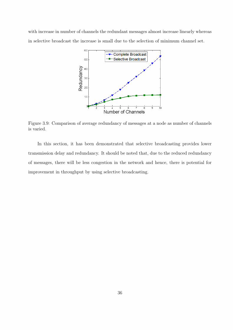
3.8 Comparison of aggregate redundancy of messages at a node as the number of

nodes is varied. . . . . . . . . . . . . . . . . . . . . . . . . . . . . . . . . . . . . 35

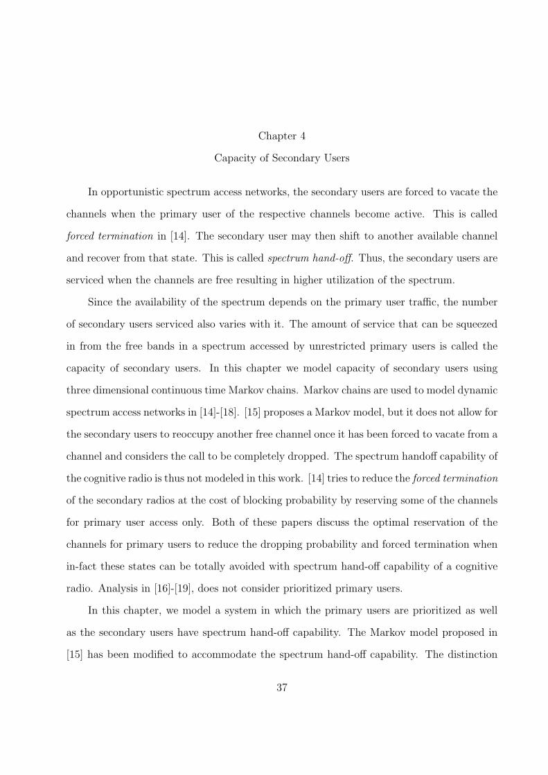
3.9 Comparison of average redundancy of messages at a node as number of channels

is varied. . . . . . . . . . . . . . . . . . . . . . . . . . . . . . . . . . . . . . . . 36

4.1 Random access in five channels. . . . . . . . . . . . . . . . . . . . . . . . . . . . 39

4.2 Markov model for cognitive network with spectrum hand-off. . . . . . . . . . . . 40

4.3 SU Drop probability with λp, with and without spectrum hand-off. . . . . . . . 42

4.4 Reservation based access in five channels. . . . . . . . . . . . . . . . . . . . . . 44

4.5 Non-random access in five channels. . . . . . . . . . . . . . . . . . . . . . . . . 45

4.6 Channel Utilization of reservation-based assignment with spectrum hand-off over

reservation-based assignement without spectrum hand-off. . . . . . . . . . . . . 46

4.7 Non-random access in five channels. . . . . . . . . . . . . . . . . . . . . . . . . 46

4.8 Markov model for non-random channel assignment method with spectrum hand-off. 47

viii

4.9 SU Dropping probability with the variation of λp. . . . . . . . . . . . . . . . . . 48

4.10 SU Blocking probability with the variation of λp. . . . . . . . . . . . . . . . . . 48

4.11 SU Dropping probability with the variation of λs. . . . . . . . . . . . . . . . . . 49

4.12 SU Blocking probability with the variation of λs. . . . . . . . . . . . . . . . . . 49

5.1 Dynamic spectrum access network with three SUs and two PUs. . . . . . . . . . 52

5.2 Scanning cycles used by the SSLL [5]. . . . . . . . . . . . . . . . . . . . . . . . 53

5.3 Random access in five channels. . . . . . . . . . . . . . . . . . . . . . . . . . . . 57

5.4 Markov model for dynamic spectrum access network with spectrum hand-off. . . 58

5.5 Variation of SU blocking probability as PU’s arrival rate is varied for different

number of channels. . . . . . . . . . . . . . . . . . . . . . . . . . . . . . . . . . 59

5.6 TCP throughput as a function of scanning time. pe = 10−7, NF = 2, MSS = 512

Bytes, Tsr = Tp = 10 ms, λs = λp = 0.5, N = 5. . . . . . . . . . . . . . . . . . . 60

5.7 TCP throughput as a function of number of channels. pe = 10−7, pf = 10−6,

nmax = 1, NF = 2, MSS = 512 Bytes, Tsr = Tp = 10 ms, λs = 0.5. . . . . . . . . 60

5.8 TCP throughput as a function of PU traffic rate, λp. pe = 10−7, NF = 2,

MSS = 512 Bytes, Tsr = Tp = 10 ms, λs = 0.5. . . . . . . . . . . . . . . . . . . 61

5.9 TCP throughput as a function of SU traffic rate, λs. pe = 10−7, NF = 2,

MSS = 512 Bytes, Tsr = Tp = 10 ms, λp = 0.5, N = 7. . . . . . . . . . . . . . . 62

6.1 The three phases in a Cognitive Radio Network operation. . . . . . . . . . . . . 65

6.2 Payoff Matrix in a two player cooperative sensing game. The Nash Equilibrium

is represented by the shaded cell. . . . . . . . . . . . . . . . . . . . . . . . . . . 67

ix

6.3 Two nodes participating in the forwarding game. . . . . . . . . . . . . . . . . . 68

6.4 Extensive form representation of the packet forwarding game. The Nash Equi-

librium is represented by the thicker line. . . . . . . . . . . . . . . . . . . . . . . 68

6.5 The payoff matrix of the Cross-Layer game and its Nash equilibrium using iter-

ated dominance. . . . . . . . . . . . . . . . . . . . . . . . . . . . . . . . . . . . 70

x

Chapter 1

Introduction

Guglielmo Marconi’s first Radio Broadcast was a point-to-point communication. With

the emerging radio technologies such as Wi-Fi, WiMax, Bluetooth, ZigBee and the grow-

ing panoply of cellular and satellite communication, we need to pack the radio waves to

accommodate each of these services. To minimize interference, each of these technologies is

restricted to specific bands of the spectrum. If we tried imposing this sort of regime on road

transportation, we might wind up with a system in which buses, cars and trucks were each

restricted to their own separate roadways.

1.1 Dynamic Spectrum Access

Radio spectrum allocation is rigorously controlled by regulatory authorities through

licensing processes. Most countries have their own regulatory bodies, though regional regu-

lators do exist. In the U.S., regulation is done by the Federal Communications Commission

(FCC). Spectrum has long been allocated in a first-come, first-served manner. According to

the FCC [1], temporal and geographical variations in the utilization of the assigned spectrum

range from 15% to 85% [2]. If radios could somehow use a portion of this unutilized spec-

trum without causing interference, then there would be more room to operate and exploit.

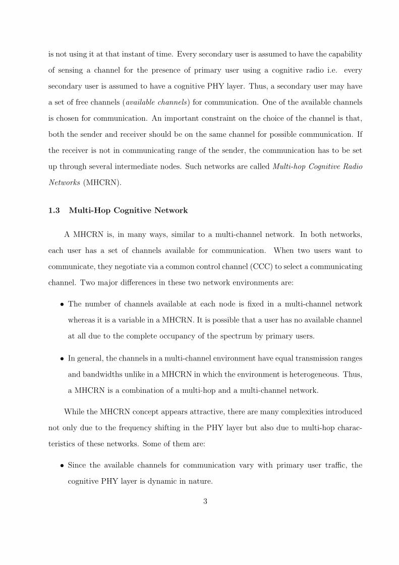
Such an idea is called Dynamic Spectrum Access and is depicted in fig. 1.1 as was shown in

[2]. This figure shows a three dimensional model of radio communication in which a device

communicates in a finite band of frequency (called a channel in general) for a certain period

of time and using an amount of power (regulated by FCC). Among such bands/channels of

operation, those channels which are unused for a certain period of time are considered vacant

and are refered to as spectrum holes or spectrum oppurtunities [3].

1

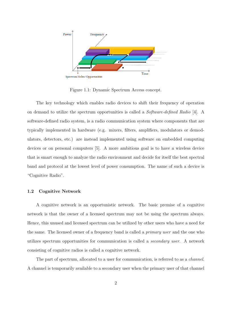
Figure 1.1: Dynamic Spectrum Access concept.

The key technology which enables radio devices to shift their frequency of operation

on demand to utilize the spectrum opportunities is called a Software-defined Radio [4]. A

software-defined radio system, is a radio communication system where components that are

typically implemented in hardware (e.g. mixers, filters, amplifiers, modulators or demod-

ulators, detectors, etc.) are instead implemented using software on embedded computing

devices or on personal computers [5]. A more ambitious goal is to have a wireless device

that is smart enough to analyze the radio environment and decide for itself the best spectral

band and protocol at the lowest level of power consumption. The name of such a device is

“Cognitive Radio”.

1.2 Cognitive Network

A cognitive network is an opportunistic network. The basic premise of a cognitive

network is that the owner of a licensed spectrum may not be using the spectrum always.

Hence, this unused and licensed spectrum can be utilized by other users who have a need for

the same. The licensed owner of a frequency band is called a primary user and the one who

utilizes spectrum opportunities for communication is called a secondary user. A network

consisting of cognitive radios is called a cognitive network.

The part of spectrum, allocated to a user for communication, is referred to as a channel.

A channel is temporarily available to a secondary user when the primary user of that channel

2

is not using it at that instant of time. Every secondary user is assumed to have the capability

of sensing a channel for the presence of primary user using a cognitive radio i.e. every

secondary user is assumed to have a cognitive PHY layer. Thus, a secondary user may have

a set of free channels (available channels) for communication. One of the available channels

is chosen for communication. An important constraint on the choice of the channel is that,

both the sender and receiver should be on the same channel for possible communication. If

the receiver is not in communicating range of the sender, the communication has to be set

up through several intermediate nodes. Such networks are called Multi-hop Cognitive Radio

Networks (MHCRN).

1.3 Multi-Hop Cognitive Network

A MHCRN is, in many ways, similar to a multi-channel network. In both networks,

each user has a set of channels available for communication. When two users want to

communicate, they negotiate via a common control channel (CCC) to select a communicating

channel. Two major differences in these two network environments are:

• The number of channels available at each node is fixed in a multi-channel network

whereas it is a variable in a MHCRN. It is possible that a user has no available channel

at all due to the complete occupancy of the spectrum by primary users.

• In general, the channels in a multi-channel environment have equal transmission ranges

and bandwidths unlike in a MHCRN in which the environment is heterogeneous. Thus,

a MHCRN is a combination of a multi-hop and a multi-channel network.

While the MHCRN concept appears attractive, there are many complexities introduced

not only due to the frequency shifting in the PHY layer but also due to multi-hop charac-

teristics of these networks. Some of them are:

• Since the available channels for communication vary with primary user traffic, the

cognitive PHY layer is dynamic in nature.

3

• Due to the multi-hop nature, the choice of a channel for each secondary user is now

constrained by the available channel set at every user along the route. A route is

possible only if every pair of users along the route have at-least one common channel

available at their respective locations.

• After a communication path is established through a set of intermediate nodes, still

the route may fail due to the dynamic nature of the PHY layer at each node. A new

route has to be discovered with the new set of available channels.

Centralized/Distributed Architectures

In a Cognitive Radio Network, the unused spectrum is shared among a group of inde-

pendent users. As a result, there should be a way to control and coordinate access to the

spectrum. This can be achieved using a centralized control or by a cooperative distributed

approach. In a centralized architecture, a single entity, called spectrum administrator, con-

trols the usage of the spectrum by secondary users [8]. The spectrum administrator gathers

information about free channels either by sensing its entire domain (area of coverage) or by

integrating the information collected by potential secondary users in their respective local

areas. These users send information to the spectrum administrator through a dedicated

control channel. This approach is not feasible for dynamic multi-hop networks. Moreover,

a direct attack such as a Denial of Service attack (DoS) [4] on the spectrum administrator

would incapacitate the network. Thus, a distributed approach is preferred over a centralized

control.

In a distributed approach, there is no central administrator. As a result, all users should

cooperatively sense and share the free channels. The information sensed by a user should be

shared with other users in the network to enable certain essential tasks like route discovery in

a MHCRN. Such control information is broadcast to its neighbors in a traditional network.

The Cognitive Radio technology represents a significant paradigm change in spectrum

regulation and usage, from exclusive use by licensed users (or, primary users) to dynamic

4

spectrum access (DSA) by secondary users. While considerable progress is made in under-

standing the PHY layer aspects of Cognitive Radio (CR) and on developing effective DSA

schemes, it is now imperative to study how the enhanced spectrum usage can affect or benefit

the upper layers, such as medium access, network and transport layers. In this dissertation

some of the important issues related to the implementation of Cognitive Radio Networks

and their performance modeling are studied which are briefly described below.

1.4 What’s in this Dissertation

Chapter 2

The concept of Cognitive Radio Networks has introduced a new way of sharing the

open spectrum flexibly and efficiently. However, there are several issues that hinder the

deployment of such dynamic networks. The common control channel problem is one such

issue. Cognitive radio networks are designed by assuming the availability of a dedicated

control channel. In this chapter, we identify and discuss the Network Setup Problem as

a part of the Common Control Channel Problem. Probabilistic and deterministic ways to

start the initial communication and setup a Cognitive Radio network without the need of

having a common control channel in both centralized and multi-hop scenarios are suggested.

Extensive MATLAB simulations validate the effectiveness of the algorithms.

Chapter 3

Cognitive networks enable efficient sharing of the radio spectrum. Control signals used

to setup a communication are broadcast to the neighbors in their respective channels of

operation. But since the number of channels in a cognitive network is potentially large,

broadcasting control information over all channels will cause a large delay in setting up

the communication. Thus, exchanging control information is a critical issue in cognitive

radio networks. This chapter deals with selective broadcasting in multi-hop cognitive radio

networks in which, control information is transmitted over pre-selected set of channels. We

introduce the concept of neighbor graphs and minimal neighbor graphs to derive the essential

5

set of channels for transmission. It is shown through simulations that selective broadcasting

reduces the delay in disseminating control information and yet assures successful transmission

of information to all its neighbors. It is also demonstrated that selective broadcasting reduces

redundancy in control information and hence reduces network traffic.

Chapter 4

Cognitive radio networks deal with opportunistic spectrum access leading to greater

utilization of the spectrum. The extent of utilization depends on the primary users traffic

and also on the way the spectrum is accessed by the primary and secondary users. In

this chapter, Continuous-time Markov chains are used to model the spectrum access. The

proposed three dimensional model represents a more accurate cognitive system than the

existing models with increased spectrum utilization than the random and reservation based

spectrum access. A non-random access method is proposed to remove the forced termination

states. In addition, call dropping and blocking probabilities are reduced. It is further shown

that channel utilization is higher than in random access and reservation based access.

Chapter 5

Transmission Control Protocol (TCP) is the most commonly used transport protocol

on the Internet. All indications assure that it will be an integral part of the future internet-

works. In this chapter, we discuss why TCP designed for wired networks is not suitable for

dynamic spectrum access networks. We develop an analytical model to estimate the TCP

throughput of Dynamic spectrum access networks. Dynamic spectrum access networks deal

with opportunistic spectrum access leading to greater utilization of the spectrum. The extent

of utilization depends on the primary users traffic and also on the manner in which spectrum

is accessed by the primary and secondary users. The proposed model considers primary and

secondary user traffic in estimating the TCP throughput by modeling the spectrum access

using continuous time Markov chains, thus providing more insight into the effect of dynamic

spectrum access on TCP performance than existing models.

Chapter 6

6

Spectrum sensing and sharing the sensing results is one of the most important tasks for

the operation of a cognitive radio network. It is even more crucial in a multi-hop cognitive

radio network, where there is no omni-present central authority. But since communicating

the sensing results periodically to other users consumes significant amount of energy, users

tend to conserve energy by not sharing their results. This non-cooperation will lead to re-

duced clarity in the spectrum occupancy map. Therefore, appropriate strategies are required

to enforce cooperative sharing of the sensing results. The classic Tit-For-Tat strategy cannot

be used because punishing a node by not broadcasting the sensing results also affects other

nodes. In this chapter, we address this problem by exploiting the unique characteristics of

cross-layer interaction in cognitive radios to sustain cooperative spectrum sensing. In this di-

rection, we design a Cross-Layer game which is a combination of the spectrum sensing game

in the physical layer and packet forwarding game in the network layer. In this strategy, users

punish those who do not share their sensing results by denying cooperation at the network

layer. The Cross-Layer game is modeled as a non-cooperative non-zero-sum repeated game

and a Generous Tit-For-Tat strategy is proposed to ensure cooperation even in the presence

of collisions and spectrum mobility. We prove that the Nash Equilibrium of this strategy is

mutual cooperation and that it is robust against attacks on spectrum sensing and sharing

session.

7

Chapter 2

Cognitive Radio Network Setup without a Common Control Channel

In a Cognitive Radio Network (CRN), the Cognitive Users (CUs) communicate only in

those frequencies in which the primary users (PUs) are inactive. So, CUs should scan for

unused bands (channels) from time to time. This process is called spectrum sensing. After

this stage, every CU has a list of free channels. The list of free channels may differ from one

CU to another. Two CUs can communicate if there is at-least one common channel in their

free channel lists.

Since the unused spectrum is shared among a group of independent users, there should

be a way to control and coordinate access to the spectrum. This can be achieved using a

centralized control or by a cooperative distributed approach. In a centralized architecture, a

single entity, called the Cognitive Base Station (CBS), controls the usage of the spectrum by

CUs [9]. The Cognitive Base Station (CBS) gathers information like the list of free channels

of each node either by sensing its entire domain or by integrating individual CUs sensed

data. The CBS maintains a database of all the collected information. When two CUs want

to start a session, they request the CBS for channel allocation. The CBS looks into the

list of free channels of each CU in its database and assigns a channel that is common to

both. The database has to be updated regularly since the list of free channels will change

with Primary Users (PUs) traffic. The negotiations between the CBS and CUs are usually

assumed to be carried over a dedicated control channel [2]. Intuitively, a separate dedicated

channel for control signals would seem a simple solution. But a dedicated CCC has several

drawbacks as discussed in [11]. Firstly, a dedicated channel for control signals is wasteful of

channel resources. Secondly, a control channel would get saturated as the number of users

increase. This is similar to what happens in a multi-hop network when a control channel is

8

used, as identified in [13]. Thirdly, an adversary can cripple the dedicated control channel

by intentionally flooding the control channel. This is the Denial of Service (DoS) attack as

discussed in [10]. So it was suggested in [11] to choose one of the free channels as the control

channel. When PU of the chosen channel returns, a new control channel is picked. But

nothing is mentioned in [11] as to how the first node contacts the CBS and how would it

be informed about the chosen control channel for the first time. This is called the Network

Setup Problem in this chapter.

In the second type of network architecture which is a distributed (multi-hop) scenario,

the CUs have to cooperatively coordinate to coexist and access the free channels. The

information sensed by a CU should be shared with other users in the network to enable

certain essential tasks like route discovery in a CRN. Since, each CU has multiple channels to

choose from, a distributed CRN is a multi-hop multi-channel network with dynamic channel

set for each user. In a multi-channel network, the control information like the choice of

the communicating channel is negotiated on a pre-defined common control channel. Again,

dedicating a control channel for the entire network is not a good idea for the above mentioned

reasons and choosing a free channel as the control channel might not work because the

chosen channel might not be free with all the users. Most of the recent papers proposed

MAC protocols which avoid a common control channel but none of them focused on how to

setup the initial network (Network Setup Problem) i.e. how would a CU contact another CU

before it can start anything?

Addressing and solving the Network Setup Problem is the motivation for this chapter.

A deterministic and probabilistic way of scanning the channels by a CU to connect to the

CBS is proposed. The proposed mechanisms are also extended to a multi-hop scenario in

which a CU searches for another CU.

9

2.1 The Network Setup Problem

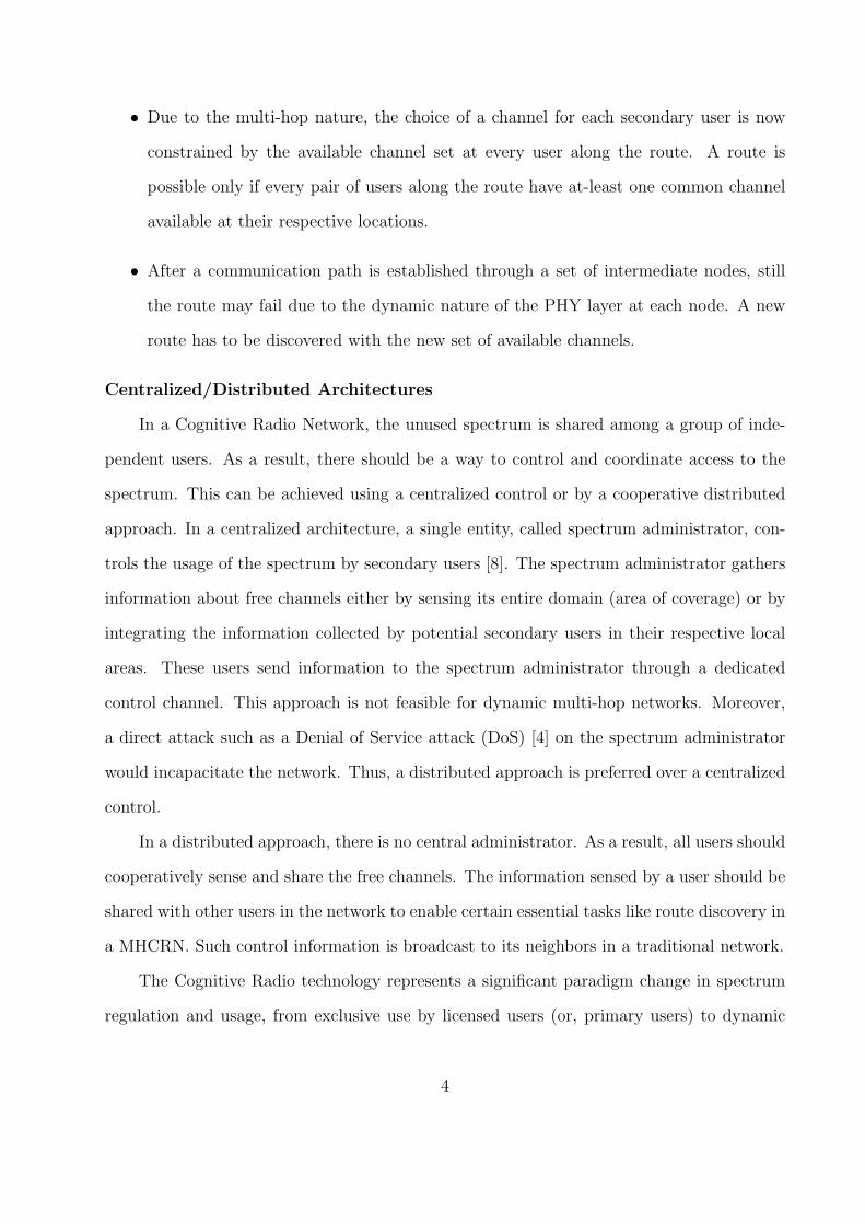
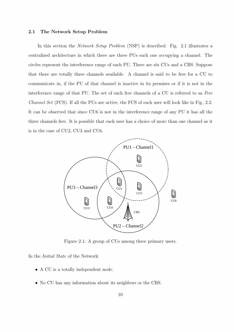
In this section the Network Setup Problem (NSP) is described. Fig. 2.1 illustrates a

centralized architecture in which there are three PUs each one occupying a channel. The

circles represent the interference range of each PU. There are six CUs and a CBS. Suppose

that there are totally three channels available. A channel is said to be free for a CU to

communicate in, if the PU of that channel is inactive in its premises or if it is not in the

interference range of that PU. The set of such free channels of a CU is referred to as Free

Channel Set (FCS). If all the PUs are active, the FCS of each user will look like in Fig. 2.2.

It can be observed that since CU6 is not in the interference range of any PU it has all the

three channels free. It is possible that each user has a choice of more than one channel as it

is in the case of CU2, CU3 and CU6.

CU1

CU5

CU2

CU3 CU4

CU6

PU1 – Channel1

PU3 – Channel3

PU2 – Channel2

CBS

Figure 2.1: A group of CUs among three primary users.

In the Initial State of the Network:

• A CU is a totally independent node.

• No CU has any information about its neighbors or the CBS.

10

CBS CU1 CU2 CU3 CU4 CU5 CU6

3

1

32 2

1 1

3 321

Figure 2.2: Free Channel Sets of the CUs and CBS.

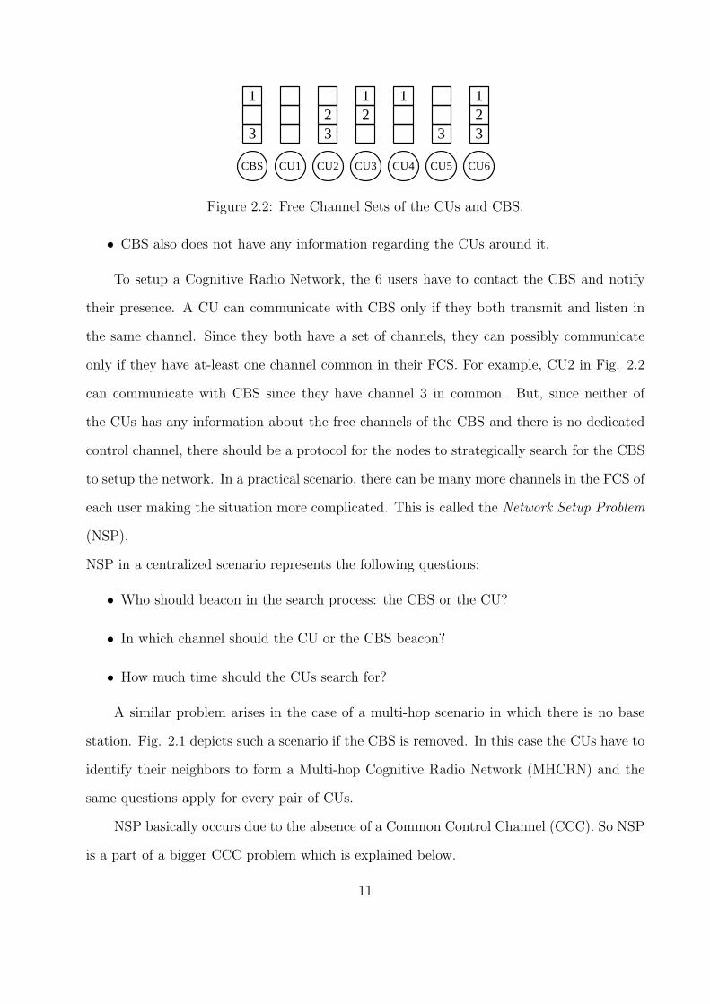
• CBS also does not have any information regarding the CUs around it.

To setup a Cognitive Radio Network, the 6 users have to contact the CBS and notify

their presence. A CU can communicate with CBS only if they both transmit and listen in

the same channel. Since they both have a set of channels, they can possibly communicate

only if they have at-least one channel common in their FCS. For example, CU2 in Fig. 2.2

can communicate with CBS since they have channel 3 in common. But, since neither of

the CUs has any information about the free channels of the CBS and there is no dedicated

control channel, there should be a protocol for the nodes to strategically search for the CBS

to setup the network. In a practical scenario, there can be many more channels in the FCS of

each user making the situation more complicated. This is called the Network Setup Problem

(NSP).

NSP in a centralized scenario represents the following questions:

• Who should beacon in the search process: the CBS or the CU?

• In which channel should the CU or the CBS beacon?

• How much time should the CUs search for?

A similar problem arises in the case of a multi-hop scenario in which there is no base

station. Fig. 2.1 depicts such a scenario if the CBS is removed. In this case the CUs have to

identify their neighbors to form a Multi-hop Cognitive Radio Network (MHCRN) and the

same questions apply for every pair of CUs.

NSP basically occurs due to the absence of a Common Control Channel (CCC). So NSP

is a part of a bigger CCC problem which is explained below.

11

2.1.1 The Common Control Channel Problem

As discussed earlier, two users in a CRN are connected if they have a common channel

for communication. It is possible that each user has a choice of more than one channel.

In that case, the sender and the receiver need to agree upon a common communicating

channel which is available to both. The initial handshake signals to negotiate the choice of a

common channel are called control signals. But such negotiations require communication over

a common signaling channel. This is called the Common control channel problem (CCCP).

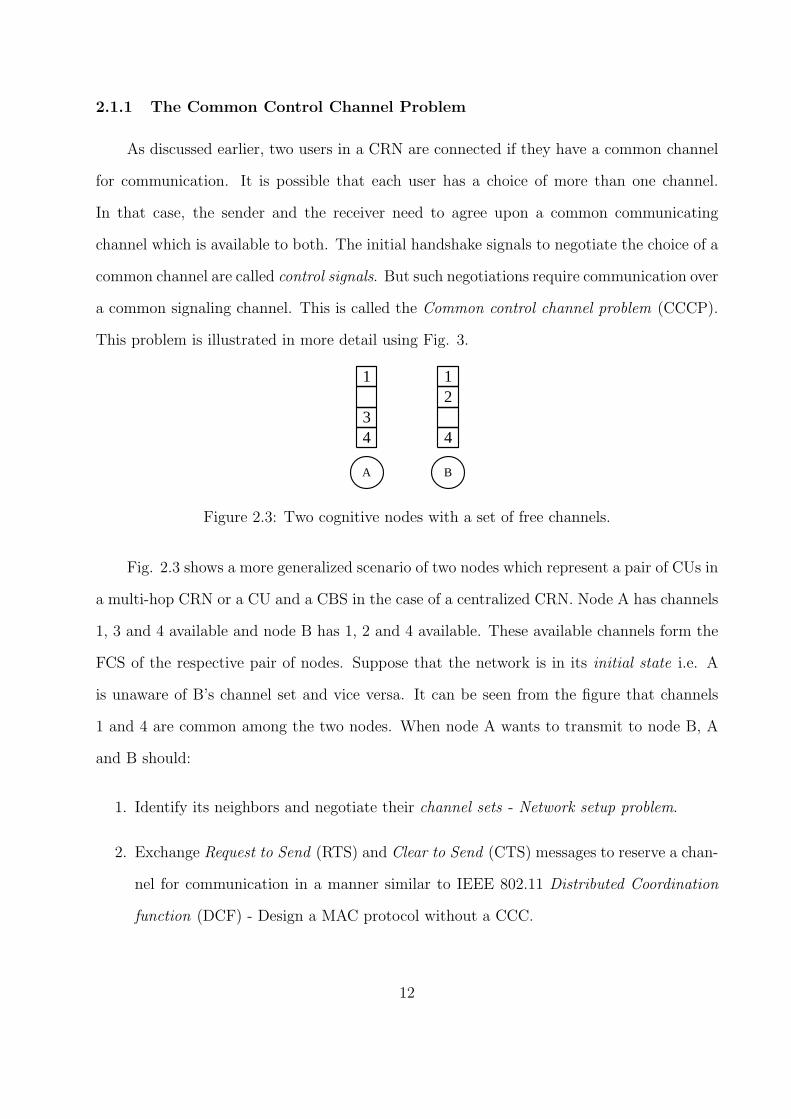
This problem is illustrated in more detail using Fig. 3.

A B

43

4

1 12

Figure 2.3: Two cognitive nodes with a set of free channels.

Fig. 2.3 shows a more generalized scenario of two nodes which represent a pair of CUs in

a multi-hop CRN or a CU and a CBS in the case of a centralized CRN. Node A has channels

1, 3 and 4 available and node B has 1, 2 and 4 available. These available channels form the

FCS of the respective pair of nodes. Suppose that the network is in its initial state i.e. A

is unaware of B’s channel set and vice versa. It can be seen from the figure that channels

1 and 4 are common among the two nodes. When node A wants to transmit to node B, A

and B should:

1. Identify its neighbors and negotiate their channel sets - Network setup problem.

2. Exchange Request to Send (RTS) and Clear to Send (CTS) messages to reserve a chan-

nel for communication in a manner similar to IEEE 802.11 Distributed Coordination

function (DCF) - Design a MAC protocol without a CCC.

12

These control messages in turn have to be negotiated via a channel. So a channel is

required to choose a channel! The later part has been addressed in several papers [6]-[8]. [6]

and [7] assume a CCC which is one among the available channels. [8] proposes a method

in which a group of users which are close together form a sub-ad hoc network and select

a channel for communicating control information. The former part of CCCP is what we

differentiated as Network Setup Problem (NSP) and are focusing on in this chapter. In the

next section three solutions to the NSP are proposed.

2.2 Network Setup Mechanisms

In this section, three different protocols to address the NSP will be explained. The

protocols define a scan and search procedure for the CBS and CUs so that they can initiate

a CRN. Before that it is important to discuss the capabilities of a CU and a CBS and some

of the terms used in the coming discussion.

A Cognitive User is capable of shifting his frequency of operation. A simple CU is

equipped with one Cognitive Radio (CR) and he can scan a channel at a maximum rate of

Rcu channels per second.

A Cognitive Base Station is at-least equipped with two CRs. It is an added advantage

if it is assumed that a CBS is capable of scanning the channels faster than a CU at a rate of

Rcbs. But, the lack of this assumption does not affect the working of the protocol in anyway.

Primary User’s Traffic Rate (PUTR): It is defined as the average rate at which the

primary user changes his state (active/inactive). This is an important factor because the

channel availability is directly related to PUTR. Higher PUTR implies that channel avail-

ability at each CU fluctuates at a higher rate.

Number of Channels (N): The total spectrum in which the Cognitive Users can operate

is divided into a fixed number of channels; N. It should be noted that N can be possibly very

large varying from tens to thousands of channels. Though the proposed protocols do not

13

depend on the value of N, for the convenience of pictorial representation N will be chosen

very small.

All proposed protocols are initially discussed for those architectures (centralized or dis-

tributed) for which they are best suited.

2.2.1 Exhaustive Protocol

This protocol implements exhaustive search and will be referred to as EX Mechanism.

The channels are searched from lower to higher frequencies by both the CBS and CUs. CBS

is assigned the task of sending beacons because of its superior infrastructure in terms of

hardware and energy. It is also assumed that PUs traffic does not vary in one search cycle.

In a Centralized Architecture, CBS maintains a timer which counts to TS seconds. It

initially starts its search from the channel with lowest frequency and starts its timer TS. It

shifts to the next channel when the timer expires. In each time slot, the channel is scanned

for the presence of a PU. If the channel is not free, then CBS will immediately shift to the

next channel and resets the timer. If the channel is free, a beacon is sent indicating its

presence in that channel. It will wait for a response for the rest of the time slot till the TS

timer expires and then tunes to the next channel after restarting the timer. If in the mean

time a response is received from a CU, a different Cognitive Radio is assigned the task of

carrying on the negotiations with the CU and CBS continuous its search for other potential

users. After all the channels are searched, it will restart from the lowest frequency again. If

all the N channels were free, CBS would take N×TS seconds to complete a cycle of searching

all the channels.

Every CU maintains a Wait timer, TW which is set to N × TS. It initially starts from

the channel with lowest frequency and scans for the availability. If the channel is not free,

it shifts to the next channel and resets its timer. If the channel is free, it waits for a beacon

from the CBS till the timer TW expires. Since, CBS will search all the channels at-least once

in TW seconds, the CU can be sure of receiving a beacon if the channel it was listening to

14

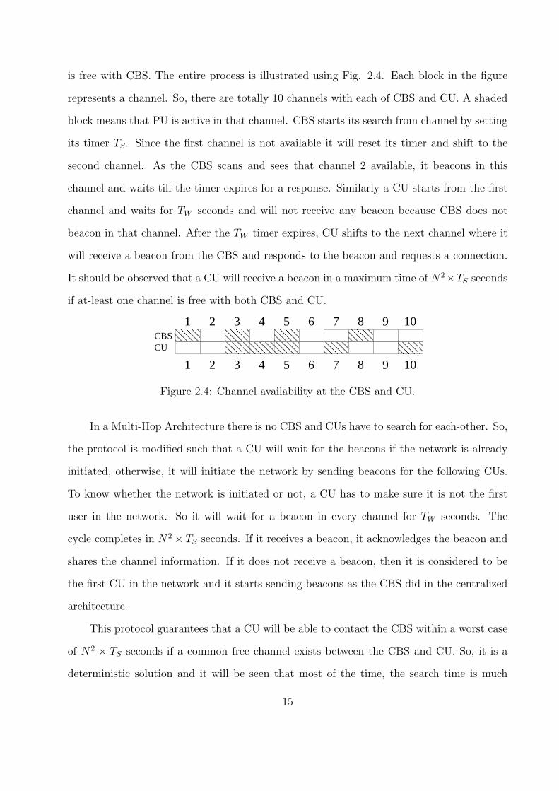
is free with CBS. The entire process is illustrated using Fig. 2.4. Each block in the figure

represents a channel. So, there are totally 10 channels with each of CBS and CU. A shaded

block means that PU is active in that channel. CBS starts its search from channel by setting

its timer TS. Since the first channel is not available it will reset its timer and shift to the

second channel. As the CBS scans and sees that channel 2 available, it beacons in this

channel and waits till the timer expires for a response. Similarly a CU starts from the first

channel and waits for TW seconds and will not receive any beacon because CBS does not

beacon in that channel. After the TW timer expires, CU shifts to the next channel where it

will receive a beacon from the CBS and responds to the beacon and requests a connection.

It should be observed that a CU will receive a beacon in a maximum time of N2×TS seconds

if at-least one channel is free with both CBS and CU.

1 2 3 4 5 6 7 8 9 10

1 2 3 4 5 6 7 8 9 10

CBSCU

Figure 2.4: Channel availability at the CBS and CU.

In a Multi-Hop Architecture there is no CBS and CUs have to search for each-other. So,

the protocol is modified such that a CU will wait for the beacons if the network is already

initiated, otherwise, it will initiate the network by sending beacons for the following CUs.

To know whether the network is initiated or not, a CU has to make sure it is not the first

user in the network. So it will wait for a beacon in every channel for TW seconds. The

cycle completes in N2 × TS seconds. If it receives a beacon, it acknowledges the beacon and

shares the channel information. If it does not receive a beacon, then it is considered to be

the first CU in the network and it starts sending beacons as the CBS did in the centralized

architecture.

This protocol guarantees that a CU will be able to contact the CBS within a worst case

of N2 × TS seconds if a common free channel exists between the CBS and CU. So, it is a

deterministic solution and it will be seen that most of the time, the search time is much

15

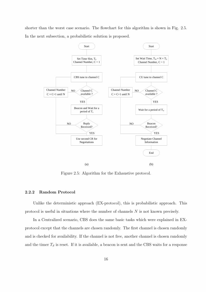
shorter than the worst case scenario. The flowchart for this algorithm is shown in Fig. 2.5.

In the next subsection, a probabilistic solution is proposed.

Start

Set Time Slot, TSChannel Number, C = 1

CBS tune to channel C

Beacon and Wait for a period of Ts

Use second CR for Negotiations

Channel Number

C = C+1 until NChannel C available ?

End

Reply Received?

Start

Set Wait Time, TW = N × TS Channel Number, C = 1

CU tune to channel C

Wait for a period of Tw

Negotiate Channel Information

Channel Number

C = C+1 until NChannel C available ?

Beacon Received?

NO

NO NO

NO

YES

YESYES

YES

(a) (b)

Figure 2.5: Algorithm for the Exhaustive protocol.

2.2.2 Random Protocol

Unlike the deterministic approach (EX-protocol), this is probabilistic approach. This

protocol is useful in situations where the number of channels N is not known precisely.

In a Centralized scenario, CBS does the same basic tasks which were explained in EX-

protocol except that the channels are chosen randomly. The first channel is chosen randomly

and is checked for availability. If the channel is not free, another channel is chosen randomly

and the timer TS is reset. If it is available, a beacon is sent and the CBS waits for a response

16

till the timer expires. CBS will keep choosing one of the C channels randomly. For example

in Fig. 2.4, if the CU happened to choose channel 8 as the first channel and wait for a beacon

in that channel continuously, it would never get a beacon since that channel is not available

for CBS unless the PU in that channel stops using it. So, shifting the channel periodically

is necessary.

There is little difference in the CU’s tasks from the tasks of a CU in EX-protocol. The

first difference is that the channels are chosen randomly. There is one more variable which

the CU maintains which is the number of Wait Slots, WS. The wait timer, TW is now set

to WS × TS instead of N × TS as in the case of EX-protocol. If the CU does not receive a

beacon, it will choose a different channel. The shifting of channel is necessary because, if

the CU waits in the same channel continuously waiting for a beacon and suppose the chosen

channel is not available for CBS, then the CU would not receive a beacon at all. If The CU

receives a beacon it responds to it and negotiates the channel information.

The value of WS is chosen strategically depending on the range of channels which the

CU is capable of scanning, C. In WS × TS seconds, CBS would have searched at-least WS

channels. If all the channels were free, the probability that the CU will receive a beacon in

one of its wait time TW is:

Pr = 1 −

(

1 −1

C

)TW

The actual probability depends on the probability of a channel being free with both

CBS and CU.

In a Multi-hop scenario, CUs will exactly follow the same rules as they did in a central-

ized scenario and additionally send beacons for every TS seconds. Moreover, the Wait Slots,

WS is randomly chosen from a predefined range of numbers. This makes each CU search the

channels at different rates which emulates the centralized scenario. Unlike in EX-protocol,

a CU cannot wait for a specified period of time for a beacon and be sure that it is the

first user if it did not receive a beacon. This is because of the randomness due to which

17

it is not possible to define a definite maximum time period during which CBS would have

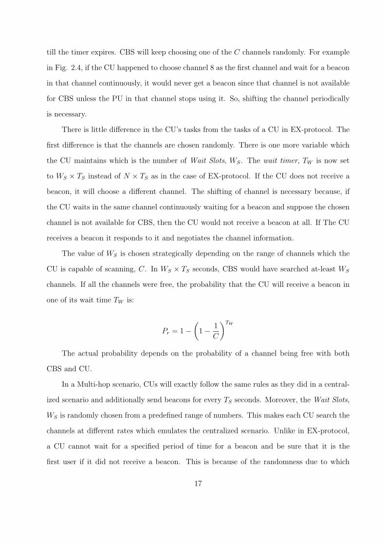
scanned all the channels at-least once. So, when a CU wants to initiate or join a network,

it chooses a random WS and a random channel in which it beacons for every TS seconds.

Upon the successful reception of a beacon by any CU, it acknowledges and exchanges the

channel information with the sender. The flowchart for this algorithm is shown in Fig. 2.6.

Start

Set Time Slot, TSSet C = Random Channel




Channel C available ?

End

Reply Received?

Start

Set Wait Time, TW = Wait Slots × TS

Set C = Random Channel






Beacon Received?

NO

NO NO

NO

YES

YESYES

YES

(a) (b)


Figure 2.6: Algorithm for the Random protocol.

2.2.3 Sequential Protocol

This protocol is a modified version of EX-protocol to make it more suitable for a multi-

hop network. So, the multi-hop scenario is explained first and then extended to the central-

ized scenario. In this protocol, the total number of channels N , is assumed to be known.

18

Multi-hop Scenario: The time slot, TS is chosen similar to other protocols. The CUs start

from a random channel. The next channel is chosen in the increasing order of frequencies.

After the last channel is reached, the next channel is chosen in decreasing order of frequencies

and not from the lowest again. If the chosen channel is not available the CU shifts to the

next channel. If the channel is available, it stays for a period of TS in that channel and

sends a beacon during that period. If it receives an acknowledgment, its neighboring CU

has received its beacon and they exchange the control information. The same thing happens

if the CU receives a beacon. Due to the symmetry in the CU tasks, this protocol is more

suitable for a multi-hop network.

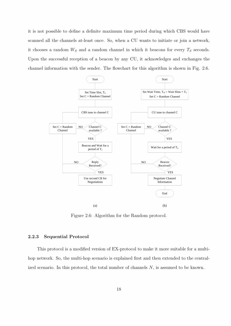
In a Centralized Scenario, the only difference is that the CU does not beacon instead

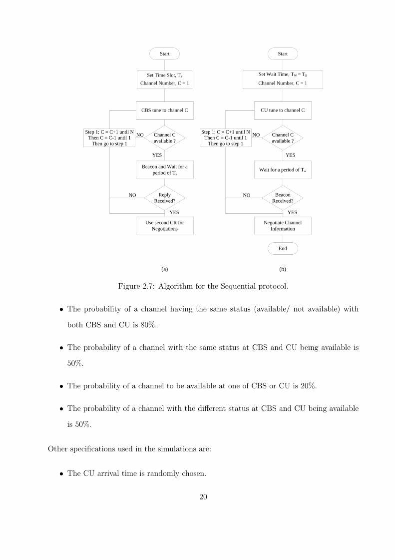
just listens in its chosen channel for a beacon. Fig. 2.7 shows the flow chart of this protocol

for CBS and CU. In the following section, the working of the proposed protocols is studied

using simulations.

2.3 Simulation Study

In this section the protocols are simulated and their performance is studied and the three

protocols are compared with each other. The simulation setup used in all these experiments

is shown below.

Simulation setup

MATLAB has been used for all simulations. The number of channels, N is varied from

10 to 1000 in each simulation. Each point on the graphs is an average of 500 simulations. The

Primary User’s traffic is compensated by setting a probability to channel availability. The

probabilities are set such that they represent realistic scenarios. In [8] it has been observed

that a CU’s neighbors will have the same channel states with high probability i.e., if a CU

has a channel available, it’s highly probable that its neighbor has the same channel available.

So, the probability of channel availabilities is chosen as shown below:

19

Start

Set Time Slot, TS

Channel Number, C = 1





End

Reply Received?

Start

Set Wait Time, TW = TS

Channel Number, C = 1




Step 1: C = C+1 until NThen C = C-1 until 1

Then go to step 1


Beacon Received?

NO

NO NO

NO

YES

YESYES

YES

(a) (b)

Step 1: C = C+1 until NThen C = C-1 until 1

Then go to step 1

Figure 2.7: Algorithm for the Sequential protocol.

• The probability of a channel having the same status (available/ not available) with

both CBS and CU is 80%.

• The probability of a channel with the same status at CBS and CU being available is

50%.

• The probability of a channel to be available at one of CBS or CU is 20%.

• The probability of a channel with the different status at CBS and CU being available

is 50%.

Other specifications used in the simulations are:

• The CU arrival time is randomly chosen.

20

• The value of Time Slot, TS = 1 sec.

• The beacon time duration is chosen as, Tb = 100 msec.

• The time taken to shift to a channel and check its availability = 100 msec.

2.3.1 Search Time

During the network setup, Setup Time is the crucial factor. The total network setup

time is directly proportional to the time each CU takes to find the CBS and connect to it.

The time taken for a CU to receive a beacon from the CBS is measured i.e., the time taken

before a Cognitive User connects to the Cognitive Base Station is referred to as Search Time

in the rest of the discussion. So, in this section the Search Time of the three protocols is

compared.

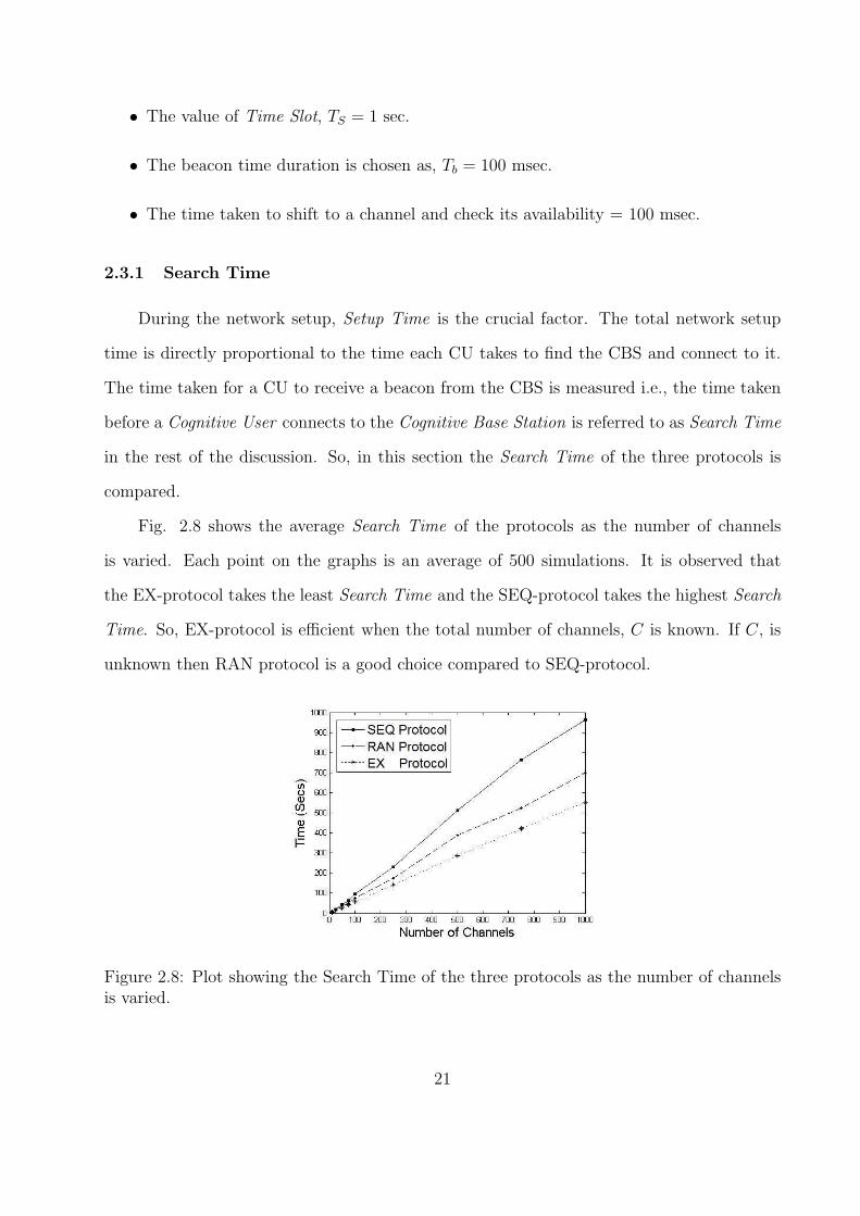
Fig. 2.8 shows the average Search Time of the protocols as the number of channels

is varied. Each point on the graphs is an average of 500 simulations. It is observed that

the EX-protocol takes the least Search Time and the SEQ-protocol takes the highest Search

Time. So, EX-protocol is efficient when the total number of channels, C is known. If C, is

unknown then RAN protocol is a good choice compared to SEQ-protocol.

Figure 2.8: Plot showing the Search Time of the three protocols as the number of channelsis varied.

21

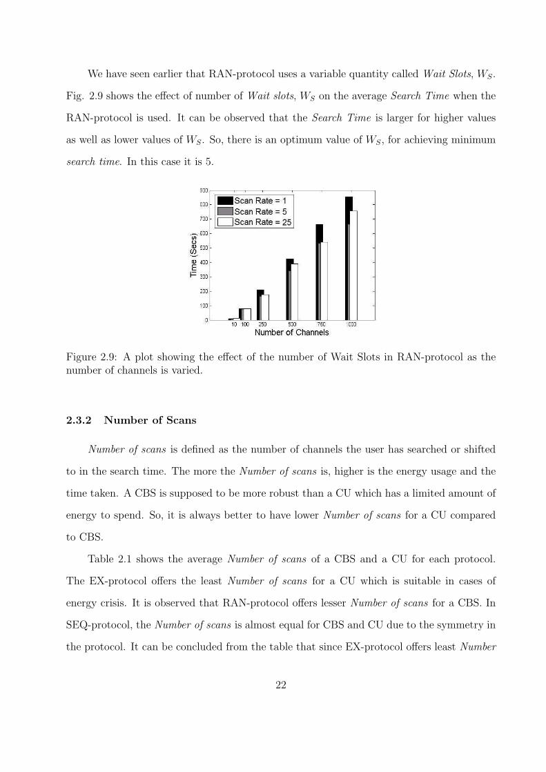
We have seen earlier that RAN-protocol uses a variable quantity called Wait Slots, WS.

Fig. 2.9 shows the effect of number of Wait slots, WS on the average Search Time when the

RAN-protocol is used. It can be observed that the Search Time is larger for higher values

as well as lower values of WS. So, there is an optimum value of WS, for achieving minimum

search time. In this case it is 5.

Figure 2.9: A plot showing the effect of the number of Wait Slots in RAN-protocol as thenumber of channels is varied.

2.3.2 Number of Scans

Number of scans is defined as the number of channels the user has searched or shifted

to in the search time. The more the Number of scans is, higher is the energy usage and the

time taken. A CBS is supposed to be more robust than a CU which has a limited amount of

energy to spend. So, it is always better to have lower Number of scans for a CU compared

to CBS.

Table 2.1 shows the average Number of scans of a CBS and a CU for each protocol.

The EX-protocol offers the least Number of scans for a CU which is suitable in cases of

energy crisis. It is observed that RAN-protocol offers lesser Number of scans for a CBS. In

SEQ-protocol, the Number of scans is almost equal for CBS and CU due to the symmetry in

the protocol. It can be concluded from the table that since EX-protocol offers least Number

22

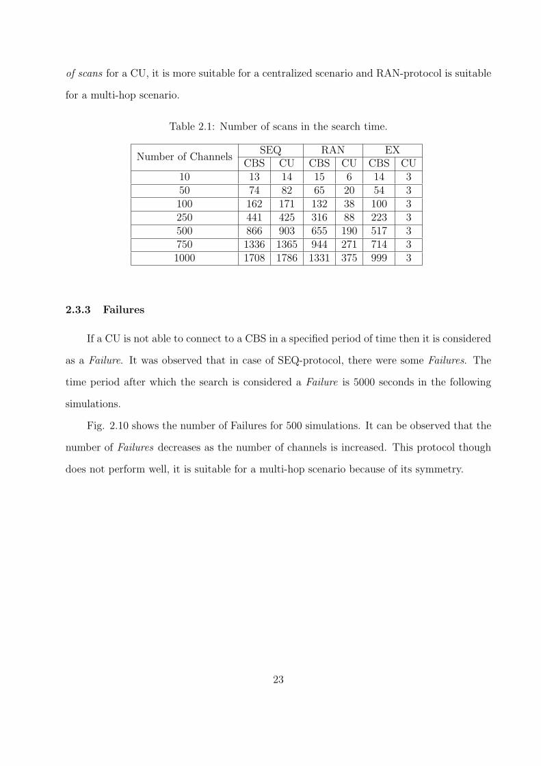
of scans for a CU, it is more suitable for a centralized scenario and RAN-protocol is suitable

for a multi-hop scenario.

Table 2.1: Number of scans in the search time.

Number of ChannelsSEQ RAN EX

CBS CU CBS CU CBS CU10 13 14 15 6 14 350 74 82 65 20 54 3100 162 171 132 38 100 3250 441 425 316 88 223 3500 866 903 655 190 517 3750 1336 1365 944 271 714 31000 1708 1786 1331 375 999 3

2.3.3 Failures

If a CU is not able to connect to a CBS in a specified period of time then it is considered

as a Failure. It was observed that in case of SEQ-protocol, there were some Failures. The

time period after which the search is considered a Failure is 5000 seconds in the following

simulations.

Fig. 2.10 shows the number of Failures for 500 simulations. It can be observed that the

number of Failures decreases as the number of channels is increased. This protocol though

does not perform well, it is suitable for a multi-hop scenario because of its symmetry.

23

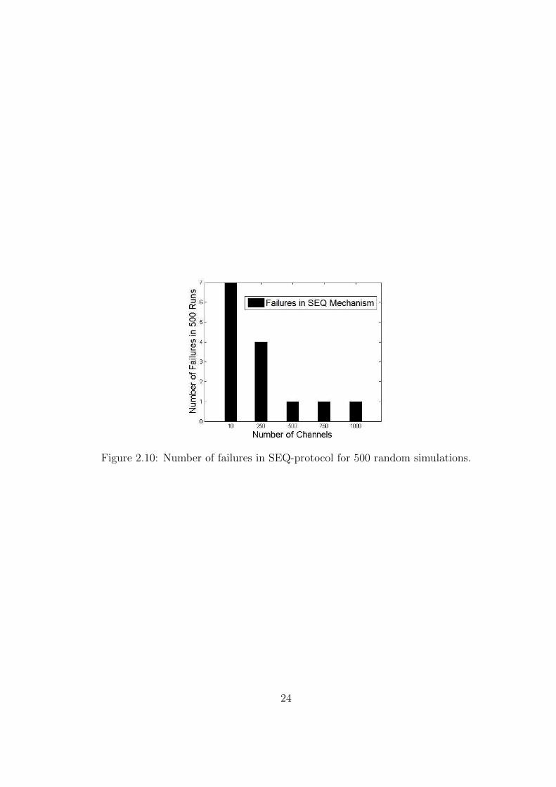
Figure 2.10: Number of failures in SEQ-protocol for 500 random simulations.

24

Chapter 3

Selective Broadcasting in Multi-Hop Cognitive Radio Networks

In a cognitive network, each node has a set of channels available, a node receives a

message only if the message was sent in the channel on which the node was listening to.

So, to ensure that a message is successfully sent to all neighbors of a node, it has to be

broadcast over every channel. This is called complete broadcasting of information. In a

cognitive environment, the number of channels is potentially large. As a result broadcasting

in every channel causes a large delay in transmitting the control information.

Another solution would be to choose one channel from among the free channels for

control signal exchange. However, the probability that a channel is common among all

cognitive users is small [11]. As a result, some of the nodes may not be reachable using

a single channel. So, it is necessary to broadcast the control information over more than

one channel to ensure that every neighbor receives a copy [12]. With the increase in the

number of nodes in the network, it is possible that the nodes are scattered over a large set

of channels. As a result, cost and delay of broadcasting over all these channels increases. A

simple, yet efficient solution would be to identify a small subset of channels which cover all

the neighbors of a node. Then use this set of channels for exchanging the control information.

This concept of transmitting the control signals over a selected group of channels instead

of flooding over all channels is called Selective Broadcasting and forms the basic idea of the

chapter. Neighbor graphs and minimal neighbor graphs are introduced to find the minimal

set of channels to transmit the control signals.

25

3.1 Selective Broadcasting

In a MHCRN, each node has a set of channels available when it enters a network. In

order to become a part of the network and start communicating with other nodes, it has to

first know its neighbors and their channel information. Also, it has to let other nodes know

its presence and its available channel information. So it broadcasts such information over all

channels to make sure that all neighbors receive the message. Similarly, when a node wants

to start a communication it should exchange certain control information useful, for example,

in route discovery. However, a cognitive network environment is dynamic due to the primary

user’s traffic [2]. The number of available channels at each node keeps changing with time

and location. To keep all nodes updated, the information change has to be transmitted

over all channels as quickly as possible. So, for effective and efficient coordination, fast

dissemination of control traffic between neighboring users is required. So, minimal delay is

a critical factor in promptly disseminating control information. Hence, the goal is to reduce

the broadcast delay of each node.

Now, consider that a node has M available channels. Let Tb be the minimum time

required to broadcast a control message. Then, total broadcast delay = M × Tb.

So, in order to have lower broadcast delay we need to reduce M . The value of Tb is

dictated by the particular hardware used and hence is fixed. M can be reduced by finding

the minimum number of channels, M ′ to broadcast, but still making sure that all nodes

receive the message. Thus, broadcasting over carefully selected M ′ channels instead of

blindly broadcasting over M (available) channels is called Selective Broadcasting. Finding

the minimum number of channels, M ′ is accomplished by using neighbor graphs and finding

out the minimal neighbor graphs.

Before explaining the idea of neighbor graph and minimal neighbor graph it is important

to understand the state of the network when selective broadcasting occurs and the difference

between multicasting and selective broadcasting.

26

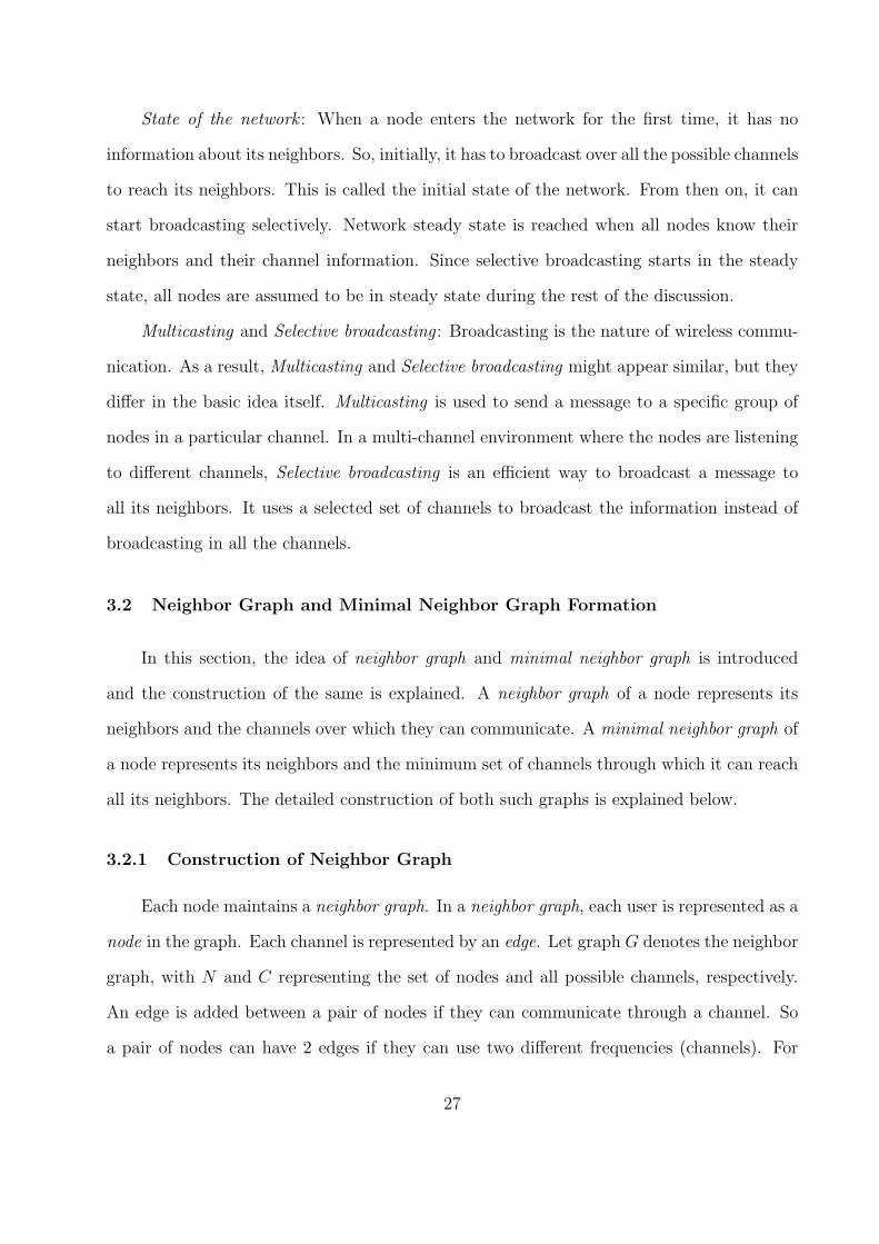
State of the network : When a node enters the network for the first time, it has no

information about its neighbors. So, initially, it has to broadcast over all the possible channels

to reach its neighbors. This is called the initial state of the network. From then on, it can

start broadcasting selectively. Network steady state is reached when all nodes know their

neighbors and their channel information. Since selective broadcasting starts in the steady

state, all nodes are assumed to be in steady state during the rest of the discussion.

Multicasting and Selective broadcasting : Broadcasting is the nature of wireless commu-

nication. As a result, Multicasting and Selective broadcasting might appear similar, but they

differ in the basic idea itself. Multicasting is used to send a message to a specific group of

nodes in a particular channel. In a multi-channel environment where the nodes are listening

to different channels, Selective broadcasting is an efficient way to broadcast a message to

all its neighbors. It uses a selected set of channels to broadcast the information instead of

broadcasting in all the channels.

3.2 Neighbor Graph and Minimal Neighbor Graph Formation

In this section, the idea of neighbor graph and minimal neighbor graph is introduced

and the construction of the same is explained. A neighbor graph of a node represents its

neighbors and the channels over which they can communicate. A minimal neighbor graph of

a node represents its neighbors and the minimum set of channels through which it can reach

all its neighbors. The detailed construction of both such graphs is explained below.

3.2.1 Construction of Neighbor Graph

Each node maintains a neighbor graph. In a neighbor graph, each user is represented as a

node in the graph. Each channel is represented by an edge. Let graph G denotes the neighbor

graph, with N and C representing the set of nodes and all possible channels, respectively.

An edge is added between a pair of nodes if they can communicate through a channel. So

a pair of nodes can have 2 edges if they can use two different frequencies (channels). For

27

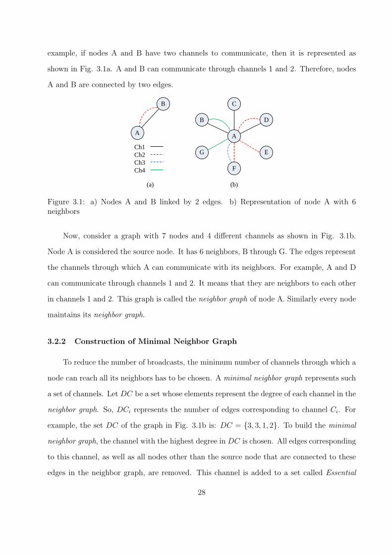
example, if nodes A and B have two channels to communicate, then it is represented as

shown in Fig. 3.1a. A and B can communicate through channels 1 and 2. Therefore, nodes

A and B are connected by two edges.

A

B

A

D

C

B

G

F

ECh1Ch2Ch3Ch4

(a) (b)

Figure 3.1: a) Nodes A and B linked by 2 edges. b) Representation of node A with 6neighbors

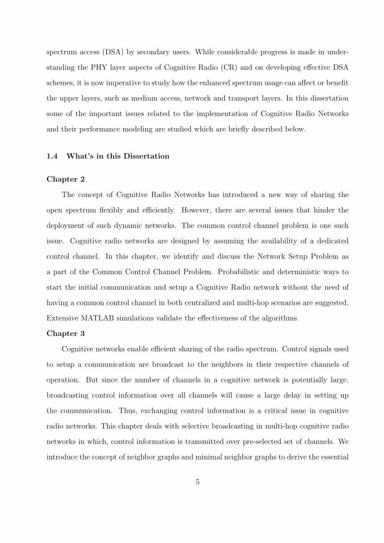
Now, consider a graph with 7 nodes and 4 different channels as shown in Fig. 3.1b.

Node A is considered the source node. It has 6 neighbors, B through G. The edges represent

the channels through which A can communicate with its neighbors. For example, A and D

can communicate through channels 1 and 2. It means that they are neighbors to each other

in channels 1 and 2. This graph is called the neighbor graph of node A. Similarly every node

maintains its neighbor graph.

3.2.2 Construction of Minimal Neighbor Graph

To reduce the number of broadcasts, the minimum number of channels through which a

node can reach all its neighbors has to be chosen. A minimal neighbor graph represents such

a set of channels. Let DC be a set whose elements represent the degree of each channel in the

neighbor graph. So, DCi represents the number of edges corresponding to channel Ci. For

example, the set DC of the graph in Fig. 3.1b is: DC = {3, 3, 1, 2}. To build the minimal

neighbor graph, the channel with the highest degree in DC is chosen. All edges corresponding

to this channel, as well as all nodes other than the source node that are connected to these

edges in the neighbor graph, are removed. This channel is added to a set called Essential

28

Channel Set, ECS which as the name implies, is the set of required channels to reach all the

neighboring nodes. ECS initially is a null set. As the edges are removed, the corresponding

channel is added to ECS.

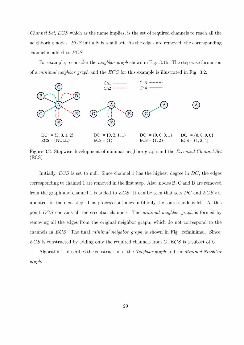
For example, reconsider the neighbor graph shown in Fig. 3.1b. The step wise formation

of a minimal neighbor graph and the ECS for this example is illustrated in Fig. 3.2.

A

D

C

B

G

F

E

DC = {3, 3, 1, 2}ECS = {NULL}

A

G

F

E

A

G

A

DC = {0, 2, 1, 1}ECS = {1}

DC = {0, 0, 0, 1}ECS = {1, 2}

DC = {0, 0, 0, 0}ECS = {1, 2, 4}

Ch1Ch2

Ch3Ch4

Figure 3.2: Stepwise development of minimal neighbor graph and the Essential Channel Set(ECS)

Initially, ECS is set to null. Since channel 1 has the highest degree in DC, the edges

corresponding to channel 1 are removed in the first step. Also, nodes B, C and D are removed

from the graph and channel 1 is added to ECS. It can be seen that sets DC and ECS are

updated for the next step. This process continues until only the source node is left. At this

point ECS contains all the essential channels. The minimal neighbor graph is formed by

removing all the edges from the original neighbor graph, which do not correspond to the

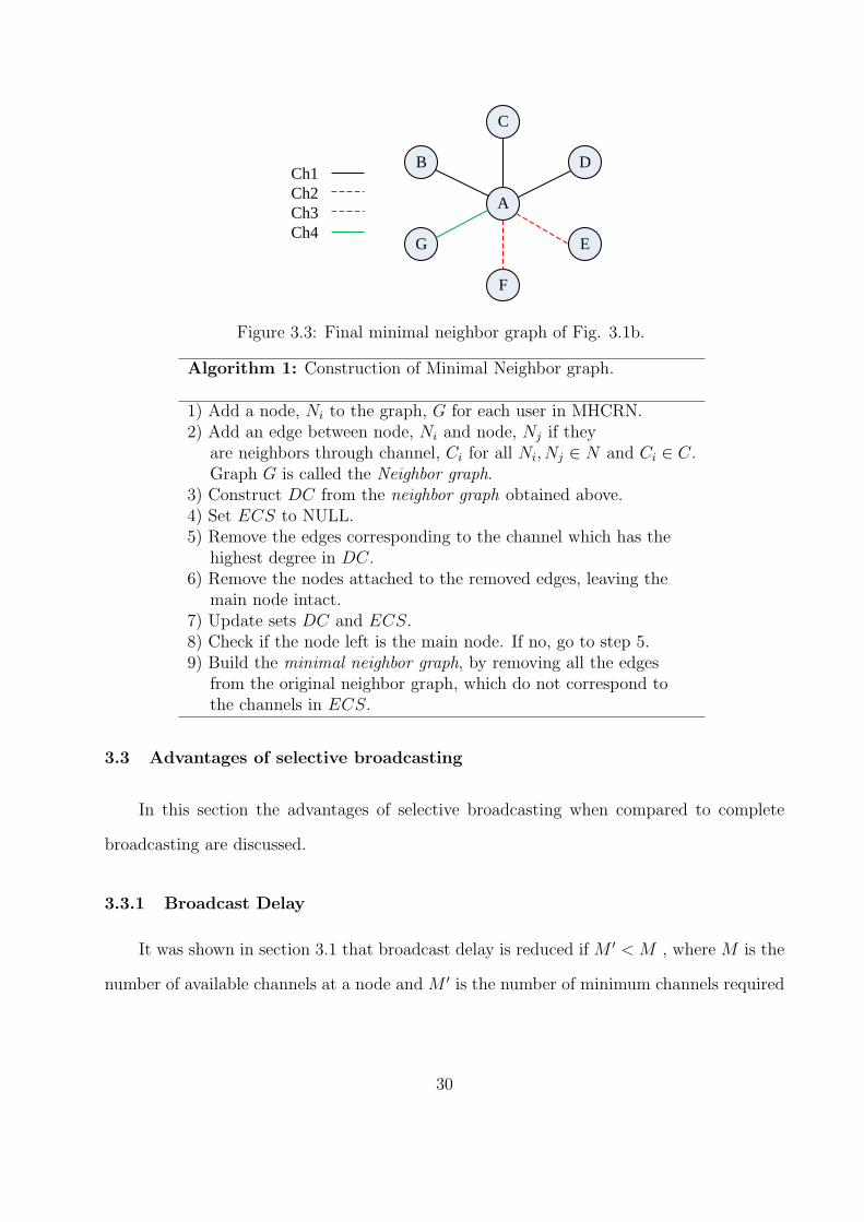
channels in ECS. The final minimal neighbor graph is shown in Fig. refminimal. Since,

ECS is constructed by adding only the required channels from C; ECS is a subset of C.

Algorithm 1, describes the construction of the Neighbor graph and the Minimal Neighbor

graph.

29

A

D

C

B

G

F

E

Ch1Ch2Ch3Ch4

Figure 3.3: Final minimal neighbor graph of Fig. 3.1b.

Algorithm 1: Construction of Minimal Neighbor graph.

1) Add a node, Ni to the graph, G for each user in MHCRN.2) Add an edge between node, Ni and node, Nj if they

are neighbors through channel, Ci for all Ni, Nj ∈ N and Ci ∈ C.Graph G is called the Neighbor graph.

3) Construct DC from the neighbor graph obtained above.4) Set ECS to NULL.5) Remove the edges corresponding to the channel which has the

highest degree in DC.6) Remove the nodes attached to the removed edges, leaving the

main node intact.7) Update sets DC and ECS.8) Check if the node left is the main node. If no, go to step 5.9) Build the minimal neighbor graph, by removing all the edges

from the original neighbor graph, which do not correspond tothe channels in ECS.

3.3 Advantages of selective broadcasting

In this section the advantages of selective broadcasting when compared to complete

broadcasting are discussed.

3.3.1 Broadcast Delay

It was shown in section 3.1 that broadcast delay is reduced if M ′ < M , where M is the

number of available channels at a node and M ′ is the number of minimum channels required

30

to reach all its neighbors. Since C is the channel set of all available channels and ECS is

the channel set of minimum channels,

M = Cardinality of C M ′ = Cardinality of ECS

But, it was shown that ECS is a subset of C. Therefore,

M ′ ≤ M

Since it is shown that the number of channels over which to transmit in selective broad-

casting is less than that in complete broadcasting, the broadcast delay is reduced.

3.3.2 Lower congestion, contention

Since in selective broadcasting, the average number of broadcasts per channel is re-

duced, the overall congestion in the network is reduced. Moreover, when the traffic in the

network increases, the total number of broadcast messages also increases. As a result, there

is increased contention in every channel. But using selective broadcasting, traffic is reduced

compared to complete broadcasting which leads to lower contention. This implies that a

potential improvement in the overall network throughput can be achieved by using selective

broadcasting.

3.3.3 No common control channel

Many MAC protocols have been proposed which assume common channel for control

message transmission [2]. But the use of common control channel introduces some problems

such as channel saturation and Denial of Service attacks (DoS) [10]. Selective broadcasting,

in addition to the above mentioned advantages, is free from DoS attack. It is due to the

fact that it inherently avoids the necessity of common control channel. Absence of common

control channel also results in significant increase in throughput as shown in [13].

In the following section, the effectiveness of the proposed concept is demonstrated using

simulations.

31

3.4 Results and Analysis

In this section the performance selective broadcast is compared with complete broad-

casting by studying the delay in transmitting control information and redundancy of the

received packets. The simulation setup used in all these experiments is shown below.

Simulation setup

MATLAB has been used for all simulations. For each experiment, a network area of

1000m×1000m is considered. The number of nodes is varied from 1 to 100. All nodes are

deployed randomly in the network. Each node is assigned a random set of channels varying

from 0 to 10 channels. The transmission range is set to 250m. Each data point in the graphs

is an average of 100 runs. Before looking at the performance of the proposed idea, two

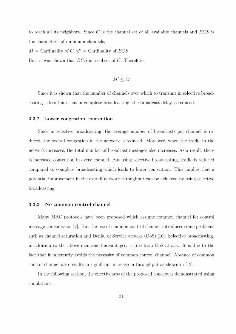
observations are made that help in understanding the simulation results. Fig. 3.4 shows the

plot of channel spread as a function of number of nodes. Channel spread is defined as the

union of all the channels covered by the neighbors of a node.

Observation 1: With increase in the number of nodes, the neighbors of a node are spread

over larger number of channels.

Figure 3.4: Plot of channel spread with respect to number of nodes for a set of 10 channels.

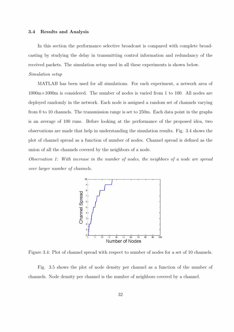
Fig. 3.5 shows the plot of node density per channel as a function of the number of

channels. Node density per channel is the number of neighbors covered by a channel.

32

Observation 2: With increase in number of channels, the number of neighbors each channel

covers increases.

Figure 3.5: Plot of node density per channel with respect to number of channels for a set of50 nodes.

3.4.1 Broadcast Delay

In this part of the simulations, transmission delay of selective broadcast and complete

broadcast are compared. Broadcast delay is defined as the total time taken by a node to

successfully transmit one control message to all its neighbors. Each point in the following

graphs is the average delay of all nodes in the network. The minimum time to broadcast in

a channel is assumed to be 5 msec.

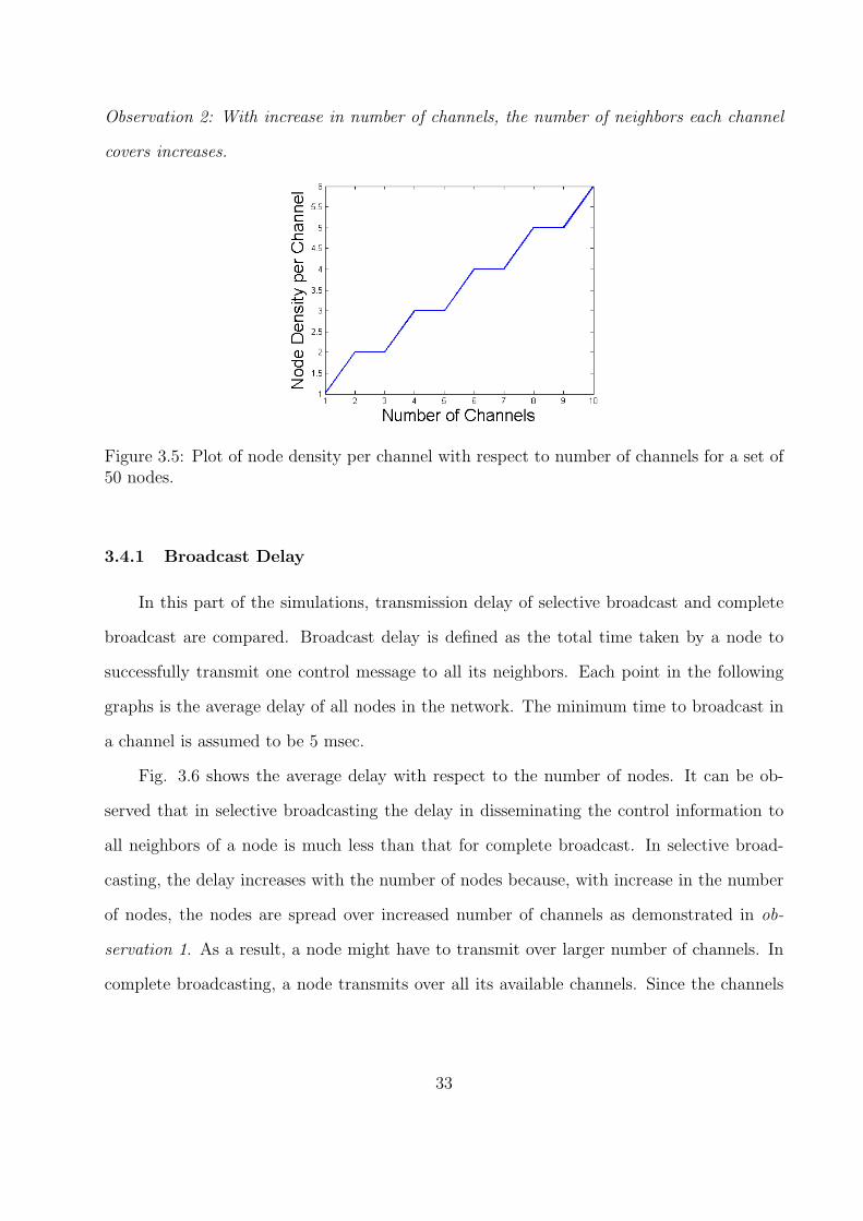
Fig. 3.6 shows the average delay with respect to the number of nodes. It can be ob-

served that in selective broadcasting the delay in disseminating the control information to

all neighbors of a node is much less than that for complete broadcast. In selective broad-

casting, the delay increases with the number of nodes because, with increase in the number

of nodes, the nodes are spread over increased number of channels as demonstrated in ob-

servation 1. As a result, a node might have to transmit over larger number of channels. In

complete broadcasting, a node transmits over all its available channels. Since the channels

33

are assigned randomly to the nodes, the average number of channels at each node is almost

constant. Therefore the delay is constant as observed in Fig. 3.6.

Figure 3.6: Comparison of average broadcast delay of a node as the number of nodes isvaried.

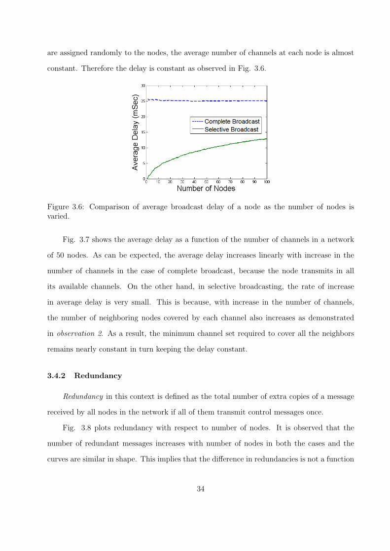
Fig. 3.7 shows the average delay as a function of the number of channels in a network

of 50 nodes. As can be expected, the average delay increases linearly with increase in the

number of channels in the case of complete broadcast, because the node transmits in all

its available channels. On the other hand, in selective broadcasting, the rate of increase

in average delay is very small. This is because, with increase in the number of channels,

the number of neighboring nodes covered by each channel also increases as demonstrated

in observation 2. As a result, the minimum channel set required to cover all the neighbors

remains nearly constant in turn keeping the delay constant.

3.4.2 Redundancy

Redundancy in this context is defined as the total number of extra copies of a message

received by all nodes in the network if all of them transmit control messages once.

Fig. 3.8 plots redundancy with respect to number of nodes. It is observed that the

number of redundant messages increases with number of nodes in both the cases and the

curves are similar in shape. This implies that the difference in redundancies is not a function

34

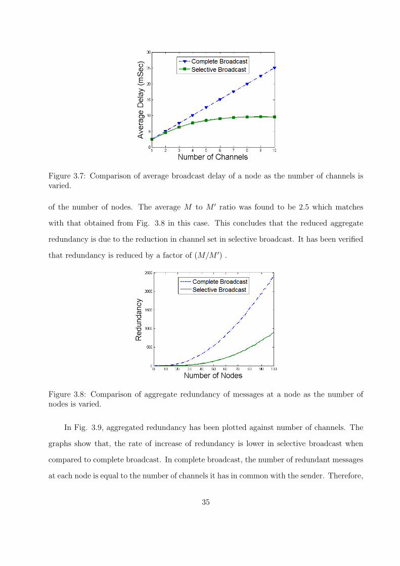
Figure 3.7: Comparison of average broadcast delay of a node as the number of channels isvaried.

of the number of nodes. The average M to M ′ ratio was found to be 2.5 which matches

with that obtained from Fig. 3.8 in this case. This concludes that the reduced aggregate

redundancy is due to the reduction in channel set in selective broadcast. It has been verified

that redundancy is reduced by a factor of (M/M ′) .

Figure 3.8: Comparison of aggregate redundancy of messages at a node as the number ofnodes is varied.

In Fig. 3.9, aggregated redundancy has been plotted against number of channels. The

graphs show that, the rate of increase of redundancy is lower in selective broadcast when

compared to complete broadcast. In complete broadcast, the number of redundant messages

at each node is equal to the number of channels it has in common with the sender. Therefore,

35

with increase in number of channels the redundant messages almost increase linearly whereas

in selective broadcast the increase is small due to the selection of minimum channel set.

Figure 3.9: Comparison of average redundancy of messages at a node as number of channelsis varied.

In this section, it has been demonstrated that selective broadcasting provides lower

transmission delay and redundancy. It should be noted that, due to the reduced redundancy

of messages, there will be less congestion in the network and hence, there is potential for

improvement in throughput by using selective broadcasting.

36

Chapter 4

Capacity of Secondary Users

In opportunistic spectrum access networks, the secondary users are forced to vacate the

channels when the primary user of the respective channels become active. This is called

forced termination in [14]. The secondary user may then shift to another available channel

and recover from that state. This is called spectrum hand-off. Thus, the secondary users are

serviced when the channels are free resulting in higher utilization of the spectrum.

Since the availability of the spectrum depends on the primary user traffic, the number

of secondary users serviced also varies with it. The amount of service that can be squeezed

in from the free bands in a spectrum accessed by unrestricted primary users is called the

capacity of secondary users. In this chapter we model capacity of secondary users using

three dimensional continuous time Markov chains. Markov chains are used to model dynamic

spectrum access networks in [14]-[18]. [15] proposes a Markov model, but it does not allow for

the secondary users to reoccupy another free channel once it has been forced to vacate from a

channel and considers the call to be completely dropped. The spectrum handoff capability of

the cognitive radio is thus not modeled in this work. [14] tries to reduce the forced termination

of the secondary radios at the cost of blocking probability by reserving some of the channels

for primary user access only. Both of these papers discuss the optimal reservation of the

channels for primary users to reduce the dropping probability and forced termination when

in-fact these states can be totally avoided with spectrum hand-off capability of a cognitive

radio. Analysis in [16]-[19], does not consider prioritized primary users.

In this chapter, we model a system in which the primary users are prioritized as well

as the secondary users have spectrum hand-off capability. The Markov model proposed in

[15] has been modified to accommodate the spectrum hand-off capability. The distinction

37

between forced termination, dropping and blocking is made clear. A non-random channel

access method is proposed in which the forced termination states are totally eliminated and

dropping and blocking probabilities are reduced resulting in higher secondary user capacity.

4.1 System Model and Assumptions

In this section three different channel assignment strategies are discussed and the system

model is developed and explained.

4.1.1 Random Channel Assignment

Let there be a total of N channels. Each channel is assumed to be of equal bandwidth.

A channel can be accessed by a secondary user if it is not occupied by a primary user.

Primary users can occupy any channel and have the right to reclaim a channel at any time

from secondary users. In the initial model it is assumed that both the primary and secondary

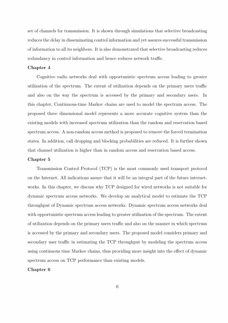
users access the channels randomly. This is explained with the help of Fig. 4.1. There are

a total of five channels of which two are occupied by PUs and one by a SU. When a new

SU arrives as shown in Fig. 4.1a, it chooses a random free channel. A PU can choose any

random channel and as shown in Fig. 4.1b, if it chooses a secondary occupied channel,

the SU jumps to a different free channel. If there is no other channel available, the SU’s

service is dropped as shown in Fig. 4.1c. An SU cannot use a channel if it does not have an

opportunity to do so as shown in Fig 4.1d.

There are four states in this model. The states are explained from the point of view of

secondary users since the focus is on the capacity and channel utilization of secondary users.

Since primary users have unrestricted usage of channels, study of their behavior is not of our

interest.

Non-blocking state: A secondary user is considered to be in this state if it is completely

serviced without being interrupted by a primary user on that channel.

38

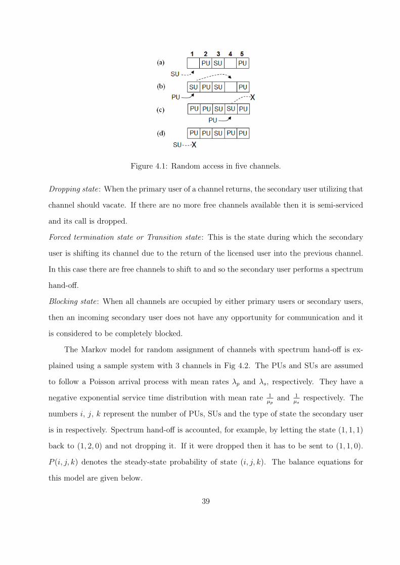
Figure 4.1: Random access in five channels.

Dropping state: When the primary user of a channel returns, the secondary user utilizing that

channel should vacate. If there are no more free channels available then it is semi-serviced

and its call is dropped.

Forced termination state or Transition state: This is the state during which the secondary

user is shifting its channel due to the return of the licensed user into the previous channel.

In this case there are free channels to shift to and so the secondary user performs a spectrum

hand-off.

Blocking state: When all channels are occupied by either primary users or secondary users,

then an incoming secondary user does not have any opportunity for communication and it

is considered to be completely blocked.

The Markov model for random assignment of channels with spectrum hand-off is ex-

plained using a sample system with 3 channels in Fig 4.2. The PUs and SUs are assumed

to follow a Poisson arrival process with mean rates λp and λs, respectively. They have a

negative exponential service time distribution with mean rate 1

µpand 1

µsrespectively. The

numbers i, j, k represent the number of PUs, SUs and the type of state the secondary user

is in respectively. Spectrum hand-off is accounted, for example, by letting the state (1, 1, 1)

back to (1, 2, 0) and not dropping it. If it were dropped then it has to be sent to (1, 1, 0).

P (i, j, k) denotes the steady-state probability of state (i, j, k). The balance equations for

this model are given below.

39

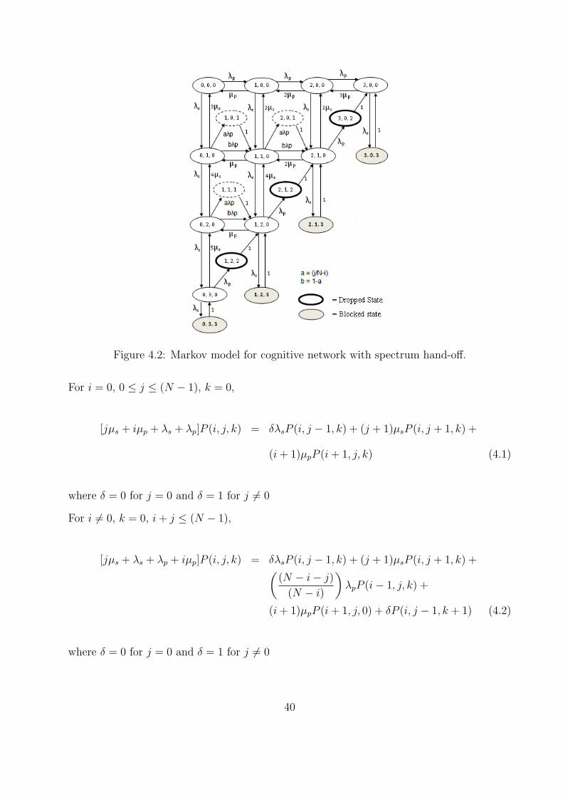
Figure 4.2: Markov model for cognitive network with spectrum hand-off.

For i = 0, 0 ≤ j ≤ (N − 1), k = 0,

[jµs + iµp + λs + λp]P (i, j, k) = δλsP (i, j − 1, k) + (j + 1)µsP (i, j + 1, k) +

(i + 1)µpP (i + 1, j, k) (4.1)

where δ = 0 for j = 0 and δ = 1 for j 6= 0

For i 6= 0, k = 0, i + j ≤ (N − 1),

[jµs + λs + λp + iµp]P (i, j, k) = δλsP (i, j − 1, k) + (j + 1)µsP (i, j + 1, k) +(

(N − i − j)

(N − i)

)

λpP (i − 1, j, k) +

(i + 1)µpP (i + 1, j, 0) + δP (i, j − 1, k + 1) (4.2)


40

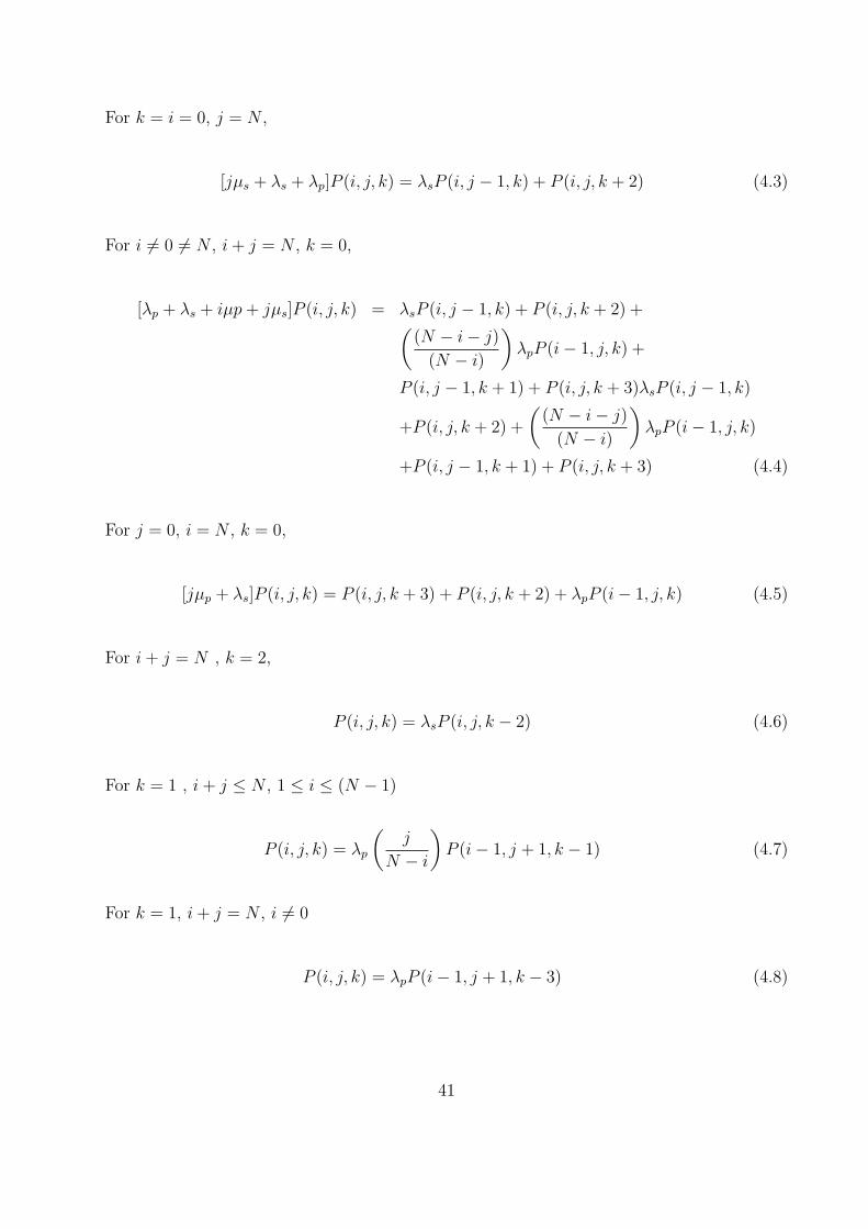
For k = i = 0, j = N ,

[jµs + λs + λp]P (i, j, k) = λsP (i, j − 1, k) + P (i, j, k + 2) (4.3)

For i 6= 0 6= N , i + j = N , k = 0,

[λp + λs + iµp + jµs]P (i, j, k) = λsP (i, j − 1, k) + P (i, j, k + 2) +(

(N − i − j)

(N − i)

)

λpP (i − 1, j, k) +

P (i, j − 1, k + 1) + P (i, j, k + 3)λsP (i, j − 1, k)

+P (i, j, k + 2) +

(

(N − i − j)

(N − i)

)

λpP (i − 1, j, k)

+P (i, j − 1, k + 1) + P (i, j, k + 3) (4.4)

For j = 0, i = N , k = 0,

[jµp + λs]P (i, j, k) = P (i, j, k + 3) + P (i, j, k + 2) + λpP (i − 1, j, k) (4.5)

For i + j = N , k = 2,

P (i, j, k) = λsP (i, j, k − 2) (4.6)

For k = 1 , i + j ≤ N , 1 ≤ i ≤ (N − 1)

P (i, j, k) = λp

(

j

N − i

)

P (i − 1, j + 1, k − 1) (4.7)

For k = 1, i + j = N , i 6= 0

P (i, j, k) = λpP (i − 1, j + 1, k − 3) (4.8)

41

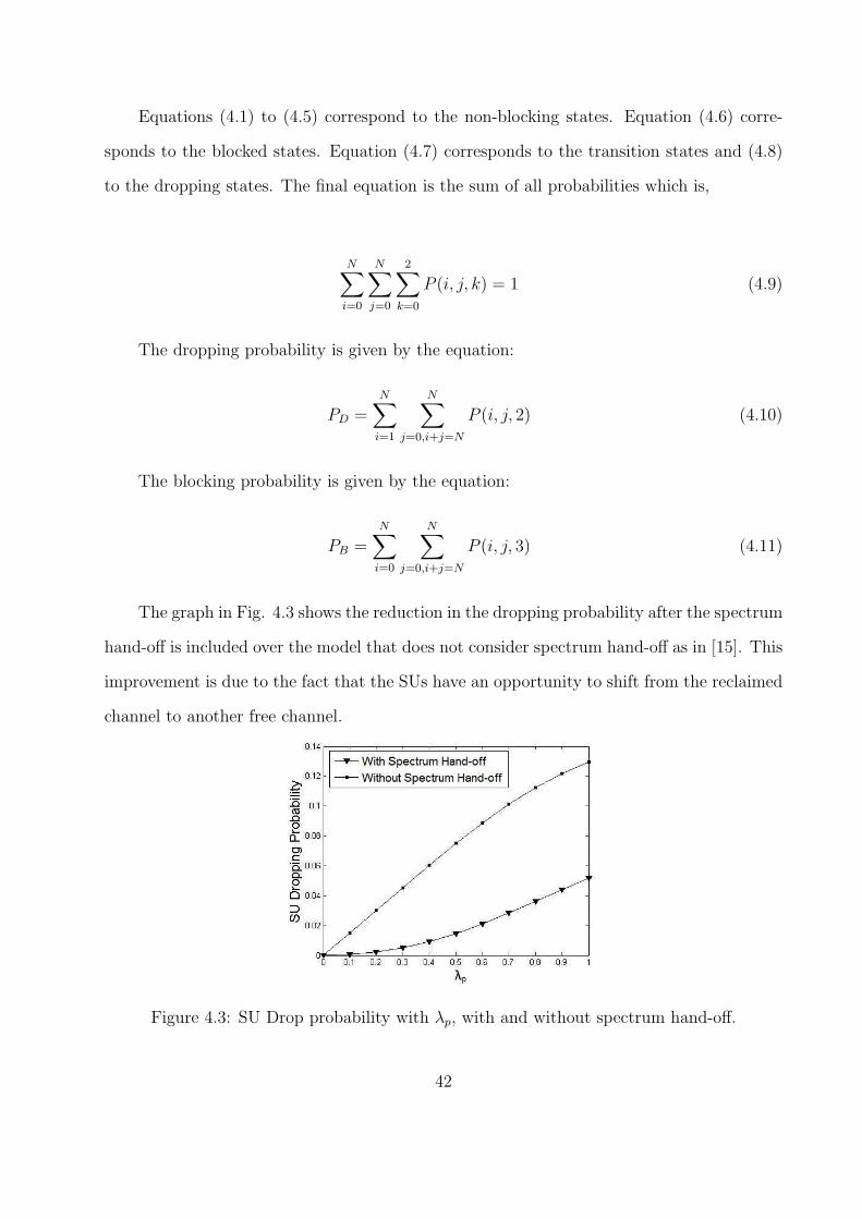
Equations (4.1) to (4.5) correspond to the non-blocking states. Equation (4.6) corre-

sponds to the blocked states. Equation (4.7) corresponds to the transition states and (4.8)

to the dropping states. The final equation is the sum of all probabilities which is,

N∑

i=0

N∑

j=0

2∑

k=0

P (i, j, k) = 1 (4.9)

The dropping probability is given by the equation:

PD =N

∑

i=1

N∑

j=0,i+j=N

P (i, j, 2) (4.10)

The blocking probability is given by the equation:

PB =N

∑

i=0

N∑

j=0,i+j=N

P (i, j, 3) (4.11)

The graph in Fig. 4.3 shows the reduction in the dropping probability after the spectrum

hand-off is included over the model that does not consider spectrum hand-off as in [15]. This

improvement is due to the fact that the SUs have an opportunity to shift from the reclaimed

channel to another free channel.

Figure 4.3: SU Drop probability with λp, with and without spectrum hand-off.

42

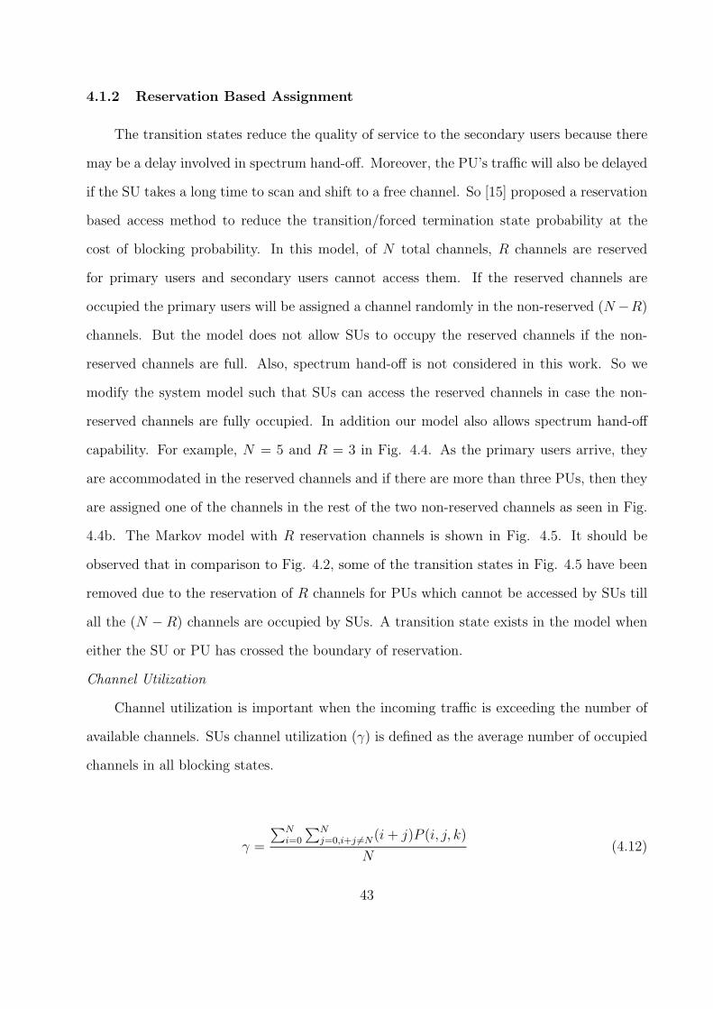
4.1.2 Reservation Based Assignment

The transition states reduce the quality of service to the secondary users because there

may be a delay involved in spectrum hand-off. Moreover, the PU’s traffic will also be delayed

if the SU takes a long time to scan and shift to a free channel. So [15] proposed a reservation

based access method to reduce the transition/forced termination state probability at the

cost of blocking probability. In this model, of N total channels, R channels are reserved

for primary users and secondary users cannot access them. If the reserved channels are

occupied the primary users will be assigned a channel randomly in the non-reserved (N −R)

channels. But the model does not allow SUs to occupy the reserved channels if the non-

reserved channels are full. Also, spectrum hand-off is not considered in this work. So we

modify the system model such that SUs can access the reserved channels in case the non-

reserved channels are fully occupied. In addition our model also allows spectrum hand-off

capability. For example, N = 5 and R = 3 in Fig. 4.4. As the primary users arrive, they

are accommodated in the reserved channels and if there are more than three PUs, then they

are assigned one of the channels in the rest of the two non-reserved channels as seen in Fig.

4.4b. The Markov model with R reservation channels is shown in Fig. 4.5. It should be

observed that in comparison to Fig. 4.2, some of the transition states in Fig. 4.5 have been

removed due to the reservation of R channels for PUs which cannot be accessed by SUs till

all the (N − R) channels are occupied by SUs. A transition state exists in the model when

either the SU or PU has crossed the boundary of reservation.

Channel Utilization

Channel utilization is important when the incoming traffic is exceeding the number of

available channels. SUs channel utilization (γ) is defined as the average number of occupied

channels in all blocking states.

γ =

∑N

i=0

∑N

j=0,i+j 6=N(i + j)P (i, j, k)

N(4.12)

43

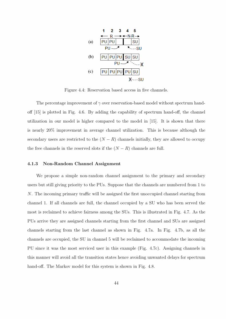
Figure 4.4: Reservation based access in five channels.

The percentage improvement of γ over reservation-based model without spectrum hand-

off [15] is plotted in Fig. 4.6. By adding the capability of spectrum hand-off, the channel

utilization in our model is higher compared to the model in [15]. It is shown that there

is nearly 20% improvement in average channel utilization. This is because although the

secondary users are restricted to the (N − R) channels initially, they are allowed to occupy

the free channels in the reserved slots if the (N − R) channels are full.

4.1.3 Non-Random Channel Assignment

We propose a simple non-random channel assignment to the primary and secondary

users but still giving priority to the PUs. Suppose that the channels are numbered from 1 to

N . The incoming primary traffic will be assigned the first unoccupied channel starting from

channel 1. If all channels are full, the channel occupied by a SU who has been served the

most is reclaimed to achieve fairness among the SUs. This is illustrated in Fig. 4.7. As the

PUs arrive they are assigned channels starting from the first channel and SUs are assigned

channels starting from the last channel as shown in Fig. 4.7a. In Fig. 4.7b, as all the

channels are occupied, the SU in channel 5 will be reclaimed to accommodate the incoming

PU since it was the most serviced user in this example (Fig. 4.7c). Assigning channels in

this manner will avoid all the transition states hence avoiding unwanted delays for spectrum

hand-off. The Markov model for this system is shown in Fig. 4.8.

44

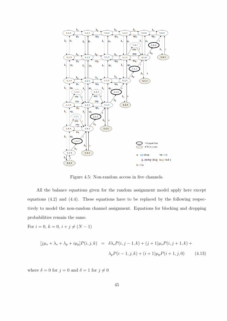
Figure 4.5: Non-random access in five channels.

All the balance equations given for the random assignment model apply here except

equations (4.2) and (4.4). These equations have to be replaced by the following respec-

tively to model the non-random channel assignment. Equations for blocking and dropping

probabilities remain the same.

For i = 0, k = 0, i + j 6= (N − 1)

[jµs + λs + λp + iµp]P (i, j, k) = δλsP (i, j − 1, k) + (j + 1)µsP (i, j + 1, k) +

λpP (i − 1, j, k) + (i + 1)µpP (i + 1, j, 0) (4.13)


45

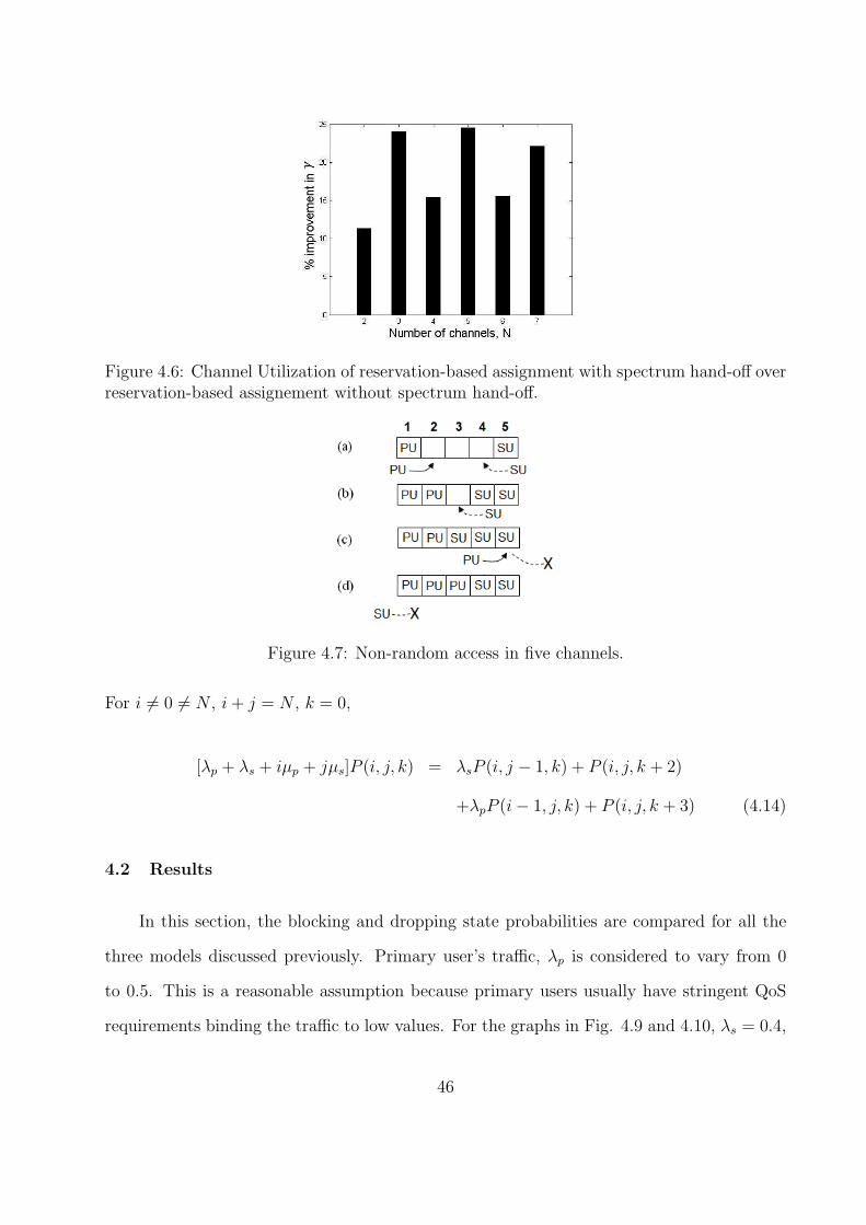
Figure 4.6: Channel Utilization of reservation-based assignment with spectrum hand-off overreservation-based assignement without spectrum hand-off.

Figure 4.7: Non-random access in five channels.

For i 6= 0 6= N , i + j = N , k = 0,

[λp + λs + iµp + jµs]P (i, j, k) = λsP (i, j − 1, k) + P (i, j, k + 2)

+λpP (i − 1, j, k) + P (i, j, k + 3) (4.14)

4.2 Results

In this section, the blocking and dropping state probabilities are compared for all the

three models discussed previously. Primary user’s traffic, λp is considered to vary from 0

to 0.5. This is a reasonable assumption because primary users usually have stringent QoS

requirements binding the traffic to low values. For the graphs in Fig. 4.9 and 4.10, λs = 0.4,

46

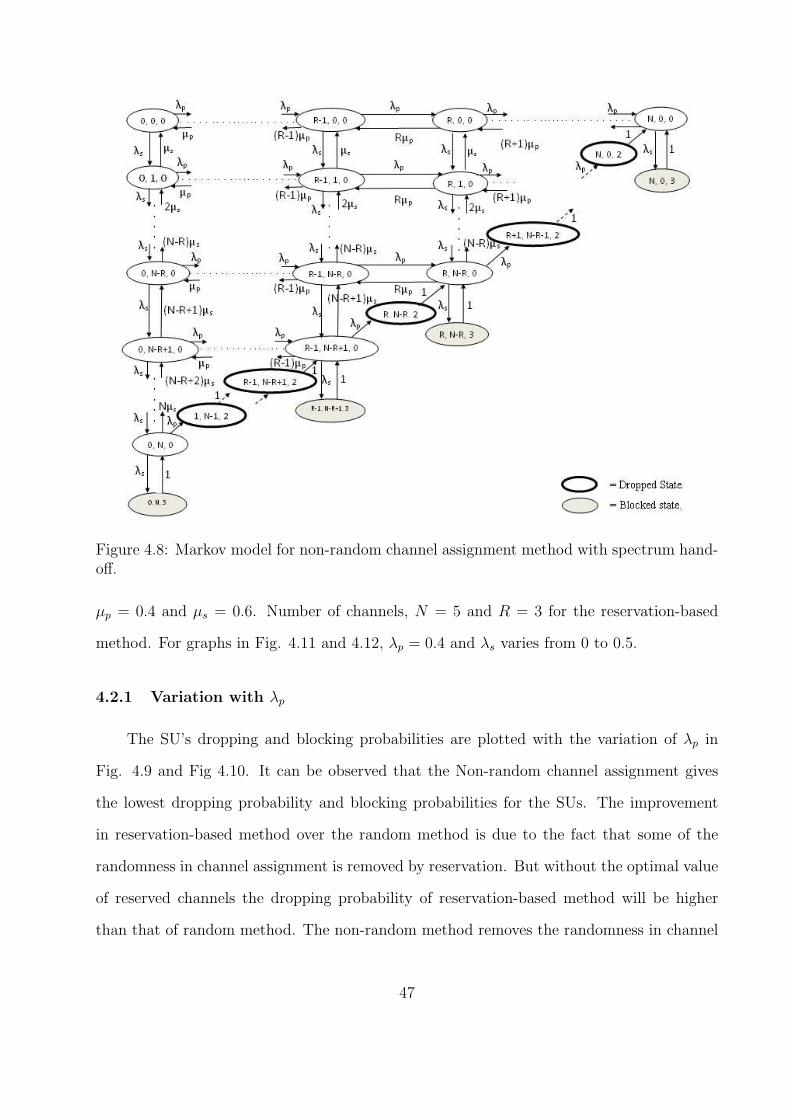
Figure 4.8: Markov model for non-random channel assignment method with spectrum hand-off.

µp = 0.4 and µs = 0.6. Number of channels, N = 5 and R = 3 for the reservation-based

method. For graphs in Fig. 4.11 and 4.12, λp = 0.4 and λs varies from 0 to 0.5.

4.2.1 Variation with λp

The SU’s dropping and blocking probabilities are plotted with the variation of λp in

Fig. 4.9 and Fig 4.10. It can be observed that the Non-random channel assignment gives

the lowest dropping probability and blocking probabilities for the SUs. The improvement

in reservation-based method over the random method is due to the fact that some of the

randomness in channel assignment is removed by reservation. But without the optimal value

of reserved channels the dropping probability of reservation-based method will be higher

than that of random method. The non-random method removes the randomness in channel

47

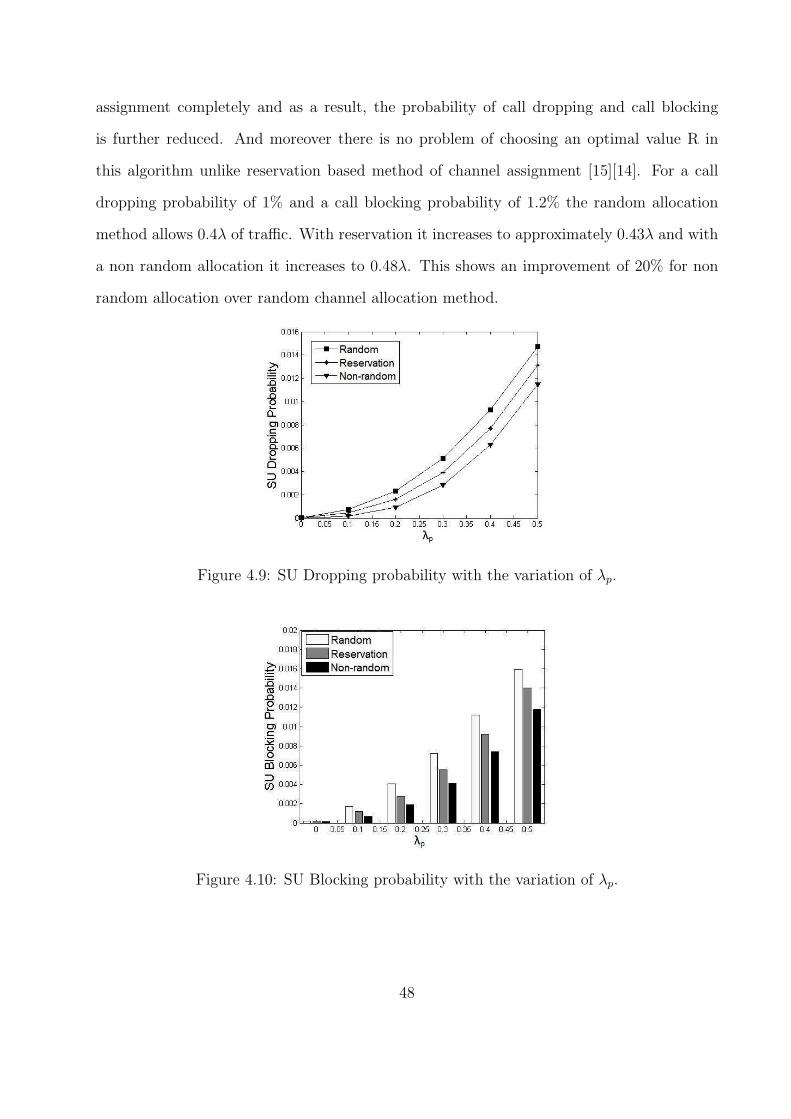
assignment completely and as a result, the probability of call dropping and call blocking

is further reduced. And moreover there is no problem of choosing an optimal value R in

this algorithm unlike reservation based method of channel assignment [15][14]. For a call

dropping probability of 1% and a call blocking probability of 1.2% the random allocation

method allows 0.4λ of traffic. With reservation it increases to approximately 0.43λ and with

a non random allocation it increases to 0.48λ. This shows an improvement of 20% for non

random allocation over random channel allocation method.

Figure 4.9: SU Dropping probability with the variation of λp.

Figure 4.10: SU Blocking probability with the variation of λp.

48

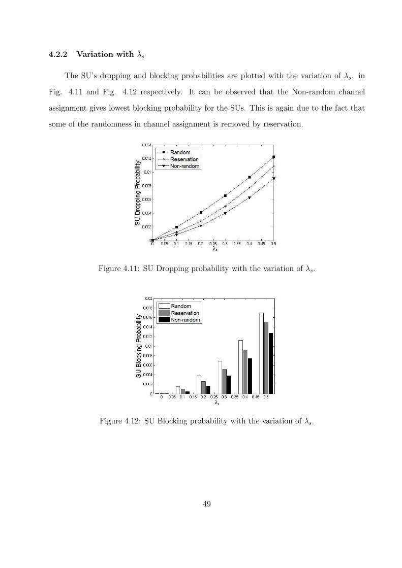
4.2.2 Variation with λs

The SU’s dropping and blocking probabilities are plotted with the variation of λs. in

Fig. 4.11 and Fig. 4.12 respectively. It can be observed that the Non-random channel

assignment gives lowest blocking probability for the SUs. This is again due to the fact that

some of the randomness in channel assignment is removed by reservation.

Figure 4.11: SU Dropping probability with the variation of λs.

Figure 4.12: SU Blocking probability with the variation of λs.

49

Chapter 5

Effect of Dynamic Spectrum Access on Transport Control

Protocol Performance

It is a known fact that TCP is inherently inefficient for wireless networks [20]. TCP was

originally designed for wired networks. In a wireless environment, packets may get lost due

to congestion or corruption of the physical medium. Cognitive networks worsen the situation

for the following reasons.

• Dynamic topology : As the channel of communication changes, some of the neighbors

who were reachable on the previous channel might not be reachable on the current

channel and vice versa. As a result the network topology changes with changes in

frequency of operation resulting in route failures and packet loss.

• Heterogeneity : Different channels may support different transmission ranges, data rates

and delay characteristics.

• Spectrum-Handoff delay : For each transition from one channel to another channel due

to the PU’s activity, there is a delay involved in the transition called Spectrum-Handoff

delay.

All these factors decrease the predictability of the cause of transit-delay and subsequent

packet loss on the network. The time latency during channel hand-off in cognitive networks

might cause the TCP round trip timer to time out. TCP will wrongly recognize the delays

and losses due to the above factors as network congestion and immediately take steps to

reduce the congestion window size knowing not the cause of packet delay. This reduces the

efficiency of the protocol in such environments.

50

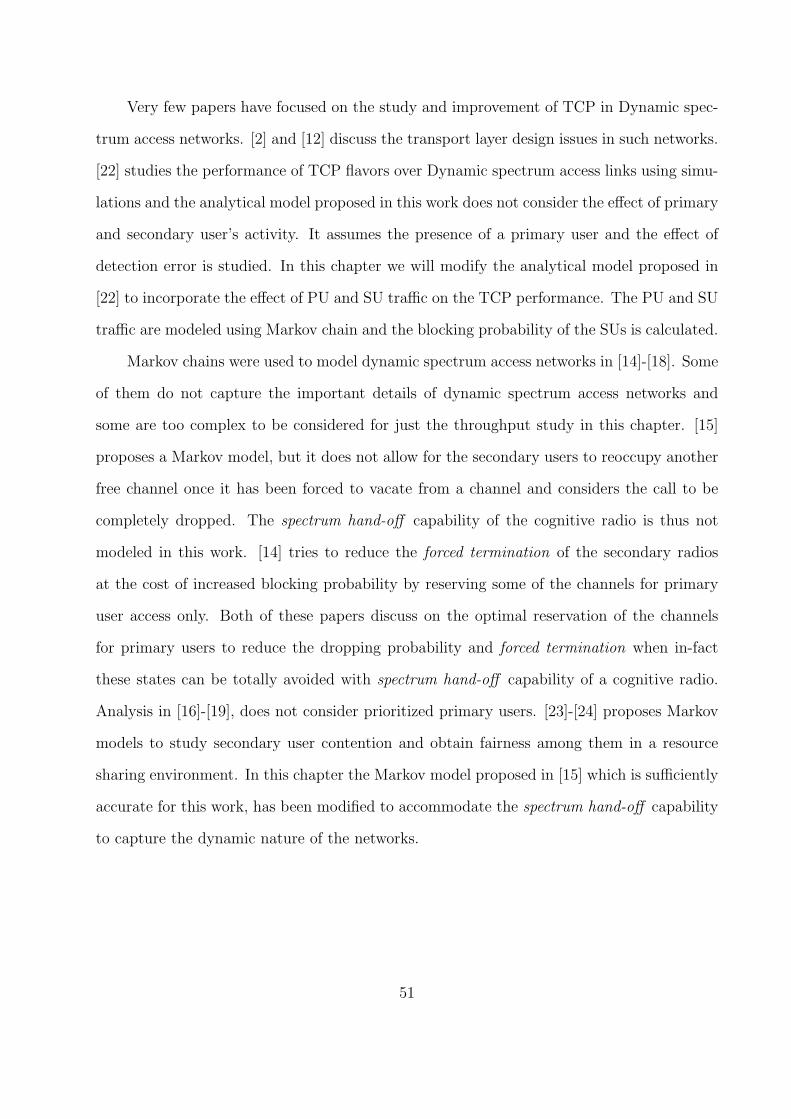
Very few papers have focused on the study and improvement of TCP in Dynamic spec-

trum access networks. [2] and [12] discuss the transport layer design issues in such networks.

[22] studies the performance of TCP flavors over Dynamic spectrum access links using simu-

lations and the analytical model proposed in this work does not consider the effect of primary

and secondary user’s activity. It assumes the presence of a primary user and the effect of

detection error is studied. In this chapter we will modify the analytical model proposed in

[22] to incorporate the effect of PU and SU traffic on the TCP performance. The PU and SU

traffic are modeled using Markov chain and the blocking probability of the SUs is calculated.

Markov chains were used to model dynamic spectrum access networks in [14]-[18]. Some

of them do not capture the important details of dynamic spectrum access networks and

some are too complex to be considered for just the throughput study in this chapter. [15]

proposes a Markov model, but it does not allow for the secondary users to reoccupy another

free channel once it has been forced to vacate from a channel and considers the call to be

completely dropped. The spectrum hand-off capability of the cognitive radio is thus not

modeled in this work. [14] tries to reduce the forced termination of the secondary radios

at the cost of increased blocking probability by reserving some of the channels for primary

user access only. Both of these papers discuss on the optimal reservation of the channels

for primary users to reduce the dropping probability and forced termination when in-fact

these states can be totally avoided with spectrum hand-off capability of a cognitive radio.

Analysis in [16]-[19], does not consider prioritized primary users. [23]-[24] proposes Markov

models to study secondary user contention and obtain fairness among them in a resource

sharing environment. In this chapter the Markov model proposed in [15] which is sufficiently

accurate for this work, has been modified to accommodate the spectrum hand-off capability

to capture the dynamic nature of the networks.

51

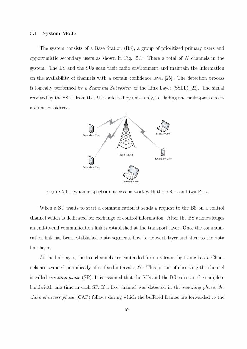
5.1 System Model

The system consists of a Base Station (BS), a group of prioritized primary users and

opportunistic secondary users as shown in Fig. 5.1. There a total of N channels in the

system. The BS and the SUs scan their radio environment and maintain the information

on the availability of channels with a certain confidence level [25]. The detection process

is logically performed by a Scanning Subsystem of the Link Layer (SSLL) [22]. The signal

received by the SSLL from the PU is affected by noise only, i.e. fading and multi-path effects

are not considered.

Primary User

Primary UserSecondary User

Secondary User

Secondary User

Base Station

Figure 5.1: Dynamic spectrum access network with three SUs and two PUs.

When a SU wants to start a communication it sends a request to the BS on a control

channel which is dedicated for exchange of control information. After the BS acknowledges

an end-to-end communication link is established at the transport layer. Once the communi-

cation link has been established, data segments flow to network layer and then to the data

link layer.

At the link layer, the free channels are contended for on a frame-by-frame basis. Chan-

nels are scanned periodically after fixed intervals [27]. This period of observing the channel

is called scanning phase (SP). It is assumed that the SUs and the BS can scan the complete

bandwidth one time in each SP. If a free channel was detected in the scanning phase, the

channel access phase (CAP) follows during which the buffered frames are forwarded to the

52

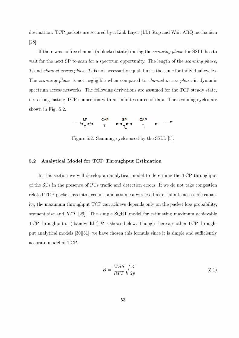
destination. TCP packets are secured by a Link Layer (LL) Stop and Wait ARQ mechanism

[28].

If there was no free channel (a blocked state) during the scanning phase the SSLL has to

wait for the next SP to scan for a spectrum opportunity. The length of the scanning phase,

Ti and channel access phase, To is not necessarily equal, but is the same for individual cycles.

The scanning phase is not negligible when compared to channel access phase in dynamic

spectrum access networks. The following derivations are assumed for the TCP steady state,

i.e. a long lasting TCP connection with an infinite source of data. The scanning cycles are

shown in Fig. 5.2.

Figure 5.2: Scanning cycles used by the SSLL [5].

5.2 Analytical Model for TCP Throughput Estimation

In this section we will develop an analytical model to determine the TCP throughput

of the SUs in the presence of PUs traffic and detection errors. If we do not take congestion

related TCP packet loss into account, and assume a wireless link of infinite accessible capac-

ity, the maximum throughput TCP can achieve depends only on the packet loss probability,

segment size and RTT [29]. The simple SQRT model for estimating maximum achievable

TCP throughput or (’bandwidth’) B is shown below. Though there are other TCP through-

put analytical models [30][31], we have chosen this formula since it is simple and sufficiently

accurate model of TCP.

B =MSS

RTT

√

3

2p(5.1)

53

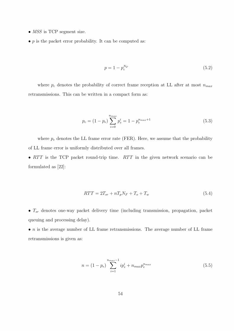
• MSS is TCP segment size.

• p is the packet error probability. It can be computed as:

p = 1 − pNFc (5.2)

where pc denotes the probability of correct frame reception at LL after at most nmax

retransmissions. This can be written in a compact form as:

pc = (1 − pe)nmax∑

i=0

pie = 1 − pnmax+1

e (5.3)

where pe denotes the LL frame error rate (FER). Here, we assume that the probability

of LL frame error is uniformly distributed over all frames.

• RTT is the TCP packet round-trip time. RTT in the given network scenario can be

formulated as [22]:

RTT = 2Tsr + nTpNF + To + Tw (5.4)

• Tsr denotes one-way packet delivery time (including transmission, propagation, packet

queuing and processing delay).

• n is the average number of LL frame retransmissions. The average number of LL frame

retransmissions is given as:

n = (1 − pe)nmax−1∑

i=1

ipie + nmaxp

nmax

e (5.5)

54

where nmax is the maximum number of retransmissions of one LL frame.

• NF is the number of LL frames per TCP packet.

• Tp is the delay of the ARQ protocol, introduced by LL frame retransmissions.

• To is the channel observation time or the scanning time.

• Tw is the average delay that a packet incurs when either channel is not available or an

improper decision is made by the scanner. In this chapter, we are concerned with the delay

(Tw) caused due to the unavailability of the channels and detection errors which is derived

below.

5.2.1 Estimation of Wait time Tw

In each individual scan, either of the following events will increase the RTT by an

inter-scanning interval of Ti.

1. A spectrum opportunity may be available or not based on the primary user’s traffic.

If there is no channel available then the user has to wait until the next scan interval

(S) by waiting Ti seconds.

2. When a channel is available, a decision on the availability of the channel may result in

an error, thus detecting that the channel is not available.

The average time a TCP packet must wait to gain access to the channel is given by Tw.

Tw = limn→∞

n∑

k=1

[pb + pf (1 − pb)]kTi

=Ti [pb + pf (1 − pb)]

1 − [pb + pf (1 − pb)](5.6)

where,

55

pf =Γ

(

WTo,ν2

)

Γ (WTo)(5.7)

where pb is the blocking probability which means that that no channel is free. pf is

the probability of false alarm, i.e. misinterpretation of a free channel as occupied. W is

the bandwidth of the PU channel, ν is the threshold of the energy detector, and Γ(., .) and

Γ(.) are upper incomplete gamma and gamma functions, respectively [26][27]. The model

proposed in [27] assumes the absence of PUs. Our model considers PU traffic and takes the

effect of probability of detecting the PU on a DSA link, limiting the probability of introducing

interference to the PU system by the DSA device.

5.2.2 Markov Model to determine Blocking probability, pb

In this sub-section a Markov model to determine the blocking probability of SU frames

is discussed.

There are a total of N channels available for both secondary and primary users. Each

channel is assumed to be of equal bandwidth. The PUs traffic in each channel is assumed to

follow an ON/OFF pattern. A channel can be accessed by a SU if it is not being occupied

by any PU. In this model it is assumed that both the PUs and SUs access the channels

randomly. This is explained with the help of Fig. 5.3. There are a total of five channels

of which two are occupied by PUs and one by an SU. When a new SU arrives as shown in

Fig. 5.3a, it chooses a random free channel. A PU can choose any random channel and as

shown in Fig. 5.3b, if it chooses a secondary occupied channel, the SU jumps to a different

free channel. If there is no other channel available, the SU’s service is dropped as shown in

Fig. 5.3c. An SU cannot use a channel if it does not have an opportunity to do so as shown

in Fig 5.3c.

56

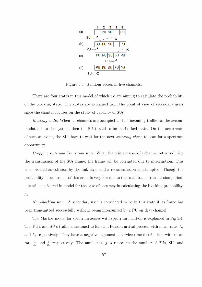
Figure 5.3: Random access in five channels.

There are four states in this model of which we are aiming to calculate the probability

of the blocking state. The states are explained from the point of view of secondary users

since the chapter focuses on the study of capacity of SUs.

Blocking state: When all channels are occupied and no incoming traffic can be accom-

modated into the system, then the SU is said to be in Blocked state. On the occurrence

of such an event, the SUs have to wait for the next scanning phase to scan for a spectrum

opportunity.

Dropping state and Transition state: When the primary user of a channel returns during

the transmission of the SUs frame, the frame will be corrupted due to interruption. This

is considered as collision by the link layer and a retransmission is attempted. Though the

probability of occurrence of this event is very low due to the small frame transmission period,

it is still considered in model for the sake of accuracy in calculating the blocking probability,

pb.

Non-blocking state: A secondary user is considered to be in this state if its frame has

been transmitted successfully without being interrupted by a PU on that channel.

The Markov model for spectrum access with spectrum hand-off is explained in Fig 5.4.

The PU’s and SU’s traffic is assumed to follow a Poisson arrival process with mean rates λp

and λs respectively. They have a negative exponential service time distribution with mean

rate 1

µpand 1

µsrespectively. The numbers i, j, k represent the number of PUs, SUs and

57

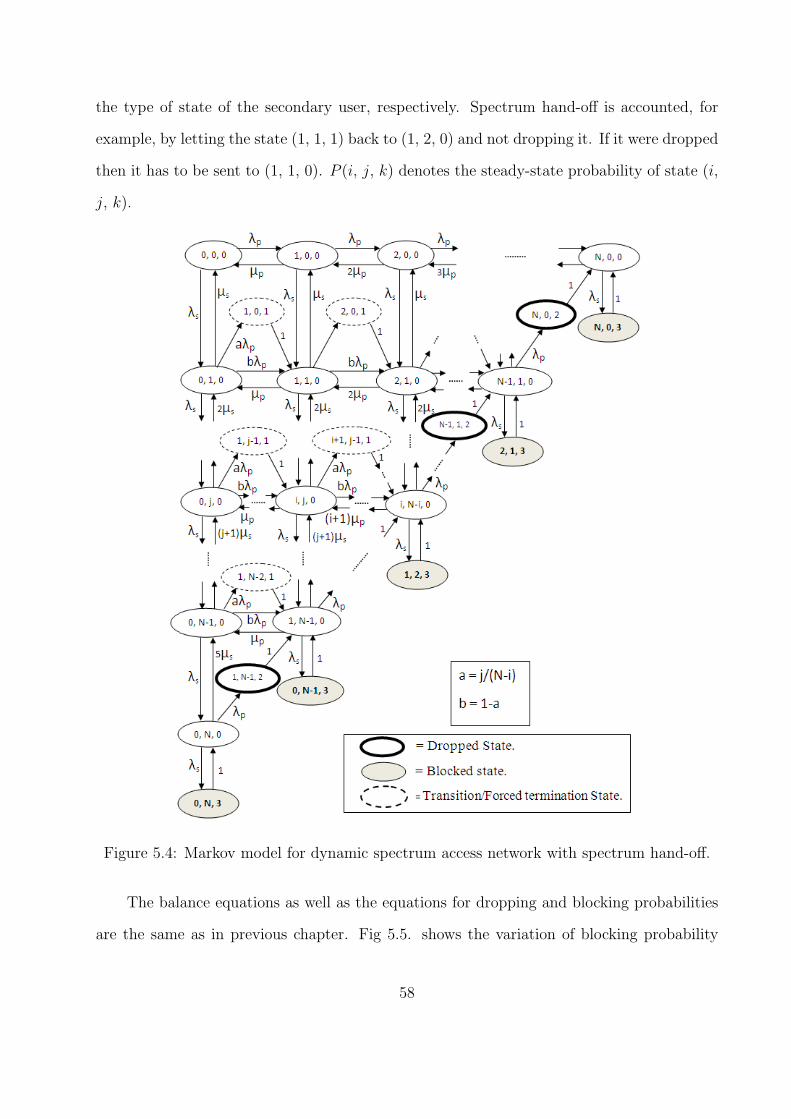
the type of state of the secondary user, respectively. Spectrum hand-off is accounted, for

example, by letting the state (1, 1, 1) back to (1, 2, 0) and not dropping it. If it were dropped

then it has to be sent to (1, 1, 0). P (i, j, k) denotes the steady-state probability of state (i,

j, k).

Figure 5.4: Markov model for dynamic spectrum access network with spectrum hand-off.

The balance equations as well as the equations for dropping and blocking probabilities

are the same as in previous chapter. Fig 5.5. shows the variation of blocking probability

58

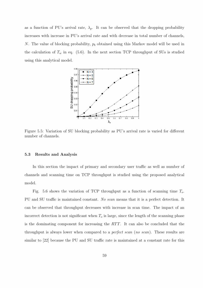
as a function of PU’s arrival rate, λp. It can be observed that the dropping probability

increases with increase in PU’s arrival rate and with decrease in total number of channels,

N . The value of blocking probability, pb obtained using this Markov model will be used in

the calculation of Tw in eq. (5.6). In the next section TCP throughput of SUs is studied

using this analytical model.

Figure 5.5: Variation of SU blocking probability as PU’s arrival rate is varied for differentnumber of channels.

5.3 Results and Analysis

In this section the impact of primary and secondary user traffic as well as number of

channels and scanning time on TCP throughput is studied using the proposed analytical

model.

Fig. 5.6 shows the variation of TCP throughput as a function of scanning time To.

PU and SU traffic is maintained constant. No scan means that it is a perfect detection. It

can be observed that throughput decreases with increase in scan time. The impact of an

incorrect detection is not significant when To is large, since the length of the scanning phase

is the dominating component for increasing the RTT . It can also be concluded that the

throughput is always lower when compared to a perfect scan (no scan). These results are

similar to [22] because the PU and SU traffic rate is maintained at a constant rate for this

59

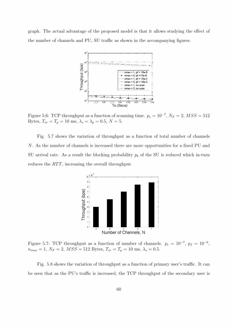
graph. The actual advantage of the proposed model is that it allows studying the effect of

the number of channels and PU, SU traffic as shown in the accompanying figures.

Figure 5.6: TCP throughput as a function of scanning time. pe = 10−7, NF = 2, MSS = 512Bytes, Tsr = Tp = 10 ms, λs = λp = 0.5, N = 5.

Fig. 5.7 shows the variation of throughput as a function of total number of channels

N . As the number of channels is increased there are more opportunities for a fixed PU and

SU arrival rate. As a result the blocking probability pb of the SU is reduced which in-turn

reduces the RTT , increasing the overall throughput.

Figure 5.7: TCP throughput as a function of number of channels. pe = 10−7, pf = 10−6,nmax = 1, NF = 2, MSS = 512 Bytes, Tsr = Tp = 10 ms, λs = 0.5.

Fig. 5.8 shows the variation of throughput as a function of primary user’s traffic. It can

be seen that as the PU’s traffic is increased, the TCP throughput of the secondary user is

60

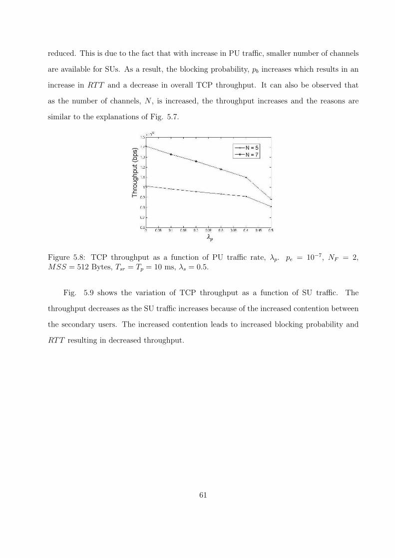
reduced. This is due to the fact that with increase in PU traffic, smaller number of channels

are available for SUs. As a result, the blocking probability, pb increases which results in an

increase in RTT and a decrease in overall TCP throughput. It can also be observed that

as the number of channels, N , is increased, the throughput increases and the reasons are

similar to the explanations of Fig. 5.7.

Figure 5.8: TCP throughput as a function of PU traffic rate, λp. pe = 10−7, NF = 2,MSS = 512 Bytes, Tsr = Tp = 10 ms, λs = 0.5.

Fig. 5.9 shows the variation of TCP throughput as a function of SU traffic. The

throughput decreases as the SU traffic increases because of the increased contention between

the secondary users. The increased contention leads to increased blocking probability and

RTT resulting in decreased throughput.

61

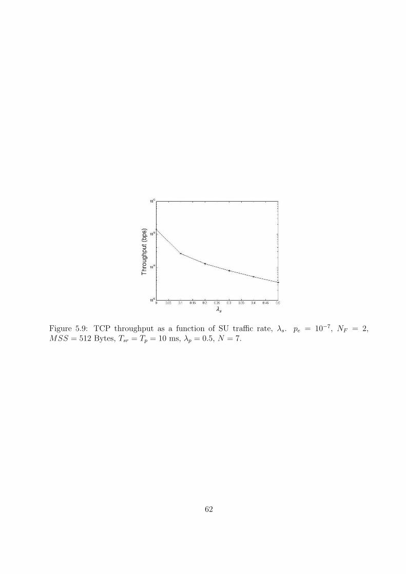
Figure 5.9: TCP throughput as a function of SU traffic rate, λs. pe = 10−7, NF = 2,MSS = 512 Bytes, Tsr = Tp = 10 ms, λp = 0.5, N = 7.

62

Chapter 6

Enforcing Cooperative Spectrum Sensing in a Multi-hop Cognitive Radio Network

Cognitive radio network is well known as an opportunistic network in which the sec-

ondary users use the spectrum owned by primary users when they are idle. In order for the

secondary users to know the primary users presence, they have to perform Spectrum Sensing

which is defined as the task of scanning the available spectrum for primary user activity.

Since the whole concept of cognitive radio network relies on sensing the primary user activity,

spectrum sensing is the most important task for the operation of a cognitive radio network.

Spectrum sensing is of two types: Distributed and Centralized sensing of which dis-

tributed sensing has been proved to be more efficient [33]. In distributed sensing all the

nodes scan their spectrum and share their results with a central authority who builds the

final spectrum availability map by combining all the sensing results. This task grows more

cumbersome and crucial in a multi-hop cognitive radio network. In a multi-hop scenario,

each node shares its sensing results with all other nodes and each node creates its own spec-

trum availability map using the results it received. Spectrum sensing is a periodic task and

so is the task of sharing the sensing results which will consume significant amount of energy.

As a result, it is possible that users will stop sharing the sensing results to conserve energy.

Such a user is called a non-cooperating/selfish user. Non-cooperation in the spectrum sens-

ing phase leads to incomplete spectrum occupancy maps. Eventually, cognitive users will

avoid using the channels with incomplete information of primary activity, leading to reduced

network throughput.

To enforce cooperation in spectrum sensing, we should either punish a non-cooperating

node or provide an incentive for cooperation. The classic Tit-For-Tat (TFT) strategy cannot

be used to achieve cooperative spectrum sensing since it is not possible to punish a node

63

individually. In other words, in a Tit-For-Tat strategy, punishing a selfish node by not broad-

casting the sensing results also affects other nodes which will in turn trigger punishments. In

the literature, only a few [34, 35] have focused on enforcing cooperative spectrum sensing. In

[34] the author proposes the use of Carrot and Stick strategy in which all nodes stop cooper-

ating once a non-cooperating node is detected and they resume cooperation after every user

stops cooperating. The biggest disadvantage of this strategy is that there will be frequent

network shutdowns due to collision errors. Also, a malicious user can take advantage of the

game model to disrupt the network by either being irrationally selfish or by intentionally

causing collisions during the sharing period of the sensing results. Moreover, the game was

not designed for multi-hop communication. [35] deals with achieving cooperative spectrum

sensing in a centralized cognitive radio network. In summary, achieving cooperation in a

multi-hop cognitive radio network has the following issues: traditional TFT strategy cannot

be used, security attacks can be launched taking advantage of an inefficient game model,

ensuring cooperation in a multi-hop scenario is complicated.

In this chapter, we address these issues by designing a Cross-Layer game which is a

combination of the spectrum sensing game in the physical layer and packet forwarding game

in the network layer. The basic idea of this model is to punish the selfish users i.e., those

who do not share their sensing results, by denying to cooperate in the network layer. This

model takes advantage of one-to-one punishments in the packet forwarding game to enforce

cooperative spectrum sensing in the physical layer. Though it is not described in this work,

the Cross-Layer game can easily be extended to a centralized cognitive network.

6.1 System Model and Assumptions

We consider a multi-hop cognitive radio network (MHCRN) where there is no central

authority to control the access to the spectrum. The nodes have to cooperate among them-

selves to form a network and exchange data to multi-hop destinations. Under steady state

64

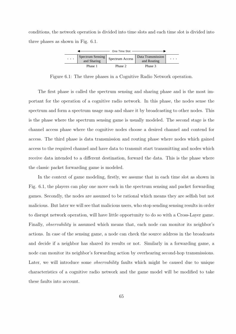
conditions, the network operation is divided into time slots and each time slot is divided into

three phases as shown in Fig. 6.1.

Spectrum Sensing and Sharing

Spectrum AccessData Transmission

and Routing

Phase 1 Phase 3Phase 2

. . .. . .

One Time Slot

Figure 6.1: The three phases in a Cognitive Radio Network operation.

The first phase is called the spectrum sensing and sharing phase and is the most im-

portant for the operation of a cognitive radio network. In this phase, the nodes sense the

spectrum and form a spectrum usage map and share it by broadcasting to other nodes. This

is the phase where the spectrum sensing game is usually modeled. The second stage is the

channel access phase where the cognitive nodes choose a desired channel and contend for

access. The third phase is data transmission and routing phase where nodes which gained

access to the required channel and have data to transmit start transmitting and nodes which

receive data intended to a different destination, forward the data. This is the phase where

the classic packet forwarding game is modeled.

In the context of game modeling, firstly, we assume that in each time slot as shown in

Fig. 6.1, the players can play one move each in the spectrum sensing and packet forwarding

games. Secondly, the nodes are assumed to be rational which means they are selfish but not

malicious. But later we will see that malicious users, who stop sending sensing results in order

to disrupt network operation, will have little opportunity to do so with a Cross-Layer game.

Finally, observability is assumed which means that, each node can monitor its neighbor’s

actions. In case of the sensing game, a node can check the source address in the broadcasts

and decide if a neighbor has shared its results or not. Similarly in a forwarding game, a

node can monitor its neighbor’s forwarding action by overhearing second-hop transmissions.

Later, we will introduce some observability faults which might be caused due to unique

characteristics of a cognitive radio network and the game model will be modified to take

these faults into account.

65

6.2 Game Theory Applied to Multi-hop Cognitive Radio Network

In this section, we define Spectrum Sensing and Packet Forwarding games which are

required for designing the Cross-Layer game. Each of these games is independent and is

played in different layers of the protocol stack.

6.2.1 Cooperative Spectrum Sensing Game

Spectrum Sensing is performed at the physical layer and we categorize the Cooperative

Spectrum Sensing game as being played at the physical layer of the protocol stack. The

Cooperative Spectrum Sensing is a two stage process. The first stage is the sensing period

in which, each node senses its environment for primary user activity and creates a spectrum

usage map. The second stage is the cooperative sharing period in which, each node broad-

casts its map to its neighbors. The later task of sharing the spectrum map is more resource

consuming than sensing. So the selfish nodes might deviate from cooperating by not sharing

their map in which case the deviating node receives all other maps but other nodes do not

receive the deviating node’s map. Assume that there are N nodes in the network and each

node gains α units if it receives all N maps and loses Csh units by sharing its map. Since

the spectrum usage maps of all the nodes is important for analyzing the overall primary

user activity, every node is in constant need of the cooperation of all other nodes. So, the

interaction between all nodes can be defined as a strategic game where each player’s strategy

is to either share (denoted as 1) or not share (denoted as 0) the sensing results. Following

the standard game theoretic notation [38], we will write i to denote a generic player, and −i

to denote all other N − 1 players. Thus, we have the following

Definition 1: A spectrum sensing game is the game G = 〈N, {ai}, {Ui}〉 where,

• N = 1, 2, 3, . . . is a set of players.

• ai ∈ {0, 1} is the action of node i.

• Ui = αa−i − Csai is the payoff of player i.

66

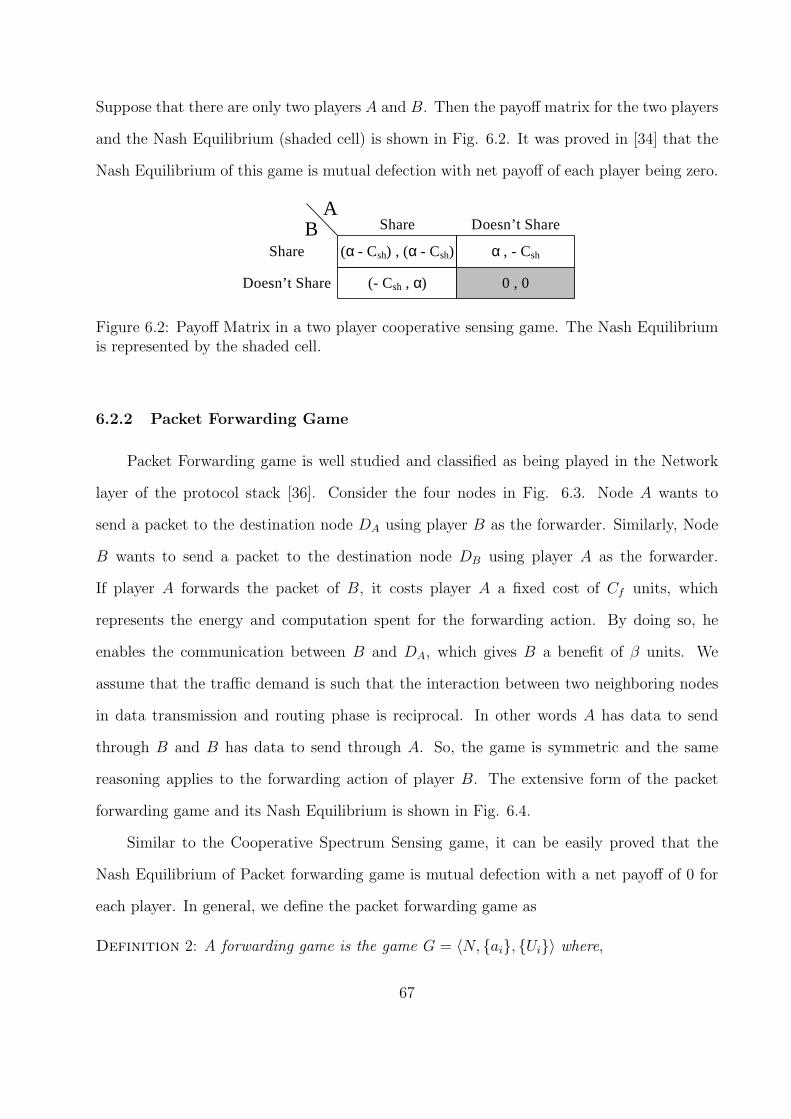
Suppose that there are only two players A and B. Then the payoff matrix for the two players

and the Nash Equilibrium (shaded cell) is shown in Fig. 6.2. It was proved in [34] that the

Nash Equilibrium of this game is mutual defection with net payoff of each player being zero.

(α - Csh) , (α - Csh) α , - Csh

(- Csh , α) 0 , 0

AShare Doesn’t Share

Share

Doesn’t Share

B

Figure 6.2: Payoff Matrix in a two player cooperative sensing game. The Nash Equilibriumis represented by the shaded cell.

6.2.2 Packet Forwarding Game

Packet Forwarding game is well studied and classified as being played in the Network

layer of the protocol stack [36]. Consider the four nodes in Fig. 6.3. Node A wants to

send a packet to the destination node DA using player B as the forwarder. Similarly, Node

B wants to send a packet to the destination node DB using player A as the forwarder.

If player A forwards the packet of B, it costs player A a fixed cost of Cf units, which

represents the energy and computation spent for the forwarding action. By doing so, he

enables the communication between B and DA, which gives B a benefit of β units. We

assume that the traffic demand is such that the interaction between two neighboring nodes

in data transmission and routing phase is reciprocal. In other words A has data to send

through B and B has data to send through A. So, the game is symmetric and the same

reasoning applies to the forwarding action of player B. The extensive form of the packet

forwarding game and its Nash Equilibrium is shown in Fig. 6.4.

Similar to the Cooperative Spectrum Sensing game, it can be easily proved that the

Nash Equilibrium of Packet forwarding game is mutual defection with a net payoff of 0 for

each player. In general, we define the packet forwarding game as

Definition 2: A forwarding game is the game G = 〈N, {ai}, {Ui}〉 where,

67

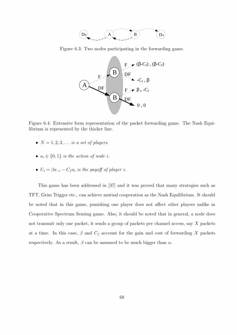
A B DA DB

Figure 6.3: Two nodes participating in the forwarding game.

A

B

B

-Cf , β

(β-Cf) , (β-Cf)

β , -Cf

0 , 0

DF

DF

F

FDF

F

Figure 6.4: Extensive form representation of the packet forwarding game. The Nash Equi-librium is represented by the thicker line.


• ai ∈ {0, 1} is the action of node i.

• Ui = βa−i − Cfai is the payoff of player i.

This game has been addressed in [37] and it was proved that many strategies such as

TFT, Grim Trigger etc., can achieve mutual cooperation as the Nash Equilibrium. It should

be noted that in this game, punishing one player does not affect other players unlike in

Cooperative Spectrum Sensing game. Also, it should be noted that in general, a node does

not transmit only one packet, it sends a group of packets per channel access, say X packets

at a time. In this case, β and Cf account for the gain and cost of forwarding X packets

respectively. As a result, β can be assumed to be much bigger than α.

68

6.3 Cross-Layer Game

In this section, we introduce a Cross-Layer game as a combination of the spectrum

sensing game and the packet forwarding games which are now the sub-games of the Cross-

Layer game. The basic idea behind the design of the Cross-Layer game is that the nodes are

interested in the combined utilization than the independent sub-game utilizations.

In a single stage Cross-Layer game, a player i’s action (ai), comprises of two moves in

one time slot, called the sensing action (asi ) and the forwarding action (af

i ). The sensing

action is the same action as in the spectrum sensing game, and asi = 1 means that player

i cooperates and shares his map which costs him Csh units. ashi = 0 means that player i

defects and it doesn’t incur him any cost. If the opponents, denoted by −i, share their maps,

player i gains α units. Similarly, the forwarding action is the same action as in the packet

forwarding game and afi = 1 means that player i cooperates and forwards player, −i’s packet

which costs him Cf units. afi = 0 means that player i defects and he saves Cf units. If the

opponent, −i forwards i’s packets, player i gains β units. The utilization of each player is

the sum of the utilizations of their sensing and forwarding actions. Thus, the Cross-Layer

game is defined as:

Definition 3: A Cross-Layer game is the game G = 〈N, {ai}, {Ui}〉 where,


• ai = (asi , a

fi ) is the action of node i where, as

i ∈ {0, 1} is the sensing action and

afi ∈ {0, 1} is the forwarding action of the node.

• Ui = αas−i − Csa

si + βaf

−i − Cfafi is player i’s payoff.

As an example, reconsider Fig. 6.3 in which there are four nodes forming a multi-hop

cognitive radio network. Suppose nodes DA and DB always cooperate, we are only interested

in the action of nodes A and B. The nodes, as players in the Cross-Layer game have to decide

69

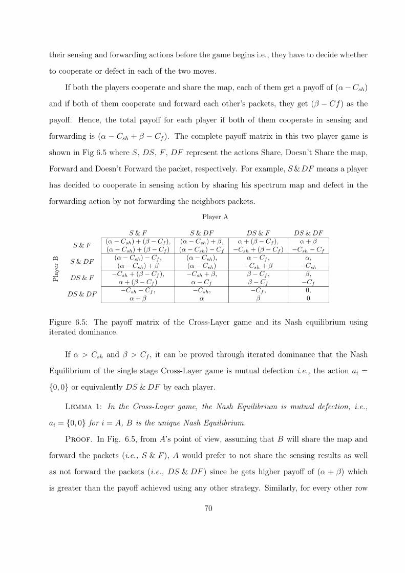
their sensing and forwarding actions before the game begins i.e., they have to decide whether

to cooperate or defect in each of the two moves.

If both the players cooperate and share the map, each of them get a payoff of (α−Csh)

and if both of them cooperate and forward each other’s packets, they get (β − Cf) as the

payoff. Hence, the total payoff for each player if both of them cooperate in sensing and

forwarding is (α − Csh + β − Cf ). The complete payoff matrix in this two player game is

shown in Fig 6.5 where S, DS, F , DF represent the actions Share, Doesn’t Share the map,

Forward and Doesn’t Forward the packet, respectively. For example, S &DF means a player

has decided to cooperate in sensing action by sharing his spectrum map and defect in the

forwarding action by not forwarding the neighbors packets.

Player A

S & F S & DF DS & F DS & DF

Pla

yer

B

S & F(α − Csh) + (β − Cf ), (α − Csh) + β, α + (β − Cf ), α + β

(α − Csh) + (β − Cf ) (α − Csh) − Cf −Csh + (β − Cf ) −Csh − Cf

S & DF(α − Csh) − Cf , (α − Csh), α − Cf , α,(α − Csh) + β (α − Csh) −Csh + β −Csh

DS & F−Csh + (β − Cf ), −Csh + β, β − Cf , β,

α + (β − Cf ) α − Cf β − Cf −Cf

DS & DF−Csh − Cf , −Csh, −Cf , 0,

α + β α β 0

Figure 6.5: The payoff matrix of the Cross-Layer game and its Nash equilibrium usingiterated dominance.

If α > Csh and β > Cf , it can be proved through iterated dominance that the Nash

Equilibrium of the single stage Cross-Layer game is mutual defection i.e., the action ai =

{0, 0} or equivalently DS & DF by each player.

Lemma 1: In the Cross-Layer game, the Nash Equilibrium is mutual defection, i.e.,

ai = {0, 0} for i = A, B is the unique Nash Equilibrium.

Proof. In Fig. 6.5, from A’s point of view, assuming that B will share the map and

forward the packets (i.e., S & F ), A would prefer to not share the sensing results as well

as not forward the packets (i.e., DS & DF ) since he gets higher payoff of (α + β) which

is greater than the payoff achieved using any other strategy. Similarly, for every other row

70

of B’s action, A would prefer the strategy DS & DF as it strictly dominates over other

strategies. So, we can eliminate the first three columns, since a rational player A will never

choose these strategies. A similar reasoning, now from the point of view of player B, leads

to the elimination of the first three rows of the matrix. As a result, the Nash Equilibrium

of the game is DS & DF by both the players leading to a payoff of 0 for each player. 2

While the above result indicates that mutual defection is the only Nash Equilibrium if

the game is played only once, we will show in the rest of the chapter that cooperation can

emerge under certain conditions, if the game is repeatedly played.

6.3.1 Cross-Layer Game without Observability Faults

In any network, there is usually more than one interaction between the neighboring

nodes. This implies that the interaction between the neighboring nodes can be modeled as

a repeated game. In such a game, the players have to take into account the future effects of

their present actions. Assuming that each stage of the Cross-Layer game comprises of one

game each of spectrum sensing and packet forwarding game, we have the following definition.

Definition 4: A Repeated Cross-Layer Game is the multistage game Γ = 〈N, si, Ui〉

where


• ai(t) = (asi (t), a

fi (t)) is the action of player i at stage\time t.

• Ui(t) = αas−i(t) − Csa

si (t) + βaf

−i(t) − Cfafi (t) is the payoff of player i.

• si = (ai(0), ai(1), . . .) is the strategy of player i.

• Ui = (1 − δ)∑∞

t=0Ui(t) · δ

t is the normalized discounted payoff of player i.

The discount parameter 0 ≤ δ ≤ 1 is a measure of the subjective evaluation of the

future by the players. The parameter δ can also be interpreted as the probability that each

71

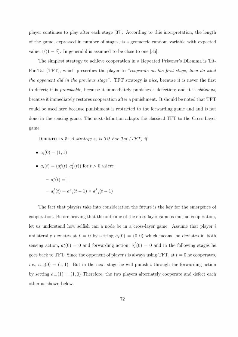
player continues to play after each stage [37]. According to this interpretation, the length

of the game, expressed in number of stages, is a geometric random variable with expected

value 1/(1 − δ). In general δ is assumed to be close to one [36].

The simplest strategy to achieve cooperation in a Repeated Prisoner’s Dilemma is Tit-

For-Tat (TFT), which prescribes the player to “cooperate on the first stage, then do what

the opponent did in the previous stage”. TFT strategy is nice, because it is never the first

to defect; it is provokable, because it immediately punishes a defection; and it is oblivious,

because it immediately restores cooperation after a punishment. It should be noted that TFT

could be used here because punishment is restricted to the forwarding game and and is not

done in the sensing game. The next definition adapts the classical TFT to the Cross-Layer

game.

Definition 5: A strategy si is Tit For Tat (TFT) if

• ai(0) = (1, 1)

• ai(t) = (asi (t), a

fi (t)) for t > 0 where,

– asi (t) = 1

– afi (t) = as

−i(t − 1) × af−i(t − 1)

The fact that players take into consideration the future is the key for the emergence of

cooperation. Before proving that the outcome of the cross-layer game is mutual cooperation,

let us understand how selfish can a node be in a cross-layer game. Assume that player i

unilaterally deviates at t = 0 by setting ai(0) = (0, 0) which means, he deviates in both

sensing action, asi (0) = 0 and forwarding action, af

i (0) = 0 and in the following stages he

goes back to TFT. Since the opponent of player i is always using TFT, at t = 0 he cooperates,

i.e., a−i(0) = (1, 1). But in the next stage he will punish i through the forwarding action

by setting a−i(1) = (1, 0) Therefore, the two players alternately cooperate and defect each

other as shown below.

72

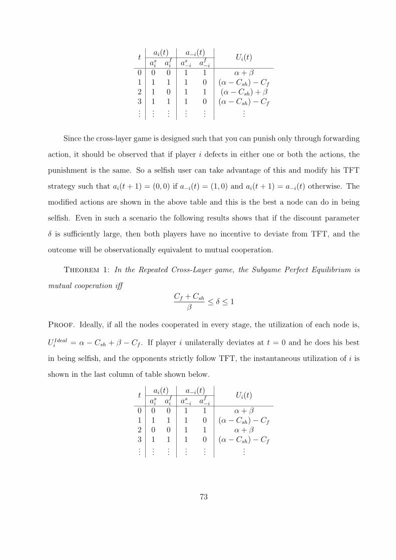
tai(t) a−i(t) Ui(t)

asi af

i as−i af

−i

0 0 0 1 1 α + β1 1 1 1 0 (α − Csh) − Cf

2 1 0 1 1 (α − Csh) + β3 1 1 1 0 (α − Csh) − Cf

......

......

......

Since the cross-layer game is designed such that you can punish only through forwarding

action, it should be observed that if player i defects in either one or both the actions, the

punishment is the same. So a selfish user can take advantage of this and modify his TFT

strategy such that ai(t + 1) = (0, 0) if a−i(t) = (1, 0) and ai(t + 1) = a−i(t) otherwise. The

modified actions are shown in the above table and this is the best a node can do in being

selfish. Even in such a scenario the following results shows that if the discount parameter

δ is sufficiently large, then both players have no incentive to deviate from TFT, and the

outcome will be observationally equivalent to mutual cooperation.

Theorem 1: In the Repeated Cross-Layer game, the Subgame Perfect Equilibrium is

mutual cooperation iff

Cf + Csh

β≤ δ ≤ 1

Proof. Ideally, if all the nodes cooperated in every stage, the utilization of each node is,

U Ideali = α − Csh + β − Cf . If player i unilaterally deviates at t = 0 and he does his best

in being selfish, and the opponents strictly follow TFT, the instantaneous utilization of i is

shown in the last column of table shown below.

tai(t) a−i(t) Ui(t)

asi af

i as−i af

−i

0 0 0 1 1 α + β1 1 1 1 0 (α − Csh) − Cf

2 0 0 1 1 α + β3 1 1 1 0 (α − Csh) − Cf

......

......

......

73

The total Utilization, Ui is the sum of all instantaneous utilizations, Ui(t) which can be

written as:

Ui = (1 − δ) [(α + β) + δ (α − Csh − Cf ) +

δ2 (α + β) + δ3 (α − Csh − Cf ) + . . .]

= (1 − δ)[

α(

1 + δ + δ2 + . . .)

+

(β − δCsh − δCf )(

1 + δ2 + δ4 + . . .)]

= α +(β − δCsh − δCf )

(1 + δ)(6.1)

This is the maximum utilization achieved when one of the nodes does his best in being

selfish. Cooperation can be achieved only if the utilization achieved by defecting is less than

or equal to the utilization achieved by cooperating i.e., Ui ≤ U Ideali . So, player i will have

no incentive from deviating from cooperation if and only if, Ui ≤ α − Csh + β − Cf , i.e., iff

δβ ≥ Cf + Csh. From the one-step deviation principle [38], if deviating in one stage is not

profitable, then it is not profitable to deviate in more than one consecutive stage. Hence,

mutual cooperation is a Subgame Perfect Equilibrium. 2

This result shows that cooperation can emerge in a network of selfish nodes, if they are

sufficiently far-sighted. But this is not surprising. What is important is that the Cross-Layer

game can achieve cooperation in both spectrum sensing and packet forwarding by using pun-

ishments in the packet forwarding stage alone. Since the cognitive radio network’s operation

is strongly dependent on spectrum sensing results, it is important that the spectrum sensing

action of players is not disturbed due to few non-cooperating nodes. The most important

advantage of the Cross-layer game over traditional game models is that, the defection by a

single player does not disturb the spectrum sensing action of other players which avoids any

disruption to the entire cognitive network.

74

The above cross-layer model does not take into account the broadcast nature of the

wireless medium and the spectrum handoffs in cognitive radio networks which cause observ-

ability faults. In the next subsection we extend this result to a more realistic cognitive radio

network scenario.

6.3.2 Cross-Layer Game with Observability Faults

Observability Faults are defined as the events, where a node cannot observe the sensing or

forwarding actions of his neighbor and assumes that the neighbor has defected. Observability

faults occur due to spectrum handoff and collisions. When a node’s neighbor changes his

frequency of operation before forwarding the packets or if there is collision such that the

second-hop transmissions cannot be overheard, the node will not know whether his neighbor

forwarded his packets or not. Observability faults due to spectrum handoff are unique to

cognitive radio networks where as faults due to collisions are common to all wireless multi-hop

networks.

This situation can be modeled as a prisoner’s Dilemma with noise [39] where the noise

accounts for both packet collisions and spectrum handoffs. Let psh be the probability of a

observability fault in the spectrum sensing game and let pf be the probability of observability

faults in the packet forwarding game. We can capture the distortion introduced by the

observability faults by defining the perceived action of a node as the product of his action

and the probability that it was heard without a observability fault.

Definition 6: The perceived action of player i at time t is denoted by

ai(t) = (asi (t), a

fi (t)) where,

asi (t) = (1 − psh)a

si (t) is the perceived sensing action.

afi (t) = (1 − pf )a

fi (t) is the perceived forwarding action.

Similarly we have to redefine the instantaneous payoff and discounted utilization and

the TFT strategy as follows.

75

Definition 7: The perceived Payoff of player i at time t denoted by Ui(t) is

Ui(t) = αas−i(t) − Csa

si (t) + βaf

−i(t) − Cfafi (t)

Definition 8: The perceived Normalized Discounted Payoff of player i at time t denoted

by Ui is

Ui(t) = (1 − δ)∞

∑

t=0

Ui(t) · δt

Definition 9: A strategy si is Tit For Tat (TFT) if

• ai(0) = (1, 1)

• ai(t) = (asi (t), a


– asi (t) = 1

– afi (t) = as

−i(t − 1) × af−i(t − 1)

Because of observability faults, cooperation of the players might often be perceived

as defections. Hence, in a repeated game where players use TFT to achieve cooperation,

the observability faults might trigger the retaliation process which will eventually lead to

zero throughput though all the players cooperated. A natural and classical solution to

this problem is to add a tolerance threshold to the pure Tit-For-Tat strategy, so that a

limited number of perceived defections will be tolerated after which the retaliation process

is triggered. In the Cross-Layer game, there is one threshold for spectrum mobility and one

for collision observability faults. It was proved in [37] that, the optimum tolerance threshold

to achieve mutual cooperation is equal to the probability of observability fault. In this case,

the optimal tolerance threshold for the sensing game is psh and for the forwarding game is

pf . Using these tolerances, a player i will cooperate i.e., ai(t) = (1, 1) if af−i(t − 1) ≤ pf

and as−i(t − 1) ≤ psh. Alternatively, player i will punish i.e., ai(t) = (1, 0) if af

−i(t − 1) ≤ pf

or as−i(t − 1) ≤ psh where, psh = (1 − psh) and pf = (1 − pf ). The modified TFT is called

Generous Tit-For-Tat [39] and it is defined as follows.

76

Definition 10: A strategy si is Generous TFT (GTFT) if

• ai(0) = (1, 1)

• ai(t) = (asi (t), a


– asi (t) = 1

– afi (t) =

0 if (as−i(t − 1) ≤ psh) & (af

−i(t − 1) ≤ pf )

1 otherwise

We will show now that if both the players use GTFT with tolerance as specified above,

then if the discount parameter δ is sufficiently large, it is not rational for the players to

defect. In other words, if the repeated game is played long enough, mutual cooperation will

be achieved using GTFT.

Theorem 2: In the Repeated Cross-Layer game, the Subgame Perfect Equilibrium is

mutual cooperation iff

Cf + Csh

βpf

≤ δ ≤ 1

Proof. Assume that player i deviates at t = 0 and from then on modifies is GTFT

such that he takes the advantage of being punished only in the forwarding layer though he

defects in both sensing and forwarding actions. The below table shows i’s strategies, the

actions of his opponents as he perceives them and his instantaneous perceived payoffs.

tai(t) a−i(t)

Ui(t)asi af

i as−i af

−i

0 0 0 psh pf αpsh + βpf

1 1 1 psh 0 (αpsh − Csh) − Cf

2 0 0 psh pf αpsh + βpf

3 1 1 psh 0 (αpsh − Csh) − Cf

......

......

......

In this case, player i’s total payoff can be derived similar to equation. 1 and is given by,

Ui = αpsh +(βpf − δCsh − δCf )

(1 + δ)(6.2)

77

If all the users cooperated, the payoff of each player is, U Ideali = αpsh −Csh + βpf −Cf .

Player i will cooperate only if his perceived payoff, Ui ≥ U Ideali i.e., iff δβpf ≥ Cf + Csh.

From the one-step deviation principle [38], if deviating in one stage is not profitable, then it

is not profitable to deviate in more than one consecutive stage. Hence, mutual cooperation

is a Subgame Perfect Equilibrium. 2

Comparing Theorem 2 with Theorem 1, we can observe that the effect of observability

faults is an increase in the minimum value of the discount parameter δ by a factor 1

pf. The

other important factor is that there is no effect of observability fault due to spectrum mobility,

psh on δ. Which means that, cooperation cannot be disturbed by attacks on spectrum sensing

session, which is the second major advantage of the cross-layer game. A final note: Since a

cognitive radio already has a strong cross-layer interaction between the physical, data link

and network layers of the protocol stack for efficient operation, physical layer information

required by network layer, to implement the Cross-Layer game can be made available easily.

78

Chapter 7

Conclusion

In this dissertation we have studied and addressed some of the important issues related

to the implementation and performance modeling of Cognitive Radio Networks.

In chapter 2, we have identified the Network Setup Problem (NSP) which is a part of

the Common Control Channel Problem. The NSP is discussed in detail and three proto-

cols are proposed to set up a centralized Cognitive Radio Network (CRN) or a Multi-hop

CRN (MHCRN). The protocols were verified and the results are analyzed using MATLAB

simulations. It was observed that the EX-protocol is very efficient in a centralized scenario;

SEQ-protocol is more suitable for a multi-hop network. But, EX-protocol cannot be used

when the exact number of possible channels is not known. RAN-protocol, is useful in such

scenarios and moreover it has optimum performance compared to SEQ and EX-protocols.

In chapter 3, a new concept of selective broadcasting in MHCRNs is introduced. A

minimum set of channels called the Essential Channel Set (ECS), is derived using neighbor

graph and minimal neighbor graph. This set contains the minimum number of channels which

cover all neighbors of a node and hence transmitting in this selected set of channels is called

selective broadcasting in contrast to complete broadcast or flooding. It has been demonstrated,

using MATLAB simulations that by using selective broadcasting the transmission delay

can be reduced significantly. It performs better with increase in the number of nodes and

channels. It has also been shown that redundancy in the network is reduced by a factor of(

MM ′

)

. As a result there is a potential for improvement in overall network throughput.

In chapter 4, the secondary users capacity in the presence of unrestricted primary users

is modeled using three dimensional Markov chains. Unlike in other models, spectrum hand-

off has been included and the model is extended to reservation-based assignment system.

79

A non-random channel assignment is proposed in-order to avoid the transition states and

to decrease the dropping and blocking probabilities of the SUs. It is shown through the

analysis that the non-random channel assignment gives a better result compared to the

random channel assignment.

In chapter 5, we discussed how regular TCP which was designed for wired networks is

not suitable for dynamic spectrum access networks. We modified a simple yet sufficiently

accurate TCP model to incorporate the delay caused by primary and secondary user’s traffic

and detection errors and analyze the throughput of Dynamic spectrum access networks

by modeling the spectrum access using continuous-time Markov chains. Simulations were

used to visualize the effect of primary and secondary user’s traffic, number of channels and

the length of the scan period on the performance of TCP throughput. Thus, the proposed

analytical model proved to be efficient in capturing the dynamic nature of dynamic spectrum

access networks unlike existing models.

Cooperative spectrum sensing is an essential task for multi-hop cognitive radio network

operation. Classic TFT cannot be used to sustain cooperation since punishing individually

is not possible, because spectrum results are shared by broadcasting. In chapter 6, we

have designed a Cross-Layer game such that any node deviating from sending the sensing

results is punished individually in the network layer by not forwarding the defecting node’s

packets. It was proved that mutual cooperation can be achieved in both spectrum sensing and

packet forwarding with Tit-For-Tat strategy among sufficiently far-sighted players even in the

presence of observability faults caused due to spectrum mobility and packet collisions. The

Cross-Layer game not only achieves cooperation but also uninterrupted network operation

and robustness against security attacks on spectrum sensing session.

80

Bibliography

[1] FCC, ET Docket No 03-222 Notice of proposed rule making and order, December 2003.

[2] Akyildiz, Ian F. ,Lee, Won-Yeol, Vuran, Mehmet C, Mohanty, Shantidev, “NeXt genera-tion/dynamic spectrum access/cognitive radio wireless networks: A survey”, ComputerNetworks, v 50, n 13, Sep 15, 2006, pp. 2127-2159.

[3] Q. Zhao, B.M. Sadler, “A Survey of Dynamic Spectrum Access: Signal Processing,Networking, and Regulatory Policy,” IEEE Signal Processing Magazine, May, 2007.

[4] Joseh Mitola and G. Q. Maguire. “Cognitive radio: making software radios more per-sonal” IEEE Personal Communications, 6(4): pp. 13-18, 1999.

[5] M. Dillinger, K.Madani, and N. Alonistioti, Eds., “Software Defined Radio: Architec-tures, Systems and Functions,” John Wiley & Sons, Chichester, UK, 2003.

[6] S. Krishnamurthy, M. Thoppian, S. Venkatesan, and R. Prakash, “Control Channel-based MAC-layer Configuration, Routing and Situation Awareness for Cognitive RadioNetworks”, in: MILCOM 2005, Atlantic City, NJ, October 2005.

[7] C. M. Cordeiro and K. Challapali, “C-MAC: A Cognitive MAC Protocol for Multi-Channel Wireless Networks”, in IEEE Symposium on New Frontiers in Dynamic Spec-trum Access Networks, April 2007.

[8] Q. Zhao, L. Tong, A. Swami, and Y. Chen, “Decentralized Cognitive MAC for Oppor-tunistic Spectrum Access in Ad Hoc Networks: A POMDP Framework”, submitted toIEEE Journal on Selected Areas in Communications, February, 2006.

[9] Chunsheng Xin, Bo Xie, Chien-Chung Shen, “A novel layered graph model for topologyformation and routing in dynamic spectrum access networks”, Proc. IEEE DySPAN2005, November 2005, pp. 308-317.

[10] K. Bian and J. M. Park, “MAC-layer misbehaviors in multi-hop cognitive radio net-works,” 2006 US - Korea Conference on Science, Technology, and Entrepreneurship(UKC2006), Aug. 2006.

[11] J. Zhao, H. Zheng, G.-H. Yang, “Distributed coordination in dynamic spectrum alloca-tion networks”, in: Proc. IEEE DySPAN November 2005, pp. 259-268.

[12] Pradeep Kyasanur, Nitin H. Vaidya, “Protocol Design Challenges for Multi-hop Dy-namic spectrum Access Networks”, Proc. IEEE DySPAN November 2005, pp. 645-648.

81

[13] J. So, N. Vaidya; “Multi-Channel MAC for Ad Hoc Networks: Handling Multi-ChannelHidden Terminals Using A Single Transceiver”, Proc. ACM MobiHoc 2004.

[14] Xiaorong Zhu, Lianfeng Shen, Tak-Shing Peter Yum , “Analysis of Cognitive RadioSpectrum Access with Optimal Channel Reservation”, IEEE Communications Letters,Vol. 11, pp.304-306, April 2007

[15] Tang P.K., Chew Y.H, Ong L.C, Haldar M.K, “Performance of Secondary Radios inSpectrum Sharing with Prioritized Primary Access”, Military Communications Confer-ence 2006.

[16] Xing Y, Chandramouli R, Mangold S, Sai Shankar N, “Dynamic Spectrum Access inOpen Spectrum Wireless Networks”, IEEE J. on SelectedAreas in Commun., Vol. 24,No. 3, pp.626 - 637, Mar. 2006.

[17] Xing Y, Chandramouli R, Mangold S, Sai Shankar N, “Analysis and performance eval-uation of a fair channel access protocol for open spectrum wireless networks”, IEEEIntern. Conf on Commun. ’05, Vol. 2, 16-20 May, pp. 1179 - 1183, 2005.

[18] Raspopovic M, Thompson C, Chandra K, “Performance Models for Wireless SpectrumShared by Wideband and Narrowband Sources”, IEEE Military Commun. Conf ’05,17-20 Oct., pp. 1-6, 2005.

[19] Capar F, Martoyo I, Weiss T, Jondral F, “Comparison of Bandwidth Utilization forcontrolled and Uncontrolled Channel Assignment in a Spectrum Pooling System”, IEEEVehicular Technol. Conf’02, Vol. 3, pp. 1069-1073, May 2002.

[20] Hari Balakrishnan, Venkata N. Padmanabhan, Srinivasan Seshan and Randy H. Katz,“A Comparison of Mechanisms for Improving TCP Performance over Wireless Links”,IEEE/ACM Transactions on Networking, Vol 5, No. 6, 756-769, 1997.

[21] Pradeep Kyasanur, Nitin H. Vaidya, “Protocol Design Challenges for Multi-hop Dy-namic spectrum Access Networks”, Proc. IEEE DySPAN 2005, November 2005, pp.645- 648.

[22] Slingerland, A.M.R., Pawelczak, P., Prasad, R.V., Lo, A., Hekmat, R., “Performanceof Transport Control Protocol Over Dynamic Spectrum Access Links,” New Frontiersin Dynamic Spectrum Access Networks, 2007. DySPAN 2007. 2nd IEEE InternationalSymposium on , pp.486-495, 17-20 April 2007.

[23] Beibei Wang, Zhu Ji, Liu K J R., “Primary-Prioritized Markov Approach for DynamicSpectrum Access”, New Frontiers in Dynamic Spectrum Access Networks, 2007. DyS-PAN 2007. 2nd IEEE International Symposium on, pp.507-515, 17-20 April 2007.

[24] Wang, Beibei; Ji, Zhu; Liu, K. J. Ray, “Self-Learning Repeated Game Framework forDistributed Primary-Prioritized Dynamic Spectrum Access”, Networking Technologiesfor Software Define Radio Networks, 2007 2nd IEEE Workshop on, pp.1-8, 18-21 June2007.

82

[25] IEEE, “Standard definitions and concepts for spectrum management and advanced radiotechnologies,” Institute of Electrical and Electronics Engineers Standards ActivitiesDepartment, P1900.1 Draft Standard (v0.28), Feb. 2007.

[26] Digham, F. F., Alouini, M.S., Simon, M. K., “On the Energy Detection of UnknownSignals Over Fading Channels,” Communications, IEEE Transactions on , vol.55, no.1,pp.21-24, Jan. 2007.

[27] Pawelczak, P., Janssen, G.J.M., Prasad, R.V., “WLC10-4: Performance Measures ofDynamic Spectrum Access Networks,” Global Telecommunications Conference, 2006.GLOBECOM ’06. IEEE , pp.1-6, Nov. 27 2006-Dec. 1 2006.

[28] Cianca, E.; Prasad, R., De Sanctis, M.; De Luise, A., Antonini, M.; Teotino, D.;Ruggieri, M., “Integrated satellite-HAP systems,” Communications Magazine, IEEE, vol.43, no.12, pp. supl.33-supl.39, Dec. 2005.

[29] M. Mathis, J. Semke, J. Mahdavi, and T. Ott, “The macroscopic behaviour of theTCP congestion avoidance algorithm,” ACM SIGCOMM Computer CommunicationsReview, vol. 27, no. 3, pp. 67-82, July 1997.

[30] J. Padhye, V. Firoiu, D. F. Towsley, and J. F. Kurose, “Modeling TCP Reno perfor-mance: a simple model and its empirical validation,” IEEE/ACM Trans. Networking,vol. 8, no. 2, pp. 133-145, Apr. 2000.

[31] Z. Chen, T. Bu, M. Ammar, and D. Towsley, “Comments on modeling TCP Reno per-formance: a simple model and its empirical validation,” IEEE/ACM Trans. Networking,vol. 14, no. 2, pp. 451-453, Apr. 2006.

[32] P. Pawelczak, C. Guo, R. Venkatesha Prasad and R. Hekmat, “Cluster-Based SpectrumSensing Architecture for Opportunistic Spectrum Access Networks” IRCTR-S-004-07Report, 12 Feb. 2007.

[33] A. Ghasemi and E. Sousa, “Collaborative spectrum sensing for opportunistic access infading environments,” in New Frontiers in Dynamic Spectrum Access Networks, 2005.DySPAN 2005. 2005 First IEEE International Symposium on, 8-11 2005, pp. 131 -136.

[34] C. Song and Q. Zhang, “Achieving cooperative spectrum sensing in wireless cognitiveradio networks,” SIGMOBILE Mob. Comput. Commun. Rev., vol. 13, no. 2, pp. 14-25,2009.

[35] C. Sun, W. Chen, and K. Ben Letaief, “Joint scheduling and cooperative sensing in cog-nitive radios: A game theoretic approach,” in Wireless Communications and NetworkingConference, 2009. WCNC 2009. IEEE, april 2009, pp. 1-5.

[36] M. Felegyhazi and J.-P. Hubaux, “Game Theory in Wireless Networks a Tutorial,” inEPFL Technical Report: LCA-REPORT-2006-002., 2006.

83

[37] F. Milan, J. J. Jaramillo, and R. Srikant, “Achieving cooperation in multihop wirelessnetworks of selfish nodes,” in GameNets ’06: Proceeding from the 2006 workshop onGame theory for communications and networks. New York, NY, USA: ACM, 2006.

[38] D. Fudenberg and J. Tirole, Game Theory. Cambridge, MA, USA: MIT Press, 1991.

[39] J. Wu and R. Axelrod, “How to cope with noise in the iterated prisoner’s dilemma,”The Journal of Conflict Resolution, vol. 39, no. 1, pp. 183-189, 1995.

[40] Yogesh R Kondareddy and Prathima Agrawal, “Synchronized MAC Protocol for Multi-Hop Cognitive Radio Network”, IEEE International Conference on Communications,May 2008, Beijing, China.

[41] Yogesh R Kondareddy and Prathima Agrawal, “Cognitive Radio Network Setup withouta Common Control Channel”, IEEE Military Communications Conference, November2008, San Diego, CA.

[42] Yogesh R Kondareddy and Prathima Agrawal, “A Graph Based Routing Algorithmfor Multi-hop Cognitive Radio Networks”, Wireless Internet Conference, ACM Interna-tional Conference Proceeding Series, November 2008 , Lahaina, Hawaii.

[43] Yogesh R Kondareddy and Prathima Agrawal, “Selective Broadcasting for Multi-HopCognitive Radio Networks”, IEEE Sarnoff Symposium, April 2008, Princeton, NJ.

[44] Yogesh R Kondareddy, Nirmal Andrews and Prathima Agrawal, “On the Capacity ofSecondary Users in a Cognitive Radio Network”, IEEE Sarnoff Symposium, April 2009,Princeton, NJ.

[45] Yogesh R Kondareddy and Prathima Agrawal, “Effect of Dynamic Spectrum accesson TCP Performance”, IEEE Global Telecommunications Conference, December 2009,Honolulu, Hawaii.

84

protocol design and performance issues in cognitive radio

Documents