protein recovery from whisky by products: a study of using ion
TRANSCRIPT

Protein recovery from whisky by-products: a study of using ion
exchange chromatography for the recovery of proteins from pot ale
by
Julio Enrique Traub Modinger
Submitted for the degree of Doctor of Philosophy
Heriot-Watt University
Institute of Biological Chemistry, Biophysics and Bioengineering
School of Engineering and Physical Sciences
Heriot-Watt University
Edinburgh Campus
Edinburgh
EH14 4AS
May 2015
The copyright in this thesis is owned by the author. Any quotation from the
thesis or use of any of the information contained in it must acknowledge
this thesis as the source of the quotation or information.

ABSTRACT
Liquid and solid by-products samples from malt whisky (MW), grain whisky (GW) and
brewing (B) origin across several Scottish distilleries and breweries were collected and
analysed for physical, chemical and nutritional properties. Nutritional properties
assessed included protein quantification.
Among the by-products analysed, the focus in this work was placed on pot ale, the
liquid by-product from MW processing. Approximately, 2-3 million tonnes of pot ale
are generated in Scotland annually, with a protein content of ~1% protein (w/v) or 40%
(w/w) on dry matter basis. Current technologies for the recovery of the protein from pot
ale, i.e. evaporation, are expensive, require large amounts of energy and produce a low
value product called pot ale syrup.
A less energy intensive method with the potential to create a higher value product from
pot ale was developed in this work using an ion exchange chromatography (IEC)
technique that exploits protein electric charge. Pot ale proteins were found to be
positively charged (due to low pH) and cation exchangers were used to bind pot ale
proteins. The method was tested and up-scaled from 50 ml to 1400 ml of pot ale at flow
rates from 1 ml/min to 30ml/ min.
An economic analysis included in this work showed that using IEC for protein recovery
from pot ale can be applied at commercial scale and the protein product used in higher
value markets such as aquaculture.

ACKNOWLEDGEMENTS
I would like to thank all the people who have helped me over the last years. It has been
almost four years… that I have enjoyed very much!
My three supervisors: Dr Nik Willoughby, Dr Lydia Campbell, and Alan Harper. Thank
you for this opportunity, your guidance and your support.
The Horizon Proteins team: Prof. Paul Hughes, Dr Dawn Maskell and Dr Jane White.
Special thanks to Jane for helping with method development, analytical tests, your
advice and help.
Many thanks to technicians from Heriot-Watt University: Eileen McEvoy, Vicky
Goodfellow, Craig Bell, Sean McMenamy and Margaret Stobie. Thank you for training
me on how to use the equipment and show me how to do the tests: pipettes,
microscopes, Kjeldahl, AAS, CODs, particle analyser, etc.
Thank you people from the Whisky Industry: special mention to Dr Gordon Steele from
the Scotch Whisky Research Institute (SWRI) and Scott Sneddon (Operations Manager
Glenkinchie Distillery) for allowing to pick up numerous pot ale samples.
Thank you to the students Barbara Kallek and Sara Bages for their help with the cell
disruption experiments.
Thank you to the Scottish Funding Council (SFC) for funding my PhD.
And of course, thank you to my family: my dear wife Keara and my two little girls
Lucie and Amy (born during the course of the PhD) for your support and good humour
during these years…. (I’ll be home soon…).

DEDICATION
To Keara, Lucie, Amy and my parents.

DECLARATION STATEMENT
ACADEMIC REGISTRY Research Thesis Submission
Name: JULIO ENRIQUE TRAUB MODINGER
School/PGI: EPS/ IB3
Version: (i.e. First,
Resubmission, Final) Final Degree Sought
(Award and Subject area)
PhD
Declaration In accordance with the appropriate regulations I hereby submit my thesis and I declare that:
1) the thesis embodies the results of my own work and has been composed by myself 2) where appropriate, I have made acknowledgement of the work of others and have made reference to
work carried out in collaboration with other persons 3) the thesis is the correct version of the thesis for submission and is the same version as any electronic
versions submitted*. 4) my thesis for the award referred to, deposited in the Heriot-Watt University Library, should be made
available for loan or photocopying and be available via the Institutional Repository, subject to such conditions as the Librarian may require
5) I understand that as a student of the University I am required to abide by the Regulations of the University and to conform to its discipline.
* Please note that it is the responsibility of the candidate to ensure that the correct version of the thesis
is submitted.
Signature of Candidate:
Date:
Submission
Submitted By (name in capitals):
Signature of Individual Submitting:
Date Submitted:
For Completion in the Student Service Centre (SSC)
Received in the SSC by (name in
capitals):
Method of Submission (Handed in to SSC; posted through internal/external mail):
E-thesis Submitted (mandatory for
final theses)
Signature:
Date:

i
TABLE OF CONTENTS
– INTRODUCTION ................................................................................ 1 CHAPTER 1
1.1 Background ........................................................................................................ 1
1.2 Thesis objectives ................................................................................................ 2
1.3 Thesis layout ....................................................................................................... 2
- LITERATURE REVIEW ..................................................................... 3 CHAPTER 2
2.1 Whisky and whisky by-products ........................................................................ 3
2.2 Pot ale ................................................................................................................. 6
2.3 Pot ale syrup ....................................................................................................... 8
2.4 Copper content ................................................................................................. 13
2.5 By-products from the Ethanol and Brewing Industry ...................................... 14
2.5.1 Bioethanol Industry ................................................................................... 14
2.5.2 Brewing Industry ....................................................................................... 16
2.6 Market price and prospects for pot ale syrup ................................................... 20
2.7 Current and future demand for pot ale ............................................................. 22
2.7.1 Animal Feed .............................................................................................. 23
2.7.2 Aquaculture ............................................................................................... 24
2.7.3 Experience of Distiller's by-products in Aquaculture ............................... 27
2.7.4 Experience of brewer's by-products in Aquaculture ................................. 27
2.7.5 Food applications ...................................................................................... 27
2.8 Proteins Economics .......................................................................................... 29
2.8.1 Calculation of the economic value ............................................................ 29
2.8.2 Price comparison between protein sources and grades ............................. 31
2.9 Conclusions ...................................................................................................... 33
- BREWING AND DISTILLING BY-PRODUCTS CHAPTER 3
CHARACTERISATION .............................................................................................. 35
3.1 Introduction ...................................................................................................... 36
3.2 Materials and Methods ..................................................................................... 37
3.2.1 By-product sourcing, type and storage ..................................................... 37
3.2.2 Solids content (liquid by-product samples)............................................... 39
3.2.3 Dry matter content (solid by-product samples) ......................................... 40
3.2.4 Densities (liquid by-product samples) ...................................................... 41
3.2.5 Cell count .................................................................................................. 41
3.2.6 pH analysis ................................................................................................ 41

ii
3.2.7 Freeze drying ............................................................................................. 41
3.2.8 Total Nitrogen Content (Kjeldahl Method) .............................................. 42
3.2.9 Soluble Protein Content (Bradford Assay) ............................................... 44
3.2.10 Polyphenols content .................................................................................. 45
3.2.11 Metal Content (Cu, Fe Zn, Mn) ................................................................ 46
3.2.12 Particle size analysis ................................................................................. 49
3.2.13 Microscopic Imaging ................................................................................ 49
3.3 Results and Discussion ..................................................................................... 50
3.3.1 Solid content (liquid by-product samples) ................................................ 50
3.3.2 Dry Matter content of solid by-product-samples ...................................... 51
3.3.3 Densities, pH and cell count (liquid by-product samples) ........................ 52
3.3.4 Crude protein content ................................................................................ 53
3.3.5 Soluble protein and polyphenols content .................................................. 57
3.3.6 Particle size analysis ................................................................................. 58
3.3.7 Metal content ............................................................................................. 62
3.4 Conclusions ...................................................................................................... 64
– PROTEIN EXTRACTION FROM YEAST USING CHAPTER 4
MECHANICAL AND ENZYMATIC METHODS ................................................... 65
4.1 Introduction ...................................................................................................... 66
4.2 Literature review .............................................................................................. 67
4.2.1 Yeast cell wall ........................................................................................... 67
4.2.2 Cell disruption ........................................................................................... 68
4.2.3 High pressure homogenizer....................................................................... 69
4.2.4 Enzymatic Treatment ................................................................................ 71
4.2.5 Combined Methods ................................................................................... 74
4.3 Methods and Materials ..................................................................................... 75
4.3.1 Pot ale samples and preparation of yeast suspension ................................ 75
4.3.2 Analytical methods.................................................................................... 75
4.3.3 High pressure homogeniser ....................................................................... 75
4.3.4 Enzymatic treatment.................................................................................. 77
4.3.5 Combined method ..................................................................................... 78
4.4 Results and discussion ...................................................................................... 79
4.4.1 High pressure homogeniser experiments .................................................. 79
4.4.2 Enzymatic treatment experiments ............................................................. 80

iii
4.4.3 Combined method ..................................................................................... 83
4.4.4 Economic analysis discussion ................................................................... 86
4.5 Conclusion ........................................................................................................ 87
- SOLID- LIQUID SEPARATION OF POT ALE: A SCALE-UP CHAPTER 5
ANALYSIS .................................................................................................................... 88
5.1 Introduction ...................................................................................................... 88
5.2 Centrifugation theory ....................................................................................... 89
5.2.1 Classification of centrifuges ...................................................................... 89
5.2.2 Disc stack centrifuges ............................................................................... 90
5.3 Theoretical considerations ................................................................................ 91
5.4 Methods and Materials ..................................................................................... 92
5.5 Results and discussion ...................................................................................... 95
5.6 Conclusion ...................................................................................................... 100
– PRELIMINARY STUDIES OF POT ALE PROTEINS CHAPTER 6
CONCENTRATED AND PURIFIED WITH COMMERCIALLY AVAILABLE
RESINS USING ION EXCHANGE CHROMATOGRAPHY ............................... 101
6.1 Introduction .................................................................................................... 102
6.2 Theoretical Background ................................................................................. 105
6.2.1 Ion exchange Chromatography ............................................................... 105
6.2.2 Chromatography techniques.................................................................... 106
6.2.3 Peak parameters ...................................................................................... 107
6.2.4 Protein profile of pot ale ......................................................................... 109
6.3 Materials and Methods ................................................................................... 111
6.3.1 Pot ale samples and buffer preparation ................................................... 111
6.3.2 Pot ale analysis ........................................................................................ 111
6.3.3 Buffers ..................................................................................................... 111
6.3.4 Liquid Chromatography system .............................................................. 112
6.3.5 Chromatography media ........................................................................... 113
6.3.6 Chromatography protocols ...................................................................... 114
6.3.7 SDS-page analysis .................................................................................. 116
6.4 Results and discussion .................................................................................... 118
6.4.1 Pot ale sample analysis............................................................................ 118
6.4.2 Media selection experiments (Experiment 1) ......................................... 118
6.4.3 Extended sample loading with Capto S at pH 4.5 (Experiment 2) ......... 125
6.4.4 SDS-PAGE .............................................................................................. 128

iv
6.5 Conclusions .................................................................................................... 130
- POT ALE PROTEIN ADSORPTION USING LOW COST CHAPTER 7
MATERIALS .............................................................................................................. 131
7.1 Introduction .................................................................................................... 132
7.2 Theoretical background .................................................................................. 133
7.2.1 Zeolites .................................................................................................... 133
7.2.2 Adsorption mechanism on zeolites ......................................................... 135
7.2.3 Point of Zero Charge ............................................................................... 136
7.2.4 Z potential ............................................................................................... 137
7.3 Methods and materials .................................................................................... 138
7.3.1 Pot ale ...................................................................................................... 138
7.3.2 Adsorption and desorption experiments ................................................. 138
7.3.3 Pre-treatment of the adsorbents ............................................................... 138
7.3.4 Adsorption experiments .......................................................................... 139
7.3.5 Desorption experiments .......................................................................... 139
7.3.6 Buffers ..................................................................................................... 141
7.3.7 Z-potential analysis ................................................................................. 141
7.4 Results and discussion .................................................................................... 142
7.4.1 Adsorption experiments .......................................................................... 142
7.4.2 Effect of pH on protein adsorption.......................................................... 145
7.4.3 Desorption experiments .......................................................................... 145
7.4.4 Z-potential analysis ................................................................................. 151
7.5 Conclusions .................................................................................................... 152
- PROTEIN CONCENTRATION USING A ZEOLITE PACKED CHAPTER 8
COLUMN: PART I. .................................................................................................... 153
8.1 Introduction .................................................................................................... 154
8.2 Methods and Materials ................................................................................... 156
8.2.1 Experiment description ........................................................................... 156
8.2.2 Sample Loading ...................................................................................... 157
8.2.3 Washing................................................................................................... 157
8.2.4 Elution ..................................................................................................... 158
8.2.4.4 Experiment .............................................................................................. 158
8.2.5 Cleaning .................................................................................................. 158
8.2.6 Packing and conditioning of the zeolite in the column ........................... 159

v
8.2.7 Peak areas ................................................................................................ 160
8.2.8 Protein yield and concentration factor determination ............................. 160
8.2.9 Pressure measurements ........................................................................... 161
8.2.10 SDS-Page analysis .................................................................................. 161
8.3 Results and discussion .................................................................................... 163
8.3.1 Pressure measurement ............................................................................. 163
8.3.2 Breakthrough curves ............................................................................... 165
8.3.3 Chromatograms ....................................................................................... 166
8.3.4 SDS-page analysis ................................................................................... 172
8.3.5 Peak areas ................................................................................................ 173
8.3.6 Protein yield and concentration factor .................................................... 174
8.4 Conclusions .................................................................................................... 176
- PROTEIN CONCENTRATION USING A ZEOLITE PACKED CHAPTER 9
COLUMN: PART II. .................................................................................................. 177
9.1 Introduction .................................................................................................... 178
9.2 Methods and Materials ................................................................................... 179
9.2.1 Pot ale samples and analysis ................................................................... 179
9.2.2 Chemical Oxygen demand ...................................................................... 179
9.2.3 Experiment description ........................................................................... 181
9.2.4 Peak areas ................................................................................................ 182
9.2.5 Dynamic binding capacity....................................................................... 183
9.2.6 Mass balance ........................................................................................... 183
9.3 Results and discussion .................................................................................... 185
9.3.1 Chromatograms ....................................................................................... 185
9.3.2 Breakthrough curves ............................................................................... 188
9.3.3 Dynamic binding capacity....................................................................... 189
9.3.4 Chemical oxygen demand ....................................................................... 190
9.3.5 Mass Balance .......................................................................................... 192
9.4 Qualitative assessment ................................................................................... 196
9.5 Conclusions .................................................................................................... 198
- PROTEIN ADSORPTION KINETICS ........................................ 199 CHAPTER 10
10.1 Introduction ................................................................................................. 203
10.2 Theoretical background and literature review ............................................ 204
10.2.1 Zeolite pore size ...................................................................................... 204

vi
10.2.2 Adsorption kinetics ................................................................................. 204
10.2.3 Column efficiency ................................................................................... 205
10.2.4 Mass transfer mechanisms ...................................................................... 206
10.2.5 External mass transfer ............................................................................. 207
10.2.6 Pore diffusion .......................................................................................... 208
10.2.7 Mass conservation equations................................................................... 209
10.2.8 Bohart-Adams model for rectangular isotherms ..................................... 211
10.3 Methods and Materials................................................................................ 213
10.3.1 Column media and pot ale....................................................................... 213
10.3.2 Breakthrough curves ............................................................................... 213
10.3.3 Model fitting ........................................................................................... 213
10.4 Results and Discussion ............................................................................... 214
10.4.1 Determination of the rate determining step ............................................. 214
10.4.2 Constant pattern solutions (LDF model) ................................................. 219
10.4.3 Bohart Adams model (BA model) .......................................................... 222
10.4.4 Adsorption capacity ................................................................................ 225
10.5 Conclusions ................................................................................................. 227
–CONCLUSIONS AND FUTURE WORK ..................................... 228 CHAPTER 11
11.1 General Conclusions ................................................................................... 228
11.2 Review of the objectives ............................................................................. 229
11.3 Future work ................................................................................................. 230
- REFERENCES ................................................................................ 232 CHAPTER 12
APPENDIX 1 - POT ALE EVAPORATION ECONOMICS ..................................... 1
APPENDIX 2 – SCALE UP OF AN ION EXCHANGE COLUMN FOR PROTEIN
RECOVERY FROM POT ALE IN MEDIUM SIZE MALT WHISKY
DISTILLERY .................................................................................................................. 7
APPENDIX 3 – ECONOMIC ANALYSIS OF PROTEIN RECOVERY USING
AN ION EXCHANGE PROCESS ............................................................................... 11
APPENDIX 4 – ECONOMIC ANALYSIS OF ANAEROBIC DIGESTION OF
POT ALE ....................................................................................................................... 14
APPENDIX 5 – ECONOMICAL COMPARISON OF POT ALE PROCESSING
TECHNOLOGIES ........................................................................................................ 15

vii
LISTS OF TABLES
Table 2-1. Annual production of malt whisky (MW) and pot ale (PA) (Crawshaw 2001)
........................................................................................................................................... 4
Table 2-2. Typical composition of whisky pot ale from the Hakushu distillery in
Suntory, Japan (Kida et al. 1999). ..................................................................................... 6
Table 2-3. Composition of pot ale solids from Hakushu distillery in Suntory, Japan.
(Tokuda et al. 1998) .......................................................................................................... 7
Table 2-4. Organic compounds and organic matter of pot ale and spent wash samples.
(Tokuda et al. 1998) .......................................................................................................... 7
Table 2-5. Characteristics of Pot Ale (Blair Athol distillery, Perthshire, Scotland).
Adapted from Graham et al. 2012. .................................................................................... 8
Table 2-6. Nutritional properties and chemical composition of PAS. ............................ 12
Table 2-7. Maximum copper content of the complete feedingstuff. (Commission
Regulation (EC) No 1334/2003 ). ................................................................................... 13
Table 2-8. Typical volumes and protein content of solid by-products from the brewing
industry. ........................................................................................................................... 16
Table 2-9. Comparison between Distillers Dried Grains with Solubles (DDGS),
Brewer's Dried yeast (BDY) and Pot Ale Syrup (PAS). ................................................. 19
Table 2-10. Recommended daily feed rates of commercial pot ale syrup. ..................... 23
Table 2-11. Feed consumption of feeds for the major cultivated fish species groups
(Albert and Marc 2008). .................................................................................................. 25
Table 2-12 Nutrient content (as-fed basis) of fish meal and targeted ranges in alternative
ingredients derived from grains and oilseeds (Gatlin et al. 2007). ................................. 26
Table 2-13. Price calculation of PAS based on SBM. .................................................... 30
Table 2-14. Protein prices comparison. .......................................................................... 32
Table 3-1. Brief description of brewing and distilling by-products. ............................. 38
Table 3-2. Matrix of by-product sources, origin and types. .......................................... 38
Table 3-3. Kjeldahl Factors (KF) used for Crude Protein (CP) content calculations. .... 44
Table 3-4. Definitions of the parameters for particle size analysis. ................................ 49
Table 3-5. Densities, pH and cell count of liquid by-product samples from Breweries
and Distilleries ................................................................................................................ 52
Table 3-6. Soluble protein and polyphenols content of brewing and distilling liquid by-
products. .......................................................................................................................... 57

viii
Table 3-7. Particle size analysis of pot ale and spent wash samples............................... 58
Table 4-1. Major components of yeast cell wall ............................................................. 67
Table 4-2. Glucan types found in yeast cell wall ............................................................ 67
Table 4-3. Variables and Parameters of the Simple Model ............................................ 73
Table 4-4. Conditions used for the enzymatic treatment experiments. ........................... 77
Table 4-5. Estimated processing cost using enzymatic treatment................................... 86
Table 5-1. Parameters used for scale-up calculations. .................................................... 93
Table 5-2. Parameters used for lab scale calculations..................................................... 93
Table 6-1. Buffers utilised for the elution step. ............................................................ 112
Table 6-2. Properties of the chromatography of the 1 ml chromatography columns
Capto Q and Capto used during the experiments including type of matrix, ion exchange
type, charged group, total ionic capacity, particle size and dynamic binding capacity.113
Table 6-3. Summary of the protocols used for experiments 1 and 2: including buffers,
concentrations, pH and volumes used on each step of the chromatography protocol. . 115
Table 6-4. Properties of pot ale used during the experiments. ...................................... 118
Table 6-5. Resolution and asymmetry of peaks identified in the chromatogram of
experiment 2. ................................................................................................................. 127
Table 6-6. Correlation between wells and experiments with HiTrap Capto S column. 128
Table 7-1. List of adsorbents used for the pot ale protein adsorption experiments. ..... 138
Table 7-2. Protein adsorption and the variation of pot ale and adsorbent amounts. ..... 144
Table 8-1. Conditions maintained during the experiments. .......................................... 157
Table 8-2. Summary of experimental conditions, materials and steps. ........................ 157
Table 9-1. Conditions maintained during the experiments. .......................................... 182
Table 9-2. Summary of experimental conditions, materials and steps. ........................ 182
Table 9-3. Dynamic binding capacity results. ............................................................... 189
Table 10-1. Zeolite pore size found in literature. .......................................................... 204
Table 10-2. Rate equations describing protein adsorption in spherical adsorbent
particles. ........................................................................................................................ 210
Table 10-3. Constant pattern expressions for the breakthrough curve with the Langmuir
or constant separation factor isotherm with R<1. ......................................................... 211
Table 10-4. Column and adsorbent properties assumed for the model. ........................ 214
Table 10-5. Calculated properties of Protein Z and LTP1. ........................................... 215

ix
LIST OF FIGURES
Figure 2-1. By-products from malt distilleries. ................................................................. 5
Figure 2-2 Weekly material flow for a medium-sized distillery. ...................................... 5
Figure 2-3. Two-effect evaporator (principle) (Piggott et al. 1989) ................................. 9
Figure 2-4. Two-stage MVR evaporator with finisher (Piggott et al. 1989)................... 10
Figure 2-5. Process diagram of maize (corn) bio-ethanol (Bothast and Schlicher 2005).
......................................................................................................................................... 15
Figure 2-6. Brewing process in breweries and main by-products generated (Olajire
2012). .............................................................................................................................. 16
Figure 2-7 Historical and forecasted production of DDGS in the US (Wisner 2010). ... 21
Figure 2-8 Historical price of DDGS as percentage of soy bean meal (SBM). (Wisner
2010). .............................................................................................................................. 21
Figure 2-9 Fishmeal (FM) and Soybean meal (SBM) prices between 2003-2014. ........ 31
Figure 3-1. Dry weights of liquid by-products samples from breweries and distilleries.
......................................................................................................................................... 50
Figure 3-2. Dry matter content of solid by-products samples from breweries and
distilleries. ....................................................................................................................... 51
Figure 3-3. Crude protein content (dry matter basis) of liquid by-products samples from
brewery and distillery sources. ........................................................................................ 54
Figure 3-4. Comparison between crude protein content obtained by mass balanced
(SN(c)) and by experimentation (SN). ............................................................................ 54
Figure 3-5. Crude Protein Content (dry matter basis) of solid by-products samples from
breweries and distilleries sources. ................................................................................... 55
Figure 3-6. Crude Protein Content (as “is” basis) of liquid by-products samples from
Breweries and Distilleries sources. ................................................................................. 56
Figure 3-7. Distribution of protein content in solid and liquid fractions of liquid by-
products samples from breweries and distilleries sources .............................................. 56
Figure 3-8. Particle size distribution (volume) of liquid distilleries by-product samples.
......................................................................................................................................... 59
Figure 3-9. Particle Size distribution (number) of liquid distilleries by-product samples.
......................................................................................................................................... 60
Figure 3-10. Microscopic images of liquid distilleries by-product samples. ................. 61
Figure 3-11. Metal content analysis (Copper, Iron, Zinc and Manganese) ..................... 62

x
Figure 4-1. Composition and structure of the envelope of Saccharomyces cerevisiae
(Walker 1998) ................................................................................................................. 68
Figure 4-2. Techniques applicable for large-scale disruption of microorganisms
(Middelberg 1995). ......................................................................................................... 69
Figure 4-3. Valve-seat configuration in High Pressure Homogenizers (APV 2008) ...... 70
Figure 4-4. Reaction pathways for structured model (Hunter and Asenjo 1986) ........... 74
Figure 4-5. High pressure homogeniser used for the experiments.................................. 76
Figure 4-6. High pressure homogeniser diagram. ........................................................... 76
Figure 4-7. Protein release over time using a high pressure homogeniser...................... 79
Figure 4-8. Enzymatic treatment experiments: comparison chart of protein release using
the enzymes Rohalase (300 mg dose), Beta-Glucanase and Lyticase after 2 hours of
treatment. ......................................................................................................................... 80
Figure 4-9. Protein release overtime using 100, 200 and 300 mg of Rohalase BX. ....... 82
Figure 4-10. Protein release over time using 100 mg of Beta-glucanase........................ 82
Figure 4-11. Protein release over time using enzymatic treatment (Lyticase) ................ 83
Figure 4-12. Comparison of protein release using a high pressure homogeniser and
combined method with pre-enzymatic treatment (Rohalase BX with a 200 and 300 mg
dose). ............................................................................................................................... 84
Figure 4-13. Protein release over time using a combined method (200 mg of Rohalase
for 2 hours followed by HPH). ........................................................................................ 85
Figure 4-14. Protein release over time using a combined method (300 mg of Rohalase
for 2 hours followed by HPH). ........................................................................................ 85
Figure 5-1. Centrifuge types with approximate capabilities and range of g forces
(Beveridge 2000). ............................................................................................................ 89
Figure 5-2. Bowl section of a self-cleaning disc stack centrifuge (Beveridge 2000). .... 90
Figure 5-3. Technical data of the disc stack centrifuge (GEA-Westfalia. model SC6) for
upscale calculations. ........................................................................................................ 94
Figure 5-4. Cross section of the GEA-Westfalia model SC6 centrifuge. ....................... 94
Figure 5-5. Clarification vs time chart of the GK sample. .............................................. 97
Figure 5-6. Clarification vs. Vlab/ tlabClablab chart of the GK sample. ............................ 97
Figure 5-7. The probability–log relationship of percent clarification and equivalent flow
rate per centrifuge separation area for yeast particles in pot ale samples. ...................... 98

xi
Figure 5-8. Theoretical flowrate of a disc stack centrifuge against rotational speed and
clarification level for a Glenkinchie (GK), Speyside (SS) and a high pressure
homogensied (GK-HPH) pot ale sample. ....................................................................... 99
Figure 6-1. Effect of pH on protein net charge (GE-Lifesciences). .............................. 105
Figure 6-2. Typical peak shapes observed in a chromatogram (GE Healthcare
Lifesciences). ................................................................................................................ 107
Figure 6-3. Asymmetry ratio (GE Healthcare Lifesciences). ....................................... 108
Figure 6-4. Photo of the Äkta Avant - Liquid Chromatography system. ...................... 112
Figure 6-5. HiTrap Capto S and HiTrap Capto Q columns utilised during the
experiments. .................................................................................................................. 113
Figure 6-6. Comparison of peak and height (a) and area (b) of the Capto S and Capto Q
columns. ........................................................................................................................ 120
Figure 6-7. HiTrap Capto S chromatogram for the experiments conducted at pH 4.5
(blue), pH 5.8 (green), pH 7.2 (red) and pH 10.1 (brown)............................................ 121
Figure 6-8. HiTrap Capto Q chromatograms for the experiments conducted at pH 4.5
(blue), pH 5.8 (green), pH 7.2 (red) and pH 10.1 (brown)............................................ 122
Figure 6-9. Relative soluble protein concentration at maximum peak height to pot ale
for the experiments conducted at pH 4.5, 5.8, 7.2 and 10.1 using the Capto S and Capto
Q columns. .................................................................................................................... 123
Figure 6-10. Relative carbohydrate concentration at maximum peak height to pot ale for
the experiments conducted at pH 4.5, 5.8, 7.2 and 10.1 using the Capto S and Capto Q
columns. ........................................................................................................................ 123
Figure 6-11. Samples eluted at pH 4.5 – using a HiTrap Capto S column - (left) and pH
10.1 – using a HiTrap Capto Q column (right). ............................................................ 124
Figure 6-12. HiTrap Capto Q (up) and HiTrap Capto S (down) columns after 4
consecutive experiments. .............................................................................................. 124
Figure 6-13 Chromatogram of experiment 2: elution at pH 4.5 with 200 ml of pot ale
loaded. ........................................................................................................................... 126
Figure 6-14. Parameters of peak 1, peak 2 and peak 3 from experiment 2 (elution at pH
4.5, 200 ml pot ale loaded) including relative area, height and width of the peaks. ..... 127
Figure 6-15. Conductivity measurements of peaks 1, 2 and 3 during experiment 2
(elution at pH 4.5, 200 ml pot ale loaded) at start, top and end of the peak. ................ 127
Figure 6-16. SDS-PAGE (TGX 4-20%) of eluted samples at pH 4.5 using a HiTrap
Capto S column. ............................................................................................................ 129

xii
Figure 7-1. Main components of the clinoptilolite structure (Cooney et al. 1999a). .... 134
Figure 7-2. Zeolite–protein interactions under different pH conditions (Sakaguchi et al.
2005) ............................................................................................................................. 135
Figure 7-3. Variations of the pzc value of a silica–alumina mixture as a function of
silica content (Reymond and Kolenda 1999) ................................................................ 137
Figure 7-4. Example of procedure used for adsorption/ desorption experiments. ........ 140
Figure 7-5. Relative protein adsorption of 1 ml pot ale supernatant proteins on the
materials tested during the experiments. ....................................................................... 143
Figure 7-6. Effect on protein adsorption when the ratio of pot ale to adsorbent was
varied. ............................................................................................................................ 144
Figure 7-7. Effect of pH conditioning on protein adsorption using Diaguard particles as
the adsorbent materials. ................................................................................................. 145
Figure 7-8. Protein desorbed from the material used during the experiments (Diaguard,
Zeolites C, sand, celpure, glass beads and AW Hyflow) under different pH conditions.
....................................................................................................................................... 146
Figure 7-9. Effect of pH on protein desorption using Zeolite C as the adsorbent material.
....................................................................................................................................... 148
Figure 7-10. Colour of the desorbed protein samples under different pH conditions
(from pH 8 to pH 14). ................................................................................................... 149
Figure 7-11. Protein desorption from Diaguard particles under different pH conditions
and subsequent buffer washes. ...................................................................................... 150
Figure 7-12. Zeta potential analysis of Zeolite C fractions (less than 90 microns, more
than 90 microns and “as is” fractions) under different pH conditions. ......................... 151
Figure 8-1. Particle size distribution of Zeolite C (provided by Holistic Valley). ........ 155
Figure 8-2. Liquid Chromatography system used for the experiments. ........................ 156
Figure 8-3. Steps used for column packing. .................................................................. 159
Figure 8-4. Photography of the column used during the experiments packed with zeolite
as the adsorbent material. .............................................................................................. 161
Figure 8-5. System Pressure using different fluids ....................................................... 164
Figure 8-6. Pressure contribution of filter, column and packing using distilled water. 164
Figure 8-7. Breakthrough curves at different flowrates (6, 10, 20 and 30 ml/ min). .... 165
Figure 8-8. Experiment I (6 ml/ min) chromatogram. .................................................. 167
Figure 8-9. Experiment II (10 ml/ min) chromatogram. ............................................... 168
Figure 8-10. Experiment III (20 ml/ min) chromatogram. ............................................ 169

xiii
Figure 8-11. Experiment IV (30 ml/ min) chromatogram............................................. 170
Figure 8-12. SDS-page analysis of experiment II. ........................................................ 172
Figure 8-13. Peak areas from the chromatograms of experiments I, II, III and IV....... 173
Figure 8-14. Concentration factor of the eluted proteins from experiments I, II, III and
IV. ................................................................................................................................. 174
Figure 8-15. Protein yield from the eluted proteins from experiments I, II, III and IV
from the NaHCO3-Na2CO3 and NaOH peaks. .............................................................. 175
Figure 9-1. Process flow diagram of the experiments conducted. ................................ 184
Figure 9-2.Total peak areas of the chromatograms from Experiments I, II, II and IV. 186
Figure 9-3. Contribution of individual peaks to total area. ........................................... 186
Figure 9-4. Chromatograms of Experiments I, II, III and IV. ....................................... 187
Figure 9-5. Breakthrough curves of Experiments I, III and IV. .................................... 188
Figure 9-6. Chemical oxygen demand of raw, centrifuged and deproteinated pot ale. 190
Figure 9-7. COD and soluble protein breakthrough curves (experiments III and IV
only). ............................................................................................................................. 191
Figure 9-8. Total solids, carbohydrate, soluble protein and copper content of the
fractions of Experiments II, III and IV.......................................................................... 194
Figure 9-9. Mass balance (including carbohydrates, protein and copper) of Experiments
II, III and IV. ................................................................................................................. 195
Figure 9-10. Breakthrough fractions (experiment III). ................................................. 197
Figure 9-11. Elution fractions (experiment III)............................................................. 197
Figure 9-12. Elution fractions (experiment IV). ........................................................... 197
Figure 10-1. Generalised van Deemter plot (Carta et al. 2005) .................................... 206
Figure 10-2. Location of transport and kinetic resistances to protein adsorption in
porous particles. (Carta and Jungbauer 2010) ............................................................... 207
Figure 10-3. Relationship between pore radius and number of transfer units (npore) for a
20 cm column length and Protein Z. ............................................................................. 216
Figure 10-4. Relationship between flowrate, reduced velocity (v') and Sherwood
number (Sh). .................................................................................................................. 217
Figure 10-5. Number of transfer units (n) for the external film, pore diffusion and LDF
models for different volumetric flowrates (Q), proteins (left: Protein Z and right LTP1
protein) and column length (L). .................................................................................... 218
Figure 10-6. Constant pattern solution (LDF model) for Q= 20 ml/ min and H=10 cm
and 30 cm. ..................................................................................................................... 219

xiv
Figure 10-7. Constant pattern solution (LDF model) for H=10 cm and Q=6, 10, 20 and
30 ml/min. ..................................................................................................................... 221
Figure 10-8. Bohart-Adams solution for Q= 20 ml/ min and H=10 cm and 30 cm. ..... 222
Figure 10-9. Bohart-Adams solution for Q= 6, 10, 20 and 30 ml/ min and H=10 cm.. 223
Figure 10-10. Linearised Bohart-Adams solution for Q= 6, 10, 20 and 30 ml/ min and
H=10 cm ........................................................................................................................ 224
Figure 10-11. Adsorption capacity vs. column length (L) at Q=20 ml/ min calculated
wiht the BA and LDF models. ...................................................................................... 225
Figure 10-12. Adsorption capacity vs. volumetric flowrate for the BA and LDF models
for the experiment using a 10 cm column height. ......................................................... 226

1
– INTRODUCTION CHAPTER 1
1.1 Background
Brewing and distilling are important economic activities in Scotland, providing more
than 10,000 jobs and generating over £3 billion in revenues annually. A high quality
environment and raw materials are essential to these industries. Between 2010 and
2014, Heriot-Watt University carried out several projects to address sustainability issues
of whisky production.
In this context, the Scottish Founding council (SFC) funded a three year project which
started in September 2011. The project was named "Horizon Proteins, Fermentation
process co-products: Integrated protein, energy and feedstock recovery".
The overall aim of the project was to design and implement a process to separate and
recover protein from by-products which can then be used in aquafeed. The objective
was to design an innovative process which had the potential to add-value to distillery
by-products, provide a local and sustainable source of protein feed for salmon farmers
in Scotland and recover protein for feed purposes which otherwise may be lost from the
food chain. The focus was specifically on application of protein from pot ale as an
ingredient in salmon feeds.
The vision was to develop a patented process and to have the technical know-how,
people and industrial contacts in place after the three years of funding to ensure the
commercialisation of the technology. As a first step in commercialisation, the team took
part in the Converge Challenge 2013 and made it through to the final. The bid involved
writing a comprehensive Business Plan and pitching to a 6-member judging panel.
Following on from this, the team received funding from Scottish Enterprise (SE)
through the High Growth Spin-Out Programme (HGSP). This allowed Horizon Proteins
to develop into a high-growth spin-out company, aiming revenues for £20 million
within five years.

2
1.2 Thesis objectives
The thesis objectives were aligned with SFC-Horizon Proteins goals explained earlier.
But, specifically, for the purpose of this PhD thesis, there were two main areas on which
the research was focused:
Development of a novel and sustainable process for the recovery of whisky pot ale
proteins
Assessment and development of ion exchange chromatography as a technique for
protein concentration and separation from pot ale.
As an additional task, the economics behind traditional whisky by-products processing
were investigated and compared with the process developed during this work.
It is important to highlight that this work concentrated on whisky pot ale rather than
working on all whisky by-products. The degree to which the thesis objectives have been
achieved were discussed in the Final Conclusions Chapter.
1.3 Thesis layout
The thesis contains twelve chapters, including the introduction, conclusion and
references chapters. The second chapter consists of a literature review about whisky by-
products. An understanding of the nutritional, chemical and physical properties of
whisky by-products and potential uses for the proteins recovered were studied. This
chapter provided the basis of the business plan for Horizon Proteins.
On chapters 3 to 10, more technical and scientific aspects were considered. Protein
extraction methods and solid liquid separation studies were presented in Chapter 4 and
Chapter 5, respectively. Between Chapter 6 and Chapter 10 the focus was on studying
ion exchange chromatography as method for protein concentration and purification.
Finally, in the appendices, the overall process for protein recovery is described and
additionally an economical evaluation analysis is included.

3
- LITERATURE REVIEW CHAPTER 2
2.1 Whisky and whisky by-products
Whisky spirit uses either malted barley as the sole cereal substrate or a mixture of
unmalted cereal grain together with sufficient malted barley to provide the enzymes to
convert the cereal starch. It is important to distinguish between the two kinds of Scotch
Whisky (i.e. malt and grain) and the cereals used, since the properties of the whisky and
its by-products could be affected.
Scotch whisky ingredients for malt whisky production are malt barley, yeast and water.
Nothing else is permitted by law. This law was defined in the UK in 1909 and
recognised in European (EC) Legislation in 1989. Current UK and Scottish legislation
related to Scotch Whisky is the Scotch Whisky Regulations (2009). The term co-
products is also used interchangeably with by-products – by-products will be the
preferred term in this thesis as it is the legal term used in the Scotch Whisky industry.
By-products are clearly defined by European legislation under Article 5 of Directive
2008/98/EC (EU 2008).
A list of the brewing and distilling by-products and their definitions (Crawshaw 2001,
Harper 2010) are shown below:
Pot ale: residues from first distillation in malt whisky. Also known as burnt Ale.
Spent Wash: pot ale equivalent from Grain distilling.
Draff: grain solids left after starch and enzyme extraction. Sometimes referred as
distillers' grains and used as animal feed or if dried can be used as biomass for heat
generation.
Dreg: solid fraction of the spent wash. It contains denatured proteins.
Spent Yeast: post fermentation, may be combined with draff if all‐in fermentation
Spent Lees: Residual liquor after second distillation in malt whisky. Mostly water,
but also contains some volatile components of the wash other than alcohol.
Nutritive value is negligible and normally treated in bioplants.
Carbon dioxide (CO2)

4
Figure 2-1 shows a simplified process flow diagram of malt distilleries adapted from
Russell (Russell et al. 2003) and Figure 2-2 (also modified from Russell et al) shows a
weekly mass balance and process flow diagrams for a mid-sized distillery. A ratio of
nearly 11 litres of pot ale for every litre of alcohol produced is in agreement with
another source (Mohana et al. 2009). However, another reference (Crawshaw 2001)
shows a value about 50% smaller than the figure mentioned previously. From this data,
presented Table 2-1, it can be calculated that for every litre of alcohol, on average 5.5
litres of pot ale are produced. More recent figures from the Scotch Whisky Association
(SWA 2012) showed that overall whisky production has increase by 49 %, and malt
whisky production was up by almost 63% between 2001 and 2011. Assuming a malt
whisky production of 255 million lpa, current pot ale generation in Scotland can be
estimated between 2-3 million tonnes annually.
Table 2-1. Annual production of malt whisky (MW) and pot ale (PA) (Crawshaw 2001)
Year MW
million lpa
PA
million tonne
Ratio
PA/MW
1970 151 832 5.51
1975 187 1032 5.52
1980 164 904 5.51
1985 102 560 5.49
1990 182 1000 5.49
1995 158 872 5.52
2000 179 984 5.50
Malt whisky (MW) production expressed in lpa (liters of pure alcohol) and density of pot ale (PA)
assumed 1 (kg/ L).
Concern for the environment has been and it is a major priority for the whisky industry
(SWA 2014). Conventional ways of dealing with pollution have been reconsidered due
to social, environmental and economic factors. Several procedures for waste treatment
include chemical and/ or biological processes and have reported to have a significant
economic impact to the industry (Mohana et al. 2009).

5
Figure 2-1. By-products from malt distilleries.
Maltings
Distillery
Barley120 t
Steep Water600 t
Water Vapour 80 t
CO2
50 t
Process Water120 t
Yeast2 t
Liquid Residues530 t
Malt100 t
CO2
32 t
Spent lees and washings388 t
Draff100 t
Pot Ale345 t
Spirit32 t alcohol20 t water
Figure 2-2 Weekly material flow for a medium-sized distillery.
Mash tun
Fermenter
(washback)
Wash still
(2nd
distillation)
Spirit still
(1st distillation)
Draff
Pot ale
Spent lees
Milled Malt
New-make spirit Bioplant
Evaporator
Dryer Dark
grains
Pot ale
syrup

6
2.2 Pot ale
Several texts (Crawshaw 2001, Russell et al. 2003) describe pot ale (PA) as a light
brownish turbid liquid, with acidic pH (below 4) with high concentration of organic
materials and solids. These solids are mainly intact yeast, yeast residues, soluble protein
and carbohydrates and a significant but variable amount of copper. Several sources
report different values between 40-140 mg copper/ kg dry matter (DM) (Buxton and
Hughes 2013). The origin of this copper is due to the gradual dissolution of copper from
the distillation stills leading to the presence of Cu(II) ions in pot ale and spent lees (Lu
and Gibb 2008).
Table 2-2 shows a typical composition of pot ale of four different samples from the
Hakushu distillery of Suntory in Japan. Table 2-3 presents the analysis of the contents in
the separated solids from the same distillery, but presented in another study, which
concluded that on a dry basis, 50% of the solids are crude proteins (Kida et al. 1999).
Table 2-2. Typical composition of whisky pot ale from the Hakushu distillery in Suntory, Japan
(Kida et al. 1999).
Component mg l-1
Total Organic Carbon (TOC) 15,380 – 17,460
Suspended Solids (SS) 8,950 – 13,390
Volatile Suspended Solids (VSS) 8,402 – 12,980
Volatile Fatty Acids (VFA) 11,411 – 14,821
Protein 8,392 – 8,980
NH4+ 58 – 80
K+ 290 – 971
Mg2+
148 -277
Ca2+
46 – 58
NO3- 1.9 - 2.5
PO43-
1,560 - 1,580
SO43-
223 - 285
pH 3 - 4
In an earlier work (Tokuda et al. 1998), malt whisky pot ale and grain spirit spent wash
without suspended solids were analysed for saccharides and aliphatic acids as shown in
Table 2-4. There was, in general, not much difference between them except in the levels

7
of lactic and propionic acids. However, dextrin contents differed markedly. Based on
this work, carbohydrates accounted for 2.51% and 1.41% (w/v) of pot ale and spent
wash content, respectively. Dextrin proportion in the carbohydrates was 83.7% (pot ale)
and 76.6% (spent wash). In the same work, total organic carbon concentration (TOC) of
both pot ale and spent wash of 10,000 to 15,000mg/L, and sometimes as high as 17,000
mg/L was reported.
Table 2-3. Composition of pot ale solids from Hakushu distillery in Suntory, Japan. (Tokuda et al.
1998)
Items Content ratio (%)
Water 78.23
Crude protein 11.26
Crude fat 0.64
Crude fiber 0.22
Crude ash 0.91
Others (non-nitrogen) 99.09
Table 2-4. Organic compounds and organic matter of pot ale and spent wash samples. (Tokuda et
al. 1998)
Organic compounds and organic matter (% w/v) Pot ale Spent wash
Glucose 0.18 0.18
Fructose 0.08 0.09
Maltose 0.15 0.06
Dextrin with oligosaccharide 2.1 1.08
Lactic acid 0.61 0.42
Acetic acid 0.06 0.06
Propionic acid 0.03 0.12
In a more recent study (Mallick et al. 2010) using material from Blair Athol malt
whisky distillery (Perthshire, Scotland, UK) different values and parameters for PA are
presented in Table 2-5. These data are in agreement with the work presented by Graham
et al. 2012 (Graham et al. 2012), where an average BOD value (Biochemical oxygen
demand) of 24.9 g/L (with a range of 12.9 – 35.3 g/L) and a COD value (chemical
oxygen demand) of 46.8 g/l (with a range of 38.4 -62.9 g/L) from an unnamed distillery
were reported. This study revealed significant inconsistencies in distillery pot ale

8
composition throughout an 8 week sampling period and concluded that compositional
variation in pot ale was more due to the inherent differences in pot ale composition,
rather than sampling techniques.
Table 2-5. Characteristics of Pot Ale (Blair Athol distillery, Perthshire, Scotland). Adapted from
Graham et al. 2012.
Parameter
Total solids (g/l) 17.0
Total suspended solids (g/l) 8.3
Volatile suspended solids (g/l) 8.1
Total Kjeldahl nitrogen (mg/l) 92.0
Total COD (g/l) 61.5
pH 4.1
2.3 Pot ale syrup
In the early years of the 20th century PA was used as animal feed, but due its low solid
content, became uneconomical. The solution in those days was to use the PA either as a
fertiliser or to dispose the material into the sea. Economic and environmental
considerations have made this practice no longer possible and led to the development of
Pot Ale Syrup (PAS), which is simply PA concentrated by evaporation. However,
using evaporation these days as a method for concentration is no longer an optimal
solution from an economic and environmental perspective.
Another important consideration is that protein degradation has been reported during the
process of dehydration (Crawshaw 2001). The extent of the protein quality lost seems
to be proportional to the temperature and is one of the "most serious problems in the
utilization of food waste as animal feed". (Kawashima 2004).
Typical evaporators used in the malt whisky industry can be classified into two types
(Piggott et al. 1989): multiple effect (ME) evaporators and mechanical vapour
recompression (MVR) evaporators. ME evaporators consists of several evaporators
connected in series so that the vapour from the inside of the evaporator tubes serve as a
heating medium on the outside of the tubes for the next effect. This configuration
improves heat economy (kg steam per kg of water evaporated). ME evaporators with

9
more than six effects are normally not used, due to capital restrictions. An example of a
two-effect evaporator is depicted in Figure 2-3.
Figure 2-3. Two-effect evaporator (principle) (Piggott et al. 1989)
The main difference between the ME and the MVR evaporator is that in the latter the
vapour is not condensed in a condenser, but it is directed to a vapour compressor,
recompressed and directed to the outside of the tubes (Figure 2-4). Efficiencies of MVR
are superior to ME evaporators, however, the cost for small distilleries makes them
unaffordable.

10
Figure 2-4. Two-stage MVR evaporator with finisher (Piggott et al. 1989).

11
The extent of evaporation achieved varies between distilleries. The limiting factor on
achieving maximum concentration is the viscosity of the syrup. Typical dry matter
content of PAS is between 30-50 per cent. Some of the nutritional benefits of PAS for
animal feeding (bovine and pigs) found in the literature (Crawshaw 2001) are
summarised below:
High protein content (34-38% DM)
High palatability
Good amino acid balance due to yeast content
Significant ash content, mainly due to phosphorous content
Presence of the enzyme phytase from malt and yeast makes this phosphorous highly
available to non-ruminant animals
High digestibility by ruminants. Organic matter digestibility between 89 and 93%
High Gross Energy (GE) content (20-20.4 MJ/kg DM), which combined with high
digestibility results in high Digestibility Energy (DE) and Metabolised Energy (ME)
values
The low pH makes it good for storage

12
In Table 2-6 the nutritional values of PAS found in literature sources and other
commercially available feeds from Whisky origin (Trafford Syrup®, Vitagold® and
Spey Syrup®) promoted in the web are compared
Table 2-6. Nutritional properties and chemical composition of PAS.
PAS1 Spey Syrup
2 Trafford
Syrup2
Vitagold2
Dry matter % 30-50 42 30 35
Crude Protein % 34-38 32 28 36
Crude Fibre % 0.20 0.17 1.20 4.69
Calcium % 0.14-0.20 0.15 0.10 0.08
Phosphorous % 1.6-2.2 0.21 0.57 0.45
Magnesium % 0.65 0.60 0.17 0.06
Sodium % 0.10-0.15 0.10 1.53 0.01
Potassium % 2.1-2.3 0.22 1.47 0.21
Copper mg/kg 60-180 40.9 3.5 6.0
Cystine % 0.7 2.11 1.52 2.01
Histidine N/A 3.23 2.06 3.01
Isoleucine % 1.3 N/A
Lysine % 2.1 6.47 3.90 3.01
Methionine % 0.35 1.06 1.41 1.84
Threonine % 1.9 5.61 3.04 3.60
pH 3.5 – 3.8
Notes:
1 (Crawshaw 2001)
2 http://www.kwalternativefeeds.co.uk
Values are expressed as in basis and dry matter basis
N/A: Information Not Available

13
2.4 Copper content
Copper is an essential element necessary to all animals and humans. It is necessary for
the proper growth, development, and maintenance of bone, connective tissue, brain,
heart, and many other organs. It has been reported that copper is involved in the
formation of red blood cells, the absorption and utilization of iron, the metabolism of
cholesterol and glucose, and the synthesis and release of life-sustaining proteins and
enzymes. These enzymes in turn produce cellular energy and regulate nerve
transmission, blood clotting, and oxygen transport. (Fox 2003)
In animal feeds, copper is incorporated in diets in trace levels. Minimum requirements
are recommended and maximum levels are set to avoid or minimise negative effects
(i.e. toxicity, anaemia, liver and kidney problems) to humans and animals as well as to
the environment (EFSA 2003). Table 2-7 shows the maximum limits of copper content
in food diets set by European Regulations (Commission Regulation (EC) No 1334/2003
).
Table 2-7. Maximum copper content of the complete feedingstuff. (Commission Regulation (EC) No
1334/2003 ).
Animal Maximum limit (in mg/ kg of the complete feedingstuff
Pigs Piglets up to 12 weeks 170 Other pigs 25
Bovine Before the start of rumination 15 Other bovine 35
Ovine 15 Fish 25 Crustaceans 50 Other species 25
Due to its high copper content PAS has been utilised mainly as cattle and pig feed.
Reported copper concentration levels as high of 100 mg/ kg DM in PAS, might
constitute a risk if fed to sheep. However, there are some disagreements about this
matter (Lewis 2002, Suttle and Underwood 2010).

14
Based on an American document (Committee on Animal Nutrition 1993) fish appear to
have a higher tolerance of copper in diets than of dissolved copper in water.
Concentrations of 0.8 to 1.0 ppm of copper sulphate in water are toxic to many fish
species, but coho salmon (Oncorhynchus kisutch) "resisted up to 1,000 mg copper/kg of
copper in the diet with only retarded growth and impaired pigmentation". The same
report mentions no harmful effects of feeding diets containing 150 mg copper/ kg
rainbow trout (Oncorhynchus mykiss) for 20 weeks.
2.5 By-products from the Ethanol and Brewing Industry
Detailed nutritional properties of PA/ PAS and economic data (i.e. price, volumes) are
difficult to find. However, other by-products from similar industries were researched
that might be helpful for future comparisons and references. The by-products of the
bioethanol and brewing industries will be described in the following sections.
2.5.1 Bioethanol Industry
Information about the Bioethanol Industry (BEI) by-products, such as nutritional
properties (Liu 2011, Belyea et al. 1998, Belyea et al. 2006) and economic data (Cottrill
2007), are abundant and variable. Some of these materials can be found in web sites of
(U.S) states agricultural offices, Universities, trade or commodity organizations
(University of Minnesota. Department of Animal Science).
By-products from the bioethanol plants include distiller's dried grains (DDG), distiller's
dried solubles (DDS), and distiller's dried grains with solubles (DDGS). Additionally,
after the fermented mash is distilled, the soluble portion of the remaining residue is
condensed by evaporation to produce another by-product called condensed distiller's
solubles (CDS). A diagram of a typical bioethanol process is presented in Figure 2-5
(Bothast and Schlicher 2005).
Normally, ethanol plants blend and dry DDS and DDG to produce DDGS, which is the
only form available to the feed industry. DDS has a higher concentration of nutrients
compared to DDG and DDGS. It is a rich source of vitamins, and is the lowest in fibre
and highest in fat, yielding a high DE value (approximately 91% of that found in corn).

15
Since DDGS is a blend of DDS and DDG, the nutrient composition of DDGS is a
mixture between DDS and DDG.
Figure 2-5. Process diagram of maize (corn) bio-ethanol (Bothast and Schlicher 2005).

16
2.5.2 Brewing Industry
Solid by-product streams from breweries include spent grains, trub (also known as hot
break), tank bottoms (cold break) and spent/excess yeast. A diagram of the brewing
process and the main by-products generated can be observed in Figure 2-6. A summary
of typical brewing by-product volumes and protein content is presented in Table 2-8.
Figure 2-6. Brewing process in breweries and main by-products generated (Olajire 2012).
Table 2-8. Typical volumes and protein content of solid by-products from the brewing industry.
By- product Volume
(kg of by-product per m3
of beer produced)
Protein content
(g of protein per liter of
beer produced)
Protein content
(DM basis)
Spent-Grain 150 100-200 19-30%
Spent yeast 2.0 15 40-50%
Trub 0.8 1-2 40-50%

17
Spent grains are the leftover solids after milled cereals have been mashed to release
carbohydrates and other desirable compounds for use in the fermentation. They vary in
composition both across, and within breweries, with average protein levels ranging from
19 to 30% (dry matter basis). These variations are attributed to the raw materials and
differences in extraction efficiencies of the individual brewhouses. Some brewers will
add cereal adjuncts, which may also influence the levels of protein present in the spent
grain. Variety may also be introduced into the final composition of spent grains
dependent upon the brewing and milling techniques used (Briggs et al. 2004).
Prior to fermentation, the carbohydrate-rich liquid (the wort) is separated from the spent
grains and boiled with hops to release protein and add flavour to the final product. Trub
(hot break) is removed in the form of precipitated solids during this boiling step. The
protein in trub forms strong hydrogen and hydrophobic bonds with polyphenols, which
can be separated. Although trub has a high protein content of around 40-50% dry matter
(Hardwick 1994), this protein is not highly digestible (20-30% digestible crude protein)
(Hough et al. 2012) which may be presumed to be due to known anti-nutritional
compounds such as polyphenols and phytate (Doria et al. 2012, Dai et al. 2007). This
sub-optimal protein however only represents a small fraction of the available protein
and separation of this protein from anti-nutritional compounds is possible.
When the hot wort is cooled prior to fermentation, or beer cools after fermentation (cold
storage/maturation), cold break will be formed, and can continue forming during
fermentation. Cold break also consists of protein precipitates, but these are smaller in
size than those associated with hot break, and as a result slower to settle, and can require
the addition of fining agents to aid their removal. This process is often followed by a
filtration step. The quantity of cold break formed is temperature, and thus process
dependent, and varies between 0.1-0.7 g/L (Hough et al. 2012). Cold break has been
reported to be comprised of up to 70% by weight of protein (South 1996) but the
process used to remove cold break will influence the availability of this protein for
recovery and reuse.
Excess yeast is removed by brewers at the end of fermentation, and can be pressed or
centrifuged to recover the beer, leaving the yeast in the form of pressed cake (Boulton
and Quain 2001). This pressed cake is around 30% dry matter (Crawshaw 2001) of
which 40-50% is protein. Usually around 20% of the yeast will be kept for re-use in

18
future fermentations and the remainder is available for protein recovery (Crawshaw
2001). The high protein content in excess/spent yeast makes it a desirable foodstuff and
it is commonly sold to farmers as swine feed (Bamforth 2009, Ferreira et al. 2010). In
volume terms, Brewer's yeast is the second largest by-product and similar to pot ale.
Table 2-9 contrast the main nutritional properties (i.e. amino acids and minerals) of
these two compounds and DDGS mentioned earlier.
There can be a large degree of variation between these streams in terms of composition
and how they are handled or indeed combined in some cases. However, brewers co-
products represent a source of protein from grains and yeast potentially totalling well
over 100,000 tonnes per annum in the UK alone, which could be recovered for use in
feedstock (Huige 2006).

19
Table 2-9. Comparison between Distillers Dried Grains with Solubles (DDGS), Brewer's Dried
yeast (BDY) and Pot Ale Syrup (PAS).
DDGS1
BDY1 PAS
2
DM (%) 92 93 30-50
CP (%) 29 48 34-38
Fibre (%) 5 7 0.2
Cystine % 1.3 1.1 0.7
Isoleucine % 5.5 4.7 1.3
Leucine % 8.5 N/A
Lysine % 2.6 7.0 2.1
Methionine % 1.8 1.6 0.35
Threonine % 3.5 4.7 N/A
Calcium (%) 0.17 0.12 0.14-0.20
Phosphorous (%) 0.84 1.43 1.6-2.2
Magnesium (%) 0.21 0.24 0.65
Sodium (%) 0.04 0.09 0.10-0.15
Potassium (%) 0.65 1.71 2.1-2.3
Copper (mg/kg) 59 33.0 60-180
Manganese (mg/kg) 29 5.7 N/A
Selenium (mg/kg) 0.38 1.25 N/A
Sources:
1 (Huige 2006)
2 (Crawshaw 2001)

20
2.6 Market price and prospects for pot ale syrup
Examples of products found in the market were mentioned before (Trafford Syrup®,
Vitagold® and Spey Syrup®). All these products are marketed as high protein feeds
and compete with other feeding stuffs found in the market (i.e. Soy bean meal, maize,
etc.)
The economic value of PAS as animal feed will be discussed later in section 2.8.
Typically the price of PAS is in the range of £80-100 per tonne (Scottish Agricultural
College 2012). It is worth to mention that protein and energy content are the main
parameters when evaluating the price of a feed compound. However, suspended solids
and flow ability are factors to take into account since it affects PAS market price.
No historical information about the market prices can be obtained for PAS, but lesson
could be learned from the bioethanol industry (i.e. DDGS). In Figure 2-7 from (Wisner
2010) it can be observed that the production of DDGS expanded very rapidly in the last
10 years with the explosive growth in corn processing for ethanol production. In 2005
approximately 20 billion litres of ethanol were produced in the United States (U.S.) and
by 2014 this figure more than double to 53 billion litres. Another source indicates that
approximately 35 million metric tonnes of DDGS were produced North America in
2011 (University of Minnesota. Department of Animal Science).
Due to this very fast production growth, concerns about the balance between supply and
demand of DDGS have been pointed out (Hoffman and Baker 2010). Issues such as the
supply of DDGS exceeding the animal feed market raise questions about the economic
feasibility of DDGS.
The same scenario could be thought to happen to PAS in the UK. The Scottish whisky
and distilling industry is an expanding business and together with new bioethanol
plants, would eventually increase the supply of PAS and similar animal feed products
with the consequence of bringing the price of PAS down.
One example of bio-ethanol plants in the UK is the £300 million Vivergo plant at
Saltend near Hull, which started production in 2012 (FWi 2012) with a capacity of 420
million litres of bioethanol annually and 0.5 million tonnes of animal feed. In

21
comparison with PAS, it could be calculated that the potential supply of animal feed
from PAS in the UK is about 1 M tonne (assuming whisky production volume of 458
million lpa per year, Whisky Production to PAS generation ratio at 10 and PAS density
of 1 kg per litre).
Figure 2-7 Historical and forecasted production of DDGS in the US (Wisner 2010).
Figure 2-8 Historical price of DDGS as percentage of soy bean meal (SBM). (Wisner 2010).

22
2.7 Current and future demand for pot ale
Previous sections focused on understanding the supply (i.e. the availability or
production) of PA/ PAS and similar by-products (DDGS and BDY). This section will
concentrate on the demand side (i.e. the consumption) of PA/ PAS from current and
potential customers. Different uses were identified previously by other authors (Russell
et al. 2003), including animal feed, human food, fertiliser, fuel and biomass production,
all of them with limited viability.
This document will revisit the animal and human markets adding new research material
found in the literature. It is important to mention that the work (from Russel et al) did
not consider the aquaculture industry as a potential user of PA. The option of this
potential market will be analysed in depth in this review.
Other uses rather than food and feed are also important to consider, but due to the limits
of this work and two important facts: the growing world population and potential
synergies between the Scottish whisky and salmon industry; the focus of this review
will stay on food and feed applications.
The world’s population will be around 9 billion people by 2050. A bigger population
will demand more animal proteins like beef, poultry and fish. It is crucial that the
animal feed industry can meet this challenge in a sustainable and safe way. The second
fact is that Scotland is one of the biggest producers of salmon and the whisky industry
should take advantage of this.
Both facts raise questions about protein sources and methods used to obtain them, i.e.
sustainable means. There is a lot of public debate about this issue (The Guardian 2010)
and plenty of material has been written and researched about this topic (Harry 2011,
Speedy 2004). Sustainability considerations should be taken for the development of
alternative PA protein concentration methods and the usage to protein obtained.

23
2.7.1 Animal Feed
Global compound feed production is estimated at almost 1 billion tonnes annually with
sales equivalent to US$370 billion worldwide (IFIF 2015). European production of
animal feed is 150 million tonnes while the UK market is around 15 million tonnes
(FEFAC 2013).
To meet this protein demand, it is important to look for alternative protein sources as
well as improved efficiencies of protein conversion. Different animals have different
protein requirements and different protein conversion ratios.
Approximately 80% of the protein needed for agriculture in the UK is imported
(Vivergo Fuels 2012). Proteins contained in PA would help to reduce this dependency.
However, the animal feed market could be considered to have limitations, since
restricted amounts of PA could be included in the (animal) diets. Moreover, due to the
high copper content, it is recommended to avoid the intake for certain animal (i.e.
sheep).
Table 2-10 shows a few examples of recommended maximum daily feed rates (per head
basis) of commercial PA (Trafford Syrup®, Vitagold® and Spey Syrup®) for several
animals. Values vary from 10 to 50% of the animals Dry Matter Intake (DMI).
Table 2-10. Recommended daily feed rates of commercial pot ale syrup.
Spey Syrup Trafford Syrup Vitagold
Milking Cows 5 6 15
Calves (to 12 weeks) 0.75 (10%) 0.75 (10%) 5 (30%)
Growing Cattle 4 (15%) 5 (15%) ad lib (50%)
Finishing Cattle 5 (20%) 6 (20%) ad lib (50%)
Note:
Figures are in kg per animal head. Figures in brackets represent the %age of the DMI
Source: http://www.kwalternativefeeds.co.uk

24
2.7.2 Aquaculture
In 2012 global fish production (including crustaceans, molluscs and other aquatic
animals) reached 158 million tonnes and it is projected to achieve 164 million tonnes by
2020. Current global aquaculture production is 70 million tonnes and is expected to
reach 74 million tonnes by 2020. The Fish Farming Industry in the UK produces mainly
Atlantic Salmon (Salmo Salar). The production volume in 2013 was 163 thousand
tonnes with a worldwide retail value worth over £1 billion (The Scottish Government
2013).
Aquaculture feeds (aquafeeds – AQF) have traditionally relied heavily on fishmeal
(FM) and fish oil (FO) but the supply of these raw materials is not increasing at the
same speed of the demand (EWOS 2010). An expansion in aquaculture capacity
implies that the AQF Industry will need to diverge from its dependency on marine
resources. This means finding suitable alternative feed sources that promote fish
growth and quality, whilst maintaining the human health benefits associated with
salmon meat.
The results of a global survey concerning the estimated use of FM and FO within feeds
for the major cultivated species groups (includes Salmo salar, Oncorhynchus kisutch
and O. tshawytscha) are shown in Table 2-11 (Albert and Marc 2008). Wide variations
were observed concerning FM and FO use within and between countries for the same
species. For Atlantic salmon, FM usage varies from 20 to 50% and FO from 9 to 35%.
To a large extent these variations reflect the differences within and between countries
regarding the production systems employed, feed ingredients (FM and FO) availability,
quality, cost, legislation, subsidies, incentives and the intended market and market value
of the culture species.
For example, the United Kingdom reported the highest usage of FM and FO within
salmon feeds in 2006 (36 and 28%, respectively). This is primarily due to the restrictive
demands of the resident national salmon farming associations, major salmon retailers
and supermarket chain retailers within the UK concerning the use of FM and FO
replacers. This includes the prohibition of some terrestrial animal by-products (i.e.
poultry) and genetically modified feed ingredient sources within compound feeds.

25
Table 2-11. Feed consumption of feeds for the major cultivated fish species groups (Albert and
Marc 2008).
Country Feed produced
(K tonnes)
Mean
FM use %
Mean
FO use %
Australia (2007) 36.5 25 12
Canada 125-150 30 18
Chile 600-700 28 17
Japan (2005) 15.5-16.4 - -
Norway 834-844 31 21
UK 160-190 36 28
Global average 1,771-1,937 30 20
FM: Fish Meal
FO: Fish Oil
The same work (Albert and Marc 2008) agrees that FM and FO usage is expected to
decrease in the long term due to decreasing market availability from capture fisheries,
increasing market cost and an increased global use of cheaper plant and animal
alternative protein and lipid sources.
Some plant proteins, such as soy beans (i.e. SBM) have been used to replaced FM and
FO. They are considered an economical alternative with good nutritional properties
(e.g. high protein content, good amino acid profile), however certain nutritional
characteristics and the presence of several antinutritional factors deserve further
analysis. Among the undesirable components in the feeds a few including protease
inhibitors, phytate (or phytic acid), saponinins, tanninns and phytoestrogens are cited
(Chiesa and Gnansounou 2011). From the same report, negative and positive effects are
presented, but a further analysis and the impact to aquaculture feeds is beyond the scope
of this review.
To be a viable alternative feedstuff to FM, a candidate ingredient must possess certain
characteristics, including “wide availability, competitive price, plus ease of handling,
shipping, storage and use in feed production” (Gatlin et al. 2007). From a nutritional
perspective the same source adds that these alternative feeds must have “low levels of
fibre, starch, especially nonsoluble carbohydrates and anti-nutritional compound, plus

26
have a relatively high protein content, favourable amino acid profile, high nutrient
digestibility and reasonable palatability”. From the same document Table 2-12
summarizes the nutrients found in FM (expressed on an as-fed basis), and the range of
nutrient concentrations that alternative ingredients (i.e. SBM, DDGS, PAS, etc.) should
have to be viable alternatives to FM. Erasmus and other authors recognize that "the
primary driver for the use of a particular feed ingredient is its cost, followed by purity,
nutrient availability and digestibility. The cost of the nutrient is not only defined in
terms of price per tonne, but also in terms of price per kg of live fish weight generated
over the entire growth cycle of the fish". (Erasmus 2009)
Some authors conclude that a combination of plant-derived feed ingredients will be
required to replace fish meal (Eldar Åsgard et al. 2011, Hardy 2010). Additionally
supplements, such as amino acids, flavourings and possibly exogenous enzymes (i.e.
phytase), will be needed to produce aquafeeds without or minimal FM that support
growth rates necessary for the economic production of farmed fish (Hardy 2000).
Table 2-12 Nutrient content (as-fed basis) of fish meal and targeted ranges in alternative
ingredients derived from grains and oilseeds (Gatlin et al. 2007).
Category/ Nutrient Fish Meal Target Range for alternative
ingredients
Crude protein (%) 65-72 48-80
Crude lipid (%) 5-8 2-20
Fibre (%) <2 <6
Ash (%) 7-15 4-8
Arginine (%) 3.75 >3.0
Lysine (%) 4.72 >3.5
Methionine (%) 1.75 >1.5
Threonine (%) 2.5 >2.2
Potential substitution of vegetable meals and oils in place of animal-derived ingredients
(i.e. FM and FO) offers significant opportunities to decrease environmental pressure of
Aquaculture Industries (i.e. Salmon) and the improvement of resource efficiencies.

27
2.7.3 Experience of Distiller's by-products in Aquaculture
Limited research has been carried out regarding the usage of DDGS in Aquaculture.
Gatlin et al (Gatlin et al. 2007) stated that the "relatively high fibre content" (5% against
less than 0.2% of FM) limits the use of DDGS in AQF. Based on this fact PA could
have a good chance to be incorporated in AQF (fibre content around 0.2%). Another
review is provided in the DDGS - University of Minnesota website, where maximum
inclusion rates of 8% for salmon and trout are suggested (Shurson 2004).
2.7.4 Experience of brewer's by-products in Aquaculture
In Ferreira's review of brewer's by-products (Ferreira et al. 2010) several publications
name brewer's yeast as a potential substitute for live food in the production of certain
fish species (including rainbow trout and salmon) or as a replacement for FM. The
same work reports up to 50% replacement of FM with no negative effect in fish
performance and up to a 30% inclusion of BDY in fish diets improved feed efficiency.
An important point made here is in regards to protein digestibility. From the same
work, lessons can also be learned about BDY used in rainbow trout. The disruption of
cell wall has been suggested to increase protein digestibility. This is in line with
previous research carried out by Heriot-Watt (Traub 2011).
2.7.5 Food applications
Based on figures from 2000, the Food and Agriculture Organization of the United
Nations (FAO) estimated a protein supply for human consumption from animal origin
(Meat: 233 million tonnes, Milk: 568 million tonnes, and Eggs: 55 million tonnes) in 65
million tonnes. That figure of Global meat production and consumption (233 million
tonnes) increased in the year 2008 to 281 million tonnes and it is forecast to expand to
300 million tonnes by the year 2020. (Speedy 2004)
Traditional protein sources might not be the enough to this satisfy the increased
demand. Alternative protein together with improved production efficiencies (i.e. less
waste) will be needed (Harry 2011).

28
Among the alternative protein sources food yeast or fungal food has been named a good
candidate. PA, due to its yeast and protein content, could have a place in this market,
too. The work of Russell (Russell et al. 2003) did not forecast a big opportunity for
whisky by-products in the food market due to high fibre and copper content; however,
specific analysis about PA (with lower fibre content) was not included.
Food yeast is defined by the European Association for Specialty Yeast Products
(EURASYP) as Food "a nutritional ingredient consisting of baker's, brewer's or lactic
yeast which has been inactivated by heat and consequently has no more fermentative
capability." (EURASYP)
A recent review (Ghorai et al. 2009), confirms that over the recent years, the
consumption of fungal food has augmented, due to an increased awareness about dietary
and health issues among the consumers. The same work revisits the uses and varieties
of fungi in food and feed including the strain Fusarium venenatum, used to produce
myco-protein "Quorn". The nutritional properties of Quorn® are summarised below:
good protein content having all the essential amino acids (specially enriched with
lysine)
chitinous wall act as a source of dietary fibre
high vitamin B content
low in fat
virtually free of cholesterol
However, there are problems associated with the intake of fungal food. More research
is needed and particularly the use of PA in humans will need to be investigated. An
important fact mentioned in the literature is the nucleic acid content in fungal food
products. The amount of nucleic acid, primarily ribonucleic acid (RNA), that is present
in yeast, can lead to gout (Huige 2006). However, techniques and reagents are used to
isolate yeast protein from low RNA (Ferreira et al. 2010).
Finally, consumer acceptance is another factor to be considered. An example of this is
provided in a review (Siro et al. 2008), where it is affirmed that the consumer
acceptance is "widely recognised as a key success factor for market orientation,

29
consumer led product development, and successfully negotiating marketing
opportunities."
2.8 Proteins Economics
2.8.1 Calculation of the economic value
The economic value of any feed is determined by the nutrients contents (i.e. protein,
energy, mineral content). Feeds that compete with a by-product depend on the primary
nutrient(s) contributed. Protein requirement for beef cattle for example, the feed values
are normally compared to soybean meal (SBM).
There are several ways of estimating the value of any feedstuff, including by-products.
These range from simple calculations based on the value of the nutrient in one common
feedstuff to very specific ration analyses and comparison. The simpler methods may
help determine if a feedstuff is generally priced so that it may be a competitive
alternative (Iowa Beef Center. Iowa State University 2007).
Comparisons should be made on a dry basis. The effect of moisture might also have a
negative effect on the price by increasing storage and handling costs and storage losses.
These factors need to be considered when determining the value of high moisture or not
easy to handle material.
A price for PAS (PPAS) can be calculated using equations (E. 1) and (E. 2), assuming the
following data:
Soybean meal price (PSBM) assumed at £230 per tonne
88% dry matter content for soy bean meal (DMSB) and between 30 to 50% for PAS
(DMPAS)
48% Crude protein content for soybean meal (CPSBM) and between 34-38% for PAS
(CPPAS)

30
(E. 1) PPAS [£/ton] =
PBP−SBM [£/ton]
DMSBM ∗ CPSBM
(E. 2) PBP−SBM [£/ton] = PSBM [£/ton] ∗ DMPAS ∗ CPPAS
The calculations show a price for PAS between £ 56 – 103 per tonne, and a bulk protein
price (PBP-SBM) of £545 per tonne. A similar analysis could be made using fishmeal
(FM), another important protein source for animal feeding. The parameters to calculate
the bulk protein price for FM are presented below:
Price (PFM): £832 per ton
Crude protein (CPFM): 65%
Dry Matter (DMFM): 92%
With the above numbers the bulk protein price would be £1,391 per tonne. A summary
of these results are presented in Table 2-13. It must be mentioned that the maximum
and minimum price of SBM in the last five years were £111.44 (April 2007) and £270.1
(June 2009) respectively, while the minimum price for FM was £497.96 (November
2007) and the maximum was £1,303.92 (May 2010). A chart of the prices over 2003-
2014 of both protein sources (FM and SBM) are presented in Figure 2-9 (Source:
http://www.indexmundi.com/commodities/).
Table 2-13. Price calculation of PAS based on SBM.
FM SBM PAS
Average Price (£/ ton) 832 230 56 – 103
Dry Matter % 92% 88% 30-50%
Crude protein % 65% 48% 34-38%
Bulk Protein Price (£/ ton) 1391 545 545

31
Figure 2-9 Fishmeal (FM) and Soybean meal (SBM) prices between 2003-2014.
2.8.2 Price comparison between protein sources and grades
Toride (Toride 2004) defined the animal industry as “an industry producing proteins of
higher value (meat, milk) from less expensive protein sources (vegetable proteins, i.e.
soybean meal).”
In Table 2-14 the price of different protein sources are compared. It is important to
highlight that food grade protein (i.e. for human consumption) is approximately 30
times more expensive than feed grade (i.e. animal consumption). Quorn® is
considerably more expensive than the other protein sources. This fact might be
explained because of Quorn® is a value added product, while beef and fish are
commodities.
0
200
400
600
800
1000
1200
1400
1600
1800
May
-03
De
c-0
3
Jul-
04
Feb
-05
Sep
-05
Ap
r-0
6
No
v-0
6
Jun
-07
Jan
-08
Au
g-0
8
Mar
-09
Oct
-09
May
-10
De
c-1
0
Jul-
11
Feb
-12
Sep
-12
Ap
r-1
3
No
v-1
3
Jun
-14
GB
P p
er
me
tric
to
n
Fishmeal price
Soy bean price

32
Table 2-14. Protein prices comparison.
Feed Grade proteins Food Grade Proteins
SBM FM Beef Fish Quorn ®
Average Price £/ tonne 230 832 2,733 3,100 6,300
DM % 88% 92% 75% 60% 75%
CP % 48% 65% 20% 21% 14.5%
Protein Price £/ tonne 663 1,391 18,222 24,603 57,931
Ratio to SBM
Price
1.0 2.1 27.5 37.1 87.4

33
2.9 Conclusions
PAS might lose commercial attractiveness as animal feed due to economic and
environmental factors. With the start-up of new bioethanol plants, concerns about over
supply of animal feed products have been expressed. Additionally protein damage has
been reported during the traditional protein concentration methods (evaporation). To
remain as a competitive product for the animal feed market a more sustainable method
to concentrate and purify the proteins from PA must be developed.
PA competes with other by-products from the food and beverages industry (including
brewing and distilling) in the animal feed market. The economic value of PA is driven
by its protein content, moisture content and the price of soy bean meal. A value between
£56 and £103 per tonne was estimated for PAS based on these three variables. Other
nutritional properties such as amino acid profile, mineral (i.e. P, K, Ca) and fibre
content also influence the price. The relatively high copper content in PA is something
that needs to be carefully considered in regards to different animal markets.
Not much detail is available about the nutritional properties of PA. Differences in
composition are common between commercially available PAS. These variations seem
to happen in other by-products (i.e. DDGS) as well. A good understanding of the
nutritional properties of PA such as amino acid profile and mineral content are crucial to
establish a market and a price for PA.
Alternative markets to animal feeding (i.e. poultry, pigs, cows and sheep) were also
reviewed. Aquaculture is an interesting and logical option to explore, since Scotland is
one of the biggest producers of Salmon in the world. Economic and environmental
benefits for both industries (synergies) could be obtained. The salmon industry - and
particularly the UK - relies heavily on fish meal and fish oil, non-renewable resources,
to satisfy its requirements.
Another option investigated for PA was human food. This alternative has some
potential, but its viability is uncertain. Unknowns about health issues, cost
considerations, added complexity to the process and consumer acceptance were
highlighted.

34
Sustainability issues should be taken in to account for process and product development.
There is increasing concern about future protein supply for both human and animal
needs. This fact could play in favour to both whisky and salmon Industry.
Proteins were the main product investigated, but other components of PA such as chitin
and glucans (e.g. yeast wall components) should be investigated too. These substances
might have higher value than proteins, thus offering good opportunities for further
research and commercial applications.
In the next chapter of this thesis, characterisation of brewing and distilling by-products
collected during the course of the project will be presented and compared with the
information already discussed in this chapter.

35
- BREWING AND DISTILLING BY-PRODUCTS CHAPTER 3
CHARACTERISATION
Abstract
Methods for the characterisation of malt distillery by-products were developed in this
chapter. Additionally, grain whisky and brewing by-products were analysed. Some of
the methods developed were solids content, pH analysis, total nitrogen (crude protein
content), soluble protein and metal analysis.
Total protein content in pot ale was calculated at 15 g/L, of which approximately 70% is
found in the liquid fraction. The solid fraction was also found to have ~70% of the
copper. This fact, that the liquid component of pot ale contains most of the protein and a
fraction of copper, led to the decision of focusing future work on the liquid component
of pot ale.

36
3.1 Introduction
In this Chapter, the methods for the characterisation of distillery by-products will be
presented. These methods were used through the whole project.
In addition to malt whisky by-products, grain whisky and brewing by-products were
also analysed. As discussed in the previous chapter, these by-products have similar
properties and future work could contemplate the recovery of proteins from these by-
products.
Pot ale from only two sources were analysed in this chapter (Glenkinchie and
Speyside). However, during the course of the project other sources were used for
protein concentration experiment and a full characterisation of the by-product was
conducted. This information is however, not included in this thesis chapter.

37
3.2 Materials and Methods
3.2.1 By-product sourcing, type and storage
Liquid and solid by-products were obtained from several sources including Breweries
and Distilleries located in Scotland. Additionally a by-product from a whisky produced
in International Centre for Brewing and Distilling (ICBD) of Heriot-Watt University
was analysed.
Brewery sources included Lager (Wellpark - WP) and Ale (Caledonian Brewery – CB).
By-products analysed include Spent Grains (SG), Spent Yeast (SY), Trub (TR) and
Spent Hops (SH).
Malt Whisky sources included Glenkinchie (GK) Distillery and a Speyside1 (SS)
Distillery. The type of by-products received included Pot Ale (PA) and Draff
(equivalent to SG and classified as SG for the purpose of this work). Spent Wash (SW)
was the only Grain Whisky by-product and it was sourced from North British (NB)
Distillery.
Heriot-Watt University (HW) “whisky” was made utilising molasses and yeast
(Saccharomyces cerevisiae) as the main ingredients. The by-product generated was of
similar appearance of Pot Ale and hence it was classified as Pot Ale for this work.
Liquid samples (PA, SW, SY and TR) were stored immediately once received at 4°C
for a maximum of one week and analyses were performed in this period of time. The
residual samples were stored at -15°C for subsequent analysis.
1 Due to confidentially issues the distillery could not be named.

38
Solid by-products (SH and SG) were oven dried at 60°C for 2 to 3 days to remove
moisture content and then they were placed in sealed plastic bags to avoid samples
absorbing ambient moisture.
A brief description of the by-products is presented in Table 3-1 and a summary of the
samples collected including source, origin (brewery or distillery) and type is offered in
Table 3-2.
Table 3-1. Brief description of brewing and distilling by-products.
By-product Abbreviation Description
Draff DR Solid material with moisture content composed mainly by barley.
Pot Ale PA Liquid material with solids content- mainly yeast cells.
Spent Grains SG Solid material with moisture content composed mainly by wheat.
Spent Hops SH Solid material composed mainly by hops with moisture content.
Spent Wash SW Solid material composed mainly by grains (other than barley) with
moisture content.
Spent Yeast SY Liquid material composed primarily of (dead) yeast cells
Trub TR Liquid material composed primarily of spent hops
Table 3-2. Matrix of by-product sources, origin and types.
By-product type
Source Brewery (B)
Distillery(D)/) PA SG SH SW SY TR
Caledonian Brewery (CB) B
Glenkinchie (GK) D
Heriot-Watt (HW) D
North British (NB) D
Speyside (SS) D
Wellpark (WP) B

39
3.2.2 Solids content (liquid by-product samples)
3.2.2.1 Totals solids content
Total solids (TS) correspond to the dry weight of the whole liquid sample after oven
drying it at 105°C for 24 hours. The analyses were performed in triplicate, the weights
recorded in grams (g) and volumes in millilitre (mL).
An aluminium dish (Fisher, FB71085) was pre-dried by placing it in an oven at 105°C
for a minimum of 4 hours. The dish was cooled in a desiccator and the weight was
recorded in grams. The liquid sample was thoroughly mixed and 10 ml was added to
each dish. The weight of each sample - including the dish - was recorded. The
aluminium dish containing the sample was put in an oven at 105°C for 24 h and then the
sample was removed and placed in a desiccator to cool. The dry weight of the dish
containing the oven-dried sample was recorded.
Total Solids on a weight basis (TS 105°C, w/w) was calculated using Equation 1 (E.1.).
Total solids on a volume basis (TS 105°C, w/v) was obtained with E.2. Total Solids in
grams per litre of by-product (TS 105°C, g/ L) was calculated with E.3.
E.1. TS 105℃, w/w=
WDD+DS-WDD
WDD+WS-WDDx100 (g/ g)
E.2. TS 105℃, w/v =
WDD+DS-WDD
10x1000 (g/ L)
E.3. TS 105℃, g/L =
WDD+DS-WDD
10x1000 (g/ L)
Where:
WDD: Weight of the dry dish (g)
WDD+WS: Weight of the wet sample including the weight of the dry dish (g)
WDD+DS: weight of the dry sample including the weight of the dry dish (g)

40
3.2.2.2 Total centrifuged solids
The total centrifuged solids correspond to the dry weight of washed solids pellet after
centrifugation.
10 ml of the liquid by-product were added to a 15 ml (Anachem, ABCT-15) tube and
then centrifuged at 4000 rpm (Heraeus Multifuge 3SR) for 10 minutes. The supernatant
was transfer to a dried, pre-weighed aluminium dish and the weight was recorded. The
solid content on a weight basis (%TSw/w) was calculated using E.1 and solids content in
grams per litre (g/ L) of by-product (TS g/ L) was obtained with E.3.
The remaining pellet after the centrifugation step was resuspended in 5 ml of ddH2O
and then centrifuged again at 4000 rpm for 10 min. The Supernatant was removed and
discarded. This step was repeated one more time and the pellet was resuspended in 10
ml of ddH2O. The pellet was transferred to a dried, pre-weighed aluminium dish. The
samples were dried at 105°C for 24 h. Similarly to the calculations of the supernatant
solid content, solids content on a weight basis and in g/ L was obtained by using E.1
and E.3 respectively.
3.2.3 Dry matter content (solid by-product samples)
Dry matter content of moist solid samples correspond to the dry weight of the whole
liquid sample after drying it at 105°C for 24 hours
This analysis was performed using 6 samples of solid by-products (i.e. DR, SG and
TR). Between 5-30 grams of the samples were added to a dried, pre-weighed
aluminium dish (Fisher, FB71085) and the weight was recorded. The dry matter content
on a weight basis (%DM w/w) was calculated using E.4 and the dry matter content in
grams of dried by-product per kilogram of wet by-product (DM g/ kg) was calculated
with E.5. Symbols of the equations are the same used in section 3.2.2.1 explained
above.

41
E.4. DM 105°C, w/w=WDD+DS-WDD
WDD+WS-WDDx100 (g/ g)
E.5. DM 105°C, g/kg =WDD+DS-WDD
WDD+WS-WDDx1000 (g/ kg)
3.2.4 Densities (liquid by-product samples)
Similar to the procedure explained above in section 3.2.2, the density () of the liquid
samples, expressed in g/ L was calculated using E.6. Symbols of the equations are the
same used in section 3.2.2.1 explained above.
E.6. 𝜌 =WWS-WDD
10× 1000 (g/ L)
3.2.5 Cell count
The concentration of intact yeast cells in liquid by-product samples was determined by
direct counting using a haemocytometer. Samples were gently agitated to ensure yeast
cells were resuspended and then the samples were diluted with distilled-deionised water
(ddH2O) in a 1 in 10 proportion. Finally, the diluted samples were thoroughly mixed
and the cells were counted and the results reported in number of cells per mL of sample.
3.2.6 pH analysis
Prior to pH analysis, the pH meter (Hanna Instruments, pH 201 microprocessor pH
Meter) was calibrated with pH 4 and pH 7 buffers. The electrode probe was rinsed in
distilled ddH2O and then the probe was inserted into the sample and gently agitated.
The reading was allowed to settle and then result was recorded.
3.2.7 Freeze drying
Total or fractionated (centrifuged supernatant and solids) samples were freeze-dried
(Edwards Freeze Dryer Super Modulyo) for Total Nitrogen (TN) analysis (section
3.2.8) as the samples were too dilute for the TN detection.

42
A known volume of sample (Vs in mL) was added to 100 ml pre-weighed boats.
Samples were first frozen at -40°C and then left in the freeze-dryer (-60°C, 10-1
mbar)
for at least 2 days or until most of the moisture content was removed. Afterwards, the
samples were re-weighed, the solids content of the freeze dried samples in g/ L (TS FD,
g/L) was calculated with and the dry matter content of the freeze dried sample (DM FD)
was determined with E.8., by reference to the solid content of similar samples oven
dried at 105°C (E.3.). Dried samples were ground with a mortar and pestle and used
directly for TN Analysis. The freeze-dried samples were stored in a dessicator to avoid
the samples absorbing atmospheric moisture and too keep them for long term storage.
Symbols of the equations used are the same as in section 3.2.2.1 and other symbols
were explained earlier in this paragraph.
E.7.
TS FD, g/L=WDD+DS‐WDD
VS×1000 (g/ L)
E.8.
DM FD =TS 105℃, g/L
TS FD, g/L×100 (g/ g)
3.2.8 Total Nitrogen Content (Kjeldahl Method)
Total Nitrogent (TN) content was determined by the Kjeldahl method using an
automated system (Foss Tecator Kjeldahl). This method (Kjeldahl 1883) is suitable for
solid samples containing 2-12% protein. Freeze-dried samples with known dry matter
content were weighed (0.4-0.6 g) onto nitrogen-free paper (Pergamyn paper) and added
to digestion tubes. Digestion, distillation and titration were performed according to the
standard protocol. The samples were digested in concentrated H2SO4 with selenium
catalyst. After cooling, the acid solution was diluted with water and made alkaline by
addition of 10 M NaOH. The liberated ammonia was distilled into an excess of boric
acid solution and titrated against 0.1 M HCl.
For liquid by-product samples, Total nitrogen content (TN g/g) was calculated using E.9.
(and reported in g of Nitrogen per grams of dry sample), where T is the volume
(reported in mL) of the 0.1 M HCl utilised to titrate the distilled sample, DM FD the dry
matter content of the Freeze dried sample (in reference to E.8 and reported in g/g) and
ws is the weight of the freeze dried sample (reported in g).

43
Crude Protein content of liquid by-products (CP - reported in g of Protein per g of dried
sample) was obtained by multiplying TN g/g by a factor (KF) as shown in E.10. KF
values used for individual by-product samples are tabulated in Table 3-3 .
TN and CP values in a g/ L basis (grams of nitrogen or protein per Litre of by-product)
were obtained using E.11 and E.12, respectively. Where TS 105°C, g/ L was defined and
calculated previously in E.3.
TN and CP values for solid by-product samples were obtained in a similar way to liquid
by-product samples. E.13 corresponds to Total nitrogen Content (gram per gram basis),
E.14 is TN on g per kg of wet product basis and E.15 corresponds to the CP on a g per
kg of wet product basis.
E.9. TN g/g =T×1.4007
ws× DM FD× 100 (g/g)
E.10. CP g/g = TN g/g× KF (g/g)
E.11. TNg/L = TN g/g× TS 105℃, g/L (g/L)
E.12. CP g/L = CP g/g× TS 105℃, g/L (g/L)
E.13. TN g/g =T×1.4007×100
ws (g/g)
E.14. TNg/kg = TN g/g× DM 105°C, g/kg (g/kg)
E.15. CP g/kg = CP g/g× TS 105℃, g/L (g/kg)

44
Table 3-3. Kjeldahl Factors (KF) used for Crude Protein (CP) content calculations.
By-product KF
CB-SG 6.25
CB-SH 6.25
CB-SY 6.25
GK-PA 6.25
GK-SG 6.25
HW-PA 6.25
NB-SW 5.75
SS-PA 6.25
WP-SG 5.75
WP-SY 6.25
WP-TR 6.25
3.2.9 Soluble Protein Content (Bradford Assay)
Bradford reagent was prepared by dissolving 100 mg of Coomassie Brilliant Blue G-
250 (Fisher, BP100-25) in 50 ml 95% ethanol in a 1 L volumetric flask and then 100 ml
of 85% phosphoric acid was added and finally distilled deionised water (ddH2O) was
supplemented to make up to 1 L. The reagent was be stored in the fridge and protected
from light. Bovine Serum Albumin (BSA, 200 mg/ml protein standard; Fluka, P5369)
was used for preparing the calibration standards. Diluted BSA (2 mg/ml in 0.15 M
NaCl) was stored as 1 ml aliquots in eppendorfs in the freezer and diluted to 1 mg/ml
with 0.15 M NaCl before preparing 100 µl standards as follows:
Samples and standards were analysed by adding 30 µl to a 2 ml eppendorf and adding
1.5 ml Bradford reagent, mixed by vortexing and then the absorbance was read at 595
nm between 2 min and 1 hour. All samples and standards were analysed in triplicate.
Samples out of the range of the calibration standards were diluted and then re-analysed
for the Bradford assay (Bradford 1976).

45
Table 2: BSA calibration standards for the Bradford assay.
Standard BSA
mg/l
BSA stock
µl
Water
µl
0 0 100
100 10 90
250 25 75
500 50 50
750 75 25
1000 100 0
3.2.10 Polyphenols content
Total polyphenols in the supernatant fraction was analysed according to the ASBC
Method Beer-35 for total Polyphenol analysis of beer (ASBC 1976). Polyphenols react
with ferric iron in alkaline solution and the red colour produced is measured at 600 nm.
The carboxymethylcellulose (CMC/EDTA) reagent (1% solution of CMC in 0.2%
EDTA) was prepared by adding 10 g CMC (low viscosity, sodium salt of
carboxymethylcellulose, Sigma C5678) and 2 g EDTA (disodium salt, Fisher, BPE120)
to approximately 500 ml of distilled deionised water with stirring and left to mix for at
least 3 hours until the CMC was completely dissolved. The solution was transferred to
a 1 L volumetric flask and the remaining volume was made up with ddH2O.
The Ferric reagent (3.5% green ammonium ferric citrate) was prepared by adding 3.5 g
of Ammonium Iron(III) citrate (green, 16% Fe, Sigma 09713) to a 100 ml volumetric
flask and made up to volume with ddH2O and mixed. It was made sure that the solution
was completely clear and a used within a week.
Samples were analysed in a fume hood. 10 ml of the sample were added to 8 ml
CMC/EDTA reagent into a 25 ml volumetric flask and well mixed. Then 0.5 ml ferric
reagent was added and again the solution was well mixed. Afterwards 0.5 ml ammonia
reagent (Ammonium hydroxide solution, Sigma 320145) was added and the solution
mixed thoroughly. Finally the volume of the solution was made up to 25 ml using
ddH2O and mixed once more. After 10 min the absorbance was measured in a 10 mm
cuvette at 600 nm against a blank in a spectrophotometer (Jenway, Model 7305).

46
The blank was prepared by mixing 10 ml sample and 8 ml CMC/EDTA reagent in a 25
ml volumetric. Ammonia regent was added (0.5 ml), mixed and the solution was made
up to 25 ml with ddH2O. The solution was allowed to stand for at least 10 min before
analysing the blank in the spectrophotometer.
The Polyphenols concentration of the liquid by-product supernatant ([PP] reported in
mg/ L) was calculated using E.16 where OD600 is the Optical Density of the sample
analysed.
E.16. [PP] = OD600×820 (mg/ L)
3.2.11 Metal Content (Cu, Fe Zn, Mn)
Flame Atomic Absorption Spectroscopy (FAAS) was used to determine the
concentration of Copper (Cu), Iron (Fe), Manganese (Mn) and Zinc (Zn). A Perkin
Elmer AAnalyst 200 with an air/nitrous oxide flame and a multi-element (Cu, Fe, Mn
and Zn) hollow cathode lamp were used for analysis (Perkin Elmer, NS3050212). This
method determines the soluble metal concentration and samples must be free of solids.
All samples were processed in triplicate. All glass and plastic ware were washed in acid
(2% HNO3) and rinsed three times with ddH2O prior to its use.
3.2.11.1 Procedure for metal content analysis in liquid and solid phases
10 ml of the liquid samples were centrifuged at 4000 rpm for 10 min (Heraeus
Multifuge 3SR). The Supernatant (SN) was removed and retained. This (liquid)
fraction corresponds to the soluble metal in the by-product under analysis. The
remaining material or pellet (P) was washed and resuspended in 5 ml of ddH2O. Then
the material was centrifuged (4000 rpm, 10 mins) and the liquid fraction was removed
and retained. The washing step was repeated one more time and the liquid fraction of
the washed material were combined. These combined washed fractions correspond to
the loosely bound material (LB). The remaining pellet was resuspended in 1 ml of 6 M
HNO3 and transferred to a boiling tube were it was heated at 105°C for 1 hour on a
heating block (Hanna Instruments HI 39800 COD Reactor) .

47
The samples were allowed to cool and 6 ml of ddH2O were added and mixed
thoroughly. This material corresponds to the solid-bound (SB) fraction. Solids still
present in the sample were centrifuged and only the supernatant was analysed to avoid
blockage of the FAAS aspirator. To the liquid (SN) and wash fractions (LB) 200 µl of
69% HNO3 (15.7M) were added and mixed thoroughly. The samples were stored in the
fridge (4°C) for up to two weeks prior to analysis.
Standards for each element were prepared using 1000 mg/ L stock solutions of Cu
(Fluka 38995), Fe (Fluka 16596), Mn (Fluka 77036) and Zn (Fluka 18827). Cu and Fe
standards were in the range 0 to 5 mg/ L. Mn and Zn standards were in the range 0 to
2.5 mg/ L.
The metal concentration in each sample was determined directly using the method
loaded on the Perkin Elmer AAnalyst 200. A blank (ddH2O) and the standards were
first analysed, then individual samples, with a mean of three determinations reported in
mg/l. Samples out of the range of the standards were diluted (with ddH2O) and a
dilution factor was included in the calculations.
The concentration of metal in the soluble liquid fraction ([SN]) was determined by
FAAS with correction for sample acidification as required (i.e. samples diluted with 200
µl HNO3). The concentration of metals in the loosely-bound ([LB] - reported in mg of
metal per litre of by-product) and solid-bound ([P] - reported in mg of metal per litre of
by-product) fractions were calculated using E.17 and E.18, respectively. In these
equations A is the absorption reading from the FAAS (reported in mg/L), V0 is the
original sample volume (in mL), Va is the diluted acid volume (in mL) and VW is the
combined volume of washed material (in mL).
E.17. [LB]=A×Vw
V0 (mg/ L)
E.18. [P] =A×Va
V0
(mg/ L)

48
3.2.11.2 Total metal content analysis
The total metal concentration was calculated ([T]c) as the sum of the concentration in
the fractions detailed in section 3.2.11.1 above and explained in E.19. At the same time
samples were analysed directly following acid digest of a sample. However in some
occasions (samples with low metal concentration), the limit of detection of the FAAS
was below the equipment capabability. In this case the [T]c value was preferred.
For total sample digestion, 0.6 ml of the liquid by-product sample and 0.4 ml of 69%
HNO3 was added to a boiling tube and then heated on the heating block at 105°C for 1
hour. Tubes were removed and allowed to cool. 6 ml of ddH2O water were added and
mixed thoroughly. Cu, Fe, Mn and Zn content was analysed by FAAS according to
section 3.2.11.1 The concentration of each metal in liquid by-products ([T] - reported in
mg per litre of by-product) was calculated using E.20. Symbols were described earlier
in section 3.2.11.1
E.19. [T]C= [SN]+[LB] + [P] (mg/ L)
E.20. [T] =A×Va
V0
(mg/ L)

49
3.2.12 Particle size analysis
A particle size analyser (Mastersizer 2000, Malvern Instruments) was used to measure
particle size distribution of the Glenkinchie and Speyside pot ale and the spent wash
samples. According to the ASTM method (ASTM 2009) and the equipment
manufacturers’ guidelines, a few ml of each sample were placed into instrument and
diluted with tap water to achieve an obscuration of less than 20%. Definitions of the
parameters obtained with this analysis are presented in below:
Table 3-4. Definitions of the parameters for particle size analysis.
Parameter Description
D[4,3] Mean diameter over volume (also called the DeBroukere mean)
D[3,2] Volume/surface mean (also called the Sauter mean)
D(v, 0.1), D(n, 0.1) 10% of the volume (v) or number (n) distribution is below this value.
D(v, 0.5), D(n,0.5) Median diameter for a volume (v) or number (n) distribution, where 50% of the
distribution (by volume or number) is above and 50% is below this value.
D(v, 0.9) 90% of the volume (v) or number (n) distribution is below this value.
Span D(v, 0.9)-D(v,0.1)
D(v,0.5) or
D(n, 0.9)-D(n,0.1)
D(n,0.5)
3.2.13 Microscopic Imaging
Samples were suspended and then diluted in a 1 in 10 ratio with ddH2O and placed
under microscope (Axiophot, Zeiss) and the images processed with the ZEN software.

50
3.3 Results and Discussion
3.3.1 Solid content (liquid by-product samples)
The results of the solid content from liquid samples (pot ale, spent yeast, spent wash and
trub) were summarised in Figure 3-1. The sample with the highest solid content was
trub (163 g/L) and the lowest was the spent wash (43 g/L). Solids content in pot ale
samples also showed a degree of variation. Pot ale from industrial sources (GK and SS)
showed a solid content of around 50 g/L, while the pot ale obtained from Heriot-Watt
University was around 100 g/L.
When the fractions were separated (solid and liquid), the liquid fraction showed a higher
amount of solids than the liquid fraction in almost all the samples examined (the
exception were spent yeast and spent wash). Supernatant from Glenkinchie pot ale
contained approximately 80% of the totals solids. Solids from Speyside were difficult to
quantify (less than 1 g/L).
P = Pellet or solid fraction SN = Supernatant T = Total (SN +P) Error bars in the graph describe the standard deviation of the triplicates.
Figure 3-1. Dry weights of liquid by-products samples from breweries and distilleries.
0
20
40
60
80
100
120
140
160
180
SY PA PA SW PA SY TR
CB GK HW NB SS WP
Dry
we
igh
t (g
/L)
P
SN
T

51
3.3.2 Dry Matter content of solid by-product-samples
Dry matter content of solids by-products samples (spent grains and spent hops), shown
in Figure 3-2, were in the order of 10% (hops) and 15-25% (grains). No substantial
difference in the moisture (dry matter) content was observed between distilling (GK)
and brewing (WP) grains. The lower value for the Caledonian Brewery could be
explained by the sampling method and differences in the brewing process. Caledonian
brewery uses a mash tun system, while Wellpark Brewery uses mash filter. It has been
reported that mash filtration typically produces grains of lower moisture content than
mash tun systems (Andrews et al. 2011).
SG = spent grains (draff) SH = Spent Hops Error bars in the graph describe the standard deviation of the triplicates.
Figure 3-2. Dry matter content of solid by-products samples from breweries and distilleries.
0%
5%
10%
15%
20%
25%
30%
CB GK WP
Dry
Mat
ter
Co
nte
nt
SG
SH

52
3.3.3 Densities, pH and cell count (liquid by-product samples)
The results are presented in the table below (Table 3-5). Densities for all by-products
were close to 1 g/ ml. pH was not possible to record in all cases, but pH for pot ale
sample were close to pH 4, which is in agreement with other literature sources. Same
applied to cell count, the value were close to 108 cells per ml.
Table 3-5. Densities, pH and cell count of liquid by-product samples from Breweries and Distilleries
Origin By-product Average density
(g/ml)
pH
Cell Count
(108 cells/ mL)
CB SY 0.94 ± 2.11E-02 - -
GK PA 1.00 ± 7.45E-03 4.02 3.17
HW PA 1.05 ± 7.55E-03 - 2.74
NB SW 1.02 ± 1.72E-02 3.69 1.23
SS PA 0.98 ± 5.53E-03 4.20 0.85
WP SY 1.03 ± 4.49E-04 - -
WP TR 1.04 ± 2.68E-02 - -

53
3.3.4 Crude protein content
Crude protein content was analysed for the solid (pellet), liquid and the combined
fractions (total) and the results were reported on a dry matter basis (Figure 3-3). The
crude protein content for the combined fractions (total) was around 30% for the
distilling by-products. Heriot-Watt pot ale and trub from Wellpark had a crude protein
content of 16% and 14% respectively.
Protein content of the solids fractions (pellet) were around 25%-50%, with the
exception of pot ale from Speyside (73%). This result might be misleading since the
solid content from this source was lower than the other sources and not enough material
was available to repeat the experiment.
Protein content from the liquid fractions (supernatant) was calculated by difference
(mass balance) due to problems with some of the samples becoming too sticky after the
drying process. This phenomenon might be related to the presences of carbohydrates in
the samples. Carbohydrates analysis was not conducted in this chapter; however, in
Section 9.3.5 carbohydrate from three pot ale samples were quantified obtaining values
between 10-20 g/L, which are in agreement with the work carried out by Tokuda
(Tokuda et al. 1998), discussed earlier in this report (Section 2.2).
A comparison of the protein content from the liquid fractions calculated by difference
and experimentally is shown in Figure 3-4Figure 3-4. Comparison between crude
protein content obtained by mass balanced (SN(c)) and by experimentation (SN). . No
substantial difference can be observed between the methods, so it might be reasonable
to use the calculated method (mass balance) to report the protein content of
supernatants.

54
P = Pellet or solid fraction SN(c) = Supernatant (calculated). Difference between Total and Pellet fractions. T = Total (SN +P) Error bars in the graph describe the standard deviation of the triplicate. Figure 3-3. Crude protein content (dry matter basis) of liquid by-products samples from brewery
and distillery sources.
Error bars in the graph describe the standard deviation of the triplicate.
Figure 3-4. Comparison between crude protein content obtained by mass balanced (SN(c)) and by
experimentation (SN).
0
10
20
30
40
50
60
70
80
SY PA PA SW PA SY TR
CB GK HW NB SS WP
%C
rud
e P
rote
in C
on
ten
t (D
M b
asis
)
P
SN(c)
T
0
10
20
30
40
50
60
70
SY PA PA SW PA SY TR
CB GK HW NB SS WP
%C
rud
e P
rote
in C
on
ten
t (D
M)
SN(c)
SN

55
Protein content of solid by-products was around 15-25% for the grains and 27% for the
hops (Figure 3-5).
G= grains, SH= Hops
Error bars in the graph describe the standard deviation of the triplicates.
Figure 3-5. Crude Protein Content (dry matter basis) of solid by-products samples from breweries
and distilleries sources.
Protein content of the liquid by-products were also reported on an “as is” basis (Figure
3-6). The protein content in the samples varied from 7 g/L (SW-NB) to 40 g/L (SY-
WP). Pot ale samples analysed had ~15 g/ L of protein.
By analysing solid and liquid fractions separately (Figure 3-7), it was observed that in
pot ale samples >70% of the proteins can be found in the liquid fraction. This result was
quite important for future considerations regarding process design.
0
5
10
15
20
25
30
CB GK WP
%C
rud
e P
rote
in C
on
en
t (
DM
bas
is)
G
SH

56
P= Pellet, SN(c) = supernatant calculated by mass balance. Error bars in the graph describe the standard deviation of the triplicates. Figure 3-6. Crude Protein Content (as “is” basis) of liquid by-products samples from Breweries and
Distilleries sources.
P= Pellet, SN(c) = supernatant calculated by mass balance. Error bars in the graph describe the standard deviation of the triplicates.
Figure 3-7. Distribution of protein content in solid and liquid fractions of liquid by-products
samples from breweries and distilleries sources
0
5
10
15
20
25
30
35
40
45
SY PA PA SW PA SY TR
CB GK HW NB SS WP
Cru
de
Pro
tein
Co
nte
nt
(g/
L)
P
SN(c)
0%
10%
20%
30%
40%
50%
60%
70%
80%
90%
100%
SY PA PA SW PA SY TR
CB GK HW NB SS WP
% o
f P
rote
in D
istr
ibu
tio
n in
th
e S
oild
an
d
Liq
uid
Fra
ctio
ns
P
SN(c)

57
3.3.5 Soluble protein and polyphenols content
Soluble protein content of pot ale samples were in the range of 0.7-1.0 g/L. Spent wash
and Heriot-Watt pot ale had lower protein content than Glenkinchie and Speyside pot
ale.
It also important to highlight that protein content calculated with the Kjeldahl method
was higher than the Bradford. For example, for GK-PA, considering only the liquid
fraction, the protein content was 10 g/L, while with the Bradford method only 0.7 g/L
were obtained (a ratio of ~14).
This discrepancy between the Kjeldahl and the Bradford methods, is that the latter
responds better to proteins greater than 3 kDa and to peptides comprised of aromatic
(phenylalanine, tyrosine and tryptophan) and basic (arginine, histidine and lysine)
amino acids. The Kjeldahl method assumes that all nitrogen is protein and it is the
standard method for protein analysis used in the food, feed and drink industries (Krohn
2001, Möller 2009).
Table 3-6. Soluble protein and polyphenols content of brewing and distilling liquid by-products.
By-product Soluble Protein Content
(mg/L)
Polyphenols Content
(mg/L)
CB-SY ND ND
GK-PA 771 519
HW-PA 332 ND
NB-SW 350 ND
SS-PA 1,041 252
WP-SY ND ND
WP-TR ND ND

58
3.3.6 Particle size analysis
A full particle analysis of the spent wash and pot ale samples is presented over the
following pages (Table 3-7, Figure 3-8 and Figure 3-9). Average particle size of pot ale
samples were calculated between 3-5 microns (in agreement with reported values of
yeast cells), while spent wash was 23 microns. The microscopic images confirm these
results (Figure 3-10).
Table 3-7. Particle size analysis of pot ale and spent wash samples.
GK SS SW
VOLUME DISTRIBUTION
D(v, 0.1) m 3.03 1.24 10.98
D(v, 0.5) m 5.34 6.04 149.25
D(v, 0.9) m 31.90 41.65 544.95
Span
5.411 6.684 3.578
Uniformity
1.492 2.002 1.108
NUMBER DISTRIBUTION
D(n, 0.1) m 0.58 0.53 0.54
D(n, 0.5) m 0.76 0.69 0.75
D(n, 0.9) m 3.41 1.17 1.68
Span 3.47E+00 9.92E-01 1.52E+00
Uniformity 9.47E-01 3.77E-01 5.31E+01
AVERAGES
D[3,2] m 4.77 3.48 22.82
D[4,3] m 11.77 15.35 221.03

59
GK-PA
SS-PA
NB-SW
Left side of the graph indicates the origin and the by-product type (i.e. GK-PA: Glenkinchie, Pot Ale)
Figure 3-8. Particle size distribution (volume) of liquid distilleries by-product samples.
Particle Diameter (µm.)
Volume (%)
0
10
20
0
10
20
30
40
50
60
70
80
90
100
0.1 1.0 10.0 100.0 1000.0 10000.0
Particle Diameter (µm.)
Volume (%)
0
10
0
10
20
30
40
50
60
70
80
90
100
0.1 1.0 10.0 100.0 1000.0 10000.0
Particle Diameter (µm.)
Volume (%)
0
10
0
10
20
30
40
50
60
70
80
90
100
0.1 1.0 10.0 100.0 1000.0 10000.0

60
GK-PA
SS-PA
NB-SW
Left side of the graph indicates the origin and the by-product type (i.e. GK-PA: Glenkinchie, Pot Ale)
Figure 3-9. Particle Size distribution (number) of liquid distilleries by-product samples.
Particle Diameter (µm.)
Number (%)
0
10
20
30
0
10
20
30
40
50
60
70
80
90
100
0.1 1.0 10.0 100.0 1000.0 10000.0
Particle Diameter (µm.)
Number (%)
0
10
20
30
0
10
20
30
40
50
60
70
80
90
100
0.1 1.0 10.0 100.0 1000.0 10000.0
Particle Diameter (µm.)
Number (%)
0
10
20
30
0
10
20
30
40
50
60
70
80
90
100
0.1 1.0 10.0 100.0 1000.0 10000.0

61
GK-PA zoomed 40x (A1) and 100x (A2); SS-PA zoomed 40x (B1) and 100x (B2); and NB-SW zoomed 10x (C1) and 40x (C2).
Figure 3-10. Microscopic images of liquid distilleries by-product samples.
A1 A2
B1 B2
C1 C2

62
0.0
1.0
2.0
3.0
4.0
5.0
6.0
PA-GK SW-NB PA-SS
Co
pp
er
Co
nte
nt
(mg/
L)
Pellet
Soluble
3.3.7 Metal content
The copper, iron, zinc and manganese content of pot ale and spent wash samples are
presented in Figure 3-11. Due to the potential toxicity in feedstuffs (discussed in section
2.4), only copper content was considered in this section. Pot ale samples showed a
higher copper content (2-2.5 mg/ L) compared to spent wash (<1 mg/ L). Another,
important result to highlight, is that approximately 70% of the copper was found to be
bound to the solids (yeast).
Error bars in the graph describe the standard deviation of the triplicates.
Figure 3-11. Metal content analysis (Copper, Iron, Zinc and Manganese)
0
1
2
3
4
5
6
PA-GK SW-NB PA-SS
Cu
co
nte
nt
(mg/
L)
0
1
2
3
4
5
6
PA-GK SW-NB PA-SS
Fe C
on
ten
t (m
g/ L
)
0
1
2
3
PA-GK SW-NB PA-SS
Zn C
on
ten
t (m
g/ L
)
0
1
2
3
PA-GK SW-NB PA-SS
Mn
Co
nte
nt
(mg/
L)

63
Since, the majority of the copper was bound to the yeast, solids separation can produce
a product a less toxic product and be incorporated in animal diets as discussed earlier in
the previous chapter.
Other minerals were not determined since only one cathode lamp was available.
However, the analysis of other metals such as calcium and sodium might be beneficial
too and could be incorporated in future work.

64
3.4 Conclusions
This chapter described analytical techniques used during the rest of the thesis and
provided with some examples of the characterisation of by-products from brewing and
distilling sources.
Of importance to the work developed through this project, protein from pot ale samples
was quantified. Total protein content was calculated at 15 g/L, of which approximately
70% is found in the liquid fraction. The solid fraction was also found to have ~70% of
the copper. This fact, that the liquid component of pot ale contains most of the protein
and a fraction of copper, led to the decision of focusing future work on the liquid
component of pot ale.
Additionally, the protein component seems to be large enough to warrant investigation
of recovery, suggesting the possibility of PA as worthwhile protein source
commercially.

65
– PROTEIN EXTRACTION FROM YEAST USING CHAPTER 4
MECHANICAL AND ENZYMATIC METHODS1
Abstract
A high pressure homogeniser and enzymatic methods were used to disrupt yeast cells
from pot ale for the release of intracellular protein. 76 mg of soluble protein per gram of
dry yeast was released at 800 bar after 10 minutes of recirculation. With a combined
method (homogeniser + enzyme) 104 mg/ g were registered.
1 Part of this work counted with the collaboration of the MEng Chemical Engineering student Mrs.
Barbara Kalek and the MSc student Sara Bages.

66
4.1 Introduction
From the previous chapter it was understood that pot ale contains approximately 1%
(w/w) yeast with at least 50% protein content on a dry matter basis. However, these
intracellular proteins need to be extracted in order to be suitable for feeding purposes or
for the recovery of individual proteins.
This chapter aimed to develop a method for the release of soluble protein from yeast
cells suspended in pot ale. Three different methods were tested: mechanical, enzymatic,
and a combination of both methods.
For the mechanical method and the combined method a high pressure homogeniser was
used. A theoretical review of large scale cell disruption methods is presented in the
following section together with a review of yeast cell wall properties, as it is an
important factor is yeast disruption.
It is also important to highlight the differences in the methodology of this work from the
experiments carried out previously by the author (Traub 2011). In that work pot ale was
passed through a high pressure homogeniser, whereas in this study, yeast was separated
from pot ale supernatant, resuspended and then processed with mechanical and/ or
enzymatic methods.

67
4.2 Literature review
4.2.1 Yeast cell wall
Four main functions have been identified for the yeast cell wall (Klis et al. 2006, Kollar
et al. 1997): stabilization of internal osmotic conditions, protection against physical
stress, maintenance of cell shape and as a scaffold for proteins.
The major components of fungal cell walls (Saccharomyces cerevisiae) are
mannoproteins, glucans and chitin, in order in which they are found in the cell wall
from the outside to the inside. A typical composition of cell wall is presented in Table
4-1 Figure 4-1below and Figure 4-1 shows a diagram of yeast cell wall (Walker 1998).
Mannoproteins are mannans linked to proteins and its function seems to be as “filler”.
Glucans are defined on the basis of the solubility and the three types of glucans reported
in literature are presented Table 4-2 below. Chitin is a linear polysaccharide (of
repeating N- acetylglucosamine units) and might be not essential for the mechanical
strength of the lateral walls.
Table 4-1. Major components of yeast cell wall
Component % of wall mass Function
Mannoproteins 30 – 50 Filler and Porosity of cell wall.
Glucans 35 – 55 Mechanical (rigidity, shape flexibility)
Chitin 1.5 – 6 No mechanical purposes
Table 4-2. Glucan types found in yeast cell wall
Glucan type Solubility Function
(1-3)-glucan Alkali and acid insoluble Maintains wall rigidity and shape
(1-6)-glucan Alkali soluble Links the components of the inner and
outer wall
(1-3)-glucan with 8-
12% (1-6)-glucan
Alkali soluble Confers flexibility to the wall

68
Figure 4-1. Composition and structure of the envelope of Saccharomyces cerevisiae (Walker 1998)
4.2.2 Cell disruption
For products such as enzymes and proteins which remain intracellularly (inside of the
yeast), cell disruption is performed in order to release the target product. Methods to
achieve cell disruption have been categorized as Mechanical and Non Mechanical
Methods and summarised in Figure 4-2 below (Middelberg 1995).
Mechanical methods are more commonly used in large-scale operations, but
disadvantages of its use include a release of contaminants and micronisation (fine cell
debris). Non mechanical methods are generally used at the laboratory scale, because of
economical limitations and potential inference in the target product (Middelberg 1995).

69
Figure 4-2. Techniques applicable for large-scale disruption of microorganisms (Middelberg 1995).
4.2.3 High pressure homogenizer
The High Pressure Homogenizer (HPH) is a widely used technique for cell disruption
(APV 2008). A basic HPH design consists of a positive displacement pump that forces a
cell suspension through the centre of a valve seat and radially across the seat face. Three
different homogeniser valve designs are presented in Figure 4-3. The standard or
conventional style is used for most emulsion and dispersion applications, and the CR
and CD styles are used for cell disruption.
Several studies (Middelberg 1995) have examined the disruption of yeast cells by HPH
which included the release of vitamins from beer during fermentation, the establishment
of a cheap process for the manufacturing of single cell protein and enzyme release.

70
Figure 4-3. Valve-seat configuration in High Pressure Homogenizers (APV 2008)
4.2.3.1 Mechanism of disruption
There is some controversy in literature about the explanation of microorganism
disruption. General consensus is that impingement of cells on the impact ring is the
major cause of disruption. Rapid release of pressure does not cause significant
disruption of yeast. Normal stresses are only 20% as efficient as impact. Impact is an
important factor in yeast disruption using HPH. (Middelberg 1995, E Keshavarz and
Dunnill 1990).
Among other mechanism hypothesis cited in literature (Clarke et al. 2010) include:
turbulence, cavitation, shear stress.
4.2.3.2 High pressure homogeniser model
Yeast disruption in a Manton-Gaulin homogenizer was modelled for the disruption of S.
cerevisiae and soluble protein release was described by a kinetic-rate law (Doran 1995):
Ln (𝑅𝑚
𝑅𝑚 − 𝑅) = 𝑘𝑁𝑝𝛼 (1)
In Equation (1), Rm is the maximum protein available for release, R is the amount of
protein release after N passes through the homogenizer, 𝑘 is a temperature dependent
rate constant and p is the operating pressure. The exponent 𝛼 is a measure of the
resistance of the cells to disruption. S. cerevisiae has a value of 2.9, but this depends on
the growth conditions. Cell concentration seems not to affect cell disruption.

71
Equation 1 suggests that protein release has a strong dependence on pressure. A smaller
number of passes is preferred, because every pass increases micronisation. This
phenomenon can cause problems in downstream processes. Pressure increment can,
however, lead to temperature rise which cause protein deactivation. Typical operating
pressures are in the range from 55 to 200 MPa and temperature increments are 2°C per
10 MPa .
Three to five passes are usually required to release more than 90% of the protein but
fewer passes are typically used for practical and economical reasons. The incremental
protein released by increased pressure or passes may not justify the cost.
4.2.4 Enzymatic Treatment
There are three enzymatic methods used in cell disruption: autolysis (Iida et al. 2008),
phage lysis and foreign lytic enzyme. This document will focus on the latter method.
Due to the high specificity of enzymes, different kinds of enzymes are required for yeast
cell wall degradation. A good disruption strategy requires degradation of the
mannoprotein, glucans and the chitin. Most lytic systems for yeast include a protease
and a glucanase (Crapisi et al. 1993, Iida et al. 2008, Salazar and Asenjo 2007).
One the most cited advantages of enzymatic treatment are its specificity and mildness.
Enzymatic treatment is an alternative for process scale disruption, however its cost
remain a concern. Additionally the high specificity of the enzyme could also mean a
disadvantage since the treated yeast could have different properties depending on the
growth stage and the yeast strain.
4.2.4.1 Enzymatic lysis model
Several papers prepared by Hunter (Hunter and Asenjo 1985, Hunter and Asenjo 1987a,
Hunter and Asenjo 1987b, Hunter and Asenjo 1990, Hunter and Asenjo 1986) suggest
two models of enzymatic lysis of yeast cells. A simplified two-step model, accounting
for protein release at cell lysis followed by proteolysis, and a more complex mechanistic
model which describes the removal of the two layers of yeast cell wall (glucans and
mannoproteins) and the extrusion and rupture of the protoplast and organelles.

72
Simple model
The simple model treats cell lysis and proteolysis as single-step reactions in sequence.
Both reactions are modelled with Michealis-Menten kinetics. Yeast, the substrate of the
first reaction, is particulate and the proteins are soluble. The different enzymes of the
lytic system are grouped together into an all-inclusive single enzyme, bearing both the
proteolytic and yeast lytic activities. All of the cell structures are also considered
together as a unified yeast cell mass. When a cell is attacked by enzymes it is presumed
to dissolve instantaneously, releasing its entire mass as soluble proteins, peptides and
carbohydrates.
This model has two independent Variables Y and E. The measured variables are P, S
and C. Definitions of the variables are presented in Table 4-3 together with the
parameters of the model. The values of the parameters can be found in Hunter’s work,
but they will need to be checked for the experiments to be carried out if the yeast and
enzyme concentration are out of the model’s specified range.
𝑑𝑌
𝑑𝑡= −𝑘𝑎(𝑌 − 𝑌∞) −
𝑘𝑟𝐸 ∙ (𝑌 − 𝑌∞)
(𝑌 − 𝑌∞) + 𝐾𝑚 (2)
𝑑𝑃
𝑑𝑡= −𝑓𝑝𝑦 (
𝑑𝑌
𝑑𝑡) −
𝑘𝑝𝐸 ∙ 𝑃
𝑃 + 𝑆 + 𝐾𝑚𝑝 (1 +𝑌𝐾𝑖
)
(3)
𝑑𝑆
𝑑𝑡= −𝑓𝑠𝑦 (
𝑑𝑌
𝑑𝑡) +
𝑘𝑝𝐸 ∙ 𝑃
𝑃 + 𝑆 + 𝐾𝑚𝑝 (1 +𝑌𝐾𝑖
)
(4)
𝑑𝐶
𝑑𝑡= −𝑓𝑐𝑦 (
𝑑𝑌
𝑑𝑡) (5)
𝑌∞
𝑌0= 𝑎 + 𝑏𝐸 + 𝑐𝑌0 +
𝑑
𝑌0 (6)
On the right hand side of Equation (2), the initial term represents autolysis and the
second term, enzymatic lysis. Equation (3) describes protein breakdown by product-
degrading proteases. The first term on the right hand side stands for protein released
from lysing cells, and the second term, breakdown of the protein already in solution.
Equation (4) shows that peptides are released from lysing yeast, but also arise from

73
breakdown of longer proteins (P). Since the protease activity against soluble proteins is
considered non-specific, both long- and short- chains proteins will be attacked by the
enzyme with essentially the same affinity per gram of substrate. Hence, the peptides (S)
will act as a competitive inhibitor of the enzyme against P, where the inhibition constant
is equal to the Michaelis constant Kmp. Carbohydrates release is shown in Equation (5).
Table 4-3. Variables and Parameters of the Simple Model
Variables Parameters
Y Yeast, mg/ l Y0 Original yeast concentration, mg/ l 𝑌∞ Ultimate yeast concentration, mg/ l; proportional to residual turbidity P Protein (TCA
1 – insoluble), mg/l
S Peptides (TCA – soluble), mg/l C Carbohydrates, mg/l E Enzyme, % (v/v) of reaction mixture 1 Trichloroacetic Acid
ka Rate constant for autolysis kr Rate constant for lysis Km Michealis constant for lysis kp Rate constant for proteolysis Kmp Michealis constant, proteolysis Ki Inhibition constant, proteolysis fpy Fraction of protein in yeast fsy Fraction of peptides in yeast fcy Fraction of carbohydrates in yeast a, b, c, d are constants
Structured Model
This model considers lysis of the cell from the viewpoint of progressive breakdown of
the cell structures, starting from the outer wall layer and progressing to the subcellular
structures inside the protoplast. Here the cell is divided into four regions; the outer wall
or wall protein; inner wall or wall glucan; the cytosol and the organelles, here grouped
together as mitochondria. A schematic of the reaction pathways are shown in Figure
4-4.

74
Figure 4-4. Reaction pathways for structured model (Hunter and Asenjo 1986)
4.2.5 Combined Methods
Both mechanical and non-mechanical methods have advantages and disadvantages as
previously discussed. It makes sense, then to combine both techniques in order to
maximize protein release at a lower cost. Two approaches of combined methods
identified in literature (Doran 1995) include :
Combination of chemical /physical/ enzymatic treatments
Pre-treatment with a chemical, physical or enzymatic method followed by
mechanical disruption
Pre-treatment methods were reviewed and specifically enzymatic pre-treatment
followed by HPH of S. cerevisiae broths. In one study (Middelberg 1995), 2 hours of
Zymolase pretreatment were combined with a Microfluidizer (4 passes at 95 MPa),
which resulted in complete disruption. HPH without pretreatment showed 32%
disruption and pure enzymatic treatment resulted in negligible protein release (5%).
In another study (Verduyn et al. 1999)the effect of a commercial baker's yeast treated
with HPH and the protease papain was analysed. Isolated HPH treatment released a
maximum of 30% of the solids and 34% of the total nitrogen (TN). After the papain
treatment of the whole homogenized slurry, high yields of solids and TN (up to 81 and
85%, respectively) were obtained.

75
4.3 Methods and Materials
4.3.1 Pot ale samples and preparation of yeast suspension
Pot ale (Glenkinchie, UK) was centrifuged (Heraeus Multifuge 3SR at 4000 rpm for 10
minutes), the supernatant discarded and then the solids were washed three times in
distilled deionised water (to remove extracellular protein) and finally resuspended in an
appropriate buffer solution (pH depending on each experiment) to a concentration of
approximately 10 g/ L to mimic yeast suspension in pot ale and to avoid blockage in the
homogeniser. The suspensions were then processed with enzymatic and mechanical
methods for protein release.
4.3.2 Analytical methods
Protein release is reported in this document in mg of protein per dry weight of yeast.
Exact dry weight concentrations were measured by drying 10 ml of the suspension in an
oven at 105 °C for 24 hours and then recording the weight of the dried solids. Protein
content analysis was determined by the Bradford micros assay. All tests were performed
in triplicate.
4.3.3 High pressure homogeniser
For the mechanical treatment experiments, a High Pressure Homogeniser (HPH) -
model APV-1000 from APV Systems was used (Figure 4-5). The homogeniser was
mounted with a CD (cell disruption) style valve. A diagram of the experiment can be
seen in Figure 4-6.
Prior to the experiments, the HPH was flushed and cleaned with hot water. The water
was then emptied from the HPH and 300 ml of a yeast suspension (yeast suspended in
0.2M sodium acetate + 0.2 M acetic acid, pH 4.5) was placed in to the HPH feed
hopper.
The HPH pump was then started and the yeast suspension was recirculated for a few
minutes at 0 bar, to ensure yeast particles were suspended in the buffer and not settled in
the feed hopper. Subsequently, pressure was slowly increased (~1-2 minutes) to the
specified pressure (200, 600 and 800 bar) and the suspension was recirculated up to ~15

76
minutes. ~10 ml samples were collected every ~2 minutes, cooled down, centrifuged
and the supernatant analysed for protein content.
Figure 4-5. High pressure homogeniser used for the experiments.
Figure 4-6. High pressure homogeniser diagram.

77
4.3.4 Enzymatic treatment
Three different enzymes - Rohalase BX (AB Enzymes), Beta-glucanase (Bio-Cat Inc.)
and Lyticase (Sigma Aldrich) were dissolved in appropriate buffer (recommended by
the manufacturer) and mixed with 300 ml of yeast suspension prepared with the same
buffer used for the enzyme solution (same pH). Enzyme dosage, temperature and pH
were adjusted for each type of enzyme according to the manufacturers’ recommendation
(Table 4-4). The experiments were conducted in a 1 L agitated vessel under constant pH
and temperature conditions for 2 hours.
Samples were collected every 10 minutes for the first hour and then every 20 minutes
until 120 minutes. Subsequently, samples were placed in a water bath at 85°C for
minutes (to terminate enzyme activity), then cooled down to ambient temperature and
then centrifuged (Heraeus Multifuge 3SR) at 4000 rpm for 10 minutes. The supernatant
was assessed for protein content. For consistency of reporting, t=0 was defined as the
time when the temperature reached the set point.
Table 4-4. Conditions used for the enzymatic treatment experiments.
Enzyme pH Buffer Temperature
(o
C)
Dose (g) Activity
Rohalase BX 4.5 0.2M acetic acid-sodium
acetate
45 100-300 At least 2,000 units/ mg of protein, with
+20% protein by biuret
Beta-Glucanase 5.2 0.2M acetic acid-sodium
acetate
37 100 3,000 units/g
Lyticase 7.5 0.2M Potassium phosphate
27 5.6 10,000 units/ g

78
4.3.5 Combined method
Two experiments were carried out using the enzyme Rohalase BX as a pre-treatment
before HPH disruption. 200 mg and 300 mg of the enzyme were added to the yeast
suspension and mixed for 2 hours under controlled pH (4.5) and temperature (45°C) and
then passed through the homogeniser. Protein release was monitored over time under
different pressures (200, 600 and 800 bar).

79
4.4 Results and discussion
4.4.1 High pressure homogeniser experiments
The experiments performed confirmed the seemed theory outlines in Equation 1. The
results presented in Figure 4-7, showed that an increase in the operating pressure and
the recirculation time (number of passes) resulted in higher protein concentration in the
supernatant of the yeast suspension.
In all experiments, it was observed that at t = 0 (beginning of the experiment), the
protein content of the supernatant was well above 0 mg/L. This measurement could be
attributed to the initial recirculation of the suspension and the time needed to reach the
pressure set-point (1-2 minutes).
The experiment conducted at 200 bar, showed little protein release after 10 minutes
(~18 mg of protein per gram of dried yeast). At 600 bar and 800 bar, 61 mg /g and 76
mg/g were achieved, respectively. After 10 minutes of recirculation, in the 800 bar
experiment, protein release seemed to be constant.
Error bars in the graph describe the standard deviation of the triplicates.
Figure 4-7. Protein release over time using a high pressure homogeniser.
0
10
20
30
40
50
60
70
80
90
0 2 4 6 8 10 12 14
Pro
tein
re
lea
se
(mg
/ g
dri
ed y
east
)
time [min]
200 bar
600 bar
800 bar

80
4.4.2 Enzymatic treatment experiments
A comparison chart of the protein release using the enzymes Rohalase (300 mg dose),
Beta-Glucanase and Lyticase after 2 hours of treatment is presented in Figure 4-8. It is
clear from the graph that Lyticase showed the highest amount of protein released (39.6
mg/g), with nearly 10 times more protein released than the other enzymes (3.96 mg/g
for Rohalase and 1.85 mg/g for Beta-glucanase). It is also important to highlight that the
Lyticase dosage was 2-6% of the other enzymes.
Error bars in the graph describe the standard deviation of the triplicates.
Figure 4-8. Enzymatic treatment experiments: comparison chart of protein release using the
enzymes Rohalase (300 mg dose), Beta-Glucanase and Lyticase after 2 hours of treatment.
0
5
10
15
20
25
30
35
40
45
Rohalase Beta glucanase Lyticase
Pro
tein
rel
ease
(m
g/g
of
dry
yea
st)

81
Based on the literature review previously presented, the factors that might have
influenced the amount of protein released are the enzymatic activity and the specificity
of the enzyme. In the first case, as reported by the enzyme manufacturer (Table 4-4), the
enzymatic activity of Lyticase is about 40 times higher than Rohalase and 200 times
higher than Beta-glucanase1.
The other factor that might have influenced protein release from yeast cells is the
specificity of the enzymes. Lyticase and Rohalase are reported to have -1,3 and -1,6
glucanase and protease activity, while for the enzyme Beta-glucanase only beta-
glucanase activity is reported (it is not specified what type of glucanase). For an
effective yeast wall disruption the three types of enzyme activity are needed.
Protein release for each individual enzyme was monitored over time, and the results are
presented in the following graphs. For the Rohalase experiments (Figure 4-9), no
benefit (in terms of protein release) was found by increasing the enzyme dose (100 to
300 mg) and by extending the experiment to 120 minutes. For the Beta-glucanase
experiments (Figure 4-10), a similar trend to the Rohalase experiments was found. Over
time no significant increase in protein release was witnessed.
However, for the Lyticase experiments (Figure 4-11), protein release seemed to increase
overtime and a maximum value of 40 mg/g was obtained. Experiments using a higher
Lyticase dose were not continued due to economically non-viability, which is discussed
later in this chapter.
1 Assuming that Lyticase activity is 2000 units per mg protein with 20% protein content , equivalent to
400 units per mg of product.

82
Error bars in the graph describe the standard deviation of the triplicates.
Figure 4-9. Protein release overtime using 100, 200 and 300 mg of Rohalase BX.
Error bars in the graph describe the standard deviation of the triplicates.
Figure 4-10. Protein release over time using 100 mg of Beta-glucanase.
0
1
2
3
4
5
6
7
8
9
10
0 20 40 60 80 100 120 140
Pro
tein
rele
ase
(m
g/g
)
time [min]
100 mg
200 mg
300 mg
0
1
2
3
4
5
6
7
8
9
10
0 20 40 60 80 100 120 140
Pro
tein
rel
ease
(m
g/g
)
time [min]

83
Error bars in the graph describe the standard deviation of the triplicates.
Figure 4-11. Protein release over time using enzymatic treatment (Lyticase)
4.4.3 Combined method
Only the enzyme Rohalase was used for the combined experiments due to its lower cost
compared to Lyticase and the superior results compared to Beta-glucanase obtained in
the enzymatic experiments discussed earlier. Additionally Rohalase is extensively used
in the wine industry, making it available as a food grade product.
A comparison of the HPH and the combined experiments is shown in Figure 4-12. At
lower pressure (200 and 600 bar), an increase in protein release was observed by using a
combined method compared to the pure HPH process. However the enzyme dose did
not produce a significant difference in the results.
At 800 bar however, both utilisation and dose of enzyme showed higher protein release
compared to pure HPH method. A 200 mg and 300 mg of enzyme dose increased the
protein release by 22.6% and 37.8% equivalent to 93.2 and 104.4 mg/g, respectively.
This result compared favourably to the work carried out previously with a sonicator
(Iida et al. 2008), where 46.7 mg/g of protein was attained.
0
5
10
15
20
25
30
35
40
45
50
0 20 40 60 80 100 120
Pro
tein
e r
ele
ase
(m
g/g
dry
yea
st)
time [min]

84
Error bars in the graph describe the standard deviation of the triplicates.
Figure 4-12. Comparison of protein release using a high pressure homogeniser and combined
method with pre-enzymatic treatment (Rohalase BX with a 200 and 300 mg dose).
Protein release over time using a combined method (200 mg and 300 mg of Rohalase
for 2 hours followed by HPH) are shown in Figure 4-13 and Figure 4-14. With 200 mg
of enzyme at 200 and 600 bar, steady state seemed to happen in the first 2 min of HPH
treatment, which suggest a more rapid disruption compared to pure HPH treatment
(more than 12 minutes, Figure 4-7).
The combined method experiments showed that Rohalase might have a “weakening”
effect on the yeast cell wall. The pure application of Rohalase released a small amount
of protein, but when the enzyme treatment was followed by HPH, larger amounts of
protein were released.
0
20
40
60
80
100
120
200 bar 600 bar 800 bar
Pro
tein
rel
ease
(m
g/
g)
No Enzyme
200 mg Rohalase
300 mg Rohalase

85
Error bars in the graph describe the standard deviation of the triplicates.
Figure 4-13. Protein release over time using a combined method (200 mg of Rohalase for 2 hours
followed by HPH).
Error bars in the graph describe the standard deviation of the triplicates.
Figure 4-14. Protein release over time using a combined method (300 mg of Rohalase for 2 hours
followed by HPH).
0
20
40
60
80
100
120
0 2 4 6 8 10 12 14
Pro
tein
re
lea
se
(mg
/ g
dri
ed y
east
)
time [min]
200 bar
600 bar
800 bar
0
20
40
60
80
100
120
0 2 4 6 8 10 12 14
Pro
tein
re
lea
se
(mg
/ g
dri
ed y
east
)
time [min]
200 bar
600 bar
800 bar

86
4.4.4 Economic analysis discussion
Although the exact price for the application of the enzymes on a large scale could not be
obtained, suggested prices are presented in Table 4-4 together with the estimated
processing cost. These values were obtained by extrapolating the results discussed
earlier and range from £10-70 per g protein. Typical feed protein prices are £1-£2 per kg
(see Chapter 2), making the enzymatic treatment process unfeasible for the feed market.
Table 4-5. Estimated processing cost using enzymatic treatment
Enzyme
Enzyme used
(mg)
Protein released
(mg)
Enzyme price1
(£ per g enzyme)
Cost
(£ per g protein)
Rohalase 100 11 1 10
Beta-glucanase 100 5.6 1 18
Lyticase 5.6 120 1400 66
The potential economic advantages in the utilisation of a pre-enzymatic treatment can
be translated in lower processing costs: reduced recirculation times (number of passes)
and working pressure. For downstream processes lower micronisation could lead to the
design of a smaller centrifuge.
1 Enzyme prices were estimated from manufacturer’s websites and interviews.

87
4.5 Conclusion
HPH is a method that can be used to extract intracellular proteins from yeast suspended
in pot ale. Pressure and processing time increase protein release, although beyond 10
minutes of processing, protein release seemed to cease. On the other hand higher
pressure could have implications to downstream processes by increasing (yeast) particle
micronisation, thus impacting the overall processing costs.
As an alternative to HPH, enzymatic treatment was studied. Only one of the enzymes
tested showed (pot ale) yeast wall lytic potential. However, enzyme cost and a lower
protein release compared to HPH, might not allow scaling the process up by utilising
purely enzymatic treatment. Finally, a combined method (enzyme +HPH) was studied.
With this method, at least a 20% increase to pure HPH was achieved.
Although the process economics were not studied in depth, the release and recovery of
proteins from pot ale yeast cells seems to be incompatible for the feed market. Perhaps
the proteins recovered could be used in higher value protein markets, but more research
need to be conducted. In order to minimise cost, an enzyme recovery step could be
added, however, the cost effectiveness remains at this stage unknown.
Furthermore, the effect on the enzymes in the final product is also uncertain, like
product contamination (i.e. toxicity to salmon) and the effect on protein functionality.

88
- SOLID- LIQUID SEPARATION OF POT ALE: A CHAPTER 5
SCALE-UP ANALYSIS
5.1 Introduction
Protein concentration using ion exchange chromatography (explained later in Section 9)
requires solid participles to be removed from the liquid phase. Generally, centrifuges are
used in large scale processes for the separation of suspended solids from liquids.
The Department of Chemical Engineering from the School of Engineering and Physical
Sciences of Heriot-Watt University holds a process scale disc stack centrifuge (GEA-
Westfalia model SC-6) that potentially could be used for future pilot and/ or commercial
trials in an average size malt whisky distillery.
In this Chapter a method to predict the throughput and clarification of pot ale using a
large scale disc stack centrifuge was developed. The method is based on scale down
models (Boychyn et al. 2000, Tustian et al. 2007).
Additionally disrupted yeast cells in pot ale were assessed for clarification tests in order
to understand the effect on particle size and clarification requirements.

89
5.2 Centrifugation theory
5.2.1 Classification of centrifuges
Centrifuges could be classified into sedimentation and filter centrifuges. In
sedimentation centrifuges, solids are transported to the periphery wall of the rotating
machine bowl and collected against this surface; liquid is removed from the solids by
the close packing of the individual particulates (Brunner and Hemfort 1988, Don and
Robert 2008). In filter centrifuges the solids are transported to the surface of a filter
element and the solids trapped on this filter, while the liquid drains through the
particulates and exits through the filter surface. Another way of classifying centrifuges
in based on its operation mode: continuous or batch mode. Generally, continuous
centrifuge are often considered for large scale solid-liquid separations. Examples of
centrifuge types with approximate capabilities and range of g forces available from each
machine type are shown in Figure 5-1 (Beveridge 2000).
(A) and (B) Approximate capabilities of various centrifuge forms to sediment/separate particles and levels of suspended solids applicable. NA, Not applicable or not relevant (generally less than 1500 g).
Figure 5-1. Centrifuge types with approximate capabilities and range of g forces (Beveridge 2000).

90
5.2.2 Disc stack centrifuges
Disc-stack centrifuges (DSC) are widely used in the brewing and biotechnology
industry for the recovery of cells and cell debris (Boychyn et al. 2000). DSCs key
features are a central stack of conical discs, in which most of the separation occurs, and
its ability to perform intermittent solids discharge (Figure 5-2). It usually achieves good
clarification but relatively poor dewatering compared with solid-bowl centrifuges such
as the tubular bowl or multichamber bowl (Boychyn et al. 2004).
Figure 5-2. Bowl section of a self-cleaning disc stack centrifuge (Beveridge 2000).

91
5.3 Theoretical considerations
Centrifugation performance can be described using the Sigma () concept of equivalent
settling area (Doran 2012) through continuous (Q) or batch flowrate (V/t), and a
correction factor (c) to allow for deviations from ideal flow. For a laboratory batch
centrifuge with a swing-out rotor, the settling area lab can be calculated using Eq. 1,
where Vlab is the volume of material in the tube, is the angular velocity, R1 and R2 are
the inner and outer radii, and x and y are the fractional times required for acceleration
and deceleration, respectively(Tustian et al. 2007).
Σlab=Vlabω2(3-2x-2y)
6gln (2R2
R2+R1)
Eq. 1
For a disc-stack centrifuge, the settling area ds can be calculated using Eq. 2 where N is
the number of discs, is the half disc angle, r1 and r2 are the respective inner and outer
radii of the discs.
Σds=2π N ω2(r2
3-r13)
3g tanθ
Eq. 2
A comparison of centrifuges of different designs and sizes is achieved with Eq. 3
𝑄𝑑𝑠
𝑐𝑑𝑠Σ𝑑𝑠=
𝑉𝑙𝑎𝑏
𝑡𝑙𝑎𝑏𝑐𝑙𝑎𝑏Σ𝑙𝑎𝑏
Eq. 3
Eq1., Eq2, and Eq.3 assume low particle concentration (no hindered settling), laminar
settling of the particle, i.e. Re =vs d/<0.5, where Re is the Reynolds number, vs is the
particle settling velocity, is the suspension density, d is the particle diameter, and is
the suspension viscosity, and particles start at half the settling distance will just be
removed from the suspension. Eq. 3 should only be used in the linear region plot of %
clarification against Q/c on probability–logarithmic axes.

92
The particle size settling velocity vs can also be determined by Stoke’s law (Eq.4),
where g is the acceleration gravitational constant (9.8 m/s2).
𝑣𝑠 = 𝑑2(𝜌𝑠 − 𝜌𝑓)𝑔
18𝜇
Eq. 4
5.4 Methods and Materials
Pot ale samples from Glenkinchie (GK), Spey Side (SS) and high pressure homogenised
Glenkinchie (GK-HPH) sample were used for the experiments. 10 ml of pot ale was
centrifuged (Heraeus Multifuge 3SR) for several minutes and angular velocities (100,
300 and 480 radians per second). The samples were then assessed for clarification using
Eq. 5 by optical density (OD) at 670 nm with a spectrophotometer (Jenway 7315
Spectrophotomer), where the suffix of OD indicates the feed (f), supernatant (s) and
reference (r). ODr was determined by running the samples in a Minifuge (Eppendorf)
centrifuge at maximum speed (14000 g) for 10 min.
%C= (ODf - ODs
ODf - ODr) ∙ 100
Eq. 5
A high pressure homogeniser (HPH) - model APV-1000 from APV Systems- was used
to disrupt the yeast cells. Approximately 1 L of pot ale was introduced into the
homogeniser and recirculated for 12 min at 800 bar to achieve complete cell disruption.
The homogenised samples were diluted in a 1:1 proportion using distilled-deionised
water to ensure that all readings were in the linear range of the spectrophotometer (0.05
to 1.0). All the experiments were performed in triplicate.
The disc stack centrifuge for the process scale calculations was a GEA-Westfalia model
SC6 with nominal capacity of 3 m3/h and capable of centrifugal speeds between 8000
and 12000 rpm. Geometrical properties and other characteristic of this centrifuge are
presented in Figure 5-3 and Figure 5-4. For the scale-up calculations the parameters
used are in Table 5-1 and Table 5-2.

93
Table 5-1. Parameters used for scale-up calculations.
Number of discs (N) 81
Outer diameter (r2) 124 mm
Inner diameter (r1) 68mm
Half angle () 50°
Table 5-2. Parameters used for lab scale calculations
Vlab 10 ml
R2 192 mm
R1 110 mm
Acceleration (x) 45 s
Deceleration (y) 45 s

94
Figure 5-3. Technical data of the disc stack centrifuge (GEA-Westfalia. model SC6) for upscale
calculations.
Figure 5-4. Cross section of the GEA-Westfalia model SC6 centrifuge.

95
5.5 Results and discussion
The results of the clarification tests using a laboratory batch centrifuge were plotted on
probability–logarithmic axes as shown in Figure 5-7. The use of these scales on the
graph axis allows an easier visualisation of the results and the linearization of the
curves.
The correction factor c lab used was 1.0 (Boychyn et al. 2000). From this graph (Figure
5-7), it can be determined that for the same level of clarification, disrupted samples
require a higher area because slower settling rates are achieved (Stoke’s law).
For example, to achieve a 90% clarification, at least one order of magnitude was
detected between the GK (4.91x10⁻⁷
m/s) and the GK-HPH samples (5.38x10⁻⁸
m/s).
GK and SS samples require areas in the same order of magnitude. The settling velocities
for a 90% clarification level of SS samples were 2.50 x10⁻⁷
m/s.
To determine if the process scale centrifuge was adequate to separate yeast particles for
a medium size distillery (average pot ale flow rate of 3 m3/h), the Qds was calculated
using Eq. 3. The right hand side of the equation was obtained using Figure 5-7 for
different clarification levels (85%, 90%, 95% and 99%). Since the ds depends on the
rotational speed of the centrifuge, Qds was plotted against this parameter. The correction
factor cds used for the calculations was 0.4 (Boychyn et al. 2004)
From the graphs in Figure 5-8 it can observed that the disc stack centrifuge under
consideration can theoretically operate at the nominal capacity (3 m3/h) and produce
acceptable clarification levels (>90%) for the GK and SS samples. For the GK-HPH
sample reduced, clarification levels below 90% can be achieved by operating the
centrifuge at lower flowrates and the highest rotational speed. Potential consequences of
this operational strategy (low flow rate, high centrifugal speed) would require more
energy and increased cooling requirements to avoid overheating of the centrifuge.
Another aspect to consider with the GK-HPH is the cost and sizing of filtration steps
downstream of the centrifuge. Conventional large-scale disk-stack centrifuges, as the
one reviewed in this Chapter are not effective in the removal of particles less than 1
micron. As particles decrease in size, removing them efficiently decreases

96
exponentially. A study by Kempken (Kempken et al. 1995) showed that high numbers
of small particles (ranging from 1 to 6 microns) were not effectively removed by the
centrifugation process. Because of this small-particle loading may have detrimental
effects on downstream chromatography or other purification, it is suggested that at least
one secondary clarification step might be used after the centrifuge. Centrifuges can be
applied to the removal of very high cell densities, but their use as the sole clarification
step is often limited (Yavorsky et al. 2003).
Since the GK-HPH sample would have more debris and suspended material than non-
disrupted (yeast) pot ale, the replacement requirements of filters need to be increased,
thus increasing the cost of the operation.

97
Figure 5-5. Clarification vs time chart of the GK sample.
Figure 5-6. Clarification vs. Vlab/ tlabClablab chart of the GK sample.
20%
30%
40%
50%
60%
70%
80%
90%
100%
110%
0 10 20 30 40 50 60 70 80 90 100
%C
lari
fica
tio
n
time (min)
100 rad/s
300 rad/ s
480 rad/s
0%
20%
40%
60%
80%
100%
120%
0.0E+00 5.0E-07 1.0E-06 1.5E-06 2.0E-06 2.5E-06
%C
lari
fica
tio
n
Vlab/ tlabClablab
100 rad/s
300 rad/s
480 rad/s

98
Figure 5-7. The probability–log relationship of percent clarification and equivalent flow rate per
centrifuge separation area for yeast particles in pot ale samples.
1E-8 1E-7 1E-65
10
30
50
70
90
98
99.5
99.99
SS
GK
GK - HPH (D)
% C
larific
ation
Vlab
/(clab
tlab
lab) [ms
-1]

99
Figure 5-8. Theoretical flowrate of a disc stack centrifuge against rotational speed and clarification
level for a Glenkinchie (GK), Speyside (SS) and a high pressure homogensied (GK-HPH) pot ale
sample.
0
5
10
15
20
25
30
8,000 9,000 10,000 11,000 12,000
Qd
s (m
3 /h
)
(rpm)
GK
99%
95%
90%
Nominal Q
0
5
10
15
20
25
30
8,000 9,000 10,000 11,000 12,000
Qd
s (m
3/h
)
(rpm)
SS
99%
95%
90%
85%
Nominal Q
0.0
0.5
1.0
1.5
2.0
2.5
3.0
3.5
4.0
4.5
5.0
8,000 9,000 10,000 11,000 12,000
Qd
s (m
3 /h
)
(rpm)
GK-HPH
99%
95%
90%
85%
Nominal Q

100
5.6 Conclusion
Based on theoretical considerations, the studied disc stack centrifuge (GEA Westfalia
SC6) is adequate choice of equipment, capable of separating yeast cells from pot ale for
further processing at the required flow rates supplied by an average size distillery.
However, the installation of a downstream filtration step is necessary in order to avoid
damaging effects to downstream chromatography or protein purification steps.
The addition of a disruption step upstream of the solid/ liquid separation increases the
required settling area by a factor of 10. This of course, raises the capital and operational
requirements for the separation step. A further economic analysis needs to be carried in
order to understand cost/ benefits of cell disruption.
In the next chapters of this thesis, the focus will be on the liquid stream of pot ale, i.e.
the material that has been centrifuged and/ or filtered. From Chapter 6 and Chapter 10
the focus will be on protein concentration and purification methods, particularly ion
exchange chromatography. It is also important to highlight that the discarded solids
(yeast) from the centrifugation step might have some economic value and further
scientific and commercial research is advised in order to maximise the profits of a
potential large scale operation for the recovery of protein from pot ale.

101
– PRELIMINARY STUDIES OF POT ALE PROTEINS CHAPTER 6
CONCENTRATED AND PURIFIED WITH COMMERCIALLY
AVAILABLE RESINS USING ION EXCHANGE
CHROMATOGRAPHY
Abstract
In this chapter, two sets of experiments were conducted in order to prove that liquid
chromatography is a suitable technique to purify and concentrate proteins contained in
pot ale. The experiments were carried out using 1 ml columns with commercially
available chromatography media, one a cation exchanger (HiTrap Capto S) and the
other an anion exchanger (HiTrap Capto Q).
In the first set of experiments, eight trials were conducted. For each column, 50 ml of
solids free pot ale was loaded into the column at a loading rate of 1 ml/min. Proteins
were then eluted with a 0.5M NaCl gradient over 10 column volumes at four pH
conditions (4.5/ 5.8/ 7.2/ 10.1). Elution, washing and equilibration pH conditions were
the same for each run. Protein binding was assessed by measuring the areas of the peaks
during elution. Maximum protein binding was achieved at a pH value of 4.5 with a
HiTrap Capto S column. Overall, the cation exchanger showed higher binding affinity
than the anion exchanger and binding capacity decreased with higher pH for the HiTrap
Capto S column while the opposite was observed with the HiTrap Capto Q column.
In the second set of experiments, 200 ml of clarified pot ale was loaded into a HiTrap
Capto S column and then the proteins were eluted at 4.5 pH using 5 CV steps of 0.2M
NaCl increments until reaching 1M NaCl. Three peaks were detected (at 0.2M NaCl,
0.4M and 0.6M NaCl). Properties of the peaks were calculated (area, height, width,
resolution and asymmetry) were analysed. Peak area and height decreased with the
increased salt concentration while the opposite was observed with the peak width.
An SDS-page analysis was also included, which confirmed the separation of Protein Z
and LTP1 from other pot ale components using the HiTrap Capto S column media.

102
6.1 Introduction
Ion Exchange Chromatography (IEC) was evaluated to concentrate protein contained in
pot samples. IEC works on the principle of reversible interaction between a charged
protein and an oppositely charged chromatography medium (Doran 2012). A theoretical
review of this method for protein concentration is covered later in this chapter.
No evidence could be found in literature of using IEC for protein recovery in whisky
by-products, specifically pot ale. In the process described in patent GB2094084, pot ale
was treated with a caustic material (NaOH, KOH or ammonium hydroxide) to raise the
pH causing protein precipitation. The protein precipitate was then allowed to settle and
recovered by mechanical means. This method requires a large amount of caustic
material which translates into high processing costs. Additionally, a low protein
recovery yield was reported (50-60%) (Gilmour et al. 1982).
Ultrafiltration (UF) is another method used for the concentration and purification of
proteins (van Reis et al. 2007). There is however, no evidence in literature of UF used in
the whisky industry for the recovery of proteins. It has been reported that the
Glenllachie Distillery in the North east of Scotland commissioned a waste water system
in 2008 compromising membrane bioreactors and cross-flow ultrafiltration technology
(Robinson 2009). Another mention of UF technology used in the whisky industry can
be found in patent WO 2005/113118 A2 (Peyton et al. 2007). In both cases UF was
mentioned as a method for water purification rather than protein recovery.
In the dairy industry, protein recovery from by-products is a well-established process. In
a work presented by Daufin et al (Daufin et al. 2001), membrane technology was
reported to be a major tool in food processing. This research mentioned that during the
1980’s and 1990’s considerable interest was put on the development of extraction
procedures for milk proteins.
Fractionation of the main whey protein was first attempted more than 25 years ago by
exploiting the low heat stability of calcium free -lactalbumin. During recent years this
process has improved. Removal of calcium from -lactalbumin is obtained by a pH
reduction (to about 3.8) or by the addition of a sequestering agent such as citric acid or
sodium citrate, resulting in much reduced thermal stability compared to the native

103
protein. Subsequent heating around 55°C for a limited period of time leads to a
reversible and partially denatured form, which undergoes aggregation.
Other processes were also developed from this property of -lactalbumin. One of these
processes uses ultrafiltration, pH adjustment (~4.2) and thermal treatment. This process
allows also immunoglobulin and the serum albumin together with -lactalbumin to
precipitate. Further separation is achieved with a clarifier and ultrafiltration.
A recent analysis of the recovery of organic waste in the Spanish wine industry by
Ruggieri et al (Ruggieri et al. 2009) find out that some of these wastes were used as by-
products whereas the rest were traditionally incinerated or disposed in landfill. This
work proposes composting for the recovery of stalk and wastewater sludge to produce
sanitised organic amendment for the application of vineyard.
A major disadvantage of UF against IEC is that IEC can selectively separate proteins
whereas UF would not be as selective. In UF, depending on the molecular weight cut-
off (MWCO) other pot ale components in addition to the proteins will be concentrated
as well. This argument, was however challenged in a work from van Reis (van Reis et
al. 1997), where UF membranes were used for protein purification using a process
known as high performance tangential flow filtration (HPTFF). In bioprocessing
HPTFF can potentially be used throughout the purification process to remove specific
impurities and/or eliminate protein oligomers or degradation products. In addition,
HPTFF can effect simultaneous purification, concentration, and buffer exchange,
providing an opportunity to combine several different separation steps into a single
scalable unit operation.
Another consideration of UF and precipitation is that these processes are volume
dependent separation methods. This means that capital and manufacturing cost are
proportional to the volume of solution processed and not to the quantity of product
produced (Lightfoot et al. 1987). For dilute protein solutions, such as pot ale (typically
~1% protein content), a large volume must be processed to recover a fixed amount of
protein. IEC in contrast is less volume dependent, because its capacity depends mostly
on the mass of protein adsorbed, not the volume of liquid (pot ale) processed. In an
example found in literature (Etzel 2004), the recovery of 1 kg of lactoferrin from whey

104
using UF and IEC were compared. In both processes 10,000 L of whey (concentration
of lactoferrin in whey is 0.1 g/L) were required. In this comparison, it was highlighted
that fluxes of the IEC process were ~300 greater than UF.
In summary, for future work in this thesis and further process development, IEC was
chosen as a protein recovery method (purification and concentration). There are
technical, economical and other reasons (novelty for the whisky industry) that support
this decision in favour to other methods mentioned earlier (UF and precipitation).
However, these methods could be integrated in downstream processes and should not be
discarded.
An initial step in protein purification using IEC involves the selection of the
chromatographic medium. Variables such as surface charge (cationic or anionic), pore
size and chemical stability need to be tested in order to achieve maximum protein
recovery and throughput. In the experiments presented in this chapter, pot ale samples
were loaded into cationic and anionic media and then the proteins bound to the media
were eluted at different pH conditions.
Two sets of experiments were conducted. The first experiments aimed to determine
which column media (cation or anion exchanger) achieves maximum protein binding
and at what pH conditions. The second experiment - based on the results of the first
experiment- was designed to identify proteins typically present in pot ale using a SDS-
page analysis.

105
6.2 Theoretical Background
6.2.1 Ion exchange Chromatography
Ion exchange chromatography is based on the binding of charged sample molecules to
oppositely charged groups attached to an insoluble matrix. Substances are bound to ion
exchangers when they carry a net charge opposite to that of the ion exchanger. This
binding is electrostatic and reversible. The pH value at which a biomolecule carries no
net charge is called the isoelectric point (pI). When exposed to a pH below its pI, the
biomolecule will carry a positive net charge and should bind to a cation exchanger. At
pH's above its pI the biomolecule will carry a negative net charge and should bind
(under appropriate conditions) to an anion exchanger.
Figure 6-1. Effect of pH on protein net charge (GE-Lifesciences).

106
6.2.2 Chromatography techniques
A typical chromatography operation involves five consecutive steps assuming: column
equilibration, sample loading (adsorption), washing, elution and column regeneration.
Typically a down flow pattern is used, at a flowrate appropriate to the column’s
hardware specifications (pressure). To minimise peak width, the elution step is carried
out lower flowrates. (Willoughby 2002).
In the column equilibration step, a buffer is pumped through the column in order to
allow and maximise effective binding to the target molecules, i.e. proteins. Typically
salt (NaCl) or acids are used.
The sample is usually pumped (downwards) through the column and the length of the
load period will depend on the conditions required. In most cases samples will be
loaded until a certain percentage breakthrough (typically 10%) of product is detected.
During the washing step, the same buffer used for the equilibration step is run through
the column until all unwanted or loosely bound material is removed from the system.
After washing, during the elution step the required products and any remaining
contaminants are removed from the column. In the event of any other contaminant being
still present on the column then a second elution or multiple elutions are carried out.
Typically pH changes or salt gradients are utilised. To ensure that the column is clean,
usually NaOH solution (1M) is used, although attention must be paid to resin or media
stability.
If the column will be used for another cycle, the equilibration buffer is pumped through
the column once again to regenerate the column. If the column will not be used
immediately, the column is rinsed with water and stored in 20% ethanol or sodium azide
solution to prevent bacterial growth.

107
6.2.3 Peak parameters
The definitions of peak parameters (width, width at half height, resolution and
asymmetry) are based on Figure 6-2 below.
Figure 6-2. Typical peak shapes observed in a chromatogram (GE Healthcare Lifesciences).
6.2.3.1 Width
Difference in retention between the peak end and peak start, time or volume base (G-A
in the diagram above).
6.2.3.2 Width at half height
Calculated by taking the maximum height of the peak above the baseline, then
determining the peak width at half this value above the baseline. Time or volume base.
(B-D in the diagram above, where BD bisects CF),
6.2.3.3 Resolution
Resolution can be affected significantly by peak sizes and shapes. The resolution
algorithm utilised was:
((VR2 - VR1) / (2 x (Wh2 + Wh1))) / 2.354

108
Where VR1 and Wh1 are the retention, width, Sigma and width at half height of the
previous peak. VR2 and Wh2 are the retention and width at half height of the current
peak.
6.2.3.4 Asymmetry
Peak Asymmetry is simply the ratio of the segments B and A (Asymmetry = B / A)
from Figure 6-3. Where A and B are partial peak width, measured at a 10% the peak
height.
Figure 6-3. Asymmetry ratio (GE Healthcare Lifesciences).

109
6.2.4 Protein profile of pot ale
There is little information about protein profile of pot ale. However, more information
can be found about beer. Since similar raw materials are used during the production
process of whisky and beer, it can be assumed that pot ale and beer have similar protein
profiles. The proteins in beer mainly originate from the barley, which are extracted and
undergo modification during malting, mashing, boiling, fermentation and beer
clarification steps. Proteins from yeast have been identified although these are present in
much lower concentration (Colgrave et al., 2011). The main differences in whisky and
beer production is that in brewing, proteins are precipitated from the wort during boiling
with hops as the hot break or trub and during cooling as cold break. Many of the large
barley storage proteins and in particular hordeins are precipitated and removed during
the mashing and boiling stages (Picariello et al., 2011). During wort boiling, proteins
are also modified by glycation, acylation and denaturation reactions. This step is
omitted in the malt whisky process, although similar high-temperature modifications of
soluble proteins may occur during distillation. The boiling step in brewing also
deactivates malt enzymes whereas in the whisky process proteolytic enzymes remain
active during fermentation allowing continual modification of barley proteins in the
wash.
Beer contains a variable amount of protein (20-600 mg/l) with molecular masses
ranging from 5 kDa to greater than 100 kDa (Mainente et al., 2011). These proteins are
partially glycated through the Maillard reactions that occur during malting and wort
production. Protein characterisation has mainly focused on proteins involved in
formation of foam and haze. The most important proteins involved in foam formation
are the lipid transfer protein LTP1, a 9.7 kDa hydrophobic protein; protein Z a 40 kDa
polypeptide; and various hordein-derived polypeptides ranging in size from 10-30 kDa
(Evans and Bamforth 2009). LTP1 originates from the barley aleurone and is expressed
at the final stages of grain development. It is concentrated in beer foam and constitutes
only 1% of the total malt protein (Evans and Hejgaard 1999). Different isoforms with
variable molecular weights have been reported (Leiper et al., 2003a, b). Lipid transfer
proteins have been isolated from several plants and seem to have several properties in
common i.e. molecular weight around 10 kDa, considerable amino acid sequence

110
homology with four disulphide bridges between 8 conserved cysteines, high isoelectric
point and lack of specificity for phospholipids (Sorensen et al., 1993).
Protein Z describes a family of barley Serpins (Serine Proteinase Inhibitors), an
albumin-type protein that is estimated to constitute up to 2% of total malt protein
(Evans and Hejgaard 1999). It has two isoforms, Z4 and Z7 and it is estimated that it is
the most abundant non-dialyzable protein in beer at 10-25% (Evans and Bamforth
2009). In beer, it may be highly glycated with both hexoses and pentoses resulting in
increased molecular weights being detected by SDS-PAGE analysis (Leiper et al.,
2003a, b). Both LTPl and protein Z are abundant in the barley seed and show amino
acid sequence homology to protease inhibitors and this may be the reason why they are
not degraded by the proteolytic enzymes present during the malting and brewing
processes and survive wort boiling (Sorensen et al., 1993).
Some of the properties of Protein Z were reported by Heejgard (Heejgard 1982) which
include foaming properties and was also confirmed later by Evans (Evans et al. 1999).
In the food processing, functional properties of proteins in addition to the nutritional
value, are important aspects to consider, since they affect product performance. Some of
the functional properties cited in literature (Kinsella et al. 1976) include solubility,
binding properties, surfactant properties, viscogenic texturizing characteristics and
foaming properties.

111
6.3 Materials and Methods
6.3.1 Pot ale samples and buffer preparation
Pot ale samples were collected from Glenkinchie distillery and kept at 5°C to avoid
spoilage. Prior to the chromatography step, suspended solids of the samples were
centrifuged for 15 minutes at 5000g.
6.3.2 Pot ale analysis
Soluble proteins were measured with the Bradford assay (Bradford 1976) described
earlier in the thesis. Conductivity and pH were measured with the online conductivity
and pH monitors incorporated in the liquid chromatography system (Äkta Avant 150
from GE-Healthcare) described below.
Carbohydrates content was measured using a colorimetric assay described in Fournier
(Fournier 2001). Briefly, the method involved building a calibration curve using glucose
a standard. Samples and standards (5 to 50 μl) were mixed with 500 μl of 4% phenol
followed by 2.5 ml 96% sulphuric acid and then absorbance was measured at 490 nm
with a spectrophotometer.
6.3.3 Buffers
The buffers used for the experiments were selected accordingly to the pH used i.e. 4.5,
5.8, 7.2 and 10.1. Table 6-1 describes the buffer used for each experiment.

112
Table 6-1. Buffers utilised for the elution step.
pH Buffer
4.5 0.1 M Sodium Acetate – Acetic Acid
5.8 0.1 M Potassium Sodium phosphate
7.2 0.1 M Potassium Sodium phosphate
10.1 0.1 M Sodium Carbonate – Sodium Bicarbonate
6.3.4 Liquid Chromatography system
The liquid chromatography system used was Äkta Avant 150 from GE-Healthcare
(Figure 6-4). The system measures online absorbance, conductivity and pH. Absorbance
at 280 nm of the eluted streams was used as protein quantification indicator in addition
to the off-line protein assay (Bradford assay).
This equipment uses a fraction collector system and for the experiments every 5 ml of
the eluted material were collected in 8 ml tubes (BD Biosciences) for further analysis.
Figure 6-4. Photo of the Äkta Avant - Liquid Chromatography system.

113
6.3.5 Chromatography media
Commercially available 1 ml columns Hi-Trap Capto S and Hi-Trap Capto Q from GE-
Healthcare were used for the experiments (Figure 6-5). The properties of the Capto S
and Q columns are presented in Table 6-2.
Figure 6-5. HiTrap Capto S and HiTrap Capto Q columns utilised during the experiments.
Table 6-2. Properties of the chromatography of the 1 ml chromatography columns Capto Q and
Capto used during the experiments including type of matrix, ion exchange type, charged group,
total ionic capacity, particle size and dynamic binding capacity.
Parameter Capto S Capto Q
Matrix Agarose with dextran
surface extender
Agarose with dextran
surface extender
Ion Exchange type Strong cation Strong anion
Charged Group -SO3- -N
+(CH3)3
Total ionic capacity 0.11 to 0.14 mmol Na+ /ml
medium
0.16 to 0.22 mmol Cl-/ml
medium
Particle Size 90 m 90 m
Dynamic binding capacity >120 mg lysozyme/ ml
medium
>100 mg BSA/ ml medium
>150mg ovalbumin/ ml
medium

114
6.3.6 Chromatography protocols
The chromatography experiments were divided in two (experiment 1 and experiment 2)
described in detail later and presented in Table 6-3. Briefly, the protocols consisted in
five steps: column equilibration, sample loading, washing (to remove loosely bound
proteins and impurities), elution (of proteins) and column cleaning. For this last step, a
sequence of distilled water (5 CV), 1M NaOH (5CV or until the absorbance monitor
was stable), distilled water and finally 2M NaCl (5CV) were passed through the
columns.
6.3.6.1 Experiment 1: Media and pH selection experiments
A total of eight sub-experiments were carried out under four different pH conditions
(pH 4.5/ 5.8/7.2/ 10.1) using two column media (Hi-Trap Capto Q and Hi-Trap Capto
S). Flowrate (1 ml/ min) and pH were maintained during the equilibration, washing and
elution steps. 50 ml of pot ale supernatant was loaded into the column. The elution step
consisted of a 0.5M NaCl salt gradient over 10 CV followed by a 1M NaCl step over 5
CV.
6.3.6.2 Experiment 2: Extended sample loading with HiTrap Capto S at pH 4.5
Similar to the Experiment 1, but in this case, 200 ml of pot ale supernatant was loaded
to the previously equilibrated (pH 4.5 - 0.1 M Sodium acetate-acetic acid buffer) 1 ml
Hi-Trap Capto S column at a flow rate of 2 ml/ min. After the loading step, a 30 CV
washing step was included. Elution was performed at a pH of 4.5 (0.1 M Sodium
acetate-acetic acid buffer solution) with 5 CV of 20% increments in salt concentration
until reaching 1 M NaCl concentration. The elution was followed by a washing step of
1M NaCl over 5 CV.
During the loading, elution and cleaning steps, samples were collected every 5 ml and
subsequently analysed for protein content using the Bradford method. These analyses
were performed in triplicate.
The steps involved in experiments 1 and 2 are summarised in Summary of the protocols
used for experiments 1 and 2

115
Table 6-3. Summary of the protocols used for experiments 1 and 2: including buffers,
concentrations, pH and volumes used on each step of the chromatography protocol.
Step Experiment 1 Experiment 2
Equilibration pH 4.5/ 5.8/ 7.2 /10.1 (same
as elution)
pH 4.5
Loading 50 ml (= 50CV) 200 ml (= 200 CV)
Washing pH 4.5/ 5.8/ 7.2 /10.1 (same
as elution) over 20 CV
pH 4.5 over 30 CV
Elution pH 4.5/ 5.8/ 7.2 /10.1 with
a 0.5M NaCl gradient over
10 CV followed by a step
of 1M NaCl + buffer over 5
CV
pH 4.5 over 5 CV steps
with 0.2M NaCl increments
to 1M NaCl followed by
1M NaCl over 5 CV.
Cleaning pH 4.5/ 5.8/ 7.2 /10.1 (same
as elution) + 1M NaCl over
5 CV.
pH 4.5/ 5.8/ 7.2 /10.1 (same
as elution) + 1M NaCl over
5 CV.

116
6.3.7 SDS-page analysis 1
Proteins were analysed using either Bio-Rad Mini-PROTEAN Tris-Glycine (TGX) or
Tris-Tricine gels (Bio-Rad Mini-Protean precast gels, Bio-Rad Laboratories, Herts, UK)
along with the corresponding samples and running buffers.
For analysis using the TGX system, samples of known protein concentration, diluted in
water where required, were mixed with equal volumes of Laemmli sample buffer
(Laemmli 2× concentrate sample buffer, Sigma-Aldrich Ltd., Dorset, England). These
were heated at 90°C for 5 min or 70°C for 10 min, centrifuged and loaded on to 4-20%
(catalogue #456-1094) or 10% precast polyacrylamide gels (catalogue #456-1034). Gels
were run using a Bio-Rad Mini-Protean Tetra Cell System for mini precast gels with
Tris-Glycine running buffer. A 10× Tris-Glycine running buffer consisting of (g/l) Tris-
Base 30.28; Glycine 144.25; and SDS 10, was diluted to the working volume with water
before use. A pre-stained, broad range protein marker (7-175 kD from New England
Biolabs Ltd., Herts, UK or 2-250 kD, Precision Plus Protein Dual Extra Standard from
Bio-Rad) was run with all gels to estimate protein molecular weight. The exact
electrophoresis conditions corresponding to each gel are provided in the results section.
After electrophoresis, gels were rinsed with water and stained overnight with a
Colloidal Coomassie Blue stain (Pink et al., 2010) consisting of 5% (w/v) aluminium
sulphate hydrate (14-18 degree of hydration), 10% (v/v) ethanol, 0.02% (w/v)
Coomassie Brilliant blue G-250 and 8% (v/v) orthophosphoric acid. Gels were rinsed
and destained with water until the background stain was removed. The SDS-PAGE gels
were scanned with a ChemiDoc XRS+ imaging system (Bio-Rad) and images were
analysed using GelAnalyzer software (www.gelanalyzer.com) to estimate the molecular
weight of protein bands.
1 Gels performed with the assistance of Dr. Jane White.

117
For analysis using the Tris-tricine system for peptide analysis, samples were mixed with
an equal volume of tricine sample buffer (Catalog #161-0739, Bio-Rad) containing 2%
βmercaptoethanol (catalog #161-0710) and heated at 70°C for 10 min. These were
loaded on to 10-20% Mini-PROTEAN Tris-tricine gels (catalog #456-3114) and run
using 1× Tris-Tricine running buffer (catalog #161-0744, Bio-Rad) with the
electrophoresis conditions as specified in the results below. 15 µl of the Precision Plus
Protein Dual Extra Standard was run with all gels to estimate protein molecular weight.
After electrophoresis, the gels were rinsed with water and fixed with destain solution for
60 min before staining. The destain contained 2% phosphoric acid and 10% ethanol and
colloidal coomassie blue (CCB) stain was as described in Pink et al (Pink et al. 2010).
Gels were stained overnight, rinsed with water and incubated with destain for a further 2
hours and rinsed with water until all background stain had been removed. Images were
obtained as described above.
Samples were heated with sample buffer at 70°C for 10 min and the electrophoresis run
conditions were 150 V for approximately 1 hour.

118
6.4 Results and discussion
6.4.1 Pot ale sample analysis
Relevant properties of the pot ale supernatant used during the experiments are presented
in Table 6-4 below.
Table 6-4. Properties of pot ale used during the experiments.
Soluble protein concentration 414 mg/ L
Conductivity 5.3 mS/ cm
pH 4.0
Carbohydrate concentration 18.5 g/ L
6.4.2 Media selection experiments (Experiment 1)
The absorbance over time (or CV) of the eluted fractions under the conditions described
earlier were plotted in the chromatograms shown in Figure 6-7 (HiTrap Capto S) and
Figure 6-8 (HiTrap Capto Q). From the chromatograms, different peaks can be observed
after 70 CV (during the elution step).
The area and height of these peaks were compared in Figure 6-6. The area of the curve
is proportional to the amount of protein in the elution. In all cases the area of HighTrap
Capto S experiments are bigger than the areas of the HiTrap Capto Q experiments. This
is an indication that Capto S has better affinity for the proteins in pot ale.
The maximum area was found at a pH of 4.5 using HiTrap Capto S (cation exchanger).
The area of the peak decreases as the pH increases when the HiTrap Capto S column is
used, however the opposite is observed when using the HiTrap Capto Q column. This is
due that at lower pH conditions (acid) more protons (H+) are available to be exchange
with the negatively charged chromatographic medium (HiTrap Capto S) and the
proteins are then desorbed from the medium and dissolved in the solution. Similarly, at
higher pH conditions (alkali), OH- ions are adsorbed with the positively charged
medium and exchanged with the (positively charged) proteins.

119
The fraction corresponding to the peak height of each experiment (column and pH)
were taken for further soluble protein and carbohydrate analysis. The results are
presented in Figure 6-9 (protein) and Figure 6-10 (carbohydrates). The soluble protein
results correspond to the results presented earlier in Figure 6-6, where a decline in
protein concentration was observed with a pH increase, except for the experiment
conducted at pH 10.1. However, if the chromatogram in Figure 6-7 is taken into
account, the absorbance of the experiments conducted at pH 4.5 and 10.1 have the same
magnitude (~ 900 mAU).
Interestingly and not surprisingly, is that carbohydrate concentration at maximum peak
height was less than 1.0% of the original sample. This is due that the carbohydrates lack
of charge (unlike proteins) flowing through the column media while protein bind to the
media.
Another interesting effect observed during the chromatography experiments was the
difference in colour on both the eluted samples and the column. Figure 6-11 shows that
the elution fraction of the HiTrap Capto S experiment at pH 4.5 had a transparent
colour, while the HiTrap Capto Q (pH 10.1) samples had a brown colour similar to the
original pot ale. Additionally, after the 4 consecutive experiments, the HiTrap Capto S
column remained visually clean (white), while the HiTrap Capto Q column seemed to
have accumulated some brown material in the interior (Figure 6-12). There were
unsuccessful attempts to clean this material from the column with other solvents apart
from the ones mentioned ealier (i.e NaOH, ethanol) such as iso-propanol, but the
discussion of this is beyond the scope of this chapter.

120
Figure 6-6. Comparison of peak and height (a) and area (b) of the Capto S and Capto Q columns.
0%
50%
100%
4.5 5.8 7.2 10.1
Re
lati
ve h
eig
ht
Elution pH
0%
50%
100%
4.5 5.8 7.2 10.1
Re
lati
ve A
rea
Elution pH
a
b

121
Figure 6-7. HiTrap Capto S chromatogram for the experiments conducted at pH 4.5 (blue), pH 5.8
(green), pH 7.2 (red) and pH 10.1 (brown).
The absorbance on each experiment was measured at 280 nm and the values were reported in mAU on the
primary vertical axis. The secondary vertical axis, represents the values of the salt gradient (black line),
where 1M = 100%.
___ pH 4.5
___ pH 5.8
___ pH 7.2 ___ pH 10.1
___ NaCl concentration (100% = 1M)
Capto S

122
Figure 6-8. HiTrap Capto Q chromatograms for the experiments conducted at pH 4.5 (blue), pH
5.8 (green), pH 7.2 (red) and pH 10.1 (brown).
The absorbance on each experiment was measured at 280 nm and the values were reported in mAU on the
primary vertical axis. The secondary vertical axis, represents the values of the salt gradient (black line),
where 1M = 100%.
___ pH 4.5 ___ pH 5.8
___ pH 7.2
___ pH 10.1
___ NaCl concentration (100% = 1M)
Capto Q

123
Figure 6-9. Relative soluble protein concentration at maximum peak height to pot ale for the
experiments conducted at pH 4.5, 5.8, 7.2 and 10.1 using the Capto S and Capto Q columns.
Figure 6-10. Relative carbohydrate concentration at maximum peak height to pot ale for the
experiments conducted at pH 4.5, 5.8, 7.2 and 10.1 using the Capto S and Capto Q columns.

124
Figure 6-11. Samples eluted at pH 4.5 – using a HiTrap Capto S column - (left) and pH 10.1 – using
a HiTrap Capto Q column (right).
Figure 6-12. HiTrap Capto Q (up) and HiTrap Capto S (down) columns after 4 consecutive
experiments.

125
6.4.3 Extended sample loading with Capto S at pH 4.5 (Experiment 2)
In this experiment a 4 fold increase in sample loading allowed the detection of 3 distinct
peaks during the elution (Figure 6-13). The peaks (1, 2 and 3, from left to right in the
following graphs and tables) appeared at each incremental salt step (0.2, 0.4 and 0.6 M
NaCl). After the 0.8M NaCl step, no peaks were detected.
The main peaks parameters (area, width and height) were compared in Figure 6-14.
Peak area and specially, peak height decreased as the experiment progressed, but overall
the peaks broadened overtime. Additionally, peaks asymmetry and resolution were
calculated and the results are presented in Table 6-5. From a peak resolution
perspective, it can be said that this was not achieved, but the objective of this
experiment was not aimed to produce well resolved peaks.
The conductivity of the mobile phase was monitored continuously, but to simplify the
appearance of the results, only the start, highest point and end of the peaks are presented
in Figure 6-15. As expected, conductivity increased with salt concentration.
Conductivity of the start of peak 3 was seven times higher compared to the start of peak
1, but salt concentration increased only 3 times (from 0.2M NaCl to 0.6M NaCl).
Conductivity with 1M NaCl was 87 mS/ cm, about 15 times the conductivity recorded
at beginning of the elution, but little protein was unbound from the column, with most
of the protein desorption happening at the first elution step (0.2 M NaCl), equivalent to
a conductivity to 6-25 mS/ cm.

126
Figure 6-13 Chromatogram of experiment 2: elution at pH 4.5 with 200 ml of pot ale loaded.
The absorbance was measured at 280 nm (blue line) and 254 nm (red line) and the values were reported in
mAU on the primary vertical axis. The secondary vertical axis, represents the values of the salt gradient
(green line), where 1M = 100%. Three peaks were indentified and labelled “1”, “2” and “3” in the figure
above.
___ A280 nm
___ A254 nm
___ NaCl
concentration
(100% =
1M)
1
2
3

127
Figure 6-14. Parameters of peak 1, peak 2 and peak 3 from experiment 2 (elution at pH 4.5, 200 ml
pot ale loaded) including relative area, height and width of the peaks.
Figure 6-15. Conductivity measurements of peaks 1, 2 and 3 during experiment 2 (elution at pH 4.5,
200 ml pot ale loaded) at start, top and end of the peak.
Table 6-5. Resolution and asymmetry of peaks identified in the chromatogram of experiment 2.
Peak No. Resolution Asymmetry
Peak 1 - 2.21
Peak 2 0.55 4.22
Peak 3 0.54 20.52

128
6.4.4 SDS-PAGE
Only HiTrap Capto S samples eluted at pH 4.5 using 0.1 M sodium acetate buffer from
Experiment 1 (wells A and B in Figure 6-16) and Experiment 2 (wells C-H) were
analysed. The images in Figure 6-16 are presented in black and white (a) and colour (b)
format to ease the identification of the protein bands in the gel.
Samples in wells A and B were taken from the maximum absorbance values of the 4.5
pH peak collected between 85 to 91 CV (chromatogram in Figure 6-7). Wells C and D
correspond to Peak 1 of the chromatogram in Figure 6-13, while wells E and F correlate
to Peak 2 and wells G and H to Peak 3. As described earlier, Peaks 1, 2 and 3,
correspond to NaCl concentration of 0.2 M, 0.4 M and 0.6 M in the 0.1 M sodium
acetate buffer (pH 4.5), respectively. The total µg of protein loaded in each well is
shown beneath the labels. A summary of wells and experiments is presented in Table
6-6.
Table 6-6. Correlation between wells and experiments with HiTrap Capto S column.
Well Experiment Elution pH NaCl concentration Peak
A-B 1 4.5 1.0 M -
C-D 2 4.5 0.2 M 1
E-F 2 4.5 0.4 M 2
G-H 2 4.5 0.6 M 3
From this analysis it could be observed that wells A-B contain low molecular weight
proteins (< 7 kDa) while wells C-D indicate the presence of higher molecular weight
proteins (30-46 kDa). This band also seems to appear in wells E and F, but it is less
evident and not noticeable in wells G and H. The 30-46 kDa band indicates the presence
of Protein Z (40 kDa), while LTP1 is around 10 kDa.
The significance of this finding is that individual proteins (Protein Z and LTP1) have
been identified in pot ale. Potentially these proteins can be recovered and isolated from
other proteins in pot ale. Protein Z, for example, has known functional properties, such
as foaming. Functional properties, in addition to the nutritional properties of the
proteins might result in a higher value product compared to an ingredient for salmon

129
(a)
170
80
58 46
30 25 17 7
kD
(b)
170
80 58 46
30 25 17 7
kD
A B C D E F G
A B C D E F G H
Figure 6-16. SDS-PAGE (TGX 4-20%) of eluted samples at pH 4.5 using a HiTrap Capto S column.
The figures are presented in black and white (a) and colour (b) format to ease the identification of the protein
bands in the gel.
feeding, which value is purely based on nutritional properties (as reviewed earlier in
Section 2.8). Yields, quantification and further characterisation is beyond the scope of
this thesis and could be proposed for further development.

130
6.5 Conclusions
Proteins in pot ale can be recovered and separated by ion exchange chromatography
(IEC). There are other methods available that potentially can be utilised and were
discussed in this chapter. Ultrafiltration (UF), high performance tangential flow
filtration (HPTFF) and precipitation were suggested as protein recovery methods for pot
ale proteins. However, it was concluded that IEC was the method that will be further
investigated in this thesis, but the possibility of introducing these unit operations to the
overall protein recovery process must be further investigated.
The experiments presented here, demonstrated that a negatively charged column media
(HiTrap Capto S) resulted in higher protein capture compared to the positively charged
column (HiTrap Capto Q).
The effect of pH on protein recapturing was also studied, showing that the lower pH, the
higher the protein recovered. At pH 4.5 maximum recovery was achieved, however
when these purified proteins were analysed with SDS-page, no clear protein bands were
recognised.
A second experiment with a fourfold increase in the sample loading was conducted
(using the HiTrap Capto S column at pH 4.5). This experiment showed 3 distinctive, but
not well resolved, peaks during elution. The peaks were analysed with SDS-page, where
a clear band around the expected size of Protein Z can be visualised. The identification
of Protein Z in pot ale could result in future work where specific proteins can be
recovered, offering a product with higher value than nutritional proteins. Protein Z, for
example, has been reported to have foaming properties.
Although these experiments were conducted at 1-2 ml/ min, it is possible to increase
capacity with larger columns, already available commercially. However, cost of the
Capto S media would be a concern. Experiments at higher flowrate, using more
economic media will be described in the following chapters.

131
- POT ALE PROTEIN ADSORPTION USING LOW CHAPTER 7
COST MATERIALS
Abstract
A rapid method to assess pot ale protein adsorption and desorption was developed. The
adsorbents used in these experiments had a significantly lower cost compared to the
HiTrap Capto S and Q resins (GE Healthcare) described in the earlier chapter. The
materials tested included sand, zeolites, glass beads and diatomaceous earth.
For the adsorption experiments 1 ml of clarified pot ale was mixed with a previously
treated adsorbent (acid, alkali and water washes) in a 2 ml Eppendorf tube. The mixture
of pot ale and adsorbent was centrifuged, and the supernatant was separated again and
the soluble protein content was measured and compared with the protein content of pot
ale prior to the contact with the adsorbent. Among the adsorbents tested, Zeolite C
(zeolite clinoptilolite) and Diaguard (diatomaceous earth) showed the highest protein
adsorption results (> 95%).
Desorption experiments focused on Zeolite C and Diaguard, and showed that exposing
these materials to high pH conditions (pH>8) resulted in high protein release. A 1 M
NaOH solution in contact with the Zeolite or Diaguard resulted in virtually all the
protein being desorbed.

132
7.1 Introduction
In the previous chapter, ion exchange chromatography was utilised as a method for the
separation of proteins from pot ale. Commercially available pre-packed columns
(HiTrap Capto Q and HiTrap Capto S, from GE Healthcare) were used successfully;
however the cost of the media was a concern for upscaling purposes. Typically the cost
of Capto S/ Capto Q media is around £5000 per litre (GE Healthcare, Merck-Millipore);
whereas the materials used for the experiments presented in this chapter were in the
order of £1-£100 per litre (Holistic Valley, Amazon). Other sources indicate a price
about US$ 0.03– 0.12 per kg, depending on the quality of the mineral (Babel and
Kurniawan 2003).
A quick and simple method was developed to determine the suitability of protein
adsorption. Small quantities of pot ale (1 ml) and adsorbent (0.1 mg) were used and the
amount of pot ale and adsorbent together with conditions such as salt concentration and
pH was evaluated.
A brief literature review is also included which focuses on zeolites, their applications as
adsorbent materials and the physicochemical principles behind adsorption.

133
7.2 Theoretical background
Adsorption is a technique widely used for the removal of pollutants from water such as
heavy metals and dyes (Crini 2006). In food processing several materials are used
including charcoal, clay, carbon of animal origin, zeolites and in last decades activated
carbon, synthetic zeolites and further synthetic resins based in polystyrene, polyacrylic
esters have become more popular (Kammerer et al. 2010). However, synthetic resins
and activated carbon cannot be suitable for the recovery of bio-compounds, i.e. proteins
from food processing streams, due to their relative higher cost compared to natural
materials such as zeolites (Crini 2006). Hence, natural zeolite is becoming a popular
alternative as adsorbent in several industries as it is described below.
7.2.1 Zeolites
The name “zeolite” was introduced by the Swedish mineralogist Cronstedt in 1756 for
certain silicate minerals in allusion to their behaviour on heating in a borax bead (Greek
zeo = boil; lithos = stone). More than 40 species of zeolites are available in natural
form, with zeolite clinoptilolite being the most abundant and frequently studied
(Coombs et al. 1997).
There is not much information available about protein adsorption using zeolite,
although some work has been reported on the use of zeolite on waste water treatment
and specifically, ammonia removal. Experiments on this subject studied by Cooney
(Cooney et al. 1999a), (Cooney et al. 1999b) revealed that the highest ammonium
removal efficiency was achieved when the zeolite’s exchange sites were converted to
the sodium form. Multicomponent equilibrium experiments were carried out to
determine the effects of competing cations on the ammonium-exchange capacity of the
zeolite. The laboratory study indicated the zeolite’s selectivity for ammonium ions over
other cations typically present in sewage (calcium, magnesium, and potassium), and
provided information relevant to the design and operation of a continuous process.
The main components in the natural clinoptilolite structure, are presented in Figure 7-1
(Cooney et al. 1999a), where M1 to M4 describe the molecular bonds between the
elements (Na, Ca, K and Mg) and water within the zeolite crystal. The crystal lattice

134
comprises channels of two different sizes, and each type may display different
selectivity behaviour for certain cations.
Figure 7-1. Main components of the clinoptilolite structure (Cooney et al. 1999a).
Apart from economic reasons, other advantages cited about zeolites, include high ion-
exchange capacity and relatively high specific surface areas. Another advantage of
zeolites over resins is the ion selectivity generated by their rigid porous structures.
Cation selectivity is different for each zeolite, and clinoptilolite is highly ammonium-
ion selective. Ion selectivity for clinoptilolite follows the order shown below (Cooney et
al. 1999a):
Cs+ > Rb
+ >K+ > NH4
+ > Ba
+ > Sr2
+ > Na
+ > Ca2
+ > Fe3
+ Al3
+ > Mg2
+ > Li
+
This is due to the size and charge of the hydrated cation and specific crystal structure of,
and distribution of, the exchange sites in the zeolite. Zeolite-exchange selectivity
depends on its particle size, shape, uniformity, purity, and consistency. Due to their
regular, uniform structure, zeolites exclude ions by an “ion sieve” action, and the degree
of exclusion is specific for each zeolite.

135
7.2.2 Adsorption mechanism on zeolites
The adsorption mechanism on zeolite particles is complex because of their porous
structure, inner and outer charged surfaces, mineralogical heterogeneity and other
imperfections on the surface. However, it is recognized that, like clay, the adsorption
properties of zeolites result mainly from their ion-exchange capabilities (Duarte-Silva et
al. 2014).
Sakaguchi (Sakaguchi et al. 2005) concluded that there are three physicochemical
principles that may underlie adsorption: (1) below the pI, mainly Coulomb’s attractions
may occur, as in ion-exchange chromatography, (2) at the pI, hydrophobic interactions
(a kind of van der Waal’s attraction) plus the three-dimensional mesopore structure are
involved, (3) above the pI, the sum of the Coulomb’s repulsions and attractions (such as
hydrophobic interactions) and substitution reactions of water on the Al molecule with a
protein amino base might be important. At high Si/Al ratios in the presence of a small
amount of Al and with mesopores between the zeolite particles, maximal absorption
was seen at the pI, suggesting a dependence both on the number of hydrophobic
interaction points on the mesopores and on the mesopore morphology (Figure 7-2).
Figure 7-2. Zeolite–protein interactions under different pH conditions (Sakaguchi et al. 2005)

136
7.2.3 Point of Zero Charge
The point of zero charge (pzc) corresponds to the pH value of the liquid surrounding
oxide particles when the sum of surface positive charges balance the sum of surface
negative charges. The pzc value characterizes surface acidity: when oxide particles are
introduced in an aqueous environment their surface charge is positive if
pH(solution)<pzc and is negative if pH(solution)>pzc.
Experimental methods used to determine the pzc of colloidal particles (particle size less
than 1 μm) include zeta potential determination and electrophoretic micromobility, are
difficult to apply to larger particles (particle size bigger than 20 μm). It can be noticed
that zeta potential of coarse particles can be determined from potential flow method.
In the work carried out by Reymond and Kolenda (Reymond and Kolenda 1999), the
relationship between silica oxide content of a silica-alumina mixture and pzc is plotted
in Figure 7-3. When silica content increases from 0 to 85 wt.% the mixture pzc value
varies linearly as a function of silica content. This variation differs from a barycentre
law where each oxide behaves independently and contributes to the pzc of the oxide
mixture proportionally to its content in the mixture. This suggests that alumina hydrate
offers more sites per gram for solid–liquid reactions. When silica content is very high
(>90 wt.%) silica surface coverage by alumina particles decreases, silica surface charge
becomes predominant. The oxide mixture pzc sharply lowers towards silica pzc.

137
Figure 7-3. Variations of the pzc value of a silica–alumina mixture as a function of silica content
(Reymond and Kolenda 1999)
7.2.4 Z potential
Electrophoretic light scattering is the most commonly method used for zeta potential
measurement due to its sensitivity, accuracy, and versatility. Other methods cited
include capillary electrophoresis, acoustic, and electroacoustic.
Theoretical and experimental results have confirmed that zeta potential is affected not
only by the suspension conditions such as pH, temperature, ionic strength, and even the
types of ions in the suspension, but also by the particle properties such as size and
concentration (Wang et al. 2013)

138
7.3 Methods and materials
7.3.1 Pot ale
Pot ale (collected from Glenkinchie and kept at 4°C) was centrifuged for 15 minutes at
5000g. Solids were then discarded and 1 ml of pot ale supernatant was placed into a 2
ml Eppendorf tube together with the pre-treated adsorbent material as described below.
Prior to the adsorption experiments pot ale supernatant was analysed for soluble protein
concentration using the Bradford assay (Bradford 1976).
7.3.2 Adsorption and desorption experiments
A list of the adsorbents used for the experiments are presented in Table 7-1 below.
Table 7-1. List of adsorbents used for the pot ale protein adsorption experiments.
Adsorbent Details Silica oxide content
Diaguard Diatomaceous earth. JJS Minerals. 94.9%
Zeolite C Zeolite clinoptilolite. Holistic Valley. 71.0 71.0%
Celpure Diatomite, Amorphous Siliceous Earth. Advanced
Minerals.
96-98%
Glass beads
(3 mm)
Sigma Aldrich -
Glass beads
(0.8 mm)
Sigma Aldrich. -
AW Hyflow Flux Calcined Diatomaceous earth. Advanced
Minerals.
Acid washed, up to 44%
Crystalline Silica
7.3.3 Pre-treatment of the adsorbents
Prior to exposing the adsorbents to pot ale, the adsorbents were pre-treated with a series
of caustic, water and acid washes, to ensure contaminants were removed and the surface
of the adsorbent were adequately charge for protein binding.

139
Approximately 100 mg of adsorbent (the exact weight was recorded) was placed in a 2
ml Eppendorf tube and mixed with 1 ml 1M NaOH. The mixture of adsorbent and
NaOH was suspended with a vortex mixer for 20 seconds, left to settle for at least 60 s
and the mixed again. This step was repeated 2 more times. The suspension was then
centrifuged (Minifuge, Eppendorf) at 14000 rpm for 90 seconds and the liquid was
discarded with care of not losing any adsorbent from the tube (a pipette was used in
some cases). Subsequently, distilled deionised water and then acetic acid- sodium
acetate buffer (0.1 M acetic acid – sodium acetate pH 3.8) was mixed with the adsorbent
using the same procedure used with the caustic treatment.
In some experiments the ratio of pot ale to adsorbent was modified (i.e. 100 mg of
adsorbent was increased to 1000 mg), and the experiments were conducted in 15 or 50
ml tubes.
7.3.4 Adsorption experiments
For the adsorption experiments, 1 ml of pot ale supernatant was placed into a 2 ml
Eppendorf tube together with the pre-treated adsorbent material. The mixture of pot ale-
adsorbent was suspended with a vortex for 20 s and the tubes were placed in an orbital
shaker for 30 minutes at 150 rpm (gentle mixing). After this, the suspension was
centrifuged (Minifuge, Eppendorf at 14000 rpm for 90 s), the pot ale separated from the
adsorbent (with care of not losing any adsorbent) and analysed for soluble protein
content. The adsorbent was kept in the tube for the desorption experiments explained
below. The tests were performed in triplicate and the results reported as % Protein
Adsorbed (Protein Adsorbed = 1 − c/𝑐0) where c0 an c are the soluble protein
content before (original pot ale sample) and after the adsorption step, respectively.
7.3.5 Desorption experiments
For the desorption experiments, the adsorbent material from the adsorption experiments
kept in the Eppendorf tube was suspended with a vortex mixer in 1 ml of a buffer
solution (detailed in the next section) using the same procedure described in the
adsorption experiments (20 s vortex, 60 s settle, repeat 2 more times) and then the
discarded buffer was analysed for soluble protein content. The tests were performed in
triplicate and the results reported as % Protein Desorbed (Protein Desorbed = c/

140
𝑐0) where c0 an c are the soluble protein content before (original pot ale supernatant )
and after the desorption step, respectively.
In some cases, the buffers were added to adsorbent as a sequence of washes and the
results are reported as Wash 1 and Wash 2. An example of the procedures used for the
experiments is shown in Figure 7-4.
Figure 7-4. Example of procedure used for adsorption/ desorption experiments.

141
7.3.6 Buffers
All the buffers were prepared using distilled deionised water and included:
0.1 M sodium acetate- acetic acid (NaOAc-HAc) pH 3.8
0.1 M sodium acetate- acetic acid (NaOAc-HAc) pH 3.8 + 1M NaCl
0.1 M sodium acetate- acetic acid (NaOAc-HAc) pH 5.6
0.1 M sodium acetate- acetic acid (NaOAc-HAc) pH 5.6 + 1M NaCl
0.1 M potassium phosphate buffer pH 7.0 and 7.8
0.1 M sodium carbonate – sodium bicarbonate buffer( pH 8.4- 10.8)
0.01M, 0.1M and 1M NaOH
7.3.7 Z-potential analysis
A ZetaSizer Nano ZS (Malvern Instruments, UK) with a laser Doppler electrophoresis
technique was used to analyse the potential electric charge of zeolite. Zeolite samples
were separated in fine (<90 micron) and coarse (>90 micron) particles using a 90
micron sieve. Samples of the fine, coarse and the original zeolite as supplied were
suspended in 0.1 M sodium carbonate – sodium bicarbonate buffer at a pH 8.4, 10.1 and
11.4. 9 samples were produced in total.
The zetasizer required 2 ml samples, with 50 micrograms of zeolite per ml of sodium
carbonate. Accordingly, 20 ml of buffer were thoroughly mixed with 1000 micrograms
of zeolite, from which smaller samples were taken for the zetasizer analysis. Before
testing, zeolite was resuspended by running each sample for two minutes in an
Ultrawave ultrasonic bath mixer. A 2 ml sample was pipetted to an injection cuvette,
which was placed into the machine to take triplicate readings.

142
7.4 Results and discussion
7.4.1 Adsorption experiments
From the adsorption experiments, in Figure 7-5, it can be observed that Diaguard and
Zeolite C were the adsorbents with better results in terms of protein adsorption. The
Diaguard tests resulted in virtually all protein adsorbed and Zeolite C in 95.9% of
protein adsorbed. In third place, with 70.3% protein adsorption was the sand. However,
in this case 1000 mg were used, but when 100 mg were used (bar on the far right), only
13.1% of protein adsorption was achieved, suggesting a very low binding capacity.
Similarly, for the glass bead experiments, 1000 mg and 100 mg were used, but only the
former amount is reported to simplify the results. With the other adsorbents- Celpure
and AW Hyflow - less than 50% adsorption was achieved. This result might be due that
AW Hyflow has a lower silica content compared to the other materials as described
earlier in Table 7-1.
Based on these results, subsequent experiments - desorption and continuous adsorption
– were carried out using Diaguard and Zeolite C as the adsorbents.

143
Figure 7-5. Relative protein adsorption of 1 ml pot ale supernatant proteins on the materials tested
during the experiments.
The quantity of material is indicated in brackets. Typically 100 mg were used, except for sand and glass
bead, where 1000 mg were required. The error bars represent the standard deviation of the triplicates of
the experiments.
0%
20%
40%
60%
80%
100%
120%
Diaguard(0.1 g)
Zeolite C(0.1 g)
Sand (1.0 g)
Celpure (0.1 g)
Glass beads3 mm(1.0 g)
Glass beads0.8 mm(1.0 g)
AW Hyflow(0.1 g)
Sand(0.1 g)
Pro
tein
Ad
sorb
ed

144
In another experiment, the effect on protein adsorption when the ratio of pot ale to
adsorbent was varied is presented in Figure 7-6 and Table 7-2. By increasing the pot ale
to adsorbent ratio the amount of protein adsorbed per gram of adsorbent increased
almost in the same proportion (left graph in Figure 7-6). However, when the
experiments were conducted on the bigger tubes (15 and 50 ml), it was observed that
the relative protein adsorbed from the original concentration decreased from ~100% to
less than 93% (right graph in Figure 7-6). This phenomenon could be explained to
mixing effects or a lower residence time to allow proteins to bind to the adsorbent.
Figure 7-6. Effect on protein adsorption when the ratio of pot ale to adsorbent was varied.
Table 7-2. Protein adsorption and the variation of pot ale and adsorbent amounts.
Pot ale
volume
(ml)
Adsorbent
mass
(g)
Pot ale to
adsorbent
ratio
(ml /g)
Protein
adsorbed
(g)
Protein
adsorbed per
gram of
adsorbent
(mg/ g)
% of initial
protein
adsorbed
1.0 0.103 9.73 0.755 7.3 98.4%
1.0 0.0517 19.35 0.824 16.0 99.7%
1.5 0.1042 14.40 1.216 11.7 98.2%
20 1.0264 19.49 15.771 15.4 93.3%
40 2.0240 19.76 27.214 13.4 90.9%
0.0
2.0
4.0
6.0
8.0
10.0
12.0
14.0
16.0
18.0
5 10 15 20 25
Pro
tein
ad
sorb
ed
(m
g p
rote
in/
g ad
sorb
en
t)
Sample to adsorbent ratio (ml sample/ g adsorbent)
90%
91%
92%
93%
94%
95%
96%
97%
98%
99%
100%
101%
5 10 15 20 25
Re
lati
ve P
rote
in a
dso
rbe
d
Sample to adsorbent ratio (ml sample/ g adsorbent)

145
7.4.2 Effect of pH on protein adsorption
In Figure 7-7, the effect of pH conditioning (prior to the introduction of pot ale) on
protein adsorption was studied using Diaguard as the adsorbent material. Acidic pH and
below a pH of 8, resulted in more favourable conditions for protein adsorption (close to
100% adsorption). More alkaline conditions (pH > 9), about 5% of the protein remain
unbound to the Diaguard particles.
Figure 7-7. Effect of pH conditioning on protein adsorption using Diaguard particles as the
adsorbent materials.
7.4.3 Desorption experiments
From the desorption experiments (Figure 7-8), it can be observed that when the
materials were exposed to 1M NaOH, the majority of the protein was detached from the
adsorbent. In the case of Diaguard more than 100% of the original protein amount
loaded was detected after the introduction of 1M NaOH. These results could be
explained due to the presence of impurities that were not removed during the pre-
treatment of Diaguard.
For Zeolite C, 76.4% of the original protein was desorbed with the introduction of
NaOH and a further 1.9% with the pH 3.8 buffer, another 2.4 % with pH 3.8 and 1 M
91%
92%
93%
94%
95%
96%
97%
98%
99%
100%
3.8 5.6 7.0 7.8 9.2 10.1 10.8
Pro
tein
ad
sorb
ed
Conditioning (pre-loading) pH

146
NaCl and nothing detected at pH 5.6 + 1 M NaCl. With the other adsorbent the
contribution of NaOH in protein desorption became less important.
Figure 7-8. Protein desorbed from the material used during the experiments (Diaguard, Zeolites C,
sand, celpure, glass beads and AW Hyflow) under different pH conditions.
The effect of pH on protein desorption using Zeolite C as the adsorbent material is
shown in Figure 7-9. At high pH (or higher NaOH concentration), a higher amount of
protein desorption was achieved. At pH 13 and 14, protein desorbed was ~80% of the
initial protein content added to the zeolite. At pH 12, protein desorption was ~20% and
below pH 11, using NaOH and HCl to adjust the pH, little protein was unbound from
the Zeolite. However, when the same experiment was conducted using a sodium
carbonate - sodium bicarbonate buffer (pH 9 - 11), higher levels of protein desorption
were measured (70 - 80%). At pH 8, using a sodium phosphate buffer, 45% of the
protein was recovered from the zeolite. It was also observed that samples with darker
colour have higher protein content as depicted in Figure 7-10.
From the experiments described earlier in Figure 7-7, protein desorption on Diaguard
particles was studied under different pH conditions (Figure 7-11). After the adsorption
step, 1 ml of the same buffer (same pH) was added to the diatoms (1st wash) and the
0%
20%
40%
60%
80%
100%
120%
Diaguard(0.1 g)
Zeolite C(0.1 g)
Sand (1.0 g)
Celpure (0.1 g)
Glass beads3 mm…
Glass beads0.8 mm…
AW Hyflow(0.1 g)
Sand(0.1 g)
Re
lati
ve p
rote
in d
eso
rpti
on
1M NaOH
pH =5.6 + 1M NaCl
pH= 3.8 +1M NaCl
pH = 3.8

147
soluble protein was measured. Subsequently, a second wash (the same buffer pH + 1 M
NaCl) and finally third with 1M NaOH was added to the solids.
For low pH conditions, negligible protein is released. Most of the protein is unbound
with final wash (NaOH wash). At higher pH values (pH>7), some of the protein is
desorbed, but again the majority of the protein released with the final wash. The
addition of salt (2nd
wash) resulted in little protein release compared to the other washes.
The results were in agreement with the theory described earlier in in section 6.2.1,
where it was suggested that an increased pH would change the surface charge of the
proteins. At low pH, the proteins will be positively charged and at higher pH, protein
charge will change from positive to a negative charge, thus detaching from the zeolites
or the other materials studied, which are negatively charged.
Another factor that might explain the discrepancy in protein adsorption (and desorption)
on the materials studied is the porosity of the materials. Diaguard and zeolite are porous
materials, while sand and the glass bead are non-porous. This property was not
investigated and discussed in depth in this chapter, but it will be discussed later in
Chapter 10.

148
Figure 7-9. Effect of pH on protein desorption using Zeolite C as the adsorbent material.
0%
25%
50%
75%
100%
pH
14
(1M
NaO
H)
pH
13
(0.1
M N
aOH
)
pH
12
(0.0
1M
NaO
H)
pH
11
(N
aOH
+ H
Cl)
pH
10
(NaO
H +
HC
l)
pH
11
(NaH
CO
3-
Na2
CO
3)
pH
10
(NaH
CO
3-
Na2
CO
3)
pH
9(N
aHC
O3
-N
a2C
O3
)
pH
8 (
NaP
O4
)
Re
lati
ve p
rote
in d
eso
rpti
on

149
Figure 7-10. Colour of the desorbed protein samples under different pH conditions (from pH 8 to
pH 14).

150
Figure 7-11. Protein desorption from Diaguard particles under different pH conditions and
subsequent buffer washes.
1st wash= buffer with no NaCl addition, 2
nd wash = buffer + 1M NaCl addition, 3
rd wash= 1M NaOH
wash.
0%
20%
40%
60%
80%
100%
120%
3.8 5.6 7.0 7.8 9.2 10.1 10.8
% p
rote
in r
ele
ase
fro
m in
itia
l co
nce
ntr
atio
n
Conditioning (pre-loading) pH
NaOH Wash
2nd Wash
1st Wash
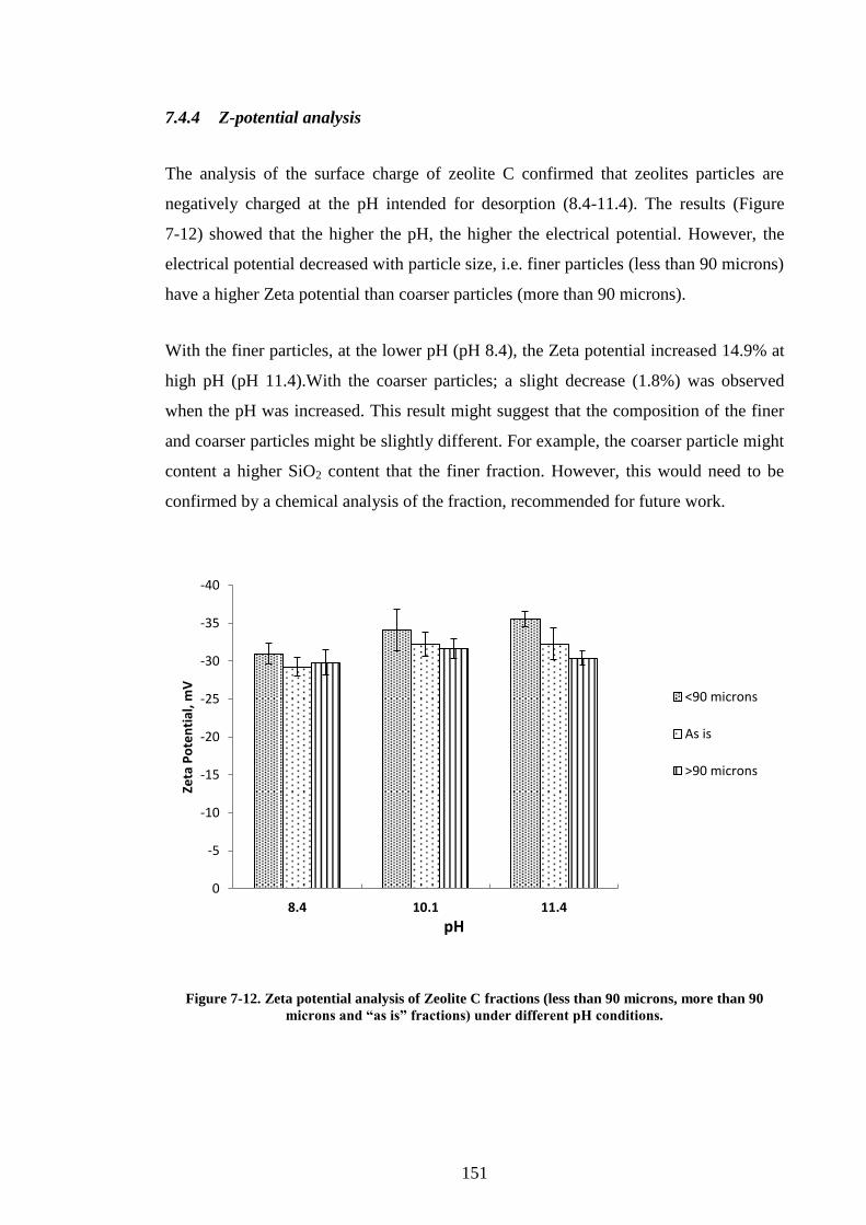
151
7.4.4 Z-potential analysis
The analysis of the surface charge of zeolite C confirmed that zeolites particles are
negatively charged at the pH intended for desorption (8.4-11.4). The results (Figure
7-12) showed that the higher the pH, the higher the electrical potential. However, the
electrical potential decreased with particle size, i.e. finer particles (less than 90 microns)
have a higher Zeta potential than coarser particles (more than 90 microns).
With the finer particles, at the lower pH (pH 8.4), the Zeta potential increased 14.9% at
high pH (pH 11.4).With the coarser particles; a slight decrease (1.8%) was observed
when the pH was increased. This result might suggest that the composition of the finer
and coarser particles might be slightly different. For example, the coarser particle might
content a higher SiO2 content that the finer fraction. However, this would need to be
confirmed by a chemical analysis of the fraction, recommended for future work.
Figure 7-12. Zeta potential analysis of Zeolite C fractions (less than 90 microns, more than 90
microns and “as is” fractions) under different pH conditions.
-40
-35
-30
-25
-20
-15
-10
-5
0
8.4 10.1 11.4
Zeta
Po
ten
tial
, mV
pH
<90 microns
As is
>90 microns

152
7.5 Conclusions
Diaguard and Zeolite C were the adsorbents that showed better results in terms of
protein adsorption. Common sand showed also good protein adsorption properties, but
to have comparable results with Diaguard and Zeolite C, the amount of sand utilised
was 10 times higher than the amount utilised with Diaguard and Zeolite, suggesting a
much lower binding capacity.
All the materials studied have a similar chemical composition, i.e. a high content in
silica oxide (more than 70%, except for AW Hyflow with 44% silica content), and the
difference in binding capacity might be due to a physical property of the materials: the
porosity. More analysis of the material porosity will need to be conducted; however,
this aspect will be discussed later in Chapter 10 of this thesis.
From the desorption experiments, it was found that proteins easily desorbed from
Diaguard and Zeolite C using alkaline pH (pH>7). Salt addition (ionic effects) does not
seem to desorb proteins from Diaguard and Zeolite.
Further studies using continuous adsorption (ion exchange columns) other parameters
need to be assessed, such as, particle size. Finer particles may result in higher pressure
drops across the ion change column, which translates in lower flowrates.

153
- PROTEIN CONCENTRATION USING A ZEOLITE CHAPTER 8
PACKED COLUMN: PART I.
Abstract
In this chapter a method for packing zeolite clinoptilolite (zeolite C) into a column
(internal diameter 26 mm, height 10 cm) and a method for the concentration of protein
contained in pot ale using a liquid chromatography system (Äkta Avant 150) are
explained in detailed.
Following the method mentioned above, pot ale samples were loaded into a column at
four different flowrates (6, 10, 20 and 30 ml/ min). Breakthrough curves for each case
were plotted and at approximately after 5 CV (in all cases), 10% of the initial protein
content was measured from the column outlet. The ratio of the protein content in the
feed and the column outlet reached a certain level and remained constant for the rest of
the experiment, but column saturation (c/c0=1) was not possible to confirm. The level
on which the ratio remained constant seemed to increase with the flowrate.
For the elution, it was confirmed (from the batch experiments described in chapter 7)
that proteins eluted a high pH (pH>8) and salt (2M NaCl) elution did not seem to
release any proteins bound to the zeolite.
A maximum yield of 47.5% was possible to obtain, although the method was not
optimised for yield.

154
8.1 Introduction
In previous chapters it was demonstrated that ion exchange chromatography is a
technique that could be used to separate proteins in pot ale. Commercially available
media -HiTrap Capto S and Capto Q - were used for this purpose; however, the cost for
large scale operations was pointed out as a concern. In chapter Chapter 7, low cost
materials were tested for protein adsorption using batch experiments. From these
experiments, two materials had potentially showed good results for protein adsorption:
Diaguard and Zeolite C.
In this chapter, both materials were packed into a column and tested for protein
adsorption using a larger volume of pot ale (1400 ml) under continuous flow. The
objectives of this chapter were to achieve flowrates higher than 10 ml/ min (equivalent
to 113 cm/ h), depending on column pressure restrictions and to upscale previous
experiments conducted with 1 ml columns conducted at 1-2 ml/ min (equivalent to 155-
311 cm/h). The maximum recommended pressure for the column used for these
experiments (XK-26 columns from GE-Healthcare Life Sciences) was 0.5 MPa.
Before introducing pot ale into the column, tap water was pumped through the column
to test flowrates and pressure drops. Flowrates achieved using Diaguard were lower
than the target (~2 ml/ min) at the maximum pressure that the column could withstand
(0.5 MPa). Further experiments with Diaguard were then stopped, since at larger scale
this process would be become unfeasible. Particle size of Diaguard was 40 microns on
average, which might explain the large pressure drop across the column and hence the
low flow rates.
Flowrates achieved with Zeolite C, were up to 60 ml/ min, but the experiments reported
here were conducted between 6 and 30 ml/ min.
The zeolites particles were classified as 300 microns based on its manufacturing
specifications (Holistic Valley), although a large proportion of the particles passed the
90 microns sieve (~75%) as can be observed in Figure 8-1.

155
Figure 8-1. Particle size distribution of Zeolite C (provided by Holistic Valley).

156
8.2 Methods and Materials
8.2.1 Experiment description
All the experiments were conducted using the Äkta 150 liquid Chromatography system,
an XK 26 column and Zeolite C as the protein binding media as presented in Figure 8-2.
The pot ale used for the experiment was collected from Glenkinchie (GK).
Figure 8-2. Liquid Chromatography system used for the experiments.
A total of four experiments were carried out. The conditions maintained during all the
experiment are summarised in Table 8-1. Flowrate and elution conditions, i.e.
proportion of NaHCO3 and Na2CO3, pH and salt concentration were changed and are
summarised in Table 8-2. To equilibrate the column at least 3 CV of acetic acid-sodium
acetate buffer (pH 4.5) were used until the conductivity and pH readings were stable.
Buffers
XK26 Column
packed with Zeolite
C
Pumps, tubing and
valves
Fraction collection
cabinet
Sample
(Clarified pot ale)

157
Table 8-1. Conditions maintained during the experiments.
Sample volume 1400 ml
Column internal diameter 26 mm
Column height 10 cm
Packing media Zeolite C (Holistic Valley)
Column type XK 26 (GE Healthcare)
Table 8-2. Summary of experimental conditions, materials and steps.
Experiment I II III IV
Pot ale source Glenkinchie (GK)
Glenkinchie (GK)
Glenkinchie (GK)
Glenkinchie (GK)
Flowrate ml/min (cm/h)
6 (67)
10 (113)
20 (226)
30 (339)
Elution
2M Salt gradient followed by a pH
10.1 step.
pH 10.1 (Sodium
carbonate buffer)
20% incremental steps of Na2CO3.
pH 8-11.
pH 10.1 (Sodium
carbonate buffer)
8.2.2 Sample Loading
In each experiment the chromatography protocol comprised four stages: Sample
loading, column washing, protein elution and cleaning. On each stage samples were
collected for further analysis. For the loading stage, exactly 1400 ml of clarified pot ale
was pumped through the column. For pot ale clarification, approximately 2L of pot ale
was transferred into 1L bottles (equal amounts) and centrifuged for 1 hour at 4500 rpm
using a centrifuge (AVANTI j-265 p, Beckman Coulter, rotor JLA 8.1). The clarified
material was then syphoned into a 2L bottle ensuring no solids were collected. The
clarified material pumped through the column was collected in 50 ml samples for
further analysis.
8.2.3 Washing
The washing stage consisted of pumping 100 mM acetic acid – sodium acetate buffer
(pH 4.5) through the column to remove loosely bound proteins or other contaminants. A
maximum of 10 CV (Column Volumes) of acetic acid – sodium acetate buffer (pH 4.5)

158
or until the absorbance at 280 nm (A280) was lower than 100 mAU was used for column
washing.
8.2.4 Elution
For the elution several conditions were tested. These are summarised in Table 9-2 and
explained below:
8.2.4.1 Experiment I
Acetic acid-sodium acetate buffer (pH 4.5) with a 2M NaCl gradient (0-50%) over 10
CV, followed by 10 CV of 2M NaCl and finally 10 CV of 0.1M NaHCO3-Na2CO3
buffer (pH 10.1).
8.2.4.2 Experiment II
10 CV of 0.1M NaHCO3-Na2CO3 buffer (pH 10.1).
8.2.4.3 Experiment III
0.1M NaHCO3-Na2CO3 buffer. With the proportion of Na2CO3 increased by 20% in 5
CV steps. pH of this mixture varied from ~8 to ~11.
8.2.4.4 Experiment IV
Same as experiment II (pH 10.1 elution).
8.2.5 Cleaning
Finally, the cleaning stage, 3 CV of 1M NaOH were passed through the column and the
material was collected for analysis.

159
8.2.6 Packing and conditioning of the zeolite in the column
The zeolites were conditioned prior to be introduced into the column to give maximum
(protein) adsorption capacity and processing flow rates while maintaining a low
pressure drop across the column.
Three sequential steps (Figure 8-3) were necessary in order to achieve the objectives
mentioned above (maximum protein adsorption, maximum flowrate and minimum
pressure drop). The “Particle Classification” step aimed to remove small size particles
(less than 90 micrometres diameter). To achieve this, a 90 microns sieve was used to
retain zeolites particles bigger than 90 microns which were subsequently transferred
into the column. Approximately 11 to 12 cm (lengthwise) of zeolite were used.
Figure 8-3. Steps used for column packing.
Tap water was pumped at a rate between 10 to 20 ml/ min from the bottom of the
column (up flow mode in the Akta) keeping the top end of the column opened allowing
smaller zeolite particles to float and escape from the column. This process is also known
as elutriation, and its objective was to ensure that all the small particles were removed.
This process was carried out for at least 1 hour.
The second step “Bed packing” aimed to maximise the quantity (mass) of the solid
phase per unit of volume. To achieve this, water was pumped through the column from
the top to the bottom. For the XK-26 column (26 mm internal diameter), typical

160
flowrates utilised were in the order of 40 – 60 ml/ min for at least 2 hours. It was
important to ensure that no air was trapped inside of the column and that the column
was not pressurising over time. By the end of this step the packing compressed to ~10
cm.
The final step, “Bed equilibration” aimed to remove contaminants attached to the resin
and to charge the zeolite particles in order to ensure maximum protein-adsorbent
interaction. A solution of 1M sodium hydroxide (NaOH) was used for this step at a
flowrate of 10 ml/ min (downwards flow) for at least 1 hour.
Subsequently, distilled, deionised water was used to remove any salts at a flowrate of 10
ml/ min for at least 1 hour. Finally an acidic buffer solution (i.e. acetate) with a pH
range between 4 -6 pH units, was used to ensure that solid particles were charged
accordingly in order to ensure maximum attachment of proteins to the zeolites. This
step normally was carried out at a flowrate between 20 – 30 ml/ min for at least one
hour.
8.2.7 Peak areas
The areas of the elution peaks (at absorbance of 280 nm) were calculated using the
software Unicorn™ 6.1 incorporated with Äkta system. The calculation is defined as the
area between the curve and the baseline, between the peak start and peak end, time or
volume base. A zero baseline was chosen for the calculations of this work, i.e. straight
line at zero level.
8.2.8 Protein yield and concentration factor determination
During the NaHCO3-Na2CO3 elution, samples with absorbance (280 nm) over 500
mAU were collected, the exact volume recorded and measured for soluble protein
content. The yield was calculated as the mass of proteins in the elution divided by the
mass of proteins in the feed stream.
The concentration factor was calculated by dividing the protein concentration of the
eluted stream by the concentration of the proteins in the feed stream. Protein
concentration was determined by the Bradford assay.

161
Figure 8-4. Photography of the column used during the experiments packed with zeolite as the
adsorbent material.
8.2.9 Pressure measurements
Prior to the introduction of pot ale into the column the pressure was measured with the
online pressure monitors incorporated in the Akta system. Three different fluids
(distilled water, sodium hydroxide and a 2M NaCl solution), increasing the flowrate in 5
ml/ min steps, until the pressure reading were stable and then it was recorded.
The experiment was conducted by analysing individual components of the system that
might increase the pressure such as filters, columns and the packing (zeolite).
8.2.10 SDS-Page analysis
The full procedure was explained earlier in Section 6.3.7. But here, additionally, pot ale
samples were passed through ultracentrifugation tubes in order to concentrate the
proteins and then compared with the samples passed through the zeolite column.

162
For the ultra-centrifuged samples, pot ale was centrifuged at 4000 rpm for 5 min and the
10 ml of the supernatant were added to the filter cups (Amicon Ultra-15 Centrifugal
Filter Tubes Merck Millipore Ltd) and centrifuged at 4000 rpm, 4°C for approximately
2 hours, until the volume of retentate was reduced by 95%. The filtrate was removed
and volume of retentate adjusted to 10 ml with distilled deionised water for dialysis.
The retentate was centrifuged as previous and this dialysis step repeated once more. The
retentate was transferred to an eppendorf tube, the concentration of protein analysed by
Bradford assay. The gel was heated at 70°C for 10 min and the electrophoresis run
conditions were 150V for 1 hour.

163
8.3 Results and discussion
8.3.1 Pressure measurement
In the first part of these measurements (Figure 8-5) it can be observed, as expected that
higher flowrates increased the pressure system and the more viscous fluids (1M NaOH
and 2M NaCl) registered higher pressures than water for the same flowrate. Since the
column was rated to a maximum of 0.5 MPa, the protein separation experiments were
conducted to maximum flowrate of 30 ml/ min.
In the second part (Figure 8-6), only water was used, but the objective of this exercise
was to determine if the packing (zeolites) were causing flow restriction (high pressure).
From this experiment, it was concluded that flow resistance due to the zeolites were
minimal compared to the system components. It is important to mention that some of
the tubing used for these experiments have internal diameter of 0.75 mm. Based on the
manufacturers guidance, 100 cm of this tubing generates 0.02 MPa of pressure at
flowrate of 10 ml/ min.

164
Figure 8-5. System Pressure using different fluids
Figure 8-6. Pressure contribution of filter, column and packing using distilled water.
0
0.1
0.2
0.3
0.4
0.5
0.6
5 10 15 20 25 30 35 40 45 50 55 60 65
Pre
ssu
re (M
pa)
Flowrate (ml/ min)
ddH2O
1M NaOH
2M NaCl
0
0.05
0.1
0.15
0.2
0.25
0.3
0.35
0.4
0.45
0.5
5 10 15 20 25 30 35 40 45 50 55 60
Pre
ssu
re (M
pa)
Flowrate (ml/ min)
Packed
Empty column
Filter
No Filter

165
8.3.2 Breakthrough curves
The breakthrough curves are presented in Figure 8-7. It can be observed that at
approximately 5 CV, ~10% of the soluble protein passed through the column in all the
experiments (flowrates). Between ~5 and ~10 CV the ratio c/c0 increased rapidly and
after ~10 CV the ratio remained constant, but a different value was observed for every
experiment. The general trend observed was that the higher the flowrate, the higher the
c/c0 ratio. This is in agreement with theory, since higher flowrates translates into less
residence time.
The kinetics behind protein binding into zeolite was studied in more depth in Chapter
10, where a kinetic model is proposed.
Figure 8-7. Breakthrough curves at different flowrates (6, 10, 20 and 30 ml/ min).
0.0
0.1
0.2
0.3
0.4
0.5
0.6
0.7
0.8
0.9
1.0
0 5 10 15 20 25 30
Re
lati
ve p
rote
in c
on
cen
trat
ion
to
th
e f
ee
d (
c/c 0
)
CV
6 ml/ min
10 ml/ min
20 ml/ min
30 ml/ min

166
8.3.3 Chromatograms
The chromatograms presented in the following pages (Figure 8-8 to Figure 8-11) report
only the elution and cleaning steps of the experiments. The horizontal axis shows the
volume of materials passed through the column (ml), the left vertical axis the
absorbance of the material leaving the column (at 280 nm) and the right vertical axis the
pH. An additional line (green) shows the concentration of Na2CO3 in the buffer mixture.
Figure 8-8 shows the chromatogram of Experiment I (flowrate 6 ml/ min). In this case, a
salt (NaCl) gradient was used and no peaks were detected (between ~2200 -2900 ml),
indicating that salt did not desorb the proteins attached to the zeolite. This result is
agreement with the batch experiments conducted earlier in this thesis (Figure 7-8 and
Figure 7-9).
The absorbance reading under these conditions was ~400 mAU. Fluctuations in the
absorbance readings were due to flow problems (due to pressure build up in the column,
which was corrected in subsequent experiments). After the NaCl buffer introduction
into the column, sodium carbonate – sodium bicarbonate buffer (pH 10.1) was pumped
and a first peak was detected (~2800 mAU). The second peak was detected with
introduction of NaOH.
An interesting observation detected, was that the absorbance peak followed the increase
in pH. The increase in absorbance could be associated with proteins “leaking” out of the
column. A possible explanation of this phenomenon (reviewed earlier in section 6.2.1)
is that by increasing the pH, the proteins bound to the columns will change their electric
charge. At low pH (below 5), the proteins will be positively charged and at higher pH,
protein charge will change from positive to a negative charge, thus detaching from the
zeolites which are negatively charged.

167
Figure 8-8. Experiment I (6 ml/ min) chromatogram.
The blue line of the chromatogram represents the UV absorption (measured at 280 nm) and is reported in
mAU on the primary vertical axis of the chromatogram. The green line represent the salt concentration (0-
100%, where 100%= 1M NaCl) and the purple line the pH of the sample reported on the secondary axis.

168
For Experiment II (10 ml/ min) the elution was conducted at pH 10.1 (carbonate buffer).
Only two peaks could be detected as shown in Figure 8-9. The first peak at pH 10.1
(from ~2700 ml to 3200 ml) and the second peak (between 3600-3800 ml) eluted with
1M NaOH. From the fraction eluted at pH 10.1 (first peak) a sample was taken for SDS
analysis, shown in Figure 8-12.
As well, as in Experiment I, in this experiment, the absorbance increased coincided with
the pH increase. It is worth noticing though that the peak in the absorbance when the pH
was around 8. Above pH ~8, the absorbance started to decrease, although the slope of
the tail is less pronounced than the start of the peak. After 3000 ml this is even more
evident, the absorbance trend became almost flat. This suggests that the majority of the
proteins detached from the column at pH ~8 and the elution process could be stopped
when this pH value has been reached.
Figure 8-9. Experiment II (10 ml/ min) chromatogram.
The blue line of the chromatogram represents the UV absorption (at 280 nm) reported in mAU on the
primary vertical axis of the chromatogram. The green line represent the salt concentration (0-100%,
where 100%= 1M NaCl) and the purple line the pH of the sample reported on the secondary axis. In this
experiment, however, no salt or pH gradient was conducted, i.e. the elution was conducted at constant pH
(= 10.8).

169
For Experiment III (Figure 8-10), increasing amounts of Na2CO3 were introduced into
the buffer mixture which translated into higher pH buffer. A total of four peaks were
detected, although again, as in Experiment I, fluctuation in the absorbance was observed
(due pressure build up in the system) and some of the peaks were difficult to detect.
Peak 1 and peak 4 were the highest peaks and with the biggest area. This suggests that
elution could be simplified, eluting a lower pH (~pH=8) and using only NaHCO3 in the
buffer instead of a combination of NaHCO3 – Na2CO3.
Figure 8-10. Experiment III (20 ml/ min) chromatogram.
The blue line of the chromatogram represents the UV absorption (measured at 280 nm) and is reported in
mAU on the primary vertical axis of the chromatogram. The green line represent the salt concentration (0-
100%, where 100%= 1M NaCl) and the purple line describes the pH of the sample reported on the
secondary axis. The four peaks detected on the chromatogram were labelled as “Peak 1”, “Peak 2”, “Peak
3” and “Peak 4”.
Peak 1
Peak 2
Peak 3
Peak 4

170
Experiment IV, performed under similar conditions of Experiment II, but at a higher
flowrate 30 ml/ min (Figure 8-11) showed again two peaks , at pH 10.1 and another at
pH ~14 (1M NaOH).
Again, as in the previous experiments, it was observed that the absorbance increase was
related to the pH surge. In this experiment the absorbance peaked at 2600 mAU when
the pH was ~8.
Figure 8-11. Experiment IV (30 ml/ min) chromatogram.
The blue line of the chromatogram represents the UV absorption (measured at 280 nm) and is reported in
mAU on the primary vertical axis of the chromatogram. The green line represent the salt concentration (0-
100%, where 100%= 1M NaCl) and the purple line describes the pH of the sample reported on the
secondary axis.
Although these experiments were carried out using different elution conditions
(buffers), it might be reasonable to conclude that the elution of the proteins (measured
by absorbance) coincided when the pH was increased. It was also noticed that the
absorbance increased rapidly as the pH increased and then slowly decreased (a long tail
in the peak).

171
This phenomenon could be due to the buffering capacity of the reagents used (carbonate
buffer and acetic acid for example). In all the chromatograms it was observed that the
absorbance peak occurred before pH reached steady state (i.e. the pH of the elution
buffer). On average, it took approximately 200 ml (~4 CV) until the elution pH was
stable. Apart from extending the duration of the batch, this could affect the purity and
concentration of the product. A theory is that the majority of the proteins elute at the
start of the peak (start of the peak the product could be potentially protein rich with low
salt/ buffer content) and that the tail of the peak could have less protein and more salt
(from the buffer). This needs to be checked and future work will need to analyse the
different fractions of the peak (start, top and tail for example) to confirm purity and
quantities of the eluted proteins.
A possible way to overcome the long tail of the absorbance peak could be to use a more
dilute washing buffer, a different buffer (citric acid) or just water. In these experiments
the concentration of the washing buffer (acetic acic- sodium acetate) was 100mM, but
this could be reduced to 50 mM or less if possible. On a large scale process, process this
would result in a more economic process due to less buffer (volume) required to
increase the pH of the elution buffer and less salts required to prepare the buffers.
Another way to improve the purity of the eluted material could be by manipulating the
control on the Äkta system. In these experiments, the collection of the product was set
over 500 mAU, but this can be easily changed. For example, the Äkta could be
programmed to start collecting product when the absorbance is 1000 mAU and stop
collecting when the absorbance is 2000 mAU. This would need to be checked in future
experiments.
Another suggestion for a potential commercial scale production is that the process could
be controlled by pH, rather than absorbance if online absorbance instruments are not
suitable or available for larger operations. In addition to simplifying the process, this
could translate in lower capital requirements too.

172
8.3.4 SDS-page analysis
Samples from peaks 1 and peaks 2 from Experiment II (Figure 8-9) were analysed using
SDS-page analysis (Figure 8-12). R1 and R2 corresponded to the retentate from pot ale
samples passed through the Amicon Ultra-15 centrifugal filter tubes, P1 relates to the
first peak of experiment 2 (0.1M NaHCO3-NA2CO3 pH 10 buffer) and P2 corresponds
to the second peak of experiment 2 (1M NaOH, pH~14).
From the gel, R1 and R2 wells, the presence of protein Z (40 kDa) are clearly visible,
however, the same cannot be confirmed for the samples eluted with zeolite C (P1 and
P2). This might be a concentration effect, with sample loading too low to show the
presence of this band after staining with coomasie blue.
Figure 8-12. SDS-page analysis of experiment II.
The red oval highlights the presence of protein Z aroun the 40 kDa mark. The molecualr weigh of the
proteins are placed on the left the figure and the columns correspond to the samples analysed.
kDa
175
80
58
46
30
25
17
7
R1 R1 R2 R2 P1 P1 P2 P2

173
8.3.5 Peak areas
The areas of the two biggest peaks (based on height) of the chromatograms presented
earlier were compared in the graph below (Figure 8-13). For the first 3 experiments, the
results are in agreement with theory. Higher flowrates, imply less residence time
(contact of pot ale with zeolite), resulting in a potential smaller proportion of protein
bound to the zeolites. However, Experiment IV (highest flowrate) showed the second
biggest area.
Experiment II (10 ml/ min) and Experiment IV (30 ml/ min) were conducted at similar
conditions (except for the flowrate) and similar areas were obtained. It is also worth to
mention that for these experiments, 63% of the total peak area was from the NaHCO3-
Na2CO3 peak.
Figure 8-13. Peak areas from the chromatograms of experiments I, II, III and IV.
0
100,000
200,000
300,000
400,000
500,000
600,000
700,000
800,000
900,000
1,000,000
6 10 20 30
Pe
ak a
rea
(ml*
mA
U)
Flowrate (ml/ min)
NaOH peak
NaHCO3-Na2CO3 peak

174
8.3.6 Protein yield and concentration factor
In Figure 8-14, the protein concentration factor from the NaHCO3-Na2CO3 and NaOH
peaks are presented. In experiment I (6 ml/ min), only the NaHCO3-Na2CO3 peak
concentration was measured. In all experiments it can be observed that the NaOH peak
had highest concentration. The protein concentration factors for NaHCO3-Na2CO3 peaks
of all the experiments varied from 1.5 to 2.7, but no clear trend was possible to detect.
Figure 8-14. Concentration factor of the eluted proteins from experiments I, II, III and IV.
0.0
0.5
1.0
1.5
2.0
2.5
3.0
3.5
6 10 20 30
con
cen
tra
tio
n f
act
or
(c/c
o)
Loading flowrate (ml/ min)
c/ co (NaHCO3-Na2CO3)
c/ co (NaOH)

175
The yield was also calculated in all the experiments and the results are presented in
Figure 8-15 for the NaHCO3-Na2CO3 and NaOH peaks. When the proteins from both
peaks were combined a maximum of 47.5% yield was obtained. However, when only
the NaHCO3-Na2CO3 peak was considered only 37% was recovered. The NaOH
contained on average ~10% of the protein.
Possible protein losses could be found in the flow through and wash streams and
unbound proteins that remained in the column (attached to the zeolites). A full mass
balance was carried out in following chapter.
Figure 8-15. Protein yield from the eluted proteins from experiments I, II, III and IV from the
NaHCO3-Na2CO3 and NaOH peaks.
0%
5%
10%
15%
20%
25%
30%
35%
40%
6 10 20 30
Yie
ld
Loading flowrate (ml/ min)
NaHCO3-Na2CO3 peak
NaOH peak

176
8.4 Conclusions
The purpose for the experiments explained here was to prove that zeolite c is a suitable
adsorbent for protein recovery using ion exchange. The zeolite must however, need to
be treated prior to the introduction to the column.
Zeolites need to be classified (particles smaller than 90 microns separated and not used
in the column), packed (to minimise column volume) and finally equilibrated (wash at
low pH to maximise protein adsorption). After the separation of the small zeolite
particles, it was possible to obtain high flowrates with negligible pressure drop.
A second objective of this chapter was to develop a protocol for the concentration of pot
ale proteins using the Äkta 150 liquid Chromatography system. A method consisting in
sample loading, the washing of loosely bound components, followed by the elution of
the proteins using a high pH buffer, and finally a cleaning step of the column (with 1M
NaOH) was presented in this chapter.
Although the method was not optimised for yield, concentration or purification, it can
be said that on average a ~2X concentration factor was achieved and the protein purity
(assessed by SDS-page analysis) remained uncertain, since the bands on the SDS- page
analysis were not clearly visible.
During the elution step, it was observed in these experiments that the increase of the
absorbance readings (related to protein content) matched the pH increase. However, the
maximum absorbance reading did not occur when the maximum or steady state pH was
reached. A long tail in the absorbance peaks was observed in all the experiments,
suggesting further work to improve this process such as the usage of a more diluted
buffer for the washing step which precedes the elution step.
In the following chapter the flowrate and buffers will be kept constant and the column
length will be modified (from 10 to 30 cm) to understand the effects on the protein
recovery process.

177
- PROTEIN CONCENTRATION USING A ZEOLITE CHAPTER 9
PACKED COLUMN: PART II.
Abstract
Continuing with the zeolite packed column experiments described earlier in this thesis,
here, in this chapter the effects of column height on protein yield, concentration and the
selective removal of carbohydrate and copper were studied.
Four experiments were carried out maintaining sample loading (1400 ml), flowrate (20
ml/ min), column diameter (26 mm) and media packing (zeolite C). Column height
(H=10, 20 and 30 cm), media equilibration conditions (pH 4.5 and pH 7) and elution
conditions (proportion of NaHCO3 and Na2CO3) were changed.
The combined areas of the elution peaks from the chromatograms were calculated. A
66% difference in peak areas was observed between the maximum (H=30 cm, pH= 4.5)
and minimum (H=10 cm, pH 7.0) areas.
Breakthrough curves were plotted to determine the dynamic binding capacity. The
highest capacity was obtained for the largest column equilibrated at pH 4.5 (1.8 mg
protein/ ml of zeolite).
The effect on the chemical oxygen demand (COD) based on protein content was
analysed on the four experiments. On average a 19% decreased in COD levels was
observed by centrifugation and an additional 15% by removing the proteins (flow
through of the chromatographic step).
Finally a protein, carbohydrate and copper mass balance was conducted. On average,
the combined elution fractions contained 38.7% of the original protein content (feed),
while carbohydrates and copper in the eluates contained only 1.3% and 8.8%, of the
original content, respectively.

178
9.1 Introduction
Following the method presented in previous chapter, where a process for the adsorption
of pot ale proteins using zeolites as the binding material was developed, in this chapter
the focus will be on column height and its influence in the process outputs. Specifically,
protein yield, concentration and the selective removal of carbohydrate and copper from
proteins were studied.
In the process described in the previous chapter, pot ale was pumped through a column
packed with zeolites. In theory, proteins contained in pot ale adsorbed to the zeolites
and the rest of the pot ale components flow through. This resultant material (the flow
through) becomes then “deproteinated” pot ale.
In the Introductory chapter, it was mentioned that proteins have a detrimental effect on
Anaerobic Digestion (AD) a common process used for effluent treatment (i.e. pot ale) in
the whisky industry. Some authors recognise the need for a pre-treatment process of pot
ale prior to AD. Pre-treatment options are based on enzymatic hydrolysis of yeast cells,
solid-liquid separations and pH control (Dionisi et al. 2014, Mallick et al. 2010, Tokuda
et al. 1999).
A parallel study was conducted by Dr. Thomas Aspray (School of Life Sciences,
Heriot-Watt University) using the deproteinated pot ale obtained out of the experiments
presented in this chapter. The deproteinated material was tested for batch biochemical
methane potential (BMP) and found to be comparable to untreated pot ale based on
comparative chemical oxygen demand loading. These results will be presented and
made available in literature (Aspray et al., in preparation), however COD analyses will
be presented here.

179
9.2 Methods and Materials
9.2.1 Pot ale samples and analysis
Pot ale samples were collected from four different distilleries (Glenkinchie-GK,
Balblair –BB, Balmenach – BM, Strathairn – SE) and kept at 4°C.
The procedure for determining total solids, soluble protein and carbohydrates was
explained earlier in this thesis, but a brief description can be seen below.
Total solids were measured by placing 10 ml of the liquid samples in to an aluminium
boat and placed into an oven at 105°C for 24 hours. The analyses were performed in
triplicate, the weights recorded in grams (g) and volumes in millilitre (mL).
Soluble proteins were measured with the Bradford assay (Bradford 1976) described
earlier in the thesis. Conductivity and pH were measured with the online conductivity
and pH monitors incorporated in the liquid chromatography system (Äkta Avant 150
from GE-Healthcare). The analyses were performed in triplicate, and the results are
reported in mg of soluble protein per litre of pot ale.
Carbohydrates content was measured using a colorimetric assay described in Fournier
(Fournier 2001). Briefly, the method involved building a calibration curve using glucose
as a standard. Samples and standards (5 to 50 μl) were mixed with 500 μl of 4% phenol
followed by 2.5 ml 96% sulphuric acid and then absorbance was measured at 490 nm
with a spectrophotometer.
Copper content was detected by flame atomic absorption spectroscopy (FAAS) and the
the method was also described earlier in the Thesis.
9.2.2 Chemical Oxygen demand
Chemical oxygen demand (COD) was also measured, but since the procedure has not
been explained before a detailed description is provided below. The limits of detection
for the procedure is in the range of 9-400 mg/ml. Samples with higher concentration
were diluted and the results adjusted accordingly. The procedure was taken from

180
standards methods available in literature (American Public Health et al. 1995), (Tebbutt
1977).
2 ml of sample was mixed with 0.1 ml silver nitrate (Ag NO3), placed into a digestion
tube, and allowed to stand for two minutes. Subsequently 0.1 ml of Chromium III
Potassium Sulphate solution was added to 3.70 ml of COD reagent (oxidising mixture).
The mixture was thoroughly mixed allowing any evolved gas to escape by removing the
cap.
Four blank solutions prepared in exactly the same way as described earlier, but 2.00 ml
of distilled water in place of the sample was used. Samples and blanks were placed in
the heating block and allowed to digest at 150°C for 2h. After this time, the digestion
tubes were allowed to cool in the air for 5 minutes, and then under running water until
the temperature was below 20°C.
Once the tubes were cooled, samples and blanks were transferred to 100 ml conical
flasks. The residual dichromate was rinsed into the flask using 10 ml of distilled water.
Subsequently, no more than two drops of Ferroin indicator (1,10-Phenanthroline ferrous
solution 0.025M from Fisher Scientific, catalogue # 10244490) was added and the
residual dichromate was titrated with standardised ferrous ammonium sulphate (FAS).
The volume of dichromate used to titrated the samples (Vs) and blanks (Vb) was
recorded and used to calculate the COD values (reported in mg/ ml) using the formula
below, where M is defined in the paragraph below.
COD = 4000M (Vb-Vs)
For the standardisation of FAS, 10 ml of concentrated H2SO4 was added to 50 ml of
distilled water in a 250 ml flask. The acid water mixture was allowed to cool and
exactly 5 ml of 0.02083M potassium dichromate was added with one drop of Ferroin
indicator. The solution was titrated with FAS. The volume of FAS was recorded and
used to calculate the molarity of the FAS solution (M), using the formula below, where
V is the volume (ml) of titrant used.
M= 5/8V

181
9.2.3 Experiment description
All the experiments were conducted using the Äkta 150 liquid Chromatography system,
an XK 26 column and Zeolite C as the protein binding media.
The four experiments (Experiment I, II, III and IV) were carried out maintaining the
conditions summarised in Table 9-1. Column height (H=10, 20 and 30 cm), media
equilibration conditions (pH) and elution conditions (proportion of NaHCO3 and
Na2CO3) were changed and are summarised in Table 9-2. To equilibrate the column at
least 3 CV of water or appropriate buffer were used until the conductivity and pH
readings were stable.
In each experiment the chromatography protocol comprised four stages: Sample
loading, column washing, protein elution and cleaning. On each stage samples were
collected for further analysis. For the loading stage, exactly 1400 ml of clarified pot ale
was pumped through the column. For pot ale clarification, approximately 2L of pot ale
was transferred into 1L bottles (equal amounts) and centrifuged for 1 hour at 4500 rpm
using centrifuge (AVANTI j-265 p, Beckman Coulter, rotor JLA 8.1). The clarified
material was then syphoned into a 2L bottle ensuring no solids were collected. The
clarified material pumped thorough the column was collected in 50 ml samples for
further analysis.
The washing stage consisted of pumping either water (pH 7) or an acetic acid – sodium
acetate buffer (pH 4.5) through the column to remove loosely bound proteins or other
contaminants. A maximum of 10 CV (Column Volumes) of water or buffer or until the
absorbance at 280 nm (A280) was lower than 100 mAU was used for column washing.
For the elution stage a 0.1M NaHCO3-Na2CO3 buffer was pumped through the column.
The proportion of NaHCO3 and Na2CO3 in the mixture was varied in each experiment.
For example in Experiment I, the proportion of Na2CO3 was increased in 20%
incremental steps. For each incremental step the eluted material was collected for
further analysis. Each step consumed 5 CV of buffer and the material collected for
analysis was higher than 500 mAU (A280). Below this limit the material was discarded.

182
Finally, the cleaning stage, 3 CV of 1M NaOH were passed through the column and the
material was collected for analysis.
Table 9-1. Conditions maintained during the experiments.
Sample volume 1400 ml
Loading flow rate 20 ml/ min
Column internal diameter 26 mm
Packing media Zeolite C (Holistic Valley)
Column type XK 26 (GE Healthcare)
Table 9-2. Summary of experimental conditions, materials and steps.
Experiment I II III IV
Pot ale source Balblair
(BB)
Strathairn
(SA)
Balmenach
(BM)
Glenkinchie
(GK)
Column Height (cm) 10 20 30 30
Equilibration pH 7.0 4.5 7.0 4.5
Washing pH 7.0 4.5 7.0 4.5
Elution
(Na2CO3 increment/
number of steps)
20%/ 6 50%/ 3 60%/ 1 50%/ 3
Cleaning 1M NaOH 1M NaOH 1M NaOH 1M NaOH
9.2.4 Peak areas
The areas of the elution peaks were calculated using the software Unicorn™ 6.1
incorporated with Äkta system. The calculation is defined as the area between the curve

183
and the baseline, between the peak start and peak end, time or volume base. A zero
baseline was chosen for the calculations of this work, i.e. straight line at zero level.
9.2.5 Dynamic binding capacity
The dynamic binding capacity (DBC) was calculated with the formula below (Carta and
Jungbauer 2010), where CF is the protein concentration in the feed, tb and Vb are the
breakthrough time and load volume, respectively. Q is the volumetric flowrate and Vc is
the column volume. Breakthrough was defined as a value of 10% of the feed
concentration.
DBC=CFVb
Vc
=CFQt
b
Vc
9.2.6 Mass balance
A protein, carbohydrate and copper mass balance of the chromatographic step was
conducted. The inputs and outputs volumes were quantified, and with the concentration
determined experimentally (described earlier), the mass of protein, carbohydrate and
coper was calculated.
An example of the inputs and output is shown in Figure 9-1. It was assumed that the
only in input stream containing protein, carbohydrate or copper was the feed (F) stream.
For the output streams 9, 10 and 11, it was assumed that the protein content was low or
negligible. These streams correspond to fractions on which the absorbance was below
the 500 mAU as described earlier.

184
Figure 9-1. Process flow diagram of the experiments conducted.

185
9.3 Results and discussion
9.3.1 Chromatograms
The combined areas of the elution peaks from the chromatograms (Figure 9-4) were
calculated and the results are presented in Figure 9-2 and Figure 9-3. From the graphs, it
can be noticed that a 66% difference in peak areas was observed between the maximum
(H=30 cm, pH= 4.5) and minimum (H=10 cm, pH 7.0) areas. Generally, it was observed
that the larger the column, the bigger the area, which is in agreement with theory.
In Experiment I, only 3 peaks were detected during the elution phase, although six
incremental steps of Na2CO3 were used for the experiment. This suggested to simplify
the elution strategy to have only 3 elution steps (0, 50 and 100% Na2CO3) for
subsequent experiments.
Experiments III and IV were carried using the same column height (30 cm), but the pre-
equilibration step was changed from pH 7.0 to 4.5, an increment of 10% of the peaks
areas was calculated. Another difference with both experiments is that in Experiment III
the elution was carried out at pH 10.1 (single step) and in Experiment IV, multiple steps
were used. In the final elution step (100% Na2CO3), a small peak was detected, which
area was calculated at 12% of the total peak area.
The analysis of the contribution of each peak area is presented in Figure 9-3. For
example, in Experiment II (Figure 9-4), four peaks were detected during the elution and
cleaning stage. From left to right in the chromatogram, the first peak was detected at
~2600 ml using a buffer mixture of 0.1M- 100% NaHCO3 - 0% Na2C03, corresponding
to the lower pH conditions (pH 8.4). A second and third peak was observed at ~3300 ml
(50% NaHCO3/ Na2CO3 mixture, pH 9.7) and at ~3900 ml (0% NaHCO3 - 100%
Na2CO3, pH 10.8), respectively. The fourth peak (~4500 ml), corresponds to the elution
conditions of 1M NaOH.
Following the example from the above paragraph, the areas of peaks 1, 2, 3 and 4 were
compared together with the peak areas of the other experiments (Figure 9-3). In all
experiments, it was observed that the biggest areas were obtained with the lower
Na2CO3 buffer mixture across all experiments (~pH 8). In Experiment II, for example,

186
peak 1 represented 37%, peak 2 – 27%, peak 3 – 13% and peak 4 23% of the total area
of the peaks.
Figure 9-2.Total peak areas of the chromatograms from Experiments I, II, II and IV.
Figure 9-3. Contribution of individual peaks to total area.
0%
25%
50%
75%
100%
0
500
1,000
1,500
2,000
2,500
I(BB, H=10 cm)
II (SA, H=20 cm)
III(BM, H=30 cm)
IV(GK, H= 30 cm)
A/
Am
ax
Tota
l pe
ak a
reas
(A
U*m
l)
0%
10%
20%
30%
40%
50%
60%
70%
80%
90%
100%
I(BB, H=10 cm)
II (SA, H=20 cm)
III(BM, H=30 cm)
IV(GK, H= 30 cm)
Re
lati
ve a
rea
to t
ota
l pe
ak a
rea
1M NaOH
100% -Na2CO320-60%Na2CO3

187
Figure 9-4. Chromatograms of Experiments I, II, III and IV.
The blue lines in the chromatograms represent the absorbance measured at 280 nm and it is reported on
the primary axis in mAU. The brown lines represent the conductivity, measured in mS/ cm and reported
in the secondary axis. Finally the green lines denote the proportion of Na2CO3 in the buffer mixture.
50% Na2CO3
100% Na2CO3
100% Na2CO3
50% Na2CO3
20% Na2CO3
40% Na2CO3
60% Na2CO3
80% Na2CO3
60% Na2CO3
Exp I (BB, H=10 cm)
Exp III (BM, H=30 cm)
Exp II (SA, H=20 cm)
Exp IV (GK, H=30 cm)

188
9.3.2 Breakthrough curves
Breakthrough curves of Experiments I, II and IV were plotted in Figure 9-5. It can be
observed that these three curves followed the same sigmoidal pattern. Up until ~5CV,
~20% of the protein were bound to the zeolites. From this time (or CV) a rapid increase
in the relative protein concentration was detected.
Unfortunately for all the experiments column saturation (c/c0=1) was not possible to
obtain due to the lack of material. Experiments III and IV concluded at approximately 9
CV. At this point the relative protein concentration of the samples were ~60% of the
original concentration. For experiment I, a smaller column was used, the experiment
continued until ~27 CV of pot ale were passed through the column. In this case, a slow
increase in the relative protein concentration (c/c0) from ~0.7 (at ~10CV) to ~0.9 was
measured.
Exp I (BB, H=10 cm)
Exp III (BM, H= 30 cm)
Exp IV (GK, H= 30 cm)
Figure 9-5. Breakthrough curves of Experiments I, III and IV.
0.0
0.1
0.2
0.3
0.4
0.5
0.6
0.7
0.8
0.9
1.0
0 5 10 15 20 25 30
Re
lati
ve p
rote
in c
on
cen
trat
ion
(c/
c 0)
Column Volumes

189
9.3.3 Dynamic binding capacity
The dynamic binding capacity (DBC) calculations are presented in Table 9-3. For the
smaller column (Experiment I, H= 10 cm), the BC was calculated at 1.40 mg of protein
per ml of zeolite. Small improvements (20 -30%) were achieved by increasing the
column height and by pH pre-equilibration. The highest capacity was obtained for
Experiment IV (1.8 mg protein/ ml of zeolite).
Although the DBC of the commercial resins studied earlier (HiTrap Capto Q and Capto
S) were not determined, their manufacturer specifications mentioned a DBC of ~100
mg/ ml. Based on the results presented here, zeolites have a capacity of ~50 times
smaller than Capto Q/S. The price per unit of volume of these commercial resins is
however, about 300 times more expensive. An economic analysis considering column
sizing and other aspects must be carried out, to determine if zeolites were a viable
material for the process at a larger scale. However, this assessment is out of the scope
this thesis.
Table 9-3. Dynamic binding capacity results.
Experiment No. I II III IV
Column Height (cm) 10 20 30 30
Equilibration pH 7.0 4.5 7.0 4.5
Vb,10% (ml) 100 ND 400 550
CVb,10% 1.88 ND 2.51 3.45
DBC10% (mg/ ml) 1.40 ND 1.7 1.8
Relative improvement
to Experiment I 0% ND 23% 30%
ND: Not determined

190
9.3.4 Chemical oxygen demand
The effect on the chemical oxygen demand (COD) based on protein content was
analysed on the four experiments and the results are presented in Figure 9-6. On average
a 19% reduction in COD levels was observed by centrifugation and an additional 15%
by removing the proteins (flow through of the chromatographic step).
Figure 9-6. Chemical oxygen demand of raw, centrifuged and deproteinated pot ale.
In Experiment I, no reduction in COD was observed from the centrifuged and
deproteinated pot ale. This result could be do an error in the centrifuged pot ale analysis,
since in the other experiments (II, III and IV) higher CODs were obtained in the
samples analysed.
For Experiments III and IV, COD and soluble protein were monitored during the
loading stage. The results are plotted in Figure 9-7 and both COD and soluble protein
are reported as the fraction of the initial COD and soluble protein, respectively. The
soluble protein curves have an exponential shape (tending to reach saturation point =
100%), while the COD curve shape is logarithmic and tending to reach ~75% of initial
COD.
0
10,000
20,000
30,000
40,000
50,000
60,000
I II III IV
CO
D (
mg/
L)
Experiment
Raw Pot ale
Centrifuged Pot Ale
Centrifuged + DeproteinatedPot ale

191
% initial COD
% of initial soluble protein conten
Figure 9-7. COD and soluble protein breakthrough curves (experiments III and IV only).
0%
25%
50%
75%
100%
0 2 4 6 8 10
CV
Experiment IV (GK, H=30 cm)
0%
25%
50%
75%
100%
0 2 4 6 8 10
CV
Experiment III (BM, H=30 cm)

192
9.3.5 Mass Balance
On each experiment (with the exception of Experiment I, samples were not collected),
total solids, carbohydrate, soluble protein and copper content of the fractions (i.e. Flow
through, washing, elution and cleaning) obtained during the chromatography
experiments were compared with the original material (pot ale supernatant). The results
are presented in Figure 9-8 and it can be observed from these graphs that carbohydrate
and copper content in the flow through (FT) was higher compared to the other fractions
and at similar levels of the original material (SN). Soluble protein content, however,
was low in the FT fraction and relatively higher in the elution (E1, E2 an E3) and
cleaning (C) fractions. To repeat, E1 corresponded to 1st peak (from left to right in the
chromatogram) with the lower pH conditions (high NaHCO3 concentration).
The concentration of the proteins in the elution fractions were lower than feed. These
results indicated that the method was not optimised for protein concentration, but this
could be rectified by altering the program in the Äkta system. From the chromatograms
(Figure 9-4) it can be observed that elution peaks had long tails. The method was
programed to collect fractions when then absorbance reading were higher than 500
mAU. Increasing this parameter to 1000 mAU might increase the concentration factor,
but the expense of protein yield loss.
The volumes of each fraction were taken into account; a mass balance was produced for
each experiment. Additionally the results were averaged and presented in Figure 9-9.
On average, the combined elution fractions contained 38.7% (SN), the cleaning (C)
fraction 30.4%, the flow through fraction (FT) 9.5% and the washing (W) fraction 3.5%
of the original soluble protein mass (SN), respectively. By difference, the losses of the
process were estimated at 18.0%, which could be explained by the material that was not
collected (i.e. mAU < 500). When the elution fractions were analysed separately, E1
contained on average 24.6% of the original protein, while E2 and E3 captured 9.1% and
5.0% of the original protein. These results were in agreement with the previously
discussed results of Figure 9-3, where it was noticed that the bigger areas of the
chromatograms corresponded with the lower pH elution conditions (E1).

193
Similarly, based on the average results, carbohydrates in the FT fraction contained
103.3% of the original content. The figure higher than 100%, could be explained due to
the use acetic acid for column equilibration. The procedure for carbohydrate analysis
described earlier (Fournier 2001), suggest possible interference with other organic
compounds such as organic acids. Apart from the W-fraction, all the other fractions had
less or close to 1.0% of the original carbohydrate content. The losses, in this case were -
12.5%, which confirmed that carbohydrate might have been “added” to the system.
Finally, the copper content in the elution fraction (on average) was 8.8% of the original
content. The FT and the C fractions had 76.5% and 14.5% of the original copper,
respectively. The losses were calculated as -3.2%.
The significance of this finding is that the protein product (the elution fraction) contains
mostly protein. Carbohydrates and copper are mostly found in the in the flow through
fractions suggesting that they did not bind to the zeolite.
On a large scale operation, with a potential incorporation of the flow through into an
Anaerobic Digestion (AD) unit it would mean that these carbohydrates could
theoretically easily be converted into gas (bio-methane). The influence of copper on AD
performance would be hard to predict, but as most of biological systems, copper toxicity
could become an issue. But, since the amount of copper introduced into the AD unit
would lower than pot ale (assuming that the yeast is also removed from pot ale), it is
anticipated that the copper content in the flowtrough would not be an issue for AD and
gas generation.

194
Exp II (SA, H=20 cm)
Exp III (BM, H= 30 cm)
Exp IV (GK, H= 30 cm)
SN= Supernatant, FT= Flowthrough, W= Washing,
E1= Elution (peak1), E2=Elution (peak 2), E3=
Elution (peak 3), C=Cleaning
Figure 9-8. Total solids, carbohydrate, soluble protein and copper content of the fractions of
Experiments II, III and IV.
0
10
20
30
40
50
60
70
80
90
SN E1 E2 E3 C
g/ L
Total solids content
0
5
10
15
20
25
SN FT W E1 E2 E3 C
g/ L
Carbohydrate content
0
100
200
300
400
500
600
700
800
900
SN FT W E1 E2 E3 C
mg/
L
Soluble protein content
0.0
0.2
0.4
0.6
0.8
1.0
1.2
1.4
SN FT W E1 E2 E3 C
mg/
L
Copper content

195
FT= Flowthrough, W= Washing, Et= Combined
elution, C=Cleaning, L= Losses
Figure 9-9. Mass balance (including carbohydrates, protein and copper) of Experiments II, III and
IV.
-40%
-20%
0%
20%
40%
60%
80%
100%
120%
FT W Et C L
Re
lati
ve m
ass
con
ten
t to
fe
ed
Experiment II (SA, H=20 cm)
-40%
-20%
0%
20%
40%
60%
80%
100%
120%
FT W Et C L
Re
lati
ve m
ass
con
ten
t to
fe
ed
Experiment III (BM, H=30 cm)
-40%
-20%
0%
20%
40%
60%
80%
100%
120%
FT W Et C L
Re
lati
ve m
ass
con
ten
t to
fe
ed
Experiment IV (GK, H=30 cm)
-40%
-20%
0%
20%
40%
60%
80%
100%
120%
FT W Et C L
Re
lati
ve m
ass
con
ten
t to
fe
ed
Average of Experiments

196
9.4 Qualitative assessment
Samples were taken during the experiments to assess the colour differences. A few
examples are mentioned below.
In Figure 9-10, several samples from the loading phase of Experiment III were
compared with the original sample (SN). From this pictured it can be seen that the
darkness in the sample increased with the time, e.g. tube 2 (fraction 1 of the loading
phase) had a light brownish colour and tube 7 (fraction 28 of the loading phase) had a
darker brown colour, similar to the original pot ale sample (SN).
In Figure 9-11, the washing (tube 2), elution (tube 3) and cleaning (tube 4) were
compared with the original sample (SN) of Experiment III. Also, in difference in the
colours of these fractions can be observed. The darkest colour (almost black)
corresponded to the elution fraction. The W fraction was almost transparent, while the C
fraction had a lighter brown colour compared to the original SN.
Finally, in Figure 9-12, peak fractions of Experiment IV, were compared and also
difference in the colour was observed. The elution material from peak 1 (bottle 2) had a
black colour, while peak 2 (bottle 3) had a dark brown colour and peak 3 (bottle 4) and
the C- fraction (bottle 5) had light brown colour.
There were other compounds that were not analysed during these experiments such as
polyphenols (PP), but PP content in pot ale was briefly mentioned in section 3.2.10. PP
or protein-PP complex formation could also explain the difference in colour among the
fractions. Protein-PP complex formation has received extensive attention in the beer
industry and thus precursors to this complex have become the the target for beer haze
treatments (Aron and Shellhammer 2010).
From a process control perspective, this qualitative (or visual) assessment can be used
to determine protein content if instrumentation becomes unavailable for economic
reasons for example.

197
Legend: 1=Feed (Supernatant), 2-7=Flow through (fractions 1,7, 13, 19, 25 and 28 respectively)
Figure 9-10. Breakthrough fractions (experiment III).
Legend: 1=Feed (Supernatant), 2=Wash 3= Elution pH 10.1 (peak 1) 4 = 1M NaOH cleaning fraction
Figure 9-11. Elution fractions (experiment III).
Legend: 1=Feed (Supernatant), 2= Elution peak 1 3= Elution peak 2 4= Elution peak 3 5=1M NaOH cleaning fraction
Figure 9-12. Elution fractions (experiment IV).
1 2 3 4 5 6 7
1 2 3 4
1 2 3 4 5

198
9.5 Conclusions
The purpose for the experiments explained here was to study the influence of column
height on protein capture. By measuring the area of peaks during the elution, it was
observed that by increasing the column volume (height) by a factor of three, a 66%
increase in peak areas was measured.
During protein elution, a maximum of three peaks were counted. The elution was
conducted with an increasing pH profile (increasing Na2CO3 concentration). The first
peak (from left to right in the chromatograms) corresponded to lower pH conditions.
The peaks or fractions were analysed for carbohydrate, copper and protein. An
important conclusion from these experiments is that on average the combined elution
fractions contained 38.7% of the original protein, but virtually all of the carbohydrates
(>98%) and copper (>90%) were removed. Although the protein yield was relatively
low, it was confirmed that the purity of the protein material was increased
(carbohydrates and copper removed).
Another aspect of this work was the analysis of the de-proteinated of pot ale (or flow
thorough). It was demonstrated that COD was reduced from the pot ale whilst retaining
the residual carbohydrate. This protein poor/ carbohydrate rich material could be
integrated to an AD process, thus providing energy (gas) to the whisky process.
The benefits of de-proteinated pot ale are related to ammonia formation (due to possible
protein degradation) causing operational problems with the AD process (toxicity to AD
microorganism). Reduced COD levels could translate into lower residence times (time
necessary to complete the bio-chemical reactions in AD), thus translating in lower
capital and operational costs. The effect on copper on AD performance remains unclear
and further research would be needed to assess this impact. However, and in spite of the
de-proteinated pot ale containing the majority of the copper, the amount incorporated
into an AD unit would be less than the original pot ale, since part of the copper remains
in the protein product and most of the copper (~70% as reported in section 3.3.7) in pot
ale is found in the yeast fraction, suggesting that copper content would not negatively
influence AD performance..

199
- PROTEIN ADSORPTION KINETICS CHAPTER 10
Abstract
From previous Chapter, 1400 ml of clarified pot ale (from several distilleries across
Scotland) was passed through a zeolite packed column at several flowrates (6, 10, 20
and 30 ml per minute). The column length was increased from 10 cm to 30 cm.
Samples were collected every 50 ml and analysed for soluble protein content. The
experimental data were fitted to the Linear Driving Force (LDF) and Bohart Adams
(BA) models. Other models were also investigated, but both LDF and BA models
resulted in fairly good approximations.
The estimation of the adsorption capacity of the pot ale proteins on zeolite using these
models were also possible. Although the results differed with each model, the LDF
model showed higher adsorption capacities. A trend common to both models was
however observed: the higher the flow rate, the lower the adsorption capacity. The
maximum capacity (~21.03 mg of protein / ml of zeolite) was obtained when the
flowrate was decreased to 6 ml/ min.
Shorter columns showed also higher capacities compared to longer columns. This
means that some parts of the larger columns were not in contact with the fluid (pot ale)
and potentially (zeolite) packing was poor.

200
Nomenclature
𝐶 Concentration of the protein in the mobile phase
CF Concentration of the protein in the feed
C0 Initial protein concentration
Cs Protein concentration in mobile phase at particle surface
D0 Protein diffusivity in mobile phase
De Effective pore diffusivity
dp Particle diameter
H Height equivalent to a theoretical plat (HETP)
h Reduced HETP
J Mass transfer flux at particle surface
𝐾 Equilibrium constant
kBA Rate constant for the Bohart Adams model
kf Film mass transfer coefficient
L Column length
N Plate number
⟨�̂�𝑖⟩ Particle average adsorbate concentration
qF Adsorbed protein concentration in equilibrium with feed
qm Monolayer capacity
R Separation factor for isotherm parameter

201
Re Reynolds number
Sc Schmidt number
Sh Sherwood number
T Temperature
u Superficial mobile phase linear velocity
v Interstitial velocity
v’ Reduced velocity
r pore Particle’s pore radius
rp Particle radius
q0 Adsorption capacity per unit volume of fixed bed
qt Protein concentration in the stationary phase at time 𝑡

202
Greek characters
𝜂 Mobile phase viscosity
Extra particle void fraction
εp Intra-particle porosity factor
τp Intra-particle tortuosity factor
ψp Diffusional hindrance coefficient
𝜆𝑚 Protein and pore radii ratio
τ1 Dimensionless time
𝜙 Ratio of stationary and mobile phase volumes in column
p Diffusional hindrance coefficient

203
10.1 Introduction
In the previous chapters, a chromatography protocol was developed to concentrate
proteins contained in pot ale using zeolite as a capture media. It was demonstrated that
proteins can be separated from other components in pot ale (i.e. carbohydrates and
copper) on a laboratory scale. In order to up scale the chromatography process, two
approaches are normally cited in literature (Harrison 1993). The first approach is more
empiric and practical, and focuses in the total cycle, i.e. loading, washing, elution,
cleaning. This approach will be reviewed in Appendix 2.
The second approach relies heavily on mathematical analysis involving the solution of
partial differential equations. The aim of this approach is to determine the controlling
mechanism for each part of the cycle of protein adsorption and construct a valid
mathematical model. This approach will be used in this chapter, taking into account
some of the models already available in literature and focusing only on the loading step
of the ion exchange cycle.
The objective of this chapter is then, to obtain in a kinetic model of protein adsorption
onto zeolite. Additionally, and based on the model, the protein adsorption capacity can
be calculated.
As presented in earlier chapters, the main proteins found in pot ale were LTP1 and
Protein Z (ProZ). The models developed in this chapter, will then assume the properties
of these proteins and typical ion exchange chromatography conditions for laboratory
scale.
A theoretical background, presenting and describing the equations utilised for the
mathematical models are included in the following section. Additionally, the utilisation
of zeolites is reviewed.

204
10.2 Theoretical background and literature review
10.2.1 Zeolite pore size
Of importance for protein adsorption modelling is the knowledge of the pore size and
shape. Size and shape of zeolite pores found in literature differ substantially. As an
example, in the same paper of Cooney mentioned earlier, the pores are described as
elliptical windows having approximate dimensions of 7.9 Å by 3.5 Å; the other
channels have a set of windows with dimensions of about 4.4 Å by 3.0 Å. Other papers
(Kowalczyk et al. 2006) reported the evaluation of pore size distribution of clinoptilolite
using scanning electron microscopy (SEM) techniques showed that the pores of
fracture-type clinoptilolite grains range from 25–50 nm to 100 nm in size, as well as
pores between crystal aggregates up to 500 nm in size. Other values reported in
literature are presented in Table 10-1.
Table 10-1. Zeolite pore size found in literature.
Reference Pore size (nm)
(Nilchi et al. 2006) 0.46-0.76
(Cooney et al. 1999a) 0.45-0.60
(Sprynskyy et al. 2010) 4.00-19.7
(Kowalczyk et al. 2006) 25–50
10.2.2 Adsorption kinetics
The kinetics of protein adsorption on ion exchange media is affected by the nature of
the adsorption isotherm. A commonly used expression is the Langmuir isotherm
presented in Eq. (6) and rearranged in Eq. (7).
𝑞 =
𝑞𝑚𝐾𝐶
1 + 𝐾𝐶
(6)

205
𝑞
𝑞𝑟𝑒𝑓=
𝐶𝐶𝑟𝑒𝑓
⁄
𝑅 + (1 − 𝑅) 𝐶𝐶𝑟𝑒𝑓
⁄
(7)
Where qm is the monolayer capacity, K equilibrium constant and C the concentration of
the protein in the mobile phase, R is the separation factor defined in Eq. (8)and Cref is
the reference concentration, normally the feed concentration. The isotherm is
approximately linear when R1 and rectangular when R0.
𝑅 =
1
1 + 𝐾𝐶𝑟𝑒𝑓
(8)
10.2.3 Column efficiency
The efficiency of a chromatographic column can be defined in terms of the height
equivalent to a theoretical plate (HETP), H, and the corresponding plate number N,
relating to each other as shown in Eq. (9), where L is the column length.
𝑁 =
𝐻
𝐿
(9)
The expression for the reduced HETP (h) is presented in Eq. (10) from the reduced van
Deemter curve, plotted in Figure 10-1 (Carta et al. 2005), where v’ is the reduced
velocity and , a, b and c are constants with typical values for b=2, a=1 and c=0.05. The
dominant contribution to reduced HETP and the approximate range of reduced
velocities encountered in practical applications are depicted in Figure 10-1. These
curves are used for estimates only.
Eq. (11) defines the reduced velocity 𝑣′, as a function of particle diameter dp, interstitial
velocity v and protein diffusivity D0. In Eq. (12) u is the superficial mobile phase linear
velocity and extra particle void fraction.
ℎ =
𝐻
𝑑𝑝=
𝑏
𝑣′+ 𝑎(𝑣′)0.33 + 𝑐𝑣′
(10)

206
𝑣′ =
𝑣𝑑𝑝
𝐷0
(11)
𝑣 =𝑢
𝜀
(12)
Figure 10-1. Generalised van Deemter plot (Carta et al. 2005)
10.2.4 Mass transfer mechanisms
For large scale operations, mass transfer controls the overall rate of (mass) protein
adsorption (Figure 10-1). The main limitations that protein molecules in the mobile
phase found in a typical packed bed of porous adsorbent particles cited in literature
(Carta and Jungbauer 2010) include: External Mass transfer, Pore diffusion, Kinetic
resistance to binding and Solid or adsorbed phase diffusion.
Figure 10-2 depicts the resistances found in typical chromatography process. For the
conditions used in the experiments and for large scale chromatography, only the
external mass transfer and pore diffusion resistance will be reviewed.

207
Figure 10-2. Location of transport and kinetic resistances to protein adsorption in porous particles.
(Carta and Jungbauer 2010)
10.2.5 External mass transfer
The external mass transfer resistance is represented by a film mass transfer
coefficient 𝑘𝑓, defined in Eq. (13), where 𝐽 is the mass transfer flux at the particle
surface, 𝐶 is the protein concentration in the mobile phase and 𝐶𝑠 is the protein
concentration in mobile phase at particle surface.
𝐽 = 𝑘𝑓(𝐶 − 𝐶𝑠) (13)
Engineering correlations for mass transfer coefficients in packed adsorption beds,
expressed in terms of the Sherwood (Sh), Reynolds (Re) and Schmidt (Sc) numbers are
presented in Eq. (14) to Eq. (17) for protein chromatography in laminar flow conditions
(Re<2000).
𝑆ℎ =
1.09
𝜀𝑅𝑒0.33𝑆𝑐0.33
(14)
𝑆ℎ =
𝑘𝑓𝑑𝑝
𝐷0
(15)

208
𝑅𝑒 =
𝑣𝑑𝑝
𝜐
(16)
𝑆𝑐 =𝜂
𝜌𝐷0 (17)
10.2.6 Pore diffusion
Pore diffusion occurs in pores that are sufficiently large for the solute to diffuse without
interacting with the force field exerted by the pore wall. The molecular diffusion
coefficient or diffusivity in solution (D0) is a function of the size of the solute, the
viscosity of the solution and temperature. In general, proteins diffusivities are in the
range of 10-6
to 10-7
cm2 s
-1. Tyn and Gusek (Carta et al. 2005) proposed Eq.(18) for
globular proteins where 𝜂 is the mobile phase viscosity (mPa s), T the temperature (K)
and Mr is the molecular mass (Da).
D0𝜂
𝑇=
9.2 ∙ 10−8
(𝑀𝑟)1/3
(18)
Pore diffusion is typically expressed in terms of the effective pore diffusivity (De)
defined in Eq. (19), where εp is the intra-particle porosity factor, τp tortuosity factor and
ψp is the diffusional hindrance coefficient. There are some correlations available
relating εp and τp such as Eq. (20), but in general, τp increases as εp decreases. Typical
εp values ranges between 0 (for pellicular stationary phases) to 0.9 (or higher for low
density gels).
The diffusional hindrance coefficient (p) is generally related to the ratio of protein and
pore radii 𝜆𝑚 = 𝑟𝑚/𝑟𝑝𝑜𝑟𝑒. Eq. (21) and Eq. (22) have been suggested to relate 𝜆𝑚 to p
(Carta et al. 2005), where the protein radius (rm) can be estimated from the Stokes-
Einstein Equation Eq.(23), where 𝑘𝑏 is the Boltzmann’s constant (= 1.38·10-23
Joule/K).
De=
εpD0
τpψp
(19)

209
τp = εp + 1.5(1 − εp) (20)
ψp = (1 +
9
8𝜆𝑚ln 𝜆𝑚 − 1.539𝜆𝑚)
for 𝜆𝑚 < 0.2
(21)
ψp = 0.865(1 − 𝜆𝑚)2(1 − 2.1044𝜆𝑚 + 2.089𝜆𝑚3 − 0.984𝜆𝑚
5)
for 𝜆𝑚 > 0.2
(22)
𝑟𝑚 =
𝑘𝑏𝑇
6𝜋𝜂𝐷0
(23)
10.2.7 Mass conservation equations
A simplified model of chromatography with M components and for each species i, is
presented in Eq. (24) to Eq.(27). This model consists of a mass balance equation, mass
transfer rate equations and boundary conditions. It assumes plug flow reactor conditions
of the mobile phase thorough a uniformly packed sorption bed. In these equations, ⟨�̂�𝑖⟩
represents the particle average adsorbate concentration and z is the column axial
coordinate. If axial dispersion is neglected, i.e. 𝐷𝐿 = 0, the right hand side of Eq. (24)
becomes 0.
ε
𝜕𝐶𝑖
𝜕𝑡+ (1 − ε)
𝜕⟨�̂�𝑖⟩
𝜕𝑡+ εv
𝜕𝐶𝑖
𝜕𝑧= ε𝐷𝐿
𝜕2𝐶𝑖
𝜕2𝑧
(24)
𝜕⟨�̂�𝑖⟩
𝜕𝑡= 𝑓𝑖(𝐶𝑗,𝑞𝑗
∗) j = 1, 2, … . , M (25)
z = 0: 𝐶𝑖 = 𝐶𝑖
𝐹 +𝐷𝐿
𝑣
𝜕𝐶𝑖
𝜕𝑧
(26)
z = L:
𝜕𝐶𝑖
𝜕𝑧= 0
(27)

210
Rate equations for each mechanism are presented in Table 10-2. A simplified rate
equation, named the Linear Driving Force (LDF) approximation can be used instead of
the External film and Pore diffusion models. The LDF approximation is obtained when
the driving force is expressed as a concentration difference. An approximate prediction
for the rate parameter k in in the LDF model can be taken from Eq. (28).
k =
60𝐷𝑒𝐶0
𝑑𝑝2𝑞𝐹
(28)
Analytical solutions of this model for each mechanism are presented in Table 10-3 in a
dimensionless form where n is the number of transfer units and τ1 is the dimensionless
time defined in Eq. (29), where L is the column length and 𝑞F is the adsorbed protein
concentration in equilibrium with feed. When τ1 = 1 the column has been supplied with
an amount of feed equal to that required to obtain complete saturation of the adsorbent
at equilibrium with the feed concentration.
Table 10-2. Rate equations describing protein adsorption in spherical adsorbent particles.
Mechanism Rate Equation
External film 𝑑�̂�
𝑑𝑡=
3𝑘𝑓
𝑟𝑝
(𝐶 − 𝐶𝑠), �̂� = �̂�∗
Pore diffusion 𝜕�̂�
𝜕𝑡=
1
𝑟2
𝜕𝑦
𝜕𝑟(𝐷𝑒𝑟2
𝜕𝑐
𝜕𝑟) �̂� = �̂�∗
(𝜕𝑐
𝜕𝑟)
𝑟=0= 0, (𝐷𝑒
𝜕𝑐
𝜕𝑟)
𝑟=𝑟𝑝
= 𝑘𝑓(𝐶 − 𝑐𝑟=𝑟𝑝),
LDF model 𝑑�̂�
𝑑𝑡= 𝑘(�̂�∗ − ⟨�̂�⟩),
τ1 =
𝑣𝑡/𝐿 − 1
((1 − 𝜀)𝑞F)/𝜀𝐶0
(29)

211
Table 10-3. Constant pattern expressions for the breakthrough curve with the Langmuir or
constant separation factor isotherm with R<1.
Mechanism Number of
transfer units (n)
Constant pattern solution
External film
𝑛 =3𝜙𝑘𝑓
𝑟𝑝
𝐿
𝑣 𝑛(1 − 𝜏1) = −1 +
1
1 − 𝑅ln [
(1 − 𝐶𝐶0
⁄ )𝑅
𝐶𝐶0
⁄]
Pore
diffusion 𝑛 =15𝜙𝐷𝑒
𝑟𝑝2
𝐿
𝑣
𝑛(1 − 𝜏1) =15
2ln [1 + (1 − 𝐶
𝐶0⁄ )
1/3
+ (1 − 𝐶𝐶0
⁄ )2/3
]
−15
√3tan−1 [
2
√3(1 − 𝐶
𝐶0⁄ )
1/3
+1
√3] +
5𝜋
2√3−
5
2
LDF model
𝑛 =𝜙𝑘𝑞𝐹
𝑐𝐹
𝐿
𝑣 𝑛(1 − 𝜏1) = 1 +
1
1 − 𝑅ln [
1 − 𝐶𝐶0
⁄
(𝐶𝐶0
⁄ )𝑅 ]
10.2.8 Bohart-Adams model for rectangular isotherms
The Bohart–Adams (BA) model (Chu 2010) assumes a rectangular isotherm (R=0) with
a quasi-chemical rate expression and ignores dispersive effects (axial dispersion and
finite resistance to mass transfer). In this model it is assumed that the sorbate-adsorbent
interaction can be represented by a quasi-chemical rate described in Eq.(30), where 𝑘𝐵𝐴
is the rate constant for the BA model, 𝐶 is the protein concentration in the mobile phase,
𝑞0 is the adsorption capacity per unit volume of fixed bed and 𝑞𝑡 is protein
concentration in the stationary phase at time 𝑡.
𝜕𝑞𝑡
𝜕𝑡= 𝑘BA𝐶(𝑞0 − 𝑞𝑡)
(30)
The analytical solution for the previous equation is presented in Eq. (31) to Eq. (33),
where C0 si the initial protein concentration, 𝐿 is the column length, 𝑣 the interstitial
velocity and 𝜀 the column void fraction.

212
C
C0=
exp(α)
exp(α) + exp(β) + 1
(31)
α = 𝑘BAC0 (𝑡 −𝐿
𝑣)
(32)
β =𝑘BAq0𝐿
𝑣(
1 − 𝜀
𝜀)
(33)
The above equations may be converted to the commonly quoted form of the Bohart–
Adams model (Eq. ((34)) using simple algebra and two assumptions. First, the two
exponential terms exp(α) and exp(β) are usually much greater than unity, so the third
term in the dominator (i.e. 1) on the right-hand side of Eq. (31) can be neglected. And
second, because of the adsorption time needed for the adsorbate (i.e. protein) to exit the
column is far longer than the time needed for the bulk solution to flow from the column
inlet to the outlet, which is given by the expression 𝐿𝑣⁄ . Therefore, it can be assumed
that t ≫ 𝐿𝑣⁄ and disregard the 𝐿
𝑣⁄ term in the expression for α. These two
approximations simplify Eq. (31) to Eq. (34), which has the form a straight line (i.e. y=
mx+b, where m is the slope and b the y-axis intercept) and 𝑢 is the superficial velocity.
The slope and y-axis intercept can be obtained graphically, and the unknowns 𝑘𝐵𝐴 and
𝑞0 can be calculated.
ln (
𝑐0
𝑐− 1) =
𝑘BA𝑞0𝐿
𝑢− 𝑘BA𝐶0𝑡
(34)

213
10.3 Methods and Materials
10.3.1 Column media and pot ale
A full chromatography protocol including packing, equilibration and elution was
described earlier in this thesis. But briefly, zeolite (Zeolite Clinoptilolite - Holistic
Valley) was packed in a XK-26 column (GE-Healthcare) and 1400 ml of clarified pot
ale (from several distilleries across Scotland) was passed through the column at several
flowrates (6, 10, 20 and 30 ml per minute). The column length was increased from 10
cm to 30 cm. The 30 cm experiment was repeated with an pre-equilibration step, which
involved of running an acidic buffer (pH 4.5, 0.1M sodium acetate-acetic acid) through
the column until the conductivity was stable around ~7 mS/cm.
10.3.2 Breakthrough curves
From the 1400 ml of pot ale passed through the column, 50 ml samples were collected
during the protein loading stage of the chromatography protocol. The 50 ml samples
were subsequently analysed in triplicate for soluble protein content (Bradford assay)
using a 96 multi well plate reader. Briefly, 10 l of the samples were mixed with 200 l
of the Bradford reagent and then the absorption was read at 595 nm. A 0.15M NaCl
solution was used as a blank.
10.3.3 Model fitting
The experimental data of the breakthrough curves were fitted to the LDF and BA
models explained earlier in the theoretical background section. All graphs presented are
based on Protein Z properties and assumed a value of R=0.5.
For the LDF model, the x-axis is composed of the variables n and 1. The n values were
calculated using the equations provided in Table 10-3 and 1 was calculating using MS-
Excel solver by finding the minimum value of the sum of the squares of difference
between the experimental method and the LDF model, with qF being the variable to
adjust. Similarly with the BA model, Eq. (34) was fitted to a line and the values qo and
kBA were obtained by finding the slope and y –axis intercept.

214
10.4 Results and Discussion
10.4.1 Determination of the rate determining step
The experiments were conducted at flowrates between 6 ml/ min to 30ml/ min, so the
reduced velocity (v’) falls in the range of 350 to 3500 and 240 to 2400 (dimensionless
units) for protein Z and LTP1, respectively (see Figure 10-4). For this range of v’, it can
be assumed that the controlling mechanism in mass transfer (Figure 10-1). Physical
conditions for the experiments assumed a viscosity of 1 cP = 10-3
Pas and a
temperature T=298 K. Other parameters used for the model are presented in Table 10-4
(column and adsorbent properties)
Among the proteins properties presented in Table 10-5, it is worth discussing the
protein radius (rm). The radius of Protein Z and LTP1 was calculated at 2.5 nm and 1.7
nm, respectively. Zeolites pore size was assumed at 10 nm. As discussed earlier in the
Literature Review, there is controversy about the pore size of zeolites, but for the
purpose of this model, a pore size greater than the protein size was chosen, in order to
test the pore diffusion model. The hindrance coefficient p for both proteins is bigger
than the recommend value of 0.5 (Carta and Jungbauer 2010) to avoid excessive
diffusional hindrance and to achieve this, the pore radius needs to be about eight times
the protein radius or 𝜆𝑚<0.125. In this work, the values for 𝜆𝑚 for Protein Z and LTP1
resulted in at 0.25 and 0.17, respectively.
Table 10-4. Column and adsorbent properties assumed for the model.
Particle pore size (rpore) 10 nm
Particle size (dp) 100 m
Particle porosity 0.5
Column voidage 0.4
Column internal diameter 26 mm

215
Table 10-5. Calculated properties of Protein Z and LTP1.
Protein Mr
(kDa)
rm
(10-9
m)
Do
(10-7
cm2 s
-1)
De
(10-7
cm2 s
-1)
p
(10-7
cm2 s
-1)
k
(10-3
s-1
)
Sc
Z 30 2.51 8.68 0.84 0.24 1.52 11,527
LTP1 9.7 1.73 12.6 1.99 0.39 3.58 7,912
The influence of pore radius on the number of transfer units is presented in Figure 10-3
for Protein Z and a 20 cm height column. It can be observed that there is linear
relationship between pore size and npore for rpore values < 20 nm. As an example,
assuming a flowrate of 20 ml/ min, an increment of the pore radius from 10 to 20 nm
(𝜆𝑚 decreases to ~ 0.125), npore increased from 10 units to ~20 units.

216
In the case of larger pore radius (rpore > 50 nm), the approximate values for npore are 70,
30 and 10 (dimensionless).
Figure 10-3. Relationship between pore radius and number of transfer units (npore) for a 20 cm
column length and Protein Z.
The Sherwood number (Sh) can also be obtained using Figure 10-4 (secondary axis) and
thus the mass transfer coefficient for the external mass film model 𝑘𝑓 can be determined
and then plugged into the equation for the number of transfer units (nexternal) for the
external film model (first row Table 10-3). A graphical solution is shown in Figure 10-5
(top row) for different column lengths (10-30 cm) and volumetric flowrates used during
the experiments, where it can be observed that n decreases with the volumetric flowrate
and increases with column length. As an example, for Protein Z and a 30 cm column
length, it can be observed that nexternal values range between 300 (5 ml/ min) and 60
units (50 ml/ min).
0
10
20
30
40
50
60
70
80
0 20 40 60 80 100
np
ore
Pore radius (rpore) - nm
10 ml/ min
20 ml/ min
30 ml/ min

217
Figure 10-4. Relationship between flowrate, reduced velocity (v') and Sherwood number (Sh).
The number of transfer units for the pore diffusion model (npore) for the flowrates and
column lengths mentioned earlier was also plotted in Figure 10-5 (central row). The
equation for the calculation of npore is presented in Table 10-3 (central row). The main
difference with external film model, is that in the pore diffusion model, n is proportional
to 1/𝑟𝑝2 instead of 1/ 𝑟𝑝 (𝑟𝑝 = particle or zeolite radius). Therefore values of npore are
expected to be smaller than nexternal. Using the example mentioned in the earlier
paragraph, for Protein Z and a 30 cm column length, it can be observed that npore values
vary between 60 (5 ml/ min) and 10 units.
The rate determining step is the one that gives the least number of transfer units when
evaluated with the data specific to the situation under study. For both protein Z and
protein LTP1, it can be observed that the pore diffusion model gives the least number of
transfer unit, so it can be assumed that it is limitation step is pore diffusion.
The number of transfer units was also determined with the LDF model (nLDF) using the
equation presented in Table 10-3 (last row). In this case, the variables qF was assumed
at 20 mg/ ml and cF at 0.6 mg/ml and k was calculated using Eq. (28) for each protein
(results presented in Table 10-5 last row). The results using the LDF model are very
cloe to the pore diffusion model (npore), suggesting that LDF model is a suitable
approximation.
-
5
10
15
20
25
30
35
40
45
-
500
1,000
1,500
2,000
2,500
3,000
3,500
4,000
0 10 20 30 40 50 60
Sh =
1.0
9/
*Re
0.3
3 *Sc
0.3
3
Re
Sc =
v'
Flowrate (ml/ min)
Protein Z
LTP1

218
Figure 10-5. Number of transfer units (n) for the external film, pore diffusion and LDF models for
different volumetric flowrates (Q), proteins (left: Protein Z and right LTP1 protein) and column
length (L).
0
50
100
150
200
250
300
350
0 20 40 60
ne
xte
rna
l
Flowrate (ml/ min)
Protein Z
L=30 cm
L=20 cm
L=10 cm
0
50
100
150
200
250
300
0 20 40 60
ne
xte
rna
l
Flowrate (ml/ min)
LTP1
L=30 cm
L=20 cm
L=10 cm
0
10
20
30
40
50
60
70
0 20 40 60
np
ore
Flowrate (ml/ min)
Protein Z
L=30 cm
L=20 cm
L=10 cm
0
20
40
60
80
100
120
140
160
0 20 40 60
np
ore
Flowrate (ml/ min)
LTP1
L=30 cm
L=20 cm
L=10 cm
-
10
20
30
40
50
60
70
0 20 40 60
nLD
F
Flowrate (ml/ min)
Protein Z
L=30 cm
L=20 cm
L=10 cm
-
20
40
60
80
100
120
140
160
0 20 40 60
nLD
F
Flowrate (ml/ min)
LTP1
L=30 cm
L=20 cm
L=10 cm

219
10.4.2 Constant pattern solutions (LDF model)
The results of the experiments at constant flowrate (Q = 20 ml/ min) with column height
increased from 10 cm to 30 cm is shown in Figure 10-6, while the results of the
experiments on which the flowrate was altered (Q= 6, 10, 20 and 30 ml/ min) and the
height maintained (L=10 cm) is shown in Figure 10-7.
For the constant flowrate experiments (Q=20 ml/ min), it can be observed that the
model is well suited to the experimental data. For the 10 cm column, n was set to 3
units, while for the 30 cm column, n was set to 5 transfer units. The values for qF are
presented and discussed later in section 10.4.4. The saturation of the column (c/ c0=1)
occurs at values of n(1-1) approaching to 10 and 90% of saturation capacity is reached
when n(1-1) ~3.5.
L=10 cm L=30 cm L=30 cm (pre-eq)
Symbol () represents the experimental data and the solid lines the LDF model .
Assumptions for the LDF model are based on protein Z properties and a value of R =0.5
Figure 10-6. Constant pattern solution (LDF model) for Q= 20 ml/ min and H=10 cm and 30 cm.
0.00
0.10
0.20
0.30
0.40
0.50
0.60
0.70
0.80
0.90
1.00
-10 -5 0 5 10
c/c 0
n(1-1)
0.00
0.10
0.20
0.30
0.40
0.50
0.60
0.70
0.80
0.90
1.00
-10 -5 0 5 10
c/c 0
n(1-1)
0.00
0.10
0.20
0.30
0.40
0.50
0.60
0.70
0.80
0.90
1.00
-10 -5 0 5 10
c/c 0
n(1-1)

220
From the graphs showing the experiments with fixed column length (L=10 cm) and
variable flowrate fitted to the LDF model (Figure 10-7), it can be observed that at the
lower and higher flowrates i.e. Q= 6 ml/ min and Q= 30 ml/ min, data fitting to the
model becomes less evident compared to the middle range flowrates (Q=10 and 20 ml/
min).
Additionally, it can be detected that the column (adsorbent) at Q= 30 ml/ min, nearly
reaches saturation. This could be explained due to poor column packing, i.e. channelling
and the reduction of the contact time (residence time) between protein and adsorbent.

221
Symbol () represents the experimental data and the lines the theoretical model.
Assumptions for the LDF model are based on protein Z properties and a value of R =0.5.
Figure 10-7. Constant pattern solution (LDF model) for H=10 cm and Q=6, 10, 20 and 30 ml/min.
0
0.1
0.2
0.3
0.4
0.5
0.6
0.7
0.8
0.9
1
-10 -5 0 5 10 15
c/c 0
n(1-1)
6 ml/ min
0
0.1
0.2
0.3
0.4
0.5
0.6
0.7
0.8
0.9
1
-10 -5 0 5 10 15
c/c 0
n(1-1)
10 ml/ min
0
0.1
0.2
0.3
0.4
0.5
0.6
0.7
0.8
0.9
1
-10 -5 0 5 10 15
c/c 0
n(t1-1)
20 ml/ min
0
0.1
0.2
0.3
0.4
0.5
0.6
0.7
0.8
0.9
1
-10 -5 0 5 10 15
c/c 0
n(1-1)
30 ml/ min

222
10.4.3 Bohart Adams model (BA model)
Similarly to the LDF model, the experimental data were fitted to the BA model, but in
this case a linear regression analysis was possible and the R2 values were presented in
the graphs for both constant flowrate experiments (Figure 10-8) and constant column
length (Figure 10-9).
For the constant flowrate experiments it can be observed that for the taller column tests
(L=30 cm) the model fits better the data than the lower column trial (R2= 0.88 – 0.93
compared to 0.73 for the 10 cm column length).
L=10 cm L=30 cm L=30 cm (pre-eq)
Symbol () represents the experimental data and the lines the theoretical model.
Figure 10-8. Bohart-Adams solution for Q= 20 ml/ min and H=10 cm and 30 cm.
R² = 0.73
-3.0
-2.0
-1.0
0.0
1.0
2.0
3.0
4.0
5.0
0 2000 4000 6000
ln(
(c0/
c-1
)
time (s)
R² = 0.88
-1.0
0.0
1.0
2.0
3.0
4.0
5.0
6.0
0 2000 4000 6000
ln(
(c0/
c-1
)
time (s)
R² = 0.93
-2.0
-1.0
0.0
1.0
2.0
3.0
4.0
5.0
0 2000 4000 6000ln
( (c
0/c-
1)
time (s)
-
0.10
0.20
0.30
0.40
0.50
0.60
0.70
0.80
0.90
1.00
0 5000 10000
c/c o
time (s)
-
0.10
0.20
0.30
0.40
0.50
0.60
0.70
0.80
0.90
1.00
0 5000 10000
c/c 0
time (s)
-
0.10
0.20
0.30
0.40
0.50
0.60
0.70
0.80
0.90
1.00
0 5000 10000
c/c 0
time (s)

223
Symbol () represents the experimental data and the lines the theoretical model
Figure 10-9. Bohart-Adams solution for Q= 6, 10, 20 and 30 ml/ min and H=10 cm
0.0
0.1
0.2
0.3
0.4
0.5
0.6
0.7
0.8
0.9
1.0
0 5000 10000 15000 20000 25000 30000
c/c 0
time (s)
6 ml/ min
0.0
0.1
0.2
0.3
0.4
0.5
0.6
0.7
0.8
0.9
1.0
0 5000 10000 15000 20000 25000 30000
c/c 0
time (s)
10 ml/ min
0.0
0.1
0.2
0.3
0.4
0.5
0.6
0.7
0.8
0.9
1.0
0 5000 10000 15000
c/c 0
time (s)
20 ml/ min
0.0
0.1
0.2
0.3
0.4
0.5
0.6
0.7
0.8
0.9
1.0
0 1000 2000 3000 4000 5000
c/c 0
time (s)
30 ml/ min

224
Also for the constant height experiment, and like the LDF model, a better fit for the BA
model at intermediate flowrates can be observed as shown in the linear fit regression
analysis of the curves in Figure 10-10.
Figure 10-10. Linearised Bohart-Adams solution for Q= 6, 10, 20 and 30 ml/ min and H=10 cm
R² = 0.6282
-1.5
-1.0
-0.5
0.0
0.5
1.0
1.5
2.0
2.5
3.0
3.5
0 2000 4000 6000 8000 10000
ln(
(c0/
c-1
)
time (s)
R² = 0.8408
-2.0
-1.0
0.0
1.0
2.0
3.0
4.0
0 2000 4000 6000 8000 10000ln
( (c
0/c-
1)
time (s)
R² = 0.7301
-3.0
-2.0
-1.0
0.0
1.0
2.0
3.0
4.0
5.0
0 2000 4000 6000 8000 10000
ln(
(c0/
c-1
)
time (s)
R² = 0.5593
-7.0
-6.0
-5.0
-4.0
-3.0
-2.0
-1.0
0.0
1.0
2.0
3.0
4.0
0 2000 4000 6000 8000 10000
ln(
(c0/
c-1
)
time (s)

225
10.4.4 Adsorption capacity
The adsorption capacity was calculated with the BA and LDF models, with the latest
showing higher capacities. In general, it was observed, that the difference in capacity
between the models decreases as the column height and flowrate increases.
For the experiments at constant flow rate (Figure 10-11) using the LDF model, the
adsorption capacity was calculated at 13.96, 7.89 and 5.71 mg of protein per ml of
zeolite for the 10 cm, 30 cm and 30 cm (pre-eq) experiments, respectively. For the same
experiment, but using the BA model, the adsorption capacity was calculated at 5.37,
3.41 and 2.47 mg/ ml for the 10 cm, 30 cm and 30 cm (pre-eq) experiments.
Figure 10-11. Adsorption capacity vs. column length (L) at Q=20 ml/ min calculated wiht the BA
and LDF models.
Similarly, with the experiments at constant height (Figure 10-12), with the LDF model
the adsorption capacity was calculated at 21.03 mg/ ml at a flowrate of 6 ml/ min while
a decrease to 8.57 mg/ ml was detected at a flowrate of 30 ml/ min. The calculations
based on the BA model, for the same points mentioned before, a capacity of 7.86 and
2.06 mg/ ml was obtained for the low and high flowrates, respectively.
-
2
4
6
8
10
12
14
16
L=10cm L=30cm L=30cm (pre-eq)
Ad
sorp
tin
cap
acit
y (m
g/m
l)
LDF
BA

226
Figure 10-12. Adsorption capacity vs. volumetric flowrate for the BA and LDF models for the
experiment using a 10 cm column height.
-
5
10
15
20
25
0 5 10 15 20 25 30 35
Ad
sorp
tio
n c
apac
ity
(mg/
ml)
Volumetric flowrate (ml/ min)
BA
LDF

227
10.5 Conclusions
For the conditions carried out during the experiments (i.e. flowrate), it was calculated
that mass transfer controls the overall rate of protein adsorption. Among the mass
transfer mechanism cited in literature, the external film and pore diffusion models were
investigated. Further calculations showed that pore diffusion was the controlling step
(least number of transfer units).
The pore diffusion model is however difficult to model and analytical solutions are only
available for rectangular or irreversible isotherms (R=0). The other complication with
this model is the assumption of the zeolite pore size. There is conflict in literature about
zeolites pore size and due to the limitations of time and resources, the zeolites pore size
could not be determined experimentally. It was assumed a pore size radius of 10 nm. In
contrast, Protein Z and LTP1, the main proteins in pot ale, have a radius of 2.5 and 1.7
nm, based on empirical correlations calculated in this chapter.
There are however simpler approximations. The LDF (linear driving force) and BA
(Bohart-Adams) kinetic models for protein adsorption were studied and represented a
good approximation for the experiments carried out using zeolite packed columns and
pot ale proteins.
Both approximations allowed also the estimation of the adsorption capacity of the pot
ale proteins on zeolite. The results differed with each model, with the LDF model
showing higher adsorption capacities. A trend common to both model was however
observed: the higher the flow rate, the lower the adsorption capacity. The maximum
capacity (~21.03 mg of protein / ml of zeolite) was obtained when the flowrate was
decreased to 6 ml/ min.
Shorter columns demonstrated also higher capacities (per unit of volume) compared to
longer columns. This means that some parts of the larger columns were not in contact
with the fluid (pot ale) and potentially (zeolite) packing was poor.

228
–CONCLUSIONS AND FUTURE WORK CHAPTER 11
11.1 General Conclusions
From the characterisation chapter (Chapter 3) it was concluded that pot ale, the liquid
by-product from malt whisky processing, contain important amounts of protein that are
currently underutilised. In the literature review chapter (Chapter 2), it was estimated that
approximately 2-3 million tonnes of pot ale are generated in Scotland annually.
Assuming 1% (w/v) protein content, it can be easily calculated that there are potentially
20-30 thousand tonnes of protein (worth between £40-60 million) available from pot
ale.
Current processes to dispose or treat pot ale include: direct disposal to the sea, spreading
on land as fertiliser, evaporation to produce pot ale syrup and anaerobic digestion.
However, all these methods for disposal or treatment have their limitations and do not
fully exploit the value of the proteins in pot ale.
In this thesis, a process was developed to purify and concentrate the proteins found in
pot ale. The process includes a solid-liquid separation and a simultaneous concentration
and purification step.
On a commercial scale, the solid liquid separation can be achieved by the use of a disc
stack centrifuge. A model to upscale the requirements of large scale centrifugation was
presented in Chapter 5.
For the protein purification and concentration step, ion exchange chromatography was
proved to be successful. This method takes advantage of the electric charge of the
proteins. Due to the low pH of pot ale, most of the proteins are positively charge. A
commercially available cation exchanger (HiTrap Capto S) was used to confirm that the
proteins can bind to the (Capto S) resin and then elute in a purified and concentrated
form.
A problem with commercially available resins is, however, the cost. Low cost
alternatives were tested on a batch mode to determine the suitability of protein
adsorption in Chapter 7. Among the materials experimented, zeolite c was further
analysed for continuous adsorption using a packed column (Chapters 8-10). The zeolite

229
experiments showed that pot ale can be processed at equivalent flow rates used with the
Capto S resin (~300 cm/h) and obtain protein recovery yields around 40% (a maximum
yield of 47.5% was obtained). The purity of the product (in terms of specific proteins,
i.e. protein Z and LTP1) with zeolite c was lower than Capto S. However the zeolites
experiments showed that little copper and carbohydrate can be found in elution fractions
the (less than 10% and 1% for copper and carbohydrates, respectively).
This technology is not restricted for the production of protein for aquaculture feeds.
With further improvements it could result in the manufacture of specific proteins
(fractionation of proteins) with functional properties. This could include alternatives to
whey and egg proteins, and proteins which have attractive solubility, emulsifying,
foaming and gelling properties and could potentially be included in human foods.
11.2 Review of the objectives
The first objective presented earlier in this work: the development of a novel and
sustainable process for the recovery of whisky pot ale proteins, it can be concluded that
this objective has been achieved.
In terms of the novelty of the work, no evidence was found of the utilisation of ion
exchange chromatography as a method for protein recovery from pot ale. This work
served as the basis for the patent GB 1411943.2 (Process and protein product), which
allowed to carry out further research on protein recovery from distillery by-products at
Heriot-Watt University and the incorporation of the University’s spin-out business
“Horizon Proteins”.
The sustainability of the process has yet to be analysed. Data from a large scale
operation needs to be collected and compared with existing pot ale processing methods.
However, it would be fair to mention that this method requires lower amount of energy
to process pot ale than evaporation.
The sustainability of the product (protein) also needs to be assessed with real data, but
an advantage of this product is the proximity to the customer compared to other protein
sources utilised in Scottish aquaculture, i.e. fishmeal and soy bean meal. A life cycle

230
analysis could be suggested as future work to evaluate the sustainability of both product
and process.
In terms of the waste streams generated with the process developed in this work (yeast
and de-proteinated pot ale mainly), it would be reasonable to recommend processing
methods. The flow through (or de-proteinated pot ale), for instance can be processed in
an anaerobic digestor, from which methane can be obtained. The methane can be then
burned and used as an energy source for the distillery requirements or for drying
requirements of the protein product. It this not clear though, if the de-proteination of pot
ale has a detriment in gas production yields. This can be then suggested as future work.
The second objective of the thesis, the assessment and development of ion exchange
chromatography as a technique for protein concentration and separation from pot ale,
was also carried out successfully. The process has yet to be optimised (yield increase),
but several modifications to improve protein yields were mentioned in the thesis. These
adjustments can be considered for future work.
Finally, the economic analysis in the appendices allowed the understanding of the
economics behind pot ale processing. It resulted evident that pot ale syrup processing
and the use of pot ale as fertiliser offer little value compared to the recovery of protein
with the method developed in this work.
11.3 Future work
For the cell disruption experiments, some of the topics suggested to be included for
future works are: economic analysis of high pressure homogenisation, the utilisation of
spent lees for yeast suspension and the increment of yeast cell concentration to reduce
processing times.
In terms of the final product further research to determine full nutritional properties of
the product is needed. It is also very important to test the product as an aquafeed
ingredient, from formulation to feed trials.
Further effort would be also needed to determine market opportunities for individual
proteins available in pot ale, such as such as Protein Z and LTP1. It was highlighted in
this thesis that Protein Z, for example has well known foaming properties. Exploiting

231
the functional properties of pot ale proteins could lead to new market opportunities and
increase the value of the recovered proteins. It is necessary, however, to forecast
demand, price and investigate customers’ requirements for the production of these
proteins.
From a process perspective, further work needs to be conducted in order to maximise
yield. Areas to look at include zeolite conditioning (pH, particle size, buffers) and
flowrates (for loading and eluting). Also the work should not be limited to use zeolite c
as the sole resin used for protein recovery. Another suggested research area is process
cost reduction. Buffer utilisation and concentration are a few examples that were
mention in this thesis (Section 8.3.3).
Another aspect that needs to be investigated is the drying of the protein product. This
step would require significant energy (however less than pot ale evaporation since a
lower volume would be processed due to the concentration step obtained with the
chromatography). An integrated process that recovers the energy potential from the flow
through material was discussed earlier.

232
- REFERENCES CHAPTER 12
Albert, G. J. T. and Marc, M. (2008) 'Global overview on the use of fish meal and fish
oil in industrially compounded aquafeeds: Trends and future prospects',
Aquaculture, 285, 146-158.
American Public Health, A., Eaton, A. D., Clesceri, L. S. and Greenberg, A. E. (1995)
Standard methods for the examination of water and wastewater, 19th ed. / joint
editorial board, Andrew D. Eaton, Leonre S. Clesceri, Arnold E. Greenberg. ed.,
Washington, D.C.: American Public Health Association.
Andrews, J. M. H., Hancock, J. C., Ludford-Brooks, J., Murfin, I. J., Houldsworth, L.
and Phillips, M. (2011) '125th Anniversary Review: Some Recent Engineering
Advances in Brewing and Distilling', Journal of the Institute of Brewing, 117(1),
23-32.
APV (2008) 'Cell Disruption by Homogenization.', [online], available:
http://www.apv.com/pdf/catalogs/Cell_Disruption_by_Homogenization_3006_0
1_06_2008_US.pdf].
Aron, P. M. and Shellhammer, T. H. (2010) 'A discussion of polyphenols in beer
physical and flavour stability', Journal of the Institute of Brewing, 116(4), 369-380.
ASBC (1976) Methods of analysis of the American Society of Brewing Chemists, 7th
rev. ed. -. ed., St. Paul, Minn.: American Society of Brewing Chemists.
ASTM (2009) 'E799-03, Standard Practice for Determining Data Criteria and
Processing for Liquid Drop Size Analysis', available: www.astm.org [accessed
10/05/2013].
Babel, S. and Kurniawan, T. A. (2003) 'Low-cost adsorbents for heavy metals uptake
from contaminated water: a review', Journal of Hazardous Materials, 97(1–3),
219-243.
Bamforth, C. (2009) 'The world of brewery co-products', [online], available:
http://www.brewersguardian.com/features/brewing-features/brewing-
environment/667.html [Accessed 10-12 2014].

233
Belyea, R., Eckhoff, S., Wallig, M. and Tumbleson, M. (1998) 'Variability in the
nutritional quality of distillers solubles', Bioresource Technology, 66(3), 207-
212.
Belyea, R. L., Clevenger, T. E., Singh, V., Tumbleson, M. and Rausch, K. D. (2006)
'Element concentrations of dry-grind corn-processing streams', Applied
Biochemistry and Biotechnology, 134(2), 113-128.
Beveridge, T. (2000) 'Large-scale centrifugation', ID Wilson, ER Adlard, M. Cooke and
CF Poole, Encyclopedia of Separation Science, Academic Press, London, 320-
342.
Bothast, R. J. and Schlicher, M. A. (2005) 'Biotechnological processes for conversion of
corn into ethanol', Applied microbiology and biotechnology, 67(1), 19-25.
Boulton, C. and Quain, D. (2001) Brewing yeast and fermentation, Oxford: Blackwell
Science.
Boychyn, M., Doyle, W., Bulmer, M., More, J. and Hoare, M. (2000) 'Laboratory
scaledown of protein purification processes involving fractional precipitation
and centrifugal recovery', Biotechnology and Bioengineering, 69(1), 1-10.
Boychyn, M., Yim, S. S. S., Bulmer, M., More, J., Bracewell, D. G. and Hoare, M.
(2004) 'Performance prediction of industrial centrifuges using scale-down
models', Bioprocess and Biosystems Engineering, 26(6), 385-391.
Bradford, M. (1976) 'A rapid and sensitive method for the quantitation of microgram
quantities of protein utilizing the principle of protein-dye binding', Analytical
Biochemistry, 72(1-2), 248-254.
Briggs, D. E., Brookes, P., Stevens, R. and Boulton, C. (2004) Brewing: science and
practice, Elsevier.
Brunner, K. and Hemfort, H. (1988) 'Centrifugal separation in biotechnological
processes', Downstream Processes: Equipment and Techniques. Advances in
Biotechnological Processes, 8, 1.

234
Buxton, I. and Hughes, P. S. (2013) The Science and Commerce of Whisky, Royal
Society of Chemistry.
Carta, G. and Jungbauer, A. (2010) Protein chromatography : process development and
scale-up, Weinheim: Wiley-VCH.
Carta, G., Ubiera, A. R. and Pabst, T. M. (2005) 'Protein mass transfer kinetics in ion
exchange media: Measurements and interpretations', Chemical Engineering &
Technology, 28(11), 1252-1264.
Chiesa, S. and Gnansounou, E. (2011) 'Protein extraction from biomass in a bioethanol
refinery - Possible dietary applications: Use as animal feed and potential
extension to human consumption', Bioresource Technology, 102(2), 427-436.
Chu, K. H. (2010) 'Fixed bed sorption: Setting the record straight on the Bohart–Adams
and Thomas models', Journal of Hazardous Materials, 177(1–3), 1006-1012.
Clarke, A., Prescott, T., Khan, A. and Olabi, A. (2010) 'Causes of breakage and
disruption in a homogeniser', Applied Energy, 87(12), 3680-3690.
Colgrave, M. L., Goswami, H., Howitt, C. A., and Tanner, G. J. (2011). What is in a
beer? Proteomic characterization and relative quantification of hordein (gluten)
in beer. Journal of proteome research, 11(1), 386-396.
Commission Regulation (EC) No 1334/2003 (2003) 'Commission Regulation (EC) No
1334/2003 of 25 July 2003 amending the conditions for authorisation of a
number of additives in feedingstuffs belonging to the group of trace elements',
Official Journal- European Union Legislation, 46(11-15).
Committee on Animal Nutrition, B. o. A., National Research Council (1993) Nutrient
requirements of fish, Washington, D.C. : National Academy Press.
Coombs, D. S., Alberti, A., Armbruster, T., Artioli, G., Colella, C., Galli, E., Grice, J.
D., Liebau, F., Mandarino, J. A., Minato, H., Nickel, E. H., Passaglia, E.,
Peacor, D. R., Quartieri, S., Rinaldi, R., Ross, M., Sheppard, R. A., Tillmanns,
E. and Vezzalini, G. (1997) 'Recommended nomenclature for zeolite minerals:
Report of the subcommittee on zeolites of the International Mineralogical
Association, Commission on New Minerals and Mineral Names', Canadian
Mineralogist, 35, 1571-1606.

235
Cooney, E. L., Booker, N. A., Shallcross, D. C. and Stevens, G. W. (1999a) 'Ammonia
Removal from Wastewaters Using Natural Australian Zeolite. I.
Characterization of the Zeolite', Separation Science and Technology, 34(12),
2307-2327.
Cooney, E. L., Booker, N. A., Shallcross, D. C. and Stevens, G. W. (1999b) 'Ammonia
Removal from Wastewaters Using Natural Australian Zeolite. II. Pilot-Scale
Study Using Continuous Packed Column Process', Separation Science and
Technology, 34(14), 2741-2760.
Cottrill, B. (2007) Opportunities and implications of using co-products from biofuel
production as feeds for livestock, London: Home-Grown Cereals Authority.
Crapisi, A., Lante, A., Pasini, G. and Spettoli, P. (1993) 'Enhanced Microbial Cell-Lysis
by the Use of Lysozyme Immobilized on Different Carriers', Process
Biochemistry, 28(1), 17-21.
Crawshaw, R. (2001) Co-product feeds: animal feeds from the food and drinks
industries, Nottingham University Press Nottingham.
Crini, G. (2006) 'Non-conventional low-cost adsorbents for dye removal: A review',
Bioresource Technology, 97(9), 1061-1085.
Dai, F., Wang, J., Zhang, S., Xu, Z. and Zhang, G. (2007) 'Genotypic and environmental
variation in phytic acid content and its relation to protein content and malt
quality in barley', Food Chemistry, 105(2), 606-611.
Daufin, G., Escudier, J. P., Carrere, H., Berot, S., Fillaudeau, L. and Decloux, M. (2001)
'Recent and emerging applications of membrane processes in the food and dairy
industry', Food and Bioproducts Processing, 79(C2), 89-102.
Dionisi, D., Bruce, S. S. and Barraclough, M. J. (2014) 'Effect of pH adjustment, solid–
liquid separation and chitosan adsorption on pollutants’ removal from pot ale
wastewaters', Journal of Environmental Chemical Engineering, 2(4), 1929-1936.
Don, W. G. and Robert, H. P. (2008) 'Centrifuges' in Perry's Chemical Engineers'
Handbook, Eighth Edition, McGraw Hill Professional, Access Engineering.

236
Doran, P. M. (1995) Bioprocess engineering principles, London: Academic Press.
Doran, P. M. (2012) Bioprocess engineering principles, Second edition. ed., Oxford:
Academic Press.
Doria, E., Campion, B., Sparvoli, F., Tava, A. and Nielsen, E. (2012) 'Anti-nutrient
components and metabolites with health implications in seeds of 10 common
bean (Phaseolus vulgaris L. and Phaseolus lunatus L.) landraces cultivated in
southern Italy', Journal of Food Composition and Analysis, 26(1), 72-80.
Duarte-Silva, R., Villa-García, M. A., Rendueles, M. and Díaz, M. (2014) 'Structural,
textural and protein adsorption properties of kaolinite and surface modified
kaolinite adsorbents', Applied Clay Science, 90(0), 73-80.
E Keshavarz, M. and Dunnill, P. (1990) 'Disruption of bakers' yeast in a high pressure
homogeniser: new evidence on mechanism', Enzyme and Microbial Technology,
12, 764-770.
EFSA (2003) Scientific Opinion on the safety and efficacy of copper compounds (E4) as
feed additives for all species: cupric chelate of amino acids hydrate, based on a
dossier submitted by Zinpro Animal Nutrition Inc..
Eldar Åsgard, B., Chris André, J., Hanne Jorun, O. and Malcolm, J. (2011) 'Sustainable
aquafeeds: Progress towards reduced reliance upon marine ingredients in diets
for farmed Atlantic salmon (Salmo salar L.)', Aquaculture, 314, 132-139.
Erasmus, C. (2009) 'Vegetable and cereal protein exploitation for fish feed' in W., W.
K., ed. Handbook of waste management and co-product recovery in food
processing (Volume 2), Woodhead Publishing Ltd 2010-03-12T14:02:05Z 2010-
03-12T14:02:05Z 2009.
Etzel, M. R. (2004). Manufacture and use of dairy protein fractions. The Journal of
Nutrition, 134(4), 996S-1002S.
Evans, D. E., and Hejgaard, J. (1999). The impact of malt derived proteins on beer foam
quality. Part I. The effect of germination and kilning on the level of protein Z4,
protein Z7 and LTP1. Journal of the Institute of Brewing, 105(3), 159-170.

237
Evans, D. E., Sheehan, M. C., and Stewart, D. C. (1999). The Impact of Malt Derived
Proteins on Beer Foam Quality. Part II: The Influence of Malt Foam‐positive
Proteins and Non‐starch Polysaccharides on Beer Foam Quality. Journal of the
Institute of Brewing, 105(3), 171-178.
Evans, D. E., and Bamforth, C. W. (2009). Beer foam: achieving a suitable head. Beer:
a quality perspective, 1-60.
EURASYP 'Food Yeast', [online], available:
http://www.yeastextract.info/public/documents/yeast-products/food_yeast.pdf
[Accessed 08 May 2012].
EWOS (2010) 'Sustainable Salmon Feed: Marine Ingredients', [online], available:
http://net-flo-26-06.ewos.com/portal/spotlight/2_2010/ [Accessed 08 May
2012].
FEFAC (2013) 'Feed & Food. Statistical Yearbook 2013', [online], available:
http://www.fefac.eu/file.pdf?FileID=37267 [Accessed 02 August 2015].
Ferreira, I. M. P. L. V. O., Pinho, O., Vieira, E. and Tavarela, J. G. (2010) 'Brewer's
Saccharomyces yeast biomass: characteristics and potential applications', Trends
in Food Science & Technology, 21(2), 77-84.
Fournier, E. (2001) 'Colorimetric Quantification of Carbohydrates' in Current Protocols
in Food Analytical Chemistry, John Wiley & Sons, Inc.
Fox, P. L. (2003) 'The copper-iron chronicles: the story of an intimate relationship',
Biometals, 16(1), 9-40.
FWi (2012) 'Hull bioethanol plant a step closer to opening', [online], available:
http://www.fwi.co.uk/Articles/28/02/2012/131660/Hull-bioethanol-plant-a-step-
closer-to-opening.htm].
Gatlin, D. M., Barrows, F. T., Brown, P., Dabrowski, K., Gaylord, T. G., Hardy, R. W.,
Herman, E., Hu, G., Krogdahl, Å., Nelson, R., Overturf, K., Rust, M., Sealey,
W., Skonberg, D., J. Souza, E., Stone, D., Wilson, R. and Wurtele, E. (2007)
'Expanding the utilization of sustainable plant products in aquafeeds: a review',
Aquaculture Research, 38(6), 551.

238
Ghorai, S., Banik, S. P., Verma, D., Chowdhury, S., Mukherjee, S. and Khowala, S.
(2009) 'Fungal biotechnology in food and feed processing', Food Research
International, 42(5-6), 577-587.
Gilmour, M. J., Wall, J. M. E., Brian, C. J. and Joseph, B. G. F. (1982) Process for the
production of a protein-containing product GB2094804.
Graham, J., Peter, B., Walker, G. M., Wardlaw, A. and Campbell, E. (2012)
'Characterisation of the pot ale profile from a malt whisky distillery', Distilled
Spirits: Science and Sustainability.
Hardwick, W. (1994) Handbook of brewing, CRC Press.
Hardy, R. W. (2000) 'New developments in aquatic feed ingredients, and potential of
enzyme supplements', [online], available: http://aquatech.com.ve/pdf/hardy.pdf
[Accessed 08 May 2012].
Hardy, R. W. (2010) 'Utilization of plant proteins in fish diets: effects of global demand
and supplies of fishmeal', Aquaculture Research, 41(5), 770-776.
Harper, A. (2010) 'Integrated Protein and Feedstock Recovery from Fermentation
Process Co‐products.', [online], available:
https://connect.innovateuk.org/c/document_library/get_file?p_l_id=55361&fold
erId=2005996&name=DLFE-20446.pdf [Accessed 08 May 2012].
Harrison, R. (1993) Protein purification process engineering, CRC Press.
Harry, A. (2011) 'Review: Future protein supply', Trends in Food Science &
Technology, 22, 112-120.
Hejgaard, J. (1982). Purification and properties of protein Z – a major albumin of barley
endosperm. Physiologia Plantarum, 54(2), 174-182.
Hoffman, L. and Baker, A. (2010) Market Issues and Prospects for U.S. Distillers’
Grains: Supply, Use, and Price Relationships, United States Department of
Agriculture.

239
Hough, J. S., Briggs, D. E., Stevens, R. and Young, T. W. (2012) Malting and Brewing
Science: Volume II Hopped Wort and Beer, Springer.
Huige, N. (2006) 'Brewery By-Products and Effluents' in Handbook of Brewing, Second
Edition, CRC Press, 655-713.
Hunter, J. B. and Asenjo, J. A. (1985) 'Applications of Mathematical-Models for the
Enzymatic Lysis and Disruption of Microbial-Cells', Abstracts of Papers of the
American Chemical Society, 190(Sep), 98-MBD.
Hunter, J. B. and Asenjo, J. A. (1986) 'Structured and Simple Models of Enzymatic
Lysis and Disruption of Yeast Cells' in Separation, Recovery, and Purification
in Biotechnology [doi:10.1021/bk-1986-0314.ch002], American Chemical
Society, 9-31.
Hunter, J. B. and Asenjo, J. A. (1987a) 'A Distributed Model of Enzymatic Lysis of
Microbial-Cells', Annals of the New York Academy of Sciences, 506, 649-656.
Hunter, J. B. and Asenjo, J. A. (1987b) 'Kinetics of enzymatic lysis and disruption of
yeast cells: I. Evaluation of two lytic systems with different properties',
Biotechnology And Bioengineering, 30(4), 471-480.
Hunter, J. B. and Asenjo, J. A. (1990) 'A Population Balance Model of Enzymatic Lysis
of Microbial-Cells', Biotechnology And Bioengineering, 35(1), 31-42.
IFIF (2015) 'International Feed Industry Federation', [online], available:
http://www.ifif.org/pages/t/Global+feed+production [Accessed 02 August
2015].
Iida, Y., Tuziuti, T., Yasui, K., Kozuka, T. and Towata, A. (2008) 'Protein release from
yeast cells as an evaluation method of physical effects in ultrasonic field',
Ultrasonics Sonochemistry, 15(6), 995-1000.
Iowa Beef Center. Iowa State University (2007) 'Factors Affecting the Economics of
Corn Coproducts in Cattle Feeds', Ethanol Coproducts for Cattle [online],
available: http://www.extension.iastate.edu/Publications/IBC28.pdf [Accessed
08 May 2012].

240
Kammerer, J., Carle, R. and Kammerer, D. R. (2010) 'Adsorption and ion exchange:
Basic principles and their application in food processing', Journal of
Agricultural and Food Chemistry, 59(1), 22-42.
Kawashima, T. (2004) 'The use of food waste as a protein source for animal feed -
current status and technological development in Japan -' in Protein sources for
the animal feed industry : Expert Consultation and Workshop, Bangkok, 29
April - 3 May 2002., Rome: Food and Agriculture Organization of the United
Nations.
Kempken, R., Preissmann, A. and Berthold, W. (1995) 'Assessment of a disc stack
centrifuge for use in mammalian cell separation', Biotechnology And
Bioengineering, 46(2), 132-138.
Kida, K., Morimura, S., Mochinaga, Y. and Tokuda, M. (1999) 'Efficient removal of
organic matter and NH4+ from pot ale by a combination of methane
fermentation and biological denitrification and nitrification processes', Process
Biochemistry, 34(6-7), 567-575.
Kinsella, J. E., & Melachouris, N. (1976). Functional properties of proteins in foods: a
survey. Critical Reviews in Food Science & Nutrition, 7(3), 219-280.
Kjeldahl, J. (1883) 'A new method for the determination of nitrogen in organic matter',
Z. Anal. Chem, 22(366), 10.1007.
Klis, F. M., Boorsma, A. and De Groot, P. W. J. (2006) 'Cell wall construction in
Saccharomyces cerevisiae', Yeast, 23(3), 185-202.
Kollar, R., Reinhold, B. B., Petrakova, E., Yeh, H. J. C., Ashwell, G., Drgonova, J.,
Kapteyn, J. C., Klis, F. M. and Cabib, E. (1997) 'Architecture of the yeast cell
wall - beta(1->6)-glucan interconnects mannoprotein, beta(1-3)-glucan, and
chitin', Journal of Biological Chemistry, 272(28), 17762-17775.
Kowalczyk, P., Sprynskyy, M., Terzyk, A. P., Lebedynets, M., Namieśnik, J. and
Buszewski, B. (2006) 'Porous structure of natural and modified clinoptilolites',
Journal of Colloid and Interface Science, 297(1), 77-85.

241
Krohn, R. I. (2001) 'The Colorimetric Detection and Quantitation of Total Protein' in
Current Protocols in Cell Biology, John Wiley & Sons, Inc.
Leiper, K. A., Stewart, G. G., & McKeown, I. P. (2003a). Beer polypeptides and silica
gel Part I. Polypeptides involved in haze formation. Journal of the Institute of
Brewing, 109(1), 57-72.
Leiper, K. A., Stewart, G. G., & McKeown, I. P. (2003b). Beer polypeptides and silica
gel part II. polypeptides involved in foam formation. Journal of the Institute of
Brewing, 109(1), 73-79.
Lewis, M. (2002) 'Distillery Feeds And Copper', [online], available:
http://www.sac.ac.uk/mainrep/pdfs/ofts21distilleryfeedscopper.pdf [Accessed 08
May 2012].
Liu, K. S. (2011) 'Chemical Composition of Distillers Grains, a Review', Journal of
Agricultural and Food Chemistry, 59(5), 1508-1526.
Lu, S. and Gibb, S. W. (2008) 'Copper removal from wastewater using spent-grain as
biosorbent', Bioresource Technology, 99(6), 1509-1517.
Mainente, F., Simonato, B., Zoccatelli, G., & Rizzi, C. (2011). A method for the
preparative separation of beer proteins and glycocompounds. Journal of the
Institute of Brewing, 117(3), 435-439.
Mallick, P., Akunna, J. C. and Walker, G. M. (2010) 'Anaerobic digestion of distillery
spent wash: Influence of enzymatic pre-treatment of intact yeast cells',
Bioresource Technology, 101(6), 1681-1685.
Middelberg, A. P. J. (1995) 'Process-Scale Disruption of Microorganisms',
Biotechnology Advances, 13(3), 491-551.
Mohana, S., Acharya, B. K. and Madamwar, D. (2009) 'Distillery spent wash:
Treatment technologies and potential applications', Journal of Hazardous
Materials, 163(1), 12-25.
Möller, J. (2009) 'Kjeldahl-still going strong', Focus, 33(1), 14-16.

242
Nilchi, A., Maalek, B., Khanchi, A., Ghanadi Maragheh, M., Bagheri, A. and Savoji, K.
(2006) 'Ion exchangers in radioactive waste management: Natural Iranian
zeolites', Applied Radiation and Isotopes, 64(1), 138-143.
Olajire, A. A. (2012) 'The brewing industry and environmental challenges', Journal of
Cleaner Production [online], available:
http://www.sciencedirect.com/science/article/pii/S0959652612001369
[Accessed 01 May 2015]
Peyton, T. O., Ahring, B. K., & Rohold, L. E. (2007).U.S. Patent No. 7,267,774.
Washington, DC: U.S. Patent and Trademark Office.
Picariello, G., Bonomi, F., Iametti, S., Rasmussen, P., Pepe, C., Lilla, S., & Ferranti, P.
(2011). Proteomic and peptidomic characterisation of beer: Immunological and
technological implications. Food Chemistry, 124(4), 1718-1726.
Piggott, J. R., Sharp, R. and Duncan, R. E. B. (1989) The science and technology of
whiskies, Longman, 1989.
Pink, M., Verma, N., Rettenmeier, A. W. and Schmitz-Spanke, S. (2010) 'CBB staining
protocol with higher sensitivity and mass spectrometric compatibility',
ELECTROPHORESIS, 31(4), 593-8.
Reymond, J. P. and Kolenda, F. (1999) 'Estimation of the point of zero charge of simple
and mixed oxides by mass titration', Powder Technology, 103(1), 30-36.
Robinson, T (2009) 'Wastewater treatment: Membrane bioreactor cleans up distillery
wastewater', [online] available: http://www.filtsep.com/view/7259/wastewater-
treatment-membrane-bioreactor-cleans-up-distillery-wastewater/ [Accessed13
Sep 2012].
Ruggieri, L., Cadena, E., Martínez-Blanco, J., Gasol, C. M., Rieradevall, J., Gabarrell,
X., Gea, T., Sort, X. and Sánchez, A. (2009) 'Recovery of organic wastes in the
Spanish wine industry. Technical, economic and environmental analyses of the
composting process', Journal of Cleaner Production, 17(9), 830-838.
Russell, I., Bamforth, C., and Stewart, G. (2003) Whisky : technology, production and
marketing. [eBook], Academic Press. Available
from:<http://www.myilibrary.com?ID=216713> 01 May 2015

243
Sakaguchi, K., Matsui, M. and Mizukami, F. (2005) 'Applications of zeolite inorganic
composites in biotechnology: current state and perspectives', Applied
microbiology and biotechnology, 67(3), 306-311.
Salazar, O. and Asenjo, J. A. (2007) 'Enzymatic lysis of microbial cells', Biotechnology
Letters, 29(7), 985-994.
Scottish Agricultural College (2012) 'Relative Feed Values', [online], available:
http://www.sac.ac.uk/mainrep/pdfs/infonote101feedvalues.pdf [Accessed 08
May 2012].
Shurson, J. (2004) 'Use of new generation corn DDGS in feeds for Swine, Poultry and
Aquaculture', [online], available: http://www.ddgs.umn.edu/ppt-swine/2004-
Shurson-%20Corn%20DDGS%20Part%203.pdf [Accessed 08 may 2012].
Siro, I., Kapolna, E., Kapolna, B. and Lugasi, A. (2008) 'Functional food. Product
development, marketing and consumer acceptance-A review', Appetite, 51(3),
456-467.
Sorensen S.B., Bech L.M., Muldbjerg M., Beenfeldt T., Breddam K. (1993) Barley lipid
transfer protein 1 is involved in beer foam formation." Master Brewers
Association of the Americas: Technical quarterly. 30:136-145.
South, J. (1996) 'Prediction of wort cold break performance of malt and its applications',
Journal of the Institute of Brewing, 102(3), 149-154.
Speedy, A. W. (2004) 'Overview of world feed protein needs and supply', FAO Animal
Production and Health Proceedings [online], available:
http://www.fao.org/docrep/007/y5019e/y5019e05.htm#fn1 [Accessed 08 May
2012].
Sprynskyy, M., Golembiewski, R., Trykowski, G. and Buszewski, B. (2010)
'Heterogeneity and hierarchy of clinoptilolite porosity', Journal of Physics and
Chemistry of Solids, 71(9), 1269-1277.
Suttle, N. F. and Underwood, E. J. (2010) Mineral nutrition of livestock, 4th ed.,
Wallingford: CAB International.

244
SWA (2012) 'Scotch Whisky Association Statistical Report 2012', [online], available:
http://www.scotch-whisky.org.uk/media/62024/2012_statistical_report.pdf
[Accessed 08 May 2013].
SWA (2014) 'Scotch Whisky Industry Environmental Strategy Report 2013', [online],
available: http://www.scotch-
whisky.org.uk/media/63703/enviro_strategy_updated_dec13.pdf?Action=downl
oad [Accessed 28 April 2015].
Tebbutt, T. H. Y. (1977) Principles of water quality control, 2nd ed. ed., Oxford:
Pergamon.
The Guardian (2010) 'UK-imported animal feed blamed for rainforest destruction',
[online], available: http://www.theguardian.com/environment/2010/jul/21/uk-
south-america-soy-rainforest-emissions [Accessed 08 May 2012].
The Scottish Government (2013) 'Scottish Fish Farms Annual Production Survey 2013',
[online], available:
http://www.scotland.gov.uk/Publications/2011/11/17152846/3 [Accessed 02
August 2015].
Tokuda, M., Fujiwara, Y. and Kida, K. (1999) 'Pilot plant test for removal of organic
matter, N and P from whisky pot ale', Process Biochemistry, 35(3-4), 267-275.
Tokuda, M., Ohta, N., Morimura, S. and Kida, K. (1998) 'Methane fermentation of pot
ale from a whisky distillery after enzymatic or microbial treatment', Journal of
Fermentation and Bioengineering, 85(5), 495-501.
Toride, Y. (2004) Lysine and other amino acids for feed: production and contribution to
protein utilization in animal feeding, translated by Rome, Food and Agriculture
Organization of the United Nations, [Great Britain], 161-166.
Traub, J. (2011) Protein recovery from whisky pot ale using enzymatic treatment and a
high pressure homogeniser, unpublished thesis (MSc), Heriot-Watt University.
Tustian, A. D., Salte, H., Willoughby, N. A., Hassan, I., Rose, M. H., Baganz, F.,
Hoare, M. and Titchener-Hooker, N. J. (2007) 'Adapted ultra scale-down

245
approach for predicting the centrifugal separation behavior of high cell density
cultures', Biotechnology Progress, 23(6), 1404-1410.
University of Minnesota. Department of Animal Science 'Distillers Grains By-products
in Livestock and Poultry Feeds', [online], available: http://www.ddgs.umn.edu
[Accessed 08 May 2012].
van Reis, R., Gadam, S., Frautschy, L. N., Orlando, S., Goodrich, E. M., Saksena, S., ...
& Zydney, A. L. (1997). High performance tangential flow filtration.
Biotechnology and bioengineering, 56(1), 71-82.
van Reis, R., & Zydney, A. (2007). Bioprocess membrane technology. Journal of
Membrane Science, 297(1), 16-50.
Verduyn, C., Suksomcheep, A. and Suphantharika, M. (1999) 'Effect of high pressure
homogenization and papain on the preparation of autolysed yeast extract', World
Journal of Microbiology & Biotechnology, 15(1), 63-71.
Vivergo Fuels (2012) 'Animal Feed', [online], available:
http://www.vivergofuels.com/page/animal-feed [Accessed 08 May 2012].
Walker, G. M. (1998) Yeast physiology and biotechnology, Chichester: J. Wiley &
Sons.
Wang, N., Hsu, C., Zhu, L., Tseng, S. and Hsu, J.-P. (2013) 'Influence of metal oxide
nanoparticles concentration on their zeta potential', Journal of Colloid and
Interface Science, 407, 22-28.
Willoughby, N. A. (2002) Expanded bed adsorption: a study of bed behaviour during
the recovery of a typical bioproduct, unpublished thesis (PhD), University
College London (University of London).
Wisner, R. (2010) 'Distillers grain price relationships and export developments',
[online], available: http://www.agmrc.org/renewable_energy/ethanol/distillers-
grain-price-relationships-and-export-developments/ [Accessed 08 May 2012].

246
Yavorsky, D., Blanck, R., Lambalot, C. and Brunkow, R. (2003) 'The clarification of
bioreactor cell cultures for biopharmaceuticals', Pharmaceutical technology,
27(3), 62-77.

1
Appendix 1 - Pot ale evaporation economics
Mass Balance
Assuming a single effect evaporator is used to concentrate the solids in pot ale, an
overall and solids (sugars, proteins, yeast cells, etc.) mass balance can be conducted as
presented in the equations below (Eq. 1 and Eq.2) and shown in Figure 1. F represents
the feed (pot ale), V the Vapour stream (or water removal) and P the product stream
(pot ale syrup) and xs,F, xs,V, xs,P are the solid content for the feed, vapour and product
streams.
F = V+P Eq. 1
F𝑥s,F = V𝑥s,V+P𝑥s,P Eq. 2
Figure 1. Process flow diagram of pot ale evaporation.
Typical solid contents of the process streams in the pot ale syrup evaporation process
are xs,F = 5%, xs,V = 0% and xs,P = 45%. The water removal rate (WRR) or V can be
established as the calculation basis and for this example, it can be assumed as
V=1 ton/h. From these values, it can be calculated that F=1.125 ton/ h and P=0.125
ton/h.

2
Energy Balance
The quantity of steam required per hour (S) and the area of heat transfer surface (A) can
be calculated by performing an energy balance around the evaporator.
Assuming that the temperature of the feed (Tf) is 45°C, the working pressure in the
evaporator is 77 kPa absolute and that pot ale has similar properties of water: boiling
point of 91°C at 77 kPa, specific heat (cp) = 4.186 x 10³
J kg-1
°C-1
and latent heat of
vaporization ()= 2281 kJ kg-1
at 91°C. Steam is supplied at 300 kPa. The overall heat
transfer coefficient1 (U) is 2500 J m
-2 s
-1 °C
-1 [3].
From steam tables, at 300 kPa the specific heat of vaporisation λs is 2164 kJ kg-1
; and
the boiling point temperature at 77 kPa (abs) is 91°C and latent heat is 2281 kJ kg-1
.
In the absence of heat losses, the heat transferred from the steam to the tubes of the
evaporator (qs) equals that transferred from the tubes to the pot ale (q). From Eq.3 and
Eq.4, it can be determined that S = 1154 kg/ h.
qs= Sλs Eq. 3
q = Fcp(T-Tf)+Vλ Eq. 4
To determine the Heat transfer Area (A) Eq. 5 is used, where T is the overall
temperature drop (and equal to T-Tf ). Solving Eq. 5 for A, it gives a value of
A= 6.03 m2.
q = UA ΔT Eq. 5
Steam requirement for the evaporation of pot ale decreases proportionally to the number
of effects (n). Table 1 shows the steam requirement (kg steam per kg of water removed)
based on the number of effects [4]. Naturally, lower steam consumption means lower
operational costs. However, by increasing the number of effects capital requirements
escalate.
1 Typical overall coefficients for long tube evaporators are in the range of 2000 -5000 J
m-2
s-1
°C-1

3
Table 1 - Steam economy per number of effects.
n Kg steam/ kg H2O evaporated
1 1.2
2 0.6
3 0.4
4 0.3
5 0.25
Processing and capital costs estimation
Medium sized distilleries in Scotland generate on average 2 - 3 tonnes of pot ale per
hour. Based, on this flow rate range, the water removal rate to concentrate pot ale can be
estimated at 2 tonnes per hour for medium sized distilleries. Large distilleries in
Scotland have a capacity of approximately 10 times bigger than medium size
distilleries; hence the water removal rate for pot ale evaporation for large scale
distilleries can be estimated at 20 tonnes per hour.
The processing cost of four different scenarios was calculated for medium and large
scale distilleries (WRR of 2 and 20 tonne per hour, respectively). The scenarios
considered were a processing plant with three Multiple Effect Evaporator (3 ME), five
Multiple Effect Evaporator (5 ME), five Multiple Effect Evaporator with Thermal
Vapour Recompression (5 ME+TVR) and Mechanical Vapour Recompression (MVR).
The latest case (MVR) steam consumption is neglible, but electricity consumption is
substantially higher than the other configurations.
Cost of steam and a cost of electricity were assumed at £7 per tonne and 7.2 p/ kWh,
respectively [5]. Capital costs were estimated by a combination of quick methods
defined by Coulson and Richardson and Evaporators suppliers (APV). The market price
of the product (pot ale) is typically sold in the range of £60-70 per tonne [6].
Detailed costs are presented below and a summary of the calculated processing costs is
presented in Figure 2. It is clear that concentrating pot ale using evaporation methods
for medium size distilleries is not an economically viable option. For larger distilleries,
it is an option, but a larger capital investment is required.
Total Fixed Capital Cost (TFC) was estimated as the addition of the Capital Cost (CC)
and the Physical Plant Costs (PPC)
TFC = CC +PPC

4
Capital Cost was estimated as the addition of several items including Major Equipment
(ME), equipment erection, piping, (all detailed in the table below). All items are a
function of the Major Equipment.
Table 2 – Capital cost estimation of pot ale evaporation
Capital Cost (CC) % of ME
Major Equipment (ME) 100%
Equipment erection 45%
Piping 45%
Instrumentation 15%
Electrical 10%
Building Process 10%
SUBTOTAL (CC) 225%
Physical Plant Cost was estimated by the addition of items such as Design and
Engineering (see Table below).
Physical Plant Cost (PPC) % of CC
Design and Engineering 25%
Contractor's fees 5%
Contingency 10%
SUBTOTAL (PPC) 40%
The Operational Cost was calculated adding the variable cost (VC) and the fixed cost
(FC). The variable cost was assumed to be mainly electricity and steam. The Fixed cost
was calculated as a function of the Total Fixed Capital Cost (TFC), detailed in the table
below.

5
Fixed costs % of TFC
Maintenance 10%
Labor 0%
Depreciation 10%
Insurance 1%
Taxes 2%
Total Fixed Cost (FC) 23%
The Total Fixed capital Costs (TFC) for a 2 and 20 tph water removal rate evaporator
based on 3 multiple effect evaporator (3 ME) , 5 multiple effect evaporator (5 ME), 5
multiple effect evaporator + thermal vapour recompression (5 ME + TVR) and
Mechanical vapour recompression (MVR) are shown in the Table below. Figures are
presented in thousands of pounds.
3 ME 5 ME 5 ME + TVR MVR
2 tph WRR 473 1,418 1,575 1,733
20 tph WRR 663 2,215 2,626 2,728
Figure 2. Cost of pot ale evaporation.
0
50
100
150
200
250
3 M-E 5 M-E 5 M-E + TVR MVR
Co
st o
f e
vap
ora
tio
n
(£
/ to
n o
f P
AS)
2tph WRR
20 tph WRR
PAS Market price

6
Conclusions
The production of pot ale syrup for small to medium sized distilleries is not
economically feasible and requires large amount of energy. It is however, an option for
larger distilleries, although significant capital is required to build an evaporation plant.
References
[1] Russel, Bamforth and Stewart 2003. Whisky : technology, production and marketing / by Inge
Russell, Charles Bamforth and Graham Stewart [eBook], Elsevier, 2003.
[2] Crawshaw 2001. Co-product feeds : animal feeds from the food and drinks industries / by Robin
Crawshaw, Nottingham Univ. P., 2001.
[3] McCabe , Smith and Harriott 2005. Unit operations of chemical engineering, McGraw-Hill.
[4] SPX. (2008). Evaporator Handbook [Online]. Available:
http://www.spx.com/en/assets/pdf/Evaporator_Handbook_10003_01_08_2008_US.pdf.
[5] Sinnott, R. K., Coulson, J. M. & Richardson, J. F. 2005. Coulson & Richardson's chemical
engineering Volume 6. Chemical engineering design. 4th ed. Oxford: Elsevier Butterworth-
Heinemann.
[6] http://www.feedsmarketing.co.uk/pot-ale-syrup

7
Appendix 2 – Scale up of an ion exchange column for protein recovery
from pot ale in medium size malt whisky distillery
Theoretical Background
There are two approaches available for scaling up chromatography. The first approach
relies on mathematical analysis involving the solution of partial differential equations.
This approach was reviewed earlier in Chapter 10. A second approach is more empirical
and practical, and involves only simple equations. This method was taken from
Simpson [1].
In this model, the protein production rate (Q), a known quantity can be expressed by
three factors:
Q = NcPcCd Eq. 1
Where (Nc) is the number of columns, Pc productivity per cycle per column (kg protein/
cycle/ column) and Cd the number of cycles per day (cycles/ day). The production rate
(kg protein/ day) can be calculated from the protein concentration and output of pot ale
from the distillery. In this case the protein rate is 43 kg/ day (assuming 3000 L/h pot ale
flow rate, with 0.6 g of protein concentration per L and 90% protein yield recovery).
To calculate Pc, Eq.2 is used where, C is the column dynamic binding capacity (kg
protein per L of resin), D is the column diameter and h column height (expressed in
cm).
Pc =
πCD2h
4000
Eq. 2
In Eq. 3, the number of cycles per day, is dependent on bed height (h, cm), linear
flowrate (v, cm/h), BL (Bed volumes of the loading step, dimensionless), BW (bed
volumes of the Washing step, dimensionless), BE (Bed volumes of the Elution step,
dimensionless), BR (Bed volumes of the Regeneration step, dimensionless) and tH , the
holding time (hours). BL can be calculated using Eq. 4, where CF is the protein
concentration in the feed (kg protein/ L of pot ale).
Cd =
24
hv
(BL + BW + BE + BR) + tH
Eq. 3

8
BL =
1000C
cF
Eq. 4
Previous equations can be combined and the number of columns Nc expressed as a
function of known parameters as shown in Eq.5
Nc =53.05Q (
hv (
1000CUcF
+ BW + BE + BR) + tH)
CD2h
Eq .5
If the holding time (tH) is zero or negligible, Nc becomes independent of bed height as
shown in Eq. 6.
Nc =53.05Q (
1000CcF
+ BW + BE + BR)
CD2v
Eq. 6
Another case is when the loading step dominates all others. This case is applicable when
the protein concentration in the feed stream is very low, then Eq. 5 becomes Eq. 7. At
low feed concentration the number of columns is independent of bed height and
capacity. The column’s primary role has changed from separation to concentration
Nc =
53050Q
D2v𝑐𝐹
Eq. 7
Assumptions
In Table 1 the process parameters are presented. A medium size distillery with an
average pot ale flowrate of 3000 L/h was used for the calculations. In Table 2, the
column parameters were chosen based on the experiments conducted earlier in the
thesis. Column height and linear velocity were maintained and a column diameter of 50
cm was assumed. Similarly, in Table 3, the ion exchange parameters used previously in
the thesis were used to scale up the ion exchange step.

9
Table 1. Process parameters.
Parameters Value Units
Pot ale flowrate 3000 L/ h
Protein concentration in pot ale (cF) 0.6 g/ L
Protein recovery yield 90%
Table 2. Column and resin parameters.
Parameters Value Units
Dynamic binding capacity (C) 0.030 Kg protein/ L resins
Column height (h) 30 cm
Column diameter (D) 50 cm
Linear velocity (v) 700 cm/h
Table 3. Ion exchange process parameters.
Parameters Value Units
Washing step bed volumes (BW) 3 -
Elution step bed volumes (BE) 5 -
Regeneration step bed volumes (BC) 5 -
Holding time (tH) 0.25 h
Results and Discussion
The results are presented in Table 4. From the calculations 3 columns are necessary to
keep with supply of pot ale (3000 L/h). The columns specified must contain 59 L of
resin. Another alternative would be to double the column diameter (D=100 cm), while
maintaining column height (h= 30 cm) and linear flowrate (700 cm/h). This change
would decrease column requirements four times (Nc~ 1/D2) and only 1 column would
be necessary.
In large scale protein purification, rather short columns from 15 to 45 cm are used
[2],[3], mainly due to adsorption-desorption behaviour of the protein contradicts almost
all of the benefit of long columns. Additionally, long columns contribute to pressure
drop and resin compression, which must be avoided. [4]

10
However, with short, wide columns a good flow distribution is needed. Modern ion
exchange columns are equipped with flow distributors that direct the flow evenly over
the face of the column minimising dead volumes [5],[6].
Table 4. Results of the ion exchange column design for a medium size malt whisky distillery.
Parameters Value Units
Number of Columns (Nc) 2.92~3 -
Productivity per column per cycle (Pc) 1.77 kg protein/ cycle/ column
Number of cycles per day (Cd ) 7.53 (cycles/ day)
Protein production rate (Q) 38.9 h
References
[1] Simpson, J. M. "Conventional chromatography." Bioprocess technology 18 (1993): 209-258.
[2] Amicon Division, W.R. Grace, Danvers, Mass. (1988). “Moduline Chromatography Columns for
Pilot and Process Scale Chromatography.” Pub 852.
[3] Groundwater, E. "Guidelines for chromatography scale-up." Laboratory Practice 34 (1985): 17.
[4] Rathore, Anurag S., and Ajoy Velayudhan. "An overview of scale-up in preparative
chromatography."Scale-Up and Optimization in Preparative Chromatography: Principles and
Biopharmaceutical Applications 88 (2002): 1.
[5] Chase, Howard Allaker. "Scale-up of immunoaffinity separation processes." Journal of
Biotechnology 1.2 (1984): 67-80.
[6] Janson, J. C., and P. Dunhill. "Factors affecting scale-up of chromatography." Proceedings of FEBS
Meet 30 (1974): 81-105.

11
Appendix 3 – Economic analysis of protein recovery using an ion
exchange process
A block diagram of the process developed in this work for the recovery of protein from
pot ale is presented in Figure 1. The process counts with 4 unit operations:
centrifugation, filtration, a simultaneous protein concentration/ purification step (Ion
Exchange Chromatography) and a final drying step.
Centrifugation Filtration IEX
Pot ale1% Suspend Solids (yeast)2% Carbohydrates
1% Protein1% Cu, Zn, Fe, Polyphenols, etc.
Suspended Solids
Suspended Solids
WaterCarbohydratesCu, Zn, Fe, Mn
PoliphenolsSalts
SaltsWater
10-30% ProteinsSaltsWater
Figure 1. Process block diagram of pot ale protein recovery
For the economic model it was assumed that pot ale protein content is 10 g of protein /
L of pot ale and the final product has a protein content of 70% on a dry matter basis.
The market price of the product (pot ale protein) was assumed at 80% of fishmeal
protein £1600 per tonne. A large malt whisky distillery was used for the calculations for
the purpose of comparison with alternative pot ale processing technologies (to be
discussed in Appendix 5). Annual protein production was estimated at 605 tonne. This
information can be seen in Table 2.
Capital costs were estimated by a combination of quick methods [2],[3].Total Fixed
Capital Cost (TFC) was estimated as the addition of the Capital Direct Cost (DC) and
the Capital Indirect Costs IC). In this case, the total fixed capital cost required amount
~£2.1 million (Tables 3, 4 and 5).
Processing costs were estimated at ~£1400 per tonne of protein (Table 6), of which
spray drying costs were estimated at £131/ tonne. For the spray dryer, it was assumed
350 kW of gas 15 kW were needed [1]. Chromatography resins can be used up to 300
cycles.

12
Table 1. Distillery parameters.
Parameter Value Units
Distillery capacity 10 Million litre of pure alcohol per annum (m Lpa/ y)
Distillery utilisation factor 90% -
Pot ale factor 10 L of pot ale/ Lpa
Protein concentration in pot ale 10 g/ L
Table 2. Protein price.
Parameter Value Source
Fish meal protein (FMp) £2000 www.indexmundii.com
Pot ale protein price (% of FMp) 80%
Price inflation 10% pa
Table 3. Major equipment (ME) costs.
Equipment Value Source
Centrifuge £500,000 Interview with suppliers
IEX columns £90,000 Interview with suppliers
Spray drier £300,000
Total Major Equipment (TME) £890,000
Table 4. Direct Cost (DC)
Item Value % of TME
Major Equipment £890,000 100%
Installation £347,100 39%
Piping £178,000 20%
Instrumentation £133,500 15%
Electrical £89,000 10%
Building process £89,000 10%
TOTAL Direct Cost (DC) £1,726,600
Table 5. Indirect Cost (IC)
Item Value % of DC
Design and Engineering £172,660 10%
Contractor's fees £86,330 5%
Contingency £172,660 10%
SUBTOTAL £431.650

13
Table 6. Processing costs.
Item Factor Basis
Cost,
thousand
£/y
Cost, £/ ton of
protein
Raw materials 0.0 of pot ale disposal cost 0.0 0
Operating labor 1.0 Operators @ £30k pa 30.0 50
Operating supervision 0.15 of operating labour 4.5 7
Utilities Calculated (Table 7) 89.2 148
Maintenance and repairs 0.06 of FCI 129.5 214
Operating supplies 0.15 of maintenance & repair 19.4 32
Laboratory charges 0.15 of operating labour 0.7 1
Resins and buffers
Calculated (Table 7) 356.6 590
Variable cost = 630.0 1,042
Depreciation 0.1 Of FCI 215.83 357
TOTAL COST 1,399
Table 7. Cost of utilities.
Gas 0.025 £/ kWh
Electricity 0.12 £/ kWh
Water 0.26 £/ m3
Solvent 0.5 £/ m3
Resin 0.5 £/ m3
Cost of fuel can be offset by anaerobic digestion (AD) of de-proteinated pot ale. An
economic analysis of AD is presented in Appendix 4
References
[1] Shofinita, Dian, and T. A. G. Langrish. "Spray drying of orange peel extracts: Yield, total phenolic
content, and economic evaluation." Journal of Food Engineering 139 (2014): 31-42.
[2] APV dryer handbook. http://userpages.umbc.edu/~dfrey1/ench445/apv_dryer.pdf
[3] Towler, Gavin P., and Ray K. Sinnott. Chemical engineering design: principles, practice, and
economics of plant and process design. Elsevier, 2013.

14
Appendix 4 – Economic analysis of anaerobic digestion of pot ale
Gas Production Pot ale COD 0.035 kg COD/ L pot ale Range 0.030-0.060
Factor 0.245 Nm3/ kg COD Heat capacity 8.30 kWh/ Nm3 methane 6.1-8.3 kWh/ Nm3 (55-75% v/v Methane)
Volume 857,500 Nm3/ y Energy 7,117,250 kWh/ y
Renewable Heat incentive (RHI) RIH tariff 6.8 p/ kWh
Subsidies £483,973
Heavy fuel Oil Heat value 11.72 kWh/ L
Cost 4.5 p/ kWh
Fuel expenses (offset) £320,276
Capital Cost AD Boiler £130,000
AD £1,200,000 Total £1,330,000

15
Appendix 5 – Economical comparison of pot ale processing
technologies
As discussed earlier, a comparison of different pot ale processing technologies is
presented in this Appendix. The processing technologies available are: (1) fertiliser, (2)
anaerobic digestion and (3) protein recovery + anaerobic digestion.
For technology (3) it was assumed that gas production is reduced by 40% due to COD
drop (as review in chapter 9). Capital reductions due to lower COD were not
incorporated in the model.
For the economic evaluation, the net present value (NPV) was calculated assuming a
10% discount rate over 5 years.

16
Pot ale products
Initial investment
(£k)
Yield (per
tonne of pot ale) Units
Market Price per
unit of product
Processing Cost per unit of
product
Income (loss) per
unit of product
Median Size distillery
Income (loss) pa (£k)
NPV (£k)
NPV + disposal savings
Fertiliser £0 1 tonne £0.0 £12.50 -£12.50 -£1,250 -£4,738 £0
Pot ale syrup £1 1/9 tonne £70.0 £48.00 £22.00 £244 £926 £5,664
Biogas (75% methane) £1,330 8.58 m3 £0.94 £0.04 £0.90 £771 £1,593 £6,331
Gas+proteins £3,430 £1,263 £1,356 £6,095
Gas
5.15 m3 £0.94 £0.04 £0.90 £463 Proteins
1.0% tonne £2,000 £1,400 £600 £600
Yeast
1.00% tonne £200 £0.00 £200 £200

17