protective structures with waiting links and their damage

UNCORRECTEDPROOF

TECHBOOKS Journal: MUBO MS Code: 04015X PIPS No: 5395166 Typeset 30-9-2004 19:2 Pages: 15

Multibody System Dynamics xxx: 1–15, 2004.C© 2004 Kluwer Academic Publishers. Printed in the Netherlands. 1

Protective Structures with Waiting Links1

and Their Damage Evolution2

ANDREJ CHERKAEV1 and LIYA ZHORNITSKAYA231Bradenburg University of Technology, Cottbus, Germany; 2Department of Mathematics, Universityof Utah, Salt Lake City, UT 84112, USA

45

(Received: 19 May 2004; accepted in revised form: 19 May 2004)6

Abstract. The paper is concerned with simulation of the damage spread in protective structureswith “waiting links.” These highly nonlinear structures switch their elastic properties whenever theelongation of a link exceeds a critical value; they are stable against dynamic impacts due to theirmorphology. Waiting link structures are able to spread “partial damage” through a large region,thereby dissipating the energy of the impact. We simulate various structures with waiting links andcompare their characteristics with conventional designs. The figures show the damage propagation inseveral two-dimensional structures.

789

10111213

Keywords: dynamics of damage, failure, structures14

1. Introduction15

1.1. WAITING ELEMENTS AND SPREAD OF DAMAGE16

This paper describes protective structures that exhibit an unusually high dissipation17

if they are subject to a concentrated (ballistic) impact. Under this impact, the struc-18

ture experiences very large forces applied during a short time. The kinetic energy19

of the projectile must be absorbed in the structure. We want to find a structure20

that absorbs maximal kinetic energy of the projectile without rupture or breakage.21

Here, we consider dilute structures. Specifically, we define the structure as an as-22

sembly (network) of rods connected in knots. The structure may be submerged into23

a viscous substance.24

While theoretically a material can absorb energy until it melts, real structures are25

destroyed by a tiny fraction of this energy due to material instabilities and an uneven26

distribution of the stresses throughout the structure. Therefore, we increase the sta-27

bility of the process of damage by a special morphology of the structural elements.28

The increase of the stability is achieved due to special structural elements used29

for the assembly: the so-called “waiting links”. These elements contain parts that30

are initially inactive and start to resist only when the strain is large enough; they lead31

to large but stable pseudo-plastic strains; structures distribute the strain over a large32

area, in contrast to unstructured solid materials where the strain is concentrated33

near the zone of an impact. Similar structures are considered in [1, 4, 6, 9, 10]. The34

continuum models are discussed in [2]; experimental study is performed in [8].35

HOUSE PROOFS

UNCORRECTEDPROOF

2 A. CHERKAEV AND L. ZHORNITSKAYA

In this paper we introduce a model for dynamic failure of links made from 36

brittle-elastic materials, discuss the dynamics of networks of waiting links, a model 37

of the penetrating projectile and the criteria of resistance of deteriorating structures. 38

We simulate the damage spread in the lattices and optimize their parameters. The 39

figures demonstrate elastic waves and waves of damage in the lattices and visualize 40

the damage evolution. 41

2. Equations and Algorithms 42

2.1. BRITTLE-ELASTIC BAR 43

Consider a stretched rod from a homogeneous elastic-brittle material. If slowly 44

loaded, this material behaves as a linear elastic one, unless the length z reaches a 45

critical value z f , and fails (becomes damaged) after this. The critical value z f is 46

proportional to the length L of the rod at equilibrium 47

z f = L(1 + ε f ) (1)

where the critical strain ε f is a material’s property. The static force Fstatic in such a 48

rod depends on its length z as 49

Fstatic(z) ={

ks(z/L − 1) if z < z f

0 if z ≥ z f(2)

where k is elastic modulus and s is the cross-section of the rod. 50

2.1.1. Dynamic Model of Damage Increase 51

We are interested to model the dynamics of damageable rods; therefore we need 52

to expand the model of brittle material adding the assumption of the dynamics of 53

the failure. We assume that the force F in such a rod depends on its length z and on 54

damage parameter c: 55

F(z, c) = ks(1 − c)(z/L − 1). (3)

The damage parameter c is equal to zero if the rod is not damaged and is equal to 56

one if the rod is destroyed; in the last case the force obviously is zero. Development 57

of the damage is described as the increase of the damage parameter c(z, t) from 58

zero to one. The damage parameter equals zero in the beginning of the deformation 59

and it remains zero until a moment when the elongation exceeds a critical value; it 60

can only increase in time. This parameter depends on the history of the deformation 61

of the sample. 62

HOUSE PROOFS

UNCORRECTEDPROOF

PROTECTIVE STRUCTURES WITH WAITING LINKS AND THEIR DAMAGE EVOLUTION 3

We suggest to describe the increase of the damage parameter by the differential63

equation64

dc(z, t)

dt=

{vd if z ≥ z f and c < 1

0 otherwise, c(0) = 0 (4)

where z f is the maximal elongation that the element can sustain without being65

damaged, and vd is the speed of damage. This equation states that the damage66

increases in the instances when the elongation exceeds the limit z f ; the increase of67

damage stops if the element is already completely damaged. The speed vd can be68

chosen as large as needed.69

Remark 1. The damage can also be modeled by a discontinuous function cH that70

is equal to zero if the element is undamaged and equal to one if it is disrupt:71

cH (z, t) = limvd→∞ c(z, t).

Use of a continuously varying damage parameter (4) instead of a discontinuous one72

increases stability of the computational scheme.73

Remark 2. One can argue about the behavior of the rod with an intermediate74

value of the damage parameter. We do not think that these states need a special75

justification: they simply express the fact that the stiffness rapidly deteriorates to76

zero when the sample is over-strained. We notice that in the simulations presented77

here the time of transition from undamaged to damaged state is short.78

2.2. WAITING LINKS79

Here we introduce special structural elements – waiting links – that several times80

increase the resistivity of the structure due to their morphology. These elements81

and their quasistatic behavior are described in [1]. The link is an assembly of two82

elastic-brittle rods, lengths L and �(� > L) joined by their ends (see Figure 1,83

left). The longer bar is initially slightly curved to fit. When the link is stretched by a84

slowly increasing external elongation, only the shortest rod resists in the beginning.85

If the elongation exceeds a critical value, this rod breaks at some place between86

two knots. The next (longer) rod then assumes the load replacing the broken one.87

Assume that a unit volume of material is used for both rods. This amount is88

divided between the shorter and longer rod: the amount α is used for the shorter89

(first) rod and the amount 1 − α is used for the longer (second) one. The cross-90

sections s1 and s2 of rods are:91

s1(α) = α

Land s2(α) = 1 − α

�, (5)

HOUSE PROOFS

UNCORRECTEDPROOF


Figure 1. Left above: The waiting link in the initial state. Left below: The waiting link afterthe first rod is broken. Right: The force versus length dependence for a monotone elongation.

so that 92

s1(α)L + s2(α)� = volume = 1

The force versus elongation dependence in the shorter rod is: 93

F1(z) = ks1(α)

(z

L−

)(1 − c1) (6)

where c1 = c1(z, t) is the damage parameter for this rod; it satisfies the equation 94

similar to (4) 95

dc1(z, t)

dt=

{vd if z ≥ z f1 and c1(z, t) < 1

0 otherwisec1(z, 0) = 0 (7)

where z f1 = L(1 + ε f ). 96

The longer rod starts to resist when the elongation z is large enough to straighten 97

this rod. After the rod is straight, the force versus elongation dependence is similar 98

to that for the shorter rod: 99

F2(z) ={

ks2(α)(

z�

− 1)

(1 − c2), if z ≥ �

0, if z < �. (8)

Here F2 is the resistance force and c2 = c2(z, t) is the damage parameter for the 100

second rod: 101

dc2(z, t)

dt=

{vd if z ≥ z f2 and c2(z, t) < 1

0 otherwisec2(z, 0) = 0 (9)

Those equations are similar to (6), (7), where the cross-section s1(α) is replaced by 102

s2(α) and the critical elongation z f1 by z f2 = �(1 + ε f ). The difference between 103

the two rods is that the longer (slack) rod starts to resist only when the elongation 104

is large enough. 105

HOUSE PROOFS

UNCORRECTEDPROOF


The total resistance force F(z) in the waiting link is the sum of F1(z) and F2(z):106

F(z) = F1(z) + F2(z). (10)

The graph of this force versus elongation dependence for the monotone external107

elongation is shown in Figure 1 (right) where the damage parameters jump from108

zero to one at the critical point z f1 .109

One observes that the constitutive relation F(z) is nonmonotone. Therefore one110

should expect that the dynamics of an assembly of such elements is characterized111

by abrupt motions and waves (similar systems but without damage parameter were112

investigated in [5, 6]).113

2.3. DYNAMICS114

It is assumed that the inertial masses mi are concentrated in the knots joined by the115

inertialess waiting links (nonlinear springs), therefore the dynamics of the structure116

is described by ordinary differential equations of motion of the knots. We assume117

that the links are elastic-brittle, as it is described above. Additionally, we assume that118

the space between the knots is filled with a viscous substance with the dissipation119

coefficient γ . The role of the viscous medium is important: We will demonstrate that120

even a slow external excitation leads to intensive waves in the system, the energy121

of these waves are eventually adsorbed by the viscosity. Without the viscosity, the122

system never reaches a steady state.123

The motion of the ith knot satisfies the equation124

mi zi + γ zi =∑

j∈N (i)

Fi j (|zi − zj|)|zi − zj| (zi − zj) (11)

where zi is the vector of coordinates of ith knot, | · | is length of the vector, N (i) is125

the set of knots neighboring the knot i, mi is the mass of the ith knot. The force Fi j126

in the ijth link depends on the damage parameters ci j,1 and ci j,2 given in (10). The127

set of neighboring knots depends on the geometric configuration.128

Remark 3. In this model, the masses are permitted to travel as far as the elastic129

links permit. Particularly, when these links are completely broken, the concentrated130

mass moves “between” other masses without impact interaction with them.131

Below in Section 4.4, we discuss a special model for the projectile that is “large132

enough” and does not slip through the rows of linked masses.133

2.3.1. Setting134

The speed of waves in a structure is of the order of the speed of sound in the material135

which the structure is made of (approximately 5000 m/s for steel). In our numerical136

experiments, we assume that the speed of the impact is much smaller (recall that137

HOUSE PROOFS

UNCORRECTEDPROOF


the speed of sound in the air is 336 m/s). A slow-moving projectile does not excite 138

intensive waves in stable structures, but it does excite mighty waves of damage 139

in the waiting structure. The reason is that the energy stored in the elastic links 140

suddenly releases when the links are broken. This phenomenon explains the superb 141

resistance of the waiting structure: The energy of the projectile is spent to excite 142

the waves of damage. 143

2.4. NUMERICAL ALGORITHM 144

To solve the system (11) numerically, we first rewrite it as an autonomous system 145

of first-order differential equations: 146

zi = pi, (12)

pi = 1

mi(φi − γ pi) (13)

where 147

φi =∑

j∈N (i)

Fi j (|zi − zj|)|zi − zj| (zi − zj). (14)

Introducing the notation 148

�x = {zi, pi}, �f ={

pi,1

mi(φi − γ pi)

},

we get 149

�x = �f(�x).

We solve the resulting system via the second-order Runge–Kutta method

�xn+1 = �xn + k

2(�f(�xn) + �f(�xn + h �k(�xn))), (15)

where k denotes the time step. Note that the stability condition of the resulting 150

method depends on the damage speed vd from (7) and (9) and the dissipation 151

coefficient γ . In all numerical experiments that follow we establish convergence 152

empirically via time step refinement. 153

3. Damage of a Homogeneous Strip 154

We consider a homogeneous strip made as a triangular lattice with waiting links. 155

The left side of the strip is fixed while the right one is pulled with a given constant 156

speed V. 157

HOUSE PROOFS

UNCORRECTEDPROOF


Figure 2. Evolution of damage in a fastly pulled lattice with waiting elements (α = 25%).

Figure 3. Evolution of damage in a slowly pulled lattice with waiting elements (α = 25%).

The next three figures show the comparison of damage evolution in the waiting158

link structures (Figures 2 and 3; α = 0.25) and the structure from conventional159

brittle-elastic materials (Figure 4; α = 1.0). Intact waiting links (both rods are160

undamaged) are shown by bold lines: partially damaged links (the shorter rod is161

destroyed, the longer one is undamaged) correspond to dashed lines; destroyed162

links (both links are damaged) are not shown.163

Figures 2 and 3 illustrate an interesting phenomenon: controllability of the wave164

of damage. If the speed V is high, the wave of “partial breakage” (colored gray)165

propagates starting from the point of impact; when the wave reaches the other end166

of the chain, it reflects and the magnitude of stress increases; at this point, the167

chain breaks. Notice that the breakage occurs in the opposite to the impact end of168

the chain. If the speed is smaller, the linear elastic wave propagates instead of the169

wave of partial damage; the propagation starts at the point of impact. When this170

wave reaches the opposite end of the strip and reflects, it initiates a wave of partial171

damage that propagates toward the point of impact. Later, the strip will break near172

the point of impact (not shown).173

HOUSE PROOFS

UNCORRECTEDPROOF


Figure 4. Evolution of damage in a slowly pulled lattice without waiting elements (α = 1).

Figures 3 and 4 compare the waiting link structures with conventional brittle- 174

elastic structures (with the same pulling speed V and final time). One can see that 175

the conventional strip breaks near the point of impact as well as near the fixed side. 176

Note that only several links in the conventional structure break while all others stay 177

undamaged. To the contrary, the waiting link structure spreads “partial damage” 178

through the whole region, thereby dissipating the energy of the impact. As a result, 179

the waiting link strip preserves the structural integrity due to absorbing the kinetic 180

energy of the pulling. 181

Remark 4. The direct comparison of conventional and waiting link structures is 182

not easy: the energy dissipated in a conventional structure is proportional to its 183

cross-section (Figure 4) while the energy dissipated in the waiting link structure is 184

proportional to its volume (Figure 3). 185

4. Structures Under a Concentrated Impact 186

In this section, we investigate the resistance and failure of structures from waiting 187

links impacted by a massive concentrated projectile. The kinetic energy of the 188

projectile must be absorbed in the structure without its total failure. 189

4.1. MODEL OF THE PROJECTILE 190

Modeling the projectile, one needs to take into account the penetration of it through 191

the structure, and prevent it from slipping through the line of knots. Therefore one 192

cannot model the projectile as another “heavy knot” in the structure with an initial 193

kinetic energy: Such a model would lead to the failure of the immediate neighbor 194

links after which the projectile slips through the net without interaction with other 195

knots. 196

HOUSE PROOFS

UNCORRECTEDPROOF


In our experiments, the projectile is modeled as an “elastic ball” of the mass Mp197

centered at the position z p. Motion of the mass satisfies the equation198

Mp zp =∑

j

Fpj (|zp − zj|)|zp − zj| (zp − zj) (16)

similar to (11), but the force Fpj is found from the equation199

Fpj (z) =

0 if z > Bln

(B−Az−A

)if A < z ≤ B

+∞ if z ≤ A(17)

In the numerical experiments that follow we set A = 0.5L , B = 2L .200

This model states that a repulsive force is applied to the knots when the distance201

between them and zp is smaller than a threshold B. This force grows when the202

distance decreases and becomes infinite when the distance is smaller than A. This203

model roughly corresponds to the projectile in the form of a nonlinearly elastic ball204

with a rigid nucleus. When it slips through the structure, the masses in the knots205

are repulsed from its path causing deformation and breaks of the links.206

4.2. EFFECTIVENESS OF A DESIGN207

Comparing the history of damage of several designs, we need to work out a quan-208

titative criterion of the effectiveness of the structure. This task is nontrivial, since209

different designs are differently damaged after the collision.210

4.2.1. Effectiveness Criterion211

We suggest an integral criterion that is not sensitive to the details of the damage;212

instead, we are measuring the variation of the impulse of the projectile. It is assumed213

here that the projectile hits the structure flying into it vertically down.214

To evaluate the effectiveness, we compute the ratio R in the vertical component215

pv : pP = [pn, pv]T of the impulse pP of the projectile before and after the impact:216

R = pv(Tfinal)

|pv(T0)| (18)

where T0 and Tfinal are the initial and the final moments of the observation, re-217

spectively. The variation of impulse of the projectile R shows how much of it is218

transformed to the motion of structural elements. Parameter R evaluates the struc-219

ture’s performance using the projectile as the measuring device without considering220

the energy dissipated in each element of the structure; it does not vary when the221

projectile is not in contact with the structure.222

Different values of the effectiveness parameter are presented in the Table I. An223

absolute elastic impact corresponds to the final impulse opposite to the initial one;224

HOUSE PROOFS

UNCORRECTEDPROOF


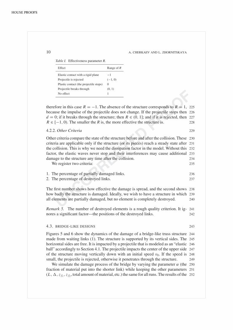
Table I. Effectiveness parameter R.

Effect Range of R

Elastic contact with a rigid plane −1

Projectile is rejected (−1, 0)

Plastic contact (the projectile stops) 0

Projectile breaks through (0, 1)

No effect 1

therefore in this case R = −1. The absence of the structure corresponds to R = 1, 225

because the impulse of the projectile does not change. If the projectile stops then 226

d = 0; if it breaks through the structure; then R ∈ (0, 1]; and if it is rejected, then 227

R ∈ [−1, 0). The smaller the R is, the more effective the structure is. 228

4.2.2. Other Criteria 229

Other criteria compare the state of the structure before and after the collision. These 230

criteria are applicable only if the structure (or its pieces) reach a steady state after 231

the collision. This is why we need the dissipation factor in the model. Without this 232

factor, the elastic waves never stop and their interferences may cause additional 233

damage to the structure any time after the collision. 234

We register two criteria: 235

1. The percentage of partially damaged links. 236

2. The percentage of destroyed links. 237

The first number shows how effective the damage is spread, and the second shows 238

how badly the structure is damaged. Ideally, we wish to have a structure in which 239

all elements are partially damaged, but no element is completely destroyed. 240

Remark 5. The number of destroyed elements is a rough quality criterion. It ig- 241

nores a significant factor—the positions of the destroyed links. 242

4.3. BRIDGE-LIKE DESIGNS 243

Figures 5 and 6 show the dynamics of the damage of a bridge-like truss structure 244

made from waiting links (1). The structure is supported by its vertical sides. The 245

horizontal sides are free. It is impacted by a projectile that is modeled as an “elastic 246

ball” accordingly to Section 4.1. The projectile impacts the center of the upper side 247

of the structure moving vertically down with an initial speed v0. If the speed is 248

small, the projectile is rejected, otherwise it penetrates through the structure. 249

We simulate the damage process of the bridge by varying the parameter α (the 250

fraction of material put into the shorter link) while keeping the other parameters 251

(L , �, z f1, z f2 , total amount of material, etc.) the same for all runs. The results of the 252

HOUSE PROOFS

UNCORRECTEDPROOF


Figure 5. Evolution of damage in a lattice with waiting elements (left column α = 25%, right,column: α = 10%).

simulation are summarized in Table II. One can see from Table II that as α decreases253

from 1.00 (conventional structure) to 0.10 the percentage of partially damaged links254

increases as the percentage of destroyed links decreases making the structure more255

resistant. Table II also shows that α = 0.25 is optimal for both minimizing the256

number of destroyed links and minimizing the effectiveness parameter R (see the257

discussion in Section 4.2).258

The structures with α = 0.50 and α = 1.00 (conventional structure) soon259

develop cracks and fall apart allowing the projectile to go through (see Figure 6)260

while the structures with α = 0.10 and α = 0.25 preserve the structural integrity261

by dissipating energy and taking the stress away from the point of impact; this262

results in the rejection of the projectile (see Figure 5). Notice that the final time263

Tfinal is twice as small in the last two examples.264

HOUSE PROOFS

UNCORRECTEDPROOF


Figure 6. Evolution of damage in a lattice with (right, α = 50%) and without (left, α = 100%)waiting elements.

The propagation of the damage is due to several factors: the local instabilities of 265

the part of the network that contains a damaged link: the force acting on neighboring 266

links significantly increases and the damage spreads: the waves that propagate 267

through the network and initiate the damage in the remote from the collision point 268

areas. 269

4.4. DAMAGE OF A MASSIVE STRUCTURE 270

The following section describes the result of simulation of damage/destruction of 271

network made from the waiting links and compares these structures with the nets 272

from conventional links. 273

This series of experiments aims to show the wave of damage and strains in a 274

“large” domain (the block). The block is supported from the sides, the bottom is 275

HOUSE PROOFS

UNCORRECTEDPROOF


Table II. Damage and/or destruction of a bridge.

% of % of destroyed Final timeFigure α damaged links links Effectiveness R Tfinal

Figure 5 (right) 0.10 94 3.8 −0.26 500

Figure 5 (left) 0.25 42 3.8 −0.32 500

Figure 6 (right) 0.50 4.6 6.3 0.54 250

Figure 6 (left) 1.00 0 8.6 0.46 250

free (see Figure 7). As in the above mentioned simulations of the bridges, the block276

is impacted by a projectile that is modeled as an “elastic ball”. It is assumed that the277

projectile hits the center of the upper side of the structure moving vertically down278

with an initial speed v0.279

Figure 7 demonstrates propagation of the elastic waves and the waves of partial280

and total damage of elements of the block. The conventional link structure soon281

develops cracks and gets destroyed, while the waiting link structure preserves its282

structural integrity. Notice that the damage is concentrated in conventional design283

and spread in the waiting link design.284

5. Discussion285

5.1. RESUME286

1. Our numerical experiments have demonstrated the possibility of control of the287

damage process: Waiting links allow to increase the resistivity, increase the time288

of rupture, increase the absorbed energy, and decrease the level of concentration289

of damage.290

2. The results emphasize the necessity of dynamics simulation versus computation291

of the quasi-static equilibrium: one can see from Figure 7 that damage can start292

in parts of the structure distant from the zone of impact. Development of damage293

is caused by excited waves and local instabilities.294

3. We observe that the results strongly depend on parameters of the structure and295

projectile.296

5.2. CONTINUUM AND DISCRETE MODEL297

We use a discrete model of the structure rather then the continuous model for several298

reasons. First, it models the structures that can be made as we described. However,299

one may ask how to simplify the computation of the dynamics using a homogenized300

description of the networks. The process of damage is similar to the process of phase301

transition, since the initial (undamaged) phase is replaced by the partially damaged302

state and then by the destroyed state of structure in a small scale; such processes303

tan also be described as a phase transition in solids, see for example [9].304

HOUSE PROOFS

UNCORRECTEDPROOF


Figure 7. Evolution of damage in a lattice with waiting elements. Left field: lattice fromelastic-brittle material: right field: lattice from waiting links, α = 0.25.

The observed process is also significantly controlled by intensive waves caused 305

by vibration of individual masses. The fast-oscillating motion carries significant 306

energy and it is responsible for initiation of the damage in the parts of the structure 307

that are not connected to the zone of impact, but are close to reflecting boundaries. 308

In the continuum model, these oscillations would disappear and it is still unclear 309

how to account for this energy in the homogenized model. 310

HOUSE PROOFS

UNCORRECTEDPROOF


5.3. OPTIMIZATION311

The demonstrated structures show the ability to significantly increase the resistance312

comparing with conventional materials. However, these results are still far away313

from the limit that can be achieved by optimizing the response by new design314

variables: The ratio α and the additional (slack) length (�−L) of the waiting rod. In315

principle, these parameters can be separately assigned to each link, keeping the total316

amount of material fixed. However, there are natural requirements of robustness:317

A structure should equally well resist all projectiles independently of the point of318

impact, and should well resist projectiles approaching with various speed. Such319

considerations decrease the number of controls; it is natural to assign the same320

values of the design parameters to all elements in the same level of the structure.321

One may minimize the absorbed energy, restricting the weight, admissible elon-322

gation, and the threshold after which the damage starts. In addition, one needs to323

restrict the range of parameters of a projectile: its mass, direction, and speed. The324

range of parameters is important: because of strong nonlinearity, the qualitative325

results are expected to be sensitive to them. The optimization problem is com-326

putationally very intensive since the dependence of parameters is not necessarily327

smooth or even continuous. We plan to address the optimization problem in the328

future research.329

Acknowledgment330

This work was supported by ARO and NSF.331

References332

1. Cherkaev, A. and Slepyan, L., ‘Waiting element structures and stability under extension’, Inter-333national Journal of Damage Mechanics 4(1), 1955, 58–82.334

2. Francfort, G.A. and Marigo, J.-J., ‘Stable damage evolution in a brittle continuous medium’,335European Journal of Mechanics A: Solids 12(2), 1993, 149–189.336

3. Timoshenko, S.P. and Goodier, J.N., Theory of Elasticity, 2nd edn. McGraw-Hill Book Company,337Inc., New York, Toronto, London, 1951.338

4. Slepian, L.I., Models and Phenomena in Fracture Mechanics, Springer-Verlag, 2002.3395. Balk, A., Cherkaev, A. and Slepyan, L., ‘Dynamics of chains with non-monotone stress–strain340

relations. I. Model and numerical experiments’, Journal of Mechanics, Physics and Solids 49,3412001, 131–148.342

6. Balk, A., Cherkaev, A. and Slepyan, L., ‘Dynamics of chains with non-monotone stress–strain343relations. II. Nonlinear waves and wave of phase transition’, Journal of Mechanics, Physics and344Solids 49, 2001, 149–171.345

7. Slepyan, L.I. and Ayzenberg-Stepanenko, M.V., ‘Some surprising phenomena in weak-bond frac-346ture of a triangular lattice’, Journal of Mechanics, Physics and Solids 50(8), 2002, 1591–1625.347

8. Kyriafides, Stelios, ‘Propagating instabilities in structures’, Advances in Applied Mechanics34830, 1994, 68–186.349

9. Nekorkin, V.I. and Velarde, M.G., Synergetic Phenomena in Active Lattices, Springer-Verlag,3502002.351

10. Morikazu, Toda, Theory of Nonlinear Lattices, Springer-Verlag, 1989.352

HOUSE PROOFS

protective structures with waiting links and their damage

Documents