PROSTATE TISSUE DIAGNOSIS USING QUANTITATIVE PHASE

IMAGING TECHNIQUES

BY

SHAMIRA SRIDHARAN

THESIS

Submitted in partial fulfillment of the requirements for the degree of Master of Science in Bioengineering

in the Graduate College of the University of Illinois at Urbana-Champaign, 2012

Urbana, Illinois

Adviser:

Assistant Professor Gabriel Popescu

ii

Abstract

The lifetime risk of a man getting diagnosed with prostate cancer is 1 in 6. The diagnosis is

made by the pathologist using staining methods and immunohistochemical markers to detect

malignancy on tissue biopsy sections. Quantitative phase imaging methods eliminate the need

for stains and markers. It exploits the intrinsic contrast from the refractive index differences in

tissue. The quantitative nature of this technique eliminates inter-observer variability. QPI is

sensitive to sub-nanometer level changes in tissue architecture. Light scattering information is

also accessible from QPI images since it records both the amplitude and the phase of light that

passes through the sample. In this thesis, I show the ability of QPI to distinguish between

cancerous and benign samples. I also show its ability to detect changes in stroma and nuclei

through different stages of prostate cancer progression that are not detectable using conventional

methods.

iii

Contents

1. Introduction ............................................................................................................................................... 1

1.1 Overview ............................................................................................................................................. 1

1.2 Outline................................................................................................................................................. 2

2. Light-tissue interaction ............................................................................................................................. 3

2.1 Scattering window .............................................................................................................................. 3

2.2 Scattering phase theorem .................................................................................................................... 5

2. 3 Correlation induced spectral changes in tissue .................................................................................. 7

3. Prostate Cancer ....................................................................................................................................... 11

3.1 Benign Prostate Conditions ............................................................................................................... 12

3.1.1 Benign Prostatic Hyperplasia (BPH) ......................................................................................... 12

3.1.2 High-grade prostatic intra-epithelial neoplasia (HGPIN) .......................................................... 13

3.2 Prostate Cancer ................................................................................................................................. 13

3.2.1 Gleason Grading of Prostate Cancer .......................................................................................... 15

4. Qualitative Diagnosis Methods ............................................................................................................... 19

4.1 Gradient Field Microscopy (GFM) ................................................................................................... 19

4.2 HGPIN Diagnosis using GFM .......................................................................................................... 21

5. Quantitative Diagnosis ............................................................................................................................ 23

5.1 Spatial Light Interference Microscopy (SLIM) ................................................................................ 23

5.2 Fourier Transform Light Scattering (FTLS) ..................................................................................... 24

5.3 Optical changes in prostate stroma ................................................................................................... 25

5.3.1 Motivation .................................................................................................................................. 25

5.3.2 Materials and Methods ............................................................................................................... 26

5.3.3 Results ........................................................................................................................................ 28

5.3.4 Discussion .................................................................................................................................. 30

5.4 Optical changes in prostate nuclei .................................................................................................... 32

5.4.1 Motivation .................................................................................................................................. 32

5.4.2 Materials and Methods ............................................................................................................... 32

5.4.3 Results ........................................................................................................................................ 34

5.4.4 Discussion .................................................................................................................................. 38

6. Summary & Future Work ....................................................................................................................... 40

References ................................................................................................................................................... 42

1

1. Introduction

1.1 Overview

Optically thin slices of tissue do not significantly scatter or absorb light. Due to its transparent

nature, in clinical pathology, contrast is extrinsically generated by adding dyes to make

structures visible. Tissue biopsy sections are traditionally stained with hematoxylin and eosin

(H&E). Hematoxylin stains nucleus in a deep blue-purple by a reaction that is not completely

understood, whereas eosin non-specifically stains proteins pink and makes the cytoplasm and

extra-cellular matrix visible[1]. When the pathologist suspects the presence of cancer on the

H&E stained biopsy, a consecutive biopsy section is stained with specialized stains,

immunohistochemical markers and/or molecular markers to make a final diagnosis. These

techniques can be expensive and time-consuming.

Cells and tissue have intrinsic contrast in the form of refractive index differences between

various structures. In the 1930s, Zernike developed phase contrast microscopy in which the

unscattered and scattered components of light are separated by a π/2 phase value, making

transparent structures visible[2]. However, phase contrast images are qualitative. Quantitative

phase imaging (QPI) techniques image transparent structures and quantitate the change in the

path length of light as it transmits through these structures. In constant thickness samples such

as tissue sections, the phase value is only dependent on the refractive index. QPI techniques are

sensitive to path length changes at the nanoscale level.

In tissue, nanoscale fluctuations in path length correspond to changes in tissue architecture.

Light scattering parameters can also be obtained from quantitative phase images. This scattering

information and quantitative phase information can be used in the diagnosis of disease. In the

2

past, QPI has been used to diagnose prostate cancer in label-free tissue biopsies[3]. In this

thesis, I describe the utility of QPI in studying optical changes in prostate tissue of varying

severity of cancer.

1.2 Outline

In chapter 2, I elaborate on the interaction between light and tissue, and how information about

light scattering through various structures can be retrieved from quantitative phase images.

In chapter 3, I present the problems associated with prostate cancer diagnosis, more specifically,

benign mimickers of prostate cancer and discuss the importance of prognostic tools.

In chapter 4, I introduce gradient field microscopy (GFM) which is a quantitative tool that can

help in separating prostate cancer from its benign mimickers by detection of the basal cell layer

(myo-epithelial layer) that is absent in prostate cancer.

In chapter 5, I discuss spatial light interference microscopy (SLIM), a quantitative phase imaging

method and Fourier transform light scattering (FTLS), a tool to study tissue scattering. I show

some results on the utility of SLIM in detection of changes in stroma of prostate cancer of

various Gleason grades and FTLS changes in nuclei of various stages of prostate disease.

Finally, I summarize this thesis and discuss the future direction of this research.

3

2. Light-tissue interaction1

When light is propagated through tissue, there is a change in the irradiance, spectrum,

polarization, phase, direction and coherence due to which information about tissue can be

obtained [4-6]. The light-tissue interaction can be classified as elastic and inelastic. Elastic light

scattering occurs when the frequency of light is conserved. This is different from dynamic light

scattering where Doppler shifts caused by dynamic specimen such as live cells cause small

changes in light frequency[7]. In diseases such as cancer, the morphological changes in tissue

modify light properties such as scattering parameters and this can be used to diagnose disease.

Tissue scattering basics are reviewed in this chapter in greater detail.

While inelastic interactions such as emission and absorption are out of the scope of this thesis,

spectral changes due to elastic scattering can hinder measurements based on inelastic interactions

between light and tissue and is discussed in greater detail below[8].

2.1 Scattering window

Biological tissue and cells is composed of various structures and organelles that have different

refractive indices. This difference in refractive index makes tissue highly scattering. The optical

microscope is a scattering instrument that makes measurement in real space (x,y,z)[9].

The three major structures in cell are cell membrane, nucleus and cytoplasm. The cell membrane

encompasses the cytoplasm and is made of a phospholipid bilayer composed of proteins and

glycoproteins that float on lipids. The cytoplasm encompasses cytosol in which various

1 The text in this chapter is adapted from:

Kim, T., Sridharan, S., Popescu, G. Fourier transform light scattering of tissues in Coherent-domain optical

methods, Second Edition, Edited by Tuchin, V.V., Springer (2012).

Zhu, R., Sridharan, S., Tangella, K., Balla, A., Popescu, G. Correlation induced spectral changes in tissues. Optics

Letters 36(21), 2011.

4

organelles such as mitochondria, golgi apparatus, endoplasmic reticulum, peroxisomes,

lysosomes are suspended. The cell nucleus is separated from the cytoplasm by the nuclear

envelope and is the site of DNA replication and RNA translation[10].

The different cellular structures have different refractive indices due to varying compositions.

This makes the cell a scattering medium. Large structures such as nucleus scatter light at smaller

angles whereas smaller organelles such as mitochondria scatter at large angles[11, 12].

Light is absorbed by cells in accordance with the Beer-Lambert’s law which helps quantitate the

decrease in intensity as light travels through material of thickness L:

L

L

eI

eII

0

0

Where ε is the extinction coefficient, ρ is the concentration of absorbing material and α is the

absorption coefficient. Since the human body is primarily composed of water, it is important to

note that water does not absorb light significantly in the 200-1300nm spectral region as shown

by studies by Hale and Querry [13]. Hemoglobin, a red blood cell protein that transports oxygen

to tissue, is also a major contributor to the absorption spectrum[14]. Hemoglobin gets

oxygenated by binding oxygen to iron atoms as red blood cells pass through the lungs and gets

deoxygenated in tissue, changing its absorption spectrum. Hemoglobin absorbs most in blue and

green spectral regions.

5

Figure 12: The graph for absorption coefficient vs. wavelength is shown for water,

hemoglobin and deoxygenated hemoglobin. From the absorption spectra, the tissue optical

window can be obtained.

In the 800-1300nm window, also referred to as the tissue optical window, the tissue exhibits low

light absorption. In this window, the scattering effect is dominant and absorption is an

insignificant contributor. This is the spectral region where tissue scattering experiments are

performed.

2.2 Scattering phase theorem

Scattering phase theorem allows us to calculate the scattering mean free path ( sl ) and optical

anisotropy (g) from the phase distribution in a tissue section of thickness L<< sl [15, 16].

2 Figure adapted from Kim, T., Sridharan, S., Popescu, G. Fourier transform light scattering of tissues in Coherent-

domain optical methods, Second Edition, Edited by Tuchin, V.V., Springer (2012).

6

Figure 23: (a): Light with amplitude U0 travels through tissue section of thickness L for

which ls is the scattering mean free path. (b): ko is the incident wave vector and ks is the

scattered wave vector, q represents transfer of momentum, g is the optical anisotropy

where g=cos θ

The scattering mean free path ( sl ) is defined from the Lambert-Beer’s law as the length over

which the intensity of unscattered light drops to 1/e of its original value. In tissue, this is the

average step between two scattering events. sl is inversely proportional to the phase variance

averaged over a certain tissue region as shown in equation[15] (1).

r

sr

Ll

)(2 (1)

Optical anisotropy is defined as the average cosine of the angle associated with a single

scattering event. It is the change in the direction of light propagation due to scattering. g

accounts for forward scattering and scales sl to a higher value called transport mean free path ( tl

3 Figure adapted from Kim, T., Sridharan, S., Popescu, G. Fourier transform light scattering of tissues in Coherent-

domain optical methods, Second Edition, Edited by Tuchin, V.V., Springer (2012).

7

) where tl = sl /(1-g). Optical anisotropy is related to both the phase gradient distribution and

scattering mean free path in the region of interest as shown in equation[15] (2).

2

0

2

2

2

)]([)(1

k

r

L

lg rs

(2)

From the scattering phase theorem, it is evident that when the inhomogeneity in tissue is

increased, the propagated light is scattered more which means the optical anisotropy value

increases while the scattering mean free path reduces in length.

2. 3 Correlation induced spectral changes in tissue

Correlation induced spectral shifts or Wolf shifts refers to Wolf’s prediction that spatial

correlations in a primary source affects the optical spectrum in the far zone[17]. These

predictions were experimentally confirmed in acoustic waves, spectroscopic measurements on

stellar objects and scattering media[18-21]. The frequency shift in spectral lines was explained

by the medium scattering various wavelengths with differing strength which was dependent on

the scattering angle[20].

Figure 34: A quantitative phase image of a prostate tissue microarray core of 4micron

thickness with a region zoomed in.

4 Figure reprinted from Zhu, R., Sridharan, S., Tangella, K., Balla, A., Popescu, G. Correlation induced spectral

changes in tissues. Optics Letters 36(21), 2011.

300

m

Phase [rad]

8

We measured this spatial correlation function on a quantitative phase image of an unstained 4µm

thick prostate cancer tissue section which is shown in Fig. 3.

We calculate the optical spectrum associated with scattering angle θ by starting with the

Helmholtz equation:

),()(),(),( 2

0

2

0

2 rUrkrUkrU

Where k0 is the incident wave vector, χ is the dielectric susceptibility of optically thin specimen

and the field is a function of the angular frequency ω and spatial coordinate r. According to the

Born approximation, the incident plane wave remains a plane wave inside the tissue. By

applying the Born approximation to (3) we get:

zikeAzyxkrUkrU 0)()(),(),(),( 2

0

2

0

2

Where zikeA 0)( is the incident plane wave. We take the Fourier transform of the above equation

with respect to r to obtain the field in wave vector form

)(~)(),(~

2

0

2

2

0ikkA

kk

kkU

The above equation expression is a variation of diffraction tomography in which the scattered

field measured along the wave vector direction provides information about the spatial frequency

component q=k-ki. The scattering angle θ is related to the momentum transfer q by

q=2k0sin(θ/2). The susceptibility term is only dependent on kx and ky, so we define a new term

2

1

22 )( yx kkk and therefore )( 22

0

2

kkQ and equation 3 becomes:

9

)(~)(11

2),(

~2

0

kA

kQkQQ

kkU

zz

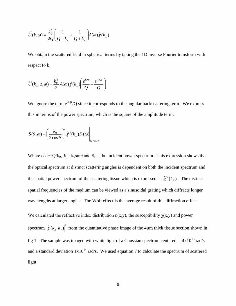
We obtain the scattered field in spherical terms by taking the 1D inverse Fourier transform with

respect to kz

Q

e

Q

ekA

kzkU

iQziQz

)(~)(2

),,(~

2

0

We ignore the term e-iQz

/Q since it corresponds to the angular backscattering term. We express

this in terms of the power spectrum, which is the square of the amplitude term:

ck

iSkk

S

/

2

2

0

0

)()(~

cos2),(

Where cosθ=Q/k0, k =k0sinθ and Si is the incident power spectrum. This expression shows that

the optical spectrum at distinct scattering angles is dependent on both the incident spectrum and

the spatial power spectrum of the scattering tissue which is expressed as )(~2

k . The distinct

spatial frequencies of the medium can be viewed as a sinusoidal grating which diffracts longer

wavelengths at larger angles. The Wolf effect is the average result of this diffraction effect.

We calculated the refractive index distribution n(x,y), the susceptibility χ(x,y) and power

spectrum 2

),(~yx kk from the quantitative phase image of the 4µm thick tissue section shown in

fig 1. The sample was imaged with white light of a Gaussian spectrum centered at 4x1015

rad/s

and a standard deviation 1x1014

rad/s. We used equation 7 to calculate the spectrum of scattered

light.

10

Figure 45: (a): Spectrum Vs Angle for scattered light from the tissue in Fig 1 (b): The

relative change of mean frequency; negative values correspond to a shift in the red light

spectrum.

When we closely examine the scattered spectrum at each angle, we notice that there is a

modification from the original spectrum with red spectral shifting (Fig 3a). This is consistent

with static scattering. We quantified the overall shift by defining 000 /)'()( where ω’

is the shift in mean frequency and ω0 is the original mean frequency. The red shifts are

significant (Fig 3b). The maximum shift in red is more than 10%. By plotting the spectrum in

absence of correlations, we see that the normalized spectrum at different angles does not change

(Fig 3b inset). This proves that the shift is entirely due to spatial correlations.

Our study shows that the measured scattering spectrum at various angles is affected by tissue

spatial correlations. These spatial correlations change the shape of the emitted field without

affecting the emission process. This effect can cause errors in spectroscopic measurements of

tissue due to the significant effect in angular and spectral resolved measurements. This can be

resolved by simultaneous measurement of morphology and spectroscopy.

5 Figure reprinted from Zhu, R., Sridharan, S., Tangella, K., Balla, A., Popescu, G. Correlation induced spectral

changes in tissues. Optics Letters 36(21), 2011.

11

3. Prostate Cancer

The prostate is an exocrine gland weighing 30-40g in the adult male reproductive system that is

located at the base of the urinary bladder. The urethra and the ejaculatory duct pass through the

prostate gland. The prostate secretes 12% of the ejaculatory fluid into the duct which opens into

the prostatic urethra [22]. In 1968, McNeal performed serial sectioning of the prostate gland to

study the various structures within the prostate. The gland can be divided into four zones. The

central zone comprises approximately 25% of the gland and surrounds the ejaculatory duct. It

consists of large acini with irregular contours that project into the lumen of the gland; the

epithelium comprises big nuclei in a crowded arrangement with granular cytoplasm [23, 24].

The peripheral zone, which comprises 70% of the prostate, surrounds the distal region of the

urethra and has small acini with smooth walls; the epithelium has pale cytoplasm with small

basal nuclei [24]. Most cases of prostate cancer arise within the peripheral zone of the prostate

gland [25]. The third zone is the transition zone which comprises 5% of the prostate and

surrounds the proximal portion of the urethra; the epithelium is histologically similar to the

peripheral zone [24]. Most cases of benign prostatic hyperplasia arise in the peripheral zone of

the prostate gland [26]. The fourth zone of the prostate is the anterior fibromuscular stroma,

which is a non-glandular region anterior to the prostate gland [23].

The acini of the prostate open into prostatic ducts which in turn secrete into the prostatic urethra.

The acinar cells primarily are made of columnar epithelium, neuroendocrine cells and basal cells

[22, 27]. The columnar epithelial cells are 10-12µm in size and secrete prostate specific antigen

(PSA) and prostatic acid phosphatase (PAP); it also requires androgen for maintenance [23].

Neuroendocrine cells are scattered throughout the acini and basal cells rest on the basement

12

membrane [23]. Prostatic stroma is a collection of various cell types, such as fibroblasts, smooth

muscle cells, blood, lymphatic vessels and autonomic nerve fibers [28].

The most common initial symptom of prostate disorder is urinary difficulty, since the urethra

passes through the prostate gland. A person might get a needle biopsy to check for prostate

cancer if their serum PSA reading is above the normal cut-off of 4.0ng/L or suspicion during a

digital rectal exam (DRE). The needle biopsy specimen is embedded in paraffin and sliced using

a microtome. The tissue slice is then placed on a glass slide and stained with hematoxylin and

eosin (H&E) stain. The pathologist examines the H&E stained biopsy for the presence of the

basal or myo-epithelial layer to exclude the diagnosis of prostate cancer. The basal cell

membrane is breached in prostate cancer and cancerous epithelium invades the surrounding

stromal region. Conditions such as high-grade prostatic intra-epithelial neoplasia, which is a

benign mimicker of prostate cancer, can make the diagnosis difficult. In the following section, I

discuss benign prostate conditions and prostate cancer in more detail.

3.1 Benign Prostate Conditions

The two benign prostate conditions that were studied using QPI are benign prostatic hyperplasia

(BPH) which commonly affects older men and is often characterized by an enlarged prostate and

high grade prostatic intra-epithelial neoplasia (HGPIN) which is a benign mimicker of prostate

cancer.

3.1.1 Benign Prostatic Hyperplasia (BPH)

Approximately 50% of all men over the age of 40 will develop benign prostatic hyperplasia

(BPH) [29]. BPH is a condition in which the number of epithelial and stromal cells in the

prostate is increased. The increased cell count could be due to increased epithelial or stromal

13

proliferation or decreased rate of apoptosis [30]. BPH is diagnosed on a trans-urethral resection

of the prostate (TURP) samples. A diagnosis of BPH cannot be made on a needle biopsy sample

since the transition zone is not sampled in most needle biopsies. In our study of prostate

conditions, we used tissue from individuals with BPH as control since it’s a common condition

afflicting individuals in the age-group primarily affected by prostate cancer.

3.1.2 High-grade prostatic intra-epithelial neoplasia (HGPIN)

High-grade prostatic intraepithelial neoplasia (HGPIN) is a benign condition that is considered to

be a precursor to prostate cancer [25, 31, 32]. HGPIN is observed in 0 to 24.6% of prostate

needle biopsies with mean reported incidence of 7.6% [33, 34]. Prominent nucleoli and presence

of Roman bridges are common hallmarks of high-grade PIN [33, 34]. HGPIN is not very

common in the transition zone, has evenly spaced glands with focal to no necrosis and patchy

basal cell layer distinguishing it from prostate adenocarcinoma [33, 34]. Detection of

myoepithelial cells or basal cells by usage of antibody against cytokeratin 34BE12 and/or p63

marker is performed by the pathologist to exclude the diagnosis of carcinoma in suspected cases

of HGPIN [34]. The diagnosis of HGPIN is often made in patients suspected of having prostate

cancer and usage of special stains can delay diagnosis causing anxiety to patients. In our lab, we

developed a qualitative imaging technique, Gradient Field Microscopy (GFM) that detects the

basal cell layer in real-time preventing the delays caused by immunostains. GFM is described in

detail in the next chapter.

3.2 Prostate Cancer

Cancer statistics from 2010 indicate that prostate cancer is the most commonly diagnosed cancer

among men (not including skin cancer) in the United States of America and the second leading

cause of cancer-related deaths[35]. The SEER program by National Cancer Institute estimates

14

that there will be 241,740 new cases of prostate cancer and 28,170 men will die of prostate

cancer in the United States in 2012[36]. Due to the high fatality rate and economic costs related

to prostate cancer care, there was a need for an early detection tool for prostate cancer.

A good screening tool will diagnose a condition in its early stages and the number of people

diagnosed with the condition through screening will stabilize to the pre-screening numbers after

an initial spike. The prostate specific antigen test (PSA) was developed to detect early prostate

cancer and needle biopsies were performed in individuals with serum PSA above 4.0 ng/L. PSA

screening increased the number of people diagnosed with prostate cancer and the numbers did

not go down to the pre-screening era levels [37].

Figure 56: PSA screening was introduced in 1986. Panel A shows that while the spike

associated with screening reduced, it did not stabilize to pre-screening levels. Panel B

shows the increasing trend in the ratio of prostate cancer incidence relative to 1986 when

screening was first introduced.

6 Figure reprinted from Welch, H.G. and P.C. Albertsen, Prostate cancer diagnosis and treatment after the

introduction of prostate-specific antigen screening: 1986-2005. Journal of the National Cancer Institute, 2009. 101(19): p. 1325-9.

15

The median age of diagnosis of prostate cancer is 67 years while the median age of death due to

prostate cancer is 80 years with 71% of death due to disease occurring at age above 75 years

[36]. Hence, in 2008, the United States Preventive Services Task Force recommended against

PSA screening for men over the age of 75 years [38]. Further studies showed that while the life-

time risk for prostate cancer diagnosis is 15.9%, the risk of dying of the disease is 2.8% and that

1.2 million new cases of prostate cancer would be diagnosed if all American men between the

ages of 62 and 75 years underwent prostate biopsy [39]. Studies have shown that 1/3rd

of all men

in the age group of 40-60 years and 3/4th

of all men above the age of 75 years have histologic

prostate cancer [40, 41]. Out of every 1000 men who undergo surgery to treat prostate cancer,

10-70 men suffer serious complications; 200-300 men have undesirable long-term effects such as

bowel dysfunction, urinary incontinence and erectile dysfunction[42]. Based on these findings,

the USPSTF recommended against PSA screening for men of all ages in 2012 [39].

Current data and research indicate that prostate cancer is over-diagnosed. Among men affected

by the disease, some have asymptomatic slow growing tumors while others have a more

aggressive form of the disease which requires early and aggressive intervention. Hence there is a

need for prognostic tools in prostate cancer such as Gleason grading.

3.2.1 Gleason Grading of Prostate Cancer

The Gleason grade is the most widely used grading scheme in prostate cancer. The system was

developed by Dr. Donald Gleason in the 1960s and is based on glandular differentiation seen in

hematoxylin and eosin (H&E) stained slides [43, 44]. The Gleason score has been proven to be

an indicator of tumor size, metastasis, treatment and outcome [44-47].

16

The variation in grades on a scale from 1-5, in order of increasing severity, is based on glandular

differentiation and glandular presence in stroma [43, 44, 48, 49]. The primary grade is the

pattern present in maximum biopsy area and the secondary grade is the second most prominent

pattern. The secondary area has to encompass atleast 3% of total biopsy area [50]. The two

grades are added to provide a Gleason score of 1-10. More recently, tertiary patterns are

reported (area <5%) on the pathology report if it is of Grade 4 or 5 due to possible presence of

metastasis [51].

Figure 67: Standard drawing of Gleason grading system made by Dr. Donald F. Gleason

7 Figure reprinted from Gleason, D.F., Classification of prostatic carcinomas. Cancer Chemother Rep, 1966. 50(3): p.

125-8

17

A modified Gleason grading system was adopted in 2005 at the United States and Canadian

Academy of Pathology meeting [52]. Gleason grading is done at 4X or 10X magnification with

confirmation at 20X or 40X to detect fusion of glands and necrosis.

In current clinical practice, cancer of Gleason grade 1 is rarely diagnosed. It is suspected that

immunostains would re-label the cases categorized by Dr. Gleason as Grade 1 would be re-

categorized as adenosis and some cases of cribriform grade 3 adenocarcinoma as high-grade

prostatic intra-epithelial neoplasia (HGPIN) [33, 53].

Gleason grade 2 consists of irregular glands that are smaller than normal, but larger than other

cancerous glands and the tumor is well circumscribed. The cribriform pattern described by Dr.

Donald Gleason is no longer considered Gleason grade 2 [33, 52]. Gleason grade 2 is rarely

diagnosed due to poor reproducibility among pathologists and poor correlation on radical

prostatectomy specimen [33]. The diagnosis of Gleason score 2-4 (grades 1,2) has decreased

from 24% in 1991 to 2.4% in 2001 [54].

Gleason grade 3 glands are medium to small size, singular with infiltrating edges [44]. The

cribriform (gland within gland pattern) is also observed in Gleason grade 3, however, they do not

have necrosis [44]. Cribriform Gleason grade 3 glands resemble HGPIN glands with the absence

of basal cell layer, reduced spacing between glands and possible perineural invasion or extra-

prostatic extension [33]. Singular cells as described by Dr. Gleason are no longer considered

grade 3 [52].

Gleason grade 4 consists of small glands that are fusing into one another and cribriform patterns

with irregular edges as opposed to the smooth edges seen in cribriform glands of Gleason grade 3

18

[33]. Gleason grade 4 also has a hypernephromatoid subtype which has similar glandular pattern

as other grade 4 glands but has cleared cytoplasm resembling renal cells [43].

Gleason grade 5 comprises of sheets or cords of cells with no glandular differentiation [43]. A

cribriform pattern that looks like Gleason grade 4 with central region displaying necrosis, termed

comedonecrosis is also considered Gleason grade 5 pattern [44].

Gleason scores are often grouped together as score 2-4: well-differentiated; score 5-6:

moderately differentiated; score 7: moderately to poorly differentiated and 8-10: poorly

differentiated [33]. There have been studies that have shown that Gleason score 7 is a

heterogeneous disease with differential outcomes for Gleason grade 4+3 as opposed to Gleason

grade 3+4 [33, 55]. However, there are also studies disputing this finding [56-58]. The reasons

for this disagreement in results could be the inter-observer differences reported in Gleason

grading or the difference between the grades seen in needle biopsy and prostatectomy specimen

[59-61].

In this thesis, I studied differences in the stroma adjoining the gland of Gleason grade 3 and

Gleason grade 4 glands to explore the possibility of Gleason score 7 being a heterogeneous

disease. I also studied the difference in nuclear scattering in prostate tissue of varying levels of

glandular differentiation. This is explained in detail in Chapter 5.

19

4. Qualitative Diagnosis Methods8

The distinction between cancer and normal biopsies is made by the detection of basal cell layer.

Gradient field microscopy (GFM) is a high contrast method that detects these basal cells. GFM

also has the advantage of high acquisition speed. Since the contrast is increased optically, there

is no need of post-image processing. Thus, GFM naturally provides an ability to image in real-

time and the acquisition speed is limited only by the acquisition speed of the detector used in the

setup.

4.1 Gradient Field Microscopy (GFM)

Figure 1 shows the setup for gradient field microscopy (GFM), which is an experimental setup

for the Fourier filtering using a sinusoidal amplitude mask. GFM is built as an additional

module to a commercial bright field microscope, which is composed of the components from the

condenser lens to the tube lens. The aperture stop closed down to the minimum size in order to

obtain high spatial coherence in the white light illumination. From the image plane of the

microscope, there is a relay of optical components comprising two lenses to form a 4f system and

a spatial light modulator (SLM). The first Fourier lens, L1, with the focal distance f1=75mm is at

f1 away from the image plane, and the SLM is located at f1 away from L1 which is the Fourier

plane of the image plane of the microscope. The second Fourier lens is at its focal distance,

f2=150mm, away from the SLM and forms the modulated image at f2 away from itself, where the

8 The text in this chapter is reprinted with permission from:

Kim, T., Sridharan, S., Popescu, G. Gradient field microscopy of unstained specimens, Optics Express 20(6), 2012.

Kim, T., Sridharan, S., Popescu, G., Gradient field microscopy allows label-free disease diagnosis (invited), Laser

Focus World, 48 (8), (2012)

Kim, T., Sridharan, S., Kajdacsy-Balla, A., Tangella, K., Popescu,G.,, Gradient field microscopy for label-free

diagnosis of human biopsies, Appl. Opt. (Special Issue on Holography), 52 (1), A92-A96 (2013)

20

detector (Andor iXon+ EMCCD) is located. As a whole, GFM module increases the contrast by

imaging the first-order derivative of the phase of the sample as well as the magnification

determined by the ratio between the two Fourier lenses, which is 2 in our setup.

The SLM in our setup is a liquid crystal panel taken from Epson Powerlite S5 commercial

projector sandwiched between two cross polarizers. The top inset of figure 1 is projected to the

amplitude SLM and the bottom is the profile of the sinusoidal modulation taken along the dashed

line. The contrast ratio of this device, 400/1, provides enough attenuation at where the projected

value on the liquid crystal is zero. Furthermore, the sine modulation period is calculated to be

7.8mm (13μm/pixel, 600pixels/period) and it yields the shift of 2λf/a=20µm between the two

separated beams and the DC field locates at the middle of the two beams.

Figure 79: GFM Set-up. The inset shows the modulation filter projected on SLM for sine-

GFM (top) and linear-GFM (bottom).

9 Figure reprinted from Kim, T., Sridharan, S., Popescu, G. Gradient field microscopy of unstained specimens,

Optics Express 20(6), 2012

21

4.2 HGPIN Diagnosis using GFM

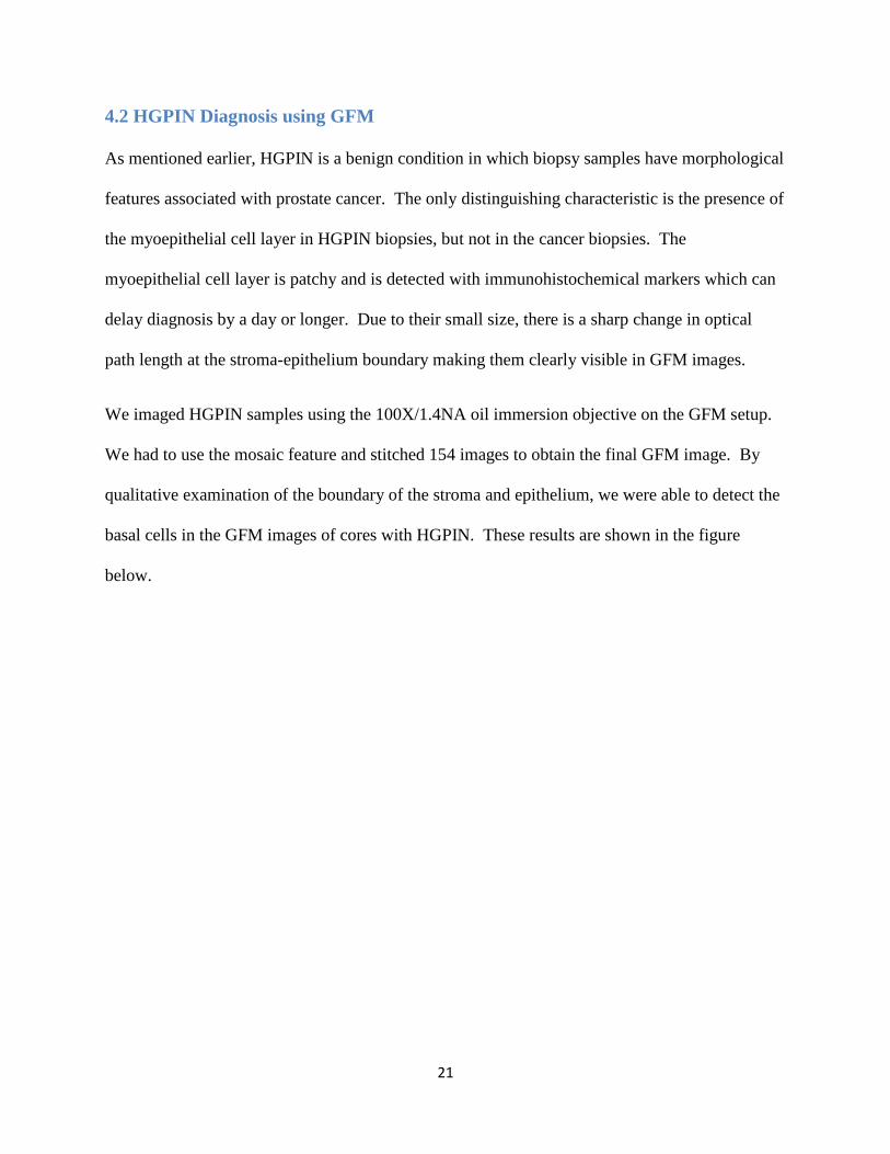
As mentioned earlier, HGPIN is a benign condition in which biopsy samples have morphological

features associated with prostate cancer. The only distinguishing characteristic is the presence of

the myoepithelial cell layer in HGPIN biopsies, but not in the cancer biopsies. The

myoepithelial cell layer is patchy and is detected with immunohistochemical markers which can

delay diagnosis by a day or longer. Due to their small size, there is a sharp change in optical

path length at the stroma-epithelium boundary making them clearly visible in GFM images.

We imaged HGPIN samples using the 100X/1.4NA oil immersion objective on the GFM setup.

We had to use the mosaic feature and stitched 154 images to obtain the final GFM image. By

qualitative examination of the boundary of the stroma and epithelium, we were able to detect the

basal cells in the GFM images of cores with HGPIN. These results are shown in the figure

below.

22

Figure 810

: Left shows a prostate tissue microarray core with HGPIN imaged with GFM.

Due to its high contrast, edges are prominent. The figures on the right show areas from

prostate TMA zoomed in with the basal cell layer highlighted.

10

Figure reprinted from Kim, T., Sridharan, S., Popescu, G. Gradient field microscopy of unstained specimens,

Optics Express 20(6), 2012.

23

5. Quantitative Diagnosis

Zernike developed the Nobel-prize winning technique, phase contrast microscopy, in the 1930s.

In a phase contrast microscope, the sample is illuminated by spatially coherent white light. The

component of light that passes through cellular structures is retarded in phase, and by adding an

additional π/2 delay to this scattered component, the path-length difference between the scattered

and unscattered components of light increases to λ/2 making transparent objects visible[62]. In

the 1940s, Gabor developed holography which enabled the recording of both the amplitude and

phase information[63].

Spatial light interference microscopy (SLIM) was developed in the Quantitative Light Imaging

(QLI) group at University of Illinois by combining principles from Zernike’s phase contrast

microscopy and Gabor’s holography as a quantitative phase imaging method that is sensitive to

path-length changes of upto 0.3nm spatially and 0.03nm temporally[64].

5.1 Spatial Light Interference Microscopy (SLIM)

Figure 9: SLIM is an add-on module to a commercial phase contrast microscope.

Commercial Phase

Contrast Microscope

IP

L1 150 350 500 L2PL3300

DA

Q

Co

mp

uter

L1P

L2L3 L4CCD

Commercial Phase Contrast Microscope

SLM

24

Spatial light interference microscopy (SLIM) is a quantitative phase imaging method that is

described in detail in [64]. Briefly, SLIM is an add-on module to the commercial phase contrast

microscope (Zeiss Axio Observer Z1) and adds 3 additional phase shifts in increments of π/2 to

the un-scattered component of light passing through the sample. The SLIM module projects the

back focal plane of the objective to the liquid crystal phase modulator which introduces the

additional phase shifts. We record 4 intensity images and calculate a quantitative phase map

from these images. The final image is calculated by the formula:

,

0

0

2, , ,

h x y

x y n x y z n dz

(54)

Each term in this equation is defined as follows.

λ: Central wavelength of light. In SLIM, light used is white light, so it corresponds to 552.3nm,

h(x,y): Local thickness fluctuations n(x,y,z): Local refractive index fluctuations, n0: Refractive

index of surrounding medium.

SLIM measures optical path length changes with a sensitivity of 0.3nm spatially which

corresponds to dry mass sensitivity of 1.5fg/μm2[65]. In the past, our group demonstrated that

refractive index could be used as a marker to differentiate cancer and normal areas of the prostate

as well as to measure cell growth and dynamics[65-68].

5.2 Fourier Transform Light Scattering (FTLS)

QPI techniques such as SLIM record both the amplitude and the phase of the field at the image

plane. Since complete information about the field is available, the field distribution at all other

planes can be calculated. The image and scattering field have a Fourier transform relationship.

25

Fourier transform light scattering (FTLS) is a sensitive method to study angular scattering

information since the field is measured at the highly uniform image plane [69, 70].

We used SLIM and FTLS to quantitatively study changes in prostate nuclei and stroma through

various pathological stages.

5.3 Optical changes in prostate stroma

5.3.1 Motivation

The Gleason grading system focuses primarily on changes in the glandular structure and

therefore the epithelium. The immunostains used in prostate pathology, such as high molecular

weight cytokeratin, p63 and AMACR focus on various aspects of the epithelium. More recently,

some molecular studies have focused on the stroma in prostate cancer.

The stroma is a complex environment consisting of the extracellular matrix, fibroblasts, smooth

muscle cells, growth factors, regulatory receptors, blood vessels, nerve fibers and immune cells

[28]. In the prostate, the primary stromal components are fibroblasts and smooth muscle cells

[71]. The various components of the stroma provide adhesion, growth factor secretion and

regulation, structural framework and support, cell attachment and migration and permeability

[72, 73]. In response to carcinoma in the epithelium, the repair mechanism in stroma is activated

[74]. The stromal changes seen in cancer using immunohistochemistry or molecular studies

mimic the changes seen in wound healing mechanisms such as increased growth factor secretion,

angiogenesis, matrix remodeling, elevated immune response and increased protease activity [75-

79]. These changes also include a switch to the activated myofibroblast phenotype from

fibroblast characterized by increased secretion of vimentin and smooth muscle to myofibroblast

with reduced levels of α-smooth muscle actin and calponin [74, 77, 78, 80, 81].

26

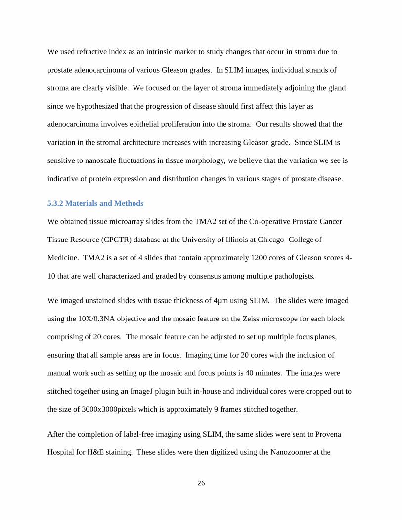
We used refractive index as an intrinsic marker to study changes that occur in stroma due to

prostate adenocarcinoma of various Gleason grades. In SLIM images, individual strands of

stroma are clearly visible. We focused on the layer of stroma immediately adjoining the gland

since we hypothesized that the progression of disease should first affect this layer as

adenocarcinoma involves epithelial proliferation into the stroma. Our results showed that the

variation in the stromal architecture increases with increasing Gleason grade. Since SLIM is

sensitive to nanoscale fluctuations in tissue morphology, we believe that the variation we see is

indicative of protein expression and distribution changes in various stages of prostate disease.

5.3.2 Materials and Methods

We obtained tissue microarray slides from the TMA2 set of the Co-operative Prostate Cancer

Tissue Resource (CPCTR) database at the University of Illinois at Chicago- College of

Medicine. TMA2 is a set of 4 slides that contain approximately 1200 cores of Gleason scores 4-

10 that are well characterized and graded by consensus among multiple pathologists.

We imaged unstained slides with tissue thickness of 4µm using SLIM. The slides were imaged

using the 10X/0.3NA objective and the mosaic feature on the Zeiss microscope for each block

comprising of 20 cores. The mosaic feature can be adjusted to set up multiple focus planes,

ensuring that all sample areas are in focus. Imaging time for 20 cores with the inclusion of

manual work such as setting up the mosaic and focus points is 40 minutes. The images were

stitched together using an ImageJ plugin built in-house and individual cores were cropped out to

the size of 3000x3000pixels which is approximately 9 frames stitched together.

After the completion of label-free imaging using SLIM, the same slides were sent to Provena

Hospital for H&E staining. These slides were then digitized using the Nanozoomer at the

27

Institute of Genomic Biology, University of Illinois at Urbana-Champaign. Using the

information from the CPCTR database, we identified cores with Gleason grade 3 cancer from a

final score of 6 and Gleason grade 4 cancer from a final score of 8 (4+4), 7 (4+3) and 9 (4+5).

Occasionally, the final Gleason grade diagnosed on the patient and the Gleason grade observed

on the tissue sample we obtained are not the same. To eliminate errors due to sampling, our

collaborating pathologists confirmed the presence of grade 3 and grade 4 glands in the cores we

used for our analysis.

We then segmented individual strands of stroma on the SLIM images on the pathologist-

identified glands of a specific grade using ImageJ and a Wacom tablet with the H&E image as a

reference for both grade 3 and grade 4. One advantage we had with the SLIM images over H&E

stained images is the clear visibility of individual stromal strands between glands, including

fusing glands. We calculated the magnitude and standard deviation of the phase and the

magnitude of the gradient of the phase in these stromal regions of interest (ROI) using another

plugin built in-house combined with the measurement features on ImageJ. With these

measurements we were able to calculate the ratio of the phase gradient to the square of the

variance, which is related to g (anisotropy factor), the average cosine of the scattering angle

associated with a single scattering event [15, 16].

28

Figure 10: SLIM image with the corresponding H&E image of a tissue microarray (TMA)

core of prostate with Gleason score 6 (3+3) adenocarcinoma. On the H&E, pink areas are

stroma and the purple areas are nuclei, epithelium. On SLIM, we can clearly see

individual strands of stroma even at 10X/0.3NA. The SLIM image is 3000x3000pixels and

is approximately 10 images stitched together from the mosaic imaging set up on Zeiss.

Also, an individual strand of stroma surround the gland has been marked for 4 glands on

the SLIM image.

5.3.3 Results

55 cores with Gleason grade 3 cancer and 55 cores with grade 4 cancer were used for analysis.

A single layer of stroma adjoining the gland was segmented to generate 118 ROIs for grade 3

and 117 ROIs for grade 4. We found significant differences in the square of the ratio of phase

gradient to phase variance (anisotropy factor analog) as shown in Fig. 4, 5. Using the non-

parametric Mann-Whitney test, the values for anisotropy-analog were determined to be higher

for grade 4 (p=3.76E-6). Also, the value for the magnitude of the phase gradient was higher in

cases with grade 4 cancer than grade 3 (p=7. 5E-5) (results not shown).

29

Figure 11: The distribution of anisotropy values is over a wider range for the stroma

surrounding grade 4 glands and the difference between the two groups is significant.

We further analyzed Gleason grade 4 stroma since the value of the anisotropy parameter was

distributed over a wide range of values. We compared anisotropy values in the grade 4 stroma

among 15 patients (34 ROIs) with final diagnosis of Gleason score 8 (4+4) and 16 patients (42

ROIs) with final diagnosis Gleason score 9 (4+5) as shown in Fig. 6. Our analysis showed that

the level of disorganization is higher in patients with Gleason score 9 (Mann-Whitney, p=5.91E-

5).

Figure 12: The distribution of anisotropy values is over a wider range for the stroma

surrounding grade 4 glands from patients with a final diagnosis of Gleason score 9 (4+5)

adenocarcinoma than that of Gleason score 8 (4+4) adenocarcinoma. The difference

between the two groups is significant.

30

5.3.4 Discussion

We calculated the square of the ratio of the phase gradient to phase variance, which is the

variable term in the calculation of the anisotropy factor (g). This substitution was made since an

anisotropy calculation over a small area of stroma which the number of scattering angles

measured. This in turn, pushes g to higher cosine values. Anisotropy is directly related to the

optical roughness of the tissue. We can see that the anisotropy is higher for the stroma adjoining

glands of grade 4 cancer and the distribution is over a very wide range, whereas for grade 3, the

value is small and distributed over a narrow range. These results also translate over when we

compare grade 4 regions among patients with final diagnosis of Gleason score 8 and 9. In

immunohistochemistry studies performed by other groups, hyaluronan (HA) level was observed

to be high in the stroma of prostate biopsies of higher Gleason grades but HA receptor CD 44

level is inversely related to Gleason grade [82]. High platelet-dervived growth factor (PDGFR-

β) expression and low expression of whey acidic protein family member WFDC1/PS20 has also

been seen in stroma adjoining high Gleason grade glands [83, 84]. In another study, an increased

level of stromal cells with fibroblast and myo-fibroblast phenotype and reduced levels of smooth

muscle actin cells were observed in proliferative cancerous tissue of prostate [85]. In-vitro

studies have shown the ability of prostate fibroblasts to transform into myo-fibroblast cells [86,

87]. While the label-free nature of SLIM prevents us from knowing the exact molecular or

morphological change that leads to the increased diversity we see in the anisotropy measurement,

all the changes documented with immunohistochemistry would contribute to increased

disorganization in the stroma which we measure as optical anisotropy. One advantage of SLIM

is that we can measure the final effect of all the molecular changes which cannot be done in

immunohistochemistry due to its inherent reactive nature.

31

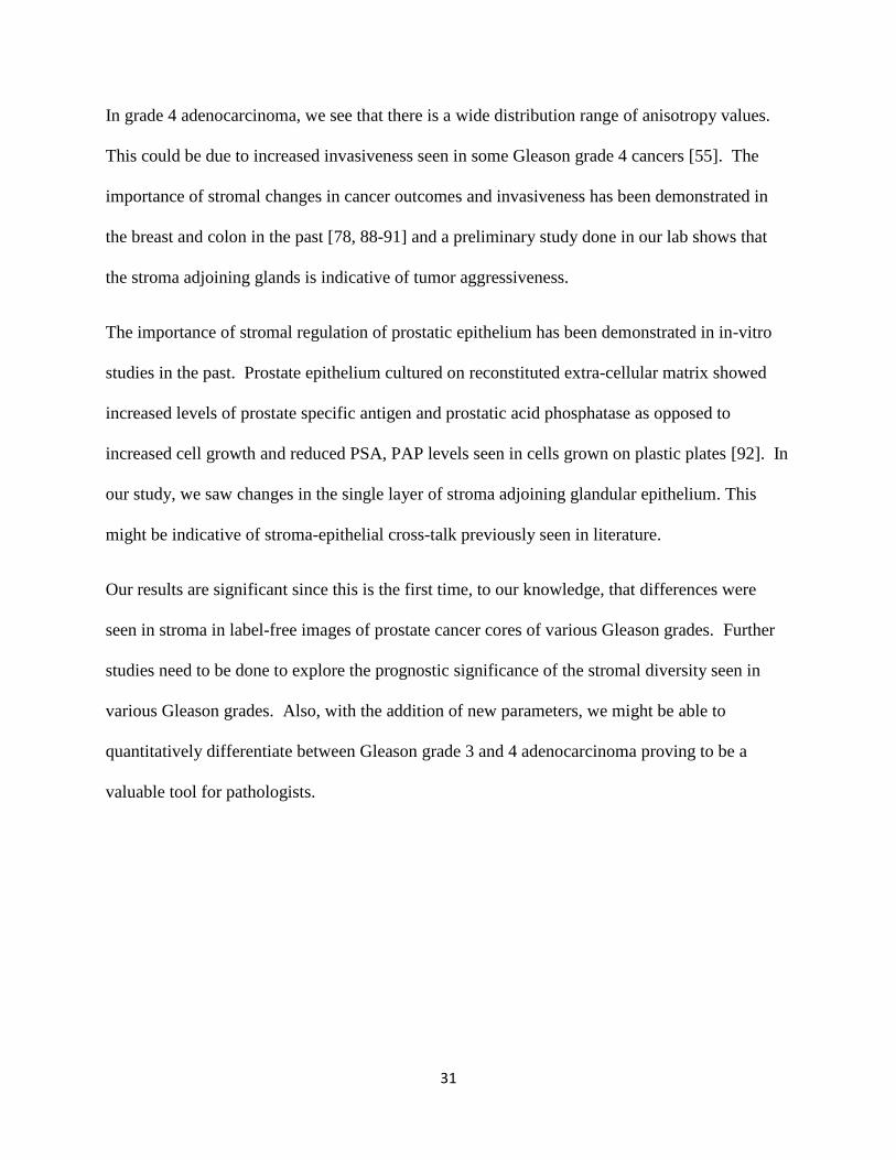
In grade 4 adenocarcinoma, we see that there is a wide distribution range of anisotropy values.

This could be due to increased invasiveness seen in some Gleason grade 4 cancers [55]. The

importance of stromal changes in cancer outcomes and invasiveness has been demonstrated in

the breast and colon in the past [78, 88-91] and a preliminary study done in our lab shows that

the stroma adjoining glands is indicative of tumor aggressiveness.

The importance of stromal regulation of prostatic epithelium has been demonstrated in in-vitro

studies in the past. Prostate epithelium cultured on reconstituted extra-cellular matrix showed

increased levels of prostate specific antigen and prostatic acid phosphatase as opposed to

increased cell growth and reduced PSA, PAP levels seen in cells grown on plastic plates [92]. In

our study, we saw changes in the single layer of stroma adjoining glandular epithelium. This

might be indicative of stroma-epithelial cross-talk previously seen in literature.

Our results are significant since this is the first time, to our knowledge, that differences were

seen in stroma in label-free images of prostate cancer cores of various Gleason grades. Further

studies need to be done to explore the prognostic significance of the stromal diversity seen in

various Gleason grades. Also, with the addition of new parameters, we might be able to

quantitatively differentiate between Gleason grade 3 and 4 adenocarcinoma proving to be a

valuable tool for pathologists.

32

5.4 Optical changes in prostate nuclei11

5.4.1 Motivation

In clinical practice, the nuclear aspects that are of interest to pathologists are nuclear size and

shape, mitotic count, nucleolar count and chromatin changes. In a wide range of cancers,

lobulation of nuclei, asymmetric arrangement of heterochromatin aggregates, irregular folds in

nuclear membrane, enlarged nucleoli and cell-to-cell variation in number of nucleoli are

hallmarks of cancer [93]. While prostate cancer and PIN (prostatic intra-epithelial neoplasia) is

characterized by increased nucleolar count and prominently basal nucleoli, nuclear properties are

not a part of the Gleason grading system.

We used quantitative phase imaging methods to study changes in nuclei in unstained tissue

increasing Gleason grades. We characterized changes in the dry mass, dry mass density and area

of the nucleus from quantitative phase images obtained from SLIM. We also studied the spatial

organization of the nucleus by studying the spatial scattering of light passing through the nuclei.

Our results show that there is a change in nuclear dry mass of cancerous and normal tissue; and

spatial scattering spectrum can be used to separate tissue of varying Gleason grades.

5.4.2 Materials and Methods

We obtained tissue microarray (TMA) set from the Cooperative Prostate Cancer Tissue Resource

(CPCTR) database. For our analysis, we had 2 patients with benign prostatic hyperplasia (BPH),

1 patient with Gleason score 4 (2+2) adenocarcinoma, 1 patient with Gleason score 6 (3+3)

adenocarcinoma, 1 patient with Gleason score 7 (4+3) adenocarcinoma and 1 patient with

Gleason score 8 (4+4) adenocarcinoma. They were grouped into three groups for analysis

11

The text in this section is adapted from:

Sridharan, S., Pham, H., Wickland, D., Tangella, K., Macias, V., Kajdacsy-Balla,A., Popescu, G., FTLS of nucleus

during prostate cancer progression (manuscript in preparation)

33

purposes: “BPH” with 2 patients with benign prostatic hyperplasia, “low-grade tumor” with the

patients with Gleason scores 4 and 6 and “high-grade tumors” with the patients with Gleason

scores 7 and 8. Each core had 150-800 nuclei that were used in our analysis. We used benign

prostatic hyperplasia (BPH) tissue as control due to its high incidence in the demographic

affected by prostate cancer. BPH affects 50-60% of men in their 60s and 80-90% of men in their

70s; and the median age for patients with prostate cancer is 67 years [38, 94]. While Gleason

score 7 is usually considered intermediate risk, we categorized our patient as high-grade cancer

since his Gleason score was 4+3 which is associated with worse prognosis that 3+4 [55].

The unstained tissue microarray slides were imaged using the 40X/0.75NA objective in SLIM.

The mosaic feature on Zeiss was used to image each core which was approximately 100 frames.

The mosaic feature can be adjusted to set up multiple focus planes, ensuring that all sample areas

are in focus. The images were stitched together using an ImageJ plugin built in-house and

individual cores were cropped out to the size of 10000x10000 pixels which is approximately 100

frames stitched together (Fig 13.1).

The images were segmented using a Wacom tablet, ImageJ and plug-in built in our lab.

Individual nuclei were isolated as regions of interest (ROI) manually using a Wacom tablet. Our

in-house plugin crops and pastes the phase images of the isolated nuclei in a zero-phase

background image in their original positions (Fig 13.3). This allows us to study the spatial light

scattering of the nuclei.

34

Figure 1312

: Top Left: 40X SLIM image of prostate TMA core with Gleason score 4 (2+2)

adenocarcinoma with the highlighted area zoomed in on Top Right image. Bottom Left:

Isolated Nuclei from the image on Top Left, with the highlighted area zoomed in on Bottom

Right image.

5.4.3 Results

5.4.3.1 Nuclear Dry Mass Density, Area of Nucleus and Nuclear Dry Mass

In order to study the nuclear changes that occur in prostate cancer we studied the distribution of

nuclear area, nuclear density and the dry mass of nucleus. The nuclear area was calculated by

manually segmenting the nucleus and using ImageJ to measure the area of each nucleus. We

found that the area of the nucleus increases in higher grade nuclei (Gleason score 7 and 8) when

compared to that of benign prostatic hyperplasia patients (t-test, p=2.42E-10). However, the

nuclear area of low-grade cancer is comparable to that of BPH while significantly lower than

high-grade cancer nuclei (t-test, p=1.19E-79). We compared the nuclear density which is related

to phase value by the following relation:

12

Figure reprinted from Sridharan, S., Pham, H., Wickland, D., Tangella, K., Macias, V., Kajdacsy-Balla,A.,

Popescu, G., FTLS of nucleus during prostate cancer progression (manuscript in preparation)

100 µm

35

( )

( )

where φ is the phase value measured by SLIM in radians and γ =0.2ml/g is the refractive

increment. We found that the nuclear density is increased in lower grade cancer (Gleason score

4, 6) when compared with BPH nuclei (t-test, p=1.6E-57). In higher grade cancer, the nuclear

density is comparable to that of BPH nuclei but significantly different from that of lower grade

cancer (t-test, p=1.82E-50).

Figure 1413

: Left: Illustrates the differences in the distribution of nuclear area among

prostate cancer cores of various grades Right: Illustrates the differences in the distribution

of nuclear dry mass densities among the various progression groups.

Nuclear dry mass in all grades of prostate cancer is higher than that of BPH due to the increased

mass density in lower grade cancer and higher nuclear area in high grade cancers (t-test,

p=2.13E-25).

13

Figure reprinted from Sridharan, S., Pham, H., Wickland, D., Tangella, K., Macias, V., Kajdacsy-Balla,A.,

Popescu, G., FTLS of nucleus during prostate cancer progression (manuscript in preparation)

36

Figure 1514

: The nuclear dry mass is comparable among all the cancer groups but is

significantly greater than the control (BPH) group nuclear dry mass.

5.4.3.2 FTLS Study of Prostate Cancer Progression

We obtained the power spectrum of the phase images of the nuclei since these provide us with

spatial scattering information at different length scales. We calculated the point spread function

using a 40X SLIM image and normalized the spatial scattering image of the nuclei. We also did

additional normalization to account for differences in amount of nuclei in each sample by

normalization with a 1-D area obtained from the power spectrum images.

We see multiple peaks in the low frequency (high length scale) region that corresponds to

nucleus size and the peak is pushed to lower frequencies when multiple nuclei are in close

proximity as seen in the Gleason score 4 adenocarcinoma patient. In the higher frequency

region, we obtain information regarding the nucleolar distribution and nuclear envelope

continuity. We notice that the peaks are arranged in the high-frequency region corresponding to

14

Figure reprinted from Sridharan, S., Pham, H., Wickland, D., Tangella, K., Macias, V., Kajdacsy-Balla,A.,

Popescu, G., FTLS of nucleus during prostate cancer progression (manuscript in preparation)

37

6 radians/micron and 10 radians/micron in order of increasing severity with the only anomaly

being the Gleason score 4 patient.

Figure 1615

: Top left: This shows the angular power spectrum for nuclei from Gleason

score 4 (2+2) without any normalization, the inset shows the QPI image of the case. Top

right: In inset shows the point-spread function (PSF) and the curves show the measured

and interpolated point spread function. Bottom: Shows the normalized version of the

power spectrum for the Gleason score 4 QPI image, where it has been normalized for both

PSF and 1D area of the nuclei.

15

Figure reprinted from Sridharan, S., Pham, H., Wickland, D., Tangella, K., Macias, V., Kajdacsy-Balla,A.,

Popescu, G., FTLS of nucleus during prostate cancer progression (manuscript in preparation)

38

Figure 1716

: This shows the normalized power spectrum for the nuclei from various

progression groups and in high frequency regions they align in order of increasing severity.

5.4.4 Discussion

Our results show that nuclear density is increased in low grade cancers whereas nuclear area is

increased in higher grade cancers. Previous studies have documented that nucleolar size is

smaller in fast-growing tumors and is bigger in slow-growing prostate lesions [95]. Nucleolar

count increase is also indicative of highly proliferative tumors since they are a reflection of

ribosome production [96, 97]. Nuclear morphology is primarily determined by nuclear matrix

proteins and lamins. A study by Partin et. Al. showed a nuclear matrix protein PC1 was present

in cancer nuclei but not in normal or BPH nuclei [98-101]. The nuclear lamina serves as

16

Figure reprinted from Sridharan, S., Pham, H., Wickland, D., Tangella, K., Macias, V., Kajdacsy-Balla,A.,

Popescu, G., FTLS of nucleus during prostate cancer progression (manuscript in preparation)

39

attachment points for heterochromatin on the inner surface and also determines nuclear shape.

Nuclear shape changes in papillary thyroid carcinoma with corresponding aggregation changes

of heterochromatin has been documented before [93]. A change in nuclear matrix proteins

would alter nuclear shape, whereas a change in nuclear lamin proteins would change nuclear

density and nuclear shape. It is not surprising that nuclear density would increase due to increase

in the number of nucleoli since this is also a result of increased cellular proliferation and

therefore DNA multiplication. All of these explain the changes in nuclear density and area.

The low frequency region in the nuclear spectroscopy reflects the nuclear size. As expected

from the nuclear analysis, the nuclear size is bigger in higher cancer grades. The multiple peaks

in this region, correspond to multiple nuclei adjacent to each other which is caused by increased

proliferation seen in cancer. In the higher frequency region (>5rad/micron), the spatial

spectroscopy results organize the different grades of prostate disease in order of severity. Since

the information we obtain from phase images is related to dry protein distributions we think we

measure information related to nuclear envelope discontinuities, nucleolar count and nuclear

matrix protein distributions. The spatial spectroscopy also summarizes the results from the

nuclear density and area studies. Study of spatial scattering from nuclei could prove to be a

valuable pathological tool. However, the data we studied here is limited and further studies need

to be done to explore the clinical utility of this tool.

40

6. Summary & Future Work

Prostate cancer has a very high incidence rate and the diagnostic process is expensive due to the

use of expensive immunohistochemical markers. Qualitative imaging methods such as GFM

make the diagnosis of prostate cancer without the additional cost and delay associated with

current clinical pathology practice. Quantitative phase imaging methods such as SLIM

combined with FTLS can detect very sensitive changes in tissue architecture without the use of

stains. We were able to show changes in both prostate nuclei and stroma in the intermediate risk

categories where Gleason grading does not provide good prognostic measure.

These methods show potential for a multitude of future applications:

1. Gleason Grading: Studies have shown that urologic pathologists show a consensus of

70% on Gleason grades whereas among general pathologists the consensus drops below

50% for Gleason scores 5-7 [60, 61]. Since the Gleason grades determine the course of

treatment, a more objective method is necessary to perform grading and remove inter-

observer variability. QPI techniques can be used for this purpose.

2. Prediction of prostate cancer recurrence: The current gold-standard to predict

recurrence of prostate cancer is the CAPRA-S nomogram developed in University of

California San Fransisco. However, CAPRA-S discrimination is low in the D’Amico

intermediate risk category. Using QPI, we were able to detect changes in stroma among

patients in this category, but we had no recurrence information associated with those

patients. We believe that QPI might have the sensitivity to improve the accuracy of

recurrence prediction in this intermediate risk group.

3. Field Effect Detection: There are instances where prostate cancer is not detected in a

biopsy but is diagnosed in a repeat biopsy at an advanced stage. This could be due to a

41

sampling error at the biopsy stage. A sensitive tool that can detect pre-malignant changes

and field effect associated with prostate cancer can solve this problem. QPI shows

promise in this area.

42

References

1. Fischer, A.H., et al., Hematoxylin and eosin staining of tissue and cell sections. CSH

Protoc, 2008. 2008: p. pdb prot4986.

2. Zernike, F., How I discovered phase contrast. Science, 1955. 121(3141): p. 345-9.

3. Wang, Z., et al., Topography and refractometry of nanostructures using spatial light

interference microscopy. Opt Lett. 35(2): p. 208-10.

4. Bohren, C.F. and D.R. Huffman, Absorption and scattering of light by small

particles1983, New York: Wiley. xiv, 530 p.

5. Hulst, H.C.v.d., Light scattering by small particles1981, New York: Dover Publications.

470 p.

6. Ishimaru, A., Electromagnetic wave propagation, radiation, and scattering1991,

Englewood Cliffs, N.J.: Prentice Hall. xviii, 637 p.

7. Berne, B.J. and R. Pecora, Dynamic light scattering with applications to chemistry,

biology and Physics1976, New York: Wiley.

8. Zhu, R., et al., Correlation-induced spectral changes in tissues. Opt Lett. 36(21): p.

4209-11.

9. Milestones in light microscopy. Nat Cell Biol, 2009. 11(10): p. 1165-1165.

10. Alberts, B., Essential cell biology : an introduction to the molecular biology of the cell. 2

ed2004, New York: Garland Pub. 1 v. (various pagings).

11. Dunn, A. and R. Richards-Kortum, Three-dimensional computation of light scattering

from cells. Ieee Journal of Selected Topics in Quantum Electronics, 1996. 2(4): p. 898-

905.

12. Mourant, J.R., et al., Mechanisms of light scattering from biological cells relevant to

noninvasive optical-tissue diagnostics. Applied Optics, 1998. 37(16): p. 3586-3593.

13. Hale, G.M. and M.R. Querry, Optical-Constants of Water in 200-Nm to 200-Mum

Wavelength Region. Applied Optics, 1973. 12(3): p. 555-563.

14. Takatani, S. and M.D. Graham, Theoretical-Analysis of Diffuse Reflectance from a 2-

Layer Tissue Model. Ieee Transactions on Biomedical Engineering, 1979. 26(12): p. 656-

664.

15. Wang, Z., H. Ding, and G. Popescu, Scattering-phase theorem. Optics Letters, 2011. 36:

p. 1215.

16. Ding, H., et al., Measuring the scattering parameters of tissues from quantitative phase

imaging of thin slices. Optics Letters, 2011. 36: p. 2281.

17. Wolf, E., Invariance of the Spectrum of Light on Propagation. Physical Review Letters,

1986. 56(13): p. 1370-1372.

18. Bocko, M.F., D.H. Douglass, and R.S. Knox, Observation of Frequency-Shifts of

Spectral-Lines Due to Source Correlations. Physical Review Letters, 1987. 58(25): p.

2649-2651.

19. Wolf, E., Non-Cosmological Redshifts of Spectral-Lines. Nature, 1987. 326(6111): p.

363-365.

20. Wolf, E., J.T. Foley, and F. Gori, Frequency-Shifts of Spectral-Lines Produced by

Scattering from Spatially Random-Media. Journal of the Optical Society of America a-

Optics Image Science and Vision, 1989. 6(8): p. 1142-1149.

21. Dogariu, A. and E. Wolf, Spectral changes produced by static scattering on a system of

particles. Opt. Lett., 1998. 23(17): p. 1340-1342.

43

22. Frick, J. and W. Aulitzky, Physiology of the prostate. Infection, 1991. 19 Suppl 3: p.

S115-8.

23. McNeal, J.E., Anatomy of the prostate: An historical survey of divergent views. The

Prostate, 1980. 1(1): p. 3-13.

24. McNeal, J.E., Regional morphology and pathology of the prostate. American journal of

clinical pathology, 1968. 49(3): p. 347-57.

25. McNeal, J.E., Origin and development of carcinoma in the prostate. Cancer, 1969. 23(1):

p. 24-34.

26. McNeal, J.E., Origin and evolution of benign prostatic enlargement. Investigative

urology, 1978. 15(4): p. 340-5.

27. Hadley, H.L., Physiology of the prostate. Medical arts and sciences, 1952. 6(1): p. 22-3.

28. Farnsworth, W.E., Prostate stroma: physiology. The Prostate, 1999. 38(1): p. 60-72.

29. Roehrborn C, M.J., Etiology, pathophysiology, epidemiology and natural history of

benign prostatic hyperplasia, in Campbell's Urology, R.A. Walsh P, Vaughan E, Wein A

Editor 2002, Saunders: Philadelphia. p. 1297-1336.

30. Roehrborn, C.G., Pathology of benign prostatic hyperplasia. Int J Impot Res, 2008. 20

Suppl 3: p. S11-8.

31. Bostwick, D.G., et al., High-grade prostatic intraepithelial neoplasia. Rev Urol, 2004.

6(4): p. 171-9.

32. Bostwick, D.G. and M.K. Brawer, Prostatic intra-epithelial neoplasia and early invasion

in prostate cancer. Cancer, 1987. 59(4): p. 788-94.

33. Epstein, J.I. and G.J. Netto, Biopsy Interpretation of the Prostate2007: Lippincott

Williams & Wilkins.

34. Epstein, J.I. and M. Herawi, Prostate needle biopsies containing prostatic intraepithelial

neoplasia or atypical foci suspicious for carcinoma: implications for patient care. J Urol,

2006. 175(3 Pt 1): p. 820-34.

35. Jemal, A., et al., Cancer statistics, 2010. CA Cancer J Clin. 60(5): p. 277-300.

36. Howlader N, N.A., Krapcho M, Neyman N, Aminou R, Altekruse SF, Kosary CL, Ruhl J,

Tatalovich Z, Cho H, Mariotto A, Eisner MP, Lewis DR, Chen HS, Feuer EJ, Cronin KA.

SEER Cancer Statistics Review, 1975-2009. 2011 2012 [cited 2012 November, 10].

37. Welch, H.G. and P.C. Albertsen, Prostate cancer diagnosis and treatment after the

introduction of prostate-specific antigen screening: 1986-2005. Journal of the National

Cancer Institute, 2009. 101(19): p. 1325-9.

38. Screening for prostate cancer: U.S. Preventive Services Task Force recommendation

statement. Annals of internal medicine, 2008. 149(3): p. 185-91.

39. Moyer, V.A., Screening for prostate cancer: U.S. Preventive Services Task Force

recommendation statement. Annals of internal medicine, 2012. 157(2): p. 120-34.

40. Sakr, W.A., et al., The frequency of carcinoma and intraepithelial neoplasia of the

prostate in young male patients. The Journal of urology, 1993. 150(2 Pt 1): p. 379-85.

41. Gronberg, H., Prostate cancer epidemiology. Lancet, 2003. 361(9360): p. 859-64.

42. Force, U.S.P.S.T. Screening for prostate cancer: final recommendation statement. [cited

2012 November, 10].

43. Gleason, D.F., Classification of prostatic carcinomas. Cancer Chemother Rep, 1966.

50(3): p. 125-8.

44. Humphrey, P.A., Gleason grading and prognostic factors in carcinoma of the prostate.

Mod Pathol, 2004. 17(3): p. 292-306.

44

45. Epstein, J.I., et al., Prediction of progression following radical prostatectomy. A

multivariate analysis of 721 men with long-term follow-up. Am J Surg Pathol, 1996.

20(3): p. 286-92.

46. Partin, A.W., et al., Combination of prostate-specific antigen, clinical stage, and Gleason

score to predict pathological stage of localized prostate cancer. A multi-institutional

update. JAMA, 1997. 277(18): p. 1445-51.

47. Egevad, L., et al., Prognostic value of the Gleason score in prostate cancer. BJU Int,

2002. 89(6): p. 538-42.

48. Gleason, D.F. and G.T. Mellinger, Prediction of prognosis for prostatic adenocarcinoma

by combined histological grading and clinical staging. 1974. J Urol, 2002. 167(2 Pt 2): p.

953-8; discussion 959.

49. Gleason, D.F. and G.T. Mellinger, Prediction of prognosis for prostatic adenocarcinoma

by combined histological grading and clinical staging. J Urol, 1974. 111(1): p. 58-64.

50. Gleason, D.F., Undergrading of prostate cancer biopsies: a paradox inherent in all

biologic bivariate distributions. Urology, 1996. 47(3): p. 289-91.

51. Pan, C.C., et al., The prognostic significance of tertiary Gleason patterns of higher grade

in radical prostatectomy specimens: a proposal to modify the Gleason grading system.

The American journal of surgical pathology, 2000. 24(4): p. 563-9.

52. Epstein, J.I., et al., The 2005 International Society of Urological Pathology (ISUP)

Consensus Conference on Gleason Grading of Prostatic Carcinoma. The American

journal of surgical pathology, 2005. 29(9): p. 1228-42.

53. Amin, M.B., D.S. Schultz, and R.J. Zarbo, Analysis of cribriform morphology in prostatic

neoplasia using antibody to high-molecular-weight cytokeratins. Archives of pathology

& laboratory medicine, 1994. 118(3): p. 260-4.

54. Ghani, K.R., et al., Trends in reporting Gleason score 1991 to 2001: changes in the

pathologist's practice. European urology, 2005. 47(2): p. 196-201.

55. Makarov, D.V., et al., Gleason score 7 prostate cancer on needle biopsy: is the

prognostic difference in Gleason scores 4 + 3 and 3 + 4 independent of the number of

involved cores? The Journal of urology, 2002. 167(6): p. 2440-2.

56. Grober, E.D., et al., Correlation of the primary Gleason pattern on prostate needle

biopsy with clinico-pathological factors in Gleason 7 tumors. The Canadian journal of

urology, 2004. 11(1): p. 2157-62.

57. Merrick, G.S., et al., Biochemical outcome for hormone-naive intermediate-risk prostate

cancer managed with permanent interstitial brachytherapy and supplemental external

beam radiation. Brachytherapy, 2002. 1(2): p. 95-101.

58. Merrick, G.S., et al., Biochemical outcome for hormone-naive patients with Gleason

score 3+4 versus 4+3 prostate cancer undergoing permanent prostate brachytherapy.

Urology, 2002. 60(1): p. 98-103.

59. Gonzalgo, M.L., et al., Relationship between primary Gleason pattern on needle biopsy

and clinicopathologic outcomes among men with Gleason score 7 adenocarcinoma of the

prostate. Urology, 2006. 67(1): p. 115-9.

60. Allsbrook, W.C., Jr., et al., Interobserver reproducibility of Gleason grading of prostatic

carcinoma: urologic pathologists. Human pathology, 2001. 32(1): p. 74-80.

61. Allsbrook, W.C., Jr., et al., Interobserver reproducibility of Gleason grading of prostatic

carcinoma: general pathologist. Human pathology, 2001. 32(1): p. 81-8.

62. Zernike, F., How I discovered phase contrast. Science, 1955. 121: p. 345.

45

63. Gabor, D., A new microscopic principle. Nature, 1948. 161: p. 777.

64. Wang, Z., et al., Spatial light interference microscopy (SLIM). Optics Express, 2011.

19(2): p. 1016.

65. Mir, M., et al., Measuring Cell Cycle-Dependent Mass Growth Proc. Nat. Acad. Sci.,

2011. 108(32): p. 13124.

66. Popescu, G., et al., Label-free intracellular transport measured by spatial light

interference microscopy. Journal of Biomedical Optics, 2011. 16(2).

67. Wang, R., et al., One-dimensional deterministic transport in neurons measured by

dispersion-relation phase spectroscopy. J. Phys.: Cond. Matter, 2011. 23: p. 374107.

68. Babacan, S.D., et al., Cell imaging beyond the diffraction limit using sparse

deconvolution spatial light interference microscopy. Biomed Opt Express. 2(7): p. 1815-

27.

69. Ding, H.F., et al., Fourier Transform Light Scattering of Biological Structure and

Dynamics. Ieee Journal of Selected Topics in Quantum Electronics, 2010. 16(4): p. 909-

918.

70. Ding, H.F., et al., Fourier Transform Light Scattering (FTLS) of Cells and Tissues.

Journal of Computational and Theoretical Nanoscience, 2010. 7(12): p. 2501-2511.

71. Tuxhorn, J.A., et al., Reactive stroma in human prostate cancer: induction of

myofibroblast phenotype and extracellular matrix remodeling. Clinical cancer research :

an official journal of the American Association for Cancer Research, 2002. 8(9): p. 2912-

23.

72. Guidebook to the extracellular matrix and adhesion proteins Edited by T Kreis and R

Vale. pp 176. Oxford University Press. 1993. £40 or £18.50 (pbk) ISBN 0-19-859934-X

or -859933-1s. Biochemical Education, 1993. 21(4): p. 209-210.

73. Taipale, J. and J. KeskiOja, Growth factors in the extracellular matrix. Faseb Journal,

1997. 11(1): p. 51-59.

74. Tuxhorn, J.A., G.E. Ayala, and D.R. Rowley, Reactive stroma in prostate cancer

progression. The Journal of urology, 2001. 166(6): p. 2472-83.

75. Noel, A. and J.M. Foidart, The role of stroma in breast carcinoma growth in vivo. Journal

of mammary gland biology and neoplasia, 1998. 3(2): p. 215-25.

76. Gregoire, M. and B. Lieubeau, The role of fibroblasts in tumor behavior. Cancer

metastasis reviews, 1995. 14(4): p. 339-50.

77. Ayala, G., et al., Reactive stroma as a predictor of biochemical-free recurrence in

prostate cancer. Clinical cancer research : an official journal of the American

Association for Cancer Research, 2003. 9(13): p. 4792-801.

78. Ronnov-Jessen, L., O.W. Petersen, and M.J. Bissell, Cellular changes involved in

conversion of normal to malignant breast: importance of the stromal reaction. Physiol

Rev, 1996. 76(1): p. 69-125.

79. Rowley, D.R., What might a stromal response mean to prostate cancer progression?

Cancer metastasis reviews, 1998. 17(4): p. 411-9.

80. Schmitt-Graff, A., A. Desmouliere, and G. Gabbiani, Heterogeneity of myofibroblast

phenotypic features: an example of fibroblastic cell plasticity. Virchows Archiv : an

international journal of pathology, 1994. 425(1): p. 3-24.

81. Seemayer, T.A., et al., Myofibroblasts in the stroma of invasive and metastatic

carcinoma: a possible host response to neoplasia. The American journal of surgical

pathology, 1979. 3(6): p. 525-33.

46

82. Lipponen, P., et al., High stromal hyaluronan level is associated with poor differentiation

and metastasis in prostate cancer. Eur J Cancer, 2001. 37(7): p. 849-56.

83. Hagglof, C., et al., Stromal PDGFRbeta expression in prostate tumors and non-

malignant prostate tissue predicts prostate cancer survival. PLoS One. 5(5).

84. McAlhany, S.J., et al., Decreased stromal expression and increased epithelial expression

of WFDC1/ps20 in prostate cancer is associated with reduced recurrence-free survival.

Prostate, 2004. 61(2): p. 182-91.

85. Hayward, S.W., G.R. Cunha, and R. Dahiya, Normal development and carcinogenesis of

the prostate. A unifying hypothesis. Annals of the New York Academy of Sciences, 1996.

784: p. 50-62.

86. Peehl, D.M. and R.G. Sellers, Induction of smooth muscle cell phenotype in cultured

human prostatic stromal cells. Experimental cell research, 1997. 232(2): p. 208-15.

87. Gerdes, M.J., et al., Regulation of rat prostate stromal cell myodifferentiation by

androgen and TGF-beta1. The Prostate, 2004. 58(3): p. 299-307.

88. Ronnov-Jessen, L. and O.W. Petersen, Induction of alpha-smooth muscle actin by

transforming growth factor-beta 1 in quiescent human breast gland fibroblasts.

Implications for myofibroblast generation in breast neoplasia. Lab Invest, 1993. 68(6): p.

696-707.

89. Brown, L.F., et al., Vascular stroma formation in carcinoma in situ, invasive carcinoma,

and metastatic carcinoma of the breast. Clin Cancer Res, 1999. 5(5): p. 1041-56.

90. Lagace, R., et al., Myofibroblastic stromal reaction in carcinoma of the breast: variations

of collagenous matrix and structural glycoproteins. Virchows Arch A Pathol Anat

Histopathol, 1985. 408(1): p. 49-59.

91. Martin, M., P. Pujuguet, and F. Martin, Role of stromal myofibroblasts infiltrating colon

cancer in tumor invasion. Pathol Res Pract, 1996. 192(7): p. 712-7.

92. Fong, C.J., et al., Reconstituted Basement-Membrane Promotes Morphological and

Functional-Differentiation of Primary Human Prostatic Epithelial-Cells. Prostate, 1991.

19(3): p. 221-235.

93. Zink, D., A.H. Fischer, and J.A. Nickerson, Nuclear structure in cancer cells. Nature

reviews. Cancer, 2004. 4(9): p. 677-87.

94. Roehrborn, C.G., Benign prostatic hyperplasia: an overview. Reviews in urology, 2005.

7 Suppl 9: p. S3-S14.

95. Fischer, A.H., S. Bardarov, Jr., and Z. Jiang, Molecular aspects of diagnostic nucleolar

and nuclear envelope changes in prostate cancer. J Cell Biochem, 2004. 91(1): p. 170-

84.

96. Fischer, A.H., S. Bardarov, Jr., and Z. Jiang, Molecular aspects of diagnostic nucleolar

and nuclear envelope changes in prostate cancer. Journal of cellular biochemistry, 2004.

91(1): p. 170-84.

97. Derenzini, M., et al., Nucleolar size indicates the rapidity of cell proliferation in cancer

tissues. The Journal of pathology, 2000. 191(2): p. 181-6.

98. Partin, A.W., et al., Preliminary immunohistochemical characterization of a monoclonal

antibody (PRO:4-216) prepared from human prostate cancer nuclear matrix proteins.

Urology, 1997. 50(5): p. 800-8.

99. Partin, A.W., et al., Nuclear matrix protein patterns in human benign prostatic

hyperplasia and prostate cancer. Cancer Res, 1993. 53(4): p. 744-6.

47

100. Leman, E.S. and R.H. Getzenberg, Nuclear matrix proteins as biomarkers in prostate

cancer. J Cell Biochem, 2002. 86(2): p. 213-23.

101. Subong, E.N., et al., Monoclonal antibody to prostate cancer nuclear matrix protein

(PRO:4-216) recognizes nucleophosmin/B23. Prostate, 1999. 39(4): p. 298-304.