Mon. Not. R. Astron. Soc. 000, 000–000 (0000) Printed 3 August 2017 (MN LATEX style file v2.2)

Prospects for Measuring Cosmic Microwave Background SpectralDistortions in the Presence of Foregrounds

Maximilian H. Abitbol1?, Jens Chluba2†, J. Colin Hill3, and Bradley R. Johnson11 Department of Physics, Columbia University, New York, NY, 10027, USA2 Jodrell Bank Centre for Astrophysics, University of Manchester, Oxford Road, Manchester M13 9PL, UK3 Department of Astronomy, Columbia University, Pupin Hall, New York, New York 10027, USA

Accepted 2017 June 20. Received 2017 May 03. Published 2017 June 30.

ABSTRACTMeasurements of cosmic microwave background spectral distortions have profound implica-tions for our understanding of physical processes taking place over a vast window in cosmo-logical history. Foreground contamination is unavoidable in such measurements and detailedsignal-foreground separation will be necessary to extract cosmological science. In this paper,we present MCMC-based spectral distortion detection forecasts in the presence of Galacticand extragalactic foregrounds for a range of possible experimental configurations, focusingon the Primordial Inflation Explorer (PIXIE) as a fiducial concept. We consider modificationsto the baseline PIXIE mission (operating ' 12 months in distortion mode), searching for op-timal configurations using a Fisher approach. Using only spectral information, we forecast anextended PIXIE mission to detect the expected average non-relativistic and relativistic ther-mal Sunyaev-Zeldovich distortions at high significance (194σ and 11σ, respectively), evenin the presence of foregrounds. The ΛCDM Silk damping µ-type distortion is not detectedwithout additional modifications of the instrument or external data. Galactic synchrotron ra-diation is the most problematic source of contamination in this respect, an issue that could bemitigated by combining PIXIE data with future ground-based observations at low frequencies(ν . 15−30 GHz). Assuming moderate external information on the synchrotron spectrum, weproject an upper limit of |µ| < 3.6×10−7 (95% c.l.), slightly more than one order of magnitudeabove the fiducial ΛCDM signal from the damping of small-scale primordial fluctuations, buta factor of ' 250 improvement over the current upper limit from COBE/FIRAS. This limitcould be further reduced to |µ| < 9.4 × 10−8 (95% c.l.) with more optimistic assumptionsabout extra low-frequency information and would rule out many alternative inflation modelsas well as provide new constraints on decaying particle scenarios.

Key words: Cosmology: cosmic microwave background – theory – observations

1 INTRODUCTION

Spectral distortions of the cosmic microwave background (CMB)are one of the next frontiers in CMB science (Chluba & Sun-yaev 2012; Sunyaev & Khatri 2013; Tashiro 2014; Silk & Chluba2014; Chluba 2014; De Zotti et al. 2016). The intensity spectrumof the CMB was precisely measured by COBE/FIRAS over twodecades ago (Mather et al. 1990; Fixsen et al. 1996) and is con-sistent with a blackbody at temperature T0 = 2.72548 ± 0.00057 Kfrom ν ' 3 GHz to 3,000 GHz (Fixsen 2009). This agrees with avariety of other CMB observations including COBRA, TRIS, andARCADE (Gush et al. 1990; Gervasi et al. 2008; Kogut et al. 2006;Seiffert et al. 2011). These impressive measurements already placevery tight constraints on the thermal history of the Universe (e.g.,Sunyaev & Zeldovich 1970c; Zeldovich et al. 1972; Illarionov &

? E-mail:mha2125@columbia.edu† E-mail:jens.chluba@manchester.ac.uk

Sunyaev 1974; Danese & de Zotti 1977), limiting early energy re-lease to ∆ργ/ργ . 6 × 10−5 (95% c.l.) relative to the CMB energydensity (Fixsen et al. 1996; Fixsen & Mather 2002).

Most of our detailed current cosmological picture stemsfrom measurements of the CMB temperature and polarizationanisotropies, which have been well characterized by WMAP (Hin-shaw et al. 2013), Planck (Planck Collaboration et al. 2015), andmany sub-orbital experiments (e.g., Netterfield et al. 2002; Rubino-Martin et al. 2003; Pearson et al. 2003; Reichardt et al. 2009;Keisler et al. 2011; Dunkley et al. 2011). More precise measure-ments of the polarization anisotropies are being targeted by an ar-ray of ongoing experiments including BICEP2/3 and the KECKarray, ACTPol, SPTPol, POLARBEAR, CLASS, SPIDER, and theSimons Array (BICEP2 and Keck Array Collaborations et al. 2015;Naess et al. 2014; Keisler et al. 2015; Harrington et al. 2016; Filip-pini et al. 2010), all with the goal to further refine our understandingof the Universe and its constituents. Measurements of CMB spec-tral distortions could complement these efforts and provide access

c© 0000 RAS

arX

iv:1

705.

0153

4v2

[as

tro-

ph.C

O]

2 A

ug 2

017

2 Abitbol et al.

to qualitatively new information that cannot be probed via the an-gular anisotropy (see Chluba 2016, for an overview of the standardΛCDM distortions).

Spectral distortions are caused by processes (e.g., energy orphoton injection) that affect the thermal equilibrium between mat-ter and radiation (Zeldovich & Sunyaev 1969; Sunyaev & Zel-dovich 1970b; Illarionov & Sunyaev 1974; Burigana et al. 1991;Hu & Silk 1993a; Chluba & Sunyaev 2012; Chluba 2015). Oneof the standard distortions, known as the Compton y-distortion, iscreated in the regime of inefficient energy transfer between elec-trons and photons, relevant at redshift z . 5 × 104. Processes cre-ating this type of distortion include the inverse-Compton scatteringof CMB photons off hot electrons during the epoch of reioniza-tion and structure formation (Sunyaev & Zeldovich 1972; Hu et al.1994b; Refregier & et al. 2000; Hill et al. 2015), also known inconnection with the thermal Sunyaev-Zeldovich (tSZ) effect (Zel-dovich & Sunyaev 1969), but can also be related to non-standardphysics, e.g., the presence of long-lived decaying particles (Sarkar& Cooper 1984; Ellis et al. 1992; Hu & Silk 1993b; Chluba 2013a).

Chemical potential or µ-type distortions (Sunyaev & Zel-dovich 1970b), on the other hand, are generated by energy releaseat earlier stages (z & 5 × 104), when interactions are still extremelyefficient and able to establish kinetic equilibrium between electronsand photons under repeated Compton scattering and photon emis-sion processes (i.e., double Compton and Bremsstrahlung). The lat-ter are particularly important at z & 2×106, leading to a strong sup-pression of the distortion amplitude (e.g., Hu & Silk 1993a). Ex-pected sources of µ-distortions include the Silk damping of small-scale acoustic modes in the early Universe (Sunyaev & Zeldovich1970a; Daly 1991; Hu et al. 1994a; Chluba et al. 2012b) and the ex-traction of energy from the photon bath due to the adiabatic coolingof ordinary matter (Chluba 2005; Chluba & Sunyaev 2012).

The Primordial Inflation Explorer (PIXIE) is a proposed satel-lite mission designed to constrain the primordial B-mode po-larization power spectrum and target spectral distortions of theCMB (Kogut et al. 2011b, 2016). The instrument is a polarizingMichelson interferometer spanning 15 to 6,000 GHz with a mir-ror stroke length corresponding to ' 15 GHz channels. In orderto detect the small spectral distortion signals, Galactic and extra-galactic foreground emission has to be precisely modeled, charac-terized, and marginalized over in the cosmological analysis. In thispaper we forecast the capabilities of PIXIE-like experimental con-cepts for detecting spectral distortions in the presence of knownforegrounds, extending simpler forecasts presented earlier (e.g., byKogut et al. 2011b; Chluba & Jeong 2014; Hill et al. 2015).1

Our analysis solely considers the spectral energy distribution(SED) of the sky monopole, relying on the spectral behavior of dif-ferent components in order to separate them. In contrast, we notethat the COBE/FIRAS analysis relied on spatial information in orderto separate the extragalactic monopole from Galactic foregrounds[and the CMB dipole] (Fixsen et al. 1996). An optimal analysiswould combine spectral and spatial information, with the latter pri-marily helping to isolate Galactic foregrounds. We shall leave amore rigorous assessment to future work and for now focus on theavailable spectral information.

We apply a Fisher matrix approach to the fiducial PIXIE in-strument configuration, spectral distortion signals, and standardforeground models to estimate uncertainties on the CMB signal pa-

1 Forecasts for the polarization sensitivity of PIXIE were described mostrecently in Calabrese et al. (2016) and will not be addressed here.

rameters. We consider a range of foreground models and vary thePIXIE mission configuration to search for an optimal instrumentsetup based on the assumed sky signals. We compare part of the re-sults to full Monte Carlo Markov Chain (MCMC) analyses, whichdo not rely on the assumption of Gaussian posteriors, finding goodagreement. The considered signals and total foreground emissionare illustrated in Fig. 1 and will be discussed in detail below.

The paper is organized as follows. We describe the PIXIE mis-sion, fiducial CMB spectral distortions, and foreground models inSections 2, 3, and 4, respectively. We summarize the forecastingcalculations in Section 5. The CMB-only forecast is presented inSection 6. Forecasts with foregrounds are discussed in Section 7.We search for an optimal mission configuration in Section 7.3 andconclude in Section 8.

2 PIXIE MISSION CONFIGURATION

We use the nominal PIXIE mission configuration as describedin Kogut et al. (2011a). (A slightly updated concept was recentlyproposed2 but the modifications do not significantly change theforecast.) The center of the lowest frequency bin is 15 GHz, witha corresponding 15 GHz bin width. The highest frequency bin inthe nominal design is ' 6 THz; however, due to the complexity ofdust emission at such high frequencies, we use 3 THz as the high-est bin edge, yielding a total of 200 channels for distortion science.This choice does not affect the forecasted uncertainties because thehigh-frequency foregrounds are not the limiting factor. In addition,the spectral distortion signals cut off well below 3 THz (see Fig. 1).

Assuming 12 months of spectral distortion mode integrationtime (PIXIE will also spend time in polarization observation mode),the noise per 1◦ ×1◦ pixel is ' 747 Jy at low frequencies, which weconvert to Jy/sr and assume 70% of the sky is used in the analysis.The projected noise increases at frequencies above 1 THz due to alow-pass filter in the instrument. For most of the forecasting below,we scale the sensitivity to an extended mission with 86.4 months ofintegration time (representing a 9 year mission with 80% of theobservation time spent in distortion mode), with the noise scal-ing down as the square root of the mission duration. For a FourierTransform Spectrometer (FTS) such as PIXIE, the lowest frequencybin is set by the size of the instrument. The mirror stroke length de-termines the frequency resolution. Additionally, increasing the binwidth (i.e., reducing the mirror stroke) by a multiplicative factor de-creases the noise by the same factor. This is due to the fact that thenoise scales with the square root of the bandwidth and the squareroot of the integration time, both of which increase when increasingthe bin size. We discuss the trade-off between frequency resolutionand sensitivity in Section 7.3.

3 CMB SPECTRAL DISTORTION MODELING

At the level of PIXIE’s expected sensitivity, the average CMB spec-tral distortion signal can be efficiently described by only a few pa-rameters. We model the sky-averaged spectral radiance relative tothe assumed CMB blackbody, ∆Iν, as:

∆Iν = ∆Bν + ∆Iyν + ∆Irel−tSZ

ν + ∆Iµν + ∆Ifgν . (1)

Here, ∆Bν = Bν (TCMB) − Bν(T0) represents the deviation ofthe true CMB blackbody spectrum, Bν(TCMB), at a temperatureTCMB = T0(1 + ∆T ), from that of a blackbody with temperature

2 Al Kogut, priv. comm.

c© 0000 RAS, MNRAS 000, 000–000

PIXIE Spectral Distortion Forecast 3

5 10 100 1000Frequency [GHz]

10 1

100

101

102

103

104

105

106

107

Spec

tral R

adia

nce

[Jy/s

r]

PIXIE Sensitivity

FIRAS Sensitivity

TCMB

|y|| |

|Relativistic SZ|Total Foregrounds

Figure 1. Spectral distortion signals compared to the PIXIE sensitivity and foregrounds. The signals include the CMB blackbody (blue) as well as theΛCDM-predicted Compton-y (red), relativistic SZ (cyan), and µ (green) spectral distortions. The dashed and solid curves indicate negative and positive values,respectively. The total foreground model, which dominates over all non-blackbody signals, is shown in dotted magenta. The black points represent the PIXIEsensitivity for the nominal and extended mission, assuming fsky = 0.7 and 12 or 86.4 months of integration time, respectively. The horizontal error bars onthe noise curve points represent the width of the 15 GHz PIXIE frequency bins. For comparison, the COBE/FIRAS raw detector sensitivity is illustrated by theblue dots.

T0 = 2.726 K; ∆Iyν is the y-type distortion; ∆Irel−tSZ

ν is the relativis-tic temperature correction to the tSZ distortion; ∆Iµν is the µ-typedistortion; and ∆Ifg

ν represents the sum of all foreground contri-butions. We describe our fiducial models for these signal compo-nents below. The results are shown in Figure 1 in comparison to thePIXIE (nominal/extended mission) sensitivity and the total fore-ground level (described in Sect. 4).

Blackbody Component. The average CMB blackbody tempera-ture must be determined in the analysis, as it is not currently knownat the necessary precision (e.g., see Chluba & Jeong 2014). Wework to first order in ∆T = (TCMB − T0)/T0, describing the temper-ature shift spectrum as

∆Bν ≈ Iox4ex

(ex − 1)2 ∆T , (2)

with Io = (2h/c2) (kT0/h)3 ≈ 270 MJy/sr and x = hν/kT0. Forillustration, we assume a fiducial value ∆T = 1.2 × 10−4, consistentwith current constraints (Fixsen 2009). The analysis is not affectedsignificantly by this choice.

While simple estimates indicate that PIXIE is expected tomeasure TCMB to the ' nK level (Chluba & Jeong 2014), an im-provement over COBE/FIRAS does not immediately provide newcosmological information simply because there is no cosmologi-cal prediction for the average photon temperature. By comparingthe local (↔ current) value of TCMB with measurements at earliertimes, e.g., at recombination (Planck Collaboration et al. 2015) orduring BBN (Steigman 2009), constraints on entropy production

can be deduced (Steigman 2009; Jeong et al. 2014); however, theseare not limited by the current ' mK uncertainty of TCMB.

Cumulative Thermal SZ (y) Distortion. We adopt the model forthe sky-averaged thermal SZ signal from Hill et al. (2015), includ-ing both the standard non-relativistic (Compton-y) and relativisticcontributions.3 The Compton-y signal (tSZ) includes contributionsfrom the intracluster medium (ICM) of galaxy groups and clusters(which dominate the overall signal), the intergalactic medium, andreionization, yielding a total value of y = 1.77 × 10−6 (Hill et al.2015). This is a conservative estimate as with increased AGN feed-back larger values for y could be feasible (De Zotti et al. 2016).Note that the actual monopole y value measured by PIXIE or otherexperiments will also contain a primordial contribution in general,but this is expected to be 2–3 orders of magnitude smaller than thestructure formation contributions (Chluba et al. 2012b). We further-more assume that the average y-distortion caused by the CMB tem-perature dipole, ysup = (2.525 ± 0.012) × 10−7 (Chluba & Sunyaev2004; Chluba 2016), is subtracted. The non-relativistic tSZ signaltakes the standard Compton-y form (Zeldovich & Sunyaev 1969):

∆Iyν = Io

x4ex

(ex − 1)2

[x coth

( x2

)− 4

]y , (3)

with cross-over frequency ν ' 218 GHz.We model the sky-averaged relativistic corrections to the

3 PIXIE may also have sufficient sensitivity to constrain the sky-averagednon-thermal SZ signal, but we do not investigate this possibility here.

c© 0000 RAS, MNRAS 000, 000–000

4 Abitbol et al.

tSZ signal, ∆Irel−tSZν , using the moment-based approach described

in Hill et al. (2015), whose calculation used the results of Nozawaet al. (2006) up to fourth order in the electron temperature. For theMCMC calculations below, we generate the signal using momentsof the optical-depth-weighted ICM electron temperature distribu-tion of SZpack (Chluba et al. 2013), with parameter values identi-cal to those in Hill et al. (2015), to which we refer the reader formore details. However, at PIXIE’s sensitivity, the SZ signal can berepresented most efficiently using moments of the y-weighted ICMelectron temperature distribution. In particular, using only the firsttwo y-weighted moments is sufficient to reproduce the relativisticcorrection signal for our purpose. This is explained in more detailby Battaglia et al. (in prep.) and greatly simplifies comparisons tothe results of cosmological hydrodynamics simulations.

While we emphasize that the fiducial signal is generated us-ing the more accurate optical-depth-weighted approach (in theMCMC case), the Fisher forecasts and MCMC fits below use they-weighted moment approach in the analysis. The two approachesare equivalent in the limit of many temperature moments, but to re-duce the number of parameters, the y-weighted approach providesan efficient re-summation of the signal templates. We denote thefirst moment of the y-weighted ICM electron temperature distri-bution as kTeSZ. The fiducial value is kTeSZ = 1.245 keV, whichis recovered in noiseless estimates of the full signal (including allhigher temperature moments) for PIXIE channel settings.

One can think of all-sky SZ observations as the ultimate stack-ing method for SZ halos. In foreground-free forecasts, the secondmoment of the underlying relativistic electron temperature distribu-tion, ωeSZ

2 , is also detectable with an extended PIXIE mission (seeTable 2). In this case, the recovered noiseless relativistic correc-tion parameters are kTeSZ = 1.282 keV and ωeSZ

2 = 1.152 (again,for default PIXIE channel settings). The spectral templates for therelativistic tSZ signal can be expressed as

∆Irel−SZν = Io

x4ex

(ex − 1)2

{Y1(x) θe + Y2(x) θ2

e + Y3(x) θ3e

+[Y2(x) θ2

e + 3Y3(x) θ3e

]ωeSZ

2

}y (4)

to sufficient precision for our analysis. Here, θe = kTeSZ/mec2 andYi(x) are the usual functions obtained by asymptotic expansions ofthe relativistic SZ signal (Sazonov & Sunyaev 1998; Challinor &Lasenby 1998; Itoh et al. 1998). By characterizing the relativis-tic tSZ contribution one can learn about feedback processes duringstructure formation (Hill et al. 2015; Battaglia et al. in prep.).

Primordial µ Distortion. Chemical potential µ-type distortions(Sunyaev & Zeldovich 1970b) can be generated by many formsof energy release at redshifts 5 × 104 . z . 2 × 106, including de-caying or annihilating particles (e.g., Sarkar & Cooper 1984; Hu &Silk 1993b; McDonald et al. 2001; Chluba 2013a), the damping ofsmall-scale density fluctuations (e.g., Sunyaev & Zeldovich 1970a;Daly 1991; Barrow & Coles 1991; Chluba et al. 2012b), and in-jection from cosmic strings (Ostriker & Thompson 1987; Tashiroet al. 2012, 2013) or primordial black holes (Carr et al. 2010; Ali-Haımoud & Kamionkowski 2016). A negative µ distortion is alsogenerated by the Compton-cooling of CMB photons off the adiabat-ically evolving electrons (Chluba 2005; Chluba & Sunyaev 2012).

Here, we assume only the “vanilla” sources exist in our Uni-verse, in particular the µ signals from acoustic damping and adia-batic cooling (Chluba et al. 2012b; Chluba 2016). The latter sig-nal is expected to be roughly one order of magnitude smaller thanthe former. We adopt a fiducial value of µ = 2 × 10−8, consistent

with current constraints on the primordial power spectrum (Chlubaet al. 2012b; Chluba & Jeong 2014; Cabass et al. 2016; Chluba2016). The spectral dependence of the µ-distortion is given by (e.g.,Chluba et al. 2012b; Chluba 2013b):

∆Iµν = Iox4ex

(ex − 1)2

[1β−

1x

]µ . (5)

with β ≈ 2.1923. This distortion has a shape that is similar to thatof the y-type distortion, but with a zero-crossing at ν ' 125 GHzrather than ν ' 218 GHz (see Fig. 1). By measuring the µ-distortionparameter one can place tight limits on the amplitude of the primor-dial power spectrum at small scales corresponding to wavenumberk ' 103 Mpc−1 (e.g., Chluba et al. 2012b,a; Clesse et al. 2014).

Residual Distortions. For a given energy release history, in gen-eral spectral distortions are generated which are not fully de-scribed by the sum of the µ- and y-type shapes (Chluba & Sun-yaev 2012; Khatri & Sunyaev 2012; Chluba 2013b), yielding theso-called “residual” or r-type distortion. However, for the concor-dance ΛCDM cosmology, the lowest-order r-type distortion is ex-pected to be well below PIXIE’s sensitivity (Chluba & Jeong 2014;Chluba 2016). Thus, we neglect this contribution in the forecastscarried out below. In an analysis of actual PIXIE data, it will be in-teresting to search for and constrain this signal, as it can be sizeablein non-standard scenarios, e.g., those related to energy release fromdecaying particles (Chluba & Jeong 2014).

Cosmological Recombination Spectrum. The cosmological re-combination process occurring at z ' 103 also causes a very smalldistortion of the CMB spectrum visible at ν ' 1 GHz − 3 THzthrough photon injection (Zeldovich et al. 1968; Dubrovich 1975;Sunyaev & Chluba 2009). This signal can now be accurately com-puted (Rubino-Martın et al. 2006; Chluba & Sunyaev 2006; Chlubaet al. 2010; Ali-Haımoud 2013a; Chluba & Ali-Haımoud 2016)and would provide a novel way to constrain cosmological parame-ters, such as the baryon density and primordial helium abundance(Chluba & Sunyaev 2008; Sunyaev & Chluba 2009). However,since this signal is about one order of magnitude below the sensitiv-ity of PIXIE (Desjacques et al. 2015), we neglect it in our analysis.A detection of the recombination signal could become feasible inthe future using ground-based detector arrays operating at low fre-quencies, ν ' 2 − 6 GHz (Sathyanarayana Rao et al. 2015).

4 FOREGROUND MODELING

We consider six main astrophysical foregrounds which contami-nate CMB measurements in the frequency range from 10 GHz to3 THz: Galactic thermal dust, cosmic infrared background (CIB),synchrotron, free-free, integrated CO, and spinning dust emission(anomalous microwave emission, or AME). We use the Planckresults to estimate each component’s SED (Planck Collaborationet al. 2016). While Planck measured intensity fluctuations, PIXIEwill measure the absolute sky intensity. We assume that the SEDsof the fluctuations measured by Planck can be used to model themonopole SED for each foreground.

Figure 2 shows each foreground SED and Table 1 lists the rel-evant parameters. All SEDs are given in absolute intensity units ofspectral radiance [Jy/sr]. The results presented below do not de-pend strongly on the amplitudes of the foregrounds (within reason-able ranges), but they do depend on the spectral shapes of the fore-grounds and the associated number of free parameters (see Sect. 7.1for discussion). The foreground-to-signal level sets the calibration

c© 0000 RAS, MNRAS 000, 000–000

PIXIE Spectral Distortion Forecast 5

5 10 100 1000Frequency [GHz]

10−1

100

101

102

103

104

105

106

107Sp

ectra

l Rad

ianc

e [Jy

/sr]

DustCIBFree-Free

SynchrotronCO LinesAME

Figure 2. Foreground spectral radiance relative to the CMB blackbody, ∆Ifgν , for the components in our model (as labeled in the figure). The black points with

horizontal error bars represent the PIXIE sensitivity and bin width for the nominal and extended mission duration, as in Figure 1. Galactic and extragalacticdust emission dominates at high frequencies, but multiple components are important at low frequencies (ν . 100 GHz).

Table 1. Foreground model motivated by Planck data. All SEDs, ∆IX, are in units of Jy/sr. For each component, we also give the value of ∆IX(νr) atνr = 100 GHz for reference.

Foreground Spectral Radiance [Jy/sr] Free Parameters and Values Additional Information

Thermal Dustx = hν

kTDAD = 1.36 × 106 Jy/sr ∆ID(νr) = 6, 608 Jy/sr

∆ID(ν) = AD xβD x3

ex−1 βD = 1.53

TD = 21 K

CIBx = hν

kTCIBACIB = 3.46 × 105 Jy/sr ∆ICIB(νr) = 6, 117 Jy/sr

∆ICIB(ν) = ACIB xβCIB x3

ex−1 βCIB = 0.86

TCIB = 18.8 K

SynchrotronAS = 288.0 Jy/sr ∆IS(νr) = 288 Jy/sr

∆IS(ν) = AS(νν0

)αS[1 + 1

2ωS ln2(νν0

) ]αS = −0.82 10% prior assumed on AS and αS

ωS = 0.2 ν0 = 100 GHz

Free-Freeνff = νFF (Te/103 K)3/2 AFF = 300 Jy/sr ∆IFF(νr) = 972 Jy/sr

∆IFF(ν) = AFF

(1 + ln

[1 +

(νffν

)√3/π ]){Te, νFF} = {7000 K, 255.33 GHz}

Integrated COΘCO(ν) = CO template(ν) ACO = 1 ∆ICO(νr) = 1, 477 Jy/sr

∆ICO(ν) = ACOΘCO(ν) Template in Jy/sr

Spinning DustΘSD(ν) = SD template(ν) ASD = 1 ∆ISD(νr) = 0.25 Jy/sr

∆ISD(ν) = ASDΘSD(ν) Template in Jy/sr

c© 0000 RAS, MNRAS 000, 000–000

6 Abitbol et al.

requirement for the instrument, but we ignore instrumental system-atics for the purposes of this work. Our results hold as long as theshapes of the foreground emission do not deviate strongly from theassumed models.

An important note is that for this analysis we assume theseSEDs represent the sky-averaged spectra of the foregrounds. Theforeground emission varies across the sky and the average of aspecific SED model over a distribution of parameter values is notin general represented by the same SED with a single set of pa-rameter values. For example, averaging many modified blackbodyspectra with different temperatures does not correspond exactly toa modified blackbody with a single temperature [similarly, averag-ing over the CMB temperature anisotropy itself produces a smally-distortion (Chluba & Sunyaev 2004)]. A moment expansion ap-proach could appropriately handle the effects of different averag-ing processes (Chluba et al. 2017). Spatial information about theGalactic foreground emission could also help in separating signalsfrom foregrounds. We limit the scope of this paper to understand-ing how the shapes of known foreground SEDs impact our abilityto measure spectral distortions and leave spatial considerations tofuture work. In addition, we do not consider effects due to imper-fect modeling, as described for example in Hervıas-Caimapo et al.(2017) for a polarization forecast.

For PIXIE, we find below that the limiting foregrounds arethose which dominate at low frequency, specifically synchrotronand free-free emission, and spinning dust to a lesser extent. Addi-tional measurements of these signals below 100 GHz will be nec-essary for a detection of the standard ΛCDM µ-type spectral dis-tortion. PIXIE will set the most stringent constraints to date on thethermal dust and CIB emission and these limits could only be im-proved by increasing the effective integration time of the experi-ment. We consider including information from external datasets inthe form of priors on select foreground parameters in Section 7.2.In total there are 12 free foreground parameters. We describe ourmodel for each foreground SED in the following.

Thermal Dust and Cosmic Infrared Background. The brightestforegrounds at frequencies above 100 GHz are due to Galactic ther-mal dust and the cumulative redshifted emission of thermal dust indistant galaxies, called the cosmic infrared background (CIB). Thephysical characteristics of dust grains, such as the molecular com-position, grain size, temperature, and emissivity, vary widely in theGalaxy, but for CMB analyses this is often summed into a mod-ified blackbody spectrum. Planck finds empirically that a single-temperature modified blackbody describes the observed emissionwell, and we therefore adopt this model (Planck Collaboration et al.2016). We similarly use a modified blackbody to represent theCIB emission, and use data from Planck to determine the param-eters (Planck Collaboration et al. 2014). Due to the more complexemission and absorption spectra of dust at frequencies near andabove 1 THz, the Planck analysis cautions against the use of themodel at such high frequencies. However, for the purpose of thisforecast we extend the model to 3 THz. Cutting the forecast off at1 THz only marginally affects the forecasted PIXIE performance.

Each modified blackbody is characterized by 3 parameters: theamplitude, spectral index, and dust temperature, for a total of 6 ther-mal dust and CIB foreground parameters. This list can be extendedusing a moment expansion method (Chluba et al. 2017); how-ever, in this case the use of spatial information, possibly from fu-ture high-resolution CMB imagers (The COrE Collaboration et al.2011; Andre et al. 2014), is essential but beyond the scope of thiswork, so that we limit ourselves to a 6-parameter model.

Synchrotron. The most dominant low-frequency foregroundcomes from the synchrotron emission of relativistic cosmic rayelectrons deflected by Galactic magnetic fields. The shape of thisemission is predicted to obey a power law with a spectral indexof approximately αsync ' −1 in intensity units (i.e., approximatelyαT

sync ' −3 in brightness temperature). Empirically, Planck findsa power law with a flattening at low frequencies to best fit thedata (Planck Collaboration et al. 2016). Additional low-frequencySED modeling is discussed in de Oliveira-Costa et al. (2008)and Sathyanarayana Rao et al. (2017), with the latter introducingphysically-motivated SED approximations.

To avoid the use of a template and allow for a more generalSED we use a power law with logarithmic curvature to describe theGalactic synchrotron emission. Such spectral curvature genericallyarises when averaging over power-law SEDs with different spectralindices (e.g., Chluba et al. 2017). There are thus 3 free parametersin our model: the amplitude, spectral index, and curvature index.Spectral curvature is usually neglected for single-pixel SED mod-eling; however, line-of-sight and beam averages cannot be avoidedand thus require its inclusion at the level of sensitivity reached byPIXIE (Chluba et al. 2017).

We estimate the synchroton parameters by fitting this modelto the Planck synchrotron spectrum. Unless stated otherwise, weimpose a 10% prior on the synchrotron amplitude and spectralindex throughout the forecasting to represent the use of externaldatasets such as the Haslam 408 MHz map, WMAP, Planck, C-BASS, QUIJOTE, or future observations (Haslam et al. 1981, 1982;Remazeilles et al. 2015; Bennett et al. 2013; Planck Collaborationet al. 2016; Irfan et al. 2015; Genova-Santos et al. 2015). We findthat in particular future low-frequency (. 15 − 30 GHz) observa-tions that can constrain the synchrotron SED or limit its contribu-tion using spatial information to better than 1% will be very valu-able for tightening the constraints on µ.

Free-free Emission. The next brightest foreground at low fre-quencies, following a relatively shallow spectrum, is the thermalfree-free (↔ Bremsstrahlung) emission from electron-ion colli-sions within the Galaxy (for example in HII regions). The shape ofthe spectrum is derived from Draine (2011). We neglect the smallhigh-frequency suppression (at ν & 1 THz) caused by the presenceof CMB photons in the spectral template (Chluba et al. 2017). Atthe relevant frequencies, the spectrum is very weakly dependenton the electron temperature, and we therefore only allow for onefree parameter, corresponding to the overall amplitude in intensityunits. We estimate the amplitude by fitting this model to the free-free spectrum from Planck (Planck Collaboration et al. 2016).

Cumulative CO. The cumulative CO emission from distant galax-ies adds another foreground that will interfere with CMB spectraldistortion measurements. From the theoretical point of view, theexact spectral shape is very uncertain and depends on the star-formation history (Righi et al. 2008). Recent observations withALMA place a lower limit on the integrated cosmic CO signal (Car-illi et al. 2016), which is consistent with these models.

Here, we take the spectra calculated by Mashian et al. (2016)and produce a template with one free amplitude parameter to modelthe average CO emission. In principle, one could allow the spectralshape of each individual line to vary (with some relative constraintson the amplitudes), but for simplicity we use only one template. Wenote that cross-correlations with galaxy redshift surveys could pro-vide an independent estimate of the CO SED (and other lines) viaintensity mapping (Serra et al. 2016; Switzer 2017), which couldbe used to improve the modeling.

c© 0000 RAS, MNRAS 000, 000–000

PIXIE Spectral Distortion Forecast 7

Spinning Dust Grains. Lastly, we consider AME, which is non-negligible at ν ' 10 − 60 GHz and thought to be sourced by spin-ning dust grains with an electric dipole moment (Draine & Lazar-ian 1998). We adopt the model used by Planck, which generates atemplate from a theoretically calculated SED (Planck Collaborationet al. 2016) [see also Ali-Haımoud (2013b) and references therein].We allow one free parameter for the amplitude of the AME tem-plate. This is a relatively rigid parameterization, but the AME isnot a dominant source of error in the forecast and we find that ex-panding the model does not significantly change the results. Wefurthermore anticipate that future ground-based observations willhelp to improve the modeling of this component, given its poten-tial relevance to ongoing and planned B-mode searches (Irfan et al.2015; Genova-Santos et al. 2015).

Other Components. For the purpose of our forecast, we only in-clude the above foregrounds, which are well-known and (relatively)well-characterized. We neglect several other potential foregroundsignals, such as additional spectral lines (e.g., CII; see Carilli et al.2016; Serra et al. 2016) or intergalactic dust (Imara & Loeb 2016).In an effort to capture the dominant effects of the known fore-grounds, we also do not include more general models for our fore-ground signals, with some possible generalizations being discussedin Chluba et al. (2017). One could also use physical models insteadof templates for the CO and AME, or extended dust models withdistributions of temperatures and emissivities (e.g., Kogut & Fixsen2016; Chluba et al. 2017). This will be studied in the future and alsorequires taking spectral-spatial information into account.

5 FORECASTING METHODS

We implement two methods to estimate the capability of PIXIE(or other CMB spectrometers) to constrain the signals describedabove. First, we use a Markov Chain Monte Carlo (MCMC) sam-pler to calculate the parameter posterior distributions. This allowsus to determine the most likely parameter values and the parameteruncertainties, even in the case of highly non-Gaussian posteriors,as can be encountered close to the detection threshold. Second, weemploy a Fisher matrix calculation to determine the parameter un-certainties, assuming Gaussian posteriors. The Fisher method hasthe benefit of running much more quickly than the MCMC, whichallows us to more easily explore the effects of modifying the instru-ment configuration. In the high-sensitivity limit (i.e., when Gaus-sianity is an excellent approximation), the two methods convergeto identical results. The Fisher information matrix is calculated as

Fi j =∑a,b

∂(∆Iν)a

∂piC−1

ab∂(∆Iν)b

∂p j. (6)

Here the sum is over frequency bins indexed by {a, b}, pi stands forparameter i, and Cab is the PIXIE noise covariance matrix, whichwe assume to be diagonal. The parameter covariance matrix is thencalculated by inverting the Fisher information, Fi j.

For the MCMC sampling, we use the emcee package(Foreman-Mackey et al. 2012), with wrappers developed previ-ously as part of SZpack (Chluba et al. 2013) and CosmoTherm(Chluba 2013a). This method allows us to obtain realistic estimatesfor the detection thresholds when non-Gaussian contributions to theposteriors become noticeable. It also immediately reveals parame-ter biases introduced by incomplete signal modeling. We typicallyuse N ' 200 independent walkers and vary the total number ofsamples to reach convergence in each case. Unless stated other-wise, flat priors over a wide range around the input values are as-

sumed for each parameter. We impose a lower limit Async > 0, asin many of the estimation problems this unphysical region wouldotherwise be explored due to the large error on Async. For high-dimensional cases (14 and 16 parameters), we find the convergenceof the affine-invariant ensemble sampler in the emcee package tobecome extremely slow, so that in the future alternative samplersshould be used.

6 CMB-ONLY DISTORTION SENSITIVITIES

To estimate the maximal amount of information that PIXIE couldextract given its noise level, we perform several MCMC fore-casts omitting foreground contamination. The CMB parameters are∆T = (TCMB − T0)/T0, y, kTeSZ, and µ. Considering the cases withonly ∆T , y, and µ (i.e., neglecting the relativistic SZ temperaturecorrections), the baseline mission (12 months spent in distortionmode) yields a significant detection of the y-parameter, but only amarginal indication for non-zero µ (see Table 2). This situation im-proves for an extended mission (86.4 months in distortion mode),suggesting that a ' 4σ detection of µ would be possible. In bothcases, the constraints are driven by channels at ν . 1 THz.

When adding the relativistic temperature correction to the SZsignal and modeling the data using ∆T , y, µ, and the y-weightedelectron temperature kTeSZ = 〈y kTe〉 / 〈y〉, only a small penalty ispaid in the constraint on µ: the error increases from σµ ' 1.3×10−8

to σµ ' 1.4 × 10−8 for the baseline mission, consistent with the re-sults of Hill et al. (2015). A very significant measurement of kTeSZ

is expected. The central value of µ is biased high by ∆µ ' 0.3×10−8,since the relativistic SZ correction model includes contributionsfrom higher-order moments that are not captured by only addingkTeSZ (see Sect. 3). When also adding the second moment of they-weighted electron temperature to the analysis (ωeSZ

2 ), this biasdisappears. The main penalty for adding this parameter is paidby kTeSZ, for which the detection significance degrades by a fac-tor of ' 1.4. The second temperature moment is seen at a similarlevel of significance as µ. The relativistic distortion signal receivesextra information from frequencies ν ' 1 THz − 2 THz, whichmakes it distinguishable from µ without impacting its constraint.For baseline settings, we find µ = (2.0 ± 1.4) × 10−8 (' 1.4σ),kTeSZ = (1.279±0.042) keV (' 31σ) andωeSZ

2 = 1.12+0.84−0.93 (' 1.1σ),

and practically unaltered constraints on ∆T and y. Overall, we con-clude that for an extended mission and a foreground-free sky, thenoise level of PIXIE would be sufficient to detect the standardΛCDM µ distortion at moderate significance, as well as the y andkTeSZ signals at high significance. As we show below, the presenceof foregrounds significantly changes the conclusion for µ, but theoutlook for the y and kTeSZ signals is still very positive.

7 FOREGROUND-MARGINALIZED DISTORTIONSENSITIVITY ESTIMATES

We estimate the capability of a PIXIE-like experiment to detect the∆T , y, kTeSZ, and µ spectral distortion parameters in the presenceof the foregrounds described in Sect. 4. To understand the effect ofeach individual foreground on the distortion parameter forecast, wecompare the effects of each component in Table 3. The forecastsassume an extended PIXIE mission and a 10% prior on the syn-chrotron amplitude and index, AS and αS, unless stated otherwise.We find that in general the µ and kTeSZ signals are the most ob-scured by foregrounds, which is expected since they are the faintestdistortion signals. ∆T and y are measured with high significance

c© 0000 RAS, MNRAS 000, 000–000

8 Abitbol et al.

Table 2. CMB-only MCMC forecasts. This table gives noise-limited constraints for CMB spectral distortion parameters in a no-foreground scenario, derivedvia MCMC methods. The fiducial parameter values are ∆f

T = 1.2 × 10−4, yf = 1.77 × 10−6, µf = 2.0 × 10−8, and kT feSZ = 1.245 keV. The table lists the

MCMC-recovered values with 1σ uncertainties, as well as detection significances in parentheses (fiducial parameter value divided by 1σ error). We illustratethe improvement resulting from an extended nine-year PIXIE mission (86.4 months of integration time in spectral distortion mode). We consider spectraldistortion models of increasing complexity to examine potential biases in the parameters. Parameter values that are left blank were not included in the model.The small biases seen in µ and ∆T are due to the fact that the relativistic SZ signal includes contributions from higher-order temperature moments. This biasdisappears when including the y-weighted temperature dispersion, ωeSZ

2 , in the analysis. In this case, one expects to find kTeSZ ' 1.282 keV and ωeSZ2 ' 1.152

in noiseless observations (see Sect. 6 for more discussion).

Parameter Baseline Extended Baseline Extended Extended

(∆T − ∆fT ) [10−9] 0.0+2.3

−2.3 0.00+0.85−0.85 −0.5+2.3

−2.3 −0.53+0.84−0.86 0.00+0.87

−0.87y [10−6] 1.7700+0.0012

−0.0012 (1475σ) 1.77000+0.00044−0.00044 (4023σ) 1.7692+0.0012

−0.0012 (1474σ) 1.76921+0.00044−0.00044 (4021σ) 1.76996+0.00050

−0.00050 (3540σ)µ [10−8] 2.0+1.3

−1.3 (1.5σ) 2.00+0.50−0.50 (4.0σ) 2.3+1.4

−1.4 (1.6σ) 2.30+0.53−0.52 (4.3σ) 2.00+0.53

−0.53 (3.8σ)kTeSZ [keV] − − 1.244+0.029

−0.030 (42σ) 1.244+0.011−0.011 (113σ) 1.281+0.016

−0.016 (80σ)ωeSZ

2 − − − − 1.14+0.32−0.33 (3.5σ)

Figure 3. Comparison of the CMB spectral distortion parameter contours for varying foreground complexity. – Left panel: CMB-only (blue), CMB+Dust+CO(red), and CMB+Sync+FF+AME (black) parameter cases. Adding Dust+CO has a small effect on µ, while adding Sync+FF+AME has a moderate effect onkTeSZ. – Right panel: CMB+Dust+CIB+CO (blue), CMB+Sync+FF+Dust+CIB (red), and all foreground (black) parameter cases. The degradation of µ dueto the foregrounds is more severe than that for the other parameters. The axis scales are different between the left and right panels and offsets are added.

even in the worst cases. We therefore focus on the impact of theforegrounds on the kTeSZ and µ spectral distortion parameters. As areference point, note that for the CMB-only extended mission, wefound in the previous section that kTeSZ is measured at 113σ and µat 3.8σ. Including all foreground parameters, this degrades to 10σfor kTeSZ and 0.11σ for µ (Table 3).

We find that the kTeSZ measurement is mainly affected bythe high-frequency foregrounds of Galactic thermal dust and CIB,bringing the detection significance down to 16σ when includingthese components. The integrated CO emission and dust alone havea more marginal effect (compare the 8 and 11 parameter dust casesin Table 3). This degradation is also illustrated in Fig. 3, wherewe show the CMB distortion parameter posteriors for various skymodels. It appears to be related to the fact that a superposition ofmodified blackbody spectra (thermal dust and CIB) produces a sig-

nal that mimics a Compton-y distortion and relativistic correctionin the Wien tail of the spectrum (Chluba et al. 2017).

The µ distortion measurement is primarily obscured by thelow-frequency synchrotron and free-free foregrounds (this will befurther illustrated in Sect. 7.2). The three synchrotron parametersare poorly constrained by PIXIE and significantly degrade the µ de-tection significance. The free-free spectrum is relatively flat in thisfrequency range and parameterized by only its amplitude, which isbetter measured than the synchrotron parameters by PIXIE. AME,the other low-frequency foreground, affects only a fairly narrowband and thus only has a small effect on µ. These three foregroundsalone bring the µ detection significance down to 1.2σ for an ex-tended mission (see Table 3 and Fig. 3). Combining the four bright-est components – synchrotron, free-free, thermal dust, and CIB –reduces the kTeSZ detection significance to 11σ and completely ob-

c© 0000 RAS, MNRAS 000, 000–000

PIXIE Spectral Distortion Forecast 9

Table 3. Forecasts with foregrounds, using MCMC. All results are for the extended mission (86.4 months), except for the first column (12 months). The givennumbers represent the average of the two-sided 1σ marginalized uncertainty on each parameter. The models for the extended mission are sorted using theerrors on y and kTe. Values in parentheses are the detection significance (i.e., fiducial parameter value divided by 1σ error). We assume a 10% prior on thesynchrotron amplitude and spectral index, AS and αS, to represent external datasets. This only has a noticeable effect for the 14 and 16 parameter cases. Noband average is included, but this is found to have only a small effect.

Sky Model CMB CMB Dust, CO Sync, FF, Sync, FF, Dust, CIB, Sync, FF, Sync, FF, AME(baseline) AME Dust CO Dust, CIB Dust, CIB, CO

# of parameters 4 4 8 9 11 11 14 16

σ∆T [10−9] 2.3 0.86 2.2 3.9 9.7 5.3 59 75σy[10−9] 1.2 (1500σ) 0.44 (4000σ) 0.65 (2700σ) 0.88 (2000σ) 2.7 (660σ) 4.8 (370σ) 12 (150σ) 14 (130σ)σkTeSZ [10−2 keV] 2.9 (42σ) 1.1 (113σ) 1.8 (71σ) 1.3 (96σ) 4.1 (30σ) 7.8 (16σ) 11 (11σ) 12 (10σ)σµ[10−8] 1.4 (1.4σ) 0.53 (3.8σ) 0.55 (3.6σ) 1.7 (1.2σ) 2.6 (0.76σ) 0.75 (2.7σ) 14 (0.15σ) 18 (0.11σ)

Table 4. Errors on CMB parameters as a function of synchrotron parameter priors, using MCMC. These results assume an extended PIXIE mission and variouspriors (deduced from external data sets) on the synchrotron spectral index and amplitude, as indicated by the percentage values in the first row, respectively.In the final four columns, the µ parameter is not included in the data analysis (although it is present in the signal), yielding improved constraints on kTeSZ. Forcomparison, we also show the CMB-only (foreground-free) constraints (4th and 8th column).

Parameter 1% / – 10% / 10% 1% / 1% CMB only none (no µ) 10% / 10% (no µ) 1% / 1% (no µ) CMB only

σ∆T [10−9] 194 75 18 0.86 17 4.4 3.7 0.42σy[10−9] 32 (55σ) 14 (130σ) 5.9 (300σ) 0.44 (4000σ) 9.1 (194σ) 4.6 (380σ) 4.6 (390σ) 0.28 (6200σ)σkTeSZ [10−2 keV] 23 (5.5σ) 12 (10σ) 8.6 (14σ) 1.1 (113σ) 12 (11σ) 7.9 (16σ) 7.6 (17σ) 1.0 (120σ)σµ[10−8] 47 (0.04σ) 18 (0.11σ) 4.7 (0.43σ) 0.53 (3.8σ) – – – –

scures the µ distortion (0.15σ). In the presence of all six foregroundcomponents, the kTeSZ distortion is still detected at 10σ signifi-cance (see Figure 3 and the last column of Table 3). However, theΛCDM µ-distortion seems to be out of reach without additionalinformation.

For completeness, we list the forecasts for the baseline PIXIEmission with 12 months of spectral distortion mode integrationtime. With no priors (including, in this case, no priors on thesynchrotron parameters) and all foreground components included,the 1σ uncertainties are: σ∆T = 6.9 × 10−7, σy = 1.2 × 10−7,σkTeSZ = 0.9 keV, and σµ = 1.5 × 10−6. Comparing to the 1σlimits of COBE/FIRAS, σ∆T ' 2.0 × 10−4, σy ' 7.5 × 10−6 andσµ ' 4.5 × 10−5, shows that with 12 months in spectral distor-tion mode PIXIE will improve the parameter constraints by morethan a factor of ' 30. However, this comparison is not preciselyvalid, as the COBE/FIRAS limits are derived on combinations oftwo parameters only (σ∆T and y or µ). For example, omitting µ

and kTeSZ we find the baseline sensitivities σ∆T = 4.1 × 10−8 andσy = 8.7×10−9, which highlights the large improvement in the rawsensitivity (& 1000 times better than COBE/FIRAS; see Fig. 1.).4

Assuming 10% priors on the synchrotron index and ampli-

4 We show the raw sensitivity of the COBE/FIRAS mission in Fig. 1, butthe cosmological parameter constraints quoted in the text include additionaldegradation due to systematic errors. Furthermore, as mentioned in Sect. 1,the COBE/FIRAS analysis methodology differs significantly from ours. Inparticular, that analysis relies entirely on spatial information to separateGalactic foregrounds from the extragalactic monopole, while ours relies en-tirely on spectral information to separate different components at the levelof the monopole SED. An optimal analysis would combine both sets of

tude and the baseline mission sensitivity gives: σ∆T = 9.6 × 10−8,σy = 2.1×10−8, σkTeSZ = 0.25 keV, and σµ = 2.3×10−7. The priorscarry a significant amount of information about the low-frequencyforegrounds. In the framework of this analysis, the biggest gains onCMB parameters come from better constraining these foregrounds,in particular the synchrotron emission. A side effect of includingexternal priors is that they necessarily reduce the efficiency of in-creasing the mission sensitivity in a Fisher analysis. The extendedmission has ≈

√86.4/12 ≈ 2.68 times better sensitivity than the

baseline mission, but we see only a factor of ≈ 1.3 improvementin the CMB parameter constraints due to the external priors domi-nating the information on the synchrotron SED. When comparingthe baseline and extended mission without priors, we find an im-provement of almost exactly 2.68, but the constraints are of coursebetter with the external priors applied, as seen in Figures 5, 6, and 7(discussed in detail below).

7.1 Foreground Model Assumptions

We consider the effects of varying the foreground models and pa-rameter values on the spectral distortion forecast using the Fishermethod. First, we vary each foreground amplitude parameter by upto a factor of 5 and find very little change in the projected spec-tral distortion uncertainties. Next, we find that the forecasts are stillaccurate when varying the spectral indices or component temper-atures by up to ≈ 20%. Further modification of the spectral shape

information, but this requires the simulation of detailed sky maps at eachPIXIE frequency.

c© 0000 RAS, MNRAS 000, 000–000

10 Abitbol et al.

Table 5. Percent errors on foreground parameters, using MCMC. These results assume an extended PIXIE mission and various priors on the synchrotronspectral index and amplitude, as labeled in the first column. The average of the two-sided errors is quoted. The recovered parameter posterior distributionsfor the final three cases (no µ in the analysis) are shown in Figure A1. The synchrotron and free-free parameters are the least well constrained by PIXIE,suggesting that low-frequency (. 15 GHz) ground-based measurements could provide important complementary information.

Prior αS / AS AS αS ωS AFF AAME Ad βd Td ACIB βCIB TCIB ACO

1% / – 34.0% 1.0% 106.0% 23.0% 1.7% 0.35% 0.087% 0.0051% 1.2% 0.32% 0.1% 0.33%10% / 10% 9.6% 9.3% 52.0% 7.3% 0.9% 0.18% 0.051% 0.0046% 0.58% 0.17% 0.053% 0.23%

1% / 1% 0.99% 1.0% 5.5% 1.1% 0.77% 0.13% 0.04% 0.0045% 0.3% 0.11% 0.031% 0.22%

none (no µ) 33.0% 29.0% 93.0% 8.9% 1.3% 0.18% 0.048% 0.0049% 0.6% 0.17% 0.069% 0.33%10% / 10% (no µ) 7.3% 7.0% 21.0% 2.2% 0.85% 0.14% 0.043% 0.0046% 0.35% 0.12% 0.029% 0.21%1% / 1% (no µ) 0.95% 0.95% 5.1% 0.47% 0.61% 0.12% 0.038% 0.0042% 0.29% 0.1% 0.028% 0.16%

parameters, in particular the synchrotron spectral index and curva-ture, can noticeably change the forecast estimates, but these modi-fications are not consistent with current observations (e.g., Bennettet al. 2013; Planck Collaboration et al. 2016) which indicate thatαsync only varies at the ' 5 − 10% level across the sky.

We also consider simplifying the synchrotron model to a two-parameter power law, which improves the detection significance byabout a factor of 2 on µ and by 1.3 on kTeSZ. This is expected, sincewe saw previously that low-frequency foregrounds mainly degradethe detection significance of µ (e.g., Fig. 3). However, this scenariois again unrealistic, as the curvature of the synchrotron spectrumis an inevitable result of the average of the synchrotron emissionover the sky and along the line-of-sight. Spatial information onαsync could be used to further constrain ωsync, but the effects of line-of-sight and beam averaging will not be separable in this way. Inaddition, due to the rather low angular resolution of PIXIE, a com-bination with other experiments might be required in this case, sothat we leave this aspect for future explorations.

Removing the CIB emission entirely results in the largest (fac-tor of ' 5) improvement in the detection of all CMB parameters,but this is also unrealistic. Rather, we expect a more complicatedmodel for the dust components to be required, which directly han-dles and models the information from spatial variations of the SEDparameters. Allowing the peak frequency of the spinning dust SEDto be a free parameter negligibly affects the µ and kTeSZ detectionsignificance when assuming the 10% prior on Async and αsync. Infact with this synchrotron prior, the entire spinning dust SED pro-vides only a marginal (< 20%) reduction in CMB parameter detec-tions. Even when relaxing the synchrotron priors, the spinning dustaffects the CMB parameters’ detection significance by less than afactor of 2. Overall, we find that the forecast is robust to moderatevariations in the assumed foreground model and parameters. Ratherthan the specific amplitude of the signals, the shapes and covari-ance with the distortion parameters is most important in driving theCMB parameter limits.

7.2 Addition of External Data Using Priors

We examine the use of external information in the form of a pri-ori knowledge of the foreground SED parameters. The biggest im-provements can be expected for the low-frequency foreground pa-rameters, as the high-frequency components generally are found tobe constrained with high precision (. 1%) due to the large numberof high-frequency channels in FTS concepts. We thus compare re-sults using combinations of 10% and 1% priors on the synchrotron

amplitude and spectral index in Tables 4 and 5. This is meant tomimic information from future ground-based experiments similarto C-BASS and QUIJOTE, possibly with extended capabilities re-lated to absolute calibration, or when making use of extra spatialinformation in the analysis.

Focusing on Table 4, the ΛCDM µ distortion is still not de-tectable even with tightened priors, but the kTeSZ detection signifi-cance could be improved to 14σ when imposing 1% priors on Async

and αsync. In this case, an upper limit of |µ| < 9.4 × 10−8 (95% c.l.)could be achieved. Comparing this with the CMB-only constraintsreveals that foregrounds introduce about one order of magnitudedegradation of the constraint. To detect the ΛCDM µ distortion at2σ requires a ' 0.1% prior on the synchrotron amplitude, index,curvature, and the free-free amplitude. This is not met by PIXIEalone, but could possibly be achieved by adding constraints fromground-based observations at lower frequencies. In particular thesteepness of the synchrotron SED might help in this respect, withincreasing leverage as lower frequencies are targeted. Performingsimilar measurements with a space mission will be very challeng-ing due to constraints on the size of the instrument.

Nevertheless, PIXIE could significantly improve the existinglimit from COBE/FIRAS, placing tight constraints on the amplitudeof the small-scale scalar power spectrum, As, around wavenumberk ' 740 Mpc−1, corresponding to (cf., Chluba & Jeong 2014)

As(k ' 740 Mpc−1) < 2.8 × 10−8[

|µ|

3.6 × 10−7

](95% c.l.), (7)

when assuming a scale-invariant (spectral index ns = 1) small-scalepower spectrum. Here, |µ| is the 2σ upper limit on the chemical po-tential. This would already rule out many alternative early-universemodels with enhanced small-scale power (Chluba et al. 2012a;Clesse et al. 2014). Assuming 1% priors on Async and αsync, onecould obtain As(k ' 740 Mpc−1) < 7.3 × 10−9(95% c.l.), bringingus closer to the value obtained from CMB anisotropy observations,As(k ' 0.05 Mpc−1) ' 2.2×10−9 (Planck Collaboration et al. 2015)at much larger scales.

As mentioned above, the biggest issue for the µ detection in-deed lies in the synchrotron emission. Table 5 shows the expecteduncertainties on foreground parameters with various assumed syn-chrotron SED priors. The thermal dust, CIB, and CO parametersare all measured to < 1%, while the low-frequency foregroundshave much larger uncertainties. This implies that the largest gainsin terms of CMB distortion science can be expected by improvingground-based measurements at low frequencies. These measure-

c© 0000 RAS, MNRAS 000, 000–000

PIXIE Spectral Distortion Forecast 11

0 20 40 60 80 100 120 140 160 180 [GHz]

0

2

4

6

8

10

12/

use all binsdrop one bin

drop two binsdrop five bins

0 20 40 60 80 100 120 140 160 180 [GHz]

0

50

100

150

200

250

300

350

kTeS

Z/

kTeS

Z

use all binsdrop one bin

drop two binsdrop five bins

Figure 4. Estimated CMB-only (i.e., no foregrounds; extended mission) de-tection significance for the ΛCDM µ (upper panel) and kTeSZ (lower panel)signals as a function of the frequency resolution, ∆ν. The different curvesshow the effect of dropping a varying number of the lowest-frequency chan-nels to mimic systematic-related channel degradation.

ments will also be required to complement CMB B-mode experi-ments, aiming at detection of a tensor-to-scalar ratio r < 10−3.

Generally, we also find that imposing a prior on αsync alonedoes not significantly improve the results. For example, we findthe distortion constraints with 10% and 1% prior on αsync to bepractically the same (the 1% prior on αsync case is shown in Ta-ble 4). This is due to the strongly non-Gaussian posteriors of themodel parameters (see Fig. A1 for the cases without µ) and addinga 10% prior on Async immediately improves the CMB distortionconstraints by a factor ' 2. This means that it will be crucial toobtain additional low-frequency constraints on the absolute sky-intensity, while simple differential measurements will only help inconstraining the spatially-varying contributions to ωsync.

Further improvements for kTeSZ are seen when µ is excludedfrom the parameter analysis (although the signal is still present inthe sky model). In this case, the kTeSZ detection significance canreach 17σ (see Table 5). The addition of 10% priors on Async andαsync are sufficient to achieve this. This can also be seen in Fig. A1and stems from the highly non-Gaussian tails of the kTeSZ posteriorwithout external prior. We also find small biases in the deduced dis-tortion parameters (see Fig. A1). For example, for the case with 1%priors on Async and αsync, we obtain y = (1.7676 ± 0.0045) × 10−6

and kTeSZ = (1.182± 0.075) keV, corresponding to marginal biasesof ' −0.5σ and ' −0.8σ, respectively. These can usually be ne-glected. CMB spectral distortion measurements are thus expectedto yield robust constraints on kTeSZ.

7.3 Optimal Mission Configuration Search

In an effort to optimize the instrument configuration in the pres-ence of foregrounds, we study the effect of varying the mission pa-rameters, such as sensitivity, frequency resolution, and frequencycoverage, all assuming an FTS concept. Aside from extending themission duration, the overall sensitivity can only be increased byincreasing the aperture and detector array (to increase the etendue),as concepts like PIXIE are already photon-noise-limited. The FTSmirror stroke controls the frequency resolution and the physicalsize of the detector array limits the lowest frequency channels. Thisimplies that changing the above experimental parameters is a strongcost driver, and complementarity between different experimentalconcepts needs to be explored.

We characterize the mission in terms of the detection signifi-cance for the CMB spectral distortion fiducial ΛCDM µ and kTeSZ

parameters (y and ∆T are detected at high significance in all scenar-ios and will not be further highlighted). We assume the extendedmission and consider varying the priors on the synchrotron ampli-tude and spectral index, AS and αS. The lower edge of the lowestfrequency channel is set to νmin ' 7.5 GHz (similar to PIXIE), de-termined by the physical dimension of the instrument. We assumean otherwise ideal instrument with a top-hat frequency response5

and, in terms of systematics, consider white noise only.

7.3.1 Optimal setup without foregrounds

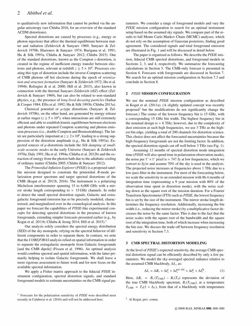
In Figure 4, we show the estimated CMB-only detection signifi-cance for the ΛCDM µ and kTeSZ signals as a function of the fre-quency resolution, ∆ν, which in principle can be varied in-flightby adjusting the mirror stroke. The sensitivity per channel scalesas ' ∆ν/15 GHz (i.e., wider frequency bins have higher sensitiv-ity). The lowest frequency channels are susceptible to instrument-related systematic errors, so we also consider forecasts in whichwe drop a fixed number of the lowest frequency bins. When ignor-ing foreground contamination, the optimal configuration for mea-suring the µ distortion is ∆ν ' 142 GHz when all channels areincluded, yielding a 10.4σ detection of the standard ΛCDM value,µ ' 2 × 10−8. This drops steeply to ' 5.5σ, 4.0σ, 2.6σ for optimalresolutions ∆ν ' 50 GHz, 27 GHz, 11 GHz, if the lowest one, two,or five frequency channels cannot be used, respectively.

A similar trend is found for the optimal configuration aim-ing to detect kTeSZ (lower panel, Fig. 4), with the optimal res-olution being ∆ν ' 135 GHz when all channels are includedin the analysis, giving a > 300σ detection of the signal. Thisdegrades to ' 226σ, 178σ, 118σ for optimal resolutions ∆ν '

83 GHz, 54 GHz, 25 GHz, if the lowest one, two or five frequencychannels cannot be used, respectively.

The error is mainly driven by the competition between sen-sitivity per channel (↔ frequency bin size) and frequency cover-age (↔ lowest frequency bin) to allow the separation of the distor-tion parameters, with kTeSZ and µ usually most strongly correlated.In particular, the sensitivity to µ drops when the design is near aregime in which no independent frequency channel is present be-low the null of the µ-distortion signal at ν ' 130 GHz. For in-stance, assuming all channels can be included, one would expecta configuration with one bin between 7.5 GHz and 130 GHz, giv-ing ∆ν ' 120GHz, to be roughly optimal. Dropping the lowest

5 For large ∆ν, the band average becomes very important.

c© 0000 RAS, MNRAS 000, 000–000

12 Abitbol et al.

5 10 15 20 25 30 35 40 45 [GHz]

10 2

10 1

100/

1% priors10% priors1% priorsdrop bin 110% priorsdrop bin 11% priorsdrop bins 1, 210% priorsdrop bins 1, 2

Figure 5. Estimated detection significance (foregrounds included; extendedmission) for the ΛCDM µ-distortion signal as a function of the frequencyresolution, ∆ν (note the logarithmic scale on the vertical axis). The differ-ent curves show the effect of dropping the lowest-frequency channels andchanging the priors on Async and αsync.

frequency bin, one would expect a configuration with two bins be-tween 7.5 GHz and 130 GHz, giving ∆ν ' 120GHz/2 ' 60 GHz, tobe optimal, and so on. These numbers are in good agreement withthe true optimal frequency bin widths found above.

7.3.2 Optimal setup with foregrounds

When including foreground contamination, the picture changes sig-nificantly. Focusing on the detection significance for µ (Fig. 5), wesee that when including all channels the optimal frequency reso-lution is ∆ν . 27 GHz, independent of the chosen prior on thesynchrotron parameters (blue curves in Fig. 5). The sensitivity re-mains rather constant in this regime, since most of the informationis already delivered by including external data as represented bythe 10% or 1% priors on Async and αsync. A sharp drop in the µ-sensitivity is found around ∆ν ' 30 GHz. This is roughly wherein our model the transition between low- and high-frequency fore-ground components occurs (see Fig. 2), driving the trade-off in thefrequency resolution toward lower frequencies. For ∆ν ' 30 GHzall of the low-frequency foreground information is contained in onechannel, which limits the ability of such a setup to separate indi-vidual components. This feature is also seen in Figures 6 and 7(discussed below).

The sensitivity, even for the extended mission, is not sufficientto detect the ΛCDM µ distortion, but greatly improved limits of|µ| . few × 10−7 are within reach. The increase in detection sig-nificance at lower frequencies is due primarily to better constrain-ing the synchrotron and free-free SEDs. Dropping the lowest fre-quency channels further pushes the optimal frequency resolutionto ∆ν . 15 GHz. This statement is relatively independent of theassumed synchrotron priors and indicates that the µ-distortion sen-sitivity of PIXIE is relatively robust with respect to the inclusion ofthe lowest FTS channels. However, modest improvements are seenwhen choosing ∆ν . 10 GHz.

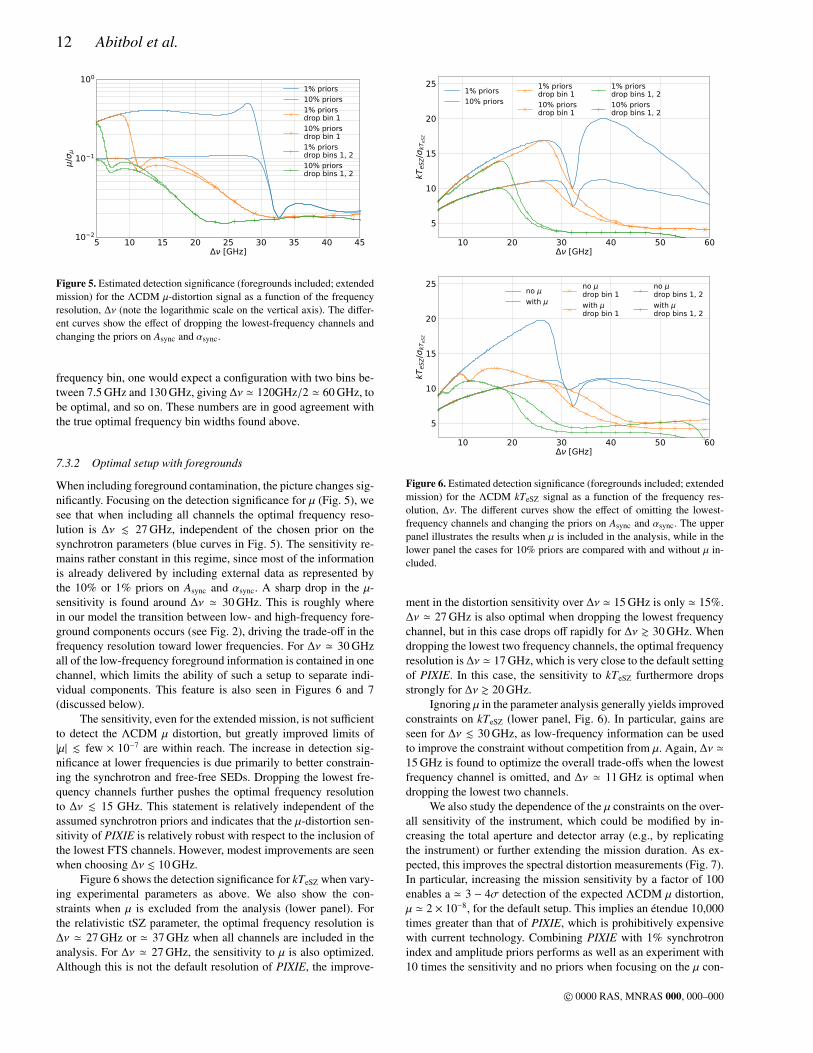
Figure 6 shows the detection significance for kTeSZ when vary-ing experimental parameters as above. We also show the con-straints when µ is excluded from the analysis (lower panel). Forthe relativistic tSZ parameter, the optimal frequency resolution is∆ν ' 27 GHz or ' 37 GHz when all channels are included in theanalysis. For ∆ν ' 27 GHz, the sensitivity to µ is also optimized.Although this is not the default resolution of PIXIE, the improve-

10 20 30 40 50 60 [GHz]

5

10

15

20

25

kTeS

Z/

kTeS

Z

1% priors10% priors

1% priorsdrop bin 110% priorsdrop bin 1

1% priorsdrop bins 1, 210% priorsdrop bins 1, 2

10 20 30 40 50 60 [GHz]

5

10

15

20

25

kTeS

Z/

kTeS

Z

no with

no drop bin 1with drop bin 1

no drop bins 1, 2with drop bins 1, 2

Figure 6. Estimated detection significance (foregrounds included; extendedmission) for the ΛCDM kTeSZ signal as a function of the frequency res-olution, ∆ν. The different curves show the effect of omitting the lowest-frequency channels and changing the priors on Async and αsync. The upperpanel illustrates the results when µ is included in the analysis, while in thelower panel the cases for 10% priors are compared with and without µ in-cluded.

ment in the distortion sensitivity over ∆ν ' 15 GHz is only ' 15%.∆ν ' 27 GHz is also optimal when dropping the lowest frequencychannel, but in this case drops off rapidly for ∆ν & 30 GHz. Whendropping the lowest two frequency channels, the optimal frequencyresolution is ∆ν ' 17 GHz, which is very close to the default settingof PIXIE. In this case, the sensitivity to kTeSZ furthermore dropsstrongly for ∆ν & 20 GHz.

Ignoring µ in the parameter analysis generally yields improvedconstraints on kTeSZ (lower panel, Fig. 6). In particular, gains areseen for ∆ν . 30 GHz, as low-frequency information can be usedto improve the constraint without competition from µ. Again, ∆ν '

15 GHz is found to optimize the overall trade-offs when the lowestfrequency channel is omitted, and ∆ν ' 11 GHz is optimal whendropping the lowest two channels.

We also study the dependence of the µ constraints on the over-all sensitivity of the instrument, which could be modified by in-creasing the total aperture and detector array (e.g., by replicatingthe instrument) or further extending the mission duration. As ex-pected, this improves the spectral distortion measurements (Fig. 7).In particular, increasing the mission sensitivity by a factor of 100enables a ' 3 − 4σ detection of the expected ΛCDM µ distortion,µ ' 2 × 10−8, for the default setup. This implies an etendue 10,000times greater than that of PIXIE, which is prohibitively expensivewith current technology. Combining PIXIE with 1% synchrotronindex and amplitude priors performs as well as an experiment with10 times the sensitivity and no priors when focusing on the µ con-

c© 0000 RAS, MNRAS 000, 000–000

PIXIE Spectral Distortion Forecast 13

10 20 30 40 50 60 [GHz]

10 2

10 1

100

101/

sensitivity ×1

sensitivity ×10

sensitivity ×100

1% priors 10% priors no priors

Figure 7. Estimated detection significance (foregrounds included; extendedmission) for the ΛCDM µ-distortion signal as a function of the frequencyresolution, ∆ν, and for varying priors on Async and αsync and increasing theoverall mission sensitivity (note the logarithmic scale on the vertical axis).

straints, for ∆ν . 30 GHz. This emphasizes the impact externalsynchrotron datasets, possibly also exploiting spatial information,could have when combined with PIXIE.

Our analysis shows that ultimately the biggest hurdle to mea-suring µ comes down to the low-frequency foregrounds, in partic-ular the synchrotron and free-free emission. A dedicated ground-based, low-frequency instrument with spatial resolution at least asgood as PIXIE will be essential in constraining these foregrounds.Alternatively, one could think about adding a low-frequency instru-ment not based on the FTS concept to the payload. A detailed anal-ysis of these ideas is left to future work, but a rough estimate withthe Fisher method seems to indicate that tens of spectral channelsbetween ' 1 and 30 GHz with sensitivity equal to or better thanthe baseline PIXIE mission would be required. This leads to < 1%constraints on the synchrotron, free-free, and spinning dust SEDsand could yield |µ| < 2.0 × 10−8 (95% c.l.).

8 CONCLUSIONS

Measurements of CMB spectral distortions will shed new light onphysics in both the early (↔ µ distortion) and late (↔ y and kTeSZ

signals) periods of cosmic history. This will open a new era in CMBcosmology, with clear distortion signals awaiting us. However, de-tecting spectral distortions will require extreme precision and con-trol of systematics over large bandwidths. Our analysis shows thatforegrounds strongly affect the expected results and demand dedi-cated observations and experimental designs, particularly with im-proved sensitivity at low frequencies (ν . 15 − 30 GHz).

We considered foreground models motivated by availableCMB observations to forecast the capability of PIXIE or other fu-ture missions to detect spectral distortions, focusing on FTS con-cepts. We find that PIXIE has the capability to measure the CMBtemperature to ' nK precision and to detect the Compton-y and rel-ativistic tSZ distortions at high significance (see Table 4). With con-servative assumptions about extra information at low frequenciesfrom external data, we expect detections at 194σ and 11σ for y andkTeSZ, respectively. We emphasize that kTeSZ is detected at above5σ with no modification of the PIXIE mission and no external data.The kTeSZ detection significance is increased to > 11σ when µ isignored in the parameter analysis (shown in the last 3 columns ofTable 4 and in Figure A1). These measurements would provide newconstraints on models of baryonic structure formation, thus provid-

ing novel information about astrophysical feedback mechanisms(Hill et al. 2015; Battaglia et al. in prep.).

Due to its many high-frequency channels, PIXIE will providethe best measurements of thermal dust and CIB emission to date(see Table 5). These sub-percent absolute measurements will pro-vide invaluable information for the modeling of CMB foregroundsrelevant to B-mode searches from the ground. They will further-more allow improvements in the channel inter-calibration, poten-tially allowing us to reach sensitivities required to extract resonantscattering signals caused by atomic species (e.g., Basu et al. 2004;Rubino-Martın et al. 2005). They will also greatly advance our un-derstanding of Galactic dust properties and physics, providing in-valuable absolutely calibrated maps in many bands.

The fiducial ΛCDM µ distortion (µ ' 2 × 10−8) is unlikelyto be detected in the presence of known foregrounds without bet-ter sensitivity or additional high-fidelity datasets that constrain theamplitude and shape of low-frequency foregrounds. Nevertheless,PIXIE could improve upon the existing limit from COBE/FIRAS bya factor of 250, yielding |µ| < 3.6×10−7 (95% c.l.) for conservativeassumptions about available external data. This would place tightconstraints on the amplitude of the small-scale scalar power spec-trum at wavenumber k ' 740 Mpc−1 (Sect. 7.2) and would rule outcurrently allowed parameter space for long-lived decaying particleswith lifetimes ' 106 − 1010 s (e.g., see Chluba & Jeong 2014).

We find PIXIE’s frequency resolution of ∆ν ' 15 GHz to beclose to optimal, although for µ slight improvements could be ex-pected when using ∆ν ' 10 GHz, depending on the quality of thelow-frequency channels (Sect. 7.3). A similar choice seems optimalfor kTeSZ, in particular if the lowest frequency channels cannot beused in the data analysis due to systematic errors (see Fig. 7).

The most practical way to improve the µ results from a PIXIE-like experiment is to complement it with ground-based observa-tions of the low-frequency synchrotron, free-free, and AME fore-grounds. Measuring the synchrotron and free-free SEDs to 0.1%would enable PIXIE to detect µ at ' 2σ. Some of the challengescould be avoided by selecting specific patches on the sky with lowforeground contamination, but we generally find that the distortionsensitivity is mostly limited by the lack of constraints on the shapeof the foreground SEDs rather than their amplitude (Sect. 7.1).

Our analysis only uses spectral information to separate dif-ferent components. Adding spatial information would yield a re-duction in the total contribution of fluctuating foreground compo-nents (e.g., Galactic contributions) to the sky-averaged spectrum.In addition, a more optimal sky-weighting scheme could be imple-mented for the monopole measurement, as opposed to the simpleaverage taken on 70% of the sky assumed in our analysis. Extra-galactic signals (e.g., CIB) will, however, not be significantly re-duced by considering spatial information, unless high-resolutionand high-sensitivity measurements become available. In this case,extended foreground parameterizations, which explicitly includethe effects of spatial averages across the sky and along the line-of-sight (Chluba et al. 2017), should be used. Since PIXIE has afairly low angular resolution (∆θ ' 1.6◦), a combination with fu-ture high-resolution CMB imagers might also be beneficial. A moredetailed analysis is required to assess the overall trade-offs in thesedirections.

We close by mentioning that information from the CMBdipole spectrum could also help in extracting the CMB distortionsignals (Danese & de Zotti 1981; Balashev et al. 2015). In particu-lar, these measurements do not require absolute calibration and thuscan also be carried out in the PIXIE anisotropy observing mode.This can furthermore be used to test for systematic effects. Also,

c© 0000 RAS, MNRAS 000, 000–000

14 Abitbol et al.

Galactic (↔ comoving) and extragalactic foregrounds are affectedin a different way by our motion with respect to the CMB restframe, so that this could provide additional leverage for foregroundseparation. All this is left to future analysis.

ACKNOWLEDGMENTS

The authors gratefully thank Al Kogut, Dale Fixsen, and Eric Switzer fortheir insight and extensive comments, as well as for providing PIXIE mis-sion parameters and sensitivity. We also thank David Spergel and Jo Dunk-ley for valuable comments on the manuscript. The authors furthermorecordially thank Daniel Foreman-Mackey for useful discussions about theemcee software package. We thank Jacques Delabrouille for noting an errorin the COBE/FIRAS sensitivity curve. JC is supported by the Royal Societyas a Royal Society University Research Fellow at the University of Manch-ester, UK. This work was partially supported by a Junior Fellow award fromthe Simons Foundation to JCH.

APPENDIX A: PARAMETER POSTERIORDISTRIBUTIONS

REFERENCES

Ali-Haımoud Y., 2013a, Phys.Rev.D, 87, 023526Ali-Haımoud Y., 2013b, Advances in Astronomy, 2013, 462697Ali-Haımoud Y., Kamionkowski M., 2016, ArXiv:1612.05644Andre P. et al., 2014, JCAP, 2, 6Balashev S. A., Kholupenko E. E., Chluba J., Ivanchik A. V., Varshalovich

D. A., 2015, ApJ, 810, 131Barrow J. D., Coles P., 1991, MNRAS, 248, 52Basu K., Hernandez-Monteagudo C., Sunyaev R. A., 2004, A&A, 416,

447Battaglia N., Hill J. C., McCarthy I. G., Chluba J., Ferraro S., Schaan E.,

Spergel D. N., in prep.Bennett C. L. et al., 2013, ApJS, 208, 20BICEP2 and Keck Array Collaborations et al., 2015, ApJ, 811, 126Burigana C., Danese L., de Zotti G., 1991, A&A, 246, 49Cabass G., Melchiorri A., Pajer E., 2016, Phys.Rev.D, 93, 083515Calabrese E., Alonso D., Dunkley J., 2016, ArXiv:1611.10269Carilli C. L. et al., 2016, ApJ, 833, 73Carr B. J., Kohri K., Sendouda Y., Yokoyama J., 2010, Phys.Rev.D, 81,

104019Challinor A., Lasenby A., 1998, ApJ, 499, 1Chluba J., 2005, PhD thesis, LMU MunchenChluba J., 2013a, MNRAS, 436, 2232Chluba J., 2013b, MNRAS, 434, 352Chluba J., 2014, ArXiv:1405.6938Chluba J., 2015, MNRAS, 454, 4182Chluba J., 2016, MNRAS, 460, 227Chluba J., Ali-Haımoud Y., 2016, MNRAS, 456, 3494Chluba J., Erickcek A. L., Ben-Dayan I., 2012a, ApJ, 758, 76Chluba J., Hill J. C., Abitbol M. H., 2017, ArXiv:1701.00274Chluba J., Jeong D., 2014, MNRAS, 438, 2065Chluba J., Khatri R., Sunyaev R. A., 2012b, MNRAS, 425, 1129Chluba J., Sunyaev R. A., 2004, A&A, 424, 389Chluba J., Sunyaev R. A., 2006, A&A, 458, L29Chluba J., Sunyaev R. A., 2008, A&A, 478, L27Chluba J., Sunyaev R. A., 2012, MNRAS, 419, 1294Chluba J., Switzer E., Nelson K., Nagai D., 2013, MNRAS, 430, 3054Chluba J., Vasil G. M., Dursi L. J., 2010, MNRAS, 407, 599Clesse S., Garbrecht B., Zhu Y., 2014, JCAP, 10, 046Daly R. A., 1991, ApJ, 371, 14Danese L., de Zotti G., 1977, Nuovo Cimento Rivista Serie, 7, 277Danese L., de Zotti G., 1981, A&A, 94, L33de Oliveira-Costa A., Tegmark M., Gaensler B. M., Jonas J., Landecker

T. L., Reich P., 2008, MNRAS, 388, 247

De Zotti G., Negrello M., Castex G., Lapi A., Bonato M., 2016, JCAP, 3,047

Desjacques V., Chluba J., Silk J., de Bernardis F., Dore O., 2015, MNRAS,451, 4460

Draine B. T., 2011, Physics of the Interstellar and Intergalactic MediumDraine B. T., Lazarian A., 1998, ApJL, 494, L19Dubrovich V. K., 1975, Soviet Astronomy Letters, 1, 196Dunkley J. et al., 2011, ApJ, 739, 52Ellis J., Gelmini G. B., Lopez J. L., Nanopoulos D. V., Sarkar S., 1992,

Nuclear Physics B, 373, 399Filippini J. P. et al., 2010, in Society of Photo-Optical Instrumentation En-

gineers (SPIE) Conference Series, Vol. 7741, Millimeter, Submillime-ter, and Far-Infrared Detectors and Instrumentation for Astronomy V, p.77411N

Fixsen D. J., 2009, ApJ, 707, 916Fixsen D. J., Cheng E. S., Gales J. M., Mather J. C., Shafer R. A., Wright

E. L., 1996, ApJ, 473, 576Fixsen D. J., Mather J. C., 2002, ApJ, 581, 817Foreman-Mackey D., Hogg D. W., Lang D., Goodman J., 2012,

ArXiv:1202.3665Genova-Santos R. et al., 2015, in Highlights of Spanish Astrophysics VIII,

Cenarro A. J., Figueras F., Hernandez-Monteagudo C., Trujillo Bueno J.,Valdivielso L., eds., pp. 207–212

Gervasi M., Zannoni M., Tartari A., Boella G., Sironi G., 2008, ApJ, 688,24

Gush H. P., Halpern M., Wishnow E. H., 1990, Phys. Rev. Lett., 65, 537Harrington K. et al., 2016, in Society of Photo-Optical Instrumentation

Engineers (SPIE) Conference Series, Vol. 9914, Millimeter, Submillime-ter, and Far-Infrared Detectors and Instrumentation for Astronomy VIII,p. 99141K

Haslam C. G. T., Klein U., Salter C. J., Stoffel H., Wilson W. E., ClearyM. N., Cooke D. J., Thomasson P., 1981, A&A, 100, 209

Haslam C. G. T., Salter C. J., Stoffel H., Wilson W. E., 1982, A&A Supp.,47, 1

Hervıas-Caimapo C., Bonaldi A., Brown M. L., 2017, ArXiv:1701.02277Hill J. C., Battaglia N., Chluba J., Ferraro S., Schaan E., Spergel D. N.,

2015, Physical Review Letters, 115, 261301Hinshaw G. et al., 2013, ApJS, 208, 19Hu W., Scott D., Silk J., 1994a, ApJL, 430, L5Hu W., Scott D., Silk J., 1994b, Phys.Rev.D, 49, 648Hu W., Silk J., 1993a, Phys.Rev.D, 48, 485Hu W., Silk J., 1993b, Physical Review Letters, 70, 2661Illarionov A. F., Sunyaev R. A., 1974, Astronomicheskii Zhurnal, 51, 1162Imara N., Loeb A., 2016, ApJ, 825, 130Irfan M. O. et al., 2015, MNRAS, 448, 3572Itoh N., Kohyama Y., Nozawa S., 1998, ApJ, 502, 7Jeong D., Pradler J., Chluba J., Kamionkowski M., 2014, Physical Review

Letters, 113, 061301Keisler R. et al., 2015, ApJ, 807, 151Keisler R. et al., 2011, ApJ, 743, 28Khatri R., Sunyaev R. A., 2012, JCAP, 9, 16Kogut A., Chluba J., Fixsen D. J., Meyer S., Spergel D., 2016, in Soci-

ety of Photo-Optical Instrumentation Engineers (SPIE) Conference Se-ries, Vol. 9904, Space Telescopes and Instrumentation 2016: Optical, In-frared, and Millimeter Wave, p. 99040W

Kogut A. et al., 2006, New Astronomy Reviews, 50, 925Kogut A., Fixsen D. J., 2016, ApJ, 826, 101Kogut A. et al., 2011a, JCAP, 7, 25Kogut A. et al., 2011b, ApJ, 734, 4Mashian N., Loeb A., Sternberg A., 2016, MNRASMather J. C. et al., 1990, ApJL, 354, L37McDonald P., Scherrer R. J., Walker T. P., 2001, Phys.Rev.D, 63, 023001Naess S. et al., 2014, JCAP, 10, 007Netterfield C. B. et al., 2002, ApJ, 571, 604Nozawa S., Itoh N., Suda Y., Ohhata Y., 2006, Nuovo Cimento B Serie,

121, 487Ostriker J. P., Thompson C., 1987, ApJL, 323, L97Pearson T. J. et al., 2003, ApJ, 591, 556

c© 0000 RAS, MNRAS 000, 000–000

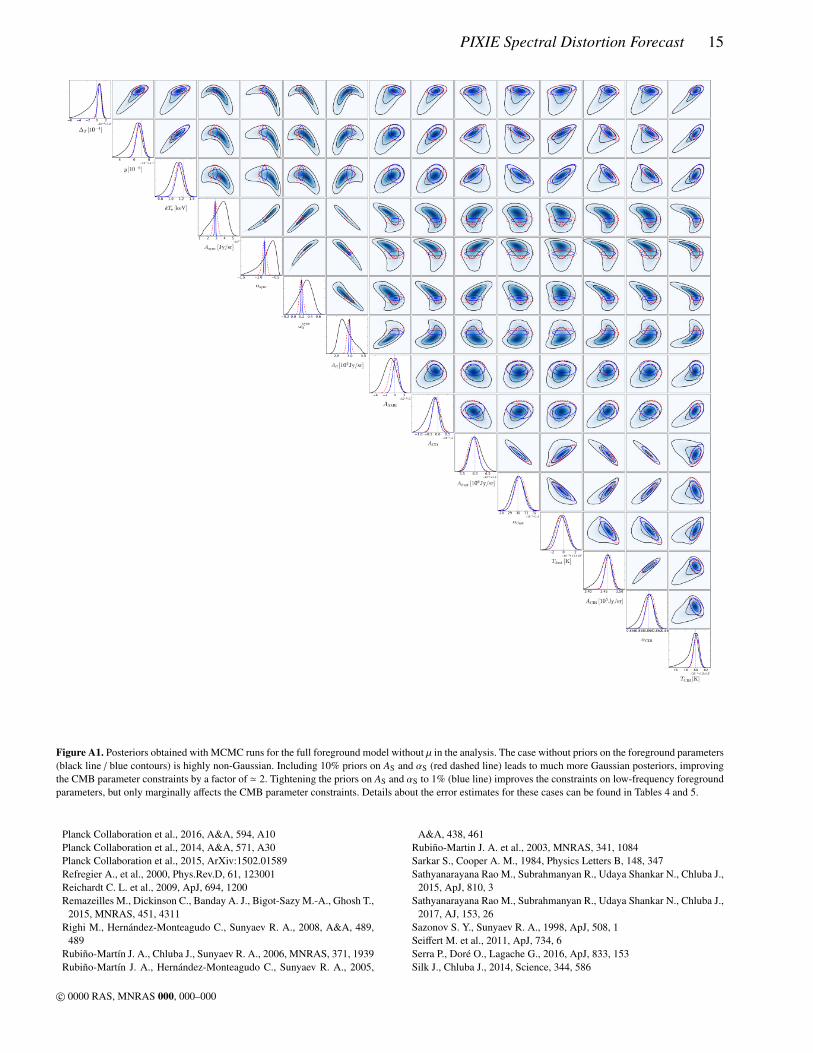
PIXIE Spectral Distortion Forecast 15

Figure A1. Posteriors obtained with MCMC runs for the full foreground model without µ in the analysis. The case without priors on the foreground parameters(black line / blue contours) is highly non-Gaussian. Including 10% priors on AS and αS (red dashed line) leads to much more Gaussian posteriors, improvingthe CMB parameter constraints by a factor of ' 2. Tightening the priors on AS and αS to 1% (blue line) improves the constraints on low-frequency foregroundparameters, but only marginally affects the CMB parameter constraints. Details about the error estimates for these cases can be found in Tables 4 and 5.

Planck Collaboration et al., 2016, A&A, 594, A10Planck Collaboration et al., 2014, A&A, 571, A30Planck Collaboration et al., 2015, ArXiv:1502.01589Refregier A., et al., 2000, Phys.Rev.D, 61, 123001Reichardt C. L. et al., 2009, ApJ, 694, 1200Remazeilles M., Dickinson C., Banday A. J., Bigot-Sazy M.-A., Ghosh T.,

2015, MNRAS, 451, 4311Righi M., Hernandez-Monteagudo C., Sunyaev R. A., 2008, A&A, 489,

489Rubino-Martın J. A., Chluba J., Sunyaev R. A., 2006, MNRAS, 371, 1939Rubino-Martın J. A., Hernandez-Monteagudo C., Sunyaev R. A., 2005,

A&A, 438, 461Rubino-Martin J. A. et al., 2003, MNRAS, 341, 1084Sarkar S., Cooper A. M., 1984, Physics Letters B, 148, 347Sathyanarayana Rao M., Subrahmanyan R., Udaya Shankar N., Chluba J.,

2015, ApJ, 810, 3Sathyanarayana Rao M., Subrahmanyan R., Udaya Shankar N., Chluba J.,

2017, AJ, 153, 26Sazonov S. Y., Sunyaev R. A., 1998, ApJ, 508, 1Seiffert M. et al., 2011, ApJ, 734, 6Serra P., Dore O., Lagache G., 2016, ApJ, 833, 153Silk J., Chluba J., 2014, Science, 344, 586

c© 0000 RAS, MNRAS 000, 000–000

16 Abitbol et al.

Steigman G., 2009, in American Institute of Physics Conference Series,Vol. 1135, American Institute of Physics Conference Series, van Steen-berg M. E., Sonneborn G., Moos H. W., Blair W. P., eds., pp. 94–101

Sunyaev R. A., Chluba J., 2009, Astronomische Nachrichten, 330, 657Sunyaev R. A., Khatri R., 2013, International Journal of Modern Physics

D, 22, 30014Sunyaev R. A., Zeldovich Y. B., 1970a, ApSS, 9, 368Sunyaev R. A., Zeldovich Y. B., 1970b, ApSS, 7, 20Sunyaev R. A., Zeldovich Y. B., 1970c, Comments on Astrophysics and

Space Physics, 2, 66Sunyaev R. A., Zeldovich Y. B., 1972, A&A, 20, 189Switzer E. R., 2017, ArXiv:1703.07832Tashiro H., 2014, Prog. of Theo. and Exp. Physics, 2014, 060000Tashiro H., Sabancilar E., Vachaspati T., 2012, Phys.Rev.D, 85, 103522Tashiro H., Sabancilar E., Vachaspati T., 2013, JCAP, 8, 35The COrE Collaboration et al., 2011, ArXiv:1102.2181Zeldovich Y. B., Illarionov A. F., Sunyaev R. A., 1972, SJETP, 35, 643Zeldovich Y. B., Kurt V. G., Syunyaev R. A., 1968, Zhurnal Eksperimental

noi i Teoreticheskoi Fiziki, 55, 278Zeldovich Y. B., Sunyaev R. A., 1969, ApSS, 4, 301

c© 0000 RAS, MNRAS 000, 000–000