prosodic features for a maximum entropy language model
TRANSCRIPT

Prosodic Features for a Maximum
Entropy Language Model
Oscar Chan
This thesis is presented for the degree ofDoctor of Philosophy
ofThe University of Western Australia
School of Electrical, Electronic and Computer EngineeringThe University of Western Australia
July 2008

ii

Abstract
A statistical language model attempts to characterise the patterns present in a nat-
ural language as a probability distribution defined over word sequences. Typically,
they are trained using word co-occurrence statistics from a large sample of text. In
some language modelling applications, such as automatic speech recognition (ASR),
the availability of acoustic data provides an additional source of knowledge. This
contains, amongst other things, the melodic and rhythmic aspects of speech referred
to as prosody. Although prosody has been found to be an important factor in human
speech recognition, its use in ASR has been limited.
The goal of this research is to investigate how prosodic information can be em-
ployed to improve the language modelling component of a continuous speech recog-
nition system. Because prosodic features are largely suprasegmental, operating over
units larger than the phonetic segment, the language model is an appropriate place
to incorporate such information. The prosodic features and standard language model
features are combined under the maximum entropy framework, which provides an
elegant solution to modelling information obtained from multiple, differing knowl-
edge sources. We derive features for the model based on perceptually transcribed
Tones and Break Indices (ToBI) labels, and analyse their contribution to the word
recognition task.
While ToBI has a solid foundation in linguistic theory, the need for human tran-
scribers conflicts with the statistical model’s requirement for a large quantity of
training data. We therefore also examine the applicability of features which can
be automatically extracted from the speech signal. We develop representations of
an utterance’s prosodic context using fundamental frequency, energy and duration
features, which can be directly incorporated into the model without the need for
manual labelling. Dimensionality reduction techniques are also explored with the
aim of reducing the computational costs associated with training a maximum en-
tropy model. Experiments on a prosodically transcribed corpus show that small but
statistically significant reductions to perplexity and word error rates can be obtained
by using both manually transcribed and automatically extracted features.
iii

iv

Acknowledgements
First of all, I would like to express my deepest gratitude to my supervisor, Roberto
Togneri. It was he who first sparked my interest in speech and language processing.
His expert guidance and advice, as well as his encouragement during the more dif-
ficult times, have been invaluable. This work would not have been possible without
him.
Special thanks is due to John Henderson, for those few but insightful discussions
on prosody. His ideas and suggestions have been very helpful, and were a major
factor in the formulation of this thesis. I am grateful to Ramachandran Chan-
drasekhar, for generously providing his LaTeX thesis templates. Thanks also go to
the staff members in the School of Electrical, Electronic and Computer Engineering,
especially Linda.
I wish to extend my appreciation to my friends and colleagues in CIIPS – Aik
Ming, Marco, Serajul, Daniel and Weiqun. It has been a great pleasure working
together with them, and the many stimulating discussions we have had, technical
or otherwise, have made this experience a very enjoyable and rewarding one.
I would also like to acknowledge the Australian Postgraduate Awards programme
and the Australasian Speech Science Technology Association for providing financial
assistance during my candidature.
Finally, I wish to thank my family and friends for all the support they have
provided over the years.
v

vi

Contents
Abstract iii
Acknowledgements v
Contents x
List of Figures xii
List of Tables xiv
1 Introduction 1
1.1 Research Objectives . . . . . . . . . . . . . . . . . . . . . . . . . . . . 2
1.2 Document Overview . . . . . . . . . . . . . . . . . . . . . . . . . . . 3
2 Language Modelling for ASR 5
2.1 Language Modelling . . . . . . . . . . . . . . . . . . . . . . . . . . . 6
2.1.1 N -gram models . . . . . . . . . . . . . . . . . . . . . . . . . . 7
2.1.2 Smoothing . . . . . . . . . . . . . . . . . . . . . . . . . . . . . 7
2.1.3 N-gram extensions and other models . . . . . . . . . . . . . . 11
2.1.4 Decision trees . . . . . . . . . . . . . . . . . . . . . . . . . . . 15
2.2 Automatic Speech Recognition . . . . . . . . . . . . . . . . . . . . . . 16
2.2.1 Feature extraction . . . . . . . . . . . . . . . . . . . . . . . . 17
2.2.2 Acoustic modelling . . . . . . . . . . . . . . . . . . . . . . . . 18
2.3 Decoding . . . . . . . . . . . . . . . . . . . . . . . . . . . . . . . . . . 20
2.3.1 Viterbi decoding . . . . . . . . . . . . . . . . . . . . . . . . . 21
2.3.2 Stack decoding . . . . . . . . . . . . . . . . . . . . . . . . . . 22
2.3.3 Multi-pass decoding . . . . . . . . . . . . . . . . . . . . . . . 23
2.4 Evaluation . . . . . . . . . . . . . . . . . . . . . . . . . . . . . . . . . 26
2.4.1 ASR evaluation . . . . . . . . . . . . . . . . . . . . . . . . . . 26
2.4.2 Statistical significance . . . . . . . . . . . . . . . . . . . . . . 27
vii

CONTENTS
2.4.3 Perplexity . . . . . . . . . . . . . . . . . . . . . . . . . . . . . 28
3 Prosody 31
3.1 Prosodic Features . . . . . . . . . . . . . . . . . . . . . . . . . . . . . 32
3.1.1 Pitch . . . . . . . . . . . . . . . . . . . . . . . . . . . . . . . . 32
3.1.2 Loudness . . . . . . . . . . . . . . . . . . . . . . . . . . . . . . 32
3.1.3 Length . . . . . . . . . . . . . . . . . . . . . . . . . . . . . . . 33
3.1.4 Stress . . . . . . . . . . . . . . . . . . . . . . . . . . . . . . . 34
3.1.5 Tone . . . . . . . . . . . . . . . . . . . . . . . . . . . . . . . . 34
3.1.6 Intonation . . . . . . . . . . . . . . . . . . . . . . . . . . . . . 34
3.2 Functions of Prosody . . . . . . . . . . . . . . . . . . . . . . . . . . . 34
3.2.1 Roles in human communication . . . . . . . . . . . . . . . . . 35
3.2.2 Cross-linguistic differences . . . . . . . . . . . . . . . . . . . . 39
3.3 Modelling Prosody . . . . . . . . . . . . . . . . . . . . . . . . . . . . 40
3.3.1 Pierrehumbert’s model . . . . . . . . . . . . . . . . . . . . . . 41
3.3.2 Tones and Break Indices . . . . . . . . . . . . . . . . . . . . . 42
3.3.3 Alternate modelling approaches . . . . . . . . . . . . . . . . . 46
3.4 Prosody in ASR . . . . . . . . . . . . . . . . . . . . . . . . . . . . . . 47
3.5 Prosodic Knowledge for Language Modelling . . . . . . . . . . . . . . 52
4 Maximum Entropy 55
4.1 Maximum Entropy Principle . . . . . . . . . . . . . . . . . . . . . . . 55
4.2 Maximum Entropy Models . . . . . . . . . . . . . . . . . . . . . . . . 57
4.2.1 Representing knowledge . . . . . . . . . . . . . . . . . . . . . 57
4.2.2 Conditional models . . . . . . . . . . . . . . . . . . . . . . . . 57
4.2.3 Minimum divergence . . . . . . . . . . . . . . . . . . . . . . . 60
4.3 Parameter Estimation . . . . . . . . . . . . . . . . . . . . . . . . . . 61
4.3.1 Iterative scaling . . . . . . . . . . . . . . . . . . . . . . . . . . 61
4.3.2 Gradient based methods . . . . . . . . . . . . . . . . . . . . . 63
4.4 Smoothing . . . . . . . . . . . . . . . . . . . . . . . . . . . . . . . . . 64
4.4.1 Feature selection . . . . . . . . . . . . . . . . . . . . . . . . . 64
4.4.2 Regularisation . . . . . . . . . . . . . . . . . . . . . . . . . . . 65
4.5 Combining Knowledge Sources . . . . . . . . . . . . . . . . . . . . . . 68
5 Language Modelling with ToBI Features 71
5.1 Corpus . . . . . . . . . . . . . . . . . . . . . . . . . . . . . . . . . . . 72
5.2 Evaluating Prosodic Features . . . . . . . . . . . . . . . . . . . . . . 74
5.3 Language Modelling . . . . . . . . . . . . . . . . . . . . . . . . . . . 78
viii

CONTENTS
5.3.1 Baseline . . . . . . . . . . . . . . . . . . . . . . . . . . . . . . 78
5.3.2 ToBI features . . . . . . . . . . . . . . . . . . . . . . . . . . . 78
5.3.3 Perplexity results . . . . . . . . . . . . . . . . . . . . . . . . . 80
5.4 Speech Recognition . . . . . . . . . . . . . . . . . . . . . . . . . . . . 83
5.4.1 Multi-pass decoding . . . . . . . . . . . . . . . . . . . . . . . 84
5.4.2 Results . . . . . . . . . . . . . . . . . . . . . . . . . . . . . . . 85
5.5 Conclusion . . . . . . . . . . . . . . . . . . . . . . . . . . . . . . . . . 90
6 Automatic Feature Extraction 91
6.1 Aims . . . . . . . . . . . . . . . . . . . . . . . . . . . . . . . . . . . . 92
6.2 Prosodic Feature Extraction . . . . . . . . . . . . . . . . . . . . . . . 92
6.2.1 Duration . . . . . . . . . . . . . . . . . . . . . . . . . . . . . . 93
6.2.2 Fundamental frequency . . . . . . . . . . . . . . . . . . . . . . 98
6.2.3 Energy . . . . . . . . . . . . . . . . . . . . . . . . . . . . . . . 101
6.3 Feature Analysis . . . . . . . . . . . . . . . . . . . . . . . . . . . . . 102
6.3.1 Duration . . . . . . . . . . . . . . . . . . . . . . . . . . . . . . 102
6.3.2 F0 and RMS energy . . . . . . . . . . . . . . . . . . . . . . . 104
6.4 Summary . . . . . . . . . . . . . . . . . . . . . . . . . . . . . . . . . 108
7 Language Modelling with Raw Features 111
7.1 Handling Non-Binary Features . . . . . . . . . . . . . . . . . . . . . . 112
7.1.1 Real-valued features . . . . . . . . . . . . . . . . . . . . . . . 112
7.1.2 Quantisation . . . . . . . . . . . . . . . . . . . . . . . . . . . 113
7.2 Dimensionality Reduction . . . . . . . . . . . . . . . . . . . . . . . . 114
7.2.1 Linear dimensionality deduction . . . . . . . . . . . . . . . . . 114
7.2.2 Locality Preserving Projections . . . . . . . . . . . . . . . . . 116
7.3 Prosody Labelling . . . . . . . . . . . . . . . . . . . . . . . . . . . . . 117
7.3.1 Baseline model . . . . . . . . . . . . . . . . . . . . . . . . . . 118
7.3.2 Prosodic model features . . . . . . . . . . . . . . . . . . . . . 118
7.3.3 Results . . . . . . . . . . . . . . . . . . . . . . . . . . . . . . . 119
7.3.4 Language modelling results . . . . . . . . . . . . . . . . . . . 121
7.4 Direct Modelling . . . . . . . . . . . . . . . . . . . . . . . . . . . . . 122
7.4.1 Motivation . . . . . . . . . . . . . . . . . . . . . . . . . . . . . 122
7.4.2 Word clustering in prosody space . . . . . . . . . . . . . . . . 123
7.4.3 Modelling prosodic history . . . . . . . . . . . . . . . . . . . . 126
7.4.4 Results . . . . . . . . . . . . . . . . . . . . . . . . . . . . . . . 127
7.5 Noise Robustness . . . . . . . . . . . . . . . . . . . . . . . . . . . . . 130
7.5.1 Sources of noise . . . . . . . . . . . . . . . . . . . . . . . . . . 131
ix

CONTENTS
7.5.2 Results . . . . . . . . . . . . . . . . . . . . . . . . . . . . . . . 131
7.6 Conclusion . . . . . . . . . . . . . . . . . . . . . . . . . . . . . . . . . 134
8 Conclusion 137
8.1 Summary . . . . . . . . . . . . . . . . . . . . . . . . . . . . . . . . . 137
8.2 Future Research . . . . . . . . . . . . . . . . . . . . . . . . . . . . . . 139
8.2.1 Alternate Corpus . . . . . . . . . . . . . . . . . . . . . . . . . 140
8.2.2 Improved Prosody Modelling . . . . . . . . . . . . . . . . . . . 140
8.2.3 System Integration . . . . . . . . . . . . . . . . . . . . . . . . 140
A Penn Treebank Tag Set 143
Bibliography 160
x
List of Figures
2.1 Back-off paths of a factored language model. . . . . . . . . . . . . . . 13
2.2 Structure of a speech recogniser. . . . . . . . . . . . . . . . . . . . . . 17
2.3 HMM generation of an observation sequence. . . . . . . . . . . . . . . 19
2.4 Trellis for of Viterbi decoding. . . . . . . . . . . . . . . . . . . . . . . 21
2.5 Generation of hypotheses for multi-pass decoding. . . . . . . . . . . . 24
2.6 An N-best list. . . . . . . . . . . . . . . . . . . . . . . . . . . . . . . 25
2.7 A fragment of a word hypothesis graph. . . . . . . . . . . . . . . . . . 26
3.1 Finite-state grammar of allowable tone sequences. . . . . . . . . . . . 41
3.2 A ToBI transcription of an utterance. . . . . . . . . . . . . . . . . . . 45
5.1 Distribution of pitch accents and break indices in the training parti-
tion of the RNC data. . . . . . . . . . . . . . . . . . . . . . . . . . . 73
5.2 Oracle accuracies of N-best lists for 1 ≤ N ≤ 100. . . . . . . . . . . . 85
5.3 Histogram of the rank of the oracle hypothesis before and after re-
ranking by LM-ABS. . . . . . . . . . . . . . . . . . . . . . . . . . . . 89
6.1 Speaker-dependent duration PDFs for the word state. . . . . . . . . . 96
6.2 Post-processing of an F0 contour. . . . . . . . . . . . . . . . . . . . . 99
6.3 F0 features derived from the automatically extracted pitch contour. . 100
6.4 Distribution of normalised word durations for the four prosodic classes.102
6.5 Distribution of normalised durations for accented phrase-final words,
separated by POS. . . . . . . . . . . . . . . . . . . . . . . . . . . . . 103
6.6 A typical rise-fall F0 pattern occurring during the word reaches, and
the (dotted) least squares regression line fitted over the region. . . . . 106
7.1 A language model rescoring system using intermediate labelling. . . . 121
7.2 A language model rescoring system using direct prosodic features. . . 124
7.3 Projections of word cluster centroids onto a 3-dimensional LPP space. 126
7.4 Modelling of two types of noise sources in the speech signal. . . . . . 131
xi

LIST OF FIGURES
7.5 F0 contours extracted from signals corrupted with additive noise at
a SNR of 0 dB. . . . . . . . . . . . . . . . . . . . . . . . . . . . . . . 133
7.6 F0 contour extracted from a signal in the presence of reverberation
with a RT60 of 0.5 s. . . . . . . . . . . . . . . . . . . . . . . . . . . . 134
xii

List of Tables
3.1 The relationships between the acoustic and perceptual realisations of
prosody, and their major linguistic functions. . . . . . . . . . . . . . . 39
5.1 Mutual information between a word and its features over the training
set. . . . . . . . . . . . . . . . . . . . . . . . . . . . . . . . . . . . . . 77
5.2 Perplexities of language models using features comprising length m
sequences of ToBI labels. . . . . . . . . . . . . . . . . . . . . . . . . . 81
5.3 Distribution of pitch accents and break indices in the training set. . . 83
5.4 Recognition accuracies of language models using ToBI features. . . . 86
5.5 Misrecognitions of three systems according to error type. . . . . . . . 88
6.1 Average KL distances between word duration distributions for three
different normalisation schemes. . . . . . . . . . . . . . . . . . . . . . 95
6.2 Means and standard deviations (in brackets) of z-score normalised
phone durations for the three phonemes in the word state. . . . . . . 97
6.3 Means (and standard deviations) of raw and normalised word dura-
tions for each of the four prosodic classes. . . . . . . . . . . . . . . . 102
6.4 Means (and standard deviations) of voicing, F0 and RMS energy
features for the four combinations of pitch accent and break index. . . 105
6.5 Means (and standard deviations) of quantised F0 and RMS energy
features for the four combinations of pitch accent and break index. . . 107
6.6 Relationship between prosodic events and automatically extracted
features. Entries for which a feature is useful for determining the
prosodic class are marked as either H (indicating the mean feature
value is higher than average) or L (lower than average). . . . . . . . . 109
7.1 Pitch accent and break index classification accuracies using prosodic
features and LPP dimensionality reduction. . . . . . . . . . . . . . . 119
7.2 Cosine similarities between words and cluster centroids. . . . . . . . . 125
xiii

LIST OF TABLES
7.3 Perplexities and word recognition accuracies of models using cosine
similarity features. . . . . . . . . . . . . . . . . . . . . . . . . . . . . 128
7.4 Pitch accent and break index classification accuracies using prosodic
features and LPP dimensionality reduction. . . . . . . . . . . . . . . 130
7.5 Word accuracies of LM-D8 when using prosodic features extracted
from data corrupted by additive noise. . . . . . . . . . . . . . . . . . 132
7.6 Word accuracies of LM-D8 when using prosodic features extracted
from data corrupted by reverberant noise. . . . . . . . . . . . . . . . 134
xiv
Chapter 1
Introduction
Spoken languages contain a wide range of information. While speech is used pri-
marily to convey a sequence of words, the speech signal contains more than just
the acoustic properties defining the phonemic segments. There is paralinguistic in-
formation which includes speaker-specific information such as their gender, are and
emotions. There is also prosody, which bears linguistic content pertaining to the
message being conveyed. The term prosody is broadly used to refer to the melodic
and rhythmic aspects of speech, but there is less agreement on a more precise def-
inition. Cutler et al. [1] identifies a continuum of interpretations. At one end,
prosody is defined as the abstract phonological structure of speech, without con-
sideration of its realisation. At the other extreme, no distinction is made between
the phonological structure and its acoustic realisation, and the term prosody has
been used synonymously with prosodic features. A more comprehensive definition is
also given, which takes into account both the phonetic and phonological aspects of
prosody: “the linguistic structure which determines the suprasegmental properties
of utterances”. Prosodic features are considered to be suprasegmental because they
operate on domains larger than the phonemic segment. These range from the small-
est domain of the syllable, up through words, phrases, utterances and paragraphs,
to the largest domain of the discourse. Unlike speech segments, which can largely
be characterised in terms of absolute acoustic parameters, prosodic features tend to
be meaningful only with reference to a time series [2, 3]. Prosodic features are also
inherent in speech segments, and these are sometimes included in the definition of
prosody as microprosodic features.
The complex nature of prosody has been responsible, at least in part, for its
lack of use in automatic speech processing. Despite being an important aspect of
human-to-human communication, its precise functions are difficult to quantify and
model. Automatic speech processing systems tend to have a modular design, with
1
1.1. RESEARCH OBJECTIVES
each component being responsible for a specific task. In contrast, prosody has a
multitude of functions including, but not limited to, conveying emotion, guiding
dialogue structure [4], resolving ambiguity [5], demarcating word and phrase bound-
aries [6], and in some languages, distinguishing between phonetically similar sounds.
All these functions are realised as variations in the acoustic parameters of funda-
mental frequency, energy and duration, and this makes if difficult, if not impossible,
to isolate the phonological factors governing their changes.
There is also some disparity between the traditional lines of prosody research
and the requirements of speech processing systems. While there is a large body of
research covering many aspects of prosody, much of it is not directly applicable to
automated systems. These systems, taking advantage of recent advances in com-
puting power, simply treat the speech processing task as a more general statistical
pattern matching problem. Inputs to such systems are typically statistics gathered
by observing a large data sample. To be effective, these statistics need to be both
general and reliable. Highly specific knowledge about prosodic behaviour, or knowl-
edge that is situational, therefore tends to be of lesser value to an automatic speech
processing system.
Despite these difficulties, though, there are many potential uses for prosody in
speech systems. At the lowest level, prosody can help word recognition [7] either
directly, or by aiding correct segmentation of continuous speech. The close relation-
ship between prosodic and syntactic structure [8] makes it a a good candidate for
use in keyword spotting and speech understanding applications. Correct prosody is
vital aspect of natural sounding speech [9], and a speech synthesis system must take
this into account. The ultimate goal, of course, is to use prosody in all aspects of
speech processing – from guiding dialogue choices through to recognising speech and
generating responses. While this may be a long-term goal, the topic has garnered
substantial interest, and much progress has been made in recent years.
1.1 Research Objectives
The goal of this research is to further the understanding of prosody in the context
of automatic speech processing. The focus, in particular, is on the use of supraseg-
mental features to assist in continuous speech recognition. More specifically, the
objectives are to:
• Examine how prosody behaves at and above the word level, and how this
behaviour is related to word identity and syntax.
2

INTRODUCTION
• Investigate prosodic realisations to obtain a set of representative acoustic pa-
rameters that are both highly correlated with prosodic events and can be
extracted from the speech signal without human supervision.
• Formulate these parameters into features for a statistical language model that
capture relationships between prosody and lexical information for the purposes
of word prediction.
• Evaluate the models, both in isolation and when coupled to a speech recogniser,
and examine the effects of introducing prosodic knowledge into the system.
1.2 Document Overview
The remainder of this dissertation is organised as follows. Chapter 2 will provide
an introduction to the ASR problem. It will cover the operation of a typical speech
recognition system, with particular emphasis on the role of language models in
recognising continuous speech. It will also examine some difficulties involved with
developing language models, and a number of alternatives to the standard n-gram
model will be reviewed.
Chapter 3 will present an overview of the prosody of speech. It will outline some
of the roles that prosody plays in human-to-human communication, as well as ways
in which it has been used in automatic processing. Prosody is perceptual, and this
chapter will review some methods of quantifying prosodic information.
The maximum entropy model lies at the core of this research, and it will be
discussed in Chapter 4. The chapter will begin with an example demonstrating
the principle of maximum entropy, and then present the general form of the model.
Some of the advantages and disadvantages of this model will be examined. This
chapter will describe how these models can be used for language modelling, and
highlight the model’s ability to combine diverse sources of knowledge under a con-
sistent framework.
Chapter 5 will present an approach to developing language models using prosodic
information. It will make use of of a prosodically transcribed corpus, and an inves-
tigation of the relationship between prosody, words and syntax will be performed.
Following this, prosodic features for maximum entropy models will be derived, and
the models evaluated using both information theoretic criteria and application in a
speech recognition system.
In Chapter 6, the issue of automatically extracting prosodic features is consid-
ered. Because perceptual annotation of prosody is a difficult and time-consuming
3

1.2. DOCUMENT OVERVIEW
task, there are substantial benefits to being able to obtain this information in an
unsupervised manner. This chapter will examine the relationship between two types
of prosodic events, accents and boundaries, and various acoustic parameters. It will
focus specifically on the behaviour of these parameters at the word level, as this is
the natural unit of the language model.
In Chapter 7, the acoustic parameters obtained from the investigations of Chap-
ter 6 are applied to language modelling tasks. Two approaches are described. The
first makes use of some perceptual information to train prosodic labelling models.
The second approach does not use any perceptual transcriptions, and trains lan-
guage models directly on acoustic parameters. The performance of both approaches
are examined. Finally, an investigation of the robustness of the prosodic features
under a variety of noise conditions is conducted.
A summary of the findings are presented in Chapter 8. A number of further
research directions will also be explored here.
4

Chapter 2
Language Modelling for ASR
A natural language is a language used as a means of communication amongst hu-
mans. Unlike formal languages, which adhere to strict rules specifying their syntax,
natural languages contain many complexities and ambiguities which make them dif-
ficult to define. The goal of language modelling is to develop a good approximation
of a natural language by identifying and characterising patterns within the language.
Many natural language processing (NLP) tasks make use of a language modelling
component to provide higher level knowledge. Acoustic models used in automatic
speech recognition (ASR) systems generally model sub-word units such as phones,
and are therefore unable to capture information at the linguistic level. For all but
the most highly constrained ASR tasks, a language model providing this additional
knowledge is a necessary component of the system. Another task in which lan-
guage models are used is machine translation. Language structure can vary greatly
in both syntax and morphology, and a machine translation system is required to
have detailed models of both source and target languages. Yet more applications of
language models include information retrieval, optical character recognition, hand-
writing recognition and others.
This chapter will examine the role of language modelling in the context of auto-
matic speech recognition. It will begin with an overview of the language modelling
problem, and introduce the widely used n-gram model. Issues pertaining to param-
eter estimation of n-gram models will also be examined in this section. The second
section will provide an overview of the speech recognition process, which consists of
four distinct tasks: feature extraction, acoustic modelling, language modelling and
decoding. These tasks and their inter-operation will be briefly summarised in this
section. In the third section, the task of combining acoustic and language mod-
els is considered. It will discuss search algorithms used in the decoding process,
as well as rescoring techniques used in multi-pass decoding. The final section of
5
2.1. LANGUAGE MODELLING
this chapter will describe evaluation techniques for speech recognisers as well as in-
troduce perplexity, a recogniser-independent metric for evaluating language model
performance.
2.1 Language Modelling
Like many solutions to NLP tasks, a distinction can be drawn between knowledge-
based and data-driven approaches to the statistical language modelling problem.
Knowledge-based approaches attempt to directly apply human knowledge of linguis-
tic structure to describe the language. A commonly used, and well known example
is the Context Free Grammar, which defines a set of hierarchical rules represent-
ing syntactic constraints. The alternative data-driven approaches rely on automatic
training of statistical models by observing a sample of data. These models enjoy a
number of advantages over knowledge-based models, including:
• Simplicity: Unsupervised or partially supervised training algorithms for statis-
tical language models can greatly decrease the amount of human effort required
to develop them.
• Reusability: The training procedures for statistical models are very general,
and can be applied to data from a variety of domains.
• Consistency: Learning parameters by observing empirical data ensures the
model does not contain inconsistent information. Additionally, automatic
training procedures are capable of identifying relevant patterns in the data
which may not be readily apparent.
The main disadvantages to statistical models are:
• Data requirements: In order to accurately estimate model parameters, a large
number of training samples are required. Creating this data can be costly and
time-consuming.
• Limited knowledge representation: The knowledge which can be learnt by a
statistical model is inherently restricted by the model’s form. For example,
a model which applies a Markovian assumption is incapable of modelling de-
pendencies which extend beyond the available context. It can also be difficult
to incorporate potentially useful prior knowledge into a statistical framework.
6
LANGUAGE MODELLING FOR ASR
With the increasing availability of large databases designed for NLP tasks, the data
requirements of training statistical language models becomes easier to satisfy. Ad-
ditionally, significant increases in computing power have allowed the use of sophis-
ticated models which are capable of modelling more complex phenomena.
2.1.1 N-gram models
The probability of a length m word sequence (w1, . . . , wm) ≡ wm1 can be decomposed,
via application of the chain rule, to:
p(wm1 ) =
m∏
i=1
p(wi|wi−11 ) (2.1)
The purpose of a language model is to provide an estimate of p(wi|wi−11 ). The
potential number of parameters in a model of this form is |V |m where |V | is the size
of the vocabulary, so calculating such a model would be infeasible even for moderate
|V | and m. Therefore, some additional constraints are required in order to obtain
a practicable model. The approach applied in n-gram language modelling is to use
a Markov model approximation such that the identity of a word is conditional only
on the previous n − 1 words:
p(wi|wi−11 ) ≈ p(wi|wi−1
i−n+1) (2.2)
for some fixed n. Typical values of n are one, two or three, and these are commonly
referred to as unigram, bigram and trigram models respectively.
2.1.2 Smoothing
Maximum likelihood (ML) estimates of n-gram model probabilities, p(wi|wi−1i−n+1),
can be obtained by observing word frequencies in a training corpus:
p(wi|wi−1i−n+1) =
c(wii−n+1)
c(wi−1i−n+1)
(2.3)
where c(·) is the count of occurrences of a specified word sequence. In practice,
however, it is unlikely that reliable estimates of all model parameters can be obtained
from limited data resources. This is the data sparsity problem, and it is a pervasive
issue in NLP tasks. Often, many events will not be seen in a given set of training
data, and performing the ML estimation of Equation (2.3) will result in these events
being assigned zero probability. Consequently probabilities of non-zero count events
7

2.1. LANGUAGE MODELLING
are overestimated, leading to over-fitting of the model.
Smoothing refers to techniques for redistributing a model’s probability mass in
order to cope with the effects of sparse data. All smoothing schemes employ some
form of discounting to redistribute probability mass away from observed events to
unobserved events. Some smoothing schemes also make use of lower order proba-
bility distributions in combination with discounting to more accurately model rare
events. A number of well-established smoothing methods are described below.
Additive smoothing
The simplest form of smoothing, additive smoothing [10], increases the count of
all events, both seen and unseen, by a constant value k. ML estimation is then
performed using the modified counts, giving:
p(wi|wi−1i−n+1) =
c(wii−n+1) + k
c(wi−1i−n+1) + k|V |
The performance of this method of smoothing is poor, as it tends to overestimate
the probabilities of unseen events [11].
Good-Turing smoothing
In Good-Turing smoothing [12], the discount applied to an event is determined by
its observed frequency in the training data. More specifically, the probability mass
of events occurring with frequency r + 1 is reallocated to r count events. An event
observed r times in a sample of size n will therefore have probability r∗
n, where the
adjusted count, r∗, is defined as:
r∗ = (r + 1)E(nr+1)
E(nr)
E(nr) is an estimate of the number of events occurring exactly r times and some-
times its empirical value in the training data, nr, is used instead. This is a noisy
measure, however, and it is quite common to have nr = 0 for large r. Therefore, the
distribution of nr itself needs to be smoothed [12,13].
Jelinek-Mercer smoothing
The discounting techniques described above redistribute probability mass uniformly
to unseen events, but this is not necessarily desirable. Intuitively, a common word
is more likely to occur for a given context than a rare word, even if both were
8

LANGUAGE MODELLING FOR ASR
unobserved in the training data. This issue is addressed by Jelinek-Mercer smooth-
ing [14], which interpolates a high order model with lower order models to improve
the accuracy of its estimates. The smoothed n-gram model is defined as a linear
interpolation of an ML-estimated n-gram, pML(wi|wi−1i−n+1), with a smoothed (n-1)-
gram pλ(wi−1i−n+2). This recursive definition can be stopped at either a unigram or a
uniform model. The distribution of the smoothed n-gram model is:
pλ(wi|wi−1i−n+1) = λwi−1
i−n+1pML(wi|wi−1
i−n+1) +(
1 − λwi−1i−n+1
)
pλ(wi−1i−n+2) (2.4)
The interpolation weights, λwi−1i−n+1
, are dependent on the context and can be esti-
mated using a set of held-out data. Bahl et al. [15] suggested the use of deleted
interpolation, in which the data is partitioned into a number of subsets used for
training either the model or interpolation weights. These are iteratively rotated
similarly to cross-validation, and the resulting weights averaged.
Back-off smoothing
Like the Jelinek-Mercer method, back-off smoothing uses model interpolation to
deal with sparsity. The general form of a back-off model is:
pbo(wi|wi−1i−n+1) =
{
α(wi|wi−1i−n+1) if c(wi
i−n+1) > 0
γ(wi−1i−n+1)pbo(wi|wi−1
i−n+2) if c(wii−n+1) = 0
(2.5)
where α(wi|wi−1i−n+1) is a discounted higher order distribution, pbo(wi|wi−1
i−n+2) is a
lower order back-off distribution and γ(wi−1i−n+1) is a normalisation term. Back-off
models differ from Jelinek-Mercer smoothed models in that interpolation only takes
place for zero count events. Otherwise, the discounted ML estimate is used.
A specific instance of the back-off method is Katz smoothing [16]. In this tech-
nique, counts of events having a frequency above some threshold rt, are unmodified.
Counts of the remaining observed events are discounted by a factor dr, and this
probability mass is redistributed to unseen events according to the distribution of
the lower order model. The justification for the thresholding is that the distribution
of frequently occurring events in the training data can be considered sufficiently
accurate that the original ML estimates should be retained. This gives the following
discounted distribution:
α(wi|wi−1i−n+1) =
c(wii−n+1)
c(wi−1i−n+1)
if c(wii−n+1) > rt
dr
c(wii−n+1)
c(wi−1i−n+1)
if 0 < c(wii−n+1) ≤ rt
9

2.1. LANGUAGE MODELLING
In Katz smoothing, dr is chosen such that the discounts are proportional to that of
Good-Turing smoothing, resulting in:
dr =
r∗
r− (rt + 1)nrt+1
n1
1 − (rt + 1)nrt+1n1
Katz smoothing is widely used, and has been found to perform consistently well [17].
Absolute discounting
In absolute discounting [18], a constant 0 ≤ D ≤ 1 is subtracted from the counts of
all observed events. This is combined with linear interpolation to give:
p(wi|wi−1i−n+1) =
max{c(wii−n+1) − D, 0}
∑
wic(wi
i−n+1)+
(
1 − λwi−1i−n+1
)
p(wi|wi−1i−n+2)
where the weights are chosen to ensure the probabilities sum to one:
1 − λwi−1i−n+1
=D
∑
wic(wi
i−n+1)N1+(wi−1
i−n+1·) (2.6)
N1+(wi−1i−n+1·) is the number of distinct words appearing after the sequence wi−1
i−n+1,
and the discount value D is usually set to [18]:
D =n1
n1 + 2n2
where n1 and n2 are the number of higher-order n-grams observed one and two times
respectively. Absolute discounting has been found to provide an accurate estimate
of true event counts in testing data [17].
Kneser-Ney smoothing
An extension of absolute discounting, known as Kneser-Ney smoothing, was pro-
posed in [19]. While it uses back-off interpolation of the form Equation (2.5), it
differs from other interpolated smoothing techniques in its construction of the lower
order distribution. Rather than being defined analogously to the higher order dis-
tribution, it is designed to satisfy the constraint that the marginals of the smoothed
higher order distribution equal those observed in the training sample:
p(wi|wi−1i−n+2) =
∑
wi−n+1
p(wi|wi−1i−n+1)p(wi−n+1|wi−1
i−n+2)
10

LANGUAGE MODELLING FOR ASR
with p(wi|wi−1i−n+2) being the empirical distribution. The solution satisfying this
constraint is:
p(wi|wi−1i−n+2) =
N1+(·wi)∑
wiN1+(·wi)
where N1+(·wi) is the number of distinct words preceding wi. This approach is
motivated by the idea that the absence of an n-gram event in the higher order
distribution may be meaningful, and not necessarily a consequence of sparse data.
Kneser and Ney [19] noted that in the Wall Street Journal corpus, the word dollars
has a high unigram frequency; however, it only appears in a very limited context,
namely after numbers and country names. It is claimed, then, that backing off to
a lower order distribution for such words would result in an inappropriately high
probability. The construction of the lower order distribution in this fashion has been
found to be one of the major factors contributing to Kneser-Ney smoothing’s good
performance [17].
Modified Kneser-Ney smoothing
Based on observations from an evaluation of smoothing techniques, Chen and Good-
man [17] proposed a modified version of Kneser-Ney smoothing. This variant of
Kneser-Ney smoothing uses linear interpolation of the form of Equation (2.4) as op-
posed to the original back-off interpolation. Additionally, instead of using a single
fixed discount D as in Equation (2.6), the value of the discount is dependent on the
frequency of the event to be discounted. Specifically, three discount parameters are
used: D1, D2, and D3+ for events with one, two and three or more counts respec-
tively. The values of D can either be optimised using held-out data, or approximated
as:D1 = 1 − 2Y n2
n1
D2 = 2 − 3Y n3
n2
D3+ = 3 − 4Y n4
n3
(2.7)
where Y = n1
n1+2n2. Modified Kneser-Ney smoothing was shown to outperform a
number of other smoothing algorithms under a wide range of conditions [17].
2.1.3 N-gram extensions and other models
Class N-gram models
Traditional N-gram models have seen widespread use because of their speed and
simplicity. A major weakness, however, is that they have very little expressive
power. Increasing the value of n can improve their ability to model dependencies in
11
2.1. LANGUAGE MODELLING
the data, but this solution is heavily restricted by practical considerations.
Class-based n-grams [20] are an extension of standard n-gram models which
cluster words into equivalence classes and explicitly model both word and class
distributions. A class n-gram model has the form:
p(wi|wi−1i−n+1) = p(wi|Ci)p(Ci|Ci−1
i−n+1)
where Ci is the class to which word wi belongs. Alternative formulations of the
class-based model also include [21]:
p(wi|wi−1i−n+1) = p(Ci|wi−1
i−n+1)p(wi|wi−1i−n+1Ci)
p(wi|wi−1i−n+1) = p(wi|Ci−1
i−n+1)
p(wi|wi−1i−n+1) = p(Ci|Ci−1
i−n+1)p(wi|Cii−n+1)
By modelling class contexts rather than word contexts, the parameter space, and
therefore storage and computation requirements, of the model is reduced. Addition-
ally, this lowers the model’s susceptibility to data sparsity in comparison to word
n-grams of the same order. Intuitive support for this approach can also be found.
Different words can have similar meaning and these words will often be observed
in similar circumstances. For example, it is not unreasonable to expect that the
word Monday can appear in the same context as the word Tuesday. Grouping to-
gether such similar words can allow a model to more accurately predict an event
based on its class membership, even if that event was not observed in training. The
performance of this type of model is obviously dependent on the cluster mapping,
and finding this is not a trivial task. Clustering words by semantics or syntax is
an intuitive choice; however, this does not necessarily perform well in the statistical
framework of a language model. More often, the clustering process is guided by
information theoretic measures with respect to the data [20,22].
Factored models
A factored language model represents each word as a vector of K factors, wi ≡{f 1
i , . . . , fKi }, where a factor may be any property of a word, such as its stem,
semantics, syntactic class or morphological class. The model provides a distribution
over factors p(f 1:Ki |f 1:K
i−n+1:i−1) much like an n-gram. In fact, an n-gram model can
be considered to be a special case of a factored language model in which the surface
form of a word is its only factor, while a class-based model is the equivalent of a
factored model with both the word’s form and its class as factors. An example of
12

LANGUAGE MODELLING FOR ASR
1
2 3
5
P( F | F1 , F2 , F3 )
P( F | F1 , F2 ) P( F | F1 , F3 ) 4 P( F | F2 , F3 )
6
8
7 P( F | F1 ) P( F | F2 ) P( F | F3 )
P( F)
Figure 2.1: Back-off paths of a factored language model.
a factored language model is that of Kirchhoff et al. [23], which used the root, ri,
pattern, pi, and morphological class, mi, of word wi as factors in a factored trigram
to model the morphologically complex Arabic language:
p(wi|wi−1, wi−2) = p(ri, pi,mi|wi−1, wi−2)
= p(ri|pi,mi, wi−1, wi−2)
p(pi|mi, wi−1, wi−2)
p(mi|wi−1, wi−2) (2.8)
As with class-based models, the reduction in the space of modelled parameters can
lead to greater robustness against sparse data.
Factored language models perform back-off interpolation, and the formulation
of the model allows great flexibility in this process. In a standard n-gram, the
context used by the lower order distribution, as given in Equation (2.5), is simply
the original context with the oldest word removed. This is a logical choice, as the
predictive power of a word in the context will tend to decrease as its distance from
the predicted word increases. In a factored language model, however, there can be
multiple factors having the same distance from the target word. In addition, the
heterogeneity of the factors means that discarding parent variables based on distance
alone may be suboptimal. The set of all potential back-off paths can be described
by a directed graph where each node specifies a different context, as shown in Figure
2.1.
13

2.1. LANGUAGE MODELLING
The choice of back-off path can be decided in advance, or chosen dynamically
based on statistical criteria. It is also possible to combine scores of multiple paths us-
ing Generalized Parallel Backoff [24]. The back-off equation, assuming two parents,
is given by:
pGBO =
{
α(f |f1, f2) if c(f, f1, f2) > τ
γ(f1, f2)g(f, f1, f2) if otherwise
where α(f |f1, f2) is a ML distribution discounted by any of the standard discounting
techniques, γ(f1, f2) is a normalising term and g(f, f1, f2) is the back-off function.
As the name suggests, this is a generalisation of the standard n-gram back-off of
Equation (2.5), and the two are equivalent when the factors (f, f1, f2) correspond to
words (wi, wi−1, wi−2), and g(f, f1, f2) = p(f |f1). The function g(f, f1, f2) specifies
how back-off paths are selected and the way in which probabilities are estimated
from these paths. An example g would be to back-off to the node having the highest
probability amongst all parent nodes. Alternatives include combining estimates
across subsets of parents using mean or weighted mean functions [25]. A factored
n-gram with k factors per word has 2nk subsets of conditioning factors, and a set of
m factors describes m! back-off paths. It is therefore not possible to determine the
optimal model structure through an exhaustive search. Instead, genetic algorithms
are used to rapidly converge on a solution. While this approach does not necessarily
find the optimal solution, it has been demonstrated to outperform a manual search
based on linguistic knowledge [26].
Grammatical models
A fundamental flaw of the n-gram modelling paradigm is its incorrect independence
assumption. Assuming a word is dependent only on the previous two words, as
done by the common trigram model, is obviously incorrect. N-grams are also very
knowledge deficient. Although they are used to model natural languages, the model
merely treats words as a collection of symbols without giving consideration to the
structure of the language. A class of language models which attempt to address these
issues are grammatical language models. Grammatical language models attempt to
incorporate linguistic knowledge into the model in the form of grammars. These
grammars, often with foundations in linguistic research, provide a much richer view
of natural languages than that which an n-gram can infer from local contextual
information.
A simple, well known grammar is the Context Free Grammar (CFG). A CFG
consists of a finite set of terminal and non-terminal symbols, and production rules
14

LANGUAGE MODELLING FOR ASR
governing the expansion of non-terminal symbols. Terminal symbols of the grammar
are the words in the vocabulary, and non-terminals represent syntactic constituents.
A sentence can then be described using a CFG by repeatedly expanding non-terminal
symbols into one or more other terminal or non-terminal symbols, until only terminal
symbols remains. This forms a hierarchical, tree-like structure where the leaf nodes
of the tree correspond to the words of the sentence. A CFG can be extended to
a Probabilistic Context Free Grammar (PCFG), in which a non-terminal can have
multiple possible expansions described by a probability distribution. Training of a
PCFG is performed using an annotated corpus, or treebank, and the Inside/Outside
algorithm [27] is used to learn ML estimates of rule probabilities. While CFGs and
PCFGs are most commonly used in parsing tasks, it is noted by Charniak [28] that
many parsers compute a joint probability p(π, s), where π is the parse of sentence
s. Language model probabilities p(s) can then be calculated by marginalising over
all legal parses:
p(s) =∑
π
p(π, s)
PCFGs provide a well structured way of incorporating linguistic knowledge into a
language model, and a number of solutions have taken this approach [29,30,31].
Another grammatical formalism which has been used in language modelling is
the dependency grammar [32]. Rather than decomposing a sentence into a tree-
like structure, dependency grammars construct links between words having a head-
dependent relationship. The inclusion of this type information allows word predic-
tion to be conditioned more intelligently than simply using a fixed length history, and
has performance improvements have been demonstrated in speech recognition [33]
and information retrieval [34] tasks.
2.1.4 Decision trees
A decision tree can be used as a language model [35] by partitioning the histories
with a set of binary questions. Each leaf in the tree contains a probability dis-
tribution, and each internal node contains one arbitrary binary decision about the
history. Trees are constructed by greedily choosing, at each node, the question that
maximises some specified criteria about the resulting partitions. Given a complete
tree, the probability of a word sequence can be determined by traversing the tree
along a path specified by evaluations of the history. The result of the question
contained at each node determines which child node to evaluate next, and this is
repeated until a leaf node containing a final distribution is reached.
Decision tree models can avoid the very strict Markov assumption of n-grams,
15

2.2. AUTOMATIC SPEECH RECOGNITION
although some limitations on the history and set of potential questions, still need
to be enforced in order to reduce computational costs. Another advantage of this
approach over n-gram modelling is that the number of distributions is dependent on
the training data rather than the vocabulary size or the number of classes, and can
possibly describe it more accurately. However, the process of constructing the tree
can be very computationally intensive.
Maximum entropy models
Maximum entropy models, also known as exponential or multinomial logistic regres-
sion models, were first suggested for use in language modelling in [36]. These models
will be discussed in greater detail in Chapter 4.
2.2 Automatic Speech Recognition
Given a speech waveform represented by a sequence of observations O = (o1, . . . , ot),
the task of an automatic speech recognition (ASR) system is to determine the word
sequence W = (w1, . . . , wn), which is most likely to have generated the input signal.
It is often referred to as the noisy channel model, as the speech waveform can be
considered to be an encoding of the word sequence which has been passed through a
noisy communications channel. The recogniser is then required to recover the origi-
nal information from the noisy input. This process can be expressed probabilistically
as:
W = arg maxW
p(W |O) (2.9)
The space of the acoustic observations is very large, so p(W |O) is difficult to esti-
mate. However, Bayes’ rule can be applied to obtain a more easily computable form
of the expression:
W = arg maxW
p(O|W )p(W )
p(O)
= arg maxW
p(O|W )p(W ) (2.10)
The p(O) term on the denominator is fixed for each maximisation, and can therefore
be ignored without affecting the result. Equation (2.10) gives the basic problem a
speech recogniser is required to solve. The process is typically decomposed into a
number of sub-tasks, as depicted by Figure 2.2.
16

LANGUAGE MODELLING FOR ASR
Corpus
Feature Extraction
Acoustic Models
Language Model
Speech
Text
Decoder
P(O | W )
P( W )
Unknown utterance
Transcription
Training Testing
Figure 2.2: Structure of a speech recogniser.
The first stage of this process is feature extraction. The goal of this step is to
transform the raw speech signal into a representation which is simpler to model
and has high discriminatory properties. The transformed speech, represented as
a sequence of features O, is then used to train acoustic models of linguistic units
which provide estimates of p(O|W ). p(W ) is estimated by the language model,
which is trained using text transcriptions of the speech data. Finally, given the
observations of an unknown utterance, the decoder searches for the sequence W
which maximises p(O|W )p(W ). Language models have been discussed in section
2.1, and the remaining components are described below.
2.2.1 Feature extraction
Speech waveforms exhibit a large amount of variability, the causes of which include
phonetic identity, background noise, channel effects, speaker physiology and emo-
tion. Therefore, it is undesirable to use the speech signal directly in a speech recog-
niser. Instead, feature extraction is performed in order to isolate those character-
istics associated with phonetic identity while simultaneously eliminating variability
caused by other effects.
The first step of any speech signal analysis is digitisation, which involves sampling
the amplitude of the speech waveform at regular intervals using an analog to digital
converter. Common sampling rates are 8kHz and 16kHz. Each sample is stored
with a fixed number of bits, so amplitude values are also quantised in this process.
The goal of feature extraction is to derive a set of parameters from the speech
signal which describe the envelope of the power spectrum. Speech is considered to
be short-time stationary, and the durations of acoustic events such as phones lie in
the 10 – 100 ms range. Therefore, analysis of the signal is also done on a comparable
time scale. The short-term spectra are calculated, typically every 10 ms, by taking
17

2.2. AUTOMATIC SPEECH RECOGNITION
the Fourier transform of the signal multiplied by a window function with a width of
20 – 30 ms. A window function with tapered ends, such as the Hamming window,
is commonly used.
There are many types of feature representations, such as linear predictive coding
(LPC) [37], perceptual linear prediction (PLP) [38], and Mel-Frequency Cepstral
Coefficients (MFCCs) [39]. The latter are perhaps the most widely used features
in current speech recognition systems. The mel-frequency scale is a perceptually
motivated scale which is approximately linear below 1 kHz and logarithmic above 1
kHz:
Mel(f) = 2595 log10
(
1 +f
700
)
In MFCC feature extraction, the spectrum is mapped onto the mel-scale by applying
a bank of band-pass filters uniformly spaced on the mel-scale. The logarithm of the
squared magnitude of the filter-bank output is then taken to perform a range com-
pression similar to that of human hearing. Finally, MFCC parameters are obtained
by performing an inverse Fourier transform on the mel log amplitudes. Typically,
only the first 12 MFCCs are used.
MFCCs are static features which characterise the spectral properties of a short-
time stationary segment of speech. The performance of a speech recognition can
be improved by also including dynamic features representing the changes in the
spectrum over time. A common way of computing these features is to take the first
and second order time derivatives of the static features.
2.2.2 Acoustic modelling
Acoustic models are required to provide the likelihoods p(O|W ) of Equation (2.10).
The high dimensionality of the observation sequence O makes it prohibitive to es-
timate the distribution directly from the training corpus. The solution that has
dominated current speech technology has been the use of the hidden Markov model
(HMM) [40,37].
An HMM is a stochastic finite state automaton defined by two stochastic pro-
cesses: a Markov chain, and an output random variable associated with each state.
State changes occur at discrete time intervals, and transition probabilities are sta-
tionary. It is also assumed that the output generated on entry to each state is
independent of both previous observations and the state history. Because the out-
put of the HMM is probabilistic, the underlying state sequence for a given output
sequence is effectively hidden from the observer, giving rise to the model’s name.
An HMM λ = (A,B, Π) can be specified by:
18
LANGUAGE MODELLING FOR ASR
a 34 a 23 a 12 1 2 3 4
a 11 a 22 a 33 a 44
b 1 ( o 1 ) b 3 ( o 3 ) b 4 ( o 5 ) b 2 ( o 2 ) b 3 ( o 4 )
o 1 o 2 o 5 o 4 o 3
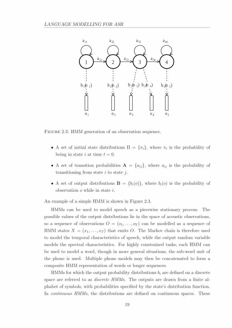
Figure 2.3: HMM generation of an observation sequence.
• A set of initial state distributions Π = {πi}, where πi is the probability of
being in state i at time t = 0.
• A set of transition probabilities A = {aij}, where aij is the probability of
transitioning from state i to state j.
• A set of output distributions B = {bi(o)}, where bi(o) is the probability of
observation o while in state i.
An example of a simple HMM is shown in Figure 2.3.
HMMs can be used to model speech as a piecewise stationary process. The
possible values of the output distributions lie in the space of acoustic observations,
so a sequence of observations O = (o1, . . . , oT ) can be modelled as a sequence of
HMM states X = (x1, . . . , xT ) that emits O. The Markov chain is therefore used
to model the temporal characteristics of speech, while the output random variable
models the spectral characteristics. For highly constrained tasks, each HMM can
be used to model a word, though in more general situations, the sub-word unit of
the phone is used. Multiple phone models may then be concatenated to form a
composite HMM representation of words or longer sequences.
HMMs for which the output probability distributions bi are defined on a discrete
space are referred to as discrete HMMs. The outputs are drawn from a finite al-
phabet of symbols, with probabilities specified by the state’s distribution function.
In continuous HMMs, the distributions are defined on continuous spaces. These
19

2.3. DECODING
distributions are often constrained to be mixtures of a particular family of distribu-
tions, such as Gaussians, which have simple parameterisations. This alleviates some
of the added computational costs associated with using continuous distributions.
Semicontinuous HMMs [41] have also been proposed as a compromise, using a fixed
set of mixture components and state-dependent output probabilities specifying the
weights of these components.
Training an HMM involves estimating the parameters of the model given a set of
observation sequences. This is done using the Baum-Welch re-estimation procedure
[42], an instance of the Expectation Maximization (EM) algorithm [43]. Given an
initial set of HMM parameters, the Baum-Welch algorithm iteratively calculates
updated parameters and is guaranteed to converge on a locally optimal solution
that maximises the likelihood of the training data.
2.3 Decoding
For an HMM with known parameters, λ = (A,B, Π), the probability of generating
an observation sequence O by traversing through state sequence X is:
p(O,X|λ) =T
∏
t=1
ax(t)x(t+1)bj(ot)
The likelihood of the observation sequence p(O|λ) can then be calculated by sum-
ming over all state sequences:
p(O|λ) =∑
X
(
T∏
t=1
ax(t)x(t+1)bj(ot)
)
(2.11)
Often, most of the probability is contained in a single state sequence [44]. Therefore,
rather than performing the computationally expensive summation, Equation (2.11)
can be approximated using only the most likely sequence:
p(O|λ) = maxX
T∏
t=1
ax(t)x(t+1)bj(ot) (2.12)
If each HMM represents a single word w, then Equation (2.12) can be considered
to be equivalent to p(O|w). This likelihood, combined with the language model’s a
priori probability, give the two terms required to solve the recognition problem of
Equation (2.10). Since the space of all possible word sequences is very large, a direct
computation is infeasible. An alternate solution to Equation (2.10) is to construct
20

LANGUAGE MODELLING FOR ASR
State
Time
a 11
1
4
3
2
1
5 4 3 2
a 34
b 2 ( o 3 )
0
Figure 2.4: Trellis for of Viterbi decoding.
a network of HMMs by connecting word HMMs in sequence. If the transition prob-
abilities between words are governed by a language model, then searching through
the resulting composite HMM using Equation (2.12) gives p(O|W )p(W ).
2.3.1 Viterbi decoding
One way of efficiently calculating Equation (2.12) is with the Viterbi algorithm, a
dynamic programming algorithm which assumes the optimal path to any interme-
diate state forms a part of the optimal path to the final state. The globally optimal
path can then be calculated recursively as a concatenation of optimal sub-paths.
If φj(t) is defined as the probability of being in state j at time t after observing
sequence (o1, . . . , ot), and:
φj(1) = πjbj(ot)
then the Viterbi recursion is given by:
φj(t) = maxi
{φi(t − 1)aij}bj(ot)
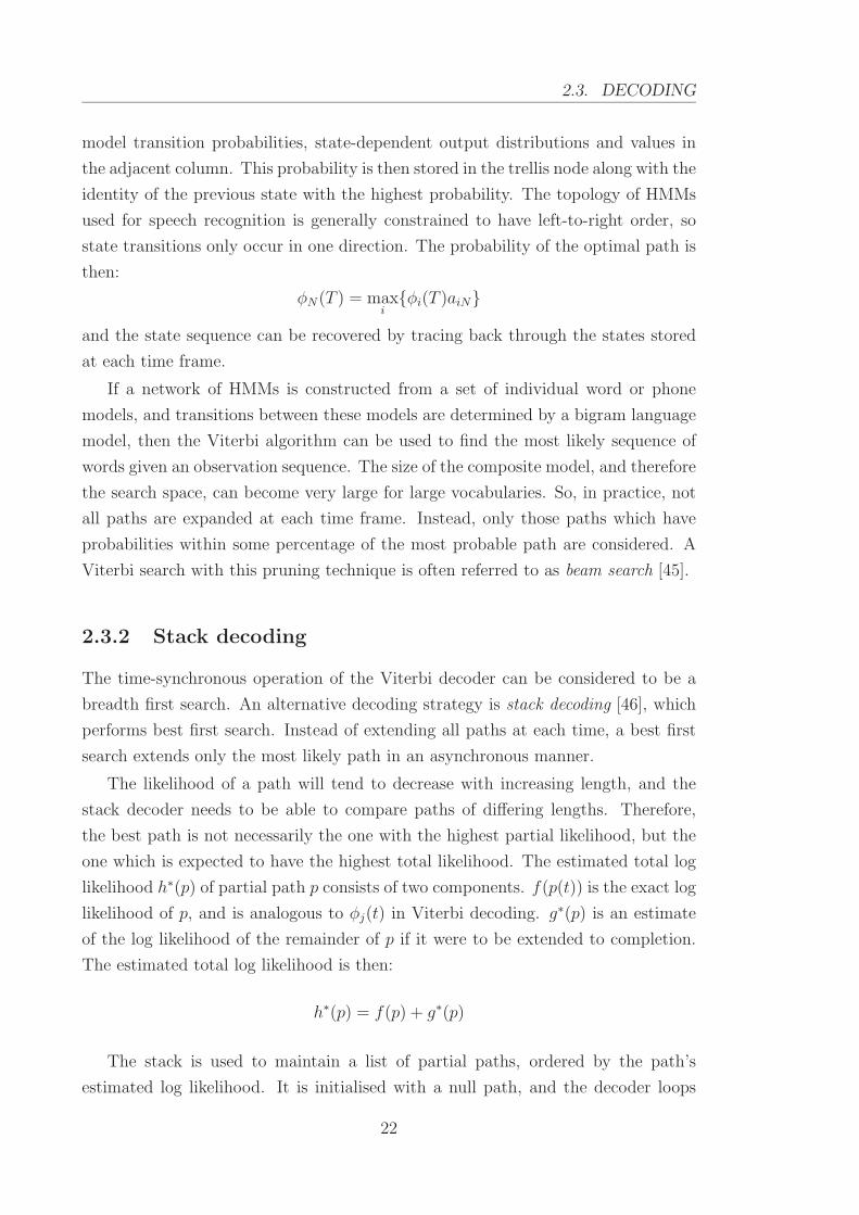
for 1 < j < N . The execution of this algorithm can be visualised as a traversal
through a 2-dimensional matrix called a trellis, an example of which is shown in
Figure 2.4.
The horizontal dimension represents time, and the vertical dimension represents
HMM states. The trellis is traversed in a column-wise manner, starting from the
left. At each time frame t, a new probability is calculated by Equation (2.3.1) using
21
2.3. DECODING
model transition probabilities, state-dependent output distributions and values in
the adjacent column. This probability is then stored in the trellis node along with the
identity of the previous state with the highest probability. The topology of HMMs
used for speech recognition is generally constrained to have left-to-right order, so
state transitions only occur in one direction. The probability of the optimal path is
then:
φN(T ) = maxi
{φi(T )aiN}
and the state sequence can be recovered by tracing back through the states stored
at each time frame.
If a network of HMMs is constructed from a set of individual word or phone
models, and transitions between these models are determined by a bigram language
model, then the Viterbi algorithm can be used to find the most likely sequence of
words given an observation sequence. The size of the composite model, and therefore
the search space, can become very large for large vocabularies. So, in practice, not
all paths are expanded at each time frame. Instead, only those paths which have
probabilities within some percentage of the most probable path are considered. A
Viterbi search with this pruning technique is often referred to as beam search [45].
2.3.2 Stack decoding
The time-synchronous operation of the Viterbi decoder can be considered to be a
breadth first search. An alternative decoding strategy is stack decoding [46], which
performs best first search. Instead of extending all paths at each time, a best first
search extends only the most likely path in an asynchronous manner.
The likelihood of a path will tend to decrease with increasing length, and the
stack decoder needs to be able to compare paths of differing lengths. Therefore,
the best path is not necessarily the one with the highest partial likelihood, but the
one which is expected to have the highest total likelihood. The estimated total log
likelihood h∗(p) of partial path p consists of two components. f(p(t)) is the exact log
likelihood of p, and is analogous to φj(t) in Viterbi decoding. g∗(p) is an estimate
of the log likelihood of the remainder of p if it were to be extended to completion.
The estimated total log likelihood is then:
h∗(p) = f(p) + g∗(p)
The stack is used to maintain a list of partial paths, ordered by the path’s
estimated log likelihood. It is initialised with a null path, and the decoder loops
22
LANGUAGE MODELLING FOR ASR
over the following operations until a complete path is found:
1. Pop the highest scoring partial sequence off the stack.
2. For each potential next word:
(a) Extended the partial hypothesis with the candidate word, and calculate
its likelihood. The new hypothesised path is then placed on the stack in
a position determined by its score.
Extensions to the path are usually found using a fast match procedure [47], which is
a computationally inexpensive method of narrowing down the potential next word
candidates.
Stack decoding is admissible if g∗(p) provides an upper bound of the true value
of the remaining log likelihood g(p). The solution found by the algorithm is optimal
because the true likelihood of a path will always be less than the estimated likelihood.
Therefore, any paths remaining after a solution has been found are guaranteed to
have lower likelihood than that of the solution.
2.3.3 Multi-pass decoding
While the use of both the acoustic and language models in a single search pass
is desirable, it can also present some problems. In the case of Viterbi decoding,
this approach is only practical for n-grams of short length. Using larger n-gram
models significantly increases the search space, and it rapidly becomes infeasible
to calculate. It is also only optimal for bigrams. N-grams with n > 2 violate the
dynamic programming invariant assumed by the algorithm. Finally, it is not obvious
how more sophisticated language models can be applied in this framework.
Although the stack decoder is capable of addressing these issues, the complexity
is then shifted to finding an appropriate heuristic. Stack decoding is only guaranteed
to find the optimal solution if the evaluation function is admissible. Furthermore, if
the function does not provide a sufficiently tight bound, the decoder becomes very
inefficient, degenerating to a breadth first search in the worst case.
The complexities involved in incorporating more advanced knowledge sources
into the decoding process has given rise to multiple-pass strategies in which more
sophisticated models are used to re-evaluate a set of hypotheses generated by an
HMM/bigram decoder. These hypotheses are then successively re-evaluated using
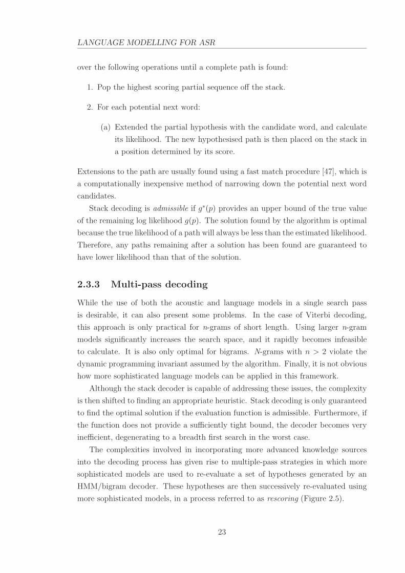
more sophisticated models, in a process referred to as rescoring (Figure 2.5).
23
2.3. DECODING
HMMs Bigram A*/ Viterbi Decoder
Multiple hypotheses
Advanced LM
Rescore Best re-ranked hypothesis
Figure 2.5: Generation of hypotheses for multi-pass decoding.
This approach has the advantage of greatly reduced computational complexity
and improved scalability, as the more expensive knowledge sources are only applied
to smaller search spaces. Separating the decoding process can also allow each com-
ponent to be independently developed and optimised. Of course, the trade-off for
this reduced complexity is the inability to bring all relevant knowledge to bear in
the initial stage of decoding, which has the potential to propagate errors through to
subsequent passes.
N-best lists
One possible interface between the different decoding passes is a ranked list of the
best N word sequences. This N-best list can be generated by a Viterbi decoder
with some modifications [48]. The decoder is required to rank its output based
on scores of word sequences, so the words associated with state sequences are also
stored. Multiple paths are retained at each time frame, corresponding to different
word histories, and if more than one path maps to the same word sequence, then
their scores are summed. Up to N paths are retained for the backtrace step of the
algorithm, and an additional beam width can be introduced to prune paths based
on word sequence probabilities.
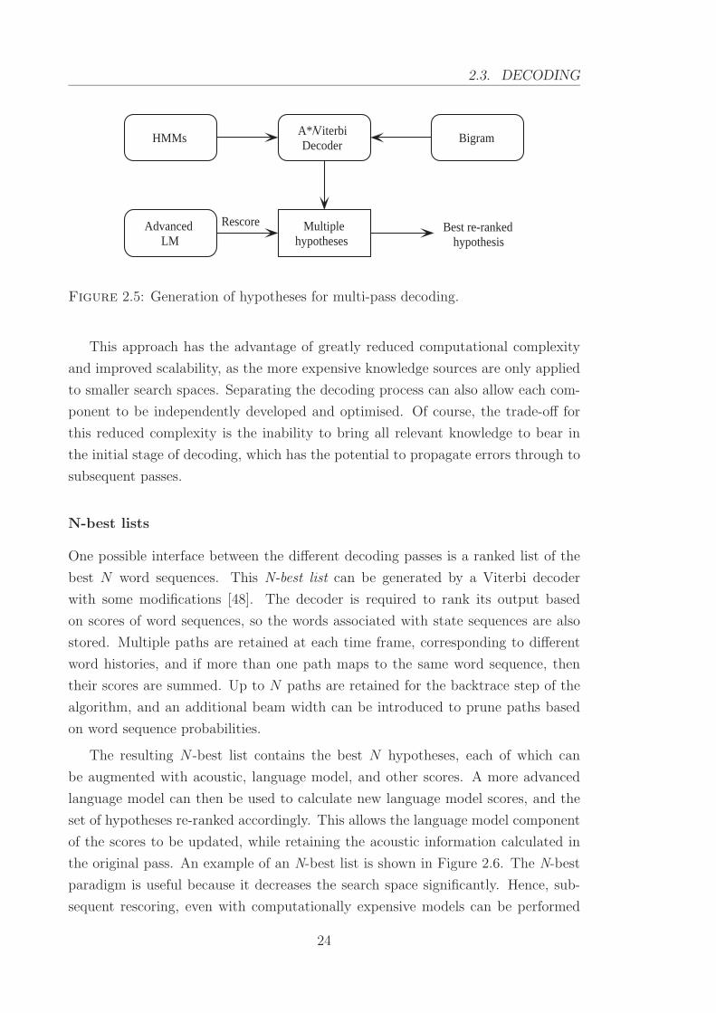
The resulting N -best list contains the best N hypotheses, each of which can
be augmented with acoustic, language model, and other scores. A more advanced
language model can then be used to calculate new language model scores, and the
set of hypotheses re-ranked accordingly. This allows the language model component
of the scores to be updated, while retaining the acoustic information calculated in
the original pass. An example of an N-best list is shown in Figure 2.6. The N-best
paradigm is useful because it decreases the search space significantly. Hence, sub-
sequent rescoring, even with computationally expensive models can be performed
24
LANGUAGE MODELLING FOR ASR
1. The latest limit index ... 2. The latest of limit index ... 3. The latest lemons index ... 4. The latest limit in tax ... ... 100. The latest of lemons index ...
-16782.5 -16783.8 -16788.8 -16789.5 ... -16808.9
Figure 2.6: An N-best list. Each sentence is annotated with a log probability score.Probabilities and time boundaries may also be specified for individual words.
quickly. Another benefit is that providing a set of complete hypotheses allows rescor-
ing with long-distance models to be performed easily, without the need for complex
decoding procedures.
Word lattices
The main drawback of N-best lists is that they only contain a small number of
hypotheses. Reducing the search space so dramatically may result in the best hy-
pothesis being eliminated from the list of likely candidates, thus restricting the
potential improvements made by incorporating more advanced knowledge sources.
Increasing N allows for a larger set of hypotheses, but rescoring very large N-best
lists is inefficient. This is particularly evident when dealing with long utterances,
where competing hypotheses will often share many similar fragments. An alterna-
tive, compact representation of multiple hypotheses is provided by the word lattice.
A word lattice is a directed, acyclic graph in which nodes represent words occur-
ring at specific times, and arcs indicate allowable transitions between words. A
hypothesis is then a path through this graph. The finer granularity of this repre-
sentation allows lattices to provide much greater coverage than N-best lists without
an equivalent increase in storage requirements.
A lattice can also be simplified into a word graph by merging paths which share
the same word sequence. Timing and acoustic information are lost in this represen-
tation, so it is useful for rescoring with models employing linguistic knowledge only.
An example of a word graph is shown in Figure 2.7.
Word lattices can be generated by a Viterbi decoder which retains information
about which words end at each node during the search. The best path is extended
as in standard decoding, and the additional information is used in the backtrace
step to generate a lattice of hypotheses [49]. This process can be performed with
minimal impact on the complexity of the decoding step.
25

2.4. EVALUATION
NINE FINE
A
<s>
FIND
ME
THE
AN
FLYING
-2.2 -5.2
-5.4
-1.5
-9.3
-1.3
-5.2 -0.8
-4.6
-1.5 -0.9
-2.3
-3.0 -2.5
-5.4
Figure 2.7: A fragment of a word hypothesis graph. Links are annotated withacoustic model (not shown) and language model log probabilities.
2.4 Evaluation
2.4.1 ASR evaluation
The performance of a speech recogniser can be measured by comparing the extent
to which its output differs from a correct, reference transcription. A minimum edit
distance algorithm [50] is first used to align the hypothesised transcription to the
reference. Errors can then be categorised into three groups. Substitution (S) errors
are the result of a word being incorrectly identified. Insertion (I) and deletion (D)
errors occur when the output transcription either contains extraneous words or omits
a correct word. An example of these types of errors is shown below:
reference: The trial is expected to last three to five weeks
hypothesis: The trial is expect is to last three five weeks
error: S I D
26
LANGUAGE MODELLING FOR ASR
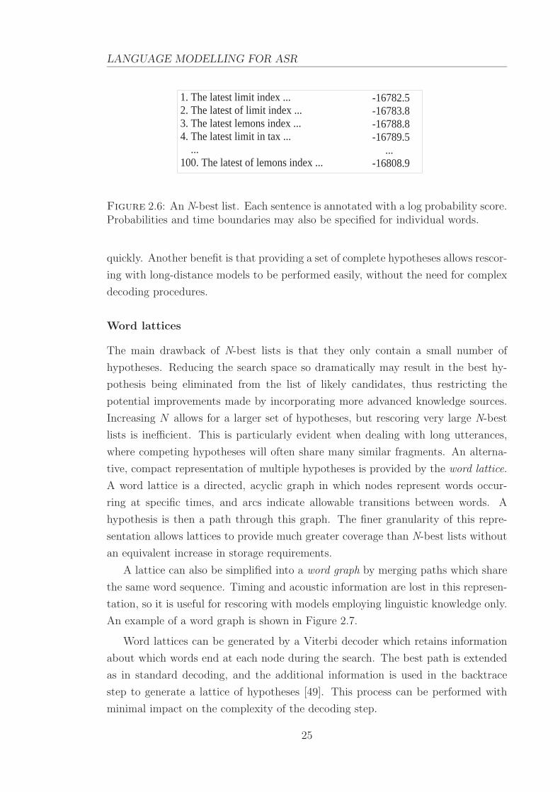
Given these counts, the Word Error Rate (WER) can be calculated as:
WER =D + S + I
N× 100% (2.13)
where N is the number of words in the reference transcription. Recogniser perfor-
mance may also be reported in terms of word accuracy, which is simply 100−WER.
2.4.2 Statistical significance
When comparing the performance of two speech recognition algorithms, it is often
useful to know if any improvements in accuracies are statistically significant. Par-
ticularly when dealing with small gains, it is important to determine whether or not
the observable differences can be attributed to chance. Only when this possibility is
sufficiently low may the conclusion be drawn that one algorithm is superior to the
other.
One test which is appropriate for analysing results generated by continuous
speech recognition systems is the Matched Pairs Sentence-Segment Word Error
(MAPSSWE) Test [51, 52]. This is a parametric test which compares the num-
ber of errors made by two systems on the same data over a number of segments.
These segments are required to satisfy the criterion that the errors in a given segment
are statistically independent of the errors in any other segment. In the MAPSSWE
test, this independence is approximated by selecting segments such that they are
bounded on both sides by either two consecutive correctly recognised words, or a
sentence boundary token.
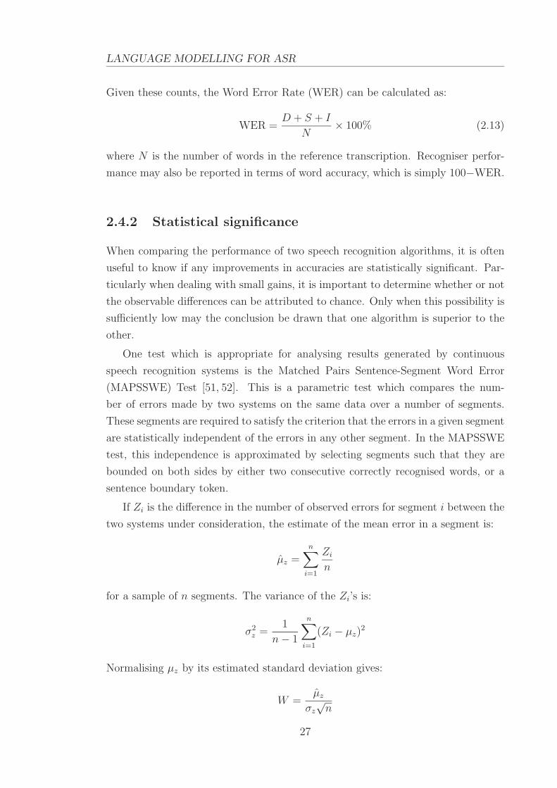
If Zi is the difference in the number of observed errors for segment i between the
two systems under consideration, the estimate of the mean error in a segment is:
µz =n
∑
i=1
Zi
n
for a sample of n segments. The variance of the Zi’s is:
σ2z =
1
n − 1
n∑
i=1
(Zi − µz)2
Normalising µz by its estimated standard deviation gives:
W =µz
σz
√n
27

2.4. EVALUATION
which, for large n, has an approximate normal distribution with unit variance [51].
The null hypothesis H0 : µz = 0 postulates that W has zero mean. It can be rejected
if:
2 × p(Z ≥ |w|) ≤ α (2.14)
where Z is the standard normal distribution and w is the realised value of W .
Commonly reported values of α are 0.05, 0.01 and 0.001.
2.4.3 Perplexity
If a language model is used for ASR, then the performance of the language model can
also be evaluated in terms of WER so long as the other components remain fixed.
However, it is often beneficial to be able to gauge the quality of a language model
without the need for a recogniser, and this is necessary if the intended application
of the language model is not speech recognition. One such measure is perplexity, a
metric commonly used to compare language model performance.
Entropy, in the information theoretic sense, provides a measure of the average
uncertainty associated with a random variable. The entropy of a discrete random
variable W is defined as:
H(W ) = −∑
w∈W
p(w) log2 p(w)
This can be interpreted as a lower bound on the number of bits required to encode
the outcomes of W given its distribution. For a Markov chain data source generating
a sequence of such random variables, wm1 , the per-symbol entropy, or entropy rate,
H of the source is given by:
H = − limm→inf
1
m
∑
wm1
p(wm1 ) log2 p(wm
1 )
If the generation of words in a natural language is considered to be a Markov chain,
then some additional assumptions can be made. Firstly, two occurrences of the
same word may be separated by any number of words. Secondly, with enough text,
it is possible to observe any word from any given starting point. These properties
indicate that natural languages are both aperiodic and irreducible, and therefore
ergodic. The entropy rate of an ergodic Markov chain reduces to:
H = − limm→inf
1
mlog2 p(wm
1 )
28

LANGUAGE MODELLING FOR ASR
With a sufficiently large m, this can then be approximated by:
H ≈ − 1
mlog2 p(wm
1 ) (2.15)
which provides an estimate of the entropy rate of the language.
A language model can only approximate of the true distribution of the language,
so cross entropy is used to compare the two distributions. The per-word cross
entropy of the true distribution p(w) given the model’s estimate, p(w) is defined as:
H(p, p) = − limm→inf
1
mlog2 p(wm
1 )
By applying a similar argument to that used to obtain Equation (2.15), this can be
reduced to:
H(p, p) = − 1
mlog2 p(wm
1 )
This gives the per-word cross entropy in terms of the model p and an empirical
sample, so it then becomes possible to use this to measure a model’s quality. A
property of the cross entropy is that:
H(p) ≤ H(p, p)
As the model estimate p becomes closer to the true distribution, the cross entropy
approaches the entropy of the language. Therefore, the better the model, the lower
the cross entropy will be. Although it is possible to evaluate language models using
cross entropy, it is more common to use the closely related measure of perplexity:
PP = 2H(p,p) (2.16)
Perplexity has an intuitive interpretation as the average number of equiprobable
choices the model encounters when presented with a sample of the language.
29

30

Chapter 3
Prosody
A spoken language contains information beyond that which is available in its tex-
tual representation. A speaker can control properties of an utterance in order to
convey additional information on semantics, syntax and pragmatics. Paralinguistic
information, such as attitude, emotional state, age and gender, can also be commu-
nicated through speech. These types of information are largely signalled through
variations in the prosodic features of pitch, loudness and length. While the precise
relationship between prosodic features and their linguistic and paralinguistic func-
tions has proven difficult to characterise, it is clear that prosodic information plays
an important role in human comprehension of spoken language.
This chapter will present an introduction to prosody and examine its relevance to
ASR. The first section will describe the perceptual and acoustic correlates of prosody,
and note commonly used techniques for automatically extracting this information
from a speech signal. In the second section, an overview of the functions of prosody
will be provided, focusing in particular on the role prosody plays in human-to-
human communication. The high degree of variability in the use of prosody between
languages and speakers will also be highlighted. The third section will describe some
approaches to modelling prosody. It will cover Pierrehumbert’s model of intonation
and an annotation scheme based on the model. The applicability of the Tones and
Break Indices annotation framework to automatic speech processing systems will be
examined, and some alternatives discussed. The fourth section will investigate the
ways in which prosody may be of use to ASR, and will include a review of previous
work in this area. This chapter will conclude with a description of how prosodic
knowledge can be incorporated into a language model for ASR, and a discussion of
the advantages and disadvantages of doing so.
31
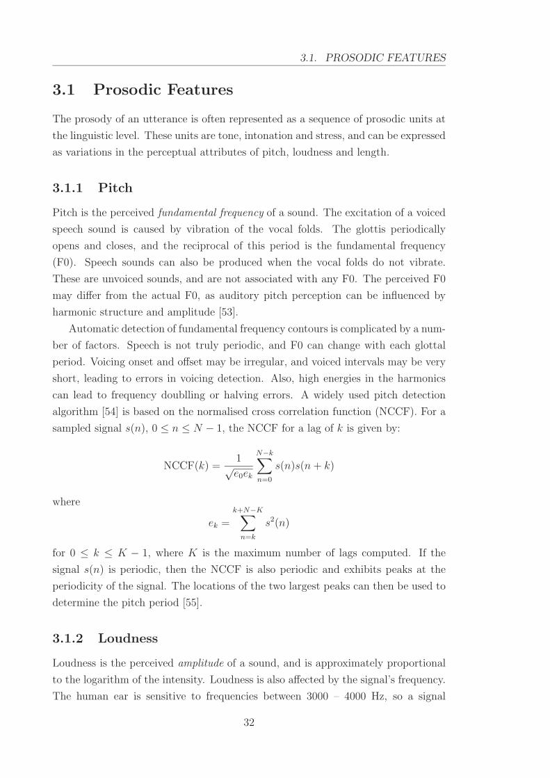
3.1. PROSODIC FEATURES
3.1 Prosodic Features
The prosody of an utterance is often represented as a sequence of prosodic units at
the linguistic level. These units are tone, intonation and stress, and can be expressed
as variations in the perceptual attributes of pitch, loudness and length.
3.1.1 Pitch
Pitch is the perceived fundamental frequency of a sound. The excitation of a voiced
speech sound is caused by vibration of the vocal folds. The glottis periodically
opens and closes, and the reciprocal of this period is the fundamental frequency
(F0). Speech sounds can also be produced when the vocal folds do not vibrate.
These are unvoiced sounds, and are not associated with any F0. The perceived F0
may differ from the actual F0, as auditory pitch perception can be influenced by
harmonic structure and amplitude [53].
Automatic detection of fundamental frequency contours is complicated by a num-
ber of factors. Speech is not truly periodic, and F0 can change with each glottal
period. Voicing onset and offset may be irregular, and voiced intervals may be very
short, leading to errors in voicing detection. Also, high energies in the harmonics
can lead to frequency doublling or halving errors. A widely used pitch detection
algorithm [54] is based on the normalised cross correlation function (NCCF). For a
sampled signal s(n), 0 ≤ n ≤ N − 1, the NCCF for a lag of k is given by:
NCCF(k) =1√e0ek
N−k∑
n=0
s(n)s(n + k)
where
ek =k+N−K∑
n=k
s2(n)
for 0 ≤ k ≤ K − 1, where K is the maximum number of lags computed. If the
signal s(n) is periodic, then the NCCF is also periodic and exhibits peaks at the
periodicity of the signal. The locations of the two largest peaks can then be used to
determine the pitch period [55].
3.1.2 Loudness
Loudness is the perceived amplitude of a sound, and is approximately proportional
to the logarithm of the intensity. Loudness is also affected by the signal’s frequency.
The human ear is sensitive to frequencies between 3000 – 4000 Hz, so a signal
32

PROSODY
lying in this range will be perceived to be louder than a signal with equal intensity
outside this frequency range. Similarly, sounds with a frequency below 300 Hz will
be perceived as being softer due to the ear’s reduced sensitivity in this region.
Loudness metrics corresponding closely to perception have been proposed [56].
It is more common, though, to use short-time root mean square (RMS) amplitude
as an estimate of loudness. For a frame j containing N samples, aj1...jN , the RMS
amplitude is calculated as:
RMSj =
√
√
√
√
1
N
N∑
i=1
aji
where aji is the squared magnitude of the ith sample in frame j:
aji = |s(jN + i)|2
3.1.3 Length
Length encompasses a number of duration-based features. These include segment,
syllable and pause durations, as well as speaking rate and rhythm.
Speaking rate can be calculated as the reciprocal of the average of the phone du-
rations within a certain time interval [57]. In this calculation, the phone durations
must be normalised in order to preclude the effects of phone intrinsic values [58].
Also, speaking rate is not linearly related to segmental durations. Durations are
highly context dependent [59], and temporally compressing the segments of an ut-
terance by a fixed value results in unnatural sounding speech. On average, conso-
nants have higher duration variability than do vowels, particularly if the vowels are
stressed.
Rhythm refers to the temporal organisation of strong syllables (containing full
vowels) and weak syllables (containing reduced vowels) [60], and is largely percep-
tual. There are many factors which affect durations of speech sounds, and it can
be difficult to isolate those sources of variability which determine the perception
of rhythmic structure [61]. Examples of such rhythmic phenomena are compen-
satory shortening, in which stressed syllable durations decrease as the number of
succeeding syllables increases, and final lengthening, where the durations of the fi-
nal unstressed syllable in an utterance are significantly longer than those of other
unstressed syllables.
33

3.2. FUNCTIONS OF PROSODY
3.1.4 Stress
Stress is a combination of pitch, loudness and length effects. Some syllables are
pronounced with greater prominence than other syllables in their context. These
stressed syllables are characterised by higher fundamental frequency and amplitude,
and longer durations [62], although some experiments have found the influence of
F0 to be minimal [63]. Although stress always occurs on individual syllables, there
can be multiple levels of stress. These can be associated with words or syntactic
groups of words, termed word stress and phrasal stress, respectively.
3.1.5 Tone
Tones, or tone levels, refer to distinct functional patterns of pitch, typically at
the syllabic level. The precise number of tones varies depending on the language.
Mandarin Chinese, for example, has four tones (high, rising, low and falling), while
Thai has an additional mid tone. In English, a distinction is made between only
two tones, high and low.
3.1.6 Intonation
Patterns of controlled pitch variation over the longer prosodic domains, such as the
phrase or sentence, are referred to as intonation. Pitch is affected by physiologi-
cal factors such as age and gender. These influences are outside the control of the
speaker and do not convey linguistic information. Therefore, it is the relative pitch
movements that are important to intonation analysis, rather than absolute pitch
values. A human listener can consider an intonation contour to be a successful
imitation of another contour despite noticeable perceptual differences. Such percep-
tually equivalent [64] intonation patterns are assumed to have the same phonological
structure and therefore convey the same linguistic information.
3.2 Functions of Prosody
Prosody conveys a diverse range of information. At the lexical level, it affects
the acoustic realisations of phonemes and words. Prosody also influences higher
level linguistic structures such as syntax and semantics, and provides paralinguistic
information such as emotion. Some of the major linguistic functional roles of prosody
include:
• Distinguishing between phonetically similar words (lexical distinction).
34

PROSODY
• Aiding in structural processing.
• Providing discourse information.
Examples of how prosody performs these roles in human communication, and which
features are involved in these processes, are described below.
3.2.1 Roles in human communication
The importance of prosody in human speech comprehension has been demonstrated
in numerous studies. Experiments with nonsense syllables are often used in order
to minimise the effects of subjects’ prior knowledge. Under auditory presentation
of nonsense syllables, prosody has been found to facilitate the ability to recall these
sequences [65]. Confusions in recognition of nonsense bisyllables are more likely to
occur between those bearing the same stress pattern [66]. Given a pair of these bi-
syllables, such as [bisev, jubim], listeners misrecognised them more frequently when
presented with [bibim, jusev] as opposed to [bisev, jubim]. Similar behaviour can
also be observed in the recognition of incorrectly stressed English words spoken by
non-native speakers [67]. However, this incorrect stressing also results in segmental
differences, and the possibility that the recognition errors are caused by segmental
information alone cannot be ruled out [1].
Shadowing tasks, which require a listener to repeat words as they are heard,
give an indication of the latency involved in human word recognition. Subjects’
performances on shadowing of grammatical strings were shown to be aided by the
presence of prosody [68]. In an experiment by Darwin [69], listeners were presented
with a different speech stream in each ear, and asked to shadow the speech from the
left or right ear only. At some point during the speech, the sources were switched.
An example of this (taken from [70]) is shown below.
L: an impression of grace and
R: it was jumping in the tree
∣
∣
∣
∣
∣
is idiotic idea of almost there is cabbage
charm and a distinct suggestion of watchfulness
Listeners in this experiment demonstrated a tendency to reproduce speech from
the incorrect stream if there was a prosodic discontinuity at the point when the
streams were swapped. Significantly fewer errors were observed if the discontinuities
were only semantic in nature, indicating that the retention of prosodic continuity is
useful in speech perception. Similarly, disruptions to prosodic structure can result in
degradation in word target recognition times [71] and semantic comprehension [72].
In experiments performed using spectrally rotated speech, humans were found
35

3.2. FUNCTIONS OF PROSODY
to perform well on word recognition tests [73]. Cues to phonetic identity are pre-
dominantly spectral, so corrupting the spectra destroys phonetic information while
retaining prosodic phenomena such as pitch, loudness and duration. Sentence recog-
nition experiments showed subjects were also able to correctly recognise function
words as well as retrieve syntactic information on speech corrupted in this way. The
results of these experiments indicated listeners were able use whichever acoustic
cues were available, as well as weight them appropriately according to their relative
information content.
It has also been suggested that prosody interacts differently with closed-class
and open-class words. A closed class is a class of words to which new terms cannot
normally be added, such as prepositions, determiners and pronouns. The set of
closed class words is relatively small, but these words occur frequently in natural
languages. They are also acoustically low in salience, making them difficult to
recognise in isolation. In contrast, open classes such as nouns and verbs readily
admit new members. Open-class words tend to contain more information content,
while closed-class words are generally associated with structural roles. Recognition
of closed-class words has been found to be highly dependent on prosodic context,
while recognition of open-class words exhibits less reliance [74].
Given a stream of continuous speech, successful word recognition requires the
identification of word boundaries. Speech contains no direct equivalent of the punc-
tuation and whitespace present in text, yet processing of speech requires a decom-
position of the utterance into smaller units. In order to perform this segmentation,
listeners must rely on acoustic cues which are not completely reliable [6]. Duration
is one potential indicator of boundary location. There are durational differences be-
tween a syllable occurring as a monosyllabic word and the same syllable at the start
of a polysyllabic word, which may be exploited to infer word boundaries. Rhythmic
properties may also cue boundary locations. English listeners favour segmentation
before strong syllables, and can more easily identify words with strong-weak syllabic
patterns. For example, listeners recognised a given word, such as mint, more quickly
if it preceded a monosyllabic suffix containing a weak vowel (esh) than if it preceded
one with a full vowel (ayve) [75].
Prosody is also relevant in the segmentation of utterances into units above the
word level. Like syntactic structure, phonological structure is typically regarded
as being hierarchical, and the organisation of utterances into intermediate and full
intonational phrases is cued by prosodic information. While prosodic structure is
not isomorphic with syntactic structure, boundaries of intonational phrases often
correspond to syntactic boundaries [76], and major syntactic boundaries can be ac-
36

PROSODY
curately determined using only prosodic information [8]. Consequently, prosodic
boundaries can be used to disambiguate some utterances which are otherwise syn-
tactically ambiguous [6]. Acoustic cues of these prosodic boundaries include pre-
boundary lengthening of segments, and pitch rise or fall-rise patterns. In English,
low and medium strength boundaries are signalled primarily by durational features,
while major boundaries are closely related to both pitch and duration correlates [77].
The role of prosody in grouping and segmentation of speech units has also been
demonstrated in experiments using disrupted speech, such as an utterance containing
a superimposed click. Listeners, after being presented with the disrupted utterance,
were asked to recall the position in which the click occurred. If prosodic boundaries
were consistent with syntactic boundaries, then the perception of disruptions tended
to move toward these boundaries. When prosodic and syntactic structure conflicted,
though, this effect was not observed [78], suggesting that prosody is used by listeners
to assist with syntactic parsing.
Another possible contribution of prosody in structural processing is local ambi-
guity resolution. Syntactic ambiguities of an incomplete utterance may be resolved
in an early processing step through the use of prosodic information. Consider the
two endings to the following sentence:
The city council argued the mayor’s position
∣
∣
∣
∣
∣
forcefully.
was incorrect.
With the first ending, the mayor’s position is the direct object of argued, while
with the second ending, it is the subject of a sentence complement. In experiments
in which English listeners were presented with only the syntactically ambiguous
fragment of such sentences, the listeners were able to determine which of the variants
the fragment belonged to [79]. Similar experiments with sentence onsets found
listeners were also able to decide whether the sentence contained no more words,
three more words, or six or more remaining words [5]. Pitch and duration features
of the last presented word were the primary cues employed by the subjects in these
tasks [80].
At the higher levels of the spoken communication process, prosody plays a role
in a number of discourse functions. As with lexical and syntactic functions, though,
not all discourse functions are realised prosodically. Functions which are at least
partly cued by prosody include conveying speaker attitudes, turn-taking, feedback
and speech act signalling. Prosody is also used to give prominence to the salient
information in a discourse [4]. The accentuation of a particular word is dependent
on the importance of that word in the sentence, as well as its context, and these
37

3.2. FUNCTIONS OF PROSODY
words are more easily processed by listeners. While the increased acoustic clarity
of stressed syllables associated with accented words improves speed and efficiency
of comprehension, it is not the sole reason for this effect. In an experiment using
acoustically identical copies of an accented word in two different prosodic contexts,
faster reaction times in recognition of the accented word were observed for the
case when prosody was consistent with an accent in the target location [81]. While
manipulation of either pitch or duration alone did not hamper this effect, consistency
between the various prosodic factors appeared to be important [82].
The accent structure of an utterance is related to its semantics, and in particular,
its focus. Whether an item represents given or new information in a discourse affects
a speaker’s decisions about accentuation and deaccentuation. Grammatical function
and word position are also factors contributing to this choice [83]. The relationship
between accentuation and new or given information is exploited by listeners in speech
comprehension, particularly when recognition of segmental identity is obscured [84].
In these situations, accented words are more likely to be interpreted by listeners as
new information.
Prosody can also provides cues to the identification of topics in discourse. Top-
ics are often started high in the speaker’s pitch range and show a rise in amplitude,
while the end is associated with a compressed pitch range and amplitude fall [85].
Corpus-based studies using professionally read speech have found statistically sig-
nificant correlations between discourse segmentation and prosodic features including
pitch range, amplitude and timing [86]. These correlations were evident with both
discourse elements obtained from the text only, as well as those obtained from a
combination of text and speech.
Prosodic continuity is an important factor in speech processing. Conversely, dis-
ruptions to this continuity can cause difficulties in comprehension, even if the speech
is otherwise fluent. Prosody may then act as an indicator of disfluencies such as hes-
itations and speech repairs. Disfluencies are characterised by an error, also known
as a reparandum, followed by an editing phase, and a subsequent correction to the
reparandum. They may occur for various reasons, including problems with lexical
retrieval or speech planning. Hesitations are associated primarily with pausing and
syllable lengthening [87]. While textual properties, such as the presence of word
fragments [88], are good indicators of speech repairs, acoustic and prosodic cues to
these events also exist. Silent pauses, especially, tend to be good indicators of inter-
ruptions, and there are durational differences between these types of pauses when
compared to the pauses present in fluent speech [89]. Glottalisation at the end of the
reparandum is also commonly observed [89], particularly in the case of vowel-final
38

PROSODY
Acoustic Correlates Perceptual Correlates Functions
F0 level, f0 contour Pitch level, pitch contour, Lexical distinction, prominence,tone, intonation, stress focus, grouping into intonational
phrases, discourse segmentationAmplitude Loudness, stress Prominence, focus, segmentationSegment duration, Rhythm, pause, stress Prominence, focus, grouping,syllable duration, stress segmentation, disfluenciessilence
Table 3.1: The relationships between the acoustic and perceptual realisations ofprosody, and their major linguistic functions.
fragments.
The relationships between the various aspects of prosody are complex and diffi-
cult to isolate. Each of the prosodic features of F0, amplitude and duration, provide
cues to a number of linguistic functions. Similarly, the prosodically-dependent func-
tions are influenced simultaneously by multiple features. An attempt to summarise
the interaction of the acoustic and perceptual correlates of prosody, as well as their
major prosodic functions is shown in Table 3.1.
3.2.2 Cross-linguistic differences
Prosody is present in all spoken languages; however, its functions are largely lan-
guage dependent. While there is some evidence to support a universal mechanism
for communicating certain types of emotion [90], the linguistic aspects of prosody
vary greatly between languages.
One notable distinction is found in the use of tones. In some languages, called
tonal languages, tones perform a lexical role. These languages contain words which
consist of the same phonemic sequences but are distinguished by different tones. The
tones therefore form part of a word’s identity, and are necessary to determine its
meaning. There are two types of tonal languages. In tone languages, each syllable is
associated with its own tone. Most South-East Asian and African languages, such
as Mandarin, Thai and Yoruba are tone languages. In pitch accent languages, such
as Japanese and Swedish, words, rather than syllables, are associated with distinct
tonal melodies. Because these pitch accents perform the same role as tones in tone
languages, they therefore are not used to signal focus and information structure.
In contrast to tone languages, stress languages do not use tones directly in the
lexicon. Some of these languages use stress, of which pitch is a component, to
perform a similar role. In English, the noun and verb forms of certain words are
39

3.3. MODELLING PROSODY
distinguished by their stress pattern (e.g. SUBject vs subJECT). In other stress
languages, stress placement is predictable, always occurring on the same syllable.
In Finnish, the first syllable of a word is stressed, and in Polish, stress falls on the
penultimate syllable. Stress is also used to indicate focus on words. For example, in
the sentence The meeting is on MONDAY, not TUESDAY, stress effects are more
pronounced on the words Monday and Tuesday than on meeting, even though the
first syllable of meeting is also stressed.
Prosodic indicators of word boundaries are also language specific. Segmentation
is performed using rhythmic cues; however, the nature of these cues differ depend-
ing on the language. For instance, the rhythmic structure of English is described
in terms of stress (it is a stress-timed language), while French is syllable-timed
and Japanese is based on a constituent of the syllable called a mora (usually a
consonant-vowel pair). In addition, the use of segmentation cues is highly depen-
dent on the listener. While the French language is optimally segmented based on
syllable structure, Japanese listeners of French speech do not perform this [91]. Sim-
ilarly, French listeners of Japanese speech showed no evidence of using mora-based
segmentation [92].
Given the amount of variation in these fundamental aspects of prosody, it is
unsurprising that the higher level linguistic functions of prosody also exhibit many
cross-linguistic differences. Furthermore, different dialects of the same language
can have considerable differences in how prosody is used to signal syntactic and
semantic information. The production and interpretation of prosodic cues can even
vary between different speakers [93]. This study will focus on one particular speaking
style only. The database used here consists of professionally read American English
speech, and will be described in more detail in Chapter 5.
3.3 Modelling Prosody
Differing motivations for studying prosody have resulted in a wide range of represen-
tations of prosodic information. Linguistic studies have focused on the phonological
aspect of prosody, giving rise to models of phonological constituents. At the other
end of the scale, the problem has been approached with regard to the acoustic and
phonetic properties, which are often more directly applicable to the automatic pro-
cessing of prosodic information. In general, though, a model of prosody should be
capable of describing the full range of prosodic phenomena in terms of both phono-
logical units and their acoustic realisations.
40
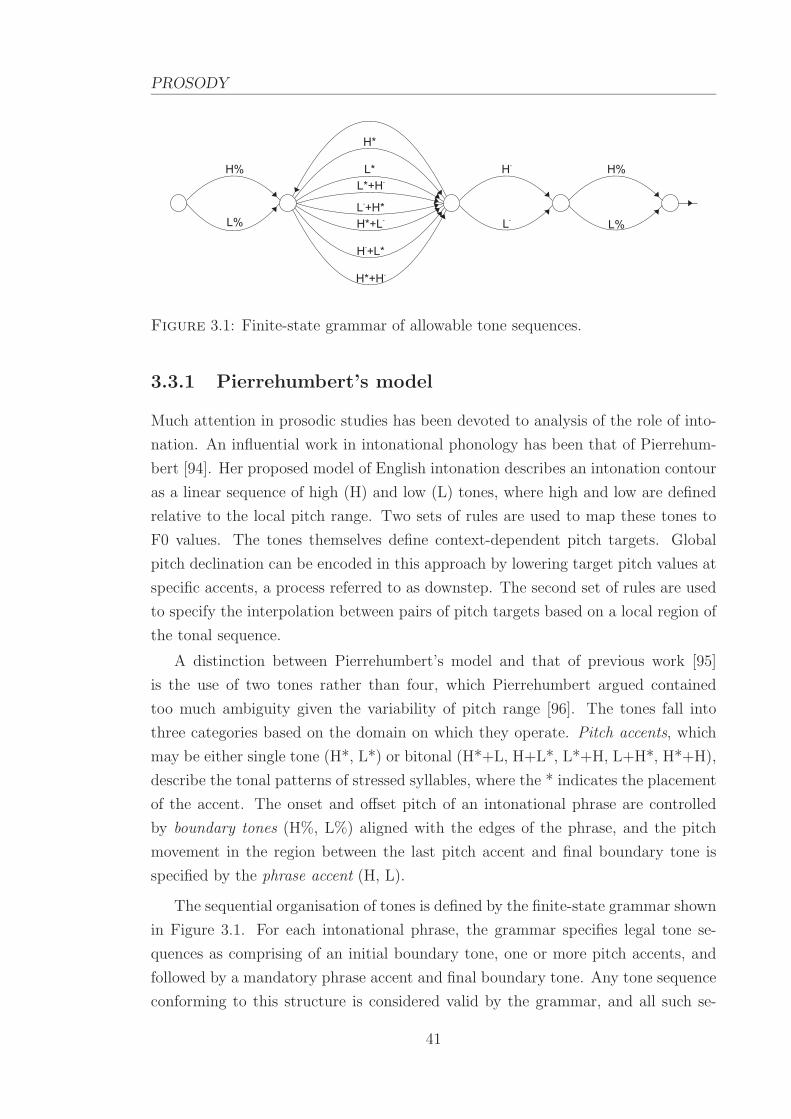
PROSODY
H%
H*
L*
L*+H-
H*+L-
L +H*-
H*+H-
H +L*-
H-
H%
L-
L%L%
Figure 3.1: Finite-state grammar of allowable tone sequences.
3.3.1 Pierrehumbert’s model
Much attention in prosodic studies has been devoted to analysis of the role of into-
nation. An influential work in intonational phonology has been that of Pierrehum-
bert [94]. Her proposed model of English intonation describes an intonation contour
as a linear sequence of high (H) and low (L) tones, where high and low are defined
relative to the local pitch range. Two sets of rules are used to map these tones to
F0 values. The tones themselves define context-dependent pitch targets. Global
pitch declination can be encoded in this approach by lowering target pitch values at
specific accents, a process referred to as downstep. The second set of rules are used
to specify the interpolation between pairs of pitch targets based on a local region of
the tonal sequence.
A distinction between Pierrehumbert’s model and that of previous work [95]
is the use of two tones rather than four, which Pierrehumbert argued contained
too much ambiguity given the variability of pitch range [96]. The tones fall into
three categories based on the domain on which they operate. Pitch accents, which
may be either single tone (H*, L*) or bitonal (H*+L, H+L*, L*+H, L+H*, H*+H),
describe the tonal patterns of stressed syllables, where the * indicates the placement
of the accent. The onset and offset pitch of an intonational phrase are controlled
by boundary tones (H%, L%) aligned with the edges of the phrase, and the pitch
movement in the region between the last pitch accent and final boundary tone is
specified by the phrase accent (H, L).
The sequential organisation of tones is defined by the finite-state grammar shown
in Figure 3.1. For each intonational phrase, the grammar specifies legal tone se-
quences as comprising of an initial boundary tone, one or more pitch accents, and
followed by a mandatory phrase accent and final boundary tone. Any tone sequence
conforming to this structure is considered valid by the grammar, and all such se-
41
3.3. MODELLING PROSODY
quences are also well-formed in English according to Pierrehumbert. The model uses
a metrical grid [95], which specifies the patterns of stressed and unstressed syllables,
as well as the relative strengths of stressed syllables. A set of rules are also defined
for aligning this metrical representation of the text with the tone sequence.
The Pierrehumbert model provides both a description of prosody at a phono-
logical level and a mapping from phonology to F0 contours. However, it does not
specify a mapping in the opposite direction. In fact, Pierrehumbert claims that such
a mapping does not exist. This point has been criticised by Taylor [97], who believed
the problem to lie with the interpolation rules which he considered too unprincipled.
The lack of a F0 to phonology mapping poses problems for automatic processing, as
F0 contours can often be the only available source of prosodic information. It is pos-
sible, though, to obtain a phonological representation from acoustic data by means
other than inverting the original interpolation rules. Such approaches [98, 99, 100]
rely on statistical methods to perform labelling based on acoustic similarities.
3.3.2 Tones and Break Indices
The ideas evinced in Pierrehumbert’s model have been adapted into the Tones and
Break Indices (ToBI) framework [101] for labelling prosodic phenomena. The devel-
opment of ToBI was motivated by the need for a standardised system for transcribing
prosody, and was targeted in particular at corpora development. While originally
designed for American English, ToBI systems for other languages have also been de-
veloped. The English ToBI system attempts to capture two types of prosodic events
in particular: the intonation patterns, and the rhythmic structure of stressed and
unstressed words. Those events which are not suited to categorical representations
are left out, as are events which can be reliably predicted, such as the location of
stressed syllables within a word [102].
Labels for events are organised into four parallel tiers:
• Orthographic tier
• Tone tier
• Break index tier
• Miscellaneous tier
Each tier describes a specific stream of information, with the core prosodic analysis
contained in the tone and break index tiers. All tiers are also temporally aligned
with both the original utterance and its F0 contour.
42

PROSODY
The orthographic tier contains the transcribed words of the utterance in standard
English orthography. These words are marked at the end of their final segments.
Comments and any phenomena which cannot be transcribed onto the tone or break
index tiers are placed in the miscellaneous tier. Examples of events marked on this
tier include disfluencies and audible breathing.
The tone tier contains the phonological analysis of the utterance’s intonation
contour. It corresponds closely to Pierrehumbert’s representation, although there
are some differences. ToBI defines an intermediate intonational phrase in addition to
the full intonational phrase. Adopted from revisions of Pierrehumbert’s model [103],
the intermediate intonational phrase contains one or more pitch accents followed
by a phrasal tone, which is distinct from the boundary tone. Downstepping is
marked explicitly in ToBI (as !H*), in contrast to Pierrehumbert’s approach in which
downstepping was triggered by certain tone sequences. The explicit annotation of
downstepping eliminates the need for the H*+L downstep trigger; H*+L has been
removed from ToBI’s inventory of tones.
The full set of tone labels described by ToBI are [104]:
• L-, H- phrase accents, occurring at the boundaries of intermediate or full
intonational phrases.
• L%, H% final boundary tones, occurring at full intonational phrase bound-
aries.
• %H high initial boundary tone, indicating that a phrase begins high in the
speaker’s pitch range. Mid or low pitch range phrase onsets are assumed by
default.
• H* peak accent, representing a tone target on an accented syllable which is
in the upper or middle part of the speaker’s pitch range for the phrase.
• L* low accent, representing a tone target which is in the lowest part of the
speaker’s pitch range.
• L*+H scooped accent, representing a low tone target followed by a sharp rise
to a peak in the upper part of the speaker’s pitch range.
• L+H* rising peak accent, representing a high tone target immediately follow-
ing a sharp rise from the lowest part of the speaker’s pitch range.
• H+!H* downstep onto an accented syllable from a high pitch or preceding
high pitch accent.
43

3.3. MODELLING PROSODY
Pitch accents are aligned with accented syllables, while phrasal tones are aligned
to the end of intonational phrases. Full intonational phrases consist of one or more
intermediate phrases, therefore boundaries of full intonational phrases are marked
with both a phrase accent and a boundary tone.
The break index tier represents the other component of ToBI’s prosodic analysis.
Break index values indicate the perceived degree of juncture between pairs of words,
and between utterance final words and the following silence. This tier provides a
representation of the rhythmic characteristics of an utterance, complementing the
tone tier’s description of the intonation. Five levels of break indices are defined in
ToBI:
• 0 boundary with clear phonetic indicators of a clitic group.
• 1 regular word boundary.
• 2 boundary marked either by a pause but no tonal indicator, or an unexpect-
edly weak intonational boundary.
• 3 intermediate intonational phrase boundary.
• 4 full intonational phrase boundary.
This approach of labelling word boundary strengths derives from Price et al. [77] who
proposed seven break index levels. Their system additionally defined break index 5
as boundaries between groups of intonational phrases, and break index 6 as sentence
boundaries. The major prosodic breaks in the original system, corresponding to
break indices of 4, 5, and 6, have been merged into the full intonational phrase
boundary (break index 4) in ToBI. A sample utterance, along with its orthographic,
tone and break index transcriptions, is shown in Figure 3.2.
There is some redundancy between the tone and break index tiers. By definition,
break indices of 3 and 4 occur at intermediate and full intonational phrase bound-
aries, respectively. Therefore, these breaks can then be determined solely from the
tone tier. A problem arising from this is that the limited number of remaining labels
can restrict the ability of the transcriber to mark perceptual differences in relative
boundary strengths [105].
Another issue with ToBI, and transcription systems in general, is the level of
consistency which can obtained by different labellers. Ideally, all labellers transcrib-
ing the same utterance should produce identical transcriptions. An explicit design
goal of ToBI was to achieve an inter-transcriber agreement of at least 80% [101].
44

PROSODY
a Cape Cod attorney is free on bail
H* !H* L+!H* L–L L+H*
1 1 1 4– 1 1 1
Time (s)0 2.1
Figure 3.2: A ToBI transcription of an utterance.
A study of inter-transcriber consistency conducted on an English corpus [106] re-
ported an 81% pairwise agreement on the presence versus absence of pitch accents.
Similarly, agreement on the presence of phrase accents and boundary tones were
90% and 91% respectively. Agreement on break index values within a margin of ±1
levels was 92%. The data used in this study covered a wide range of speech styles,
including both read and spontaneous speech. Transcribers also had varying levels of
experience, with 6 out of the 26 having had no prior experience with prosodic tran-
scription. A separate study by Syrdal and McGory [107], in which all transcribers
had the same amount of training, reported even higher consistencies.
While inter-transcriber consistency on the presence and absence of labels is high
in general, agreement on specific label identity is significantly lower. In Syrdal and
McGory’s study [107], agreement on pitch accent type for male speakers exceeded
50% for only two types of accent: H* and L+H*. In the other categories, three of
six boundary tones, and two of five break indices had an agreement above this value.
All phrase accent agreements were also below 50%. While the results for females
were slightly higher (four pitch accents and one phrase accent exceeded 50%), the
overall consistencies were still low, especially considering that all labellers in this
study received identical training.
45

3.3. MODELLING PROSODY
3.3.3 Alternate modelling approaches
ToBI is the most widespread prosodic annotation scheme for English. Its advantages
include a solid foundation in phonological theory combined with clear guidelines for
labelling speech data. It can describe both intonational and rhythmic phenomena,
and a number of tools are available to aid and streamline the labelling process. Inter-
transcriber agreement is also high when using a reduced set of labels (i.e. presence
versus absence), and this aspect of ToBI has been investigated more comprehensively
than for other labelling approaches.
ToBI is not without its drawbacks, however, particularly when considered in
the context of speech technology applications. A characteristic of most speech pro-
cessing systems is the use of statistical learning methods, which require a large
amount of training data. Labelling speech in accordance with the ToBI frame-
work requires both highly trained transcribers and significant time investment. It
commonly takes between 20 – 30 minutes to label 10 seconds of speech [108], so
creating sufficiently large corpora is problematic. The difficulties involved in manu-
ally transcribing speech has led to the development of automatic or semi-automatic
methods for assisting the annotation of utterances. Syrdal et al. [108] automatically
assigned default labels based on predictions from the text, which were then man-
ually corrected. This decreased the average labelling times without any significant
introduction of labelling bias. Wightman et al. [109] used a decision tree to predict
a collapsed set of ToBI labels, and reported a 69% accuracy for recognition of pitch
accents and 93% accuracy for phrase boundaries when compared to manual labels.
The possibility of accurate automatic detection and assignment of ToBI labels
then raises the question of whether such a step is necessary at all. Obtaining the
phonology of an utterance is rarely the final goal of a speech processing system;
rather, it is used as an intermediate representation. Batliner et al. [110] note that
if a mapping exists from acoustic data to phonological elements, and if there is a
subsequent mapping from these constituents to a target linguistic category, then a
direct acoustic to target mapping also exists. This direct modelling approach [111]
brings about some practical advantages. If the acoustic to linguistic mapping can be
learnt automatically , the need for time consuming manual transcriptions is removed.
This allows for the use of much larger data sets, as well as eliminating the possibility
of human-induced errors in the transcription process. Acoustic features can also be
selected and weighted in order to optimise performance for a given task. Using an
intermediate representation can potentially discard useful information or introduce
quantisation errors, and this can be avoided in the direct modelling method.
The approach described by Kompe [57] represents a step away from the use of
46

PROSODY
phonological representations in automatic speech processing. They defined a set
of boundary and accent labels which are distinguished as being either syntactic,
prosodic-syntactic or prosodic. Syntactic labels can be obtained from textual data
only, while prosodic labels are based on perception and analysis of the F0 contour.
The prosodic-syntactic labels are syntactic labels organised with respect to their
expected prosodic characteristics. Automatic labelling from acoustic features was
also a primary consideration in the selection of these labels. The prosodic-syntactic
labels were shown to be particularly useful in training statistical classifiers.
3.4 Prosody in ASR
Traditionally, prosodic information has not been utilised in speech recognition sys-
tems. It is the spectral component of speech which carries the most important cues
to phonetic identity, and models designed to use short-time spectral features, such as
HMMs, are not well suited to modelling longer duration phenomena. Prosodic fea-
tures such as F0 are also highly speaker-dependent, which is an undesirable property
in most ASR applications.
Some of the earliest suggestions for using prosody in automatic speech processing
were presented by Lea [112], who proposed the use of prosodic cues to detect sentence
and phrase boundaries, as well as some syntactic properties of words. Waibel [7]
was able to reduce the average rank of the correct word recogniser hypothesis by
rescoring them with a variety of prosodic knowledge sources. Pitch, duration, stress,
and especially intensity, were found to contribute to the gains. In addition, using a
combination of prosodic and phonetic features resulted in further improvements in
performance.
Efforts have also been made to incorporate prosodic information into the HMM
framework. Distinct phone models have been used which are dependent on prosodic
factors, such as lexical stress [113] and phrasing [114]. Prosody can affect the spectral
properties of phonemes. For example, phrase initial vowels exhibit more coarticula-
tion than phrase final vowels, and accented vowels have greater durations and less
coarticulation [115]. Introducing phone models that incorporate prosodic state al-
lows such prosody-induced effects to be captured, while retaining the powerful HMM
modelling structure and efficient parameter estimation techniques. Computational
requirements are increased, though, as a result of the larger parameter count. Also,
another disadvantage of this approach is the need for prior labelling of the prosodic
phenomena.
The Markov assumption used in HMMs implies a geometric state duration dis-
47

3.4. PROSODY IN ASR
tribution specified by the self transition probability. The distribution of phone
durations, however, more closely resembles the gamma distribution [116]. This
discrepancy has led to modifications to the HMM structure to allow for explicit
specification of state durations, such as the expanded state HMM [117] and the
hidden semi-Markov model [116]. Including additional duration distributions into
model states has been demonstrated to improve recognition accuracy, but at a cost
to time performance. The Baum-Welch and Viterbi algorithms used for parameter
estimation and decoding rely on the Markov assumption, which is violated by ex-
plicit duration modelling. These algorithms then need to be altered to accommodate
for this, usually resulting in a loss of efficiency. It has also been argued that the
inherent geometric distribution of HMMs is not problematic, as a combination of
multiple states sharing the same observation distribution can be used to achieve a
broader range of distributions [118].
In an examination of pronunciation variation, Ostendorf et al. [119] found cor-
relations between pronunciation distance, a measure of the difference between the
baseform and surface form of phonemes, and prosodic features. The correlation for
some F0 and duration features, in particular, were higher than that of trigram proba-
bilities. Using prosodic features in a decision tree trained to predict phonetic surface
forms of words in the Switchboard corpus resulted in a small reduction in error rate.
Additionally, F0 features were found to have been frequently used in tree questions,
even after the inclusion of word-based features. The prosodically conditioned pro-
nunciation model can then be incorporated into an ASR system by supplementing
the acoustic features with additional prosodic features, F , and calculating:
W ∗ = arg maxW
p(W |O,F )
= arg maxW
p(O|F,W )p(F |W )p(W )
≈ arg maxW,φ
p(O|φ, F )p(φ|F,W )p(F |W )p(W ) (3.1)
where φ represents the pronunciation sequence. This allows the variation in pro-
nunciation and speaking style, modelled by pitch, energy and duration features, to
be combined into the recognition process.
Another use for prosodic information is for post-processing of word hypotheses.
An N-best or word lattice output of a speech recogniser can be evaluated using
a prosodic knowledge source to select those hypotheses which are consistent with
the new information. Hirschberg et al. [120] found significant differences between
the prosodic patterns of correctly and incorrectly recognised utterances. Adding
48

PROSODY
prosodic features to a misrecognition classifier improved prediction of erroneous
hypotheses over using ASR-based features alone. The 13% prediction error obtained
by using confidence scores and hypothesised strings was reduced to 11% after the
inclusion of prosody.
Veilleux and Ostendorf [121] used prosody to rescore N-best hypotheses by mod-
elling the relationship between labelled prosodic constituents and syntactic parse
structure. Parses consisted of part-of-speech information and syntactic bracketing.
The probability of an observed sequence of F0, energy and duration measurements,
x = {x1, . . . , xn}, was calculated as:
p(x|parse) =∑
a
p(x|a)p(a|parse)
where a = {a1, . . . , an} is a sequence of break index and prominence labels. Binary
decision trees were used for both the acoustic-prosodic models, p(x|a), and the
prosodic-syntactic models, p(a|parse). Tree leaves were associated with probability
distributions, which were used to calculate the total prosodic probability of a given
parse. Linear combinations of the prosodic scores with acoustic and language model
scores obtained from the recogniser were then used to reorder an N-best list. For
utterances in which the correct hypothesis was present in the top ten hypotheses,
this rescoring approach resulted in a relative 23% improvement in the average rank
of the correct hypothesis.
Batliner and Noth [122] describe the use of prosodic information in the VERB-
MOBIL speech-to-speech translation system. The extraction of prosodic features in
this approach is based on the output of a speech recogniser. F0, energy and duration
features are extracted from regions demarcated by hypothesised word boundaries.
This allows for the mapping of prosody onto units that are directly usable by subse-
quent processing modules. The inputs to the prosody module are the speech signal
and a word hypotheses graph (WHG), and the output is a word graph annotated
with various prosodic phenomena such as accents and boundaries. A set of 95
prosodic features plus an additional 30 part-of-speech (POS) features are used in
this system, calculated at context sizes of up to ±2 words. Because the same feature
may be calculated for multiple contexts, there are highly correlated features in the
resulting set. These features are used directly in a multi layer perceptron to classify
the prosodic events. Therefore, in this approach, the statistical classifier is relied
upon to determine the appropriate relationships between extracted features and the
prosodic classes.
Using a very large feature set can be computationally costly and can also increase
49

3.4. PROSODY IN ASR
the potential for over-training. If there are strong correlations between the features,
then it is possible to apply dimensionality reduction techniques to reduce the number
of features with minimal loss of information. Batliner et al. [123] applied linear
discriminant analysis (LDA) to reduce a set of prosodic features used for classifying
word accents and boundaries. The 276 original features were reduced to 6 features for
accent classification and 11 features for boundary classification, with a performance
degradation of 2–3%.
Annotating a WHG with prosodic information has a number of benefits. Firstly,
WHGs are a commonly used data structure and it is simple to extract the relevant
prosodic information from them. Aligning prosodic features with words is also much
cheaper computationally than aligning with the underlying phonemes. While the
phone sequence is calculated by the decoder in the recognition process, it is normally
not accessible to subsequent processing steps. Performing forced alignment on the
output to recover the HMM state sequence can be a very slow process. Phonetic
alignments can be useful, however. Syllabic units, which are the units primarily
associated with accentuation, can be determined more reliably from segmental in-
formation than from word information. Pause durations, too, can be easily obtained
from silence models.
A general framework for incorporating prosodic information into ASR systems is
presented in Shriberg and Stolcke [111]. An important aspect of this approach is that
explicit identification of phonological constituents is not used. Rather, stochastic
methods are employed to learn relations between acoustic observations and linguistic
entities. The inclusion of a prosodic feature stream, F , into the ASR equation gives:
W ∗ = arg maxW
p(W |O,F )
= arg maxW
p(W )p(O,F |W )
≈ arg maxW
p(W )p(O|F,W )p(F |W ) (3.2)
p(W ) is a standard language model. The acoustic model, p(O|F,W ) can be addition-
ally conditioned on prosody. If it is assumed that the acoustic and prosodic features
are independent given the word sequence, then this can be reduced to a standard,
prosody-independent acoustic model p(O|W ). p(F |W ) is used to model the interac-
tion between prosodic features and word identities. For example, Gadde [124] used
this approach to incorporate duration features into a recogniser. Each word was
associated with a vector of phone durations, modelled by Gaussian mixture models
(GMMs). Durations of N-best list hypotheses were obtained by forced alignment,
and these were rescored using a combined score from the acoustic, language and
50

PROSODY
duration models. Reductions in WER of up to 1% were obtained on two test sets
using this duration model rescoring method.
The previous modelling approach can be further extended by modelling the in-
teraction of prosody with linguistic structures above the word level. Instead of
estimating p(F |W ) directly, it is modelled with respect to an intermediate linguistic
structure, S, giving:
W ∗ = arg maxW
p(W )p(O|W )p(F |W )
= arg maxW
p(W )p(O|W )∑
S
p(F |S,W )p(S|W ) (3.3)
p(F |S,W ) models the relationship between prosody and linguistic structure, and
p(S|W ) models the relationship between the structures and the word sequence.
These components are trained on data labelled with the linguistic structures, which
are simpler to annotate than perceptual prosodic classes. There is also no need to
train these models on the same data as the acoustic or language models, giving them
a high level of reusability for different tasks.
An instance of this modelling approach is that of Stolcke et al. [125]. The lin-
guistic structures used, called hidden events, included boundaries, pauses and disflu-
encies. An n-gram model was used to model the sequence of words and structures
p(W,S). Posterior probabilities p(S|F,W ) were modelled by a decision tree, and
these probabilities were used to calculate p(F |S,W ). By assuming that prosodic
features correlate locally with structural events S = {E1, . . . , En} located at word
boundaries, p(F |S,W ) can be defined as:
p(F |S,W ) ≈n
∏
i−1
p(Fi|Ei,W )
These were used as the emission probabilities of an HMM modelling p(F, S,W ).
States of this HMM correspond to (W,S) pairs, and state transitions were deter-
mined by p(W,S). The summation in Equation (3.3) can be efficiently calculated
using the forward algorithm for HMMs. Rescoring 100-best lists with the prosodic
models resulted in a 0.9% absolute reduction in WER compared to a trigram model.
Chen and Hasegawa-Johnson [126] also described an approach for modelling the
interaction between words, syntax, and prosody in a language model. Word-prosody
pairs, (wi, pi), were modelled in a factored bigram. The prosodic factor consisted of
ToBI pitch accent and break index labels, each simplified to a binary value. Because
the introduction of a prosodic variable into the word identity greatly fragments the
51
3.5. PROSODIC KNOWLEDGE FOR LANGUAGE MODELLING
data, the estimation of probabilities were further conditioned on POS categories.
The prosody dependent word bigram probabilities were approximated as:
p(wj, pj|wi, pi) =∑
ci,cj
p(pj|cj, ci, wj, wi, pi)p(cj, ci|wj, wi, pi)p(wj|wi, pi)
≈∑
ci,cj
p(pj|cj, ci, pi)p(cj, ci|wj, wi)p(wj|wi, pi) (3.4)
where ci is the POS label of word wi. The approximation:
p(pj|cj, ci, wj, wi, pi) ≈ p(pj, cj, ci, pi)
assumes that, given the grammatical context, prosodic labels are independent of
word identities. This allows for robust estimation of model parameters, as the
number of POS and prosody labels are small in comparison to the number of words.
This language model, when combined with acoustic models allowing for prosody-
induced allophonic variation, reduced the WER on a corpus of read speech by 2.2%
compared to a standard back-off bigram model.
3.5 Prosodic Knowledge for Language Modelling
The inclusion of prosodic knowledge has been demonstrated to be able to improve
continuous speech recognition performance. Prosodic features, however, are inher-
ently different from the spectral features used by recognisers to determine phonetic
identity. While some aspects of prosody affect the spectral characteristics of speech,
a large component of prosody is predominantly temporal in nature. The time scale
on which prosody operates is also both longer and more variable. Accentuation, for
instance, affects syllables, while intonational effects such as those relating to speaker
attitudes can span utterances and dialogues. While such long span phenomena may
not have a clearly defined effect on the underlying word sequence, they are not com-
pletely independent. An example of this is accentuation, which can be impacted on
by dialogue structure and focus.
Incorporating prosodic information into a speech recogniser therefore requires
modelling the interaction between prosody and linguistic units of varying scope. A
language model would appear to be a suitable choice for this. Indeed, some of the
work discussed in the previous section has made effective use of prosodic information
in language models. Language models have the advantage of being able to describe
a wide range of phenomena, as exemplified by the hidden event modelling approach.
52

PROSODY
In our work, we intend to further explore some areas not fully covered by the previous
research. In particular, work such as that of Gadde [124] and Chen et al. [126] have
concentrated on the use of a limited set of features, such as duration and F0 only,
and modelled them with approaches specific to those features. We will attempt to
use a broader range of features, and incorporate them in a more general framework.
We plan to do this using the maximum entropy model, which provides a consistent
method for including multiple and varied sources of knowledge. Using this model
also allows us to further investigate the correlations between prosody and syntax,
and use this information without being restricted by specific modelling constraints.
The theory behind maximum entropy modelling will be detailed in the next chapter.
From a system design perspective, combining the prosodic knowledge into the
language model maintains simplicity and modularity. A language model can be
developed and optimised independently of the acoustic models, which can provide
significant time benefits. Language models also have numerous applications besides
ASR, and a modular approach allows them to be easily adapted for other tasks.
The counterpoint to this is that the separation of the acoustic and language models
can restrict the level of interaction between them. It is possible that fully exploiting
some prosodic effects requires tightly integrated modelling of both segmental and
suprasegmental properties. In particular, language models are not designed to model
sub-word phenomena. Therefore, the effects of prosody on phonetic variation are
difficult to capture. This is only one of many realisations of prosody, though, and
the majority of prosodic features are suprasegmental. This, in combination with
the development and computational advantages, means the language model is still
a useful medium for integration of prosodic knowledge.
53

54

Chapter 4
Maximum Entropy
Many NLP problems can be formulated as a statistical classification problem in
which a probability distribution must be learned from a sample of data. An empir-
ical sample can only provide an incomplete representation of the true distribution,
and there are many possible distributions which can be consistent with the data.
Given a number of competing models, it might be reasonable to seek justification for
preferring one particular form of distribution over another. Of those models which
are computationally tractable, an intuitive choice might be the one which makes
the fewest assumptions about the unobserved aspects of the data. This is the idea
underlining the maximum entropy model, which makes use of information theory to
formalise the concept of minimal assumptions.
This chapter will begin by introducing the principle of maximum entropy. A
simple example is used to highlight the main ideas behind this method. The sec-
ond section will describe how knowledge is represented in the maximum entropy
framework. Following this, the concepts will be formalised into a mathematical
model. The third section will discuss the parameter estimation problem, and how
this can be tackled using iterative scaling algorithms tailored for solving maximum
entropy models, as well as more general constrained optimisation techniques. The
data sparsity issue will be addressed in the fourth section, and it will describe some
techniques which can be used to smooth parameter estimates in these models. The
final section in this chapter will discuss how different types of information can be
effectively combined under the maximum entropy framework.
4.1 Maximum Entropy Principle
A simple example will be used to illustrate the principle of maximum entropy. Con-
sider the scenario of guessing the suit of a card, drawn from a standard deck of 52.
55

4.1. MAXIMUM ENTROPY PRINCIPLE
Let s ∈ {♣,♦,♥,♠} be the suit of the card. If no other information is provided, a
good choice for the distribution of s is:
s ♣ ♦ ♥ ♠p(s) 1/4 1/4 1/4 1/4
This distribution can be arrived at by assuming that every card in the deck has
an equal chance of being chosen. Now, assume that the original deck is no longer
standard. Instead, the 52 cards are composed of 10 clubs, and an unknown quantity
of each of the three remaining suits. The previous estimate of the distribution is
not consistent with this new information, so a new distribution should be chosen.
There are numerous solutions which satisfy the requirement. For example:
s ♣ ♦ ♥ ♠p(s) 10/52 0 21/52 21/52
is a valid solution. Of course, a distribution such as this is hard to justify, and
would require making some unfounded assumptions about the organisation of the
other cards. Intuitively, a much more reasonable solution would be:
s ♣ ♦ ♥ ♠p(s) 10/52 14/52 14/52 14/52
This remains consistent with the known facts but, unlike the previous solution,
avoids making any guesses about unknown information. It does so by assigning the
most uniform distribution possible without violating the given constraints. This
is known as the maximum entropy estimate, and it is the solution which is “max-
imally noncommittal with regard to missing information” [127]. The maximum
entropy principle can be applied to problems for which only partial evidence is
available. Such under-specification is very common in NLP tasks, in which models
are developed from samples providing only an incomplete representation of the true
distribution to be modelled.
For a basic scenario such as the one described here, obtaining the maximum
entropy solution is trivial. As the number of constraints grows, though, the problem
quickly becomes difficult to solve analytically. The formalisation of some intuitions
used in this example, and the mathematical framework for solving more general
problems, will be presented in the next section.
56

MAXIMUM ENTROPY
4.2 Maximum Entropy Models
4.2.1 Representing knowledge
In the example described previously, the task was to estimate the distribution of
s. When no additional information was given, s was assumed to have uniform
distribution. When a fact about s was provided, a new distribution was derived,
somewhat intuitively, which was consistent with that fact. Under the maximum
entropy framework, these known facts are formulated as a set of feature functions,
or more simply, features. Feature functions are commonly binary valued, although
real valued features are also possible. In the example, something is known about
the number of clubs in the deck. Therefore, the following feature function can be
used to encode this knowledge:
f(s) =
{
1 : if s = ♣0 : otherwise
This is an indicator function that is active whenever s = ♣. To use the knowledge
that p(s) = 1052
, the expected value of f with respect to the model, p, can be set to
equal the desired target:
Ep[f ] =10
52
This constraint equation imposes a linear constraint on the solution in the space of
all possible models. If more than one constraint equation exists, their intersection
defines the feasible region in which the solution lies. This is the subset of models
which satisfy the specified constraints. So long as there are no inconsistent con-
straints, this subset will be non-empty, and a (possibly non-unique) solution will
exist.
4.2.2 Conditional models
The previous example dealt with an unconditional probability distribution, p(s). In
many NLP problems, it is often necessary to find conditional probabilities. Gener-
ally, the requirement is to estimate a class label w ∈ W given some some observed
context h ∈ H. In an n-gram language model, for example, W would represent the
set of words in the vocabulary, and H the set of (n − 1) length word histories. A
binary feature in a conditional model, then, has the form:
f(h,w) =
{
1 : if (h,w) ∈ X
0 : otherwise(4.1)
57

4.2. MAXIMUM ENTROPY MODELS
where X is an arbitrary subset of the event space H×W . The purpose of the feature
is to identify co-occurrences of a given target and context pair. The specific identity
of a feature is dependent on the task required, and must be provided as an input to
the modelling process.
As done in the previous example, incorporating knowledge about a problem into
the model is done by equating the model’s feature expectations to target values using
constraint equations. In language modelling applications, where a large sample of
data is usually available, target values can be determined empirically. For a sample
of n observations, (h1, w1), (h2, w2), . . . , (hn, wn), the expected value of a feature
f(h,w) with respect to the empirical distribution p(h,w) is:
Ep[f ] =∑
h,w
p(h,w)f(h,w) (4.2)
where p(h,w) = c(h,w)n
and c(h,w) is the number of times (h,w) occurs in the sample.
The expectation of feature f(h,w) with respect to a conditional model p(w|h) is
given by:
Ep[f ] =∑
h,w
p(h)p(w|h)f(h,w) (4.3)
Equation (4.3) does not calculate feature expectations with respect to the true model
distribution p(h,w). Because the space of contexts, H, can be very large, a sum-
mation over the event space may be intractable. The approximation is therefore
made to circumvent the need for this. Although it is unlikely that p(h)p(w|h) can
be accurately approximated by p(h)p(w|h), this is not actually necessary. Typically,
for any given feature fi, fi(h,w) evaluates to zero for the large majority of (h,w)
pairs. Subsequently, the two distributions need to be close only for the cases when
fi(h,w) is non-zero, which is a more reasonable assumption.
Combining Equation (4.2) and Equation (4.3) gives the final form of the con-
straint equation for conditional models:
∑
h,w
p(h)p(w|h)f(h,w) =∑
h,w
p(h,w)f(h,w) (4.4)
A distinguishing characteristic of the maximum entropy model is that it is max-
imally uniform given the constraints. Uniformity, in this case, is quantified in terms
of the model’s conditional entropy:
H(p) = −∑
h,w
p(h)p(w|h) log p(w|h)
58

MAXIMUM ENTROPY
Therefore, of the set of all models which are consistent with the constraints, P , the
one with the maximal entropy, p∗, is:
p∗ = arg maxp∈P
H(p) (4.5)
subject to k constraints of the form of Equation (4.4), and the implicit constraint
that p(w|h) describes a probability distribution:
∑
w
p(w|h) = 1 (4.6)
This is a problem in constrained optimisation, and Equation (4.5) is referred to as
the primal problem. Introducing a Lagrange multiplier, λi, for each of the k + 1
constraints gives the Lagrangian function:
L(p, λ) = H(p) +k
∑
i=1
λi (Ep[fi] − Ep[fi]) + λ0
(
∑
w
p(w|h) − 1
)
Setting the derivative of L(p, λ), with respect to the primal variable p(w|h), to zero:
∂
∂p(w|h)L(p, λ) = p(x)
(
− log p(w|h) − 1 +k
∑
i=1
λifi(h,w) + λ0
)
= 0
and substituting the result back into Equation (4.6) gives the parametric form of
p(w|h):
p∗(w|h) =1
Z(h)exp
(
k∑
i=1
λifi(h,w)
)
(4.7)
Z(h) =∑
w
exp
(
k∑
i=1
λifi(h,w)
)
(4.8)
Z(h) is a normalisation term ensuring∑
h,w p(w|h) = 1, and is called the partition
function. The value of the Lagrangian when p = p∗:
L(p∗, λ) =∑
h
p(h) log Z(h) −k
∑
i=1
λiEp[fi] (4.9)
is the dual function. This satisfies the Karush-Kuhn-Tucker optimality conditions
[128], and the original primal problem given by Equation (4.5) is concave. There-
fore, strong duality holds and the solution to the entropy maximisation problem of
59

4.2. MAXIMUM ENTROPY MODELS
Equation (4.5) is equivalent to the solution of the dual minimisation problem:
arg maxp∈P
H(p) = arg minλ
L(p∗, λ)
Solving the problem in the domain of the dual has two advantages. Firstly, it involves
unconstrained optimisation of a convex function. Therefore, any local minimum
is also the global minimum. Secondly, its parameters are the set of k real-valued
variables Λ = {λ1, . . . , λk}, while the dimension of the primal problem is determined
by the distribution’s number of degrees of freedom, and may be unbounded.
The maximum entropy solution also has another property that is desirable in
statistical modelling. The log-likelihood of a set of samples of (h,w), given a condi-
tional probability distribution with the form of Equation (4.7), is:
L(Λ) =∑
h,w
p(h,w) log p(w|h)
=∑
h,w
p(h,w)∑
i
λifi(h,w) −∑
h
p(h) log Z(h)
= −L(p∗, λ)
The log-likelihood is the negative of Equation (4.9), and therefore the set of Lagrange
multipliers, Λ, that minimises the dual function also specifies the model, amongst the
family of exponential models, that maximises the likelihood of the empirical data.
This, in conjunction with the minimal bias property, provides additional motivation
for the use of the maximum entropy model.
4.2.3 Minimum divergence
Another interpretation of entropy maximisation is to consider it as a minimisation
of the distance between two probability distributions. The Kullback-Leibler (KL)
divergence [129] between the model distribution, p(x), and a reference distribution
[130], q(x), is given by:
D(p‖q) =∑
x
p(x) logp(x)
q(x)(4.10)
If q(x) is the uniform distribution, then D(p‖q) = −H(p), and therefore, minimising
the KL divergence is equivalent to maximising the entropy function of p. Minimising
D(p‖q) when q is not uniform gives the Minimum Discrimination Information (MDI)
solution that incorporates the knowledge contained in q. This form of the model
is particularly useful when q is large, or represents information which is difficult
60

MAXIMUM ENTROPY
to formulate as maximum entropy features. In language modelling, for example, n-
gram models can encode a large amount of information in a faster and more scalable
manner than maximum entropy models. The MDI solution is to use the n-gram as
a reference distribution, resulting in the following model:
p∗(w|h) =q(w|h)
Z(h)exp
(
k∑
i=1
λifi(h,w)
)
(4.11)
Z(h) =∑
w
q(w|h) exp
(
k∑
i=1
λifi(h,w)
)
(4.12)
4.3 Parameter Estimation
Solving the dual problem requires finding the vector of parameters, Λ, which min-
imises the dual function, or equivalently, maximises the log-likelihood. The objective
(log-likelihood) function is concave in Λ, so it has a global maximum where its gra-
dient is zero. In general, this has no closed form solution, so the problem is solved
numerically. If a model is initialised with an arbitrary set of parameters, Λ, and a
new set of parameters:
Λ + ∆ = {λ1 + δi, . . . , λk + δk}
can be chosen such that the log-likelihood of the model with the updated parameters
does not decrease, then this process can be iterated until the maximum is reached.
An additional terminating condition may also be specified, such as when the gain
in log-likelihood falls below a given threshold.
4.3.1 Iterative scaling
The Generalized Iterative Scaling (GIS) [131] algorithm is one method for calcu-
lating the update values. In order to guarantee convergence, its is required that∑k
i=1 fi(h,w) = f# for all (h,w), where f# is a constant. This condition can be
enforced through the use of a correction feature:
f# = maxh,w
k∑
i=1
fi(h,w)
fk+1(h,w) = f# −k
∑
i=1
fi(h,w)
61

4.3. PARAMETER ESTIMATION
At the point of convergence, the constraints of the problem are satisfied. That is,
Ep[fi] = Ep[fi] for all i. Under GIS, updates are calculated based on the ratio of
these two expectations:
δi =1
f#log
(
Ep[fi]
Ep[fi]
)
Each δi is calculated independently of the others, so the scaling of the update by1
f# is performed to avoid overshooting of parameters due to feature interactions.
However, this also has the effect of slowing the convergence rate, since the step size
is inversely proportional to f#. By slowing all parameter updates to match the
worst case, the number of iterations required to converge is significantly increased.
The Improved Iterative Scaling (IIS) [132] algorithm does not require the sum
of features over the set of samples to be a constant, and therefore does not need
the correction feature. It can be used, and is guaranteed to converge, for the case
when all feature functions are non-negative. IIS uses a lower bound on the change
in log-likelihood, ∆L(Λ):
∆L(Λ) ≥∑
h,w
p(h,w)k
∑
i=1
δifi(h,w) + 1 −
∑
h
p(h)∑
w
p(w|h)k
∑
i=1
fi(h,w)
f#(h,w)exp(δif
#(h,w))
where f#(h,w) =∑k
i=1 fi(h,w). The updates in IIS are then computed by max-
imising this lower bound function with respect to each λi. They are found as the
solutions of:
∑
h,w
p(x)p(w|h)fi(h,w) exp(δif#(h,w)) =
∑
h,w
p(h,w)fi(h,w)
and can be efficiently calculated using Newton’s method. IIS generally converges in
fewer iterations than GIS; however, the computation cost at each iteration is also
higher.
A tighter lower bound is used in the Faster Iterative Scaling (FIS) algorithm [133]
by not completely decoupling the correlations between the δi’s:
∆L(Λ) ≥∑
h,w
p(h,w)∑
i
δifi(h,w) −
∑
h
p(x)∑
i
fi(h,w)
f#(h,w)log
(
∑
w
p(w|h) exp(δif#(h,w))
)
62
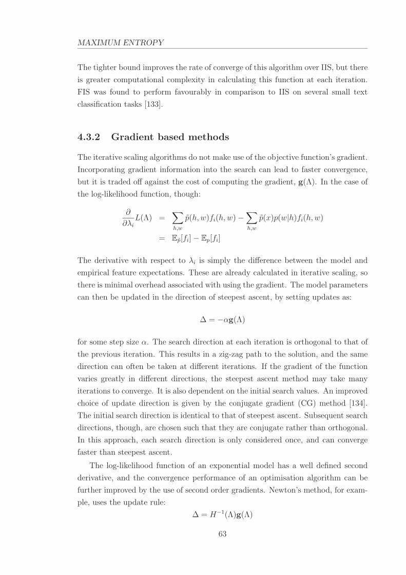
MAXIMUM ENTROPY
The tighter bound improves the rate of converge of this algorithm over IIS, but there
is greater computational complexity in calculating this function at each iteration.
FIS was found to perform favourably in comparison to IIS on several small text
classification tasks [133].
4.3.2 Gradient based methods
The iterative scaling algorithms do not make use of the objective function’s gradient.
Incorporating gradient information into the search can lead to faster convergence,
but it is traded off against the cost of computing the gradient, g(Λ). In the case of
the log-likelihood function, though:
∂
∂λi
L(Λ) =∑
h,w
p(h,w)fi(h,w) −∑
h,w
p(x)p(w|h)fi(h,w)
= Ep[fi] − Ep[fi]
The derivative with respect to λi is simply the difference between the model and
empirical feature expectations. These are already calculated in iterative scaling, so
there is minimal overhead associated with using the gradient. The model parameters
can then be updated in the direction of steepest ascent, by setting updates as:
∆ = −αg(Λ)
for some step size α. The search direction at each iteration is orthogonal to that of
the previous iteration. This results in a zig-zag path to the solution, and the same
direction can often be taken at different iterations. If the gradient of the function
varies greatly in different directions, the steepest ascent method may take many
iterations to converge. It is also dependent on the initial search values. An improved
choice of update direction is given by the conjugate gradient (CG) method [134].
The initial search direction is identical to that of steepest ascent. Subsequent search
directions, though, are chosen such that they are conjugate rather than orthogonal.
In this approach, each search direction is only considered once, and can converge
faster than steepest ascent.
The log-likelihood function of an exponential model has a well defined second
derivative, and the convergence performance of an optimisation algorithm can be
further improved by the use of second order gradients. Newton’s method, for exam-
ple, uses the update rule:
∆ = H−1(Λ)g(Λ)
63

4.4. SMOOTHING
where H(Λ) is the hessian matrix of L(Λ). Because calculating H(Λ) and its inverse
is computationally expensive, quasi-Newton methods such as BFGS use a local ap-
proximation of the inverse hessian. The hessian is a symmetric k×k matrix where k
is the number of variables of the objective function. For large problems, storing the
hessian is not practical. The limited memory BFGS [135] method reduces the space
requirements by generating matrices using information from previous iterations.
Malouf [136] compared GIS, IIS, steepest ascent, CG and BFGS algorithms on
NLP classification tasks. The iterative scaling methods were found to perform quite
poorly, while BFGS outperformed the other algorithms in all experiments. Similar
results were obtained by Minka [137] in a comparison of optimisation algorithms for
logistic regression. The CG and BFGS methods both performed well, with especially
good results obtained by CG when features were uncorrelated.
4.4 Smoothing
As was shown in Section 4.2, the maximum entropy solution is also the maximum
likelihood solution of the family of models having exponential form. Like other
maximum likelihood models, they are subject to over-training, especially when large
numbers of features are used. Therefore, some form of smoothing is required to
obtain robust estimates. For the language modelling problem, one option is to apply
standard n-gram discounting techniques, such as those described in Section 2.1.2,
to the data before fitting the model. The expectations of model features can then
be constrained to their discounted, rather than true averages over the training data.
For the maximum entropy model, though, there are other more general approaches
which can be used to achieve the same goal.
4.4.1 Feature selection
One of the objectives of smoothing is to assign some probability mass to events
that have not occurred in training. There is, however, a notable difference between
how maximum entropy models and n-gram models handle unseen events. Consider
a maximum entropy model using only bigram features. If we assume the feature
context to be the previous word only, h = wi−1, then for every bigram in the
training data, (x, y), a feature of the following form is defined:
fx,y(h,w) =
{
1 : if h = x and w = y
0 : otherwise
64

MAXIMUM ENTROPY
Expectations of the features are constrained to equal their empirical values accord-
ing to Equation (4.4). Now, assume that during testing, a particular bigram was
encountered, say Monday evening, which did not appear in training. An unsmoothed
bigram model trained on the same data would assign pbg(evening|Monday) = 0. In
the maximum entropy model, fx,y(Monday, evening) = 0 for all features fx,y. The
model probability is then:
pme(evening|Monday) =1
Z(Monday)
where Z(Monday) is the normalising term calculated over all bigrams beginning
with the word Monday. As a result, pme 6= 0. If Monday also did not occur in the
training data, the probability becomes a uniform distribution based on the size of
the vocabulary, |W |:pme(evening|Monday) =
1
|W |Therefore, a limited degree of smoothing can be achieved simply by not constraining
a feature. This allows the problem of over-training to be approached from the point
of view of feature selection.
The most basic application of this is to use count cutoffs to eliminate rare fea-
tures. It avoids over-fitting the model to potentially unreliable parts of the training
data. It also benefits the model by reducing the number of parameters. Ratna-
parkhi [138] achieved good performance in several NLP classification tasks by using
count cutoffs. However, a problem with this naive approach is that it makes no
distinction between features having low counts because they are under-represented
by the data and those which truly represent uncommon information. Discarding all
such features inevitably results in the loss of some useful knowledge. More sophis-
ticated feature selection algorithms incorporate features into the model based on
their predictive power. Berger et al. [139] presented a greedy, incremental algorithm
for selecting a subset from a large set of potential features. An approximated log-
likelihood gain was used to measure the contribution of a candidate feature. The
feature providing the greatest increase in likelihood was then added to the model’s
feature set, and the process repeated. Della Pietra [132] proposed a similar algorithm
using an information gain criterion.
4.4.2 Regularisation
Relying solely on the uniform property of maximum entropy models for smooth-
ing tends to be inadequate, as it only provides very weak smoothing. If the model
65

4.4. SMOOTHING
parameters Λ are very large, some events may still receive near-zero probabilities.
Another problem can occur with explicit modelling of a zero-count feature. If a
particular feature does not occur in the training data, its parameter tends towards
negative infinity. For any subsequent event where that feature is active, the proba-
bility assigned by the model is zero. In order to sufficiently smooth a model trained
on sparse data, further smoothing techniques are still required.
Chen and Rosenfeld [140] described the application of a zero mean Gaussian
prior distribution on the model parameters. Rather than performing maximum
likelihood estimation, maximum a posterior (MAP) estimation is performed to find
the parameters that maximise the modified objective function:
L′(Λ) = L(Λ) −k
∑
i=1
λ2i
2σ2i
where σ2 is the variance of the prior. The second term in this equation is a weighted
l2 norm of the parameters, and assists smoothing by penalising models which diverge
from the uniform distribution. Under this regularised model, feature expectations
are no longer constrained to equal their empirical expectations. Instead, they are
discounted such that:
Ep[fi] = Ep[fi] −λi
σ2i
This results in model expectations that are generally lower than their empirical
targets, which is reasonable given that the empirical values tend to overestimate
probabilities of observed events. Chen and Rosenfeld found that a maximum en-
tropy model with Gaussian prior smoothing performed competitively with modified
a Kneser-Ney smoothed n-gram. These two approaches consistently outperformed
other n-gram smoothing methods, as well as a maximum entropy model smoothed
with Katz smoothing.
Placing a Gaussian prior over the model parameters is equivalent to constraining
the feature expectations to a discounted empirical value. Kazama and Tsujii [141]
proposed an inequality model in which features were constrained to lie within a
given range. This was formulated as an entropy maximisation problem subject to
the two inequality constraints:
Ep[fi] − Ep[fi] − Ai ≤ 0
Ep[fi] − Ep[fi] − Bi ≤ 0
for Ai, Bi > 0, representing upper and lower bounds, respectively. If there is a solu-
66
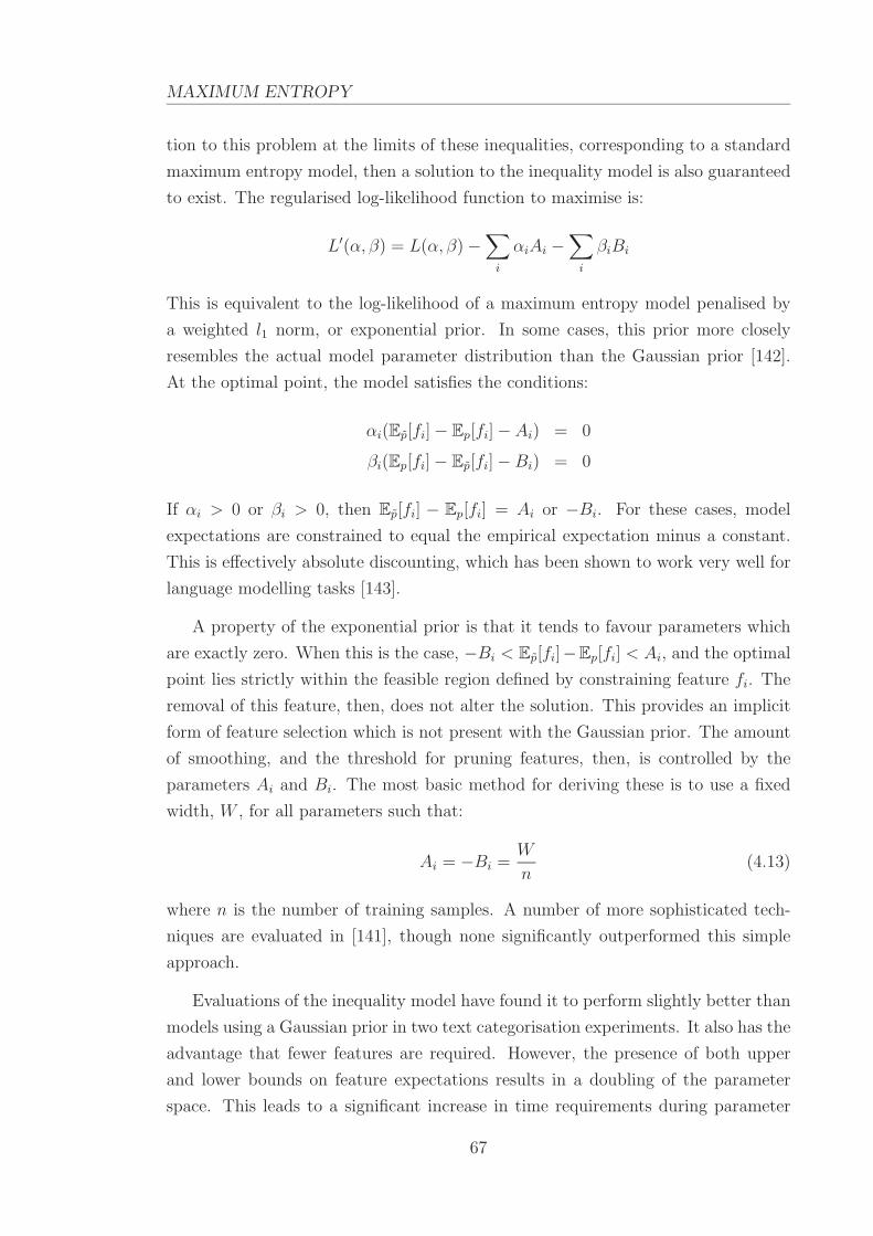
MAXIMUM ENTROPY
tion to this problem at the limits of these inequalities, corresponding to a standard
maximum entropy model, then a solution to the inequality model is also guaranteed
to exist. The regularised log-likelihood function to maximise is:
L′(α, β) = L(α, β) −∑
i
αiAi −∑
i
βiBi
This is equivalent to the log-likelihood of a maximum entropy model penalised by
a weighted l1 norm, or exponential prior. In some cases, this prior more closely
resembles the actual model parameter distribution than the Gaussian prior [142].
At the optimal point, the model satisfies the conditions:
αi(Ep[fi] − Ep[fi] − Ai) = 0
βi(Ep[fi] − Ep[fi] − Bi) = 0
If αi > 0 or βi > 0, then Ep[fi] − Ep[fi] = Ai or −Bi. For these cases, model
expectations are constrained to equal the empirical expectation minus a constant.
This is effectively absolute discounting, which has been shown to work very well for
language modelling tasks [143].
A property of the exponential prior is that it tends to favour parameters which
are exactly zero. When this is the case, −Bi < Ep[fi]−Ep[fi] < Ai, and the optimal
point lies strictly within the feasible region defined by constraining feature fi. The
removal of this feature, then, does not alter the solution. This provides an implicit
form of feature selection which is not present with the Gaussian prior. The amount
of smoothing, and the threshold for pruning features, then, is controlled by the
parameters Ai and Bi. The most basic method for deriving these is to use a fixed
width, W , for all parameters such that:
Ai = −Bi =W
n(4.13)
where n is the number of training samples. A number of more sophisticated tech-
niques are evaluated in [141], though none significantly outperformed this simple
approach.
Evaluations of the inequality model have found it to perform slightly better than
models using a Gaussian prior in two text categorisation experiments. It also has the
advantage that fewer features are required. However, the presence of both upper
and lower bounds on feature expectations results in a doubling of the parameter
space. This leads to a significant increase in time requirements during parameter
67

4.5. COMBINING KNOWLEDGE SOURCES
estimation.
4.5 Combining Knowledge Sources
The maximum entropy model has a number of useful properties. It provides the
least biased estimate given incomplete information. It is also the maximum likeli-
hood model of the exponential family. Parameter estimation is independent of the
modelling task, and efficient parameter estimation techniques exist for training the
model. Perhaps its greatest advantage, though, is its flexibility in modelling phe-
nomena. It provides a principled and consistent framework for encoding knowledge.
The feature function representation of information, used to capture co-occurrences
between contexts and target classes, is extremely general. Any property which can
be expressed as statistics of context and target pairs can subsequently be included
into the model, irrespective of what information it contains.
Features are incorporated into the maximum entropy model using the constraint
equations of the form of Equation (4.4). These constraints can be considered to be
weak in the sense that they only constrain the features’ expectations. Consider a cor-
pus in which the word, evening, and word bigram Monday evening, occur with prob-
abilities p(evening) and p(Monday evening) respectively. These are also the prob-
abilities assigned by an unsmoothed bigram model (i.e. pbg(evening) = p(evening)
and pbg(Monday evening) = p(Monday evening)). If the word sequence Monday
evening was observed frequently in the training data, then pbg(Monday evening)
does not take into account any information about the unigram probability. A
back-off model will use discounted estimates of either the bigram distribution if
the frequency of the event is above a given threshold, or the unigram probability
if the event is infrequent. In both situations, only one of the distributions is di-
rectly used. An interpolated model makes use of both distributions by assigning
pbg(Monday evening) = αp(evening) + (1 − α)p(evening|Monday) for some weight
α. While this incorporates both the unigram and bigram information, the resulting
probability does not necessarily resemble what is observed in the data.
The same information can be included into a maximum entropy model by using
the features:
f1(h,w) =
{
1 : if w = evening
0 : otherwise
f2(h,w) =
{
1 : if w = evening and h = Monday
0 : otherwise
68

MAXIMUM ENTROPY
where h is the previous word. Unlike the bigram model, a maximum entropy
model with constraints on features f1 and f2, on the other hand, does not require
pme(evening) = p(evening) or pme(evening|Monday) = p(evening|Monday) in every
case. Instead, it is only necessary that these features match their empirical targets
on average over the training data. By placing restrictions only on feature expecta-
tions rather than directly on model probabilities, the maximum entropy model is
able to simultaneously make use of the information provided by both features while
at the same time remaining consistent with the observations.
Another useful property of features under the maximum entropy framework is
that there is no need for them to be statistically independent. Multiple features may
be used to provide constraints on the same target, and their interaction will be taken
into account during the training process. This is particularly useful if features are to
be derived from multiple, correlated knowledge sources. Part-of-speech information,
for example, may be used to augment word-based information in language modelling.
A feature such as:
f(h,w) =
{
1 : if w = hundred and g(h) = ordinal
0 : otherwise
could be added to the set of standard n-gram features, where g(h) gives the POS tag
of the previous word. Importantly, adding information from a different knowledge
source in this way does not require any changes to be made to the form of the model.
Adding such information to an n-gram model, for example, may result in a frag-
mentation of the data into word-POS pairs, or require a decoupling of the variables
by making assumptions of their independence, both of which are undesirable.
The flexibility of the maximum entropy model has meant it has successfully
found use in a wide range of NLP problems. Berger et al. [139] described the use of
maximum entropy models in statistical translation. A number of sub-tasks involved
in the process, including context-sensitive word translation, segmentation and word
reordering, were formulated under the maximum entropy framework. Rosenfeld [144]
used a maximum entropy to incorporate trigger features in a language model, which
significantly reduced perplexity. Ratnaparkhi [138] used maximum entropy models
for variety of problems, including sentence boundary detection, POS tag assignment
and parsing. He showed that state-of-the-art performance could be achieved on
these tasks using features customised for the specific problem, but under the same
modelling framework.
69

70

Chapter 5
Language Modelling with ToBI
Features
When training a language model for use in an ASR system, acoustic information is
already available, and it may be worthwhile to incorporate this into the language
model. The maximum entropy framework discussed in Chapter 4 is a theoretically
sound method for combining multiple information sources, such as word and prosodic
class sequences, in a statistical classifier. This only solves half of the problem,
though, as it is still necessary to derive a set of constraints for the model. In order
to be effective, these constraints must provide useful information to the classification
task, and their target values need to be robustly estimated from a training sample.
This chapter will describe an approach for including prosodic information, in
the form of ToBI features, into a language model. The first section will introduce
a speech corpus that has been transcribed according to ToBI conventions. It will
examine the distribution of these prosodic labels, and explain the simplified prosodic
representation used in the experiments. The second section will describe some met-
rics for evaluating the potential contribution of the prosodic feature sets, and provide
some supporting evidence for the use of combined prosodic and syntactic informa-
tion. In the third section, the experimental setup will be detailed, and the form of
the models and prosodic features explained. This section will also provide perplexity
results for models, and offer some interpretations of their results. The fourth sec-
tion of this chapter will present the results of speech recognition tests using the new
language models. It will describe the baseline recogniser, as well as the multi-pass
decoding process.
71
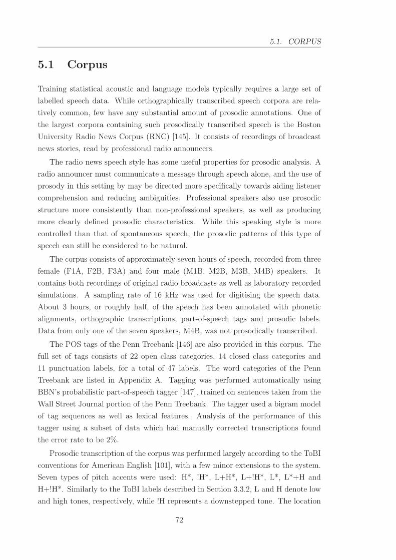
5.1. CORPUS
5.1 Corpus
Training statistical acoustic and language models typically requires a large set of
labelled speech data. While orthographically transcribed speech corpora are rela-
tively common, few have any substantial amount of prosodic annotations. One of
the largest corpora containing such prosodically transcribed speech is the Boston
University Radio News Corpus (RNC) [145]. It consists of recordings of broadcast
news stories, read by professional radio announcers.
The radio news speech style has some useful properties for prosodic analysis. A
radio announcer must communicate a message through speech alone, and the use of
prosody in this setting by may be directed more specifically towards aiding listener
comprehension and reducing ambiguities. Professional speakers also use prosodic
structure more consistently than non-professional speakers, as well as producing
more clearly defined prosodic characteristics. While this speaking style is more
controlled than that of spontaneous speech, the prosodic patterns of this type of
speech can still be considered to be natural.
The corpus consists of approximately seven hours of speech, recorded from three
female (F1A, F2B, F3A) and four male (M1B, M2B, M3B, M4B) speakers. It
contains both recordings of original radio broadcasts as well as laboratory recorded
simulations. A sampling rate of 16 kHz was used for digitising the speech data.
About 3 hours, or roughly half, of the speech has been annotated with phonetic
alignments, orthographic transcriptions, part-of-speech tags and prosodic labels.
Data from only one of the seven speakers, M4B, was not prosodically transcribed.
The POS tags of the Penn Treebank [146] are also provided in this corpus. The
full set of tags consists of 22 open class categories, 14 closed class categories and
11 punctuation labels, for a total of 47 labels. The word categories of the Penn
Treebank are listed in Appendix A. Tagging was performed automatically using
BBN’s probabilistic part-of-speech tagger [147], trained on sentences taken from the
Wall Street Journal portion of the Penn Treebank. The tagger used a bigram model
of tag sequences as well as lexical features. Analysis of the performance of this
tagger using a subset of data which had manually corrected transcriptions found
the error rate to be 2%.
Prosodic transcription of the corpus was performed largely according to the ToBI
conventions for American English [101], with a few minor extensions to the system.
Seven types of pitch accents were used: H*, !H*, L+H*, L+!H*, L*, L*+H and
H+!H*. Similarly to the ToBI labels described in Section 3.3.2, L and H denote low
and high tones, respectively, while !H represents a downstepped tone. The location
72

LANGUAGE MODELLING WITH TOBI FEATURES
H*
!H*
L+H*
L+!H*
L*L*+H
H+!H**
(a) Pitch accent distribution.
0
12
3
4+
(b) Break index distribution.
Figure 5.1: Distribution of pitch accents and break indices in the training partitionof the RNC data.
of the accent in bitonal events is indicated by the *. Intermediate phrase boundaries
were marked in this corpus by L-, H- or !H-, and full intonational phrase bound-
aries were marked by either H% or L%. Two additional break index values were
also specified. The intonational phrase boundary, 4, was extended to additionally
distinguish between groupings of intonational phrases, marked by a break index of
5, as well as sentence boundaries corresponding to break index 6.
Inter-transcriber agreement on the presence versus absence of pitch accents on
the prosodically transcribed subset of this corpus was 91% [145]. Among the words
which were labelled as having accents, there was a 60% correspondence on pitch
accent types, increasing to 80% when the H* and L+H* accents were combined.
For break indices, there was a 95% agreement when allowing for uncertainty by
merging adjacent levels.
The distribution of pitch accents and break indices is shown in Figure 5.1. Break
index values of 5 and 6 were not used in some transcriptions, so these were considered
to be equivalent to 4. A number of categories, both in pitch accents and break
indices, occur very infrequently. Lack of training data is a significant problem when
training statistical models, and the rarity of these features may negatively impact
on the model. Additionally, a small number of pitch accents (denoted by * or X*?)
were marked as being accents, but their specific category was not indicated. For
these reasons, we adopt an approach similar to other related work (e.g. [126]) and
simplify both features to binary values. Words are then marked as being accented
(a) or unaccented (u), and the degree of prosodic juncture between two words may
73

5.2. EVALUATING PROSODIC FEATURES
either be a regular word boundary (1, corresponding to break indices of 0 – 3 in the
standard notation) or a phrase boundary (4, corresponding to break indices of 4 or
greater). The break index is therefore used to model the presence or absence of an
intonational phrase boundary.
The data sets used in the following experiments were taken from the prosodically
transcribed portion of this corpus. This consisted of approximately 3 hours of speech
from six of the seven speakers (three male and three female), totalling about 30,000
words. The paragraph sized utterances were split into individual sentences, and
randomly partitioned into three sets. 85% of the samples were used for training,
10% for testing, and the remaining 5% formed the development test set. This data
organisation is similar to the multi-speaker speaker-dependent partitioning described
in Hasegawa-Johnson et al. [148]. Log-likelihood gain on the development set was
used to provide an early stopping criterion for the training algorithm.
5.2 Evaluating Prosodic Features
Chapter 3 described a number of potential ways in which prosody can assist speech
recognition. In order to recognise words from continuous speech, correct segmen-
tation is critical, and a number of prosodic attributes can act as cues to boundary
locations. Prosodic phrasing, accentuation and deaccentuation are all related to
syntactic structure. Two issues should be considered when applying this knowledge
to an ASR system. Firstly, these prosodic events are difficult to quantify in terms
of acoustic parameters. Sometimes, their correlation with acoustic features can be
weak, or conditionally dependent on other factors. Secondly, the way in which a
statistical model processes speech is fundamentally different to a human’s. In gen-
eral, the information which statistical models can apply is much more limited, and
they are also significantly affected by noisy or unreliable training data.
The use of prosodic annotations which have been transcribed perceptually allows
the first issue to be circumvented to a certain extent. While the development of a
fully automatic system would require prosodic features to also be extracted auto-
matically, ToBI transcriptions such as those provided by the RNC data offer a simple
starting point for investigations. The second point is potentially more difficult to
address. Computational limitations restrict the amount of information a model may
use, as does inaccurate and sparse data. The choice of the maximum entropy model,
though, does offer some advantages. In particular, there is no inherent restriction
on the complexity of features other than computational expense. This is of partic-
ular use when modelling the relationship between prosodic and word sequences, as
74

LANGUAGE MODELLING WITH TOBI FEATURES
no assumptions about their independence need to be made. Since the interaction
between prosody and words is quite complex, it is desirable to assume as little as
possible about what has not been observed in data. This is a fundamental precept
of the maximum entropy principle which is particularly applicable in this scenario.
Given a number of candidate features which may be included a model, it is often
helpful to have an estimate of their potential contribution. This can allow for more
informed choices regarding which features to incorporate, as well as provide some
preliminary information on how they behave. One metric which can be used for this
purpose is mutual information (MI). The MI, I(X; Y ), between random variables,
X and Y , is a measure of the amount of information one of the random variables
provides about the other. It is defined as:
I(X; Y ) = H(X) − H(X|Y )
=∑
x
∑
y
p(x, y) logp(x, y)
p(x)p(y)
MI is bounded below by zero, and above by H(X). If X and Y are independent,
then p(x, y) = p(x)p(y), and I(X; Y ) = 0. This is quite intuitive, as knowing X
does not provide any information about Y , and vice versa, if they are independent.
Conversely, if X and Y are identical, then H(X|Y ) = 0, and I(X; Y ) = H(X) =
H(Y ). MI is also symmetric, so I(X; Y ) = I(Y ; X). If X carries some information
about Y , then Y also contains that information about X.
The effectiveness of a feature can be assessed by measuring the MI between the
feature and the word it is being used to predict. A bigram feature, for example,
uses the identity of the previous word as a predictor. The MI between a word, wi,
and the feature, f(wi) = wi−1, can then be approximated with respect to a training
corpus:
I(w; f(w)) =1
N
∑
wi−1,wi
logp(wi−1, wi)
p(wi−1)p(wi)
where N is the size of the training set and p(·) is the probability of the specified
word, or word sequence, in the training data.
We have examined the mutual information between words and their prosodic
labels. Due to the close relationship between prosody and syntax, we have also
chosen to include syntactic information in the analysis. POS tags are used as the
basic units bearing syntactic information, as these are already provided in the corpus.
It is worth noting, though, that POS labels are a fairly weak representation of
syntax. Full, or even partial parse trees would be capable of describing syntactic
75
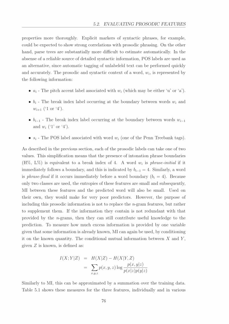
5.2. EVALUATING PROSODIC FEATURES
properties more thoroughly. Explicit markers of syntactic phrases, for example,
could be expected to show strong correlations with prosodic phrasing. On the other
hand, parse trees are substantially more difficult to estimate automatically. In the
absense of a reliable source of detailed syntactic information, POS labels are used as
an alternative, since automatic tagging of unlabeleld text can be performed quickly
and accurately. The prosodic and syntactic context of a word, wi, is represented by
the following information:
• ai - The pitch accent label associated with wi (which may be either ‘u’ or ‘a’).
• bi - The break index label occurring at the boundary between words wi and
wi+1 (‘1 or ‘4’).
• bi−1 - The break index label occurring at the boundary between words wi−1
and wi (‘1’ or ‘4’).
• si - The POS label associated with word wi (one of the Penn Treebank tags).
As described in the previous section, each of the prosodic labels can take one of two
values. This simplification means that the presence of intonation phrase boundaries
(H%, L%) is equivalent to a break index of 4. A word wi is phrase-initial if it
immediately follows a boundary, and this is indicated by bi−1 = 4. Similarly, a word
is phrase-final if it occurs immediately before a word boundary (bi = 4). Because
only two classes are used, the entropies of these features are small and subsequently,
MI between these features and the predicted word will also be small. Used on
their own, they would make for very poor predictors. However, the purpose of
including this prosodic information is not to replace the n-gram features, but rather
to supplement them. If the information they contain is not redundant with that
provided by the n-grams, then they can still contribute useful knowledge to the
prediction. To measure how much excess information is provided by one variable
given that some information is already known, MI can again be used, by conditioning
it on the known quantity. The conditional mutual information between X and Y ,
given Z is known, is defined as:
I(X; Y |Z) = H(X|Z) − H(X|Y, Z)
=∑
x,y,z
p(x, y, z) logp(x, y|z)
p(x|z)p(y|z)
Similarly to MI, this can be approximated by a summation over the training data.
Table 5.1 shows these measures for the three features, individually and in various
76
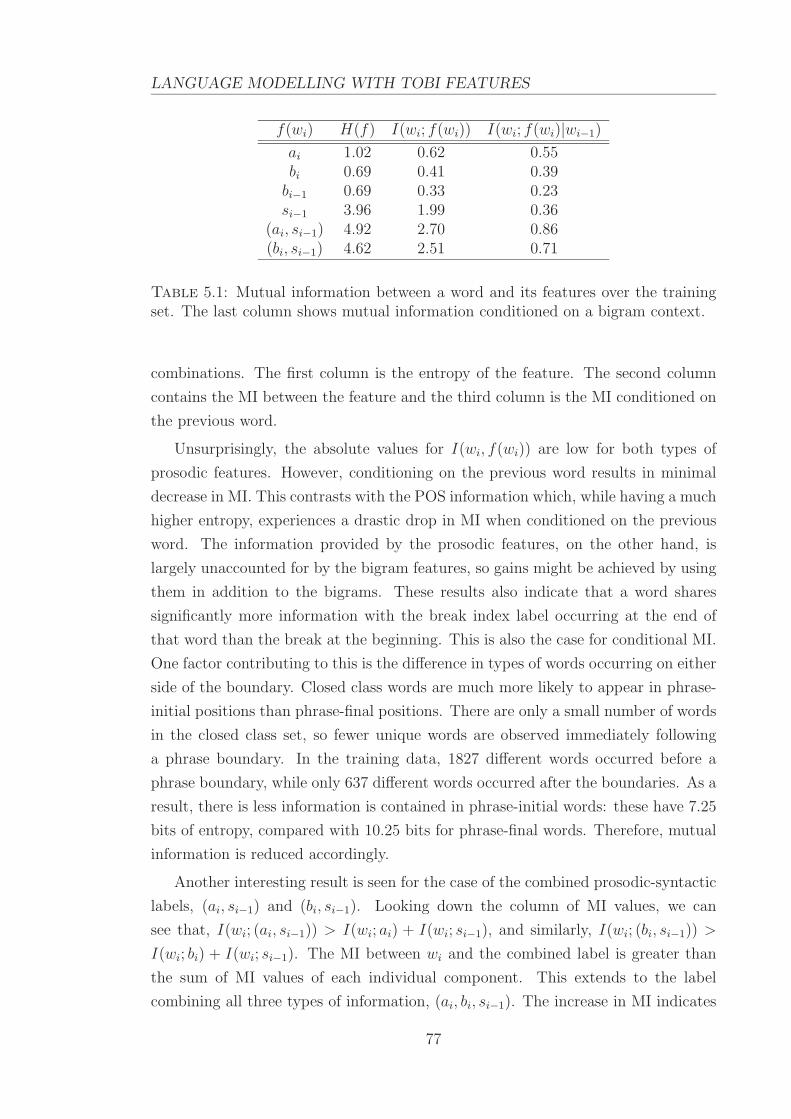
LANGUAGE MODELLING WITH TOBI FEATURES
f(wi) H(f) I(wi; f(wi)) I(wi; f(wi)|wi−1)
ai 1.02 0.62 0.55bi 0.69 0.41 0.39
bi−1 0.69 0.33 0.23si−1 3.96 1.99 0.36
(ai, si−1) 4.92 2.70 0.86(bi, si−1) 4.62 2.51 0.71
Table 5.1: Mutual information between a word and its features over the trainingset. The last column shows mutual information conditioned on a bigram context.
combinations. The first column is the entropy of the feature. The second column
contains the MI between the feature and the third column is the MI conditioned on
the previous word.
Unsurprisingly, the absolute values for I(wi, f(wi)) are low for both types of
prosodic features. However, conditioning on the previous word results in minimal
decrease in MI. This contrasts with the POS information which, while having a much
higher entropy, experiences a drastic drop in MI when conditioned on the previous
word. The information provided by the prosodic features, on the other hand, is
largely unaccounted for by the bigram features, so gains might be achieved by using
them in addition to the bigrams. These results also indicate that a word shares
significantly more information with the break index label occurring at the end of
that word than the break at the beginning. This is also the case for conditional MI.
One factor contributing to this is the difference in types of words occurring on either
side of the boundary. Closed class words are much more likely to appear in phrase-
initial positions than phrase-final positions. There are only a small number of words
in the closed class set, so fewer unique words are observed immediately following
a phrase boundary. In the training data, 1827 different words occurred before a
phrase boundary, while only 637 different words occurred after the boundaries. As a
result, there is less information is contained in phrase-initial words: these have 7.25
bits of entropy, compared with 10.25 bits for phrase-final words. Therefore, mutual
information is reduced accordingly.
Another interesting result is seen for the case of the combined prosodic-syntactic
labels, (ai, si−1) and (bi, si−1). Looking down the column of MI values, we can
see that, I(wi; (ai, si−1)) > I(wi; ai) + I(wi; si−1), and similarly, I(wi; (bi, si−1)) >
I(wi; bi) + I(wi; si−1). The MI between wi and the combined label is greater than
the sum of MI values of each individual component. This extends to the label
combining all three types of information, (ai, bi, si−1). The increase in MI indicates
77

5.3. LANGUAGE MODELLING
that the presence of the syntactic labels increases the correlation between a word
and its prosodic label. This positive interaction information provides motivation for
combining syntactic and prosodic knowledge from an information theory perspective,
as there is some synergy between these sources.
While the MI values of the prosodic features may indicate that they reduce the
uncertainty of the predicted word, it does not guarantee that modelling those fea-
tures will improve classification performance. MI shows the amount of information
which is shared between the variables, and represents an upper bound on the po-
tential gain. It does not consider how the features interact when they are combined
in a model. Also, in the case of these prosodic features which have relatively low
MI compared to n-gram features, the additional knowledge they provide may be in-
consequential. If the model can predict a word accurately using only n-grams, then
any extra reduction in uncertainty will not affect the outcome. Conversely, if the
language model considers a correct word sequence to be sufficiently unlikely, then a
relatively minor boost to its probability from the inclusion of prosodic information
may still have no impact on the final classification.
5.3 Language Modelling
5.3.1 Baseline
The baseline language model used for comparison was a standard trigram model. It
used modified Kneser-Ney smoothing, as this exhibited superior performance to the
other smoothing techniques in an evaluation using our data. Free parameters were
calculated according to the heuristics shown in Equation (2.7). This model was
constructed using the SRI Language Modeling (SRILM) toolkit [149]. Although
this model is used as a baseline to compare against the prosodically augmented
maximum entropy models, it should be noted that silences are explicitly modelled
as part of the n-gram sequences. Since pausing can be considered to be a prosodic
feature, the trigram is therefore not completely independent of prosody.
5.3.2 ToBI features
We formulated some simple features for directly incorporating the prosodic and
syntactic contextual information. These are described in terms of a class label
w and the context, h. In all cases, w is a member of the set of words in the
training vocabulary, and the context consists of the sequence h = (h1, . . . , hi). Each
element in h represents word, pitch accent, break index and POS information as
78
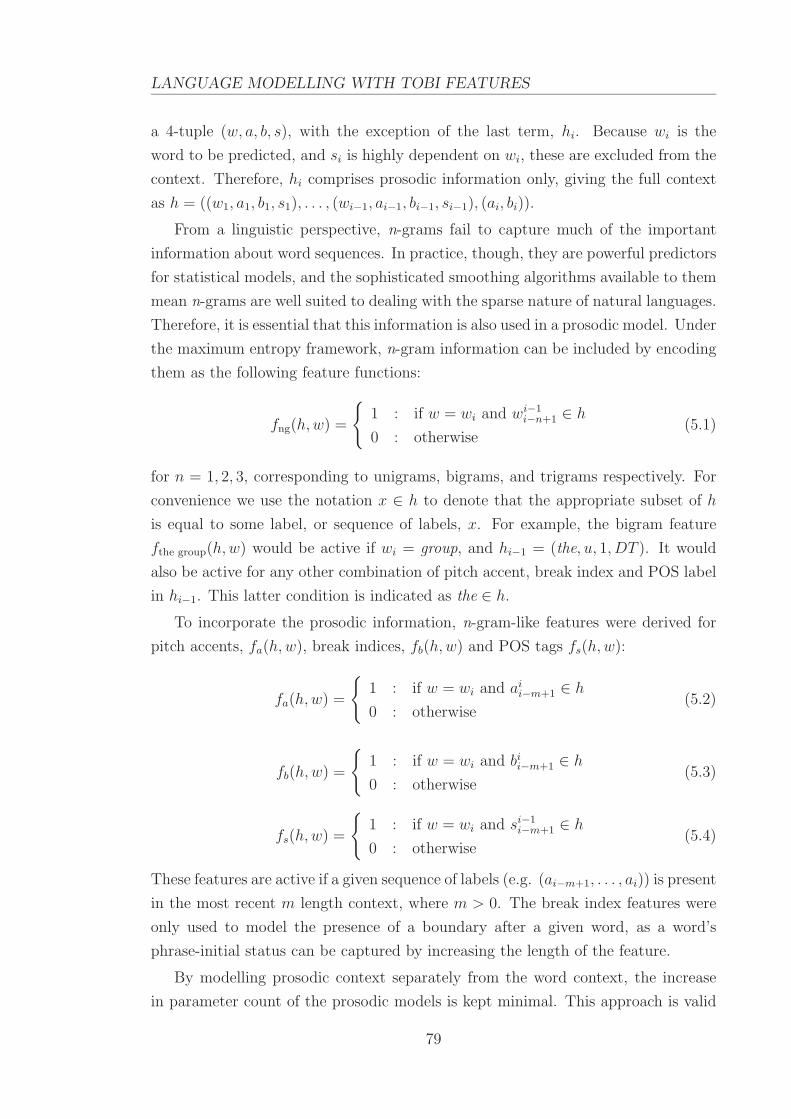
LANGUAGE MODELLING WITH TOBI FEATURES
a 4-tuple (w, a, b, s), with the exception of the last term, hi. Because wi is the
word to be predicted, and si is highly dependent on wi, these are excluded from the
context. Therefore, hi comprises prosodic information only, giving the full context
as h = ((w1, a1, b1, s1), . . . , (wi−1, ai−1, bi−1, si−1), (ai, bi)).
From a linguistic perspective, n-grams fail to capture much of the important
information about word sequences. In practice, though, they are powerful predictors
for statistical models, and the sophisticated smoothing algorithms available to them
mean n-grams are well suited to dealing with the sparse nature of natural languages.
Therefore, it is essential that this information is also used in a prosodic model. Under
the maximum entropy framework, n-gram information can be included by encoding
them as the following feature functions:
fng(h,w) =
{
1 : if w = wi and wi−1i−n+1 ∈ h
0 : otherwise(5.1)
for n = 1, 2, 3, corresponding to unigrams, bigrams, and trigrams respectively. For
convenience we use the notation x ∈ h to denote that the appropriate subset of h
is equal to some label, or sequence of labels, x. For example, the bigram feature
fthe group(h,w) would be active if wi = group, and hi−1 = (the, u, 1, DT ). It would
also be active for any other combination of pitch accent, break index and POS label
in hi−1. This latter condition is indicated as the ∈ h.
To incorporate the prosodic information, n-gram-like features were derived for
pitch accents, fa(h,w), break indices, fb(h,w) and POS tags fs(h,w):
fa(h,w) =
{
1 : if w = wi and aii−m+1 ∈ h
0 : otherwise(5.2)
fb(h,w) =
{
1 : if w = wi and bii−m+1 ∈ h
0 : otherwise(5.3)
fs(h,w) =
{
1 : if w = wi and si−1i−m+1 ∈ h
0 : otherwise(5.4)
These features are active if a given sequence of labels (e.g. (ai−m+1, . . . , ai)) is present
in the most recent m length context, where m > 0. The break index features were
only used to model the presence of a boundary after a given word, as a word’s
phrase-initial status can be captured by increasing the length of the feature.
By modelling prosodic context separately from the word context, the increase
in parameter count of the prosodic models is kept minimal. This approach is valid
79

5.3. LANGUAGE MODELLING
because the model does not require there to be any independence between features.
While a large amount of redundancy is not desirable, a feature selection procedure
can be applied to prune off those features which do not contribute any additional
information to the model. Another benefit of not jointly modelling prosodic and
word contexts is that it can allow greater history lengths to be used. Sparse data is
the primary reason n-gram models are restricted to using a very short context. The
small number of possible prosodic classes, on the other hand, means the expectations
of prosodic feature can be estimated robustly from empirical data over much longer
distances. All pitch accent sequences of length 4, for example, were observed a
minimum of 300 times in the training data. Therefore, we extended the lengths of
these prosodic and syntactic features beyond the history size of two which was used
for standard n-grams.
5.3.3 Perplexity results
As a proof of concept, we trained some maximum entropy models using the features
described in Section 5.3.2, and evaluated their perplexities. Because we used the
manually transcribed labels during the testing process, these values can be consid-
ered to be what is attainable in the best case scenario. While this is not practicable,
it gives an indication of how much information is contained in the prosodic features,
and how well the models can extract that information and apply it to the task.
Inaccuracies in automatic labelling methods, which will be discussed in greater de-
tail in the next chapter, would reduce the amount of useful information available,
although it should be remembered that even the manual transcriptions are not nec-
essarily completely accurate. In our experiments, ToBI labels were paired up with
words based on time. A word was labelled as accented if an appropriate pitch ac-
cent occurred within its duration. Break index labels were distributed to the nearest
word edge.
All features in the models were constrained to equal their empirical values in the
training set. Smoothing and feature selection were handled by applying an exponen-
tial prior over model parameters, with the smoothing parameters chosen according
to Equation (4.13). The maximum entropy classification library of Kazama and
Tsujii [141] was used, which in turn used Benson and Moore’s [150] limited memory
variable metric bounded constrained optimisation routine for parameter estimation.
Training was performed either until convergence or until the likelihood on the held-
out set stopped increasing. Perplexities were quite sensitive to the variance of the
prior, and this value was optimised separately for each model using the development
80
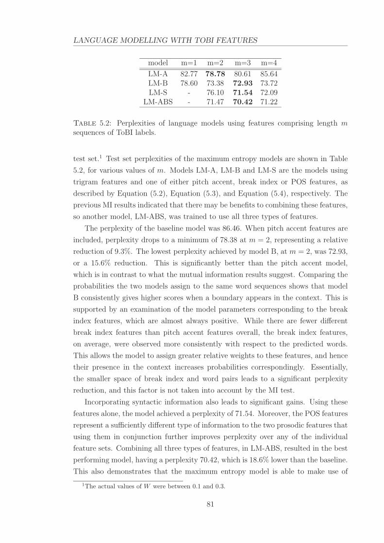
LANGUAGE MODELLING WITH TOBI FEATURES
model m=1 m=2 m=3 m=4
LM-A 82.77 78.78 80.61 85.64LM-B 78.60 73.38 72.93 73.72LM-S - 76.10 71.54 72.09
LM-ABS - 71.47 70.42 71.22
Table 5.2: Perplexities of language models using features comprising length msequences of ToBI labels.
test set.1 Test set perplexities of the maximum entropy models are shown in Table
5.2, for various values of m. Models LM-A, LM-B and LM-S are the models using
trigram features and one of either pitch accent, break index or POS features, as
described by Equation (5.2), Equation (5.3), and Equation (5.4), respectively. The
previous MI results indicated that there may be benefits to combining these features,
so another model, LM-ABS, was trained to use all three types of features.
The perplexity of the baseline model was 86.46. When pitch accent features are
included, perplexity drops to a minimum of 78.38 at m = 2, representing a relative
reduction of 9.3%. The lowest perplexity achieved by model B, at m = 2, was 72.93,
or a 15.6% reduction. This is significantly better than the pitch accent model,
which is in contrast to what the mutual information results suggest. Comparing the
probabilities the two models assign to the same word sequences shows that model
B consistently gives higher scores when a boundary appears in the context. This is
supported by an examination of the model parameters corresponding to the break
index features, which are almost always positive. While there are fewer different
break index features than pitch accent features overall, the break index features,
on average, were observed more consistently with respect to the predicted words.
This allows the model to assign greater relative weights to these features, and hence
their presence in the context increases probabilities correspondingly. Essentially,
the smaller space of break index and word pairs leads to a significant perplexity
reduction, and this factor is not taken into account by the MI test.
Incorporating syntactic information also leads to significant gains. Using these
features alone, the model achieved a perplexity of 71.54. Moreover, the POS features
represent a sufficiently different type of information to the two prosodic features that
using them in conjunction further improves perplexity over any of the individual
feature sets. Combining all three types of features, in LM-ABS, resulted in the best
performing model, having a perplexity 70.42, which is 18.6% lower than the baseline.
This also demonstrates that the maximum entropy model is able to make use of
1The actual values of W were between 0.1 and 0.3.
81
5.3. LANGUAGE MODELLING
additional knowledge sources without degrading the effectiveness of the original
information.
While the inclusion of pitch accent, break index and POS information all im-
proved perplexity, the effectiveness of modelling longer sequences of these features
was limited. The optimal length for the sequences of pitch accents was m = 2,
which is equivalent to the history length used by bigram features. While perplexity
decreased further at m = 3 for both POS and break index features, the improvement
for the break index features was only very slight. As the lengths of the prosodic and
POS features were increased beyond these small values, perplexities rose. Although
data sparsity is less of an issue with the small number of prosodic and POS classes,
there are other factors which may cause this. It may simply be the case that the
contextual information beyond this length does not contain useful information. The
average amount of shared information contained in word pairs decreases quickly as
the distance between them increases [144], and it is not unreasonable to expect that
a similar reduction would also be experienced by other knowledge sources. Given
the much lower initial information content of the prosodic and syntactic features,
their contribution at longer distances would quickly become negligible. It should
be noted, however, that while these results indicate that no gains are obtained for
these longer span features, it does not mean that long distance prosodic and syntac-
tic contexts are not useful. Rather, it is only the information represented by these
particular sequences of pitch accent, break index and POS labels which does not
assist the classification.
Another possible explanation for ineffectiveness of the longer distance prosodic
features may be that the prosodic labelling is not consistent enough to use as a
predictor. Differences in the ways the various speakers used prosodic markers could
also be a contributing factor to this. Ostendorf et al. [145] noted that, in the RNC
data, speaker F2B used phrase boundaries, pitch accents and low phrase tones more
frequently than speaker M1B. Reducing the number of values each variable may
take reduces the degree of inconsistency, but differences can still be seen in the
distribution of accent and boundary usage in our training data, as shown in Table
5.3. While a small level of unreliability in the transcriptions does not severely hinder
the model’s ability to effectively use short sequences, attempting to model longer
sequences of these labels would exacerbate the inconsistencies and subsequently lead
to a degradation in classification performance.
82
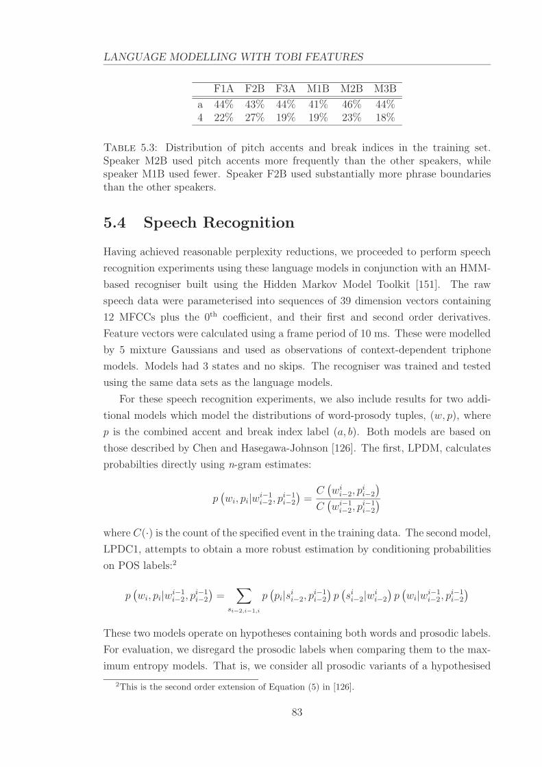
LANGUAGE MODELLING WITH TOBI FEATURES
F1A F2B F3A M1B M2B M3B
a 44% 43% 44% 41% 46% 44%4 22% 27% 19% 19% 23% 18%
Table 5.3: Distribution of pitch accents and break indices in the training set.Speaker M2B used pitch accents more frequently than the other speakers, whilespeaker M1B used fewer. Speaker F2B used substantially more phrase boundariesthan the other speakers.
5.4 Speech Recognition
Having achieved reasonable perplexity reductions, we proceeded to perform speech
recognition experiments using these language models in conjunction with an HMM-
based recogniser built using the Hidden Markov Model Toolkit [151]. The raw
speech data were parameterised into sequences of 39 dimension vectors containing
12 MFCCs plus the 0th coefficient, and their first and second order derivatives.
Feature vectors were calculated using a frame period of 10 ms. These were modelled
by 5 mixture Gaussians and used as observations of context-dependent triphone
models. Models had 3 states and no skips. The recogniser was trained and tested
using the same data sets as the language models.
For these speech recognition experiments, we also include results for two addi-
tional models which model the distributions of word-prosody tuples, (w, p), where
p is the combined accent and break index label (a, b). Both models are based on
those described by Chen and Hasegawa-Johnson [126]. The first, LPDM, calculates
probabilties directly using n-gram estimates:
p(
wi, pi|wi−1i−2, p
i−1i−2
)
=C
(
wii−2, p
ii−2
)
C(
wi−1i−2, p
i−1i−2
)
where C(·) is the count of the specified event in the training data. The second model,
LPDC1, attempts to obtain a more robust estimation by conditioning probabilities
on POS labels:2
p(
wi, pi|wi−1i−2, p
i−1i−2
)
=∑
si−2,i−1,i
p(
pi|sii−2, p
i−1i−2
)
p(
sii−2|wi
i−2
)
p(
wi|wi−1i−2, p
i−1i−2
)
These two models operate on hypotheses containing both words and prosodic labels.
For evaluation, we disregard the prosodic labels when comparing them to the max-
imum entropy models. That is, we consider all prosodic variants of a hypothesised
2This is the second order extension of Equation (5) in [126].
83

5.4. SPEECH RECOGNITION
word to be correct so long as the word component is correct.
5.4.1 Multi-pass decoding
Training and evaluating maximum entropy models is computationally expensive,
so it is common to apply them to a reduced search space in the later stages of a
muti-pass decoding approach. In these experiments, an N-best list was obtained
from the standard speech recogniser, which was re-ranked using the new language
models. We chose to rescore N-best lists rather than word lattices for a number of
reasons. Firstly, N-best list rescoring is simple to perform, and relatively fast for
reasonable sized lists. Rescoring lattices can be much slower. Secondly, maximum
entropy models allow for the use of information arbitrarily far back in the context.
This violates the dynamic programming assumption used by the Viterbi decoding
algorithm. A consequence, then, is that the decoder may prefer paths to which the
original n-gram model assigns the highest probability, while overlooking other paths
which initially have lower scores. A* decoding can be used as an alternative, but the
problem then shifts to obtaining a suitable estimate of the remaining probabilities
of partial paths. Och et al. [152] used the function:
p(wi) = max(wi−2,wi−1)
p(wi|wi−2, wi−1)
as an upper bound on the probability of each word. This is an admissible heuristic
and will guarantee an optimal solution for a trigram language model. However, it is
not directly applicable to a maximum entropy model in general. Evaluating over all
possible histories is feasible for the trigram, but an event in the maximum entropy
model may have arbitrarily many features associated with it, and these features
may be dependent on very large histories. An approximation to this value can be
obtained by selecting the maximum value over the training set; however, it is then
no longer guaranteed to be admissible. In [152], this function was combined with a
number of other estimates to derive the final heuristic. We have found that, on its
own, this is too loose a bound, and results in prohibitively long decoding times.
Nguyen et al. [153] evaluated an N-best rescoring approach against lattice decod-
ing, and found little difference in word accuracies. In some cases, rescoring the large
number of hypotheses available in the lattice resulted in a performance degradation,
as the higher level knowledge sources selected an incorrect hypothesis which was not
present in the N-best list. They also note that N-best lists provide advantages for
experimentation, as it eliminates the need to develop a general search strategy, as
well as allowing for more rapid optimisation of tunable parameters.
84

LANGUAGE MODELLING WITH TOBI FEATURES
0 10 20 30 40 50 60 70 80 90 10076
77
78
79
80
81
82
N
Acc
urac
y (%
)
N−best list oracle accuracies
Figure 5.2: Oracle accuracies of N-best lists for 1 ≤ N ≤ 100.
In order to select an appropriate size for the N-best list, we examined the oracle
accuracies for up lists of up to 100 hypotheses per utterance. The oracle accuracy
is the accuracy of the hypothesis in the list which is closest to the reference tran-
scription. It is therefore the upper bound on the possible improvement which can be
achieved by rescoring a list of that size. The oracle accuracies are shown in Figure
5.2. At N = 1, the word accuracy is 76.21%. This is also the accuracy of the trigram
baseline. Accuracies increase fairly steeply as N increases for small values of N , and
plateaus at around N = 65. At this point, the accuracy is 81.43%. From N = 65 to
N = 100, it only rises a further 0.23%, to 81.66%. Based on these results, we have
chosen to rescore 65-best lists in the following experiments. The grammar scaling
factor was held fixed at 15.0 for all models, and no word insertion penalty was used.
5.4.2 Results
The word error rates for the language models are presented in Table 5.4. Both
the inclusion of pitch accent features and break index features improved recognition
accuracy, to 76.94% and 77.12%, respectively. These gains over the 76.21% baseline
were significant at the level of p < 0.05, according to the MAPSSWE test described
in Section 2.4.2. The improvements in recognition rate, and the effect of increased
feature lengths, are also fairly consistent with the perplexity results. Combining the
85

5.4. SPEECH RECOGNITION
model m=1 m=2 m=3 m=4
LM-A 76.77 76.94 76.55 76.77LM-B 76.83 76.89 77.12 76.89LM-S - 76.89 77.06 77.00
LM-ABS - 77.51 77.40 77.12LPDM - - 75.86 -LPDC1 - - 77.00 -
Table 5.4: Recognition accuracies of language models using ToBI features.
three sets of features gives the best model with an accuracy of 77.51%. This 1.3%
absolute gain is significant at the level of p < 0.01.
The model LPDC1 also improved on the baseline, but the gain of 0.8% was less
than that reported by Chen and Hasegawa-Johnson [126]. While the 1.2% gain of
LPDC1 over LPDM is comparable, the model LPDM itself performed worse than
the word-only trigram. In contrast to the 0.35% performance loss seen here, the
bigram version of LPDM evaluated by Chen and Hasegawa-Johnson improved upon
the word-only bigram by 1.4%. We believe the reason for this discrepancy is that the
approach of introducing each prosodic variant of a word as a distinct entity in the
vocabulary scales poorly with context length. Therefore, while the assumptions and
approximations made by this method are valid, the trigram variants of the models
LPDM and LPDC1 suffer considerably more from data sparsity problems than their
bigram counterparts, and their performance degrades accordingly.
A more detailed breakdown of the results for the best performing variants of
LM-A and LM-B is presented in Table 5.5. It is evident that the primary source
of the improvements of these two models is the reduced number of substitution
errors. All three models had a comparable number of insertion errors, while the two
prosodic models showed a very slight reduction in deletion errors. The corrected
deletions almost always occurred near a corrected substitution, so the lower number
of deletion errors is more likely a side-effect of corrected substitutions rather than
an ability of the prosodic features to repair this type of error.
While the improvements to recognition accuracy are the result of an interaction
between multiple features, it is still possible to identify some cases in which specific
prosodic features may have contributed significantly to the correction. Consider
the following partial transcriptions from the trigram and LM-A, together with the
alignment of pitch accents:
86

LANGUAGE MODELLING WITH TOBI FEATURES
accent: . . . u a u u a a a . . .
trigram: . . . as well as four another revenue raising . . .
LM-A: . . . as well as for another revenue raising . . .
In this scenario, no pitch accent is observed in the vicinity of the hypothesised
words for/four. The word four, though, is much more likely to be accented than for.
In the training data, an accented four was observed 26 times, while its unaccented
form occurred only 5 times. In contrast, the word for was accented only 6 times in
the training set, and it was unaccented the other 257 times. Subsequently, when the
word four is encountered with no pitch accent, the model considers this to be an
unlikely event and decreases the score of the associated hypothesis. Observing the
unaccented form of for, on the other hand, is well supported by the training data,
and hence its probability is increased relative to the alternatives. The increased
probability of the latter hypothesis, in this case, was sufficient to raise its rank
above the original and eliminate the substitution error.
Similar situations can be identified for the break index model. Consider the
following transcriptions:
break: . . . 1 1 4 4
trigram: . . . at the was university
LM-B: . . . at the university
The hypothesis which received the highest trigram probability is dispreferred
by the maximum entropy model due to the co-occurrence of the word was with a
boundary. Because the model is capable of identifying the fact that was is highly
unlikely to be a phrase-final word, it considers the second option to be the better
alternative. The occurrence of two consecutive boundaries is also somewhat unusual,
so this further contributes to the decrease in the score of the original hypothesis.
In general, the improvements made by both LM-A and LM-B were the result of
downgrading the rank of hypotheses which conflicted with the prosodic information.
Of course, the opposite effect can also occur. If an event which is prosodically
uncommon does occur, such as a phrase-final function word, the new model may
incorrectly prefer other alternatives. The final score, though, is determined by the
combination of active features for the relevant events, and on average, the corrections
made by the addition of prosodic features outweigh any new errors they introduce.
In both of the previous examples, the original errors involved the misrecogni-
tion of a closed-class word. These types of errors form a significant proportion of
overall recognition errors. The fact that corrections to such errors are made by the
87
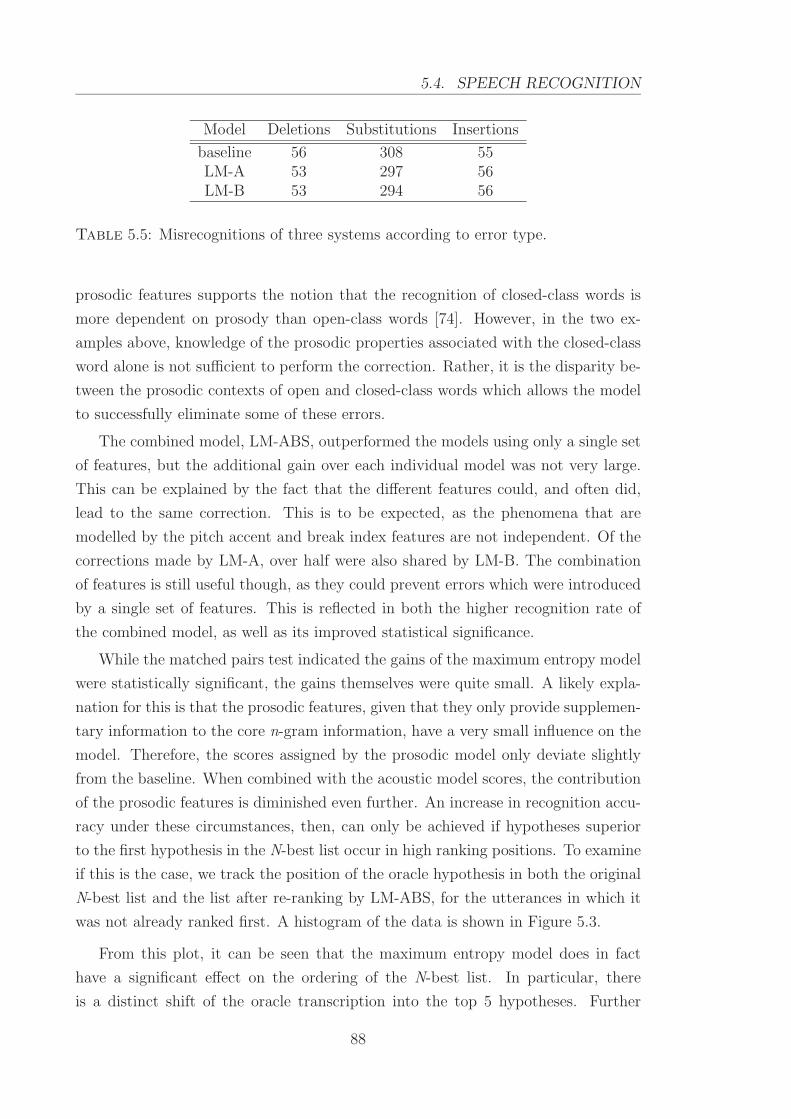
5.4. SPEECH RECOGNITION
Model Deletions Substitutions Insertions
baseline 56 308 55LM-A 53 297 56LM-B 53 294 56
Table 5.5: Misrecognitions of three systems according to error type.
prosodic features supports the notion that the recognition of closed-class words is
more dependent on prosody than open-class words [74]. However, in the two ex-
amples above, knowledge of the prosodic properties associated with the closed-class
word alone is not sufficient to perform the correction. Rather, it is the disparity be-
tween the prosodic contexts of open and closed-class words which allows the model
to successfully eliminate some of these errors.
The combined model, LM-ABS, outperformed the models using only a single set
of features, but the additional gain over each individual model was not very large.
This can be explained by the fact that the different features could, and often did,
lead to the same correction. This is to be expected, as the phenomena that are
modelled by the pitch accent and break index features are not independent. Of the
corrections made by LM-A, over half were also shared by LM-B. The combination
of features is still useful though, as they could prevent errors which were introduced
by a single set of features. This is reflected in both the higher recognition rate of
the combined model, as well as its improved statistical significance.
While the matched pairs test indicated the gains of the maximum entropy model
were statistically significant, the gains themselves were quite small. A likely expla-
nation for this is that the prosodic features, given that they only provide supplemen-
tary information to the core n-gram information, have a very small influence on the
model. Therefore, the scores assigned by the prosodic model only deviate slightly
from the baseline. When combined with the acoustic model scores, the contribution
of the prosodic features is diminished even further. An increase in recognition accu-
racy under these circumstances, then, can only be achieved if hypotheses superior
to the first hypothesis in the N-best list occur in high ranking positions. To examine
if this is the case, we track the position of the oracle hypothesis in both the original
N-best list and the list after re-ranking by LM-ABS, for the utterances in which it
was not already ranked first. A histogram of the data is shown in Figure 5.3.
From this plot, it can be seen that the maximum entropy model does in fact
have a significant effect on the ordering of the N-best list. In particular, there
is a distinct shift of the oracle transcription into the top 5 hypotheses. Further
88

LANGUAGE MODELLING WITH TOBI FEATURES
0 10 20 30 40 50 600
2
4
6
8
10
12
14
16
18
20
Rank
Cou
nt
Rank of oracle hypothesis
OriginalReranked
Figure 5.3: Histogram of the rank of the oracle hypothesis before and after re-ranking by LM-ABS. Each pair of bars represents a bin of 5 hypotheses.
evidence of this shift is seen in the drop in average rank of the oracle hypothesis,
from 20.4 in the original list, to 13.8 after re-ranking. While the new language
model significantly improves the rank of the best transcription, placing it in the
top 5 hypotheses 19 times, the hypothesis was ranked outright first in only 6 of
these cases. The remaining times, other hypotheses existed for which the model
assigned an even higher score. This behaviour can possibly be attributed to the
features’ lack of discriminatory power. It is reasonable to expect that, of the 65
hypotheses present in the N-best list, more than one will be consistent with the
prosodic context. Beyond the closed-class/open-class word distinction, the prosodic
information is limited in its ability to distinguish between words. A misrecognition
such as the substitution of tape for cape, then, is unlikely to be corrected by prosodic,
or even syntactic information. These features merely serve to elevate the ranking
of a subset of hypotheses. If, within this subset, there remain incorrect hypotheses,
one of these may still be selected in preference to the oracle.
89
5.5. CONCLUSION
5.5 Conclusion
In this chapter, we have formulated some simple prosodic features for use in a
maximum entropy language model. These features were derived from a perceptually
transcribed corpus according to the ToBI conventions. The reduced form of these
transcriptions, into a binary opposition of pitch accents and break indices, showed
a synergy with syntactic information in the form of POS tags in an examination
of the mutual information between words, prosody and syntax. Combining this
information into the language model led to a 19% decrease in perplexity over the
baseline trigram model, and an absolute gain of 1.3% in word accuracy.
The results of the recognition tests correlated strongly with the perplexity re-
sults, and both experiments indicated that the most useful prosodic information
was contained in the local context of the word. Extending the modelled context
beyond one or two words, though, led to a degradation in both perplexity and word
recognition rates. This, we believe, was due to the reliability of the labelling being
insufficient for the purposes of training a statistical model.
Through an examination of the re-ranked N-best list, we have found substantial
improvements to the rank of the oracle transcription in the list, which indicates a
potential for further gains. It is possible that more detailed modelling of prosody,
beyond the simple binary opposition of pitch accents and break indices, may help to
discriminate between multiple hypotheses which are all consistent with the simplified
representation of prosodic context. Using the full set of ToBI labels is one way in
which more detailed prosody modelling may be achieved. Our analyses in this
chapter, though, have not supported this approach. An alternative is to use the
acoustic-prosodic features, such as F0 and energy, directly. This will be examined
further in the next chapter.
90

Chapter 6
Automatic Feature Extraction
Perceptually annotating speech, even when using a well-defined framework such as
ToBI, is a labour-intensive process and requires trained labellers to achieve high
inter-transcriber consistency. A fundamental requirement for training statistical
models is the need for sufficient data to accurately represent the true distribution
of the modelled classes, and it is difficult to meet this requirement when the data
generation requires significant human effort. This is reflected in the very limited
numbers of prosodically transcribed speech corpora in comparison to other corpora.
Given the relative abundance of raw speech data, it would be desirable to be able
to extract prosodic information from the speech in an unsupervised fashion.
This chapter will describe processes by which acoustic-prosodic features can be
extracted automatically from a speech signal. The first section will provide a gen-
eral overview of the main aims of automatic feature extraction in the context of
this work, and how these features may be used. The second section will describe
how the acoustic correlates of prosody are extracted from the signal. It will detail
normalisation methods for these data, as this is an important step when dealing
with the highly speaker-dependent prosodic information. We focus on extracting
this information at the word level, and introduce a set of features tailored to this
purpose. In the third section, an analysis of a number of features derived from the
automatically extracted data is performed. The focus of this analysis is to deter-
mine how useful the features are for identifying prosodic events at the word level.
A summary of how these features relate to the various prosodic events is given in
the final section.
91

6.1. AIMS
6.1 Aims
There is a substantial amount of research exploring the problem of labelling prosodic
phenomena using cues extracted directly from a speech signal (e.g. [98,100]). Often,
this focuses on features which are correlated with prosodic events such as bound-
aries, accentuation and stress markers. While language modelling is a different
task to recognising prosodic events, this information is not entirely irrelevant. We
have shown in Chapter 5 that accentuation and prosodic phrase boundaries carry
information which is helpful to word prediction. If these prosodic events can be
automatically detected and classified, then it allows language models such as those
previously described to be developed. These features can also be used directly in
the model if desired, and this will be explored further in the next chapter.
In this work, we are primarily concerned with discerning whether a particular
word is associated with an accent or boundary. We assume that a (possibly incorrect)
transcription is available, from which we can obtain word identities and segmentation
information. Labelling words with prosodic events in this scenario is a somewhat
simpler task than attempting to identify prosodic events from the speech signal
alone, as the available lexical information provides a valuable source of knowledge.
For speech synthesis systems such as Festival [154], prosody prediction is performed
solely using this lexical information.
Previous studies of this nature, such as the work of Milone and Rubio [155],
have focused on the relationship between acoustic parameters and individual syl-
lables, rather than words. While syllables are the basic unit with which accents
are associated, we have assumed that only word level information is accessible. We
therefore wish to examine how well prosodic events correlate with the raw acoustic
parameters extracted over word regions.
6.2 Prosodic Feature Extraction
Duration, fundamental frequency, and energy are considered to be the primary
acoustic correlates of prosody. This is well supported by experimental evidence,
although findings with regard to the relative importance of each have varied [63].
Differences between languages, dialects, speakers and speaking styles may all be
contributing factors to the variations in results. In this section, we examine the rela-
tionship between various acoustic features and prosodic events in the RNC data. As
with the previous experiments, we focus on differentiating only between the presence
and absence of pitch accents and phrase boundaries. Because we would eventually
92
AUTOMATIC FEATURE EXTRACTION
like to use these features in conjunction with a language model, which typically does
not have access to sub-word information, we also concentrate on examining features
which apply at or above the word level.
Speaker differences will be evident when examining acoustic-prosodic parameters
of speech from multiple speakers. For example, F0 of female speech is substantially
higher than that of male speech. In our training data, the mean F0 value of speech
from the female speakers was 175 Hz, while the value for male speech was 132 Hz.
This difference is meaningless for the purposes of classifying prosodic events, and
will likely hinder the use of any direct representation of prosodic parameters. Two
simple options available to account for these differences are to either normalise the
data, or use speaker-specific parameters. We have opted for the former approach,
as there is only very limited data available for some speakers (M3B in particular)
in our training set. This also allows for a more generalised approach which can be
applied to speech from any additional speakers. The specifics of the normalisation
approaches will be described in more detail in the subsections pertaining to each
type of feature.
6.2.1 Duration
Extracting word duration information is relatively straight-forward. Durations for
the training data are obtained by performing a forced alignment using the Viterbi
decoder. During the recognition phase, the durations of hypothesised words can also
be provided by the decoder.
The raw word duration values can be normalised to account for speaking rate
differences. The magnitude of lengthening or shortening due to speaking rate is
dependent on the speech sound category, with vowels generally displaying greater
variation than consonants. This results in a non-linear relationship between speaking
rate and word durations. One possible normalisation technique is to scale the dura-
tion of each word based on the identity of the underlying phonemic sequence. This
approach is taken by Batliner et al. [156]. In their experiments, though, normalised
duration features of this form were found to perform worse than absolute durations
in both accent and boundary classification. Through an examination of the interac-
tion between duration and syntactic features, they concluded that there was some
structural information relating to a word’s syntactic role which was being lost by
performing the phoneme-dependent normalisation. Additionally, the speaking rate
was estimated locally from a short window surrounding the analysed word. In a
word classification experiment, Gadde [124] found gains from normalisation based
93
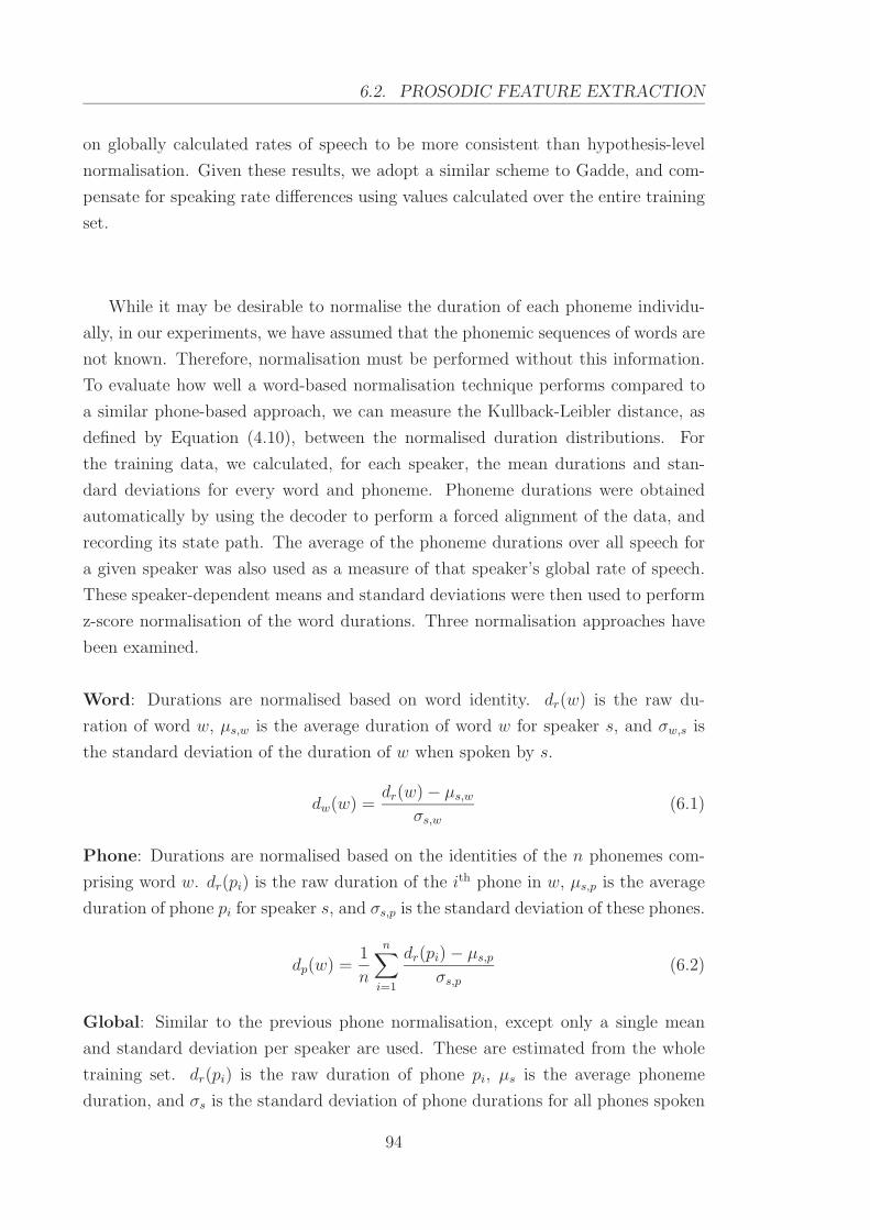
6.2. PROSODIC FEATURE EXTRACTION
on globally calculated rates of speech to be more consistent than hypothesis-level
normalisation. Given these results, we adopt a similar scheme to Gadde, and com-
pensate for speaking rate differences using values calculated over the entire training
set.
While it may be desirable to normalise the duration of each phoneme individu-
ally, in our experiments, we have assumed that the phonemic sequences of words are
not known. Therefore, normalisation must be performed without this information.
To evaluate how well a word-based normalisation technique performs compared to
a similar phone-based approach, we can measure the Kullback-Leibler distance, as
defined by Equation (4.10), between the normalised duration distributions. For
the training data, we calculated, for each speaker, the mean durations and stan-
dard deviations for every word and phoneme. Phoneme durations were obtained
automatically by using the decoder to perform a forced alignment of the data, and
recording its state path. The average of the phoneme durations over all speech for
a given speaker was also used as a measure of that speaker’s global rate of speech.
These speaker-dependent means and standard deviations were then used to perform
z-score normalisation of the word durations. Three normalisation approaches have
been examined.
Word: Durations are normalised based on word identity. dr(w) is the raw du-
ration of word w, µs,w is the average duration of word w for speaker s, and σw,s is
the standard deviation of the duration of w when spoken by s.
dw(w) =dr(w) − µs,w
σs,w
(6.1)
Phone: Durations are normalised based on the identities of the n phonemes com-
prising word w. dr(pi) is the raw duration of the ith phone in w, µs,p is the average
duration of phone pi for speaker s, and σs,p is the standard deviation of these phones.
dp(w) =1
n
n∑
i=1
dr(pi) − µs,p
σs,p
(6.2)
Global: Similar to the previous phone normalisation, except only a single mean
and standard deviation per speaker are used. These are estimated from the whole
training set. dr(pi) is the raw duration of phone pi, µs is the average phoneme
duration, and σs is the standard deviation of phone durations for all phones spoken
94

AUTOMATIC FEATURE EXTRACTION
Global Phone Word
0.274 0.236 0.177
Table 6.1: Average KL distances between word duration distributions for threedifferent normalisation schemes.
by speaker s.
dg(w) =1
n
n∑
i=1
dr(pi) − µs
σs
(6.3)
These normalised durations therefore provide estimates, at varying levels of gran-
ularity, of how much the duration of a word differs from its mean, after compensating
for speaking rate. Table 6.1 shows the KL distances between word duration distri-
butions in the training set for the three normalisation methods. This was calculated
as follows: First, the KL distance for each word was calculated as the average pair-
wise distance between a chosen speaker, and all other speakers. The KL distance
over the corpus was then taken to be the average of the word-specific KL distances,
weighted by the frequency of the word. Formally, this is:
Davg =1
n
∑
w
C(w)1
m
∑
i
D(p ‖ qi) (6.4)
where n is the number of samples, C(w) is the number of occurrences of word w, p
is the normalised duration distribution of word w for a reference speaker (we used
F1A) and the qi are normalised duration distributions of w for the remaining m
speakers.
The worst performing method, according to these results, is the global normal-
isation. Because this method only scales durations based on a single mean and
standard deviation calculated over the entire data, it cannot account for phoneme
or word specific differences between speakers. An example of this is illustrated in
Figure 6.1. This shows the duration distributions for the word state, spoken by two
speakers. Of the 6 speakers in the data, F2B had the slowest average speech rate,
at 14.0 phonemes/s, while M1B had the highest, at 15.2 phonemes/s.
The global and phone based approaches exhibited similar behaviour, and there is
a noticeable difference in the means of the distributions between the two speakers. A
breakdown of the duration means and standard deviations of each of the underlying
phones of state, which is composed of the sequence {/s/, /t/, /ey/, /t/}, for the two
speakers is shown in Table 6.2. The values for these phones, when they appear in
the context of the word state, are also shown.
95

6.2. PROSODIC FEATURE EXTRACTION
−0.6 −0.5 −0.4 −0.3 −0.2 −0.1 0 0.1 0.2 0.30
0.05
0.1
0.15
0.2
0.25
0.3
0.35
0.4
0.45
0.5
std devs
Global normalisation
f2bm1b
(a) Global normalisation
−1 −0.8 −0.6 −0.4 −0.2 0 0.2 0.4 0.6 0.80
0.05
0.1
0.15
0.2
0.25
0.3
0.35
0.4
std devs
Phone normalisation
f2bm1b
(b) Phone normalisation
−1.5 −1 −0.5 0 0.5 1 1.5 2 2.5 30
0.05
0.1
0.15
0.2
0.25
0.3
0.35
0.4
0.45
std devs
Word normalisation
f2bm1b
(c) Word normalisation
Figure 6.1: Speaker-dependent duration PDFs for the word state.
The higher speech rate of speaker M1B is reflected in the lower mean durations.
The global normalisation approach used a single mean and standard deviation value
per speaker, shown in the last row of Table 6.2, to normalise all phone durations.
How well this method normalises durations at the word level, then, is highly depen-
dent on the phone composition of the given word. For a word with a low proportion
of vowels, which typically have durations that are greater than the average, nor-
malisation using the corpus averages would tend to over-adjust the durations. This
results in a distribution with a negative mean, as can be seen in Figure 6.1(a). This
effect is particularly prominent for speaker F2B, where the average phone duration
over the corpus is substantially larger than the average durations of phones within
the word state. There are also some words for which F2B’s speech rate, at the
word level, was faster than that of M1B. In these instances, applying the global
96

AUTOMATIC FEATURE EXTRACTION
all words statePhone f2b m1b f2b m1b
/s/ 0.098 (0.033) 0.081 (0.029) 0.091 (0.021) 0.092 (0.027)/t/ 0.045 (0.027) 0.036 (0.025) 0.018 (0.008) 0.013 (0.006)/ey/ 0.134 (0.068) 0.126 (0.042) 0.124 (0.039) 0.129 (0.025)
average 0.072 (0.052) 0.066 (0.055) 0.061 (0.050) 0.059 (0.050)
Table 6.2: Means and standard deviations (in brackets) of z-score normalised phonedurations for the three phonemes in the word state. Scores for these phones, averagedover the entire data set, are shown on the left side, while the right side only considersthose phones which occur in the context of state. The bottom row shows the averagemeans and standard deviations for all phones.
normalisation would result in an increased distance between the distributions. This
occurred for roughly a third of the vocabulary, and accounted for 17% of the data.
As a result this approach provides little or no benefit for a considerable subset of
the data.
Phone-dependent normalisation improved on the performance of the global nor-
malisation. Unlike the global normalisation approach, the phone-dependent normal-
isation is able to account for duration differences in speech sound categories between
speakers. By modelling durations of the underlying phonemes, it can also take into
account the non-linear effect speaking rate has on word durations. Despite these ad-
vantages, this approach still under-performs the word-based normalisation. Figure
6.1(b) shows that, for the word state, the impact of this type of normalisation is very
similar to that of the global normalisation. Rather than being limited by the single
mean and variance, though, the main source of error lies with the differing behaviour
of the phoneme /t/ in this word compared to the more general case. Durations of
/t/, spoken in state, are much shorter than the average. Again, this results in an
inability to appropriately characterise mean durations.
Another reason for the inability to improve on the word normalisation result is
practical rather than theoretical. Because the phoneme duration statistics were cal-
culated using automatically aligned data, it is likely to contain segmentation errors.
A normalisation scheme based on phonemic information is highly sensitive to such
errors, and this contributes to the poor performance of this type of normalisation.
Therefore, while this approach may work well in theory, its need for accurate seg-
mental alignments will limit its benefit in some applications. Phoneme durations are
also affected by their surrounding phones, which may hinder estimation of normal-
ising parameters. This, however, can be addressed by the use of context-dependent
phonemes. Having separate acoustic models for stressed and unstressed vowels, as
97

6.2. PROSODIC FEATURE EXTRACTION
done by Wightman et al. [157], could also improve the automatic segmentation.
Of the three normalisation techniques, the word-based approach gave the best
results. This approach allows more detailed information about individual word char-
acteristics to be used than the global normalisation, while being less susceptible to
automatic alignment errors than phoneme normalisation. It can also be performed
using only word duration information, which is more readily obtainable than the du-
rations of underlying phonemes. One disadvantage of this approach is the potential
lack of training data. Duration estimates based on observations of rarely occurring
words are likely to be unreliable. To overcome this, means and standard deviations
of low count words can be estimated from the phonemes of the most common pro-
nunciation variant, and stored as word-based parameters. This alleviates the need
to have the phoneme sequence during recognition. Word-based normalisation of
durations will be used for the remainder of this work. Another drawback is that
the location of lengthening within a word is lost. This information would be useful,
in particular, for identifying the phrase-final lengthening that occurs in the final
syllable.
6.2.2 Fundamental frequency
Fundamental frequency (F0) is closely related to pitch. To represent pitch informa-
tion, we use automatically extracted F0 values provided by the Entropic XWaves
get f0 tool. This is an implementation of Talkin’s pitch tracking algorithm [54], and
calculates the following data at intervals of 10 ms:
• F0
• Probability of voicing
• RMS energy
A number of post-processing steps, similar to those described by Taylor [97], are
performed on this raw pitch contour. Firstly, a 7 point median filter is applied to
eliminate any clear pitch tracking errors. Small perturbations in the F0 contour,
which are unimportant in prosodic analysis [158], are also removed by this filtering.
Ideally, this process should retain the macroscopic movements in the contour. To
obtain a continuous pitch contour, which is a more desirable representation of in-
tonation, unvoiced regions are linearly interpolated. The continuous pitch contour
is smoothed using a 15 point median filter and finally, normalisation is performed
according to the following:
F0z(t) =F0(t) − µ
σ
98
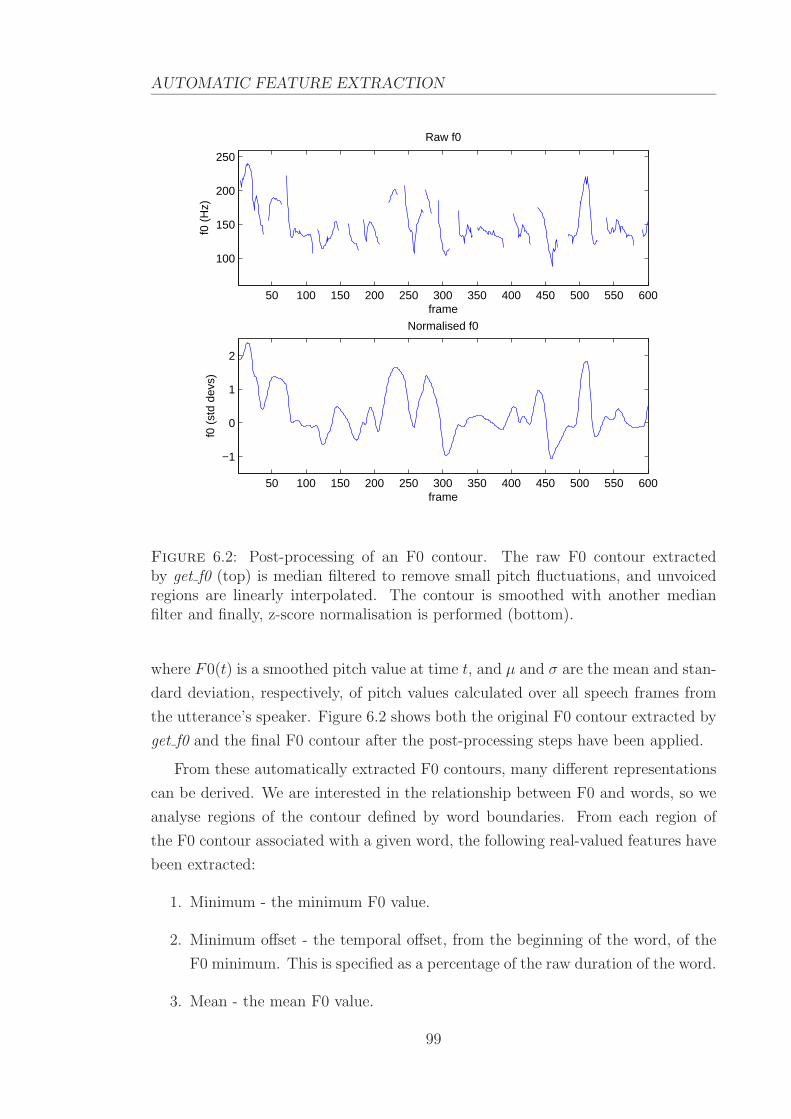
AUTOMATIC FEATURE EXTRACTION
50 100 150 200 250 300 350 400 450 500 550 600
100
150
200
250
frame
f0 (
Hz)
Raw f0
50 100 150 200 250 300 350 400 450 500 550 600
−1
0
1
2
frame
Normalised f0
f0 (
std
devs
)
Figure 6.2: Post-processing of an F0 contour. The raw F0 contour extractedby get f0 (top) is median filtered to remove small pitch fluctuations, and unvoicedregions are linearly interpolated. The contour is smoothed with another medianfilter and finally, z-score normalisation is performed (bottom).
where F0(t) is a smoothed pitch value at time t, and µ and σ are the mean and stan-
dard deviation, respectively, of pitch values calculated over all speech frames from
the utterance’s speaker. Figure 6.2 shows both the original F0 contour extracted by
get f0 and the final F0 contour after the post-processing steps have been applied.
From these automatically extracted F0 contours, many different representations
can be derived. We are interested in the relationship between F0 and words, so we
analyse regions of the contour defined by word boundaries. From each region of
the F0 contour associated with a given word, the following real-valued features have
been extracted:
1. Minimum - the minimum F0 value.
2. Minimum offset - the temporal offset, from the beginning of the word, of the
F0 minimum. This is specified as a percentage of the raw duration of the word.
3. Mean - the mean F0 value.
99

6.2. PROSODIC FEATURE EXTRACTION
15.1 15.15 15.2 15.25 15.3 15.35 15.4 15.45−0.2
0
0.2
0.4
0.6
0.8
t
f0 (
std
devs
)
1
3
y=mx+b
2
4
5
6
7
Figure 6.3: F0 features derived from the automatically extracted pitch contour.Dotted vertical lines indicate word boundaries.
4. Maximum - the maximum F0 value.
5. Maximum offset - the temporal offset of the F0 maximum.
6. Range - the difference between the maximum and minimum values.
7. Slope - the gradient of the least squares regression line fitted over the specified
region.
8. Voicing percentage - the proportion of frames which are voiced.
These features are illustrated in Figure 6.3. There is likely some redundancy in this
set of features; however, for this analysis, we are primarily interested in a complete
description of the contour rather than obtaining a compact representation.
A potential shortcoming of the previously described features is their very fine
granularity. Typically, it is variations such as rises and falls in these values which are
indicative of prosodic events, rather than the actual values themselves. Small differ-
ences may not only be meaningless, but could also introduce errors into a classifier.
Therefore, these features naturally lend themselves to some form of quantisation.
Here, we propose to extend the feature set with some additional discrete features
based on the following identities:
100

AUTOMATIC FEATURE EXTRACTION
• Rise - a sequence of at least 5 consecutive frames (50 ms) having a gradient
greater than a given threshold.
• Fall - a sequence of at least 5 consecutive frames having a gradient lower than
a given threshold.
• Peak - a point which lies between a rising segment on the left, and a falling seg-
ment on the right. If a peak exists, the surrounding regions are not considered
to be rises or falls.
• Trough - a point lying between a falling segment on the left and a rising
segment on the right. This is the opposite of a peak.
Features are then defined as the counts of each of these patterns in the region of
the F0 contour specified by the given word boundaries. These features attempt
to more concisely represent meaningful patterns in the F0 contour. Accentuation is
associated with syllables, and extracting features such as minima or maxima directly
from the contour over word regions may give inconsistent results. Polysyllabic words,
in particular, could interfere with the reliability of those features. By identifying
and counting occurrences of specific patterns in a given region, on the other hand,
the discrete features should be able to better handle these cases. The threshold for
the gradient used in the discrete features was chosen to be ± 0.1 standard deviations
per frame. While it is certainly possible for both the gradient threshold and number
of frames defining an event to be tuned, the precise methods by which this can be
done, and the criteria to optimise, is not obvious. We have therefore simply left
these as fixed values.
6.2.3 Energy
The F0 extraction tool, get f0, provides RMS energy estimates in addition to F0.
Energy is closely related to perceived loudness, so the same extraction and post-
processing steps used for F0 are applied here. Similarly, the same set of features are
extracted from the energy contour, with the exception of the voicing feature as it is
not applicable in the case of energy.
101
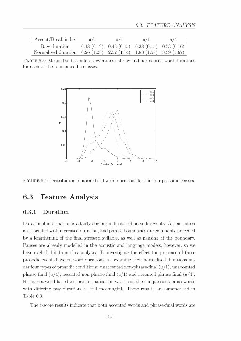
6.3. FEATURE ANALYSIS
Accent/Break index u/1 u/4 a/1 a/4
Raw duration 0.18 (0.12) 0.43 (0.15) 0.38 (0.15) 0.53 (0.16)Normalised duration 0.26 (1.28) 2.52 (1.74) 1.88 (1.58) 3.39 (1.67)
Table 6.3: Means (and standard deviations) of raw and normalised word durationsfor each of the four prosodic classes.
−4 −2 0 2 4 6 8 100
0.05
0.1
0.15
0.2
0.25
Duration (std devs)
p
u/1u/4a/1a/4
Figure 6.4: Distribution of normalised word durations for the four prosodic classes.
6.3 Feature Analysis
6.3.1 Duration
Durational information is a fairly obvious indicator of prosodic events. Accentuation
is associated with increased duration, and phrase boundaries are commonly preceded
by a lengthening of the final stressed syllable, as well as pausing at the boundary.
Pauses are already modelled in the acoustic and language models, however, so we
have excluded it from this analysis. To investigate the effect the presence of these
prosodic events have on word durations, we examine their normalised durations un-
der four types of prosodic conditions: unaccented non-phrase-final (u/1), unaccented
phrase-final (u/4), accented non-phrase-final (a/1) and accented phrase-final (a/4).
Because a word-based z-score normalisation was used, the comparison across words
with differing raw durations is still meaningful. These results are summarised in
Table 6.3.
The z-score results indicate that both accented words and phrase-final words are
102
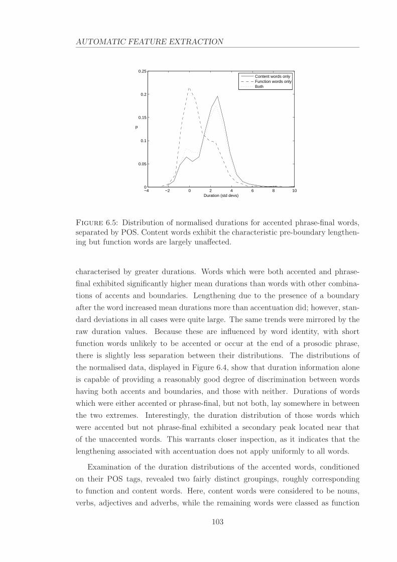
AUTOMATIC FEATURE EXTRACTION
−4 −2 0 2 4 6 8 100
0.05
0.1
0.15
0.2
0.25
Duration (std devs)
p
Content words onlyFunction words onlyBoth
Figure 6.5: Distribution of normalised durations for accented phrase-final words,separated by POS. Content words exhibit the characteristic pre-boundary lengthen-ing but function words are largely unaffected.
characterised by greater durations. Words which were both accented and phrase-
final exhibited significantly higher mean durations than words with other combina-
tions of accents and boundaries. Lengthening due to the presence of a boundary
after the word increased mean durations more than accentuation did; however, stan-
dard deviations in all cases were quite large. The same trends were mirrored by the
raw duration values. Because these are influenced by word identity, with short
function words unlikely to be accented or occur at the end of a prosodic phrase,
there is slightly less separation between their distributions. The distributions of
the normalised data, displayed in Figure 6.4, show that duration information alone
is capable of providing a reasonably good degree of discrimination between words
having both accents and boundaries, and those with neither. Durations of words
which were either accented or phrase-final, but not both, lay somewhere in between
the two extremes. Interestingly, the duration distribution of those words which
were accented but not phrase-final exhibited a secondary peak located near that
of the unaccented words. This warrants closer inspection, as it indicates that the
lengthening associated with accentuation does not apply uniformly to all words.
Examination of the duration distributions of the accented words, conditioned
on their POS tags, revealed two fairly distinct groupings, roughly corresponding
to function and content words. Here, content words were considered to be nouns,
verbs, adjectives and adverbs, while the remaining words were classed as function
103

6.3. FEATURE ANALYSIS
words. This distinction is illustrated in Figure 6.5, in which the distribution of
accented, non-phrase-final words has been further partitioned based on their POS
labels. It can be seen that introducing this distinction largely accounts for the
two dominant peaks that appear in the combined distribution. This highlights the
importance of considering syntax in investigations of prosody, as the two are closely
related. Individually, POS and duration information both provide useful cues to
determining the prosodic state of a given word. Using both knowledge sources in
conjunction, though, can further improve the discriminative ability through their
interaction. This, in fact, is similar to the results of Section 5.2, in which positive
interaction information was found between word identity, prosodic information and
POS.
6.3.2 F0 and RMS energy
Results of a similar analysis of the real-valued voicing, F0 and energy features are
presented in Table 6.4. The values in the first row, showing the percentage of
voiced frames in a word, are slightly higher for accented words than their unac-
cented variants. Accentuation tends to increase a word’s duration, and typically it
is the durations of (voiced) vowels which undergo the greatest lengthening. This
explanation, however, does not account for the contrary behaviour observed with
the phrase-final words. For both accented and unaccented words, the percentage
of voiced frames was lower when the word was followed by a boundary than when
there was no boundary. Boundaries generally cause a lengthening of the preceding
word, and the statistics in Table 6.3 indicate the magnitude of this lengthening is
even greater than that of accentuation. The pre-boundary lengthening, then, would
appear to affect unvoiced sounds to a greater degree than lengthening caused by
accentuation. It is also possible that the occurrence of phonemes in the last syllable
of phrase-final words, where lengthening is most pronounced, is skewed towards un-
voiced sounds. In our data, the high frequency of the unvoiced fricative /s/ in these
syllables could contribute to the reduced percentage of voiced frames.
The results for the slope feature were almost identical irrespective of the prosodic
events associated with the given word. Additionally, the low standard deviations of
this feature suggest that the values are consistently very small. A likely explanation
for this is that a regression line can be quite a poor fit of the data, even if its purpose
is only to be an estimate of the gradient. A common realisation of the H* pitch
accent involves a rise-fall movement of the pitch contour, such as that shown in
Figure 6.6. The linear approximation to this type of data would completely fail to
104

AUTOMATIC FEATURE EXTRACTION
Accent/Break index u/1 u/4 a/1 a/4
Voicing% voiced 0.72 (0.26) 0.62 (0.20) 0.72 (0.19) 0.68 (0.18)
F0min -0.43 (0.82) -1.53 (1.00) -0.36 (0.83) -1.31 (0.92)
min offset 0.52 (0.38) 0.54 (0.28) 0.46 (0.43) 0.65 (0.32)mean -0.10 (0.68) -0.70 (0.70) 0.38 (0.64) -0.15 (0.58)max 0.21 (0.71) 0.21 (0.75) 0.87 (0.73) 0.80 (0.71)
max offset 0.40 (0.40) 0.40 (0.43) 0.49 (0.27) 0.39 (0.27)range 0.64 (0.67) 1.74 (1.00) 1.23 (0.85) 2.11 (1.01)slope 0.03 (0.07) 0.03 (0.04) 0.03 (0.04) 0.03 (0.03)
RMSmin -0.48 (0.70) -1.04 (0.62) -0.69 (0.66) -1.01 (0.59)
min offset 0.51 (0.38) 0.62 (0.37) 0.45 (0.38) 0.62 (0.39)mean 0.15 (0.50) -0.03 (0.45) 0.33 (0.42) 0.20 (0.40)max 0.56 (0.46) 0.58 (0.39) 0.90 (0.35) 0.89 (0.35)
max offset 0.42 (0.32) 0.35 (0.28) 0.45 (0.22) 0.37 (0.20)range 1.04 (0.68) 1.63 (0.53) 1.59 (0.63) 1.91 (0.54)slope 0.02 (0.09) 0.02 (0.04) 0.02 (0.04) 0.02 (0.03)
Table 6.4: Means (and standard deviations) of voicing, F0 and RMS energy featuresfor the four combinations of pitch accent and break index.
capture any relevant information about the contour, instead giving a gradient which
is close to zero. Another reason is that there may be more than one pitch movement
associated with polysyllabic words. In these cases, the regression line can only
provide an estimate of the net movement in F0 across the entire word. Therefore,
the average gradient of the F0 contour using a word-based analysis window often
does not contain any meaningful information.
The features sampled directly from the contour displayed varying properties de-
pending on their prosodic class. Pitch accents are often associated with local peaks
in the F0 contour, and this is reflected in the higher F0 mean and maxima of ac-
cented words. The equivalent energy features also were greater for these words.
Minimum F0 and energy values were not significantly affected by a word’s accen-
tuation. Boundaries, on the other hand, did decrease the average values of the F0
and energy minima, and this is consistent with the final lowering observed in declar-
ative speech [159]. The lowering in words preceding boundaries is also evident in
the mean results, which was generally lower for unaccented phrase-final words than
other types. Mean values for unaccented non-phrase-final and accented phrase-final
words were quite similar due to the opposing influences of boundaries and accents.
105

6.3. FEATURE ANALYSIS
7.35 7.4 7.45 7.5 7.55 7.6 7.65 7.7 7.75 7.8−0.6
−0.5
−0.4
−0.3
−0.2
−0.1
0
0.1
t
f0
Figure 6.6: A typical rise-fall F0 pattern occurring during the word reaches, andthe (dotted) least squares regression line fitted over the region.
While F0 values tend to fall in the presence of a boundary, accentuation is typically
associated with a local maximum. The combination of these two effects results in
means which are not much different from that of words without any prosodic event.
The actual contours themselves, though, are not necessarily similar. This can be
seen in the differences in the minimum and maximum values for each combination
of prosodic events. The range values too, which increased with both accents and
boundaries, support this interpretation. In the case of accents, this is largely due to
the increase in maxima caused by sharp pitch and energy rises, while the decreased
minima caused by final lowering similarly contributes to an increase in the range
over the region of the word.
The two offset features, specifying the times at which the minima and maxima
occur within the word have a relatively small range between the classes. In unac-
cented words, there was no observable difference in these offset values. Accented
words displayed greater variability, with minima occurring later if the word was
phrase-final, and earlier otherwise. F0 maxima also tended to occur later for ac-
cented phrase-final words. While these features do have lower standard deviations
in comparison to the other feature types, giving them increased reliability, on the
whole they provide only minimal beneficial information.
The RMS slope feature, like its F0 equivalent, did not provide much discrimina-
tory information, probably for the same reasons. The remaining features behaved
similarly to the F0 features, but exhibited smaller variation in general. There is a
106

AUTOMATIC FEATURE EXTRACTION
Accent/Break index u/1 u/4 a/1 a/4
F0rise 0.26 (0.45) 0.66 (0.51) 0.34 (0.50) 0.50 (0.54)fall 0.35 (0.49) 0.39 (0.55) 0.66 (0.51) 0.57 (0.56)
peak 0.05 (0.22) 0.16 (0.39) 0.55 (0.53) 0.73 (0.51)trough 0.06 (0.25) 0.58 (0.53) 0.15 (0.38) 0.52 (0.57)
RMSrise 0.21 (0.42) 0.22 (0.45) 0.28 (0.47) 0.17 (0.40)fall 0.50 (0.55) 1.02 (0.64) 0.90 (0.64) 1.22 (0.65)
peak 0.19 (0.43) 0.71 (0.70) 0.75 (0.66) 1.04 (0.67)trough 0.11 (0.33) 0.54 (0.64) 0.44 (0.61) 0.60 (0.69)
Table 6.5: Means (and standard deviations) of quantised F0 and RMS energyfeatures for the four combinations of pitch accent and break index.
strong positive correlation between these F0 and energy features, with classes which
were characterised by higher F0 invariably having higher energy. This is to be ex-
pected, as both types of prosodic events often involve changes in F0 and energy
occurring in the same direction. Like their F0 counterparts, the RMS offset features
also provided little discriminative information.
In contrast to the poor discriminative ability of the slope feature, the quantised
F0 rise and fall features demonstrated substantially different behaviour depending
on prosodic class. These results, as well as those for the peak and trough features,
are shown in Table 6.5. This shows a number of differences between F0 and en-
ergy. While this set of F0 features was quite good at capturing the accented versus
unaccented and boundary vs non-boundary words, the equivalent energy features
provided less distinction. This approach, therefore, seems to be an appropriate way
of encoding F0 information. In the case of energy, the discrimination provided by
these features are less evident. Because the energy contour is influenced to a greater
degree by segmental identity, its correlation to prosodic events is weaker. Locating
specific patterns in this contour, then, is of less value than it is for F0; however,
they still contribute some useful information.
As expected, the ability to identify the rise-fall and fall-rise patterns, particularly
in F0 contours, was useful for separating words of differing prosodic classes. F0 peaks,
especially, showed quite distinct values for every class. In general, accented words
contained considerably more peaks than unaccented words, and the occurrence of
troughs was increased by the presence of a phrase boundary. It is also important
that these particular F0 patterns be distinguished from simple rises and falls, which
the results indicate are affected differently by accents and boundaries. By counting
107
6.4. SUMMARY
occurrences of these specific patterns rather than attempting to fit a function to the
whole contour segment, these features also provide more meaningful results when
there is more than a single intonational event in the region under consideration.
This is particularly useful when dealing with polysyllabic words, which may have
multiple weaker accents in addition to the primary accent.
6.4 Summary
In this chapter, we have described methods for extracting duration information and
fundamental frequency and RMS energy contours. These are all highly speaker de-
pendent, and an important consideration in their use is normalisation. For duration,
we have found a simple word-based z-score normalisation to perform well, despite
it being unable to capture the non-linear effect that speaking rate has on word du-
rations. Phoneme-based normalisation, while theoretically superior, was hindered
by the use of automatic segmentation and the lack of lexical stress modelling in
our acoustic models. Z-score normalisation was also used to normalise for speaker-
specific means and dynamic ranges of F0 and energy values. This normalisation was
performed after post-processing the contours to smooth and interpolate them.
Representing all values in terms of standard deviations from their means allows
for a comparison of the normalised values across different words. A number of
features were derived from the duration information and F0 and energy contours.
In addition to the real-valued features obtained directly from these sources, we also
proposed a quantisation scheme for the F0 and energy contours. These quantised
features were designed to identify specific patterns in the contours, and could be used
to produce meaningful statistics for polysyllabic words that potentially contained
more than a single prosodic event.
An analysis of the relationship between the acoustic-prosodic parameters and the
occurrences of accents and boundaries in words showed a number of correlations.
The most relevant features for distinguishing between the prosodic classes, and their
relationship to these classes, are summarised in Table 6.6. Most of the features ex-
amined here contributed some useful information to the distinction between events,
though there is significant redundancy in the full feature set. Of particular note
are the results of the quantised features, which were very effective at characterising
differences in the F0 contours associated with the various prosodic events. This is
largely due to the explicit identification of the rise-fall and fall-rise patterns which
commonly occur in the F0 contour. The final set of duration, F0 and energy features
should serve to provide good discrimination between the prosodic classes.
108

AUTOMATIC FEATURE EXTRACTION
Accent/Break index u/1 u/4 a/1 a/4
raw duration L Hnormalised duration L H
% voiced LF0 min L LF0 mean L HF0 max H HF0 range L H HF0 rise H HF0 fall H H
F0 peak H HF0 trough H HRMS min L L
RMS mean LRMS max H HRMS range L HRMS rise HRMS fall L H
RMS peak L HRMS trough L
Table 6.6: Relationship between prosodic events and automatically extracted fea-tures. Entries for which a feature is useful for determining the prosodic class aremarked as either H (indicating the mean feature value is higher than average) or L(lower than average).
109

110

Chapter 7
Language Modelling with Raw
Features
The language models derived thus far have relied on the presence of manually tran-
scribed prosodic labels. A major drawback of this is the fact that the transcriptions
are costly and time-consuming to develop. Even corpora developed for research
purposes are very limited in terms of prosodic annotations, and these transcriptions
will be unavailable in practice. A language model incorporating prosodic informa-
tion will therefore have to make use of automatically extracted features to be of any
practical benefit. If a small set of prosodically labelled data is accessible, models
can be trained to perform automatic transcription. If no such data can be obtained,
fully automated procedures need to be considered.
This chapter will describe the construction of language models using both ap-
proaches. The first section of this chapter will discuss how non-binary features
such as the automatically extracted prosodic features derived in Chapter 6 can be
incorporated into maximum entropy models. It will cover the advantages and dis-
advantages of each of the alternatives, and describe the method to be used in these
experiments. The second section will introduce dimensionality reduction techniques,
and discuss why they are relevant for the prosodic features. In particular, it will
focus on the Locality Preserving Projection and how the properties of this technique
are useful for the current task. In the third section, the construction of a maximum
entropy model used to annotate word sequences is detailed. This model is also used
to transcribe the N-best output of a recogniser, which is then rescored by a language
model employing ToBI features. The fourth section of this chapter will consider the
direct usage of raw prosodic information in the language model. This makes the
assumption that no transcribed data is available at all. Model features are derived
which can compactly encode both the prosodic state of a given word and its re-
111

7.1. HANDLING NON-BINARY FEATURES
cent history. The effectiveness of these features are evaluated and compared against
manually transcribed features. A summary of the findings will be presented in the
final section.
7.1 Handling Non-Binary Features
7.1.1 Real-valued features
In the maximum entropy models described so far, only binary-valued features have
been considered. The prosodic information extracted in Chapter 6, however, consists
of both integer and real-valued features. There are a few common approaches to
dealing with these types of features. In general, the maximum entropy framework
does not preclude the use of real-valued features, and these can simply be included
directly into a model. An integer feature f(h,w) = n is equivalent to n occurrences of
the binary feature f(h,w) = 1, with the feature becoming inactive when n = 0. For
our count-based features, namely rises, falls, peaks and troughs, this interpretation is
quite sensible. Real-valued features can also be considered to be a further extension
of this to non-integer values.
For the special case when the feature values are logarithms of conditional prob-
abilities (i.e. fi(h,w) = log pi(w|h)), incorporating such features is equivalent to a
log-linear combination of the component distributions [160]. The greatest advantage
of introducing the additional models pi(h|w), is the potential for decreasing the pa-
rameter count. A probability distribution defined on a subset of H×W can be used
to encapsulate multiple binary features. Under this approach, the binary features
themselves can be interpreted as probability distributions, each having a support of
a single event [161]. Using the intermediate distributions allows for information to
be incorporated which would otherwise lead to an intractable model.
This approach, however, introduces an additional level of complexity, as it re-
quires the use of an appropriate model p(h|w). There is also a problem with the
potential loss of information as a result of the reduction of the original feature space
into a single probability measure. By performing model combination, rather than
feature combination, the maximum entropy model’s ability to appropriately weight
information is fundamentally restricted. The contributions of individual pieces of
evidence are determined by the intermediate model, and are not subject to the
maximum entropy criterion. Furthermore, if ML estimation is used to calculate the
distribution p(w|h), it may also be necessary to consider smoothing. If the context,
h, provides only limited information on the target to be classified, the probability
112

LANGUAGE MODELLING WITH RAW FEATURES
estimates may also be prone to error. In these cases, it may be beneficial to provide
the full set of features to the model, thus allowing it to perform feature selection
and parameter estimation in conjunction with other model features.
7.1.2 Quantisation
An alternative to handling real-valued features is quantisation. Under this approach,
all real values falling within a specified range are considered to belong to the same
bin, and each bin is treated as a unique binary feature. This can be advantageous if
minor differences in the real-valued data are relatively unimportant, as is normally
the case with acoustic-prosodic features. Grouping similar values together into a
single equivalence class can allow more robust estimates to be obtained if the range of
prosodic feature values spanned by the bin have the same influence on the modelled
target. Choosing appropriate values for the number of bins, their sizes, and the
mapping from real values to bins are an important part of the quantisation process.
However these parameters depend on the specific nature of the data, and finding
optimal values is generally not a simple task. Selecting too many bins can result in
problems of sparsity and over-training, while using too few bins can mask patterns
in the data. For the mapping issue, uniform occupancy binning has been found to
perform well for spectral features in maximum entropy acoustic models [162].
A major disadvantage of the quantisation approach is the increase in parame-
ter count. Partitioning a real valued feature into n bins results in an additional
(n − 1) × |W | possible features to the model. This is a serious issue for maximum
entropy models, which have computationally expensive parameter estimation proce-
dures. Another drawback of this approach is the inability to encode the relationship
between bins. By binning the features, the model loses information relating to the
actual values specified by the bins. For example, instances of a feature f(h,w) = 2
and f(h,w) = 3 may be considered to be close, while f(h,w) = 8 represents a
drastic difference. If each of these features belong to separate bins, however, this
relationship cannot be captured.
In our experiments, we have chosen to incorporate the non-binary features di-
rectly into the model, primarily due to the simplicity of this technique. It also
results in fewer parameters than quantisation, and does not require selection of bin-
ning parameters. Although using probabilities as features can further decrease the
number of parameters, we believe allowing the full level of feature interaction to be
preferable. We will investigate other methods for reducing the parameter count in
the next section.
113

7.2. DIMENSIONALITY REDUCTION
7.2 Dimensionality Reduction
The prosody extraction process described in Chapter 6 provides a set of 19 integer
and real-valued features describing the prosodic context of each word. Although it
is possible to incorporate these directly as model features, there are some disadvan-
tages to doing so. The first is that these features are likely to contain a high level
of redundancy. As noted in the previous chapter, a number of these features exhibit
very similar patterns with respect to prosodic classes. For instance, high F0 and
energy maxima are both correlated with pitch accents. Intuitively, merging these
into a single feature could result in a more compact representation with minimal
loss of information. In addition, compressing the feature space can provide a gen-
eralisation of the original data. The automatically extracted features are subject
to a variety of estimation errors. Minor perturbations caused by these inaccuracies
can be considered to be noise, and may negatively affect classifier performance. If
these effects can be removed or ignored, a more accurate model of the data, and
any patterns it exhibits, could be obtained. Even if some useful information is lost
by reducing the number of features, this trade-off may be worthwhile if the features
are to be used in models, such as the maximum entropy model, which are expensive
to train.
To a lesser extent, the curse of dimensionality also motivates the use of lower
dimensional features. While the dimensionality of our particular problem is much
smaller than that encountered in other NLP problems, such as document clustering,
it is heavily reliant on the use of distance metrics as indicators of similarity between
features. Increasing the dimension of a space leads to an exponential increase in
volume. As a result, points in high-dimensional spaces tend to become equidistant,
thus making automatic learning based on distances difficult. For the same reason,
the sparsity of a fixed amount of data also increases exponentially, introducing
additional problems for statistical models.
7.2.1 Linear dimensionality deduction
Dimensionality reduction methods can be broadly categorised into linear and non-
linear approaches. Linear techniques such as Principal Components Analysis (PCA)
and Linear Discriminant Analysis (LDA) project data onto subspaces by forming
linear combinations of the data vectors. One of the biggest advantages of these ap-
proaches is their low computational cost. However, they cannot accurately represent
data that are non-linearly embedded in the high dimensional space. Many techniques
have been proposed to deal with such data (see van der Maaten et al. [163] for a
114
LANGUAGE MODELLING WITH RAW FEATURES
review). These are able to find more complex structures in the data, but suffer from
higher computational costs. In addition, while they perform very well for artificial
data sets, they often fail to significantly outperform linear techniques on real world
data [163]. The subspace mappings generated by some non-linear techniques are also
defined only on training data. For applications which require unknown points to be
projected onto the subspace, such techniques are inappropriate. This is the case
for our task, in which predictions need to be made based on the prosodic context
of unseen samples. For these reasons, we will focus only on linear dimensionality
reduction methods.
In linear dimensionality reduction, data in the original space are approximated
as linear combinations of a set of lower dimensional basis vectors. A set of d-
dimensional data points, X = {x1,x2, . . . ,xn}, can be mapped onto an r-dimensional
(r < d) subspace through the use of a d × r transformation matrix A:
yi = ATxi (7.1)
where yi is the lower dimensional representation of xi. The choice of A can be
guided by a variety of criteria, and this choice will affect the resulting data and
its properties. PCA, for example, selects the set of orthogonal basis functions that
maximises the retention of data variance. Assuming the samples of X are centred
about the origin (which can be achieved by subtracting the column means from X)
the linear mapping a is chosen to maximise:
a∗ = arg maxa
aT XXTa
subject to aTa = 1. The principal components forming the columns of A can be
calculated as the leading eigenvectors of the sample covariance matrix XXT . A
transformed sample, y = ATx, is then the closest approximation to x in the least-
squares sense.
By retaining the greatest possible variance, PCA provides the optimal linear
transformation for data reconstruction. For the purposes of classification, though,
this is not necessarily the desired outcome. If multiple classes exhibit strong vari-
ations in the same direction, that direction will have a higher corresponding eigen-
value than those directions which provides more discrimination between the classes.
Because directions of lower variance are considered to be less important by PCA,
potentially useful information may be discarded by selecting only the principal eigen-
vectors.
115
7.2. DIMENSIONALITY REDUCTION
7.2.2 Locality Preserving Projections
A more recently proposed approach to linear dimensionality reduction is the Locality
Preserving Projection (LPP) [164]. This technique differs to PCA in that it attempts
to retain the local structure of the space. In LPP, the optimising criterion requires
the minimisation of the objective function:
a∗ = arg mina
∑
i
∑
j
(aTxi − aTxj)2Sij
Sij encodes the similarity between points xi and xj, and the set of these values
forms the similarity matrix, S. If two points have high similarity, then this function
penalises mappings which result in a large distance between their transformations.
This ensures that any points which are close to each other in the original space
remain close after the projection. The transformation is found by solving the gen-
eralised eigenvalue problem:
XLXTa = λXDXTa
where L = D−S, and the entries of the diagonal matrix D are given by Dii =∑
j Sij.
L is also the graph Laplacian [165], and the LPP solution is a linear approximation
of the non-linear Laplacian Eigenmap technique [166]. The transformation matrix,
A, comprises the eigenvectors corresponding to the r lowest eigenvalues. In practice,
a PCA usually needs to be performed as a pre-processing step to ensure XDXT is
non-singular.
The similarity matrix, S, is calculated from an adjacency graph of the data.
Each node in the graph corresponds to a data point, and node nj is connected to
node ni by an undirected arc if the point xj is one of the k nearest neighbours of xi
in the original space. An entry in the similarity matrix, Sij, is the weight of the arc
connecting ni and nj. Sij is zero if the respective nodes are unconnected. Obtaining
S therefore requires the following to be defined:
• The similarity metric between two points.
• The number of nearest neighbours, k.
• The weighting function for arcs.
To measure the similarity between points, represented as vectors in the original
prosody space, we have used the cosine similarity function commonly employed in
document clustering and information retrieval applications. The cosine similarity
116

LANGUAGE MODELLING WITH RAW FEATURES
between two vectors, xi and xj, is given by:
cosim(xi,xj) = cos(xi,xj) =xi · xj
|xi||xj|(7.2)
The choice of k dictates the degree of localisation of the resulting projection. For
a small value of k, the graph will only capture information within a very limited
neighbourhood. A large k incorporates more global structure, and LPP performed
using a complete graph bears a resemblance to PCA [167]. Finally, the magnitude of
the similarity between two points is encoded as the cosine similarity between their
respective points. A number of other approaches for selecting parameters in the
construction of the graph, as well as weighting its links, have been investigated by
Cai et al. [167].
7.3 Prosody Labelling
The language models developed in Chapter 5 required words to be explicitly tran-
scribed with ToBI labels. Because this process involves human input, it will not be
available in most cases. In order to be of practical use, then, the data need to be la-
belled by some unsupervised means. Here, we will investigate the use of the prosodic
information extracted in Chapter 6 for the purpose of automatic annotation.
The required task of the automatic transcription system is to take, as input,
some context, h, and output its prosodic label p, while making use of various lexical,
syntactic and acoustic-prosodic knowledge sources. The word sequence is assumed
to be known, although it may contain errors if recogniser output is used. The
possible outputs of our labelling system are the same four prosodic classes, P =
{u/1, u/4, a/1, a/4}, used in the previous chapter’s analyses. The labelling can be
formulated as the classification problem:
p = arg maxp∈P
p(p|h) (7.3)
To perform this classification, we used maximum entropy models trained to calculate
p(pi|h1, . . . , hi). The context at position i is the tuple:
hi = (wi, si,xi)
where wi is the word to be labelled, si is its POS label and xi is the vector of
duration, F0 and energy parameters described in Chapter 6. The feature functions
used by these models will be detailed in Section 7.3.2.
117

7.3. PROSODY LABELLING
7.3.1 Baseline model
Lexical information such as a word’s surface form, as well as its POS tag, already
provide a significant amount of information about its prosodic class. To examine
the additional contribution of the prosodic features, we compare models to a base-
line constructed using only this textual information. The baseline model uses the
following word and POS feature types:
fw(h,w) =
{
1 : if w = wi and wii−m ∈ h
0 : otherwise(7.4)
fs(h,w) =
{
1 : if w = wi and sii−m ∈ h
0 : otherwise(7.5)
for 0 ≤ m ≤ 2. These resemble the standard n-gram and POS features used in
Chapter 5; however, they differ by also including information obtained from the
current word.
7.3.2 Prosodic model features
For every word in the training set, an acoustic-prosodic feature vector was con-
structed according to the procedure documented in Chapter 6. These samples were
then projected onto a linear subspace determined by LPP. The similarity matrix
used in LPP is very large (n×n), so only a subset (of approximately 5000 samples)
of the data was used to obtain the transformation matrix. The prosodic feature
vectors we used contain a diverse set of information derived from varying sources,
and some dimensions are more prone to variation than others. We have therefore
chosen a fairly high number of nearest neighbours (k = 50) when constructing the
adjacency graph in order to ensure that it is not localised only to those dimensions
with low variance.
The values of the prosodic feature vectors, extracted using the hypothesised
boundaries of word wi and projected onto the LPP subspace, yi, were then incor-
porated into the model as the following maximum entropy features:
fl(h,w) =
{
yil : if w = wi
0 : otherwise(7.6)
yil is the value of yi along the lth axis for l = 1, . . . , r and where r, as defined in
Section 7.2.2, is the reduced number of dimensions after performing the LPP. Each
feature in the model represents the position of a word’s prosodic vector in a single
118

LANGUAGE MODELLING WITH RAW FEATURES
Dimensions Pitch accent Break index Combined
chance 53.59 80.41 38.65baseline 84.93 88.34 75.99AP11 86.24 90.71 78.88AP19 86.90 90.84 79.54L1 85.06 87.95 75.99L2 85.54 88.12 76.38L3 85.80 88.34 76.86L4 85.93 88.39 77.08L5 86.90 88.39 77.74L6 86.77 90.23 78.88L7 86.77 90.80 79.49L8 87.25 90.89 80.06
L9 86.68 90.36 79.23
Table 7.1: Pitch accent and break index classification accuracies using prosodicfeatures and LPP dimensionality reduction.
dimension, giving a total of r features per class.
7.3.3 Results
Classification experiments were conducted with a number of different types of lan-
guage models. The baseline model used only the textual features described in Section
7.3.1. Two models were trained using the acoustic-prosodic features in the original
space, incorporated using the feature function defined by Equation (7.6). Model
AP11 used the 11 real-valued parameters only, while model AP19 used the full 19-
dimensional parameter vector. These were used in addition to the features of the
baseline. In the third type of model, the set of 19 prosodic features were replaced
by their lower dimensional subspace projections. The values chosen for r in these
LPP models ranged from 1 through to 9, corresponding to models L1 to L9, respec-
tively. The performance of the models in this experiment were relatively insensitive
to the type and variance of the prior, so all reported results have been obtained
using inequality constraints (cf. Equation (4.13)) and a fixed width of W = 0.001.
Classification accuracies for pitch accents alone, break indices alone, and the
combined accent and break index labels are shown in Table 7.1. These were cal-
culated simply as the number of correctly recognised labels as a proportion of the
total number of labels. Only one joint classification was performed, and the results
for the individual label types were obtained by ignoring the classification outcome
of the other label.
119

7.3. PROSODY LABELLING
The first point of interest in these results is that the baseline already performed
quite well. It was well above chance, and the 84.9% accuracy for pitch accents is
within the neighbourhood of human inter-transcriber agreement. As expected, there
is a substantial amount of useful information provided by the lexical and syntac-
tic features alone. Incorporating the real-valued prosodic features directly further
improved performance for pitch accents and break indices individually, as well as
in combination. The 2.9% absolute improvement in combined label classification
accuracy is significant at p < 0.01. Appending the discrete features in model AP19
increased the accuracy by a further 0.7%. Most of this gain stemmed from an im-
proved recognition of pitch accents, supporting our claim that these features could
effective capture contour information associated with accentuation. We find that
using binary, integer and real-valued features in conjunction did not negatively im-
pact the effectiveness of the model. The high levels of redundancy present in the
feature set also did not appear to be a hindrance.
The performance of the LPP models, at very low dimensionalities, were close to
that of the baseline. As the number of dimensions increased, though, performance
increased quite sharply. At l = 5, the pitch accent classification accuracy was greater
than model AP11 and equal to AP19. Boundary classification accuracies for models
L7 and L8 were comparable to, but did not significantly exceed, that of the two
AP models. This would suggest that differences between accented and unaccented
words are more pronounced than the distinction between boundary presence and
absence, thus making their discrimination simpler to achieve with fewer features.
Performance did not improve noticeably as the number of dimensions were increased
beyond l = 8, which is indicative of the high redundancy of the feature set. The
feature reduction can also be seen as a method of increasing robustness, as the
unimportant fluctuations are confined to the higher-order dimensions and excluded
from the model.
The best results, for all types of labels, were obtained by a model using the
reduced dimension features, L8. This highlights the effectiveness of the subspace
projections. Performance well above the baseline could be achieved with as few as
4 dimensions. The loss of information resulting from this rather aggressive feature
reduction was largely offset by the increased discrimination between the prosodic
classes. Increasing the size of the projected feature vector to 8 dimensions in L8
raised the accuracy to 80%, representing a 5.4% relative improvement over the base-
line. The fact that this model performed better than AP19 with fewer than half the
number of prosodic features demonstrates the effectiveness of the LPP in emphasis-
ing the separability between classes. The greatly reduced number of dimensions also
120

LANGUAGE MODELLING WITH RAW FEATURES
Prosodic Corpus
Decoder
Prosody Labeller
Train
N -best list Transcribed
list
Annotate
Prosodic LM
Rescore
Best re-ranked hypothesis
Figure 7.1: A language model rescoring system using intermediate labelling. Thelabeller is used to annotate the N-best output of a speech recogniser. These tran-scribed lists are then rescored by a language model that has previously been trainedon the prosodic label information.
contributes to superior performance through its positive effect on distance metrics,
as well as reducing computational cost.
7.3.4 Language modelling results
Given the reasonably good performance of this automatic prosody transcription
system, it is worthwhile to attempt to apply it to the language modelling task.
Assuming that a prosodically transcribed data set is available, a language can be
trained on ToBI features using the process described in Chapter 5. A second model
for classifying the prosodic events can also be trained on the same data. This
prosodic classifier can then be used to transcribe the first-pass recogniser output of
the test data, thereby allowing the original language models to be used for rescoring.
This process is illustrated in Figure 7.1.
To investigate whether or not the prosody classification accuracies of the previous
models are sufficient for the purposes of language modelling, we have taken the
best performing of our prosodic classifiers, which used the 8-dimensional LPP, and
automatically transcribed the N-best list generated by the recogniser in conjunction
with the trigram. The language model LM-ABS, was then used to rescore this list.
Surprisingly, the 77.51% accuracy achieved by this approach is identical to the
result obtained using manual transcriptions. Despite the errors introduced by the
automatic labelling process, the overall language model performance was largely
unaltered. There are two reasons why this may be the case. The first is that the
automatic labelling accuracies are almost as good as the manual transcriptions. We
believe this to be the less likely explanation, though, as the 90% accuracies achieved
for break index classification are still below the level of human inter-transcriber
121

7.4. DIRECT MODELLING
agreement. It is also unreasonable to claim that break index features do not con-
tribute to the language model, as this is contrary to the results presented in Chapter
5. Instead, the lack of any substantial performance degradation is likely due to the
nature of misclassifications. Content words dominate phrase-final positions in the
utterances, and these are less prone to recognition errors than function words. Mis-
labelling a phrase-final word as not having a boundary, then, would have minimal
impact on the overall recognition rate. If the recogniser is sufficiently confident in
its hypothesis, the small discouragement given by the incorrect break index feature
is unlikely to alter the final decision which is based on a weighted combination of
all active features.
Another possible factor contributing to this performance is the absence of percep-
tual measures in the prosody classification process. As a result, any events which
are not demarcated acoustically are eliminated. This has benefits for statistical
models and the resulting transcriptions, while having less agreement with human
transcriptions, are highly consistent. This is a particularly important factor which
can help to offset errors introduced by incorrect classifications.
7.4 Direct Modelling
7.4.1 Motivation
In the previous section, we used automatically extracted prosodic information in a
maximum entropy model to perform labelling of our data. This approach can be
used to transcribe hypotheses, thus allowing the ToBI-style features to be used in the
testing process. This is a straightforward approach, and its validity was supported
experimentally, but it may still not be the best solution for a number of reasons.
Firstly, the automatic detection of prosodic events is far from perfect. This is
supported by our results, and the 80% accuracy achieved in the 4-way classification
still leaves plenty of room for improvement. While the overall language modelling
performance using the automatically transcribed N-best list was comparable to that
of using the manual transcriptions, there is undoubtedly some beneficial information
being lost by misclassifications.
Secondly, one of the potential limitations of the models identified in Chapter
5 was their inability to differentiate between alternate, prosodically consistent hy-
potheses. This occurred as a result of the lack of discrimination provided by the
simple binary prosodic classes. Detecting these classes from the speech signal, and
subsequently modelling sequences of them, introduces a quantisation error that has
122

LANGUAGE MODELLING WITH RAW FEATURES
to be traded off against accuracy of prosodic event recognition. This issue can be
addressed, though, through the use of posterior probabilities [168] instead of hard
boundaries.
The cascaded system also requires a second model, separate to the language
model, to be developed. While training the prosodic classifier is relatively fast due to
the small number of classes, this still represents an additional step in what is already
a rather lengthy process. Correct transcriptions are also required for training both
models. This is not entirely a disadvantage, though, as the prosodic classification
component has significant re-use potential and can be trained independently of the
language model.
Finally, as far as the model is concerned, the phonological representation may
well be unnecessary. A statistical model is able to directly map features to the
desired target classes without the need for an intermediate step. Doing this has the
additional advantage of allowing the model to capture relationships which may be
lost by the simplification into phonological classes. Therefore, there are benefits to
using the prosodic information directly.
7.4.2 Word clustering in prosody space
One way in which prosodic features can be used directly in the language model
is to incorporate them as per Equation (7.6). This was feasible for the prosodic
classifier as each dimension of the prosodic vector introduced only 4 features into
the maximum entropy model (1 per target class). Our language model, on the other
hand, has approximately 4000 classes, and adding the prosodic features directly,
even after dimensionality reduction, greatly increases the parameter count. Because
these features are not binary, they are also active for every training sample, resulting
in a very expensive parameter estimation stage.
An alternative, less costly, solution is to use a single feature per class representing
the closeness of the target given the prosodic context. This can be a probability
distribution, such as that used by Sandrini et al. [161], although it is not strictly
necessary. We have explained earlier in this chapter that this approach results in
some loss of information by not allowing the maximum entropy model to perform
feature combination; however, we consider the trade-off of the reduced feature count
to be worthwhile in this situation.
Recall that the construction of the similarity matrix S used by the LPP trans-
formation made use of cosine similarities to measure the closeness of points. The
cosine similarity therefore provides a natural metric for comparisons in the projected
123

7.4. DIRECT MODELLING
Prosodic Corpus
Decoder
Prosodic LM
Train
N -best list
Rescore
Best re-ranked hypothesis
Figure 7.2: A language model rescoring system using direct prosodic features.Model features are based on the extracted prosodic parameters, thus forgoing theneed for an intermediate labelling stage.
subspace. We have chosen to use these directly as model features, rather than at-
tempt to derive a secondary probability model. This procedure gives the system
architecture illustrated in Figure 7.2. For any word wi, the set of prosodic feature
vectors for all occurrences of that word in the training set can be considered to
form a cluster in the prosody space. The locality of these clusters are preserved by
LPP, so centroids in the subspace, µi, can be obtained for each word by taking the
means of the projected vectors. A cosine similarity between a cluster centroid and
an instance of a prosody vector can then be used as model features. Formally, the
features we use are defined as:
fc(h,w) =
{
cosim(yi,µi) : if w = wi
0 : otherwise(7.7)
where yi is the feature vector of word wi.
It may seem unusual to attempt to represent words in a prosody space since
the same word can have multiple prosodic patterns; however, we offer the following
justifications for doing so:
• Not all of the prosodic features we have used are entirely independent of word
identity. In particular, features such as raw duration and some energy features
depend on the underlying phoneme sequence. As a result, variations in the
prosodic realisation of any given word is likely to move its position through only
a subspace of the entire space spanned by the basis vectors. A similarity metric
between a representative prosodic vector and an incorrectly hypothesised word
can still yield a meaningful result.
• As an extension to the previous point, LPP optimises a criterion based on local
124

LANGUAGE MODELLING WITH RAW FEATURES
wi wj g(wi, wi) g(wi, wj)
A THE 0.75 0.66A BUT 0.75 0.40
TO DO 0.71 0.33IN THAN 0.68 0.55IT THAT 0.56 0.33
Table 7.2: Cosine similarities between words and cluster centroids. These partic-ular words are easily misrecognised, leading to substitution errors.
similarities of points in the feature space, and not prosody explicitly. To the
extent that word-specific information is contained in the features, separation
between those words will also be improved by the projection.
• Content words, which can take on the greatest amounts of prosodic variations,
are well modelled by the acoustic models. Conversely, the low acoustic salience
of function words tend to make them more readily misclassified. These are
less likely to exhibit high levels of prosodic variation (e.g. they are often unac-
cented, and rarely occur immediately before a phrase boundary) and therefore
exhibit less scatter in the prosody space. As a result, a similarity metric cal-
culated in this space can be quite accurate and is a good complement to the
acoustic modelling. This should result in improved recognition rates through
fewer substitution errors.
To further emphasise the third point, we examine the original N-best list for some of
the most frequently misclassified words. These are predominantly function words,
and their misclassification typically results in substitution errors in the recogniser.
For each occurrence of these words in the training set, we calculate the cosine simi-
larities between its subspace projected vector, yi, and the centroids, c, of both the
correct and incorrect word clusters. The average across all n instances of word wi
can be used as an indicator of how much separation there is between the various
clusters. This is calculated as:
g(wi, wj) =1
n
n∑
i=1
cosim(yi, cj) (7.8)
The results for a selection of these words are presented in Table 7.2. Inspecting
Figure 7.3’s plot of the cluster centroids, projected onto 3 dimensions, shows a
reasonable amount of separation (the words to and do have been omitted for clarity).
This is also conveyed by the average similarity scores, which are higher for the
125

7.4. DIRECT MODELLING
−2
0
2
−0.8−0.6−0.4−0.200.20.40.6
−0.4
−0.3
−0.2
−0.1
0
0.1
0.2
0.3
A
THE
BUT
IT
THAT
INTHAN
Figure 7.3: Projections of word cluster centroids onto a 3-dimensional LPP space.
within-class case than for the between-class case. All of these words, with the
exception of but, lie in the positive half of the first axis. This to be expected,
as they share many similarities in their usage. However, there is still sufficient
distinction between the words in the remaining dimensions for the cosine similarity
measure to be meaningful. Also, the actual similarity values are calculated using
more dimensions than the 3 displayed in the figure, so there is in fact slightly more
separability than what is depicted.
7.4.3 Modelling prosodic history
The cosine similarity features give an indication of how closely the prosodic pattern
matches what is expected of the hypothesised word. However, it is based solely
on the prosodic information extracted from the region of the word, and does not
take into consideration any history of the prosody. Our experiments in Chapter 5
have indicated that modelling the prosodic pattern of at least one prior word can
be beneficial, so we devise additional features to incorporate this knowledge.
To capture an aspect of the dynamics of the prosodic patterns, we propose to
model the changes in the feature vectors in a way similar to the delta features used in
acoustic models. At every position, we calculate the difference between the feature
vectors of the current and previous words. This delta vector therefore contains
information on how each dimension of the prosodic properties changes from word
126

LANGUAGE MODELLING WITH RAW FEATURES
to word. It is then appended onto the original feature vector, and these extended
vectors are used to calculate an LPP projection. Given the new transformation, word
cluster cosine similarities can again be formulated. The precise steps are detailed
below:
• For word wi, calculate its prosodic feature vector yi.
• Calculate the difference vector as ∆i = yi − yi−1.
• Obtain the full feature vector, y′i by appending ∆i to yi.
• Calculate the LPP transformation matrix based on the {y′i} of the training
samples.
• Using projected word cluster means, µ′i, derive the model features as:
fd(h,w) =
{
cosim(y′i,µ
′i) : if w = wi
0 : otherwise(7.9)
The resulting features, which can be used in place of those described by Equation
(7.7), measure the similarity between a given sample and its expected prosodic
realisation based on both its current prosodic parameters as well as its change over
time. Incorporating this additional dynamic information should help to capture
some important aspects of the prosodic pattern. The increase in computation is
also negligible, as no more features are being added to the model. However, it is
possible that this could result in a fragmentation of the word clusters in the prosody
space due to the additional variation that is being modelled. This, combined with
the potential need for an increase in the number of dimensions required to accurately
represent the extra information, may lead to a loss of accuracy in the cosine similarity
function. Its effects will be tested experimentally in the next section, where we
present results for both types of features.
7.4.4 Results
Maximum entropy models were trained using the standard n-gram features (Equa-
tion (5.1)), POS features (Equation (5.4)), and the two types of prosodic features
described by Equation (7.7) and Equation (7.9). LM-Cd models used the cosine
similarity features based on the original feature vectors, and LM-Dd models used
the feature vectors extended with first order information, where d indicates the
number of dimensions of the LPP subspace. All of these models also used the n-
gram and POS features. The LM-C and LM-D models therefore differ from LM-S
127

7.4. DIRECT MODELLING
Model Perplexity Accuracy p
Baseline 86.46 76.21 -LM-S 71.54 77.06 0.05
LM-ABS 71.47 77.51 0.01LM-C1 71.89 77.74 0.01LM-C2 68.52 77.80 0.01LM-C3 67.97 77.80 0.01LM-C4 67.33 77.74 0.01LM-C5 66.61 77.91 0.01LM-C6 66.42 77.85 0.01LM-C7 66.82 77.85 0.01LM-C8 66.72 77.85 0.01LM-C9 66.79 77.85 0.01LM-D1 73.66 77.63 0.01LM-D2 70.45 77.80 0.01LM-D3 69.17 77.68 0.01LM-D4 68.49 77.97 0.001LM-D5 68.43 77.97 0.001LM-D6 68.38 77.91 0.01LM-D7 68.37 78.02 0.001LM-D8 68.76 78.14 0.001LM-D9 69.03 78.08 0.001
Table 7.3: Perplexities and word recognition accuracies of models using cosinesimilarity features.
only by the addition of the raw prosodic features. The number of basis vectors
used in the subspace projection was varied from 1 to 9 inclusive, and a cutoff of
3 was used when forming the word clusters to eliminate potentially unreliable cen-
troids. Consequently, no cosine similarity features were defined for rarely occurring
words. Inequality constraints were again used for smoothing, using a fixed width of
W = 0.2.
The perplexity and word recognition results on our language modelling task are
shown in Table 7.3. For ease of comparison, the baseline, POS-only (LM-S) and best
performing ToBI model (LM-ABS) results obtained in Chapter 5 are listed again
here.
Both types of features, in conjunction with the POS features, led to improve-
ments in perplexity and word accuracy. LM-D8, the model with the highest accu-
racy, had a 20.5% relative perplexity improvement, and a 1.93% absolute improve-
ment in accuracy over the baseline. The word accuracy gains were significant at the
level p < 0.001. We previously posited that the inclusion of the cosine similarity
128

LANGUAGE MODELLING WITH RAW FEATURES
features would aid recognition by reducing occurrences of substitution errors, and
this is supported by the experimental results. In fact, the gains of LM-C and LM-D
over LM-S are due almost entirely to corrections of this nature, as can be seen in
the summary of error types (Table 7.4). Examination of the resulting transcriptions
confirms that this approach improves modelling of function words.
Given that these features are tailored to improving the recognition of only a
small subset of words, the gains may seem disproportionately large. However, the
benefits of this improved modelling extend beyond simply correcting misrecogni-
tions of function words. It is also likely that subsequent corrections will arise as
a consequence of the altered state of the language model. An example of this is
demonstrated in the following transcription:
reference: in three years act up has grown
trigram: and three years act up his ground
LM-D: and three years act up has grown
Here, the correction of the word has can be attributed to the improved modelling
by the prosodic features. A second correction by LM-D8 in the immediately following
word, ground, though, is not necessarily due to the same cause. Consider the state
of a bigram language model at the point where his has just been recognised. If
has has been misrecognised as his, then the probabilities associated with the two
best options for the subsequent word are p(his ground) and p(his grown). Neither
one of these is explicitly defined in the language model, so no one hypothesis is
particularly favoured over the other. Therefore, the language model only provides
a minor contribution to their selection. However, when has is correctly recognised,
the probabilities for the next word are changed to p(has ground) and p(has grown).
The sequence has grown is a more reasonable hypothesis based on the observed
training data, thus it is assigned a high probability by the bigram model. This, in
turn, provides greater weight to this particular hypothesis and allows the superior
transcription to be selected. This correction can therefore occur even if we make
the assumption that the prosodic information does not directly influence the choice
of the second word.
The difference between the two best models of each type, LM-C5 and LM-D8,
with respect to the types of types of recognition errors made, is that LM-D8 produced
slightly fewer insertions. This indicates that the addition of the dynamic features
aids not by improving the word similarity metric, but by better modelling context
and transitions between words. The extra information present in the larger feature
129
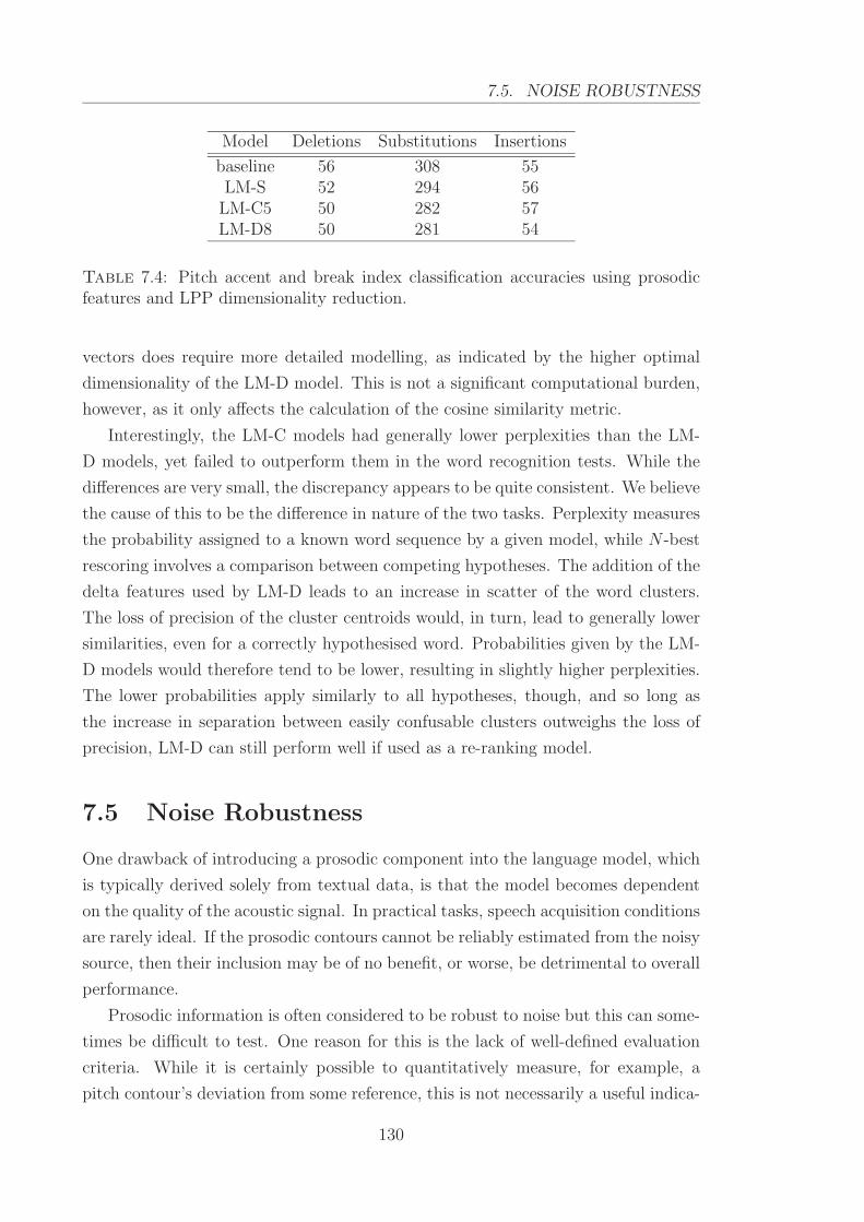
7.5. NOISE ROBUSTNESS
Model Deletions Substitutions Insertions
baseline 56 308 55LM-S 52 294 56
LM-C5 50 282 57LM-D8 50 281 54
Table 7.4: Pitch accent and break index classification accuracies using prosodicfeatures and LPP dimensionality reduction.
vectors does require more detailed modelling, as indicated by the higher optimal
dimensionality of the LM-D model. This is not a significant computational burden,
however, as it only affects the calculation of the cosine similarity metric.
Interestingly, the LM-C models had generally lower perplexities than the LM-
D models, yet failed to outperform them in the word recognition tests. While the
differences are very small, the discrepancy appears to be quite consistent. We believe
the cause of this to be the difference in nature of the two tasks. Perplexity measures
the probability assigned to a known word sequence by a given model, while N -best
rescoring involves a comparison between competing hypotheses. The addition of the
delta features used by LM-D leads to an increase in scatter of the word clusters.
The loss of precision of the cluster centroids would, in turn, lead to generally lower
similarities, even for a correctly hypothesised word. Probabilities given by the LM-
D models would therefore tend to be lower, resulting in slightly higher perplexities.
The lower probabilities apply similarly to all hypotheses, though, and so long as
the increase in separation between easily confusable clusters outweighs the loss of
precision, LM-D can still perform well if used as a re-ranking model.
7.5 Noise Robustness
One drawback of introducing a prosodic component into the language model, which
is typically derived solely from textual data, is that the model becomes dependent
on the quality of the acoustic signal. In practical tasks, speech acquisition conditions
are rarely ideal. If the prosodic contours cannot be reliably estimated from the noisy
source, then their inclusion may be of no benefit, or worse, be detrimental to overall
performance.
Prosodic information is often considered to be robust to noise but this can some-
times be difficult to test. One reason for this is the lack of well-defined evaluation
criteria. While it is certainly possible to quantitatively measure, for example, a
pitch contour’s deviation from some reference, this is not necessarily a useful indica-
130

LANGUAGE MODELLING WITH RAW FEATURES
Linear Filter
Clean speech
Noisy speech
Additive noise
Figure 7.4: Modelling of two types of noise sources in the speech signal.
tor of the robustness of features derived from the contour. The wide variety of uses
for prosodic information, as well as the numerous different realisations of prosodic
features means any evaluation will be dependent on the intended application. In
this section, we examine the effects of several types of noise on our specific task and
implementation of prosodic features.
7.5.1 Sources of noise
There are two main types of effects which can lead to a degradation of the speech
signal. One is the presence of other acoustic sources, such as vehicle traffic or
speech from other speakers. Noise from these sources are typically considered to be
additive and uncorrelated with the speech signal of interest. This type of noise is
further classed as being either stationary (time invariant) or non-stationary. White
and pink noise are examples of stationary noise. White noise is characterised by a
flat power spectrum, while the spectrum of pink noise is inversely proportional to
frequency. In practice, though, most noise is of the non-stationary type.
The other source of degradation is channel distortion. This may be the result
of the properties of the recording equipment or transmission channel, such as a
telephone line. These result in a convolutional distortion of the speech signal, and
are modelled as a linear filter. Reverberation effects caused by echoic environments
are another example of convolutional noise. There is also some additive noise due
to reverberation, as energy from reflected speech is combined with the actual signal.
The noise distortion process for the two forms of noise are illustrated in Figure 7.4.
7.5.2 Results
For investigating additive noise, the test set samples were mixed with one of white,
pink, babble or factory1 noise samples obtained from the NOISEX-92 database [169].
1factory1.wav
131

7.5. NOISE ROBUSTNESS
SNR (dB)noise
20 10 5 0white 78.14 78.14 78.14 78.14pink 78.14 78.14 78.14 77.97
babble 78.14 77.97 77.91 77.85factory 78.14 78.08 78.08 77.91
Table 7.5: Word accuracies of LM-D8 when using prosodic features extracted fromdata corrupted by additive noise.
This was performed using the Filtering and Noise Adding Tool [170], for SNRs2 rang-
ing from 20 dB down to 0 dB. Because we wish to isolate the prosodic component,
MFCC parameters used by the acoustic models were calculated from clean speech in
both training and testing. Only the F0 and RMS energy extraction procedures were
performed on the corrupted speech in the testing phase. Dimensionality reduction
during testing was performed by transforming the noisy prosodic feature vector with
a projection matrix calculated from clean training data. Therefore, the following
results are not indicative of the performance of the complete system under noisy
conditions. All results are reported using the language model LM-D8.
The results in Table 7.5 demonstrate that these features are very robust to
additive stationary noise. No degradation in performance was observed for white
noise, and there was only a minor decrease in accuracy at 0 and 5 dB for pink noise.
The prosodic features we have used are derived from the automatically extracted
pitch contour, so their behaviour in noisy conditions will be closely related. Because
both white and pink noise do not have any periodicity, their presence has minimal
effect on the pitch tracking algorithm. As a result, the prosodic features derived
from this output are similarly unaffected. In the presence of babble and factory
noise, the performance degradation was more evident. Babble noise, in particular,
can interfere with the pitch extraction at low SNRs. Segments of F0 contours, all
extracted from the same region, but for different types of noise, are illustrated in
Figure 7.5. Babble and factory noise alter the contour to a greater extent than the
two stationary noises; however, all contours exhibited noticeable deviations from
the clean contour. The fact that performance under white and pink noise remained
high, then, suggests that the following stages of feature processing (i.e. smoothing,
subspace projection and clustering) are also robust to this type of noise.
The models retain good performance at fairly low SNRs, but at SNRs below
0 dB, the pitch tracker would often fail completely. Without a pitch contour, no
2SNRs were calculated after applying an A-weight filter
132

LANGUAGE MODELLING WITH RAW FEATURES
0 50 100 150 200 250−1.5
−1
−0.5
0
0.5
1
1.5
t
f0
cleanwhitepink
(a) Stationary noise
0 50 100 150 200 250−1
−0.8
−0.6
−0.4
−0.2
0
0.2
0.4
0.6
0.8
1
t
f0
clean babble factory
(b) Non-stationary noise
Figure 7.5: F0 contours extracted from signals corrupted with additive noise at aSNR of 0 dB.
meaningful features can be derived. Therefore, these prosodic features are of no use
in extremely noisy conditions, but are highly robust up to this threshold.
Similar tests were conducted for reverberant noise. The Roomsim package [171]
was used to simulate the impulse response of an enclosed rectangular room with
dimensions 8 m x 8 m x 2.5 m. The receiver was positioned at 2 m x 4 m x 1.1
m, and the source was located 1m away at the same elevation, at 3 m x 4 m x
1.1 m. The level of reverberation can be quantified in terms of reverberation time
(RT60), which specifies the length of time required for a sound to decay by 60 dB.
Five impulse responses were generated by adjusting the surface absorptions of the
walls such that their RT60s ranged from 0.1 s to 0.5 s, in 0.1 s increments. The
dimensions of the room remained the same in all cases. The results in Table 7.5.2
were obtained by performing prosodic feature extraction on the convolution of the
clean speech signal with one of the simulated impulse responses.
Once again, the prosodic features exhibited a high degree of robustness in this
type of noise. Examination of the extracted pitch contours (Figure 7.6) shows that
F0 is largely invariant to channel distortions. Reverberation results in the presence
of an attenuated form of the signal occurring at a slight delay, and causes sampled
feature values to be merged across the time domain. While this poses a problem for
short-time spectral features, it is not a major issue for the suprasegmental prosodic
features, which are calculated over longer time periods. In fact, the effect of rever-
beration is not entirely dissimilar to the median smoothing applied to the F0 and
133

7.6. CONCLUSION
0 50 100 150 200 250−1
−0.8
−0.6
−0.4
−0.2
0
0.2
0.4
0.6
0.8
1
t
f0
cleanreverberant
Figure 7.6: F0 contour extracted from a signal in the presence of reverberationwith a RT60 of 0.5 s.
RT60noise0.1 0.2 0.3 0.4 0.5
reverberant 78.14 78.14 78.14 78.08 77.91
Table 7.6: Word accuracies of LM-D8 when using prosodic features extracted fromdata corrupted by reverberant noise.
energy contours in the post-processing stage.
Another explanation for the high level of robustness, particularly against rever-
berant noise, is that the feature vector contains duration information derived from
the original N-best list. If this list were to be regenerated under noisy conditions, the
differences to the hypothesised words and their time alignments would impact upon
the duration features. However, it should also be noted that the transformation
applied to the feature vector prevents the resulting model from attributing undue
weight to the durational information alone. Therefore, we believe that these results
do indicate that F0 and energy features are quite robust to noise.
7.6 Conclusion
In this chapter, we have described two methods in which automatically extracted
features may be used for language modelling. Irrespective of which approach is
taken, it is useful to first perform dimensionality reduction on the original prosodic
134
LANGUAGE MODELLING WITH RAW FEATURES
feature vectors. Doing so can greatly reduce the number of candidate features. For
a model that is computationally expensive to train, this is of significant benefit.
Reductions in computation are not the sole reason, though. Dimensionality reduc-
tion can serve to minimise the effects of noise in the data, and techniques such as
LPP can emphasis the separation of classes in the lower dimensional space. When
modelled in an appropriate manner, the combination of these effects can lead to
performance in excess of what can be obtained using the original, high-dimensional
feature vectors.
One potential use for the automatically extracted prosodic features is prosody
labelling. Our maximum entropy model, trained to classify four combinations of
accentuation and boundaries, benefited significantly from the subspace projected
features. This model can be used to annotate the output of a speech recogniser,
enabling language models augmented with ToBI features to be applied. Experiments
conducted with this approach gave an improvement of 1.3% over the trigram model,
which was equal to the gain achieved by the models in Chapter 5 using manually
transcribed data.
We also presented a technique for using the prosodic information directly in the
language model. Such an approach has the benefit of avoiding the intermediate
transcription step. In fact, it does not require any knowledge of phonological classes
at all. This is important for statistical modelling, as it opens up the possibility of
using much larger, unannotated corpora. The large number of classes in the language
model, as well as the weak relationship between prosody and word identity, means
care needs to be taken when formulating model features. We proposed an approach
based on cosine similarities, which is the same metric used by the subspace projection
algorithm. We also derived a compact set of features to represent the short-term
prosodic history. Language models trained on these two types of features performed
well, and actually exceeded the accuracies achieved by using ToBI features (1.9% vs
1.3%).
Lastly, we conducted some experiments to test the robustness of these prosodic
features in various noisy conditions. We find that they are very robust to reverberant
noise. Only minimal performance degradations were observed, up to and including
an RT60 of 0.5 s. This is due to the accurate pitch tracking in these conditions, which
is largely invariant to convolutional distortion. Robustness to stationary additive
noise was also high. Performance did not suffer under white noise until the SNR
dropped 0 dB, and 5 dB under pink noise. Although the pitch extraction was
influenced by the noise, the subsequent processing stages were able to compensate
for the minor deviations. In the presence of babble and factory noise, the prosodic
135

7.6. CONCLUSION
features were slightly less robust at low SNRs. The major issue with additive noise
is the tendency for the pitch tracking algorithm to fail to identify a meaningful
contour. Up until this point, though, the features demonstrated good robustness in
general.
136

Chapter 8
Conclusion
This chapter will briefly summarise the main findings of this research, and highlight
its contributions. It will also present some further research directions and extensions
to this work.
8.1 Summary
Research into the use of prosody for ASR and other speech processing systems has
gained momentum in recent years, and many approaches for modelling prosody
have been developed. With regard to ASR applications, the focus has primarily
been on augmenting phoneme models with prosodic parameters. In our work, we
have considered prosody as a higher level phenomenon, and proposed an approach
for incorporating this information into a language model.
In Chapter 5, we investigated some possible uses of perceptually transcribed
prosodic information for enhancing language models. An analysis of the mutual
information between words and their POS and ToBI labels indicated that there
were strong correlations between the three knowledge sources. Syntax and prosody
are closely related; however, the POS and ToBI labels were not redundant, and
in fact provided complementary information to each other. ToBI labels also did
not demonstrate a rapid decline in mutual information with word identities as the
distance from the word increased.
We modelled sequences of POS, pitch accent and break index labels by formulat-
ing them as features for a maximum entropy language model. These models provide
an effective framework for combining information from multiple, potentially dis-
parate knowledge sources, and this was demonstrated by the gains obtained through
using the additional features. Using the three types of features, in conjunction with
word n-gram features, led to a 19% relative improvement in perplexity over the base-
137

8.1. SUMMARY
line trigram model. The maximum entropy model also performed well in N-best list
reranking tests, increasing the recognition accuracy by a relative 1.7%.
Our experiments also highlighted some limitations to the use of ToBI transcrip-
tions in this manner. Firstly, we found no benefit to modelling contexts longer than
3 words. Both perplexity and recognition accuracies were degraded by modelling
longer histories. The primary reason for this, we believe, is that the labelling of the
data is not sufficiently consistent to be fully exploited by the model. Attempting to
gather statistics from long sequences of these labels exacerbates any inconsistencies,
and as a result, the statistics will be unreliable.
The prosodic features aid the language model by penalising hypotheses that are
not consistent with the observed prosodic context. However, the features themselves
have very coarse granularity. In an N-best list, there are many similar hypotheses,
and it is very likely that it will contain more than one hypothesis that is consistent
with the modelled prosodic information. Therefore, the new models tend to im-
prove the rankings of several hypotheses equally, while being unable to differentiate
between individual options within that subset.
Drawing from these findings, we extended our analysis to raw acoustic-prosodic
data. In the work documented in Chapter 6, we examined a number of duration,
F0 and energy features for correlations to prosodic events. Because sub-word time
alignment was not readily available in our task, we concentrated on the use of
word level features only, and developed a parameterisation of F0 and energy con-
tours designed specifically to encode information at this level. The analysis of the
acoustic-prosodic data has contributed to the understanding of the behaviour of
these parameters under differing prosodic conditions, and has also shown that our
proposed features are particularly effective at characterising the contour patterns
associated with accentuation.
To confirm the validity of the set of prosodic features developed in Chapter 6,
we used them to train a prosody classifier in Chapter 7. The results supported our
claim that the additional features we proposed were effective at capturing relevant
information on accentuation. In this chapter, we also discussed the applicability of
linear dimensionality reduction methods for our feature set, and explained why the
properties of the LPP technique made it suitable for our task. This was confirmed
experimentally in the prosody classification experiment, where the model trained
on a reduced set of features outperformed an equivalent model using the full set
of features. The best performing model used a feature vector with fewer than half
the original number of dimensions, and achieved a 5.4% relative improvement in
classification accuracy over a baseline model using lexical features.
138

CONCLUSION
In Section 7.4 we explored the problem of directly using the raw prosodic param-
eters in a language model. Creating phonological transcriptions of data is laborious,
and some prior work in this area has alleviated the burden by developing techniques
for automatically annotating data with prosodic-syntactic information. In our ap-
proach, we have taken this idea further and removed the need for the intermediate
transcription step altogether. We proposed a novel technique of representing the
prosodic information based on the properties of the subspace projection that is both
compact and effective at characterising the prosodic context of words. An examina-
tion of words commonly misclassified by the original trigram model suggested that
these features, when used by a language model, provided a good complement to
the acoustic models. Evaluation of models trained using these features showed that
they performed well, and actually exceeded the ToBI feature models in both per-
plexity and recognition accuracy. As with the prosody classification experiments,
a moderate dimensionality reduction gave the best results, with the best model
demonstrating a 20.5% relative improvement in perplexity over the baseline, and a
2.5% relative gain in recognition rate.
Prosody is considered to be robust against noise, but this is not often tested. In
the final section of this chapter, we conducted experiments to verify the robustness
of our prosodic features under a variety of noisy environments. Including acoustic-
prosodic information into the language model has the drawback of introducing a
dependence on speech signal quality, and this could potentially negate benefits of
using the features if they degrade rapidly with noise. Our experiments indicated
that this was not a major issue, however, as the features exhibited a high degree of
robustness to all types of tested conditions. The pitch contour extraction procedure
was largely unaffected by the presence of convolutional distortion, and subsequently,
so were our derived features. Additive noise did influence the pitch extraction, but
the dimensionality reduction and further processing of the features also proved to
be quite robust. Overall, only minimal performance degradation was observed, even
at the relatively low SNR of 0 dB.
8.2 Future Research
There is still much to learn about the nature of prosody, both in human-to-human
communication and as it applies to automatic speech processing. With regard to
our current research, though, there are a number of specific issues which are worth
drawing attention to.
139
8.2. FUTURE RESEARCH
8.2.1 Alternate Corpus
Firstly, it would be worthwhile to test our methods on a different corpus. The RNC
has been purposefully designed for prosody research, and the professionally read
speech gives very controlled and prosodically well-formed realisations. It is possible
that the statistical analyses and modelling used here may utilise these regularities to
the exclusion of other prosodic effects. In particular, spontaneous and conversational
speech is significantly different in its prosodic structure, and it is not apparent how
our techniques would perform on such data.
8.2.2 Improved Prosody Modelling
Throughout this study we have, where possible, attempted to use prosodic infor-
mation directly as features in the maximum entropy models. This was primarily
motivated by the belief that a direct approach can eliminate a potential source of
error caused by an intermediate modelling step. The simple features have also been
a useful tool in helping to understanding the behaviour and interaction of prosodic
information. However, much like n-grams, such basic features do not capture the
full extent of the relationship between the modelled variables. Our last set of exper-
iments, too, have shown that intermediate representations of prosody can be useful,
provided they are sufficiently reliable. More detailed features are certainly not prob-
lematic given the very general framework of the maximum entropy model. As an
example, encouraging results have been achieved by encoding dependency gram-
mar constraints into a maximum entropy language model [33]. Similarly, explicitly
modelling prosodic structure could also lead to further gains. There is a wealth of
knowledge available about many aspects of prosody and phonology, though coercing
this information into a representation conducive to statistical modelling is not a
trivial task.
8.2.3 System Integration
Tighter integration between language and acoustic models is another important
issue, not only for our work, but for language modelling research in general. While
the N-best rescoring approach we have used is helpful for developmental purposes,
a complete system should make use of the prosodic knowledge at an earlier stage in
order to avoid the propagation of errors. Word graphs and lattices are superior to
N-best lists in terms of coverage, but are still generated using phoneme models and
linguistically deficient n-grams. Managing the trade-off between early application of
140

CONCLUSION
knowledge sources and computational tractability remains a difficult problem, yet
it is one that needs to be addressed in order to fully exploit prosodic and syntactic
information.
In this work, we have demonstrated some ways in which suprasegmental prosodic
information can aid word recognition. Ultimately, though, prosody is responsible
for higher level structures relating to syntax, semantics and dialogue. While these
effects are not directly relevant to the automatic word recognition problem, they
are an important component of human speech comprehension. Due to the close and
complex relationships between the many levels of speech communication, examining
each one in isolation is perhaps less meaningful than considering it as a single,
integrated unit. Prosody is not necessarily the only aspect of speech which affects
so many levels of the process, but the difficulties encountered in quantifying its
precise functionality certainly underlines the need for a more holistic approach to
developing automatic speech processing systems.
141

142

Appendix A
Penn Treebank Tag Set
This is the set of word categories in the Penn Treebank with which the Boston
University Radio Speech Corpus has been annotated.
CC Coordinating conjunction
CD Cardinal number
DT Determiner
EX Existential there
FW Foreign word
IN Preposition or subordinating conjunction
JJ Adjective
JJR Adjective, comparative
JJS Adjective, superlative
LS List item marker
MD Modal
NN Noun, singular or mass
NNS Noun, plural
NP Proper noun, singular
NPS Proper noun, plural
PDT Predeterminer
POS Possessive ending
PP Personal pronoun
PP$ Possessive pronoun
RB Adverb
RBR Adverb, comparative
RBS Adverb, superlative
RP Particle
143

SYM Symbol
TO to
UH Interjection
VB Verb, base form
VBD Verb, past tense
VBG Verb, gerund or present participle
VBN Verb, past participle
VBP Verb, non-3rd person singular present
VBZ Verb, 3rd person singular present
WDT Wh-determiner
WP Wh-pronoun
WP$ Possessive wh-pronoun
WRB Wh-adverb
144

Bibliography
[1] A. Cutler, D. Dahan, and W. van Donselaar, “Prosody in the comprehension
of spoken language: A literature review,” Language and Speech, vol. 40, no. 2,
pp. 141–201, 1997.
[2] R. Jakobson, C. Gunnar, M. Fant, and M. Hall, Preliminaries to Speech Anal-
ysis: The Distinctive Features and their Correlates. Cambridge, USA: MIT
Press, 1967.
[3] D. R. Ladd, Intonational Phonology. Cambridge, Great Britain: Cambridge
University Press, 1996.
[4] D. L. Bolinger, “Intonation across languages,” Universals of Human Language,
vol. 2, pp. 471–524, 1978.
[5] F. Grosjean, “How long is the sentence? Prediction and prosody in the on-line
processing of language,” Linguistics, vol. 21, pp. 501–529, 1983.
[6] I. Lehiste, “The timing of utterances and linguistic boundaries,” Journal of
the Acoustical Society of America, vol. 51, no. 6B, pp. 2018–2024, 1972.
[7] A. Waibel, Prosody and Speech Recognition. San Mateo, USA: Morgan Kauf-
mann Publishers, 1988.
[8] R. Collier and J. ’t Hart, “The role of intonation in speech perception,” in
Structure and Process in Speech Perception, A. Cohen and S. G. Nooteboom,
Eds. New York, USA: Springer-Verlag, 1975.
[9] I. Bulyko, M. Ostendorf, and P. Price, “On the relative importance of differ-
ent prosodic factors for improving speech synthesis,” in Proc. International
Congress of Phonetic Sciences, San Francisco, CA, USA, 1999, pp. 81–84.
[10] G. Lidstone, “Note on the general case of the Bayes-Laplace formula for in-
ductive or a posteriori probabilities,” Transactions of the Faculty of Actuaries,
vol. 8, pp. 182–192, 1920.
145

BIBLIOGRAPHY
[11] W. Gale and K. Church, “What is wrong with adding one?” in Corpus-Based
Research into Language, N. Oostdijk and P. D. Haan, Eds. Amsterdam, The
Netherlands: Rodopi, 1994, pp. 189–198.
[12] I. J. Good, “The population frequencies of species and the estimation of pop-
ulation parameters,” Biometrika, vol. 40, no. 3–4, pp. 237–264, 1953.
[13] W. A. Gale, “Good-Turing smoothing without tears,” AT&T Bell Laborato-
ries, Tech. Rep., 2000.
[14] F. Jelinek and R. L. Mercer, “Interpolated estimation of Markov source pa-
rameters from sparse data,” in Proc. Workshop on Pattern Recognition in
Practice, Amsterdam, The Netherlands, 1980, pp. 381–397.
[15] L. R. Bahl, F. Jelinek, and R. L. Mercer, “A maximum likelihood approach to
continuous speech recognition,” IEEE Transactions on Pattern Analysis and
Machine Intelligence, vol. 5, no. 2, pp. 179–190, 1983.
[16] S. M. Katz, “Estimation of probabilities from sparse data for the language
model component of a speech recognizer,” IEEE Transactions on Acoustics,
Speech, and Signal Processing, vol. 35, no. 3, pp. 400–401, 1987.
[17] S. F. Chen and J. Goodman, “An empirical study of smoothing techniques
for language modeling,” Computer Speech and Language, vol. 10, pp. 359–393,
1999.
[18] H. Ney, U. Essen, and R. Kneser, “On structuring probabilistic dependencies
in stochastic language modelling,” Computer Speech and Language, vol. 8,
no. 1, pp. 1–38, 1994.
[19] R. Kneser and H. Ney, “Improved backing-off for m-gram language modeling,”
in Proc. International Conference on Acoustics, Speech, and Signal Processing,
1995, pp. 181–184.
[20] P. F. Brown, V. J. Della Pietra, P. V. deSouza, and J. C. Lai, “Class-based
n-gram models of natural language,” Computational Linguistics, vol. 18, no. 4,
pp. 467–479, 1992.
[21] J. Gao, J. Goodman, and J. Miao, “The use of clustering techniques for Asian
language modeling,” Computational Linguistics and Chinese Language Pro-
cessing, vol. 6, no. 1, pp. 27–60, 2001.
146

BIBLIOGRAPHY
[22] R. Kneser and H. Ney, “Improved clustering techniques for class-based statis-
tical language modeling,” in Proc. Eurospeech, 1993, pp. 973–976.
[23] K. Kirchhoff, J. Bilmes, S. Das, N. Duta, M. Egan, G. Ji, F. He, J. Hender-
son, D. Liu, M. Noamany, P. Schone, R. Schwartz, and D. Vergyri, “Novel
approaches to Arabic speech recognition: Report from the 2002 John-Hopkins
summer workshop,” in Proc. International Conference on Acoustics, Speech,
and Signal Processing, Hong Kong, China, 2003, pp. 344–347.
[24] J. Bilmes and K. Kirchhoff, “Factored language models and generalized par-
allel backoff,” in Proc. Conference of the North American Chapter of the As-
sociation for Computational Linguistics on Human Language Technology, Ed-
monton, Canada, 2003, pp. 4–6.
[25] K. Kirchhoff and M. Yang, “Improved language modeling for statistical ma-
chine translation,” in Proc. ACL Workshop on Building and Using Parallel
Texts, 2005.
[26] K. Duh and K. Kirchhoff, “Automatic learning of language model structure,”
in Proc. International Conference on Computational Linguistics, Geneva,
Switzerland, 2004, pp. 148–154.
[27] J. Baker, “Trainable grammars for speech recognition,” in Proc. Spring Con-
ference of the Acoustical Society of America, Boston, MA, USA, 1979, pp.
547–550.
[28] E. Charniak, “Immediate-head parsing for language models,” in Proc. 39th
Annual Meeting of the Association for Computational Linguistics, San Fran-
cisco, CA, USA, 2001, pp. 116–123.
[29] A. Stolcke and J. Segal, “Precise n-gram probabilities from stochastic context-
free grammars,” in Proc. 32nd Annual Meeting of the Association for Compu-
tational Linguistics, Las Cruces, NM, USA, 1994, pp. 74–79.
[30] J. H. W. H. Lloyd-Thomas and G. J. F. Jones, “An integrated gram-
mar/bigram language model using path scores,” in Proc. International Con-
ference on Acoustics, Speech, and Signal Processing, Detroit, MI, USA, 1995,
pp. 173–176.
[31] C. Chelba and F. Jelinek, “Exploiting syntactic structure for language mod-
eling,” in Proc. 36th Annual Meeting of the Association for Computational
Linguistics, Montreal, Canada, 1998, pp. 225–231.
147

BIBLIOGRAPHY
[32] L. Tesniere, Elements de Syntaxe Structurale. Paris, France: Klincksieck,
1959.
[33] C. Chelba, D. Engle, F. Jelinek, V. Jimenez, S. Khudanpur, L. Mangu,
H. Printz, E. Ristad, R. Rosenfeld, A. Stolcke, and D. Wu, “Structure and
performance of a dependency language model,” in Proc. European Confer-
ence on Speech Communication and Technology, Rhodes, Greece, 1997, pp.
2775–2778.
[34] J. Gao, J.-Y. Nie, G. Wu, and G. Cao, “Dependence language model for in-
formation retrieval,” in Proc. 27th Annual International ACM SIGIR Confer-
ence on Research and Development in Information Retrieval, Sheffield, United
Kingdom, 2004, pp. 170–177.
[35] L. R. Bahl, P. F. Brown, P. V. deSouza, and R. L. Mercer, “A tree-based
statistical language model for natural language speech recognition,” IEEE
Transactions on Acoustics, Speech, and Signal Processing, vol. 37, no. 7, pp.
1001–1008, 1989.
[36] R. Rosenfeld, “A maximum entropy approach to adaptive statistical language
modeling,” Computer Speech and Language, vol. 10, no. 3, pp. 187–228, 1996.
[37] L. R. Rabiner, “A tutorial on hidden Markov models and selected applications
in speech recognition,” Proceedings of the IEEE, vol. 77, no. 2, pp. 257–286,
1989.
[38] H. Hermansky, “Perceptual linear predictive (PLP) analysis of speech,” Jour-
nal of the Acoustical Society of America, vol. 87, no. 4, pp. 1738–1752, 1990.
[39] S. B. Davis and P. Mermelstein, “Comparison of parametric representations
for monosyllabic word recognition in continuously spoken sentences,” IEEE
Transactions on Acoustics, Speech, and Signal Processing, vol. 28, no. 4, pp.
357–366, 1980.
[40] L. R. Rabiner and B. H. Juang, “An introduction to hidden Markov models,”
IEEE ASSP Magazine, vol. 3, no. 1, pp. 4–16, 1986.
[41] X. D. Huang and M. A. Jack, “Semi-continuous hidden Markov models in
isolated word recognition,” in Proc. 9th International Conference on Pattern
Recognition, Rome, Italy, 1988, pp. 406–408.
148

BIBLIOGRAPHY
[42] L. E. Baum, T. Petrie, G. Soules, and N. Weiss, “A maximization technique oc-
curring in the statistical analysis of probabilistic functions of Markov chains,”
Annals of Mathematical Statistics, vol. 41, no. 1, pp. 164–171, 1970.
[43] A. P. Dempster, N. M. Laird, and D. B. Rubin, “Maximum likelihood from in-
complete data via the EM algorithm,” Journal of the Royal Statistical Society,
vol. 39, no. 1, pp. 1–21, 1977.
[44] N. Merhav and Y. Ephraim, “Maximum likelihood hidden Markov modeling
using a dominant sequence of states,” IEEE Transactions on Signal Processing,
vol. 39, no. 9, pp. 2111–2114, 1991.
[45] B. T. Lowerre, “The HARPY speech recognition system,” Ph.D. dissertation,
Carnegie Mellon University, 1976.
[46] F. Jelinek, “A fast sequential decoding algorithm using a stack,” IBM Journal
of Research and Development, vol. 13, pp. 675–685, 1969.
[47] L. R. Bahl, P. S. Gopalakrishnam, D. Kanevsky, and D. Nahamoo, “Matrix
fast match: A fast method for identifying a short list of candidate words for
decoding,” in Proc. International Conference on Acoustics, Speech, and Signal
Processing, Glasgow, Scotland, 1989, pp. 81–84.
[48] Y. Chow and R. Schwartz, “The N-best algorithm: An efficient procedure for
finding top N sentence hypotheses,” in Proc. DARPA Workshop on Speech
and Natural Language, Cape Cod, MA, USA, 1989, pp. 199–202.
[49] X. Aubert, C. Dugast, H. Ney, and V. Steinbiss, “Large vocabulary contin-
uous speech recognition of Wall Street Journal data,” in Proc. International
Conference on Acoustics, Speech, and Signal Processing, Adelaide, Australia,
1994, pp. 129–132.
[50] R. A. Wagner and M. J. Fischer, “The string-to-string correction problem,”
Journal of the Association for Computing Machinery, vol. 21, pp. 168–173,
1974.
[51] L. Gillick and S. Cox, “Some statistical issues in the comparison of speech
recognition algorithms,” in Proc. International Conference on Acoustics,
Speech, and Signal Processing, Glasgow, Scotland, 1989, pp. 523–535.
[52] D. S. Pallett, W. M. Fisher, and J. G. Fiscus, “Tools for the analysis of
benchmark speech recognition tests,” in Proc. International Conference on
149

BIBLIOGRAPHY
Acoustics, Speech, and Signal Processing, Albuquerque, NM, USA, 1990, pp.
97–100.
[53] S. Coren, L. M. Ward, and J. T. Enns, Sensation and Perception. New York,
USA: Academic Press, 1979.
[54] D. Talkin, “A robust algorithm for pitch tracking,” in Speech Coding and
Synthesis, W. B. Kleijn and K. K. Paliwal, Eds. Elsevier, 1995.
[55] T. Shimamura and H. Kobayashi, “Weighted autocorrelation for pitch extrac-
tion of noisy speech,” IEEE Transactions on Speech and Audio Processing,
vol. 9, no. 7, pp. 727–730, 2001.
[56] H. Fletcher and W. A. Munson, “Loudness, its definition, measurement and
calculation,” Journal of the Acoustical Society of America, vol. 5, pp. 82–108,
1933.
[57] R. Kompe, Prosody in Speech Understanding Systems, ser. Lecture Notes in
Artificial Intelligence. Berlin, Germany: Springer-Verlag, 1997.
[58] C. W. Wightman, “Automatic detection of prosodic constituents for parsing,”
Ph.D. dissertation, Boston University, 1992.
[59] J. P. H. van Santen, “Assignment of segmental duration in text-to-speech
synthesis,” Computer Speech and Language, vol. 8, no. 2, pp. 95–128, 1994.
[60] M. Liberman and A. Prince, “On stress and linguistic rhythm,” Linguistic
Inquiry, vol. 8, no. 2, pp. 249–336, 1977.
[61] S. Nooteboom, “The prosody of speech: Melody and rhythm,” in The Hand-
book of Phonetic Sciences, W. J. Hardcastle and J. Laver, Eds. Blackwell,
1997, pp. 640–673.
[62] P. Lieberman, “Some acoustic correlates of word stress in American English,”
The Journal of the Acoustical Society of America, vol. 32, no. 4, pp. 451–454,
1960.
[63] G. Kochanski, E. Grabe, J. Coleman, and B. Rosner, “Loudness predicts
prominence: Fundamental frequency lends little,” The Journal of the Acous-
tical Society of America, vol. 118, no. 2, pp. 1038–1054, 2005.
[64] J. ’t Hart, R. Collier, and A. Cohen, A Perceptual Study of Intonation. Cam-
bridge, Great Britain: Cambridge University Press, 1990.
150
BIBLIOGRAPHY
[65] L. B. Leonard, “The role of intonation in the recall of various linguistic stim-
uli,” Language and Speech, vol. 16, no. 4, pp. 327–335, 1973.
[66] G. M. Robinson, “Rhythmic organization in speech processing,” Journal of
Experimental Psychology: Human Perception and Performance, vol. 3, pp.
83–91, 1977.
[67] R. K. Bansal, The Intelligibility of Indian English. Central Institute of English
and Foreign Languages, 1976.
[68] J. G. Martin, “Temporal word spacing and the perception of ordinary, anoma-
lous, and scrambled strings,” Journal of Verbal Learning and Verbal Behavior,
vol. 7, pp. 154–157, 1968.
[69] C. J. Darwin, “On the dynamic use of prosody in speech perception,” in
Structure and Process in Speech Perception, A. Cohen and S. G. Nooteboom,
Eds. New York, USA: Springer-Verlag, 1975.
[70] A. Treisman, “Contextual cues in selective listening,” Quarterly Journal of
Experimental Psychology, vol. 12, pp. 242–248, 1960.
[71] R. H. Meltzer, J. G. Martin, C. B. Mills, D. L. Imhoff, and D. Zohar, “Re-
action time to temporally-displaced phoneme targets in continuous speech,”
Journal of Experimental Psychology: Human Perception and Performance,
vol. 2, no. 2, pp. 277–290, 1976.
[72] F. Ferreira, M. D. Anes, and M. D. Horine, “Exploring the use of prosody
during language comprehension using the auditory moving window technique,”
Journal of Psycholinguistic Research, vol. 25, no. 2, pp. 273–290, 1996.
[73] B. A. Blesser, “Perception of spectrally rotated speech,” Ph.D. dissertation,
Massachusetts Institute of Technology, 1969.
[74] D. T. Herron, “Context, word-class, and prosody in the recognition of open-
and closed-class words,” Ph.D. dissertation, University of California, 1998.
[75] A. Cutler and D. Norris, “The role of strong syllables in segmentation for
lexical access,” Journal of Experimental Psychology: Human Perception and
Performance, vol. 14, pp. 113–121, 1988.
[76] D. H. Klatt, “Linguistic uses of segmental duration in English: Acoustic and
perceptual evidence,” Journal of the Acoustical Society of America, vol. 59,
no. 5, pp. 1208–1221, 1976.
151

BIBLIOGRAPHY
[77] P. Price, M. Ostendorf, S. Shattuck-Hufnagel, and C. Fong, “The use of
prosody in syntactic disambiguation,” Journal of the Acoustical Society of
America, vol. 90, no. 6, pp. 2956–2965, 1991.
[78] A. Wingfield, “The intonation-syntax interaction: Prosodic features in percep-
tual processing of sentences,” in Structure and Process in Speech Perception,
A. Cohen and S. G. Nooteboom, Eds. New York, USA: Springer-Verlag, 1975.
[79] C. M. Beach, “The interpretation of prosodic patterns at points of syntactic
structure ambiguity: Evidence for cue trading relations,” Journal of Memory
and Language, vol. 30, no. 6, pp. 644–663, 1991.
[80] F. Grosjean and C. Hirt, “Using prosody to predict the end of sentences in
English and French: Normal and brian-damaged subjects,” Language and Cog-
nitive Processes, vol. 11, no. 1/2, pp. 107–134, 1996.
[81] A. Cutler, “Phoneme-monitoring reaction time as a function of preceding in-
tonation contour,” Perception and Psychophysics, vol. 20, no. 1, pp. 55–60,
1976.
[82] A. Cutler, “Components of prosodic effects in speech recognition,” in Proc.
Eleventh International Congress of Phonetic Sciences, Tallinn, Estonia, 1987,
pp. 84–87.
[83] J. Terken and J. Hirschberg, “Deaccentuation of words representing “given”
information: Effects of persistence of grammatical function and surface posi-
tion,” Language and Speech, vol. 37, pp. 125–145, 1994.
[84] W. van Donselaar and J. Lentz, “The function of sentence accents and
given/new information in speech processing: Different strategies for normal-
hearing and hearing-impaired listeners?” Language and Speech, vol. 37, no. 4,
pp. 375–391, 1994.
[85] G. Brown, K. L. Currie, and J. Kenworthy, Questions of Intonation. London,
Great Britain: Croom Helm, 1980.
[86] J. Hirschberg and B. Grosz, “Intonational features of local and global discourse
structure,” in Proc. Workshop on Speech and Natural Language, San Mateo,
CA, USA, 1992, pp. 441–446.
[87] R. Carlson, K. Gustafson, and E. Strangert, “Modelling hesitation for syn-
thesis of spontaneous speech,” in Proc. Speech Prosody, Dresden, Germany,
2006.
152

BIBLIOGRAPHY
[88] C. Nakatani and J. Hirschberg, “A speech-first model for repair detection and
correction,” in Proc. 31st Annual Meeting of the Association for Computa-
tional Linguistics, Columbus, OH, USA, 1993, pp. 46–53.
[89] J. Bear, J. Dowding, and E. Shriberg, “Integrating multiple knowledge
sources for detection and correction of repairs in human-computer dialog,” in
Proc. 30th Annual Meeting of the Association for Computational Linguistics,
Newark, NJ, USA, 1992, pp. 56–63.
[90] A. Tickle, “English and Japanese speakers’ emotion vocalisation and recog-
nition: A comparison highlighting vowel quality,” in ISCA Tutorial and Re-
search Workshop on Speech and Emotion, Newcastle, Northern Ireland, 2000,
pp. 104–109.
[91] T. Otake, G. Hatano, and K. Yoneyama, “Speech segmentation by Japanese
listeners,” in Phonological Structure and Language Processing: Cross-
Linguistic Studies, T. Otake and A. Cutler, Eds. Berlin, Germany: Mouton
de Gruyter, 1996.
[92] T. Otake, G. Hatano, A. Cutler, and J. Mehler, “Mora or syllable? Speech
segmentation in Japanese,” Journal of Memory and Language, vol. 32, pp.
358–378, 1993.
[93] S. Peppe, J. Maxim, and B. Wells, “Prosodic variation in southern British
English,” Language and Speech, vol. 43, no. 3, pp. 309–334, 2000.
[94] J. B. Pierrehumbert, “The phonology and phonetics of english intonation,”
Ph.D. dissertation, Massachusetts Institute of Technology, 1980.
[95] M. Liberman, “The intonational system of english,” Ph.D. dissertation, Mas-
sachusetts Institute of Technology, 1975.
[96] J. B. Pierrehumbert, “Automatic recognition of intonation patterns,” in Proc.
21st Annual Meeting of the Association for Computational Linguistics, Cam-
bridge, MA, USA, 1983, pp. 85–90.
[97] P. A. Taylor, “A phonetic model of english intonation,” Ph.D. dissertation,
University of Edinburgh, 1992.
[98] C. W. Wightman and M. Ostendorf, “Automatic labeling of prosodic pat-
terns,” IEEE Transactions on Speech and Audio Processing, vol. 2, no. 4, pp.
469–481, 1994.
153
BIBLIOGRAPHY
[99] K. Ross and M. Ostendorf, “Prediction of abstract prosodic labels for speech
synthesis,” Computer Speech and Language, vol. 10, no. 3, pp. 155–185, 1996.
[100] N. Braunschweiler, “Automatic detection of prosodic cues,” Ph.D. disserta-
tion, Universitat Konstanz, 2003.
[101] K. Silverman, M. Beckman, J. Pitrelli, M. Ostendorf, C. Wightman, P. Price,
J. Pierrehumbert, and J. Hirschberg, “TOBI: A standard for labeling English
prosody,” in Proc. International Conference on Spoken Language Processing,
Banff, Canada, 1992.
[102] M. E. Beckman and G. A. Elam, “Guidelines for ToBI labelling,” Ohio State
University, Tech. Rep., 1997.
[103] M. Beckman and J. Pierrehumbert, “Intonation structure in Japanese and
English,” Phonology Yearbook, vol. 3, pp. 255–309, 1986.
[104] J. Hirschberg and M. E. Beckman, “The ToBI annotation conventions,” Ohio
State University, Tech. Rep., 1994.
[105] C. W. Wightman, “ToBI or not ToBI,” in Proc. International Conference on
Speech Prosody, Aixen-Provence, France, 2002.
[106] J. Pitrelli, M. Beckman, and J. Hirschberg, “Evaluation of prosodic transcrip-
tion labeling reliability in the ToBI framework,” in Proc. International Con-
ference on Spoken Language Processing, Yokohama, Japan, 1994, pp. 123–126.
[107] A. K. Syrdal and J. McGory, “Inter-transcriber reliability of ToBI prosodic
labeling,” in Proc. International Conference on Spoken Language Processing,
Beijing, China, 2000, pp. 235–238.
[108] A. K. Syrdal, J. Hirschberg, J. McGory, and M. Beckman, “Automatic ToBI
prediction and alignment to speed manual labeling of prosody,” Speech Com-
munication, vol. 33, no. 1–2, pp. 135–151, 2001.
[109] C. W. Wightman, A. K. Syrdal, G. Stemmer, A. Conkie, and M. Beutnagel,
“Perceptually based automatic prosody labeling and prosodically enriched unit
selection improve concatenative text-to-speech synthesis,” in Proc. Interna-
tional Conference on Spoken Language Processing, Beijing, China, 2000, pp.
71–74.
154

BIBLIOGRAPHY
[110] A. Batliner, B. Mobius, G. Mohler, A. Schweitzer, and E. Noth, “Prosodic
models, automatic speech understanding, and speech synthesis: Towards the
common ground,” in Proc. European Conference on Speech Communication
and Technology, vol. 4, Aalborg, Denmark, 2001, pp. 2285–2288.
[111] E. Shriberg and A. Stolcke, “Prosody modeling for automatic speech recog-
nition and understanding,” in Mathematical Foundations of Speech and Lan-
guage Processing, ser. The IMA Volumes in Mathematics and its Applications,
M. Johnson, S. P. Khudanpur, M. Ostendorf, and R. Rosenfeld, Eds. New
York, USA: Springer-Verlag, 2004, vol. 138, pp. 105–114.
[112] W. A. Lea, “Prosodic aids to speech recognition,” in Trends in Speech Recog-
nition, W. A. Lea, Ed. Prentice-Hall, Inc., 1980, pp. 166–205.
[113] K. Bishop, “Modeling sentential stress in the context of a large vocabulary
continuous speech recognizer,” in Proc. International Conference on Spoken
Language Processing, Banff, Canada, 1992, pp. 437–440.
[114] K. Chen and M. Hasegawa-Johnson, “How prosody improves word recogni-
tion,” in Proc. International Conference on Speech Prosody, Nara, Japan,
2004.
[115] T. Cho, “Effects of prosody on articulation in english,” Ph.D. dissertation,
University of California at Los Angeles, 2001.
[116] S. E. Levinson, “Continuously variable duration hidden Markov models for
speech analysis,” in Proc. International Conference on Acoustics, Speech, and
Signal Processing, Tokyo, Japan, 1986, pp. 1241–1244.
[117] M. J. Russell and A. E. Cook, “Experimental evaluation of duration modelling
techniques for automatic speech recognition,” in Proc. International Confer-
ence on Acoustics, Speech, and Signal Processing, Dallas, TX, USA, 1987, pp.
2376–2379.
[118] J. Bilmes, “What HMMs can’t do: A graphical model perspective”,” in Proc.
ATR Workshop Beyond HMMs, Kyoto, Japan, 2004.
[119] M. Ostendorf, I. Shafran, and R. Bates, “Prosody models for conversational
speech recognition,” in Proc. of the 2nd Plenary Meeting and Symposium on
Prosody and Speech Processing, 2003, pp. 147–154.
155

BIBLIOGRAPHY
[120] J. Hirschberg, D. Litman, and M. Swerts, “Prosodic cues to recognition er-
rors,” in Proc. of the Automatic Speech Recognition and Understanding Work-
shop, Keystone, CO, USA, 1999.
[121] N. M. Veilleux and M. Ostendorf, “Prosody/parse scoring and its applications
in ATIS,” in Proc. ARPA HLT Workshop, Princeton, NJ, USA, 1993, pp.
335–340.
[122] A. Batliner and E. Noth, “Prosody and automatic speech recognition – why
not yet a success story and where to go from here,” in Proc. 2nd Plenary
Meeting and Symposium on Prosody and Speech Processing, Tokyo, Japan,
2003, pp. 357–364.
[123] A. Batliner, J. Buckow, R. Huber, V. Warnke, E. Noth, and H. Niemann,
“Prosodic feature evaluation: Brute force or well designed?” in Proc. 14th
Int. Congress of Phonetic Sciences, San Francisco, CA, USA, 1999, pp. 2315–
2318.
[124] V. R. R. Gadde, “Modeling word durations,” in Proc. International Conference
on Spoken Language Processing, Beijing, China, 2000, pp. 601–604.
[125] A. Stolcke, E. Shriberg, D. Hakkani-Tur, and G. Tur, “Modeling the prosody
of hidden events for improved word recognition,” in Proc. 6th European Con-
ference on Speech Communication and Technology, Budapest, Hungary, 1999,
pp. 307–310.
[126] K. Chen and M. Hasegawa-Johnson, “Improving the robustness of prosody
dependent language modeling based on prosody syntax dependence,” in IEEE
Workshop on Automatic Speech Recognition and Understanding, St. Thomas,
U.S. Virgin Islands, 2003, pp. 435–440.
[127] E. T. Jaynes, “Information theory and statistical mechanics,” Physics Review,
vol. 106, no. 4, pp. 620–630, 1957.
[128] H. W. Kuhn and A. W. Tucker, “Nonlinear programming,” in Proc. Second
Berkeley Symposium on Mathematical Statistics and Probability. Berkeley,
CA, USA: University of California Press, 1951, pp. 481–490.
[129] S. Kullback, Information Theory and Statistics. New York, USA: Wiley, 1959.
[130] F. Jelinek, Statistical Methods for Speech Recognition. Cambridge, USA: MIT
Press, 1998.
156

BIBLIOGRAPHY
[131] J. Darroch and D. Ratcliff, “Generalized iterative scaling for log-linear mod-
els,” Annals of Mathematical Statistics, vol. 43, no. 5, pp. 1470–1480, 1972.
[132] S. Della Pietra, V. Della Pietra, and J. Lafferty, “Inducing features of ran-
dom fields,” IEEE Transactions on Pattern Analysis and Machine Intelligence,
vol. 19, no. 4, pp. 380–393, 1997.
[133] R. Jin, R. Yan, J. Zhang, and A. Hauptmann, “A faster iterative scaling algo-
rithm for conditional exponential model,” in Proc. International Conference
on Machine Learning, Washington DC, USA, 2003.
[134] R. Fletcher and C. M. Reeves, “Function minimization by conjugate gradi-
ents,” The Computer Journal, vol. 7, no. 2, pp. 149–154, 1964.
[135] J. Nocedal, “Updating quasi-newton matrices with limited storage,” Mathe-
matics of Computation, vol. 35, no. 151, pp. 773–782, 1980.
[136] R. Malouf, “A comparison of algorithms for maximum entropy parameter
estimation,” in Proc. Sixth Conference on Natural Language Learning, 2002,
pp. 49–55.
[137] T. P. Minka, “A comparison of numerical optimizers for logistic regression,”
http://research.microsoft.com/ minka/papers/logreg/minka-logreg.pdf, 2003.
[138] A. Ratnaparkhi, “Maximum entropy models for natural language ambiguity
resolution,” Ph.D. dissertation, University of Pennsylvania, 1998.
[139] A. L. Berger, S. A. Della Pietra, and V. J. Della Pietra, “A maximum entropy
approach to natural language processing,” Computational Linguistics, vol. 22,
no. 1, pp. 39–72, 1996.
[140] S. F. Chen and R. Rosenfeld, “A Gaussian prior for smoothing maximum
entropy models,” Carnegie Mellon University, Tech. Rep., 1999.
[141] J. Kazama and J. Tsujii, “Evaluation and extension of maximum entropy
models with inequality constraints,” in Proc. Conference on Empirical Methods
in Natural Language Processing, Sapporo, Japan, 2003, pp. 137–144.
[142] J. Goodman, “Exponential priors for maximum entropy models,” in Proc.
Annual Meeting of the Association for Computational Linguistics, 2004.
157

BIBLIOGRAPHY
[143] S. F. Chen and J. T. Goodman, “An empirical study of smoothing techniques
for language modeling,” in Proc. 34th Meeting of the Association for Compu-
tational Linguistics, Santa Cruz, CA, USA, 1996, pp. 310–318.
[144] R. Rosenfeld, “Adaptive statistical language modeling: A maximum entropy
approach,” Ph.D. dissertation, Carnegie Mellon University, 1994.
[145] M. Ostendorf, P. Price, and S. Shattuck-Hufnagel, “The Boston University
Radio News Corpus,” Boston University, Tech. Rep., 1995.
[146] M. Marcus and B. Santorini, “Building a very large natural language corpora:
The Penn Treebank,” Computational Linguistics, vol. 19, no. 2, pp. 313–330,
1993.
[147] M. Meteer, R. Schwartz, and R. Weischedel, “POST: Using probabilities in
language processing,” in Proc. International Joint Conference on Artifical In-
telligence, Sydney, Australia, 1991, pp. 960–965.
[148] M. Hasegawa-Johnson, K. Chen, J. Cole, S. Borys, S. Kim, A. Cohen,
T. Zhang, J. Choi, H. Kim, T. Yoon, and S. Chavarria, “Simultaneous recog-
nition of words and prosody in the Boston University radio speech corpus,”
Speech Communication, vol. 46, no. 3–4, pp. 418–439, 2005.
[149] A. Stolcke, “SRILM - an extensible language modeling toolkit,” in Proc. Inter-
national Conference on Spoken Language Processing, Denver, CO, USA, 2002,
pp. 901–904.
[150] S. J. Benson and J. J. More, “A limited memory variable metric for bound
constrained minimization,” Mathematics and Computer Science Division, Ar-
gonne National Laboratory, Tech. Rep., 2001.
[151] S. J. Young, “The HTK hidden Markov model toolkit: Design and philosophy,”
Cambridge University Engineering Department, Tech. Rep., 1994.
[152] F. J. Och, N. Ueffing, and H. Ney, “An efficient A* search algorithm for
statistical machine translation,” in Proc. Workshop on Data-Driven Methods
in Machine Translation, Toulouse, France, 2001, pp. 1–8.
[153] L. Nguyen, R. Schwartz, Y. Zhao, and G. Zavaliagkos, “Is N-best dead?” in
Proc. Workshop on Human Language Technology, Plainsboro, NJ, USA, 1994,
pp. 411–414.
158
BIBLIOGRAPHY
[154] P. Taylor, A. W. Black, and R. Caley, “The architecture of the Festival
speech synthesis system,” in Proc. Third ESCA Workshop in Speech Synthesis,
Jenolan Caves, Australia, 1998, pp. 147–151.
[155] D. H. Milone and A. J. Rubio, “Prosodic and accentual information for auto-
matic speech recognition,” IEEE Transactions on Speech and Audio Process-
ing, vol. 11, no. 4, pp. 321–333, 2003.
[156] A. Batliner, E. Noth, J. Buckow, R. Huber, V. Warnke, and H. Niemann, “Du-
ration features in prosodic classification: Why normalization comes second,
and what they really encode,” in Proc. ISCA Tutorial and Research Work-
shop on Speech recognition and Understanding, Red Bank, NJ, USA, 2001,
pp. 23–28.
[157] C. W. Wightman, S. Shattuck-Hufnagel, M. Ostendorf, and P. J. Price, “Seg-
mental durations in the vicinity of prosodic phrase boundaries,” Journal of
the Acoustical Society of America, vol. 91, no. 3, pp. 1707–1717, 1992.
[158] P. Taylor, “Analysis and synthesis of intonation using the Tilt model,” Journal
of the Acoustical Society of America, vol. 107, no. 3, pp. 1697–1714, 2000.
[159] R. Herman, M. Beckman, and K. Honda, “Subglottal pressure and final low-
ering in English,” in Proc. International Conference on Spoken Language Pro-
cessing, Philadelphia, PA, USA, 1996.
[160] D. Klakow, “Log-linear interpolation of language models,” in Proc. Interna-
tional Conference on Spoken Language Processing, Sydney, Australia, 1998,
pp. 1695–1698.
[161] V. Sandrini, M. Federico, and M. Cettolo, “Maximum entropy tagging with
binary and real-valued features,” in Proc. Workshop on Learning Structured
Information in Natural Language Applications, 11th Conference of the Euro-
pean Chapter of the Association for Computational Linguistics, Trento, Italy,
2006, pp. 1–8.
[162] C. White, J. Droppo, A. Acero, and J. Odell, “Maximum entropy confi-
dence estimation for speech recognition,” in Proc. International Conference
on Acoustics, Speech, and Signal Processing, Honolulu, Hawaii, USA, 2007,
pp. 809–812.
[163] L. J. P. van der Maaten, E. O. Postma, and H. J. van den Henrik, “Di-
mensionality reduction: A comparative review,” Maastricht University, Tech.
159

BIBLIOGRAPHY
Rep., 2007, submitted to IEEE Transactions on Pattern Analysis and Machine
Intelligence.
[164] X. He and P. Niyogi, “Locality preserving projections,” in Advances in Neural
Information Processing Systems 16, S. Thrun, L. Saul, and B. Scholkopf, Eds.
Cambridge, USA: MIT Press, 2003.
[165] F. R. K. Chung, Spectral Graph Theory. American Mathematical Society,
1997.
[166] M. Belkin and P. Niyogi, “Laplacian eigenmaps and spectral techniques for
embedding and clustering,” Advances in Neural Information Processing Sys-
tems, vol. 14, pp. 585–591, 2002.
[167] D. Cai, X. He, and J. Han, “Document clustering using locality preserving
indexing,” IEEE Transactions on Knowledge and Data Engineering, vol. 17,
no. 12, pp. 1624–1637, 2005.
[168] J. G. Kahn, M. Lease, E. Charniak, M. Johnson, and M. Ostendorf, “Effec-
tive use of prosody in parsing conversational speech,” in Proc. Conference on
Empirical Methods in Natural Language Processing, Vancouver, Canada, 2005,
pp. 233–240.
[169] A. Varga, H. J. M. Steeneken, M. Tomlinson, and D. Jones, “The NOISEX-92
study on the effect of additive noise on automatic speech recognition,” DRA
Speech Research Unit, Tech. Rep., 1992.
[170] H. Hirsch, “Filtering and noise adding tool,” http://dnt.kr.hs-
niederrhein.de/download.html.
[171] D. R. Campbell, K. J. Palomaki, and G. J. Brown, “Roomsim, a MATLAB
simulation of “shoebox” room acoustics for use in teaching and research,”
Computing and Information Systems, vol. 9, no. 3, pp. 48–51, 2005.
160