proposal of a simplified analytical approach for the ... · proposed approach for the prediction of...
TRANSCRIPT
Proposal of a simplified analytical approach for the characterisation of the
end-plate component in circular tube connection
Hoang Van-Long, Demonceau Jean-François, Jaspart Jean-Pierre
ArGEnCo Department, Liège University, Belgium
Abstract: This paper presents a study realised at Liège University on the behaviour of the
rectangular end-plate in bending and the bolt in tension components met in circular tube-to-
circular tube connections and in circular tubular column bases. Analytical formulas for the
mentioned components are firstly proposed considering different yield line patterns for the end-
plate. Then the results predicted through the proposed analytical approach are validated
through comparisons to experimental and finite element results. Finally, the application of the
proposed approach for the prediction of the strength of tube-to-tube joints and also for the
prediction of the bolt force of column bases is demonstrated.
Key words: Bolted end-plate connections; Column bases; Circular tube structures; Yield line
analysis; Experimental tests; Finite element analysis.
Highlights
The component “end-plate in bending” met in tubular construction is investigated
Analytical formulas for the prediction of the strength of this component is proposed
These formulas are validated through comparisons to experimental and FEM results
How these formulas can be used to predict the connection strength is described
It is shown how they can be used to predict the bolt tensile loads in column bases
1. Introduction
Bolted connections using end-plates is one of efficient solutions for steel structures
using tubular members, as buildings, bridges, offshores, etc. This type of connection can be
used in member-to-member joints or in column bases. However, regarding the literature, most
of developments have been devoted to welded connections (e.g [1, 2]) and the design rules are
available in codes (e.g [3]), the same observation cannot be drawn for bolted end-plate
connections. The developments on the bolted end-plate connection with circular tube members
are therefore necessary, on which the key is the behaviour of the “end-plate in bending”
component.
2
In the Eurocodes [3], the behaviour of the component “end-plate in bending” is
characterised through the definition of equivalent T-stub, identifying for the latterthree failure
modes (I, II and III). For the definition of the equivalent T-stub, the effective lengths
representing the “length” of the equivalent T-stub needed to be defined; these effective lengths
are directly linked to the development of plastic yield lines within the end-plate when the
column subjected to bending or tension.
Researches on the component “end-plate in bending” for joints with I/H shaped
members has been widely developed in the last decades (e.g. [4, 5, 6, 7]) and is covered in
Eurocode-3, part 1-8 [3]. Also, the behaviour of end-plate in connections between rectangular
hollow members has been studied by Wald et al [8]; in particular, effective lengths for the
definition of equivalent T-stub for such connections are proposed and analytical formulas to
predict these effective lengths are given. These formulas have been recently generalized to the
case of column basis joints of circular tubular columns by Horová et al [9]. However, the
considered yielding patterns for the definition of the effective lengths are limited as only one
straight line is supposed for the failure mechanism (per bolt), and the possible bolt group effect
is omitted in Wald and Horová works [8,9]. In another research, a model for designing end-
plate connections using rectangular hollow sections with four bolts has been proposed by
Wheeler et al [10], in which more sophisticated yielding patterns, with multi straight yield
lines, are considered. Wheeler et al [11] also generalized their models to the case of
connections between rectangular hollow members with eight bolts. However, Wheeler models
[10,11] are not yet extended to the case of circular tubular members.
In this paper, a model for the characterisation of end-plates welded to circular tubular
members is proposed. Both tube-to-tube joints and column bases using rectangular end plate
with four bolts are considered (Fig.1). Yielding patterns with multi straight yield lines, taking
into account the possible bolt group effect, are considered for the end-plate in bending
(Sections 2.1 and 2.2). Analytical formulas for new yield line patterns are derived and then
validated through comparisons to experimental and finite element (FE) results (Sections 2.3
and 2.4). The application of the proposed formulas to predict the strength of the tube-to-tube
joints and the bolt forces in column bases is also presented in Section 3.
2. Characterisation of the components “end-plate in bending” and “bolts in
tension”
2.1. Generalities
This section aims at computing the plastic strength of the system shown in Fig.2a by
using the kinematical approach of limit analysis. In the model, a rigid-plastic approach is used
3
for the end plate and the bolts while the foundation and the tube are assumed to be infinitely
rigid.
A straight yield line throughout the plate is supposed in the compression zone while different
configurations of yield lines are contemplated for the tension zone (Fig.3). The limit load
corresponding to the yielding line patterns given in “a”, “b”, “c” and “f” in Fig.3 can be found
in the literature, e.g. [5], while the one corresponding to “d” and “e” is not yet covered and is
studied in the following sections. It will be illustrated later on that the yield patterns “b”, “c”
“e” and “f” may be considered as particular cases of the yielding pattern “d”.
The parameters which will be used for the development are listed here after (the geometrical
parameters are given in Fig.2):
fy is the yield strength of the end-plate steel
fyb is the yield strength of the bolt material
fu is the nominal ultimate tensile strength of the end-plate steel
M is the applied bending moment to the connection
ro is the outside radius of the tube
r is the outside diameter of the tube including the weld, so 0
2(0,8 2)r r a
mp is the unit plastic moment of the end plate ( 20.25p p y
m t f )
mu is the unit ultimate moment of the end plate ( 20.25u p u
m t f )
Bp is the resistant plastic load per bolt (p s yb
B A f with As , the net tensile area of the
bolt shank)
Bu is the ultimate load per bolt (the value can be found in Eurocode-3, part 1-8 [3])
2.2. Solution for yield pattern “d”
Fig.4 gives the detailed geometry of mechanism “d”. In fact, yield pattern “d” may be
considered as a family of mechanisms which are governed by the position of point B on the y
axis (or the position of the point A on x axis). For mechanism “d”, six (6) yield lines are
formed and the end-plate is devised into four (4) rigid planes (Fig.4): plane 0 (contact surface,
Fig.4a), plane 1 (DBB’), plane 2 (ABD), and plane 3 (AB’D). The aim is to find an optimal
mechanism that absorbs a minimal energy which will correspond to the actual mechanism; this
can be achieved by identifying the optimal position of point B (or A).
The starting point is the virtual work principle as written in Eq.(1):
4
E IW W (1)
where WE is the external work depending of the virtual rotation as given in Eq.(2) and WI
the internal work given in Eq.(3):
EW M , (2)
I p ij ijW m l . (3)
In Eq. (3), ij and lij are the rotations and the lengths of the yield line between the plane i and
the plane j, respectively. They may be computed using Eqs.(4) and (5):
2 2
, ,ij ij x ij yl l l (4)
i j
ij
i j
n n
n n
(5)
In Eq.(4), ,ij x
l and ,ij y
l are of the projections of ij
l on the x and y axes, respectively. ni and nj in
Eq.(5) are the normal vectors of plane i and plane j respectively. The formulas to determine,ij x
l ,
,ij yl , ni and nj are presented in Table 1.
All the coordinates (x,y) of points A, C, D, E and F (see Table 1) can be written as a function
of yB, as given in Table 2.
Accordingly, using Eqs. (1) to (5), the applied moment can be now written as
( )I B
M W y , (6)
and the optimal mechanism may be obtained by solving the following problem (Eq.(7)):
0 optimal mechanismI
B
dW
dy
(7)
In principle, the analytical solution of Eq.(7) can be determined but its explicit form is
quite complicated and not suitable for a direct application in practice. However, the problem
of Eq.(7) can be easily solved through computer program with automatic calculations. For
practical purpose, an approximate solution is proposed and presented in Section 2.3. Also, a
computer program solving Eq.(7) was implemented to obtain the optimal solutions; the latter
are validated through comparisons to experimental and FE results (Section 2.4.1). Finally,
these optimal solutions are used to assess the proposed approximate solution (Section 2.4.2).

5
2.3. Approximate solution for “d” mechanism
To obtain a simplified analytical formulas, the following assumption is made (Fig.5):
the inclined yield line HD (Fig.4b) is tangent to the tube (i.e. tangent to the outside surface of
the tube taking into account of the welds) and perpendicular to the line passing by the bolt
centre and the tube centre. With this simplification, the yield line pattern is defined and the
plastic moment (Eq.(6)) is explicitly obtained, meaning that Eq.(7) is automatically satisfied.
The different equations for the different possible failure mode are as follows.
Plastic moment for a failure mode I (thin plate, Fig.3d):
01 01 12 12 20 20 23 23( )I
p pM l l l l m . (8)
Plastic moment for a failure mode II (intermediate plate, Fig.3e):
01 01 12 12 23 23( ) 2II
p p b pM l l l m B . (9)
Plastic moment for a failure mode III (thick plate, Fig.3f):
01 01 2III III
p p b pM l m B . (10)
It would to note that in the failure modes II and III (Eqs. (9) and (10)) the yields of the bolts in
tension are considered.
The rotations and the lengths of the yield lines in Eqs. (8), (9) and (10) are obtained as follows.
- Rotations of the yield lines (Eq.(11) to Eq.(14)):
10 1 ; (11)
12 2 2( ) ( )
h
h b
h r e
h e b e r
;
(12)
02
1 sin
sin cos (tan tan tan / cos 1/ sin 1)
;
(13)
23
2 tan (1 1/ sin )
tan tan tan / cos 1/ sin 1
.
(14)
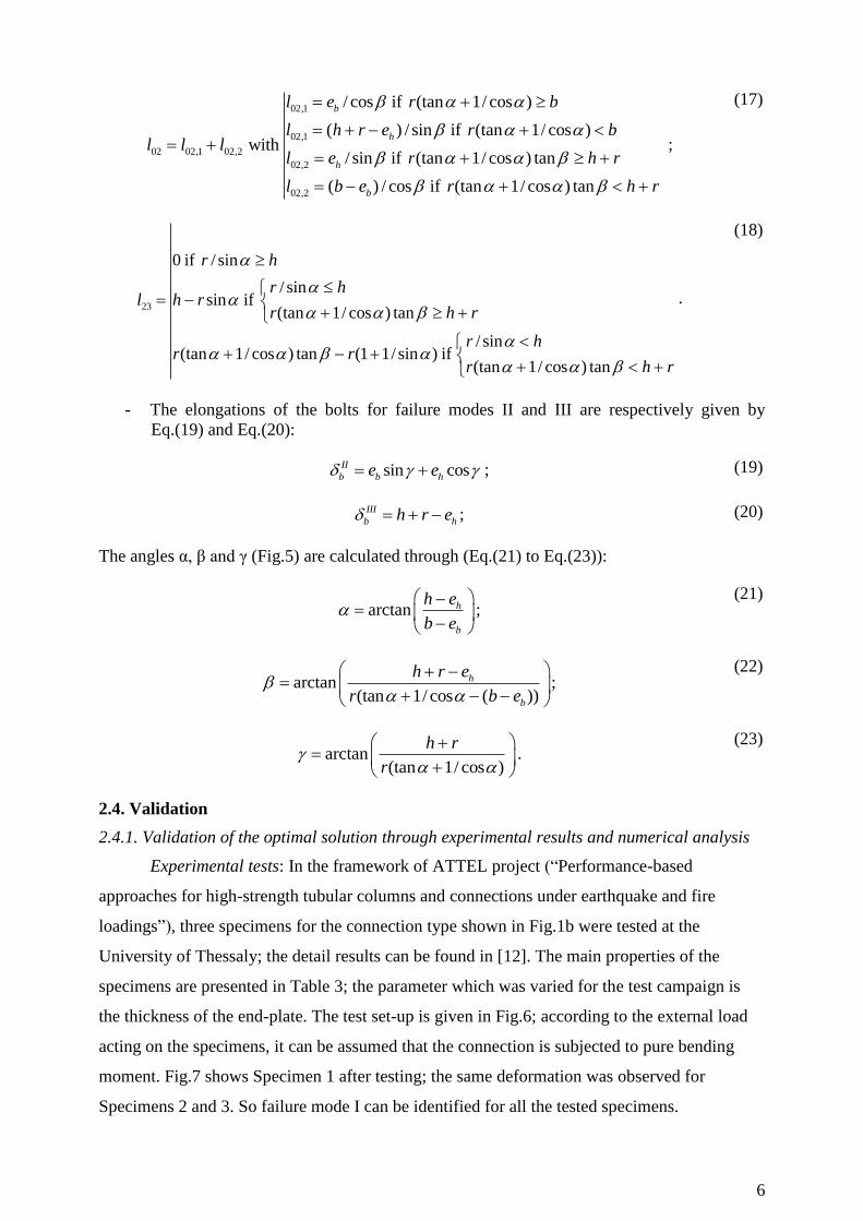
- Length of the yield lines (Eq.(15) to Eq.(18)):
01 2l b ; (15)
12,1
12,1
12 12,1 12,2
12,2
12,2
( cos ) / sin if (tan 1/ cos )
(tan 1/ cos ) if (tan 1/ cos )with
/ tan if / sin
( sin ) / cos if / sin
l b r r b
l r r bl l l
l r r h
l h r r h
;
(16)
6
02,1
02,1
02 02,1 02,2
02,2
02,2
/ cos if (tan 1/ cos )
( ) / sin if (tan 1/ cos )with
/ sin if (tan 1/ cos ) tan
( ) / cos if (tan 1/ cos ) tan
b
h
h
b
l e r b
l h r e r bl l l
l e r h r
l b e r h r
;
(17)
23
0 if / sin
/ sinsin if
(tan 1/ cos ) tan
/ sin(tan 1/ cos ) tan (1 1/ sin ) if
(tan 1/ cos ) tan
r h
r hl h r
r h r
r hr r
r h r
.
(18)
- The elongations of the bolts for failure modes II and III are respectively given by
Eq.(19) and Eq.(20):
sin cosII
b b he e ; (19)
III
b hh r e ; (20)
The angles α, β and γ (Fig.5) are calculated through (Eq.(21) to Eq.(23)):
arctan h
b
h e
b e
;
(21)
arctan(tan 1/ cos ( ))
h
b
h r e
r b e
;
(22)
arctan(tan 1/ cos )
h r
r
.
(23)
2.4. Validation
2.4.1. Validation of the optimal solution through experimental results and numerical analysis
Experimental tests: In the framework of ATTEL project (“Performance-based
approaches for high-strength tubular columns and connections under earthquake and fire
loadings”), three specimens for the connection type shown in Fig.1b were tested at the
University of Thessaly; the detail results can be found in [12]. The main properties of the
specimens are presented in Table 3; the parameter which was varied for the test campaign is
the thickness of the end-plate. The test set-up is given in Fig.6; according to the external load
acting on the specimens, it can be assumed that the connection is subjected to pure bending
moment. Fig.7 shows Specimen 1 after testing; the same deformation was observed for
Specimens 2 and 3. So failure mode I can be identified for all the tested specimens.

7
Numerical simulation: a numerical study was also performed in the framework of the
ATTEL RFCS project. A detail description of this study, which is summarised here below can
be found in [13]. For this study, LAGAMINE, a nonlinear finite element code developed at
Liege University [14], was used to perform the numerical simulations in which geometrical
nonlinearities including large deformation and material nonlinearities were taken into account.
As the joint is fully symmetric, the computation was carried out on only ¼ of the considered
joint as shown in Fig.8. Moreover, the bolts located in the compression zone of the connection
are not introduced in the model as they are not activated. The tube, the end-plate, the weld and
the bolts are modelled using 8-node brick BLZ3D elements with reduced integration, while the
contact surfaces are modelled using CFI3D elements for which the Coulomb law is applied.
The detailed properties of these elements can be found in [14]. Considering the meshing, a
quite fine mesh with adaptive element sizes is used to suit the geometry shape of the joint. It is
assumed that the washer is fully connected to the bolt head as the relative displacement
between them is negligible. Moreover, as there is a gap between the bolt’s shank and the inner
surface of the hole in the end-plates, it is assumed that no contact force is generated between
them. As a consequence, only two contact surfaces are modelled: (i) washer-plate interface
with friction (coefficient = 0.25) and (ii) plate-rigid foundation interface with no friction
(Fig.8). Regarding the bolt modelling, the Agerskov’s length [15] is adopted for the effective
length of the bolt shank. With respect to the material modelling, the actual - curves of the
materials are implemented in the numerical models.
Yield line analysis: a computer program solving the optimal solution of Eq.(7) was
implemented, the strengths of the tested connections are automatic calculated and the so-
obtained values are reported in Table 4. In the calculations, both yield and ultimate strengths
(i.e. fy and fu) are used to compute Mp and Mu respectively.
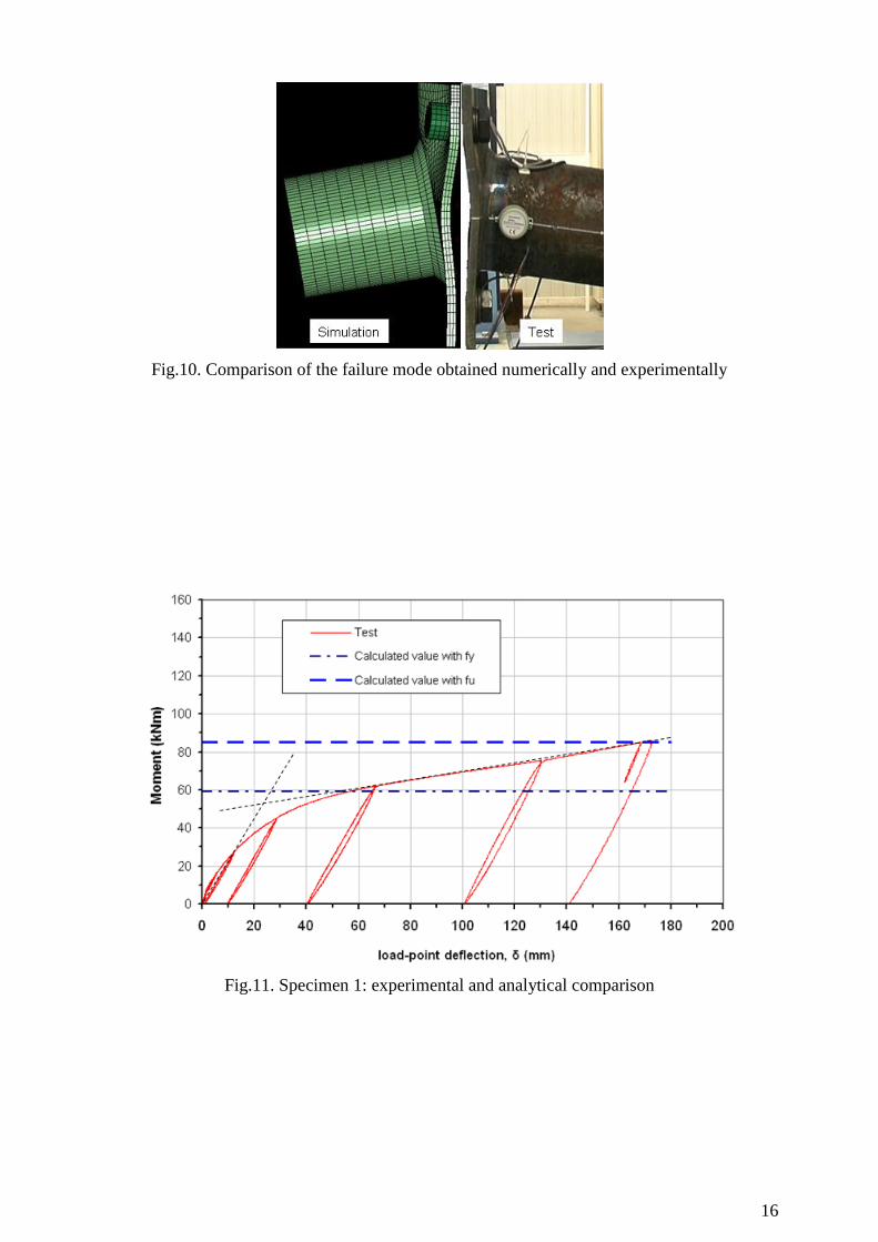
Experimental and FE analysis comparison: load-displacement curves and the failure
modes are compared and reported in Figs. 9 and 10. The connection strengths given by FE
analyses are a bit higher than the test ones while the failure mode I is identified for all three
specimens in both experimental and FE results. It can be concluded that a good agreement is
obtained between the numerical predictions and the experimental results.
Experimental and yield line analysis comparison: plastic and ultimate moments are
compared and shown in Figs.11, 12 and 13; it can be observed that a good agreement is
obtained. “It is necessary to note that the ultimate moment resistance of the connections can’t
be reached during the tests because of too large displacement; the maximal moments given by
the tests are used to compare with the calculated values.”
8
FE analysis and yield line analysis comparison: the development of the plastic
deformations are compared and presented in Fig.14. A rather good agreement is identified in
the tension zone while a small difference is observed in the compression zone.
Discussions: the comparisons between the experimental, numerical and analytical
results demonstrate that the proposed yield line pattern for the failure mode of the end plate is
quite close to the actual one; a good agreement is observed in terms of plastic and ultimate
resistances. Accordingly, the proposed analytical model appears to be appropriate.
Remark: the bolt size has influence on the plastic capacity of the end-plate through the
yield lines passing the bolt positions. Then, the bolt size effect should be considered in many
cases where the effect is significant. For example, with a standard T-stub and the failure mode I
is concerned, there are two yield lines (equal to 50% total length of all yield lines) influenced
by bolt size leading to a considerable impact. In the present case, the length of yield lines that
can be affected by the bolt size is quite small in comparison with the total length of all yield
lines (the length of the yield lines 02 and 03 in comparison with the total length of all yield
lines in Fig.5). Therefore, the effect of the bolt size in the investigated case may be neglected.
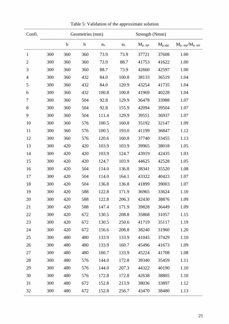
2.4.2. Validation of the approximate solution by comparing to the optimal solution
Considering the optimal solution validated in the previous section as reference results,
the results obtained through the simplified approach will be compared to these reference
results. The comparison is performed on a series of connections ( 36 different configurations)
for which three parameters are varied (see Fig.15 and Table 5): (1) the ratio between the end-
plate width and the tube diameter (b/r = 1.2 to 1.6); (2) the ratio between the height and the
width of the end-plate (h/b= 1.0 to 1.6); and (3) the bolt positions(three positions (Fig.15)
defined through different values of eb and eh (Fig.2b)). The plastic moments (Mp,app and Mp,opt)
of the connection given by the approximate and optimal solutions are compared; the obtained
results are reported in Table 5. It can be observed from Table 5 that the approximate solution
exhibits a rather good agreement with the optimal solution, in particular for configuration with
square end-plates; the observed difference increases when the height/width ratio of the
rectangular end-plate increases. The mean difference of around 10% demonstrates that the
approximate formulas could be proposed for practical applications.
3. Applications
Formulas for the all the mechanisms shown in Fig.3 are now available and may be used
to predict the strength of tube-to-tube joints (Fig.1b) and to calculate the force in the bolts in
tension of column bases (Fig.1a). The procedure to be followed are given here below.

9
3.1. For tube-to-tube joints
The results of the proposed model for the joints shown in Fig.3 can be directly applied
to determine the plastic strength of the tube-to-tube connections (Fig.1b). As the upper bound
approach is adopted, the plastic strength of the joints is the smallest among the values given in
Table 6, corresponding to the limit loads of the mechanisms shown in Fig.3. The same
formulas may be used to estimate the ultimate strength of the joints if the unit ultimate moment
mu is used instead of mp, and Bu instead of Bp.
3.2. For column bases
The application of the component method to the column base has been presented in
many documents, e.g. [4, 7]. The concrete in compression, the end-plate in bending and the
bolts in tension are the three main components of the column bases under bending moment and
axial force. How to calculate the concrete in compression component for the column bases with
circular tubular column have been presented in many literature, e.g. [9, 16, 17, 18] and they are
not reported herein. The tension force in bolts depends on three parameters: (1) the strength of
the bolt shanks; (2) the resistance of the end-plate in bending; and (3) the anchorage strength of
the bolts in the foundation. It is important to note that the failure in the bolt shanks and in the
concrete are not recommended as they lead to a brittle failures. Also, the anchorage failure
(bond or cone failure) is not the objective of the present paper, as this master is dealt in the
literature, e.g. [19]. The strength of the bolt shanks is known as Bu, and the bending strength of
the plate is presented in Section 2. However, many experimental tests demonstrated that the
prying forces don’t develop in the column bases, due to the important elongation of the anchor
bolts (in the case of non-preload bolts). Without the prying forces, the yield lines throughout
the bolt positions (Figs.3b and d) cannot develop, and the tension force in bolts can be
therefore easily found. In summary, the actual force in bolts located in the tension side of the
column bases is the smallest among the value reported in Table 7.
4. Conclusions
A study related to the behaviour of the end plate in bending and bolt in tension
components in connections with tubular sections was presented in this paper. A new yield line
pattern for the end plate is proposed and developed by using a limit analysis. Analytical
formulas for the proposed yield line pattern are proposed and validated through comparisons to
experimental and FE results, and that in terms of resistance and failure mode. It was
demonstrated that the level of accuracy of the proposed formulas may be sufficient to be
proposed for practical situations. The strength of tube-to-tube joints under bending moment can
be predicted while the bolt force in the tension zone of a column bases can be determined
through the proposed analytical approach.

10
Acknowledgements This work was carried out with a financial grant from the Research Fund for Coal and
Steel of the European Community, within the ATTEL project: “Performance-Based
Approaches for High Strength Steel Tubular Columns and Connections under Earthquake and
Fire Loadings”, Grant N0 RFSR-CT-2008-00037.
References
[1] Wardenier J. Kurobane Y., Packer J.A., Dutta D., Yeomans N. Design guide for circular
hollow section (CHS) joints under predominantly static loading. CIDECT 2008.
[2] Zhao X.L., Herion S., Packer J.A., Puthli S.R., Sedlacek G., Wardenier J., Weynand K.,
van Wingerde A.M., Yeomans N.F. Design guide for circular and rectangular hollow section
welded joints under fatigue loading. CIDECT 2001.
[3] Eurocode 3: Design of steel structures - Part 1-8: Design of joints. EN 1993-1-8, Brussels,
2003.
[4] Guisse S, Vandegans D, Jaspart JP. Application of the component method to column bases
– experimentation and development of a mechanical model for characterization. Research
Centre of the Belgian Metalworking Industry, 1996.
[5] Jaspart J.P. Recent advances in the field of steel joints: column bases and future
configurations for beam-to-column joints and beam splices. Agregation thesis, University of
Liege, 1997.
[6] Wald F., Sokol Z, Jaspart J.P. Base plate in bending and anchor bolts in tension. HERON,
Vol. 53 (2008), N0 2/3.
[7] Wald F., Sokol Z, Steenhuis M., Jaspart J.P. Component method for steel column bases.
HERON, Vol. 53 (2008), N0 2/3.
[8] Wald F., Bouguin V., Sokol Z., Muzeau J.P. Effective length of T-Stub of RHS column
base plates. Czech Technical University, 2000.
[9] Horova K., Wald F., Sokol Z. Design of circular hollow section base plates. 6th European
Conference on Steel and Composite Structures (EUROSTEEL), Budapest -2011, Vol.A, pp.
249-254.
[10] Wheeler A.T., Clarker M.J., Hancock G.J, Murray T.M. Design Model for Bolted Moment
End Plate Connections Joining Rectangular Hollow Sections. Journal of Structural
Engineering, Vol. 124, N0 2, 1998.
[11] Wheeler A.T., Clarker M.J., Hancock G.J. Design Model for Bolted Moment End Plate
Connections Joining Rectangular Hollow Sections Using Eight Bolts. Research Report N0
R827, University of Sydney, 2003.
[12] ATTEL project: “Performance-based approaches for high-strength tubular columns and
connections under earthquake and fire loadings”, Deliverable Report D.3.1: monotonic and
cyclic tests data on base-joint specimens, 2012.
[13] ATTEL project: “Performance-based approaches for high-strength tubular columns and
connections under earthquake and fire loadings”, Deliverable Report D.5.3: simulation data
relevant to the selected typologies of base joints, of HSS-CHS columns and HSS-CFT column
and of HSS-concrete composite beam-to-column joints, 2012.
[14] LAGAMINE: User’s manual, University of Liege, 2010.
[15] Agreskov H. High strength bolted connections subject to prying. J. Struc Div 1976.
11
[16] Column base plates. American Institute of Steel Constructions, 2003.
[17] Moore D.B., Wald F (Ed). Design of Structural Connections to Eurocode 3 – Frequently
Asked Questions. Czech Technical University, 2003.
[18] Steenhuis M., Wald F., Sokol Z., Stark J. Concrete in compression and base plate in
bending. HERON, Vol. 53 (2008), N0 1/2.
[19] Fastenings to Concrete and Masonry Structures. State of the Art Report, CEB, Thomas
Telfort Services Ltd, London 1994, ISBN 0 7277 19378.
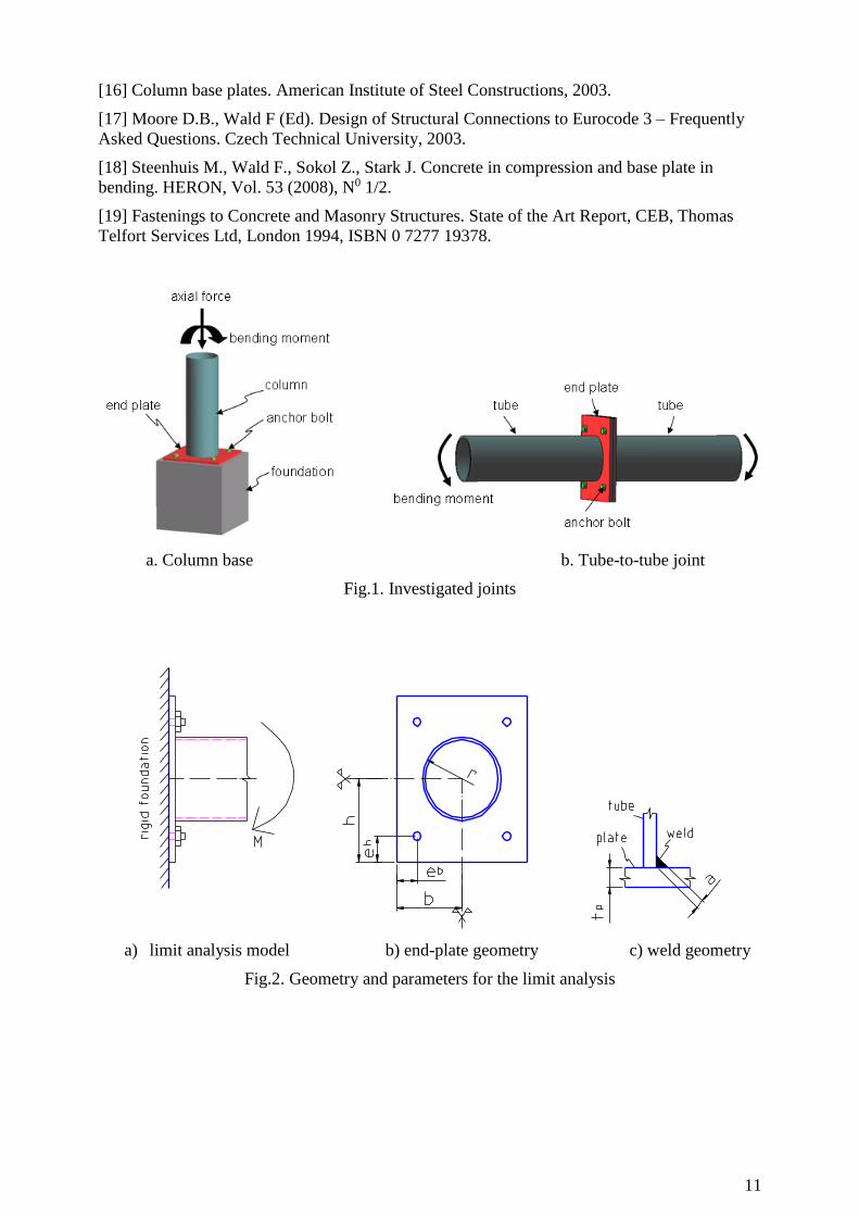
a. Column base b. Tube-to-tube joint
Fig.1. Investigated joints
a) limit analysis model b) end-plate geometry c) weld geometry
Fig.2. Geometry and parameters for the limit analysis

12
Fig.3. Considered mechanisms
a) plastic mechanism b) detailed geometries
Fig.4. Detailed geometry of yield pattern “d”

13
Fig.5. Approximate mechanism of mechanism “d” (Fig.4)
Fig.6. Test set-up

14
Fig.7. Specimen 1 at the end of the test
Fig.8. FE modelling of the tested connections (1/4 part)

15
Fig.9. Experimental and FE comparison - load-displacement curves
16
Fig.10. Comparison of the failure mode obtained numerically and experimentally
Fig.11. Specimen 1: experimental and analytical comparison

17
Fig.12. Specimen 2: experimental and analytical comparison
Fig.13. Specimen 3: experimental and analytical comparison

18
Yield line analysis FE analysis
Fig.14. Analytical and finite element comparison- plastic deformation
Fig.15. Varied geometrical parameters for the considered connections
Table 1: determination of ni, nj, lij,x and lij,y
plane i – plane j ni nj lij,x lij,y
0-1 0 0 1 i j k 0D D
z x i j k 0 'G G
y y
0-2 0 0 1 i j k 1 1 1
A B Cx y z i j k
E Gx x
G Ey y
0-3 0 0 1 i j k 1 1 1
'A B Cx y z i j k
' 'E Gx x
' 'G Ey y
1-2 0D D
z x i j k 1 1 1
A B Cx y z i j k
D Hx x
H Dy y
1-3 0D D
z x i j k 1 1 1
'A B Cx y z i j k
'D Hx x
'D Hy y
2-3 1 1 1
A B Cx y z i j k 1 1 1
'A B Cx y z i j k
F Dx x 0
The positions of the points A, B, C, D, E, E’, F, G, G’, H and H’ are shown in Fig.4b.

19
Table 2: A, C, D, E, E’ F, G, G’, H and H’ coordinates (Fig.4b) as a function of yB.
Coordinates Equations
Dx {1 cos[2 ( / )]}/ cos[2 ( / )]
D B Bx r artg r y artg r y
Ax ( ) /( )
A B h B bx y h e r y b e
Dz D D
z x
'By 'B B
y y
Cz /( )
C A D A Dz x x x x
'( )
E Ex x
Ex h r
'( )
E Ey y ( ) / (if then 0)
E B A A A Ey y x h r x x h r y
'( )
G Gx x (1 / )
G A Bx x b y
'( )
G Gy y
Gy b
'( )
H Hx x ( ) /
H D B Bx x y b y
'( )
H Hy y
Hy b
Fx F E
x x

20
Table 3: geometries and material properties of the tested specimens
Test Geometries (Fig.2, in mm) Material (N/mm2)
b h tp r0 a eb=eh fy (yield strength) fu ( ultimate strength)
1 200 200 14 96.85 16 60 418 602
2 200 200 16 96.85 16 60 418 602
3 200 200 18 96.85 16 60 418 602
Bolts with a diameter of 30mm and a 8.8 grade are used for all specimens.
Table 4: Calculated strength of the tested specimens (using optimal solution)
Test Plastic moment Mp (kNm) Ultimate moment Mu (kNm)
1 59 85
2 77 111
3 97 140
21
Table 5: Validation of the approximate solution
Confi. Geometries (mm) Strength (Nmm)
b h eb eh Mp, opt Mp,app Mp, app/Mp, opt
1
2
3
4
5
6
7
8
9
10
11
12
13
14
15
16
17
18
19
20
21
22
23
24
25
26
27
28
29
30
31
32
300
300
300
300
300
300
300
300
300
300
300
300
300
300
300
300
300
300
300
300
300
300
300
300
300
300
300
300
300
300
300
300
360
360
360
360
360
360
360
360
360
360
360
360
420
420
420
420
420
420
420
420
420
420
420
420
480
480
480
480
480
480
480
480
360
360
360
432
432
432
504
504
504
576
576
576
420
420
420
504
504
504
588
588
588
672
672
672
480
480
480
576
576
576
672
672
73.9
73.9
88.7
84.0
84.0
100.8
92.8
92.8
111.4
100.5
100.5
120.6
103.9
103.9
124.7
114.0
114.0
136.8
122.8
122.8
147.4
130.5
130.5
156.6
133.9
133.9
160.7
144.0
144.0
172.8
152.8
152.8
73.9
88.7
73.9
100.8
120.9
100.8
129.9
155.9
129.9
160.8
193.0
160.8
103.9
124.7
103.9
136.8
164.1
136.8
171.9
206.3
171.9
208.8
250.6
208.8
133.9
160.7
133.9
172.8
207.3
172.8
213.9
256.7
37721
41753
42660
38133
43254
41969
36478
42094
39551
35192
41199
37740
39965
43919
44625
38341
43322
41899
36965
42430
39828
35868
41719
38240
41045
45496
45224
39340
44322
42638
38036
43470
37608
41622
42597
36519
41735
40228
33988
39504
36937
32147
36847
33455
38018
42435
42528
35520
40423
39003
33624
38876
36449
31057
35117
31960
37429
41673
41708
35459
40190
38805
33897
38480
1.00
1.00
1.00
1.04
1.04
1.04
1.07
1.07
1.07
1.09
1.12
1.13
1.05
1.03
1.05
1.08
1.07
1.07
1.10
1.09
1.09
1.15
1.19
1.20
1.10
1.09
1.08
1.11
1.10
1.10
1.12
1.13

22
33
34
35
36
300
300
300
300
480
480
480
480
672
768
768
768
183.4
160.5
160.5
192.6
213.9
256.8
308.2
256.8
40688
36999
42802
39185
35548
30680
34489
31470
1.14
1.21
1.24
1.25
The mean difference: 10%
Table 6: plastic resistance for the tube-to-tube joints
Yield pattern Failure mode Plastic strength (Mpi)
Fig.3a Mode 1– thin plate 1
[8 ( ) 2 ]p h p
M h r e b m
Fig.3b Mode 1– thin plate 2
24( 1)
p p
h
rM bm
h r e
(*)
Fig.3c Mode 2 – intermediate plate 3
4 1 4 h
p p p
r reM bm B
h r h r
Fig.3d Mode 1- thin plate 4
I
p pM M (Eq.(8))
Fig.3e Mode 2 – intermediate plate 5
II
p pM M (Eq.(9))
Fig.3f Mode 3 – thick plate 6
III
p pM M (Eq.(10))
Remark: (*) only applied for the cases where 0h
h r e .
Table 7: determination of the tension in the bolt, Fb (for one bolt)
Yield pattern in
tension zone
Failure mode Bolt force Fb (one bolt)
Circular (Fig.3a) Mode I- thin plate 1
4b p
F m
Perpendicular
(Fig.3c)
Mode I – thin plate 2b p
h
bF m
h r e
Incline (Fig.3e) Mode I- thin plate 12 12 23 23
3
( 0.5 ) p
b
h
l l mF
h r e
(*)
- Mode III– thick plate 4b pF B
Remarks: (*)12 23 12 23, , ,l l are determined through Eqs. (12), (14), (16) and (18) respectively.