NISTIR 7873

Properties of Metal Powders for Additive Manufacturing: A Review of the State of the

Art of Metal Powder Property Testing

April Cooke John Slotwinski

http://dx.doi.org/10.6028/NIST.IR.7873

2

NISTIR 7873

Properties of Metal Powders for Additive Manufacturing: A Review of the State of the

Art of Metal Powder Property Testing

April Cooke John Slotwinski

Intelligent Systems Division

Engineering Laboratory

http://dx.doi.org/10.6028/NIST.IR.7873

July 2012

U.S. Department of Commerce

Rebecca Blank, Acting Secretary

National Institute of Standards and Technology Patrick D. Gallagher, Under Secretary of Commerce for Standards and Technology and Director

3

Certain commercial entities, equipment, or materials may be identified in this document in order to describe an experimental procedure or concept adequately.

Such identification is not intended to imply recommendation or endorsement by the National Institute of Standards and Technology, nor is it intended to imply that the entities, materials, or equipment are necessarily the best available for the purpose.

National Institute of Standards and Technology IR 7873 Natl. Inst. Stand. Technol. IR 7873, 22 Pages (July 2012)

CODEN: NTNOEF

4

TABLE OF CONTENTS

INTRODUCTION 5

TESTING OF METAL POWDER PROPERTIES 7 Powder Sampling 7 Size Determination Methods 8 Morphology Characterization Methods 10 Chemical Composition Test Methods 16 Micro Analysis Methods Surface Analysis Methods Bulk Analysis Methods Flow Characteristics Test Methods 19 Thermal Characterization Methods 19 Density Determination Methods 21

CONCLUSIONS AND NEXT STEPS 24 ACKNOWLEDGEMENTS 25 REFERENCES 26

5

INTRODUCTION This report is the second in a series of reports from the National Institute of Standards and Technology’s (NIST’s) Engineering Laboratory project titled Materials Standards for Additive Manufacturing.1 This project provides the measurement science for the additive manufacturing (AM) industry to measure material properties in a standardized way. Currently there are few consensus-based standards in this area. This project, in conjunction with NIST’s Fundamental Measurement Science for Additive Processes project,2 will provide the technical foundation necessary to develop new consensus-based standards. Development of standards will be done via ASTM-International’s (hereafter referred to as ‘ASTM’) Committee F42 on Additive Manufacturing Technologies and the newly formed International Organization for Standardization (ISO) TC261 committee on Additive Manufacturing. Determining the properties of the powder used for metal-based additive manufacturing, as well as the properties of the resulting bulk metal material, is a necessary condition for industry to be able to confidently select powder and produce consistent parts with known and predictable properties. By 2014, the project team will develop and deliver enhanced measurement techniques that support new, standardized methods for quantifying the material properties of both the powders used for additive manufacturing and the resulting manufactured products. The project’s research plan includes assessments of the current state-of-the-art testing methods for determining properties of both bulk metal materials, as reported in [1], and raw metal powder, which is the focus of this report. These methods will then be evaluated for applicability and enhanced for use on additively manufactured parts and powder used as raw material for powder-bed fusion additive manufacturing processes. NIST’s Direct Metal Laser Sintering (DMLS) machine will be used to make parts, and these new testing methods will be rigorously implemented. Using these enhanced methods, the sensitivity of part material properties to variations in initial powder properties will be determined. This is a critical step necessary for determining the scopes of relevant material standards for additive manufacturing and for the production of additive manufacturing parts with consistent properties. Metal powders for additive processes are typically made through one of two processes, gas atomization and plasma rotating electrode process (PREP). Gas atomized powders are the most commonly used raw materials for the additive manufacturing of metal parts [2]. They are made by disrupting a molten metal stream with one or more gas jets. In PREP, a rotating bar of feedstock is arced with gas plasma, and the molten metal is centrifugally atomized as it is flung off the bar. The molten metal droplets then cool into spherical powder particles [3]. In order to perform this assessment of the existing test methods for metal powder properties, 21 relevant consensus-based ASTM standards and 31 technical publications were surveyed. The report is organized into the most important properties of metal powders, which are size, morphology, chemical

1 http://www.nist.gov/el/isd/sbm/matstandaddmanu.cfm 2 http://www.nist.gov/el/isd/sbm/fundmeasursci.cfm

6

composition, flow, thermal properties, and density. Test methods for these properties described in various ASTM standards and other literature are summarized. Sampling methods, which are important to ensure that measurements of small powder samples are representative of the entire batch, are also covered.

7

TESTING OF METAL POWDER PROPERTIES Powder Sampling Due to large lot sizes it is not practical to measure an entire batch of powder. Instead, smaller representative samples are taken from the batch, and these are characterized. Sampling must be done judiciously to ensure that the measured properties of these smaller samples are representative of the entire batch of powder. A detailed synopsis of powder sampling techniques is provided in another NIST report, which addresses the determination of the particle size distributions of ceramic powders [4]. When a sample is taken from the batch of powder, it is preferable that the powder be in motion (i.e., being poured from one container to another) as the sample is taken from it. However, if motion is not possible, samples can be taken through a static sampling procedure using a device called a “sample thief,” which is shown in Figure 1. This is a long rod with a sampling chamber along its length and a device that can open and close the sampling chamber at the operator’s end. This tool should be placed in multiple representative locations within an amount of powder to extract powder representative of the bulk lot. For example, if the powder is located in a bag, representative locations include the bottom, center, top, front, and rear of the bag.

Figure 1: Sample Thief After bulk sampling, the material needs to be further sub-divided in order to make the sample size manageable. The methods described in [4] include Cone and Quartering, Scoop Sampling, Table Sampling, Chute Splitting, and Spin Riffling. Cone and Quartering involves mounding a pile of powder into a cone-shaped heap, flattening it with a spatula, dividing it into four sections, and repeating the process on one of the sections so that the final sample is 1/16th the size of the original sample. Scoop Sampling simply involves using a scoop to select a portion of the bulk sample. Table Sampling involves pouring the bulk sample of powder down an inclined plane that has a series of structures and holes used to divide it. Chute Splitting is a process in which samples are divided into two lots via dispersion through a series of chutes. Spin Riffling involves pouring the bulk sample into a hopper that empties onto a vibratory chute that leads to a series of sample containers contained in a rotating ring. Figure 2 shows illustrations of a table sampler, a chute splitter, and a spin riffler. Allen [5] reported that the statistically significant results provided by the spin riffler are so superior to other methods that it should be used whenever possible.

8

Figure 2: Illustrations of (a) a table sampler, (b) a chute splitter, and (c) a spin riffler. ASTM B215-10 [6] also describes procedures for sampling metal powders. This standard focuses on metal powders transferred from blenders or storage tanks, as well as metal powders already packaged in containers such as bags. Specific instructions for the method of collecting metal powder from a moving stream are also included in this standard. If the lot of powder to be sampled is flowing into one container, then the guidance is to pass a rectangular vessel at a constant speed through the stream of flowing powder when the container to which the powder is flowing is ¼, ½, and ¾ full. If the lot of powder is to fill several containers, then the first portion of the sample should be taken when the first container is ½ full, the second portion of the sample should be taken in the middle of the run, and the third portion of the sample should be taken near the end of the run. Size Determination Methods In additive manufacturing, powder particle size determines the minimum part layer thickness, as well as the minimum buildable feature sizes on a part. Several methods were described in the literature [4] for particle size determination, including sieving, gravitational sedimentation, microscopy-based techniques, and laser light diffraction. Sieving is the technique of shaking powder through a stacked series of sieves with decreasing mesh sizes. Gravitation sedimentation uses X-ray absorption or light scattering to determine the particle concentration at different heights within a monitored container of liquid at different times. Microscopy-based techniques use optical light microscopes, scanning electron microscopes (SEM), or transmission electron microscopes (TEM) to visually discern size information. Laser light diffraction involves deconvolving and inverting the summation of the scattered light pattern produced by each sampled particle. Several ASTM standards address particle size determination. More detailed specifications for the sieving process than what is discussed in NIST SP 960-1 are provided in ASTM B214-07(2011) [7]. This standard suggests arranging a group of sieves in consecutive order by the size of their openings, with the coarsest

(a) (b) (c)

Vibratory Chute

Direction of Flow

Direction of Flow

9

sieve on top and a solid collecting pan below the bottom sieve. The powder is placed in the top sieve, covered, and the entire apparatus is fastened into a sieve shaker where it is agitated for 15 min. The sieve mesh sizes can range from 5 µm to 1 mm, and the sieve mesh, or wire cloth, is commonly made of bronze, brass, or stainless steel. ASTM B214-07(2011) also states that the entire sieve apparatus should be 200 mm in diameter and either 25.4 mm or 50.8 mm deep. However, ASTM E161-00(2010) [8] states that the sieve can be as small as 76.2 mm in diameter with the same depth range. A method of using a horizontally collimated beam of X-rays of constant intensity to measure the relative mass concentration of particles in a liquid medium is described in ASTM B761-06(2011) [9]. First the intensity of the X-ray beam that is projected through a clear liquid medium in the central region (vertically) of a cell is measured to establish a reference. Then the cell is filled with the homogenous suspension of powder that is continuously circulated, and the intensity of the X-ray is measured after it passes through. The powder particles absorb some of the X-ray energy, and this establishes a value for full scale attenuation. Then the circulation of the mixture is ceased, which allows the particles to settle to the bottom of the cell. While this is happening, the X-ray intensity is monitored. During sedimentation, the larger particles fall below the X-ray beam at a faster rate than the smaller particles. Each mass measurement represents the cumulative mass fraction of the remaining fine particles. Eventually, all of the particles settle, which allows the X-ray to pass through the cell unattenuated, and the intensity value reaches the value of the reference. The particle size can be determined from velocity measurements by applying Stokes’ law, since the conditions of liquid density and viscosity and particle density are known. Stokes’ law demonstrates that the terminal settling velocity of a spherical particle in a fluid medium is a function of the diameter of the particle [10]. This process is applicable to particles of uniform density and composition having a particle size distribution of 0.1 µm to 100 µm. Additionally, the relationship between size and sedimentation velocity assumes that the particles settle within the laminar flow regime. Therefore, analysis for particles that settle with a Reynold’s number greater than 0.3 may be incorrect due to turbulent flow [9]. The use of light scattering to measure the particle size distribution is described in ASTM B822-10 [11]. In this technique, which is applicable for powders whose particle diameters are in the range of 0.4 µm to 2 mm, a sample of the material is dispersed in liquid and circulated through the path of a light beam. Alternatively, a dry sample can be aspirated through light in a carrier gas. The light beam is scattered by the passing particles. Photodetector arrays collect the scattered light and convert it into electrical signals, which are then analyzed. The analyzed signal is converted to size distribution through the theories of Fraunhofer Diffraction, Mie Scattering, or a combination of both [11]. Fraunhofer Diffraction approximates the laws of light scattering, while Mie Scattering represents the laws of scattering more precisely with a solution to Maxwell’s Equations, which are the set of four partial differential equations that govern the behavior of electric and magnetic fields [12]. In a study by Biancaniello [13], it was determined that using the ASTM B214 method with a modified sieve measurement, incorporating electroformed micromesh sieves with openings of 5 µm and larger

10

provided particle size distribution data that was more reliable than data produced through sedimentation and light scattering techniques. Morphology Characterization Methods The morphology of powder particles determines how well the particles lay or pack together and thus, in additive manufacturing, is an important factor in realizing the minimum part layer thickness and density. Hawkins [14] offers a comprehensive review of many of the principles for characterizing the morphology of powder particles. The first principle is the importance of ensuring that every particle of a powder lot has an equal chance of being selected for observation. This is done through the previously discussed sampling techniques. The next principle discussed in Hawkins’ book indicates that silhouettes of the individual powder particles must be made visible so that their geometric shape can be characterized. Observation of the silhouettes can be performed by a method described by Cox [15], during which “the grains may be sprinkled over a lantern slide that has been previously covered with glue or a suitable cement, the slide inserted in a projection camera, and the image obtained on the screen.” This method, archaic in its description, has been modernized through the use of current microscopy techniques. The first and simplest means of morphology characterization is qualitative. Over the years, researchers have assigned adjectives to certain shapes, and most recently, ASTM B243-11 [16] established definitions for many powder shapes. The relevant terms are listed in Table 1. The fact that some of these definitions are similar suggests that the terms are not defined through scientific rigor.

Table 1: Terms describing powder shapes in ASTM B243-11. Term Definition

acicular needle-shaped flake flat or scale-like, whose thickness is small compared with other dimensions

granular approximately equidimensional, nonspherical shapes irregular lacking symmetry needles elongated and rod-like nodular irregular, having knotted, rounded, or similar shaped platelet composed of flat particles having considerable thickness plates flat particles of metal powder having considerable thickness

spherical globular-shaped Other means of powder morphology characterization are quantitative. One method is single-number classification, in which a shape is defined by using only one number associated with a feature of a particle [14]. The single-number classification has two disadvantages. First, it is ambiguous in that more than one outline shape can have the same number. An example of this situation is presented in Luerkens [17], and the shapes displayed in Figure 3 are useful in its visualization.

11

Figure 3: Shapes useful in illustrating ambiguity of single-number classification system (e.g., projected area). All of the objects in Figure 3 have the same projected area, because they are all constructed from the same number of squares. If the number used to characterize these shapes is the projected area, then this is an example of how more than one shape can be defined by the same number. The second disadvantage of the single-number classification system is that a number alone is not descriptive enough to enable the reproduction of the shape. However, they are mathematically convenient and can be associated with the shape characteristic of interest such as the projected area. The single-number classification system is divided into four groups: dimensional, sphericity, roundness, and perimeter. In the dimensional group the form of a large particle can be expressed by a parameter that is based on the longest, shortest, and intermediate orthogonal axes. This notion is discussed in Barrett [18], which is a review paper on the subject that tabulates 12 of the dimensional parameters that have been used since 1920. Table 2 provides five of them. Table 2: Dimensional parameters used to characterize large particles, where L = Long Axis, S = Short Axis, and I = Intermediate Axis [18].

Formula Name/Description Range L+I2S

Flatness Index 1 to ∞

IL

, SI

Ordinate and Abscissa for a Plot to Characterize Shape 0 to 1

I·100L

Elongation 0 to 100

S·100L

Flatness 0 to 100

SL Flatness 0 to 1

However, it is generally accepted that small particles can be evaluated in two dimensions [14], thus allowing for the use of measurements taken of particle silhouettes. The terms of the single-number classification groups mentioned and described from this point forward are two-dimensional. One

(a) (b) (c) (d)

(e) (f) (g) (h)

12

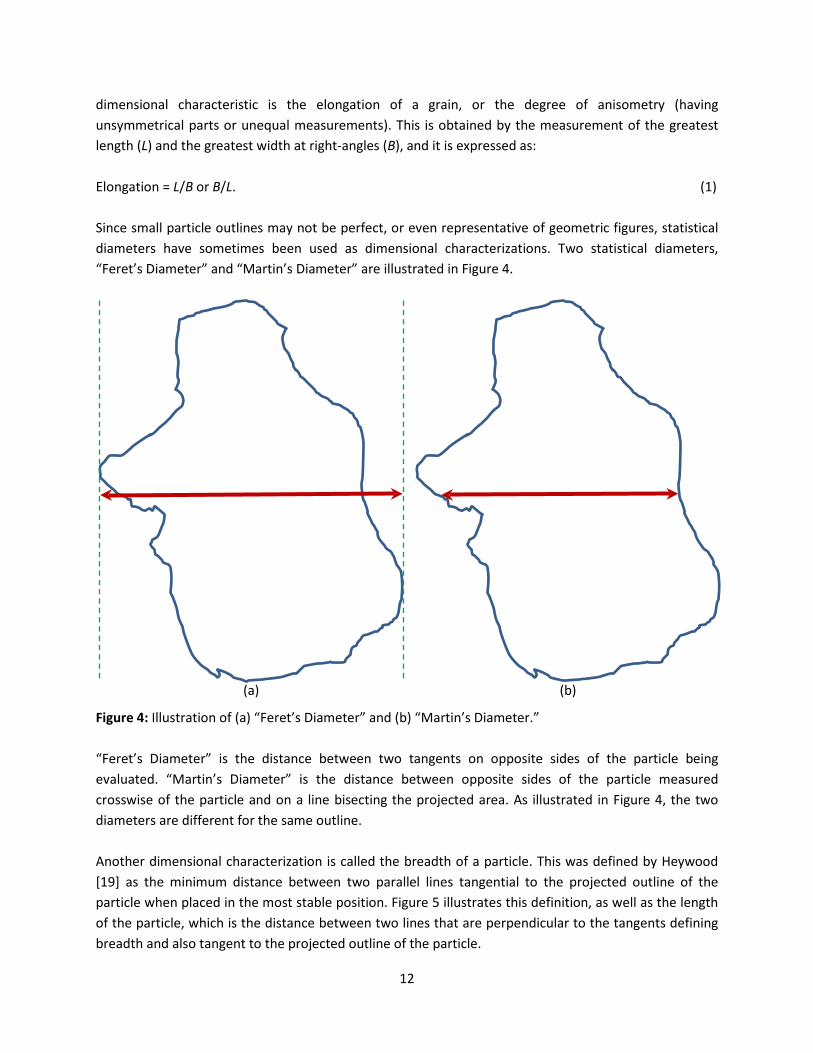
dimensional characteristic is the elongation of a grain, or the degree of anisometry (having unsymmetrical parts or unequal measurements). This is obtained by the measurement of the greatest length (L) and the greatest width at right-angles (B), and it is expressed as: Elongation = L/B or B/L. (1) Since small particle outlines may not be perfect, or even representative of geometric figures, statistical diameters have sometimes been used as dimensional characterizations. Two statistical diameters, “Feret’s Diameter” and “Martin’s Diameter” are illustrated in Figure 4.

Figure 4: Illustration of (a) “Feret’s Diameter” and (b) “Martin’s Diameter.” “Feret’s Diameter” is the distance between two tangents on opposite sides of the particle being evaluated. “Martin’s Diameter” is the distance between opposite sides of the particle measured crosswise of the particle and on a line bisecting the projected area. As illustrated in Figure 4, the two diameters are different for the same outline. Another dimensional characterization is called the breadth of a particle. This was defined by Heywood [19] as the minimum distance between two parallel lines tangential to the projected outline of the particle when placed in the most stable position. Figure 5 illustrates this definition, as well as the length of the particle, which is the distance between two lines that are perpendicular to the tangents defining breadth and also tangent to the projected outline of the particle.

(a) (b)

13

Figure 5: Tangential lines defining the distances of breadth (B) and length (L). Using the breadth (B) and length (L), the two following ratios can be formulated: Length Ratio = L/B, and (2)

Projected Area Ratio = projected area of silhouettearea of rectangle BL

. (3)

The next group in the single-number classification system is the sphericity group. Using the term “sphericity” as a two-dimensional description of a particle silhouette, although confusing, has been practiced for many years, and the best method of attaining the sphericity of a particle has long been debated. There are many different equations used to define it. Wadell [20] defines it as follows:

Sphericity = diameter of a circle equal in area to that of the particle outlinediameter of the smallest circle circumscribing the particular outline

. (4)

Another definition is given by Riley [21]:

Sphericity = 4π·area of the particle outlineperimeter of the particle outline2. (5)

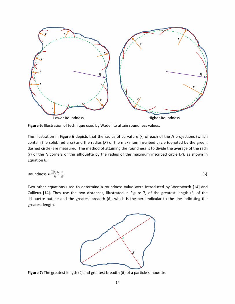
The third group in the single-number classification system is the roundness group, which defines roundness as the sharpness or smoothness of the perimeter of the silhouette of the particle. Analogous to sphericity, there are several methods of obtaining a roundness value. One method was introduced by Wadell [22] and is shown in Figure 6.

B

L

14

Figure 6: Illustration of technique used by Wadell to attain roundness values. The illustration in Figure 6 depicts that the radius of curvature (r) of each of the N projections (which contain the solid, red arcs) and the radius (R) of the maximum inscribed circle (denoted by the green, dashed circle) are measured. The method of attaining the roundness is to divide the average of the radii (r) of the N corners of the silhouette by the radius of the maximum inscribed circle (R), as shown in Equation 6.

Roundness = ∑ riNi=1N

· 1R. (6)

Two other equations used to determine a roundness value were introduced by Wentworth [14] and Cailleux [14]. They use the two distances, illustrated in Figure 7, of the greatest length (L) of the silhouette outline and the greatest breadth (B), which is the perpendicular to the line indicating the greatest length.

Figure 7: The greatest length (L) and greatest breadth (B) of a particle silhouette.

Lower Roundness Higher Roundness

R

r

r r

r

r

r

r

r

R

r r

r

r

L B

15

Using the distances depicted in Figure 7, Wentworth’s equation for roundness [14] is

Roundness = radius of curvature of the most convex part(L+B)/4

, (7)

and Cailleux’s equation for roundness [14] is

Roundness = radius of curvature of the most convex partL/2

. (8)

Finally, the perimeter group describes the circularity shape factor, widely accepted as the ratio of the square of the perimeter of the particle outline to 4π times the cross-sectional or projection area of the particle outline [14]. The equation form of this expression is as follows:

Circularity Shape Factor = (perimeter of the particle outline)2

4π·(cross-sectional or projectional area of the particle outline). (9)

Representation by series involves approximating the outlines of powder particles with complicated mathematical formulas. For example, an article by Schwarcz and Shane [23] poses that a Fourier series expression for the boundary of a particle silhouette can be expressed as follows: ρ(θ)= a0

2+∑ ai cos(iθ)+bi sin(iθ),∞

i=1 (10)

where the constants ai, bi, and a0 are defined as:

ai=1π∫ ρ(θ) cos (iθ)dθπ

-π , (11)

bi=1π∫ ρ(θ) sin (iθ)dθπ

-π , and (12)

a0= 1π∫ ρ(θ)dθπ

-π . (13)

As the order of the Fourier series increases, the accuracy of the approximation increases. This phenomenon can be simplified for better visualization. Figure 8 shows a series of six points, fit with curves of equations with increasing degrees. These curves can be used to approximate a surface created by those six points. The solid, red line represents a linear function fit to the data. The green, dashed line represents parabolic function fit to the data. A sixth-order polynomial is fit to the data, and it is represented by the purple, dotted line. Figure 8 clearly indicates that as the complexity of the equations used for curve-fitting increases, the accuracy of the approximation increases as well. By using Fourier series, a surface as complex as a human skull can be represented, which was accomplished by Lu [24].

16

Figure 8: Series of six points with curves fit to them. Chemical Composition Test Methods In practice raw metal powders used in additive manufacturing are not 100 percent pure, and contain other materials. These added materials consist of different elements that when combined and used in AM produce material properties specific to the bulk material type. Other materials might be introduced to ensure powder fidelity. The overall chemical composition of the metal powder may be a factor in the final part’s mechanical properties. Powder properties may also change over time, or in the case of recycled powder, due to repeated exposures in an AM build chamber environment. The techniques that can be used to determine the chemical composition of powders include micro analysis methods, surface analysis methods, and bulk analysis methods. The descriptions of these methods are as they are applied to bulk material, so the term “specimen” refers to bulk material, such as a block of metal, unless otherwise stated. Micro Analysis Methods Common micro analysis methods are energy dispersive spectroscopy and the use of an electron microprobe. Energy dispersive spectroscopy takes advantage of the fact that each element has a unique atomic structure. A high-energy beam of charged particles or a beam of X-rays is focused onto the sample. The incident beam may excite an electron, which would cause it to jump into a higher energy level, creating a hole where the electron was. An electron from a higher-energy level fills the hole and the difference in energy between the two levels is released in the form of an X-ray. The intensity and wavelength of the X-rays are measured with an energy dispersive spectrometer. The energy of the X-rays is characteristic of the difference in energy between the two energy levels and of the atomic

17

structure from which they were emitted, thus allowing the elemental composition of the specimen to be determined [25]. An electron microprobe focuses an electron beam onto the surface of a specimen. An X-ray is emitted as a result, and its intensity is recorded. The intensity is then divided by the intensity of the X-rays emitted by the pure substance. The result is equal to the mass concentration of the element at that location on the specimen. This method is used to determine the composition of a volume on the order of (10 to 30) µm3 or less. Also, the elements making up the specimen have to be known beforehand [26], so it is not applicable for samples that have unknown constituents. Surface Analysis Methods Surface analysis methods are atomic emission spectroscopy, X-ray photoelectron spectroscopy, and secondary ion mass spectrometry. Atomic emission spectroscopy uses the intensity of light emitted from a flame, plasma, arc, or spark at a particular wavelength to determine the quantity of an element in a sample. The wavelength of the atomic spectral line identifies the element while the intensity of the emitted light is proportional to the number of atoms of the element [27]. X-ray photoelectron spectroscopy, also called electron spectroscopy for chemical analysis (ESCA), is another method of determining the chemical composition of a specimen. Spectra are obtained by flooding X-rays onto the surface of the specimen while simultaneously measuring the kinetic energy and number of electrons that escape from the top 1 nm to 10 nm of the material. This procedure requires ultra-high vacuum conditions, and it detects all elements with an atomic number of 3 or higher. The detection of Hydrogen and Helium (atomic numbers of 1 and 2, respectively) is not possible because the diameters of these atoms are so small [28]. Secondary ion mass spectrometry sputters the surface of the specimen with a focused primary ion beam and collects and analyzes ejected secondary ions. Secondary ions are measured with a mass spectrometer to determine elemental, isotopic, or molecular composition of the surface. This process requires a high vacuum, and is a very sensitive surface analysis technique that can determine quantities to parts per billion [29]. Bulk Analysis Methods Relevant bulk analysis methods include atomic absorption spectroscopy, inductively coupled plasma optical emission spectroscopy, flame emission spectroscopy, X-ray fluorescence, X-ray powder diffraction, and inert gas fusion. Atomic absorption spectroscopy requires the sample to be atomized and reference samples with a known chemical composition to establish the relation between the measured absorbance and the elemental concentration. Energy is passed through the atomized sample, and each element absorbs a particular wavelength of light, since each element requires a unique amount of energy to promote its electrons into higher energy levels. The radiation flux with the sample in the atomizer is measured by a detector, and the radiation flux without the sample in the atomizer is

18

measured by the same detector. The ratio between the two values (the absorbance) is converted to component concentration or mass using the Beer-Lambert Law [30]. Inductively coupled plasma optical emission spectroscopy uses liquid samples that are injected into plasma using a nebulizer or other method of sample introduction. The mist is quickly dried, vaporized, and energized through collisional excitation at a high temperature (10 000 K), which promotes the atoms to excited states. The excited state atoms/ions may relax to a ground state through the emission of a photon. This atomic emission is then analyzed. The photons have characteristic energies, so the wavelengths can be used to identify the elements from which they originated. The total number of photons is directly proportional to the concentration of the originating element in the sample [31]. Flame emission spectroscopy is the process of introducing a specimen in the form of a gas or sprayed solution into a flame. The heat creates free atoms by evaporating the solvent and breaking chemical bonds. The atoms are excited by the addition of the thermal energy, so they emit light as they return to relaxed states. Characteristic wavelengths are emitted by each element, which are detected by a spectrometer [32]. In X-ray fluorescence, a specimen is excited due to exposure to X-rays or gamma rays. This causes the ejection of an electron from an atom and the emission of a photon when an electron from a higher energy level falls into the ejected electron’s original energy level. The emitted radiation has an energy that is characteristic of the atoms present [33]. X-ray powder diffraction exploits the crystalline structure of a material. X-rays are aimed at a sample, and some of the photons in the incident beam are deflected upon collision with electrons, much like billiard balls bouncing off of each other. If the atoms are arranged periodically, the diffracted waves will form interference peaks with a symmetry that matches that of the distribution of atoms. This allows the determination of the distribution of atoms in the sample, thus enabling its identification [34]. The inert gas fusion technique, which is used to determine the oxygen, nitrogen, and hydrogen content in metals, is described by ASTM E1409-08 [35], E1447-09 [36], E1569-09 [37], and E2792-11 [38]. In this process a sample is held in a chamber directly above a graphite crucible. The crucible is brought to an extremely high temperature (roughly 3000 °C). At the same time, the inert gas flows over it to remove any contaminants in what is called an “out-gassing” procedure. After “out-gassing,” the crucible temperature is lowered and the sample is added to it by lowering it from above. As the sample melts, the oxygen present reacts with the carbon in the graphite crucible to form Carbon Monoxide (CO) and Carbon Dioxide (CO2). The Nitrogen present is released as molecular Nitrogen (N2), and the Hydrogen present is released as Hydrogen gas (H2). The gases are carried out of the chamber onto a detector by the inert gas flow.

19

Flow Characteristics Test Methods How well a powder flows is an important factor for many additive manufacturing processes. Methods of determining the flow rate of powders using two types of flowmeters, the Hall flowmeter funnel and the Carney funnel, are described in ASTM B213-11 [39] and ASTM B964-09 [40], respectively. There are two types of methods for determining the flow rate: a static flow method and a dynamic flow method. The static flow method requires the user to cover the funnel opening with a dry finger and pour in a predetermined mass of powder. Then, when all the powder is loaded, the process is to start timing the flow of powder through the opening upon removal of the finger and stop timing as soon as the last of the powder has egressed. The dynamic flow method doesn’t involve covering the orifice with a dry finger. The timing begins as soon as the powder begins flowing out of the funnel and stops when all powder has finished flowing through the funnel. The flow rate value, reported in units of seconds per gram, is determined by dividing the measured time taken for all of the powder to exit the funnel by the mass of the powder sample. The difference between the Hall flowmeter funnel and the Carney funnel is the size of their orifice, with the Hall flowmeter having a 2.54 mm opening, and the Carney flowmeter having a 5.08 mm opening. The Carney flowmeter is used only for powder that will not flow through the Hall flowmeter. The process of timing powder as it flows through a Hall flowmeter is described in ASTM B855-11 [41]. However, this specifies measuring the flow by volume instead of by mass, thereby eliminating the variable of powder density. The ability to flow and pack is a function of interparticle friction, so as the surface area increases, the friction increases, which gives less efficient flow and packing. The acquisition of the correct volume of powder to use requires the use of an Arnold meter, a process that will be described later in the Density section of this report. Once the volume to be tested is attained, the process follows that of ASTM B213-11. This flow rate value is determined by dividing the measured time taken for all of the powder to exit the funnel by the volume of the powder sample, and it is reported in units of seconds per cm3. Thermal Characterization Methods Melting of powder by a high energy source is the essence of several AM processes. As such, thermal properties of powders are extremely important to AM. Sih and Barlow [42] provide a good summary of techniques used to evaluate the thermal conductivities of materials, dividing the techniques into two categories: steady-state and transient. While Sih and Barlow claim that the methods are applicable to powders, the descriptions that follow assume the specimen to be solid, bulk material in the required shape for the measurement technique. The first steady-state method is the Plate Method. An example of this method is the Guarded-Hot-Plate Method described in ASTM C177-10 [43]. Figure 9 is a diagram of a guarded-hot-plate apparatus.

20

Figure 9: Diagram of a Guarded-Hot-Plate apparatus. The components used in this method are two isothermal cold plates, a guarded-hot-plate, and two samples of the test specimen. The two samples of the test specimen sandwich the guarded-hot-plate, and the two isothermal cold plates then sandwich the test specimen/guarded-hot-plate combination. The necessary values for the calculation of the thermal conductivity of the specimen are the power supplied to the guarded-hot-plate, various surface temperature measurements, and the area and thickness of the specimen samples. Using these quantities, the thermal conductivity of the specimen can be determined through heat transfer principles. Another steady-state method of determining the thermal conductivity of a material is the Cylindrical Method. In this method, a heater resides along the axis of a cylinder of material with an unknown thermal conductivity. Guard rings are located at each end of the cylinder to prevent heat loss out of the ends. Power is supplied to the heater so that heat is radiated outward from the center of the cylinder. The temperatures at two different radii are measured and heat transfer principles are used to determine the thermal conductivity of the sample [42]. Finally, a third steady-state method consists of Spherical and Ellipsoidal Methods. In these methods, a spherical heater is placed in the center of a spherical or ellipsoidal sample. Similar to the Cylindrical Method, power is supplied to the heater so that heat radiates outward from the center of the sample. Temperatures are measured at different radii and heat transfer principles allow the calculation of the thermal conductivity [42]. In all of the steady-state methods, the calculation of the thermal conductivity involves simple heat transfer equations, and the heat losses by radiative heat transfer are assumed to be negligible. However, there is often difficulty in obtaining the required specimen shape. On the other hand, with transient methods, obtaining the thermal conductivity is much quicker although the calculations are more involved.

Insulation

Test Specimen

Test Specimen

Guarded-Hot-Plate Se

cond

ary

Gua

rd

Seco

ndar

y G

uard

Primary Guard

Primary Guard

Isothermal Cold Plate

Isothermal Cold Plate

21

One transient technique for measuring thermal conductivity is the Transient Hot Wire Method. For this method a long, thin heating wire is placed into a large specimen of material that is initially at a uniform temperature. The heater emits a constant heat when power is supplied to it. While heating up, the temperature at a specific point within the sample it monitored as a function of time. Heat transfer principles allow the calculation of the thermal conductivity by using two of the temperatures recorded at two discrete times. The Thermal Probe Method is quite similar to the Transient Hot Wire Method, but the heat source is enclosed inside a probe. This protects the wire and allows for easier insertion into the sample [42]. The Transient Hot Strip Method is another transient technique used to determine the thermal conductivity of a sample. In this method, a thin metal strip is placed within the specimen. The strip acts as a heat source and indicates its own temperature increase as well. A temperature increase causes an increase in the electrical resistance of the strip, so by monitoring the output voltage of the strip, one can obtain information about the thermal conductivity of the surrounding material [44]. A constant current is supplied to the metal strip, which provides a constant output of power. The voltage is monitored in the strip, and a change in voltage is indicative of a temperature increase within the strip. A fourth transient method used to determine the thermal conductivity of a sample is the Flash Method. In this method a brief, high-intensity light pulse is focused onto the surface of a specimen (a bed of powder). The temperature of the surface on the opposite side of the specimen is then measured. The thermal diffusivity is determined by the shape of the curve of temperature versus time at the opposing surface. The heat capacity is determined by the maximum temperature reached by the opposing surface. Finally, the thermal conductivity is determined by multiplying the heat capacity, thermal diffusivity, and the density [45, 46]. Density Determination Methods Several methods for determining the apparent density of metal powder are specified by ASTM standards. The apparent density is the ratio of the mass to a given volume of powder. The method of determining apparent density using the Hall flowmeter funnel is described in ASTM B212-09 [47]. The basic process is to let powder flow through the Hall flowmeter into a cup of definite volume. The powder should mound over the cup and a nonmagnetic spatula should be used to level off the top surface of the powder flush with the sides of the cup. Then, the cup of powder should be placed on a balance to determine the mass. The apparent density is the measured mass divided by the volume. The process of determining the apparent density of metal powder through the use of a Carney funnel is outlined in ASTM B417-11 [48]. This process mirrors that of the apparent density determination process using the Hall flowmeter funnel, only the Carney flowmeter funnel is used instead.

The process of determining apparent density using the Scott volumeter is described in ASTM B329-06 [49]. Figure 10 shows an illustration of this apparatus.

22

Figure 10: Illustration of a Scott volumeter. In this process, powder that is poured into a series of funnels at the top of the apparatus travels through the funnels, then through a series of baffles, into another funnel under the baffle box, and into a collection cup upon exiting the final funnel. The collection cup is located within an overflow tray, so after it is filled, the entire tray can be removed. The powder should form a heap over the collection cup so that a nonmagnetic spatula can scrape the excess off into the overflow tray, making the powder flush with the sides of the container. Then the collection cup is placed on a balance to determine the mass, which is divided by the volume to determine the density. The technique of determining the apparent density using the Arnold meter is described in ASTM B703-10 [50]. An Arnold meter is a steel block with a cavity in the middle and powder delivery sleeve. Figure 11 illustrates an Arnold meter. In this process, the powder delivery sleeve is placed on either side of the die cavity. Powder is poured into the sleeve, and it is slid across the cavity to allow powder to fall through and fill the die cavity. Then the sleeve is slid back across the cavity to level the amount of powder flush with the steel block. The amount of powder in the die cavity is then placed on a balance to acquire the mass. The apparent density is the mass divided by the volume of the die cavity.

Series of Funnels

Baffles

Exit Funnel

Collection Cup

Overflow Tray

23

Figure 11: Illustration of an Arnold meter. The method of determining the tap density of metallic powders and compounds is described in ASTM B527-06 [51]. The tap density is the density of a powder that has been tapped to settle the contents in a container. The basic process is to pour a known mass of a powder specimen into a graduated cylinder. The cylinder must be loaded into a tapping apparatus that permits tapping against a firm base at a rate between 100 taps per minute and 300 taps per minute. When there is no further decrease in volume due to tapping, that volume is used in the calculation of the tap density, which is the mass divided by the volume. The method of obtaining the skeletal density of metal powders by Helium or Nitrogen pycnometry is described in ASTM B923-10 [52]. This is a process during which a known mass of powder is placed into a chamber of known volume, the chamber is purged to create a vacuum, and then Helium or Nitrogen is added so that it occupies the entire chamber except what is occupied by the sample. The gas molecules are small enough to fill the nooks and crannies present in non-spherical powder particles. The volume of powder is the volume of the chamber less the volume of the added gas. To determine the skeletal density, the mass of the powder is divided by the calculated volume.

Powder Delivery Sleeve

Steel Block with Cavity

24

CONCLUSIONS AND NEXT STEPS This assessment of the current methods used in evaluating the properties of metal powder demonstrates that there are several international, consensus-based standards already in existence that cover some of the properties pertinent for metal powder used for additive manufacturing processes. They cover powder sampling techniques and methods used in determining size, flow, and density characteristics. However, other property measurements, such as those regarding the morphology, chemical composition, and thermal properties of metal powders are described by a very limited number of standards, although there are some literature references addressing those topics. The applicability of the principles discussed in this report to powders used in additive manufacturing will be addressed in a future report. At first glance though, it appears that powder sampling techniques and the methods of determining size, flow, and density characteristics are readily applicable. However, standardizing the methods of measuring the chemical composition, thermal properties, and morphology of metal powders might prove to be more challenging.

25

ACKNOWLEDGEMENTS The authors would like to thank Shawn Moylan (NIST/Intelligent Systems Division), Stephen Ridder (NIST/Surface and Microanalysis Science Division), Alexis Seven (Rowan-Cabarrus Community College/Science, Biotechnology, Mathematics and Information Technologies Department), and Elizabeth Harvey (Philadelphia School of the Future/Science Department) for their helpful comments, suggestions, and discussions.

26

REFERENCES [1] J. Slotwinski, A. Cooke and S. Moylan, Mechanical Properties Testing for Metal Parts Made via Additive Manufacturing: A Review of the State of the Art of Mechanical Property Testing, NISTIR 7847. (2012). [2] M. N. Ahsan, A. J. Pinkerton and L. Ali, A comparison of laser additive manufacturing using gas and plasma-atomized Ti-6Al-4V powders, Innovative Developments in Virtual and Physical Prototyping: Proceedings of the 5th International Conference on Advanced Research in Virtual and Rapid Prototyping. 625-633 (2012). [3] L. V. M. Antony and R. G. Reddy, Processes for Production of High-Purity Metal Powders, Journal of the Minerals, Metals and Materials Society. 55 (3), 14-18 (2003). [4] A. Jillavenkatesa, S. J. Dapkunas and L.-S. H. Lum, NIST SP 960-1: Particle Size Characterization. Washington D.C., (2001). [5] T. Allen, Particle Size Measurement. England, Chapman and Hall Ltd. (1981). [6] ASTM, B215-10: Standard Practices for Sampling Metal Powders. (2011). [7] ASTM, B214-07 (Reapproved 2011): Standard Test Method for Sieve Analysis of Metal Powders. (2011). [8] ASTM, E161-00 (Reapproved 2010): Standard Specification for Precision Electroformed Sieves. (2010). [9] ASTM, B761-06 (Reapproved 2011): Standard Test Method for Particle Size Distribution of Metal Powders and Related Compounds by X-Ray Monitoring of Gravity Sedimentation. (2011). [10] B. R. Muson, D. F. Young and T. H. Okiishi, Fundamentals of Fluid Mechanics. New York, John Wiley & Sons, Inc. (1998). [11] ASTM, B822-10: Standard Test Method for Particle Size Distribution of Metal Powders and Related Compounds by Light Scattering. (2010). [12] J. H. Simmons and K. S. Potter, Optical Properties. Academic Press. (2000). [13] F. S. Biancaniello, J. J. Conway, P. I. Espina, G. E. Mattingly and S. D. Ridder, Particle Size Measurement of Inert-gas-atomized Powder, Materials Science and Engineering: A. 124 (1), 9-14 (1990). [14] A. E. Hawkins, The Shape of Powder-Particle Outlines. England, Research Studies Press Ltd. (1993). [15] E. P. Cox, A Method of Assigning Numerical and Percentage Values to the Degree of Roundness of Sand Grains, Journal of Paleontology. 1 (3), 179-183 (1927). [16] ASTM, B243-11: Standard Terminology of Powder Metallurgy. (2011). [17] D. W. Luerkens, Theory and Application of Morphological Analysis: Fine Particles and Surfaces. CRC Press. (1991). [18] P. J. Barret, The shape of rock particles, a critical review, Sedimentology. 27 (3), 291-303 (1980). [19] H. Heywood, Numerical definitions of particle size and shape, Journal of Society of Chemical Industry. 56 (7), 149-154 (1937). [20] H. Wadell, Volume, Shape, and Roundness of Rock Particles, The Journal of Geology. 40 (5), 443-451 (1932). [21] N. A. Riley, Projection Sphericity, Journal of Sedimentary Petrology. 11 (2), 94-97 (1941). [22] H. Wadell, Volume, Shape, and Roundness of Quartz Particles, The Journal of Geology. 43 (3), 250-280 (1935). [23] H. P. Schwarcz and K. C. Shane, Measurement of Particle Shape by Fourier Analysis, Sedimentology. 13 (3/4), 213-231 (1969). [24] K. H. Lu, Harmonic Analysis of the Human Face, Biometrics. 21 (2), 491-505 (1965). [25] J. Goldstein, D. Newbury, D. Joy, C. Lyman, P. Echlin, E. Lifshin, L. Sawyer and J. Michael, Scanning Electron Microscopy and X-ray Microanalysis. New York, Kluwer Academic/Plenum Publishers. (2002).

27

[26] D. B. Wittry, Electron Probe Microanalyzer, U.S. Patent 2,916,621. (1959). [27] P. C. Uden, Element-specific chromatographic detection by atomic emission spectroscopy. Columbus, OH, American Chemical Society. (1992). [28] J. F. Moulder, W. F. Stickle, P. E. Sobol and K. D. Bomben, Handbook of X-ray Photoelectron Spectroscopy. Eden Prairie, MN, USA, Perkin-Elmer Corp. (1992). [29] A. Benninghoven, F. G. Rüdenauer and H. W. Werner, Secondary Ion Mass Spectrometry: Basic Concepts, Instrumental Aspects, Applications, and Trends. New York, Wiley. (1987). [30] A. Walsh, The application of atomic absorption spectra to chemical analysis, Spectrochimica Acta. 7 108-117 (1955). [31] X. Hou and B. T. Jones, Inductively Coupled Plasma/Optical Emission Spectroscopy, Encyclopedia of Analytical Chemistry. 9468-9485 (2000). [32] R. J. Reynolds and K. C. Thompson, Atomic absorption, fluorescence, and flame emission spectroscopy: a practical approach. New York, Wiley. (1978). [33] B. Beckhoff, B. Kanngießer, N. Langhoff, R. Wedell and H. Wolff, Handbook of Practical X-Ray Fluorescence Analysis. Springer. (2006). [34] L. Brügemann and E. K. E. Gerndt, Detectors for X-ray diffraction and scattering: a user's overview, Nuclear Instruments and Methods in Physics Research A. 531 (1-2), 292-301 (2004). [35] ASTM, E1409-08: Standard Test Method for Determination of Oxygen and Nitrogen in Titanium and Titanium Alloys by the Inert Gas Fusion Technique. (2008). [36] ASTM, E1447-09: Standard Test Method for Determination of Hydrogen in Titanium and Titanium Alloys by Inert Gas Fusion Thermal Conductivity/Infrared Detection Method. (2009). [37] ASTM, E1569-09: Standard Test Method for Determination of Oxygen in Tantalum Powder by Inert Gas Fusion Technique. (2009). [38] ASTM, E2792-11: Standard Test Method for Determination of Hydrogen in Aluminum and Aluminum Alloys by Inert Gas Fusion. (2011). [39] ASTM, B213-11: Standard Test Methods for Flow Rate of Metal Powders Using the Hall Flowmeter Funnel. (2011). [40] ASTM, B964-09: Standard Test Methods for Flow Rate of Metal Powders Using the Carney Funnel. (2009). [41] ASTM, B855-11: Standard Test Method for Volumetric Flow Rate of Metal Powders Using the Arnold Meter and Hall Flowmeter Funnel. (2011). [42] S. S. Sih and J. W. Barlow, The Measurement of the Thermal Properties and Absorptances of Powders Near Their Melting Temperatures, Proceedings of the Solid Freeform Fabrication Symposium. 131-140 (1992). [43] ASTM, C177-10: Standard Test Method for Steady-State Heat Flux Measurements and Thermal Transmission Properties by Means of the Guarded-Hot-Plate Apparatus. (2010). [44] S. E. Gustafsson, E. Karawacki and M. N. Khan, Transient hot-strip method for simultaneously measuring thermal conductivity and thermal diffusivity of solids and fluids, Journal of Physics D: Applied Physics. 12 (9), 1411-1421 (1979). [45] W. J. Parker, R. J. Jenkins, C. P. Butler and G. L. Abbott, Flash Method of Determining Thermal Diffusivity, Heat Capacity, and Thermal Conductivity, Journal of Applied Physics. 32 (9), 1679-1684 (1961). [46] ASTM, E1461-07: Standad Test Method for Thermal Diffusivity by the Flash Method. (2008). [47] ASTM, B212-09: Standard Test Method for Apparent Density of Free-Flowing Metal Powders Using the Hall Flowmeter Funnel. (2010). [48] ASTM, B417-11: Standard Test Method for Apparent Density of Non-Free-Flowing Metal Powders Using the Carney Funnel. (2011).

28

[49] ASTM, B329-06: Standard Test Method for Apparent Density of Metal Powders and Compounds Using the Scott Volumeter. (2006). [50] ASTM, B703-10: Standard Test Method for Apparent Density of Metal Powders and Related Compounds Using the Arnold Meter. (2010). [51] ASTM, B527-06: Standard Test Method for Determination of Tap Density of Metallic Powders and Compounds. (2006). [52] ASTM, B923-10: Standard Test Method for Metal Powder Skeletal Density by Helium or Nitrogen Pycnometry. (2010).