properties of dusty tori in active galactic nuclei – ii

Mon. Not. R. Astron. Soc. 399, 1206–1222 (2009) doi:10.1111/j.1365-2966.2009.15390.x

Properties of dusty tori in active galactic nuclei – II. Type 2 AGN

E. Hatziminaoglou,1� J. Fritz2 and T. H. Jarrett31European Southern Observatory, Karl-Schwarzschild-Str. 2, 85748 Garching bei Munchen, Germany2INAF/Astronomical Observatory of Padova, Vicolo dell’Osservatorio 2, 35122 Padova, Italy3IPAC, California Institute of Technology, 770 South Wilson Avenue, Pasadena, CA 91125, USA

Accepted 2009 July 13. Received 2009 July 13; in original form 2009 May 5

ABSTRACTThis paper is the second part of a work investigating the properties of dusty tori in activegalactic nuclei (AGN) by means of multicomponent spectral energy distribution (SED) fitting.It focuses on low-luminosity, low-redshift (z ≤ 0.25) AGN selected among emission linegalaxies in the overlapping regions between Spitzer Wide-area Infrared Extragalactic Survey(SWIRE) and Sloan Digital Sky Survey Data Release 4 as well as X-ray, radio and mid-infrared selected type 2 AGN samples from the literature. The available multiband photometrycovers the spectral range from the u band up to 160 μm. Using a standard χ2 minimization,the observed SED of each object is fit to a set of multicomponent models comprising a stellarcomponent, a high optical depth (τ 9.7 ≥ 1.0) torus and cold emission from a starburst (SB).The torus components assigned to the majority of the objects were those of the highest opticaldepth of our grid of models (τ 9.7 = 10.0). The contribution of the various components (stars,torus, SB) is reflected in the position of the objects on the Infrared Array Camera (IRAC)colour diagram, with star-, torus- and SB-dominated objects occupying specific areas of thediagrams and composite objects lying in between. The comparison of type 1 (as derivedfrom Hatziminaoglou et al.) and type 2 AGN properties is broadly consistent with the unifiedscheme. The estimated ratio between type 2 and 1 objects is about 2–2.5:1. The AGN accretion-to-infrared luminosity ratio is an indicator of the obscuration of the AGN since it scales downwith the covering factor. We find evidence supporting the receding torus paradigm, with theestimated fraction of obscured AGN, derived from the distribution of the covering factor,decreasing with increasing optical luminosity (λL5100) over four orders of magnitude. Theaverage star formation rates (SFRs) are of ∼10 M� yr−1 for the low-z sample, ∼40 M� yr−1

for the other type 2 AGN and ∼115 M� yr−1 for the quasars; this result however, mightsimply reflect observational biases, as the quasars under study were one to two orders ofmagnitude more luminous than the various type 2 AGN. For the large majority of objectswith 70 and/or 160 μm detections, an SB component was needed in order to reproduce thedata points, implying that the far-infrared emission in AGN arises mostly from star formation;moreover, the SB-to-AGN luminosity ratio shows a slight trend with increasing luminosity.

Key words: galaxies: active – quasars: general – galaxies: starburst – infrared: general.

1 IN T RO D U C T I O N

Dust is the cornerstone of the active galactic nuclei (AGN) unifiedscheme that postulates that the diversity of the observed properties ofAGN are merely a result of the different lines of sight with respectto obscuring material surrounding the active nucleus (Antonucci1993; Urri & Padovani 1995; Tadhunter 2008). The elements nec-essary for understanding the nature of AGN and the variety of theirproperties are in fact the geometry of the circumnuclear dust andthe amount of obscuration. The latter is also needed in order tounderstand the physical conditions of the dust enshrouded nuclear

�E-mail: [email protected]

region and to estimate the intrinsic ultraviolet (UV) to optical prop-erties of the AGN. Obscuring dusty material should reradiate in theinfrared (IR) the fraction of accretion luminosity it absorbs, pro-viding thus a direct metric for the study of the medium. Indeed, allspectroscopically confirmed AGN lying in regions covered by thevarious Spitzer Space Telescope (Spitzer) surveys show significantIR emission down to the detection limits.

The conventional wisdom is that dust, distributed in a more orless toroidal form around the nucleus, mainly consists of silicateand graphite grains, leaving unmistakable signatures in the observedSEDs of AGN. The most important dust features are the T � 1500blackbody like rise of the IR emission at λ ≥ 1 μm, correspondingto the sublimation temperature of the graphite grains, and the

C© 2009 The Authors. Journal compilation C© 2009 RAS

Dust tori in AGN 1207

∼9.7 μm feature in emission/absorption attributed to silicates.While silicates in absorption were already long ago observed ina variety of type 2 objects, Infrared Space Observatory (ISO) ob-servations only provided faint indications of their presence in emis-sion in the spectra of type 1, challenging the unified scheme, as allsmooth torus models predicted a feature in emission for the unob-scured AGN. Clumpy models, on the other hand, provided a naturalattenuation of the feature (Nenkova, Ivezic & Elitzur 2002). Obser-vations of tens of objects carried out with the Infrared Spectrograph(IRS) onboard Spitzer allowed, however, the detection of the silicatefeature (first reported by Siebenmorgen et al. 2005 and observed byseveral others since) predicted by smooth tori models in emission fortype 1 AGN and quasars (e.g. Pier & Krolik 1992; Granato & Danese1994; Fritz, Franceschini & Hatziminaoglou 2006). Thus far, thereis no consensus on the dust distribution among astronomers; for anoverview of the issues involving the two approaches, see Dullemond& van Bemmel (2005), Elitzur (2008) and Nenkova et al. (2008).

Until very recently, the number of spectroscopically confirmedtype 2 AGN was rather limited; in the last few years however, the ad-vent of large-scale multiwavelength surveys has led to a revolutionin AGN studies. We are now in a position to compile statisticallylarge type 2 AGN samples at all redshifts, selected in a multitudeof ways. In this work, we try to characterize the observed spectralenergy distribution (SED) of type 2 AGN using the smooth torusmodels described in Fritz et al. (2006) and the methodology de-scribed in (Hatziminaoglou et al. 2008, hereafter Paper 1), in whichwe dealt with the IR properties of quasars. The aim of the presentwork is to model a large sample of type 2 AGN and, by compar-ison with the results derived from the study of type 1 quasars inPaper 1, test the unified scheme. The various type 2 AGN sampleswill be discussed in detail in Section 2. Section 3 will briefly de-scribe the various model components as well as the basics of thestandard χ 2-minimization technique and assumptions. The resultson the individual samples will be presented in Section 4 while thecombined results from all samples, including the quasars (typicalrepresentatives of type 1 AGN) from Paper 1, will be shown in Sec-tion 5. A final discussion on the future of such studies is presentedin Section 6.

2 THE SAMPLES

In this work, we will be analysing a variety of type 2 AGN samples,namely a low-redshift, low-luminosity AGN sample, an X-ray andradio selected sample in the Cosmic Evolution Survey (COSMOS)field and a mid-infrared (MIR) selected sample from the EuropeanLarge Area ISO Survey (ELAIS) fields. We will be also revisitingthe Sloan Digital Sky Survey (SDSS)/SWIRE quasar sample studiedin Paper 1 (hereafter quasar sample).

2.1 Low-luminosity, low-redshift AGN

The low-luminosity, low-redshift AGN sample, hereafter low-z sam-ple, is part of an updated version of an emission line galaxies sampleclassified as AGN. The selection was made among hundreds of thou-sands of emission line galaxies from the SDSS Data Release 4 (DR4;Adelman-McCarthy et al. 2006), based on the relative strength ofthe emission lines on a log([O III]/Hβ) - log([N II]/Hα) diagram, af-ter careful subtraction of the stellar continuum, described in detailon Kauffmann et al. (2003).1 From the more than 80 000 proposedAGN, 420 reside in the northern SWIRE (Lonsdale et al. 2003,

1 http://www.mpa-garching.mpg.de/SDSS/DR4/Data/agncatalogue.html

Figure 1. Redshift histogram of the low-luminosity, low-redshift AGN sam-ple selected from Kauffmann et al. (2003). The grey shading indicatessources with good photometric coverage allowing detailed study.

2004) fields ELAIS N1, ELAIS N2 and Lockman. Among theseobjects, 388 have been detected in at least two out of the four IRACbands, with 340 having also Multi-band Imaging Photometer forSpitzer (MIPS) detections at 24 μm.2 From the 388 (340 with anadditional 24 μm detection) objects, 155 (146) and 88 (81) wereadditionally detected by MIPS at 70 and 160 μm, respectively. Thefar-infrared (FIR) measurements characterize or constrain (with up-per limits) the cold dust emission.

Due to the nature of the sample, particular care was taken inthe construction of the SEDs. We used data from the SDSS DR4,Two-Micron All-Sky Survey (2MASS) including the deeper dataset 2MASS × 6 taken in the Lockman field (Beichman et al. 2003),as well as IR data from SWIRE. For extended objects (based on theSDSS classification), we used Petrosian u, g, r , i, z magnitudes,7 arcsec radius magnitudes for 2MASS JHK, and aperture 5 fluxes(5.8 arcsec radius), the largest publicly available IRAC aperture,for the four IRAC bands, to better capture the total light arisingfrom the resolved host galaxies. The 5 arcsec 2MASS magnitudes,closer to the 5.8 arcsec aperture selected for the IRAC bands, wereproven to be inadequate when all the SEDs were visually inspectedas they were clearly falling short of both the SDSS and the IRACfluxes. For the point sources, we used point spread function (PSF)SDSS magnitudes, default (PSF) 2MASS magnitudes and aperture2 (1.9 arcsec) IRAC magnitudes (for a full description of the SWIREmagnitudes and their adequate for point-like and extended sources,see Surace et al. 2005). The redshift histogram of the 420 objects isshown in Fig. 1, with the grey histogram corresponding to the 388objects that will be studied in detail. Tables 1 and 2 show the SDSSnames, coordinates, redshifts, emission line properties, and stellarmasses (taken from the narrow emission line object catalogue),and SWIRE fluxes, respectively, for the 420 objects. The objectsbelonging to the subset (S) of 388 entries used for the study aremarked in the column ‘S’ of Table 1. The objects marked in column‘AGN’ are those that were assigned with an AGN component as aresult of the fitting procedure.

2.2 X-ray, radio and mid-IR selected type 2 AGN

The next sample, hereafter COSMOS sample, consists of AGNselected among X-ray and radio emitters in the COSMOS field(Trump et al. 2007). Among the 466 objects, for which Magellanspectroscopy was carried out, were 135 type 2 AGN and hybrids

2 The four IRAC and three MIPS channels’ effective wavelengths are 3.6,4.5, 5.8 and 8.0 μm and 24, 70 and 160 μm, respectively.

C© 2009 The Authors. Journal compilation C© 2009 RAS, MNRAS 399, 1206–1222

1208 E. Hatziminaoglou, J. Fritz and T. H. Jarrett

Table 1. SDSS names, coordinates, redshifts, emission-line properties and stellar masses for the 420 objects overlapping the SWIRE fields and thenarrow-emission-line object catalogue from Kauffmann et al (2003). Column called ‘S’ (for Subset) marks the objects that have an adequate samplingof their SEDs and will be used in the analysis. The full catalogue is available online (see the Supporting Information).

SqNr S SDSS name RA Dec. z log[O III] log[O III/Hb] log[N II/Ha] log M∗[M�]

1 SDSS_J160215.17+535456.1 16:02:15.17 +53:54:56.1 0.081 6.2711 0.341 -0.0537 11.0652 X SDSS_J160258.45+540929.1 16:02:58.45 +54:09:29.1 0.065 5.6622 0.113 0.1397 10.47653 X SDSS_J160300.04+541737.3 16:03:00.04 +54:17:37.3 0.106 5.862 0.0946 -0.0224 11.18444 X SDSS_J160221.35+541105.0 16:02:21.35 +54:11:05.0 0.066 6.4168 −0.0782 −0.2444 11.28555 SDSS_J160006.83+541717.2 16:00:06.83 +54:17:17.2 0.066 6.4527 −0.115 −0.2069 10.50416 X SDSS_J160114.70+542034.3 16:01:14.70 +54:20:34.3 0.064 7.7295 −0.1227 −0.2971 10.72847 X SDSS_J160035.48+541529.2 16:00:35.48 +54:15:29.2 0.064 6.1645 0.4281 −0.1508 10.74028 SDSS_J155713.43+543953.9 15:57:13.43 +54:39:53.9 0.045 5.9737 −0.0429 −0.0453 10.7129 X SDSS_J155813.02+543656.1 15:58:13.02 +54:36:56.1 0.047 5.6459 −0.2685 −0.2906 10.4376

10 SDSS_J155705.98+543902.0 15:57:05.98 +54:39:02.0 0.045 6.261 −0.0665 0.0228 10.827911 SDSS_J155708.97+544355.7 15:57:08.97 +54:43:55.7 0.047 5.6832 0.1481 0.0986 10.744512 X SDSS_J160007.28+545350.0 16:00:07.28 +54:53:50.0 0.084 7.264 −0.3575 −0.247 10.554513 X SDSS_J155940.66+545050.8 15:59:40.66 +54:50:50.8 0.093 6.031 0.2662 0.0451 10.910414 X SDSS_J160218.41+544718.5 16:02:18.41 +54:47:18.5 0.083 6.887 0.0743 −0.1568 10.636515 X SDSS_J160254.28+545540.7 16:02:54.28 +54:55:40.7 0.120 6.5346 0.3394 0.1132 11.194416 X SDSS_J160124.58+550120.1 16:01:24.58 +55:01:20.1 0.037 7.1557 0.7 0.0261 10.661117 X SDSS_J160512.63+545550.7 16:05:12.63 +54:55:50.7 0.064 6.0292 0.7485 −0.0783 9.979118 X SDSS_J160122.30+552213.6 16:01:22.30 +55:22:13.6 0.119 6.3901 −0.3305 −0.1667 10.927319 SDSS_J161320.00+525516.4 16:13:20.00 +52:55:16.4 0.166 8.0556 0.3297 −0.1401 11.208420 X SDSS_J161339.10+531833.6 16:13:39.10 +53:18:33.6 0.107 7.3537 −0.2625 −0.2766 11.1697

Table 2. SWIRE fluxes of the sample presented in Table 1. The typical errors on the 70 and 160 μm fluxes are 10 per cent of the fluxes. Thecolumn ‘AGN’ denotes the objects that, after the fitting, were found to have an AGN component and on which all AGN-related analysis isbased. The full sample is available online (see the Supporting Information).

SqNr S3.6 (μJy) S4.5 (μJy) S5.8 (μJy) S8.0(μJy) S24 (μJy) S70 (μJy) S160 (μJy) AGN

1 649.83 ± 25.482 982.65 ± 4.09 642.35 ± 3.17 463.57 ± 9.7 786.24 ± 8.26 522.05 ± 12.923 1601.7 ± 4.57 1112.9 ± 4.39 760.76 ± 10.71 602.03 ± 5.614 4056.2 ± 13.12 2806.7 ± 6.52 2756.1 ± 21.18 8360.2 ± 14.44 7091.1 ± 21.25 115 570.0 574 590.05 4851.0 ± 21.13 15 020.06 1707.0 ± 6.56 1213.2 ± 3.69 1483.1 ± 17.45 5734.6 ± 11.03 9659.0 ± 21.62 129 220.0 218440.07 1119.1 ± 7.12 514.31 ± 14.09 407.65 ± 16.678 1964.0 ± 14.739 826.02 ± 4.27 760.54 ± 12.53 1099.9 ± 16.91

10 5237.6 ± 20.65 92 560.0 360 010.011 480.31 ± 15.112 1321.2 ± 2.47 924.4 ± 2.53 925.13 ± 7.79 4547.6 ± 8.6 5377.6 ± 20.53 67 840.0 80250.013 1202.8 ± 2.89 825.9 ± 3.01 515.12 ± 9.01 699.14 ± 8.67 169.76 ± 17.2714 1134.7 ± 2.58 751.64 ± 2.74 559.29 ± 6.58 1201.9 ± 7.39 932.88 ± 17.1515 1379.4 ± 3.89 1008.8 ± 4.39 698.5 ± 8.38 1753.8 ± 8.52 2398.5 ± 16.42 1620.016 2722.7 ± 3.44 1720.6 ± 3.18 1365.3 ± 8.46 1661.1 ± 7.45 1232.4 ± 13.5317 512.8 ± 2.4 318.82 ± 2.88 231.09 ± 7.23 182.6 ± 8.5 171.23 ± 16.4218 929.66 ± 2.98 681.77 ± 3.56 502.83 ± 8.02 1214.6 ± 9.39 1153.0 ± 17.27 6960.0 2010.0 X19 2803.6 ± 19.2 32 840.020 1653.2 ± 2.66 1281.6 ± 3.46 1343.0 ± 8.09 8447.7 ± 12.28 9574.3 ± 22.22 131 310.0 396 400.0

(type 2s with a galaxy component; for details on the classification,see Trump et al. 2007) with optical and IRAC counterparts. Forthe optical/near-IR photometry, we used the COSMOS first releaseoptical and near-IR catalogue (Capak et al. 2007). The IRAC andMIPS photometry were taken from the S-COSMOS 2007 May re-lease, described in Sanders et al. 2007. From the 135 objects, 92have a 24 micron counterpart and they alone will be the objects tobe studied, as will be discussed in Section 4.2.

To construct the SED of these 92 objects, we used the u∗- andi∗-band Canada–France–Hawaii Telescope (CFHT) data, the g+,Vj, r+ and z+ Subaru data, the KS Kitt Peak National Observatory

(KPNO) or Cerro Tololo Inter-American Observatory (CTIO) dataand the IRAC and MIPS S-COSMOS data. Photometry from theMIPS 24 μm deep scans was used whenever available. The Bj-banddata were discarded due to the large overlap with g+ band that wouldlead to overly redundant information and the CFHT i∗ was usedinstead of the Subaru i+ because some of the objects were missingfrom the Subaru i+-band data (even though according to Capaket al. 2007 the latter observations are deeper by two magnitudes).Tables 3 and 4 show the COSMOS names, coordinates, redshiftsand type (‘q2’ for type 2 AGN, ‘q2e’ for hybrid and a question marknext to the type denotes a questionable classification) taken from



Table 3. COSMOS names, coordinates, redshifts and classification type for the COSMOS type 2 AGN sample, from Trump et al.(2007). The full catalogue is available online (see the Supporting Information).

SqNr COSMOS Names RA Dec. z Type

1 COSMOS_J100033.08+015414.4 10:00:33.08 +01:54:14.4 1.169 08 q2?2 COSMOS_J095945.18+023439.4 09:59:45.18 +02:34:39.4 0.477 17 q2e3 COSMOS_J095943.76+022008.0 09:59:43.76 +02:20:08.0 0.929 98 q2e4 COSMOS_J100035.25+015726.0 10:00:35.25 +01:57:26.0 0.848 45 q2e5 COSMOS_J100059.47+022631.8 10:00:59.47 +02:26:31.8 0.669 44 q2e6 COSMOS_J100204.84+013356.0 10:02:04.84 +01:33:56.0 0.098 15 q27 COSMOS_J100013.73+021221.3 10:00:13.73 +02:12:21.3 0.186 45 q28 COSMOS_J095933.79+014906.3 09:59:33.79 +01:49:06.3 0.133 27 q29 COSMOS_J100028.69+021745.3 10:00:28.69 +02:17:45.3 1.039 11 q2?

10 COSMOS_J100107.22+020115.8 10:01:07.22 +02:01:15.8 0.246 72 q211 COSMOS_J100223.62+021132.8 10:02:23.62 +02:11:32.8 0.122 62 q2e12 COSMOS_J100211.38+015633.2 10:02:11.37 +01:56:33.2 0.217 52 q213 COSMOS_J100243.25+020521.9 10:02:43.25 +02:05:21.9 0.213 98 q214 COSMOS_J100022.94+021312.7 10:00:22.94 +02:13:12.7 0.185 83 q215 COSMOS_J100135.22+023109.1 10:01:35.23 +02:31:09.1 0.218 98 q216 COSMOS_J095934.89+015241.1 09:59:34.89 +01:52:41.1 0.133 33 q217 COSMOS_J100152.90+020113.7 10:01:52.90 +02:01:13.7 0.220 42 q218 COSMOS_J100118.97+020822.5 10:01:18.97 +02:08:22.5 0.167 68 q219 COSMOS_J100231.87+015926.7 10:02:31.87 +01:59:26.7 0.803 14 q220 COSMOS_J095945.18+015330.4 09:59:45.18 +01:53:30.4 0.219 87 q2e

Table 4. COSMOS Spitzer fluxes of the sample presented in Table 3. The errors on the 70 and 160 μm fluxes are 10 per cent of thefluxes. The full sample is available online (see the Supporting Information).

SqNr S3.6 (μJy) S4.5 (μJy) S5.8 (μJy) S8.0 (μJy) S24 (μJy) S70 (μJy) S160 (μJy)

1 148.19 ± 0.26 145.3 ± 0.27 108.12 ± 0.74 680.25 ± 1.55 2819.9 ± 115.8 48 550.02 329.74 ± 0.4 239.16 ± 0.42 155.24 ± 0.74 302.6 ± 1.77 502.5 ± 11.53 116.34 ± 0.23 102.27 ± 0.26 96.91 ± 0.77 125.99 ± 1.47 562.8 ± 10.84 108.87 ± 0.22 114.63 ± 0.27 75.65 ± 0.74 235.19 ± 1.52 687.8 ± 111.55 10.37 ± 0.1 18.13 ± 0.17 34.93 ± 0.61 92.23 ± 1.3 851.0 ± 108.26 806.09 ± 0.89 627.66 ± 0.7 767.83 ± 1.38 5846.26 ± 4.76 8750.9 ± 170.7 187 800.07 132.39 ± 0.2 106.82 ± 0.25 71.29 ± 0.62 262.16 ± 1.44 3295.0 ± 42.38 376.01 ± 0.45 279.86 ± 0.39 267.35 ± 0.84 2175.11 ± 2.45 3684.0 ± 115.0 73 760.0 219 900.09 33.02 ± 0.14 41.25 ± 0.2 43.11 ± 0.72 44.6 ± 1.41 396.7 ± 112.0

10 73.22 ± 0.17 80.59 ± 0.24 56.14 ± 0.67 300.27 ± 1.58 517.2 ± 96.711 365.01 ± 0.4 285.97 ± 0.38 255.93 ± 0.77 1464.55 ± 1.97 1957.6 ± 108.3 55 820.012 80.37 ± 0.17 75.51 ± 0.21 48.93 ± 0.61 292.38 ± 1.39 654.9 ± 112.313 242.32 ± 0.33 228.27 ± 0.31 172.33 ± 0.78 1058.68 ± 1.69 2214.2 ± 94.014 246.44 ± 0.31 203.64 ± 0.33 159.9 ± 0.73 1273.79 ± 2.03 6399.4 ± 111.3 63 680.015 90.39 ± 0.19 84.12 ± 0.22 57.78 ± 0.68 373.63 ± 1.48 1189.4 ± 222.116 196.56 ± 0.27 164.13 ± 0.3 136.25 ± 0.67 489.73 ± 1.55 1886.0 ± 108.817 118.25 ± 0.23 114.71 ± 0.27 73.56 ± 0.71 454.65 ± 1.62 1164.5 ± 111.018 285.06 ± 0.4 231.32 ± 0.36 178.53 ± 0.84 1378.11 ± 2.13 2221.6 ± 109.6 42 480.019 22.08 ± 0.12 19.33 ± 0.18 18.82 ± 0.59 38.77 ± 1.34 1843.1 ± 94.620 81.2 ± 0.17 72.98 ± 0.2 42.49 ± 0.67 142.2 ± 1.21 432.0 ± 88.7

(Trump et al. 2007, table 2) and the Spitzer fluxes (from Sanderset al. 2007), respectively, for the first 20 objects of the sample. Thefull tables are available online.

We also use a list of type 2 AGN taken from the MIR-selectedspectroscopic sample of galaxies and AGN from the 15 μm ELAIS–SWIRE survey, presented in Gruppioni et al. (2008). From the 203spectroscopically identified objects in the sample (hereafter ELAISsample), we selected a total of 23 type 2 AGN that had sufficientphotometric coverage. The ELAIS names and Spitzer (SWIRE)fluxes for these objects can be found in Gruppioni et al. (2008,table 1).

2.3 Combined sample properties

Fig. 2 shows the position of the galaxies on the IRAC colour–colour diagram S8.0/S4.5 versus S5.8/S3.6. In the left-hand panel,the samples in black, red, blue and green are the low-z, COSMOS,ELAIS and the quasar samples, respectively. The points inside opencircles denote detections at 70 μm. The different loci formed by thefour different samples reflect the distinct selection techniques andhence properties of the objects. As suggested by Sajina, Lacy &Scott (2005) from a study based on empirical templates, and as willbe demonstrated shortly, the objects at the lower left of the plot are



Figure 2. IRAC colour–colour plot (S8.0/S4.5 versus S5.8/S3.6) illustrating the objects of all the samples detected in the four IRAC bands. Left-hand panel:the samples in black, red and blue are the low-z, COSMOS and ELAIS, respectively. The quasar sample (green) is shown for comparison. The points insideopen circles denote detections at 70 μm. The right-hand panel shows the same diagram but with the colours of the points indicating their redshift.

dominated by stellar emission; the objects rising in S8.0/S4.5 whilemaintaining a low S5.8/S3.6 (i.e. the bulk of the low-z sample withabout a third of the COSMOS sample lying in the same region)are those dominated by polycyclic aromatic hydrocarbon (PAH)emission while the objects with both colours rising, towards theupper-right corner of the plot, are continuum dominated objects.The quasar locus occupies a very well-confined region of the colourspace, as shown already (e.g. Lacy et al. 2004); in their majorityand up to a redshift of ∼2, they lie on a straight line of slope of one,simply indicating the rise of the torus emission as a power law. Weshould note that the position of X-ray-selected AGN has alreadybeen shown by Cardamone et al. (2008), that sample, however,contained a much smaller fraction of objects with star formation, andwas plagued by a large fraction of objects with unknown redshifts.Interestingly, their colours tend to populate the lower-right part ofthe colour space, which is strikingly empty in our larger sample.

One should keep in mind that the various samples have not onlydifferent observed properties but also very different average red-shifts, as seen in the right-hand panel of Fig. 2. A histogram ofthe redshift distributions is shown in the upper panel of Fig. 3. Themiddle and lower panels of Fig. 3 show the distributions of the 3.6and 24 μm luminosities of the various samples.

3 O BSERVED AND MODEL SEDS

The observed UV to FIR SED of a galaxy can be decomposed inthree distinct components: stars with the bulk of their power emittedin the optical and near-IR; hot dust mainly heated by UV/opticalemission from gas accreting on to the central supermassive blackhole and whose emission peaks somewhere between a few and a fewtens of microns and cold dust principally heated by star formation.In this work, we consider all three components, which we model asfollows.

3.1 The stellar component

The stellar component is the sum of Simple Stellar Population (SSP)models of different age, all having a common (solar) metallicity. Theset of SSPs is built using the Padova evolutionary tracks (Bertelliet al. 1994), a Salpeter initial mass function (IMF) with masses inthe range 0.15– 120 M� and the Jacoby, Hunter & Christian (1984)

Figure 3. Redshift (upper panel), 3.6 μm luminosity (middle panel) and24 μm luminosity (lower panel) histograms for the low-z, COSMOS, ELAISand quasar samples. Colour coding follows Fig. 2. The black arrow indicatesthe location of the low-z sample.



library of observed stellar spectra in the optical domain. The exten-sion to the UV and IR range is derived from the Kurucz theoreticallibraries. Dust emission from circumstellar envelopes of AGB starshas been added by Bressan, Granato & Silva (1998). The weight inthe final spectrum of each SSPs, as a function of age, is computedaccording to a Schmidt law for the SFR:

SFR(t) =(

TG − t

TG

)× exp

(−TG − t

TGτsf

), (1)

where TG is the age of the galaxy (i.e. of the oldest SSP), whichis assumed to be as old as the age of the universe at the galaxy’sredshift, and τ sf is the duration of the burst in units of TG. Extinctionis applied to the final SED by assuming a uniform foreground dustscreen with a standard Galactic extinction law (Cardelli, Clayton &Mathis 1989). The free parameters are, therefore, the duration ofthe initial burst and the amount of extinction.

3.2 The torus component

The models for dust emission in AGN are those presented in Fritzet al. (2006). To summarize, the dust distribution is smooth, the torusgeometry is that of a ‘flared disc’, the dust consists of graphite andsilicate grains. The graphite grains, with sublimation temperaturearound 1500 K are responsible for the blackbody like emissionin the near-IR part of the AGN spectra, creating a minimum inthe observed SEDs between the falling accretion emission and therising torus emission, while the silicate grains are responsible forthe absorption feature at 9.7 micron, seen in the IR spectra of all type2 AGN. The size of the inner torus radius, Rin, depends both on thesublimation temperature of the grains, T1500, and on the accretionluminosity, Lacc, according to Barvainis (1987):

Rin � 1.3√

LaccT−2.8

1500 (pc). (2)

The dust density within the torus is allowed to vary along both theradial and the angular coordinates:

ρ(r, θ ) = αrβe−γ | cos(θ)| (3)

We give here, as a reminder, the parameter values for the discretegrid of torus models that will be used, as presented in Paper 1:β = 0.0, −0.5, −1.0 and γ = 0.0, 6.0 (see equation 2); opticaldepth τ 9.7 = 1.0, 2.0, 3.0, 6.0, 10.0; torus opening angle � = 20◦,40◦, 60◦ and outer-to-inner radius ratio Rout/Rin = 30 and 100. Thislast set of parameters only holds when β = 0.0, i.e. when the dustdensity is constant with the distance from the centre. For the modelswith β < 0.0, Rout is recalculated to be the distance at which thedust density drops at 10 per cent of its value at Rin.

3.3 The starburst component

For the cold dust component, which is the major contributor to thebolometric emission at wavelengths longer than ∼30 μm, we choosesix well-studied observational starburst (SB) templates: M82 as arepresentative of a ‘typical’ SB IR emission; Arp 220 as represen-tative of a very extinguished SB and the templates of NGC 1482,4102, 5253 and 7714 as intermediate SB templates.

3.4 Fitting the observed SEDs

The SED fitting procedure is that of a standard χ 2 minimization. Asa first step, the UV-to-near-IR (rest-frame) data points are fitted bymeans of a stellar host component that dominates the emission inthis range (since the accretion emission of the low-luminosity AGN

of the sample is most probably masked under the stellar light). Thebest fit to the observed data points in this wavelength range is foundby exploring a grid of τ sf and E(B − V ) values (see Section 3.1).

In the next step, the MIR points are then fit by a torus component.Since all the objects under study are type 2 AGN and therefore thecentral source is hidden behind the torus, we will focus on theresults of the run realized with torus models of high optical depth,τ 9.7 ≥ 1.0 with the exception of the low-z sample, for which we willallow a full run, including τ 9.7 < 1.0 torus models, since for theselow-luminosity objects obscuration might also be the result of thedust in the host galaxy. In order to properly constrain the part ofthe SED where the cold dust is dominant, one would need at leastone FIR measurement, in this case a 70 and/or 160 μm detection(the MIR 24 μm point alone is probably not enough to distinguishbetween a torus-like and an SB-like emission). Correspondingly, anSB component will only be allowed in the presence of a 70 (and/or160) μm data point(s), along the lines of Paper 1. A single deviationfrom this will be discussed in Section 4.1.

As detailed in Paper 1, the SED fitting leads to the computationof a series of physical parameters, namely the accretion luminosity,Lacc, the IR luminosity, LIR, integrated between 1 and 1000 μm, theinner and outer torus radii, Rin (defined in equation 2) and Rout, theoptical depth (or extinction) and hydrogen column density alongthe line of sight, the covering factor (CF) i.e. the fraction of theradiating source covered by the obscuring material, and the massof dust, MDust. A quantity that was not dealt with in Paper 1 due tothe nature of the sample (type 1 quasars and hence almost completelack of stellar components) is the stellar mass, M∗, derived directlyby the SSPs, that we will also include in the analysis of the low-zsample.

For the degeneracies related to the various torus models param-eters and the limitations inhibited in our approach, we defer thereader to sections 5.6 and 6 of Paper 1, where all these issues werediscussed in detail. Dealing with quasars, the stellar and SB compo-nents were of secondary importance. In the present study, however,these two components play a more important role. The stellar com-ponent (SSPs), even though used to fit mainly the UV-to-opticalpart of the SEDs whenever necessary, is not studied any further andtherefore discussing degeneracies between the relevant parametersis well outside the scope of this work, but a relevant discussion canbe found in Berta et al. (2004). The only remaining issue is that ofthe normalization of the SB template, particularly in the absenceof a sufficient number of data points. After an initial normalizationof the mentioned template to the 70 μm point, an iterative processresults in the best normalization factor after the torus emission hasbeen excluded. In other words, the SB template is finally used to fitthe emission that is not accounted for by the torus model. This couldintroduce a bias, maximizing the estimated AGN and minimizingthe SB contributions, respectively. However, since the iterative pro-cess takes into account not only the best-fitting torus model but alsothe best 30 torus models, we are confident that these deviations willnot be more than a few per cent.

4 TESTI NG THE I NDI VI DUAL SAMPLES

4.1 Low-luminosity, low-redshift AGN

The distribution of the reduced χ 2 of the sample is very broad andin general the values are quite large (Fig. 4, plain line). The reasonsfor these high values has been explained in detail in Paper I andrelate, among other things, to the small values of the photometric



Figure 4. Distribution of the minimum χ2 from the analysis of the low-zsample from the ‘standard’ run when no SB component was allowed in theabsence of 70 (and/or 160) μm data (plain line) and from the run allowing anadditional SB component in the presence of a 24 μm detection (dashed line).In grey, is the final χ2 distribution selecting, for each object, the minimumχ2 between the two runs.

errors as well as the crudeness of the X-ray-to-optical spectrum ofthe AGN models.

Examples of the observed SEDs and the best-fitting models forobjects assigned a torus template are shown in Fig. 5. The sequencenumber (SqNr) shown in the plots correspond to the SqNr shownin Table 1. The signature of a torus would be a large increase ofthe 24 μm flux with respect to the 8.0 μm point while the presencesof an SB will usually be revealed by a rise in the 8 μm flux due

to the PAH features, but with a subsequent flattening or slow riseof the SED towards the redder (24 μm) wavelength. The absenceof any component other than the stellar is marked by a monotonedecrease of the SED after the stellar near-IR bump (∼2–3 μm).The best fits for all 388 objects are provided as online material (seethe Supporting Information).

In Fig. 6, we also provide three examples of objects for which thefitting method completely failed to reproduce the observed SEDs,in order to give the reader a flavour of the various problems we haveencountered. Object with SqNr 124 (left-hand plot in Fig. 6) hasvery strong MIR-to-FIR emission that none of our SB templateswas able to account for; object 164 (middle plot) has a stellar-likeSED up to 5.8 μm, but the subsequent rise in flux at 8 μm and dropat 24 μm cannot be reproduced by any combination of torus and/orSB templates; and the fitting method simply did not work for objectNr 367 (right-hand plot), where both the assigned SSPs and thetorus model reproduce very poorly the observed SED.

Going back to the best fits now, there is a correspondence betweenthe weighted contribution of the various model components and theIRAC colours of the objects. Fig. 7 illustrates the position of theobjects on the IRAC colour diagram (as in Fig. 2). In agreement withthe predictions (e.g. Sajina et al. 2005), almost all objects assigneda stellar component alone are gathered at the lower-left part ofthe diagram (stars), SBs (large open circles) form the bulk of thesample and AGN (objects with a torus component shown as smallfilled circles) occupy the space towards the upper-right part of the

Figure 5. Best-fitting SEDs for the first 12 low-z objects with reduced χ2 < 16.0 that were assigned a torus component. Data points (in the rest frame) areshown in red; the stellar model denoted with a green dashed line, the torus with a blue line and the cold dust component with a dashed light green line. Thebest fits for all 388 objects are provided as online material (see the Supporting Information).



Figure 6. Examples of failed fits for three objects in the low-z sample.

Figure 7. IRAC colour–colour diagram (see Fig. 2) indicating the objectswith a stellar component alone (stars), with a torus component (small filledcircles) and an SB component (large open circles). The symbols in redrepresent objects with a 70 μm cold dust component.

diagram. Note, however, the large overlap between SBs and stellar-dominated galaxies, which suggests their close physical relationshipand fitting redundancy between these two types of galaxies.

Drawing a conclusion on the nature of the objects with no 70 μmdetection is actually not straight forward. There are cases where theIRAC fluxes are monotonically decreasing, tracing unmistakablythe stellar emission. While in other objects the 8 and/or 24 μmflux is slowly increasing (unlike a torus signature), indicating thepresence of an SB, yet no FIR is detected for some of these cases.Objects with predominantly SB as opposed to AGN activity andSEDs dominated by emission in the MIR (∼ 24 μm) rather than theFIR (λ ≥ 60 μm) are actually known to exist (see e.g. Engelbrachtet al. 2008).

The observed SEDs of these objects were poorly reproduced withthe combination of a stellar and a torus components alone. As a test,and conversely to the process followed in Paper I, we performed anextra run allowing for the use of an SB template even in the absenceof a 70 μm detection. The results of this run should, therefore, influ-ence the objects without 70 μm counterparts, representing howeverthe majority (2/3) of the sample. The distribution of the reduced χ 2

for this run, shown by a dashed line in Fig. 4, is narrower than that

of the ‘standard’ run, peaking at χ 2 ∼ 2. This improvement comesmainly from better fitting the 8 and/or 24 μm points of the objectsthat were only assigned a stellar component, by an additional SBcomponent. In order to combine the results of the two runs, wewill simply select the best χ 2 from the two runs, shown in Fig. 4with a grey histogram. For consistency with the study in Paper 1,we will consider ‘good’ all fits with χ 2 < 16, whose limit includes∼70 per cent of the sample. Note, however, that we run the sameanalysis on the entire sample (388 objects) and found none of theresults differ in any way if all fits are included.

The sample of objects harbouring an AGN according to thepresent analysis shows very specific trends: the majority of ob-jects (87 per cent) were assigned very high optical depth tori(τ 9.7 = 10.0) and 90 per cent were assigned tori models with de-creasing dust density from the centre (β < 0.0 in equation 3). Infact, there is a clear preference for models with β = −0.5, with72 per cent of the objects assigned such a torus component. Almost85 per cent of the sample have small outer to inner radius ratio(Rout/Rin = 30). The combined result is very small tori with innerradii of less than 1.4 pc (0.185 pc average) and outer radii reachingin a few cases 100 pc. These average values are approximately twotimes smaller than the average values for Rin derived for the quasarsand reflect the lower average accretion luminosity, Lacc, of the low-zsample. In fact, the lower (by a factor of ∼25) 〈Lacc〉 of this samplewith respect to the quasars is not only due to the different redshiftranges covered by the two samples but also to the very nature of theobjects.

The contribution of the AGN to the IR luminosity, for the 75‘good’ fits that have been assigned a torus component, is shown inFig. 8, with the greyed out region corresponding to the 20 objectswith an extra SB component. Due to the nature of the objects, theAGN fraction tends to be very low compared to the values derivedfrom the SWIRE/SDSS quasar sample of Paper 1.

All 91 objects with a 70 μm detection, for which the fits areoptimally constrained, were assigned an SB component; of thattotal, 20 of them show evidence for the presence of a torus. Fig. 9depicts the relative intensities of emission lines (log([O III]/Hβ)versus log([N II]/Hα), as a function of the extinction-corrected [O III]luminosity. Six of nine objects that occupy the space commonlyagreed to be populated by Seyfert 2 galaxies (upper-right cornerin Fig. 9) have indeed been assigned an AGN component. Anotherfour lie very close to the dividing lines, and a total of six in the low-ionization nuclear emission region (lower-right part). The majority



Figure 8. Histogram of the fraction of IR luminosity attributed to the AGN,for objects assigned a torus component (open histogram) and those with anextra SB component (grey region).

Figure 9. Emission line ratios as a function of extinction corrected [O III]line luminosity, for those objects with a 70 μm counterpart. Large openand small filled circles denote SB and torus component, respectively. Thedashed line shows the usual – and more conservative – AGN selectioncriterion suggested by Kewley et al. (2001), according to which the AGNshould occupy the upper-right part of the graph.

Table 5. The average values for the [O III] luminosityand the log([O III]/Hβ) ratio for the objects with anAGN component, an additional SB component and anSB component alone.

Component No. log([O III]) log([O III]/Hβ)

AGN 20 8.18 ± 0.60 0.299 ± 0.42AGN + SB 91 7.38 ± 0.75 0.006 ± 0.37SB alone 71 7.16 ± 0.64 −0.077 ± 0.31

of the objects were assigned an SB component alone and wouldhave not been part of the AGN catalogue at all, had the Kewleyet al. (2001) AGN selection criterion been applied (shown here in adashed line).

The average values for the [O III] luminosity and thelog([O III]/Hβ) ratio for the objects with an AGN component, anadditional SB component and an SB component alone are given inTable 5. Both quantities have larger values when an AGN componentis present and lower when an SB component alone is responsiblefor the cold(er) dust emission.

Our analysis is only able to identify a torus component in aboutone-third of the total low-z sample (75 [142 if no cut in the χ 2

is imposed] out of 266 [388]). Even though evidence of changingbehaviour of (clumpy) tori (Honig & Beckert 2007) or even com-

Figure 10. CF distribution for the low-z sample.

plete disappearance of the torus (Elitzur & Shlosman 2006) towardsthe lower luminosity regimes (L < 1042 erg s−1) has been reported,these effects are not what we observe here, as the lowest accretionluminosity estimated for objects with a torus component is of theorder of 1044 erg s−1, seen in the first plot of Fig. 18. We thereforeconclude that either we are unable to detect the signature of AGNwith Lacc < 1044 erg s−1 or the criteria used by Kauffmann et al.(2003) to select AGN were too generous and many objects with nonuclear activity may have made it into the suggested AGN sample.

Another issue to consider is the distribution of the resulting CF,shown in Fig. 10. Were the computed values for CF correct, theywould translate to a ratio of type2:type1 objects of about 1:1 in thelocal and low-z universe, a much lower value than that observed.

This discrepancy could again be seen as a result of the AGN can-didate selection and the somewhat sparse samples of the observedSEDs, the combination of which does not always allow the fittingcode to give robust results.

Allowing for torus models with τ 9.7 < 1.0 does not have anyeffect on the results, as only 18 out of the 388 objects were betterfit by a model including such a torus component, with a single oneamong them assigned a χ 2 < 16.0.

4.1.1 Properties of the host galaxies

The SSPs used to reproduce the blue part of the SEDs provideinformation about the stellar mass of the host galaxy. To computethe stellar mass, we exploit the fact that SSP spectra are given inluminosity units per one solar mass. We also account for the factthat a certain percentage of stars, depending on the SSP’s age, hasevolved and is not shining anymore, so the mass value we provide isactually ‘luminous mass’. Fig. 11 shows a comparison of the stellarmass computed in this work and that provided in the narrow-lineAGN catalogue (Kauffmann et al. 2003). The line shows the linearcorrelation between the two quantities, M∗

here = 1.59 + (1.06M∗K).

Note that the systematic differences in the mass values are the resultof the different IMF used by Kauffmann et al. (2003), a Kroupa(2001) IMF, which differs from ours both in the slope and in themass limits.

We now compute the SFR according to Kennicutt (1998) as

SFR (M� yr−1) = 4.5 × 10−44 × LFIR, (4)

where LFIR is the IR luminosity of the SB component, integratedbetween 8 and 1000 micron. Fig. 12 shows the distribution of theSFRs for all objects with an SB component and χ 2 < 16.0 (blackhistogram), with the greyed region corresponding to the objectswithout an AGN component. The average SFR of the entire samplewithout imposing a cut on the χ 2 values is of 2.8 M� yr−1, and



Figure 11. Comparison of the stellar mass derived from this work based onSED fitting and that presented in Kauffmann et al. (2003).

Figure 12. Star formation rates for all objects with an SB component andχ2 < 16.0 (black histogram) and those without an AGN component (greyhistogram).

drops to 2.2 when only objects with χ 2 < 16.0 are consider and to1.85 when objects with an AGN component are excluded.

Note that all objects with a torus component are gathered in thepart of the histogram with the higher SRFs. We will get back to thediscussion on SFRs in Section 5.4.

4.2 Type 2 AGN and hybrids from the COSMOS sampleand mid-IR-selected ELAIS AGN

The spectroscopic sample of X-ray emitters selected in theCOSMOS field presented in Trump et al. (2007) comprises 80 type2 AGN, 47 type 2 AGN and red galaxy hybrid and 8 type 2 AGNwhose classification is not 100 per cent secure. 92 out of these 135objects have a 24 micron counterpart and, as already mentioned inSection 2, we will be concentrating on this subsample alone. Thiswas not a constraint applied to the low-redshift sample, however,due to the average (low) redshift of this sample as well as its nature(see Fig. 3). The SEDs are dominated by the stellar light all theway to the IRAC3 band (5.8 μm) and even though the presence ofa torus is somewhat revealed from the lower S8.0/S5.8 colour (withrespect to objects without a torus component), a single data pointat 8.0 μm (IRAC4) is not enough to constrain the torus properties.For the record, 36 of the remaining objects (those without a 24 μmdetection) were indeed assigned a torus component while six otherswere better represented by SSPs alone.

Figure 13. Histogram of the minimum χ2 from the analysis of theCOSMOS (solid line) and the ELAIS (dashed line) samples.

Fig. 13 shows the minimum χ 2 distribution for the subsample of92 objects whose SEDs extend at least up to 24 μm, (solid line),excluding two objects with minimum χ 2 > 90 that are obviouslyerroneous and will not be taken into account in what follows. Againfor consistency, we will adopt a cut-off χ 2 of 16, keeping in mindthough that including the rest of the fits will not influence the resultsin any significant way.

Examples of SED fits of objects assigned an AGN componentare shown in Figs 14 and 15, for the COSMOS and ELAIS samples,respectively. The fits for all objects are available as online material(see the Supporting Information).

Note that in the upper- and lower-left plots in Fig. 14 (objectsCOSMOS_J100137.69+002844.1 and COSMOS_J100249.59+013520.2, respectively), the observed 24 μm points lie well abovethe model (in both cases consisting only of stars and a torus). Suchcases indicate the possible existence of an additional SB component,which we did not use for these fits because of the lack of observed70 and/or 160 μm data points, as discussed in detail in Section 3.4.Similarly, for the lower-right object in Fig. 15 (ELAIS_J003718-421924), the fit fails to reproduce the 160 μm point, despite thesimultaneous existence of a torus and an SB components. This caseshows that either the SB templates used are not always adequateor, most probably, we are lacking a diffuse component that wouldaccount for the cold dust in the host galaxy.

The fitting results show a clear preference for models withdust density decreasing with the distance from the centre, with95 per cent of the objects finding a better fit with β < 0.0 models(75 per cent with β = −0/5). A further dependence of the dustspatial distribution on the altitude from the equator was found, with87 per cent of the objects having a best-fitting model with γ = 6.0.The resulting tori sizes do not depend on the type of object (AGNor hybrid) and the estimated average inner tori radii, Rin, are of0.85 ± 0.50 and 0.91 ± 0.58 pc, for AGN and hybrids, respectively,and with about 60 per cent of the objects better matching torus mod-els with small sizes (Rout/Rin = 30). More than half of the objectswere found to have a large CF (>80 per cent). A comparative studyon the CF derived from the various samples will follow shortly.

Once again, the position of the objects in the IRAC colour dia-gram (Fig. 2) and the contribution of the various components in theirglobal SEDs are in very good agreement. Fig. 16 shows the IRACcolour diagram for the COSMOS (circles) and ELAIS (squares)samples.

The majority of objects with a 70 micron detection and an as-signed SB template gather in the PAH-dominated locus (upper-leftpart of the diagram) while the AGN contribution to the IR lumi-nosity increases as objects move along the continuum-dominatedlocus, becoming redder in the S5.8/S3.6 axis.



Figure 14. The best fits for the first 12 COSMOS objects with reduced χ2 < 16.0 that were assigned a torus component. Data points (in the rest frame) areshown in red; the stellar model denoted with a green dashed line, the torus with a blue line and the cold dust component with a dashed light green line. The fitsfor all objects are available as online material (see the Supporting Information).

From the 23 objects composing the MIR-selected type 2 ELAISAGN sample, 21 were found to have a torus component, all of whichwith τ 9.7 ≥ 6.0, γ = 6.0 and β < 0.0, among which 15 found abetter fit with β = −0.5 templates. The average estimated sizes ofthe tori were very similar to those of the COSMOS sample. Thereduced χ 2 distribution for the fits is shown in Fig. 13 in dashedlines.

The AGN contribution to the IR luminosity for both samplesis shown in Fig. 17, with the greyed region representing the ob-jects with an additional SB component. The plain (dashed) line andgreyed (black) region correspond to the COSMOS (ELAIS) sam-ple. Again, the existence of such a component can be, in general,well constrained only in the presence of data points longwards λ =24 μm and this is valid for only 25 and 50 per cent of COSMOSand ELAIS samples, respectively.

5 C OMBINED AG N PRO PERTIES

We will now attempt to put all the results from the various AGNsamples together and construct a common description of their dustproperties. To this end, we will first present a summary of the re-sults of Paper 1, that will also be used in this combined study.The low-z sample will be excluded from this analysis, because ofthe unconfirmed (stellar versus SB) nature of the objects. Theywill be taken into account, however, when discussing the star for-mation, as the results on this issue seem to be more robust, andonly marginally affected by the presence of tori, as suggested fromFig. 8.

5.1 Type 1 SWIRE/SDSS quasars

Paper 1 focused on the study of 278 SDSS/SWIRE quasars and theproperties of dust surrounding them. Comparing the results betweenthe ‘restricted’ run, where only high τ 9.7 models were allowed andthe ‘full’ run, where optical depths as low as 0.1 were allowed, thehypothesis of the existence of low optical depth tori could not beruled out. In fact, the majority of objects found a better match oftheir SEDs with low-τ 9.7 models (τ 9.7 < 1). The computed averageinner radius was of ∼2.6 pc with a tendency for higher Rout/Rini(=100) for the full run (59 per cent) with respect to the restricted run(46 per cent), as reported in Paper 1. The CF depended of course onthe choice of the optical depth but had a relatively flat distributionin both cases, taking values from as low as <0.1 to as high as 0.95.As for the dust density, there was no clear preference between γ =0.0 and 6.0 models, in any of the runs, while β < 0.0 models werealways favoured. The accretion and IR luminosities were the twobetter constrained quantities and were almost independent on thechoice of τ 9.7. The subsample of 70 objects with 70 μm detectionsenabled an estimation of the contribution of an SB to the total IRluminosity, indicating contributions of up to 80 per cent.

5.2 Comparative study of type 1 and 2 AGN

Section 2.3 described the observed properties of the combined AGNsample. Although the sample is not complete, the combined studyof the various AGN subsamples composing it will allow for com-parative conclusions.



Figure 15. The best fits for the first 12 ELAIS AGN with reduced χ2 < 16.0 that were assigned a torus component. As in Figs 5 and 13, data points are shownin red; the stellar model is marked with a green dashed line, the torus with a blue line, and the cold dust component with a dashed light green line. The fits forall objects are available as online material (see the Supporting Information).

Figure 16. IRAC colour diagram for the COSMOS (circles) and ELAIS(squares) AGN. Small filled symbols denote an AGN component, largeopen symbols an SB component, for objects with a good χ2. Small opensymbols mark the objects whose fits were not acceptable.

Fig. 18 shows the distribution of the various parameters for thedifferent samples. From top to bottom and left- to right-hand panels,and following the colour coding introduced in the left-hand panel ofFig. 2, we present: the accretion luminosity and the IR luminosityattributed to the torus component (i.e. excluding the stellar emission

Figure 17. Histogram of the fraction of IR luminosity attributed to theAGN, for objects from the COSMOS and ELAIS samples.

from coming either the SSPs and/or the SB components); the CF; theviewing angle; the hydrogen column density along the line of siteand the mass of dust confined inside the torus. The open histogramcorresponds to the ‘restricted’ run, where only high optical depthtori models (τ 9.7 ≥ 1.0) were allowed (Paper 1).

The combined quasar and type 2 AGN samples cover four ordersof magnitude in Lacc, with the quasar Lacc distribution peaking atluminosities of about an order of magnitude brighter than the type2s (see Fig. 18, upper-left panel). This observational bias affects,for example, the fraction of the IR luminosity attributed to the toruscomponent (Fig. 18, upper-right panel).

The viewing angle as derived from the fits, shown in the right-hand column, second row, is consistent with the unified scheme



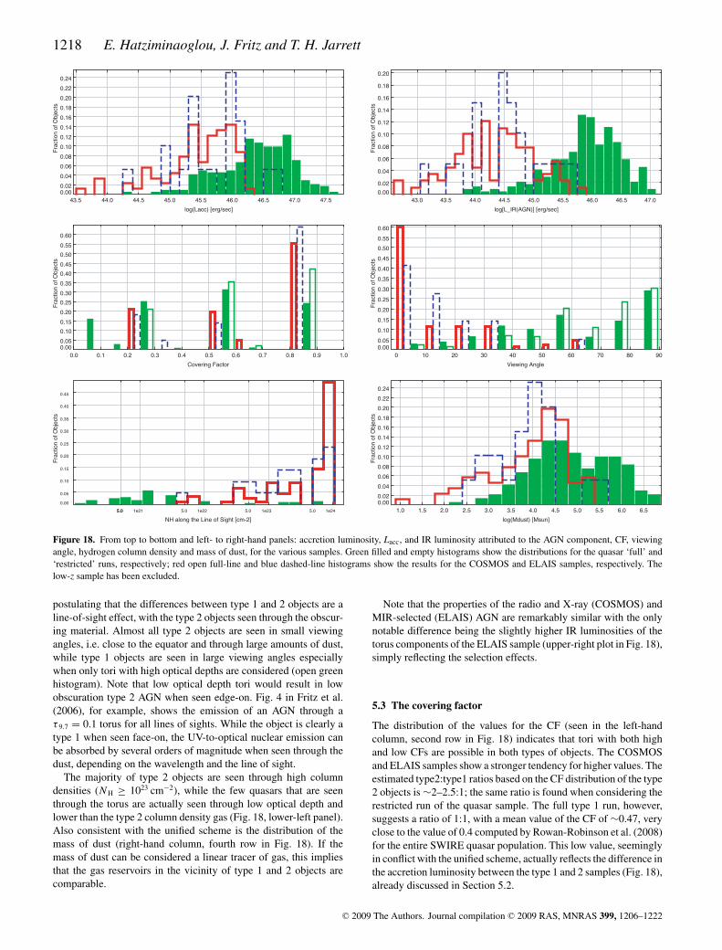
Figure 18. From top to bottom and left- to right-hand panels: accretion luminosity, Lacc, and IR luminosity attributed to the AGN component, CF, viewingangle, hydrogen column density and mass of dust, for the various samples. Green filled and empty histograms show the distributions for the quasar ‘full’ and‘restricted’ runs, respectively; red open full-line and blue dashed-line histograms show the results for the COSMOS and ELAIS samples, respectively. Thelow-z sample has been excluded.

postulating that the differences between type 1 and 2 objects are aline-of-sight effect, with the type 2 objects seen through the obscur-ing material. Almost all type 2 objects are seen in small viewingangles, i.e. close to the equator and through large amounts of dust,while type 1 objects are seen in large viewing angles especiallywhen only tori with high optical depths are considered (open greenhistogram). Note that low optical depth tori would result in lowobscuration type 2 AGN when seen edge-on. Fig. 4 in Fritz et al.(2006), for example, shows the emission of an AGN through aτ 9.7 = 0.1 torus for all lines of sights. While the object is clearly atype 1 when seen face-on, the UV-to-optical nuclear emission canbe absorbed by several orders of magnitude when seen through thedust, depending on the wavelength and the line of sight.

The majority of type 2 objects are seen through high columndensities (NH ≥ 1023 cm−2), while the few quasars that are seenthrough the torus are actually seen through low optical depth andlower than the type 2 column density gas (Fig. 18, lower-left panel).Also consistent with the unified scheme is the distribution of themass of dust (right-hand column, fourth row in Fig. 18). If themass of dust can be considered a linear tracer of gas, this impliesthat the gas reservoirs in the vicinity of type 1 and 2 objects arecomparable.

Note that the properties of the radio and X-ray (COSMOS) andMIR-selected (ELAIS) AGN are remarkably similar with the onlynotable difference being the slightly higher IR luminosities of thetorus components of the ELAIS sample (upper-right plot in Fig. 18),simply reflecting the selection effects.

5.3 The covering factor

The distribution of the values for the CF (seen in the left-handcolumn, second row in Fig. 18) indicates that tori with both highand low CFs are possible in both types of objects. The COSMOSand ELAIS samples show a stronger tendency for higher values. Theestimated type2:type1 ratios based on the CF distribution of the type2 objects is ∼2–2.5:1; the same ratio is found when considering therestricted run of the quasar sample. The full type 1 run, however,suggests a ratio of 1:1, with a mean value of the CF of ∼0.47, veryclose to the value of 0.4 computed by Rowan-Robinson et al. (2008)for the entire SWIRE quasar population. This low value, seeminglyin conflict with the unified scheme, actually reflects the difference inthe accretion luminosity between the type 1 and 2 samples (Fig. 18),already discussed in Section 5.2.



Figure 19. Left panel: L5100 measured on the quasar SDSS spectra for objects with redshift lower than ∼0.8, versus Lacc, computed from the SED fitting.The linear correlation, shown in a solid line, is given by log(L5100) = 0.692 × log(Lacc) − 1.5767. Right panel: fraction of obscured AGN in bins of L5100.Filled circles (open squares) represent the results of the full (restricted) run. The solid line represents the fraction of obscured AGN as found by Maiolino et al.(2007), while the dashed lines trace the uncertainties due to bolometric corrections.

From the type 1 quasars with redshifts below ∼0.8, we can mea-sure the flux at 5100 Å, which we can then scale with the ac-cretion luminosity, Lacc, as seen in the left-hand panel of Fig. 19.Assuming this relation holds for all redshifts as well as for type2 objects, we can translate Lacc to L5100. We can then compute thefraction of obscured AGN in bins of L5100, shown in the right-hand panel of Fig. 19. The black circles and open squares makeuse of the results of the full and restricted runs, respectively. Thefull and two dashed lines show the results and uncertainties (dueto bolometric corrections) obtained by Maiolino et al. (2007) whoconducted a study of 25 high-luminosity, high-redshift (2 < z <

3.5) quasars with IRS spectroscopy. The observed trend, i.e. thedecreasing average torus CF with increasing AGN luminosity, isin support of the receding torus paradigm, suggested by Lawrence1991.

Despite the crude conversion of Lacc to L5100, our results makinguse of the full run are in very good agreement (i.e. within theuncertainties) with those derived by Maiolino et al. (2007) basedon totally independent method and sample, while the results basedon the restricted run, even though still consistent (excluding thebrightest two bins) show a quite different trend. We can thereforestill not conclude on the relative occurrence of low-τ 9.7 tori withrespect to high-τ 9.7 tori but, based on the above, we can still providesome evidence for their existence.

Previous studies (e.g. Maiolino et al. 2007) assume that the ratiobetween the primary AGN radiation (here measured by Lacc) and thethermal IR emission attributed to the AGN is a direct indicator of thetorus CF. Our findings confirm this assumption, as shown in Fig. 20where the accretion-to-IR AGN luminosity of each individual objectof each sample is plotted against the computed CF. The slope ofthe correlation is very similar for type 1 and 2 samples. Type 2objects, however, have considerably larger Lacc/LIR(AGN) ratiosthan the quasars. This ‘jump’ in the values is due to the differentviewing angles and occurs right when the line of sight interceptsthe obscuring torus. In order to illustrate this effect, we show theLacc/LIR(AGN) ratios as a function of the viewing angle for theextreme models of both type 1 and 2 objects (higher and lower redpoints; higher and lower green points in Fig. 20) in Fig. 21.

Figure 20. Accretion-to-IR luminosity attributed to the AGN component asa function of the CF. The green solid and dashed lines obtained as linear fitscorresponding to the full and restricted runs, respectively, for type 1 objects,while blue and red lines correspond to ELAIS and COSMOS type 2 AGN,respectively.

5.4 Starburst activity in AGN

The study of objects with at least one data point at wavelengthslongwards of λ = 24 μm shows that the IR emission of AGN can-not be attributed to the torus component alone. In the vast majorityof cases, and in order to reproduce the 70 (and, whenever available,160) μm points, an additional SB component was necessary. Fur-thermore, in all those cases the contribution of the AGN emissionin the IR is typically smaller than 50 per cent, as seen in Figs 8 and17 for the type 2 objects, and a bit higher in type 1 quasars (Paper 1,fig. 12).

Fig. 22 shows the estimated SFRs for the various samples (withthe same colour coding as in Fig. 2) computed from equation 4 for allobjects with an SB and an AGN components. The average SFR forthe low-redshift sample is about 10 M� yr−1, while those computed



Figure 21. Accretion-to-IR luminosity attributed to the torus as a functionof viewing angle for the type 1 (green dashed lines) and 2 (red solid lines)objects with the highest and lowest Lacc/LIR(AGN) in Fig. 19. The differ-ences in this fraction are mainly attributable to dust self absorption which ismore efficient for type 2 line of sights.

Figure 22. SFRs estimated from the Kennicutt (1998) formalism for thevarious samples.

for the COSMOS and ELAIS samples are of ∼40 M� yr−1 but witha larger span. That of type 1 quasars (shown in green), however, hasan average SFR of 115 M� yr−1, with some cases reaching SFRs ofthe order of 103 M� yr−1. These values are well in agreement withthe findings of Serjeant & Hatziminaoglou (2009), a study basedon stacking analysis of a variety of quasar samples. These valuesdo not necessarily imply that star formation activity is stronger intype 1 quasars in general. More likely, it reflects the observationalbiases of the samples, both in terms of average redshifts and lumi-nosities (Figs 3 and 18).

The SB-to-AGN luminosity ratio for the combined sample showsa slight tendency to decrease with increasing accretion luminosity,as seen in Fig. 23. This is in apparent agreement with previousworks on type 1 quasars alone (again by Maiolino et al. 2007), andif confirmed for the entire sample would imply that type 1 and 2objects behave in the same way in this respect. On the other hand,we cannot assert beyond doubt that there is no implicit dependencyon the redshift. In fact, examining the quasar sample alone (opensymbols) we would be tempted to claim an increase with Lacc, butwhich is likely attributed to the L − z degeneracy.

Figure 23. Starburst-to-AGN IR luminosity ratio as a function of the accre-tion luminosity, Lacc, and the redshift. Filled and open symbols depict thetype 2 and 1 objects, respectively.

6 D ISCUSSION

This work focuses on the IR properties type 2 AGN, the type 1 issueshaving already been discussed in a previous paper (Paper 1). Thecollection of data used for this paper comes from: (1) a low-redshift(0.02 < z < 0.2) AGN sample, selected via standard emission-lines ratios criteria; (2) a higher-redshift (0.1 < z < 1.4) samplefrom the COSMOS and ELAIS fields, selected with X-ray and MIRcriteria. The observed SEDs were reproduced by means of a threecomponent model, including emission from stars, hot dust fromAGN and warm dust from SB activity, and acceptable fits wereobtained for the majority of the objects.

Despite the fact that the samples we analysed were not chosen ho-mogeneously, a comparison of the behaviour between the physicalproperties of the type 1 and 2 AGN shows an overall agreement. InPaper I, we found the CF to have a broad trend towards lower valuesas the accretion luminosity, i.e. the power of the central engine, in-creased with small, on-average, CFs. Applying the Lacc versus L5100

correlation derived for quasars in Paper I, we derived the flux at5100 Å for the type 2 samples and checked the correlation betweenthe optical luminosity and the CF, which in turn can be convertedinto a type 1 to type 2 fraction. The results provided by the SEDfitting analysis show a very good agreement with the relation pre-sented in Maiolino et al. (2007), who find a correlation betweenthe fraction of obscured AGN as a function of the optical lumi-nosity (i.e. at 5100 Å). Another indication of the dusty torus wasthought to be ratio between the accretion luminosity and the torusIR luminosity. In fact, the latter is just reprocessed radiation whichscales linearly with the primary source: what makes the differenceis the fraction of ‘heating radiation’ which is intercepted by thedust, which again depends on the CF. We find a very similar trendfor these quantities, in both type 1 and 2 objects, also showing howdifferences in the amount of obscuration are very well explainedby dust self-absorption, i.e. thermal dust emission absorbed by dustitself.

For the low-z sample, we found no evidence of emission froman AGN component for ∼70 per cent of the objects. Although wecannot rule out the absence of an AGN from these sources, we canset an upper limit to its luminosity since it is not observed at MIRwavelengths where its emission is the strongest as compared to boththat of the stellar and of the SB-heated dust. This sample suffers fromhigh contamination from the stellar emission component, even at



MIR wavelengths where (on the contrary) it is the AGN componentthat usually dominates when present. The question to ask, therefore,is what can be really constrained with three or four data points. Oneof the most reliable quantities should be the optical depth, since lowvalues would make the torus emission stand over the stellar (SBor stars) in the MIR. In this respect, the low-z sample may be toogenerous in selecting really active AGN. There is, sometimes, noevidence for an MIR excess at all with respect, for example, not onlyto a ‘normal’ SB emission but also to a passively evolving galaxy.The absence of any evidence for a hot dust emission in the MIR,which is the place where the stellar component is less importantand the AGN contribution is increasingly brighter, will remove theAGN component from the fits even though this could also be turnedinto an upper limit. In the cases where there is a MIR excess withrespect to a pure stellar emission, we explore two possibilities: torusand PAH emission. In some cases, a better fit was obtained addingPAH – i.e. an SB component alone – to the model instead of AGNwhich should instead dilute the PAH emission (Lutz et al. 1998).

Comparison between clumpy and smooth tori models(e.g. Dullemond & van Bemmel 2005) indicate that globally theSEDs produced by the two models are quite similar, but with somedetails characteristic for one or the other model: the silicate fea-ture observed in absorption in objects seen edge-on is shallower forclumpy models; the average near-IR flux is weaker in smooth mod-els and the clumpy models tend to produce slightly wider SEDs atcertain inclinations. Furthermore, clumpy models can produce verysmall tori sizes with Rout/Rin ∼ 5–10 (Nenkova et al. 2008), whilestill producing a broad MIR emission. Subsequently, the selectionof a smooth torus for the present study might have resulted in over-estimated tori sizes without, however, jeopardising the estimateson the properties related to the IR emission or our conclusions onthe unification scheme. SED fitting may not be a sensitive enoughmethod to distinguish between the differences introduced by thetwo approaches, not only because of the width of the filters and thescarce sampling of the observed SEDs but also because the variouscharacteristics of the torus component can be altered or diluted by,for example, the presence of an SB component. Notwithstandingthese limitations, SED fitting is still the best tool available for ex-tracting the maximum information from large photometric AGNsamples and is now proving to be a powerful technique in relat-ing the dust properties to the accretion properties as well as theproperties of the larger host galaxy.

Because AGN are of the order of hundred times less numerousthan galaxies and also prone to selection biases, such AGN studiesare only possible with the advent of multiwavelength surveys thatprobe large volumes and allow the construction of well-sampledSEDs. Even though we cannot address all issues related to dustytori, our understanding of their properties has been greatly improvedover the last decade thanks to the Spitzer Observatory. This spaceIR telescope allowed, among other things, the construction of SEDsof hundreds of AGN of all types thanks to the IRAC and MIPSphotometry (e.g. Franceschini et al. 2005, Paper 1; Richards et al.2006; Polletta et al. 2008). Spitzer also opened the doors to detailedand coherent studies of the interplay between AGN and SB activity(e.g. Hernan-Caballero et al. 2009 and references therein), pavingthe way for Herschel.

In fact, Herschel with its two cameras/medium resolution spec-trographs (Photodetector Array Camera and Spectrometer (PACS);Poglitsch & Altieri 2009 and Spectral and Photometric Imaging Re-ceiver (SPIRE); Griffin et al. 2009) and a very high resolution het-erodyne spectrometer (Heterodyne Instrument for the Far-Infrared(HIFI); de Graauw et al. 2009) will be the first space facility to

completely cover the range between 60 and 670, where the bulk ofenergy is emitted in the Universe, allowing for a more detailed sam-pling of the observed FIR SEDs and the cold dust emission. Largeparts of the Herschel key science will focus on the formation andevolution of galaxies and the studies of star formation. HerMES, theHerschel Multitiered extragalactic Survey, is the largest project thatwill be conducted by Herschel, with dedicated ∼900 h that will mapover 70 deg2 including most of the SWIRE fields (where most of theIR photometry of all the objects in this study comes from) as well asother extragalactic survey fields covered by several missions in allwavelengths (e.g. COSMOS or the Groth Strip), and will addressamong others the issue of AGN and SB connection (Griffin et al.2006; Hatziminaoglou et al. 2007). Additionally with Herschel,the Astrophysical Terahertz Large Area Survey will cover about500 deg2 and will observe all SDSS quasars with redshift z < 0.2as well as all the brightest FIR SDSS quasars (with luminosities10 times larger than the mean), amounting to ∼330 individual de-tections of quasars in the area covered (Serjeant & Hatziminaoglou2009) (a factor of ∼5 more than all the SDSS quasars with 70 μmdetections). These studies will allow us to significantly improveour understanding of the AGN phenomenon, disentangle the con-tribution of cold and hot dust emission in their SEDs and study theconcomitant occurrence of nuclear activity and star formation.

AC K N OW L E D G M E N T S

This work is based on observations made with the Spitzer SpaceTelescope, which is operated by the Jet Propulsion Laboratory,California Institute of Technology under NASA contract 1407. Sup-port for this work, part of the Spitzer Space Telescope Legacy Sci-ence Programme, was provided by NASA through an award issuedby the Jet Propulsion Laboratory, California Institute of Technologyunder NASA contract 1407.

Funding for the creation and distribution of the SDSS Archivehas been provided by the Alfred P. Sloan Foundation, the Partici-pating Institutions, the National Aeronautics and Space Adminis-tration, the National Science Foundation, the U.S. Department ofEnergy, the Japanese Monbukagakusho and the Max Planck Society.The SDSS web site is http://www.sdss.org/.

This publication makes use of data products from the 2MASS,which is a joint project of the University of Massachusetts andthe Infrared Processing and Analysis Center/California Institute ofTechnology, funded by the National Aeronautics and Space Admin-istration and the National Science Foundation.

This work made use of Virtual Observatory tools and ser-vices, namely TOPCAT (http://www.star.bris.ac.uk/mbt/topcat/)and VizieR (http://vizier.u-strasbg.fr/cgi-bin/VizieR).

We would like to thank R. Maiolino for kindly providing ma-terial for Fig. 19.

We would also like to thank the anonymous referee for theirin-depth study of the paper and the subsequent comments that, webelieve, greatly improved the manuscript.

REFERENCES

Adelman-McCarthy J. et al., 2006, ApJS, 162, 38Antonucci R., 1993, ARA&A, 31, 473Barvainis R., 1987, ApJ, 320, 537Beichman C. A., Cutri R., Jarrett T., Stiening R., Skrutskie M., 2003. AJ,

125, 2521Berta S., Fritz J., Franceschini A., Bressan A., Lonsdale C., 2004, A&A,

418, 913



Bertelli G., Bressan A., Chiosi C., Fagotto F., Nasi E., 1994, A&AS, 106,275

Bressan A., Granato G. L., Silva L., 1998, A&A, 332, 135Capak P. et al., 2007, ApJS, 172, 99Cardamone C. N. et al., 2008, ApJ, 680, 130Cardelli J. A., Clayton G. C., Mathis J. S., 1989, ApJ, 345, 245de Graauw Th. et al., 2009, in Pagani L., Gerin M., eds, EAS Publications

Series, Vol. 34, p. 3Dullemond C. P., van Bemmel I. M., 2005, A&A, 436, 47Elitzur M., 2008, New Astron. Rev., 52, 274Elitzur M., Shlosman I., 2006, ApJ, 648, 101Engelbracht C. W., Rieke G. H., Gordon K. D., Smith J.-D. T., Werner M.

W., Moustakas J., Willmer C. N. A., Vanzi L., 2008, ApJ, 678, 804Franceschini A. et al., 2005, AJ, 129, 2074Fritz J., Franceschini A., Hatziminaoglou E., 2006, MNRAS, 366, 767Granato G. L., Danese L., 1994, MNRAS, 268, 235Griffin M. et al., 2009, in Pagani L., Gerin M., eds, EAS Publications Series,

Vol. 34, p. 33Griffin M. J. et al., 2006, in the proceedings of the conference ‘Study-

ing Galaxy Evolution with Spitzer and Herschel’, May 2006, AgiosNikolaos, Crete

Gruppioni C. et al., 2008, ApJ, 684, 136Hatziminaoglou E. et al., 2005, AJ, 129, 1198Hatziminaoglou E. et al., 2007, ASP Conf. Ser. Vol. 380, Astron. Soc. Pac,

San Francisco, p. 367Hatziminaoglou E. et al., 2008, MNRAS, 386, 1252 (Paper 1)Hernan-Caballero A. et al., 2009, MNRAS, 395, 1695Honig S. F., Beckert T., 2007, MNRAS, 380, 1172Jacoby G. H., Hunter D. A., Christian C. A., 1984, ApJS, 56, 257Kauffmann G. et al., 2003, MNRAS, 346, 1055Kennicutt R. C., 1998, ApJ, 498, 541Kewley L. J., Dopita M. A., Sutherland R. S., Heisler C. A., Trevena J.,

2001, ApJ, 556, 121Kroupa P., 2001, MNRAS, 322, 231Lacy M. et al., 2004, ApJS, 154, 166Lawrence A., 1991, MNRAS, 252, 586Lonsdale C. et al., 2003, PASP, 115, 897Lonsdale C. et al., 2004, ApJS, 154, 54Lutz D., Spoon H. W. W., Rigopoulou D., Moorwood A. F. M., Genzel R.,

1998, ApJ, 505, 103LMaiolino R., Shemmer O., Imanishi M., Netzer H., Oliva E., Lutz D., Sturm

E., 2007, A&A, 468, 979Nenkova M., Sirocky M. M., Nikutta R., Ivezic Z., Elitzur M., 2008, ApJ,

685, 160Nenkova M., Ivezic Z., Elitzur M., 2002, ApJ, 570, 9Pier E. A., Krolik J. H., 1992, ApJ, 401, 99Poglitsch A., Altieri B., 2009, in Pagani L., Gerin M., eds, EAS Publications

Series, Vol. 34, p. 43

Polletta M., Weedman D., Hoenig S., Lonsdale C. J., Smith H., Houck J.,2008, ApJ, 675, 960

Richards G. T. et al., 2006, ApJS, 166, 470Rowan-Robinson M. et al., 2008, MNRAS, 386, 697Sajina A., Lacy M., Scott D., 2005, MNRAS, 621, 256Sanders D. B. et al., 2007, ApJS, 172, 86Serjeant S., Hatziminaoglou E., 2009, MNRAS, 397, 265Siebenmorgen R., Haas M., Krugel E., Schulz B., 2005, A&A, 436,

L5Surace J. et al., 2005, SWIRE Data Release Document 2, http://data.

spitzer.caltech.edu/popular/swire/20050603_enhanced/documentation/SWIRE2_doc_083105.pdf

Tadhunter C., 2008, New Astron. Rev., 52, 227Trump J. R. et al., 2007, ApJS, 172, 383Urry C. M., Padovani P., 1995, PASP, 107, 803

SUPPORTI NG INFORMATI ON

Additional Supporting Information may be found in the online ver-sion of this article:

Table 1. SDSS names, coordinates, redshifts, emission line prop-erties and stellar masses for the 420 objects overlapping theSWIRE fields and the narrow emission line object catalogue fromKauffmann et al. (2003).Table 2. SWIRE fluxes of the sample presented in Table 1.Table 3. COSMOS names, coordinates, redshifts and classificationtype for the COSMOS type 2 AGN sample, from Trump et al.(2007).Table 4. COSMOS Spitzer fluxes of the sample presented in Table 3.Figure 5. Best-fitting SEDs for the low-z objects with reducedχ 2 < 16.0 that were assigned a torus component.Figure 14. The best fits for the COSMOS objects with reducedχ 2 < 16.0 that were assigned a torus component.Figure 15. The best fits for the ELAIS AGN with reduced χ 2 <

16.0 that were assigned a torus component.

Please note: Wiley-Blackwell are not responsible for the content orfunctionality of any supporting materials supplied by the authors.Any queries (other than missing material) should be directed to thecorresponding author for the article.

This paper has been typeset from a TEX/LATEX file prepared by the author.


properties of dusty tori in active galactic nuclei – ii

Documents