properly pricing the catastrophe exposure
DESCRIPTION
Properly Pricing the Catastrophe Exposure. David Chernick, FCAS, MAAA Michael Devine, FCAS, MAAA Sara Drexler, FCAS, MAAA CAS Ratemaking Seminar March, 2004. Agenda. Introduction History of Methods Terminology Exposure Base Capping Discussion of Several Alternative Approaches - PowerPoint PPT PresentationTRANSCRIPT

04/19/231
Properly Pricing the Properly Pricing the Catastrophe ExposureCatastrophe Exposure
David Chernick, FCAS, MAAAMichael Devine, FCAS, MAAASara Drexler, FCAS, MAAACAS Ratemaking SeminarMarch, 2004

04/19/232
AgendaAgenda Introduction History of Methods
– Terminology– Exposure Base– Capping
Discussion of Several Alternative Approaches– Traditional– Methods Using Cat/AIY – State Based– Methods Using Cat/AIY – Countrywide Based
Wrap-up

04/19/233
IntroductionIntroduction
The PanelistsThe DataThe Issue

04/19/234
IntroductionIntroduction
The Panelists
IntroductionsSara DrexlerMichael DevineDavid Chernick

04/19/235
IntroductionIntroduction The Data
The base data we are using in this presentation is included in the handouts.Real dataLarge Catastrophe in 1998
343.2% loss ratio9.67 Ratio of Cat/AIY

04/19/236
IntroductionIntroduction
The Issue– Operating results
$19.1 Million profit prior to 1998$41.4 Million loss in 1998
– StatisticsMean:1998 was 22.7 Standard Deviations from mean.
04/19/237
IntroductionIntroduction
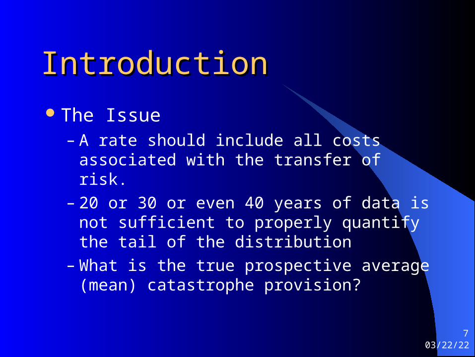
The Issue– A rate should include all costs associated with
the transfer of risk.– 20 or 30 or even 40 years of data is not
sufficient to properly quantify the tail of the distribution
– What is the true prospective average (mean) catastrophe provision?

04/19/238
IntroductionIntroduction
The Issue– Perspective of this presentation is from large
insurers without reinsurance coverage.– Reinsurance covering some portion of the
catastrophe exposure would most likely be an upper bound of the true mean.
– What is the true prospective average (mean) catastrophe provision?

04/19/239
TerminologyTerminology
AIY – Amount of Insurance years 1AIY=$1,000 of dwelling coverage
Losses/AIY – Damage Ratios or Cat/AIY

04/19/2310
History of MethodsHistory of Methods
Category Data
Averaging MethodsAdjustment for Extreme Cats
Category # 1ISO Excess Wind &Variations
A. Ratio of wind losses to ex-wind losses
B. Ratio of cat losses to ex-cat losses
Base: Non-wind incurred lossesCat Data: Annual wind incurred losses over threshold
Base: Non-cat incurred lossesCat Data: Incurred event losses over fixed external threshold
Arithmetic average of excess wind factors and average wind to ex-wind ratios. For each additional year, give 95% weight for long-term average, 5% weight for additional year.
Can give less weight to unusual years
Can adjust catastrophes for unusual years
Category #2Cat/AIY Methods
A. Utilize state Cat/AIY with no direct use of countrywide cat experience
B. Utilize state Cat/AIY with direct use of countrywide cat experience
Base: AIYCat Data: Incurred event losses over fixed external threshold
Straight long-term average Confidence interval
approach Average adjusted catastro-
phes and add increment for extreme
Trended exponential smoothing
Balance state provisions to countrywide expectation
May or may not include adjustments for extreme catastrophes
Category #3Modeled Cat Losses
Base: AIYCat Data: Computer appli- cation generated losses
Average annual losses are based on the stochastic event set
Extreme events are given their appropriate statistical weight
Category #4Reinsurance Cost Based
Cat cover reinsurance cost passed through primary pricing

04/19/2311
What Base to Relate Catastrophes To?What Base to Relate Catastrophes To?
Premium:Cat provisions impacted by rate changesTrends in non-catastrophe loss & expense dictate cat provision

04/19/2312
What Base to Relate Catastrophes To?What Base to Relate Catastrophes To?
Premium:Cat provisions impacted by rate changesTrends in non-catastrophe loss & expense dictate cat provision
Non-Cat Loss/Ex-Wind Loss:Still heavily dictated by trends in Crime, Liability, etc. lossEx-wind losses can include catastrophic losses

04/19/2313
What Base to Relate Catastrophes To?What Base to Relate Catastrophes To?
Premium:Cat provisions impacted by rate changesTrends in non-catastrophe loss & expense dictate cat provision
Non-Cat Loss/Ex-Wind Loss:Still heavily dictated by trends in Crime, Liability, etc. lossEx-wind losses can include catastrophic losses
AIY or Amount of Insurance Years Definition: $1000 of Building Coverage in force for one year
Inflation sensitiveDirect measurement of exposure – incorporates policy growth and changes in building costs

04/19/2314
Should Individual CatastrophesBe Capped?

04/19/2315
Should Individual CatastrophesBe Capped?
Stabilizes provision Can serve to more appropriately match experience period used with event return periods Potentially more accurate estimate of expected value results

04/19/2316
What Are Some Problems WithCapping Individual Catastrophes?

04/19/2317
What Are Some Problems WithCapping Individual Catastrophes?
What criteria should be used? The “unthinkable” is happening every year somewhere. Is the result systematic underestimation of loss costs? How do we really know appropriate event return periods?

04/19/2318
Insurance Services Office (ISO)Insurance Services Office (ISO)Excess Wind ProcedureExcess Wind ProcedureBasic Approach Separate wind & non-wind losses Examine wind/non-wind ratios Years where wind/non-wind exceed 1.5 times
median are “excess” Average factor for excess wind Factor developed for excess wind applied to non-wind,
non-excess losses

04/19/2319
Insurance Services Office (ISO)Insurance Services Office (ISO)Excess Wind ProcedureExcess Wind ProcedureBasic Approach Separate wind & non-wind losses Examine wind/non-wind ratios Years where wind/non-wind exceed 1.5 times
median are “excess” Average factor for excess wind Factor developed for excess wind applied to non-wind,
non-excess losses
Characteristics Straightforward application Definition of “excess wind” can change as median changes Assumes stable relationship between wind & non-wind losses Doesn’t consider variability of wind losses Doesn’t consider non-wind catastrophes

04/19/2320
The Fix ‘Em Up Insurance GroupThe Fix ‘Em Up Insurance GroupHomeownersHomeowners
The State of Mich-con-otaThe State of Mich-con-ota20-Year Average Approach20-Year Average Approach
Year
Amount ofInsurance Years
(AIY)Cat Incurred
Loss CAT/AIYRunningProvision
1993199419951996199719981999200020012002
4,276,1354,306,8154,540,9134,774,7835,001,1645,193,1905,367,5665,574,5065,745,3446,223,199
$ 307,946 259,784 4,378 1,529,513 2,736,486 50,241,886 8,141,594 6,676,296 12,086,512 6,091,053
0.07200.06030.00100.32030.54729.67461.51681.19762.10370.9788
0.21480.21020.17190.18620.21280.69480.71140.75660.84650.8929
Provision (20-Year Average ) 0.8929

04/19/2321
Confidence Interval Approach
Factors include risk tolerance, surplus position/ availability of capital, reinsurance Determine confidence demands for long-term companywide cat provision Calculate companywide mean cat/aiy Calculate standard deviation of mean cat/aiy
Step 1 – Establish Company Objective:

04/19/2322
Confidence Interval Approach
Company has established that it would like to be 90% certain it has an adequate catastrophe provision over the long-term The following have been calculated from the companywide catastrophe history: Mean Cat/AIY = .3151
Standard Deviation of Mean Cat/AIY = .0372
Step 1 – Establish Company Objective (Cont.):

04/19/2323
Confidence Interval Approach
The long-run companywide benchmark cat provision is established as follows: Provision (Cat/AIY) = Mean + (t) x (Standard Deviation) = .3151 + (1.323) x (.0372) = .3643 Where : Mean = average cat/aiy companywide 1.323 = t – stat for 90% and (N-1) degrees of freedom .0372 = standard deviation of the mean
Step 1 – Establish Company Objective (Cont.):

04/19/2324
Confidence Interval Approach
Goal period becomes interval rates are in effect Need to be reasonably certain provision is adequate Desire to use cap on individual cats to limit volatility Largest 5% of companywide cats exceeded .65/AIY Establish required confidence for state capped average
Step 2 – Establish State Level Objective:

04/19/2325
Non-Hurricane Catastrophe ProvisionsNon-Hurricane Catastrophe Provisions
ConfidenceIntervals
Sum of StatesUncapped Capped
CompanywideUncapped
50% 55 60 65 70 75 80 85 90 95
0.3334 0.2682 0.3825 0.2998 0.4328 0.3323 0.4848 0.3657 0.5392 0.4008 0.5988 0.4392 0.6657 0.4823 0.7447 0.5332 0.8452 0.5981 0.9999 0.6973
0.31510.31980.32470.32970.33490.34060.34710.35460.36430.3791
04/19/2326
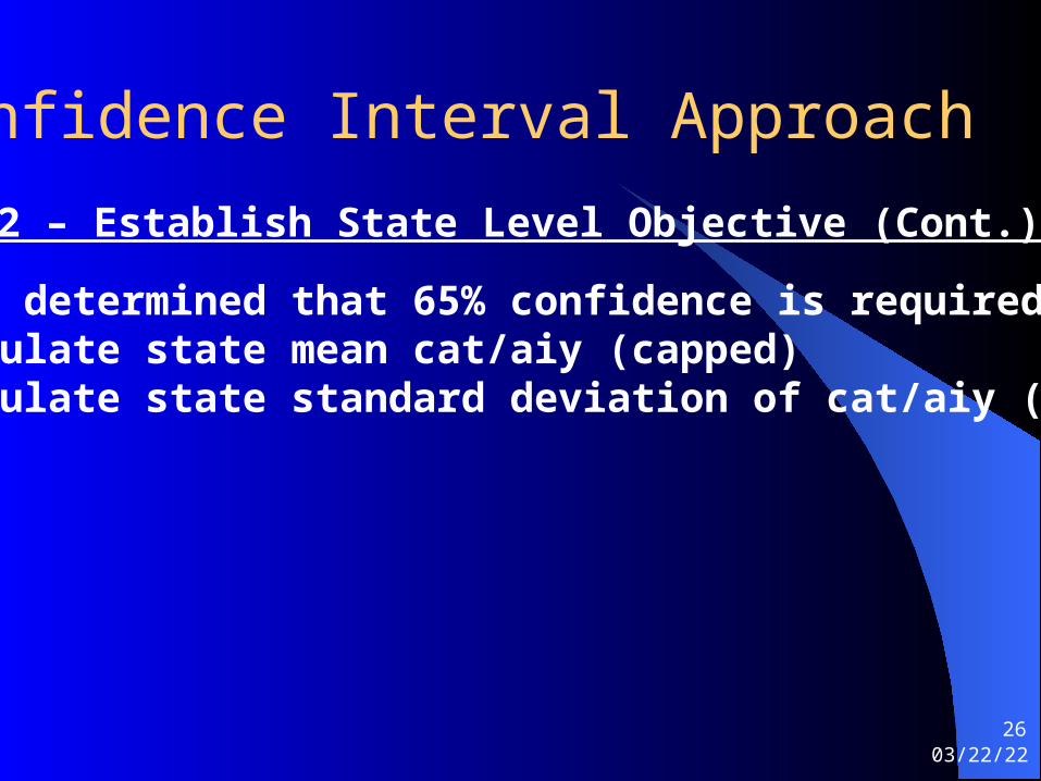
Confidence Interval Approach
It’s determined that 65% confidence is required Calculate state mean cat/aiy (capped) Calculate state standard deviation of cat/aiy (capped)
Step 2 – Establish State Level Objective (Cont.):

04/19/2327
Confidence Interval Approach
The following was calculated from the capped state level catastrophe history:
Mean Cat/AIY = .3912Standard Deviation of Cat/AIY = .5450
The short-run state cat provision is established as follows: Provision (Cat/AIY) = Mean + (t) x (standard deviation) = (.3912) + (.389) x (.5450)
= .6032 Where: Mean = average capped cat/aiy for Mich-con-ota .389 = t – stat for 65% and (N-1) degrees of freedom .5450 = standard deviation of the annual capped cat/aiy
Step 3 – Calculate State Provision:

04/19/2328
The Fix ‘Em Up Insurance GroupThe Fix ‘Em Up Insurance GroupHomeownersHomeowners
The State of Mich-con-otaThe State of Mich-con-otaConfidence Interval ApproachConfidence Interval Approach
Year
Amount ofIns. Years
(AIY)Cat Incurred
Loss CAT/AIYCapped
CAT/AIYRunningProvision
1993199419951996199719981999200020012002
4,276,1354,306,8154,540,9134,774,7835,001,1645,193,1905,367,5665,574,5065,745,3446,223,199
$ 307,946 259,784 4,378 1,529,513 2,736,486 50,241,886 8,141,594 6,676,296 12,086,512 6,091,053
0.07200.06030.00100.32030.54729.67461.51681.19762.10370.9788
0.07200.06030.00100.32030.54721.61751.51681.19761.95370.9788
0. 29830.29110.28250.28650.30160.39340.46120.50040.58350.6032
Provision (Confidence Interval Approach) 0.6032
04/19/2329
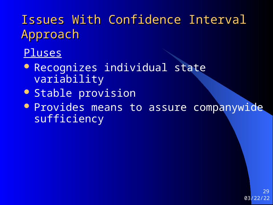
Issues With Confidence Interval ApproachIssues With Confidence Interval Approach
Pluses Recognizes individual state variability Stable provision Provides means to assure companywide sufficiency

04/19/2330
Issues With Confidence Interval ApproachIssues With Confidence Interval Approach
Pluses Recognizes individual state variability Stable provision Provides means to assure companywide sufficiency
Drawbacks Not particularly responsive to distributional changes,
coverage changes, etc. (data back to 1971) Capping can result in less responsiveness Recognition of variability interpreted as risk margin

04/19/2331
The Fix ‘Em Up Insurance GroupThe Fix ‘Em Up Insurance GroupHomeownersHomeowners
The State of Mich-con-otaThe State of Mich-con-otaExtreme Events AdjustmentExtreme Events Adjustment
Year
Amount ofIns. Years
(AIY)Cat Inc.
Loss
ExtremeCat Inc.
Loss
NonExtremeCat Inc.
LossExtreme
CAT/AIY
Contrib.From
Extreme
Contrib.FromNon
ExtremeRunningProvision
1993199419951996199719981999200020012002
4,276,1354,306,8154,540,9134,774,7835,001,1645,193,1905,367,5665,574,5065,745,3446,223,199
$ 307,946 259,784 4,378 1,529,513 2,736,486 50,241,886 8,141,594 6,676,296 12,086,512 6,091,053
$
45,217,697
$ 307,946 259,784 4,378 1,529,513 2,736,486 5,024,189 8,141,594 6,676,296 12,086,512 6,091,053
8.7071 1.7414
0.07200.06030.00100.32030.54720.96751.51681.19762.10370.9788
0.21480.21020.17190.18620.21280.34650.36310.40830.49820.5446
20 Year Average 0.0871 0.4576
Provision (Extreme plus Non-Extreme) 0.5446

04/19/2332
Extreme Events AdjustmentExtreme Events Adjustment
PlusesRelatively stableAs opposed to censoring, reflects events fully
DrawbacksAccurate determination of event return period
difficultCan be viewed as arbitrary and difficult to
explain

04/19/2333
95% / 5% Trended Approach:
All years used Exponential smoothing Trend factor applied – recognizes static cat definition 10% annual cap to change in provision
Methodology:

04/19/2334
The Fix ‘Em Up Insurance GroupThe Fix ‘Em Up Insurance GroupHomeownersHomeowners
The State of Mich-con-otaThe State of Mich-con-ota95/5 Trended95/5 Trended
Year
Amount ofInsurance Years
(AIY)Cat Incurred
Loss CAT/AIYRunningProvision
1993199419951996199719981999200020012002
4,276,1354,306,8154,540,9134,774,7835,001,1645,193,1905,367,5665,574,5065,745,3446,223,199
$ 307,946 259,784 4,378 1,529,513 2,736,486 50,241,886 8,141,594 6,676,296 12,086,512 6,091,053
0.07200.06030.00100.32030.54729.67461.51681.19762.10370.9788
0. 19720.19300.20540.22590.24850.27330.30070.33070.36380.4002
Provision (95/5 Trended) 0.4002

04/19/2335
95% / 5% Trended Approach:
Not volatile, yet responsive for non-extreme events Simple to understand Trend factor to compensate for static definition of cats Reduced data complications
Advantages:

04/19/2336
Summary of Results So Far:Summary of Results So Far:
Approach
Mich-con-otaCat/AIY
StabilityRank
Cat/Ex-Cat20-Year AverageConfidence Interval ApproachExtreme Events95% / 5% TrendedAll Years Weighted Average
.7292
.8929
.6032
.5446
.4002
.9940
452316

04/19/2337
Pivotal Question: Can Countrywide or Regional Data Help Quantify the True ProspectiveMean Catastrophe Loss in a GivenState?

04/19/2338
Pivotal Question:Can Countrywide or Regional DataHelp Quantify the True ProspectiveMean Catastrophe Loss in a GivenState?
Provisions need to reflect adequacy and stability All company surplus is generally available and at risk Are regional or sub state provisions appropriate? Perceived cost sharing will be scrutinized
Issues:

04/19/2339
Goals of Relativity MethodGoals of Relativity Method
Develop accurate, stable results by state that results in an appropriate provision on a countrywide basis
Systematic approach to handle extreme events so a single outlying year does not drive the cat provision for a state
Appropriate application of credibility procedure Provide result that is responsive to recent
demographic and cat definition shifts

04/19/2340
Issues AddressedIssues Addressed
How to be responsive to changes in risk due to population shifts or cat definition changes while still including an appropriate number of years
How does one define an outlying event– Individual state vs. countrywide
How to incorporate credibility

04/19/2341
State Relativity Weighted with Countrywide State Relativity Weighted with Countrywide Complement – General OutlineComplement – General Outline
I. Develop State Damage RatiosII. Calculate Countywide Damage RatiosIII. Calculate State RelativitiesIV. Cap State RelativitiesV. Average Capped RelativitiesVI. Credibility Weight with CW Average of 1.000VII. Balance Back to CW Average of 1.000VIII. Calculate Statewide Catastrophe Provision

04/19/2342
State Relativity Weighted with State Relativity Weighted with Countrywide ComplementCountrywide Complement Develop each state’s damage ratios for years 1981-2000
– State Damage Ratios – Losses/AIY
– Only use years 1981 forward. Data for years 1971 through 1980
is sparse as evidenced by yearly variance.
I. Develop State Damage Ratios
II. Calculate Countrywide Damage Ratios
III. Calculate State Relativities
IV. Cap State Relativities
V. Average Capped Relativities
VI. Credibility Weight with CW Average of 1.000
VII. Balance Back to CW Average of 1.000
VIII. Calculate Statewide Catastrophe Provision

04/19/2343
State Relativity Weighted with State Relativity Weighted with Countrywide ComplementCountrywide Complement Each year’s Countrywide damage ratio is
calculated as the weighted average of state damage ratios using latest year AIYs as weights– Eliminates distortion of state distributional shifts over
time Countrywide catastrophe provision is the
arithmetic average of the most recent 10 years of damage ratios
I. Develop State Damage Ratios
II. Calculate Countrywide Damage Ratios
III. Calculate State Relativities
IV. Cap State Relativities
V. Average Capped Relativities
VI. Credibility Weight with CW Average of 1.000
VII. Balance Back to CW Average of 1.000
VIII. Calculate Statewide Catastrophe Provision

04/19/2344
CW Cat damage ratios including 2000
0.00
0.10
0.20
0.30
0.40
0.50
0.60
0.70
0.80
1970 1975 1980 1985 1990 1995 2000 2005
Year
Da
ma
ge
ra
tio
Years Linear trend
1971-1978 0.006
1979-1989 0.000
1990-1999 -0.019
1990-2000 -0.010
Figure 1Figure 1

04/19/2345
State Relativity Weighted with State Relativity Weighted with Countrywide ComplementCountrywide Complement
Calculate state relativities as the ratio of state damage ratios to countrywide damage ratios
Relativities should be more stable than damage ratios Trend should not be a problem so we can use more years
of data than the Countrywide Catastrophe Provision
I. Develop State Damage Ratios
II. Calculate Countrywide Damage Ratios
III. Calculate State Relativities
IV. Cap State Relativities
V. Average Capped Relativities
VI. Credibility Weight with CW Average of 1.000
VII. Balance Back to CW Average of 1.000
VIII. Calculate Statewide Catastrophe Provision

04/19/2346
State Relativity Weighted with State Relativity Weighted with Countrywide ComplementCountrywide Complement Any relativity greater than the mean plus three
standard deviations is capped to the next lowest relativity (not the cap number)– Intuitively we are replacing a once in a hundred year
event with a once in 20 Benefit of capping process
– Represents a systematic approach to dealing with extreme events
– Cap is dynamic and is allowed to shift if exposure in a state is changing over time
– Censoring at the cap would not have much impact and therefore would not result in increased stability
I. Develop State Damage Ratios
II. Calculate Countrywide Damage Ratios
III. Calculate State Relativities
IV. Cap State Relativities
V. Average Capped Relativities
VI. Credibility Weight with CW Average of 1.000
VII. Balance Back to CW Average of 1.000
VIII. Calculate Statewide Catastrophe Provision

04/19/2347
State Relativity Weighted with State Relativity Weighted with Countrywide ComplementCountrywide Complement
Calculate arithmetic average of 1981-2000 capped relativities– Using a arithmetic average is simple
– No benefit of weighting relativities has been shown since relationship of variability to exposure level is unclear
– Arithmetic average relativity does not differ significantly from an AIY weighted average
I. Develop State Damage Ratios
II. Calculate Countrywide Damage Ratios
III. Calculate State Relativities
IV. Cap State Relativities
V. Average Capped Relativities
VI. Credibility Weight with CW Average of 1.000
VII. Balance Back to CW Average of 1.000
VIII. Calculate Statewide Catastrophe Provision

04/19/2348
State Relativity Weighted with State Relativity Weighted with Countrywide ComplementCountrywide Complement
Uses Buhlmann credibility factor: n/(n+k)– n = number of years of relativities in average
We use number of years rather than exposures because exposures not
independent, especially past a certain threshold where exposure
concentration increases
– k = average process variance/variance of hypothetical means The process variance and variance of hypothetical means are
calculated using all available years of capped relativities across all states.
Complement of credibility of 1.000 is not appropriate when there is a wide spread of average relativities– Solution lies in balancing process described on next slide
I. Develop State Damage Ratios
II. Calculate Countrywide Damage Ratios
III. Calculate State Relativities
IV. Cap State Relativities
V. Average Capped Relativities
VI. Credibility Weight with CW Average of 1.000
VII. Balance Back to CW Average of 1.000
VIII. Calculate Statewide Catastrophe Provision

04/19/2349
State Relativity Weighted with State Relativity Weighted with Countrywide ComplementCountrywide Complement At this point, the individual state relativities result in a
countrywide relativity of less than 1.000. Relativities are adjusted to achieve an overall adequate level as follows:– Determined on a countrywide basis what our expected losses
would be based on the countrywide selected catastrophe factor– Sum the pre-balanced expected losses across all states – We distribute the difference between 1 and 2 in proportion to
each state’s standard deviation measured in latest year expected losses.
Using this approach has several benefits:– Results in an appropriate provision countrywide – It compensates for high (low) relativity states being
underestimated (overestimated) by the use of a 1.000 complement of credibility.
– Each state’s resulting cat load is a function of its own size and variability
I. Develop State Damage Ratios
II. Calculate Countrywide Damage Ratios
III. Calculate State Relativities
IV. Cap State Relativities
V. Average Capped Relativities
VI. Credibility Weight with CW Average of 1.000
VII. Balance Back to CW Average of 1.000
VIII. Calculate Statewide Catastrophe Provision

04/19/2350
State Relativity Weighted with State Relativity Weighted with Countrywide ComplementCountrywide Complement
Statewide catastrophe provision is calculated by multiplying capped, credibility weighted, balanced relativity by the countrywide catastrophe provision
Benefits of method:– Allows use of long term data to determine relativity
while using more responsive data for countrywide provision
– Adjustments to data are determined objectively with each state’s characteristics used to determine both capping and balancing
I. Develop State Damage Ratios
II. Calculate Countrywide Damage Ratios
III. Calculate State Relativities
IV. Cap State Relativities
V. Average Capped Relativities
VI. Credibility Weight with CW Average of 1.000
VII. Balance Back to CW Average of 1.000
VIII. Calculate Statewide Catastrophe Provision

04/19/2351
Issues AddressedIssues Addressed How to be responsive to changes in risk due to population
shifts or cat definition changes while still including an appropriate number of years– We use as many years of relativities as possible while using only the
latest 10 years of Countrywide to determine the Countrywide load. How do you define an outlying event
– Greater than the mean plus 3 standard deviation in any given state. On a countrywide basis these “outlying” events occur fairly regularly (about 2% of relativities have been capped)
How to incorporate credibility– Uses Buhlmann credibility to account for variability in relativities.
Used a relativity of 1.000 as complement. Balancing method adjusts for bias in complement for when a 1.000 may not be an appropriate complement.

04/19/2352
Summary of Results:Summary of Results:
Approach
Mich-con-otaCat/AIY
Cat/Ex-Cat20-Year AverageConfidence Interval ApproachExtreme Events95% / 5% TrendedAll Years Weighted AverageRelativity Method
.7292
.8929
.6032
.5446
.4002
.9940
.6270

04/19/2353
ConclusionConclusion
We have made significant progress as a profession in quantifying the catastrophe exposure.
Do our current methods capture the true mean?
My purpose will be achieved if this session helps to keep focus on this issue

04/19/2354
ConclusionConclusion
Comments and Discussion