propeller performance analysis using lifting line...
TRANSCRIPT
Propeller Performance Analysis
Using Lifting Line Theory
by
Kevin M. Flood B.S., (1997) Hobart College
M.A., (2002) Webster University
Submitted to the Department of Mechanical Engineering in Partial Fulfillment of the Requirements for the Degrees of
Naval Engineer and
Master of Science in Mechanical Engineering at the
MASSACHUSETTS INSTITUTE OF TECHNOLOGY June 2009
©2008 K. M. Flood. All rights reserved The author hereby grants to MIT permission to reproduce and to distribute
publicly paper and electronic copies of this thesis document in whole or in part in any medium now known or hereafter created.
Signature of Author__________________________________________________________________
Department of Mechanical Engineering May 8, 2009
Certified by______________________________________________________________________
Mark Welsh Professor of Naval Architecture Thesis Supervisor Certified by______________________________________________________________________
Richard W. Kimball Thesis Supervisor Accepted by______________________________________________________________________
David E. Hardt Chairman, Departmental Committee on Graduate Students
Department of Mechanical Engineering


3
Propeller Performance Analysis Using Lifting Line Theory
by Kevin M. Flood
Submitted to the Department of Mechanical Engineering on May 8, 2009
in Partial Fulfillment of the Requirements for the Degrees of Naval Engineer
and Master of Science in Mechanical Engineering
Abstract
Propellers are typically optimized to provide the maximum thrust for the minimum torque at a specific number of revolutions per minute (RPM) at a particular ship speed. This process allows ships to efficiently travel at their design speed. However, it is useful to know how the propeller performs during off-design conditions. This is especially true for naval warships whose missions require them to perform at a wide range of speeds. Currently the Open-source Propeller Design and Analysis Program can design and analyze a propeller only at a given operating condition (i.e. a given propeller RPM and thrust). If these values are varied, the program will design a new optimal propeller for the given inputs. The purpose of this thesis is to take a propeller that is designed for a given case and analyze how it will behave in off-design conditions. Propeller performance is analyzed using non-dimensional curves that depict thrust, torque, and efficiency as functions of the propeller speed of advance. The first step in producing the open water diagram is to use lifting line theory to characterize the propeller blades. The bound circulation on the lifting line is a function of the blade geometry along with the blade velocity (both rotational and axial). Lerbs provided a method to evaluate the circulation for a given set of these conditions. This thesis implements Lerbs method using MATLAB® code to allow for fast and accurate modeling of circulation distributions and induced velocities for a wide range of operating conditions. These values are then used to calculate the forces and efficiency of the propeller. The program shows good agreement with experimental data. Thesis Supervisor: Mark Welsh Title: Professor of Naval Architecture Thesis Supervisor: Richard W. Kimball

4
Acknowledgements
The author thanks the following individuals for all of their support and assistance with this
thesis:
Professor Rich Kimball for all his wisdom and guidance during not only the thesis process but
also during the two classes he taught. His classes and teaching method were among the best
experienced at MIT.
CAPT Patrick Keenan for the leadership and direction he provided throughout his time leading
the course 2N program. His course was one of the most interesting the author experienced at
MIT.
CAPT Mark Welsh for the leadership and support he provided in the “home stretch” of my MIT
experience.
And most of all, my family for all of their support and understanding during my time at MIT.
Missy, Margaret, Josh, and I had a wild ride filled with fun and frustration for the past three
years.
5
Table of Contents Abstract ......................................................................................................................................3
Acknowledgements.....................................................................................................................4
List of Figures.............................................................................................................................7
List of Tables..............................................................................................................................7
1. Introduction and Recent Propeller Design Advances .........................................................8
1.1 Recent Advances.............................................................................................................11
2. Theoretical Foundation ...................................................................................................13
2.1 Velocity Field of Symmetrically Spaced Helical Vortex Lines.........................................13
2.2 Velocity Field of Symmetrically Spaced Helical Vortex Sheets .......................................17
2.3 Application to Moderately Loaded Free-Running Non-Optimum Propellers....................20
2.4 Determining the Circulation and Induced Velocities........................................................22
3. Implementation and Validation .......................................................................................25
3.1 MATLAB® Implementation of the “Building Blocks” ....................................................25
3.2 Validation of the “Building Blocks” with Lerbs’ Example Data.......................................26
3.3 MATLAB® Implementation for Finding Circulation, Induced Velocities, and the
Resultant Forces .............................................................................................................28
3.4 Validation of Circulation, Induced Velocity, and Forces Using OpenProp .......................30
3.5 MATLAB® Implementation for Determining Propeller Performance Characteristics at
Off-Design Advance Ratios ............................................................................................34
3.6 Validation of Propeller Performance Characteristics at Off-Design Advance Ratios ........35
4. Conclusions and Recommendations ................................................................................41
4.1 Conclusions.....................................................................................................................41
4.2 Recommendations for future work...................................................................................41
6
References ................................................................................................................................43
Appendix A. MATLAB® Code ...............................................................................................45
A.1 Find_Lerb_Induction_Factors.m.....................................................................................45
A.2 Calculate_Induction_Fourier_Coefficients.m..................................................................46
A.3 Calculate_hm_factors.m .................................................................................................47
A.4 Calculate_Angle_of_Zero_Lift.m ...................................................................................48
A.5 Calculate_Gm_and_new_AlphaI.m ................................................................................49
A.6 Forces.m.........................................................................................................................50
A.7 Some_Open_Water_Characteristics.m............................................................................52
A.8 Open_Water_Characteristics.m ......................................................................................55

7
List of Figures
Figure 1: Vortex Patter Representing a Lifting Wing................................................................10
Figure 2: Pitch Angle Relationships to Velocities and Forces ...................................................21
Figure 3: Velocity Diagram of a Moderately Loaded Propeller.................................................23
Figure 4: Non-Dimensional Circulation Comparison................................................................33
Figure 5: Non-Dimensional Induced Velocities Comparison ....................................................33
Figure 6: Performance Curves of Generic Propeller..................................................................36
Figure 7: Robustness Results....................................................................................................36
Figure 8: OpenProp Input Parameters for the DTMB 4119 Propeller........................................38
Figure 9: OpenProp Representation of the DTMB 4119 Propeller ............................................39
Figure 10: DTMB 4119 Propeller Performance Curves ............................................................40
List of Tables
Table 1: Input Data for Lerbs' Example....................................................................................26
Table 2: Axial Induction Factor Difference ..............................................................................26
Table 3: Tangential Induction Factor Difference ......................................................................27
Table 4: Axial Induction Factor Fourier Coefficient Difference................................................27
Table 5: Tangential Induction Factor Fourier Coefficient Difference........................................27
Table 6: Axial hm Factor Difference .........................................................................................28
Table 7: Tangential hm Factor Difference .................................................................................28
Table 8: Thrust, Torque, and Efficiency Differences ................................................................34
Table 9: Geometry of the DTMB 4119 Propeller......................................................................37
8
1. Introduction and Recent Propeller Design Advances
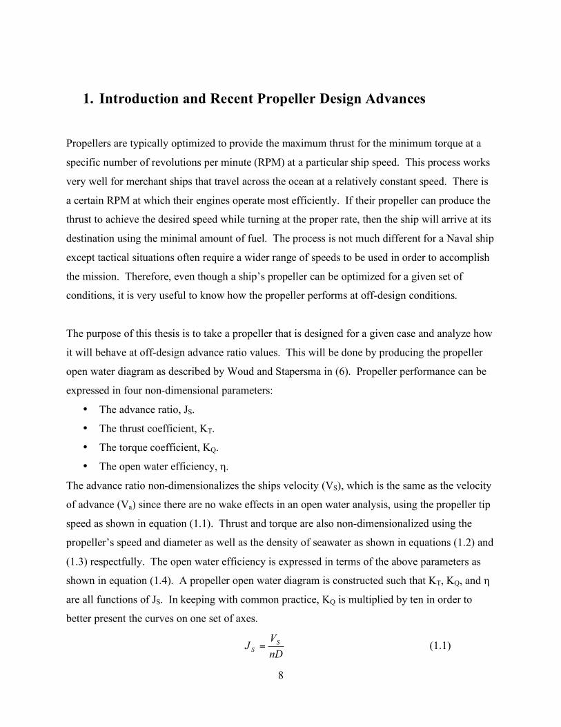
Propellers are typically optimized to provide the maximum thrust for the minimum torque at a
specific number of revolutions per minute (RPM) at a particular ship speed. This process works
very well for merchant ships that travel across the ocean at a relatively constant speed. There is
a certain RPM at which their engines operate most efficiently. If their propeller can produce the
thrust to achieve the desired speed while turning at the proper rate, then the ship will arrive at its
destination using the minimal amount of fuel. The process is not much different for a Naval ship
except tactical situations often require a wider range of speeds to be used in order to accomplish
the mission. Therefore, even though a ship’s propeller can be optimized for a given set of
conditions, it is very useful to know how the propeller performs at off-design conditions.
The purpose of this thesis is to take a propeller that is designed for a given case and analyze how
it will behave at off-design advance ratio values. This will be done by producing the propeller
open water diagram as described by Woud and Stapersma in (6). Propeller performance can be
expressed in four non-dimensional parameters:
• The advance ratio, JS.
• The thrust coefficient, KT.
• The torque coefficient, KQ.
• The open water efficiency, η.
The advance ratio non-dimensionalizes the ships velocity (VS), which is the same as the velocity
of advance (Va) since there are no wake effects in an open water analysis, using the propeller tip
speed as shown in equation (1.1). Thrust and torque are also non-dimensionalized using the
propeller’s speed and diameter as well as the density of seawater as shown in equations (1.2) and
(1.3) respectfully. The open water efficiency is expressed in terms of the above parameters as
shown in equation (1.4). A propeller open water diagram is constructed such that KT, KQ, and η
are all functions of JS. In keeping with common practice, KQ is multiplied by ten in order to
better present the curves on one set of axes.
nD
VJ
S
S= (1.1)
9
42
Dn
TKT
!= (1.2)
52
Dn
QKQ
!= (1.3)
Q
ST
K
JK!=
"#
2
1 (1.4)
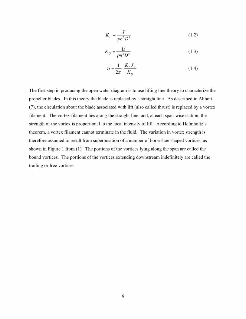
The first step in producing the open water diagram is to use lifting line theory to characterize the
propeller blades. In this theory the blade is replaced by a straight line. As described in Abbott
(7), the circulation about the blade associated with lift (also called thrust) is replaced by a vortex
filament. The vortex filament lies along the straight line; and, at each span-wise station, the
strength of the vortex is proportional to the local intensity of lift. According to Helmholtz’s
theorem, a vortex filament cannot terminate in the fluid. The variation in vortex strength is
therefore assumed to result from superposition of a number of horseshoe shaped vortices, as
shown in Figure 1 from (1). The portions of the vortices lying along the span are called the
bound vortices. The portions of the vortices extending downstream indefinitely are called the
trailing or free vortices.
10
Figure 1: Vortex Patter Representing a Lifting Wing
The effect of the trailing vortices corresponding to a positive lift is to induce a downward
component of velocity at and behind the blade. This downward component is called the
downwash. The magnitude of the downwash at any section along the span is equal to the sum of
the effects of all the trailing vortices along the entire span. The effect of the downwash is to
change the relative direction of the fluid stream over the section. The section is assumed to have
the same hydrodynamic characteristics with respect to the rotated stream as it had in the normal
two-dimensional flow. The rotation of the flow effectively changes the angle of attack. (7)
The method described by Lerbs in (8) is used to determine the circulation and induced velocity
distributions for given values of JS using the hydrodynamic properties of the foil sections at
specified radial distances along the propeller blade. With the circulation and velocities
calculated, functions built into OpenProp then determine the values of KT, KQ, and η. Finally,
the whole process is repeated again for another value of JS until the entire diagram is produced.

11
1.1 Recent Advances
Open-source Propeller Design and Analysis Program (OpenProp) is an open source
MATLAB®-based suite of propeller numerical design tools. This program is an enhanced
version of the MIT Propeller Vortex Lattice Lifting Line Program (PVL) developed by Professor
Justin Kerwin at MIT in 2001. OpenProp v1.0, originally titled MPVL, was written in 2007 by
Hsin-Lung Chung and Kate D’Epagnier and is described in detail in (1) and (2). Two of its main
improvements versus PVL are its intuitive graphical user interfaces (GUIs) and greatly improved
data visualization which includes graphic output and three-dimensional renderings. OpenProp
v2.0 was written in 2008 by John Stubblefield and is described in detail in (3). The main
improvement of version 2 was the ability to model an axially symmetric ducted-propeller with no
gap between the duct and the propeller. OpenProp v3.0 was written by Brenden Epps. The main
improvement of version 3 was …(?)
OpenProp was designed to perform two primary tasks: parametric analysis and single propeller
design. Both tasks begin with a desired operating condition defined primarily by the required
thrust, ship speed, and inflow profile. The parametric analysis produces efficiency diagrams for
all possible combinations of number of blades, propeller speed, and propeller diameter for ranges
and increments entered by the user. The efficiency diagrams are then used to determine the
optimum propeller parameters for the desired operating conditions given any constraints (e.g.
propeller speed or diameter) specified by the user. The single propeller design routine produces
a complete propeller design which is optimized for the desired operating condition and defined
propeller parameters (number of blades, propeller speed, propeller diameter, hub diameter, etc).
If these values are varied, the program will design a new optimal propeller for those given inputs,
but it will not analyze the same propeller at new conditions.
In 2008 Christopher Peterson developed MATLAB® executables that interface with a modified
version of XFOIL for determining the minimum pressure of a foil operating in an inviscid fluid
which are described in detail in (4). XFOIL is an analysis and design system for Low Reynolds
Number Airfoils. XFOIL uses an inviscid linear-vorticity panel method with a Karman-Tsien
compressibility correction for direct and mixed-inverse modes. Source distributions are

12
superimposed on the airfoil and wake permitting modeling of viscous layer influence on the
potential flow. Both laminar and turbulent layers are treated with an e9-type amplification
formulation determining the transition point. The boundary layer and transition equations are
solved simultaneously with the inviscid flow field by a global Newton method as described by
Drela in (5). Peterson’s code creates minimum pressure envelopes, similar to those published by
Brockett (1965). The modified XFOIL and MATLAB® interface was intended for future
interface with OpenProp.
13
2. Theoretical Foundation
The free vortex lines described in Section 1 are not acted on by forces. Their directions,
according to wing theory, coincide with that of the resultant lifting system. This results in the
free vortex lines of a propeller forming a general helical shape. When all the free vortex lines
are combined, they form a free vortex sheet that is in the shape of a general helical surface. The
shape of the helical sheets and their induced velocities are mutually dependant so certain
assumptions about the shape of the helical sheets are required. The methods described in this
thesis are applicable to moderately loaded propellers, therefore the following assumptions apply.
The induced velocities are allowed to influence the shape of the free helical sheets. However,
the effects of centrifugal forces and wake contraction on the shape of the sheets are neglected.
The work of Betz, Lock, and Kramer showed that for a moderately loaded propeller with an
optimum circulation distribution, the assumption that the deformation of the helical sheets in the
axial direction can be neglected produced results in close agreement with experimental data. The
assumption that the axial deformation can be neglected will be extended here to non-optimum
circulation distributions. Therefore, the vortex sheets discussed in the upcoming sections are of
general helical shape and are made up of cylindrical vortex lines of a constant diameter and pitch
angle in the axial direction. In addition, the curling up of the vortex sheets a certain distance
behind the propeller caused by the sheet’s self motion is also disregarded. (8)
2.1 Velocity Field of Symmetrically Spaced Helical Vortex Lines
There are two possible ways to determine the velocity field of symmetrically spaced helical
vortex lines, the integral by Biot-Savart and Laplace’s differential equation. Kawada in (9) used
the Laplace equation approach to develop analytical expressions for the velocity potential. These
expressions provide numerical results more readily than the elaborate numerical integration
carried out by Strscheletzky in (10) following the Biot-Savart method. (8)
Kawada considers a propeller of g blades modeled as a symmetric system of g helical tip vortices
combined with an axial hub vortex which has the same strength of all the tip vortices combined.
14
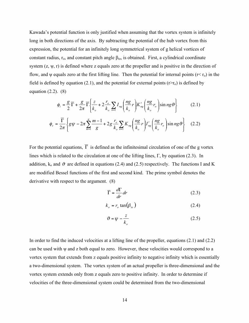
Kawada’s potential function is only justified when assuming that the vortex system is infinitely
long in both directions of the axis. By subtracting the potential of the hub vortex from this
expression, the potential for an infinitely long symmetrical system of g helical vortices of
constant radius, ro, and constant pitch angle βio, is obtained. First, a cylindrical coordinate
system (z, ψ, r) is defined where z equals zero at the propeller and is positive in the direction of
flow, and ψ equals zero at the first lifting line. Then the potential for internal points (r< ro) in the
field is defined by equation (2.1), and the potential for external points (r>ro) is defined by
equation (2.2). (8)
!"#
$%&
''(
)**+
,-''
(
)**+
,+.+.= /
=1
sin222 n
o
o
ng
o
ng
o
o
o
i ngrk
ngKr
k
ngI
k
r
k
zgg0
12 (2.1)
!"#
$%&
''(
)**+
,-''
(
)**+
,+
..
/= 00
== 11
sin21
22 n
o
o
ng
o
ng
g
m o
oe ngr
k
ngIr
k
ngK
k
rg
g
mg 123
24 (2.2)
For the potential equations, ! is defined as the infinitesimal circulation of one of the g vortex
lines which is related to the circulation at one of the lifting lines, Г, by equation (2.3). In
addition, ko and ! are defined in equations (2.4) and (2.5) respectively. The functions I and K
are modified Bessel functions of the first and second kind. The prime symbol denotes the
derivative with respect to the argument. (8)
drdr
d!=! (2.3)
( )iooo
rk !tan= (2.4)
ok
z!="# (2.5)
In order to find the induced velocities at a lifting line of the propeller, equations (2.1) and (2.2)
can be used with ψ and z both equal to zero. However, these velocities would correspond to a
vortex system that extends from z equals positive infinity to negative infinity which is essentially
a two-dimensional system. The vortex system of an actual propeller is three-dimensional and the
vortex system extends only from z equals zero to positive infinity. In order to determine if
velocities of the three-dimensional system could be determined from the two-dimensional
15
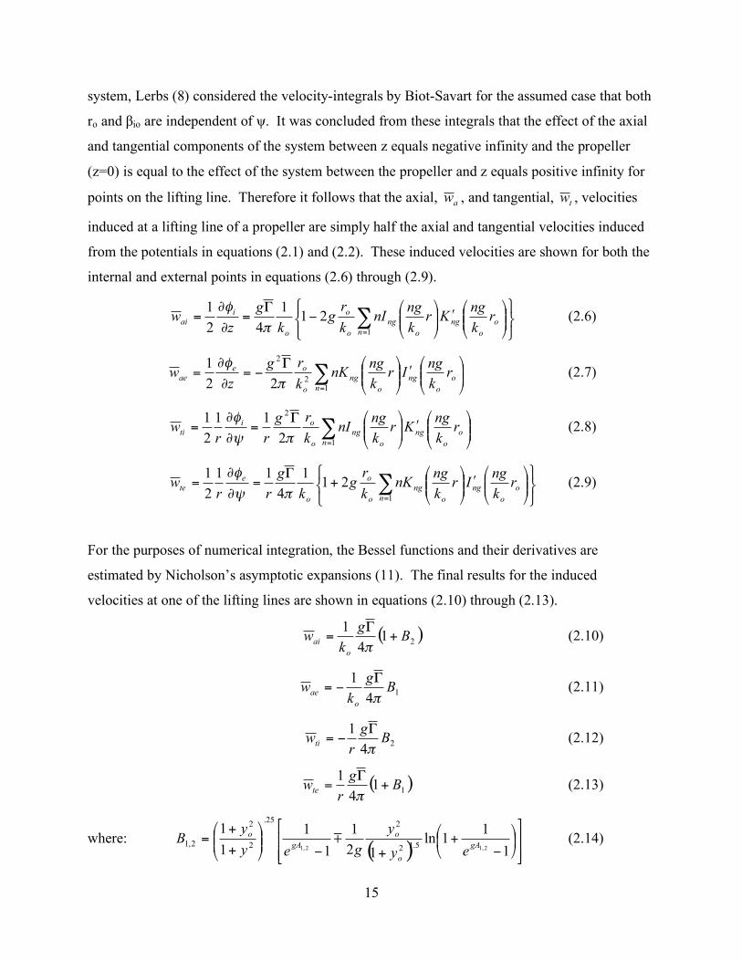
system, Lerbs (8) considered the velocity-integrals by Biot-Savart for the assumed case that both
ro and βio are independent of ψ. It was concluded from these integrals that the effect of the axial
and tangential components of the system between z equals negative infinity and the propeller
(z=0) is equal to the effect of the system between the propeller and z equals positive infinity for
points on the lifting line. Therefore it follows that the axial, aw , and tangential,
tw , velocities
induced at a lifting line of a propeller are simply half the axial and tangential velocities induced
from the potentials in equations (2.1) and (2.2). These induced velocities are shown for both the
internal and external points in equations (2.6) through (2.9).
!"#
$%&
''(
)**+
,-''
(
)**+
,.
/=
0
0= 1
=1
211
42
1
n
o
o
ng
o
ng
o
o
o
iai r
k
ngKr
k
ngnI
k
rg
k
g
zw
2
3 (2.6)
!=
""#
$%%&
'(""
#
$%%&
')*=
+
+=
1
2
2
22
1
n
o
o
ng
o
ng
o
oeae r
k
ngIr
k
ngnK
k
rg
zw
,
- (2.7)
!=
""#
$%%&
'(""
#
$%%&
')=
*
*=
1
2
2
11
2
1
n
o
o
ng
o
ng
o
oiti r
k
ngKr
k
ngnI
k
rg
rrw
+,
- (2.8)
!"#
$%&
''(
)**+
,-''
(
)**+
,+
.=
/
/= 0
=1
211
4
11
2
1
n
o
o
ng
o
ng
o
o
o
ete r
k
ngIr
k
ngnK
k
rg
k
g
rrw
12
3 (2.9)
For the purposes of numerical integration, the Bessel functions and their derivatives are
estimated by Nicholson’s asymptotic expansions (11). The final results for the induced
velocities at one of the lifting lines are shown in equations (2.10) through (2.13).
( )2
14
1B
g
kw
o
ai +!
="
(2.10)
1
4
1B
g
kw
o
ae!
"#= (2.11)
2
4
1B
g
rwti
!
"#= (2.12)
( )1
14
1B
g
rwte +
!=
" (2.13)
where: ( ) !
!"
#
$$%
&'(
)*+
,
-+
+-''(
)**+
,
+
+=
1
11ln
12
1
1
1
1
1
2,12,1 5.12
225.
2
2
2,1 gA
o
o
gA
o
ey
y
gey
yB m (2.14)
16
( ) ( )( )( )( )!
!
"
#
$$
%
&
'+++
++'++'+±=
1111
1111ln2
111
22
22
22
2,1
yy
yyyyA
o
o
o m (2.15)
( )ioo
oo
k
ry
!tan
1== (2.16)
( )iooo x
x
k
ry
!tan== (2.17)
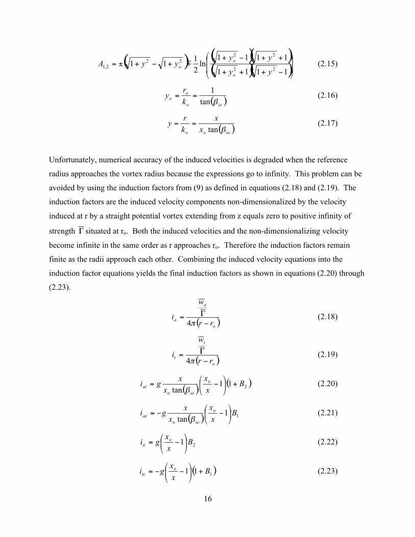
Unfortunately, numerical accuracy of the induced velocities is degraded when the reference
radius approaches the vortex radius because the expressions go to infinity. This problem can be
avoided by using the induction factors from (9) as defined in equations (2.18) and (2.19). The
induction factors are the induced velocity components non-dimensionalized by the velocity
induced at r by a straight potential vortex extending from z equals zero to positive infinity of
strength ! situated at ro. Both the induced velocities and the non-dimensionalizing velocity
become infinite in the same order as r approaches ro. Therefore the induction factors remain
finite as the radii approach each other. Combining the induced velocity equations into the
induction factor equations yields the final induction factors as shown in equations (2.20) through
(2.23).
( )
o
a
a
rr
w
i!
"=#4
(2.18)
( )
o
t
t
rr
w
i!
"=#4
(2.19)
( )
( )2
11tan
Bx
x
x
xgi o
ioo
ai +!"
#$%
&'=
( (2.20)
( ) 1
1tan
Bx
x
x
xgi o
ioo
ae !"
#$%
&''=
( (2.21)
2
1 Bx
xgi o
ti !"
#$%
&'= (2.22)
( )1
11 Bx
xgi o
te +!"
#$%
&''= (2.23)
17
It is interesting to note that the induction factors are functions of geometric properties (i.e. the
relative position of the reference point and where the vortex is shed as well as the angle at which
it is shed) and are not dependant on the circulation. Also of note is that the above expressions
apply to only one lifting line. In general, there will also be induced velocities at each lifting line
(i.e. each blade) from all other lifting lines. However, if the propeller is symmetric, these effects
will cancel each other out. (8)
In order to evaluate the accuracy of the assumptions leading to the calculation of the induction
factors, Lerbs (8) compared the calculated values to those calculated using direct numerical
integration of the Biot-Savart integral by Strscheletzky (10) in the case of g equals 3. He found
the method of Strscheletzky produced higher values than the method explained above, but only
when iti is smaller than 0.06. Differences when the induction factor is so small have a negligible
effect on the overall final values.
2.2 Velocity Field of Symmetrically Spaced Helical Vortex Sheets
Section 2.1 developed the velocity field for g helical vortex lines. When multiple vortex lines
are shed from the same lifting line, a vortex sheet is formed. The velocity components which are
produced by the vortex sheets are obtained by integrating the effects of the vortex lines over the
span of the lifting line. By integrating over the free vortices and using equations (2.3), (2.18),
and (2.19), expressions for the induced velocities (non-dimensionalized with the speed of
advance) at station x of the lifting line are shown in equations (2.24) and (2.25). These equations
are in terms of the non-dimensional circulation (G) as defined in equation (2.26). (8)
( )! "
=1
1
2
1
hx
oa
ooS
adxi
xxdx
dG
V
w (2.24)
( )! "
=1
1
2
1
hx
ot
ooS
tdxi
xxdx
dG
V
w (2.25)
S
DVG
!
"= (2.26)

18
Expanding on the method used by Glauert (12) in airfoil theory, the values of the integrals in
equations (2.24) and (2.25) can be determined. This requires a new variable, φ, as defined in
equation (2.27) which is zero when x equals the hub radius, xh, and π when x is at the blade tip.
( ) ( ) ( )!cos12
11
2
1
hhxxx ""+= (2.27)
For the purpose of analysis, G is estimated to go to zero at the hub and at the tip. For a real
propeller, the hub does carry some circulation as described in (12). Therefore, this assumption is
not always valid, but it does provide a good first order approximation. This assumption also
does not hold true for propellers with a zero-gap duct, but that is beyond the scope of this thesis.
Circulation is continuous along the span of the blade, therefore G can be written as the Fourier
series shown in equation (2.28). The continuity of G also ensures that single vortices of finite
strength do not occur and that the series for G, when placed into equations (2.24) and (2.25),
gives the complete induced velocity components. (8)
( )!=
=1
sin
m
mmGG " (2.28)
In addition to the pitch angle and the number of blades, the induction factors from Section 2.1
also depend on φ and φo. The induction factors, with respect to φo, can be written as an even
Fourier series as described by Schubert (13). This is shown in equation (2.29).
( ) ( )!=
=0
cos)(,n
ononIi """" (2.29)
It follows that the expressions for the non-dimensional induced velocities become as shown in
equations (2.30) and (2.31) where t
mh is defined in equation (2.32). ( a
mh will be defined later.)
( )!="
=11
1
m
a
mm
hS
ahmG
xV
w# (2.30)
( )!="
=11
1
m
t
mm
hS
thmG
xV
w# (2.31)
19
( )( ) ( )( ) ( )
( )( )( )( ) ( )
( )( )( ) ( )! ""
"
#$%
&'(
)
)+
)
+=
)=
**
*
+++
++
++
++
+++
++++
00
0
coscos
cos
coscos
cos
2
1
coscos
cos,
o
o
o
o
o
ot
n
o
o
oott
m
dnm
dnm
I
dmi
h
(2.32)
The two integrals inside the summation of equation (2.32) can be solved by following Glauert’s
method (12). For values of m>n, the summation become equation (2.33), and for values of m<n,
the summation becomes equation (2.34). With these substitutions made, the final form of t
mh
becomes equation (2.35). A similar process is followed for a
mh resulting in equation (2.36).
( )
( ) ( ) ( )!=
m
n
t
nnIm
0
cossinsin
""""
# (2.33)
( )
( ) ( ) ( )!+= 1
sincossin mn
t
nnIm """
"
# (2.34)
( )( )
( ) ( ) ( ) ( ) ( ) ( )!"
#$%
&+= ''
+== 10
sincoscossinsin mn
t
n
m
n
t
n
t
mnImnImh ((((((
(
)( (2.35)
( )( )
( ) ( ) ( ) ( ) ( ) ( )!"
#$%
&+= ''
+== 10
sincoscossinsin mn
a
n
m
n
a
n
a
mnImnImh ((((((
(
)( (2.36)
Equations (2.35) and (2.36) become indefinite at the hub (φ = 0º) and at the blade tip (φ = 180º).
L’Hospital’s rule provides values for the functions at these points as shown in equations (2.37)
and (2.38).
( ) ( ) ( )!"
#$%
&°+°=° ''
+== 1
,
0
,,000
mn
at
n
m
n
at
n
at
mnIImh ( (2.37)
( ) ( ) ( ) ( )!"
#$%
&°'+°'°'(=° ))
+== 1
,
0
,,180cos180cos180cos180
mn
at
n
m
n
at
n
at
mnnInImmh * (2.38)
The above equations allow the induced velocity components to be related to the circulation
distribution and the induction factors. The induction factors are known from equations (2.20)
through (2.23). Therefore the induced velocity for any circulation distribution that can be
represented by equation (2.28) can be calculated, or vice versa. However, it will be necessary to
20
use successive iterations and approximations since the induction factors depend on the pitch
angles of the sheets which, in turn, depend on the induced velocities. (8)
2.3 Application to Moderately Loaded Free-Running Non-Optimum Propellers
The vortex sheets described in Section 2.2 are made up of cylindrical vortex lines whose pitch
does not change in the axial direction. The next step is to determine the conditions imposed on
the variations of the pitch of the vortex lines in the radial direction such that the entire system
accurately models the vortex system of an actual propeller.
The force and the flow generated at a lifting line by the vortex sheets of Section 2.2 can be
related using an energy balance of the propeller flow. The input power equals the useful power
plus the increase in kinetic energy within the volume that passes through the slipstream in a
single unit of time. Input power is also made up of an external input plus the work done by the
centrifugal pressure on the volume of water in a single unit of time. As stated earlier, for a
moderately loaded propeller, it is acceptable to neglect the effects of the centrifugal pressure.
Therefore, the energy balance takes the form of equation (2.39) where the integral is taken over a
disc with the same diameter as the propeller and ΔE is the kinetic energy of the induced flow
within the volume of fluid that passes a point in the ultimate wake in one unit of time. (8)
( ) EvdTdQrA
!="# $ (2.39)
At the lifting line, the left hand side of equation (2.39) can be expressed in terms of the relative
flow’s pitch by substituting dQ and dT with their respective expressions from the Kutta-
Joukowski law. The Kutta-Joukowski law states that the force at the lifting line is perpendicular
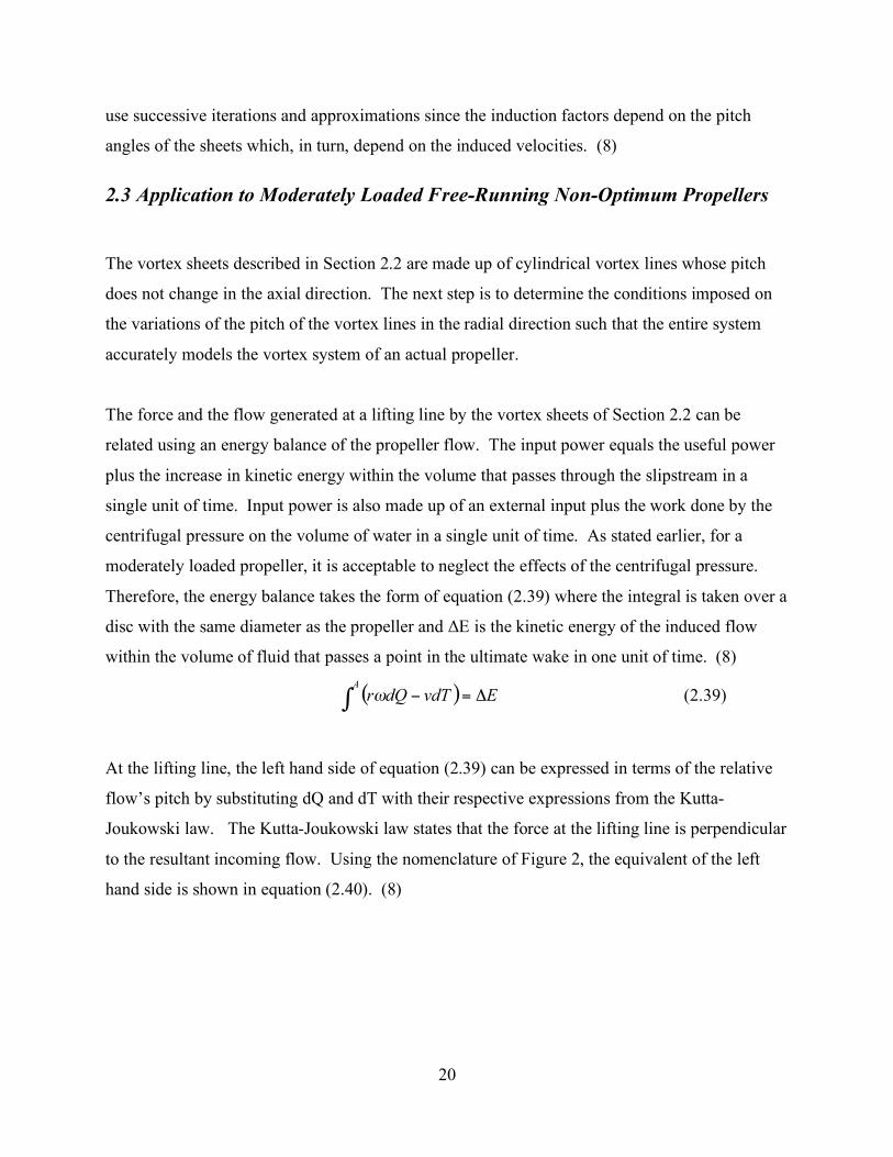
to the resultant incoming flow. Using the nomenclature of Figure 2, the equivalent of the left
hand side is shown in equation (2.40). (8)
21
Figure 2: Pitch Angle Relationships to Velocities and Forces
( ) ( )( )( )!! ""
#
$%%&
'++(=)
R
r
t
i
aa
A
h
drww
wvgvdTdQr*
+,tan
(2.40)
Using Green’s theorem, the kinetic energy of the flow which is included in a certain volume can
be represented by an integral over the surface of the volume. Applying this to the right hand side
of equation (2.39) allows it to be expressed in terms of the pitch of the vortex lines as shown in
equation (2.41). (8)
( )( )( )
( )( )( )!
!
"#
$%&
'++(=
+(=
)
)
R
r
t
i
aa
R
r i
na
h
h
drww
wvg
drw
wvgE
*+
*+
tan
sin
(2.41)
Since the left hand side must equal the right hand side, the integrals in equations (2.40) and
(2.41) must be the same. Therefore ( )ri
! must equal ( )ri
!" . In other words, the vortex lines
must leave the lifting line at a pitch angle equal to the angle of the resultant inflow. The angle of
the resultant flow is dependent on the accuracy of the approximations of the induced flow
distributions, wa(x) and wt(x). The level of accuracy of the flows caused by the vortex sheets in
Section 2.2 is ascertained by comparing them to a known solution of the flow past a propeller.

22
One solution for comparison is that of an optimum propeller for which the Betz condition
(defined in equation (2.42)) holds. (8)
constant2
2=
+
!
a
t
wv
wr
r
v "
" (2.42)
Equation (2.43) shows the expansion of both the numerator and denominator of the Betz
condition. This shows that the Betz condition is met if the induced velocity terms of order two
or greater can be neglected. From this it is expected that for an arbitrary circulation distribution,
the induced velocity at a lifting line is sufficiently estimated from the vortex sheets of Section
2.2 when higher order terms of the axial and tangential induced velocities are small compared to
v and ωr, respectively. To this degree, the difference in the shape of the actual and modeled
vortex sheets is insignificant. (8)
( )
( ) !!"
#$$%
&+'++=+
!!"
#$$%
&''''='
...12
...12
2
2
22
2
v
w
v
wwvwv
r
w
r
wwrwr
aa
aa
tt
tt
((((
(2.43)
2.4 Determining the Circulation and Induced Velocities
Given that the geometry and polar curves of a propeller are known, it is possible to estimate the
circulation and induced velocity distributions for a given advance ratio. In order to ease the
calculations, the advance coefficient will be used in lieu of the advance ratio. The advance
coefficient is defined as the advance ratio divided by pi.
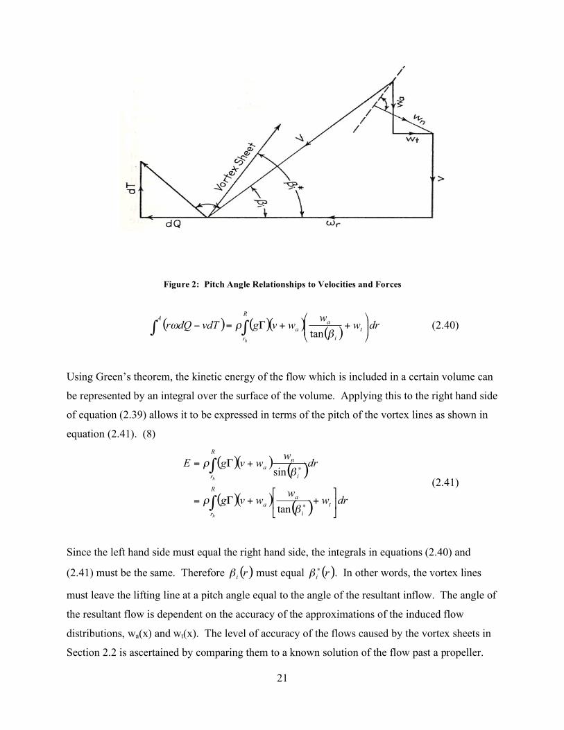
The first step is to use the Kutta-Joukowski law and the nomenclature of Figure 3 from (8) to
derive the relationship between the lift coefficient and the circulation at any radius along the
blade as shown in equation (2.44). The solidity of the propeller, s, is defined in equation (2.45)
where l is the chord length at a specified radius.
23
Figure 3: Velocity Diagram of a Moderately Loaded Propeller
V
gGvsCL
2= (2.44)
D
gls
!= (2.45)
For a small angle of attack α, the lift curve slope is approximately constant. Therefore, the lift
coefficient can be found as shown in equation (2.46) which also shows the rearrangement of the
different angular values base on Figure 3. Figure 3 can also be used to determine expressions for
both the non-dimensional inflow velocity and the tangent of (β+αi) as functions of the advance
coefficient which are shown in equations (2.47) and (2.48), respectively.
( ) ( ) ( )[ ]io
L
o
L
L
d
dC
d
dCC !"!#
!!!
!+$+=+= % (2.46)
( )
i
t
v
wx
v
V
!"
#
+
$
=cos
(2.47)
24
( )!"
#$%
&'
!"
#$%
&+
=+
v
wx
v
w
t
a
i
(
)*
1
tan (2.48)
Combining equations (2.44), (2.46), and (2.47) results in equation (2.49).
( ) ( ) ( )iiL
oLt gG
d
dCs
d
dCs
v
wx!"!
!"!#
!$+=%
&
'()
*+++,
-
./0
1+ 2
cos2 (2.49)
The next step is to substitute the expressions for wa, wt, and G (defined above in equations
(2.24), (2.25), and (2.28) ) into equations (2.49) and (2.48). The results of this substitution are
shown in equations (2.50) and (2.51).
( )[ ]
( ) ( ) ( )[ ]!=
"
"
#$%
&'(
))+)
++
=))+
1 1cossin2
...
m
ioL
h
t
mim
ioL
sd
dC
x
mhmgG
xs
d
dC
*+*,*
*+-
*+*,.*
(2.50)
( )
!
!
=
=
""
"+
=+
1
1
1
1
1
11
tan
m
t
mm
h
m
a
mm
h
i
hmGx
x
hmGx
#
$% (2.51)
The final step in finding an approximation for the circulation distribution and the induced
velocities at the lifting line is to satisfy equations (2.50) and (2.51) at m stations along the blade.
Successive iterations become necessary by starting with a reasonable guess for the distribution of
αi and solving equation (2.50) for the Fourier coefficients, Gm. These coefficients are then used
in equation (2.51) to determine a new αi distribution. The average of the new and the old αi
distributions are taken as the starting distribution for the next round of iteration. This process is
repeated until the new and the old αi distributions differ by only a small amount. A difference of
less than °± 2.0 is considered sufficient accuracy. (8)
25
3. Implementation and Validation
Given the basic geometry and polar curves of a propeller, along with an educated guess for the
hydrodynamic pitch angle of the resultant inflow, the theories of Section 2 will produce the
circulation and induced velocity distributions at the lifting line approximation of the propeller
blade for a given advance ratio. This data can then be used with the Forces.m function defined
in OpenProp to determine the thrust, torque, and efficiency information for the propeller.
3.1 MATLAB® Implementation of the “Building Blocks”
In order to implement the theories of Section 2 as a fast and reliable propeller analysis tool, the
equations were coded using MATLAB®. Although the only equations that are necessary for the
analysis are equations (2.50) and (2.51) , the major required inputs were coded as separate
functions in order to provide greater understanding to the reader as well as greater ease in
troubleshooting the code. All of the MATLAB® functions described in Section 3 can be found
in Appendix A.
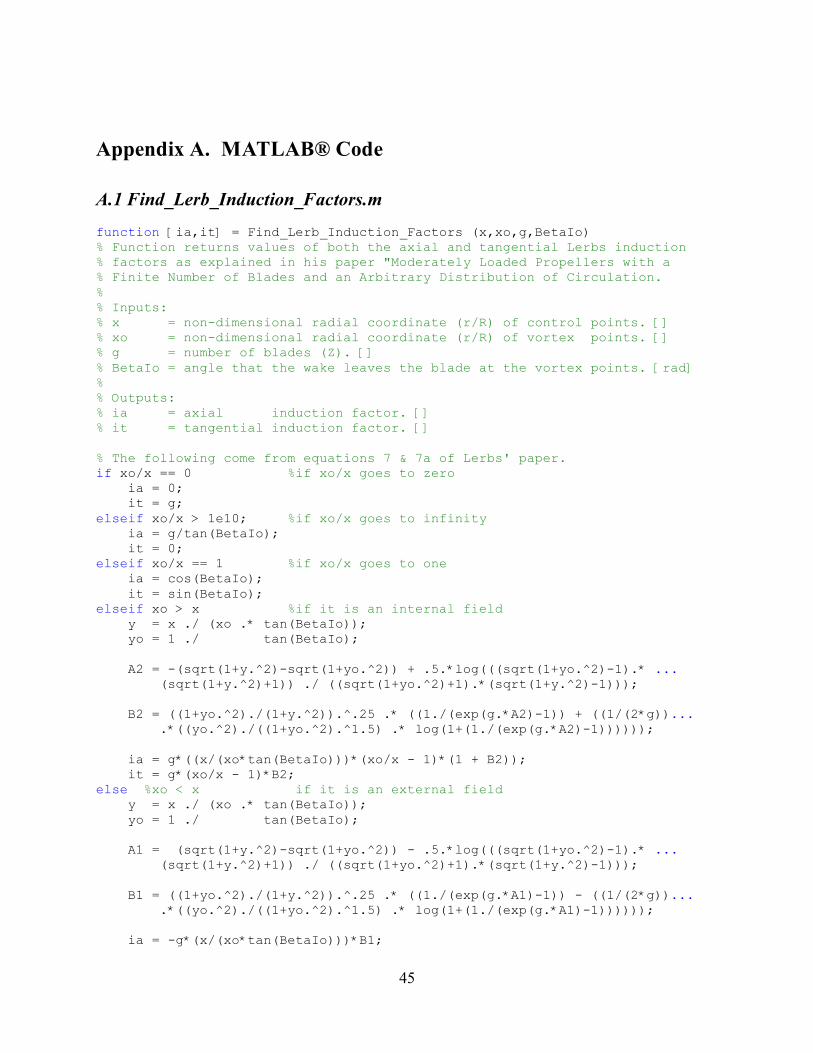
The first function in the process is named Find_Lerbs_Induction_Factors.m. This function takes
as input the non-dimensional radial coordinate of a control point and a vortex shedding point in
addition to the number of blades of the propeller and the pitch distribution of the vortex sheets.
Then, using equations (2.20) through (2.23), it calculates the axial and tangential induction
factors. The function can only do this process for a single set of inputs, therefore it must be
called multiple times in a loop to determine the induction factors at all control points caused by
the entire vortex system.
The next function is named Calculate_Induction_Fourier_Coefficients.m. This function also
takes as input the non-dimensional radial coordinates of control points and vortex shedding
points with the axial and tangential induction factors determined in the previous function. It
returns both the axial and tangential Fourier coefficients defined in equation (2.29).
The next function is named Calculate_hm_factors.m. This function takes the induction Fourier
coefficients and the non-dimensional radial coordinates of the control points as inputs in order to
26
return the factors a
mh and t
mh from the induced velocity equations as they are defined in
equations (2.35) through (2.38).
3.2 Validation of the “Building Blocks” with Lerbs’ Example Data
The functions in Section 3.1 provide the basic building blocks needed to solve for the unknown
circulation distribution and induced velocities. In order to ensure the MATLAB® functions did
not contain errors, their outputs were compared to the Lerbs’ example from Part 2 Section A-1 of
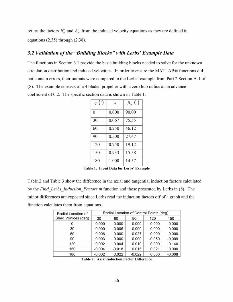
(8). The example consists of a 4 bladed propeller with a zero hub radius at an advance
coefficient of 0.2. The specific section data is shown in Table 1.
( )°! x ( )°io
!
0 0.000 90.00
30 0.067 75.55
60 0.250 46.12
90 0.500 27.47
120 0.750 19.12
150 0.933 15.58
180 1.000 14.57 Table 1: Input Data for Lerbs' Example
Table 2 and Table 3 show the difference in the axial and tangential induction factors calculated
by the Find_Lerbs_Induction_Factors.m function and those presented by Lerbs in (8). The
minor differences are expected since Lerbs read the induction factors off of a graph and the
function calculates them from equations.
Radial Location of Control Points (deg) Radial Location of Shed Vortices (deg) 30 60 90 120 150
0 0.000 0.000 0.000 0.000 0.000 30 0.000 -0.006 0.000 0.000 0.000 60 -0.006 0.000 -0.027 0.000 0.000 90 0.003 0.000 0.000 -0.050 -0.009 120 -0.002 0.004 -0.010 0.000 -0.140 150 -0.004 -0.018 0.015 0.021 0.000 180 -0.002 0.022 -0.022 0.000 -0.008
Table 2: Axial Induction Factor Difference
27
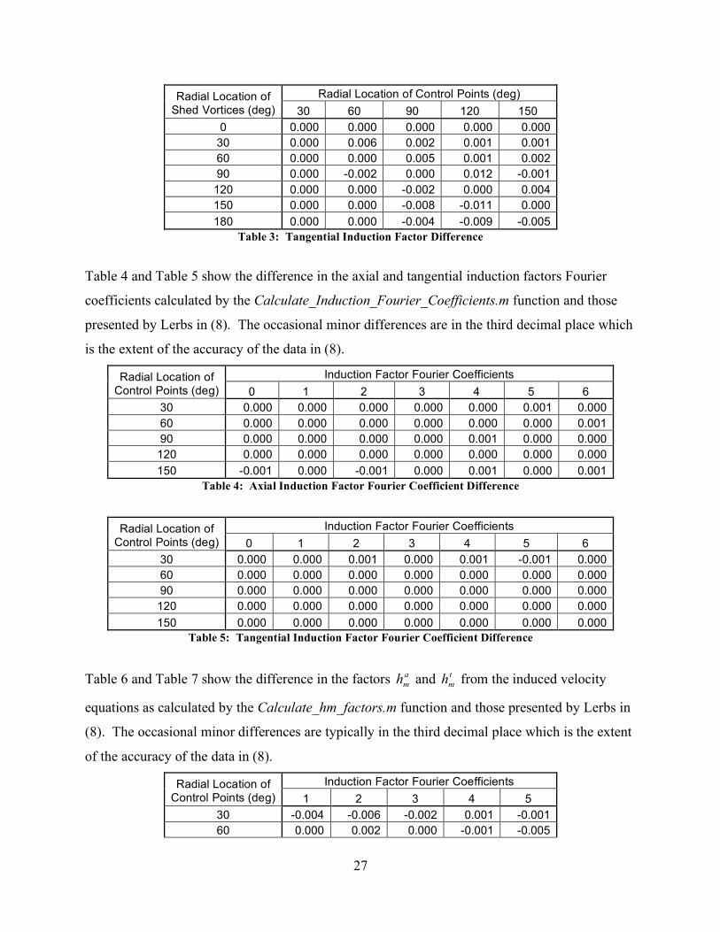
Radial Location of Control Points (deg) Radial Location of Shed Vortices (deg) 30 60 90 120 150
0 0.000 0.000 0.000 0.000 0.000 30 0.000 0.006 0.002 0.001 0.001 60 0.000 0.000 0.005 0.001 0.002 90 0.000 -0.002 0.000 0.012 -0.001 120 0.000 0.000 -0.002 0.000 0.004 150 0.000 0.000 -0.008 -0.011 0.000 180 0.000 0.000 -0.004 -0.009 -0.005
Table 3: Tangential Induction Factor Difference
Table 4 and Table 5 show the difference in the axial and tangential induction factors Fourier
coefficients calculated by the Calculate_Induction_Fourier_Coefficients.m function and those
presented by Lerbs in (8). The occasional minor differences are in the third decimal place which
is the extent of the accuracy of the data in (8).
Induction Factor Fourier Coefficients Radial Location of Control Points (deg) 0 1 2 3 4 5 6
30 0.000 0.000 0.000 0.000 0.000 0.001 0.000 60 0.000 0.000 0.000 0.000 0.000 0.000 0.001 90 0.000 0.000 0.000 0.000 0.001 0.000 0.000 120 0.000 0.000 0.000 0.000 0.000 0.000 0.000 150 -0.001 0.000 -0.001 0.000 0.001 0.000 0.001
Table 4: Axial Induction Factor Fourier Coefficient Difference
Induction Factor Fourier Coefficients Radial Location of Control Points (deg) 0 1 2 3 4 5 6
30 0.000 0.000 0.001 0.000 0.001 -0.001 0.000 60 0.000 0.000 0.000 0.000 0.000 0.000 0.000 90 0.000 0.000 0.000 0.000 0.000 0.000 0.000 120 0.000 0.000 0.000 0.000 0.000 0.000 0.000 150 0.000 0.000 0.000 0.000 0.000 0.000 0.000
Table 5: Tangential Induction Factor Fourier Coefficient Difference
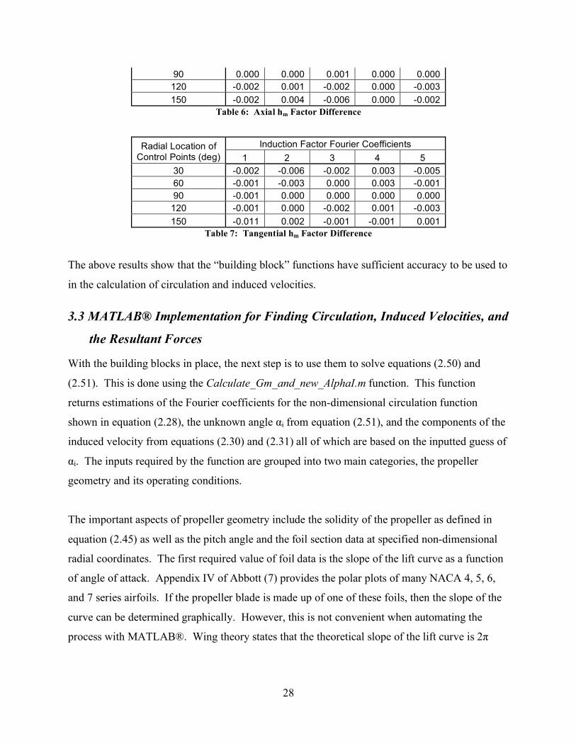
Table 6 and Table 7 show the difference in the factors a
mh and t
mh from the induced velocity
equations as calculated by the Calculate_hm_factors.m function and those presented by Lerbs in
(8). The occasional minor differences are typically in the third decimal place which is the extent
of the accuracy of the data in (8).
Induction Factor Fourier Coefficients Radial Location of Control Points (deg) 1 2 3 4 5
30 -0.004 -0.006 -0.002 0.001 -0.001 60 0.000 0.002 0.000 -0.001 -0.005
28
90 0.000 0.000 0.001 0.000 0.000 120 -0.002 0.001 -0.002 0.000 -0.003 150 -0.002 0.004 -0.006 0.000 -0.002
Table 6: Axial hm Factor Difference
Induction Factor Fourier Coefficients Radial Location of Control Points (deg) 1 2 3 4 5
30 -0.002 -0.006 -0.002 0.003 -0.005 60 -0.001 -0.003 0.000 0.003 -0.001 90 -0.001 0.000 0.000 0.000 0.000 120 -0.001 0.000 -0.002 0.001 -0.003 150 -0.011 0.002 -0.001 -0.001 0.001
Table 7: Tangential hm Factor Difference
The above results show that the “building block” functions have sufficient accuracy to be used to
in the calculation of circulation and induced velocities.
3.3 MATLAB® Implementation for Finding Circulation, Induced Velocities, and
the Resultant Forces
With the building blocks in place, the next step is to use them to solve equations (2.50) and
(2.51). This is done using the Calculate_Gm_and_new_AlphaI.m function. This function
returns estimations of the Fourier coefficients for the non-dimensional circulation function
shown in equation (2.28), the unknown angle αi from equation (2.51), and the components of the
induced velocity from equations (2.30) and (2.31) all of which are based on the inputted guess of
αi. The inputs required by the function are grouped into two main categories, the propeller
geometry and its operating conditions.
The important aspects of propeller geometry include the solidity of the propeller as defined in
equation (2.45) as well as the pitch angle and the foil section data at specified non-dimensional
radial coordinates. The first required value of foil data is the slope of the lift curve as a function
of angle of attack. Appendix IV of Abbott (7) provides the polar plots of many NACA 4, 5, 6,
and 7 series airfoils. If the propeller blade is made up of one of these foils, then the slope of the
curve can be determined graphically. However, this is not convenient when automating the
process with MATLAB®. Wing theory states that the theoretical slope of the lift curve is 2π

29
radians (7). Experimental results have shown close agreement with this value, therefore it will
be used for this thesis.
The next required piece of data for the foil sections is the angle of attack that produces no lift
(also called the angle of zero lift). Abbott (7) provides many ways to determine this angle. If the
propeller blade is made up of foil section contained in Appendix IV of (7), the angle of zero lift
can be graphically determined from the polar plots. Again, this is not convenient for the
computing environment. If the mean line distribution is known, Abbott outlines a method
derived by Munk to estimate the angle of zero lift with equation (3.1). It requires that the
ordinates of the mean line as a percent of the chord, y1 through y5, are known at specific chord-
wise percentages, x1 through x5, defined below. The constants k1 through k5 are defined such
that the angle of zero lift is returned in degrees.
5544332211ykykykykyko ++++=!" (3.1)
00542.0
12574.0
50000.0
87426.0
99458.0
97817.5
6838.15
5959.32
048.109
24.1252
:
5
4
3
2
1
5
4
3
2
1
=
=
=
=
=
=
=
=
=
=
x
x
x
x
x
k
k
andk
k
k
where
The function Calculate_Angle_of_Zero_Lift.m approximates the angle of zero lift for a NACA
a=0.8 mean line foil. The function is easily adaptable to other mean lines by entering new x-y
coordinates. The coordinates of many mean lines are listed in Abbott’s Appendix II (7). The
function takes as input the maximum chamber ratio and scales the mean line ordinates from the
design conditions to the desired conditions. It then uses equation (3.1) to calculate and return the
angle of zero lift in degrees.
The final inputs for the Calculate_Gm_and_new_AlphaI.m function are the operating conditions.
They consist of the advance coefficient, angle of flow, the factors a
mh and t
mh , and the estimation
of αi. The propellers rotational and axial speeds dictate the advance coefficient (as described in
Section 2.4) as well as the angle of flow, β, as shown in Figure 3. The factors a
mh and t
mh are
30
define in equations (2.35) and (2.36). The initial guess of the angle αi can be obtained from
OpenProp.
With all of the inputs determined, the Calculate_Gm_and_new_AlphaI.m function starts with
equation (2.50). The left-hand side of the equation is calculated for every control point and the
values are stored in a row vector of k elements, where k is the number of control points. Next,
everything inside the curly brackets on the right-hand side of the equation is calculated at all k
control points using the values 1 to k for m thus creating a k by k matrix. The complete right-
hand side of equation (2.50) is the sum of the non-dimensional circulation Fourier coefficients
(Gm) times everything inside the curly brackets. In matrix notation the sum of the products is
simply the matrix multiplication of the curly bracket matrix (k by k) with Gm (k by 1). The built
in MATLAB® function linsolve is then used to solve for the unknown Gm column vector.
Now that the coefficients for the circulation series (based on the estimate of αi) are known,
equation (2.51) is used to calculate a new estimate for the distributions of αi and subsequently βi.
Next, βi is used as the vortex sheet pitch angle distribution. This leads to new induction factors
with their own Fourier coefficients. These new coefficients are used to calculate new a
mh and t
mh
factors for input again into the Calculate_Gm_and_new_AlphaI.m function. The values of the
circulation series coefficients are also used to estimate the axial and tangential velocities in
equations (2.30) and (2.31). This process is repeated until the original and new estimate of αi
agree to within °± 2.0 .
Once there is convergence on the value of αi, the Forces.m function from OpenProp is used.
This function is shown in Appendix A for completeness, but it was not altered from its most
recent release. The forces of note for propeller analysis, as explained in Section 1, are the thrust
coefficient, the torque coefficient, and the efficiency.
3.4 Validation of Circulation, Induced Velocity, and Forces Using OpenProp
OpenProp was chosen to design a propeller because it has been proven to provide accurate
circulation and induced velocity distributions for a given design point. OpenProp also designs
the blade shape and pitch angle based on wing theory. Therefore it should be possible to use all

31
of the geometric data and the Lerbs method (8) to arrive back at the same circulation and induced
velocity distributions. Lerbs modeling of the circulation as a Fourier sine series necessitates that
the circulation goes to zero at both the hub and blade tip. For this reason, in designing the
propeller with the Single Propeller Design option in OpenProp, the “Hub Image Flag” and
“Ducted propeller” options were both left unchecked. Throughout the validation process, errors
were discovered with the OpenProp code that affected the way the blades were designed but not
the calculation of the circulation and induced velocity distributions.
The first error noted was in the calculation of “Vstar” just prior to generating the
“OpenProp_Performance.txt” reporting file. This value was supposed to be the magnitude of the
resultant inflow to the lifting line at each control point non-dimensionalized by the speed of the
ship. However, the “ωr” term had units of length over time. This problem was solved by
dividing the term by the speed of the ship. This error also cascaded into the circulation,
“Gamma”, and the lift coefficient, “Cl”, reported in “OpenProp_Performance.txt” file. This lift
coefficient was used by the Geometry.m function to scale the chamber of the mean line.
The next error detected also affects the scaling of the chamber of the mean line. The Single
Propeller Design graphical user interface allows the designer to enter the maximum chamber
divided by chord length for multiple radial positions along the blade. This information in turn is
multiplied by the lift coefficient in the Geometry.m function to set a new maximum chamber
ratio. According to Abbott (7), the maximum chamber ratio can be scaled by a constant factor to
produce the desired lift; however, the factor must be as shown in equation (3.2). In general, if
the designer inputs an arbitrary maximum chamber distribution, the corresponding lift coefficient
is unknown and therefore the scaling factor cannot be determined. This problem was solved for
this validation run by inputting the maximum chamber ratio for the NACA a=0.8 mean line from
Appendix II of (7) into the graphical user interface. This data corresponds to a lift coefficient of
1.0. Thus the scaling factor is simply the desired lift coefficient.
!!
"
#
$$
%
&=
OriginalL
DesiredL
C
CFactorScaling (3.2)
32
The final error detected was with the calculation of the pitch angle in OpenProp. The program
simply took the “Ideal Angle of Attack” inputted in the graphical user interface and added it to
the hydrodynamic pitch angle, βi, that was calculated as part of the optimization routine. As
described in Abbott (7), if the chamber is scaled by a constant factor to achieve a desired lift, the
ideal angle of attack must also be scaled by the same factor. This problem was solved by
multiplying the ideal angle of attack by the factor in equation (3.2) before determining the pitch
angle of the foil section.
OpenProp was used to design a single propeller using all of the default settings except for the
modifications noted above. The outputs of that design process were then used as inputs to the
Lerbs method for determining the circulation and induced velocity distributions. Figure 4 shows
both the OpenProp and Lerbs method non-dimensional circulation distributions. Figure 5 show
the induced velocity components for both the OpenProp and Lerbs method. Both figures show
close agreement in the values. The largest differences occur in at the blade root. It is possible
this difference occurs because the Lerbs method forces the circulation to be zero at the hub.
Even though the option to eliminate hub effects in OpenProp was chosen, the OpenProp
circulation does not approach zero as quickly as the Lerbs method.
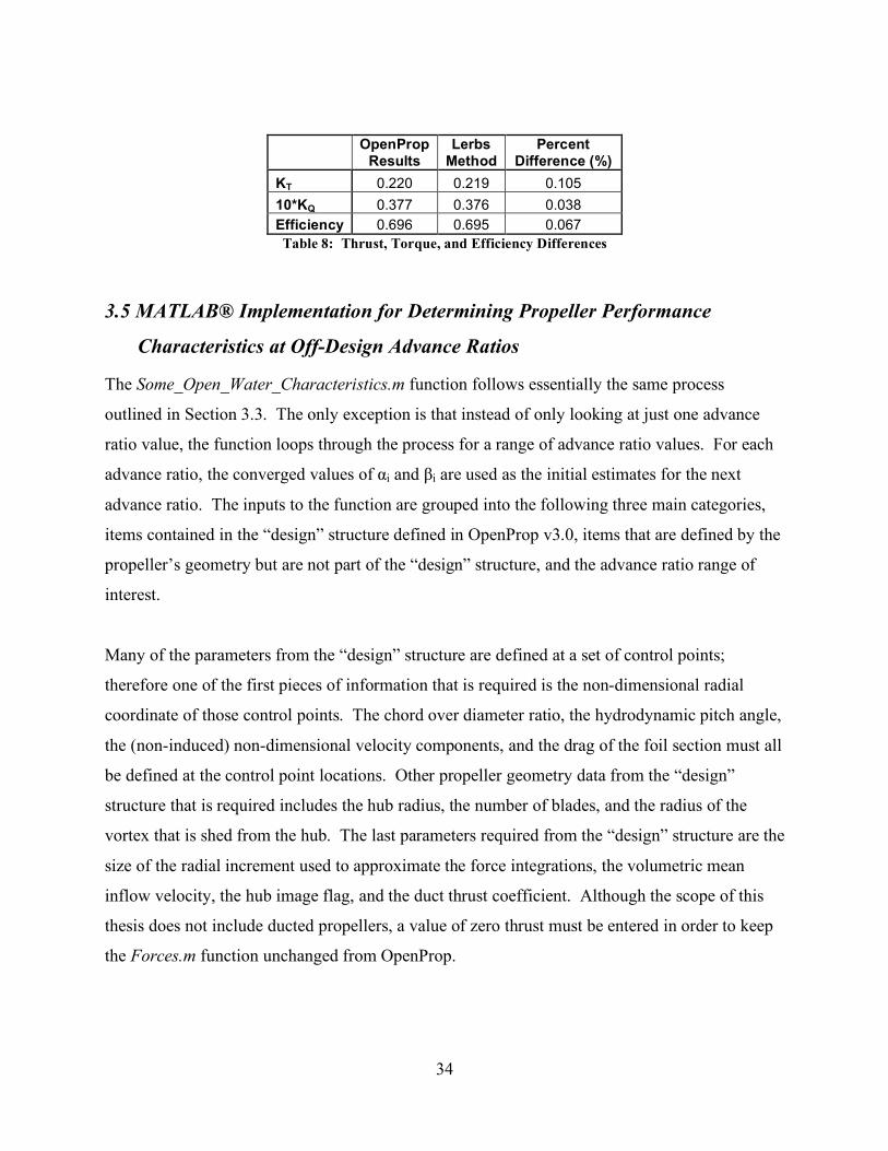
With accurate estimates of the circulation and velocities, the next step is to calculate the resultant
forces and compare them to the forces calculated in OpenProp. The values of the thrust
coefficient, the torque coefficient, and the efficiency from using both the Lerbs method and
OpenProp are shown in Table 8. The maximum difference between the values is only
approximately .1%. It is concluded that the minor differences in the velocity and circulation
values have a negligible effect on the forces produced by the propeller.

33
0 0.1 0.2 0.3 0.4 0.5 0.6 0.7 0.8 0.9 10
0.005
0.01
0.015
0.02
0.025
0.03
Non-Dimensional Radial Coordinate
Non-Dimensional Circulation (G)
Lerbs Method
OpenProp Results
Figure 4: Non-Dimensional Circulation Comparison
0 0.1 0.2 0.3 0.4 0.5 0.6 0.7 0.8 0.9 1
-0.1
-0.05
0
0.05
0.1
0.15
0.2
0.25
0.3
0.35
Non-Dimensional Radial Coordinate
Non-Dimensional Induced Velocity Components
Lerbs Method (Axial)
OpenProp Results (Axial)
Lerbs Method (Tangential)
OpenProp Results (Tangential)
Figure 5: Non-Dimensional Induced Velocities Comparison
34
OpenProp
Results Lerbs
Method Percent
Difference (%) KT 0.220 0.219 0.105 10*KQ 0.377 0.376 0.038 Efficiency 0.696 0.695 0.067 Table 8: Thrust, Torque, and Efficiency Differences
3.5 MATLAB® Implementation for Determining Propeller Performance
Characteristics at Off-Design Advance Ratios
The Some_Open_Water_Characteristics.m function follows essentially the same process
outlined in Section 3.3. The only exception is that instead of only looking at just one advance
ratio value, the function loops through the process for a range of advance ratio values. For each
advance ratio, the converged values of αi and βi are used as the initial estimates for the next
advance ratio. The inputs to the function are grouped into the following three main categories,
items contained in the “design” structure defined in OpenProp v3.0, items that are defined by the
propeller’s geometry but are not part of the “design” structure, and the advance ratio range of
interest.
Many of the parameters from the “design” structure are defined at a set of control points;
therefore one of the first pieces of information that is required is the non-dimensional radial
coordinate of those control points. The chord over diameter ratio, the hydrodynamic pitch angle,
the (non-induced) non-dimensional velocity components, and the drag of the foil section must all
be defined at the control point locations. Other propeller geometry data from the “design”
structure that is required includes the hub radius, the number of blades, and the radius of the
vortex that is shed from the hub. The last parameters required from the “design” structure are the
size of the radial increment used to approximate the force integrations, the volumetric mean
inflow velocity, the hub image flag, and the duct thrust coefficient. Although the scope of this
thesis does not include ducted propellers, a value of zero thrust must be entered in order to keep
the Forces.m function unchanged from OpenProp.
35
The parameters that are not part of the “design” structure but are defined at the control points are
the pitch over diameter and the maximum chamber ratio distributions. The diameter of the
propeller is also required. The last required input is the advance ratio range over which the
propeller is to be analyzed.
The value of αi is easily obtained from the information contained in the “design” structure.
OpenProp provides this information at the design point of the propeller. Therefore, the
Open_Water_Characteristics.m function starts at the design advance ratio and then works to
both extremes of the advance ratio range of interest with a step size of 0.01. The
Open_Water_Characteristics.m function calls the Some_Open_Water_Characteristics.m
function first for the range of advance ratios less than the design value and then again for the
range above the design value. After calculating the forces and efficiencies over the entire range,
the function checks to see if the efficiency ever becomes negative. This point is where the
propeller is “wind-milling” and no longer providing any useful thrust to the ship. The function
then returns the JS, KT, KQ, and efficiency values for points before the “wind-milling” point.
3.6 Validation of Propeller Performance Characteristics at Off-Design Advance
Ratios
The same propeller designed by OpenProp in Section 3.4 was used to validate the propeller
performance MATLAB® code described in Section 3.5. The result is shown in Figure 6. In
order to determine the robustness of the described in Section 3.5, the code was altered so that it
would not only start at the design point and work toward the endpoints, but also so it started at
the lowest value in the advance ratio range and worked up to the highest and vice versa. In both
cases, the initial guess of αi (corresponding to the design point) was used. The results are shown
in Figure 7. There is no significant difference in the results of the three methods; therefore the
method is not very sensitive to the initial guess of αi.

36
0 0.2 0.4 0.6 0.8 1 1.2 1.40
0.1
0.2
0.3
0.4
0.5
0.6
0.7
0.8
Advance Ratio (Js)
KT,
10*K
Q, !
Thrust Coefficient (KT)
10*Torque Coefficient (KQ
)
Efficiency (!) Figure 6: Performance Curves of Generic Propeller
0 0.2 0.4 0.6 0.8 1 1.2 1.40
0.5
Advance Ratio (Js)
KT
0 0.2 0.4 0.6 0.8 1 1.2 1.40
0.5
1
Advance Ratio (Js)
10*KQ
0 0.2 0.4 0.6 0.8 1 1.2 1.40
0.5
1
Advance Ratio (Js)
!
Solid Line = Start at Design Js, Square = Start at Low J
s, + = Start at High J
s
Figure 7: Robustness Results
37
It is important to note that the general shape of the curves in Figure 6 is similar to the examples
in Woud (6). However, there is no data for this particular propeller to validate that the values are
accurate. Therefore, the numerical accuracy of the program is validated using the DTMB 4119
propeller. The DTMB 4119 propeller was chosen for the validation due to its relatively simple
geometry (it has no rake or skew) and the extensive amount of experimental data available for it.
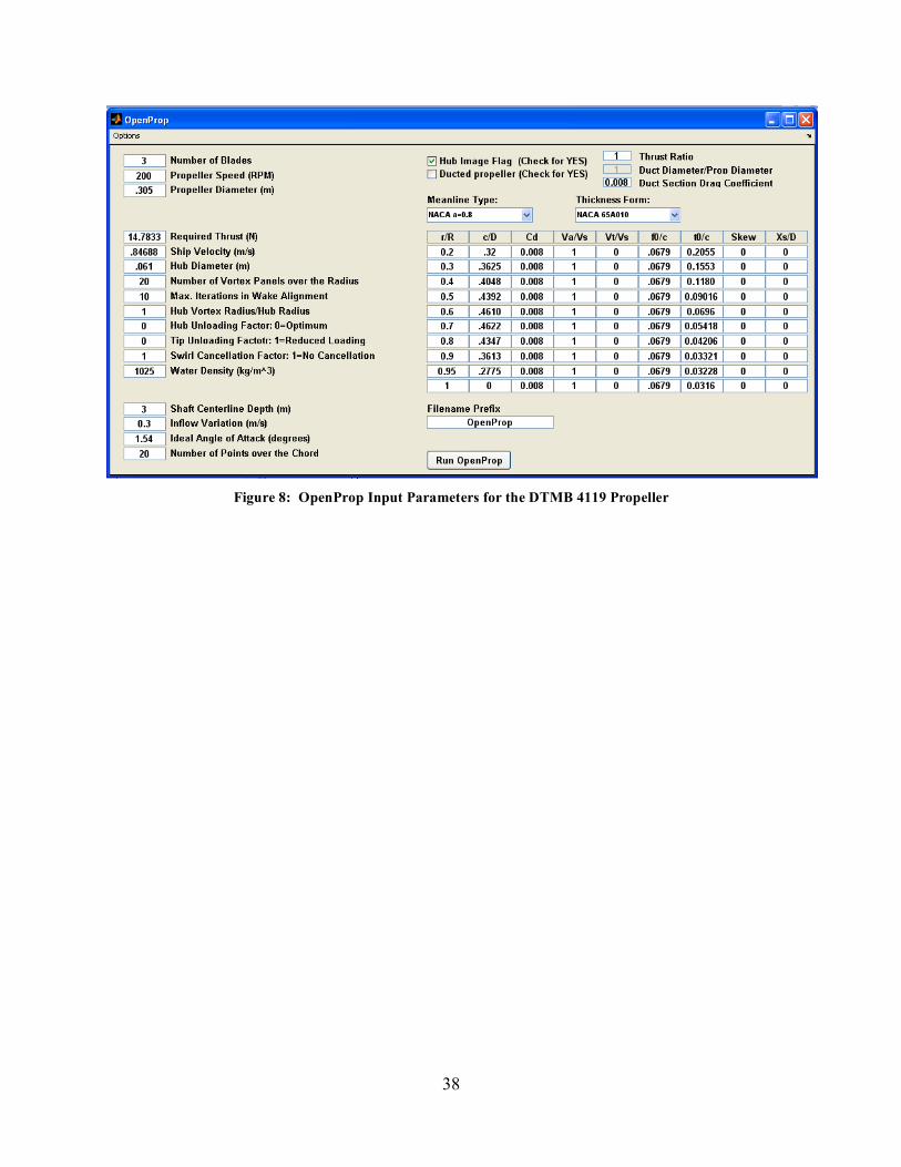
The geometric characteristics of the DTMB 4119 propeller as reported by Black (14) are shown
in Table 9. This data was entered into OpenProp in the Single Propeller Design GUI shown in
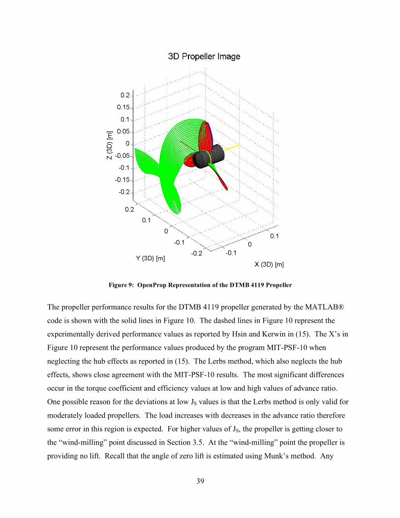
Figure 8. The propeller produced by OpenProp with these inputs is shown in Figure 9. The
thickness form of the DTMB 4119 propeller is the NACA 66 (DTMB modified). OpenProp does
not currently design propellers with this thickness form so the NACA 65A010 form was used
instead. Neither OpenProp nor any of MATLAB® function described above use the thickness of
the blade in any calculations. Therefore the difference in the thickness forms is not considered a
problem for the validation of the performance curves
Table 9: Geometry of the DTMB 4119 Propeller
38
Figure 8: OpenProp Input Parameters for the DTMB 4119 Propeller
39
Figure 9: OpenProp Representation of the DTMB 4119 Propeller
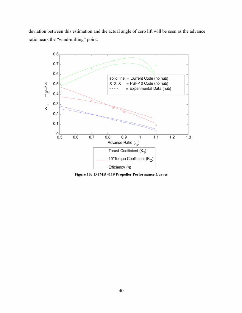
The propeller performance results for the DTMB 4119 propeller generated by the MATLAB®
code is shown with the solid lines in Figure 10. The dashed lines in Figure 10 represent the
experimentally derived performance values as reported by Hsin and Kerwin in (15). The X’s in
Figure 10 represent the performance values produced by the program MIT-PSF-10 when
neglecting the hub effects as reported in (15). The Lerbs method, which also neglects the hub
effects, shows close agreement with the MIT-PSF-10 results. The most significant differences
occur in the torque coefficient and efficiency values at low and high values of advance ratio.
One possible reason for the deviations at low JS values is that the Lerbs method is only valid for
moderately loaded propellers. The load increases with decreases in the advance ratio therefore
some error in this region is expected. For higher values of JS, the propeller is getting closer to
the “wind-milling” point discussed in Section 3.5. At the “wind-milling” point the propeller is
providing no lift. Recall that the angle of zero lift is estimated using Munk’s method. Any
40
deviation between this estimation and the actual angle of zero lift will be seen as the advance
ratio nears the “wind-milling” point.
0.5 0.6 0.7 0.8 0.9 1 1.1 1.2 1.30
0.1
0.2
0.3
0.4
0.5
0.6
0.7
0.8
Advance Ratio (Js)
KT,
10*K
Q, !
Thrust Coefficient (KT)
10*Torque Coefficient (KQ
)
Efficiency (!)
solid line = Current Code (no hub)
X X X = PSF-10 Code (no hub)
- - - - = Experimental Data (hub)
Figure 10: DTMB 4119 Propeller Performance Curves

41
4. Conclusions and Recommendations
4.1 Conclusions
This thesis successfully implements the methods derived by Lerbs for determining the circulation
and induced velocity distributions of a propeller using MATLAB® code. The only requirements
that are necessary are that the geometry of the propeller and a reasonable estimate of the angle of
the incoming flow are known. Furthermore, the circulation and velocities are used to determine
the thrust coefficient, torque coefficient, and the efficiency of the propeller. These values are
calculated at multiple advance ratios in order to produce an open water performance diagram for
the propeller.
The performance curves show excellent agreement with OpenProp at the design point of the
propeller. They also show adequate agreement with experimental and more sophisticated
numerical programs. The code and theories presented in this thesis utilize lifting line theory
which is often used at the early stage of propeller design. The MATLAB® code explained above
will give the designer propeller performance information at off-design advance coefficients that
would normally not be available until more detailed design and modeling was completed. In
addition, the performance curves are provided in a matter of one to two minutes. This allows the
designer to make changes to the propeller and quickly analyze if they had the desired effect.
4.2 Recommendations for future work
One area of future work that would enhance the features of this thesis is the incorporation of this
work into the OpenProp code. The code was designed with this feature in mind; therefore it
should be relative quick to implement. The only road block is that currently OpenProp does not
save the variables for the maximum chamber or pitch over diameter distributions. Since these
are both calculated in the Geometry.m function, the variables would have to be added as outputs
to that function and saved with an appropriate name in the main part of the OpenProp code. The
user interface would also have to be updated to give the user the option to produce the
performance curves and the desired advance ratio range. Obviously, additional output reports
could also be generated so the performance can be viewed in tabular form as well.

42
Another area of future work to enhance the features of this thesis is in obtaining better estimates
of the characteristics of the foil sections. This could be done by building on Peterson’s work (4)
of having MATLAB® using XFOIL to obtain foil data. Examples of ways XFOIL can be used
to improve the accuracy of the model include using it to determine the angle of zero lift, the
slope of the lift curve, and detailed viscous data for the foils. XFOIL can also be used to obtain
cavitation information at any advance ratio.
Another area of future work involves enhancing the Lerbs method to work when the circulation
at the hub and/or tip of the blade do not go to zero. This is needed since the hub typically carries
a certain amount of circulation that is shed in a hub vortex. Additionally, if the propeller had a
zero gap duct around it, the circulation at the blade tip would be a non-zero value. One possible
way to approach this is using a method of images to create a “virtual” wall at the hub and/or
blade tip through which no fluid will pass. It might also be possible to model the circulation not
as a Fourier sine series, but as a Fourier series of sines and cosines. This would remove the
stipulation of the function going to zero at both ends of the blade. This was explored briefly, and
it appears that in equation (2.50) there would be two unknown values (the sine and cosine
coefficients) with only one equation.
One final area for future work involves applying the methods of this thesis to more general cases.
One thought of how to do this is to first use the Lerbs method to obtain an initial estimate of the
circulation distribution. Next, use that to obtain the total inflow velocity. With this velocity, the
current method of OpenProp could be utilized to determine the circulation without the
constraints on the end points of the blade. After some number of iterations, this could converge
on a more general solution.
43
References
1. Chung, H. An Enhanced Propeller Design Program Based on Propeller Vortex Lattice Lifting
Line Theory, Master's Thesis. s.l. : Massachusetts Institute of Technology, Department of
Mechanical Engineering, 2007.
2. D'Epagnier, K. A Computational Tool for the Rapid Design and Prototyping of Propellers
for Underwater Vehicles, Master's Thesis. s.l. : Massachusetts Institute of Technology,
Department of Mechanical Engineering, 2007.
3. Stubblefield, J. Numerically-Based Ducted Propeller Design Using Vortex Lattice Lifting
Line Theory, Master's Thesis. s.l. : Massachusetts Institute of Technology, Department of
Mechanical Engineering, 2008.
4. Peterson, C. Minimum Pressure Envelope Cavitation Analysis Using Two-Dimensional
Panel Method, Master's Thesis. s.l. : Massachusetts Institute of Technology, Department of
Mechanical Engineering, 2008.
5. Drela, Mark. XFOIL: An Analysis and Design System for Low Reynolds Number Airfoils. In:
T.J. Mueller, editor. Low Reynolds Number Aerodynamics: Proceedings for the Conference,
Notre Dame, Indiana, USA, 5-7 June 1989. Springer-Verlag, p. 1-12.
6. Woud, Hans Klein and Stapersma, Douwe. Design of propulsion and electric power
generation systems. London: IMarEST, Institute of Marine Engineering, Science and
Technology, 2002.
7. Abbott, Ira H. and Von Doenhoff, Albert E. Theory of Wing Sections. New York: Dover
Publications, Inc., 1959.
8. Lerbs, H. W. Moderately Loaded Propellers with a Finite Number of Blades and an
Arbitrary Distribution of Circulation. In: The Society of Naval Architects and Marine
Engineers Transactions Vol. 60 1952. New York: SNAME, 1952, p. 73-123.
9. Kawada, S. Induced Velocities of Helical Vortices. In: Journal of the Aeronautical Sciences
Vol. 3, 1936. Also: Report of the Aeronautical Research Institute, Tokyo, Imperial University,
No. 172, 1939.
44
10. Strscheletzky, M. A Method for Determining the Velocities Which Are Induced by the Free
Vortices of a Propeller. In: Rpt. Aerodynamische Versuchsantstalt, Goettingen, 1944. Also:
Hydrodynamics for Designing Ship Propellers. Karlsruhe, G. Braun, 1950.
11. Nicholson, J. W. The Approximate Calculation of Bessel Functions of Imaginary
Arguments. Philosophical Magazine, Vol.20, 1910.
12. Kerwin, Justin E. Hydrofoils and Propellers Lecture Notes. s.l. : Massachusetts Institute of
Technology, 2001.
13. Schubert, H. The Determination of the Aeordynamic Characteristics of Lightly Loaded Air-
propellers of Arbitrary Shape. Jahrb. 1940 der Deutschen Luftfahrtforschung.
14. Black, Scott Donald. Integrated Lifting Surface/Navier-Stokes Design and Analysis
Methods for Marine Propulsors. s.l. : Massachusetts Institute of Technology, Department of
Ocean Engineering, 1997.
15. Hsin, Ching-Yeh and Kerwin, Justin E. Steady Performance for Two Propellers using
MIT-PSF-10. Prepared for 20th ITTC Propulsor Committee Comparative Calculation of
Propellers by Surface Panel Methods. July 17, 1992.
45
Appendix A. MATLAB® Code
A.1 Find_Lerb_Induction_Factors.m function [ia,it] = Find_Lerb_Induction_Factors (x,xo,g,BetaIo) % Function returns values of both the axial and tangential Lerbs induction % factors as explained in his paper "Moderately Loaded Propellers with a % Finite Number of Blades and an Arbitrary Distribution of Circulation. % % Inputs: % x = non-dimensional radial coordinate (r/R) of control points. [] % xo = non-dimensional radial coordinate (r/R) of vortex points. [] % g = number of blades (Z). [] % BetaIo = angle that the wake leaves the blade at the vortex points. [rad] % % Outputs: % ia = axial induction factor. [] % it = tangential induction factor. [] % The following come from equations 7 & 7a of Lerbs' paper. if xo/x == 0 %if xo/x goes to zero ia = 0; it = g; elseif xo/x > 1e10; %if xo/x goes to infinity ia = g/tan(BetaIo); it = 0; elseif xo/x == 1 %if xo/x goes to one ia = cos(BetaIo); it = sin(BetaIo); elseif xo > x %if it is an internal field y = x ./ (xo .* tan(BetaIo)); yo = 1 ./ tan(BetaIo); A2 = -(sqrt(1+y.^2)-sqrt(1+yo.^2)) + .5.*log(((sqrt(1+yo.^2)-1).* ... (sqrt(1+y.^2)+1)) ./ ((sqrt(1+yo.^2)+1).*(sqrt(1+y.^2)-1))); B2 = ((1+yo.^2)./(1+y.^2)).^.25 .* ((1./(exp(g.*A2)-1)) + ((1/(2*g))... .*((yo.^2)./((1+yo.^2).^1.5) .* log(1+(1./(exp(g.*A2)-1)))))); ia = g*((x/(xo*tan(BetaIo)))*(xo/x - 1)*(1 + B2)); it = g*(xo/x - 1)*B2; else %xo < x if it is an external field y = x ./ (xo .* tan(BetaIo)); yo = 1 ./ tan(BetaIo); A1 = (sqrt(1+y.^2)-sqrt(1+yo.^2)) - .5.*log(((sqrt(1+yo.^2)-1).* ... (sqrt(1+y.^2)+1)) ./ ((sqrt(1+yo.^2)+1).*(sqrt(1+y.^2)-1))); B1 = ((1+yo.^2)./(1+y.^2)).^.25 .* ((1./(exp(g.*A1)-1)) - ((1/(2*g))... .*((yo.^2)./((1+yo.^2).^1.5) .* log(1+(1./(exp(g.*A1)-1)))))); ia = -g*(x/(xo*tan(BetaIo)))*B1;
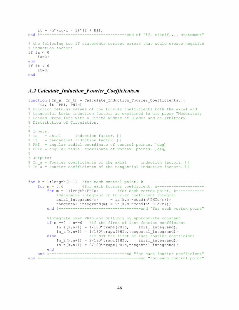
46
it = -g*(xo/x - 1)*(1 + B1); end %-------------------------------------end of "if, elseif,... statement" % the following two if statements correct errors that would create negative % induction factors if ia < 0 ia=0; end if it < 0 it=0; end
A.2 Calculate_Induction_Fourier_Coefficients.m function [In_a, In_t] = Calculate_Induction_Fourier_Coefficients... (ia, it, PHI, PHIo) % Function returns values of the fourier coefficients both the axial and % tangential Lerbs induction factors as explained in his paper "Moderately % Loaded Propellers with a Finite Number of Blades and an Arbitrary % Distribution of Circulation. % % Inputs: % ia = axial induction factor. [] % it = tangential induction factor. [] % PHI = angular radial coordinate of control points. [deg] % PHIo = angular radial coordinate of vortex points. [deg] % % Outputs: % In_a = Fourier coefficients of the axial induction factors. [] % In_a = Fourier coefficients of the tangential induction factors. [] for k = 1:length(PHI) %for each control point, k-------------------------- for n = 0:6 %for each fourier coefficient, n-------------------- for m = 1:length(PHIo) %for each vortex point, k------------ %determine integrand in fourier coefficent integral axial_integrand(m) = ia(k,m)*cosd(n*PHIo(m)); tangental_integrand(m) = it(k,m)*cosd(n*PHIo(m)); end %-----------------------------------end "for each vortex point" %Integrate over PHIo and multiply by appropriate constant if n ==0 | n==6 %if the first of last fourier coefficient In_a(k,n+1) = 1/180*trapz(PHIo, axial_integrand); In_t(k,n+1) = 1/180*trapz(PHIo,tangental_integrand); else %if NOT the first of last fourier coefficient In_a(k,n+1) = 2/180*trapz(PHIo, axial_integrand); In_t(k,n+1) = 2/180*trapz(PHIo,tangental_integrand); end end %--------------------------------end "for each fourier coefficient" end %------------------------------------------end "for each control point"
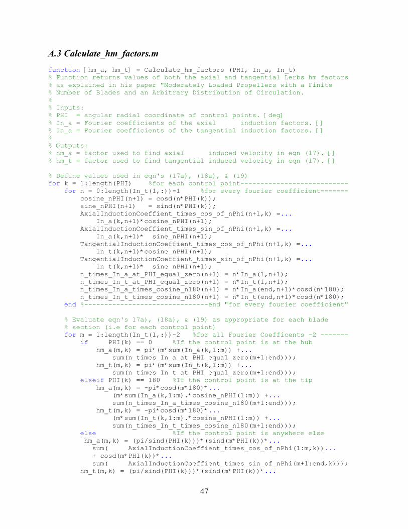
47
A.3 Calculate_hm_factors.m function [hm_a, hm_t] = Calculate_hm_factors (PHI, In_a, In_t) % Function returns values of both the axial and tangential Lerbs hm factors % as explained in his paper "Moderately Loaded Propellers with a Finite % Number of Blades and an Arbitrary Distribution of Circulation. % % Inputs: % PHI = angular radial coordinate of control points. [deg] % In_a = Fourier coefficients of the axial induction factors. [] % In_a = Fourier coefficients of the tangential induction factors. [] % % Outputs: % hm_a = factor used to find axial induced velocity in eqn (17). [] % hm_t = factor used to find tangential induced velocity in eqn (17). [] % Define values used in eqn's (17a), (18a), & (19) for k = 1:length(PHI) %for each control point--------------------------- for n = 0:length(In_t(1,:))-1 %for every fourier coefficient------- cosine_nPHI(n+1) = cosd(n*PHI(k)); sine_nPHI(n+1) = sind(n*PHI(k)); AxialInductionCoeffient_times_cos_of_nPhi(n+1,k) =... In_a(k,n+1)*cosine_nPHI(n+1); AxialInductionCoeffient_times_sin_of_nPhi(n+1,k) =... In_a(k,n+1)* sine_nPHI(n+1); TangentialInductionCoeffient_times_cos_of_nPhi(n+1,k) =... In_t(k,n+1)*cosine_nPHI(n+1); TangentialInductionCoeffient_times_sin_of_nPhi(n+1,k) =... In_t(k,n+1)* sine_nPHI(n+1); n_times_In_a_at_PHI_equal_zero(n+1) = n*In_a(1,n+1); n_times_In_t_at_PHI_equal_zero(n+1) = n*In_t(1,n+1); n_times_In_a_times_cosine_n180(n+1) = n*In_a(end,n+1)*cosd(n*180); n_times_In_t_times_cosine_n180(n+1) = n*In_t(end,n+1)*cosd(n*180); end %-------------------------------end "for every fourier coefficient" % Evaluate eqn's 17a), (18a), & (19) as appropriate for each blade % section (i.e for each control point) for m = 1:length(In_t(1,:))-2 %for all Fourier Coefficents -2 ------- if PHI(k) == 0 %If the control point is at the hub hm_a(m,k) = pi*(m*sum(In_a(k,1:m)) +... sum(n_times_In_a_at_PHI_equal_zero(m+1:end))); hm_t(m,k) = pi*(m*sum(In_t(k,1:m)) +... sum(n_times_In_t_at_PHI_equal_zero(m+1:end))); elseif PHI(k) == 180 %If the control point is at the tip hm_a(m,k) = -pi*cosd(m*180)*... (m*sum(In_a(k,1:m).*cosine_nPHI(1:m)) +... sum(n_times_In_a_times_cosine_n180(m+1:end))); hm_t(m,k) = -pi*cosd(m*180)*... (m*sum(In_t(k,1:m).*cosine_nPHI(1:m)) +... sum(n_times_In_t_times_cosine_n180(m+1:end))); else %If the control point is anywhere else hm_a(m,k) = (pi/sind(PHI(k)))*(sind(m*PHI(k))*... sum( AxialInductionCoeffient_times_cos_of_nPhi(1:m,k))... + cosd(m*PHI(k))*... sum( AxialInductionCoeffient_times_sin_of_nPhi(m+1:end,k))); hm_t(m,k) = (pi/sind(PHI(k)))*(sind(m*PHI(k))*...

48
sum(TangentialInductionCoeffient_times_cos_of_nPhi(1:m,k))... + cosd(m*PHI(k))*... sum(TangentialInductionCoeffient_times_sin_of_nPhi(m+1:end,k))); end end %------------------------------end "for all Fourier Coefficents -2" end %-------------------------------------------end"for each control point"
A.4 Calculate_Angle_of_Zero_Lift.m function alphao = Calculate_Angle_of_Zero_Lift (fo_over_c) % Function takes as input the maximum camber over chord ratio (could be % scalar or vector containing fo/c values at all of the points of interest. % It returns an approximate value of thet the angle of zero lift in degrees % for the NACA a=0.8 meanline (the meanline can be changed if needed) % using the equations derived by Munk as presented in "Theory of Wing % Sections" by Abbott and Doenhoff on page 72 of the second edition % % Inputs: % fo_over_c = vector or scalar of fo/c at control points. [] % % Outputs: % alphao = vector or scalar of angles of zero lift. [deg] % NACA a=0.8 meanline data downloaded from http://www.pdas.com/avd.htm and % verified with Abbott and Doenhoff x = [0, 0.5, 0.75, 1.25, 2.5, 5, 7.5, 10, 15, 20, 25, 30, 35, 40, 45,... 50, 55, 60, 65, 70, 75, 80, 85, 90, 95, 100] / 100; y = [0, 0.287, 0.4035, 0.6158, 1.0768, 1.8408, 2.4826, 3.0426, 3.9852,... 4.748, 5.3672, 5.8631, 6.2478, 6.5283, 6.7086, 6.7896, 6.7696,... 6.6442, 6.4049, 6.037, 5.5139, 4.7713, 3.6826, 2.4349, 1.1626 ,0] /100; % NACA 64 data used to test code by verifying angle of zero lift for NACA % 6409 in XFOIL % x = [0, 0.5, 0.75, 1.25, 2.5, 5, 7.5, 10, 15, 20, 25, 30, 35, 40, 45,... % 50, 55, 60, 65, 70, 75, 80, 85, 90, 95, 100]/100; % y = [0, 0.1491, 0.2229, 0.3691, 0.7266, 1.4063, 2.0391, 2.625, 3.6562,... % 4.5, 5.1563, 5.625, 5.9063, 6, 5.9583, 5.8333, 5.625, 5.3333,... % 4.9583, 4.5, 3.9583, 3.3333, 2.625, 1.8333, 0.9583, 0]/100; % Define Monk's coeeficients (kn) and foil locations (xn) xn = [.99458, .87426, .5, .12574, .00542]; kn = [1252.24; 109.048; 32.5959; 15.6838; 5.97817]; for m = 1:length(fo_over_c) %for each foil section inputted--------------- %scale the tabulated data based on inputed fo/c fscale(m) = fo_over_c(m) / max(y); MeanLineOrdinates(m,:) = fscale(m)*y; %create meanline function and evaluate at locations specified by Monk yn(m,:) = pchip(x, MeanLineOrdinates(m,:), xn); %evaluate angle of zero lift using Monk's equation. The negative sign %is dropped because the program requires the magnitude of the angle alphao(m) = yn(m,:)*kn;
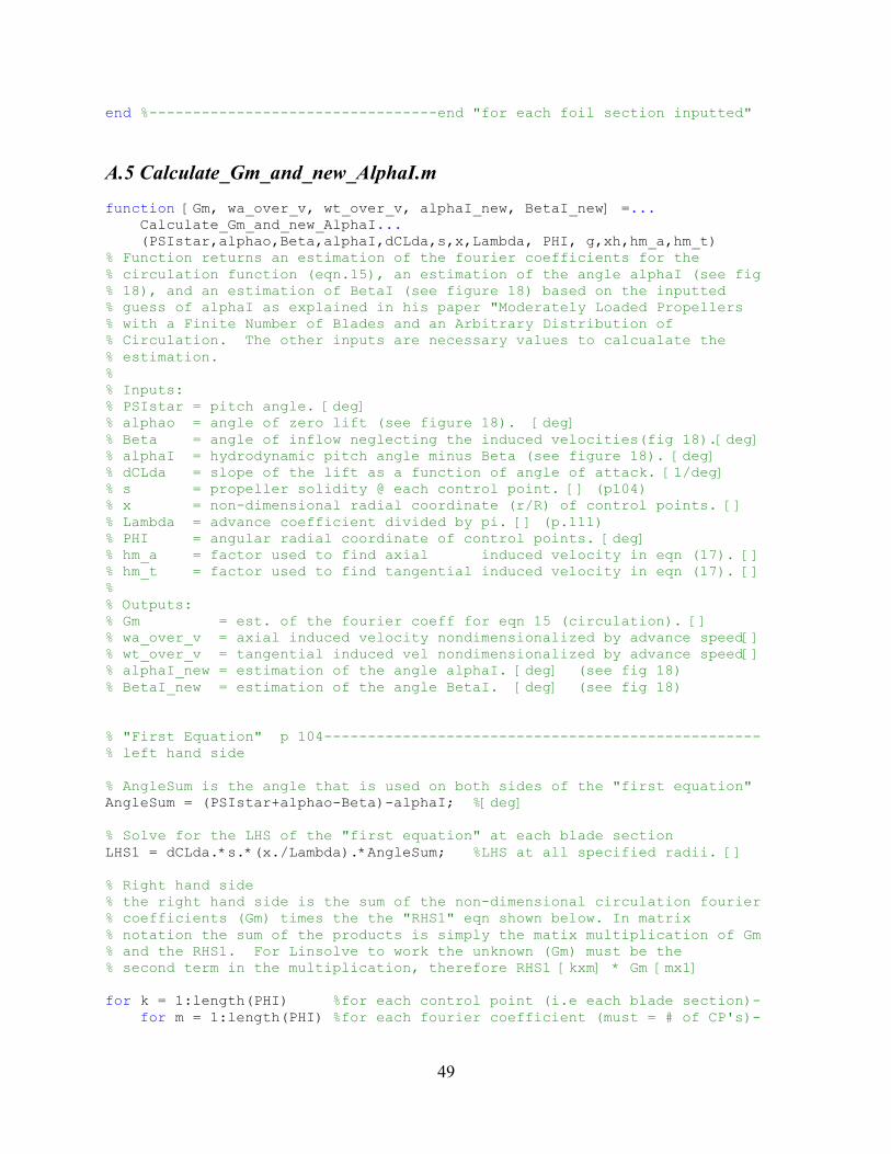
49
end %---------------------------------end "for each foil section inputted"
A.5 Calculate_Gm_and_new_AlphaI.m function [Gm, wa_over_v, wt_over_v, alphaI_new, BetaI_new] =... Calculate_Gm_and_new_AlphaI... (PSIstar,alphao,Beta,alphaI,dCLda,s,x,Lambda, PHI, g,xh,hm_a,hm_t) % Function returns an estimation of the fourier coefficients for the % circulation function (eqn.15), an estimation of the angle alphaI (see fig % 18), and an estimation of BetaI (see figure 18) based on the inputted % guess of alphaI as explained in his paper "Moderately Loaded Propellers % with a Finite Number of Blades and an Arbitrary Distribution of % Circulation. The other inputs are necessary values to calcualate the % estimation. % % Inputs: % PSIstar = pitch angle. [deg] % alphao = angle of zero lift (see figure 18). [deg] % Beta = angle of inflow neglecting the induced velocities(fig 18).[deg] % alphaI = hydrodynamic pitch angle minus Beta (see figure 18). [deg] % dCLda = slope of the lift as a function of angle of attack. [1/deg] % s = propeller solidity @ each control point. [] (p104) % x = non-dimensional radial coordinate (r/R) of control points. [] % Lambda = advance coefficient divided by pi. [] (p.111) % PHI = angular radial coordinate of control points. [deg] % hm_a = factor used to find axial induced velocity in eqn (17). [] % hm_t = factor used to find tangential induced velocity in eqn (17). [] % % Outputs: % Gm = est. of the fourier coeff for eqn 15 (circulation). [] % wa_over_v = axial induced velocity nondimensionalized by advance speed[] % wt_over_v = tangential induced vel nondimensionalized by advance speed[] % alphaI_new = estimation of the angle alphaI. [deg] (see fig 18) % BetaI_new = estimation of the angle BetaI. [deg] (see fig 18) % "First Equation" p 104-------------------------------------------------- % left hand side % AngleSum is the angle that is used on both sides of the "first equation" AngleSum = (PSIstar+alphao-Beta)-alphaI; %[deg] % Solve for the LHS of the "first equation" at each blade section LHS1 = dCLda.*s.*(x./Lambda).*AngleSum; %LHS at all specified radii. [] % Right hand side % the right hand side is the sum of the non-dimensional circulation fourier % coefficients (Gm) times the the "RHS1" eqn shown below. In matrix % notation the sum of the products is simply the matix multiplication of Gm % and the RHS1. For Linsolve to work the unknown (Gm) must be the % second term in the multiplication, therefore RHS1 [kxm] * Gm [mx1] for k = 1:length(PHI) %for each control point (i.e each blade section)- for m = 1:length(PHI) %for each fourier coefficient (must = # of CP's)-
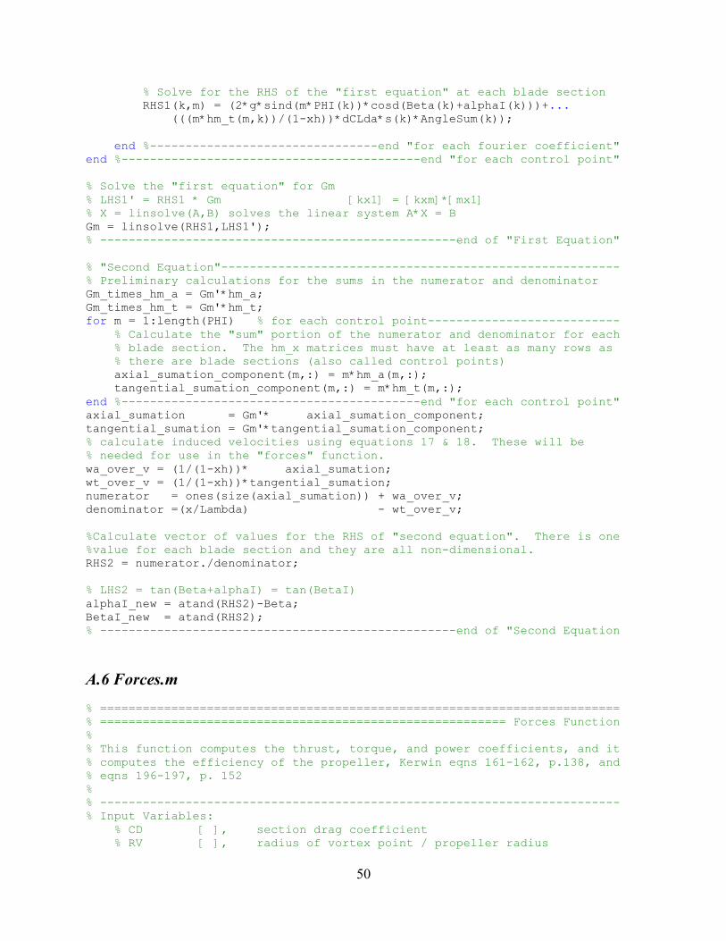
50
% Solve for the RHS of the "first equation" at each blade section RHS1(k,m) = (2*g*sind(m*PHI(k))*cosd(Beta(k)+alphaI(k)))+... (((m*hm_t(m,k))/(1-xh))*dCLda*s(k)*AngleSum(k)); end %--------------------------------end "for each fourier coefficient" end %------------------------------------------end "for each control point" % Solve the "first equation" for Gm % LHS1' = RHS1 * Gm [kx1] = [kxm]*[mx1] % X = linsolve(A,B) solves the linear system A*X = B Gm = linsolve(RHS1,LHS1'); % --------------------------------------------------end of "First Equation" % "Second Equation"-------------------------------------------------------- % Preliminary calculations for the sums in the numerator and denominator Gm_times_hm_a = Gm'*hm_a; Gm_times_hm_t = Gm'*hm_t; for m = 1:length(PHI) % for each control point--------------------------- % Calculate the "sum" portion of the numerator and denominator for each % blade section. The hm_x matrices must have at least as many rows as % there are blade sections (also called control points) axial_sumation_component(m,:) = m*hm_a(m,:); tangential_sumation_component(m,:) = m*hm_t(m,:); end %------------------------------------------end "for each control point" axial_sumation = Gm'* axial_sumation_component; tangential_sumation = Gm'*tangential_sumation_component; % calculate induced velocities using equations 17 & 18. These will be % needed for use in the "forces" function. wa_over_v = (1/(1-xh))* axial_sumation; wt_over_v = (1/(1-xh))*tangential_sumation; numerator = ones(size(axial_sumation)) + wa_over_v; denominator =(x/Lambda) - wt_over_v; %Calculate vector of values for the RHS of "second equation". There is one %value for each blade section and they are all non-dimensional. RHS2 = numerator./denominator; % LHS2 = tan(Beta+alphaI) = tan(BetaI) alphaI_new = atand(RHS2)-Beta; BetaI_new = atand(RHS2); % --------------------------------------------------end of "Second Equation
A.6 Forces.m % ========================================================================= % ========================================================= Forces Function % % This function computes the thrust, torque, and power coefficients, and it % computes the efficiency of the propeller, Kerwin eqns 161-162, p.138, and % eqns 196-197, p. 152 % % ------------------------------------------------------------------------- % Input Variables: % CD [ ], section drag coefficient % RV [ ], radius of vortex point / propeller radius
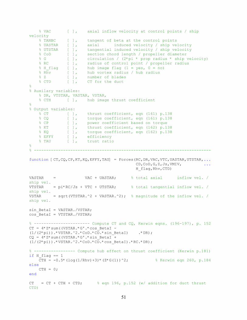
51
% VAC [ ], axial inflow velocity at control points / ship velocity % TANBC [ ], tangent of beta at the control points % UASTAR [ ], axial induced velocity / ship velocity % UTSTAR [ ], tangential induced velocity / ship velocity % CoD [ ], section chord length / propeller diameter % G [ ], circulation / (2*pi * prop radius * ship velocity) % RC [ ], radius of control point / propeller radius % H_flag [ ], hub image flag (1 = yes, 0 = no) % Rhv [ ], hub vortex radius / hub radius % Z [ ], number of blades % CTD [ ], CT for the duct % % Auxilary variables: % DR, VTSTAR, VASTAR, VSTAR, % CTH [ ], hub image thrust coefficient % % Output variables: % CT [ ], thrust coefficient, eqn (161) p.138 % CQ [ ], torque coefficient, eqn (161) p.138 % CP [ ], power coefficient based on torque % KT [ ], thrust coefficient, eqn (162) p.138 % KQ [ ], torque coefficient, eqn (162) p.138 % EFFY [ ], efficiency % TAU [ ], trust ratio % % ------------------------------------------------------------------------- function [CT,CQ,CP,KT,KQ,EFFY,TAU] = Forces(RC,DR,VAC,VTC,UASTAR,UTSTAR,... CD,CoD,G,Z,Js,VMIV, ... H_flag,Rhv,CTD) VASTAR = VAC + UASTAR; % total axial inflow vel. / ship vel. VTSTAR = pi*RC/Js + VTC + UTSTAR; % total tangential inflow vel. / ship vel. VSTAR = sqrt(VTSTAR.^2 + VASTAR.^2); % magnitude of the inflow vel. / ship vel. sin_BetaI = VASTAR./VSTAR; cos_BetaI = VTSTAR./VSTAR; % ----------------------- Compute CT and CQ, Kerwin eqns. (196-197), p. 152 CT = 4*Z*sum((VSTAR.*G'.*cos_BetaI - (1/(2*pi)).*VSTAR.^2.*CoD.*CD.*sin_BetaI) .*DR); CQ = 4*Z*sum((VSTAR.*G'.*sin_BetaI + (1/(2*pi)).*VSTAR.^2.*CoD.*CD.*cos_BetaI).*RC.*DR); % ----------------- Compute hub effect on thrust coefficient (Kerwin p.181) if H_flag == 1 CTH = -0.5*(log(1/Rhv)+3)*(Z*G(1))^2; % Kerwin eqn 260, p.184 else CTH = 0; end CT = CT + CTH + CTD; % eqn 196, p.152 (w/ addition for duct thrust CTD)
52
CP = CQ*pi/Js; % power coefficient based on torque KT = CT*Js^2*pi/8; % eqn 167, p.139 KQ = CQ*Js^2*pi/16; % eqn 167, p.139 EFFY = CT*VMIV/CP; % efficiency TAU = (CT-CTD)/CT; % thrust ratio % % ===================================================== END Forces Function % =========================================================================
A.7 Some_Open_Water_Characteristics.m function [KT, KQ, EFFY] = Some_Open_Water_Characteristics... (design, JsRange, PoD_input, fo_over_c_input, D) % This function returns estimations of the thrust and torque coefficients, % along with the efficiency of a propeller using a method developed by % Lerbs to determine the circulation and induced velocity as presented in % his paper "Moderately Loaded Propellers with a Finite Number of Blades % and an Arbitrary Distribution of Circulation". The inputs required by % the function are grouped into two main categories, propeller geometry % and the operating conditions. The inputs are explained in more detail % below. % % Inputs contained in "design" % design.CoD = Chord over diameter at control points. [] % design.BetaIC = Hydrodynamic pitch angle at control points. [rad] % design.VAC = Axial speed at control points. [] % design.VTC = Tangential speed at control points. [] % design.Rhub_oR = Hub radius (rh/R). [] % design.Z = Number of propeller blades (g). [] % design.RC = Radial oordinate of control points (r/R). [] % design.DR = Integration increment for force calculation. [] % design.CD = Section drag coefficient. [] % design.VMIV = Volumetric Mean Inflow Velocity. [] % design.H_flag = Hub image flag (1 = yes, 0 = no). [] % design.Rhv = Hub vortex radius / hub radius. [] % design.CTD = Thrust coefficient for the duct. [] % % Inputs NOT contained in "design" % PoD_input = Pitch over Diameter ratios at control points. [] % fo_over_c_input = Maximum chamber divided by chord at control points. [] % D = Propeller diameter. [length] % JsRange = Range of advance ratios to analyze. [] % ***note: Lerb equations lambda = Js/pi and it is referenced to Va not Vs. % ***Assume Va=Vs since it is an open water curve % % Outputs % KT = Propeller thrust coefficient. [ ] % KQ = Propeller torque coefficient. [ ] % EFFY = Propeller efficiency. [ ] % Unpack necessary values from "design" CoD_input = design.CoD; Beta_input = atand(design.TANBC); BetaI_input = rad2deg(design.BetaIC);
53
VAC_input = design.VAC; VTC_input = design.VTC; xh = design.Rhub_oR; g = design.Z; R = .5*D; % Values that don't change with design------------------------------------- % Theoretical slope of the lift as a function of angle of attack. [1/deg] dCLda = 2*pi*(pi/180); % Angular radial coordinate of control and vortex points. [deg] PHI = [30,60,90,120,150]; PHIo = [0,30,60,90,120,150,180]; % Non-dimensional radial coordinate (r/R) of control and vortex points. [] x = .5*(1+xh) - .5*(1-xh)*cosd(PHI); %eqn 14 P.90 xo = .5*(1+xh) - .5*(1-xh)*cosd(PHIo); % -------------------------------end "Values that don't change with design" % Interpolate data at contol points---------------------------------------- CoD = pchip(design.RC, CoD_input, x); Beta = pchip(design.RC, Beta_input, xo); BetaI = pchip(design.RC, BetaI_input, xo); VAC = pchip(design.RC, VAC_input, x); VTC = pchip(design.RC, VTC_input, x); PoD = pchip(design.RC, PoD_input, x); fo_over_c = pchip(design.RC, fo_over_c_input, x); % ----------------------------------end "Interpolate data at contol points" % Calculate other values and angles necessary for analysis----------------- s = g*CoD/pi; %vector of prop solidity at CPs (p104) Pitch = PoD*D; %Pitch at specified radii [length] PSIstar = atand(Pitch./(2*pi*x*R));%Pitch angle at specified radii [deg] % Calculate angles based on figure 18 (page 94) from Lerbs alphao = Calculate_Angle_of_Zero_Lift (fo_over_c); % [deg] BetaIo_deg = BetaI; % Assume wake comes off at angle of BetaI BetaIo = deg2rad(BetaIo_deg); % Angle of helical wake. [rad] % ------------------------------------------end "Calculate other values..." for Js_index = 1:length(JsRange) % For Js_index---------------------------- Js = JsRange(Js_index); % Advance ratio [] Lambda = Js/pi; % Advance coefficient [] Beta = atand(VAC./(pi.*x./Js + VTC)); % [deg] alphaI = BetaI(2:end-1)-Beta; % Differance between BetaI and Beta [deg] % Set up values for "While loop" iteration interation_counter = 0; % Counter for the number of iterations. [] interation_max = 40; %Maximum number of iterations. [] alphaI_new = alphaI*100; %Initial setting to ensure loop starts. [deg] alphaI_next_loop = alphaI;%Set value to be used in the first loop [deg] % Print which advance ratio value is being calculated so the user knows % where they are at in the process fprintf(['Calculating circulation for J = ',num2str(Js), ' ']); % While Loop-----------------------------------------------------------
54
% Input estimate of alphaI to calculate estimate of non-dimensional % fourier coeffiecents of circulation. Use those coefficients to % determine new estimate of alphaI and interate until the new estimate % and the original estimate of alphaI differ by less than .2 degrees or % the maximum number of iterations is reached. while (interation_counter<=interation_max) &&... any(abs(alphaI-alphaI_new)>.2) %Print rotating clock to screen so the user knows the program is %"thinking" if rem(interation_counter,4) == 0 fprintf('\b|'); else if rem(interation_counter,4) == 1 fprintf('\b/'); else if rem(interation_counter,4) == 2 fprintf('\b-'); else fprintf('\b\\'); end end end %-------------------------------------------end rotating clock alphaI = alphaI_next_loop; for n = 1:length(x) %for each control point, n---------------- for m = 1:length(xo) %for each vortex point, m----------- [ia(n,m), it(n,m)] = Find_Lerb_Induction_Factors... (x(n),xo(m),g,BetaIo(m)); end %-------------------------------end "for each vortex point" end %----------------------------------end "for each control point" [In_a, In_t]= Calculate_Induction_Fourier_Coefficients... (ia, it, PHI, PHIo); [hm_a, hm_t]= Calculate_hm_factors (PHI, In_a, In_t); [Gm, wa_over_v,wt_over_v, alphaI_new, BetaI_new] =... Calculate_Gm_and_new_AlphaI... (PSIstar,alphao,Beta,alphaI,dCLda,s,x,Lambda,PHI,g,xh,hm_a, hm_t); % Set up values for next iteration BetaI = BetaI_new; BetaI = pchip(x, BetaI, xo); BetaIo = deg2rad(BetaI); %assume wake comes off at angle of BetaI %Set alphaI to average of new and old distribution (see page 109) alphaI_next_loop = (alphaI_new+alphaI)/2; interation_counter = interation_counter +1; % Increment counter end %----------------------------------------------------end While Loop fprintf('\b\n'); % set up for next line in screen output % Calculate Non-dimensional circulation (G) from fourier coefficients for m = 1:length(PHI) sine_of_m_times_PHI(m,:) = sind(m*PHI); end Lerbs_G_coarse = Gm'*sine_of_m_times_PHI; %G from eqn 15. []
55
% Prepare variables for "Forces" function Lerbs_G = pchip(x, Lerbs_G_coarse, design.RC); uastar = pchip(x, wa_over_v , design.RC); utstar = pchip(x, wt_over_v , design.RC); [CT,CQ,CP,KT(Js_index),KQ(Js_index),EFFY(Js_index),TAU] =... Forces(design.RC, design.DR , design.VAC, design.VTC,uastar,... -utstar,design.CD, design.CoD,Lerbs_G',design.Z,Js,design.VMIV,... design.H_flag, design.Rhv, design.CTD); % disp(['The number of iterations for Js = ',num2str(Js),... % ' was: ',num2str(interation_counter)]), end %---------------------------------------------------end "J_index" loop
A.8 Open_Water_Characteristics.m function [Js, KT, KQ, EFFY] = Open_Water_Characteristics... (design, Js_low, Js_high, PoD_input, fo_over_c_input, D) % This function returns the advance ration and estimations of the % corresponding thrust and torque coefficients, along with the efficiency % of a propeller using a method developed by Lerbs to determine the % circulation and induced velocity as presented in his paper % "Moderately Loaded Propellers with a Finite Number of Blades and an % Arbitrary Distribution of Circulation". The inputs required by % the function are grouped into two main categories, propeller geometry % and the operating conditions. The inputs are explained in more detail % below. The function starts at the propellers design point and works to % Js_low in increments of .01. Next, it starts at the design point again % and works to Js_high in increments of .01. If the efficiency drops below % zero, the data is disregarded. % % Inputs contained in "design" % design.Js = Advance ratio at the design point. [] % design.CoD = Chord over diameter at control points. [] % design.BetaIC = Hydrodynamic pitch angle at control points. [rad] % design.VAC = Axial speed at control points. [] % design.VTC = Tangential speed at control points. [] % design.Rhub_oR = Hub radius (rh/R). [] % design.Z = Number of propeller blades (g). [] % design.RC = Radial oordinate of control points (r/R). [] % design.DR = Integration increment for force calculation. [] % design.CD = Section drag coefficient. [] % design.VMIV = Volumetric Mean Inflow Velocity. [] % design.H_flag = Hub image flag (1 = yes, 0 = no). [] % design.Rhv = Hub vortex radius / hub radius. [] % design.CTD = Thrust coefficient for the duct. [] % % Inputs NOT contained in "design" % PoD_input = Pitch over Diameter ratios at control points. [] % fo_over_c_input = Maximum chamber divided by chord at control points. [] % D = Propeller diameter. [length]
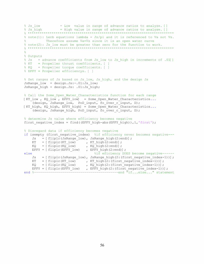
56
% Js_low = Low value in range of advance ratios to analyze. [] % Js_high = High value in range of advance ratios to analyze. [] % ************************************************************************* % note(1): Lerb equations lambda = Js/pi and it is referenced to Va not Vs. % Therefore assume Va=Vs since it is an open water curve % note(2): Js_low must be greater than zero for the function to work. % ************************************************************************* % % Outputs % Js = advance coefficients from Js_low to Js_high in increments of .01[] % KT = Propeller thrust coefficients. [ ] % KQ = Propeller torque coefficients. [ ] % EFFY = Propeller efficiencys. [ ] % Set ranges of Js based on Js_low, Js_high, and the design Js JsRange_low = design.Js:-.01:Js_low; JsRange_high = design.Js: .01:Js_high; % Call the Some_Open_Water_Characteristics function for each range [KT_low , KQ_low , EFFY_low] = Some_Open_Water_Characteristics... (design, JsRange_low, PoD_input, fo_over_c_input, D); [KT_high, KQ_high, EFFY_high] = Some_Open_Water_Characteristics... (design, JsRange_high, PoD_input, fo_over_c_input, D); % determine Js value where efficiency becomes negative first_negative_index = find((EFFY_high-abs(EFFY_high)),1,'first'); % Disregard data if efficiency becomes negative if isempty (first_negative_index) %if efficiency never becomes negative--- Js = [fliplr(JsRange_low), JsRange_high(2:end)]; KT = [fliplr(KT_low) , KT_high(2:end)]; KQ = [fliplr(KQ_low) , KQ_high(2:end)]; EFFY = [fliplr(EFFY_low) , EFFY_high(2:end)]; else %if eficiency DOES become negative------ Js = [fliplr(JsRange_low), JsRange_high(2:(first_negative_index-1))]; KT = [fliplr(KT_low) , KT_high(2:(first_negative_index-1))]; KQ = [fliplr(KQ_low) , KQ_high(2:(first_negative_index-1))]; EFFY = [fliplr(EFFY_low) , EFFY_high(2:(first_negative_index-1))]; end %------------------------------------------end "if...else..." statement