propagation effects of wind and temperature on acoustic ... · 0,s = subscripts denoting ground and...

44thd AIAA Aerospace Sciences Meeting and Exhibit AIAA-2006-0411 9-14 January 2006, Reno, Nevada

- 1 - American Institute of Aeronautics and Astronautics

Propagation Effects of Wind and Temperature on Acoustic Ground Contour Levels

Stephanie L. Heath1 and Gerry L. McAninch2 NASA Langley Research Center, Hampton, Virginia 23681-2199

Propagation characteristics for varying wind and temperature atmospheric conditions are identified using physically-limiting propagation angles to define shadow boundary regions. These angles are graphically illustrated for various wind and temperature cases using a newly developed ray-tracing propagation code.

Nomenclature k = gas constant (γ*Rair*gc) sr

= slowness vector wr

= wind vector d wr

/dz = wind gradient vector nr

= wavefront normal T = temperature x, y, z = Cartesian coordinates with z defined as height or altitude dimension 0,s = subscripts denoting ground and source locations respectively β = linear coefficient for temperature (lapse rate) ϑ = azimuthal angle φ = elevation angle Ω = ratio of sound speed to effective sound speed χ = critical elevation emission angle ζ = critical azimuthal shadow boundary (reception) angle

I. Introduction

N recent years, variations in the ground acoustic levels over large areas, such as an airport community, have been noted.(4,8) It is presumed that most of these variations are attributable to atmospheric conditions, and in particular

wind and temperature gradients, which can bend the acoustic ray paths and affect the noise heard on the ground.(11) This paper characterizes significant propagation effects associated with wind and temperature on ground acoustic levels. A ray-tracing code was developed to account for the wind and temperature gradients. While developing the ray-tracing method to account for wind and temperature effects, an increased understanding of complex propagation paths and explicit characterization of ground contour patterns was obtained. An accompanying theoretical discussion of these propagation characteristics is given by McAninch and Heath1. The shadow boundary regions (or zones of silence) on the ground are characterized by an asymptotic limiting angle. This angle, which is set by wind and temperature conditions, is illustrated by examining the 1921 explosion of a

1 Aeronautical Engineer, Aeroacoustics Branch, MS 461 NASA LaRC, Member AIAA. 2 Sr. Aeronautical Engineer, Structural Acoustics Branch, MS 463 NASA LaRC.

I

https://ntrs.nasa.gov/search.jsp?R=20060004780 2018-07-27T11:37:03+00:00Z



chemical plant in Oppau, Germany (S.K. Mitra, The Upper Atmosphere.)7 By interviewing observers on the ground, the Oppau study mapped out a complicated acoustic pattern (figure 1) defining alternating audible and silent zones. Over the years, the radial patterns of the Oppau acoustic footprint have been attributed to turning (refracting) and trapping (ducting) of sound waves from a layer of air in the upper atmosphere. Instead of characterizing the radial pattern of silent zones, as was done in previous works,2, 9, 10 this paper identifies an angle, ζ, that envelopes the audible region as shown in figure 1.

Figure 1. Results of audibility survey for a large ground-based explosion at Oppau, Germany in 1921. –Explosion heard, – Explosion not heard.

This characteristic angle, ζ, is particularly useful in that it quickly defines the angular confines of the shadow boundary on the ground before any effort is put forth to trace the acoustic rays. More detail regarding this angle will be discussed in this paper. In addition to the characteristic angle, this paper quantifies general ground contour characteristics apparent when including both wind and temperature atmospheric effects. By comparing ray-tracing propagation ground contours associated with non-homogeneous atmospheres against a homogeneous case, it is shown that even small atmospheric gradients can significantly influence resulting ground contours.

II. An Advanced Ray-Tracing Code NASA currently uses ANOPP3 (Aircraft NOise Prediction Program) to predict both aircraft source noise and noise propagation. ANOPP assumes straight line (spherically spread) propagation paths and does not account for varying wind and temperature, therefore a new ray-tracing propagation code was created to add these capabilities. Ray-tracing methods were used because they offer certain advantages.

Wind Vector ζ

ζ



First, ray-tracing methods account for refraction (the bending and turning of ray paths) in three dimensions, which are necessary to account for wind and temperature. While a more complex method was needed to gain refraction capabilities, it is desired that the code run quickly with minimal numerical calculations. The second advantage of ray-tracing methods is that they are easily simplified. The challenge is to adequately account for the physical effects desired, without having to solve multiple simultaneous equations. To this end, a ray-tracing code with simplifying assumptions was created. The two simplifications necessary to achieve this are 1) representation of the atmosphere as a stratified medium, and 2) representation of the atmosphere with linearly varying properties within stratified layers. And finally, ray-tracing methods are advantageous in that they can be expanded to include future capabilities, such as multi-path propagation effects, ducted ray effects, ground reflection effects, and terrain effects.

A. Stratified Medium

The first simplification is the assumption of stratified medium. The atmospheric properties in a stratified medium are constant within a horizontal plane, and vary only as a function of height (or z), see figure 2.

Figure 2. Example of an atmosphere modeled as a stratified medium with linearly varying properties within layers.

The ray-tracing equations are often expressed in terms of a common quantity called the slowness vector. Without getting into too much detail, the slowness vector is the reciprocal of the effective sound speed with which the acoustic wavefront moves normal to itself. A good explanation of the slowness vector is given by Pierce2. In a stratified medium, the horizontal components of the slowness vector (i.e. sx and sy) remain constant along any given ray. Because of this, the traditional set of ray-tracing equations may be represented by a single equation2 (equation 1) in terms of the slowness vector components, with Ω defined as the local sound speed, c, divided by the local effective sound speed, ceff, and sr is the slowness vector. This single equation is critical to code efficiency because it eliminates the need to solve multiple simultaneous equations.

21

2y

2x

2

z sscΩs

⎥⎥⎦

⎤

⎢⎢⎣

⎡−−⎟

⎠⎞

⎜⎝⎛±= (1)

Wind Vector (wx(z) and wy(z))

Height, z

Z=0 (ground)

Temperature T(z)



B. Linearly Varying Properties Including refraction (to account for varying wind and temperature effects) adds both physical and mathematical complexity. The mathematics needs to account for all conditions to ensure the code is tracing rays correctly (both through turning points and in regions that are physically realizable). The physical conditions encountered while tracing a ray trajectory through a stratified medium are presented by McAninch and Heath1. Determining the turning points quickly and accurately is essential to building an efficient code. The zeros of the z-component of the slowness vector correspond to the turning points of the ray (the locations where the ray turns from propagating downward to propagating upward). To aid in determining the zeros, atmospheric properties are assumed to vary linearly within each layer. By linearly expressing the atmosphere within layers, closed form solutions exist for the turning points (or zeros of the slowness vector in the z-direction) as well as closed form solutions for other key propagation characteristics. Also, this linear assumption does not greatly restrict the application of the propagation code, in that an atmosphere may be represented by as many layers as desired to accurately model almost any atmosphere.

III. Classification of Wind and Temperature Effects Specific characteristics of the shadow boundaries are determined by two distinct angles, 1) the ray angles at the source that create the shadow boundaries and, 2) the characteristic angle defining the extent of the shadow boundary within the ground contour (as was shown for the Oppau explosion, figure 1). Full derivation, implementation and programming details are contained in the Ray-Tracing Program User’s Manual6.

Here, the effects of temperature and wind are first examined individually, and then combined to show the more complex effects, including the two angles described above.

A. Temperature effects. Temperature variations within the atmosphere are described using a lapse rate, β, which is defined as the negative rate of change of temperature with altitude (-dT/dz). Thus, lapse rate is positive when temperature decreases with increasing height, and negative when the temperature is increasing with height. Standard temperature profiles (which are described with a positive lapse rate) cause acoustic rays to refract upward, creating a shadow zone. On the other hand, inverted temperature profiles (described with a negative lapse rate) refract toward the ground. These effects are seen in figure 3, along with the constant temperature case in which the rays propagate in straight radial lines from a spherical source. The shadow-forming ray has an associated elevation angle defined at the source, called the critical emission angle.



Figure 3. Ray paths for linearly varying temperature profiles

B. Wind Effects The presence of wind causes a two-fold effect. The first effect is refraction due to wind gradients, dw/dz, and the second is convection due to a constant wind. Wind gradients refract the rays as shown in figure 4. The rays are refracted upward when flow with a positive dw/dz is approaching the acoustic source and downward when the same flow is moving away from the acoustic source.

Figure 4. Wind effects on the ray paths

Source

Varying Wind (wx(z) and wy(z))

Altitude,z

Z=0 (ground)

No Wind

Critical Emission Angle

Shadow Region

Straight Line Propagation (no wind effects included)

Grazing Ray (upwind of source)

Bending Ray (downwind of source)

Source

Temperature Positive Lapse

Altitude, z

Z=0 (ground)

Temperature Negative Lapse

Constant

Critical Emission Angle

Grazing Ray (positive lapse rate)

Shadow Region

Straight Line Propagation (Constant Temperature) Bending Ray

(negative lapse rate)



Convection results in an increased effective sound speed in the direction of the flow. This effect is usually small with respect to the refractive effect of the wind gradient, and thus, is difficult to see on the resulting ground contours. The convective effects are represented by a slight horizontal shift of the ground contour from the source center and will be discussed further in the results. Wind gradient effects shown in figure 4 are angularly dependant. The maximum upward refraction occurs in the direction toward the oncoming flow and diminishes until there is zero refraction perpendicular to the flow. Similarly, the downstream downward refraction also diminishes as it approaches a line that is perpendicular to the flow.

C. More complex combined effects

When both wind and temperature gradients are present, the results are not the same as if either is acting independently. The combined interactions create interesting angular characteristics. Two specific angles which help to define the shadow zones for wind and temperature combinations are the critical emission angle and the critical shadow boundary angle.

The critical emission angle is the initial elevation angle of the shadow-forming rays (or the rays that graze the ground and refract away from the ground at zero altitude). This angle defines the confines of the shadow region and is helpful for programming efficiency because it avoids mathematical chaos (by ensuring that numerical functions remain in well-behaved regions of real interest) and tracing only those rays which are less than the limiting emission angle and will reach the ground. There is one unique critical emission angle for each source azimuthal angle. This critical emission angle, χ, is based on temperature (i.e., sound speed) and wind parameters at both the source altitude and the ground. The expression for the critical emission angle, χ, is,

( )⎥⎥⎦

⎤

⎢⎢⎣

⎡

−−=

ϑϑϑ

sinwcoswcc

cosχysxs0

s1- (2)

where c is the local sound speed, with subscripts s and 0, indicating the appropriate quantities at the source and ground respectively. This result for χ is independent of intermediate atmospheric layers. Since turning points may occur in the intermediate layers, it remains necessary to always check for zeros of the z-component of the slowness vector in each layer while tracing the ray path. The second angle of interest is the critical shadow boundary angle which is more global in nature as seen in figure 1. It defines the overall extent of the shadow region observed on the ground from all downward propagating rays leaving the source. This angle allows characterization of the audible regions on the ground given the temperature and wind gradients, prior to tracing any rays. The critical shadow boundary angle, ζ, is determined by solving equation (3).

0

0yx

2Tβc

sinζdz

dwcosζ

dzdw

≥⎥⎦

⎤⎢⎣

⎡+− (3)

Where, dz

dwand

dzdw yx are the wind gradients in the x and y directions respectively; and β, c0, and T0 are the lapse

rate, speed of sound and temperature on the ground. This theoretical equation developed for the shadow boundary angle has been validated against the acoustic ground contours predicted using the ray-tracing code. The resulting angles from the code and theory show very good agreement. Although rays emitted at the critical emission angles trace out the shadow boundary, it is the critical shadow boundary angle that characterizes the ground contour shape. With wind alone the shadow boundary ends at a line perpendicular to the wind, and thus the characteristic angle is 90 degrees. When both wind and temperature exist, the shadow boundary angle varies as the temperature profile changes. For standard profiles (i.e., a positive lapse rate) the angle becomes greater than 90 degrees, and for inverted temperature profiles (i.e., a negative lapse rate) the angle is less than 90 degrees. These characteristic angles are evident in the cases presented in the following section.



IV. Results Ground contour variations due to temperature and wind gradients are presented. Specific characteristics of the

shadow zone patterns are determined by the critical emission and shadow boundary angles discussed in Section III.

The major characteristics are illustrated for a single layer atmosphere for simplicity, but these effects exist and are accumulative for multiple layer cases as well. A realistic velocity profile has been included to show the multiple layer compilation effects due to wind only. Six cases are presented; two temperature only cases with single linear layers, two wind only cases (one single layer and one multi-layer), and two combined temperature and wind cases with a single layer.

Ground sound pressure level (SPL) contours are presented below for a stationary point source to show sample effects of special temperature and wind variations. The SPL levels include raytube area spreading and Blokhinsev invariant1 corrections. For ease of comparison, the sound pressure level at the source is zero dB (re 20 μPa) with a source radius of one foot. The atmospheric effects on the noise contours are referenced to the spherical spreading case, and show significant magnitude and pattern variations. The cases presented here are not extreme: the lapse rate is +/- 0.003564 deg F/ft and the linear wind velocity gradient is 0.01 ft/sec/ft, which results in a wind velocity of 50 ft/sec at the source height of 5000 feet.

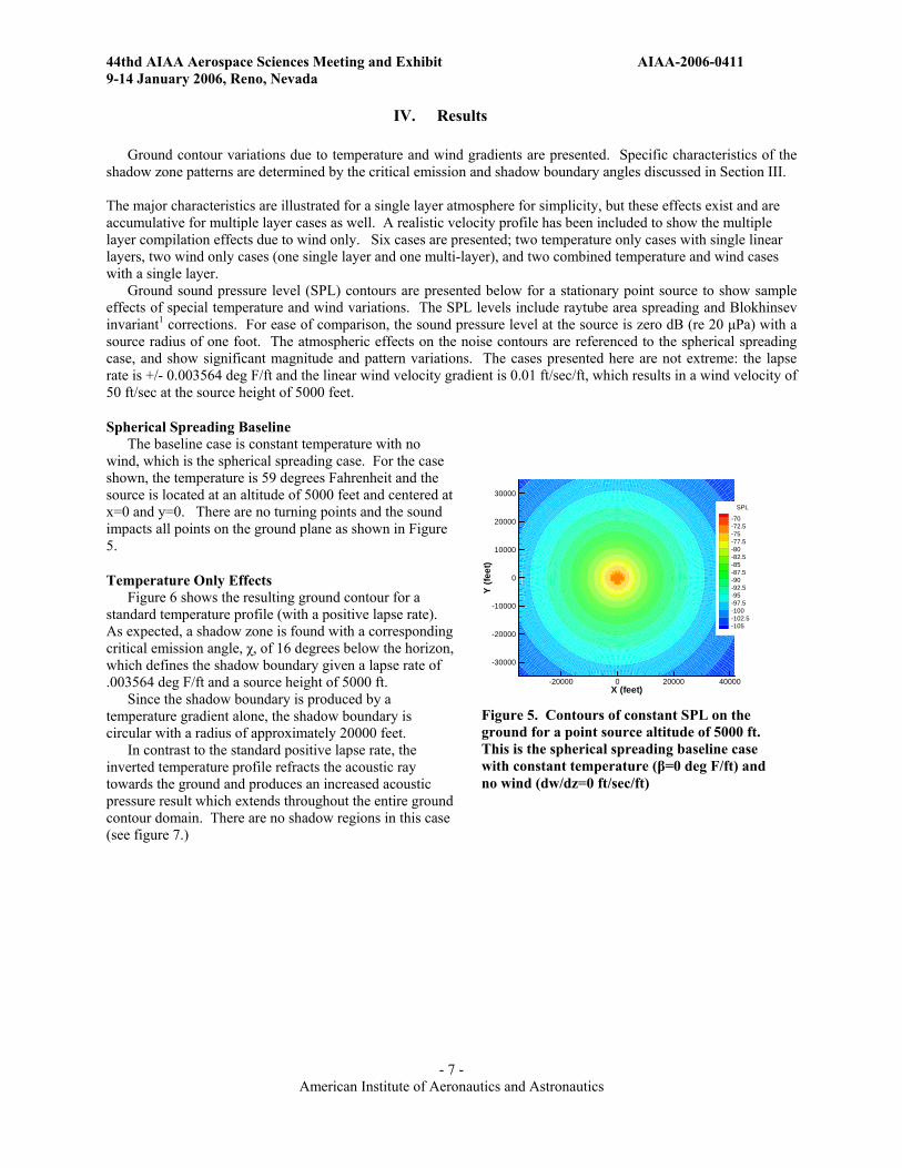
Spherical Spreading Baseline The baseline case is constant temperature with no

wind, which is the spherical spreading case. For the case shown, the temperature is 59 degrees Fahrenheit and the source is located at an altitude of 5000 feet and centered at x=0 and y=0. There are no turning points and the sound impacts all points on the ground plane as shown in Figure 5.

Temperature Only Effects Figure 6 shows the resulting ground contour for a

standard temperature profile (with a positive lapse rate). As expected, a shadow zone is found with a corresponding critical emission angle, χ, of 16 degrees below the horizon, which defines the shadow boundary given a lapse rate of .003564 deg F/ft and a source height of 5000 ft.

Since the shadow boundary is produced by a temperature gradient alone, the shadow boundary is circular with a radius of approximately 20000 feet.

In contrast to the standard positive lapse rate, the inverted temperature profile refracts the acoustic ray towards the ground and produces an increased acoustic pressure result which extends throughout the entire ground contour domain. There are no shadow regions in this case (see figure 7.)

X (feet)

Y(fe

et)

-20000 0 20000 40000

-30000

-20000

-10000

0

10000

20000

30000

SPL

-70-72.5-75-77.5-80-82.5-85-87.5-90-92.5-95-97.5-100-102.5-105

Figure 5. Contours of constant SPL on the ground for a point source altitude of 5000 ft. This is the spherical spreading baseline case with constant temperature (β=0 deg F/ft) and no wind (dw/dz=0 ft/sec/ft)



Wind Only Effects Two study cases are included to represent wind

only effects: a single layer case and a multiple layer case which approximates a typical one-seventh velocity profile. The results show a distinctive shadow boundary angle of 90 degrees which is typical of uni-directional wind only cases.

For simplicity, the direction of the wind is in the positive x-direction and the velocity gradient, dw/dz, is positive. The acoustic point source is located at x=0, and y=0. Also note that the nominal wind at the ground is zero in all directions.

When looking at the single-layer case, the ground contours take shape. Both convective and refractive effects are evident in the wind only cases.

As stated earlier, the convective wind effect is relatively small with respect to the wind gradient effects. The convective shift (or horizontal translation) on the ground contour for a wind gradient of 0.01 ft/sec/ft from a source height of 5000 feet, and emission angle of 45 degrees is approximately 150 feet. The predicted shift in the x position along the x-axis using the ray-tracing code at the same parameters is approximately 1600 feet. The difference of 1600 feet and 150 feet is 1450 feet which is attributed to refraction effects. Since the refraction effects are substantially more than the convective effects, the wind results are discussed mainly in terms of wind speed gradient.

Wind gradients (as previously defined) disrupt the radial symmetry seen in the temperature only cases. There is an angular dependence as you move through 360 degrees azimuthally in the horizontal plane of the source. The maximum upward refraction occurs in the direction toward the oncoming flow (when the azimuthal angle,

X (feet)

Y(fe

et)

-20000 0 20000 40000

-30000

-20000

-10000

0

10000

20000

30000

SPL

-70-72.5-75-77.5-80-82.5-85-87.5-90-92.5-95-97.5-100-102.5-105

Figure 7. Contours of constant SPL on the ground for a point source at 5000 ft altitude. This case represents an inverted lapse rate (β=-0.003564 deg F/ft) and no wind gradient (dw/dz=0.0 ft/sec/ft).

X (feet)

Y(fe

et)

-20000 0 20000 40000

-30000

-20000

-10000

0

10000

20000

30000

SPL

-70-72.5-75-77.5-80-82.5-85-87.5-90-92.5-95-97.5-100-102.5-105

Figure 6. Contours of constant SPL on the ground for a point source at 5000 ft altitude. This case represents a standard lapse rate (β=0.003564 deg F/ft) and no wind gradient (dw/dz=0.0 ft/sec/ft).

Truncated for rays above elevation angle of -5˚.

X (feet)

Y(fe

et)

0 50000 100000

-40000

-20000

0

20000

40000 SPL

-70-72.5-75-77.5-80-82.5-85-87.5-90-92.5-95-97.5-100-102.5-105

ζ

Shadow Boundary

Propagation discontinuedat -5 degrees

Figure 8. Contours of constant SPL on the ground for a point source at of 5000 ft altitude. This case represents wind-only effects with a wind gradient of dwx/dz=0.01 ft/sec/ft. Resulting shadow boundary angle is 90 degrees.

Shadow Boundary



θ=180 deg.) and diminishes until there is zero refraction perpendicular to the flow (θ=+/- 90 deg.) This refraction boundary defines the asymptotic shadow zone limit that is predicted by the critical shadow boundary, equation (3). For the case where the lapse rate is zero, ζ is always +/- 90 degrees. In the azimuthal arc between 0 degrees and +/-90 degrees the acoustic rays refract downward as the flow is moving away from the acoustic source. The refraction diminishes as +/- 90 degrees is approached. There are no shadow regions downstream of the source. Thus, the ground contour is characterized by the upstream shadow boundary which begins at θ=180 degrees and extending to the asymptotic angular limits, +/-ζ: these results are shown in Figure 8.

A realistic wind profile, constructed using multiple linear layers, approximates a typical one-seventh power wind profile with a maximum wind velocity of 100 ft/sec as shown in figure 9. The acoustic ground contour for the multi-layer wind-only case (figure 10) displays the same characteristics (including the 90 degree shadow boundary angle) as the single-layer wind-only case.

Multiple Layer Wind Velocity Profile

0

200

400

600

800

1000

1200

0 50 100 150

Wind Vel (ft/s)

Hei

ght (

ft)

Figure 9. Realistic Wind Velocity Profile

Combined Temperature and Wind Gradient Effects Combined wind and temperature gradients lead to an interesting critical shadow boundary angle and

corresponding shadow region. The shadow boundary angle is less than 90 degrees for negative lapse rates and greater than 90 degrees for positive lapse rates. The combined condition with an inverted temperature lapse rate of β= -0.003564 deg F/ft and wind gradient of dwx/dz=0.01 ft/sec/ft yields a critical reception angle of 68 degrees (i.e., 90 - 22 degrees). For a standard temperature profile with β=0.003564 deg F/ft and dwx/dz=0.01 ft/sec/ft the critical reception angle is 112 degrees (i.e., 90 + 22 degrees). These predicted critical reception angles are consistent with the ray-tracing code results shown in Figures 11 and 12 below.

X (feet)

Y(fe

et)

0 50000 100000

-40000

-20000

0

20000

40000 SPL

-70-72.5-75-77.5-80-82.5-85-87.5-90-92.5-95-97.5-100-102.5-105

ζ

Shadow Boundary


Figure 10. Contours of constant SPL on the ground for a point source at of 5000 ft altitude. This case represents wind-only effects with a realistic wind profile with varying wind gradient represented by multiple linear atmospheric layers. Resulting shadow boundary angle is 90 degrees.



Returning to the Oppau, Germany explosion presented in the introduction; if in fact one could simplify the temperature and wind gradients into a single atmospheric layer with linearly varying properties, then the ground contour could be predicted as seen in figure 1. The shadow boundary angle of 72 degrees (90-18 degrees) is obtained by presuming a southeastward wind, an inverted lapse rate of β=-.003654 deg F/ft and a wind gradient of approximately .005 ft/sec. Although these numbers are hypothetical, since there is no measured atmospheric data to support them, this example illustrates the importance of the angular propagation characteristics presented in this paper.

V. Conclusion Wind and temperature propagation effects significantly change acoustic ground contours, even for relatively mild wind and temperature gradients. Basic characteristics associated with these variations and accompanying theoretical work1 have helped to de-mystify some of the characteristics noted when observing real acoustic ground contours. A code has been developed to predict higher fidelity acoustic ground contours which include atmospheric effects. This ray-tracing code runs quickly and computes acoustic ground contour results for all propagation conditions that one might encounter. Case studies using the ray-tracing code consistently overlay the characteristic angles defined theoretically1, and serves to validate both the ray-tracing code and the theory. With increased knowledge of the propagation characteristics, acousticians are one step closer toward understanding various noise contours surrounding airports. And possibly one step closer to minimizing the community noise impact by determining the quietest flight path (runway or trajectory) for an aircraft, given current local atmospheric conditions4.

References 1McAninch, G. L., and Heath, S. L., “On the Determination of Shadow Boundaries and Relevant Eigenrays for

Sound Propagation in Stratified Moving Media,” AIAA Paper 2006-0412, 2006. 2Pierce, A.D., Acoustics: An Introduction to Its Physical Principles and Applications, 1st ed., McGraw-Hill, New

York, 1981. 3ANOPP, Aircraft Noise Prediction Program, NASA Langley Research Center, VA, 1977. 4Huber, J., and Clarke, J., “Three Dimensional Atmospheric Propagation Module for Noise Prediction,” AIAA

Paper 2002-0925, 2002.

X (Feet)

Y(fe

et)

0 50000

-40000

-20000

0

20000

40000SPL

-70-72.5-75-77.5-80-82.5-85-87.5-90-92.5-95-97.5-100-102.5-105

Shadow Boundary

ζ


Figure 12. Contours of constant SPL on the ground for a point source at altitude of 5000 ft. This case represents a standard temperature profile (β=+0.003654 deg F/ft) and a wind gradient of (dwx/dz=0.01 ft/sec/ft). The shadow boundary angle, ζ , is 112 degrees.

X (feet)

Y(fe

et)

0 50000 100000

-40000

-20000

0

20000

40000 SPL

-70-72.5-75-77.5-80-82.5-85-87.5-90-92.5-95-97.5-100-102.5-105

Shadow Boundary

ζ


Figure 11. Contours of constant SPL on the ground for a point source at altitude of 5000 ft. This case represents an inverted temperature profile (β= -0.003654 deg F/ft) and a wind gradient of (dwx/dz=0.01 ft/sec/ft). The shadow boundary angle, ζ , is 68 degrees.



5Zorumski, W.E., “Aircraft Noise Prediction Program Theoretical Manual, Parts 1 and 2,” NASA Technical Memorandum-83199-PT-1 and PT-2, National Aeronautics and Space Administration, Langley Research Center, Hampton, VA, February, 1982.

6Heath, S.L., “RTP- Ray Tracing Propagation Code User’s Manual,” NASA Technical Memorandum, National Aeronautics and Space Administration, Langley Research Center, Hampton, VA, in-progress.

7Mitra, S.K., 1952: The Upper Atmosphere. The Asiatic Society, 713pp. 8Huber, J., Clarke, J.B, Maloney, S, “Aircraft Noise Impact Under Diverse Weather Conditions,” AIAA Paper

2003-3276, 2003. 9R.K.Cook, Sound, 1:13 (1962) 10Jones, Gu, and Bedard, “Infrasonic Atmospheric Propagation Studies Using A 3-D Ray Trace Model”, ASM

22nd Conference on Severe Local Storms, Hyannis, MA, October 3-8, 2004. 11Osborne Reynolds, “On the Refraction of Sound by the Atmosphere”, Philosophical Transactions of the Royal

Society of London, Vol. 166 (1876), pp. 315-324.

propagation effects of wind and temperature on acoustic ... · 0,s = subscripts denoting ground and...

Documents