PROMOTION OF BIODEGRADABLE CHEMICALS IN THE TEXTILE INDUSTRY

Report to the

Water Research Commission

by

M BINDA, P GOUNDER, CA BUCKLEY and BM BROUCKAERT

on behalf of the

Pollution Research Group School of Chemical Engineering

University of KwaZulu-Natal Durban

WRC REPORT No 1363/1/08 ISBN 978-1-77005-752-4

OCTOBER 2008

DISCLAIMER

This report has been reviewed by the Water Research Commission (WRC) and approved for publication. Approval does not signify that the contents necessarily reflect the views and policies of the WRC, nor does mention of trade names or commercial products constitute endorsement or

recommendation for use

i

Executive Summary South Africa is a relatively water scarce country with a growing demand for water in all sectors of society and the economy. Therefore the protection and management of both surface and ground water are critical national priorities. South Africa depends mainly on surface water resources for most of its urban, industrial and irrigation requirements. Deterioration of the quality of surface water resources is one of the most important problems facing South Africa in trying to ensure an adequate (quality and volume) and environmentally sustainable water supply to meet its various needs.

The textile industry is not only amongst the largest industrial liquid waste generators, it is also chemically intensive. As a result, very large volumes of effluent containing a wide range of dyes, auxiliaries, salts, acids, alkalis and occasionally even heavy metals, are often generated (Barclay and Buckley, 2002). Some pollutants in the textile effluent are of particular concern because they are not degraded in conventional wastewater treatment processes. These include colour residues, salinity, COD and compounds contributing to aquatic toxicity. Preventing these pollutants getting into the effluent is the best way to control them (EPA, 1996).

The proposed Waste Charge Discharge Costs system (DWAF, 2003a) expands the range of regulated determinands from COD and settleable solids to include conductivity, phosphorous and nitrogen compounds. In addition, DWAF has become more stringent with respect to trade effluent toxicity (DWAF, 2003b). These developments will result in local authorities changing bylaws and modifying tariff procedures to bring them in line with the new national policy. Factories will have to conform to these changes or face penalty fees.

The clothing and textile industry is South Africa’s sixth largest employer in the manufacturing sector and the 11th largest exporter of manufactured goods (Feinstein, 2004). In South Africa, as in many other parts of the world, the textile and clothing industry is under threat from cheap imports from Asia. In order to position itself internationally, the South African textile industry needs to focus on the markets for high value products in developed countries. Important market imperatives for penetrating such markets are sound social and environmental practices.

The Score System is one of the many tools that can assist in the prevention of pollution and the replacement of potentially toxic chemicals with less harmful alternatives. It is a management tool which can be used to select or set priorities on chemicals that are deemed to be undesirable due to their environmental fate. The system was originally developed in Denmark and was identified as being potentially applicable to South Africa, following two study tours to Denmark by role-players in the South African textile industry.

The score system is based on four parameters which are important for characterizing the impact of chemicals and dyestuffs on the environment. These are:

A – Discharged amount of substance to drain over a given period, B – Biodegradability, C – Bioaccumulation, and D – Toxicity.

Each parameter (i.e. A, B, C or D) is given a score between 1 and 4, with 1 indicating the least environmental impact and 4 indicating the most serious impact. In the case of missing information required to determine the parameter score, the highest score is assigned along with a remark “4u” (“u” indicating unknown).

The product of A, B and C (i.e. A x B x C) is called the Exposure score. The Exposure score gives an indication of the potential presence (level, persistence and distribution) of the substance in the environment.

ii

0

8

16

24

32

40

48

56

64

0 1 2 3 4

Toxicity (D-Score)

Exp

osur

e (A

xBxC

)

High Scoring Chemicals

Low Scoring Chemicals

Figure 1 Score plot, plot of exposure against toxicity to identify the high impact chemicals

The Exposure score is plotted against the Toxicity score to determine whether the substance has a low impact or high impact on the environment. The score plot is presented in Figure 1. The substances that fall left of the diagonal line have relatively lower environmental impacts and those which fall to the right of the diagonal line have relatively higher environmental impacts and are considered highly toxic. Efforts to reduce the environmental impact of the effluent should focus on the high scoring chemicals

A particular attractiveness of the system is that it is not data intensive and relies on information contained within the Material Safety Data Sheets (MSDS) of the products under question. MSDS are regulated under international convention and are required to be drawn up by all chemical manufacturers. Existing national occupational health and safety legislation (Occupational Health and Safety Act, 1993) requires MSDS of all dyestuffs and chemicals used in a factory to be available to all employees at all times.

This report describes efforts to promote the use of more environmentally friendly dyes and chemicals in the South African textile industry using the score system. Part I of the report describes a pilot study involving the implementation and assessment of the score system at 16 different volunteer textile factories. Part I also provides a detailed description of the score system itself, the toxic nature of textile effluent, relevant environmental legislation and feedback from regulators, factories and suppliers of dyes and chemicals obtained at several workshops designed to introduce the score system to these various stakeholders. The results of a laboratory study comparing the relative environmental impacts of five different commonly used reactive dye chemistries are also presented.

The score system is designed to assess the impact of pollutants in textile effluent once they are discharged into the environment. In practice, textile factories often discharge their effluent to municipal treatment plants which treat a mixture domestic and industrial wastewater. A major concern is that since dyes in particular are usually designed to resist degradation, they will pass through the treatment plant largely unaltered and be discharged in the treatment plant effluent and/or persist in the waste sludge. In addition, the toxic nature of the textile effluent may negatively impact the overall treatment plant by inhibiting the various biological processes.

Current municipal by-laws do not directly address the potentially inhibitory nature of industrial effluents; however, research is underway to develop methods to quantify these types effects in order to incorporate them into trade effluent tariff calculations. Inhibitory effects should be determined on the basis of whole effluent toxicity since the toxicity of a mixture of substances is generally different to the sum of its toxic constituents. Therefore tariff calculation should ideally be based on direct measurements of actual effluent toxicity.

The score system only characterises the toxicity of individual substances. However, it is still a useful way of identifying which components of a mixture are likely to be most problematic. In practice, it would be far too expensive and time consuming to attempt to characterise the toxic effects of every possible mixture that could occur. The score system is an important tool for factories to determine which products to avoid in order to reduce their

iii

effluent tariffs. Part II of this report describes an experimental and modelling study into the inhibitory effects of two different textile dyes on the metabolism of the biomass from a wastewater treatment works. A high and low scoring dye were selected in order to determine whether the score system is in fact helpful for predicting which dyes will have the greatest negative impact on biological treatment plant performance.

Part I Pilot Study

1. Aims and Approach Part I of this report describes a pilot study into the implementation of the Score System at a limited number of volunteer factories. The primary aims of the current project were as follows:

1. Demonstrate the Score System to the textile industry.

2. Evaluate the Score System at a limited number of factories and assess the impact on sewage works.

3. Determine the information and capacity requirements for widespread implementation of the Score System in South Africa.

4. Encourage co-operative environmental agreements between industry and the authorities.

5. Promote environmental improvements in South Africa.

This part of the project was divided into the following components:

� Training of South African researchers by Danish experts in the Score System.

� creation of a spreadsheet capable of handling the storage and manipulation of the Score System data for the calculation of the scores.

� Implementation of the pilot score project at volunteer textile factories in and around Durban.

� Report back on the Score System analysis results to the factories concerned.

� Use of workshops and conferences to reach more interested parties.

� Further expansion of the score analysis to include all other interested factories.

� Demonstration of the Score System to the authorities.

� Demonstration of in-house experimental procedures that dye-houses can use to use to assist in the selection of dyes with lower environmental impacts.

2. Pilot implementation of the score system at volunteer factories Factory score reports were completed for 14 companies in total. Of these, 7 went on to complete a second score report and 1 company completed a third report. In addition, 4 companies requested reports for their printing departments alone. Two had already completed whole factory reports and 2 were new participants.

Overall, there was a wide range of performance in the Score reports of different factories with some companies performing better in certain areas than others. In particular, companies tended to perform better and made greater improvements in the information available about their dyes than about the chemicals they were using. This was in part because the Score reports completed in this study included inorganic chemicals which the Score system is not actually designed to handle. Inorganic chemicals typically lacked biodegradation, bioaccumulation and fish toxicity data and were therefore automatically scored as toxic. It was subsequently decided to exclude inorganic chemicals from future score analyses (Barclay, 2006).

The project team did observe improvements in MSDS collection and storage with participation in the project. About half of the factories which continued their participation for at least two reporting periods reduced the proportion of missing MSDS by the second report. However, on average the rate of missing MSDS remained approximately the same (21 to 24% for dyes and ~18% for chemicals).

The proportion of incomplete MSDS remained approximately constant at about 50% for chemicals and about 20 to 30% for dyes. This indicates that companies generally either did not or were unsuccessful in following up with suppliers to obtain the missing information. This illustrates the importance of educating suppliers about the score system and getting them directly involved in its implementation.

Reducing the proportion of missing and incomplete MSDS did not reduce the proportion of the chemical mass in the effluent considered toxic and it remained at close to 100% for most factories. However, all the factories which were

iv

able to reduce the proportion of missing and incomplete dye MSDS were also able to reduce the proportion of toxic dye mass in the effluent.

The only factor which significantly reduced the toxic chemical mass to drain was obtaining actual fixation rates which reduced the mass assumed to be discharged to less than 100% of consumption. Obtaining more accurate dye fixation rates also substantially reduced the dye mass to drain at most companies. For companies completing at least two score reports, average chemical mass to drain was reduced from 100% to 89% of consumption while average dye mass was reduced from 48% to 20% of consumption by the second report. Companies which were able to provide more accurate chemical fixation rates were on average able to reduce their proportion of mass to drain by 20% with a maximum of 38%. Companies which provided better dye fixation rates reduced their proportion of mass to drain by an average of 32% with a maximum of 35%.

Results for printing departments were not substantially different from whole factory reports except that fewer products were used and that much higher fixation rates were available for both chemicals and dyes even for the companies that had not previously been involved in the score project.

3. Score reduction techniques A number of methods for companies to reduce their score profiles were identified. These include ensuring all the information required for accurate scoring of products is available (fixation rates, MSDS and all relevant chemical test information in the MSDS). Cleaner production techniques include good housekeeping practices to reduce spills and wastage, reuse of water and dyes where possible, counter-current washing and detergent free rinsing also reduce the levels of pollutants leaving the factory in the effluent. Replacing toxic products with more benign alternatives should also always be considered. Finally, companies may also consider effluent treatment. Activated carbon absorption and membrane separation have both been successfully applied to textile effluent treatment. In both cases, the water recovered can usually be reused in the textile processing. In the case of membranes, dyes and salts can sometimes also be recovered for re-use.

4. Dye trials In the case where products are actually toxic and not simply scored toxic due to missing information, then companies should consider replacing them with less toxic products. This issue was raised with all participants. However, there does not appear to have been any concerted effort by factories to pursue this option in the time frame of the project. This may be because selecting alternative products is not straight forward and cannot be made simply on the basis of the MSDS for the various options even assuming factories have ready access to them. This is because not only must it be demonstrated that the substitute product provides the same performance as the original, but the amounts required and fixation rates for the new dyes and auxiliaries as well as the relative costs also needs to be taken into consideration. This information would generally have to be obtained through dye trials.

A laboratory-scale investigation into the relative environmental impacts of using 5 different reactive dye chemistries (TrifluorPyrimidine (TFP), FluorChloroPyrimidine (FCP), MonochloroTriazine(1) (MCT(1)), MonochloroTriazine + VinylSulphone / TrifluorPyrimidine (MCT+VS/TFP), MonoChloroTriazine(2) (MCT(2), MonochloroTriazine + VinylSulphone (MCT+VS)) to dye cotton in 5 standard shades (beige, brown, navy, violet and black). It was not possible to achieve all shades with all chemistries. The fixation rate for each shade and chemistry was determined and the combined spent dye bath and rinse water analysed for pH, conductivity, colour and COD.

The goal was to assist dye-house managers in selecting better performing chemistries and to establish protocols for in-house testing which companies can use to optimise their operations. The chemistries investigated were selected based on their availability and popularity within the South African textile industry.

Only 3 out of the 24 fixation rates measured were less than 50%, the default value assumed for reactive dyes in the calculation of the A score, therefore determining these values can potentially help companies improve their score profiles.

Averaged over all chemistries, beige, brown and violet shades had the highest fixation rates at about 75% while black had the lowest at 36%. Averaged over all shades, TFP and MCT(2) had the highest fixation rates at about 80% while MCT + VS/TFP had the lowest at 57%.

Fixation rate alone does not always predict which chemistry will produce the most concentrated effluent because of the different amounts of chemicals, and dyes are required to achieve the same result. Furthermore, the optimal chemistry depends on the shade to be achieved. When considering four parameters: salinity, COD, pH and ADMI (colour) (COD and conductivity are regulated under current provisions of the Water Act), the lowest overall environmental impact for beige shades was achieved with MCT(1) and MCT+VS; with MCT(2) for brown; with FCP for navy and with MCT+VS for both violet and black.

v

These results indicate the importance of being able to optimise dye selection in order to minimize the environmental impact of a factory’s effluent. Ideally, dyehouses should compare the various options and select the optimal chemistry for each individual shade. In practice, other considerations would also have to be taken into account including economics, logistics, water and energy consumption, and the relative contribution of each shade to the total dyehouse effluent.

5. Conclusions � In the absence of comprehensive waste management practices, the textile industry is one of the most polluting

industries in the world due to the large number and quantities of dyes, chemicals and detergents used in textile production and processing. The South African textile industry is facing increasing pressure both from more stringent environmental regulations and cheap textile imports from Asia. Adopting more environmentally conscious manufacturing practices is a way to both comply with environmental standards and improve access to and competitiveness in international markets where there is a growing demand for “eco-labelled” products.

� The score system is an administrative method for ranking dyes and chemicals according to their expected environmental impact based on the amount discharged in the effluent and information obtained from the product MSDS which the OSH Act requires all chemical suppliers to provide and all factories to keep onsite. It allows companies to identify the most problematic products in their inventory so they can take steps to either replace them or minimise the amount being discharged. It is also a more efficient, cost-effective and comprehensive method of monitoring complex and variable effluents than direct testing for concentrations of specific pollutants. The score system has successfully been used for co-regulation of the Danish textile industry since the 1980s.

� The score system concept has been introduced to South African stakeholders in the textile industry (textile manufacturers, regulators, chemical and dye suppliers) at a series of workshops and broadly accepted by all parties. Regulators see it as a practical tool for meeting the increasingly stringent and complex requirements of environmental and water legislation while textile companies see the benefit of the system as management tool to target their most serious pollution problems. Suppliers indicated a willingness to co-operate with textile manufacturers to ensure that all the necessary information about their products be readily available.

� The score system has now been demonstrated at 16 South African textile companies and incorporated into the eThekwini Municipality trade effluent permitting system. The increasing quality of data contained in the MSDS makes the Score System very attractive to regulators, factory managers and textile purchasers as it enables the data to be viewed in a compact fashion. It can be used to guide purchasing decisions of both dyes and fabrics.

� The score system is designed for organic chemicals and dyes. MSDS of inorganic chemicals, including widely used inorganic salts, acids and bases, generally do not include bio-accumulation and bio-degradation information since most of these chemicals do not undergo either process. The inclusion of inorganic chemicals in this study contributed to a substantial portion of the mass in the effluent scored as toxic due to missing information. It was subsequently decided that inorganic chemicals should not be included in future score calculations.

� The A-score calculation (discharge amount) was originally developed for Danish conditions where textile factories are generally much smaller than those typically found in South Africa and therefore generate smaller amounts of waste. The setting of discharge ranges which are more appropriate for South African conditions requires further investigation.

� The score system is intended not simply as a method of estimating a textile company’s effluent toxicity but is meant to provide guidance on reducing in it. Methods for reducing a factory’s score profile include ensuring all relevant data, including fixation rates and MSDS, are available; using cleaner production techniques to minimise waste and maximise re-use of water, chemicals and dyes; replacing toxic compounds with less toxic alternatives and finally, effluent treatment.

� In this study, participant factories were able to reduce their calculated effluent toxicity by providing more accurate fixation data and locating and updating missing and incomplete MSDS. The results for dyes were generally better than for non-dye chemicals.

� The proportion of incomplete MSDS remained approximately constant at ~ 50% for chemicals and about 20 to 30% for dyes. The high rate of incomplete chemical MSDS was partly due to the inclusion of inorganic chemicals in the analysis.

� Reducing the proportion of missing and incomplete MSDS did not reduce the proportion of the chemical mass in the effluent considered toxic and it remained at close to 100% for most factories. However, all the factories

vi

which were able to reduce the proportion of missing and incomplete dye MSDS were also able to reduce the proportion of toxic dye mass in the effluent

� The only factor which significantly reduced the toxic chemical mass to drain was obtaining actual fixation rates which reduced the mass assumed to be discharged to less than 100% of consumption. Obtaining more accurate dye fixation rates also substantially reduced the dye mass to drain at most companies. For companies completing at least two score reports, average chemical mass to drain was reduced from 100% to 89% of consumption while average dye mass was reduced from 48% to 20% of consumption by the second report. Companies which were able to provide more accurate chemical fixation rates were on average able to reduce their proportion of mass to drain by 20% with a maximum of 38%. Companies which provided better dye fixation rates reduced their proportion of mass to drain by an average of 32% with a maximum of 35%.

� Product substitution was discussed with companies but not implemented in the time frame of the investigation. This was in part because companies did not have easy access to information on alternatives. A laboratory investigation into the relative environmental impact of using five different common reactive dye chemistries to dye cotton five different standard shades found that different chemistries were environmentally better for different shades. Only 3 out of the 24 fixation rates measured were less than 50%, the default value assumed for reactive dyes in the calculation of the A score, therefore determining these values would generally help companies improve their score profiles. However, fixation rate alone did not always predict which chemistry will produce the most concentrated effluent because of the different amounts of chemicals and dyes that are required to achieve the same result. The results indicated the importance of being able to optimise dye selection in order to minimize the environmental impact of a factory’s effluent. Ideally, dyehouses should compare the various options and select the optimal chemistry for each individual shade. In practice, other considerations would also have to be taken into account including economics, logistics, water and energy consumption, and the relative contribution of each shade to the total dyehouse effluent.

� Initial problems associated with the availability of MSDS had largely been overcome by the end of the project and most suppliers readily supply the necessary information. The extent of the data available on the dye and organic chemical MSDS has improved during the course of the project. The fact that labour legislation requires the MSDS information to be available to all employees has assisted in promoting easy access to the information.

6. Recommendations Based on the work conducted in this part of the study, the following is recommended:

� The South African textile industry needs to continue to embrace and develop cleaner production techniques including the score system in order to comply with national and international environmental standards and to increase their international competitiveness.

� eThekwini Water and Sanitation have embarked on a process to regularly evaluate and update the permits for the discharge of industrial effluents. One of the requirements is that Cleaner Production procedures are implemented. The textile sector is one of the initial sectors to be targeted. The implementation of the Score System is considered as a cleaner production procedure. This strategy could be adopted by other regulators.

� The score system should always be implemented through a co-regulatory approach, i.e. good communication between factories and regulators is essential to its success. The regulators will need to be assured that the implementation of the system is transparent and can be audited. The Score reports need to be audited and signed off by a statutorily competent person. As production data are considered strategic and confidential information the maintenance of confidentiality is essential.

� An acceptable independent organisation which will implement the score system needs to be found or created if the system is to gain widespread acceptance.

� Regulators and any other organisations involved in the implementation of the score system should work with the Department of Labour to ensure that companies are aware of the legal requirement to keep a complete set of up to date chemical and dye MSDS on site.

� The score system should be implemented in conjunction with other cleaner production techniques, in particular, waste minimisation practices, to minimise effluent toxicity.

� Substitution of toxic chemicals and dyes with more environmentally benign alternatives is a critical part of the score system and factories need more support and guidance in this area. Standardised test procedures for assessing the environmental impact of different dyes and dyeing operations need to be developed and disseminated to the textile companies. The reactive dye trials conducted during this project are a good starting point.

vii

� The setting of discharge ranges for the A-score calculation which are more appropriate to the South African situation needs to be investigated further.

Part II Modelling of the effects of textile industry wastewaters on the performance of a municipal wastewater treatment plant

Municipal wastewater treatment plants are designed to treat domestic wastewater. Industrial wastewaters are accepted to sewer provided they do not adversely affect the performance of the wastewater treatment plant. Although by-laws have been promulgated to control the discharge of industrial wastes, they do not directly address the potential inhibitory nature of the discharge. The recalcitrant nature of most dyes, together with their toxicity to micro organisms, makes biological treatment difficult.

Municipal authorities have promoted the use of low environmental impact chemicals in the textile industry through a co-regulatory approach by scoring the textile chemicals. The objective of this investigation was to model the effects of textile industry wastewater, made up of dyes of different scores, on the performance of a wastewater treatment works (WWTW). The score system (Laursen et al., 2002) was used to choose a high (Drimarene Violet K2-RL) and low scoring dye (Levafix Blue CA gran) to be used in laboratory experiments.

1. Aims The specific aims of the work described in Part II were to:

� Design a respirometric experiment that provides rapid and reliable experimental data that can be used for process modelling.

� Create or use an existing activated sludge model, along with respirometric experiment data to obtain kinetic data which can represent the inhibition caused by textile dyes.

� Create or use existing wastewater treatment works model, along with kinetic data collected from the process modelling, to assess whether the high scoring dye has a greater negative impact on the wastewater treatment works activated sludge processes.

Part II attempts to provide:

� A methodology to evaluate the impact of toxic substances on wastewater treatment works activated sludge processes.

� An optimal respirometric experiment design that will provide reliable data to be used in process modelling.

� An activated sludge model which can be used to determine kinetic data to be used later in wastewater treatment works modelling.

� A protocol for using the COST Simulation Benchmark procedure (Copp, 2001) to evaluate the effect of toxic substances on a wastewater treatment works model.

2. Batch respirometric experiments Batch respirometry was used as the experiment since it is a robust and sensitive method. The optimal experiment design method (Dochain and Vanrolleghem, 2001) was used to design the batch respirometric experiment, the optimal batch respirometric experiment design provided rapid and reliable experimental data that was used in parameter estimation. Batch respirometric experiments were performed with dyes as the test substance, sodium acetate and ammonium chloride being the reference substrates, and activated sludge from Umbilo wastewater treatment works aeration basin. Performing batch respirometric experiments with a series of different dye concentrations of the dyes allowed the deduction of the dependence of the kinetic parameters on the dye concentrations. The results from the respirometric experiments performed with both dyes indicated that the dyes have a greater inhibitory effect on the autotrophic biomass growth process as compared heterotrophic biomass growth process.

3. Modelling and parameter estimation A Batch Respirometric Experiment (BRE) Model was created and the model calibration involved the assessment of the relevant bio-kinetic parameters. Biomass growth kinetic parameter estimations were performed using the measured data from the batch respirometric experiments, the BRE model and numerical optimisation algorithms provided in WEST software package. The results from the parameter estimation indicated that both dyes used in this investigation have a mixed inhibition effect on both heterotrophic and autotrophic biomass growth process.

viii

Inhibition kinetics for both dyes were determined using the estimated kinetic parameters, thereafter the resultant inhibition kinetics was inputted into the activated sludge process model of the COST simulation benchmark model (Copp, 2001). The COST Simulation Benchmark Model is an activated sludge wastewater treatment model that was designed to evaluate different control strategies. A fully defined protocol is implemented in the Simulation Benchmark Model, which provides an unbiased basis for comparison without reference to any particular wastewater treatment works. The COST simulation benchmark protocol was used to assess the impact of both dyes on the performance of the COST simulation benchmark wastewater treatment works model. The benchmark model has a fully defined protocol which provides an unbiased basis without reference to any particular wastewater treatment works. From the results of the COST benchmark simulations it was concluded that the high scoring dye had a greater negative impact on the performance of the wastewater treatment works model as compared to the low scoring dye.

4. Conclusions It has been concluded from the results of this study that:

� The high scoring dye had a greater negative impact on the WWTP performance than the low scoring dye. This implies that score system can be effectively used to identify textile dyes that have a negative impact on the environment and should be subject to closer examination.

� The optimal experimental design method was an efficient method for designing the batch respirometric experiment. The batch respirometric experiment design provided rapid and reliable experimental data that could be used to obtain reliable parameter estimates.

� The conservative approach of selecting test sludge, reference substrate and test substance used in this study, was successful in providing respirometric experiment data. Un-acclimatised activated sludge Umbilo wastewater treatment works (WWTW) was used as test sludge; sodium acetate and ammonium chloride were used as substrates and the test substance used in the experiments was pure dye.

� Autotrophic biomass responsible for nitrification process is more sensitive to toxic substances (in this study, textile dyes) than the heterotrophic biomass which is responsible for the carbon source degradation process.

� The traditionally used activated sludge models No. 1 (ASM1) and ASM3 were determined to be too complex to obtain reliable parameter estimates with the current batch respirometric design. The batch respirometric experiment (BRE) model was developed with the objective of obtaining accurate estimates. A simplified model combining both ASM1 and ASM3 model concepts was used.

� The batch respirometric experiment (BRE) activated sludge model and the respirometric experimental data collected were successfully used to obtain kinetic data which represented the inhibition caused by textile dyes.

� The COST benchmark model standard evaluation criteria were successfully used to compare the impact of the two dyes investigated on municipal WWTW performance.

5. Recommendations Based on the work conducted in this part of the study, the following is recommended:

� A more rigorous approach to selecting test sludge, reference substrate and test substance should be developed. This may produce respirometric experiment data that more accurately represents the bioprocesses in an actual treatment plant. This would ideally involve using activated sludge which is already acclimatised to the test effluent as test sludge, composite feed to the relevant WWTW as reference substrate, and raw effluent from the textile companies as the test substance.

� To reduce the number of experiments required, a combined respirometric-titrimetric experiment set-up should be considered. This would allow the determination of both biological carbon source degradation and nitrogen removal information in a single experiment, hence reducing the number of required experiments.

� The inclusion of an anoxic sensor to the experiment design would enable the impact of the inhibitory substances on the anoxic processes to be assessed.

� A structural identifiability analysis should be performed on the BRE model.

� The application of the COST benchmark simulation procedure on an actual municipal WWTW that receives inhibitory substances should be investigated.

ix

� The design of tariffs for inhibitory substance discharged by industries to WWTW should be investigate further. The relationship between inhibitory substance concentration and the economic implications such as increasing operating costs for the WWTP should be established.

x

xi

Acknowledgements Funding for this project was provided by the South African Water Research Commission.

The pilot study resulted from a Cleaner Production Demonstration Project in the Textile Industry which was funded by Danida (Danced), Denmark. The Danida project staff and consultants, in particular, Karen Lundbo, Tove Anderson (Danish Textile Institute) and Susan Barclay (Susan Barclay cc) have provided invaluable assistance to this project – their input is acknowledged and greatly appreciated.

The following individuals were also directly involved in the project:

� Dr Valerie Naidoo, Pollution Research Group

� Dr Enrico Remigi, Pollution Research Group

� Ellen Hogh and Lican Mally, Danish Textile Design College – set up of the original Score project

� Carsten Lauridsen and Jesper Poulsen, Aalborg University, Denmark – assistance with data collection and spreadsheet development

� Poshendra Moodley and Krishni Arumugan, University of Natal – undergraduate research assistants

The pilot project would not have been possible without the participation of the 16 volunteer companies:

� Coats SA, Hammarsdale

� David Whiteheads and Sons

� Dyefin Textiles, Pinetown

� Frame Denim, New Germany

� Frame Fabrics, Mobeni

� Frame Knitting Mills, Mobeni

� Gelvenor Textiles, Hammarsdale

� Ninian and Lester, Pinetown

� Ulster Carpets, Umlazi

� da Gama, King Williams Town

� Gregory Knitting Mills, Johannesburg

� Nouwens Carpets, Harrismith

� Romatex Home, Cape Town

� Spectrum, Durban

� Tinlyn’s, Durban

� Team Puma, Cape Town

In addition, the assistance of the following individuals and organisations is gratefully acknowledged:

� The dyeing trials were undertaken at Dyefin Textiles and assistance of the staff and management is greatly appreciated.

� The assistance by members of eThekwini Water and Sanitation in providing information and operating data for various wastewater treatment works is appreciated.

� Wolfgang Paulig (Adwetex) – assistance in the assessment of the reactive dyes.

� Lief Theilgaard, head of the Industrial Environment Section, Ringkjøbing County Department of Environment and Infrastructure – presentations on Danish regulator experience with the score system.

xii

� University of Gent (Department of Applied Mathematics Biometrics and Process Control), in particular Dr G Sin and Prof PA Vanrolleghem, for assistance with the batch respirometric experiment design and modelling.

� The WEST computer package has been made available through a NRF/Flemish Government cooperative research agreement between the PRG and the Biomath section of Gent University.

� The staff of the Umbilo Wastewater Treatment Works – for assistance in the dye inhibition project.

� Katherine Foxon, Pollution Research Group for assistance in setting up the batch respirometric experiment and the use of WEST.

Finally, the project team would like to acknowledge the valued input of the project steering committee:

� Ms A Moolman Water Research Commission (Chairperson)

� Mr G Steenveld Water Research Commission (Chairperson)

� Miss S Chetty Water Research Commission (Committee Secretary)

� Mr M Paeper Frame Textiles

� Ms S Barclay Susan Barclay cc

� Dr J Burgess Rhodes University

� Ms K Lundbo Danida Cleaner Textile Production Project

� P Foure Clothing & Textile Environmental Linkage Centre

� Ms H Alcock Frame Textiles

� Mr S Mokoena Department of Environmental Affairs and Tourism

� Mr C Fennemore eThekwini Water and Sanitation

� Ms S Redelinghuys eThekwini Water and Sanitation

� Mr PJ Herbst Department of Water Affairs and Forestry

xiii

Contents

Executive Summary ....................................................................................................................................................... i Acknowledgements...................................................................................................................................................... xi Contents ..................................................................................................................................................................... xiii Part I Phase 1 – Pilot Study Part II Modelling of the effects of textile industry wastewaters on the performance of a municipal wastewater treatment plant Capacity Building ...................................................................................................................................................CB-1 Technology Transfer ............................................................................................................................................... TT-1

xiv

PART I

Phase 1 – Pilot Study

Part I

i

Table of Contents Table of Contents ...........................................................................................................................................................i List of Figures ..............................................................................................................................................................iv List of Tables.................................................................................................................................................................v List of Symbols and Abbreviations .............................................................................................................................vii Chapter 1 Introduction……………………………………………………………………………………………….1-1

1.1 Water as a scarce commodity...................................................................................................................... 1-1 1.2 The South African textile industry: Economic contribution and international competitiveness ................. 1-1 1.3 Need for Score System Analysis ................................................................................................................. 1-1 1.4 Project Approach......................................................................................................................................... 1-2 1.5 Part 1 Outline .............................................................................................................................................. 1-2

Chapter 2 Textile Manufacturing and Effluent Toxicity ........................................................................................... 1-3 2.1 Growth of the global textile industry .......................................................................................................... 2-1 2.2 Textile manufacturing processes ................................................................................................................. 2-2 2.3 Dye chemistry ............................................................................................................................................. 2-3

2.3.1 Dye structure and classification......................................................................................................... 2-3 2.3.2 Composition of commercial dyes (dyestuffs) .................................................................................... 2-4 2.3.3 Chemistry of the dyeing process........................................................................................................ 2-4

2.4 Detergents ................................................................................................................................................... 2-6 2.5 Environmental problems associated with textile effluent............................................................................ 2-6

2.5.1 Wastewater ........................................................................................................................................ 2-7 Chapter 3 The Danish Score System ......................................................................................................................... 3-1

3.1 History......................................................................................................................................................... 3-1 3.1.1 Overview of the system ..................................................................................................................... 3-1 3.1.2 Data levels ......................................................................................................................................... 3-3 3.1.3 A-Score: Discharge amount............................................................................................................... 3-3 3.1.4 B-Score: Biodegradability ................................................................................................................. 3-4 3.1.5 C-Score: Bioaccumulation................................................................................................................. 3-4 3.1.6 D-score: Toxicity ............................................................................................................................... 3-5 3.1.7 How the Danish authorities run the Score system ............................................................................. 3-6

Chapter 4 Chemical Test Methods ............................................................................................................................ 4-1 4.1 Biodegradation ............................................................................................................................................ 4-1

4.1.1 Biodegradation and environmental fate ............................................................................................. 4-1 4.1.2 Biodegradability test levels................................................................................................................ 4-2

4.2 Bio-accumulation ........................................................................................................................................ 4-6 4.2.1 Mechanisms involved ........................................................................................................................ 4-6 4.2.2 Prediction of a chemical’s bioaccumulation potential ....................................................................... 4-7

4.3 Toxicity ..................................................................................................................................................... 4-10

Part I

ii

4.3.1 Dose-effect relationship................................................................................................................... 4-11 4.3.2 Test organism selection ................................................................................................................... 4-11 4.3.3 Toxicity tests on aquatic organisms................................................................................................. 4-11 4.3.4 Toxicity tests on sludge cultures...................................................................................................... 4-13

4.4 Summary and conclusions......................................................................................................................... 4-14 Chapter 5 Environmental Legislation........................................................................................................................ 5-1

5.1 Environmental legislation in the EU ........................................................................................................... 5-1 5.1.1 Protection of water............................................................................................................................. 5-1 5.1.2 Control of chemical pollution............................................................................................................ 5-1

5.2 South African legislation............................................................................................................................. 5-2 5.2.1 South African Constitution ................................................................................................................ 5-2 5.2.2 Environment Conservation Act (1989).............................................................................................. 5-3 5.2.3 National Environmental Management Act (1998)............................................................................. 5-3 5.2.4 National Water Act (1998) ................................................................................................................ 5-4 5.2.5 Occupational Health and Safety Act (1993) ...................................................................................... 5-4

5.3 Conclusions................................................................................................................................................. 5-4 Chapter 6 Score System Methodology ...................................................................................................................... 6-1

6.1 Danida Pilot Project .................................................................................................................................... 6-1 6.1.1 Training by score expert .................................................................................................................... 6-2 6.1.2 Data collection................................................................................................................................... 6-2 6.1.3 Spreadsheet development .................................................................................................................. 6-2 6.1.4 Score report contents ......................................................................................................................... 6-2 6.1.5 Report back to companies.................................................................................................................. 6-3

6.2 Expansion of the Project ............................................................................................................................. 6-3 6.2.1 Additional participants....................................................................................................................... 6-3 6.2.2 Database ............................................................................................................................................ 6-5

6.3 Workshops .................................................................................................................................................. 6-6 Chapter 7 Results and Analysis ................................................................................................................................. 7-1

7.1 Analysis of Score results ............................................................................................................................. 7-1 7.1.1 Summary of 1st Score reports (2000 – 2002) ..................................................................................... 7-1 7.1.2 Summary of 2nd Score Reports (2002 – 2004)................................................................................... 7-2 7.1.3 Comparing Score reports over three consecutive years ..................................................................... 7-5 7.1.4 Printing department reports ............................................................................................................... 7-7

7.2 General observations from the factory visits............................................................................................... 7-9 7.3 Summary and conclusions........................................................................................................................... 7-9

Chapter 8 Score Reduction Techniques..................................................................................................................... 8-1 8.1 General techniques ...................................................................................................................................... 8-1

8.1.1 Missing MSDS .................................................................................................................................. 8-1 8.1.2 Missing data....................................................................................................................................... 8-1 8.1.3 Fixation.............................................................................................................................................. 8-1

Part I

iii

8.1.4 Exposure ............................................................................................................................................ 8-1 8.2 Process modifications.................................................................................................................................. 8-2

8.2.1 Preventative approaches .................................................................................................................... 8-2 8.2.2 Remedial approaches ......................................................................................................................... 8-3

8.3 Example: The impact of Cleaner production and effluent treatment on a company’s Score profile........... 8-5 Chapter 9 Dye Trials ................................................................................................................................................. 9-1

9.1 Introduction................................................................................................................................................. 9-1 9.2 Literature Review: Reactive dyes and exhaust dyeing of cotton................................................................. 9-1

9.2.1 Reactive dyestuff classification ......................................................................................................... 9-1 9.2.2 Batch dyeing of cotton with reactive dyestuffs.................................................................................. 9-3 9.2.3 Factors affecting fixation efficiency .................................................................................................. 9-4

9.3 Experimental work ...................................................................................................................................... 9-4 9.3.1 Approach ........................................................................................................................................... 9-4 9.3.2 Materials used.................................................................................................................................... 9-5 9.3.3 Procedures ......................................................................................................................................... 9-5

9.4 Results and discussion................................................................................................................................. 9-6 9.4.1 Consistency of squeeze...................................................................................................................... 9-6 9.4.2 Fabric shade matching test................................................................................................................. 9-7 9.4.3 Fixation rates ..................................................................................................................................... 9-7 9.4.4 Effluent analysis results..................................................................................................................... 9-8

9.5 Summary and conclusions......................................................................................................................... 9-11 Chapter 10 Stakeholder Benefits and Perceptions................................................................................................... 10-1

10.1 Benefit spectrum................................................................................................................................... 10-1 10.1.1 Suppliers .......................................................................................................................................... 10-1 10.1.2 Factory............................................................................................................................................. 10-1 10.1.3 Authorities ....................................................................................................................................... 10-2 10.1.4 Customers ........................................................................................................................................ 10-3

10.2 Acceptance of the score system by various industry players................................................................ 10-3 10.2.1 Textile Federation workshop, Durban, June 2001 ........................................................................... 10-3 10.2.2 November 2004 visit by Danish regulator ....................................................................................... 10-6

10.3 Adoption of the score system by local regulators................................................................................. 10-7 Chapter 11 Conclusions........................................................................................................................................... 11-1 Chapter 12 Recommendations................................................................................................................................. 12-1 Appendix A An Example of the 16 Point Material Safety Data Sheet ......................................................................A-1 Appendix B Score Calculation Examples..................................................................................................................B-1 Appendix C Microsoft Excel Spreadsheets ...............................................................................................................C-1 Appendix D Selected Score System Reports.............................................................................................................D-1 Appendix E Score System Database Structure ....................................................................................................... E-12 Appendix F Dyeing Procedures................................................................................................................................. F-1 Appendix G Dye Trials Analytical Procedures .........................................................................................................G-1

Part I

iv

List of Figures Figure 3-1 Score plot: plot of exposure against toxicity to identify the high impact chemicals.......................... 3-2 Figure 3-2 Implementation of Score system by Danish authorities..................................................................... 3-7 Figure 8-1 Activated carbon demonstration plant. .............................................................................................. 8-5 Figure 8-2 Score graphs showing (a) assumed toxic dyestuffs for year 2 before the installation of ........................

activated carbon and (b) year 2 after installation of activated carbon ............................................... 8-6 Figure 9-1 Reactivity and dyeing temperatures of different reactive groups (Hunger, 2003) ............................. 9-3 Figure 9-2 Standard deviations of squeezed fabric mass for different shades..................................................... 9-6 Figure 9-3 Colour differences (delta E) between suppliers’ master shades and the laboratory dyed shades ...... 9-7 Figure 9-4 Physicochemical effluent analysis results for different chemistries and shades ................................ 9-9 Figure 9-5 Effluent analysis averages for each chemistry................................................................................. 9-10 Figure 9-6 Best chemistry by shade .................................................................................................................. 9-11 Figure 10-1 The responses to questions regarding perceptions about the score system...................................... 10-4

Part I

v

List of Tables Table 2-1 Relative annual global consumption of fibres and dyes estimated for year 2000 (Source Hunger,

2003) 2-2 Table 2-2 Dye classification .............................................................................................................................. 2-3 Table 2-3 Typical ranges for affinity, liquor ratio, and exhaustion (EPA, 1996)............................................... 2-5 Table 2-4 Typical exhaustion/fixation rates for dyes of various classes (after EPA, 1996)............................... 2-6 Table 2-5 General pollution types, sources and traits of textile factory............................................................. 2-7 Table 2-6 Chemical characteristics of textile effluents ...................................................................................... 2-7 Table 2-7 Sources of aquatic toxicity in textile effluent (EPA, 1996) ............................................................... 2-8 Table 2-8 Common textile effluent metals and their sources............................................................................. 2-8 Table 3-1 Exposure component parameter scores (adapted from Laursen et al., 2002)..................................... 3-2 Table 3-2 Presumed utilisation percentages of particular dyes if no further information is available ............... 3-3 Table 3-3 Determining the C-score from qualitative information...................................................................... 3-5 Table 3-4 Toxicity score (adapted from Compendium, 1994) ........................................................................... 3-6 Table 4-1 List of standardised biodegradability tests (Beek, 2001)................................................................... 4-2 Table 4-2 Overview of methods for calculation of Pow values (Calow, 1994)................................................... 4-9 Table 4-3 List of standardised aquatic toxicity tests ........................................................................................ 4-12 Table 6-1 List of companies participating in the Danida Pilot Project (2001)................................................... 6-1 Table 6-2 List of additional companies participating in the WRC project (2002 – 2004) ................................. 6-4 Table 6-3 Number of whole factory Score system reports prepared for different companies............................ 6-5 Table 7-1 Summary of Sore analysis results for 1st Score reports (2000 – 2002) ............................................. 7-2 Table 7-2 Summary of chemical results for 2nd Score reports (2002 – 2004)................................................... 7-3 Table 7-3 Summary of dye results for 2nd Score reports (2002 – 2004) ........................................................... 7-4 Table 7-4 Impact of reducing missing MSDS and test data on the toxic dye mass to drain .............................. 7-5 Table 7-5 Production and consumption data for Company G............................................................................ 7-6 Table 7-6 Chemical and dye Score profiles over thee consecutive reports for Company G.............................. 7-7 Table 7-7 Summary of Score analysis for printing departments........................................................................ 7-8 Table 8-1 Organic compounds with affinity for activated carbon adsorption (Source: USEPA, 2000) ........... 8-3 Table 9-1 Reactive groups used in commercial reactive dyes with reactivity under neutral ..................................

conditions (Broadbent, 2001) ............................................................................................................ 9-2 Table 9-2 Dye chemistries and shades investigated........................................................................................... 9-5 Table 9-3 Chemicals and auxiliaries used.......................................................................................................... 9-5 Table 9-4 Dye bath samples collected ............................................................................................................... 9-6 Table 9-5 % Fixation for different chemistries and shades................................................................................ 9-8 Table 10-1 Advantages of the Score system compared to direct testing of effluent composition ..................... 10-2 This dye is easily soluble in water, therefore score C = 1 based on ..............................................................................1 Water solubility is 100g/L at 30 C, therefore score C = 2 based on .............................................................................3 Table 1 : MSDS Status for Chemicals and Dyestuffs used ...........................................................................................1 Table 2 : Analysis of High Toxicity Products ...............................................................................................................2

Part I

vi

Table 3: Production for 2000 / 2001..............................................................................................................................3 Table 4: Chemical names with all the scores and cumulative mass percentages...........................................................4 Table 5: Dyestuff names with all the scores and cumulative mass percentages ............................................................5

Part I

vii

List of Symbols and Abbreviations

BOD Biological oxygen demand

BCF Bio-concentration factor

COD Chemical oxygen demand

CTPP Cleaner Textiles Production Project

Danida Danish International Development Agency

DEEEP Direct estimation of ecological effect potential

DWAF Department of Water Affairs and Forestry

EC50 Half maximal effect concentration, i.e. the concentration at which the effect is half way between the baseline and the maximum.

FBR Fed batch reactor

FOG Fats, oils and grease

LC0 Concentration at which no mortality in test organism group is observed

LC50 Concentration at which 50% mortality in test group is observed

MW Molecular weight

LOEC Lowest observable effect concentration = lowest concentration at which a statistically significant effect is observed

OHS Occupational Health and Safety Act

PAC Powdered activated carbon

SS Suspended solids

VOC Volatile organic carbon

VS Volatile solids

Part I

Part I

1-1

CHAPTER 1 Introduction

1.1 WATER AS A SCARCE COMMODITY

South Africa is a relatively water scarce country with a growing demand for water in all sectors of society and the economy therefore the protection and management of both surface and ground water are critical national priorities. South African depends chiefly on surface water resources for most of its urban, industrial and irrigation requirements. Due to the predominantly hard rock nature of the South African geology, only about 20% of groundwater occurs in major aquifers. The 320 major dams of South Africa have a total capacity of more than 32 400 million kL and this is equivalent to 66% of the total mean annual runoff (fresh water resource) in the country (DWAF, 2004). DWAF estimated water requirements in 2000 to have been 12 871 million kL. Irrigation made up 62% of this and 23% was for urban supply. Mining and bulk industry took a 6% share (DWAF, 2004).

Deterioration of the quality of surface water resources is one of the most important problems facing South Africa in trying to ensure an adequate (quality and volume) and environmentally sustainable water supply to meet its various needs. Agricultural runoff, inadequately treated urban wastewater, effluent from mining and other industries and areas with insufficient sanitation services are major contributors to surface water resource pollution (DWAF, 2004). This report introduces the Score system, a tool for reducing the negative impacts of the highly important but environmentally problematic textile industry on the nation’s water resources.

1.2 THE SOUTH AFRICAN TEXTILE INDUSTRY: ECONOMIC CONTRIBUTION AND INTERNATIONAL COMPETITIVENESS

The South African textile and clothing industries have concentrated strongly on the export market. This industry has a turnover that exceeds R 24 billion per annum (Feinstein, 2004). During 2003 the local textile industry was responsible for 1.5% of South Africa’s Gross Domestic Production (GDP) while the clothing industry accounted for 2.2% (Classens, 2004b). The South African textile and clothing industry is second to mining as the largest consumer of electricity and also second largest source of tax revenue (Feinstein, 2004).

The clothing and textile industry is South Africa’s sixth largest employer in the manufacturing sector and the 11th largest exporter of manufactured goods (Feinstein, 2004). In 2004, this industry provided direct and indirect employment to about 200 000 and 500 000 people respectively.

In South Africa, as in many other parts of the world, the textile and clothing industry is under threat from cheap Chinese imports. Due to its low production costs, China is able to sell textile goods at very low prices. Between January and October of 2003, textiles worth R 5.1 billion and clothing worth R 1.9 billion were imported by South Africa (Classens, 2004a). These figures represent increases of 12.7% and 23% respectively compared to the same period in 2002. During 2003 imports made up more than 50% of total consumption of textiles and clothing in South Africa. As a result of the ability of other countries to produce textile and clothing at substantially lower prices as well as several other local factors including currency exchange rates, the South African textile and clothing industry suffered a loss of 20 000 jobs in 2003 alone (Feinstein, 2004).

In order to position itself internationally, the South African textile industry needs to focus on the markets in high value products for developed countries. One of the important market imperatives for such markets is sound social and environmental practices. The Score system for the selection of dyestuffs and chemicals is a regulatory tool that can guide the industry into a quantifiably lower environmental impact and to reduce the exposure of workers and consumers to harmful chemicals.

1.3 NEED FOR SCORE SYSTEM ANALYSIS

The textile industry is not only amongst the largest industrial liquid waste generators, it is also chemically intensive. As a result, very large volumes of effluent containing a wide range of dyes, auxiliaries, salts, acids, alkalis and occasionally even heavy metals are often generated (Barclay and Buckley, 2002). Some pollutants in the textile effluent are of particular concern because they are not degraded in conventional wastewater treatment processes.

Part I

1-2

These include colour residues, salinity, COD and compounds contributing to aquatic toxicity Preventing these pollutants getting into the effluent is the best way to control them (EPA, 1996).

The Score system is one of the many tools that can assist in the prevention of pollution and the replacements of potentially toxic chemicals with less harmful alternatives. It is a management tool which can be used to select or set priorities on chemicals that are deemed to be undesirable due to their environmental fate. The system was originally developed in Denmark and was identified as being potentially applicable to South Africa by two Danish study tours.

A particular attractiveness of the system is that it is not data intensive and relies on information contained within the Material Safety Data Sheets (MSDS) of the products under question. MSDS are regulated under international convention and are required to be drawn up by all chemical manufacturers. Existing occupational health and safety legislation (Occupational Health and Safety Act, 1993) requires MSDS of all dyestuffs and chemicals used in a factory to be available to all employees at all times.

In South Africa, the Department of Water Affairs and Forestry (DWAF) is entrusted with the responsibility of ensuring sustainable water use through the formulation and implementation of policies governing national water resources. Local authorities then develop policies, bylaws and tariffs which are in line with national policies. The proposed Waste Charge Discharge Costs system (DWAF, 2003a) expands the range of regulated determinands from COD and settleable solids to include conductivity, phosphorous and nitrogen compounds. In addition DWAF has becoming more stringent with respect to trade effluent toxicity (DWAF, 2003b). These developments will result in local authorities changing bylaws and modifying tariff procedures to bring them in line with the new national policy. Factories will have to conform to these changes or face penalty fees.

1.4 PROJECT APPROACH

Part 1 of this report describes a pilot study into the implementation of the Score system at a limited number of volunteer factories. The primary aims of the current project were as follows:

1. Demonstrate the Score system to the textile industry.

2. Evaluate the Score system at a limited number of factories and assess the impact on sewage works.

3. Determine the information and capacity requirements for wide spread implementation of the Score system in South Africa.

4. Encourage co-operative environmental agreements between industry and the authorities.

5. Promote environmental improvements in South Africa.

This part of the project was divided into the following components.

� training of South African researchers by Danish experts in the Score system.

� creation of a spreadsheet capable of handling the storage and manipulation of the Score system data for the calculation of the scores.

� implementation of the pilot score project at volunteer textile factories in and around Durban.

� report back on the Score system analysis results to the factories concerned.

� use of workshops and conferences to reach more interested parties.

� further expansion of the score analysis to include all other interested factories.

� demonstration of the Score system to the authorities.

� Demonstration of in-house experimental procedures that dye-houses can use to use to assist in the selection of dyes with lower environmental impacts

1.5 PART 1 OUTLINE

Part 1 of this report has been organised in the following manner:

Chapter 1: Provides background on the motivation for the project and introduces its aims and focus.

Chapter 2: Deals with textile manufacturing process and its overall environmental impact.

Part I

1-3

Chapter 3: Introduces the Danish Score system.

Chapter 4: Reviews chemical test methods used to obtain the information on bio-availability, bio-concentration potential and toxicity require by the Score system.

Chapter 5: Describes European Union and South African legislation dealing with the protection of water resources, control of industrial pollution and the regulation and use of Material Safety Data Sheets which are the primary source of information used in the Score system.

Chapter 6: Describes how the project was tackled from pilot to full-scale.

Chapter 7: Presents a summary of the results of the Score exercises conducted at the participating factories.

Chapter 8: Discusses various methods by which factories can improve their Score profiles.

Chapter 9: Presents the results of experimental dye trials to determine the fixation rates and relative environmental impacts of various commonly used reactive dye chemistries.

Chapter 10: Discusses the potential benefits to various stakeholders and their perceptions of the Score system as determined from various workshops held during the course of the study.

Chapter 11: Presents conclusions from the project and recommendations for its wider implementation.

Part I

2-1

CHAPTER 2 Textile Manufacturing and Effluent Toxicity

Since the birth of the synthetic dye industry, generations of chemists have applied their minds to the challenge of designing dyes for an ever-increasing range of fibre substances and application methods. The vast number of dyes in use today bears witness to their creativity and innovation in successfully meeting this challenge. However our environment suffers the consequences for their success (Cooper, 1995).

The textile industry produces a multiple-component waste that can be difficult to treat. The pollutants in the textile industry effluents include dyes, detergents, insecticides, fungicides, grease and oils, sulphide compounds, solvents, heavy metals, inorganic salts and fibres (Balanosky et al., 2000). The dye contained in the effluent can vary daily or even hourly (O'Neill, 2000).

In many cases, textile effluents are discharged to municipal wastewater treatment plants where they are mixed with other industrial effluents and domestic sewage in the influent. The domestic sewage assists the biodegradation of the industrial effluent by buffering pH, diluting of the effluent and lastly providing the necessary nutrients, such as nitrogen and phosphorus, for biological treatment. (Cooper, 1995). However, some components of the industrial effluents are not easily degraded and will ultimately be discharged into the environment in the treatment plant effluent. Furthermore, toxic pollutants in wastewater can negatively impact biological treatment processes.

This chapter discusses the types of pollutants which occur in textile effluent, their sources in the manufacturing process and their potential environmental impacts. In order to be able to understand the nature of the effluent and how to reduce its quantity and toxicity, one has to start from an understanding of the processes which generate the waste. Section 2.2 provides a brief overview of the various steps involved in textiles manufacturing while Section 2.5 discusses the waste generated at each step and the environmental problems which may result.

2.1 GROWTH OF THE GLOBAL TEXTILE INDUSTRY

The use of textiles, first for clothing and later for upholstery items, is as old as civilization. Before the 20th century, textiles were prepared by hand from natural fibres like linen, wool, silk, and cotton. The first synthetic fibres were produced from extruded cellulose nitrate in 1884 (Broadbent, 2001). Textile dyeing originally utilised natural dyes extracted from plant and animal sources in an aqueous medium, sometimes under conditions involving fermentation. The natural textiles were dyed by soaking in the aqueous extract followed by drying. The first synthetic dye, mauvine, was discovered by accident in 1856 by a man named William H Perkin who was trying to produce the anti-malaria drug quinine. Perkins went on to start a mauvine factory and is now considered by some to be the founder of the modern chemical industry (Broadbent, 2001).

The growth of the textile industry has resulted in a corresponding growth in demand for different types of dyes and more efficient dyeing procedures. Global textile production has grown steadily to an estimated 35x106 t per year by 1990 with cotton and polyester leading the natural and synthetic fibres respectively (Hunger, 2003). Dye production increased to 1x106 per year in 1990 with the greatest demand being for reactive and disperse dyes (Broadbent, 2001). These patterns of textile and dye production persisted into the 21st century as indicated in Table 2-1. It was estimated that global fibre production for 2000 was 5x1010 t and 8x108 t for fibre and dyes respectively.

For most of the 20th century, almost all key discoveries in the dyestuff and colouration industry came from Western Europe (Broadbent, 2001; Hunger, 2003). The leading countries were Britain, Switzerland and Germany which were home to several of the most important dye and chemical manufacturers in the world: Bayer, Hoechst and BASF in Germany; ICI and Clariant in UK; Sandoz, and Ciba Geigy in Switzerland (Hunger, 2003). Over the last two decades, however, the supremacy of Western Europe has been slowly eroded by the emergence of budding chemical industries in several developing countries. The following factors contributed immensely to this trend:

Part I

2-2

� Emergence of other textile manufacturers namely Japan, India, China, and Korea due to global availability of technology

� Increased environmental and health and safety regulatory pressures on industries operating in Europe through legislation for dyestuff production and use.

� The lapse of the patent period for the majority of substances currently in use and reduced interest or hope in further discoveries in the textile fibres and dye fields (Broadbent, 2001).

Table 2-1 Relative annual global consumption of fibres and dyes estimated for year 2000 (Source Hunger, 2003)

Dyes % Use Fibres % Use

Reactive Vat Direct

20

17

10

Cotton 48

Disperse 20 Polyester 25

Acid & Mordant 12 Nylon

Wool

9

6

Basic 6 Acrylics 7

Sulphur 5 Rayon 5

2.2 TEXTILE MANUFACTURING PROCESSES

Textile manufacturing can be divided into 6 different production steps from beginning to finish (EPA, 1996), namely:

� Fibre preparation (natural) or fibre manufacturing (artificial)

� Conversion of fibre to yarn (spinning)

� Manufacturing of textile from yarn (weaving and knitting)

� Preparation of textile for colouration (scouring and bleaching)

� Colouring and

� Finishing of textiles

Preparation of natural fibres (cotton and wool) involves sorting the raw fibre according to grade, cleaning and blending the fibres to create a consistent fibre mix, carding and combing to disentangle and align the fibres for spinning, drawing and drafting to produce roving which is then spun to produce yarn

Man-made fibres are produced from polymers either manufactured from wood fibres (viscose, cupro, lyocell, acetate and triacetate) or of petrochemical origin (polyester, polyamide, acrylic, polypropylene and elastane) (EC, 2003).

For natural fibres, the roving is spun by twisting to produce yarn (EPA, 1996). The production of yarn with man-made fibre starts with forcing a liquid through a small opening wherein it solidifies to form a continuous filament called filament yarn. Spinning of this filament involves one of three different processes, namely wet spinning (rayon, acrylic, and modacrylic), dry spinning (acetate, triacetate, spandex, and aramid) and melt spinning (used for nylon, polyester, olefin, and fibre glass).

Textiles are produced from yarn by either weaving, knitting or tufting. At this stage the textile is called grey or greige to indicate that it has not been prepared for colouration. Preparation is carried out to clean and whiten the

Part I

2-3

material for improved wetting and dye absorption. This involves washing or scouring and bleaching. Scouring is a process used to remove natural impurities, lubricating oils (added to aid carding, spinning or knitting), and size (referred to as desizing). Bleaching removes any colour impurities on the fabric which is important before dyeing both pale and bright shades (Broadbent, 2001).

Dyeing or printing can be applied at various stages of textile manufacturing namely, stock, tow, yarn, textile, and garment. Textiles can be dyed using continuous or batch dyeing procedures. Dyeing requires contact between the material being dyed and the dye solution or dispersion of dyes. On the other hand printing is the localised application of different dyes to specific areas on the face of the fabric according to a predetermined colour design (Broadbent, 2001).

Finishing is the treatment of the final product to enhance appearance, texture, or performance. Finishing can be divided into mechanical and chemical finishing. Mechanical finishing includes texturising, optical finishing, brushing and napping, softening, shearing, compacting, etc. Chemical finishing includes Absonsent and soil release finishes, softeners and abrasion-resistant finishers, addition of stiffeners and weighting agents, crease-resistant and stabilising finishes, etc. (EPA, 1996; Broadbent, 2001).

2.3 DYE CHEMISTRY

Among all the processing steps discussed in Section 2.2, the greatest environmental concerns are attached to colouration, especially dyeing, due to the variety of chemicals, auxiliaries and dyestuffs employed to obtain a uniform shade. Especially problematic are the ingredients employed in the dyeing of cotton since they are resistant to conventional wastewater treatment plant processes. Reactive dyeing of cotton is most commonly used dyeing procedure worldwide and increased global demand for cotton is resulting in increasing reactive dye consumption (Laursen et al., 2002). Furthermore, reactive dyes have relatively low fixation rates (Broadbent, 2001) resulting in effluents with high COD, conductivity and colour (Gilfillan, 1997; Barclay and Buckley, 2002). This section discusses the various types of dyes used in the textile industry and the chemistry of the dyeing process. Reactive dyeing of cellulosic fibres is discussed in greater detail in Section 9.2.

2.3.1 Dye structure and classification Due to the variety of textile fibres and other material which require dyeing, and the different levels of wear and tear to which they are subjected, many thousands of different dyestuffs are currently being produced.

All dyestuffs should have the following properties:

1. Intense colour

2. In almost all cases, solubility in an aqueous solution (permanently or during dyeing)

3. Ability to be absorbed and retained by the fibre (substantivity) or to be chemically combined with the fibre (reactivity).

4. Ability to withstand the treatment the fibre undergoes in manufacturing and in normal use (fastness).

Table 2-2 Dye classification

Classification according to chemical constitution

Classification according to textile usage

Azo dyes Anthraquinone dyes Heterocyclic dyes Indigoid dyes Nitro dyes Phthalocyanine dyes Polymethine dyes Stilbene dyes Sulphur dyes

Acid dyes

Azoic dyes

Basic dyes

Direct dyes

Disperse dyes

Mordant dyes

Pigment dyes

Part I

2-4

Triphenylmethane dyes Reactive dyes

Sulphur dyes

Vat dyes

To meet all these requirements chemists combine suitable groups in an organic molecule to obtain a product exhibiting the most satisfactory combination of these properties for any desired use. Most organic dye molecules consist of an unsaturated colour donating group named the chromophore and an auxochrome (electron-donor or electron acceptor group(s) or atoms), which help intensify the colour of the dye molecule. Chromophores are usually cyclic rings while auxochromes are mostly CO groups, NO2 (i.e. electron acceptors) or hydroxyl or amino groups or derivatives (i.e. electron donors) (Giles, 1971).

Dyes can be classified either according to their chemical constitution or according to their usage (Broadbent, 2001) as shown in Table 2-2. Dyes are also typically characterised in terms of their Colour Index (CI). The first Colour Index was published by the Society of Dyers and Colourists (SDC) in 1924. The fourth edition is published jointly by the SDC and the American Association of Textile Chemists and Colourists (AATCC) and is now only available online (http://www.colour-index.org). Dyes are classified based on both their chemical structure and usage. Dyes of known molecular structure are given a CI Constitution number (5 digits) example: Indigo, CI Vat Blue 1, Constitution 73000.

2.3.2 Composition of commercial dyes (dyestuffs) Commercial dyes are sold in different forms including fine powders or granules (to avoid dust problems), liquid solutions or dispersions. Commercial dyes also contain various other chemicals besides the principal dyestuff. These include diluents such as salts or starch, wetting agents, dispersants, impurities from manufacturing such as residual intermediate chemicals, anti-dusting agents (oils), buffers, stabilizers, and shading agents (Broadbent, 2001).

More often than not, dyestuffs do not consist of a single principal coloured chemical. Some are mixtures of different isomeric colourants, or contain substantial amounts of other coloured by-products from the dye-forming reaction. Some are mixtures of different pre-made dyes while others are prepared from mixtures of intermediates. In some cases, such as sulphur dyes, the chemical composition may be unknown and may be a complex mixture of coloured chemicals (Broadbent, 2001).

2.3.3 Chemistry of the dyeing process Dyeing may be batch or continuous. Continuous dyeing is usually only economically feasible when large quantities of fabric (> 2 000 to 10 000 m) are being dyed a single colour (EPA, 1996). The focus of this section is batch dyeing. Here the goal is to maximise both exhaustion and fixation.

Exhaustion is the process by which dye moves from the dye bath and attaches to the fibre. The attachment is not however necessarily permanent. Fixation is the formation of the final permanent bond between the dye molecule and the fabric. The type of bond formed may be different from the temporary bond formed during exhaustion and depends in the nature of the dye. Many methods for fixing dyes have been developed, including chemical insolubilisation of dye by oxidation or coupling (vat, sulphur, and napthol dyes), chemical reaction of the dye with the fibre to form a covalent bond (fibre reactive dyes), reaction of dyes with the fibre to form an anionic bond (acid and basic dyes), formation of solid solutions (disperse dyes), and the use of fixative agents (direct and fibre reactive dyes).

To maximize dye exhaustion, the dyer must understand the relationships between the three major process control parameters: exhaustion, affinity, and dyebath ratio (ratio of liquor mass to mass of fabric processed) (EPA, 1996). Affinity is a partition coefficient describing the ratio in which the dye is distributed between the fibre and dyebath at equilibrium as shown in Equation 2.1.

s

f

ccK

2-1

Part I

2-5

where: K = affinity

cf = concentration of dye in fibre at equilibrium

cs = concentration of dye in dyebath at equilibrium

In practice, the value of K depends on dye constitution and concentration, dye bath liquor ratio, and the concentration of ions in the solution. Affinity is an important factor in determining dye exhaustion and a dye of high affinity generally exhibits high exhaustion (EPA, 1996). Exhaustion, dye bath ratio and affinity are related as follows:

LKKE 2-2

where: E = exhaustion

L = dye bath liquor ratio = ratio of liquor volume to fabric mass

Maximising E is desirable from both and economic (reducing dye costs) and environmental (reducing dye in the effluent) point of view. From Equation 2.2, decreasing the liquor ratio increases exhaustion resulting in less dye wastage (and reduced effluent volume). This effect is most pronounced at low affinities. However, high affinities result in greater exhaustion (EPA, 1996). Typical ranges for affinity, liqour ratio, and exhaustion are summarised in Table 2-3

Table 2-3 Typical ranges for affinity, liquor ratio, and exhaustion (EPA, 1996)

Parameter Range

K (affinity) 50 to 1000 for various dye/fibre combinations

L (liqour ratio) 5 to 50 for various machines

E (exhaustion) 0.50 to 1.00 (50% - 100%)

Affinity is a function of both the dye and fibre used. Different dye classes tend to have affinities for particular types of fibre. However, there is usually a wide range of affinities for a specific fibre among different dyes in the same class. Table 2-2 summarises “typical” affinities and fixation rates for different dye classes. However, it must be born in mind that actual affinities may vary widely depending on the specific dye used (EPA, 1996).

Part I

2-6

Table 2-4 Typical exhaustion/fixation rates for dyes of various classes (after EPA, 1996)

Dye Class Typical K Typical Fixation (%) Fibres Typically Applied to

Acid Azoic Basic Direct Disperse Premets Reactive Sulfur Vat

130

200

700

100

120

470

50

50

130

80 to 93

90 to 95

97 to 98

70 to 95

80 to 92

95 to 98

50 to 80

60 to 70

80 to 95

Wool, nylon

Cellulose

Acrylic

Cellulose

Synthetic

Wool

Cellulose

Cellulose

Cellulose

The typical K in Table 2-4 is computed by assuming a bath ratio of 17:1 (typical for becks dyeing machines) and solving for K = EL / (1 - E), where E is on a scale from 0 to 1 (EPA, 1996).

2.4 DETERGENTS

Detergents have traditionally been used in both the preparation of fabrics for colouration and in the rinsing stages following dyeing or printing. The key ingredient in any detergent is the surfactant, a surface agent working at the surface or interface between water and air, dirt, and oil modifying the properties of both surfaces. The surfactant monolayer that forms between two phases reduces surface tension (measure of energy required to form a surface) of air and water by about 25% and that between water and oil by more than 10 fold, thus promoting wetting (Connel, 1997).

Surfactants molecules owe their stability at interfaces to their amphiphilicity (non-polar hydrophobic body and polar hydrophilic head). The polar or ionic head has a strong affinity for water while the non-polar or non-ionic body has strong aversion to water which translates into an affinity for non-polar molecules on the other side of the phase boundary (gas, solid, immiscible liquid) (Manahan, 2005). The surfactants traps dirt inside micelles (clumps of about 50 to 100 surfactants molecules) and thus is able to remove it from the material being cleaned.

The use of detergents results in a number of environmental problems which are discussed in Section 2.5.1.3.

2.5 ENVIRONMENTAL PROBLEMS ASSOCIATED WITH TEXTILE EFFLUENT

Textile industry environmental problems include hazardous waste, pollution from solid waste, pollution from liquid waste (effluent) and air emissions (EPA, 1996). Fibre preparation, yarn and fabric production generate mostly solid waste while fibre colouring, and finishing produce most of the liquid waste (Barclay, 1996). A considerable quantity of the pollutants that emanate from textile manufacturing are inherited from agricultural methods employed in growing the fibre being processed as indicated in Table 2-5.

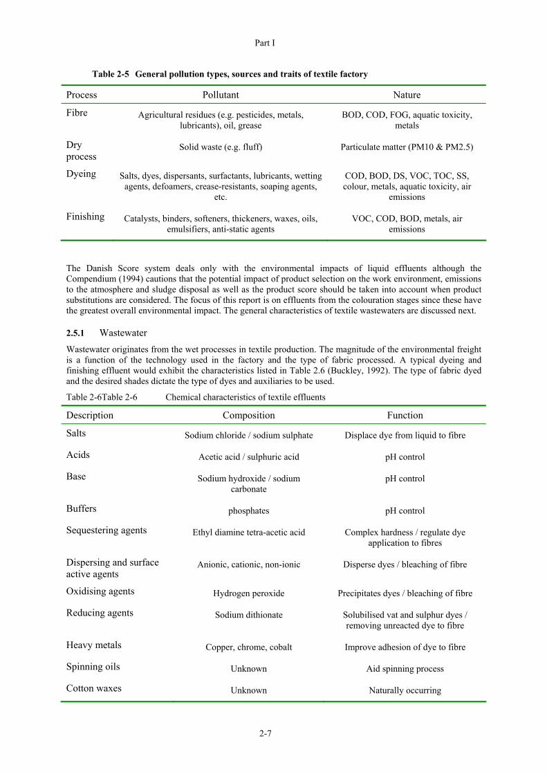
Part I

2-7

Table 2-5 General pollution types, sources and traits of textile factory

Process Pollutant Nature

Fibre Agricultural residues (e.g. pesticides, metals, lubricants), oil, grease

BOD, COD, FOG, aquatic toxicity, metals

Dry process

Solid waste (e.g. fluff) Particulate matter (PM10 & PM2.5)

Dyeing Salts, dyes, dispersants, surfactants, lubricants, wetting agents, defoamers, crease-resistants, soaping agents,

etc.

COD, BOD, DS, VOC, TOC, SS, colour, metals, aquatic toxicity, air

emissions

Finishing Catalysts, binders, softeners, thickeners, waxes, oils, emulsifiers, anti-static agents

VOC, COD, BOD, metals, air emissions

The Danish Score system deals only with the environmental impacts of liquid effluents although the Compendium (1994) cautions that the potential impact of product selection on the work environment, emissions to the atmosphere and sludge disposal as well as the product score should be taken into account when product substitutions are considered. The focus of this report is on effluents from the colouration stages since these have the greatest overall environmental impact. The general characteristics of textile wastewaters are discussed next.

2.5.1 Wastewater Wastewater originates from the wet processes in textile production. The magnitude of the environmental freight is a function of the technology used in the factory and the type of fabric processed. A typical dyeing and finishing effluent would exhibit the characteristics listed in Table 2.6 (Buckley, 1992). The type of fabric dyed and the desired shades dictate the type of dyes and auxiliaries to be used.

Table 2-6Table 2-6 Chemical characteristics of textile effluents

Description Composition Function

Salts Sodium chloride / sodium sulphate Displace dye from liquid to fibre

Acids Acetic acid / sulphuric acid pH control

Base Sodium hydroxide / sodium carbonate

pH control

Buffers phosphates pH control

Sequestering agents Ethyl diamine tetra-acetic acid Complex hardness / regulate dye application to fibres

Dispersing and surface active agents

Anionic, cationic, non-ionic Disperse dyes / bleaching of fibre

Oxidising agents Hydrogen peroxide Precipitates dyes / bleaching of fibre

Reducing agents Sodium dithionate Solubilised vat and sulphur dyes / removing unreacted dye to fibre

Heavy metals Copper, chrome, cobalt Improve adhesion of dye to fibre

Spinning oils Unknown Aid spinning process

Cotton waxes Unknown Naturally occurring

Part I

2-8

Dyes Various Colour fibre

Fibres Various Fabric, fibre break-down

Table 2-7 Sources of aquatic toxicity in textile effluent (EPA, 1996)

Product Example Typical Source

Salt NaCl, Na2SO4 Dyeing

Surfactants Ethoxylated phenols Multiple sources

Metals Copper, zinc, etc. Dyes

Organics Chlorinated solvents Scour, machine cleaning

Biocides Pentachlorophenol Wool fibre contamination

Toxic anions Sulphides Sulphur dyeing

2.5.1.1 Aquatic toxicity Due to the complex and variable nature of textile industry effluents, it would be impractical and prohibitively expensive for either textile companies or regulatory authorities to identify and quantify each and every product in any given effluent which could contribute to its aquatic toxicity. Furthermore, interactions between various components of the wastewater can have a significant impact on its overall toxicity. Consequently, permitting limits should ideally be set based on whole effluent toxicity tests (Compendium, 1994). Nonetheless, it is still useful to consider the toxicity of individual products used in the textile manufacturing process and always desirable to avoid using toxic substances whenever possible. Using the aquatic toxicity data provided in each product’s MSDS is a cost effective way of estimating its potential impact on effluent toxicity and determining which compounds are likely to be most problematic (Compendium, 1994). Table 2-7 lists a number of products which are known contributors to effluent toxicity.

2.5.1.2 Metals and chelating agents Not all textile effluents contain significant quantities of toxic metals (EC, 2003), however where they are present they are of particular concern because they are difficult to treat in conventional waste water treatment plants and can also cause inhibition of biological treatment processes (EPA, 1996). This results in them finding their way into the receiving waters where they are potentially hazardous for both human and animal life (Smith, 1986). Bioaccumulation of metals in human causes a number of chronic diseases such as Wilson’s disease, and disorders of the liver which affect the central nervous system (Rashmi, 2000).

Sources of metals in textile mills include incoming fibre, water, metal complex dyes, plumbing, and chemical impurities in dye and other products used. Table 2-8 lists of metals commonly found in textile effluents (EPA, 1996).

Table 2-8 Common textile effluent metals and their sources

Metal Sources

Arsenic Fibres, incoming water, fugitive, treated timber

Cadmium Impurity in salts used in dyeing

Chrome Dyes, laboratory

Part I

2-9

Cobalt Dyes

Copper Dyes, incoming water, fibre

Lead Dyes, plumbing, shop

Manganese Permanganate strip (mildew removal repair procedure)

Mercury Dye / commodity chemical impurity

Nickel Dyes

Silver Photo operations

Tin Finishing chemicals, plumbing

Zinc Dyes, impurity in commodity chemicals, incoming water, plumbing

Titanium Fibre

The main sources of metals in textile effluents are the dyeing and printing processes. Metals may be present in dyes as impurities from the dye manufacturing processes or as part of the dye molecule in metal complex dyes (EC, 2003). Due to environmental concerns and regulatory pressures, dye manufacturers are working both to reduce metal impurities in dyestuffs and to replace metal complex dyes with less hazardous alternatives such as phthalocynine dyes, however, there remain some domains (e.g. certain shades and levels of fastness to light) where the metal complex dyes are difficult to replace (EC, 2003). Metals typically exhibit lower toxicity when chelated with dye molecules, forming an integral part of the molecular structure. However, chelates are susceptible to biodegradation in wastewater treatments which can result in the release of metals (EPA, 1996).

In addition to metals, textile effluents often contain the chelating agent ethylene diamine tetra acetate (EDTA). EDTA is used in the textile industry as a sequestering agent, in fabric washing powders and as a bleach stabiliser, chelating metal ions in water to reducing water hardness. EDTA is a hexadentate chelator containing 4 carboxylic acid and 2 tertiary amine groups, and although it chelates with most monovalent, divalent, trivalent, and tetravalent metal ions it forms particularly strong complexes with Ni, Zn, Pb, Ca, Co (III), Fe(III), and Cu (Manahan, 2005).

The persistent nature of EDTA in nature, its low susceptibility to degradation during wastewater treatment, and its chelating ability pose environmental challenges as elevated concentrations of chelating agents in the environment enhance the transport of metals (including heavy metals) in soils, and migration of radioactive materials from disposal sites. EDTA in wastewater chelates metal ions in treatment plants thus making them unavailable for biological assimilation. This reduces metal removal with sludge (Manahan, 2005).

2.5.1.3 Detergents in textile effluents The extensive use of detergents in industry creates a number of environmental problems. Unlike soap that generally loses its action once it enters a sewage plantor aquatic systems by precipitating into calcium and magnesium salts with eventual biodegradation and elimination from the environment, detergents generally do not loose their action and are persistent (Alloway and Ayres, 1993). The use of alkyl benzene sulfonates (ABS) in common surfactants used in detergent formulas in the 1960s lea to concerns about their slow biodegradability and foaming on water bodies (Alloway and Ayres, 1993). The foaming problem has been greatly reduced by replacing ABS with a more biodegradable linear alkyl sulfonate chain (LAS) (Manahan, 2005). Non-ionic detergents containing alkylphenol polyethoxylates do not respond to sewage treatment and are thought to be xenoestrogens. The use of sewage sludge as a fertiliser introduces these xenoestrogens to plants and they might eventually find their way to human beings (Manahan, 2005).

From about 1947 to 1970, the increased use of sodium tripolyphosphate as an additive (detergent builders) to detergents to fight water hardness, resulted in increased phosphate levels in receiving waters which led to significant eutrophication problems (Alloway and Ayres, 1993). In an effort to control algal growth in receiving waters sodium tripolyphosphate additives were replaced with sequestering agents like nitriloacetic acid (NTA)

Part I

2-10

However, NTA is now suspected of binding heavy metals (lead and cadmium) from sediments and thus making them available for bio-accumulation in living organisms (Alloway and Ayres, 1993).

Part I

3-1

CHAPTER 3 The Danish Score System

Synthetic organic colourants from textile industry wastewaters are among those pollutants which are not readily biodegradable and are therefore likely to enter the aqueous environment in wastewater treatment plant effluent. In spite of continuous improvements in the effluent treatment processes, remedial processes need to be accompanied by preventative methods in order to substantially reduce the detrimental impact of industrial wastewaters have on the environment The Score system is a proven cleaner production tool which was developed in Denmark through close co-operation between the local authorities and the textile industry. The system is an administrative method of sorting chemicals on basis of their consumption and ecological information acquired from the chemical supplier’s material safety data sheet (MSDS) (Laursen et al., 2002). The Danish system operates on the basis of co-regulation within a strict ecotoxological and precautionary principle framework. It provides a mechanism for industry to prioritise the implementation of cleaner production projects and it passes the responsibility of determining the environmental safety of products back to the supplier.

3.1 HISTORY

The original system was developed by Rinkjoebing County, Denmark and the Danish Water Quality Institute in 1989. The system was initially based on the environmental hazard ranking (EHR) system that evolved in Germany. The system was set up because of the large number and amounts of different chemicals and dyestuffs being used in 3 dyeing mills. The complex mixture of chemicals made any attempt to develop a comprehensive program for monitoring the actual levels of each chemical in the wastewater extremely difficult and prohibitively expensive (Anderson and Naidoo, 2001).

One year later (1990) the system was introduced to a further 10 companies. However, these companies found that the system was too rigid, and asked the Danish Federation of Textile Industries to cooperate with the authorities in developing a better and more versatile system. This was completed in 1992. After using the system in 13 companies over a period of more than 1½ years, the system was revised in 1994. In 2001, the system was still being used in more than 15 companies in Denmark (Anderson and Naidoo, 2001).

3.1.1 Overview of the system The ranking of the various chemicals and dyes used by a company according to their utilisation amounts and environmental exposure enables that company’s management structure to perform a prioritised identification of chemicals that require a closer examination. The company could also try to adjust the utilisation amount of chemicals in their production processes.

Upon assessment of the score of a particular chemical or dye, the company will be aware of the possible impact the chemical has on the environment. Based on their findings, they could decide on the use of more environmentally friendly chemicals or dyes to obtain the same or similar product result. The aim of the Score system is to reduce the negative environmental impact of the chemicals used in the textile sector through a preventative approach.

The Score system is based on four parameters which are important for characterizing the impact of chemicals and dyestuffs on the environment. These are:

A – Discharged amount of substance to drain over a given period, B – Biodegradability C – Bioaccumulation and D – Toxicity.

Each parameter (i.e. A, B, C or D) is given a score between 1 and 4, with 1 indicating the least environmental impact and 4 indicating the most serious impact. In the case of missing information required to determine the parameter score, the highest score is assigned along with a remark “4u” (“u” indicating unknown).

The product of A, B and C (i.e. A x B x C) is called the Exposure score. The Exposure score gives an indication of the potential presence (level, persistence and distribution) of the substance in the environment. The calculation of the Exposure score is summarised in Table 3-1.

Part I

3-2

Table 3-1 Exposure component parameter scores (adapted from Laursen et al., 2002)

1 2 3 4

A – Discharged amount of substance to drain

kg/week < 1 1 – 10 > 10 - 100 > 100

kg/year < 50 50 - 500 >500 - 5000 > 5000

B – Biodegradability

Surface water (%) > 60 (50 – 100) 10 - 60 <10

Sludge culture (%) > 70 20 - 70 <20

BOD/COD ratio >0.5 ≤ 0.5

C – Bioaccumulation

Bio-concentration factor (BCF),

Or C1,C2, C3

< 100 ≥ 100

C1 If MW > 1000 g/mol *

C2 If 500 ≤ MW ≤1000 g/mol

POW – data < 1000 ≥ 1000

Water solubility g/L > 10 10 - 2 < 2

C3 If MW < 500 g/mol

POW – data < 1000 ≥ 1000

Water solubility g/L > 100 100 - 2 > 2 – 0.02 <0.02

The asterisks (*) represents the bioaccumulation score of substance

0

8

16

24

32

40

48

56

64

0 1 2 3 4

Toxicity (D-Score)

Exp

osur

e (A

xBxC

)

High Scoring Chemicals

Low Scoring Chemicals

Figure 3-1 Score plot: plot of exposure against toxicity to identify the high impact chemicals

Part I

3-3

The Exposure score is plotted against the Toxicity score to determine whether the substance has a low impact or high impact on the environment. The score plot is presented in Figure 3-1. The substances that fall left of the diagonal line have relatively lower environmental impacts and those which fall to the right of the diagonal line have relatively higher environmental impacts. Efforts to reduce the environmental impact of the effluent should focus on the high scoring chemicals

The following sections describe the calculation procedure for each score component and are adapted from Score System for Sorting of Chemicals on the Basis of Environment Data and Information on Consumption, Compendium, 2nd revised edition, January 1994. The full document maybe obtained online as Annex A to (Laursen et al., 2002). Example calculations are also given in Appendix B of the Part I in this report.

3.1.2 Data levels Table 3-1 and Table 3-4 indicate that a number of different types of data may be used to determine each of the score components. However, the system requires that the highest level of data available should be used. According to the Compendium, the highest level is the one for which the test conditions correspond most closely to natural aquatic systems. Parameters for the calculation of B, C and D are listed in descending order of level in Table 3-1 and Table 3-4, i.e. surface water biodegradability, the bio-concentration factor and toxicity to aquatic organisms are the preferred bases for the B, C and D scores.

3.1.3 A-Score: Discharge amount The A-score (discharge amount) is determined from the amount of dye or chemical that is discharged to drain by the facility per year. The amount to drain is the total amount of product used less the quantity of product which adheres to the textile. The amount retained varies depending primarily on the chemical substance and textile involved and only slightly on the processes employed. A protocol for the determining the fixation rates of various reactive dye chemistries is described in Chapter 9.

In the absence of other information, dye fixation rates can be estimated from Table 3-2. However, non-dye chemicals are assigned a default utilisation rate 0f 0% (i.e. everything goes to drain) in the absence of evidence to the contrary. If the % utilisation rate is given as “> x %” the actual utilisation rate is presumed to be x %. Accessory agents, which are converted during the production process, are scored on basis of the conversion information product. If this information is not available, then they should be scored on basis of the starting substance with percent utilisation of 0%.

Table 3-2 Presumed utilisation percentages of particular dyes if no further information is available

Vat, Azo dyestuff 50%

Acid dyestuff 95%

Dispersing dyestuff 90%

Metal complex dyestuff 95%

Cationic dyestuff 98%

Direct dyestuff 80%

Sulphur dyestuff 60%

Reactive dyestuff 50%

All other dyestuff 50%

Part I

3-4

The A-score is determined from the discharge amount as shown in Table 3-1. The discharge amount may be calculated either on an annual basis if the chemical is used at a fairly steady rate and on a weekly basis if it is used intermittently.

3.1.4 B-Score: Biodegradability Biodegradibility in surface water is the preferred basis (level one information) for the calculation of the B score. The results are stated as percent degradation after a fixed test period. If the data are only stated as intervals, “50 – 100%” is used synonymously with “> 60%”. However, in most cases the B-score for biological degradability is based on the substance biodegradability in sludge (level two). In the absence of degradability data, the B score is obtained from the BOD5/COD ratio. The B-score is determined from the % biodegradability as shown in Table 3-1.

A substance is described as “readily degradable” in surface water, i.e. B-score = 1 if the degradation results in an elimination of 70% of the dissolved organic carbon, 60% of the theoretical oxygen consumption or formation of 60% of the theoretical quantity of carbon dioxide. Moreover, the substance is considered to be readily biodegradable if other scientifically well-researched tests have shown that the substance is decomposed biologically or on-biologically at a level > 70%. The degradation is to take place within 10 days of the 28 days test period. Inorganic components are estimated to be 100% decomposable.

In principle, the biodegradation tests performed on sludge can only be applied to predict the non-degradability of a substance, but not its possible degradability in the recipient. Substances which are decomposed by less than 20% by using sludge culture methods are considered to be “not readily decomposable”, and they are often described as persistent. Substances decomposable by more than 70% are described as “potentially degradable” (inherent biodegradability). Substances decomposed by between 20% and 70% are generally considered decomposable, but it is likely than their degradation will produce stable metabolites

For products consisting of a mixture of the substances, the degradability of each individual substance should ideally be separately determined. However, if the only data available is for the degradability of the mixed product, then the calculated score should be accompanied by a note to this effect.

Test methods approved for determining biodegradability involve the total degradation of the substance to carbon dioxide, water and other inorganic molecules. Biodegradation and the tests used to determine biodegradability are discussed in Section 4.1.

Some MSDS only list eliminability information. If the substance is decomposed or eliminated due to a non-biological process, this information can also be used in the calculation of the B-score using the scale for degradability in sludge cultures (Table 3-1).

3.1.5 C-Score: Bioaccumulation The C-score is ideally calculated from the bioconcentration factor (BCF) which is the ratio of the concentration of a substance in an organism (usually fish) to the concentration in the surrounding environment. The bioconcentration factor is discussed in Section 4.2.2.1. If BCF data is not available, then the C-Score can be calculated from the molecular weight of the substance and either the octanol-water partition coefficient (Pow) or the aqueous solubility as shown in Table 3-1. Molecular size can constitute a barrier to the possible absorption of a substance through a cell membrane. Therefore, the Score system has been drawn up with 3 sub-scales (C1, C2, C3) for biodegradation based on molecular weight (MW). For chemicals with MW > 1000 mg/mol the score figure is fixed to be 1. In the absence of quantitative data, the score can temporarily be made on the basis of qualitative information on solubility (dispersing ability, miscibility, emulsion, etc.) as shown in Table 3.3.

Bioaccumulation tests on fish are considered unnecessary when dealing with the following:

� Pigments which have a very poor solubility in the water phase (< 0.2 mg/L) and organic phase (< 10 mg/L) are considered to be non-accumulative.

� Dyestuffs, which are highly water-soluble (>2 mg/L) are expected to have low affinity to biological tissues and therefore non-accumulative. Dyestuffs having a molecular weight (MW) of more than 450g/mol and a cross section bigger than 1.05 nm are supposed to be bulky and unable to cross the cell membrane barrier. This makes them non-accumulative.

Part I

3-5

Table 3-3 Determining the C-score from qualitative information

Qualitative information Score by dyestuff Score by chemical

Dispersible 3 4

Miscible, fully miscible or mixable 3 4

Emulsion, dilatable emulsion 3 4

Colloidally soluble, soluble, easily soluble 1 1

Insoluble 3 4

Negligible 3 4

Bioaccumulation and the tests used to characterise it are discussed further in Section 4.2. C-scores for products consisting of a mixture of substances are calculated according the same principles discussed in Section 3.1.4.

3.1.6 D-score: Toxicity The D-score is based on information about the substance toxicity to fish or other water fauna/algae in the form of LC0 (concentration at which no mortality in test organism group is observed) or LC50 (concentration at which 50% mortality in test group is observed) values, or on information concerning inhibitory effects of the substance in activated sludge. For test performed on fresh water fauna or algae, toxicity should be stated as LC0. In cases where LC50 is given, it may be assumed that LC0 = LC50/3 if, and only if, LC50 is less than 100 mg/L. This conversion is in reasonable accordance with EPA’s “Criteria Maximum Concentration”, which is defined as 0.3 times the lowest LC50 value foe acute toxicity towards at least three species. If LC50 > 100 mg/L then no conversion is made.

The D – score is fixed in relation to the difference between the concentration that gives a toxic effect and the concentration that found in the effluent. The method for determining the Toxicity score is detailed in Table 3-4. The average concentration refers to the annual loss of chemical to the effluent divided by the annual water volume consumption. This is used for a substance that is used steadily throughout the year. The extreme concentration is the annual chemical loss to the wastewater divided by 24 hours’ water volume consumption. This would be used for a chemical which is only used intermittently. The score should always be stated with reference to the conditions calculated, i.e. according to average concentration or extreme concentration.

Part I

3-6

Table 3-4 Toxicity score (adapted from Compendium, 1994)

1 2 3 4

D – Effect concentration divided by effluent concentration D1 Effect level for fresh water fauna/algae divided by average concentration D2 Effect level for fresh water fauna/algae divided by the extreme concentration D3 Effect level for sludge culture or bacteria divided by the average concentration D4 Effect level for sludge culture or bacteria divided by the extreme concentration

> 1000 1000 - 101 100 – 10 < 10

The toxicity of composite wastewater is known to be difficult to characterise on basis of the information on its individual components. Some substances may react mutually and the toxicity may be reduced or increased because of their interaction. Therefore toxicity should ideally be regulated on the basis of whole effluent toxicity .to ensure that possible synergistic effects are included. Nonetheless, it is still useful to look at individual substance toxicities in order estimate their potential contribution to the effluent toxicity and to render problem substances more visible.

3.1.7 How the Danish authorities run the Score system Figure 3-2 shows the various steps that the Danish authorities go through in order to assess the score of a product. Consumption data from old and new chemicals and dyestuffs are used to calculate the score. The chemicals are then sorted out based on the individual scores and a score report is prepared. The total score, exposure and toxicity score are evaluated. These are mutually evaluated by the companies and authorities. The authorities and the companies normally agree on what action to take and mostly it is an agreement on investigation of possibilities for substitution. However, authorities can set time limits for companies on issues of substitutions and consumption (Anderson and Naidoo, 2001).

Part I

3-7

Consumptionon ”old”chemicals anddyestuffs

Consumptionon ”new ”chemicals anddyestuffs

1992

Data on chemicals and Score calculation

Sorting on score / Score report

Annual

Whenused?

Evaluation :Score evaluationExposure scoreToxicity score

Company / authorities :Mutual evaluationAssess consumptionSubstitutionTechnology

Encroachments by the authorities :Time limitFurther investigationsSubstitutionRestrictions on consumption

Figure 3-2 Implementation of Score system by Danish authorities

Part I

4-1

CHAPTER 4 Chemical Test Methods

This chapter reviews the various test methods used to determine the biodegradability, bioaccumulation potential and toxicity of substances, i.e. the parameters on which the Score system is based. These results should be included in the MSDS along with the test method used. Since the type of test method used has a bearing on the interpretation of the results as well as the data quality level as described in Section 3.1.2, it is important to understand the theoretical basis of and differences between the various methods.

4.1 BIODEGRADATION

Biodegradation maybe defined as the molecular break down of a chemical compound resulting from the action of micro-organisms acting on that particular compound (Calow, 1993). The term is usually reserved for the enzymatic breakdown of organic substances leading to the complete destruction of the parent molecular structure. This breakdown can take place in the presence or absence of oxygen resulting in the generation of carbon dioxide, water and smaller organic compounds or methane respectively (Calow, 1993).

4.1.1 Biodegradation and environmental fate Biodegradation is the most important property of a chemical, governing its speed of disappearance from natural soil and aquatic systems. This property of a molecule presents an opportunity for re-availing chemical nutrients, which would be otherwise lost for ever, back to the environment. The recycling of chemicals in nature also depends on abiotic degradation through processes like photodegradation, chemical reactions and adsorption to sludge solids (Calow, 1993). Major players in the biodegradation process are micro-organisms, namely bacteria, which owing to their relatively simple organisation and structure are capable of utilising an infinite variety of organic compounds as nutrients. The abiotic and biotic chemical degradation processes are collectively known as bioelimination (Calow, 1993).

The overall biodegradation process is oxidation, and it is largely by such means that dead organic matter is broken down in nature into simpler molecules once again available for use by the living organisms (Swisher, 1970). Biodegradation is catabolism during which larger complex molecules are broken down into smaller, simpler molecules with the release of energy some of which can be used for anabolism and the remainder lost as heat (William et al., 1973). The process can be simplified as:

)incomplete tionbiodegrada if smetabolite(energy biomassOHCO microbesO molecule organic 222

4-1

Biodegradation may however occur in the absence of oxygen and in such cases the end products would be methane and the process is said to be anaerobic. Biodegradation of a compound is understood to be divided into two phases: Primary and Ultimate biodegradation.

4.1.1.1 Primary biodegradation Primary biodegradation is defined as a process where the molecule has been initially altered or oxidised by bacterial action to such an extent that the physicochemical nature and properties exhibited by the original molecule are no longer evident (Swisher, 1970; Calow, 1993). This process can be quantified when the primary biodegradation molecule no longer responds to analytical procedures more or less specific for the detection of the parent molecule (Swisher, 1970).

The concept of primary degradation has been criticised because of its inability to give insight on the possible formation of persistent biodegradation residues (Calow, 1993). In spite of this sound criticism, primary biodegradation remains important because of the fact that it usually coincides with the loss of toxic properties of the parent compound (e.g. detergent surfactants that lose surface active properties after primary biodegradation). The methods recommended by the Organisation for Economic Cooperation and Development (OECD) (1971) for biodegradation testing of detergents consists of a screening test (water-die-way static system) and a confirmatory test (a continuous activated sludge model), both of which test for primary biodegradation (Calow, 1993).

Part I

4-2

4.1.1.2 Ultimate biodegradation Ultimate biodegradation is the complete bioconversion of a molecule to carbon dioxide, water, inorganic salts and constitutive material into biomass (Swisher, 1970). Methods to provide adequate evidence of ultimate biodegradability use detection techniques which are related directly or indirectly to the measure of the oxidation of organic carbon. Standard methods that use carbon dioxide production, oxygen consumption or dissolved organic carbon (DOC) disappearance are not specific to the chemical but allow progress of the oxidation of organic carbon to be followed. More research-oriented studies use 14C –labelled derivatives to allow tracking of the mineralisation of organic carbon molecules at low concentrations in realistic matrices.

In reality the term biodegradability may have two different meanings that are not exactly the same. First biodegradation can refer to the extent and /or the rate of biodegradation of a chemical in a given test or environmental condition (readily biodegradable). Second, it can also refer to the maximum level of biodegradation, which a chemical may reach, in optimum conditions and with long enough exposure periods (inherent biodegradability). In the first case, the assessment of biodegradability may depend as much on the test conditions as on the intrinsic properties of the chemical itself while is the other second case it depends solely on the chemical’s intrinsic properties (Calow, 1993).

4.1.2 Biodegradability test levels In context of the safety assessment of industrial chemicals, the OECD has published test guidelines that include three levels of biodegradation testing (OECD, 1981). These guidelines cover methods to measure the biodegradability of the parent molecule and its metabolites (Calow, 1993).

Two types of biodegradability test exists namely screening tests and simulation tests. Screening tests include methods for testing for both ready and inherent biodegradability. The ready biodegradability screening test are characterised by low inoculum and high initial substrate loads similar to surface water conditions found in nature whereas tests designed for inherent biodegradability are characterised by high inoculum loads and relatively low initial substrate concentrations representing wastewater treatment plant conditions (Beek, 2001). Table 4-1 lists standardise biodegradability tests methods published by OECD.

Table 4-1 List of standardised biodegradability tests (Beek, 2001)

Test No Test name Detection Poorly soluble substances

Volatile soluble substances

Pass %

OECD Readily biodegradability tests:

301 A DOC die away DOC - - 70

301 B CO2 evolution CO2 + - 60

301 C Modified MITI (I) DOC - +/- 60

301 D Closed bottle test BOD +/- + 60

301 E Modified OECD screening

DOC - - 70

301 F Manomeric respiratory test

BOD + +/- 60

OECD Inherent biodegradability tests:

302 A Modified SCAS DOC - -

302 B Modified Zahn-Wellens DOC - -

302 C Modified MITI (II) BOD + -

Part I

4-3

4.1.2.1 Ready biodegradability test The general principle is the incubation of a relatively small amount of inoculum, containing a variety of aerobic microorganisms, in a suitable medium (water and minerals only). The pH should be neutral, with an inoculum concentration above 2 mg/l and a temperature between 20 and 25 C. The test chemical should be the only carbon source. The measure of biodegradation is based either on oxygen consumption, carbon dioxide production or dissolved organic carbon (DOC) disappearance. These methods thus measure the level of ultimate biodegradation in the test system, but in conditions so strict to the chemicals that they can only serve screening tests to identify ‘readily biodegradable’ chemicals (Calow, 1993).

Ready biodegradability test are often called screening tests due to the fact that they give an indication of the biodegradability if the test compound and are fairly easily done as they use determinands like COD or BOD. Screening tests share a number of common features, namely:

� Control tests are run parallel to the actual test to check the operation of the procedure

� The test media is a mineral solution composed of prescribed concentrations of potassium and sodium phosphates plus ammonium chloride, magnesium sulphate, and iron (III) chloride. For the modified OECD screening test, trace elements such as Mn, B, Zn, Mo and yeast extracts are added.

� The inoculum is acclimatised to the test conditions but not the test substance.

� Test duration is 28 days but can be lengthened or shortened depending on the rate of biodegradation.

� The incubation temperature is 20°C or room temperature

Screening tests are more for qualitative analysis (classification) and not quantitative prediction of the fate of a chemical as they have been found to produce differing results for some compounds especially for 4-Nitrophenols, chlorobenzenes, and nitrilotriacetates (Beek, 2001).

Biological Oxygen Demand methods The test methods discussed below are the most important tests standardised by the OECD, EC (European Community) and ISO (International Organization for Standardization). The standard OECD protocols require oxygen consumption or carbon dioxide evolution values to be determined theoretically or experimentally and for theoretical determination, one has to know the chemical structure of the chemical under investigation (Calow, 1994).

These tests are indirect biodegradation test methods because they use theoretical oxygen demand (ThOD) or chemical oxygen demand (COD) to determine the biodegradability of the test substance (Beek, 2001).

The Closed Bottle Test The standard version of the closed bottle test is the OECD 301 D method (OECD, 1981) and the EC method C6 (Directive 84/449/EEC, 1984). A bottle is completely filled with a mineral solution containing known amounts of dissolved oxygen, test material and inoculum and allowed to digest over 28 days at suitable temperature. Oxygen consumption is monitored using oxygen sensitive electrodes and biodegradation from the percentage difference between theoretical oxygen demand (ThOD), calculated form the empirical formula of the test compound, and the oxygen depletion reading (Beek, 2001). In cases where ThOD can not be calculated COD of the test substance is used although this results in less accuracy (Calow, 1994). A control run is made under conditions which are identical in all respects except that the test compound is omitted, and its oxygen uptake is subtracted to give a net value for the compound.

An important advantage of this method is that it can handle insoluble substances. Even with the use of a correction factor one must be careful with the interpretation of the results as the available oxygen is also used for nitrogen and sulphur oxidation during the test in addition to being used for biodegradation of the test molecule’s organic carbon to carbon dioxide and water (Calow, 1993).

MITI (I) Test The Ministry of International Trade and Industry (MITI) test requires that an analytical determination of the contents of the test solution be available. To make sure that microorganisms are fit for the task of degrading the chemical under examination, the inoculum is sourced from ten different media. The 104 to 105 cell forming units per millimetre (cfu/ml) mixed inoculum (including industrial sewage) is, somewhat, compromised by acclimatisation in a laboratory to synthetic sewage having glucose as the energy source over one to three months (Calow, 1994; Beek, 2001).

Part I

4-4

Carbon dioxide evolution test Carbon dioxide production is the most direct evidence of oxidation of organic carbon during biodegradation. The standard version of this kind of test is the OECD, 302B (OECD, 1981) and the European Commission (EC Method C5 in Directive 84/449/EEC). This method can handle 20 mg/l of test material, inoculum and BOD water (diluted solution of calcium chloride, magnesium sulphate, ammonium chloride, ferric chloride, and sodium potassium phosphate buffer in distilled water) (Swisher, 1970) as a nutrient. Air (containing no carbon dioxide) is passed through the test liquors. Carbon dioxide generated during biodegradation is trapped in a barium or sodium hydroxide solution and measured by titration of the residual hydroxide or as organic carbon. This measurement is then corrected using the carbon dioxide emitted by the blank (Beek, 2001).

Advantages are: the test can handle insoluble materials, biodegradation not limited by availability of oxygen and this allows for 104 to 105 cfu/ml and 10 to 20 mg DOC/L inoculum (Calow, 1993). The test is not applicable to volatile substances and is cumbersome (Beek, 2001).

Dissolved Organic Carbon tests Similarly to the oxygen uptake and carbon dioxide evolution test, the test compound is the only carbon source. These die away systems are tests where the test compound is exposed to the medium in an isolated system and the progress of biodegradation is observed by analysis at certain intervals as the test compound dies away (Swisher, 1970).

The sample is acidified and the inorganic carbon stripped away as carbon dioxide by blowing inert gas through the sample. The resulting sample containing only organic carbon is then oxidised by combustion or by using a strong oxidant and the absorption of infrared (IR) carbon dioxide is measured using an IR-detector. Total carbon or dissolved carbon will be determined depending on whether a natural or pre-treated (centrifuged) sample was used. DOC is then analysed. The test is not suitable for volatile organic material (Beek, 2001).

4.1.2.2 Inherent biodegradability test If the results for ready biodegradability tests are negative, test substances are then subjected to inherent biodegradability screening tests. These are run with much higher levels of inoculum obtained from municipal activated sludge. They are characterised by ratios of test compounds/biomass which is more comparable to sewage treatment conditions. Contact time of the test compound with the activated sludge is very long to allow for maximum biodegradation if the compound is biodegradable to any degree, hence the name. Biodegradation is determined mainly by measuring the disappearance of DOC (Calow, 1993; Beek, 2001).

Activated sludge systems A semi or continuous activated sludge (SCAS) unit represents a considerable investment of space, time and money for its installation, operation and maintenance. It is also susceptible to many difficulties inherent in keeping any continuous process in smooth operation (Swisher, 1970).

Modified SCAS Test

The modified SCAS test adapted for DOC analysis is derived from the US Soap and Detergent Association procedure. This test uses a SCAS system, with a contact time of 24 hours between 20 mg/L of the test chemical and the sludge. The test is started with activated sludge mixed liquor. This test uses either DOC detection or specific analytical methods for primary biodegradation assessment. The mixed liquor is settled daily and its supernatant analysed for DOC and then discarded. Since the test provides for adaptation of the microbes and also uses high levels of inoculum with long exposure time, its biodegradation results could be taken as the inherent biodegradability of the chemical. The SCAS test was adapted by the OECD and classified as method 302A method 302 A (OECD, 1981).

Zahn-Wellens Test

This is a very powerful batch activated sludge test, employing high levels of test compound (100 mg/L), test duration of 28 days and ultimate biodegradation measured by DOC. The Zahn-Wellen test is used to assess inherent ultimate biodegradability and was adapted as the OECD method 302 B (OECD, 1981).

4.1.2.3 Simulation tests: Simulation tests use small-scale models for ecosystems (natural or sewage works) performed in the laboratory using one or more of carbon sources such as natural water, sediment, or soil samples instead of mineral salts media as is the practice with screening tests (Calow, 1993; Beek, 2001). The simulation test is so named due to

Part I

4-5

the fact that the environmental conditions are mimicked as far as possible. This requires a very good understanding of the environment being simulated. A number of factors including the sampling of a representative inoculum, acclimatisation of the inoculum in the laboratory with minimum disturbance of the natural biodiversity and concentration and adaptation of inoculum to the test substrate are critical to the success of the simulation test (Beek, 2001).

The standardised activated sludge simulation test is the OECD confirmatory test (OECD 303 A, ISO 11733). The test conditions are relatively close to real sewage treatment, particularly when real sewage is used instead of a synthetic feed (inoculum). Although designated as a test for biodegradation (both primary and ultimate), this test monitors the removal of a specific chemical in the system and therefore is only taken as biodegradation when there is sufficient evidence that the removal is not due to any other process but biological elimination. There are four versions of this test, three dealing with primary biodegradability and one dealing with inherent biodegradability (Calow, 1993).

4.1.2.4 BOD/COD ratio In cases where none of the above mentioned biodegradability tests were performed, the biodegradability of a chemical may be estimated from its biological oxygen demand and chemical oxygen demand ratio (BOD5/COD). However, as discussed below, there are several limitations inherent to the BOD test which make this the least preferred method of estimating biodegradability for the purposes of the Score system.

Biological oxygen demand (BOD) Oxygen is present in the aquatic environment as dissolved, molecular oxygen. Although poorly soluble in water. oxygen plays a critical role in supporting plant, animal and microbial life in all water bodies (Vesilind, 2003). At room temperature the amount of oxygen dissolved in ambient water is 9 mg/L. Oxygen solubility decreases with increasing temperature (Vesilind, 2003).

Oxygen is also part of the water molecule and present in dissolved anions such as carbonate, nitrate, sulphate and phosphate. These anions are used by some microorganisms, such as anaerobic bacteria, as sources of oxygen. However most aquatic organisms are entirely dependent on molecular oxygen either dissolved in water or obtained directly from the atmosphere (Calow, 1994).

Biological oxygen demand is the rate at which oxygen is depleted in the water and can be an indication of lack of microorganisms in water, unavailability of organic matter in the water, or that the microorganisms present are unable or uninterested in degrading the available organic matter (Vesilind, 2003).

The main process of oxygen removal from natural waters is biological oxidation or biodegradation. Since biodegradation processes are oxidative, complete biodegradation generally occurs only in the presence of oxygen. Under anaerobic conditions, although bound oxygen in the form of anions may still be available, conversions are slower and often incomplete (Calow, 1994).

BOD test

The biological oxygen demand test is performed using a 300 mL standard BOD bottle. After an initial measurement of the dissolved oxygen, the bottle is sealed and stored in a dark incubator at 20 C for five days hence the name BOD5 (Alloway and Ayres, 1993). Dissolved oxygen is measure again after the period of incubation, and the difference is BOD. It is necessary to make a series of dilutions for waters containing large amounts of organic matter to ensure that the oxygen is not exhausted (i.e. final dissolved oxygen reading equal to 0 mg/L). The final BOD reading is then multiplied by the appropriate dilution factors. The extent of dilution depends on the anticipated BOD of the sample. Acceptable dilutions limit oxygen depletion during incubation to between 30% – 70% of the initial oxygen concentration (Calow, 1994).

Samples not having enough bacteria due to the conditions to the samples were exposed prior to collection (e.g. industrial wastewaters with high temperatures, low or high pH, etc.) can be “seeded” by adding some bacteria from another source in order for one to be able to carry out the BOD test (Vesilind, 2003).

Limitations of the BOD test

a) The BOD5 test method has a number of limitations including the following (Calow, 1994):

b) Dilution – the dilution and the diluent used in the five day laboratory test bears no resemblance to the real conditions.

Part I

4-6

c) Limiting oxygen concentration – oxidation rates in BOD bottles maybe constrained by decreasing oxygen concentration

d) Mismatched microflora – often the seed flora do not represent the microbes encountered in natural situations

e) Irrelevant incubation period – the test duration has neither theoretical nor practical significance. It was adapted because oxygen uptake due to biochemical oxidation of some readily degraded materials was virtually complete by the 5th day.

f) Precision – the BOD5 has been found to have poor precision with a variation of around 20%.

g) Dilution – this is done to prevent complete oxygen uptake. The dilution is just an educated guess and could miss the mark to give misleading results.

h) Algal interference – the algae in the test solution could die because they are unable to photosynthesise. This would lead to release of substrates for further microbial oxidation.

Chemical oxygen demand (COD) The chemical oxygen demand (COD) test is done by heating a portion of sample in an acidic chromate solution, which chemically oxidises organic matter. The amount of chromate remaining (measured by titration), or the amount of reduced chromium produced (measured spectrophotometrically), is translated into oxygen demand value. The equivalent amount of oxygen required to oxidize the organic matter to carbon dioxide is equal to the COD of the wastewater and is determined from the amount of dichromate consumed in the COD test. The more chromate used the more organics in the sample and therefore the higher the COD. The test is completed in about two hours and its figure is always higher than the BOD5 value (Vesilind, 2003).

4.2 BIO-ACCUMULATION

Bio-accumulation is defined as a process by which living organisms can collect and concentrate chemicals both directly from their surroundings (bio-concentration) and indirectly from their food. Simply put, bio-accumulation is the concentration of a chemical over time in a biological organism in levels higher than those found in the immediate environment. This process occurs any time the pollutants are taken up and stored faster than they are broken down or excreted (Nussey G, 2000). Bio-accumulation in aqueous environments is usually characterized using data for fish due to a number of ecological and economic considerations (Calow, 1993). Bio-accumulation is the net result of the interaction of uptake, storage and elimination of a chemical. These processes are discussed next.

4.2.1 Mechanisms involved

Uptake In order for the chemical to exert its effect on an organism it must move from the ambient environment into the organism. Chemical uptake is the movement of the chemical from the environment into an organism’s cells. Generally toxicants traverse the cell membrane by the following processes: passive diffusion, facilitated diffusion, and active transport with passive diffusion being the prevalent method of the three entry mechanisms (Alloway and Ayres, 1993). Pollutants can enter a fish as follows: ingestion through the gastrointestinal tracts (food and non-food particles), inhalation through the respiratory systems (gills), and absorption through the skin (Nussey G, 2000). Of the three phenomena, both types of diffusion require a concentration gradient to be the driving force and the force or pressure for diffusion is called chemical potential (Alloway and Ayres, 1993). It is important to note than factors such as the hydrophobicity of a chemical (solubility in lipids) could increase the chemical potential of a substance. This is understood to be due to the fact that hydrophobic compounds tend to move out of water and into cells of an organism where there are liphophilic environments. During active transport, the toxicant is transported by a carrier molecule and this process is not dependent on chemical potentials but on the energy of the carrier (Alloway and Ayres, 1993).

Storage Once inside the organism the chemical is distributed through out the body by blood depending on its ionic state, molecular size, lipophilicity, viscosity, and concentration. In the blood the chemical will be distributed (partition) into each of the three blood constituents or phases (water, lipids, and proteins) based on its physico-chemical properties (Alloway and Ayres, 1993). Water soluble toxicants are referred to as “free” toxicants

Part I

4-7

because they are not bound to any molecules as is the case with hydrophobic chemicals that bind to molecules like lipids and proteins in the blood. The toxicants are deposited in tissues from the blood depending on the toxicants affinity for the tissues. This is a reversible process and therefore obeys the laws of equilibrium which in this case regulate the concentration of the toxicant in the blood components and the tissues (Alloway and Ayres, 1993).

Once inside a fish, some chemicals may be stored temporary in the organism by binding to proteins or dissolving in fats (liphophilic) while others could be transported by blood to the liver for transformation and/ or storage (Nussey G, 2000).

Accumulation in fat reserves serves to detoxify the chemical by removing it from contact with other organs. However, when fat reserves are utilised to provide energy for an organism, the stored chemical may be remobilised within the organism and may again be potentially toxic. If the fat reserves are utilised quickly, significant toxic effects may be seen from the remobilisation of the chemical (Alloway and Ayres, 1993). The concentration of toxicants found in different tissues after environmental exposure, for a specific time, depends on several dynamic processes all taking place concurrently (Heath, 1991).

Elimination Another deciding factor affecting bioaccumulation is whether the organism can degrade or excrete the chemical. Toxicants can be eliminated through urinary process, faecal formation, and through respiratory process depending on the organism type and toxicant properties (Alloway and Ayres, 1993). Elimination by excretion of water soluble chemicals is dependant on the kidney where the aqueous component of the blood is filtered. The faecal elimination is composed of chemicals not absorbed from the food in the gut and bile excretion which contain toxicants eliminated by the liver. Elimination by lungs or gills is for gaseous and highly volatile compounds and the dominant mechanism of transport is passive diffusion. Lipophilic chemicals tend to be slowly eliminated by an organism, thus have greater accumulation potential. Many metabolic reactions alter a chemical into more water-soluble metabolites that are more readily excreted (Alloway and Ayres, 1993).

4.2.2 Prediction of a chemical’s bioaccumulation potential In order to prevent environmental deterioration, it is of utmost importance to be able to look at certain chemical properties and be able to predict the chemicals environmental impact. The following properties have been agreed upon by scientists as being fundamental in predicting a chemical’s bio-accumulative ability.

4.2.2.1 Bioconcentration factor The bioconcentration factor (BCF) is the ratio of the concentration of a substance in an organism to the concentration in the surrounding environment. The BCF depends on:

i) The composition of the water (e.g. its hardness, dissolved and particulate organic carbon content, and pH).

j) The organism’s ability to metabolise the toxicant and its fat (lipid) content.

k) The chemical properties of the substance (e.g. solubility in water and in fat and its susceptibility to metabolism or biodegradation).

The BCF can thus vary widely. However for a given organism (e.g. fish) using standard test procedures and test water, the BCF that is obtained will reflect the toxicant’s properties and thus be characteristic for that substance (Vesilind, 2003).

Metal in fish can be determined by thawing and drying the tissue samples (gill, liver, muscle, skin) at about 60 C. The moisture content of each sample is determined by weighing the dry and the wet mass of each sample. A mixture of 55% nitric acid (10 ml) and 5 ml of 70% perchloric acid is then added to the sample for digestion, which takes place at around 200 to 250 C for at least four hours until the solution is clear. Each sample is filtered and stored in a sterile acid-washed bottle for a period of time until the metal concentration can be measured (Kotze P, 1999; Avent-Oldewage A and HM, 2000; Nussey G, 2000). Once the metal concentration in the fish organs is known then the BCF can be calculated by dividing the metal concentration in tissue by that obtained from the water in which the fish resided.

4.2.2.2 Octanol-water partition coefficient (Pow) In the late 1800 various researchers discovered that a pure compound partitioned between phases in a constant ratio essentially independent of the concentration of the compound. This constant ratio was described as the distribution ratio, later to be called partition coefficient. Hansch and co-workers (1962) suggested that n-octanol

Part I

4-8

would provide a better lipid phase than oily fats used at the time (Hansch G, 1962). After some researchers proposed that the bio-concentration of chemicals by fish was a partition process, relationships were established between the octanol-water partition coefficient and bio-concentration. Partition coefficient has been shown to be useful for describing the attraction of neutral, non-polar and poorly metabolised substances to the lipids in an organism (Calow, 1994).

Pow is principally used for hydrophobic organic compounds and is considered to be a measure of their hydrophobicity. The solution of non-polar solutes into water does not result in binding between solute molecules and the water solvent. In fact the non-polar molecules distort and displace the overall matrix of water molecules which are held together by strong intermolecular forces. Water then forms a surface around the molecules and this results in water molecules orientating to form hydrogen bonds between adjacent molecules. Consequently intermolecular forces are generated. The solubility of the non-polar molecules is thus reduced. The 1-octanol-water partition coefficient (Pow) is a defining characteristic of the hydrophobic class of organic compounds and is defined as (Calow, 1994; Connel, 1997):

W

OW CC

P O 4-2

Where: Co = equilibrium solute concentration in the octanol phase

CW = equilibrium solute concentration in the aqueous phase.

The partition coefficient is dependent on the polarity of the substance, molecular weight, and the relationship of the polarity of the solvents (Connel, 1997).

The values of Co and Cw are expressed in the same units so that Pow is dimensionless (unitless). Liphophilic compounds usually have Pow values between 100 – 1000 000. Since this range of data is difficult to present effectively on a linear graph, logarithms of the Pow values are commonly used, thus log Pow values range from about 2 to 6 for liphophilic compound (Connel, 1997). An increase in partition coefficient reflects increasing lipophilicity and values of 100 and more (Pow >100) are considered to indicate hydrophobic compounds (Connel, 1997).

BCF is favoured for the prediction of bio-concentration because it takes into account the metabolism by the target organism whereas the chemically determined Pow does not. The octanol-water partition coefficient is a function of temperature and usually Pow values are measured at 20 - 25 C (Calow, 1994).

Shake Flask Method Partition coefficients can be determined experimentally using the shake flask method. The traditional method involved placing the two immiscible solvents together in a vessel, adding a small concentration of the solute (below the maximum solubility) and shaking the vessel for a period of time. This was followed by chemical analysis of the two phases to yield the concentration contained and subsequently the Pow (OECD, 1981).

Disadvantages of the shake flask method led to the use of chromatographic methods and generator columns. These methods avoid the following problems found with the shake flask:

Very low aqueous phase concentrations for lipophilic compounds, and

due to the presence of very small aggregates or miscelles of the solute, the true concentration can be extremely difficult to measure accurately.

More sophisticated method include: Rekker and Mannhold (1992) and OECD 117 – 1989 (an HPLC method). The five original OECD test guidelines are known as test 305 A – 305 E and they employ different species and test conditions (Calow, 1993).

Pow estimation A number of different models for predicting POW have also been developed, some of which and are listed in Table 4-2.

Part I

4-9

Table 4-2 Overview of methods for calculation of Pow values (Calow, 1994)

Method Information required

Substituant constants Parent compound and additive values for common functional groups

Fragmental constants Values for structural fragments within a molecule

Parachor Values for atoms and structural features of a molecule

Molecular connectivity Regression equation relating molecular connectivity to Pow and molecular connectivity of the compound

Other partition coefficients Regression equation relating other partition coefficients to Pow and corresponding partition coefficients of the test compound

Water solubility Regression equation relating water solubility to Pow and water solubility of test compound

� Substituant constants

This is one of the earliest methods for estimating Pow. The substituant constants x are defined as the change in log Pow value due to the addition of functional group x to the a parent molecule (Calow, 1994).

hxx PP loglog 4-3

Where: Ph = POW value of the parent molecule

Px = POW value of the derivative of the parent molecule with a substituant x.

� Fragmental constants

This method was devised by Rekker (1977) and Hansch and Leo (1979) and requires a set of fragmental constants (f) that represent structural fragments within molecules. The log Pow value is obtained as the sum of the structural fragments for the whole molecule. The equation is:

∑ nnOW faPlog 4-4

Where: a = a numerical factor indicating the incidence of the fragment within the molecule

f = the fragmental value

� Parachor

The parachor concept was developed as a measure of molar volume and has been related to POW by the following equation (Calow, 1994):

aOW EPP 012.0log 4-5

Where: P = the parachor

aE = the correction to account for the interaction of solute and the solvent molecule.

Part I

4-10

� Molecular connectivity and other partition coefficients

Warner and co-workers (1990) evaluated the utility of a set of 39 molecular descriptors and physicochemical properties to model the octanol-water partition coefficient of lipophilic compounds. They found that satisfactory relationships were expressed by multiparametric linear regression equations. These physicochemical parameters included molecular connectivity and other partition coefficients (e.g. carbon matter partition coefficient - Koc) (Calow, 1994).

� Solubility in Water

In many cases the most readily available physicochemical characteristic of a compound is its water solubility. The POW could be calculated from water solubility using this equation (Calow, 1994):

bPaS OW⎟⎠⎞

⎜⎝⎛ log1log 4-6

Where: ba, = empirical constants for different chemical groups

S = solubility

Water solubility Water solubility is the ability of a chemical to dissolve in water. Water is a polar molecule with a moderately high dielectric constant and dipole moment. Polar solutes dissolve in water and the strong attraction forces between the polar solvents and the polar water molecules stabilise the matrix which forms a solution. Compounds that dissolve are called hydrophilic (Calow, 1994). Usually, compounds that are highly water soluble have a low potential to bio-accumulate and do not readily enter the organism’s cells. Once inside the organism, they are easily removed unless the cells have a specific mechanism for retaining them. Heavy metals such as mercury and certain other water soluble chemicals are the exception because they bind tightly to specific sites within the body of the organism. When this occurs even highly water soluble chemicals can accumulate. Such an example is cobalt, which binds tightly and specifically to liver sites and accumulates despite its water solubility. Similar accumulation processes occur for mercury, copper, cadmium, and lead (Alloway and Ayres, 1993; Vesilind, 2003).

4.3 TOXICITY

Toxicity is defined as the ability of the compound (toxicant) to cause adverse effects on a living organism or environment (eco-toxicants) at relatively low concentrations by causing damage to the organism’s cell structure and function, which in extreme cases might lead to death. All substances are toxic at sufficiently high doses (Connel D, 1999).

A chemical’s impact on an ecosystem is initiated when it enters the environment and its fate depends on a number of factors including:

a) Physicochemical properties of the substance

b) Physical, chemical, and biological properties of the ecosystem, and

c) Origin, amount, environmental availability, chemical form and fate of the chemical in the environment.

Once inside the target organism, toxic chemicals may be distributed by the circulatory system to various parts of the organism. Some chemicals such as strong acids and alkalis exert their toxic effect in a non-specific way by denaturing proteins and dissolving tissues. On the other hand, some toxic chemicals affect components of the biological system. Chemicals can only exert their toxic effect when bound to specific sites of toxic action (receptors). These receptors maybe parts of cells confined to certain tissues, specific protein regions with nerve synapses or membranes distributed among the cells, or the nucleic acid of an organism (Connel D, 1999).

Toxicants are substances that cause deleterious biological effects on exposed living organisms. These can be sub-divided into three categories, namely teratogens (affect reproductive processes), mutagens (those affecting nucleic acids, e.g. DNA), and carcinogens (cancer causing agents).

Part I

4-11

4.3.1 Dose-effect relationship The dose-effect relationship provides the basis for assessment of hazard and risk presented by chemicals in the environment. It is necessary when determining the dose-effect relationship, to distinguish between the chemical concentration in the environment and the concentration that reaches a target tissue. Due to the difficulty in determining the chemical amount reaching the target tissue, the total amount taken up by the organism is used. In determining this relationship it is assumed that the toxicant has a receptor site inside the organism, toxicity is proportional to the chemical concentration, and the higher the dose administered the greater the concentration of the chemical (Connel D, 1999). It is very difficult to relate the toxicity of a chemical to its dose because of the size of the test organism. Toxicity is, because of this reason, expressed in terms of the toxicant concentration rather than total amounts.

To assess the toxicity of a compound to an organism, an observable and well defined end point must be identified. Mortality measurements are employed because death satisfies these requirements and more over they allow the researchers to compare toxicities of a variety of chemicals without requiring prior understanding of the mechanisms involved (Connel D, 1999). Toxicity test can be done both with terrestrial and aquatic organisms.

4.3.2 Test organism selection A careful selection of the organisms is vitally important and a number of issues should be taken into account. Ideally the organism should fulfil the following criteria:

a) A group of organisms, preferably at least one from each trophic level (e.g. algae, macro-invertebrates and fish) rather than a single species should be used whenever possible.

b) Test organisms showing noticeable responses over a wide range of chemical concentration are preferred.

c) Test organisms with a wide geographical range are preferred.

d) The toxicity testing should be carried out on local or native species whenever possible.

e) Ecologically valuable species, in terms of taxonomy, niche or trophic levels are preferred

f) Test organisms should occupy a position within a food chain leading to man or other important species.

g) The organisms with recreational and economic values are obvious candidates.

h) Species that would be easy to maintain in laboratory cultures are preferred.

i) The test organisms that can be identified easily and for which there is enough biological background (e.g. genetics, physiology, ecological niche) are ideal for the test (Connel D, 1999).

4.3.3 Toxicity tests on aquatic organisms In testing for toxicity using aquatic animals, one has to identify the correct or effective concentration range in water. This is achieved by exposing a small number (two or three) of test organisms to a wide range of test chemical concentration on a log scale. The results obtained in this test can then be used on a full scale toxicity test, where larger groups of the test organisms (ten or multiples of ten per group) are exposed to an increasing, narrower range of concentration centric on the LC50 estimated from the ranging test. The LC50 number of dead organisms in each group is recorded after a fixed period of exposure (e.g. 96 hours). The percentage data obtained can be used to plot a cumulative responses (%) versus aqueous concentration (mg/L) (Walker et al., 1997).

One difficulty in aquatic toxicity testing is the maintenance of a constant test chemical in water. Chemical concentration can decrease in water due to several processes such as absorption and metabolism by test organism, and volatisation, degradation and adsorption from water. As a result, certain tests have been designed to counteract the negative effect of these chemical losses in order to obtain reliable toxicity results. Where the rate of loss is relatively low, tests may be performed using static or semi-static systems. With the static systems, the water is not changed for the duration of the test while with the semi-static system water is replaced at regular intervals (24 hours). A better, but more complex and expensive, method for renewing test solutions is provided by a continuous flow (flow-through) system (Walker et al., 1997).

Part I

4-12

Table 4-3 List of standardised aquatic toxicity tests

Test No. Title

OECD 201 Algal growth inhibition

OECD 202 Acute toxicity to crustaceans (Daphnia magna) –static, 24 & 48 hours

OECD 202 II Daphnia magna growth and reproduction (21 days)

OECD 203 Acute toxicity to fish (Oncorhynchus mykiss) –semi static

OECD 204 Fish, Prolonged toxicity test: 14 day study (Oncorhynchus mykiss) –semi static

OECD 210 Fish early life stage toxicity test (Oncorhynchus mykiss)

4.3.3.1 Algal growth inhibition test (OECD 201, EEC C3, ISO/DIS 10253) Freshwater species such as Chorella vulgaris and Scenedesmus subspicatus or marine species such as Skeletonema costatum and Phaeodactylum tricornumtum are used for this test.

The growth test is performed semi-axenically (i.e. minimising contamination by other organisms) in a 250 ml flask under controlled conditions. Growth of the algae is determined by cell counting or spectrophotometrically at 24 hour intervals for periods of exposure up to 96 hours.

4.3.3.2 Acute toxicity for crustaceans (OECD 202, EEC C2) Daphnia magna, less than 24 hour old, are placed into glass vessels containing a series of concentrations of the test substance in water. Daphnia are observed after 24 and 28 hours and the immobilised number in each vessel recorded. The results are expressed as EC50 (half maximal effect concentration) values for 24 and 48 hours exposure. Classification is based on the 48 hour EC50 value. The maximum no effect concentration and minimum concentration that result in significant (P3 0.05) immobility (LOEC = lowest observable effect concentration) are reported.

4.3.3.3 Daphnia magna growth and reproduction (OECD 202 II) The results of the acute immobilisation study are used to select the concentration of the test substance. The duration of the study is 21 days and the number of offspring produced together with adult and juvenile survival is reported. A semi-static system is recommended and the frequency of the test media renewal depends on the stability of the substance.

4.3.3.4 Fish, acute toxicity test (OECD 203, EE C1) Rainbow trout (Oncorhynchus mykiss), bluegill fish (Lepomis macrochiras) or zebra fish (Brachydanio rerio) are the preferred species in fresh water. Turbot (Scopthalmus maximus) or sheepshead minnows (Cyprinodon variegatus) are the preferred saltwater species.

Fish are introduced into glass vessels containing water of known quality to which the test substance has been added at known concentrations. Fish are observed for mortality and sub-lethal symptoms at specified periods of time. The test results are expressed in the form of LC50 values. The duration of exposure is normally 96 hours. The NOEC (no observable effect concentration) and the minimum concentration at which 100% mortality occurs are also reported together with observations of toxic symptoms. The slope of the dose/response curve is also provided where possible. This provides useful extra information for use in environmental risk assessment or hazard classification of the test substance.

Part I

4-13

4.3.3.5 Fish, early life stage toxicity (OECD 210) The early life stages of fish are exposed to the chemical usually under flow-through conditions. The study starts by placing fertilised eggs in the test chamber and continues until all the fish are free swimming and feeding exogenously. Lethal and sub-lethal effects such as stunted growth are assessed and compared with controls. The larva and early fry stages are usually the most sensitive to the effects of xenobiotics.

4.3.4 Toxicity tests on sludge cultures Many organics exhibit a threshold concentration at which they inhibit the heterotropic and/or nitrifying organisms in the activated sludge process. Several protocols have been developed to evaluate bio-inhibition effects of chemicals. These methods are: a) Fed-batch reactor of Philbrook and Grady, b) Watkin and Eckenfelder, c) the OECD Method 209 of Volskay and Grady, and d) glucose inhibition test of Larson and Schaefer. Depending on particular wastewater, one or more of these test methods will be applicable (Eckenfelder and Grau, 1992).

4.3.4.1 OECD Method 209 The OECD Method involves measurement of activated sludge oxygen consumption rate from synthetic substrate to which the test compound has been added at various concentrations. The consumption of oxygen is read immediately after the addition of the test compound and after 30 minutes of aeration. The EC50 value is determined as the concentration of the test compound at which the oxygen uptake rate (at 30 minutes) is 50% of the uninhibited oxygen uptake rate. To ensure that the test is working properly and that the biomass has the appropriate sensitivity, this method uses 3,5-dichlorophenol as a reference toxicant. The reference EC50 value should be between 5 and 30 mg/L for the test to be valid (Eckenfelder and Grau, 1992).

4.3.4.2 Fed-batch reactor (FBR) Previously used to determine nitrification kinetics, the fed-batch reactor has three essential characteristics: (a) substrate is continuously introduced at a sufficiently high concentration and low flow rate so that the reactor volume is not significantly changed during the test, (b) the feed rate exceeds the maximum substrate utilisation rate, (c) short test duration and therefore simple modelling of biological solids growth, and (d) various acclimated activated sludge are employed (Eckenfelder and Grau, 1992).

This reactor uses two litres of test sludge. Prior to the start of the feed flow, an initial sample is taken for determination of oxygen uptake rate, mixed liquor volatiles and total suspended solids. The feed flow is then introduced at a rate of 100 ml/hour and aliquots of the reactor contents are sampled from the FBR every 20 minutes for the duration of the three-hour test. Suspended solids determinations are made every hour during the test (Eckenfelder and Grau, 1992).

4.3.4.3 Glucose inhibition test This method was developed by Larson and Schaeffer (1982). Modifications were made to the initial method in order to allow this test to be applicable to various industrial wastewaters.

Sample (10 ml) is placed into a centrifuge tube and a stock solution (1 ml) of glucose added. Activated sludge (10 ml) is added to the tube and aerated at low rate. After an hour, hydrochloric acid (two drops) is added to the mixture and the tube transferred to the centrifuge. Glucose is then measured. Sludge and glucose controls are made in order to calculate the glucose inhibition, and the percent inhibition is calculated as follows (Eckenfelder and Grau, 1992):

BC0

B

CC-C Inhibition % 4-7

Where: C = final glucose concentration in sample solution

CB= final glucose concentration in sludge control sample

C0 = initial glucose concentration (glucose control)

Part I

4-14

4.3.4.4 Inhibition of nitrification In many industrial wastewaters, carboneous oxidation is not inhibited, but the more sensitive nitrifiers are inhibited. Small doses of powdered activated carbon (PAC) may absorb the inhibiting organics, permitting nitrification to proceed. Nitrification inhibition kinetics can be studied using the FBR and/or the following protocol to evaluate the effects of carbon addition:

Different ranges of PAC (30 – 100 mg/L) are added to wastewater and mixed until almost at equilibrium (about two hours). To wash the activated sludge containing active nitrifiers, wastewater-carbon mixture is added and aerated for 24 hours with intermediate sampling for analysis of ammonia-, nitrite- and nitrate ions. Nitrification rate is determined and compared to wastewater aliquots aerated without PAC. Carbon dosage that maximises nitrification rate should be selected (Eckenfelder and Grau, 1992).

Toxicity potency of a chemical is expressed using one of the following terms, depending on the nature of the environment.

a) Median lethal concentration (LC50), defined as the concentration at which the test organism group exhibited 50% mortality.

b) Median lethal dose (LD50), defined as the dose at which the test organism group exhibited 50% mortality.

c) Median inhibition concentration (IC50), defined as the concentration at which the test organism group exhibited 50% inhibition in growth or activity.

d) Median effective concentration (EC50), defined as the concentration at which 50% of the predicted effect is observed.

e) LC0 defined as the concentration of the chemical at which the test organism group exhibit no (0%) mortality

f) Median effective dose (ED50) defined as the effective dose at which the test organism group exhibit 50% mortality.

It is important to note that EC50 and IC50 of the same chemical should be lower than LC50, because they represent impairment while the latter represents death. The smaller the LC50, the more toxic the compound in question is (Connel D, 1999). Other terms used in relation to toxicity testing are the No Observed Effect Dose (NOED) and the No Observed Effect Concentration (NOEC), and the Lowest Observed Effect concentration (LOEC) and Lowest Observed Effect Dose (LOED). The first two terms describe the highest dose or concentration of the toxicant that does not cause harm to the test organism while the last two indicate the lowest concentration or dose of the test compound where an effect was first noticed. They can be determined only where a higher dose or concentration has produced an effect in the same toxicity test (Walker et al., 1997).

Acute tests are tests designed to evaluate relative toxicity of a chemical for selected organisms upon short-term exposure (e.g. 48 or 96 hours) to various concentrations of the test chemical. In spite of the popularity of mortality compared to other end points (immobility or inhibition of growth), there are growing concerns about the sub-lethal effects of environmental toxicants. A toxicant may not kill the organism in the duration of the test but may very well still have long-term deleterious impact on the organism (e.g. impairment of future reproductive output, or reduced growth). In a complete chronic toxicity test, the test organisms are exposed to low toxicant concentration (at least five different concentrations) for an entire reproductive life cycle (e.g. egg to egg). To save time and money, partial-life cycle tests are used, choosing only the most sensitive life stages (embryo to larva). For formulation of meaningful chronic tests, important biological information about the test organism, nutritional and physiological requirements, life cycle, physical requirements and so on need to be collected (Connel D, 1999).

4.4 SUMMARY AND CONCLUSIONS

In the Score system, assessing the potential environmental impact of various industrial chemicals depends on the inclusion of data on their bio-availability (B-score), bio-concentration potential (C-score) and toxicity (D-score) in the MSDS. Unlike the discharge amount required for the calculation of the A-score, obtaining accurate information on which to base the other three scores is not straight forward. The results obtained furthermore depend on the type of testing done and the test conditions. In applying the Score system, it is therefore important to understand the various test methods, their significance and limitations and to always use the highest level data available. It is also important that the MSDS always includes the test methods and conditions used to obtain the data provided.

Part I

5-1

CHAPTER 5 Environmental Legislation

As with other chemically intensive industries, the growth of the textile industry has resulted in increasing environmental problems and a correspondingly increasing need for environmental legislation to control them. Globalisation, which results in vast quantities of raw materials, chemicals and finished goods crossing national boundaries, provides additional challenges and has necessitated the development of international norms and standards for dealing with potentially harmful substances and materials. The European Union is both one of the largest producers and consumers of textiles in the world. It is also a trendsetter in controlling the use of hazardous chemicals in consumer goods (EU REACH programme, Regulation EC 1907/2006). Section 5.1 discusses European environmental legislation pertaining to the chemical industry as an example of international legislative trends. Particular emphasis is place on legislation governing the development of Material Safety Data Sheets (MSDS) which are one of the main sources of information used in the Score system. Section 5.2 discusses the relevant South African legislation which deals with pollution from the chemical industry as well as occupational health and safety issues including requirements for MSDS to be available in the work place.

5.1 ENVIRONMENTAL LEGISLATION IN THE EU

This section looks at EU directives and regulations which, together with the national legislation of member states, are designed to protect water resources and control chemical pollution both in the environment and the work place.

5.1.1 Protection of water Water legislation developed in Europe over the past 20 years can be divided into legislation directed at setting water quality objectives, control of dangerous industrial effluent discharged into water courses, and prevention of marine pollution by land-based sources (NCTE, 2000).

Water quality laws set standards for surface water for drinking (Council Directive 75/440/EEC, 1975), fresh water for fish (Directive 2006/44/EC, 2006), bathing water (Council Directive 76/160/EEC, 1975),etc. Industrial effluent control laws set limits for the discharge of dangerous substances in effluent such as mercury (Council Directive 82/176/EEC, 1982), etc.

5.1.2 Control of chemical pollution The directives designed to deal with chemical pollution cover a number of issues such as labelling, marketing, accidents and emergency responses, export and import, etc. (NCTE, 2000). Most relevant to the Score system project is the notification and labelling laws which gave rise to the MSDS that are used as one of the main sources of information when compiling score profiles for factories. The series of laws governing the compilation of MSDS are discussed in more detail below.

Directive 67/548/EEC (Notification and labelling) Directive 67/548/EEC (1967) can be labelled as the mother of all Directives relating to the chemicals industry. It was formally enacted on the 27 of June 1967 and since then has been constantly updated to reflect advances in science and technology (European Commission, 2007) with the last amendment being Directive 2006/121/EC (2006)). The classification and labelling system of the Directive 67/548/EEC is being replaced by a new Commission proposal for a Regulation on the Classification, Labelling and Packaging of Substances and Mixtures COM(2007) 355. The new proposal incorporates the classification criteria and labelling rules agreed at UN level, the so called Globally Harmonised System of Classification and Labelling of Chemicals (GHS).

The purpose of Directive 67/548/EEC is to approximate or harmonise the laws, regulations and administrative provisions of the member states relating to the classification, packaging, and labelling of dangerous substances which are placed on the market within the EU. This directive does not apply to dangerous substances exported to third countries. The Directive defines the word “dangerous” as explosive, oxidising, flammable, toxic, harmful, corrosive or irritant.

Part I

5-2

Directive 88/379/EEC Council Directive 88/379/EEC (1988) was one of the first Directives to require chemical producers to compile material safety data sheets for their products and to supply them to consumers. Article 10 of this Directive provided for the setting up of an information system in the form of safety data sheets relating to dangerous preparations and specified that this information was principally intended for industrial users and must enable them to ensure protection of health and safety in the workplace.

Directives 91/155/EEC and 93/112/EC Directive 91/155/EEC (1991) defined and laid down the detailed arrangements for the system of specific information relating to dangerous preparations in the implementation of Article 10 of Directive 88/379/EEC. Article 1 of Directive 91/155/EEC stated that any person responsible for placing a dangerous substance or preparation on the market shall supply recipients with a safety data sheet containing information set out in Article 3 of the Directive, free of charge and at latest when the substance or preparation is first supplied. Article 3 listed the 16 mandatory headings to be furnished by the person responsible and an annex provided a guide to the compilation of safety data sheets to facilitate the protection of health and safety at the workplace, and to protect the environment. The annex was replaced by the annex to Commission Directive 93/112/EC (1993) which elaborated on the headings and how they should be furnished. Appendix A gives an example of a 16 point MSDS.

Directive 1999/45/EC Directive 1999/45/EC (1999) extended the requirement for safety data sheet provision to include preparations that are not considered as dangerous according to Article 5, 6 and 7 of Directive 1999/45/EC but may present a danger to users . It then stated that a safety data sheet providing proportionate information was required for any preparation containing any individual substance with concentration of ≥ 1% by weight for non-gaseous preparations and ≥ 2% by volume for gaseous preparations which poses a health or environmental hazard or has a Community workplace exposure limits.

Directive 2001/58/EC Directive 2001/58/EC was the second amendment to Directive 91/155/EC (2001). This is a Directive formulated due to the realisation that the safety data sheets were of poor quality and did not provide adequate information for the users. A remedial attempt was focused on providing guidance to safety data sheet compilers in the form of an annex to this Directive. The annex stated that in cases where it emerges that information on certain properties is of no significance and / or it is technically impossible to provide the reasons, for this must be clearly stated under each heading.

Over the period from 1967 to date various adaptations (30 to date) have been adopted by the EU to update the test procedures in Council Directive 67/548/EEC in order to keep pace with technological developments.

5.2 SOUTH AFRICAN LEGISLATION

Since the attainment of democracy in 1994 the South African Government has made it a priority to align the South African constitution / legislation with those of the international community with regards to human rights and environmental protection.

5.2.1 South African Constitution The South African constitution introduces a number of fundamental human rights with environmental implications. In particular, Section 24 states:

Everyone has the right:-

3.1. to an environment that is not harmful to their health or well being; and

3.2. to have the environment protected, for the benefit of present and future generations, through reasonable legislative and other measures that:-

i) prevent pollution and ecological degradation;

ii) promote conservation; and

iii) secure ecologically sustainable development and use of natural resources while promoting justifiable economic and social development.

Part I

5-3

The ‘everyone’ means that citizens and non-citizens can claim this right. Section 38 of the constitution lists people who can approach the court (locus standi) as:

a) anyone acting in their own interest

b) anyone acting on behalf of another person who cannot act in their own name

c) anyone acting as a member of, or in the interest of, a group or class of persons’

d) anyone acting in the public interest; and

e) an association acting in the interest of its members

Effectively this means that everyone has the right to take environmental offenders to task.

Being the highest law of the land the constitution opens avenues for promulgation of underlying laws (primary and sub-ordinate legislation) which put action to the constitutional ideals. Some of the environmental related primary legislation (acts) and sub-ordinate legislation (regulations) are discussed below.

5.2.2 Environment Conservation Act (1989) The Environment Conservation Act (ECA, 1989) was designed to coordinate environmental conservation matters and was later partially repealed by National Environmental Management Act 107 of 1998 (NEMA).

Part V of ECA seeks to control activities which may have detrimental effects on the environment. Activities which will probably have a detrimental effect on the environment are listed in subsection (2) of section 21 of ECA and include water use and disposal, industrial processes, waste disposal and chemical treatment. Written authorisation from the Minister of Environmental Affairs and Tourism or competent authorities designated by the Minister is required before performing any of the listed activities. Environmental impact assessments (EIA) are necessary to support the application to undertake a listed activity as indicated in subsection (2) of section 22 of ECA. Part V of ECA however is repealed by Chapter 5 of NEMA that deals with integrated environmental management.

5.2.3 National Environmental Management Act (1998) The National Environmental Management Act (1998) is the primary piece of environmental legislation and creates legislative frameworks for environmental protection at national level. Its first amendment, NEMA First Amendment Bill (2003) contains detailed compliance and enforcement provisions.

Section 2 of NEMA is a list of principles that form a framework for interpretation and implementation of laws concerned with protection or management of the environment. Some internationally recognised principles are incorporated namely: polluter pays, duty of care, sustainable development, etc.

Section 28 of part one of chapter 7 of the National Environmental Management Act, 1998 deals with duty of care and remediation of environmental damage.

2) Every person who causes, has caused or may cause significant pollution or degradation of the environment must take reasonable measures to prevent such pollution or degradation from occurring, continuing or recurring, or, in so far as such harm to the environment is authorised by law or cannot reasonably be avoided or stopped, to minimise and rectify such pollution or degradation of the environment.

3) Without limiting the generality of the duty in subsection (1), the persons on whom subsection (1) imposes an obligation to take reasonable measures, include an owner of land or premises, a person in control of land or premises or a person who has the right to use the land or premises on which or in which-

a) Any activity or process is or was performed or undertaken; or

b) Any other situation exists,

Which causes, has caused or is likely to cause significant pollution or degradation of the environment

This section lays the responsibility with the owner of the land, person in control and/or person who occupies the land to prevent pollution from occurring, continuing or recurring. It is important to note that this law has the potential to be applied retrospectively as implied by the ‘has caused’ in subsection (1). This means that the duty of care does not lapse with time.

Part I

5-4

The Director-General of Environmental Affairs and Tourism or a provincial head is given powers by subsection 4 of this act to direct the responsible person (s) to take rehabilitative measures before a given date, continue with them and complete them before a specific reasonable date. Should the person fail to comply or inadequately comply, the Director-General or provincial head may take reasonable measures and recover all costs incurred from any or all of the liable persons as indicated in subsection (7) and (8) of NEMA.

5.2.4 National Water Act (1998) Section 2 of the act states that the purpose of the act is to, inter alia, make sure that water resources are protected, used, developed and conserved taking into consideration among other things protecting aquatic and associated ecosystems and their biological diversity, reducing and preventing pollution and degradation of water resources.

Schedule 1 of the water act lists permissible water use including:

‘….discharge of ….wastewater from any ….industrial sites into ….sea outfall, other conduit (e.g. sewers) controlled by another person authorised to undertake the purification, treatment or disposal of …water containing waste subject to approval of the person controlling the ….sea oufall or other conduit’.

Section 19 (subsection 1) of chapter 3 of the National Water Act (1998) requires that a person who uses land on which any activity is performed and is likely to cause water pollution must take all reasonable measures to prevent such pollution. Sub-section 2 lists compliance with the prescribed waste standards or management practice as one of the preventative measures to be taken.

Chapter 16 of the Water Act lists offences that include failure to comply with any condition attached to a permitted water use, committing or omitting of an act which pollutes or is likely to pollute a water resource. Offenders are liable for a fine and / or prison term from five to ten years. The court handling the case may recoup remedial costs from the polluter and may award damages to the adversely affected parties.

Industrial effluent discharge to sewers is controlled by local authorities and by the department of Water and Forestry (DWAF) if discharged directly to natural water resources. Municipalities are required to stipulate Sewage Disposal Bylaws that govern water related issues including the billing, standards of waters discharged to sewers. Trade permits and licences with waste standards to promote pollution prevention are prepared by the authorities and companies are requires to comply or face withdrawal of the permit and operation closure.

5.2.5 Occupational Health and Safety Act (1993) The Occupational Health and Safety Act (1993) was designed to protect workers and others from various hazards in the workplace, including exposure to substances which are potentially harmful to their health. Section 10 (subsection 3) of the act name “general duties of manufacturers and others regarding articles and substances for use at work” to include the requirement that any person who manufactures, imports, sells or supplies any substance for use at work to ensure that the substance is safe and without risk to health when properly used. It also requires the supplier to provide sufficient information regarding use, health and safety risks, and accidents. The Hazardous Chemical Substance Regulations (1995) promulgated under the OSH Act dealt more specifically with exposure to hazardous chemicals. In 2003, the Hazardous Chemical Substances Regulations were amended by the insertion of Section 9A. and Annexure 8 (OSH General Amendment, 2003). Section 9A specifically requires that any person who manufactures, imports, sells or supplies any hazardous chemical substance for use at work provides, free of charge, a material safety data sheet (MSDS) in a form given in Annexure 8 of this regulation which complies with ISO 1 1014 or ANSIZ400.1.1993 with regard to the mandatory 16 information points to be furnished in the MSDS. This regulation goes further to say that the MSDS are to be made available to any interested or affected person who makes a request for them.

5.3 CONCLUSIONS

The environmental legislation discussed above all places legal and financial responsibility for minimising pollution, damage to ecosystems and harm to human health on any organisation whose activities are likely to lead to any of these effects. Along with occupational health and safety legislation, it also requires anyone who produces potentially hazardous products to provide all relevant information to the user in the form of the MSDS. The Score system was specifically designed to operate in this regulatory environment. First it is intended to be a cost effective tool for helping companies to determine where remedial or preventative measures will have the

Part I

5-5

greatest impact. Second, companies complying with occupation health and safety laws will already have most of the information they need to use the system.

Part I

6-1

CHAPTER 6 Score System Methodology

This chapter describes the background to and the implementation of the pilot score project in KwaZulu-Natal and its subsequent expansion to include factories in other provinces. Section 6.1 discusses the original Danida sponsored pilot project from which the current WRC project originated. Section 6.2 describes the expansion of the project to include additional volunteer factories and the development of a database to handle the larger volumes of data generated. Section 6.3 describes a series of workshops held to introduce the Score system to various stakeholders.

6.1 DANIDA PILOT PROJECT

Prior to the introduction of the Score system to South Africa, two South African study tours were held in Denmark. The participants in the two tours identified the Score system as having potential in the South African textile industry. At a workshop convened by the Textile Federation and funded by the South African Water Research Commission in June 2001, it was recommended that a pilot exercise be undertaken at selected factories in order to confirm the applicability of the system under South African conditions. Study tours to further demonstrate the application of the Danish Score system were arranged by the Danish Agency for Development Assistance (Danida), formerly known as (Danced), in Denmark as a follow up to a series of workshops and seminars given by Danida in South Africa to all stakeholders in the textile industry from factories, consultants, authorities, academic institutions.

The Pollution Research Group (PRG) of the University of KwaZulu-Natal was awarded the pilot project and the province of KwaZulu-Natal (which is where the PRG is situated) was chosen as the region for the pilot project. Nine textile factories in the Durban – Pinetown area volunteered to participate in the pilot project: Coats SA, David Whiteheads and Sons, Dyefin, Frame Denim, Frame Fabrics, Frame Knitting Mills, Gelvenor Textiles, Ninian and Lester and Ulster. Since the data collected from each factory was confidential, they will hereafter be referred to as Companies A to I. Descriptions of each factory are listed in Table 6-1. The pilot project commenced in September 2001 and ran until to 31 January 2002.

Table 6-1 List of companies participating in the Danida Pilot Project (2001)

Name Profile

Company A Commission dyers and finishers of 100% cotton, poly/cotton blends.

Company B Cotton / Filament thread finishing and dyeing.

Company C Continuous and discontinuous dyeing, finishing and printing of cotton and its blends for apparel and home textiles.

Company D Spinning, weaving, knitting and finishing, yarn dyeing and lubrication.

Company E

Spinning, weaving, knitting, dyeing and finishing, cotton, cotton / polyester, open width tubular.

Company F

Indigo dyeing and finishing, denim fabrics.

Company G Nylon / polyester weaving, dyeing and finishing.

Company H Spinning, weaving, dyeing and finishing carpet fabrics

Company I Fully integrated vertical mill dyeing, printing and finishing cotton and cotton / polyester for apparel and home textiles.

Part I

6-2

6.1.1 Training by score expert A Danish Score system expert visited South Africa for 2 weeks in September 2001 to initiate the pilot score project. This involved training one South African and two Danish students to collect the required data, perform the necessary calculations and generate the score reports. Three of the volunteer factories (David Whiteheads, Ulster Carpets and Frame Knittings manufacturers) were used in the training exercise and their preliminary score reports were prepared and presented to them by score project team.

6.1.2 Data collection Each participating company was requested to supply the following information for the period September 2000 to September 2001:

Lists of all dyes and chemicals used

Annual consumption of dyes and chemicals

Exhaustion/fixation rates

MSDS for all dyes and chemicals

Total annual effluent volume

Total annual production

Project team members initially met with a contact person at each company to explain the system and the data requirements. As much information as possible was collected at the first meeting but it was generally necessary to follow up by email and/or fax and/or physically return to the factory to recover outstanding data and MSDS.

6.1.3 Spreadsheet development A spreadsheet was developed using Microsoft Excel to perform the necessary calculations for the preliminary score reports. The spreadsheet was continually improved during the course of the project. Both the original and latest versions of the spreadsheet are presented in Appendix C. Details of the calculations are presented in Appendix B. The final spreadsheet included the following:

� The guidelines, the analysis methods, test duration, test species, and endpoints of the different test.

� The automatic calculation of the C-score.

� Additional columns to automate the calculation of the data required for the preparation of the exposure versus fish toxicity co-ordinate system.

6.1.4 Score report contents Each completed Score report included the following information:

� Table 1: showing the number of products used, mass consumed and mass to drain and the availability of their MSDS

� Figure 1: a co-ordinates system indicating the number of products assumed to be toxic as well the number assumed to be non-toxic based on exposure and toxicity scores. Separate plots were prepared for dyes and non-dye chemicals as shown in Figure 6-1. All products with an exposure 48 and toxicity score 3 were regarded as priority chemicals and therefore occupied the priority block on the top right hand corner of the co-ordinate system.

� Table 2: Further analysis of the products in the assumed toxic section indicating their D-scores (toxicity) and contribution to mass to drain.

� Table 3: Annual production and consumption figures, effluent volume and concentration.

� Tables 4 and 5: Identification of the top ten priority chemicals and dyes respectively showing their contribution to the total mass to drain and missing information to be obtained to possibly lower their scores. These are the chemicals and dyes that the company should focus on first and consider replacing with products with lower environmental impact.

� Recommendations: the project team provided a list of recommendations for the factory to lower their overall Score profile

Part I

6-3

Figure 6-1 shows the typical co-ordinate system appearing in score reports. All the products having exposure score 48 and toxicity score 3 are regarded as priority chemicals.

2

3

1323

18 315221243 116 113 2152

1 2 3 4Toxicity (fish)

08

16243240485664

Expo

sure

(AxB

xC) Toxic half

55 of 13279% by mass

101

2 20

1 12422213 7452614911

3112 111 42 31 52

1 2 3 4Toxicity (fish)

08

16243240485664

Expo

sure

(AxB

xC) Toxic Half

119 of 15597% by mass

(a) (b)

Figure 6-1 Score graphs of chemicals (a) and dyestuffs (b) indicating exposure and toxicity (fish) values. The numbers inside the plot are represents the number of products lying on the same point

Examples of company Score reports are given in

6.1.5 Report back to companies After the scores reports were completed, a meeting was set-up and the report was discussed with the company. The meetings are aimed at promoting discussion with the companies about the highly toxic chemicals as well as pointing out ways in which the score could be improved. In all cases the companies were encouraged to ask their suppliers for all information lacking in the available material and safety data sheets. The replacement of highly toxic chemicals with less toxic substitutes was discussed as a possibility.

The meetings were largely successful with some companies showing significant interest in the report. The reports were handed to the companies together with a hard disk containing the excel database of scores for all the listed chemicals.

6.2 EXPANSION OF THE PROJECT

6.2.1 Additional participants On conclusion of the pilot project, in January 2002 involving the nine KwaZulu-Natal factories, it was recommended that a follow-on project be run under the Water Research Commission (WRC). This project ran from April 2002 to March 2006. This project involved the original nine factories from the Danida study plus ten additional companies which expressed interest in the project. Seven of the newcomers went on to complete at least one Score exercise while the other three dropped out before a Score report was completed. The seven new factories were: Da Gama (King Williams Town), Gregory Knitting Mills (Johannesburg), Nouwens Carpets (Harrismith), Romatex Home (Cape Town), Spectrum (Durban), Tinlyn’s (Durban) and Team Puma (Cape Town). These seven companies are hereafter referred to as Companies J to P. Descriptions are provide in Table 6-2.

Part I

6-4

Table 6-2 List of additional companies participating in the WRC project (2002 – 2004)

Name Profile

Company J Carpet manufacturer with exhaust and hank dyeing and printing of polyester, polyamide, polyacrylic and wool.

Company K Exhaust dyeing of cellulose and polyester for bedspreads and toilet sets.

Company L A garment dye house doing exhaust dyeing in 9 drum dyeing machines.

Company M

Mainly continuous dyeing and printing of cotton and polyester/cotton woven fabrics.

Company N Commission printer with pigment dyes mainly on cotton and polyester/cotton.

Company O Manufacture, dyeing and finishing of circular and warp knitted fabrics.

Company P

Circular knitters, dyers and finishers of cotton, elastene blends and technical products.

Table 6-3 indicates the number and type of report completed for each company. Most reports covered the entire factory but four companies chose to look at their printing departments separately. Of the four companies that did the Score report for their printing departments, two (Company E and Company I) also had whole factory Score reports Some factory reports were done for more that one financial year with the longest period being three years and the shortest being one year. This was mainly dependent on the response time of the company in supplying the necessary information required for compiling the report.

Company financial calendars were chosen for the Score reports over the production calendar to shorten the time between the taking of a decision by the company board members and the actual implementation of the decision in the manufacturing process.

Part I

6-5

Table 6-3 Number of whole factory Score system reports prepared for different companies

Factory Name Whole factory report

Year 1 Year 2 Year 3

Printing department

only

Company A X - X -

Company B X X - -

Company C X S - -

Company D X X - -

Company E X X - X

Company F X - - -

Company G X X X -

Company H X - - -

Company I X S - X

Company J X - - -

Company K X - - -

Company L X - - -

Company M - - - X

Company N - - - X

Company O X X - -

Company P X X - -

X = report completed

S = report started but not completed

A summary and analysis of Score results for all participating factories is presented in Chapter 7.

6.2.2 Database As the number of participating factories increased it became apparent that better data handling and storage methods were required. With the data manipulation involved in order to prepare a score report (all of which was initially done manually), the sorting of data for the construction of the co-ordinate system and the ever increasing volume of data being scrutinised, it became clear that the amount of manual input required for the latest version of the spreadsheet made the work susceptible to a great degree of human error. A database was needed to ensure transparency in terms of how the score decisions were reached in times of review and reduce error in the data handling to a minimum. MS Access became the database program of choice due to the following reasons:

� It enables one to query data

� Modules can be written in to minimise the amount of manual data manipulation required

Part I

6-6

� It does not require the user to have knowledge of what the Score system is about to be able to use it.

6.2.2.1 Design of the database The database is basically an organised list of information. This information is stored in records (rows) and fields (columns) of tables. The program used is Microsoft Access 2000 because it can store information in multiple related tables and thereby allowing the user to treat these tables as one and be able to manipulate the information as he or she desires.

Programming Level The whole database was developed based on three main tables namely a) Factory, b) MSDS, and c) FactoryToMSDS. The factory table contains information on the different factories involved in the Score system project. The MSDS table records information about the actual substance MSDS, e.g. identification code, MSDS date, substance name, suppliers, biodegradation, bioaccumulation, etc. The third table named FactoryToMSDS contains information about unique identity numbers for all the entries in the Factory and MSDS table which allows for connection of the information in the two tables and therefore results in a link between the three different tables. This allows for scoring of the product parameters spanning the Factory and MSDS tables. The rest of the data stored in the FactoryToMSDS table is the amount purchased, fixation, amount to drain, aquatic toxicity and sludge toxicity data.

For all the calculation involved in the scoring of individual substances, codes have been developed to considered the relevant information, perform the necessary calculations and write the output in the relevant table fields. Output of the B- and C-score calculations is written to the MSDS table while the output of both the D-scores is written into the FactoryToMSDS table.

User interface Data input is achieved using an input form. This form accepts data for the factory table and has two sub-forms for putting in data into MSDS and FactoryToMSDS tables. This linkage of forms allows for the relation of the different information (records) put into the three tables.

An analysis form was created to calculate all data needed to produce a Score report. Additional data manipulation codes were added to produce results on which products are new or dropped from year to year, number of updated MSDS, which score changed from year to year, etc. The last part of the Score database development will be the writing of a code which will allow for automatic report writing into a report upon a click of a button.

A diagrammatic explanation of the Score system database is provided in Appendix E. More information on the database development principles and how these were applied in constructing the score database is contained in Remigi et al (2006).

6.3 WORKSHOPS

During the course of the project, several workshops were held to introduce the Score system to various stakeholders and to gauge their acceptance of the system and willingness to participate in its implementation. The first workshop was convened by the Textile Federation in Durban in June 2001. The attendants included factory and supplier representatives, regulators and other interested parties. In November 2004, a Danish regulator with experience in the implementation of the Score system was invited to South Africa to discuss its potential implementation in South Africa with regulators, suppliers and industry representatives. During the visit meetings were held with DWAF, WRC and Gregory Knitting Mills and workshops were held in both Cape Town and Durban. The outcomes of these workshops are discussed in Section 10.2.

Part I

7-1

CHAPTER 7 Results and Analysis

This chapter presents an overview of the results of the pilot implementation of the Score system at 16 volunteer factories. Section 7.1 presents a summary of the score profiles of the participating companies and the improvements over multiple reporting periods. The emphasis is on the availability and completeness of the MSDS at the various factories, the toxic component of the effluent and the contribution of missing information to the fraction of the mass to drain considered toxic. Section 7.2 discusses common misconceptions and mistakes in MSDS collection and storage which were encountered at various factories. These were mistakes which could lead products to be scored as toxic due to missing information.

7.1 ANALYSIS OF SCORE RESULTS

The goal of the Score system is not only to quantify the potential environmental impact of a given factory’s effluent, but also to provide guidance on how to reduce it. One would therefore hope to see an improvement in performance with each subsequent reporting period. Fourteen companies completed at least one score report. The results of the first score reports are presented in Section 7.1.1 and represent the situation at factories without any previous exposure to the Score system. Seven of the original 14 factories went on to complete second score reports. Section 7.1.2 presents the results of the second score reports as well as the improvements achieved since the previous reporting period. Only one factory, Company G, completed 3 score reports. A year to year comparison of Company G’s performance is presented in Section 7.1.3. Four companies elected to conduct score exercises just for their printing departments. Two of these factories had already completed whole factory reports while the other two were newcomers to the project. These results are presented in Section 7.1.4.

7.1.1 Summary of 1st Score reports (2000 – 2002) Score reports were completed for 14 companies using data for the years 2000 to 2002 (Year 1 in Table 6-3). Table 7-1 summarises the results of the Score analysis for these 14 reports. Most companies did not provide production data during this period and there was some uncertainty in the data from the few factories which did so production data is not presented.

Up to 42% of the non-dye chemical MSDS (16% on average) at any given factory were missing and 20 – 100% (55% of average) of the available chemical MSDS were missing test data (usually fish toxicity) required in the SCORE analysis. Only one of the companies (Company J) was able to supply chemical utilisation rate data while 100% of the chemical mass consumed was assumed to go to drain for the other 13. Company J also had MSDS for all its chemicals with 80% containing all the relevant test data and the component of the chemical effluent considered highly toxic was negligible. By contrast, 71 – 100% by mass of the chemicals in the effluent from the other 13 factories was considered highly toxic, and 74 – 100% of the highly toxic mass involved missing or incomplete MSDS.

Dye data was generally more easily obtained than chemical data. Dye MSDS were available at roughly the same rate overall as chemical MSDS but they were more likely to include all the information required in the score analysis. On average, 72% of the dye MSDS at any given factory had complete information compared to only 45% of chemical MSDS. This was in part because the chemicals scored included inorganic chemicals which typically did not have bioaccumulation and/or toxicity data in the MSDS. Most factories were not able to provide dye utilisation rates for the first report and the approximate rates listed in Table 3-2 were used instead with minimum estimated utilisation rate being 50%. This resulted in much lower estimated effluent concentrations compared to chemical concentrations. On average 38% of the dye mass consumed at any given factory was assumed to go to drain and 60% of this mass was assumed to be highly toxic. On average, 52% of the toxic mass to drain involved missing or incomplete MSDS.

Part I

7-2

Table 7-1 Summary of Sore analysis results for 1st Score reports (2000 – 2002)

(a) Results for Chemicals Used

Number used

% MSDS missing

% MSDS incomplete

% Mass to drain*

% Toxic mass **

% Toxic due to

incomplete data***

Effluent concentration

(g/L)

Average 64 16% 55% 94% 89% 87% 4.3

Maximum 236 42% 100% 100% 100% 100% 22

Minimum 10 0% 20% 14% 0% 60% 0.03

(b) Results for Dyes Used

Number used

% MSDS missing

% MSDS incomplete

% Mass to drain*

% Toxic mass **

% Toxic due to

incomplete data***

Effluent concentration

(g/L)

Average 60 16% 28% 38% 60% 52% 0.12

Maximum 225 66% 75% 50% 100% 100% 0.93

Minimum 3 0% 3% 2% 0% 0% 0.003

* % of mass consumed

** % of mass to drain

*** % of toxic mass

7.1.2 Summary of 2nd Score Reports (2002 – 2004) Second score reports were completed for 7 out of the 14 companies participating in the first reporting period. The results are summarised in Table 7-2. The 1st score report results and the improvement/deterioration between the two reports for this subset of the original 14 factories is also shown. A decrease in any value (% < 0) is considered an improvement while an increase (% > 0) is considered a deterioration.

Less than half of the factories were able to reduce the % of chemicals with missing MSDS or % of toxic chemical mass involving missing data and chemical concentration in the effluent. None of the companies were able to significantly reduce the % mass to drain considered toxic regardless of whether they were able reduce the amount of missing information (MSDS and test data). Four out of the 7 companies were able to provide chemical utilisation rates which lowered their mass to drain to less than 100% of mass consumed. The % of MSDS lacking complete information for the calculation of scores was essentially constant at ~ 50%.

The results for dyes were somewhat better. The majority of the companies were able to reduce their % mass to drain, % toxic mass, % toxic mass involving missing or incomplete data and effluent dye concentration. There was also a slight improvement in the available MSDS with missing information (25% down to 19%) and the % of dyes at any given factory without an MSDS (24% down to 21%). Note that it was not possible to calculate 2002- 2003 effluent concentrations for Company P because the project team was unable to obtain a reliable estimate of the annual effluent volume.

Furthermore, all the companies which were able to reduce the % of dyes with missing information (MSDS and test data), that is Company B, D, G and P were also able to reduce the % of mass to drain considered toxic. This is shown in Table 7-4.

Part I

7-3

Table 7-2 Summary of chemical results for 2nd Score reports (2002 – 2004)

Number used

% MSDS missing

% MSDS incomplete

% Mass

to drain*

% Toxic mass **

% Toxic due to

incomplete data***

Effluent concentration

(g/L)

2nd Score report

Average 66 18% 50% 89% 99% 85% 2.59

Maximum 170 56% 69% 100% 100% 96% 3.81

Minimum 33 0% 36% 62% 96% 59% 1.66

1st Score report

Number used

% MSDS missing

% MSDS incomplete

% Mass to

drain*

% Toxic

mass **

% Toxic due to

incomplete data***

Effluent concentration

(g/L)

Average 76 18% 50% 100% 98% 78% 3.31

Maximum 155 42% 70% 100% 100% 91% 6.51

Minimum 27 0% 26% 100% 93% 60% 0.44

Improvement/Deterioration

Number improving

4 3 4 4 2 2 2

Number deteriorating

3 4 3 0 5 5 4

Number unchanged

0 0 0 3 0 0 0

Average improvement

-23% -22% -3% -20% -0.26% -9% -30%

Maximum improvement

-48% -38% -7% -38% -0.34% -16% -41%

Average deterioration

19% 17% 6% - 2% 13% 181%

Maximum deterioration

26% 56% 10% - 7% 34% 408%

* % of mass consumed

** % of mass to drain

*** % of toxic mass

Part I

7-4

Table 7-3 Summary of dye results for 2nd Score reports (2002 – 2004)

Number

used

% MSDS missing

% MSDS incomplete

% Mass

to drain*

% Toxic mass **

% Toxic due to

incomplete data***

Effluent concentration

(g/L)

2nd Score report

Average 77 21% 19% 20% 55% 41% 0.025

Maximum 136 66% 39% 50% 91% 100% 0.039

Minimum 40 0% 3% 8% 3% 5% 0.014

1st Score report

Average 72 24% 25% 48% 70% 66% 0.068

Maximum 140 66% 41% 50% 91% 100% 0.143

Minimum 38 0% 8% 40% 0% 0% 0.015

Improvement/Deterioration

Number improving 4 4 3 6 5 4 5

Number deteriorating 3 2 3 1 2 3 1

Number unchanged 0 1 1 0 0 0 0

Average improvement -11% -24% -26% -32% -36% -61% -63%

Maximum improvement -31% -44% -29% -35% -88% -95% -80%

Average deterioration 54% 36% 13% 0.03% 36% 23% 135%

Maximum deterioration 105% 36% 17% 0.03% 59% 42% 135%

* % of mass consumed

** % of mass to drain

*** % of toxic mass

Part I

7-5

Table 7-4 Impact of reducing missing MSDS and test data on the toxic dye mass to drain

Company Change in % dyes with missing information

Change in % dye mass to drain considered toxic

Company A 3% -3%

Company B -31% -36%

Company D -29% -6%

Company E 34% 13%

Company G (Year 1-2) -21% -45%

Company G (Year 2-3) -18% -9%

Company O 31% 59%

Company P -52% -88%

7.1.3 Comparing Score reports over three consecutive years Factory Score reports were completed for all three periods for only one company (Company G). Table 7-5 shows the production and consumption data for this company. Note that this company provided production figures in units of metres rather than kilograms of fabric per year.

Table 7-6 shows the improvement in Score profile over three reporting periods for Company G. Table 7-6 (a) and (b) show the percentages of the chemicals and dyes consumed ending up in the effluent and break them down further into the highly toxic components and the components considered highly toxic due to missing data. Table 7-6 (c) and (d) show the percentages of chemicals and dyes used with complete, incomplete and missing MSDS while Table 7-6 (e) and (f) show the total and toxic chemical and dye concentrations in the effluent.

Company G reduced both the number of chemicals and dyes they were using (Table 7-5) and the percentage of chemicals and dyes with missing MSDS (Table 7-6 (c) and (d)) in the final year of the study. Overall, the % of complete chemical and dye MSDS increased. However, the percentage of available chemical MSDS with missing test information remained essentially the same over the three reports (47 – 54%). The % of incomplete available dye MSDS actually increased from the first year (8%) to 25% in the second year, then dropping back slightly to 18% in the third year although the % of missing dye MSDS was reduced to 2% by the third score report. This was because a substantial number of the missing MSDS which were found were still incomplete. Overall, Company G was able to increase the % of dyes with complete MSDS from 41 to 80%

In spite of the company’s’ efforts to obtain the missing chemical MSDS, the fraction of the chemical waste to drain considered highly toxic remained close to 100%, with missing fish toxicity data contributing the major portion. In addition, Company G was not able to supply chemical fixation data therefore it was assumed that 100% of the chemical mass went to drain. Overall, the total and toxic effluent concentration (Table 7-6 (e)) increased with increasing chemical consumption.

However, Company G was able to reduce the dye mass consumed (Table 7-5) and, after the first reporting period, they were also able to provide more accurate dye fixation rates resulting in 61% and 76% decreases in % mass to drain and effluent concentration respectively. Company G also reduced the % of dyes with missing MSDS or test information with each subsequent reporting period (See Table 7-4). Consequently, Company G was able to significantly decrease the toxic dye component of its effluent both as a fraction of the total (34% to 2%) and the absolute effluent concentration (0.06 to 0.005 g/L).

Part I

7-6

Table 7-5 Production and consumption data for Company G

Year 1 Year 2 Year 3

Production, m/y No data provided 11 024 361 10 111 674

Number of chemicals used

155 170 136

Number of dyes used

140 136 97

Chemical mass consumed, kg/y

326 288 266 997 387 572

Dye mass consumed, kg/y

44 192 26 144 31 586

Effluent volume, kL/y

263 581 150968 157 530

Specific chemical concentration, kg/m

- 0.02 0.04

Specific dye concentration, kg/m

- 1.88 x10-4 2.48 x10-4

Specific effluent volume, L/m

- 14 16

Part I

7-7

Chemicals Dyes

0%

20%

40%

60%

80%

100%

2000-2002 2002-2003 2003-2004

Cum

ulat

ive

% o

f che

mic

al

mas

s con

sum

ed

Toxic mass due to missing data Toxic mass Mass to drain

0%

20%

40%

60%

80%

100%

2000-2002 2002-2003 2003-2004

Cum

ulat

ive

% o

f dye

mas

s co

nsum

ed

Toxic mass due to missing data Toxic mass Mass to drain

(a) (b)

0%

20%

40%

60%

80%

100%

2000-2002 2002-2003 2003-2004

% o

f che

mic

als u

sed

MSDS Missing Incomplete Complete

0%

20%

40%

60%

80%

100%

2000-2002 2002-2003 2003-2004

% o

f dye

s use

d

MSDS Missing Incomplete Complete

(c) (d)

0

0.5

1

1.5

2

2.5

3

2000-2002 2002-2003 2003-2004

Che

mic

al e

fflu

ent

conc

entr

atio

n, g

/L

Missing data Toxic Total

00.010.020.030.040.050.060.070.08

2000-2002 2002-2003 2003-2004

Dye

eff

luen

t con

cent

ratio

n,

g/L

Missing data Toxic Total

(e) (f)

Table 7-6 Chemical and dye Score profiles over thee consecutive reports for Company G

7.1.4 Printing department reports Four companies decided to restrict the Score exercise to their printing departments only. Of these two companies had already undertaken Score exercises for their whole factories (Company E – 2 factory reports and Company I – 1 factory report) while the other two, Company M and Company N were undertaking the exercise for the first time.

Part I

7-8

Table 7-7 Summary of Score analysis for printing departments

(a) Results for Chemicals Used

Factory Number used

% MSDS missing

% MSDS incomplete

% Mass

to drain*

% Toxic mass **

% Toxic due to

incomplete data***

Effluent concentration

(g/L)

Company E 17 0% 53% 9% 100% 25% 0.16

Company I 16 31% 55% 10% 100% 96% 0.30

Company M 30 20% 58% 47% 100% 28% ++

Company N 12 17% 60% 10% 100% 93% 43.00

Average 19 17% 56% 19% 100% 60% -

(b) Results for Dyes Used

Factory Number used

% MSDS missing

% MSDS incomplete

% Mass

to drain*

% Toxic mass **

% Toxic due to

incomplete data***

Effluent concentration

(g/L)

Company E 24 4% 39% 11% 100% 41% 0.03

Company I 17 47% 56% 10% 51% 61% 0.02

Company M 46 11% 34% 14% 99% 34% ++

Company N 27 63% 20% 10% 99% 86% 7.0

Average 29 31% 37% 11% 87% 55% -

* % of mass consumed

** % of mass to drain

*** % of toxic mass

++ printing department effluent volume not available

Company E which had already two whole factory reports had the least missing MSDS (0% of chemicals and 4% of dyes). It also had the highest chemical fixation rates and lowest chemical effluent concentration. The other factory, Company I, had among the highest rates of missing MSDS for both chemicals and dyes but also had high fixation rates for both dyes and chemicals and low effluent concentrations. They also appeared to be using less toxic dyes than the other factories since only half the mass to drain was scored as highly toxic compared to ~ 100% for the other factories. In the case of the two new participants, both were missing ~ 20% of their chemical MSDS but Company N was missing 63% of its dye MSDS compared to only 11% for Company M. On the other hand, only 10% of Company N chemical mass consumed went to drain (best in category) compared to 47% for Company M (worst in category). Dye mass to drain was comparable to the other two factories (10 – 14%). Slightly more than half of all chemical MSDS were missing test data while 20 – 56% of dye MSDS in any given printing department were incomplete.

Comparing the printing department results to the whole factory reports: rates of missing and incomplete chemical MSDS were about the same but the % chemical mass consumed going to drain was significantly lower compared to the 1st and 2nd whole factory reports. The % chemical mass to drain considered toxic was ~ 100% for both and the printing departments and 2nd rear whole factory reports although the % of the toxic chemical mass associated with missing data was substantially lower (average 60% compare to averages of 85% - 87% for

Part I

7-9

the whole factory reports) due to fewer missing MSDS. However, rates of missing and incomplete dye MSDS were higher for the printing departments (average 31% missing MSDS and 37% incomplete) than the whole factory reports (averages 16 – 21% and 25 – 28%). Dye fixation rates were however substantially better for the printing departments (average 11% dye mass to drain compared to 38% and 20% respectively on average for the 1st and 2nd whole factory reports. However, the % of discharged dye mass considered toxic was higher for the printing departments (average 55%) compared to the 2nd reports (34%) although it was similar to the 1st reports (average 52%). The % of printing department waste dye mass considered toxic due to missing data was however relatively small (34%) compared to the whole factory reports (87% 1st report and 41% on average for the 2nd reports). Overall, there were not any marked differences between the printing department and whole factory reports except for better data on fixation rates for the printing departments.

7.2 GENERAL OBSERVATIONS FROM THE FACTORY VISITS

1. Not all companies were initially aware of the OSH requirement to have MSDS of all products stored and used at the factory to be available on site.

2. It was noticed that one of the factories gave Technical Data Sheets instead of Material Safety Data Sheets. Companies were advised to take note of this and distinguish between the two.

3. The names of some products given in the factory stock database were not identical to the name given in the MSDS. This might have been due to spelling error or product not being the same. Factories were also advised to make sure that this does not happen as it would result in the MSDS for that product being indicated as missing.

4. Factories also used generic or other equivalents for some products for cost or supply reasons and did not include the MSDS for the substitute chemicals in the set of MSDS sent for the construction of a score report. They were advised against this practice because chemical equivalents might have the same dyeing effect but this does not necessarily mean they have the same chemical composition or toxicological effects.

5. It was detected that factories sometimes purchase chemicals from different suppliers for various reason and because it is the same chemical name they take it for granted that the chemical make up of the product is exactly the same. They were informed that chemicals with the same name and dyeing function but bought from different suppliers may have different scores.

Initial problems associated with the availability of MSDS had largely been overcome and most suppliers readily supplied the necessary information. The extent of the data available on the MSDS (specifically dyes and organic chemicals) improved during the course of the project. The fact that labour legislation requires the MSDS information to be available to all employees assisted in promoting easy access to the information. The increasing quality contained in the MSDS makes the Score system very attractive to regulators, factory managers and textile purchasers as it enables the data to be viewed in a compact fashion. It can be used to guide purchasing decisions of both dyes and fabrics

7.3 SUMMARY AND CONCLUSIONS

Overall, there was a wide range of performance in the Score reports of different factories with some companies performing better in certain areas than others. In particular, companies tended to perform better and made greater improvements in the information available about their dyes than the other chemicals they were using. This was in part because the Score reports completed in this study included inorganic chemicals which the Score system is not actually designed to handle. Inorganic chemicals typically lacked biodegradation, bioaccumulation and fish toxicity data and were therefore automatically scored as toxic. It was therefore subsequently decided to exclude inorganic chemicals from future score analyses (Barclay, 2006).

The project team did observe improvements in MSDS collection and storage with participation in the project, particularly when the issues raised in Section 7.2 were brought to participants’ attention. About half of the factories which continued their participation for at least two reporting periods reduced the % of missing MSDS by the second report. However, on average the rate of missing MSDS remained approximately the same (21-24% for dyes and ~18% for chemicals).

The % of incomplete MSDS remained approximately constant at ~ 50% for chemicals and ~ 20 – 30% for dyes. This indicates that companies generally either did not or were unsuccessful in following up with suppliers to obtain the missing information. This illustrates the importance of educating suppliers about the Score system and getting them directly involved in its implementation.

Part I

7-10

Reducing the proportion of missing and incomplete MSDS did not reduce the % of the chemical mass in the effluent considered toxic and it remained at close to 100% for most factories. However, all the factories which were able to reduce the % of missing and incomplete dye MSDS were also able to reduce the % toxic dye mass in the effluent

The only factor which significantly reduced the toxic chemical mass to drain was obtaining actual fixation rates which reduced the mass assumed to be discharged to less than 100% of consumption. Obtaining more accurate dye fixation rates also substantially reduced the dye mass to drain at most companies. For companies completing at least two score reports, average chemical mass to drain was reduced from 100% to 89% of consumption while average dye mass was reduced from 48% to 20% of consumption by the second report. Companies which were able to provide more accurate chemical fixation rates were on average able to reduce their % mass to drain by 20% with a maximum of 38%. Companies which provided better dye fixation rates reduced their % mass to drain by an average of 32% with a maximum of 35%.

Results for printing departments were not substantially different from whole factory reports except that fewer products were used and the much higher fixation rates were available for both chemicals and dyes even for the companies that had not previously been involved in the score project.

In the case where products are actually toxic and not simply scored toxic due to missing information, then companies should consider replacing them with less toxic products. This issue was raised with all participants, however, there does not appear to have been any concerted effort by factories to pursue this option in the time frame of the project. This may be because selecting alternative products is not straight forward and cannot be made simply on the basis of the MSDS for the various options even assuming factories have ready access to them. This is because not only must it be demonstrated that the substitute product provides the same performance as the original but the amounts required and fixation rates for the new dyes and auxiliaries as well as the relative costs also needs to be taken into consideration. This information would generally have to be obtained through dye trials. Chapter 9 describes laboratory procedures for determining the fixation rates and relative environmental impacts of using different reactive dye chemistries to obtain several standard shades in the dyeing of cotton. Chapter 8 provides a more detailed discussion of various methods for reducing the toxicity of textile effluents.

Part I

8-1

CHAPTER 8 Score Reduction Techniques

8.1 GENERAL TECHNIQUES

Scores on the Score system can be reduces in two ways 1) by reducing the exposure score which is a product of the A-, B-, and C-score and 2) by reducing the toxicity score through product substitution.

Once a score report has been completed and studied by the management of a company there are a number of avenues that can be explored to improve the score profile. These range from simple exercises (e.g. collecting more MSDS) to more laborious scientific experiments (e.g. recipe selection).

8.1.1 Missing MSDS Missing MSDS means “4u” for all the score parameters and this leads to the highest exposure (64) and toxicity of 4u. The toxicity value of 4 automatically renders a product toxic. In some factories it has been noticed that the contact person gathers technical sheets instead of MSDS and once this has been brought to their attention they find that the MSDS were available at the factory.

Furthermore, there were many situations where it was not clear that the MSDS provided actually corresponded to the Product being used. For example, the names of some products given in the factory stock database were not identical to the name given in the MSDS. This might have been due to spelling error or product not being the same.

Factories also used generic or other equivalents for some products for cost or supply reasons and did not include the MSDS for the substitute chemicals in the set of MSDS sent for the construction of a score report. However, chemical equivalents might have the same dyeing effect but this does not necessarily mean they have the same chemical composition or toxicological effects. Therefore under the precautionary principle, the generic would have to be score as toxic until the proper MSDS could be located

It was also detected that factories sometimes purchase chemicals from different suppliers for various reasons and because it is the same chemical name they take it for granted that the chemical make up of the product is exactly the same. They were informed that chemicals with the same name and dyeing function but bought from different suppliers may have different scores and therefore require different MSDS.

Therefore it is extremely important that companies keep accurate records and have a complete set of MSDS for the products actually being used to ensure that the MSDS are not counted as being missing.

8.1.2 Missing data Missing data in an MSDS is assigned the highest score “4u” as prescribed by the precautionary principle. Data can be missing in more than one ways. In some cases the information can be available but presented in a manner that can not be scored. An example would be a case where toxicity is qualitatively (e.g. not toxic) instead of quantitatively. As scoring of toxicity is a calculation the result for such an example would be a “4u” which will mean that the product is toxic. Another case would be where biodegradability is given as qualitative data and not in quantitative form. The problem with this is in the design of the Score system rather than the data itself. The Score system is only designed to score quantitative biodegradability data.

8.1.3 Fixation Fixation determines the amount of product that will be discharged in the effluent. This makes it an important parameter for A-score manipulation. The greater the fixation, the smaller the product mass in the effluent. When fixation data is not available, conservative estimates are used which can result in a product being scored as worse than it really is. In this study, obtaining better fixation rate data had the greatest impact on lowering the calculated toxic mass to drain.

8.1.4 Exposure Exposure is a product of the A-, B-, and C-scores therefore one or more of these scores must be reduced to lower the overall exposure. A-score reduction (amount to drain) may be achieved in a variety of ways in

Part I

8-2

addition to obtaining better fixation rate data. These include good house keeping practices, equipment and recipe selection and optimisation. For example, it might involve the reduction of spillages, servicing or calibration of weighing equipment and the selection of recipes which consume the least resources. Factories can do very little to improve the B- and C-scores of a product except for ensuring that the most accurate data is available.

8.2 PROCESS MODIFICATIONS

Process modifications include both preventative (waste minimisation) and remedial (waste treatment) measures. These techniques require more process knowledge and technical expertise than those described in Section 8.1.

8.2.1 Preventative approaches

8.2.1.1 Reuse (dyes and water) The textile industry is highly reliant on water for a number processing operations including dye bath preparation, scouring, bleaching, desizing, rinsing, etc. Solute concentrations in the effluent from various unit processes vary according to the position of the unit in the textile processing chain and the equipment used for the process.

The most common categories of wastewater in a textile factory are:

non-contact – cooling water lost as steam

storm – water from parking lots and roof drains

cleanup – cleaning of facilities, utensils, machines, filter backwash

process – water from fabric preparation, dyeing, and finishing

condensation – water from boiler traps and blowdown

Each of the wastewater categories listed present different opportunities for volume reduction, recycling, and reuse (EPA, 1996). Three common ways of reusing wastewater from the cleanup and process categories are counter-current washing, and reuse of wash water for cleanup purposes (U.S. Environmental Protection Agency, 1996).

Counter-current washing is basically using the final washwater for the first wash of the next batch. This exploits the efficiency of the proceeding wash step to reduce the impurities in the washed fabric and is repeated until the water reaches first wash quality (U.S. Environmental Protection Agency, 1996).

The reuse of washwater for cleaning purposes is most common in the printing and preparation department and exploits the fact that printing has high fixing dyes and preparation has none. Washwater from printing can be used for backgray blanket washing, screen and squeegee cleaning, colour shop cleaning, and equipment and facility cleanup. Reuse of water from the preparation department depends on the compatibility of chemicals and auxiliaries used with that of the reuse step. Examples of reuse include: reuse of scour rinses for desizing, reuse of merciriser washwater for scouring, reuse of bleach washwater for scouring, and reuse of wet-jet loom washwater for desizing (U.S. Environmental Protection Agency, 1996). Unused dye mass can often also be recovered but this generally involves a significant investment in technology. Methods for recovery dyes for reuse are discussed in 8.2.2.1 and 8.3.

8.2.1.2 Recipe selection

The score reduction process is a multifaceted exercise where one can focus on the factory’s technology; consumption of chemicals, auxiliaries and dyestuff; and properties of the used products. In any given factory, harmonising the products used with respect to the dominant shades, dye chemistries, and used technology, although complex and time consuming, may lead to reduced operating costs and effluent treatment. Chapter 9 presents an experimental investigation into the relative environmental impacts of various chemistries used to achieve five different standard shades in exhaust dyeing of cellolosic fibres with reactive dyes.

Part I

8-3

8.2.1.3 Detergent free rinsing Detergents are often used in rinsing cotton after reactive dyeing even though surplus and non-fixed reactive dyestuffs are highly water soluble (Laursen et al., 2002). Environmental problems associated with the use of detergents were discussed in 2.5.1.3. Several studies in the international literature have shown that detergents do not improve the removal of hydrolysed dyestuffs from fabric and it has been successfully demonstrated that detergents can be omitted from the rinsing stages without negative impact on the product quality (Laursen et al., 2002).

8.2.2 Remedial approaches

8.2.2.1 Effluent treatment Apart from being highly visible and therefore disturbing to the public, the presence of residual dye in textile wastewater discharges is also a threat to aquatic plant and animal life as a result of its toxicity (Demmin and Uhrich, 1988). A number of studies have looked at using various technologies for removing residual dyes from the textile effluent. Among the most promising are activated carbon and membrane separation which are discussed in this section.

Activated carbon Activated carbon can be prepared from a number of carbon-based materials by two steps, namely simple cooking or carbonisation and activation (Bansal et al., 1988). The activation step gives the carbon particles their porosity and consequently large surface area which is critical for the preferential sorption of non-polar organic substances (Bansal et al., 1988; Walker and Weatherley, 2000).

Table 8-1 lists the various classes of organic compounds which can be removed by activated carbon. The sorption properties of activated carbon have attracted interest from a number of economic sectors ranging from food, chemical, pharmaceutical, petroleum, nuclear, mining, automobile, textile, etc (Bansal et al., 1988).

Table 8-1 Organic compounds with affinity for activated carbon adsorption (Source: USEPA, 2000)

Class Example

Aromatic solvents Benzene, toluene, xylene

Polynuclear aromatics Napthalene, biphenyl

Chlorinated aromatics Chlorobenzene, PCBs, endrin, toxaphene, DDT

Phenols Phenol, cresol, resorcinol, nitrophenols, chlorophenols, alkyl phenols

Aromatic amines & high molecular weight aliphatic amines

Aniline, toluene diamine

Surfactants Alkyl benzene sulfonates

Soluble organic dyes Methylene blue, textiles, dyes

Fuels Gasoline, kerosene, oil

Chlorinated solvents Carbon tetrachloride, perchloroethylene

Aliphatic & aromatic acids Tar acids, benzoic acids

Pesticides / herbicides 2,4-D atrazine, simazine, aidicarb, alachlor, carbofuran

Part I

8-4

Several studies have investigate the role that can be played by various activated carbons as dye molecule adsorbents (Magdy, 1996; Walker and Weatherley, 1997; Walker and Weatherley, 2000; Kannan and Meenakshisundaram, 2002; Namasivayam and Kavitha, 2002; Malik, 2003; Santhy and Selvapathy, 2006). Once exhausted, the spent activated carbon can be disposed of or regenerated to a working state. Both options pose environmental concerns while regeneration involves high energy costs (USEPA, 2000). Membrane separation technology avoids some of the environmental problems of activated carbon and creates the potential of recovering dyes and other reagents for reuse. This is discussed next.

Membrane technology The use of membrane technology in water and wastewater treatment has been increasing rapidly for some time now. Membrane technology includes four different membrane groups with different pores sizes and therefore different operating conditions. The pressure gradient between the two sides of a membrane is the driving force for membrane operation and is a function of a number of factors including membrane pore size and the viscosity of the solution (Dvarioniene et al., 2003; Williams, 2003). Membrane separation results in two streams, the permeate - which contains material that passed through the membrane and concentrate - containing non-permeate substances (Bes-Pia et al., 2002).

The choice of membranes depends on a number of factors, but primarily on the nature of separation required (Buckley, 1992; Dvarioniene et al., 2003):

a) Microfiltrations (MF) – separates suspended particles from solution. This includes colloidal dye particles from disperse dyeing of polyester and sulphur, vat and azoic dyeing of cotton and viscose (Buckley, 1992).

b) Ultrafiltration (UF) – separates macromolecules from solution. Its retains molecular mass ranges between 300 to 300 000 g/mol.

c) Reverse Osmosis (RO) – separates dissolved salts and other ionic solutes from solution. This includes soluble dye molecules (acid, metal complex, direct, basic or cationic and reactive) and auxiliaries including salts used in the dyeing process (Buckley, 1992).

d) Nanofiltration (NF) – removes substances in the size range between those for UF and RO.

Textile effluent contains a wide range of different pollutants including salts, dyes, surfactants, oils, grease, reducing and oxidising agents which result in its high COD, BOD, pH, AOX, TSS and heavy metals which can potentially be removed by membrane separation (World Bank, 1999; Broadbent, 2001; Dvarioniene et al., 2003)

The use of cross-flow microfiltration to remove colloidal dyes from disperse dyeing of polyester has been investigated by in a 40 m3/day woven firehose microfiltration plant. The effluent was pretreated with alum but the resulting precipitate was highly dispersed due to the presence of surfactants and dispersants in the dyeing solution. The microfilter permeate could be reused in making up fresh dyebaths and in rinsing although the dye could not be reused do to the presence of the alum.

Groves et al. (1988) also reported on the use of reverse osmosis to remove colour, total carbon, conductivity and sodium ions from a range of dyehouse effluents using a 40m3/day two stage reverse osmosis plant consisting of six spiral wrap elements per stage. The feed to the reverse osmosis plant was pretreated by cross-flow microfiltration as described above to remove colloidal material in order to prevent membrane fouling. The first stage of the reverse osmosis plant used brack water membranes was found to reject 96% of the salts, sodium ions and total solids. There was also 90%c rejection of colour and 87% rejection of total carbon. The concentrate from the first stage was used to feed the second stage which consisted of sea water reverse osmosis membranes In this stage, 94% rejection of colour (dissolved unfixed dyes), 90% rejection of total carbon and over 98% rejection of salts, sodium ions, total solids was achieved. The final permeate quality compared favourably with that of tap water and was used in cotton/polyester dyeings with out any problems.

Neytzell-de Wilde et al. (1988; 1989) investigated the treatment of polyester/viscose dyehouse effluent using composite dynamic ultrafiltration membranes formed by hydrous zirconium (IV) oxide on porous stainless tubes then converting it to a membrane using polyacrylic acid. 95% or better colour removal, 80% conductivity removal and 85% water recovery was achieved. The permeate was returned to the dyehouse for reuse.

Erswell et al. (1988) investigated the use of nanofiltration to decolour cotton dyehouse effluent and to recover sodium chloride solution for reuse. Over 99% colour rejection was possible and the amount of electrolyte discharged to the environment could be reduced by over 90%.

Part I

8-5

8.3 EXAMPLE: THE IMPACT OF CLEANER PRODUCTION AND EFFLUENT TREATMENT ON A COMPANY’S SCORE PROFILE

Towards the end of the study period, Company A was in the processes of implementing an activated carbon and a membrane filtration unit to reclaim all salts and reactive dyes from their effluent. The project ended before the impact of these new treatment units could be assessed; however, the main environmental benefits were expected to be a reduction in both the consumption and discharge of the chemicals and dyestuffs used by the factory.

The layout of the demonstration plant is shown in Figure 8-1. The spent dyebath effluent was to be passed through activated carbon (Ac) to retain all salts and reactive dyes. The saline water from the activated carbon unit would then used as feed for the next dyeing without adverse effect on fabric shade and fastness. This would result in a salt and colour free dyeing effluent. All the rinsing water was to be passed through a membrane filter (MF) to reclaim dyestuffs and other components. The low volume concentrate would then be returned to the activated carbon unit for more colour removal before discharge for treatment or incineration. Permeate from the membrane filter would be reused for rinsing.

Dyeing

Ac

R1 R2 R3Soap

MF

Figure 8-1 Activated carbon demonstration plant.

In order to model the effect of the treatment units, it was assumed that all reactive dyestuffs would be removed from the effluent. Dyestuffs were then scored using information supplied for year 2, without reactive dyestuffs to see what changes the implementation of the activated carbon would bring about in their score profile. The results are shown in Figure 8-2.

Ac = activated carbon

R = rinse

MF = microfiltration

Part I

8-6

5

22 13

122 12 2

1 2 3 4Toxicity (fish)

08

16243240485664

Expo

sure

(AxB

xC)

Toxic Half15 of 2394% by mass

7

2212 11

3 41122 342 12 25 233

1 2 3 4Toxicity (fish)

08

16243240485664

Expo

sure

(AxB

xC) Toxic Half

20 of 565% by mass

(a) (b)

Figure 8-2 Score graphs showing (a) assumed toxic dyestuffs for year 2 before the installation of activated carbon and (b) year 2 after installation of activated carbon

In Figure 8-2 (a), the number reactive dyestuffs represented more than half of dyestuffs used by company A in the second year and their removal resulted in a drop in the dyestuff number used from 56 to 23. The reactive dyestuffs constituted 10 672 kg of the total 11 056 kg dyestuff load that was discharged with the effluent. According to this exercise only 384 kg would be released as part of the effluent with the treatment units in place. This is only 3% of what went to drain in year two. However, 94% of the 384 kg mass lies in the assumed toxic section.

Part I

9-1

CHAPTER 9 Dye Trials

9.1 INTRODUCTION

The successful adoption of the Score system requires that companies not only gather all the relevant information about existing reagents and processes, but also take steps to reduce the toxicity of their effluent. This involves replacing high scoring dyes and chemicals with low scoring alternatives as well as optimising processes to minimise waste. As the results in the previous chapter showed, increasing the fixation rates of dyes and chemicals is the most effective way of reducing the toxic component of the effluent. In terms of score calculation, it can potentially lower both the exposure score and the toxicity (D) score which is based on concentration level.

In South Africa, as in the rest of the world, the use of reactive dyes for the exhaust dyeing of cellulosic fibres is of particular concern. Compared to dyestuff classes for other fibres, namely acrylic, nylon and wool, the rate of exhaustion/fixation exhibited by reactive dyestuff is relatively low and the careful addition of salt is required to assist the dyeing process for better bath exhaustion. This results in highly coloured, high conductivity spent liquors. The problems are compounded by the fact that reactive dyes account for over 80% of dyestuffs used over the whole shade spectrum, particularly bright shades.

The South African textile industry has come under increased pressure due to the implementation effluent discharge limits for colour, chemical oxygen demand (COD) and salinity (DWAF, 1999). Efforts to reduce colour, conductivity and COD to meet the standards introduce additional expenses for textile mills in a form of modifications to effluent treatment infrastructure and buying of specialist chemicals.

Various chemical companies have recently invented new chemistries for cellulosic (CEL) reactive dyes in their efforts to help dye-houses meet their discharge limits. Their research has concentrated on the creation of products with higher rates of exhaustion/fixation using less salt and reduced dyeing time, water consumption and discharge loads of colour, COD and salinity.

Various suppliers have established dyestuff exhaustion/fixation rates for their ranges but require the use of specialist chemicals to achieve the indicated exhaustion/fixation rates. This makes these new products more expensive to use and comparison of the different chemistries involved difficult. The economics of dye-house operation have necessitated an objective positioning of CEL reactive dyes for exhaust dying using standard dyeing chemicals and auxiliaries.

This chapter presents an experimental investigation into determining the probable environmental impacts of various dye chemistries. The goal was to assist dye-house managers in selecting better performing chemistries and to establish protocols for in-house testing which companies can use to optimise their operations. The chemistries investigated were selected based on their availability and popularity within the South African textile industry.

9.2 LITERATURE REVIEW: REACTIVE DYES AND EXHAUST DYEING OF COTTON

9.2.1 Reactive dyestuff classification The idea of immobilizing a dye molecule by covalent bond formation with reactive groups in a fibre originated in the early 1900s. In 1955, Rattee and Stephen developed a procedure for dyeing cotton with fibre-reactive dyes at ICI in England. The dyes had very good fastness to washing and would only bleed from the cotton after hydrolysis of the covalent bond between the dyes and the fibre. (Broadbent, 2001). The first range of reactive dyes, the MonoChloroTriazines (MCT) became commercially available from ICI (Procion ranges) in 1956. Other major dyestuff manufacturers quickly followed suit with Cibacron (Ciba), Remazol (FH), Levafix (Fby now Dystar), Primazin (BASF), Drimarene (S), Reactone (Gy) and others (Giles, 1971).

The main structural feature of reactive dyes are the chromophoric system, the sulphonate groups for water solubility, the reactive group and the bridging group that attaches the reactive group either directly to the chromophore or to some other part of the dyes molecule (Broadbent, 2001). Typical structures include the azo, anthraquinone, triphenodioxazine or copper phthalocyanine.

Part I

9-2

Dyeing normally takes place in aqueous solutions, so that the dye must contain substituant groups conferring solubility in water. For reactive dyes, the most commonly used solubilising group is sulphonic acid (-SO3Na (or -COONa)), which has permanent solubilising effects (Giles, 1971).

The final choices of fibre-reactive groups for commercial dyes are limited by certain constraints. Reactive groups in reactive dyes form covalent bonds with the fibre in aqueous conditions to produce a coloured product. The reactive group must have adequately high affinity for the fibre and low reactivity towards water molecules that can deactivate it by hydrolysis, which is a similar reaction to the dye-fibre reaction (Broadbent, 2001).

Reactive groups are of two main types: 1) Those reacting with fibre by nucleophilic substitution of a labile chlorine, fluorine, methyl

sulphone or nicotinyl leaving group activated by an adjacent nitrogen atom in a heterocyclic ring. 2) Those reacting with cellulose by nucleophilic addition to a carbon-carbon double bond, usually

activated by an adjacent electron-attracting sulphone group (Broadbent, 2001).

Typical fibre-reactive groups in commercial reactive dyes are dichlorotriazine (DCT), monochlorotriazine (MCT), monoflourotriazine (MFT), nicotinyltriazine (NT), trichloropyrimidine (TCP), dichloroquinoxaline (DCQ), diflourochloropyrimidine (DFCP) and vinylsulphone (VS) (Broadbent, 2001).

Table 9-1 Reactive groups used in commercial reactive dyes with reactivity under neutral conditions (Broadbent, 2001)

Reactive group Commercial name Reactivity Exhaust dyeing temperature (oC)

DCT MCT MFT DCQ DFCP VS TCP NT

Procoin MX (BASF)

Procion H

Basilen

Cibacron (Ciba)

Cibacron F (Ciba)

Levafix E (Dystar)

Drimarene K (Clariant)

Remazol (Dystar)

Drimarene X (Clariant)

Kayacelon React (Nippon Kayaku)

High

Low

Moderate

Low

Moderate to high

Moderate

Low

Moderate

25-40

80-85

40-60

50-70

30-50

40-60

80-95

100-130

Reactive dyes have been recently classified as:

1. Alkali-controllable dyes. These have relatively high reactivity and only moderate substantivity. These types of fibre-reactive dyes are applied at relatively low temperatures and level dyeing requires careful control of the rate of addition of alkali to initiate the fixation stage. Examples include dyes with dichlorotriazine (DCT), difluorochloropyramidine (DFCP), and vinylsulphone (VS) fibre-reactive groups.

Part I

9-3

2. Salt controllable dyes. These are dyes with relatively low reactivity towards cotton under alkaline conditions and therefore the dyeing temperature will be as high as 80 C. They exhibit appreciable substantivity and level dyeing requires careful addition of salt to promote exhaustion. Examples include trichloropyramidine (TCP), monochlorotriazine (MCT), as well as monofluorotriazine (MFT) reactive dyes.

3. Temperature-controllable dyes. They undergo fixation at high temperatures even under neutral conditions. The nicotinyltriazine (NT) reactive dyes are in this class.

The relative reactivities and exhaustion bath temperatures are summarised in Table 9-1 and Figure 9-1.

One way to increase the attraction between the dye and the fabric is to increase the number of reactive group per dye molecule. Many of the new reactive dyes are bifunctional with identical or different reactive groupings that help increase the dye-fibre affinity. Bifunctional dyes with two reactive groups of different reactivity towards the fibre and different optimal fixation conditions give a more uniform degree of fixation over a wider range of dyeing temperature and pH compared to dyes with identical reactive groups. These reactive dyes have high fixation yields and therefore minimum bleeding during subsequent production steps (Broadbent, 2001).

Figure 9-1 Reactivity and dyeing temperatures of different reactive groups (Hunger, 2003)

9.2.2 Batch dyeing of cotton with reactive dyestuffs A typical exhaust dyeing process for cellulosic materials using reactive dyes has three distinct phases:

Initial exhaustion stage. During this stage of dyeing some reactive dye will be absorbed by the fibre. Substantivity is important to determine the extent of dye initial absorption and migration follows to promote level dyeing. Sodium chloride or sulphate will often be present from the begging or be added gradually to the dyebath during this stage to enhance exhaustion. The dyebath temperature may also be increased gradually to aid penetration of dye into the fibres and advance migration.

Fixation stage. If not added before dyeing (all-in dyeing), once the optimum dye onto fibre fixation temperature is reached the appropriate alkali (often soda ash and or caustic soda) amount and type is added. The rate of dyebath pH increase is dependant on the way of addition of the alkali (all at once or gradual). The pH increase causes dissociation of some of the hydroxyl groups in the cellulose and subsequent reaction

Hot Dyers 80°C

Warm Dyers 60°C

Cold Dyers 40°C

(TCP) TriChloroPyrimidine

(MCT) MonoChloroTriazine (1956)

(VS) VinylSulphone

(DCQ) DiChloroQuinoxaline

(MFT) MonoFluoroTriazine

(DFCP) DiFluoroChloroPyrimidine

(DCT) DiChloroTriazine

Reactivity

Part I

9-4

(nucleophilic addition or substitution) between dye reactive groups and the fibre. The fixation process then results in additional dye absorption, to re-establish the dye equilibrium. Dye absorption from dyebath and reaction with the fibre then progress until no further dye is taken up.

Post-dyeing washing (wash-off). The rinsed dye is made up of dye bonded to the cellulose, absorbed but unreacted dye, and hydrolysed dye. Present are also alkali residuals and salt. All the salt can be removed by successive rinsing in cold and then warm water but only some dye can be removed by washing. The remaining dye is removed by using a boiling detergent solution (soaping). For some dye chemistries decreasing of pH to neutral (neutralisation), by rinsing in acetic acid solution of between 5.5 and 6.5 pH, is necessary before soaping. The dyed fabric is then finally rinsed in warm water.

The key to high fixation, and consequently less colour in spent dyebath, in batch dyeing of fibre reactive dyes is to get high exhaustion by:

a) using high-affinity dyes

b) using low-bath-ratio dyeing machines

c) achieving maximum exhaustion before adding alkali

d) allowing sufficient time for full fixation

e) using optimised temperature, salt, and alkali concentrations.

For some dyes, such as vinyl sulfone types that react by the nucleophilic addition mechanism, the activation energy for hydrolysis is not as great as the activation energy for the reaction with cellulose. The triazine dyes on the other hand react by nucleophilic substitution reaction and thus have the same activation energy for water and for cellulose. This result in temperature increases favouring dye hydrolysis during the nucleophilic addition and have no effect during nucleophilic substitution (Anon). Factors affecting the efficiency of fixation of reactive dyes are discussed in greater detail next.

9.2.3 Factors affecting fixation efficiency Fixation of fibre reactive dyes is defined as the ratio of the dye fixed (desired reaction) to the dye hydrolysed (undesired reaction) and is influenced by many factors including shape of the fibre, liquor ratio, affinity, and reaction constant. The parameters have a complex interaction but role of each parameter could still be evaluated. The standard theoretical analysis is in terms of fixation efficiency (E), which should be maximised to reduce colour in spent dyebath.

Fixation efficiency is an extremely complex and widely misunderstood subject. The problem of estimating fixation relates to simultaneous diffusion and first-order kinetic reactions. Despite these difficulties, equations and data verified by experiments show that three main factors are important, namely:

a) process design

b) dye affinity / low-bath-ratio / maximum exhaustion

c) dye reactivity

Factors affecting and methods for improving fixation efficiency are discussed in greater detail in EPA (1996).

9.3 EXPERIMENTAL WORK

9.3.1 Approach The objective of the experimental investigation was to simulate the exhaust dyeing of cotton using different reactive dye chemistries at the laboratory scale in order to determine the relative environmental impacts of the different chemistries. Since different shades have different chemical and process requirements and fixation rates for the same chemistry and not all chemistries are suitable for all shades, it was important to consider a variety of shades. Five standard shades were selected and dyed using various chemistries as shown in Table 9.2.

Part I

9-5

Table 9-2 Dye chemistries and shades investigated

Chemistry Shades

TriFluoroPyrimidine (TFP) beige, brown, navy, violet

FluoroChloroPyrimidine (FCP) beige, brown, navy, violet, black

MonoCloroTriazine [MCT (1)] beige, brown, navy, violet

MCT + VS / TFP & MCT + VinylSulphone/TFP beige, brown, navy, violet

MonoCloroTriazine [MCT (2)] beige, brown, navy

MCT + VS & MCT + VinylSulphone beige, brown, navy, violet, black

Recipes provided by the dye suppliers were adjusted so that, whenever possible, colour variation between the dyed shade and the master was within delta E (∆E) value of 1.2 as determined using DCI (Data Colour International) colour matching software and visual determination in a light box using D65 light. This was to ensure a consistent basis for comparison of the environmental impact of

9.3.2 Materials used 10 g of pre-bleached 100% cotton knitwear material was used in each dyeing trial. Dyes and dye recipes used are listed in Appendix F. Suppliers were provided with master shades to match in their laboratories and gave their recommendations regarding optimal salt/alkali quantity, dyeing times/temperatures and rinsing steps. The standard chemicals and auxiliaries used during the trial are listed in Table 9-3.

Table 9-3 Chemicals and auxiliaries used

Lubricating agent

Dispersing / Soaping agent

Anti-Reduction agent

Wetting agent

Electrolyte / Salt (Common / Glauber’s salt)

Alkali (Soda Ash and / or Caustic Soda)

9.3.3 Procedures Dye trials were carried out at Dyefin Textiles, Westmead by Mr M.A. Binda. Each trial consisted of a dyeing step, a rinsing step, a soaping step and then a final rinsing step. Detailed procedures for each chemistry used are provided in Appendix F. All the trials were carried out in a liquor ratio of 1:10, i.e. 10g fabric and 100 mL liquor. Samples were collected at each step of the dyeing process and combined into a final cocktail for pH, conductivity, colour and COD measurements.

Table 9-4 outlines the various steps and samples taken. pH and conductivity measurements were performed at the dye house on the same day of the trials while COD and colour were measured on the following day at the University of KwaZulu-Natal Chemical Engineering laboratory. Analytical procedures are described in Appendix G.

Part I

9-6

After the final rinsing, fabric samples were dried in an oven. Once dry, they are left to equilibriate at ambient conditions and then a colour matching test was performed using the DCI colour matching program (delta E) and visual evaluation under D65 light in the light box.

Table 9-4 Dye bath samples collected

9.4 RESULTS AND DISCUSSION

9.4.1 Consistency of squeeze At the end of each step the treated fabric was squeezed gently to reduce the treatment liquor absorbed. This liquor was added to the non-absorbed liquor (remaining in the dye bath) to attain a sample volume of 100 ml. Figure 9-2 shows the consistency of the degree of the fabric squeeze by calculating the standard deviation of the squeezed fabric mass after squeezing for the different shades.

0

0.5

1

1.5

2

2.5

Beige Brown Navy Violet Turquoise Black

Shade

Sque

ezed

fabr

ic m

ass s

td d

evia

tion,

g

TFP FCP MCT(1) MCT + VS/TFP MCT(2) MCT+VS

Figure 9-2 Standard deviations of squeezed fabric mass for different shades

Step Description

1. Preparation of 2 dye-baths of 100 ml each. One bath measured for control and the other used for dyeing

2. After dyeing (100 ml), fabrics was squeezed, liquor collected and tested

3. Dyed fabrics were rinsed according to supplier’s recommendation x-times in 100 ml of water for 10 min and liquor collected for measurement

4. Fabrics were soaped in 100 ml bath and liquor kept for measurement

5. Dyed fabrics were given a final rinsing (100 ml) and liquor kept for measurement

6. Equal proportion of steps 2, 3, 4 & 5 were mixed to 100 ml and cocktail tested

Part I

9-7

Figure 9-2 shows that the FCP black samples had the highest deviation (standard deviation 2.08g, average sample 36.71g). Apart from FCP, the squeezed fabric mass for other shades were below 2g deviation from their mean masses. This indicates that a good level of consistency was achieved for each dye-bath sample and therefore squeeze variations of one step should not have had a significant effect on the dye-bath colour of the next step.

9.4.2 Fabric shade matching test The colour differences between the masters, from the suppliers, and the laboratory dyed fabrics are given in Figure 9-3.

0

0.5

1

1.5

2

2.5

3

3.5

4

Beige Brown Navy Violet Turquoise Black

Shade

Del

ta E

TFP FCP MCT(1) MCT + VS/TFP MCT(2) MCT+VS

Figure 9-3 Colour differences (delta E) between suppliers’ master shades and the laboratory dyed shades

It can be seen, that FCP was the most problematic dyestuff group. All shades except beige had a delta value greater than 2 for this chemistry. Both black shades were also above the delta value of 2. The black recipes could not be adjusted due to the fact that the shades were achieved using only one dyestuff.

9.4.3 Fixation rates The % dye fixation was calculated from the difference between the colour measurement for the dye bath liquor directly after dyeing (Step 2 in Table 9-4) and the colour measurement for the control. The results are presented in Table 9-5.

The lowest fixation rates were for the black shades with an average of 36% compared to ≥ 68% for all other shades. The TCP and MCT(2) chemistries gave the highest average fixation rates at 80% and 81% respectively while MCT+VS/TFP gave the lowest with an average of 57%. Only three experiments (the two black shades and MCT+VS/TFP navy) had fixation rates less than 50%, the default value for reactive dyes used in the Score system (See Table 3-2).

Part I

9-8

Table 9-5 % Fixation for different chemistries and shades

TFP FCP MCT(1) MCT + VS/TFP

MCT(2) MCT+ VS

Average for shade

Beige 70 54 - 79 84 86 75

Brown 87 58 75 75 71 77 74

Navy 78 86 67 15 88 75 68

Violet 87 81 67 59 - 88 76

Black - 26 - - - 46 36

Average for chemistry

80 61 70 57 81 75

9.4.4 Effluent analysis results Figure 10-1 indicates the averages of different tests for the different chemistries. Effluent strength is the colour (ADMI) of the effluent (cocktail) and is calculated as a percentage of the colour reading of the control.

Figure 9-4 shows that, for beige, MCT + VS/TFP and MCT+VS had the lowest effluent strengths at 11% while FCP had the highest at 37%. The lowest average salinities were recorded for MCT + VS / TFP and MCT+VS (13 mS/cm at 25°C average temperature) and highest for TFP (26 mS/cm at 23.4°C average temperature) with 20 g/L and 50 g/L common salt added to their dye-baths respectively. MCT (2) had the highest COD (9.2 gO2/L) and MCT(1) has the highest ADMI (1411.16) while MCT + VS / TFP had the lowest COD (2.9 g O2/L) and MCT+VS had the lowest ADMI (744).

For each chemistry, the same set of dyes and auxiliaries were used for dyeing the beige and brown shades although in differing amounts. The pattern of results was fairly similar for the two shades although effluent strength, ADMI and conductivity tended to be higher for the brown shades. Effluent strength was lowest for MCT + VS/TFP and MCT + VS at 18% and highest for FCP at 37%. TFP and MCT(2) exhibited the lowest average ADMI ~ 1450 while MCT (1) had the highest at 2 086 and the second highest effluent strength at 31%. MCT (2) had the highest salinity with 29 mS/cm (average temperature 23 °C) as a result of its highest common salt addition (60 g/L) and MCT + VS had the lowest electrolyte addition (50 g/L Glauber’s salt) and consequently the lowest conductivity at 15 mS/cm at 25°C. MCT + VS exhibited the highest average COD at 9.88 g O2/L while MCT + VS / TFP had the lowest at 4.21 g O2/L.

With regards to the navy shade MCT (1) had the highest average ADMI (5458.86) and lowest effluent strength at 7%. MCT + VS / TFP had the highest effluent strength at 26%. Although MCT + VS had the second highest effluent strength (23%) it exhibited the lowest average ADMI at 2 493.96. TFP had the highest average salinity at 37 mS/cm at room temperature in spite of being third in salt addition at 70 g/L common salt. MCT + VS had the lowest salinity with 20 mS/cm at 25°C average temperature. This corresponded to it having the lowest salt addition at 8 g Glauber’s salt. TFP had the highest COD at 8.01 g O2/L and MCT (2) had the lowest at 2.46 g O2/L.

The violet figure shows that MCT(1) and MCT + VS / TFP had the highest effluent strength at ~ 37%. MCT+VS/TFP also had the highest average ADMI of 4 954 while MCT(1) was second highest at 2719. TFP and MCT+VS h had the lowest effluent strengths at ~ 15% and exhibited the lowest average ADMI at ~ 1 600. MCT + VS had the lowest electrolyte addition (50 g/L Glauber’s salt) and the lowest average salinity, 13.33 mS/cm, at 25°C average temperature. TFP exhibited the highest average salinity at 29.84 mS/cm and had the second lowest electrolyte addition at 50 g/L common salt .after. The lowest COD was recorded at 4.45 g O2/L with MCT + VS / TFP and the highest at 10.75 g O2/L with FCP.

Part I

9-9

0

10

20

30

40

TFP FCP MCT(1) MCT + VS/TFP MCT(2) MCT+VS

Val

ue

02004006008001000120014001600

AD

MI

(a) Beige

0

10

20

30

40

TFP FCP MCT(1) MCT + VS/TFP MCT(2) MCT+VS

Val

ue

0

500

1000

1500

2000

2500

AD

MI

(b) Brown

0

10

20

30

40

TFP FCP MCT(1) MCT + VS/TFP MCT(2) MCT+VS

Val

ue

0

1000

2000

3000

4000

5000

6000

AD

MI

(c) Navy

0

10

20

30

40

TFP FCP MCT(1) MCT + VS/TFP MCT+VS

Val

ue

0

1000

2000

3000

4000

5000

6000

AD

MI

(d) Violet

0

10

20

30

40

FCP MCT+VS

Val

ue

840086008800900092009400960098001000010200

AD

MI

(e) Black

% Effluent strength Salinity (mS/cm) COD (g O2/L) pH ADMI

Figure 9-4 Physicochemical effluent analysis results for different chemistries and shades

Part I

9-10

Only 2 chemistries black shade were done namely MCT + VS and FCP. FCP had the lower effluent strength at 14.4% and higher average ADMI at 10077.86. The MCT + VS effluent strength was at 17.7% and its average ADMI was 9 049.82. FCP had 80 g/L of common salt added to its dye-bath while MCT + VS had 80 g/L of Glauber’s salt added. These resulted in FCP exhibiting 31.34 mS/cm salinity at 26°C and MCT + VS having 19.9 mS/cm at 25.65°C. MCT + VS also had the lower average COD at 7.85 g O2/L and FCP having the higher at 9.06 g O2/L.

Figure 9-5 shows the average value for each parameter calculated over all shades. The ADMI values however were calculated excluding the black shade results because the ADMI for the black dye bath effluent samples were more than double most of the results for the other shades and therefore would skew the averages towards the only two chemistries with which black shades were produced.

0

10

20

30

40

TFP FCP MCT(1) MCT + VS/TFP MCT(2) MCT+VS

Val

ue

0

500

1000

1500

2000

2500

3000

3500

AD

MI

% Effluent strength Salinity (mS/cm) COD (g O2/L) pH ADMI

Figure 9-5 Effluent analysis averages for each chemistry

On average, MCT+VS had the lowest effluent strength, salinity and ADMI averages at 17%, 16 mS/cm and 1622 respectively. However, along with FCP, it had the highest COD levels at ~ 8 g O2/L. MCT(1) gave the highest effluent strengths at 25%, TFP gave the highest salinities at an average of 29 mS/cm and MCT(1) and MCT+VS/TFP had the highest ADMI at ~ 2900. MCT+VS/TFP had the lowest COD at 4.5 g O2/L.

In order to estimate the overall relative environmental impacts of using various chemistries for a particular shade, each chemistry was ranked from lowest (=1) to highest according to each of the four parameters: salinity, COD, pH and ADMI. The rankings for each parameter were then averaged and the chemistries then ranked according to the averages to obtain a number representing the relative environmental impact. The results are plotted in Figure 9-6 .Note that the results only show relative rankings within a particular shade. For example, the results for black are lower than for the other shades since the maximum relative ranking was only 2.

Figure 9-6 shows that different chemistries were better for different shades. MCT(1) and MCT+VS were the best chemistries for beige but MCT+VS was better than MCT(1) for black. FCP was one of the worst chemistries for beige and brown but the best for navy. MCT(2) was the best chemistry for brown but the worst for violet. TFP was the best for violet but the worst for navy. MCT+VS was best for violet and beige but one of the worst for brown.

Part I

9-11

0

1

2

3

4

5

6

7

Beige Brown Navy Violet Black

Che

mic

al fr

eigh

t im

pact

pos

ition

TFP MCT(1) MCT + VS/TFP MCT(2) FCP MCT+VS

Figure 9-6 Best chemistry by shade

9.5 SUMMARY AND CONCLUSIONS

This study demonstrated procedures for determining the fixation rates for various chemistries and shades as well as other potential environmental impacts not directly quantified in the Score system. Only 3 out of the 24 fixation rates measured were less than 50%, the default value assumed for reactive dyes in the calculation of the A score, therefore determining these values can potentially help companies improve their score profiles.

Averaged over all chemistries, beige, brown and violet shades had the highest fixation rates at ~ 75% while black had the lowest at 36%. Averaged over all shades, TFP and MCT(2) had the highest fixation rates at ~ 80% while MCT + VS/TFP had the lowest at 57%.

Fixation rate alone does not always predict which chemistry will produce the most concentrated effluent because of the different amounts of chemicals and dyes that are required to achieve the same result. Furthermore, the optimal chemistry depends on the shade to be achieved. When considering four parameters: salinity, COD, pH and ADMI (colour) (COD and conductivity are regulated under current provisions of the Water Act) the lowest overall environmental impact for beige shades was achieved with MCT(1) and MCT+VS; with MCT(2) for brown; with FCP for navy and with MCT+VS for both violet and black.

These results indicate the importance of being able to optimise dye selection in order to minimize the environmental impact of a factory’s effluent. Ideally, dyehouses should compare the various options and select the optimal chemistry for each individual shade. In practice, other considerations would also have to be taken into account including economics, logistics, water and energy consumption, and the relative contribution of each shade to the total dyehouse effluent. The procedures outlined in this chapter provide a means to obtain some of the information required to make these decisions.

Part I

10-1

CHAPTER 10

Stakeholder Benefits and Perceptions 10.1 BENEFIT SPECTRUM

The Score system is not a tool focused on benefiting the environment only. In its case the benefit to the environment is the final link on the textile life chain. The benefits are felt right from the suppliers down the chain to the consumer as well as the environment. The Score system could also be a tool for aligning legislation and regulations in various countries and international organisations to achieve a world where the most environmentally friendly companies are rewarded for their efforts.

The potential benefits of implementing the Score system to various stakeholders in the textile life cycle chains are discussed below.

10.1.1 Suppliers

� The production of environmentally friendly chemicals, dyestuff, and auxiliaries can give the supplier a competitive advantage when selling to environmentally enlightened customers as well as assist them in gaining access to international markets. For example, the EU in particular, has strict regulations controlling the trade of dangerous substances within and across its borders (European Commission, 2007).

� The proof of environmental friendliness of products would have to be demonstrated through the environmental test results in the MSDS and this provides an added incentive for suppliers to comply with the 16 point MSDS.

� The above two points may contribute to improving the suppliers’ relationships with local communities, environmental lobby groups and the authorities.

10.1.2 Factory

� The Score system report can serve as a support document for the applying for the EU flower logo (European eco-labelling scheme for textiles. For more information go to http://ec.europa.eu/environment/ecolabel/whats_eco/index_en.htm) which in turn will boost the brand and open trade opportunities for the factory in the overseas market.

� The OSH act of 1998 (discussed in Section 5.2.5) requires factories to have MSDS available for all substances used for any interested person (s) to see. The use of the MSDS in Score system will help to ensure that MSDS are up to date, complete and readily available in the factory. During the course of the current study it was indeed observed that the collection and storage of MSDS did indeed intend to improve with participation in the score exercise.

� The implementation of the Score system may also help in promoting safer working conditions and chemical storage thereby reducing the risk of accidental exposure to hazardous substances. Having the complete set of MSDS available will also reduce liability when accidents dues occur..

� The Score system can be used in conjunction with ISO 14000 as a targeting tool to prevent and reduce environmental pollution.

� The Score system profile of a factory can help demonstrate its commitment to environmental improvement to the immediate community and local authorities.

� Management can use the system as a decision support system for selecting which products to use and which suppliers to purchase from.

Part I

10-2

10.1.3 Authorities

� The Score system is a self monitoring tool with readily accessible audit points which makes it easier for authorities to categories different companies according to their effluent characteristics and to determine where the effluent should be discharged.

� The Score system could also provide the authorities with an additional way to police the adherence of companies to the OSH act, 1998.

� The availability of different company score profiles facilitates assessment of their environmental commitment.

� The Score system presents an opportunity for the authorities to have leverage on the suppliers in reducing undesirable products as these products can be easily identified. In addition, since missing information on the MSDS typically results in products being scored as toxic, factories will put pressure on their suppliers to provide all relevant environmental data.

The Score system was originally developed for characterising complex effluents where determining the concentration of each and every component of potential concern would be prohibitively difficult and expensive. Table 10-1 summarises the advantages of the Score system as a regulatory tool compared to direct monitoring of textile effluent composition.

Table 10-1 Advantages of the Score system compared to direct testing of effluent composition

Water testing against limits Score system

Cost of regular water testing Score system depends on volumes, and MSDS information – can be updated centrally and relatively cheaply

Calculated annually or semi-annually

Water testing is just random samples. Performance between the samples remains unknown.

Score relates to total environmental performance for the whole year

Water testing is against limits published in Bylaws. These Bylaws only look at levels of each substance. They do not look at the total environmental footprint

The Score system looks at the environmental effect of the chemicals in the effluent

Some environmentally unfriendly substances may be overlooked in the Bylaws.

All chemicals used will be included and their environmental effects shown as part of the score report

Is performed by an outside agency Basic information is supplied by the company itself. Calculation of score can be done by an external agency.

Information on chemicals used may not always be available to all companies

Comprehensive up-to-date MSDS must be supplied for all chemicals used.

No discussions with chemical suppliers regarding improvements

Encourages companies to discuss environmental performance of alternative chemicals with suppliers

Difficult to measure improvements from year to year

Excellent way of measuring improvements from year to year.

Part I

10-3

10.1.4 Customers

� Customers will be able to buy garments with less harmful residues as toxic chemicals and dyes are replaced with safer alternatives

� The availability of information (eco-labelling and company score profiles) would give customers the opportunity to promote environmental sustainability through their buying power.

10.2 ACCEPTANCE OF THE SCORE SYSTEM BY VARIOUS INDUSTRY PLAYERS

The Score system is an administrative tool for companies to assess and to attempt to reduce their own environmental impact. Therefore for companies to adopt the system, they first have to see the need for such an exercise and also to be convinced that the Score system is an effective way to achieve their goals. In Denmark where it originated, the Score system has also been successfully used as a tool for co-regulation (Laursen et al., 2002), i.e. the Score system can be incorporated into environmental permitting or effluent tariff calculations. This requires that the system also be accepted by the relevant local authorities. Finally, since the system relies heavily on the data included in MSDSs, the cooperation of the chemical suppliers is also required to ensure that the factories receive the MSDS for every chemical that they use and the data is as complete as possible.

During the course of the project, several workshops were held to introduce the Score system to various stakeholders and to gauge their acceptance of the system and willingness to participate in its implementation. This section presents the outcomes of the workshops in terms of the various stakeholders perceptions of the usefulness of the system and the discussions of how it should be implemented in South Africa.

The first workshop was convened by the Textile Federation in Durban in June 2001. The attendants included factory and supplier representatives, regulators and other interested parties. The outcomes of the workshop are discussed in Section 10.2.1. In November 2004, a Danish regulator with experience in the implementation of the Score system was invited to South Africa to discuss its potential implementation in South Africa with regulators, suppliers and industry representatives. During the visit meetings were held with DWAF, WRC and Gregory Knitting Mills and workshops were held in both Cape Town and Durban. Issues arising from these meetings and workshops are summarised in Section 10.2.2 .

10.2.1 Textile Federation workshop, Durban, June 2001 The Score system workshop was run as part of the Danish aid agency Danced’s Cleaner Textile Production Project (CTPP) in South Africa. The aim of the workshop was to investigate the feasibility and practical possibility of introducing Score system to the South African textile manufacturing sector (Barclay, 2004). The workshop was held at the Durban Metro Wastewater Division in Prior Road, Durban. The function was sponsored by the Textile Federation and Water Research Commission of South Africa.

Presentations on the advantages of the Score system in relation to the Water Act were given by Frank Stevens (Durban Metro) and Paul Herbst (Department of Water Affairs and Forestry. This was followed by an outline of the organisation of the Score system in the Danish textile industry by George Wynne from the South African Dyers and Finishers Association. Finally, a voting session was held during which all the participants were invited to vote on a standard set of questions dealing with the Score system, and the possibilities of implementing it in South Africa.

There were 51 attendants in the meeting breaking down as follows: 39% supplier representatives, 8% regulators, 33% factory representatives, 20% from various other groups who could potentially be involved in the implementing the Score system (University of Natal Pollution Research Group, CSIR, Cleaner Textiles Production Project and the Textile Federation). The attendants were given questionnaires that contained 19 questions grouped into three categories a) questions that focused on how the attendants felt about the environmental impact of the textile sector, b) questions that sought to establish how the attendants saw the Score system, and c) question that dealt with who they thought would be best organisation to run the Score system.

All the votes were tallied immediately, and the results of the voting projected onto a screen for observation and discussion. The voting exercise turned out to be extremely successful, as it helped to identify barriers to the implementation of this system in the early stages of the project. It also helped to identify the prime motives for each sector (industry, research, supplier, regulator, etc.) for supporting this type of initiative (Barclay, 2004).

This section discusses the responses to questions relating to attendants’ perceptions of the Score system in order to evaluate the following hypotheses:

Part I

10-4

Question 6: Co-regulation is an advantage to industry

39% 19% 19%

3%

11%

8%

0% 20% 40% 60% 80% 100%

Agree

Disagree

Not sure

Don't know

Question 7: The score system is a good start to co-regulation

14%42%

3%

11% 19%

6% 6%

0% 20% 40% 60% 80% 100%

Agree

Disagree

Not sure

Don't know

Question 8: The score system is necessary

11%

3%

46% 3%

31% 6%

0% 10% 20% 30% 40% 50% 60% 70%

Agree

Disagree

Not sure

Don't know

Question 9: The score system needs further investigation

14%

14%

29% 9%

3% 6%

23%

3%

0% 20% 40% 60% 80%

Agree

Disagree

Not sure

Don't know

Question 10: The score system cannot work in South Africa

7%

32% 12% 17%

10%

2%

20%

0% 20% 40% 60% 80% 100%

Agree

Disagree

Not sure

Don't know

Question 10: The score system cannot work in South Africa

7%

32% 12% 17%

10%

2%

20%

0% 20% 40% 60% 80% 100%

Agree

Disagree

Not sure

Don't know

Factories Regulators Suppliers Others

Figure 10-1 The responses to questions regarding perceptions about the Score system

The Score system will be not be accepted by the industry because it means additional work in collecting the necessary data and presenting it in a convenient format to prepare the Score system reports.

the system will not be accepted by suppliers because it requires them to furnish the all the MSDS with the necessary data and provide MSDS to all their customer factories.

the system will not be accepted by the authorities because they will not find it helpful in reducing or monitoring environmental pollution emanating form the textile factories.

the Score system will not be accepted by customers because it does not benefit them.

Part I

10-5

Figure 10-1 shows the responses to the questions about perceptions of the Score system broken down by stakeholder category.

10.2.1.1 Question 6: Co-regulation is an advantage to industry 71% of attendants responded to the question on whether co-regulation would be an advantage to the textile industry. 89% of the respondents agreed and 11% were not sure. All of the regulators responded and agreed. 88% of factories responded with 93% agreeing and 7% unsure. The response rates in the supplier and other categories were 50% and 70% respectively with 70% of supplier respondents and all of the other respondents agreeing. Overall, the results indicate that the majority of attendees, and in particular the regulators and factory representatives, i.e. those groups most directly involved, saw co-regulation as an advantage to the industry. None of the attendants indicated that they did not consider it an advantage.

10.2.1.2 Question 7: The Score system is a good start to co-regulation The overall response rate to this question was 71% of attendees. 86% of respondents believed that the Score system was a good start to co-regulation, 11% were not sure and 3% indicated that they did not know. Once again, all the regulators responded and supported the proposition. 94% of factory representatives responded with an overwhelming majority (94% of respondents) in favour and 6% of respondents indicating they were unsure. The lowest response rate (45%) was in the supplier category. 78% of these respondents were in favour while 22% indicated they were not sure. There was 70% response rate from other attendees with 71% in favour in 29% unsure. Overall, the responses to Question 7 were closely correlated with those in Question 7 but with respondents slightly less sure that the Score system was the way to go in the “other” category. None of the respondents indicated that they thought it was not a good option.

10.2.1.3 Question 8: The Score system is necessary This question had a 69% response rate. 60% of the respondents indicated that they felt the Score system was necessary, 37% were unsure and 3% did not know. This time, only 25% of the regulators responded and supported the proposition. There was however strong support from the factory representatives: 100% response rate, 94% agreeing and 6% indicating that they did not know. 55% of suppliers responded, all indicating that they were not sure. 60% of the “other” category responded with 67% agreeing and 33% unsure. While the majority of attendees agreed with the proposition, not everyone who was in favour of the Score system, was convinced that it was absolutely necessary.

10.2.1.4 Question 9: The Score system needs further investigation 69% of attendees responded with 74% of respondents agreeing and the other 26% unsure. All of the regulators responded with the majority (75%) agreeing and the remainder unsure. 88% of the factories responded with 67% agreeing. Response rates were lower in the other two categories (50% of suppliers and 60% of others) however, respondents agreed with the proposition at roughly the same rate as the first two categories (80% for suppliers and 83% for others). Overall it can be concluded that while the majority of respondents viewed the Score system favourably, they wanted more information on how it would work and proof of its usefulness before committing to its implementation.

10.2.1.5 Question 10: The Score system cannot work in South Africa 80% of attendees responded (the highest rate for questions in this category) with 80% of respondents disagreeing, 2% unsure and 17% saying that they did not know. All the regulators and 80% of attendees in the “other” category responded with all respondents in these categories disagreeing with the statement. Factory representatives on the whole also felt the Score system could work in South Africa (94% response rate, 81% disagreeing with the statement and 19% saying they did not know). Least convinced were the suppliers. 60% responded with only 58% disagreeing with the statement, 8% unsure and the remaining 33% saying they did not know. Overall it can be concluded that the majority of attendees felt that the system could be adapted to South African conditions even though it had been developed within a different political and economic framework. Regulators were particularly enthusiastic about its chances for success.

10.2.1.6 Question 11: The suppliers will not provide the necessary data Chemical and dye suppliers play a critical role in the successful implementation of the Score system since if they fail to provide the relevant data for their products, accurate scoring and prioritising of substances used is not possible. There is a risk that they would resist providing information that would put their products in a bad

Part I

10-6

light or might not want to incur the additional expenses of the necessary testing. The responses to this question were therefore particularly interesting.

The overall response rate in all categories was 73% with the overwhelming majority (81%) disagreeing with the statement, only 3% (1 respondent) agreeing, 11% unsure and 5% saying they did not know. There was a 60% response rate in the supplier category, with only one supplier agreeing with the statement (8%) but 83% disagreeing and 8% unsure. To some extent, suppliers may have felt under pressure to appear willing to co-operate, however, the majority of other respondents, and in particular factory representatives (88% response rate and 87% of respondents disagreeing with the statement) believed that their suppliers would act in good faith. The majority of the regulators (75%) and other organisation representatives (67% of respondents) agreed with the factories. Therefore it is clear that in general, the workshop participants did not expect non-co-operation from the suppliers to be a barrier to implementing the system.

10.2.1.7 Conclusions on the reception of the Score system by the South African textile industry stakeholders

With regards to the questionnaire statements and questions posed to the attendants the following can be concluded: The regulators demonstrated the highest interest in the Score system issue with five 100% responses to the six questions. They clearly saw the Score system as a viable option in the increasingly complex task of managing water resources to meet the goals of evolving water legislation. The next highest response rates came from the factory group which obviously would be the most directly impacted. This group overwhelmingly saw co-regulation as an advantage to industry and the majority felt that the Score system was a workable solution.

The “other” category consisted primarily of groups who would potentially be involved in the implementation of the system but as such, had the least stake in the status quo or in the process of changing it. However, this group broadly supported the concept of the Score system. The least committed group was the suppliers (45 – 60% response rate compared to minimum 60% response rate in all other categories) however, the majority viewed the system favourably and felt that their companies would be prepared to co-operate with factories and authorities with only one representative believing that they would not be willing to provide the required information. This is significant because as long as some suppliers are willing comply with the system requirements, others will soon find themselves at a competitive disadvantage if they do not. In addition, the factories generally believed that their suppliers would co-operate.

Overall, it was clear that co-regulation was supported by all parties and the Score system was seen as the first step toward achieving this goal. An overwhelming majority though that the Score system could be successful in South Africa but it needed further investigation.

The warm reception of the Score system by the factories was confirmed by the ease with which the first nine factories volunteered to part take in the pilot project and thereafter the steady growth of the number of participant factories over the score project period from the initial nine in September 20001 to 22 by December 2004.

10.2.2 November 2004 visit by Danish regulator As mentioned in Chapter 1, the Score system has been used to assist the local authorities in regulating the textile industry in Denmark since the late 1980s. Due to the vast amount of experience in implementing the Score system in Denmark, and in order to increase the knowledge of this system in South Africa, a request was made to the Danida CTPP by the PRG to fund a visit by a Danish regulator with experience in implementing and managing the Score system in Denmark to address the South African regulators, industry, and suppliers. Lief Theilgaard, head of the Industrial Environment Section, Ringkjøbing County Department of Environment and Infrastructure, visited South Africa from 3rd to 12th November. Meetings were held with the Department of Water Affairs and Forestry (DWAF), the WRC, and Gregory Knitting Mills; and separate workshops were held for regulators and industry and suppliers in both Durban and Cape Town.

These meetings and workshops resulted in a large amount of discussion on the implementation of the Score system in South Africa (Barclay, 2003). The regulators were very interested in including the Score system as a permitting requirement for the textile companies. The textile companies could see the benefits of the system as a management tool, and also understood the need for some method of monitoring their environmental performance. Discussions were also held as to how this service could be offered to the companies, with suggestions being made that the system is managed through the Textile Federation, but funded by, for example, by DWAF.

Part I

10-7

The main outcomes of these workshops can be summarised as follows:

1. The Score system was designed to be a tool for co-regulation. It is very important that the system is developed and implemented in co-operation between regulators and industry and that it is not simply imposed on industry. Key to its success is maintaining good communication between the two.

2. The calculation of the A score were developed for Danish companies which are typically much smaller than South African factories which consequently would have much higher consumption rates. It was therefore recommended that the setting of limits more appropriate to South African conditions be further investigated.

3. Based on Danish experience, it is important to manage the system through an independent organisation that is acceptable to both industry and regulators.

4. The Score system allows regulators to influence suppliers of dyes and chemicals through the industries which are purchasing them. In Denmark, the larger suppliers have typically taken a progressive and have made the effort to find solutions with their customer companies. In some cases, textile companies have stopped purchasing from suppliers who are not willing to co-operate

5. The need to establish a data base of dyes and chemicals used in South Africa was identified.

6. Not all companies and suppliers were aware of the legal requirement to have MSDS on-site. It was recommended that the Department of Labour, which is responsible for the enforcement of industrial health and safety requirements, be contacted to assist in ensuring that companies and suppliers are aware of this requirement.

10.3 ADOPTION OF THE SCORE SYSTEM BY LOCAL REGULATORS

Based on the success of the system in Denmark, regulators from both Durban and Cape Town were interested in using the Score system in the permitting requirements of the industry in their areas, with a pilot study being undertaken first to determine the impact on the wastewater treatment works. The eThekwini Municipality subsequently revised their trade effluent permitting system to include incentives for companies to adopt cleaner production practices such as the Score system. Section 2.3 of the trade effluent permit application reads as follows”

"Section 2.3 Duty to evaluate substances and use lower hazard substances

The permit holder has a duty to evaluate, understand the composition of and have awareness of the dangers of harmful effects on the internal and external environment caused by chemicals and raw materials used or products manufactured. This should include knowledge of the bio-degradability, toxicity, bio-accumulation and sensitising properties of each substance.

Substitution with alternative substances posing less of environmental impact or side effects shall be considered for chemicals and raw materials whose properties and application in the process could lead to environmental hazard, nuisance, damage to council infrastructure or detrimental effect on the operation thereof. In such cases the permit holder shall select these alternatives as long as this can be done without any undue expense and inconvenience.

Demonstration of continual improvement in reducing the environmental hazard of chemicals used on site is a permit requirement. The permit holder is not permitted to use a more hazardous substance in the place of a less hazardous substance without prior approval."

The new permitting system has been piloted in the Hammarsdale and South Durban areas with a particular focus on the textile industry (Barclay, 2006). The system has also been progressively rolled out in other areas. In Hammarsdale in particular companies are also questioned as to whether they are using the Score system.

Part I

11-1

CHAPTER 11

Conclusions � In the absence of comprehensive waste management practices, the textile industry is one of the most

polluting industries in the world due to the large number and quantities of dyes, chemicals and detergents used in textile production and processing. The South African textile industry is facing increasing pressure both from more stringent environmental regulations and cheap textile imports from Asia. Adopting more environmentally conscious manufacturing practices is a way to both comply with environmental standards and improve access to and competitiveness in international markets where there is a growing demand for “eco-labelled” products.

� The Score system is an administrative method for ranking dyes and chemicals according to their expected environmental impact based on the amount discharged in the effluent and information obtained from the product MSDS which the OSH Act requires all chemical suppliers to provide and all factories to keep onsite. It allows companies to identify the most problematic products in their inventory so they can take steps to either replace them or minimise the amount being discharged. It is also a more efficient, cost-effective and comprehensive method of monitoring complex and variable effluents than direct testing for concentrations of specific pollutants. The Score system has successfully been used for co-regulation of the Danish textile industry since the 1980s.

� The Score system concept has been introduced to South African stakeholders in the textile industry (textile manufacturers, regulators, chemical and dye suppliers) at a series of workshops and broadly accepted by all parties. Regulators see it as a practical tool for meeting the increasingly stringent and complex requirements of environmental and water legislation while textile companies see the benefit of the system as management tool to target their most serious pollution problems. Suppliers indicated a willingness to co-operate with textile manufacturers to ensure that all the necessary information about their products be readily available.

� The Score system has now been demonstrated at 16 South African textile companies and incorporated into the eThekwini Municipality trade effluent permitting system. The increasing quality of data contained in the MSDS makes the Score system very attractive to regulators, factory managers and textile purchasers as it enables the data to be viewed in a compact fashion. It can be used to guide purchasing decisions of both dyes and fabrics.

� The Score system is designed for organic chemicals and dyes. MSDS of inorganic chemicals, including widely used inorganic salts, acids and bases, generally do not include bio-accumulation and bio-degradation information since most of these chemicals do not undergo either process. The inclusion of inorganic chemicals in this study contributed to a substantial portion of the mass in the effluent scored as toxic due to missing information. It was subsequently decided that inorganic chemicals should not be included in future score calculations.

� The A-score calculation (discharge amount) was originally developed for Danish conditions where textile factories are generally much smaller than those typically found in South Africa and therefore generate smaller amounts of waste. The setting of discharge ranges which are more appropriate for South African conditions requires further investigation.

� The Score system is intended not simply as a method of estimating a textile company’s effluent toxicity but is meant to provide guidance on reducing it. Methods for reducing a factory’s score profile include ensuring all relevant data, including fixation rates and MSDS, are available; using cleaner production techniques to minimise waste and maximise re-use of water, chemicals and dyes; replacing toxic compounds with less toxic alternatives and finally, effluent treatment.

� In this study, participant factories were able to reduce their calculated effluent toxicity by providing more accurate fixation data and locating and updating missing and incomplete MSDS. The results for dyes were generally better than for non-dye chemicals.

� The proportion of incomplete MSDS remained approximately constant at ~ 50% for chemicals and about 20 to 30% for dyes. The high rate of incomplete chemical MSDS was partly due to the inclusion of inorganic chemicals in the analysis.

Part I

11-2

� Reducing the proportion of missing and incomplete MSDS did not reduce the proportion of the chemical mass in the effluent considered toxic and it remained at close to 100% for most factories. However, all the factories which were able to reduce the proportion of missing and incomplete dye MSDS were also able to reduce the proportion of toxic dye mass in the effluent.

� The only factor which significantly reduced the toxic chemical mass to drain was obtaining actual fixation rates which reduced the mass assumed to be discharged to less than 100% of consumption. Obtaining more accurate dye fixation rates also substantially reduced the dye mass to drain at most companies. For companies completing at least two score reports, average chemical mass to drain was reduced from 100% to 89% of consumption while average dye mass was reduced from 48% to 20% of consumption by the second report. Companies which were able to provide more accurate chemical fixation rates were on average able to reduce their proportion of mass to drain by 20% with a maximum of 38%. Companies which provided better dye fixation rates reduced their proportion of mass to drain by an average of 32% with a maximum of 35%.

� Product substitution was discussed with companies but not implemented in the time frame of the investigation. This was in part because companies did not have easy access to information on alternatives. A laboratory investigation into the relative environmental impact of using five different common reactive dye chemistries to dye cotton five different standard shades found that different chemistries were environmentally better for different shades. Only 3 out of the 24 fixation rates measured were less than 50%, the default value assumed for reactive dyes in the calculation of the A score, therefore determining these values would generally help companies improve their score profiles. However, fixation rate alone did not always predict which chemistry will produce the most concentrated effluent because of the different amounts of chemicals and dyes that are required to achieve the same result. The results indicated the importance of being able to optimise dye selection in order to minimize the environmental impact of a factory’s effluent. Ideally, dyehouses should compare the various options and select the optimal chemistry for each individual shade. In practice, other considerations would also have to be taken into account including economics, logistics, water and energy consumption, and the relative contribution of each shade to the total dyehouse effluent.

� Initial problems associated with the availability of MSDS had largely been overcome by the end of the project and most suppliers readily supply the necessary information. The extent of the data available on the dye and organic chemical MSDS has improved during the course of the project. The fact that labour legislation requires the MSDS information to be available to all employees has assisted in promoting easy access to the information.

Part I

12-1

CHAPTER 12

Recommendations Based on the work conducted in this part of the study, the following is recommended:

� The South African textile industry needs to continue to embrace and develop cleaner production techniques including the Score system in order to comply with national and international environmental standards and to increase their international competitiveness.

� eThekwini Water and Sanitation have embarked on a process to regularly evaluate and update the permits for the discharge of industrial effluents. One of the requirements is that Cleaner Production procedures are implemented. The textile sector is one of the initial sectors to be targeted. The implementation of the Score system is considered as a cleaner production procedure. This strategy could be adopted by other regulators.

� The Score system should always be implemented through a co-regulatory approach, i.e. good communication between factories and regulators is essential to its success. The regulators will need to be assured that the implementation of the system is transparent and can be audited. The Score reports need to be audited and signed off by a statutorily competent person. As production data are considered strategic and confidential information, the maintenance of confidentiality is essential.

� An acceptable independent organisation which will implement the Score system needs to be found or created if the system is to gain widespread acceptance.

� Regulators and any other organisations involved in the implementation of the Score system should work with the Department of Labour to ensure that companies are aware of the legal requirement to keep a complete set of up-to-date chemical and dye MSDS on site.

� The Score system should be implemented in conjunction with other cleaner production techniques, in particular, waste minimisation practices, to minimise effluent toxicity.

� Substitution of toxic chemicals and dyes with more environmentally benign alternatives is a critical part of the Score system and factories need more support and guidance in this area. Standardised test procedures for assessing the environmental impact of different dyes and dyeing operations need to be developed and disseminated to the textile companies. The reactive dye trials conducted during this project are a good starting point.

� The setting of discharge ranges for the A-score calculation which are more appropriate to the South African situation needs to be investigated further.

Part I

R-1

References Directive 67/548/EEC (1967) 1.

Council Directive 75/440/EEC of 16 June 1975 concerning the quality required of surface water intended for the abstraction of drinking water in the member states (1975) OJL 194, 25.7.1975, p. 26-31. http://europa.eu.int/eur-lex/lex/

Council Directive 76/160/EEC of 8 December 1975 concerning the quality of bathing water (1975) OJ L 31, 5.2.1976, p. 1–7 http://europa.eu.int/eur-lex/lex/

Council Directive 82/176/EEC of 22 March 1982 on limit values and quality objectives for mercury discharges by the chlor-alkali electrolysis industry (1982) OJ L 081 , 27/03/1982 P. 0029 - 0034. http://eur-lex.europa.eu/LexUriServ/LexUriServ.do?uri=CELEX:31982L0176:EN:HTML

Commission Directive 84/449/EEC of 25 April 1984 adapting to technical progress for the sixth time Council Directive 67/548/EEC on the approximation of laws, regulations and administrative provisions relating to the classification, packaging and labelling of dangerous substances (1984) Official Journal L 251 , 19/09/1984 p. 1 - 223.

Directive 88/379/EEC (1988) 14.

Environment Conservation Act (1989) Act No. 73 of 1989http://faolex.fao.org/docs/pdf/saf12908.pdf

Commission Directive 91/155/EEC of 5 March 1991 defining and laying down the detailed arrangements for the system of specific information relating to dangerous preparations in implementation of Article 10 of Directive 88/379/EEC (1991) OJ L 76, 22.3.1991, p. 35–41.

Commission Directive 93/112/EC of 10 December 1993 amending Commission

Directive 91/155/EEC defining and laying down detailed arrangements for the

system of specific information relating to dangerous preparations in implementation

of Article 10 of Council Directive 88/379/EEC (1993) OJ L314 p. 38.

Occupational Health and Safety Act (1993) Act No. 85 of 1993. Government Gazette, 2 July 1993, Vol. 337, No. 14918. http://www.acts.co.za/OHS/ohs_act.htm#occupational_health_and_safety_act_1993.htm

(1995). Hazardous Chemical Substances Regulations.

National Environmental Management Act (1998) Government Gazette Vol. 401 No. 19519, p. 1-72. http://www.info.gov.za/gazette/acts/1998/a107-98.pdf

National Water Act (1998)

Directive 1999/45/EC of the European Parliament and of the Council of 31 May 1999 concerning the approximation of the laws, regulations and administrative provisions of the Member States relating to the classification, packaging and labelling of dangerous preparations (1999) OJ L 200, 30.7.1999, p. 1. http://eur-lex.europa.eu/LexUriServ/LexUriServ.do?uri=CONSLEG:1999L0045:19990101:EN:PDF

Directive 2001/58/EC (2001) OJ L L 212/24 7.8.2001. http://eur-lex.europa.eu/smartapi/cgi/sga_doc?smartapi!celexapi!prod!CELEXnumdoc&lg=en&numdoc=32001L0058&model=guichett

National Environmental Management: First Amendment Bill (2003) Government Gazette, 3 June 2003, p.3 - 48. . http://www.info.gov.za/gazette/bills/2003/25052a.pdf

Occupational Health and Safety Act General Amendment (2003) Government Gazette, 25 June 2003, Vol. 456, No. 25130, p.3-9.

Directive 2006/44/EC of the European Parliament and of the Council on the quality of fresh waters needing protection or improvement in order to support fish life. (2006)

OJ L 264, 25 September 2006, pp. 20-31. http://faolex.fao.org/docs/pdf/eur66122.pdf

Directive 2006/121/EC of the European Parliament and of the Council of 18 December 2006 amending Council Directive 67/548/EEC on the approximation of laws, regulations and administrative provisions relating to the classification, packaging and labelling of dangerous substances in order to adapt it to regulation (EC)

Part I

R-2

No 1907/2006 concerning the Registration, Evaluation, Authorisation and Restriction of Chemicals (REACH) and establishing a European Chemicals Agency (2006) OJ L 396, 30/12/2006 p. 850-856. http://eur-lex.europa.eu/LexUriServ/site/en/oj/2006/l_396/l_39620061230en08500856.pdf

Allen William, Prescott WB, Derby Jr. RE, Garland CE, Peret JM, Saltzman Max (1973). Determination of Color of Water and Wastewater by Means of ADMI Color Values. Proceedings. Industrial Waste Conference, Perdue University, Lafayette, Indiana, USA, May 1-3, 1973.

Alloway, B J and D C Ayres (1993). Chemical Principles of Environmental Pollution. Blackie Academic & Professional.

Anderson, T.L. and V. Naidoo (2001). Implementation of Score System in the South African Textile Industry.

APHA (1985). Standard Methods for the Examination of Waters and Wastewaters. 16th. American Public Health Association.

APHA (1998). Standard methods for the examination of water and wastewater. 20th. United Book Press Inc., Baltimore, Maryland.

Avent-Oldewage A and Marx HM (2000). "Bioaccumulation of Chromium, Copper, and Iron in the Olifants River Kruger National Park." Water S.A 36: 569 - 582.

Balanosky, E, F Lopez and J Kiwi (2000). "Oxidative degradation of textile wastewater. Modelling Reactor performance." Water Research 32(2): 582 - 596.

Bandyopadhyay, B., AE. Humphrey and H. Taguchi (1967). "Dynamic measurement of the volumetric oxygen transfer coefficient in fermentation systems." Biotechnology and Bioengineering 9: 533-544.

Bansal, Roop Chand, Jean-Baptiste Donnet and Fritz Stoeckli (1988). Activated Carbon. Marcel Dekker, Inc, New York.

Barclay, A. (2003). Report on Danish Regulator Input to the Score System Project. Prepared for the Royal Danish Ministry of Foreign Affairs: Danida.

Barclay, S. (2006). Score Assessments: Report to Danida on updating the score system for 10 South African textile companies.

Barclay, Susan (1996). The regional treatment of textile and industrial effluent. 456, Water Research Commission.

Barclay, Susan and Chris Buckley (2002). Waste Minimisation Guide for the Textile Industry: A step towards cleaner production. Water Research Commission, Durban, South Africa.

Barclay, Susan J (2004). Report on workshop held in Durban June 2001 to the Cleaner Textile Production Project Steering Committee. University of KwaZulu-Natal, Durban.

Beck, MB. (1989). System identification and control. Dynamic modelling and expert systems in wastewater engineering. G. Patry and D. Chapman. Chelsea, Michigan, Lewis Publishers: 261-323.

Beek, Bernd (2001). "Biodegradation and Persistance." 2: 327.

Bes-Pia, A., J.A. Mendoza-Roca, M.I. Alcaina-Miranda, A. Iborra-Clar and M.I. Iborra-Clar (2002). "Reuse of waste water of the textile industry after its treatment with a combination of physico-chemical treatment and membrane technologies." Desalination 149: 169 - 174.

Blok, J. (1974). "Respirometric measurements on activated sludge." Water Research 8: 11-18.

Blum, D. and RE. Speece (1991). "A database of chemical toxicity to environmental bacteria and its use in interspecies comparisons and correlations." Res. J. Wat. Pollut. Control Fed. 63: 198-207.

Boyle, WC. and PM. Berthouex (1974). "Biological wastewater treatment model building: fits and misfits." Biotechnology and Bioengineering 16: 1139-1159.

Broadbent, Arthur D (2001). Basic Principles of Textile Coloration. Society of Dyers and Colourists, England.

Brun, R., M. Kuhni, H. Siegrist, W. Gujer and P. Reichert (2002). "Practical identifiability of ASM2d parameters-systematic selection and tuning of parameter subsets." Water Research 36: 4113-4127.

Buckley, C. A (1992). "Membrane Technology for the Treatment of Dyehouse Effluent." Water Science Technology 25(10): 203 - 209.

Burns, E R and C Marshall (1965). "Correlation for chloride interference in the chemical oxygen demand test." WPCF 37(12): 1716 - 1721.

Part I

R-3

Author (1993). Handbook of Ecotoxicology. Calow, P, Ed. Blackwell Scientific Publishers.

Author (1994). Handbook of Ecotoxicology. Calow, P, Ed. Blackwell Scientific Publishers.

Castensen, J., PA. Vanrolleghem, W. Rauch and P. Reichert (1997). "Terminology and methodology in modelling for water quality management - a review." Water Science and Technology 36(5): 157-168.

Cech, JS., J. Chudoba and P. Grau (1984). "Determination of kinetic constants of activated sludge microorganisms." Water Science and Technology 17(2-3): 259-72.

Classens, Helena (2004a). Marketing and Statistics: Textile Federation. Textiles Unlimited: 5.

Classens, Helena (2004b). The current status of the South African Textile Industry. Textiles Unlimited: 3.

Author (1994). Score System for Sorting of Chemicals on basis of environmental data and information on consumption, Compendium. Compendium, Ed.

Connel D, Richardson B, Lam P, and Wu R (1999). Introduction to Ecotoxicology. Blackwell Science Ltd, UK.

Connel, D W (1997). Basic Concepts of Environmental Chemistry. Lewis Publishers, New York, NY.

Cooper, P (1995). "Colour in dyehouse effluent." Society of Dyers and Colorists: 102.

Copp, J.B. (2001). The COST simulation benchmark - Description and simulator manual. European Communities, Luxembourg, Belgium.

COST 624 (2005). "http://www.ensic.inpl-nancy.fr/COSTWWTP/."

De Pauw, D. (2005). Optimal experimental design for calibration bioprocess models: A validated software toolbox. PhD thesis. Department of applied mathematics, biometrics and process control, Gent University, Gent.

Demmin, Timothy R and Kevin D Uhrich (1988). "Improving carpet Wastewater Treatment." American Dyestuff Reporter: 13 - 17.

Dochain, D. and PA. Vanrolleghem (2001). Dynamical modelling and estimation in wastewater treatment processes. IWA Publishing, London, UK.

Dochain, D., PA. Vanrolleghem and M. Van Daele (1995). "Structural identifiability of biokinetic models of activated sludge respiration." Water Research 29(11): 2571-2578.

Dold, P. (1980). "A general model for the activated sludge process." Prog. Wat. Tech. 12(6): 47-77.

Dvarioniene, Jolanta, Zaneta Stasiskiene and Hans Henrik Knudsen (2003). "Pilot Scale Membrane Filtration Study on Water Reuse of Rinsing Water after Reactive Cotton Dyeing " Environmental research, engineering and management 3(25): 3 - 10.

DWAF (1999). General authorisations in terms of Section 39 of the National Water Act, 1998 ( Act No. 36 of 1998) Government Gazette No 20526. Pretoria, 1999.

DWAF (2003a). Water Quality Management Series. Sub-series No. MS11. Towards a Strategy for a Waste Discharge System, 1st Ed. Pretoria, September 2003.

DWAF (2003b). The Management of Complex Industrial Wastewater Discharges. Introducing the Direct Estimation of Ecological Potential (DEEEP) Approach. A Discussion Document, Pretoria, South Africa, January 2003.

DWAF (2004). National Water Resource Strategy, 1st Ed. Pretoria, South Africa, September, 2004. http://www.dwaf.gov.za/Documents/Policies/NWRS/Default.htm,

EC (2003). Reference Document on Best Available Techniques for the Textile Industry, Seville, Spain,

Eckenfelder, W.W. and P. Grau (1992). Activated Sludge Process Design and Control: Theory and Practice. 2nd Ed. Technomic Publishing Co. Inc.

Ellis, TG., DS. Barbeau, BF. Smets and C. Grady (1996). "Respirometric techniques for determination of extant kinetic parameters describing biodegradation." Water Environ Res 38: 917-926.

EPA, U.S. Environmental Protection Agency - (1996). Manual: Best Management Practises for Pollution Prevention in the Textile Industry. EPA/625/R-96/004, Cincinnati, Ohio.

Erswell, A., C.J. Brouckaert and C.A. Buckley (1988). "The Reuse of Reactive Dye Liquors Using Charged Ultrafiltration Membrane Technology." Desalination 70: 157-167.

Part I

R-4

European Commission. (2007). "The Directive on Dangerous Substances." Retrieved 25 September 2007, from http://ec.europa.eu/environment/dansub/home_en.htm.

European Parliament and Council (2006). Regulation (EC) No 1907/2006 of the European Parliament and of the Council of 18 December 2006 concerning the Registration, Evaluation, Authorisation and Restriction of Chemicals (REACH). http://eur-lex.europa.eu/LexUriServ/LexUriServ.do?uri=CELEX:32006R1907:EN:NOT

Farkas, PA. (1981). "The use of respirography in biological treatment plant control." Water Science and Technology 13: 125-131.

Feinstein, Martin (2004). Proudly South African Textiles. Pursuit: 28.

Flege, RK. (1970). Determination of degraded dyes and auxiliary chemicals in effluents from textile dyeing processes.

Gernaey, K., B. Petersen, D. Dochain and PA. Vanrolleghem (2002). "Modeling aerobic carbon source degradation processes using titrimetric data and combined respirometric-titrimetric data: structural and practical identifiability." Biotechnology and Bioengineering 79(7): 754-766.

Gernaey, K., B. Petersen, JP. Ottoy and PA. Vanrolleghem (2001). "Activated sludge monitoring with combined respirometric-titrimetric measurements." Water Research 35(5): 1280-1294.

Gernaey, K., PA. Vanrolleghem and W. Verstraete (1998). "On-line estimation of nitrosomonas kinetic parameters in activated sludge samples using titration in-sensor-experiments." Water Research 32(1): 71-80.

Gernaey, K., L. Verschuere, L. Luyten and W. Verstraete (1997). "Fast and sensitive acute toxicity detection with an enrichment nitrifying culture." Water Environ Res 69: 1163-1169.

Giles, Charles Hughes (1971). A Laboratory Course in Dyeing. 2nd. The Society of Dyers and Colourists, Bradford, U.K.

Gilfillan, C M (1997). Water and Effluent Management in the South African Textile Industry. Chemical Engineering, University of Natal, Durban.

Godefroy, S. (1993). The regional treatment of textile and industrial effluent. Water Research Commission.

Godfrey, KR. and JJ. Di Stefano III (1985). Identifiability of model parameters. Identification and System Parameter Estimation. Oxford, Pergamon Press: 89-114.

Gounder, P (2006). Modelling of the effects of textile industry wastewaters on the performance of a municipal wastewater treatment plant. School of Chemical Engineering, University of KwaZulu-Natal, Durban.

Groves, G.R., C.A. Buckley and K. Treffley-Goatley (1988). A Guide for the Planning, Design and Implementation of Wastewater Treatment Plants in the Textile Industry - Part II: Effluent Treatment/Water Recycle Systems for Textile Dyeing and Printing Effluents Water Research Commission.

Gujer, W., M. Henze, T. Mino and M.C.M. Van Loosdrecht (1999). "Activated sludge model No. 3." Water Science and Technology 39(1): 183-193.

Hansch, C. and A.J. Leo (1979). Substituant Constants for Correlation Analysis in Chemistry and Biology. John Wiley and Sons, New York.

Hansch G, Maloney P, Fujita T, and Muir RM (1962). "Correlation of biological activity of phenoxy acetic acid with Hammet substituant constants and partition coefficient." Nature 192: 178 - 179.

Hartmann, L. and G. Laubenberger (1968). "Toxicity measurements in activated sludge." J. San. Engr. Div. Proc. Am. Soc. Civ. Eng 94: 247.

Heath, A G (1991). Water Pollution and Fish Physiology. Lewis Publishers, Florida, USA.

Henze, M., Jr. Grady CPL, W. Gujer, GvR. Marais and T. Matsuo (1987). Activated sludge model No.1., IWA Publishing, London, UK.

Henze, M., W. Gujer, T. Mino, T. Matsuo, MCM. Wentzel and GvR. Marais (1995). Activated Sludge Model No. 2. IWA Publishing, London, UK.

Henze, M., W. Gujer, T. Mino, MCM. Wentzel, M.C.M. Van Loosdrecht, GvR. Marais and T. Matsuo (1999). "Activated sludge model No. 2d, ASM2d." Water Science and Technology 39(1): 165-182.

Part I

R-5

Holmberg, A. (1982). "On the practical identifiability of microbial growth models incorporating Michaelis-Menten type nolinearities." Math. Biosci. 62: 23-43.

Hunger, Klaus (2003). Industrial Dyes: Chemistry, Properties, Applications. Druckhaus Darmstadt GmbH, Darmstadt.

Insel, G., D. Orhon and PA. Vanrolleghem (2003). "Identification and modelling of aerobic hydrolysis - application of optimal experimental design." Journal of Chemical Technology and Biotechnology 78: 437-445.

Jeppsson, U. and MN. Pons (2004). "The COST benchmark simulation model - current state and future perspective." Control Engineering Practice 12(Control Engineering Practice): 299-304.

Kannan, N and M Meenakshisundaram (2002). "Adsorption of Congo Red on various activated carbons: A comparative study." Water, Air, and Soil Pollution 138: 289 - 305.

Kappler, J. and W. Gujer (1992). "Estimation of kinetic parameters of heterotrophic biomass under aerobic conditions and characterization of wastewater for activated sludge modelling." Water Science and Technology 25(6): 125-139.

Kong, Z., PA. Vanrolleghem, P. Willems and W. Verstraete (1996). "Simultaneous determination of inhibition kinetics of carbon oxidation and nitrification with a respirometer." Water Research 30(4): 825-836.

Kotze P, du Prees HH, van Vuren JHJ (1999). "Bioaccumulation of Copper and Zinc in Oreochromis mossambicus and Clarias gerepinus, from the Olifants River, Mpumalanga. South Africa." Water Research 25: 99 - 110.

Kristensen, GH., PE. Jorgensen and M. Henze (1992). "Charaterization of functional microorganism groups and substrate in activated sludge and wastewater by AUR, NUR and OUR." Water Science and Technology 25(6): 43-57.

Laing (1991). "The impact of effluent regulations on the dyeing industry." Rev. Prog. Coloration 21: 56-71.

Larson, R.J. and S.L. Schaeffer (1982). "A rapid method of determining the toxicity of chemicals to activated sludge." Water Research 16(5): 675 - 680.

Laursen, SE., HH. Knudsen, J. Hansen and TL. Andersen (2002). Danish experience. Best Available Techniques – BAT - in the clothing and textile industry. Danish Technological Institute (DTI), Denmark.

Ljung, L. (1999). System Identification - Theory for the User. Prentice-Hall, Englewood Cliffs, NJ.

Magdy, Y.H (1996). "Adsorption of Mixed Dyes (acid and basic)." Adsorption Science and Technology 13(5): 367 - 375.

Malik, P.K (2003). "Use of activated carbons prepared from sawdust and rice husk for adsorption of acid dyes: a case study of Acid Yellow 36." Dyes and Pigments 56: 239 - 249.

Author (2005). Environmental Chemistry. Manahan, Stanley E, Ed. CRC Press, Florida.

McLaren, K (1970). "The Adams-Nickerson Colour-difference Formula." Journal of Society of Dyers and Colorists 86(8): 354 - 366.

Munack, A. (1989). "Optimal feeding strategy for identification of Monod-type models by fed-batch experiments." Proc. Comp. Appl. in Ferm. Techn.: Mod. and Control of Biotech. Proc.: 195-204.

Munack, A. (1991). "Optimization of sampling." Biotechnology, aMulti-volume Comprehensive Treatise 4: 251-264.

Namasivayam, C and D Kavitha (2002). "Adsorptive removal of Congo Red from water by adsorption onto activated carbon prepared from coir pith." Dyes and Pigments 54: 47 - 48.

NCTE. (2000). "EU Environmental Information and Legislation Database." Retrieved 12 June 2006, 2006, from http://www.ncte.ie/environ/.

Neytzell-de Wilde, F.G., C.A. Buckley and M.P.R. Cawdron (1988). Contribution to the Workshop on Desalination and Membrane Processes. Ohrigstad, South Africa.

Neytzell-de Wilde, F.G., R.B. Townsend and C.A. Buckley (1989). Hydrous Zirconium (IV) Oxide and Zirconium Polyelectrolyte Membranes on Porous Stainless Steel Supports. Proceedings. First International Conference on Inorganic Membranes, Montpellier, France, July, 3-6.

Nopens, I., LN. Hopkins and PA. Vanrolleghem (2001). "An overview of the posters presented at Watermatex 2000. III: Model selection and calibration/optimal experimental design." Water Science and Technology 43(7): 387-389.

Part I

R-6

Novak, L., L. Larrea and J. Wanner (1994). "Estimation of maximum specific growth rate of heterotrophic and autotrophic biomass: A combined technique of mathematical modelling and batch cultivations." Water Science and Technology 30(11): 171-180.

Nussey G, van Vuren JHJ, and du Preez HH (2000). "Bioaccumulation of chromium, manganese, nickel and lead in the tissues of the moggel, Labeo umbratus (Cyprinidae), from Witbank Dam, Mpumalanga." Water Research 26(2): 269 - 284.

O'Neill, C. Hawkes, F.R. Hawkes, D.L. Esteves, S. Wilcox, S.J. (2000). "Anearobic-aerobic biotreatment of simulated textile effluent containing varied ratios of starch and Azo dye." Water Research 34(8): 2355 - 2361.

OECD, Organisation of Economic Cooperation and Development - (1981). Guidelines for the testing of chemicals,Section 3, Degradation and Accumulation. Organisation of Economic Cooperation and Development (OECD), Paris, France.

Pagga, U. and D. Brown (1986). "The degradation of dyestuffs: Part II; Behaviour of dyestuffs in aerobic biodegradation tests." Chemosphere 15(4): 479-491.

Patterson, JW. and PL. Brezonik (1969). "Discussion of 'Toxicity Measurements in Activated Sludge'." J. San. Engr. Div. Proc. Am. Soc. Civ. Eng 95(775).

Petersen, B. (2000). Calibration, identifiability and optimal experimental design of activated sludge models PhD thesis. Department of applied mathematics, biometrics and process control, Universiteit Gent, Gent.

Petersen, B., K. Gernaey, M. Devisscher, D. Dochain and PA. Vanrolleghem (2003). "A simplified method to assess structurally identifiable parameters in Monod-based activated sludge models." Water Research 37: 2893-2904.

Ramadori, R., A. Rozzi and V. Tandoi (1980). "An automated system for monitoring the kinetics of biological oxidation of ammonia." Water Research 14: 1555-1557.

Randall, EW., A. Wilkinson and GA. Ekama (1991). "An instrument for the direct determination of oxygen utilization rate." Water SA 17(1): 11-18.

Rashmi, Sanghi (2000). "What's up with chelates." Current Science 78(11): 1 - 5.

Razo-Flores, E. (1997). "Biotransformation and biodegradation of azo dyes by anaerobic granular sludge bed reactors." Appl. Microbiol. and Biotechnol 47: 83-90.

Rekker, R.E. (1977). The Hydrophobic Fragmental Constant. Elsevier, Amsterdam.

Rekker, R.E. and R. Mannhold (1992). Calculation of drug lipophilicity. The hydrophobic fragmental constant approach. VCH, Welheim, Germany.

Remigi, E., M. Binda, C. Buckley, S. Barclay and P. Foure (2006). A database application for the efficient management of Score System Related information. Proceedings. WISA 2006 Biennial Conference and Exhibition, Durban International Convention Centre, May 21-25.

Robinson, JA. (1985). "Determining microbial parameters using nonlinear regression analysis: Advantages and limitations in microbial ecology." Adv. Microb. Ecol. 8: 61-114.

Ros, M., M. Dular and PA. Farkas (1988). "Measurement of repiration of activated sludge." Water Research 22: 1405-1411.

Santhy, K and P Selvapathy (2006). "Removal of reactive dyes from wastewater by adsorption on coir pith activated carbon." Bioresource Technology 97(11): 1329 - 1336.

Sin, G. (2004). Systematic calibration of activated sludge models PhD thesis. Department of applied mathematics, biometrics and process control, Gent University, Gent.

Sin, G., K. Malisse and PA. Vanrolleghem (2003). "An integrated sensor for the monitoring of aerobic and anoxic activated sludge activities in biological nitrogen removal plants." Water Science and Technology 47(2): 141-148.

Smith, B (1986). Identification and reduction of pollution sources in textile wet processing. North California Department of natural Resources and community Development, Raleigh, North California.

Society of Dyers and Colourists (1924). Colour Index. 1st. Society of Dyers and Colourists, Bradford, UK.

Part I

R-7

Society of Dyers and Colourists and American Association of Textile Chemists and Colorists (2002). Colour Index International - Fourth Edition Online, http://www.colour-index.org.

Spanjers, H. (1993). Respirometry in activated sludge. PhD thesis. Landbouwuniversiteit, Wageningen, Netherlands.

Spanjers, H. and PA. Vanrolleghem (1995). "Respirometry as a tool for rapid characterisation of wastewater and activated sludge." Water Science and Technology 31(2): 105-114.

Spanjers, H., PA. Vanrolleghem, K. Nguyen, H. Vanhooren and GG. Patry (1998). "Towards a simulation-benchmark for evaluating respirometry-based control strategies." Water Science and Technology 37(12): 219-226.

Spanjers, H., PA. Vanrolleghem, G. Olsson and P. Dold (1998). Respirometry in control of the activated sludge process. International Association on Water Quality, London, UK.

Speece, RE. (1996). Anaerobic biotechnology for industrial wastewaters. Archae Press, Nashville, Tennessee.

Suschka, J. and E. Ferreira (1986). "Activated sludge respirometric measurements." Water Research 20: 137-144.

Swisher, R D (1970). Surfactant Biodegradation. Marcel Dekker, Inc.

Takacs, I., GG. Patry and D. Nolasco (1991). "A dynamic model of the clarification thickening process." Water Research 25(10): 1263-1271.

Takamatsu, T., S. Shioya, K. Morisaki and D. Ihara (1982). "On-line monitoring and control of an activated sludge process for wastewater using 'MMOUR'." Eur J Appl Microbiol Biotech 14: 187-192.

U.S. Environmental Protection Agency (1996). Manual: Best Management Practices for Pollution Prevention in the Textile Industry. EPA/625/R-96/004, Cincinnati, Ohio.

USEPA (2000). Wastewater Technology Fact Sheet: Granular Activated Carbon Absorption and Regeneration. Washington, D.C.

Vanhooren, H., J. Meirlaen, Y. Amerlinck, F. Claeys, H. Vangheluwe and PA. Vanrolleghem (2003). "WEST: modelling biological wastewater treatment." Journal of Hydroinformatics 5(1): 27-50.

Vanrolleghem, PA. and S. Gillot (2002). "Robustness and economic measures as control benchmark performance criteria." Water Science and Technology 45(4-5): 117-126.

Vanrolleghem, PA., U. Jeppsson, J. Carstensen, B. Carlsson and G. Olsson (1996). "Integration of wastewater treatment plant design and operation - a systematic approach to cost functions." Water Science and Technology 34(3-4): 159-171.

Vanrolleghem, PA., Z. Kong, G. Rombouts and W. Verstraete (1994). "An on-line respirographic sensor for the characterization of load and toxicity of wastewaters." J Chem Tech Biotechnol 59: 321-333.

Vanrolleghem, PA., G. Sin and K. Gernaey (2004). "Transient response of aerobic and anoxic activated sludge activities to sudden substrate concentration changes." Biotechnology and Bioengineering 86(3): 277-290.

Vanrolleghem, PA. and H. Spanjers (1998). "A hybrid respirometric method for more reliable assessment of activated sludge model parameter." Water Science and Technology 37(12): 237-246.

Vanrolleghem, PA., H. Spanjers, B. Petersen, P. Ginestet and I. Takacs (1999). "Estimating (combinations of) activated sludge model No.1 parameters and components by respirometry." Water Science and Technology 39(1): 195-214.

Author (2003). Wastewater Treatment Plant Design. Vesilind, P Aarne, Ed. IWA Publishing, London.

Volskay, V. and C. Grady (1988). "Toxicity of selected RCRA compounds to activated sludge microorganisms." Journal of Water Pollution Control Federation 60(10): 1850-1856.

Walker, C.H. , S.P. Hopkin, R.M. Sibly and D.B. Peakall (1997). Principles of Ecotoxicology. Taylor and Francis Publishers.

Walker, G. M and L.R Weatherley (1997). "Adsorption of acid dyes on to granular activated carbon in fixed beds." Water Research 8: 2093 - 2101.

Walker, G.M and L.R Weatherley (2000). "Textile Waste Treatment Using Granular Activated Carbon Adsorption in Fixed Beds." Seperation Science and Technology 35(9): 1329 - 1341.

Watts, JB. and WF. Garber (1993). "On-line respriometry: A powerful tool for activated sludge plant operation and design." Water Science and Technology 28(11-12): 389-399.

Part I

R-8

Weijers, SR. and PA. Vanrolleghem (1997). "A procedure for selecting best identifiable parameters in calibrating activated sludge model no.1 to full-scale plant data." Water Science and Technology 36(5): 69-79.

Wentzel, MCM., A. Mbewe and GA. Ekama (1995). "Batch test for measurement of readily biodegradable COD and active organism concentrations in municipal waste waters." Water SA 21(2): 117-124.

Willetts, J. (1999). Thermophilic treatment of textile dye wastewater. PhD Thesis. School of Civil and Environmental Engineering, University of New South Wales.

William, Allen, W B Prescott, R E Derby, Jr., C E Garland, J M Peret and Max Saltzman (1973). "Determination of colour of water and wastewater by means of ADMI colour values." Proceedings of the 28th industrial waste conference, May 1,2, and 3, 1973 142: 661 - 675.

Williams, Micheal. E (2003). A Review of Reverse Osmosis. EET Corporation and Williams Engineering Services Company, Inc: 1 - 24.

World Bank (1999). Pollution Prevention and Abatement Handbook 1998: Toward Cleaner Production World Bank Group.

www.hemmis.com (2006). Hemmis, http://www.hemmis.com/products/west/history_west.htm.

Part I

A-1

Appendix A An example of the 16 point Material

Safety Data Sheet Below is an example of the MSDS the as required by Directive 2001/58/EC and OSH Act 1998 with all the relevant information (physical and chemical data, ecological data and more ecological data) for Score system highlighted by a black frame around it.

Ciba Specialty Chemicals

SAFETY DATA SHEET (2001/58/EC) Product-Ident-No. 0992288

Edition 5 from 23.07.2002 Replaces Edition 4.000 from 12.09.1996

TRADE NAME

CIBACRON NAVY C-B

1. IDENTIFICATION OF THE SUBSTANCE/PREPARATION AND OF THE COMPANY/UNDERTAKING

Identification of the substance or preparation

Chemical description Disazo dye preparation

Use of the substance/preparation

Textile dye

Company/undertaking identification

Product responsibility Ciba Specialty Chemicals CH-4002 Basle

Responsible department Product Safety & Registration TE2.1 Fax 0041 61 636 7996

Supplier Ciba Specialty Chemicals Ltd.CH-4002 Basel

Emergency telephone 0041 61 696 5151

2. COMPOSITION / INFORMATION ON INGREDIENTS

Information on ingredients Content CAS-No. Symbol R-Phrases

- Sodium 4-Amino-5-hydroxy-6-[[3-[[[2-[[2-(sulfoxy)ethyl]sulfonyl]ethyl]amino]carbonyl]phenyl]azo]-3-[[4-[[2-(sulfoxy)ethyl]sulfonyl]phenyl]azo]-2,7-naphthalenedisulfonate EC No.: 404-320-5 60-65 % 116889-78-2 Xi 43

Part I

A-2

3. HAZARDS IDENTIFICATION

May cause sensitisation by skin contact

4. FIRST-AID MEASURES

Inhalation See section 16 of MSDS

Skin contact Remove contaminated clothing. Wash affected skin with soap and plenty of water.

Eye contact Rinse immediately with plenty of water for at least 10 minutes.

Ingestion Wash out mouth with water. Drink plenty of water.

Advice for the doctor Symptomatic treatment

5. FIRE-FIGHTING MEASURES

Fire extinguishing agents Waterspray, foam, powder, carbon dioxide.

Restrictions No restrictions.

Fire/explosion hazard None

Main combustion gas Carbon, nitrogen and sulfur oxides

Personal protection Self contained breathing apparatus.

6. ACCIDENTAL RELEASE MEASURES

Personal protection Gloves, respiratory protection.

Environmental precautions No special precautions

Spillage procedure Damp down. Avoid dust. Scoop into marked containers for disposal as chemical waste. Flush residues away with water.

7. HANDLING AND STORAGE

Handling

Occupational hygiene Avoid ingestion, inhalation, skin and eye contact. Handle in accordance with good industrial hygiene practice and any legal requirements.

Storage

Fire precautions

Storage facilities Store in a cool, dry area with adequate ventilation

Segregation No special precautions.

Storage conditions Keep containers closed.Sensitive to heat over 40 °C.

Part I

A-3

8. EXPOSURE CONTROLS AND PERSONAL PROTECTION

Exposure limit values

Components with occupational exposure limits

None. Ensure adequate ventilation

Exposure Controls

Occupational exposure controls

General Personal Protection Gloves, respiratory protection.

9. PHYSICAL AND CHEMICAL PROPERTIES

General information

Appearance

Form Powder

Colour Blue

Odour None

Important health safety and environmental information

pH 4.5 - 5.5 1 g/l

Boiling point -- °C

Flash point -- °C

Oxidising properties None

Vapour pressure -- mbar

Solubility in water 100 g/l 100 g/l

at 30 °Cat 90 °C

Partition coefficient -12.4

Viscosity- -- mPa.s

Other information

Melting point -- °C

Thermal decomposition > 210 °C

Ignition temperature > 500 °C BAM

Explosion limits (Vol%)

Lower --

Upper --

Part I

A-4

10. STABILITY AND REACTIVITY

Conditions to avoid None.

Materials to avoid None

Hazardous decomposition products

None under normal storage conditions

11. TOXICOLOGICAL INFORMATION

Acute toxicity

- LD50 oral > 2000 mg/kg Rat

- LD50 dermal > 2000 mg/kg Rat

Sub-acute toxicity NOEL 1000 mg/kg/28d

Primary irritation

(Skin) Non-irritant Rabbit OECD 404

(Eye) Non-irritant Rabbit OECD 405

Skin sensitisation Sensitizing Guinea Pig OECD 406

Adverse effects in man See 16 in MSDS

Additional information

12. ECOLOGICAL INFORMATION

Ecotoxicity

Bacterial toxicity

IC50 > 100 mg/l 3 hour

Fish toxicity LC0 LC50

560 mg/l> 1000 mg/l

96 hour Zebra fish OECD 203

Daphnia toxicity EC50 > 1000 mg/l 24 hour OECD 202

Earthworm toxicity LC50 > 1000 mg/l 14 day OECD 207

Summary Not toxic or harmful to aquatic organisms

Persistence and degradability

Bioelimination <10%, DOC Analysis, OECD 301A

Summary Not readily biodegradable

Behaviour in treatment plants No inhibition. No nitrification inhibition known

Part I

A-5

Additional Ecology Data

BOD5 0 mgO2/g

COD 880 mgO2/g

TOC 30.5 %

Nitrogen content 5.1 %

Phosphorus content --

Organohalogen content -- %

Metal content Metal content under the ETAD recommended limits

Tested material Product/ active component

Additional information

13. DISPOSAL CONSIDERATIONS

Product disposal Incineration, landfill. Observe local regulations.

Contaminated packaging Contaminated, empty containers must be disposed of as chemical waste.

14. TRANSPORT INFORMATION

KEEP AWAY FROM FOODSTUFFS

Transport road and rail

UN Number ADR/RID FREE

Correct technical name ADR/RID

ADR/RID Class

Packing Group

Transport air

UN Number ICAO FREE

Proper shipping name

ICAO Class

Packing Group

Part I

A-6

Transport sea

UN Number IMO FREE

Proper shipping name

IMDG Class

Packing Group

15. REGULATORY INFORMATION

CLASSIFICATION AND LABELLING

Symbol and classification Xi - Irritant

R-Phrases R43:May cause sensitisation by skin contact

S-Phrases S22 : Do not breathe dustS24 : Avoid contact with skin

Contains C.I. Reactive Blue 238

EU Guideline 83/467

16. OTHER INFORMATION

Cases of respiratory sensitisation have been observed with reactive dyes.Care should be taken to avoid inhalation.Should an individual become sensitized a physician should be consulted and all contact with reactive dyes must cease immediately.

List of relevant R-phrases (Section 2)

R43 : May cause sensitisation by skin contact

Recommended restrictions on use

Ciba textile, paper and leather dyes and chemicals are technical grade and unless otherwise stated or agreed are recommended only for industrial use in applications involving the pretreatment dyeing or finishing of textiles, paper or leather. Other intended uses including their use in consumer products governed by specific legislation or standards should be referred to the manufacturer. The data contained in the SDS apply only to Ciba Specialty Chemicals products sold under the stated trade names. Technical information in support will be provided by Ciba Specialty Chemicals at the request of competent authorities.

member of ETAD

MSDS Changes This Safety Data Sheet has been updated in accordance with EU Directives 2001/58/EC (The Safety Data Sheet Directive) and 1999/45/EC (The Preparations Directive)

Part I

B-1

Appendix B Score calculation examples

Example 1: BEZAKTIV BRILL. BLUE V-R SPEC. (Dye)

a. Calculation of Score A

This is the score for the excess chemical amount present in the effluent.

E.g. Amount dye put in = 549 kg/yr

To know what kind of dye you are dealing with look under point number 2 (Composition/Data on

components) for chemical description, in the chemical safety data sheet.

Kind of dye = Reactive dye

Percent dye utilisation = 50%

Excess percent dye = 50%

Excess dye amount in effluent = 549 kg/yr x (100 – 50% / 100%)

= 274.5 kg/yr

This is the amount that goes out with the effluent wastewater and therefore is the one given a score

because it is the one likely to impact the environment.

Score A is therefore = 2 based on Table 3-1.

b. Calculation of Score B

This is the score for the biodegradability or elimination of the chemical. For such information one has

to look under point number 12 (Ecological information), of the chemical safety data sheet. First look

for biodegradation expresses in terms of surface water (301A-F), then sludge cultures (302 A-C) and

lastly BOD5: COD ratio. Once any of the above information is found, then one assigns a score to the

chemical.

In this case biodegradability is 20 – 50% (elimination), therefore score B = 3 based on Table 3-1.

c. Calculation of Score C

This is the score for bioaccumulative ability of the chemical in living organisms. For such information

one has to look under point number 9 (Physical and chemical properties) of the chemical safety data

sheet. First look for BCF, then Pow, and lastly water solubility. If water solubility is the one provided,

one has to further look at the qualitative data to be able to assign a score to the chemical.

This dye is easily soluble in water, therefore score C = 1 based on

Table 3-3.

d. Calculation of Score D

Part I

B-2

This is the score for the toxicity of the chemical. For such information one has to look under point 12

(Ecological information) of the chemical safety data sheet.

E.g. Wastewater amount = 295 600 m3

Excess dye amount in effluent = 274.5 kg/yr (see score A)

Toxicity (LC0) = >100 mg/L (see MSDS)

Because toxicity is given in mg/L the mass must be expressed in milligrams (mg) and volume in litres

(L) for the calculation of the D score.

Conversion of wastewater amount: 295 600 x 1000 = 295 600 000 L

Conversion of excess dye amount: 274.5 x 1000 000 = 274 500 000 mg/yr

D -score = LC0 / (concentration of dye in effluent)

=LC0 / (excess dye amount / wastewater amount)

= (100 mg/L) / (274 500 000 mg / 295 600 000 L)

= (100 mg/L) / 0.928 mg/L

= 107.758

Therefore score D = 3 based on Table 3-4.

Example 2: LANASET BROWN B (DYE)

e. Calculation of Score A

This is the score for the excess chemical amount.

E.g. Amount dye put in = 1200 kg/yr

To know what kind of dye you are dealing with look under point number 1 (Identification of the

substance/preparation and of the company/undertaking) for chemical description, in the chemical safety

data sheet.

Kind of dye = Metal complex dye

Percent dye utilisation = 95%

Excess percent dye = 5% (i.e. 100 – 95%)

Excess dye amount (in effluent) = 1200 kg/yr x (100 – 5% / 100%)

= 600 kg/yr

This is the amount that goes out with the effluent wastewater and therefore is the one given a score

because it is the one likely to impact the environment.

Score A is therefore = 3 based on table 5.

f. Calculation of Score B

Part I

B-3

This is the score for the biodegradability or elimination of the chemical. For such information one has

to look under point number 12 (Ecological information), of the chemical safety data sheet. First look

for biodegradation expresses in terms of surface water (301A-F), then sludge cultures (302 A-C) and

lastly BOD5: COD ratio. Once any of the above information is found, then one assigns a score to the

chemical.

In this case biodegradability is 10 – 20% (bioelimination), therefore score B = 4 based ob table 6.

g. Calculation of Score C

This is the score for bioaccumulative ability of the chemical in living organisms. For such information

one has to look under point number 9 (Physical and chemical properties) of the chemical safety data

sheet. First look for BCF, then Pow, and lastly water solubility. If water solubility is the one provided,

one has to further look at the qualitative data to be able to assign a score to the chemical.

Water solubility is 100g/L at 30 C, therefore score C = 2 based on

Table 3-3.

h. Calculation of Score D

This is the score for the toxicity of the chemical. For such information one has to look under point 12

(Ecological information) of the chemical safety data sheet.

Wastewater amount = 295 600 m3

Excess dye amount (in effluent) = 600 kg/yr

Toxicity (LC0) here is given as LC50 so we have to change the LC50 value to LC0:

LC50 / 3 = LC0

Therefore 5 mg/L / 3 = 1.66 mg/L

As discussed previously, because toxicity is given in mg/L the n every mass must be expressed in

milligrams (mg) and the volume in litres (L). Therefore:

1. Conversion of wastewater amount: 295 6000 x 1000 = 295 600 000 L

2. Conversion of excess dye amount: 600 x 1000 000 = 600 000 000 mg/yr

D -score = LC0 / (concentration of dye in effluent)

=LC0 / (excess dye amount / wastewater amount)

= (100 mg/L) / (600 000 000 mg / 295 600 000 L)

= (100 mg/L) / 2.029 mg/L

= 49.285

Therefore score D = 3 based on Table 3-4.

Part I

C-1

Appendix C Microsoft Excel spreadsheets

C.1 Early version of the score spreadsheet

Figure C.1 The first Microsoft Excel spreadsheet used to calculate the scores

Comments: � The only information capture in these spreadsheets with regards to identification of both the

product and the MSDS was the product name and supplier. � With regards to the A-score all the vital information was captured � The B-score had three columns on which the biodegradation results were typed in. The user

needed to identify which column did the MSDS biodegradation data belong to and input the result value in the appropriate column.

� Score-C was calculated manually and the result put into the C-score column. � Both Fish and Sludge toxicity required the user to put in the effect concentrations into the

appropriate columns.

A-score

Consumption Utilisation Waste

Product and MSDS ID

Product Name Supplier

B-score

Surface BOD/COD Sludge

C-score

Manual calculation

Fish Toxicity

Effect concentration

Sludge Toxicity

Effect concentration

Part I

C-2

C.2 Latest version of the spreadsheet

Figure C.2 The latest Microsoft Excel spreadsheet used to calculate the scores

A-score

Consumption Utilisation Waste

Product and MSDS ID

Product Name Supplier

Composition MSDS Date

Organic / Inorganic

B-score

Guidelines Analysis Value (%)

Surface BOD/COD Sludge

C-score

Bioconcentration factor (BFC)

Qualitative (soluble) / Quantitative [water solubility (g/L)]

Fish & Sludge Toxicity

Guidelines Analysis Value (%)

Species name

Test duration Test endpoint

Water solubility

Octanol / water Coefficient (Pow)

MW (mg/mol) Temperature (°C)

Part I

C-3

Comments:

� The information captured in the final spreadsheet regarding product identification was not only the

product name and the supplier it includes product composition, whether the product was organic or inorganic. This additional data was important for identify which types of dyes and chemicals are used and showing how much inorganics a factory uses. The MSDS date is important for identify the MSDS to enable the reader to identify updated MSDS from the Score system report.

� The A-score information was the same as that of the first spreadsheet. � To enable the reviewers to see in full what data was considered for the B-score calculation it was

important not only to capture the levels (surface, sludge, and BOD/COD) but to include the guidelines, analysis, and their values. The first additional data was important because it tells the B-score calculator column where the value belongs (surface, sludge, or BOD/COD).

� In this spreadsheet the C-score was automated. Both qualitative and quantitative water solubility data were captured. Both bio-concentration factor (BCF) data and octanol / water coefficient data (Pow) were capture as well. Molecular weight (MW) was captured as it is important in the score calculation based on water solubility and Pow. Also important to the waster solubility data is the temperature of the test water and this was captured as well.

� Not only effect concentration (value) is captured for both fish and sludge toxicity in the final spreadsheet. Guidelines, analysis, test species, test duration, and test endpoints are captured. This additional data is important in trying to see which tests dominate and on what species are they preformed on.

Part I

D-1

Appendix D Selected Score System Reports

D.1 Company G-year 1

SCORE REPORT FOR

COMPANY G (July 2002)

The information indicated in this report was gathered working in accordance with the list of products used by Company G in the year 2000 / 2001. The Pollution Research Group (PRG) of University of Natal received the Material Safety Data Sheets (MSDS) of the products appearing in the list in September 2001.

Table 1 : MSDS Status for Chemicals and Dyestuffs used

Missing MSDS

Number Mass

Product Number used Mass Bought (kg/y)

Mass to Drain

(kg)

No. (% ) (kg) (% m/m)

Chemicals 155 326105 326105 12 8 40 769 13

Dyestuff 140 44 192 17 817 77 55 11 267 63

Total 295 370 297 343 922 89 30 52 037 15

Table 1 indicates that Company G provided 206 chemical and dyestuff material safety data sheet of the total 295 products used in 2000 / 2001. The remaining 89 MSD sheets are currently being sought by Company G through communications with their suppliers. The PRG has also contacted Ciba to facilitate the provision of the missing sheets and missing information. Other suppliers will be contacted. The chemicals and dyestuffs which do not have MSD sheets have been provisionally allocated scores of 4u.

Based on the scores of the chemicals and dyestuffs, a co-ordinate system of Exposure score versus fish Toxicity score was plotted (Figure 1). The upper right triangles in Figures 1(a) and 1(b) indicate the high exposure, high toxicity section. A total of 123 out of 155 of the chemicals used lie in this half of the graph (Figure 1(a)). Highly toxic chemicals represent 98% of the mass of organic chemicals used in 2000 / 2001. For dyestuff (Figure 1(b)), 90 out of 140 products occupy the highly toxic products section and they constitute 78% of the total dyestuff mass used in 2000 / 2001.

Part I

D-2

51

1722

23116522

1124111 13471612111024 11 81 311 511 2

1 2 3 40

8

16

24

32

40

48

56

64Toxic Half123 of 15598% by mass

1

11

128

211 38211342

32 3224 2486 12 111 2

1 2 3 40

8

16

24

32

40

48

56

64Toxic Half90 of 14078% by mass

(a) (b)

Figure 1 : Score graphs of chemicals (1a) and dyestuffs (1b). The numbers inside the plot are represents the number of products lying on the same point

Toxicity scores of chemicals (Figure 1(a)) and dyestuffs (Figure 1(b)) occupying the high exposure, high toxicity section are further analysed in Table 2.

Table 2 : Analysis of High Toxicity Products

D-score Mass to Drain (kg) Products Toxic

Total 4u 4 3 2 1 Toxic

Mass

Total Product % (m/m)

Chemicals 123 76 24 17 6 0 320199 326 104 98

Dyestuff 90 77 11 2 0 0 13 920 17 817 78

Total 213 153 35 19 6 0 334 119 343 922 97

As shown in Table 2, 153 of the products classified as highly toxic are due to missing information necessary for scoring fish toxicity and therefore could have lower scores once the missing information is available.

Table 3 shows the distribution of water within the production process of a factory for year 2000/1. Completing Table 3 will give the company a chance to see how much water their production methods allows them to spend per kilogram of fabric processed. Table 3 could give Company G an easy way of monitoring the improvements each change implemented brings to their manufacturing process requirements.

Part I

D-3

Table 3: Production for 2000 / 2001

Item Units Amount

Yarn/Fabric production kg/y IR

Chemicals bought kg/y 326105

Chemicals to drain kg/y 326105

Av. chemical conc. in effluent mg/L 1237.2

Dyestuff bought kg/y 44 192

Dyestuff to drain kg/y 17 817

Av. dyestuff conc. in effluent mg/L 67.6

Water in kL/y IR

Effluent kL/y 263 581

Specific effluent kL/kg IR

IR – Information requested from Company G

As shown in Table 2, the trade names of the first ten priority (by mass) chemicals and dyes indicated in Figure 1 are listed in Table 4 and 5.

Part I

D-4

Table 4: Chemical names with all the scores and cumulative mass percentages.

Product Name Supplier Mass Bought

(kg/y)

% Exh.Mass to Drain (kg/y)

Cum.

%

A B C Exp. D

Fish

D

Sludge

Missing

Test

Missing

MSDS

Seaflex 77 Seaflex 20 619 0 20 619 9 4 4u 4 64 4u 4u Yes -

Alcosperse RJL Ciba 18 115 0 18 115 16 4 4u 4 64 4u 4u Yes -

Avolan IS Bayer 16 294 0 16 294 22 4 2 4 32 4 4 - -

Perenin G392 Bohme 13 087 0 13 087 29 4 2 2 16 4u 4 Yes -

Seaflex 78 Seaflex 12 897 0 12 897 34 4 4u 4 64 4u 4u Yes -

Merse RTD Sybron 11 445 0 11 445 39 4 4 4 64 4 4 - -

Tebolan UFN Bohme 11 169 0 11 169 44 4 4u 2 32 3 3 Yes -

Delinol VB Bohme 10 046 0 10 046 49 4 4 2 32 3 3 - -

Mesitol NBS Liquid Bayer 9 822 0 9 822 52 4 2 4 32 4 3 - -

Polyurethane RU 9005 Stahl 8 005 0 8 005 54 4 4u 4u 64 4u 4u Yes -

From Table 4, half of the chemicals have incomplete scores due to missing toxicity to fish data in their MSDS. Cumulative percentages (by mass) for the chemicals are also given to help the factory know how much of the problem they will be tackling when gathering the missing information for the chemicals. The percentage exhaustion is 0% for chemicals. However, companies are encouraged to supply relevant exhaustion percentages for chemicals that they know are absorbed to the fabric. This will have major impact on the A-score for chemicals.

Part I

D-5

Table 5: Dyestuff names with all the scores and cumulative mass percentages

Product Name Supplier Mass Bought

(kg/y)

% Exh. Mass to Drain (kg/y)

Cum.

%

A B C Exp. D

Fish

D

Sludge

Missing

Test

Missing

MSDS

Dispersol Black CMD Unknown 5082 50 2541 13 4 4u 4u 64 4u 4u Yes Yes

Erionyl Black 2G Unknown 2883 50 1441 19 3 4u 4u 48 4u 4u Yes Yes

Dispersol Navy CVS 300% Dystar 1469 50 734 25 3 4 2 24 4 3 - -

Teratop Blue HLB Unknown 1307 50 654 30 3 2 3 18 4 4 - -

Tiacron Navy-Blue S-BLT 200% Unknown 1256 50 628 36 3 4u 4u 48 4u 4u Yes Yes

Cibacron Navy CB Unknown 1251 50 626 41 3 4u 4u 48 4u 4u Yes Yes

Foron Yellow-Brown S2RFL 150% Clariant 1109 50 554 44 3 4u 4u 48 4u 4u Yes Yes

Multiactive Black B 133% Unknown 738 50 369 47 3 4u 4u 48 4u 4u Yes Yes

Nylosan Blue NBLN Clariant 738 50 369 50 3 4 3 36 3 3 - -

Cibacron Yellow CR-01 Unknown 734 50 367 53 2 4u 3 24 4u 2 Yes -

Note: % exh. represents percentage exhaustion

Cum.% represents cumulative percent calculated using the total mass of highly toxic chemicals or dyes.

A, B, C, D represent scores

Exp. represents exposure score.

4u represents “unknown” due to missing data for assigning a true score

Table 5 shows that only three dyestuffs had MSDS and complete scores for all parameters. Percentages of cumulative mass are also given for all dyestuffs to indicate how much each information acquired would help in solving the problem. The 50% exhaustion is a guideline value provided for scoring these dyestuffs. Companies are once again encouraged to provide relevant information on exhaustion % based on their tests or suppliers information.

Recommendations

It would be useful for the completion of the score reports if Company G could:

7. Get the missing MSDS and forward them to PRG, University of Natal.

8. Obtain the missing information with toxicological properties from the supplier and

9. Forward contact persons for all suppliers (Name, Telephone number, Fax. and E-mail).

10. Decrease the use of chemicals and dyestuff with unknown scores (4u).

11. Consider a more accurate determination of amounts of chemicals and dyestuff to drain.

Part I

D-6

12. Examine recipes using the high priority chemicals and dyestuffs to see if the mass can be reduced.

13. Consider techniques to reduce products to drain.

14. Consider product substitution or recipe changes.

15. Should supply us with the amount of yarn or fabric processed in 2000 / 2001 (kg/y) for calculating production (see Table 3).

Part I

D-7

D.2 Factory G-year 2

SCORE REPORT FOR

COMPANY G (August 2003)

The information indicated in this report was gathered working in accordance with the list of products used by Company G in the year 2002. The Pollution Research Group (PRG) of University of Natal received the Material Safety Data Sheets (MSDS) of the products appearing in the list in August 2003.

Table 1 : MSDS Status for Chemicals and Dyestuffs used

Missing MSDS

Number Mass

Product Numberused

Mass Bought (kg/y)

Mass to Drain

(kg)

No. (% ) (kg) (% m/m)

Chemicals 169 266 997 266 997 25 15 43 913 16

Dyestuff 136 26 144 2 076 37 27 48 2

Total 305 293 141 269 073 62 20 43 961 16

Table 1 indicates that Company G provided 243 chemical and dyestuff material safety data sheet of the total 305 products used in 2002. The chemicals and dyestuffs which do not have MSD sheets have been provisionally allocated scores of 4u.

Based on the scores of the chemicals and dyestuffs, a co-ordinate system of Exposure score versus fish Toxicity score was plotted (Figure 1). The upper right triangles in Figures 1(a) and 1(b) indicate the high exposure, high toxicity section. A total of 133 out of 169 of the chemicals used lie in this half of the graph (Figure 1(a)). Highly toxic chemicals represent 84% of the mass of organic chemicals used in 2002. For dyestuff (Figure 1(b)), 50 out of 136 products occupy the highly toxic products section and they constitute 49% of the total dyestuff mass used in 2002.

Part I

D-8

4

21

7199

231017 151

2

6

23114

41 21

2434

2121

115

143

0 1 2 3 4Toxicity (Fish)

08

16243240485664

Expo

sure

(AxB

xC) Toxic Half

133 of 16996% by

1

26155

2 141

3

26 24313 15235 5

0 1 2 3 4Toxicity (Fish)

08

16243240485664

Expo

sure

(AxB

xC)

Toxic Half50 of 13639% by mass

(a) (b) Figure 1 : Score graphs of chemicals (1a) and dyestuffs (1b). The numbers inside the plot are represents the number of products lying on the same point

Toxicity scores of chemicals (Figure 1(a)) and dyestuffs (Figure 1(b)) occupying the high exposure, high toxicity section are further analysed in Table 2.

Table 2 : Analysis of High Toxicity Products

D-score Mass to Drain (kg) Products Toxic

Total 4u 4 3 2 1 Toxic

Mass

Total Product

% (m/m)

Chemicals 133 86 22 19 6 0 255 810 266 997 97

Dyestuff 50 47 3 0 0 0 804 2 076 49

Total 183 133 25 19 6 0 256 614 269 073 96

As shown in Table 2, 133 of the products classified as highly toxic are due to missing information necessary for scoring fish toxicity and therefore could have lower scores once the missing information is available.

Table 3 shows the distribution of water within the production process of a factory for year 2002. Completing Table 3 will give the company a chance to see how much water their production methods allows them to spend per kilogram of fabric processed. Table 3 could give Company G an easy way of monitoring the improvements each change implemented brings to their manufacturing process requirements.

Part I

D-9

Table 3: Production for 2002

Item Units Amount

Yarn/Fabric production m/y 11 024 361

Chemicals bought kg/y 266 997

Chemicals to drain kg/y 266 997

Av. chemical conc. in effluent g/L 4.6

Dyestuff bought kg/y 26 144

Dyestuff to drain kg/y 2 076

Av. dyestuff conc. in effluent g/L 0.04

Water in kL/y IR

Effluent kL/y 57 484

Specific effluent kL/m 0.005

IR – Information requested from Company G

As shown in Table 2, the trade names of the first ten priority (by mass) chemicals and dyes indicated in Figure 1 are listed in Table 4 and 5.

Part I

D-10

Table 4 : Chemical names with all the scores and cumulative mass percentages.

Product Name Supplier Mass

Bought

(kg/y)

Exh. Mass to Drain (kg/

Cum.

% A B C Exp. D

Fish

D

Sludge

Missing

Test

Missing

MSDS

Caustic Liquid Protea 26748 0 26748 4 4u 4u 64 4u 4u Yes Yes

CTA / B2 - Base Coat Cosmotex 12915 0 12915 4 4 4 64 4 4 - -

CTA / TI - Top Coat Cosmotex 12754 0 12754 4 4 4 64 4 4 - -

Sodium Hydrosulphite JLM 12691 0 12691 4 4u 4u 64 4u 4u Yes -

Fadex Liq. Conc. Clariant 12393 0 12393 4 3 4 48 4 4 - -

Polyurethane RU 9005 Mendelson & Frost 9809 0 9809 4 4u 4u 64 4u 4u Yes -

Tebolan UFN Bohme 9502 0 9502 4 4 2 32 3 3 - -

Perenin G 392 Bohme 8164 0 8164 4 2 2 16 4u 4 Yes -

Cibafsat N Ciba 8005 0 8005 4 3 4u 48 4 4u Yes -

Knittex Catalyst AP Ciba 6582 0 6582 4 3 4 48 3 4 - -

From Table 4, half of the chemicals have incomplete scores due to missing toxicity to fish data in their MSDS. Cumulative percentages (by mass) for the chemicals are also given to help the factory know how much of the problem they will be tackling when gathering the missing information for the chemicals. The percentage exhaustion is 0% for chemicals. However, companies are encouraged to supply relevant exhaustion percentages for chemicals that they know are absorbed to the fabric. This will have major impact on the A-score for chemicals.

Part I

D-11

Table 5 : Dyestuff names with all the scores and cumulative mass percentages

Product Name Supplier Mass

Bought

(kg/y)

% Exh. Mass to Drain (kg/y)

Cum.

% A B C Exp. D

Fish

D

Sludge

Missing

Test

Missing

MSDS

Dianix Black CMD Dystar 4361 90 436 2 2 3 12 4 4 - -

Erionyl Black 2G Ciba 1663 95 83 2 2 2 8 4 2 - -

Serilene Rubine 2B-LS 150% JLM 699 90 69 2 4u 3 24 3 1 Yes -

Tiacron Navy - Blue S-BLT 200% JLM 595 90 60 2 4u 4u 32 4u 4u Yes Yes

Telon Navy AMF Dystar 866 95 43 1 4 3 12 4 2 - -

Dianix Black S-R 200% Dystar 378 90 38 1 4u 3 12 4u 1 Yes -

Serisol Fast Navy-Blue ECF JLM 186 90 19 1 4u 3 12 4u 4u Yes -

Serosol Yellow ECF JLM 174 90 17 1 4 3 12 4u 4u Yes -

Nylosan Blue NBLN Clariant 343 95 17 1 4 3 12 4 2 - -

Nylosan Dark Blue GN 150% Clariant 169 95 17 1 4 3 12 4u 4u Yes -

Note: % exh. represents percentage exhaustion

Cum.% represents cumulative percent calculated using the total mass of highly toxic chemicals or dyes.

A, B, C, D represent scores

Exp. represents exposure score.

4u represents “unknown” due to missing data for assigning a true score

Table 5 shows that only four dyestuffs had MSDS and complete scores for all parameters. Percentages of cumulative mass are also given for all dyestuffs to indicate how much each information acquired would help in solving the problem. The 50% exhaustion is a guideline value provided for scoring these dyestuffs. Companies are once again encouraged to provide relevant information on exhaustion % based on their tests or suppliers information.

Recommendations

It would be useful for the completion of the score reports if Company G could :

1. Get the missing MSDS and forward them to PRG, University of Natal.

2. Obtain the missing information with toxicological properties from the supplier and

forward contact persons for all suppliers (Name, Telephone number, Fax. and E-mail).

3. Decrease the use of chemicals and dyestuff with unknown scores (4u).

4. Consider a more accurate determination of amounts of chemicals and dyestuff to

drain.

Part I

D-12

5. Examine recipes using the high priority chemicals and dyestuffs to see if the mass can

be reduced.

6. Consider techniques to reduce products to drain.

7. Consider product substitution or recipe changes.

8. Should supply us with the amount of yarn or fabric processed in 2002 (kg/y) for

calculating production (see Table 3).

Part I

E-1

Appendix E Score System Database Structure

Factory data:

1. ID

2. Name

3. Period

4. Production

FactoryToMSDS:

1. IDFactory

2. IDMSDS

3. A-score data

3. D-score (fish) data

MSDS data:

1. ID

2. Name

3. Chem / Dye

4. Org / Inorg

5. MSDS date

6. B-score data

FACTORY AND MSDS DATA INPUT FORM

ACTION FORM:

New Record

Edit Record

Delete Record

Back

MAIN FORM:

EDIT

FILTER

REPORT

QUIT

Part I

E-2

Comments:

Step 1: Open MS Access database. On opening the Score system database the main form appears.

Step 2: Choose between Edit, Filter, and Report icons.

Step 3: On choosing the Edit options the Action form appears with further option (New record, Edit existing record, and Delete existing record).

Step 4: On choosing any of the three options on the Action form, the Factory data and MSDS data INPUT Form appears.

Step 5: The user can put in a new record or edit existing records, or delete existing records.

Mass sums:

1. Mass bought

2. Mass to drain

3. Available MSDS

4. Missing MSDS

5. Complete MSDS

6. Incomplete MSDS

7. Toxic products

Counts:

1. No. of products

2. Available MSDS

3. Missing MSDS

4. Complete MSDS

5. Incomplete MSDS

6. Missing scores (4u)

7. Toxic products

Output:

1. Temporal table 1 with all the mass sums and counts results.

2. Temporal table 2 all the graph data necessary for plotting.

ANALYSIS FORM:

Factory

Period

Chem / Dye

Org / Inorg

Toxic / Non-Toxic

ENTER

REPORT

Exports temporal table 1 to Excel for graphical presentation of all the results and creation of score graph.

MAIN FORM:

EDIT

FILTER

REPORT

QUIT

Part I

E-3

Step 6: Once done the user should press ENTER on the form to activate the calculation of the scores and storage of all the new information on the underlying tables.

Step 7: The user can then select the Filter icon on the Main Form for data analysis.

Step 8: The Analysis Form appears and prompts the user to select the Factory Name, Period, choose between chemicals and dyestuff or both, choose between organic products and inorganic products or both, choose between toxic and non-toxic products.

Step 9: on Enter the underlying codes calculates the mass sums and counts calculations and present the results in temporal table 1 (sums and counts results) and 2 (score graph data).

Step 10: Press the report button to export the contents of table 1 and 2 to an excel worksheet of the user’s choice for graphical presentation of the results and Score system graph creation.

Step 11: The user can then press the Quit button on the Main Form to close the Score system database.

Part I

F-1

Appendix F Dyeing Procedures

F.1 Drimarene HF Dyeing Procedure

Supplier: Clariant

Substrate: 10 g of 100% cotton single jersey knit, bleached.

Liquor ratio: 10:1 (ml liquor / g fabric)

Dye type: Reactive Dyes

Dye class: Drimarene HF

Chemistry: Triflouropyrimidine (TFP)

Procedure: Exhaust

Table F-1 Drimarene HF dyeing recipe

Recipes Amounts Beige Brown Violet Navy

Dyes

Drimarene Yellow HF-R % on fabric 0.270 0.750 - 0.188

Drimarene Red HF-3B % on fabric 0.139 0.359 0.260 0.660

Drimarene Blue HF-RL % on fabric 0.150 0.380 0.930 -

Drimarene Navy HF-GN % on fabric - - - 3.000

Auxiliaries

Tebolan UFN Ml 2.000 2.000 2.000 2.000

Dekol AA-D Ml 6.000 6.000 6.000 6.000

Avcoson LL Ml 8.000 8.000 8.000 8.000

Chemicals

Common Salt (NaCl) (Grade?) g/l 50.000 50.000 50.000 70.000

Soda Ash (NaCO3) (hydrous?) g/l 8.000 10.000 10.000 20.000

Soaping Solution

Dekol AA-D 10g/5L H2O 100.000 100.000 100.000 100.000

Part I

F-2

Dyeing Process:

Figure F-1 Drimarene HF dyeing process

After Dyeing Treatment:

Figure F-2 Drimarene HF after dyeing fabric treatment

Comments: HF = High Fixing Said to exhibit higher fixation than all other Drimarene reactive dyes.

Soap in 100ml Dekol solution

Rinse (100ml water,

pH 6.0)

25ºC 10 min

100oC 10 min

Rinse (100ml water,

pH 6.0)

25ºC 10 min

Keep Liquor Keep Liquor Keep Liquor Keep Liquor

Drop to < 26ºC

Drop to < 26ºC

Aux. / Dye / NaCl / Fabric

80oC 30 min

60ºC 30 min

NaCO3 (Soda Ash)

>2ºC / min

25ºC

Part I

F-3

F.2 Drimarene X Dyeing Procedure

Supplier: Clariant

Substrate: 10g of 100% cotton single jersey knit, bleached

Liquor ratio: 10:1 (ml liquor / g fabric)

Dye type: Reactive Dyes

Dye class: Drimarene X

Chemistry: Trichloropyrimidine (TCP)

Procedure: Exhaust

Table F-2 Drimarene X dyeing recipe

Recipes Amounts Beige Brown Violet Navy

Dyes

Drimarene Yellow X-4RN % on fabric - - - 0.720

Drimarene Disch Orange X-3LG % on fabric 0.475 1.235 - -

Drimarene Red X-6BN % on fabric - - - 1.200

Drimarene Rubinole X-3LR % on fabric 0.130 0.300 - -

Drimarene Blue X-3LR % on fabric 0.230 0.500 0.080 -

Drimarene Navy X-GN % on fabric - - - 4.100

Drimarene Turquoise X-BN 200 % on fabric - - - -

Drimarene Violet X-2RL % on fabric - - 0.792 -

Drimarene Blue X-BLN % on fabric - - 0.700 -

Auxiliaries

Tebolan UFN ml 2.000 2.000 2.000 2.000

Dekol AA-D ml 6.000 6.000 6.000 6.000

Avcoson LL ml 8.000 8.000 8.000 8.000

Chemicals

Common Salt (NaCl) g/l 40.000 50.000 - 80.000

Glauber’s Salt g/l - - 50.000 -

Soda Ash (NaCO3) g/l 10.000 15.000 15.000 20.000

Soaping Solution

Dekol AA-D 10g/ 5L H2O 100.000 100.000 100.000 100.000

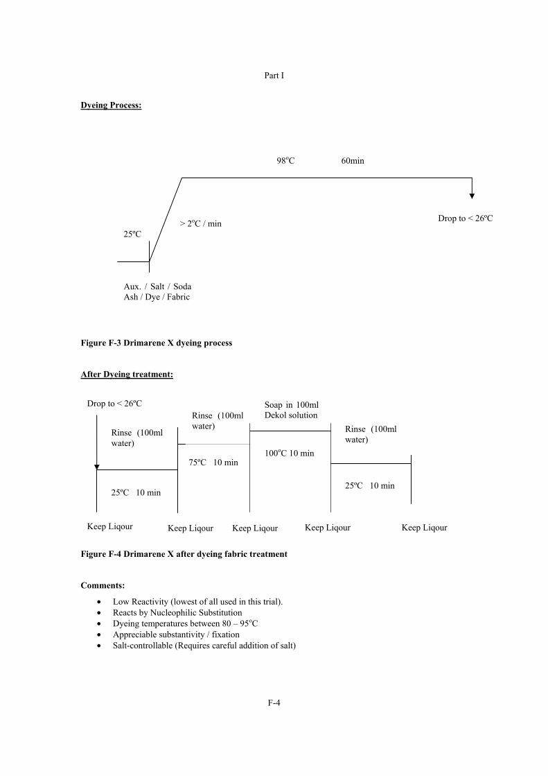
Part I

F-4

Dyeing Process:

Figure F-3 Drimarene X dyeing process

After Dyeing treatment:

Figure F-4 Drimarene X after dyeing fabric treatment

Comments:

Low Reactivity (lowest of all used in this trial). Reacts by Nucleophilic Substitution Dyeing temperatures between 80 – 95oC Appreciable substantivity / fixation Salt-controllable (Requires careful addition of salt)

98oC 60min

Aux. / Salt / Soda Ash / Dye / Fabric

25ºC > 2oC / min Drop to < 26ºC

Soap in 100ml Dekol solution

100oC 10 min

Rinse (100ml water)

25ºC 10 min

Keep Liqour Keep Liqour

Rinse (100ml water)

25ºC 10 min

Keep Liqour Keep Liqour

Drop to < 26ºC

Keep Liqour

Rinse (100ml water)

75ºC 10 min

Part I

F-5

F.3 Drimarene K Dyeing Procedure

Supplier: Clariant

Substrate: 10g 100% cotton single jersey knit, bleached

Liquor ratio: 10:1 (ml liquor / g fabric)

Dye type: Reactive Dyes

Dye class: Drimarene K

Chemistry: Flourochloropyrimidine (FCP)

Procedure: Exhaust

Table F-3 Drimarene K dyeing recipe

Recipes Amounts Beige Brown Violet Navy

Dyes

Drimarene Yellow K-2R % on fabric 0.400 1.134 - 0.548

Drimarene Brill. Red K-4BL % on fabric 0.164 0.430 - 1.090

Drimarene Blue K-2RL % on fabric 0.200 0.540 0.880 -

Drimarene Navy K-BNN % on fabric - - - 2.204

Drimarene Turquoise K-2B % on fabric - - - -

Drimarene Violet K-2RL % on fabric - - 0.660 -

Drimarene Black K-WO % on fabric - - - -

Auxiliaries

Tebolan UFN ml 2.000 2.000 2.000 2.000

Dekol AA-D ml 6.000 6.000 6.000 6.000

Avcoson LL ml 8.000 8.000 8.000 8.000

Chemicals

Common Salt (NaCl) g/l 40.000 60.000 60.000 80.000

Glauber’s Salt % on fabric - - - -

Soda Ash (NaCO3) g/l 1.500 2.500 2.500 4.000

Soaping Solution

Dekol AA-D 10g / 5L H2O 100.000 100.000 100.000 100.000

Part I

F-6

Dyeing Process:

Figure F-5 Drimarene K dyeing process

After Dyeing Treatment:

Figure F-6 Drimarene K after dyeing fabric treatment

Comments:

Relatively high reactivity Moderate fixation Dyeing temperatures between 40 – 60oC Alkali-controllable

Soap in 100ml Dekol solution

100oC 10 min

Rinse (100ml water)

25ºC 10 min

Keep Liquor Keep Liquor

Rinse (100ml water)

25ºC 10 min

Keep Liquor Keep Liquor

Drop to < 26ºC

Rinse (100ml water)

Keep Liquor

75ºC 10 min

60oC 60min

Drop to < 26ºC

25ºC

Aux. / Salt / NaCO3 /Dye / Fabric

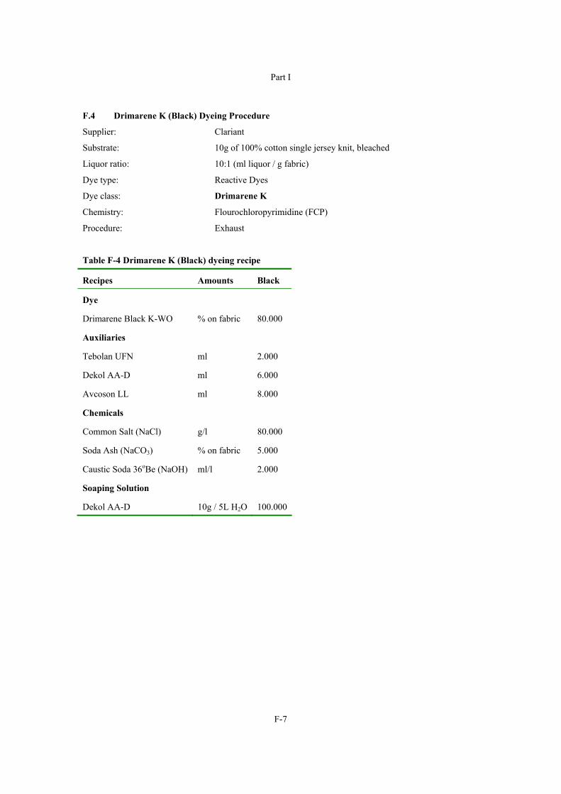
Part I

F-7

F.4 Drimarene K (Black) Dyeing Procedure

Supplier: Clariant

Substrate: 10g of 100% cotton single jersey knit, bleached

Liquor ratio: 10:1 (ml liquor / g fabric)

Dye type: Reactive Dyes

Dye class: Drimarene K

Chemistry: Flourochloropyrimidine (FCP)

Procedure: Exhaust

Table F-4 Drimarene K (Black) dyeing recipe

Recipes Amounts Black

Dye

Drimarene Black K-WO % on fabric 80.000

Auxiliaries

Tebolan UFN ml 2.000

Dekol AA-D ml 6.000

Avcoson LL ml 8.000

Chemicals

Common Salt (NaCl) g/l 80.000

Soda Ash (NaCO3) % on fabric 5.000

Caustic Soda 36oBe (NaOH) ml/l 2.000

Soaping Solution

Dekol AA-D 10g / 5L H2O 100.000

Part I

F-8

Dyeing Process:

Figure F-7 Drimarene K (Black) dyeing process

After Dyeing Treatment:

Figure F-8 Drimarene K (Black) after dyeing fabric treatment

Comments:

Relatively high reactivity Moderate fixation Dyeing temperatures between 40 – 60oC Alkali-controllable

Soap in 100ml Dekol solution

100oC 10 min

Rinse (100ml water)

25ºC 10 min

Keep Liqour Keep Liqour

Rinse (100ml water)

25ºC 10 min

Keep Liqour Keep Liqour

Drop to < 26ºC

Keep Liqour

Rinse (100ml water)

75ºC 10 min

50oC Start Cold with Dye / Salt / Fabric

60oC 30min 30min

Cool

Rinse Cold

Rinse Hot

Soda Ash Sodium Hydroxide (Caustic Soda)

> 2oC / min

Part I

F-9

F.5 Levafix CA Dyeing Procedure

Supplier: Dystar

Substrate: 10g of 100% cotton single jersey knit, bleached

Liquor ratio: 10:1 (ml liquor / g fabric)

Dye type: Reactive Dyes

Dye class: Levafix CA

Chemistry:

Procedure: Exhaust

Table F-5 Levafix CA dyeing recipe

Recipes Amounts Beige Brown Navy Violet

Dyes

Levafix Yellow CA gran % on fabric 0.460 1.150 0.740 0.031

Levafix Red CA gran % on fabric 0.120 0.314 0.740 -

Levafix Blue CA gran % on fabric 0.190 0.410 2.020 -

Levafix Brill. Red E-RN gran % on fabric - - - 0.460

Levafix Brill. Blue E-FFN gran 150% % on fabric - - - 2.250

Auxiliaries

Dekol AA-D ml 1.500 1.500 1.500 1.500

Subitol ml 2.500 2.500 2.500 2.500

Chemicals

Common Salt (NaCl) g/l 20.000 30.000 50.000 40.000

Soda Ash (NaCO3) g/l 6.000 9.000 14.000 12.000

Soaping Solution

Dekol AA-D 10g / 5L H2O 100.000 100.000 100.000 100.000

Part I

F-10

Dyeing Process:

Figure F-9 Levafix CA dyeing process

After dyeing Treatment:

Figure F-10 Levafix CA after dyeing fabric treatment

Keep Liquor

Soap in 100ml Dekol solution

100oC 10 min

Rinse (100ml water)

25ºC 10 min

Keep Liquor Keep Liquor

Rinse (100ml water)

25ºC 10 min

Keep Liquor

Drop to < 26ºC

Aux. / Dye / Salt / Soda Ash / Fabric

60oC 60min

25ºC > 2oC / min Drop to 26ºC

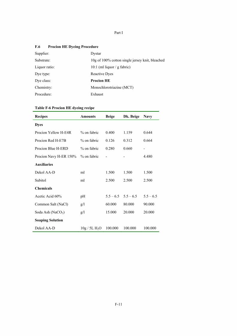
Part I

F-11

F.6 Procion HE Dyeing Procedure

Supplier: Dystar

Substrate: 10g of 100% cotton single jersey knit, bleached

Liquor ratio: 10:1 (ml liquor / g fabric)

Dye type: Reactive Dyes

Dye class: Procion HE

Chemistry: Monochlorotriazine (MCT)

Procedure: Exhaust

Table F-6 Procion HE dyeing recipe

Recipes Amounts Beige Dk. Beige Navy

Dyes

Procion Yellow H-E4R % on fabric 0.400 1.159 0.644

Procion Red H-E7B % on fabric 0.126 0.312 0.664

Procion Blue H-ERD % on fabric 0.280 0.660 -

Procion Navy H-ER 150% % on fabric - - 4.480

Auxiliaries

Dekol AA-D ml 1.500 1.500 1.500

Subitol ml 2.500 2.500 2.500

Chemicals

Acetic Acid 60% pH 5.5 – 6.5 5.5 – 6.5 5.5 – 6.5

Common Salt (NaCl) g/l 60.000 80.000 90.000

Soda Ash (NaCO3) g/l 15.000 20.000 20.000

Soaping Solution

Dekol AA-D 10g / 5L H2O 100.000 100.000 100.000

Part I

F-12

Dyeing Process:

Figure F-11 Procion HE dyeing process

After Dyeing Treatment:

Figure F-12 Procion HE after dyeing fabric treatment

Comments:

Low reactivity Dyeing temperatures between 80 – 85oC Appreciable substantivity Salt-controllable

Soap in 100ml Dekol solution

100oC 10 min

Rinse (100ml water)

25ºC 10 min

Keep Liquor Keep Liquor Keep Liquor

Rinse (100ml water)

25ºC 10 min

Keep Liquor

30ºC

(pH 10.6 – 11.0)

Keep Liquor

Rinse (100ml water)

100ºC

10 min

Aux. / Dye / Salt / Acetic acid / Fabric (pH 5.5 – 6.5)

80oC 60min

50oC 10min > 1.5oC / min

80oC 20min

Soda Ash 70oC

Drop to 30oC

(pH 10.6 – 11.0)

Part I

F-13

F.7 Bezaktive S Dyeing Procedure

Supplier: CHT

Substrate: 10g of 100% cotton single jersey knit, bleached

Liquor ratio: 10:1 (ml liquor / g fabric)

Dye type: Reactive Dyes

Dye class: Bezaktive S

Chemistry:

Procedure: Exhaust

Table F-7 Bezaktive S dyeing recipe

Recipes Amounts Beige Brown Purple Navy Black

Dyes

Bezaktive Yellow S-3R 150% % on fabric 0.374 0.100 - 0.350 -

Bezaktive Red S-3B 150% % on fabric 0.117 0.340 - 0.711 -

Bezaktive Blue S-GN 150% % on fabric 0.170 0.380 - - -

Bazaktive Red S-B % on fabric - - 0.340 - -

Bezaktive Blue S-FR 150% % on fabric - - 1.400 - -

Bezaktive Navy S-BL % on fabric - - - 2.698 -

Bezaktive Turq. V-G Conc. % on fabric - - - - -

Bezaktive Black S-GR % on fabric - - - - 7.600

Auxiliaries

Dekol AA-D ml 1.500 1.500 1.500 1.500 1.500

Subitol ml 2.500 2.500 2.500 2.500 2.500

Chemicals

Glauber’s Salt g/l 40.000 50.000 50.000 80.000 80.000

Soda Ash (NaCO3) g/l 5.000 5.000 5.000 5.000 5.000

Caustic Soda 38oBe (NaOH) ml/l 1.200 1.600 1.600 2.500 2.500

Soaping Solution

Dekol AA-D 10g / 5L H2O 100.000 100.000 100.000 100.000 100.000

Part I

F-14

Dyeing process:

Figure F-13 Bezaktive S dyeing process

After Dyeing Treatment:

Figure F-14 Bezaktive S after dyeing fabric treatment

F.8 Preparation of stock solutions

F.8.1 Preparation of 1% dyestuff solutions:

Weigh 1g of dry dyestuff powder or granules. Put it in a beaker and add little cold (dyeing) water. Paste up well and wash into a 100 ml flat bottom volumetric flask, preferably at 20ºC, to bring total volume to 100 ml.

Rinse (100ml water)

50ºC 10 min

Keep Liquor Keep Liquor

Drop to < 26ºC

Keep Liquor

Soap in 100ml Dekol solution

100oC 10 min

Keep Liquor Keep Liquor

Rise (100ml water)

25ºC 25ºC

10 min

Rinse

(100ml )

Aux. / Salt / Soda Ash /

Dye / Fabric

60oC 10min

Caustic Soda

60oC 50min

25oC Drop to < 26ºC

Part I

F-15

F.8.2 Preparation of auxiliary solutions 10% Dekol AA-D solution

Weigh 10 g of Dekol AA-D powder and add water to make up a total mass of 100 g. 10% Tebolan UFN

Weigh 10 g of Tebolan UFN powder and add water to make up a total mass of

100 g. 10% Avcoson LL

Weigh 10 g of Avcoson LL powder and add water to make up a total mass of

100 g. 10% Subitol

Weigh 10 g of Subitol powder and add water to make up a total mass of

100 g. 20% Soda Ash

Weigh 20 g of Soda Ash powder and add water to make up a total mass of

100 g. 38Be (100%) Caustic Soda

Take the concentrated Caustic Soda as given in the container without diluting it. 36Be (95%) Caustic Soda

Measure up 19 ml of concentrated Caustic Soda, add 1 ml water to make a total volume of 20 ml. 60% Acetic Acid

Measure up 12 ml of concentrated acetic acid and fill up to 20 ml with distilled water.

F.8.3 Preparation of Dekol AA-D soaping solution

Weigh 10 g of concentrated Dekol AA-D solution and add dyeing water to make up a total volume of

5 L.

F.9 Calculation of dyestuff and auxiliary quantities

All dyestuff stock solutions were prepared to have a 1% concentration in the manner described above.

Calculation of the volume of dyestuff to be used is as follows:

/V WxP C

Where: V = volume (ml)

W = weight (g) of sample to be dyed

P = percentage of dye or auxiliary to be used (on weight of fibre)

C = concentration (%) of stock solution

Part I

G-1

Appendix G Dye Trials Analytical Procedures

G.1 pH and conductivity

The conductivity measurements were performed using a Model 4310 Jenway conductivity meter with auto ranging from 0.01 µS/m to 1 999.9 mS/m and conductivity reading accuracy of ±2 digits and temperature accuracy of 0.5°C.

The pH measurements were performed using a Jenway 3310 pH meter with accuracy of ±2 digits.

G.2 Chemical oxygen demand (COD)

COD measurements were performed using the Open Reflux Method and measured in gO2 / L (APHA, 1985). Chloride ions interference was avoided by diluting the samples 60 times with distilled was to ensure chloride ion concentrations below the recommended limit of 2 000 mg/L ((Burns and Marshall, 1965); (APHA, 1985) ).

G.3 Colour measurements

Colour in the effluent was determined using ADMI (American Dye Manufacturers Institute) values as described by Allen et al. (1973). The conversion of tristimulus to Munsell values were taken from the appendix of McLaren’s colour difference formula paper of 1970 (McLaren, 1970).

The values for the XYZ Munsell values were plotted in Excel and the curve was used to generate automatic Munsell values from tristimulus values. The sum of errors for the Vx, Vy, and Vz Munsell values were 0.04, 0.02, and 8.49 respectively.

Calibration of the spectrophotometer was prepared according to Allen et al., 1973 and the calibration curve is given in Figure G1.

Part I

G-2

y = 1502.8x - 4.6279R2 = 0.9973

0

100

200

300

400

500

600

0 0.05 0.1 0.15 0.2 0.25 0.3 0.35 0.4

Delta E

AD

MI C

olou

r V

alue

s

Figure G1 Calibration curve for the ADMI colour standards

Allen et al. (1973) mentioned that the calibration factor for standard of APHA 50, APHA 100 and APHA 150 colour intensity should be around 14 000 and that the average calibration factor of all the standard aliquots can be used instead of a single calibration factor. For this experiment the calibration factor for APHA 50 and APHA 100 was 1 515 and was 1 497 for APHA 150. An average calibration factor of 1 498, (average of calibration factors for APHA 50 to 500) was used for all the ADMI calculations.

PART II

Modelling of the effects of textile industry wastewaters on the performance of a municipal watewater treatment plant

Part II

i

Table of Contents List of Figures.............................................................................................................................................. v List of Tables ............................................................................................................................................. vii Glossary .................................................................................................................................................... viii List of Abbreviations and Symbols............................................................................................................. ix Chapter 1 Introduction .............................................................................................................................. 1-1

1.1 Motivation ............................................................................................................................. 1-1 1.2 Aims ...................................................................................................................................... 1-1 1.3 Outline ................................................................................................................................... 1-2

Chapter 2 Literature review ...................................................................................................................... 2-1 2.1 The Toxicity and Inhibitory Nature of Textile Wastewaters ................................................. 2-1 2.2 Respirometry ......................................................................................................................... 2-1

2.2.1 Respirometric Techniques................................................................................................. 2-2 2.3 Optimal Experimental Design (OED).................................................................................... 2-4

2.3.1 Optimal Experimental Design Concept ............................................................................ 2-4 2.4 Description of Activated Sludge Kinetic Models .................................................................. 2-6

2.4.1 Activated Sludge Model No. 1 (ASM1) ........................................................................... 2-6 2.4.2 Activated Sludge Model 3 (ASM3) ................................................................................ 2-11

2.5 Mathematical Process Model Building................................................................................ 2-16 2.5.1 Problem Formulation ...................................................................................................... 2-17 2.5.2 Prior Knowledge Collection............................................................................................ 2-17 2.5.3 Frame Definition............................................................................................................. 2-17 2.5.4 Model Structure Selection............................................................................................... 2-18 2.5.5 Parameter Estimation ...................................................................................................... 2-18 2.5.6 Model Diagnosis ............................................................................................................. 2-18 2.5.7 Model Testing ................................................................................................................. 2-18

2.6 Identifiability Study for Dynamic Process Models.............................................................. 2-18 2.6.1 Structural Identifiability.................................................................................................. 2-19 2.6.2 Practical Identifiability.................................................................................................... 2-19

2.7 Parameter Estimation of Dynamic Models .......................................................................... 2-19 2.7.1 Selection of parameters................................................................................................... 2-19 2.7.2 Initial Estimates of the Parameters.................................................................................. 2-20

2.8 COST Benchmark Model .................................................................................................... 2-20 Chapter 3 Mathematical Modelling Theory.............................................................................................. 3-1

3.1 Kinetic Effect of Inhibition.................................................................................................... 3-1 3.2 Description of the Batch Respirometric Experiment (BRE) Model....................................... 3-2

3.2.1 BRE Components.............................................................................................................. 3-4 3.2.2 BRE Processes .................................................................................................................. 3-4

Part II

ii

3.3 BRE Model Inputted into WEST Simulation Engine ............................................................ 3-5 3.3.1 Background of WEST Software Package ......................................................................... 3-5 3.3.2 WEST Subprograms ......................................................................................................... 3-5

3.4 Identifiability Study of Dynamic ModelS.............................................................................. 3-6 3.4.1 Structural Identifiability.................................................................................................... 3-6 3.4.2 Practical Identifiability...................................................................................................... 3-7

3.5 Parameter Estimation of BRE Model .................................................................................... 3-9 3.5.1 Objectives in Parameter Estimation: Estimators ............................................................... 3-9 3.5.2 Using WEST for Parameter Estimation of BRE Model.................................................... 3-9

Chapter 4 Batch Respirometric Experiment ............................................................................................. 4-1 4.1 Batch Respirometric Experiments Setup ............................................................................... 4-1

4.1.1 The bioreactor and respirometer ....................................................................................... 4-1 4.1.2 Oxygen Uptake Rate (OUR) Meter................................................................................... 4-2 4.1.3 Computer System.............................................................................................................. 4-5

4.2 Analytical Tests ..................................................................................................................... 4-5 4.3 Application of the OED Procedure to the Batch Respirometric Experiment Design............. 4-5

4.3.1 First Series of Respirometric Experiments: ...................................................................... 4-6 4.3.2 Second Series of Respirometric Experiments ................................................................... 4-8 4.3.3 Third Series of Respirometric Experiments: ..................................................................... 4-9 4.3.4 Fourth Series of Respirometric Experiments .................................................................. 4-11

4.4 The Batch Respirometric Optimal Experiment Design ....................................................... 4-16 4.5 Results of Batch Respirometric Experiments ...................................................................... 4-17

Chapter 5 BRE Model Simulation Results and Discussion ...................................................................... 5-1 5.1 Identifiability Study of BRE Model....................................................................................... 5-1

5.1.1 Structural Identifiability of BRE Model ........................................................................... 5-1 5.1.2 Practical Identifiability of BRE Model ............................................................................. 5-1

5.2 Parameter Estimation of BRE Model .................................................................................... 5-4 Chapter 6 Assessment of Wastewater Treatment Works Performance..................................................... 6-1

6.1 Background on COST and the COST Simulation Benchmark .............................................. 6-1 6.2 Overview of The COST Simulation benchmark Model ........................................................ 6-1

6.2.1 Process models.................................................................................................................. 6-3

6.3 Modifications made to the simulation benchmark kinetic process model ............................. 6-5 6.4 Simulation Procedure............................................................................................................. 6-6

6.4.1 Steady-state simulations.................................................................................................... 6-7 6.4.2 Dynamic simulations ........................................................................................................ 6-7

6.5 Performance indices of simulation benchmark...................................................................... 6-7 6.5.1 Effluent quality index........................................................................................................ 6-7 6.5.2 Effluent Violations............................................................................................................ 6-9 6.5.3 Operational Costs.............................................................................................................. 6-9

6.6 Results from COST benchmark simulations for both dyes.................................................. 6-11

Part II

iii

Chapter 7 Discussion ................................................................................................................................ 7-1 7.1 Respirometric Experiments.................................................................................................... 7-1 7.2 Batch Respirometric Experiment (BRE) model..................................................................... 7-1 7.3 Assessment of Impact to WWTW Performance .................................................................... 7-2

Chapter 8 Conclusions and Recommendations......................................................................................... 8-1 References................................................................................................................................................ R-1 Appendix A Reagent Preparation ........................................................................................................... A-1 Appendix B Equipment and Calibration ................................................................................................. B-1 Appendix C Estimating COD ................................................................................................................. C-1 Appendix D Experimental Procedures.................................................................................................... D-1

Part II

iv

Part II

v

List of Figures Figure 2-1 Flow diagram of a respirometer (Spanjers et al., 1998) .................................................... 2-2 Figure 2-2 Schematic of Optimal Experimental Design (OED) procedure (De Pauw, 2005) ........... 2-5 Figure 2-3 COD components of ASM1 adapted from (Petersen, 2000)............................................. 2-9 Figure 2-4 Nitrogen components of ASM1 adapted from (Petersen, 2000) ..................................... 2-10 Figure 2-5 COD components of ASM3 adapted from (Petersen, 2000)........................................... 2-14 Figure 2-6 Nitrogen components of ASM3 adapted from (Gujer et al., 1999)................................. 2-15 Figure 2-7 The model building procedure (Castensen et al., 1997).................................................. 2-17 Figure 2-8 Flow diagram of the 'simulation benchmark' configuration showing activated sludge .........

units (ASU) 1 and 2 mixed and unaerated and ASU 3, 4 and 5 aerated.......................... 2-20 Figure 2-9 COST simulation benchmark model configuration as appears in WEST ....................... 2-21 Figure 4-1 Schematic of respirometer used in Batch Respirometric Experiments ............................. 4-2 Figure 4-2 Overview of components of the Batch Respirometric Experiment adapted from .................

(Randall et al., 1991)......................................................................................................... 4-2 Figure 4-3 Saw-tooth waveform of the DO concentration-time trace obtained from on-off ..................

aeration adapted from (Randall et al., 1991)..................................................................... 4-4 Figure 4-4 Regressed fits of OUR when nitrification is inhibited ...................................................... 4-7 Figure 4-5 Regressed fits of OUR when nitrification is uninhibited .................................................. 4-7 Figure 4-6 Regressed fits of OUR when nitrification is uninhibited .................................................. 4-8 Figure 4-7 Regressed fits of OUR when nitrification is uninhibited .................................................. 4-9 Figure 4-8 Regressed fits of OUR when nitrification is uninhibited ................................................ 4-11 Figure 4-9 Regressed fits of OUR when nitrification is uninhibited ................................................ 4-11 Figure 4-10 OUR profile with two sodium acetate (60mgCOD/L) substrate spikes .......................... 4-14 Figure 4-11 OUR profile with two ammonia chloride (4mgN/L) substrate spikes............................. 4-14 Figure 4-12 Regressed fits of OUR after addition of 60 mg/L sodium acetate................................... 4-15 Figure 4-13 Regressed fits of OUR after addition of 4 mg/L ammonium chloride ............................ 4-16 Figure 4-14 (a) OUR profile with sodium acetate (30mgCOD/L) substrate and high scoring ............

toxicant dye Drimarene Violet K2-RL. (b) OUR profile with ammonium ....................... chloride (8mgN/L) substrate and high scoring toxicant dye Drimarene .......................... Violet K2-RL............................................................................................................... 4-19

Figure 4-15 (a) OUR profile with sodium acetate (30mgCOD/L) substrate and low scoring .............. toxicant dye Levafix Blue CA gran, (b) OUR profile with ammonium ............................ chloride (8mgN/L) substrate and low scoring toxicant dye Levafix Blue CA gran .... 4-20

Figure 5-1 Heterotrophic parameters sensitivity measure .................................................................. 5-2 Figure 5-2 Autotrophic parameters sensitivity measure ..................................................................... 5-3 Figure 5-3 (a-d) Regressed fits of OUR for acetate substrate and high scoring dye runs. .................. 5-5 Figure 5-4(a-d) Regressed fits of OUR for ammonia substrate and high scoring dye runs. ..................... 5-6 Figure 5-5 (a-e) Regressed fits of OUR for acetate substrate and low scoring dye runs ................... 5-7 Figure 5-6 (a-d) Regressed fits of OUR for ammonia substrate and low scoring dye runs ............... 5-8 Figure 6-1 Schematic representation of the simulation benchmark plant layout ............................... 6-1 Figure 6-2 COST simulation benchmark model configuration as appears in WEST ......................... 6-6

Part II

vi

Figure 6-3 The relationship between effluent quality index and dye concentration for high and ........... low scoring dyes. ............................................................................................................ 6-12

Figure 6-4 The relationship between sludge disposal and dye concentration for high and .................... low scoring dyes. ............................................................................................................ 6-12

Figure 6-5 The relationship between total sludge production and dye concentration for high and ........ low scoring dyes. ............................................................................................................ 6-13

Figure 6-6 The relationship between Number of effluent violation and dye concentration for .............. (a) high and (b) low scoring dyes.................................................................................... 6-14

Figure 6-7 The relationship between time in violation and dye concentration for (a) high and .............. (b) low scoring dyes....................................................................................................... 6-15

Part II

vii

List of Tables Table 2-1 Typical Petersen matrix .................................................................................................... 2-6 Table 2-2 ASM1 process matrix (Henze et al., 1987) ....................................................................... 2-8 Table 2-3 Stoichiometric matrix of ASM3 (Gujer et al., 1999) ...................................................... 2-12 Table 2-4 Process rate equations of ASM3 (Gujer et al., 1999)...................................................... 2-13 Table 3-1 Definition of inhibition types (Volskay and Grady, 1988)................................................ 3-1 Table 3-2 Quantification of inhibitory effects using simple reversible linear inhibition .......................

models adapted from (Volskay and Grady, 1988) ............................................................ 3-2 Table 3-3 Batch Respirometric Experiment (BRE) kinetic model .................................................... 3-3 Table 3-4 Identifiable parameter combinations for heterotrophic growth kinetics ...............................

(Dochain et al., 1995)........................................................................................................ 3-6 Table 4-1 Estimated parameters obtained from the first experiment design data compared .................

to those presented in literature .......................................................................................... 4-6 Table 4-2 Estimated parameters obtained from the second experiment design data compared ............

to those presented in literature .......................................................................................... 4-9 Table 4-3 Estimated parameters obtained from the third experiment design data compared ................

to those presented in literature ........................................................................................ 4-10 Table 4-4 Parameter estimate results and confidence intervals performed on experimental .................

data obtained from sodium acetate and ammonium chloride experiments ..................... 4-13 Table 4-5 Cumulative dye concentrations used for respirometric experiments (mg/L) .................. 4-21 Table 5-1 Heterotrophic parameters ranked according to importance............................................... 5-2 Table 5-2 Autotrophic parameters ranked according to importance ................................................. 5-3 Table 5-3 BRE model parameters and defaults values...................................................................... 5-4 Table 5-4 Parameter estimate results and confidence intervals performed on experimental .................

data obtained from high scoring dye respirometric experiments ...................................... 5-9 Table 5-5 Parameter estimate results and confidence intervals performed on experimental .................

data obtained from low scoring dye respirometric experiments ....................................... 5-9 Table 5-6 Inhibition parameter values for high and low scoring dyes ............................................ 5-10 Table 6-1 Physical attributes of the activated sludge units and settler for the COST ............................

simulation benchmark plant configuration........................................................................ 6-2 Table 6-2 System variables of the COST simulation benchmark plant configuration ...................... 6-2 Table 6-3 ASM1 stoichiometric parameter default values used in the simulation benchmark.......... 6-3 Table 6-4 ASM1 kinetic parameter default values used in the simulation benchmark ..................... 6-4 Table 6-5 Settler model parameters and default values..................................................................... 6-5 Table 6-6 Flow-weighted average dry weather influent composition (COST 624, 2005)................. 6-5

Table 6-7 i Factors for composite variables .................................................................................. 6-9

Table 6-8 Effluent constraints values ................................................................................................ 6-9

Part II

viii

Glossary Acclimation The adaptation of a microbial community to degrade a previously recalcitrant

compound through prior exposure.

Activated sludge A mixed association of prokaryotic and eukaryotic micro organisms, which aerobically decompose waste in a activated sludge effluent treatment system.

Adaptation A change in the microbial community that increases the rate of transformation of a test compound as a result of prior exposure to that test compound.

Aerobic The condition of living or acting only in the presence of molecular oxygen.

Algae Organisms that perform oxygenic photosynthesis and possess chloroplasts. May be single or multi cellular organisms.

Azo dyes Dyes which contain at least one azo group (-N=N-), and can contain up to four azo groups.

Bacteria Single-cell, prokaryotic micro organisms.

Batch culture A closed culture environment in which conditions are continuously changing according to the metabolic state of the microbial culture.

Biodegradable A property which allows the microbial decomposition of an organic compound to inorganic molecules.

Chemical oxygen demand

A measure of the total amount of organic waste stream.

Degrade Breakdown into simpler substances by bacterial action.

Effluent A stream flowing from a sewage tank or industrial process.

Inhibition An impairment of bacterial function.

Kinetics The explanation of the observed characteristics of chemical reactions.

Pollution An adverse alteration of the environment.

Reactive dyes Reactive dyes are coloured components capable of forming a covalent bond between the dye molecule and the fibre.

Recalcitrant Resistant to microbial degradation.

Respiration The oxidative breakdown and release of energy from nutrient molecules by reactions with molecular oxygen.

Seeding The use of an actively digesting sludge to aid the start-up of a digester by supplying a quantity of the preferred types of organisms. This usually reduces the time taken for a digester to become active.

Sludge The general term applied to the accumulated solids separated from wastewater. A large portion of the sludge material in a digester consists of bacteria which are responsible for its decomposition.

Suspended solids

Undissolved non-settleable solids present in wastewater.

Toxicity An adverse effect (not necessarily lethal) on bacterial metabolism.

Wastewater General term to denote a combination or mixture of domestic sewage and industrial effluents.

Part II

ix

List of Abbreviations and Symbols 1. Abbreviations

Name Description Unit

a Mole hydrogen in 1 mol-C of biomass

ASM Activated sludge model

ASM1 Activated sludge model number 1

ASM2 Activated sludge model number 2

ASM2d Activated sludge model number 2d

ASM3 Activated sludge model number 3

ATU Allylthiourea

b Mole oxygen in 1 mol-C of biomass

BOD Biological oxygen demand mg O2/L

BRE Batch respirometric experiment

c Mole nitrogen in 1 mol-C of biomass

CHaObNc Molecular composition of biomass 1 mol-C

COD Chemical oxygen demand mg COD/L

COV Covariance matrix (inverse of FIM)

DWAF Department of Water Affairs and Forestry

EU European Union

FIM Fisher Information Matrix

KLa Mass transfer coefficient

MLVSS Mixed liquor volatile suspended solids mg SS/L

NH4-N Ammonium concentration mg N/L

NH3 Ammonia nitrogen mg NH3-N/L

NO2-N Nitrite nitrogen mg NO2-N/L

NO3-N Nitrite nitrogen mg NO3-N/L

ODE Ordinary differential equation

OED Optimal experimental design

pH Negative logarithm of proton concentration

S0/X0 Initial substrate to biomass ratio

S/X Substrate to biomass ratio

TKN Total kjeldahl nitrogen mg N/L

Part II

x

WWTW Wastewater treatment works

2. Roman symbols

Symbol Description Unit

Ab Endogenous decay coefficient of autotrophic biomass 1/d

Hb Endogenous decay coefficient of heterotrophic biomass 1/d

DO Dissolved oxygen concentration mg O2/L

Pf Inert particulate fraction of the biomass

I Inhibitor concentration mg/L

J Objective function

hk Hydrolysis rate 1/d

NHK Ammonium half-saturation constant mg N/L

NOK Nitrate half-saturation constant mg N/L

OAK Oxygen half-saturation constant for autotrophic biomass mg O2/L

OHK Oxygen half-saturation constant for biomass heterotrophic mg O2/L

SK Substrate half-saturation constant mg COD/L

XK Particulate COD half-saturation constant mg COD/L

N Number of data points

p Number of parameters

OUR Oxygen uptake rate mg O2/L.min

endOUR Endogenous oxygen uptake rate mg O2/L.min

exoOUR Exogenous oxygen uptake rate mg O2/L.min

maxOUR Maximum oxygen uptake rate value mg O2/L.min

Q Measurement error covariance matrix

NDS Soluble degradable organic nitrogen mg N/L

0NHS Initial ammonium concentration mg N/L

NHS Ammonium concentration mg N/L

Part II

xi

NOS Nitrate concentration mg N/L

OS Oxygen concentration mg O2/L

0SS Initial soluble readily biodegradable COD mg COD/L

SS Soluble readily biodegradable COD mg COD/L

V Reactor volume L

0v Maximum settling velocity

AY Autotrophic yield coefficient mg COD/mg NH4-N

HY Heterotrophic yield coefficient mg COD/mg COD

BAX Autotrophic biomass concentration mg COD/L

0BHX Initial heterotrophic biomass concentration mg COD/L

BHX Heterotrophic biomass concentration mg COD/L

NDX Particulate degradable organic nitrogen mg N/L

SX Slowly biodegradable COD mg COD/L

3. Greek symbols

Symbol Description Unit

msqr Parameter sensitivity

g Anoxic growth reduction factor

Parameter

A Growth rate for autotrophic biomass 1/d

mA Maximum growth rate of autotrophic biomass 1/d

H Growth rate for heterotrophic biomass 1/d

mH Maximum growth rate of autotrophic biomass 1/d

A First order time constant in autotrophic activity min

H First order time constant in heterotrophic activity min

Standard deviation

Part II

xii

2 Variance

Part II

1-1

CHAPTER 1 Introduction

1.1 MOTIVATION

Sewage treatment processes have evolved substantially over the past 50 years, however their primary objective is the biological degradation of organic compounds from faecal and household waste, the transformation of nitrogen to nitrates or nitrogen gas and the removal of phosphorus in the waste sludge. Sewage treatment works have not been developed to degrade xenobiotic compounds and salts. The regulatory authorities attempt to limit the harm to the water resources (and to the sewage treatment processes) by devising "trade effluent regulations". However due to the large and increasing range of industrial chemicals in use it is not possible for the authorities to monitor all chemicals discharged by industry. The use of proprietary formulations and the presence of trace co-products and by-products add to the difficulty of surveillance. If industrial effluents are to be allowed to be conveyed from industry using the sewerage system, proactive methods need to be investigated to manage the large of potential harmful chemicals that could be discharged.

Part 2 describes the experimental determination and modelling of the inhibitory effects of textile dyes on activated sludge processes. More specifically it investigates whether the score system accurately describes the negative impact of the textile dyes on wastewater treatment works activated sludge processes. Reliable laboratory and modelling methods are required to assess the inhibitory effect of the textile dyes on activated sludge processes. It is envisaged that this combined laboratory-modelling method will aid in the future aims of the Pollution Research Group; of creating a database of eThekwini Municipality wastewater treatment works models and creating a new tariff system for industries which discharge industrial effluent to wastewater treatment works.

1.2 AIMS

The specific aims of the work described in section were to:

use the score system to choose a high and low scoring dye to be used in laboratory experiments.

design a respirometric experiment that provides rapid and reliable experimental data that can be used for process modelling.

create or use an existing activated sludge model, along with respirometric experiment data to obtain kinetic data which can represent the inhibition caused by textile dyes.

create or use existing wastewater treatment works model, along with kinetic data collected from the process modelling to assess whether the high scoring dye has a greater negative impact on the wastewater treatment works activated sludge processes.

This section attempts to provide:

A methodology to evaluate the impact of toxic substances on wastewater treatment works activated sludge processes.

An optimal respirometric experiment design that will provide reliable data to be used in process modelling.

An activated sludge model which can be used to determine kinetic data to be used later in wastewater treatment works modelling.

A protocol to using the COST Simulation Benchmark procedure (Copp, 2001) to evaluate the effect of toxic substances on a wastewater treatment works model.

Part II

1-2

1.3 OUTLINE

Part 2 is structured as follows:

Chapter 2: This chapter is the Literature Review and includes a detailed discussion of the inhibitory nature of textile wastewaters, respirometry, Optimal Experiment Design (OED) (Dochain and Vanrolleghem, 2001) and activated sludge kinetic modelling. A brief description of mathematical process modelling and the COST simulation benchmark model (Copp, 2001) used in this study is provided in this chapter. Mathematical process modelling theory is discussed in Chapter 3. The COST simulation benchmark model is described in detail in Chapter 6.

Chapter 3: This chapter provides the mathematical process modelling theory used in the quantification of the inhibitory nature of textile dye effluent on the activated sludge processes. A Batch Respirometric Experiment (BRE) model was created to obtain the relevant information to quantify the inhibition of textile dyes on the kinetics of biomass respiratory activity. To determine which of the parameters of the model are central in quantifying the inhibition, the kinetic effects of inhibition have been investigated. Subsequently the BRE model was inputted into wastewater treatment modelling program WEST. A continuity check and the identifiability study were performed of the BRE model. The model theory of parameter estimation and the method used in WEST is also discussed.

Chapter 4: This chapter describes the batch respirometric experimental protocol developed to quantify the inhibitory effects of textile dyes. The respirometric protocol developed provides information rich data which reliable parameter estimation can be performed. Previous unsuccessful experimental designs used during the optimising of the experimental design are discussed. The batch respirometric experimental optimal design along with the results from this experiment design is presented. This experimental data is used in Chapter 5 for parameter estimation.

Chapter 5: In this chapter the results from the identifiability study and parameter estimation performed on the BRE model are presented and discussed. The type of inhibition and the resultant inhibition kinetics of both dyes used in this study are presented. These inhibition kinetics are inputted in the COST benchmark simulation model in Chapter 6.

Chapter 6: In this chapter the impact of the textile dyes on the wastewater treatment works performance is assessed, the COST simulation benchmark was used for this assessment. Background information on COST and the concept of the COST simulation benchmark are discussed. The simulation benchmark model was used in this study to quantify the inhibitory effect of two dyes and determine whether the high scoring dye has a greater negative impact on wastewater treatment works performance than the low scoring dye.

Chapter 7: In this chapter the broad spectrum impact of the results presented in Chapter 4, Chapter 5 and Chapter 6 are discussed. The formulation of the conclusion and recommendations stated in Chapter 8 is presented in this chapter.

Chapter 8: This chapter presents the conclusion and recommendations.

Part II

2-1

CHAPTER 2 Literature review

This chapter provides some background information on the theoretical concepts referred to in this report. Descriptions of the inhibitory nature of textile wastewaters, the score system, respirometry, activated sludge kinetic models, Optimal Experiment Design (OED), mathematical process modelling and the COST simulation benchmark model used in this study are provided in this chapter. The COST simulation benchmark model, the respirometric experiments and the activated sludge model used in parameter estimation will be discussed in greater detail at a later stage.

2.1 THE TOXICITY AND INHIBITORY NATURE OF TEXTILE WASTEWATERS

Toxicity is an adverse effect (not necessarily lethal) on the metabolism of bacteria, and inhibition is the impairment of bacteria function (Speece, 1996). Aesthetic environmental impacts is a recognised problem associated with textile dye effluents but potential toxic effects are also of concern. Toxic effects on algal growth (Willetts, 1999) has a major impact on the ecosystem as algal photosynthesis is a major source of oxygen in river water. Toxicity to fish has also been documented (Laing, 1991).

In addition to being potentially toxic if discharged to the environment, textile dyes are designed to be resistant to oxidation. Hence textile dye effluents are also resistant to oxidative microbial breakdown in conventional aerobic wastewater treatment. The treatment of textile dyes by activated sludge has been researched extensively by many researchers (Flege, 1970; Pagga and Brown, 1986), who have found that some dyes are partially degraded but most remain untreated.

Azo reactive dyes are particularly difficult to treat biologically and account for about 70% of all the textile dyestuffs produced. They are water-soluble synthetic organic colourants possessing the characteristics azo (-N=N-) bond and are capable of forming a covalent bond between the dye molecule and fibre (Godefroy, 1993). Studies have shown that aerobic processes at conventional wastewater treatment works are unable to substantially degrade azo dyes since the strong electron withdrawing character of the azo group stabilizes these aromatic pollutants against conversion by bacteria (Razo-Flores, 1997).

In addition to being difficult to treat, dyes may be toxic to the activated sludge and result in a decrease of overall process performance. Autotrophic biomass responsible for nitrification process is considered to be more sensitive to toxins, than the heterotrophic biomass which is responsible for the carbon oxidation process (Blum and Speece, 1991).

The Score system described in Part I of this report is a system for ranking industrial chemicals such as dyes based on their expected negative environmental impacts. The hypothesis of this is study is that a low score translates to a low toxicity to the activated sludge processes at a municipal wastewater treatment works. Therefore the Score System may be a an effective tool for identifying those dyes which will have the greatest negative impact on wastewater treatment plants in order to replace them with more benign alternatives.

2.2 RESPIROMETRY

In this study, respirometry was used to determine the impacts of two different dyes on biological processes in activated sludge. Respirometry is frequently used in wastewater characterisation and in the determination of activated sludge model kinetics. Respirometry is a measure of the respiration rate of activated sludge biomass and is defined as the amount of oxygen per unit volume and time consumed by the activated sludge biomass. Respirometric data can be used for modelling purposes and in the control of aerobic activated sludge processes (Henze et al., 1987; Vanrolleghem et al., 1999). Figure 2-1 shows a generalised flow diagram of a respirometer (Spanjers et al., 1998) Respirometers can be classified based on two criteria:

1. The phase in which the oxygen concentration is measured (liquid or gas phase)

2. Batch or continuous flow regime of the gas and liquid phases (flowing or static flow)

Part II

2-2

Figure 2-1 Flow diagram of a respirometer (Spanjers et al., 1998)

In most cases dissolved oxygen concentration is measured in the liquid phase. By performing a general mass balance for dissolved oxygen concentration OS presented in Equation 2-1, the respiration rate can

be obtained. The equation consists of a transport term ,in

O in OQ S SV

, aeration term

0L O OK a S S and the oxygen uptake rate OUR of the biomass. The transportation term and

aeration term may be removed depending on the configuration of the respirometer.

0,

O inO in O L O O

dS Q S S K a S S OURdt V

2-1

2.2.1 Respirometric Techniques In the following the sections different respirometric techniques are examined and the advantages and disadvantages of these techniques in wastewater and kinetic characterisation are discussed.

2.2.1.1 Static gas – flowing liquid Static gas – flowing liquid respirometers is a continuous system in which the dissolved oxygen concentration ( OS ) is measured at the inlet and outlet of a closed respiration vessel (Spanjers, 1993).

Aerated sludge is continuously pumped through the respiration vessel. The OUR is calculated from the dissolved oxygen mass balance over the unaerated respiration vessel, shown in Equation 2-2:

,O in

O in OdS Q S S OURdt V

2-2

Where:

,O inS = inlet dissolved oxygen concentration

OS = outlet dissolved oxygen concentration

inQ V = residence time in respiration vessel

For this type of respirometer a closed respiration vessel the aeration term 0L O OK a S S in

Equation 2-1 is absent from the dissolved oxygen mass balance, hence complex substrates such as

GAS

LIQUID

Part II

2-3

wastewater can be used because the LK a value determination is not required. Knowledge of the flow

rate and reactor volume is required to calculate the residence time inQ V . The flowrate should be adjusted so as to prevent oxygen limitation condition. When there is a small difference between the two dissolved oxygen probes ,O in OS S drift in the electrodes may result in erroneous OUR data. To

resolve this problem the dissolved oxygen concentration of the inlet and outlet are measured by the same dissolved oxygen probe, this is achieved by switching the direction of flow in the respiration vessel (Spanjers, 1993). This frequent switch in flow direction results in lower measurement frequency of OUR (Vanrolleghem and Spanjers, 1998).

2.2.1.2 Static gas – static liquid Static gas – static liquid respirometers are typically operated by aerating for short period of time thereafter monitoring the decline of dissolved oxygen concentration with time in a closed vessel (Cech et al., 1984; Kappler and Gujer, 1992; Kristensen et al., 1992). For this type of respirometer the mass balance of dissolved oxygen shown in Equation 2-1 is simplified to Equation 2-3, since the transportation and aeration terms are removed.

OdS OURdt

2-3

These respirometers are closed vessels with no head space, since no aeration of the activated sludge sample through surface aeration or bubble in the liquid phase must occur during the experiment. In the case of an open vessel being used the measured data may be influenced by surface aeration, in this case an aeration term may be included in the mass balance equation. Typically the influence of surface aeration is ignored (Takamatsu et al., 1982; Randall et al., 1991). The oxygen transferred through the liquid-air interface can be limited by covering the liquid surface with plastic balls (Wentzel et al., 1995), or by using a vessel that is the diameter of the dissolved oxygen electrode (Gernaey et al., 1997).

The experiments performed with this design are carried out with high substrate concentration and low biomass concentrations (high 0 0S X ratio) to prevent oxygen limitation conditions. The danger in

performing the respirometric experiment under high 0 0S X ratio is that the sludge behaviour may not be representative of the full scale system (Novak et al., 1994). This type of respirometer is limited in the characterisation of wastewater and determination of activated sludge kinetics. Since the experiments are performed under high 0 0S X ratio the maximum specific growth rate ( max ) may be determined but

the half-saturation constant ( SK ) cannot be determined because the substrate concentration may never

drop near the value of SK . Furthermore the problem of oxygen limitation condition associated with this type of respirometer has been resolved by frequent re-aeration of the sample (Suschka and Ferreira, 1986; Watts and Garber, 1993). In addition another solution to the oxygen limitation problem condition has been to over saturate the activated sludge sample with oxygen (Ellis et al., 1996), but the shortcoming of this solution is that the dissolved oxygen concentration will differ from the full-scale operating condition.

Static gas - static liquid respirometers sampling frequency of OUR cycle are rather low, since one OUR value would be obtained per aeration. This low sampling frequency is a disadvantage, because it results in difficulties in determining activated sludge kinetic parameters (Vanrolleghem and Spanjers, 1998).

2.2.1.3 Flowing gas – static liquid

In flowing gas – static liquid respirometers high concentration of sludge (low 0 0S X ratio) can be used because the vessel is continuously aerated, therefore no oxygen limitation does not occur (Blok, 1974; Farkas, 1981; Ros et al., 1988). An advantage of high sludge concentration 0X is shorter time for experiments. For this type of respirometer the mass balance of dissolved oxygen shown in Equation 2-1 is simplified to Equation 2-4, since the transportation is removed.

Part II

2-4

0OL O O

dS K a S S OURdt

2-4

To obtain reliable OUR data an optimal aeration should be determined. If the aeration is too high the OUR data may contain significant amount of measurement noise.

In general, oxygen uptake rate ( OUR ) can be considered to consist of two components (Spanjers, 1993) as shown in Equation 2-5; the exogenous oxygen uptake rate ( exoOUR ) which the uptake of the

degradable substrate and the endogenous oxygen uptake rate ( endOUR ).

exo endOUR OUR OUR 2-5

Under the assumption that endOUR is constant, Equation 2-4 can be changed to Equation 2-6 (Vanrolleghem et al., 1994).

,O

L O eq O exodS K a S S OURdt

2-6

When exoOUR is zero, the oxygen concentration in the vessel reaches a steady state value of ,O eqS which indicates that the oxygen transfer and endogenous respiration balance each other out. A flowing gas – static liquid respirometer allows a high frequency measure of OUR data as compared to the static gas – static liquid respirometers (Vanrolleghem et al., 1994). There are several methods to determine the value of the oxygen transfer coefficient LK a . It can be determined from a separate re-aeration experiment with sludge in the endogenous state (Bandyopadhyay et al., 1967) or from a re-aeration curve obtained after an addition of a known amount of readily biodegradable substrate to the system (Vanrolleghem et al., 1994).

2.3 OPTIMAL EXPERIMENTAL DESIGN (OED)

In this section the concept of is introduced and a detailed discussion is provided for the concept of OED applied to the design of an experiment in which the data will be used for parameter estimation..

2.3.1 Optimal Experimental Design Concept In this study, the optimal experimental design (ODE) methodology of Dochain and Vanrolleghem (Dochain and Vanrolleghem, 2001) was used to obtain the optimal batch respirometric experiment design. Obtaining quality experimental data is a critical task when this data is to be used in model building, model selection and parameter estimation. The experimental design is an important task for modelling, since the experiment design is the critical factor in obtaining good information-rich experiment data. The goals pursed in an experimental design procedure can be categorised in three areas; experiment design for a reliable selection of an adequate mathematical model structure of the process, the design of experiment for precise estimation of model parameters, and the dual problem of structure characterisation and parameter estimation (Dochain and Vanrolleghem, 2001).

There are a number of quantitative functions associated with the respective goal of the experimental design. The focus of this study is the design of an experiment for precise estimation of model parameters; therefore the experiment design procedure associated with this goal is discussed in detail. The Optimal Experimental Design (OED) procedure (Dochain and Vanrolleghem, 2001) is summarised in Figure 2-2 (De Pauw, 2005).

Part II

2-5

Once a preliminary model is created based on previously acquired data, the experiment degrees of freedom and constraints for the experimental design procedure are defined (De Pauw, 2005). The experiment degrees of freedom are subdivided into measurements and manipulations categories (Dochain and Vanrolleghem, 2001). With regard to the measurements in the experiment category several question can be posed: (1) what to measure, (2) where to measure and (3) when to measure (Dochain and Vanrolleghem, 2001). The manipulation category often is the most important category and relates to the excitation signal that acts on the system to produce highly qualitative information.

Figure 2-2 Schematic of Optimal Experimental Design (OED) procedure

(De Pauw, 2005)

The optimal experiment design procedure for parameter estimation (Dochain and Vanrolleghem, 2001) was applied in the design of this studies batch respirometric experiments. The assessment of the quality of a set of parameter estimates can be based on the way the parameters allow a model to make good predictions of process behaviour. However the most popular method of assessing the quality of parameter estimates is by providing information on the parameter estimation errors in the form of confidence intervals or by providing the covariance matrix. These concept are related to practical identifiability which and are discussed in detail in Section 2.6.2 and Chapter 3, Section 3.4.2.

Perform Initial Experiment(s)

Perform Proposed Experiment

Proposed Experiment

Calibrated Model

OK Calibrated Model

Simulate Experiment

Evaluate Objective Function

OK

Yes

Yes

No

No

Lab/Sensor Computer

Part II

2-6

2.4 DESCRIPTION OF ACTIVATED SLUDGE KINETIC MODELS

The most common wastewater treatment method is the activated sludge process. In this process bacteria (biomass) remove pollutants; these are in the form of organic carbon, nitrogen and phosphorus. The design of the wastewater treatment works determines which of the pollutants are removed. Dynamic kinetic models of the activated sludge processes have been created as a result of knowledge gained from research into the mechanisms of the different biological degradation processes. This review will focus primarily on Activated Sludge Model No. 1 (ASM1) (Henze et al., 1987), which is the most popular activated sludge model used in the design and operation of wastewater treatment works.

Information of the ASM1 (Henze et al., 1987) and ASM3 (Gujer et al., 1999) activated sludge models are covered. The activated sludge models which include phosphorus removal are not covered in this study, hence ASM2 and ASM2d (Henze et al., 1995; Henze et al., 1999) are not described.

2.4.1 Activated Sludge Model No. 1 (ASM1) ASM1 is presented in Petersen matrix format in Table 2-2 (Henze et al., 1987). Carbon substrates are defined in terms of Chemical Oxygen Demand (COD) and nitrogen substrates in terms of nitrogen content.

2.4.1.1 Fundamentals of Petersen matrix The Petersen matrix consists of the components (Ci), parameters (p), and processes (j). The components are state variables and vary with time. Processes are the transformation in which the components take part. The parameters are found in the stoichiometric expressions ( ji ) and in the process rate equations

( j ), these parameters are constant in respect to independent variables.

Table 2-1 Typical Petersen matrix

Components ↓ Processes

C1 C2 Ci Cn Process Rates

Process 1 11 12

1i 1n 1

Process j 1j

ji j

Process m mn m

In the Petersen matrix the mass conservation principle is applied, this is described by Equation 2-7:

10

n

jij∑ 2-7

The dynamics of the i-th component of the Petersen matrix is described by the differential equation, Equation 2-8:

Part II

2-7

1

k

i ji jj

d Cdt ∑ 2-8

2.4.1.2 ASM1 components Total COD is subdivided based on solubility, biodegradability, biodegradation and biomass. This partitioning of COD is shown in Figure 2-3. Total COD is divided into biodegradable, non-biodegradable and active mass groups. The biodegradable and non-biodegradable groups are then separated into soluble (S) and particulate (X) components. The non-biodegradable components pass through the system unchanged since they are biologically inert. The soluble inert (SI) enters and leaves the system at the same concentration. The particulate component XP is produced through decay of biomass, both particulate components XP and XI are removed from the system via sludge wastage. The biodegradable matter consist of readily biodegradable (SS) and slowly biodegradable (XS) substrate. Readily biodegradable substrate consists of simple molecules which are utilised by heterotrophic biomass (XBH), and slowly biodegradable substrate consists of complex molecules which are broken down into simple molecules to be consumed by heterotrophic biomass. The active mass is divided into autotrophic biomass (XBA) which consumes ammonia (SNH) and heterotrophic biomass (XBH). The partitioning of total COD is summarised in Equation 2-9.

TOTAL I S I S BH BA PCOD S S X X X X X 2-9

Part

II

2-8

Tab

le 2

-2 A

SM1

proc

ess m

atri

x (H

enze

et a

l., 1

987)

Com

pone

nt i →

12

34

56

78

910

1112

13

↓ Pr

oces

s jS

IS

SX

IX

SX

BH

XB

AX

PS

OS

NO

SN

HS

ND

XN

DS

ALK

1A

erob

ic g

row

th o

f he

tero

trop

hs1

2A

noxi

c gr

owth

of

hete

rotr

ophs

1

3A

erob

ic g

row

th o

f au

totr

ophs

1

4D

ecay

of

hete

rotr

ophs

-1

5D

ecay

of

auto

trop

hs-1

6A

mm

onifi

catio

n of

solu

ble

orga

nic

nitr

ogen

1-1

7H

ydro

lysi

s of

entr

appe

d or

gani

cs1

-1

8H

ydro

lysi

s of

entr

appe

d or

gani

c ni

trog

en1

-1

Proc

ess r

ate

j

1 HY 1 HY

1Pf

1Pf

Pf Pf

1H

HY Y

4.57

A

A

YY

1 2.86

H H

Y Y

1 AY

XBi XBi

1XB

A

iY

XBP

XPi

fi

XBP

XPi

fi

14XBi

114

2.86 14

H

H

XB

YY

i

114

7XB

A

iY

1 14

SO

mH

BHS

SO

HO

SS

XK

SK

S⎛

⎞⎛⎞

⎜⎟⎜

⎟⎝

⎠⎝⎠

SO

Hm

HS

SO

HO

NO

gBH

NO

NO

SK

KS

KS

SX

KS

⎛⎞⎛

⎞⎜

⎟⎜⎟

⎝⎠⎝

⎠⎛

⎞⎜

⎟⎝

⎠

NH

Om

ABA

NH

NH

OA

O

SS

XK

SK

S⎛

⎞⎛⎞

⎜⎟⎜

⎟⎝

⎠⎝⎠

HBH

bX

ABA

bX a

ND

BHk

SX S

BHm

hX

SBH

OO

HN

Oh

BHO

HO

OH

ON

ON

O

XX

kK

XX

SK

SX

KS

KS

KS

⎡⎤

⎛⎞

⎛⎞⎛

⎞⎢

⎥⎜

⎟⎜

⎟⎜⎟

⎝⎠

⎝⎠⎝

⎠⎣

⎦

7N

DS

XX

Part II

2-9

Figure 2-3 COD components of ASM1 adapted from (Petersen, 2000)

Total nitrogen can be subdivided in a similar way as total COD, based on solubility, biodegradability, biodegradation and active mass, this partitioning of nitrogen is displayed in Figure 2-4. Total nitrogen is divided into total kjeldahl nitrogen (TKN) and nitrate/nitrite. Nitrate/nitrite (SNO) is biodegradable nitrogen component; whereas TKN consists of biodegradable, non-biodegradable and active mass nitrogen matter components. The biodegradable and non-biodegradable groups are then separated into soluble (S) and particulate (X) components. The soluble non-biodegradable organic nitrogen (SNI) occurs in negligible amounts so is excluded from the ASM1 model, the particulate non-biodegradable organic nitrogen (XNI) is linked to non-biodegradable particulate components of COD. The biodegradable nitrogen matter consists of ammonia nitrogen (SNH), nitrate/nitrite (SNO), soluble organic nitrogen (SND) and particulate organic nitrogen (XND). The particulate organic nitrogen is hydrolysed to soluble organic nitrogen. Soluble organic nitrogen is converted to ammonia nitrogen through the process of ammonification. The ammonia nitrogen is converted in a single step process to nitrate by autotrophic biomass and also serves as the nitrogen source for biomass growth. The fraction of nitrogen content in heterotrophic and autotrophic biomass is indicated by the iXB parameter. The partitioning of total nitrogen is summarised in Equation 2-10.

( )TOTAL NH ND NO ND NI XB BH BA XP PN S S S X X i X X i X 2-10

Total COD

Biodegradable Non-biodegradable Active mass

Soluble SS

Particulate XS

Soluble SI

ParticulateXI & XP

Heterotrophs XBH

Autotrophs XBA

Part II

2-10

Figure 2-4 Nitrogen components of ASM1 adapted from (Petersen, 2000)

2.4.1.3 ASM1 processes From Table 2-2 it can be observed that there are four main processes in the ASM1 model (Henze et al., 1987). These are: (i) the growth processes of biomass, that is of heterotrophic (Process 1 and 2) and autotrophic (Process 3) biomass; (ii) the decay processes of biomass, once again of heterotrophic (Process 4) and autotrophic (Process 5) biomass; (iii) the ammonification process (Process 6) of converting organic nitrogen (SND) to ammonia nitrogen (SNH) and finally (iv) the hydrolysis of particulate organic matter processes, which is of slowly biodegradable substrate (XS) (Process 7) and particulate organic nitrogen (XND) (Process 8).

Aerobic growth of heterotrophic biomass The Monod relationship is used to describe aerobic growth of heterotrophs and autotrophs. The growth of heterotrophs occurs by the consumption of readily biodegradable substrate (SS) and oxygen (SO), ammonia is incorporated into the biomass.

Anoxic growth of heterotrophic biomass This is essentially the denitrification process, in which nitrate is used by heterotrophic biomass as a terminal electron acceptor and readily biodegradable substrate (SS) as the substrate. As a result biomass growth occurs and nitrogen gas is formed. The same Monod kinetics as the aerobic process is used, except a correction factor ( g) is included to account for the anoxic process occurring at slower rate than the aerobic process. In addition a switching function, KOH/(KOH+SO), is included to describe the inhibition resulting from the presents of oxygen.

Total Kjedahl Nitrogen

Biodegradable Non-biodegradable Active mass

Ammonia SNH

Organic Nitrogen

Soluble SNI=iNSI.SI

Particulate XNI=iNXI.XI XNP=iXP.SI

Heterotrophs iXB.XBH

Autotrophs iXB.XBH

Total Nitrogen

Nitrate/Nitrate SNO

Soluble SND

Particulate XND

Part II

2-11

Aerobic growth of Autotrophic biomass Aerobic growth of autotrophic biomass is the nitrification process of oxidising ammonia nitrogen (SNH) to nitrate (SNO). This results in the formation of autotrophic biomass and the incorporation of a fraction of SNH into the autotrophic biomass. The nitrification process impacts significantly on alkalinity.

Decay of heterotrophs The death regeneration concept (Dold, 1980) was used to describe the process reactions which occurs when biomass die. Tradition decay concepts describe the decay process as a fraction of the biomass being broken down to release energy for maintenance. The death regeneration concept has no direct link between the decay of biomass and oxygen represented as COD. The concept describes decay as resulting in the release of slowly biodegradable substrate, which is then broken down into readily biodegradable substrate. This readily biodegradable substrate is used in the growth of more biomass. Hence oxygen utilisation is associated with decay indirectly through the growth of new biomass on released substrate. Simultaneously organic nitrogen is converted to ammonia nitrogen. The magnitude of decay coefficient is greater in this concept than in traditional endogenous respiration concepts. This is as a result of the decay coefficient compensating to obtain the same oxygen utilisation per unit time due to decay. Therefore the net amount of biomass increases, as a result the biomass growth rate is higher in the death regeneration model than in reality.

Decay of autotrophs The decay of autotrophs can be explained in a similar way to the decay of heterotrophs.

Ammonification of soluble organic nitrogen Soluble organic nitrogen (SND) is converted to ammonia nitrogen (SNH) in a first order process accompanied by alkalinity changes.

Hydrolysis of entrapped organics Slowly biodegradable substrate (XS) is broken down into readily biodegradable substrate (SS). A correction factor ( h) is included to account for the hydrolysis rate decrease under anoxic conditions.

Hydrolysis of entrapped organics nitrogen The hydrolysis of entrapped organic nitrogen can be explained in a similar way to the hydrolysis of entrapped organics.

2.4.2 Activated Sludge Model 3 (ASM3) The ASM3 stoichiometry and process rate equations are presented in matrix form in Table 2-3 and Table 2-4 respectively. The major difference between ASM1 and ASM3 is that ASM3 accounts for conditions of elevated concentrations of readily biodegradable organic substrate which can lead to storage of polyhydroxy-alkanoates, lipids and glycogen (Petersen, 2000). This process is not included in ASM1; the aerobic storage process is described in ASM3 as the process of readily biodegradable substrate (SS) being stored in a cell internal component XSTO. All readily biodegradable substrate is first stored then used for growth. The energy required for this storage process is obtained from aerobic respiration. Another important difference between ASM1 and ASM3 is the replacement of the death regeneration concept by endogenous respiration. The death regeneration concept decay coefficient was difficult to determine, while the endogenous respiration process presented in ASM3 is much easier to obtain through batch experiments and is closer to what is experienced in reality (Petersen, 2000).

Part

II

2-12

Tab

le 2

-3 S

toic

hiom

etri

c m

atri

x of

ASM

3 (G

ujer

et a

l., 1

999)

C

ompo

nent

i →

12

34

56

78

910

1112

13

↓ P

roce

ss j

SI

SS

XI

XS

XH

XST

OX

AX

TSS

SO

SN

OS

NH

SN

2S

AL

K

1H

ydro

lysi

s-1

2A

erob

ic s

tora

ge o

f C

OD

-1

3A

noxi

c st

orag

e of

C

OD

-1

4A

erob

ic g

row

th1

5A

noxi

c gr

owth

1

6

Aer

obic

en

doge

nous

re

spir

atio

n of

he

tero

trop

hs

-1

7

Ano

xic

endo

geno

us

resp

irat

ion

of

hete

rotr

ophs

-1

8A

erob

ic

resp

irat

ion

of

XST

O

-1-1

9A

noxi

c re

spir

atio

n of

X

STO

-1`

10N

itri

fica

tion

1

11

Aer

obic

en

doge

nous

re

spir

atio

n of

au

totr

ophs

-1

12

Ano

xic

endo

geno

us

resp

irat

ion

of

auto

trop

hs

-11

ISf1

ISf

2,

1ST

OO

Y

2,1

1H

OY

1I

Xf

4.57

1AY

1I

Xf

1I

NX

SN

SSS

ii

f

NSS

i NSS

i

NB

Mi I

NB

MX

NX

Ii

fi

NB

Mi I

NB

MX

NX

Ii

fi 1

NB

MA

iY

IN

BM

XN

XI

if

i

IN

BM

XN

XI

if

i

,1

2.86ST

ON

OY

,1

1 2.86H

NOY

1 2.86

IXf 1

2.86

1 2.86

IXf

,1

2.86ST

ON

OY

,1

1 2.86ST

ON

OY 1 2.

86I

Xf 12.

86 1 AY 1 2.86

IXf

1

14I

NX

SN

SSS

ii

f

14NSS

i

,1

2.86

14

STO

NO

NSS

Yi

14NB

Mi

,1

1 2.86

14

STO

NO

NB

M

Yi

14I

NB

MX

NX

Ii

fi

12.

8614

I

I

XN

BM

XN

XI

fi

fi 1

142.

86 214

NB

MA

iY

14I

NB

MX

NX

Ii

fi 1 2.

8614

I

I

XN

BM

XN

XI

fi

fi

IXf

IXf 0.2 I

Xf

2,

STO

OY

,ST

ON

OY

2,1 HO

Y

,1 HN

OY

,TS

XS

i

2,

0.6

STO

OY

,0.

6ST

ON

OY

2

,,

0.6

TSB

MH

O

iY

,,0.6

TSB

MH

NO

iY

,,

II

XTS

XTS

BM

fi

i

,,

II

XTS

XTS

BM

fi

i

0.6

0.6

,TS

BM

i ,,

II

XTS

XTS

BM

fi

i

,,

II

XTS

XTS

BM

fi

i

Part II

2-13

Table 2-4 Process rate equations of ASM3 (Gujer et al., 1999)

j Process

1 Hydrolysis

2 Aerobic storage of COD

3 Anoxic storage of COD

4 Aerobic growth of heterotrophs

5 Anoxic growth of heterotrophs

6Aerobic endogenous respiration of heterotrophs

7Anoxic endogenous respiration of heterotrophs

8Aerobic respiration of XSTO

9Anoxic respiration of XSTO

10Aerobic growth of Autotrophs, Nitrification

11Aerobic endogenous respiration of autotrophs

12Anoxic endogenous respiration of autotrophs

Process rate j

S Hh H

X S H

X Xk XK X X

O SSTO H

O O S S

S Sk XK S K S

O NO SSTO NO H

O O NO NO S S

K S Sk XK S K S K S

O NH STO HALKmH H

O O NH NH ALK ALK STO STO H

S S X XS XK S K S K S K X X

O NO NH STO HALKmH NO H

O O NO NO NH NH ALK ALK STO STO H

K S S X XS XK S K S K S K S K X X

2,O

H O HO O

Sb XK S

,O NO

H NO HO O NO NO

K Sb XK S K S

2,O

STO O STOO O

Sb XK S

,O NO

STO NO STOO O NO NO

K Sb XK S K S

, , ,

O NH ALKmA A

A O O A NH NH A ALK ALK

S S S XK S K S K S

2,,

OA O A

A O O

Sb XK S

,,

, ,

A O NOA NO A

A O O A NO NO

K Sb XK S K S

2.4.2.1 ASM3 components From Figure 2-5 it is observed that ASM3 total COD components are basically defined in the same way as ASM1; except particulate inert produced through decay (XP) is incorporated into XI since it is impossible to differentiate between them, and the storage term XSTO is introduced. The breakdown of total COD is summarised in Equation 2-11.

TOTAL I S I S H A STOCOD S S X X X X X 2-11

Part II

2-14

Figure 2-5 COD components of ASM3 adapted from (Petersen, 2000)

A simplified division of total nitrogen is used in ASM3 compared to ASM1. This nitrogen breakdown is presented in Figure 2-6. Soluble and particulate organic nitrogen components are not present in ASM3 since they complicate the model and their concentrations and reaction kinetics cannot be easily determined. These components have been replaced by fractions of nitrogen in components SI, SS, XI, XS and active biomass. In addition nitrogen gas has been introduced as a component allowing a closed nitrogen balance. The breakdown of nitrogen is summarised in Equation 2-12.

2TOTAL NH NO N NSI I NSS S NXS S NBM H A NXI IN S S S i S i S i X i X X i X 2-12

Total COD

Biodegradable Non-biodegradable Active mass

Soluble SS

Particulate XS

Soluble SI

ParticulateXI

Heterotrophs XH

Autotrophs XA

Storage XSTO

Part II

2-15

Figure 2-6 Nitrogen components of ASM3 adapted from (Gujer et al., 1999)

2.4.2.2 ASM3 processes From Table 2-4 it can be observed that there are four main processes in the ASM3 model (Gujer et al., 1999). These processes are storage of readily biodegradable substrate, growth of biomass, decay of biomass and the hydrolysis of particulate organic matter.

Aerobic storage of readily biodegradable substrate In this process oxygen is consumed through the storage of readily biodegradable in the form of XSTO.

Hydrolysis This process is responsible for the breakdown of slowly biodegradable substrate to readily biodegradable substrate. The process is described in a similar method to the ASM1 hydrolysis process except that this process is now electron donor independent.

Total Kjedahl Nitrogen

Biodegradable Non-biodegradable Active mass

Ammonia SNH

Organic Nitrogen

Soluble SNI=iNSI.SI

Particulate XNI=iNXI.XI

Heterotrophs iXB.XBH

Autotrophs iXB.XBH

Total Nitrogen

Nitrate/Nitrate SNO

Soluble iNSS.SS

Particulate iNXS.XS

Nitrogen gas SN2

Part II

2-16

Anoxic storage of readily biodegradable substrate This process is identical to the above process except nitrate is used as a terminal electron acceptor instead of oxygen and a correction factor ( NO) is included to account for that only a fraction of the heterotrophic biomass maybe capable of denitrifying.

Aerobic growth of heterotrophs XSTO and oxygen is consumed during the aerobic process of heterotrophic biomass growth. Nitrogen is also incorporated into the biomass as discussed earlier.

Anoxic growth of heterotrophs

Anoxic growth is similar to aerobic growth, except a correction factor ( NO) is included to describe the reduced growth of biomass observed in anoxic respiration to aerobic respiration.

Aerobic growth of autotrophs The aerobic growth of autotrophs is similar to the ASM1 process.

Aerobic and Anoxic decay of heterotrophs The aerobic decay of heterotrophs is independent from the autotrophic biomass decay; this is the main difference from the decay regeneration concept of ASM1. There is a direct link between oxygen COD and the decay of heterotrophic biomass. Anoxic decay of heterotrophs process is described in a same way as aerobic decay.

Aerobic and anoxic decay of autotrophs The process of aerobic and anoxic decay of autotrophs is the same as the heterotrophic decay processes.

Aerobic and anoxic respiration of storage product Aerobic and anoxic respiration of storage products processes are the decay processes of the storage product (XSTO).

2.5 MATHEMATICAL PROCESS MODEL BUILDING

The modelling methodology for model building described by Dochain and Vanrolleghem (2001) is discussed below. This methodology was used to create the BRE model. The model building procedure is summarised in Figure 2-7 (Castensen et al., 1997).

Part II

2-17

Figure 2-7 The model building procedure (Castensen et al., 1997)

2.5.1 Problem Formulation The first step in the model building procedure is clearly defining the objective of the model. The overall purpose of the BRE model was to quantify the inhibitory nature of the textile dyes. Therefore the BRE model was constructed with the objective of obtaining reliable estimates of the required parameters to quantify the inhibition, using the form of inhibition kinetics used in COST Benchmark Simulation Model. The method of determining which parameters are required for inhibition quantification is discussed in detail in Section 3-1.

2.5.2 Prior Knowledge Collection This task entails the collection of relevant, available and expert knowledge, from literature or experts in model building. New experiments may be performed or experimental data from previous work may be collected and stored. The BRE model is an activated sludge model. Current models of activated sludge processes were discussed in detail in Section 2-4.

2.5.3 Frame Definition After performing the first two tasks the first iteration of the model building procedure can start. The goals of the frame definition task are to define the conditions under which the model will be used (e.g. temperature, pH, etc.), to choose the class of models that seems fit for the task (time series, state-space, distributed parameter, stochastic, etc.), to identify the variables that seem to be important for finding a

Goal

Problem Formulation

Prior Knowledge Collection (including data)

Frame Definition

Model Structure Selection Parameter Estimation

Model Testing - Test with new data sets

- Test of fit to goal

Model Diagnosis (Test with identification data set)

Application

Measurements

Experiment Design Iden

tific

atio

n

Mod

el B

uild

ing

Part II

2-18

solution to the formulated problem (inputs, outputs, states), the range of time constants that need to be covered by the model, etc.

As soon as the model objective and frame are defined and the prior knowledge collected, one or more possible candidate models are created for the system. The candidate models are created using two types of reasoning (Beck, 1989). The first involves assembling all prior hypotheses about the mechanisms and phenomena that govern the behaviour of the system and refuting or confirming these hypotheses on the basis of a set of field data. The second stage determines whether the candidate model approximates reality. This stage involves the evaluation of the model against experimental data and is described as system identification. System identification may be considered as model calibration.

The modelling process is an iterative process in which the experiments play the role of indicating areas of model deficiency and this is tackled in a new hypothesis generating step (Dochain and Vanrolleghem, 2001).

2.5.4 Model Structure Selection The objective of this task is to select a unique model structure according to the principles of a quality of fit (Dochain and Vanrolleghem, 2001).

2.5.5 Parameter Estimation Parameter estimation is based on the maximisation or minimisation of a goodness-of-fit criterion such as Least Squares, Weighted Least Squares, Maximum Likelihood and a number of other methods. The aim of parameter estimation is to provide values for parameters and state variables in the model. The identifiability analysis performed prior to the parameter estimation determines whether unique parameter values can be obtained from a given set of measured variables and a given model structure. The structural identifiability study evaluates if parameters can be given unique values given the model structure. If necessary, the model or frame definition is then altered to make the model more identifiable. Model reduction can lead to models that require less data, hence improving the models identifiability. The practical identifiability study determines the information content of the dataset intended for parameter estimation. The optimal experimental design (Dochain and Vanrolleghem, 2001) procedure is based on these methods and uses the model to calculate experimental conditions such that sufficient information is contained in the data.

2.5.6 Model Diagnosis After the parameters are estimated, it has to be determined whether the identified model violates the assumptions made in the frame definition. Statistical tests of systematic deviations between model results and measurements, and distributions are frequently used (Dochain and Vanrolleghem, 2001). Furthermore an evaluation of whether nonsense parameter values such as negative affinity constants, initial or boundary values are obtained is carried out.. This allows the diagnosis of potential violations of the experimental frame (Dochain and Vanrolleghem, 2001).

2.5.7 Model Testing The robustness of the model is evaluated by comparing its performance with data obtained under different conditions than the conditions at the time of the data collection performed for model identification (Dochain and Vanrolleghem, 2001). This process of confronting the model with new data is most often called model validation.

2.6 IDENTIFIABILITY STUDY FOR DYNAMIC PROCESS MODELS

Dynamic models of activated sludge processes are characterised by high order non linear systems incorporating a large number of parameters and a limited number of measurements which can be practically made due to the scarcity of cheap and reliable on-line sensors (Dochain and Vanrolleghem, 2001). Because of this, an identifiability study of the dynamic model is essential. The fundamental objective of the identifiability analysis is to determine whether unique values for the model parameters can be obtained from parameter estimation, given a certain number of state variables are available for measurement.

Part II

2-19

2.6.1 Structural Identifiability Structural identifiability is associated with the possibility of obtaining unique values for each parameter in a dynamic model (Dochain and Vanrolleghem, 2001). The structural identifiability of the dynamic model is determined from the given model structure and assuming the model variable data corresponds perfectly to the model. In some cases, it may be concluded from the structural identifiability study that combinations of the model parameters and not the individual parameters are identifiable. In this case knowledge of some parameters may be required to achieve identifiability.

2.6.2 Practical Identifiability Practical identifiability is related to the quality of the data - that is whether the available data are rich enough in information to identify and obtain accurate values for the model parameters (Dochain and Vanrolleghem, 2001). Structural identifiability is performed under the assumption of perfect (i.e. noiseless) data. As a result problems arise when parameter estimations are performed on highly correlated parameters using noise corrupted experimental data. Under these conditions the values of the estimated parameters may not be unique, since a change in one parameter may be compensated by a change in another parameter which could still result in a good fit between the experimental data and the model prediction (Dochain and Vanrolleghem, 2001). The Monod kinetic model has been documented as a biological system model in which parameter estimates may be highly correlated (Boyle and Berthouex, 1974; Holmberg, 1982; Munack, 1989). This problem is frequently encountered in cases in which parameter estimations are performed using insufficient experimental data over a range greater than the experimental data. To solve this problem, the use of documented parameter values to enforce parameter bounds has been suggested (Holmberg, 1982) or the sample frequency in a defined period of an experiment can be increased to increase the information content of the experimental data.

2.7 PARAMETER ESTIMATION OF DYNAMIC MODELS

Parameter estimation is defined as determining the optimum values of the mathematical model parameters with the aid of experimental data assuming the relationships between the variables and the parameters are explicitly known (Dochain and Vanrolleghem, 2001). Certain parameter values (typically for zero values) result in a part of a model structure being deleted, hence it has been assumed that all parameters do not have these (e.g. zero values) parameter values (Dochain and Vanrolleghem, 2001). In this section concepts and theory of the parameter estimation process which was used in this study are discussed.

Some preliminary steps need to be completed before the actual parameter estimation is performed. The first step discussed is the selection of parameters that will be estimated and fixed to certain assumed values. The different methods that support this selection are also discussed. In a parameter estimation algorithm, initial parameter estimates need to be given to start the iterative search procedure; hence the choosing of proper initial guesses is essential to the success of the parameter estimations. The method of choosing initial parameter guesses is discussed.

2.7.1 Selection of parameters The selection of the parameters to be estimated is an important step in the parameter estimation procedure. Parameters are estimated, whereas the variables are calculated by the model or given as time series. Some parameters and assigned assumed values derived from prior knowledge. Initial and boundary conditions of state variables and some inputs can also be formulated with the aid of parameters; hence the set of parameters considered in the parameter estimation problem contains all of these and can be estimated simultaneously (Dochain and Vanrolleghem, 2001). A few of the methods that are used to select a certain subset of model parameters are introduced. These methods are: structural and practical identifiability analysis and sensitivity analysis.

Structural identifiability analysis is a method used to identify the possible identifiable parameters or combinations thereof, provided the data is sufficiently rich in information (refer to Section 2.6.1 and Section 3.4.1). For this reason only the structurally identifiable subset will be included in the parameter estimation problem. The identifiable parameter combination for this study is presented in Section 3.4.1: 1 0H H mHY Y X and 1 H SY K . One parameter from each combination was chosen to

be estimated, mH and SK , and the remainder of parameters were set to assumed values. It should be

Part II

2-20

noted that the parameter estimates obtained are conditioned by the choice of the values of the set parameters.

Practical identifiability problems are encountered because the data are insufficiently informative to reliably estimate all parameters. A sub-selection of this parameter set can be made after an analysis of the parameter estimation error covariance matrix (refer to Section 3.4.2). By eliminating the parameter that is causing the identifiability problem from the parameter set and giving it an assumed value, the estimation of the other parameters will be highly facilitated. However, the estimates obtained will be conditional on the assumed value of the non-identifiable parameters.

A method was developed which used sensitivity analysis as a method to pre-select parameter subsets that ensure reliable estimation (Weijers and Vanrolleghem, 1997). This method requires the calculation of sensitivity functions. This becomes tedious when dealing with complex models.

2.7.2 Initial Estimates of the Parameters The minimisation algorithms used for nonlinear parameter estimation generally need initial guesses for parameter values. The choice of good initial guess determines whether the minimum is successfully obtained and how long the model takes to converge towards it. The method to obtain good initial guesses is based on intuition and prior knowledge in selecting initial guesses.

2.8 COST BENCHMARK MODEL

The COST Simulation Benchmark Model (Copp, 2001) is an activated sludge wastewater treatment model that was designed to evaluate different control strategies. A fully defined protocol is implemented in the Simulation Benchmark Model, which provides an unbiased basis for comparison without reference to any particular wastewater treatment works. This model has also been successful in comparing different wastewater treatment modelling software packages.

The Simulation Benchmark Model configuration is shown in Figure 2-8. It consists of five biological reactors in series, followed by a secondary clarifier. The first two tanks are operated under unaerated and fully mixed conditions while the last three are operated under aerated conditions. The model has two recycles, a nitrate recycle from the fifth tank to back to the first tank and a sludge recycle from the secondary clarifier underflow back to the first tank. There are two output streams, a sludge waste stream and an effluent stream.

Figure 2-8 Flow diagram of the 'simulation benchmark' configuration showing

activated sludge units (ASU) 1 and 2 mixed and unaerated and ASU 3, 4 and 5 aerated

ASU1 ASU2 ASU3 ASU4 ASU5

Clarifier

Part II

2-21

Figure 2-9 COST simulation benchmark model configuration as appears in WEST

The activated sludge reactors (refer to Figure 2-9) are modelled by the Activated Sludge Model No.1 (ASM1) (Henze et al., 1987), which has been described in detail earlier. Kinetic parameter default values expected at 15°C (Henze et al., 1987) are used in the model simulations. The effluent data are obtained from the model after it simulating 14 days of operation under dynamic influent conditions. The effluent data along with operational conditions are used to determine the effluent quality index, effluent violations and operational costs. This concept will be discussed in greater detail in Chapter 6.

Part II

3-1

CHAPTER 3 Mathematical Modelling Theory

This chapter provides the mathematical process modelling theory used in the quantification of the inhibitory nature of textile dye effluent on the activated sludge processes. A Batch Respirometric Experiment (BRE) model was created to obtain the relevant information to quantify the inhibitory effect of textile dyes on the kinetics of biomass respiratory activity. To determine which of the parameters of the model are central in quantifying the inhibition, the kinetic effects of inhibition have been investigated. Subsequently the BRE model was inputted into a wastewater treatment modelling program WEST. A continuity check and the identifiability study were performed on the BRE model. Furthermore the model theory of parameter estimation and the method used in WEST is discussed.

3.1 KINETIC EFFECT OF INHIBITION

Little is known about the inhibition of textile dyes on activated sludge biomass. Therefore it is particularly difficult to hypothesize mechanistic models from which kinetic effects maybe created. Hence empirical models must be used to aid in understanding how inhibitors are likely to influence the functioning of activated sludge processes. The most basic kinetic approach is to assume that the inhibitor effects the specific substrate removal rate of biomass in a manner analogous to the way an inhibitor influences enzyme activity (Hartmann and Laubenberger, 1968). The four main types of inhibition which occur are: competitive, non-competitive, uncompetitive and mixed (Volskay and Grady, 1988). The form of inhibition is dependent on the influence of the inhibitor on the maximum specific growth rate ( max) of biomass and the half saturation constant (Km) in a Monod kinetic growth rate expression. The definition of inhibition types is shown qualitatively in Table 3-1.

Table 3-1 Definition of inhibition types (Volskay and Grady, 1988)

Type of Inhibition Effect on max Effect on Km

Competitive None Increase

Non-competitive Decrease None

Uncompetitive Decrease Decrease

Mixed Decrease Increase

A mathematical way of expressing the effects of different inhibitions types is with simple reversible linear inhibition models (Patterson and Brezonik, 1969). If *

max and K*m represent the observed values of max

and Km in the presence of the inhibitor, they can be represented by the models shown in Table 3-2. The concentration of inhibitor is represented by I, while KI,m and KI,S is called the inhibition coefficients of maximum specific growth rate and of half saturation coefficient.

Part II

3-2

Table 3-2 Quantification of inhibitory effects using simple reversible linear inhibition models adapted from (Volskay and Grady, 1988)

Inhibitor type Effect on max Effect on KS

Competitive *max max *

,1m m

I S

IK K K⎛ ⎞⎛ ⎞

⎜ ⎟⎜ ⎟⎝ ⎠⎝ ⎠

Non-competitive * maxmax

,1

I m

IK

⎛ ⎞⎛ ⎞⎜ ⎟⎜ ⎟⎝ ⎠⎝ ⎠

*m mK K

Uncompetitive * maxmax

,1

I m

IK

⎛ ⎞⎛ ⎞⎜ ⎟⎜ ⎟⎝ ⎠⎝ ⎠

*

,1

mm

I S

KKI

K⎛ ⎞⎛ ⎞

⎜ ⎟⎜ ⎟⎝ ⎠⎝ ⎠

Mixed * maxmax

,1

I m

IK

⎛ ⎞⎛ ⎞⎜ ⎟⎜ ⎟⎝ ⎠⎝ ⎠

*

,1S S

I S

IK K K⎛ ⎞⎛ ⎞

⎜ ⎟⎜ ⎟⎝ ⎠⎝ ⎠

3.2 DESCRIPTION OF THE BATCH RESPIROMETRIC EXPERIMENT (BRE) MODEL

From the literature on inhibition discussed above it was concluded that the maximum specific growth rate and half saturation constant were the critical parameters required for the determination of the type of inhibition model.

Hence the Batch Respirometric Experiment (BRE) model was created with the objective of obtaining accurate estimates of maximum specific growth rate and half saturated constant parameters. The batch respirometric experiment model is a combination of ASM1 (Henze et al., 1987) and ASM3 (Gujer et al., 1999) model concepts. It is shown in Table 3-3. Some of the modifications made to the model were for mathematical convenience.

Part

II

3-3

Tab

le 3

-3 B

atch

Res

piro

met

ric

Exp

erim

ent (

BR

E) k

inet

ic m

odel

Com

pone

nt i →

12

34

56

78

9

↓ Pr

oces

s jS

SX

SX

BH

XB

AX

PS

OS

NO

SN

HS

ALK

1A

erob

ic g

row

th o

f he

tero

trop

hs1

2A

erob

ic g

row

th o

f au

totr

ophs

1

3D

ecay

of

hete

rotr

ophs

-1

4D

ecay

of

auto

trop

hs-1

5H

ydro

lysi

s of

entr

appe

d or

gani

cs1

-1

Proc

ess r

ate

j

1 HY

Pf Pf

1H

HY Y

4.57

A

A

YY

1 AY

XBi

1XB

A

iY

14XBi

114

7XB

A

iY

1H

tS

mH

BHS

S

Se

XK

S⎛

⎞⎜

⎟⎝

⎠

1A

tN

Hm

ABA

NH

NH

Se

XK

S⎛

⎞⎜

⎟⎝

⎠

HBH

bX

ABA

bX

SBH

hBH

XS

BH

XX

kX

KX

X

1Pf

1Pf

XBP

XPi

fi

XBP

XPi

fi

Part II

3-4

3.2.1 BRE Components The BRE model components are defined in the same way as ASM1 components except for the combination of inert particulates XI and XP into one inert particulate component XP. This is based on the same reasoning that XP is incorporated into XI in ASM3 since it is impossible to differentiate between the two inert components. This has been discussed in Section 2.4.2.1. Furthermore the BRE model has simplified the division of nitrogen in similar approach to that used in ASM3, discussed in Section 2.4.2.1. Soluble (SND) and inert (XND) organic nitrogen components are not present in BRE model. These components have been incorporated as fractions of XP, XS and active biomass. The soluble inert component (SI) is excluded from the BRE model in order to simplify it, since in the ASM1 model it is not involved in any of the processes and the concentration remains unchanged. The breakdown of total COD and total Nitrogen are summarised in Equation 3-1 and Equation 3-2 respectively.

TOTAL S S BH BA PCOD S X X X X 3-1

TOTAL NH NO XP P XB BH BAN S S i X i X X 3-2

3.2.2 BRE Processes The BRE model processes are similar to those in ASM1 except the process of anoxic growth of heterotrophs is eliminated since the experiments are performed under saturated oxygen conditions. Furthermore the hydrolysis of entrapped organic nitrogen has been removed since neither the inert organic nitrogen component XND nor the ammonification process is included since the latter occurs extremely rapidly and soluble organic nitrogen SND has not been included in the model. The BRE model presented in Table 3-3 has three main processes, namely:

� biomass growth

� biomass decay

� hydrolysis of entrapped organic matter

Aerobic Growth of Heterotrophs The processes of aerobic growth of heterotrophic and autotrophic biomass are described by the same method as ASM1 using the Monod relationship. The growth of heterotrophs occurs by the consumption of readily biodegradable substrate (SS) and oxygen (SO) and ammonia is incorporated into the biomass. An empirical factor was added to the process rate equations (Vanrolleghem et al., 2004). This term serves to represent the fast transient phase observed in respirometric profiles in reaching the maximum OUR value after a substrate pulse. The transient phenomenon is modelled as a simple first order process as follows (Vanrolleghem et al., 2004):

obs Trans 3-3

1 tTrans e 3-4

Where:

Trans = the transient first order term

the first-order time constant (s)

t = time (s)

obs = the observed specific growth rate of the biomass (s-1)

the maximum specific growth rate (s-1)

Part II

3-5

This first order approach has been successfully used in a number of batch respirometric studies (Gernaey et al., 2002; Sin, 2004).The batch experiment is operated under saturated oxygen conditions; hence oxygen concentration (SO) will be much greater than oxygen half saturation coefficient of heterotrophs (KOH). For that reason the switching term (SO/KOH+SO) is left out of the BRE model.

Aerobic Growth of Autotrophs Aerobic growth of autotrophic biomass is the nitrification process of oxidising ammonia nitrogen (SNH) to nitrate (SNO). This results in the formation of autotrophic biomass and the incorporation of a fraction of SNH into the autotrophic biomass. This process is described in a similar method to aerobic growth of heterotrophs, except for obvious reasons the switching term (SNH/KNH,N+SNH) has been excluded from the process rate expression.

Heterotrophic Decay A modified endogenous respiration process presented in ASM3 was used to describe the heterotrophic decay process instead of the death regeneration concept used in ASM1. The death regeneration concept decay coefficient was difficult to determine, while the endogenous respiration process presented in ASM3 is much easier to obtain through batch experiments and is closer to what is experienced in reality. This is explained in Section 2.4.2. The ASM1 model decay process has been observed to be inadequate for predicting the tail of respirograms where storage effects are emphasized (Sin, 2004). ASM1 does not predict the tails when the substrate pulse contains only readily biodegradable substrate which is the case in this study. To negate this problem, the decayed biomass is broken down into fractions of oxygen (SO), inert particulate (XP) and ammonia nitrogen (SNH).

Autotrophic Decay The autotrophic decay process is described in the same way as the heterotrophic decay process.

Hydrolysis of Entrapped Organics The hydrolysis of entrapped organics is described in an analogous manner to the ASM1 process described in Section 2.4.2.2, apart from the exclusion of the anoxic term since the experiment is operated under saturated oxygen conditions.

3.3 BRE MODEL INPUTTED INTO WEST SIMULATION ENGINE

The BRE model was inputted into the Worldwide Engine for Simulation, Training and automation (WEST) software package. WEST is a software package designed for environmental engineering simulations. A continuity check and a sensitivity test were performed on BRE model in WEST.

3.3.1 Background of WEST Software Package WEST was created in the early 1990s by Hemmis (www.hemmis.com, 2006) in close collaboration with the University of Gent. It is a powerful tool for dynamic modelling, simulations and optimisations.

3.3.2 WEST Subprograms WEST consists of a model base which is a collection of text files providing a mathematical description of the processes, a graphical user interface (GUI) and a simulation engine. The model base is written in MSL-USER (Model Specification Language). This is a highly hierarchical structure which represents the dynamics of the system along with symbolic information (Vanhooren et al., 2003). The four subprograms that WEST consists of are:

WEST Manager WEST Model Editor WEST Configuration Builder WEST Experimental Environment

WEST Manager is a platform in which the user can view created projects and also new projects can be created. All configurations and experiments performed in a project can be viewed and accessed.

Part II

3-6

The WEST Model Editor is used to create a new process model or edit an existing process model. This can be performed in the matrix editor or in the MSL text files. Editing any section of the hierarchal structure of WEST can be performed in the WEST Model Editor MSL text files. Furthermore a stoichiometry continuity check can be performed on newly created models or on edited models.

WEST Configuration Builder is a subprogram in which the user selects the activated sludge model for the system. Thereafter the user creates the desired system configuration by selecting the treatment process units and connecting these process units. The treatment process units are sub-models and the properties of these units can be edited in the WEST Model Editor. The process units that are available include activated sludge reactor, primary clarifier, secondary clarifier and many more.

WEST Experimental Environment is based on the system model created in WEST Configuration Builder. In this subprogram the user sets the values for treatment process unit parameters and variables. The user then has the option of performing a standard simulation, a sensitivity analysis on the system model, optimisation simulations and testing of different scenario.

A detailed description of the underlying calculations used in WEST is presented in Gounder (2006), which is available on request.

3.4 IDENTIFIABILITY STUDY OF DYNAMIC MODELS

An identifiability study of the dynamic model prior to any identification is essential for the reasons discussed in Section 2.7. The model theory of structural and practical identifiability is discussed in this section.

3.4.1 Structural Identifiability The structurally identifiable parameter combinations for heterotrophic growth of ASM1 (Henze et al., 1987) using batch respirometric experiment data is presented in Table 3-4. The same parameter combinations are identifiable for autotrophic growth using batch respirometric experiment data. For a detailed derivation of the identifiable parameter combination presented in Table 3-4 using the Taylor Series Expansion method refer to (Dochain and Vanrolleghem, 2001).

Table 3-4 Identifiable parameter combinations for heterotrophic growth kinetics (Dochain et al., 1995)

No Biomass Growth Biomass Growth

1 0HmH H

H

Y XY

1 0H

HH

Y XY

1 0H SY S 1 0H SY S

1 H SY K 1 H SY K

mH

Part II

3-7

3.4.2 Practical Identifiability Practical identifiability is related to whether the available data are rich enough in information to estimate and obtain accurate values for the model parameters. The accuracy of a parameter estimation performed using the available experimental data can be expressed by the value of the minimised quadratic objective functional presented below (Munack, 1991):

1

TN

i i i i ii

J y y Q y y⎛ ⎞ ⎛ ⎞⎜ ⎟ ⎜ ⎟⎝ ⎠ ⎝ ⎠

∑ 3-5

Where:

= vector of optimised parameters

yi = experimental data vector of N measurement values

yi( ) = model predictions at times ti (i = 1 to N)

Qi = square matrix of user supplied weighted coefficients

The expected value of the objective functional for a parameter set slightly different from the optimal on is given by (Munack, 1989):

1 1

TN NT

i i i i ii i

y yE J t Q t tr C Q⎡ ⎤⎛ ⎞ ⎛ ⎞⎡ ⎤ ⎢ ⎥⎜ ⎟ ⎜ ⎟⎣ ⎦ ⎝ ⎠ ⎝ ⎠⎢ ⎥⎣ ⎦∑ ∑ 3-6

The term Ci represents the measurement error covariance matrix, the Qi matrix is typically chosen as Ci-1

to reduce the second term to a scalar. To optimise the practical identifiability; the term between brackets [.] in Equation 3-6 has to be maximised. As a result a maximum difference between J and

J is obtained, which implies that a fit obtained from a slightly different parameter set is significantly worse (Dochain and Vanrolleghem, 2001). This in turn implies that a unique optimal parameter set exists. This term between brackets [.] in Equation 3-6 is called the Fischer Information Matrix and describes the information content of the experimental data (Ljung, 1999):

1

TN

i i ii

y yF t Q t⎛ ⎞ ⎛ ⎞⎜ ⎟ ⎜ ⎟⎝ ⎠ ⎝ ⎠

∑ 3-7

This matrix is the inverse of the parameter estimation error covariance matrix of the best linear unbiased estimator(Godfrey and Di Stefano III, 1985):

1

1

1

TN

i i ii

y yV F t Q t⎡ ⎤⎛ ⎞ ⎛ ⎞⎢ ⎥⎜ ⎟ ⎜ ⎟

⎝ ⎠ ⎝ ⎠⎢ ⎥⎣ ⎦∑ 3-8

Part II

3-8

Confidence Region of the Parameter Estimates: A critical result of a practical identifiability study is to determine the parameter estimation error. The parameter variance of the estimated parameters indicates the level of confidence that can be entrusted in the estimated parameters. In the Fischer Matrix calculation performed earlier the matrix Qi was defined as the inverse of the measurement error covariance matrix Ci

-1, hence by using the covariance matrix V approximate standard errors for the parameters can be calculated as follows:

i iiV 3-9

Furthermore confidence intervals for the parameters can be obtained as follows:

; iN pt 3-10

Where the confidence level is specified as 100(1- and t-values are obtained from the Student-t distribution.

Sensitivity Functions:

The output sensitivity y equations play an important role in evaluating the practical identifiability, since this term is a component in both the Fisher Information Matrix and parameter estimation error covariance matrix (Dochain and Vanrolleghem, 2001). Furthermore if the sensitivity equations are proportional, the covariance matrix becomes singular and the model is not practically identifiable (Robinson, 1985). In particular, in biological models, the sensitivity equations are often nearly proportional, resulting in parameter estimates that are highly correlated. This phenomenon can be described by the error functional J which looks like a valley, hence several combinations of parameters may describe the same data equally well (Dochain and Vanrolleghem, 2001). Consequently by plotting the sensitivity equations the practical identifiability can be easily evaluated.

The sensitivity equations can be determined using many different methods. The most popular is the analytical derivation and a numerical approximation of the sensitivity. The analytical derivation of the sensitivity equations is the most accurate, but with complex models software programs are necessary to derive the equation to prevent derivation errors.

A numerical approximation basically requires additional evaluations of the model with parameter values that are slightly different from the nominal values used. A parameter i is in steps of i and the

sensitivity of output variable iy to parameter i is calculated as follows:

i i i i ii

i i

y yy 3-11

Sensitivity Measure: Sensitivity measure is another form of sensitivity analysis that is used to rank the influence of parameters on the output variables. The sensitivity measure is defined as (Brun et al., 2002):

21

1 nmsqrj iji

sn∑ 3-12

Part II

3-9

j

i

i

iij

ysc

s 3-13

The sensitivity measure is the mean sensitivity of the model output to change in the parameter j (in the

mean square sense). A high msqrj means that the value of the parameter j has an important influence

on the output variable iy , and a value of zero indicates the output variable does not depend on the parameter.

3.5 PARAMETER ESTIMATION OF BRE MODEL

In this section the methodology of parameter estimation is discussed and the WEST parameter estimation method is described.

3.5.1 Objectives in Parameter Estimation: Estimators Parameter estimation usually involves the minimisation of functions which represent the goodness of fit of the model to the measured data. This minimisation process is in many dimensions: the number of dimension is the number of parameters to be estimated. The best known objective function for parameter estimation is the sum of squared errors function. This objective function is presented in Equation 3-14. It is the cost function of the WEST trajectory optimiser which was used in the parameter estimations in this study.

2

1

N

i ii

J y y⎛ ⎞⎜ ⎟⎝ ⎠

∑ 3-14

Where:

iy = the observations (a total of N observation)

iy = the model prediction for a given parameter set

The objective function J is representative of all the information contained in the observations that is not explained by fitting the model to the data

3.5.2 Using WEST for Parameter Estimation of BRE Model � The BRE model parameters were estimated using the WEST trajectory optimiser and respirometric

experiment data. The WEST trajectory optimiser estimates a number of parameters by minimising a cost function, which is a measure for the difference between the simulated results and a measured data set. In this study the cost function variable is oxygen uptake rate (OUR) and the cost functions input is the OUR experiment data. The cost function is a relationship between the available data and the simulation results. A best fit is obtained when the cost function is minimised with respect to the parameters. During a trajectory optimisation several runs are executed and after each simulation run the cost function is evaluated. An optimal fit is reached when the cost function becomes minimal. The BRE model maximum specific growth rate and half saturation coefficient parameters for both heterotrophic and autotrophic biomass growth were estimated. More details on the nonlinear minimisation procedure used by WEST are provided in Gounder (2006).

Part II

4-1

CHAPTER 4 Batch Respirometric Experiment

This chapter describes the batch respirometric experimental protocol developed to quantify the inhibitory effects of textile dyes. The respirometric protocol developed provides information rich data from which reliable parameter estimation can be performed. Previous unsuccessful experimental designs used during the optimising of the experimental design are discussed. The batch respirometric experimental optimal design along with the results from this experiment design is presented.

4.1 BATCH RESPIROMETRIC EXPERIMENTS SETUP

The Batch Respirometric Experimental system used in this study consisted of three components:

the bioreactor and respirometer

the Oxygen Uptake Rate (OUR) meter

computer system

This respirometer was operated with a cyclic on-off air supply controlled by the oxygen uptake rate ( OUR ) meter. The OUR meter measured and stored the OUR data during the air supply off phase. Consequently this system can be described by static gas – static liquid respirometer principles. The following sections describe each of the system components in detail.

4.1.1 The bioreactor and respirometer The bioreactor was a 2 L cyclic aerated continuously stirred vessel which is shown in Figure 4-1. The liquid surface was covered with pieces of plastic in order to prevent oxygen transfer across the liquid-air interface (Henze et al., 1995) and a bubble sparger was used to produce small effervescent bubbles rather than larger bubbles which could accumulate at the surface resulting in surface aeration.

The bioreactor had a dissolved oxygen probe and temperature probe which were connected to the UCT DO/OUR meter. In addition the bioreactor was equipped with a pH probe connected to a pH meter. The air supply to the reactor was controlled by the OUR meter. The air supply was switched on when the dissolved oxygen concentration (DO) reached the lower bound (LB) and switched off when the DO reached the upper bound (UB). The operation of the respirometer may be classified as static gas – static liquid since the OUR data were measured during the air supply off phase.

The respirometer OUR meter was operated with a small difference between the UB and LB dissolved oxygen concentration values (acetate spikes UB = 5.0 mgO2/L, LB = 4.5 mgO2/L and ammonia spikes UB = 5.0 mgO2/L, LB = 4.8 mgO2/L) in order to prevent. oxygen limited conditions. This allowed the respirometer to be operated with a high sludge concentration (low 0 0S X ratio). It also ensured a high

frequency of measurements of OUR and shorter duration of experiments. The high frequency measurement of OUR data was critical to this study, since this data was used for wastewater characterisation and in the determination of activated sludge kinetics (Dochain and Vanrolleghem, 2001).

The mass balance for a static liquid-static gas system is presented in Section 2.2.1.2, Equation 2-3. The measured OUR data consists of two components as shown in Section 2.2.13, Equation 2-5: the exogenous oxygen uptake rate ( exoOUR ) which is the uptake of the degradable substrate and the baseline

endogenous oxygen uptake rate ( endOUR ).

Part II

4-2

Figure 4-1 Schematic of respirometer used in Batch Respirometric Experiments

4.1.2 Oxygen Uptake Rate (OUR) Meter A UCT DO/OUR meter (Randall et al., 1991) was used for the control of dissolved oxygen concentration and determination of oxygen uptake rate (OUR). Figure 4-2 provides an overview of the components of this instrument. The electronic controller unit controls the air supply with an on-off solenoid valve based on the signal from the DO meter in order to maintain the DO concentration in the bioreactor within the specified range. The OUR meter is connected to a host computer which stores the meter’s data using the DOMPC program.

Figure 4-2 Overview of components of the Batch Respirometric Experiment adapted

from (Randall et al., 1991)

LCD

KEYPAD

Bubble Sparger

Stirrer Unit

Air Supply

Solenoid Valve DO Probe

Temp Probe

Biological Reactor

Analogue Module Single Board MPU

System Key Board and

Display

PC

Relay Signal Amp

pH Meter

pH Probe

DO

Bubble Sparger

Plastic Covering

T pH

Part II

4-3

Description of the UCT DO/OUR meter The OUR meter consists of:

controller

crystal timer

microprocessor for computing the OUR

memory

key pad for receiving instructions

liquid crystal display (LCD) for displaying the results

The dissolved oxygen and temperature probes are connected to the UCT DO/OUR meter.

The dissolved oxygen (DO) probe, meter and controller components serve to control the DO concentration between the selected upper and lower DO set points, with the aid of the microprocessor which is driven by a specially written program. The OUR is determined by collecting DO and time data pairs from the DO probe and crystal timer respectively at a pre selected time interval during the air-off period and then performing a statistical linear least-square regression analysis on the accumulated data points. The LCD displays the current DO concentration, reactor temperature, the current OUR and the corresponding correlation coefficient. Various instructions can be given with the aid of the key-pad. These functions a discussed in Appendix B.

Hardware of the UCT DO/OUR meter A schematic of the OUR meter components is shown in Figure 4-2. It consists of an analogue module, microprocessor system and keyboard/display unit. The DO signal amplifier consists of a high stability amplifier with facilities for zero and gain adjustment which are required for calibration (calibration procedure is discussed in Appendix B). A second amplifier channel on the board is for the temperature sensor. The solenoid valve control relay switches the air supply on and off in accordance with the upper and lower DO set points on the DO meter circuit board. The operation of all the input/output devices of the OUR meter is controlled by the microprocessor unit under program control. The microprocessor unit reads the analogue to digital conversions.

Determination of Oxygen Uptake Rate (OUR) The method in which the Oxygen Uptake Rate (OUR) is determined is best described by considering a complete cycle presented in the saw-tooth waveform in Figure 4-3. The dissolved oxygen concentration (DO) changes from upper bound (UB) to lower bound (LB) and back to the upper bound during an on-off aeration cycle.

After the upper bound DO set point is reached the air supply is switched off and the DO starts to decrease due the biological uptake of oxygen. To ensure that at the time the aeration is stopped, no transient values affect the slope (OUR) calculation, the slope (OUR) is calculated by the least squares linear regression method described below. The linear regression analysis of the collected DO-time data pairs is assisted by three statistical functions written into the microprocessor software for the variables time ( X ) and DO concentration (Y ). The ClearSigma statistical function clears all variables at start of each curve fitting procedure, the UpdateSigma function calculates running totals of X , Y , XY , 2X , 2Y and N (the number of data points collected) and CalcStat function calculates the following statistical parameters based on the current values of the running totals, average and standard deviation of X and Y values, m slope of the line (i.e. the OUR), c the Y intercept of the line, and r the correlation coefficient by linear least squared regression (Randall et al., 1991).

Part II

4-4

Figure 4-3 Saw-tooth waveform of the DO concentration-time trace obtained from

on-off aeration adapted from (Randall et al., 1991)

Least Squares Linear Regression Method In the least squares linear regression method, the oxygen uptake rate is calculated by fitting the collected DO-time data to the linear function presented in Equation 4-1:

Y mX c 4-1

Where:

Y = DO

X = time

The slope (i.e. the OUR), m ,of Equation 4-1 is calculated from Equation 4-2:

22

N XY X Ym

N X X∑ ∑ ∑∑ ∑

4-2

The Y intercept, c , of the linear function presented in Equation 4-1 is calculated from averages of the X and Y data sets as presented in Equation 4-3:

Y m Xc

N N∑ ∑ 4-3

AIR ON

AIR OFF

TIME

LOW SET POINT

HIGH SET POINT

OFFSET

1

2

3

SAMPLE DATA (6)

4/5

UB

LB

DO mgO2/L

Part II

4-5

The correlation coefficient, r , which is used to determine the accuracy of the linear regression is calculated from Equation 4-4:

1 22 22 2

N XY X Yr

N X X N Y Y⎡ ⎤ ⎡ ⎤⎢ ⎥ ⎢ ⎥⎣ ⎦ ⎣ ⎦

∑ ∑ ∑∑ ∑ ∑ ∑

4-4

4.1.3 Computer System The measured and calculated experiment data stored in the UCT DO/OUR meter was transferred to a personal computer (PC) by using a program named DOMPC. This data was then stored on disk and later analysed.

4.2 ANALYTICAL TESTS

For the respirometric experiments conducted, the following analyses were performed according to Standard Methods (APHA, 1998):

organic content (refer to Appendix D)

total suspended solid (refer to Appendix D)

volatile suspended solids (refer to Appendix D)

4.3 APPLICATION OF THE OED PROCEDURE TO THE BATCH RESPIROMETRIC EXPERIMENT DESIGN

The optimal experimental design procedure was applied in the design of the batch respirometric experiment. The objectives were to characterise the wastewater obtained from Umbilo Wastewater Treatment Works and obtain kinetic parameter estimates (emphases on the determination on maximum specific growth rate and half saturation constant).

The preliminary respirometric experiment design consisted of two separate experiments: the first experiment was used to determine heterotrophic hydrolysis and growth kinetics by inhibiting nitrification, and the second experiment was used to determine autotrophic growth kinetics. Each of these experiments used 1.7 L of un-concentrated activated sludge from the top of the Umbilo Wastewater Treatment Works aeration basin and the primary settler respectively. The objectives of these experiments were to characterise the wastewater, determine autotrophic growth kinetics, heterotrophic growth kinetics and hydrolysis kinetics. Nitrification in the first experiment was inhibited using Allylthiourea. The heterotrophic kinetic parameter estimates determined in the first experiment were used as default values along with data collected from the second experiment during the parameter estimation of the autotrophic kinetics.

The bioreactor, respirometer and computer system described in Section 4.1 were used in these experiments. A sample (1.7 L) of un-concentrated activated sludge was placed in the bioreactor and 0.3 L wastewater was used as the substrate spike. The respirometer OUR meter was operated with a sample rate of 10 s, 5 mg O2/L upper bound and 3 mg O2/L lower bound dissolved oxygen concentration.

Part II

4-6

4.3.1 First Series of Respirometric Experiments: The resultant parameter estimations of the measured data of first respirometric experiment design and the BRE model are presented in Table 4-1. The model fits are shown in Figure 4-4 to Figure 4-6. A second uninhibited nitrification experiment was performed in order to determine if there had been any change in the characteristics of the biomass or wastewater during the course of the experiments. It is observed from Figure 4-4 to Figure 4-6 that the substrate from the wastewater takes about 24-30 h to be consumed. Thereafter the activated sludge returns to endogenous respiration, hence a single experiment can be performed in a day and the total time taken for the three experiment runs was three days. Furthermore it is observed in Figure 4-4 to Figure 4-6 that insufficient data points are measured from the start of the spike to the maximum oxygen uptake value ( maxOUR ). As a result, unreliable parameter estimates of maximum specific growth and half saturation constants of heterotrophic and autotrophic biomass were obtained at the maxOUR value.

The curve fit of an experiment in which nitrification is inhibited is presented in Figure 4-4. It is observed that insufficient data points are measured to provide reliable parameter estimates of heterotrophic growth kinetics. The estimated parameters from the nitrification inhibited run are presented in Table 4-1. There was insufficient data to calculate confidence intervals for these parameters, hence the estimates are considered unreliable. Furthermore, as shown in Table 4-1 the heterotrophic growth kinetic parameter estimates do not match those obtained in other studies (Insel et al., 2003; Vanrolleghem et al., 2004).

The curve fits presented in Figure 4-5 and Figure 4-6 are experiments in which nitrification is not inhibited. These respirographic profiles provide no clear indication of the degradation of the ammonia component, hence unreliable estimates (refer to Table 4-1) of ammonia kinetics were obtained. Furthermore, from Table 4-1 there is a large discrepancy between the nitrification parameter estimates of the two nitrification uninhibited runs. This could be as a result of a change in the characteristics of the biomass or wastewater during the course of the experiments or because the parameter estimates were unreliable.

Table 4-1 Estimated parameters obtained from the first experiment design data compared to those presented in literature

Experiment/Literature mH

(1/d) SK

(gCOD/m3) hk

(1/d) XK

(gCOD/gCOD) mA

(1/d) NHK

( gNH3-N/m3)

Nitrification inhibited 0.952 0.687 2 0.322

Nitrification uninhibited Run 1

0.420 1.887

Nitrification uninhibited Run 2

0.731 4.977

(Insel et al., 2003) 1.104 0.509 1.168 0.0106

(Vanrolleghem et al., 2004)

0.66

(Gernaey et al., 2001) 0.0047

0.299

(Spanjers and Vanrolleghem, 1995)

0.250

Part II

4-7

Figure 4-4 Regressed fits of OUR when nitrification is inhibited, after addition of 0.3 L

wastewater into 1.7 L activated

Figure 4-5 Regressed fits of OUR when nitrification is uninhibited, after addition of 0.3 L

wastewater into 1.7 L activated

Part II

4-8

Figure 4-6 Regressed fits of OUR when nitrification is uninhibited, after addition of 0.3 L

wastewater into 1.7 L activated sludge

4.3.2 Second Series of Respirometric Experiments As stated above unreliable estimates of ammonia kinetics were obtained for the experiments in which nitrification is not inhibited (Figure 4-5 and Figure 4-6), since the respirographic profiles have no indication of the degradation of the ammonia substrate component. To solve this problem the identical experiment was performed as before, except 2 mg/L ammonium chloride along with the wastewater was added as the substrate spike to the activated sludge to produce a respirometric profile in which the degradation of ammonia and organic carbon components can be observed.

The resultant curve fit for this experiment is presented in Figure 4-7. This respirometric profile has more measured data points at the maximum oxygen uptake rate value ( maxOUR ), but once again no clear differentiation can be observed between the degradation of ammonia and organic carbon substrates. The parameter estimation performed using this measured data and the estimated parameters are presented in. These parameter estimates are still unreliable and no confidence information was obtained. Furthermore, as presented in the parameter estimates do not match those obtained in previous studies (Spanjers and Vanrolleghem, 1995; Gernaey et al., 2001; Insel et al., 2003; Vanrolleghem et al., 2004). Hence the addition of ammonia chloride with the wastewater had no positive effect on the parameter estimation process.

Part II

4-9

Table 4-2 Estimated parameters obtained from the second experiment design data compared to those presented in literature

Experiment/ Literature

mH (1/d)

SK (gCOD/m3)

hk (1/d)

XK (gCOD/gCOD)

mA (1/d)

NHK ( gNH3-N/m3)

Second respirometric design 0.5000 0.680 2 0.0004 0.223 1.999

(Insel et al., 2003) 1.104 0.509 1.168 0.0106

(Vanrolleghem et al., 2004) 0.66

(Gernaey et al., 2001) 0.0047 0.299

(Spanjers and Vanrolleghem, 1995)

0.250

Figure 4-7 Regressed fits of OUR when nitrification is uninhibited, after addition of 0.3 L

wastewater and 2 mg/L ammonium chloride into 1.7 L activated sludge for which the experimental data (squares) and BRE model (line)

4.3.3 Third Series of Respirometric Experiments: As discussed earlier the time taken to perform the experiments of the preliminary respirometric experiment design was lengthy (refer to Figure 4-4 to Figure 4-6), since the biomass had a slow rate of consumption of the substrate in the wastewater. Furthermore unreliable parameter estimates of maximum specific growth and half saturation constants of heterotrophic and autotrophic biomass were obtained, since insufficient data points were measured from the start of the spike to the maximum oxygen uptake value ( maxOUR ) and at the maxOUR value (refer to Figure 4-4 to Figure 4-6). A possible reason for these problems was that the activated sludge was too dilute, that is the biomass concentration in the bioreactor was too low. To solve this problem, an identical experiment design was used as before, except activated sludge was concentrated by first allowing the activated sludge to settle thereafter removing half the volume of top layer of supernatant liquid.

The resultant respirometric profiles from this experiment are presented in Figure 4-8 and Figure 4-9. These respirometric profiles show the duration of the experiments was shorter, since that the substrate in the wastewater is consumed in about 4 h. The parameter estimation performed using this measured data and the estimated parameters are presented in

Part II

4-10

Table 4-3. These parameter estimates are still unreliable and no confidence information was obtained. Furthermore, as presented in

Table 4-3 the parameter estimates still do not match those obtained in previous studies (Spanjers and Vanrolleghem, 1995; Gernaey et al., 2001; Insel et al., 2003; Vanrolleghem et al., 2004). Furthermore, from

Table 4-3 there is a large discrepancy between the parameter estimates of the two concentrated activated sludge runs. Once again this could be as a result of a change in the characteristics of the biomass or wastewater during the course of the experiments or since the parameter estimates were unreliable. The concentrating of the activated sludge did not aid in parameter estimation but had a significant effect on the duration of respirometric experiments, hence a greater number of experiments could be performed in a single day.

Table 4-3 Estimated parameters obtained from the third experiment design data compared to those presented in literature

Experiment/Literature mH

(1/d) SK

(gCOD/m3) hk

(1/d) XK

(gCOD/gCOD) mA

(1/d) NHK

( gNH3-N/m3)

Concentrated activated sludge Run 1

4.228 0.580 5 0.0335 0.411 2.947

Concentrated activated sludge Run 2

3.954 0.680 5 0.0296 0.345 1.441

(Insel et al., 2003) 1.104 0.509 1.168 0.0106

(Vanrolleghem et al., 2004) 0.66

(Gernaey et al., 2001) 0.0047 0.299

(Spanjers and Vanrolleghem, 1995)

0.250

Part II

4-11

Figure 4-8 Regressed fits of OUR when nitrification is uninhibited, after addition of

0.3 L wastewater into 1.7 L concentrated activated sludge

Figure 4-9 Regressed fits of OUR when nitrification is uninhibited, after addition of

0.3 L wastewater into 1.7 L concentrated activated sludge

4.3.4 Fourth Series of Respirometric Experiments The previous three experiment designs discussed above were time consuming and proved to be unable to produce sufficient measured data to provide reliable parameter estimates. The objectives of the respirometric experiment design were reassessed to possibly provide a clearer set of objectives. The previous experiment designs produced unreliable parameter estimates of maximum specific growth rates ( mH and mA ) and half saturation constants ( SK and NHK ) since they yielded insufficient data points

from the start of the spike to the maximum oxygen uptake value ( maxOUR ) and at the maxOUR value. Therefore one of the major objectives of the new experimental design was obtaining more measured data points in those areas. As discussed in Section 4.3.3, concentrating the activated sludge resulted in a shorter duration of experiments.

Part II

4-12

The initial objectives of characterising the wastewater and obtaining heterotrophic hydrolysis parameter estimates were not the critical sub objectives as the main objective of this study was to determine the inhibitory effect of textile dyes. The use of wastewater as a substrate was not essential, hence the new set of experiments used sodium acetate and ammonium chloride instead of wastewater as substrates. Wastewater characterisation and heterotrophic hydrolysis kinetic parameters estimation were no longer objectives. This reduced the number parameters to be estimated. Reducing the number of parameters ( p )

to be estimated reduces the residual mean square ( 2s ) which means there is a higher level of confidence in the estimates obtained. Since the heterotrophic hydrolysis reaction is a relatively slow process, using a readily biodegradable substrate like sodium acetate results in the elimination of the hydrolysis process, hence shorting the duration time for the consumption of a substrate and the duration of the experiment.

This respirometric experiment design consisted of two separate experiments; the first experiment was used to determine growth kinetic by inhibiting nitrification and adding sodium acetate as substrate, and the second experiment determined the autotrophic growth kinetics by adding ammonium chloride. Performing two separate experiments to determine heterotrophic and autotrophic parameter estimates has the disadvantage of being more time consuming since double the number of experiments need to be performed. However, the advantage is that more confident parameter estimates will be obtained since separate parameter estimation will performed for heterotrophic and autotrophic kinetic parameters.

A major objective of this experimental design is to obtain sufficient measured data points in the area from the start of the spike to the maximum oxygen uptake value ( maxOUR ) and at the maxOUR value. The

previous experiment design produced insufficient data points from the start of the spike to the maxOUR

and at the maxOUR value. The respirometer OUR meter was previously operated with a sample rate of 10 s, 5 mg O2/L upper bound and 3 mg O2/L lower bound dissolved oxygen concentration. To increase the number of measured data points in the first experiment design (i.e. the experiment performed with sodium acetate as substrate) the OUR meter upper and lower bound dissolved oxygen concentration was changed to 5 mg O2/L and 4.5 mg O2/L respectively. Furthermore, the sample rate was increased to sample every 6 s. For the second experiment design (i.e. the experiment performed with ammonium chloride substrate) the OUR meter the sample rate was increased to sample every 1 s and the upper and lower bound dissolved oxygen concentrations were changed to 5 mg O2/L and 4.8 mg O2/L respectively, since the ammonia spike had a lower maxOUR value.

The respirometric profiles of the sodium acetate and ammonium chloride substrate spikes of this experiment design is presented in Figure 4-10 and Figure 4-11 respectively. In both experiments the endogenous activated sludge was spiked twice with the respective substrate. The regressed fits of these substrate spikes are presented in Figure 4-12 and Figure 4-13, and resultant parameter estimates are shown in Table 4-4. This experimental design has achieved all the objectives stated above: sufficient measured data points in the area from the start of the spike to the maximum oxygen uptake value ( maxOUR ) and at the maxOUR value were obtained, reliable parameter estimates of maximum specific

growth rates ( mH and mA ) and half saturation constants ( SK and NHK ) and the duration of experiments were significantly shorter.

This experiment design respirometric profiles presented in Figure 4-12 and Figure 4-13 have significantly more data points in the area from the start of the spike to the maximum oxygen uptake value ( maxOUR )

and at the peak maxOUR . This was a critical objective achieved since more measured data points in this

area were essential for obtaining reliable parameter estimates of maximum specific growth rates ( mH

and mA ) and half saturation constants ( SK and NHK ).

Part II

4-13

Parameter estimation were performed using the measured respirometric data to obtain the maximum specific growth rates ( mH and mA ), half saturation constants ( SK and NHK ) and heterotrophic yield

coefficient ( HY ). In previous studies it has been observed that the autotrophic yield coefficient ( AY ) parameter estimates do not to vary significantly from system to system (Henze et al., 1987), hence this parameter was not estimated and fixed at a literature value of 0.24 g COD/g N (Henze et al., 1987). The estimated parameters and confidence intervals for both substrate experiments are presented in Table 4-4. The heterotrophic yield coefficient ( HY ) estimates of the first and second substrate spike do not vary significantly and these estimates (0.669 and 0.676 g COD/g COD) are relatively close to the activated sludge model No. 1 (ASM1) value of 0.67 g COD/g COD, hence in the future parameter estimations performed this value was fixed at 0.67 g COD/g COD.

The respirometric profiles for sodium acetate and ammonium chloride substrate spikes are presented in Figure 4-10 and Figure 4-11 respectively. These respirometric profiles show a significantly shorter duration for experiments: the sodium acetate substrate spikes are consumed in approximately 30 min and the ammonium chloride substrate is consumed in approximately 40 min. This higher substrate consumption rate allowed a series of substrate spikes to be performed in a single experiment, hence a series of dye-substrate spikes could be performed in a single experiment.

This respirometric experimental design was the optimal design which achieved all the objectives, hence this experimental design was used as the design for any further respirometric experiments performed in this study.

Table 4-4 Parameter estimate results and confidence intervals performed on experimental data obtained from sodium acetate and ammonium chloride experiments

Sodium Acetate Experiment

Ammonium Chloride Experiment

Parameter

First Spike Second Spike

First Spike Second Spike

Units

Maximum specific growth rate for heterotrophic biomass ( mH )

2.650±0.435 2.617±0.410 - - 1/d

Half saturation constant for heterotrophic biomass ( SK )

0.767±0.067 0.692±0.056 - - gCOD/m3

Yield for heterotrophic biomass ( HY )

0.669±0.039 0.676±0.023 - - gCOD/gCOD

Maximum specific growth rate for autotrophic biomass ( mA )

- - 0.271±0.029 0.376±0.041 1/d

Half saturation constant for autotrophic biomass ( NHK )

- - 0.069±0.085 0.170±0.092 gNH3-N/m3

Part II

4-14

0

0.2

0.4

0.6

0.8

1

1.2

1.4

0 50 100 150 200 250 300 350 400

Time (min)

OU

R (m

gO2/

L.m

in)

Figure 4-10 OUR profile with two sodium acetate (60 mgCOD/L) substrate spikes

0

0.1

0.2

0.3

0.4

0.5

0.6

0.7

0 200 400 600 800 1000 1200

Time (min)

OU

R (m

gO2/

L.m

in)

Figure 4-11 OUR profile with two ammonia chloride (4 mgN/L) substrate spikes

Part II

4-15

(a)

(b)

Figure 4-12 Regressed fits of OUR after addition of 60 mg/L sodium acetate into 1.7 L activated sludge. (a) First substrate spike and (b) Second substrate spike

Part II

4-16

(a)

(b)

Figure 4-13 Regressed fits of OUR after addition of 4 mg/L ammonium chloride into 1.7 L activated sludge. (a) First substrate spike and (b) Second substrate spike

4.4 THE BATCH RESPIROMETRIC OPTIMAL EXPERIMENT DESIGN

An optimal Batch Respirometric Experiment procedure was developed by implementing the concept of Optimal Experimental Design (Dochain and Vanrolleghem, 2001). The experimental procedure consisted of two main stages.

Before conducting the experiment, the stock solutions for the reagents were prepared. Details of the reagent preparation are presented in Appendix A. The pH in the bioreactor was monitored and maintained at a value of 7.5±0.2 using the prepared titrant reagents sodium hydroxide and hydrochloric

Part II

4-17

acid. Sodium acetate and ammonium chloride were used as substrate spike reagents in separate experiments. Keeping the experiments separate simplifies the modelling process.

Two different azo dyes were selected for the study since research has found that azo dyes are not degraded under aerobic conditions (Section 2.1). Drimarene Violet K2-RL is a high scoring (high environmental impact) dye: A-score value of 1, B-score value of 3, C-score value of 2, a resulting exposure score of 6 and a toxicity score of 4. Levafix Blue CA gran is a low scoring (low environmental impact) dye used in the respirometric experiments; this dye has an A-score value of 1, B-score value of 4, C-score value of 1, a resulting exposure score of 4 and a toxicity score of 3. Note that the A-score which represents the amount of dye discharged to drain was assumed to be 1 in both cases whereas the B, C and D-scores were calculated from data provided in the Material Safety Data Sheets. Calculation of dye scores is discussed in detail in Chapter 3 of Part I.

Stage one of the experimental procedure consisted of sampling and concentrating activated sludge. Grab samples of activated sludge were obtained from the Umbilo Wastewater Treatment Works aeration basins. The activated sludge was stored and concentrated under condition discussed in Appendix D.

The experimental procedure for stage two consists of the following steps (steps discussed in detail in Appendix D):

UCT DO/OUR meter start up

pH probe calibration

OUR meter calibration

OUR meter set point adjustments

Test monitoring

OUR meter shut down

For the batch respirometric experiments the bioreactor was filled with 1.8 L of concentrated activated sludge. Acetate and ammonia were used as substrates for heterotrophic and autotrophic biomass growth respectively since they are the predominant substrates found in wastewater. The concentrations of sodium acetate and ammonium chloride were 30 mg COD/L and 8 mg N/L respectively. To obtain representative data on the range of inhibition caused by the dyes, the IC50 concentration values (concentration which results in 50% inhibition of a given biological process) of the dyes were used as a guideline for the range of dye spike concentrations (Kong et al., 1996). The concentration of the dye spikes were doubled with each subsequent spike addition.

4.5 RESULTS OF BATCH RESPIROMETRIC EXPERIMENTS

To obtain the required inhibition data the batch respirometric experiments were performed following a similar procedure to that of Kong et al. (1996). This involving four to five spikes of mixtures of substrate and increasing concentrations of dye. The resulting respirometric profiles of the experiments performed using the high scoring dye and low scoring dye are presented in Figure 4-14 and Figure 4-15 respectively. The cumulative concentration for the two dyes used in the respirometric experiments are summarised in Table 4.5. In all the experiments the first peak occurred when endogenous activated sludge in the bioreactor was spiked with substrate only. The peaks thereafter were results of substrate and increasing concentrations of dye. The data collected from theses experiments was used in parameter estimations to assess the effect of the dyes in terms of kinetic parameters (refer to Chapter 5).

By observing the respirographic experiment profile peaks preliminary conclusions of whether the dyes have an inhibiting effect on the activated sludge processes were obtained. These conclusions can be obtained by observing the profiles’ maximum oxygen uptake rate ( maxOUR ) and the area under the

peaks. The assessment is made on the basis of the exogenous oxygen uptake rate ( exoOUR ) is observed,

that is the resultant respirometric profile ( OUR ) after substrate spike less the baseline initial endogenous respiration rate ( endOUR ).

In all four respirographic profiles shown in Figure 4-14 and Figure 4-15, it observed that as the concentration of dye increases, the maxOUR and the area under the peaks decrease. Hence from these

Part II

4-18

resultant experiment respirographic profiles it can be concluded that the dye spikes have an inhibitory effect on the activated sludge processes. The following observations are made when comparing acetate and ammonia spike respirometric profiles: in Figure 4-14 (b), as the concentration of dye increases a greater decrease in maxOUR and the area under the peaks is observed compared to Figure 4-14 (a). This is observed once again when comparing the respirometric profiles of Figure 4-15 (b) and Figure 4-15 (a). As previously discussed in Chapter 2, previous studies have shown that the autotrophic biomass are more sensitive to toxic substances than heterotrophic biomass. This is concluded once again from the comparisons between acetate and ammonia substrate profiles.

A conclusion on whether the high scoring dye has a greater inhibitory effect than the low scoring dye can not be made by comparing the respective respirometric profiles. This conclusion can only be made once inhibitory kinetic parameters are obtained (refer to Chapter 5), and are used in the COST simulation benchmark (refer to Chapter 6) and the results from the COST simulation benchmark are analysed.

Part II

4-19

0

0.1

0.2

0.3

0.4

0.5

0.6

0.7

0.8

0.9

0 100 200 300 400 500 600 700 800

Time (min)

OU

R (m

gO2/

L.m

in)

(a)

0

0.1

0.2

0.3

0.4

0.5

0.6

0 100 200 300 400 500 600 700 800 900

Time (min)

OU

R (m

gO2/

L.m

in)

(b)

Figure 4-14 (a) OUR profile with sodium acetate (30 mgCOD/L) substrate and high scoring toxicant dye Drimarene Violet K2-RL. First peak is pure sodium acetate followed by a series of mixtures of substrate and dye/ (b) OUR profile with ammonium chloride (8 mgN/L) substrate and high scoring toxicant dye Drimarene Violet K2-RL. First peak is pure ammonium chloride followed by a series of mixtures of substrate and dye

Part II

4-20

0

0.2

0.4

0.6

0.8

1

1.2

1.4

0 50 100 150 200 250 300 350 400

Time (min)

OU

R (m

gO2/

L.m

in)

(a)

0

0.1

0.2

0.3

0.4

0.5

0.6

0.7

0.8

0 200 400 600 800 1000 1200

Time (min)

OU

R (m

gO2/

L.m

in)

(b)

Figure 4-15 (a) OUR profile with sodium acetate (30 mgCOD/L) substrate and low scoring toxicant dye Levafix Blue CA gran, first peak is pure sodium acetate followed by a series of mixtures of substrate and dye (b) OUR profile with ammonium chloride (8 mgN/L) substrate and low scoring toxicant dye Levafix Blue CA gran, first peak is pure ammonium chloride followed by a series of mixtures of substrate and dye

Part II

4-21

Table 4-5 Cumulative dye concentrations used for respirometric experiments (mg/L)

Concentration Series 1 2 3 4 5

High scoring dye -Drimarene Violet K2-RL & Sodium Acetate 0 25 75 175

High scoring dye -Drimarene Violet K2-RL & Ammonium Chloride 0 25 75 175

Low scoring dye - Levafix Blue CA gran & Sodium Acetate 0 25 75 175 375

Low scoring dye - Levafix Blue CA gran & Ammonium Chloride 0 25 75 175

Part II

5-1

CHAPTER 5 BRE Model Simulation

Results and Discussion In this chapter the results from the identifiability study and parameter estimation performed on the BRE model are presented and discussed. The type of inhibition and the resultant inhibition kinetics of both dyes used in this study are presented.

5.1 IDENTIFIABILITY STUDY OF BRE MODEL

An identifiability study was performed on the BRE model. A full description of the identifiability study is provided in Gounder (2006). The results of this identifiability analysis are summarised in this section. Both the structural and practical identifiability of the BRE model was analysed.

5.1.1 Structural Identifiability of BRE Model The identifiable parameter combinations for the BRE model heterotrophic and autotrophic growth are identical to that of the ASM1 model presented in Section 3.5.1, Table 3-4 . In the batch respirometric experiments (BRE) performed, no significant biomass growth occurred since the substrate pulses were at low concentrations relative to the sludge concentration. Therefore the identifiable parameter combinations for the BRE model will be the combinations found in the first column of Table 3-4.

5.1.2 Practical Identifiability of BRE Model The practical identifiability of the BRE model was evaluated by calculating the output sensitivity functions for each of the parameters under consideration. In this case, the output was the oxygen uptake rate (OUR) calculated by the model. Sensitivity function data was generated in the sensitivity analysis mode in WEST Experiment Environment. The absolute sensitivity of the OUR variable to change in parameter i is calculated in WEST as follows

:

i i i

i i

OUR OUROURSF 5-1

The relative sensitivity of the OUR variable to change in parameter i is then calculated in WEST as follows:

i

i i

OURRSFOUR

5-2

Two different respirometric experiments were performed to determine nitrification and carbon reduction process kinetics independently, hence separate sensitivity analysis were performed on the BRE model nitrification and carbon reduction processes. The output sensitivity functions were calculated for mH , SK , hk , XK , H , mA , NHK and A .

The heterotrophic hydrolysis process parameters hk and XK output sensitivity functions were found to be correlated with each other, hence both parameters cannot be identified uniquely. Among the parameters considered, the maximum specific growth rate for heterotrophic biomass mH had the highest

Part II

5-2

sensitivity. The Monod parameters mH and SK output sensitivity functions show some correlation with each other, hence the initial values chosen for these parameters in parameter estimation are critical task to obtaining unique parameters estimates.

For the autotrophic processes the maximum specific growth rate for autotrophic biomass mA had the

highest sensitivity. The autotrophic Monod parameters mA and NHK output sensitivity functions showed a similar correlation relationship as the heterotrophic Monod parameters. Therefore, great care must be taken in selecting initial values for these parameters when performing parameter estimation.

The sensitivity measure results for heterotrophic biomass growth are present in Table 5-1 and Figure 5-1. Sensitivity measure results for autotrophic biomass growth are present in Table 5-2 and Figure 5-2.

Table 5-1 Heterotrophic parameters ranked according to importance

Parameter j Sensitivity Measure msqrj

mH 0.313

hk 0.159

XK 0.156

SK 0.150

H 0.145

Figure 5-1 Heterotrophic parameters sensitivity measure

0

0.05

0.1

0.15

0.2

0.25

0.3

0.35

dmH dkh dKx dKs dtH

Sens

itivi

ty M

easu

re

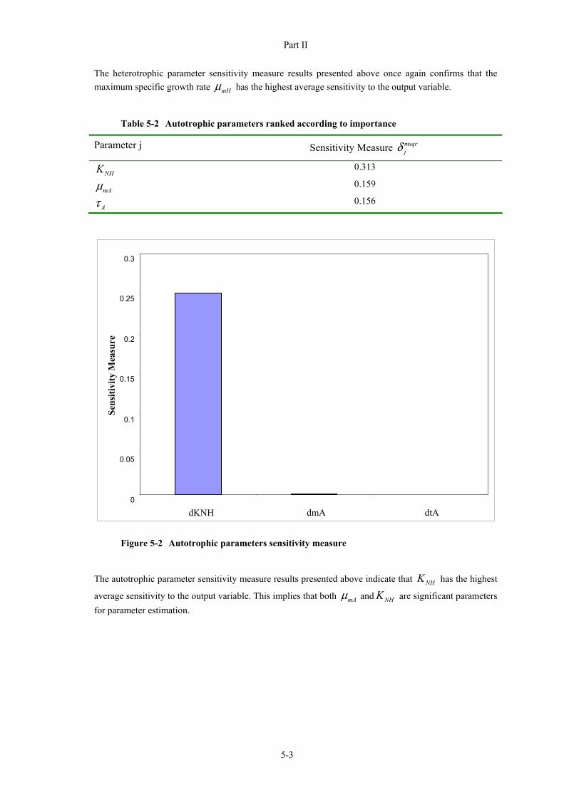
Part II

5-3

The heterotrophic parameter sensitivity measure results presented above once again confirms that the maximum specific growth rate mH has the highest average sensitivity to the output variable.

Table 5-2 Autotrophic parameters ranked according to importance

Parameter j Sensitivity Measure msqrj

NHK 0.313

mA 0.159

A 0.156

Figure 5-2 Autotrophic parameters sensitivity measure

The autotrophic parameter sensitivity measure results presented above indicate that NHK has the highest

average sensitivity to the output variable. This implies that both mA and NHK are significant parameters for parameter estimation.

0

0.05

0.1

0.15

0.2

0.25

0.3

dKNH dmA dtA

Sens

itivi

ty M

easu

re

Part II

5-4

5.2 PARAMETER ESTIMATION OF BRE MODEL

Parameter estimation was performed using the experimental data obtain from the Batch Respirometric Experiments (refer to Section 4.5) and the BRE model created in WEST. The parameters of the BRE model which were not included in the estimation are presented along with the default values used in

Table 5-3. The WEST Experimental Environment trajectory optimiser was used for the parameter estimation. Regressed data fits for the high scoring dye - acetate and high scoring dye - ammonia mixtures are presented in Figure 5-3 and Figure 5-4 respectively. Also the regressed data fits for the low scoring dye - acetate and low scoring dye - ammonia mixtures are presented in Figure 5-5 and Figure 5-6 respectively.

Table 5-3 BRE model parameters and defaults values

Parameter Symbol Value Units Reference

Yield for heterotrophic biomass HY 0.67 gCOD/gCOD (Henze et al., 1987)

Yield for autotrophic biomass AY 0.24 gCOD/gN (Henze et al., 1987)

Heterotrophic first-order time constant H 1.25 min (Vanrolleghem et al.,

2004)

Autotrophic first-order time constant A 3 min (Spanjers and

Vanrolleghem, 1995)

Mass of nitrogen per mass of COD in biomass XBi 0.086 gN/gCOD (Henze et al., 1987)

Mass of nitrogen per mass of COD in products from biomass XPi 0.02 gN/gCOD (Gujer et al., 1999)

Fraction of biomass leading to particulate products Pf 0.2 - (Gujer et al., 1999)

Part II

5-5

(a) (b)

(c) (d)

Figure 5-3 (a-d) Regressed fits of OUR for acetate substrate and high scoring dye runs. The concentration of the dye spikes increase from (a) to (d)

Part II

5-6

(a) (b)

(c) (d)

Figure 5-4(a-d) Regressed fits of OUR for ammonia substrate and high scoring dye runs. The concentration of the dye spikes increase from (a) to (d)

Part II

5-7

(a) (b)

(c) (d)

(e)

Figure 5-5 (a-e) Regressed fits of OUR for acetate substrate and low scoring dye runs for which the experimental data (squares) and BRE model (line), the concentration of the dye spikes increase from (a) to (e)

Part II

5-8

(a) (b)

(c) (d)

Figure 5-6 (a-d) Regressed fits of OUR for ammonia substrate and low scoring dye runs for which the experimental data (squares) and BRE model (line), the concentration of the dye spikes increase from (a) to (d)

The BRE model kinetic parameters for high and low scoring dyes obtained from the parameter estimation are shown in Table 5-4 and Table 5-5 respectively. It is observed from the estimated parameters that both dyes cause mixed type of inhibition of both the carbon reduction and nitrification, i.e. dyes cause a decrease in maximum specific growth rate and an increase in the half saturation constant (Volskay and Grady, 1988). Refer to Section 3.1, Table 3-2 for the mixed inhibition type kinetic model.

Part II

5-9

Table 5-4 Parameter estimate results and confidence intervals performed on experimental data obtained from high scoring dye respirometric experiments

Cumulative concentration of dye added (ppm) Parameter 0 25 75 175

Heterotrophic maximum specific growth rate mH

0.620±0.025 0.605±0.032 0.574±0.068 0.520±0.093

Heterotrophic half saturation coefficient SK

1.489±0.073 3.970±0.084 4.213±0.092 5.100±0.151

Autotrophic maximum specific growth rate mA

0.337±0.021 0.290±0.022 0.234±0.018 0.187±0.017

Autotrophic half saturation coefficient NHK

0.052±0.092 0.086±0.076 0.100±0.065 2.159±0.079

Table 5-5 Parameter estimate results and confidence intervals performed on experimental data obtained from low scoring dye respirometric experiments

Cumulative concentration of dye added (ppm) Parameter

0 25 75 175 275

Heterotrophic maximum specific growth rate mH

0.840±0.072 0.750±0.065 0.746±0.078 0.703±0.031 0.710±0.085

Heterotrophic half saturation coefficient SK

0.609±0.081 0.685±0.093 0.691±0.085 0.151±0.075 0.461±0.090

Autotrophic maximum specific growth rate mA

0.600±0.095 0.597±0.093 0.530±0.034 0.455±0.091 -

Autotrophic half saturation coefficient

NHK

0.641±0.064 0.824±0.073 3.100±0.045 5.187±0.075 -

The effect of mixed inhibition type on activated sludge processes can be quantified by Equation 5-3 and Equation 5-4.

* maxmax

,1

I m

IK

⎛ ⎞⎛ ⎞⎜ ⎟⎜ ⎟⎝ ⎠⎝ ⎠

5-3

*

,1S S

I S

IK K K⎛ ⎞⎛ ⎞

⎜ ⎟⎜ ⎟⎝ ⎠⎝ ⎠ 5-4

Part II

5-10

Using the data presented in Table 5-4 and Table 5-5 the ,I mK and ,I SK inhibition parameters were calculated through regression. These inhibition parameters for the high and low scoring dyes are presented in Table 5-6. The inhibition function and the respective parameters were inputted into the COST simulation benchmark model (a detailed description of this model is provided in Chapter 6). The maximum specific growth rate is temperature dependent and obtained at the experimental temperature of 25°C, hence the this parameter was adjusted to 15°C, the temperature used in the COST simulation benchmark by using the Arrhenius equation (Equation 5-5).

( ) rT Trk T k T e 5-5

Table 5-6 Inhibition parameter values for high and low scoring dyes

Heterotrophic biomass growth Autotrophic biomass growth Inhibiting Dye

,I mK ,I SK ,I mK ,I SK

High scoring dye -Drimarene Violet K2-RL

921.800 61.113 194.246 5.103

Low scoring dye - Levafix Blue CA gran

1131.698 1.29x109 576.369 24.008

Part II

6-1

CHAPTER 6 Assessment of Wastewater

Treatment Works Performance In this chapter the impact of the textile dyes on the wastewater treatment works performance is assessed using the COST simulation benchmark to quantify the inhibitory effect of two different dyes and determine whether the high scoring dye has a greater negative impact on wastewater treatment works performance than the low scoring dye.

6.1 BACKGROUND ON COST AND THE COST SIMULATION BENCHMARK

COST (founded in 1971) is a European intergovernmental framework for co-operation in the field of scientific and technical research in order to allow the coordination of European national funds. COST is the largest European framework for research co-operation with almost 200 Actions and involving nearly 30 000 scientists and more than 50 participating institutions.

The COST Simulation Benchmark Model (Copp, 2001) is a fully defined simulation protocol developed through a co-operative effort involving two COST Actions: COST Action 682 ‘Integrated Wastewater Management’ (1992-1998) and COST Action 624 (COST 624, 2005). The former focuses on biological wastewater treatment processes and the optimisation of design and operation based on process models while the latter is dedicated to the optimisation of the performance and cost-effectiveness of wastewater management systems. The goal of the COST simulation benchmark was to provide a tool for evaluating and comparing different wastewater treatment works control strategies on a consistent and unbiased basis and has been used as such in a number of different studies (Spanjers et al., 1998; Vanrolleghem and Gillot, 2002).

The simulation benchmark model was used in the current study to evaluate the impact of different dye chemicals on wastewater treatment plant performance because it is a well understood calibrated model, with a clearly defined simulation protocol. The standard evaluation criteria (effluent requirements and treatment costs) provided with the benchmark model were used instead of local site specific data in order to provide an unbiased basis for comparison of the effect of the two dyes and to provide a suitable reference against which results from real treatment plants could ultimately be compared.

6.2 OVERVIEW OF THE COST SIMULATION BENCHMARK MODEL

The section provides an overview of the simulation benchmark model and describes plant layout, process models and influent components. More details can be found in (Copp, 2001) which was also available online at the time of writing this report.

6.2.1 Plant layout of simulation benchmark A schematic representation of the simulation benchmark plant layout is presented in Figure 6-1. The plant design consists of five activated sludge reactors in series with a secondary settling tank.

Figure 6-1 Schematic representation of the simulation benchmark plant layout

showing activated sludge units (ASU) 1& 2 mixed and unaerated, ASU 3, 4 & 5 aerated, and 10 layer secondary settler

ASU1 ASU2 ASU3 ASU4 ASU5

Clarifier

Part II

6-2

The physical attributes of the activated sludge units and settler are presented in Table 6-1 and the system variables are listed in Table 6-2. Activated sludge units (ASU) 1& 2 each have a biological volume of 1 000 m3 and are unaerated fully mixed reactors. ASU 3, 4 & 5 each have a biological volume of 1 333 m3 and are aerated. The saturated dissolved oxygen concentration (DO) is specified to be 8 g O2/m3. The oxygen transfer coefficient ( LK a ) value in ASU 3 & 4 is 10 1/h, whereas the LK a value in ASU 5 is 3.5 1/h.

Table 6-1 Physical attributes of the activated sludge units and settler for the COST simulation benchmark plant configuration

Biological Process Unit Physical Configuration Units

Volume – Tank 1 1 000 m3

Volume – Tank 2 1 000 m3

Volume – Tank 3 1 333 m3

Volume – Tank 4 1 333 m3

Volume – Tank 5 1 333 m3

Depth – Settler 4 m

Area – Settler 1 500 m2

Volume - Settler 6 000 m3

Table 6-2 System variables of the COST simulation benchmark plant configuration

System Variable Default System Flow Rates Units

Influent flow rate 18 446 m3/d

Recycle flow rate 18 446 m3/d

Internal recycle flow rate 55 338 m3/d

Wastage flow rate 385 m3/d

LK a – ASU 1 n/a -

LK a – ASU 2 n/a -

LK a – ASU 3 10 1/h

LK a – ASU 4 10 1/h

LK a – ASU 5 3.5 1/h

The secondary settler is a 10 layer non-reactive settler with a volume of 6 000 m3 (area of 1 500 m2 and a depth of 4 m). The feed enters the settler in the middle of the sixth layer, i.e. the feed point is 2.2 m from the bottom of the settler. The plant design has two internal recycles: a nitrate recycle from the fifth ASU to the first ASU with a rate of 55 338 m3/d, and an activated sludge recycle from the underflow of the

Part II

6-3

secondary settler to the first ASU with a flow rate of 18 446 m3/d. The waste activated sludge is pumped continuously from the underflow at a rate of 385 m3/d.

6.2.2 Process models The COST benchmark simulation model uses internationally accepted models to describe both the biological processes and the settling process. The Activated Sludge Model 1 (ASM1) (Henze et al., 1987) is used as the biological process model and the double-exponential settling velocity function is used as the settler process model (Takacs et al., 1991).

6.2.2.1 Biological kinetic process model As mention in Section 2.5 a number of new activated sludge models have been proposed since ASM1 model was developed. These models include ASM2, ASM2d and ASM3. The ASM1 model is still the most popular model used internationally. There are a number of limitations to the ASM1 model which have been discussed in Section 2.5.1, but the worldwide appeal and practical confirmation of this model provide the motivation for its use as the biological model in the simulation benchmark model. A detailed description and Petersen matrix representation of the ASM1 model are presented in Section 2.5.1.

The default stoichiometric and kinetic parameter values are presented in Table 6-3 and Table 6-4 respectively. The listed parameter estimates assume a temperature of 15 °C.

Table 6-3 ASM1 stoichiometric parameter default values used in the simulation benchmark

Parameter Value Units

Autotrophic yield ( AY ) 0.24 gCOD/gN

Heterotrophic yield ( HY ) 0.67 gCOD/gCOD

Fraction of biomass to particulate products ( pf ) 0.08 -

Fraction nitrogen in biomass ( XBi ) 0.08 gN/gCOD

Fraction nitrogen in particulate products ( XPi ) 0.06 gN/gCOD

Part II

6-4

Table 6-4 ASM1 kinetic parameter default values used in the simulation benchmark

Parameter Value Units

Maximum specific heterotrophic growth rate ( mH ) 4.00 1/d

Heterotrophic growth half-saturation coefficient ( SK ) 10.00 gCOD/m3

Heterotrophic oxygen half-saturation coefficient ( OHK ) 0.20 gO2/m3

Half-saturation coefficient for nitrate ( NOK ) 0.50 gNO3-N/m3

Heterotrophic decay rate ( Hb ) 0.30 1/d

Anoxic growth rate correction factor ( g ) 0.80 -

Anoxic hydrolysis rate correction factor ( h ) 0.80 -

Maximum specific hydrolysis rate ( hk ) 3.00 gCOD/gCOD.d

Hydrolysis half-saturation coefficient ( XK ) 0.10 g/gCOD

Maximum specific autotrophic growth rate ( mA ) 0.50 1/d

Autotrophic growth half-saturation coefficient ( NHK ) 1.00 gNH3-N/m3

Autotrophic decay rate ( Hb ) 0.05 1/d

Autotrophic oxygen half-saturation coefficient ( OAK ) 0.40 gO2/m3

Ammonification rate ( ak ) 0.05 m3/gCOD.d

6.2.2.2 Settling process model The settling process model used in the simulation benchmark is the Takacs double-exponential settling velocity function (Takacs et al., 1991) shown in Equation 6-1. This function is based on the solid flux concept and, unlike other common settling models, is applicable to both hindered and flocculent settling conditions,

* *

0 0h j p jr X r X

sjv v e v e 6-1

Where:

sjv is the settling velocity in layer j (m/d), subject to 0 ≤ sjv ≥ '0v

*jX is the suspended solids concentration in layer j (g/m3), subject to *

minj jX X X

jX is the suspended solids concentration in layer j (g/m3)

minX is the minimum attainable suspended solids concentration (g/m3), calculated from

min ns inX f X ( inX is the mixed liquor suspended solids concentration entering the settler and nsf is the non-settleable fraction)

The settler model parameters and default values are shown in Table 6-5.

Part II

6-5

Table 6-5 Settler model parameters and default values

Parameter Value Units

Maximum settling velocity ( '0v ) 250 m/d

Maximum Vesilind settling velocity ( 0v ) 474 m/d

Hindered zone settling parameter ( hr ) 0.000576 m3/g

Flocculent zone settling parameter ( pr ) 0.00286 m3/g

Non-settle able fraction ( nsf ) 0.00228 -

6.2.2.3 Influent composition In the COST simulation benchmark protocol, control strategies are evaluated by subjecting the wastewater treatment plant model to three well-defined disturbances in the influent composition. These are available as input files which can be downloaded from the COST 624 web site (COST 624, 2005).

The three disturbances are intended to represent dry weather, a storm event and an extended rainy period. These are described in greater detail in Section 2.3 of (Copp, 2001). The ability of a control strategy to handle these disturbances determines its performance.

In this study the impact of the two dye inhibitions were evaluated by making the two dyes serve as the disturbances to the system while using the dry weather influent composition. The flow-weighted dry weather influent composition is presented in Table 6-6 (COST 624, 2005).

Table 6-6 Flow-weighted average dry weather influent composition (COST 624, 2005)

Component Dry weather Units

SS 69.50 gCOD/m3

BHX 28.17 gCOD/m3

SX 202.32 gCOD/m3

IX 51.20 gCOD/m3

NHS 31.56 gN/m3

IS 30.00 gCOD/m3

NDS 6.95 gN/m3

NDX 10.59 gN/m3

Q 18446 m3/d

6.3 MODIFICATIONS MADE TO THE SIMULATION BENCHMARK KINETIC PROCESS MODEL

In Section 5.2 the type of inhibition and inhibition kinetics caused to activated sludge processes by the two dyes (high scoring dye Drimarene Violet K2-RL and low scoring dye Levafix Blue CA gran) used in this study were determined. It was found that both dyes exhibit a mixed inhibition type to both the

Part II

6-6

activated sludge processes of carbon reduction and nitrification. The mixed inhibition type influence on the maximum specific growth rate and half saturation value can be represented by Equation 6-2 and Equation 6-3 respectively.

* maxmax

,1

I m

IK

⎛ ⎞⎛ ⎞⎜ ⎟⎜ ⎟⎝ ⎠⎝ ⎠

6-2

*

,1S S

I S

IK K K⎛ ⎞⎛ ⎞

⎜ ⎟⎜ ⎟⎝ ⎠⎝ ⎠ 6-3

The parameter estimates listed in Table 6-3 and Table 6-4 assume a temperature of 15 °C. Since the batch respirometric experiments were performed at 25 °C the parameter estimates had to be corrected to 15 °C where necessary. The maximum specific growth rates were the only temperature dependent parameters and were corrected to 15 °C using the Arrhenius equation (refer to Section 5.2). The inhibition kinetic parameter values for both dyes obtained from regression of estimated parameter were presented in Section 5.2, Table 5-6.

The dye (inhibitor) concentration I shown in Equation 6-2 and Equation 6-3 was assumed to be a constant parameter value and not a concentration variable since both dyes are azo dyes and do not degrade under aerobic condition as discussed in Section 2.1.2.

The mixed inhibition function presented in Equation 6-2 and Equation 6-3, and the inhibition kinetic parameter values presented in Table 5-6 (Section 5.2) were inputted into the simulation benchmark biological kinetic model using the WEST Model Editor.

6.4 SIMULATION PROCEDURE

Simulations were carried out using WEST. The configuration of the benchmark model as it appears in WEST Configuration Builder is presented in Figure 6-2.

Figure 6-2 COST simulation benchmark model configuration as appears in WEST

A two step simulation procedure as defined in the simulation benchmark (Copp, 2001) was performed in WEST Experimental Environment. This involves a steady state simulation followed by a dynamic simulation using the dry weather influent input files.

Part II

6-7

6.4.1 Steady-state simulations The first step in the simulation procedure is to run the simulation benchmark model under steady-state conditions using an influent of constant flow and composition. The flow-weighted dry weather data presented in Table 6-6 is used for this purpose and the simulation is run for 60 d using a constant influent. The steady state solution is then used as the initial condition for the dynamic simulations. This ensures a consistent starting point in order to eliminate the influence of starting conditions on the generated dynamic output.

6.4.2 Dynamic simulations The second step is the dynamic simulation which is performed using dynamic influent data (COST 624, 2005). The dynamic simulation is started from the steady state solution using the dry weather dynamic influent file and run for 14 d. The resulting state variable values for all unit processes are saved and used to evaluate the impact of the inhibitor disturbance on the dynamic performance of the plant. The dynamic simulation output data generated during the last 7 d of simulation is used to examine the dynamic performance of the plant. Output data is recorded at 15 min intervals.

The above two-step procedure was repeated for dye (inhibitor) concentrations I ranging from 0 to 100 mg/L. The WEST Scenario Analysis function was used to reduce the time required to perform the simulations. The WEST Scenario Analysis function allows multiple simulations to be performed using a vector of parameter values. In this study the parameter vector is dye (inhibitor) concentration I . Separate Scenario Analysis simulations were performed for each of the two dyes being investigated.

6.5 PERFORMANCE INDICES OF SIMULATION BENCHMARK

The benchmark simulation protocol defines a set of performance indices which are used to facilitate the comparison of the impact of different control strategies on plant performance. In this study, the same indices were used to compare the impact of the two dyes on the performance of the plant. The performance index is a set of site independent measures that combine the output data into a small number of composite terms which characterise various aspects of the plant performance. Three aspects of plant performance were considered in this study. These were:

effluent quality index

effluent violations

operational costs

6.5.1 Effluent quality index The effluent quality of the simulation benchmark model is characterised as an effluent quality index ( EQ ) which quantifies the effluent pollution load to a receiving water body in a single term.

The composite variables used in the calculation of EQ are; eTSS , eCOD , eBOD , eTKN , eNO and

,tot eN . These variables are defined by Equation 6-4, 6-5, 6-6, 6-7, 6-8 and 6-9 respectively.

, , , , ,0.75e S e BH e BA e P e I eTSS X X X X X 6-4

, , , , , , ,e S e I e S e BH e BA e P e I eCOD S S X X X X X 6-5

, , , ,0.25 1e S e S e p BH e BA eBOD S X f X X 6-6

, , , , , , ,e NH e ND e ND e XB BH e BA e XP P e I eTKN S S X i X X i X X 6-7

,e NO eNO S 6-8

Part II

6-8

,tot e e eN TKN NO 6-9

The effluent quality ( EQ ) is calculated from the average values of each of the pollutants above over the final 7 days of the dry weather simulation as shown in Equation 6-10. The units of EQ are kg pollution units per day (kgPU/d).

7

0

11000

dayst

TSS COD BOD TKN NO et

EQ PU t PU t PU t PU t PU t Q t dtT

⎡ ⎤⎣ ⎦∫ 6-10

The composite variables used in Equation 6-10 to calculate effluent quality index are converted to pollution units by multiplying the composite variables by their respective i factors. The unit conversions for the respective composite variables are shown in Equation 6-11 to Equation 6-15.

TSS TSS ePU t TSS t 6-11

COD COD ePU t COD t 6-12

BOD BOD ePU t BOD t 6-13

TKN TKN ePU t TKN t 6-14

NO NO ePU t NO t 6-15

The i factors presented in Table 6-7 were determined, in part, based on empirical component weightings. The weightings are based on a Flanders effluent quality formula for calculating fines to be imposed on polluters (Vanrolleghem et al., 1996). That formula is based on several terms including terms for organics, nutrients, metals and heat. The metals and heat terms are not of concern to the simulation benchmark, but the organics and nutrient terms are related. Organic and nutrient terms can be calculated using the Flanders equation and steady-state data from each of the layouts. From these terms it is then possible to determine the specific fraction that each term makes up of the fine formula, that is % nutrients nutrients organicsnutrients N N N . The i factors reflect these calculated fractions

(Copp, 2001). For the COST benchmark layout, the steady state EQ was found to be weighted as 22% nutrients and 78% organics (Copp, 2001).

Part II

6-9

Table 6-7 i Factors for composite variables

i Factor Value

TSS 2

COD 1

BOD 2

TKN 20

NO 20

6.5.2 Effluent Violations In addition to the effluent quality index, which represents the total pollutant load being discharged, the plant performance was also evaluated in terms of the frequency and duration of effluent quality violations. The violations are calculated for five terms: ammonia, total nitrogen, BOD5, total COD and suspended solids. The effluent constraint values for these five constraint terms are presented in Table 6-8.

Table 6-8 Effluent constraints values

Effluent Constraint Adopted Effluent Constraint Value

Units

Ammonia ( ,NH eS ) 4 gN/m3

Total Nitrogen ( ,tot eN ) 18 gN/m3

BOD5 ( eBOD ) 10 gBOD/m3

Total COD ( eCOD ) 100 gCOD/m3

Suspended Solids ( eTSS ) 30 gSS/m3

Two quantities are reported: the number of violations and percentage time plant is in violation. These are calculated from the model output data generated at 15 min intervals over the last 7 days of the simulation. The number of violations represents the number of incidents which result in the plant effluent concentration increasing above the effluent constraint. This value does not represent the length of time the wastewater treatment plant is in violation. The percentage time the plant is in violation is proportional to the number of 15 minute samples which exceed the effluent constraints.

6.5.3 Operational Costs Three aspects of plant performance which have a major impact on operating costs were considered: sludge production, energy required for pumping and energy required for aeration. Each of these was integrated as a function of time over the last 7 days of the dry weather data simulations.

Sludge Production Sludge production consists of (i) sludge for disposal and (ii) total sludge production.

(i) Sludge for disposal (kg/d) is calculated from Equation 6-16.

Part II

6-10

sludge system WP M TSS M TSS T⎡ ⎤⎣ ⎦ 6-16

Where:

systemM TSS = change in system sludge mass over the final 7 days.

wTSSM = total mass of solids discharged in the sludge waste stream over the last 7 days

The change in system sludge mass is calculated using Equation 6-17 to Equation 6-19.

28 21system system systemday dayM TSS M TSS M TSS 6-17

system reactors settlerM TSS M TSS M TSS 6-18

7

0

, , , , ,0.75dayst

w S w BH w BA w P w I w wt

M TSS X t X t X t X t X t Q t dt⎡ ⎤⎣ ⎦∫ 6-19

Where:

wQ t = waste sludge flow rate at time t (m3/d)

(ii) Total sludge production (kg/d) is calculated from Equation 6-20.

_total sludge sludge eP P M TSS T 6-20

Where:

7

0

, , , , ,0.75dayst

e S e BH e BA e P e I e et

M TSS X t X t X t X t X t Q t dt⎡ ⎤⎣ ⎦∫ 6-21

Pumping Energy The pumping energy (kWh/d) is calculated using Equation 6-22.

7

0

0.04 dayst

a r wt

PE Q t Q t Q t dtT

⎡ ⎤⎣ ⎦∫ 6-22

Part II

6-11

Where:

aQ t = internal recycle flow rate at time t (m3/d)

rQ t = return sludge recycle flow rate at time t (m3/d)

Aeration Energy The aeration energy (kWh/d) is calculated using Equation 6-23.

7

0

52

1

24 0.4032 7.8408dayst i

L i L iit

AE K a t K a t dtT

⎡ ⎤⎣ ⎦∑∫ 6-23

Where:

L iK a t = the mass transfer coefficient (1/h) in ith aerated reactor at time t

6.6 RESULTS FROM COST BENCHMARK SIMULATIONS FOR BOTH DYES

The COST simulation benchmark model was used in this study to quantify the inhibitory effect of two dyes (high scoring dye Drimarene Violet K2-RL and low scoring dye Levafix Blue CA gran) and determine whether the high scoring dye has a greater negative impact on wastewater treatment works than the low scoring dye. This evaluation is based on the performance indices (refer to Section 6.5) calculated using output data obtained from simulations performed using the modified COST simulation benchmark model (refer to Section 6.3). Simulations were carried out for each dye with dye (inhibitor) concentration I ranging from 0 to 100 mg/L.

Figure 6-3 presents the effluent quality indices (EQI) for both dyes as a function of dye concentration. From Figure 6-3 it can be concluded that both dyes have an inhibitory effect on wastewater treatment works processes since, in both cases, the effluent quality index (EQI) increases with increasing dye concentration. This implies the processes of nutrient reduction are inhibited by the dyes, since greater amounts of nutrients are present in the effluent (i.e. higher EQI values). Furthermore the high scoring dye (Drimarene Violet K2-RL) has a much greater negative impact on the performance of the wastewater treatment works model than the low scoring dye (Levafix Blue CA gran) as reflected in the EQI..

The impact on sludge disposal and total sludge production of each dye is presented as a function of concentration in Figure 6-4 and Figure 6-5 respectively. In both cases, the sludge disposal and total sludge production decrease with increasing dye concentration as a result of the inhibitory effect of the dyes on the activated sludge processes are inhibited by the dyes. Once again, the impact of the high scoring dye (Drimarene Violet K2-RL) is greater than that of the low scoring dye (Levafix Blue CA gran).

Part II

6-12

0

2000

4000

6000

8000

10000

12000

14000

0 10 20 30 40 50 60 70 80 90 100

Inhibitor Concentration (mg/L)

Eff

luen

t Qua

lity

Inde

x (k

g PU

/L)

High ScoreLow Score

Figure 6-3 The relationship between effluent quality index and dye concentration for

high and low scoring dyes.

1740

1760

1780

1800

1820

1840

1860

1880

0 10 20 30 40 50 60 70 80 90 100

Inhibitor Concentration (mg/L)

Slud

ge fo

r D

ispo

sal (

kgSS

/d)

High ScoreLow Score

Figure 6-4 The relationship between sludge disposal and dye concentration for high

and low scoring dyes.

Part II

6-13

1920

1940

1960

1980

2000

2020

2040

2060

2080

0 10 20 30 40 50 60 70 80 90 100

Inhibitor Concentration (mg/L)

Tot

al S

ludg

e Pr

oduc

tion

(kgS

S/d)

High ScoreLow Score

Figure 6-5 The relationship between total sludge production and dye concentration

for high and low scoring dyes.

(b) Figure 6-6 and Figure 6-7 present the number of violations and time in violation respectively for each of the pollutants listed in Table 6-8 as functions of concentration of each of the dyes. The greatest number of violations and time spent in violation occur for ammonia (effluent concentrations above 4 gN/m3). The high scoring dye results in 100% time in violation for concentrations greater than 30 mg/L while the low score dye approaches 90% time in violation at 100 mg/L. The high scoring dye also results in violations of the total nitrogen constraint (18 gN/m3) for concentrations of 30 mg/L and greater with 100% time in violation occurring at 60 mg/L. No total nitrogen violations were observed for the low scoring dye. No BOD, COD and suspended solids effluent violations were observed for either dyes. These results indicate that the inhibitory effects of the dyes on the nitrification processes is much more serious than on the carbon removal processes (refer to (b) Figure 6.6).

(b)

Figure 6-6In the uncontrolled scenario used in these simulations, aeration and pumping rates are constants and therefore the associated energy consumption remains unaffected by the dyes.

To summarise the simulation benchmark model results indicate that both dyes used in this study have a significant inhibitory effect on wastewater treatment processes, particularly the nitrification processes and that the high scoring dye has a greater negative impact than the low scoring dye.

Part II

6-14

0

100

200

300

400

500

600

700

0 10 20 30 40 50 60 70 80 90 100

Inhibitor Concentration (mg/L)

Num

ber

of V

iola

tions

AmmoniaTotal NitrogenBODCODSuspended Solids

(a)

0

100

200

300

400

500

600

0 10 20 30 40 50 60 70 80 90 100

Inhibitor Concentration (mg/L)

Num

ber

of V

iola

tions

AmmoniaTotal NitrogenBODCODSuspended Solids

(b)

Figure 6-6 The relationship between Number of effluent violation and dye concentration for (a) high and (b) low scoring dyes.

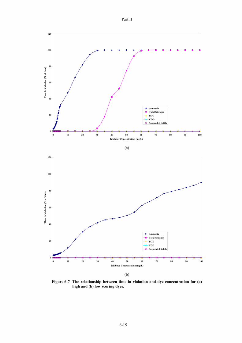
Part II

6-15

0

20

40

60

80

100

120

0 10 20 30 40 50 60 70 80 90 100

Inhibitor Concentration (mg/L)

Tim

e in

Vio

latio

n (%

of t

ime)

AmmoniaTotal NitrogenBODCODSuspended Solids

(a)

0

20

40

60

80

100

120

0 10 20 30 40 50 60 70 80 90 100

Inhibitor Concentration (mg/L)

Tim

e in

Vio

latio

n (%

of t

ime)

AmmoniaTotal NitrogenBODCODSuspended Solids

(b)

Figure 6-7 The relationship between time in violation and dye concentration for (a) high and (b) low scoring dyes.

Part II

7-1

CHAPTER 7 Discussion

In this chapter the broad spectrum impact of the results presented in the previous chapters are discussed. The formulation of the conclusion and recommendations of this study stated in Chapter 8 is discussed.

7.1 RESPIROMETRIC EXPERIMENTS

The test activated sludge used in the batch respirometric experiments was obtained from the Umbilo wastewater treatment works (WWTW) and represented normal operating conditions of the WWTW. Activated sludge in a wastewater treatment works acclimatises after prolonged exposure to toxic effluent, hence a more accurate measure of the inhibition caused by the toxic effluent probably may have been obtained if the activated sludge had been allowed to acclimatise to the test effluent before being used in the batch respirometric experiments. The reference substrate used in the experiments was sodium acetate and ammonium chloride, the primary components of wastewater. The use of a composite feed to the treatment plant would have been more representative of normal operating conditions but the wastewater entering the WWTW would have to be characterised to determine its composition for modelling purposes. Pure dye was used as the test substance in these experiments to quantify the inhibition caused by the textile dye effluent. More accurately raw effluent from the textile companies should be used as the test substance. However, if the raw effluent is used as the test substance, a study into the biodegradability of the test substance needs to be performed since a biodegradation process will be required in the inhibition kinetic model.

The optimal experimental design (OED) (Dochain and Vanrolleghem, 2001) method of optimising data collection for model selection and calibration and was used in this study to design the batch respirometric experiment. This technique is used to obtain experiment designs which produce the most amount of information with the least amount of effort (Nopens et al., 2001). This method has been successfully used to design experiments and calibration of sensors in previous studies (Petersen, 2000; Insel et al., 2003; Sin, 2004; De Pauw, 2005). The OED method was effectively used in this study to design a batch respirometric experiment that produced information rich experimental data to facilitate reliable parameter estimation.

The batch respirometer used in this study followed the principle of static gas-static liquid respirometer (refer to Section 2.3.1.2). These respirometers are typically characterised by low sampling frequency resulting in difficulties in determining kinetic parameters. By applying the OED technique the maximum amount of information was obtained from the batch respirometer utilised in this study. Although the measured data obtained from the batch respirometric experiment was sufficient to obtain reliable parameter estimates, the addition of a titrimetric measurement would definitely aid in the estimation of kinetic parameters. Titrimetry is a method for gaining information about the biological nitrogen removal processes of the activated sludge by monitoring pH. Nitrification and denitrification causes pH to decrease and increase respectively due to proton production and proton consumption respectively. The frequently used titrimetric method for monitoring the acid and base consumption rate to keep pH of the activated sludge constant (Ramadori et al., 1980) is effective for monitoring nitrification since nitrification has a clearly defined effect on pH (Gernaey et al., 1998). A combined respirometric-titrimetric experiment setup (Petersen, 2000; Gernaey et al., 2001; Gernaey et al., 2002; Sin, 2004) could allow the determination of both biological carbon source degradation and nitrogen removal information in a single experiment, hence the number of required experiments would be reduced.

This study only investigated the effect of the test substances on the aerobic activated sludge processes. The inclusion of an anoxic sensor similar to the sensor used by Sin et al. (2003) in the experiment design would enable the impact of the test substances to the anoxic processes to be assessed.

7.2 BATCH RESPIROMETRIC EXPERIMENT (BRE) MODEL

In this study, it was assumed that the same combination of the model parameters determined in the structural identifiability study by Taylor expansion method performed on the ASM1 model (Dochain and Vanrolleghem, 2001) applied for the BRE model. In a future study a structural identifiability analysis can be performed on the BRE model itself. There are many methods to determine structural identifiability (Weijers and Vanrolleghem, 1997; Dochain and Vanrolleghem, 2001; Petersen et al., 2003). If the

Part II

7-2

experiment setup is changed to a respirometric-titrimetric design then some changes to the BRE model will be required: a proton concentration variable replacing the alkalinity concentration variable ALKS , accounting for cumulative protons consumed or produced during biodegradation, must be added (Gernaey et al., 1998); the nitrification process in the BRE model is also required and should be split into two processes to enable the titrimetric measured data to be used for parameter estimation (Gernaey et al., 2001) and a carbon stripping process should be included (Gernaey et al., 1998).

7.3 ASSESSMENT OF IMPACT TO WWTW PERFORMANCE

In this study, the COST simulation benchmark model was used to assess the impact of a high scoring dye and a low scoring dye on the operation of a waste water treatment plant. The study demonstrates that high scoring reactive dyes are likely to a have a significantly worse impact on waste water treatment plants. These results therefore underscore the rationale for eThekwini’s current trade effluent permitting rules which award substantial discounts in discharge tariffs to companies which implement recognised cleaner production policies including the Score system. Under proposed future legislation, discharge tariffs will be calculated based on the expected negative impact of a particular effluent on the municipal plant that will be treating it and therefore the Score system could be an effective tool for companies wishing to reduce their discharge tariffs. It is also useful to companies which are considering building their own biological treatment systems.

The COST simulation benchmark model (Copp, 2001) is an activated sludge wastewater treatment model designed to evaluate different control strategies (Vanrolleghem and Gillot, 2002; De Pauw, 2005). More than a hundred scientific papers which include features of the benchmark model have been published world-wide (Jeppsson and Pons, 2004). In this study the benchmark model was adapted to assess the impact of the test substances concentration on the performance of the wastewater treatment works (WWTW) model. The assessment was based on performance indices which were calculated from the simulation data. From the results obtained from the simulations on the benchmark, indications are that for both test dyes, inhibition increases with increasing concentration. Furthermore, the high scoring dye had a greater negative impact on the WWTW model performance than the low scoring dye. Hence this study concludes that the Score system can be used to select dyes which are less to toxic to biological treatment processes.

The limitation of the assessment was that the performance indices used in the assessment can not be converted to monetary values. A possible solution to this limitation is to include a control scheme such as that used by Vanrolleghem and Gillot (2002) were the dissolved oxygen concentration is controlled by manipulating the mass transfer coefficient ( LK a ). The LK a variable is used in the benchmark protocol to calculate aeration cost which is in the form of power (kW/h); hence, a relationship between inhibitor concentration and aeration can be obtained, and the aeration cost can be easily converted to a monetary value. Therefore the relationship between the test substance concentration and the WWTP’s increased operating costs can be calculated. This relationship can then be used in the design of effluent tariffs.

The COST benchmark simulation model is not an actual municipal WWTW. In a future study the COST benchmark simulation procedure can be used on a model of an actual municipal WWTW (e.g. Umbilo WWTW). In this study the COST benchmark simulation model was sufficient to investigate the relative effects of the test substances. If an actual municipal WWTW model was used along with the COST benchmark procedure, a more accurate assessment of the test substances’ impact on the performance of the WWTW could be obtained. The use of an actual WWTW would only be necessary if the information was to be used in a tariff calculation.

Part II

8-1

CHAPTER 8 Conclusions and Recommendations

It has been concluded from the results of this study that:

1. The high scoring dye had a greater negative impact on the WWTP performance than the low scoring dye. This implies that score system can be effectively used to identify textile dyes that have a negative impact on the environment and should be subject to closer examination.

2. The optimal experimental design method was an efficient method for designing the batch respirometric experiment. The batch respirometric experiment design provided rapid and reliable experimental data that could be used to obtain reliable parameter estimates.

3. The conservative approach of selecting test sludge, reference substrate and test substance used in this study, was successful in providing respirometric experiment data. Un-acclimatised activated sludge Umbilo wastewater treatment works (WWTW) was used as test sludge, sodium acetate and ammonium chloride were used as substrates and the test substance used in the experiments was pure dye.

4. Autotrophic biomass responsible for nitrification process is more sensitive to toxic substances (in this study, textile dyes) than the heterotrophic biomass which is responsible for the carbon source degradation process.

5. The traditionally used activated sludge models No. 1 (ASM1) and ASM3 were determined to be too complex to obtain reliable parameter estimates with the current batch respirometric design. The batch respirometric experiment (BRE) model was developed with the objective of obtaining accurate estimates. A simplified model combining both ASM1 and ASM3 model concepts was used.

6. The batch respirometric experiment (BRE) activated sludge model and the respirometric experimental data collected were successfully used to obtain kinetic data which represented the inhibition caused by textile dyes.

7. The COST benchmark model standard evaluation criteria were successfully used to compare the impact of the two dyes investigated on municipal WWTW performance..

Based on the work conducted in this study, the following is recommended:

1. A more rigorous approach to selecting test sludge, reference substrate and test substance should be developed. This may produce respirometric experiment data that more accurately represents the bioprocesses in an actual treatment plant. This would ideally involve using activated sludge which is already acclimatised to the test effluent as test sludge, composite feed to the relevant WWTW as reference substrate, and raw effluent from the textile companies as the test substance.

2. To reduce the number of experiments required, a combined respirometric-titrimetric experiment setup should be considered. This would allow the determination of both biological carbon source degradation and nitrogen removal information in a single experiment, hence reducing the number of required experiments.

3. The inclusion of an anoxic sensor to the experiment design would enable the impact of the inhibitory substances on the anoxic processes to be assessed.

4. A structural identifiability analysis should be performed on the BRE model.

5. The application of the COST benchmark simulation procedure on an actual municipal WWTW that receives inhibitory substances should be investigated.

6. The design of tariffs for inhibitory substance discharged by industries to WWTW should be investigate further. The relationship between inhibitory substance concentration and the economic implications such as increasing operating costs for the WWTP should be established.

Part II

R-1

References APHA (1998). Standard methods for the examination of water and wastewater. 20th. United

Book Press Inc., Baltimore, Maryland.

Bandyopadhyay, B., AE. Humphrey and H. Taguchi (1967). "Dynamic measurement of the volumetric oxygen transfer coefficient in fermentation systems." Biotechnology and Bioengineering 9: 533-544.

Beck, MB. (1989). System identification and control. Dynamic modelling and expert systems in wastewater engineering. G. Patry and D. Chapman. Chelsea, Michigan, Lewis Publishers: 261-323.

Blok, J. (1974). "Respirometric measurements on activated sludge." Water Research 8: 11-18.

Blum, D. and RE. Speece (1991). "A database of chemical toxicity to environmental bacteria and its use in interspecies comparisons and correlations." Res. J. Wat. Pollut. Control Fed. 63: 198-207.

Boyle, WC. and PM. Berthouex (1974). "Biological wastewater treatment model building: fits and misfits." Biotechnology and Bioengineering 16: 1139-1159.

Brun, R., M. Kuhni, H. Siegrist, W. Gujer and P. Reichert (2002). "Practical identifiability of ASM2d parameters-systematic selection and tuning of parameter subsets." Water Research 36: 4113-4127.

Castensen, J., PA. Vanrolleghem, W. Rauch and P. Reichert (1997). "Terminology and methodology in modelling for water quality management - a review." Water Science and Technology 36(5): 157-168.

Cech, JS., J. Chudoba and P. Grau (1984). "Determination of kinetic constants of activated sludge microorganisms." Water Science and Technology 17(2-3): 259-72.

Copp, J.B. (2001). The COST simulation benchmark - Description and simulator manual. European Communities, Luxembourg, Belgium.

COST 624 (2005). "http://www.ensic.inpl-nancy.fr/COSTWWTP/."

De Pauw, D. (2005). Optimal experimental design for calibration bioprocess models: A validated software toolbox. PhD thesis. Department of applied mathematics, biometrics and process control, Gent University, Gent.

Dochain, D. and PA. Vanrolleghem (2001). Dynamical modelling and estimation in wastewater treatment processes. IWA Publishing, London, UK.

Dochain, D., PA. Vanrolleghem and M. Van Daele (1995). "Structural identifiability of biokinetic models of activated sludge respiration." Water Research 29(11): 2571-2578.

Dold, P. (1980). "A general model for the activated sludge process." Prog. Wat. Tech. 12(6): 47-77.

Ellis, TG., DS. Barbeau, BF. Smets and C. Grady (1996). "Respirometric techniques for determination of extant kinetic parameters describing biodegradation." Water Environ Res 38: 917-926.

Part II

R-2

Farkas, PA. (1981). "The use of respirography in biological treatment plant control." Water Science and Technology 13: 125-131.

Flege, RK. (1970). Determination of degraded dyes and auxiliary chemicals in effluents from textile dyeing processes.

Gernaey, K., B. Petersen, D. Dochain and PA. Vanrolleghem (2002). "Modeling aerobic carbon source degradation processes using titrimetric data and combined respirometric-titrimetric data: structural and practical identifiablity." Biotechnology and Bioengineering 79(7): 754-766.

Gernaey, K., B. Petersen, JP. Ottoy and PA. Vanrolleghem (2001). "Activated sludge monitoring with combined respirometric-titrimetric measurements." Water Research 35(5): 1280-1294.

Gernaey, K., PA. Vanrolleghem and W. Verstraete (1998). "On-line estimation of nitrosomonas kinetic parameters in activated sludge samples using titration in-sensor-experiments." Water Research 32(1): 71-80.

Gernaey, K., L. Verschuere, L. Luyten and W. Verstraete (1997). "Fast and sensitive acute toxicity detection with an enrichment nitrifying culture." Water Environ Res 69: 1163-1169.

Godefroy, S. (1993). The regional treatment of textile and industrial effluent. Water Research Commission.

Godfrey, KR. and JJ. Di Stefano III (1985). Identifiability of model parameters. Identification and System Parameter Estimation. Oxford, Pergamon Press: 89-114.

Gounder, P (2006). Modelling of the effects of textile industry wastewaters on the performance of a municipal wastewater treatment plant. School of Chemical Engineering, University of KwaZulu-Natal, Durban.

Gujer, W., M. Henze, T. Mino and M.C.M. Van Loosdrecht (1999). "Activated sludge model No. 3." Water Science and Technology 39(1): 183-193.

Hartmann, L. and G. Laubenberger (1968). "Toxicity measurements in activated sludge." J. San. Engr. Div. Proc. Am. Soc. Civ. Eng 94: 247.

Henze, M., Jr. Grady CPL, W. Gujer, GvR. Marais and T. Matsuo (1987). Activated sludge model No.1., IWA Publishing, London, UK.

Henze, M., W. Gujer, T. Mino, T. Matsuo, MCM. Wentzel and GvR. Marais (1995). Activated Sludge Model No. 2. IWA Publishing, London, UK.

Henze, M., W. Gujer, T. Mino, MCM. Wentzel, M.C.M. Van Loosdrecht, GvR. Marais and T. Matsuo (1999). "Activated sludge model No. 2d, ASM2d." Water Science and Technology 39(1): 165-182.

Holmberg, A. (1982). "On the practical identifiability of microbial growth models incorporating Michaelis-Menten type nolinearities." Math. Biosci. 62: 23-43.

Insel, G., D. Orhon and PA. Vanrolleghem (2003). "Identification and modelling of aerobic hydrolysis - application of optimal experimental design." Journal of Chemical Technology and Biotechnology 78: 437-445.

Part II

R-3

Jeppsson, U. and MN. Pons (2004). "The COST benchmark simulation model - current state and future perspective." Control Engineering Practice 12(Control Engineering Practice): 299-304.

Kappler, J. and W. Gujer (1992). "Estimation of kinetic parameters of heterotrophic biomass under aerobic conditions and characterization of wastewater for activated sludge modelling." Water Science and Technology 25(6): 125-139.

Kong, Z., PA. Vanrolleghem, P. Willems and W. Verstraete (1996). "Simultaneous determination of inhibition kinetics of carbon oxidation and nitrification with a respirometer." Water Research 30(4): 825-836.

Kristensen, GH., PE. Jorgensen and M. Henze (1992). "Charaterization of functional microorganism groups and substrate in activated sludge and wastewater by AUR, NUR and OUR." Water Science and Technology 25(6): 43-57.

Laing (1991). "The impact of effluent regulations on the dyeing industry." Rev. Prog. Coloration 21: 56-71.

Ljung, L. (1999). System Identification - Theory for the User. Prentice-Hall, Englewood Cliffs, NJ.

Munack, A. (1989). "Optimal feeding strategy for identification of Monod-type models by fed-batch experiments." Proc. Comp. Appl. in Ferm. Techn.: Mod. and Control of Biotech. Proc.: 195-204.

Munack, A. (1991). "Optimization of sampling." Biotechnology, aMulti-volume Comprehensive Treatise 4: 251-264.

Nopens, I., LN. Hopkins and PA. Vanrolleghem (2001). "An overview of the posters presented at Watermatex 2000. III: Model selection and calibration/optimal experimental design." Water Science and Technology 43(7): 387-389.

Novak, L., L. Larrea and J. Wanner (1994). "Estimation of maximum specific growth rate of heterotrophic and autotrophic biomass: A combined technique of mathematical modelling and batch cultivations." Water Science and Technology 30(11): 171-180.

Pagga, U. and D. Brown (1986). "The degradation of dyestuffs: Part II; Behaviour of dyestuffs in aerobic biodegradation tests." Chemosphere 15(4): 479-491.

Patterson, JW. and PL. Brezonik (1969). "Discussion of 'Toxicity Measurements in Activated Sludge'." J. San. Engr. Div. Proc. Am. Soc. Civ. Eng 95(775).

Petersen, B. (2000). Calibration, identifiablity and optimal experimental design of activated sludge models PhD thesis. Department of applied mathematics, biometrics and process control, Universiteit Gent, Gent.

Petersen, B., K. Gernaey, M. Devisscher, D. Dochain and PA. Vanrolleghem (2003). "A simplified method to assess structurally identifiable parameters in Monod-based activated sludge models." Water Research 37: 2893-2904.

Ramadori, R., A. Rozzi and V. Tandoi (1980). "An automated system for monitoring the kinetics of biological oxidation of ammonia." Water Research 14: 1555-1557.

Part II

R-4

Randall, EW., A. Wilkinson and GA. Ekama (1991). "An instrument for the direct determination of oxygen utilization rate." Water SA 17(1): 11-18.

Razo-Flores, E. (1997). "Biotransformation and biodegradation of azo dyes by anaerobic granular sludge bed reactors." Appl. Microbiol. and Biotechnol 47: 83-90.

Robinson, JA. (1985). "Determining microbial parameters using nonlinear regression analysis: Advantages and limitations in microbial ecology." Adv. Microb. Ecol. 8: 61-114.

Ros, M., M. Dular and PA. Farkas (1988). "Measurement of repiration of activated sludge." Water Research 22: 1405-1411.

Sin, G. (2004). Systematic calibration of activated sludge models PhD thesis. Department of applied mathematics, biometrics and process control, Gent University, Gent.

Sin, G., K. Malisse and PA. Vanrolleghem (2003). "An integrated sensor for the monitoring of aerobic and anoxic activated sludge activities in biological nitrogen removal plants." Water Science and Technology 47(2): 141-148.

Spanjers, H. (1993). Respirometry in activated sludge. PhD thesis. Landbouwuniversiteit, Wageningen, Netherlands.

Spanjers, H. and PA. Vanrolleghem (1995). "Respirometry as a tool for rapid characterisation of wastewater and activated sludge." Water Science and Technology 31(2): 105-114.

Spanjers, H., PA. Vanrolleghem, K. Nguyen, H. Vanhooren and GG. Patry (1998). "Towards a simulation-benchmark for evaluating respirometry-based control strategies." Water Science and Technology 37(12): 219-226.

Spanjers, H., PA. Vanrolleghem, G. Olsson and P. Dold (1998). Respirometry in control of the activated sludge process. International Association on Water Quality, London, UK.

Speece, RE. (1996). Anaerobic biotechnology for industrial wastewaters. Archae Press, Nashville, Tennessee.

Suschka, J. and E. Ferreira (1986). "Activated sludge respirometric measurements." Water Research 20: 137-144.

Takacs, I., GG. Patry and D. Nolasco (1991). "A dynamic model of the clarification thickening process." Water Research 25(10): 1263-1271.

Takamatsu, T., S. Shioya, K. Morisaki and D. Ihara (1982). "On-line monitoring and control of an activated sludge process for wastewater using 'MMOUR'." Eur J Appl Microbiol Biotech 14: 187-192.

Vanhooren, H., J. Meirlaen, Y. Amerlinck, F. Claeys, H. Vangheluwe and PA. Vanrolleghem (2003). "WEST: modelling biological wastewater treatment." Journal of Hydroinformatics 5(1): 27-50.

Vanrolleghem, PA. and S. Gillot (2002). "Robustness and economic measures as control benchmark performance criteria." Water Science and Technology 45(4-5): 117-126.

Vanrolleghem, PA., U. Jeppsson, J. Carstensen, B. Carlsson and G. Olsson (1996). "Integration of wastewater treatment plant design and operation - a systematic approach to cost functions." Water Science and Technology 34(3-4): 159-171.

Part II

R-5

Vanrolleghem, PA., Z. Kong, G. Rombouts and W. Verstraete (1994). "An on-line respirographic sensor for the characterization of load and toxicity of wastewaters." J Chem Tech Biotechnol 59: 321-333.

Vanrolleghem, PA., G. Sin and K. Gernaey (2004). "Transient response of aerobic and anoxic activated sludge activities to sudden substrate concentration changes." Biotechnology and Bioengineering 86(3): 277-290.

Vanrolleghem, PA. and H. Spanjers (1998). "A hybrid respirometric method for more reliable assessment of activated sludge model parameter." Water Science and Technology 37(12): 237-246.

Vanrolleghem, PA., H. Spanjers, B. Petersen, P. Ginestet and I. Takacs (1999). "Estimating (combinations of) activated sludge model No.1 parameters and components by respirometry." Water Science and Technology 39(1): 195-214.

Volskay, V. and C. Grady (1988). "Toxicity of selected RCRA compounds to activated sludge microorganisms." Journal of Water Pollution Control Federation 60(10): 1850-1856.

Watts, JB. and WF. Garber (1993). "On-line respriometry: A powerful tool for activated sludge plant operation and design." Water Science and Technology 28(11-12): 389-399.

Weijers, SR. and PA. Vanrolleghem (1997). "A procedure for selecting best identifiable parameters in calibrating activated sludge model no.1 to full-scale plant data." Water Science and Technology 36(5): 69-79.

Wentzel, MCM., A. Mbewe and GA. Ekama (1995). "Batch test for measurement of readily biodegradable COD and active organism concentrations in municipal waste waters." Water SA 21(2): 117-124.

Willetts, J. (1999). Thermophilic treatment of textile dye wastewater. PhD Thesis. School of Civil and Environmental Engineering, University of New South Wales.

www.hemmis.com (2006). Hemmis, http://www.hemmis.com/products/west/history_west.htm.

Part II

A-1

Appendix A Reagent Preparation

Hydrochloric Acid Titrant

[HCl]aq = 0.01 M

[ ] = n / V

n = [ ] . V

= (0.01 x 1) mol/Lx L

= 0.01 mol

n = m / Mm

Mm = 36.46 g/mol

m = (0.01 x 36.46) mol x g/mol

= 0.3646 g

Using a 32% (w/w) solution of HCl

0.32 : 0.3646 g

1 : X

X = 1.1394 g

Sodium Hydroxide Titrant

[NaOH]aq = 0.01 M

n = [ ] . V

= (0.01 x 1) mol/L x L

= 0.01 mol

Using Sodium Hydroxide pellets of 98% purity.

n = m / Mm

Mm = 40.00 g/mol

m = (0.01 x 40.00) mol x g/mol

= 0.40 g

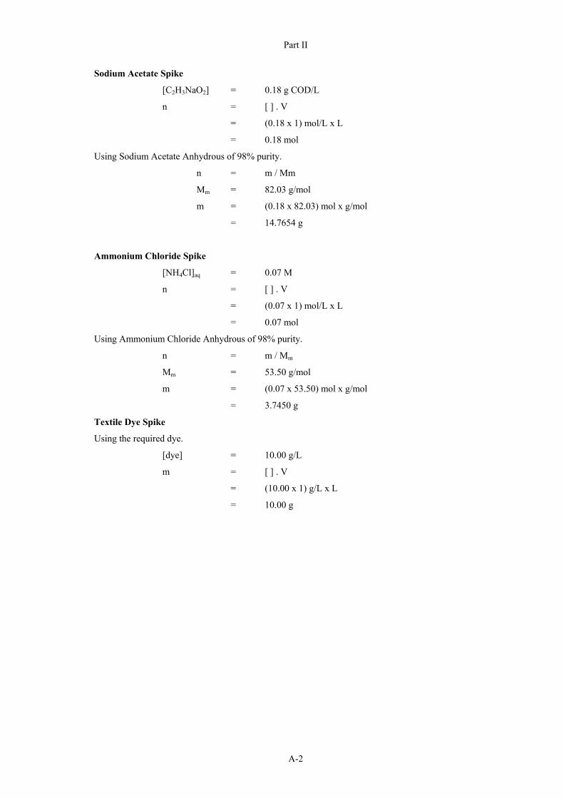
Part II

A-2

Sodium Acetate Spike

[C2H3NaO2] = 0.18 g COD/L

n = [ ] . V

= (0.18 x 1) mol/L x L

= 0.18 mol

Using Sodium Acetate Anhydrous of 98% purity.

n = m / Mm

Mm = 82.03 g/mol

m = (0.18 x 82.03) mol x g/mol

= 14.7654 g

Ammonium Chloride Spike

[NH4Cl]aq = 0.07 M

n = [ ] . V

= (0.07 x 1) mol/L x L

= 0.07 mol

Using Ammonium Chloride Anhydrous of 98% purity.

n = m / Mm

Mm = 53.50 g/mol

m = (0.07 x 53.50) mol x g/mol

= 3.7450 g

Textile Dye Spike

Using the required dye.

[dye] = 10.00 g/L

m = [ ] . V

= (10.00 x 1) g/L x L

= 10.00 g

Part II

B-1

Appendix B Equipment and Calibration

B.1 Equipment

Dissolved Oxygen Probe Type: YSI 5739 Field Probe

Membrane: FEP Teflon

Cathode: Gold

Anode: Silver

Electrolyte: Half-saturated KCL

Temperature Range: -5 to 45°C

Polarizing Voltage: 0.8 V

Probe Current: 19 mA

Oxygen Uptake Rate Meter Type: UCT DO/OUR Meter

Key Pad Functions:

� When in Mode A – press the “B” key. Display confirms – Mode B Selected.

� When in operation display indicates; DO (mg/L), Temperature (°C), Hi Limit and Lo Limit (mg O2/L).

� Set Hi and Lo limits by holding down the following keys:

� C - Increases Hi Limit

� D - Decreases Hi Limit

� E - Increases Lo Limit

� F - Decreases Lo Limit

� Re-selecting Mode A clears all accumulated data.

� The 10 most recent OUR determinations are available via the LCD.

� Hold down “0” key – display current cycle OUR

� Hold down “1” key – display current cycle – 1 OUR

� .. .. .. .. ..

� Hold down “9” key – display current cycle - 9 OUR

Part II

B-2

B.1 Equipment Calibration

Oxygen Uptake Rate Meter Requirements:

Sodium sulphite solution of 27 g/L concentration.

Beaker of distilled Water.

Procedure:

� Connect DO electrode to the “probe” socket and temperature probe to “temp” socket.

� Switch on instrument.

� Push the “A” key to get meter in Mode A, instrument displays dissolved oxygen concentration (mg/L) and temperature (°C).

� To set DO zero, place DO probe in sodium sulphite solution (27 g/L) and leave in solution until dissolved oxygen concentration (DO) reading is stable for about 1 minute. Adjust ZERO pot on rear of instrument such the DO reading is 0.0 mg/L.

� Remove DO probe from sodium sulphite solution and flush in distilled water.

� To set DO gain, place DO probe in beaker of distilled water. Bubble air into the water such that the water becomes saturated with oxygen. Continue bubbling air until reading is constant. Use the temperature probe to measure the water temperature. Refer to Table B-1 to determine the saturated value of DO at the current temperature. A correction factor for the atmospheric pressure should be included, see Table B-2.

� Example

� DO = 9.00 mg/L at 21 oC (at 1 atmosphere)

� DO = (9.00 x 0.88) = 7.92 mg/L (at 669 mmHg)

� Adjust GAIN pot on rear of instrument such that the DO reading is correct.

� Verify the zero setting by replacing the probe in the sodium sulphite solution.

Part II

B-3

Table B-1 Oxygen Solubility (at Sea Level)

Temperature (°C)

Dissolved Oxygen (mg/L)

Temperature (°C)

Dissolved Oxygen (mg/L)

1 14.60 23 8.70

2 14.20 24 8.50

3 13.90 25 8.40

4 13.50 26 8.20

5 13.20 27 8.10

6 12.80 28 7.90

7 12.40 29 7.80

8 11.90 30 7.70

9 11.60 31 7.50

10 11.30 32 7.40

11 11.10 33 7.30

12 10.80 34 7.20

13 10.60 35 7.10

14 10.40 36 7.00

15 10.20 37 6.80

16 9.90 38 6.70

17 9.70 39 6.60

18 9.50 40 6.50

19 9.30 41 6.40

20 9.20 42 6.30

21 9.00 43 6.20

22 8.80 44 6.10

Part II

B-4

Table B-2 Atmospheric Pressure Correction Factors

Atmospheric Pressure (mmHg)

Correction Factor

760 1.00

745 0.98

730 0.96

714 0.94

699 0.92

684 0.90

669 0.88

654 0.86

638 0.84

623 0.82

608 0.80

593 0.78

578 0.76

562 0.74

547 0.72

532 0.70

517 0.68

502 0.66

Oxygen Solubility at Sea Level

y = -6E-05x3 + 0.0071x2 - 0.3903x + 14.6050.02.04.06.08.0

10.012.014.016.0

0.0 10.0 20.0 30.0 40.0 50.0Temperature (oC)

DO

(mg/

L)

Figure B-1 Oxygen Solubility at Sea Level

Part II

B-5

Atmospheric Pressure Correction Factor

y = 0.0013161x - 0.00020.60

0.70

0.80

0.90

1.00

1.10

480 530 580 630 680 730 780

Atmospheric Pressure (mmHg)

Cor

rect

ion

Fact

or

Figure B-2 Atmospheric Pressure Correction Factor

Part II

C-1

Appendix C Estimating COD

The theoretical COD can be determined by using the following equation:

2 32 7 2 2 4

8 38 22n a b c

a d cC H O N dCr O d c H nCO H O cNH dCr C-1

Where:

23 6 3 2n a b cd C-2

(3/ 2)COD d C-3

An example of the calculation to determine the theoretical COD is presented and the results summarised in Table C-2. The molecular weights of the reacting species are required for this calculation and are shown below in Table C-1.

Table C-1 Compound Molecular Formulae and Weights

Compound Formula Molecular Weight g/mol

Acetate CH3COONa 82

Biomass C5H7O2N 113

Acetate: n = 2 a = 3 b = 2 c = 1

Substituting into equation C-2:

d = 0.67 moles of O2

Resultantly equation (C-1) is: 2 3

2 3 2 2 7 2 20.66 6.28 2 5.28 1.32C H O Na Cr O H CO H O Na Cr

Hence, using equation (C-3):

1 mole CH3COONa = (3/2)d

= 1 mole of O2

But, 1 mole CH3COONa = 82 g

1 mole O2 = 32 g

Thus for the complete oxidation of 82 g of CH3COONa, 32 g of oxygen is required.

Part II

C-2

Therefore: 1g CH3COONa requires 0.392 gO2 or equivalently 0.392 gCOD.

Table C-2 Theoretical Estimates of Chemical Oxygen Demand

Compound Formula N a b c d gCOD

Acetate CH3COONa 2 3 2 1 0.67 0.392

Biomass C5H7O2N 5 7 2 1 3.33 1.416

Part II

D-1

Appendix D Experimental Procedures

D.1 Operating Manual

STAGE ONE

The activated sludge sampled from the aeration basin maybe stored for no more than 2 weeks before concentration. The sludge must be kept in a dark cold room set at 4°C with no substrate.

Biomass Concentration

� Remove raw activated sludge from 4°C cold room.

� Allow particulates to settle in container.

� Concentrate activated sludge by removing as much supernatant liquid from container.

� Place container of sludge in warm bath, leave in bath until sludge reaches 25°C. The sludge is now ready to be used in reactor.

STAGE TWO

Start up

� Locate UCT DO/OUR meter main socket. Ensure that the amplifier and computer are plugged in.

� Check that the computer and amplifier are connected to UCT DO/OUR meter.

� Switch on UCT DO/OUR meter at main switch, the LCD displays:

� DO Meter V2.1

� UCT Chem Eng 1992

� Switch on computer and in DOS mode start the programme, i.e. (C:\doprogs\DOMPC.exe).

� A blue main menu screen should appear.

Probe Calibration

The pH electrode is calibrated using pH4 and pH 7 buffer solutions. The pH probe is immersed in the lower pH buffer solution then into the higher pH buffer solution. The temperature probe does not require calibration.

OUR Meter Calibration

Calibrate UCT DO/OUR meter as described in Appendix B.

Set point Adjustment

The set points adjustments for sodium acetate spikes and ammonium chloride spikes experiments are different. This is so as a result of noise effects and the differing rates at which the two substrates are consumed.

Sodium Acetate Spike Experiments: � The Hi and Lo limits for dissolved oxygen (DO) concentration must be set on the DO/OUR meter.

� Press “B” key on the meter to get into Mode B.

� The Hi limit for DO concentration is increased by pressing “C” key and decreased by pressing “D” key. Set Hi Limit of DO concentration to 5.00 mg/L.

� The Lo limit for DO concentration is increased by pressing “E” key and decreased by pressing “F” key. Set Lo Limit of DO concentration to 4.50 mg/L.

� The offset DO value and the sample rate are adjusted in the main menu of the DOMPC programme.

Part II

D-2

� Select the “Offset” option in the main menu.

� Set offset to a value of zero. Press ENTER to return to the main menu.

� Select the “Sample rate” option in the main menu.

� Set Sample rate to 6 s. Press ENTER to return to the main menu.

Ammonium Chloride Spike Experiments: � The Hi and Lo limits for dissolved oxygen (DO) concentration must be set on the DO/OUR meter.

� Press “B” key on the meter to get into Mode B.

� The Hi limit for DO concentration is increased by pressing “C” key and decreased by pressing “D” key. Set Hi Limit of DO concentration to 5.00 mg/L.

� The Lo limit for DO concentration is increased by pressing “E” key and decreased by pressing “F” key. Set Lo Limit of DO concentration to 4.80 mg/L.

� The offset DO value and the sample rate are adjusted in the main menu of the DOMPC programme.

� Select the “Offset” option in the main menu.

� Set offset to a value of zero. Press ENTER to return to the main menu.

� Select the “Sample rate” option in the main menu.

� Set Sample rate to 1 s. Press ENTER to return to the main menu.

Test Monitoring

� The pH of the reactor must be monitored continually and controlled at a value of pH 7.5 (± 0.2), using the hydrochloric acid and sodium hydroxide 0.01 M titrate solutions.

� At intervals of 3 hr or sooner depending on the rate of activity, OUR data should be analysed until endogenous respiration conditions are observed.

� After spiking with substrate the OUR data should be analysed at intervals of about 30 min, once again depending on the rate of activity.

� Select the “Collect Historic data” option in the main menu.

� Choose the “Write disk only” option. Press ENTER to return to the main menu.

Shut down

� Collect the remaining OUR data.

� Exit from DOMPC program. Select “Quit to DOS” option.

� Remove all probes from reactor.

� Rinse pH probe with distilled water and cap it. Place some potassium chloride solution into cap before placing it over the probe.

� Rinse DO probe with distilled water and place probe in bottle. Ensure moist sponge is in the bottle.

� Rinse Temperature probe.

D.1 Analytical Test Procedures

Organic Content The Chemical oxygen demand (COD) was used as a measure of the oxygen equivalent of the organic matter content of samples that were susceptible to oxidation by a strong chemical oxidant.

COD Open Reflux Method:

This method is suitable for wastes where a larger, more concentrated sample is preferred. The test was used to evaluate the COD of the wastewater which was used as a substrate in the respirometric experiments. A sample is refluxed in strong acid solution with a known excess of potassium dichromate

Part II

D-3

(K2Cr2O7). After digestion, the remaining unreduced K2Cr2O7 is titrated with ferrous ammonium sulphate to determine the amount of K2Cr2O7 consumed and the oxidizable matter is calculated in terms of oxygen equivalent. The procedure of the open reflux method is presented below.

A 250 mL sample of the test substance was diluted to 500 mL in a volumetric flask. The dilution is necessary because the sample COD could be greater than 900 mg O2/L. A 10 mL aliquot of this was placed into a 250 mL refluxing flask. To this was added 0.04 g of mercuric sulphate, several glass beads and 5 mL aliquot of potassium dichromate solution (0.0417 M) was added. A 5 mL of sulphuric acid reagent was added to this. The flask was attached to the condenser and cooling water turned on. The mixture was refluxed for 2 h. A blank consisting of 10 mL distilled water, instead of the substrate, was refluxed in the same way. The samples were allowed to cool and the condenser was rinsed with 80 mL distilled water. Thereafter, they were titrated with ferrous ammonium sulphate solution (FAS) using ferroin indicator.

The COD of the sample was evaluated using Equation D-1

8000

S

A B CCOD

V D-1

A = FAS (Blank) [mL]

B = FAS (Sample) [mL]

C = Molarity of FAS [M]

SV = Volume of Sample [mL]

Total Suspended Solids: The test was used to evaluate the total solid content of the activated sludge which was used in the respirometric experiments. A well-mixed sample is filtered through a weighed standard glass-fiber filter and the residue retained on the filter is dried to a constant weight at 103 °C. The increase in weight of the filter represents the total suspended solids. The procedure of the total suspended solids test is presented below.

10 mL, 20 mL and 30 mL well-mixed samples of activated sludge were filtered separately through 3 weighed standard glass-fiber filter papers respectively and the residue retained on the filters is dried to a constant weight at 103 °C. The filter with this residue is allowed to cool in a desiccator then weighed.

The total suspended solids of the sample were evaluated using Equation D-2

1000

S

A BTSS

V D-2

A = weight of filter + dried residue [mg]

B = weight of filter [mg]

SV = Volume of Sample [mL]

Volatile Suspended Solids: This measurement of volatile solids is an approximation of the amount of organic matter present in the solid fraction of the activated sludge. The residue from the TSS test is ignited at 550 °C for 2 h. The remaining solids represent the fixed total, dissolved, or suspended solids while the weight lost on ignition is the volatile solids. The procedure of the volatile suspended solids test is presented below.

Part II

D-4

The residue of the 3 samples from the TSS test is ignited at 550 °C for 2 hr. The filter with this residue after ignition is allowed to cool in a desiccator then weighed.

The volatile suspended solids of the sample were evaluated using Equation D-3.

1000

S

A BVSS

V D-3

A = weight of filter + dried residue after ignition [mg]

B = weight of filter + dried residue before ignition [mg]

SV = Volume of Sample [mL]

CB-1

Capacity Building

This project supported two MScEng research projects:

Prelan Gounder (BScEng, University of Natal)

Thesis title: Modelling of the effects of textile industry wastewaters on the performance of a municipal wastewater treatment plant

Completed: 2006

Mlungiseleli Binda (BSc, University of Fort Hare)

Thesis title: The demonstration and evaluation of a system to select high environmental impact dyes and chemicals used in the textile industry.

To be completed

Mr Binda joined the KwaZulu-Natal Department of Agricultural and Environmental Affairs in December 2005 and is currently an Environmental Officer in the environmental Compliance Monitoring and Enforcement Unit.

In addition, two undergraduate chemical engineering students were involved in the project as research assistants:

Poshendra Moodley: 2002

Krishni Arumugan: 2003 and 2004

All four of these students are members of previously disadvantaged groups.

Two students from the Danish Textile Design College (TEKO), Ellen Hogh and Lican Mally, were involved in the initial set up of the Score system and training of Mr Binda. This took place under the supervision of Tove Anderson from the Danish Technological Institute.

Two students from Aalborg University, Denmark: Carsten Lauridsen and Jesper Poulsen spent 6 months with the PRG as part of their engineering training.

TT-1

Technology Transfer Technology transfer was achieved through several workshops, seminars and conference papers and through collaboration with the DANIDA Cleaner Textile Production Project (CTPP).

4. Workshops The score system has been widely demonstrated to the textile industry through a series of workshops and seminars

The first workshop was convened by the Textile Federation in Durban in June 2001. The attendants included factory and supplier representatives, regulators and other interested parties. The goal of the workshop was to introduce the Score System to the various stakeholders and to gauge their acceptance of the system and willingness to participate in its implementation

Presentations on the Score System and the current project have been made at two DANIDA Cleaner Textile Production Project Dissemination events: the CCTP Dissemination Week held in Durban and Cape Town from 3-7 March 2003 and subsequent CCTP Dissemination event on 16 November 2004.

An oral presentation entitled “Score System for the Selection of Textile Dyes” was also given at the CTPP sponsored Cleaner Production Workshop held in Westmead on the 4th of March 2005. Lief Theilgaard, head of the Industrial Environment Section, Ringkjøbing County Department of Environment and Infrastructure, visited South Africa from 3rd to 12th November 2004. Meetings were held with the Department of Water Affairs and Forestry (DWAF), the WRC, and Gregory Knitting Mills; and separate workshops were held for regulators and industry and suppliers in both Durban and Cape Town. These meetings and workshops resulted in a large amount of discussion on the implementation of the score system in South Africa.

5. Conference presentations BINDA M, NAIDOO V and BUCKLEY C.A. (2002) Score System for the Selection of Textile Chemicals and Dyes in South Africa. Proceedings: Wastecon 2002 – International Waste Management Biennial Conference and Exhibition, Durban, South Africa, 30 September – 4 October 2002.

BINDA M and BUCKLEY C.A. (2003) The Score System in the South African Textile Industry. Proceedings: International Water Association Conference on Environmental Biotechnology Advancement on Water and Wastewater Applications in the Tropics, Kuala Lumpur, Malaysia, 2-3 May 2003.

REMIGI, E., BINDA, M., BUCKLEY, C., BARCLAY, S. and FOURE, P.(2006) A Database Application for the Efficient Management of Score System Related Information. Proceedings: WISA 2006 - Water Institute of Southern Africa Biennial Conference & Exhibition, Durban, South Africa, 21-23 May 2006, pp 1-8. (Poster).

BINDA M., BUCKLEY C.A. and PAULIG W. (2006) Environmental Impact of Different CEL Reactive Dyes. Proceedings: South African Dyers and Finishers NATCON Conference, Durban., South Africa, 15-17 March 2006.

6. Interaction with other WRC projects The Batch Respirometric Experimental methodology developed in this project to characterise the inhibitory effect of textile dyes on wastewater treatment plants is being modified to use WWTP influent as the test substrate and textile effluent as the test substance in WRC Project 1734 Protocol for the quantitative assessment of industrial effluents for discharge permitting. The new project also aims to develop a model of the actual treatment plant the test sludge and influent is taken from to use instead of the COST benchmark model for the purpose of calculating the effluent tariffs. There was also an interaction between the current project and WRC 1542 - Dye liquor recycle using activated carbon. Both the current project and WRC-1542 arose out of recommendations from WRC Project No. 760 - Waste minimisation guide for the textile industry: A step towards Cleaner Production.