Promemorior från P/STM 1983:9. Regression analysis and ratio analysis for domains : a randomization theory approach / Eva Elvers m.fl. Digitaliserad av Statistiska centralbyrån (SCB) 2016.

urn:nbn:se:scb-PM-PSTM-1983-9

INLEDNING

TILL

Promemorior från P/STM / Statistiska centralbyrån. – Stockholm : Statistiska

centralbyrån, 1978-1986. – Nr 1-24.

Efterföljare:

Promemorior från U/STM / Statistiska centralbyrån. – Stockholm : Statistiska

centralbyrån, 1986. – Nr 25-28.

R & D report : research, methods, development, U/STM / Statistics Sweden. –

Stockholm : Statistiska centralbyrån, 1987. – Nr 29-41.

R & D report : research, methods, development / Statistics Sweden. – Stockholm :

Statistiska centralbyrån, 1988-2004. – Nr. 1988:1-2004:2.

Research and development : methodology reports from Statistics Sweden. –

Stockholm : Statistiska centralbyrån. – 2006-. – Nr 2006:1-.

STATISTISKA CENTRALBYRÅN 1983-06-20

PROMEMORIOR FRÅN P/STM

NR 9

REGRESSION ANALYSIS AND RATIO ANALYSIS FOR DOMAINS,

A RANDOMIZATION THEORY APPROACH

AV EVA ELVERS, CARL ERIK SÄRNDAL,

JAN H WRETMAN OCH GÖRAN ÖRNBERG

MARCH, 1983

REGRESSION ANALYSIS AND RATIO ANALYSIS FOR DOMAINS,

A RANDOMIZATION THEORY APPROACH

by

Eva ELVERS*, Carl Erik SÄRNDAL**, Jan H. WRETMAN* and Göran ÖRNBERG***

*Statistics Sweden, Stockholm

**Université de Montreal

***Department of Mathematical Statistics, University of Stockholm

ABSTRACT

In most surveys, inference for domains poses a difficult problem because

of data shortage. This paper presents a design-inference (or randomization theory)

approach to some common types of statistical analysis for domains of a surveyed

population. Simple and multiple regression analysis, and analysis of ratios are

considered. Two new methods are constructed and explored which, with the aid of

auxiliary information, can improve substantially over the ordinary method based

on straight ir-inverse (product) sums. The theoretical conclusions are supported

by empirical results from Monte Carlo experiments.

Key words: Domains, survey sampling, design inference, regression analysis,

analysis of ratios.

- This work was supported in part by the Natural Sciences and Engineering Research Council of Canada

2

1. THE RESEARCH QUESTION

Inference for domains is required in most surveys, and extensive research

efforts are currently directed to this problem area. The question that initiated

our work was: given survey data from a population divided into many domains, how

do we make inference, domain by domain and in the standard randomization theory

fashion, about measures of relationship between a criterion variable y and

explanatory variables x, ,...,x , such as simple ratios or (multiple) regression

slopes? The possible shortage of observations in any given domain poses a diffi­

culty which is overcome, in our methods below, by exploiting auxiliary information.

Let U = {!,...,k,...,N} denote a finite population of labelled units

and let U be divided into nonoverlapping domains u\. of sizes Nj. ,

d = 1.....D ; N=Z . , N. . If U is a country, and the units households, the

Ud# may represent a possibly large number of geographical subdivisions of U .

A sample survey is carried out on U according to a perhaps complex survey design.

A random, often small number of observations will fall in a given domain U. .

With only one x-variable, we have in mind the estimation of parameters measuring

the rate of change in y given x , such as, for d = 1.....D ,

(1.1)

(1.2)

(E. denotes sum over k in the set A) . More generally we seek to estimate

multiple regression coefficients for the d:th domain. Frequently in surveys

one wishes not only to estimate such rate-of-change measures, but also to test

for their significant differences between domains. Only the estimation part is

dealt with below, but the paper contains the basis for futher work on the

hypothesis testing problem.

3

We work under the randomization theory principle of adjustment for varying

inclusion probabilities by "Tr-inverse weighting" of units. In this spirit, Kish

and Frankel (1974) studied the estimation of (multiple) regression coefficients

for the entire population. Fuller (1975), Shah, Holt and Folsom (1977) contributed

further to the theory. They did not examine regression analysis for domains, and

the use auxiliary information was not discussed. Important is that these authors

see the regression slopes as descriptive finite population parameters, not as

superpopulation model parameters. Here we share that view; extensions to

discriminant analysis and logistic regression are reported in Binder (1982).

Whether the finite population parameter or the superpopulation parameter

perspective should be adopted depends on the situation. The latter view is held

in the interesting model-based regression analysis of Nathan and Holt (1980),

Holt, Smith and Winter (1980), Smith (1981). In Section 8 we discuss their approach,

which permits auxiliary information to be incorporated, but again does not consider

the domain estimation problem.

2. STATEMENT OF PROBLEM AND GENERAL PROCEDURE

Associated with unit k(k = 1,...,N) is the vector (y. »x. ,6k) . where

x. = (x.......Xj.,...,x. )' , and domain membership is indicated by the D-vector

<5k with typical element <5dk = 1 if k £ U. and $.. = 0 otherwise. In

regression with an intercept, x., = 1 for k = 1.....N . Prior to sampling,

(y. ,x. ) and often 6. , too, are unknown. However in two methods discussed

below (F and P) , knowledge about domain membership is assumed to permit

improvement of the basic C-method.

The problem is to estimate, for d = 1,...,D , the regression coefficient

vector of y on x defined for the d:th domain as

4

(2.1)

N where A. = I, &liicY

li,\xl anc' A. is analogous, that is, the r-vector

x.y. replaces the r x r matrix x.xj" in A. . The known constants w. ,

if not all equal to one, are to permit weighted regression.

Our interest in B, is in line with the concern often present in

surveys to estimate descriptive quantities for the finite population, rather than

parameters in models. One notes that B. is the weighted least squares estimator

of 0 that would arise in the hypotehtical "census fit" of the superpopulation

model y. = x/B + £. to a!! N. points of U\ , if the £. are independant

with mean 0 and variances wj" . Simple examples of (2.1) are (1.1), arising

when r = 1 and /.,. .--• x,- ~ w" ,. and (1.2), arising when r = 2 , x. = (1 ,x,)' ,

w. = 1 . Their estimation is dealt with in Sections 5 and 6.

Å probability sample s of fixed size n is drawn from U by a sampling

design p(s) with strictly positive inclusion probabilities u. = P(kes) ,

nkl " ^..tes) • "ne Part of s that happens to fall within UH# is denoted

s, , of random size n, „ where n = E. n,, . The estimators will be built

on the data (y^x,,) for k e s . For estimation of B. , we examine three

methods,, called C , F and P , each containing a Step 1 for constructing the

estimator B, , and a Step 2 for constructing an estimated variance-covariance

matrix, V (B.) , of B \ s theoretical variance-covariance matrix, vD(Bd) •

STEP 1, First estimate Ad x x and A. by, respectively, A d x x and ~_] -

Adxv , w 'ach then define the B .-estimator as 8^ = A d x xA d x v .

STEP 2. Calculate an estimated (design-based) variance-covariance

matrix of §, bv d

5

(2.2)

where the ij": th element (i,j = l,...,r) of the r x r matrix YG, is

the Yates-Grundy type quantity

where udki is to be defined and A ^ = (^/"'Yt^lcfc '

The three methods propose different A. , A. in Step 1 and will

give rise to different u.. . in Step 2. Computationally, Methods F and P

also involve a preliminary Step 0. A brief statement of the three computational

procedures is given in Section 3; discussion is saved for later sections. For

interval estimation of B.. with 100(l-a)% confidence,

(2.3)

Z, /0 being the normal score, is recommended until more accurate methods have I-a/2 3

been explored. If n is very large and the domain not too small, (2.3) gives

roughly the right coverage rate for the procedures stated in Section 3. However:

our Monte Carlo studies show that the normal score if often too modest to reach

the nominal 100(l-ct)% coverage of the true slope B.. in repeated samples

drawn by the fixed design. For a given total sample size n , the achieved

coverage rate deteriorates with smallness of domain; further work may improve

the confidence interval procedure.

3. SKELETON OUTLINE OF PROCEDURE, METHODS C , F AND P

The C method (C for Common) uses straight ir-inverse weighting in

estimating each (product) sum. When applied to the full population, the C-method

6

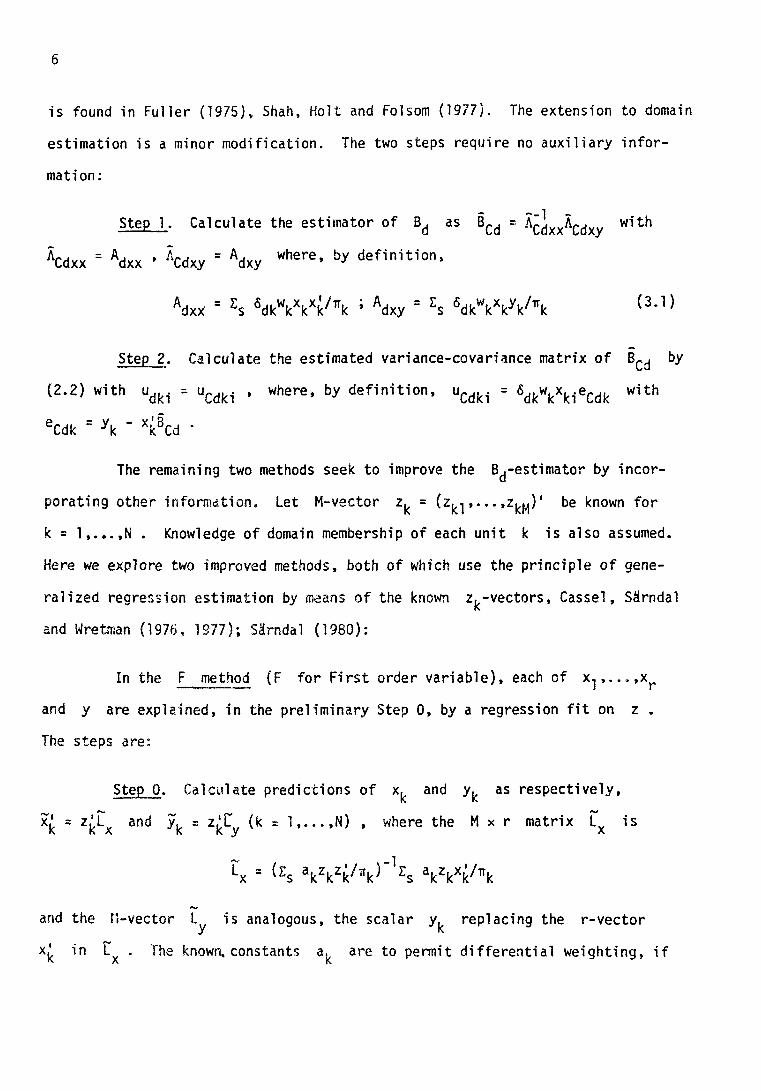
is found in Fuller (1975), Shah, Holt and Folsom (1977). The extension to domain

estimation is a minor modification. The two steps require no auxiliary infor­

mation:

Step 1. Calculate the estimator of Bd as §Cd = ÄcdxxÄcdxy with

ÄCdxx = Adxx • ÄCdxy = Adxy w h e r e' by definition,

(3.1)

Step 2. Calculate the estimated variance-covariance matrix of Bcd by

(2.2) with udk. uCdk- , where, by definition, u ^ . = ^ v y ^ . e ^ with

eCdk = y k ' xkBCd '

The remaining two methods seek to improve the B .-estimator by incor­

porating other information. Let M-vector z. = (z.,,... »z^.J' be known for

k = 1,...,N . Knowledge of domain membership of each unit k is also assumed.

Here we explore two improved methods, both of which use the principle of gene­

ralized regression estimation by means of the known z.-vectors, Cassel, Särndal

and Wretman (1976, 1977); Särndal (1980):

In the F method (F for First order variable), each of x,,...,x

and y are explained, in the preliminary Step 0, by a regression fit on z .

The steps are:

Step 0. Calculate predictions of x. and yk as respectively,

x^ = z^Lx and yk = z^t (k = 1.....N) , where the M x r matrix Lx is

and the fl-vector L is analogous, the scalar y, replacing the r-vector y K

xk in L . The known, constants a, are to permit differential weighting, if

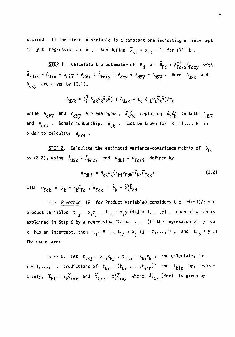
7

desired. If the first x-variable is a constant one indicating an intercept

in y,s regression on x , then define x., = x., = 1 for all k .

STEP 1. Calculate the estimator of B. as Bc. = lZ. ÄCJ with d rd Fdxx rdxy

AFdxx = Adxx + Adxx " Adxx ; AFdxy = Adxy + Adxy " Adxy • H e r e Adxx and

Adxy a r e g i v e n by (3.1)'

while A.~^ and A.~~ are analogous, x.y. replacing x.x' in both A.~~

and A.~~ . Domain membership, S.. , must be known for k = 1.....N in

order to calculate A,~~ .

STEP 2. Calculate the estimated variance-covariance matrix of Bp

by (2.2), using Äd x x = Ä F d x x and udki = u p d k i defined by

(3.2)

The P method (P for Product variable) considers the r(r+l)/2 + r

product variables t.. = x.x. , t. = x.y (i<j = 1 r) , each of which is 1J I J 10 l

explained in Step 0 by a regression f i t on z . ( I f the regression of y on

x has an intercept, then t „ = 1 , t . . = x. ( j = 2 , . . . , r ) , and t l o = y .)

The steps are:

SIEP_0. Let t k i j = x k i x k j , t k i o = xk .yk , and calculate, for

i = 1 r , predictions of t k - = ( t k n . . . . , t k l > ) ' and tkiQ by, respec­

t ive ly , ? ' . = zk3f.xx and t k . 0 = zk3f.xy where J - x x (Mxr) is given by

8

and J. (Mxl) is analogous, the scalar t. . replacing the r-vector t/.

in X . For the intercept case, define t.,, = t.,, = 1 for k = 1.....N

STEP 1. Calculate the estimator of Bd as Bpd = Apd x xAp d with

APdxx = Adxx + Ad(5a) " Ad(x£) ; APdxy = Adxy + Ad(xy) " Ad(xy)

Here, Ad x x and A d x y are given by (3.1); A d ( r x ) and A d ( - } are r x r N matrices whose i :th rows are given, respectively, by E, <Sd)<wkt/. and

Zs ^ d ^ Ä i ^ k wni^e tne r x 1 columns A^-r^x and A^-^x are analogous,

their i:th element having the scalar t. . in place of the r-vector

t. . . As in Method F , domain membership, 6.. , must be known for

k = 1.....N .

STEP 2. Calculate the estimated variance-covariance matrix of Bpd

by (2.2) using Ädx x = Ä p d x x and udki = upd k 1 defined by

with

Our Monte Carlo experiments so far (see Section 8) have not shown

any great differences in efficiency between Methods F and P , both of

which can however improve greatly over Method C .

9

4. DERIVING VARIANCE-COVARIANCE ESTIMATES

The variance-covan'ance estimates in Step 2 of the C- , F- and

P-methods rest on approximations. For the C-method, reference to Fuller

(1975) suffices. As for the other two methods, we choose to illustrate how

V (Bc.) is obtained, p Fd

In the F-method, L estimates its population analogue

The j : t h column of L° is made up of the weighted least squares regression

coefficients that would arise in the "census f i t " of x. on z using the N

data points of the whole population. Let the resulting r-vector of f i t ted

values for unit k be x° = z/L° . Similarly, the k:th f i t t ed y-value

would be y? = z/Ly , where L° is analogous to L° , with yk in place

of x.1 . Set

We express the error of the F-estimator as B^ - Bd = Ap(jxx( ' : i+F2^

where the r-vectors F, and F„ are

10

We arr ive at V (BF.) by way of an approximation of the theoret ica l

mat r ix , V (Bp.) . In large samples, F„ w i l l be near zero in p robab i l i t y

(as determined by the sampling design) for the twofold reason: (a) each

A-matrix is close to i t s A-counterpart, and (b) L and L° are c lose, as A A

are L and L° , so that A d x 0 y 0 and Ad~~ are close, as are Adxoyo

and A . — , etc. The design variance contributed by F2 is expected to be

small relative to that coming from F, , which is near zero in probability

for only the first of the two reasons. Further, in a first approximation to

variance, ÄZ. may be replaced by its target, A V . Thus, we take

Br. - B . = A "J F. as the basis for an approximate variance-covariance calcu­

lation. Alternatively,

where u F d k = (uFdkl.. • • »^dkr^' is d e t e r m i n e d b^

Now F. involves simple Horvitz-Thompson estimators, so directly

where Vp. is r x r with ij-element

This contains the unknowns A. , B. , L° and L° . For an estimated matrix,

replace each of these by its sample couterpart, Ap. , Bpd , U and t ,

which implies replacement of vipdkl- by Uprf. . given by (3.2). Replacement

of

11

completes the procedure. We have obtained the variance-covariance estimate given

in the F-method's Step 2.

5. DOMAINWISE ESTIMATION OF A RATIO OF AGGREGATES

A special case of the foregoing is to estimate, domain by domain, the

ratio R. , formula (1.1), of two domain sums. Important applications are of

the type where one seeks to estimate "acreage under wheat (y) to total acreage

(x)" for farms belonging to the d:th of D geographical subdivisions of a sampled

larger region. Now R. is the ratio of two scalars, the linear sums

N N A M = £, öj.yi and A., = £, 6 ., x. . Their estimation is simple in the C-method. diy i dk k dix 1 dK K

The F-method as given in Section 3 also provides for estimation of linear sums,

since the r-vector x. may contain the constant one.

The C-method gives simply

with estimated design variance

£S

w h e r e ucdk = 5 dk ( y k - x Ad } •

In the F-method's Step 0, we have

12

and analogously for y. , with y. replacing x^ in xk . In carrying out

Step 1, look upon Arflx as zj <5dxxkoxk , where xkQ = 1 = xko for all k ,

and analogously for A,, . We get

where

and analogously for Äp., , with y. and yk instead of xk and x. . The

estimated variance, from Step 2, is

with

The performance of the two methods has been tested in Monte Carlo experiments on

which we comment in Section 8.

6. DOMAINWISE SIMPLE REGRESSION ANALYSIS

To enrich the brief statement in Section 3, let us discuss our three

methods with another simple application in mind: We seek to estimate, for each

of the D domains, the slope B. , given by (1.2), of a simple regression with

intercept of y on x . Frequently one needs to compare slopes in different

domains, so the standard error calculations given below are important.

In practice one often exploits the homogeneity gained by an a priori

known categorization of the units. Let z. = (z.,,...,z.,...,z.„)' required

in Step 0 be a category»indicator, with z. =1 if k e U and z, = 0

13

otherwise; m = 1.....M . The mutually exclusive categories U cut across the •m

domains Ud> . Possibilities discussed in Section 7 are: (1) the categories are

M = G "postgroups" (called groups in the following) that do not participate in

the sampling design but are exploited after sampling to reduce the estimator's

variance; (2) the categories are the M = H strata in a stratified random

sampling design; (3) the categories are the M = GH cells resulting from a

crossclassification of G groups with H strata. In the third case there will

thus be three dimensions involved: if units are households, the domains

could be smaller administrative areas of a sampled country, the strata could be

larger geographical areas, and the groups family types.

Domains crossed with the categories of z divides the population into

DM cells U. of sizes N, . These latter are the auxiliary quantities that

must be known, from census or other reliable sources, in order to make the F-

and P-methods work. We have

(6.1)

The respective parts of the sample s that happen to fall in U#m and Udm are

denoted s „ , of size n , and s. , of size n.m . Then (6.1) holds with •m -m dm dm

small n's substituted for the capital N's . In the general formulas of Section

3, let x. = 0 » x k ) ' , and assume equal weights: wk = ak = 1 for all k .

Let I indicate the method used; I = C , F or P . The slope estimator is in

all three cases of the form

(6.2)

where £TJ and ZT. are defined below, and the estimated variance is Idxy Idxx

(6.3)

14

Detai ls for each method are as fo l lows: Set N, = L 1/TT, . Use the symbol dm

~ to indicate "Ti-means", that i s , i t - inversely weighted averages such as

and analogously fo r several other ir-means used below.

In the C-method, use I = C in (6.2) and (6.3), where

Let t ing eC( jk = y k - y ^ - B ^ - ^ ) . we have

(6.4)

To simplify the F- and P-methods, create centered variables X. , Y.

for the d:th domain as

where

is the estimate of the domain mean x.. = L. X U / N H . produced by both the d« d.

F- and P-methods, and y* is analogous. sd-

In the F-method, use I = F in (6.2) and (6.3), where

and Epdx v is analogous, with X,. Y» and X.$ Yrfs replacing Xrfk and „ y »m «m

(X d s ^ ) . Letting e p d k - Ydk - B ^ , with Tr-mean e ^ in s.m . we

have for k in s •m

15

(6.5)

In the P-method, use I = P in (6.2) and (6 .3 ) , where

~i 2 where (X ) d s is the 7r-mean of Xd- for k in s# . Further, Lp. i s

analogous, w i th Xd(<Ydk and (XY)ds replacing Xdk and (X )d . With •m «m

ePdk = Ydk " BPdXdk ' w e h a v e f o r k in s.m

(6.6)

where (Xe)D. is the 7r-mean of X ,, en , , over k in s Pds m dk Pdk «m •m

The u-quantities (6.4), (6.5) and (6.6) explain heuristically why the

F- and P-methods are often superior to the C-method, as discussed in the next

section.

7. DISCUSSION OF SIMPLE REGRESSION ANALYSIS

In the C-method, u c „ is (apart from the 6-factor) structured

as "centered x-variable times residual". By contrast, in the F- and P-methods

uFdk and uPdk ^ave (aPart rom 5 ) tne f o r m "centered x-variable times resi­

dual minus category mean adjustment", the latter being X\ eV. and , -m #m

(Xe)pd , respectively. This difference explains the variance reductions •m

realizable by the F- and P-methods, as seen more clearly for some simple

designs:

(i) Simple random sampling (srs) and G groups. The z-vector

indicates membership in one of M = G groups labelled g = 1,...,G . The

16

estimated variance (6.3) becomes

where f = n/N and

is the sample variance of the iu .. . The respective group mean adjustments

contained in up - and up., are X. eV. and (Xe)p. , the overbar •g .g .g

indicating straight average over the group part, s#Q , of the whole sample, s .

In methods F and P , the sample variance of u thus consists essentially of

within group components. It will be substantially smaller than in the C-method,

if the groups are efficient so that their mean adjustments differ markedly.

With G - 1 group only, the F- and P-methods are identical, but the two are

not identical to the C-method, as a first guess may have been. However, essen­

tially no variance reduction will be realized by the F = P method, since the

one and only group adjustment applies to every unit k .

(ii) Stratified random sampling (strs) and G groups. The strata,

labelled h = 1,...,H , ordinarily cut across the G groups (g = 1,...,G)

as well as the D domains (d = 1,...,D). Let N . , n . and f^ = i\>h/Nt>h

denote stratum population size, stratum sample size and stratum sampling fraction.

Then (6.3) becomes

(7.1)

where v (u I d ) i s the variance of Ur .. over k in the sample s. selected h

randomly from stratum h . Here too , the F- and P-methods w i l l lead to

substant ial variance reductions over the C-method, i f the grouping s t rongly

supplements, rather than closely copies, the s t r a t i f i c a t i o n . The argument is

17

as in case (i) above: updk and up contain a group mean adjustment, which

can strongly reduce the stratum variance of u if the grouping is efficient.

There are at least two possibilities to code the z-vector necessary in Step 0

of the F- and P-methods: (a) simply let z be the G-vector that indicates

group membership; (b) let z be the extended vector of dimension GH indicating

one of the cells in the crossclassification of groups with strata. For each of

the three methods separately, (a) and (b) will not cause much difference in effi­

ciency. The possible gains from stratification are essentially discounted already

in method (a), through the stratumwise buildup of (7.1).

(iii) strs without grouping. Let z. indicate stratum membership.

Clearly here one does not expect the F- and P-methods to be superior to the

C-method. This can be seen more formally from (7.1), where v (uId) is the _ h

stratum variance of u... , or, equivalently, of Uj » - u.. , which in all h

three methods is "centered x-variables times residual minus stratum mean adjustment".

In the F- and P-methods, the stratum mean adjustment is already present in u

itself and tL. = up. = 0 ; in the C-method, the stratum adjustment is h h _

created through u-. . For a given unit k , u... - u. . is not exactly the h h

same number in the C- , F- and P-methods, but the calculated values of

v (u ) will be essentially equal in the three methods.

Our methods have the generality of permitting more complex designs,

including cases of two or more stages. The variance reducing effects of Methods

F and P will continue to be strong when the z-vector contains essential

extraneous information.

8. MONTE CARLO EXPERIMENTS

Our Monte Carlo experiments were designed primarily to assess the

18

variance reductions realizable by the F- and P-methods over the simple C-

method, and to see if the F- and P-methods differ by much in efficiency. It

must be kept in mind that the results of any simulation depend entirely on the

nature of the population chosen for study. A detailed account of our simulations

will be given elsewhere. We simulated the estimation of the ratio R. given by

(1.1) through the methods of Section 5, and the estimation of the slope B.

given by (1.2) through the methods of Sections 6-7. Many conclusions are similar.

Here we give only a brief summary of the results concerning B. .

Three populations, called REAL , ART! and ART2, were used. REAL

consisted of real data on 1202 Swedish households divided into D = 24 domains

by Sweden's major admistrative regions (län) and into 6 = 5 groups by

size and age characteristics of a household; y and x were, respectively,

disposable household income and taxable household income. The groups were a

rather weak explanatory factor for x as well as for y , so a priori the struc­

ture of REAL does not strongly favour the F- and P-methods. The artificial

populations ART1 and ÅRT2 were therefore created to have a smaller within group

variance, relative to the between group variance, in x as well as in y .

The ART1 population shared a number of features with REAL : the cell

frequencies N. , and the x-means, y-means and x-to-y correlations in each

group. Group by group, each (x,y)-point of REAL was replaced by a new

randomly generated point with the objective to reduce the within group vari­

ance. ÅRT2 was created to provoke a situation where extremely large efficiency

gains are expected from the F- and P-methods. The cell frequencies Nd were

as in REAL , but the (x.y)-values were chosen so that the within group to

between postgroup variance was very small, and in addition the regression of y

on x was markedly non-linear.

19

The domains varied in size from 20% to about 1% of the total population.

1000 repeated simple random samples of size n = 300 (and n = 600 in a second

round of experiments) were drawn, so the situation was that of case (i) in Section

7. For each domain and sample we calculated the B.-estimate and the confidence

interval (2.3), by each of methods C , F and P as given Section 3. Summary

statistics for the 1000 repetitions were calculated, including each estimator's

mean, variance, average estimated variance and coverage rate (= the percentage

of the 1000 samples with a confidence interval covering the true slope Bj) .

The three methods C , F and P shared the following features: (1)

The design bias of each estimator is very small; (2) The variance of the esti­

mates agrees well with the average of the estimated variances in the larger

domains, but the two differed markedly in some of the smaller domains; (3) The

achieved coverage rates were close to (but always somewhat short of) the nominal

95% or 90% in the larger domains, but considerably less in the smallest domains,

when n = 300 . The increase in sample size to n = 600 improved these trailing

coverage rates.

The following emerged in the comparison of the three methods: (4) The

F- and P-methods performed very similarly for all three populations, in terms

of variance as well as coverage rate. There was some indication that the P-

method is prone to more erratic behavior for the smallest domains; (5) The

variance reductions realized by the F- and P-methods over the C-method were

modest for most domains (30%-0%) in the REAL population, strong in virtually

all domains (60%-20%) in the ART1 population, and dramatically large in all

domains (over 90%) in the ART2 population.

20

9. IMPLICATIONS FOR THE ESTIMATION OF COVARIANCE MATRICES

In this section we disregard the important issue of domain estimation

and compare our approach with some earlier work. Consider the estimation of the

finite population covariance matrix

where x = Z, x./N . Let the earlier y-variable be included with other vari­

ables in the x-vector, which in this section is assumed not to contain the

constant one indicating intercept. Indirectly, we dealt with domainwise cova­

riance estimation in Section 6. The F- and P-methods of the earlier sections

estimate product sums, rather than covariances directly. But

(9.1)

where A = E, x.x' and x = I, x./N . Therefore we can carry out the F- or

P-method's Steps 0 and 1 for the intercept case to obtain estimators of A and

x which, substituted in (9.1), yield an estimator of Z

For the F-method, this works as follows: let z^ and x? = z/t be

the auxiliary vector and the prediction constructed in Step 0. The F-estimator

of E is approximately design unbiased and given by

(9.2)

(9.3)

As for the P-method's estimator, Ep , x* is the same, but Apxx

is replaced by Äp structured as (9.3) but with the obvious changes implied

by the P-method's Step 0.

21

Nathan and Holt (1980), Holt, Smith and Winter (1980), Smith (1981),

Skinner (1982) use a model-based approach to estimating a mean vector and a cova-

riance matrix when a selection procedure may cause bias in the straightforward

estimators, unless corrective steps are taken. They use a result, described by

Bimbaum, Paulson and Andrews (1950) and going back to Lawley (1943) and to Karl

Pearson, about random vectors x and q following some multidimensional (super-

population) distribution: Me have made N observations on q „ For a selected

subset of n , we have also observed x . The selection of the n from the N

may depend on q . Under assumptions that (a) the regression of x given q is

linear and (b) the conditional variances and covariances of x given q do not

depend on q , one arrives at "selection-corrected" estimators of the superpo-

pulation's mean vector of x and its covariance matrix of x . One can proceed

to study estimators of superpopulation regression coefficients and their model-

based confidence intervals, as done, in part by Monte Carlo techniques, in Nathan

and Holt (1980), Holt, Smith and Winter (1980).

The method, translated into the survey sampling setting, leads to the

following estimator of the superpopulation's covariance matrix of x , see Holt,

Smith and Winter (1980), Smith (1981)

(9.4)

Here, S = Z (x.-x )(x.-x )'/n is the simple uncorrected sample matrix» and

the corrective second term is defined by

where q. , x , q.. are vectors of straight sample or population means. Since

22

the reasoning is model-based, no inclusion probabilities appear in these formulas.

Instead, the correction term is meant to remove the biasing effect of, say, a non-

proportional statified selection through the inclusion in q of the "design

variables". They cons.ist, in the stratified case, of a vector indicating stratum

membership, and q may contain other known variables.

For an example, let q be the GH-vector indicating membership in one

of the cells, labelled gh , in the crossclassification of G groups with H

strata sampled by varying selection fractions. This is the situation ii(b) of

Section 7, except that domains no longer exist. The estimator (9.4) can after

rearrangement be partitioned as a within-cell term plus a between-cell term,

(9.5)

where

To compare, le t us find the F-method's estimator in the same situation.

In (9.2), let tr. = n .n/N# h = fh "for k in stratum h , and let the z-vector

indicate membership in one of the GH cel ls . Defining N . = N . nau/n#n '

we arrive at

(9.6)

In the P-method, we obtain

(9.7)

To set the comparison straight, note that the design-based estimators

(9.6) and (9.7) were conceived to estimate the finite population parameter (9.1),

which has the partitioning

23

(9.8)

where U . indicates mean vector or covariance matrix for the population cell

U , . By contrast, the model-based (9.5) rather estimates the superpopulation's

covariance matrix, so we do not have full comparability. All three estimators

(9.5), (9.6) and (9.7) require that the N , be known. They differ only in the

weights attached to the within-cell matrix S „„ ; n ,/n , N ./N and N ./N . xxs h gh gh' gh'

In large samples, the common between-cell component of (9.5), (9.6) and

(9.7) converges in design probability to its finite population counterpart in

(9.8). Moreover, Svvc converges to S ,. for each cell. A priori, ED

xxsgh ssugh PXX seems the more natural estimator since it applies the known proportions N . /N

as weights for the S . However, the weights N u/N used by L- gives gh y

the same large sample performance, so that both (9.6) and (9.7) converge to (9.8).

By contrast, the weight n ./n of S causes design bias in the model-gn xxsgh

based method (9.5); it does not conform to the design-based standards of this

paper, when allocation to strata is non-proportional. However, the weight nQn/n

seems natural under the assumed model that the covariance structure of x given

q does not depend on q .

24

REFERENCES

Binder, D. (1982). On the variance of asymptotically normal estimators from

complex surveys. Report, Institutional and Agriculture Survey Methods

Division, Statistics Canada.

Birnbaum, Z.W., Paulson, E. and Andrews, F.C. (1950). On the effect of selection

performed on some coordinates of a multidimensional population. Psychometrika,

15, 191-204.

Cassel , CM., Särndal, C.E. and Wretman, J.H. (1976). Some results on generalized

difference estimation and generalized regression estimation for finite popu­

lations. Biometrika, 63, 615-620.

Cassel, CM., Särndal, C.E. and Wretman, J.H. (1977). Foundations of Inference

in Survey Sampling. New York: Wiley.

Fuller, W.A. (1975). Regression analysis for sample survey. Sankhya C,

37, 117-132.

Holt, D., Smith, T.M.F. and Winter, P.D. (1980). Regression analysis of data

from complex surveys. J. Roy. Statist. Soc. A, 143, 474-487.

Kish, L., and Frankel, M.R. (1974). Inference from complex samples. J. Roy.

Statist. Soc. B, 36, 1-37

Lawley, O.N. (1943). A note on Karl Pearson's selection formula. Proc. Roy.

Soc. Edin., Sect A, 62, 28-30.

Nathan, G. and Holt, D. (1980). The effect of survey design on regression

analysis. J. Roy. Statist. Soc. B, 42, 377-386.

25

Särndal, C.E. (1980). On iT-inverse weighting versus best linear unbiased weighted

in probability sampling. Biometrika, 67, 639-650.

Shah, B.V., Holt, M.M. and Folsom, R.E. (1977). Inference about regression models

from sample survey data. Bull, Internet.. Statist. Inst., 47 (2), 43-57.

Skinner, C.J. (1982). Multivariate prediction from selected samples. Department

of Social Statistics, University of Southampton.

Smith, T.M.F. (1981). Regression analysis for complex surveys. In: 0. Krewski,

R. Platek and J.N.K. Rao (eds.): Current Topics in Survey Sampling. New

York: Academic Press, 267-292.