projective modules and vector bundles the basic
TRANSCRIPT

CHAPTER I
PROJECTIVE MODULES AND VECTOR BUNDLES
The basic objects studied in algebraic K-theory are projective modules over aring, and vector bundles over schemes. In this first chapter we introduce the castof characters. Much of this information is standard, but collected here for ease ofreference in later chapters.
Here are a few running conventions we will use. The word ring will always meanan associative ring with 1. If R is a ring, the word R-module will mean right R-module unless explicitly stated otherwise. We will often use ‘f.g.’ to denote ‘finitelygenerated.’
§1. Free modules, GLn and stably free modules
If R is a field, or a division ring, then R-modules are called vector spaces. Clas-sical results in linear algebra state that every vector space has a basis, and thatthe rank (or dimension) of a vector space is independent of the choice of basis.However, much of this fails for arbitrary rings.
As with vector spaces, a basis of an R-module M is a subset eii∈I such thatevery element of M can be expressed in a unique way as a finite sum
∑eiri with
ri ∈ R. If M has a fixed basis we call M a based free module, and define the rankof the based free module M to be the cardinality of its given basis. Finally, we saythat a module M is free if there is a basis making it into a based free module.
The canonical example of a based free module is Rn, which consists of n-tuplesof elements of R, or “column vectors” of length n.
Unfortunately, there are rings for which Rn ∼= Rn+t, t 6= 0. We make thefollowing definition to avoid this pathology, referring the curious reader to theexercises for more details. (If κ is an infinite cardinal number, then every basis ofRκ has cardinality κ. In particular Rκ cannot be isomorphic to Rn for finite n. Seech.2, 5.5 of [Cohn65].)
Definition 1.1 (IBP). We say that a ring R satisfies the (right) invariant basisproperty (or IBP) if Rm and Rn are not isomorphic for m 6= n. In this case, therank of a free R-module M is an invariant, independent of the choice of basis of M .
Most of the rings we will consider satisfy the invariant basis property. For exam-ple, commutative rings satisfy the invariant basis property, and so do group ringsZ[G]. This is because a ring R must satisfy the IBP if there exists a ring mapf :R → F from R to a field or division ring F . (If R is commutative we may takeF = R/m, where m is any maximal ideal of R.) To see this, note that any basis ofM maps to a basis of the vector space V = M ⊗R F ; since dim V is independent ofthe choice of basis, any two bases of M must have the same cardinality.
Typeset by AMS-TEX
1

2 I. PROJECTIVE MODULES AND VECTOR BUNDLES
Our choice of right modules dictates that we write R-module homomorphismson the left. In particular, homomorphisms Rn → Rm may be thought of as m× nmatrices with entries in R, acting on the column vectors in Rn by matrix multipli-cation. We write Mn(R) for the ring of n× n matrices, and write GLn(R) for thegroup of invertible n× n matrices, i.e., the automorphisms of Rn. We will usuallywrite R× for the group GL1(R) of units in R.
Example 1.1.1. Any finite-dimensional algebra R over a field (or division ring)F must satisfy the IBP, because the rank of a free R-module M is an invariant:
rank(M) = dimF (M)/ dimF (R).
For a simple artinian ring R we can say even more. Classical Artin-Wedderburntheory states that R = Mn(F ) for some n and F , and that every right R-moduleM is a direct sum of copies of V = (Fn)t, the R-module consisting of row vectorsover F of length n. Moreover, the number of copies of V is an invariant of M ,called its length; the length is also dimF (M)/n since dimF (V ) = n. In this case wealso have rank(M) = length(M)/n = dimF (M)/n2.
There are noncommutative rings which do not satisfy the IBP, i.e., which haveRm ∼= Rn for some m 6= n. Rank is not an invariant of a free module over theserings. One example is the infinite matrix ring EndF (F∞) of endomorphisms of aninfinite-dimensional vector space over a field F . Another is the cone ring C(R)associated to a ring R. (See the exercises.)
Unimodular Rows and Stably Free Modules
Definition 1.2. An R-module P is called stably free (of rank n−m) if P⊕Rm ∼=Rn for some m and n. (If R satisfies the IBP then the rank of a stably free moduleis easily seen to be independent of the choice of m and n.) Every stably free moduleis the kernel of a surjective m× n matrix σ: Rn → Rm, because a lift of a basis forRm yields a decomposition P ⊕Rm ∼= Rn.
This raises a question: when are stably free modules free? Over some ringsevery stably free module is free (fields, Z and the matrix rings Mn(F ) of Example1.1.1 are classical cases), but in general this is not so even if R is commutative; seeexample 1.2.2 below.
1.2.1. The most important special case, at least for inductive purposes, is whenm = 1, i.e., P ⊕R ∼= Rn. In this case σ is a row vector, and we call σ a unimodularrow. It is not hard to see that the following conditions on a sequence σ = (r1, ..., rn)of elements in R are equivalent for each n:• σ is a unimodular row;• Rn ∼= P ⊕R, where P = ker(σ);• R = r1R + · · ·+ rnR;• 1 = r1s1 + · · ·+ rnsn for some si ∈ R.
If Rn ∼= P ⊕ R with P free, then a basis of P would yield a new basis for Rn
and hence an invertible matrix g whose first row is the unimodular row σ:Rn → Rcorresponding to P . This gives us a general criterion: P is a free module iff thecorresponding unimodular row may be completed to an invertible matrix. (Theinvertible matrix is in GLn(R) if R satisfies the IBP).

I. PROJECTIVE MODULES AND VECTOR BUNDLES 3
When R is commutative, every unimodular row of length 2 may be completed.Indeed, if r1s1 + r2s2 = 1, then the desired matrix is:
(r1 r2
−s2 s1
)
Hence R2 ∼= R ⊕ P implies that P ∼= R. In §3 we will obtain a stronger result:every stably free module of rank 1 is free. The fact that R is commutative is crucial;in Ex. 1.6 we give an example of a unimodular row of length 2 which cannot becompleted over D[x, y], D a division ring.
Example 1.2.2. Here is an example of a unimodular row σ of length 3 whichcannot be completed to an element of GL3(R). Hence P = ker(σ) is a rank 2 stablyfree module P which is not free, yet P ⊕ R ∼= R3. Let σ be the unimodular rowσ = (x, y, z) over the commutative ring R = R[x, y, z]/(x2 + y2 + z2 = 1). Everyelement (f, g, h) of R3 yields a vector field in 3-space (R3), and σ is the vector fieldpointing radially outward. Therefore an element in P yields a vector field in 3-spacetangent to the 2-sphere S2. If P were free, a basis of P would yield two tangentvector fields on S2 which are linearly independent at every point of S2 (becausetogether with σ they span the tangent space of 3-space at every point). It is wellknown that this is impossible: you can’t comb the hair on a coconut. Hence Pcannot be free.
The following theorem describes a “stable range” in which stably free modulesare free (see 2.3 for a stronger version). A proof may be found in [Bass, V.3.5],using the “stable range” condition (Sn) of Ex. 1.5 below. Example 1.2.2 shows thatthis range is sharp.
Bass Cancellation Theorem for Stably Free Modules 1.3. Let R bea commutative noetherian ring of Krull dimension d. Then every stably free R-module of rank > d is a free module. Equivalently, every unimodular row of lengthn ≥ d + 2 may be completed to an invertible matrix.
The study of stably free modules has a rich history, and we cannot do it justicehere. An excellent source for further information is the book [Lam].
EXERCISES
1.1. Semisimple rings. An R-module M is called simple if it has no submodulesother than 0 and M , and semisimple if it is the direct sum of simple modules. Aring R is called semisimple if R is a semisimple R-module. If R is semisimple, showthat R is a direct sum of a finite (say n) number of simple modules. Then usethe Jordan-Holder Theorem, which states that the length of a semisimple moduleis an invariant, to show that every stably free module is free. In particular, thisshows that semisimple rings satisfy the IBP. Hint: Show that length= n · rank isan invariant of free R-modules.
1.2. (P.M.Cohn) Consider the following conditions on a ring R:(I) R satisfies the invariant basis property (IBP);(II) For all m and n, if Rm ∼= Rn ⊕ P then m ≥ n;

4 I. PROJECTIVE MODULES AND VECTOR BUNDLES
(III) For all n, if Rn ∼= Rn ⊕ P then P = 0.Show that (III) ⇒ (II) ⇒ (I). For examples of rings satisfying (III) but not (II),resp. (II) but not (I), see [Cohn66].
1.3. Show that (III) and the following matrix conditions are equivalent:(a) For all n, every surjection Rn → Rn is an isomorphism;(b) For all n, and f, g ∈ Mn(R), if fg = 1n, then gf = 1n and g ∈ GLn(R).
Then show that commutative rings satisfy (b), hence (III).
1.4. Show that right noetherian rings satisfy condition (b) of the previous exercise.Hence they satisfy (III), and have the right invariant basis property.
1.5. Stable Range Conditions. We say that a ring R satisfies condition (Sn) if forevery unimodular row (r0, r1, ..., rn) in Rn+1 there is a unimodular row (r′1, ..., r
′n)
in Rn with r′i = ri − r0ti for some t1, ..., tn in R. The stable range of R, sr(R), isdefined to be the smallest n such that R satisfies condition (Sn). (Warning: our(Sn) is the stable range condition SRn+1 of [Bass].)(a) (Vaserstein) Show that (Sn) holds for all n ≥ sr(R).(b) If sr(R) = n, show that all stably free projective modules of rank ≥ n are free.
Bass’ Cancellation Theorem [Bass, V.3.5], which is used to prove 1.3 and 2.3below, actually states that sr(R) ≤ d+1 if R is a d-dimensional commutativenoetherian ring, or more generally if Max(R) is a finite union of spaces ofdimension ≤ d.
(c) Show that sr(R) = 1 for every artinian ring R. Conclude that all stably freeprojective R-modules are free over artinian rings.
(d) Show that if I is an ideal of R then sr(R) ≥ sr(R/I).(e) (Veldkamp) If sr(R) = n for some n, show that R satisfies the invariant basis
property (IBP). Hint: Consider an isomorphism B: RN ∼= RN+n, and apply(Sn) to convert B into a matrix of the form
(C0
).
1.6. (Ojanguren-Sridharan) Let D be a division ring which is not a field. Chooseα, β ∈ D such that αβ− βα 6= 0, and show that σ = (x + α, y + β) is a unimodularrow over R = D[x, y]. Let P = ker(σ) be the associated rank 1 stably free module;P ⊕R ∼= R2. Prove that P is not a free D[x, y]-module, using these steps:
(i) If P ∼= Rn, show that n = 1. Thus we may suppose that P ∼= R with 1 ∈ Rcorresponding to a vector [rs] with r, s ∈ R.
(ii) Show that P contains a vector[fg
]with f = c1x + c2y + c3xy + c4y
2 andg = d1x + d2y + d3xy + d4x
2, (ci, di ∈ D).(iii) Show that P cannot contain any vector
[fg
]with f and g linear polynomials
in x and y. Conclude that the vector in (i) must be quadratic, and may betaken to be of the form given in (ii).
(iv) Show that P contains a vector[fg
]with f = γ0+γ1y+y2, g = δ0+δ1x−αy−xy
and γ0 = βu−1βu 6= 0. This contradicts (iii), so we cannot have P ∼= R.
1.7. For any ring R, let R∞ be a fixed free R-module on a countably infinite basis.Then R∞ is naturally a left module over the endomorphism ring E = EndR(R∞),and we can identify E with the ring of infinite column-finite matrices. If V is anyR-module summand of R∞, show that the right ideal I = f ∈ E : f(R∞) ⊆ V is a projective E-module. Conclude that E ∼= E2 ∼= E3 ∼= · · · as right E-modules,and that P ⊕ E ∼= E for every f.g. projective E-module P . Is E ∼= E∞?

I. PROJECTIVE MODULES AND VECTOR BUNDLES 5
1.8. Cone Ring. For any ring R, the endomorphism ring EndR(R∞) of the previousexercise contains a smaller ring, namely the subring C(R) consisting of row-and-column finite matrices. The ring C(R) is called the cone ring of R. Show thatC(R) ∼= C(R)⊕ C(R) as right C(R)-modules.1.9. To see why our notion of stably free module involves only finitely generatedfree modules, let R∞ be the infinitely generated free module of exercise 1.7. Provethat if P ⊕Rm ∼= R∞ then P ∼= R∞. Hint: The image of Rm is contained in someRn ⊆ R∞. Writing R∞ ∼= Rn ⊕ F and Q = P ∩ Rn, show that P ∼= Q ⊕ F andF ∼= F ⊕Rm. This trick is a version of the Eilenberg Swindle of §2.1.10. Excision for GLn. If I is a ring without unit, let Z ⊕ I be the canonicalaugmented ring with underlying abelian group Z⊕I. Let GLn(I) denote the kernelof the map GLn(Z⊕ I) → GLn(Z), and let Mn(I) denote the matrices with entriesin I. If g ∈ GLn(I) then clearly g − 1n ∈ Mn(I).
(i) Characterize the set of all x ∈ Mn(I) such that 1 + x ∈ GLn(I).(ii) If I is an ideal in a ring R, show that GLn(I) is the kernel of GLn(R) →
GLn(R/I), and so is independent of the choice of R.(iii) If x = (xij) is any nilpotent matrix in Mn(I), such as a strictly upper trian-
gular matrix, show that 1n + x ∈ GLn(I).1.11. (Whitehead) If g ∈ GLn(R), verify the following identity in GL2n(R) :
(g 00 g−1
)=
(1 g0 1
)(1 0
−g−1 1
)(1 g0 1
)(0 −11 0
).
Conclude that if S → R is a ring surjection then there is a matrix h ∈ GL2n(S)mapping to the block diagonal matrix with entries g, g−1 displayed above.1.12. Radical Ideals. A 2-sided ideal I in R is called a radical ideal if 1 + x is aunit of R for every x ∈ I, i.e., if (∀x ∈ I)(∃y ∈ I)(x+y +xy = 0). Every ring has aunique largest radical ideal, called the Jacobson radical of R; it is the intersectionof the maximal left ideals of R.
(i) Show that every nil ideal is a radical ideal. (A nil ideal is an ideal in whichevery element is nilpotent.)
(ii) A ring R is local if it has a unique maximal 2-sided ideal m, and R/m is a fieldor division ring. Show that m is the Jacobson radical of R.
(iii) If I is a radical ideal, show that Mn(I) is a radical ideal of Mn(R) for everyn. Hint: Use elementary row operations to diagonalize any matrix which iscongruent to 1n modulo I.
(iv) If I is a radical ideal, show that GLn(R) → GLn(R/I) is surjective for eachn. That is, there is a short exact sequence of groups:
1 → GLn(I) → GLn(R) → GLn(R/I) → 1.
(v) If I is a radical ideal, show that sr(R) = sr(R/I), where sr is the stable rangeof Exercise 1.5. Conclude that sr(R) = 1 for every local ring R.
1.13. A von Neumann regular ring is a ring R such that for every r ∈ R there isan x ∈ R such that r = rxr. It is called unit-regular if for every r ∈ R there is aunit x ∈ R such that r = rxr. If R is von Neumann regular, show that:

6 I. PROJECTIVE MODULES AND VECTOR BUNDLES
(a) R is unit-regular ⇐⇒ R has stable range 1 (in the sense of Exercise 1.5);(b) If R is unit-regular then R satisfies condition (III) of Exercise 1.2. (The
converse does not hold; see Example 5.10 of [Gdearl].)A rank function on R is a set map ρ:R → [0, 1] such that: (i) ρ(0) = 0 and ρ(1) = 1;(ii) ρ(x) > 0 if x 6= 0; (iii) ρ(xy) ≤ ρ(x), ρ(y); and (iv) ρ(e + f) = ρ(e) + ρ(f) ife, f are orthogonal idempotents in A. Goodearl and Handelman proved (18.4 of[Gdearl]) that if R is a simple von Neumann ring then:
(III) holds ⇐⇒ R has a rank function.(c) Let F be a field or division ring. Show that the matrix ring Mn(F ) is unit-
regular, and that ρn(g) = rank(g)/n is a rank function on Mn(F ). Then showthat the ring EndF (F∞) is von Neumann regular but not unit-regular.
(d) Consider the union R of the matrix rings Mn!(F ), where we embed Mn!(F )in M(n+1)!(F ) ∼= Mn!(F ) ⊗ Mn+1(F ) as Mn! ⊗ 1. Show that R is a simplevon Neumann regular ring, and that the union of the ρn of (c) gives a rankfunction ρ: R → [0, 1] with image Q ∩ [0, 1].
(e) Show that a commutative ring R is von Neumann regular if and only if it isreduced and has Krull dimension 0. These rings are called absolutely flat ringsby Bourbaki, because every R-module is flat. Use Exercise 1.12 to concludethat every commutative 0-dimensional ring R has stable range 1 (and is unit-regular).
§2. Projective Modules
Definition 2.1. An R-module P is called projective if there exists a module Qso that the direct sum P ⊕ Q is free. This is equivalent to saying that P satisfiesthe projective lifting property: For every surjection s: M → N of R-modules andevery map g: P → N there exists a map f : P → M so that g = sf .
P∃f ↓ g
Ms−→ N → 0
To see that these are equivalent, first observe that free modules satisfy this liftingproperty; in this case f is determined by lifting the image of a basis. To see thatall projective modules satisfy the lifting property, extend g to a map from a freemodule P⊕Q to N and lift that. Conversely, suppose that P satisfies the projectivelifting property. Choose a surjection π: F → P with F a free module; the liftingproperty splits π, yielding F ∼= P ⊕ ker(π).
If P is a projective module, then P is generated by n elements iff there is adecomposition P ⊕ Q ∼= Rn. Indeed, the generators give a surjection π:Rn → P ,and the lifting property yields the decomposition.
We will focus most of our attention on the category P(R) of finitely generatedprojective R-modules (f.g. projective modules for short); the morphisms are the R-module maps. Since the direct sum of projectives is projective, P(R) is an additivecategory. We may regard P as a covariant functor on rings, since if R → S is aring map then there is an additive functor P(R) → P(S) sending P to P ⊗R S.

I. PROJECTIVE MODULES AND VECTOR BUNDLES 7
Hom and ⊗. If P is a projective R-module, then it is well-known that P ⊗R −is an exact functor on the category of (left) R-modules, and that HomR(P,−) is anexact functors on the category of (right) R-modules. (See [WHomo] for example.)That is, any exact sequence 0 → L → M → N → 0 of R-modules yields exactsequences
0 → P ⊗ L → P ⊗M → P ⊗N → 0
and0 → Hom(P, L) → Hom(P, M) → Hom(P, N) → 0.
Examples 2.1.1. Of course free modules and stably free modules are projec-tive.
(1) If F is a field (or a division ring) then every F -module (vector space) is free,but this is not so for all rings.
(2) Consider the matrix ring R = Mn(F ). The R-module V of Example 1.1.1is projective but not free, because length(V ) = 1 < n = length(R).
(3) Componentwise free modules. Another type of projective module arises forrings of the form R = R1 × R2; both P = R1 × 0 and Q = 0 × R2 areprojective but cannot be free because the element e = (0, 1) ∈ R satisfiesPe = 0 yet Rne 6= 0. We say that a module M is componentwise freeif there is a decomposition R = R1 × · · · × Rc and integers ni such thatM ∼= Rn1
1 ×· · ·×Rncc . It is easy to see that all componentwise free modules
are projective.(4) Topological Examples. Other examples of nonfree projective modules come
from topology, and will be discussed more in section 4 below. Considerthe ring R = C0(X) of continuous functions X → R on a paracompacttopological space X. If η: E → X is a vector bundle then by Ex. 4.8 theset Γ(E) = s:X → E : ηs = 1X of continuous sections of η forms aprojective R-module. For example, if Tn is the trivial bundle Rn×X → Xthen Γ(Tn) = Rn. I claim that if E is a nontrivial vector bundle then Γ(E)cannot be a free R-module. To see this, observe that if Γ(E) were free thenthe sections s1, ..., sn in a basis would define a bundle map f : Tn → Esuch that Γ(Tn) = Γ(E). Since the kernel and cokernel bundles of f haveno nonzero sections they must vanish, and f is an isomorphism.
When X is compact, the category P(R) of f.g. projective C0(X)-modulesis actually equivalent to the category of vector bundles over X; this resultis called Swan’s Theorem. (See Ex. 4.9 for a proof.)
Idempotents 2.1.2. An element e of a ring R is called idempotent if e2 = e.If e ∈ R is idempotent then P = eR is projective because R = eR ⊕ (1 − e)R.Conversely, given any decomposition R ∼= P ⊕Q, there are unique elements e ∈ P ,f ∈ Q such that 1 = e + f in R. By inspection, e and f = 1 − e are idempotent.Thus idempotent elements of R are in 1-1 correspondence with decompositionsR ∼= P ⊕Q.
If e 6= 0, 1 and R is commutative then P = eR cannot be free, because P (1−e) =0 but R(1− e) 6= 0. The same is true for noetherian rings by Ex.1.4, but obviouslycannot be true for rings such that R ∼= R⊕R; see Ex.1.2 (III).

8 I. PROJECTIVE MODULES AND VECTOR BUNDLES
Every finitely generated projective R-module arises from an idempotent elementin a matrix ring Mn(R). To see this, note that if P ⊕Q = Rn then the projection-inclusion Rn → P → Rn is an idempotent element e of Mn(R). By inspection, theimage e(Rn) of e is P . The study of projective modules via idempotent elementscan be useful, especially for rings of operators on a Banach space.
If R is a Principal Ideal Domain (PID), such as Z or F [x], then all projectiveR-modules are free. This follows from the Structure Theorem for modules over aPID (even for infinitely generated projectives).
Not many other classes of rings have all (f.g.) projective modules free. A famoustheorem of Quillen and Suslin states that if R is a polynomial ring (or a Laurentpolynomial ring) over a field or a PID then all projective R-modules are free; a goodreference for this is the book [Lam]. In particular, if G is a free abelian group thenthe group ring Z[G] is the Laurent polynomial ring Z[x, x−1, ..., z, z−1], and hasall projectives free. In contrast, if G is a nonabelian torsion-free nilpotent group,Artamanov proved in [Art] that there are always projective Z[G]-modules P whichare stably free but not free: P ⊕ Z[G] ∼= (Z[G])2.
It is an open problem to determine whether or not all projective Z[G]-modulesare stably free when G is a finitely presented torsion-free group. Some partialresults and other examples are given in [Lam].
For our purposes, local rings form the most important class of rings with allprojectives free. A ring R is called a local ring if R has a unique maximal (2-sided)ideal m, and R/m is either a field or a division ring.
Lemma 2.2. If R is a local ring then every finitely generated projective R-moduleP is free. In fact P ∼= Rp, where p = dimR/m(P/mP ).
Proof. We first observe that every element u ∈ R − m is a unit of R, i.e.,uv = vu = 1 for some v. Indeed, by multiplying by a representative for the inverseof u ∈ R/m we may assume that u ∈ 1 + m. Since m is the Jacobson radical of R,any element of 1 + m must be a unit of R.
Suppose that P ⊕ Q ∼= Rn. As vector spaces over F = R/m, P/mP ∼= F p andQ/mQ ∼= F q for some p and q. Since F p ⊕ F q ∼= Fn, p + q = n. Choose elementse1, ..., ep of P and e′1, ..., e′q of Q mapping to bases of P/mP and Q/mQ. Theei and e′j determine a homomorphism Rp ⊕ Rq → P ⊕ Q ∼= Rn, which may berepresented by a square matrix (rij) ∈ Mn(R) whose reduction (rij) ∈ Mn(F )is invertible. But every such matrix (rij) is invertible over R by Exercise 1.12.Therefore e1, ..., ep, e
′1, ..., e
′q is a basis for P ⊕Q, and from this it follows that P
is free on basis e1, ..., ep.
Remark 2.2.1. Even infinitely generated projective R-modules are free whenR is local. See [Kap58].
Corollary 2.2.2. If p is a prime ideal of a commutative ring R and P is af.g. projective R-module, then the localization Pp is isomorphic to (Rp)n for some

I. PROJECTIVE MODULES AND VECTOR BUNDLES 9
n ≥ 0. Moreover, there is an s ∈ R− p such that the localization of P away from sis free:
(P [1s]) ∼= (R[
1s])n.
In particular, Pp′ ∼= (Rp′)n for every other prime ideal p′ of R not containing s.
Proof. If P ⊕ Q = Rm then Pp ⊕ Qp∼= (Rp)m, so Pp is a f.g. projective Rp-
module. Since Rp is a local ring, Pp is free by 2.2. Now every element of Pp is of theform p/s for some p ∈ P and s ∈ R−p. By clearing denominators, we may find an R-module homomorphism f : Rn → P which becomes an isomorphism upon localizingat p. As coker(f) is a finitely generated R-module which vanishes upon localization,it is annihilated by some s ∈ R−p. For this s, the map f [ 1s ]: (R[ 1s ])n → P [ 1s ] is onto.Since P [ 1s ] is projective, (R[ 1s ])n is the direct sum of P [ 1s ] and a f.g. R[ 1s ]-moduleM with Mp = 0. Since M is annihilated by some t ∈ R− p we have
f [1st
]: (R[1st
])n ∼=−→ P [1st
].
Suppose that there is a ring homomorphism f : R → F from R to a field or adivision ring F . If M is any R-module (projective or not) then the rank of M at fis the integer dimF (M ⊗R F ). However, the rank depends upon f , as the exampleR = F ×F , M = F ×0 shows. When R is commutative, every such homomorphismfactors through the field k(p) = Rp/pRp for some prime ideal p of R, so we mayconsider rank(M) as a function on the set Spec(R) of prime ideals in R.
Recall that the set Spec(R) of prime ideals of R has the natural structure of atopological space in which the basic open sets are
D(s) = p ∈ Spec(R) : s /∈ p ∼= Spec(R[1s]) for s ∈ R.
Definition 2.2.3 (Rank). Let R be a commutative ring. The rank of a f.g.R-module M at a prime ideal p of R is rankp(M) = dimk(p) M ⊗R k(p). SinceMp/pMp
∼= k(p)rankp(M), rankp(M) is the minimal number of generators of Mp.If P is a f.g. projective R-module then rank(P ): p 7→ rankp(P ) is a continuous
function from the topological space Spec(R) to the discrete topological space N ⊂ Z,as we see from Corollary 2.2.2. In this way, we shall view rank(P ) as an element ofthe two sets [Spec(R),N] and [Spec(R),Z] of continuous maps from Spec(R) to Nand to Z, respectively.
We say that P has constant rank n if n = rankp(P ) is independent of p. IfSpec(R) is topologically connected, every continuous function Spec(R) → N mustbe constant, so every f.g. projective R-module has constant rank. For example,suppose that R is an integral domain with field of fractions F ; then Spec(R) isconnected, and every f.g. projective R-module P has constant rank: rank(P ) =dimF (P ⊗R F ).
If a module M is not projective, rank(M) need not be a continuous function onSpec(R), as the example R = Z, M = Z/p shows.

10 I. PROJECTIVE MODULES AND VECTOR BUNDLES
Componentwise free modules 2.2.4. Every continuous f : Spec(R) → N in-duces a decomposition of Spec(R) into the disjoint union of closed subspaces f−1(n).In fact, f takes only finitely many values (say n1, ..., nc), and it is possible to writeR as R1 × ...×Rc such that f−1(ni) is homeomorphic to Spec(Ri). (See Ex. 2.4.)Given such a function f , form the componentwise free R-module:
Rf = Rn11 × ...×Rnc
c .
Clearly Rf has constant rank ni at every prime in Spec(Ri) and rank(Rf ) = f .For n ≥ maxni, Rf ⊕ Rn−f = Rn, so Rf is a f.g. projective R-module. Hencecontinuous functions Spec(R) → N are in 1-1 correspondence with componentwisefree modules.
The following variation allows us to focus on projective modules of constant rankin many arguments. Suppose that P is a f.g. projective R-module, so that rank(P )is a continuous function. Let R ∼= R1×· · ·×Rc be the corresponding decompositionof R. Then each component Pi = P⊗RRi of P is a projective Ri-module of constantrank and there is an R-module isomorphism P ∼= P1 × · · · × Pc.
The next theorem allows us to further restrict our attention to projective modulesof rank ≤ dim(R). Its proof may be found in [Bass, IV]. We say that two R-modulesM , M ′ are stably isomorphic if M ⊕Rm ∼= M ′ ⊕Rm for some m ≥ 0.
Bass-Serre Cancellation Theorem 2.3. Let R be a commutative noether-ian ring of Krull dimension d, and let P be a projective R-module of constant rankn > d.(a) (Serre) P ∼= P0 ⊕Rn−d for some projective R-module P0 of constant rank d.(b) (Bass) If P is stably isomorphic to P ′ then P ∼= P ′.(c) (Bass) For all M,M ′, if P ⊕M is stably isomorphic to M ′ then P ⊕M ∼= M ′.
Remark 2.3.1. If P is a projective module whose rank is not constant, thenP ∼= P1×· · ·×Pc for some decomposition R ∼= R1×· · ·×Rc. (See Ex. 2.4.) In thiscase, we can apply the results in 2.3 to each Pi individually. The reader is invitedto phrase 2.3 in this generality.
Locally Free Modules 2.4. Let R be commutative. An R-module M iscalled locally free if for every prime ideal p of R there is an s ∈ R− p so that M [ 1s ]is a free module. We saw in Corollary 2.2.2 that f.g. projective R-modules arelocally free. In fact, the following are equivalent:
(1) M is a finitely generated projective R-module;(2) M is a locally free R-module of finite rank (i.e., rankp(M) < ∞ for all p);(3) M is a finitely presented R-module, and for every prime p of R:
Mp is a free Rp-module.
Proof. The implication (2) ⇒ (3) follows from the theory of descent; nowa-days we would say that M is coherent (locally finitely presented), hence finitelypresented. (See [Hart, II].) To see that (3) ⇒ (1), note that finite presentationgives an exact sequence
Rm → Rn ε−→ M → 0.
I. PROJECTIVE MODULES AND VECTOR BUNDLES 11
We claim that the map ε∗: HomR(M, Rn) → HomR(M, M) is onto. To see this, re-call that being onto is a local property; locally ε∗p is Hom(Mp, R
np ) → Hom(Mp,Mp).
This is a split surjection because Mp is projective and εp: Rnp → Mp is a split sur-
jection. If s:M → Rn is such that ε∗(s) = εs is idM , then s makes M a directsummand of Rn, and M is a f.g. projective module.
Open Patching Data 2.5. It is sometimes useful to be able to build pro-jective modules by patching free modules. The following data suffices Supposethat s1, ..., sc ∈ R form a unimodular row, i.e., s1R + · · · + scR = R. ThenSpec(R) is covered by the open sets D(si) ∼= Spec(R[ 1
si]). Suppose we are given
gij ∈ GLn(R[ 1sisj
]) with gii = 1 and gijgjk = gik in GLn(R[ 1sisjsk
]) for every i, j, k.Then
P = (x1, ..., xc) ∈c∏
i=1
(R[1si
])n : gij(xj) = xi for all i, j
is a f.g. projective R-module by 2.4, because each P [ 1si
] is isomorphic to R[ 1si
]n.
Milnor Squares 2.6. Another type of patching arises from an ideal I in Rand a ring map f : R → S such that I is mapped isomorphically onto an ideal of S,which we also call I. In this case R is the “pullback” of S and R/I :
R = (r, s) ∈ (R/I)× S : f(r) ≡ s modulo I;the square
Rf−−−−→ S
yy
R/If−−−−→ S/I
is called a Milnor square, because their importance for in patching was emphasizedby J. Milnor in [Milnor].
One special kind of Milnor square is the conductor square. This arises when R iscommutative and S is a finite extension of R (S is often the integral closure of R).The ideal I is chosen to be the conductor ideal, i.e., the largest ideal of S containedin R, which is just I = x ∈ R : xS ⊂ R = annR(S/R). If S is reduced then Icannot lie in any minimal prime of R or S, so the rings R/I and S/I have lowerKrull dimension.
Given a Milnor square, we can construct an R-module M = (M1, g,M2) from thefollowing “descent data”: an S-module M1, an R/I-module M2 and a S/I-moduleisomorphism g:M2 ⊗ S/I ∼= M1/IM1. In fact M is the kernel of the map
M1 ×M2 → M1/IM1, (m1,m2) 7→ m1 − g(f(m2)).
We call M the R-module obtained by patching M1 and M2 together along g.An important special case is when we patch Sn and (R/I)n together along a
matrix g ∈ GLn(R/I). For example, R is obtained by patching R and R/I togetheralong g=1. We will return to this point when we study K1(R) and K0(R).
Here is Milnor’s result.

12 I. PROJECTIVE MODULES AND VECTOR BUNDLES
Milnor Patching Theorem 2.7. In a Milnor square,(1) If P is obtained by patching together a f.g. projective S-module P1 and a
f.g. projective R/I-module P2, then P is a f.g. projective R-module;(2) P ⊗R S ∼= P1 and P/IP ∼= P2;(3) Every f.g. projective R-module arises in this way;(4) If P is obtained by patching free modules along g ∈ GLn(S/I), and Q is
obtained by patching free modules along g−1, then P ⊕Q ∼= R2n.
We shall prove part (3) here; the rest of the proof will be described in Exercise2.8. If M is any R-module, the Milnor square gives a natural map from M to theR-module M ′ obtained by patching M1 = M⊗RS and M2 = M⊗R(R/I) = M/IMalong the canonical isomorphism
(M/IM)⊗R/I (S/I) ∼= M ⊗R (S/I) ∼= (M ⊗R S)/I(M ⊗R S).
Tensoring M with 0 → R → (R/I)⊕ S → S/I → 0 yields an exact sequence
TorR1 (M, S/I) → M → M ′ → 0,
so in general M ′ is just a quotient of M . However, if M is projective, the Tor-term is zero and M ∼= M ′. Thus every projective R-module may be obtained bypatching, as (3) asserts.
Remark 2.7.1. Other examples of patching may be found in [Landsbg].
Eilenberg Swindle 2.8. The following “swindle,” discovered by Eilenberg,explains why we restrict our attention to finitely generated projective modules. LetR∞ be an infinitely generated free module. If P ⊕Q = Rn, then
P ⊕R∞ ∼= P ⊕ (Q⊕ P )⊕ (Q⊕ P )⊕ · · · ∼= (P ⊕Q)⊕ (P ⊕Q)⊕ · · · ∼= R∞.
Moreover R∞ ∼= R∞⊕R∞, and if P ⊕Rm ∼= R∞ then P ∼= R∞ (see Ex. 1.9). Hereare a few more facts about infinitely generated projective modules:• (Bass) If R is noetherian, every infinitely generated projective module is free;• (Kaplansky) Every infinitely generated projective module is the direct sum of
countably generated projective modules;• (Kaplansky) There are infinitely generated projectives P whose rank is finite
but rank(P ) is not continuous on Spec(R). (See Ex. 2.13)
EXERCISES
2.1 Radical ideals. Let I be a radical ideal in R (Exercise 1.12). If P1, P2 aref.g. projective R-modules such that P1/IP1
∼= P2/IP2, show that P1∼= P2. Hint:
Modify the proof of 2.2, observing that Hom(P, Q) → Hom(P/I, Q/I) is onto.2.2 Idempotent lifting. Let I be a nilpotent ideal, or more generally an ideal that iscomplete in the sense that every Cauchy sequence
∑∞n=1 xn with xn ∈ In converges
to a unique element of I. Show that there is a bijection between the isomorphismclasses of f.g. projective R-modules and the isomorphism classes of f.g. projectiveR/I-modules. To do this, use Ex. 2.1 and proceed in two stages:

I. PROJECTIVE MODULES AND VECTOR BUNDLES 13
(i) Show that every idempotent e ∈ R/I is the image of an idempotent e ∈ R,and that any other idempotent lift is ueu−1 for some u ∈ 1 + I. Hint: it suffices tosuppose that I2 = 0 (consider the tower of rings R/In). If r is a lift of e, considerelements of the form e = r + rxr + (1− r)y(1− r) and (1 + xe)e(1 + xe)−1.
(ii) By applying (i) to Mn(R), show that every f.g. projective R/I-module is ofthe form P/IP for some f.g. projective R-module P .2.3 Let e, e1 be idempotents in Mn(R) defining projective modules P and P1. Ife1 = geg−1 for some g ∈ GLn(R), show that P ∼= P1. Conversely, if P ∼= P1 showthat for some g ∈ GL2n(R):
(e1 00 0
)= g
(e 00 0
)g−1.
2.4 Rank. If R is a commutative ring and f : Spec(R) → Z is a continuous function,show that we can write R = R1×· · ·×Rc in such a way that Spec(R) is the disjointunion of the Spec(Ri), and f is constant on each of the components Spec(Ri) of R.To do this, proceed as follows.
(i) Show that Spec(R) is quasi-compact and conclude that f takes on only finitelymany values, say n1, ..., nc. Each Vi = f−1(ni) is a closed and open subset ofSpec(R) because Z is discrete.
(ii) It suffices to suppose that R is reduced, i.e., has no non-zero nilpotentelements. To see this, let N be the ideal of all nilpotent elements in R, so R/N isreduced. Since Spec(R) ∼= Spec(R/N), we may apply idempotent lifting (Ex. 2.2).
(iii) Let Ii be the ideal defining Vi, i.e., Ii = ∩p : p ∈ Vi. If R is reduced, showthat I1 + · · · + Ic = R and that for every i 6= j Ii ∩ Ij = ∅. Conclude using theChinese Remainder Theorem, which says that R ∼= ∏
Ri.2.5 Show that the following are equivalent for every commutative ring R:
(1) Spec(R) is topologically connected(2) Every f.g. projective R-module has constant rank(3) R has no idempotent elements except 0 and 1.
2.6 Dual Module. If P is a f.g. projective R-module, the dual module is P =HomR(P, R). Show that P is a f.g. projective Rop-module, where Rop denotes Rwith multiplication reversed. Now suppose that R is commutative, so that R = Rop.Show that rank(P ) = rank(P ) as functions from Spec(R) to Z.2.7 Tensor Product. Let P and Q be projective modules over a commutative ringR. Show that the tensor product P ⊗R Q is also a projective R-module, and isfinitely generated if P and Q are. Finally, show that
rank(P ⊗R Q) = rank(P ) · rank(Q).
2.8 Milnor Patching. In this exercise we prove the Milnor Patching Theorem 2.7,that any R-module obtained by patching f.g. projective modules over S and R/Iin a Milnor square is a f.g. projective R-module. Prove the following:
(i) If g ∈ GLn(S/I) is the image of a matrix in either GLn(S) or GLn(R/I), thethe patched module P = (Sn, g, (R/I)n) is a free R-module.

14 I. PROJECTIVE MODULES AND VECTOR BUNDLES
(ii) Show that (P1, g, P2)⊕ (Q1, h, Q2) ∼= (P1 ⊕Q1,(
g 00 h
), P2 ⊕Q2).
(iii) If g ∈ GLn(S/I), let M be the module obtained by patching S2n and (R/I)2n
together along the matrix
(g 00 g−1
)∈ GL2n(S/I).
Use Ex. 1.11 to prove that M ∼= R2n. This establishes Theorem 2.7, part (4).(iv) Given P1⊕Q1
∼= Sn, P2⊕Q2∼= (R/I)n and isomorphisms P1/IP1
∼= P2⊗S/I,Q1/IQ1
∼= Q2⊗S/I, let P and Q be the R-modules obtained by patching thePi and Qi together. By (ii), P ⊕ Q is obtained by patching Sn and (R/I)n
together along some g ∈ GLn(S/I). Use (iii) to show that P and Q are f.g.projective.
(v) If P1⊕Q1∼= Sm and P2⊕Q2
∼= (R/I)n, and g: P1/IP1∼= P2⊗S/I, show that
(Q1 ⊕ Sn) ⊗ S/I is isomorphic to (R/Im ⊕ Q2) ⊗ S/I. By (iv), this provesthat (P1, g, P2) is f.g. projective, establishing part (1) of Theorem 2.7.
(vi) Prove part (2) of Theorem 2.7 by analyzing the above steps.
2.9 Consider a Milnor square (2.6). Let P1, Q1 be f.g. projective S-modules, andP2, Q2 be f.g. projective R/I-modules such that there are isomorphisms g: P2 ⊗S/I ∼= P1/IP1 and h:Q2 ⊗ S/I ∼= Q1/IQ1.
(i) If f : Q2 ⊗ S/I ∼= P1/IP1, show that (P1, g, P2)⊕ (Q1, h,Q2) is isomorphic to(Q1, gf−1h, P2)⊕ (P1, f,Q2). Hint: Use Ex. 2.8 and the decomposition
(g 00 h
)=
(gf−1h 0
0 f
)(h−1f 0
0 f−1h
).
(ii) Conclude that (Sn, g, R/In)⊕ (Sn, h, R/In) ∼= (Sn, gh, R/In)⊕Rn.
2.10 Suppose P, Q are modules over a commutative ring R such that P ⊗Q ∼= Rn
for some n 6= 0. Show that P and Q are finitely generated projective R-modules.Hint: Find a generating set pi⊗qi|i = 1, ...,m for P ⊗Q; the pi⊗qj⊗pk generateP ⊗Q⊗ P . Show that pi define a split surjection Rm → P .
2.11 Let M be a finitely generated module over a commutative ring R. Show thatthe following are equivalent for every n:
(1) M is a f.g. projective module of constant rank n(2) Mp
∼= Rnp for every prime ideal p of R.
Conclude that in 2.4 we may add:(4) M is finitely generated, Mp is free for every prime ideal p of R, and rank(M)
is a continuous function on Spec(R).
2.12 If f : R → S is a homomorphism of commutative rings, there is a continuousmap f∗: Spec(S) → Spec(R) sending p to f−1(p). If P is a f.g. projective R-module,show that rank(P ⊗R S) is the composition of f∗ and rank(P ). In particular, showthat if P has constant rank n, then so does P ⊗R S.
2.13 (Kaplansky) Here is an example of an infinitely generated projective mod-ule whose rank is not continuous. Let R be the ring of continuous functions

I. PROJECTIVE MODULES AND VECTOR BUNDLES 15
f : [0, 1] → R on the unit interval and I the ideal of all functions f which van-ish on some neighborhood [0, ε) of 0. Show that I is a projective R-module, yetrank(I): Spec(R) → 0, 1 is not continuous, so I is neither finitely generated norfree. We remark that every f.g. projective R-module is free; this follows fromSwan’s Theorem, since every vector bundle on [0, 1] is trivial (by 4.6.1 below).
Hint: Show that the functions fn = max0, t − 1n generate I, and construct a
splitting to the map R∞ → I. To see that rank(I) is not continuous, consider therank of I at the primes mt = f ∈ R : f(t) = 0, 0 ≤ t ≤ 1.
§3. The Picard Group of a commutative ring
An algebraic line bundle L over a commutative ring R is just a f.g. projectiveR-module of constant rank 1. The name comes from the fact that if R is the ring ofcontinuous functions on a compact space X, then a topological line bundle (vectorbundle which is locally R × X → X) corresponds to an algebraic line bundle bySwan’s Theorem (see example 2.1.1(4) or Ex. 4.9 below).
The tensor product L⊗R M ∼= M ⊗R L of line bundles is again a line bundle (byEx. 2.7), and L⊗R R ∼= L for all L. Thus up to isomorphism the tensor product isa commutative associative operation on line bundles, with identity element R.
Lemma 3.1. If L is a line bundle, then the dual module L = HomR(L,R) is alsoa line bundle, and L⊗R L ∼= R.
Proof. Since rank(L) = rank(L) = 1 by Ex. 2.6, L is a line bundle. Considerthe evaluation map L ⊗R L → R sending f ⊗ x to f(x). If L ∼= R, this map isclearly an isomorphism. Therefore for every prime ideal p the localization
(L⊗R L)p = (Lp) ⊗Rp Lp → Rp
is an isomorphism. Since being an isomorphism is a local property of an R-modulehomomorphism, the evaluation map must be an isomorphism.
Definition. the Picard group Pic(R) of a commutative ring R is the set ofisomorphism classes of line bundles over R. As we have seen, the tensor product⊗R endows Pic(R) with the structure of an abelian group, the identity elementbeing [R] and the inverse being L−1 = L.
Proposition 3.2. Pic is a functor from commutative rings to abelian groups.That is, if R → S is a ring homomorphism then Pic(R) → Pic(S) is a homomor-phism sending L to L⊗R S.
Proof. If L is a line bundle over R, then L ⊗R S is a line bundle over S (seeEx. 2.12), so ⊗RS maps Pic(R) to Pic(S). The natural isomorphism (L⊗R M)⊗R
S ∼= (L⊗R S)⊗S (M ⊗R S), valid for all R-modules L and M , shows that ⊗RS isa group homomorphism.
Lemma 3.3. If L is a line bundle, then EndR(L) ∼= R.
Proof. Multiplication by elements in R yields a map from R to EndR(L). Asit is locally an isomorphism, it must be an isomorphism.

16 I. PROJECTIVE MODULES AND VECTOR BUNDLES
Determinant line bundle of a projective module
If M is any module over a commutative ring R and k ≥ 0, the kth exteriorproduct ∧kM is the quotient of the k-fold tensor M ⊗ · · · ⊗M by the submodulegenerated by terms m1 ⊗ · · · ⊗mk with mi = mj for some i 6= j. By convention,∧0M = R and ∧1M = M . The following facts are classical; see [B-AC, ch.2].
(i) ∧k(Rn) is the free module of rank (nk ) generated by terms ei1 ∧ · · · ∧ eik
with1 ≤ i1 ≤ · · · ≤ ik ≤ n. In particular, ∧n(Rn) ∼= R on e1 ∧ · · · ∧ en.
(ii) If R → S is a ring map, there is a natural isomorphism (∧kM) ⊗R S ∼=∧k(M ⊗R S), the first ∧k being taken over R and the second being taken overS. In particular, rank(∧kM) =
(rank M
k
)as functions from Spec(R) to N.
(iii) (Sum Formula) If M = P ⊕Q, there is a natural isomorphism
∧k(P ⊕Q) ∼=k⊕
i=1
(∧iP )⊗ (∧k−iQ).
If P is a projective module of constant rank n, then ∧kP is a f.g. projectivemodule of constant rank
(nk
), because ∧kP is locally free: if P [ 1s ] ∼= (R[ 1s ])n then
(∧kP )[ 1s ] ∼= (R[ 1s ])(nk). In particular, ∧nP is a line bundle, and ∧kP = 0 for k > n.
We write det(P ) for ∧nP , and call it the determinant line bundle of P .If the rank of a projective module P is not constant, we define the determinant
line bundle det(P ) componentwise, using the following recipe. From §2 we find adecomposition R ∼= R1×· · ·×Rc so that P ∼= P1×· · ·×Pc and each Pi has constantrank ni as an Ri-module. We then define det(P ) to be (∧n1P1) × · · · × (∧ncPc);clearly det(P ) is a line bundle on R. If P has constant rank n, this agrees with ourabove definition: det(P ) = ∧nP .
As the name suggests, the determinant line bundle is related to the usual de-terminant of a matrix. An n × n matrix g is just an endomorphism of Rn, so itinduces an endomorphism ∧ng of ∧nRn ∼= R. By inspection, ∧ng is multiplicationby det(g).
Using the determinant line bundle, we can also take the determinant of an endo-morphism g of a f.g. projective R-module P . By the naturality of ∧n, g induces anendomorphism det(g) of det(P ). By Lemma 3.3, det(g) is an element of R, actingby multiplication; we call det(g) the determinant of the endomorphism g.
Here is an application of the det construction. Let L, L′ be stably isomorphicline bundles. That is, P = L ⊕ Rn ∼= L′ ⊕ Rn for some n. The Sum Formula(iii) shows that det(P ) = L, and det(P ) = L′, so L ∼= L′. Taking L′ = R, thisshows that R is the only stably free line bundle. It also gives the following slightimprovement upon the Cancellation Theorem 2.3 for 1-dimensional rings:
Proposition 3.4. Let R be a commutative noetherian 1-dimensional ring. Thenall f.g. projective R-modules are completely classified by their rank and determinant.In particular, every f.g. projective R-module P of rank ≥ 1 is isomorphic to L⊕Rf ,where L = det(P ) and f = rank(P )− 1.

I. PROJECTIVE MODULES AND VECTOR BUNDLES 17
Invertible Ideals
When R is a commutative integral domain (=domain), we can give a particularlynice interpretation of Pic(R), using the following concepts. Let F be the fieldof fractions of R; a fractional ideal is a nonzero R-submodule I of F such thatI ⊆ fR for some f ∈ F . If I and J are fractional ideals then their productIJ = ∑ xiyi : xi ∈ I, yi ∈ J is also a fractional ideal, and the set Frac(R) offractional ideals becomes an abelian monoid with identity element R. A fractionalideal I is called invertible if IJ = R for some other fractional ideal J ; invertibleideals are sometimes called Cartier divisors. The set of invertible ideals is thereforean abelian group, and one writes Cart(R) or Pic(R,F ) for this group.
If f ∈ F×, the fractional ideal div(f) = fR is invertible because (fR)(f−1R) =R; invertible ideals of this form are called principal divisors. Since (fR)(gR) =(fg)R, the function div:F× → Cart(R) is a group homomorphism.
This all fits into the following overall picture (see Ex. 3.7 for a generalization).
Proposition 3.5. If R is a commutative integral domain, every invertible idealis a line bundle, and every line bundle is isomorphic to an invertible ideal. If I andJ are fractional ideals, and I is invertible, then I ⊗R J ∼= IJ . Finally, there is anexact sequence of abelian groups:
1 → R× → F× div−−→ Cart(R) → Pic(R) → 0.
Proof. If I and J are invertible ideals such that IJ ⊆ R, then we can interpretelements of J as homomorphisms I → R. If IJ = R then we can find xi ∈ I andyi ∈ J so that x1y1 + ... + xnyn = 1. The xi assemble to give a map Rn → Iand the yi assemble to give a map I → Rn. The composite I → Rn → I is theidentity, because it sends r ∈ I to
∑xiyir = r. Thus I is a summand of Rn, i.e., I
is a f.g. projective module. As R is an integral domain and I ⊆ F , rank(I) is theconstant dimF (I ⊗R F ) = dimF (F ) = 1. Hence I is a line bundle.
This construction gives a set map Cart(R) → Pic(R); to show that it is a grouphomomorphism, it suffices to show that I ⊗R J ∼= IJ for invertible ideals. Supposethat I is a submodule of F which is also a line bundle over R. As I is projective,I ⊗R − is an exact functor. Thus if J is an R-submodule of F then I ⊗R J is asubmodule of I ⊗R F . The map I ⊗R F → F given by multiplication in F is anisomorphism because I is locally free and F is a field. Therefore the composite
I ⊗R J ⊆ I ⊗R Fmultiply−−−−−→ F
sends∑
xi ⊗ yi to∑
xiyi. Hence I ⊗R J is isomorphic to its image IJ ⊆ F . Thisproves the third assertion.
The kernel of Cart(R) → Pic(R) is the set of invertible ideals I having anisomorphism I ∼= R. If f ∈ I corresponds to 1 ∈ R under such an isomorphismthen I ∼= fR = div(f). This proves exactness of the sequence at Cart(R).
Clearly the units R× of R inject into F×. If f ∈ F× then fR = R iff f ∈ R andf is in no proper ideal, i.e., iff f ∈ R×. This proves exactness at R× and F×.
Finally, we have to show that every line bundle L is isomorphic to an invertibleideal of R. Since rank(L) = 1, there is an isomorphism L⊗R F ∼= F . This gives an

18 I. PROJECTIVE MODULES AND VECTOR BUNDLES
injection L ∼= L ⊗R R ⊂ L ⊗R F ∼= F , i.e., an isomorphism of L with a fractionalideal I. Choosing an isomorphism L ∼= J , Lemma 3.1 yields
R ∼= L⊗R L ∼= I ⊗R J ∼= IJ.
Hence IJ = fR for some f ∈ F×, and I(f−1J) = R, so I is invertible.
Dedekind domains
Historically, the most important applications of the Picard group have been forDedekind domains. A Dedekind domain is a commutative integral domain which isnoetherian, integrally closed and has Krull dimension 1.
There are many equivalent definitions of Dedekind domain in the literature.Here is another: an integral domain R is Dedekind iff every fractional ideal of R isinvertible. In a Dedekind domain every nonzero ideal (and fractional ideal) can bewritten uniquely as a product of prime ideals pn1
1 · · · pnrr . Therefore Cart(R) is the
free abelian group on the set of (nonzero) prime ideals of R, and Pic(R) is the setof isomorphism classes of (actual) ideals of R.
Another property of Dedekind domains is that every f.g. torsionfree R-moduleM is projective. To prove this fact we use induction on rank0(M) = dimF (M ⊗F ),the case rank0(M) = 0 being trivial. Set rank0(M) = n+1. As M is torsionfree, itis a submodule of M⊗F ∼= Fn+1. The image of M under any coordinate projectionFn+1 → F is a fractional ideal I0. As I0 is invertible, the projective lifting propertyfor I0 shows that M ∼= M ′⊕I0 with rank0(M ′) = n. By induction, M ∼= I0⊕· · ·⊕In
is a sum of ideals. By Propositions 3.4 and 3.5, M ∼= I⊕Rn for the invertible idealI = det(M) = I0 · · · In.
Examples. Here are some particularly interesting classes of Dedekind domains.• A principal ideal domain (or PID) is a domain R in which every ideal is rRfor some r ∈ R. Clearly, these are just the Dedekind domains with Pic(R) = 0.Examples of PID’s include Z and polynomial rings k[x] over a field k.• A discrete valuation domain (or DVR) is a local Dedekind domain. By Lemma2.2, a DVR is a PID R with a unique maximal ideal M = πR. Fixing π, it isn’thard to see that every ideal of R is of the form πiR for some i ≥ 0. Consequentlyevery fractional ideal of R can be written as πiR for a unique i ∈ Z. By Proposition3.5, F× ∼= R× × πi. There is a (discrete) valuation ν on the field of fractionsF : ν(f) is that integer i such that fR ∼= πiR.
Examples of DVR’s include the p-adic integers Zp, the power series ring k[[x]]over a field k, and localizations Zp of Z.• Let F be a number field, i.e., a finite field extension of Q. An algebraic integerof F is an element which is integral over Z, i.e., a root of a monic polynomialxn +a1x
n−1 + · · ·+an with integer coefficients (ai ∈ Z). The set OF of all algebraicintegers of F is a ring—it is the integral closure of Z in F . A famous result in ringtheory asserts that OF is a Dedekind domain with field of fractions F . It followsthat OF is a lattice in F , i.e., a free abelian group of rank dimQ(F ).
In Number Theory, Pic(OF ) is called the ideal class group of the number fieldF . A fundamental theorem states that Pic(OF ) is always a finite group, but theprecise structure of the ideal class group is only known for special number fields
I. PROJECTIVE MODULES AND VECTOR BUNDLES 19
of small dimension. For example, if ξp = e2πi/p then Z[ξp] is the ring of algebraicintegers of Q(ξp), and the class group is zero if and only if p ≤ 19; Pic(Z[ξ23]) isZ/3. More details may be found in books on number theory, such as [BSh].• If C is a smooth affine curve over a field k, then the coordinate ring R of C is aDedekind domain. One way to construct a smooth affine curve is to start with asmooth projective curve C. If p0, ..., pn is any nonempty set of points on C, theRiemann-Roch theorem implies that C = C − p0, ..., pn is a smooth affine curve.
If k is algebraically closed, Pic(R) is a divisible abelian group. Indeed, thepoints of the Jacobian variety J(C) form a divisible abelian group, and Pic(R) isthe quotient of J(C) by the subgroup generated by the classes of the prime idealsof R corresponding to p1, ..., pn.
This is best seen when k = C, because smooth projective curves over C are thesame as compact Riemann surfaces. If C is a compact Riemann surface of genus g,then as an abelian group the points of the Jacobian J(C) form the divisible group(R/Z)2g. In particular, when C = C − p0 then Pic(R) ∼= J(C) ∼= (R/Z)2g.
For example, R = C[x, y]/(y2 − x(x − 1)(x − β)) is a Dedekind domain withPic(R) ∼= (R/Z)2 if β 6= 0, 1. Indeed, R is the coordinate ring of a smooth affinecurve C obtained by removing one point from an elliptic curve (= a projective curveof genus g = 1).
The Weil Divisor Class group
Let R be an integrally closed domain (= normal domain) with field of fractions F .If R is a noetherian normal domain, it is well-known that:
(i) Rp is a discrete valuation ring (DVR) for all height 1 prime ideals p;(ii) R = ∩Rp, the intersection being over all height 1 primes p of R, each Rp being
a subring of F ;(iii) Every r 6= 0 in R is contained in only finitely many height 1 primes p.An integral domain R satisfying (i), (ii) and (iii) is called a Krull domain.
Krull domains are integrally closed because every DVR Rp is integrally closed.For a Krull domain R, the group D(R) of Weil divisors is the free abelian group onthe height 1 prime ideals of R. An effective Weil divisor is a divisor D =
∑ni[pi]
with all the ni ≥ 0.We remark that effective divisors correspond to “divisorial” ideals of R, D cor-
responding to the intersection ∩p(ni)i of the symbolic powers of the pi.
If p is a height 1 prime of R, the p-adic valuation νp(I) of an invertible ideal Iis defined to be that integer ν such that Ip = pνRp. By (iii), vp(I) 6= 0 for onlyfinitely many p, so ν(I) =
∑νp(I)[p] is a well-defined element of D(R). By 3.5,
this gives a group homomorphism:
ν: Cart(R) → D(R).
If I is invertible, ν(I) is effective iff I ⊆ R. To see this, observe that ν(I) iseffective ⇐⇒ Ip ⊆ Rp for all p ⇐⇒ I ⊆ ∩Ip ⊆ ∩Rp = R. It follows that ν is aninjection, because if both ν(I) and ν(I−1) are effective then I and I−1 are idealswith product R; this can only happen if I = R.
The divisor class group Cl(R) of R is defined to be the quotient of D(R) bythe subgroup of all ν(fR), f ∈ F×. This yields a map Pic(R) → Cl(R) which isevidently an injection. Summarizing, we have proven:

20 I. PROJECTIVE MODULES AND VECTOR BUNDLES
Proposition 3.6. Let R be a Krull domain. Then Pic(R) is a subgroup of theclass group Cl(R), and there is a commutative diagram with exact rows:
1 → R∗ → F ∗ div→ Cart(R) → Pic(R) → 0↓= ↓= ⋂
ν⋂
1 → R∗ → F ∗ div→ D(R) → Cl(R) → 0.
Remark 3.6.1. Both the Picard group and the divisor class group of a Krulldomain R are invariant under polynomial and Laurent polynomial extensions. Thatis, Pic(R) = Pic(R[t]) = Pic(R[t, t−1]) and Cl(R) = Cl(R[t]) = Cl(R[t, t−1]). Mostof this assertion is proven in [B-AC, ch.7,§1]; the Pic[t, t−1] assertion is proven in[BM, 5.10].
Recall that an integral domain R is called factorial, or a Unique FactorizationDomain (UFD) if every nonzero element r ∈ R is either a unit or a product of primeelements. (This implies that the product is unique up to order and primes differingby a unit). It is not hard to see that UFD’s are Krull domains; the followinginterpretation in terms of the class group is taken from [Matsu, §20].
Theorem 3.7. Let R be a Krull domain. Then R is a UFD ⇐⇒ Cl(R) = 0.
Definition. A noetherian ring R is called regular if every R-module M has afinite resolution 0 → Pn → · · · → P0 → M → 0 with the Pi projective. Everylocalization S−1R of a regular ring R is also a regular ring, because S−1R-modulesare also R-modules, and a localization of an R-resolution is an S−1R-resolution.
Now suppose that (R, m) is a regular local ring. It is well-known [Matsu, §14,19]that R is a noetherian, integrally closed domain (hence Krull), and that if s ∈ m−m2
then sR is a prime ideal.
Theorem 3.8. Every regular local ring is a UFD.
Proof. We proceed by induction on dim(R). If dim(R) = 0 then R is a field; ifdim(R) = 1 then R is a DVR, hence a UFD. Otherwise, choose s ∈ m−m2. SincesR is prime, Ex. 3.8(b) yields Cl(R) ∼= Cl(R[ 1s ]). Hence it suffices to show thatS = R[ 1s ] is a UFD. Let P be a height 1 prime of S; we have to show that P is aprincipal ideal. For every prime ideal Q of S, SQ is a regular local ring of smallerdimension than R, so by induction SQ is a UFD. Hence PQ is principal: xSQ forsome x ∈ S. By 2.4, P is projective, hence invertible. Let p be the prime ideal ofR such that P = p[ 1s ] and choose an R-resolution 0 → Pn → · · · → P0 → p → 0of p by f.g. projective R-modules Pi. Since R is local, the Pi are free. Since Pis projective, the localized sequence 0 → Pn[ 1s ] → · · · → P0[ 1s ] → P → 0 splits.Letting E (resp. F ) denote the direct sum of the odd (resp. even) Pi[ 1s ], we haveP⊕ E ∼= F . Since stably free line bundles are free, P is free. That is, P = xS forsome x ∈ P, as desired.
Corollary 3.8.1. If R is a regular domain, then Cart(R) = D(R), and hence
Pic(R) = Cl(R).

I. PROJECTIVE MODULES AND VECTOR BUNDLES 21
Proof. We have to show that every height 1 prime ideal P of R is invertible.For every prime ideal p of R we have Pp
∼= Rp in the UFD Rp. By 2.4 and 3.5, Pis an invertible ideal.
Remark 3.8.2. A ring is called locally factorial if Rp is factorial for every primeideal p of R. For example, regular rings are locally factorial by 3.8. The proof ofCor. 3.8.1 shows that if R is a locally factorial Krull domain then Pic(R) = Cl(R).
Non-normal rings
The above discussion should make it clear that the Picard group of a normal domainis a classical object, even if it is hard to compute in practice. If R isn’t normal,we can get a handle on Pic(R) using the techniques of the rest of this section.For example, the next lemma allows us to restrict attention to reduced noetherianrings with finite normalization, because the quotient Rred of any commutative ringR by its nilradical (the ideal of nilpotent elements) is a reduced ring, and everycommutative ring is the filtered union of its finitely generated subrings–rings havingthese properties.
Lemma 3.9. (1) Pic(R) = Pic(Rred).(2) Pic commutes with filtered direct limits of rings. In particular, if R is the
filtered union of subrings Rα, then Pic(R) ∼= lim−→Pic(Rα).
Proof. Part (1) is an instance of idempotent lifting (Ex. 2.2). To prove (2),recall from 2.5 that a line bundle L over R may be given by patching data: aunimodular row (s1, ..., sc) and units gij over the R[ 1
sisj]. If R is the filtered direct
limit of rings Rα, this finite amount of data defines a line bundle Lα over one ofthe Rα, and we have L = Lα ⊗Rα R. If Lα and L′α become isomorphic over R, theisomorphism is defined over some Rβ , i.e., L and L′ become isomorphic over Rβ .
If R is reduced noetherian, its normalization S is a finite product of normaldomains Si. We would like to describe Pic(R) in terms of the more classical groupPic(S) =
∏Pic(Si), using the conductor square of 2.6. For this it is convenient
to assume that S is finite over R, an assumption which is always true for rings offinite type over a field.
More generally, suppose that we are given a Milnor square (2.6):
Rf→ S
↓ ↓R/I
f→ S/I.
Given a unit β of S/I, the Milnor Patching Theorem 2.7 constructs a f.g. projectiveR-module Lβ = (S, β, R/I) with Lβ ⊗R S ∼= S and Lβ/ILβ
∼= R/I. In fact Lβ isa line bundle, because rank(Lβ) = 1; every map from R to a field factors througheither R/I or S (for every prime ideal p of R either I ⊆ p or Rp
∼= Sp). By Ex. 2.9,Lα ⊕ Lβ
∼= Lαβ ⊕ R; applying ∧2 yields Lα ⊗R Lβ∼= Lαβ . Hence the formula
∂(β) = [Lβ ] yields a group homomorphism
∂: (S/I)× → Pic(R).

22 I. PROJECTIVE MODULES AND VECTOR BUNDLES
Theorem 3.10 (Units-Pic sequence). Given a Milnor square, the followingsequence is exact. Here ∆ denotes the diagonal map and ± denotes the differencemap sending (s, r) to sf(r)−1, resp. (L′, L) to L′ ⊗S S/I ⊗R/I L−1.
1 → R× ∆→ S×× (R/I)× ±→ (S/I)× ∂→ Pic(R) ∆→ Pic(S)× Pic(R/I) ±→ Pic(S/I)
Proof. Since R is the pullback of S and R/I, exactness at the first two placesis clear. Milnor Patching 2.7 immediately yields exactness at the last two places,leaving only the question of exactness at (S/I)×. Given s ∈ S× and r ∈ (R/I)×,set β = ±(s, r) = sf(r)−1, where s denotes the reduction of s modulo I. Byinspection, λ = (s, r) ∈ Lβ ⊂ S × R/I, and every element of Lβ is a multiple ofλ. It follows that Lβ
∼= R. Conversely, suppose given β ∈ (S/I)× with Lβ∼= R. If
λ = (s, r) is a generator of Lβ we claim that s and r are units, which implies thatβ = sf(r)−1 and finishes the proof. If s′ ∈ S maps to β ∈ S/I then (s′, 1) ∈ Lβ ;since (s′, 1) = (xs, xr) for some x ∈ R this implies that r ∈ (R/I)×. If t ∈ S mapsto f(r)−1β−1 ∈ S/I then st ≡ 1 modulo I. Now I ⊂ sR because I × 0 ⊂ Lβ , sost = 1 + sx for some x ∈ R. But then s(t− x) = 1, so s ∈ S× as claimed.
Example 3.10.1. (Cusp). Let k be a field and let R be k[x, y]/(x3 = y2), thecoordinate ring of the cusp in the plane. Setting x = t2, y = t3 makes R isomorphicto the subring k[t2, t3] of S = k[t]. The conductor ideal from S to R is I = t2S, sowe get a conductor square with R/I = k and S/I = k[t]/(t2). Now Pic(k[t]) = 0 and(S/I)× ∼= k××k with α ∈ k corresponding to (1+αt) ∈ (S/I)×. Hence Pic(R) ∼= k.A little algebra shows that a nonzero α ∈ k corresponds to the invertible prime idealp = (1−α2x, x−αy)R corresponding to the point (x, y) = (α−2, α−3) on the cusp.
Example 3.10.2. (Node). Let R be k[x, y]/(y2 = x2 + x3), the coordinate ringof the node in the plane over a field k with char(k) 6= 2. Setting x = t2 − 1 andy = tx makes R isomorphic to a subring of S = k[t] with conductor ideal I = xS.We get a conductor square with R/I = k and S/I ∼= k×k. Since (S/I)× ∼= k××k×
we see that Pic(R) ∼= k×. A little algebra shows that α ∈ k× corresponds to theinvertible prime ideal p corresponding to the point (x, y) =
(4α
(α−1)2 , 4α(α+1)(α−1)3
)on
the node corresponding to t =(
1+α1−α
).
Seminormal rings
A reduced commutative ring R is called seminormal if whenever x, y ∈ R satisfyx3 = y2 there is an s ∈ R with s2 = x, s3 = y. If R is an integral domain, there is anequivalent definition: R is seminormal if every s in the field of fractions satisfyings2, s3 ∈ R belongs to R. Normal domains are clearly seminormal; the node (3.10.2)is not normal (t2 = 1 + x), but it is seminormal (see Ex. 3.13). Arbitrary productsof seminormal rings are also seminormal, because s may be found slotwise. Thecusp (3.10.1) is the universal example of a reduced ring which is not seminormal.
Our interest in seminormal rings lies in the following theorem, first proven by C.Traverso for geometric rings and extended by several authors. For normal domains,it follows from Remark 3.6.1 above. Our formulation is taken from [Swan80].
I. PROJECTIVE MODULES AND VECTOR BUNDLES 23
Theorem 3.11. (Traverso). The following are equivalent for a commutativering R:
(1) Rred is seminormal;(2) Pic(R) = Pic(R[t]);(3) Pic(R) = Pic(R[t1, ..., tn]) for all n.
Remark 3.11.1. If R is seminormal, it follows that R[t] is also seminormal.By Ex. 3.11, R[t, t−1] and the local rings Rp are also seminormal. However, thePic[t, t−1] analogue of Theorem 3.11 fails. For example, if R is the node (3.10.2)then Pic(R[t, t−1]) ∼= Pic(R)× Z. For more details, see [Weib91].
To prove Traverso’s theorem, we shall need the following standard result aboutunits of polynomial rings.
Lemma 3.12. Let R be a commutative ring with nilradical N. If r0 + r1t+ · · ·+rntn is a unit of R[t] then r0 ∈ R× and r1, ..., rn are nilpotent. Consequently, ifNU(R) denotes the subgroup 1 + tN[t] of R[t]× then:
(1) R[t]× = R× ×NU(R);(2) If R is reduced then R× = R[t]×;(3) Suppose that R is an algebra over a field k. If char(k) = p, NU(R) is a
p-group. If char(k) = 0, NU(R) is a uniquely divisible abelian group (= aQ-module).
Proof of Traverso’s Theorem. We refer the reader to Swan’s paper forthe proof that (1) implies (2) and (3). By Lemma 3.9, we may suppose that R isreduced but not seminormal. Choose x, y ∈ R with x3 = y2 such that no s ∈ Rsatisfies s2 = x, s3 = y. Then the reduced ring S = R[s]/(s2 − x, s3 − y)red isstrictly larger than R. Since I = xS is an ideal of both R and S, we have Milnorsquares
Rf→ S
↓ ↓R/I
f→ S/I
andR[t]
f→ S[t]↓ ↓
R/I[t]f→ S/I[t].
The Units-Pic sequence 3.10 of the first square is a direct summand of the Units-Picsequence for the second square. Using Lemma 3.12, we obtain the exact quotientsequence
0 → NU(R/I) → NU(S/I) ∂−→ Pic(R[t])Pic(R)
.
By construction, s /∈ R and s /∈ R/I. Hence ∂(1 + st) is a nonzero element ofthe quotient Pic(R[t])/ Pic(R). Therefore if R isn’t seminormal we have Pic(R) 6=Pic(R[t]), which is the (3) ⇒ (2) ⇒ (1) half of Traverso’s theorem.
EXERCISES
In these exercises, R is always a commutative ring.3.1 Show that the following are equivalent for every R-module L:(a) There is a R-module M such that L⊗M ∼= R.(b) L is an algebraic line bundle.(c) L is a finitely generated R-module and Lp
∼= Rp for every prime ideal p of R.Hint: Use Exercises 2.10 and 2.11.

24 I. PROJECTIVE MODULES AND VECTOR BUNDLES
3.2 Show that the tensor product P ⊗R Q of two line bundles may be describedusing “Open Patching” 2.5 as follows. Find s1, ..., sr ∈ R forming a unimodularrow, such that P (resp. Q) is obtained by patching the R[ 1
si] by units gij (resp.
hij) in R[ 1sisj
]×. Then P ⊗R Q is obtained by patching the R[ 1si
] using the unitsfij = gijhij).3.3 Let P be a locally free R-module, obtained by patching free modules of rank nby gij ∈ GLn(R[ 1
sisj]). Show that det(P ) is the line bundle obtained by patching
free modules of rank 1 by the units det(gij) ∈ (R[ 1sisj
])×.
3.4 Let P and Q be f.g. projective modules of constant ranks m and n respectively.Show that there is a natural isomorphism (det P )⊗n ⊗ (det Q)⊗m → det(P ⊗ Q).Hint: Send (p11∧· · ·⊗· · ·∧pmn)⊗(q11∧· · ·⊗· · ·∧qmn) to (p11∧q11)∧· · ·∧(pmn∧qmn).Then show that this map is locally an isomorphism.3.5If an ideal I ⊆ R is a projective R-module and J ⊆ R is any other ideal, showthat I ⊗R J is isomorphic to the ideal IJ of R.3.6 Excision for Pic. If I is a commutative ring without unit, let Pic(I) denote thekernel of the canonical map Pic(Z⊕ I) → Pic(Z). Write I× for the group GL1(I)of Ex. 1.10. Show that if I is an ideal of R then there is an exact sequence:
1 → I× → R× → (R/I)× ∂→ Pic(I) → Pic(R) → Pic(R/I).
3.7 (Roberts-Singh) This exercise generalizes Proposition 3.5. Let R ⊆ S be aninclusion of commutative rings. An R-submodule I of S is called an invertibleR-ideal of S if IJ = R for some other R-submodule J of S.
(i) If I ⊆ S is an invertible R-ideal of S, show that I is finitely generated overR, and that IS = S.
(ii) Show that the invertible R-ideals of S form an abelian group Pic(R,S) undermultiplication.
(iii) Show that every invertible R-ideal of S is a line bundle over R. Hint: useEx. 3.5 to compute its rank. Conversely, if I is a line bundle over R containedin S and IS = S, then I is an R-ideal.
(iv) Show that there is a natural exact sequence:
1 → R× → S× div−→ Pic(R,S) → Pic(R) → Pic(S).
3.8 Relative Class groups. Suppose that R is a Krull domain and that RS = S−1Rfor some multiplicatively closed set S in R. Let D(R,RS) denote the free abeliangroup on the height 1 primes p of R such that p ∩ S 6= φ. Since D(RS) is free onthe remaining height 1 primes of R, D(R) = D(R, RS)⊕D(RS).(a) Show that the group Pic(R, RS) of Ex. 3.7 is a subgroup of D(R, RS), and
that there is an exact sequence compatible with Ex. 3.7
1 → R× → R×S → D(R, RS) → Cl(R) → Cl(RS) → 0.
(b) Suppose that sR is a prime ideal of R. Prove that (R[ 1s ])× ∼= R× × Zn andthat Cl(R) ∼= Cl(R[ 1s ]).

I. PROJECTIVE MODULES AND VECTOR BUNDLES 25
(c) Suppose that every height 1 prime p of R with p∩S 6= φ is an invertible ideal.Show that Pic(R, RS) = D(R, RS) and that Pic(R) → Pic(RS) is onto. (Thisalways happens if R is a regular ring, or if the local rings RM are uniquefactorization domains for every maximal ideal M of R with M ∩ S 6= ∅.)
3.9 Suppose that we are given a Milnor square with R ⊆ S. If s ∈ (S/I)× is theimage of a nonzerodivisor s ∈ S, show that ∂(s) ∈ Pic(R) is the class of the ideal(sS) ∩R.3.10 Let R be a 1-dimensional noetherian ring with finite normalization S, and letI be the conductor ideal from S to R. Show that for every maximal ideal p of R,p is a line bundle ⇐⇒ I 6⊆ p. Using Ex. 3.9, show that these p generate Pic(R).3.11 If R is seminormal, show that every localization S−1R is seminormal.3.12 Seminormality is a local property. Show that the following are equivalent:(a) R is seminormal;(b) Rm is seminormal for every maximal ideal m of R;(c) Rp is seminormal for every prime ideal p of R.
3.13 If R is a pullback of a diagram of seminormal rings, show that R is seminormal.This shows that the node (3.10.2) is seminormal.3.14 Normal rings. A ring R is called normal if each local ring Rp is an integrallyclosed domain. If R and R′ are normal rings, so is the product R × R′. Showthat normal domains are normal rings, and that every reduced 0-dimensional ringis normal. Then show that every normal ring is seminormal.3.15 Seminormalization. Show that every reduced commutative ring R has anextension R ⊆ +R with +R seminormal, satisfying the following universal property:if S is seminormal, then every ring map R → S has a unique extension +R → S.The extension +R is unique up to isomorphism, and is called the seminormalizationof R. Hint: First show that it suffices to construct the seminormalization of anoetherian ring R whose normalization S is finite. In that case, construct theseminormalization as a subring of S, using the observation that if x3 = y2 forx, y ∈ R, there is an s ∈ S with s2 = x, s3 = y.3.16 An extension R ⊂ R′ is called subintegral if Spec(R′) → Spec(R) is a bijection,and the residue fields k(p) = Rp/pRp and R′p/pR′p are isomorphic. Show that theseminormalization R ⊂ +R of the previous exercise is a subintegral extension.3.17 Let R be a commutative ring with nilradical N.(a) Show that the subgroup 1 + N[t, t−1] of R[t, t−1]× is the product of the three
groups 1 + N, NtU(R) = 1 + tN[t], and Nt−1U(R) = 1 + t−1N[t−1].(b) Show that there is a homomorphism t: [Spec(R),Z] → R[t, t−1]× sending f to
the unit tf of R[t, t−1] which is tn on the factor Ri of R where f = n. HereRi is given by 2.2.4 and Ex. 2.4.
(c) Show that there is a natural decomposition
R[t, t−1]× ∼= R× ×NtU(R)×Nt−1U(R)× [Spec(R),Z],
or equivalently, that there is a split exact sequence:
1 → R× → R[t]× ×R[t−1]× → R[t, t−1]× → [Spec(R),Z] → 0.

26 I. PROJECTIVE MODULES AND VECTOR BUNDLES
3.18 Show that the following sequence is exact:
1 → Pic(R) → Pic(R[t])× Pic(R[t−1]) → Pic(R[t, t−1]).
Hint: If R is finitely generated, construct a diagram whose rows are Units-Picsequences 3.10, and whose first column is the naturally split sequence of Ex. 3.17.
3.19 (NPic) Let NPic(R) denote the cokernel of the natural map Pic(R)→Pic(R[t]).Show that Pic(R[t]) ∼= Pic(R) × NPic(R), and that NPic(R) = 0 iff Rred is aseminormal ring. If R is an algebra over a field k, prove that:(a) If char(k) = p > 0 then NPic(R) is a p-group;(b) If char(k) = 0 then NPic(R) is a uniquely divisible abelian group.
To do this, first reduce to the case when R is finitely generated, and proceed byinduction on dim(R) using conductor squares.
§4. Topological Vector Bundles and Chern Classes
Because so much of the theory of projective modules is based on analogy withthe theory of topological vector bundles, it is instructive to review the main aspectsof the structure of vector bundles. Details and further information may be foundin [CC], [Atiyah] or [Huse]. We will work with vector spaces over R or C.
Let X be a topological space. A family of vector spaces over X is a topologicalspace E, together with a continuous map η: E → X and a finite dimensional vectorspace structure (over R or C) on each fiber Ex = η−1(x), x ∈ X. We requirethe vector space structure on Ex to be compatible with the topology on E. By ahomomorphism from one family η:E → X to another family ϕ: F → X we mean acontinuous map f : E → F with η = ϕf , such that each induced map fx: Ex → Fx
is a linear map of vector spaces. There is an evident category of families of vectorspaces over X and their homomorphisms.
For example, if V is an n-dimensional vector space, the projection from Tn =X ×V to X forms a “constant” family of vector spaces. We call such a family, andany family isomorphic to it, a trivial vector bundle over X.
If Y ⊆ X, we write E|Y for the restriction η−1(Y ) of E to Y ; the restrictionη|Y : E|Y → Y of η makes E|Y into a family of vector spaces over Y . More generally,if f :Y → X is any continuous map then we can construct an induced familyf∗(ξ): f∗E → Y as follows. The space f∗E is the subspace of Y × E consistingof all pairs (y, e) such that f(y) = ξ(e), and f∗E → Y is the restriction of theprojection map. Since the fiber of f∗E at y ∈ Y is Ef(y), f∗E is a family of vectorspaces over Y .
A vector bundle over X is a family of vector spaces η:E → X such that everypoint x ∈ X has a neighborhood U such that η|U :E|U → U is trivial. A vectorbundle is also called a locally trivial family of vector spaces.
The most historically important example of a vector bundle is the tangent bundleTX → X of a smooth manifold X. Another famous example is the Mobius bundleE over S1; E is the open Mobius strip and Ex
∼= R for each x ∈ S1.Suppose that f : X → Y is continuous. If E → X is a vector bundle, then the
induced family f∗E → Y is a vector bundle on Y . To see this, note that if E istrivial over a neighborhood U of f(y) then f∗E is trivial over f−1(U).

I. PROJECTIVE MODULES AND VECTOR BUNDLES 27
The symbol VB(X) denotes the category of vector bundles and homomorphisms.If emphasis on the field is needed, we write VBR(X) or VBC(X). The inducedbundle construction gives rise to an additive functor f∗ from VB(X) to VB(Y ).
The Whitney sum E ⊕ F of two vector bundles η: E → X and ϕ: F → X isthe family of all the vector spaces Ex ⊕ Fx, topologized as a subspace of E × F .Since E and F are locally trivial, so is E ⊕ F ; hence E ⊕ F is a vector bundle. Byinspection, the Whitney sum is the product in the category VB(X). Since there isa natural notion of the sum f + g of two homomorphisms f, g:E → F , this makesVB(X) into an additive category with Whitney sum the direct sum operation.
A sub-bundle of a vector bundle η: E → X is a subspace F of E which is a vectorbundle under the induced structure. That is, each fiber Fx is a vector subspace ofEx and the family F → X is locally trivial. The quotient bundle E/F is the unionof all the vector spaces Ex/Fx, given the quotient topology. Since F is locally aWhitney direct summand in E, we see that E/F is locally trivial, hence a vectorbundle. This gives a “short exact sequence” of vector bundles in VB(X):
0 → F → E → E/F → 0.
A vector bundle E → X is said to be of finite type if there is a finite coveringU1, . . . , Un of X such that each each E|Ui is a trivial bundle. Every bundle over acompact space X must be of finite type; the same is true if X is a finite-dimensionalconnected CW complex [Huse, §3.5], or more generally if there is an integer n suchthat every open cover of X has a refinement V such that no point of X is containedin more that n elements of V. We will see in Exercise 4.15 that the canonical linebundle on infinite dimensional projective space P∞ is an example of a vector bundlewhich is not of finite type.
Riemannian Metrics. Let E → X be a real vector bundle. A Riemannianmetric on E is a family of inner products βx: Ex × Ex → R, x ∈ X, which variescontinuously with x (in the sense that β is a continuous function on the Whitneysum E⊕E). The notion of Hermitian metric on a complex vector bundle is definedsimilarly. A fundamental result [Huse, 3.5.5 and 3.9.5] states that every vectorbundle over a paracompact space X has a Riemannian (or Hermitian) metric.
Dimension of vector bundles
If E is a vector bundle over X then dim(Ex) is a locally constant function on Xwith values in N = 0, 1, .... Hence dim(E) is a continuous function from X to thediscrete topological space N; it is the analogue of the rank of a projective module.An n-dimensional vector bundle is a bundle E such that dim(E) = n is constant;1-dimensional vector bundles are frequently called line bundles. The Mobius bundleis an example of a nontrivial line bundle.
A vector bundle E is called componentwise trivial if we can write X as a disjointunion of components Xi in such a way that each E|Xi is trivial. Isomorphismclasses of componentwise trivial bundles are in 1-1 correspondence with the set[X,N] of all continuous maps from X to N. To see this, note that any continuousmap f : X → N induces a decomposition of X into components Xi = f−1(i). Givensuch an f , let T f denote the disjoint union
T f =∐
i∈NXi × F i, F = R or C.

28 I. PROJECTIVE MODULES AND VECTOR BUNDLES
The projection T f → qXi = X makes T f into a componentwise trivial vectorbundle with dim(T f ) = f . Conversely, if E is componentwise trivial, then E ∼=T dim(E). Note that T f ⊕ T g ∼= T f+g. Thus if f is bounded then by choosingg = n− f we can make T f into a summand of the trivial bundle Tn.
The following result, which we cite from [Huse, 3.5.8 and 3.9.6], illustrates someof the similarities between VB(X) and the category of f.g. projective modules. Itis proven using the Riemannian (or Hermitian) metric on E: F⊥x is the subspace ofEx perpendicular to Fx.
Subbundle Theorem 4.1. Let E → X be a vector bundle on a paracompacttopological space X. Then:
(1) If F is a sub-bundle of E, there is a sub-bundle F⊥ such that E ∼= F ⊕F⊥.(2) E has finite type if and only if E is isomorphic to a sub-bundle of a trivial
bundle. That is, if and only if there is another bundle F such that E ⊕ Fis trivial.
Corollary 4.1.1. Suppose that X is compact, or that X is a finite-dimensionalCW complex with finitely many components. Then every vector bundle over X isa Whitney direct summand of a trivial bundle.
Example 4.1.2. If X is a smooth d-dimensional manifold, its tangent bundleTX → X is a d-dimensional real vector bundle. Embedding X in Rn allows us toform the normal bundle NX → X; NxX is the orthogonal complement of TxX inRn. Clearly TX ⊕ NX is the trivial n-dimensional vector bundle X × Rn → Xover X.
Example 4.1.3. Consider the canonical line bundle E1 on projective n-space;a point x of Pn corresponds to a line Lx in n + 1-space, and the fiber of E1 at x isjust Lx. In fact, E1 is a subbundle of the trivial bundle Tn+1. Letting Fx be then-dimensional hyperplane perpendicular to Lx, the family of vector spaces F formsa vector bundle such that E1 ⊕ F = Tn+1.
Example 4.1.4. (Global sections) A global section of a vector bundle η:E → Xis a continuous map s: X → E such that ηs = 1X . It is nowhere zero if s(x) 6= 0for all x ∈ X. Every global section s determines a map from the trivial line bundleT 1 to E; if s is nowhere zero then the image is a line subbundle of E. If X isparacompact the Subbundle Theorem determines a splitting E ∼= F ⊕ T 1.
Patching vector bundles
4.2 One technique for creating vector bundles uses transition functions. The ideais to patch together a collection of vector bundles which are defined on subspacesof X. A related technique is the clutching construction discussed in 4.7 below.
Let η: E → X be an n-dimensional vector bundle on X over the field F (F isR or C). Since E is locally trivial, we can find an open covering Ui of X, andisomorphisms hi : Ui × Fn ∼= E|Ui. If Ui ∩ Uj 6= φ, the isomorphism
h−1i hj : (Ui ∩ Uj)× Fn ∼= η|Ui ∩ Uj
∼= (Ui ∩ Uj)× Fn
sends (x, v) ∈ (Ui ∩ Uj)× Fn to (x, gij(x)(v)) for some gij(x) ∈ GLn(F ).

I. PROJECTIVE MODULES AND VECTOR BUNDLES 29
Conversely, suppose we are given maps gij : Ui ∩Uj → GLn(F ) such that gii = 1and gijgjk = gik on Ui ∩ Uj ∩ Uk. On the disjoint union of the Ui × Fn, form theequivalence relation ∼ which is generated by the relation that (x, v) ∈ Uj ×Fn and(x, gij(x)(v)) ∈ Ui × Fn are equivalent for every x ∈ Ui ∩ Uj . Let E denote thequotient space (
∐Ui × Fn)/ ∼. It is not hard to see that there is an induced map
η: E → X making E into a vector bundle over X.We call E the vector bundle obtained by patching via the transition functions
gij ; this patching construction is the geometric motivation for open patching ofprojective modules in 2.5.
Construction 4.2.1. (Tensor product). Let E and F be vector bundles overX. There is a vector bundle E ⊗ F over X whose fiber over x ∈ X is the vectorspace tensor product Ex ⊗ Fx, and dim(E ⊗ F ) = dim(E) dim(F ).
To construct E ⊗ F , we first suppose that E and F are trivial bundles, i.e.,E = X×V and F = X×W for vector spaces V , W . In this case we let E⊗F be thetrivial bundle X× (V ⊗W ). In the general case, we proceed as follows. Restrictingto a component of X on which dim(E) and dim(F ) are constant, we may assumethat E and F have constant ranks m and n respectively. Choose a covering Ui andtransition maps gij , g′ij defining E and F by patching. Identifying Mm(F )⊗Mn(F )with Mmn(F ) gives a map GLm(F ) × GLn(F ) → GLmn(F ), and the elementsgij ⊗ g′ij give transition maps from Ui ∩ Uj to GLmn(F ). The last assertion comesfrom the classical vector space formula dim(Ex ⊗ Fx) = dim(Ex) dim(Fx).
Construction 4.2.2. (Determinant bundle). For every n-dimensional vectorbundle E, there is an associated “determinant” line bundle det(E) = ∧nE whosefibers are the 1-dimensional vector spaces ∧n(Ex). In fact, det(E) is a line bundleobtained by patching, the transition functions for det(E) being the determinantsdet(gij) of the transition functions gij of E. More generally, if E is any vectorbundle then this construction may be performed componentwise to form a linebundle det(E) = ∧dim(E)E. As in §3, if L is a line bundle and E = L ⊕ T f , thendet(E) = L, so E uniquely determines L. Taking E trivial, this shows that linebundles cannot be stably trivial.
Orthogonal and unitary structure groups 4.2.3. We say that an n-dimensional vector bundle E → X has structure group On or Un if the transitionfunctions gij map Ui ∩ Uj to the subgroup On of GLn(R) or the subgroup Un ofGLn(C). If X is paracompact, this can always be arranged, because then E hasa (Riemannian or Hermitian) metric. Indeed, it is easy to continuously modifythe isomorphisms hi:Ui × Fn → E|Ui so that on each fiber the map Fn ∼= Ex isan isometry. But then the fiber isomorphisms gij(x) are isometries, and so belongto On or Un. Using the same continuous modification trick, any vector bundleisomorphism between vector bundles with a metric gives rise to a metric-preservingisomorphism. If X is paracompact, this implies that VBn(X) is also the set ofequivalence classes of vector bundles with structure group On or Un.
The following pair of results forms the historical motivation for the Bass-SerreCancellation Theorem 2.3. Their proofs may be found in [Huse, 8.1].
Real Cancellation Theorem 4.3. Suppose X is a d-dimensional CW com-plex, and that η: E → X is an n-dimensional real vector bundle with n > d. Then
30 I. PROJECTIVE MODULES AND VECTOR BUNDLES
(i) E ∼= E0 ⊕ Tn−d for some d-dimensional vector bundle E0
(ii) If F is another bundle and E ⊕ T k ∼= F ⊕ T k, then E ∼= F .
Corollary 4.3.1. Over a 1-dimensional CW complex, every real vector bundleE of rank ≥ 1 is isomorphic to L⊕ T f , where L = det(E) and f = dim(E)− 1.
Complex Cancellation Theorem 4.4. Suppose X is a d-dimensional CWcomplex, and that η: E → X is a complex vector bundle with dim(E) ≥ d/2.
(i) E ∼= E0 ⊕ T k for some vector bundle E0 of dimension ≤ d/2(ii) If F is another bundle and E ⊕ T k ∼= F ⊕ T k, then E ∼= F .
Corollary 4.4.1. Let X be a CW complex of dimension ≤ 3. Every complexvector bundle E of rank ≥ 1 is isomorphic to L ⊕ T f , where L = det(E) andf = dim(E)− 1.
Vector bundles are somewhat more tractable than projective modules, as thefollowing result shows. Its proof may be found in [Huse, 3.4.7].
Homotopy Invariance Theorem 4.5. If f, g: Y → X are homotopic mapsand Y is paracompact, then f∗E ∼= g∗E for every vector bundle E over X.
Corollary 4.6. If X and Y are homotopy equivalent paracompact spaces,there is a 1-1 correspondence between isomorphism classes of vector bundles onX and Y.
Application 4.6.1. If Y is a contractible paracompact space then every vectorbundle over Y is trivial.
Clutching Construction 4.7. Here is an analogue for vector bundles of Mil-nor Patching 2.7 for projective modules. Suppose that X is a paracompact space,expressed as the union of two closed subspaces X1 and X2, with X1 ∩ X2 = A.Given vector bundles Ei → Xi and an isomorphism g: E1|A → E2|A, we form avector bundle E = E1 ∪g E2 over X as follows. As a topological space E is thequotient of the disjoint union (E1
∐E2) by the equivalence relation indentifying
e1 ∈ E1|A with g(e1) ∈ E2|A. Clearly the natural projection η: E → X makes E afamily of vector spaces, and E|Xi
∼= Ei. Moreover, E is locally trivial over X (see[Atiyah, p.21]; paracompactness is needed to extend g off of A). The isomorphismg:E1|A ∼= E2|A is called the clutching map of the construction. As with Milnorpatching, every vector bundle over X arises by this clutching construction. A newfeature, however, is homotopy invariance: if f, g are homotopic clutching isomor-phisms E1|A ∼= E2|A, then E1 ∪f E2 and E1 ∪g E2 are isomorphic vector bundlesover X.
Proposition 4.8. Let SX denote the suspension of a paracompact space X. Achoice of basepoint for X yields a 1-1 correspondence between the set VBn(SX)of isomorphism classes of n-dimensional (real, resp. complex) vector bundles overSX and the set of based homotopy classes of maps
[X, On]∗, resp. [X,Un]∗,
from X to the orthogonal group On, resp. to the unitary group Un.
Sketch of Proof. SX is the union of two contractible cones C1 and C2 whoseintersection is X. As every vector bundle on the cones Ci is trivial, every vector

I. PROJECTIVE MODULES AND VECTOR BUNDLES 31
bundle on SX is obtained from an isomorphism of trivial bundles over X via theclutching construction. Such an isomorphism is given by a homotopy class of mapsfrom X to GLn, or equivalently to the deformation retract On, resp. Un of GLn.The indeterminacy in the resulting map from [X, GLn] to classes of vector bundlesis eliminated by insisting that the basepoint of X map to 1 ∈ GLn.
Vector Bundles on Spheres
Proposition 4.8 allows us to use homotopy theory to determine the vector bundleson the sphere Sd, because Sd is the suspension of Sd−1. Hence n-dimensional (real,resp. complex) bundles on Sd are in 1-1 correspondence with elements of πd−1(On)and πd−1(Un), respectively. For example, every line bundle over Sd is trivial ifd ≥ 3, because the appropriate homotopy groups of O1
∼= S0 and U1∼= S1 vanish.
The classical calculation of the homotopy groups of On and Un (see [Huse, 7.12])yields the following facts:
(4.9.1) On S1, there are |π0(On)| = 2 real vector bundles of dimension n for alln ≥ 1. The nontrivial line bundle on S1 is the Mobius bundle. The Whitney sumof the Mobius bundle with trivial bundles yields all the other nontrivial bundles.Since |π0(Un)| = 1 for all n, every complex vector bundle on S1 is trivial.
(4.9.2) On S2, the situation is more complicated. Since π1(O1) = 0 there areno nontrivial real line bundles on S2. There are infinitely many 2-dimensional realvector bundles on S2 (indexed by the degree d of their clutching functions), becauseπ1(O2) = Z. However, there is only one nontrivial n-dimensional real vector bundlefor each n ≥ 3, because π1(On) = Z/2. A real 2-dimensional bundle E is stablytrivial (and E ⊕ T ∼= T 3) iff the degree d is even. The tangent bundle of S2 hasdegree d = 2.
There are infinitely many complex line bundles Ld on S2, indexed by the degreed (in π1(U1) = Z) of their clutching function. The Complex Cancellation theo-rem (4.4) states that every other complex vector bundle on S2 is isomorphic to aWhitney sum Ld ⊕ Tn, and that all the Ld ⊕ Tn are distinct.
(4.9.3) Every vector bundle on S3 is trivial. This is a consequence of the classicalresult that π2(G) = 0 for every compact Lie group G, such as G = On or Un.
(4.9.4) As noted above, every line bundle on S4 is trivial. S4 carries infinitelymany distinct n-dimensional vector bundles for n ≥ 5 over R, and for n ≥ 2 overC, because π3(On) = Z for n ≥ 5 and π3(Un) = Z for n ≥ 2. In the intermediaterange, we have π3(O2) = 0, π3(O3) = Z and π3(O4) = Z⊕ Z. Every 5-dimensionalreal bundle comes from a unique 3-dimensional bundle but every 4-dimensional realbundle on S4 is stably isomorphic to infinitely many other distinct 4-dimensionalvector bundles.
(4.9.5) For d ≥ 3 there are no 2-dimensional real vector bundles on Sd, because theappropriate homotopy groups of O2
∼= S1×Z/2 vanish. This vanishing phenomenondoesn’t persist though; if d ≥ 5 the 2-dimensional complex bundles, as well as the 3-dimensional real bundles on Sd, correspond to elements of πd−1(O3) ∼= πd−1(U2) ∼=πd−1(S3). This is a finite group which is rarely trivial.

32 I. PROJECTIVE MODULES AND VECTOR BUNDLES
Classifying Vector Bundles
One feature present in the theory of vector bundles, yet absent in the theory ofprojective modules, is the classification of vector bundles using Grassmannians.
If V is any finite-dimensional vector space, the set Gn(V ) of all n-dimensionallinear subspaces of V is a smooth manifold, called the Grassmann manifold of n-planes in V . If V ⊂ W , then Gn(V ) is naturally a submanifold of Gn(W ). Theinfinite Grassmannian Gn is the union of the Gn(V ) as V ranges over all finite-dimensional subspaces of a fixed infinite-dimensional vector space (R∞ or C∞);thus Gn is an infinite-dimensional CW complex. For example, if n = 1 then G1 iseither RP∞ or CP∞, depending on whether the vector spaces are over R or C.
There is a canonical n-dimensional vector bundle En(V ) over each Gn(V ), whosefibre over each x ∈ Gn(V ) is the linear subspace of V corresponding to x. Totopologize this family of vector spaces, and see that it is a vector bundle, we defineEn(V ) to be the sub-bundle of the trivial bundle Gn(V )× V → Gn(V ) having theprescribed fibers. For n = 1 this is just the canonical line bundle on projectivespace described in Example 4.1.3.
The union (as V varies) of the En(V ) yields an n-dimensional vector bundleEn → Gn, called the n-dimensional classifying bundle because of the followingtheorem (see [Huse, 3.7.2]).
Classification Theorem 4.10. Let X be a paracompact space. Then the setVBn(X) of isomorphism classes of n-dimensional vector bundles over X is in 1-1correspondence with the set [X, Gn] of homotopy classes of maps from X into Gn:
VBn(X) ∼= [X, Gn].
In more detail, every n-dimensional vector bundle η: E → X is isomorphic tof∗(En) for some map f : X → Gn, and E determines f up to homotopy.
Remark 4.10.1. (Classifying Spaces) The Classification Theorem 4.10 statesthat the contravariant functor VBn is “representable” by the infinite GrassmannianGn. Because X is paracompact we may assume (by 4.2.3) that all vector bundleshave structure group On, resp. Un. For this reason, the infinite Grassmannian Gn
is called the classifying space of On, resp. Un (depending on the choice of R or C).It is the custom to write BOn, resp. BUn, for the Grassmannian Gn (or any spacehomotopy equivalent to it) over R, resp. over C.
In fact, there are homotopy equivalences Ω(BOn) ' On and Ω(BUn) ' Un.We can deduce this from 4.8 and 4.10: for any paracompact space X we have[X, On]∗ ∼= VBn(SX) ∼= [SX, BOn] ∼= [X, Ω(BOn)]∗, and [X, Un]∗ ∼= [X, Ω(BUn)]∗similarly. Taking X to be On and Ω(BOn), resp. Un and Ω(BUn), yields thehomotopy equivalences.
It is well-known that there are canonical isomorphisms [X,RP∞] ∼= H1(X;Z/2)and [X,CP∞] ∼= H2(X;Z) respectively. Therefore the case n = 1 may be reformu-lated as follows.
Classification Theorem for Line Bundles 4.11. If X is paracompact,there are natural isomorphisms:
w1 : VB1,R(X) = real line bundles on X ∼= H1(X;Z/2)

I. PROJECTIVE MODULES AND VECTOR BUNDLES 33
c1 : VB1,C(X) = complex line bundles on X ∼= H2(X;Z).
Remark 4.11.1. Since H1(X) and H2(X) are abelian groups, it follows thatthe set VB1(X) of isomorphism classes of line bundles is an abelian group. Wecan understand this group structure in a more elementary way, as follows. Thetensor product E ⊗ F of line bundles is again a line bundle by 4.2.1, and ⊗ is theproduct in the group VB1(X). The inverse of E in this group is the dual bundleE of Ex. 4.3, because E ⊗ E is a trivial line bundle (see Ex. 4.4).
Riemann Surfaces 4.11.2. Here is a complete classification of complex vectorbundles on a Riemann surface X. Recall that a Riemann surface is a compact2-dimensional oriented manifold; the orientation gives a canonical isomorphismH2(X;Z) = Z. If L is a complex line bundle, the degree of L is that integer d suchthat c1(L) = d. By Theorem 4.11, there is a unique complex line bundle O(d) ofeach degree on X. By Corollary 4.4.1, every complex vector bundle of rank r on Xis isomorphic to O(d) ⊕ T r−1 for some d. Therefore complex vector bundles on aRiemann surface are completely classified by their rank and degree.
For example, the tangent bundle TX of a Riemann surface X has the structureof a complex line bundle, because every Riemann surface has the structure of a1-dimensional complex manifold. The Riemann-Roch Theorem states that TX hasdegree 2−2g, where g is the genus of X. (Riemann surfaces are completely classifiedby their genus g ≥ 0, a Riemann surface of genus g being a surface with g “handles.”)
In contrast, there are 22g distinct real line bundles on X, because H1(X;Z/2) ∼=(Z/2)2g. The Real Cancellation Theorem 4.3 shows that every real vector bundle isthe sum of a trivial bundle and a bundle of dimension ≤ 2, but there are infinitelymany 2-dimensional bundles over X. For example, the complex line bundles O(d)all give distinct 2-dimensional real vector bundles on X; they are distinguished byan invariant called the Euler class (see [CC]).
Characteristic Classes
By Theorem 4.11, the determinant line bundle det(E) of a vector bundle E yieldsa cohomology class: if E is a real vector bundle, it is the first Stiefel-Whitney classw1(E) in H1(X;Z/2); if E is a complex vector bundle, it is the first Chern classc1(E) in H2(X,Z). These classes fit into a more general theory of characteristicclasses, which are constructed and described in the book [CC]. Here is an axiomaticdescription of these classes.
Axioms for Stiefel-Whitney classes 4.12. The Stiefel–Whitney classes ofa real vector bundle E over X are elements wi(E) ∈ Hi(X;Z/2), which satisfy thefollowing axioms. By convention w0(E) = 1.(SW1) (Dimension) If i > dim(E) then wi(E) = 0.(SW2) (Naturality) If f : Y → X is continuous then f∗: Hi(X;Z/2) → Hi(Y ;Z/2)sends wi(E) to wi(f∗E). If E and E′ are isomorphic bundles then wi(E) = wi(E′).(SW3) (Whitney sum formula) If E and F are bundles, then in the graded coho-mology ring H∗(X;Z/2) we have:
wn(E ⊕ F ) =∑
wi(E)wn−i(F ) = wn(E) + wn−1(E)w1(F ) + · · ·+ wn(F ).

34 I. PROJECTIVE MODULES AND VECTOR BUNDLES
(SW4) (Normalization) For the canonical line bundle E1 over RP∞, w1(E1) is theunique nonzero element of H1(RP∞;Z/2) ∼= Z/2.
The axioms (SW2) and (SW4), together with the Classification Theorem 4.10,show that w1 classifies real line bundles in the sense that it gives the isomorphismVB1(X) ∼= H1(X;Z/2) of Theorem 4.11. The fact that w1(E) = w1(det E) isa consequence of the “Splitting Principle” for vector bundles, and is left to theexercises.
Since trivial bundles are induced from the map X → ∗, it follows from (SW1)and (SW2) that wi(Tn) = 0 for every trivial bundle Tn (and i 6= 0). The sameis true for componentwise trivial bundles; see Ex. 4.2. From (SW3) it follows thatwi(E ⊕ Tn) = wi(E) for every bundle E and every trivial bundle Tn.
The total Stiefel-Whitney class w(E) of E is defined to be the formal sum
w(E) = 1 + w1(E) + · · ·+ wi(E) + ...
in the complete cohomology ring H∗(X;Z/2) =∏
i Hi(X;Z/2), which consists ofall formal infinite series a0+a1+. . . with ai ∈ Hi(X;Z/2). With this formalism, theWhitney sum formula becomes a product formula: w(E ⊕ F ) = w(E)w(F ). Nowthe collection U of all formal sums 1 + a1 + · · · in H∗(X;Z/2) forms an abeliangroup under multiplication (the group of units of H∗(X;Z/2) if X is connected).Therefore if E⊕F is trivial we can compute w(F ) via the formula w(F ) = w(E)−1.
For example, consider the canonical line bundle E1(Rn) over RPn. By axiom(SW4) we have w(E1) = 1+x in the ring H∗(RPn;Z/2) ∼= F2[x]/(xn+1). We saw inExample 4.1.3 that there is an n-dimensional vector bundle F with F ⊕E1 = Tn+1.Using the Whitney Sum formula (SW3), we compute that w(F ) = 1+x+ · · ·+xn.Thus wi(F ) = xi for i ≤ n and wi(F ) = 0 for i > n.
Stiefel-Whitney classes were named for E. Stiefel and H. Whitney, who discoveredthe wi independently in 1935, and used them to study the tangent bundle of asmooth manifold.
Axioms for Chern classes 4.13. If E is a complex vector bundle over X,the Chern classes of E are certain elements ci(E) ∈ H2i(X;Z), with c0(E) = 1.They satisfy the following axioms. Note that the natural inclusion of S2 ∼= CP1 inCP∞ induces a canonical isomorphism H2(CP∞;Z) ∼= H2(S2;Z) ∼= Z.
(C1) (Dimension) If i > dim(E) then ci(E) = 0
(C2) (Naturality) If f : Y → X is continuous then f∗:H2i(X;Z) → H2i(Y ;Z) sendsci(E) to ci(f∗E). If E ∼= E′ then ci(E) = ci(E′).
(C3) (Whitney sum formula) If E and F are bundles then
cn(E ⊕ F ) =∑
ci(E)cn−i(F ) = cn(E) + cn−1(E)c1(F ) + · · ·+ cn(F ).
(C4) (Normalization) For the canonical line bundle E1 over CP∞, c1(E1) is thecanonical generator x of H2(CP∞;Z) ∼= Z.

I. PROJECTIVE MODULES AND VECTOR BUNDLES 35
Axioms (C2) and (C4) and the Classification Theorem 4.10 imply that the firstChern class c1 classifies complex line bundles; it gives the isomorphism VB1(X) ∼=H2(X;Z) of Theorem 4.11. The identity c1(E) = c1(detE) is left to the exercises.
The total Chern class c(E) of E is defined to be the formal sum
c(E) = 1 + c1(E) + · · ·+ ci(E) + · · · .
in the complete cohomology ring H∗(X;Z) =∏
i Hi(X;Z). With this formalism,the Whitney sum formula becomes c(E ⊕F ) = c(E)c(F ). As with Stiefel-Whitneyclasses, axioms (C1) and (C2) imply that for a trivial bundle Tn we have ci(Tn) = 0(i 6= 0), and axiom (C3) implies that for all E
ci(E ⊕ Tn) = ci(E).
For example, consider the canonical line bundle E1(Cn) over CPn. By axiom(C4), c(E1) = 1 + x in the truncated polynomial ring H∗(CPn;Z) ∼= Z[x]/(xn+1).We saw in Example 4.1.3 that there is a canonical n-dimensional vector bundle Fwith F ⊕ E1 = Tn+1. Using the Whitney Sum Formula (C3), we compute thatc(F ) =
∑(−1)ixi. Thus ci(F ) = (−1)ixi for all i ≤ n.
Chern classes are named for S.-S. Chern, who discovered them in 1946 whilestudying L. Pontrjagin’s 1942 construction of cohomology classes pi(E) ∈ H4i(X;Z)associated to a real vector bundle E. In fact, pi(E) is (−1)ic2i(E⊗C), where E⊗Cis the complexification of E (see Ex. 4.5). However, the Whitney sum formula forPontrjagin classes only holds up to elements of order 2 in H4n(X;Z); see Ex. 4.13.
EXERCISES
4.1 Let η: E → X and ϕ:F → X be two vector bundles, and form the inducedbundle η∗F over E. Show that the Whitney sum E ⊕ F → X is η∗F , consideredas a bundle over X by the map η∗F → E → X.
4.2 Show that all of the uncountably many vector bundles on the discrete spaceX = N are componentwise trivial. Let TN → N be the bundle with dim(TNn ) = nfor all n. Show that every componentwise trivial vector bundle T f → Y over everyspace Y is isomorphic to f∗TN. Use this to show that the Stiefel-Whitney andChern classes vanish for componentwise trivial vector bundles.
4.3 If E and F are vector bundles over X, show that there are vector bundlesHom(E, F ), E and ∧kE over X whose fibers are, respectively: Hom(Ex, Fx), thedual space (Ex) and the exterior product ∧k(Ex). Then show that there are naturalisomorphisms (E ⊕ F ) ∼= E ⊕ F , E ⊗ F ∼= Hom(E,F ), ∧1E ∼= E and
∧k(E ⊕ F ) ∼= ∧kE ⊕ (∧k−1E ⊗ F )⊕ · · · ⊕ (∧iE ⊗ ∧k−iF )⊕ · · · ⊕ ∧kF.
4.4 Show that the global sections of the bundle Hom(E, F ) of Ex. 4.3 are in 1-1correspondence with vector bundle maps E → F . (Cf. 4.1.4.) If E is a line bundle,show that the vector bundle E ⊗ E ∼= Hom(E,E) is trivial.

36 I. PROJECTIVE MODULES AND VECTOR BUNDLES
4.5 Complexification. Let E → X be a real vector bundle. Show that there is acomplex vector bundle EC → X with fibers Ex ⊗R C and that there is a naturalisomorphism (E ⊕ F )C ∼= (EC) ⊕ (FC). Then show that EC → X, considered as areal vector bundle, is isomorphic to the Whitney sum E ⊕ E.4.6 Complex conjugate bundle. If F → X is a complex vector bundle, given bytransition functions gij , let F denote the complex vector bundle obtained by usingthe complex conjugates gij for transition functions; F is called the complex conju-gate bundle of F . Show that F and F are isomorphic as real vector bundles, andthat the complexification FC → X of Ex. 4.5 is isomorphic to the Whitney sumF ⊕ F . If F = EC for some real bundle E, show that F ∼= F . Finally, show thatfor every complex line bundle L on X we have L ∼= L.4.7 Use the formula L ∼= L of Ex. 4.6 to show that c1(E) = −c1(E) in H2(X;Z)for every complex vector bundle E.4.8 Global sections. If η:E → X is a vector bundle, let Γ(E) denote the set of allglobal sections of E (see 4.1.4). Show that Γ(E) is a module over the ring C0(X)of continuous functions on X (taking values in R or C). If E is an n-dimensionaltrivial bundle, show that Γ(E) is a free C0(X)-module of rank n.
Conclude that if X is paracompact then Γ(E) is a locally free C0(X)-modulein the sense of 2.4, and that Γ(E) is a finitely generated projective module if X iscompact or if E is of finite type. This is the easy half of Swan’s theorem; the restis given in the next exercise.4.9 Swan’s Theorem. Let X be a compact space, and write R for C0(X). Showthat the functor Γ of the previous exercise is a functor from VB(X) to the categoryP(R) of f.g. projective modules, and that the homomorphisms
Γ:HomVB(X)(E, F ) → HomP(R)(Γ(E), Γ(F )) (∗)
are isomorphisms. This proves Swan’s Theorem, that Γ is an equivalence of cate-gories VB(X) ≈ P(C0(X)). Hint: First show that (∗) holds when E and F aretrivial bundles, and then use Corollary 4.1.1.4.10 Projective and Flag bundles. If E → X is a vector bundle, consider thesubspace E0 = E −X of E, where X lies in E as the zero section. The units R×(or C×) act fiberwise on E0, and the quotient space P(E) obtained by dividing outby this action is called the projective bundle associated to E. If p:P(E) → X is theprojection, the fibers p−1(x) are projective spaces.(a) Show that there is a line sub-bundle L of p∗E over P(E). Use the Subbundle
Theorem to conclude that p∗E ∼= E′ ⊕ L.Now suppose that E → X is an n-dimensional vector bundle, and let F(E) be theflag space f :F(E) → X obtained by iterating the construction
· · · → P(E′′) → P(E′) → P(E) → X.
(b) Show that the bundle f∗E → F(E) is a direct sum L1 ⊕ · · · ⊕ Ln of linebundles.
4.11 If E is a direct sum L1 ⊕ · · · ⊕ Ln of line bundles, show that det(E) ∼= L1 ⊗· · · ⊗ Ln. Then use the Whitney Sum formula to show that w1(E) = w1(det(E)),
I. PROJECTIVE MODULES AND VECTOR BUNDLES 37
resp. c1(E) = c1(det(E)). Prove that every wi(E), resp. ci(E) is the ith elementarysymmetric function of the n cohomology classes w1(Li), resp. c1(Li).4.12 Splitting Principle. Write Hi(X) for Hi(X;Z/2) or H2i(X;Z), depending onwhether our base field is R or C, and let p:F(E) → X be the flag bundle of a vectorbundle E over X (see Ex. 4.10). Prove that p∗:Hi(X) → Hi(F(E)) is an injection.Then use Ex. 4.11 to show that the characteristic classes wi(E) or ci(E) in Hi(X)may be calculated inside Hi(F(E)). Hint: for a trivial bundle this follows easilyfrom the Kunneth formula.4.13 Pontrjagin classes. In this exercise we assume the results of Ex. 4.6 on theconjugate bundle F of a complex bundle F . Use the Splitting Principle to showthat ci(F ) = (−1)ici(F ). Then prove the following:
(i) The Pontrjagin classes pn(F ) of F (considered as a real bundle) are
pn(F ) = cn(F )2 + 2n−1∑
i=1
(−1)icn−i(F )cn+i(F ) + (−1)n2c2n(F ).
(ii) If F = E ⊗C for some real bundle E, the odd Chern classes c1(F ), c3(F ), . . .all have order 2 in H∗(X;Z).
(iii) The Whitney sum formula for Pontrjagin classes holds modulo 2:
pn(E ⊕ E′)−∑
pi(E)pn−i(E′) has order 2 in H4n(X;Z).
4.14 Disk with double origin. This exercise shows that the classification theorems4.10 and 4.11 fail for locally compact spaces which aren’t Hausdorff. Let D denotethe closed unit disk in R2. The disk with double origin is the non-Hausdorff spaceX obtained from the disjoint union of two copies of D by identifying together thecommon subsets D − 0. Show that [X,BOn] = [X, BUn] = 0 for all n, but thatVB2,R(X) ∼= Z, VBn,R(X) ∼= Z/2 for n ≥ 3 and VBn,C(X) ∼= Z ∼= H2(X;Z) forall n ≥ 1.4.15 Show that the canonical line bundles E1 over RP∞ and CP∞ do not have finitetype. Hint: Use characteristic classes and the Subbundle Theorem, or II.3.7.2.4.16 Consider the suspension SX of a paracompact space X. Show that everyvector bundle E over SX has finite type. Hint: If dim(E) = n, use 4.8 andEx. 1.11 to construct a bundle E′ such that E ⊕ E′ ∼= T 2n.

38 I. PROJECTIVE MODULES AND VECTOR BUNDLES
§5. Algebraic Vector Bundles
Modern Algebraic Geometry studies sheaves of modules over schemes. This gener-alizes modules over commutative rings, and has many features in common with thetopological vector bundles that we considered in the last section. In this section wediscuss the main aspects of the structure of algebraic vector bundles.
We will assume the reader has some rudimentary knowledge of the language ofschemes, in order to get to the main points quickly. Here is a glossary of the basicconcepts; details for most things may be found in [Hart], but the ultimate sourceis [EGA].
A ringed space (X,OX) is a topological space X equipped with a sheaf of ringsOX ; it is a locally ringed space if each OX(U) is a commutative ring, and if for everyx ∈ X the stalk ring OX,x = lim−→x∈U
OX(U) is a local ring. By definition, an affine
scheme is a locally ringed space isomorphic to (Spec(R), R) for some commutativering R (where R is the canonical structure sheaf), and a scheme is a ringed space(X,OX) which can be covered by open sets Ui such that each (Ui,OX |Ui) is anaffine scheme.
An OX -module is a sheaf F on X such that (i) for each open U ⊆ X the set F(U)is an OX(U)-module, and (ii) if V ⊂ U then the restriction map F(U) → F(V ) iscompatible with the module structures. A morphism F → G of OX -modules is asheaf map such that each F(U) → G(U) is OX(U)-linear. The category OX -modof all OX -modules is an abelian category.
A global section of an OX -module F is an element ei of F(X). We say thatF is generated by global sections if there is a set eii∈I of global sections of Fwhose restrictions ei|U generate F(U) as an OX(U)-module for every open U ⊆ X.We can reinterpret these definitions as follows. Giving a global section e of F isequivalent to giving a morphism OX → F of OX -modules, and to say that F isgenerated by the global sections ei is equivalent to saying that the correspondingmorphism ⊕i∈I OX → F is a surjection.
Free modules. We say that F is a free OX-module if it is isomorphic to a directsum of copies of OX . A set ei ⊂ F(X) is called a basis of F if the restrictions ei|Uform a basis of each F(U), i.e., if the ei provide an explicit isomorphism ⊕OX
∼= F .The rank of a free OX -module F is not well-defined over all ringed spaces. For
example, if X is a 1-point space then OX is just a ring R and an OX -module is justan R-module, so our remarks in §1 about the invariant basis property (IBP) apply.There is no difficulty in defining the rank of a free OX -module when (X,OX) isa scheme, or a locally ringed space, or even more generally when any of the ringsOX(U) satisfy the IBP. We shall avoid these difficulties by assuming henceforththat (X,OX) is a locally ringed space.
We say that an OX -module F is locally free if X can be covered by open sets Ufor which F|U is a free OU -module. The rank of a locally free module F is definedat each point x of X: rankx(F) is the rank of the free OU -module F|U , where Uis a neighborhood of x on which F|U is free. Since the function x 7→ rankx(F) islocally constant, rank(F) is a continuous function on X. In particular, if X is aconnected space then every locally free module has constant rank.

I. PROJECTIVE MODULES AND VECTOR BUNDLES 39
Definition 5.1 (Vector Bundles). A vector bundle over a ringed space X isa locally free OX -module whose rank is finite at every point. We will write VB(X)or VB(X,OX) for the category of vector bundles on (X,OX); the morphisms inVB(X) are just morphisms of OX -modules. Since the direct sum of locally freemodules is locally free, VB(X) is an additive category.
A line bundle L is a locally free module of constant rank 1. A line bundle is alsocalled an invertible sheaf because as we shall see in 5.3 there is another sheaf L′such that L ⊗ L′ = OX .
These notions are the analogues for ringed spaces of f.g. projective modules andalgebraic line bundles, as can be seen from the discussion in 2.4 and §3. However,the analogy breaks down if X is not locally ringed; in effect locally projectivemodules need not be locally free.
Example 5.1.1. (Topological spaces). Fix a topological space X. Then Xtop =(X,Otop) is a locally ringed space, where Otop is the sheaf of (R or C-valued)continuous functions on X: Otop(U) = C0(U) for all U ⊆ X. The followingconstructions give an equivalence between the category VB(Xtop) of vector bundlesover the ringed space Xtop and the category VB(X) of (real or complex) topologicalvector bundles over X in the sense of §4. Thus our notation is consistent with thenotation of §4.
If η: E → X is a topological vector bundle, then the sheaf E of continuous sectionsof E is defined by E(U) = s: U → E : ηs = 1U. By Ex. 4.8 we know that E is alocally free Otop-module. Conversely, given a locally free Otop-module E , choose acover Ui and bases for the free Otop-modules E|Ui; the base-change isomorphismsover the Ui ∩ Uj are elements gij of GLn(C0(Ui ∩ Uj)). Interpreting the gij asmaps Ui ∩Uj → GLn(C), they become transition functions for a topological vectorbundle E → X in the sense of 4.2.
Example 5.1.2 (Affine schemes). Suppose X = Spec(R). Every R-moduleM yields an OX -module M , and R = OX . Hence every free OX -module arises asM for a free R-module M . The OX -module F = P associated to a f.g. projectiveR-module P is locally free by 2.4, and the two rank functions agree: rank(P ) =rank(F). Conversely, if F is locally free OX -module, it can be made trivial ona covering by open sets of the form Ui = D(si), i.e., there are free modules Mi
such that F|Ui= Mi. The isomorphisms between the restrictions of Mi and Mj to
Ui ∩Uj amount to open patching data defining a projective R-module P as in 2.5.In fact it is not hard to see that F ∼= P . Thus vector bundles on Spec(R) are in1-1 correspondence with f.g. projective R-modules. And it is no accident that thenotion of an algebraic line bundle over a ring R in §3 corresponds exactly to thenotion of a line bundle over the ringed space (Spec(R), R).
More is true: the categories VB(X) and P(R) are equivalent when X = Spec(R).To see this, recall that an OX -module is called quasicoherent if it is isomorphic tosome M ([Hart, II.5.4]). The above correspondence shows that every vector bundleis quasicoherent. It turns out that the category OX -modqcoh of quasicoherent OX -modules is equivalent to the category R-mod of all R-modules (see [Hart, II.5.5]).Since the subcategories VB(Spec R) and P(R) correspond, they are equivalent.

40 I. PROJECTIVE MODULES AND VECTOR BUNDLES
Definition (Coherent modules). Suppose that X is any scheme. We saythat a sheaf of OX -modules F is quasicoherent if X may be covered by affine opensUi = Spec(Ri) such that each F|Ui is Mi for an Ri-module Mi. (If X is affine, thisagrees with the definition of quasicoherent in Example 5.1.2 by [Hart, II.5.4].) Wesay that F is coherent if moreover each Mi is a finitely presented Ri-module.
If X is affine then F = M is coherent iff M is a finitely presented R-moduleby [EGA, I(1.4.3)]. In particular, if R is noetherian then “coherent” is just asynonym for “finitely generated.” If X is a noetherian scheme, our definition ofcoherent module agrees with [Hart] and [EGA]. For general schemes, our definitionis slightly stronger than in [Hart], and slightly weaker than in [EGA, 0I(5.3.1)]; OX
is always coherent in our sense, but not in the sense of [EGA].The equivalent conditions for locally free modules in 2.4 translate into:
Lemma 5.1.3. For every scheme X and OX-module F , the following conditionsare equivalent:
(1) F is a vector bundle (i.e., is locally free of finite rank);(2) F is quasicoherent and the stalks Fx are free OX,x-modules of finite rank;(3) F is coherent and the stalks Fx are free OX,x-modules;(4) For every affine open U = Spec(R) in X, F|U is a f.g. projective R-module.
Example 5.1.4. (Analytic spaces). Analytic spaces form another family oflocally ringed spaces. To define them, one proceeds as follows. On the topologicalspace Cn, the subsheaf Oan of Otop consisting of analytic functions makes (Cn,Oan)into a locally ringed space. A basic analytic set in an open subset U of Cn is thezero locus V of a finite number of holomorphic functions, made into a locally ringedspace (V,OV,an) as follows. If IV is the subsheaf of OU,an consisting of functionsvanishing on V , the quotient sheaf OV,an = OU,an/IV is supported on V , and is asubsheaf of the sheaf OV,top. By definition, an analytic space Xan = (X,Oan) is aringed space which is locally isomorphic to a basic analytic set. A good referencefor analytic spaces is [GA]; the original source is Serre’s [GAGA].
Let Xan be an analytic space. For clarity, a vector bundle over Xan (in the senseof Definition 5.1) is sometimes called an analytic vector bundle. There is also anotion of coherence on an analytic space: an Oan-module F is called coherent if itis locally finitely presented in the sense that in a neighborhood U of any point it ispresented as a cokernel:
OnU,an → Om
U,an → F|U → 0.
One special class of analytic spaces is the class of Stein spaces. It is known thatanalytic vector bundles are the same as topological vector bundles over a Steinspace. For example, any analytic subspace of Cn is a Stein space. See [GR].
Morphisms of ringed spaces
Here are two basic ways to construct new ringed spaces and morphisms:(1) If A is a sheaf of OX -algebras, (X,A) is a ringed space;(2) If f : Y → X is a continuous map and (Y,OY ) is a ringed space, the direct
image sheaf f∗OY is a sheaf of rings on X, so (X, f∗OY ) is a ringed space.

I. PROJECTIVE MODULES AND VECTOR BUNDLES 41
A morphism of ringed spaces f : (Y,OY ) → (X,OX) is a continuous map f :Y → Xtogether with a map f#:OX → f∗OY of sheaves of rings on X. In case (1) there is amorphism i: (X,A) → (X,OX); in case (2) the morphism is (Y,OY ) → (X, f∗OY );in general, every morphism factors as (Y,OY ) → (X, f∗OY ) → (X,OX).
A morphism of ringed spaces f :X → Y between two locally ringed spaces is amorphism of locally ringed spaces if in addition for each point y ∈ Y the map ofstalk rings OX,f(y) → OY,y sends the maximal ideal mf(y) into the maximal idealmy. A morphism of schemes is a morphism of locally ringed spaces f :Y → Xbetween schemes.
If F is an OY -module, then the direct image sheaf f∗F is an f∗OY -module, andhence also an OX -module. Thus f∗ is a functor from OY -modules to OX -modules,making OX -mod covariant in X. If F is a vector bundle over Y then f∗F is a vectorbundle over (X, f∗OY ). However, f∗F will not be a vector bundle over (X,OX)unless f∗OY is a locally free OX -module of finite rank, which rarely occurs.
If f :Y → X is a proper morphism between noetherian schemes then Serre’s“Theorem B” states that if F is a coherent OY -module then the direct image f∗Fis a coherent OX -module. (See [EGA, III(3.2.2)] or [Hart, III.5.2 and II.5.19].)
Example 5.2.1 (Projective Schemes). When Y is a projective scheme overa field k, the structural map π: Y → Spec(k) is proper. In this case the direct imageπ∗F = H0(Y,F) is a finite-dimensional vector space over k. Indeed, every coherentk-module is finitely generated. Not surprisingly, dimk H0(Y,F) gives an importantinvariant for coherent modules (and vector bundles) over projective schemes.
The functor f∗ has a left adjoint f∗ (from OX -modules to OY -modules):
HomOY (f∗E ,F) ∼= HomOX (E , f∗F)
for every OX -module E and OY -module F . The explicit construction is given in[Hart, II.5], and shows that f∗ sends free OX -modules to free OY -modules, withf∗OX
∼= OY . If i: U ⊂ X is the inclusion of an open subset then i∗E is just E|U ; itfollows that if E|U is free then (f∗E)|f−1(U) is free. Thus f∗ sends locally free OX -modules to locally free OY -modules, and yields a functor f∗:VB(X) → VB(Y ),making VB(X) contravariant in the ringed space X.
Example 5.2.2. If R and S are commutative rings then ring maps f#: R → Sare in 1-1 correspondence with morphisms f : Spec(S) → Spec(R) of ringed spaces.The direct image functor f∗ corresponds to the forgetful functor from S-modulesto R-modules, and the functor f∗ corresponds to the functor ⊗RS from R-modulesto S-modules.
Associated analytic and topological bundles 5.2.3. Suppose that X isa scheme of finite type over C, such as a subvariety of Pn
C or AnC = Spec(C[x1, ..., xn]).
The closed points X(C) of X have the natural structure of an analytic space; inparticular it is a locally compact topological space. Indeed, X(C) is covered byopen sets U(C) homeomorphic to analytic subspaces of An(C), and An(C) ∼= Cn.Note that if X is a projective variety then X(C) is compact, because it is a closedsubspace of the compact space Pn(C) ∼= CPn.
Considering X(C) as topological and analytic ringed spaces as in Examples5.1.1 and 5.1.4, the evident continuous map τ : X(C) → X induces morphisms of

42 I. PROJECTIVE MODULES AND VECTOR BUNDLES
ringed spaces X(C)top → X(C)an −→ X. This yields functors from VB(X,OX) toVB(X(C)an), and from VB(Xan) to VB(X(C)top) ∼= VBC(X(C)). Thus everyvector bundle E over the scheme X has an associated analytic vector bundle Ean,as well as an associated complex vector bundle τ∗E over X(C). In particular, everyvector bundle E on X has topological Chern classes ci(E) = ci(τ∗E) in the groupH2i(X(C);Z).
The main theorem of [GAGA] is that if X is a projective algebraic variety overC then it has there is an equivalence between the categories of coherent modulesover X and over Xan. In particular, the categories of vector bundles VB(X) andVB(Xan) are equivalent.
A similar situation arises if X is a scheme of finite type over R. Let X(R) denotethe closed points of X with residue field R; it too is a locally compact space. Weconsider X(R) as a ringed space, using R-valued functions as in Example 5.1.1.There is a morphism of ringed spaces τ : X(R) → X, and the functor τ∗ sendsVB(X) to VBR(X(R)). That is, every vector bundle F over X has an associatedreal vector bundle τ∗F over X(R); in particular, every vector bundle F over X hasStiefel-Whitney classes wi(F) = wi(τ∗F) ∈ Hi(X(R);Z/2).
Patching and Operations 5.3. Just as we built up projective modules bypatching in 2.5, we can obtain a locally free sheaf F by patching (or glueing)locally free sheaves Fi of OUi-modules via isomorphisms gij between Fj |Ui ∩ Uj
and Fi|Ui ∩ Uj , as long as gii = 1 and gijgjk = gik for all i, j, k.The patching process allows us to take any natural operation on free modules
and extend it to locally free modules. For example, if OX is commutative we canconstruct tensor products F ⊗ G, Hom-modules Hom(F ,G), dual modules F andexterior products ∧iF using P ⊗R Q, HomR(P, Q), P and ∧iP . If F and G arevector bundles, then so are F ⊗ G, Hom(F ,G), F and ∧iF . All of the naturalisomorphisms such as F ⊗ G ∼= Hom(F ,G) hold for locally free modules, because asheaf map is an isomorphism if it is locally an isomorphism.
The Picard group and determinant bundles
If (X,OX) is a commutative ringed space, the set Pic(X) of isomorphism classesof line bundles forms a group, called the Picard group of X. To see this, we modifythe proof in §3: the dual L of a line bundle L is again a line bundle and L⊗L ∼= OX
because by Lemma 3.1 this is true locally. Note that if X is Spec(R), we recoverthe definition of §3: Pic(Spec(R)) = Pic(R).
If F is locally free of rank n, then det(F) = ∧n(F) is a line bundle. Operatingcomponentwise as in §3, every locally free OX -module F has an associated deter-minant line bundle det(F). The natural map det(F)⊗ det(G) → det(F ⊕ G) is anisomorphism because this is true locally by the Sum Formula in §3 (see Ex. 5.4 fora generalization). Thus det is a useful invariant of a locally free OX -module. Wewill discuss Pic(X) in terms of divisors at the end of this section.
Projective schemes
If X is a projective variety, maps between vector bundles are most easily describedusing graded modules. Following [Hart, II.2], this trick works more generally if X isProj(S) for a commutative graded ring S = S0⊕S1⊕· · · . By definition, the scheme

I. PROJECTIVE MODULES AND VECTOR BUNDLES 43
Proj(S) is the union of the affine open sets D+(f) = Spec S(f), where f ∈ Sn (n ≥ 1)and S(f) is the degree 0 subring of the Z-graded ring S[ 1
f ]. To cover Proj(S), itsuffices to use D+(f) for a family of f ’s generating the ideal S+ = S1 ⊕ S2 ⊕ · · · ofS. For example, projective n-space over R is Pn
R = Proj(R[X0, ..., Xn]); it is coveredby the D+(Xi) and if xj = Xj/Xi then D+(Xi) = Spec(R[x1, ..., xn]).
If M = ⊕i∈ZMi is a graded S-module, there is an associated OX -module M onX = Proj(S). The restriction of M to D+(f) is the sheaf associated to M(f), theS(f)-module which constitutes the degree 0 submodule of M [ 1
f ]; more details ofthe construction of M are given in [Hart, II.5.11]. Clearly S = OX . The functorM 7→ M is exact, and has the property that M = 0 whenever Mi = 0 for large i.
Example 5.3.1 (Twisting Line Bundles). The most important example ofthis construction is when M is S(n), the module S regraded so that the degreei part is Sn+i; the associated sheaf S(n) is written as OX(n). If f ∈ S1 thenS(n)(f)
∼= S(f), so if S is generated by S1 as an S0-algebra then OX(n) is a linebundle on X = Proj(S); it is called the nth twisting line bundle. If F is anyOX -module, we write F(n) for F ⊗OX(n), and call it “F twisted n times.”
We will usually assume that S is generated by S1 as an S0-algebra, so that theOX(n) are line bundles. This hypothesis ensures that every quasicoherent OX -module has the form M for some M ([Hart, II.5.15]). It also ensures that thecanonical maps M ⊗OX N → (M ⊗S N ) are isomorphisms, so if F = M then F(n)is the OX -module associated to M(n) = M⊗S S(n). Since S(m)⊗S(n) ∼= S(m+n)we have the formula
OX(m)⊗OX(n) ∼= OX(m + n).
Thus there is a homomorphism from Z to Pic(X) sending n to OX(n). Operatingcomponentwise, the same formula yields a homomorphism [X,Z] → Pic(X).
Here is another application of twisting line bundles. An element x ∈ Mn givesrise to a graded map S(−n) → M and hence a sheaf map OX(−n) → M . Takingthe direct sum over a generating set for M , we see that for every quasicoherent OX -module F there is a surjection from a locally free module ⊕OX(−ni) onto F . Incontrast, there is a surjection from a free OX -module onto F iff F can be generatedby global sections, which is not always the case.
If P is a graded f.g. projective S-module, the OX -module P is a vector bundleover Proj(S). To see this, suppose the generators of P lie in degrees n1, ..., nr andset F = S(−n1)⊕ · · · ⊕S(−nr). The kernel Q of the surjection F → P is a gradedS-module, and that the projective lifting property implies that P ⊕Q ∼= F . HenceP ⊕ Q is the direct sum F of the line bundles OX(−ni), proving that P is a vectorbundle.
Example 5.4 (No projective vector bundles). Consider the projectiveline P1
R = Proj(S), S = R[x, y]. Associated to the “Koszul” exact sequence ofgraded S-modules
0 → S(−2)(y,−x)−→ S(−1)⊕ S(−1)
(x,y)−→ S → R → 0 (5.4.1)
is the short exact sequence of vector bundles over P1R:
0 → OP1(−2) → OP1(−1)⊕OP1(−1) → OP1 → 0. (5.4.2)

44 I. PROJECTIVE MODULES AND VECTOR BUNDLES
The sequence (5.4.2) cannot split, because there are no nonzero maps from OP1 toOP1(−1) (see Ex. 5.2). This shows that the projective lifting property of §2 fails forthe free module OP1 . In fact, the projective lifting property fails for every vectorbundle over P1
R; the category of OP1 -modules has no “projective objects.” Thisfailure is the single biggest difference between the study of projective modules overrings and vector bundles over schemes.
The strict analogue of the Cancellation Theorem 2.3 does not hold for projectiveschemes. To see this, we cite the following result from [Atiy56]. A vector bundle iscalled indecomposable if it cannot be written as the sum of two proper sub-bundles.For example, every line bundle is indecomposable.
Krull-Schmidt Theorem 5.5 (Atiyah). Let X be a projective scheme overa field k. Then the Krull-Schmidt theorem holds for vector bundles over X. Thatis, every vector bundle over X can be written uniquely (up to reordering) as a directsum of indecomposable vector bundles.
In particular, the direct sums of line bundles OX(n1) ⊕ · · · ⊕ OX(nr) are alldistinct whenever dim(X) 6= 0, because then all the OX(ni) are distinct.
Example 5.5.1. If X is a smooth projective curve over C, then the associatedtopological space X(C) is a Riemann surface. We saw in 4.11.2 that every topolog-ical line bundle on X(C) is completely determined by its topological degree, andthat every topological vector bundle is completely determined by its rank and de-gree. Now it is not hard to show that the twisting line bundle OX(d) has degreed. Hence every topological vector bundle E of rank r and degree d is isomorphicto the direct sum OX(d)⊕ T r−1. Moreover, the topological degree of a line bundleagrees with the usual algebraic degree one encounters in Algebraic Geometry.
The Krull-Schmidt Theorem shows that for each r ≥ 2 and d ∈ Z there areinfinitely many vector bundles over X with rank r and degree d. Indeed, thereare infinitely many ways to choose integers d1, . . . , dr so that
∑di = d, and these
choices yield the vector bundles OX(d1)⊕ · · · ⊕OX(dr), which are all distinct withrank r and degree d.
For X = P1k, the only indecomposable vector bundles are the line bundles O(n).
This is a theorem of A. Grothendieck, proven in [Groth57]. Using the Krull-SchmidtTheorem, we obtain the following classification.
Theorem 5.6 (Classification of Vector Bundles over P1k). Let k be an
algebraically closed field. Every vector bundle F over X = P1k is a direct sum of
the line bundles OX(n) in a unique way. That is, F determines a finite decreasingfamily of integers n1 ≥ · · · ≥ nr such that
F ∼= OX(n1)⊕ · · · ⊕ OX(nr).
The classification over other spaces is much more complicated than it is forP1. The following example is taken from [Atiy57]. Atiyah’s result holds over anyalgebraically closed field k, but we shall state it for k = C because we have not yetintroduced the notion on the degree of a line bundle. (Using the Riemann-Rochtheorem, we could define the degree of a line bundle L over an elliptic curve as theinteger dim H0(X,L(n))− n for n >> 0.)

I. PROJECTIVE MODULES AND VECTOR BUNDLES 45
Classification of vector bundles over elliptic curves 5.7. Let X bea smooth elliptic curve over C. Every vector bundle E over X has two integerinvariants: its rank, and its degree, which we saw in 5.5.1 is just the Chern classc1(E) ∈ H2(X(C);Z) ∼= Z of the associated topological vector bundle over theRiemann surface X(C) of genus 1, defined in 5.2.3. Let VBind
r,d (X) denote the setof isomorphism classes of indecomposable vector bundles over X having rank r anddegree d. Then for all r ≥ 1 and d ∈ Z:
(1) All the vector bundles in the set VBindr,d (X) yield the same topological vector
bundle E over X(C). This follows from Example 5.5.1.(2) There is a natural identification of each VBind
r,d (X) with the set X(C); inparticular, there are uncountably many indecomposable vector bundles ofrank r and degree d.
(3) Tensoring with the twisting bundle OX(d) induces a bijection betweenVBind
r,0 (X) and VBindr,d (X).
(4) The rth exterior power ∧r maps VBindr,d (X) onto VBind
1,d (X). This mapis a bijection iff r and d are relatively prime. If (r, d) = h then for eachline bundle L of degree d there are h2 vector bundles E with rank r anddeterminant L.
Construction 5.8 (Projective bundles). If E is an vector bundle over ascheme X, we can form a projective space bundle P(E), which is a scheme equippedwith a map π:P(E) → X and a canonical line bundle O(1). To do this, we firstconstruct P(E) when X is affine, and then glue the resulting schemes together.
If M is any module over a commutative ring R, the ith symmetric productSymiM is the quotient of the i-fold tensor product M ⊗ · · · ⊗M by the permuta-tion action of the symmetric group, identifying m1 ⊗ · · · ⊗mi with mσ(1) ⊗ · · · ⊗mσ(i) for every permutation σ. The obvious concatenation product (SymiM) ⊗R
(SymjM) → Symi+jM makes Sym(M) = ⊕Symi(M) into a graded commutativeR-algebra, called the symmetric algebra of M . As an example, note that if M = Rn
then Sym(M) is the polynomial ring R[x1, ..., xn]. This construction is natural inR: if R → S is a ring homomorphism, then Sym(M)⊗R S ∼= Sym(M ⊗R S).
If E is a f.g. projective R-module, let P(E) denote the scheme Proj(Sym(E)).This scheme comes equipped with a map π:P(E) → Spec(R) and a canonical linebundle O(1); the scheme P(E) with this data is called the projective space bundleassociated to E. If E = Rn, then P(E) is just the projective space Pn−1
R . Ingeneral, the fact that E is locally free implies that Spec(R) is covered by open setsD(s) = Spec(R[ 1s ]) on which E is free. If E[ 1s ] is free of rank n then the restrictionof P(E) to D(s) is
P(E[1s]) ∼= Proj(R[
1s][x1, ..., xn]) = Pn−1
D(s).
Hence P(E) is locally just a projective space over Spec(R). The vector bundlesO(1) and π∗E on P(E) are the sheaves associated to the graded S-modules S(1)and E ⊗R S, where S is Sym(E). The concatenation E ⊗Symj(E) → Sym1+j(E)yields an exact sequence of graded modules,
0 → E1 → E ⊗R S → S(1) → R(−1) → 0 (5.8.1)

46 I. PROJECTIVE MODULES AND VECTOR BUNDLES
hence a natural short exact sequence of P(E)-modules
0 → E1 → π∗E → O(1) → 0. (5.8.2)
Since π∗E and O(1) are locally free, E1 is locally free and rank(E1) = rank(E)− 1.For example, if E = R2 then P(E) is P1
R and E1 is O(−1) because (5.8.1) is thesequence (5.4.1) tensored with S(1). That is, (5.8.2) is just:
0 → O(−1) → O⊕O → O(+1) → 0.
Having constructed P(E) over affine schemes, we now suppose that E is a vectorbundle over any scheme X. We can cover X by affine open sets U and constructthe projective bundles P(E|U) over each U . By naturality of the construction ofP(E|U), the restrictions of P(E|U) and P(E|V ) to U ∩V may be identified with eachother. Thus we can glue the P(E|U) together to obtain a projective space bundleP(E) over X; a patching process similar to that in 5.3 yields a canonical line bundleO(1) over P(E).
By naturality of E ⊗R Sym(E) → Sym(E)(1), we have a natural short exactsequence of vector bundles on P(E), which is locally the sequence (5.8.2):
0 → E1 → π∗E → O(1) → 0. (5.8.3)
Let ρ denote the projective space bundle P(E1) → P(E) and let E2 denote the kernelof ρ∗E1 → O(1). Then (πρ)∗E has a filtration E2 ⊂ ρ∗E1 ⊂ (ρπ)∗E with filtrationquotients O(1) and ρ∗O(1). This yields a projective space bundle P(E2) → P(E1).As long as Ei has rank ≥ 2 we can iterate this construction, forming a new projectivespace bundle P(Ei) and a vector bundle Ei+1. If rank E = r, Er−1 will be a linebundle. We write F(E) for P(Er−2), and call it the flag bundle of E . We maysummarize the results of this construction as follows.
Theorem 5.9 (Splitting Principle). Given a vector bundle E of rank r ona scheme X, there exists a morphism f :F(E) → X such that f∗E has a filtration
f∗E = E ′0 ⊃ E ′1 ⊃ · · · ⊃ E ′r = 0
by sub-vector bundles whose successive quotients E ′i/E ′i+1 are all line bundles.
Cohomological classification of vector bundles
The formation of vector bundles via the patching process in 5.3 may be cod-ified into a classification of rank n vector bundles via a Cech cohomology setH1(X, GLn(OX)) which is associated to the sheaf of groups G = GLn(OX). Thiscohomology set is defined more generally for any sheaf of groups G as follows. ACech 1-cocycle for an open cover U = Ui of X is a family of elements gij inG(Ui ∩ Uj) such that gij = 1 and gijgjk = gik for all i, j, k. Two 1-cocycles gijand hij are said to be equivalent if there are fi ∈ G(Ui) such that hij = figijf
−1j .
The equivalence classes of 1-cocycles form the set H1(U ,G). If V is a refinementof a cover U , there is a set map from H1(U ,G) to H1(V,G). The cohomology setH1(X,G) is defined to be the direct limit of the H1(U ,G) as U ranges over thesystem of all open covers of X.
We saw in 5.3 that every rank n vector bundle arises from patching, using a1-cocycle for G = GLn(OX). It isn’t hard to see that equivalent cocycles giveisomorphic vector bundles. From this, we deduce the following result.

I. PROJECTIVE MODULES AND VECTOR BUNDLES 47
Classification Theorem 5.10. For every ringed space X, the set VBn(X)of isomorphism classes of vector bundles of rank n over X is in 1-1 correspondencewith the cohomology set H1(X,GLn(OX)):
VBn(X) ∼= H1(X, GLn(OX)).
When G is an abelian sheaf of groups, such as O∗X = GL1(OX), it is known thatthe Cech set H1(X,G) agrees with the usual sheaf cohomology group H1(X,G) (seeEx. III.4.4 of [Hart]). In particular, each H1(X,G) is an abelian group. A littlework, detailed in [EGA, 0I(5.6.3)]) establishes:
Corollary 5.10.1. For every locally ringed space X the isomorphism of The-orem 5.10 is a group isomorphism:
Pic(X) ∼= H1(X,O∗X).
As an application, suppose that X is the union of two open sets V1 and V2. WriteU(X) for the group H0(X,O∗X) = O∗X(X) of global units on X. The cohomologyMayer-Vietoris sequence translates to the following exact sequence.
1 → U(X) → U(V1)× U(V2) → U(V1 ∩ V2)∂−→
∂−→ Pic(X) → Pic(V1)× Pic(V2) → Pic(V1 ∩ V2).(5.10.2)
To illustrate how this sequence works, consider the standard covering of P1R by
Spec(R[t]) and Spec(R[t−1]). Their intersection is Spec(R[t, t−1]). Comparing(5.10.2) with the sequences of Ex. 3.17 and Ex. 3.18 yields
Theorem 5.11. For any commutative ring R,
U(P1R) = U(R) = R∗ and Pic(P1
R) ∼= Pic(R)× [Spec(R),Z].
As in 5.3.1, the continuous function n: Spec(R) → Z corresponds to the line bundleO(n) on P1
R obtained by patching R[t] and R[t−1] together via tn ∈ R[t, t−1]∗.
Here is an application of Corollary 5.10.1 to nonreduced schemes. Suppose thatI is a sheaf of nilpotent ideals, and let X0 denote the ringed space (X,OX/I).Writing I∗ for the sheaf GL1(I) of Ex. 1.10, we have an exact sequence of sheavesof abelian groups:
1 → I∗ → O∗X → O∗X0→ 1.
The resulting long exact cohomology sequence starts with global units:
U(X) → U(X0) → H1(X, I∗) → Pic(X) → Pic(X0) → H2(X, I∗) · · · . (5.11.1)
Thus Pic(X) → Pic(X0) may not be an isomorphism, as it is in the affine case(Lemma 3.9).
Invertible ideal sheaves
Suppose that X is an integral scheme, i.e., that each OX(U) is an integral domain.The function field K(X) of X is the common quotient field of the integral domainsOX(U). Following the discussion in §3, we use K to denote the constant sheafU 7→ K(X) and consider OX -submodules of K. Those that lie in some fOX wecall fractional; a fractional ideal I is called invertible if IJ = OX for some J . Asin Proposition 3.5, invertible ideals are line bundles and I ⊗ J ∼= IJ . The setCart(X) of invertible ideals in K is therefore an abelian group.

48 I. PROJECTIVE MODULES AND VECTOR BUNDLES
Proposition 5.12. If X is an integral scheme, there is an exact sequence
1 → U(X) → K(X)∗ → Cart(X) → Pic(X) → 1. (5.12.1)
Proof. The proof of 3.5 goes through to prove everything except that every linebundle L on X is isomorphic to an invertible ideal. On any affine open set U wehave (L⊗K)|U ∼= K|U , a constant sheaf on U . This implies that L⊗K ∼= K, becauseover an irreducible scheme like X any locally constant sheaf must be constant. Thusthe natural inclusion of L in L⊗K expresses L as an OX -submodule of K, and therest of the proof of 3.5 goes through.
Here is another way to understand Cart(X). Let K∗ denote the constant sheafof units of K; it contains the sheaf O∗X . Associated to the exact sequence
1 → O∗X → K∗ → K∗/O∗X → 1
is a long exact cohomology sequence. Since X is irreducible and K∗ is constant, wehave H0(X,K∗) = K(X)∗ and H1(X,K∗) = 0. Since U(X) = H0(X,O∗X) we getthe exact sequence
1 → U(X) → K(X)∗ → H0(X,K∗/O∗X) → Pic(X) → 1. (5.12.2)
Motivated by this sequence, we use the term Cartier divisor for a global section ofthe sheaf K∗/O∗X . A Cartier divisor can be described by giving an open cover Uiof X and fi ∈ K(X)∗ such that fi/fj is in O∗X(Ui ∩ Uj) for each i and j.
Lemma 5.12.3. Over every integral scheme X, there is a 1-1 correspondencebetween Cartier divisors on X and invertible ideal sheaves. Under this identificationthe sequences (5.12.1) and (5.12.2) are the same.
Proof. If I ⊂ K is an invertible ideal, there is a cover Ui on which it istrivial, i.e., I|Ui
∼= OUi . Choosing fi ∈ I(Ui) ⊆ K(X) generating I|Ui gives aCartier divisor. This gives a set map Cart(X) → H0(X,K∗/O∗X); it is easily seento be a group homomorphism compatible with the map from K(X)∗, and with themap to Pic(X) = H1(X,O∗X). This gives a map between the sequences (5.12.1)and (5.12.2); the 5-lemma implies that Cart(X) ∼= H0(X,K∗/O∗X).
Variation 5.12.4. Let D be a Cartier divisor, represented by (Ui, fi). His-torically, the invertible ideal sheaf associated to D is the subsheaf L(D) of K definedby letting L(D)|Ui be the submodule of K(X) generated by f−1
i . Since fi/fj isa unit on Ui ∩ Uj , these patch to yield an invertible ideal. If I is invertible andD is the Cartier divisor attached to I by (5.12.3), then L(D) is I−1. Under thecorrespondence D ↔ L(D) the sequences (5.12.1) and (5.12.2) differ by a minussign.
For example if X = P1R, let D be the Cartier divisor given by tn on Spec(R[t])
and 1 on Spec(R[t−1]). The correspondence of Lemma 5.12.3 sends D to O(n), butL(D) ∼= O(−n).

I. PROJECTIVE MODULES AND VECTOR BUNDLES 49
Weil divisors
There is a notion of Weil divisor corresponding to that for rings (see 3.6). We saythat a scheme X is normal if all the local rings OX,x are normal domains (if X isaffine this is the definition of Ex. 3.14), and Krull if it is integral, separated andhas an affine cover Spec(Ri) with the Ri Krull domains. For example, if X isnoetherian, integral and separated, then X is Krull iff it is normal.
A prime divisor on X is a closed integral subscheme Y of codimension 1; thisis the analogue of a height 1 prime ideal. A Weil divisor is an element of thefree abelian group D(X) on the set of prime divisors of X; we call a Weil divisorD =
∑niYi effective if all the ni ≥ 0.
Let K(X) be the function field of X. Every prime divisor Y yields a discretevaluation on K(X), because the local ringOX,y at the generic point y of Y is a DVR.Conversely, each discrete valuation on K(X) determines a unique prime divisor onX, because X is separated [Hart, Ex. II(4.5)]. Having made these observations,the discussion in §3 applies to yield group homomorphisms ν:K(X)∗ → D(X) andν: Cart(X) → D(X). We define the divisor class group Cl(X) to be the quotientof D(X) by the subgroup of all Weil divisors ν(f), f ∈ K(X)∗. The proof ofProposition 3.6 establishes the following result.
Proposition 5.13. Let X be Krull. Then Pic(X) is a subgroup of the divisorclass group Cl(X), and there is a commutative diagram with exact rows:
1 → U(X) → K(X)∗ → Cart(X) → Pic(X) → 1↓ ↓ ∩ ν ∩
1 → U(X) → K(X)∗ → D(X) → Cl(X) → 1.
A scheme X is called regular (resp. locally factorial) if the local rings OX,x areall regular local rings (resp. UFD’s). By (3.8), regular schemes are locally factorial.Suppose that X is locally factorial and Krull. If IY is the ideal of a prime divisorY and U = Spec(R) is an affine open subset of X, IY |U is invertible by Corollary3.8.1. Since ν(IY ) = Y , this proves that ν : Cart(X) → D(X) is onto. Inspectingthe diagram of Proposition 5.13, we have:
Proposition 5.14. Let X be an integral, separated and locally factorial scheme.Then
Cart(X) ∼= D(X) and Pic(X) ∼= Cl(X).
Example 5.14.1. ([Hart, II(6.4)]). If X is the projective space Pnk over a field
k, then Pic(Pnk ) ∼= Cl(Pn
k ) ∼= Z. By Theorem 5.11, Pic(Pn) is generated by O(1).The class group Cl(Pn) is generated by the class of a hyperplane H, whose corre-sponding ideal sheaf IH is isomorphic to O(1). If Y is a hypersurface defined by ahomogeneous polynomial of degree d, we say deg(Y ) = d; Y ∼ dH in D(Pn).
The degree of a Weil divisor D =∑
niYi is defined to be∑
ni deg(Yi); thedegree function D(Pn) → Z induces the isomorphism Cl(Pn) ∼= Z. We remark thatwhen k = C the degree of a Weil divisor agrees with the topological degree of theassociated line bundle in H2(CPn;Z) = Z, defined by the first Chern class as inExample 4.11.2.

50 I. PROJECTIVE MODULES AND VECTOR BUNDLES
Blowing Up 5.14.2. Let X be a smooth variety over an algebraically closedfield, and let Y be a smooth subvariety of codimension ≥ 2. If the ideal sheaf ofY is I, then I/I2 is a vector bundle on Y . The blowing up of X along Y is anonsingular variety X, containing a prime divisor Y ∼= P(I/I2), together with amap π: X → X such that π−1(Y ) = Y and X − Y ∼= X − Y (see [Hart, II.7]). Forexample, the blowing up of a smooth surface X at a point x is a smooth surfaceX, and the smooth curve Y ∼= P1 is called the exceptional divisor.
The maps π∗: Pic(X) → Pic(X) and Z→ Pic(X) sending n to n[Y ] give rise toan isomorphism (see [Hart, Ex. II.8.5 or V.3.2]):
Pic(X) ∼= Pic(X)⊕ Z.
Example 5.14.3. Consider the rational ruled surface S in P1 × P2, defined byXiYj = XjYi (i, j = 1, 2), and the smooth quadric surface Q in P3, defined byxy = zw. Now S is obtained by blowing up P2
k at a point [Hart, V.2.11.5], whileQ is obtained from P2
k by first blowing up two points, and then blowing down theline between them [Hart, Ex. V.4.1]. Thus Pic(S) = Cl(S) and Pic(Q) = Cl(Q)are both isomorphic to Z × Z. For both surfaces, divisors are classified by a pair(a, b) of integers (see [Hart, II.6.6.1]).
EXERCISES
5.1 Give an example of a ringed space (X,OX) such that the rank of OX(X) iswell-defined, but such that the rank of OX(U) is not well-defined for any properopen U ⊆ X.5.2 Show that the global sections of the vector bundle Hom(E ,F) are in 1-1 cor-respondence with vector bundle maps E → F . Conclude that there is a non-zeromap O(m) → O(n) over P1
R only if m ≤ n.5.3 Projection Formula. If f : (X,OX) → (Y,OY ) is a morphism of ringed spaces,F is an OX -module and E is a locally free OY -module of finite rank, show thatthere is a natural isomorphism f∗(F ⊗OX
f∗E) ∼= f∗(F)⊗OYE .
5.4 Let 0 → E → F → G → 0 be an exact sequence of locally free sheaves. Showthat each ∧nF has a finite filtration
∧nF = F 0 ⊇ F 1 ⊇ · · · ⊇ Fn+1 = 0
with successive quotients F i/F i+1 ∼= (∧iE) ⊗ (∧n−iG). In particular, show thatdet(F) ∼= det(E)⊗ det(G).5.5 Let S be a graded ring generated by S1 and set X = Proj(S). Show thatOX(n) ∼= OX(−n) and Hom(OX(m),OX(n)) ∼= OX(n−m).5.6 Serre’s “Theorem A.” Suppose that X is Proj(S) for a graded ring S which isfinitely generated as an S0-algebra by S1. Recall from 5.3.1 (or [Hart, II.5.15]) thatevery quasicoherent OX -module F is isomorphic to M for some graded S-moduleM . In fact, we can take Mn to be H0(X,F(n)).(a) If M is generated by M0 and the Mi with i < 0, show that the sheaf M is
generated by global sections. Hint: consider M0 ⊕M1 ⊕ · · · .

I. PROJECTIVE MODULES AND VECTOR BUNDLES 51
(b) By (a), OX(n) is generated by global sections if n ≥ 0. Is the converse true?(c) If M is a finitely generated S-module, show that M(n) is generated by global
sections for all large n (i.e., for all n ≥ n0 for some n0).(d) If F is a coherent OX -module, show that F(n) is generated by global sections
for all large n. This result is known as Serre’s “Theorem A,” and it impliesthat OX(1) is an ample line bundle in the sense of [EGA, II(4.5.5)].
5.7 Let X be a d-dimensional quasi-projective variety, i.e., a locally closed integralsubscheme of some Pn
k , where k is an algebraically closed field.(a) Suppose that E is a vector bundle generated by global sections. If rank(E) > d,
Bertini’s Theorem implies that E has a global section s such that sx /∈ mxEx
for each x ∈ X. Establish the analogue of the Serre Cancellation Theorem2.3(a), that there is a short exact sequence of vector bundles
0 → OXs→ E → F → 0.
(b) Now suppose that X is a curve. Show that every vector bundle E is a successiveextension of invertible sheaves in the sense that there is a filtration of E
E = E0 ⊃ E1 ⊃ · · · ⊃ Er = 0.
by sub-bundles such that each Ei/Ei+1 is a line bundle. Hint: by Ex. 5.6(d),E(n) is generated by global sections for large n.
5.8 Complex analytic spaces. Recall from Example 5.1.4 that a complex analyticspace is a ringed space (X,OX) which is locally isomorphic to a basic analyticsubset of Cn.(a) Use Example 5.2.3 to show that every analytic vector bundle on Cn is free,
i.e., Oran for some r. What about Cn − 0?
(b) Let X be the complex affine node defined by the equation y2 = x3 − x2. Wesaw in 3.10.2 that Pic(X) ∼= C×. Use (4.9.1) to show that Pic(X(C)an) = 0.
(c) (Serre) Let X be the scheme Spec(C[x, y])−0, 0 being the origin. Using theaffine cover of X by D(x) and D(y), show that Pic(X) = 0 but Pic(Xan) 6= 0.
5.9 Picard Variety. Let X be a scheme over C and Xan = X(C)an the associatedcomplex analytic space of Example 5.1.4. There is an exact sequence of sheaves ofabelian groups on the topological space X(C) underlying Xan:
0 → Z 2πi−→ OXan
exp−→ O∗Xan→ 0, (∗)
where Z is the constant sheaf on X(C).(a) Show that the Chern class c1: Pic(Xan) → H2(X(C)top;Z) of Example 5.2.3
is naturally isomorphic to the composite map
Pic(Xan) ∼= H1(Xan,O∗Xan) ∼= H1(X(C)top;O∗Xan
) ∂−→ H2(X(C)top;Z)
coming from Corollary 5.10.1, the map Xan → X(C)top of Example 5.1.4, andboundary map of (∗).
Now suppose that X is projective. The image of Pic(X) ∼= Pic(Xan) in H2(X(C);Z)is called the Neron-Severi group NS(X) and the kernel of Pic(X) → NS(X)

52 I. PROJECTIVE MODULES AND VECTOR BUNDLES
is written as Pic0(X). Since H2(X(C);Z) is a finitely generated abelian group,so is NS(X). It turns out that H1(X(C),OXan) ∼= Cn for some n, and thatH1(X(C);Z) ∼= Z2n is a lattice in H1(X,OXan
).(b) Show that Pic0(X) is isomorphic to H1(X,OX)/H1(X(C);Z). Thus Pic0(X)
is a complex analytic torus; in fact it is the set of closed points of an abelianvariety, called the Picard variety of X.
5.10 If E and F are f.g. projective R-modules, show that their projective bundlesP(E) and P(F ) are isomorphic as schemes over R if and only if E ∼= F ⊗R L forsome line bundle L on R.5.11 Let X be a Krull scheme and Z an irreducible closed subset with complementU . Define a map ρ: Cl(X) → Cl(U) of class groups by sending the Weil divisor∑
niYi to∑
ni(Yi ∩ U), ignoring terms niYi for which Yi ∩ U = φ. (Cf. Ex. 3.8.)(a) If Z has codimension ≥ 2, show that ρ:Cl(X) ∼= Cl(U).(b) If Z has codimension 1, show that there is an exact sequence
Z [Z]−→ Cl(X)ρ→ Cl(U) → 0.
(c) If X is a smooth projective curve over a field k and x ∈ X is a closed point, the
complement U = X−x is affine. Show that the map Z [x]−→ Pic(X) = Cl(X)in part (b) is injective. If k(x) = k, conclude that Pic(X) ∼= Pic(U)×Z. Whathappens if k(x) 6= k?

CHAPTER II
THE GROTHENDIECK GROUP K0
There are several ways to construct the “Grothendieck group” of a mathematicalobject. We begin with the group completion version, because it has been the mosthistorically important. After giving the applications to rings and topological spaces,we discuss λ-operations in §4. In sections 6 and 7 we describe the Grothendieckgroup of an “exact category,” and apply it to the K-theory of schemes in §8. Thisconstruction is generalized to the Grothendieck group of a “Waldhausen category”in §9.
§1. The Group Completion of a monoid
Both K0(R) and K0(X) are formed by taking the group completion of an abelianmonoid—the monoid P(R) of f.g. projective R-modules and the monoid VB(X) ofvector bundles over X, respectively. We begin with a description of this construc-tion.
Recall that an abelian monoid is a set M together with an associative, commu-tative operation + and an “additive” identity element 0. A monoid map f : M → Nis a set map such that f(0) = 0 and f(m + m′) = f(m) + f(m′). The most famousexample of an abelian monoid is N = 0, 1, 2, ..., the natural numbers with additiveidentity zero. If A is an abelian group then not only is A an abelian monoid, butso is any additively closed subset of A containing 0.
The group completion of an abelian monoid M is an abelian group M−1M ,together with a monoid map [ ]: M → M−1M which is universal in the sense that,for every abelian group A and every monoid map α: M → A, there is a uniqueabelian group homomorphism α: M−1M → A such that α([m]) = α(m) for allm ∈ M .
For example, the group completion of N is Z. If A is an abelian group thenclearly A−1A = A; if M is a submonoid of A (additively closed subset containing0), then M−1M is the subgroup of A generated by M .
Every abelian monoid M has a group completion. One way to contruct it is toform the free abelian group F (M) on symbols [m], m ∈ M , and then factor out bythe subgroup R(M) generated by the relations [m+n]− [m]− [n]. By universality,if M → N is a monoid map, the map M → N → N−1N extends uniquely to ahomomorphism from M−1M to N−1N . Thus group completion is a functor fromabelian monoids to abelian groups. A little decoding shows that in fact it is leftadjoint to the forgetful functor, because of the natural isomorphism
Hommonoids(M, A) ∼= Homgroups(M−1M, A).
Typeset by AMS-TEX
1
2 II. THE GROTHENDIECK GROUP K0
Proposition 1.1. Let M be an abelian monoid. Then:(a) Every element of M−1M is of the form [m]− [n] for some m,n ∈ M ;(b) If m,n ∈ M then [m] = [n] in M−1M iff m + p = n + p for some p ∈ M ;(c) The monoid map M×M → M−1M sending (m, n) to [m]−[n] is surjective.(d) Hence M−1M is the set-theoretic quotient of M × M by the equivalence
relation generated by (m,n) ∼ (m + p, n + p).
Proof. Every element of a free abelian group is a difference of sums of genera-tors, and in F (M) we have ([m1] + [m2] + · · · ) ≡ [m1 + m2 + · · · ] modulo R(M).Hence every element of M−1M is a difference of generators. This establishes (a)and (c). For (b), suppose that [m] − [n] = 0 in M−1M . Then in the free abeliangroup F (M) we have
[m]− [n] =∑
([ai + bi]− [ai]− [bi])−∑
([cj + dj ]− [cj ]− [dj ]) .
Translating negative terms to the other side yields the following equation:
(∗) [m] +∑
([ai] + [bi]) +∑
[cj + dj ] = [n] +∑
[ai + bi] +∑
([cj ] + [dj ]).
Now in a free abelian group two sums of generators∑
[xi] and∑
[yj ] can onlybe equal if they have the same number of terms, and the generators differ by apermutation σ in the sense that yi = xσ(i). Hence the generators on the left andright of (∗) differ only by a permutation. This means that in M the sum of theterms on the left and right of (∗) are the same, i.e.,
m +∑
(ai + bi) +∑
(cj + dj) = n +∑
(ai + bi) +∑
(cj + dj)
in M . This yields (b), and part (d) follows from (a) and (b).
The two corollaries below are immediate from Proposition 1.1, given the followingdefinitions. A cancellation monoid is an abelian monoid M such that for all m,n, p ∈M , m + p = n + p implies m = n. A submonoid L of an abelian monoid M iscalled cofinal if for every m ∈ M there is an m′ ∈ M so that m + m′ ∈ L.
Corollary 1.2. M injects into M−1M if and only if M is a cancellationmonoid.
Corollary 1.3. If L is cofinal in an abelian monoid M , then:(a) L−1L is a subgroup of M−1M ;(b) Every element of M−1M is of the form [m]− [`] for some m ∈ M , ` ∈ L;(c) If [m] = [m′] in M−1M then m + ` = m′ + ` for some ` ∈ L.
A semiring is an abelian monoid (M, +), together with an associative product ·which distributes over +, and a 2-sided multiplicative identity element 1. That is,a semiring satisfies all the axioms for a ring except for the existence of subtraction.The prototype semiring is N.
The group completion M−1M (with respect to +) of a semiring M is a ring, theproduct on M−1M being extended from the product on M using 1.1. If M → Nis a semiring map, then the induced map M−1M → N−1N is a ring homomor-phism. Hence group completion is also a functor from semirings to rings, and fromcommutative semirings to commutative rings.

II. THE GROTHENDIECK GROUP K0 3
Example 1.4. Let X be a topological space. The set [X,N] of continuous mapsX → N is a semiring under pointwise + and ·. The group completion of [X,N] isthe ring [X,Z] of all continuous maps X → Z.
If X is (quasi-)compact, [X,Z] is a free abelian group. Indeed, [X,Z] is a sub-group of the group S of all bounded set functions from X to Z, and S is a freeabelian group (S is a “Specker group”; see [Fuchs]).
Example 1.5 (Burnside Ring). Let G be a finite group. The set M of (iso-morphism classes of) finite G-sets is an abelian monoid under disjoint union, ‘0’being the empty set ∅. Suppose there are c distinct G-orbits. Since every G-setis a disjoint union of orbits, M is the free abelian monoid Nc, a basis of M beingthe classes of the c distinct orbits of G. Each orbit is isomorphic to a coset G/H,where H is the stabilizer of an element, and G/H ∼= G/H ′ iff H and H ′ are con-jugate subgroups of G, so c is the number of conjugacy classes of subgroups of G.Therefore the group completion A(G) of M is the free abelian group Zc, a basisbeing the set of all c coset spaces [G/H].
The direct product of two G-sets is again a G-set, so M is a semiring with ‘1’ the1-element G-set. Therefore A(G) is a commutative ring; it is called the Burnsidering of G. The forgetful functor from G-sets to sets induces a map M → N andhence an augmentation map ε: A(G) → Z. For example, if G is cyclic of primeorder p, then A(G) is the ring Z[x]/(x2 = px) and x = [G] has ε(x) = p.
Example 1.6. (Representation ring). Let G be a finite group. The set RepC(G)of finite-dimensional representations ρ:G → GLnC (up to isomorphism) is anabelian monoid under ⊕. By Maschke’s Theorem, CG is semisimple and RepC(G) ∼=Nr, where r is the number of conjugacy classes of elements of G. Therefore the groupcompletion R(G) of RepC(G) is isomorphic to Zr as an abelian group.
The tensor product V ⊗C W of two representations is also a representation, soRepC(G) is a semiring (the element 1 is the 1-dimensional trivial representation).Therefore R(G) is a commutative ring; it is called the Representation ring of G.For example, if G is cyclic of prime order p then R(G) is isomorphic to the groupring Z[G], a subring of Q[G] = Q×Q(ζ), ζp = 1.
Every representation is determined by its character χ: G → C, and irreduciblerepresentations have linearly independent characters. Therefore R(G) is isomorphicto the ring of all complex characters χ:G → C, a subring of Map(G,C).
Definition. A (connected) partially ordered abelian group (A,P ) is an abeliangroup A, together with a submonoid P of A which generates A (so A = P−1P ) andP ∩ (−P ) = 0. This structure induces a translation-invariant partial ordering ≥on A: a ≥ b if a− b ∈ P . Conversely, given a translation-invariant partial order onA, let P be a ∈ A : a ≥ 0. If a, b ≥ 0 then a + b ≥ a ≥ 0, so P is a submonoid ofA. If P generates A then (A,P ) is a partially ordered abelian group.
If M is an abelian monoid, M−1M need not be partially ordered (by the imageof M), because we may have [a] + [b] = 0 for a, b ∈ M . However, interestingexamples are often partially ordered. For example, the Burnside ring A(G) andRepresentation ring R(G) are partially ordered (by G-sets and representations).
When it exists, the ordering on M−1M is an extra piece of structure. Forexample, Zr is the group completion of both Nr and M = 0 ∪ (n1, ..., nr) ∈ Nr :n1, ..., nr > 0. However, the two partially ordered structures on Zr are different.
4 II. THE GROTHENDIECK GROUP K0
EXERCISES
1.1 Show that the group completion of a non-abelian monoid M is a group M ,together with a monoid map M → M which is universal for maps from M togroups. Show that every monoid has a group completion in this sense, and thatif M is abelian M = M−1M . If M is the free monoid on a set X, show that thegroup completion of M is the free group on the set X.1.2 If M = M1×M2, show that M−1M is the product group (M−1
1 M1)×(M−12 M2).
1.3 If M is the filtered colimit of abelian monoids Mα, show that M−1M is thefiltered colimit of the abelian groups M−1
α Mα.1.4 Mayer-Vietoris for group completions. Suppose that a sequence L → M1 ×M2 → N of abelian monoids is “exact” in the sense that whenever m1 ∈ M1 andm2 ∈ M2 agree in N then m1 and m2 are the image of a common ` ∈ L. IfL is cofinal in both M1 and M2, show that there is an exact sequence L−1L →(M−1
1 M1)⊕ (M−12 M2) → N−1N , where the first map is the diagonal inclusion and
the second map is the difference map (m1,m2) 7→ m1 − m2.1.5 Classify all abelian monoids which are quotients of N = 0, 1, . . . and showthat they are all finite. How many quotient monoids M = N/∼ of N have m
elements and group completion M = Z/nZ?

II. THE GROTHENDIECK GROUP K0 5
§2. K0 of a ring
Let R be a ring. The set P(R) of isomorphism classes of f.g. projective R-modules, together with direct sum ⊕ and identity 0, forms an abelian monoid. TheGrothendieck group of R, K0(R), is the group completion P−1P of P(R).
When R is commutative, K0(R) is a commutative ring with 1 = [R], becausethe monoid P(R) is a commutative semiring with product ⊗R. This follows fromthe following facts: ⊗ distributes over ⊕; P ⊗R Q ∼= Q ⊗R P and P ⊗R R ∼= P ; ifP, Q are f.g. projective modules then so is P ⊗R Q (by Ex. I.2.7).
For example, let F be a field or division ring. Then the abelian monoid P(F )is isomorphic to N = 0, 1, 2, . . . , so K0(F ) = Z. The same argument applies toshow that K0(R) = Z for every local ring R by (I.2.2), and also for every PID (bythe Structure Theorem for modules over a PID). In particular, K0(Z) = Z.
The Eilenberg Swindle I.2.8 shows why we restrict to finitely generated projec-tives. If we included R∞, then the formula P⊕R∞ ∼= R∞ would imply that [P ] = 0for every f.g. projective R-module, and therefore that K0(R) = 0.
K0 is a functor from rings to abelian groups, and from commutative rings tocommutative rings. To see this, suppose that R → S is a ring homomorphism. Thefunctor ⊗RS:P(R) → P(S) (sending P to P ⊗R S) yields a monoid map P(R) →P(S), hence a group homomorphism K0(R) → K0(S). If R, S are commutativerings then ⊗RS: K0(R) → K0(S) is a ring homomorphism, because ⊗S :P(R) →P(S) is a semiring map:
(P ⊗R Q)⊗R S ∼= (P ⊗R S)⊗S (Q⊗R S).
The free modules play a special role in understanding K0(R) because they arecofinal in P(R). By Corollary 1.3 every element of K0(R) can be written as [P ]−[Rn] for some P and n. Moreover, [P ] = [Q] in K0(R) iff P, Q are stably isomorphic:P ⊕ Rm ∼= Q⊕ Rm for some m. In particular, [P ] = [Rn] iff P is stably free. Themonoid L of isomorphism classes of free modules is N iff R satisfies the InvariantBasis Property of Chapter 1, §1. This yields the following information about K0(R).
Lemma 2.1. The monoid map N → P(R) sending n to Rn induces a grouphomomorphism Z→ K0(R). We have:
(1) Z→ K0(R) is injective iff R satisfies the Invariant Basis Property (IBP);(2) Suppose that R satisfies the IBP (e.g., R is commutative). Then
K0(R) ∼= Z iff every f.g. projective R-module is stably free.
Example 2.1.1. Suppose that R is commutative, or more generally that thereis a ring map R → F to a field F . In this case Z is a direct summand of K0(R),because the map K0(R) → K0(F ) ∼= Z takes [R] to 1. A ring with K0(R) = Q isgiven in Exercise 2.12 below.
Example 2.1.2 (Simple rings). Consider the matrix ring R = Mn(F ) over afield F . We saw in Example I.1.1 that every R-module is projective (because it isa sum of copies of the projective module V ∼= Fn), and that length is an invariantof finitely generated R-modules. Thus length is an abelian group isomorphismK0(Mn(F ))
∼=−→ Z sending [V ] to 1. Since R has length n, the subgroup of K0(R) ∼=Z generated by the free modules has index n. In particular, the inclusion Z ⊂ K0(R)of Lemma 2.1 does not split.

6 II. THE GROTHENDIECK GROUP K0
Example 2.1.3. (Karoubi) We say a ring R is flasque if there is an R-bimoduleM , f.g. projective as a right module, and a bimodule isomorphism θ : R⊕M ∼= M .If R is flasque then K0(R) = 0. This is because for every P we have a naturalisomorphism P ⊕ (P ⊗R M) ∼= P ⊗R (R⊕M) ∼= (P ⊗R M).
If R is flasque and the underlying right R-module structure on M is R, we saythat R is an infinite sum ring. The right module isomorphism R2 ∼= R underlyingθ makes R a direct sum ring (Ex. I.1.7). The Cone Rings of Ex. I.1.8, and the ringsEndR(R∞) of Ex. I.1.7, are examples of infinite sum rings, and hence flasque rings;see exercise 2.15.
If R = R1 × R2 then P(R) ∼= P(R1) × P(R2). As in Example 1.2, this impliesthat K0(R) ∼= K0(R1)×K0(R2). Thus K0 may be computed componentwise.
Example 2.1.4 (Semisimple rings). Let R be a semisimple ring, with sim-ple modules V1, ..., Vr (see Ex. I.1.1). Schur’s Lemma states that each Di =HomR(Vi, Vi) is a division ring; the Artin-Wedderburn Theorem states that
R ∼= Mn1(D1)× · · · ×Mnr (Dr),
where dimDi(Vi) = ni. By (2.1.2), K0(R) ∼= ∏K0(Mni(Di)) ∼= Zr.
Another way to see that K0(R) ∼= Zr is to use the fact that P(R) ∼= Nr: the Krull-Schmidt Theorem states that every f.g. (projective) module M is V `1
1 × · · · × V `rr
for well-defined integers `1, ..., `r.
Example 2.1.5 (Von Neumann regular rings). A ring R is said to be vonNeumann regular if for every r ∈ R there is an x ∈ R such that rxr = r. Sincerxrx = rx, the element e = rx is idempotent, and the ideal rR = eR is a projectivemodule. In fact, every finitely generated right ideal of R is of the form eR for someidempotent, and these form a lattice. Declaring e ' e′ if eR = e′R, the equivalenceclasses of idempotents in R form a lattice: (e1 ∧ e2) and (e1 ∨ e2) are defined tobe the idempotents generating e1R + e2R and e1R ∩ e2R, respectively. Kaplanskyproved in [Kap58] that every projective R-module is a direct sum of the moduleseR. It follows that K0(R) is determined by the lattice of idempotents (modulo ')in R. We will see several examples of von Neumann regular rings in the exercises.
Many von Neumann regular rings do not satisfy the (IBP), the ring EndF (F∞)of Ex. I.1.7 being a case in point.
We call a ring R unit-regular if for every r ∈ R there is a unit x ∈ R such thatrxr = rx. Every unit-regular ring is Von Neumann regular, has stable range 1, andsatisfies the (IBP) (Ex. I.1.13). In particular, Z ⊆ K0(R). It is unknown whetheror not for every simple unit-regular ring R the group K0(R) is strictly unperforated,meaning that whenever x ∈ K0(R) and nx = [Q] for some Q, then x = [P ] for someP . Goodearl [Gdrl1] has given examples of simple unit-regular rings R in whichthe group K0(R) is strictly unperforated, but has torsion.
An example of a von Neumann regular ring R having the IBP and stable range2, and K0(R) = Z⊕ Z/n is given in [MM82].
Suppose that R is the direct limit of a filtered system Ri of rings. Then everyf.g. projective R-module is of the form Pi⊗Ri R for some i and some f.g. projectiveRi-module Pi. Any isomorphism Pi ⊗Ri R ∼= P ′i ⊗Ri R may be expressed using

II. THE GROTHENDIECK GROUP K0 7
finitely many elements of R, and hence Pi ⊗RiRj
∼= P ′i ⊗RiRj for some j. That
is, P(R) is the filtered colimit of the P(Ri). By Ex. 1.3 we have
K0(R) ∼= lim−→K0(Ri).
This observation is useful when studying K0(R) of a commutative ring R, becauseR is the direct limit of its finitely generated subrings. As finitely generated com-mutative rings are noetherian with finite normalization, properties of K0(R) maybe deduced from properties of K0 of these nice subrings. If R is integrally closedwe may restrict to finitely generated normal subrings, so K0(R) is determined byK0 of noetherian integrally closed domains.
Here is another useful reduction; it follows immediately from the observation thatif I is nilpotent (or complete) then idempotent lifting (Ex. I.2.2) yields a monoidisomorphism P(R) ∼= P(R/I). Recall that an ideal I is said to be complete if everyCauchy sequence
∑∞n=1 xn with xn ∈ In converges to a unique element of I.
Lemma 2.2. If I is a nilpotent ideal of R, or more generally a complete ideal,then
K0(R) ∼= K0(R/I).
In particular, if R is commutative then K0(R) ∼= K0(Rred).
Example 2.2.1 (0-dimensional commutative rings). Let R be a commu-tative ring. It is elementary that Rred is Artinian iff Spec(R) is finite and discrete.More generally, it is known (see Ex. I.1.13) that the following are equivalent:
(i) Rred is a commutative von Neumann regular ring (2.1.5);(ii) R has Krull dimension 0;(iii) X = Spec(R) is compact, Hausdorff and totally disconnected. (For example,
to see that a commutative von Neumann regular R must be reduced, observethat if r2 = 0 then r = rxr = 0.)
When R is a commutative von Neumann regular ring, the modules eR are com-ponentwise free; Kaplansky’s result states that every projective module is compo-nentwise free. By I.2, the monoid P(R) is just [X,N], X = Spec(R). By (1.4) thisyields K0(R) = [X,Z]. By Lemma 2.2, this proves
Pierce’s Theorem 2.2.2. For every 0-dimensional commutative ring R:
K0(R) = [Spec(R),Z].
Example 2.2.3 (K0 does not commute with infinite products). Let Rbe an infinite product of fields
∏Fi. R is von Neumann regular, so X = Spec(R) is
an uncountable totally disconnected compact Hausdorff space. By Pierce’s Theo-rem, K0(R) ∼= [X,Z]. This is contained in but not equal to the product
∏K0(Fi) ∼=∏
Z.

8 II. THE GROTHENDIECK GROUP K0
Rank and H0
Definition. When R is commutative, we write H0(R) for [Spec(R),Z], thering of all continuous maps from Spec(R) to Z. Since Spec(R) is quasi-compact,we know by (1.4) that H0(R) is always a free abelian group. If R is a noetherianring, then Spec(R) has only finitely many (say c) components, and H0(R) ∼= Zc. IfR is a domain, or more generally if Spec(R) is connected, then H0(R) = Z.
H0(R) is a subring of K0(R). To see this, consider the submonoid L of P(R)consisting of componentwise free modules Rf . Not only is L cofinal in P(R), butL → P(R) is a semiring map: Rf⊗Rg ∼= Rfg; by (1.3), L−1L is a subring of K0(R).Finally, L is isomorphic to [Spec(R),N], so as in (1.4) we have L−1L ∼= H0(R). Forexample, Pierce’s theorem (2.2.2) states that if dim(R) = 0 then K0(R) ∼= H0(R).
Recall from I.2 that the rank of a projective module gives a map from P(R)to [Spec(R),N]. Since rank(P ⊕ Q) = rank(P ) + rank(Q) and rank(P ⊗ Q) =rank(P ) rank(Q) (by Ex. I.2.7), this is a semiring map. As such it induces a ringmap
rank:K0(R) → H0(R).
Since rank(Rf ) = f for every componentwise free module, the composition H0(R) ⊂K0(R) → H0(R) is the identity. Thus H0(R) is a direct summand of K0(R).
Definition 2.3. The ideal K0(R) of the ring K0(R) is defined as the kernel ofthe rank map. By the above remarks, there is a natural decomposition
K0(R) ∼= H0(R)⊕ K0(R).
We will see later (in §4, §6) that K0(R) is a nil ideal. Since H0(R) is visibly areduced ring, K0(R) is the nilradical of K0(R).
Lemma 2.3.1. If R is commutative, let Pn(R) denote the subset of P(R) con-sisting of projective modules of constant rank n. There is a map Pn(R) → K0(R)sending P to [P ]−[Rn]. This map is compatible with the stabilization map Pn(R) →Pn+1(R) sending P to P ⊕R, and the induced map is an isomorphism:
lim−→Pn(R) ∼= K0(R).
Proof. This follows easily from (1.3).
Corollary 2.3.2. Let R be a commutative noetherian ring of Krull dimensiond — or more generally any commutative ring of stable range d + 1 (Ex. I.1.5). Forevery n > d the above maps are isomorphisms: Pn(R) ∼= K0(R).
Proof. If P and Q are f.g. projective modules of rank > d, then by BassCancellation (I.2.3b) we may conclude that
[P ] = [Q] in K0(R) iff P ∼= Q.
Here is another interpretation of K0(R): it is it is the intersection of the kernelsof K0(R) → K0(F ) over all maps R → F , F a field. This follows from naturalityof rank and the observation that K0(F ) = 0 for every field F .

II. THE GROTHENDIECK GROUP K0 9
This motivates the following definition for a noncommutative ring R: let K0(R)denote the intersection of the kernels of K0(R) → K0(S) over all maps R → S,where S is a simple artinian ring. If no such map R → S exists, we set K0(R) =K0(R). We define H0(R) to be the quotient of K0(R) by K0(R). When R iscommutative, this agrees with the above definitions of H0 and K0, because themaximal commutative subrings of a simple ring S are fields.
H0(R) is a torsionfree abelian group for every ring R. To see this, note thatthere is a set X of maps R → Sx through which every other R → S′ factors. Sinceeach K0(Sx) → K0(S′) is an isomorphism, K0(R) is the intersection of the kernelsof the maps K0(R) → K0(Sx), x ∈ X. Hence H0(R) is the image of K0(R) in thetorsionfree group
∏x∈X K0(Sx) ∼= ∏
x Z ∼= Map(X,Z).
Example 2.4 (Whitehead group Wh0). If R is the group ring ZG of agroup G, the (zero-th) Whitehead group Wh0(G) is the quotient of K0(ZG) by thesubgroup K0(Z) = Z. The augmentation map ε:ZG → Z sending G to 1 induces adecomposition K0(ZG) ∼= Z⊕Wh0(G), and clearly K0(ZG) ⊆ Wh0(G). It followsfrom a theorem of Swan ([Bass, XI(5.2)]) that if G is finite then K0(ZG) = Wh0(G)and H0(ZG) = Z. I do not know whether or not K0(ZG) = Wh0(G) for everygroup.
The group Wh0(G) arose in topology via the following result of C.T.C. Wall.We say that a CW complex X is dominated by a complex K if there is a mapf :K → X having a right homotopy inverse; this says that X is a retract of K inthe homotopy category.
Theorem 2.4.1 (Wall Finiteness Obstruction). Suppose that X is dom-inated by a finite CW complex, with fundamental group G = π1(X). This datadetermines an element w(X) of Wh0(G) such that w(X) = 0 iff X is homotopyequivalent to a finite CW complex.
Hattori-Stallings trace map
For any associative ring R, let [R, R] denote the subgroup of R generated by theelements [r, s] = rs− sr, r, s ∈ R.
For each n, the trace of an n× n matrix provides an additive map from Mn(R)to R/[R, R] invariant under conjugation; the inclusion of Mn(R) in Mn+1(R) viag 7→
(g 00 0
)is compatible with the trace map. It is not hard to show that the trace
Mn(R) → R/[R, R] induces an isomorphism:
Mn(R)/[Mn(R),Mn(R)] ∼= R/[R, R].
If P is a f.g. projective, choosing an isomorphism P ⊕Q ∼= Rn yields an idempo-tent e in Mn(R) such that P = e(Rn) and Aut(P ) = eMn(R)e. By Ex. I.2.3, anyother choice yields an e1 which is conjugate to e in some larger Mm(R). Thereforethe trace of an automorphism of P is a well-defined element of R/[R,R], indepen-dent of the choice of e. This gives the trace map Aut(P ) → R/[R,R]. In particular,the trace of the identity map of P is the trace of e; we call it the trace of P .
If P ′ is represented by an idempotent matrix f then P ⊕P ′ is represented by theidempotent matrix
(e0
0f
)so the trace of P⊕P ′ is trace(P )+trace(P ′). Therefore the

10 II. THE GROTHENDIECK GROUP K0
trace is an additive map on the monoid P(R). The map K0(R) → R/[R, R] inducedby universality is called the Hattori-Stallings trace map, after the two individualswho first studied it.
When R is commutative, we can provide a direct description of the ring mapH0(R) → R obtained by restricting the trace map to the subring H0(R) of K0(R).Any continuous map f : Spec(R) → Z induces a decomposition R = R1×· · ·×Rc byEx. I.2.4; the coordinate idempotents e1, ..., ec are elements of R. Since trace(eiR)is ei, it follows immediately that trace(f) is
∑f(i)ei. The identity trace(fg) =
trace(f)trace(g) which follows immediately from this formula shows that trace is aring map.
Proposition 2.5. If R is commutative then the Hattori-Stallings trace factorsas
K0(R) rank−−−→ H0(R) → R.
Proof. The product over all p in Spec(R) yields the commutative diagram:
K0(R) −−−−→ ∏K0(Rp)
trace
yytrace
Rdiagonal−−−−−→inclusion
∏Rp.
The kernel of the top arrow is K0(R), so the left arrow factors as claimed.
Example 2.5.1 (Group rings). Let k be a commutative ring, and supposethat R is the group ring kG of a group G. If g and h are congugate elements ofG then h − g ∈ [R,R] because xgx−1 − g = [xg, x−1]. From this it is not hardto see that R/[R, R] is isomorphic to the free k-module ⊕k[g] on the set G/∼ ofconjugacy classes of elements of G. We write
trace(P ) =∑
rP (g)[g].
The coefficients rP (g) of trace(P ) are therefore functions on the set G/∼ for eachP .
If G is finite, then any f.g. projective kG-module P is also a projective k-module,and we may also form the trace map Autk(P ) → k and hence the “character”χP : G → k by the formula χP (g) = trace(g). Hattori proved that if ZG(g) denotesthe centralizer of g ∈ G then Hattori’s formula holds:
(2.5.2) χP (g) = |ZG(g)| rP (g−1).
Corollary 2.5.3. If G is a finite group, the ring ZG has no idempotents except0 and 1.
Proof. Let e be an idempotent element of ZG. χP (1) is the rank of the Z-module P = eZG, which must be less than the rank |G| of ZG. Since rP (1) ∈ Z,this contradicts Hattori’s formula χP (1) = |G| rP (1).
Bass has conjectured that for every group G and every f.g. projective ZG-moduleP we have rP (g) = 0 for g 6= 1 and rP (1) = rankZ(P ⊗ZG Z). For G finite, thisfollows from Hattori’s formula and Swan’s theorem (cited in 2.3.2) that K0 = Wh0.See [Bass76].

II. THE GROTHENDIECK GROUP K0 11
Example 2.5.4. Suppose that F is a field of characteristic 0 and that G is afinite group with c conjugacy classes, so that FG/[FG, FG] ∼= F c. By Maschke’stheorem, FG is a product of simple F -algebras: S1 × · · · × Sc so FG/[FG, FG] isF c. By (2.1.4) K0(FG) ∼= Zc. Hattori’s formula (and some classical representationtheory) shows that the trace map from K0(FG) to FG/[FG, FG] is isomorphic tothe natural inclusion of Zc in F c.
Determinant
Suppose now that R is a commutative ring. Recall from I.3 that the determinantof a fin. gen. projective module P is an element of the Picard group Pic(R).
Proposition 2.6. The determinant induces a surjective group homomorphism
det: K0(R) → Pic(R)
Proof. By the universal property of K0, it suffices to show that det(P ⊕Q) ∼=det(P ) ⊗R det(Q). We may assume that P and Q have constant rank m and n,respectively. Then ∧m+n(P ⊕ Q) is the sum over all i, j such that i + j = m + nof (∧iQ) ⊗ (∧jP ). If i > m or j > n we have ∧iP = 0 or ∧jQ = 0, respectively.Hence ∧m+n(P ⊕Q) = (∧mP )⊗ (∧nQ), as asserted.
Definition 2.6.1. Let SK0(R) denote the subset of K0(R) consisting of theclasses x = [P ] − [Rm], where P has constant rank m and ∧mP ∼= R. This is thekernel of det: K0(R) → Pic(R), by Lemma 2.3.1 and Proposition 2.6.
SK0(R) is an ideal of K0(R). To see this, we use Ex. I.3.4: if x = [P ] − [Rn]and Q has rank n then det(x ·Q) = (det P )⊗n(det Q)⊗m(det Q)⊗−m = R.
Corollary 2.6.2. For every commutative ring R there is a surjective ring ho-momorphism with kernel SK0(R):
rank⊕det: K0(R) → H0(R)⊕ Pic(R)
Corollary 2.6.3. If R is a 1-dimensional commutative noetherian ring, thenthe classification of f.g. projective R-modules in I.3.4 induces an isomorphism:
K0(R) ∼= H0(R)⊕ Pic(R).
Morita EquivalenceWe say that two rings R and S are Morita equivalent if mod-R and mod-S areequivalent as abelian categories. That is, if there exist additive functors T and U
mod-RT−→←−U
mod-S
such that UT ∼= idR and TU ∼= idS . Set P = T (R) and Q = U(S); P is an R-Sbimodule and Q is a S-R bimodule via the maps R = EndR(R) T−→ EndS(P ) andS = EndS(S) U−→ EndR(Q). Both UT (R) ∼= P⊗S Q ∼= R and TU(S) ∼= Q⊗RP ∼= Sare bimodule isomorphisms. The following result is taken from [Bass, II.3].
12 II. THE GROTHENDIECK GROUP K0
Structure Theorem for Morita Equivalence 2.7. If R and S are Moritaequivalent, and P,Q are as above, then:
(a) P and Q are f.g. projective, both as R-modules and as S-modules;(b) EndS(P ) ∼= R ∼= EndS(Q)op and EndR(Q) ∼= S ∼= EndR(P )op;(c) P and Q are dual S-modules: P ∼= HomS(Q, S) and Q ∼= HomS(P, S);(d) T (M) ∼= M ⊗R P and U(N) ∼= N ⊗S Q for every M and N ;(e) P is a “faithful” S-module in the sense that the functor HomS(P,−) from
mod-S to abelian groups is a faithful functor. (If S is commutative then Pis faithful iff rank(P ) ≥ 1.) Similarly, Q is a “faithful” R-module.
Since P and Q are f.g. projective, the Morita functors T and U also induce anequivalence between the categories P(R) and P(S). This implies the following:
Corollary 2.7.1. If R and S are Morita equivalent then K0(R) ∼= K0(S).
Example 2.7.2. R = Mn(S) is always Morita equivalent to S; P is the bimoduleSn of “column vectors” and Q is the bimodule (Sn)t of “row vectors.” More gen-erally suppose that P is a “faithful” f.g. projective S-module. Then R = EndS(P )is Morita equivalent to S, the bimodules being P and Q = HomS(P, S). By 2.7.1,we see that K0(S) ∼= K0(Mn(S)).
Additive Functors 2.8. Any R-S bimodule P which is f.g. projective as aright S-module, induces an additive (hence exact) functor T (M) = M ⊗R P fromP(R) to P(S), and therefore induces a map K0(R) → K0(S). If all we want isan additive functor T from P(R) to P(S), we do not need the full strength ofMorita equivalence. Given T , set P = T (R). By additivity we have T (Rn) =Pn ∼= Rn ⊗R P ; from this it is not hard to see that T (M) ∼= M ⊗R P for everyf.g. projective M , and that T is isomorphic to –⊗RP . See Ex. 2.14 for more details.
A bimodule map (resp., isomorphism) P → P ′ induces an additive natural trans-formation (resp., isomorphism) T → T ′. This is the case, for example, with thebimodule isomorphism R⊕M ∼= M defining a flasque ring (2.1.3).
Example 2.8.1 (Basechange and Transfer maps). Suppose that f :R → Sis a ring map. Then S is an R–S bimodule, and it represents the basechangefunctor f∗:K0(R) → K0(S) sending P to P ⊗R S. If in addition S is f.g. projectiveas a right R-module then there is a forgetful functor from P(S) to P(R); it isrepresented by S as a S–R bimodule because it sends Q to Q ⊗S S. The inducedmap f∗:K0(S) → K0(R) is called the transfer map. We will return to this point in7.8 below, explaining why we have selected the contravariant notation f∗ and f∗.
Mayer-Vietoris sequences
For any ring R with unit, we can include GLn(R) in GLn+1(R) as the matrices(g 00 1
). The group GL(R) is the union of the groups GLn(R). Now suppose we are
given a Milnor square of rings, as in I.2:
Rf−−−−→ S
yy
R/If−−−−→ S/I

II. THE GROTHENDIECK GROUP K0 13
Define ∂n:GLn(S/I) → K0(R) by Milnor patching: ∂n(g) is [P ] − [Rn], where Pis the projective R-module obtained by patching free modules along g as in (I.2.6).The formulas of Ex. I.2.9 imply that ∂n(g) = ∂n+1
(g0
01
)and ∂n(g)+∂n(h) = ∂n(gh).
Therefore the ∂n assemble to give a group homomorphism ∂ from GL(S/I) toK0(R). The following result now follows from (I.2.6) and Ex. 1.4.
Theorem 2.9 (Mayer-Vietoris). Given a Milnor square as above, the se-quence
GL(S/I) ∂−→ K0(R) ∆−→ K0(S)⊕K0(R/I) ±−→ K0(S/I)
is exact. The image of ∂ is the double coset space
GL(S)\GL(S/I)/GL(R/I) = GL(S/I)/ ∼
where x ∼ gxh for x ∈ GL(S/I), g ∈ GL(S) and h ∈ GL(R/I).
Example 2.9.1. If R is the coordinate ring of the node over a field F (I.3.10.2)then K0(R) ∼= Z ⊕ F×. If R is the coordinate ring of the cusp over F (I.3.10.1)then K0(R) ∼= Z ⊕ F . Indeed, the coordinate rings of the node and the cusp are1-dimensional noetherian rings, so 2.6.3 reduces the Mayer-Vietoris sequence to theUnits-Pic sequence I.3.10.
We conclude with a useful construction, anticipating several later developments.
Definition 2.10. Let T : P(R) → P(S) be an additive functor, such as thebasechange or transfer of 2.8.1. P(T ) is the category whose objects are triples(P, α, Q), where P, Q ∈ P(R) and α : T (P ) → T (Q) is an isomorphism. A mor-phism (P, α, Q) → (P ′, α′, Q′) is a pair of R-module maps p : P → P ′, q : Q → Q′
such that α′T (p) = T (q)α. An exact sequence in P(T ) is a sequence
(∗) 0 → (P ′, α′, Q′) → (P, α,Q) → (P ′′, α′′, Q′′) → 0
whose underlying sequences 0 → P ′ → P → P ′′ → 0 and 0 → Q′ → Q → Q′′ → 0are exact. We define K0(T ) to be the abelian group with generators the objects ofP(T ) and relations:
(a) [(P, α, Q)] = [(P ′, α′, Q′)] + [(P ′′, α′′, Q′′)] for every exact sequence (∗);(b) [(P1, α, P2)] + [(P2, β, P3)] = [(P1, βα, P3)].
If T is the basechange f∗, we write K0(f) for K0(T ).
It is easy to see that there is a map K0(T ) → K0(R) sending [(P, α,Q)] to[P ] − [Q]. If T is a basechange functor f∗ associated to f : R → S, or moregenerally if the T (Rn) are cofinal in P(S), then there is an exact sequence:
(2.10.1) GL(S) ∂−→ K0(T ) → K0(R) → K0(S).
The construction of ∂ and verification of exactness is not hard, but lengthy enoughto relegate to exercise 2.17. If f : R → R/I then K0(f∗) is the group K0(I) ofEx. 2.4; see Ex. 2.4(e).

14 II. THE GROTHENDIECK GROUP K0
EXERCISES
2.1 Let R be a commutative ring. If A is an R-algebra, show that the functor⊗R:P(A)×P(R) → P(A) yields a map K0(A)⊗ZK0(R) → K0(A) making K0(A)into a K0(R)-module. If A → B is an algebra map, show that K0(A) → K0(B) isa K0(R)-module homomorphism.
2.2 Projection Formula. Let R be a commutative ring, and A an R-algebra whichas an R-module is f.g. projective of rank n. By Ex. 2.1, K0(A) is a K0(R)-module,and the basechange map f∗: K0(R) → K0(A) is a module homomorphism. Weshall write x · f∗y for the product in K0(A) of x ∈ K0(A) and y ∈ K0(R); this isan abuse of notation when A is noncommutative.
(a) Show that the transfer map f∗: K0(A) → K0(R) of Example 2.8.1 is aK0(R)-module homomorphism, i.e., that the projection formula holds:
f∗(x · f∗y) = f∗(x) · y for every x ∈ K0(A), y ∈ K0(R).
(b) Show that both compositions f∗f∗ and f∗f∗ are multiplication by [A].(c) Show that the kernels of f∗f∗ and f∗f∗ are annihilated by a power of n.
2.3 Excision for K0. If I is an ideal in a ring R, form the augmented ring R ⊕ Iand let K0(I) = K0(R, I) denote the kernel of K0(R⊕ I) → K0(R).
(a) If R → S is a ring map sending I isomorphically onto an ideal of S, showthat K0(R, I) ∼= K0(S, I). Thus K0(I) is independent of R. Hint. Showthat GL(S)/GL(S ⊕ I) = 1.
(b) If I ∩ J = 0, show that K0(I + J) ∼= K0(I)⊕K0(J).(c) Ideal sequence. Show that there is an exact sequence
GL(R) → GL(R/I) ∂−→ K0(I) → K0(R) → K0(R/I).
(d) If R is commutative, use Ex. I.3.6 to show that there is a commutativediagram with exact rows, the vertical maps being determinants:
GL(R) −−−−→ GL(R/I) ∂−−−−→ K0(I) −−−−→ K0(R) −−−−→ K0(R/I)y
yy
yy
R× −−−−→ (R/I)× ∂−−−−→ Pic(I) −−−−→ Pic(R) −−−−→ Pic(R/I).
2.4 K0I. If I is a ring without unit, we define K0(I) as follows. Let R be a ringwith unit acting upon I, form the augmented ring R ⊕ I, and let K0(I) be thekernel of K0(R⊕ I) → K0(R). Thus K0(R⊕ I) ∼= K0(R)⊕K0(I) by definition.
(a) If I has a unit, show that R⊕I ∼= R×I as rings with unit. Since K0(R×I) =K0(R) × K0(I), this shows that the definition of Ex. 2.3 agrees with theusual definition of K0(I).
(b) Show that a map I → J of rings without unit induces a map K0(I) → K0(J)(c) Let M∞(R) denote the union ∪Mn(R) of the matrix groups, where Mn(R)
is included in Mn+1(R) as the matrices(
g0
00
). M∞(R) is a ring without unit.
Show that the inclusion of R = M1(R) in M∞(R) induces an isomorphism
K0(R) ∼= K0(M∞(R)).
(d) If F is a field, show that R = F ⊕M∞(F ) is a von Neumann regular ring.Then show that H0(R) = Z and K0(R) ∼= Z⊕ Z.

II. THE GROTHENDIECK GROUP K0 15
(e) If f : R → R/I, show that K0(I) is the group K0(f∗) of 2.10. Hint: Usef0 : R⊕ I → R and Ex. 2.3(c).
2.5 Radical ideals. Let I be a radical ideal in a ring R (see Ex. I.1.12, I.2.1).(a) Show that K0(I) = 0, and that K0(R) → K0(R/I) is an injection.(b) If I is a complete ideal, K0(R) ∼= K0(R/I) by Lemma 2.2. If R is a semilocal
but not local domain, show that K0(R) → K0(R/I) is not an isomorphism.
2.6 Semilocal rings. A ring R is called semilocal if R/J is semisimple for someradical ideal J . Show that if R is semilocal then K0(R) ∼= Zn for some n > 0.2.7 Show that if f : R → S is a map of commutative rings, then:
ker(f) contains no idempotents(6= 0) ⇔ H0(R) → H0(S) is an injection.
Conclude that H0(R) = H0(R[t]) = H0(R[t, t−1]).2.8 Consider the following conditions on a ring R (cf. Ex. I.1.2):
(IBP) R satisfies the Invariant Basis Property (IBP);(PO) K0(R) is a partially ordered abelian group (see §1);(III) For all n, if Rn ∼= Rn ⊕ P then P = 0.
Show that (III) ⇒ (PO) ⇒ (IBP ). This implies that K0(R) is a partially orderedabelian group if R is either commutative or noetherian. (See Ex. I.1.4.)2.9 Rim squares. Let G be a cyclic group of prime order p, and ζ = e2πi/p aprimitive pth root of unity. Show that the map ZG → Z[ζ] sending a generatorof G to ζ induces an isomorphism K0(ZG) ∼= K0(Z[ζ]) and hence Wh0(G) ∼=Pic(Z[ζ]). Hint: Form a Milnor square with ZG/I = Z, Z[ζ]/I = Fp, and considerthe cyclotomic units u = ζi−1
ζ−1 , 1 ≤ i < p.2.10 Let R be a commutative ring. Prove that
(a) If rank(x) > 0 for some x ∈ K0(R), then there is an n > 0 and a fin. gen.projective module P so that nx = [P ]. (This says that the partially orderedgroup K0(R) is “unperforated” in the sense of [Gdearl].)
(b) If P , Q are f.g. projectives such that [P ] = [Q] in K0(R), then there is ann > 0 such that P ⊕ · · · ⊕ P ∼= Q⊕ · · · ⊕Q (n copies of P , n copies of Q).
Hint: First assume that R is noetherian of Krull dimension d < ∞, and use Bass-Serre Cancellation. In the general case, write R as a direct limit.2.11 A (normalized) dimension function for a von Neumann regular ring R is agroup homomorphism d : K0(R) → R so that d(Rn) = n and d(P ) > 0 for everynonzero f.g. projective P .
(a) Show that whenever P ⊆ Q any dimension function must have d(P ) ≤ d(Q)(b) If R has a dimension function, show that the formula ρ(r) = d(rR) defines
a rank function ρ:R → [0, 1] in the sense of Ex. I.1.13. Then show thatthis gives a 1-1 correspondence between rank functions on R and dimensionfunctions on K0(R).
2.12 Let R be the union of the matrix rings Mn!(F ) constructed in Ex. I.1.13.Show that the inclusion Z ⊂ K0(R) extends to an isomorphism K0(R) ∼= Q.2.13 Let R be the infinite product of the matrix rings Mi(C), i = 1, 2, ...
(a) Show that every f.g. projective R-module P is componentwise trivial in thesense that P ∼= ∏
Pi, the Pi being f.g. projective Mi(C)-modules.

16 II. THE GROTHENDIECK GROUP K0
(b) Show that the map from K0(R) to the group∏
K0(Mi(C)) =∏Z of infinite
sequences (n1, n2, ...) of integers is an injection, and that K0(R) = H0(R)is isomorphic to the group of bounded sequences.
(c) Show that K0(R) is not a free abelian group, even though it is torsionfree.Hint: Consider the subgroup S of sequences (n1, ...) such that the power of2 dividing ni approaches ∞ as i →∞; show that S is uncountable but thatS/2S is countable.
2.14 Bivariant K0. If R and R′ are rings, let Rep(R,R′) denote the set of isomor-phism classes of R–R′ bimodules M such that M is finitely generated projective asa right R′-module. Each M gives a functor ⊗RM from P(R) to P(R′) sending P toP ⊗R M . This induces a monoid map P(R) → P(R′) and hence a homomorphismfrom K0(R) to K0(R′). For example, if f : R → R′ is a ring homomorphism and R′
is considered as an element of Rep(R,R′), we obtain the map ⊗RR′. Show that:(a) Every additive functor P(R) → P(R′) is induced from an M in Rep(R, R′);(b) If K0(R,R′) denotes the group completion of Rep(R, R′), then M ⊗R′ N
induces a bilinear map from K0(R, R′)⊗K0(R′, R′′) to K0(R, R′′);(c) K0(Z, R) is K0(R), and if M ∈ Rep(R, R′) then the map ⊗RM : K0(R) →
K0(R′) is induced from the product of (b).(d) If R and R′ are Morita equivalent, and P is the R-R′ bimodule giving
the isomorphism mod-R ∼= mod-R′, the class of P in K0(R,R′) gives theMorita isomorphism K0(R) ∼= K0(R′).
2.15 In this exercise, we connect the definition 2.1.3 of infinite sum ring with a moreelementary description due to Wagoner. If R is a direct sum ring, the isomorphismR2 ∼= R induces a ring homomorphism ⊕ : R×R ⊂ EndR(R2) ∼= EndR(R) = R.
(a) Suppose that R is an infinite sum ring with bimodule M , and write r 7→ r∞
for the ring homomorphism R → EndR(M) ∼= R arising from the left action of Ron the right R-module M . Show that r ⊕ r∞ = r∞ for all r ∈ R.
(b) Conversely, suppose that R is a direct sum ring, and that R∞−→ R is a ring
map so that r ⊕ r∞ = r∞ for all r ∈ R. Show that R is an infinite sum ring.(c) (Wagoner) Show that the Cone Rings of Ex. I.1.8, and the rings EndR(R∞)
of Ex. I.1.7, are infinite sum rings. Hint: R∞ ∼= ∐∞i=1 R∞, so a version of the
Eilenberg Swindle I.2.8 applies.2.16 For any ring R, let J be the (nonunital) subring of E = EndR(R∞) of all f suchthat f(R∞) is finitely generated (Ex. I.1.7). Show that M∞(R) ⊂ Jn induces anisomorphism K0(R) ∼= K0(J). Hint: For the projection en : R∞ → Rn, Jn = enEmaps onto Mn(R) = enEen with nilpotent kernel. But J = ∪Jn.2.17 This exercise shows that there is an exact sequence (2.10.1) when T is cofinal.
(a) Show that [(P, α,Q)] + [(Q,−α−1, P )] = 0 and [(P, T (γ), Q)] = 0 in K0(T ).(b) Show that every element of K0(T ) has the form [(P, α, Rn)].(c) Use cofinality and the maps ∂(α) = [(Rn, α, Rn)] of 2.10(b), from Aut(TRn)
to K0(T ), to show that there is a homomorphism K1(S) → K0(T ).(d) Use (a), (b) and (c) to show that (2.10.1) is exact at K0(T ).(e) Show that (2.10.1) is exact at K0(R).

II. THE GROTHENDIECK GROUP K0 17
§3. K(X), KO(X) and KU(X) of a topological space
Let X be a paracompact topological space. The sets VBR(X) and VBC(X) ofisomorphism classes of real and complex vector bundles over X are abelian monoidsunder Whitney sum. By Construction I.4.2, they are commutative semirings under⊗. Hence the group completions KO(X) of VBR(X) and KU(X) of VBC(X) arecommutative rings with identity 1 = [T 1]. If the choice of R or C is understood,we will just write K(X) for simplicity.
Similarly, the set VBH(X) is an abelian monoid under ⊕, and we write KSp(X)for its group completion. Although it has no natural ring structure, the constructionof Ex. I.4.18 endows KSp(X) with the structure of a module over the ring KO(X).
For example if ∗ denotes a 1-point space then K(∗) = Z. If X is contractible,then KO(X) = KU(X) = Z by I.4.6.1. More generally, K(X) ∼= K(Y ) wheneverX and Y are homotopy equivalent by I.4.6.
The functor K(X) is contravariant in X. Indeed, if f : Y → X is continuous, theinduced bundle construction E 7→ f∗E yields a monoid map f∗:VB(X) → VB(Y )and hence a ring homomorphism f∗: K(X) → K(Y ). By the Homotopy InvarianceTheorem I.4.5, the map f∗ depends only upon the homotopy class of f in [Y,X].
For example, the universal map X → ∗ induces a ring map from Z = K(∗) intoK(X), sending n > 0 to the class of the trivial bundle Tn over X. If X 6= ∅ thenany point of X yields a map ∗ → X splitting the universal map X → ∗. Thusthe subring Z is a direct summand of K(X) when X 6= ∅. (But if X = ∅ thenK(∅) = 0.) For the rest of this section, we will assume X 6= ∅ in order to avoidawkward hypotheses.
The trivial vector bundles Tn and the componentwise trivial vector bundles T f
form sub-semirings of VB(X), naturally isomorphic to N and [X,N], respectively.When X is compact, the semirings N and [X,N] are cofinal in VB(X) by theSubbundle Theorem I.4.1, so by Corollary 1.3 we have subrings
Z ⊂ [X,Z] ⊂ K(X).
More generally, it follows from Construction I.4.2 that dim:VB(X) → [X,N] is asemiring map splitting the inclusion [X,N] ⊂ VB(X). Passing to Group Comple-tions, we get a natural ring map
dim: K(X) → [X,Z]
splitting the inclusion of [X,Z] in K(X).The kernel of dim will be written as K(X), or as KO(X) or KU(X) if we wish
to emphasize the choice of R or C. Thus K(X) is an ideal in K(X), and there is anatural decomposition
K(X) ∼= K(X)⊕ [X,Z].
Warning. If X is not connected, our group K(X) differs slightly from the no-tation in the literature. However, most applications will involve connected spaces,where the notation is the same. This will be clarified by Theorem 3.2 below.
18 II. THE GROTHENDIECK GROUP K0
Consider the set map VBn(X) → K(X) sending E to [E] − n. This map iscompatible with the stabilization map VBn(X) → VBn+1(X) sending E to E⊕T ,giving a map
lim−→VBn(X) → K(X). (3.1.0)
We can interpret this in terms of maps between the infinite Grassmannian spaces Gn
(= BOn, BUn or BSpn) as follows. Recall from the Classification Theorem I.4.10that the set VBn(X) is isomorphic to the set [X, Gn] of homotopy classes of maps.Adding a trivial bundle T to the universal bundle En over Gn gives a vector bundleover Gn, so again by the Classification Theorem there is a map in: Gn → Gn+1
such that En ⊕ T ∼= i∗n(En+1). By Cellular Approximation there is no harm inassuming in is cellular. Using I.4.10.1, the map Ωin: ΩGn → ΩGn+1 is homotopicto the standard inclusion On → On+1 (resp. Un → Un+1 or Spn → Spn+1), which
sends an n × n matrix g to the n + 1 × n + 1 matrix(
g 00 1
). By construction,
the resulting map in: [X, Gn] → [X, Gn+1] corresponds to the stabilization map.The direct limit lim−→ [X, Gn] is then in 1-1 correspondence with the direct limitlim−→VBn(X) of (3.1.0).
Stabilization Theorem 3.1. Let X be either a compact space or a finite di-mensional connected CW complex. Then the map (3.1.0) induces an isomorphismK(X) ∼= lim−→VB(X) ∼= lim−→ [X, Gn]. In particular,
KO(X) ∼= lim−→ [X,BOn], KU(X) ∼= lim−→ [X,BUn] and KSp(X) ∼= lim−→ [X, BSpn].
Proof. We argue as in Lemma 2.3.1. Since the monoid of (componentwise)trivial vector bundles T f is cofinal in VB(X) (I.4.1), we see from Corollary 1.3that every element of K(X) is represented by an element [E]−n of some VBn(X),and if [E] − n = [F ] − n then E ⊕ T ` ∼= F ⊕ T ` in some VBn+`(X). ThusK(X) ∼= lim−→VBn(X), as claimed.
Examples 3.1.1 (Spheres). From I(4.9) we see that KO(S1) ∼= Z ⊕ Z/2 butKU(S1) = Z, KO(S2) = Z ⊕ Z/2 but KU(S2) = Z ⊕ Z, KO(S3) = KU(S3) = Zand KO(S4) ∼= KU(S4) = Z⊕ Z.
By Prop. I.4.8, the n-dimensional (R, C or H) vector bundles on Sd are classifiedby the homotopy groups πd−1(On), πd−1(Un) and πd−1(Spn), respectively. By theStabilization Theorem, KO(Sd) = lim
n→∞πd−1(On) and KU(Sd) = lim
n→∞πd−1(Un).
Now Bott Periodicity says that the homotopy groups groups of On, Un and Spn
stabilize for n À 0. Moreover, if n ≥ d/2 then πd−1(Un) is 0 for d odd and Z ford even. Thus KU(Sd) = Z ⊕ KU(Sd) is periodic of order 2 in d > 0: the idealKU(Sd) is 0 for d odd and Z for d even, d 6= 0.
Similarly, the πd−1(On) and πd−1(Spn) stabilize for n ≥ d and n ≥ d/4; both areperiodic of order 8. Thus KO(Sd) = Z⊕KO(Sd) and KSp(Sd) = Z⊕KSp(Sd) areperiodic of order 8 in d > 0, with the groups KO(Sd) = πd−1(O) and KSp(Sd) =πd−1(Sp) being tabulated in the following table.
II. THE GROTHENDIECK GROUP K0 19
d (mod 8) 1 2 3 4 5 6 7 8
KO(Sd) Z/2 Z/2 0 Z 0 0 0 ZKSp(Sd) 0 0 0 Z Z/2 Z/2 0 Z
Both of the ideals KO(Sd) and KU(Sd) are of square zero.
Remark 3.1.2. The complexification maps Z ∼= KO(S4k) → KU(S4k) ∼= Zare multiplication by 2 if k is odd, and by 1 if k is even. Similarly, the mapsZ ∼= KU(S4k) → KSp(S4k) ∼= Z are multiplication by 2 if k is odd, and by 1 if kis even. These calculations are taken from [MT] IV.5.12 and IV.6.1.
Let BO (resp. BU , BSp) denote the direct limit of the Grassmannians Grassn.As noted after (3.1.0) and in I.4.10.1, the notation reflects the fact that Ω Grassn
is On (resp. Un, Spn), and the maps in the direct limit correspond to the standardinclusions, so that we have ΩBO ' O =
⋃On, ΩBU ' U =
⋃Un and ΩBSp '
Sp =⋃
Spn.
Theorem 3.2. For every compact space X:
KO(X) ∼= [X,Z×BO] and KO(X) ∼= [X,BO];
KU(X) ∼= [X,Z×BU ] and KU(X) ∼= [X, BU ];
KSp(X) ∼= [X,Z×BSp] and KSp(X) ∼= [X,BSp].
In particular, the homotopy groups πn(BO) = KO(Sn), πn(BU) = KU(Sn) andπn(BSp) = KSp(Sn) are periodic and given in Example 3.1.1.
Proof. If X is compact then we have [X, BO] = lim−→ [X, BOn] and similarly for[X, BU ] and [X, BSp]. The result now follows from Theorem 3.1 for connected X.For non-connected compact spaces, we only need to show that the maps [X, BO] →KO(X), [X, BU ] → KU(X) and [X,BSp] → KSp(X) of Theorem 3.1 are stillisomorphisms.
Since X is compact, every continuous map X → Z is bounded. Hence the rank ofevery vector bundle E is bounded, say rank E ≤ n for some n ∈ N. If f = n−rankEthen F = E ⊕ T f has constant rank n, and [E] − rankE = [F ] − n. Hence everyelement of K(X) comes from some VBn(X).
To see that these maps are injective, suppose that E, F ∈ VBn(X) are such that[E] − n = [F ] − n. By (1.3) we have E ⊕ T f = F ⊕ T f in VBn+f (X) for somef ∈ [X,N]. If f ≤ p, p ∈ N, then adding T p−f yields E ⊕ T p = F ⊕ T p. Hence Eand F agree in VBn+p(X).
Definition 3.2.1. For every paracompact X we write KO0(X) for [X,Z×BO],KU0(X) for [X,Z × BU ] and KSp0(X) for [X,Z × BSp]. By Theorem 3.2, wehave KO0(X) ∼= KO(X), KU0(X) ∼= KU(X) and KSp0(X) ∼= KSp(X) for everycompact X. Similarly, we shall write KO0(X), KU0(X) and KSp0(X) for [X, BO],[X, BU ] and [X, BSp]. When the choice of R, C or H is clear, we will just writeK0(X) and K0(X).

20 II. THE GROTHENDIECK GROUP K0
If Y is a subcomplex of X, we define relative groups K0(X, Y ) = K0(X/Y )/Zand K0(X, Y ) = K0(X/Y ).
When X is paracompact but not compact, K0(X) and K(X) are connected bystabilization and the map (3.1.0):
KO(X) ←− lim−→VB(X) ∼= lim−→[X, BOn] −→ [X, BO] = KO0(X)
and similarly for KU(X) and KSp(X). We will see in Example 3.7.2 and Ex. 3.2that the left map need not be an isomorphism. Here is an example showing thatthe right map need not be an isomorphism either.
Example 3.2.2. (McGibbon) Let X be the infinite bouquet of odd-dimensionalspheres S3 ∨ S5 ∨ S7 ∨ · · · . By homotopy theory, there is a map f : X → BO3
whose restriction to S2p+1 is essential of order p for each odd prime p. If E denotesthe 3-dimensional vector bundle f∗E3 on X, then the class of f in lim−→[X, BOn]corresponds to [E] − 3 ∈ KO(X). In fact, since X is a suspension, we havelim−→[X, BOn] ∼= KO(X) by Ex. 3.8.
Each (n+3)-dimensional vector bundle E⊕Tn is nontrivial, since its restrictionto S2p+1 is nontrivial whenever 2p > n + 3 (again by homotopy theory). Hence[E] − 3 is a nontrivial element of KO(X). However, the corresponding elementin KO0(X) = [X, BO] is zero, because the homotopy groups of BO have no oddtorsion.
Proposition 3.3. If Y is a subcomplex of a CW complex X, the followingsequences are exact:
K0(X/Y ) → K0(X) → K0(Y ),
K0(X, Y ) → K0(X) → K0(Y ).
Proof. Since Y ⊂ X is a cofibration, we have an exact sequence [X/Y, B] →[X, B] → [Y, B] for every connected space B; see III(6.3) in [Wh]. This yieldsthe first sequence (B is BO, BU or BSp). The second follows from this and theclassical exact sequence H0(X/Y ;Z) → H0(X;Z) → H0(Y ;Z).
Change of structure field 3.4. If X is any space, the monoid (semiring)map VBR(X) → VBC(X) sending [E] to [E ⊗ C] (see Ex. I.4.5) extends by uni-versality to a ring homomorphism KO(X) → KU(X). For example, KO(S8n) →KU(S8n) is an isomorphism but KO(S8n+4) ∼= Z embeds in KU(S8n+4) ∼= Z as asubgroup of index 2.
Similarly, the forgetful map VBC(X) → VBR(X) extends to a group homomor-phism KU(X) → KO(X). As dimR(V ) = 2 · dimC(V ), the summand [X,Z] ofKU(X) embeds as 2[X,Z] in the summand [X,Z] of KO(X). Since E⊗C ∼= E⊕Eas real vector bundles (by Ex. I.4.5), the composition KO(X) → KU(X) → KO(X)is multiplication by 2. The composition in the other direction is more complicated;see Exercise 3.1. For example, it is the zero map on KU(S8n+4) ∼= Z but is multi-plication by 2 on KU(S8n) ∼= Z.
There are analogous maps KU(X) → KSp(X) and KSp(X) → KU(X), whoseproperties we leave to the exercises.

II. THE GROTHENDIECK GROUP K0 21
Higher Topological K-theory
Once we have a representable functor like K0, standard techniques in infinite loopspace theory all us to expand it into a generalized cohomology theory. Rather thanget distracted by infinite loop spaces now, we choose to adopt a rather pedestrianapproach, ignoring the groups Kn for n > 0. For this we use the suspensions SnXof X, which are all connected paracompact spaces.
Definition 3.5. For each integer n > 0, we define KO−n(X) and KO−n(X)by:
KO−n(X) = KO0(SnX) = [SnX,BO]; KO−n(X) = KO−n
(X)⊕ KO(Sn).
Replacing ‘O’ by ‘U ’ yields definitions KU−n(X) = KU0(SnX) = [SnX, BU ] and
KU−n(X) = KU−n
(X) ⊕ KU(Sn); replacing ‘O’ by ‘Sp’ yields definitions forKSp−n(X) and KSp−n(X). When the choice of R, C or H is clear, we shall dropthe ‘O,’ ‘U ’ and ‘Sp,’, writing simply K−n(X) and K−n(X).
We shall also define relative groups as follows. If Y is a subcomplex of X, andn > 0, we set K−n(X, Y ) = K−n(X/Y ).
Based maps 3.5.1. Note that our definitions do not assume X to have a base-point. If X has a nondegenerate basepoint and Y is an H-space with homotopyinverse (such as BO, BU or BSp), then the group [X, Y ] is isomorphic to the groupπ0(Y ) × [X, Y ]∗, where the second term denotes homotopy classes of based mapsfrom X to Y ; see pp. 100 and 119 of [Wh]. For such spaces X we can interpret theformulas for KO−n(X), KU−n(X) and KSp−n(X) in terms of based maps, as isdone in [Atiyah, p.68].
If X∗ denotes the disjoint union of X and a basepoint ∗, then we have the usualformula for an unreduced cohomology theory: K−n(X) = K(Sn(X∗)). This easilyleads (see Ex. 3.11) to the formulas for n ≥ 1:
KO−n(X) ∼= [X, ΩnBO], KU−n(X) ∼= [X, ΩnBU ] and KSp−n(X) ∼= [X, ΩnBSp].
Theorem 3.6. If Y is a subcomplex of a CW complex X, we have the exactsequences (infinite to the left):
· · ·→K−2(Y )→K−1(X/Y )→K−1(X)→K−1(Y )→K0(X/Y )→K0(X)→K0(Y ),
· · ·→K−2(Y )→K−1(X, Y )→K−1(X)→K−1(Y )→K0(X,Y )→K0(X)→K0(Y ).
Proof. Exactness at K0(X) was proven in Proposition 3.3. The mapping conecone(i) of i: Y ⊂ X is homotopy equivalent to X/Y , and j:X ⊂ cone(i) inducescone(i)/X ' SY . This gives exactness at K0(X, Y ). Similarly, cone(j) ' SYand cone(j)/cone(i) ' SX, giving exactness at K−1(Y ). The long exact sequencesfollows by replacing Y ⊂ X by SY ⊂ SX.

22 II. THE GROTHENDIECK GROUP K0
Characteristic Classes 3.7. The total Stiefel-Whitney class w(E) of a realvector bundle E was defined in Ch. I, §4. By (SW3) it satisfies the product formula:w(E ⊕ F ) = w(E)w(F ). Therefore if we interpret w(E) as an element of theabelian group U of all formal sums 1+a1 + · · · in H∗(X;Z/2) we get a get a grouphomomorphism w:KO(X) → U . It follows that each Stiefel-Whitney class inducesa well-defined set map wi: KO(X) → Hi(X;Z/2). In fact, since w vanishes on eachcomponentwise trivial bundle T f it follows that w([E]− [T f ]) = w(E). Hence eachStiefel-Whitney class wi factors through the projection KO(X) → KO(X).
Similarly, the total Chern class c(E) = 1 + c1(E) + · · · satisfies c(E ⊕ F ) =c(E)c(F ), so we may think of it as a group homomorphism from KU(X) to theabelian group U of all formal sums 1 + a2 + a4 + · · · in H∗(X;Z). It followsthat the Chern classes ci(E) ∈ H2i(X;Z) of a complex vector bundle define setmaps ci: KU(X) −→ H2i(X;Z). Again, since c vanishes on componentwise trivialbundles, each Chern class ci factors through the projection KU(X) → KU(X).
Example 3.7.1. For even spheres the Chern class cn: KU(S2n) → H2n(Sn;Z)is an isomorphism. We will return to this point in Ex. 3.6 and in §4.
Example 3.7.2. The map lim−→[RP∞, BOn] → KO(RP∞) of (3.1.0) cannot beonto. To see this, consider the element η = 1− [E1] of KO(RP∞), where E1 is thecanonical line bundle. Since w(−η) = w(E1) = 1 + x we have w(η) = (1 + x)−1 =∑∞
i=0 xi, and wi(η) 6= 0 for every i ≥ 0. Axiom (SW1) implies that η cannot equal[F ]− dim(F ) for any bundle F .
Similarly, lim−→[CP∞, BUn] → KU(CP∞) cannot be onto; the argument is similar,again using the canonical line bundle: ci(1− [E1]) 6= 0 for every i ≥ 0.
EXERCISES
3.1 Let X be a topological space. Show that there is an involution of VBC(X)sending [E] to the complex conjugate bundle [E] of Ex. I.4.6. The correspond-ing involution c on KU(X) can be nontrivial; use I(4.9.2) to show that c is mul-tiplication by −1 on KU(S2) ∼= Z. (By Bott periodicity, this implies that c
is multiplication by (−1)k on KU(S2) ∼= Z.) Finally, show that the compositeKU(X) → KO(X) → KU(X) is the map 1 + c sending [E] to [E] + [E].3.2 If qXi is the disjoint union of spaces Xi, show that K(qXi) ∼=
∏K(Xi). Then
construct a space X such that the map lim−→VBn(X) → K(X) of (3.1.0) is not onto.3.3 External products. Show that there is a bilinear map K(X1) ⊗ K(X2) →K(X1 ×X2) for every X1 and X2, sending [E1]⊗ [E2] to [π∗1(E1)⊗ π∗2(E2)], wherepii:X1 × X2 → Xi is the projection. Then show that if X1 = X2 = X thecomposition with the diagonal map ∆∗: K(X×X) → K(X) yields the usual productin the ring K(X), sending [E1]⊗ [E2] to [E1 ⊗ E2].3.4 Recall that the smash product X ∧ Y of two based spaces is the quotientX × Y/X ∨ Y , where X ∨ Y is the union of X × ∗ and ∗ × Y . Show that
K−n(X × Y ) ∼= K−n(X ∧ Y )⊕ K−n(X)⊕ K−n(Y ).
3.5 Show that KU−2(∗)⊗KU−n(X) → KU−n−2(X) induces a “periodicity” iso-morphism β: KU−n(X) ∼−→ KU−n−2(X) for all n. Hint: S2 ∧ SnX ' Sn+2X.

II. THE GROTHENDIECK GROUP K0 23
3.6 Let X be a finite CW complex with only even-dimensional cells, such as CPn.Show that KU(X) is a free abelian group on the set of cells of X, and thatKU(SX) = Z, so that KU−1(X) = 0. Then use Example 3.7.1 to show thatthe total Chern class injects the group KU(X) into
∏H2i(X;Z).
3.7 Chern character for CPn. Let E1 be the canonical line bundle on CPn, and let xdenote the class [E1]− 1 in KU(CPn). Use Chern classes and the previous exerciseto show that 1, [E1], [E1 ⊗ E1], . . . , [E⊗n
1 ], and hence 1, x, x2, . . . , xn, forms abasis of the free abelian group KU(CPn). Then show that xn+1 = 0, so that thering KU(CPn) is isomorphic to Z[x]/(xn+1). We will see in Ex. 4.11 below thatthe Chern character ch maps the ring KU(CPn) isomorphically onto the subringZ[t]/(tn+1) of H∗(CPn;Q) generated by t = ec1(x) − 1.3.8 Consider the suspension X = SY of a paracompact space Y . Use Ex. I.4.16 toshow that lim−→[X, BOn] ∼= KO(X).3.9 If X is a finite CW complex, show by induction on the number of cells thatboth KO(X) and KU(X) are finitely generated abelian groups.
3.10 Show that KU(RP2n) = KU(RP2n+1) = Z ⊕ Z/2n. Hint: Try the totalStiefel-Whitney class, using 3.3.3.11 Let X be a compact space with a nondegenerate basepoint. Show thatKO−n(X) ∼= [X, ΩnBO] ∼= [X, Ωn−1O] and KU−n(X) ∼= [X, ΩnBU ] ∼= [X, Ωn−1U ]for all n ≥ 1. In particular, KU−1(X) ∼= [X,U ] and KO−1(X) ∼= [X,O].3.12 Let X be a compact space with a nondegenerate basepoint. Show thatthe homotopy groups of the topological groups GL(RX) = Hom(X, GL(R)) andGL(CX) = Hom(X,GL(C)) are (for n > 0):
πn−1GL(RX) = KO−n(X) and πn−1GL(CX) = KU−n(X).
3.13 If E → X is a complex bundle, there is a quaternionic vector bundle EH → Xwith fibers Ex ⊗C H, as in Ex. I.4.5; this induces the map KU(X) → KSp(X)mentioned in 3.4. Show that EH → X, considered as a complex vector bundle, isisomorphic to the Whitney sum E ⊕ E. Deduce that the composition KU(X) →KSp(X) → KU(X) is multiplication by 2.3.14 Show that H ⊗C H is isomorphic to H ⊕ H as an H-bimodule, on generators1⊗1± j⊗ j. This induces a natural isomorphism V ⊗CH ∼= V ⊕V of vector spacesover H. If E → X is a quaternionic vector bundle, with underlying complex bundleuE → X, show that there is a natural isomorphism (uE)H ∼= E⊕E. Conclude thatthe composition KSp(X) → KU(X) → KSp(X) is multiplication by 2.3.15 Let E be the complex conjugate bundle of a complex vector bundle E → X;see Ex. I.4.6. Show that EH ∼= EH as quaternionic vector bundles. This shows thatKU(X) → KSp(X) commutes with the involution c of Ex. 3.1.
Using exercises 3.1 and 3.14, show that the composition KSp(X) → KO(X) →KSp(X) is multiplication by 4.

24 II. THE GROTHENDIECK GROUP K0
§4. Lambda and Adams Operations
A commutative ring K is called a λ-ring if we are given a family of set operationsλk: K → K for k ≥ 0 such that for all x, y ∈ K:• λ0(x) = 1 and λ1(x) = x for all x ∈ K;• λk(x + y) =
∑ki=0 λi(x)λk−i(y) = λk(x) + λk−1(x)λ1y + · · ·+ λk(y).
This last condition is equivalent to the assertion that there is a group homo-morphism λt from the additive group of K to the multiplicative group W (K) =1 + tK[[t]] given by the formula λt(x) =
∑λk(x)tk.
Example 4.1.1 (Binomial Rings). . The integers Z and the rationals Q areλ-rings with λk(n) =
(nk
). If K is any Q-algebra, we define
(xk
)= x(x−1)···(x−k+1)
k!
for x ∈ K and k ≥ 1; again the formula λk(x) = (xk) makes K into a λ-ring.
More generally, a binomial ring is a subring K of a Q-algebra KQ such that forall x ∈ K and k ≥ 1,
(xk
) ∈ K. We make a binomial ring into a λ-ring by settingλk(x) =
(xk
). If K is a binomial ring then formally λt is given by the formula
λt(x) = (1 + t)x. For example, if X is a topological space, then the ring [X,Z] is aλ-ring with λk(f) =
(fk
), the function sending x to
(f(x)
k
).
The notion of λ-semiring is very useful in constructing λ-rings. Let M be asemiring (see §1); we know that the group completion M−1M of M is a ring.We call M a λ–semiring if it is equipped with operations λk: M → M such thatλ0(x) = 1, λ1(x) = x and λk(x + y) =
∑λi(x)λk−i(y).
If M is a λ-semiring then the group completion K = M−1M is a λ-ring. To seethis, note that sending x ∈ M to the power series
∑λk(x)tk defines a monoid map
λt:M → 1 + tK[[t]]. By universality of K, this extends to a group homomorphismλt from K to 1 + tK[[t]], and the coefficients of λt(x) define the operations λk(x).
Example 4.1.2 (Algebraic K0). Let R be a commutative ring and set K =K0(R). If P is a f.g. projective R-module, consider the formula λk(P ) = [∧kP ].The decomposition ∧k(P ⊕ Q) ∼= ∑
(∧iP ) ⊗ (∧k−1Q) given in ch.I, §3 shows thatP(R) is a λ-semiring. Hence K0(R) is a λ-ring.
Since rank(∧kP ) =(rank P
k
), it follows that rank: K0(R) → [Spec(R),Z] is a
morphism of λ-rings, and hence that K0(R) is a λ-ideal of K0(R).
Example 4.1.3 (Topological K0). Let X be a topological space and let Kbe either KO(X) or KU(X). If E → X is a vector bundle, let λk(E) be the exteriorpower bundle ∧kE of Ex. I.4.3. The decomposition of ∧k(E⊕F ) given in Ex. I.4.3shows that the monoid VB(X) is a λ-semiring. Hence KO(X) and KU(X) areλ-rings, and KO(X) → KU(X) is a morphism of λ-rings.
Since dim(∧kE) =(dim E
k
), it follows that KO(X) → [X,Z] and KU(X) →
[X,Z] are λ-ring morphisms, and that KO(X) and KU(X) are λ-ideals.
Example 4.1.4 (Representation Ring). Let G be a finite group, and con-sider the complex representation ring R(G) constructed in Example 1.6. R(G) isthe group completion of RepC(G), the semiring of finite dimensional representa-tions of G; as an abelian group R(G) ∼= Zc, where c is the number of conjugacyclasses of elements in G. The exterior powers Λi(V ) of a representation V are alsoG-modules, and the decomposition of Λk(V ⊕W ) as complex vector spaces used in(4.1.2) shows that RepC(G) is a λ-semiring. Hence R(G) is a λ-ring.

II. THE GROTHENDIECK GROUP K0 25
If d = dimC(V ) then dimC(ΛkV ) =(
dk
), so dimC is a λ-ring map from R(G) to
Z. The kernel R(G) of this map is a λ-ideal of R(G).
Example 4.1.5. Let X be a scheme, or more generally a locally ringed space(Ch. I, §5). We will define a ring K0(X) in §7 below, using the category VB(X).As an abelian group it is generated by the classes of vector bundles on X. We willsee in §8 that the operations λk[E ] = [∧kE ] are well-defined on K0(X) and make itinto a λ-ring. (The formula for λk(x + y) will follow from Ex. I.5.4.)
Positive structures
Not every λ-ring is well-behaved. In order to avoid pathologies, we introducea further condition, satisfied by the above examples: the λ-ring K must have apositive structure and satisfy the Splitting Principle.
Definition 4.2.1. By a positive structure on a λ-ring K we mean: 1) a λ-subring H0 of K which is a binomial ring; 2) a λ-ring surjection ε: K → H0 whichis the identity on H0 (ε is called the augmentation); and 3) a subset P ⊂ K (thepositive elements), such that
(1) N = 0, 1, 2, · · · is contained in P.(2) P is a λ-sub-semiring of K. That is, P is closed under addition, multipli-
cation, and the operations λk.(3) Every element of the kernel K of ε can be written as p−q for some p, q ∈ P .(4) If p ∈ P then ε(p) = n ∈ N. Moreover, λi(p) = 0 for i > n and λn(p) is a
unit of K.
Condition (2) states that the group completion P−1P of P is a λ-subring of K;by (3) we have P−1P = Z ⊕ K. By (4), ε(p) > 0 for p 6= 0, so P ∩ (−P ) = 0;therefore P−1P is a partially ordered abelian group in the sense of §1. An element` ∈ P with ε(`) = 1 is called a line element; by (4), λ1(`) = ` and ` is a unit of K.That is, the line elements form a subgroup L of the units of K.
The λ-rings in examples (4.1.2)–(4.1.5) all have positive structures. The λ-ringK0(R) has a positive structure with
H0 = H0(R) = [Spec(R),Z] and P = [P ] : rank(P ) is constant;
the line elements are the classes of line bundles, so L = Pic(R). Similarly, theλ-rings KO(X) and KU(X) have a positive structure in which H0 is H0(X,Z) =[X,Z] and P is [E] : dim(E) is constant, as long as we restrict to compact spacesor spaces with π0(X) finite, so that (I.4.1.1) applies. Again, line elements are theclasses of line bundles; for KO(X) and KU(X) we have L = H1(X;Z/2) andL = H2(X;Z), respectively. For R(G), the classes [V ] of representations V are thepositive elements; H0 is Z, and L is the set of 1-dimensional representations of G.Finally, if X is a scheme (or locally ringed space) then in the positive structure onK0(X) we have H0 = H0(X;Z) and P is [E ] : rank(E) is constant; see I.5.1. Theline bundles are again the line elements, so L = Pic(X) = H1(X,OX×) by I.5.10.1.
There is a natural group homomorphism “det” from K to L, which vanishes onH0. If p ∈ P we define det(p) = λn(p), where ε(p) = n. The formula for λn(p + q)and the vanishing of λi(p) for i > ε(p) imply that det: P → L is a monoid map,

26 II. THE GROTHENDIECK GROUP K0
i.e., that det(p + q) = det(p) det(q). Thus det extends to a map from P−1P to L.As det(n) = (n
n) = 1 for every n ≥ 0, det(Z) = 1. By (iii), defining det(H0) = 1extends det to a map from K to L. When K is K0(R) the map det was introducedin §2. For KO(X),det is the first Stiefel-Whitney class; for KU(X), det is the firstChern class.
Having described what we mean by a positive structure on K, we can now statethe Splitting Principle.
Definition 4.2.2. The Splitting Principle states that for every positive elementp in K there is a extension K ⊂ K ′ (of λ-rings with positive structure) such thatp is a sum of line elements in K ′.
The Splitting Principle for KO(X) and KU(X) holds by Ex. 4.12. Using alge-braic geometry, we will show in 8.7 that the Splitting Principle holds for K0(R) aswell as K0 of a scheme. The Splitting Principle also holds for R(G); see [AT, 1.5].The importance of the Splitting Principle lies in its relation to “special λ-rings,” anotion we shall define after citing the following motivational result from [FL, ch.I].
Theorem 4.2.3. If K is a λ-ring with a positive structure, the Splitting Prin-ciple holds iff K is a special λ-ring.
In order to define special λ-ring, we need the following technical example:
Example 4.3 (Witt Vectors). For every commutative ring R, the abeliangroup W (R) = 1 + tR[[t]] has the structure of a commutative ring, natural in R;W (R) is called the ring of (big) Witt vectors of R. The multiplicative identity of thering W (R) is (1− t), and multiplication ∗ is completely determined by naturality,formal factorization of elements of W (R) as f(t) =
∏∞i=1(1− rit
i) and the formula:
(1− rt) ∗ f(t) = f(rt).
It is not hard to see that there are “universal” polynomials Pn in 2n variablesso that:
(∑
aiti) ∗ (
∑bjt
j) =∑
cntn, with cn = Pn(a1, . . . , an; b1, . . . , bn).
Grothendieck observed that there are operations λk on W (R) making it into aλ-ring; they are defined by naturality, formal factorization and the formula
λk(1− rt) = 0 for all k ≥ 2.
Another way to put it is that there are universal polynomials Pn,k such that:
λk(∑
aiti) =
∑bntn, with bn = Pn,k(a1, ..., ank).
Definition 4.3.1. A special λ-ring is a λ-ring K such that the group homo-morphism λt from K to W (K) is a λ-homomorphism. In effect, a special λ-ring isa λ-ring K such that• λk(1) = 0 for k 6= 0, 1• λk(xy) is Pk(λ1(x), ..., λk(x); λ1(y), ..., λk(y)), and• λn(λk(x)) = Pn,k(λ1(x), ..., λnk(x)).

II. THE GROTHENDIECK GROUP K0 27
Example 4.3.2. The formula λn(s1) = sn defines a special λ-ring structure onthe polynomial ring U = Z[s1, ..., sn, ...]; see [AT]. Clearly if x is any element in anyspecial λ-ring K then the map U → K sending sn to λn(x) is a λ-homomorphism.The λ-ring U cannot have a positive structure by Theorem 4.6 below, since U hasno nilpotent elements except 0.
Adams operations
For every augmented λ-ring K we can define the Adams operations ψk:K → K fork ≥ 0 by setting ψ0(x) = ε(x), ψ1(x) = x, ψ2(x) = x2 − 2λ2(x) and inductively
ψk(x) = λ1(x)ψk−1(x)−λ2(x)ψk−2(x)+ · · ·+(−1)kλk−1(x)ψ1(x)+(−1)k−1kλk(x).
From this inductive definition we immediately deduce three facts:• if ` is a line element then ψk(`) = `k;• if I is a λ-ideal with I2 = 0 then ψk(x) = (−1)k−1kλk(x) for all x ∈ I;• For every binomial ring H we have ψk = 1. Indeed, the formal identity
x∑k−1
i=0 (−1)i(xi
)= (−1)k+1k
(xk
)shows that ψk(x) = x for all x ∈ H.
The operations ψk are named after J.F. Adams, who first introduced them in 1962in his study of vector fields on spheres.
Here is a slicker, more formal presentation of the Adams operations. Defineψk(x) to be the coefficient of tk in the power series:
ψt(x) =∑
ψk(x)tk = ε(x)− td
dtlog λ−t(x).
The proof that this agrees with the inductive definition of ψk(x) is an exercise informal algebra, which we relegate to Exercise 4.6 below.
Proposition 4.4. Assume K satisfies the Splitting Principle. Each ψk is aring endomorphism of K, and ψjψk = ψjk for all j, k ≥ 0.
Proof. The logarithm in the definition of ψt implies that ψt(x + y) = ψt(x) +ψt(y), so each ψk is additive. The Splitting Principle and the formula ψk(`) = `k
for line elements yield the formulas ψk(pq) = ψk(p)ψk(q) and ψj(ψk(p)) = ψjk(p)for positive p. The extension of these formulas to K is clear.
Example 4.4.1. Consider the λ-ring KU(S2n) = Z ⊕ Z of 3.1.1. On H0 = Z,ψk = 1, but on KU(Sn) ∼= Z, ψk is multiplication by kn/2. (See [Atiyah, 3.2.2].)
Example 4.4.2. Consider KU(RP2n), which by Ex. 3.10 is Z⊕ Z/2n. I claimthat for all x ∈ KU(X):
ψk(x) =
x if k is odd0 if k is even.
To see this, note that KU(RP2n) ∼= Z/2n is additively generated by (`− 1), where` is the nonzero element of L = H2(RP2n;Z) = Z/2. Since `2 = 1, we see thatψk(`− 1) = (`k − 1) is 0 if k is even and (`− 1) if k is odd. The assertion follows.

28 II. THE GROTHENDIECK GROUP K0
γ-operations
Associated to the operations λk are the operations γk: K → K. To constructthem, note that if we set s = t/(1 − t) then K[[t]] = K[[s]] and t = s/(1 + s).Therefore we can rewrite λs(x) =
∑λi(x)si as a power series γt(x) =
∑γk(x)tk
in t. By definition, γk(x) is the coefficient of tk in γt(x). Since γt(x) = λs(x) wehave γt(x + y) = γt(x)γt(y). In particular γ0(x) = 1, γ1(x) = x and γk(x + y) =∑
γi(x)γk−i(y). That is, the γ-operations satisfy the axioms for a λ-ring structureon K. An elementary calculation, left to the reader, yields the useful identity:
Formula 4.5. γk(x) = λk(x + k − 1). This implies that γ2(x) = λ2(x) + xand
γk(x) = λk(x + k − 1) = λk(x) +(
k − 11
)λk−1(x) + · · ·+
(k − 1k − 2
)λ2(x) + x.
Example 4.5.1. If H is a binomial ring then for all x ∈ H we have
γk(x) =(
x + k − 1k
)= (−1)k
(−x
k
).
Example 4.5.2. γk(1) = 1 for all k. More generally, if ` is a line element thenγk(`) = ` for all k ≥ 1.
Lemma 4.5.3. If p ∈ P is a positive element with ε(p) = n, then γk(p− n) = 0for all k > n. In particular, if ` ∈ K is a line element then γk(`− 1) = 0 for everyk > 1.
Proof. If k > n then q = p+(k−n−1) is a positive element with ε(q) = k−1.Thus γk(p− n) = λk(q) = 0.
If x ∈ K, the γ-dimension dimγ(x) of x is defined to be the largest integer nfor which γn(x− ε(x)) 6= 0, provided n exists. For example, dimγ(h) = 0 for everyh ∈ H0 and dimγ(`) = 1 for every line element ` (except ` = 1 of course). Bythe above remarks if p ∈ P and n = ε(p) then dimγ(p) = dimγ(p − n) ≤ n. Thesupremum of the dimγ(x) for x ∈ K is called the γ–dimension of K.
Examples 4.5.4. If R is a commutative noetherian ring, the Serre CancellationI.2.4 states that every element of K0(R) is represented by [P ] − n, where P is af.g. projective module of rank < dim(R). Hence K0(R) has γ-dimension at mostdim(R).
Suppose that X is a CW complex with finite dimension d. The Real CancellationTheorem I.4.3 allows us to use the same argument to deduce that KO(X) has γ-dimension at most d; the Complex Cancellation Theorem I.4.4 shows that KU(X)has γ-dimension at most d/2.
Corollary 4.5.5. If K has a positive structure in which N is cofinal in P , thenevery element of K has finite γ-dimension.
Proof. Recall that “N is cofinal in P” means that for every p there is a p′ sothat p+p′ = n for some n ∈ N. Therefore every x ∈ K can be written as x = p−mfor some p ∈ P with m = ε(p). By Lemma 4.5.3, dimγ(x) ≤ m.

II. THE GROTHENDIECK GROUP K0 29
Theorem 4.6. If every element of K has finite γ-dimension (e.g., K has apositive structure in which N is cofinal in P ), then K is a nil ideal. That is, everyelement of K is nilpotent.
Proof. Fix x ∈ K, and set m = dimγ(x), n = dimγ(−x). Then both γt(x) =1+xt+γ2(x)t2+· · ·+γm(x)tm and γt(−x) = 1−xt+· · ·+γn(−x)tn are polynomialsin t. Since γt(x)γt(−x) = γt(0) = 1, the polynomials γt(x) and γt(−x) are unitsin the polynomial ring K[t]. By (I.3.12), the coefficients of these polynomials arenilpotent elements of K.
Corollary 4.6.1. The ideal K0(R) is the nilradical of K0(R) for every com-mutative ring R.
If X is compact (or connected and paracompact) then KO(X) and KU(X) arethe nilradicals of the rings KO(X) and KU(X), respectively.
Example 4.6.2. The conclusion of Theorem 4.6 fails for the representation ringR(G) of a cyclic group of order 2. If σ denotes the 1-dimensional sign representation,then L = 1, σ and R(G) ∼= Z is generated by (σ − 1). Since (σ − 1)2 = (σ2 −2σ + 1) = (−2)(σ − 1), we see that (σ − 1) is not nilpotent, and in fact thatR(G)n = (2n−1)R(G) for every n ≥ 1. The hypothesis of Corollary 4.5.5 fails herebecause σ cannot be a summand of a trivial representation. In fact dimγ(1−σ) = ∞,because γn(1− σ) = (1− σ)n = 2n−1(1− σ) for all n ≥ 1.
The γ-Filtration
The γ-filtration on K is a descending sequence of ideals:
K = F 0γ K ⊃ F 1
γ K ⊃ · · · ⊃ Fnγ K ⊃ · · · .
It starts with F 0γ K = K and F 1
γ K = K (the kernel of ε). The first quotient F 0γ /F 1
γ
is clearly H0 = K/K. For n ≥ 2, Fnγ K is defined to be the ideal of K generated by
the products γk1(x1) · · · γkm(xm) with xi ∈ K and∑
ki ≥ n. In particular, Fnγ K
contains γk(x) for all x ∈ K and k ≥ n.It follows immediately from the definition that F i
γF jγ ⊆ F i+j
γ . For j = 1, thisimplies that the quotients F i
γK/F i+1γ K are H-modules. We will prove that the
quotient F 1γ /F 2
γ is L:
Theorem 4.7. If K satisfies the Splitting Principle, then the map ` 7→ ` − 1induces a group isomorphism, split by the map det:
L∼=−→ F 1
γ K/F 2γ K.
Corollary 4.7.1. For every commutative ring R, the first two ideals in the γ-filtration of K0(R) are F 1
γ = K0(R) and F 2γ = SK0(R). (See 2.6.2.) In particular,
F 0γ /F 1
γ∼= H0(R) and F 1
γ /F 2γ∼= Pic(R).
30 II. THE GROTHENDIECK GROUP K0
Corollary 4.7.2. The first two quotients in the γ-filtration of KO(X) are
F 0γ /F 1
γ∼= [X,Z] and F 1
γ /F 2γ∼= H1(X;Z/2).
The first few quotients in the γ-filtration of KU(X) are
F 0γ /F 1
γ∼= [X,Z] and F 1
γ /F 2γ∼= H2(X;Z).
For the proof of Theorem 4.7, we shall need the following consequence of theSplitting Principle. A proof of this principle may be found in [FL, III.1].
Filtered Splitting Principle. Let K be a λ-ring satisfying the SplittingPrinciple, and let x be an element of Fn
γ K. Then there exists a λ-ring extensionK ⊂ K ′ such that Fn
γ K = K∩Fnγ K ′, and x is an H-linear combination of products
(`1 − 1) · · · (`m − 1), where the `i are line elements of K ′ and m ≥ n.
Proof of Theorem 4.7. Since (`1 − 1)(`2 − 1) ∈ F 2γ K, the map ` 7→ `− 1 is
a homomorphism. If `1, `2, `3 are line elements of K,
det((`1 − 1)(`2 − 1)`3) = det(`1`2`3) det(`3)/det(`1`3) det(`2`3) = 1.
By Ex. 4.3, the Filtered Splitting Principle implies that every element of F 2γ K can
be written as a sum of terms (`1 − 1)(`2 − 1)`3 in some extension K ′ of K. Thisshows that det(F 2
γ ) = 1, so det induces a map K/F 2γ K → L. Now det is the
inverse of the map ` 7→ `− 1 because for p ∈ P the Splitting Principle shows thatp− ε(p) ≡ det(p)− 1 modulo F 2
γ K.
Proposition 4.8. If the γ-filtration on K is finite then K is a nilpotent ideal.If K is a nilpotent ideal which is finitely generated as an abelian group, then theγ-filtration on K is finite. That is, FN
γ K = 0 for some N .
Proof. The first assertion follows from the fact that Kn ⊂ Fnγ K for all n. If
K is additively generated by x1, ..., xs, then there is an upper bound on the k forwhich γk(xi) 6= 0; using the sum formula there is an upper bound n on the k forwhich γk is nonzero on K. If Km = 0 then clearly we must have Fmn
γ K = 0.
Example 4.8.1. If X is a finite CW complex, both KO(X) and KU(X) arefinitely generated abelian groups by Ex. 3.9. Therefore they have finite γ-filtrations.
Example 4.8.2. If R is a commutative noetherian ring of Krull dimension d,then F d+1
γ K0(R) = 0 by [FL, V.3.10], even though K0(R) may not be a finitelygenerated abelian group.
Example 4.8.3. For the representation ring R(G), G cyclic of order 2, we sawin Example 4.6.2 that R is not nilpotent. In fact Fn
γ R(G) = Rn = 2n−1R 6= 0. Aneven worse example is the λ-ring RQ = R(G)⊗Q, because Fn
γ RQ = RQ ∼= Q for alln ≥ 1.
Remark 4.8.4. Fix x. It follows from the nilpotence of the γk(x) that there isan integer N such that xN = 0, and for every k1, . . . , kn with
∑ki > N we have
γk1(x)γk2(x) · · · γkn(x) = 0.
The best general bound for such an N is N = mn = dimγ(x) dimγ(−x).

II. THE GROTHENDIECK GROUP K0 31
Proposition 4.9. Let k, n ≥ 1 be integers. If x ∈ Fnγ K then modulo Fn+1
γ K:
ψk(x) ≡ knx; and λk(x) ≡ (−1)kkn−1x.
Proof. If ` is a line element then modulo (`− 1)2 we have
ψk(`− 1) = (`k−1 + ... + ` + 1)(`− 1) ≡ k(`− 1).
Therefore if `1, · · · , `m are line elements and m ≥ n we have
ψk((`1 − 1) · · · (`n − 1)) ≡ kn(`1 − 1) · · · (`n − 1) modulo Fn+1γ K.
The Filtered Splitting Principle implies that ψk(x) ≡ knx modulo Fn+1γ K for
every x ∈ Fnγ K. For λk, we use the inductive definition of ψk to see that knx =
(−1)k−1kλk(x) for every x ∈ Fnγ K. The Filtered Splitting Principle allows us to
consider the universal case W = Ws of Exercise 4.4. Since there is no torsion inFn
γ W/Fn+1γ W , we can divide by k to obtain the formula kn−1x = (−1)k−1λk(x).
Theorem 4.10 (Structure of K ⊗Q). Suppose that K has a positive struc-ture in which every element has finite γ-dimension (e.g., if N is cofinal in P ).Then:
(1) The eigenvalues of ψk on KQ = K ⊗Q are a subset of 1, k, k2, k3, ... foreach k;
(2) The subspace K(n)Q = K
(n,k)Q of eigenvectors for ψk = kn is independent of
k;(3) K
(n)Q is isomorphic to Fn
γ KQ/Fn+1γ KQ ∼= (Fn
γ K/Fn+1γ K)⊗Q;
(4) K(0)Q
∼= H0 ⊗Q and K(1)Q
∼= L⊗Q;
(5) The ring K⊗Q is isomorphic to the graded ring K(0)Q ⊕K
(1)Q ⊕· · ·⊕K
(n)Q ⊕· · · .
Proof. For every positive p, consider the universal λ-ring UQ = Q[s1, ...] ofExample 4.3.2, and the map UQ → KQ sending s1 to p and sk to λk(p). If ε(p) = nthen si maps to zero for i > n and each si −
(ni
)maps to a nilpotent element by
Theorem 4.6. The image A of this map is a λ-ring which is finite-dimensional overQ, so A is an artinian ring. Clearly FN
γ A = 0 for some large N . Consider the linearoperation
∏Nn=0(ψ
k − kn) on A; by Proposition 4.9 it is trivial on each Fnγ /Fn+1
γ ,so it must be zero. Therefore the characteristic polynomial of ψk on A dividesΠ(t− kn), and has distinct integer eigenvalues. This proves (1) and that KQ is thedirect sum of the eigenspaces K
(n,k)Q for ψk. As ψk preserves products, Proposition
4.9 now implies (3) and (4). The rest is immediate from Theorem 4.7.
Chern class homomorphisms
The formalism in §3 for the Chern classes ci: KU(X) → H2i(X;Z) extends tothe current setting. Suppose we are given a λ-ring K with a positive structure anda commutative graded ring A = A0 ⊕ A1 ⊕ · · · . Chern classes on K with valuesin A are set maps ci: K → Ai for i ≥ 0 with c0(x) = 1, satisfying the followingaxioms:

32 II. THE GROTHENDIECK GROUP K0
(CC0) The ci send H0 to zero (for i ≥ 1): ci(h) = 0 for every h ∈ H0.
(CC1) (Dimension) ci(p) = 0 whenever p is positive and i ≥ ε(p).
(CC2) (Sum Formula) For every x, y in K and every n:
cn(x + y) =n∑
i=0
ci(x)cn−i(y).
(CC3) (Normalization) c1: L → A1 is a group homomorphism. That is, for `, `′:
c1(``′) = c1(`) + c1(`′).
The total Chern class of x is the element c(x) =∑
ci(x) of the completion A =∏
Ai
of A. In terms of the total Chern class, (CC2) becomes the product formula
c(x + y) = c(x)c(y).
Example 4.11.1. The Stiefel-Whitney classes wi:KO(X) → Ai = Hi(X;Z/2)and the Chern classes ci:KU(X) → Ai = H2i(X;Z) are Chern classes in this sense.
Example 4.11.2. Associated to the γ-filtration on K we have the associatedgraded ring Gr•γK with Gri
γK = F iγ/F i+1
γ . For a positive element p in K, defineci(p) to be γi(p − ε(p)) modulo F i+1
γ . The multiplicative formula for γt impliesthat ci(p + q) = ci(p) + ci(q), so that the ci extend to classes ci:K → Gr•γK.The total Chern class c: K → Gr•γK is a group homomorphism with torsion kernel
and cokernel, because by Theorem 4.10 and Ex. 4.10 the induced map cn: K(n)Q →
Grnγ KQ ∼= K
(n)Q is multiplication by (−1)n(n− 1)!.
The Splitting Principle implies the following Splitting Principle (see [FL, I.3.1]).
Chern Splitting Principle. Given a finite set pi of positive elements of K,there is a λ-ring extension K ⊂ K ′ in which each pi splits as a sum of line elements,and a graded extension A ⊂ A′ such that the ci extend to maps ci: K ′ → (A′)i
satisfying (CC1) and (CC2).
The existence of “Chern roots” is an important consequence of this SplittingPrinciple. Suppose that p ∈ K is positive, and that in an extension K ′ of K we canwrite p = `1 + · · ·+ `n, n = ε(p). The Chern roots of p are the elements ai = c1(`i)in (A′)1; they determine the ck(p) in Ak. Indeed, because c(p) is the product ofthe c(`i) = 1 + ai, we see that ck(p) is the kth elementary symmetric polynomialσk(a1, ..., an) of the ai in the larger ring A′. In particular, the first Chern class isc1(p) =
∑ai and the “top” Chern class is cn(p) =
∏ai.
A famous theorem of Isaac Newton states that every symmetric polynomial inn variables t1, ..., tn is in fact a polynomial in the symmetric polynomials σk =σk(t1, ..., tn), k = 1, 2, · · · . Therefore every symmetric polynomial in the Chernroots of p is also a polynomial in the Chern classes ck(p), and as such belongs tothe subring A of A′. Here is an elementary application of these ideas.
II. THE GROTHENDIECK GROUP K0 33
Proposition 4.11.3. Suppose that K satisfies the Splitting Principle. Thencn(ψkx) = kncn(x) for all x ∈ K. That is, the following diagram commutes:
Kcn−−−−→ An
yψk
ykn
Kcn−−−−→ An.
Corollary 4.11.4. If Q ⊂ A then cn vanishes on K(i)Q , i 6= n.
Chern character
As an application of the notion of Chern roots, suppose given Chern classesci:K → Ai, where for simplicity A is an algebra over Q. If p ∈ K is a positiveelement, with Chern roots ai, define ch(p) to be the formal expansion
ch(p) =n∑
i=0
exp(ai) =∞∑
k=0
1k!
(n∑
i=0
aki
)
of terms in A′. The kth term 1k!
∑ak
i is symmetric in the Chern roots, so it is apolynomial in the Chern classes c1(p), ..., ck(p) and hence belongs to Ak. Thereforech(p) is a formal expansion of terms in A, i.e., an element of A =
∏Ak. For
example, if ` is a line element of K then ch(`) is just exp(c1(`)). From the definition,it is immediate that ch(p + q) = ch(p) + ch(q), so ch extends to a map from P−1P
to A. Since ch(1) = 1, this is compatible with the given map H0 → A0, and so itdefines a map ch: K → A, called the Chern character on K. The first few terms inthe expansion of the Chern character are
ch(x) = ε(x) + c1(x) +12[c1(x)2 − c2(x)] +
16[c1(x)3 − 3c1(x)c2(x) + 3c3(x)] + · · ·
An inductive formula for the term in ch(x) is given in Exercise 4.14.
Proposition 4.12. If Q ⊂ A then the Chern character is a ring homomorphism
ch:K → A.
Proof. By the Splitting Principle, it suffices to verify that ch(pq) = ch(p)ch(q)when p and q are sums of line elements. Suppose that p =
∑`i and q =
∑mj
have Chern roots ai = c1(`i) and bj = c1(mj), respectively. Since pq =∑
`imj ,the Chern roots of pq are the c1(`imj) = c1(`i) + c1(mj) = ai + bj . Hence
ch(pq) =∑
ch(`imj) =∑
exp(ai + bj) =∑
exp(ai) exp(bj) = ch(p)ch(q).
Corollary 4.12.1. Suppose that K has a positive structure in which everyx ∈ K has finite γ-dimension (e.g., N is cofinal in P ). Then the Chern characterlands in A, and the induced map from KQ = ⊕K
(n)Q to A is a graded ring map.
That is, the nth term chn: KQ → An vanishes on K(i)Q for i 6= n.

34 II. THE GROTHENDIECK GROUP K0
Example 4.12.2. The universal Chern character ch:KQ → KQ is the identitymap. Indeed, by Ex. 4.10(b) and Ex. 4.14 we see that chn is the identity map oneach K
(n)Q .
The following result was proven by M. Karoubi in [Kar63]. (See Exercise 4.11for the proof when X is a finite CW complex.)
Theorem 4.13. If X is a compact topological space and H denotes Cech coho-mology, then the Chern character is an isomorphism of graded rings.
ch: KU(X)⊗Q ∼=⊕
H2i(X;Q)
Example 4.13.1 (Spheres). For each even sphere, we know by Example 3.7.1that cn maps KU(S2n) isomorphically onto H2n(S2n;Z) = Z. The inductive for-mula for chn shows that in this case ch(x) = dim(x) + (−1)ncn(x)/(n − 1)! forall x ∈ KU(X). In this case it is easy to see directly that ch: KU(S2n) ⊗ Q ∼=H2∗(S2n;Q)
EXERCISES4.1 Show that in K0(R) or K0(X) we have
λk([P ]− n) =∑
(−1)i
(n + i− 1
i
)[∧k−iP ].
4.2 For every group G and every commutative ring R, let RA(G) denote the groupK0(RG, R) of Ex. 2.14, i.e., the group completion of the monoid Rep(RG, R) of allRG-modules which are f.g. projective as R-modules. Show that RA(G) is a λ-ringwith a positive structure given by Rep(RG, R). Then show that RA(G) satisfiesthe Splitting Principle.4.3 Suppose that a λ-ring K is generated as an H-algebra by line elements. Showthat Fn
γ = Kn for all n, so the γ-filtration is the adic filtration defined by theideal K. Then show that if K is any λ-ring satisfying the Splitting Principle everyelement x of Fn
γ K can be written in an extension K ′ of K as a product
x = (`1 − 1) · · · (`m − 1)
of line elements with m ≥ n. In particular, show that every x ∈ F 2γ can be written
as a sum of terms (`i − 1)(`j − 1)` in K ′.4.4 Universal special λ-ring. Let Ws denote the Laurent polynomial ringZ[u1, u
−11 , ..., us, u
−1s ], and ε: Ws → Z the augmentation defined by ε(ui) = 1.
(a) Show that Ws is a λ-ring with a positive structure, the line elements beingthe monomials uα =
∏uni
i . This implies that Ws is generated by the groupL ∼= Zs of line elements, so by Exercise 4.3 Fn
γ Ws is Wn.(b) Show that each Fn
γ W/Fn+1γ W is a torsionfree abelian group.
(c) If K is a special λ-ring show that any family `1, ..., `s of line elementsdetermines a λ-ring map Ws → K sending ui to `i.

II. THE GROTHENDIECK GROUP K0 35
4.5 A line element ` is called ample for K if for every x ∈ K there is an integerN = N(x) such that for every n ≥ N there is a positive element pn so that`nx = pn − ε(pn). (The terminology comes from Algebraic Geometry; see 8.7.4below.) If K has an ample line element, show that every element of K is nilpotent.4.6 Verify that the inductive definition of ψk agrees with the ψt definition of ψk.4.7 If p is prime, use the Splitting Principle to verify that ψp(x) ≡ xp modulo p forevery x ∈ K.4.8 Adams e-invariant. Suppose given a map f : S2m−1 → S2n. The mapping cone
C(f) fits into a cofibration sequence S2ni½ C(f)
j³ S2m. Associated to this is the
exact sequence:
0 → KU(S2m)j∗−→KU(C) i∗−→KU(S2n) → 0.
Choose x, y ∈ KU(C) so that i∗(x) generates KU(S2n) ∼= Z and y is the image ofa generator of KU(S2m) ∼= Z. Since j∗ is a ring map, y2 = 0.(a) Show by applying ψk that xy = 0, and that if m 6= 2n then x2 = 0. (When
m = 2n, x2 defines the Hopf invariant of f ; see the next exercise.)(b) Show that ψk(x) = knx + aky for appropriate integers ak. Then show (for
fixed x and y) that the rational number
e(f) =ak
km − kn
is independent of the choice of k.(c) Show that a different choice of x only changes e(f) by an integer, so that e(f)
is a well-defined element of Q/Z; e(f) is called the Adams e-invariant of f .(d) If f and f ′ are homotopic maps, it follows from the homotopy equivalence
between C(f) and C(f ′) that e(f) = e(f ′). By considering the mapping coneof f ∨ g, show that the well-defined set map e:π2m−1(S2n) → Q/Z is a grouphomomorphism. J.F. Adams used this e-invariant to detect an importantcyclic subgroup of π2m−1(S2n), namely the “image of J.”
4.9 Hopf Invariant One. Given a continuous map f :S4n−1 → S2n, define an integerH(f) as follows. Let C(f) be the mapping cone of f . As in the previous exercise,we have an exact sequence:
0 → KU(S4n)j∗−→KU(C(f)) i∗−→KU(S2n) → 0.
Choose x, y ∈ KU(C(f)) so that i∗(x) generates KU(S2n) ∼= Z and y is the imageof a generator of KU(S4n) ∼= Z. Since i∗(x2) = 0, we can write x2 = Hy for someinteger H; this integer H = H(f) is called the Hopf invariant of f .(a) Show that H(f) is well-defined, up to ± sign.(b) If H(f) is odd, show that n is 1, 2, or 4. Hint: Use Ex. 4.7 to show that
the integer a2 of the previous exercise is odd. Considering e(f), show that 2n
divides pn − 1 for every odd p.It turns out that the classical “Hopf maps” S3 → S2, S7 → S4 and S15 → S8 allhave Hopf invariant H(f) = 1. In contrast, for every even integer H there is a mapS4n−1 → S2n with Hopf invariant H.

36 II. THE GROTHENDIECK GROUP K0
4.10 Operations. A natural operation τ on λ-rings is a map τ : K → K defined forevery λ-ring K such that fτ = τf for every λ-ring map f : K → K ′. The operationsλk, γk, and ψk are all natural operations on λ-ring.(a) If K satisfies the Splitting Principle, generalize Proposition 4.9 to show that
every natural operation τ preserves the γ-filtration of K and that there areintegers ωn = ωn(τ), independent of K, such that for every x ∈ Fn
γ K
τ(x) ≡ ωnx modulo Fn+1γ K.
(b) Show that for τ = γk and x ∈ Fnγ we have:
γk(x) =
0 if n < k
(−1)k−1(k − 1)! if n = k
ωn 6= 0 if n > k
(c) Show that xk 7→ λk gives a ring map from the power series ring Z[[x1, x2, · · · ]]to the ring C of all natural operations on λ-rings. In fact this is a ringisomorphism; see [Atiyah, 3.1.7].
4.11 By Example 4.13.1, the Chern character ch:KU(Sn) ⊗ Q → H2∗(Sn;Q) isan isomorphism for every sphere Sn. Use this to show that ch: KU(X) ⊗ Q →H2∗(X;Q) is an isomorphism for every finite CW complex X.4.12 Let K be a λ-ring. Given a K-module M , construct the ring K⊕M in whichM2 = 0. Given a sequence of K-linear endomorphisms ϕk of M with ϕ1(x) = x,show that the formulae λk(x) = ϕk(x) extend the λ-ring structure on K to a λ-ringstructure on K ⊕M . Then show that K ⊕M has a positive structure if K does,and that K ⊕M satisfies the Splitting Principle whenever K does. (The elementsin 1 + M are to be the new line elements.)4.13 Hirzebruch characters. Suppose that A is an H0-algebra and we fix a powerseries α(t) = 1+α1t+α2t
2+ · · · in A0[[t]]. Suppose given Chern classes ci: K → Ai.If p ∈ K is a positive element, with Chern roots ai, define chα(p) to be the formalexpansion
chα(p) =n∑
i=0
α(ai)∞∑
k=0
αk
(n∑
i=0
aki
)
of terms in A′. Show that chα(p) belongs to the formal completion A of A, and thatit defines a group homomorphism chα: K → A. This map is called the Hirzebruchcharacter for α.4.14 Establish the following inductive formula for the nth term chn in the Cherncharacter:
chn − 1n
c1chn−1 + · · · ± 1i!(ni
)cichn−i + · · ·+ (−1)n
(n− 1)!cn = 0.
To do this, set x = −ti in the identity∏
(x + ai) = xn + c1xn−1 + · · ·+ cn.
II. THE GROTHENDIECK GROUP K0 37
§5. K0 of a Symmetric Monoidal Category
The idea of group completion in §1 can be applied to more categories than just thecategories P(R) in §2 and VB(X) in §3. It applies to any category with a “directsum”, or more generally any natural product ¤ making the isomorphism classesof objects into an abelian monoid. This leads us to the notion of a symmetricmonoidal category.
Definition 5.1. A symmetric monoidal category is a category S, equipped witha functor ¤: S × S → S, a distinguished object e and four basic natural isomor-phisms:
e¤s ∼= s, s¤e ∼= s, s¤(t¤u) ∼= (s¤t)¤u, and s¤t ∼= t¤s.
These basic isomorphisms must be “coherent” in the sense that two natural iso-morphisms of products of s1, . . . , sn built up from the four basic ones are the samewhenever they have the same source and target. (We refer the reader to [Mac] forthe technical details needed to make this definition of “coherent” precise.) Coher-ence permits us to write expressions without parentheses like s1¤ · · ·¤sn unam-biguously (up to natural isomorphism).
Example 5.1.1. Any category with a direct sum ⊕ is symmetric monoidal; thisincludes additive categories like P(R) and VB(X) as we have mentioned. Moregenerally, a category with finite coproducts is symmetric monoidal with s¤t = sqt.Dually, any category with finite products is symmetric monoidal with s¤t = s× t.
Definition 5.1.2 (K0S). Suppose that the isomorphism classes of objects ofS form a set, which we call Siso. If S is symmetric monoidal, this set Siso is anabelian monoid with product ¤ and identity e. The group completion of this abelianmonoid is called the Grothendieck group of S, and is written as K¤
0 (S), or simplyas K0(S) if ¤ is understood.
From §1 we see that K¤0 (S) may be presented with one generator [s] for each
isomorphism class of objects, with relations that [s¤t] = [s] + [t] for each s andt. From Proposition 1.1 we see that every element of K¤
0 (S) may be written as adifference [s]− [t] for some objects s and t.
Examples 5.2. (1) The category P(R) of f.g. projective modules over a ring Ris symmetric monoidal under direct sum. Since the above definition is identical tothat in §2, we see that we have K0(R) = K⊕
0 (P(R)).(2) Similarly, the category VB(X) of (real or complex) vector bundles over a
topological space X is symmetric monoidal, with ¤ being the Whitney sum⊕. Fromthe definition we see that we also have K(X) = K⊕
0 (VB(X)), or more explicitly:
KO(X) = K⊕0 (VBR(X)), KU(X) = K⊕
0 (VBC(X)).
(3) Let Setsf denote the category of finite sets. It has a coproduct, the disjointsum q, and it is not hard to see that Kq
0 (Setsf ) = Z. It also has a product (×),but since the empty set satisfies ∅ = ∅ ×X for all X we have K×
0 (Setsf ) = 0.(4) The category Sets×f of nonempty finite sets has for its isomorphism classes the
set N>0 = 1, 2, . . . of positive integers, and the product of finite sets corresponds

38 II. THE GROTHENDIECK GROUP K0
to multiplication. Since the group completion of (N>0,×) is the multiplicativemonoid Q×>0 of positive rational numbers, we have K×
0 (Sets×f ) ∼= Q×>0.(5) If R is a commutative ring, let Pic(R) denote the category of algebraic line
bundles L over R and their isomorphisms (§I.3). This is a symmetric monoidalcategory with ¤ = ⊗R, and the isomorphism classes of objects already form agroup, so K0Pic(R) = Pic(R).
Cofinality
Let T be a full subcategory of a symmetric monoidal category S. If T contains eand is closed under finite products, then T is also symmetric monoidal. We saythat T is cofinal in S if for every s in S there is an s′ in S such that s¤s′ is inT , i.e., if the abelian monoid T iso is cofinal in Siso in th sense of §1. When thishappens, we may restate Corollary 1.3 as follows.
Cofinality Theorem 5.3. Let T be cofinal in a symmetric monoidal categoryS. Then (assuming Siso is a set):
(1) K0(T ) is a subgroup of K0(S);(2) Every element of K0(S) is of the form [s]− [t] for some s in S and t in T ;(3) If [s] = [s′] in K0(S) then s¤t = s′¤t for some t in T .
Example 5.4.1 (Free modules). Let R be a ring. The category F(R) off.g. free R-modules is cofinal (for ¤ = ⊕) in the category P(R) of f.g. projec-tive modules. Hence K0F(R) is a subgroup of K0(R). In fact K0F(R) is is acyclic abelian group, equal to Z whenever R satisfies the Invariant Basis Property.Moreover, the subgroup K0F(R) of K0(R) = K0P(R) is the image of the mapZ→ K0(R) described in Lemma 2.1.
K0F(R) is also cofinal in the smaller category Pst.free(R) of f.g. stably freemodules. Since every stably free module P satisfies P ⊕Rm ∼= Rn for some m andn, the Cofinality Theorem yields K0F(R) = K0Pst.free(R).
Example 5.4.2. Let R be a commutative ring. A f.g. projective R-module iscalled faithfully projective if its rank is never zero. The tensor product of faithfullyprojective modules is again faithfully projective by Ex. 2.7. Hence the categoryFP(R) of faithfully projective R-modules is a symmetric monoidal category underthe tensor product ⊗R. For example, if R is a field then the monoid FPiso isthe multiplicative monoid (N>0,×) of Example 5.2(4), so in this case we haveK⊗
0 FP(R) ∼= Q×>0. We will describe the group K⊗0 FP(R) in the exercises below.
Example 5.4.3 (Brauer groups). Suppose first that F is a field, and letAz(F ) denote the category of central simple F -algebras. This is a symmetricmonoidal category with product ⊗F , because if A and B are central simple then sois A ⊗F B. The matrix rings Mn(F ) form a cofinal subcategory, with Mm(F ) ⊗F
Mn(F ) ∼= Mmn(F ). From the previous example we see that the Grothendieck groupof this subcategory is Q×>0. The classical Brauer group Br(F ) of the field F isthe quotient of K0Az(F ) by this subgroup. That is, Br(F ) is generated by classes[A] of central simple algebras with two families of relations: [A⊗F B] = [A] + [B]and [Mn(F )] = 0.
More generally, suppose that R is a commutative ring. Recall that an R-algebraA is is called an Azumaya algebra if there is another R-algebra B such that A⊗RB ∼=

II. THE GROTHENDIECK GROUP K0 39
Mn(R) for some n. The category Az(R) of Azumaya R-algebras is thus symmetricmonoidal with product ⊗R. If P is a faithfully projective R-module, EndR(P )is an Azumaya algebra. Since EndR(P ⊗R P ′) ∼= EndR(P ) ⊗R EndR(P ′), thereis a monoidal functor EndR from FP(R) to Az(R), and a group homomorphismK0FP(R) → K0Az(R). The cokernel Br(R) of this map is called the Brauergroup of R. That is, Br(R) is generated by classes [A] of Azumaya algebras withtwo families of relations: [A⊗R B] = [A] + [B] and [EndR(P )] = 0.
Burnside Ring 5.4.4. Suppose that G is a finite group, and let G-Setsfin
denote the category of finite G-sets. It is a symmetric monoidal category underdisjoint union. We saw in Example 1.5 that K0(G-Setsfin) is the Burnside RingA(G) ∼= Zc, where c is the number of conjugacy classes of subgroups of G.
Representation ring 5.4.5. Similarly, the finite-dimensional complex repre-sentations of a finite group G form a category RepC(G). It is symmetric monoidalunder ⊕. We saw in Example 1.6 that K0RepC(G) is the representation ring R(G)of G, which is a free abelian group on the classes [V1], ..., [Vr] of the irreduciblerepresentations of G.
G-bundles and equivariant K-theory
The following discussion is taken from the very readable book [Atiyah]. Supposethat G is a finite group and that X is a topological space on which G acts contin-uously. A (complex) vector bundle E over X is called a G-vector bundle if G actscontinuously on E, the map E → X commutes with the action of G, and for eachg ∈ G and x ∈ X the map Ex → Egx is a vector space homomorphism. The cate-gory VBG(X) of G-vector bundles over X is symmetric monoidal under the usualWhitney sum, and we write K0
G(X) for the Grothendieck group K⊕0 VBG(X). For
example, if X is a point then VBG(X) = RepC(G), so we have K0G(point) = R(G).
More generally, if x is a fixed point of X, then E 7→ Ex defines a monoidal functorfrom VBG(X) to RepC(G), and hence a group map K0
G(X) → R(G).If G acts trivially on X, every vector bundle E on X can be considered as a
G-bundle with trivial action, and the tensor product E ⊗ V with a representationV of G is another G-bundle. The following result is proven on p. 38 of [Atiyah].
Proposition 5.5 (Krull-Schmidt Theorem). Let V1, ..., Vr be a completeset of irreducible G-modules, and suppose that G acts trivially on X. Then forevery G-bundle F over X there are unique vector bundles Ei = HomG(Vi, F ) sothat
F ∼= (E1 ⊗ V1)⊕ · · · ⊕ (Er ⊗ Vr).
Corollary 5.5.1. If G acts trivially on X then K0G(X) ∼= KU(X)⊗Z R(G).
The Witt ring W (F ) of a field
5.6. Symmetric bilinear forms over a field F provide another classical applicationof the K0 construction. The following discussion is largely taken from the prettybook [M-SBF], and the reader is encouraged to look there for the connections withother branches of mathematics.

40 II. THE GROTHENDIECK GROUP K0
A symmetric inner product space (V, B) is a finite dimensional vector space V ,equipped with a nondegenerate symmetric bilinear form B : V ⊗ V → F . Thecategory SBil(F ) of symmetric inner product spaces and form-preserving maps issymmetric monoidal, where the operation ¤ is the orthogonal sum (V, B)⊕(V ′, B′),defined as the vector space V⊕V ′, equipped with the bilinear form β(v⊕v′, w⊕w′) =B(v, w) + B′(v′, w′).
A crucial role is played by the hyperbolic plane H, which is V = F 2 equipped withthe bilinear form B represented by the symmetric matrix
(01
10
). An inner product
space is called hyperbolic if it is isometric to an orthogonal sum of hyperbolic planes.Let (V, B)⊗(V ′, B′) denote the tensor product V ⊗V ′, equipped with the bilinear
form β(v ⊗ v′, w ⊗ w′) = B(v, w)B′(v′, w′); this is also a symmetric inner productspace, and the isometry classes of inner product spaces forms a semiring under ⊕and ⊗ (see Ex. 5.9). Thus K0SBil(F ) is a commutative ring with unit 1 = 〈1〉,and the forgetful functor SBil(F ) → P(F ) sending (V, B) to V induces a ringaugmentation ε : K0SBil(F ) → K0(F ) ∼= Z. We write I for the augmentation idealof K0SBil(F ).
Example 5.6.1. For each a ∈ F×, we write 〈a〉 for the inner product space withV = F and B(v, w) = avw. Clearly 〈a〉 ⊗ 〈b〉 ∼= 〈ab〉. Note that a change of basis1 7→ b of F induces an isometry 〈a〉 ∼= 〈ab2〉 for every unit b, so the inner productspace only determines a up to a square.
If char(F ) 6= 2, it is well known that every symmetric bilinear form is diagonaliz-able. Thus every symmetric inner product space is isometric to an orthogonal sum〈a1〉 ⊕ · · · ⊕ 〈an〉. For example, it is easy to see that H ∼= 〈1〉 ⊕ 〈−1〉. This alsoimplies that I is additively generated by the elements 〈a〉 − 1.
If char(F ) = 2, every symmetric inner product space is isomorphic to 〈a1〉⊕· · ·⊕〈an〉 ⊕ N , where N is hyperbolic; see [M-SBF, I.3]. In this case I has the extragenerator H − 2.
If char(F ) 6= 2, there is a Cancellation Theorem due to Witt: if X, Y , Z areinner product spaces, then X ⊕ Y ∼= X ⊕ Z implies that Y ∼= Z. For a proof, werefer the reader to [M-SBF]. We remark that cancellation fails if char(F ) = 2; seeEx. 5.10(d). The following definition is due to Knebusch.
Definition 5.6.2. Suppose that char(F ) 6= 2. The Witt ring W (F ) is definedto be the quotient of the ring K0SBil(F ) by the subgroup nH generated by thehyperbolic plane H. This subgroup is an ideal by Ex. 5.10, so W (F ) is also acommutative ring.
Since the augmentation K0SBil(F ) → Z has ε(H) = 2, it induces an augmen-tation ε: W (F ) → Z/2. We write I for the augmentation ideal ker(ε) of W (F ).
When char(F ) = 2, W (F ) is defined similarly, as the quotient of K0SBil(F ) bythe subgroup of “split” spaces; see Ex. 5.10. In this case we have 2 = 0 in the Wittring W (F ), because the inner product space 〈1〉 ⊕ 〈1〉 is split (Ex. 5.10(d)).
When char(F ) 6= 2, the augmentation ideals of K0SBil(F ) and W (F ) are iso-morphic: I ∼= I. This is because ε(nH) = 2n, so that nH ∩ I = 0 in K0SBil(F ).
Since (V, B) + (V,−B) = 0 in W (F ) by Ex. 5.10, every element of W (F ) isrepresented by an inner product space. In particular, I is additively generated bythe classes 〈a〉+ 〈−1〉, even if char(F ) = 2. The powers In of I form a decreasing

II. THE GROTHENDIECK GROUP K0 41
chain of ideals W (F ) ⊃ I ⊃ I2 ⊃ · · · . We shall describe I/I2 now, and return tothis topic in chapter III, §7.
The discriminant of an inner product space (V, B) is a classical invariant withvalues in F×/F×2, where F×2 denotes a2|a ∈ F×. For each basis of V , there isa matrix M representing B, and the determinant of M is a unit of F . A changeof basis replaces M by AtMA, and det(AtMA) = det(M) det(A)2, so w1(V,B) =det(M) is a well defined element in F×/F×2, called the first Stiefel-Whitney classof (V,B). Since w1(H) = −1, we have to modify the definition slightly in order toget an invariant on the Witt ring.
Definition 5.6.3. If dim(V ) = r, the discriminant of (V, B) is defined to bethe element d(V,B) = (−1)r(r−1)/2 det(M) of F×/F×2.
For example, we have d(H) = d(1) = 1 but d(2) = −1. It is easy to verify thatthe discriminant of (V, B)⊕ (V ′, B′) is (−1)rr′d(V,B)d(V ′, B′), where r = dim(V )and r′ = dim(V ′). In particular, (V, B) and (V, B)⊕H have the same discriminant.It follows that the discriminant is a well-defined map from W (F ) to F×/F×2, andits restriction to I is additive.
Theorem 5.6.4. (Pfister) The discriminant induces an isomorphism betweenI/I2 and F×/F×2.
Proof. Since the discriminant of 〈a〉 ⊕ 〈−1〉 is a, the map d : I → F×/F×2
is onto. This homomorphism annihilates I2 because I2 is additively generated byproducts of the form
(〈a〉 − 1)(〈b〉 − 1
)= 〈ab〉+ 〈−a〉+ 〈−b〉+ 1,
and these have discriminant 1. Setting these products equal to zero, the identity〈a〉+ 〈−a〉 = 0 yields the congruence
(5.6.5)(〈a〉 − 1
)+
(〈b〉 − 1) ≡ 〈ab〉 − 1 mod I2.
Hence the formula s(a) = 〈a〉−1 defines a surjective homomorphism s : F× → I/I2.Since ds(a) = a, it follows that s is an isomorphism with inverse induced by d.
Corollary 5.6.6. W (F ) contains Z/2 as a subring (i.e., 2 = 0) if and only if−1 is a square in F .
Classical Examples 5.6.7. If F is an algebraically closed field, or more gen-erally every element of F is a square, then 〈a〉 ∼= 〈1〉 and W (F ) = Z/2.
If F = R, every bilinear form is classified by its rank and signature. For example,〈1〉 has signature 1 but H has signature 0, with H⊗H ∼= H⊕H. Thus K0SBil(R) ∼=Z[H]/(H2 − 2H) and the signature induces a ring isomorphism W (R) ∼= Z.
If F = Fq is a finite field with q odd, then I/I2 ∼= Z/2, and an elementaryargument due to Steinberg shows that the ideal I2 is zero. The structure of thering W (F ) now follows from 5.6.6: if q ≡ 3 (mod 4) then W (F ) = Z/4; if q ≡ 1(mod 4), W (Fq) = Z/2[η]/(η2), where η = 〈a〉 − 1 for some a ∈ F .
If F is a finite field extension of the p-adic rationals, then I3 = 0 and I2 iscyclic of order 2. If p is odd and the residue field is Fq, then W (F ) contains Z/2as a subring if q ≡ 1 (mod 4) and contains Z/4 if q ≡ 3 (mod 4). If p = 2 then

42 II. THE GROTHENDIECK GROUP K0
W (F ) contains Z/2 as a subring iff√−1 ∈ F . Otherwise W (F ) contains Z/4 or
Z/8, according to whether or not −1 is a sum of two squares, an issue which issomewhat subtle.
If F = Q, the ring map W (Q) → W (R) = Z is onto, with kernel N satisfyingN3 = 0. Since I/I2 = Q×/Q×2, the kernel is infinite but under control.
Quadratic Forms
The theory of symmetric bilinear forms is closely related to the theory of qua-dratic forms, which we now sketch.
Definition 5.7. Let V be a vector space over a field F . A quadratic form onV is a function q : V → F such that q(av) = a2 q(v) for every a ∈ F and v ∈ V ,and such that the formula Bq(v, w) = q(v + w) − q(v) − q(w) defines a symmetricbilinear form Bq on V . We call (V, q) a quadratic space if Bq is nondegenerate, andcall (V, Bq) the underlying symmetric inner product space. We write Quad(F ) forthe category of quadratic spaces and form-preserving maps.
The orthogonal sum (V, q)⊕(V ′, q′) of two quadratic spaces is defined to be V ⊕V ′
equipped with the quadratic form v⊕ v′ 7→ q(v)+ q′(v′). This is a quadratic space,whose underlying symmetric inner product space is the orthogonal sum (V, Bq) ⊕(V ′, Bq′). Thus Quad(F ) is a symmetric monoidal category, and the underlyingspace functor Quad(F ) → SBil(F ) sending (V, q) to (V, Bq) is monoidal.
Here is one source of quadratic spaces. Suppose that β is a (possibly non-symmetric) bilinear form on V . The function q(v) = β(v, v) is visibly quadratic,with associated symmetric bilinear form Bq(v, w) = β(v, w)+β(w, v). By choosingan ordered basis of V , it is easy to see that every quadratic form arises in this way.Note that when β is symmetric we have Bq = 2β; if char(F ) 6= 2 this shows thatβ 7→ 1
2q defines a monoidal functor SBil(F ) → Quad(F ) inverse to the underlyingfunctor, and proves the following result.
Lemma 5.7.1. If char(F ) 6= 2 then the underlying space functor Quad(F ) →SBil(F ) is an equivalence of monoidal categories.
A quadratic space (V, q) is said to be split if it contains a subspace N so thatq(N) = 0 and dim(V ) = 2 dim(N). For example, the quadratic forms q(x, y) =xy + cy2 on V = F 2 are split.
Definition 5.7.2. The group WQ(F ) is defined to be the quotient of the groupK0Quad(F ) by the subgroup of all split quadratic spaces.
It follows from Ex. 5.10 that the underlying space functor defines a homo-morphism WQ(F ) → W (F ). By Lemma 5.7.1, this is an isomorphism whenchar(F ) 6= 2.
When char(F ) = 2, the underlying symmetric inner product space of a quadraticspace (V, q) is always hyperbolic, and V is always even-dimensional; see Ex. 5.12.In particular, WQ(F ) → W (F ) is the zero map when char(F ) = 2. By Ex. 5.12,WQ(F ) is a W (F )-module with WQ(F )/I ·WQ(F ) given by the Arf invariant. Wewill describe the rest of the filtration In · WQ(F ) in III.7.10.4.
II. THE GROTHENDIECK GROUP K0 43
EXERCISES
5.1. Let R be a ring and let P∞(R) denote the category of all countably generatedprojective R-modules. Show that K⊕
0 P∞(R) = 0.
5.2. Suppose that the Krull-Schmidt Theorem holds in an additive category C,i.e., that every object of C can be written as a finite direct sum of indecomposableobjects, in a way that is unique up to permutation. Show that K⊕
0 (C) is the freeabelian group on the set of isomorphism classes of indecomposable objects.
5.3. Use Ex. 5.2 to prove Corollary 5.5.1.
5.4. Let R be a commutative ring, and let H0(Spec R,Q×>0) denote the freeabelian group of all continuous maps from Spec(R) to Q×>0. Show that [P ] 7→rank(P ) induces a split surjection from K0FP(R) onto H0(SpecR,Q×>0). In thenext two exercises, we shall show that the kernel of this map is isomorphic toK0(R)⊗Q.
5.5. Let R be a commutative ring, and let U+ denote the subset of the ringK0(R)⊗Q consisting of all x such that rank(x) takes only positive values.(a) Use the fact that the ideal K0(R) is nilpotent to show that U+ is an abelian
group under multiplication, and that there is a split exact sequence
0 → K0(R)⊗Q exp−−→ U+rank−−−→ H0(Spec R,Q×>0) → 0.
(b) Show that P 7→ [P ]⊗ 1 is an additive function from FP(R) to the multiplica-tive group U+, and that it induces a map K0FP(R) → U+.
5.6. (Bass) Let R be a commutative ring. Show that the map K0FP(R) → U+
of the previous exercise is an isomorphism. Hint: The map is onto by Ex. 2.10.Conversely, if [P ]⊗ 1 = [Q]⊗ 1 in U+, show that P ⊗Rn ∼= Q⊗Rn for some n.
5.7. Suppose that a finite group G acts freely on X, and let X/G denote the orbitspace. Show that VBG(X) is equivalent to the category VB(X/G), and concludethat K0
G(X) ∼= KU(X/G).
5.8. Let R be a commutative ring. Show that the determinant of a projectivemodule induces a monoidal functor det:P(R) → Pic(R), and that the resultingmap K0(det): K0P(R) → K0Pic(R) is the determinant map K0(R) → Pic(R) ofProposition 2.6.
5.9. If X = (V, B) and X ′ = (V ′, B′) are two inner product spaces, show thatthere is a nondegenerate bilinear form β on V ⊗ V ′ satisfying β(v ⊗ v′, w ⊗ w′) =B(v, w)B′(v′, w′) for all v, w ∈ V and v′, w′ ∈ V ′. Writing X ⊗ X ′ for this innerproduct space, show that X ⊗X ′ ∼= X ′ ⊗X and (X1 ⊕X2) ⊗X ′ ∼= (X1 ⊗X ′) ⊕(X2 ⊗X ′). Then show that X ⊗H ∼= H ⊕ · · · ⊕H.
5.10. A symmetric inner product space S = (V, B) is called split if it has a basis sothat B is represented by a matrix
(0I
IA
). Note that the sum of split spaces is also
split, and that the hyperbolic plane is split. We define W (F ) to be the quotient ofK0SBil(F ) by the subgroup of classes [S] of split spaces.(a) If char(F ) 6= 2, show that every split space S is hyperbolic. Conclude that
this definition of W (F ) agrees with the definition given in 5.6.2.(b) For any a ∈ F×, show that 〈a〉 ⊕ 〈−a〉 is split.

44 II. THE GROTHENDIECK GROUP K0
(c) If S is split, show that each (V,B)⊗S is split. In particular, (V,B)⊕(V,−B) =(V,B) ⊗ (〈1〉 ⊕ 〈−1〉) is split. Conclude that W (F ) is also a ring whenchar(F ) = 2.
(d) If char(F ) = 2, show that the split space S = 〈1〉 ⊕ 〈1〉 is not hyperbolic,yet 〈1〉 ⊕ S ∼= 〈1〉 ⊕H. This shows that Witt Cancellation fails if char(F ) =2. Hint: consider the associated quadratic forms. Then consider the basis(1, 1, 1), (1, 0, 1), (1, 1, 0) of 〈1〉 ⊕ S.
5.11. If a + b = 1 in F , show that 〈a〉 ⊕ 〈b〉 ∼= 〈ab〉 ⊕ 〈1〉. Conclude that in bothK0SBil(F ) and W (F ) we have the Steinberg identity
(〈a〉 − 1)(〈b〉 − 1
)= 0.
5.12. Suppose that char(F ) = 2 and that (V, q) is a quadratic form.(a) Show that Bq(v, v) = 0 for every v ∈ V .(b) Show that the underlying inner product space (V,Bq) is hyperbolic, hence
split in the sense of Ex. 5.10. This shows that dim(V ) is even, and that themap WQ(F ) → W (F ) is zero. Hint: Find two elements x, y in V so thatBq(x, y) = 1, and show that they span an orthogonal summand of V .
(c) If (W,β) is a symmetric inner product space, show that there is a uniquequadratic form q′ on V ′ = V ⊗W satisfying q′(v⊕w) = q(v)β(w, w), such thatthe underlying bilinear form satisfies Bq′(v ⊗ w, v′ ⊗ w′) = Bq(v, v′)β(w, w′).Show that this product makes WQ(F ) into a module over W (F ).
(d) (Arf invariant) Let ℘ : F → F denote the additive map ℘(a) = a2 + a. By(b), we may choose a basis x1, . . . , xn, y1 . . . , yn of V so that each xi, yi spana hyperbolic plane. Show that the element ∆(V, q) =
∑q(xi)q(yi) of F/℘(F )
is independent of the choice of basis, called the Arf invariant of the quadraticspace (after C. Arf, who discovered it in 1941). Then show that ∆ is anadditive surjection. H. Sah showed that the Arf invariant and the modulestructure in (c) induces an isomorphism WQ(F )/I ·WQ(F ) ∼= F/℘(F ).
(e) Consider the quadratic forms q(a, b) = a2 + ab + b2 and q′(a, b) = ab onV = F 2. Show that they are isometric if and only if F contains the field F4.
5.13. (Kato) If char(F ) = 2, show that there is a ring homomorphism W (F ) →F ⊗F p F sending 〈a〉 to a−1 ⊗ a.

II. THE GROTHENDIECK GROUP K0 45
§6. K0 of an Abelian Category
Another important situation in which we can define Grothendieck groups is whenwe have a (skeletally) small abelian category. This is due to the natural notion ofexact sequence in an abelian category. We begin by quickly reminding the readerwhat an abelian category is, defining K0 and then making a set-theoretic remark.
It helps to read the definitions below with some examples in mind. The readershould remember that the prototype abelian category is the category mod-R ofright modules over a ring R, the morphisms being R-module homomorphisms. Thefull subcategory with objects the free R-modules 0, R, R2, . . . is additive, and sois the slightly larger full subcategory P(R) of f.g. projective R-modules (this obser-vation was already made in chapter I). For more information on abelian categories,see textbooks like [MacCW] or [WHomo].
Definitions 6.1. (1) An additive category is a category containing a zero object‘0’ (an object which is both initial and terminal), having all products A × B, andsuch that every set Hom(A,B) is given the structure of an abelian group in such away that composition is bilinear. In an additive category the product A×B is alsothe coproduct A q B of A and B; we call it the direct sum and write it as A ⊕ Bto remind ourselves of this fact.
(2) An abelian category A is an additive category in which (i) every morphismf :B → C has a kernel and a cokernel, and (ii) every monic arrow is a kernel, andevery epi is a cokernel. (Recall that f : B → C is called monic if fe1 6= fe2 for everye1 6= e2: A → B; it is called epi if g1f 6= g2f for every g1 6= g2: C → D.)
(3) In an abelian category, we call a sequence Af−→ B
g−→ C exact if ker(g) equalsim(f) ≡ kerB → coker(f). A longer sequence is exact if it is exact at all places.By the phrase short exact sequence in an abelian category A we mean an exactsequence of the form:
0 → A′ → A → A′′ → 0. (∗)
Definition 6.1.1 (K0A). Let A be an abelian category. Its Grothendieck groupK0(A) is the abelian group presented as having one generator [A] for each objectA of A, with one relation [A] = [A′] + [A′′] for every short exact sequence (∗) in A.
Here are some useful identities which hold in K0(A).a) [0] = 0 (take A = A′).b) if A ∼= A′ then [A] = [A′] (take A′′ = 0).c) [A′ ⊕A′′] = [A′] + [A′′] (take A = A′ ⊕A′′).If two abelian categories are equivalent, their Grothendieck groups are naturally
isomorphic, as b) implies they have the same presentation. By c), the group K0(A)is a quotient of the group K⊕
0 (A) defined in §5 by considering A as a symmetricmonoidal category.
Universal Property 6.1.2. An additive function from A to an abelian groupΓ is a function f from the objects ofA to Γ such that f(A) = f(A′)+f(A′′) for everyshort exact sequence (∗) in A. By construction, the function A 7→ [A] defines anadditive function from A to K0(A). This has the following universal property: anyadditive function f from A to Γ induces a unique group homomorphism f :K0(A) →Γ, with f([A]) = f(A) for every A.

46 II. THE GROTHENDIECK GROUP K0
For example, the direct sum A1 ⊕ A2 of two abelian categories is also abelian.Using the universal property of K0 it is clear that K0(A1⊕A2) ∼= K0(A1)⊕K0(A2).More generally, an arbitrary direct sum
⊕Ai of abelian categories is abelian, andwe have K0(
⊕Ai) ∼=⊕
K0(Ai).
Set-theoretic Considerations 6.1.3. There is an obvious set-theoretic dif-ficulty in defining K0A when A is not small; recall that a category A is called smallif the class of objects of A forms a set.
We will always implicitly assume that our abelian category A is skeletally small,i.e., it is equivalent to a small abelian category A′. In this case we define K0(A)to be K0(A′). Since any other small abelian category equivalent to A will also beequivalent to A′, the definition of K0(A) is independent of this choice.
Example 6.1.4 (All R-modules). We cannot take the Grothendieck groupof the abelian category mod-R because it is not skeletally small. To finessethis difficulty, fix an infinite cardinal number κ and let modκ-R denote the fullsubcategory of mod-R consisting of all R-modules of cardinality < κ. As long asκ ≥ |R|, modκ-R is an abelian subcategory of mod-R having a set of isomorphismclasses of objects. The Eilenberg Swindle I.2.8 applies to give K0(modκ-R) = 0.In effect, the formula M ⊕M∞ ∼= M∞ implies that [M ] = 0 for every module M .
The natural type of functor F :A → B between two abelian categories is an addi-tive functor; this is a functor for which all the maps Hom(A,A′) → Hom(FA, FA′)are group homomorphisms. However, not all additive functors induce homomor-phisms K0(A) → K0(B).
We say that an additive functor F is exact if it preserves exact sequences—that is,for every exact sequence (∗) in A, the sequence 0 → F (A′) → F (A) → F (A′′) → 0is exact in B. The presentation of K0 implies that any exact functor F defines agroup homomorphism K0(A) → K0(B) by the formula [A] 7→ [F (A)].
Suppose given an inclusion A ⊂ B of abelian categories. If the inclusion is anexact functor, we say that A is an exact abelian subcategory of B. As with all exactfunctors, the inclusion induces a natural map K0(A) → K0(B).
Definition 6.2 (G0R). If R is a (right) noetherian ring, let M(R) denotethe subcategory of mod-R consisting of all finitely generated R-modules. Thenoetherian hypothesis implies that M(R) is an abelian category, and we write G0(R)for K0M(R). (We will give a definition of M(R) and G0(R) for non-noetherian ringsin Example 7.1.4 below.)
The presentation of K0(R) in §2 shows that there is a natural map K0(R) →G0(R), which is called the Cartan homomorphism (send [P ] to [P ]).
Associated to a ring homomorphism f :R → S are two possible maps on G0: thecontravariant transfer map and the covariant basechange map.
When S is finitely generated as an R-module (e.g., S = R/I), there is a “trans-fer” homomorphism f∗: G0(S) → G0(R). It is induced from the forgetful functorf∗:M(S) → M(R), which is exact.
Whenever S is flat as an R-module, there is a “basechange” homomorphismf∗:G0(R) → G0(S). Indeed, the basechange functor f∗:M(R) → M(S), f∗(M) =M ⊗R S, is exact iff S is flat over R. We will extend the definition of f∗ in §7 to

II. THE GROTHENDIECK GROUP K0 47
the case in which S has a finite resolution by flat R-modules using Serre’s Formula(7.8.3): f∗([M ]) =
∑(−1)i[TorR
i (M,S)].If F is a field then every exact sequence in M(F ) splits, and it is easy to see
that G0(F ) ∼= K0(F ) ∼= Z. In particular, if R is an integral domain with field offractions F , then there is a natural map G0(R) → G0(F ) = Z, sending [M ] to theinteger dimF (M ⊗R F ).
Example 6.2.1 (Abelian groups). When R = Z the Cartan homomorphismis an isomorphism: K0(Z) ∼= G0(Z) ∼= Z. To see this, first observe that the se-quences
0 → Z n−→ Z→ Z/nZ→ 0
imply that [Z/nZ] = [Z] − [Z] = 0 in G0(Z) for every n. By the FundamentalTheorem of f.g. Abelian Groups, every f.g. abelian group M is a finite sum ofcopies of the groups Z and Z/n. Hence G0(Z) is generated by [Z]. To see thatG0(Z) ∼= Z, observe that since Q is a flat Z-module there is a homomorphism fromG0(Z) to G0(Q) ∼= Z sending [M ] to r(M) = dimQ(M ⊗ Q). In effect, r(M) is anadditive function; as such it induces a homomorphism r: G0(Z) → Z. As r(Z) = 1,r is an isomorphism.
More generally, the Cartan homomorphism is an isomorphism whenever R is aprincipal ideal domain, and K0(R) ∼= G0(R) ∼= Z. The proof is identical.
Example 6.2.2 (p-groups). Let Abp denote the abelian category of all finitep-groups for some prime p. Then K0(Abp) ∼= Z on generator [Z/p]. To see this,we observe that the length `(M) of a composition series for a finite p-group M iswell-defined by the Jordan-Holder Theorem. Moreover ` is an additive function,and defines a homomorphism K0(Abp) → Z with `(Z/p) = 1. To finish we needonly observe that Z/p generates K0(Abp); this follows by induction on the length ofa p-group, once we observe that any L ⊂ M yields [M ] = [L] + [M/L] in K0(Abp).
Example 6.2.3. The category Abfin of all finite abelian groups is the directsum of the categories Abp of Example 6.2.2. Therefore K0(Abfin) =
⊕K0(Abp)
is the free abelian group on the set [Z/p], p prime.Example 6.2.4. The category M(Z/pn) of all finite Z/pn-modules is an exact
abelian subcategory of Abp, and the argument above applies verbatim to provethat the simple module [Z/p] generates the group G0(Z/pn) ∼= Z. In particular, thecanonical maps from G0(Z/pn) = K0M(Z/pn) to K0(Abp) are all isomorphisms.
Recall from Lemma 2.2 that K0(Z/pn) ∼= Z on [Z/pn]. The Cartan homomor-phism from K0
∼= Z to G0∼= Z is not an isomorphism; it sends [Z/pn] to n[Z/p].
Definition 6.2.5 (G0X). Let X be a noetherian scheme. The category M(X)of all coherent OX -modules is an abelian category. (See [Hart, II.5.7].) We writeG0(X) for K0M(X). When X = Spec(R) this agrees with Definition 6.2: G0(X) ∼=G0(R), because of the equivalence of M(X) and M(R).
If f : X → Y is a morphism of schemes, there is a basechange functor f∗:M(Y ) →M(X) sending F to f∗F = F ⊗OY OX ; see I.5.2. When f is flat, the basechangef∗ is exact and therefore the formula f∗([F ]) = [F ] defines a homomorphismf∗:G0(Y ) → G0(X). Thus G0 is contravariant for flat maps.

48 II. THE GROTHENDIECK GROUP K0
If f :X → Y is a finite morphism, the direct image f∗F of a coherent sheaf F iscoherent, and f∗:M(X) → M(Y ) is an exact functor [EGA, I(1.7.8)]. In this casethe formula f∗([F ]) = [f∗F ] defines a “transfer” map f∗:G0(X) → G0(Y ).
If f : X → Y is a proper morphism, the direct image f∗F of a coherent sheaf F iscoherent, and so are its higher direct images Rif∗F . (This is Serre’s “Theorem B”;see I.5.2 or [EGA, III(3.2.1)].) The functor f∗:M(X) → M(Y ) is not usually exact(unless f is finite). Instead we have:
Lemma 6.2.6. If f : X → Y is a proper morphism of noetherian schemes, thereis a “transfer” homomorphism f∗:G0(X) → G0(Y ). It is defined by the formulaf∗([F ]) =
∑(−1)i[Rif∗F ]. The transfer homomorphism makes G0 functorial for
proper maps.
Proof. For each coherent F the Rif∗F vanish for large i, so the sum is finite.By 6.2.1 it suffices to show that the formula gives an additive function. But if0 → F ′ → F → F ′′ → 0 is a short exact sequence in M(X) there is a finite longexact sequence in M(Y ):
0 → f∗F ′ → f∗F → f∗F ′′ → R1f∗F ′ → R1f∗F → R1f∗F ′′ → R2f∗F ′ → · · ·
and the alternating sum of the terms is f∗[F ′]−f∗[F ]+f∗[F ′′]. This alternating summust be zero by Proposition 6.6 below, so f∗ is additive as desired. (Functorialityis relegated to Ex. 6.15.)
The next Lemma follows by inspection of the definition of A.
Lemma 6.2.7 (Filtered colimits). Suppose that Aii∈I is a filtered familyof abelian categories and exact functors. Then the colimit ( =“direct limit”) A =lim−→Ai is also an abelian category, and
K0(A) = lim−→K0(Ai).
Example 6.2.8 (S-torsion modules). Suppose that S is a multiplicativelyclosed set of elements in a noetherian ring R. Let MS(R) be the subcategory ofM(R) consisting of all f.g. R-modules M such that Ms = 0 for some s ∈ S. Forexample, if S = pn then MS(Z) = Abp was discussed in Example 6.2.2. Ingeneral MS(R) is not only the union of the M(R/RsR), but is also the union ofthe M(R/I) as I ranges over the ideals of R with I ∩ S 6= φ. By 6.2.7,
K0MS(R) = lim−→I∩S 6=φ
G0(R/I) = lim−→s∈S
G0(R/RsR).
Devissage
The method behind the computation in Example 6.2.4 that G0(Z/pn) ∼= K0Abp iscalled Devissage, a French word referring to the “unscrewing” of the compositionseries. Here is a formal statement of the process, due to Alex Heller.

II. THE GROTHENDIECK GROUP K0 49
Devissage Theorem 6.3. Let B ⊂ A be small abelian categories. Suppose that(a) B is closed in A under subobjects and quotient objects, and(b) Every object A of A has a finite filtration A = A0 ⊃ A1 · · · ⊃ An = 0 with all
quotients Ai/Ai+1 in B.Then the inclusion functor B ⊂ A is exact and induces an isomorphism
K0(B) ∼= K0(A).
Proof. It follows immediately from (a) that B is an exact abelian subcategoryof A; let i∗: K0(B) → K0(A) denote the canonical homomorphism. To see thati∗ is onto, observe that every filtration A = A0 ⊃ A1 ⊃ · · · ⊃ An = 0 yields[A] =
∑[Ai/Ai+1] in K0(A). This follows by induction on n, using the observation
that [Ai] = [Ai+1]+[Ai/Ai+1]. Since by (b) such a filtration exists with the Ai/Ai+1
in B, this shows that the canonical i∗ is onto.For each A in A, fix a filtration A = A0 ⊃ A1 ⊃ · · · ⊃ An = 0 with each
Ai/Ai+1 in B, and define f(A) to be the element∑
[Ai/Ai+1] of K0(B). We claimthat f(A) is independent of the choice of filtration. Because any two filtrationshave equivalent refinements (Ex. 6.2), we only need check refinements of our givenfiltration. By induction we need only check for one insertion, say changing Ai ⊃Ai+1 to Ai ⊃ A′ ⊃ Ai+1. Appealing to the exact sequence
0 → A′/Ai+1 → Ai/Ai+1 → Ai/A′ → 0,
we see that [Ai/Ai+1] = [Ai/A′] + [A′/Ai+1] in K0(B), as claimed.
Given a short exact sequence 0 → A′ → A → A′′ → 0, we may constructa filtration Ai on A by combining our chosen filtration for A′ with the inverseimage in A of our chosen filtration for A′′. For this filtration we have
∑[Ai/Ai+1] =
f(A′) + f(A′′). Therefore f is an additive function, and defines a map K0(A) →K0(B). By inspection, f is the inverse of the canonical map i∗.
Corollary 6.3.1. Let I be a nilpotent ring of a noetherian ring R. Then theinclusion mod-(R/I) ⊂ mod-R induces an isomorphism
G0(R/I) ∼= G0(R).
Proof. To apply Devissage, we need to observe that if M is a f.g. R-module,the filtration M ⊇ IM ⊇ I2M ⊇ · · · ⊇ InM = 0 is finite, and all the quotientsInM/In+1M are f.g. R/I-modules. Notice that this also proves the scheme version:
Corollary 6.3.2. Let X be a noetherian scheme, and Xred the associated re-duced scheme. Then G0(X) ∼= G0(Xred).
Application 6.3.3 (R-modules with support). Example 6.2.2 can be gen-eralized as follows. Given a central element s in a ring R, let Ms(R) denote theabelian subcategory of M(R) consisting of all f.g. R-modules M such that Msn = 0for some n. That is, modules such that M ⊃ Ms ⊃ Ms2 ⊃ · · · is a finite filtration.By Devissage,
K0Ms(R) ∼= G0(R/sR).
50 II. THE GROTHENDIECK GROUP K0
More generally, suppose we are given an ideal I of R. Let MI(R) be the (exact)abelian subcategory of M(R) consisting of all f.g. R-modules M such that thefiltration M ⊃ MI ⊃ MI2 ⊃ · · · is finite, i.e., such that MIn = 0 for some n. ByDevissage,
K0MI(R) ∼= K0M(R/I) = G0(R/I).
Example 6.3.4. Let X be a noetherian scheme, and i: Z ⊂ X the inclusionof a closed subscheme. Let MZ(X) denote the abelian category of coherent OX -modules Z supported on Z, and I the ideal sheaf in OX such that OX/I ∼= OZ .Via the direct image i∗:M(Z) ⊂ M(X), we can consider M(Z) as the subcategoryof all modules M in MZ(X) such that IM = 0. Every M in MZ(X) has a finitefiltration M ⊃ MI ⊃ MI2 ⊃ · · · with quotients in M(Z), so by Devissage:
K0MZ(X) ∼= K0M(Z) = G0(Z).
The Localization Theorem
Let A be an abelian category. A Serre subcategory of A is an abelian subcategoryB which is closed under subobjects, quotients and extensions. That is, if 0 → B →C → D → 0 is exact in A then
C ∈ B ⇔ B, D ∈ B.
Now assume for simplicity that A is small. If B is a Serre subcategory of A, wecan form a quotient abelian category A/B as follows. Call a morphism f in A aB-iso if ker(f) and coker(f) are in B. The objects of A/B are the objects of A, andmorphisms A1 → A2 are equivalence classes of diagrams in A:
A1f←− A′
g−→ A2, f a B-iso.
Such a morphism is equivalent to A1 ← A′′ → A2 if and only if there is a commu-tative diagram:
A′
↑ A1 ← A → A2
↓ A′′
where A′ ← A → A′′ are B-isos.
The composition with A2f ′←− A′′ h−→ A3 is A1
f←− A′ ←− A −→ A′′ h−→ A3, where Ais the pullback of A′ and A′′ over A2. The proof that A/B is abelian, and that thequotient functor loc:A → A/B is exact, may be found in [Swan, p.44ff] or [Gabriel].(See the appendix to this chapter.)
It is immediate from the construction of A/B that loc(A) ∼= 0 if and only if A isan object of B, and that for a morphism f :A → A′ in A, loc(f) is an isomorphismiff f is a B-iso. In fact A/B solves a universal problem (see op. cit.): if T :A → Cis an exact functor such that T (B) ∼= 0 for all B in B, then there is a unique exactfunctor T ′:A/B → C so that T = T ′ loc.

II. THE GROTHENDIECK GROUP K0 51
Localization Theorem 6.4. (Heller) Let A be a small abelian category, andB a Serre subcategory of A. Then the following sequence is exact:
K0(B) → K0(A) loc−−→ K0(A/B) → 0.
Proof. By the construction of A/B, K0(A) maps onto K0(A/B) and the com-position K0(B) → K0(A/B) is zero. Hence if Γ denotes the cokernel of the mapK0(B) → K0(A) there is a natural surjection Γ → K0(A/B); to prove the theoremit suffices to give an inverse. For this it suffices to show that γ(loc(A)) = [A] definesan additive function from A/B to Γ, because the induced map γ: K0(A/B) → Γwill be inverse to the natural surjection Γ → K0(A/B).
Since loc:A → A/B is a bijection on objects, γ is well-defined. We claim that ifloc(A1) ∼= loc(A2) in A/B then [A1] = [A2] in Γ. To do this, represent the isomor-
phism by a diagram A1f←− A
g−→ A2 with f a B-iso. As loc(g) is an isomorphism inA/B, g is also a B-iso. In K0(A) we have
[A] = [A1] + [ker(f)]− [coker(f)] = [A2] + [ker(g)]− [coker(g)].
Hence [A] = [A1] = [A2] in Γ, as claimed.To see that γ is additive, suppose given an exact sequence in A/B of the form:
0 → loc(A0)i−→ loc(A1)
j−→ loc(A2) → 0;
we have to show that [A1] = [A0]+[A2] in Γ. Represent j by a diagram A1f←− A
g−→A2 with f a B-iso. Since [A] = [A1] + [ker(f)]− [coker(f)] in K0(A), [A] = [A1] inΓ. Applying the exact functor loc to
0 → ker(g) → Ag−→ A2 → coker(g) → 0,
we see that coker(g) is in B and that loc(ker(g)) ∼= loc(A0) in A/B. Hence [ker(g)] ≡[A0] in Γ, and in Γ we have
[A1] = [A] = [A2] + [ker(g)]− [coker(g)] ≡ [A0] + [A2]
proving that γ is additive, and finishing the proof of the Localization Theorem.
Application 6.4.1. Let S be a central multiplicative set in a ring R, and letmodS(R) denote the Serre subcategory of mod-R consisting of S-torsion modules,i.e., those R-modules M such that every m ∈ M has ms = 0 for some s ∈ S.Then there is a natural equivalence between mod-(S−1R) and the quotient cate-gory mod-R/modS(R). If R is noetherian and MS(R) denotes the Serre subcate-gory of M(R) consisting of f.g. S-torsion modules, then M(S−1R) is equivalent toM(R)/MS(R). The Localization exact sequence becomes:
K0MS(R) → G0(R) → G0(S−1R) → 0.
In particular, if S = sn for some s then by Application 6.3.3 we have an exactsequence
G0(R/sR) → G0(R) → G0(R[1s]) → 0.

52 II. THE GROTHENDIECK GROUP K0
More generally, if I is an ideal of a noetherian ring R, we can consider the Serresubcategory MI(R) of modules with some MIn = 0 discussed in Application 6.3.3.The quotient category M(R)/MI(R) is known to be isomorphic to the categoryM(U) of coherent OU -modules, where U is the open subset of Spec(R) definedby I. The composition of the isomorphism K0M(R/I) ∼= K0MI(R) of 6.3.3 withK0MI(R) → K0M(R) is evidently the transfer map i∗: G0(R/I) → G0(R). Hencethe Localization Sequence becomes the exact sequence
G0(R/I) i∗−→ G0(R) → G0(U) → 0
Application 6.4.2. Let X be a scheme, and i: Z ⊂ X a closed subscheme withcomplement j: U ⊂ X. Let modZ(X) denote the Serre subcategory of OX -modconsisting of all OX -modules F with support in Z, i.e., such that F|U = 0. Gabrielproved in Des categories abeliennes, Bull. Soc. Math. France 90 (1962), 323-448that j∗ induces an equivalence: OU -mod ∼= OX -mod/modZ(X).
Morover, if X is noetherian and MZ(X) denotes the category of coherent sheavessupported in Z, then M(X)/MZ(X) ∼= M(U). The inclusion i:Z ⊂ X inducesan exact functor i∗:M(Z) ⊂ M(X), and G0(Z) ∼= K0MZ(X) by Example 6.3.4.Therefore the Localization sequence becomes:
G0(Z) i∗−→ G0(X)j∗−→ G0(U) → 0.
For example, if X = Spec(R) and Z = Spec(R/I), we recover the exact sequencein the previous application.
Application 6.4.3 (Higher Divisor Class Groups). Given a commutativenoetherian ring R, let Di(R) denote the free abelian group on the set of primeideals of height exactly i; this is generalizes the group of Weil divisors in Ch.I, §3.Let Mi(R) denote the category of f.g. R-modules M whose associated prime idealsall have height ≥ i. Each Mi(R) is a Serre subcategory of M(R); see Ex. 6.9. LetF iG0(R) denote the image of K0Mi(R) in G0(R) = K0M(R). These subgroupsform a filtration · · · ⊂ F 2 ⊂ F 1 ⊂ F 0 = G0(R), called the coniveau filtration ofG0(R).
It turns out that there is an equivalence Mi/Mi+1(R) ∼= ⊕Mp(Rp), ht(p) = i.
By Application 6.3.3 of Devissage, K0Mp(Rp) ∼= G0(Rp/pRp) ∼= Z, so there isan isomorphism Di(R)
∼=−→ K0Mi/Mi+1(R), [p] 7→ [R/p]. By the LocalizationTheorem, we have an exact sequence
K0Mi+1(R) → K0Mi(R) → Di(R) → 0.
Thus G0(R)/F 1 ∼= D0(R), and each subquotient F i/F i+1 is a quotient of Di(R).For i ≥ 1, the generalized Weil divisor class group CHi(R) is defined to be the
subgroup of K0Mi−1/Mi+1(R) generated by the classes [R/p], ht(p) ≥ i. Thisdefinition is due to L. Claborn and R. Fossum; the notation reflects a theorem (inChapter 5 below) that the kernel of Di(R) → CHi(R) is generated by rationalequivalence. For example, we will see in Ex. 6.9 that if R is a Krull domain thenCH1(R) is the usual divisor class group Cl(R).

II. THE GROTHENDIECK GROUP K0 53
Similarly, if X is a noetherian scheme, there is a coniveau filtration on G0(X).Let Mi(X) denote the subcategory of M(X) consisting of coherent modules whosesupport has codimension ≥ i, and let Di(X) denote the free abelian group on theset of points of X having codimension i. Then each Mi(X) is a Serre subcategoryand Mi/Mi+1(X) ∼= ⊕
Mx(OX,x), where x runs over all points of codimensioni in X. Again by Devissage, there is an isomorphism K0Mi/Mi+1(X) ∼= Di(X)and hence G0(X)/F 1 ∼= D0(X). For i ≥ 1, the generalized Weil divisor classgroup CHi(X) is defined to be the subgroup of K0Mi−1/Mi+1(X) generated bythe classes [OZ ], codimX(Z) = i. We will see later on (in chapter 5) that CHi(X)is the usual Chow group of codimension i cycles on X modulo rational equivalence,as defined in [Fulton]. The verification that CH1(X) = Cl(X) is left to Ex. 6.10.
We now turn to a clasical application of the Localization Theorem: the Fun-damental Theorem for G0 of a noetherian ring R. Via the ring map π:R[t] → Rsending t to zero, we have an inclusion M(R) ⊂ M(R[t]) and hence a transfer mapπ∗:G0(R) → G0(R[t]). By 6.4.1 there is an exact localization sequence
G0(R) π∗−→ G0(R[t])j∗−→ G0(R[t, t−1]) → 0. (6.4.4)
Given an R-module M , the exact sequence of R[t]-modules
0 → M [t] t−→ M [t] → M → 0
shows that in G0(R[t]) we have
π∗[M ] = [M ] = [M [t]]− [M [t]] = 0.
Thus π∗ = 0, because every generator [M ] of G0(R) becomes zero in G0(R[t]).From the Localization sequence (6.4.4) it follows that j∗ is an isomorphism. Thisproves the easy part of the following result.
Fundamental Theorem for G0-theory of Rings 6.5. For every noether-
ian ring R, the inclusions Ri
→ R[t]j
→ R[t, t−1] induce isomorphisms
G0(R) ∼= G0(R[t]) ∼= G0(R[t, t−1]).
Proof. The ring inclusions are flat, so they induce maps i∗:G0(R) → G0(R[t])and j∗: G0(R[t]) → G0(R[t, t−1]). We have already seen that j∗ is an isomorphism;it remains to show that i∗ is an isomorphism.
Because R = R[t]/tR[t], Serre’s formula defines a map π∗:G0(R[t]) → G0(R) bythe formula: π∗[M ] = [M/Mt] − [annM (t)], where annM (t) = x ∈ M : xt = 0.(See Ex. 6.6 or 7.8.3 below.) Since π∗i∗[M ] = π∗[M [t]] = [M ], i∗ is an injectionsplit by π∗.
We shall present Grothendieck’s proof that i∗: G0(R) → G0(R[t]) is onto, whichassumes that R is a commutative ring. A proof in the non-commutative case (dueto Serre) will be sketched in Ex. 6.13.
If G0(R) 6= G0(R[t]), we proceed by noetherian induction to a contradiction.Among all ideals J for which G0(R/J) 6= G0(R/J [t]), there is a maximal one.

54 II. THE GROTHENDIECK GROUP K0
Replacing R by R/J , we may assume that G0(R/I) = G0(R/I[t]) for each I 6= 0 inR. Such a ring R must be reduced by Corollary 6.3.1. Let S be the set of non-zerodivisors in R; by elementary ring theory S−1R is a finite product
∏Fi of fields
Fi, so G0(S−1R) ∼= ⊕G0(Fi). Similarly S−1R[t] =∏
Fi[t] and G0(S−1R[t]) ∼=⊕G0(Fi[t]). By Application 6.4.1 and Example 6.2.8 we have a diagram with exactrows:
lim−→G0(R/sR) −−−−→ G0(R) −−−−→ ⊕G0(Fi) −−−−→ 0
∼=yi∗
yi∗y
lim−→G0(R/sR[t]) −−−−→ G0(R[t]) −−−−→ ⊕G0(Fi[t]) −−−−→ 0.
Since the direct limits are taken over all s ∈ S, the left vertical arrow is an iso-morphism by induction. Because each Fi[t] is a principal ideal domain, (2.6.3) andExample 6.2.1 imply that the right vertical arrow is the sum of the isomorphisms
G0(Fi) ∼= K0(Fi) ∼= Z ∼= K0(Fi[t]) ∼= G0(Fi[t]).
By the 5-lemma, the middle vertical arrow is onto, hence an isomorphism.
We can generalize the Fundamental Theorem from rings to schemes by a slightmodification of the proof. For every scheme X, let X[t] and X[t, t−1] denote theschemes X × Spec(Z[t]) and X × Spec(Z[t, t−1]) respectively. Thus if X = Spec(R)we have X[t] = Spec(R[t]) and X[t, t−1] = Spec(R[t, t−1]). Now suppose that Xis noetherian. Via the map π: X → X[t] defined by t = 0, we have an inclusionM(X) ⊂ M(X[t]) and hence a transfer map π∗: G0(X) → G0(X[t]) as before. Theargument we gave after (6.4.4) above goes through to show that π∗ = 0 here too,because any generator [F ] of G0(X) becomes zero in G0(X[t]). By 6.4.2 we havean exact sequence
G0(X) π∗−→ G0(X[t]) → G0(X[t, t−1]) → 0
and therefore G0(X[t]) ∼= G0(X[t, t−1]).
Fundamental Theorem for G0-theory of Schemes 6.5.1. If X is a noe-
therian scheme then the flat maps X[t, t−1]j
→ X[t]i
→ X induce isomorphisms:
G0(X) ∼= G0(X[t]) ∼= G0(X[t, t−1]).
Proof. We have already seen that j∗ is an isomorphism. By Ex. 6.7 there isa map π∗: G0(X[t]) → G0(X) sending [F ] to [F/tF ]− [annF (t)]. Since π∗i∗[F ] =(iπ)∗[F ] = [F ], we again see that i∗ is an injection, split by π∗.
It suffices to show that i∗ is a surjection for all X. By noetherian induction, wemay suppose that the result is true for all proper closed subschemes Z of X. Inparticular, if Z is the complement of an affine open subscheme U = Spec(R) of X,we have a commutative diagram whose rows are exact by Application 6.4.2.
G0(Z) −−−−→ G0(X) −−−−→ G0(R) −−−−→ 0
∼=yi∗
yi∗ ∼=yi∗
G0(Z[t]) −−−−→ G0(X[t]) −−−−→ G0(R[t]) −−−−→ 0The outside vertical arrows are isomorphisms, by induction and Theorem 6.5. Bythe 5-lemma, G0(X) i∗−→ G0(X[t]) is onto, and hence an isomorphism.

II. THE GROTHENDIECK GROUP K0 55
Euler Characteristics
Suppose that C·: 0 → Cm → · · · → Cn → 0 is a bounded chain complex of objectsin an abelian category A. We define the Euler characteristic χ(C·) of C· to be thefollowing element of K0(A):
χ(C·) =∑
(−1)i[Ci].
Proposition 6.6. If C· is a bounded complex of objects in A, the element χ(C·)depends only upon the homology of C· :
χ(C·) =∑
(−1)i[Hi(C·)].
In particular, if C· is acyclic (exact as a sequence) then χ(C·) = 0.
Proof. Write Zi and Bi−1 for the kernel and image of the map Ci → Ci−1,respectively. Since Bi−1 = Ci/Zi and Hi(C·) = Zi/Bi, we compute in K0(A):
∑(−1)i[Hi(C·)] =
∑(−1)i[Zi]−
∑(−1)i[Bi]
=∑
(−1)i[Zi] +∑
(−1)i[Bi−1]
=∑
(−1)i[Ci] = χ(C·).
Let Chhb(A) denote the abelian category of (possibly unbounded) chain com-plexes of objects in A having only finitely many nonzero homology groups. We callsuch complexes homologically bounded.
Corollary 6.6.1. There is a natural surjection χH : K0(Chhb) → K0(A) send-ing C· to
∑(−1)i[Hi(C·)]. In particular, if 0 → A· → B· → C· → 0 is a exact
sequence of homologically bounded complexes then:
χH(B·) = χH(A·) + χH(C·).
EXERCISES
6.1 Let R be a ring and modfl(R) the abelian category of R-modules with finitelength. Show that K0modfl(R) is the free abelian group
⊕m Z, a basis being
[R/m], m a maximal right ideal ofR. Hint: Use the Jordan-Holder Theorem formodules of finite length.6.2 Schreier Refinement Theorem. Let A = A0 ⊇ A1 ⊇ · · · ⊇ Ar = 0 andA = A′0 ⊇ A′1 ⊇ · · · ⊇ A′s = 0 be two filtrations of an object A in an abelian categoryA. Show that the subobjects Ai,j = (Ai ∩ A′j) + Ai+1, ordered lexicographically,form a filtration of A which refines the filtration Ai. By symmetry, there is alsoa filtration by the A′j,i = (Ai ∩A′j) + A′j+1 which refines the filtration A′j.
Prove Zassenhaus’ Lemma, that Ai,j/Ai,j+1∼= A′j,i/A
′j,i+1. This shows that the
factors in the two refined filtrations are isomorphic up to a permutation; the sloganis that “any two filtrations have equivalent refinements.”

56 II. THE GROTHENDIECK GROUP K0
6.3 Jordan-Holder Theorem in A. An object A in an abelian category A is calledsimple if it has no proper subobjects. We say that an object A has finite lengthif it has a composition series A = A0 ⊃ · · · ⊃ As = 0 in which all the quotientsAi/Ai+1 are simple. By Ex. 6.2, the Jordan-Holder Theorem holds in Afl: thesimple factors in any composition series of A are unique up to permutation andisomorphism. Let Afl denote the subcategory of objects in A finite length. Showthat Afl is a Serre subcategory of A, and that K0(Afl) is the free abelian groupon the set of isomorphism classes of simple objects.
6.4 Let A be a small abelian category. If [A1] = [A2] in K0(A), show that thereare short exact sequences in A
0 → C ′ → C1 → C ′′ → 0, 0 → C ′ → C2 → C ′′ → 0
such that A1 ⊕C1∼= A2 ⊕C2. Hint: First find sequences 0 → D′
i → Di → D′′i → 0
such that A1 ⊕D′1 ⊕D′′
1 ⊕D2∼= A2 ⊕D′
2 ⊕D′′2 ⊕D1, and set Ci = D′
i ⊕D′′i ⊕Dj .
6.5 Resolution. Suppose that R is a regular noetherian ring, i.e., that every R-module has a finite projective resolution. Show that the Cartan homomorphismK0(R) → G0(R) is onto. (We will see in Theorem 7.7 that it is an isomorphism.)
6.6 Serre’s Formula. (Cf. 7.8.3) If s is a central element of a ring R, show thatthere is a map π∗: G0(R) → G0(R/sR) sending [M ] to [M/Ms]− [annM (s)], whereannM (s) = x ∈ M : xs = 0. Theorem 6.5 gives an example where π∗ is onto, andif s is nilpotent the map is zero by Devissage 6.3.1. Hint: Use the map M
s−→ M .
6.7 Let Y be a noetherian scheme over the ring Z[t], and let Xπ→ Y be the
closed subscheme defined by t = 0. If F is an OY -module, let annF (t) denote thesubmodule of F annihilated by t. Show that there is a map π∗:G0(Y ) → G0(X)sending [F ] to [F/tF ]− [annF (t)].
6.8 (Heller-Reiner) Let R be a commutative domain with field of fractions F . IfS = R − 0, show that there is a well-defined map ∆ : F× → K0MS(R) sendingthe fraction r/s ∈ F× to [R/Rr] − [R/Rs]. Then use Ex. 6.4 to show that thelocalization sequence extends to the exact sequence
1 → R× → F× ∆−→ K0MS(R) → G0(R) → Z→ 0.
6.9 Weil Divisor Class groups. Let R be a commutative noetherian ring.(a) Show that each Mi(R) is a Serre subcategory of M(R).(b) Show that K0Mi−1/Mi+1(R) ∼= CHi(R) ⊕Di−1(R). In particular, if R is a
1-dimensional domain then G0(R) = Z⊕ CH1(R).(c) Show that each F iG0(R)/F i+1G0(R) is a quotient of the group CHi(R).(d) Suppose that R is a domain with field of fractions F . As in Ex. 6.8, show
that there is an exact sequence generalizing Proposition I.3.6:
0 → R× → F× ∆−→ D1(R) → CH1(R) → 0.
In particular, if R is a Krull domain, conclude that CH1(R) ∼= Cl(R).

II. THE GROTHENDIECK GROUP K0 57
6.10 Generalize the preceding exercise to a noetherian scheme X, as indicated inApplication 6.4.3. Hint: F becomes the function field of X, and (d) becomes I.5.12.6.11 If S is a multiplicatively closed set of central elements in a noetherian ring R,show that
K0MS(R) ∼= K0MS(R)[t]) ∼= K0MS(R[t, t−1]).
6.12 Graded modules. When S = R ⊕ S1 ⊕ S2 ⊕ · · · is a noetherian graded ring,let Mgr(S) denote the abelian category of f.g. graded S-modules. Write σ for theshift automorphism M 7→ M [−1] of the category Mgr(S). Show that:(a) K0Mgr(S) is a module over the ring Z[σ, σ−1](b) If S is flat over R, there is a map from the direct sum G0(R)[σ, σ−1] =⊕
n∈ZG0(R)σn to K0Mgr(S) sending [M ]σn to [σn(M ⊗ S)].(c) If S = R, the map in (b) is an isomorphism: K0Mgr(R) ∼= G0(R)[σ, σ−1].(d) If S = R[x1, · · · , xm] with x1, · · · , xm in S1, the map is surjective, i.e.,
K0Mgr(S) is generated by the classes [σnM [x1, ..., xm]]. We will see inEx. 7.14 that the map in (b) is an isomorphism for S = R[x1, · · · , xm].
(e) Let B be the subcategory of Mgr(R[x, y]) of modules on which y is nilpotent.Show that B is a Serre subcategory, and that
K0B ∼= K0Mgr(R) ∼= G0(R)[σ, σ−1]
6.13 In this exercise we sketch Serre’s proof of the Fundamental Theorem 6.5 whenR is a non-commutative ring. We assume the results of the previous exercise. Showthat the formula j(M) = M/(y − 1)M defines an exact functor j:Mgr(R[x, y]) →M(R[x]), sending B to zero. In fact, j induces an equivalence
Mgr(R[x, y])/B ∼= M(R[x]).
Then use this equivalence to show that the map i∗: G0(R) → G0(R[x]) is onto.6.14 G0 of projective space. Let k be a field and set S = k[x0, · · · , xm], withX = Pm
k . Using the notation of Exercises 6.3 and 6.12, let Mgr(S)fl denote theSerre subcategory of Mgr(S) consisting of graded modules of finite length. It iswell-known (see [Hart, II.5.15]) that every coherent OX -module is of the form Mfor some M in Mgr(S), i.e., that the associated sheaf functor Mgr(S) → M(X) isonto, and that if M has finite length then M = 0. In fact, there is an equivalence
Mgr(S)/Mgr(S)fl∼= M(Pm
k ).
(See [Hart, Ex. II.5.9(c)].) Under this equivalence σi(S) represents OX(−i).(a) Let F denote the graded S-module Sm+1, whose basis lies in degree 0. Use
the Koszul sequence exact sequence of (I.5.3):
0 → σn(n∧
F ) → · · · → σ2(2∧
F ) → σ Fx0,...−−−→ S → k → 0
to show that in K0Mgr(S) every f.g. k-module M satisfies
[M ] =∑
(−1)i
(m + 1
i
)σi [M ⊗k S] = (1− σ)m+1[M ⊗k S].

58 II. THE GROTHENDIECK GROUP K0
(b) Show that in G0(Pmk ) every [OX(n)] is a linear combination of the classes
[OX ], [OX(−1)], · · · , [OX(−m)].(c) We will see in Ex. 7.14 that the map in Ex. 6.12(b) is an isomorphism:
K0Mgr(S) ∼= G0(R)[σ, σ−1].
Assume this calculation, and show that
G0(Pmk ) ∼= Zm on generators [OX ], [OX(−1)], · · · , [OX(−m)].
6.15 Naturality of f∗. Suppose that Xf−→ Y
g−→ Z are proper morphisms betweennoetherian schemes. Show that (gf)∗ = g∗ f∗ as maps G0(X) → G0(Z).

II. THE GROTHENDIECK GROUP K0 59
§7. K0 of an Exact Category
If C is an additive subcategory of an abelian category A, we may still talk aboutexact sequences: an exact sequence in C is a sequence of objects (and maps) in Cwhich is exact as a sequence in A. With hindsight, we know that it helps to requireC to be closed under extensions. Thus we formulate the following definitions.
Definition 7.0 (Exact categories). An exact category is a pair (C, E), whereC is an additive category and E is a family of sequences in C of the form
0 → Bi−→ C
j−→ D → 0, (†)
satisfying the following condition: there is an embedding of C as a full subcategoryof an abelian category A so that
(1) E is the class of all sequences (†) in C which are exact in A;(2) C is closed under extensions in A in the sense that if (†) is an exact sequence
in A with B, D ∈ C then C ∈ C.The sequences in E are called the short exact sequences of C. We will often abusenotation and just say that C is an exact category when the class E is clear. We calla map in C an admissible monomorphism (resp. an admissible epimorphism) if itoccurs as the monomorphism i (resp. as the epi j) in some sequence (†) in E .
The following hypothesis is commonly satisfied in applications, and is needed forEuler characteristics and the Resolution Theorem 7.5 below.(7.0.1) We say that C is closed under kernels of surjections in A provided thatwhenever a map f : B → C in C is a surjection in A then ker(f) ∈ C. The well-readreader will observe that the definition of exact category in [Bass] is what we call anexact category closed under kernels of surjections.
An exact functor F :B → C between exact categories is an additive functor Fcarrying short exact sequences in B to exact sequences in C. If B is a full subcategoryof C, and the exact sequences in B are precisely the sequences (†) in B which areexact in C, we call B an exact subcategory of C. This is consistent with the notionof an exact abelian subcategory in §6.
Definition 7.1 (K0). Let C be a small exact category. K0(C) is the abeliangroup having generators [C], one for each object C of C, and relations [C] = [B]+[D]for every short exact sequence 0 → B → C → D → 0 in C.
As in 6.1.1, we have [0] = 0, [B ⊕D] = [B] + [D] and [B] = [C] if B and C areisomorphic. As before, we could actually define K0(C) when C is only skeletallysmall, but we shall not dwell on these set-theoretic intricacies. Clearly, K0(C)satisfies the universal property 6.1.2 for additive functions from C to abelian groups.
Example 7.1.1. The category P(R) of f.g. projective R-modules is exact byvirtue of its embedding in mod-R. As every exact sequence of projective modulessplits, we have K0P(R) = K0(R).
Any additive category is a symmetric monoidal category under ⊕, and the aboveremarks show that K0(C) is a quotient of the group K⊕
0 (C) of §5. Since abeliancategories are exact, Examples 6.2.1–4 show that these groups are not identical.

60 II. THE GROTHENDIECK GROUP K0
Example 7.1.2 (Split exact categories). A split exact category C is anexact category in which every short exact sequence in E is split (i.e., isomorphic to0 → B → B ⊕D → D → 0). In this case we have K0(C) = K⊕
0 (C) by definition.For example, the category P(R) is split exact.
If X is a topological space, the embedding of VB(X) in the abelian categoryof families of vector spaces over X makes VB(X) into an exact category. Bythe Subbundle Theorem I.4.1, VB(X) is a split exact category, so that K0(X) =K0(VB(X)).
We will see in Exercise 7.7 that any additive category C may be made into asplit exact category by equipping it with the class Esplit of sequences isomorphic to0 → B → B ⊕D → D → 0
Warning. Every abelian category A has a natural exact category structure,but it also has the split exact structure. These will yield different K0 groups ingeneral, unless something like a Krull-Schmidt Theorem holds in A. We will alwaysuse the natural exact structure unless otherwise indicated.
Example 7.1.3 (K0 of a scheme). Let X be a scheme (or more generally aringed space). The category VB(X) of algebraic vector bundles on X, introducedin (I.5), is an exact category by virtue of its being an additive subcategory of theabelian category OX -mod of all OX -modules. We write K0(X) for K0VB(X). IfX is noetherian, the inclusion VB(X) ⊂ M(X) yields a Cartan homomorphismK0(X) → G0(X). We saw in (I.5.3) that exact sequences in VB(X) do not alwayssplit, so VB(X) is not always a split exact category.
Example 7.1.4 (G0 of non-noetherian rings). If R is a non-noetherianring, the category modfg(R) of all finitely generated R-modules will not be abelian,because R → R/I has no kernel inside this category. However, it is still anexact subcategory of mod-R, so once again we might try to consider the groupK0modfg(R). However, it turns out that this definition does not have good prop-erties (see Ex. 7.3 and 7.4).
Here is a more suitable definition, based upon [SGA6, I.2.9]. An R-module M iscalled pseudo-coherent if it has an infinite resolution · · · → P1 → P0 → M → 0 byf.g. projective R-modules. Pseudo-coherent modules are clearly finitely presented,and if R is right noetherian then every finitely generated module is pseudo-coherent.Let M(R) denote the category of all pseudo-coherent R-modules. The “HorseshoeLemma” [WHomo, 2.2.8] shows that M(R) is closed under extensions in mod-R, soit is an exact category. (It is also closed under kernels of surjections, and cokernelsof injections in mod-R, as can be seen using the mapping cone.)
Now we define G0(R) = K0M(R). Note that if R is right noetherian then M(R)is the usual category of §6, and we have recovered the definition of G0(R) in 6.2.
Example 7.1.5. The opposite category Cop has an obvious notion of exact se-quence: turn the arrows around in the exact sequences of C. Formally, this arisesfrom the inclusion of Cop in Aop . Clearly K0(C) ∼= K0(Cop).
Example 7.1.6. The direct sum C1⊕C2 of two exact categories is also exact, theambient abelian category being A1 ⊕A2. Clearly K0(C1 ⊕ C2) ∼= K0(C1)⊕K0(C2).More generally, the direct sum
⊕ Ci of exact categories is an exact category (insidethe abelian category ⊕Ai), and as in 6.1.2 this yields K0(⊕Ci) ∼= ⊕K0(Ci).

II. THE GROTHENDIECK GROUP K0 61
Example 7.1.7 (Filtered colimits). Suppose that Ci is a filtered familyof exact subcategories of a fixed abelian category A. Then C = ∪Ci is also an exactsubcategory of A, and by inspection of the definition we see that
K0(⋃Ci) = lim−→K0(Ci).
As a case in point, if a ring R is the union of subrings Rα then P(R) is the directlimit of the P(Rα), and we have K0(R) = lim−→K0(Rα), as in §2.
Cofinality Lemma 7.2. Let B be an exact subcategory of C which is closedunder extensions in C, and which is cofinal in the sense that for every C in C thereis a C ′ in C so that C ⊕ C ′ is in B. Then K0B is a subgroup of K0C.
Proof. By (1.3) we know that K⊕0 B is a subgroup of K⊕
0 C. Given a short exactsequence 0 → C0 → C1 → C2 → 0 in C, choose C ′0 and C ′2 in C so that B0 = C0⊕C ′0and B2 = C2 ⊕ C ′2 are in B. Setting B1 = C1 ⊕ C ′0 ⊕ C ′2, we have the short exactsequence 0 → B0 → B1 → B2 → 0 in C. As B is closed under extensions in C,B1 ∈ B. Therefore in K⊕
0 C:[C1]− [C0]− [C2] = [B1]− [B0]− [B2].
Thus the kernel of K⊕0 C → K0C equals the kernel of K⊕
0 B → K0B, which impliesthat K0B → K0C is an injection.
Idempotent completion.
7.2.1. A category C is called idempotent complete if every idempotent endomorphisme of an object C factors as C → B → C with the composite B → C → B beingthe identity. Given C, we can form a new category C whose objects are pairs (C, e)with e an idempotent endomorphism of an object C of C; a morphism from (C, e) to(C ′, e′) is a map f : C → C ′ in C such that f = e′fe. The category C is idempotentcomplete, since an idempotent endomorphism f of (C, e) factors through the object(C, efe).C is called the idempotent completion of C. To see why, consider the natural
embedding of C into C sending C to (C, id). It is easy to see that any functor fromC to an idempotent complete category D must factor through a functor C → D thatis unique up to natural equivalence. In particular, if C is idempotent then C ∼= C.
If C is an additive subcategory of an abelian category A, then C is equivalentto a larger additive subcategory C′ of A (see Ex. 7.6). Moreover, C is cofinal in C,because (C, e) is a summand of C in A. By the Cofinality Lemma 7.2, we see thatK0(C) is a subgroup of K0(C).
Example 7.2.2. Consider the subcategory F(R) of M(R) consisting of f.g. freeR-modules. The idempotent completion of F(R) is the category P(R) of f.g. projec-tive modules. Thus the cyclic group K0F(R) is a subgroup of K0(R). If R satisfiesthe Invariant Basis Property (IBP), then K0F(R) ∼= Z and we have recovered theconclusion of Lemma 2.1.
Example 7.2.3. Let R → S be a ring homomorphism, and let B denote thefull subcategory of P(S) on the modules of the form P ⊗R S for P in P(R). Sinceit contains all the free modules Sn, B is cofinal in P(S), so K0B is a subgroup ofK0(S). Indeed, K0B is the image of the natural map K0(R) → K0(S).

62 II. THE GROTHENDIECK GROUP K0
Products
Let A, B and C be exact categories. A functor F : A × B → C is called biexactif F (A,−) and F (−, B) are exact functors for every A in A and B in B, andF (0,−) = F (−, 0) = 0. (The last condition, not needed in this chapter, can alwaysbe arranged by replacing C by an equivalent category.) The following result iscompletely elementary.
Lemma 7.3. A biexact functor F :A× B → C induces a bilinear map
K0A⊗K0B → K0C.[A]⊗ [B] 7→ [F (A,B)]
Application 7.3.1. Let R be a commutative ring. The tensor product ⊗A
defines a biexact functor P(R) × P(R) → P(R), as well as a biexact functorP(R) × M(R) → M(R). The former defines the product [P ][Q] = [P ⊗ Q] inthe commutative ring K0(R), as we saw in §2. The latter defines an action ofK0(R) on G0(R), making G0(R) into a K0(R)-module.
Application 7.3.2. Let X be a scheme (or more generally a locally ringedspace) The tensor product of vector bundles defines a biexact functor VB(X) ×VB(X) → VB(X) (see I.5.3). This defines a product on K0(X) satisfying [E ][F ] =[E ⊗ F ]. This product is clearly commutative and associative, so it makes K0(X)into a commutative ring. We will discuss this ring further in the next section.
If X is noetherian, recall from 6.2.5 that G0(X) denotes K0M(X). Since thetensor product of a vector bundle and a coherent module is coherent, we have afunctor VB(X)×M(X) → M(X). It is biexact (why?), so it defines an action ofK0(X) on G0(X), making G0(X) into a K0(X)-module.
Application 7.3.3 (Almkvist). If R is a ring, let End(R) denote the exactcategory whose objects (P, α) are pairs, where P is a fin. gen. projective R-moduleand α is an endomorphism of P . A morphism (P, α) → (Q, β) in End(R) is amorphism f : P → Q in P(R) such that fα = βf , and exactness in End(R) isdetermined by exactness in P(R).
If R is commutative, the tensor product of modules gives a biexact functor
⊗R : End(R)×End(R) → End(R),
((P, α), (Q, β)) 7→ (P ⊗R Q,α⊗R β).
As ⊗R is associative and symmetric up to isomorphism, the induced product makesK0End(R) into a commutative ring with unit [(R, 1)]. The inclusion of P(R) inEnd(R) by α = 0 is split by the forgetful functor, and the kernel End0(R) ofK0End(R) → K0(R) is not only an ideal but a commutative ring with unit 1 =[(R, 1)]−[(R, 0)]. Almkvist proved that (P, α) 7→ det(1−αt) defines an isomorphismof End0(R) with the subgroup of the multiplicative group W (R) = 1 + tR[[t]]consisting of all quotients f(t)/g(t) of polynomials in 1 + tR[t] (see Ex. 7.18).Almkvist also proved that End0(R) is a subring of W (R) under the ring structureof 4.3.
If A is an R-algebra, ⊗R is also a pairing End(R)×End(A) → End(A), makingEnd0(A) into an End0(R)-module. We leave the routine details to the reader.

II. THE GROTHENDIECK GROUP K0 63
Example 7.3.4. If R is a ring, let Nil(R) denote the category whose objects(P, ν) are pairs, where P is a f.g. projective R-module and ν is a nilpotent endo-morphism of P . This is an exact subcategory of End(R). The forgetful functorNil(R) → P(R) sending (P, ν) to P is exact, and is split by the exact functorP(R) → Nil(R) sending P to (P, 0). Therefore K0(R) = K0P(R) is a direct sum-mand of K0Nil(R). We write Nil0(R) for the kernel of K0Nil(R) → P(R), sothat there is a direct sum decomposition K0Nil(R) = K0(R) ⊕ Nil0(R). Since[P, ν] = [P ⊕ Q, ν ⊕ 0] − [Q, 0] in K0Nil(R), we see that Nil0(R) is generated byelements of the form
[(Rn, ν)
]−n[(R, 0)
]for some n and some nilpotent matrix ν.
If A is an R-algebra, then the tensor product pairing on End restricts to a biexactfunctor F :End(R)×Nil(A) → Nil(A). The resulting bilinear map K0End(R)×K0Nil(A) → K0Nil(A) is associative, and makes Nil0(A) into a module over thering End0(R), and makes Nil0(A) → End0(A) an End0(R)-module map.
Any additive functor T : P(A) → P(B) induces an exact functor Nil(A) →Nil(B) and a homomorphism Nil0(A) → Nil0(B). If A and B are R-algebrasand T is R-linear, Nil0(A) → Nil0(B) is an End0(R)-module homomorphism.(Exercise!)
Example 7.3.5. If R is a commutative regular ring, and A = R[x]/(xN ), wewill see in III.3.8.1 that Nil0(A) → End0(A) is an injection, identifying Nil0(A)with the ideal (1 + xtA[t])× of End0(A), and identifying [(A, x)] with 1− xt.
This isomorphism End0(A) ∼= (1 + xtA[t])× is universal in the following sense.If B is an R-algebra and (P, ν) is in Nil(B), with νN = 0, we may regard P asan A–B bimodule. By 2.8, this yields an R-linear functor Nil0(A) → Nil0(B)sending (A, x) to (P, ν). By 7.3.4, there is an End0(R)-module homomorphism(1 + xtA[t])× → Nil0(B) sending 1− xt to [(P, ν)].
The following result shows that Euler characteristics can be useful in exact cat-egories as well as in abelian categories, and is the analogue of Proposition 6.6.
Proposition 7.4. Suppose that C is closed under kernels of surjections in anabelian category A. If C· is a bounded chain complex in C whose homology Hi(C·)is also in C then in K0(C):
χ(C·) =∑
(−1)i[Ci] equals∑
(−1)i[Hi(C·)].
In particular, if C· is any exact sequence in C then χ(C·) = 0.
Proof. The proof we gave in 6.6 for abelian categories will go through, providedthat the Zi and Bi are objects of C. Consider the exact sequences:
0 → Zi → Ci → Bi → 0
0 → Bi → Zi → Hi(C·) → 0.
Since Bi = 0 for i << 0, the following inductive argument shows that all the Bi
and Zi belong to C. If Bi−1 ∈ C then the first sequence shows that Zi ∈ C; sinceHi(C·) is in C, the second sequence shows that Bi ∈ C.

64 II. THE GROTHENDIECK GROUP K0
Corollary 7.4.1. Suppose C is closed under kernels of surjections in A. Iff :C ′· → C· is a morphism of bounded complexes in C, inducing an isomorphism onhomology, then
χ(C ′·) = χ(C·).
Proof. Form the mapping cone cone(f), which has Cn⊕C ′n−1 in degree n. Byinspection, χ(cone(f)) = χ(C·)− χ(C ′·). But cone(f) is an exact complex becausef is a homology isomorphism, so χ(cone(f)) = 0.
The Resolution Theorem
We need a definition in order to state our next result. Suppose that P is an additivesubcategory of an abelian category A. A P-resolution P· → C of an object C of Ais an exact sequence in A
· · · → Pn → · · · → P1 → P0 → C → 0
in which all the Pi are in P. The P-dimension of C is the minimum n (if it exists)such that there is a resolution P· → C with Pi = 0 for i > n.
Resolution Theorem 7.5. Let P ⊂ C ⊂ A be an inclusion of additive cate-gories with A abelian (A gives the notion of exact sequence to P and C). Assumethat:(a) Every object C has finite P-dimension; and(b) C is closed under kernels of surjections in A.
Then the inclusion P ⊂ C induces an isomorphism K0(P) ∼= K0(C).
Proof. To see that K0(P) maps onto K0(C), observe that if P· → C is a finiteP-resolution, then the exact sequence
0 → Pn → · · · → P0 → C → 0
has χ = 0 by 7.4, so [C] =∑
(−1)i[P ] = χ(P·) in K0(C). To see that K0(P) ∼=K0(C), we will show that the formula χ(C) = χ(P·) defines an additive functionfrom C to K0(P). For this, we need the following lemma, due to Grothendieck.
Lemma 7.5.1. Given a map f : C ′ → C in C and a finite P-resolution P· → C,there is a finite P-resolution P ′· → C ′ and a commutative diagram
0 −→ P ′m −→ · · · −→ P ′n −→ · · · −→ P ′1 −→ P ′0 −→ C ′ −→ 0y
yy f
y0 −→ Pn −→ · · · −→ P1 −→ P0 −→ C −→ 0
We will prove this lemma in a moment. First we shall use it to finish the proofof Theorem 7.5. Suppose given two finite P-resolutions P· → C and P ′· → C of anobject C. Applying the lemma to the diagonal map C → C⊕C and P·⊕P ′· → C⊕C,we get a P-resolution P ′′· → C and a map P ′′· → P· ⊕ P ′· of complexes. Sincethe maps P· ← P ′′· → P ′· are quasi-isomorphisms, Corollary 7.4.1 implies that

II. THE GROTHENDIECK GROUP K0 65
χ(P·) = χ(P ′′· ) = χ(P ′· ). Hence χ(C) = χ(P·) is independent of the choice ofP-resolution.
Given a short exact sequence 0 → C ′ → C → C ′′ → 0 in C and a P-resolutionP· → C, the lemma provides a P-resolution P ′· → C ′ and a map f :P ′· → P·. Formthe mapping cone complex cone(f), which has Pn⊕P ′n[−1] in degree n, and observethat χ(cone(f)) = χ(P·)− χ(P ′· ). The homology exact sequence
Hi(P ′) → Hi(P ) → Hi(cone(f)) → Hi−1(P ′) → Hi−1(P )
shows that Hicone(f) = 0 for i 6= 0, and H0(cone(f)) = C ′′. Thus cone(f) → C ′′
is a finite P-resolution, and so
χ(C ′′) = χ(cone(f)) = χ(P·)− χ(P ′· ) = χ(C)− χ(C ′).
This proves that χ is an additive function, so it induces a map χ: K0C → K0(P).If P is in P then evidently χ(P ) = [P ], so χ is the inverse isomorphism to the mapK0(P) → K0(C). This finishes the proof of the Resolution Theorem 7.5.
Proof of Lemma 7.5.1. We proceed by induction on the length n of P·. Ifn = 0, we may choose any P-resolution of C ′; the only nonzero map P ′n → Pn isP ′0 → C ′ → C ∼= P0. If n ≥ 1, let Z denote the kernel (in A) of ε: P0 → C and letB denote the kernel (in A) of (ε,−f): P0 ⊕ C ′ → C. As C is closed under kernels,both Z and B are in C. Moreover, the sequence
0 → Z → B → C ′ → 0
is exact in C (because it is exact in A). Choose a surjection P ′0 → B with P ′0 in Pand let Y denote the kernel of the surjection P ′0 → B → C ′. By induction appliedto Y → Z, we can find a P-resolution P ′· [+1] of Y and maps fi:P ′i → Pi makingthe following diagram commute (the rows are not exact at Y and Z):
· · · −→ P ′2 −→ P ′1 −→ Y −→ P ′0 −→ C ′ −→ 0y
yy
yyf
· · · −→ P2 −→ P1 −→ Z −→ P0 −→ C −→ 0
Splicing the rows by deleting Y and Z yields the desired P-resolution of C ′.
Definition 7.6 (H(R)). Given a ring R, let H(R) denote the category of allR-modules M having a finite resolution by f.g. projective modules, and let Hn(R)denote the subcategory in which the resolutions have length ≤ n.
By the Horseshoe Lemma [WHomo, 2.2.8], both H(R) and Hn(R) are exactsubcategories of mod-R. The following Lemma shows that they are also closedunder kernels of surjections in mod-R.
Lemma 7.6.1. If 0 → L → Mf−→ N → 0 is a short exact sequence of modules,
with M in Hm(R) and N in Hn(R), then L is in H`(R), where ` = minm,n−1.Proof. If P· → M and Q· → N are projective resolutions, and P· → Q· lifts
f , then the kernel P ′0 of the surjection P0 ⊕ Q1 → Q0 is f.g. projective, and thetruncated mapping cone · · · → P1 ⊕Q2 → P ′0 is a resolution of L.

66 II. THE GROTHENDIECK GROUP K0
Corollary 7.6.2. K0(R) ∼= K0H(R) ∼= K0Hn(R) for all n ≥ 1.
Proof. Apply the Resolution Theorem to P(R) ⊂ H(R).
Here is a useful variant of the above construction. Let S be a multiplicativelyclosed set of central nonzerodivisors in a ring R. We say module M is S-torsionif Ms = 0 for some s ∈ S (cf. Example 6.2.8), and write HS(R) for the exactsubcategory H(R) ∩MS(R) of S-torsion modules M in H(R). Similarly, we writeHn,S(R) for the S-torsion modules in Hn(R). Note that H0,S(R) = 0, and thatthe modules R/sR belong to H1,S(R).
Corollary 7.6.3. K0HS(R) ∼= K0Hn,S(R) ∼= K0H1,S(R) for all n ≥ 1.
Proof. We apply the Resolution Theorem with P = H1,S(R). By Lemma 7.6.1,each Hn,S(R) is closed under kernels of surjections. Every N in Hn,S(R) is finitelygenerated, so if Ns = 0 there is an exact sequence 0 → L → (R/sR)m → N → 0.If n ≥ 2 then L is in Hn−1,S(R) by Lemma 7.6.1. By induction, L and hence Nhas a P-resolution.
Corollary 7.6.4. If S is a multiplicatively closed set of central nonzerodivisorsin a ring R, the sequence K0HS(R) → K0(R) → K0(S−1R) is exact.
Proof. If [P ] − [Rn] ∈ K0(R) vanishes in K0(S−1R), S−1P is stably free(Cor. 1.3). Hence there is an isomorphism (S−1R)m+n → S−1P ⊕(S−1R)m. Clear-ing denominators yields a map f :Rm+n → P ⊕Rm whose kernel and cokernel areS-torsion. But ker(f) = 0 because S consists of nonzerodivisors, and thereforeM = coker(f) is in H1,S(R). But the map K0HS(R) → K0H(R) = K0(R) sends[M ] to [M ] = [P ]− [Rn].
Let R be a regular noetherian ring. Since every module has finite projective di-mension, H(R) is the abelian category M(R) discussed in §6. Combining Corollary7.6.2 with the Fundamental Theorem for G0 6.5, we have:
Fundamental Theorem for K0 of regular rings 7.7. If R is a regularnoetherian ring, then K0(R) ∼= G0(R). Moreover,
K0(R) ∼= K0(R[t]) ∼= K0(R[t, t−1]).
If R is not regular, we can still use the localization sequence 7.6.4 to get a partialresult, which will be considerably strengthened by the Fundamental Theorem forK0 in chapter III.
Proposition 7.7.1. The map K0(R[t]) → K0(R[t, t−1]) is injective for everyring R.
To prove this, we need the following lemma. Recall from Example 7.3.4 thatNil(R) is the category of pairs (P, ν) with ν a nilpotent endomorphism of P ∈ P(R).
Lemma 7.7.2. Let S be the multiplicative set tn in the polynomial ring R[t].Then Nil(R) is equivalent to the category H1,S(R[t]) of t-torsion R[t]-modules Min H1(R[t]).
Proof. If (P, ν) is in Nil(R), let Pν denote the R[t]-module P on which t actsas ν. It is a t-torsion module because tnPν = νnP = 0 for large n. A projective

II. THE GROTHENDIECK GROUP K0 67
resolution of Pν is given by the “characteristic sequence” of ν:
(7.7.3) 0 → P [t] t−ν−−→ P [t] → Pν → 0,
Thus Pν is an object of H1,S(R[t]). Conversely, each M in H1,S(R[t]) has a pro-jective resolution 0 → P → Q → M → 0 by f.g. projective R[t]-modules, and M iskilled by some power tn of t. From the exact sequence
0 → TorR[t]1
(M, R[t]/(tn)
) → P/tnP → Q/tnQ → M → 0
and the identification of the first term with M we obtain the exact sequence0 → M
tn
−→ P/tnP → P/tnQ → 0. Since P/tnP is a projective R-module andpdR(P/tnQ) ≤ 1, we see that M must be a projective R-module. Thus (M, t) is anobject of Nil(R).
Combining Lemma 7.7.2 with Corollary 7.6.3 yields:
Corollary 7.7.4. K0Nil(R) ∼= K0HS(R[t]).
Proof of Proposition 7.7.1. By Corollaries 7.6.4 and 7.7.4, we have an exactsequence
K0Nil(R) −→ K0(R[t]) → K0(R[t, t−1]).
The result will follow once we calculate that the left map is zero. This map isinduced by the forgetful functor Nil(R) → H(R[t]) sending (P, ν) to P . Since thecharacteristic sequence (7.7.3) of ν shows that [P ] = 0 in K0(R[t]), we are done.
Basechange and Transfer Maps for Rings
7.8. Let f : R → S be a ring homomorphism. We have already seen that thebasechange ⊗RS:P(R) → P(S) is an exact functor, inducing f∗:K0(R) → K0(S).If S ∈ P(R), we observed in (2.8.1) that the forgetful functor P(S) → P(R) isexact, inducing the transfer map f∗: K0(S) → K0(R).
Using the Resolution Theorem, we can also define a transfer map f∗ if S ∈ H(R).In this case every f.g. projective S-module is in H(R), because if P ⊕ Q = Sn
then pd(P ) ≤ pd(Sn) = pd(S) < ∞. Hence there is an (exact) forgetful functorP(S) → H(R), and we define the transfer map to be the induced map
f∗:K0(S) = K0P(S) → K0H(R) ∼= K0(R). (7.8.1)
A similar trick works to construct basechange maps for the groups G0. We sawin 6.2 that if S is flat as an R-module then ⊗RS is an exact functor M(R) → M(S)and we obtained a map f∗:G0(R) → G0(S). More generally, suppose that S hasfinite flat dimension fdR(S) = n as a left R-module, i.e., that there is an exactsequence
0 → Fn → · · · → F1 → F0 → S → 0
of R-modules, with the Fi flat. Let F denote the full subcategory of M(R) consist-ing of all f.g. R-modules M with TorR
i (M, S) = 0 for i 6= 0; F is an exact categoryconcocted so that ⊗RS defines an exact functor from F to M(S). Not only does
68 II. THE GROTHENDIECK GROUP K0
F contain P(R), but from homological algebra one knows that (if R is noether-ian) every f.g. R-module has a finite resolution by objects in F : for any projectiveresolution P· → M the kernel of Pn → Pn−1 (the nth syzygy) of any projectiveresolution will be in F . The long exact Tor sequence shows that F is closed underkernels, so the Resolution Theorem applies to yield K0(F) ∼= K0(M(R)) = G0(R).Therefore if R is noetherian and fdR(S) < ∞ we can define the basechange mapf∗:G0(R) → G0(S) as the composite
G0(R) ∼= K0(F) ⊗−→ K0M(S) = G0(S). (7.8.2)
The following formula for f∗ was used in §6 to show that G0(R) ∼= G0(R[x]).
Serre’s Formula 7.8.3. Let f : R → S be a map between noetherian rings withfdR(S) < ∞. Then the basechange map f∗: G0(R) → G0(S) of (7.8.2) satisfies:
f∗([M ]) =∑
(−1)i[TorR
i (M,S)].
Proof. Choose an F-resolution L· → M (by R-modules Li in F):
0 → Ln → · · · → L1 → L0 → M → 0.
From homological algebra, we know that TorRi (M, S) is the ith homology of the
chain complex L· ⊗R S. By Prop. 7.4, the right-hand side of (7.8.3) equals
χ(L· ⊗R S) =∑
(−1)i[Li ⊗R S] = f∗(∑
(−1)i[Li]) = f∗([M ]).
EXERCISES
7.1 Suppose that P is an exact subcategory of an abelian category A, closed underkernels of surjections in A. Suppose further that every object of A is a quotientof an object of P (as in Corollary 7.6.2). Let Pn ⊂ A be the full subcategory ofobjects having P-dimension ≤ n. Show that each Pn is an exact category closedunder kernels of surjections, so that by the Resolution Theorem K0(P) ∼= K0(Pn).Hint. If 0 → L → P → M → 0 is exact with P ∈ P and M ∈ P1, show that L ∈ P.7.2 Let A be a small exact category. If [A1] = [A2] in K0(A), show that there areshort exact sequences in A
0 → C ′ → C1 → C ′′ → 0, 0 → C ′ → C2 → C ′′ → 0
such that A1 ⊕ C1∼= A2 ⊕ C2. (Cf. Ex. 6.4.)
7.3 This exercise shows why the noetherian hypothesis was needed for G0 in Corol-lary 6.3.1, and motivates the definition of G0(R) in 7.1.4. Let R be the ring k ⊕ I,where I is an infinite-dimensional vector space over a field k, with multiplicationgiven by I2 = 0.(a) (Swan) Show that K0modfg(R) = 0 but K0modfg(R/I) = G0(R/I) = Z.(b) Show that every pseudo-coherent R-module is isomorphic to Rn for some n.
Conclude that G0(R) = Z.
II. THE GROTHENDIECK GROUP K0 69
7.4 The groups G0(Z[G]) and K0modfg(Z[G]) are very different for the free groupG on two generators x and y. Let I be the two-sided ideal of Z[G] generated by y,so that Z[G]/I = Z[x, x−1]. As a right module, Z[G]/I is not finitely presented.(a) (Luck) Construct resolutions 0 → Z[G]2 → Z[G] → Z→ 0 and 0 → Z[G]/I →
Z[G]/I → Z→ 0, and conclude that K0modfg(Z[G]) = 0(b) Gersten proved in [Ger74] that K0(Z[G]) = Z by showing that every finitely
presented Z[G]-module is in H(Z[G]), i.e., has a finite resolution by f. g. pro-jective modules. Show that G0(Z[G]) ∼= K0(Z[G]) ∼= Z.
7.5 Naturality of basechange. Let Rf−→ S
g−→ T be maps between noetherian rings,with fdR(S) and fdS(T ) finite. Show that g∗f∗ = (gf)∗ as maps G0(R) → G0(T ).7.6 Idempotent completion. Suppose that (C, E) is an exact category. Show thatthere is a natural way to make the idempotent completion C of C into an exactcategory, with C an exact subcategory. As noted in 7.2.1, this proves that K0(C) isa subgroup of K0(C).7.7 Let C be a small additive category, and A = AbC the (abelian) category ofall additive functors from C to Ab. The Yoneda embedding h: C → A, defined byh(C) = HomC(−, C), embeds C as a full subcategory of A. Show that every objectof C is a projective object in A. Then conclude that this embedding makes C intoa split exact category (see 7.1.2).7.8 (Quillen). Let C be an exact category, with the family E of short exact sequences(and admissible monics i and admissible epis j)
0 → Bi−→ C
j−→ D → 0 (†)as in Definition 7.0. Show that the following three conditions hold:
(1) Any sequence in C isomorphic to a sequence in E is in E . If (†) is a sequencein E then i is a kernel for j (resp. j is a cokernel for i) in C. The class Econtains all of the sequences
0 → B(1,0)−−−→ B ⊕D
(0,1)−−−→ D → 0.
(2) The class of admissible epimorphisms (resp. monomorphisms) is closed un-der composition. If (†) is in E and B → B′′, D′ → D are maps in Cthen the base-change sequence 0 → B → (C ×D D′) → D′ → 0 and thecobase-change sequence 0 → B′′ → (B′′ qB C) → D → 0 are in E .
(3) If C → D is a map in C possessing a kernel, and there is a map C ′ → C in Cso that C ′ → D is an admissible epimorphism, then C → D is an admissibleepimorphism. Dually, if B → C has a cokernel and some B → C → C ′′ isadmissible monomorphism, then so is B → C.
Keller [Ke90, App. A] has proven that (1) and (2) imply (3).Quillen observed that a converse is true: let C be an additive category, equipped
with a family E of sequences of the form (†). If conditions (1) and (2) hold, thenC is an exact category in the sense of definition 7.0. The ambient abelian categoryA(E) used in 7.0 is the category of contravariant additive functors F : C → Abwhich carry each (†) to a “left” exact sequence
0 → F (D) → F (C) → F (B),
and the embedding C ⊂ A(E) is the Yoneda embedding.

70 II. THE GROTHENDIECK GROUP K0
We refer the reader to Appendix A of [TT] for a detailed proof that E is the classof sequences in C which are exact in A(E), as well as the following useful result: IfC is idempotent complete then it is closed under kernels of surjections in A(E).7.9 Let Ci be a filtered system of exact categories and exact functors. Use Ex. 7.8to generalize Example 7.1.7, showing that C = lim−→Ci is an exact category and thatK0(C) = lim−→K0(Ci).7.10 Projection Formula for rings. Suppose that R is a commutative ring, andA is an R-algebra which as an R-module is in H(R). By Ex. 2.1, ⊗R makesK0(A) into a K0(R)-module. Generalize Ex. 2.2 to show that the transfer mapf∗:K0(A) → K0(R) is a K0(R)-module map, i.e., that the projection formula holds:
f∗(x · f∗y) = f∗(x) · y for every x ∈ K0(A), y ∈ K0(R).
7.11 For a localization f : R → S−1R at a central set of nonzerodivisors, every α :S−1P → S−1Q has the form α = γ/s for some γ ∈ HomR(P, Q) and s ∈ S. Showthat [(P, γ/s, Q)] 7→ [Q/γ(P )]−[Q/sQ] defines an isomorphism K0(f) → K0HS(R)identifying the sequences (2.10.1) and 7.6.4.7.12 This exercise generalizes the Localization Theorem 6.4. Let C be an exactsubcategory of an abelian category A, closed under extensions and kernels of sur-jections, and suppose that C contains a Serre subcategory B of A. Let C/B denotethe full subcategory of A/B on the objects of C. Considering B-isos A → C withC in C, show that the following sequence is exact:
K0(B) → K0(C) loc−−→ K0(C/B) → 0.
7.13 δ-functors. Let T = Ti: C → A, i ≥ 0 be a homological δ-functor from anexact category C to an abelian category A, i.e., for every exact sequence (†) in Cwe have a long exact sequence in A:
· · · → T1(D) δ−→ T0(B) → T0(C) → T0(D) → 0.
Let F denote the category of all C in C such that Ti(C) = 0 for all i > 0, andassume that every C in C is a quotient of some object of F .(a) Show that K0(F) ∼= K0(C), and that T defines a map K0(C) → K0(A) sending
[C] to∑
(−1)i[TiC]. (Cf. Ex. 6.6.)(b) Suppose that f :X → Y is a map of noetherian schemes, and that OX has
finite flat dimension over f−1OY . Show that there is a basechange mapf∗: G0(Y ) → G0(X) satisfying f∗g∗ = (gf)∗, generalizing (7.8.2) and Ex. 7.5.
7.14 This exercise is a refined version of Ex. 6.12. Consider S = R[x0, · · · , xm] asa graded ring with x1, · · · , xn in S1, and let Mgr(S) denote the exact category off.g. graded S-modules.(a) Use Ex. 7.13 with Ti = TorS
i (−, R) to show that K0Mgr(S) ∼= G0(R)[σ, σ−1].(b) Use (a) and Ex. 6.12(e) to obtain an exact sequence
G0(R)[σ, σ−1] i−→ G0(R)[σ, σ−1] → G0(R[x]) → 0.
Then show that the map i sends α to α− σα.(c) Conclude that G0(R) ∼= G0(R[x]).

II. THE GROTHENDIECK GROUP K0 71
7.15 Let R be a noetherian ring. Show that the groups K0Mi(R) of Application6.4.3 are all K0(R)-modules, and that the subgroups F i in the coniveau filtrationof G0(R) are K0(R)-submodules. Conclude that if R is regular then the F i areideals in the ring K0(R).
7.16 (Grayson) Show that the operations λn(P, α) = (∧nP,∧nα) make K0End(R)and End0(R) into λ-rings. Then show that the ring map End0(R) → W (R) (of7.3.3) is a λ-ring injection, where W (R) is the ring of big Witt vectors of R (seeExample 4.3). Conclude that End0(R) is a special λ-ring (4.3.1).
7.17 This exercise is a refinement of 7.3.4. Let FnNil(R) denote the full subcategoryof Nil(R) on the (P, ν) with νn = 0. Show that FnNil(R) is an exact subcategoryof Nil(R). If R is an algebra over a commutative ring k, show that the kernelFnNil0(R) of K0FnNil(R) → K0P(R) is an End0(k)-module, and FnNil0(R) →Nil0(R) is a module map.
7.18 Let αn = αn(a1, ..., an) denote the n× n matrix over a commutative ring R:
αn(a1, ..., an) =
0 −an
1 0 −an−1
. . . . . ....
1 −a1
.
(a) Show that [(Rn, αn)] = 1 + a1t + · · · + antn in W (R). Conclude that theimage of the map End0(R) → W (R) in 7.3.3 is indeed the subgroup of all quotientsf(t)/g(t) of polynomials in 1 + tR[t].
(b) Let A be an R-algebra. Recall that (Rn, αn) ∗ [(P, ν)] = [(Pn, αnν)] inthe End0(R)-module Nil0(A) (see 7.3.4). Show that (Rn+1, αn+1(a1, . . . , an, 0)) ∗[(P, ν)] = (Rn, αn) ∗ [(P, ν)].
(c) Use 7.3.5 with R = Z[a1, ..., an] to show that (Rn, αn) ∗ [(P, ν)] = [(Pn, β)],β = αn(a1ν, ..., anνn). If νN = 0, this is clearly independent of the ai for i ≥ N .
(d) Conclude that the End0(R)=module structure on Nil0(A) extends to aW (R)-module structure by the formula
(1 +
∑ait
i) ∗ [(P, ν)] = (Rn, αn(a1, ..., an)) ∗ [(P, ν)], n À 0.
7.19 (Lam) If R is a commutative ring, and Λ is an R-algebra, we write GR0 (Λ) for
K0RepR(Λ), where RepR(Λ) denotes the full subcategory of mod-Λ consisting ofmodules M which are finitely generated and projective as R-modules. If Λ = R[G]is the group ring of a group G, the tensor product M ⊗R N of two R[G]-modulesis again an R[G]-module where g ∈ G acts by (m⊗ n)g = mg ⊗ ng. Show that:(a) ⊗R makes GR
0 (R[G]) an associative, commutative ring with identity [R].(b) GR
0 (R[G]) is an algebra over the ring K0(R), and K0(R[G]) is a GR0 (R[G])-
module.(c) If R is a regular ring and Λ is f.g. projective as an R-module, GR
0 (Λ) ∼= G0(Λ).(d) If R is regular and G is finite, then G0(R[G]) is a commutative K0(R)-algebra,
and that K0(R[G]) is a module over G0(R[G]).

72 II. THE GROTHENDIECK GROUP K0
7.20 A filtered object in an abelian category A is an object A together with a finitefiltration · · · ⊆ WnA ⊆ Wn+1A ⊆ · · · . The category Afilt of filtered objects in Ais additive but not abelian (because images and coimages can differ). Let E denotethe collection of all sequences 0 → A → B → C → 0 in Afilt such that eachsubsequence 0 → WnA → WnB → WnC → 0 is exact in A.(a) Show that (Afilt, E) is an exact category.(b) Show that K0(Afilt)
∼= Z×K0(A).
7.21 Replete exact categories. A sequence 0 → Bi−→ C
j−→ D → 0 in an additivecategory C is called replete if i is the categorical kernel of j, and j is the categoricalcokernel of i. Let Erep denote the class of all replete sequences, and show that(C, Erep) is an exact category.7.22 Consider the full subcategory C of the category Abp of all finite abelian p-groups arising as direct sums of the group Z/p2i where p is some prime. Showthat C is an additive category, but not an exact subcategory of Abp. Let E be thesequences in C which are exact in Abp; is (C, E) an exact category?7.23 Give an example of a cofinal exact subcategory B of an exact category C, suchthat the map K0B → K0C is not an injection (see 7.2).7.24 Suppose that Ci are exact categories. Show that the product category
∏ Ci isan exact category. Need K0(
∏ Ci) →∏
K0(Ci) be an isomorphism?7.25 (Claborn-Fossum). Set Rn = C[x0, · · · , xn]/(
∑x2
i = 1). This is the complexcoordinate ring of the n-sphere; it is a regular ring for every n, and R1
∼= C[z, z−1].In this exercise, we show that
K0(Rn) ∼= KU(Sn) ∼=
0 if n is oddZ if n is even, (n 6= 0)
.
(a) Set z = x0 + ix1 and z = x0 − ix1, so that zz = x20 + x2
1. Show that
Rn[z−1] ∼= C[z, z−1, x2, . . . , xn]
Rn/zRn∼= Rn−2[z], n ≥ 2.
(b) Use (a) to show that K0(Rn) = 0 for n odd, and that if n is even there is asurjection β:K0(Rn−2) → K0(Rn).
(c) If n is even, show that β sends [Rn−2] to zero, and conclude that there is asurjection Z→ K0(Rn).
Fossum produced a f.g. projective R2n-module Pn such that the map K0(R2n) →KU(S2n) ∼= Z sends [Pn] to the generator. (See [Foss].)(d) Use the existence of Pn to finish the calculation of K0(Rn).

II. THE GROTHENDIECK GROUP K0 73
§8. K0 of Schemes and Varieties
We have already introduced the Grothendieck group K0(X) of a scheme X inExample 7.1.3. By definition, it is K0VB(X), where VB(X) denotes the (exact)category of vector bundles on X. The tensor product of vector bundles makesK0(X) into a commutative ring, as we saw in 7.3.2. This ring structure is naturalin X: K0 is a contravariant functor from schemes to commutative rings. Indeed,we saw in I.5.2 that a morphism of schemes f : X → Y induces an exact basechangefunctor f∗:VB(Y ) → VB(X), preserving tensor products, and such an exact func-tor induces a (ring) homomorphism f∗: K0(Y ) → K0(X).
In this section we shall study K0(X) in more depth. Such a study requiresthat the reader has somewhat more familiarity with algebraic geometry than weassumed in the previous section, which is why this study has been isolated in itsown section. We begin with two general invariants: the rank and determinant of avector bundle.
Let H0(X;Z) denote the ring of continuous functions X → Z. We saw in I.5.1that the rank of a vector bundle F is a continuous function, so rank(F) ∈ H0(X;Z).Similarly, we saw in I.5.3 that the determinant of F is a line bundle on X, i.e.,det(F) ∈ Pic(X).
Theorem 8.1. Let X be a scheme. Then H0(X;Z) is a subring of K0(X), andthe rank of a vector bundle induces a split surjection of rings
rank: K0(X) → H0(X;Z).
Similarly, the determinant of a vector bundle induces a surjection of abelian groups
det: K0(X) → Pic(X).
The sum rank⊕ det: K0(X) → H0(X;Z)⊕ Pic(X) is a surjective ring map.
Proof. Let 0 → E → F → G → 0 be a short exact sequence of vector bundles onX. At any point x of X we have an isomorphism of free Ox-modules Fx
∼= Ex⊕Gx,so rankx(F) = rankx(E) + rankx(G). Hence each rankx is an additive function onVB(X). As x varies rank becomes an additive function with values in H0(X;Z),so by 6.1.2 it induces a map rank: K0(X) → H0(X;Z). This is a ring map, sincethe formula rank(E ⊗ F) = rank(E) · rank(F) may be checked at each point x. Iff :X → N is continuous, the componentwise free module Of
X has rank f . It followsthat rank is onto. Since componentwise free OX -modules are closed under ⊕ and⊗, the elements [Of
X ]− [OgX ] in K0(X) form a subring isomorphic to H0(X;Z).
Similarly, det is an additive function, because we have det(F) ∼= det(E)⊗det(G)by Ex. I.5.4. Hence det induces a map K0(X) → Pic(X) by 6.1.2. If L is a linebundle on X, then the element [L]− [OX ] of K0(X) has rank zero and determinantL. Hence rank⊕det is onto; the proof that it is a ring map is given in Ex. 8.5.
Definition 8.1.1. As in 2.3 and 2.6.1, the ideal K0(X) of K0(X) is defined tobe the kernel of the rank map, so that K0(X) = H0(X;Z)⊕ K0(X) as an abeliangroup. In addition, we let SK0(X) denote the kernel of rank⊕ det. By Theorem8.1, these are both ideals of the ring K0(X). In fact, they form the beginning ofthe γ-filtration.
74 II. THE GROTHENDIECK GROUP K0
Regular Noetherian Schemes and the Cartan Map
Historically, the group K0(X) first arose in [RR], when X is a smooth projectivevariety. The following theorem was central to Grothendieck’s proof of the Riemann-Roch Theorem.
Recall from §6 that G0(X) is the Grothendieck group of the category M(X)of coherent OX -modules. The inclusion VB(X) ⊂ M(X) induces a natural mapK0(X) → G0(X), called the Cartan homomorphism (see 7.1.3).
Theorem 8.2. If X is a separated regular noetherian scheme, then the Cartanhomomorphism is an isomorphism:
K0(X)∼=−→ G0(X).
Proof. By [SGA6, II, 2.2.3 and 2.2.7.1], we know that every coherent OX -module F has a finite resolution by vector bundles. Hence the Resolution Theorem7.5 applies to the inclusion VB(X) ⊂ M(X).
Proposition 8.2.1 (Nonsingular Curves). Let X be a 1-dimensional sep-arated regular noetherian scheme. Then SK0(X) = 0, and K0(X) = H0(X;Z) ⊕Pic(X).
Proof. Given Theorem 8.2, this does follow from Ex. 6.10 (see Example 8.2.2below). However, we shall give a slightly different proof here.
Without loss of generality, we may assume that X is irreducible. If X is affine,this is just Corollary 2.6.3. Otherwise, choose any closed point P on X. By [Hart,Ex. IV.1.3] the complement U = X − P is affine, say U = Spec(R). Under theisomorphism Pic(X) ∼= Cl(X) of I.5.14, the line bundles L(P ) correspond to theclass of the Weil divisor [P ]. Hence the right-hand square commutes in the followingdiagram
G0(P ) i∗−→ K0(X) −→ K0(R) −→ 0...∨ ↓ det ∼= ↓ det
0 → Z L(P )−−−−→ Pic(X) −→ Pic(R) −→ 0.
The top row is exact by 6.4.2 (and 8.2), and the bottom row is exact by I.5.14 andEx. I.5.11. The right vertical map is an isomorphism by 2.6.2.
Now G0(P ) ∼= Z on the class [OP ]. From the exact sequence 0 → L(−P ) →OX → OP → 0 we see that i∗[OP ] = [OX ]− [L(−P )] in K0(X), and det(i∗[OP ]) =detL(−P )−1 in Pic(X). Hence the isomorphism G0(P ) ∼= Z is compatible with theabove diagram. A diagram chase yields K0(X) ∼= Pic(X).
Example 8.2.2 (Classes of subschemes). Let X be a separated noetherianregular scheme. Given a subscheme Z of X, it is convenient to write [Z] for theelement [OZ ] ∈ K0M(X) = K0(X). By Ex. 6.10(d) we see that SK0(X) is thesubgroup of K0(X) generated by the classes [Z] as Z runs through the irreduciblesubschemes of codimension ≥ 2. In particular, if dim(X) = 2 then SK0(X) isgenerated by the classes [P ] of closed points (of codimension 2).

II. THE GROTHENDIECK GROUP K0 75
Transfer for finite and proper maps to regular schemes 8.2.3. Letf :X → Y be a finite morphism of separated noetherian schemes with Y regular.As pointed out in 6.2.5, the direct image f∗ is an exact functor M(X) → M(Y ).In this case we have a transfer map f∗ on K0 sending [F ] to [f∗F ]: K0(X) →G0(X) → G0(Y ) ∼= K0(X).
If f : X → Y is a proper morphism of separated noetherian schemes with Yregular, we can use the transfer G0(X) → G0(Y ) of Lemma 6.2.6 to get a functorialtransfer map f∗:K0(X) → K0(Y ), this time sending [F ] to
∑(−1)i[Rif∗F ].
A Non-separated Example 8.2.4. Here is an example of a regular but non-separated scheme X with K0(X) 6= G0(X). Let X be “affine n-space with a doubleorigin” over a field F , where n ≥ 2. This scheme is the union of two copies of An =Spec(F [x1, ..., xn]) along An−0. Using the localization sequence for either originand the Fundamental Theorem 6.5, one can show that G0(X) = Z ⊕ Z. Howeverthe inclusion An ⊂ X is known to induce an equivalence VB(X) ∼= VB(An) (see[EGA, IV(5.9)]), so by Theorem 7.7 we have K0(X) ∼= K0(F [x1, ..., xn]) ∼= Z.
Definition 8.3. Let H(X) denote the category consisting of all quasicoherentOX -modules F such that: F|U has a finite resolution by vector bundles for eachaffine open subscheme U = Spec(R) of X. Since F|U is defined by the finitelygenerated R-module M = F(U) this just means that M is in the category H(R) ofDefinition 7.6.
If X is regular, then we saw in the proof of Theorem 8.2 that H(X) = M(X).If X = Spec(R), it is easy to see that H(X) is equivalent to the category H(R).
H(X) is an exact subcategory of OX -mod, closed under kernels of surjections,because each H(R) is closed under extensions and kernels of surjections in R-mod.
To say much more about the relation between H(X) and K0(X), we need torestrict our attention to quasi-compact schemes such that every F in H(X) is aquotient of a vector bundle E0. This implies that every module F ∈ H(X) has afinite resolution 0 → Ed → · · · → E1 → E0 → F → 0 by vector bundles. Indeed, thekernel F ′ of a quotient map E0 → F is always locally of lower projective dimensionthan F , and X has a finite affine cover by Ui = Spec(Ri), it follows that the dth
syzygy is a vector bundle, where d = maxpdRiMi, Mi = F(Ui).For this condition to hold, it is easiest to assume that X is quasi-projective (over
a commutative ring k), i.e., a locally closed subscheme of some projective space Pnk .
By [EGA II, 4.5.5 and 4.5.10], this implies that every quasicoherent OX -module offinite type F is a quotient of some vector bundle E0 of the form E0 =
⊕OX(ni).
Proposition 8.3.1. If X is quasi-projective (over a commutative ring), thenK0(X) ∼= K0H(X).
Proof. Because H(X) is closed under kernels of surjections in OX -mod, andevery object in H(X) has a finite resolution by vector bundles, the ResolutionTheorem 7.5 applies to VB(X) ⊂ H(X).
Technical remark 8.3.2. Another assumption that guarantees that every Fin H(X) is a quotient of a vector bundle is that X be quasi-separated and quasi-compact with an ample family of line bundles. Such schemes are called divisorialin [SGA6, II.2.2.4]. For such schemes, the proof of 8.3.1 goes through to show thatwe again have K0(X) ∼= K0H(X).

76 II. THE GROTHENDIECK GROUP K0
Restricting Bundles 8.3.3. Given an open subscheme U of a quasi-projectivescheme X, let B denote the full subcategory of VB(U) consisting of vector bundlesF whose class in K0(U) is in the image of j∗:K0(X) → K0(U). We claim thatthe category B is cofinal in VB(U), so that K0B is a subgroup of K0(U) by theCofinality Lemma 7.2. To see this, note that each vector bundle F on U fits into anexact sequence 0 → F ′ → E0 → F → 0, where E0 =
⊕OU (ni). But then F ⊕ F ′is in B, because in K0(U)
[F ⊕ F ′] = [F ] + [F ′] = [E0] =∑
j∗[OX(ni)].
Transfer Maps for Schemes
8.4 We can define a transfer map f∗: K0(X) → K0(Y ) with (gf)∗ = g∗f∗ associatedto various morphisms f :X → Y . If Y is regular, we have already done this in 8.2.3.
Suppose first that f is a finite map. In this case, the inverse image of any affineopen U = Spec(R) of Y is an affine open f−1U = Spec(S) of X, S is finitelygenerated as an R-module, and the direct image sheaf f∗OX satisfies f∗O(U) = S.Thus the direct image functor f∗ is an exact functor from VB(X) to OY -modules(as pointed out in 6.2.5).
If f is finite and f∗OX is a vector bundle then f∗ is an exact functor from VB(X)to VB(Y ). Indeed, locally it sends each f.g. projective S-module to a f.g. projectiveR-module, as described in Example 2.8.1. Thus there is a canonical transfer mapf∗:K0(X) → K0(Y ) sending [F ] to [f∗F ].
If f is finite and f∗OX is in H(X) then f∗ sends VB(X) into H(X), becauselocally it is the forgetful functor P(S) → H(R) of (7.8.1). Therefore f∗ defines ahomomorphism K0(X) → K0H(Y ). If Y is quasi-projective then composition withK0H(Y ) ∼= K0(Y ) yields a “finite” transfer map K0(X) → K0(Y ).
Now suppose that f :X → Y is a proper map between quasi-projective noetherianschemes. The transfer homomorphism f∗: G0(X) → G0(Y ) was constructed inLemma 6.2.6, with f∗[F ] =
∑(−1)i[Rif∗F ].
If in addition f has finite Tor-dimension, then we can also define a transfer mapf∗:K0(X) → K0(Y ), following [SGA 6, IV.2.12.3]. Recall that an OX -module Fis called f∗-acyclic if Rqf∗F = 0 for all q > 0. Let P(f) denote the category of allvector bundles F on X such that F(n) is f∗-acyclic for all n ≥ 0. By the usualyoga of homological algebra, P(f) is an exact category, closed under cokernels ofinjections, and f∗ is an exact functor from P(f) to H(Y ). Hence the followinglemma allows us to define the transfer map as
K0(X)∼=←− K0P(f)
f∗−→ K0H(Y )∼=←− K0(Y ) (8.4.1)
Lemma 8.4.2. Every vector bundle F on X has a finite resolution
0 → F → P0 → · · · → Pm → 0
by vector bundles in P(f). Hence by the Resolution Theorem K0P(f) ∼= K0(X).
Proof. For n ≥ 0 the vector bundle OX(n) is generated by global sections.Dualizing the resulting surjection Or
X → OX(n) and twisting n times yields a

II. THE GROTHENDIECK GROUP K0 77
short exact sequence of vector bundles 0 → OX → OX(n)r → E → 0. Hencefor every vector bundle F on X we have a short exact sequence of vector bundles0 → F → F(n)r → E ⊗ F → 0. For all large n, the sheaf F(n) is f∗-acyclic (see[EGA, III.3.2.1] or [Hart, III.8.8]), and F(n) is in P(f). Repeating this processwith E ⊗ F in place of F , we obtain the desired resolution of F .
Like the transfer map for rings, the transfer map f∗ is a K0(Y )-module homo-morphism. (This is the projection formula; see Ex. 7.10 and Ex. 8.3.)
Projective Bundles
Let E be a vector bundle of rank r + 1 over a quasi-compact scheme X, andlet P = P(E) denote the projective space bundle of Example I.5.8. (If E|U is freeover U ⊆ X then P |U is the usual projective space Pr
U .) Via the structural mapπ:P → X, the basechange map is a ring homomorphism π∗:K0(X) → K0(P),sending [M] to [f∗M], where f∗M = OP ⊗X M. In this section we give Quillen’sproof [Q341, §8] of the following result, originally due to Berthelot [SGA6, VI.1.1].
Projective Bundle Theorem 8.6. Let P be the projective bundle over aquasi-compact scheme X. Then K0(P) is a free K0(X)-module with basis the twist-ing line bundles 1 = [OP], [OP(−1)], ..., [OP(−r)].
To prove this result, we would like to apply the direct image functor π∗ to avector bundle F and get a vector bundle. This requires a vanishing condition.The proof of this result rests upon the following notion, which is originally due toCastelnuovo. It is named after David Mumford, who exploited it in [Mum].
Definition 8.6.1. A quasicoherent OP-module F is called Mumford-regularif for all q > 0 the higher derived sheaves Rqπ∗(F(−q)) vanish. Here F(n) isF ⊗ OP(n), as in Example I.5.3.1. We write MR for the additive category of allMumford-regular vector bundles, and abbreviate ⊗X for ⊗OX .
Examples 8.6.2. If N is a quasicoherent OX -module then the standard coho-mology calculations on projective spaces show that π∗N = OP ⊗X N is Mumford-regular, with π∗π∗N = N . More generally, if n ≥ 0 then π∗N (n) is Mumford-regular, with π∗π∗N (n) = SymnE ⊗X N . For n < 0 we have π∗π∗N (n) = 0. Inparticular, OP(n) = π∗OX(n) is Mumford-regular for all n ≥ 0.
If X is noetherian and F is coherent, then for n À 0 the twists F(n) areMumford-regular, because the higher derived functors Rqπ∗F(n) vanish for large nand also for q > r (see [Hart, III.8.8]).
The following facts were discovered by Castelnuovo when X = Spec(C), andproven in [Mum, Lecture 14] as well as [Q341, §8]:
Proposition 8.6.3. If F is Mumford-regular, then(1) The twists F(n) are Mumford-regular for all n ≥ 0;(2) Mumford-regular modules are π∗-acyclic, and in fact Rqπ∗F(n) = 0 for all
q > 0 and n ≥ −q;(3) The canonical map ε: π∗π∗(F) → F is onto.
Remark. Suppose that X is affine. Since π∗π∗(F) = OP ⊗X π∗F , and π∗F isquasicoherent, item (3) states that Mumford-regular sheaves are generated by theirglobal sections.
78 II. THE GROTHENDIECK GROUP K0
Lemma 8.6.4. Mumford-regular modules form an exact subcategory of OP-mod,and π∗ is an exact functor from Mumford-regular modules to OX-modules.
Proof. Suppose that 0 → F ′ → F → F ′′ → 0 is a short exact sequence ofOP-modules with both F ′ and F ′′ Mumford-regular. From the long exact sequence
Rqπ∗F ′(−q) → Rqπ∗F(−q) → Rqπ∗F ′′(−q)
we see that F is also Mumford-regular. Thus Mumford-regular modules are closedunder extensions, i.e., they form is an exact subcategory of OP-mod. Since F ′(1)is Mumford-regular, R1π∗F ′ = 0, and so we have an exact sequence
0 → π∗F ′ → π∗F → π∗F ′′ → 0.
This proves that π∗ is an exact functor.
The following results were proven by Quillen in [Q341, §8].
Lemma 8.6.5. Let F be a vector bundle on P.(1) F(n) is a Mumford-regular vector bundle on P for all large enough n;(2) If F(n) is π∗-acyclic for all n ≥ 0 then π∗F is a vector bundle on X.(3) Hence by 8.6.3, if F is Mumford-regular then π∗F is a vector bundle on X.(4) π∗N ⊗P F(n) is Mumford-regular for all large enough n, and all quasico-
herent OX-modules N .
Definition 8.6.6 (Tn). Given a Mumford-regular OP-module F , we define anatural sequence of OX -modules Tn = TnF and OP-modules Zn = ZnF , startingwith T0F = π∗F and Z−1 = F . Let Z0 be the kernel of the natural map ε:π∗π∗F →F of Proposition 8.6.3. Inductively, we define TnF = π∗Zn−1(n) and define Zn tobe ker(ε)(−n), where ε is the canonical map from π∗Tn = π∗π∗Zn−1(n) to Zn−1(n).
Thus we have sequences (exact except possibly at Zn−1(n))
0 → Zn(n) → π∗(TnF) ε−→ Zn−1(n) → 0 (8.6.7)
whose twists fit together into the sequence of the following theorem.
Quillen Resolution Theorem 8.6.8. If F is Mumford-regular then Zr = 0,and the sequences (8.6.7) are exact for n ≥ 0, so there is an exact sequence
0 → (π∗TrF)(−r)ε(−r)−−−→ · · · → (π∗TiF)(−i)
ε(−i)−−−→ · · · ε(−1)−−−→ (π∗T0F) ε−→ F → 0.
Moreover, each F 7→ TiF is an exact functor from Mumford-regular modules toOX-modules.
Proof. We first prove by induction on n ≥ 0 that (a) the module Zn−1(n) isMumford-regular, (b) π∗Zn(n) = 0 and (c) the canonical map ε: π∗Tn → Zn−1(n)is onto, i.e., that (8.6.7) is exact for n.
We are given that (a) holds for n = 0, so we suppose that (a) holds for n. Thisimplies part (c) for n by Proposition 8.6.3. Inductively then, we are given that(8.6.7) is exact, so π∗Zn(n) = 0 and the module Zn(n + 1) is Mumford-regular by

II. THE GROTHENDIECK GROUP K0 79
Ex. 8.6. That is, (b) holds for n and (a) holds for n+1. This finishes the first proofby induction.
Using (8.6.7), another induction on n shows that (d) each F 7→ Zn−1F(n) isan exact functor from Mumford-regular modules to itself, and (e) each F 7→ TnFis an exact functor from Mumford-regular modules to OX -modules. Note that (d)implies (e) by Lemma 8.6.4, since Tn = π∗Zn−1(n).
Since the canonical resolution is obtained by splicing the exact sequences (8.6.7)together for n = 0, ..., r, all that remains is to prove that Zr = 0, or equivalently,that Zr(r) = 0. From (8.6.7) we get the exact sequence
Rq−1π∗Zn+q−1(n) → Rqπ∗Zn+q(n) → Rqπ∗(π∗Tn(−q))
which allows us to conclude, starting from (b) and 8.6.2, that Rqπ∗(Zn+q) = 0 forall n, q ≥ 0. Since Rqπ∗ = 0 for all q > r, this shows that Zr(r) is Mumford-regular.Since π∗π∗Zr(r) = 0 by (b), we see from Proposition 8.6.3(3) that Zr(r) = 0 aswell.
Corollary 8.6.9. If F is Mumford-regular, each TiF is a vector bundle on X.
Proof. For every n ≥ 0, the nth twist of the Quillen resolution 8.6.8 yieldsexact sequences of π∗-acyclic modules. Thus applying π∗ yields an exact sequenceof OX -modules, which by 8.6.2 is
0 → Tn → E ⊗ Tn−1 → · · · → Symn−iE ⊗ Ti → · · · → π∗F(n) → 0.
The result follows from this sequence and induction on i, since π∗F(n) is a vectorbundle by Lemma 8.6.5(3).
Let MR(n) denote the nth twist of MR; it is the full subcategory of VB(P)consisting of vector bundles F such that F(−n) is Mumford-regular. Since twistingis an exact functor, each MR(n) is an exact category.
Proposition 8.6.10. The inclusions MR(n) ⊂ VB(P) induce isomorphismsK0MR ∼= K0MR(n) ∼= K0(P).
Proof. By Lemma 8.6.3 we have MR(n) ⊂ MR(n− 1), and the union of theMR(n) is VB(P) by Lemma 8.6.5(1). By Example 7.1.7 we have K0VB(P) =lim−→K0MR(n), so it suffices to show that each inclusion MR(n) ⊂ MR(n − 1)induces an isomorphism on K0. Let ui:MR(n−1) → MR(n) be the exact functorF 7→ F ⊗X ∧iE . It induces a homomorphism ui:K0MR(n− 1) → K0MR(n). ByProposition 7.4 (Additivity), we see that the map
∑i>0(−1)i−1ui is an inverse to
the map ιn: K0MR(n) → K0MR(n− 1) induced by the inclusion. Hence ιn is anisomorphism, as desired.
Proof of Projective Bundle Theorem 8.6. Each Tn is an exact functorfrom MR to VB(X) by Theorem 8.6.8 and 8.6.9. Hence we have a homomorphism
t: K0MR → K0(X)r+1, [F ] 7→ ([T0F ],−[T1F ], . . . , (−1)r[TrF ]).
This fits into the diagram
K0(P)∼=←− K0MR t−→ K0(X)r+1 u−→ K0(P)
∼=←− K0MR v−→ K0(X)r+1

80 II. THE GROTHENDIECK GROUP K0
where u(a0, ..., ar) = π∗a0 + π∗a1 · [OP(−1)] + · · · + π∗ar · [OP(−r)] and v[F ] =([π∗F ], [π∗F(1)], . . . , [π∗F(r)]). The composition ut sends [F ] to the alternatingsum of the [(π∗TiF)(−i)], which equals [F ] by Quillen’s Resolution Theorem. Henceu is a surjection.
Since the (i, j) component of vu sends Nj to π∗(π∗Nj(i− j)) = Symi−jE ⊗X Nj
by Example 8.6.2, it follows that the composition vu is given by a lower triangularmatrix with ones on the diagonal. Therefore vu is an isomorphism, so u is injective.
λ-operations in K0(X)
The following result was promised in Example 4.1.5.
Proposition 8.7. The operations λk[F ] = [∧kF ] are well-defined on K0(X),and make K0(X) into a λ-ring.
Proof. It suffices to show that the formula λt(F) =∑
[∧kF ]tk defines an addi-tive homomorphism from VB(X) to the multiplicative group 1+ tK0(X)[[t]]. Notethat the constant term in λt(F) is 1 because ∧0F = OX . Suppose given an exactsequence of vector bundles 0 → F ′ → F → F ′′ → 0. By Ex. I.5.4, each ∧kF hasa finite filtration whose associated quotient modules are the ∧iF ′ ⊗ ∧k−iF ′′, so inK0(X) we have
[∧kF ] =∑
[∧iF ′ ⊗ ∧k−iF ′′] =∑
[∧iF ′] · [∧k−iF ′′].
Assembling these equations yields the formula λt(F) = λt(F ′)λt(F ′′) in the group1 + tK0(X)[[t]], proving that λt is additive. Hence λt (and each coefficient λk) iswell-defined on K0(X).
Splitting Principle 8.7.1 (see 4.2.2). Let f :F(E) → X be the flag bundle ofa vector bundle E over a quasi-compact scheme X. Then K0(F(E)) is a free moduleover the ring K0(X), and f∗[E ] is a sum of line bundles
∑[Li].
Proof. Let f :F(E) → X be the flag bundle of E ; by Theorem I.5.9 the bundlef∗E has a filtration by sub-vector bundles whose successive quotients Li are linebundles. Hence f∗[E ] =
∑[Li] in K0(F(E)). Moreover, we saw in I.5.8 that the
flag bundle is obtained from X by a sequence of projective bundle extensions,beginning with P(E). By the Projective Bundle Theorem 8.6, K0(F(E)) is obtainedfrom K0(X) by a sequence of finite free extensions.
The λ-ring K0(X) has a positive structure in the sense of Definition 4.2.1. The“positive elements” are the classes [F ] of vector bundles, and the augmentationε: K0(X) → H0(X;Z) is given by Theorem 8.1. In this vocabulary, the “lineelements” are the classes [L] of line bundles on X, and the subgroup L of units inK0(X) is just Pic(X). The following corollary now follows from Theorems 4.2.3and 4.7.
Corollary 8.7.2. K0(X) is a special λ-ring. Consequently, the first two idealsin the γ-filtration of K0(X) are F 1
γ = K0(R) and F 2γ = SK0(R). In particular,
F 0γ /F 1
γ∼= H0(X;Z) and F 1
γ /F 2γ∼= Pic(X).

II. THE GROTHENDIECK GROUP K0 81
Corollary 8.7.3. For every commutative ring R, K0(R) is a special λ-ring.
Proposition 8.7.4. If X is quasi-projective, or more generally if X has anample line bundle L then every element of K0(X) is nilpotent. Hence K0(X) is anil ideal of K0(X).
Proof. By Ex. 4.5, it suffices to show that ` = [L] is an ample line element.Given x = [E ]−[F ] in K0(X), the fact that L is ample implies that F(n) = F⊗L⊗n
is generated by global sections for all large n. Hence there are short exact sequences
0 → Gn → Orn
X → F(n) → 0
and therefore in K0(X) we have the required equation:
`nx = [E(n)]− [Orn
X ] + [Gn] = [E(n)⊕ Gn]− rn.
Remark 8.7.5 (Nilpotence). If X is noetherian and quasiprojective of di-mension d, then K0(X)d+1 = 0, because it lies inside F d+1
γ , which vanishes by[SGA6, VI.6.6] or [FL, V.3.10]. (See Example 4.8.2.)
Limits of Schemes 8.8. The following construction is the analogue for schemesof the fact that every commutative ring is the filtered union of its finitely generated(noetherian) subrings. By [EGA, IV.8.2.3], every quasi-compact separated schemeX is the inverse limit of a filtered inverse system i 7→ Xi of noetherian schemes,each finitely presented over Z, with affine transition maps.
Let i 7→ Xi be any filtered inverse system of schemes such that the transitionmorphisms Xi → Xj are affine, and let X be the inverse limit scheme lim←−Xi. Thisscheme exists by [EGA, IV.8.2]. In fact, over an affine open subset Spec(Rj) of anyXj we have affine open subsets Spec(Ri) of each Xi, and the corresponding affineopen of X is Spec(lim−→Ri). By [EGA, IV.8.5] every vector bundle on X comes froma bundle on some Xj , and two bundles on Xj are isomorphic over X just in casethey are isomorphic over some Xi. Thus the filtered system of groups K0(Xi) hasthe property that
K0(X) = lim−→K0(Xi).
EXERCISES
8.1 Suppose that Z is a closed subscheme of a quasi-projective scheme X, withcomplement U . Let HZ(X) denote the subcategory of H(X) consisting of modulessupported on Z.(a) (Deligne) Let (R, m) be a 2-dimensional local noetherian domain which is not
Cohen-Macauley, meaning that for every x, y in m there is a z 6∈ xR withyz ∈ xR. Setting X = Spec(R) and Z = m, show that HZ(X) = 0.
(b) Suppose that U = Spec(R) for some ring R, and that Z is locally defined bya nonzerodivisor. (The ideal IZ is invertible; see §I.5.12.) As in Cor. 7.6.4,show that there is an exact sequence: K0HZ(R) → K0(X) → K0(U).

82 II. THE GROTHENDIECK GROUP K0
(c) Suppose that Z is contained in an open subset V of X which is regular. Showthat HZ(X) is the abelian category MZ(X) of 6.4.2, so that K0HZ(X) ∼=G0(Z). Then apply Ex. 7.12 to show that there is an exact sequence
G0(Z) → K0(X) → K0(U) → 0.
8.2 Let X be a curve over an algebraically closed field. By Ex. I.5.7, K0(X) isgenerated by classes of line bundles. Show that K0(X) = H0(X;Z)⊕ Pic(X).8.3 Projection Formula for schemes. Suppose that f : X → Y is a proper mapbetween quasi-projective schemes, both of which have finite Tor-dimension.(a) Given E in VB(X), consider the subcategory L(f) of M(Y ) consisting of co-
herent OY -modules which are Tor-independent of both f∗E and f∗OX . Showthat K0(Y ) ∼= K0L(f).
(b) Using 7.3.2 and the ring map f∗: K0(Y ) → K0(X), both K0(X) and G0(X)are K0(Y )-modules. Show that the transfer maps f∗: G0(X) → G0(Y ) ofLemma 6.2.6 and f∗: K0(X) → K0(Y ) of (8.4.1) are K0(Y )-module homo-morphisms, i.e., that the projection formula holds for every y ∈ K0(Y ):
f∗(x · f∗y) = f∗(x) · y for every x ∈ K0(X) or x ∈ G0(X).
8.4 Suppose given a commutative square of quasi-projective schemes
X ′ g′−−−−→ X
f ′y
yf
Y ′ g−−−−→ Y
with X ′ = X ×Y Y ′ and f proper. Assume that g has finite flat dimension, andthat X and Y ′ are Tor-independent over Y , i.e., for q > 0 and all x ∈ X, y′ ∈ Y ′
and y ∈ Y with y = f(x) = g(y′) we have
TorOY,yq (OX,x,OY ′,y′) = 0.
Show that g∗f∗ = f ′∗g′∗ as maps G0(X) → G0(Y ′).
8.5 Let F1 and F2 be vector bundles of ranks r1 and r2, respectively. ModifyEx. I.2.7 to show that det(F1 ⊗ F2) ∼= (detF1)r2 ⊗ (detF2)r1 . Conclude thatK0(X) → H0(X;Z)⊕ Pic(X) is a ring map.8.6 Let π:P→ X be a projective bundle as in 8.6, and let F be a Mumford-regularOP-module. Let N denote the kernel of the canonical map ε: π∗π∗F → F . Showthat N (1) is Mumford-regular, and that π∗N = 0.

II. THE GROTHENDIECK GROUP K0 83
§9. K0 of a Waldhausen category
It is useful to be able to define the Grothendieck group K0(C) of a more generaltype of category than exact categories, by adding a notion of weak equivalence.A structure that generalizes well to higher K-theory is that of a category of cofi-brations and weak equivalences, which we shall call a “Waldhausen category” forbrevity. The definitions we shall use are due to Friedhelm Waldhausen, althoughthe ideas for K0 are due to Grothendieck and were used in [SGA6].
We need to consider two families of distinguished morphisms in a category C,the cofibrations and the weak equivalences. For this we use the following device.Suppose that we are given a family F of distinguished morphisms in a category C.We assume that these distinguished morphisms are closed under composition, andcontain every identity. It is convenient to regard these distinguished morphisms asthe morphisms of a subcategory of C, which by abuse of notation we also call F .
Definition 9.1. Let C be a category equipped with a subcategory co = co(C)of morphisms in a category C, called “cofibrations” (and indicated with featheredarrows ½). The pair (C, co) is called a category with cofibrations if the followingaxioms are satisfied:
(W0) Every isomorphism in C is a cofibration;(W1) There is a zero object ‘0’ in C, and the unique map 0 ½ A in C is a cofibration
for every A in C;(W2) If A ½ B is a cofibration, and A → C is any morphism in C, then the pushout
B ∪A C of these two maps exists in C, and moreover the map C ½ B ∪A C isa cofibration.
A ½ Byy
C ½ B ∪A C
These axioms imply that two constructions make sense in C: (1) the coproductB q C of any two objects exists in C (it is the pushout B ∪0 C), and (2) everycofibration i: A ½ B in C has a cokernel B/A (this is the pushout B∪A 0 of i alongA → 0). We refer to A ½ B ³ B/A as a cofibration sequence in C.
For example, any abelian category is naturally a category with cofibrations:the cofibrations are the monomorphisms. More generally, we can regard any exactcategory as a category with cofibrations by letting the cofibrations be the admissiblemonics; axiom (W2) follows from Ex. 7.8(2). In an exact category, the cofibrationsequences are exactly the admissible exact sequences.
Definition 9.1.1. A Waldhausen category C is a category with cofibrations,together with a family w(C) of morphisms in C called “weak equivalences” (abbre-viated ‘w.e.’ and indicated with decorated arrows ∼−→). Every isomorphism in C isto be a weak equivalence, and weak equivalences are to be closed under composition(so we may regard w(C) as a subcategory of C). In addition, the following “Glueingaxiom” must be satisfied:

84 II. THE GROTHENDIECK GROUP K0
(W3) Glueing for weak equivalences. For every commutative diagram of the form
C ← A ½ B↓∼ ↓∼ ↓∼C ′ ← A′ ½ B′
(in which the vertical maps are weak equivalences and the two right horizontalmaps are cofibrations), the induced map
B ∪A C → B′ ∪A′ C ′
is also a weak equivalence.Although a Waldhausen category is really a triple (C, co, w), we will usually dropthe (co, w) from the notation and just write C.
Definition 9.1.2 (K0C). Let C be a Waldhausen category. K0(C) is the abeliangroup presented as having one generator [C] for each object C of C, subject to therelations
(1) [C] = [C ′] if there is a weak equivalence C∼−→ C ′
(2) [C] = [B] + [C/B] for every cofibration sequence B ½ C ³ C/B.Of course, in order for this to be set-theoretically meaningful, we must assume thatthe weak equivalence classes of objects form a set. We shall occasionally use thenotation K0(wC) for K0(C) to emphasize the choice of wC as weak equivalences.
These relations imply that [0] = 0 and [B qC] = [B] + [C], as they did in §6 forabelian categories. Because pushouts preserve cokernels, we also have [B ∪A C] =[B] + [C]− [A]. However, weak equivalences add a new feature: [C] = 0 whenever0 ' C.
Example 9.1.3. Any exact category A becomes a Waldhausen category, withcofibrations being admissible monics and weak equivalences being isomorphisms.By construction, the Waldhausen definition of K0(A) agrees with the exact categorydefinition of K0(A) given in §7.
More generally, any category with cofibrations (C, co) may be considered as aWaldhausen category in which the category of weak equivalences is the categoryiso C of all isomorphisms. In this case K0(C) = K0(iso C) has only the relation (2).We could of course have developed this theory in §7 as an easy generalization ofthe preceding paragraph.
Topological Example 9.1.4. To show that we need not have additive cat-egories, we give a topological example due to Waldhausen. Let R = R(∗) be thecategory of based CW complexes with countably many cells (we need a boundon the cardinality of the cells for set-theoretic reasons). Morphisms are cellularmaps, and Rf = Rf (∗) is the subcategory of finite based CW complexes. Bothare Waldhausen categories: “cofibration” is a cellular inclusion, and “weak equiva-lence” means weak homotopy equivalence (isomorphism on homotopy groups). Thecoproduct B∨C is obtained from the disjoint union of B and C by identifying theirbasepoints.
The Eilenberg Swindle shows that K0R = 0. In effect, the infinite coproductC∞ of copies of a fixed complex C exists in R, and equals C ∨ C∞. In contrast,the finite complexes have interesting K-theory:

II. THE GROTHENDIECK GROUP K0 85
Proposition 9.1.5. K0Rf∼= Z.
Proof. The inclusion of Sn−1 in the n-disk Dn has Dn/Sn−1 ∼= Sn, so [Sn−1]+[Sn] = [Dn] = 0. Hence [Sn] = (−1)n[S0]. If C is obtained from B by attaching ann-cell, C/B ∼= Sn and [C] = [B] + [Sn]. Hence K0Rf is generated by [S0]. Finally,the reduced Euler characteristic χ(C) =
∑(−1)i dim Hi(X;Q) defines a surjection
from K0Rf onto Z, which must therefore be an isomorphism.
BiWaldhausen Categories 9.1.6. In general, the opposite Cop need not bea Waldhausen category, because the quotients B ³ B/A need not be closed undercomposition: the family quot(C) of these quotient maps need not be a subcategoryof Cop. We call C a category with bifibrations if C is a category with cofibrations, Cop
is a category with cofibrations co(Cop) = quot(C), the canonical map AqB → A×Bis always an isomorphism, and A is the kernel of each quotient map B ³ B/A.We call C a biWaldhausen category if C is a category with bifibrations, havinga subcategory w(C) so that both (C, co, w) and (Cop, quot, wop) are Waldhausencategories. The notions of bifibrations and biWaldhausen category are self-dual, sowe have:
Lemma 9.1.6.1. K0(C) ∼= K0(Cop) for every biWaldhausen category.
Example 9.1.3 shows that exact categories are biWaldhausen categories. We willsee in 9.2 below that chain complexes form another important family of biWald-hausen categories.
Exact Functors 9.1.7. A functor F : C → D between Waldhausen categoriesis called an exact functor if it preserves all the relevant structure: zero, cofibrations,weak equivalences and pushouts along a cofibration. The last condition meansthat the canonical map FB ∪FA FC → F (B ∪A C) is an isomorphism for everycofibration A ½ B. Clearly, an exact functor induces a group homomorphismK0(F ): K0C → K0D.
A Waldhausen subcategory A of a Waldhausen category C is a subcategory whichis also a Waldhausen category in such a way that: (i) the inclusion A ⊆ C is anexact functor, (ii) the cofibrations in A are the maps in A which are cofibrations inC and whose cokernel lies in A, and (iii) the weak equivalences in A are the weakequivalences of C which lie in A.
For example, suppose that C and D are exact categories (in the sense of §7),considered as Waldhausen categories. A functor F : C → D is exact in the abovesense if and only if F is additive and preserves short exact sequences, i.e., F is anexact functor between exact categories in the sense of §7. The routine verificationof this assertion is left to the reader.
Here is an elementary consequence of the definition of exact functor. Let Aand C be Waldhausen categories and F , F ′, F ′′ three exact functors from A to C.Suppose moreover that there are natural transformations F ′ ⇒ F ⇒ F ′′ so thatfor all A in A
F ′A ½ FA ³ F ′′A (9.1.8)
is a cofibration sequence in C. Then [FA] = [F ′A]+ [F ′′A] in K0C, so as maps fromK0A to K0C we have K0(F ) = K0(F ′) + K0(F ′′).

86 II. THE GROTHENDIECK GROUP K0
Chain complexes
9.2 Historically, one of the most important families of Waldhausen categories arethose arising from chain complexes. The definition of K0 for a category of (co)chaincomplexes dates to the 1960’s, being used in [SGA6] to study the Riemann-RochTheorem. We will work with chain complexes here, although by reindexing wecould equally well work with cochain complexes.
Given a small abelian category A, let Ch = Ch(A) denote the category of allchain complexes in A, and let Chb denote the full subcategory of all boundedcomplexes. The following structure makes Ch into a Waldhausen category, withChb(A) as a Waldhausen subcategory. We will show below that K0Ch = 0 butthat K0Chb ∼= K0A.
A cofibration C → D is a chain map such that every map Cn ½ Dn is monic inA. Thus a cofibration sequence is just a short exact sequence of chain complexes.A weak equivalence C
∼−→ D is a quasi-isomorphism, i.e., a chain map inducingisomorphisms on homology.
Here is a slightly more general construction, taken from [SGA6, IV(1.5.2)]. Sup-pose that C is an exact category, embedded in an abelian category A. Let Ch(C),resp. Chb(C), denote the category of all (resp. all bounded) chain complexes in C.A cofibration A· ½ B· in Ch(C) (resp. ChbC) is a map which is a degreewise admis-sible monomorphism, i.e., such that each Cn = Bn/An is in C, yielding short exactsequences An ½ Bn ³ Cn in C. To define the weak equivalences, we use the notionof homology in the ambient abelian category A: let wCh(C) denote the family ofall chain maps in Ch(C) which are quasi-isomorphisms of complexes in Ch(A).With this structure, both Ch(C) and Chb(C) become Waldhausen subcategories ofCh(A).
Subtraction in K0Ch and K0Chb is given by shifting indices on complexes. Tosee this, recall from [WHomo, 1.2.8] that the nth translate of C is defined to be thechain complex C[n] which has Ci+n in degree i. (If we work with cochain complexesthen Ci−n is in degree i.) Moreover, the mapping cone complex cone(f) of a chaincomplex map f : B → C fits into a short exact sequence of complexes:
0 → C → cone(f) → B[−1] → 0.
Therefore in K0 we have [C]+ [B[−1]] = [cone(f)]. In particular, if f is the identitymap on C, the cone complex is exact and hence w.e. to 0. Thus we have [C] +[C[−1]] = [cone(id)] = 0. We record this observation as follows.
Lemma 9.2.1. Let C be any Waldhausen subcategory of Ch(A) closed undertranslates and the formation of mapping cones. Then [C[n]] = (−1)n[C] in K0(C).In particular, this is true in K0Ch(C) and K0Chb(C) for every exact subcategoryC of A.
A chain complex C is called bounded below (resp. bounded above) if Cn = 0 forall n ¿ 0 (resp. all n À 0). If C is bounded above, then each infinite direct sumCn ⊕ Cn+2 ⊕ · · · is finite, so the infinite direct sum of shifts
B = C ⊕ C[2]⊕ C[4]⊕ · · · ⊕ C[2n]⊕ · · ·

II. THE GROTHENDIECK GROUP K0 87
is defined in Ch. From the exact sequence 0 → B[2] → B → C → 0, we see that inK0Ch we have the Eilenberg swindle: [C] = [B]− [B[2]] = [B]− [B] = 0. A similarargument shows that [C] = 0 if C is bounded below. But every chain complex Cfits into a short exact sequence
0 → B → C → D → 0
in which B is bounded above and D is bounded below. (For example, take Bn = 0for n > 0 and Bn = Cn otherwise.) Hence [C] = [B] + [D] = 0 in K0Ch. Thisshows that K0Ch = 0, as asserted.
If C is any exact category, the natural inclusion of C into Chb(C) as the chaincomplexes concentrated in degree zero is an exact functor. Hence it induces ahomomorphism K0(C) → K0Chb(C).
Theorem 9.2.2 ([SGA6], I.6.4). Let A be an abelian category. Then
K0(A) ∼= K0Chb(A),
and the class [C] of a chain complex C in K0A is the same as its Euler character-istic, namely χ(C) =
∑(−1)i[Ci].
Similarly, if C is an exact category closed under kernels of surjections in anabelian category (in the sense of 7.0.1), then K0(C) ∼= K0Chb(C), and again wehave χ(C) =
∑(−1)i[Ci] in K0(C).
Proof. We give the proof for A; the proof for C is the same, except one cites7.4 in place of 6.6. As in Proposition 6.6 (or 7.4), the Euler characteristic χ(C)of a bounded complex is the element
∑(−1)i[Ci] of K0(A). We saw in 6.6 (and
7.4.1) that χ(B) = χ(C) if B → C is a weak equivalence (quasi-isomorphism). IfB ½ C ³ D is a cofibration sequence in Chb, then from the short exact sequences0 → Bn → Cn → Dn → 0 in A we obtain χ(C) = χ(B) + χ(C/B) by inspection(as in 7.4.1). Hence χ satisfies the relations needed to define a homomorphism χ
from K0(Chb) to K0(A). If C is concentrated in degree 0 then χ(C) = [C0], so thecomposite map K0(A) → K0(Chb) → K0(A) is the identity.
It remains to show that [C] = χ(C) in K0Chb for every complex
C: 0 → Cm → · · · → Cn → 0.
If m = n, then C = Cn[−n] is the object Cn of A concentrated in degree n; wehave already observed that [C] = (−1)n[Cn[0]] = (−1)n[Cn] in this case. If m > n,let B denote the subcomplex consisting of Cn in degree n, and zero elsewhere.Then B ½ C is a cofibration whose cokernel C/B has shorter length than C. Byinduction, we have the desired relation in K0Chb, finishing the proof:
[C] = [B] + [C/B] = χ(B) + χ(C/B) = χ(C).
Remark 9.2.3 (K0 and derived categories). Let C be an exact category.Theorem 9.2.2 states that the group K0Chb(C) is independent of the choice ofambient abelian category A, as long as C is closed under kernels of surjections inA. This is the group k(C) introduced in [SGA6], Expose IV(1.5.2). (The contextof [SGA6] was triangulated categories, and the main observation in loc. cit. is thatthis definition only depends upon the derived category Db
C(A). See Ex. 9.5 below.)We warn the reader that if C is not closed under kernels of surjections in A, then
K0Chb(C) can differ from K0(C). (See Ex. 9.11).

88 II. THE GROTHENDIECK GROUP K0
If A is an abelian category, or even an exact category, the category Chb =Chb(A) has another Waldhausen structure with the same weak equivalences: weredefine cofibration so that B → C is a cofibration iff each Bi → Ci is a splitinjection in A. If splitChb denotes Chb with this new Waldhausen structure,then the inclusion splitChb → Chb is an exact functor, so it induces a surjectionK0(splitChb) → K0(Chb).
Lemma 9.2.4. If A is an exact category then
K0(splitChb) ∼= K0(Chb) ∼= K0(A).
Proof. Lemma 9.2.1 and enough of the proof of 9.2.2 go through to prove that[C[n]] = (−1)n[C] and [C] =
∑(−1)n[Cn] in K0(splitChb). Hence it suffices to
show that A 7→ [A] defines an additive function from A to K0(splitChb). If A isan object of A, let [A] denote the class in K0(splitChb) of the complex which is Aconcentrated in degree zero. Any short exact sequence E: 0 → A → B → C → 0 inA may be regarded as an (exact) chain complex concentrated in degrees 0, 1 and 2so:
[E] = [A]− [B] + [C]
in K0(splitChb). But E is weakly equivalent to zero, so [E] = 0. Hence A 7→ [A] isan additive function, defining a map K0(A) → K0(splitChb).
Extension Categories 9.3. If C is a Waldhausen category, the cofibrationsequences A ½ B ³ C in C form the objects of a category E . A morphism E → E′
in E is a commutative diagram:E : A ½ B ³ Cy
yy
yE′ : A′ ½ B′ ³ C ′
We can make E in to a Waldhausen category as follows. A morphism E → E′ in Eis a cofibration if A → A′, C → C ′ and A′ ∪A B → B′ are cofibrations in C. Thisis required by axiom (W2), and implies that the composite B ½ A′ ∪A B ½ B′ isa cofibration too. A morphism in E is a weak equivalence if its component mapsA → A′, B → B′, C → C ′ are weak equivalences in C.
There is an exact functor q: C × C → E , sending (A,C) to A ½ A q C ³ C.Conversely, there are three exact functors (s, t and q) from E to C, which sendA ½ B ³ C to A, B and C, respectively. By the above remarks, t∗ = s∗ + q∗ asmaps K0(E) → K0(C).
Proposition 9.3.1. K0(E) ∼= K0(C)×K0(C).Proof. Since (s, q) is a left inverse to q, q∗ is a split injection from K0(C) ×
K0(C) to K0(E). Thus it suffices to show that for every E:A ½ B ³ C in E we have[E] = [q(A, 0)] + [q(0, C)] in K0(E). This relation follows from the fundamentalrelation (2) of K0, given that
q(A, 0) : A=½ A ³ 0
∨↓∥∥∥
∨↓ ↓E : A ½ B ³ C
is a cofibration in E with cokernel q(0, C) : 0 ½ C ³ C.

II. THE GROTHENDIECK GROUP K0 89
Example 9.3.2 (Higher Extension categories). Here is a generalizationof the extension category E = E2 constructed above. Let En be the category whoseobjects are sequences of n cofibrations in a Waldhausen category C:
A : 0 = A0 ½ A1 ½ · · · ½ An.
A morphism A → B in En is a natural transformation of sequences, and is a weakequivalence if each component Ai → Bi is a w.e. in C. It is a cofibration when foreach 0 ≤ i < j < k ≤ n the map of cofibration sequences
Aj/Ai ½ Ak/Ai ³ Ak/Ajyy
yBj/Bi ½ Bk/Bi ³ Bk/Bj
is a cofibration in E . The reader is encouraged in Ex. 9.4 to check that En is aWaldhausen category, and to compute K0(En).
Cofinality Theorem 9.4. Let B be a Waldhausen subcategory of C closedunder extensions. If B is cofinal in C (in the sense that for all C in C there is a C ′
in C so that C q C ′ is in B), then K0(B) is a subgroup of K0(C).Proof. Considering B and C as symmetric monoidal categories with product
q, we have Kq0 (B) ⊂ Kq
0 (C) by (1.3). The proof of cofinality for exact categories(Lemma 7.2) goes through verbatim to prove that K0(B) ⊂ K0(C).
Products
9.5 Our discussion in 7.3 about products in exact categories carries over to theWaldhausen setting. Let A, B and C be Waldhausen categories, and suppose givena functor F :A× B → C. The following result is completely elementary:
Lemma 9.5.1. If each F (A,−):B → C and F (−, B):A → C is an exact functor,then F :A× B → C induces a bilinear map
K0A⊗K0B → K0C[A]⊗ [B] 7→ [F (A,B)].
Note that the 3 × 3 diagram in C determined by F (A ½ A′, B ½ B′) yields thefollowing relation in K0(C).
[F (A′, B′)] = [F (A,B)] + [F (A′/A,B)] + [F (A,B′/B)] + [F (A′/A,B′/B)]
Higher K-theory will need this relation to follow from more symmetric consider-ations, viz. that F (A ½ A′, B ½ B′) should represent a cofibration in the categoryE of all cofibration sequences in C. With this in mind, we introduce the followingdefinition.
Definition 9.5.2. A functor F :A× B ½ C between Waldhausen categories iscalled biexact if each F (A,−) and F (−, B) is exact, and the following condition issatisfied:
For every pair of cofibrations (A ½ A′ in A, B ½ B′ in B) the map
F (A′, B) ∪F (A,B) F (A,B′) ½ F (A′, B′)
must be a cofibration in C.

90 II. THE GROTHENDIECK GROUP K0
Our next result requires some notation. Suppose that a category with cofibra-tions C has two notions of weak equivalence, a weak one v and a stronger one w.(Every map in v belongs to w.) We write vC and wC for the two Waldhausencategories (C, co, v) and (C, co, w). The identity on C is an exact functor vC → wC.
Let Cw denote the full subcategory of all w-acyclic objects in C, i.e., those C forwhich 0 ½ C is in w(C); Cw is a Waldhausen subcategory (9.1.7) of vC, i.e., of thecategory C with the v-notion of weak equivalence.
We say that a Waldhausen category B is saturated if: whenever f, g are compos-able maps and fg is a weak equivalence, f is a weak equivalence iff g is.
Localization Theorem 9.6. Suppose that C is a category with cofibrations,endowed with two notions (v ⊂ w) of weak equivalence, with w saturated, and thatCw is defined as above.
Assume in addition that every map f : C1 → C2 in C factors as the compositionof a cofibration C1 ½ C and an equivalence C
∼−→ C2 in v(C).Then the exact inclusions Cw → vC → wC induce an exact sequence
K0(Cw) → K0(vC) → K0(wC) → 0.
Proof. Our proof of this is similar to the proof of the Localization Theorem6.4 for abelian categories. Clearly K0(vC) maps onto K0(wC) and K0(Cw) maps tozero. Let L denote the cokernel of K0(Cw) → K0(vC); we will prove the theoremby showing that λ(C) = [C] induces a map K0(wC) → L inverse to the naturalsurjection L → K0(wC). As vC and wC have the same notion of cofibration, itsuffices to show that [C1] = [C2] in L for every equivalence f : C1 → C2 in wC.Our hypothesis that f factors as C1 ½ C
∼−→ C2 implies that in K0(vC) we have[C2] = [C] = [C1] + [C/C1]. Since wC is saturated, it contains C1 ½ C. Thefollowing lemma implies that C/C1 is in Cw, so that [C2] = [C1] in L. This is therelation we needed to have λ define a map K0(wC) → L, proving the theorem.
Lemma 9.6.1. If B∼½ C is both a cofibration and a weak equivalence in a
Waldhausen category, then 0 ½ C/B is also a weak equivalence.
Proof. Apply the Glueing Axiom (W3) to the diagram:
0 ← B = B∥∥∥ ‖ ∼ ↓∼0 ← B ½ C.
Here is a simple application of the Localization Theorem. Let (C, co, v) be aWaldhausen category, and G an abelian group. Given a surjective homomorphismπ: K0(C) → G, we let Cπ denote the Waldhausen subcategory of C consisting of allobjects C such that π([C]) = 0.
Proposition 9.6.2. Assume that every morphism in a Waldhausen category Cfactors as the composition of a cofibration and a weak equivalence. There is a shortexact sequence
0 → K0(Cπ) → K0(C) π−→ G → 0.

II. THE GROTHENDIECK GROUP K0 91
Proof. Define wC to be the family of all morphisms A → B in C with π([A]) =π([B]). This satisfies axiom (W3) because [C ∪A B] = [B] + [C] − [A], and thefactorization hypothesis ensures that the Localization Theorem 9.6 applies to v ⊆ w.Since Cπ is the category Cw of w-acyclic objects, this yields exactness at K0(C).Exactness at K0(Cπ) will follow from the Cofinality Theorem 9.4, provided weshow that Cπ is cofinal. Given an object C, factor the map C → 0 as a cofibrationC ½ C ′′ followed by a weak equivalence C ′′ ∼−→ 0. If C ′ denotes C ′′/C, we computein G that
π([C q C ′]) = π([C]) + π([C ′]) = π([C] + [C ′]) = π([C ′′]) = 0.
Hence C q C ′ is in Cπ, and Cπ is cofinal in C.Approximation Theorem 9.7. Let F :A → B be an exact functor between two
Waldhausen categories. Suppose also that F satisfies the following conditions:(a) A morphism f in A is a weak equivalence if and only if F (f) is a w.e. in B.(b) Given any map b:F (A) → B in B, there is a cofibration a: A ½ A′ in A and
a weak equivalence b′: F (A′) ∼−→ B in B so that b = b′ F (a).(c) If b is a weak equivalence, we may choose a to be a weak equivalence in A.
Then F induces an isomorphism K0A ∼= K0B.
Proof. Applying (b) to 0 ½ B, we see that for every B in B there is a weakequivalence F (A′) ∼−→ B. If F (A) ∼−→ B is a weak equivalence, so is A
∼−→ A′ by(c). Therefore not only is K0A → K0B onto, but the set W of weak equivalenceclasses of objects of A is isomorphic to the set of w.e. classes of objects in B.
Now K0B is obtained from the free abelian group Z[W ] on the set W by moddingout by the relations [C] = [B] + [C/B] corresponding to the cofibrations B ½ C inB. Given F (A) ∼−→ B, hypothesis (b) yields A ½ A′ in A and a weak equivalenceF (A′) ∼−→ C in B. Finally, the Glueing Axiom (W3) applied to
0 ← F (A) ½ F (A′)∥∥∥ ↓∼ ↓∼0 ← B ½ C
implies that the map F (A′/A) → C/B is a weak equivalence. Therefore the relation[C] = [B]+[C/B] is equivalent to the relation [A′] = [A]+[A′/A] in the free abeliangroup Z[W ], and already holds in K0A. This yields K0A ∼= K0B, as asserted.
Saturated categories 9.7.1. We say that a Waldhausen category B is satu-rated if: whenever f, g are composable maps and fg is a weak equivalence, f is aweak equivalence iff g is. If B is saturated, then condition (c) is redundant in theApproximation Theorem, because F (a) is a weak equivalence by (b) and hence by(a) the map a is a w.e. in A.
All the categories mentioned earlier in this section are saturated.
Example 9.7.2. Recall from Example 9.1.4 that the category R(∗) of basedCW complexes is a Waldhausen category. Let Rhf (∗) denote the Waldhausensubcategory of all based CW-complexes weakly homotopic to a finite CW complex.The Approximation Theorem applies to the inclusion of Rf (∗) into Rhf (∗); this

92 II. THE GROTHENDIECK GROUP K0
may be seen by using the Whitehead Theorem and elementary obstruction theory.Hence
K0Rhf (∗) ∼= K0Rf (∗) ∼= Z.
Example 9.7.3. If A is an exact category, the Approximation Theorem appliesto the inclusion splitChb ⊂ Chb = Chb(A) of Lemma 9.2.4, yielding a more el-egant proof that K0(splitChb) = K0(Chb). To see this, observe that any chaincomplex map f :A → B factors through the mapping cylinder complex cyl(f) asthe composite A ½ cyl(f) ∼−→ B, and that splitChb is saturated (see 9.7.1).
Example 9.7.4 (Homologically bounded complexes). Fix an abelian cat-egory A, and consider the Waldhausen category Ch(A) of all chain complexes overA, as in (9.2). We call a complex C· homologically bounded if it is exact almost ev-erywhere, i.e., if only finitely many of the Hi(C) are nonzero. Let Chhb(A) denotethe Waldhausen subcategory of Ch(A) consisting of the homologically boundedcomplexes, and let Chhb
− (A) ⊂ Chhb(A) denote the Waldhausen subcategory of allbounded above, homologically bounded chain complexes 0 → Cn → Cn−1 → · · · .These are all saturated biWaldhausen categories (see 9.1.6 and 9.7.1). We will provethat
K0Chhb(A) ∼= K0Chhb− (A) ∼= K0Chb(A) ∼= K0(A),
the first isomorphism being Theorem 9.2.2. From this and Proposition 6.6 it followsthat if C is homologically bounded then
[C] =∑
(−1)i[Hi(A)] in K0A.
We first claim that the Approximation Theorem 9.7 applies to Chb ⊂ Chhb− ,
yielding K0Chb ∼= K0Chhb− . If C· is bounded above then each good truncation
τ≥nC = (· · ·Cn+1 → Zn → 0) of C is a bounded subcomplex of C such thatHi(τ≥nC) is Hi(C) for i ≥ n, and 0 for i < n. (See [WHomo, 1.2.7].) Thereforeτ≥nC
∼−→ C is a quasi-isomorphism for small n (n ¿ 0). If B is a bounded complex,any map f :B → C factors through τ≥nC for small n; let A denote the mappingcylinder of B → τ≥nC (see [WHomo, 1.5.8]). Then A is bounded and f factors asthe cofibration B ½ A composed with the weak equivalence A
∼−→ τ≥nC∼−→ C.
Thus we may apply the Approximation Theorem, as claimed.The Approximation Theorem does not apply to Chhb
− ⊂ Chhb, but rather toChhb
+ ⊂ Chhb, where the “+” indicates bounded below chain complexes. Theargument for this is the same as for Chb ⊂ Chhb
− . Since these are biWaldhausencategories, we can apply 9.1.6.1 to Chhb
− (A)op = Chhb+ (Aop) and Chhb(A)op =
Chhb(Aop) to get
K0Chhb− (A) = K0Chhb
+ (Aop) ∼= K0Chhb(Aop) = K0Chhb(A).
This completes our calculation that K0(A) ∼= K0Chhb(A).

II. THE GROTHENDIECK GROUP K0 93
Example 9.7.5 (K0 and Perfect Complexes). Let R be a ring. A chaincomplex M· of R-modules is called perfect if there is a quasi-isomorphism P·
∼−→ M·,where P· is a bounded complex of f.g. projective R-modules, i.e., P· is a complex inChb(P(R)). The perfect complexes form a Waldhausen subcategory Chperf(R) ofCh(mod-R). We claim that the Approximation Theorem applies to Chb(P(R)) ⊂Chperf(R), so that
K0Chperf(R) ∼= K0ChbP(R) ∼= K0(R).
To see this, consider the intermediate Waldhausen category Chbperf of bounded per-
fect complexes. The argument of Example 9.7.4 applies to show that K0Chbperf
∼=K0Chperf(R), so it suffices to show that the Approximation Theorem applies toChbP(R) ⊂ Chb
perf . This is an elementary application of the projective liftingproperty, which we relegate to Exercise 9.2.
Example 9.7.6 (G0 and Pseudo-coherent Complexes). Let R be a ring.A complex M· of R-modules is called pseudo-coherent if there exists a quasi-isomorphism P·
∼−→ M·, where P· is a bounded below complex · · · → Pn+1 →Pn → 0 of f.g. projective R-modules, i.e., P· is a complex in Ch+(P(R)). Forexample, if R is noetherian we can consider any finitely generated module M as apseudo-coherent complex concentrated in degree zero. Even if R is not noetherian,it follows from Example 7.1.4 that M is pseudo-coherent as an R-module iff it ispseudo-coherent as a chain complex. (See [SGA6], I.2.9.)
The pseudo-coherent complexes form a Waldhausen subcategory Chpcoh(R) ofCh(mod-R), and the category Chhb
pcoh of homologically bounded pseudo-coherentcomplexes is also Waldhausen. Moreover, the above remarks show that M(R)is a Waldhausen subcategory of both of them. We will see in Ex. 9.7 that theApproximation Theorem applies to the inclusions M(R) ⊂ Chhb
+ P(R) ⊂ Chhbpcoh,
so that in particular we have
K0Chhbpcoh
∼= G0(R).
Chain complexes with supportSuppose that S is a multiplicatively closed set of central elements in a ring R.Let Chb
SP(R) denote the Waldhausen subcategory of C = ChbP(R) consisting ofcomplexes E such that S−1E is exact, and write K0(R on S) for K0Chb
SP(R).The category Chb
SP(R) is the category Cw of the Localization Theorem 9.6,where w is the family of all morphisms P → Q in C such that S−1P → S−1Q is aquasi-isomorphism. By Theorem 9.2.2 we have K0(C) = K0(R). Hence there is anexact sequence
K0(R on S) → K0(R) → K0(wC) → 0.
Theorem 9.8. The localization wC → ChbP(S−1R) induces an injection onK0, so there is an exact sequence
K0(R on S) → K0(R) → K0(S−1R).
Proof. Let B denote the category of S−1R-modules of the form S−1P for P inP(R). By Example 7.2.3 and Theorem 9.2.2, K0Chb(B) = K0(B) is a subgroup ofK0(S−1R). Therefore the result follows from the following Proposition.

94 II. THE GROTHENDIECK GROUP K0
Proposition 9.8.1. The Approximation Theorem 9.7 applies to wC → Chb(B).
Proof. Let P be a complex in ChbP(R) and b:S−1P → B a map in B. Becauseeach Bn has the form S−1Qn and each Bn → Bn−1 is s−1
n dn for some sn ∈ S anddn:Qn → Qn−1 such that dndn−1 = 0, B is isomorphic to the localization S−1Q ofa bounded complex Q in P(R), and some sb is the localization of a map f : P → Q
in ChbP(R). Hence f factors as P ½ cyl(f) ∼−→ Q. Since b is the localization off , followed by an isomorphism S−1Q ∼= B in B, it factors as desired.
EXERCISES
9.1 Retracts of a space. Fix a CW complex X and let R(X) be the category of CWcomplexes Y obtained from X by attaching cells, and having a retraction Y → X.Let Rf (X) be the subcategory of those Y obtained by attaching only finitely manycells. Let Rfd(X) be the subcategory of those Y which are finitely dominated,i.e., are retracts up to homotopy of spaces in Rf (X). Show that K0Rf (X) ∼= Zand K0Rfd(X) ∼= K0(Z[π1X]). Hint: The cellular chain complex of the universalcovering space Y is a chain complex of free Z[π1X]-modules.9.2 Let R be a ring. Use the projective lifting property to show that the Approx-imation Theorem applies to the inclusion ChbP(R) ⊂ Chb
perf of Example 9.7.5.Conclude that K0(R) = K0Chperf(R).
If S is a multiplicatively closed set of central elements of R, show that theApproximation Theorem also applies to the inclusion of Chb
SP(R) in Chperf,S(R),and conclude that K0(R on S) ∼= K0Chperf,S(R).
9.3 Consider the category Chb = Chb(A) of Theorem 9.2.2 as a Waldhausen cate-gory in which the weak equivalences are the isomorphisms, isoChb, as in Example9.1.3. Let Chb
acyc denote the subcategory of complexes whose differentials are allzero. Show that Chb
acyc is equivalent to the category ⊕n∈ZA, and that the inclusionin Chb induces an isomorphism
K0(isoChb) ∼=⊕
n∈ZK0(A).
9.4 Higher Extension categories. Consider the category En constructed in Example9.3.2, whose objects are sequences of n cofibrations in a Waldhausen category C.Show that En is a Waldhausen category, and that
K0(En) ∼=n⊕
i=1
K0(C).
9.5 ([SGA6, IV(1.6)]) Let B be a Serre subcategory of an abelian category A, ormore generally any exact subcategory of A closed under extensions and kernelsof surjections. Let Chb
B(A) denote the Waldhausen subcategory of Chb(A) ofbounded complexes C with Hi(C) in B for all i. Show that
K0B ∼= K0Chb(B) ∼= K0ChbB(A).

II. THE GROTHENDIECK GROUP K0 95
9.6 Perfect injective complexes. Let R be a ring and let Ch+inj(R) denote the Wald-
hausen subcategory of Ch(mod-R) consisting of perfect bounded below cochaincomplexes of injective R-modules 0 → Im → Im+1 · · · . (Recall from Example9.7.5 that I · is called perfect if it is quasi-isomorphic to a bounded complex P · off.g. projective modules.) Show that
K0Ch+inj(R) ∼= K0(R).
9.7 Pseudo-coherent complexes and G0(R). Let R be a ring. Recall from Example9.7.6 that Chhb
pcoh denotes the Waldhausen category of all homologically boundedpseudo-coherent chain complexes of R-modules. Show that:(a) The category M(R) is a Waldhausen subcategory of Chbh
pcoh.(b) K0(Chpcoh) = K0Ch+P(R) = 0(c) The Approximation Theorem applies to M(R) ⊂ Chhb
+ P(R) ⊂ Chhbpcoh, and
therefore G0(R) ∼= K0Chhb+ P(R) ∼= K0(Chhb
pcoh).
9.8 Pseudo-coherent complexes and Gder0 . Let X be a scheme. A cochain complex
E· of OX -modules is called strictly pseudo-coherent if it is bounded above complexof vector bundles, and pseudo-coherent if it is locally quasi-isomorphic to a strictlypseudo-coherent complex, i.e., if every point x ∈ X has a neighborhood U , astrictly pseudo-coherent complex P · on U and a quasi-isomorphism P · → E·|U .Let Chhb
pcoh(X) denote the Waldhausen category of all pseudo-coherent complexesE· which are homologically bounded, and set Gder
0 (X) = K0Chhbpcoh; this is the
definition used in [SGA6], Expose IV(2.2).(a) If X is a noetherian scheme, show that every coherent OX -module is a pseudo-
coherent complex concentrated in degree zero, so that we may consider M(X)as a Waldhausen subcategory of Chhb
pcoh(X). Then show that a complex E· ispseudo-coherent iff is it homologically bounded and all the homology sheavesof E· are coherent OX -modules.
(b) If X is a noetherian scheme, show that G0(X) ∼= Gder0 (X).
(c) If X = Spec(R) for a ring R, show that Gder0 (X) is isomorphic to the group
K0Chhbpcoh(R) of the previous exercise.
9.10 Perfect complexes and Kder0 . Let X be a scheme. A complex E· of OX -
modules is called strictly perfect if it is a bounded complex of vector bundles, i.e., acomplex in ChbVB(X). A complex is called perfect if it is locally quasi-isomorphicto a strictly perfect complex, i.e., if every point x ∈ X has a neighborhood U ,a strictly perfect complex P · on U and a quasi-isomorphic P · → E·|U . WriteChperf(X) for the Waldhausen category of all perfect complexes, and Kder
0 (X) forK0Chperf(X); this is the definition used in [SGA6], Expose IV(2.2).(a) If X = Spec(R), show that K0(R) ∼= Kder
0 (X). Hint: show that the Approxi-mation Theorem 9.7 applies to Chperf(R) ⊂ Chperf(X).
(b) If X is noetherian, show that the category C = Chqcperf of perfect complexes
of quasi-coherent OX -modules also has K0(C) = Kder0 (X).
(c) If X is a regular noetherian scheme, show that a homologically bounded com-plex is perfect iff it is pseudo-coherent, and conclude that Kder
0 (X) ∼= G0(X).(d) Let X be the affine plane with a double origin over a field k, obtained by
glueing two copies of A2 = Spec(k[x, y]) together. X is a regular noetherian

96 II. THE GROTHENDIECK GROUP K0
scheme. Show that K0(X) = Z but Kder0 (X) = Z⊕Z. Hint. Use the fact that
A2 → X induces an isomorphism VB(X) ∼= VB(A2) and the identificationof Kder
0 (X) with G0(X) from part (c).9.11 Give an example of an exact subcategory C of an abelian category A inwhich K0(C) 6= K0Chb(C). Here Chb(C) is the Waldhausen category describedbefore Definition 9.2. Note that C cannot be closed under kernels of surjections, byTheorem 9.2.2.9.12 Finitely dominated complexes. Let C be a small exact category, closed underextensions and kernels of surjections in an ambient abelian category A (Definition7.0.1). A bounded below complex C· of objects in C is called finitely dominatedif there is a bounded complex B· and two maps C· → B· → C· whose compositeC· → C· is chain homotopic to the identity. Let Chfd
+ (C) denote the category offinitely dominated chain complexes of objects in C. (If C is abelian, this is thecategory Chhb
+ (C) of Example 9.7.4.)(a) Let e be an idempotent endomorphism of an object C, and let tel(e) denote
the nonnegative complex
· · · e−→ C1−e−−→ C
e−→ C → 0.
Show that tel(e) is finitely dominated.(b) Let C denote the idempotent completion 7.2.1 of C. Show that there is a map
from K0(C) to K0Chfd+ (C) sending [(C, e)] to [tel(e)].
(c) Show that the map in (b) induces an isomorphism K0(C) ∼= K0Chfd+ (C).
9.13 Let S be a multiplicatively closed set of central nonzerodivisors in a ring R.Show that K0HS(R) ∼= K0(R on S), and compare Cor. 7.6.4 to Theorem 9.8.

II. THE GROTHENDIECK GROUP K0 97
Appendix. Localizing by categories of fractions
If C is a category and S is a collection of morphisms in C, then the localization ofC with respect to S is a category CS , together with a functor loc: C → CS such that
(1) For every s ∈ S, loc(s) is an isomorphism(2) If F : C → D is any functor sending S to isomorphisms in D, then F factors
uniquely through loc: C → CS .
Example. We may consider any ring R as an additive category R with oneobject. If S is a central multiplicative subset of R, there is a ring S−1R obtainedby localizing R at S, and the corresponding category is RS . The useful fact thatevery element of the ring S−1R may be written in standard form s−1r = rs−1
generalizes to morphisms in a localization CS , provided that S is a “locally smallmultiplicative system” in the following sense.
Definition A.1. A collection S of morphisms in C is called a multiplicativesystem if it satisfies the following three self-dual axioms:(FR1) S is closed under composition and contains the identity morphisms 1X of all
objects X of C. That is, S forms a subcategory of C with the same objects.(FR2) (Ore condition) If t : Z → Y is in S, then for every g : X → Y in C there is
a commutative diagram in C with s ∈ S:
Wf−→ Z
s
yyt
Xg−→ Y.
(The slogan is “t−1g = fs−1 for some f and s.”) Moreover, the symmetricstatement (whose slogan is “fs−1 = t−1g for some t and g”) is also valid.
(FR3) (Cancellation) If f, g:X → Y are parallel morphisms in C, then the followingtwo conditions are equivalent:
(a) sf = sg for some s:Y → Z in S(b) ft = gt for some t: W → X in S.
Example A.1.1. If S is a multiplicatively closed subset of a ring R, then Sforms a multiplicative system if and only if S is a “2–sided denominator set.”
Example A.1.2 (Gabriel). Let B be a Serre subcategory (see §6) of an abeliancategory A, and let S be the collection of all B-isos, i.e., those maps f such thatker(f) and coker(f) is in B. Then S is a multiplicative system in A; the verificationof axioms (FR2), (FR3) is a pleasant exercise in diagram chasing. In this case, AS
is the quotient abelian category A/B discussed in the Localization Theorem 6.4.
We would like to say that every morphism X → Z in CS is of the form fs−1.However, the issue of whether or this construction makes sense (in our universe)involves delicate set-theoretic questions. The following notion is designed to avoidthese set-theoretic issues.
We say that S is locally small (on the left) if for each X in C there is a set SX ofmorphisms X ′ s−→ X in S such that every map Y → X in S factors as Y → X ′ s−→ Xfor some s ∈ SX .

98 II. THE GROTHENDIECK GROUP K0
Definition A.2 (Fractions). A (left) fraction between X and Y is a chainin C of the form:
fs−1 : Xs←− X1
f−→ Y, s ∈ S.
Call fs−1 equivalent to X ← X2 → Y just in case there is a chain X ← X3 → Yfitting into a commutative diagram in C:
X1
↑ X ← X3 → Y
↓ X2
It is easy to see that this is an equivalence relation. Write HomS(X, Y ) for theequivalence classes of such fractions between X and Y . (HomS(X, Y ) is a set whenS is locally small.)
We cite the following theorem without proof from [WHomo, 10.3.7], relegatingits routine proof to Exercises A.1 and A.2.
Gabriel-Zisman Theorem A.3. Let S be a locally small multiplicative systemof morphisms in a category C. Then the localization CS of C exists, and may beconstructed as follows.CS has the same objects as C, but HomCS
(X, Y ) is the set of equivalence classesof chains X ← X ′ → Y with X ′ → X in S, and composition is given by the Orecondition. The functor loc: C → CS sends X → Y to the chain X
=←− X → Y , andif s: X → Y is in S its inverse is represented by Y ← X
=−→ X.
Corollary A.3.1. Two parallel arrows f, g: X → Y become identified in CS iffthe conditions of (FR3) hold.
Corollary A.3.2. Suppose that C has a zero object, and that S is a multiplica-tive system in C. Assume that S is saturated in the sense that if s and st are in Sthen so is t. Then for every X in C:
loc(X) ∼= 0 ⇔ The zero map X0−→ X is in S.
Proof. Since loc(0) is a zero object in CS , loc(X) ∼= 0 iff the parallel maps0, 1:X → X become identified in CS .
Now let A be an abelian category, and C a full subcategory of the categoryCh(A) of chain complexes over A, closed under translation and the formation ofmapping cones. Let K be the quotient category of C, obtained by identifying chainhomotopic maps in C. Let Q denote the family of (chain homotopy equivalenceclasses of) quasi-isomorphisms in C. The following result states that Q forms amultiplicative system in K, so that we can form the localization KQ of K withrespect to Q by the calculus of fractions.

II. THE GROTHENDIECK GROUP K0 99
Lemma A.4. The family Q of quasi-isomorphisms in the chain homotopy cate-gory K forms a multiplicative system.
Proof. (FR1) is trivial. To prove (FR2), consider a diagram Xu−→ Y
s←− Zwith s ∈ Q. Set C = cone(s), and observe that C is acyclic. If f :Y → C is thenatural map, set W = cone(fu), so that the natural map t: W → X[−1] is a quasi-isomorphism. Now the natural projections from each Wn = Zn−1 ⊕ Yn ⊕Xn−1 toZn−1 form a morphism v: W → Z of chain complexes making the following diagramcommute:
Xfu−→ C −→ W
t−→ X[−1]
u
y∥∥∥
yv
y
Zs−→ Y
f−→ C −→ Z[−1]s[−1]−−−→ Y [−1].
Applying X 7→ X[1] to the right square gives the first part of (FR2); the secondpart is dual and is proven similarly.
To prove (FR3), we suppose given a quasi-isomorphism s: Y → Y ′ and setC = cone(s); from the long exact sequence in homology we see that C is acyclic.Moreover, if v denotes the map C[1] → Y then there is an exact sequence:
HomK(X, C[1]) v−→ HomK(X, Y ) s−→ HomK(X,Y ′)
(see [WHomo, 10.2.8]). Given f and g, set h = f − g. If sh = 0 in K, there is amap w: X → C[1] such that h = vw. Setting X ′ = cone(w)[1], the natural mapX ′ t−→ X must be a quasi-isomorphism because C is acyclic. Moreover, wt = 0, sowe have ht = vwt = 0, i.e., ft = gt.
Definition A.5. Let C ⊂ Ch(A) be a full subcategory closed under translationand the formation of mapping cones. The derived category of C, D(C), is definedto be the localization KQ of the chain homotopy category K at the multiplicativesystem Q of quasi-isomorphisms. The derived category of A is D(A) = D(Ch(A)).
Another application of calculus of fractions is Verdier’s formation of quotienttriangulated categories by thick subcategories. We will use Rickard’s definition ofthickness, which is equivalent to Verdier’s.
Definition A.6. Let K be any triangulated category (see [WHomo, 10.2.1]).A full additive subcategory E of K is called thick if:
(1) In any distinguished triangle A → B → C → A[1], if two out of A,B,C arein E then so is the third.
(2) if A⊕B is in E then both A and B are in E .
If E is a thick subcategory of K, we can form a quotient triangulated categoryK/E , parallel to Gabriel’s construction of a quotient abelian category in A.1.2.That is, K/E is defined to be S−1K, where S is the family of maps whose cone isin E . By Ex. A.6, S is a saturated multiplicative system of morphisms, so S−1Kcan be constructed by the calculus of fractions (theorem A.3).
To justify this definition, note that because S is saturated it follows from A.3.2and A.6(2) that: (a) X ∼= 0 in K/E if and only if X is in E , and (b) a morphismf : X → Y in K becomes an isomorphism in K/E if and only if f is in S.

100 II. THE GROTHENDIECK GROUP K0
EXERCISES
A.1 Show that the construction of the Gabriel-Zisman Theorem A.3 makes CS intoa category by showing that composition is well-defined and associative.A.2 If F : C → D is a functor sending S to isomorphisms, show that F factorsuniquely through the Gabriel-Zisman category CS of the previous exercise as C →CS → D. This proves the Gabriel-Zisman Theorem A.3, that CS is indeed thelocalization of C with respect to S.A.3 Let B be a full subcategory of C, and let S be a multiplicative system in Csuch that S ∩ B is a multiplicative system in B. Assume furthermore that one ofthe following two conditions holds:(a) Whenever s: C → B is in S with B in B, there is a morphism f : B′ → C with
B′ in B such that sf ∈ S(b) Condition (a) with the arrows reversed, for s: B → C.
Show that the natural functor BS → CS is fully faithful, so that BS can be identifiedwith a full subcategory of CS .A.4 Let F :A → A′ be an exact functor between two abelian categories, and letS be the family of morphisms s in Ch(A) such that F (s) is a quasi-isomorphism.Show that S is a multiplicative system in ChA.A.5 Suppose that C is a subcategory of Ch(A) closed under translation and theformation of mapping cones, and let Σ be the family of all chain homotopy equiva-lences in C. Show that the localization CΣ is the quotient category K of C describedbefore Lemma A.4. Conclude that the derived category D(C) is the localizationof C at the family of all quasi-isomorphisms. Hint: If two maps f1, f2: X → Y arechain homotopic then they factor through a common map f : cyl(X) → Y out ofthe mapping cylinder of X.A.6 Let E be a thick subcategory of a triangulated category K, and S the mor-phisms whose cone is in E , as in A.6. Show that S is a multiplicative system ofmorphisms. Then show that S is saturated in the sense of A.3.2.

CHAPTER III
K1 AND K2 OF A RING
Let R be an associative ring with unit. In this chapter, we introduce the classicaldefinitions of the groups K1(R) and K2(R). These definitions use only linear algebraand elementary group theory, as applied to the groups GL(R) and E(R). We alsodefine relative groups for K1 and K2, as well as the negative K-groups K−n(R)and the Milnor K-groups KM
n (R).In the next chapter we will give another definition: Kn(R) = πnK(R) for all
n ≥ 0, where K(R) is a certain topological space built using the category P(R)of f.g. projective R-modules. We will then have to prove that these topologicallydefined groups agree with the definition of K0(R) in chapter II, as well as with theclassical constructions of K1(R) and K2(R) in this chapter.
§1. The Whitehead Group K1 of a ring
Let R be an associative ring with unit. Identifying each n×n matrix g with thelarger matrix
(g0
01
)gives an embedding of GLn(R) into GLn+1(R). The union of
the resulting sequence
GL1(R) ⊂ GL2(R) ⊂ · · · ⊂ GLn(R) ⊂ GLn+1(R) ⊂ · · ·
is called the infinite general linear group GL(R).Recall that the commutator subgroup [G,G] of a group G is the subgroup gen-
erated by its commutators [g, h] = ghg−1h−1. It is always a normal subgroup of G,and has a universal property: the quotient G/[G,G] is an abelian group, and everyhomomorphism from G to an abelian group factors through G/[G,G].
Definition 1.1. K1(R) is the abelian group GL(R)/[GL(R), GL(R)].
The universal property of K1(R) is this: every homomorphism from GL(R)to an abelian group must factor through the natural quotient GL(R) → K1(R).Depending upon our situation, we will sometimes think of K1(R) as an additivegroup, and sometimes as a multiplicative group.
A ring map R → S induces a natural map from GL(R) to GL(S), and hencefrom K1(R) to K1(S). That is, K1 is a functor from rings to abelian groups.
Example 1.1.1 (SK1). If R happens to be commutative, the determinant of amatrix provides a group homomorphism from GL(R) onto the group R× of unitsof R. It is traditional to write SK1(R) for the kernel of the induced surjectiondet: K1(R) → R×. The special linear group SLn(R) is the subgroup of GLn(R)consisting of matrices with determinant 1, and SL(R) is their union. Since thenatural inclusion of the units R× in GL(R) as GL1(R) is split by the homomorphism
Typeset by AMS-TEX
1

2 III. K1 AND K2 OF A RING
det: GL(R) → R×, we see that GL(R) is the semidirect product SL(R)oR×, andthere is a direct sum decomposition: K1(R) = R× ⊕ SK1(R).
Example 1.1.2. If F is a field, then K1(F ) = F×. We will see this below(see Lemma 1.2.2 and 1.3.1 below), but it is more fun to deduce this from an1899 theorem of L.E.J. Dickson, that SLn(F ) is the commutator subgroup of bothGLn(F ) and SLn(F ), with only two exceptions: GL2(F2) = SL2(F2) ∼= S3, whichhas order 6, and GL2(F3) = F×3 × SL2(F3), in which SL2(F3) has order 24.
Example 1.1.3. If R is the product R′ × R′′ of two rings, then K1(R) =K1(R′)⊕K1(R′′). Indeed, GL(R) is the product GL(R′)×GL(R′′), and the com-mutator subgroup decomposes accordingly.
We will show that the commutator subgroup of GL(R) is the subgroup E(R)generated by “elementary” matrices. These are defined as follows.
Definition 1.2. If i 6= j are distinct positive integers and r ∈ R then theelementary matrix eij(r) is the matrix in GL(R) which has 1 in every diagonalspot, has r in the (i, j)-spot, and is zero elsewhere.
En(R) denotes the subgroup of GLn(R) generated by all elementary matriceseij(r) with 1 ≤ i, j ≤ n, and the union E(R) of the En(R) is the subgroup of GL(R)generated by all elementary matrices.
Example 1.2.1. A signed permutation matrix is one which permutes the stan-dard basis ei up to sign, i.e., it permutes the set ±e1, . . . ,±en. The followingsigned permutation matrix belongs to E2(R):
w12 = e12(1)e21(−1)e12(1) =(
0 1−1 0
).
By changing the subscripts, we see that the signed permutation matrices wij belongto En(R) for n ≥ i, j. Since the products wjkwij correspond to cyclic permutationsof 3 basis elements, every matrix corresponding to an even permutation of basiselements belongs to En(R). Moreover, if g ∈ GLn(R) then we see by Ex. I.1.11that E2n(R) contains the matrix
(g0
0g−1
).
1.2.2. If we interpret matrices as linear operators on column vectors, then eij(r)is the elementary row operation of adding r times row j to row i, and En(R) isthe subset of all matrices in GLn(R) which may be reduced to the identity matrixusing only these row operations. The quotient set GLn(R)/En(R) measures theobstruction to such a reduction.
If F is a field this obstruction is F×, and is measured the determinant. That is,En(F ) = SLn(F ) for all n ≥ 1. Indeed, standard linear algebra shows that everymatrix of determinant 1 is a product of elementary matrices.
Remark 1.2.3 (Surjections). If I is an ideal of R, each homomorphismEn(R) → En(R/I) is onto, because the generators eij(r) of En(R) map onto thegenerators eij(r) of En(R/I). In contrast, the maps GLn(R) → GLn(R/I) areusually not onto unless I is a radical ideal (Ex. I.12(iv)). Indeed, the obstructionis measured by the group K0(I) = K0(R, I); see Proposition 2.3 below.

III. K1 AND K2 OF A RING 3
Division rings 1.2.4. The same linear algebra that we invoked for fields showsthat if D is a division ring (a “skew field”) then every invertible matrix may bereduced to a diagonal matrix diag(r, 1, ..., 1), and that En(D) is a normal subgroupof GLn(D). Thus each GLn(D)/En(D) is a quotient group of the nonabelian groupD×. Dieudonne proved in 1943 that in fact GLn(D)/En(D) = D×/[D×, D×] forall n. A proof of this result is sketched in Exercise 1.1 below.
If D is a finite-dimensional algebra over its center F (which must be a field), thenthe action of D upon its underlying vector space induces an inclusion D ⊂ Mn(F ),where n = dimF (D). The composite map D× ⊂ GLn(F ) det−−→ F× is called thereduced norm Nred. We define SK1(D) to be the kernel of the induced map
Nred:K1(D) → K1Mn(F ) ∼= K1(F ) = F×.
In 1950 S. Wang showed that SK1(D) = 1 if F is a number field, or if the Schurindex i =
√n of D is squarefree. In 1976 V. Platanov produced the first examples
of a D with SK1(D) 6= 1, by constructing a map from SK1(D) to a subquotient ofthe Brauer group Br(F ).
Remark 1.2.5. There is no a priori reason to believe that the subgroups En(R)are normal, except in special cases. For example, we shall show in Ex. 1.2 that if Rhas stable range d+1 then En(R) is a normal subgroup of GLn(R) for all n ≥ d+2.Vaserstein proved [V69] that K1(R) = GLn(R)/En(R) for all n ≥ d + 2.
If R is commutative, we can do better: En(R) is a normal subgroup of GLn(R)for all n ≥ 3. This theorem was proven by A. Suslin in [S77]; we give Suslin’s proofin Ex. 1.9. Suslin also gave examples of Dedekind domains for which E2(R) is notnormal in GL2(R) in [S81]. For noncommutative rings, the En(R) are only knownto be normal for large n, and only then when the ring R has finite stable range inthe sense of Ex. I.1.5; see Ex. 1.2 below.
Commutators 1.3. Here are some easy-to-check formulas for multiplying ele-mentary matrices. Fixing the indices, we have eij(r)eij(s) = eij(r+s), and eij(−r)is the inverse of eij(r). The commutator of two elementary matrices is easy tocompute and simple to describe (unless j = k and i = `):
(1.3.1) [eij(r), ek`(s)] =
1 if j 6= k and i 6= `
ei`(rs) if j = k and i 6= `
ekj(−sr) if j 6= k and i = `.
Recall that a group is called perfect if G = [G,G]. If a subgroup H of G is perfect,then H ⊆ [G,G]. The group E(R) is perfect, as are most of its finite versions:
Lemma 1.3.2. If n ≥ 3 then En(R) is a perfect group.
Proof. If i, j, k are distinct then eij(r) = [eik(r), ekj(1)].
We know from Example 1.1.2 that E2(R) is not always perfect; in fact E2(F2)and E2(F3) are solvable groups.
Rather than become enmeshed in technical issues, it is useful to “stabilize” byincreasing the size of the matrices we consider. One technical benefit of stability isgiven in Ex. 1.3. The following stability result was proven by J.H.C. Whitehead inthe 1950 paper [Wh], and in some sense is the origin of K-theory.

4 III. K1 AND K2 OF A RING
Whitehead’s Lemma 1.3.3. E(R) is the commutator subgroup of GL(R).Hence K1(R) = GL(R)/E(R).
Proof. The commutator subgroup contains E(R) by Lemma 1.3.2. Conversely,every commutator in GLn(R) can be expressed as a product in GL2n(R):
(1.3.4) [g, h] =(
g 00 g−1
)(h 00 h−1
)((hg)−1 0
0 hg
).
But we saw in Example 1.2.1 that each of these terms is in E2n(R).
Example 1.3.5. If F is a field then K1(F ) = F×, because we have alreadyseen that E(R) = SL(R). Similarly, if R is a Euclidean domain such as Z or F [t]then it is easy to show that SK1(R) = 0 and hence K1(R) = R×; see Ex. 1.4. Inparticular, K1(Z) = Z× = ±1 and K1(F [t]) = F×.
To get a feeling for the non-commutative situation, suppose that D is a divisionring. Diedonne’s calculation of GLn(D)/En(D) (described in 1.2.4 and Ex. 1.1)gives an isomorphism K1(D) ∼= D×/[D×, D×].
Example 1.3.6. If F is a finite field extension of Q (a number field) and R isan integrally closed subring of F , then Bass, Milnor and Serre proved in [BMS,4.3] that SK1(R) = 0, so that K1(R) ∼= R×. We mention that, by the DirichletUnit Theorem, K1(R) = R× is a finitely generated abelian group isomorphic toµ(F )⊕ Zs−1, where µ(F ) denotes the cyclic group of all roots of unity in F and sis the number of “places at infinity” for R.
Lemma 1.4. If R is a semilocal ring then the natural inclusion of R× = GL1(R)into GL(R) induces an isomorphism K1(R) ∼= R×/[R×, R×].
If R is a commutative semilocal ring, then
SK1(R) = 0 and K1(R) = R×.
Proof. By Example 1.1.1 (and Ex. 1.1 in the noncommutative case), it sufficesto prove that R× maps onto K1(R). This will follow by induction on n once we showthat GLn(R) = En(R)GLn−1(R). Let J denote the Jacobson radical of R, so thatR/J is a finite product of division rings. By examples 1.1.3 and 1.2.4, (R/J)× mapsonto K1(R/J). That is, every g ∈ GLn(R/J) is a product eg1, where e ∈ En(R/J)and g1 ∈ GL1(R/J).
Given g ∈ GLn(R), its reduction g in GLn(R/J) may be decomposed as above:g = eg1. By Remark 1.2.3, we can lift e to an element e ∈ En(R). The matrixe−1g is congruent to the diagonal matrix g1 modulo J , so its diagonal entries areall units and its off-diagonal entries lie in J . Using elementary row operationseij(r) with r ∈ J , it is an easy matter to reduce e−1g to a diagonal matrix, say toD = diag(r1, ..., rn). By Ex. I.1.11, the matrix diag(1, ..., 1, rn, r−1
n ) is in En(R).Multiplying D by this matrix yields a matrix in GLn−1(R), finishing the inductionand the proof.
Commutative Banach Algebras
Let R be a commutative Banach algebra over the real or complex numbers. Forexample, R could be the ring RX of continuous real-valued functions of a compactspace X. As subspaces of the metric space of n × n matrices over R, the groupsSLn(R) and GLn(R) are topological groups.

III. K1 AND K2 OF A RING 5
Proposition 1.5. En(R) is the path component of the identity matrix in thespecial linear group SLn(R), n ≥ 2. Hence we may identify the group SK1(R) withthe group π0SL(R) of path components of the topological space SL(R).
Proof. To see that En(R) is path-connected, fix an element g =∏
eiαjα(rα).
The formula t 7→ ∏eiαjα
(rαt), 0 ≤ t ≤ 1 defines a path in En(R) from the identityto g. To prove that En(R) is open subset of SLn(R) (and hence a path-component),it suffices to prove that En(R) contains Un−1, the set of matrices 1+(rij) in SLn(R)with ||rij || < 1
n−1 for all i, j. We will actually show that each matrix in Un−1 canbe expressed naturally as a product of n2 + 5n − 6 elementary matrices, each ofwhich depends continuously upon the entries rij ∈ R.
Set u = 1 + r11. Since n−2n−1 < ||u||, u has an inverse v with ||v|| < n−1
n−2 .Subtracting vr1j times the first column from the jth we obtain a matrix 1 + r′ijwhose first row is (u, 0, ..., 0) and
||r′ij || <1
n− 1+
n− 1n− 2
(1
n− 1
)2
=1
n− 2.
We can continue to clear out entries in this way so that after n(n− 1) elementaryoperations we have reduced the matrix to diagonal form.
By Ex. I.1.10, any diagonal matrix(
u0
0u−1
)is the product of 6 elementary ma-
trices. By induction, it follows that any diagonal n × n matrix of determinant 1can be written naturally as a product of 6(n− 1) elementary matrices.
Let V denote the path component of 1 in the topological group R×, i.e., thekernel of R× → π0R
×. By Ex. 1.8, V is a quotient of the additive group R.
Corollary 1.5.1. If R is a commutative Banach algebra, there is a naturalsurjection from K1(R) onto π0GL(R) = π0(R×) × π0SL(R). The kernel of thismap is the divisible subgroup V of R×.
Example 1.5.2. If R = R then K1(R) = R× maps onto π0GL(R) = ±1, andthe kernel is the uniquely divisible multiplicative group V = (0,∞). If R = C thenV = C×, because K1(C) = C× but π0GL(C) = 0.
Example 1.5.3. Let X be a compact space with a nondegenerate basepoint.Then SK1(RX) is the group π0SL(RX) = [X, SL(R)] = [X, SO] of homotopyclasses of maps from X to the infinite special orthogonal group SO. By Ex. II.3.11we have π0GL(RX) = [X, O] = KO−1(X), and there is a short exact sequence
0 → RX exp−−→ K1(RX) → KO−1(X) → 0.
Similarly, SK1(CX) is the group π0SL(CX) = [X, SL(C)] = [X,SU ] of ho-motopy classes of maps from X to the infinite special unitary group SU . Sinceπ0GL(CX) = [X,U ] = KU−1(X) by II.3.5.1 and Ex. II.3.11, there is a naturalsurjection from K1(CX) onto KU−1(X), and the kernel V is the divisible group ofall contractible maps X → C×.

6 III. K1 AND K2 OF A RING
Example 1.5.4. When X is the circle S1 we have SK1(RS1) = [S1, SO] =
π1SO = Z/2. On the other hand, we have π0SL2(RS1) = π1SL2(R) = π1SO2 = Z,
generated by the matrix A =(
cos θ− sin θ
sin θcos θ
). Since π1SO2(R) → π1SO is onto, the
matrix A represents the nonzero element of SK1(RS1).
The ring R = R[x, y]/(x2 + y2 − 1) may be embedded in the ring RS1by x 7→
cos(θ), y 7→ sin(θ). Since the matrix(
x−y
yx
)maps to A, it represents a nontrivial
element of SK1(R). In fact it is not difficult to show that SK1(R) ∼= Z/2 usingMennicke symbols (Ex. 1.10).
K1 and projective modules
Now let P be a f.g. projective R-module. Choosing an isomorphism P ⊕Q ∼= Rn
gives a group homomorphism from Aut(P ) to GLn(R). (Send α to α⊕ 1Q.)
Lemma 1.6. The homomorphism from Aut(P ) to GL(R) =⋃
GLn(R) is well-defined up to inner automorphism of GL(R). Hence there is a well-defined homo-morphism Aut(P ) → K1(R).
Proof. First suppose that Q and n are fixed. Two different isomorphismsbetween P ⊕Q and Rn must differ by an automorphism of Rn, i.e., by an elementg ∈ GLn(R). Thus if α ∈ Aut(P ) maps to the matrices A and B, respectively,we must have A = gBg−1. Next we observe that there is no harm in stabilizing,i.e., replacing Q by Q ⊕ Rm and P ⊕ Q ∼= Rn by P ⊕ (Q ⊕ Rm) ∼= Rn+m. Thisis because GLn(R) → GL(R) factors through GLn+m(R). Finally, suppose givena second isomorphism P ⊕ Q′ ∼= Rm. Since Q ⊕ Rm ∼= Rn ⊕ Q′, we may stabilizeboth Q and Q′ to make them isomorphic, and invoke the above argument.
Corollary 1.6.1. If R and S are rings, there is a natural external productoperation K0(R)⊗K1(S) → K1(R⊗ S).
If R is commutative and S is an R-algebra, there is a natural product operationK0(R)⊗K1(S) → K1(S), making K1(S) into a module over the ring K0(R).
Proof. For each f.g. projective R-module P and each m, Lemma 1.6 providesa homomorphism Aut(P ⊗ Sm) → K1(R ⊗ S). For each β ∈ GLm(S), let [P ] · βdenote the image of the automorphism 1P ⊗β of P ⊗Sm under this map. Fixing βand m, the isomorphism (P ⊕P ′)⊗Sm ∼= (P ⊗Sm)⊕ (P ′⊗Sm) yields the identity[P ⊕P ′] ·β = [P ] ·β+[P ′] ·β in K1(R⊗S). Hence P 7→ [P ] ·β is an additive functionof P ∈ P(R), which means that it factors through K0(R). Now fix P and vary β;the resulting map from GLm(S) to K1(R ⊗ S) is compatible with stabilization inm. Thus the map β 7→ [P ] · β factors through a map GL(S) → K1(R ⊗ S), andthrough a map K1(S) → K1(R ⊗ S). This shows that the product is well-definedand bilinear.
When R is commutative, K0(R) is a ring by II, §2. If S is an R-algebra, there isa ring map R⊗S → S. Composing the external product with K1(R⊗S) → K1(S)yields a natural product operation K0(R)⊗K1(S) → K1(S). The verification that[P ⊗Q] · β = [P ] · ([Q] · β is routine.
Here is a homological interpretation of K1(R). Recall that the first homologyH1(G;Z) of any group G is naturally isomorphic to G/[G,G]. (See [WHomo, 6.1.11]

III. K1 AND K2 OF A RING 7
for a proof.) By Whitehead’s Lemma, we have
(1.6.2) K1(R) = H1(GL(R);Z) = limn→∞
H1(GLn(R);Z).
By Lemma 1.6, we also have well-defined compositions
H1(Aut(P );Z) → H1(GLn(R);Z) → K1(R),
which are independent of the choice of isomorphism P ⊕Q ∼= Rn.Here is another description of K1(R) in terms of the category P(R) of f.g. pro-
jective R-modules. Consider the translation category tP of P(R): its objects areisomorphism classes of f.g. projective modules, and the morphisms between P andP ′ are the isomorphism classes of Q such that P ⊕ Q ∼= P ′. This is a filteringcategory [WHomo, 2.6.13], and P 7→ H1(Aut(P );Z) is a well-defined functor fromtP to abelian groups. Hence we can take the filtered direct limit of this functor.Since the free modules are cofinal in tP, we see from (1.6.2) that we have
Corollary 1.6.3 (Bass). K1(R) ∼= lim−→P∈tPH1(Aut(P );Z).
Recall from II.2.7 that if two rings R and S are Morita equivalent then thecategories P(R) and P(S) are equivalent. By Corollary 1.6.3 we have the following:
Proposition 1.6.4 (Morita invariance of K1). The group K1(R) dependsonly upon the category P(R). That is, if R and S are Morita equivalent rings thenK1(R) ∼= K1(S). In particular, the maps R → Mn(R) induce isomorphisms on K1:
K1(R) ∼= K1(Mn(R)).
Transfer maps
Let f : R → S be a ring homomorphism. We will see later on that a transferhomomorphism f∗:K1(S) → K1(R) is defined whenever S has a finite R-moduleresolution by f.g. projective R-modules. This construction requires a definition ofK1 for an exact category such as H(R), and is analogous to the transfer map inII(7.8.1) for K0. Without this machinery, we can still construct the transfer mapwhen S is f.g. projective as an R-module, using the analogue of the method usedfor the K0 transfer map in example II.2.8.1.
Lemma 1.7. Suppose that S is f.g. projective as an R-module. Then there is anatural transfer homomorphism f∗: K1(S) → K1(R).
If R is commutative, the composite
K1(R)f∗−→ K1(S)
f∗−→ K1(R)
is multiplication by [S] ∈ K0(R).
Proof. If P is a f.g. projective S-module, then we can also consider P to be af.g. projective R-module, and AutS(P ) ⊂ AutR(P ). Applying H1 gives a naturaltransformation of functors defined on the translation category tP(S) of all f.g.projective S-modules. By Corollary 1.6.3, K1(S) = lim−→P∈P(S)
H1(AutS(P );Z).

8 III. K1 AND K2 OF A RING
The map tP(S) → tP(R) induces a map
K1(S) → lim−→P∈P(S)
H1(AutR(P );Z) → lim−→Q∈P(R)
H1(AutR(Q);Z) = K1(R).
The composite K1(S) → K1(R) is the transfer map f∗.To compute the composite f∗f∗, we compute its effect upon an element α ∈
GLn(R). Taking P = Sn, we can identify the R-module Sn with S ⊗R Rn. Thusthe matrix f∗(α) = 1⊗α lies in GLn(S) = AutS(S⊗RRn). To apply f∗ we consider1⊗α as an element of the group AutR(Sn) = AutR(S⊗R Rn), which we then mapinto GL(R). But this is just the product [S] · α of 1.6.1.
Example 1.8 (Whitehead group Wh1). If R is the group ring ZG of a groupG, the (first) Whitehead group Wh1(G) is the quotient of K1(ZG) by the subgroupgenerated by ±1 and the elements of G, considered as elements of GL1. If G isabelian, then ZG is a commutative ring and ±G is a subgroup of K1(ZG), so by1.3.4 we have Wh1(G) = (ZG)×/ ± G ⊕ SK1(ZG). If G is finite then Wh1(G) isa finitely generated group whose rank is r − q, where r and q are the number ofsimple factors in RG and QG, respectively. This and other calculations related toWh1(G) may be found in R. Oliver’s excellent sourcebook [Oliver].
The group Wh1(G) arose in Whitehead’s 1950 study [Wh] of simple homotopytypes. Two finite CW complexes have the same simple homotopy type if they areconnected by a finite sequence of “elementary expansions and collapses.” Givena homotopy equivalence f : K → L of complexes with fundamental group G, thetorsion of f is an element τ(f) ∈ Wh1(G). Whitehead proved that τ(f) = 0 iff fis a simple homotopy equivalence, and that every element of Wh1(G) is the torsionof some f . An excellent source for the geometry behind this is [Cohen].
Here is another area of geometric topology in which Whitehead torsion has playeda crucial role, piecewise-linear (“PL”) topology. We say that a triple (W,M, M ′)of compact PL manifolds is an h-cobordism if the boundary of W is the disjointunion of M and M ′, and both inclusions M ⊂ W , M ′ ⊂ W are simple homotopyequivalences. In this case we can define the torsion τ of M ⊂ W , as an elementof Wh1(G), G = π1M . The s-cobordism theorem states that if M is fixed withdim(M) ≥ 5 then (W,M, M ′) ∼= (M × [0, 1],M × 0,M × 1) iff τ = 0. Moreover,every element of Wh1(G) arises as the torsion of some h-cobordism (W,M, M ′).
To apply the s-cobordism, suppose given an h-cobordism (W,M, M ′), and let Nbe the union of W , the cone on M and the cone on M ′. Then N is PL homeomorphicto the suspension SM of M iff (W,M, M ′) ∼= (M × [0, 1], M × 0,M × 1) iff τ = 0.
This gives a counterexample to the “Hauptvermutung” that two homeomorphiccomplexes would be PL homeomorphic. Indeed, if (W,M,M ′) is an h-cobordismwith nonzero torsion, then N and SM cannot be PL homeomorphic, yet the theoryof “engulfing” implies that they must be homeomorphic manifolds.
Another application, due to Smale, is the Generalized Poincare Conjecture. LetN be an n-dimensional PL manifold of the homotopy type of the sphere Sn, n ≥ 5.Then N is PL homeomorphic to Sn. To see this, let W be obtained by removingtwo small disjoint n-discs D1, D2 from N . The boundary of these discs is theboundary of W , and (W,Sn−1, Sn−1) is an h-cobordism. Its torsion must be zero
III. K1 AND K2 OF A RING 9
since π1(Sn−1) = 0 and Wh1(0) = 0. Hence W is Sn−1 × [0, 1], and this impliesthat N = W ∪D1 ∪D2 is Sn.
EXERCISES
1.1 Semilocal rings. Let R be a noncommutative semilocal ring (Ex. II.2.6). Showthat there exists a unique “determinant” map from GLn(R) onto the abelian groupR×/[R×, R×] with the following properties: (i) det(e) = 1 for every elementarymatrix e, and (ii) If ρ = diag(r, 1, ..., 1) and g ∈ GLn(R) then det(ρ · g) = r ·det(g).Then show that det is a group homomorphism: det(gh) = det(g) det(h). Concludethat K1(R) ∼= R×/[R×, R×].1.2 Suppose that a ring R has stable range sr(R) = d + 1 in the sense of Ex. I.1.5.(For example, R could be a d-dimensional commutative noetherian ring.) Thiscondition describes the action of Ed+2(R) on unimodular rows in Rd+2.
(a) Show that GLn(R) = GLd+1(R)En(R) for all n > d + 1, and deduce thatGLd+1(R) maps onto K1(R).
(b) Show that En(R) is a normal subgroup of GLn(R) for all n ≥ d + 2. Hint:Conjugate enj(r) by g ∈ GLd+2(R).
1.3 Let R be the polynomial ring F [x, y] over a field F . Show that the matrix
g =(
1 + xy x2
−y2 1− xy
)is in E3(R)∩GL2(R). P.M. Cohn proved in 1966 that g is
not in E2(R).1.4 Let R be a Euclidean domain, such as Z or the polynomial ring F [t] over afield. Show that En(R) = SLn(R) for all n, and hence that SK1(R) = 0.1.5 Here is another interpretation of the group law for K1. For each m,n, let ⊕mn
denote the group homomorphism GLm(R)×GLn(R) → GLm+n(R) sending (α, β)to the block diagonal matrix
(α 00 β
). Show that in K1(R) we have [α⊕mnβ] = [α][β].
1.6 Let E = EndR(R∞) be the ring of infinite row-finite matrices over R of Ex. I.1.7.Show that K1(E) = 0. Hint: If α ∈ GLn(E), form the block diagonal matrixα∞ = diag(α, α, . . . ) in GL(E), and show that α⊕ α∞ is conjugate to α∞.1.7 In this exercise we show that the center of E(R) is trivial. First show that anymatrix in GLn(R) commuting with En(R) must be a diagonal matrix diag(r, ..., r)with r in the center of R. Conclude that no element in En−1(R) is in the center ofEn(R), and pass to the limit as n →∞.1.8 If R is a commutative Banach algebra, let exp(R) denote the image of theexponential map R → R×. Show that exp(R) is the path component of 1 in R×.1.9 In this exercise we suppose that R is a commutative ring, and give Suslin’sproof that En(R) is a normal subgroup of GLn(R) when n ≥ 3. Let v =
∑ni=1 viei
be a column vector, and let u,w be row vectors such that u · v = 1 and w · v = 0.(a) Show that w =
∑i<j rij(vjei − viej), where rij = wiuj − wjui.
(b) Conclude that the matrix In + (v · w) is in En(R) if n ≥ 3.(c) If g ∈ GLn(R) and i < j, let v be the ith column of g and w the jth row of
g−1, so that w · v = 0. Show that geij(r)g−1 = In + (v · rw) for all r ∈ R. By(b), this proves that En(R) is normal.
10 III. K1 AND K2 OF A RING
1.10 Mennicke symbols. Let (r, s) be a unimodular row over a commutative ringR. Choosing t, u ∈ R such that ru − st = 1, we define the Mennicke symbol
[sr
]to be the class in SK1(R) of the matrix
(rt
su
). Show that this Mennicke symbol
is independent of the choice of t and u, that[
rs
]=
[sr
],
[sr
][s′
r
]=
[ss′
r
]and[
sr
]=
[s+xr
r
].
If R is noetherian of dimension 1, or more generally has sr(R) ≤ 2, then weknow by Ex. 1.2 that GL2(R) maps onto K1(R), and hence SK1(R) is generatedby Mennicke symbols.
1.11 Transfer. Suppose that R is a Dedekind domain and p is a prime ideal ofR. Show that there is a map π∗ from K1(R/p) = (R/p)× to SK1(R) sendings ∈ (R/p)× to the Mennicke symbol
[sr
], where s ∈ R maps to s and r ∈ R is an
element of p − p2 relatively prime to s. Another construction of the transfer mapπ∗ will be given in chapter V.
1.12 If H is a normal subgroup of a group G, then G acts upon H and henceits homology H∗(H;Z) by conjugation. Since H always acts trivially upon itshomology [WHomo, 6.7.8]), the group G/H acts upon H∗(H;Z). Taking H = E(R)and G = GL(R), use Example 1.2.1 to show that GL(R) and K1(R) act triviallyupon the homology of E(R).
§2. Relative K1
Let I be an ideal in a ring R. We write GL(I) for the kernel of the natural mapGL(R) → GL(R/I); the notation reflects the fact that GL(I) is independent of R(see Ex. I.1.10). In addition, we define E(R, I) to be the smallest normal subgroupof E(R) containing the elementary matrices eij(x) with x ∈ I. More generally, foreach n we define En(R, I) to be the normal subgroup of En(R) generated by thematrices eij(x) with x ∈ I and 1 ≤ i 6= j ≤ n. Clearly E(R, I) is the union of thesubgroups En(R, I).
Relative Whitehead Lemma 2.1. E(R, I) is a normal subgroup of GL(I),and contains the commutator subgroup of GL(I).
Proof. For any matrix g = 1 + α ∈ GL(I), the identity
(g 00 g−1
)=
(1 10 1
)(1 0α 1
)(1 −10 1
)(1 g−1α0 1
) (1 0
−gα 1
).
shows that the matrix(
g 00 g−1
)is in E2n(R, I). Hence if h ∈ En(R, I) then the
conjugate (ghg−1 0
0 1
)=
(g 00 g−1
)(h 00 1
)(g−1 00 g
)
is in E(R, I). Finally, if g, h ∈ GLn(I) then [g, h] is in E2n(R, I) by equation (1.3.4).
Definition 2.2. The relative group K1(R, I) is defined to be the quotientGL(I)/E(R, I). By the Relative Whitehead Lemma, it is an abelian group.

III. K1 AND K2 OF A RING 11
The inclusion of GL(I) in GL(R) induces a map K1(R, I) → K1(R). Moregenerally, if R → S is a ring map sending I into an ideal J of S, the natural mapsGL(I) → GL(J) and E(R) → E(S) induce a map K1(R, I) → K1(S, J).
Remark 2.2.1. Suppose that R → S is a ring map sending an ideal I of Risomorphically onto an ideal of S. The induced map from K1(R, I) to K1(S, I)must be a surjection, as both groups are quotients of GL(I) (Ex. I.1.10ii). However,Swan discovered that they need not be isomorphic. One of his simple examples isgiven in Ex. 2.3 below.
Proposition 2.3. There is an exact sequence
K1(R, I) → K1(R) → K1(R/I) ∂−→ K0(I) → K0(R) → K0(R/I).
Proof. By Ex. II.2.3 there is an exact sequence
1 → GL(I) → GL(R) → GL(R/I) ∂−→ K0(I) → K0(R) → K0(R/I).
Since the K1 groups are quotients of the GL groups, and E(R) maps onto E(R/I),this gives exactness except at K1(R). Suppose g ∈ GL(R) maps to zero underGL(R) → K1(R) → K1(R/I). Then the reduction g of g mod I is in E(R/I).Since E(R) maps onto E(R/I), there is a matrix e ∈ E(R) mapping to g, i.e.,ge−1 is in the kernel GL(I) of GL(R) → GL(R/I). Hence the class of ge−1 inK1(R, I) is defined, and maps to the class of g in K1(R). This proves exactness atthe remaining spot.
The relative group SK1(R, I)
If R happens to be commutative, the determinant map K1(R) → R× of Example1.1.1 induces a relative determinant map det:K1(R, I) → GL1(I), since the deter-minant of a matrix in GL(I) is congruent to 1 modulo I. It is traditional to writeSK1(R, I) for the kernel of det, so the canonical map GL1(I) → K1(R, I) inducesa direct sum decomposition K1(R, I) = GL1(I) ⊕ SK1(R, I) compatible with thedecomposition K1(R) = R× ⊕ SK1(R) of Example 1.1.1. Here are two importantcases in which SK1(R, I) vanishes:
Lemma 2.4. Let I be a radical ideal in R. Then:(1) K1(R, I) is a quotient of the multiplicative group 1 + I = GL1(I).(2) If R is a commutative ring, then SK1(R, I) = 0 and K1(R, I) = 1 + I.
Proof. As in the proof of Lemma 1.4, it suffices to show that GLn(I) =En(R, I)GLn−1(I) for n ≥ 2. If (xij) is a matrix in GLn(I) then xnn is a unitof R, and for i < n the enties xin, xni are in I. Multiplying by the diagonal matrixdiag(1, . . . , 1, xnn, x−1
nn), we may assume that xnn = 1. Now multiplying on the leftby the matrices ein(−xin) and on the right by eni(−xni) reduces the matrix to onein GLn−1(I).
The next theorem extends the calculation mentioned in Example 1.3.6 above.We cite it from [BMS, 4.3], mentioning only that its proof involves calculations withMennicke symbols (see Ex. 1.10 and 2.5).

12 III. K1 AND K2 OF A RING
Bass-Milnor-Serre Theorem 2.5. Let R be an integrally closed subring of anumber field F , and I an ideal of R. Then
(1) If F has any embedding into R then SK1(R, I) = 0.(2) If F is “totally imaginary” (has no embedding into R), then SK1(R, I) ∼= Cn
is a finite cyclic group whose order n divides the order m of the group of rootsof unity in R. The exponent ordp n of p in the integer n is the minimumover all prime ideals p of R containing I of the integer
inf
ordp m, sup0,
[ordp(I)ordp(p)
− 1p− 1
]
The Mayer-Vietoris Exact Sequence
Suppose we are given a ring map f :R → S and an ideal I of R mapped isomor-phically into an ideal of S. Then we have a Milnor square of rings, as in I.2:
Rf−−−−→ S
yy
R/If−−−−→ S/I
Theorem 2.6 (Mayer-Vietoris). Given a Milnor square as above, there isan exact sequence
K1(R) ∆−→ K1(S)⊕K1(R/I)→K1(S/I) ∂−→ K0(R) ∆−→ K0(S)⊕K0(R/I) ±−→ K0(S/I).
Proof. By Theorem II.2.9 we have an exact sequence
GL(S/I) ∂−→ K0(R) ∆−→ K0(S)⊕K0(R/I) ±−→ K0(S/I).
Since K0(R) is abelian, we may replace GL(S/I) by K1(S/I) in this sequence. Thisgives the sequence of the Theorem, and exactness at all the K0 places. Also byII.2.9, the image of ∂: K1(S/I) → K0(R) is the double coset space
GL(S)\GL(S/I)/GL(R/I).
Therefore the kernel of ∂ is the subgroup of K1(S/I) generated by the images ofGL(S) and GL(R/I), and the sequence is exact at K1(S/I). To prove exactnessat the final spot, suppose given g ∈ GLn(R/I), h ∈ GLn(S) and an elementarymatrix e ∈ E(S/I) such that f(g)e ≡ h (mod I). Lifting e to an e ∈ En(S) (byRemark 1.2.3) yields f(g) ≡ he−1 (mod I). Since R is the pullback of S and R/I,there is a g ∈ GLn(R), equivalent to g modulo I, such that f(g) = he−1. Thisestablishes exactness at the final spot.

III. K1 AND K2 OF A RING 13
EXERCISES
2.1 Suppose we are given a Milnor square in which R and S are commutative rings.Using the Units-Pic sequence (I.3.10), conclude that there are exact sequences
SK1(R, I) → SK1(R) → SK1(R/I) ∂−→ SK0(I) → SK0(R) → SK0(R/I),
SK1(R) → SK1(S)⊕SK1(R/I) ∂−→ SK0(R) → SK0(S)⊕SK0(R/I) → SK0(S/I).
2.2 Rim Squares. Let Cp be a cyclic group of prime order p with generator t, andlet ζ = e2πi/p. The ring Z[ζ] is the integral closure of Z in the number field Q(ζ).Let f :ZCp → Z[ζ] be the ring surjection sending t to ζ, and let I denote the kernelof the augmentation ZCp → Z.(a) Show that I is isomorphic to the ideal of Z[ζ] generated by ζ − 1, so that we
have a Milnor square with the rings ZCp, Z[ζ], Z and Fp.(b) Show that for each k = 1, ..., p−1 the “cyclotomic” element (ζk−1)/(ζ−1) =
1 + · · ·+ ζk−1 is a unit of Z[ζ], mapping onto k ∈ F×p . If p ≥ 3, the DirichletUnit Theorem says that the units of Z[ζ] split as the direct sum of the finitegroup ±ζk of order 2p (p 6= 2) and a free abelian group of rank (p− 3)/2.
(c) Conclude that if p > 3 then both K1(ZCp) and Wh1(Cp) are nonzero. Infact, SK1(ZCp) = 0.
2.3 Failure of Excision for K1. Here is Swan’s simple example to show that K1(R, I)depends upon R. Let F be a field and let R be the algebra of all upper triangular
matrices r =(
x y0 z
)in M2(F ). Let I be the ideal of all such matrices with x =
z = 0, and let R0 be the commutative subalgebra F ⊕ I. Show that K1(R0, I) ∼= Fbut that K1(R, I) = 0. Hint: Calculate e21(r)e12(y)e21(−r).2.4 (Vaserstein) If I is an ideal of R, and x ∈ I and r ∈ R are such that (1 + rx) isa unit, show that (1− xr) is also a unit, and that (1 + rx)(1 + xr)−1 is in E(R, I).Hint: Start by calculating e21(−x)e12(−r)(1 + rx)e21(x)e12(r), and then use theRelative Whitehead Lemma.2.5 Mennicke symbols. If I is an ideal of a commutative ring R, r ∈ (1 + I) ands ∈ I, we define the Mennicke symbol
[sr
]to be the class in SK1(R, I) of the
matrix(
rt
su
), where t ∈ I and u ∈ (1 + I) satisfy ru − st = 1. Show that this
Mennicke symbol is independent of the choice of t and u, with[
sr
][sr′
]=
[s
rr′],[
sr
][s′
r
]=
[ss′
r
]. (Hint: Use Ex. 1.10.) Finally, show that if t ∈ I then
[s
r
]=
[s + rt
r
]=
[s
r + st
].
2.6 The obstruction to excision. Let R → S be a map of commutative rings,sending an ideal I of R isomorphically onto an ideal of S. Given x ∈ I and s ∈ S,let ψ(x, s) denote the Mennicke symbol
[x
1−sx
]in SK1(R, I).
(a) Verify that ψ(x, s) vanishes in SK1(S, I).(b) Prove that ψ is bilinear, and that ψ(x, s) = 1 if either x ∈ I2 or s ∈ R. Thus
ψ induces a map from (I/I2)⊗ (S/R) to SK1(R, I).

14 III. K1 AND K2 OF A RING
(c) Prove that the Leibniz rule holds: ψ(x, ss′) = ψ(sx, s′)ψ(s′x, s).For every map R → S, the S-module ΩS/R of relative Kahler differentials is pre-sented with generators ds, s ∈ S, subject to the following relations: d(s + s′) =ds + ds′, d(ss′) = s ds′ + s′ ds, and if r ∈ R then dr = 0. (See [WHomo].)(d) (Vorst) Show that ΩS/R ⊗S I/I2 is the quotient of (S/R) ⊗ (I/I2) by the
subgroup generated by the elements s⊗s′x+s′⊗sx−ss′⊗x. Then concludethat ψ induces a map ΩS/R ⊗S I/I2 → SK1(R, I).
Swan proved in [Swan71] that the resulting sequence is exact:
ΩS/R ⊗S I/I2 ψ−→ SK1(R, I) → SK1(S, I) → 1.
2.7 Suppose that the ring map R → R/I is split by a map R/I → R. Show thatK1(R) ∼= K1(R/I)⊕K1(R, I). The corresponding decomposition of K0(R) followsfrom the ideal sequence 2.3, or from the definition of K0(I), since R ∼= R/I⊕ I; seeEx. II.2.4.
§3. The Fundamental Theorems for K1 and K0
The Fundamental Theorem for K1 is a calculation of K1(R[t, t−1]), and describesone of the many relationships between K1 and K0. The core of this calculationdepends upon the construction of an exact sequence (see 3.2 below and II.7.7.1):
K1(R[t]) → K1(R[t, t−1]) ∂−→ K0Htn(R[t]) → 0
We will construct a localization sequence connecting K1 and K0 in somewhatgreater generality first. Recall from chapter II, Theorem 9.8 that for any multi-plicatively closed set S of central elements in a ring R there is an exact sequenceK0(R on S) → K0(R) → K0(S−1R), where K0(R on S) denotes K0 of the Wald-hausen category Chb
SP(R). If S consists of nonzerodivisors, K0(R on S) also equalsK0HS(R) by Ex. II.9.13; see Corollary II.7.6.4.
Our first goal is to extend this sequence to the left using K1, and we begin byconstructing the boundary map ∂.
Let α be an endomorphism of Rn. We say that α is an S-isomorphism ifS−1 ker(α) = S−1coker(α) = 0, or equivalently, α/1 ∈ GLn(S−1R). Write cone(α)for the mapping cone of α, which is the chain complex Rn −α−−→ Rn concentrated indegrees 0 and 1; see [WHomo, 1.5.1]. It is clear that α is an S-isomorphism if andonly if cone(α) ∈ Chb
SP(R).
Lemma 3.1. Let S be a multiplicatively closed set of central elements in a ringR. Then there is a group homomorphism
K1(S−1R) ∂−→ K0(R on S)
sending each S-isomorphism α to the class [cone(α)] of the mapping cone of α. Inparticular, each s ∈ S is an endomorphism of R so ∂(s) is the class of the chaincomplex cone(s) : R
−s−−→ R.
Before proving this lemma, we give one important special case. When S consistsof nonzerodivisors, every S-isomorphism α must be an injection, and coker(α) is
III. K1 AND K2 OF A RING 15
a module of projective dimension one, i.e., an object of HS(R). Moreover, underthe isomorphism K0Chb
SP(R) ∼= K0HS(R) of Ex. II.9.13, the class of cone(α) inK0Chb
SP(R) corresponds to the element [coker(α)] ∈ K0HS(R). Thus we immedi-ately have:
Corollary 3.1.1. If S consists of nonzerodivisors then there is a homomor-phism K1(S−1R) ∂−→ K0HS(R) sending each S-isomorphism α to [coker(α)], andsending s ∈ S to [R/sR].
Proof of 3.1. If β ∈ End(Rm) is also an S-isomorphism, then the diagram
0 ½ Rn=³ Rn
↓ ↓ (1, β) ↓ β
Rn(10)½ Rn ⊕Rn
(01)³ Rn
αβ ↓ ↓ (αβ−α
) ↓Rn
=½ Rn ³ 0
is a short exact sequence in ChbSP(R), where we regard the columns as chain
complexes. Since the middle column of the diagram is quasi-isomorphic to itssubcomplex 0 → 0⊕Rn −α−−→ Rn, we get the relation
[cone(α)
]− [cone(αβ)
]=
[cone(β)[−1]
]= −[
cone(β)],
or [cone(α)
]+
[cone(β)
]=
[cone(αβ)
](3.1.2)
in K0ChbSP(R). In particular, if β is the diagonal matrix diag(t, ..., t) then cone(β)
is the direct sum of n copies of cone(t), so we have
[cone(αt)
]=
[cone(α)
]+ n
[cone(t)
]. (3.1.3)
Every g ∈ GLn(S−1R) can be represented as α/s for some S-isomorphism α andsome s ∈ S, and we define ∂(g) = ∂(α/s) to be the element
[cone(α)
]−n[cone(s)
]
of K0ChbSP(R). By (3.1.3) we have ∂(α/s) = ∂(αt/st), which implies that ∂(g) is
independent of the choice of α and s. By (3.1.2) this implies that ∂ is a well-definedhomomorphism from each GLn(S−1R) to K0Chb
SP(R). Finally, the maps ∂ arecompatible with the inclusions GLn ⊂ GLn+1, because
∂
(α/s
001
)= ∂
((α
001
)/s
)=
[cone
(α
00s
)]− (n + 1)
[cone(s)
]
=[cone(α)
]+
[cone(s)
]− (n + 1)[cone(s)
]= ∂(α/s).
Hence ∂ extends to GL(S−1R), and hence must factor through the universal mapto K1(S−1R).

16 III. K1 AND K2 OF A RING
Key Example 3.1.4. For the Fundamental Theorem, we shall need the fol-lowing special case of this construction. Let T be the multiplicative set tn inthe polynomial ring R[t]. Then the map ∂ goes from K1(R[t, t−1]) to K0HT (R[t]).If ν is a nilpotent endomorphism of Rn then t − ν is a T -isomorphism, becauseits inverse is the polynomial t−1(1 + νt−1 + ν2t−2 + . . . ). If (Rn, ν) denotes theR[t]-module Rn on which t acts as ν,
∂(t− ν) =[R[t]n/(t− ν)
]=
[(Rn, ν)
],
∂(1− νt−1) = ∂(t− ν)− ∂(t · idn) =[(Rn, ν)
]− n[(R, 0)
].
We can also compose ∂ with the product K0(R)⊗K1(Z[t, t−1]) ·−→ K1(R[t, t−1])of Corollary 1.6.1. Given a f.g. projective R-module P , the product [P ] · t is theimage of t · idP [t,t−1] under the map Aut(P [t, t−1]) → K1(R[t, t−1]) of Lemma 1.6.To compute ∂([P ] · t), choose Q such that P ⊕ Q ∼= Rn. Since the cokernel oft · idP [t]: P [t] → P [t] is the R[t]-module (P, 0), we have an exact sequence of R[t]-modules:
0 → R[t]nt·idP [t]⊕1·idQ[t]−−−−−−−−−−→ R[t]n → (P, 0) → 0.
Therefore we have the formula ∂([P ] · t) =[(P, 0)
].
Lemma 3.1.5. K0ChbSP(R) is generated by the classes [Q·] of chain complexes
concentrated in degrees 0 and 1, i.e., by complexes Q· of the form Q1 → Q0.The kernel of K0Chb
SP(R) → K0(R) is generated by the complexes Rn α−→ Rn
associated to S-isomorphisms, i.e., by the classes ∂(α) =[cone(α)
].
Proof. By the Shifting Lemma II.9.2.1, K0 is generated by bounded complexesof the form 0 → Pn → · · · → P0 → 0. If n ≥ 2, choose a free R-module F = RN
mapping onto H0(P·). By assumption, we have sH0(P·) = 0 for some s ∈ S. Bythe projective lifting property, there are maps f0, f1 making the diagram
Fs−−−−→ F −−−−→ F/sF −−−−→ 0
f1
y f0
yy
P1 −−−−→ P0 −−−−→ H0(P ) −−−−→ 0
commute. Thus if Q· denotes the complex Fs−→ F we have a chain map Q·
f−→P· inducing a surjection on H0. The mapping cone of f fits into a cofibrationsequence P· ½ cone(f) ³ Q·[−1] in Chb
SP(R), so we have [P·] = [Q·] + [cone(f)]in K0(R on S). Moreover, H0(cone(f)) = 0, so there is a decomposition P1 ⊕ F ∼=P0 ⊕ P ′1 so that the mapping cone is the direct sum of an exact complex P0
∼=−→ P0
and a complex P ′· of the form 0 → Pn → · · · → P3 → P2 ⊕ F → P ′1 → 0. Since P ′·has length n− 1, induction on n implies that [cone(f)] = [P ′· ] is a sum of terms ofthe form [Q1 → Q0].
Hence every element of K0 has the form x = [P1α−→ P0] − [Q1
β−→ Q0]. Chooses ∈ S so that sβ−1 is represented by an S-isomorphism Q0
γ−→ Q1; adding γ toboth terms of x, as well as the appropriate zero term Q′ =−→ Q′, we may assume
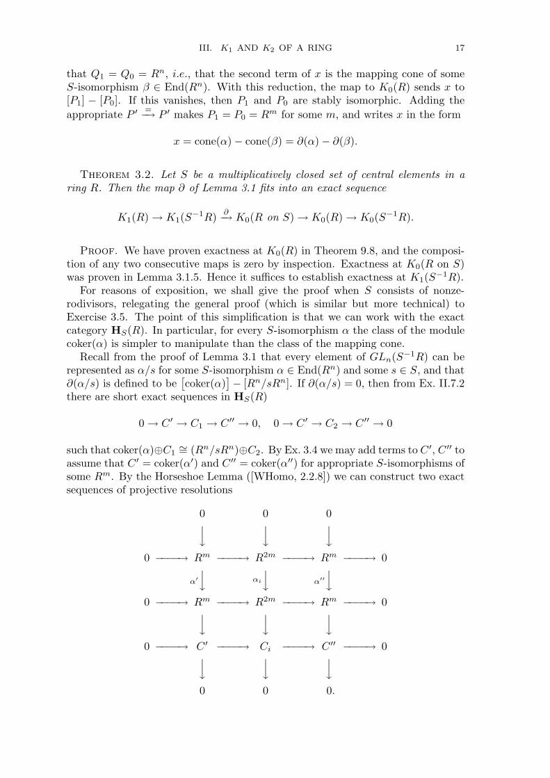
III. K1 AND K2 OF A RING 17
that Q1 = Q0 = Rn, i.e., that the second term of x is the mapping cone of someS-isomorphism β ∈ End(Rn). With this reduction, the map to K0(R) sends x to[P1] − [P0]. If this vanishes, then P1 and P0 are stably isomorphic. Adding theappropriate P ′ =−→ P ′ makes P1 = P0 = Rm for some m, and writes x in the form
x = cone(α)− cone(β) = ∂(α)− ∂(β).
Theorem 3.2. Let S be a multiplicatively closed set of central elements in aring R. Then the map ∂ of Lemma 3.1 fits into an exact sequence
K1(R) → K1(S−1R) ∂−→ K0(R on S) → K0(R) → K0(S−1R).
Proof. We have proven exactness at K0(R) in Theorem 9.8, and the composi-tion of any two consecutive maps is zero by inspection. Exactness at K0(R on S)was proven in Lemma 3.1.5. Hence it suffices to establish exactness at K1(S−1R).
For reasons of exposition, we shall give the proof when S consists of nonze-rodivisors, relegating the general proof (which is similar but more technical) toExercise 3.5. The point of this simplification is that we can work with the exactcategory HS(R). In particular, for every S-isomorphism α the class of the modulecoker(α) is simpler to manipulate than the class of the mapping cone.
Recall from the proof of Lemma 3.1 that every element of GLn(S−1R) can berepresented as α/s for some S-isomorphism α ∈ End(Rn) and some s ∈ S, and that∂(α/s) is defined to be
[coker(α)
]− [Rn/sRn]. If ∂(α/s) = 0, then from Ex. II.7.2there are short exact sequences in HS(R)
0 → C ′ → C1 → C ′′ → 0, 0 → C ′ → C2 → C ′′ → 0
such that coker(α)⊕C1∼= (Rn/sRn)⊕C2. By Ex. 3.4 we may add terms to C ′, C ′′ to
assume that C ′ = coker(α′) and C ′′ = coker(α′′) for appropriate S-isomorphisms ofsome Rm. By the Horseshoe Lemma ([WHomo, 2.2.8]) we can construct two exactsequences of projective resolutions
0 0 0y
yy
0 −−−−→ Rm −−−−→ R2m −−−−→ Rm −−−−→ 0
α′y αi
y α′′y
0 −−−−→ Rm −−−−→ R2m −−−−→ Rm −−−−→ 0y
yy
0 −−−−→ C ′ −−−−→ Ci −−−−→ C ′′ −−−−→ 0y
yy
0 0 0.

18 III. K1 AND K2 OF A RING
Inverting S makes each αi an isomorphism conjugate to(
α′
00
α′′). Thus in K1(S−1R)
we have [α1] = [α′]+[α′′] = [α2]. On the other hand, the two endomorphisms α⊕α1
and s · idn⊕α2 of R2m+n have isomorphic cokernels by construction. Lemma 3.2.1below implies that in K1(S−1R) we have
[α/s] = [α⊕ α1]− [s · idn ⊕ α2] = g for some g ∈ GL(R).
This completes the proof of Theorem 3.2.
Lemma 3.2.1. Suppose that S consists of nonzerodivisors. If α, β ∈ EndR(Rn)are S-isomorphisms with Rn/αRn isomorphic to Rn/βRn, then there is a g ∈GL4n(R) such that [α] = [g][β] in K1(S−1R).
Proof. Put M = coker(α) ⊕ coker(β), and let γ:Rn/αRn ∼= Rn/βRn bean automorphism. By Ex. 3.3(b) with Q = R2n we can lift the automorphism(
0γ
γ−1
0
)of M to an automorphism γ0 of R4n. If π1 and π2 denote the projections
R4n (pr,0,0,0)−−−−−−→ coker(α), and R4n (0,pr,0,0)−−−−−−→ coker(β), respectively, then we haveγπ1 = π2γ0. This yields a commutative diagram
0 −−−−→ R4n α,1,1,1−−−−→ R4n π1−−−−→ Rn/αRn −−−−→ 0yγ1 ∼=
yγ0 ∼=yγ
0 −−−−→ R4n 1,β,1,1−−−−→ R4n π2−−−−→ Rn/βRn −−−−→ 0
in which γ1 is the induced map. Since γ and γ0 are isomorphisms, so is γ1. Becauseγ0(α, 1, 1, 1) = (1, β, 1, 1)γ1 in GL4n(S−1R), we have [γ0] + [α] = [β] + [γ1], or[α] = [γ1γ
−10 ][β] in K1(S−1R).
NK1 and the group Nil0
Definition 3.3 (NF ). If F is any functor from rings to abelian groups, we writeNF (R) for the cokernel of the natural map F (R) → F (R[t]); NF is also a functoron rings. Moreover, the ring map R[t] t=1−−→ R provides a splitting F (R[t]) → F (R)of the natural map, so we have a decomposition F (R[t]) ∼= F (R)⊕NF (R).
In particular, when F is Ki (i = 0, 1) we have functors NKi and a decompositionKi(R[t]) ∼= Ki(R)⊕NKi(R). Since the ring maps R[t] t=r−−→ R are split surjectionsfor every r ∈ R, we see by Proposition 2.3 and Ex. 2.7 that for every r we also have
NK0(R) ∼= K0(R[t], (t− r)) and NK1(R) ∼= K1(R[t], (t− r)).
We will sometimes speak about NF for functors F defined on any category ofrings closed under polynomial extensions and containing the map “t = 1,” such ask-algebras or commutative rings. For example, the functors NU and N Pic werediscussed briefly for commutative rings in chapter I, Ex. 3.17 and 3.19.
III. K1 AND K2 OF A RING 19
Definition 3.3.1 (F -regular rings). We say that a ring R is F -regular ifF (R) = F (R[t1, . . . , tn]) for all n. Since NF (R[t]) = NF (R)⊕N2F (R), we see byinduction on n that R is F -regular if and only if NnF (R) = 0 for all n ≥ 1.
For example, we saw in II.6.5 that any regular ring is K0-regular. We will see inchapter V that regular rings are also K1-regular, and more generally that they areKm-regular for every m. Rosenberg has also shown that commutative C∗-algebrasare Km-regular for all m; see [Ro96].
Lemma 3.3.2. Let R = R0 ⊕ R1 ⊕ · · · be a graded ring. If NF (R) = 0 thenF (R) ∼= F (R0).
Proof. Write F (t = r) for the map F (R[t]) → F (R) arising from evaluation at“t = r”. By assumption, the maps F (t = r) are all identical, equal to the inverseof the natural map F (R) → F (R[t]). Let f denote the ring map R → R[t] definedby f(rn) = rntn for every rn ∈ Rn. Since the composition of f and “t = 1” is theidentity on R, F (f) is an isomorphism with inverse F (t = 1) = F (t = 0). But thecomposition of f and “t = 0” is the projection R → R0 → R, so the compositionF (R) → F (R0) → F (R) must be the identity on F (R). The result follows, sinceF (R0) → F (R) → F (R0) is the identity on F (R0).
3.4 We are going to describe the group NK1(R) in terms of nilpotent matrices. Forthis, we need the following trick, which was published by Graham Higman in 1940.For clarity, if I = fA is an ideal in A we write GL(A, f) for GL(I).
Higman’s Trick 3.4.1. For every g ∈ GL(R[t], t) there is a nilpotent matrix νover R such that [g] = [1− νt] in K1(R[t]).
Similarly, for every g ∈ GL(R[t, t−1], t− 1) there is a nilpotent matrix ν over Rsuch that [g] = [1− ν(t− 1)] in K1(R[t, t−1], t− 1).
Proof. Every invertible p× p matrix over R[t] can be written as a polynomialg = γ0 + γ1t + γ2t
2 + · · · + γntn with the γi in Mp(R). If g is congruent to theidentity modulo t, then γ0 = 1. If n ≥ 2 and we write g = 1 − ht + γntn, thenmodulo E2p(R[t], t) we have
(g 00 1
)∼
(g γntn−1
0 1
)∼
(1− ht γntn−1
−t 1
)= 1−
(h −γntn−2
1 0
)t.
By induction on n, [g] is represented by a matrix of the form 1− νt. The matrix νis nilpotent by Ex. 3.1.
Over R[t, t−1] we can use a similar argument. After multiplying by a power oft, we may write g as a polynomial in t. Such a polynomial may be rewritten as apolynomial
∑γix
i in x = (t− 1). If g is congruent to the identity modulo (t− 1)then again we have γ0 = 1. By Higman’s trick (applied to x), we may reduce g toa matrix of the form 1− νx, and again ν must be nilpotent by Ex. 3.1.
We will also need the category Nil(R) of II.7.3.4. Recall that the objects of thiscategory are pairs (P, ν), where P is a f.g. projective R-module and ν is a nilpotentendomorphism of P . Let T denote the multiplicative set tn in R[t]. From II.7.7.4we have
K0(R[t] on T ) ∼= K0Nil(R) ∼= K0(R)⊕Nil0(R),
20 III. K1 AND K2 OF A RING
where Nil0(R) is the subgroup generated by elements of the form[(Rn, ν)
] −n[(R, 0)
]for some n and some nilpotent matrix ν.
Lemma 3.4.2. For every ring R, the product with t ∈ K1(Z[t, t−1]) induces asplit injection K0(R) ·t−→ K1(R[t, t−1]).
Proof. Since the forgetful map K0Nil(R) → K0(R) sends[(P, ν)
]to [P ], the
calculation in Example 3.1.4 shows that the composition
K0(R) ·t−→ K1(R[t, t−1]) ∂−→ K0Nil(R) → K0(R)
is the identity map. Hence the first map is a split injection.
Momentarily changing variables from t to s, we now define an additive functionτ from Nil(R) to K1(R[s]). Given an object (P, ν), let τ(P, ν) be the image ofthe automorphism 1− νs of P [s] under the natural map Aut(P [s]) → K1(R[s]) ofLemma 1.6. Given a short exact sequence
0 → (P ′, ν′) → (P, ν) → (P ′′, ν′′) → 0
in Nil(R), a choice of a splitting P ∼= P ′ ⊕ P ′′ allows us to write
(1− νs) =(
1− ν′s γs0 1− ν′′s
)=
(1− ν′s 0
0 1− ν′′s
)(1 γ′s0 1
)
in Aut(P [s]). Hence in K1(R[s]) we have [1 − νs] = [1 − ν′s][1 − ν′′s]. Thereforeτ is an additive function, and induces a homomorphism τ :K0Nil(R) → K1(R[s]).Since τ(P, 0) = 1 for all P and 1− νs is congruent to 1 modulo s, we see that τ isactually a map from Nil0(R) to K1(R[s], s).
Proposition 3.4.3. Nil0(R) ∼= NK1(R), and K0Nil(R) ∼= K0(R)⊕NK1(R).
Proof. For convenience, we identify s with t−1, so that R[s, s−1] = R[t, t−1].Applying Lemma 3.1 to R[t] and T = 1, t, t2, . . . , we form the composition
K1(R[s], s) → K1(R[s]) →K1(R[s, s−1])
=K1(R[t, t−1]) ∂−→ K0(R on T ) → Nil0(R).(3.4.4)
Let us call this composition δ. We claim that τ is the inverse of δ. By Higman’sTrick, every element of K1(R[s], s) is represented by a matrix 1−νs with ν nilpotent.In Example 3.1.4 we saw that δ(1−νs) =
[(Rn, ν)
]−n[(R, 0)
]. By the construction
of τ we have the desired equations: τδ(1− νs) = τ[(Rn, ν)
]= (1− νs) and
δτ
([(Rn, ν)
]− n[(R, 0)
])= δ(1− νs) =
[(Rn, ν)
]− n[(R, 0)
].
Corollary 3.4.5. K1(R[s]) → K1(R[s, s−1]) is an injection for every ring R.
Proof. By Ex. 2.7, we have K1(R[s]) ∼= K1(R) ⊕K1(R[s], s). Since K1(R) isa summand of K1(R[s, s−1]), the isomorphism δ: K1(R[s], s) ∼= Nil0(R) of (3.3.4)factors through K1(R[s], s) → K1(R[s, s−1])/K1(R). This quotient map must thenbe an injection. The result follows.

III. K1 AND K2 OF A RING 21
The Fundamental Theorems for K1 and K0
Fundamental Theorem for K1 3.5. For every ring R, there is a split sur-jection K1(R[t, t−1]) ∂−→ K0(R), with inverse [P ] 7→ [P ] · t. This map fits into anaturally split exact sequence:
0 → K1(R) ∆−→ K1(R[t])⊕K1(R[t−1]) ±−→ K1(R[t, t−1] ∂−→ K0(R) → 0.
Consequently, we have a natural direct sum decomposition:
K1(R[t, t−1] ∼= K1(R)⊕K0(R)⊕NK1(R)⊕NK1(R).
Proof. We merely assemble the pieces of the proof from §3.4. The first assertionis just Lemma 3.4.2. The natural maps from K1(R) into K1(R[t]), K1(R[t−1]) andK1(R[t, t−1]) are injections, split by “t = 1” (as in 3.4), so the obviously exactsequence
(3.5.1) 0 → K1(R) ∆−→ K1(R)⊕K1(R) ±−→ K1(R) → 0
is a summand of the sequence we want to prove exact. From Proposition II.7.7.1,Theorem 3.2 and Corollary 3.4.5, we have an exact sequence
(3.5.2) 0 → K1(R[t]) → K1(R[t, t−1]) ∂−→ K0Nil(R) → 0.
Since K0Nil(R) ∼= K0(R) ⊕ Nil0(R), the map ∂ in (3.5.2) is split by the mapsof 3.4.2 and 3.4.3. The sequence in the Fundamental Theorem for K1 is obtainedby rearranging the terms in sequences (3.5.1) and (3.5.2).
In order to formulate the corresponding Fundamental Theorem for K0, we defineK−1(R) to be the cokernel of the map K0(R[t])⊕K0(R[t−1]) → K0(R[t, t−1]). Wewill reprove the following result more formally in the next section.
Fundamental Theorem for K0 3.6. For every ring R, there is a naturallysplit exact sequence:
0 → K0(R) ∆−→ K0(R[t])⊕K0(R[t−1]) ±−→ K0(R[t, t−1] ∂−→ K−1(R) → 0.
Consequently, we have a natural direct sum decomposition:
K0(R[t, t−1] ∼= K0(R)⊕K−1(R)⊕NK0(R)⊕NK0(R).
Proof. Let s be a second indeterminate. The Fundamental Theorem for K1,applied to the variable t, gives a natural decomposition
K1(R[s, t, t−1]) ∼= K1(R[s])⊕NK1(R[s])⊕NK1(R[s])⊕K0(R[s]),
and similar decompositions for the other terms in the map
K1(R[s, t, t−1])⊕K1(R[s−1, t, t−1]) → K1(R[s, s−1, t, t−1]).
Therefore the cokernel of this map also has a natural splitting. But the cokernelis K0(R[t, t−1]), as we see by applying the Fundamental Theorem for K1 to thevariable s.

22 III. K1 AND K2 OF A RING
EXERCISES
3.1 Let A be a ring and a ∈ A, show that the following are equivalent: (i) a isnilpotent; (ii) 1− at is a unit of A[t]; (iii) 1− a(t− 1) is a unit of A[t, t−1].3.2 Let α, β:P → Q be two maps between fin. gen. projective R-modules. If S isa central multiplicatively closed set in R and S−1α, S−1β are isomorphisms, theng = β−1α is an automorphism of S−1P . Show that ∂(g) = [cone(α)]− [cone(β)]. Inparticular, if S consists of nonzerodivisors, show that ∂(g) = [coker(α)]−[coker(β)].3.3 (Bass) Prove that every module M in H(R) has a projective resolution P· → Msuch that every automorphism α of M lifts to an automorphism of the chain complexP·. To do so, proceed as follows.(a) Fix a surjection π:Q → M , and use Ex. I.1.11 to lift the automorphism
α⊕ α−1 of M ⊕M to an automorphism β of Q⊕Q.(b) Defining e: Q⊕Q → M to be e(x, y) = π(x), show that every automorphism
of M can be lifted to an automorphism of Q⊕Q.(c) Set P0 = Q ⊕ Q, and repeat the construction on Z0 = ker(e) to get a finite
resolution P· of M with the desired property.3.4 Suppose that S consists of nonzerodivisors, and that M is a module in HS(R).(a) Prove that there is a module M ′ and an S-isomorphism α ∈ End(Rm) so that
coker(α) = M ⊕M ′. Hint: Modify the proof of Lemma 3.1.5, where M is the
cokernel of a map P0β−→ P1.
(b) Given S-isomorphisms α′, α′′ ∈ End(Rm) and a short exact sequence of S-torsion modules 0 → coker(α′) → M → coker(α′′) → 0, show that there is anS-isomorphism α ∈ R2m with M ∼= coker(α).
3.5 Modify the proofs of the previous two exercises to prove Theorem 3.2 when Scontains zerodivisors.3.6 Noncommutative localization. By definition, a multiplicatively closed set S ina ring R is called a right denominator set if it satisfies the following two conditions:(i) For any s ∈ S and r ∈ R there exists an s′ ∈ S and r′ ∈ R such that sr′ = rs′;(ii) if sr = 0 for any r ∈ R, s ∈ S then rs′ = 0 for some s′ ∈ S. This is the mostgeneral condition under which a (right) ring of fractions S−1R exists, in which everyelement of S−1R has the form r/s = rs−1, and if r/1 = 0 then some rs = 0 in R.
Prove Theorem 3.2 when S is a right denominator set consisting of nonzerdivi-sors. To do this, proceed as follows.(a) Show that for any finite set of elements xi in S−1R there is an s ∈ S and
ri ∈ R so that xi = ri/s for all i.(b) Reprove II.7.6.3 and II.9.8 for denominator sets, using (a); this yields exact-
ness at K0(R).(c) Modify the proof of Lemma 3.1 and 3.1.5 to construct the map ∂ and prove
exactness at K0HS(R).(d) Modify the proof of Theorem 3.2 to prove exactness at K1(S−1R).
§4. Negative K-theory
In the last section, we defined K−1(R) to be the cokernel of the map K0(R[t])⊕K0(R[t−1]) → K0(R[t, t−1]). Of course we can keep going, and define all the nega-tive K-groups by induction on n:

III. K1 AND K2 OF A RING 23
Definition 4.1. For n > 0, we inductively define K−n(R) to be the cokernel ofthe map
K−n+1(R[t])⊕K−n+1(R[t−1]) → K−n+1(R[t, t−1]).
Clearly, each K−n is a functor from rings to abelian groups.
To describe the properties of these negative K-groups, it is convenient to castthe Fundamental Theorems above in terms of Bass’ notion of contracted functors.With this in mind, we make the following definitions.
Definition 4.1.1 (Contracted functors). Let F be a functor from ringsto abelian groups. For each R, we define LF (R) to be the cokernel of the mapF (R[t])⊕F (R[t−1]) → F (R[t, t−1]). We write Seq(F, R) for the following sequence:
0 → F (R) ∆−→ F (R[t])⊕ F (R[t−1]) ±−→ F (R[t, t−1]) → LF (R) → 0.
We say that F is acyclic if Seq(F, R) is exact for all R. We say that F is a contractedfunctor if F is acyclic and in addition there is a splitting h = ht,R of the definingmap F (R[t, t−1]) → LF (R), a splitting which natural in both t and R.
By iterating this definition, we can speak about the functors NLF , L2F , etc.For example, Definition 4.1 states that K−n = Ln(K0).
Example 4.1.2 (Fundamental Theorem for K−n). The Fundamental The-orems for K1 and K0 may be restated as the assertions that these are contractedfunctors. It follows from Proposition 4.2 below that each K−n is a contractedfunctor; by Definition 4.1, this means that there is a naturally split exact sequence:
0 → K−n(R) ∆−→ K−n(R[t])⊕K−n(R[t−1]) ±−→ K−n(R[t, t−1]) ∂−→ K−n−1(R) → 0.
As with the definition of NF , we can define LF for functors F which are definedon a category of rings closed under polynomial and Laurent polynomial extensions,such as the functors U and Pic, which are defined only for commutative rings.
Example 4.1.3 (Units). Let U(R) = R× denote the group of units in acommutative ring R. By Ex. I.3.17, U is a contracted functor with contractionLU(R) = [Spec(R),Z]; the splitting map LU(R) → U(R[t, t−1] sends a functionf : Spec(R) → Z to the unit tf of R[t, t−1]. From Ex. 4.2 below we see that thefunctors L2U and NLU are zero. Thus we can write a simple formula for the unitsof any extension R[t1, t−1
1 , . . . , tn, t−1n ]. If R is reduced, so that NU(R) vanishes
(Ex. I.3.17), then we just have
U(R[t1, t−11 , . . . , tn, t−1
n ]) = U(R)×n∐
i=1
[Spec(R),Z] · ti.

24 III. K1 AND K2 OF A RING
Example 4.1.4 (Pic). Recall from chapter I, §3 that the Picard group Pic(R)of a commutative ring is a functor, and that N Pic(R) = 0 exactly when Rred
is seminormal. By Ex. I.3.18 the sequence Seq(Pic, R) is exact. In fact Pic is acontracted functor with NL Pic = L2 Pic = 0; see [Weib91]. The group L Pic(R) isthe etale cohomology group H1
et(Spec(R),Z).
A morphism of contracted functors is a natural transformation η: F ⇒ F ′ be-tween two contracted functors such that the following square commutes for all R.
LF (R) h−−−−→ F (R[t, t−1])
(Lη)R
yyηR[t,t−1]
LF ′(R) h′−−−−→ F ′(R[t, t−1])
Proposition 4.2. Let η:F ⇒ F ′ be a morphism of contracted functors. Thenboth ker(η) and coker(η) are also contracted functors.
In particular, if F is contracted, then NF and LF are also contracted functors.Moreover, there is a natural isomorphism of contracted functors NLF ∼= LNF .
Proof. If Cφ−→ D is a morphism between split exact sequences, which have
compatible spittings, then the sequences ker(φ) and coker(φ) are always split exact,with splittings induced from the splittings of C and D. Applying this remark toSeq(F, R) → Seq(F ′, R) shows that both Seq(ker(η), R) and Seq(coker(η), R) aresplit exact. That is, both ker(η) and coker(η) are contracted functors. It also showsthat
0 → ker(η)(R) → F (R)ηR−→ F ′(R) → coker(η)(R) → 0
is an exact sequence of contracted functors.Since NF (R) is the cokernel of the morphism F (R) → F ′(R) = F (R[t]) and
LF (R) is the cokernel of the morphism ± in Seq(F, R), both NF and LF arecontracted functors. Finally, the natural isomorphism NLF (R) ∼= LNF (R) arisesfrom inspecting one corner of the large commutative diagram represented by
0 → Seq F (R[s], s) → Seq F (R[s]) → Seq F (R) → 0.
Example 4.2.1 (SK1). If R is a commutative ring, it follows from Exam-ples 1.1.1 and 4.1.3 that det:K1(R) → U(R) is a morphism of contracted func-tors. Hence SK1 is a contracted functor. The contracted map L det is the maprank: K0(R) → H0(R) = [Spec(R),Z] of II.2.3; it follows that L(SK1)(R) = K0(R).From Ex. 4.2 we also have L2(SK1)(R) = LK0(R) = K−1(R).
We can give an elegant formula for F (R[t1, t−11 , . . . , tn, t−1
n ]), using the followingnotation. If p(N, L) =
∑mijN
iLj is any formal polynomial in N and L withinteger coefficients mij > 0, and F is a functor from rings to abelian groups, we setp(N, L)F equal to the direct sum of mij copies of each group N iLjF (R).
Corollary 4.2.2. F (R[t1, . . . , tn]) ∼= (1 + N)nF (R) for every F . If F is acontracted functor, then F (R[t1, t−1
1 , . . . , tn, t−1n ]) ∼= (1 + 2N + L)nF (R).
Proof. The case n = 1 follows from the definitions, and the general case followsfrom induction.

III. K1 AND K2 OF A RING 25
For example, if L2F = 0 and R is F -regular, then (1+2N +L)nF (R) stands forF (R) ⊕ n LF (R). In particular, the formula for units in Example 4.1.3 is just thecase F = U of 4.2.2.
Example 4.2.3. Since LjK0 = K−j , K0(R[t1, t−11 , . . . , tn, t−1
n ]) is the directsum of many pieces N iK−j(R), including K−n(R) and
(nj
)copies of K−j(R).
Conjecture 4.2.4. Let R be a commutative noetherian ring of Krull dimensiond. It is conjectured that K−j(R) vanishes for all j > d, and that R is K−d-regular;see [Weib80]. This is so for d = 0, 1 by exercises 4.3 and 4.4, and Example 4.3.1below shows that the bound is best possible.
The Mayer-Vietoris sequence
Suppose that f : R → S is a ring map, and I is an ideal of R mapped isomor-phically into an ideal of S. By Theorem 2.6 there is an exact “Mayer-Vietoris”sequence:
K1(R) ∆−→ K1(S)⊕K1(R/I)→K1(S/I) ∂−→ K0(R) ∆−→ K0(S)⊕K0(R/I) ±−→ K0(S/I).
Applying the contraction operation L to this sequence gives a sequence relating K0
to K−1, whose first three terms are identical to the last three terms of the displayedsequence. Splicing these together yields a longer sequence. Repeatedly applying Land splicing sequences leads to the following result.
Theorem 4.3 (Mayer-Vietoris). Suppose we are given a ring map f :R → Sand an ideal I of R mapped isomorphically into an ideal of S. Then the Mayer-Vietoris sequence of Theorem 2.6 continues as a long exact Mayer-Vietoris sequenceof negative K-groups.
· · · ∆−→K0(S)⊕K0(R/I)
±−→K0(S/I) ∂−→ K−1(R) ∆−→ K−1(S)⊕K−1(R/I)
±−→ K−1(S/I) ∂−→ K−2(R) →
· · · → K−n+1(S/I) ∂−→ K−n(R) ∆−→ K−n(S)⊕K−n(R/I)
±−→ K−n(S/I) ∂−→ K−n−1(R) · · ·
Example 4.3.1 (B. Dayton). Fix a regular ring R, and let ∆n(R) denotethe coordinate ring R[t0, . . . , tn]/(f), f = t0 · · · tn(1 − ∑
ti) of the n-dimensionaltetrahehron over R. Using I = (1 −∑
ti)∆n(R) and ∆n(R)/I ∼= R[t1, . . . , tn] viat0 7→ 1− (t1 + · · ·+ tn), we have a Milnor square
∆n(R) −−−−→ Anyy
R[t1, . . . , tn] −−−−→ ∆n−1(R)
where An = R[t0, . . . , tn]/(t0 · · · tn). By Ex. 4.7, the negative K-groups of An vanishand Ki(An) = Ki(R) for i = 0, 1. Therefore we have K0(∆n(R)) ∼= K1(∆n−1(R)),and K−j(∆n(R)) ∼= K1−j(∆n−1(R)) for j > 0. These groups vanish for j > n, with

26 III. K1 AND K2 OF A RING
K−n(∆n(R)) ∼= K0(R). In particular, if F is a field then ∆n(F ) is an n-dimensionalnoetherian ring with K−n(∆n(F )) ∼= Z; see Conjecture 4.2.4.
When we have introduced higher K-theory, we will see that in fact K0(∆n(R)) ∼=Kn(R) and K1(∆n(R)) ∼= Kn+1(R). This is just one way in which higher K-theoryappears in classical K-theory.
EXERCISES
4.1 Suppose that 0 → F ′ → F → F ′′ → 0 is an exact sequence of functors, withF ′ and F ′′ contracted. Show that F is acyclic, but need not be contracted.4.2 For a commutative ring R, let H0(R) denote the group [Spec(R),Z] of allcontinuous functions from Spec(R) to Z. Show that NH0 = LH0 = 0, i.e., thatH0(R) = H0(R[t]) = H0(R[t, t−1]).4.3 Let R be an Artinian ring. Show that R is K0-regular, and that K−n(R) = 0for all n > 0.4.4 (Bass-Murthy) Let R be a 1-dimensional commutative noetherian ring withfinite normalization R and conductor ideal I. Show that R is K−1-regular, andthat K−n(R) = 0 for all n ≥ 2. If h0(R) denotes the rank of the free abeliangroup H0(R) = [Spec(R),Z], show that K−1(R) ∼= L Pic(R) ∼= Zr, where r =h0(R)− h0(R) + h0(R/I)− h0(R/I).4.5 (Carter) Let S be a multiplicative set in a commutative ring R. Regard-ing F (A) = K0(A on S) as a functor on R-algebras, define K−n(A on S) to beLnK0(A on S). Deduce from the Localization sequence that these are acyclic func-tors, and that the Localization Sequence of Theorem 3.2 continues into negativeK-theory for every R-algebra A.
· · · → K0(A) → K0(S−1A) ∂−→ K−1(A on S) → K−1(A) →K−1(S−1A) ∂−→ K−2(A on S) → K−2(A) → · · ·
With the help of higher K-theory to define K1(A on S), and construct the product“·t”, it will follow that the Ki(A on S) are actually contracted functors.
4.6 Let G be a finite group of order n, and let R be a “maximal order” in Q[G]. Itis well known that R is a regular ring containing Z[G], and that I = nR is an idealof Z[G]; see [Bass, p. 560]. Show that K−nZ[G] = 0 for n ≥ 2, and that K−1 hasthe following resolution by free abelian groups:
0 → Z→ H0(R)⊕H0(Z/n[G]) → H0(R/nR) → K−1(Z[G]) → 0.
D. Carter has shown in [Carter] that K−1Z[G] ∼= Zr ⊕ (Z/2Z)s, where s equals thenumber of simple components Mni(Di) of the semisimple ring Q[G] such that theSchur index of D is even (see 1.2.4), but the Schur index of Dp is odd at each primep dividing n. In particular, if G is abelian then K−1Z[G] is torsionfree (see [Bass,p. 695]).4.7 Coordinate hyperplanes. Let R be a regular ring. By induction on n, show thatthe graded rings An = R[t0, . . . , tn]/(t0 · · · tn) are Ki-regular for all i ≤ 1. Concludethat K1(An) = K1(R), K0(An) = K0(R) and Ki(An) = 0 for all i < 0.

III. K1 AND K2 OF A RING 27
§5. Milnor’s K2 of a ring
The group K2 of a ring was defined by J. Milnor in 1967, following a 1962 paperby R. Steinberg on Universal Central Extensions of Chevalley groups. Milnor’s1971 book [Milnor] is still the best source for the fundamental theorems about it.In this section we will give an introduction to the subject, but we will not provethe harder theorems.
Following Steinberg, we define a group in terms of generators and relations de-signed to imitate the behavior of the elementary matrices, as described in (1.2.1).To avoid technical complications, we shall avoid any definition of St2(R).
Definition 5.1. For n ≥ 3 the Steinberg group Stn(R) of a ring R is the groupdefined by generators xij(r), with i, j a pair of distinct integers between 1 and nand r ∈ R, subject to the following “Steinberg relations”(5.1.1) xij(r)xij(s) = xij(r + s)
(5.1.2) [xij(r), xk`(s)] =
1 if j 6= k and i 6= `
xi`(rs) if j = k and i 6= `
xkj(−sr) if j 6= k and i = `.
As observed in (1.3.1), the Steinberg relations are also satisfied by the elementarymatrices eij(r) which generate the subgroup En(R) of GLn(R). Hence there is acanonical group surjection φn: Stn(R) → En(R) sending xij(r) to eij(r).
The Steinberg relations for n+1 include the Steinberg relations for n, so there isan obvious map Stn(R) → Stn+1(R). We write St(R) for lim−→Stn(R), and observethat by stabilizing the φn induce a surjection φ: St(R) → E(R).
Definition 5.2. The group K2(R) is the kernel of φ: St(R) → E(R). Thusthere is an exact sequence of groups
1 → K2(R) → St(R)φ−→ GL(R) → K1(R) → 1.
It will follow from Theorem 5.3 below that K2(R) is an abelian group. Moreover,it is clear that St and K2 are both covariant functors from rings to groups, just asGL and K1 are.
Theorem 5.2.1 (Steinberg). K2(R) is an abelian group. In fact it is preciselythe center of St(R).
Proof. If x ∈ St(R) commutes with every element of St(R), then φ(x) mustcommute with all of E(R). But the center of E(R) is trivial (by Ex. 1.7) so φ(x) = 1,i.e., x ∈ K2(R). Thus the center of St(R) is contained in K2(R).
Conversely, suppose that y ∈ St(R) satisfies φ(y) = 1. Then in E(R) we have
φ([y, p]) = φ(y)φ(p)φ(y)−1φ(p)−1 = φ(p)φ(p)−1 = 1
for every p ∈ St(R). Choose an integer n large enough that y can be expressedas a word in the symbols xij(r) with i, j < n. For each element p = xkn(s) withk < n and s ∈ R, the Steinberg relations imply that the commutator [y, p] is anelement of the subgroup Pn of St(R) generated by the symbols xin(r) with i < n.

28 III. K1 AND K2 OF A RING
On the other hand, we know by Ex. 5.2 that φ maps Pn injectively into E(R). Sinceφ([y, p]) = 1 this implies that [y, p] = 1. Hence y commutes with every generatorxkn(s) with k < n.
By symmetry, this proves that y also commutes with every generator xnk(s)with k < n. Hence y commutes with all of Stn(R), since it commutes with everyxkl(s) = [xkn(s), xnl(1)] with k, l < n. Since n can be arbitrarily large, this provesthat y is in the center of St(R).
Example 5.2.2. The group K2(Z) is cyclic of order 2. This calculation uses theEuclidean Algorithm to rewrite elements of St(Z), and is given in §10 of [Milnor].In fact, Milnor proves that the symbol −1,−1 =
x12(1)x21(−1)x12(1)
4 is theonly nontrivial element of ker(φn) for all n ≥ 3. It is easy to see that −1,−1 isin the kernel of each φn, because the 2 × 2 matrix e12(1)e21(−1)e12(1) =
(0−1
10
)has order 4 in GLn(Z). We will see in Example 6.2.1 below that −1,−1 is stillnonzero in K2(R).
Tate has used the same Euclidean Algorithm type techniques to show thatK2(Z[
√−7]) and K2(Z[√−15]) are also cyclic of order 2, generated by the symbol
−1,−1, while K2(R) = 1 for the imaginary quadratic rings R = Z[i], Z[√−3],
Z[√−2] and Z[
√−11]. See the appendix to [BT] for details.
Example 5.2.3. For every field F we have K2(F [t]) = K2(F ). This was orig-inally proven by K. Dennis and J. Sylvester using the same Euclidean Algorithmtype techniques as in the provious example. We shall not describe the details,because we shall see in chapter V that K2(R[t]) = K2(R) for every regular ring.
Universal Central Extensions
The Steinberg group St(R) can be described in terms of universal central extensions,and the best exposition of this is [Milnor, §5]. Properly speaking, this is a subjectin pure group theory; see [Suz, 2.9]. However, since extensions of a group G areclassified by the cohomology group H2(G), the theory of universal central extensionsis also a part of homological algebra; see [WHomo, §6.9]. Here are the relevantdefinitions.
Let G be a group and A an abelian group. A central extension of G by A is ashort exact sequence of groups 1 → A → X
π−→ G → 1 such that A is in the centerof X. We say that a central extension is split if it is isomorphic to an extension ofthe form 1 → A → A×G
pr−→ G → 1, where pr(a, g) = g.If A or π is clear from the context, we may omit it from the notation. For
example, 1 → K2(R) → St(R) → E(R) → 1 is a central extension by Steinberg’sTheorem 5.2.1, but we usually just say that St(R) is a central extension of E(R).
Two extensions X and Y of G by A are said to be equivalent if there is anisomorphism f :X → Y which is the identity on A and which induces the identitymap on G. It is well-known that the equivalence classes of central extensions of Gby a fixed group A are in 1–1 correspondence with the elements of the cohomologygroup H2(G;A); see [WHomo, §6.6].
More generally, by a homomorphism over G from Xπ−→ G to another central
extension 1 → B → Yτ−→ G → 1 we mean a group map f :X → Y such that
π = τf .

III. K1 AND K2 OF A RING 29
Definition 5.3.1. A universal central extension of G is a central extensionX
π−→ G such that for every other central extension Yτ−→ G there is a unique
homomorphism f over G from X to Y . Clearly a universal central extension isunique up to isomorphism over G, provided it exists.
Lemma 5.3.2. If G has a universal central extension X, then both G and Xmust be perfect groups.
Proof. Otherwise B = X/[X, X] is nontrivial, and there would be two homo-morphisms over G from X to the central extension 1 → B → B × G → G → 1,namely the maps (0, π) and (pr, π), where pr is the natural projection X → B.
Lemma 5.3.3. If X and Y are central extensions of G, and X is a perfect group,there is at most one homomorphism over G from X to Y .
Proof. If f and f1 are two such homomorphisms, then for any x and x′ in Xwe can write f1(x) = f(x)c, f1(x′) = f(x′)c′ for elements c and c′ in the centerof Y . Therefore f1(xx′x−1(x′)−1) = f(xx′x−1(x′)−1). Since the commutators[x, x′] = xx′x−1(x′)−1 generate X we must have f1 = f .
Example 5.3.4. Every presentation of G gives rise to two natural central ex-tensions as follows. A presentation corresponds to the choice of a free group Fmapping onto G, and a description of the kernel R ⊂ F . Since [R,F ] is a normalsubgroup of F , we may form the following central extensions:
1 → R/[R, F ] →F/[R, F ] → G → 1,
1 → (R ∩ [F, F ])/[R, F ] →[F, F ]/[R, F ] → [G,G] → 1.(5.3.5)
The group (R∩ [F, F ])/[R, F ] in (5.3.5) is the homology group H2(G;Z); this iden-tity was discovered in 1941 by Hopf [WHomo, 6.8.8]. If G = [G,G], both areextensions of G, and (5.3.5) is the universal central extension by the followingtheorem.
Recognition Theorem 5.4. Every perfect group G has a universal centralextension, namely the extension (5.3.5):
1 → H2(G;Z) → [F, F ]/[R, F ] → G → 1.
Let X be any central extension of G, the following are equivalent: (1) X is auniversal central extension; (2) X is perfect, and every central extension of Xsplits; (3) H1(X;Z) = H2(X;Z) = 0.
Proof. Given any central extension X of G, the map F → G lifts to a maph: F → X because F is free. Since h(R) is in the center of X, h([R,F ]) = 1. Thus hinduces a map from [F, F ]/[R,F ] to X over G. This map is unique by Lemma 5.3.3.This proves that (5.3.5) is a universal central extension, and proves the equivalenceof (1) and (3). The implication (1) ⇒ (2) is Lemma 5.3.2 and Ex. 5.7, and (2) ⇒ (1)is immediate.

30 III. K1 AND K2 OF A RING
Theorem 5.5 (Kervaire, Steinberg). The Steinberg group St(R) is the uni-versal central extension of E(R). Hence
K2(R) ∼= H2(E(R);Z).
This theorem follows immediately from the Recognition Theorem 5.4, and thefollowing splitting result:
Proposition 5.5.1. If n ≥ 5, every central extension Yπ−→ Stn(R) is split.
Hence Stn(R) is the universal central extension of En(R).
Proof. We first show that if j 6= k and l 6= i then every two elements y, z ∈Y with π(y) = xij(r) and π(z) = xkl(s) must commute in Y . Pick t distinctfrom i, j, k, l and choose y′, y′′ ∈ Y with π(y′) = xit(1) and π(y′′) = xtj(r). TheSteinberg relations imply that both [y′, z] and [y′′, z] are in the center of Y , andsince π(y) = π[y′, y′′] this implies that z commutes with [y′, y′′] and y.
We now choose distinct indices i, j, k, l and elements u, v, w ∈ Y with
π(u) = xij(1), π(v) = xjk(s) and π(w) = xkl(r).
If G denotes the subgroup of Y generated by u, v, w then its commutator subgroup[G,G] is generated by elements mapping under π to xik(s), xjl(sr) or xil(sr).From the first paragraph of this proof it follows that [u,w] = 1 and that [G,G] isabelian. By Ex. 5.3 we have [[u, v], w] = [u, [v, w]]. Therefore if π(y) = xik(s) andπ(z) = xjl(sr) we have [y, w] = [u, z]. Taking s = 1, this identity proves that theelement
yil(r) = [u, z], where π(u) = xij(1), π(z) = xjl(r)
doesn’t depend upon the choice of j, nor upon the lifts u and z of xij(1) and xjl(r).We claim that the elements yij(r) satisfy the Steinberg relations, so that there is a
group homomorphism Stn(R) → Y sending xij(r) to yij(r). Such a homomorphismwill provide the desired splitting of the extension π. The first paragraph of thisproof implies that if j 6= k and l 6= i then yij(r) and ykl(s) commute. The identity[y, w] = [u, z] above may be rewritten as
[yik(r), ykl(s)] = yil(rs) for i, k, l distinct.
The final relation yij(r)yij(s) = yij(r+s) is a routine calculation with commutatorsleft to the reader.
Remark 5.5.2 (Stability for K2). The kernel of Stn(R) → En(R) is writtenas K2(n,R), and there are natural maps K2(n,R) → K2(R). If R is noetherian ofdimension d, or more generally has sr(R) = d+1, then the following stability resultholds: K2(n,R) ∼= K2(R) for all n ≥ d+3. This result evolved in the mid-1970’s asa sequence of results by Dennis, Vaserstein, van der Kallen and Suslin-Tulenbaev.We refer the reader to section 19C25 of Math Reviews for more details.

III. K1 AND K2 OF A RING 31
Transfer maps on K2
Here is a description of K2(R) in terms of the translation category tP(R) of f.g.projective R-modules, analogous to the description given for K1 in Corollary 1.6.3.
Proposition 5.6 (Bass). K2(R) ∼= lim−→P∈tPH2([Aut(P ), Aut(P )];Z).
Proof. If G is a group, then G acts by conjugation upon [G,G] and hence uponthe homology H2([G,G];Z). Taking coinvariants, we obtain the functor H ′
2 fromgroups to abelian groups defined by H ′
2(G) = H0(G; H2([G, G];Z)). By construc-tion, G acts trivially upon H ′
2(G) and commutes with direct limits of groups.Note that if G acts trivially upon H2([G, G];Z) then H ′
2(G) = H2([G, G];Z). Forexample, GL(R) acts trivially upon the homology of E(R) = [GL(R), GL(R)] byEx. 1.12. By Theorem 5.5 this implies that H ′
2(GL(R)) = H2(E(R);Z) = K2(R).Since morphisms in the translation category tP(R) are well-defined up to iso-
morphism, it follows that P 7→ H ′2(Aut(P )) is a well-defined functor from tP(R)
to abelian groups. Hence we can take the filtered colimit of this functor, as we didin 1.6.3. Since the free modules are cofinal in tP(R), the result follows from theidentification of the colimit as
limn→∞
H ′2(GLn(R)) ∼= H ′
2(GL(R)) = K2(R).
Corollary 5.6.1 (Morita Invariance of K2). The group K2(R) dependsonly upon the category P(R). That is, if R and S are Morita equivalent rings(see II.2.7) then K2(R) ∼= K2(S). In particular, the maps R → Mn(R) induceisomorphisms on K2:
K2(R) ∼= K2(Mn(R)).
Let f : R → S be a ring homomorphism such that the R-module S is finitely gen-erated and projective. In chapter VI, we will construct a transfer map f∗:Kn(R) →Kn(S) for all n. However, it is easy to construct the transfer map directly on K2,which is sometimes also called the norm homomorphism NS/R.
Corollary 5.6.2 (Finite transfer). Suppose that S is f.g. projective as anR-module. Then there is a natural transfer homomorphism f∗: K2(S) → K2(R).
If R is commutative, so that K2(R) is a K0(R)-module by Ex. 5.4, the com-position f∗f∗:K2(R) → K2(S) → K2(R) is multiplication by [S] ∈ K0(R). Inparticular, if S is free of rank n, then f∗f∗ is multiplication by n.
Proof. The construction of f∗ is obtained by replacing H1(Aut) by H ′2(Aut)
in the proof of Lemma 1.7. The composite f∗f∗ is obtained by composing thefunctor H2([Aut, Aut]) with tP(R) ⊗S−−→ tP(S) −→ tP(R). But this composite is theself-map ⊗RS on tP(R) giving rise to multiplication by [S] on K2(R) in Ex. 5.5.
Remark 5.6.3. We will see in chapter V that we can also define a transfer mapK2(S) → K2(R) when S is a finite R-algebra of finite projective dimension over R.

32 III. K1 AND K2 OF A RING
Relative K2 and relative Steinberg groups
Given an ideal I in a ring R, we may construct the augmented ring R⊕ I, withmultiplication (r, x)(s, y) = (rs, ry + xs + xy). This ring is equipped with twonatural maps pr, add:R ⊕ I → R, defined by pr(r, x) = r and add(r, x) = r + x.This ring was used to define the relative group K0(I) in Ex. II.2.3.
Let St′(R, I) denote the normal subgroup of St(R⊕ I) generated by all xij(0, v)with v ∈ I. Clearly there is a map from St′(R, I) to the subgroup E(R⊕ I, 0⊕ I)of GL(R⊕ I) (see Lemma 2.1), and an exact sequence
1 → St′(R, I) → St(R⊕ I)pr−→ St(R) → 1.
The following definition is taken from [Keune] and [Loday78].
Definition 5.7. The relative Steinberg group St(R, I) is defined to be the quo-tient of St′(R, I) by the normal subgroup generated by all “cross-commutators”[xij(0, u), xkl(v,−v)] with u, v ∈ I.
Clearly the homomorphism St(R⊕I) add−−→ St(R) sends these cross-commutatorsto 1, so it induces a homomorphism St(R, I) add−−→ St(R) whose image is the normalsubgroup generated by the xij(v), v ∈ I. By the definition of E(R, I), the surjectionSt(R) → E(R) maps St(R, I) onto E(R, I). We define K2(R, I) to be the kernelof the map St(R, I) → E(R, I).
Theorem 5.7.1. If I is an ideal of a ring R, then the exact sequence of Propo-sition 2.3 extends to an exact sequence
K2(R, I) → K2(R) → K2(R/I) → K1(R, I) → K1(R) → K1(R/I) → K0(I) · · ·
Proof. We have a commutative diagram with exact rows:
K2(R, I) −−−−→ St(R, I) −−−−→ GL(I) −−−−→ K1(R, I)y add
y into
yy
K2(R) −−−−→ St(R) −−−−→ GL(R) −−−−→ K1(R)y onto
yy
yK2(R/I) −−−−→ St(R/I) −−−−→ GL(R/I) −−−−→ K1(R/I)
The exact sequence now follows from the Snake Lemma and Ex. 5.1.
If I and J are ideals in a ring R with I ∩ J = 0, we may also consider I as anideal of R/J . As in §1, these rings form a Milnor square:
R −−−−→ R/Jy
yR/I −−−−→ R/(I + J).

III. K1 AND K2 OF A RING 33
Theorem 5.8 (Mayer-Vietoris). If I and J are ideals of R with I ∩ J = 0,then the Mayer-Vietoris sequence of Theorem 2.6 can be extended to K2:
K2(R) ∆−→K2(R/I)⊕K2(R/J) ±−→ K2(R/I + J) ∂−→K1(R) ∆−→K1(R/I)⊕K1(R/J) ±−→ K1(R/I + J) ∂−→ K0(R) −→ · · ·
Proof. By Ex. 5.10, we have the following commutative diagram:
K2(R, I) −→ K2(R) −→ K2(R/I) −→ K1(R, I) −→ K1(R) −→ K1(R/I)
onto
yy
y∥∥∥
yy
K2(R/J, I) −→ K2(R/J) −→ K2( RI+J ) −→ K1(R/J, I) −→ K1(R/J) −→ K1( R
I+J )
By chasing this diagram, we obtain the exact Mayer-Vietoris sequence.
Commutative Banach Algebras
Let R be a commutative Banach algebra over the real or complex numbers. Justas SK1(R) = π0SL(R) and K1(R) surjects onto π0GL(R) (by 1.5 and 1.5.1), thereis a relation between K2(R) and π1GL(R).
Proposition 5.9. Let R be a commutative Banach algebra. Then there is asurjection from K2(R) onto π1SL(R) = π1E(R).
Proof. ([Milnor, p.59]) By Proposition 1.5, we know that En(R) is the pathcomponent of the identity in the topological group SLn(R), so π1SL(R) = π1E(R).Using the exponential map Mn(R) → GLn(R), we see that En(R) is locally con-tractible, so it has a universal covering space En. The group map En → En(R) isa central extension with kernel π1En(R). Taking the direct limit as n → ∞, weget a central extension 1 → π1E(R) → E → E(R) → 1. By universality, thereis a unique homomorphism φ:St(R) → E over E(R), and hence a unique mapK2(R) → π1E(R). Thus it suffices to show that φ is onto.
The map φ may be constructed explicitly as follows. Let eij(r) ∈ E be the end-point of the path which starts at 1 and lifts the path t 7→ eij(tr) in E(R). We claimthat the map φ sends xij(r) to eij(r). To see this, it suffices to show that the Stein-berg relations (5.1) are satisfied. But the paths eij(tr)eij(ts) and [eij(tr), ekl(s)]cover the two paths eij(tr)eij(s) and [eij(tr), ekl(s)] in E(R). Evaluating at t = 1yields the Steinberg relations.
By Proposition 1.5 there is a neighborhood Un of 1 in SLn(R) in which wemay express every matrix g as a product of elementary matrices eij(r), where rdepends continuously upon g. Replacing each eij(r) with eij(r) defines a continuouslifting of Un to En. Therefore the image of each map φ: Stn(R) → En contains aneighborhood Un of 1. Since any open subset of a connected group (such as En)generates the entire group, this proves that each φn is surjective. Passing to thelimit as n →∞, we see that φ: St(R) → E is also surjective.

34 III. K1 AND K2 OF A RING
Example 5.9.1. If R = R then π1SL(R) ∼= π1SO is cyclic of order 2. It followsthat K2(R) has at least one nontrivial element. In fact, the symbol −1,−1 ofExample 5.1.1 maps to the nonzero element of π1SO. We will see in 6.8.3 below thatthe kernel of K2(R) → π1SO is a uniquely divisible abelian group with uncountablymany elements.
Example 5.9.2. Let X be a compact space with a nondegenerate basepoint.By Ex. II.3.11, we have KO−2(X) ∼= [X, ΩSO] = π1SL(RX), so K2(RX) mapsonto the group KO−2(X).
Similarly, since ΩU ' Z × ΩSU , we see by Ex. II.3.11 that KU−2(X) ∼=[X, ΩU ] = [X,Z]× [X, ΩSU ]. Since π1SL(CX) = π1(SUX) = [X, ΩSU ] and [X,Z]is a subgroup of CX , we can combine Proposition 5.9 with Example 1.5.3 to obtainthe exact sequence
K2(CX) → KU−2(X) → CX exp−−→ K1(CX) → KU−1(X) → 0.
Steinberg symbols
If two matrices A,B ∈ E(R) commute, we can construct an element in K2(R) bylifting their commutator to St(R). To do this, choose a, b ∈ St(R) with φ(a) = A,φ(b) = B and define AFB = [a, b] ∈ K2(R). This definition is independent of thechoice of a and b because any other lift will equal ac, bc′ for central elements c, c′,and [ac, bc′] = [a, b].
If P ∈ GL(R) then (PAP−1)F(PBP−1) = AFB. To see this, suppose thatA,B, P ∈ GLn(R) and let g ∈ St2n(R) be a lift of the block diagonal matrixD = diag(P, P−1). Since gag−1 and gbg−1 lift PAP−1 and PBP−1 and [a, b] iscentral we have the desired relation: [gag−1, gbg−1] = g[a, b]g−1 = [a, b].
The F symbol is also skew-symmetric and bilinear: (AFB)(BFA) = 1 and(A1A2)FB = (A1FB)(A2FB). These relations are immediate from the commu-tator identies [a, b][b, a] = 1 and [a1a2, b] = [a1, [a2, b]][a2, b][a1, b].
Definition 5.10. If r, s are units in a commutative ring R, we define the Stein-berg symbol r, s ∈ K2(R) to be
r, s =
rr−1
1
F
s1
s−1
=
r1
r−1
F
ss−1
1
.
Because the F symbols are skew-symmetric and bilinear, so are the Steinbergsymbols: r, ss, r = 1 and r1r2, s = r1, sr2, s.
Example 5.10.1. For any unit r of R we set wij(r) = xij(r)xji(−r−1)xij(r)and hij(r) = wij(r)wij(−1). In GL(R), φwij(r) is the monomial matrix with r and−r−1 in the (i, j) and (j, i) places, while φhij(r) is the diagonal matrix with r andr−1 in the ith and jth diagonal spots. By definition we then have:
r, s = [h12(r), h13(s)] = [hij(r), hik(s)].
III. K1 AND K2 OF A RING 35
Lemma 5.10.2. If both r and 1− r are units of R, then in K2(R) we have:
r, 1− r = 1 and r,−r = 1.
Proof. By Ex. 5.8, w12(−1) = w21(1) = x21(1)x12(−1)x21(1), w12(r)x21(1) =x12(−r2)w12(r) and x21(1)w12(s) = w12(s)x12(−s2). If s = 1−r we can successivelyuse the identities r − r2 = rs, r + s = 1, s− s2 = rs and 1
r + 1s = 1
rs to obtain:
w12(r)w12(−1)w12(s) = x12(−r2)w12(r)x12(−1) w12(s)x12(−s2)
= x12(rs)x21(−r−1)x12(0)x21(−s−1)x12(rs)
= x12(rs)x21
(−1rs
)x12(rs)
= w12(rs).
Multiplying by w12(−1) yields h12(r)h12(s) = h12(rs) when r + s = 1. By Ex. 5.9,this yields the first equation r, s = 1. Since −r = (1 − r)/(1 − r−1), the firstequation implies the second equation:
(5.10.3) r,−r = r, 1− rr, 1− r−1−1 = r−1, 1− r−1 = 1.
Remark 5.10.4. The equation r,−r = 1 holds more generally for every unitr, even if 1 − r is not a unit. This follows from the fact that K2(Z[r, 1
r ]) injectsinto K2(Z[r, 1
r , 11−r ]), a fact we shall establish in chapter V. For a direct proof, see
[Milnor, 9.8].The following useful result was proven for fields and division rings in §9 of [Mil-
nor]. It was extended to commutative semilocal rings by Dennis and Stein [DS],and we cite it here for completeness.
Theorem 5.10.5. If R is a field, division ring, local ring, or even a semilocalring, then K2(R) is generated by the Steinberg symbols r, s.
Definition 5.11 (Dennis-Stein symbols). If r, s ∈ R commute and 1− rs isa unit then the element
〈r, s〉 = xji
(−s(1− rs)−1)xij(−r)xji(s)xij
((1− rs)−1r
)hij(1− rs)−1
of St(R) belongs to K2(R), because φ〈r, s〉 = 1. By Ex. 5.11, it is independent ofthe choice of i 6= j, and if r is a unit of R then 〈r, s〉 = r, 1− rs. If I is an idealof R and s ∈ I then we can even consider 〈r, s〉 as an element of K2(R, I); see 5.7.These elements are called Dennis-Stein symbols because they were first studied in[DS], where the following identities were established.(D1) 〈r, s〉〈s, r〉 = 1(D2) 〈r, s〉〈r, t〉 = 〈r, s + t− rst〉(D3) 〈r, st〉 = 〈rs, t〉〈tr, s〉 (this holds in K2(R, I) if any of r, s, or t are in I.)
We warn the reader that the meaning of the symbol 〈r, s〉 changed circa 1980.We use the modern definition of this symbol, which equals 〈−r, s〉−1 in the oldliterature, including that of loc.cit..
The following result is essentially due to Maazen, Stienstra and van der Kallen.However, their work preceded the correct definition of K2(R, I) so the correct his-torical reference is [Keune].

36 III. K1 AND K2 OF A RING
Theorem 5.11.1. (a) Let R be a commutative local ring, or a field. Then K2(R)may be presented as the abelian group generated by the symbols 〈r, s〉 with r, s ∈ Rsuch that 1− rs is a unit, subject only to the relations (D1), (D2) and (D3).
(b) Let I be a radical ideal, contained in a commutative ring R. Then K2(R, I)may be presented as the abelian group generated by the symbols 〈r, s〉 with eitherr ∈ R and s ∈ I, or else r ∈ I and s ∈ R. These generators are subject only to therelations (D1), (D2), and the relation (D3) whenever r, s, or t is in I.
The product K1(R)⊗K1(R) → K2(R)
Let R be a commutative ring, and suppose given two invertible matrices g ∈GLm(R), h ∈ GLn(R). Identifying the tensor product Rm ⊗ Rn with Rm+n, theng⊗ 1n and 1m⊗ h are commuting automorphisms of Rm⊗Rn. Hence there is a ringhomomorphism from A = Z[x, x−1, y, y−1] to E = EndR(Rm ⊗ Rn) ∼= Mm+n(R)sending x and y to g ⊗ 1n and 1m ⊗ h. Recall that by Morita Invariance 5.6.1 thenatural map K2(R) → K2(E) is an isomorphism.
Definition 5.12. The element g, h of K2(R) is defined to be the image ofthe Steinberg symbol x, y under the homomorphism K2(A) → K2(E) ∼= K2(R).
Note that if m = n = 1 this agrees with the definition of the usual Steinbergsymbol in 5.10, because R = E.
Lemma 5.12.1. The symbol g, h is independent of the choice of m and n, andis skew-symmetric. Moreover, for each α ∈ GLm(R) we have g, h = αgα−1, h.
Proof. If we embed GLm(R) and GLn(R) in GLm′(R) and GLn′(R), respec-tively, then we embed E into the larger ring E′ = EndR(Rm′ ⊗Rn′), which is alsoMorita equivalent to R. Since the natural maps K2(R) → K2(E) → K2(E′) areisomorphisms, and K2(A) → K2(E) → K2(E′) ∼= K2(R) defines the symbol withrespect to the larger embedding, the symbol is independent of m and n.
Any linear automorphism of Rm+n induces an inner automorphism of E. Sincethe composition of R → E with such an automorphism is still R → E, the symbolg, h is unchanged by such an operation. Applying this to α ⊗ 1n, the map A →E → E sends x and y to αgα−1⊗1n and 1m⊗ h, so g, h must equal αgα−1, h.
As another application, note that if m = n the inner automorphism of E inducedby Rm⊗Rn ∼= Rn⊗Rm sends h, g to the image of y, x under K2(A) → K2(E).This proves skew-symmetry, since y, x = x, y−1.
Theorem 5.12.2. For every commutative ring R, there is a skew-symmetricbilinear pairing K1(R)⊗K1(R) → K2(R) induced by the symbol g, h.
Proof. We first show that the symbol is bimultiplicative when g and g′ com-mute in GLm(R). Mapping A[z, z−1] into E by z 7→ g′ ⊗ 1n allows us to deducegg′, h = g, hg′, h from the corresponding property of Steinberg symbols. If gand g′ do not commute, the following trick establishes bimultiplicativity:
gg′, h =(
g
001
)(10
0g′
), h
=
(g
001
), h
(10
0g′
), h
= g, hg′, h.
If either g of h is a commutator, this implies that the symbol g, h vanishes in theabelian group K2(R). Since the symbol g, h is compatible with stabilization, it
III. K1 AND K2 OF A RING 37
describes a function K1(R)×K1(R) → K2(R) which is multiplicative in each entry:gg′, h = g, hg′, h. If we write K1 and K2 additively the function is additivein each entry, i.e., bilinear.
EXERCISES
5.1 Relative Steinberg groups. Let I be an ideal in a ring R. Show that there is anexact sequence St(R, I) add−−→ St(R) → St(R/I) → 1.5.2 Consider the function ρn:Rn−1 → Stn(R) sending (r1, ..., rn−1) to the productx1n(r1)x2n(r2) · · ·xn−1,n(rn−1). The Steinberg relations show that this is a grouphomomorphism. Show that ρ is an injection by showing that the compositionφρ: Rn−1 → Stn(R) → GLn(R) is an injection. Then show that the elementsxij(r) with i, j < n normalize the subgroup Pn = ρ(Rn) of Stn(R), i.e., thatxij(r)Pnxij(−r) = Pn.5.2 Use the previous exercise and induction to show that there the subgroup Tn ofStn(R) generated by the xij(r) with i < j maps isomorphically onto the subgroupof lower triangular matrices in GLn(R).5.3 Let G be a group whose commutator group [G,G] is abelian. Prove that theJacobi identity holds for every u, v, w ∈ G:
[u, [v, w]][v, [w, u]][w, [u, v]] = 1.
If in addition [u,w] = 1 this implies that [[u, v], w] = [u, [v, w]].5.4 Product with K0. Construct a product operation K0(R) ⊗ K2(A) → K2(A),assuming that R is commutative and A is an associative R-algebra. To do this,fix a f.g. projective R-module P . Each isomorphism P ⊕ Q = Rn gives rise toa homomorphism hP : GLm(A) → GLmn(A) ⊂ GL(A) sending α to α ⊗ 1 andEm(A) to E(A). Show that hP is well-defined up to conjugation by an element ofE(A). Since conjugation acts trivially on homology, this implies that the inducedmap hP ∗: H2(Em(A);Z) → H2(E(A);Z) = K2(A) is well-defined. Then show thathP⊕Q∗ = hP ∗ ⊕ hQ∗ and pass to the limit as m → ∞ to obtain the requiredendomorphism [P ]· of K2(A).5.5 If R is commutative and P ∈ P(R), show that Q 7→ Q⊗R P defines a functorfrom the translation category tP(A) to itself for every R-algebra A, and that theresulting endomorphism of K2(A) = lim−→H2([Aut(Q), Aut(Q)]) is the map hP
∗ ofthe previous exercise. Use this description to show that the product makes K2(A)into a module over the ring K0(R).5.6 Projection Formula. Suppose that f : R → S is a finite map of commutativerings, with S ∈ P(R). Show that for all r ∈ Ki(R) and s ∈ Kj(S) with i + j = 2we have f∗(f∗(r) · s) = r · f∗(s) in K2(R). The case i = 0 states that the transferf∗:K2(S) → K2(R) is K0(R)-linear, while the case i = 1 yields the useful formulaf∗r, s = r,Ns for Steinberg symbols in K2(R), where r ∈ R×, s ∈ S× andNs = f∗(s) ∈ R× is the norm of s.
5.7 If Yρ−→ X and X
π−→ G are central extensions, show that the “composition”Y
πρ−→ G is also a central extension. If X is a universal central extension of G,conclude that every central extension Y
ρ−→ X splits.

38 III. K1 AND K2 OF A RING
5.8 Show that the following identies hold in St(R) (for i, j and k distinct).(a) wij(r)wij(−r) = 1;(b) wik(r)xij(s)wik(−r) = xkj(−r−1s);(c) wij(r)xij(s)wij(−r) = xji(−r−1sr−1);(d) wij(r)xji(s)wij(−r) = xij(−rsr);(e) wij(r)wji(r−1) = 1;
5.9 Use the previous exercise to show that r, s = hij(rs)hij(s)−1hij(r)−1. Hint:Conjugate hij(s) by wik(r)wik(−1).
5.10 Excision. If I and J are ideals in a ring R with I ∩ J = 0, we may alsoconsider I as an ideal of R/J . Show that St(R, I) surjects onto St(R/J, I), whilethe subgroups E(R, I) and E(R/J, I) of GL(I) are equal. Use the 5-lemma toconclude that K1(R, I) ∼= K1(R/J, I) and that K2(R, I) → K2(R/J, I) is onto.
5.11 Dennis-Stein symbols. Let 〈r, s〉ij denote the element of St(R) given in Def-inition 5.11. Show that this element is in K2(R). Then use Ex. 5.8 to show thatif w is a product of elements wij(1) such that the permutation matrix send i, jto k, ` then w〈r, s〉ijw−1 = 〈r, s〉k`. This shows that the Dennis-Stein symbol isindependent of the choice of indices i, j.
5.12 Let A be an abelian group and F a field. Show that, for all n ≥ 5, homomor-phisms K2(F ) c−→ A are in 1–1 correspondence with central extensions of SLn(F )having kernel A.
5.13 If p is an odd prime, use Theorem 5.11.1 to show that K2(Z/pn) = 1. If n ≥ 2,show that K2(Z/2n) ∼= K2(Z/4) ∼= ±1.5.14 Let R be a commutative ring, and let ΩR denote the module of Kahler differ-entials of R over Z, as in Ex. 2.6.(a) Show that there is a surjection from K2(R, I) onto I ⊗R ΩR/I , sending 〈x, r〉
to x⊗ dr (r ∈ R, x ∈ I).(b) The dual numbers over R is the ring R[ε] with ε2 = 0. If 1
2 ∈ R, show thatthe map K2(R[ε], ε) → ΩR of part (a) is an isomorphism.
§6. K2 of fields
The following theorem was proven by Hideya Matsumoto in 1969. We refer thereader to [Milnor, §12] for a self-contained proof.
Matsumoto’s Theorem 6.1. If F is a field then K2(F ) is the abelian groupgenerated by the set of Steinberg symbols x, y with x, y ∈ F×, subject only to therelations:
(1) (Bilinearity) xx′, y = x, yx′, y and x, yy′ = x, yx, y′;(2) (Steinberg Relation) x, 1− x = 1 for all x 6= 0, 1.
In other words, K2(F ) is the quotient of F× ⊗ F× by the subgroup gener-ated by the elements x ⊗ (1 − x). Note that the calculation (5.10.3) implies thatx,−x = 1 for all x, and this implies that the Steinberg symbols are skew-symmetric: x, yy, x = x,−xyy,−xy = xy,−xy = 1.

III. K1 AND K2 OF A RING 39
Corollary 6.1.1. K2(Fq) = 1 for every finite field Fq.
Proof. If x generates the cyclic group F×q , we must show that the generator x⊗x
of the cyclic group F×q ⊗F×q vanishes in K2. If q is even, then x, x = x,−x = 1,so we may suppose that q is odd. Since x, x2 = 1 by skew-symmetry, we havex, x = x, xmn = xm, xn for every odd m and n. Since odd powers of x arethe same as non-squares, it suffices to find a non-square u such that 1 − u is alsoa non-square. But such a u exists because u 7→ (1− u) is an involution on the setFq−0, 1, and this set consists of (q−1)/2 non-squares but only (q−3)/2 squares.
Example 6.1.2. Let F (t) be a rational function field in one variable t over F .Then K2(F ) is a direct summand of K2F (t).
To see this, we construct a map λ: K2F (t) → K2(F ) inverse to the natural mapK2(F ) → K2F (t). To this end, we define the leading coefficient of the rationalfunction f(t) = (a0t
n + · · ·+ an)/(b0tm + · · ·+ bm) to be lead(f) = a0/b0 and set
λ(f, g) = lead(f), lead(g). To see that this defines a homomorphism K2F (t) →K2(F ), we check the presentation in Matsumoto’s Theorem. Bilinearity is clearfrom lead(f1f2) = lead(f1)lead(f2), and lead(f), lead(1− f) = 1 holds in K2(F )because lead(1−f) is either 1, 1−lead(f) or −lead(f), according to whether m > n,m = n or m < n.
Because K2 commutes with filtered colimits, it follows that K2(F ) injects intoK2F (T ) for every purely transcendental extension F (T ) of F .
Lemma 6.1.3. For every field extension F ⊂ E, the kernel of K2(F ) → K2(E)is a torsion subgroup.
Proof. E is an algebraic extension of some purely transcendental extensionF (X) of F , and K2(F ) injects into K2F (X) by Example 6.1.2. Thus we mayassume that E is algebraic over F . Since E is the filtered union of finite extensions,we may even assume that E/F is a finite field extension. But in this case the resultholds because (by 5.6.2) the composite K2(F ) → K2(E) → K2(F ) is multiplicationby the integer [E : F ].
The next result is useful for manipulations with symbols.
Lemma 6.1.4 (Bass-Tate). If E = F (u) is a field extension of F , then everysymbol of the form b1u− a1, b2u− a2 (ai, bi ∈ F ) is a product of symbols ci, diand ci, u− di with ci, di ∈ F .
Proof. Bilinearity allows us to assume that b1 = b2 = 1. Set x = u − a1,y = u− a2 and a = a2 − a1, so x = a + y. Then 1 = a
x + yx yields the relation 1 =
ax , y
x. Using x, x = −1, x, this expands to the desired expression: x, y =a, y−1, xa−1, x.
Together with the Projection Formula (Ex. 5.6), this yields:
Corollary 6.1.5. If E = F (u) is a quadratic field extension of F , then K2(E)is generated by elements coming from K2(F ), together with elements of the formc, u−d. Thus the transfer map NE/F : K2(E) → K2(F ) is completely determinedby the formulas NE/F c, d = c, d2, NE/F c, u− d = c, N(u− d) (c, d ∈ F )

40 III. K1 AND K2 OF A RING
Example 6.1.6. Since C is a quadratic extension of R, every element of K2(C)is a product of symbols r, s and r, eiθ with r, s, θ ∈ R. Moreover, Nr, eiθ = 1in K2(R). Under the automorphism of K2(C) induced by complex conjugation, thesymbols of the first kind are fixed and the symbols of the second kind are sent totheir inverses. We will see in Theorem 6.4 below that K2(C) is uniquely divisible,i.e., a vector space over Q, and the decomposition of K2(C) into eigenspaces for±1 corresponds to symbols of the first and second kind.
Example 6.1.7. Let F be an algebraically closed field. By Lemma 6.1.4, K2F (t)is generated by linear symbols of the form a, b and t− a, b. It will follow from6.5.2 below that every element u of K2F (t) uniquely determines finitely manyelements ai ∈ F , bi ∈ F× so that u = λ(u)
∏t− ai, bi, where λ(u) ∈ K2(F ) wasdescribed in Example 6.1.2.
Steinberg symbols
Definition 6.2. A Steinberg symbol on a field F with values in a multiplicativeabelian group A is a bilinear map c: F× ⊗ F× → A satisfying c(r, 1 − r) = 1.By Matsumoto’s Theorem, these are in 1–1 correspondence with homomorphismsK2(F ) c−→ A.
Example 6.2.1. There is a Steinberg symbol (x, y)∞ on the field R with valuesin the group ±1. Define (x, y)∞ to be: −1 if both x and y are negative, and +1otherwise. The Steinberg relation (x, 1−x)∞ = +1 holds because x and 1−x cannotbe negative at the same time. The resulting map K2(R) → ±1 is onto because(−1,−1)∞ = −1. This shows that the symbol −1,−1 in K2(Z) is nontrivial, aspromised in 5.2.2, and even shows that K2(Z) is a direct summand in K2(R).
For our next two examples, recall that a local field is a field F which is completeunder a discrete valuation v, and whose residue field kv is finite. Classically, everylocal field is either a finite extension of the p-adic rationals Qp or of Fp((t)).
Example 6.2.2 (Hilbert symbols). Let F be a local field containing 12 . The
Hilbert (quadratic residue) symbol on F is defined by setting cF (r, s) ∈ ±1 equalto +1 or −1, depending on whether or not the equation rx2+sy2 = 1 has a solutionin F . Bilinearity is classical when F is local; see [OMeara, p.164]. The Steinbergrelation is trivial, because x = y = 1 is always a solution when r + s = 1.
Of course, the definition of cF (r, s) makes sense for any field of characteristic6= 2, but it will not always be a Steinberg symbol because it can fail to be bilinearin r. It is a Steinberg symbol when F = R, because the Hilbert symbol cR(r, s) isthe same as the symbol (r, s)∞ of the previous example.
Example 6.2.3 (norm residue symbols). The roots of unity in a local fieldF form a finite cyclic group µ, equal to the group µm of all mth roots of unity forsome integer m with 1
m ∈ F . The classical mth power norm residue symbol is amap K2(F ) → µm defined as follows (see [S-LF] for more details).
Because F×m has finite index in F×, there is a finite “Kummer” extension Kcontaining the mth roots of every element of F . The Galois group GF = Gal(K/F )is canonically isomorphic to Hom(F×, µm), with the automorphism g of K corre-sponding to the homomorphism ζ: F× → µm sending a ∈ F× to ζ(a) = g(x)/x,

III. K1 AND K2 OF A RING 41
where xm = a. In addition, the cokernel of the norm map K× N−→ F× is isomorphicto GF by the “norm residue” isomorphism of local class field theory. The compositeF× −→ F×/NK× ∼= GF
∼= Hom(F×, µm), written as x 7→ (x,−)F , is adjoint to anondegenerate bilinear map ( , )F :F× ⊗ F× → µm.
The Steinberg identity (a, 1−a)F = 1 is proven by noting that (1− a) is a normfrom the intermediate field E = F (x), xm = a. Since GE ⊂ GF corresponds tothe norm map E×/NK/EK× → F×/NK/F K×, the element g of GF = Gal(K/F )corresponding to the map ζ(a) = (a, 1 − a)F from F× to µm must belong to GE ,i.e., ζ must extend to a map E× → µm. But then (a, 1− a)F = ζ(a) = ζ(x)m = 1.
The name “norm residue” comes from the fact that for each x, the map y 7→x, y is trivial iff x ∈ NK×. Since a primitive mth root of unity ζ is not a normfrom K, it follows that there is an x ∈ F such that (ζ, x)F 6= 1. Therefore the normresidue symbol is a split surjection with inverse ζi 7→ ζi, x.
The role of the norm residue symbol is explained by the following structuralresult, whose proof we cite from the literature.
Moore’s Theorem 6.2.4. If F is a local field, then K2(F ) is the direct sumof a uniquely divisible abelian group V and a finite cyclic group, isomorphic underthe norm residue symbol to the group µ = µn of roots of unity in F .
Proof. We have seen that the norm residue symbol is a split surjection. Aproof that its kernel V is divisible, due to C. Moore, is given in the Appendix to[Milnor]. The fact that V is torsionfree (hence uniquely divisible) was proven byTate [Tate] when char(F ) = p, and by Merkur’ev [Merk] when char(F ) = 0.
Tame symbols
Every discrete valuation v on a field F provides a Steinberg symbol. Recall thatv is a homomorphism F× → Z such that v(r+s) ≥ minv(r), v(s). By convention,v(0) = ∞, so that the ring R of all r with v(r) ≥ 0 is a discrete valuation ring(DVR). The units R× form the set v−1(0), and the maximal ideal of R is generatedby any π ∈ R with v(π) = 1. The residue field kv is defined to be R/(π). If u ∈ R,we write u for the image of u under R → kv.
Lemma 6.3. For every discrete valuation v on F there is a Steinberg symbolK2(F ) ∂v−→ k×v , defined by
∂v(r, s) = (−1)v(r)v(s)
(sv(r)
rv(s)
).
This symbol is called the tame symbol of the valuation v. The tame symbol is onto,because if u ∈ R× then v(u) = 0 and ∂v(π, u) = u.
Proof. Writing r = u1πv1 and s = u2π
v2 with u1, u2 ∈ R×, we must show that∂v(r, s) = (−1)v1v2 u
v12
uv21
is a Steinberg symbol. By inspection, ∂v(r, s) is an element
of k×v , and ∂v is bilinear. To see that ∂v(r, s) = 1 when r + s = 1 we considerseveral cases. If v1 > 0 then r is in the maximal ideal, so s = 1 − r is a unit and∂v(r, s) = sv1 = 1. The proof when v2 > 0 is the same, and the case v1 = v2 = 0

42 III. K1 AND K2 OF A RING
is trivial. If v1 < 0 then v( 1r ) > 0 and 1−r
r = −1 + 1r is congruent to −1 (mod π).
Since v(r) = v(1− r), we have
∂v(r, 1− r) = (−1)v1
(1− r
r
)v1
= (−1)v1(−1)v1 = 1.
Ramification 6.3.1. Suppose that E is a finite extension of F , and that w isa valuation on E over the valuation v on F . Then there is an integer e, called theramification index, such that w(r) = e · v(r) for every r ∈ F . The natural mapK2(F ) → K2(E) is compatible with the tame symbols in the sense that for everyr1, r2 ∈ F× we have ∂w(r1, r2) = ∂v(r1, r2)
e in k×w .
K2(F ) ∂v−−−−→ k×vy e
yx7→xe
K2(E) ∂w−−−−→ k×w
Let S denote the integral closure of R in E. Then S has finitely many primeideals p1, ..., pn lying over p, with corresponding valuations w1, ..., wn on E. We saythat S is unramified over R if the ramification indices e1, ..., en are all 1; in thiscase the diagonal inclusion ∆: k×v → ∏
i k×wiis compatible with the tame symbols
in the sense that ∆∂v(r1, r2) is the product of the ∂wi(r1, r2).
Corollary 6.3.2. If F contains the rational function field Q(t) or Fp(t1, t2),then K2(F ) has the same cardinality as F . In particular, if F is uncountable thenso is K2(F ).
Proof. By hypothesis, F contains a transcendental element t. Choose a subsetX = xα of F so that X∪t is a transcendence basis for F over its ground field F0,and set k = F0(X). Then the subfield k(t) of F has a t-adic valuation with residueclass field k. Hence K2(k(t)) contains a subgroup t, k× mapped isomorphicallyunder the tame symbol to k×. By Lemma 6.1.3, the kernel of k× → K2(k(t)) →K2(F ) is contained in the torsion subgroup µ(k) of roots of unity in k. Thus thecardinality of K2(F ) is bounded below by the cardinality of k×/µ(k). Since F is analgebraic extension of k(t), and k contains either Q or Fp(t2), we have the inequality|F | = |k| = |k×/µ(k)| ≤ |K2(F )|. The other inequality |K2(F )| ≤ |F | is immediatefrom Matsumoto’s Theorem, since F is infinite.
Theorem 6.4 (Bass-Tate). When F is an algebraically closed field, K2(F ) isa uniquely divisible abelian group.
Recall that an abelian group is uniquely divisible when it is uniquely p-divisiblefor each prime p; a group is said to be uniquely p-divisible if it is p-divisible andhas no p-torsion. Therefore, the theorem is an immediate consequence of our nextproposition.

III. K1 AND K2 OF A RING 43
Proposition 6.4.1 (Bass-Tate). Let p be a prime number such that eachpolynomial tp−a (a ∈ F ) splits in F [t] into linear factors. Then K2(F ) is uniquelyp-divisible.
Proof. The hypothesis implies that F× is p-divisible. Since the tensor productof p-divisible abelian groups is always uniquely p-divisible, F× ⊗ F× is uniquelyp-divisible. Let R denote the kernel of the natural surjection F× ⊗ F× → K2(F ).By inspection (or by the Snake Lemma), K2(F ) is p-divisible and the p-torsionsubgroup of K2(F ) is isomorphic to R/pR.
Therefore it suffices to prove that R is p-divisible. Now R is generated by theelements ψ(a) = (a)⊗(1−a) of F×⊗F× (a ∈ F−0, 1), so it suffices to show thateach ψ(a) is in pR. By hypothesis, there are bi ∈ F such that tp− a =
∏(t− bi) in
F [t], so 1−a =∏
(1− bi) and bpi = a for each i. But then we compute in F×⊗F×:
ψ(a) = (a)⊗ (1− a) =∑
(a)⊗ (1− bi) =∑
(bi)p ⊗ (1− bi) = p∑
ψ(bi).
Corollary 6.4.2. If F is a perfect field of characteristic p, then K2(F ) isuniquely p-divisible.
The Localization Sequence for K2
The following result will be proven in chapter V, but we find it useful to quotethis result now. If p is a nonzero prime ideal of a Dedekind domain R, the localring Rp is a discrete valuation ring, and hence determines a tame symbol.
Localization Theorem 6.5. Let R be a Dedekind domain with field of frac-
tions F . Then the tame symbols K2(F )∂p−→ (R/p)× associated to the prime ideals
of R fit into a long exact sequence
∐p
K2(R/p) → K2(R) → K2(F )∂=‘
∂p−−−−−→∐p
(R/p)× → SK1(R) → 1
where the coproducts are over all nonzero prome ideals p of R, and the maps from(R/p)× = K1(R/p) to SK1(R) are the transfer maps of Ex. 1.11. The transfermaps K2(R/p) → K2(R) will be defined in chapter V.
Application 6.5.1 (K2Q). If R = Z then, since K2(Z/p) = 1 and SK1(Z) = 1,we have an exact sequence 1 → K2(Z) → K2(Q) ∂−→ ∐
F×p → 1. As noted inExample 6.2.1, this sequence is split by the symbol (r, s)∞, so we have K2(Q) ∼=K2(Z)⊕∐
F×p .
Application 6.5.2 (Function fields). If R is the polynomial ring F [t] forsome field F , we know that K2(F [t]) = K2(F ) (see 5.2.3). Moreover, the naturalmap K2(F ) → K2F (t) is split by the leading coefficient symbol λ of Example 6.1.2.Therefore we have a split exact sequence
1 → K2(F ) → K2F (t) ∂−→∐p
(F [t]/p)× → 1.

44 III. K1 AND K2 OF A RING
Weil’s Reciprocity Formula 6.5.3. Just as in the case R = Z, there isa valuation on F (t) not arising from a prime ideal of F [t]. In this case, it isthe valuation v∞(f) = −deg(f) associated with the point at infinity, i.e., withparameter t−1. Since the symbol (f, g)∞ vanishes on K2(F ), it must be expressablein terms of the tame symbols ∂p(f, g) = (f, g)p. The appropriate reciprocity formulafirst appeared in Weil’s 1940 paper on the Riemann Hypothesis for curves:
(f, g)∞ ·∏p
Np(f, g)p = 1 in F×.
In Weil’s formula “Np” denotes the usual norm map (F [t]/p)× → F×. To establishthis reciprocity formula, we observe that K2F (t)/K2F =
∐(F [t]/p)× injects into
K2F (t)/K2F , where F is the algebraic closure of F . Thus we may assume that Fis algebraically closed. By Example 6.1.7, K2F (t) is generated by linear symbolsof the form a, t− b. But (a, t− b)∞ = a and ∂t−b(a, t− b) = a−1, so the formulais clear.
Our next structural result was discovered by Merkur’ev and Suslin in 1981, andpublished in their landmark paper [MS]. Recall that an automorphism σ of a fieldE induces an automorphism of K2(E) sending x, y to σx, σy.
Theorem 6.6 (Hilbert’s Theorem 90 for K2). Let E/F be a cyclic Galoisfield extension of prime degree p, and let σ be a generator of Gal(E/F ). Then thefollowing sequence is exact, where N denotes the transfer map on K2:
K2(E) 1−σ−−→ K2(E) N−→ K2(F ).
Merkur’ev and Suslin gave this result the suggestive name “Hilbert’s Theorem90 for K2,” because of its formal similarity to the following result, which is univer-sally called “Hilbert’s Theorem 90 (for units)” because it was the 90th theorem inHibert’s classical 1897 survey of algebraic number theory, Theorie der AlgebraischeZahlkorper.
Theorem 6.6.1 (Hilbert’s Theorem 90 for units). Let E/F be a cyclicGalois field extension, and let σ be a generator of Gal(E/F ). If 1− σ denotes themap a 7→ a/σ(a), then the following sequence is exact:
1 → F× → E× 1−σ−−→ E× N−→ F×.
We postpone the proof of Hilbert’s Theorem 90 for K2 until chapter VI, since ituses higher algebraic K-theory in a crucial way to reduce to the following specialcase.
Proposition 6.6.2. Let F be a field containing a primitive nth root of unity ζ,and let E be a cyclic field extension of degree n, with σ a generator of Gal(E/F ).
Suppose in addition that the norm map E× N−→ F× is onto, and that F has noextension fields of degree < n. Then the following sequence is exact:
K2(E) 1−σ−−→ K2(E) N−→ K2(F ) → 1.

III. K1 AND K2 OF A RING 45
Proof. Since Nζ = 1, Hilbert’s Theorem 90 gives an r ∈ E with σ(r) = ζr.Setting c = N(r) ∈ F , it is well-known and easy to see that E = F (r), rn = c.
Again by Hilbert’s Theorem 90 for units and our assumption about norms,E× 1−σ−−→ E× N−→ F× → 1 is an exact sequence of abelian groups. Applyingthe right exact functor ⊗F× retains exactness. Therefore we have a commutativediagram with exact rows
E× ⊗ F×(1−σ)⊗1−−−−−→ E× ⊗ F× N⊗1−−−−→ F× ⊗ F× −−−−→ 1
yy
yγ
K2(E) 1−σ−−−−→ K2(E) −−−−→ C −−−−→ 1
in which C denotes the cokernel of 1− σ.Now every element of E is a polynomial f(r) in r of degree < n, and f(t) is a
product of linear terms bit−ai by our assumption. By Lemma 6.1.4, every elementof K2(E) is a product of symbols of the form a, b and a, r − b. Therefore thevertical maps F× ⊗E× → K2(E) are onto in the above diagram. Hence γ is onto.
If a ∈ F× and x ∈ E× then the projection formula (Ex. 5.6) yields
N(1− σ)a, x = Na, x/(σx) = a,Nx/N(σx) = 1.
Hence the transfer map K2(E) → K2(F ) factors through C. A diagram chaseshows that it suffices to show that γ is a Steinberg symbol, so that it factors throughK2(F ). For this we must show that for all y ∈ E we have γ(Ny ⊗ (1 −Ny)) = 1,i.e., that y, 1−Ny ∈ (1− σ)K2(E).
Fix y ∈ E and set z = NE/F (y) ∈ F . Factor tn − z =∏
fi in F [t], with thefi irreducible, and let Fi denote the field F (xi), where fi(xi) = 0 and xn
i = z.Setting t = 1, 1 − z =
∏fi(1) =
∏NFi/F (1 − xi). Setting Ei = E ⊗F Fi, so that
NFi/F (1 − xi) = NEi/E(1 − xi) and σ(xi) = xi, the projection formula (Ex. 5.6)gives
y, 1− z =∏
NEi/Ey, 1− xi =∏
NEi/Ey/xi, 1− xi.Thus it suffices to show that each NEi/Ey/xi, 1−xi is in (1−σ)K2(E). Now Ei/Fi
is a cyclic extension whose norm N = NEi/Fisatisfies N(y/xi) = N(y)/xn
i = 1. ByHilbert’s Theorem 90 for units, y/xi = vi/σvi for some vi ∈ Ei. We now compute:
NEi/Ey/xi, 1− xi = NEi/Evi/σvi, 1− xi = (1− σ)NEi/Evi, 1− xi.
Here are three pretty applications of Hilbert’s Theorem 90 for K2. When F is aperfect field, the first of these has already been proven in Proposition 6.4.1.
Theorem 6.7. If char(F ) = p 6= 0, then the group K2(F ) has no p-torsion.
Proof. Let x be an indeterminate and y = xp−x; the field extension F (x)/F (y)is an Artin-Schrier extension, and its Galois group is generated by an automorphismσ satisfying σ(x) = x + 1. By 6.5.2, K2(F ) is a subgroup of both K2F (x) andK2F (y), and the projection formula shows that the norm N :K2F (x) → K2F (y)sends u ∈ K2(F ) to up.
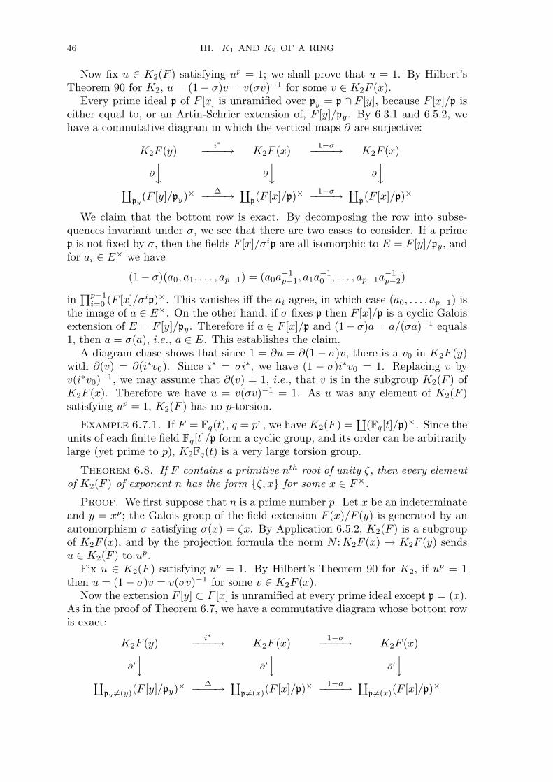
46 III. K1 AND K2 OF A RING
Now fix u ∈ K2(F ) satisfying up = 1; we shall prove that u = 1. By Hilbert’sTheorem 90 for K2, u = (1− σ)v = v(σv)−1 for some v ∈ K2F (x).
Every prime ideal p of F [x] is unramified over py = p ∩ F [y], because F [x]/p iseither equal to, or an Artin-Schrier extension of, F [y]/py. By 6.3.1 and 6.5.2, wehave a commutative diagram in which the vertical maps ∂ are surjective:
K2F (y) i∗−−−−→ K2F (x) 1−σ−−−−→ K2F (x)
∂
y ∂
y ∂
y∐
py(F [y]/py)× ∆−−−−→ ∐
p(F [x]/p)× 1−σ−−−−→ ∐p(F [x]/p)×
We claim that the bottom row is exact. By decomposing the row into subse-quences invariant under σ, we see that there are two cases to consider. If a primep is not fixed by σ, then the fields F [x]/σip are all isomorphic to E = F [y]/py, andfor ai ∈ E× we have
(1− σ)(a0, a1, . . . , ap−1) = (a0a−1p−1, a1a
−10 , . . . , ap−1a
−1p−2)
in∏p−1
i=0 (F [x]/σip)×. This vanishes iff the ai agree, in which case (a0, . . . , ap−1) isthe image of a ∈ E×. On the other hand, if σ fixes p then F [x]/p is a cyclic Galoisextension of E = F [y]/py. Therefore if a ∈ F [x]/p and (1− σ)a = a/(σa)−1 equals1, then a = σ(a), i.e., a ∈ E. This establishes the claim.
A diagram chase shows that since 1 = ∂u = ∂(1− σ)v, there is a v0 in K2F (y)with ∂(v) = ∂(i∗v0). Since i∗ = σi∗, we have (1 − σ)i∗v0 = 1. Replacing v byv(i∗v0)−1, we may assume that ∂(v) = 1, i.e., that v is in the subgroup K2(F ) ofK2F (x). Therefore we have u = v(σv)−1 = 1. As u was any element of K2(F )satisfying up = 1, K2(F ) has no p-torsion.
Example 6.7.1. If F = Fq(t), q = pr, we have K2(F ) =∐
(Fq[t]/p)×. Since theunits of each finite field Fq[t]/p form a cyclic group, and its order can be arbitrarilylarge (yet prime to p), K2Fq(t) is a very large torsion group.
Theorem 6.8. If F contains a primitive nth root of unity ζ, then every elementof K2(F ) of exponent n has the form ζ, x for some x ∈ F×.
Proof. We first suppose that n is a prime number p. Let x be an indeterminateand y = xp; the Galois group of the field extension F (x)/F (y) is generated by anautomorphism σ satisfying σ(x) = ζx. By Application 6.5.2, K2(F ) is a subgroupof K2F (x), and by the projection formula the norm N : K2F (x) → K2F (y) sendsu ∈ K2(F ) to up.
Fix u ∈ K2(F ) satisfying up = 1. By Hilbert’s Theorem 90 for K2, if up = 1then u = (1− σ)v = v(σv)−1 for some v ∈ K2F (x).
Now the extension F [y] ⊂ F [x] is unramified at every prime ideal except p = (x).As in the proof of Theorem 6.7, we have a commutative diagram whose bottom rowis exact:
K2F (y) i∗−−−−→ K2F (x) 1−σ−−−−→ K2F (x)
∂′y ∂′
y ∂′y
∐py 6=(y)(F [y]/py)× ∆−−−−→ ∐
p 6=(x)(F [x]/p)× 1−σ−−−−→ ∐p 6=(x)(F [x]/p)×

III. K1 AND K2 OF A RING 47
As before, we may modify v by an element from K2F (y) to arrange that ∂p(v) = 1for all p 6= (x). For p = (x), let a ∈ F = F [x]/(x) be such that ∂(x)(v) = a and setv′ = va, x. Then ∂(x)(v′) = 1 and ∂p(v′) = ∂p(v) = 1 for every other p. It followsfrom 6.5.2 that v′ is in K2(F ). Therefore (1 − σ)v′ = 1; since v = v′a, x−1 thisimplies that u has the asserted form:
u = (1− σ)a, x−1 = a, x−1a, ζx = a, ζ.
Now we proceed inductively, supposing that n = mp and that the theorem hasbeen proven for m (and p). If u ∈ K2(F ) has exponent n then up has exponent m,so there is an x ∈ F× so that up = ζp, x. The element uζp, x−1 has exponent p,so it equals ζm, y = ζ, ym for some y ∈ F×. Hence u = ζ, xym, as required.
Remark 6.8.1. Suslin also proved the following result in [Su87]. Let F be afield containing a primitive pth root of unity ζ, and let F0 ⊂ F be the subfieldof constants. If x ∈ F×0 and ζ, x = 1 in K2(F ) then ζ, x = 1 in K2(F0). Ifζ, y = 1 in K2(F ) for some y ∈ F× then y = xzp for some x ∈ F×0 and z ∈ F×.
Application 6.8.2. We can use Theorem 6.8 to give another proof of Theo-rem 6.4, that when F is an algebraically closed field, the group K2(F ) is uniquelydivisible. Fix a prime p. For each a ∈ F× there is an α with αp = a. Hencea, b = α, bp, so K2(F ) is p-divisible. If p 6= char(F ) then there is no p-torsionbecause ζ, a = ζ, αp = 1. Finally, if char(F ) = p, there is no p-torsion eitherby Theorem 6.7.
Application 6.8.3 (K2R). Theorem 6.8 states that −1,−1 is the only ele-ment of order 2 in K2R. Indeed, if r is a positive real number then:
−1, r = −1,√
r2 = 1, and −1,−r = −1,−1−1, r = −1,−1.
Note that −1,−1 is in the image of K2(Z), which is a summand by either Exam-ple 6.2.1 or Example 5.9.1. Recall from Example 6.1.6 that the image of K2R in theuniquely divisible group K2C is the eigenspace K2C+, and that the compositionK2R→ K2C
N−→ K2R is multiplication by 2, so its kernel is K2(Z). It follows that
K2R ∼= K2(Z)⊕K2C+.
K2 and the Brauer group
Let F be a field. Recall from II.5.4.3 that the Brauer group Br(F ) is generatedby the classes of central simple algebras with two relations: [A⊗F B] = [A] · [B] and[Mn(F )] = 0. Here is one classical construction of elements in the Brauer group; itis a special case of the construction of crossed product algebras.
Cyclic algebras 6.9. Let ζ be a primitive nth root of unity in F , and α, β ∈F×. The cyclic algebra A = Aζ(α, β) is defined to be the associative algebra withunit, which is generated by two elements x, y subject to the relations xn = α · 1,yn = β · 1 and yx = ζxy. Thus A has dimension n2 over F , a basis being the

48 III. K1 AND K2 OF A RING
monomials xiyj with 0 ≤ i, j < n. The identity (x + y)n = (α + β) · 1 is also easyto check.
When n = 2 (so ζ = −1), cyclic algebras are called quaternion algebras. Thename comes from the fact that the usual quaternions H are the cyclic algebraA(−1,−1) over R. Quaternion algebras arise in the Hasse invariant of quadraticforms.
It is classical, and not hard to prove, that A is a central simple algebra over F ;see [BA, §8.5]. Moreover, the n-fold tensor product A⊗F A⊗F · · ·⊗F A is a matrixalgebra; see [BA, Theorem 8.12]. Thus we can consider [A] ∈ Br(F ) as an elementof exponent n. We shall write nBr(F ) for the subgroup of Br(F ) consisting of allelements x with xn = 1, so that [A] ∈ nBr(F )
For example, the following lemma shows that Aζ(1, β) must be a matrix ringbecause xn = 1. Thus [Aζ(1, β)] = 1 in Br(F ).
Lemma 6.9.1. Let A be a central simple algebra of dimension n2 over a field Fcontaining a primitive nth root of unity ζ. If A contains an element u 6∈ F suchthat un = 1, then A ∼= Mn(F ).
Proof. The subalgebra F [u] of A spanned by u is isomorphic to the commu-tative algebra F [t]/(tn − 1). Since tn − 1 =
∏(t − ζi), the Chinese Remainder
Theorem yields F [u] ∼= F ×F ×· · ·×F . Hence F [u] contains n idempotents ei witheiej = 0 for i 6= j. Therefore A splits as the direct sum e1A ⊕ · · · ⊕ enA of rightideals. By the Artin-Wedderburn theorem, if A = Md(D) then A can be the directsum of at most d right ideals. Hence d = n, and A must be isomorphic to Mn(F ).
Proposition 6.9.2 (The nth power norm residue symbol). If F containsa primitive nth root of unity, there is a homomorphism K2(F ) → Br(F ) sendingα, β to the class of the cyclic algebra Aζ(α, β).
Since the image is a subgroup of exponent n, we shall think of the power normresidue symbol as a map K2(F )/nK2(F ) → nBr(F ).
This homomorphism is sometimes also called the Galois symbol.
Proof. From Ex. 6.10 we see that in Br(F ) we have [Aζ(α, β)] · [Aζ(α, γ)] =[Aζ(α, βγ)]. Thus the map F× × F× → Br(F ) sending (α, β) to [Aζ(α, β)] isbilinear. To see that it is a Steinberg symbol we must check that A = Aζ(α, 1−α)is isomorphic to the matrix algebra Mn(F ). Since the element x + y of A satisfies(x + y)n = 1, Lemma 6.9.1 implies that A must be isomorphic to Mn(F ).
Remark 6.9.3. Merkur’ev and Suslin proved in [MS] that K2(F )/nK2(F ) isisomorphic to the subgroup nBr(F ) of elements of order n in Br(F ). By Mat-sumoto’s Theorem, this implies that the n-torsion in the Brauer group is generatedby cyclic algebras. We will describe the Merkur’ev-Suslin result in chapter VI.
The Galois symbol
We can generalize the power norm residue symbol to fields not containing enoughroots of unity by introducing Galois cohomology. Here are the essential facts weshall need; see [WHomo] or [Milne].
Sketch of Galois Cohomology 6.10. Let Fsep denote the separable closureof a field F , and let G = GF denote the Galois group Gal(Fsep/F ). The family

III. K1 AND K2 OF A RING 49
of subgroups GE = Gal(Fsep/E), as E runs over all finite extensions of F , formsa basis for a topology of G. A G-module M is called discrete if the multiplicationG×M → M is continuous.
For example, the abelian group Gm = F×sep of units of Fsep is a discrete module,as is the subgroup µn of all nth roots of unity. We can also make the tensorproduct of two discrete modules into a discrete module, with G acting diagonally.For example, the tensor product µ⊗2
n = µn ⊗ µn is also a G-discrete module. Notethat the three G-modules Z/n, µn and µ⊗2
n have the same underlying abelian group,but are isomorphic GF -modules only when µn ⊂ F .
The G-invariant subgroup MG of a discrete G-module M is a left exact functoron the category of discrete GF -modules. The Galois cohomology groups Hi
et(F ;M)are defined to be its right derived functors. In particular, H0
et(F ; M) is just MG.If E is a finite separable extension of F then GE ⊂ GF . Thus there is a forgetful
functor from GF -modules to GE-modules, inducing maps Hiet(F ;M) → Hi
et(E; M).In the other direction, the induced module functor from GE-modules to GF -modulesgives rise to cohomological transfer maps trE/F : Hi
et(E;M) → Hiet(F ; M); see
[WHomo, 6.3.9 and 6.11.11].
Example 6.10.1 (Kummer Theory). The cohomology of the module Gm isof fundamental importance. Of course H0
et(F,Gm) = F×. By Hilbert’s Theo-rem 90 for units, and a little homological algebra [WHomo, 6.11.16], we also haveH1
et(F ;Gm) = 0 and H2et(F ;Gm) ∼= Br(F ).
If n is prime to char(F ), the exact sequence of discrete modules
1 → µn → Gmn−→ Gm → 1
is refered to as the Kummer sequence. Writing µn(F ) for the group µGn of all nth
roots of unity in F , the corresponding cohomology sequence is called the Kummersequence.
1 →µn(F ) → F× n−→ F× → H1et(F ;µn) → 1
1 →H2et(F ; µn) → Br(F ) n−→ Br(F )
This yields isomorphisms H1et(F ; µn) ∼= F×/F×n and H2
et(F ;µn) ∼= nBr(F ). Ifµn ⊂ F×, this yields a natural isomorphism H2
et(F ; µ⊗2n ) ∼= nBr(F )⊗ µn(F ).
There are also natural cup products in cohomology, such as the product
(6.10.2) F× ⊗ F× → H1et(F ; µn)⊗H1
et(F ; µn) ∪−→ H2et(F ; µ⊗2
n )
which satisfies the following projection formula: if E/F is a finite separable exten-sion, a ∈ F× and b ∈ E×, then trE/F (a ∪ b) = a ∪NE/F (b).
Proposition 6.10.3 (Galois symbol). The bilinear pairing (6.10.2) inducesa Steinberg symbol K2(F ) → H2
et(F ; µ⊗2n ) for every n prime to char(F ).
Proof. It suffices to show that a∪(1−a) vanishes for every a ∈ F−0, 1. Fixinga, factor the separable polynomial tn−a =
∏fi in F [t] with the fi irreducible, and

50 III. K1 AND K2 OF A RING
let Fi denote the field F (xi) with fi(xi) = 0. Setting t = 1, 1−a =∏
i NFi/F (1−xi).Writing H2
et additively, we have
a ∪ (1− a) =∑
i
a ∪NFi/F (1− xi) =∑
i
trFi/F
(a ∪ (1− xi)
)
= n∑
i
trFi/F
(xi ∪ (1− xi)
).
Since the group H2et(F ; µ⊗2
n ) has exponent n, all these elements vanish, as desired.
Remark 6.10.4. Suppose that F contains a primitive nth root of unity ζ. If weidentify Z/n with µn via 1 7→ ζ, we have a natural isomorphism
nBr(F ) ∼= nBr(F )⊗ Z/n ∼= nBr(F )⊗ µn∼= H2
et(F ; µ⊗2n ).
Tate has shown in [Tate] that this isomorphism identifies the Galois symbol ofProposition 6.10.3 with the nth power norm residue symbol of Proposition 6.9.2.The Merkur’ev-Suslin isomorphism of [MS] cited above in Remark 6.9.3 extendsto a more general isomorphism K2(F )/nK2(F ) ∼= H2
et(F ; µ⊗2n ) for all fields F of
characteristic prime to n. See chapter VI.
EXERCISES
6.1 Given a discrete valuation on a field F , with residue field k and parame-ter π, show that there is a surjection λ: K2(F ) → K2(k) given by the formulaλuπi, vπj = u, v. Example 6.1.2 is a special case of this, in which π = t−1.6.2 (Bass-Tate) If E = F (u) is a field extension of F , and e1, e2 ∈ E are monicpolynomials in u of some fixed degree d > 0, show that e1, e2 is a productof symbols e1, e
′2 and e, e′′2 with e, e′2, e
′′2 polynomials of degree < d. This
generalizes Lemma 6.1.4.6.3 If F is a number field with r1 distinct embeddings F → R, show that the r1
symbols (, )∞ on F define a surjection K2(F ) → ±1r1 .6.4 If F denotes the algebraic closure of a field F , show that K2(Q) = K2(Fp) = 1.6.5 2-adic symbol on Q. Any nonzero rational number r can be written uniquelyas r = (−1)i2j5ku, where i, k ∈ 0, 1 and u is a quotient of integers congruent to1 (mod 8). If s = (−1)i′2j′5k′u′, set (r, s)2 = (−1)ii′+jj′+kk′ . Show that this is aSteinberg symbol on Q, with values in ±1.6.6 Let ((r, s))p denote the Hilbert symbol on Qp (6.2.2), and (r, s)p the tamesymbol K2(Qp) → F×p . Assume that p is odd, so that there is a unique surjectionε:F×p → ±1. Show that ((r, s))p = ε (r, s)p for all r, s ∈ Q×p .
6.7 Quadratic Reciprocity. If r, s ∈ Q×, show that (r, s)∞(r, s)2∏
p6=2((r, s))p = +1.Here (r, s)2 is the 2-adic symbol of Ex. 6.5.
Hint: From 6.5.1 and Ex. 6.6, the 2-adic symbol of Ex. 6.5 must satisfy somerelation of the form
(r, s)2 = (r, s)ε∞∞∏
p6=2
((r, s))εpp ,

III. K1 AND K2 OF A RING 51
where the exponents εp are either 0 or 1. Since (−1,−1)2 = (−1,−1)∞ we haveε∞ = 1. If p is a prime not congruent to 1 (mod 8), consider 2, p and −1, p.If p is a prime congruent to 1 (mod 8), Gauss proved that there is a prime q <
√p
such that p is not a quadratic residue modulo q. Then ((p, q))q = −1, even though(p, q)∞ = (p, q)2 = 1. Since we may suppose inductively that εq equals 1, thisimplies that εp 6= 0.6.8 (Suslin) Suppose that a field F is algebraically closed in a larger field E. UseLemma 6.1.3 and Remark 6.8.1 to show that K2(F ) injects into K2(E).6.9 Let F be a field, and let ΩF = ΩF/Z denote the vector space of absolute Kahlerdifferentials (see Ex. 2.6). The second exterior power of ΩF is written as Ω2
F . Showthat there is a homomorphism K2(F ) → Ω2
F sending x, y to dxx ∧ dy
y .
6.10 Show that Aζ(α, β) ⊗ Aζ(α, γ) ∼= Mn(A), where A = Aζ(α, βγ). Hint: Letx′, y′ generate Aζ(α, β) and x′′, y′′ generate Aζ(α, γ), and show that x′, y = y′y′′
generate A. Then show that u = (x′)−1x′′ + y′′ has un = 1. (For another proof,see [BA, Ex. 8.5.2].)
§7. Milnor K-theory of fields
Fix a field F , and consider the tensor algebra of the group F×,
T (F×) = Z⊕ F× ⊕ (F× ⊗ F×)⊕ (F× ⊗ F× ⊗ F×)⊕ · · · .
To keep notation straight, we write l(x) for the element of degree one in T (F×)corresponding to x ∈ F×.
Definition 7.1. The graded ring KM∗ (F ) is defined to be the quotient of T (F×)
by the ideal generated by the homogeneous elements l(x)⊗ l(1− x) with x 6= 0, 1.The Milnor K-group KM
n (F ) is defined to be the subgroup of elements of degreen. We shall write x1, . . . , xn for the image of l(x1)⊗ · · · ⊗ l(xn) in KM
n (F ).That is, KM
n (F ) is presented as the group generated by symbols x1, . . . , xnsubject to two defining relations: x1, . . . , xn is multiplicative in each xi, andequals zero if xi + xi+1 = 1 for some i.
The name comes from the fact that the ideas in this section first arose in Milnor’s1970 paper [M-QF]. Clearly we have KM
0 (F ) = Z, and KM1 = F× (with the group
operation written additively). By Matsumoto’s Theorem 6.1 we also have KM2 (F ) =
K2(F ), the elements x, y being the usual Steinberg symbols, except that the groupoperation in KM
2 (F ) is written additively.Since xi, xi+1+xi+1, xi = 0 in KM
2 (F ), we see that interchanging two entriesin x1, . . . , xn yields the inverse. It follows that these symbols are alternating: forany permutation π with sign (−1)π we have
xπ1, . . . , xπn = (−1)πx1, . . . , xn.
Examples 7.2. (a) If Fq is a finite field, then KMn (Fq) = 0 for all n ≥ 2, because
KM2 (Fq) = 0 by Cor. 6.1.1. If F has transcendence degree 1 over a finite field (a
global field of finite characteristic), Bass and Tate proved in [BT] that KMn (F ) = 0
for all n ≥ 3.

52 III. K1 AND K2 OF A RING
(b) If F is algebraically closed then KMn (F ) is uniquely divisible. Divisibility is
clear because F× is divisible. The proof that there is no p-torsion is the same asthe proof for n = 2 given in Theorem 6.4, and is relegated to Ex. 7.3.
(c) When F = R we can define a symbol KMn (R) → ±1 by the following
formula: (x1, . . . , xn)∞ equals −1 if all the xi are negative, and equals +1 otherwise.When n = 2 this will be the symbol defined in Example 6.2.1.
To construct it, extend Z→ Z/2 to a ring homomorphism T (R×) → (Z/2)[t] bysending l(x) to t if x < 0 and to 0 if x > 0. This sends the elements l(x)⊗ l(1− x)to zero (as in 6.2.1), so it induces a graded ring homomorphism KM
∗ (R) → (Z/2)[t].The symbol above is just the degree n part of this map.
By induction on n, it follows that KMn (R) is the direct sum of a cyclic group of
order 2 generated by −1, . . . ,−1, and a divisible subgroup. In particular, thisshows that KM
∗ (R)/2KM∗ (R) is the polynomial ring (Z/2)[ε] on ε = l(−1). Using
the norm map we shall see later that the divisible subgroup of KMn (R) is in fact
uniquely divisible. This gives a complete description of each KMn (R) as an abelian
group.(d) When F is a number field, let r1 be the number of embeddings of F into R.
Then we have a map from KMn (F ) to KM
n (R)r1 ∼= (Z/2)r1 . Bass and Tate provedin [BT] that this map is an isomorphism for all n ≥ 3: KM
n (F ) ∼= (Z/2)r1 .
Tame symbols
Recall from Lemma 6.3 and Ex. 6.1 that every discrete valuation v on F inducesa Steinberg symbol K2(F ) ∂v−→ k×v and a map K2(F ) λ−→ K2(kv). These symbolsextend to all of Milnor K-theory.
Theorem 7.3 (Higher tame symbols). For every discrete valuation v on F ,there are two surjections
KMn (F ) ∂v−→ KM
n−1(kv) and KMn (F ) λ−→ KM
n (kv)
satisfying the following conditions. Let R = r ∈ F : v(r) ≥ 0 be the valuationring, and π a parameter for v. If ui ∈ R×, and ui denotes the image of ui inkv = R/(π) then
λu1πi1 , . . . , unπin = u1, . . . , un, ∂vπ, u2, . . . , un = u2, . . . , un.
In particular, ∂v: KM2 (F ) → k×v is the tame symbol of Lemma 6.3, and λ: K2(F ) →
K2(k) is the map of Example 6.1.2 and Ex. 6.1.
Proof. (Serre) Let L denote the graded KM∗ (kv)-algebra generated by an in-
determinate Π in L1, with the relation Π,Π = −1,Π. We claim that the grouphomomorphism
d:F× → L1 = l(k×v )⊕ Z ·Π, d(uπi) = l(u) + iΠ
satisfies the relation: for r 6= 0, 1, d(r)d(1 − r) = 0 in L2. If so, the presentationof KM
∗ (F ) shows that d extends to a graded ring homomorphism d: KM∗ (F ) → L.
Since Ln is the direct sum of KMn (kv) and KM
n−1(kv), we get two maps: λ:KMn (F ) →
III. K1 AND K2 OF A RING 53
KMn (kv) and ∂v:KM
n (F ) → KMn−1(kv). The verification of the relations is routine,
and left to the reader.If 1 6= r ∈ R×, then either 1− r ∈ R× and d(r)d(1− r) = r, 1− r = 0, or else
v(1 − r) = i > 0 and d(r) = l(1) + 0 · Π = 0 so d(r)d(1 − r) = 0 · d(1 − r) = 0. Ifv(r) > 0 then 1− r ∈ R× and the previous argument implies that d(1− r)d(r) = 0.If r 6∈ R then 1/r ∈ R, and we see from (5.10.3) and the above that d(r)d(1− r) =d(1/r)d(−1/r). Therefore it suffices to show that d(r)d(−r) = 0 for every r ∈ R. Ifr = π this is the given relation upon L, and if r ∈ R× then d(r)d(−r) = r,−r = 0by (5.10.3). Since the product in L is anticommutative, the general case r = uπi
follows from this.
Corollary 7.3.1 (Rigidity). Suppose that F is complete with respect to thevaluation v, with residue field k = kv. For every integer q prime to char(k), themaps λ⊕ ∂v: KM
n (F )/q → KMn (k)/q ⊕KM
n−1(k)/q are isomorphisms for every n.
Proof. Since the valuation ring R is complete, Hensel’s Lemma implies thatthe group 1+πR is q-divisible. It follows that l(1+πR)·KM
n−1(F ) is also q-divisible.But by Ex. 7.2 this is the kernel of the map d: KM
n (F ) → Ln∼= KM
n (kv)⊕KMn−1(kv).
Leading Coefficients 7.3.2. As in Example 6.1.2, KMn (F ) is a direct sum-
mand of KMn F (t). To see this, we consider the valuation v∞(f) = −deg(f) on
F (t) of Example 6.5.3. Since t−1 is a parameter, each polynomial f = ut−i
has lead(f) = u. The map λ:KMn F (t) → KM
n (F ), given by λf1, . . . , fn =lead(f1), . . . , lead(fn), is clearly inverse to the natural map KM
n (F ) → KMn F (t).
Except for v∞, every discrete valuation v on F (t) which is trivial on F is thep-adic valuation vp associated to a prime ideal p of F [t]. In this case kv is the fieldF [t]/p, and we write ∂p for ∂v.
Theorem 7.4 (Milnor). There is a split exact sequence for each n, natural inthe field F , and split by the map λ:
0 → KMn (F ) → KM
n F (t)∂=‘
∂p−−−−−→∐p
KMn−1(F [t]/p) → 0.
Proof. Let Ld denote the subgroup of KMn F (t) generated by those symbols
f1, . . . , fr such that all the polynomials fi have degree ≤ d. By Example 7.3.2, L0
is a summand isomorphic to KMn (F ). Since KM
n F (t) is the union of the subgroupsLd, the theorem will follow from Lemma 7.4.2 below, using induction on d.
Let π be an irreducible polynomial of degree d and set k = kπ = F [t]/(π). Theneach element a of k is represented by a unique polynomial a ∈ F [t] of degree < d.
Lemma 7.4.1. There is a unique homomorphism h = hπ: KMn−1(k) → Ld/Ld−1
carrying a2, . . . , an to the class of π, a2, . . . , an modulo Ld−1.
Proof. The formula gives a well-defined set map h from k× × · · · × k× toLd/Ld−1. To see that it is linear in a2, suppose that a2 = a′2a
′′2 . If a2 6= a′2a
′′2
then there is a nonzero polynomial f of degree < d with a2 = a′2a′′2 + fπ. Since

54 III. K1 AND K2 OF A RING
fπ/a2 = 1 − a′2a′′2/a2 we have fπ/a2, a
′2a′′2/a2 = 0. Multiplying by a3, . . . , an
givesπ, a′2a
′′2/a2, a3, . . . , an ≡ 0 modulo Ld−1.
Similarly, h is linear in a3, . . . , an. To see that the multilinear map h factors throughKM
n−1(k), we observe that if ai + ai+1 = 1 in k then ai + ai+1 = 1 in F .
Lemma 7.4.2. The homomorphisms ∂(π) and hπ induce an isomorphism betweenLd/Ld−1 and the direct sum ⊕πKM
n−1(kπ) as π ranges over all monic irreduciblepolynomials of degree d in F [t].
Proof. Since π cannot divide any polynomial of degree < d, the maps ∂(π)
vanish on Ld−1 and induce maps ∂(π): Ld/Ld−1 → KMn−1(kπ). By inspection, the
composition of ⊕hπ with the direct sum of the ∂(π) is the identity on ⊕πKMn−1(kπ).
Thus it suffices to show that ⊕hπ maps onto Ld/Ld−1. By Ex. 6.2, Ld is generatedby Ld−1 and symbols π, a2, . . . , an where π has degree d and the ai have degree< d. But each such symbol is hπ of an element of KM
n−1(kπ), so ⊕hπ is onto.
The Transfer Map
Let v∞ be the valuation on F (t) with parameter t−1. The formulas in Theo-rem 7.3 defining ∂∞ show that it vanishes on KM
∗ (F ). By Theorem 7.4, there areunique homomorphisms Np:KM
n (F [t]/p) → KMn (F ) so that −∂∞ =
∑p Np∂p.
Definition 7.5. Let E be a finite field extension of F generated by an elementa. Then the transfer map, or norm map N = Na/F : KM
∗ (E) → KM∗ (F ), is the
unique map Np defined above, associated to the kernel p of the map F [t] → Esending t to a.
We can calculate the norm of an element x ∈ KMn (E) as Np(x) = −∂v∞(y),
where y ∈ KMn+1F (t) is such that ∂p(y) = x and ∂p′(y) = 0 for all p′ 6= p.
If n = 0, the transfer map N :Z → Z is multiplication by the degree [E : F ] ofthe field extension, while if n = 1 the map N : E× → F× is the usual norm map;see Ex. 7.5. We will show in 7.6 below that N is independent of the choice of a ∈ Efor all n. First we make two elementary observations.
If we let N∞ denote the identity map on KMn (F ), and sum over the set of all
discrete valuations on F (t) which are trivial on F , the definition of the Nv yields:
Weil Reciprocity Formula 7.5.1.∑
v Nv∂v(x) = 0 for all x ∈ KMn F (t).
Projection Formula 7.5.2. Let E = F (a). Then for x ∈ KM∗ (F ) and y ∈
KM∗ (E) the map N = Na/F satisfies Nx, y = x,N(y).Proof. The inclusions of F in F (t) and F [t]/p allow us to view KM
∗ F (t) andKM∗ (F [t]/p) as graded modules over the ring KM
∗ (F ). It follows from Theorem 7.4that each ∂p is a graded module homomorphism of degree −1. This remark alsoapplies to v∞ and ∂∞, because F (t) = F (t−1). Therefore each Np is a gradedmodule homomorphism of degree 0.
Taking y = 1 in KM0 (E) = Z, so N(y) = [E : F ] by Ex. 7.5, this yields

III. K1 AND K2 OF A RING 55
Corollary 7.5.3. If the extension E/F has degree d, then the compositionKM∗ (F ) → KM
∗ (E) N−→ KM∗ (F ) is multiplication by d. In particular, the kernel of
KM∗ (F ) → KM
∗ (E) is annihilated by d.
Definition 7.6. Let E = F (a1, . . . , ar) be a finite field extension of F . Thetransfer map NE/F : KM
∗ (E) → KM∗ (F ) is defined to be the composition of the
transfer maps defined in 7.5:
KMn (E)
Nar−−→ KMn F (a1, . . . , ar−1)
Nar−1−−−−→ · · ·KMn (F (a1)
Na1−−→ KMn (F ).
The transfer map is well-defined by the following result of K. Kato.
Theorem 7.6.1 (Kato). The transfer map NE/F is independent of the choiceof elements a1, . . . , ar such that E = F (a1, . . . , ar). In particular, if F ⊂ F ′ ⊂ Ethen NE/F = NF ′/F NE/F ′ .
The key trick used in the proof of this theorem is to fix a prime p and pass from Fto the union F ′ of all finite extensions of F of degree prime to p. By Corollary 7.5.3the kernel of KM
n (F ) → KMn (F ′) has no p-torsion, and the degree of every finite
extension of F ′ is a power of p.
Lemma 7.6.2. (Kato) If E is a normal extension of F , and [E : F ] is a primenumber p, then the map NE/F = Na/F :KM
∗ (E) → KM∗ (F ) does not depend upon
the choice of a such that E = F (a).
Proof. If also E = F (b), then from Corollary 7.5.3 and Ex. 7.7 with F ′ = Ewe see that δ(x) = Na/F (x) − Nb/F (x) is annihilated by p. If δ(x) 6= 0 for somex ∈ KM
n (E) then, again by Corollary 7.5.3, δ(x) must be nonzero in KMn (F ′), where
F ′ is the union of all finite extensions of F of degree prime to p. Again by Ex. 7.7,we see that we may replace F by F ′ and x by its image in KM
n (EF ′). Since thedegree of every finite extension of F ′ is a power of p, the assertion for F ′ followsfrom Ex. 7.6, since the Projection Formula 7.5.2 yields Na/F ′y, x2, . . . , xn =N(y), x2, . . . , xn.
Corollary 7.6.3. If in addition F is a complete discrete valuation field withresidue field kv, and the residue field of E is kw, the following diagram commutes.
KMn (E) ∂w−−−−→ KM
n−1(kw)
N
yyN
KMn (F ) ∂v−−−−→ KM
n−1(kv)
Proof. Ex. 7.6 implies that for each u ∈ KMn (E) there is a finite field extension
F ′ of F such that [F ′ : F ] is prime to p and the image of u in Kn(EF ′) is generatedby elements of the form u′ = y, x2, . . . , xn (y ∈ EF ′, xi ∈ F ′). By Ex. 7.7 andEx. 7.8 it suffices to prove that Nkw/kv
∂w(u) = ∂v(NEF ′/F ′u) for every element uof this form. But this is an easy computation.

56 III. K1 AND K2 OF A RING
Proposition 7.6.4 (Kato). Let E and F ′ = F (a) be extensions of F with E/Fnormal of prime degree p. If E′ = E(a) denotes the composite field, the followingdiagram commutes.
KM∗ (E′)
Na/E−−−−→ KM∗ (E)
N
yyN
KM∗ (F ′)
Na/F−−−−→ KM∗ (F ).
Proof. The vertical norm maps are well-defined by Lemma 7.6.2. Let π ∈ F [t]and π′ ∈ E[t] be the minimal polynomials of a over F and E, respectively. Givenx ∈ KM
n (E′), we have Na/E(x) = −∂∞(y), where y ∈ KMn+1E(t) satisfies ∂π′(y) = x
and ∂w(y) = 0 if w 6= wπ′ . If v is a valuation on F (t), Ex. 7.9 gives:
∂v(NE(t)/F (t)y) =∑
w|vNE(w)/F (v)(∂wy) =
NE′/F ′(x) if v = vπ
NE/F (∂∞y) if v = v∞0 else
in KM∗ (F ′). Two applications of Definition 7.5 give the desired calculation:
Na/F (NE′/F ′x) = −∂∞(NE(t)/F (t)y) = −NE/F (∂∞y) = NE/F (Na/F x).
Proof of Theorem 7.6.1. As in the proof of Lemma 7.6.2, we see from Corol-lary 7.5.3 and Ex. 7.7 with F ′ = E that the indeterminacy is annihilated by [E : F ].Using the key trick of passing to a larger field, we may assume that the degree ofevery finite extension of F is a power of a fixed prime p.
Let us call a tower of intermediate fields F = F0 ⊂ F1 ⊂ · · · ⊂ Fr = E maximalif [Fi : Fi−1] = p for all i. By Lemma 7.6.2, the transfer maps N : KM
∗ (Fi) →KM∗ (Fi−1) are independent of the choice of a such that Fi = Fi−1(a). If F ⊂ F1 ⊂ E
and F ⊂ F ′ ⊂ E are maximal towers, Proposition 7.6.4 states that NF ′/F NE/F ′ =NF1/F NE/F1 , because if F ′ 6= F1 then E = F ′F1. It follows by induction on [E : F ]that if F = F0 ⊂ F1 ⊂ · · · ⊂ Fr = E is a maximal tower then the composition ofthe norm maps
KMn (E) N−→ KM
n (Fr−1)N−→ · · ·KM
n (F1)N−→ KM
n (F )
is independent of the choice of maximal tower.Comparing any tower to a maximal tower, we see that it suffices to prove that if
F ⊂ F1 ⊂ F ′ is a maximal tower and F ′ = F (a) then Na/F = NF1/F NF ′/F1 . Butthis is just Proposition 7.6.4 with E = F1 and E′ = F ′.
The dlog symbol and ν(n)F
For any field F , we write ΩnF for the nth exterior power of the vector space
ΩF = ΩF/Z of Kahler differentials (Ex. 2.6). The direct sum over n forms a graded-commutative ring Ω∗F , and the map dlog : F× → ΩF sending a to da
a extends to agraded ring map from the tensor algebra T (F×) to Ω∗F . By Ex. 6.9, l(a)⊗ l(1− a)maps to zero, so it factors through the quotient ring KM
∗ (F ) of T (F×). We recordthis observation for later reference.

III. K1 AND K2 OF A RING 57
Lemma 7.7. If F is any field, there is a graded ring homomorphism
dlog : KM∗ (F ) → Ω∗F , dloga1, . . . , an =
da1
a1∧ · · · ∧ dan
an.
Now let F be a field of characteristic p 6= 0, so that d(ap) = p da = 0. In fact,if xi is a p-basis of F over F p then the symbols dxi form a basis of the F -vectorspace ΩF . Note that the set dΩn−1
F of all symbols da1∧· · ·∧dan forms an F p-vectorsubspace of Ωn
F .
Definition 7.7.1. If char(F ) = p 6= 0, let ν(n)F denote the kernel of theArtin-Schrier operator ℘ : Ωn
F → ΩnF /dΩn−1
F , which is defined by
℘
(x
da1
a1∧ · · · ∧ dan
an
)= (xp − x)
da1
a1∧ · · · ∧ dan
an.
(In the literature, ℘ + 1 is the inverse of the “Cartier” operator.)
Clearly ℘(dloga1, . . . , an) = 0, so the image of the dlog map lies in ν(n)F .The following theorem, which implies that these symbols span ν(n)F , was provenby Kato [K82] for p = 2, and for general p by Bloch, Kato and Gabber [BK, 2.1].
Theorem 7.7.2. (Bloch-Kato-Gabber) Let F be a field of characteristic p 6= 0.Then the dlog map induces an isomorphism KM
n (F )/pKMn (F ) ∼= ν(n)F for every
n ≥ 0.
Using this result, Bloch and Kato also proved that the p-torsion subgroup ofKM
n (F ) is divisible [BK, 2.8]. Using this divisibility, Izhboldin found the followinggeneralization of theorem 6.7; see [Izh].
Izhboldin’s Theorem 7.8. If char(F ) = p, the group KMn (F ) has no p-torsion.
Proof. We proceed by induction on n, the case n = 2 being theorem 6.7. Asin the proof of theorem 6.7, let x be an indeterminate and y = xp − x; the fieldextension F (x)/F (y) is an Artin-Schrier extension, and its Galois group is generatedby an automorphism σ satisfying σ(x) = x + 1. By theorem 7.4, we can regardKM
n (F ) as a subgroup of both KMn F (x) and KM
n F (y).For all field extensions E of F (y) linearly disjoint from F (x), i.e., with no root
of tp− t−y, write E(x) for the field E⊗F (y) F (x). Let I(E) denote the set of all p-torsion elements in KM
n E(x) of the form v−σ(v), v ∈ KMn E(x), and let P (E) denote
the p-torsion subgroup of the kernel of the norm map Nx/E : KMn E(x) → KM
n (E).Since Nσ(v) = N(v), I(E) ⊆ P (E). Both I(E) and P (E) vary naturally with E,and are equal by proposition 7.8.2 below.
Fix u ∈ KMn (F ) with pu = 0. The projection formula 7.5.2 shows that the
norm map KMn F (x) → KM
n F (y) sends u to pu = 0. Hence u ∈ P (F (y)). Byproposition 7.8.2, u ∈ I(F (y)), i.e., there is a v ∈ KM
n F (x) so that u = v − σ(v) inKM
n F (x). Now apply the leading coefficient symbol λ of 7.3.2; since λ(σv) = λ(v)we have: u = λ(u) = λ(v)− λ(σv) = 0. This proves Izhboldin’s theorem.
Before proceeding to proposition 7.8.2, we need some facts about the group I(E).We first claim that the transcendental extension E ⊂ E(t) induces an isomorphism

58 III. K1 AND K2 OF A RING
I(E) ∼= I(E(t)). Indeed, since E(x, t) is purely transcendental over E(x), theo-rem 7.4 and induction on n imply that KM
n E(x) → KMn E(x, t) is an isomorphism
on p-torsion subgroups, and the claim follows because the leading coefficient sym-bol 7.3.2 commutes with σ.
We next claim that if E/E′ is a purely inseparable field extension then I(E′) →I(E) is onto. For this we may assume that Ep ⊆ E′ ⊂ E. The composition of theFrobenius map E → Ep with this inclusion induces the endomorphism of KM
n (E)sending a1, . . . , an to ap
1, . . . , apn = pna1, . . . , an. Hence this claim follows
from the following result.
Lemma 7.8.1. The group I(E) is p-divisible.
Proof. Pick v ∈ KMn E(x) so that u = v − σ(v) is in I(E). Now we invoke
the Bloch-Kato result, mentioned above, that the p-torsion subgroup of KMn (L)
is divisible for every field L of characteristic p. By theorem 7.7.2, this impliesthat u vanishes in KM
n E(x)/p ∼= ν(n)E(x). By Ex. 7.12 and theorem 7.7.2, theclass of v mod p comes from an element w ∈ KM
n (E), i.e., v − w = pv′ for somev′ ∈ KM
n E(x). Then u = v − σ(v) = pv′ − pσ(v′), it follows that u′ = v′ − σ(v′) isan element of I(E) with u = pu′.
Proposition 7.8.2. For all E containing F (y), linearly disjoint from F (x),P (E) = I(E).
Proof. We shall show that the obstruction V (E) = P (E)/I(E) vanishes. Thisgroup has exponent p, because if u ∈ P (E) then
pu = pu−NEL/Eu = (p− 1− σ − · · · − σp−1)u
=((1− σ) + (1− σ2) + · · ·+ (1− σp−1)
)u
is in (1 − σ)KMn E(x) and hence in I(E). It follows that V (E) injects into I(E′)
whenever E′/E is an extension of degree prime to p.Now we use the “Brauer-Severi” trick; this trick will be used again in chap-
ter VI, where the name is explained. For each b ∈ E we let Eb denote the fieldE(t1, . . . , tp−1, β) with t1, . . . , tp−1 purely transcendental over E and βp − β − y +∑
bitpi = 0. It is known that b is in the image of the norm map Eb(x)× → E×b ;
see [J37]. Since E · (Eb)p is purely transcendental over E (on β, tp2, ..., tpp−1), it
follows that I(E) → I(Eb) is onto. Since Eb(x) is purely transcendental over E(x)(why?), I(E(x)) = I(Eb(x)) and KM
n E(x) embeds in KMn Eb(x) by theorem 7.4.
Hence KMn (E(x))/I(E) embeds in KM
n Eb(x)/I(Eb). Since V (E) ⊂ KMn E(x)/I(E)
by definition, we see that V (E) also embeds into V (Eb).Now if we take the composite of all the fields Eb, b ∈ E, and then form its
maximal algebraic extension E′ of degree prime to p, it follows that V (E) embedsinto V (E′). Repeating this construction a countable number of times yields anextension field E′′ of E such that V (E) embeds into V (E′′) and every element ofE′′ is a norm from E′′(x). Hence it suffices to prove that V (E′′) = 0. The proofin this special case is completely parallel to the proof of proposition 6.6.2, and weleave the details to Ex. 7.13.
This completes the proof of Izhboldin’s Theorem 7.8.

III. K1 AND K2 OF A RING 59
Corollary 7.8.3 (Hilbert’s Theorem 90 for KM∗ ). Let j : F ⊂ L be a de-
gree p field extension, with char(F ) = p, and let σ be a generator of G = Gal(L/F ).Then KM
n (F ) ∼= KMn (L)G, and the following sequence is exact for all n > 0:
0 → KMn (F )
j∗−→ KMn (L) 1−σ−−→ KM
n (L) N−→ KMn (F ).
Proof. Since KMn (F ) has no p-torsion, Corollary 7.5.3 implies that j∗ is an
injection. To prove exactness at the next spot, suppose that v ∈ KMn (L) has
σ(v) = v. By Ex. 7.12 and theorem 7.7.2, the class of v mod p comes from anelement w ∈ KM
n (E), i.e., v− j∗(w) = pv′ for some v′ ∈ KMn E(x). Hence pσ(v′) =
σ(pv′) = pv′. Since KMn (L) has no p-torsion, σ(v′) = v′. But then pv′ equals
j∗N(v′) =∑
σi(v′), and hence v = j∗(w)+ j∗(Nv′). In particular, this proves thatKM
n (F ) ∼= KMn (L)G.
To prove exactness at the final spot, note that G acts on KMn (L), and that
ker(N)/im(1 − σ) is isomorphic to the cohomology group H1(G,KMn (L)); see
[WHomo, 6.2.2]. Now consider the exact sequence of Gal(L/F )-modules
0 → KMn (L)
p−→ KMn (L) 7.7.2−−−→ ν(n)L → 0.
Using Ex. 7.12, the long exact sequence for group cohomology begins
0 → KMn (F )
p−→ KMn (F ) → ν(n)F → H1(G,KM
n (L))p−→ H1(G,KM
n (L)).
But KMn (F ) maps onto ν(n)F by theorem 7.7.2, and the group H1(G,A) has ex-
ponent p for all G-modules A [WHomo, 6.5.8]. It follows that H1(G,KMn (L)) = 0,
so ker(N) = im(1− σ), as desired.
Relation to the Witt ring
Let F be a field of characteristic 6= 2. Recall from §5.6 of chapter II that theWitt ring W (F ) is the quotient of the Grothendieck group K0SBil(F ) of symmetricinner product spaces over F by the subgroup nH generated by the hyperbolicform 〈1〉 ⊕ 〈−1〉. The dimension of the underlying vector space induces an aug-mentation K0SBil(F ) → Z, sending nH isomorphically onto 2Z, so it inducesan augmentation ε: W (F ) → Z/2.
We shall be interested in the augmentation ideals I = ker(ε) of W (F ) and I ofK0SBil(F ). Since H ∩ I = 0, we have I ∼= I. Now I is generated by the classes〈a〉 − 1, a ∈ F − 0, 1. The powers In of I form a decreasing chain of idealsW (F ) ⊃ I ⊃ I2 ⊃ · · · .
For convenience, we shall write KMn (F )/2 for KM
n (F )/2KMn (F ).
Theorem 7.9 (Milnor). There is a unique surjective homomorphism
sn:KMn (F )/2 → In/In+1
sending each product a1, . . . , an in KMn (F ) to the product
∏ni=1
(〈ai〉− 1)
moduloIn+1. The homomorphisms s1 and s2 are isomorphisms.
Proof. Because(〈a〉 − 1
)+
(〈b〉 − 1) ≡ 〈ab〉 − 1 modulo I2 (II.5.6.5), the map
l(a1)×· · ·×l(an) 7→ ∏(〈ai〉−1)
is a multilinear map from F× to In/In+1. Moreover,
60 III. K1 AND K2 OF A RING
if ai + ai+1 = 1 for any i, we know from Ex. II.5.11 that(〈ai〉− 1
)(〈ai+1〉− 1)
= 0.By the presentation of KM
∗ (F ), this gives rise to a group homomorphism fromKM
n (F ) to In/In+1. It annihilates 2KM∗ (F ) because 〈a2〉 = 1:
2sna1, . . . , an = sna21, a2 . . . =
(〈a21〉 − 1
) n∏
i=2
(〈ai〉 − 1)
= 0.
It is surjective because I is generated by the(〈a〉− 1
). When n = 1 the map is the
isomorphism F×/F×2 ∼= I/I2 of chapter II. We will see that s2 is an isomorphismin Corollary 7.10.3 below, using the Hasse invariant w2.
Example 7.9.1. For the real numbers R, we have W (R) = Z and I = 2Zon s1(−1) = 〈−1〉 − 1 = 2〈−1〉. On the other hand, we saw in Example 7.2(c)that KM
n (R)/2 ∼= Z/2 on −1, . . . ,−1. In this case each sn is the isomorphismZ/2 ∼= 2nZ/2n+1Z.
At the other extreme, if F is algebraically closed then W (F ) = Z/2. SinceKM
n (F ) is divisible, KMn (F )/2 = 0 for all n ≥ 1. Here sn is the isomorphism 0 = 0.
Remark 7.9.2. In 1970, Milnor asked if the surjection sn: KMn (F )/2 → In/In+1
is an isomorphism for all n and F , char(F ) 6= 2 (on p. 332 of [M-QF]). Milnor provedthis was so for local and global fields. In 1996, Voevodsky proved this result for allfields and all n; see [V-MC].
Definition 7.10 (Stiefel-Whitney invariant). The (total) Stiefel-Whitneyinvariant w(M) of the symmetric inner product space M = 〈a1〉 ⊕ · · · ⊕ 〈an〉 is theelement of
∏∞i=0 KM
i (F )/2 defined by the formula
w(M) =n∏
i=1
(1 + l(ai)
)= 1 + l(a1 · · · an) + · · ·+ a1, . . . , an
The lemma below shows that w(M) is independent of the representation of M asa direct sum of 1-dimensional forms. We write w(M) = 1 + w1(M) + w2(M) + · · · ,where the ith Stiefel-Whitney invariant wi(M) ∈ KM
i (F )/2 equals the ith elemen-tary symmetric function of l(a1), . . . , l(an). For example, w1(M) = a1 · · · an ∈F×/F×2 is just the classical “discriminant” of M defined in II.5.6.3, while the sec-ond elementary symmetric function w2(M) =
∑i<jai, aj lies in K2(F )/2 and is
called the Hasse invariant of M ; see [M-SBF].For M = 〈a〉 ⊕ 〈b〉 we have w1(M) = ab and w2(M) = a, b, with wi(M) = 0
for i ≥ 3. In particular, the hyperbolic plane H has wi(H) = 0 for all i ≥ 2.
Lemma 7.10.1. w(M) is a well-defined unit in the ring∏∞
i=1 KMi (F )/2. It
satisfies the Whitney sum formula
w(M ⊕N) = w(M)w(N),
so w extends to a function on K0SBil(F ). Hence each Stiefel-Whitney invariantwi extends to a function K0SBil(F ) wi−→ KM
i (F )/2.
Proof. To show that w(M) is well defined, it suffices to consider the rank twocase. Suppose that 〈a〉 ⊕ 〈b〉 ∼= 〈α〉 ⊕ 〈β〉. Then the equation ax2 + by2 = α

III. K1 AND K2 OF A RING 61
must have a solution x, y in F . The case y = 0 (or x = 0) is straightforward,since 〈α〉 = 〈ax2〉 = 〈a〉, so we may assume that x and y are nonzero. Since thediscriminant w1 is an invariant, we have ab = αβu2 for some u ∈ F , and all wemust show is that a, b = α, β in K2(F )/2. The equation 1 = ax2/α + by2/αyields the equation
0 = ax2/α, by2/α ≡ a, b+ α, α − a, α − b, α ≡ a, b − α, ab/α
in K2(F )/2K2(F ). Substituting ab = αβu2, this implies that a, b ≡ α, βmodulo 2K2(F ), as desired.
Example 7.10.2. Since I ∼= I, we may consider the wi as functions on I ⊆W (F ). However, care must be taken as wi(M) need not equal w2(M ⊕ H). Forexample, w2(M ⊕ H) = w2(M) + w1(M),−1. In particular, w2(H ⊕ H) =−1,−1 can be nontrivial. The Hasse-Witt invariant of an element x ∈ I ⊂W (F ) is defined to be h(x) = w2(V, B), where (V, B) is an inner product spacerepresenting x so that dim(V ) ≡ 0 mod 8.
Corollary 7.10.3. The Hasse invariant w2: I → K2(F )/2 induces an isomor-phism from I2/I3 ∼= I2/I3 to KM
2 (F )/2, inverse to the map s2 of Theorem 7.9.
Proof. By Ex. 7.11, w2 vanishes on the ideal I3 ∼= I3, and hence definesa function from I2/I3 to K2(F )/2. Since the total Stiefel-Whitney invariant ofs2a, b =
(〈a〉 − 1)(〈b〉 − 1
)is 1 + a, b, this function provides an inverse to the
function s2 of Theorem 7.9.
If char(F ) = 2, there is an elegant formula for the filtration quotients of the Wittring W (F ) and the W (F )-module WQ(F ) (see II.5) due to K. Kato [K82]. Recallfrom 7.7.2 that KM
n (F )/2 ∼= ν(n)F , where ν(n)F is the kernel of the operator ℘.The case n = 0 of Kato’s result was described in Ex. II.5.12(d).
Theorem 7.10.4 (Kato [K82]). Let F be a field of characteristic 2. Then themap sn of Theorem 7.9 induces an isomorphism KM
n (F )/2 ∼= ν(n)F∼= In/In+1,
and there is a short exact sequence
0 → In/In+1 → ΩnF
℘−→ ΩnF /dΩn−1
F → In WQ(F )/In+1 WQ(F ) → 0.
The Galois symbol
For the next result, we need some facts about Galois cohomology, expandingslightly upon the facts mentioned in 6.10. Assuming that n is prime to char(F ),there are natural cohomology cup products Hi
et(F ; M)⊗Hjet(F ; N) ∪−→ Hi+j
et (F ; M⊗N) which are associative in M and N . This makes the direct sum H∗
et(F ; M⊗∗) =⊕∞i=0H
iet(F ; M⊗i) into a graded-commutative ring for every Z/n-module M over
the Galois group Gal(Fsep/F ). (By convention, M⊗0 is Z/n.) In particular, bothH∗
et(F ;Z/n) and H∗et(F ; µ⊗∗n ) are rings, and are isomorphic only when F contains
a primitive nth root of unity.

62 III. K1 AND K2 OF A RING
Theorem 7.11 (Galois Symbols). (Bass-Tate) Fix a field F and an integern prime to char(F ).
(1) If F contains a primitive nth root of unity, the Kummer isomorphism fromF×/F×n to H1
et(F ;Z/n) extends uniquely to a graded ring homomorphism
hF : KM∗ (F )/n → H∗(F ;Z/n).
(2) More generally, the Kummer isomorphism from F×/F×n to H1(F ; µn) ex-tends uniquely to a graded ring homomorphism
hF : KM∗ (F )/n → H∗
et(F ; µ⊗∗n ) = ⊕∞i=0Hiet(F ;µ⊗i
n ).
The individual maps KMi (F ) → Hi
et(F ; µ⊗in ) are called the higher Galois symbols.
Proof. The first assertion is just a special case of the second assertion. As in(6.10.2), the Kummer isomorphism induces a map from the tensor algebra T (F×)to H∗
et(F ; µ⊗∗n ), which in degree i is the iterated cup product
F× ⊗ · · ·F× = (F×)⊗n ∼=(H1
et(F ; µn))⊗i ∪−→ Hi
et(F ;µ⊗in ).
By Proposition 6.10.3, the Steinberg Relation is satisfied in H2et(F, µ⊗2
n ). Hence thepresentation of KM
∗ (F ) yields a ring homomorphism from KM∗ (F ) to H∗
et(F ; µ⊗∗n ).
Remark 7.11.1. Milnor studied the Galois symbol for n = 2 and stated (onp.340 of [M-QF]) that, “I do not know any examples for which the homomorphismhF fails to be bijective.” In 1996, Voevodsky announced a proof of this result forn = 2; see [V-MC]. The following partial had been obtained a decade earlier, byRost and Merkurjev-Suslin [MS2].
Theorem 7.11.2. If char(F ) 6= 2, the Galois symbol
KM3 (F )/2 → H3
et(F ;Z/2) = H3et(F ;µ⊗3
2 )
is an isomorphism
EXERCISES
7.1 Let v be a discrete valuation on a field F . Show that the maps λ: KMn (F ) →
KMn (kv) and ∂v: KM
n (F ) → KMn−1(kv) of Theorem 7.3 are independent of the choice
of parameter π, and that they vanish on l(u) · KMn−1(F ) whenever u ∈ (1 + πR).
Show that the map λ also vanishes on l(π) ·KMn−1(F ).
7.2 Continuing Exercise 7.1, show that the kernel of the map d: KMn (F ) → Ln of
Theorem 7.3 is exactly l(1 + πR) ·KMn−1(F ). Conclude that the kernel of the map
λ is exactly l(1 + πR) ·KMn−1(F ) + l(π) ·KM
n−1(F ).7.3 (Bass-Tate) Generalize Theorem 6.4 to show that for all n ≥ 2:(a) If F is an algebraically closed field, then KM
n (F ) is uniquely divisible.(b) If F is a perfect field of characteristic p then KM
n (F ) is uniquely p-divisible.

III. K1 AND K2 OF A RING 63
7.4 Let F be a local field with valuation v and finite residue field k. Show thatKM
n (F ) is divisible for all n ≥ 3. Hint: By Moore’s Theorem 6.2.4, KMn (F ) is
`-divisible unless F has a `th root of unity. Moreover, for every x /∈ F×` there is ay /∈ F×` so that x, y generates K2(F )/`. Given a, b, c with b, c 6∈ `K2(F ), finda′, b′ 6∈ F×` so that b′, c ≡ 0 and a′, b′ ≡ a, b modulo `K2(F ), and observethat a, b, c ≡ a′, b′, c ≡ 0.
In fact, I. Sivitskii has shown that KMn (F ) is uniquely divisible for n ≥ 3 when
F is a local field. See [Siv].
7.5 Let E = F (a) be a finite extension of F , and consider the transfer map N =Na/F : KM
n (E) → KMn (F ) in definition 7.5. Use Weil’s Formula (7.5.1) to show that
when n = 0 the transfer map N :Z→ Z is multiplication by [E : F ], and that whenn = 1 the transfer map N : E× → F× is the usual norm map.
7.6 Suppose that the degree of every finite extension of a field F is a power of somefixed prime p. If E is an extension of degree p and n > 0, use Ex. 6.2 to show thatKM
n (E) is generated by elements of the form y, x2, . . . , xn, where y ∈ E× andthe xi are in F×.
7.7 Ramification and the transfer. Let F ′ and E = F (a) be finite field extensions ofF , and suppose that the irreducible polynomial π ∈ F [t] of a has a decompositionπ =
∏πei in F ′[t]. Let Ei denote F ′(ai), where each ai has minimal polynomial
πi. Show that the following diagram commutes.
KMn (E)
e1,...,er−−−−−→ ⊕KMn (Ei)
Na/F
yyPNai/F ′
KMn (F ) −−−−→ KM
n (F ′)
7.8 Ramification and ∂v. Suppose that E is a finite extension of F , and that w isa valuation on E over the valuation v on F , with ramification index e. (See 6.3.1.)Use the formulas for ∂v and ∂w in Theorem 7.3 to show that for every x ∈ KM
n (F )we have ∂w(x) = e · ∂v(x) in KM
n−1(kw)
7.9 If E/F is a normal extension of prime degree p, and v is a valuation on F (t)trivial on F , show that ∂vNE(t)/F (t) =
∑w NE(w)/F (v)∂w, where the sum is over all
the valuations w of E(t) over v. Hint: If F (t)v and E(t)w denote the completionsof F (t) and E(t) at v and w, respectively, use Ex. 7.7 and Lemma 7.6.3 to showthat the following diagram commutes.
KMn+1E(t) −−−−→ ⊕
w KMn+1E(t)w
∂−−−−→ ⊕w KM
n E(w)
NE(t)/F (t)
yyPw NE(t)w/F (t)v
yPw Ne(w)/F (v)
KMn F (t) −−−−→ KM
n F (t)w∂−−−−→ KM
n F (v)
7.10 If v is a valuation on F , and x ∈ KMi (F ), y ∈ KM
j (F ), show that
∂v(xy) = λ(x)∂v(y) + (−1)j∂v(x)ρ(y)

64 III. K1 AND K2 OF A RING
where ρ: KM∗ (F ) → KM
∗ (kv) is a ring homomorphism characterized by the formulaρ(l(uπi)) = l((−1)iu).7.11 Let t = 2n−1 and set z =
∏ni=1
(〈ai〉 − 1); this is a generator of the ideal
In in K0SBil(F ). Show that the Stiefel-Whitney invariant w(z) is equal to: 1 +an, . . . , an,−1,−1, . . . ,−1 if n is odd, and to 1 + an, . . . , an,−1,−1, . . . ,−1 ifn is even. This shows that the invariants wi vanish on the ideal In if i < t = 2n−1,and that wt induces a homomorphism from In/In+1 ∼= In/In+1 to KM
t (F )/2.For example, this implies that w1 vanishes on I2, while w2 and w3 vanish on I3.
7.12 (Izhboldin) Let L/F be a field extension of degree p = char(F ), with Galoisgroup G. Show that Ωn
F is isomorphic to (ΩnL)G, and that Ωn
F /dΩn−1F is isomorphic
to (ΩnL/dΩn−1
L )G. Conclude that ν(n)F∼= ν(n)G
L .7.13 In this exercise we complete the proof of proposition 7.8.2, and extablisha special case of 7.8.3. Suppose that E(x) is a degree p field extension of E,char(E) = p, and that σ is a generator of Gal(E(x)/E). Suppose in addition thatthe norm map E(x)× → E× is onto, and that E has no extensions of degree < p.Modify the proof of proposition 6.6.2 to show that the following sequence is exact:
KMn E(x) 1−σ−−→ KM
n E(x) N−→ KMn E → 0.

CHAPTER IV
DEFINITIONS OF HIGHER K-THEORY
The higher algebraic K-groups of a ring R are defined to be the homotopy groupsKn(R) = πnK(R) of a certain topological space K(R), which we shall construct inthis chapter. Of course, the space K(R) is rigged so that if n = 0, 1, 2 then πnK(R)agrees with the groups Kn(R) constructed in chapters II and III.
We shall also define the higher K-theory of a category A in each of the threesettings where K0(A) was defined in chapter II: when A is a symmetric monoidalcategory (§3), an exact category (§4) and a Waldhausen category (§6). In eachcase we build a “K-theory space” KA and define the group KnA to be its ho-motopy groups: KnA = πnKA. Of course the group π0KA will agree with thecorresponding group K0A defined in chapter II.
We will show these definitions of KnA coincide whenever they coincide for K0.For example, the group K0(R) of a ring R was defined in §II.2 as K0 of the categoryP(R) of f.g. projective R-modules, but to define K0P(R) we could also regard thecategory P(R) as being either a symmetric monoidal category (II.5.2), an exactcategory (II.7.1) or a Waldhausen category (II.9.1.3). We will show that the dif-ferent constructions give homotopy equivalent spaces KP(R), and hence the samehomotopy groups. Thus the groups Kn(R) = πnKP(R) will be independent of theconstruction used.
Many readers will not be interested in the topological details, so we have designedthis chapter to allow “surfing.” Since the most non-technical way to construct K(R)is to use the “+”-construction, we will do this in §1 below.
In §2, we summarize the basic facts about the geometric realization BC of acategory C, and the basic connection between category theory and homotopy the-ory needed for the rest of the constructions. Indeed, the K-theory space KA isconstructed in each setting using the geometric realization BC of some category C,concocted out of A. For this, we assume only that the reader has a slight familiar-ity with cell complexes, or CW complexes, which are spaces obtained by successiveattachment of cells, with the weak topology.
Sections 3–6 give the construction of the K-theory spaces. Thus in §3 we havegroup completion constructions for symmetric monoidal categories (and the con-nection to the +-construction). Quillen’s Q-construction for abelian and exact cat-egories is given in §4; in §5 we prove the “+ = Q” theorem, that the Q-constructionand group completion constructions agree for split exact categories (II.7.1.2). ThewS· construction for Waldhausen categories is in §6, along with its connection tothe Q-construction.
We conclude with a short section (§7) on homotopy groups with finite coefficients.These have shown to be remarkably useful in describing the structure of the groupsKn(A), especially as related to etale cohomology.
Typeset by AMS-TEX
1

2 IV. DEFINITIONS OF HIGHER K-THEORY
§1. The BGL+ definition for Rings
Let R be an associative ring with unit. Recall from chapter III that the infinitegeneral linear group GL(R) is the union of the finite groups GLn(R), and that itscommutator subgroup is the perfect group E(R) generated by the elementary ma-trices eij(r). Moreover the group K1(R) is defined to be the quotient GL(R)/E(R).
In 1969, Quillen proposed defining the higher K-theory of a ring R to be thehomotopy groups of a certain topological space, which he called “BGL(R)+.” Be-fore describing the elementary properties of Quillen’s construction, and the relatedsubject of acyclic maps, we present Quillen’s description of BGL(R)+ and definethe groups Kn(R) for n ≥ 1.
For any group G, we can naturally construct a connected topological space BGwhose fundamental group is G, but whose higher homotopy groups are zero. More-over, the homology of the topological space BG coincides with the algebraic homol-ogy of the group G. Details of this construction are in §2 below. For G = GL(R)we obtain the space BGL(R), which is central to the following definition.
Definition 1.1. The notation BGL(R)+ will denote any CW complex X whichhas a distinguished map BGL(R) → BGL(R)+ such that
(1) π1BGL(R)+ = K1(R), and the natural map from GL(R) = π1BGL(R) toπ1BGL(R)+ is onto with kernel E(R);
(2) H∗(BGL(R); M)∼=−→ H∗(BGL(R)+;M) for every GL(R)-module M .
We will sometimes say that X is a model for BGL(R)+.For n ≥ 1, Kn(R) is defined to be the homotopy group πnBGL(R)+.
By Theorem 1.4 below, any two models are homotopy equivalent, i.e., the spaceBGL(R)+ is uniquely defined up to homotopy. Hence the homotopy groups Kn(R)of BGL(R)+ are well-defined.
By construction, K1(R) agrees with the group K1(R) = GL(R)/E(R) definedin chapter III. We will see in 1.6.1 below that K2(R) = π2BGL+(R) agrees withthe group K2(R) defined in chapter III.
Several different models for BGL(R)+ are described in 1.8 below. We willconstruct even more models for BGL(R)+ in the rest of this chapter: the spaceP−1P(R) of §3, the space ΩBQP(R) of §4 and the space Ω(iso S·S) arising fromthe Waldhausen construction in §6.
Definition 1.1.1. Write K(R) for the product K0(R) × BGL(R)+. That is,K(R) is the disjoint union of copies of the connected space BGL(R)+, one for eachelement of K0(R). By construction, K0(R) = π0K(R). Moreover, it is clear thatπnK(R) = πnBGL(R)+ = Kn(R) for n ≥ 1.
Functoriality 1.1.2. Each Kn is a functor from rings to abelian groups, whilethe topological spaces BGL(R)+ and K(R) are functors from rings to the homo-topy category of topological spaces. However, without more information about themodels used, the topological maps BGL(R)+ → BGL(R′)+ are only well-definedup to homotopy.
To see this, note that any ring map R → R′ induces a natural group mapGL(R) → GL(R′), and hence a natural map BGL(R) → BGL(R′). This inducesa map BGL(R)+ → BGL(R′)+, unique up to homotopy, by Theorem 1.4 below.Thus the group maps Kn(R) → Kn(R′) are well defined. Since the identity ofR induces the identity on BGL(R)+, only composition remains to be considered.

IV. DEFINITIONS OF HIGHER K-THEORY 3
Given a second map R′ → R′′, the composition BGL(R) → BGL(R′) → BGL(R′′)is induced by R → R′′ because BGL is natural. By uniqueness in Theorem 1.4, thecomposition BGL(R)+ → BGL(R′)+ → BGL(R′′)+ must be homotopy equivalentto any a priori map BGL(R)+ → BGL(R′′)+.
Homotopy Fiber 1.1.3. The maps π∗X → π∗Y induced by a continuous mapX
f−→ Y can always be made to fit into a long exact sequence, in a natural way.The homotopy fiber F (f) of a f , relative to a basepoint ∗Y of Y , is the space ofpairs (x, γ), where x ∈ X and γ : [0, 1] → Y is a path in Y starting at the baspointγ(0) = ∗Y , and ending at γ(1) = f(x). The key property of the homotopy fiberis that (given a basepoint ∗X with f(∗X) = ∗Y ) there is a long exact sequence ofhomotopy groups/pointed sets
· · ·πn+1Y∂−→πnF (f) → πnX → πnY
∂−→ πn−1F (f) → · · ·· · · ∂−→π1F (f) → π1X → π1Y
∂−→ π0F (f) → π0X → π0Y.
Relative groups 1.1.4. Given a ring homomorphism f : R → R′, let K(f) bethe homotopy fiber of K(R) → K(R′), and set Kn(f) = πnK(f). This constructionis designed so that these relative groups fit into a long exact sequence:
· · ·Kn+1(R′)∂−→Kn(f) → Kn(R) → Kn(R′) ∂−→ · · ·
· · ·K1(R, I) → K1(R)toK1(R′)∂−→K0(f) → K0(R) → K0(R′).
When R′ = R/I for some ideal I, we write K(R, I) for K(R → R/I). It is easy tosee (Ex. 1.10) that K0(R, I) and K1(R, I) agree with the relative groups defined inEx. II.2.3 and III.2.2, and that the ending of this sequence is the exact sequenceof III, 2.3 and 5.7. Keune and Loday have shown that K2(R, I) agrees with thedefined in III.5.7.
Acyclic Spaces and Acyclic Maps
The definition of BGL(R)+ fits into the general framework of acyclic maps, whichwe now discuss. Our discussion of acyclicity is taken from [HH] and [Berrick].
Definition 1.2 (Acyclic spaces). We call a topological space F acyclic if ithas the homology of a point, that is, if H∗(F ;Z) = 0.
Lemma 1.2.1. Let F be an acyclic space. Then F is connected, its fundamentalgroup G = π1(F ) must be perfect, and H2(G;Z) = 0 as well.
Proof. The acyclic space F must be connected, as H0(F ) = Z. BecauseG/[G, G] = H1(F ;Z) = 0, we have G = [G,G], i.e., G is a perfect group. Tocalculate H2(G), observe that the universal covering space F has H1(F ;Z) = 0.Moreover, the homotopy fiber of the canonical map F → BG is homotopy equivalentto F (consider the long exact sequence of homotopy groups 1.1.3 to see this). TheSerre Spectral Sequence for this homotopy fibration is E2
pq = Hp(G; Hq(F ;Z)) ⇒Hp+q(F ;Z) and the conclusion that H2(G;Z) = 0 follows from the associated exactsequence of low degree terms:
H2(F ;Z) → H2(G;Z) d2
−→ H1(F ;Z)G → H1(F ;Z) → H1(G;Z).

4 IV. DEFINITIONS OF HIGHER K-THEORY
Example 1.2.2 (Volodin Spaces). The Volodin space X(R) is an acyclicsubspace of BGL(R), constructed as follows. For each n, let Tn(R) denote the sub-group of GLn(R) consisting of upper triangular matrices. As n varies, the unionof these groups forms a subgroup T (R) of GL(R). Similarly we may regard thepermutation groups Σn as subgroups of GLn(R) by their representation as permu-tation matrices, and their union is the infinite permutation group Σ ⊂ GL(R). Foreach σ ∈ Σn, let Tσ
n (R) denote the subgroup of GLn(R) obtained by conjugatingTn(R) by σ. For example, if σ = (n . . . 1) then Tσ
n (R) is the subgroup of lowertriangular matrices.
Since the classifying spaces BTn(R) and BTn(R)σ are subspaces of BGLn(R),and hence of BGL(R), we may form their union over all n and σ: X(R) =⋃
n,σ BTn(R)σ. The space X(R) is acyclic (see [Suslin]). Since X(R) was firstdescribed by Volodin in 1971, it is usually called the Volodin space of R.
The image of the map π1X(R) → GL(R) = π1BGL(R) is the group E(R). Tosee this, note that the maps BT σ
n (R) → BGL(R) factor through X(R); applying π1
shows that the image of π1(X) contains all the subgroups Tσn (R) of GL(R). Hence
these subgroups contain the generators eij(r) of E(R). Since the image of theperfect group π1X(R) is contained in the commutator subgroup E(R) of GL(R),the image must be E(R).
Definition 1.3 (Acyclic maps). Let X and Y be based connected CW com-plexes. A cellular map f :X → Y is called acyclic if the homotopy fiber F (f) of fis acyclic (has the homology of a point).
From the long exact sequence of homotopy groups/pointed sets, we see that ifX → Y is acyclic, then the map π1(X) → π1(Y ) is onto, and its kernel P is aperfect normal subgroup of π1(X).
Definition 1.3.1. Let P be a perfect normal subgroup of π1(X), where X is abased connected CW complex. An acyclic map f :X → Y is called a +–constructionon X (relative to P ) if P is the kernel of π1(X) → π1(Y ).
When Quillen introduced this definition in 1969, he observed that both Y andthe map f are determined up to homotopy by the subgroup P . This is the contentof the following theorem; its proof uses topological obstruction theory. Part (a) isproven in Ex. 1.3; an explicit proof may be found in §5 of [Berrick].
Theorem 1.4 (Quillen). Let P be a perfect normal subgroup of π1(X). Then
(1) There is a +–construction f :X → Y relative to P(2) Let f : X → Y be a +–construction relative to P , and g: X → Z a map such
that P vanishes in π1(Z). Then there is a map h: Y → Z, unique up tohomotopy, such that g = hf .
(3) In particular, if g is another +–construction relative to P , then the map h
in (2) is a homotopy equivalence: h:Y ∼−→ Z.
Remark. Every group G has a unique largest perfect subgroup P , called theperfect radical of G; see Ex. 1.4. If no mention is made to the contrary, the notationX+ will always denote the +–construction relative to the perfect radical of π1(X).
The first construction along these lines was announced by Quillen in 1969, sowe have adopted Quillen’s term “+–construction” as well as his notation. A gooddescription of his approach may be found in [HH] or [Berrick].

IV. DEFINITIONS OF HIGHER K-THEORY 5
Lemma 1.5. A map f : X → Y is acyclic iff H∗(X, M) ∼= H∗(Y, M) for everyπ1(Y )-module M .
Proof. Suppose first that f is acyclic, with homotopy fiber F (f). Since themap π1F (f) → π1Y is trivial, π1F (f) acts trivially upon M . By the UniversalCoefficient Theorem, Hq(F (q); M) = 0 for q 6= 0 and H0(F ; M) = M . ThereforeE2
pq = 0 for q 6= 0 in the Serre Spectral Sequence for f :
E2pq = Hp(Y ; Hq(F (f); M)) ⇒ Hp+q(X; M).
Hence the spectral sequence collapses to yield Hp(X; M)∼=−→ Hp(Y ; M) for all p.
Conversely, we suppose first that π1Y = 0 and H∗(X;Z) ∼= H∗(Y ;Z). By the
Comparison Theorem for the Serre Spectral Sequences for F (f) → Xf−→ Y and
∗ → Y=−→ Y , we have H∗(F (f);Z) = 0. Hence F (f) and f are acyclic.
The general case reduces to this by the following trick. Let Y denote the universalcovering space of Y , and X = X×Y Y the corresponding covering space of X. Thenthere are natural isomorphisms H∗(Y ;Z) ∼= H∗(Y ; M) and H∗(X;Z) ∼= H∗(X;M),where M = Z[π1(Y )]. The assumption that H∗(X; M) ∼= H∗(Y ; M) implies thatthe map f : X → Y induces isomorphisms on integral homology. But π1(Y ) = 0, soby the special case above the homotopy fiber F (f) of f is an acyclic space. But bypath lifting we have F (f) ∼= F (f), so F (f) is acyclic. Thus f is an acyclic map.
Recall from III.3.3.3 that every perfect group P has a universal central extensionE → P , and that the kernel of this extension is the abelian group H2(P ;Z).
Proposition 1.6. Let P be a perfect normal subgroup of a group G, with cor-responding +–construction f :BG → BG+. If F (f) is the homotopy fiber of f thenπ1F (f) is the universal central extension of P , and π2(BG+) ∼= H2(P ;Z).
Proof. We have an exact sequence π2(BG) → π2(BG+) → π1F (f) → G →G/P → 1. But π2(BG) = 0, and π2(BG+) is in the center of π1F (f) by [Wh,IV.3.5]. Thus π1F (f) is a central extension of P with kernel π2(BG+). But F (f) isacyclic, so π1F (f) is perfect and H2(F ;Z) = 0 by 1.2. By the Recognition TheoremIII.3.4, π1F (f) is the universal central extension of P .
Recall from Theorem III.3.5 that the Steinberg group St(R) is the universalcentral extension of the perfect group E(R). Thus we have:
Corollary 1.6.1. The group K2(R) = π2BGL(R)+ is isomorphic to the groupK2(R) ∼= H2(E(R);Z) of chapter III.
In fact, we will see in Ex. 1.6 and 1.7 that Kn(R) ∼= πn(BE(R)+ for all n ≥ 2,and Kn(R) ∼= πn(BSt(R)+ for all n ≥ 3, with K3(R) ∼= H3(St(R);Z).
Corollary 1.6.2. The fundamental group π1X(R) of the Volodin space (1.2.2)is the Steinberg group St(R).
Construction Techniques
One problem with the +construction approach is the fact that BGL(R)+ is nota uniquely defined space. It is not hard to see that BGL(R)+ is an H-space (seeEx. 1.9). Quillen proved that that it is also an infinite loop space. We omit theproof here, because it will follow from the + = Q theorem in section 5.
Here is one of the most useful recognition criteria, due to Quillen. The proof isis an application of obstruction theory, which we omit (but see [Ger72, 1.5].)

6 IV. DEFINITIONS OF HIGHER K-THEORY
Theorem 1.7. The map i : BGL(R) → BGL(R)+ is universal for maps intoH-spaces. That is, for each map f : BGL(R) → H, where H is an H-space,there is a map g : BGL(R)+ → H so that f = gi, and such that the inducedmap πi(BGL(R)+) → πi(H) is independent of g.
Constructions 1.8. Here are some ways that BGL(R)+ may be constructed:(i) Using point-set topology, e.g., by attaching 2-cells and 3-cells to BGL(R).
This method is described Ex. 1.3, and in the books [Berrick] and [Rosenberg].(ii) By the Bousfield-Kan integral completion functor Z∞: we set BGL(R)+ =
Z∞BGL(R). This approach has the advantage of being absolutely functorial in R,and is used in [Dror] and [Gersten].
(iii) “Group completing” the H-space∐∞
n=0 BGLn(R) yields an infinite loopspace whose basepoint component is BGL(R)+. This method will be discussedmore in section 3, and is due to G. Segal [Segal].
(iv) By taking BGL of a free simplicial ring F∗(R), as in [Swan].(v) Volodin’s construction. Let X(R) denote the acyclic Volodin space of Exam-
ple 1.2.2. By Ex. 1.5, the quotient group BGL(R)/X(R) is a model for BGL(R)+.An excellent survey of these constructions (excluding Volodin’s) may be found
in [Ger72].
We conclude this section with a description of Quillen’s construction for theK-theory of finite fields, arising from his work on the Adams Conjecture [Q70].Adams had shown that the Adams operations ψk on topological K-theory (II.4.4)were represented by maps ψk : BU → BU in the sense that for each X the inducedmap
KU(X) = [X, BU ]ψk
−−→ [X, BU ] = KU(X)
is the Adams operation.Fix a finite field Fq with q elements. For each n, the Brauer lifting of the trivial
and standard n-dimensional representations of GLn(Fq) are n-dimensional complexrepresentations, given by homomorphisms 1n, ρn : GLn(Fq) → U . Since BU is anH-space, we can form the difference bn = B(ρn) − B(1n) as a map BGLn(Fq) →BU . Quillen observed that bn and bn+1 are compatible up to homotopy with theinclusion of BGLn(Fq) in BGLn+1(Fq). Hence there is a map b : BGL(Fq) → BU ,well defined up to homotopy. By Theorem 1.7, b induces a map from BGL(Fq)+
to BU .
Theorem 1.9. (Quillen) The map BGL(Fq)+ → BU identifies BGL(Fq)+ withthe homotopy fiber of ψq − 1. That is, the following is a homotopy fibration.
BGL(Fq)+b−→ BU
ψq−1−−−→ BU
On homotopy groups, II.4.4.1 shows that ψq is multiplication by qi on π2iBU =KU(S2i). Using the homotopy sequence 1.1.3 we immediately deduce:
Corollary 1.9.1. For every finite field Fq, and n ≥ 1, we have
Kn(Fq) = πnBGL(Fq)+ ∼= Z/(qi − 1) n = 2i− 1,
0 n even.
Moreover, if Fq ⊂ Fq′ then Kn(Fq) ⊂ Kn(Fq′) for all n.

IV. DEFINITIONS OF HIGHER K-THEORY 7
EXERCISES
1.1. (Kervaire) Let X be a homology n-sphere, i.e., a space with H∗(X) = H∗(Sn).Show that there is a homotopy equivalence Sn → X+. Hint: Show that π1(X) isperfect if n 6= 1, so X+ is simply connected, and use the Hurewicz theorem.1.2. a) If F is acyclic space, show that F+ is contractible.
b) If Xf−→ Y is acyclic and π1(X) = π1(Y ), show that f is a homotopy equivalence.
1.3 Here is a point-set construction of X+ relative to a perfect normal subgroup P .Form Y by attaching one 2-cell ep for each element of P , so that π1(Y ) = π1(X)/P .Show that H2(Y ;Z) is the direct sum of H2(X;Z) and the free abelian group Z[P ]on the [ep]. Next, prove that the homology classes [ep] are represented by mapshp : S2 → Y , and form Z by attaching 3-cells to Y (one for each p ∈ P ) using thehp. Finally, prove that Z is a model for X+.1.4 Perfect Radicals. Show that the union of two perfect subgroups of any groupG is itself a perfect subgroup. Conclude that G has a largest perfect subgroup P ,called the perfect radical of G, and that it is normal subgroup of G.
1.5 Let cone(i) denote the mapping cone of a map Fi−→ X. If F is an acyclic space,
show that the map X → cone(i) is acyclic. If F is a subcomplex of X then cone(i)is homotopy equivalent to the quotient space X/F , so it too is acyclic. Concludethat if X(R) is the Volodin space of Example 1.2.2 then BGL(R)/X(R) is a modelfor BGL(R)+. Hint: Consider long exact sequences in homology.1.6 Let P be a perfect normal subgroup of G. Show that BP+ is homotopyequivalent to the universal covering space of BG+. Hence πn(BP+) ∼= πn(BG+)for all n ≥ 2. Hint: BE is homotopy equivalent to a covering space of BG.
For G = GL(R) and P = E(R), This shows that BE(R)+ is homotopy equivalentto the universal covering space of BGL(R)+. Thus Kn(R) ∼= πnBE(R)+ for n ≥ 2.
If R is a commutative ring, show that the group map SL(R) → GL(R) inducesisomorphisms πnBSL(R)+ ∼= Kn(R) for n ≥ 2, and that π1BSL(R)+ ∼= SK1(R).1.7 Suppose that A → S → P is a universal central extension (III.5.3). In par-ticular, S and P are perfect groups. Show that there is a homotopy fibrationBA → BS+ → BP+. Conclude that πn(BS+) = 0 for n ≤ 2, and that πn(BS+) ∼=πn(BP+) ∼= πn(BG+) for all n ≥ 3. In particular, π3(BP+) ∼= H3(S;Z).
Since the Steinberg group St(R) is the universal central extension of E(R), thisshows that Kn(R) ∼= πnSt(R)+ for all n ≥ 3, and that K3(R) ∼= H3(St(R);Z).1.8 For n ≥ 3, let Pn denote the normal closure of the perfect group En(R) inGLn(R), and let BGLn(R)+ denote the +–construction on BGLn(R) relative toPn. Corresponding to the inclusions GLn ⊂ GLn+1 we can choose a sequence ofmaps BGLn(R)+ → BGLn+1(R)+. Show that lim−→BGLn(R)+ is BGL(R)+.
1.9 For each m and n, the group map ¤ : GLm(R) × GLn(R) → GLm+n(R) ⊂GL(R) induces a map BGLm(R) × BGLn(R) → BGL(R) → BGL(R)+. Showthat these maps induce an H-space structure on BGL(R)+.1.10 Let I be an ideal in a ring R. Show that π0K(R → R/I) is isomorphic to thegroup K0(I) defined in Ex. II.2.3, and that the maps K1(R/I) → K0(I) → K0(R)in loc. cit. agree with those of 1.1.4. Hint: Use excision.
Use Ex. III.2.8 to show that π1K(R → R/I) is isomorphic to the group K1(R, I)of III.2.2, and that the maps K2(R/I) → K1(R, I) → K1(R) in III.2.3 agree withthose of 1.1.4..

8 IV. DEFINITIONS OF HIGHER K-THEORY
§2. Geometric realization of a small category
Recall (II.6.1.3) that a “small” category is a category whose objects form a set.If C is a small category, its geometric realization BC is a CW complex constructednaturally out of C. By definition, BC is the geometric realization |NC| of the nerveNC of C; see 2.1.3 below. However, it is characterized in a simple way.
Characterization 2.1. The realization BC of a small category C is the CWcomplex uniquely characterized up to homeomorphism by the following properties:
(1) (Naturality) A functor F : C → D induces a cellular map BF : BC → BD,and BF BG = B(FG);
(2) If C is a subcategory of D, BC is a subcomplex of BD;(3) If C is the colimit of categories Cα then BC =
⋃BCα is the colimit of
the BCα;(4) B(C ×D) is homeomorphic to (BC)× (BD).(5) Bn is the standard (n − 1)–simplex, where n denotes the category with n
objects 0, 1, · · · , n− 1, with exactly one morphism i → j for each i ≤ j.
Here are some useful special cases of (4) for small n:B0 = ∅ is the empty set, because 0 is the empty category.B1 = 0 is a one-point space, since 1 is the one object-one morphism category.B2 = [0, 1] is the unit interval, whose picture is: 0 · −→ · 1.B3 is the 2-simplex, whose picture is:
1·
g f
0 · −−−−−−→fg
· 2
The small categories form the objects of a category CAT , whose morphisms arefunctors. By (1), we see that geometric realization is a functor from CAT to thecategory of CW complexes and cellular maps.
Recipe 2.1.1. The above characterization of the CW complex BC gives it thefollowing explicit cellular decomposition. The 0-cells (vertices) are the objects ofC. The 1-cells (edges) are the morphisms in C, excluding all identity morphisms,and they are attached to their source and target. For each pair (f, g) of composablemaps in C, attach a 2-simplex, using the above picture of B3 as the model. (Ignorepairs (f, g) where either f or g is an identity.) Inductively, given an n-tuple ofcomposable maps in C (none an identity map), attach an n-simplex, using B(n + 1)as the model. By (2), BC is the union of these spaces, equipped with the weaktopology.
Notice that this recipe implies a canonical cellular homeomorphism between BCand the realization BCop of the opposite category Cop. In effect, the recipe doesn’tnotice which way the arrows run.
Example 2.1.2. Let C2 be the category with one object and one nontrivialmorphism σ satisfying σ2 = 1. The recipe tells us that BC2 has exactly one n-cellfor each n, attached to the (n − 1)-cell by a map of degree 2 (corresponding tothe first and last faces of the n-simplex). Therefore the n-skeleton of BC2 is theprojective n-space RPn, and their union BC2 is the infinite projective space RP∞.

IV. DEFINITIONS OF HIGHER K-THEORY 9
Although the above recipe gives an explicit description of the cell decompositionof BC, we were a bit vague about the attaching maps. To be more precise, weshall assume that the reader has a slight familiarity with the basic notions in thetheory of simplicial sets, as found for example in [WHomo] or [May]. For example,a simplicial set X is a sequence of sets X0, X1, . . . , together with “face” maps∂i : Xn → Xn−1 and “degeneracy maps” σi : Xn → Xn+1 (0 ≤ i ≤ n), subject tocertain identities for the compositions of these maps.
The above recipe for BC is broken down into two steps. First we constructs asimplicial set NC, called the nerve of the category C, and then we set BC = |NC|.
Definition 2.1.3 (The nerve of C). The nerve NC of a small category Cis the simplicial set defined by the following data. Its n-simplices are functorsc:n + 1 → C, i.e., diagrams in C of the form
c0 → c1 → · · · → cn.
The ith face ∂i(c) of this simplex is obtained by deleting ci in the evident way; toget the ith degeneracy σi(c), one replaces ci by ci
=−→ ci.The geometric realization |X·| of a simplicial set X· is defined to be the CW
complex obtained by following the recipe 2.1.1 above, attaching an n-cell for eachnondegenerate n-simplex x, identifying the boundary faces of the simplex with the(n − 1)-simplices indexed by the ∂ix. See [WHomo, 8.1.6] or [May, §14] for moredetails.
BC is defined as the geometric realization |NC| of the nerve of C. From thisprescription, it is clear that BC is given by recipe 2.1.1 above.
By abuse of notation, we will say that a category is contractible, or connected,or has any other topological property if its geometric realization has that property.Similarly, we will say that a functor F :C → D is a homotopy equivalence if BF isa homotopy equivalence BC ' BD.
Homotopy-theoretic properties 2.2. A natural transformation η:F0 ⇒ F1
between two functors Fi: C → D gives a homotopy BC × [0, 1] → BD between themaps BF0 and BF1. This follows from (1) and (3), because η may be viewed as afunctor from C × 2 to D whose restriction to C × i is Fi.
As a consequence, any adjoint pair of functors L: C → D, R: D → C induces ahomotopy equivalence between BC and BD, because there are natural transforma-tions LR ⇒ idD and idC ⇒ RL.
Example 2.2.1 (Skeleta). Any equivalence C0F−→ C between small categories
induces a homotopy equivalence BC0∼−→ BC, because F has an adjoint.
In practice, we will often work with a category C, such as P(R) or M(R), whichis not actually a small category, but which is skeletally small (II.6.1.3). This meansthat C is equivalent to a small category, say to C0. In this case, we can use BC0
instead of the mythical BC, because any other choice for C0 will have a homotopyequivalent geometric realization. We shall usually overlook this fine set-theoreticpoint in practice, just as we did in defining K0 in chapter II.
Example 2.2.2 (Initial objects). Any category with an initial object is con-tractible, because then the natural functor C → 1 has a left adjoint. Similarly, anycategory with a terminal object is contractible.

10 IV. DEFINITIONS OF HIGHER K-THEORY
For example, suppose given an object d of a category C. The comma categoryC/d of objects over d has as its objects the morphisms f : c → d in C with target d.A morphism in the comma category from f to f ′: c′ → d is a morphism h: c → c′ sothat f = f ′h. The comma category C/d is contractible because it has a terminalobject, namely the identity map idd: d
=−→ d. The dual comma category d\C withobjects d → c is similar, and left to the reader.
Example 2.2.3 (Comma categories). Suppose given a functor F : C → Dand an object d of D. The comma category F/d has as its objects all pairs (c, f)with c an object in C and f a morphism in D from F (c) to d. By abuse of notation,
we shall write such objects as F (c)f−→ d. A morphism in F/d from this object to
F (c′)f ′−→ d is a morphism h: c → c′ in C so that the following diagram commutes
in D.F (c)
F (h)−−−→ F (c′)f f ′
d
There is a canonical forgetful functor j: F/d → C, j(c, f) = c, and there is a naturaltransformation η(c,f) = f from the composite F j:F/d → D to the constant functorwith image d. So B(F j) is a contractible map. It follows that there is a naturalcontinuous map from B(F/d) to the homotopy fiber of BC → BD.
There is a dual comma category d\F , whose objects are written as d −→ F (c), andmorphisms are morphisms h: c → c′ in C. It also has a forgetful functor to C, and amap from B(d\F ) to the homotopy fiber of BC → BD. In fact, d\F = (d/F op)op.
The set π0 of components of a category
The set π0(X) of connected components of any CW complex X can be describedas the set of vertices modulo the incidence relation of edges. For BC this takes thefollowing form. Let obj(C) denote the set of objects of C.
Lemma 2.3. Let ∼ be the equivalence relation on obj(C) which is generated bythe relation that c ∼ c′ if there is a morphism in C between c and c′. Then
π0(BC) = obj(C)/ ∼ .
Translation categories 2.3.1. Suppose that G is a group, or even a monoid,acting on a set X. The translation category G
∫X is defined as the category whose
objects are the elements of X, with Hom(x, x′) = g ∈ G|g ·x = x′. By Lemma 2.3,π0(G
∫X) is the orbit space X/G. The components of G
∫X are described in Ex. 2.2.
Thinking of a G-set X as a functor G → CAT , the translation category becomesa special case of the following construction, due to Grothendieck.
Example 2.3.2. Let I be a small category. Given a functor X: I → Sets, letI∫
X denote the category of pairs (i, x) with i an object of I and x ∈ X(i), in whicha morphism (i, x) → (i′, x′) is a morphism f : i → i′ in I with X(f)(x) = x′. ByLemma 2.3 we have π0(I
∫X) = colimi∈I X(i).
More generally, given a functor X: I → CAT , let I∫
X denote the category ofpairs (i, x) with i an object of I and x an object of X(i), in which a morphism(f, φ): (i, x) → (i′, x′) is given by a morphism f : i → i′ in I and a morphismφ: X(f)(x) → x′ in X(i′). Using Lemma 2.3, it is not hard to show that π0(I
∫X) =
colimi∈I π0X(i).

IV. DEFINITIONS OF HIGHER K-THEORY 11
The fundamental group π1 of a category
Suppose that T is a set of morphisms in a category C. The graph of T is the1-dimensional subcomplex of BC consisting of the edges corresponding to T andtheir incident vertices. We say that T is a tree in C if its graph is contractible (i.e., atree in the sense of graph theory). If C is connected then (by Zorn’s Lemma) a treeT is maximal (a maximal tree) just in case every object of C is either the source ortarget of a morphism in T . The following well-known formula for the fundamentalgroup of BC is a straight-forward application of Van Kampen’s Theorem.
Lemma 2.4. Suppose that T is a maximal tree in a small connected category C.Then the group π1(BC) has the following presentation: it is generated by symbols[f ], one for every morphism in C, modulo the relations that
(1) [t] = 1 for every t ∈ T , and [idc] = 1 for the identity morphism idc of eachobject c.
(2) [f ] · [g] = [f g] for every pair (f, g) of composable morphisms in C.
This presentation does not depend upon the choice of the object c0 of C chosenas the basepoint. Geometrically, the class of f : c1 → c2 is represented by the uniquepath in T from c0 to c1, followed by the edge f , followed by the unique path in Tfrom c2 back to c0.
Application 2.4.1 (Groups). Let G be a group, considered as a category withone object. Since BG has only one vertex, BG is connected. By Lemma 2.4 (withT empty) we see that π1(BG) = G. In fact, πi(BG) = 0 for all i ≥ 2. (See Ex. 2.2.)BG is often called the classifying space of the group G, for reasons discussed inExamples 2.8.2 and 2.8.3 below.
Application 2.4.2 (Monoids). If M is a monoid then BM has only one ver-tex. This time, Lemma 2.4 shows that the group π = π1(BM) is the group com-pletion (Ex. II.1.1) of the monoid M .
For our purposes, one important thing about BG is that its homology is thesame as the ordinary Eilenberg-MacLane homology of the group G (see [WHomo,6.10.5 or 8.2.3]). In fact, if M is any G-module then we may consider M as a localcoefficient system on BG (see 2.5.1). The chain complex used to form the simplicialhomology with coefficients in M is the same as the canonical chain complex used tocompute the homology of G, so we have H∗(BG; M) = H∗(G; M). As a special case,we have H1(BG;Z) = H1(G;Z) = G/[G,G], where [G,G] denotes the commutatorsubgroup of G, i.e., the subgroup of G generated by all commutators [g, h] =ghg−1h−1 (g, h ∈ G).
(2.5) The homology of C and BC. The ith homology of a CW complexX such as BC is given by the homology of the cellular chain complex C∗(X). Bydefinition, Cn(X) is the free abelian group on the n-cells of X. If e is an n + 1-celland f is an n-cell, then the coefficient of [f ] in the boundary of [e] is the degree of
the attaching map of e, followed by projection onto f : Sn → X(n) f−→ Sn. attachedFor example, H∗(BC;Z) is the homology of the cellular chain complex C∗(BC),
which in degree n is the free abelian group on the set of all n-tuples (f1, ..., fn) of
composable morphisms in C, composable in the order cnfn−→ · · · → c1
f1−→ c0. The

12 IV. DEFINITIONS OF HIGHER K-THEORY
boundary map in this complex sends the generator (f1, ..., fn) to the alternatingsum obtained by succesively deleting the ci in the evident way:
(f2, ..., fn)− (f1f2, f3, ..., fn) + · · · ± (..., fifi+1, ...)∓ · · · ± (..., fn−1fn)∓ (..., fn−1).
More generally, for each functor M : C → Ab we let Hi(C; M) denote the ith
homology of the chain complex
· · · →∐
cn→···→c0
M(cn) → · · · →∐
c1→c0
M(c1) →∐c0
M(c0).
The final boundary map sends the copy of M(c1) indexed by c1f−→ c0 to M(c0)⊕
M(c1) by x 7→ (fx,−x). The cokernel of this map is the usual description for thecolimit of the functor M , so H0(C;M) = colimc∈C M(c).
Local coefficients 2.5.1. A functor C → Sets is said to be morphism-inverting if it carries all morphisms of C into isomorphisms. By Ex. 2.1, morphism-inverting functors are in 1–1 correspondence with covering spaces of BC. Thereforethe morphism-inverting functors M : C → Ab are in 1–1 correspondence with localcoefficient systems on the topological space BC. In this case, the groups Hi(C; M)are canonically isomorphic to Hi(BC; M), the topologist’s homology groups of BCwith local coefficients M . The isomorphism is given in [Wh, VI.4.8].
Homotopy Fibers of Functors
If F : C → D is a functor, it is useful to study the realization map BF : BC → BDin terms of homotopy groups, and for this we want a category-theoretic interpre-tation of the homotopy fiber (1.1.3). The naıve approximations to the homotopyfiber are the realization of the comma categories F/d and its dual d\F . Indeed, wesaw in 2.2.3 that there are continuous maps from both B(F/d) and B(d\F ) to thehomotopy fiber.
Here is the fundamental theorem used to prove that two categories are homotopyequivalent. We cite it without proof from [Q341].
2.6 Quillen’s Theorem A. Let F :C → D be a functor such that F/d iscontractible for every d in D. Then BF : BC
'−→ BD is a homotopy equivalence.
Example 2.6.1. If F :C → D has a right adjoint G, then F/d is isomorphic tothe comma category C/G(d), which is contractible by Example 2.2.2. In this case,Quillen’s Theorem A recovers the observation in 2.2 that C and D are homotopyequivalent.
Example 2.6.2. Consider the inclusion of monoids i : N → Z as a functorbetween categories with one object ∗. Then ∗\i isomorphic to the translationcategory N
∫Z, which is contractible (why?). Quillen’s Theorem A shows that
BN ' BZ ' S1.
The inverse image F−1(d) of an object d is the subcategory of C consisting ofall objects c with F (c) = d, and all morphisms h in C mapping to the identity ofd. It is isomorphic to the full subcategory of F/d consisting of pairs (c, F (c) =−→ d),and also to the full subcategory of pairs (d =−→ F (c), c) of d\F . It will usually notbe homotopy equivalent to either entire comma category.
One way to ensure that F−1(d) is homotopic to a comma category is to assumethat F is either pre-fibered or pre-cofibered in the following sense.

IV. DEFINITIONS OF HIGHER K-THEORY 13
Fibered and Cofibered functors 2.6.2. (Cf. [SGA 1, Exp. VI]) We say thata functor F :C → D is pre-fibered if for every d in D the inclusion F−1(d) → d\Fhas a right adjoint. This implies that BF−1(d) ' B(d\F ), and the base-changefunctor f∗: F−1(d′) → F−1(d) associated to a morphism f : d → d′ in D is definedas the composite F−1(d′) → (d\F ) → F−1(d). F is called fibered if it is pre-fiberedand g∗f∗ = (fg)∗ for every pair of composable maps f, g, so that F−1 gives acontravariant functor from D to CAT .
Dually, we say that F is pre-cofibered if for every d the inclusion F−1(d) → F/dhas a left adjoint. In this case we have BF−1(d) ' B(F/d). The cobase-changefunctor f∗: F−1(d) → F−1(d′) associated to a morphism f : d → d′ in D is definedas the composite F−1(d) → (F/d′) → F−1(d′). F is called cofibered if it is pre-cofibered and (fg)∗ = f∗g∗ for every pair of composable maps f, g, so that F−1
gives a covariant functor from D to CAT .
These notions allow us to state a variation on Quillen’s Theorem A.
Corollary 2.6.3. Suppose that F : C → D is either pre-fibered or pre-cofibered,and that F−1(d) is contractible for each d in D. Then BF is a homotopy equivalenceBC ' BD.
Example 2.6.4. Cofibered functors over D are in 1–1 correspondence with func-tors D → CAT . We have already mentioned one direction: if F :C → D is cofibered,F−1 is a functor from D to CAT . Conversely, for each functor X: D → CAT ,the category D
∫X of Example 2.3.2 is cofibered over D by the forgetful functor
(d, x) 7→ d. It is easy to check that these are inverses: C is equivalent to D∫
F−1.
Here is the fundamental theorem use to construct homotopy fibration sequencesof categories. We cite it without proof from [Q341], noting that it has a dualformulation in which F/d is replaced by d\F ; see Ex. 2.6.
2.7 Quillen’s Theorem B. Let F :C → D be a functor such that for everymorphism d → d′ in D the induced functor F/d → F/d′ is a homotopy equivalence.Then for each d in D the geometric realization of the sequence
F/dj−→ C
F−→ D
is a homotopy fibration sequence. Thus there is a long exact sequence
· · · → πi+1(BD) ∂−→ πiB(F/d)j−→ πi(BC) F−→ πi(BD) ∂−→ · · · .
Corollary 2.7.1. Suppose that F is pre-fibered, and for every f : d → d′ in Dthe base-change f∗ is a homotopy equivalence. Then for each d in D the geometricrealization of the sequence
F−1(d)j−→ C
F−→ D
is a homotopy fibration sequence. Thus there is a long exact sequence
· · · → πi+1(BD) ∂−→ πiBF−1(d)j−→ πi(BC) F−→ πi(BD) ∂−→ · · · .
14 IV. DEFINITIONS OF HIGHER K-THEORY
Topological Categories 2.8. If C = Ctop is a topological category (i.e.,the object and morphism sets form topological spaces), then the nerve of Ctop
is a simplicial topological space. Using the appropriate geometric realization ofsimplicial spaces, we can form the topological space BCtop = |NCtop|. It has thesame underlying set as our previous realization BCδ (the δ standing for “discrete,”i.e., no topology), but the topology of BCtop is more intricate. Since the identitymay be viewed as a continuous functor Cδ → Ctop between topological categories,it induces a continuous map BCδ → BCtop.
For example, any topological group G = Gtop is a topological category, so we needto distinguish between the two connected spaces BGδ and BGtop. It is traditionalto write BG for BGtop, reserving the notation BGδ for the less structured space.As noted above, BGδ has only one nonzero homotopy group: π1(BGδ) = Gδ. Incontrast, the loop space Ω(BGtop) is Gtop, so πiBGtop = πi−1G
top for i > 0.
Example 2.8.1. Let G = R be the topological group of real numbers underaddition. Then BRtop is contractible because Rtop is, but BRδ is not contractiblebecause π1(BRδ) = R.
Example 2.8.2 (BU). The unitary groups Un are topological groups, and wesee from I.4.10.1 that BUn is homotopy equivalent to the infinite complex Grass-mannian manifold Gn, which classifies n-dimensional complex vector bundles byTheorem I.4.10. The unitary group Un is a deformation retract of the complexgeneral linear group GLn(C)top. Thus BUn and BGLn(C)top are homotopy equiv-alent spaces. Taking the limit as n → ∞, we have a homotopy equivalenceBU ' BGL(C)top.
By Theorem II.3.2, KU(X) ∼= [X,Z × BU ] and KU(X) ∼= [X, BU ] for everycompact space X. By Ex. II.3.11 we also have KU−n(X) ∼= [X, Ωn(Z×BU)] for alln ≥ 0. In particular, for the one-point space ∗ the groups KU−n(∗) = πn(Z×BU)are periodic of order 2: Z if n is even, 0 if not. This follow from the observation inII.3.2 that the homotopy groups of BU are periodic — except for π0(BU), whichis zero as BU is connected.
A refinement of Bott periodicity states that ΩU ' Z× BU . Since Ω(BU) ' U ,we have Ω2(Z×BU) ' Ω2BU ' Z×BU and Ω2U ' U . This yields the periodicityformula: KU−n(X) = KU−n−2(X).
Example 2.8.3 (BO). The orthogonal group On is a deformation retract of thereal general linear group GLn(R)top. Thus the spaces BOn and BGLn(R)top arehomotopy equivalent, and we see from I.4.10.1 that they are also homotopy equiv-alent to the infinite real Grassmannian manifold Gn. In particular, they classifyn-dimensional real vector bundles by Theorem I.4.10. Taking the limit as n →∞,we have a homotopy equivalence BO ' BGL(R)top.
Bott periodicity states that the homotopy groups of BO are periodic of order 8— except for π0(BO) = 0, and that the homotopy groups of Z × BO are actuallyperiodic of order 8. These homotopy groups are tabulated in I.3.1.1. A refinementof Bott periodicity states that Ω7O ' Z × BO. Since Ω(BO) ' O, we haveΩ8(Z×BO) ' Ω8(BO) ' Z×BO and Ω8O ' O.
By Definition II.3.5 and Ex. II.3.11, the (real) topological K-theory of a compactspace X is given by the formula KO−n(X) = [X, Ωn(Z×BO)], n ≥ 0. This yieldsthe periodicity formula: KO−n(X) = KO−n−8(X).

IV. DEFINITIONS OF HIGHER K-THEORY 15
EXERCISES
2.1 Covering spaces. If X: I → Sets is a morphism-inverting functor, use therecipe 2.1.1 to show that the forgetful functor I
∫X → I of Example 2.3.1 makes
B(I∫
X) into a covering space of BI with fiber X(i) over each vertex i of BI.Conversely, if E
π−→ BI is a covering space, show that X(i) = π−1(i) defines amorphism-inverting functor on I, where i is considered as a 0-cell of BI. Concludethat these constructions give a 1–1 correspondence between covering spaces of BIand morphism-inverting functors.2.2 Translation categories. Suppose that a group G acts on a set X, and formthe translation category G
∫X. Show that B(G
∫X) is homotopy equivalent to
the disjoint union of the classifying spaces BGx of the stabilizer subgroups Gx,one space for each orbit in X. For example, if X is the coset space G/H thenB(G
∫X) ' BH.
In particular, if X = G is given the G-set structure g · g′ = gg′, this showsthat B(G
∫G) is contractible, i.e., the universal covering space of BG. Use this to
calculate the homotopy groups of BG, as described in Example 2.4.1.
2.3 Let H be a subgroup of G, and ι:H → G the inclusion as a subcategory.(a) Show that ι/∗ is the category H
∫G of Ex. 2.1. Conclude that the homotopy
fiber of BH → BG is the discrete set G/H, while Bι−1(∗) is a point.(b) Use Ex. 2.2 to give another proof of (a).
2.4 If C is a filtering category [WHomo, 2.6.13], show that BC is contractible.Hint: By [Wh, V.3.5] it suffices to show that all homotopy groups are trivial. Butany map from a sphere into a CW complex lands in a finite subcomplex, and everyfinite subcomplex of BC lands in the realization BD of a finite subcategory D ofC. Show that D lies in another subcategory D′ of C which has a terminal object.
2.5 Mapping telescopes. If ∪n denotes the union of the categories n of 2.1, thena functor ∪n C−→ CAT is just a sequence C1 → C2 → C3 → · · · of categories.Show that the geometric realization of the category L = (∪n)
∫C of Example 2.3.2
is homotopy equivalent to BC, where C is the colimit of the Cn. In particular, thisshows that BL ' limn→∞BCn. Hint: Cn ' n
∫C.
2.6 Suppose that F : C → D is pre-cofibered (definition 2.6.2).(a) Show that F op : Cop → Dop is pre-fibered. If F is cofibered, F op is fibered.(b) Derive the dual formulation of Quillen’s theorem B, using d\F , from 2.7.(c) If each cobase-change functor f∗ is a homotopy equivalence, show that the
geometric realization of F−1(d) −→ CF−→ D is a homotopy fibration sequence
for each d in D, and there is a long exact sequence:
· · · → πi+1(BD) ∂−→ πiBF−1(d) −→ πi(BC) F−→ πi(BD) ∂−→ · · · .
2.7 Let F :C → D be a cofibered functor (2.6.2). Construct a first quadrantdouble complex E0 in which E0
pq is the free abelian group on the pairs (c0 →· · · → cq, F (cq) → d0 → · · · → dp) of sequences of composable maps in C and D.By filtering the double complex by columns, show that the homology of the totalcomplex Tot E0 is Hq(Tot E0) ∼= Hq(C;Z). Then show that the row filtrationyields a spectral sequence converging to H∗(C;Z) with E2
pq = Hp(D; HqF−1), the
homology of D with coefficients in the functor d 7→ Hq(F−1(d);Z) described in 2.5.

16 IV. DEFINITIONS OF HIGHER K-THEORY
2.8 A lax functor M: I → CAT consists of functions assigning: (1) a category M(i)
to each object i; (2) a functor f∗:M(i) → M(j) to every map if−→ j in I; (3) a
natural transformation (idi)∗ ⇒ idM(i) for each i; (4) a natural transformation(fg)∗ ⇒ f∗g∗ for every pair of composable maps in I. This data is required to be“coherent” in the sense that the two transformations (fgh)∗ ⇒ f∗g∗h∗ agree, andso do the various transformations f∗ ⇒ f∗. For example, a functor is a lax functorin which (3) and (4) are identities.
Show that the definitions of objects and morphisms in Example 2.3.2 definea category I
∫M, where the map φ′′ in the composition (f ′f, φ′′) of (f, φ) and
(f ′, φ′) is (f ′f)∗(x) → f ′∗f∗(x) → f ′∗(x′) → x′′. Show that the projection functor
π: I∫
M → I is pre-cofibered.2.9 Subdivision. If C is a category, its Segal subdivision Sub(C) is the categorywhose objects are the morphisms in C; a morphism from i : A → B to i′ : A′ → B′
is a pair of maps (A′ −→ A,B −→ B′) so that i′ is A′ −→ Ai−→ B −→ B′.
(a) Draw the Segal subdivisions of the unit interval 2 and the 2-simplex 3.(b) Show that the source and target functors Cop ←− Sub(C) −→ C are homotopy
equivalences. Hint: Use Quillen’s Theorem A and 2.2.2.2.10 Given a simplicial set X, its Segal subdivision Sub(X) is the sequence of setsX1, X3, X5, . . . , made into a simplicial set by declaring the face maps ∂′i : X2n+1 →X2n−1 to be ∂i∂2n+2−i and σ′i : X2n+1 → X2n+3 to be σiσ2n+2−i.
If X is the nerve of a category C, show that Sub(X) is the nerve of the Segalsubdivision category Sub(C) of Ex. 2.9.2.11 If C is a category, its arrow category C/C has the morphisms of C as its objects,and a map (a, b) : f → f ′ in Ar(C) is a commutative diagram in C:
Af−−−−→ B
a
yyb
A′f ′−−−−→ B′
If f : A → B then the source s(f) = A and target t(f) = B of f define functorsC/C → C.
Show that s is a fibered functor, and that t is a cofibered functor. Then showthat both s and t are homotopy equivalences.

IV. DEFINITIONS OF HIGHER K-THEORY 17
§3. Symmetric Monoidal Categories
The geometric realization BS of a symmetric monoidal category is an H-spacewith a homotopy-commutative, homotopy-associative product. To see this, recallfrom Definition I.5.1 that a symmetric monoidal category is a category S witha functor ¤:S × S → S which has a unit object “e” and is associative and iscommutative, all up to coherent natural isomorphism. By 2.1(4) the geometricrealization of ¤ is the “product” map (BS) × (BS) ∼= B(S × S) → BS. Thenatural isomorphisms s¤e ∼= s ∼= e¤s imply that the vertex e is an identity up tohomotopy, i.e., that BS is an H-space. The other axioms imply that the producton BS is homotopy commutative and homotopy associative.
In many cases e is an initial object of S, and therefore the H-space BS is con-tractible by Example 2.2.2. For example, any additive category A is symmetricmonoidal category (with ¤ = ⊕), and e = 0 is an initial object, so BA is con-tractible. Similarly, the category Setsf of finite sets is symmetric monoidal (¤being disjoint union) by I.5.2, and e = ∅ is initial, so BSetsf is contractible.
Here is an easy way to modify S in order to get an interesting H-space.
Definition 3.1. Let iso S denote the subcategory of isomorphisms in S. It hasthe same objects as S, but its morphisms are the isomorphisms in S. Because iso Sis also symmetric monoidal, B(isoS) is an H-space.
By Lemma 2.3, the abelian monoid π0(iso S) is just the set of isomorphism classesof objects in S — the monoid Siso considered in §II.5. In fact, iso S is equivalentto the disjoint union
∐AutS(s) of the one-object categories AutS(s), and B(iso S)
is homotopy equivalent to the disjoint union of the classifying spaces B Aut(s),s ∈ Siso.
Examples 3.1.1. B(isoS) is often an interesting H-space.(a) In the category Setsf of finite sets, the group of automorphisms of any n-
element set is isomorphic to the permutation group Σn. Thus the subcategoryisoSetsf is equivalent to
∐Σn, the disjoint union of the one-object categories Σn.
Thus the classifying space B(isoSetsf ) is homotopy equivalent to the disjoint unionof the classifying spaces BΣn, n ≥ 0.
(b) The additive category P(R) of f.g. projective R-modules has 0 as an initialobject, so BP(R) is a contractible space. However, its subcategory P = isoP(R)of isomorphisms is more interesting. The topological space BP is equivalent tothe disjoint union of the classifying spaces B Aut(P ) as P runs over the set ofisomorphism classes of f.g. projective R-modules.
(c) Fix a ring R, and let F = F(R) be the category∐
GLn(R) whose objects arethe based free R-modules 0, R, R2, · · · , Rn, · · · . There are no maps in F betweenRm and Rn if m 6= n, and the self-maps of Rn form the group GLn(R). This is asymmetric monoidal category: Rm¤Rn = Rm+n by concatenation of bases. Thespace BF(R) is equivalent to the disjoint union of the classifying spaces BGLn(R).
If R satisfies the Invariant Basis Property (I.1.1), then F(R) is a full subcategoryof isoP(R). In this case, we saw in II.5.4.1 that F(R) is cofinal in isoP(R).
(d) Fix a commutative ring R, and let S = Pic(R) be the category of invertibleR-modules and their isomorphisms. This is a symmetric monoidal category in which¤ is tensor product and e is R; see II.5.2(5). In this case, S = iso S and Siso is thePicard group Pic(R) discussed in §I.3. By Lemma I.3.3, Aut(L) = R× for everyL. Thus Pic(R) is equivalent to a disjoint union of copies of R×, and B(Pic) ishomotopy equivalent to the product Pic(R)×B(R×).
18 IV. DEFINITIONS OF HIGHER K-THEORY
(e) If F is a field, we saw in II.5.7 that the categories SBil(F ) and Quad(F ) =Quad+(F ) of symmetric inner product spaces and quadratic spaces are symmetricmonoidal categories. More generally, let A be any ring with involution, and ε = ±1.Then the category Quadε(A) of nonsingular ε-quadratic A-modules is a symmetricmonoidal category with ¤ = ⊕ and e = 0. See [B72, Bak] for more details.
The S−1S Construction
In [GQ], Quillen gave a construction of a category S−1S such that K(S) =B(S−1S) is a “group completion” of BS (see 3.4 below), provided that every map inS is an isomorphism and every translation s¤: AutS(t) → AutS(s¤t) is an injection.The motivation for this construction comes from the construction of the universalabelian group completion of an abelian monoid given in Chapter II, §1.
Definition 3.2 (S−1S). The objects of S−1S are pairs (m,n) of objects of S.A morphism in S−1S is an equivalence class of composites
(m1,m2)s¤−−→ (s¤m1, s¤m2)
(f,g)−−−→ (n1, n2).
This composite is equivalent to
(m1, m2)t¤−→ (t¤m1, t¤m2)
(f ′,g′)−−−−→ (n1, n2)
exactly when there is an isomorphism α: s '−→ t in S so that composition with α¤mi
sends f ′ and g′ to f and g.
Explanation 3.2.1. There are two basic types of morphisms in S−1S. Thefirst type is a pair of maps (f1, f2): (m1,m2) → (n1, n2) with fi: mi → ni in S,arising from the inclusion of S × S in S−1S. The second type is a formal maps¤: (m,n) → (s¤m, s¤n).
We shall say that “translations are faithful” in S if every translation Aut(s) →Aut(s¤t) in S is an injection. In this case every map in S−1S determines its objects up to unique isomorphism.
Remark 3.2.2. S−1S is a symmetric monoidal category, with (m, n)¤(m′, n′) =(m¤m′, n¤n′), and the functor S → S−1S sending m to (e,m) is monoidal. Hencethe natural map BS → B(S−1S) is an H-space map, and π0(S) → π0(S−1S) is amap of abelian monoids.
In fact π0(S−1S) is an abelian group, the inverse of (m,n) being (n,m). Thisfollows from the existence of a morphism η in S−1S from (e, e) to (m,n)¤(n,m) =(m¤n, n¤m). Warning: η is not a natural transformation! See Ex. 3.3.
Definition 3.3. Let S be a symmetric monoidal category in which every mor-phism is an isomorphism. Its K-groups are the homotopy groups of B(S−1S):
K¤n (S) = πn(BS−1S).
It is sometimes convenient to write K¤(S) for the geometric realization B(S−1S),and call it the K-theory space of S, so that K¤
n (S) = πnK¤(S).

IV. DEFINITIONS OF HIGHER K-THEORY 19
In order to connect this definition up with the definition of K¤0 (S) given in
section II.5, we recall from 3.2.2 that the functor S → S−1S induces a map ofabelian monoids from π0(S) = Siso to π0(S−1S).
Lemma 3.3.1. The abelian group K¤0 (S) = π0(S−1S) is the group completion
of the abelian monoid π0(S) = Siso. Thus definition 3.3 agrees with the definitionof K¤
0 (S) given in II.5.1.2.
Proof. Let A denote the group completion of π0(S), and consider the functionα(m,n) = [m] − [n] from the objects of S−1S to A. If s ∈ S and fi:mi → ni aremorphisms in S then in A we have α(m, n) = α(s¤m, s¤n) and α(m1,m2) = [m1]−[m2] = [n1]− [n2] = α(n1, n2). By Lemma 2.3, α induces a set map π0(S−1S) → A.By construction, α is an inverse to the universal homomorphism A → π0(S−1S).
Group Completions
Group completion constructions for K-theory were developed in the early 1970’sby topologists studying infinite loop spaces. These constructions all apply to sym-metric monoidal categories.
Any discussion of group completions depends upon the following well-knownfacts (see [Wh, III.7]). Let X be a homotopy commutative, homotopy associativeH-space. Its set of components π0X is an abelian monoid, and H0(X;Z) is themonoid ring Z[π0(X)]. Moreover, the integral homology H∗(X;Z) is an associativegraded-commutative ring with unit.
We say that a homotopy associative H-space X is group-like if it has a homotopyinverse; see [Wh, III.4]. Of course this implies that π0(X) is a group. When X is aCW complex, the converse holds [Wh, X.2.2]: if the monoid π0(X) is a group, thenX is group-like.
For example, if S = iso S then π0(BS) is the abelian monoid Siso of isomorphismclasses, and H0(BS;Z) is the monoid ring Z[Siso]. In this case, the above remarksshow that BS is grouplike if and only Siso is an abelian group under ¤.
Definition 3.4 (Group Completion). Let X be a homotopy commutative,homotopy associative H-space. A group completion of X is an H-space Y , togetherwith an H-space map X → Y , such that π0(Y ) is the group completion of theabelian monoid π0(X) (in the sense of §I.1), and the homology ring H∗(Y ; k) isisomorphic to the localization π0(X)−1H∗(X; k) of H∗(X; k) by the natural map,for all commutative rings k.
If X is a CW complex (such as X = BS), we shall assume that Y is also a CWcomplex. This hypothesis implies that the group completion Y is group-like.
It is possible to show directly that Z × BGL(R)+ is a group completion of BSwhen S =
∐GLn(R); see Ex. 3.9. We will see in theorems 3.6 and 3.7 below that
the K-theory space B(S−1S) is a group completion of BS, and that B(S−1S) ishomotopy equivalent to Z×BGL(R)+.
Lemma 3.4.1. If X is a group-like H-space then X its own group completion,and any other group completion f : X → Y is a homotopy equivalence.
Proof. Since f is a homology isomorphism, it is an isomorphism on π0 andπ1. Therefore the map of basepoint components is a +–construction relative to thesubgroup 1 of π1(X), and Theorem 1.4 implies that X ' Y .

20 IV. DEFINITIONS OF HIGHER K-THEORY
Segal’s ΩB Method 3.4.2. If X is a topological monoid, such as∐
BGLn(R)or
∐BΣn, then we can form BX, the geometric realization of the (one-object)
topological category X. In this case, ΩBX is an infinite loop space and the naturalmap X → ΩBX is a group completion. For example, if X is the one-object monoidN then BN ' S1, π0(ΩBN) is Z, and every component of ΩBN is contractible. See[Adams] for more details.
Machine Methods 3.4.3. (See [Adams].) If X isn’t quite a monoid, but thehomotopy associativity of its product is nice enough, then there are constructionscalled “infinite loop space machines” which can construct a group completion Y ofX, and give Y the structure of an infinite loop space. All machines produce thesame infinite loop space Y (up to homotopy); see [MT]. Some typical machines aredescribed in [Segal], and [May74].
The realization X = BS of a symmetric monoidal category S is nice enoughto be used by infinite loop space machines. These machines produce an infiniteloop space K(S) and a map BS → K(S) which is a group completion. Mostinfinite loop machines will also produce explicit deloopings of K(S) in the formof an Ω-spectrum K(S), the K-theory spectrum of S. The production of K(S)is natural enough that monoidal functors between symmetric monoidal categoriesinduce maps of the corresponding spectra.
Actions on other categories
To show that B(S−1S) is a group completion of BS, we need to fit the definitionof S−1S into a more general framework.
Definition 3.5. A monoidal category S is said to act upon a category X by afunctor ¤:S ×X → X if there are natural isomorphisms s¤(t¤x) ∼= (s¤t)¤x ande¤x ∼= x for s, t ∈ S and x ∈ X, satisfying coherence conditions for the productss¤t¤u¤x and s¤e¤x analogous to the coherence conditions defining S.
Definition 3.5.1. If S acts upon X, the category 〈S,X〉 has the same objects as
X. A morphism from x to y in 〈S, X〉 is an equivalence class of pairs (s, s¤xφ−→ y),
where s ∈ S and φ is a morphism in X. Two pairs (s, φ) and (s′, φ′) are equivalent
in case there is an isomorphism s ∼= s′ identifying φ′ with s′¤x ∼= s¤xφ−→ y.
We shall write S−1X for 〈S, S × X〉, where S acts on both factors of S × X.Note that when X = S this definition recovers the definition of S−1S given in 3.2above. If S is symmetric monoidal, then the formula s¤(t¤x) = (s¤t, x) definesan action of S on S−1X.
For example, if every arrow in S is an isomorphism, then e is an initial object of〈S, S〉 and therefore the space B〈S, S〉 is contractible.
We say that S acts invertibly upon X if each translation functor s¤:X → Xis a homotopy equivalence. For example, S acts invertibly on S−1X (if S is sym-metric) by the formula s¤(t, x) = (s¤t, x), the homotopy inverse of the translation(t, x) 7→ (s¤t, x) being the translation (t, x) 7→ (t, s¤x), because of the naturaltransformation (t, x) 7→ (s¤t, s¤x).
Now π0S is a multiplicatively closed subset of the ring H0(S) = Z[π0S], so itacts on H∗(X) and acts invertibly upon H∗(S−1X). Thus the functor X → S−1Xsending x to (0, x) induces a map
(3.5.2) (π0S)−1Hq(X) → Hq(S−1X).

IV. DEFINITIONS OF HIGHER K-THEORY 21
Theorem 3.6 (Quillen). If every map in S is an isomorphism and translationsare faithful in S, then the map (3.5.2) is an isomorphism for all X and q.
In particular, B(S−1S) is a group completion of the H-space BS.
Proof. (See [GQ, p. 221].) By Ex. 3.4, the projection functor ρ: S−1X → 〈S, S〉is cofibered with fiber X. By Ex. 2.7 there is an associated spectral sequence E2
pq =Hp(〈S, S〉;Hq(X)) ⇒ Hp+q(S−1X). Localizing this at the multiplicatively closedsubset π0S of H0(S) is exact, and π0S already acts invertibly on H∗(S−1X) byEx. 2.7, so there is also a spectral sequence E2
pq = Hp(〈S, S〉; Mq) ⇒ Hp+q(S−1X),where Mq = (π0S)−1Hq(X). But the functors Mq are morphism-inverting, so byEx. 2.1 and the contractibility of 〈S, S〉, the group Hp(〈S, S〉; Mq) is zero for p 6= 0,and equals Mq for p = 0. Thus the spectral sequence degenerates to the claimedisomorphism (3.5.2).
The final assertion is immediate from this and definition 3.4, given remark 3.2.2and lemma 3.3.1.
Bass gave a classical definition of K1(S) and K2(S) in [B72]; we gave themimplicitly in III.1.6.3 and III.5.6. We can now state these classical definitions, andshow that they coincide with the K-groups defined in this section.
Corollary 3.6.1. If S = iso S and translations are faithful in S, then:
K1(S) = lim−→s∈S
H1(Aut(s);Z),
K2(S) = lim−→s∈S
H2([Aut(s), Aut(s)];Z).
Proof. ([We81]) The localization of Hq(BS) = ⊕s∈SHq(Aut(s) at π0(X) =Siso is the direct limit of the groups Hq(Aut(s), taken over the translation categoryof all s ∈ S. Since π1(X) = H1(X;Z) for every H-space X, this gives the formulafor K1(S) = π1B(S−1S).
For K2 we observe that any monoidal category S is the filtered colimit of itsmonoidal subcategories having countably many objects. Since K2(S) and Bass’ H2
definition commute with filtered colimits, we may assume that S has countablymany objects. In this case the proof is relegated to Ex. 3.10, which is worked outin [We81].
Relation to the +–construction
Let S = F(R) =∐
GLn(R) be the monoidal category of free R-modules, as inexample 3.1.1(c). In this section, we shall identify the +–construction on BGL(R)with the basepoint component of K(S) = B(S−1S). As theorems 3.6 and 1.7suggest, we need to find an acyclic map from BGL(R) to a connected componentof B(S−1S).
Any group map η from GLn(R) to AutS−1S(Rn, Rn) gives a map from BGLn(R)to B(S−1S). Consider the maps η = ηn defined by ηn(g) = (g, 1). Because
GLn(R)η−−−−→ Aut(Rn, Rn)
¤R
y ¤(R,R)
yGLn+1(R)
η−−−−→ Aut(Rn+1, Rn+1)

22 IV. DEFINITIONS OF HIGHER K-THEORY
commutes, there is a natural transformation from η to η(¤R). The resulting ho-motopy of maps BGLn(R) → B(S−1S) gives a map from the “mapping telescope”construction of BGL(R) to B(S−1S); see Ex. 2.5. In fact, this map lands in theconnected component YS of the identity in B(S−1S). Since B(S−1S) is an H-space,so is the connected component YS of the identity.
................................................................................................................................................................................................................................................................................................................
........................................................................................................................................................
..............................................................................................................................................................................................................................................................................................................................................................................................
............................................................................
................................................................................................................................................................................................................................................................................................................
......................................................................................................................................................................................................................................................................................................................................................................................................................................................................................................................................
...................................
........................................................
.........................................................................................................................................................................................................................................................................................................................................................................................................................................................
...............
...................................................................................................................................................................................................................................................................................................................................................................................................................................................................................................................................................................................................................................................................
...........................................................
...........................................................
BGL1
BGL2
BGL3
etc.
−−−→BS−1S
Figure 1. The mapping telescope of BGL(R) and B(S−1S).
Theorem 3.7. When S is∐
GLn(R),
B(S−1S) ' Z×BGL(R)+.
Proof. (Quillen) We shall show that the map BGL(R) → YS is acyclic. Bytheorem 1.7, this will induce an acyclic map BGL(R)+ → YS . This must be ahomotopy equivalence by lemma 3.4.1, and the theorem will then follow.
Let e ∈ π0BS be the class of R. By theorem 3.6, H∗B(S−1S) is the localiza-tion of the ring H∗(BS) at π0(S) = en. But this localization is the colimit ofthe maps H∗(BS) → H∗(BS) coming from the translation ⊕R : S → S. HenceH∗B(S−1S) ∼= H∗(YS) ⊗ Z[e, e−1], where YS denotes the basepoint component ofB(S−1S), and H∗(YS) ∼= colim H∗(BGLn(R)) = H∗(BGL(R)). This means thatthe map BGL(R) → YS is acyclic, as required.
Example 3.7.1. (Segal) Consider the symmetric monoidal category S =∐
Σn,equivalent to the category Setsf of example 3.1.1(a). The infinite symmetric groupΣ is the union of the symmetric groups Σn along the inclusions ¤1 from Σn toΣn+1, and these inclusions assemble to give a map from the mapping telescopeconstruction of BΣ to B(S−1S), just as they did for GL(R). Moreover the proof oftheorem 3.7 formally goes through to prove that B(S−1S) ' K(Setsf ) is homotopyequivalent to Z×BΣ+. This is the equivalence of parts (a) and (b) in the followingresult. We refer the reader to [BP71] and [Adams, §3.2] for the equivalence of parts(b) and (c).
The Barratt-Priddy-Quillen-Segal Theorem 3.7.2. The following threeinfinite loop spaces are the same:(a) the group completion K(Setsf ) of BSetsf ;(b) Z×BΣ+, where Σ is the union of the symmetric groups Σn; and(c) The infinite loop space Ω∞S∞ = limn→∞ ΩnSn.
Hence the groups Kn(Setsf ) are the stable homotopy groups of spheres, πsn.
More generally, suppose that S has a countable sequence of objects s1, . . . suchthat sn+1 = sn¤an for some an ∈ S, and satisfying the cofinality condition thatfor every s ∈ S there is an s′ and an n so that s¤s′ ∼= sn. In this case we can formthe group Aut(S) = colimn→∞AutS(sn).

IV. DEFINITIONS OF HIGHER K-THEORY 23
Theorem 3.7.3. Let S = iso S be a symmetric monoidal whose translations arefaithful, and suppose the above condition is satisfied, so that the group Aut(S) exists.Then the commutator subgroup E of Aut(S) is a perfect normal subgroup, K1(S) =Aut(S)/E, and the +–construction on B Aut(S) is the connected component of theidentity in the group completion K(S). Thus
K(S) ' K0(S)×B Aut(S)+.
Proof. ([We81]) The assertions about E are essentially on p. 355 of [Bass].On the other hand, the mapping telescope construction mentioned above gives anacyclic map from B Aut(S) to the basepoint component of B(S−1S), and such amap is by definition a +–construction.
Cofinality
A monoidal functor f : S → T is called cofinal if for every t in T there is a t′ andan s in S so that t¤t′ ∼= f(s); cf. II.5.3. For example, the functor F(R) → P(R)of example 3.1.1(c) is cofinal, because every projective module is a summand of afree one. For Pic(R), the one-object subcategory R× is cofinal.
Cofinality Theorem 3.8. Suppose that f : S → T is cofinal. Then(a) If T acts on X then S−1X ' T−1X.(b) If AutS(s) ∼= AutT (fs) for all s in S then the basepoint components of K(S)
and K(T ) are homotopy equivalent. Consequently, for all n ≥ 1 we haveKn(S) ∼= Kn(T ).
Proof. By cofinality, S acts invertibly on X if and only if T acts invertibly onX. Hence Ex. 3.5 yields
S−1X'−→ T−1(S−1X) ∼= S−1(T−1X) '←− T−1X.
An alternate proof of part (a) is sketched in Ex. 3.7.For part (b), let YS and YT denote the connected components of B(S−1S) and
B(T−1T ). Writing the subscript s ∈ S to indicate a colimit over the translationcategory 2.3.1 of π0(S), and similarly for the subscript t ∈ T , theorem 3.6 yields:
H∗(YS) = colims∈S H∗(B Aut(s)) = colims∈S H∗(B Aut(fs))∼= colimt∈T H∗(B Aut(t)) = H∗(YT ).
Hence the connected H-spaces YS and YT have the same homology, and this impliesthat they are homotopy equivalent.
Note that K0(F) = Z is not the same as K0(P) = K0(R) in general, althoughKn(F) ∼= Kn(P) for n ≥ 1 by the Cofinality Theorem 3.8(b). By theorem 3.7 thisestablishes the following important result.
Corollary 3.8.1. Let S = isoP(R) be the category of f.g. projective R-modulesand their isomorphisms. Then
B(S−1S) ' K0(R)×BGL(R)+.
Let’s conclude with a look back at the other motivating examples in 3.1.1. Ineach of these examples, every morphism is an isomorphism and the translations arefaithful, so the classifying space of S−1S is a group completion of BS.

24 IV. DEFINITIONS OF HIGHER K-THEORY
Example 3.9.1 (Stable homotopy). The “free R-module” on a finite set de-termines a functor from Setsf to P(R), or from the subcategory
∐Σn of Setsf
to∐
GLn(R). This functor identifies the symmetric group Σn maps with the per-mutation matrices in GLn(R). Applying group completions, theorem 3.7 and 3.7.1show that this gives a map from Ω∞S∞ to K(R), hence maps πs
n → Kn(R).
Example 3.9.2 (Picard groups). Let R be a commutative ring, and con-sider the symmetric monoidal category S = Pic(R) of Example II.5.2(5). Becauseπ0(S) is already a group, S and S−1S are homotopy equivalent (by lemma 3.4.1).Therefore we get
K0Pic(R) = Pic(R), K1Pic(R) = U(R) and KnPic(R) = 0 for n ≥ 2.
The determinant functor from P = isoP(R) to Pic(R) constructed in §I.3 gives amap from K(R) = K(P) to KPic(R). Upon taking homotopy groups, this yieldsthe familiar maps det:K0(R) → Pic(R) of II.2.6 and det: K1(R) → R× of III.1.1.1.
Example 3.9.3 (L-theory). Let S = Quadε(A) denote the category of non-singular ε-quadratic A-modules, where ε = ±1 and A is any ring with involution[B72, Bak]. The K-groups of this category are the L-groups εLn(A) of Karoubiand others. For this category, the sequence of hyperbolic spaces Hn is cofinal (byEx. II.5.10), and the automorphism group of Hn is the orthogonal group εOn. Theinfinite orthogonal group εO = εO(A), which is the direct limit of the groups εOn,is the group Aut(S) in this case. By theorem 3.7.3, we have
K(Quadε(A)) ' εL0 ×BεO+.
When A = R, the classical orthogonal group O is +1O. When A = C and theinvolution is complex conjugation, the classical unitary group U is +1O(C). Thedescription of K1(S) and K2(S) in 3.6.1 is given in [B72, p. 197]. For more bellsand whistles, and classical details, we refer the reader to [Bak].
Example 3.9.4. When R is a topological ring (such as R or C), we can thinkof P(R) as a topological symmetric monoidal category. Infinite loop space machines(3.4.3) also accept topological symmetric monoidal categories, and we write K(Rtop)for K(P(R)top). This gives natural maps from the infinite loop spaces K(Rδ) toK(Rtop). The naturality of these maps allows us to utilize infinite loop spacemachinery. As an example of the usefulness, we remark that
K(Rtop) ' Z×BO and K(Ctop) ' Z×BU.
EXERCISES
3.1 Let N be the additive monoid 0, 1, ..., considered as a symmetric monoidalcategory with one object. Show that 〈N,N〉 is the union ∪n of the ordered categoriesn, and that N−1N is a poset, each component being isomorphic to ∪n.
3.2 Show that a sequence X0 → X1 → · · · of categories determines an action of Non the disjoint union X =
∐Xn, and that 〈N, X〉 is the mapping telescope category
∪n∫
X of Ex. 2.5.

IV. DEFINITIONS OF HIGHER K-THEORY 25
3.3 (Thomason) Let S be symmetric monoidal, and let ι:S−1S → S−1S be thefunctor sending (m,n) to (n,m) and (f1, f2) to (f2, f1). Show that there is nonatural transformation 0 ⇒ id¤ι. Hint: The obvious candidate is given in 3.2.2.
Thomason has shown that Bι is the homotopy inverse for the H-space structureon B(S−1S), but for subtle reasons.3.4 (Quillen) Suppose that S = isoS, and that the translations in S are faithful.Show that the projection S−1X
ρ−→ 〈S, S〉 is cofibered, where ρ(s, x) = s.3.5 Let S = iso S be a monoidal category whose translations are faithful (3.2.1).Suppose that S acts invertibly upon a category X. Show that the functors X →S−1X (x 7→ (s, x)) are homotopy equivalences for every s in S. If S acts upon acategory Y , then S always acts invertibly upon S−1Y , so this shows that S−1Y 'S−1(S−1Y ). Hint: Use exercises 2.6 and 3.4, and the contractibility of 〈S, S〉.3.6 Suppose that every map in X is monic, and that each translation AutS(s) ¤x−−→AutX(s¤x) is an injection. Show that the sequence S−1S
¤x−−→ S−1Xπ−→ 〈S,X〉
is a homotopy fibration for each x in X, where π is projection onto the secondfactor. In particular, if 〈S, X〉 is contractible, this proves that S−1S
¤x−−→ S−1X isa homotopy equivalence. Hint: Show that π and S−1π: S−1(S−1X) → 〈S,X〉 arecofibered, and use the previous exercise.3.7 Use exercises 3.4 and 3.5 to give another proof of the Cofinality Theorem 3.8(b).3.8 If S is a symmetrical monoidal category, so is its opposite category Sop. Showthat the group completions K(S) and K(Sop) are homotopy equivalent.3.9 Fix a ring R and set S =
∐GLn(R). The maps BGLn(R) → BGL(R) →
n×BGL(R)+ assemble to give a map from BS to Z×BGL(R)+. Use Ex. 1.9 toshow that it is an H-space map. Then show directly that this makes Z×BGL(R)+
into a group completion of BS.3.10 Let S be a symmetric monoidal category with countably many objects, sothat the group Aut(S) exists and its commutator subgroup E is perfect, as in 3.7.3.Let F denote the homotopy fiber of the H-space map B Aut(S)+ → B(K1S).(a) Show that π1(F ) = 0 and H2(F ;Z) ∼= π2(F ) ∼= K2(S).(b) ([We81]) Show that the natural map BE → F induces H∗(BE) ∼= H∗(F ), so
that F = BE+. Hint: Show that K1S acts trivially upon the homology ofBE and F , and apply the comparison theorem for spectral sequences.
(c) Conclude that K2(S) ∼= H2(E) ∼= lim−→s∈SH2([Aut(s),Aut(s)];Z).
3.11 If f : X → Y is a functor, we say that an action of S on X is fiberwise ifS ×X
¤−→ Xf−→ Y equals the projection S ×X → X followed by f .
(a) Show that a fiberwise action on X restricts to an action of S on each fibercategory Xy = f−1(y), and that f induces a functor S−1X → Y whose fibers arethe categories S−1(Xy).
(b) If f is a fibered functor (2.6.2), we say that a fiberwise action is cartesianif the basechange maps commute with the action of S on the fibers. Show that inthis case S−1X → Y is a fibered functor.

26 IV. DEFINITIONS OF HIGHER K-THEORY
§4. Quillen’s Q-construction
The higher K-theory groups of a small exact category A are defined to be thehomotopy groups Kn(A) = πn+1(BQA) of the geometric realization of a certainauxiliary category QA, which we now define. This category has the same objectsas A, but morphisms are harder to describe. Here is the formal definition; we referthe reader to Ex. 4.1 for a more intuitive interpretation of morphisms in terms ofsubquotients.
Definition 4.1. A morphism from A to B in QA is an equivalence class ofdiagrams
(4.1.1) Aj´ B2
i½ B
where j is an admissible epimorphism and i is an admissible monomorphism in A.Two such diagrams are equivalent if there is an isomorphism between them which isthe identity on A and B. The composition of the above morphism with a morphismB ´ C2 ½ C is A ´ C1 ½ C, where C1 = B2 ×B C2.
C1 ½ C2 ½ C↓↓ ↓↓
A ´ B2 ½ B
Two distinguished types of morphisms play a special role in QA: the admissiblemonics A ½ B (take B2 = A) and the oppositely oriented admissible epis A ´ B(take B2 = B). Both types are closed under composition, and the composition ofA ´ B2 with B2 ½ B is the morphism (4.1.1). In fact, every morphism in QAfactors as such a composition in a way that is unique up to isomorphism.
Subobjects 4.1.2. Recall from [Mac] that (in any category) a subobject of anobject B is an equivalence class of monics B2 ½ B, two monics being equivalentif they factor through each other. In an exact category A, we call a subobjectadmissible if any (hence every) representative B2 ½ B is an admissible monic.
By definition, every morphism from A to B in QA determines a unique admissiblesubobject of B in A. If we fix a representative B2 ½ B for each subobject in A,then a morphism in QA from A to B is a pair consisting of an admissible subobjectB2 of B and an admissible epi B2 ³ A.
In particular, this shows that morphisms from 0 to B in QA are in 1-1 corre-spondence with admissible subobjects of B.
Isomorphisms in QA are in 1-1 correspondence with isomorphisms in A. To seethis, note that every isomorphism i:A ∼= B in A gives rise to an isomorphism in
QA, represented either by Ai½ B or by A
i−1
´ B. Conversely, since the subobjectdetermined by an isomorphism in QA must be the maximal subobject B
=½ B,every isomorphism in QA arises in this way.
Remark 4.1.3. Some set-theoretic restriction is necessary for QA to be a cate-gory in our universe. It suffices for A to be well-powered, i.e., for each object of Ato have a set of subobjects. We shall tacitly assume this, since we will soon needthe stronger assumption that A is a small category.
We now consider the geometric realization BQA as a based topological space,the basepoint being the vertex corresponding to the object 0. In fact, BQA is a

IV. DEFINITIONS OF HIGHER K-THEORY 27
connected CW complex, because the morphisms 0 ½ A in QA give paths in BQAfrom the basepoint 0 to every vertex A. (See Lemma 2.3.)
Proposition 4.2. The geometric realization BQA is a connected CW complexwith π1(BQA) ∼= K0(A). The element of π1(BQA) corresponding to [A] ∈ K0(A)is represented by the based loop composed of the two edges 0 ½ A and 0 ´ A:
(4.2.1) 0 ½ A ³ 0.
Proof. Let T denote the family of all morphisms 0 ½ A in QA. Since eachnonzero vertex occurs exactly once, T is a maximal tree. By Lemma 2.4, π1(BQA)has the following presentation: it is generated by the morphisms in QA, modulothe relations that [0 ½ A] = 1 and [f ] · [g] = [f g] for every pair of composablearrows in QA. Moreover, the element of π1(BQA) corresponding to a morphismfrom A to B is the based loop following the edges 0 ½ A → B ¾ 0.
Since the composition 0 ½ B2 ½ B is in T , this shows that [B2 ½ B] = 1in π1(BQA). Therefore [A ´ B2 ½ B] = [A ´ B2]. Similarly, the composition0 ´ A ´ B yields the relation [A ´ B][0 ´ A] = [0 ´ B]. Since every morphism(4.1.1) factors, this shows that π1(BQA) is generated by the morphisms [0 ´ A].
If A ½ B ³ C is an exact sequence in A, then the composition 0 ½ C ´ B inQA is 0 ´ A ½ B. This yields the additivity relation
(4.2.2) [0 ´ B] = [C ´ B][0 ´ C] = [0 ´ A][0 ´ C]
in π1(BQA), represented by the following picture in BQA:
0 ½ A ½ B↓↓ ↓↓ 0 ½ C ³ 0
Since every relation [f ] · [g] = [f g] may be rewritten in terms of the additivityrelation, π1(BQA) is generated by the [0 ´ A] with (4.2.2) as the only relation.Therefore K0(A) ∼= π1(BQA).
Definition 4.3. Let A be a small exact category. Then KA denotes the spaceΩBQA, and we set
Kn(A) = πnKA = πn+1(BQA) for n ≥ 0.
Proposition 4.2 shows that this definition of K0(A) agrees with the one given inchapter II. Note that any exact functor F :A → B induces a functor QA → QB,hence maps BQA → BQB and Kn(A) → Kn(B). Thus the space KA = Ω BQAand all the groups Kn(A) are functors from exact categories and exact functors tospaces and abelian groups, respectively. Moreover, isomorphic functors induce thesame map on K-groups, because they induce isomorphic functors QA → QA′.
Remark 4.3.1. If an exact category A is not small but has a set of isomor-phism classes of objects then we define Kn(A) to be Kn(A′), where A′ is a smallsubcategory equivalent to A. By Ex. 4.2 this is independent of the choice of A′.From now on, whenever we talk about the K-theory of a large exact category A wewill use this device, assuming tacitly that we have replaced it by a small A′. Forexample, this is the case in the following definitions.

28 IV. DEFINITIONS OF HIGHER K-THEORY
Definition 4.3.2. Let R be a ring with unit, and let P(R) denote the exactcategory of f.g. projective R-modules. We define the K-groups of R by Kn(R) =KnP(R). For n = 0, lemma 4.2 shows that this agrees with the definition of K0(R)in chapter II. For n ≥ 1, agreement with the +–construcion definition 1.1.1 willhave to wait until section 5.
If R is noetherian, let M(R) denote the category of f.g. R-modules. Otherwise,M(R) is the category of pseudo-coherent modules defined in II.7.1.4. We definethe G-groups of R by Gn(R) = KnM(R). For n = 0, this also agrees with thedefinition in chapter II.
Similarly, if X is a scheme which is quasi-projective (over a commutative ring),we define Kn(X) = KnVB(X). If X is noetherian, we define Gn(X) = KnM(X).For n = 0, this agrees with the definition of K0(X) and G0(X) in chapter II.
Morita Invariance 4.3.3. Recall from II.2.7 that if two rings R and S areMorita equivalent then there are equivalences P(R) ∼= P(S) and M(R) ∼= M(S).It follows that Kn(R) ∼= Kn(S) and Gn(R) ∼= Gn(S) for all n.
Elementary Properties 4.3.4. Here are some elementary properties of theabove definition.
If Aop denotes the opposite category of A, then Q(Aop) is isomorphic to QA byEx 4.3, so we have Kn(Aop) = Kn(A). For example, if R is a ring then P(Rop) ∼=P(R)op by P 7→ HomR(P, R), so we have Kn(R) ∼= Kn(Rop).
The product or direct sum A ⊕ A′ of two exact categories is exact by Ex-ample II.7.1.6, and Q(A ⊕ A′) = QA × QA′. Since the geometric realizationpreserves products by 2.1(4), we have BQ(A ⊕ A′) = BQA × BQA′ and henceKn(A ⊕ A′) ∼= Kn(A) ⊕ Kn(A′). For example, if R1 and R2 are rings thenP(R1 ×R2) ∼= P(R1)⊕P(R2) and we have Kn(R1 ×R2) ∼= Kn(R1)⊕Kn(R2).
Finally, suppose that i 7→ Ai is a functor from some small filtering categoryI to exact categories and exact functors. Then the filtered colimit A = lim−→Ai
is an exact category (Ex. II.7.9), and QA = lim−→QAi. Since geometric realizationpreserves filtered colimits by 2.1(3), we have BQA = lim−→BQAi and hence Kn(A) =lim−→Kn(Ai). The K0 version of this result was given in chapter II, as 6.2.7 and 7.1.7.
For example, if a ring R is the filtered union of subrings Ri we have Kn(R) ∼=lim−→Kn(Ri). However, i 7→ P(Ri) is not a functor. To fix this, we need to replacethe category P(Ri) by the equivalent category P′(Ri) whose objects are idempotentmatrices over Ri; P(R) is equivalent to the category P′(R) = lim−→Pi. Alternativelyone could use the Kleisli rectification, which is described in Ex. 4.5.
EXERCISES
4.1 Admissible subquotients. Let B be an object in an exact category A. Anadmissible layer in B is a pair of subobjects represented by a sequence B1 ½ B2 ½B of admissible monics, and we call the quotient B2/B1 an admissible subquotientof B. Show that a morphism A → B in QA may be identified with an isomorphismj:B2/B1
∼= A of A with an admissible subquotient of B, and that composition inQA arises from the fact that a subquotient of a subquotient is a subquotient.4.2 If two exact categories A and A′ are equivalent (and the equivalence respectsexactness), show that QA and QA′ are equivalent. If both are small categories,conclude that Kn(A) ∼= Kn(A′) for all n.

IV. DEFINITIONS OF HIGHER K-THEORY 29
4.3 If A is an exact category, so is its opposite category Aop (see Example II.7.1.5).Show that Q(Aop) is isomorphic to QA.4.4 Let B be an object in an exact category A. Show that the comma categoryQA/B is equivalent to the poset of admissible layers of B in the sense of Ex. 4.1.If P is an exact subcategory of A and i denotes the inclusion QP ⊂ QA, show thati/B is equivalent to the poset of admissible layers of B with B2/B1 ∈ P.4.5 Kleisli rectification. Let I be a filtering category, and let I → CAT be a laxfunctor in the sense of Ex. 2.8. Although the family of exact categories QA(i) isnot filtering, the family of homotopy groups KnA(i) is filtering. The following trickallows us make K-theoretic sense out of the phantom category A = lim−→A(i).
Let Ai be the category whose objects are pairs (Aj , jf−→ i) with Aj in A(j)
and f a morphism in I. A morphism from (Aj , jf−→ i) to (Ak, k
g−→ i) is a pair
(j h−→ k, θj) where f = gh in I and θj is an isomorphism h∗(Aj) ∼= Ak in A(k).Clearly Ai is equivalent to A(i), and i 7→ Ai is a functor. Thus if A denotes lim−→Ai
we have KnA = lim−→KnA(i).
4.6 (Gersten) Suppose given a surjective homomorphism φ : K0A → G.(a) Show that there is a functor ψ : QA → G sending the morphism (4.1.1) of
QA to φ[ker(j)], where G is regarded as a category with one object ∗. Using 4.2,show that the map π1(QA) → π1(G) is just φ.
(b) Show that the hypotheses of Theorem B are satisfied by ψ, so that B(ψ/∗)is the homotopy fiber of BQA → BG.
(c) Let B denote the full subcategory of all B in A with φ[B] = 0 in G. UseTheorem A to show that QB → ψ−1(∗) is a homotopy equivalence.
(d) Suppose in addition that for every A in A there is an A′ such that φ[A′] =−φ[A], so that K0B is the subgroup ker(φ) of K0A by II.7.2. Use Theorem Ato show that ψ−1(∗) ' ψ/∗. This proves that BQB is the homotopy fiber ofBQA → BG. Conclude that KnB ∼= KnA for all n ≥ 1.

30 IV. DEFINITIONS OF HIGHER K-THEORY
§5. The “+ = Q” Theorem
Suppose that A is an additive category. One way to define the K-theory of Ais to consider the symmetric monoidal category S = isoA (where ¤ = ⊕) and usethe S−1S construction: K⊕
n A = πnB(S−1S) and K⊕A = K(S) = B(S−1S).Another way is to suppose that A has the structure of an exact category and
form the Q-construction on A with the S−1S construction on S. Comparing thedefinitions of K⊕
0 A and K0A in II.5.1.2 and II.7.1, we see that the K0 groups arenot isomorphic in general, unless perhaps every exact sequence splits in A, i.e.,unless A is a split exact category in the sense of II.7.1.2.
Here is the main theorem of this section.
Theorem 5.1 (Quillen). If A is a split exact category and S = isoA, thenΩBQA ' B(S−1S). Hence Kn(A) ∼= Kn(S) for all n ≥ 0.
In fact, B(S−1S) is the group completion of BS by Ex. 5.1. In some circum-stances (see 3.7, 3.7.3 and 3.8.1), the S−1S construction is a +–construction. Inthese cases, theorem 5.1 shows that the Q–construction is also a +–construction.For A = P(R), this yields the “+ = Q” theorem:
Corollary 5.2 (+ = Q). For every ring R,
ΩBQP(R) ' K0(R)×BGL(R)+.
Hence Kn(R) ∼= KnP(R) for all n ≥ 0.
Definition 5.3. Given an exact category A, we define the category EA asfollows. The objects of EA are admissible exact sequences in A. A morphism fromE′ : (A′ ½ B′ ³ C ′) to E : (A ½ B ³ C) is an equivalence class of diagrams ofthe following form, where the rows are exact sequences in A:
(5.3.1)
E′ : A′ ½ B′ ³ C ′
α↑∧ || ↑↑↓ A ½ B′ ³ C ′′
|| ∨↓β∨↓
E : A ½ B ³ C.
Two such diagrams are equivalent if there is an isomorphism between them whichis the identity at all vertices except for the C ′′ vertex.
Notice that the right column in (5.3.1) is just a morphism ϕ in QA from C ′ toC, so the target C = t(A ½ B ³ C) is a functor t : EA → QA.
In order to improve legibility, it is useful to write EC for the fiber category t−1(C).
Fiber categories 5.4. If we fix ϕ as the identity map of C = C ′, we seethat the fiber category EC = t−1(C) of exact sequences with target C has for itsmorphisms all pairs (α, β) of isomorphisms fitting into a commutative diagram:
A′ ½ B′ ³ Cα ↑∼= ∼=↓ β ||
A ½ B ³ C.
In particular, every morphism in EC is an isomorphism.
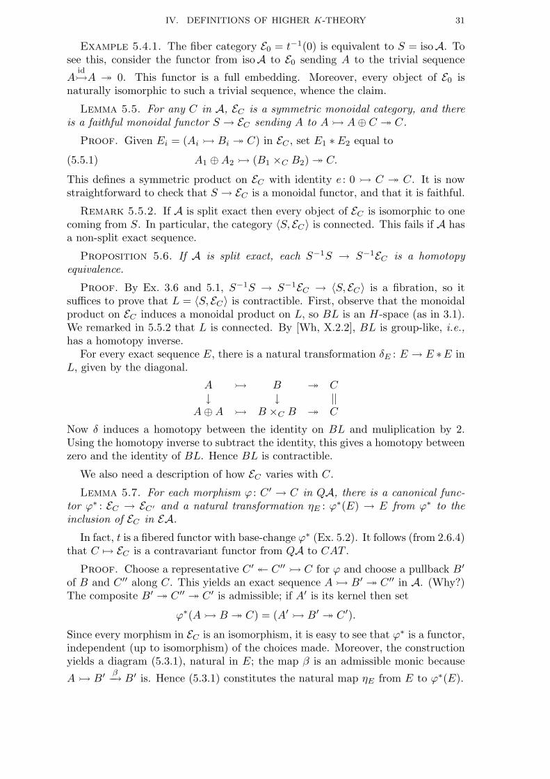
IV. DEFINITIONS OF HIGHER K-THEORY 31
Example 5.4.1. The fiber category E0 = t−1(0) is equivalent to S = isoA. Tosee this, consider the functor from isoA to E0 sending A to the trivial sequence
Aid½A ³ 0. This functor is a full embedding. Moreover, every object of E0 is
naturally isomorphic to such a trivial sequence, whence the claim.
Lemma 5.5. For any C in A, EC is a symmetric monoidal category, and thereis a faithful monoidal functor S → EC sending A to A ½ A⊕ C ³ C.
Proof. Given Ei = (Ai ½ Bi ³ C) in EC , set E1 ∗ E2 equal to
(5.5.1) A1 ⊕A2 ½ (B1 ×C B2) ³ C.
This defines a symmetric product on EC with identity e : 0 ½ C ³ C. It is nowstraightforward to check that S → EC is a monoidal functor, and that it is faithful.
Remark 5.5.2. If A is split exact then every object of EC is isomorphic to onecoming from S. In particular, the category 〈S, EC〉 is connected. This fails if A hasa non-split exact sequence.
Proposition 5.6. If A is split exact, each S−1S → S−1EC is a homotopyequivalence.
Proof. By Ex. 3.6 and 5.1, S−1S → S−1EC → 〈S, EC〉 is a fibration, so itsuffices to prove that L = 〈S, EC〉 is contractible. First, observe that the monoidalproduct on EC induces a monoidal product on L, so BL is an H-space (as in 3.1).We remarked in 5.5.2 that L is connected. By [Wh, X.2.2], BL is group-like, i.e.,has a homotopy inverse.
For every exact sequence E, there is a natural transformation δE : E → E ∗E inL, given by the diagonal.
A ½ B ³ C↓ ↓ ||
A⊕A ½ B ×C B ³ C
Now δ induces a homotopy between the identity on BL and muliplication by 2.Using the homotopy inverse to subtract the identity, this gives a homotopy betweenzero and the identity of BL. Hence BL is contractible.
We also need a description of how EC varies with C.
Lemma 5.7. For each morphism ϕ : C ′ → C in QA, there is a canonical func-tor ϕ∗ : EC → EC′ and a natural transformation ηE : ϕ∗(E) → E from ϕ∗ to theinclusion of EC in EA.
In fact, t is a fibered functor with base-change ϕ∗ (Ex. 5.2). It follows (from 2.6.4)that C 7→ EC is a contravariant functor from QA to CAT .
Proof. Choose a representative C ′ ´ C ′′ ½ C for ϕ and choose a pullback B′
of B and C ′′ along C. This yields an exact sequence A ½ B′ ³ C ′′ in A. (Why?)The composite B′ ³ C ′′ ³ C ′ is admissible; if A′ is its kernel then set
ϕ∗(A ½ B ³ C) = (A′ ½ B′ ³ C ′).
Since every morphism in EC is an isomorphism, it is easy to see that ϕ∗ is a functor,independent (up to isomorphism) of the choices made. Moreover, the constructionyields a diagram (5.3.1), natural in E; the map β is an admissible monic because
A ½ B′ β−→ B′ is. Hence (5.3.1) constitutes the natural map ηE from E to ϕ∗(E).

32 IV. DEFINITIONS OF HIGHER K-THEORY
Now the direct sum of sequences defines an operation ⊕ on EA, and S acts onEA via the inclusion of S in EA given by 5.4.1. That is, A′¤(A ½ B ³ C) is thesequence A′ ⊕ A ½ A′ ⊕ B ³ C. Since t(A′¤E) = t(E) we have an induced mapT = S−1t : S−1EA → QA. This is also a fibered functor (Ex. 5.2).
Theorem 5.8. If A is a split exact category and S = isoA, then the sequenceS−1S → S−1EA T−→ QA is a homotopy fibration.
Proof. We have to show that Quillen’s Theorem B applies, i.e., that the base-changes ϕ∗ of 5.7 are homotopy equivalences. It suffices to consider ϕ of the form0 ½ C and 0 ´ C. If ϕ is 0 ½ C, the composition of the equivalence S−1S →S−1EC of 5.6 with ϕ∗ is the identity by Ex. 5.5, so ϕ∗ is a homotopy equivalence.
Now suppose that ϕ is 0 ´ C. The composition of the equivalence S−1S →S−1EC of 5.6 with ϕ∗ sends A to A ⊕ C by Ex. 5.5. Since there is a naturaltransformation A → A ⊕ C in S−1S, this composition is a homotopy equivalence.Hence ϕ∗ is a homotopy equivalence.
Proof of theorem 5.1. This will follow from theorem 5.8, once we showthat S−1EA is contractible. By Ex. 5.3, EA is contractible. Any action of Son a contractible category must be invertible (3.5.1). By Ex. 3.5 and Ex. 5.1,EA → S−1EA is a homotopy equivalence, and therefore S−1EA is contractible.
EXERCISES
5.1 If A is an additive category, S = isoA is equivalent to the disjoint union ofone-object categories Aut(A), one for every isomorphism class in A. Show that thetranslations Aut(A) → Aut(A⊕B) are injections. Then conclude using theorem 3.6that B(S−1S) is the group completion of the H-space BS =
∐Aut(A).
5.2 Show that the target functor t : EA → QA is a fibered functor in the sense ofdefinition 2.6.2, with base-change ϕ∗ given by 5.7. Then show that the action ofS on EA is cartesian (Ex. 3.11), so that the induced functor S−1EA → QA is alsofibered, with fiber S−1S over 0.5.3 Let iQA denote the subcategory of QA whose objects are those of A but whosemorphisms are admissible monomorphisms. Show that the category EA of 5.3 isequivalent to the subdivision category Sub(iQA) of Ex. 2.9. Conclude that thecategory EA is contractible.5.4 Show that Quillen’s Theorem B can not apply to EA → QA unless A ∼= 0.Hint: Compare π0S to K0A.5.5 If ϕ is the map 0 ½ C, resp. 0 ´ C, show that ϕ∗ : EC → E0
∼= S sendsA ½ B ³ C to A, resp. to B.5.6 Describe E ′A = (EA)op, which by Ex. 2.6 and 5.2 is cofibered over (QA)op.Use E ′A to prove the + = Q Theorem 5.1. Hint: There is a new action of S. Usepushout instead of pullback in (5.5.1) to prove the analogue of proposition 5.6.5.7 Finite Sets. Let Setsf denote the category of pointed finite sets, as in 3.1.1(a).We say that a sequence A ½ B ³ C is exact just in case the first map is aninjection and the second map identifies C with B/A.(a) Copy the Q-construction 4.1 to form a category QSetsf .(b) Show that there is an extension category E ′Setsf , defined as in Ex. 5.6, whichis cofibered over (QSetsf )op with S = isoSetsf as the fiber over the basepoint.(c) Modify the proof of the + = Q theorem to prove that ΩBQSetsf ' S−1S.

IV. DEFINITIONS OF HIGHER K-THEORY 33
§6. Waldhausen’s wS. construction
Our last construction of K-theory applies to Waldhausen categories, i.e., “cate-gories with cofibrations and weak equivalences.” Unfortunately, this will occur onlyafter a lengthy list of definitions, and we ask the reader to be forgiving.
Recall from chapter II, section 9 that a category with cofibrations is a categoryC with a distinguished zero object ‘0’ and a subcategory co(C) of morphisms inC called “cofibrations” (indicated with feathered arrows ½). Every isomorphismin C is to be a cofibration, and so are the unique arrows 0 ½ A for every objectA in C. In addition, the pushout C ½ B ∪A C of any cofibration A ½ B is acofibration. (See Definition II.9.1 more precise statements.) These axioms implythat two constructions make sense: the coproduct B q C = B ∪0 C of any twoobjects, and every cofibration A ½ B fits into a cofibration sequence A ½ B ³B/A, where B/A is the cokernel of A ½ B. The following is a restatement ofDefinition II.9.1.1:
Definition 6.1. A Waldhausen category C is a category with cofibrations, to-gether with a family w(C) of morphisms in C called “weak equivalences” (indicatedwith decorated arrows ∼−→). Every isomorphism in C is to be a weak equivalence,and weak equivalences are to be closed under composition (so we may regard w(C)as a subcategory of C). In addition, a “Glueing axiom” (W3) must be satisfied,saying that the pushout of weak equivalences is a weak equivalence.
A functor F : A → C between two Waldhausen categories is called an exact func-tor if it preserves all the relevant structure: zero, cofibrations, weak equivalencesand the pushouts along a cofibration.
A Waldhausen subcategory A of a Waldhausen category C is a subcategory whichis also a Waldhausen category in such a way that: (i) the inclusion A ⊆ C is anexact functor, (ii) the cofibrations in A are the maps in A which are cofibrations inC and whose cokernel lies in A, and (iii) the weak equivalences in A are the weakequivalences of C which lie in A.
In order to describe Waldhausen’s wS. construction for K-theory, we need asequence of Waldhausen categories Sn(C). S0(C) is the zero category, and S1(C) isthe category C, but whose objects A are thought of as the cofibrations 0 ½ A. Thecategory S2(C) is the extension category E of II.9.3. For convenience, we repeat itsdefinition here.
Extension Categories 6.2. The objects of the extension category S2(C) arethe cofibration sequences A1 ½ A2 ³ A12 in C. A morphism E → E′ in S2(C) isa commutative diagram:
E : A1 ½ A2 ³ A12yy
yy
E′ : A′1 ½ A′2 ³ A′12
We make S2(C) in to a Waldhausen category as follows. A morphism E → E′ inS2(C) is a cofibration if A1 → A′1, A12 → A′12 and A′1 ∪A1 A2 → A′2 are cofibrationsin C. A morphism in S2(C) is a weak equivalence if its component maps Ai → A′i(i = 1, 2, 12) are weak equivalences in C.
The following technically convenient axiom is often imposed on C. It says thatweak equivalences are closed under extensions.

34 IV. DEFINITIONS OF HIGHER K-THEORY
Extension axiom 6.2.1. Suppose that f : E → E′ is a map between cofibrationsequences, as in 6.2. If the source and quotient maps of f (A → A′ and C → C ′)are weak equivalences, so is the total map of f (B → B′).
Definition 6.3. (S.C) If C is a Waldhausen category, let SnC be the categorywhose objects A. are sequences of n cofibrations in C:
A. : 0 = A0 ½ A1 ½ A2 ½ · · · ½ An
together with a choice of every subquotient Aij = Aj/Ai (0 < i < j ≤ n). Thesechoices are to be compatible in the sense that there is a commutative diagram:
(6.3.0)
An−1,n
↑↑· · ·
A23 ½ · · · ½ A2n↑↑ ↑↑A12 ½ A13 ½ · · · ½ A1n↑↑ ↑↑ ↑↑
A1 ½ A2 ½ A3 ½ · · · ½ An
The conventions A0j = Aj and Ajj = 0 will be convenient at times. A morphismA. → B. in SnC is a natural transformation of sequences.
If we forget the choices of the subquotients Aij we obtain the higher extensioncategory En(C) constructed in II.9.3.2. Since we can always make such choices, itfollows that the categories SnC and En(C) are equivalent. By Ex. II.9.4, En(C) is aWaldhausen category, so SnC is also a Waldhausen category. Here are the relevantdefinitions for Sn, translated from the definitions II.9.3.2 for E .
A weak equivalence in SnC is a map A. → B. such that each Ai → Bi (hence,each Aij → Bij) is a weak equivalence in C. A map A. → B. is a cofibration whenfor every 0 ≤ i < j < k ≤ n the map of cofibration sequences
Aij ½ Aik ³ Ajk
↓ ↓ ↓Bij ½ Bik ³ Bjk
is a cofibration in S2(C)(C).The reason for including choices in the definition of the categories Sn(C) is that
we can form a simplicial Waldhausen category.
Definition 6.3.1. For each n ≥ 0, the exact functor ∂0 : Sn(C) → Sn−1(C) isdefined deletion of the bottom row of (6.3.0). That is, i.e., ∂0 is defined by theformula
∂0(A.) : 0 = A11 ½ A12 ½ A13 ½ · · · ½ A1n
together with the choices ∂0(A.)ij = Ai+1,j+1. By Ex. 6.1, ∂0(A.) is in Sn−1(C).For 0 < i ≤ n we define the exact functors ∂i : Sn(C) → Sn−1(C) by omitting the
row Ai∗ and the column containing Ai in (6.3.0), and reindexing the Ajk as needed.Similarly, we define the exact functors si : Sn(C) → Sn+1(C) by duplicating Ai, andreindexing with the normalization Ai,i+1 = 0.

IV. DEFINITIONS OF HIGHER K-THEORY 35
By Ex. 6.2, the SnC fit together to form a simplicial Waldhausen category S.C,and the subcategories wSnC of weak equivalences fit together to form a simplicialcategory wS.C. Hence their geometric realizations B(wSnC) fit together to forma simplicial topological space BwS.C, and we write |wS.C| for the realization ofBwS.C. Since S0(C) is trivial, |wS.C| is a connected space.
Recall from chapter II, 9.1.2, that K0(C) is defined as the group generated bythe set of weak equivalence classes [A] of objects of C with the relations that [B] =[A] + [B/A] for every cofibration sequence
A ½ B ³ B/A.
Proposition 6.4. If C is a Waldhausen category then π1|wS.C| ∼= K0(C).Proof. If X. is any simplicial space with X0 a point, then |X.| is connected
and π1|X.| is the free group on π0(X1) modulo the relations d1(x) = d2(x)d0(x)for every x ∈ π0(X2). For X. = BwS.C, π0(BwS1C) is the set of weak equivalenceclasses of objects in C, π0(BwS2C) is the set of equivalence classes of cofibrationsequences, and the maps ∂i : S2(C) → S1(C) of 6.3.1 send A ½ B ³ B/A to B/A,B and A, respectively.
Definition 6.5. If C is a small Waldhausen category, its algebraic K-theoryspace K(C) = K(C, w) is the loop space
K(C) = Ω|wS.C|.The K-groups of C are defined to be its homotopy groups:
Ki(C) = πiK(C) = πi+1|wS.C| if i ≥ 0.
Remark 6.5.1. Since the subcategory wC is closed under coproducts in C byaxiom (W3), the coproduct gives an H-space structure to |wS.C| via the map
|wS.C| × |wS.C| ∼= |wS.C × wS.C| q−→ |wS.C|.Simplicial Model 6.5.2. Suppose that C is a small Waldhausen category in
which the isomorphisms iC are the weak equivalences. Let snC denote the set ofobjects of SnC; as n varies, we have a simplicial set s.C. Waldhausen proved in[W1126, 1.4] that the inclusion |s.C| → |iS.C| is a homotopy equivalence. ThereforeΩ|s.C| is a simplicial model for the space K(C).
Remark 6.5.3. In fact K(C) is an infinite loop space. To see this, note thatwe can apply the S. construction to each SnC, obtaining a bisimplicial Waldhausencategory S.S.C. Iterating this construction, we can form the multisimplicial Wald-hausen categories S.nC = S.S. · · ·S.C and the multisimplicial categories wS.nC ofweak equivalences. Waldhausen points out on p. 330 of [W1126] that |wS.nC| isthe loop space of |wS.n+1C|, and that the sequence of spaces
Ω|wS.C|, Ω|wS.S.C|, . . . , Ω|wS.nC|, . . .
forms a connective Ω-spectrum KC, called the K-theory spectrum of C. Manyauthors think of the K-theory of C in terms of this spectrum. This does not affectthe K-groups, because:
πi(KC) = πiK(C) = Ki(C), i ≥ 0.
An exact functor F induces a map F∗ : K(B) → K(C) of spaces, and spectra,and of their homotopy groups Ki(B) → Ki(C).

36 IV. DEFINITIONS OF HIGHER K-THEORY
Exact Categories 6.6. We saw in II.9.1.3 that any exact category A becomesa Waldhausen category in which the cofibration sequences are just the admissi-ble exact sequences, and the weak equivalences are just the isomorphisms. Wewrite i(A) for the family of isomorphisms, so that we can form the K-theory spaceK(A) = Ω|iS.A|. Waldhausen proved in [W1126, 1.9] that there is a homotopyequivalence between |iS.A| and BQA, so that this definition is consistent with thedefinition of K(A) in definition 4.3. His proof is given in exercises 6.5 and 6.6below.
Another important example of a Waldhausen category is Rf (X), introduced inII.9.1 and Ex. II.9.1. The so-called K-theory of spaces refers to the correspondingK-theory spaces A(X).
Example 6.7(A(∗)). Recall from II.9.1.4 that the category Rf = Rf (∗) of
finite based CW complexes is a Waldhausen category in which the family hRf ofweak equivalences is the family of weak homotopy equivalences. This category issaturated (II.9.7.1) and satisfies the extension axiom 6.2.1. Following Waldhausen[W1126], we write A(∗) for the space K(Rf ) = Ω|hS.Rf |. In particular, A0(∗) =K0Rf = Z by II.9.1.5.
Example 6.7.1(A(X)
). More generally, let X be a CW complex. The cate-
gory R(X) of CW complexes Y obtained from X by attaching cells, and having Xas a retract, is a Waldhausen category in which cofibrations are cellular inclusions(fixing X) and weak equivalences are homotopy equivalences (see Ex. II.9.1). Con-sider the Waldhausen subcategory Rf (X) of those Y obtained by attaching onlyfinitely many cells. Following Waldhausen [W1126], we write A(X) for the spaceK(Rf (X)) = Ω|hS.Rf (X)|. Thus A0(X) = K0Rf (X) is Z by Ex. II.9.1.
Similarly, we can form the Waldhausen subcategory Rfd(X) of those Y whichare finitely dominated. We write Afd(X) for K(Rfd(X)) = Ω|hS.Rfd(X)|. Notethat Afd
0 (X) = K0Rfd(X) is Z[π1(X)] by Ex. II.9.1.
Cylinder Functors
When working with Waldhausen categories, it is often technically convenient tohave mapping cylinders. Recall from Ex. 2.10 that the category C/C of arrows inC has the morphisms of C as its objects, and a map (a, b) : f → f ′ in Ar(C) is acommutative diagram in C:
(6.8.0)
Af−−−−→ B
a
yyb
A′f ′−−−−→ B′
The source s(f) = A and target t(f) = B of f define functors s, t : C/C → C.Definition 6.8 (Cylinders). Let C be a Waldhausen category. A (mapping)
cylinder functor on C is a functor T from the category C/C of arrows in C tothe category C, together with natural transformations j1 : s ⇒ T , j2 : t ⇒ T andp : T ⇒ t so that for every f : A → B the diagram
Aj1−→ T (f)
j2←− Bf ↓ p =
B
IV. DEFINITIONS OF HIGHER K-THEORY 37
commutes in C. The following conditions must also hold:(i) T (0 ½ A) = A, with p and j2 the identity map, for all A ∈ C.(ii) j1 q j2 : AqB ½ T (f) is a cofibration for all f : A → B.(iii) Given a map (a, b) : f → f ′ in Ar(C), i.e., a commutative square (6.8.0), if a
and b are weak equivalences in C then so is T (f) → T (f ′).(iv) Given a map (a, b) : f → f ′ in Ar(C), if a and b are cofibrations in C, then so
is T (f) → T (f ′), and the following map, induced by condition (ii), is also acofibration in C.
A′ qA T (f)qB B′ → T (f ′)
We often impose the following extra axiom on the weak equivalences of C.Cylinder Axiom 6.8.1. All maps p : T (f) → B are weak equivalences in C.Suppose C has a cylinder functor T . The cone of an object A is cone(A) = T (A ³
0), and the suspension of A is ΣA = cone(A)/A. The cylinder axiom implies thatcone(A) ∼−→ 0 is a weak equivalence. Since A ½ cone(A) ³ ΣA is a cofibrationsequence it follows from the description of K0(C) in II.9.1.2 that [ΣA] = −[A] inK0(C). (Cf. Lemma II.9.2.1.) In fact, the Additivity Theorem (see Chapter Vbelow) implies that the map Σ: K(C) → K(C) is a homotopy inverse with respectto the H-space structure on K(C), because Σ∗ + 1 = cone∗ = 0.
The name ‘cylinder functor’ comes from the following two paradigms.
Example 6.8.2. The Waldhausen categories Rf (∗) and Rf (X) of examples 6.7and 6.7.1 have a cylinder functor: T (f) is the usual (based) mapping cylinder of f .By construction, the mapping cylinder satisfies the cylinder axiom 6.8.1. Becauseof this paradigm, j1 and j2 are sometimes called the front and back inclusions.
Example 6.8.3. Let Ch be the Waldhausen category of chain complexes andquasi-isomorphisms constructed from an abelian (or exact) category C; see II.9.2.The mapping cylinder of f : A. → B. is the usual mapping cylinder chain complex,with
T (f)n = An ⊕An−1 ⊕Bn.
The suspension functor Σ(A.) = A.[−1] here is the shift operator: Σ(A.)n = An−1.
Example 6.8.4. Exact categories usually do not have cylinder functors. This isreflected by the fact that for some A ∈ A there may be no B such that [A⊕B] = 0in K0(A). However, the Waldhausen category Chb(A) of bounded chain complexesdoes have a cylinder functor, and we used it to prove that K0(A) ∼= K0Chb(A) inII.9.2.2. In fact, K(A) ' K(Chb(A) by the Gillet-Waldhausen theorem presentedin chapter V. Thus many results requiring mapping cylinders in Waldhausen K-theory can be translated into results for Quillen K-theory.
Cofinality
Let A be a Waldhausen subcategory of B. We say that A is strictly cofinal in B iffor every B in B there is an A in A so that A∧B is in A. The following result wasproven by Waldhausen in [W1126, 1.5.9]. We will prove a different cofinality resultin chapter VI.

38 IV. DEFINITIONS OF HIGHER K-THEORY
Strict Cofinality Theorem 6.9. If A is a strictly cofinal Walhausen sub-category of B, then K(A) → K(B) is a homotopy equivalence. In particular,Kn(A) ∼= Kn(B) for all n.
EXERCISES
6.1 Show that for every 0 ≤ i < j < k ≤ n the diagram
Aij ½ Aik ³ Ajk
is a cofibration sequence, and that this gives an exact functor from SnC to S2C.6.2 Show that each functor ∂i : SnC → Sn−1C is exact. Then show that S.C is asimplicial category.
6.3 Let F, F ′ : A → B be a pair of exact functors. A natural transformationη : F → F ′ is called a weak equivalence from F to F ′ if each F (A) ∼−→ F ′(A) is aweak equivalence in B. Show that a weak equivalence induces a homotopy betweenthe two maps K(A) → K(B). Hint: Show that the maps wSnA → wSnB arehomotopic in a compatible way.
6.4 If X. is any simplicial space with X0 a point, the formula for |X.| gives a mapfrom the reduced suspension ΣX1 to |X.|. Using the Freudenthal map X1 → ΩΣX1
this gives a map X1 → Ω|X.| and hence maps πi(X1) → πi+1|X.|. When X. =BwS.C, this yields a map from X1 = Bw(C) to K(C).(a) Show that every weak self-equivalence α : A
∼−→ A determines an element [α] ofK1(C). If β is another weak self-equivalence, show that [α][β] = [α ∧ β].(b) If A is an exact category, considered as a Waldhausen category, show that theresulting map B(isoA) → K(A) induces a map from the group K⊕
1 A of 3.6.1 toK1(A).
6.5 (Waldhausen) Let A be a small exact category. In this exercise we produce amap from |iS.A| ' |s.A| to BQA, where s.A is defined in 6.5.2.(a) Show that an object A. of iS3A determines a morphism in QA from A12 to A3.(b) Show that an object A. of iS5A determines a sequence A23 → A14 → A5 of rowmorphisms in QA.(c) Recall from Ex. 2.10 that the Segal subdivision Sub(s.A) is homotopy equiva-lent to s.A. Show that (a) and (b) determine a simplicial map Sub(s.A) → QA.Composing with |iS.A| ' Sub(s.A), this yields a map from |iS.A| to BQA.
6.6 We now show that the map |iS.A| → BQA constructed in the previous exerciseis a homotopy equivalence. Let iQnA denote the category whose objects are thedegree n elements of the nerve of QA, i.e., sequences A0 → · · · → An in QA, andwhose morphisms are isomorphisms.(a) Show that iQ.A is a simplicial category, and that the nerve of QA is the sim-plicial set of objects. Waldhausen proved in [W1126, 1.6.5] that BQA → |iQ.A| isa homotopy equivalence.(b) Show that for each n there is an equivalence of categories Sub(iSnA) ∼−→ iQnA,where Sub(iSnA) is the Segal subdivision category of Ex. 2.9. Then show that theequivalences form a map of simplicial categories Sub(iS.A) → iQ.A. This mapmust be a homotopy equivalence, because it is a homotopy equivalence in eachdegree.

IV. DEFINITIONS OF HIGHER K-THEORY 39
(c) Show that the map of the previous exercise fits into a diagram
|s.A| '←−−−− |Sub(s.A)| −−−−→ BQA'y '
y 'y
|iS.A| '←−−−− |Sub(iS.A)| '−−−−→ |iQ.A|.
Conclude that the map |iS.A| → BQA of Ex. 6.5 is a homotopy equivalence.6.7 Let Ch(C) be the Waldhausen category of chain complexes in an exact categoryC, as in 6.8.3. Show that Ch(C) and Chb(C) satisfy the Saturation axiom II.9.7.1,the Extension axiom 6.2.1, and the Cylinder Axiom 6.8.1.6.8 Finite Sets. Let Setsf be the Waldhausen category of finite pointed sets, wherethe cofibrations are the injections and the weak equivalences are the isomorphisms.Show that the argument of Ex. 6.5 and 6.6 may be used, together with theorem 3.7.2and Ex. 5.7, to prove that the Waldhausen K-theory space K(Setsf ) is Z×Σ+ 'Ω∞Σ∞. Thus Kn(Setsf ) ∼= πs
n for all n.

40 IV. DEFINITIONS OF HIGHER K-THEORY
§7. The Gillet-Grayson construction
Let A be an exact category. Following Grayson and Gillet [GG], we define asimplicial set G. = G.A as follows.
Definition 7.1. If A is a small exact category, G. is the simplicial set definedas follows. The set G0 of vertices consists of all pairs of objects (A,B) in A. Theset G1 of edges consists of all pairs of short exact sequences with the same cokernel:
(7.1.0) A0 ½ A1 ³ A01, B0 ½ B1 ³ A01.
The degeneracy maps G1 → G0 send (7.1.0) to (A1, B1) and (A0, B0), respectively.The set Gn consists of all pairs of triangular commutative diagrams in A of the
form
(7.1.1)
An−1,n
↑↑· · ·
A12 ½ · · · ½ A1n↑↑ ↑↑A01 ½ A02 ½ · · · ½ A0n↑↑ ↑↑ ↑↑
A0 ½ A1 ½ A2 ½ · · · ½ An
An−1,n
↑↑· · ·
A12 ½ · · · ½ A1n↑↑ ↑↑A01 ½ A02 ½ · · · ½ A0n↑↑ ↑↑ ↑↑
B0 ½ B1 ½ B2 ½ · · · ½ Bn
so that each sequence Ai ½ Aj ³ Aij and Bi ½ Bj ³ Aij is exact. As in thedefinition of S.A (6.3.1), the face maps ∂i : Gn → Gn−1 are obtained by deletingthe row Ai∗ and the columns containing Ai and Bi, while the degeneracy mapsσi : Gn → Gn+1 are obtained by duplicating Ai and Bi, and reindexing.
Omitting the choices Aij for the cokernels, we can abbreviate (7.1.1) as:
(7.1.2)A0 ½ A1 ½ A2 ½ · · · ½ An
B0 ½ B1 ½ B2 ½ · · · ½ Bn .
Remark 7.1.3. |G.| is a homotopy commutative and associative H-space. Itsproduct |G.| × |G.| → |G.| arises from the simplicial map G. × G. → G. whosecomponents Gn ×Gn → Gn are termwise ⊕.
Note that for each isomorphism A ∼= A′ in A there is an edge in G1 from (0, 0)to (A,A′), represented by (0 ½ A ³ A, 0 ½ A′ ³ A). Hence (A,A′) representszero in the group π0|G.|.
Lemma 7.2. There is a group isomorphism π0|G.| ∼= K0(A).
Proof. As in 2.3, π0|G.| is presented as the set of elements (A,B) of G0, modulothe equivalence relation that for each edge (7.1.0) we have
(A1, B1) = (A0, B0).
It is an abelian group by 7.1.3, with operation (A,B)⊕ (A′, B′) = (A⊕A′, B⊕B′).Since (A⊕B, B⊕A) represents zero in π0|G.|, it follows that (B, A) is the inverse of(A,B). From this presentation, we see that there is a map K0(A) → π0|G.| sending[A] to (A, 0), and a map π0|G.| → K0(A), sending (A,B) to [A]− [B]. These mapsare inverses to each other.

IV. DEFINITIONS OF HIGHER K-THEORY 41
(7.3) We now compare G. with the loop space of the simplicial set s.A of 6.5.2. Ifwe forget the bottom row of either of the two triangular diagrams in (7.1.1), we geta triangular commutative diagram of the form (6.3.0), i.e., an element of snA. Theresulting set maps Gn → snA fit together to form a simplicial map ∂0 : G. → s.A.
Path Spaces 7.3.1. Recall from [WHomo, 8.3.14] that the path space PX. of asimplicial set X. has PXn = Xn+1, its ith face operator is the ∂i+1 of X., and its ithdegeneracy operator is the σi+1 of X.. The forgotten face maps ∂0 : Xn+1 → Xn
form a simplicial map PX. → X., and π0(PX.) ∼= X0. In fact, σ0 induces acanonical simplicial homotopy equivalence from PX. to the constant simplicial setX0; see [WHomo, Ex. 8.3.7]. Thus PX. is contractible exactly when X0 is a point.
Now there are two maps Gn → sn+1A, obtained by forgetting one of the twotriangular diagrams (7.1.1) giving an element of Gn. The face and degeneracy mapsof G. are defined so that these yield two simplicial maps from G. to the path spaceP. = P (s.A). Clearly, either composition with the canonical map P. → s.A yieldsthe map ∂0 : G. → s.A. Thus we have a commutative diagram
(7.3.2)
G. −−−−→ P.y
yP. −−−−→ s.A.
Since s0A is a point, the path space |P.| is canonically contractible. Therefore thisdiagram yields a canonical map |G.| → Ω|s.A|. On the other hand, we saw in 6.6that |s.A| ' BQA, so Ω|s.A| ' ΩBQA = K(A).
We cite the following result from [GG, 3.1]. Its proof uses simplicial analoguesof Quillen’s theorems A and B.
Theorem 7.4. (Gillet-Grayson) Let A be a small exact category. Then the mapof (7.3) is a homotopy equivalence:
|G.| ' Ω|s.A| ' K(A).
Hence πi|G.| = Ki(A) for all i ≥ 0.
Example 7.5. A double s.e.s. in A is a pair ` of short exact sequences in A onthe same objects:
` : Af½ B
g³ C, A
f ′
½ Bg′
³ C.
Thus ` is an edge (in G1) from (A,A) to (B, B). To ` we attach the element [`] ofK1(A) = π1|G.| given by the following 3-edged loop.
(A,A) `−→ (B, B)eA eB
(0, 0)
where eA denotes the canonical double s.e.s. (0 ½ A ³ A, 0 ½ A ³ A).
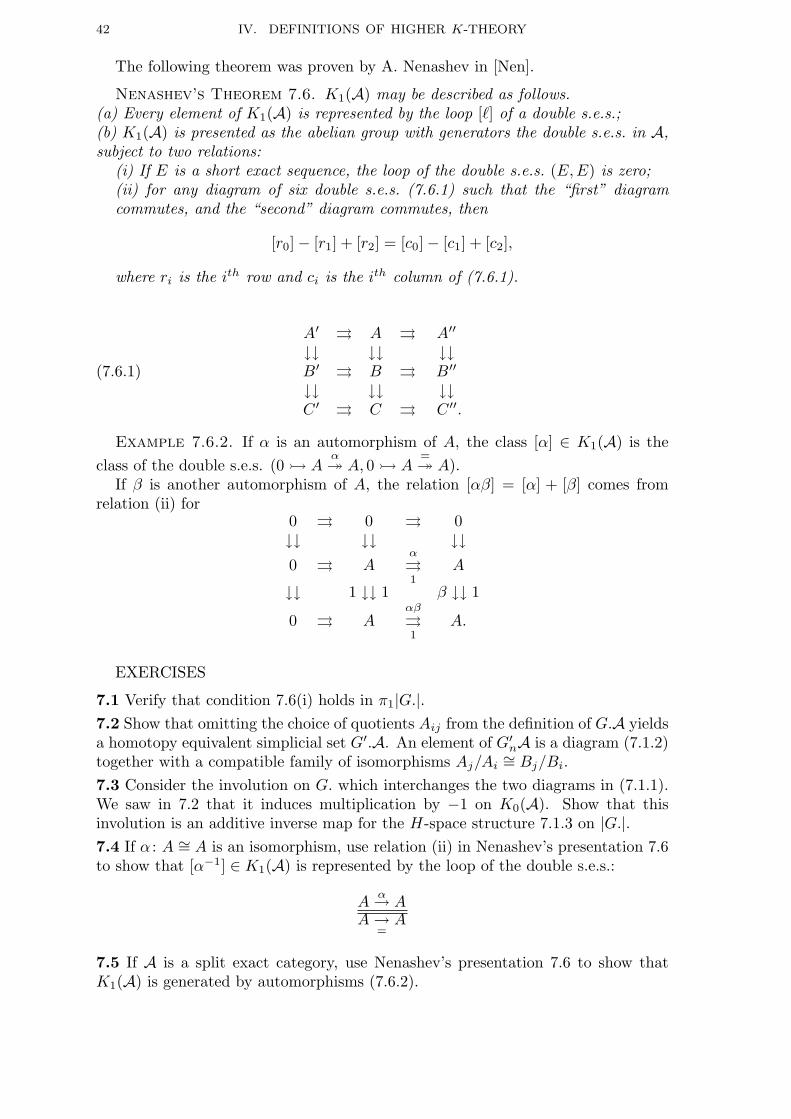
42 IV. DEFINITIONS OF HIGHER K-THEORY
The following theorem was proven by A. Nenashev in [Nen].
Nenashev’s Theorem 7.6. K1(A) may be described as follows.(a) Every element of K1(A) is represented by the loop [`] of a double s.e.s.;(b) K1(A) is presented as the abelian group with generators the double s.e.s. in A,subject to two relations:
(i) If E is a short exact sequence, the loop of the double s.e.s. (E, E) is zero;(ii) for any diagram of six double s.e.s. (7.6.1) such that the “first” diagramcommutes, and the “second” diagram commutes, then
[r0]− [r1] + [r2] = [c0]− [c1] + [c2],
where ri is the ith row and ci is the ith column of (7.6.1).
(7.6.1)
A′ ⇒ A ⇒ A′′
↓↓ ↓↓ ↓↓B′ ⇒ B ⇒ B′′
↓↓ ↓↓ ↓↓C ′ ⇒ C ⇒ C ′′.
Example 7.6.2. If α is an automorphism of A, the class [α] ∈ K1(A) is theclass of the double s.e.s. (0 ½ A
α³ A, 0 ½ A=³ A).
If β is another automorphism of A, the relation [αβ] = [α] + [β] comes fromrelation (ii) for
0 ⇒ 0 ⇒ 0↓↓ ↓↓ ↓↓0 ⇒ A
α⇒1
A
↓↓ 1 ↓↓ 1 β ↓↓ 1
0 ⇒ Aαβ
⇒1
A.
EXERCISES
7.1 Verify that condition 7.6(i) holds in π1|G.|.7.2 Show that omitting the choice of quotients Aij from the definition of G.A yieldsa homotopy equivalent simplicial set G′.A. An element of G′nA is a diagram (7.1.2)together with a compatible family of isomorphisms Aj/Ai
∼= Bj/Bi.7.3 Consider the involution on G. which interchanges the two diagrams in (7.1.1).We saw in 7.2 that it induces multiplication by −1 on K0(A). Show that thisinvolution is an additive inverse map for the H-space structure 7.1.3 on |G.|.7.4 If α : A ∼= A is an isomorphism, use relation (ii) in Nenashev’s presentation 7.6to show that [α−1] ∈ K1(A) is represented by the loop of the double s.e.s.:
Aα→ A
A →=
A
7.5 If A is a split exact category, use Nenashev’s presentation 7.6 to show thatK1(A) is generated by automorphisms (7.6.2).
IV. DEFINITIONS OF HIGHER K-THEORY 43
§8. Karoubi-Villamayor K-theory
Following Gersten, we say that a functor F from rings (or rings without unit)to sets is homotopy invariant if F (R) ∼= F (R[t]) for every R. Similarly, a functorF from rings to CW complexes (spaces) is called homotopy invariant if for everyring R the natural map R → R[t] induces a homotopy equivalence F (R) ' F (R[t]).Note that each homotopy group πnF (R) also forms a homotopy invariant functor.
Of course, this notion may be restricted to functors defined on any subcategoryof rings which is closed under polynomial extensions and contains the evaluationsas well as the inclusion R ⊂ R[t]. For example, we saw in II.6.5 and 7.8.3 thatG0(R) is a homotopy invariant functor defined on noetherian rings (and schemes)and maps of finite Tor-dimension.
Conversely, recall from III.3.1 that R is called F -regular if F (R) ∼= F (R[t1, ..., tn])for all n. Clearly, any functor F from rings to sets becomes homotopy invariantwhen restricted to the subcategory of F -regular rings. For example, we see fromII.7.7 that K0 becomes homotopy invariant when restricted to regular rings. TheFundamental Theorem in chapter V implies that the functors Kn are also homotopyinvariant when restricted to regular rings.
There is a canonical way to make F into a homotopy invariant functor.
Strict homotopization 8.1. Let F be a functor from rings to sets. Its stricthomotopization [F ] is defined as the coequalizer of the evaluations at t = 0, 1:F (R[t]) ⇒ F (R). In fact, [F ] is a homotopy invariant functor and there is auniversal transformation F (R) → [F ](R); see Ex. 8.1. Moreover, if F takes valuesin groups then so does [F ]; see Ex. 8.2.
Example 8.1.1. Recall that a matrix is called unipotent if it has the form 1+νfor some nilpotent matrix ν. Let Uni(R) denote the subgroup of GL(R) generatedby the unipotent matrices. This is a normal subgroup of GL(R), because theunipotent matrices are closed under conjugation. Since every elementary matrixeij(r) is unipotent, this contains the commutator subgroup E(R) of GL(R).
We claim that [E]R = [Uni]R = 1 for every R. Indeed, if 1 + ν is unipotent,(1 + tν) is a matrix in Uni(R[t]) with ∂0(1 + tν) = 1 and ∂1(1 + tν) = (1 + ν).Since Uni(R) is generated by these elements, [Uni]R must be trivial. The sameargument applies to the elementary group E(R).
We now consider GL(R) and its quotient K1(R). A priori, [GL]R → [K1]R is asurjection. In fact, it is an isomorphism.
Lemma 8.2. Both [GL]R and [K1]R are isomorphic to GL(R)/Uni(R).
Definition 8.2.1. For each ring R, we define KV1(R) to be GL(R)/Uni(R).Thus KV1(R) is the strict homotopization of K1(R) = GL(R)/E(R).
Proof. The composite Uni(R) → GL(R) → [GL]R is trivial, because it factorsthrough [Uni]R = 1. Hence [GL]R (and [K1]R) are quotients of GL(R)/Uni(R).By Higman’s trick III.3.4.1, if g ∈ GL(R[t]) is in the kernel of ∂0 then g ∈ Uni(R[t])and hence ∂1(g) ∈ Uni(R). Hence ∂1(NGL(R)) = Uni(R). Hence GL(R)/Uni(R)is a strictly homotopy invariant functor; universality implies that the induced maps[GL]R → [K1]R → GL(R)/Uni(R) must be isomorphisms.
To define the higher Karoubi-Villamayor groups, we introduce the simplicial ringR[∆.], and use it to define the notion of homotopization. The simplicial ring R[∆.]

44 IV. DEFINITIONS OF HIGHER K-THEORY
will also play a critical role in the last chapter, when we construct higher Chowgroups and Motivic cohomology.
Definition 8.3. For each ring R the coordinate rings of the standard simplicesform a simplicial ring R[∆.]. It may described by the diagram
R ⇔ R[t1]←←←
R[t1, t2] ⇔⇔ · · ·R[t1, . . . , tn] · · ·
with R[∆n] = R[t0, t1, · · · , tn]/ (∑
ti = 1) ∼= R[t1, · · · , tn]. The face maps are givenby: ∂i(ti) = 0; ∂i(tj) is tj for i < j and tj−1 for i > j. Degeneracies are given by:σi(ti) = ti + ti+1; σi(tj) is tj for i < j and tj+1 for i > j.
Definition 8.4 (Homotopization). Let F be a functor from rings to CWcomplexes. Its homotopization Fh(R) is the geometric realization of the simplicialspace F (R[∆.]). Thus Fh is also a functor from rings to CW complexes, and thereis a canonical map F (R) → Fh(R).
Lemma 8.4.1. Fh is a homotopy invariant functor. Moreover, if F is homotopyinvariant then F (R) ' Fh(R) for all R.
Proof. We claim that the inclusion R[∆.] ⊂ R[x][∆.] is a simplicial homo-topy equivalence, split by evaluation at x = 0. For this, we define ring mapshi : R[x][∆n] → R[x][∆n+1] by: hi(f) = σi(f) if f ∈ R[∆n] and hi(x) = x(ti+1 +· · · + tn). These maps define a simplicial homotopy between the identity map ofR[x][∆.] and the composite
R[x][∆.] x=0−−→ R[∆.] ⊂ R[x][∆.].
Applying F gives a simplicial homotopy equivalence between Fh(R[∆.]) andFh(R[x][∆.]). Geometric realization converts this into a topological homotopyequivalence between Fh(R) and Fh(R[x]).
Finally, if F is homotopy invariant then the map from the constant simplicialspace F (R) to F (R[∆.]) is a homotopy equivalence in each degree. It follows (see[Wa78]) that their realizations F (R) and Fh(R) are homotopy equivalent.
It is easy to see that F → Fh is universal (up to homotopy equivalence) forfunctors from F to homotopy invariant functors. A proof of this fact is left toEx. 8.3.
Lemma 8.5. Let F be a functor from rings to CW complexes. Then π0(Fh) isthe strict homotopization [F0] of the functor F0(R) = π0F (R).
Proof. For any simplicial space X., the group π0(|X.|) is the coequalizer of∂0, ∂1 : π0(X1) ⇒ π0(X0). In this case π0(X0) = π0F (R) and π0(X1) = π0F (R[t]).
Applying the functor GL gives us a simplicial group GL. = GL(R[∆.]).
Corollary 8.5.1. KV1(R) ∼= π0(GL.).
Definition 8.6. For n ≥ 1, we set KVn(R) = πn−1(GL.) = πn(BGL.).

IV. DEFINITIONS OF HIGHER K-THEORY 45
Corollary 8.6.1. The abelian groups KVn(R) are homotopy invariant, i.e.,
KVn(R) ∼= KVn(R[t]) for every n ≥ 1.
Gersten observed that BGL. ' BGL(R[∆.])+. In this case, the standard spec-tral sequence for a simplicial space E1
pq = πp(Xq) ⇒ πp+q|X.| becomes the firstquadrant spectral sequence (for p ≥ 1, q ≥ 0):
(8.6.2) E1pq = Kp(R[∆q]) ⇒ KVp+q(R).
If R is regular, then each simplicial group Kp(R[∆.]) is constant (by the Funda-mental Theorem in chapter V). Thus the spectral sequence degenerates at E2:
Theorem 8.7. (Gersten) If R is regular, then Kp(R) ∼= KVp(R) for all p ≥ 1.For general R, there is a natural edge map Kp(R) → KVp(R).
We now quickly develop the key points in KV -theory.
Definition 8.8. We say that a ring map f : A → B is a GL-fibration if
GL(A[t1, ..., tn])×GL(B) → GL(B[t1, ..., tn])
is onto for every n. Note that we do not require A and B to have a unit.
Remark 8.8.1. Any GL-fibration must be onto. That is, B ∼= A/I for someideal I of A. To see this, consider the (1, 2) entry α12 of a preimage of the elementarymatrix e12(bt). Since f(α12) = bt, evaluation at t = 1 gives an element of A mappingto b ∈ B. However, not every surjection is a GL-fibration; see Ex. 8.5(b).
Proposition 8.9. If A → B is a GL-fibration with kernel I, there is a longexact sequence
KVn+1(B) −→ KVn(I) → KVn(A) → KVn(B) −→ · · ·KV1(I) → KV1(A) → KV1(B) → K0(I) → K0(A) → K0(B).
Proof. Let Gn ⊂ GL(B[∆n]) denote the image of GL(A[∆n]). Then there isan exact sequence of simplicial groups
(8.9.1) 1 → GL(I[∆.]) → GL(A[∆.]) → G. → 1.
Now any short exact sequence of simplicial groups is a fibration sequence, meaningthere is a long exact sequence of homotopy groups. Since the quotient GL(B[∆.])/G.is a constant simplicial group, it is now a simple matter to splice the long exactsequences together to get the result. We have indicated the details in Ex. 8.3.
Here is an application of this result. Since R[x] → R has a section, it is a GL-fibration. By homotopy invariance, it follows that KVn(xR[x]) = 0 for all n ≥ 1.(Another proof is given in Ex. 8.4.)
Definition 8.10. For any ring R (with or without unit), we define ΩR to bethe ideal (x2 − x)R[x] of R[x].
Since ΩR is the kernel of x = 1: xR[x] → R, and this map is a GL-fibration byEx. 8.7, we have the following corollary of 8.9.
Corollary 8.10.1. For all R, KV1(R) is isomorphic to the kernel of the mapK0(ΩR) → K0(xR[x]), and KVn(R) ∼= KVn−1(ΩR) for all n ≥ 2.
This shows that we can define KVn(R) as KV1(Ωn−1R) for all n ≥ 2.

46 IV. DEFINITIONS OF HIGHER K-THEORY
The following definition is due to Karoubi and Villamayor.
Definition 8.11. A positive homotopy K-theory consists of a sequence of func-tors Kh
n , n ≥ 1, on the category of rings without unit, together with naturalconnecting maps δn : Kh
n+1(R/I) → Khn(I) and δ0 : Kh
1 (R/I) → K0(I), defined forevery GL-fibration R → R/I, satisfying the following axioms:
(1) The functors Khn are homotopy invariant;
(2) For every GL-fibration R → R/I the resulting sequence is exact:
Khn+1(R/I) δ−→ Kh
n(I) → Khn(R) → Kh
n(R/I) δ−→ Khn−1(I) →
Kh1 (R) → Kh
1 (R/I) δ−→ K0(I) → K0(R) → K0(R/I).
Theorem 8.11.1. There is a unique positive homotopy K-theory (up to isomor-phism), namely Kh
n = KVn.
Proof. The fact that KVn form a positive homotopy K-theory is given by 8.6.1and 8.9. The axioms imply that any other positive homotopy K-theory must satisfythe conclusion of 8.10.1, and so must be isomorphic to KV -theory.
EXERCISES
8.1 Let F be a functor from rings to sets. Show that [F ] is a homotopy invari-ant functor, and that every natural transformation F (R) → G(R) to a homotopyinvariant functor G factors uniquely through F (R) → [F ](R).8.2 If F is a functor from rings to groups, let NF (R) denote the kernel of themap t = 0: F (R[t]) → F (R). Show that the image F0(R) of the induced map t =1: NF (R) → F (R) is a normal subgroup of F (R), and that [F ]R = F (R)/F0(R).Thus [F ]R is a group.8.3 Let F and G be functors from rings to CW complexes, and assume that Gis homotopy invariant. Show that any natural transformation F (R) → G(R) fac-tors through maps Fh(R) → G(R) such that for each ring map R → S the mapFh(R) → Fh(S) → G(S) is homotopy equivalent to Fh(R) → Fh(S) → G(S).8.4 Let R = R0⊕R1⊕· · · be a graded ring. Show that for every homotopy invariantfunctor F on rings we have F (R0) ' F (R). In particular, if F is defined on ringswithout unit then F (xA[x]) ' F (0) for every A. Hint: Copy the proof of III.3.3.2.8.5 GL-fibrations. Let f : A → B be a GL-fibration with kernel I.(a) Show that tA[t] → tB[t] and ΩA → ΩB are GL-fibrations.(b) Show that Z→ Z/4 is not a GL-fibration, but GL(Z) → GL(Z/4) is onto.(c) If B is a regular ring (with unit), show that every surjection A → B is aGL-fibration. Hint: K1(B) ∼= K1(B[t]).8.6 Let f : A → B is a GL-fibration with kernel I, and define G. as in the proof ofProposition 8.9. Show that GL(B[∆.])/G. is a constant simplicial group. Use thisto show that πi(G.) = KVi+1(B) for all i > 0, but that the cokernel of π0(G.) →π0GL(B[∆.]) is the image of K1(B) in K0(I) under the map of III.2.3. Thencombine this with the long exact sequence of homotopy groups for (8.9.1) to finishthe proof of 8.9.8.7 Show that the map tA[t] → A, f(t) 7→ f(1), is a GL-fibration with kernel ΩA.

IV. DEFINITIONS OF HIGHER K-THEORY 47
§9. Mod ` K-theory
In addition to the usual K-groups Ki(C) of a category C, it is often useful tostudy its “mod ` K-groups” Ki(C;Z/`), where ` is a positive integer. In thissection we quickly recount the basic construction from mod ` homotopy theory.Basic properties of mod ` homotopy theory may be found in [N ].
Recall [N] that if m ≥ 2 the mod ` Moore space Pm(Z/`) is the space formedfrom the sphere Sm−1 by attaching an m-cell via a degree ` map. The suspensionof Pm(Z/`) is the Moore space Pm+1(Z/`), and as m varies this yields a suspensionspectrum, called the Moore spectrum P∞(Z/`).
Definition 9.1. If m ≥ 2, the mod ` homotopy “group” πm(X;Z/`) of a basedtopological space X is defined to be the pointed set [Pm(Z/`), X] of based homotopyclasses of maps from the Moore space Pm(Z/`) to X.
For a general space X, π2(X;Z/`) isn’t even a group, but the πm(X;Z/`) arealways groups for m ≥ 3 and abelian groups for m ≥ 4. However, if X = ΩYthen π2(X;Z/`) is a group and we can define π1(X;Z/`) as π2(Y ;Z/`); this isindependent of the choice of U by Ex. 9.1. More generally, if X = ΩkYk for k >> 0and Pm = Pm(Z/`) then the formula
πm(X;Z/`) = [Pm, X] = [Pm,ΩkYk] ∼= [Pm+k, Yk] = πm+k(Yk;Z/`)
shows that we can ignore these restrictions on m, and that πm(X;Z/`) is an abeliangroup for all m ≥ 0 (or even negative m, as long as k > 2 + |m|).
In particular, if X is an infinite loop space then abelian groups πm(X;Z/`) aredefined for all m ∈ Z, using the explicit sequence of deloopings of X provided bythe given structure on X.
If m ≥ 2, the cofibration sequence Sm−1 `−→ Sm−1 −→ Pm(Z/`) defining Pm(Z/`)induces an exact sequence of homotopy groups
πm(X) `−→ πm(X) → πm(X;Z/`) ∂−→ πm−1(X) `−→ πm−1(X).
It is convenient to adopt the notation that if A is an abelian group then `A denotesthe subgroup of all elements a of A such that ` · a = 0. This allows us to restatethe above exact sequence in a concise fashion.
Universal Coefficient Sequence 9.2. For all m ≥ 3 there is a naturalshort exact sequence
0 → (πmX)⊗ Z/` → πm(X;Z/`) ∂−→ `(πm−1X) → 0.
This sequence is split exact (but not naturally) when ` 6≡ 2 mod 4.
For π2, the sequence 9.2 of pointed sets is also exact in a suitable sense; see [N,p. 3]. However this point is irrelevant for loop spaces, so we ignore it.
Example 9.2.2. When ` = 2, the sequence need not split. For example, it isknown that πm+2(Sm;Z/2) = Z/4 for m ≥ 3, and that π2(BO;Z/2) = Z/4; see[AT65].

48 IV. DEFINITIONS OF HIGHER K-THEORY
Now suppose that C is either a symmetric monoidal category, or an exact cate-gory, or a Waldhausen category, so that the K-theory space K(C) is defined, andis an infinite loop space.
Definition 9.3. The mod ` K-groups of C are defined to be the abelian group:
Km(C;Z/`) = πm(K(C);Z/`), m ∈ Z.
If m ≥ 2 this definition states that Km(C;Z/`) = [Pm(Z/`),K(C)]. BecauseK(C) ' Y , we can define K1(C;Z/`) in a way that is independent of the choice ofY . However, the groups K0(C;Z/`) and Km(C;Z/`) for m < 0 depend not onlyupon K(C), but also upon the choice of the deloopings of K(C) in the underlyingK-theory spectrum KC. In fact, the literature is not consistent about Km(C;Z/`)when m < 2, even for K1(R; Z/`).
By Theorem 9.2, the mod ` K-groups are related to the usual K-groups.
Universal Coefficient Theorem 9.4. There is a short exact sequence
0 → Km(C)⊗ Z/` → Km(C;Z/`) → `Km−1(C) → 0
for every m ∈ Z, C, and `. It is split exact (not naturally) unless ` ≡ 2 mod 4.
In particular, for C = P(R) we have an exact sequence
0 → Km(R)⊗ Z/` → Km(R;Z/`) → `Km−1(R) → 0
Ex. 9.2 shows that the splitting in 9.4 is not natural in R.
Example 9.4.1. (` = 2) Since the isomorphism Ω∞Σ∞ → Z × BO factorsthrough K(Z) and K(R), the universal coefficient theorem and 9.2.2 show that
K2(Z;Z/2) ∼= K2(R;Z/2) ∼= π2(BO;Z/2) = Z/4.
It turns out that for ` = 2 the sequence for Km(R;Z/2) is split whenever multipli-cation by [−1] ∈ K1(Z) is the zero map from Km−1(R) to Km(R). For example,this is the case for the finite fields Fq, an observation made in [Br].
Example 9.4.2 (Bott elements). Suppose that R contains a primitive `th
root of unity ζ. The Universal Coefficient Theorem 9.4 provides an element β ∈K2(R;Z/`), mapping to ζ ∈ `K1(R). This element is called the Bott element, andit plays an important role in the product structure of the ring K∗(R;Z/`).
Remark 9.4.3. A priori, β depends not only upon ζ but also upon the choiceof the splitting in 9.4. One way to choose β is to observe that the inclusion of µ` inGL1(R) induces a map Bµ` → BGL(R) → BGL(R)+ and therefore a set functionµ` → K2(R;Z/`). A posteriori, it turns out that this is a group homomorphismunless ` ≡ 2 (mod 4).
Example 9.5. Let k be the algebraic closure of the field Fp. Quillen’s computionof K∗(Fq) in 1.9.1 shows that Kn(k) = 0 for m even (m ≥ 2), and that Km(k) =Q/Z[ 1p ] for m odd (m ≥ 1). It follows that if ` is prime to p then:
Km(k;Z/`) = Z/` if m is even, m ≥ 0
0 otherwise.

IV. DEFINITIONS OF HIGHER K-THEORY 49
In fact, K∗(k;Z/`) is the polynomial ring Z/`[β] on the Bott element β ∈K2(k;Z/`),under the K-theory product we will discuss in the next chapter. See [Br] for moredetails.
Here is another way to define mod ` homotopy groups, and hence K∗(C;Z/`).Suppose that X is a loop space, and let F denote the homotopy fiber of the mapX → X which is multiplication by `.
Proposition 9.6. There are isomorphisms πm(X;Z/`) ∼= πm−1(F ) for all m ≥2.
Proof. (Neisendorfer) Let map(A,X) be the space of pointed maps. If S = Sk
is the k-sphere then the homotopy groups of map(Sk, X) are the homotopy groupsof X (reindexed by k), while if P = P k(Z/`) is a mod ` Moore space, the homotopygroups of map(P, X) are the mod ` homotopy groups of X (reindexed by k).
Now applying map(−, X) to a cofibration sequence yields a fibration sequence,and applying map(A,−) to a fibration sequence yields a fibration sequence; this maybe formally deduced from the axioms (SM0) and (SM7) for any model structure,which hold for spaces. Applying map(−, X) to Sk → Sk → P k+1(Z/`) showsthat map(P, X) is the homotopy fiber of map(Sk, X) → map(Sk, X). Applyingmap(Sk,−) to F → X → X shows that map(Sk, F ) is also the homotopy fiber,and is therefore homotopy equivalent to map(P, X). Taking the homotopy groupsyields the result.
EXERCISES
9.1 Suppose that X is a loop space. Show that π1(X;Z/`) is independent of thechoice of Y such that X ' ΩY . This shows that K1(R;Z/`) and even K1(C;Z/`)9.2 Let R be a Dedekind domain with fraction field F . Show that the kernel of themap K1(R;Z/`) → K1(F ;Z/`) is SK1(R)/`. Hence it induces a natural map
` Pic(R)ρ−→ F×/F×`R×.
Note that F×/R× is a free abelian group by I.3.6, so the target is a free Z/`-modulefor every integer `. Finally, use I.3.6 and I.3.8.1 to give an elementary descriptionof ρ.
In particular, If R is the ring of integers in a number field F , the Bass-Milnor-Serre Theorem III.2.5 shows that the extension K1(R;Z/`) of ` Pic(R) by R× injectsinto F×/F×`.

INTRODUCTION AND REFERENCES
Algebraic K-theory has two components: the classical theory which centersaround the Grothendieck group K0 of a category and uses explicit algebraic presen-tations, and higher algebraic K-theory which requires topological or homologicalmachinery to define.
There are three basic versions of the Grothendieck group K0. One involves thegroup completion construction, and is used for projective modules over rings, vectorbundles over compact spaces and other symmetric monoidal categories. Anotheradds relations for exact sequences, and is used for abelian categories as well as exactcategories; this is the version first used in algebraic geometry. A third adds relationsfor weak equivalences, and is used for categories of chain complexes and othercategories with cofibrations and weak equivalences (“Waldhausen categories”).
Similarly, there are four basic constructions for higher algebraic K-theory: the+–construction (for rings), the group completion constructions (for symmetricmonoidal categories), Quillen’s Q-construction (for exact categories), and Wald-hausen’s wS. construction (for categories with cofibrations and weak equivalences).All these constructions give the same K-theory of a ring, but are useful in variousdistinct settings. These settings fit together like this:
number theory andother classical topics
←→ algebraic geometry
↑↓ ↑↓
Homological and+-constructionsK-theory of rings ←−−−−
Q-construction: K-theory ofvector bundles on schemes,exact categories, modulesand abelian categories
↑ ↑
Group Completionsrelations to L-theory,topological K-theory,stable homotopy theory
←−−−−Waldhausen Construction:K-theory of spaces,K-theory of chain complexestopological rings
l l
algebraic topology ↔ geometric topology
Typeset by AMS-TEX
1
2 INTRODUCTION AND REFERENCES
All the constructions have one feature in common: Some category C is concoctedfrom the given setup, and one defines a K-theory space associated to the geometricrealization BC of this category. The K-theory groups are then the homotopygroups of the K-theory space. In the first chapter, we introduce the basic cast ofcharacters: projective modules and vector bundles (over a topological space, andover a scheme). Large segments of this chapter will be familiar to many readers,but which segments are familiar will depend upon the background and interestsof the reader. The unfamiliar parts of this material may be skipped at first, andreferred back to when relevant. We would like to warn the complacent reader thatthe material on the Picard group and Chern classes for topological vector bundlesis in this first chapter.
In the second chapter, we define K0 for all the settings in the above figure,and give the basic definitions appropriate to these settings: group completions forsymmetric monoidal categories, K0 for rings and topological spaces, λ-operations,abelian and exact categories, Waldhausen categories. All definitions and manipula-tions are in terms of generators and relations. Our philosophy is that this algebraicbeginning is the most gentle way to become acquainted with the basic ideas ofhigher K-theory. The material on K-theory of schemes is isolated in a separatesection, so it may be skipped by those not interested in algebraic geometry.
In the third chapter we give a brief overview of the classical K-theory for K1
and K2 of a ring. Via the Fundamental Theorem, this leads to Bass’ “negativeK-theory,” meaning groups K−1, K−2, etc. We cite Matsumoto’s presentation forK2 of a field from [Milnor], and “Hilbert’s Theorem 90 for K2” (from chapter VI)in order to get to the main structure results. This chapter ends with a section onMilnor K-theory, including the transfer map, Izhboldin’s theorem on the lack ofp-torsion, the Galois symbol and the relation to the Witt ring of a field.
In the fourth chapter we shall describe the four constructions for higher K-theory.In the case of P(R), we show that all the constructions give the same K-groups, thegroups Kn(R). Very few theorems are present here, in order to keep this chaptershort. We do not want to get involved in the technicalities lying just under thesurface of each construction, so the key topological results we need are cited fromthe literature when needed.
The fundamental structural theorems for higher K-theory are presented in chap-ter 5?
In chapter 6 we apply the homological methods due to Suslin to describe thestructure of the K-theory of fields. We also present the Merkurjev-Suslin materialhere.
In chapter 7 we intend to give several applications to Algebraic Geometry.In chapter 8 we discuss Higher Chow Groups and Motivic Cohomology. This
material is quite new, and I don’t know how much I will say here.

INTRODUCTION AND REFERENCES 3
References
General References
[Atiyah] M. Atiyah, K-theory, Benjamin, New York, 1967.[Bass] H. Bass, Algebraic K-theory, Benjamin, 1968.[BHS] H. Bass, A. Heller and R. Swan, The Whitehead group of a polynomial extension, Publ.
Math. IHES 22 (1964), 61–79.[BMS] H. Bass, J. Milnor and J.-P. Serre, Solution of the congruence subgroup problem for
SLn (n ≥ 3) and Sp2n (n ≥ 2), Publ. Math. IHES 33 (1967), 59–137.[EGA] A. Grothendieck and J. Dieudonne, Elements de Geometrie Algebrique, Publ. Math.
IHES; I 4 (1960); II 8 (1961); III 11 (1961); 17 (1963); IV 20; (1964); 24 (1965); 28(1966); 32 (1967); I (revised) (1971), Springer-Verlag.
[Huse] D. Husemoller, Fibre Bundles, (Second Edition), Springer-Verlag, 1974.[Mac] S. MacLane, Categories for the Working Mathematician, Springer-Verlag, 1971.[May] J.P. May, Simplicial Objects in Algebraic Topology, Van Nostrand, 1967.
[Milne] J. Milne, Etale Cohomology, Princeton Univ. Press, 1980.[Milnor] J. Milnor, Introduction to Algebraic K-theory, Annals of Math. Study 72, Princeton
Univ. Press, 1971.[M-SBF] J. Milnor and D. Husemoller, Symmetric Bilinear Forms, Springer-Verlag, 1973.[Suz] M. Suzuki, Group Theory I, Springer-Verlag, 1982.[WHomo] C. Weibel, An introduction to homological algebra, Cambridge Univ. Press, 1994.[Wh] G.W. Whitehead, Elements of Homotopy Theory, Springer-Verlag, 1978.
References for chapter I (Projective modules and vector bundles)
[Art] V. Artamonov, Projective Modules over Group Rings of Nilpotent Groups, Algebra,Moskov. Gos. Univ. (1982), 7–23 (Russian); English transl. in AMS Translations,vol. 154, 1992, pp. 11–24.
[Atiy56] M. Atiyah, On the Krull–Schmidt theorem with application to sheaves, Bull. Soc. Math.France 84 (1956), 307–317.
[Atiy57] M. Atiyah, Vector bundles over an elliptic curve, Proc. London Math. Soc. 7 (1957),414–452.
[B-AC] N. Bourbaki, Algebre commutative, Chap.1-Chap.9, Hermann, Paris, 1961-83.[BM] H. Bass and M.P. Murthy, Grothendieck groups and Picard groups of abelian group
rings, Annals Math 86 (1967), 16–73.[BSh] Z. Borevich and I. Shafarevich, Number Theory, Benjamin, New York, 1967.[CC] J. Milnor and J. Stasheff, Characteristic classes, Annals of Math. Study, vol. 76, Prince-
ton Univ. Press, 1974.[Cohn65] P.M.Cohn, Universal Algebra, Harper&Row, 1965.[Cohn66] P.M. Cohn, Some remarks on the invariant basis property, Topology 5 (1966), 215–228.[GA] P. Griffiths and J. Adams, Topics in Algebraic and Analytic Geometry, Princeton U.
Press, 1974.[GAGA] J.-P. Serre, Geometrie algebrique et geometrie analytique, Ann. Inst. Fourier 6 (1956),
1–42.[Gdearl] K. Goodearl, Von Neumann regular rings, Pitman, 1979.[Gdrl1] K. Goodearl, Torsion in K0 of unit-regular rings, Proc. Edinburgh Math. Soc. 38
(1995), 331-341.[GR] H. Grauert and R. Remmert, Theory of Stein Spaces, Springer-Verlag, 1977.[Groth57] A. Grothendieck, Sur la classification des fibres holomorphes sur la sphere de Riemann,
Amer. J. Math. 79 (1957), 121–138.[Hart] R. Hartshorne, Algebraic Geometry, Springer-Verlag, 1977.[Kap58] I. Kaplansky, Projective modules, Annals of Math. 68 (1958), 372–377.[Lam] T.Y. Lam, Serre’s Conjecture, Lecture Notes in Math., vol. 635, Springer-Verlag, 1978.[Landsbg] S. Landsburg, Patching theorems for projective modules, J. Pure Appl. Alg. 21 (1981),
261–277.[Matsu] H. Matsumoto, Commutative ring theory, Cambridge Univ. Press, 1986.[Swan80] R. Swan, On Seminormality, J. Algebra 67 (1980), 210–229.

4 INTRODUCTION AND REFERENCES
[Weib91] C. Weibel, Pic is a contracted functor, Invent. Math. 103 (1991), 351–377.
References for chapter II (The Grothendieck Group K0)
[AT] M. Atiyah and D. Tall, Group Representations, λ-rings and the J-homomorphism,Topology 8 (1969), 253–297.
[Bass76] H. Bass, Euler characteristics and characters of discrete groups, Inv. Math. 35 (1976),155–196.
[FL] W. Fulton and S. Lang, Riemann-Roch Algebra, Springer-Verlag, 1985.
[Fuchs] L. Fuchs, Infinite Abelian Groups II, Academic Press, 1973.
[Fulton] W. Fulton, Intersection Theory, Ergebnisse Math., vol. 2, Springer-Verlag, 1984.
[Kar63] M. Karoubi, Expose 16, Seminaire H. Cartan, 1963/64.
[Ke90] B. Keller, Chain complexes and stable categories, Manuscripta Math. 67 (1990), 379–417.
[MM82] P. Menal and J. Moncasi, On regular rings with stable range 2, J. Pure Applied Algebra22 (1982), 25–40.
[Mum] D. Mumford, Lectures on curves on an algebraic surface, Annals Studies in Math.,vol. 59, Princeton University Press, Princeton, 1966.
[RR] A. Borel and J.-P. Serre, Le Theoreme de Riemann-Roch (d’apres Grothendieck), Bull.Soc. Math. de France 86 (1958), 97–136.
References for chapter III (K1, K2 and Milnor K-theory)
[BA] N. Jacobson, Basic Algebra II, Freeman & Co., 1980.
[BK] S. Bloch and K. Kato, p-adic etale cohomology, Publ. IHES 63 (1986), 107–152.
[BT] H. Bass and J. Tate, The Milnor ring of a global field, Lecture Notes in Math., vol. 342,Springer-Verlag, 1973.
[Carter] D. Carter, Lower K-theory of finite groups, Comm. in Alg. 8 (1980), 1927–1937.
[Cohen] M. Cohen, A Course in Simple–Homotopy Theory, Springer-Verlag, 1973.
[DS] R.K. Dennis and M. Stein, K2 of radical ideals and semilocal rings revisited, LectureNotes in Math., vol. 342, Springer-Verlag, 1973.
[Izh] O. Izhboldin, On the torsion subgroup of Milnor’s K-groups, Soviet Math. Doklady35 (1987), 493–495; On p-torsion in KM∗ for fields of characteristic p., AlgebraicK-theory, Adv. Soviet Math., vol. 4, Amer. Math. Soc., 1991, pp. 129–144.
[J37] N. Jacobson, p-alghebras of exponent p, Bull. AMS 43 (1937), 667–670.
[K82] K. Kato, Symmetric bilinear forms, Quadratic forms and Milnor K-theory in charac-teristic two, Invent. Math. 66 (1982), 493–510.
[Keune] F. Keune, The relativization of K2, J. Algebra 54 (1978), 159–177.
[Loday78] J.-L. Loday, Cohomologie et groupe de Steinberg relatifs, J. Algebra54 (1978), 178–202.
[Merk] A. Merkurjev, On the torsion in K2 of local fields, Annals of Math. 118 (1983), 375–381.
[M-QF] J. Milnor, Algebraic K-theory and Quadratic Forms, Invent. Math. 9 (1970), 318–344.
[MS] A. Merkur’ev and A. Suslin, K-cohomology of Severi-Brauer Varieties and the NormResidue Homomorphism, Math. USSR Izvestiya 21 (1983), 307–340.
[MS2] A. Merkur’ev and A. Suslin, On the norm residue homomorphism of degree three,LOMI preprint, 1986, Izv. Akad. Nauk SSSR Ser. Mat. 54 (1990), 339–356.
[Oliver] R. Oliver, Whitehead Groups of Finite Groups, Cambridge Univ. Press, 1988.
[Ro96] J. Rosenberg, The algebraic K-theory of operator algebras, preprint (1996).
[S77] A. Suslin, On the structure of the special linear group over polynomial rings, Math.USSR Izv. 11 (1977), 221–238.
[S81] A. Suslin, On a theorem of Cohn, J. Soviet Math. 17 (1981), 1801–1803.
[Siv] I. Sivitskii, Torsion in Milnor K-groups for a local field, Mat. Sb. 126 (168) (1985),576–583..
[S-LF] J.-P. Serre, Local Fields, Springer-Verlag, 1979.
[Swan71] R. Swan, Excision in algebraic K-theory, J. Pure Applied Algebra 1 (1971), 221–252..
[Tate] J. Tate, On the torsion in K2 of fields, Algebraic Number Theory (1976 Kyoto Internat.Sympos.), Japan Soc. Promotion Sci., Tokyo, 1977.

INTRODUCTION AND REFERENCES 5
[V69] L. Vaserstein, On the stabilization of the general linear group over a ring, Math USSRSb. 8 (1969), 383–400.
[V-MC] V. Voevodsky, The Milnor Conjecture, preprint, 1996.[Weib80] C. Weibel, K-theory and Analytic Isomorphisms, Invent. Math 61 (1980), 177–197.[Wh] J.H.C. Whitehead, Simple Homotopy Types, Amer. J. Math 72 (1950), 1–57.
References for chapters IV and V
[Adams] J.F. Adams, Infinite Loop Spaces, Annals Studies in Math., vol. 90, Princeton Univer-sity Press, Princeton, 1978.
[AT65] S. Araki and H. Toda, Multiplicative structures in mod q cohomology theories I, OsakaJ. Math. 2 (1965), 71–115.
[Bak] A. Bak, K-theory of Forms, Annals Studies in Math., vol. 98, Princeton UniversityPress, Princeton, 1981.
[Berrick] J. Berrick, An Approach to Algebraic K-theory, Pitman, 1982.[BG] K. Brown and S. Gersten, Algebraic K-theory as generalized sheaf cohomology, Lecture
Notes in Math., vol. 341, Springer-Verlag, 1973, pp. 266–292.[BP71] M. Barratt and S. Priddy, On the homology of non-connected monoids and their as-
sociated groups, Proc. Symp. Pure Math., vol. 22, 1971, pp. 31–36.[Br] W. Browder, Algebraic K-theory with coefficients Z/p, Lecture Notes in Math., vol. 657,
Springer-Verlag, 1978.[B72] H. Bass, Unitary algebraic K-theory, Lecture Notes in Math., vol. 342, Springer-Verlag,
1973.[Dror] E. Dror, Acyclic spaces, Topology 11 (1972), 339–348.[Ger72] S. Gersten, Higher K-theory of rings, Lecture Notes in Math., vol. 341, Springer-Verlag,
1973.[Ger74] S. Gersten, K-theory of free rings, Comm. Alg. 1 (1974), 39–64.[GG] H. Gillet and D. Grayson, The loop space of the Q-construction, Ill. J. Math. 11 (1987),
574–597.[GQ] D. Grayson, Higher algebraic K-theory: II (after D. Quillen), Lecture Notes in Math.,
vol. 551, Springer-Verlag, 1976.[HH] J.-C. Hausmann and D. Husemoller, Acyclic maps, Enseign. Math. 25 (1979), 53–75.[May74] J.P. May, E∞ ring spaces, group completions and permutative categories, London
Math. Soc. Lecture Notes, vol. 11, Cambridge Univ. Press, 1974, pp. 61–93.[MT] J.P. May and R. Thomason, The uniqueness of infinite loop space machines, Topology
17 (1978), 205–224.[N] J. Neisendorfer, Primary homotopy theory, Memoirs AMS, vol. 232, 1980.[Nen] A. Nenashev, K1 by generators and relations, to appear, J. Pure Appl. Alg. 123 (1998).[Q341] D. Quillen, Higher algebraic K-theory: I, Lecture Notes in Math., vol. 341, Springer-
Verlag, 1973, pp. 85–147.[Q70] D. Quillen, On the cohomology and K-theory of the general linear groups over a finite
field, Revised version of 1970 preprint “the K-theory associated to a finite field”, Annalsof Math. 96 (1972), 552–586.
[Segal] G. Segal, Categories and cohomology theories, Topology 13 yr1974, 293–312.[Suslin] A. Suslin, On the equivalence of K-theories, Comm. in Alg. 9 (1981), 1559–1565.[Su87] A. Suslin, Torsion in K2 of fields, K-theory 1 (1987), 5–29.[Swan72] R. Swan, Some relations between higher K-functors, J. Algebra 21 (1972), 113–136.[Wa78] F. Waldhausen, Algebraic K-theory of generalized free products, Annals in Math. 108
(1978), 135–256.[We81] C. Weibel, K-theory of Azumaya algebras, Proc. AMS 81 (1981), 1–7.[W1126] F. Waldhausen, Algebraic K-theory of spaces, Lecture Notes in Math., vol. 1126,
Springer-Verlag, 1985.