projective grid mapping for planetary terrainfredh/papers/working/isvc2011/... · 2011-05-19 ·...

Projective Grid Mapping for Planetary Terrain

Joseph Mahsman1 Cody White1 Daniel Coming2 Frederick C. Harris1

1University of Nevada, Reno2Desert Research Institute, Reno, Nevada

Abstract. Visualizing planetary terrain presents unique challenges notfound in traditional terrain visualization: displaying features that risefrom behind the horizon on a curved surface; rendering near and farsurfaces with large differences in scale; and using appropriate map pro-jections, especially near the poles. Projective Grid Mapping (PGM) is ahybrid terrain rendering technique that combines ray casting and raster-ization to create a view-dependent mesh in GPU memory. We formulatea version of PGM for planetary terrain that simplifies ray-sphere inter-section to two dimensions and ray casts the area behind the horizon. Weminimize the number of rays that do not contribute to the final imageby creating a camera that samples only the area of the planet that couldaffect the final image. The GPU-resident mesh obviates host-to-devicecommunication of vertices and allows for dynamic operations, such ascompositing overlapping datasets. We adapt two map projections to theGPU for equatorial and polar data to reduce distortion. Our methodachieves realtime framerates for a full-planet visualization of Mars.

1 Introduction

There are three problems of planetary terrain that this work addresses. Thecurved body of the planet means that for a viewer on the surface there is ahorizon that marks the boundary between what can be seen and what cannotbe seen. The terrain algorithm must ensure that the area behind the horizon isadequately sampled so that any mountains that affect the image are sampled.The second problem is the issue of the large scale of the planet. This affectsthe z-buffering algorithm which only maintains a limited precision buffer fordetermining surface depths. The final problem is using datasets in appropriatemap projections for the area depicted. This problem commonly demonstratesitself near the poles of planetary terrain renderers. Distortion is visible sincethe underlying map projection used is meant for the equatorial region, and yetthe square mipmap filter is being applied to the distorted polar regions of themipmap.

We choose to adapt a planar terrain algorithm to the sphere to enable plan-etary rendering. Projective Grid Mapping (PGM) is chosen since it allows thecreation of the terrain mesh entirely in GPU memory. This obviates the need forvertex transfer between the CPU and the GPU. PGM also generates the meshin a view-dependent manner with gradual detail transition moving further awayfrom the viewer.

2 Joseph Mahsman1 Cody White1 Daniel Coming2 Frederick C. Harris1

The GPU-resident mesh representation allows us to apply dynamic, massivelyparallel operations to the terrain mesh at runtime. In the case of planetary data,usually the visualization involves multiple data maps (heights and colors) thatmight overlap. Terrain composition as described by Kooima et al. [1] allows forthese overlapping datasets to be combined at runtime. Using deferred texturingand PGM, we implement a full planetary terrain renderer.

In order to simplify ray-sphere intersection and to create a conceptual frame-work through which to solve sampling problems, described later, we reduce ray-sphere intersection to two dimensions as a function of a ray’s angle to the lineconnecting the viewpoint and the sphere’s center (Section 3).

Before PGM can be applied to the sphere we must avoid sampling issues.This is done by selecting reference spheres for ray casting, and generating asampling camera (Section 4). The entities are used in ray casting the sphere.

The purpose of reference spheres is to avoid sampling issues when ray casting.The sampling camera minimizes the number of rays that don’t contribute eitherbecause they miss or they sample the area of the planet that does not affect thefinal image (Section 5).

Finally, the ray casting step uses these entities (Section 3). The goal is togenerate positions relative to the camera to avoid artifacts due to 32-bit floatingpoint imprecision. The output of PGM are two buffers, sized to the projectivegrid; the positions and sphere normals. Positions are used as points on the sphereto be displaced later. Sphere normals are used to determine a geographic location.

These buffers are fed into the height compositor as done by Kooima et al. [1].The mesh is then rasterized by displacing each grid point along its compositedheight value. Colors are then composited in screen space. In order to read thedata maps, map projections must be implemented on the GPU. We formulateversions of these equations for the GPU (Section 7). Finally, lighting is applied.

We demonstrate the performance of this algorithm and identify some of itsweaknesses in a simulation of a full-planet of Mars (Section 8).

2 Related Work

Terrain algorithms can be classified based on the underlying surface used fordisplacement. Extensive research has been performed for plane-based algorithms.Real-time Optimally Adapting Meshes (ROAM) by Duchaineau et al. [2] is aneffective CPU-based algorithm that progressively refines the terrain mesh forthe current view. Losasso and Hoppe [3] present geometry clipmapping, whichis capable of handling large amounts of static terrain data. Asirvatham andHoppe [4] extend geometry clipmaps to use programmable shaders, making theapproach one of the first terrain algorithms to take advantage of modern GPUcapabilities. Dick et al. [5] implement ray casting for terrain and find successwith large amounts of data.

There are few terrain rendering algorithms that address the issue of renderingon a sphere or planetary body. Cignoni et al. [6] describe Planetary BatchedDynamic Adaptive Meshes (P-BDAM). Large terrain databases are managed and

Projective Grid Mapping for Planetary Terrain 3

rendered using the batching capabilities of the GPU. The planet is divided intoa number of tiles, where each tile corresponds to an individual triangle bintree.Accuracy issues presented by high-resolution planetary datasets are resolvedusing GPU hardware.

Clasen and Hege [7] update the geometry clipmapping approach of Losassoand Hoppe [3] for planetary terrain. Although successful, their approach gen-erates the mesh for the visible part of the user’s current hemisphere entirely,and does not perform any frustum culling. Therefore, no matter where the useris looking, there is always wasted triangles being rendered. In addition, thisapproach requires the terrain to be static.

Kooima et al. [1] present a method of planetary terrain rendering that buildsa terrain mesh using the CPU and the GPU. The algorithm creates a mesh withvertices on the sphere, and later displaces these vertices based on compositedheights. First, coarse-grained refinement is performed on the CPU to determineview-dependent levels of detail within the mesh. Next, the coarse mesh is refinedon the GPU to create the final terrain. The mesh exists on the GPU as rasterdata, allowing for various height maps to be composited and displace the mesh.

To create a planetary algorithm that operates entirely on the GPU, we adaptthe projected grid approach or PGM for planetary rendering. PGM is a techniquefor approximating a surface displaced from a plane. The technique was firstapplied as a method for visualization of waves by Hinsinger et al. [8] and laterextended by Johanson [9]. Bruneton et al. [10] currently uses a projected gridfor ocean wave animation.

PGM was first applied to terrain by Livny et al. [11] and later extended tomake use of screen space error metrics to guide sampling by Loffler et al. [12].Schneider et al. [13] use PGM for planetary terrain synthesis, however they donot handle terrain beyond the horizon, instead electing to obscure the horizonwith atmosphere and fog effects.

PGM begins with a regular grid of points stretched across the viewport. Eachpoint is projected onto the terrain along its corresponding eye ray. The terrainintersection point of each projected grid point corresponds to a location withinthe height map. Therefore at each projected grid point, the height map is queriedand the point is displaced vertically along the base plane normal. The projectedand displaced grid is now interpreted as a triangle mesh and rasterized.

Fig. 1. The grid projected onto the terrain base plane.


There are some problem with this. The viewing camera may miss areas of theterrain below the camera which could include mountains that should intersect theviewing camera. This is solved by creating a special sampling camera. Anotherproblem is that the sampling rate of the projected grid becomes much lower thanthat of the height map as the distance from the viewpoint increases; althoughthis leads to a positive, gradual reduction of detail, the low sampling leads tomissing details and the appearance of wavy mesh. This can be addressed byeither increasing the number of samples of the projective grid or using filteredversions of the height map as the distance increases to reduce the samplingfrequency of the terrain function.

3 Projective Grid Mapping for Planetary Terrain

For each grid point, we need to generate a ray to ray cast the reference spheres.Since we reduce the intersection to two-dimensions, we must also generate theproper coordinate system transformation for the generated rays. Finally, we mustdetermine the position of the ray-circle intersection. This position must be cal-culated in eye space so as to mitigate floating point precision issues that wouldarise from measuring the position relative to world space.

The output of PGM consists of two buffers, where each pixel represents datafor a grid point. The first buffer is the positions buffer that holds the ray-sphereintersection point. The second buffer contains the normals to the sphere at theintersection points.

Eye Rays. PGM is carried out by binding the output buffers to the currentframebuffer and rendering a fullscreen quad. Each fragment represents a gridpoint. Thus, we can generate the eye rays for each screen fragment in parallel.The sampling camera matrix and the inverse of the sampling projection matrixare uploaded to the GPU and a fullscreen quad is rendered to start this process.The derivation of these matrices is described in Section 5.

In order to find the eye ray associated with the current fragment, we mustfirst transform the current fragment coordinate into clip space. We can then moveinto sampling camera coordinates with the use of the inverse sampling cameraprojection matrix uploaded earlier. A perspective divide is then performed tofinish the transformation. Since the origin of the sampling coordinates is theeye, the position of the grid point in sampling coordinates is also a vector fromthe eye to the grid point. Therefore, we can normalize the position and get theeye ray for the grid point.

Two-Dimensional Reduction. Inspired by the work of Fourquet et al. [14] indisplacement mapping a spherical underlying surface, we simplify ray-sphereintersection in three dimensions to ray-circle intersection in two dimensions.This approach not only simplifies the GPU implementation, but also provides amathematical framework to solve the sampling issues (Section 4 and Section 5).

We derive the trigonometric equation that maps the elevation ω of an eye rayto the elevation γ of the sphere normal at the ray-sphere intersection point, as


shown in Figure 2. The angle ω is the angle between the eye ray r and the nadirn, and the angle γ is the angle between the sphere normal s at the ray-sphereintersection point I and the antinadir −n. All vectors are assumed to be unitvectors unless otherwise noted.

O C

I

αω γ

i

j

k

r

n −n

s

Fig. 2. The calculation of the ray angle.

In order to convert an eye ray to its ray angle ω, we must calculate the localcoordinate system. This calculation begins with determining the right vectorfrom the cross product of the eye ray and the nadir, transformed into samplingcamera space by the sampling camera view matrix. The cross product of theright vector with the nadir then produces the up vector.

The three basis vectors of the coordinate system are i, j, and k, correspondingto the x-, y-, and z-axes. The nadir n is taken to be the first basis vector i. Thecross product of i and r produces the right vector j. Finally, the cross productof j and i produces the up vector k.

Before calculating the normal angle, we must first calculate the ray angleω. Working in the plane of the two-dimensional cross section, we use the dotproduct and a trigonometric identity.

Figure 2 shows the angle ω between r and n, as well as the angle α betweenr and k. Then the equation

r · k = cosα (1)

relates r and k to the angle α between them. Using the knowledge that k isperpendicular to n, we note that ω = π/2−α. The trigonometric identity cosα =sin(π/2−α) implies that cosα = sinω. Substituting this result into Equation 1,we get

ω = asin(r · k). (2)

We can now calculate the normal angle as a function of the ray angle. Fig-ure 3 illustrates the situation with a ray cast against a sphere. Points I1 and I2


O C

I1

I2

ω γ1

γ2ε1

ε2

d

r

Fig. 3. Ambiguous solutions using the law of sines.

represent the first and second intersections of the ray with the sphere. The anglesγ1 and γ2 represent the normal angles for the intersection points respectively.With the distance d of the viewpoint from the center of the sphere, the radius rof the sphere, and the ray angle ω, we have a situation in which the ambiguouscases of the law of sines can be used to find either ε1 or ε2. Either of these anglescan then be used to find γ1 or γ2.

The ambiguous case of the law of sines states that ε1 is obtuse, ε2 is acute.Applying the law of sines obtains the acute angle ε2, implying that ε1 = ε2 − π.Using the law of sines

ε2 = asin(d

rsin ω). (3)

Using the fact ω, ε2, and γ2 are three angles of a triangle, γ2 = π − ω − ε2.Solving for ε2, we get

γ2 = −asin(d

rsin ω) − ω + π, (4)

which signifies the second intersection point. We also know that γ1 = π − ω −ε1 since these three angles are of the same triangle as well. Again using theambiguity of the law of sines, we substitute ε1 = π − ε2 into the above equationto obtain γ1 = ε2 − ω. Substituting Equation 3 into this new equation obtainsthe first intersection point:

γ1 = asin(d

rsin ω) − ω, (5)

When Equation 5 is implemented on the GPU, the ratio c = d/r can be

precomputed. Additionally, let u = r · k. Then substituting Equation 2 for ω inEquation 5 results in

γ1 = asin(c u) − asin(u). (6)


Sphere Normal. Next we use Equation 6 and the ray angle to find the normalangle at the front facing intersection point for both reference spheres.

The minimum value for a ray angle is zero, corresponding to the nadir, andthe maximum value for a ray angle is equal to the tangent angle, which canbe found using Equation 9. Let b = ζ τ0 be the beginning angle of the range,where the result of interpolation is entirely from the primary reference sphere.ζ is defined as a user-defined threshold for blending from [0, 1]. The blendingfactor is calculated with the following equation:

f = (ω − τ0)/(b− τ0) (7)

where ω is the ray angle.A factor of zero corresponds to using only the primary reference sphere in-

tersection, and a factor of one corresponds to using only the secondary referencesphere intersection.

This blending factor can be used to intersect the secondary reference sphereby mixing between the beginning ray angle and the angle of the ray tangent tothe secondary reference sphere. The dot product between the new ray and theup vector in the local coordinate system is taken. With this information, we cancalculate the normal angle with the new ray and the secondary reference sphere.

To get the final normal angle, we use the blend factor to mix between thenormal angle from the primary reference sphere and the normal angle from thesecondary reference sphere. The normal angle γ along with k and −n allow usto calculate the sphere normal s.

The expression cos γ represents the horizontal component of the sphere nor-mal with respect to the antinadir, while sin γ represents the vertical component.Therefore, calculation of the sphere normal is accomplished using sine and cosinein a linear combination of the vectors:

s = −n cos γ + k sin γ (8)

O C

P

a

t

rω γ

χ

ρ

Fig. 4. The intersection position in eye space.

Position. To maintain precision, the position is generated in sampling cameraspace as opposed to world space. Our method of generating positions in this space


uses the law of sines. Consider Figure 4. a, r, ω, and γ are known. Although thereare two reference spheres, the altitude a is the viewer’s distance from the primaryreference sphere. This does not make a difference for grid points that are a resultof interpolating intersection results of the two reference spheres since γ describesa position on the planet independent of either reference sphere. The angle χ iscalculated from γ using

χ =π

2− γ

2

When we observe that any triangle formed from an arc is an isosceles triangle,the angle ρ is then

ρ =π

2+γ

2

With ρ known, we can now calculate the distance t to the intersection pointusing the law of sines.

t = asin ρ

sinχ

t and r are then used to calculate the position in sampling camera space usingP = tr.

4 Reference Spheres

We select two reference spheres, the primary and secondary reference sphere,each defined by a center and a radius. The primary reference sphere minimizesstretching and avoids shrinking while the secondary reference sphere producesintersection points that represent the occluded area. The PGM step projects thegrid points onto both spheres and interpolates the results. Because the center ofthe planet is the same for both spheres, we are concerned only with the radii.

Sampling Issues. In preparation for PGM, the reference spheres ensure that nostretching or shrinking occurs and that the pertinent area is visible. The samplingcamera is tasked with ensuring that all of the pertinent rays are generated.

Stretching occurs when grid points are excessively displaced toward theviewer. The greater the displacement distance, the larger the triangles appear inscreen space.

The effects of stretching are apparent in the extreme case where the meshis maximally displaced. This can result in parts of the mesh extending beyondthe viewing frustum. Since our objective is to generate approximately pixel-sized triangles, the displacement distance must be minimized by choosing anappropriate reference sphere.

Shrinking occurs when grid points are displaced away from the viewer. There-fore, edges of the mesh can fall within the view frustum. Although shrinking can


be solved by using the minimum sphere as the reference sphere, this results in alarge amount of stretching.

The pertinent area is the geographic area of the planet that affects the finalimage. We must take care not to undersample or oversample this area. Raysthat intersect the pertinent area on the sphere are known as pertinent rays.Using the appropriate reference sphere and sampling the entire pertinent areaallows mountains within the occluded area to be seen in the visualization.

Primary Reference Sphere. To select the radius of the primary reference sphere,we can use the minimum visible planetary radius from the previous frame. Duringthe rasterization step, the planetary radius for each fragment is written to ascreen-sized buffer. To calculate the minimum value in the buffer, a min mipmapis constructed on the GPU. After the min mipmap in constructed, the texel inthe highest level of the mipmap is read from the GPU to the CPU and saved forthe next frame. Obtaining the radius this way results in a more robust renderingthat minimizes stretching while avoiding shrinking.

Secondary Reference Sphere. To calculate the radius, the extent of the occludedarea is needed. This extent is defined by the maximum possible normal angle.This upper bound is dependent on the viewpoint, the primary reference sphere,and the maximum sphere. To find the upper bound, the tangent ray of theprimary reference sphere is intersected with the maximum sphere. The upperbound is then the normal angle for the back facing intersection point, as shownin Figure 5. Let the angle τ be the angle of the tangent ray t to the primaryreference sphere P. The ray intersects the maximum sphere M, and the vector srepresents the sphere normal at the back facing intersection point. The normalangle for s is γ0. Consider an eye ray that is just above t, that is, a ray with aray angle greater than τ .

O C

t

s

sτγ0

P M

Fig. 5. The upper bound of the normal angle.

To calculate the upper bound of the normal angle, the angle of the tangentray to the primary reference sphere is used, as shown in Figure 6. The tangentray t forms a right angle to the line segment CI. The right triangle implies that


sin τ = r/d, which can be rewritten as

τ = asin(r/d). (9)

To calculate the upper bound of the normal angle γ0, we use the tangent angleτ and Equation 4 to calculate the normal angle at the back facing intersectionof the tangent ray with the maximum sphere.

O C

I

d

rtτ

Fig. 6. The tangent angle.

O Cd

rstp

s

s

ts

γ0S P M

Fig. 7. The radius of the secondary reference sphere.

As Figure 7 shows, the ray tp is tangent to the primary reference sphere Pand intersects the maximum sphere M as it exits the sphere. The back facingintersection produces the normal angle γ0 that represents an upper bound on allnormal angles for this viewpoint. The secondary reference sphere S should be thesphere with a tangent ray ts that results in a normal angle of γ0 when intersectedwith S. The distance d to the center of the planet is the same for all spheres,and the ray ts forms a right triangle with respect to S. Therefore, the radiusrs of the secondary reference sphere is included in the equation cos γ0 = rs/d,which can be written as

rs = d cos γ0. (10)


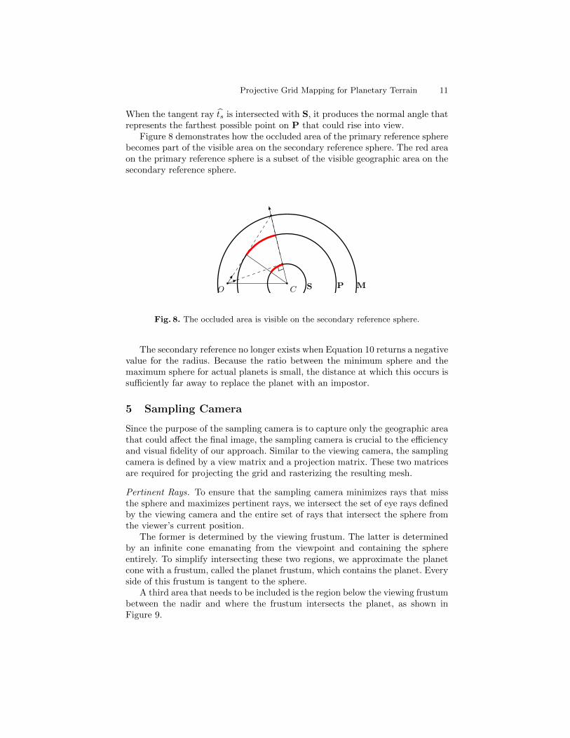
When the tangent ray ts is intersected with S, it produces the normal angle thatrepresents the farthest possible point on P that could rise into view.

Figure 8 demonstrates how the occluded area of the primary reference spherebecomes part of the visible area on the secondary reference sphere. The red areaon the primary reference sphere is a subset of the visible geographic area on thesecondary reference sphere.

O C S P M

Fig. 8. The occluded area is visible on the secondary reference sphere.

The secondary reference no longer exists when Equation 10 returns a negativevalue for the radius. Because the ratio between the minimum sphere and themaximum sphere for actual planets is small, the distance at which this occurs issufficiently far away to replace the planet with an impostor.

5 Sampling Camera

Since the purpose of the sampling camera is to capture only the geographic areathat could affect the final image, the sampling camera is crucial to the efficiencyand visual fidelity of our approach. Similar to the viewing camera, the samplingcamera is defined by a view matrix and a projection matrix. These two matricesare required for projecting the grid and rasterizing the resulting mesh.

Pertinent Rays. To ensure that the sampling camera minimizes rays that missthe sphere and maximizes pertinent rays, we intersect the set of eye rays definedby the viewing camera and the entire set of rays that intersect the sphere fromthe viewer’s current position.

The former is determined by the viewing frustum. The latter is determinedby an infinite cone emanating from the viewpoint and containing the sphereentirely. To simplify intersecting these two regions, we approximate the planetcone with a frustum, called the planet frustum, which contains the planet. Everyside of this frustum is tangent to the sphere.

A third area that needs to be included is the region below the viewing frustumbetween the nadir and where the frustum intersects the planet, as shown inFigure 9.


To generate the sampling camera, we intersect the viewing frustum with theplanet frustum and include the nadir.

n

I

Fig. 9. The area below the viewing frustum could include terrain that should intersectthe frustum.

Frustum-Frustum Intersection. The algorithm for intersecting frusta is simplifiedby the observation that the viewing frustum and the planet frustum share anapex, the viewpoint. The algorithm represents each frustum with respect to thecorners where its sides meet, and defines each corner using a ray. The viewingfrustum’s corner rays can be obtained from the attributes used to define thefrustum, i.e.the left, right, bottom, and top values which are in eye space. Theplanet frustum corner rays are defined by generating a frustum that is orientedso that its up direction is aligned to the plane of the viewing camera’s up andforward directions.

Let frustum A be the viewing frustum, B be the planet frustum, and C bethe intersection of A and B. Given the corner rays of A and B, the corner raysof C can be determined by applying two rules. First, any corner ray of A thatis in B or of B that is in A is a corner ray of C. Second, possible corner raysof C result from the intersection of the planes of A with the planes of B. Anysuch ray that is bounded by both A and B is a corner ray of C.

The planes of a frustum are the planes that contain each side of the frustum.These planes are defined by their normals, which are obtained from the crossproduct of the corner rays.

Using these two rules, our algorithm is as follows:

1. Find the rays of A that exist within B.2. Find the rays of B that exist within A.’3. Calculate the normals of the planes of A and B.4. Intersect the planes of A with the planes of B.5. For each resulting ray, if the ray is bounded by A and B it is a corner ray

of C.

This algorithm requires the ability to determine whether a ray is boundedby a frustum and the ability to intersect planes. To determine whether a ray


is bounded by a frustum, we test the ray’s angle to each plane of the frustum.Given the normal n to a plane and a ray direction r, the ray is on the positiveside of the plane if n · r > 0. When generating plane normals for the frusta,we ensure that each plane normal points inward to the frustum. The secondrequirement is to intersect to the planes. The ray that lies in the intersection oftwo planes can be determined by the cross product of the planes normals.

In the case that there is no intersection between the frusta, as when theviewer looks away from the planet, we use the corner rays of the planet frustum.

We carry out the intersection in a special coordinate system based on theviewing camera. This coordinate system is a rotated version of the viewing cam-era such that the up direction lies in the plane of the view direction and thenadir. The purpose of this is to generate a sampling camera that is orientedsuch that the top edge of the sampling frustum is aligned with the horizon. Thisminimizes the number of rays that miss the sphere, especially when the vieweris close to the surface of the planet.

View Matrix. The output of frustum-frustum intersection is a set of rays thatdescribes the corners of the intersection frustum.

To build the view matrix of the sampling camera, we first need to choosea view direction based on the intersection rays. The view direction should takeinto account all of the intersection rays, since a skewed view direction leadsto nonuniform distribution of grid points when the projective grid is stretchedacross the viewport of the sampling camera. To obtain the view direction, wefirst set its x-component to zero, since the previously described rotated spacealready aligns the top of the camera to the horizon. We then take the averageof the y- and z-components of all intersection rays. We include the nadir in thisaverage in order to include the area below the viewing camera on the planet, asdescribed earlier.

The view direction and the nadir are then used in a series of cross productsto build a basis which defines the coordinate system of the sampling camera.The three vectors of this basis are used to create the sampling camera’s viewmatrix.

Projection Matrix. The frustum of the sampling camera can be described usingthe standard left, right, top, bottom, near, and far values used to create a projec-tion matrix. These values relate to the corners of the frustum on the user-chosennear plane.

We obtain these values by intersecting all of the intersection rays, along withthe nadir, with an arbitrary near plane. This is carried out in coordinates relativeto the sampling camera, which were defined in the previous section. The user-chosen near plane is perpendicular to the view direction within that coordinatesystem. We then find the minimum and maximum x− and y−components of theresulting intersections on the near plane. The output is the left, right, bottomand top values. The distance to the far plane, like the near plane, is chosenarbitrarily. Thus, the near and far values can be the same values used to generatethe viewing frustum’s projection matrix.


6 Deferred Texturing

For height map composition, we must iterate over all height maps and combinethe height values for each grid point. The accumulated heights are stored in abuffer of 32-bit floating points that has the same dimensions as the projectivegrid. This process can be performed on the GPU by using the map equationsfrom Section 7. Color and surface normal data is composited in a similar manner,expanded for three channels of data.

The sphere normals, positions, and accumulated heights buffers describe thefinal terrain mesh. In order to decouple the performance of PGM from the perfor-mance of deferred texturing, we rasterize the grid-sized buffers into screen-sizedbuffers, an optimization described by Kooima [15]. This accomplishes perfor-mance throttling by allowing the grid size to differ from the screen size.

In order to use the three buffers as geometry, we render a triangle strip whereeach vertex corresponds to a grid point in the projective grid. Each vertex thenhas an (x, y) position equal to the corresponding grid point’s texel coordinateswithin the three buffers. By sampling each buffer, we can determine the vertex’sfinal position, which is displaced along the sphere normal.

To mitigate the issues of 24-bit depth buffer precision, we perform a two-passrasterization approach [16], rendered with a near frustum and a far frustum. Ifsecondary objects are to be rendered, a stencil buffer can be maintained to trackwhich pixels are occluded by the near terrain.

The final step is to render the outer atmosphere and combine the accumulatedcolor and surface normal buffers using standard Phong lighting equations withatmospheric effects. The shaders for rendering the outer and inner atmosphericeffects are given by Sean O’Neil [17].

7 Map Projections

For the composition of different datasets on the GPU, we must transform thenormals of the sphere into texture coordinates. Using the buffer of normals, wecan calculate the geographic location of each fragment by using a simple mappingfrom Cartesian to spherical coordinates.

Once the geographic coordinates have been determined, they must be trans-formed into projection coordinates using either an equirectangular or polar stere-ographic projection. We modify the forward mapping equation for equirectangu-lar projection [18] by removing the radius. This serves to reduce floating pointerrors from a large planetary radius.

p = (λ− λ0) cosφ0,

q = φ,

where λ and φ are the longitude and latitude components of the geographiccoordinates and λ0 and φ0 are the center longitude and latitude of the projection.


For polar stereographic projection, a slightly different equation must be used.

p = c sin(λ− λ0),

q = −c s cos(λ− λ0),

where s = sin(φ0) is the scaling value equal to −1 for the south pole or 1 for thenorth pole and c is a factor similar to both equations, calculated using

c = 2 tan(π

4− sφ

2).

We have modified the common equation [18] to allow the center latitude(either 90◦ for the north pole or −90◦ for the south pole) to affect whether theequations produce projection coordinates for a south or north polar stereographicprojection. Also, note that again the radius has been removed from this equationfor the same reason as the equirectangular projection equation.

Once the projection coordinates for a fragment have been obtained, the tex-ture coordinates can be calculated. Using GDAL [19], we can determine theprojection coordinates of the corners of a given dataset on the CPU. With thisinformation, the width and height of the dataset can be calculated in projectioncoordinates. Assuming a projection point P (defined by the above projectionequations) an upper-left dataset coordinate U , and the dimensions of the datasetD, we can determine the (s, t) texture coordinates by

(s, t) =P − U

D

giving us texture coordinates in the range of [0, 1].

8 Results

Experimental Method. To test the execution time of the algorithm, we used amachine with an Intel Core i7 processor running at 2.8GHz and 8GB of RAM.In addition, we used an Nvidia GeForce GTX 480 graphics card. For these tests,the amount of texture data in GPU memory is kept constant.

Table 1 lists detailed information about all of the datasets used, including themap scale in kilometers per pixel, which describes the resolution of the datasetat the center of projection. Dataset sizes are reported in megabytes (MB).

In order to understand the performance of separate parts of the algorithm,we measure the runtime of the PGM step as well as the entire algorithm. Inorder to see how the view affects the efficiency of the algorithm, we use threedifferent views shown in Figure 10. We test a global view of the planet, a viewclose the planet using low-resolution data, and finally a view close to the planetusing high-resolution data of Victoria Crater.

Finally, the problem size is varied with respect to two variables: the grid sizeand the screen size.


Name Scale Width Height Size

MOLA Global 2.606 8192 4096 128.0MOLA Areoid 3.705 5760 2880 63.3Victoria Heights 0.001 1279 1694 8.3MOC Tile 1 1.302 8192 8192 192.0MOC Tile 2 1.302 8192 8192 192.0Victoria Colors 0.002 3635 8192 8.3MOLA Normals 2.606 8192 4096 96.0

Table 1. Information about the datasets used for timing.

Fig. 10. Three tested views

Fig. 11. Total FPS for all three cases.

Performance Analysis. Figure 11 graphs the framerate in frames per second(FPS) for all three cases. As is evident from the graph, all three cases respondsimilarly to changes in grid and screen size. In addition, the graph shows thatthe second test case runs faster than the first test case and the third test caseruns faster than the second test case. This pattern is exaggerated as both gridsize and screen size approach 1024×1024. The first test case performs the slowestbecause it is a global view, and all of the datasets are visible. The second andthird test cases are close to the terrain, meaning that texture lookups are bothlimited to the same textures and cover a smaller area. This leads to more of aperformance benefit from the caching of texture reads.


Fig. 12. The execution time in ms of the PGM step for the first test case.

Fig. 13. The execution time in ms of the entire algorithm for the first test case.

The PGM step is unaffected by the dimensions of the screen because of thenature of the PGM algorithm. This observation is shown in Figure 12, wherethe execution time shows small variations with increasing screen size but largevariations with increasing grid size. However, both the grid size and the screensize affect the overall performance of the algorithm, as shown in Figure 13. Thisgraph shows that although deferred texturing operates on screen-sized buffers,an increase in grid size affects the overall execution time of the algorithm morethan an increase in screen size. This is because the rasterization step requiresthe entire projected grid to be rendered as a triangle mesh at once, thus testingthe triangle throughput of the GPU.

9 Conclusions and Future Work

Using a spherical approach to PGM, we have presented a planetary terrain ren-derer that accurately handles differently projected data. Additionally, we have


shown how reducing the ray-sphere intersection to a two-dimensional cross sec-tion can greatly optimize the ray casting process.

To improve our algorithm, we suggest sorting the datasets into a spatialhierarchy therefore allowing for visibility tests to be performed by the CPU,possibly eliminating entire composition passes. Additionally, finding the radiusof the primary reference sphere through min mipmapping is effective but slowdue to the reduction performed on the GPU. To improve this, we suggest theuse of CUDA [20] which allow for easier management of the shader cores. Lastly,we would like to provide a method for streaming data from the disk to RAM toGPU memory so that high-resolution data can be rendered.

10 Acknowledgments

This work is funded by NASA EPSCoR, grant # NSHE 08-51, and NevadaNASA EPSCoR, grants # NSHE 08-52, NSHE 09-41, and NSHE 10-69.

References

1. Kooima, R., Leigh, J., Johnson, A., Roberts, D., SubbaRao, M., DeFanti, T.:Planetary-scale terrain composition. IEEE Transactions on Visualization and Com-puter Graphics 15 (2009) 719–733

2. Duchaineau, M., Wolinsky, M., Sigeti, D.E., Miller, M.C., Aldrich, C., Mineev-Weinstein, M.B.: ROAMing terrain: Real-time optimally adapting meshes. In:VIS ’97: Proceedings of the 8th conference on Visualization ’97, IEEE ComputerSociety Press (1997) 81–88

3. Losasso, F., Hoppe, H.: Geometry clipmaps: terrain rendering using nested regulargrids. In: SIGGRAPH ’04: ACM SIGGRAPH 2004 Papers, ACM (2004) 769–776

4. Asirvatham, A., Hoppe, H.: Terrain rendering using GPU-based geometryclipmaps. In: GPU Gems 2. Addison-Wesley Professional (2005) 27–46

5. Dick, C., Kruger, J., Westermann, R.: GPU ray-casting for scalable terrain render-ing. In: Proceedings of Eurographics 2009–Areas Papers, Eurographics Association(2009) 43–50

6. Cignoni, P., Ganovelli, F., Gobbetti, E., Marton, F., Ponchio, F., Scopigno, R.:Planet-sized batched dynamic adaptive meshes (P-BDAM). In: Proceedings of the14th IEEE Visualization 2003, IEEE Computer Society (2003) 147–154

7. Clasen, M., Hege, H.: Terrain rendering using spherical clipmaps. In: EuroVis06:Joint Eurographics - IEEE VGTC Symposium on Visualization, Eurographics As-sociation (2006) 91–98

8. Hinsinger, D., Neyret, F., Cani, M.: Interactive animation of ocean waves. In:Proceedings of the 2002 ACM SIGGRAPH/Eurographics symposium on Computeranimation, ACM (2002) 161–166

9. Johanson, C.: Real-time water rendering. Master’s thesis, Department of ComputerScience, Lund University (2004)

10. Bruneton, E., Neyret, F., Holzschuch, N.: Real-time realistic ocean lighting usingseamless transitions from geometry to BRDF. In: Computer Graphics Forum,Wiley Online Library (2010) 487–496


11. Livny, Y., Sokolovsky, N., Grinshpoun, T., El-Sana, J.: A GPU persistent gridmapping for terrain rendering. The Visual Computer 24 (2008) 139–153

12. Loffler, F., Rybacki, S., Schumann, H.: Error-bounded GPU-supported terrainvisualisation. In: WSCG’2009: Proceedings of the 17th International Conferencein Central Europe on Computer Graphics, Visualization and Computer Vision–Communications Papers, University of West Bohemia (2009) 47–54

13. Schneider, J., Boldte, T., Westermann, R.: Real-time editing, synthesis, and ren-dering of infinite landscapes on GPUs. In: Vision, modeling, and visualization 2006:proceedings, November 22-24, 2006, Aachen, Germany, IOS Press (2006) 145–153

14. Fourquet, E., Cowan, W., Mann, S.: Geometric displacement on plane and sphere.In: Proceedings of graphics interface 2008, Canadian Information Processing Soci-ety (2008) 193–202

15. Kooima, R.: Planetary-scale Terrain Composition. PhD dissertation, Departmentof Computer Science, University of Illinois at Chicago (2008)

16. Brandstetter, W.E.: Multi-resolution deformation in out-of-core terrain rendering.Master’s thesis, Department of Computer Science and Engineering, University ofNevada, Reno (2007)

17. O’Neil, S.: Accurate atmospheric scattering. In: GPU Gems 2. Addison-WesleyProfessional (2005) 253–268

18. Eliason, E.: Hirise catalog. http://hirise.lpl.arizona.edu/PDS/CATALOG/DSMAP.CAT(Accessed July 21, 2010) (2007)

19. GDAL. (http://www.gdal.org (Accessed July 21, 2010))20. Nvidia: CUDA. http://www.nvidia.com/object/cuda home new.html (Accessed

September 13, 2010) (2007)

projective grid mapping for planetary terrainfredh/papers/working/isvc2011/... · 2011-05-19 ·...

Documents