projections of new zealand mortality using the lee-carter...

New Zealand Population Review, 36:27-53. Copyright © 2010 Population Association of New Zealand

Projections of New Zealand Mortality Using the Lee-Carter Model and its Augmented

Common Factor Extension

JACKIE LI *

Abstract This paper presents the results from an empirical study on projecting New Zealand mortality. First, we analyse mortality data from 1948 to 2009 to obtain background information for the modelling process. In particular, we examine various aspects of mortality patterns by gender such as the differences across age, declining trend over time, old-age mortality rates, movement of the survival curve, modal age at death, and continual increase in life expectancy. We then apply the Lee-Carter model and its augmented common factor extension to the mortality data and project the death rates and life expectancy. We investigate the optimal starting year for fitting the model, and carry out out-of-sample and residual analyses to assess model performance. The fitted models appear to provide further insight into the underlying mortality trends. In addition, we make use of a hypothetical example of a pension to illustrate potential financial impact of longevity risk.

ife expectancy at birth in New Zealand has increased from 69 years in 1948 to 81 in 2009. For the past ten years, life expectancy has risen by 0.3 years per annum on average, and there is no sign of the

upward trend ending in the foreseeable future. It is hence important for the government and insurance companies to properly allow for this trend and the so-called ‘longevity risk’ – the risk that a pension scheme or an insurer’s annuity portfolio pays out more than expected due to increasing life expectancy. Omission or miscalculation of this risk could potentially lead to disastrous financial outcomes.

* Nanyang Business School, Nanyang Technological University, Singapore. Email: [email protected]

L

28 Li

There are many ways to project future mortality rates. Booth (2006) provides a comprehensive review of demographic forecasting methodologies and mentions that there are broadly three approaches: extrapolation, expectation, and explanation. Some researchers criticise the extrapolation approach as being overly simple (e.g. Gutterman & Vanderhoof, 1998), in the sense that it implicitly assumes that past patterns would repeat in the future and does not take into account expert opinion or the structural relationship between the demographic and other variables. We believe, however, that studying the past patterns and trends carefully forms a solid basis for understanding how mortality changes over time, and projecting these past trends into the future serves as a robust first-step or benchmark for further analysis. Moreover, as noted in Lee and Miller (2001), there has historically been a pessimistic bias of expert opinions on mortality, which suggests that present knowledge reflects on current limitations but not future means of breaking through them. In practice, the distinction between different approaches is less clear-cut and one can always adjust the extrapolation procedure by expert opinions or related variables where appropriate. In this paper we attempt to recognise the underlying patterns of mortality changes and adopt the extrapolation approach to perform projection of future mortality and life expectancy.

We collected New Zealand deaths and population data by gender and single age for years 1948 to 2009 from Statistics New Zealand’s Infoshare series (www.stats.govt.nz) and the Human Mortality Database (www.mortality.org). Figure 1 illustrates the changes in the population size over time for the 1880, 1900, 1920, 1940, 1960, 1980, and 2000 cohorts. Without volatile migration movements and abrupt events, the curves are expected to progress smoothly for each year due mainly to the occurrence of deaths. While most parts of the curves are rather smooth, it is interesting to see a few irregular patterns, e.g. the small peak at mid-30s for the 1940 cohort and the severe trough at mid-20s for the 1960 cohort. These erratic patterns exist for a number of consecutive cohorts (not shown here) and could arise from certain temporal migration trends in the past.

Projections of New Zealand M

Figure 1: Population s

Observed Mortality

Mortality Decline

Figure 2 plots the log d2009. The shapes of the cmortality for early childhnoticeable for males; thincrease for adult mortgenerally declines over tages and periods. In parmore significant betweeespecially for males. As low levels, improvement previously for future incrthat in recent decades, mat ages 50 and above. Wmedical technology, it isnext few decades. In addaround 1975 and then gchange in direction expla1980 but smaller in 2009

Mortality using the Lee-Carter Model 2

ize for cohorts, 1880 to 2000

y Patterns

death rates against age for years 1948, 1980, ancurves are typical in nature: a drop from high infahood, then a rise to the peak at around age 20 (mohe so-called accident hump), followed by a linetality. While it is obvious to see that mortalitime, the decrease has been uneven across differerticular, the decline at middle to old ages is muen 1980 and 2009 than between 1948 and 198mortality at young ages has already reached veat older ages would tend to play a bigger role th

rease in life expectancy. Figure 3 also demonstratmortality improvement has become more promineWith continual breakthroughs in health care ans not unrealistic to expect this trend to last for tdition, we note that the 20-29 rates rise temporariget back to the declining trend in about 1985. Thains why in Figure 2 the accident hump is greater 9.

29

nd ant ore ear ity ent ch

80, ery an tes ent nd the ily his in

30

Figure 2: Log death ra

Figure 3: Log death ra

Old-Age Mortality

The data collected span death rates are more voland above, due to smallpatterns of these ages inwe chose to exclude the dlater sections.

ate for years 1948, 1980, and 2009

ate for age groups 0 to 80-89

across ages 0 to 110+. As shown in Figure 4, tlatile from age 90 onwards, especially for ages 1l exposures of these very old ages. Projecting tnto the future may produce unstable results. Hendata of ages 90 and above in our model fitting in t

Li

the 00

the nce the


Figure 4: Death rate, l1948, 1980, a

In order to ‘close ouderiving the survival cuThatcher (1999). CompHeligman and Pollard mclearly closer fit to a largdata of around 13 countwould have a point of inflog death rate curve wou


log death rate, and logit death rate for years and 2003

ut’ the life table for calculating life expectancy anurve, we apply the logistic model as proposed bpared to the traditional Gompertz, Weibull, an

models, the logistic model has been found to provige amount of old-age (80 years old and over) deatries over 30 years. The resulting death rate curflection (generally around age 100 or above) and tuld have a decreasing slope against age.

31

nd by nd ide ath rve he

32 Li

Deduced from the logistic model, Thatcher (1999) proposes the following linear relationship for high ages:

( ) xx lnlogit βαμ +≈ (1)

in which xμ is the force of mortality at age x, and α and β are regression

parameters that can readily be estimated. This linear relationship has been shown to furnish a good approximation to old-age mortality. This relationship was adopted to the death rates from ages 70 to 89 and the rates to ages 90 to 109 were projected. The fitted/projected rates (including the log and logit rates) were then plotted as curves in Figure 4.

It can be seen that the model fitting appears to be satisfactory before age 90 (the R2 values for all 62 years of data of both genders have an average of 0.98 with a minimum of 0.95.) Although the actual rates are rather volatile for ages 90 and over, they are still roughly in line with the model projections. As such, we will continue to utilize this technique in the following analysis. (We have also tried projecting the rates to age 119 and realise that the corresponding impact on life expectancy calculation is negligible, simply because the number of survivors is very small at such high ages. We therefore limit the projections to age 109.) In addition, there is a point of inflection on each death rate curve, and the log death rate curves have a decreasing slope across age.

Survival Curve

It is widely documented that the survival curves of many countries have been undergoing a process of transformation called rectangularization (e.g. Cheung et al., 2005). As infant and premature mortality (before ageing-related mortality) declines, the starting part of the survival curve becomes more horizontal, and as there is an increasing concentration of deaths around the modal age at death, the later part of the curve tends to be more vertical. The resulting effect is that the curve moves towards a rectangular shape, hence the term rectangularization.

As demonstrated in Figure 5, such phenomenon has also been happening in New Zealand. For males, it can also be seen that the movement of the curve at older ages is much larger between 1980 and 2009 than between 1948 and 1980, because mortality decline at these ages is more


significant during the latsince infant and prematuhorizontalization of thinsignificant process; andplace, the movement of something slightly similathe curve. We suspect thif both life expectancy future.

Figure 5: Survival curv

Figure 6 shows howdeviation of the ages at since 1980. As shown, thfor both genders. Moreowhich indicates an incsmoothed values of M awould be clearer and lverticalization of the sdiscussion above.


ter period, as discussed above. Over recent decadeure mortality has reduced to historically low levee survival curve has turned into a relatived while verticalization appears to continue to tathe curve for males in recent years develops in

ar to a parallel shift to the right, for certain parts at the latter phenomenon would be more promineand maximum lifespan keep on increasing in t

ve for years 1948, 1980, and 2009

w the modal age at death, M, and the standadeath above M, SD(M+), change over the peri

here is a clear tendency for M to increase over timover, there is also a decreasing trend for SD(M+creasing concentration of deaths around M. are used instead, the decreasing trend of SD(Mless volatile.) The combined effect is enhancinurvival curve, which is in accordance with o

33 es,

els, ely ake nto

of ent the

ard od me +), (If +) ng

our

34

Figure 6: Modal age atabove modal

Life Expectancy

Figure 7 shows clearlycomputation, has been risin 1948 to 83 for femalehas increased sharply sinearlier, the change in tholder ages, which is also rate of life expectancy at

Figure 7: Life expectan

The increasing trenmiddle of 1990s. The upthere is no indication thaThough we cannot denshifts or catastrophic ev

t death and standard deviation of ages at deathl age

y that life expectancy at birth, as based on osing gradually from 71 for females and 67 for mal

es and 79 for males in 2009. The slope of the trennce around 1985, particularly for males. As discusse slope is due largely to mortality improvement reflected by the considerable change in the growage 65 during the same period.

ncy at birth and life expectancy at age 65

nd seems to have slowed down slightly from tpward trend, however, remains fairly persistent anat it would come to an end in the foreseeable futurny the possibility of unpredicted major structurvents, it seems rather likely that life expectancy

Li h

our les nd ed at

wth

the nd re. ral at

Projections of New Zealand Mortality using the Lee-Carter Model 35 birth, and especially at older ages, would continue to rise steadily for the next few decades, under ongoing advancement in medical knowledge and health care and continuing decline in smoking prevalence (e.g. Harper & Howse, 2008).

Preliminary Fitting of Lee-Carter Model

The Lee-Carter model (1992) remains the most popular model for projecting future mortality rates, with various extensions and modifications suggested by different authors (e.g. Lee, 2000). The basic model has the following form:

txtkxbxatxm , ,ln ε++= (2)

in which txm , is the central death rate at age x in year t, xa depicts the

general mortality pattern, xb measures the sensitivity of the log death rate

to changes in the mortality index, tk is the mortality index, and tx,ε is the

corresponding residual term. The xa parameters are estimated by

averaging x,tmln over time. The xb and tk parameters are then obtained

by applying singular value decomposition (SVD) to { }xatxm −,ln , subject

to two constraints 1=∑x xb and 0=∑t tk . Finally the tk parameters are re-

estimated so that the fitted number of deaths and the actual number of deaths are equal for each year. The strengths of this model are mainly its

simplicity and also its ability to produce a highly linear series of tk across

time for a number of countries’ data (e.g. Lee and Miller 2001). This

linearity allows one to simply use a random walk with drift to model the tk

series and highly facilitates projection of mortality rates.

We apply the Lee-Carter model to our data from years 1948 to 2009.

The parameter estimates are set out in Figure 8. The xa estimates, as

expected, have a typical shape of log death rates across age. Moreover, the

xb estimates indicate that the highest sensitivity to general mortality

decline occurs at two age ranges: infant and early childhood, and middle age. Similar patterns are found by other researchers, e.g. Booth et al. (2002).

36 Li

Figure 8: Parameter estimates xa , xb , and tk of Lee-Carter model fitted to period 1948-2009

Interestingly, for the tk estimates, the decreasing trend is not linear and

there is a change in the slope in around 1985. Afterwards, the trend is very close to linearity, which implies that it may be more appropriate to choose a later starting year for the model fitting, in order to avoid the systematic

change in the tk series and reduce the variability of projected rates.

Nevertheless, it can also be argued that more sophisticated time series models such as ARIMA models can readily be adopted to deal with any non-linearity in the series while preserving the use of the full set of data.

Projections of New Zealand Mortality using the Lee-Carter Model 37 Regarding this viewpoint, we would like to emphasise three important issues. Firstly, the observations made previously reveal that there have been some structural changes in mortality improvement since 1980s. Inclusion of the patterns before these changes would probably be undesirable for model projections. Secondly, one of the main reasons behind the Lee-Carter model’s popularity is the highly linear series the model generates based on the data of different countries. This linearity makes the analysis of mortality decline and its projection much more straightforward and sensible. Finally,

as illustrated in Figure 9, we discover that the xb estimates using different

starting years exhibit varying patterns. Although the xb estimates from

different fitting periods are not directly comparable, it would still be preferable to select a fitting period not just as long as possible, but also within which the parameter estimates possess more consistent behaviour when switching from one starting year to the next. Booth et al. (2002) study

Australian data and discuss the same issues of non-linearity of tk and

invalidity of the assumption of constant xb over time.

We have tested each starting year from 1948 to 2000 and find that the parameter estimates display some extent of instability when the fitting period is reduced to less than 20 years or so. Accordingly, we will use at least 15 years of data in the following analysis and model fitting. Figure 9

depicts two distinct patterns of the xb estimates obtained from starting

before and after 1980 for both genders. The main difference is that for the later starting years, there is a peak at around age 25, in addition to those at

early childhood and middle age. It is also observed that the xb estimates are

less stable when the fitting period is shortened in the latter cases, and this reduction in parameter robustness is a cost of using only the most recent and relevant data.

38

Figure 9: Parameter es

Additionally, Figure

testing linearity of the

females and males, the

being 0.98 and 0.99 resp

in its slope in Figure 8. Tmuch support for choosperiod of at least 15 year1985 as the starting yea

paper. The resulting tk s

In the projections be

fitting period are taken

constrained to start at zeMiller (2001).

stimates xb using different starting years

e 10 sets forth the R2 and adjusted R2 values

tk series for different starting years. For bo

R2 values reach their maximum with year 198

ectively. This result is in line with how tk chang

To sum up, the observations thus far have providsing a later starting year, while keeping a fittinrs. Based on all the analysis above, we decide to ur, instead of the whole data set, for the rest of th

series are found to be highly linear in nature.

elow, the observed death rates in the last year of t

n as the starting point of projection and tk

ero in the projection period, as suggested in Lee an

Li

of

oth

85,

ges

ded ng

use his

the

is

nd


Figure 10: R2 and adju

Model Evaluation

For further evaluation ofitted to two periods 198and life expectancy are cthe period ending in 200(MAPE), the projected examined.

Table 1 lists the MAfitting periods. The MAPprediction appears to betwo fitting periods are qu

tk continues and is prop

be achieved, with less MAPE of the fitted log model fits reasonably wel

Table 1: MAPE of pro

(

Females

Males


sted R2 using different starting years

of model performance, the Lee-Carter model is no85-1999 and 1985-2004. The projected death ratompared against the observed values for the rest 9. In particular, the mean absolute percentage err

path of life expectancy, and the residuals a

APE of the projected log death rates for the twPE for each case is around 3% to 4%, and the mode satisfactory overall. The differences between tuite small, indicating that as long as the linearity

erly accounted for, decent prediction accuracy cou

reliance on the fitting period. Furthermore, tdeath rates for each case is close to 2%, and so tll.

ojected log death rates

Fitting Period (Projection Period) 1985-1999 (2000-2009)

1985-1999 (2000-2004)

1985-2004 (2005-2009)

3.9% 3.6% 3.5%

3.2% 3.1% 3.2%

39

ow tes of

ror are

wo del the

of

uld

the the

40

Figure 11 plots theconfidence intervals (dot

The intervals are constru

but not that of tx,ε and

there is some underestimaround 0.2 to 0.3 years oreasonably good since observed values lie well is 1948-1999 instead, theto increase with the ledemonstrate under-projelesser extent than govern

Figure 11:Projected life1999 and 198

e projected life expectancy at birth with the 95tted lines) against the observed values (solid line

ucted taking only the variability of tk into accoun

d the standard error of the parameters. As show

mation in the projected values, the size of which n average. Nevertheless, the performance still loothe underestimation is rather mild and all twithin the confidence bounds. (If the fitting peri

e underestimation is 0.9 years on average and tenength of projection.) Lee and Miller (2001) alected gains with the Lee-Carter model, but tonment forecasts.

e expectancy at birth for fitting periods 1985-85-2004

Li 5% es).

nt,

wn,

is oks the od

nds lso a

Projections of New Zealand Mortality using the Lee-Carter Model 41 Ideally, the residuals from the fitted model would be randomly spread

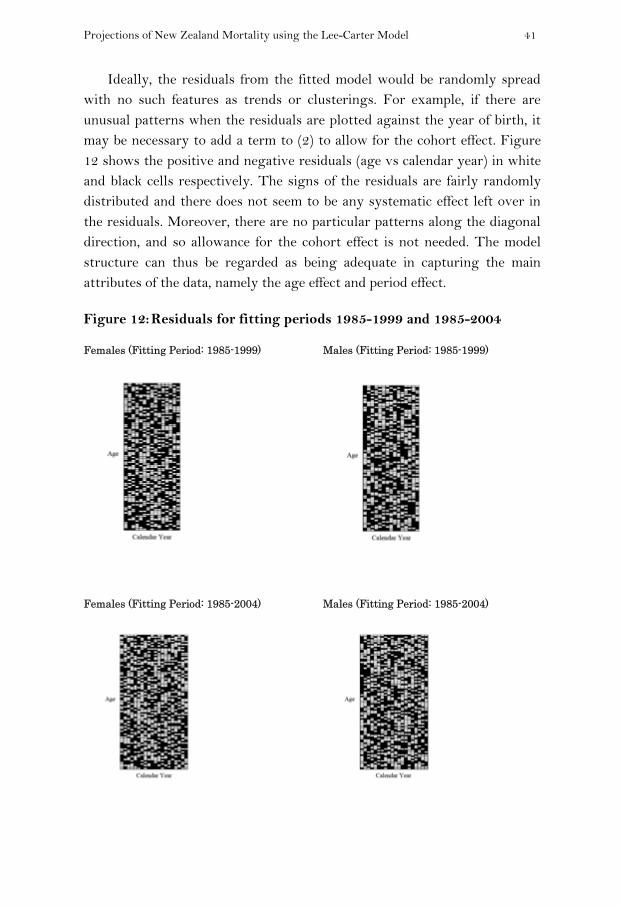
with no such features as trends or clusterings. For example, if there are unusual patterns when the residuals are plotted against the year of birth, it may be necessary to add a term to (2) to allow for the cohort effect. Figure 12 shows the positive and negative residuals (age vs calendar year) in white and black cells respectively. The signs of the residuals are fairly randomly distributed and there does not seem to be any systematic effect left over in the residuals. Moreover, there are no particular patterns along the diagonal direction, and so allowance for the cohort effect is not needed. The model structure can thus be regarded as being adequate in capturing the main attributes of the data, namely the age effect and period effect.

Figure 12: Residuals for fitting periods 1985-1999 and 1985-2004

Females (Fitting Period: 1985-1999) Males (Fitting Period: 1985-1999)

Females (Fitting Period: 1985-2004) Males (Fitting Period: 1985-2004)

42 Li

In spite of the satisfactory performance discussed above, separate projections of female and male mortality lead to two potential problems. The first is that the ratio of death rates between genders may or may not change significantly over time, and modeling two genders separately does not take this ratio into consideration at all. Figure 13 compares the projected ratio in 2009 against the observed ratio for 10-year age groups. The model projections clearly fail to realise the change in the ratio at younger ages, especially at 20-29, though the outcome at older ages is much better, due to the stability of the ratio for those ages. As illustrated in Figure 14, historically this ratio is more volatile at younger ages than at older ages, which explains why the projected ratio is more out of line for the former. In addition, except for age groups 0 and 30-49, there is an interesting pattern generally, in which the ratio increases between 1948 and 1980 and then decreases between 1980 and 2009. It is difficult to predict whether this decline in the ratio would continue in the future, and if so for how long. If the focus of the analysis is on pricing annuities for an insurer or valuing pension schemes for the government, however, failing to incorporate the gender mortality ratio into the model is unlikely to cause a serious problem, as long as the ratio remains relatively stable at older ages and the projection period is not too long.


Figure 13: Projected ratratio in 2009

Figure 14: Observed ratyears and age

There is actuallyas the projection period ibe much more severe wh

appendix of Li and Lee (

series which is then extrgender, the female anprogressively over time. may need to be avoideddivergence is to adopt thCarter model, as discusse


tio (male to female) of death rates and observe9 for fitting periods 1985-1999 and 1985-2004

tio (male to female) of death rates for differente groups

y another problem hidden in the modelling proceis only 5 to 10 years. This problem can turn out en the projection period is longer. As detailed in t

(2005), if each gender is estimated with its own

rapolated linearly and independently from the othnd male projected death rates would diver

This divergence is purely a modelling artifact and in certain applications. One way to reduce thhe augmented common factor extension of the Leed below.

43 ed

t

ess to

the

tk

her ge nd his ee-

44 Li

Augmented Common Factor Lee-Carter Model

The augmented common factor Lee-Carter model is proposed in Li and Lee (2005) as:

itxitkixbtKxBixaitxm ,,, , ,,,ln ε+++= (3)

in which the meanings of the expressions here are similar to those in (2), except that the subscript i indicates the gender considered, and that the

additional terms xB and tK refer to the aggregate population. In brief,

tKxB (common factor) allows for the main trend in mortality change of the

whole population and itkixb , , (specific factor) represents the short-term

difference from the main trend for gender i. The xB and tK parameters are

first obtained from applying the original Lee-Carter model (i.e. via xb and

tk in (2)) to the aggregate data combining two genders. All the other

parameters are then estimated separately for each gender, by fitting (2) to

{ }tKxBitxm ,,ln − . The tK series is modelled as a random walk with drift as

previously. In order to accommodate the short-term difference from the common factor and at the same time ensure this difference fades out in the

long run, the itk , series for females and males are modelled by an AR(1)

model. In this way, itk , converges to a constant value as the length of

projection increases and the disparity from the common factor then gradually disappears. Eventually, the projected ratio of male to female death rates turns into a constant at each age. The choice of the AR(1) model is also driven by its straightforwardness in fitting and implementation. We find below that for both genders the autocorrelations of the residuals are statistically insignificant for the first 6 lags (except lag 5), and there is no reason to complicate the analysis of a limited amount of data with a more sophisticated (e.g. higher order) but largely unjustifiable model.

We now apply the Lee-Carter model and also the augmented common factor extension to the period from 1985 to 2009. As listed in Table 2, the MAPE of the fitted log death rates for each case is slightly more than 2%, with little difference between the two models. Conventionally, it is more preferable to have the maximum length of the projection period

Projections of New Zealand Mortality using the Lee-Carter Model 45 approximately equal to the length of the fitting period. Thus we project the death rates and life expectancy only up to 2040. Figure 15 demonstrates that the projected values of life expectancy from the two models are fairly close. For example, life expectancy at birth for females in 2040 is projected to be 88.6 and 88.8 respectively by the two models, and for males 86.4 and 85.9. The augmented common factor model produces a higher value of life expectancy for females but a lower value for males. The main reason is that

the drift term of the random walk of tK (-2.38), being identical for both

genders, is roughly equal to the average of those of tk obtained from

applying the Lee-Carter model separately for females (-2.22) and males (-2.59). As revealed in Figure 16, the projected values depend heavily on the drift term of the random walk, and so there is a question on whether it is suitable to employ a common mortality index for both genders as in the augmented common factor model or to deal with each gender independently.

Table 2: MAPE of fitted log death rates

Gender Lee-Carter Augmented Common Factor

Females 2.3% 2.3%

Males 2.1% 2.1%

46

Figure 15: Projected lifand augment

fe expectancy at birth from Lee-Carter model ted common factor model

Li


Figure 16: Projected lifvs drift term

tK for augm

The answer to this analysis. Firstly, it is notare small between the twIf the female and male prway, the disparity amonoffsetting effect as notedmodel to use seems to bprojecting life expectancbetween genders is a matpolicy planning, it wouldarising from separate propreviously. In this regard


fe expectancy at birth in 2020, 2030, and 2040 m (in magnitude) of tk for Lee-Carter model and

mented common factor model

question probably depends on the purpose of tted that the differences in projected life expectan

wo models, even the length of projection is 31 yearrojected death rates are further aggregated in som

ngst the two models would be minimal, due to td in the example above. Hence the choice of whibe not much of an issue if one intends to focus ocy. On the other hand, if the ratio of death rattter of concern, such as in population projection and be more sensible to avoid the divergence probleojections of female and male mortality, as discussd, the augmented common factor model would ma

47 d

the ncy rs. me the ich on tes nd em ed

ake

48

sure the projected ratio oto a constant. All these seen that the gender mcommon factor model. Iunder the initial Lee-Car

Figure 17: Projected rayears and agecommon fact

of male to female death rates at each age convergissues are clearly reflected in Figure 17. It can mortality ratios converge under the augmentIn contrast, the ratios move in various directioter model.

atio (male to female) of death rates for differene groups from Lee-Carter model and augmentetor model

Li ges be

ted ons

nt ed

Projections of New Zealand Mortality using the Lee-Carter Model 49 Because the estimated dependency of itk , across time is quite weak and

the observed death rates in the final year of the fitting period are treated as the starting point of projection, the convergence is achieved quickly and the overall 2009 patterns remain in the projections. Some possible modifications are: averaging the observed rates in the last few years of the fitting period for the starting point of projection; and arbitrarily choosing parameters or model structures which bring about stronger time dependence.

Figure 18 plots the observed log death rates against age for years 1948, 1980, and 2009, and the projected rates in 2040 from the augmented common factor model. The typical shapes in the past are broadly preserved in the projection, but there are two anomalies. First, mortality improvement at around ages 30-44 has been relatively slow compared to other ages for recent decades, so the projected curve at this age range bulges up slightly. On the other hand, mortality decline at ages 50-79 has been faster than at adjacent ages, causing the projected curve less linear than the historical ones for adult mortality. If one is doubtful about whether these extrapolated features would really emerge and believes the typical shapes should be maintained, certain parameterized curves could be fitted or arbitrary adjustments be made to the projected rates.

Furthermore, the projected survival curve in Figure 19 reveals that there is continual verticalization in the projection. With regard to closing out the life table and plotting the survival curve, there is some limitation here as the death rates are only extended to age 109 using (1). More precise and voluminous old-age data are needed to verify the suitability of this technique in the case of a long projection period. As stated earlier, we suspect that there could be some degree of a parallel shift of the curve to the right under enhancing life expectancy and maximum lifespan in the future, and the application of (1) may need to be modified.

50

Figure 18: Observed an

Figure 19: Observed an

nd projected log death rates

nd projected survival curves

Li

Projections of New Zealand Mortality using the Lee-Carter Model 51 Longevity Risk

Finally, we construct a hypothetical example of a pension to illustrate potential financial impact of longevity risk, which is the risk that a pension scheme or an insurer’s annuity portfolio pays out more than expected because of rising life expectancy. The following results imply that miscalculation or omission of this risk could lead to undesirable financial consequences.

Consider a pension with regular payments of $1 payable in arrear to a female aged exactly 65 on 1 January 2010. The discount rate is assumed to be 6% p.a. (The New Zealand 10-year government bond yield was around

6% in January 2010.) We simulate 1,000 paths of tk from 2010 onwards,

based on the results of applying the Lee-Carter model to the period from

1985 to 2009 in the previous section. Both the variability of tk and the

standard error of the drift term are taken into account, while the variability

of tx,ε is not included. As the latter risk can be diversified by having more

independent lives in a pension scheme, we focus on the former risk which

cannot be diversified in the same way. The simulated tk values are then

used to generate 1,000 samples of the present value of the pension.

Using the 2009 death rates without allowing for mortality improvement, the expected present value of the pension is $10.97 as at 1 January 2010. Figure 20 shows that this value falls into the lower 1 percent region of the sampled distribution of the present value of the pension, which has a sample mean of $11.53 and 99th percentile of $12.10. In other words, completely ignoring mortality improvement would cause an underestimation of the reserves required to cover the pension by 5 percent in the sense of expectation and by 9 percent for the worst 1 percent scenario. The overall situation could get worse with the rapidly ageing population or

if there are major changes in tk , like the one in 1980s. From this simple

example, we can see that proper allowance for longevity risk is of critical importance in maintaining financial stability for pension and annuity providers.

52

Figure 20: Simulated diJanuary 2010

Concluding Remark

This paper presents the mortality for the periodvarious mortality patternperiod, rectangularizatioexpectancy - in particulaapplied the Lee-Carter mto the mortality data. 19for fitting the model. Tindicate satisfactory perfinitial Lee-Carter model similarly on the whole, convergence of the ratio through a pension exampcause significant financia

As noted earlier, proextrapolative approach cprojection period is too unrealistic, as it is difficwithout major structuraWhen one takes the exjudgement regarding theand reasonability of final

istribution of present value of a pension as at 10

ks

results from an empirical study on New Zealand from 1948 to 2009. We started with analysis ns, and noticed a general mortality decline over tn of the survival curve, and steadily increasing l

ar, structural shifts in the mortality trends. We thmodel and its augmented common factor extensio85 was identified as relatively suitable starting ye

The following out-of-sample and residual analysformance of the fitted models. It is noted that tand the augmented common factor model perforbut the latter provides an edge in ensuring tof death rates between genders. Lastly, we show

ple that failure to accommodate longevity risk coual instability to pension and annuity providers.

ojecting relevant past trends into the future via can be regarded as a robust starting point. If t

long, however, this practice would be somewhcult to justify the continuance of the same trenal changes over such an extended period of timxtrapolation method to perform projection, prope fitting period, projection period, parameter valueresults should be exercised.

Li 1

nd of

the ife en on ear ses the rm the

wed uld

an the hat nd

me. per es,

Projections of New Zealand Mortality using the Lee-Carter Model 53 References

Booth, H. (2006). Demographic forecasting: 1980 to 2005 in review. International Journal of Forecasting, 22: 547-581.

_______, Maindonald, J. and Smith, L. (2002). Applying Lee-Carter under conditions of variable mortality decline. Population Studies, 56: 325-336.

Cheung, S., Robine, J., Tu, E. and Caselli, G. (2005). Three dimensions of the survival curve: horizontalization, verticalization, and longevity extension. Demography, 42: 243-258.

Gutterman, S. and Vanderhoof, I.T. (1998). Forecasting changes in mortality: A search for a law of causes and effects. North American Actuarial Journal, 2: 135-138.

Harper, S. and Howse, K. (2008). An upper limit to human longevity? Population Ageing, 1: 99-106.

Human Mortality Database. (2010). University of California, Berkeley (USA) and Max Planck Institute for Demographic Research (Germany). www.mortality.org.

Lee, R. (2000). The Lee-Carter method for forecasting mortality, with various extensions and applications. North American Actuarial Journal, 4: 80-93.

______ and Carter, L. (1992). Modeling and forecasting U.S. mortality. Journal of the American Statistical Association, 87: 659-671.

______ and Miller, T. (2001). Evaluating the performance of the Lee-Carter method for forecasting mortality. Demography, 38: 537-549.

Li, N. and Lee, R. (2005). Coherent mortality forecasts for a group of populations: an extension of the Lee-Carter method. Demography, 42: 575-594.

Statistics New Zealand. (2010). Infoshare www.stats.govt.nz. Thatcher, A. (1999). The long-term pattern of adult mortality and the highest

attained age. Journal of the Royal Statistical Society (Series A) 162: 5-43.

projections of new zealand mortality using the lee-carter...

Documents