Projection onto the Manifold of ElongatedStructures for Accurate Extraction

Amos Sironi1∗ Vincent Lepetit1,2 Pascal Fua11CVLab, EPFL, Lausanne, Switzerland, {firstname.lastname}@epfl.ch

2TU Graz, Graz, Austria, lepetit@icg.tugraz.at

Abstract

Detection of elongated structures in 2D images and 3Dimage stacks is a critical prerequisite in many applica-tions and Machine Learning-based approaches have re-cently been shown to deliver superior performance. How-ever, these methods essentially classify individual locationsand do not explicitly model the strong relationship that ex-ists between neighboring ones. As a result, isolated erro-neous responses, discontinuities, and topological errors arepresent in the resulting score maps.

We solve this problem by projecting patches of the scoremap to their nearest neighbors in a set of ground truth train-ing patches. Our algorithm induces global spatial consis-tency on the classifier score map and returns results that areprovably geometrically consistent. We apply our algorithmto challenging datasets in four different domains and showthat it compares favorably to state-of-the-art methods.

1. IntroductionReliably extracting boundaries from images is a long-

standing open Computer Vision problem and finding 3Dmembranes, their equivalent in biomedical image stacks,while difficult is often a prerequisite to their segmentation.Similarly in both regular images and image stacks, recon-structing the centerline of linear structures is a critical firststep in many applications, ranging from road delineation in2D aerial images to modeling neurites and blood vessels in3D biomedical image stacks.

These problems are all similar in that they involve find-ing elongated structures of codimension 1 or 2 given verynoisy data. In all these cases, classification- and regression-based approaches [9, 38, 39] have recently proved to yieldbetter performance than those that rely on hand-designedfilters. This success is attributable to the representationsused by powerful machine learning techniques [23, 43] op-erating on large training datasets.

However, these methods essentially classify individual

∗This work was supported in part by the EU ERC project MicroNano.

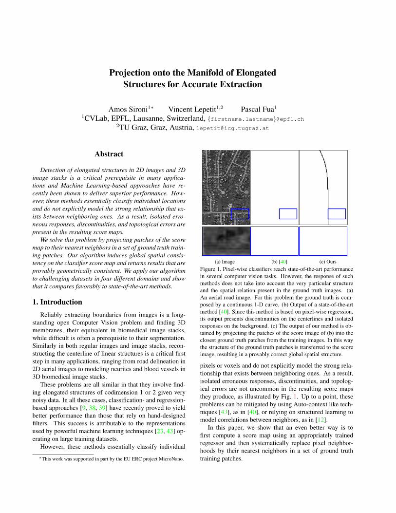
(a) Image (b) [40] (c) OursFigure 1. Pixel-wise classifiers reach state-of-the-art performancein several computer vision tasks. However, the response of suchmethods does not take into account the very particular structureand the spatial relation present in the ground truth images. (a)An aerial road image. For this problem the ground truth is com-posed by a continuous 1-D curve. (b) Output of a state-of-the-artmethod [40]. Since this method is based on pixel-wise regression,its output presents discontinuities on the centerlines and isolatedresponses on the background. (c) The output of our method is ob-tained by projecting the patches of the score image of (b) into theclosest ground truth patches from the training images. In this waythe structure of the ground truth patches is transferred to the scoreimage, resulting in a provably correct global spatial structure.

pixels or voxels and do not explicitly model the strong rela-tionship that exists between neighboring ones. As a result,isolated erroneous responses, discontinuities, and topolog-ical errors are not uncommon in the resulting score mapsthey produce, as illustrated by Fig. 1. Up to a point, theseproblems can be mitigated by using Auto-context like tech-niques [43], as in [40], or relying on structured learning tomodel correlations between neighbors, as in [12].

In this paper, we show that an even better way is tofirst compute a score map using an appropriately trainedregressor and then systematically replace pixel neighbor-hoods by their nearest neighbors in a set of ground truthtraining patches.

This is in the spirit of algorithms for image denoisingand inpainting that search for nearest neighbors within theimage itself [11, 10, 25]. It is also closely related to theapproach of [16] that improves boundary images by findingnearest neighbors using a distance defined in terms of de-scriptors extracted by a Convolutional Neural Network. Bycontrast, in our method, we compute distances in terms ofthe patches themselves and we will show that it improvesboth performance, especially near junctions, and generality.

In short, our algorithm induces global spatial consistencyon the classifier score map and improves classification per-formance, as can be seen in Fig. 1(c). Furthermore, assum-ing that the structure of all admissible ground truth imagesis well represented by the set of training patches, it can beformally shown that our method is equivalent to projectingthe score map into the manifold of all admissible groundtruth maps.

2. Related WorkIn this section, we review related work on centerline,

boundary and membrane detection.

Centerline Detection Centerline detection methods canbe divided in two main classes.

The first class relies on hand-designed filters. They aretypically used to compute the Hessian matrix [14, 36, 28,13, 29] or the Oriented Flux matrix [22, 1, 41, 33, 44],whose eigenvalues then serve to estimate the likelihood thata pixel or voxel lies on a centerline. Since the filters areoptimized for ideal tubular structure, their performance de-creases when the structures of interest become irregular.

To overcome this limitation, a second class of meth-ods that rely on Machine Learning techniques has recentlyemerged. Classification-based ones [17, 47, 7, 46] havebeen successfully applied to the segmentation of thick lin-ear structures while, regression-based ones [39, 40] havebeen shown to be particularly effective at finding centerlinepixels only. However, even if pixel-wise classification andregression methods can produce remarkable results, they donot explicitly model the strong relationship that exists be-tween neighboring pixels. As a consequence, discontinu-ities and inconsistencies may occur in their output.

Boundary Detection Boundary detection methods can bedivided in the same two classes as for centerline detection.

All the early approaches [26, 8, 32] belong to the firstone and rely on filters designed to respond to specific imageintensity profiles. Recently, attention has shifted to classi-fication based methods [5, 34, 38, 24, 12], which have pro-duced significant improvements.

More specifically, in [5] gradients on different imagechannels are fed to a logistic regression classifier to predictcontours. In [34], SVMs are trained to predict boundariesfrom features computed using sparse coding. In [9], a Deep

Convolutional Network is used to segment cell membranesin 2D Electron Microscopy slices, while a sequence of clas-sifiers is used in [38] for boundary detection in both naturalimages and Electron Microscopy data.

However, as in the case of centerline detection, noneof these methods explicitly model the relationship betweennearby pixels. In particular, the response of ConvolutionalNeural Networks [23] can be spatially inconsistent becausethey typically treat every pixel location independently, thusrelying only on the fact that neighboring patches share pix-els to enforce consistency.

By contrast, in Auto-context based methods [43, 38],features extracted from the classifiers output in earlier lay-ers enlarge the receptive field and often yield more spatiallyconsistence results. However, these methods are prone tooverfitting and require large amount of training data to pre-vent it. The method of [12] overcomes these problems byrelying on structured learning, resulting in an accurate andextremely efficient edge detector. It is inspired by the workof [20, 21] where the structured random forest framework isintroduced for image labeling purposes, predicting for everypixel an image patch, instead of single pixel probabilities.However, it is specific to the particular kind of classifierused for learning and is difficult to generalize.

Recently, Nearest Neighbors search in the space of lo-cal descriptors obtained with a Convolutional Network wasused for boundary detection purposes [16]. Given an im-age patch, the algorithm computes a corresponding descrip-tor and then looks for the Nearest Neighbor in a dictionarybuilt from the training set. While effective, this approachstrongly depends on the specific dictionary learned by theCNN. Therefore, when it fails, it is difficult to understandwhy. Our method is closely related, but we perform NearestNeighbors search in the space of the final output, rather thanof intermediate image features. We will show empiricallythat it works better, especially near junctions. Moreover,unlike other approaches, ours is provably correct under cer-tain conditions, thus giving insights and indications on howto improve the results.

Membrane Detection Membranes are the 3D equiva-lent of contours in image stacks. They are important for3D volume segmentation, especially in a biomedical con-text [45, 4, 15]. In the previous paragraph we mentionedalgorithms [9, 38] that extract them 2D slice by 2D slice.Here we discuss those that extract them as 3D surfaces.

As in the case of 2D boundaries, early approaches to de-tecting them relied on hand-crafted filters optimized to re-spond to ideal sheet-like structures. In [37, 30, 27] for ex-ample, the eigenvalues of the Hessian matrix are combinedto obtain a score value that is maximal for voxels lying on a2D surface. Similarly, the eigenvalues of the Oriented Fluxmatrix [22] can be combined to obtain a score that is lesssensitive to adjacent structures.

More recent approaches have focused on machine learn-ing techniques. For example, a Convolutional NeuralNetwork and a hierarchical segmentation framework com-bining Random Forest classifier and watersheds are usedin [19] and [3] respectively to segment neural membranes.Even though both of these methods produce excellent re-sults, they are designed for tissue samples prepared with anextra-cellular die that highlights cell membranes while sup-pressing the intracellular structures, thus making the taskcomparatively easy.

3. Motivation and Formalization

As discussed in Section 2, methods that rely on statisticalclassification techniques currently deliver the best resultsfor boundary, centerline, and membrane detection. Amongthose, it has recently been reported that regression-basedones perform best for centerline detection [39] and we willdemonstrate here that they perform equally well for bound-ary and membrane detection.

More specifically, the algorithm of [39] involves train-ing regressors to return distances to the closest centerlinein scale-space. In this way, performing non-maximum sup-pression on their output yields both centerline locations andcorresponding scales. This has proved very effective but,like for all other pixel-based techniques that do not incor-porate any a priori geometric knowledge that may be avail-able, this approach can easily result in topological mistakes.

In this paper, we first extend this approach to both bound-ary and membrane detection. We then demonstrate that wecan correct the errors it makes by projecting them into themanifold of distance transforms corresponding to the kindof structures we are trying to reconstruct. This results in atechnique that is both a more competent and more widelyapplicable method than the original one [39]. Furthermore,it is generic in the sense that it is applicable to other meth-ods returning a score map, such as [12, 9].

In the remainder of this section, we first summarizethe approach of [39] and show that it extends naturally toboundary and membrane detection. We also introduce theformalism that we will use in the next section to describeour approach to improving the distance transforms by pro-jecting them onto an appropriate manifold.

3.1. Centerline Detection

Let I ∈ RN be an image containing linear structures andlet Y be the corresponding binary ground truth image, suchthat Y (p) = 1 if pixel p is on a centerline and Y (p) = 0otherwise.

Finding the centerlines can be formulated as the pixelclassification problem of learning a mapping between a fea-ture vector fM (p, I), extracted from a local neighborhoodNM (p) of size M around pixel p in image I , and the valueY (p).

(a) (b) (c) (d) (e)

Figure 2. Centerline Detection as a Regression Problem. (a) Origi-nal image patch; (b) Centerlines Ground Truth; (c) Distance Func-tion of Eq. (1) proposed in [39]; (d) The response of a pixel-wise regressor trained to predict the function in (c) is discontin-uous and returns topologically incorrect results, also when Auto-context [43] is applied. (e) Nearest Neighbors of the score patchesin (d), found in the training set. In our method we apply NearestNeighbors search to a regressor output and take advantage of theparticular structure of ground truth patches to correct its mistakes.

Learning such a classifier, however, can be difficult inpractice because of the similar aspect of nearby pixels to thecenterline and ambiguities on the exact location of a center-line due to low resolution and blurring.

To address this difficulty, the method of [39] replaces thebinary ground truth Y by the modified distance transformof Y

d(p) =

{ea(1−DY (p)

dM) − 1 if DY (p) < dM

0 otherwise, (1)

where DY is the Euclidean distance transform of Y , a > 0is a constant that controls the exponential decrease rate of dclose to the centerline and dM a threshold value determininghow far from a centerline d is set to zero.

Function d has a sharp maximum along the center-lines and decreases as one moves further from them.Fig. 2(c) shows examples of function d computed on smallpatches. Learning a regressor to associate the feature vectorfM (p, I) to d(p) induces a unique local maximum in theneighborhood of the centerlines. This approach is more ro-bust to small displacements and returns centerlines that arebetter localized compared to classification-based methods.

To learn the regressor we apply the GradientBoost al-gorithm [18]. Given training data {fi, di}i, where fi =fM (pi, I) is the feature vector corresponding to pixel piand di = d(pi), GradientBoost learns a function ϕ(·) ofthe form ϕ(q) =

∑Tt=1 αtht(q) , where q = fM (p, I) de-

notes a feature vector, ht are weak learners and αt ∈ R areweights. Function ϕ is built iteratively, selecting one weaklearner and its weight at each iteration, to minimize a lossfunction L of the form L =

∑i L(di, ϕ(fi)).

Input Image I Regressor Score Map X Output ΠD N(X)

Nearest Neighbor

xi

Centerlines

... ...}

}Train Gt Patches

NMSΠ(xi)

φ

Figure 3. Method overview. A score map X is obtained from image I by applying a regressor ϕ trained to return distances from thecenterlines. Every patch xi of size D in X is projected onto the set of ground truth training patches, by nearest neigbor search. Theprojected patches ΠN (xi) are averaged to form the output score map ΠD→N (X). Centerlines are obtained by Non-Maxima Suppression.

In addition, to learn the best possible regressor, weadopted the Auto-context technique [43], as in [40] and us-ing the same parameters. To this end, we use the score mapϕ(·) to extract a new set of features that are added to theoriginal ones to train a new regressor.

3.2. Boundary and Membrane Detection

The method described above extends naturally to bound-ary detection. As centerlines, boundary in 2D images andmembranes in 3D image stacks are elongated structures ofcodimension 1 and there are substantial ambiguities in theexact boundary location.

Therefore, and as before, we replace the binary groundtruth, provided for such problems, by the distance transformof Eq. (1). The distance function is computed 2D for bound-aries and 3D for membranes. We then train a regressor toassociate feature vectors to the distances to the boundaries.We can obtain the boundaries from the score map returnedby the regressor by non-maxima suppression.

4. Improving the Distance FunctionThe central element of our approach is to project the dis-

tance transform produced by pixel-wise regression, as de-scribed in the previous section, onto the manifold of all pos-sible ones for the structures of interest. Since this manifoldis much too large to be computed in practice, we first pro-pose a practical computational scheme and then formallyprove that it provides a close approximation under assump-tions that can be made to hold in the real world.

4.1. Nearest Neighbors Projections

Given an image I and corresponding binary ground truthY , let dY be the image obtained by applying function d ofEq. (1) to every pixel of Y . Since it corresponds to pixelsbelonging to specific structures, Y is constrained to havewell defined geometric properties. For example, in the case

of centerlines or boundaries in images, Y is composed of1-dimensional curves, while for boundaries in 3D volumes,Y is a 2D surface. This means that the set of all admissibleground truths forms a manifold in the set of binary images.Similarly, the set of images dY forms a manifold in the setof real valued images, which we will denote byMN .

Let X be the score map obtained by applying the regres-sor ϕ to each pixel of an input image I . Ideally we wouldlikeX to be an element ofMN , so that it is guaranteed to begeometrically correct. However, this is not true in general.Fig. 2(d) shows typical errors committed at critical points,such as T-junctions. This is a standard problem with manyedge detectors, such as the Canny detector.

In theory, one way to avoid this problem is to projectX intoMN , which is equivalent to finding the element ofMN closest to X ,

ΠN (X) = arg mindY ∈MN

‖dY −X‖2. (2)

In practice, however,MN is not known or much too largeto be sampled exhaustively. Therefore, ΠN (X) can not becomputed directly.

As shown in Fig. 3, our solution is to approximate it byprojecting small patches of X onto the set of ground truthtrain patches.

Formally, let MD = {yk}Kk=1 be the set of trainingpatches of size D, extracted form local neighborhoods ND

in the ground truth training images. For each pixel pi,i = 1, . . . , N in the score image X , let xi = X(ND(pi))be the squared neighborhood of size D around pi.

For every i, we consider the projection of xi intoMD,given by

ΠD(xi) = arg miny∈MD

‖y − xi‖2. (3)

Fig. 2(d) shows examples of nearest neighbors for threescore patches. We then average all these projections to ob-tain a new score image ΠD→N (X).

X xi

ΠD N

ΠD

ΠN

Figure 4. The output ΠD→N (X) of our method can be seen asprojection of the score map X into the manifold of admissibleground truth images MN . This is achieved by projecting smallpatches xi of X into the set of ground truth patchesMD and thenaveraging the resuls to obtain ΠD→N (X).

More precisely, given the set of projected patches{ΠD(xi)}Ni=1, we take the pixel values of the new imageΠD→N (X) to be

ΠD→N (X)(p) =1

R

∑i:p−pi∈NR(p)

ΠD(xi)(p− pi), (4)

where R ≤ D is the size of the neighborhood used for av-eraging and where we take ΠD(xi) to be centered at zero,with ΠD(xi)(p− pi) the value of ΠD(xi) at p− pi.

The image ΠD→N (X) obtained in this way is an approx-imation of ΠN (X). In the next section, we introduce suf-ficient conditions under which ΠN (X) = ΠD→N (X) andwe provide a formal proof in the supplementary material.

4.2. Equivalence of ΠD→N (X) and ΠN (X)

In this section we state under which conditions the out-put ΠD→N (X) of our method is equivalent to the projec-tion ΠN (X) of the score image X into the manifold of alladmissible ground truth images MN . The two necessaryproperties are:

(i) The training set of patchesMD is composed of all ad-missible ground truth patches and averaging patchesofMD that coincide for overlapping pixels, gives animage ofMN ;

(ii) For two patches xi and xj , extracted from overlappingneighborhoodsND(pi) andND(pj) in image X , theirprojections ΠD(xi) and ΠD(xj) coincide for all pixelsin the intersection of ND(pi) ∩ND(pj).

We formalize these concepts in the supplementary material,where we also prove that under these conditions our methodamounts to project the score map X into the ground truthmanifold MN . Fig. 4 illustrates this equivalence. Intu-itively, this means that the output of our method is the bestapproximation of X , in the space of ground truth images.Therefore, it also has the same geometrical properties.

In practice, these conditions will never be strictly satis-fied. However, we also show in the supplementary material

that by relaxing them and assuming only approximated pro-jections, we can prove that the error we make is within agiven bound to the optimal solution. This bound can be es-timated from the error committed by the projections on thepatches ΠD(xi) and the size of our training set compared tothe set all admissible training patches.

5. ResultsTo demonstrate the versatility of our method, we evalu-

ate it on four very different problems, road centerline de-tection in aerial images, blood vessels delineation in reti-nal scans, membrane detection in 3D Electron Microscopy(EM) stacks and boundary detection in natural images. Thecode used in our experiments is available online.

5.1. Centerline DetectionWe use a publicly available dataset of grayscale aerial

images 1 such as the one of Fig. 1, in which we aim at find-ing the road centerlines. This dataset comprises 13 training-and 13 test-images. For each one, manually annotated roadcenterlines and widths are available. We used this trainingdata to learn the regressor of Section 3.1, for which the codeis available online 1. To compute the score maps we use asinput, we embedded the regressor in an Auto-Context [43]framework, as suggested in [40] to improve the regressoroutput. As can be seen in Fig. 1(b), the result while state-of-the-art can still be improved, especially near junctions,which is illustrated in Fig. 1(c).

To this end, we used the approach of Section 4.1 withpatch sizes D = 81 × 81 and R = 21 × 21. To build thetraining set of patches used in the nearest neighbor search,we randomly sampled 3 · 105 patches from locations withina distance of 16 pixels to the ground truth centerlines towhich we added a uniform patch of zeros, correspondingto the background. We also randomly rotated the train-ing patches to obtain a more general dataset. For NearestNeighbor search we use the FLANN library [31]. More-over, we take advantage of the sparsity of the ground truthimages to reduce the computational cost. It is easy to showthat if the maximum of a score patch xi is smaller than agiven threshold, its nearest neighbor is necessary the uni-form patch of zeros. In this way we can avoid calculat-ing the nearest neighbor for up to 50% of pixels. More de-tails are given in the supplementary material. In our Mat-lab implementation, processing a small 620 × 505 imageon a multi-core machine took a few seconds and a larger1185× 898 one about 40.

For this dataset, we found that the use of a large patchsize D is required to correct the mistakes of the regressor.However, using a too large value for D makes it difficultto gather a representative training set of patches. As a con-sequence, a large value for D can result in loss of details.

1http://cvlab.epfl.ch/software/centerline-detection.

Table 1. Aerial dataset results. The values correspond to the F-measure computed on whole image (first row) and on pixels close tojunctions only (second row). Our method is more accurate than the state-of-the-art, in particular close to junctions.

SE [12] Reg-AC [40] Reg-AC-NLM Reg-AC-KSVD Ours SingleScale Ours MultiScaleWhole image 0.93 0.91 0.93 0.93 0.94 0.95Junctions only 0.89 0.82 0.87 0.87 0.92 0.94

0.1 0.2 0.3 0.4 0.5 0.6 0.7 0.8 0.9 10.8

0.9

1

Recall

Prec

ision

SE (Dollar ’15)RegïAC (Sironi ’15)RegïACïKSVDRegïACïNLMOurs

Figure 5. Precision-Recall curves for junction accuracy on Aerialdataset. See the text for a description of the different methods. Ourmethod outperforms the baselines by a large margin and it is moreaccurate than applying standard denoising schemes to the scoremap. Best viewed in color.

To handle this trade off, we adopted a multi-scale approach.Instead of considering directly patches of size D for nearestneighbor search, we concatenate their central parts of sizeD′ and their downsampled version to size D′ together intoa single vector, and we perform nearest neighbor search onthe resulting vectors. We then use the patch of size D′ cor-responding to the nearest vector to build the projection. Inpractice, we use D = 81× 81 and D′ = 41× 41.

We will refer to our approach as Ours-SingleScale andOurs-Multiscale depending on whether we use this multi-scale approach or not.

Baselines We consider the algorithm we used to produceour input score maps [40] and the Structured Edge detectorof [12], which we will refer to as Reg-AC and SE respec-tively. For the latter, we used the code provided by [12] andtrained a structured Random Forest to predict the center-line locations. To highlight the importance of using groundtruth images for nearest neighbor search, we also appliedNon-Local Means denoising, which relies on nearest neigh-bor search of patches in image itself, to the score images weused as input for our algorithm. We also applied to them K-SVD denoising [2], where the required dictionary was builtfrom the ground truth images. We used the code providedby the authors of [35, 2]. We experimented with differentparameters and found consistently similar results. We willrefer to these approaches as Reg-AC-NLM and Reg-AC-KSVD, respectively.

(a) (b) (c)Figure 6. DRIVE dataset results. (a) Image; (b) N4-Fields [16];(c) Ours. Our method responds strongly on thin vessels and is lesssensitive to the bright structured noise on the left part of the image.

Evaluation We applied non-maxima suppression to theoutput of all methods to find the actual centerlines and usedthe evaluation procedure of the Berkeley benchmark [5].We computed Precision-Recall curves that include a toler-ance factor for centerline localization. In Table 1, we givethe results for a 2 pixel tolerance and those for different val-ues in the supplementary material. The rankings are mostlyindependent of the choice of this factor and our approachcomes out consistently ahead.

This evaluation does not account for the topologicalproperties of the centerlines. Therefore, since junctionsare present only at sparse image locations, errors close tojunctions have only a small influence on the final perfor-mance. This is a weakness of this evaluation scheme be-cause accurate delineation near junctions is particularly im-portant for subsequent processing steps. To remedy this,we recomputed the Berkeley metrics only near junctions.More precisely, we automatically identified from the testground truth images the junction locations and then con-sidered 21 × 21 regions centered around them. We thencomputed the Precision-Recall curves only there. ThePrecision-Recall curves for a tolerance of 2 pixels are shownin Fig. 5 and the corresponding F-measures given in Table 1.Note that the advantages of our method and in particular themulti-scale approach are even more marked near junctions,where ambiguities are strongest.

5.2. Vessel Segmentation

We consider the problem of segmenting blood vessels inretinal scans. To test our approach we consider the DRIVEdataset [42], which comprises 20 training images and 20test images of size 565× 584.

We train a regressor to return distances from the bloodvessels. For this task, the structure of interest, while stillelongated, is not limited to centerlines and has a visible

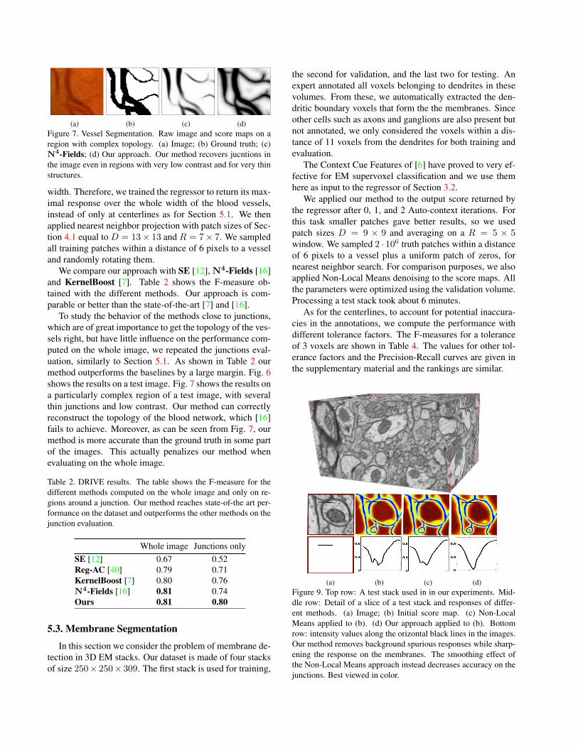
(a) (b) (c) (d)Figure 7. Vessel Segmentation. Raw image and score maps on aregion with complex topology. (a) Image; (b) Ground truth; (c)N4-Fields; (d) Our approach. Our method recovers jucntions inthe image even in regions with very low contrast and for very thinstructures.

width. Therefore, we trained the regressor to return its max-imal response over the whole width of the blood vessels,instead of only at centerlines as for Section 5.1. We thenapplied nearest neighbor projection with patch sizes of Sec-tion 4.1 equal to D = 13× 13 and R = 7× 7. We sampledall training patches within a distance of 6 pixels to a vesseland randomly rotating them.

We compare our approach with SE [12], N4-Fields [16]and KernelBoost [7]. Table 2 shows the F-measure ob-tained with the different methods. Our approach is com-parable or better than the state-of-the-art [7] and [16].

To study the behavior of the methods close to junctions,which are of great importance to get the topology of the ves-sels right, but have little influence on the performance com-puted on the whole image, we repeated the junctions eval-uation, similarly to Section 5.1. As shown in Table 2 ourmethod outperforms the baselines by a large margin. Fig. 6shows the results on a test image. Fig. 7 shows the results ona particularly complex region of a test image, with severalthin junctions and low contrast. Our method can correctlyreconstruct the topology of the blood network, which [16]fails to achieve. Moreover, as can be seen from Fig. 7, ourmethod is more accurate than the ground truth in some partof the images. This actually penalizes our method whenevaluating on the whole image.

Table 2. DRIVE results. The table shows the F-measure for thedifferent methods computed on the whole image and only on re-gions around a junction. Our method reaches state-of-the art per-formance on the dataset and outperforms the other methods on thejunction evaluation.

Whole image Junctions onlySE [12] 0.67 0.52Reg-AC [40] 0.79 0.71KernelBoost [7] 0.80 0.76N4-Fields [16] 0.81 0.74Ours 0.81 0.80

5.3. Membrane Segmentation

In this section we consider the problem of membrane de-tection in 3D EM stacks. Our dataset is made of four stacksof size 250× 250× 309. The first stack is used for training,

the second for validation, and the last two for testing. Anexpert annotated all voxels belonging to dendrites in thesevolumes. From these, we automatically extracted the den-dritic boundary voxels that form the the membranes. Sinceother cells such as axons and ganglions are also present butnot annotated, we only considered the voxels within a dis-tance of 11 voxels from the dendrites for both training andevaluation.

The Context Cue Features of [6] have proved to very ef-fective for EM supervoxel classification and we use themhere as input to the regressor of Section 3.2.

We applied our method to the output score returned bythe regressor after 0, 1, and 2 Auto-context iterations. Forthis task smaller patches gave better results, so we usedpatch sizes D = 9 × 9 and averaging on a R = 5 × 5window. We sampled 2 · 106 truth patches within a distanceof 6 pixels to a vessel plus a uniform patch of zeros, fornearest neighbor search. For comparison purposes, we alsoapplied Non-Local Means denoising to the score maps. Allthe parameters were optimized using the validation volume.Processing a test stack took about 6 minutes.

As for the centerlines, to account for potential inaccura-cies in the annotations, we compute the performance withdifferent tolerance factors. The F-measures for a toleranceof 3 voxels are shown in Table 4. The values for other tol-erance factors and the Precision-Recall curves are given inthe supplementary material and the rankings are similar.

(a) (b) (c) (d)Figure 9. Top row: A test stack used in in our experiments. Mid-dle row: Detail of a slice of a test stack and responses of differ-ent methods. (a) Image; (b) Initial score map. (c) Non-LocalMeans applied to (b). (d) Our approach applied to (b). Bottomrow: intensity values along the orizontal black lines in the images.Our method removes background spurious responses while sharp-ening the response on the membranes. The smoothing effect ofthe Non-Local Means approach instead decreases accuracy on thejunctions. Best viewed in color.

(a) (b) (c) (d) (e)

Table 3. BSDS dataset results.

ODS OIS APSCG [34] 0.74 0.76 0.77SE [12] 0.74 0.76 0.80N4-Fields [16] 0.75 0.77 0.78Ours 0.76 0.78 0.76

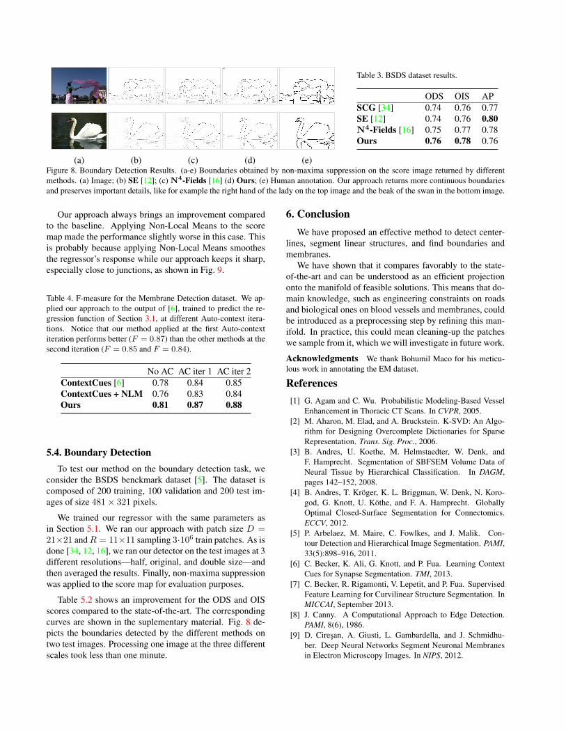
Figure 8. Boundary Detection Results. (a-e) Boundaries obtained by non-maxima suppression on the score image returned by differentmethods. (a) Image; (b) SE [12]; (c) N4-Fields [16] (d) Ours; (e) Human annotation. Our approach returns more continuous boundariesand preserves important details, like for example the right hand of the lady on the top image and the beak of the swan in the bottom image.

Our approach always brings an improvement comparedto the baseline. Applying Non-Local Means to the scoremap made the performance slightly worse in this case. Thisis probably because applying Non-Local Means smoothesthe regressor’s response while our approach keeps it sharp,especially close to junctions, as shown in Fig. 9.

Table 4. F-measure for the Membrane Detection dataset. We ap-plied our approach to the output of [6], trained to predict the re-gression function of Section 3.1, at different Auto-context itera-tions. Notice that our method applied at the first Auto-contextiteration performs better (F = 0.87) than the other methods at thesecond iteration (F = 0.85 and F = 0.84).

No AC AC iter 1 AC iter 2ContextCues [6] 0.78 0.84 0.85ContextCues + NLM 0.76 0.83 0.84Ours 0.81 0.87 0.88

5.4. Boundary DetectionTo test our method on the boundary detection task, we

consider the BSDS benckmark dataset [5]. The dataset iscomposed of 200 training, 100 validation and 200 test im-ages of size 481× 321 pixels.

We trained our regressor with the same parameters asin Section 5.1. We ran our approach with patch size D =21×21 andR = 11×11 sampling 3·106 train patches. As isdone [34, 12, 16], we ran our detector on the test images at 3different resolutions—half, original, and double size—andthen averaged the results. Finally, non-maxima suppressionwas applied to the score map for evaluation purposes.

Table 5.2 shows an improvement for the ODS and OISscores compared to the state-of-the-art. The correspondingcurves are shown in the suplementary material. Fig. 8 de-picts the boundaries detected by the different methods ontwo test images. Processing one image at the three differentscales took less than one minute.

6. ConclusionWe have proposed an effective method to detect center-

lines, segment linear structures, and find boundaries andmembranes.

We have shown that it compares favorably to the state-of-the-art and can be understood as an efficient projectiononto the manifold of feasible solutions. This means that do-main knowledge, such as engineering constraints on roadsand biological ones on blood vessels and membranes, couldbe introduced as a preprocessing step by refining this man-ifold. In practice, this could mean cleaning-up the patcheswe sample from it, which we will investigate in future work.

Acknowledgments We thank Bohumil Maco for his meticu-lous work in annotating the EM dataset.

References[1] G. Agam and C. Wu. Probabilistic Modeling-Based Vessel

Enhancement in Thoracic CT Scans. In CVPR, 2005.[2] M. Aharon, M. Elad, and A. Bruckstein. K-SVD: An Algo-

rithm for Designing Overcomplete Dictionaries for SparseRepresentation. Trans. Sig. Proc., 2006.

[3] B. Andres, U. Koethe, M. Helmstaedter, W. Denk, andF. Hamprecht. Segmentation of SBFSEM Volume Data ofNeural Tissue by Hierarchical Classification. In DAGM,pages 142–152, 2008.

[4] B. Andres, T. Kroger, K. L. Briggman, W. Denk, N. Koro-god, G. Knott, U. Kothe, and F. A. Hamprecht. GloballyOptimal Closed-Surface Segmentation for Connectomics.ECCV, 2012.

[5] P. Arbelaez, M. Maire, C. Fowlkes, and J. Malik. Con-tour Detection and Hierarchical Image Segmentation. PAMI,33(5):898–916, 2011.

[6] C. Becker, K. Ali, G. Knott, and P. Fua. Learning ContextCues for Synapse Segmentation. TMI, 2013.

[7] C. Becker, R. Rigamonti, V. Lepetit, and P. Fua. SupervisedFeature Learning for Curvilinear Structure Segmentation. InMICCAI, September 2013.

[8] J. Canny. A Computational Approach to Edge Detection.PAMI, 8(6), 1986.

[9] D. Ciresan, A. Giusti, L. Gambardella, and J. Schmidhu-ber. Deep Neural Networks Segment Neuronal Membranesin Electron Microscopy Images. In NIPS, 2012.

[10] A. Criminisi, P. Perez, and K. Toyama. Region Filling andObject Removal by Exemplar-Based Image Inpainting. TIP,2004.

[11] K. Dabov, A. Foi, and V. Katkovnik. Image Denoising bySparse 3D Transformation-Domain Collaborative Filtering.JMLR, 16(8):1–16, August 2007.

[12] P. Dollar and C. L. Zitnick. Fast Edge Detection Using Struc-tured Forests. PAMI, 2015.

[13] A. H. Foruzan, R. A. Zoroofi, Y. Sato, and M. Hori. AHessian-Based Filter for Vascular Segmentation of NoisyHepatic CT Scans. International Journal of Computer As-sisted Radiology and Surgery, 7(2):199–205, 2012.

[14] A. Frangi, W. Niessen, K. Vincken, and M. Viergever. Mul-tiscale Vessel Enhancement Filtering. Lecture Notes in Com-puter Science, 1496:130–137, 1998.

[15] J. Funke, D. Andres, F. A. Hamprecht, A. Cardona, andM. Cook. Efficient Automatic 3D-Reconstruction of Branch-ing Neurons from EM Data. CVPR, 2012.

[16] Y. Ganin and V. Lempitsky. n4-Fields: Neural NetworkNearest Neighbor Fields for Image Transforms. In ACCV,2014.

[17] G. Gonzalez, F. Aguet, F. Fleuret, M. Unser, and P. Fua.Steerable Features for Statistical 3D Dendrite Detection. InMICCAI, pages 625–32, September 2009.

[18] T. Hastie, R. Tibshirani, and J. Friedman. The Elements ofStatistical Learning. Springer, 2001.

[19] V. Jain, J. Murray, F. Roth, S. Turaga, V. Zhigulin, K. Brig-gman, M. Helmstaedter, W. Denk, and H. Seung. Super-vised Learning of Image Restoration with ConvolutionalNetworks. In ICCV, pages 1–8, 2007.

[20] P. Kontschieder, S. Bulo, H. Bischof, and M. Pelillo. Struc-tured Class-Labels in Random Forests for Semantic ImageLabelling. In ICCV, 2011.

[21] P. Kontschieder, S. R. Bulo, M. Donoser, M. Pelillo, andH. Bischof. Semantic Image Labelling as a Label PuzzleGame. In BMVC, 2011.

[22] M. Law and A. Chung. Three Dimensional CurvilinearStructure Detection Using Optimally Oriented Flux. InECCV, 2008.

[23] Y. LeCun, L. Bottou, Y. Bengio, and P. Haffner. Gradient-Based Learning Applied to Document Recognition. PIEEE,1998.

[24] J. Lim, C. L. Zitnick, and P. Dollar. Sketch Tokens: ALearned Mid-Level Representation for Contour and ObjectDetection. In CVPR, 2013.

[25] J. Mairal, F. Bach, J. Ponce, G. Sapiro, and A. Zisserman.Non-Local Sparse Models for Image Restoration. In ICCV,2009.

[26] D. Marr and E. Hildreth. Theory of Edge Detection. Pro-ceedings of the Royal Society of London, Biological Sci-ences, 207(1167):187–217, 1980.

[27] A. Martinez-Sanchez, I. Garcia, and J. Fernandez. A Ridge-Based Framework for Segmentation of 3D Electron Mi-croscopy Datasets. Journal of Structural Biology, 2013.

[28] E. Meijering, M. Jacob, J.-C. F. Sarria, P. Steiner, H. Hirling,and M. Unser. Design and Validation of a Tool for NeuriteTracing and Analysis in Fluorescence Microscopy Images.Cytometry Part A, 58A(2):167–176, April 2004.

[29] H. Mirzaalian, T. Lee, and G. Hamarneh. Hair Enhance-ment in Dermoscopic Images Using Dual-Channel Quater-nion Tubularness Filters and MRF-Based Multi-Label Opti-mization. TIP, 2014.

[30] K. Mosaliganti, F. Janoos, A. Gelas, R. Noche, N. Obholzer,R. Machiraju, and S. Megason. Anisotropic Plate DiffusionFiltering for Detection of Cell Membranes in 3D MicroscopyImages. In ICBI, 2010.

[31] M. Muja and D. G. Lowe. Scalable Nearest Neighbor Algo-rithms for High Dimensional Data. PAMI, 2014.

[32] W. Neuenschwander, P. Fua, G. Szekely, and O. Kubler. Ini-tializing Snakes. In CVPR, pages 613–615, June 1994.

[33] M. Pechaud, G. Peyre, and R. Keriven. Extraction of TubularStructures over an Orientation Domain. In CVPR, 2009.

[34] X. Ren and L. Bo. Discriminatively Trained Sparse CodeGradients for Contour Detection. In NIPS, December 2012.

[35] J. Salmon and Y. Strozecki. Patch Reprojections for NonLocal Methods. Signal Processing, 2012.

[36] A. Santamarıa-Pang, T. Bildea, C. M. Colbert, P. Saggau, andI. Kakadiaris. Towards Segmentation of Irregular TubularStructures in 3D Confocal Microscope Images. In MICCAIWorkshop in Microscopic Image Analysis and Applicationsin Biology, 2006.

[37] Y. Sato, C.-F. Westin, A. Bhalerao, S. Nakajima, N. Shiraga,S. Tamura, and R. Kikinis. Tissue Classification Based on3D Local Intensity Structure for Volume Rendering. IEEETrans. on Visualization and Computer Graphics, 2000.

[38] M. Seyedhosseini, M. Sajjadi, and T. Tasdizen. Image Seg-mentation with Cascaded Hierarchical Models and LogisticDisjunctive Normal Networks. In ICCV, 2013.

[39] A. Sironi, V. Lepetit, and P. Fua. Multiscale Centerline De-tection by Learning a Scale-Space Distance Transform. InCVPR, 2014.

[40] A. Sironi, E. Turetken, V. Lepetit, and P. Fua. MultiscaleCenterline Detection. PAMI, 2015.

[41] M. Sofka and C. Stewart. Retinal Vessel Centerline Extrac-tion Using Multiscale Matched Filters, Confidence and EdgeMeasures. TMI, 2006.

[42] J. Staal, M. Abramoff, M. Niemeijer, M. Viergever, andB. van Ginneken. Ridge Based Vessel Segmentation in ColorImages of the Retina. TMI, 2004.

[43] Z. Tu and X. Bai. Auto-Context and Its Applications toHigh-Level Vision Tasks and 3D Brain Image Segmentation.PAMI, 2009.

[44] E. Turetken, C. Becker, P. Glowacki, F. Benmansour, andP. Fua. Detecting Irregular Curvilinear Structures in GrayScale and Color Imagery Using Multi-Directional OrientedFlux. In ICCV, December 2013.

[45] A. Vazquez-Reina, M. Gelbart, D. Huang, J. Lichtman,E. Miller, and H. Pfister. Segmentation Fusion for Connec-tomics. In ICCV, 2011.

[46] J. D. Wegner, J. A. Montoya-Zegarra, and K. Schindler. AHigher-Order CRF Model for Road Network Extraction. InCVPR, 2013.

[47] Y. Zheng, M. Loziczonek, B. Georgescu, S. Zhou, F. Vega-Higuera, and D. Comaniciu. Machine Learning Based Ves-selness Measurement for Coronary Artery Segmentation inCardiac CT Volumes. SPIE, 7962(1):79621–7962112, 2011.