projection methods - school of arts & sciences | school of

Projection Methods

(Lectures on Solution Methods for Economists IV)

Jesus Fernandez-Villaverde1 and Pablo Guerron2

November 21, 2021

1University of Pennsylvania

2Boston College

Introduction

• Remember that we want to solve a functional equations of the form:

H (d) = 0

for an unknown decision rule d .

• Projection methods solve the problem by specifying:

dn (x , θ) =n∑

i=0

θiΨi (x)

We pick a basis Ψi (x)∞i=0 and “project” H (·) against that basis to find the θi ’s.

• We work with linear combinations of basis functions because theory of nonlinear approximations is

not as developed as the linear case.

1

Algorithm

1. Define n + 1 known linearly independent functions ψi : Ω→ Rm, where n <∞. We call the

ψ0 (·) , ψ1 (·) , ..., ψn (·) the basis functions.

2. Define a vector of coefficients θ = [θ0, θ1, ..., θn].

3. Define a combination of the basis functions and the θ’s:

dn ( ·| θ) =n∑

i=0

θiψn (·)

4. Plug dn ( ·| θ) into H (·) to find the residual equation:

R ( ·| θ) = H (dn ( ·| θ))

5. Find θ that make the residual equation as close to 0 as possible given some objective function

ρ : J1 × J1 → J2:

θ = arg minθ∈Rn

ρ (R ( ·| θ) , 0)2

Figure 1: Insert Title Here

R(·|θ1)

R(·|θ)

k

R(·|θ2)

k

1

3

Relation with econometrics

• Looks a lot like OLS. Explore this similarity later in more detail.

• Also with semi-nonparametric methods as Sieves.

• Compare with:

1. Policy iteration.

2. Parameterized Expectations.

4

Two issues

• We need to decide:

1. Which basis we use?

1.1 Pick a global basis⇒spectral methods.

1.2 Pick a local basis⇒finite elements methods.

2. How do we “project”?

• Different choices in 1 and 2 will result in slightly different projection methods.

• We can mix projection and perturbation methods in mixed approaches.

5

Spectral methods

• Main reference: Judd (1992).

• Spectral techniques use basis functions that are nonzero and smooth almost everywhere in Ω.

• Advantages: simplicity.

• Disadvantages: difficult to capture local behavior. Gibbs phenomenon.

• Let us start first with unidimensional problems (trick with discretization).

6

Figure 1: Title

Xt

Xt+1

(a) Square Wave Function

Xt

Xt+1

(b) 10 Terms Approximation

1

7


kt+1

kt

1

8

Monomials

c , x , x2, x3, ...

• Simple and intuitive.

• If J1 is the space of bounded measurable functions on a compact set, the Stone-Weierstrass theorem

assures completeness in the L1 norm.

• Problems:

1. (Nearly) multicollinearity. Compare the graph of x10 with x11.

The LS problem of fitting a polynomial of degree 6 to a function (the Hilbert Matrix) is a popular test

of numerical accuracy since it maximizes rounding errors!

2. Monomials vary considerably in size, leading to scaling problems and accumulation of numerical errors.

• We want an orthogonal basis. Why?9

Trigonometric series

1/ (2π)0.5, cos x/ (2π)0.5

, sin x/ (2π)0.5, ...,

cos kx/ (2π)0.5, sin kx/ (2π)0.5

, ...

• Periodic functions.

• However economic problems are generally not periodic.

• Periodic approximations to nonperiodic functions suffer from the Gibbs phenomenon: the rate of

convergence to the true solution as n→∞ is only O (n).

11

Orthogonal polynomials

• Flexible class of orthogonal polynomials of Jacobi (or hypergeometric) type.

• The Jacobi polynomial of degree n, Pα,βn (x) for α, β > −1, is defined by the orthogonality condition:∫ 1

−1

(1− x)α (1 + x)β Pα,βn (x)Pα,βm (x) dx = 0 for m 6= n

• The two most important cases of Jacobi polynomials:

1. Legendre: α = β = − 12.

2. Chebyshev: α = β = 0.

12

Alternative expressions

• The orthogonality condition implies, with the customary normalizations:

Pα,βn (1) =

(n + α

n

)

that the general n term is given by:

2−nn∑

k=0

(n + α

k

)(n + β

n − k

)(x − 1)n−k (x + 1)k

• Recursively:

2 (n + 1) (n + α + β + 1) (2n + α + β)Pn+1 =((2n + α + β + 1)

(α2 − β2

)+ (2n + α + β) (2n + α + β + 1) (2n + α + β + 2) x

)Pn

−2 (n + α) (n + β) (2n + α + β + 2)Pn−113

Chebyshev polynomials

• One of the most common tools of applied mathematics.

• References:

• Chebyshev and Fourier Spectral Methods, John P. Boyd (2001).

• A Practical Guide to Pseudospectral Methods, Bengt Fornberg (1998).

• Advantages of Chebyshev Polynomials:

1. Numerous simple close-form expressions are available.

2. They are more robust than their alternatives for interpolation.

3. They are bounded between [−1, 1].

4. They are smooth functions.

5. The move between the coefficients of a Chebyshev expansion of a function and the values of the

function at the Chebyshev nodes quickly performed by the cosine transform.

6. Several theorems bound the errors for Chebyshev polynomials interpolations.14

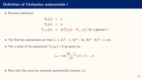
Definition of Chebyshev polynomials I

• Recursive definition:

T0 (x) = 1

T1 (x) = x

Tn+1 (x) = 2xTn (x)− Tn−1 (x) for a general n

• The first few polynomials are then 1, x , 2x2 − 1, 4x3 − 3x , 8x4 − 8x2 + 1, etc...

• The n zeros of the polynomial Tn (xk) = 0 are given by:

xk = cos2k − 1

2nπ, k = 1, ..., n

• Note that this zeros are clustered quadratically towards ±1.

15

-1 -0.5 0 0.5 10

0.5

1

1.5

2Chebyshev Polynomial of Order 0

-1 -0.5 0 0.5 1-1

-0.5

0

0.5


-1 -0.5 0 0.5 1-1

-0.5

0

0.5


-1 -0.5 0 0.5 1-1

-0.5

0

0.5


-1 -0.5 0 0.5 1-1

-0.5

0

0.5


-1 -0.5 0 0.5 1-1

-0.5

0

0.5


16

Definition of Chebyshev polynomials II

• Explicit definition:

Tn (x) = cos (n arccos x)

=1

2

(zn +

1

zn

)where

1

2

(z +

1

z

)= x

=1

2

((x +

(x2 − 1

)0.5)n

+(x −

(x2 − 1

)0.5)n)

=1

2

[n/2]∑k=0

(−1)k(n − k − 1)!

k! (n − 2k)!(2x)n−2k

=(−1)n π0.5

2nΓ(n + 1

2

) (1− x2)0.5 dn

dxn

((1− x2

)n− 12

)

17

Remarks

• The domain of the Chebyshev polynomials is [−1, 1]. Since our state space is, in general, different,

we use a linear translation from [a, b] into [−1, 1]:

2x − a

b − a− 1

• Chebyshev polynomials are orthogonal with respect to the weight function:

1

(1− x2)0.5

Chebyshev Interpolation Theorem

If an approximating function is exact at the roots of the nth order Chebyshev polynomial then, as

n→∞, the approximation error becomes arbitrarily small.

18

Multidimensional problems

• Chebyshev polynomials are defined on [−1, 1].

• However, most problems in economics are multidimensional.

• How do we generalize the basis?

• Curse of dimensionality.

19

Tensors

• Assume we want to approximate F : [−1, 1]d → R.

• Let Tj denote the Chebyshev polynomial of degree j = 0, 1, .., κ.

• We can approximate F with tensor product of Chebyshev polynomials of degree κ:

F (x) =κ∑

n1=0

. . .κ∑

nd=0

θn1,...,ndTn1 (x1) · · ·Tnd (xd)

• Beyond simplicity, an advantage of the tensor basis is that if the one-dimensional basis is orthogonal

in a norm, the tensor basis is orthogonal in the product norm.

• Disadvantage: number of elements increases exponentially. We end up having terms xκ1 xκ2 · · · xκd ,

total number of (κ+ 1)d .

20

Complete polynomials

• Solution: eliminate some elements of the tensor in such a way that there is no much numerical

degradation.

• Judd and Gaspar (1997): Use complete polynomials

Pdκ ≡

x i11 · · · x idd with

d∑l=1

il ≤ κ, 0 ≤ i1, ..., id

• Advantage: much smaller number of terms, no terms of order dκ to evaluate.

• Disadvantage: still too many elements.

21

Smolyak’s algorithm I

• Define m1 = 1 and mi = 2i−1 + 1, i = 2, ....

• Define G i = x i1, ..., x imi ⊂ [−1, 1] as the set of the extrema of the Chebyshev polynomials

x ij = −cos(π(j − 1)

mi − 1

)j = 1, ...,mi

with G 1 = 0. It is crucial that G i ⊂ G i+1, ∀i = 1, 2, . . .

• Example:

i = 1, mi = 1, G i = 0i = 2, mi = 3, G i = −1, 0, 1

i = 3, mi = 5, G i = −1,− cos(π

4

), 0,− cos

(3π

4

), 1

22

Smolyak’s algorithm II

• For q > d , define a sparse grid

H(q, d) =⋃

q−d+1≤|i|≤q

(G i1 × ...× G id ),

where |i | = i1 + . . .+ id .

• The number q defines the size of the grid and thus the precision of the approximation.

23

Smolyak’s algorithm III

• For example, let q = d + 2 = 5:

H(5, 3) =⋃

3≤|i|≤5

(G i1 × ...× G id ).

G3 × G1 × G1, G1 × G3 × G1, G1 × G1 × G3

G2 × G2 × G1, G2 × G1 × G2, G1 × G2 × G2

G2 × G1 × G1, G1 × G2 × G1, G1 × G1 × G2

G1 × G1 × G1

24

Figure 1: Grids G(3, 2), G(4, 2), G(5, 2), and G(6, 2)

25

Smolyak’s algorithm IV

• Number of points for q = d + 2

1 + 4d + 4d(d − 1)

2

• Largest number of points along one dimension

i = q − d + 1

mi = 2q−d + 1

• Rectangular grid [2q−d + 1

]d• Key: with rectangular grid, the number of grid points increases exponentially in the number of

dimensions. With the Smolyak algorithm number of points increases polynomially in the number of

dimensions.

27

Smolyak’s algorithm V

Size of the Grid for q = d + 2

d 2q−d + 1 #H(q, d)[2q−d + 1

]d2 5 13 25

3 5 25 125

4 5 41 625

5 5 61 3, 125

12 5 313 244, 140, 625

28

Smolyak’s algorithm VI

• For one dimension, denote the interpolating Chebyshev polynomials as

U i (x i ) =

mi∑j=1

θijTj(xi )

and the d-dimensional tensor product by U i1 ⊗ ...⊗ U id (x).

• For q > d , the approximating function (Smolyak’s algorithm) is:

A(q, d)(x) =∑

q−d+1≤|i|≤q

(−1)q−|i|

(d − 1

q − |i |

)(U i1 ⊗ . . .⊗ U id )(x)

• (Almost) optimal within the set of polynomial approximations (Barthelmann, Novak, and Ritter,

1999).

• Method is universal, that is, almost optimal for many different function spaces.

29

Boyd’s moral principal

1. When in doubt, use Chebyshev polynomials unless the solution is spatially periodic, in which case an

ordinary Fourier series is better.

2. Unless you are sure another set of basis functions is better, use Chebyshev polynomials.

3. Unless you are really, really sure another set of basis functions is better, use Chebyshev polynomials.

30

Finite elements

• Standard reference: McGrattan (1999).

• Bound the domain Ω of the state variables.

• Partition Ω in small in nonintersecting elements.

• These small sections are called elements.

• The boundaries of the elements are called nodes.

31

Partition into elements

• Elements may be of unequal size.

• We can have small elements in the areas of Ω where the economy will spend most of the time while

just a few, big size elements will cover wide areas of the state space infrequently visited.

• Also, through elements, we can easily handle issues like kinks or constraints.

• There is a whole area of research concentrated on the optimal generation of an element grid. See

Thomson, Warsi, and Mastin (1985).

32

Structure

• Choose a basis for the policy functions in each element.

• Since the elements are small, a linear basis is often good enough:

ψi (k) =

x−xi−1

xi−xi−1if x ∈ [xi−1, xi ]

xi+1−xxi+1−xi if k ∈ [xi , xi+1]

0 elsewhere

• Plug the policy function in the Equilibrium Conditions and find the unknown coefficients.

• Paste it together to ensure continuity.

• Why is this an smart strategy?

• Advantages: we will need to invert an sparse matrix.

• When should be choose this strategy? speed of computation versus accuracy.

33


kt+1

kt

1

34


bt

kt

1

35


bt+1

kt

1

36

Three different refinements

1. h-refinement: subdivide each element into smaller elements to improve resolution uniformly over the

domain.

2. r-refinement: subdivide each element only in those regions where there are high nonlinearities.

3. p-refinement: increase the order of the approximation in each element. If the order of the expansion

is high enough, we will generate in that way an hybrid of finite and spectral methods knows as

spectral elements.

37

Objective function

• The most common answer to the second question is given by a weighted residual.

• That is why often projection methods are also called weighted residual methods

• This set of techniques propose to get the residual close to 0 in the weighted integral sense.

• Given some weight functions φi : Ω→ Rm:

ρ (R ( ·| θ) , 0) =

0 if

∫Ωφi (x)R ( ·| θ) dx = 0, i = 0, .., n

1 otherwise

• Then the problem is to choose the θ that solve the system of equations:∫Ω

φi (x)R ( ·| θ) dx = 0, i = 0, .., n

38

Remarks

• With the approximation of d by some functions ψi and the definition of some weight functions φi (·),

we have transform a rather intractable functional equation problem into the standard nonlinear

equations system!

• The solution of this system can be found using standard methods, as a Newton for relatively small

problems or a conjugate gradient for bigger ones.

• Issue: we have different choices for an weight function.

39

Weight function I: Least Squares

• φi (x) = ∂R( x|θ)∂θi

.

• This choice is motivated by the solution of the variational problem:

minθ

∫Ω

R2 ( ·| θ) dx

with first-order condition: ∫Ω

∂R (x | θ)

∂θiR ( ·| θ) dx = 0, i = 0, .., n

• Variational problem is mathematically equivalent to a standard regression problem in econometrics.

• OLS or NLLS are regression against a manifold spanned by the observations.

40

Weight function I: Least Squares

• Least Squares always generates symmetric matrices even if the operator H is not self-adjoint.

• Symmetric matrices are convenient theoretically (they simplify the proofs) and computationally (there

are algorithms that exploit their structure to increase speed and decrease memory requirements).

• However, least squares may lead to ill-conditioning and systems of equations complicated to solve

numerically.

41

Weight Function II: Subdomain

• We divide the domain Ω in n subdomains Ωi and define the n step functions:

φi (x) =

1 if x ∈ Ωi

0 otherwise

• This choice is then equivalent to solve the system:∫Ωi

R ( ·| θ) dx = 0, i = 0, .., n

42

Weight function III: Moments

• Take

0, x , x2, ..., xn−1

and compute the first n periods of the residual function:∫Ωi

x iR ( ·| θ) dx = 0, i = 0, .., n

• This approach, widely used in engineering works well for a low n (2 or 3).

• However, for higher orders, its numerical performance is very low: high orders of x are highly collinear

and arise serious rounding error problems.

• Hence, moments are to be avoided as weight functions.

43

Weight function IV: Collocation or pseudospectral

• φi (x) = δ (x − xi ) where δ is the dirac delta function and xi are the collocation points.

• This method implies that the residual function is zero at the n collocation points.

• Simple to compute since the integral only needs to be evaluated in one point. Specially attractive

when dealing with strong nonlinearities.

• A systematic way to pick collocation points is to use a density function:

µγ (x) =Γ(

32 − γ

)(1− x2)γ π

12 Γ (1− γ)

γ < 1

and find the collocation points as the xj , j = 0, ..., n solutions to:∫ xj

−1

µγ (x) dx =j

n

• For γ = 0, the density function implies equispaced points.

44

Weight Function V: Orthogonal collocation

• Variation of the collocation method:

1. Basis functions are a set of orthogonal polynomials.

2. Collocation points given by the roots of the n − th polynomial.

• When we use Chebyshev polynomials, their roots are the collocation points implied by µ 12

(x) and

their clustering can be shown to be optimal as n→∞.

• Surprisingly good performance of orthogonal collocation methods.

45

Weight function VI: Galerkin or Rayleigh-Ritz

• φi (x) = ψi (x) with a linear approximating function∑n

i=0 θiψi (x).

• Then: ∫Ω

ψi (x)H(

n∑i=0

θiψi (x)

)dx = 0, i = 0, .., n

that is, the residual has to be orthogonal to each of the basis functions.

• Galerkin is a highly accurate and robust but difficult to code.

• If the basis functions are complete over J1 (they are indeed a basis of the space), then the Galerkin

solution will converge pointwise to the true solution as n goes to infinity:

limn→∞

n∑i=0

θiψi (·) = d (·)

• Experience suggests that a Galerkin approximation of order n is as accurate as a Pseudospectral n + 1

or n + 2 expansion.

46

A simple example

• Imagine that the law of motion for the price x of a good is given by:

d ′ (x) + d (x) = 0

• Let us apply a simple projection to solve this differential equation.

• Code: test.m, test2.m, test3.m.

• Let’s try a more serious example.

47

The stochastic neoclassical growth model

• Model:

maxE0

∞∑t=0

βt

(cνt (1− lt)

1−ν)1−γ

1− γ

ct + kt+1 = eztkαt l1−αt + (1− δ) kt , ∀ t > 0

zt = λzt−1 + σεt , εt ∼ N (0, 1)

• Solve for c (·, ·) and l (·, ·) given initial conditions.

• Characterized by:

Uc(t) = βEt

[Uc(t + 1)

(1 + αezt+1kα−1

t+1 l(kt+1, zt+1)α − δ)]

1− νν

c(kt , zt)

1− l(kt , zt)= (1− α) eztkαt l(kt , zt)

−α

• No close-form solution. 48

Chebyshev I

• We approximate the decision rules for labor as lt =∑n

i=1 θiψi (kt , zt) where ψi (k, z)ni=1 are basis

functions and θ =[θini=1

]unknown coefficients.

• We use that policy function to solve for consumption using the static first-order condition.

• We build a residual function R (k , z , θ) using the Euler equation and the static first order condition.

• Then we choose θ by solving:

∫[kmin,kmax]

∫[zmin,zmax]

φi (k , z)R (k , z , θ) = 0 for i = 1, ..., n

where φi (k , z)ni=1 are some weight functions.

49

Chebyshev II

• We use a collocation method that sets φi (k , z) = δ (k − kj , z − zv ) where δ (.) is the dirac delta

function, j = 1, ..., n1, v = 1, ..., n2 and n = n1 × n2 and collocation points kjn1

j=1 and zvn2

v=1 .

• For the technology shocks and transition probabilities we use Tauchen (1986)’s finite approximation

to an AR(1) process and obtain n2 points.

• We solve the system of n equations R (ki , zi , θ) = 0 in n unknowns θ using a Quasi-Newton method.

• We use an iteration based on the increment of the number of basis functions and a nonlinear

transform of the objective function (apply (u′)−1

).

50

Finite elements

Rewrite Euler equation as

Uc(kt , zt) =β

(2πσ)0.5

∫ ∞−∞

[Uc(kt+1, zt+1)(r(kt+1, zt+1)] exp(−ε2t+1

2σ2)dεt+1

where

Uc(t) = Uc(kt , zt)

kt+1 = ezt+1kαt l1−αt + (1− δ)kt − c(kt , zt)

r(kt+1, zt+1) = 1 + αezt+1kα−1t+1 l(kt+1, zt+1)1−α − δ

and

zt+1 = ρzt + εt+1

51

Goal

• The problem is to find two policy functions c(k , z) : R+ × [0,∞]→ R+ and

l(k, z) : R+ × [0,∞]→ [0, 1] that satisfy the model equilibrium conditions.

• Since the static first order condition gives a relation between the two policy functions, we only need

to solve for one of them.

• For the rest of the exposition we will assume that we actually solve for l(k, z) and then we find

c (l(k, z)).

52

Bounding the state space I

• We bound the domain of the state variables to partition it in nonintersecting elements.

• To bound the productivity level of the economy define λt = tanh(zt).

• Since λt ∈ [−1, 1] we can write the stochastic process as:

λt = tanh(ρ tanh−1(zt−1) + 20.5σvt)

where vt = εt20.5σ .

53

Bounding the state space II

• Now, since exp(tanh−1(zt−1)) = (1+λt+1)0.5

(1−λt+1)0.5 = λt+1, we have:

Uc(t) =β

π0.5

∫ 1

−1

[Uc(kt+1, zt+1)r(kt+1, zt+1)] exp(−v2t+1)dvt+1

where

kt+1 = λt+1kαt l (kt , zt)

1−α + (1− δ)kt − c (l(kt , zt))

r(kt+1, zt+1) = 1 + αλt+1kα−1t+1 l(kt+1, zt+1)1−α − δ

and zt+1 = tanh(ρ tanh−1(zt) + 20.5σvt+1).

• To bound the capital we fix an ex-ante upper bound kmax, picked sufficiently high that it will only

bind with an extremely low probability.

54

Partition into elements

• Define Ω = [0, kmax]× [−1, 1] as the domain of lfe(k , z ; θ).

• Divide Ω into nonoverlapping rectangles [ki , ki+1]× [zj , zj+1], where ki is the ith grid point for capital

and zj is jth grid point for the technology shock.

• Clearly, Ω = ∪i,j [ki , ki+1]× [zj , zj+1].

55

Our functional basis

• Set lfe (k, z ; θ) =∑

i,j θijΨij (k , z) =∑

i,j θijΨi (k) Ψj (z) where

Ψi (k) =

k−ki−1

ki−ki−1if k ∈ [ki−1, ki ]

ki+1−kki+1−ki if k ∈ [ki , ki+1]

0 elsewhere

Ψj (z) =

z−zj−1

zj−zj−1if z ∈ [zj−1, zj ]

zj+1−zzj+1−zj if z ∈ [zj , zj+1]

0 elsewhere

• Note that:

1. Ψij (k, z) = 0 if (k, z) /∈ [ki−1, ki ]× [zj−1, zj ]∪ [ki , ki+1]× [zj , zj+1] ∀i , j , i.e., the function is 0 everywhere

except inside two elements.

2. lfe(ki , zj ; θ) = θij ∀i , j , i.e., the values of θ specify the values of cfe at the corners of each subinterval

[ki , ki+1]× [zj , zj+1]. 56

Residual function I

• Define Uc(kt+1, zt+1)fe as the marginal utility of consumption evaluated at the finite element

approximation values of consumption and leisure.

• From the Euler equation we have a residual equation:

R(kt , zt ; θ) =

β

π0.5

∫ 1

−1

[Uc(kt+1, zt+1)feUc(kt+1, zt+1)fe

r(kt+1, zt+1)

]exp(−v2

t+1)dvt+1 − 1

• A Galerkin scheme implies that we weight the residual function by the basis functions and solve the

system of θ equations ∫[0,kmax]×[−1,1]

Ψi,j (k , z)R(k , z ; θ)dzdk = 0 ∀i , j

on the θ unknowns.

57

Residual function II

• Since Ψij (k, z) = 0 if (k , z) /∈ [ki−1, ki ]× [zj−1, zj ] ∪ [ki , ki+1]× [zj , zj+1] ∀i , j we have∫[ki−1,ki ]×[zj−1,zj ]∪[ki ,ki+1]×[zj ,zj+1]

Ψi,j (k, z)R(k, z ; θ)dzdk = 0 ∀i , j

• We use Gauss-Hermite for the integral in the residual equation and Gauss-Legendre for the integrals

in Euler equation.

• We use 71 unequal elements in the capital dimension and 31 on the λ axis.

• To solve the associated system of 2201 nonlinear equations we use a Quasi-Newton algorithm.

58

Analysis of error

• As with projection, it is important to study the Euler equation errors.

• We can improve errors:

1. Adding additional functions in the basis.

2. Refine the elements.

• Multistep schemes.

59

projection methods - school of arts & sciences | school of

Documents