project report 3d visualization of medical imaging data

Abstract—The aim of the project is 3D surface visualization of body organs from 2D slices and sections of the body parts. The input data is in the form of CT/MRI axial slices and anatomical cryo-section images of the body parts. The object of interest is extracted from the slice data after performing an interactive thresholding. There after surface views are generated using ray-casting methods. The work would serve as tool for visualizing medical objects while fusing multi modal medical imaging data. It also aims at providing an environment for measurement and estimation of damages/ deformities in the organs.

Keywords—Ray-Casting, CT, MRI, Anatomical Cryo-Section, Surface Visualization, 3-D viewing, Volume cut, Segmentation, Thresholding

1

3-Dimensional Surface Visualization of Anatomical CT/MRI Slice Data

Shashank Singh,Bachelor of Information Technology, Eighth Semester, Indian Institute of Information Technology – Allahabad

Enrollment No. 20000048Email: [email protected]

Project Supervisor: Dr. UmaShanker TiwaryAssociate Professor

Indian Institute of Information Technology – AllahabadEmail: [email protected]

mailto:[email protected]

mailto:[email protected]

CONTENTS

I. CERTIFICATE of work.II. INTRODUCTION to project.

a. Backgroundb. About data sourcec. Visible Human Projectd. Datae. Donorsf. Problems with data setg. Discoveriesh. Licensei. About 3D imaging

i. Ray Castingii. Disadvantages

iii. Possible improvementsj. Sources of Medical Imagesk. Basics and terminologyl. Objects characteristics in images

i. Graded compositionii. Hanging-togetherness

m. Preprocessingi. Volume of interest (VOI)

ii. Filteringiii. Interpolationiv. Registrationv. Segmentation

III. METHODOLOGYa. Stepsb. Steps 1,2 and 3

i. Data Formatii. Data Directory Structure

c. Steps 4 and 5i. Threshold determination

d. Steps 6 and 7i. Ray Casting

e. Step 8IV. RESULTSV. DISCUSSIONS

VI. CONCLUSIONVII. TIME LINE

VIII. ACKNOWLEDGEMENTIX. REFERENCESX. RESOURCES

a. Booksb. web

XI. COURTESY

2

I. CERTIFICATE

Certified that the work contained in the report entitled “3-Dimensional Surface Visualization of Anatomical CT/MRI Slice Data”, by Shashank Singh (Enrollment Number 20000048), has been carried out under my supervision as his B.Tech. project, and that this work has not been submitted elsewhere for a degree.

________________________(Date)

________________________________(Signatures of the project supervisor)

Dr. Umashanker TiwaryAssociate ProfessorIndian Institute of Information Technology – ALLAHABAD

( Name of the project supervisor)

3

II. INTRODUCTION

The project aims at surface visualization and 3-dimensional viewing of anatomical CT/MRI slices. Working as a part of ‘Fusion of Multi-Modal Medical Imaging Data’ project, I would provide support for 3d viewing of object of interest from various 2d data modalities like CT, MRI slices and anatomical section images.

a. BACKGROUND:

Research in three-dimensional imaging in medicine started in the 1970s. The activity in the field became very brisk in the 1980s. During this period, the technical developments – design of algorithms, software, and machine – have galloped ahead, accompanied by a considerable increase in clinical applications, but clinical validation and the study of clinical usefulness have generally lagged behind.

Although the applications that were pursued for 3D imaging in the early 1980 s were for imaging the bone via CT, with advent of MRI in the mid-1980’s, soft-tissue 3D imaging became a hot topic. This also initiated research in the better utilization of functional imaging modalities such as PET in conjunction with CT and MRI for a variety of applications. The 1990’s saw the reemergence of CT with the advent of spiral technology, and the rapid acquisition of the 3D volume data made possible new 3D imaging applications for CT. The 1990s also witnessed rapid advances in the use of 3D imaging for interventional and surgery procedures. The difficult problem of acquiring image data and processing and analyzing them for dynamic organs also continued to be pursued with steady progress.

CT, MRI and cryo-sections provide the doctors and researchers with great tools to view at body internals. But all these imaging modalities are restricted to planar view of the body sections. But these modalities provide us with the images that can be fed into a 3D visualization machine and generate 3D views. 3D visualization of the CT, MRI, cryo-sectional data provides a revolutionary way to look at the body organs. The shape, orientations and spatial locations of organs are far better perceived in 3D views as compared to the 2D slices form which these 3D views are generated. Such visualizations can of great help in surgical operations and treatments. The deformities and damages in the organs such as those in skull fractures or disfigurement can be better studied by doctors using 3D surface visualization tools.

b. ABOUT DATA SOURCE:

For obtaining faithful 3D views the data source must be reliable and truly represent the human body. That is what made us to turn to the National Library of Medicine, USA.

c. VISIBLE HUMAN PROJECT:

In 1989, the National Library of Medicine (NLM) began an ambitious project to create a digital atlas of the human anatomy. The NLM Planning Panel on Electronic Image Libraries recommended a project to create XRAY Computed Tomography (XRAY-CT), Magnetic Resonance Imaging (MRI) and physical sections of a human cadaver. The Visible Human Project is an effort to create a detailed data set of cross-sectional photographs of the human body, in order to facilitate anatomy visualization applications. A male and a female cadaver were cut into thin slices which were then photographed and digitized. The project is run by the U. S. National Library of Medicine (NLM) under the direction of Michael J. Ackerman. Planning began in 1989; the dataset of male was released in November 1994 and the one of the Female in November 1995.

4

d. DATA:

The male cadaver was frozen and cut into 1 871 axial slices (at 1 millimeter intervals) which were then photographed and digitized, yielding 15 GB of data. In 2000, the photos were rescanned at a higher resolution, yielding more than 65 gigabytes. The female cadaver was cut into slices at .33 millimeter intervals, resulting in some 40 gigabytes of data. Each cadaver was perfused with approximately 19 liters of 1% formalin (a type of preservative /fixative used for tissue specimens) and an anticoagulant shortly after death to retard deterioration. The cadavers were placed horizontally on their backs, which resulted in the feet being pointed away from the head rather than as they would be if flat on the floor in a standing height measurement. (This adds about 3" to the apparent height, which is included in the figures mentioned above.) For fiduciary markers two 3 mm OD Tygon tubes filled with 4 millimolar copper sulfate solution and 5% Omnipaque were attached with Liquid Nails to the skin surface from head to toe. The cadaver was placed in a plywood box and surrounded with Alpha Cradle AC660 (Smithers Medical Products, Inc.) foaming agent to hold in a fixed position

The data is supplemented by axial sections of the whole body obtained by CT axial sections of the head and neck obtained by MRI and coronal sections of the rest of the body also obtained by magnetic resonance imaging.

The initial aim of the Visible Human Project® is to create a digital image dataset of complete human male and female cadavers in MRI, CT and anatomical modes.

The male dataset consists of axial MR images of the head and neck taken at 4 mm intervals and longitudinal sections of the remainder of the body also at 4 mm intervals. The resolution of the MR images is 256 pixels by 256 pixels. Each pixel has 12 bits of grey tone.

The CT data consists of axial CT scans of the entire body taken at 1 mm intervals at a resolution of 512 pixels by 512 pixels where each pixel is made up of 12 bits of grey tone. The axial anatomical images are 2048 pixels by 1216 pixels where each pixel is defined by 24 bits of color, each image consisting of about 7.5 megabytes of data. The anatomical cross-sections are also at 1 mm intervals and coincide with the CT axial images. There are 1871 cross-sections for each mode, CT and anatomy, obtained from the male cadaver.

The dataset from the female cadaver has the same characteristics as the male cadaver with one exception. The axial anatomical images were obtained at 0.33 mm intervals instead of 1.0 mm intervals. This results in over 5,000 anatomical images. The female dataset is about 40 gigabytes in size. Spacing in the "Z" direction was reduced to 0.33 mm in order to match the pixel spacing in the "XY" plane which is 0.33 mm. This enables developers who are interested in three-dimensional reconstructions to work with cubic voxels.

A recent addition to the male dataset is the inclusion of higher resolution anatomical images. 70mm film taken during the original data collection phase has been digitized at a resolution of 4096 pixels by 2700 pixels where each pixel is made up of 24 bits of color. As with the original anatomical images, there are a total of 1871 of these high resolution images.

The scanning, slicing and photographing took place at the University of Colorado’s Health Sciences Center.

5

e. THE DONORS:

The male cadaver is from Joseph Paul Jernigan, a 38-year-old, 199 lb, 5' 11'', Texas murderer who was executed by lethal injection on August 5, 1993. At the prompting of a prison chaplain he had agreed to donate his body for scientific research or medical use, without knowing about the Visible Human Project. Some people have voiced ethical concerns over this.

The female donor, 59-year-old, height 5' 5.5'', remains anonymous. In the press she has been described as a Maryland housewife who died from a heart attack and whose husband requested that she be part of the project.

f. PROBLEMS WITH DATA SETS:

Freezing caused the brain of the man to be slightly swollen and his inner ear ossicles were lost during preparation of slices. Nerves are hard to make out since they have almost the same color as fat. Small blood vessels were collapsed by the freezing process. The male had only one testicle. The reproductive organs of the woman are not representative of those of a young woman.

g. DISCOVERIES:

By studying the data set, researchers at Columbia University found several errors in anatomy textbooks, related to the shape of a muscle in the pelvic region and the location of bladder and prostate.

h. LICENSE:

The data may be bought on tape or downloaded free of charge; one has to specify the intended use and sign a license agreement that allows NLM to use and modify the resulting application. NLM can cancel the agreement at any time, at which point the user has to erase the data files. IIIT Allahabad obtained its license on 5th May 2004 from the Visible Human Project Administrator at National Library of Medicine, Bethesda, Maryland USA

i. ABOUT 3D IMAGING:

The purpose of 3D imaging is: given a set of multidimensional images pertaining to an object / object system, to output qualitative/ quantitative information about the object/ object system under study.

The term volume rendering is used to describe techniques which allow the visualization of three-dimensional data. Volume rendering is a technique for visualizing sampled functions of three spatial dimensions by computing 2-D projections of a colored semitransparent volume.Currently, the major application area of volume rendering is medical imaging, where volume data is available from X-ray Computer Tomography (CT) scanners, Positron Emission Tomography (PET) scanners, and MRI scanners. CT scanners produce three-dimensional stacks of parallel plane images, each of which consist of an array of X-ray absorption coefficients. Typically X-ray CT images will have a resolution of 512 * 512 * 12 bits and there will be up to 50 slides in a stack. The slides are 1-5 mm thick, and are spaced 1-5 mm apart. In the two-dimensional domain, these slides can be viewed one at a time. The advantage of CT images over conventional X-ray images is that they only contain information from that one plane. A conventional X-ray image, on the other hand, contains information from all the planes, and the result is an accumulation of shadows that are a function of the density of the tissue, bone, organs, etc., anything that absorbs the X-rays. The availability of the stacks of parallel data produced by CT scanners prompted the development of techniques for viewing the data as a three-dimensional field rather than as individual planes. This gave the immediate advantage that the information could be viewed from any view point.

6

There are a number of different methods used:

- Rendering voxels in binary partitioned space - Marching cubes - Ray casting

There are some problems with the first two of these methods. In the first method, choices are made for the entire voxel. This can produce a "blocky" image. It also has a lack of dynamic range in the computed surface normals, which produces images wit relatively poor shading.The marching cubes approach solves this problem, but causes some others. Its biggest disadvantage is that it requires that a binary decision be made on the position of the intermediate surface that is extracted and rendered. Also, extracting an intermediate structure can cause false positive (artifacts that do not exist) and false negatives (discarding small or poorly defined features).

i. R ay Casting:

In Ray casting, also known as backward mapping, a ray is fired from each pixel in the view plane, and information from all the voxels, in the volume data, intersecting the current ray or pixel is gathered .The basic goal of ray casting is to allow the best use of the three-dimensional data and not attempt to impose any geometric structure on it. It solves one of the most important limitations of surface extraction techniques, namely the way in which they display a projection of a thin shell in the acquisition space. Surface extraction techniques fail to take into account that, particularly in medical imaging, data may originate from fluid and other materials which may be partially transparent and should be modeled as such. Ray casting doesn't suffer from this limitation.

Fig. Illustration of RAY CASTING

7

http://cs.wpi.edu/~matt/courses/cs563/talks/march_cub.html

Ray-casting sensation began with the release of a game, Wolfenstein 3D (iD Software), in 1992. In Wolfenstein 3D, the player is placed on a three dimensional maze-like environment, where he/she must find an exit while battling multiple opponents. Wolfenstein 3D becomes an instant classic for its fast and smooth animation. What enables this kind of animation is an innovative approach to three dimensional rendering known as "ray-casting."

When it pertains to volume visualization, ray casting is often referred to as ray tracing. Strictly speaking this is inaccurate, since the method of ray tracing with which most people are familiar is more complex than ray casting. However, the basic ideas of ray casting are identical to those of ray tracing, and the results are very similar.

Algorithms which implement the general ray casting technique described above involve a simplification of the integral which computes the intensity of the light arriving at the eye. The method by which this is done is called "additive re-projection." It essentially projects voxels along a certain viewing direction. Intensities of voxels along parallel viewing rays are projected to provide intensity in the viewing plane. Voxels of a specified depth can be assigned a maximum opacity, so that the depth that the volume is visualized to can be controlled. This provides several useful features:

• The volume can be visualized from any direction. • Hidden surface removal can be implemented so that, for example, front ribs can obscure back ribs. • Color can be used to enhance interpretation.

Additive re-projection uses a lighting model which is a combination of reflected and transmitted light from the voxel. All of the approaches are a subset of the model in the following figure.

In the above figure, the outgoing light is made up of:

• light reflected in the view direction from the light source • incoming light filtered by the voxel • any light emitted by the voxel

8

Several different algorithms for ray casting exist. The one presented by Marc Levoy in many of his papers [3], is used in several commercial applications. I performed ‘Early Ray Termination’ implementation of the algorithm.

ii. Disadvantages:

- Ray Casting is a computationally intensive process.

- Although, ray casting is a fairly direct algorithm to implement, it does possess the significant disadvantage that random access to all of the dataset is required for each ray - the implication being that significant memory overheads are required.

iii. Possible Improvements:

Ray Casting is a computationally intensive process. The fastest implementations of this method are achieved by combining several common computer graphics techniques, like early ray termination, octree decomposition and adaptive sampling [3] [7]. Early ray termination is a technique that can be used if the rays are traversed front-to-back. It simply ends the ray traversal after the accumulated color for that ray is above a certain threshold. Octree decomposition is a hierarchical spatial enumeration technique that permits fast traversal of empty space, thus saving substantial time in traversing the volume and calculating trilinear interpolations. Adaptive sampling tries to minimize work by taking advantage of the homogeneous parts of the volume, for each square in the image, one traverses the rays going out of the vertices of the bounding box and recursively goes down repartitioning this square into smaller ones if the difference in the image pixel value is larger than a threshold.

j. SOURCES OF IMAGES:There are several sources of digital multidimensional images in medical imaging:

2D: a digital radiograph, a tomographic slice from a data set from CT, MRI, PET, SPECT, Ultra-Sound, fMRI, magnet source imaging, and surface light scanning.3D: time sequence radiographic images or tomographic slice images of a dynamic object, a volume tomographic slice image of a static object.4D: time sequence of tomographic volume images of a dynamic object5D: time sequence of tomographic volume images of a dynamic object for each of a range of values of an imaging parameter.

k. BASICS AND TERMINOLOGY:Object: The original physical object under study. This may be a particular organ in the body, a human made device, a pathological entity etc.

Object System: A collection of objects. For example the brain is an object system made up of object like – the white matter, the gray matter the Cerebrospinal fluid (CSF).

Body Region: A finite region of 3D space within which the object system of study is embedded.

Imaging Device: A device used that produces a digital image of the body region with its object contents E.g. CT scanners, MRI devices

Pixel, Voxel: In a digital form the body region is virtually partitioned into small abutted cubical volume elements and the imaging device estimated an aggregate of property if the material within each such element. The volume element is called VOXEL. The 2D analog of voxel is a pixel (picture element).

9

Fig. Illustration of VOXEL cube and Slice Thickness

l. OBJECT CHARACTERISTICS IN IMAGES:

i. GRADED COMPOSITION:Object in any body region have heterogeneous composition. Also, the imaging device blurs object information captured in scene due to various approximations. Thus even if an object is compose of perfectly homogeneous material, the scene of its body region will invariably display a heterogeneous intensity. This property is called graded composition of object information in scenes.

ii. HANGING-TOGETHERNESS (Gestalt):In spite of graded composition, humans usually perceive objects as distinct in displays. The fact that the voxels in some body region have identical intensity values which are similar to intensity values of the voxels in other objects in vicinity, does not interfere with human ability to perform a mental grouping of voxels into objects. This property is called as hanging- togetherness or Gestalt.

m. PREPROCESSING:

The purpose of preprocessing of medical images is to facilitate identification of objects, removal of noises, and restoration of lost information, convert images to suitable format to work upon.

10

The preprocessing used commonly can be grouped as following operations:

i. V olume of interest : Converts a given scene to another scene by reducing the size of the scene domain and/or the intensity range for the purpose of minimizing the storage space.

ii. F iltering: Converts a given scene to another scene by suppressing unwanted information and/or enhancing wanted information.

iii. I nterpolation : Convert a given scene to another scene of a specified level discretization.

Medical imaging systems collect data typically in a slice-by-slice manner. Usually, the pixel size of the scene within a slice is different from spacing between adjacent slices. In addition, often the spacing between slices may not be the same for all slices. For visualization, manipulation and analysis of such anisotropic data, they often need to be converted into data of isotropic discretization or of desired level of discrete level of discretization in any of the three (or higher) dimensions.

Interpolation techniques can be divided into two categories: scene based and object based. In scene-based methods, interpolated scene intensity values are determined directly from the intensity values of the given scene. In object-based methods, some object information extracted from the given scene is used in guiding the interpolation process.

Interpolation is the process by which we estimate an image value at a location in between image pixels. For example, if you resize an image so it contains more pixels than it did originally, the software obtains values for the additional pixels through interpolation. The imresize and imrotate geometric functions use two-dimensional interpolation as part of the operations they perform.

Nearest neighbor interpolationBilinear interpolationBicubic interpolation

The interpolation methods all work in a fundamentally similar way. In each case, to determine the value for an interpolated pixel, you find the point in the input image that the output pixel corresponds to. You then assign a value to the output pixel by computing a weighted average of some set of pixels in the vicinity of the point. The weightings are based on the distance each pixel is from the point.

The methods differ in the set of pixels that are considered.

For nearest neighbor interpolation, the output pixel is assigned the value of the pixel that the point falls within. No other pixels are considered.For bilinear interpolation, the output pixel value is a weighted average of pixels in the nearest 2-by-2 neighborhood.For bicubic interpolation, the output pixel value is a weighted average of pixels in the nearest 4-by-4 neighborhood.

The number of pixels considered affects the complexity of the computation. Therefore the bilinear method takes longer than nearest neighbor interpolation, and the bicubic method takes longer than bilinear. However, the greater the number of pixels considered, the more accurate the computation is, so there is a trade-off between processing time and quality.

iv. R egistration : Convert a given scene to another scene of by matching it with another given scene to combine information about the same body region from multiple sources.

v. S egmentation : Converts a given set of scenes to a structure/ structure system.

11

III. METHODOLOGY

The entire process carried out under this project can be illustrated by following steps undertaken:

a. STEPS:

1. Obtain the data set2. Extract the compressed files3. Convert the data files in RAW format to suitable image format (.PNG)4. Crop, shrink or expand the images to fit onto one another precisely.5. Perform threshold and segmentation to retain the object of interest and remove unwanted

surrounding regions and background.6. Interpolate to obtain the missing slices.7. Perform Ray-Casting on the slices to obtain 3D surface visualization of the objects

present in the slices.8. Apply false coloring for better visual perception.

The details of the above steps are discussed in the pages that follow.

12

b. Steps 1, 2 and 3:

The data set from NLM server was downloaded via ftp over a period of 50 days. The data includes about 40 GB of Female CT, MRI and Cryo-Section Images and 15 GB of male CT, MRI and Cryo-Sections. In addition there are some more data under the folder BWH_Harvard. Recently a 70mm male cryosection data set has been released, which too has been downloaded under male folder.

i. D ata Format:

The format of the data set used for generating the images is shown below:

Cryo-section( Female )

Cryo-section( Male )

Cryo-Sections70mm Color

(Male)

CT(Male/Female)

MRI(Male/Female)

Header 0 0 0 3416 7900

Width 2048 2048 4096 512 256

Height 1216 1216 2700 512 256

Channels 3 3 3 1 1

Interlaced NO NO YES ------------ ------------

Bit Depth 8 bits 8 bits 8 bits 16 bits 16 bits

Byte Order IBM PC IBM PC IBM PC Mac Mac

Serial No. 1001 to 2730 1001 to 2878 1001 to 2878 1001 to 2734 1014 to 7584

Pixel Size( mm/pixel) 0.33 mm 0.33 mm 0.144 mm 0.489 mm 0.9375 mm

Slice Thickness 0.33 mm 1.00 mm 1.00 mm 0.50 mm 3.00 mm

Inter-slice Spacing

0 0 0 0 0

Coordinate Offset in X,Y

( in Pixels)

NONE,NONE NONE,NONE NONE,NONE NONE,NONE NONE,NONE

13

The original data is in the form of .Z compression. When these compressed files were extracted, the outputs were the data set files in the .raw format. This again was not useful for either direct viewing or processing in MATLAB. So the raw files were converted to suitable image data format. I wrote scripts in MATLAB that performed the operation for entire data set automatically and stored the images on hard-disk in the same directory hierarchy as that of the original dataset.

Script Name Purpose

readfile_cryosections.mReads .raw files from Male / Female Cryo-Sections (2048 x 1216) and converts them into .PNG files.

readfile_cryosections_70mm.mReads .rgb files from Male 70 mm Cryo-Sections (4096 x 2700) and converts them into .PNG files.

readfile_ct.mReads .raw files from Male / Female CT (512 x 512) and coverts them into .PNG files. 1

readfile_mri.mReads .raw files from Male / Female MRI (256 x 256) and coverts them into .PNG files. 2

1. The extracted files from MRI folder have extensions: ‘.pd’, ‘.t1’ and ‘.t2’. Before applying above script change the ‘.raw’ in the script file to appropriate extension.2. The extracted files from CT folder have extensions: ‘.fre’, ‘.fro’. Before applying above script change the ‘.raw’ in the script file to appropriate extension.

I chose the ‘.PNG’ format for saving the final images. This was done after an analytical comparison of the properties of different images formats. The study of which is as follows:

1. While ‘.JPG’ and ‘.GIF’ formats resulted in good degree of compression, they resulted in loss of information evidently visible as blurring at high level resolution.

2. ‘.TIFF’ and ‘.BMP’ maintained good degree of image details. But the problem was compression ratio. The size of the output images in this format was almost same as that of the original ‘.RAW’ File.

3. The ‘.PNG’ appeared most suited one as it compresses the file by a factor of 2 as well as maintains the image quality comparable to that of ‘.TIFF’ or ‘.BMP’.

To compare the space requirements of different Storage Formats, the sizes of different files are given below for a sample file ‘avf1013a.raw.Z’ and its converted images:

File name Size in KB s

avf1013a.raw.Z 3943

avf1013a.raw 7296

avf1013a.raw.JPG 169

avf1013a.raw.TIFF 7319

avf1013a.raw.BMP 7297

avf1013a.raw.PNG 2988

14

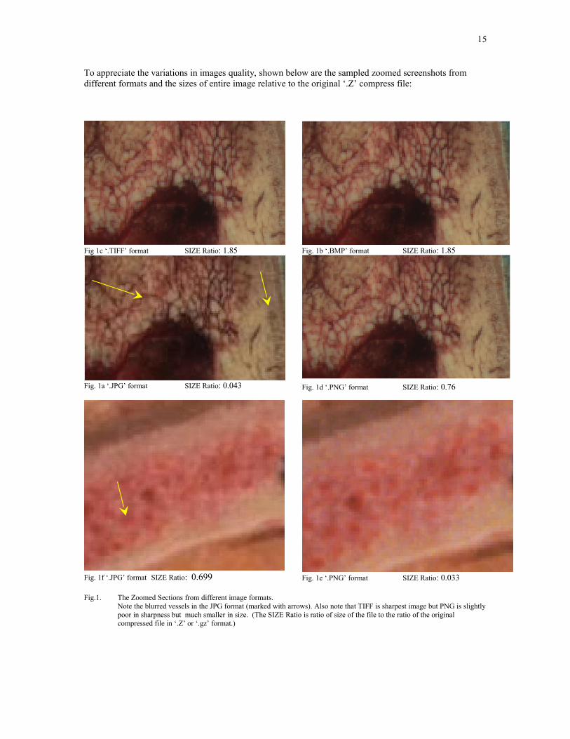
To appreciate the variations in images quality, shown below are the sampled zoomed screenshots from different formats and the sizes of entire image relative to the original ‘.Z’ compress file:

Fig 1c ‘.TIFF’ format SIZE Ratio: 1.85

Fig. 1a ‘.JPG’ format SIZE Ratio: 0.043

Fig. 1b ‘.BMP’ format SIZE Ratio: 1.85

Fig. 1d ‘.PNG’ format SIZE Ratio: 0.76

Fig. 1f ‘.JPG’ format SIZE Ratio: 0.699 Fig. 1e ‘.PNG’ format SIZE Ratio: 0.033

Fig.1. The Zoomed Sections from different image formats. Note the blurred vessels in the JPG format (marked with arrows). Also note that TIFF is sharpest image but PNG is slightly poor in sharpness but much smaller in size. (The SIZE Ratio is ratio of size of the file to the ratio of the original compressed file in ‘.Z’ or ‘.gz’ format.)

15

ii. The Directory Structure of the Data Set Repository build up at IIIT Medical Imaging Lab is depicted below:

IIIT Medical Imaging Data Set (courtesy: vhnet.nlm.nih.gov)

Female Male BWH_Harvard Utils

Fullcolor

Radiological

Head

Thorax

Abdomen

Pelvis

Thighs

Legs

Fullbody

MRI

Normal_CT

Fullcolor

Radiological

Head

Thorax

Abdomen

Pelvis

Thighs

Legs

Fullbody

MRI

Frozen_CT

fNormal_CT

70 mm

Fullbody

y

cryo

MRI_CT_DICOMM

MRI_CT_tiffs

16

c. Steps 4 and 5:

The raw data from the ‘National Library of Medicine’ is converted to standard image formats. The images include CT scan slices and anatomical images of male and female cadavers. Then an interactive method is used to determine appropriate thresholds for different objects in the images. Now, based on these thresholds, ray-casting generates the surface views of the objects in slices.

Threshold determination [1], [5]: Since medical images are best judged by human eyes, we provide the user to judge and decide the threshold himself. The user selects sample regions in the images that correspond to his object of interest. Now based on the pixel value ranges in the samples, a threshold is decided and operated upon the image. Based on segmentation results, the user can resample the pixels until sufficiently good segmentation is obtained. The values of threshold are recorded and operated on the rest of images.

d. Steps 6 and 7:

Ray-Casting [2],[3],[4],[5]: First, the images are rotated to correspond to the requested viewing direction. Then a viewing plane is determined, which involves determining its orientation, distance, shape and dimensions.

Now rendering by scene based method consists following three basic steps:a) Projection.b) Hidden part removal.c) Shading.

These are needed to impart a sense of three dimensionality to the rendered image. Additional cues for three dimensionality may be provided by techniques such as stereoscopic display, motion parallax by rotation of objects, shadowing, and texture mapping.

If ray casting is the method of projection chosen, then points equally spaced along the ray are sampled and at each such point, the scene intensity is estimated using appropriate interpolation method. Hidden part removal is then done by stopping at the first sampled point encountered along each ray that satisfies the threshold criterion. The value of shading assigned to the pixel corresponding to the ray is determined by different methods.

We determine the pixels on the projection plane. To start with, all these pixels are assigned a background value of zero. Next, to obtain the rendered value for each pixel on the viewing plane, a ray is assumed to start from that pixel and is traced into the volume data till either a volume element satisfying the constraints is encountered or the opposite boundary is reached. The front most volume element satisfying the threshold is recorded on to the pixel on the viewing plane.

This serves the first two steps mentioned above for surface rendering. First, based on the voxel encountered the pixel value and position on the projection plane is determined. Second, by stopping at the first encountered voxel all the background voxels are ignored, which serves as a hidden surface removal.

This ends the ray trace for one pixel. The same process is repeated for the all the other pixels on the viewing plane.

Now to adjust for depth perception, the distance of the selected volume element from the viewing plane is used. Here we have used a weighted combination of the selected volume element value and its distance from the viewing plane. This provides for depth perception while maintaining the local variations in the value of the pixels on the object.

17

The formula used to determine output pixel value is:

new(x, y) = light_factor* light_factor* light_factor*(1-ratio) + pixel_factor* pixel_factor* pixel_factor*ratio.

Here,

new(x, y) = resultant pixel value on the output plane.light_factor = scan depth normalized to 0 to 1.pixel_factor = pixel value at scan point normalizedto to 0 to 1. ratio = determines relative contribution of depth and pixel value factors.

Here, to obtain the final output value, the light_factor and pixel_factor cubed before multiplying with their ratios. The cubing operations allows for better depth perception as it increases the rate of variation of pixel intensity as depth increases.

The above procedure is applied to all the slices in the stack. Each slice contributes one output line, the width of which is kept proportional to the contributing slice-thickness.

The lines corresponding to missing intermediate slices are interpolated from adjacent slice scans.

To incorporate the volume cut views, we used masks to determine which all volume elements should not contribute to the final rendering. The cuts can be obtained along two intersecting planes passing through the object volume.

e. Steps 8:

To further assist output appreciation we have added false coloring to the rendered outputs. The bones are represented in ‘chrome’ color while the intersection points of the object volume and the cutting planes are shown with ‘green’.

Ray Casting generates very accurate and precise surface renderings with no false information generation or loss of small features. In spite of the good feature the one major drawback that doesn’t allow real time renderings is that Ray Casting is computationally very expensive for the following reasons:

1. The need to sample point along the ray,2. The need to interpolate,3. The need to store the entire scene in memory.

18

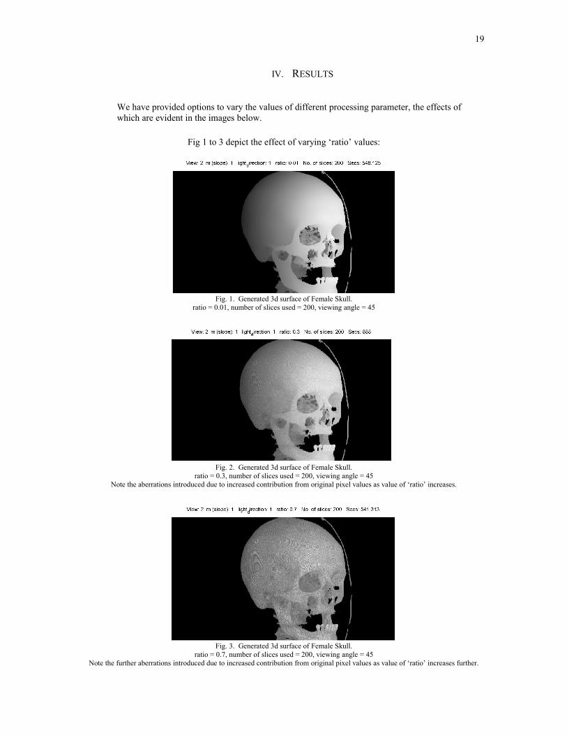
IV. RESULTS

We have provided options to vary the values of different processing parameter, the effects of which are evident in the images below.

Fig 1 to 3 depict the effect of varying ‘ratio’ values:

Fig. 1. Generated 3d surface of Female Skull.ratio = 0.01, number of slices used = 200, viewing angle = 45


Note the aberrations introduced due to increased contribution from original pixel values as value of ‘ratio’ increases.


Note the further aberrations introduced due to increased contribution from original pixel values as value of ‘ratio’ increases further.

19

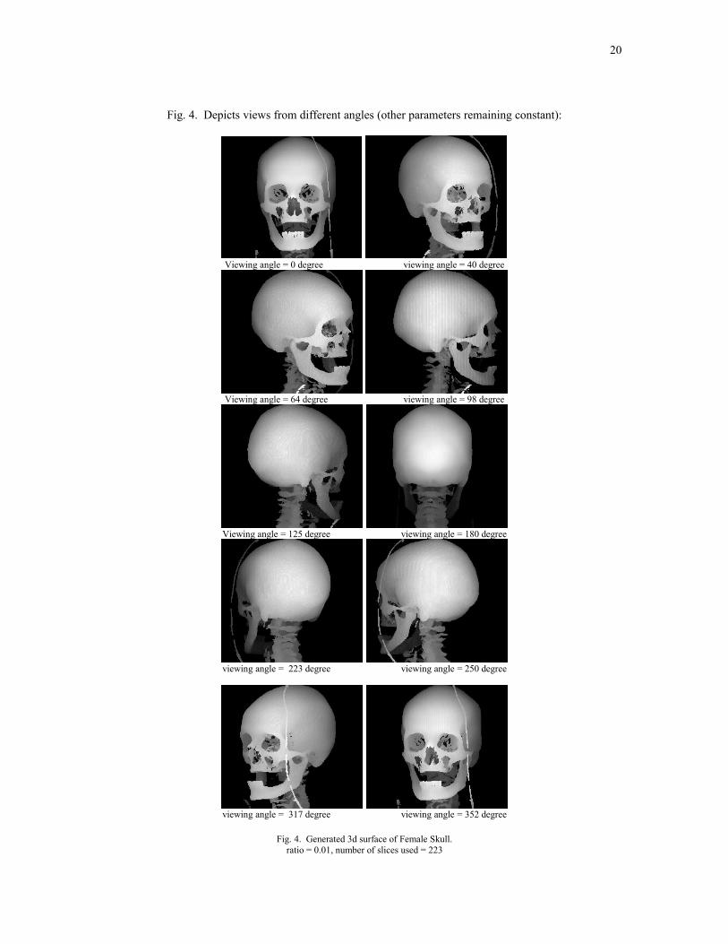
Fig. 4. Depicts views from different angles (other parameters remaining constant):

Viewing angle = 0 degree viewing angle = 40 degree



viewing angle = 223 degree viewing angle = 250 degree

viewing angle = 317 degree viewing angle = 352 degree

Fig. 4. Generated 3d surface of Female Skull.ratio = 0.01, number of slices used = 223

20

Fig. 5 to 8 are the results depicting the performance of the program to cut out a view from the whole object as the depth of cutting plane and its direction varies:

Fig. 5. Generated 3d surface of Female Skull.Cut angle = 180, cut depth = 200, viewing angle = 210






21

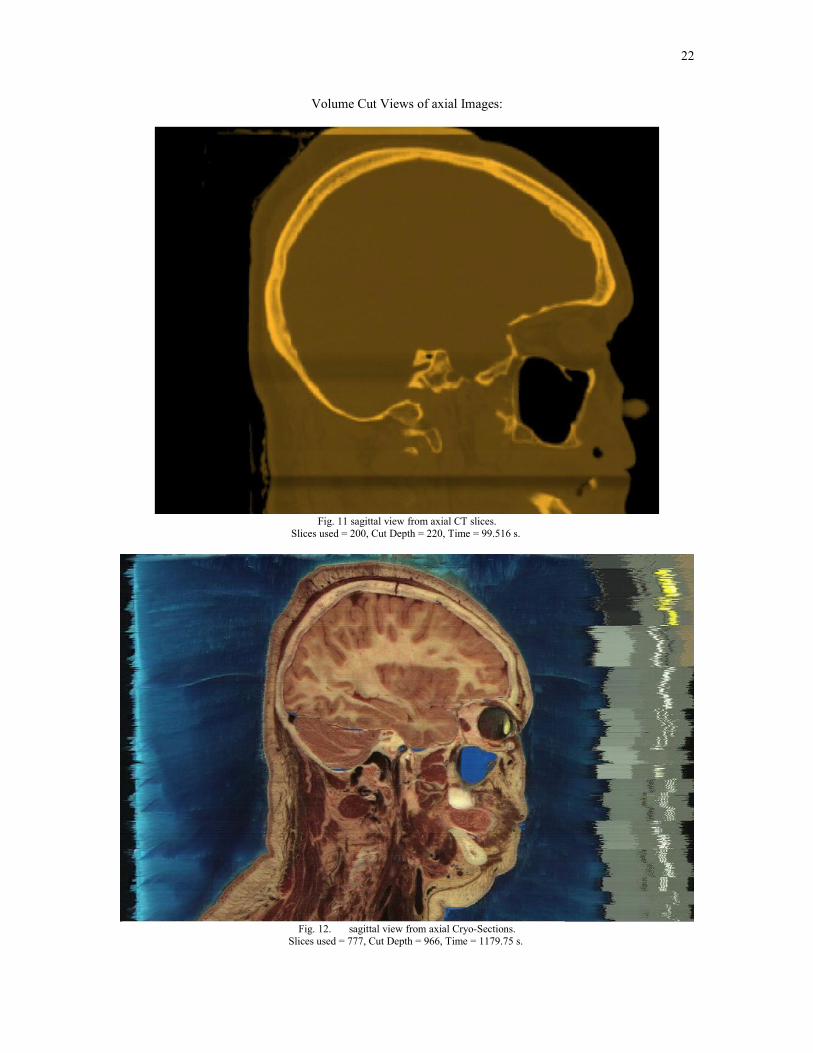
Volume Cut Views of axial Images:

Fig. 11 sagittal view from axial CT slices.Slices used = 200, Cut Depth = 220, Time = 99.516 s.

Fig. 12. sagittal view from axial Cryo-Sections.Slices used = 777, Cut Depth = 966, Time = 1179.75 s.

22

Fig. 13 Cornal view from axial Cryo-Sections.Slices used = 777, Cut Depth = 594, Time = 1170.86 s.

Fig. 14 View at 45 degree from axial Cryo-Sections.Slices used = 777, Cut Depth = 1148, Time = 9974.344 s.

23

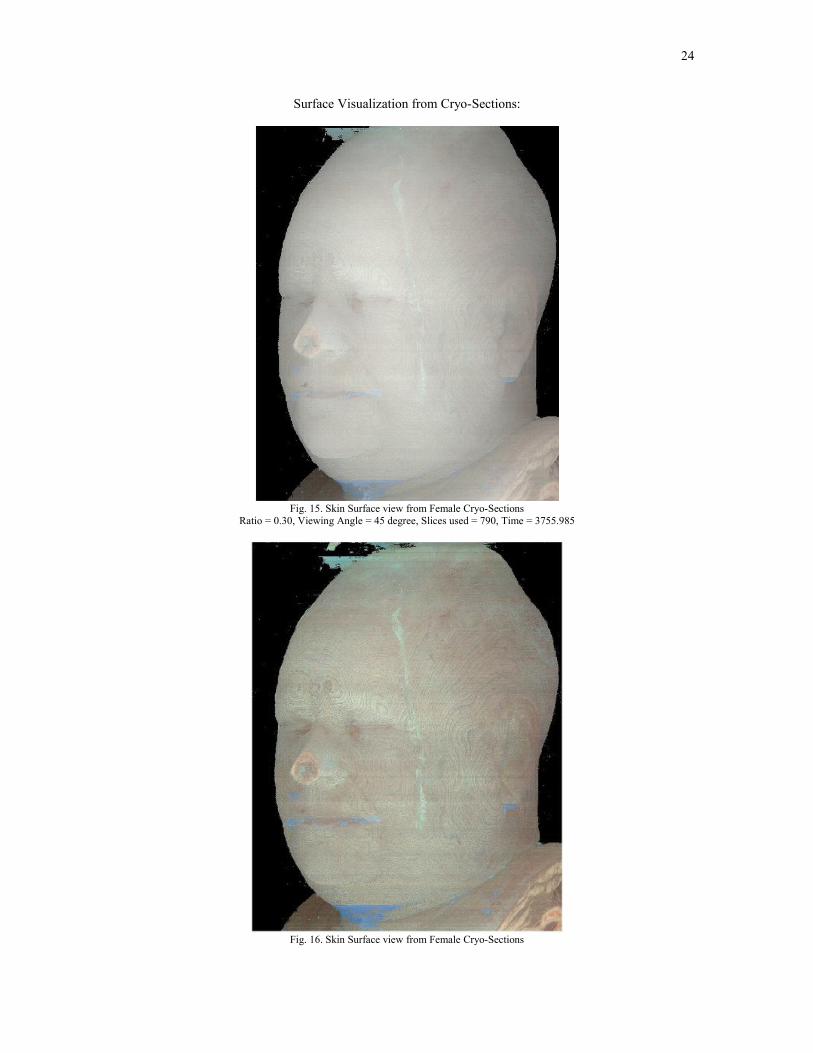
Surface Visualization from Cryo-Sections:

Fig. 15. Skin Surface view from Female Cryo-SectionsRatio = 0.30, Viewing Angle = 45 degree, Slices used = 790, Time = 3755.985

Fig. 16. Skin Surface view from Female Cryo-Sections

24

Ratio = 0.60, Viewing Angle = 45 degree, Slices used = 800, Time = 3665.781

Fig. 16. Skin Surface view from Female Cryo-SectionsRatio = 0.40, Viewing Angle = 0 degree, Slices used = 1747, Time = 15101.406

25

Noise Removal, Image Resizing and Cropping:

Fig 17. Original Image

Fig 18. Image after background Removal and cropping.

26

Variations of RGB and Gray Values in the Images:

Fig 19 RGB profile in Original Image.

27

Fig 20 RGB profile in Original Image.

Fig 21 Gray Value profile in CT Image.

Fig 22 Gray Value profile in MRI Image.

28

V. DISCUSSION

The method generates quite good quality 3-dimensioanl views of the surfaces of the objects. The gray scale views can be color coded to provide natural perception. But the scanning process is quite time consuming. So it can not be used to generate views in real time. To test the reliability of the method we generated surface views of the skull from 0 to 360 degree at 1 degree interval. The output images are saved as different files. These can be used to provide interactive viewing of the skull from any viewing direction. The volume cut operation and subsequent rendering provide good views of the object features which had been hidden behind outer surfaces. The surface visualization is applicable to color cryo-sections. The surface views of the skin are shown. The Sagittal and coronal slices were generated from axial data. But the segmentation of color images posed a real problem. In the Beginning it appeared to a simple task based on edge-detection and color component based threshold. In fact color component based threshold has been successfully used to remove the Gelatin background from the cryo-sections, in spite of the variations in background color, shade and texture within the image. But Segmenting out the body organs is a real mess. The color values as well as boundaries of the organs are so much indistinguishable that at a few instances even human eye is not able to judge out the organs from each other. The task appears mammoth for a fully automatic method. It appears that faithful segmentation of organs or organ system of interest is not possible with automatic methods and human assistance to a tedious level is apparent. Methods for human – computer interactions and fuzzy connected segmentation may be developed to try out better segmentation results.

VI. CONCLUSION

I have generated true and precise surface views from CT slice data. Surface views of Human Cadaver form cryo-sections had also been achieved. Other than these I have also been ale to generate sagittal, coronal slices form axial CT, MRI, Cryo-sections slices. The Axial Slices data is also used to generate volume cut views at any depth and from any viewing angle. Limitation is that all the views are parallel projections of the volume.

The results generated are exceptionally well in quality. Though the process is computationally expensive but the accuracy of the results supersedes this drawback. But there is a scope for improving the computational efficiency.

The surface views generated corresponding to different viewing angles’ and ’volume cut depths’ can provide useful resource for studying shapes and size deformities of the organs in the body.

29

VII. TIME LINE:

November – December:- Implemented basic operations like Gamma Correction, Noise Removal,

Histogram Equalization, FFT.- Work on building an interface for preprocessing the images.- Inter-Slice Interpolation implemented.

January - February: - Collect resources, study and explore about different 3D visualization

methods, their utility in case of medical images.- Learn from similar projects at other universities – their experiences and

difficulties.- Search for suitable data source. Finally found the repository at NLM.

March:- 5th March 2004, applied for license to use data set from VHP at NLM.- 10th March 2004, began data download from the NLM ftp server.- Trying Marching Cube and Surface Rendering Algorithm but had to

dropped them later- Switched to Ray-Casing

April 2nd – 15th - Extracted compressed data set files..- Converted raw files to .PNG format.- Segmented CT slices to obtain skull.- Obtained image intensity value profiles along a line through the middle of

the CT, MRI and Cryo-section images.- Finished with implementation of Ray Casting.

April 12th – 30th - Tested implementation on test images.- Applied the method to real CT slice data set.- Obtained first complete skull 3D surface after 400s.- Improved upon the implementation to bring down the rendering time to

220s.- Applied method to incorporate effect of pixel values variations and the

variations in lighting due to depth into the rendered surface.- Extended method to color anatomical cryo-sections.- Completed Male and Female Cadaver Data set download over a period of

50 days at about 30 KBps average download speed.

VIII. ACKNOWLEDGMENT

30

I would like express my gratitude towards my project guide Dr. UmaShanker Tiwary for his invaluable guidance and support. I would also like to acknowledge the support and help that my fellow students and the people at the institute extended to me. I worked as a junior project assistant to the MHRD funded project titled as ‘Fusion of Multi-Modal Medical Imaging Data’ and the job assigned to him was ‘3-Dimensional Surface Visualization of Anatomical CT/MRI Slice Data’ We owe the data courtesy to the ‘Visible Human Project’ [6] group at the National Library of Medicine, Bethesda, MD 20894, USA.

IX. REFERENCES

[1] Thomas Schiermann, Ulf Tiede, Karl Heinz Hohne, “Segmentation of the Visible Human for High Quality Volume based Visualization” in Medical Image Analysis , Vol.1, No. 4, pp. 263-271, 1997.

[2] Levoy, M., “Efficient Ray Tracing of Volume Rendering” ACM Transaction on Graphics 1990:9(3):245-261.

[3] Levoy M., “Displays of Surfaces from Volume Data,” in IEEE Computer Graphics and Applications 1988; (3): 29-37. Trans. Biomed. Eng., vol. 49, no. 10, pp. 1204–1210, Oct. 2002.

[4] Tiede, U., Hohne, K., Bomans, M., Pommert, A., Riemer, M. Wiebecke, G.,” Investigation of Medical 3D-Rendering Algorithms,” IEEE Computer Graphics and Applications, 1990; 10(2), 41-53.

[5] Jayaram K. Udupa, Gabor T.Herman.,” 3D Imaging in Medicine” CRC Press, Inc Boca Raton, FL, USA, Year 2000 ISBN: 0-8493-4294-5;

[6] The National Library of Medicine's Visible Human Project.,” w ww.nlm.nih.gov/research/visible/visible_human.html ”.

[7] Levoy M., “Efficient Ray Tracing Alogrothm” ACM Transations on Graphics, pages 245-261, July 1990

X. RESOURCES

BOOKS: 1) 3D Imaging in Medicine

Edited by: Jayaram K. Udupa, Ph.D.University of PennsylvaniaPhiladelphia, PA

Gabor T. Herman, Ph.D. University of PennsylvaniaPhiladelphia, PA

2) Computer Graphics: Principles and Practice By:James D. Foley, Andries van Dam, Steven K. Feiner, John F. Hughes

WEB:- The National Library of Medicine's Visible Human Project.

www.nlm.nih.gov/research/visible/visible_human.html

31

http://www.nlm.nih.gov/research/visible/visible_human.html

http://www.nlm.nih.gov/research/visible/visible_human.html

http://medweb.bham.ac.uk/mia

- IEEE Xplore. http://www.ieeexplore.ieee.org/Xplore/DynWel.jsp

- GE Medical Systems. http://www.gemedicalsystems.com

- Visualization Tool Kit resource page.

- Image Processing Fundamentals

http://www.ph.tn.tudelft.nl/Courses/FIP/noframes/fip-Contents.html .

XI. COURTESY

Resources Courtesy:

Medical Image Processing Lab,Indian Institute of Information Technology,

Allahabad.

Data Set Courtesy:

Visible Human Project®National Library of MedicineBuilding 38A, Room B1N-308600 Rockville PikeBethesda, MD 20894

32

http://www.ph.tn.tudelft.nl/Courses/FIP/noframes/fip-Contents.html

project report 3d visualization of medical imaging data

Technology

d data modalities

d slices

data source

data set

input data

data format

project supervisor

d imagingi