project no. 12-68 copy no. rotation limits for · pdf fileproject no. 12-68 copy no. rotation...

Project No. 12-68 COPY No.

ROTATION LIMITS FOR ELASTOMERIC BEARINGS

FINAL REPORT

Prepared for

NCHRP Transportation Research Board

Of The National Academies

John F. Stanton

Charles W. Roeder Peter Mackenzie-Helnwein

Christopher White, Colin Kuester and Brianne Craig

Department of Civil and Environmental Engineering University of Washington

Seattle, WA.

December 2006

- i -

- iii -

Project No. 12-68 COPY No.

ROTATION LIMITS FOR ELASTOMERIC BEARINGS

FINAL REPORT

Prepared for

NCHRP Transportation Research Board

Of The National Academies

John F. Stanton

Charles W. Roeder Peter Mackenzie-Helnwein

Christopher White, Colin Kuester and Brianne Craig

Department of Civil and Environmental Engineering University of Washington

Seattle, WA.

December 2006

- v -

Table of Contents

CHAPTER 1 INTRODUCTION AND RESEARCH APPROACH. XXVI 1.1 Bridge Bearings 1 1.2 Bearing Mechanics 1 1.3 Failure Modes, Analysis, and Design Criteria 3 1.4 Current Design Specifications 8

1.4.1 Method A 8 1.4.2 Method B 9

1.5 Motivation for this Study 10 1.6 Previous Studies 11 1.7 Survey of Practice 11 1.8 Goals, Scope and Organization of Report 12

CHAPTER 2 FINDINGS. 13 2.1 Physical Testing 13 2.2 Finite Element Analysis 18

2.2.1 Objectives 18 2.2.2 Modeling Techniques 20

2.2.2.1 Geometry and Boundary Conditions 21 2.2.2.2 Materials 21 2.2.2.3 Loading 21

2.2.3 Analyses Conducted 22 2.2.4 Results 23

2.2.4.1 Evaluation and Validation of Stiffness Coefficients 23 2.2.4.2 Bearings with Rigid External Plates – Uplift 28 2.2.4.3 Significance of Nonlinear Effects – Superposition Error 30

2.2.5 Discussion 33 2.3 Development of Design Procedures 34

2.3.1 Computation of Shear Strains using the Linearized Theory 35 2.3.2 Shear Strain Capacity 36 2.3.3 Analysis of Rotation and Axial Force Demand 41 2.3.4 Evaluation of the Design Model 42

2.4 QA/QC Issues 43 2.4.1 Quality of Current Elastomeric Bearings. 43 2.4.2 Test Requirements. 44 2.4.3 Number of Tests Required. 47 2.4.4 Material Test Requirements. 47 2.4.5 Very Large or Unusual Bearings. 49

- vii -

CHAPTER 3 INTERPRETATION, APPRAISAL AND APPLICATIONS. 51 3.1 Proposed Design Rules 51 3.2 Design Examples 56 3.3 QC/QA Procedures 77

CHAPTER 4 SUMMARY, CONCLUSIONS AND RECOMMENDATIONS. 79 4.1 Summary 79 4.2 Conclusions 79

4.2.1 Conclusions on Behavior Measured in Tests 79 4.2.2 Conclusions on Analytical and Numerical Modeling 80 4.2.3 Conclusions on Development of Design Procedures. 81

4.3 Recommendations 82 4.3.1 Recommendations for Implementation 82 4.3.2 Recommendations for Further Research 83

APPENDIX A TEST DATA A-1 A.1 Tests PMI 1a through PMI 1d. A-1 A.2 Tests PMI 4 through PMI 5. A-1 A.3 Cyclic Tests (CYC, SHR, MAT, SHF, ASR, PLT series) A-2 A.4 PMI Series A-4 A.5 CYC Series A-38 A.6 SHR Series A-97 A.7 SHF Series A-106 A.8 ASR Series A-116 A.9 MAT Series A-122 A.10 PLT Series A-128

APPENDIX B SURVEY OF CURRENT PRACTICE B-1 B.1 Introduction B-1 B.2 Elastomeric Bearing Use B-1 B.3 Design Methods B-3 B.4 Design Problems B-5 B.5 Field Problems B-7 B.6 Elastomer Type and Bearing Manufacturers B-8 B.7 Survey Highlights B-10 B.8 Summary B-12

APPENDIX C TEST APPARATUS AND PROCEDURES C-1 C.1 Introduction C-1 C.2 Rotation Tests C-1

C.2.1 Loading Apparatus C-1 C.2.2 Control and Instrumentation C-4 C.2.3 Test Rig Upgrades C-5 C.2.4 Loading the Rig C-9 C.2.5 Data Recorded C-11 C.2.6 Monotonic Tests C-12 C.2.7 Cyclic Tests C-12

- viii -

C.2.8 Procedures for Aspect Ratio, Shape Factor, Material, Shim Edge, and Shear Tests C-12 C.2.9 Limits on Loading Speed C-13

C.3 Axial Load Tests C-15 C.4 Torsion Tests (Diagnostic only) C-16 C.5 Shear Modulus Test C-19 C.6 Bulk Modulus Test C-22

APPENDIX D TEST RESULTS - OVERVIEW D-1 D.1 Introduction D-1

D.1.1 Arrangement of Test Series D-1 D.1.2 Main Test Series – Definition and Goals D-2

D.2 Main Test Series D-4 D.2.1 PMI Test Series D-4

D.2.1.1 Axial Step Load Test (PMI 1a) D-5 D.2.1.2 PMI-1b-Cyclic Axial Tests D-7 D.2.1.3 PMI-1c and PMI-1d – Axial Tests with Constant Rotation D-10 D.2.1.4 PMI-2 through PMI-5 – Monotonic Rotation Tests D-13

D.2.2 CYC Test Series D-17 D.2.2.1 Debonding Failure Mode D-17 D.2.2.2 Comparisons among Manufacturers D-24 D.2.2.3 Effects of Magnitude of Rotation and Axial Stress Level D-25 D.2.2.4 Shim Edge Treatment D-29 D.2.2.5 Long Term Test D-30 D.2.2.6 Offset Rotation D-31

D.2.3 SHR Test Series D-33 D.2.4 MAT Test Series D-36 D.2.5 SHF Test Series D-38 D.2.6 ASR Test Series D-40 D.2.7 PLT Test Series D-42

D.3 Supplemental Tests D-44 D.3.1 Material Property Tests D-45

D.3.1.1 Material Tests by Manufacturers D-45 D.3.1.2 Material Tests by the University of Washington D-50

D.3.1.2.1 Shear Modulus Tests D-50 D.3.1.2.2 Bulk Modulus tests D-52

D.3.2 Torsion Tests D-55 D.4 Analysis of Cyclic Rotation Data D-56

D.4.1 Analysis Procedures D-56 D.4.2 Shear Strains in the Elastomer D-60 D.4.3 Rotational Stiffness D-62 D.4.4 Energy Dissipation - EDC and EVD D-63

D.5 Lift-off of the Bearing D-66 D.6 Summary and Conclusions on Test Program D-68

D.6.1 Materials Testing D-68 D.6.2 Failure Criteria D-68 D.6.3 Methods of Measurement D-69 D.6.4 Monotonic and Low-cycle Axial Behavior. D-70 D.6.5 Cyclic Rotation D-70

D.6.5.1 Bearing Manufacturer D-70 D.6.5.2 Effects of Loading D-71 D.6.5.3 Effects of Bearing Characteristics D-71

- ix -

APPENDIX E FINITE ELEMENT ANALYSIS E-1 E.1 Introduction E-1 E.2 Method and Model definition E-2

E.2.1 Method E-2 E.2.2 Loading E-3 E.2.3 Geometry and boundary conditions E-3 E.2.4 Materials E-5

E.3 Evaluation and Validation of Stiffness Coefficients E-7 E.3.1 Axial Stiffness Coefficient Baz E-8

E.3.1.1 Strip-bearing with SF 6 E-8 E.3.1.2 Strip-bearing with SF 9 E-11 E.3.1.3 Strip-bearing with SF 12 E-13 E.3.1.4 Summary for the axial stiffness coefficient Baz E-16

E.3.2 Bending Stiffness Coefficient Bry E-18 E.3.2.1 Strip-bearing with SF 9 – Rotation at E-19 E.3.2.2 Strip-bearing with SF 9 – Rotation at E-21 E.3.2.3 Strip-bearing with SF 9 – Rotation at E-21 E.3.2.4 Strip-bearing with SF 9 – Rotation at E-24 E.3.2.5 Summary for the rotational stiffness coefficient Bry E-24

E.4 Evaluation of Local Shear Strain for Design Purposes E-26 E.4.1 Local Effects at the End of the Steel Shims E-26 E.4.2 Shear Strain Coefficient Cazzx for Axial Loading E-31

E.4.2.1 Strip-bearing with SF 6 E-31 E.4.2.2 Strip-bearing with SF 9 E-32 E.4.2.3 Strip-bearing with SF 12 E-33

E.4.3 Shear Strain Coefficient Cryzx for Rotation Loading E-33 E.4.4 Effect of lift-off on the local shear strain E-35 E.4.5 Bearings with Bonded External Plates – Uplift E-38

E.5 Model Error – Significance of nonlinear effects and Superposition E-43 E.6 Conclusions E-54

APPENDIX F DEVELOPMENT OF DESIGN PROCEDURES. F-1 F.1 Derivation of Shear Strains in the Elastomer. F-1

F.1.1 Response without Lift-off F-2 F.1.1.1 Internal Stresses F-2 F.1.1.2 Bearing Stiffnesses F-6 F.1.1.3 Maximum Shear Strain F-8 F.1.1.4 Combined Loading F-13 F.1.1.5 Uplift and Hydrostatic Tension F-17

F.1.2 Lift-off Permitted F-20 F.2 Shear Strain Capacity F-26

F.2.1 Linear Model F-26 F.2.2 Nonlinear Model F-29

F.2.2.1 Theoretical Basis. F-29 F.2.2.2 Monotonic Loads F-31 F.2.2.3 Cyclic Loads F-33 F.2.2.4 Summary on Nonlinear Model F-42

F.3 Axial and Rotation Demands from Dead and Live Loads. F-42 F.3.1 Background and Assumptions F-42 F.3.2 Methodology F-44 F.3.3 Computed Values F-44

F.3.3.1 Upper Bound to Rotation. F-44 F.3.3.2 Critical Combination of Compression and Rotation F-45

- x -

F.3.4 Thermal Camber F-49 F.4 Evaluation of the Design Models F-52

F.4.1 Evaluation Criteria F-52 F.4.2 Linear Model F-53 F.4.3 Nonlinear Model F-53 F.4.4 Evaluation Conclusions F-56

F.5 Detailed Development of Specification Provisions F-58 F.5.1 Method B F-58 F.5.2 Method A F-60 F.5.3 Discussion of Methods A and B. F-69

F.6 Summary and Conclusions F-70 F.6.1 Summary and Conclusions on Computation of Cyclic Shear Stress F-70 F.6.2 Summary and Conclusions on Cyclic Shear Stress Capacity F-71 F.6.3 Summary and Conclusions on Cyclic Shear Stress Demand F-71 F.6.4 Summary and Conclusions on Model Evaluation F-72

APPENDIX G PROPOSED DESIGN SPECIFICATIONS G-1 G.1 Basis G-1 G.2 Proposed Specification Provisions G-4

G.2.1 AASHTO 14.4 Movements and Loads G-4 G.2.1.1 AASHTO 14.4.1 General G-4 G.2.1.2 AASHTO 14.4.2 Design Requirements. G-4

G.2.2 AASHTO 14.7.5 Steel-Reinforced Elastomeric Bearings – Method B G-5 G.2.2.1 AASHTO 14.7.5.1 General G-5 G.2.2.2 AASHTO 14.7.5.2 Material Properties G-6 G.2.2.3 AASHTO 14.7.5.3 Design Requirements G-6

G.2.2.3.1 AASHTO 14.7.5.3.1 Scope G-6 G.2.2.3.2 AASHTO 14.7.5.3.2 G-6 G.2.2.3.3 AASHTO 14.7.5.3.3 G-6 G.2.2.3.4 AASHTO 14.7.5.3.4. G-12 G.2.2.3.5 AASHTO 14.7.5.3.5 G-12 G.2.2.3.6 AASHTO 14.7.5.3.6 G-12 G.2.2.3.7 AASHTO 14.7.5.3.7 G-12 G.2.2.3.8 AASHTO 14.7.5.3.8 G-12 G.2.2.3.9 AASHTO 14.7.6.4 Anchorage G-12

G.3 AASHTO 14.7.6 Steel Reinforced Elastomeric Bearings - METHOD A G-13 G.3.1 AASHTO 14.7.6.1 General G-13 G.3.2 AASHTO 14.7.6.2 Material Properties and 14.7.6.3.1 Scope G-13 G.3.3 AASHTO 14.7.6.3.2 Compressive Stress G-14 G.3.4 AASHTO 14.7.6.3.3 Compressive Deflection G-14 G.3.5 AASHTO 14.7.6.3.4 Shear G-14 G.3.6 AASHTO 14.7.6.3.5 Rotation G-14 G.3.7 AASHTO 14.7.6.3.6 Reinforcement G-14 G.3.8 AASHTO 14.7.6.3.7 Seismic provisions G-14 G.3.9 AASHTO 14.7.6.4 Anchorage G-14

G.4 AASHTO M-251 Materials Specification. G-15 G.5 Notes. G-16

APPENDIX H BIBLIOGRAPHY H-1

APPENDIX I NOTATION I-1

- xi -

List of Figures

Figure 1-1 Cross-section of a Steel-reinforced Elastomeric Bridge Bearing 2

Figure 1-2 Elastomeric Plain Pad Shearing to Accommodate Girder Expansion 2

Figure 1-3 Bulges without and with Steel Plates 3

Figure 1-4. Deformations of a Laminated Elastomeric Bearing Layer. 3

Figure 1-5. Tension Debonding at the Shim End and Shear Delamination at the Shim Surface 4

Figure 1-6 Fractured Steel Plates in Bearing. 4

Figure 2-1 Undamaged Bearing under Load 16

Figure 2-2 Initial Debonding of Bearing 16

Figure 2-3 Internal Damage caused by Severe Cyclic LOading 16

Figure 2-4 Progression of Debonding with Increased Load Cycles 16

Figure 2-5 Debonding for PLT Test Series 17

Figure 2-6 Damage due to Cyclic Shear Displacements (from NCHRP Report No. 298)18

Figure 2-7 Geometry and FEA Mesh for a Strip Bearing with S = 9 21

Figure 2-9 Stiffness Coefficient Ba for various S, Based on Various Definitions of L 25

Figure 2-10 Computed Hydrostatic Stress,�hyd, in (Pa) at Average Stress on Bearing of �a = 1.02GS. 28

Figure 2-11 Hydrostatic Stress: Comparison between Linear Theory and FEA Results. 29

Figure 2-12 Iso-error Plot (in %) for Shear Strain, . Bearing with S = 9 and Bonded External Plates, Based on a Fourth-order Fit. (Constructed for Shear Strain at ¼ in. Distance from the Critical Edge of the Shim). 32

Figure 2-13 Iso-error Plot (in %) for Shear Strain, . Bearing with S = 9 and no External Plates, Based on a Fourth-order Fit. (Constructed for Shear Strain at ¼ in. Distance from the Critical Edge of the Shim). 33

Figure 2-14 Shear Strains in the Elastomer due to Different Loadings 34

Figure 2-15 Lift-off: Bearing Behavior Assumed in “Semi-linear” Model 36

Figure 2-16 Shear Crack Propagation into Elastomer Layer 38

Figure 2-17. Effective Strain vs Number of Cycles: 25% Debonding. 40

Figure 2-18. Correlation Coefficient vs. Cyclic Factor. 40

Figure 2-19 Rotation due to Thermal Gradient on Girder 42

Figure A-1 Test PMI1a-A2 Summary A-4

- xii -

Figure A-2 Test PMI1a-B1 Summary A-5

Figure A-3 Test PMI1a-C1 Summary A-6

Figure A-4 Test PMI1a-D1 Summary A-7

Figure A-5 Test PMI1b-A2 Summary A-8

Figure A-6 Test PMI1b-B1 Summary A-9

Figure A-7 Test PMI1b-C1 Summary A-10

Figure A-8 Test PMI1b-D1 Summary A-11

Figure A-9 Test PMI1c-A2 Summary A-12

Figure A-10 Test PMI1c-B1 Summary A-13

Figure A-11 Test PMI1d-A2 Summary A-14

Figure A-12 Test PMI1d-B1 Summary A-15

Figure A-13 Test PMI4-A2 Summary A-16

Figure A-14 PMI4-A2 Positive Rotation Bulge Heights (a) Top of Bearing and (b) Bottom A-27

Figure A-15 PMI4-A2 Negative Rotation Bulge Heights (a) Top of Bearing and (b) Bottom A-18

Figure A-16 Test PMI4-B1 Summary A-19

Figure A-17 PMI4-B1 Positive Rotation Bulge Heights (a) Top of Bearing and (b) Bottom A-20

Figure A-18 PMI4-B1 Negative Rotation Bulge Heights (a) Top of Bearing and (b) Bottom A-21







Figure A-25 Test PMI5-B1 Summary A-28

Figure A-26 PMI5-B1 Positive Rotation Bulge Heights (a) Top of Bearing and (b) Bottom A-29

Figure A-27 PMI5-B1 Negative Rotation Bulge Heights (a) Top of Bearing and (b) Bottom A-30

- xiii -

Figure A-28 Test PMI5-C1 Summary A-31

Figure A-29 PMI5-C1 Positive Rotation Bulge Heights (a) Top of Bearing and (b) Bottom A-32

Figure A-30 PMI5-C1 Negative Rotation Bulge Heights (a) Top of Bearing and (b) Bottom A-33

Figure A-31 Test PMI5-D1 Summary A-34

Figure A-32 PMI5-D1 Positive Rotation Bulge Heights (a) Top of Bearing and (b) Bottom A-35

Figure A-33 PMI5-D1 Negative Rotation Bulge Heights (a) Top of Bearing and (b) Bottom A-36

Figure A-34 Test CYC5-A1 Summary A-38

Figure A-35 CYC5-A1 Bulge Heights (a) Top of Bearing and (b) Bottom A-39



Figure A-38 Test CYC5-B1 Summary A-42

Figure A-39 CYC5-B1 Bulge Heights (a) Top of Bearing and (b) Bottom A-43

Figure A-40 Test CYC5-C1 Summary A-44

Figure A-41 CYC5-C1 Bulge Heights (a) Top of Bearing and (b) Bottom A-45

Figure A-42 Test CYC5-D1 Summary A-46

Figure A-43 CYC5-D1 Bulge Heights (a) Top of Bearing and (b) Bottom A-47















- xiv -


































- xv -


Figure A-92 Test SHR1-B1 Summary A-97


Figure A-94 SHR3-B1 Bulge Heights (a) Top of Bearing and (b) Bottom A-99





Figure A-99 Test SHR6-A2 Summary A-104

Figure A-100 SHR6-A2 Bulge Heights (a) Top of Bearing and (b) Bottom A-105

Figure A-101 Test SHF1-C2 Summary A-106



Figure A-104 SHF3-C2 Bulge Heights (a) Top of Bearing and (b) Bottom A-109







Figure A-111 Test ASR1-C2 Summary A-116


Figure A-113 ASR2-C2 Bulge Heights (a) Top of Bearing and (b) Bottom A-118





Figure A-118 Test MAT1-C2 Summary A-122

Figure A-119 MAT1-C2 Bulge Heights (a) Top of Bearing and (b) Bottom A-123





- xvi -

Figure A-124 Test PLT1-A3 Summary A-128

Figure A-125 PLT1-A3 Bulge Heights (a) Top of Bearing and (b) Bottom A-129











Figure B-1 Histogram of Elastomeric Bearing Use. B-2

Figure B-2 Use of Design Methods A and B. B-4

Figure B-3 Design Problems Reported. B-6

Figure C-1 Multi-Load Bearing Test Rig: Diagram. C-3

Figure C-2 Multi-Load Bearing Test Rig: Photo C-3

Figure C-3 Multi-Load Bearing Test Rig: Photo of Bearing and Load Cell Detail C-4

Figure C-4 Leveling Bolt Improvements, Lowered Position C-5

Figure C-5 Level Bolt Improvements: Raised Position C-6

Figure C-6 Bearing Support Plate Improvements C-7

Figure C-7 Ram Support Improvements C-7

Figure C-8 Ram Swivels C-8

Figure C-10 Depth Gauge Shown Measuring Bulge C-11

Figure C-11 Trial Bearing after Testing at Excessive Frequency and Rotation Amplitude. C-14

Figure C-12 Relationship between Temperature Rise and Cyclic Frequency. C-14

Figure C-13 Axial Test Setup Photo C-15

Figure C-14 KT ratio vs. d/L C-17

Figure C-15 Torsion box setup C-18

Figure C-16 Torsion Box with Bearing under Load C-19

- xvii -

Figure C-17 Steps in Preparation of Shear Modulus Test Specimens. C-20

Figure C-18 Shear test specimen in various stages of production. The knife for peeling off rubber is also shown far right. C-21

Figure C-19 Shear Modulus Test C-21

Figure C-20 Bulk Modulus Test Rig and Sample C-23

Figure D 1. Typical Load vs. Displacement Graph for Axial Step Load Tests D-5

Figure D 2. Shim Fracture of Specimen PMI-1a-B1 D-7

Figure D 3. Typical Load vs. Displacement for PMI-1b Tests (PMI-1b-C1) D-8

Figure D 4. Instantaneous Tangent Stiffness during Test PMI-1b-C1 D-9

Figure D 5. Axial Load-Displacement Curves, Tests PMI-1b D-10

Figure D 6. Bearing Slips out of Tapered Plates during Test D-11

Figure D 7. Load/Displacement for Axial Test with and without 0.04 Imposed Rotation D-12

Figure D 8. Instantaneous Stiffness at Various Loads Averaged over all Load Cycles D-13

Figure D 9. Compressive Stress vs. Rotation at First Debonding for all PMI Tests D-14

Figure D 10. Photo of the "Watermelon Seed" Effect D-15

Figure D 11. Progression of Debonding Hidden by "Watermelon Seed" Effect D-15

Figure D 12. Raw Bulge Data for Different Rotation Angles D-16

Figure D 13. Relative Bulge Height for Different Rotation Angles. D-16

Figure D 14. Photo of Bearing Bulge Pattern Prior to Damage D-18

Figure D 15. Debonding Visible at Surface of Bearing D-18

Figure D 16. Photo of Tensile Separation at the Edge of the Shim (Bearing Batch A2) D-19

Figure D 17. Debonding vs. Cycle Number. Test CYC-5 (5/8P0, 3/4�0) D-20

Figure D 18. Debonding vs. Cycle Number. Test CYC-7 (5/8P0, ½�0) D-21

Figure D 19. Debonding vs. Cycle Number. Test CYC-9 (7/8P0, 3/4�0) D-21

Figure D 20. Debonding vs. Cycle Number. Test CYC-11 (7/8P0, ½�0) D-22

Figure D 21. Debonding vs. Cycle Number. Test CYC-12 (7/8P0< 1/4�0) D-22

Figure D 22. Internal Damage Caused by Continuing Severe Cycling, Batch A1 Bearing D-23

Figure D 23. Debonding for Type A2 Bearings: All CYC Tests D-25

Figure D 24. Debonding for Type B1 Bearings: All CYC Tests D-26

- xviii -

Figure D 25. Debonding for Type C1 Bearings: All CYC Tests D-26

Figure D 26. Debonding for Type D1 Bearings: All CYC Tests D-27

Figure D 27. Mean ±1 Standard Deviation for Debonding Curves, P=5/8 P0 D-28

Figure D 28. Mean ±1 Standard Deviation for Debonding Curves, P=7/8 P0 D-28

Figure D 29. Debonding for Long Term Test CYC-15_C1 and Comparison with CYC-12_C1 D-30

Figure D 30. Influence of Offset Rotation: Test CYC-7-A1 and Test CYC-13-A1 D-32

Figure D 31. Offset Rotation: Tests CYC-7-A1, CYC-7-A1, CYC-12-A1, and CYC-14-A1 D-32

Figure D 32. Debonding Comparison for SHR-5-B1 and CYC-9-B1 Bearings D-35

Figure D 33. Debonding for SHR-6-A2 and CYC-12-A2 Bearings D-36

Figure D 34. Debonding Curves for CYC-5-C1 and MAT1-C2 D-37

Figure D 35. Axial Load/Displacement Curves for Various Shape Factors D-39

Figure D 36. Axial Load-Displacement Curves for Different Aspect Ratios D-41

Figure D 37. PLT Test Series: Debonding with 5/8P0 Axial Load and 2/8�0 Rotation D-42

Figure D 38. PLT Test Series: Debonding with 7/8P0 Axial Load and 6/8�0 Rotation D-43

Figure D 39. Elongation at Break as a Function of Hardness. D-47

Figure D 40. Tensile Strength as a Function of Hardness. D-49

Figure D 41. Typical Load/Displacement Curve for Shear Modulus Test D-50

Figure D 42. Shear Modulus vs. Hardness. D-52

Figure D 43. Typical Load/Displacement Curve for Bulk Modulus Test D-54

Figure D 44. Bulk Modulus vs. Hardness. D-54

Figure D 45. Torsion Box Load/Displacement Curves Before and After Test CYC-14 D-55

Figure D 46. Typical Cyclic Moment-Rotation Plot D-58

Figure D 47. Total Strain vs. Number of Cycles to 25% Debond D-60

Figure D 48. Total Strain vs. Number of Cycles to 50% Debond D-61

Figure D 49. Cyclic Rotational Strain vs. Number of Cycles to 25% Debond D-61

Figure D 50. Cyclic Rotational Strain vs. Number of Cycles to 50% Debond D-62

Figure D 51. Test CYC-7-D1 Stiffness Variations D-63

Figure D 52. Initial EDC vs. Total Strain for All Tests D-64

Figure D 53. Initial EVD vs. Total Strain for All Tests D-64

- xix -

Figure D 54. Normalized EDC at 50% Debonding D-65

Figure D 55. Normalized EVD at 50% Debonding D-65

Figure D 56. Lift-off of the Bearing and Load Surface during Rotation D-67

Figure D 57. Tensile Stress in Elastomer due to Uplift (Lift-off Prevented) D-67

Figure E-1 Geometry and Finite Element mesh for a strip bearing with SF 6 E-4



Figure E-4 versus average axial strain for bearing with SF 6 E-9

Figure E-5 versus average axial strain for bearing with nominal SF 6 and calculation based on theoretical SF 5.67 E-10

Figure E-6 versus average axial strain for bearing with nominal SF 6 and calculation based on the average SF 5.83 E-10


Figure E-8 versus average axial strain for bearing with nominal SF 9 and calculation based on theoretical SF 8.50 E-12

Figure E-9 versus average axial strain for bearing with nominal SF 9 and calculation based on the average SF 8.75 E-13



Figure E-12 versus average axial strain for bearing with nominal SF 12 and calculation based on theoretical SF 11.33. E-15

Figure E-13 versus average axial strain for bearing with nominal SF 12 and calculation based on the average SF 11.67. E-16

Figure E-14 Hourglass modes distorting the right side of a bearing with bonded external plates subjected to rotation only E-19

Figure E-15 versus average axial strain for bearing with SF 9 at P = 0 E-20

Figure E-16 versus average axial strain for bearing with nominal SF 9 and calculation based on theoretical SF 8.75 at P = 0 E-20

Figure E-17 versus average axial strain for bearing with nominal SF 9 and calculation based on theoretical SF 8.50 at P = 0 E-20

Figure E-18 versus average axial strain for bearing with SF 9 at P = 1.0 GS A E-22

Figure E-19 versus average axial strain for bearing with nominal SF 9 and calculation based on theoretical SF 8.75 at P = 1.0 GS A E-22


- xx -







Figure E-27 Computed shear strain in (in/in) at at the edge of a steel shim. E-27

Figure E-28 Computed shear strain in (in/in) at at the edge of a steel shim. E-28

Figure E-29 Computed hydrostatic stress in (Pa) at at the edge of a steel shim. E-29

Figure E-30 Computed hydrostatic stress in (Pa) at at the edge of a steel shim. E-30

Figure E-31 Shear strain along the shim at different axial loads for a bearing with SF 9 E-30

Figure E-32 versus for bearing with SF 6 E-32



Figure E-35 Coefficients for bearing with SF 9 E-34

Figure E-36 Shear strain along a shim of a 3-layer bearing with SF 9: Axial load level and total rotation E-36

Figure E-37 Shear strain along a shim of a 3-layer bearing with SF 9: Axial load level and total rotation E-36

Figure E-38 Lift-off ratio versus rotation per layer for SF 9 bearing at various load levels E-37

Figure E-39 Tensile hydrostatic stress in (Pa) for and rad/layer E-39



Figure E-42 History of hydrostatic stress in (psi) for (Increments 60-90) E-41



Figure E-45 Collection of resulting shear strain (in/in) from 10 different nonlinear analyses of an elastomeric bearing with SF 9 E-44

Figure E-46 Fourth-order fit to simulation data for a SF 6 bearing with bonded external plates for shear strain at ¼” distance from the critical edge of the shim.

- xxi -

Simulated data (lines/curves), fitted surface (left image), and contour lines for shear strain (in/in). E-48

Figure E-47 Fourth-order fit to simulation data for a SF 9 bearing with bonded external plates for shear strain at ¼” distance from the critical edge of the shim. Simulated data (lines/curves), fitted surface (left image), and contour lines for shear strain (in/in). E-49

Figure E-48 Fourth-order fit to simulation data for a SF 6 bearing without bonded external plates for shear strain at ¼” distance from the critical edge of the shim. Simulated data (lines/curves), fitted surface (left image), and contour lines for shear strain (in/in). E-50

Figure E-49 Fourth-order fit to simulation data for a SF 9 bearing without bonded external plates for shear strain at ¼” distance from the critical edge of the shim. Simulated data (lines/curves), fitted surface (left image), and contour lines for shear strain (in/in). E-50

Figure E-50 Iso-error plot for shear strain for a SF 6 bearing with bonded external plates based on a fourth-order fit. (Constructed for shear strain at ¼” distance from the critical edge of the shim.) E-51

Figure E-51 Iso-error plot for shear strain for a SF 9 bearing with bonded external plates based on a fourth-order fit. (Constructed for shear strain at ¼” distance from the critical edge of the shim.) E-52

Figure E-52 Iso-error plot for shear strain for a SF 6 bearing without bonded external plates based on a fourth-order fit. (Constructed for shear strain at ¼” distance from the critical edge of the shim.) E-53

Figure E-53 Iso-error plot for shear strain for a SF 9 bearing without bonded external plates based on a fourth-order fit. (Constructed for shear strain at ¼” distance from the critical edge of the shim.) E-53

Figure F.1. Displacement Fields for Component Loadcases. F-2

Figure F.2. Stresses in the Elastomer due to Rotation and Compression Load. F-5

Figure F.3. Stiffness Coefficient Ba (from Stanton and Lund). F-7

Figure F.4. Stiffness Coefficient Br (from Stanton and Lund). F-7

Figure F.5. Shear Strain Coefficient Ca. F-11

Figure F.6. Shear Strain Coefficient Cr. F-11

Figure F.7. Shear Strain Coefficient Da. F-12

Figure F.8. Shear Strain Coefficient Dr. F-12

Figure F.9. Hydrostatic Tension under Combined Compression and Rotation. F-14

Figure F.10. Distribution of Vertical Strain across the Bearing. F-15

Figure F.11. Distribution of Vertical Stress across the Bearing. F-16

- xxii -

Figure F.12. Distribution of Shear Strain across the Bearing. F-16

Figure F.13. Hydrostatic Tension vs. Rotation for Various Compression Strains. S = 6. F-18

Figure F.14. Normalized Hydrostatic Stress as a Function of � and �. F-19

Figure F.15. Lift-off: Assumed Bearing Behavior. F-21

Figure F.16. Total Shear Strain for Bearing with Lift-off. F-24

Figure F.17. Post Lift-off Conditions: Ratio of Approximate and True Total Shear Strain. F-25

Figure F.18. Effective Strain vs Number of Cycles: 25% Debonding. F-28

Figure F.19. Correlation Coefficient vs Cyclic Factor. F-28

Figure F.20. Effective Strain vs Number of Cycles: 50% Debonding. F-29

Figure F.21. Tests CYC5-12 Debonding for Batch B1 Bearings. F-34

Figure F.22. Debonding vs. Number of Cycles. Test CYC05. F-36



Figure F.25. Debonding vs. Number of Cycles. Test CY11. F-37



Figure F.28. Fatigue Life for Cyclic Shear Strain due to Rotation: 25 % Debonding Criterion. F-39



Figure F.31. Fatigue Life for 25 % Debonding Criterion. Equation (F 67) vs Measured Data. F-41

Figure F.32. Effect of Span on Rotation Angle. F-46

Figure F.33. Effect of Girder Stiffness on Rotation Angle. F-47

Figure F.34. Effect of Lane Load Factor on Rotation Angle. F-47

Figure F.35. Effect of Girder Stiffness on Total Shear Strain. F-48

Figure F.36. Effect of Truck Location on Maximum Shear Strain. F-48

Figure F.37. Effects of Span and Truck Location on Maximum Shear Strain. F-49

Figure F.38. Girder and AASHTO /Design Thermal Gradient (Zone 1). F-50

Figure F.39. Rotation due to Thermal Gradient on Girder. F-51

- xxiii -

Figure F.40. Strains due to Thermal Gradient. F-51

Figure F.41. Predicted Debonding for Example Bearing. F-54

Figure F.42. Compression Fatigue: Predicted vs. Observed Debonding. F-56

Figure F.43. Axial Stress – Rotation Interaction Diagram. 9” x 22” Bearing, 4 Layers at 0.5”. F-61

Figure F.44. Axial Stress – Rotation Interaction Diagram. 14.05” x 14.05” Bearing, 3 Layers at 0.5”. F-62

Figure F.45. Axial Stress – Rotation Interaction Diagram. 14.05” x 14.05”, 4 Layers at 0.375”. F-62

Figure F.46 Allowable normalized axial stress as a function of S2/n. F-63

Figure F.47 Allowable axial stress as a function of S2/n. F-64

Figure F.48 Allowable axial load as a function of S2/n F-65

Figure F.49 Interaction Diagram: Effect of Aspect Ratio. (n = 3, hri = 0.5” for all). F-66

- xxiv -

List of Tables

Table 2 1 Summary of the Test Series 13

Table 2 2 Bearing Test Matrix 14

Table B-1 Bearing Use: Breakdown by State. B-2

Table B-2 Design Methods Used: Breakdown by State. B-4

Table B-3 Design Issues: Breakdown by State. B-6

Table B-4 Field Issues: Breakdown by State. B-7

Table B-5 Elastomer Type Used: Breakdown by State. B-8

Table B-6 Manufacturers used: Breakdown by State. B-9

Table D 1 Complete Bearing Test Matrix D-2

Table D 2 Series PMI Test Matrix D-4

Table D 3 Test PMI1a. Stress at Initial Debonding and Total Debonding at 6000 psi D-6

Table D 4. Rate of Debonding for PMI-1b Tests D-8

Table D 5. Stress Level at Initiation of Debonding with (PMI-1c) and without (PMI-1a) Rotation D-10

Table D 6. Comparison of Debonding with (PMI01d) and without (PMI-1b) Rotation D-11

Table D 7. Rotation at Initiation of Debonding During Monotonic Rotation Tests D-14

Table D 8. CYC Test Matrix D-17

Table D 9. Summary of CYC Test Loads D-19

Table D 10. CYC Series Interpolated % Debonded Values. D-24

Table D 11. Cycle Count Ratios at 50% Debonding in Relation to CYC-5 and CYC-9 D-29

Table D 12. Cycles to Reach Debonding Milestones for Shim Treatment Comparison D-30

Table D 13. SHR Test Matrix D-34

Table D 14. Cycles Needed to Initiate Debonding with 30% Constant Shear Added D-36

Table D 15. MAT Test Matrix D-37

Table D 16. Comparison of Cycles to Debonding with MAT Test Series D-37

Table D 17. SHF Test Matrix D-38

- xxv -

Table D 18. Number of Cycles to Debonding Milestones for Different Shape Factors D-40

Table D 19. ASR Test Matrix D-40

Table D 20. Number of Cycles to Debonding Milestones for Different Aspect Ratios D-41

Table D 21. PLT Test Matrix D-42

Table D 22. Tests PLT-1, 3, 5. Debonding vs. Cycle Number for Various Shim Edge Treatments D-43

Table D 23. Tests PLT-2, 4, 6. Debonding vs. Cycle Number for Various Shim Edge Treatments D-43

Table D 24. Mechanical Properties of the Elastomers in Each Batch. D-46

Table D 25. Manufacturers AASHTO and Quality Control Tests D-48

Table D 26. Steel Plate Properties from Manufacturers D-49

Table D 27. Computed Response Values for Cyclic Rotation Tests. D-57

Table E-1 Stiffness coefficients used by Gent & Meinecke (1970) and Stanton & Lund (2004) and their simplified equivalent in the proposed design equations E-7

Table E-2 Model parameters for SF 6 bearing E-9



Table E-5 Comparison of stiffness coefficient for modified definitions of S E-17

Table E-6 Coefficients for a bearing with SF 6 and with bonded external plates (creates uplift) E-45

Table E-7 Coefficients for a bearing with SF 9 and with bonded external plates (creates uplift) E-46

Table E-8 Coefficients for a bearing with SF 6 without bonded external plates (allows lift-off) E-47

Table E-9 Coefficients for a bearing with SF 9 without bonded external plates (allows lift-off) E-47

Table F 1. Computed Shear Strains at Initiation of Debonding in Monotonic Tests. F-32

Table F 2. Multipliers for Rotation Angle due to Girder Continuity. F-45 Table G 1 Summary of Proposed Section Changes in AASHTO Method B

Specifications.......................................................................................... G-3

- xxvi -

Acknowledgements The research reported herein was performed under NCHRP Project 12-68 by the Department of Civil and Environmental Engineering at the University of Washington (UW). Dr. John Stanton, Professor of Civil Engineering at UW, was the Project Director and co-Principal Investigator. The other authors of this report are Dr. Charles Roeder, Professor of Civil Engineering at UW and co-PI, Dr Peter Mackenzie-Helnwein, Assistant Professor of Civil Engineering at UW and co-PI, Mr. Christopher White, Mr. Colin Kuester and Ms. Brianne Craig, all Graduate student Assistants and MSCE recipients at UW. The work was done under the direction of Professors Stanton, Roeder and Mackenzie-Helnwein. The assistance with the laboratory work of Mr. Vince Chaijaroen, Laboratory Manager, Mr. Kevin Soderlund, Instrument Maker, and Mr. Kyle Twitchell, Undergraduate Assistant, is gratefully acknowledged. The specialty test rig that made possible the extensive cyclic testing was based on a concept developed by Mr. Ken Olson and built by Mr. Tim Rodgers, both of whom received their MSCE degrees at UW.

- xxvii -

Executive Summary The response of elastomeric bridge bearings to imposed rotations was studied using testing and analysis. The program concentrated on steel-reinforced elastomeric bearings. The demand on typical bearings was evaluated by analyzing a range of bridges and evaluating the amplitudes of the axial loads and rotations on the bearings that are likely to occur in practice. During this process, it was found that cyclic axial forces cause larger strains in the elastomer than do the cyclic rotations. However, resource limits in the program precluded cyclic axial testing, and the discovery was anyway made quite late in the program. Thus, in the development of design procedures, the effects of cyclic axial load were taken into account by analysis alone. The capacity of the bearings to accommodate the loads and rotations without excessive damage was evaluated by a program of testing and analysis of the bearings themselves. The test program included material tests, static and cyclic tests on full bearings, and diagnostic tests on full bearings to evaluate their instantaneous state of damage. In all, 78 bearings were tested. The bearings were purchased from the four largest manufacturers in the country. Static and low-cycle repeated load tests were conducted under axial load with or without a fixed rotation. Stresses up to 12,000 psi were applied. Bearings with high shape factors (9 and 12) were able to carry the loads with no damage whatsoever, while bearings with lower shape factors suffered various levels of damage. The cyclic rotation tests were conducted in a specially constructed test machine that is capable of applying simultaneously constant axial load, constant shear displacement and cyclic rotation. Peak capacities are 800 kips axial load and +/- 8% rotation. Cyclic loading was found to cause progressive damage, analogous to fatigue in metals. However, the damage was in the form of progressive debonding of the elastomer from the internal steel shims, so failure was never sudden. At the end of every cyclic test, the bearing could still easily carry the axial load, even though other properties had degraded. This finding creates the need for judgment in establishing a level of damage that constitutes failure. Failure of a component is usually expressed in terms of critical stress or strain, and the same approach was used with the bearings studied here. However, measuring local strains in rubber is difficult, so analysis was necessary to relate the internal stress and strain fields to the external loadings that caused them. Classical, closed-form analytical techniques for laminated incompressible materials were used for the purpose, and nonlinear Finite Element Analysis (NLFEA) was used to verify that the closed-form methods were sufficiently accurate to warrant their use in design procedures. Empirical fatigue models were also generated to predict the progress of damage under cyclic loading. The results of the tests and analyses were combined to develop design procedures suitable for adoption in the AASHTO LRFD Bridge Design Specifications. Major proposed changes from the present specifications include the removal of the absolute limit on compressive stress, so that the design of high shape factor bearings for high stresses will be possible, the removal of the previous “no-uplift” provisions, which were causing difficulties for designers, and a change in the testing requirements so that the second-level, more rigorous testing is required for large bearings rather than any bearing deigned by the more comprehensive “Method B”.

- xxix -

Abstract This report describes a study of elastomeric bridge bearings subjected to axial load and rotation. The study was motivated by the fact that certain features of the design provisions for bearings in the AASHTO LRFD Design Specifications were believed to be excessively conservative and were causing difficulties to designers. The study used a combination of laboratory testing, analytical modeling and numerical simulations. The demand on typical bearings was evaluated by analyzing typical bridges and evaluating the amplitudes of the axial loads and rotations likely to occur in practice. The capacity of the bearings to accommodate the loads and rotations without excessive damage was evaluated by a program of testing and analysis of the bearings themselves. The test program included material tests, static and cyclic tests on full bearings, and diagnostic tests on full bearings to evaluate their instantaneous state of damage. In all, 78 bearings were tested. The cyclic rotation tests were conducted in a specially constructed test machine. Measuring local strains in rubber is difficult, so analysis was used to estimate the strain fields induced by the various loadings. Classical closed form analytical techniques for laminated incompressible materials were modified and developed for design purposes, and Finite Element Analyses (FEA) was used to verify that the approximations in the closed form methods led to acceptably low errors. Empirical fatigue models were generated to predict the behavior of the bearings under cyclic loading. The results of the tests and analyses were combined to develop design procedures suitable for adoption in the AASHTO LRFD Bridge Design Specifications.

- xxxi -

- xxxii -

CHAPTER 1 Introduction and Research Approach.

1.1 Bridge Bearings Elastomeric bearings have been used in bridges since the late 1950's, and have grown in popularity so they are now the most common type of bridge bearing in all regions of the United States. They are capable of resisting typical bridge loads and accommodating deformations without the use of machined or moving parts, which largely eliminates any need for maintenance. This characteristic, together with their economy, has for many years made them an attractive choice. The spread of seismic design requirements throughout the country, and the fact that elastomeric bearings typically have better seismic performance than traditional bearing types, only adds to their appeal.

Elastomeric bearings are often thought of as having a limited load capacity. When loads exceed a certain threshold, designers tend to use pot, disk or spherical bearings instead. One reason is practical; the low stresses presently permitted on elastomeric bearings result in a large bearing for carrying a high load, and the space may not be available for it. Molding a large elastomeric bearing may also pose problems. However, there is no inherent reason why they should not be used for high loads. During the course of the research, the team encountered a laminated elastomeric bridge bearing designed for 16,000 kips service load. However, such large bearings are likely to have limited rotation capacity, and that may ultimately prove more of a limit than the load capacity.

1.2 Bearing Mechanics Elastomeric bridge bearings come in four principal types:

• plain elastomeric pads, used primarily in low-load situations, • cotton duck pads, which are made from very closely spaced layers of elastomer

and woven cotton. They are relatively rigid, and so are often equipped with a slider to accommodate horizontal displacements.

• fiberglass-reinforced pads, which, like cotton duck pads, have the advantage that they can be cut from a large sheet, and so do not need to be molded individually, but are seldom used today,

• steel-reinforced elastomeric bearings, which are used for the highest loads.

The main focus of this research is on rectangular steel-reinforced elastomeric bearings, as shown in Figure 1.1. Steel plates are bonded with rubber, either natural or polychloroprene, in alternating layers to form a “sandwich”. The finished product contains rubber cover on the top and bottom and around the edges, creating a sealed system in which the plates are protected against corrosion.

The rubber and steel layers are bonded together by an adhesive that is activated when the rubber is cured. Curing, or vulcanization, is the process of subjecting the raw rubber compound to high temperature and pressure, which both change its chemical structure and cause it to take the shape of the mold.

- 1 -

Figure 1.1 Cross-section of a Steel-reinforced Elastomeric Bridge Bearing

The concepts underlying behavior of laminated elastomeric bearings are quite different from those of conventional structural components made from concrete, metal or timber. They depend on the fact that elastomers can undergo reversible, elastic deformations that are enormous compared with those of conventional materials, but that fact also brings with it the need for special design procedures.

The simplest concept for accommodating expansion or contraction of the girders is to do so through the elastic shear deformations of a plain rubber block. As the bridge expands, the block changes shape from a rectangle to a parallelogram as shown in Figure 1.2.

Figure 1.2 Elastomeric Plain Pad Shearing to Accommodate Girder Expansion

To accommodate the necessary deformations the block would have to be thick, and so it would be unacceptably flexible in axial compression; trucks would experience steps in the roadway as they passed from the end of one girder to another. The challenge is thus to stiffen the bearing in compression without losing its shear flexibility. This is achieved by adding internal horizontal reinforcing plates, known as “shims”, in the bearing. Behavior under compressive load is illustrated in Figure 1.3.

A plain elastomeric pad responds to vertical load by expanding laterally, and slipping against the supporting surface as shown in Figure 1.3a. The rubber at the top and bottom surfaces of the pad is partially restrained against outward movement by friction against the support, but the rubber at mid-thickness is not. This results in some bulging at the edges. The lateral expansion leads to significant vertical deflections. By contrast, the rubber in the laminated pad is largely prevented from such expansion by its bond to the steel plates, and the layers only form small bulges, as shown in Figure 1.3b.

Rubber is almost incompressible, so the volume of rubber remains almost constant under load, and the small lateral expansion leads to only a small vertical deflection. The laminated bearing is thus much stiffer and stronger in compression than a plain pad. However, the steel plates do not inhibit the shear deformations of the rubber, so the bearing is still able to undergo the same shear deformations as the plain pad for the purpose of accommodating changes in length of the girders.

- 2 -

a) b)

Figure 1.3 Bulges without and with Steel Plates

1.3 Failure Modes, Analysis, and Design Criteria The elastomer in a bearing experiences large shear strains. These occur for axial load, rotation and shear, and are illustrated in Figure 1.4. The shear strains can be envisaged by considering regions or elements of the rubber that are rectangular when unstressed, but are forced to become parallelograms when the bearing is under load.

Figure 1.4. Deformations of a Laminated Elastomeric Bearing Layer.

The shear strains caused by axial load and rotation reach their maxima at the same place, namely the very edge of the layer where the rubber is bonded to the plate. Imposed shear deformations cause shear strains that are relatively constant over the whole layer, including the critical end of the plate.

If the steel reinforcing plates have square edges and if no cover exists, the shear stress at the corner of the rubber layer is theoretically singular. (The shear stress must be zero on the vertical free surface of the rubber, but most methods of analysis predict non-zero shear stress along the horizontal interface between steel and rubber. Yet, for equilibrium, the vertical and horizontal shear stresses must be equal). In practice, these plates have slightly rounded edges because they are deburred, and rubber cover exists, so the stress is

- 3 -

concentrated there rather than being truly singular. Under severe loading, this stress leads to local detachment of the elastomer from the steel. This starts with tensile debonding of the cover from the ends of the plates as shown in Figure 1.5 then propagates inwards along the surface as shear delamination. In this report, the terms debonding and delamination are used to indicate these two different behaviors.

Tension debonding

Shear delamination

Figure 1.5. Tension Debonding at the Shim End and Shear Delamination at the Shim Surface

Debonding is easy to see on the surface because two bulges merge into one larger bulge, as shown in Figure 1.5. However, distinguishing between local tensile debonding of the cover and shear delamination of the internal layers is difficult. This is unfortunate, because the former has little immediate effect on the bearing’s performance, whereas the latter has significant adverse consequences. The shear delamination is always preceded by the tensile debonding, so the one acts as a precursor of the other.

Figure 1.6 Fractured Steel Plates in Bearing.

The lateral expansion of the rubber layers causes tension in the steel plates. At extreme loads, the plates may fracture. They typically do this by splitting along the longitudinal axis of the bearing, as shown in Figure 1.6. With plates of the thickness used in practice, this behavior does not occur until the load has reached five to ten times its design value, so shim fracture seldom controls design. Theoretically the plates could be made thinner and they would still be strong enough in tension, but they would be more flexible in bending. Keeping them plane during molding would then become problematic.

Shear delamination is thus the most important potential mode of failure. If it were to occur in practice, the elastomer would start to extrude from the bearing, which would in turn cause significant vertical deflection, horizontal forces of unpredictable magnitude,

- 4 -

and possible hard contact between the girder and the support. While none of these necessarily creates collapse conditions in the bridge itself, any one of them will seriously degrade the serviceability and reduce the performance of the bridge.

It is necessary to relate the delamination to a local strain measure, so its onset can be predicted. Prediction of any local deformations is difficult, because elastomeric bearings have three characteristics that make conventional stress analysis invalid:

• the rubber is almost incompressible (Poisson’s ratio ≈ 0.50), • parts of the bearing undergo very large displacements, so the geometry of the

system changes significantly during the loading, • the rubber obeys a nonlinear stress-strain law.

Further difficulties are caused by the fact that the stress-strain behavior is often somewhat rate-dependent (e.g. visco-elastic) and it changes with cycling as the internal crystal structure changes with loading. The only viable way of predicting internal deformations throughout the entire rubber mass is by using Finite Element Analysis (FEA), but even that tool brings with its own additional challenges, such as element instability and difficulties with convergence of the iterative calculations. Furthermore, FEA is not an appropriate design tool for a component that may cost as little as $100.

Gent and Lindley (1959a) pioneered a simplified analysis of laminated bearings that uses small-deflection theory and depends on an assumed displacement field. It provides a remarkably accurate estimate of the strains in the rubber layers up to a point near the edge. It breaks down in the region at the very edge of the shims where the local shear stresses become singular, and it does not address the cover rubber at all, but its relative simplicity does provide the basis for estimating the shear strains near the critical region and the fact that it provides closed-form analytical solutions is beneficial. It has formed the basis for the computations in nearly every specification to date, and was used extensively in this research.

The method was originally developed for a completely incompressible material, for which conventional analysis fails. It treats the lateral deformation of the rubber layers as distributed parabolically through the layer thickness, and depends on calculating the shear stresses in the material from that assumed displacement field. It is discussed briefly in Appendix F, and in detail in Gent and Lindley (1959a), Conversy (1967), Gent and Meinecke (1970), and Stanton and Lund (2004). The latter paper provides numerical values for all the coefficients needed to evaluate stiffnesses and strains, for rectangular bearings of all aspect ratios.

The behavior can be characterized in terms of the shape factor of the layer, defined by

S = shape factor of the elastomer layer

bulgetofreeareaperimeter

arealoaded= (1-1)

For a rectangular bearing,

- 5 -

( )WLtLWS

+=

2 (1-2)

where

L = length of the bearing, parallel to the span of the bridge

W = width of the bearing, measured perpendicular to the length.

The definition of shape factor given in Equation (1-1) is expressed in terms of the gross bearing dimensions. As described in Section 2.2.4.1, a definition based on effective dimensions was found to correlate better with computed strains, and is used in the design procedures.

The shape factor defines how thin the layer is compared with its lateral dimensions. For an infinitely wide strip bearing, W is infinite and S = L/2t. For a square, S = L/4t, and for other rectangular shapes, S lies between those two bounds. Common bearings have S in the range 3 < S < 8. The shape factor also provides a useful basis for normalizing the compressive stress, since the shear strain caused by compression is, according to small displacement theory, directly proportional to σ/GS. Increasing S therefore increases the axial stiffness and strength, but it reduces the ability of the bearing to accommodate rotation.

These opposite tendencies may cause a dilemma in design. A larger bearing with a higher shape factor would carry the axial load better, but it would reduce the bearing’s ability to accommodate rotations. It is worth noting that such design involves the use of a mixture of force and displacement loadings and that this combination presents challenges. The axial load is a force yet the rotation is a displacement. Designing for both simultaneously requires that the bearing be stiff in compression yet flexible in rotation. That may be difficult, because the features (size, shape factor) that make it stiff in compression tend also to make it stiff in rotation.

Rubber is not completely incompressible, and for high shape factor bearings the slight compressibility affects the stiffness in response to both axial load and rotation. It has the greater effect on axial stiffness. The effect can be captured in the small-displacement, linear theory by means of the compressibility index, λ, developed in Stanton and Lund (2004). It characterizes the extent to which the slight compressibility of the material affects the stiffnesses, and appears naturally in the closed form equations for them. It is defined by

KGS 3

=λ (1-3)

Where

K = bulk modulus of the rubber G = shear modulus of the rubber

- 6 -

Gent’s linear, small-deflection theory has another major attraction. The assumption of linear behavior implies that the Principle of Superposition is valid, which allows strains from different load cases to be added directly. This vastly simplifies the calculations.

Many bearings, such as those shown in Figure 1.1, support the girder by direct bearing and do nothing to prevent it from lifting off, should upward load occur. Such separation of the girder from the bearing is referred to in this report as “lift-off”. This configuration is common in concrete bridges, for which elastomeric bearings have been used for many years. It may have arisen due to the difficulty of making a tension connection between the concrete and the rubber. Other bearings are fabricated with bonded external plates that permit bolting or welding to the support or girder. These are commonly used in steel bridges, in which the bearings have traditionally been made of steel and for which a tension attachment has been obligatory. With such bearings the girder cannot lose partial contact with the bearing. If large rotations occur, one side of the sole plate experiences net upward movement, the bearing necessarily follows and the elastomer experiences direct tension. That is referred to here as “uplift”. The two configurations give rise to two distinct behaviors.

When no tension connection exists between the bearing and girder, the pattern of deformations in the rubber changes after lift-off starts. Prior to lift-off, the system is approximately linear. After lift-off, it becomes a “contact problem” in which the boundary conditions at the loaded surface change as the loading progresses. The problem is thus inherently nonlinear. From an analysis viewpoint, this creates complications that require the use of approximations, if reasonably simple design equations are to be developed.

In a bearing with externally bonded steel plates, the bearing is forced to follow the rotation angle dictated by the girder or sole plate, even if it results in local tension stress and strain in the rubber on the “tension side”. The local tension stress may result in hydrostatic tension, which, in extreme cases, can cause the rubber to suffer sudden, brittle, internal rupture (Gent and Lindley 1959b). The process is somewhat analogous to the brittle fracture of a weld if the surrounding metal provides 3-dimensional restraint. Such rupture is likely only under axial uplift loading or when the loading consists of a light compressive load and a large rotation. Axial uplift is rare, occurring primarily in continuous bridges, or in some skew or curved bridges. Light axial load plus large rotation is more common and may occur when the girder is first set and the full camber is still present. That problem is most likely to be encountered in steel bridges, for which the girder self-weight is a relatively small fraction of the final load, and for which a bearing with external bonded plates is more likely to be specified.

Prevention of internal rupture should be a design consideration. In the existing AASHTO design Specifications it is prevented by the provisions that completely disallow uplift or lift-off, so no explicit calculation of the hydrostatic tension stress is required.

One more potential failure mode exists. The bearing may become thick enough that instability affects its performance. By the standards of steel columns, bearings are very short and squat, and the possibility of buckling appears remote. However, as with other aspects of their behavior, the layered construction and the very low shear modulus of the rubber combine to render conventional thinking invalid. Stability is a potential problem,

- 7 -

although only for relatively thick bearings. Analysis of it is complicated by the shear-flexibility of the layered system, which dramatically reduces the buckling load below the conventional Euler Load value, and by the fact that the bearing becomes thinner so the “length” of the “column” reduces as the load increases. The early analysis for shear-flexible systems was performed by Haryngx (1948), was considered by Timoshenko (1961) for helical springs, specialized for linear analysis of laminated bearings by Gent (1964), and modified for nonlinear behavior in bearings by Stanton et al. (1990).

Stability criteria come into play if design rotations are large. Then the bearing needs to be thick in order to reduce the rotation per layer and the corresponding shear strain due to rotation. However too thick a bearing will become unstable. It is also relevant to the selection of a minimum length for the bearing. Quite often the bearing is made as wide as possible (transverse to the bridge axis) to prevent lateral-torsional buckling of the girder during construction (e.g. Mast 1989). Then only a short length is needed to provide sufficient bearing area for supporting the axial load. However, too short a length would again risk instability. In such bearings, the axial stress may therefore be significantly lower than the limit because the indirect influence of stability requirements.

1.4 Current Design Specifications The AASHTO LRFD Bridge Design Specifications, 4th Edition, Section 14 pertains to bridge joints and bearings and contains two design methods for elastomeric bridge bearings; Method A and Method B. Method A is very simple and has tighter limits on stresses, while Method B requires a more detailed design but allows for greater loads. It is also associated with more stringent testing procedures.

1.4.1 Method A Method A specifies that the shear modulus of the elastomer should be between 0.080 ksi and 0.250 ksi and the nominal hardness should be between 50 and 70 on the Shore A scale, and all other physical properties should conform to ASTM D 4014.

The service level axial stress is limited by

GSa 0.1≤σ (1-4)

and

ksia 0.1≤σ (1-5)

where σa is the average axial stress and G is the shear modulus of the elastomer. (The terminology used here is intended to be consistent within the report, and in some cases differs slightly from that used in AASHTO). This stress can be increased by 10% if the bearing is fixed against shear displacement. The shear deflection is governed by

- 8 -

2rt

sh

≤Δ (1-6)

where hrt is the total thickness of elastomer. To ensure that lift-off is prevented, the rotation and axial stress must satisfy

nhLGS x

ria

θσ2

5.0 ⎟⎟⎠

⎞⎜⎜⎝

⎛≥ (1-7)

where

θx = the rotation applied to the bearing about the x-axis

hri = the thickness of one rubber layer

n = number of internal rubber layers

Lastly, the length and width of the bearing must each be greater than three times the total thickness to prevent instability.

1.4.2 Method B Method B specifies that the shear modulus of the elastomer should be between 0.080 ksi and 0.175 ksi and the nominal hardness should be between 50 and 60 on the Shore A scale. All other physical properties should conform to ASTM D 4014.

For bearings subject to shear deformations, the total axial stress is governed by

GSa 66.1≤σ (1-8)

and

ksia 60.1≤σ (1-9)

The live load stress is also required to be less than 0.66GS. The total load stress limits are increased to 2.0 GS and 1.75 ksi if shear displacement is prevented. The limit for shear displacement, Δs, is identical to that in Method A.

Combinations of axial load and rotation are governed by the need to prevent lift-off and to avoid excessive shear strain on the compressive side of the bearing. The requirement for prevention of lift-off is based on previous studies. (Caldwell et al. 1940) studied fatigue of small rubber coupons, and their results suggest that the rubber fatigues much more readily if the strain changes direction during cycles of load. Roeder et al. (1987) conducted fatigue tests on bearings loaded (separately) in shear and compression, and the present AASHTO Design Specifications are based at least partly on those results. However, prior to this study, no extensive investigation had been made of the effects of cyclic rotation on elastomeric bearings.

The governing equation for prevention of lift-off is

- 9 -

nhLGS x

ria

θσ2

0.1 ⎟⎟⎠

⎞⎜⎜⎝

⎛≥ (1-10)

and for preventing excessive shear strain on the compressive side

⎥⎥⎦

⎤

⎢⎢⎣

⎡⎟⎟⎠

⎞⎜⎜⎝

⎛−≤

nhLGS x

ria

θσ2

2.01875.1 (1-11)

These two equations bound the axial stress. Any stress/rotation pair lying between them will neither lift off nor cause excessive local compression.

These two equations do not distinguish explicitly between bearings with and without external plates. They do not need to, because the “no-uplift” condition mandated by Equation (1-10) ensures not only that the stresses on the compressive side can be computed without the need to consider the geometric nonlinearity caused by lift-off, but also that hydrostatic tension will never occur in a bearing with external plates. This is a simple and effective solution to avoiding those problems, but it proves to be unduly restrictive in some cases, in which it prevents the engineer from finding a design that meets all the requirements simultaneously. The only options are then to turn a blind eye to some code provisions or to use a different type of bearing.

Method B also includes detailed requirements for stability of the bearing.

1.5 Motivation for this Study The present bearing design rules were introduced in the 1st edition of the AASHTO LRFD Specifications, in 1994. They have been modified slightly in the intervening years, but never subjected to wholesale review. During that time, several drawbacks have come to light:

• The equations governing combined loading in Method B prove to be restrictive in a way that appears unrealistic. In particular, the no uplift requirement of (Equation (1-10) introduces difficulties for construction conditions. In a steel bridge, girder self-weight plus a large camber might result in an axial compressive stress of only 100 psi, plus a rotation of 0.04 radians. To prevent lift-off under these circumstances, the bearing has to be very thick, but it may then violate the stability requirements. Many engineers believe that temporary lift-off under these circumstances is unlikely to damage the bearing, and that a bearing with no external plates would in reality provide a good solution, even though it would be disallowed by the present specifications.

• In some cases the requirements of Method A allow a bearing that would not satisfy the Method B requirements.

• In some cases, a design that has been used by a state for many years does not satisfy the AASHTO specification requirements, yet it has given good service without problems.

- 10 -

• The absolute stress limit of 1.6 ksi and 1.75 ksi and the combined stress equations in Method B impose restrictions that are perceived as unnecessarily severe for design of unusual or high-load bearings.

The existing design rules for combined loadings were developed without the benefit of a rotation testing program, for which resources were unavailable at the time. Investigating the effects of fatigue, and the need to avoid lift-off or uplift in bearings, was not possible, so the conservatism in the rules is understandable and appropriate. Because of the cost-effectiveness of elastomeric bearings, and their good service over many years, AASHTO determined that rotation of those bearings warranted further study, with the intent of proposing updated design provisions that would address the problems outlined above.

1.6 Previous Studies Elastomeric bearings were developed for commercial use in the 1950s, although references exist to earlier developments, and a good summary of general research and practice up to 1980 is provided in NCHRP Report 248. Further work, on low temperature and experimental studies of fatigue loading under compression, was reported in NCHRP 298 and 325. More recently, studies were conducted on low-temperature behavior, and on the effects of various materials tests, and were reported in NCHRP 449.

Many experimental studies have been reported on elastomeric bearing behavior and design. The great majority have addressed compression with or without shear (e.g. for seismic isolation applications), but very few have been devoted to rotation. The main reason is believed to be that designing, developing and building a suitable test apparatus is difficult and expensive. (The researchers know of one only other machine, in Germany, but it automatically imposes a shear displacement simultaneously with the rotation) One of the few investigations devoted to rotation was conducted by Lund (2003), who conducted analytical and experimental studies on the rotation stiffness of bearings for the purpose of determining its effect on the lateral stability of long bridge girders during transportation and erection. However, cyclic loading, damage and fatigue in the bearings were not studied.

Considerable effort has been devoted to developing FEA approaches that can address the many difficulties posed by analysis of rubber. The Ogden family of constitutive models (Ogden 1984) provides a versatile basis for modeling rubber, and many authors have conducted analyses of bearings, particularly under compressive loading (e.g. Simo and Kelly, 1986; Seki and Fukahori 1989; Bradley, Taylor and Chang, 1997; Imbimbo and De Luca 1998, etc.) Hermann and his research team also developed some composite models that average the stiffness of the rubber and steel reinforcement over the whole domain, in order to permit more economical analyses (e.g. Herrmann et al. 1988).

1.7 Survey of Practice At the start of this research study, a telephone survey of states and manufacturers was conducted. It is reported in detail in Appendix B and is summarized here. Follow-up visits were conducted to states or manufacturers that had provided responses that were unusual or particularly enlightening. The questions focused on:

- 11 -

• how often elastomeric bearings were used, • what design methods were used, • what type of rubber was used (neoprene or natural rubber), • the manufacturer(s) from which bearings were usually purchased, • any field issues that have occurred, • any design problems caused by rotation requirements.

Responses were eventually received from 46 states. They revealed that elastomeric bearings are the bearing of choice in the overwhelming majority of applications and states. Engineers appreciate their economy, but also like them because they regard them as forgiving. The majority of states use Method A for design. One common reason is that many bearings are located in freeway overpasses, for which prestressed concrete girders are widely used. The bearing is made (nearly) the same width as the bottom flange of the girder to promote lateral stability of the girder during erection. This criterion essentially decides the dimensions of the bearing, which prove to be large enough to keep the stress relatively low. Method B is thus unnecessary for such bearings.

The most common design problem reported by the states was with rotation, and particularly with load combinations that include light axial load and large rotation. Some agencies also reported field problems with bearings slipping out of place.

Four manufacturers dominate the US market for laminated bearings: DS Brown (Ohio), Dynamic Rubber/Cosmec (Texas), Scougal Rubber (Washington) and Seismic Energy Products (Texas). Considerable geographic diversity was found in their sales patterns. Some states did not know which manufacturer provided most of their bearings, because the supplier is chosen by main the contractor for the bridge.

1.8 Goals, Scope and Organization of Report The primary goal of this research was to propose improved design provisions for rotation to be considered for use in the AASHTO LRFD Specifications. To reach this goal, it was necessary to conduct physical tests and numerical simulations of bearings, from which a better understanding of their behavior could be obtained. Secondary goals included a review of QA/QC procedures for manufacturing and installing elastomeric bearings.

The details of the work are contained in Appendices A-G. The main chapters of the report provide summaries of the work described in the appendices. Chapter 2 contains the primary findings of the report, the interpretation of them is in Chapter 3, and the conclusions are found in Chapter 4.

- 12 -

CHAPTER 2 Findings.

2.1 Physical Testing A comprehensive test program was conducted to evaluate the performance of elastomeric bearings under static and dynamic rotation. A total of 78 bearings was tested in seven major test series. Table 2.1 summarizes the major test series, and the complete test matrix is presented in Table 2.2.

Table 2.1 Summary of the Test Series

Series Type of test No. ofspecs.

Primary goals of tests

PMI Monotonic or cyclic compression. Some with static rotation.

24 To develop an interaction diagram for failure under monotonic axial force and moment. (“P-M Interaction”).

CYC Tests with constant axial load and cyclic rotation.

29 Establish relationship among static axial load, cyclic rotation, number of cycles and damage level.

MAT As CYC tests, but different materials.

3 Determine effect of material properties on resistance to combined axial load plus cyclic rotation.

SHR As CYC tests, but with constant shear deformation added.

6 Determine effect of shear displacements on resistance to combined axial load plus cyclic rotation.

SHF As CYC tests, but with different S.

6 Determine effect of shape factor on resistance to combined axial load plus cyclic rotation.

ASR As CYC tests, but different aspect ratio.

4 Determine effect of bearing geometry on resistance to combined axial load plus cyclic rotation.

PLT As CYC tests, but shims have various edge profiles.

6 Determine effect of shim plate edge treatment on resistance to combined axial load plus cyclic rotation.

Table 2.1 provides a brief overview of the 7 test series included in the study. Most test bearings were 9 in. x 22 in. steel-reinforced elastomeric bearings, approximately 2 in. thick overall, with a shape factor of approximately 6. The bearings were made of Neoprene with a Shore A durometer hardness of approximately 50. The use of a standard bearing permitted:

- 13 -

• consistent evaluation of theories and design models, • comparisons of bearings produced by different manufacturers and manufacturing

methods, and • comparisons of the effects of different loads and deformations.

Table 2.2 Bearing Test Matrix

Discussion with elastomeric manufacturers showed that this 22 x9 in. bearing is the most commonly manufactured size in the US. For example, it is the standard bearing for the state of Texas, which uses many thousand of these bearings each year, and is commonly produced by all major manufacturers. It is of a size that is suitable for medium-span bridges with moderate movements and rotations, so it provided a good basis for the research study. However, additional bearings of different shapes, sizes, shape factors and material properties were tested to provide a broad basis for the experimental investigation.

- 14 -

Each bearing was carefully inspected before testing. An individual test required a minimum of several hours and a maximum of several weeks to complete. Electronic instruments were used to monitor the bearing throughout each test, but each bearing was also inspected both visually and manually at intervals throughout each test. PMI series tests were usually completed in one day, but all other tests included cyclic rotation and lasted longer. The longest test (CYC15) lasted more than 2 weeks.

The bearings in this test program were subjected to rotations much larger than currently permitted in design or expected under normal bridge service conditions in order to accelerate the onset of damage. This procedure was adopted to shorten each individual test and to permit a larger number of different tests to be conducted. Had the researchers applied realistic rotation levels to the bearings, each test would have required many millions of cycles, and the test program would have lasted many, many years.

The cyclic rotation rate was selected to be as fast as possible without introducing spurious effects on the bearing response. A pilot test program was first carried out to investigate the rate of heat build-up. The data gathered from it was used to construct a thermal analytical model that related temperature rise to bearing geometry, rotation amplitude and frequency. The model was used to determine suitable rotation frequencies that would permit the main testing to be conducted as rapidly as possible while limiting the temperature rise of the bearing.

A complete, detailed description of each test cannot be provided here, because of the large volume of test data. However, Appendix A and Appendix D provide significant detail on each test and more detailed interpretation of the test results. Appendix A provides summary information on the properties and characteristics of each individual test. Plots of force-deflection, moment-rotation, bearing deformation, progression of damage, and deterioration of resistance and stiffness are provided for each specimen. Specific data values at key points of the tests are tabulated. Appendix D contains more detailed comparisons, analyses and evaluations of the test data and identifies trends in behavior. It contains initial conclusions regarding the test results, and these conclusions are combined with the analytical studies to develop final design recommendations. Appendix C provides details of the test apparatus and procedures.

A full battery of material property and quality control tests was required of the manufacturer for each bearing purchase. Additional tests were performed at the University of Washington on some bearings to evaluate material properties and estimate the deterioration in performance at various times during the tests. They are summarized in Appendix D.

The progression of tensile debonding, followed by shear delamination failure, is illustrated in through . (The initial debonding is quite difficult to see in Figure 2.2, but occurs in the foreground, where two discrete bulges have coalesced into one). Those figures illustrate the difficulty in distinguishing, from outside the bearing, between tensile debonding and shear delamination.

Figure 2.1 Figure 2.4

The tests showed that limited debonding does not have a significant or immediate impact on bearing performance, but delamination develops in the presence of large or repeated shear strains. If this delamination becomes severe, as illustrated in Figure 2.3, it adversely affects the service performance of the bearing to the extent that the bearing

- 15 -

may be considered to have failed. Thus, while limited debonding is tolerable, extensive delamination requires replacement of the bridge bearing. The extent of both debonding and delamination increases with increasing numbers of rotation cycles, and their rates of propagation are higher, with larger cyclic rotations or larger compressive loads. The growth is illustrated in . Figure 2.4

Figure 2.1 Undamaged Bearing under Load Figure 2.2 Initial Debonding of Bearing

D vs N. Test CYC07

0

10

20

30

40

50

60

70

80

90

100

0 10 20 30

Cycles (thousands)

A2

B1

C1

D1

Figure 2.4 Progression of Debonding with

Increased Load Cycles Figure 2.3 Internal Damage caused by

Severe Cyclic Loading

The tests showed that large shear strains associated with rotation, compressive load and shear deformation combine to cause delamination of the bearing. Repeated cycles of shear strain were also found to be significantly more damaging than constant shear strains of the same magnitude. The number of cycles required to achieve a given damage level decreases with an increase in the cyclic strain level. However, considerable scatter was evident in the results, especially among the different manufacturers. For example, Figures F-24 and F-25 in Appendix F show that the bearing from Manufacturer B performed the best in test CYC09 but not in test CYC11. However, despite this scatter, the effects of the amplitude and number of the cyclic strain cycles remain the dominant influence on the accumulation of debonding damage.

- 16 -

These parameters characterize the loading aspect of the equation. The resistance side is characterized by the material properties, shape factor and plan geometry of the bearing. A higher shape factor is predicted to improve axial load capacity by reducing the shear strain for a given load. This prediction was borne out in the tests. In fact, the improvement in performance with shape factor was even better than predicted, but the number of high shape factor tests was too small to permit development of a better theory to explain this result.

The manufacturing process, and particularly the treatment of the edges of the shims, is also important. This was first observed when testing in rotation bearings that had been specially ordered for testing in the torsion box rig described in Section C.4 of Appendix C. That rig was intended for diagnostic tests, to determine the level of debonding damage at various intervals throughout the main rotation tests. The bearings required non-rectangular shims, which were produced by machining, and that process left their edges sharp and square. Under cyclic rotation, the sharp edges caused debonding to occur faster than in the other bearings.

In order to isolate the effect of the shim edge shape from the effect of the non-standard plan geometry of the shim, more bearings were ordered with standard rectangular shims, and edges prepared in three different ways; sharp and square-cut (as-sheared), de-burred (using a belt-sander) or perfectly rounded (with the edge machined to a radius equal to half the shim thickness). The results of those tests are shown in Figure 2.5. De-burring of the as-sheared, sharp edges leads to a significant increase in the bearing life expectancy up to about 75% debonding, but machine-rounding of the edges does not provide much additional benefit. In the figure, the relative ranking of the curves representing the different processes is important, but the absolute number of cycles is not, because the amplitude of the rotation was 0.0375 radians. That value is ten to thirty times larger than the cyclic rotation expected in practice.

D vs N. Tests PLT 2,4,6.

0

10

20

30

40

50

60

70

80

90

100

0 500 1000 1500 2000 2500 3000

Cycles

Perc

ent D

ebon

ded

PLT2, Sharp Edges

PLT4, Deburred Edges

PLT6, Rounded Edges

Figure 2.5 Debonding for PLT Test Series

Bridge bearings experience shear strains due to rotation, compression and shear displacements. The strains caused by shear deformations differ from those caused by

- 17 -

rotation and compression in two respects. First, in most cases, the shear displacements are caused by expansion and contraction of the bridge deck, so the number of cycles is small compared with those induced by traffic. (In some bridges, the superstructure may be configured in such a way that truck passage causes shear as well as rotation and compression in the bearing, and in that case the shear strains due to shear displacement are clearly more numerous and should be treated as cyclic loading. Theoretically, this is true in all bridges, since bending of the girders implies elongation of the bottom flange. However, in most cases the corresponding horizontal movement causes shear deformations in the elastomer that are too small to be of much consequence).

Second, if the shear displacements of the bearing are large, they may involve some roll-over at the end of the layer, which leads to a complex state of stress there, consisting of combined shear and vertical tension. That combination appears to promote cracking at the end of the shim, as shown in Figure 2.6, taken from Report No. 298 (Roeder, Stanton and Taylor 1987). Thus, one feature of shear displacements leads to their being less important than traffic effects, and one suggests that they are more important. However, the tests conducted in this research suggest that, at the levels tested, they play only a small role and that the cyclic rotations under traffic loads are expected to be a more critical aspect of bearing design.

Figure 2.6 Damage due to Cyclic Shear Displacements (from NCHRP Report No. 298)

2.2 Finite Element Analysis

2.2.1 Objectives The project focused mainly on the experimental investigation of the rotational behavior of elastomeric bearings and the development of suitable design procedures. This requires the identification of characteristic engineering design parameters which (1) can be measured in the experiment (directly or indirectly), and (2) lead to a simple design methodology.

- 18 -

FEA provides a tool with which to simulate structural behavior and evaluate states of deformation and stress. It is particularly valuable when internal quantities, such as stress or strain, cannot be measured. Then, external quantities such as load and displacement can be measured experimentally, and FEA can be used to correlate them with the local, internal quantities that are sought. However, this is possible only for a well-defined structure made of materials whose properties are homogeneous and known. The level of accuracy of the end result therefore depends on the type of material and the quality of the available material properties. For rubber, the constitutive laws are nonlinear and complicated, and depend on many characteristic constants, some of which are not readily available. Despite this limitation, FEA was used here to identify the relationship between external loads or applied displacements and rotations, and the engineering design parameters, such as shear strain, used in a design procedure. These relationships were then used to evaluate and justify simplified design equations.

The structural testing and evaluation of the experimental data identified the local shear strain zxγ in the elastomer at (or near) the ends of the reinforcing steel shims as a suitable engineering design parameter. (The coordinate system is that x is parallel to the bridge axis, y is transverse, and z is vertical). Gent & Lindley (1959a) presented a simplified linear analysis for incompressible elastomeric bearings. Stanton & Lund (2004) extended this theory for slightly compressible elastomers and rectangular shapes of all aspect ratios. Both formulations provide simple relations between axial force and average axial strain, as well as between moment and rotation. The shape of the bearings enters these relations solely through the shape factor S of its layers. The formulations also provide a convenient correlation between those global deformation measures and the local shear strain inside the bearing. Their linearity provides a convenient basis for a design procedure. That approach, however, utilizes superposition of responses to different loadings, and the validity of doing so has to be proven.

max,zxγ

Appendix E presents a series of numerical simulations by which the following hypotheses will be proven to hold for common bearings:

• Superposition of axial and rotational effects provides a reasonably accurate representation of the response predicted by nonlinear FEA at small strain levels.

• The stiffness coefficients predicted by the linear theory of bearings by Stanton & Lund are in good agreement with a nonlinear FEA at small strain levels.

• The local shear strain predicted by the linear theory of bearings by Stanton & Lund are in good agreement with a nonlinear FEA at small strain levels.

• Internal rupture due to excessive tensile hydrostatic stress can only occur in bearings with bonded external plates and very low axial loads.

Proving these four hypotheses is necessary if use of the simple linear analysis approach of Stanton & Lund (2004) is to be justified in design.

A further problem arises in the effort to validate the linear model. The simplicity of that model is achieved partly by treating the bearing as being uniform across the cross-

- 19 -

section. This implies the absence of edge cover, which is present in field bearings and in the FE model. In the linear model, the critical strains occur at the outer edge. In the FE model, that location is occupied by the cover, in which the displacement field is drastically different from that in the body of the bearing layer. It is therefore necessary in the FE model to extrapolate the strain field from a point just inside the edge of the shim to the outer edge of the bearing, if strains in corresponding locations are to be compared. When the strain field is linear, such extrapolation is simple. When it is nonlinear, as is the case under combined compression and rotation, the exact procedure to be used for extrapolation becomes less clearly defined, and correlation of the linear and nonlinear FE models becomes more difficult.

2.2.2 Modeling Techniques The model may be discussed in terms of three main characteristics. They are the geometry of the model and the boundary conditions, the constitutive models for the materials, and the loading.

All nonlinear analyses presented in this chapter were performed using the multi-purpose FEA program MSC.Marc2003r2 by MSC software (MSC.Marc, 2003a). All analyses were performed in 2-D, using a large deformation plane strain analysis in a Lagrange setting. The 2-D analysis implies an infinite strip bearing, with an aspect ratio of zero. Three-dimensional analyses could not be performed at the necessary level of refinement due to numerical instabilities of the nearly incompressible element formulation at high hydrostatic stress. The computational demands of 3-D analyses, in terms of run time and file size, are also much heavier than those of comparable 2-D analyses, and acted as a further disincentive for 3-D analysis.

Simulations of physical tests revealed that the commonly known problems of large deformation simulations of elastomers, i.e. extensive mesh distortion and the potential loss of element stability, impose a serious limitation on the numerical analysis. (Element instability is illustrated by the “hourglass modes” visible in the right hand side of the mesh in Figure E-14). This problem is intrinsic to the element formulation for nearly incompressible materials and varies little between different software packages.

Local mesh distortions were always observed near the end of the reinforcing steel shims. When they reached a critical value, an element inverted and the analysis stopped. This limited the analysis to average stresses of =σ 2 to 3 GS and rotations of 0.008 to 0.020 rad/layer. However, these values include essentially the full range relevant to practice.

When the loading caused hydrostatic tension stresses, hourglass modes occurred (e.g. Figure E-14) and eventually caused the analysis to become unstable. However, reliable results were available for hydrostatic tensile stresses (i.e. positive values of mean normal stress) up to GE 3≈=σ , where G is the shear modulus and E is Young’s modulus. This is approximately the magnitude described by Gent & Lindley (1959b) for the onset of internal rupture. Hence, the FEA model can be used to evaluate hydrostatic tension stress up to the level corresponding to rupture in real bearings.

- 20 -

2.2.2.1 Geometry and Boundary Conditions Figure 2.7 shows the geometry and the typical FEA mesh for a 3-layer bearing with S = 9. (Symmetry allows only the top half of the bearing to be modeled. The figure is also not to scale.) “Reference point A” is the point at which shear strains are evaluated for comparison with those predicted by the linear theory. Due to the applied rotation, the model possesses only one symmetry plane. More detail on the meshes used is available in Section E.2 of Appendix E.

0.125 in.0.12 in.

0.25 in.

0.50 in. 0.12 in.

Reference Point A

0.25 in.0.25 in. 8.5 in.

Figure 2.7 Geometry and FEA Mesh for a Strip Bearing with S = 9

Bearings with rigid top and bottom plates were modeled using the same mesh and loading, but the interface properties were changed from “frictional contact” to “glue”. This permanently attached the bearing surface to the rigid loading surface and allowed identical load histories to be applied to bearings with and without rigid end-plates.

2.2.2.2 Materials The elastomer was modeled as a nonlinear, elastic, nearly incompressible material. Bearing manufacturers typically report Shore A hardness, elongation at break and nominal stress at failure, but these properties alone do not uniquely define the material. This presents a challenge because it allows some variability on the manufacturer’s side, and leads to a problem for the analyst of non-uniqueness of material parameters. Following a suggestion by the project Advisory Group, the simplifying assumptions by Yeoh (1993) were adopted. The shear modulus, G, was estimated from the hardness. It was later confirmed by shear tests performed on elastomer samples extracted from the bearings tested in the laboratory. The bulk modulus, K, was estimated from Holownia (1980) and was later verified through a similar process.

Parameters for Yeoh’s model were calibrated to match these values and an appropriately scaled representative stress-strain curve for rubber taken from Yeoh (1993). Yeoh’s model can be represented as a subset of the generalized Mooney model (Ogden 1984) which is available in MSC.Marc2003r2.

2.2.2.3 Loading One major consideration of creating the model was how to portray the loading conditions realistically. In all of the physical tests the bearing was placed between two metal plates to ensure uniform loading. To simulate the experimental conditions the loading plates

- 21 -

were represented using rigid surfaces and frictional contact between these surfaces and the bearings. The coefficient of friction used was 1.0.

The motion of the rigid loading surface can be controlled in the simulation by defining the position (or velocity) of a reference point on the surface and an angle (or angular velocity) to identify its orientation. This requires the loading to be displacement-controlled rather than load-controlled. The loading of the bearing was composed of slow axial compression to various levels of average axial strain, εa, followed by rigid body rotation of the loading surface. Forces and moments on the loading surface, as well as local strain and stress measures, were recorded for each load history.

2.2.3 Analyses Conducted Bearings of various shape factors were considered in the numerical analysis. The most representative were those with a cross section similar to the 9 in. x 22 in. bearings with S = 6 that were tested in the experimental program. The analyses were conducted on plane strain, 2-D models, which correspond to infinite strips, so either the shape factor or the layer dimensions could be kept the same, but not both. Most of the analyses were made with t = 0.75 in. which gives S = 6, but some were also conducted using layer thicknesses of 0.50 in. and 0.375 in., which correspond to S = 9 and S = 12.

The load histories were characterized by the normalized load intensity GS/σ and the imposed rotation per layer, Lθ . All combinations of shape factors (6, 9, and 12) and load histories were carried out until excessive mesh distortion near the ends of the shims, or the presence of hourglass mode patterns, caused the analysis to fail. For most bearings, reliable analyses were possible within the range of 2/0 << GSσ and

006.00 << yθ rad/layer. Depending on axial load intensity and applied rotations, some analyses could be performed beyond that domain. These were used to verify conclusions drawn based on the reduced data set. However, these extended analyses did not support an extended parameter domain but rather represent sub-domains with tighter restrictions on achievable rotations outside the confidence domain.

Several analyses were performed to help understand effects of imperfect seating or non-parallel bearing surfaces on the observed test data. These simulations are not documented in Appendix E since they do not contribute independent knowledge. However, they were very helpful for the identification and interpretation of initial loading effects.

All bearings were analyzed separately as (1) bearings with the potential for lift-off, and (2) bearings with bonded external plates. From the analysis perspective, the first set of analyses allowed the rigid loading surface to separate from the bearing, using the “friction” interface property. Post-processing was performed to identify the amount of lift-off, its effect on the local strain distribution, and maxima of local shear strain. The second set of analyses treated the bearings as permanently attached to the loading surface. These analyses were used to investigate the hydrostatic tensile stresses identified by Gent & Lindley (1959b) as responsible for internal rupture.

- 22 -

2.2.4 Results

2.2.4.1 Evaluation and Validation of Stiffness Coefficients Gent & Meinecke (1970) demonstrated that axial stiffness and rotational stiffness of bearings can be expressed in terms of shear modulus G and shape factor S. Introducing four coefficients Aa, Ba,, Ar and Br yields the following relations for the equivalent Young’s modulus for axial stiffness (in the z-direction)

( )ASBAGAE aaa23 += (2-1)

and the effective Young’s modulus for bending stiffness about the y-axis

( )ISBAGIE rrr23 += (2-2)

Stanton & Lund extended the formulation for slightly compressible material and proved that by properly adjusting the stiffness coefficients, the general form of equations (2-1) and (2-2) remains valid. They also adopted Gent and Meinecke’s assumption that

34

== ryaz AA for all strip bearings. In their analyses, they included the effects of the

slight compressibility of the elastomer by defining the Compressibility Index, λ,

KGS 3

=λ (2-3)

and making the coefficients such as Ba functions of λ. In Equation (2-3), G is the Shear Modulus, K is the Bulk Modulus of the elastomer, and S is the Shape Factor.

rr BA ,aa BA ,

Figure 2.8 Relation between Engineering Quantities and Coefficients for the Linear Analysis by Stanton & Lund (2004)

GSσ

εγ max,zxθγ max,zx

a

ε Mn

yθ

CaC r

Superposition

max,zxγ

- 23 -

Figure 2.8 shows the coefficients that relate the characteristic mechanical quantities. The left side of the figure shows the variables used for axial analysis, and the right side addresses rotation, or bending. The first circle contains the global force loading (σ/GS or Μ), the second shows the corresponding global displacement, and the third defines the peak internal local strain (γzx,max, with superscript ε or θ to indicate the loading that causes it). These local shear strains from the two loadings are superimposed in the linear theory, and it is the validity of that process that is evaluated here using FEA. The symbols next to the arrows indicate the dimensionless coefficients defined in the linear theory that relate the quantities in the circles. The typical design input is the average load intensity, GS/σ , and the total rotation (or rotation per layer yθ Lθ ). The average axial strain aε or the applied moment, M, may also be used as input values, but their use is uncommon in practice.

The aim of this section is to back-calculate these coefficients based on numerical results from nonlinear FEA. This provides insight into both the potential model error of the linear theory by Stanton & Lund (2004) and the significance of nonlinearity over the common load range for elastomeric bearings. Details of the analysis are provided in Section E.3 of Appendix E.

2.2.4.1.1 Summary for the Axial Stiffness Coefficient Ba The stiffness coefficient was evaluated for bearings with S = 6, 9, and 12. These shape factors are nominal values computed using the total length of the bearing (9.0 in.). The analytical equations by Stanton & Lund (2004), however, are based on bearings without edge cover. To evaluate the significance of the cover layer for the computation of the axial stiffness of a bearing, was back-calculated from the FEA results using Equation (2-1) and three different ways of defining the shape factor:

aB

aB

• Using the total length of the bearing, i.e. including the cover layer (L = 9.0 in), • Using the length of the shim (L = 8.5 in), and • Using the average of shim length and total length of the bearing (L = 8.75 in).

These three different definitions of S lead to three different back-calculated values for Ba. Figure 2.9 compares the three Ba values obtained from the FEA (see Figures E-11 through E-13 in Appendix E) with the one taken from linear theory (see Figure F-3 in Appendix F) for that λ. The value of Ba computed from the FEA changes with the mesh size used in the FEA, the way that L is defined, and the compressive stress. The mesh size effect is essentially an “error” in FEA, so the mesh used was the finest practical, and was the same for all three definitions, so it is expected to make little difference in the comparison. The load level has an effect on the comparison because the load-deflection curve is nonlinear, so the value of the secant stiffness depends on the stress applied. Thus, in Figure 2.9 the relative error is presented both at zero load, and at GS0.1=σ , and six curves are shown (three nominal shape factors and two different load levels).

If the objective of the comparison is to determine whether the linear theory is correct, the comparison should be made at zero load, which represents as closely as possible the assumption of infinitesimally small displacements that underlies the theory. If, on the

- 24 -

other hand, the objective is to find a value of Ba that provides the best match for design purposes, the comparison should be made at the design load level. And that varies from bearing to bearing. The approach adopted here was to address separately the errors due to geometric modeling (i.e. can the linear model without cover model the real bearing with cover, under linear conditions?) from the errors associated with constitutive laws (linear vs. nonlinear stress-strain relationships). Thus the best match was selected using zero load, and was found to occur when the length of the bearing was taken as the average of the gross length and the shim length.

The nonlinear effects were also found to become less important as the shape factor increased. No significant nonlinear effect was observed for SF 12. This behavior is attributed to the fact that the displacement field is different in the core of the bearing, where it is nearly parabolic, and near the edge, where it is highly non-uniform. The non-uniform, “outer” displacement field penetrates about one half a layer thickness back from the edge of the shim. This distance can be expressed as (0.5/S) of the half-width of the bearing, which implies that the influence of that region decreases for larger S, as was observed in the FEA.

Ba. Comparison of FEA and linear models

0.90

0.95

1.00

1.05

1.10

1.15

1.20

8.50 8.75 9.00Bearing length (in)

Ba (

FE/li

near

)

S=6, 0.0GSS=9, 0.0GSS=12, 0.0GSS=6, 1.0GSS=9, 1.0GSS=12, 1.0GS

Figure 2.9 Stiffness Coefficient Ba for various S, Based on Various Definitions of L

2.2.4.1.2 Summary for the Rotational Stiffness coefficient Br The rotational stiffness coefficient Br was analyzed for four different combinations of axial compression and simultaneous rotation. Back-calculation was performed for the same three definitions of the shape factor as were used for axial loading. The question of the conditions under which the comparison should be made is similar to that faced with the axial loading, except that an additional complication is present. The analyses were conducted by applying an axial displacement first, which was then held constant while the rotation was applied. Different axial loads were used in the four analyses, thereby presenting a larger variety of conditions under which the comparison could be made. For the same reasons as were used in the Ba comparison, the analyses were compared at zero

- 25 -

axial load and low rotation (Figures E-15 through E-17 in Appendix E). The result was that, again, the best match was found when L was defined as the average of the gross and shim dimensions, and S was computed from it. Furthermore, that match was essentially perfect. This finding is convenient for development of a design method, because it allows a single definition of L to be used for all loadings. That definition was used in the subsequent development of design procedures (Appendix F), and in the proposed specifications (Appendix G).

2.2.4.1.3 Shear Strain Coefficient Ca for Axial Loading In linear theory, the shear strain due to axial force is obtained using the coefficient Ca defined in Equation (F-21) of Appendix F. Stanton and Lund (2004) used linear theory to compute values of Ca for different bearing geometries and compressibility indices, and their values are presented in Figure F-4. Comparable FEA values were obtained by taking the local shear strain predicted by the FEA and solving Equation (F-21) for Ca, knowing the average axial strain, εa, and the shape factor, S. The difference between the values obtained by FEA and linear theory was found to be below 7.5 % in all cases. The difference is attributed to the error introduced by the simplifying assumption of an isotropic stress state in the linear analyses versus a general stress state under plane strain conditions in the FEA.

The relatively small model error justifies the use of the theoretical relations for the definition of design strains.

2.2.4.1.4 Shear Strain Coefficient Cr for Rotation Loading Due to extreme but local mesh distortion, the numerical analysis could not provide the local shear strain at the very end of the shim. (See Appendix E for a detailed discussion of the issue.) Instead, the shear strain at a distance of ¼ in. in from the end of the shim was recorded from the FEA and extrapolated to the end of the shim. This location corresponds to a distance of a half layer thickness in from the shim end for the bearing with S = 9. The distribution of shear strain along the shim is parabolic rather than linear, which makes the extrapolation difficult and subject to error. The extrapolation can be based on the location of zero shear strain along the shim, but for load combinations other than pure rotation, that point moves as the imposed rotation changes, introducing significant uncertainty and hence error to the procedure.

Due to the unreliable nature of the extrapolation procedure outlined in Section E.4.4 of Appendix E, analyses for bearings with different shape factors were not conducted. Instead, an alternative procedure was developed to verify the basic hypothesis that use of superposition results in an acceptably small error. This procedure and the results obtained are discussed in detail in Section E.5 of Appendix E.

2.2.4.1.5 Effect of Lift-off on the Local Shear Strain If lift-off occurs, it affects the relationship between local shear strain and applied rotation. The behavior was studied by analyzing load combinations for which an axial load is applied first, and is then held constant while the rotation is applied. Force, moment, local strain, and length of lift-off were recorded.

- 26 -

In the unloaded region of the bearing, i.e. the region where the lift-off occurs, the shear strain remains small and approximately constant after the start of lift-off. By contrast, the loaded region experiences a significant increase in shear strain. Because the dimensions of the loaded area change with the applied rotation, the behavior is by definition geometrically nonlinear.

In the FEA, both the axial and rotation components of the loading were displacement-controlled. This approach reduces the amount of iteration that would otherwise be necessary in the analyses and so reduces the run times. However, the use of applied displacements in a geometrically nonlinear problem leads to non-constant axial loads. This caused the FEA to underestimate the amount of lift-off compared with what would be seen under conditions of constant load, which are the ones likely in practice. Despite this difference between test and analysis, the FEA provided an understanding of the mechanism of lift-off and aided the development of the simplified semi-linear formulation for design of bearings with lift-off, as described in Appendix F.

2.2.4.1.6 Local Effects at the Ends of the Steel Shims Various levels of mesh refinement were applied to study local effects near the end of the steel shims. The shim itself remained elastic and almost rigid throughout the analysis. Very large strains were observed in the elastomer locally near the edge of the shim. If linear analysis were to be conducted, the sharp edge of the shim would introduce a singularity. The numerical simulation would predict a finite rather than infinite value of stress there, but its magnitude would increase as the mesh size was reduced. The shape of real edges of shims varies between manufacturers from sharp cuts (as-sheared) to slightly rounded (with a de-burring tool or belt-sander). Both the numerical limitations and the variability of the real product require some special consideration when analyzing and comparing numerical data and results from a linear analysis. This subsection contains a brief discussion of special phenomena observed at the ends of the steel shims

At high axial strains or applied rotations, the effect of outward expansion of the elastomer becomes the dominant mechanism in the vicinity of the end of a shim. This mechanism forces the elastomer of the cover layer to expand outward and, due to the nearly incompressible nature of the material, to experience vertical contraction (i.e. perpendicular to the direction of maximum principal strain) of approximately 50 %. Figure 2.10 illustrates the situation. At zero load, the top and bottom boundaries of all the elements were straight and horizontal. The extreme local deformations visible in the figure cause tension in both the horizontal and vertical directions. They create locally high hydrostatic tension stress, despite the fact that the average vertical stress on the bearing is compressive.

The figure shows that, over most of the domain, the hydrostatic stress is compressive. There it is shown grey, corresponding to the very bottom block of the scale. (The stress in the figure is given in Pa). However, at the edge of the shim and at the outer surface of the cover, it is tensile, and locally quite large. The results are shown for an average maximum stress on the bearing of σa = 1.02GS. The high hydrostatic tension at the edge of the shim leads to local debonding there. The tension at the surface occurs at the mid-height of the layer and can cause a split there under extreme loading. Such splits have been seen in practice, especially in bearings with thick layers.

- 27 -

Figure 2.10 Computed Hydrostatic Stress, σhyd, in (Pa) at Average Stress on

Bearing of σa = 1.02GS. At the shim edge, the volume of material subjected to hydrostatic tension is larger at low load levels and shrinks as loading progresses. However, the intensity of the hydrostatic tension stress, σhyd, increases as the applied load increases. At σa ≈ 1.02 GS, the localized hydrostatic tension at the end of the shim reaches the magnitude of σhyd ≈ E ≈ 3G. This has to be viewed in relation to observations by Gent & Lindley (1959b), who showed that internal rupture of rubber starts at σhyd ≈ 0.9E (with MPapsiE 0.2300 ≈= ).

This observation has far-reaching consequences since it indicates that separation of the cover layer can be initiated by internal rupture of the elastomer rather than failure of the adhesive bond between the elastomer and steel. During visual inspection, the failure mechanism could be incorrectly attributed to debonding, since the highest hydrostatic tension occurs close to the interface.

The intensity of the local hydrostatic tension and the local extreme shear strains cannot be predicted by the linear theory, which ignores the cover. However, they are directly related to the shear strain at the elastomer-steel interface close to the edge of the shim, and this is predicted by the linear theory. This permits the shear strain obtained from the linear theory to be used as a proxy for the local hydrostatic tension.

2.2.4.2 Bearings with Rigid External Plates – Uplift Bearings with rigid end-plates are used where lift-off cannot be permitted, or where low axial forces provide insufficient friction to hold the bearing in place against applied shear forces. These bearings do not experience the nonlinear geometric effects observed in bearings with lift-off. A problem which can arise in bearings with rigid end-plates is the presence of hydrostatic tension in the interior of the layer. (This is distinct from the hydrostatic tension at the end faces of steel shims discussed in Section 2.2.4.1.6). This

- 28 -

internal hydrostatic tension becomes most significant under combinations of light axial load and large rotation, at which conventional elastomeric bearings experience lift-off.

FEA were conducted on such bearings to investigate the phenomenon. In most of the FE analyses conducted for this research the load or rotation was limited by inversion of the elements near the end of the shims, when the local compression strain become too large. However, for these analyses of uplift, the local compression strain there was modest, and the analyses were instead limited by “hour-glassing” of the elements in the hydrostatic tension region. The elements there should remain approximately rectangular, but, when the hydrostatic tension becomes too large, they become unstable and assume the waisted shape of an hour glass. Results obtained after the onset of this phenomenon are unreliable. However, in all cases the analyses were able to progress until the hydrostatic stress reached approximately E, which is the value at which Gent and Lindley (1959b) found internal rupture in their experiments. That the physical and analytical instabilities occur at the same load is purely coincidental, but it allowed the analyses to cover the critical range.

Hydrostatic tension is addressed in Section F.1.1.5 of Appendix F. There it is shown that the peak hydrostatic stress can be predicted using the linear theory using only the variables α, which is a function of the load combination, and λ, which is a function of the bearing properties. Furthermore, the influence of λ is small. FEA were conducted on strip bearings with S = 6 and S = 9. The results were converted to the form of Figure F-14, which shows the dependence of the peak hydrostatic stress on α and λ. The comparison of FEA and linear model analysis is shown in Figure 2.11.

Normalized hydrostatic stress

0

0.05

0.1

0.15

0.2

0.25

0.3

0.35

0.4

-0.4 -0.3 -0.2 -0.1 0 0.1alpha

f(al

pha)

Ax 1 - sigma / GS = 0.0928Ax 2 - sigma / GS = 0.248Ax 3 - simga / GS = 0.481Ax 4 - sigma / GS = 0.684Ax 1.5 - sigma / GS = 0.187Linear, incompressibleLinear, compressible

Figure 2.11 Hydrostatic Stress: Comparison between Linear Theory and FEA Results.

Results were obtained using the linear theory for both the incompressible and compressible cases. (G and K were taken as 100 psi and 450,000 psi, so the Compressibility Index was only 0.18 and 0.27 for S = 6 and 9 respectively. The effect of compressibility was therefore small). The FEA were conducted by applying an axial load,

- 29 -

holding constant the compressive displacement at the middle of the bearing, and then rotating the top surface. Results are shown for a bearing with S = 6 and various axial loads, expressed in terms of the average axial stress, normalized with respect to GS. As can be seen, the agreement is very good, and substantiates use of the linear theory for design. The slight flattening out at the top of the FEA curves is due to the onset of “hour-glass” instability in the elements, which caused the analysis to become invalid before reaching the higher rotations that would lead to higher hydrostatic tension stresses.

The linear theory assumes that the hydrostatic tension is uniform through the thickness of the layer, and equal to the vertical direct stress. The FEA showed that neither of these statements is precisely true, but, especially at low loads, they both prove to be excellent approximations. They are particularly true for thin rubber layers, which correspond to high shape factors, which in turn are the conditions under which hydrostatic tension is likely to be critical. The hydrostatic tension is in fact largest at the interface between the shim and the rubber. There, the lateral constraint provided by the bond to the steel increases the mean tension stress for a given vertical stress. The behavior is analogous to the hydrostatic compression found when a short concrete cylinder is tested between platens with high friction.

2.2.4.3 Significance of Nonlinear Effects – Superposition Error One key research question behind the numerical analysis concerns the validity of the superposition principle based on the design relations by Stanton & Lund (2004). Strictly speaking, after considering the nonlinear elastic nature of elastomers and the locally large strains as observed near the ends of the steel shims, superposition is not valid for the given problem. However, nonlinear analysis provides the means to quantify the error which is introduced by the use of a linear theory and by application of the superposition principle. The following analysis proves that the error introduced by these assumptions remains within acceptable bounds for all reasonable combinations of axial loads and imposed rotations.

This proof is performed as follows:

1. Verify that the obtained results from nonlinear FEA and those obtained from the linear theory by Stanton & Lund are closely related. This was performed in Section 2.2.4.1.

2. Represent a characteristic numerical result, e.g. the local shear strain at the end of a shim, as a smooth function of average axial stress and the applied rotation.

3. Extract the linear portion of the function. This represents all possible combinations as characterized by superposition of linear models for axial and rotational behavior.

4. Analyze the difference between both functions, i.e. the error introduced by linearization and superposition. This provides an error map over the entire range of average axial stress and applied rotation.

5. Verify that the model error does not exceed an acceptable value.

Evaluating the significance of nonlinear behavior requires analysis of numerical data over the given load history for a large number of different load combinations. For elastomeric

- 30 -

bearings, the numerical information of primary interest is the maximum local shear strain at the end of each steel shim. Each loading consists of a different sequence of axial loads and rotations. Thus each nonlinear simulation represents a single curve on a force-rotation plot.

Processing these data curves for information such as load combinations which cause equivalent , or the significance of nonlinear effects, is difficult. The simulation data were analyzed by fitting an approximating surface to the data points in axial-force-rotation space. That surface could then be used to represent the data for the purpose of comparing it with other models such as the linear one. In the present case, the simulation data was fitted, using a least squares criterion, by a function of the following type:

max,zxγ

( ) jL

im

i

m

jijzx GS

a θσγ ∑∑= =

⎟⎠⎞

⎜⎝⎛=

0 0max, (2-4)

where and were restricted to i i mji ≤+ . Using the full series given in Equation (2-4) did not improve the fit obtained.

This fitting analysis was performed for four series of simulations:

• Strip bearings with S = 6 and bonded external plates. This series creates uplift at larger rotations.

• Strip bearings with S = 9 and bonded external plates. This series creates uplift at larger rotations.

• Strip bearings with S = 6 without bonded external plates. This series allows for lift-off with increasing rotation at low axial forces.

• Strip bearings with S = 9 without bonded external plates. This series allows for lift-off with increasing rotation at low axial forces.

For both S = 6 and S = 9 an almost linear relation between GSσ , Lθ , and the local shear strain zxγ was observed over most of the range of practical loads and rotations. However, the relation became nonlinear at small axial loads. This reflects the effect of lift-off.

The smooth fitted function defined by Equation (2-4) provided further insight into the overall behavior and allowed further interpretation of the analysis. Use of the linear terms in (2-4), i.e.,

( ) ( )Lji

jL

i

ijzx aGS

aaGS

aa θσθσγ 011000

1

1,100max, +⎟

⎠⎞

⎜⎝⎛+=⎟

⎠⎞

⎜⎝⎛+= ∑

==

(2-5)

provides the ideal approximation of the nonlinear behavior by means of a linear theory of bearing deformation. It is used to identify the difference between using a geometrically and physically nonlinear theory and a much simpler (and thus more usable) linear theory. This difference is measured in terms of a relative error of a linear solution defined as

- 31 -

( ) ( )( )

linearzx

linearzxnonlinearzxelError

max,

max,max,mod γ

γγ −= (2-6)

Equation (2-6) defines the error caused by analyzing a nonlinear mechanism with a linear model. Figure 2.12 shows an iso-error plot for bearings with bonded external plates for SF 9 up to normalized load levels of 5.2/ ≈GSσ and rotations per layer of

layerradL /006.0=θ . An iso-error plot show contours of constant error, or difference, between the linear and non-linear results. Figure 2.13 shows the equivalent results for similar bearings without bonded external plates.

0 0.5 1 1.5 2 2.5 30

0.002

0.004

0.006

2.52.5 2.5 2.5

2.5

2.5

2.5

2.5

5

5

5

5

7.5

7.5

7.5

7.5

10

10

10

10

12.5

12.5

12.5

12.5

15

15

15

17.5

17.5

20

20

22.5

22.5

25

25

P / GSA

p

)(radn

yL

θθ =

Figure 2.12 Iso-error Plot (in %) for Shear Strain, zxγ . Bearing with S = 9 and Bonded External

Plates, Based on a Fourth-order Fit. (Constructed for Shear Strain at ¼ in. Distance from the Critical Edge of the Shim).

Bearings that have bonded external plates and are subjected to rotations typically show a model error below 5 %, reaching maxima around 10 %. (Higher error values on the left side of Figure 2.12 lie outside the domain in which the elements remained stable). The largest model error is observed along the rotation axis ( 0/ =GSσ ).

- 32 -

0 0.5 1 1.5 2 2.5 30

0.002

0.004

0.006

2.5 2.5 2.5 2.52.5

2.5

2.5

2.5

2.5

2.5

2.5

2.5

2.5

2.5

5

5

5

5 5

5

5

5

5

7.5

7.5

7.5

7.57.5

7.5

10

10

10

10

12.5

12.5

12.5

15

15

17.5

17.5

20

20

22.525

P / GSA

p

)(radn

yL

θθ =

Figure 2.13 Iso-error Plot (in %) for Shear Strain, zxγ . Bearing with S = 9 and no External Plates, Based on a Fourth-order Fit. (Constructed for Shear Strain at ¼ in. Distance from the Critical Edge

of the Shim).

Bearings without bonded external plates experience lift-off at low load levels. This is reflected in the iso-error plots shown in Figure 2.13. The typical model error lies below 5 %. The exception is the region at the left of the plot, where lift-off occurs, behavior becomes nonlinear and the error increases. At high axial loads, higher error values are observed outside the supported domain and represent extrapolation errors introduced by the fit functions. At low axial force, the higher error value may be affected by extrapolation errors, but are also due to the geometric nonlinearity due to lift-off. This latter contribution has to be addressed in a semi-linear analysis by introducing the amount of lift-off into the analysis. This issue of implementing the effect of lift-off into a semi-linear analysis model is addressed in Appendix F.

2.2.5 Discussion Section 2.2 has presented key results from the numerical simulations. The extracted information provided proof of the key hypotheses needed for an effective while simple design procedure. These findings support the following statements.

• Superposition of axial and rotational effects provides a reasonably accurate representation of the nonlinear FEA. The error analyses proved that model errors combined with errors due to superposition are typically below 7.5 %. Only load combinations which cause significant lift-off were found to reach model errors in shear strain of up to 20 %.

• The stiffness coefficients predicted by the linear theory of bearings by Stanton & Lund are in good agreement with a nonlinear FEA and thus provide a simple way to predict axial and rotational stiffness of elastomeric bearings. Typical model errors are below 5 % for load combinations expected in practice.

- 33 -

• The local shear strain predicted by the linear theory of bearings by Stanton & Lund is in good agreement with a nonlinear FEA. Typical model errors are in the range of 5 %.

• The predicted tensile hydrostatic stress agreed closely with the predictions of the linear theory.

The relatively small overall error identified in this section justifies the general use in design of the linear analysis by Stanton & Lund (2004).

The worst model error of approximately 20 % occurs in bearings where lift-off is permitted. Most standard bearings can be designed safely within this error range. For special bearings in which extensive lift-off is expected to occur, the additional accuracy obtainable by using a custom non-linear FE analysis may be warranted.

2.3 Development of Design Procedures Design of structural components for service loads usually includes calculation of stresses caused by different load cases. The stresses can then be added and compared with an allowable value. Because elastomeric bearings are composite structures, and one of the materials is very nearly incompressible, it is not the peak direct stresses that should be added, but rather the peak shear strains. Compression, rotation and shear loadings all cause shear strains in the elastomer, as shown in Figure 2.14, and the values within the layer are all maximal at the same location, namely at the edge of the steel shim.

Steel plates

z

x

Shear strain Shear strain Shear strain

x

steel plate bulging elastomer

y

a) Compression b) Rotation c) Shear

Figure 2.14 Shear Strains in the Elastomer due to Different Loadings

The shear strains eventually lead to delamination of the elastomer from the steel. This process may occur under a monotonic load of sufficient intensity, but is more commonly caused by cyclic loading. That process is one of fatigue. Deriving a precise limit that the total strain must satisfy is then more difficult than it would be if failure were controlled by a single application of monotonic load.

Regardless of whether the loading is cyclic or monotonic, a method for computing the shear strains is needed. This, too, is complicated by the fact that elastomers can and do undergo strains that are very large by comparison with those that occur in conventional structural materials. The elastomer is also materially nonlinear. For these reasons accurate analysis for loads other than very small ones can only be achieved using FEA, as

- 34 -

discussed in Section 2.2 and Appendix E. However, such analyses are not appropriate for the design office, so a simpler alternative is needed. An approximate, linearized theory is discussed in Section 2.3.1.

2.3.1 Computation of Shear Strains using the Linearized Theory Gent and his co-workers (e.g. Gent and Lindley, 1959a, Gent and Meinecke, 1970, Lindley and Teo, 1978) pioneered the analysis of laminated bearings and developed a linearized analysis procedure. Conversy (1967) extended it to allow for finite values of the bulk modulus, and Stanton and Lund (2004) provided numerical values of all the necessary coefficients, for different bulk modulus values. That approach forms the basis of the procedure used for the design method used in this research, and is summarized here. It is approximate, because it assumes a parabolic distribution of displacement through the thickness of the elastomer within a layer, but, as the FEA shows, that approximation proves to be remarkably good, and, for the geometries and stresses used in practical bearings, the errors are small compared with those arising from other sources, such as characterization of material properties. Its simplicity compared with any other alternative makes it an attractive choice.

In a bearing that does not lift off, either because the rotation is too small or because external bonded plates prevent it, the girder always remains in contact with the bearing. The boundary conditions then remain constant during the loading. The linearized theory can then be used to relate the three fundamental quantities shown in Figure 2.8. For compression they are: external load (average stress, or force), external displacement (average strain, or deflection) and maximum local internal deformation, defined here by shear strain γa. Similar parameters exist for rotation (bending). The parameters that relate these quantities define functional relationships that are analogous to those used in conventional beam theory (e.g. M = EI * curvature, stress = My/I).

As shown in Appendix E and Section 2.2, the full nonlinear model of a bearing reduces to Gent’s linear theory if the strains are small enough. This finding satisfies a basic requirement for using the linear theory for design. The strain levels expected in practice are not infinitesimally small, so strictly the problem is no longer linear, superposition no longer strictly holds, and the strains from different load cases strictly cannot be added directly. However it was shown in Appendix E that in practice the errors involved in doing so are acceptably small compared with the other uncertainties in the problem.

Details of the linear theory are given in Appendix F. However, for the no lift-off case, two results are important. First, for a bearing subjected to combined compression and rotation, the peak shear strain on the compressive side must be computed. That can be done by computing the shear strain caused by each loading separately, and adding the results. Second, if the load is light and the rotation is large, and the bearing has external plates, the interior of the elastomer may experience hydrostatic tension stress on the tension side. Gent and Lindley (1959b) have shown that such stress can lead to brittle rupture of the elastomer, at a relatively low stress (in the range 0.9E to 1.0E, or 2.7G to 3.0G). Equations for computing the hydrostatic stress were also developed using the linearized theory, and values were verified against the FEA. The validation process is complicated slightly by the fact that the location of the peak hydrostatic stress varies with

- 35 -

the ratio of axial deformation to rotation. This causes a need to search for the element with the highest stress in the FEA, rather than simply monitoring a single element.

For the case where lift-off is possible, a closed-form analysis is more difficult, because, even under small strains and using the linear theory, the dimensions of the contact region between the sole plate and the bearing change throughout the loading. The problem then becomes inherently geometrically nonlinear. Hydrostatic tension is essentially eliminated, so the important issue concerns computation of the peak shear strain on the compressive side. A geometrically nonlinear, approximate variant of the linear theory was developed in closed form by assuming that the bearing can be divided into two parts, one of which lies under the loaded region, and the other of which remains unstressed, as shown in Figure 2.15. It is described in detail in Appendix F.

L/2

ηL

L/2

Figure 2.15 Lift-off: Bearing Behavior Assumed in “Semi-linear” Model

This “semi-linear” model ignores any horizontal stresses applied by the elastomer on one side of the interface to material on the other. The response that it predicts was compared with the nonlinear FEA, and reasonable agreement was found. (Shear strains differed by 20% in the worst case). As explained in Section 2.2, precise comparisons were difficult because they required extrapolation in the FE model. However, the semi-linear model showed that total shear strain (due to rotation plus compression) was always smaller than that computed using the truly linear no-lift-off model, with a peak error of approximately 20%. This result provides support for the use of the semi-linear model. Appendix F described not only the mathematical development, but also offers a physical explanation of why the strains in the semi-linear model should be an upper bound to the true peak strain on the compressive side. This result is valuable because it allows the linear no-lift-off model to be used safely for prediction of the critical shear strains. Doing so simplifies the calculations because it allows one model to be used for all load cases.

2.3.2 Shear Strain Capacity The procedures outlined in Section 2.3.1 are sufficiently simple for use in design, and can be used to compute the critical shear strains. However design involves the computation of both shear strain demand and capacity. This section addresses capacity.

The shear strain capacity of the elastomer was indirectly established by test, using the test procedures detailed in Appendix C, and the results given in Appendices A and D.

- 36 -

The test results were modeled for both monotonic and cyclic loads. The cyclic modeling in particular was done in some detail, so as to provide the best possible basis for a design procedure. Several difficulties were encountered. The primary ones were:

• The shear strains in the elastomer cannot be measured during the test because the deformations are too large for conventional instrumentation and because the presence of sensors would alter the strain field where the measurements are needed. Indirect methods for establishing the strains were thus necessary. One approach used was to measure the heights of the bulges of the rubber layers with a micrometer gage. However, the rubber cover smoothed out the serious shear distortions in the underlying material, so the bulge height measurements, though accurate, ultimately proved unusable.

• The shear strains were therefore computed from the axial strains using the constants Ca, etc., developed using linear theory. Even the average axial strains could not be measured during the rotation tests, because the instrumentation could only be installed after the bearing was secured in place by the clamping action of the plates of the test rig, and by that time the axial strain had been imposed. Thus the average axial stress vs. average axial strain relationship for each bearing was obtained from the axial test series (PMI 1b) on that bearing batch. Separate calibrations were needed for each batch because of the slight differences in material properties. For example, for batch A2 bearings, the axial stress-strain curve was obtained from Test PMI 1b-A2 and was used in obtaining the axial strain from the measured axial stress in tests CYC05-A2 through CYC012-A2. Use of the linear theory to link axial and shear strains, through constants Ca etc., was justified by the fact that the same constants would be used in both the design procedure and the analysis of the test data.

• The axial response of the bearing was not linear, even at low loads. At higher loads, the nonlinearity became significant. This behavior has been observed by many researchers.

• The material was not elastic, so cyclic loading caused response that was both hysteretic (because of slight visco-elasticity) and, at least during the first few cycles, non-repeatable, because of the gradual breakdown of crystallization.

Despite these difficulties, the shear strain capacity of the bearings was characterized at various levels of damage. Both debonding and delamination damage were observed. Both caused bulge patterns that appeared similar from outside the bearing, and they could be distinguished only by cutting open the bearing, which precluded further testing. That procedure was therefore used sparingly. As discussed in Sections 1.3 and 2.2.4.1.6, debonding always started by separation of the rubber cover from the vertical edge of the shim. As loading progressed, and only if it was severe, the internal cracks caused by the tension debonding then propagated as shear delamination into the interior of the rubber layers. An example is shown in Figure 2.16.

- 37 -

Extent of cracking

Figure 2.16 Shear Crack Propagation into Elastomer Layer

The crack typically propagated through the rubber and not along the steel-rubber interface. That indicates good bond. The tension debonding has essentially no adverse effect on the performance of the bearing, but the shear delamination renders it less stiff and less able to resist load.

The monotonic tests consisted of different combinations of axial and rotation loading. All of the monotonic specimens that debonded started doing so at approximately the same computed shear strain of approximately 6.7. Details are given in Table F-1. This provided a value for the static shear strain capacity. All of the pure axial tests were taken up to the test machine capacity of 2400 kips (a stress of 12 ksi, or approximately ten times the present AASHTO limit for that bearing). In some cases the shims fractured, but only at the very end of the loading, some bearings suffered some debonding, while in others there was no damage at all.

The cyclic loading test produced a large amount of data, and developing a model to represent the results was difficult. Two approaches were used. In the first, referred to as the Nonlinear Model, the axial strains were obtained from the axial stresses using an empirical, nonlinear model, because the measured axial load-deflection curves in the PMI series were clearly nonlinear. The shear strains were then derived from the axial strains using Gent’s linear theory. The shear strains due to rotation were derived directly from the rotations using Gent’s linear theory. In the second approach, referred to as the Linear Model, all strains were obtained from stresses using Gent’s linear model.

The next step required that the shear strains applied in the tests be related to a capacity. Because the capacity is not a fixed number but depends on the extent of debonding that is tolerable, an attempt was made to reflect that fact in the equations. In addition, the shear strain demand depends on the number of cycles applied, as is evident from the fact that the damage increases as more cycles are applied. Therefore the cyclic component of the shear strain demand, which in the tests consisted only of the rotation component, was multiplied by an amplification factor that was a function of the number of cycles. The final form of the Nonlinear Model is described by Equation (2-7).

- 38 -

( ) ( ) capcyscyrcyaNstsstrsta c γγγγγγγ ≤+++++ ,,,,,, (2-7)

The details of the capacity equation were developed first for the Nonlinear Model. The load amplification factor, cN, was treated as a function of the number of cycles of loading, and the capacity, γcap, was treated as function of the level of debonding, D. The model fitted the data well, and reflected both appropriate asymptotic behavior as the relevant variables approached their limits (e.g. as N, the number of cycles, reached 1 or infinity). However, when the model was applied to a typical bearing for a freeway overpass, it predicted extensive damage after only a million cycles. Such damage has not been reported from the field, so the constants were recalibrated. However, no set of constants could be found that both matched the test data well and gave plausible results for common field bearings. The calibration and evaluation of the Nonlinear Model is described in detail in Appendix F.

These difficulties appeared to raise insurmountable obstacles to the generation of workable design provisions. Therefore the Nonlinear Model was not developed to the stage of design provisions. However, it is described in detail in Appendix F, so that it could be developed to form design provisions if the necessary cyclic axial load data were to become available in the future.

A second model, referred to here as the Linear Model, was thus created. Its general form is again given by Equation (2-7). It is similar to the Nonlinear Model, but differs in three major respects:

• The shear strains are all derived from the stresses using Gent’s linear theory, • The cyclic amplification factor is a constant, and not a function of the number of

cycles, • The shear strain capacity, represented here by the term γcap, is a constant and not

an explicit function of the level of debonding deemed acceptable.

These simplifications make the model easier to use. However, because the amplification factor is not a function of the number of cycles, it is not possible to relate the progressive damage continuously to the cycle count. Instead, the total shear strain was correlated with the cycle count for two discrete levels of debonding. The plot for 25% debonding is shown in Figure 2.17. It includes all the test data that reached 25% debonding, i.e. all the tests except SHF-05. That was a high shape factor bearing that hardly debonded at all and had not reached 25% debonding when the test was abandoned to allow other specimens to be tested. Specimen SHF-06, with S = 12, also performed much better than the average. In Figure 2.17, it is the point highest and furthest to the right on the graph, with a total strain of 10.5 at log(N) = 4.2.

The cycle count is plotted on a log scale, to reflect the distribution of the data. The best fit line through the data can then be used to predict the number of cycles needed to reach 25% debonding for a given effective strain demand. The effective strain is the quantity on the left hand side of Equation (2-7), and consists of the total static strain plus the amplified cyclic strain. A similar plot, but for 50% debonding, is shown in Figure F-20 in Appendix F. 25% debonding, rather than the initiation of debonding, was used because of the scatter in the latter.

- 39 -

25% Debonding

y = -0.6634x + 9.8959R2 = 0.3211

0

2

4

6

8

10

12

0 2 4 6log(N cycles)

8

Figure 2.17. Effective Strain vs Number of Cycles: 25% Debonding.

Correlation Coefficient vs. Cyclic Factor

0.00

0.05

0.10

0.15

0.20

0.25

0.30

0.35

0 1 2 3Cyclic Amplification Factor

R2

4

25%

50%

Figure 2.18. Correlation Coefficient vs. Cyclic Factor.

In the Linear Model, the only two parameters to calibrate are cN and γcap. To establish cN, different values were tried and the scatter of the data, as represented by the correlation coefficient, R2, was plotted against cN, as shown in Figure 2.18. The best correlation was found with cN = 2.0, so that value was accepted for design. To establish γcap, the best fit line was extended to a cycle count of 50 million, on the basis that that represents the number of passages of fully laden trucks over the lifetime of a heavily-used freeway lane.

- 40 -

The corresponding effective strain was 4.7 at 25% debonding. It is argued (see Appendix F) that the number would be higher if the plot had included the bearings that did not debond at all. (That is by definition impossible in a plot to 25% debonding). For that reason, the strain capacity was rounded up to 5.0. This value is still significantly less than the 6.7 corresponding with the start of debonding in the PMI series of monotonic tests. That static data was not included in the calibration of the Linear Model because of minor questions over its accuracy; observing the start of debonding was in some cases not easy, because the lateral shift of the steel plates under large rotations pulled the critical region of the elastomer inwards so that seeing it was difficult.

Checks of the Linear Model against the performance of typical field bearings suggested that its predictions were satisfactory, in the sense that it predicted very low levels of damage in a typical freeway overpass bearing after 50 million cycles. (A typical 22” x 9” freeway overpass bearing is shown as an open circle at 50 million cycles in Figure 2.17, and lies well below the “design line”). The Linear Model was thus accepted as the basis for the proposed design procedure. Its advantages over the Nonlinear Model are that it is simpler to use, it fits the test data in an average sense at discrete levels of debonding and it gave plausible values for typical bearings in practice. The disadvantages are that it does not reflect the nonlinearity in the observed axial force–displacement curves from the PMI test series, and that it does not provide a way of tracking the progression of damage with increasing cycles.

2.3.3 Analysis of Rotation and Axial Force Demand The primary demands on the bearing consist of axial compression and rotation. Sample bridges were analyzed to determine the combinations of load and rotation that are imposed by truck traffic crossing the bridge. Details are given in Appendix F.

The analyses demonstrated two important findings. The first was that the truck imposes a cyclic axial force, which causes shear strains due to compression, γa, that are much larger than the shear strains due to the corresponding rotation, γr. Both are cyclic. Thus, if cyclic shear strains are indeed the appropriate measure for determining the propagation of debonding damage, the shear strains caused by axial loading will dominate the calculation. This finding came to light after the bearing testing was complete, so the time and resources were not available to conduct cyclic axial compression tests. Cyclic axial fatigue tests have been conducted in the past (Roeder et al. 1987), but the specimens had no cover and the debonding was, of necessity, measured in a different way than was done here. Those tests were considered in Appendix F in an attempt to account for the axial fatigue experienced by a bearing. The findings from them were consistent with the expected trends, but the differences in test conditions prevented use of numerical values from them.

The second finding is that the cyclic rotation due to truck loading will almost always be less than ±0.003 radians, and may be as low as ±0.001 radians, if the bridge satisfies the AASHTO requirement that the mid-span deflection under live load be less than l/800. A simple check of typical prestressed concrete girders showed that their stiffnesses were significantly greater than the minimum needed to meet this criterion. Steel bridges are typically more flexible than their prestressed concrete counterparts, especially if high-strength steel is used, so their mid-span deflections are likely to be closer to the limit.

- 41 -

The value of the cyclic rotation that is relevant may be further reduced by the fact that the peak shear strain of interest is the one caused by the combination of axial and rotation effects. For bridges less than 200 ft long (which constitute the great majority), the peak combined shear strain in the bearing occurs as the truck is just entering the bridge. Then, the axial load component is at its individual maximum, but the rotation typically is not. Therefore, the use of the sum of the shear strains due to the individual peak compression and peak rotation is inherently conservative.

Last, an evaluation was conducted to determine the contribution of thermal camber to girder end rotation. The AASHTO temperature gradients were used, and bridges from 80 to 180 ft span were considered. Only concrete girder bridges were evaluated, because the specified thermal gradient is higher for them. Details of the analyses are given in Appendix F.

Figure 2.19 shows the results for a high and a low temperature zone (AASHTO Zones 1 and 3 respectively). As can be seen, the rotations vary from abut 0.0010 to 0.0016 radians. This value is of the same order of magnitude as the rotation caused by truck loading. However, because it occurs much less frequently, its damaging effects are likely also to be much less and it may reasonably be regarded as a static rotation. It can therefore be concluded that thermal rotations play only a minor role. Furthermore, thermal effects typically cause upward camber, whereas the live load causes downward deflection, so the two are usually not additive.

End Rotation due to Thermal Effects

0

0.2

0.4

0.6

0.8

1

1.2

1.4

1.6

1.8

0 50 100 150 200Span (ft)

End

Rot

atio

n (r

ad/1

000)

Zone 1 Zone 3

Figure 2.19 Rotation due to Thermal Gradient on Girder

2.3.4 Evaluation of the Design Model The Linear Model for design was evaluated in the light of the findings described in Sections 2.3.1 – 2.3.3. It brought to light several issues. They are summarized here and discussed in detail in Appendix F.

- 42 -

First, the analysis of demand showed that the cyclic axial load caused shear strains that were 5 to 10 times larger than those caused by cyclic rotations. (See Appendix F, Section F.3.3.2, and the illustration in Figure F-36). If damage attributable to debonding is to be the basis for failure, it is therefore appropriate that the shear strains due to axial load should form a substantial part of the design specification. However, no test data were available to evaluate the relationship between cyclic axial load and debonding. For want of a better alternative, it was assumed that all cyclic shear strains of the same magnitude, regardless of their source, would contribute equally to the fatigue damage. This assumption allowed the test data on cyclic rotation to be used to evaluate shear strains due to cyclic compression.

The design procedure was therefore developed using the Linear Model, and uses a cyclic amplification factor, cN, that has a constant value of 2.0. This is the general approach taken by the European bearing specification EN 1337, although that specification uses different numerical values. The specification proposals are given in Appendix G.

2.4 QA/QC Issues A secondary goal of this research program was to evaluate the quality control (QC) and quality assurance (QA) issues related to steel reinforced elastomeric bridge bearings. This issue was raised in the original request for proposals, because of concerns regarding current test requirements for elastomeric bearings, recent revisions to the M251 material specifications for elastomeric bearings, and the recent recommendations of NCHRP Report 449 (Yura et al. 2001). This was a secondary goal, in that no experimental research was proposed to investigate the issues, but the research team addressed it during the research. In particular:

• Surveys of state bridge engineers and practicing engineers were performed to determine their concerns regarding the quality of elastomeric bearings and the cost and effectiveness of QA testing. Some of these survey issues are discussed in Appendix B.

• The researchers held discussions with the four major manufacturers to obtain their input on manufacturing and quality control of elastomeric bearings.

• The researchers had extensive meetings with experts such as Professor Alan Gent on elastomers and common testing requirements. These meetings were held in conjunction with Advisory Group meetings at intervals throughout the research.

• The researchers closely monitored the bearings tested in their research program to evaluate the quality and performance of the bearing, and where possible they attempted to correlate this performance to the tested properties from the QA test results.

This evaluation brought to light a number of issues, which are briefly discussed here.

2.4.1 Quality of Current Elastomeric Bearings. The researchers tested a large number of elastomeric bearings in this study, however, they have also tested a large number of elastomeric bearings in prior research as reported in NCHRP Reports 298 and 325. A comparison of the test results from this present and the prior studies shows that the quality of elastomeric bearings today is, on average,

- 43 -

higher than it was 20 years ago. This can be seen by comparing the average compressive stress at which initial debonding of elastomeric bearings was observed. That stress was larger in this study than in the earlier ones. In addition, the progression of damage was significantly smaller than in the earlier studies. This finding shows that the current QA/QC measures are proving effective.

2.4.2 Test Requirements. The requirements for testing materials and finished bearings have changed significantly in the last year.

Prior to 2006, material tests were specified largely in tables 18.2.3.1.1 (Neoprene) and 18.2.3.1.2 (Natural Rubber) of Chapter 18 of the AASHTO Bridge Construction Specifications. The tests were to be conducted on separate samples of material that did not have to be taken from the finished bearing. Most manufacturers made special samples for the purpose and cured them according to the same time & temperature history as the bearing.

Material test requirements have now been moved to the AASHTO M-251 Materials Specification. This change is certainly rational. However, two parallel testing regimes have been established, some tests have been eliminated, and some new tests have been introduced. Some problems are evident in the new arrangements. Details of the new testing arrangements are shown in Table 2.3.

Table 2.3 Material Tests

ASTM Subject Pre-2006ref. (Ch 18 Constr.) All brgs. Meth.A

2240 Hardness yes yes412 Minimum G yes yes412 Strength yes yes yes412 Elongation yes yes yes573 Heat resistance/aging yes yes395 Compression set yes yes1149 Ozone resistance yes746 Low temp brittleness yes yes yes4014 Low Temp shear stiffness yes

(cystallization)

M251-06

A major change was also introduced by permitting two different test regimes. The first is applicable to all bearings, while the second is optional, and may, at the engineer’s discretion, be used for bearings designed by Method A and specified in terms of hardness alone.

In the first, universally applicable, regime, the bearings are subject to a small number of material tests (the column headed “all bearings” in Table 2.3) that must, according to Section 4.2 of M-251, be conducted on samples taken from the finished bearing. Some finished bearings from each lot are also to be subjected to further tests, defined in Section 8.8 of M251-06. In the second regime, (applicable only to Method A bearings) and specified in Appendix X1 of M251-06, the elastomer is to be subjected to a larger battery of tests (column headed “Method A only” in Table 2.3), but the tests in Section 8.8 on

- 44 -

finished bearings need not be conducted. The wording of Appendix X1 does not make clear whether the material tests that it specifies in Table X1 are to be conducted on material taken from finished bearings, or whether special coupons may be molded for the purpose.

These changes constitute a significantly different test system for elastomers and bearings than existed before. Review of M-251-06 suggests that the new arrangements need some further massaging, because the changes have introduced some potential problems. The most important issues are summarized here.

1. Section 8.8.4. Shear modulus test. Three methods of determining the shear modulus are specified: ASTM D4014, M-251 Annex 1 (an inclined compression test) and M-251 Annex 2 (the same test rig as the shear bond test in 8.8.3, similar to half of a D4014 quad shear test rig). The following comments apply:

• Specifying three different permissible tests to determine one quantity (the shear modulus, G) is ill-advised. This is particularly true because the acceptable range for the measured G is only ±15%. Especially with natural rubber, which is subject to some variation because it is a natural product, such a tolerance might be hard to maintain even with a single test procedure. (It is worth remembering that the shear stress-strain curve is nonlinear, so the section of the curve used affects the outcome. This adds further uncertainty and is another reason for using a single method). With three different procedures, each of which uses a different shaped specimen and a different testing approach, the situation has a high potential for contractual disputes. Reliance on a single method would be preferable. Fortunately, for bearings designed by Method B, only one method (ASTM D4014) is permitted. No reasons are given.

• The geometric requirements given in M-251 A 2.3.1 are inconsistent. The rubber is to be cut from a finished bearing, yet, if the internal layer thickness is greater than 1.25 inches, no specimen can be cut from it that will meet the all geometric requirements. Such thick layers are not likely, but they are perfectly possible.

• The test purports to measure shear modulus, and is to be applied to material used in bearing designed by Method A. Yet the LRFD Design Specification now permits bearings to be designed using Method A based on hardness alone. If shear modulus is not needed for design, and is not specified, the reasons for conducting a test for it remain unclear.

2. It is believed that the tests indicated in Table 2.3 were eliminated in the interests of economy. However, Section 4.2 of M-251 now states that “The properties of the cured elastomeric compound material listed in Table 1 shall be determined using samples taken from actual bearings”. Preparing samples from a finished bearing imposes considerable extra costs, both for preparation time of the sample and in destruction and loss of a bearing. Although the changes are only just coming into force and no cost data are yet available, it is likely that the net effect will be to increase overall costs.

3. The M251-06 Specification distinguishes bearings specified by hardness and designed under Method A from all other bearings. The former may be tested

- 45 -

under what appears to be a less stringent regime. This choice raises questions, because manufacturers typically have one procedure, and one set of quality standards, for making bearings. Furthermore, they are often unaware of the method used for design. Therefore there is no reason to believe that they will build in higher or lower quality for bearings designed by Method A.. By contrast, bearing size, and especially thickness, does influence quality, because of the difficulties in maintaining accurate shim placement and layer thickness when many layers are used, and because of the difficulties in achieving an even cure through the thickness if hrt is large. (The outer layers heat up sooner, and the rubber there risks over-curing and “reverting” before the center has fully cured). The researchers therefore believe that, if different testing regimes are to be used, they should be differentiated on the basis of bearing size, and not design method. This is particularly true because the stresses used in Method A are often, but not necessarily, lower than those in Method B.

4. The material test criteria specified in M251-06 Table 1 (for use with all bearings) and those in M251-06 Table X1 (for Method A bearings only) are inconsistent. For example, in Table 1, the elongation at break for all elastomers must be > 400%, regardless of hardness or shear modulus. Yet in Table X1, the elongations are specified as 450%, 400% and 300% for hardnesses of 50±5, 60±5, 70±5 Shore A points. Inconsistency often leads to difficulties, including contractual disputes. It should be recognized that significant sums of money may depend on the outcome of a test, because in many cases the lot of bearings is to be rejected if the test fails. Therefore the tests should be as clear and unambiguous as possible. Clarity in intent is also likely to lead to more competitive pricing. If a manufacturer is unsure abut the testing regime, he is likely to add money to his bid in order to cover uncertainties associated with testing. This is a standard and understandable risk-management procedure.

5. In the AASHTO Design Specifications, Section 14.7.5.2 states the range of shear modulus permissible for use in design. The lower bound now stated in M251-06 for an as-tested value is the same (80 psi), but no upper bound is placed on the as-tested value (14.7.5.2 gives 175 psi for design). The two specifications thus differ in that respect. Note also that the design values are stated in ksi (as are all stresses in the Design Specifications) but those in M-251 are in MPa and psi.

6. Section 8.3 of M251-06 requires that the manufacturer “.. shall certify that each bearing in the lot satisfies the requirements of the design specification…”. This seems to place an unreasonable burden on the manufacturer. If the manufacturer did not design the bearings, how would he even know what load cases were used for design, let alone how to conduct the necessary stress analysis?

Prior to 2006, the AASHTO Construction Specifications required a long-term compression test (15 hours) on bearings designed by Method B. The difficulty and expense of conducting this test appeared to act as a disincentive to using Method B. The present arrangements, whereby samples have to be taken from finished bearings to construct material coupons for testing method B bearings, might continue to act as a

- 46 -

disincentive. For that reason, and those discussed in paragraph 3 above, it is recommended that the criteria for more rigorous testing be associated with bearing size, and not design method. It is proposed here that the criterion be hrt > 8 inches, or plan area > 1000 in2.

It is worth mentioning that the shear modulus of the elastomer and the required shear stiffness of the bearing should not both be specified. The existence of end effects at the ends of the elastomer layers, and some “bending” flexibility in the whole bearing, especially if it is thick, mean that the shear stiffness of the bearing is not equal to GA/hrt, where hrt is the total rubber thickness. If the shear stiffness of the bearing is computed on this simple basis and if the shear modulus is also specified, the bearing manufacturer will be placed in the impossible position of being asked to satisfy two incompatible requirements. Further difficulties may be introduced if the tapered wedge test (Yura et al. 2001) is used and the effect of axial load on the lateral stiffness of the bearing is not correctly accounted for. For similar reasons, hardness and shear modulus should not both be specified for a single material.

2.4.3 Number of Tests Required. The number of tests required is of concern. The frequency of testing depends on the number of bearings that are defined to constitute a lot, and that frequency therefore depends on the interpretation of the words “lot” and "elastomer batch". This is discussed in M251-06 Section 8.2. What happens if there are more than 100 identical bearings? Some states purchase bearings en masse, store them, and then provide them to the contractor as needed. Do the bearings need to be absolutely identical to constitute a lot, or some discrepancy permitted? etc., etc. The definition of a batch is also important, and the definition differs between manufacturers that mix their own rubber and those that buy it pre-mixed. Those that mix their own generally mean one mixer load, so the amount depends on the size of the mixer, whereas those that buy pre-mixed material tend to mean a single purchase. Such a purchase may be very large and, depending on the rubber supplier, it might include many separate mixer loads.

The frequency of testing affects the cost, and manufacturers have expressed dissatisfaction over the specification’s lack of clarity on this issue. Because the cost of testing must be included in the bid price, the latter will depend on the interpretation of the wording in the specification. The lack of clarity is therefore perceived as causing a non-level playing field, and revision of these definitions is needed.

2.4.4 Material Test Requirements. A wide range of material and QA test requirements have historically been employed. These include:

• ASTM D2240 Shore A durometer hardness • ASTM D412 Tensile strength and elongation at break • ASTM D573 Heat resistance • ASTM D395 Compression set • ASTM D1149 Ozone resistance • ASTM D1149 Low temperature crystallization

- 47 -

• ASTM D1043 Instantaneous thermal stiffening Some discussion of these tests is warranted.

The hardness test has been in the AASHTO Specifications for many years. It is somewhat imprecise, in that two individuals may measure the same rubber sample and report different hardness values. For a finished bearing, it also gives different results when the bearing is loaded or not, and it can be affected by the proximity of a steel shim (for example if it is conducted on a high shape factor bearing with thin layers). Its main virtue is that it can be performed very quickly and easily and, not surprisingly, it has a long history of use. However, shear modulus, G, is a more precise and reliable measure. Hardness can be correlated approximately with Young’s modulus, but the correlation contains some scatter. For this reason the AASHTO LRFD Design Specifications specify a range of G values that correspond to a particular hardness. Furthermore, the hardness test can easily be conducted on a finished bearing, whereas the shear modulus test requires a special coupon that must either be specially fabricated (and so may have different properties from the bearing itself, due to different curing time) or it must be cut from the bearing, a procedure that is both difficult and expensive and destroys the bearing.

The hardness measurement causes problems when an engineer specifies both hardness and shear modulus, because the relation between hardness and shear stiffness is not precise. From the point of view of accurate measurement of material properties, the hardness test should be eliminated and the industry should rely totally on shear stiffness. However, in 2006 the AASHTO LRFD Design Specifications changed to permit bearings designed by Method A to use material specified by hardness alone. It is understood that this change was made in the interests of economy (i.e. eliminating the need for the shear modulus test), and justified by the fact that some spare bearing capacity exists as a result of design by Method A so that some variation in material properties would not be critical. Whether the perceived economic benefits of this decisions warrant the reduction in quality control is open to question; some of the main manufacturers have reported to the researchers that the cost of preparing and testing shear modulus samples is trivial. The test takes less than five minutes of a technician’s time.

Questions have sometimes been raised about the precise correlation between a particular test and the final elastomer properties. Such precise correlations have in general not been established. For example, Lindley pointed out that an elastomer compound could be changed to improve any one characteristic, but only at the expense of another (Lindley 1982). Therefore imposition of minimum requirements for a number of different characteristics is the best way to ensure an elastomer that is of overall high quality. The temptation to reject a particular test, because a precise link with some characteristic of the finished bearing cannot be seen, should therefore be resisted unless the matter has been studied carefully.

The researchers could detect no correlation between bearing performance and the elastomer’s tensile strength and/or elongation at break. This finding is consistent with many specifications (e.g. EN 1337, BS5400) which treat the total strain capacity as independent of rubber properties, but inconsistent with others (e.g. BE1/76) that relate the total strain capacity to its elongation at break. All the bearings supplied for testing

- 48 -

satisfied the AASHTO tensile strength and elongation requirements, and none of them performed badly. Some of the materials had strength or elongation significantly higher than the minimum required by the specification, but that excess material capacity did not to correlate with particularly good bearing performance.

The argument in favor of testing for heat resistance and compression set is again indirect. No bearings were received that failed these tests, so it was not possible in this study to determine their effectiveness. However, that may well be an indicator that the tests are effective in keeping unsuitable material from the market-place.

All of these material tests are relatively quick and easy to perform if the manufacturer’s laboratory owns the required equipment, which is the case for the major suppliers. The cost savings that would be achieved by abandoning them appear to be trivial, especially compared to the costs of replacing even a single bearing in a bridge. Current QA/QC procedures are resulting in good quality elastomeric bearings, and relaxation of the test requirements appears to carry considerable risk without a corresponding price benefit.

2.4.5 Very Large or Unusual Bearings. Discussions with design engineers, manufacturers and state bridge engineers indicate that very large and unusual elastomeric bearings have become more common over time. Furthermore, any changes in the specifications that allow bearings to be designed for higher loads or more extreme movements are likely to increase that tendency further. Questions exist over ways to ensure good quality and good performance from such bearings. First, the specification provisions are based on design models that have been verified almost exclusively by tests on small- to moderate-sized bearings, and questions remain over whether they also apply to larger bearings. (Seismic isolation bearings are often larger - three or four feet in diameter - but they typically have shape factors that are much higher than those used for bridge expansion bearings. The compression strains are therefore much smaller, and the shear deformations are much larger, than those typically used in bridges, so they do not provide a basis for complete verification of the design models). Comparisons of test results on small- and moderate-sized bearings have not suggested the existence of a size effect, but, without reliable tests on large bearings, it cannot be stated with certainty that one does not exist. Second, the size of the bearing may create special problems in manufacturing that increase the need for testing. Elastomeric bearings are made by building up layers of elastomer and steel in the mold. Heat and pressure are then applied to vulcanize the elastomer. However, the heat is applied from the outside, and must penetrate inwards by conduction. This takes time, and the outer regions of the bearing inevitably receive more heat, and for longer, than the inner regions. This is particularly true for thick bearings for two reasons. First, the steel shims are good thermal conductors, so help to conduct the heat laterally, but this is not particularly helpful because the molding press generally applies the heat from the top and bottom only. Lateral heat flow is therefore relatively unimportant. Second, heat flow in the vertical direction is critical because it occurs

- 49 -

perpendicular to the steel and rubber layers, in which direction conduction is poor. Consequently, a thick bearing is inherently more difficult to vulcanize. If at any location the rubber is not heated long enough, it will not be fully cured, and if it is heated to too high a temperature or for too long a time, it may “revert”. Either process will prevent the desired material properties from being achieved. Some manufacturers use embedded thermocouples to check the temperature distribution throughout such large bearings. This improves control of the process, but it does not eliminate the difficulties in curing large bearings. Last, it may be difficult to test these large and unusual bearings because the required load is larger than the capacity of the available test machinery. This creates a practical problem, in that the large bearings are the ones most in need of testing for verification, yet testing them is the most difficult. Some possible alternatives are discussed in Section 3.3 of this report.

- 50 -

CHAPTER 3 Interpretation, Appraisal and Applications.

3.1 Proposed Design Rules The research showed that truck passage over a bridge causes shear strains in the bearing due to axial load effects that are much larger than the shear strains due to rotations. This fact causes difficulties in basing the design procedures directly on test results, because appropriate rotation data are available from the tests conducted for this study, but comparable compression fatigue data are not. The only ones that are available are those from NCHRP Report no 298 (Roeder et al. 1987). The tests conducted in that study were on bearings without cover, which necessitated a method of measuring debonding that was different from the one used here, and renders very difficult the process of comparing the results of the two studies. Furthermore, most of the NCHRP 298 bearings were square with S = 5, whereas those used here were 22 x 9 inches, with S = 6.2.

Attempts to construct a design model were made with both the Nonlinear and the Linear Model for stress-strain relationships. In both cases equivalence of shear strains was assumed. The Nonlinear Model predicted behavior for a common bearing size that was in disagreement with field experience, so that model was discarded, and the design methodology for Method B was based on the Linear Model. Suitable provisions for Method A were then derived from the proposed Method B architecture, by developing a maximum probable rotation value and computing the allowable axial stress that would be allowed by Method B to accompany it. That axial stress forms the basis for the Method A design procedure, in which explicit account of rotations is not required. The proposed design provisions for both methods are presented in Appendix G. The development of these procedures is discussed in detail in Appendix F.

One of the difficulties that designers have experienced with the existing Method B AASHTO LRFD design rules is that large rotations combined with light axial loads often make design impossible because the “no uplift” provisions force the bearing to be very thick, and that in turn causes problems with instability. The proposed provisions address this difficulty by allowing lift-off in bearings that have no external plates.

The proposed Method B design provisions are based on the total shear strain approach, in which the shear strains from each type of loading are computed separately, then added. This concept has underlain the AASHTO design provisions for many years, but its use has not been transparent. The change to an explicit use of that approach is proposed now because it simplifies the specifications and is easier for designers to understand because of its transparency. It is also used by specifications elsewhere (e.g. AASHTO Seismic Isolation Specifications, EN 1337), although the numerical values proposed here differ slightly from those used in other specifications. The difference with isolation bearings reflects the fact that they are typically larger and thicker than conventional bridge bearings and are subject to different loading (i.e. a very small number of large shear loadings during a lifetime). Differences with European specifications are based on the significant effect of cyclic loading seen during the tests for this project. Such extensive test data were not available during development of EN 1337. The proposed specification provisions are slightly more conservative than those of EN 1337.

- 51 -

The total allowable strain is higher than the one implicit in the 2004 AASHTO LRFD Specifications, but that fact is partially offset by the presence of a constant amplification factor that is applied to cyclic strains arising from traffic loading. The Method B design provisions in Appendix G, based on the Linear Model, provide design rules for bearings that:

• are consistent with the debonding observed in the tests,

• are readily satisfied by bearings in common use today, thus passing a necessary and objective criterion of reasonability,

• penalize cyclic loads, in accordance with the findings of the testing program, which showed that cyclic loading led to much more debonding than did monotonic loading of the same amplitude,

• remove the previous restrictions on lift-off, for bearings that have no external plates, and from which the girder can readily separate over part of the surface,

• introduce a new check for hydrostatic tension stress, to guard against internal rupture of the elastomer in bearings that have external plates and are subjected to light axial load and large rotations,

• eliminate the absolute compressive stress limit (presently 1.6 ksi or 1.75 ksi) to encourage the use of bearings with higher shape factors for high load applications. Such bearings performed extremely well in testing program. A stress limit related to GS remains.

A cyclic amplification factor of 2.0 is proposed. This is higher, and therefore more conservative, than the European value of 1.0 or 1.5 (which value is to be chosen by the bridge’s owner). However, the cyclic test program conducted for this research showed that cyclic loading is significantly more damaging than static loading. Thus the European minimum value of 1.0 appears to be unrealistically low. The European Specification (EN 1337) uses the same total strain capacity of 5.0 that is proposed here, so the existence of a higher cyclic amplification factor in the present proposals makes them inherently more conservative than those of EN 1337. Despite that, the proposed rules are still simpler, more versatile and more liberal than those in the 2004 AASHTO LRFD Specifications. Their greater simplicity, combined with the potential for higher allowable stresses when rotation is low and is explicitly taken into account, may result in designers preferring them to Method A for the majority of steel-reinforced elastomeric bearings.

The total shear strain caused by compression, rotation and shear displacements is calculated. For each component, the strain is divided into a static and a cyclic component. Strains arising from truck loading, of which several million cycles must be expected during the life of the bridge, are treated as cyclic. All others, including shear from thermal effects, are regarded as static. The total shear strain must satisfy:

( ) ( ) 0.50.2 ,,,,,, ≤+++++ cyscyrcyastsstrsta γγγγγγ (3-1)

where

- 52 -

GSD s

aaσ

γ = = shear strain caused by axial load,

iri

rr hLD θγ

2

⎟⎟⎠

⎞⎜⎜⎝

⎛= = shear strain caused by rotation,

rt

ss h

Δ=γ = shear strain caused by shear displacement,

Subscripts “st” and “cy” indicate static and cyclic loading respectively.

This single provision replaces the four equations in the existing Article 14.7.5.3.2 (“Compressive Stress”) and the six equations in the existing 14.7.5.3.5. (“Combined Compression and Rotation”). The provisions that presently limit the live load and total load separately are addressed by the presence in Equation (3-1) of the amplification factor of 2.0 on cyclic load effects. The existing restrictions on lift-off (present AASHTO Equation 14.7.5.3.5-1) have been removed for bearings without external bonded plates, because the tests showed no evidence of fatigue failure on the “tension” side of such bearings subjected to combined axial load and rotation. The potential for such fatigue was the basis for the provisions presently in force, which were based partly on research conducted on very small laboratory specimens (Caldwell et al., 1940). That study showed that reversal of strain during cycling was particularly damaging, and, because lift-off was at the time taken to imply strain reversal, the design provisions were developed to restrict lift-off. The removal of this restriction allows lift-off of the girder or sole plate from the bearing, which solves most of the existing problems with design for simultaneous light axial load and large rotation.

In the 2004 AASHTO LRFD Specifications, the total axial stress is restricted to 1.60 ksi or 1.75 ksi (in the presence or absence of shear displacements), regardless of shape factor. Study of the mechanics of bearings shows that their load-carrying ability is more logically related to the product GS (shear modulus of the rubber times the shape factor) than to an absolute stress, because GS largely controls the shear strain due to compression. The previous 1.75 ksi limit was imposed because, at the time, only a limited number of tests had been conducted on higher shape factor bearings.

However, that situation has now changed. Several bearings with higher shape factors were tested in this program, and many isolation bearings have now been built and tested, almost all of which have shape factors higher than 6, which lies near the top of the range commonly used for conventional bridge bearings. (Many isolation bearings have shape factors of 20 or more). Isolation bearings are also typically stressed more highly than conventional bearings, and the bearings tested in this program with shape factors of 9 and 12 were loaded repeatedly to a stress of 12 ksi (the test machine capacity), and showed no debonding at all (see tests SHF1-C2 and SHF2-C2 in Appendix A). The compressive capacity of such bearings is therefore well demonstrated. The proposed limit of 3.0 on the static component of γa implies a permanent axial stress no higher than approximately 2.0GS, which is still conservative. For example, in the axial load tests, debonding initiated at average axial stresses between 4.7 GS and 7.8 GS, and specimens SHF1-C2 and SHF2-C2 did not debond at all under cycles of axial load to 12GS.

- 53 -

That limiting stress of 2.0GS is not expected to be used often. The size of many bearings is controlled by the desire to make them as wide as the girder flange in order to promote lateral stability during erection of the girders. The resulting compressive stresses are then relatively low. However, the need occasionally arises for a bearing with a very large capacity, and use of higher allowable compressive stresses permits an elastomeric bearing to be considered for those cases.

An restriction against uplift is necessary if the bearing has external plates bonded to it, because large rotations combined with light axial load could lead to hydrostatic tension and brittle internal rupture of the elastomer. Previously, this provision was unnecessary, because the “no uplift” provisions prevented such behavior. Gent and Lindley (1959b) studied the problem and found that rupture occurred at a hydrostatic tension stress of approximately 0.9E, or about 2.7G. The problem is expected to arise only rarely, but it must be addressed nonetheless. It is achieved by requiring

75.03

≤Ghydσ

(3-2)

where σhyd is the peak hydrostatic tension, computed by

( )αθσ

fSG Lhyd 3

3= (3-3)

( ) (⎪⎭

⎪⎬⎫

⎪⎩

⎪⎨⎧

−−⎟⎠⎞

⎜⎝⎛ += 22 1

31

34 ααααf )

5.1

(3-4)

and

L

a

Sθεα = (3-5)

where the axial strain, εa, is given by

23 GSBa

aa

σε = (3-6)

and is to be taken as positive for compression in Equation (3-6). Constant Ba is given approximately by

( ) ( ) 2),min1(96.090.086.131.2⎭⎬⎫

⎩⎨⎧−+−+−=

LW

WLBa λλ (3-7)

where L/W is the aspect ratio of the bearing in plan. For values of α greater than 0.333, the hydrostatic stress is compressive, and no limit is required. The values of εa and θL

- 54 -

used in Equation (3-5) consist of the static components plus 2.0 times the cyclic components.

Although Equations (3-2) to (3-7) appear somewhat complicated, they are not difficult to evaluate, especially if programmed into a spreadsheet. The apparent complexity arises because the location of the maximum hydrostatic tension stress varies with the relative magnitudes of rotation and axial load. The equations were obtained for an infinite strip bearing by the linear theory and validated by FEA. Agreement was very good. They are conservative for other shapes.

The previous restriction on shear displacement (limited to half the rubber thickness) is retained without change, as are the provisions for compressive deflection, stability, steel reinforcement and seismic conditions.

The foregoing concepts define Method B. Method A was formulated with the goal of its being consistent with Method B to the greatest extent possible. That was done by developing a design rotation that represents the maximum value likely to occur in practice and using Method B to determine the corresponding allowable axial stress. Two restrictions on the use of Method A were found to be necessary. First, it should not be used if external bonded plates are present. This was done to avoid having to address the problems associated with hydrostatic tension. Most bearings are fabricated without external plates, so the restriction is not expected to be serious.

Second, Method A may not be used if S2/n > 16. This restriction is necessary to avoid excessive shear strains at the bearing’s edge when the rotation is large. Bearings with few, thin layers do not accommodate rotations well, and experience relatively large shear strains due to the rotation. They also have large values of S2/n. The restriction is, essentially, part of the price of ignoring rotations during design. The allowable axial stress is related to the limiting value of S2/n: the higher the stress used, the lower must be the largest S2/n permissible. Appendix F describes the process of selecting a suitable combination of allowable stress and maximum S2/n. Care was taken to ensure that bearings suitable for a typical freeway overpass could still be designed using Method A, which is the common practice today.

One difficulty arose. Method A covers several bearing types other than steel-reinforced elastomeric bearings, and they are designed without any amplification factors to represent the effects of cyclic loading. Because this research program did not address those bearing types, no information was generated on their response to cyclic load, and there was no basis for altering the provisions for their design. It was thus decided to leave Method A designs in terms of non-amplified stresses, and to alter the allowable stresses developed from Method B accordingly.

In that regard, Methods A and B are not fully compatible. However, in other ways, they are more compatible than is the case today. Under the 2004 Specifications, it is possible to design a bearing for a set of loads under Method A, and to find that, under Method B, that same bearing with the same loads fails to meet all the design criteria. Under the proposed specifications, such occurrences will be much less common. (Review of the development of Method A, verified by trial and error, showed that this can only happen if the rotations are larger than the “design rotations” used in the development of Method A, and this is most improbable).

- 55 -

Apart from the addition of these two restrictions, Method A follows the same structure as in the existing specifications. The allowable stresses in it are raised by 25%, in parallel with the increases in Method B.

3.2 Design Examples A spreadsheet was prepared for designing bearings, based on the proposed design provisions in Appendix G. For any set of loadings, it computes the total shear strain and the hydrostatic tension stress. It also makes the checks required by the existing AASHTO LRFD Specifications, so that the proposed and existing designs can be compared.

It was used to prepare the design examples presented in this section. In the examples, the AASHTO notation of θi is used in place of θL for the rotation per layer, and reference is made to the number of each source equation from Appendix G. Numerical values were taken from the spreadsheet. Because of rounding, they may in some cases differ slightly from those obtained by following the calculations with a hand calculator. Numerical values are given to four digit accuracy to help minimize this problem. Such accuracy is not warranted in practice by the reliability of the material properties or the design equations.

The six examples are intended to illustrate different features of the design process and are summarized in Table 3.1. The relevant features in each are highlighted in the table. Most are self-explanatory. The “Rotation Sum” feature concerns the manner in which rotations are added. If, for example, initial girder camber causes a positive rotation, not all of which is removed by the application of full dead load, then the effect of adding live load might be to reduce the relative rotation of the top and bottom surfaces of the bearing. How then should the rotations be added in applying the proposed design equations?

Table 3.1 Bearing Design Examples.

No. Bridge type Bearing type Rotn. Sum Hydrostatic Skew1 AASHTO psc "Method A" Simple No No2 PSC girder Standard Complex No No3 Steel girder Standard Simple Yes No4 Steel girder Standard Simple No Yes5 PSC box Large Simple No No6 Special High S Simple No No

Example 1. Common bearing, lift-off permitted, AASHTO Type V girders.

Design Criteria.

A prestressed concrete girder bridge is supported on elastomeric bearings. The AASHTO Type V girders span 120 ft and have 28” wide bottom flanges. Under full dead load, the load is 105 kips and the girder end is horizontal. The live load causes an axial load of 48 kips and a rotation of 0.0025 radians. Shear displacement due to thermal effects is ± 0.75 inches, all to be taken at one end of the girder, because the other end of the bridge is fixed

- 56 -

against longitudinal movement. Concrete shear keys prevent transverse movement at the girder ends. Design by Method A, if possible.

Solution

For shear displacements,

inchesh srt 5.175.0*22 ==Δ≥ Eq. (G-10)

Try W = 25 inches (to fit the flange) and two internal layers of 0.75 inches each. Select an elastomer with G = 0.110 ksi (approx. 50 durometer). Trial and error (with a spreadsheet) shows that a bearing with gross plan dimensions of 25” x 10” will work. Calculations are as follows:

inchesLeff 75.9)5.90.10(*5.0 =+=

inchesW 75.24)5.240.25(*5.0 =+=eff

( ) ( ) 663.475.975.2475.0*2

75.9*75.242

=+

=+

=effeffri

effeff

LWhS

LW

2

3.241 inLWA effeff ==

For acceptance under Method A,

There are no external bonded plates OK

16872.102

663.4 22

<==nS OK

The total axial stress is

ksiksia 25.16340.03.24148105

<=+

=σ OK

The total axial stress/GS is

25.1236.1663.4*110.0

6340.0<==

GSaσ OK

The bearing is thus satisfactory under Method A. It also proves to be satisfactory under both the existing and the proposed Method B approaches. It does not satisfy the existing Method A because the axial stress/GS exceeds the limit of 1.0.

- 57 -

Example 2. Common bearing, lift-off permitted

Design Criteria.

A prestressed concrete girder bridge is supported on elastomeric bearings. The girders span 125 ft and have 25” wide bottom flanges. Under construction conditions, the load is 50 kips and the rotation is 0.008 radians, due to camber. Under full dead load, the load is 120 kips and the girder end is horizontal. The live load causes a load of 70 kips and a rotation of 0.002 radians. Shear displacement due to thermal effects is ± 0.75 inches, all to be taken at one end of the girder, because the other end of the bridge is fixed against longitudinal movement. Concrete shear keys prevent transverse movement at the girder ends. Thermal camber causes a rotation of 0.0015 radians.

Solution

For shear displacements,

inchesh srt 5.175.0*22 ==Δ≥ Eq. (G-10)

Try W = 23 inches (to fit the flange) and three internal layers of 0.5 inches each. Select an elastomer with G = 0.110 ksi (approx. 50 durometer). Assume K = 450 ksi (default value).

Trial and error shows that the minimum possible gross length is 7.013 inches. Use 8 inches, to avoid the absolute minimum. Edge cover is 0.25 inches. The shims are therefore 22.5 x 7.5 inches. Calculations are as follows. The subscripts para and perp indicate conditions relevant to rotation about axes parallel and perpendicular to the support face. Thus, in a bridge without skew, bending of the girder causes a rotation θpara, while torsion of the girder would cause an end rotation θperp. Here the long side of the bearing is placed parallel to the support face.

inchesLeff 75.7)5.70.8(*5.0 =+=

inchesW 75.22)5.220.23(*5.0 =+=eff

( ) ( ) 781.575.775.225.0*2

75.7*75.222

=+

=+

=effeffri

effeff

LWhS

LW

2


1565.0450

11.0*3781.53===

KGSλ

Coefficients needed for shear strains are 1030.1413.0210.0060.1 2

1 =++= λλaD 5048.1406.0071.0506.1 2

2 =+−= λλaD

- 58 -

2856.0047.0195.0315.0 23 −=−+−= λλaD

4075.1

75.2275.72856.05048.1,1030.1max

,max 321,

=⎭⎬⎫

⎩⎨⎧

⎟⎠⎞

⎜⎝⎛ −=

⎭⎬⎫

⎩⎨⎧

⎟⎠⎞

⎜⎝⎛ +=

WLDDDD aaaparaa

1030.175.775.222856.05048.1,1030.1max, =

⎭⎬⎫

⎩⎨⎧

⎟⎠⎞

⎜⎝⎛ −=perpaD Eq. (G-4)

5.05.0,3407.01565.0*156.0233.2

1565.0*627.0552.1min

5.0,156.0233.2

627.0552.1min,

=⎭⎬⎫

⎩⎨⎧

++−

=⎭⎬⎫

⎩⎨⎧

++−

=WL

D parar λλ

Eq. (G-7)

2800.05.0,9355.21565.0*156.0233.2

1565.0*627.0552.1min

5.0,156.0233.2

627.0552.1min,

=⎭⎬⎫

⎩⎨⎧

++−

=⎭⎬⎫

⎩⎨⎧

++−

=WL

D perpr λλ

Eq. (G-7)

Under service conditions:

Axial load = 120 kips DL + 70 kips LL

Shear deformation = 0.75 in.

Rotation (rad) = 0.005 misalignment + 0.0015 thermal + 0.002 LL

ksia 475.13.176

70*0.2120=

+=σ

Because the rotation occurs about the weak axis, the shear strains on the long side are critical. Shear strain there due to (amplified) axial load is

264.3781.5*110.0

475.14075.1, ===GS

D aparaaa

σγ Eq. (G-3)

Initial

DL

DL+LL

DL+thermal+LL

Initial

DL

DL+thermal

Figure 3.1 Girder End Rotations Components

- 59 -

The components of the total amplified rotation are illustrated in Figure 3.1. Under full DL, the girder is horizontal. If thermal camber is ignored, the rotation under amplified (DL + LL) is (0.0 + 2*0.002) = 0.004 rad downwards. However, the thermal camber is always upwards so, if it is included, the amplified sum of the DL + thermal + 2*LL gives a smaller total of only 0.0015 rad. downwards, and is not the critical load case. Alternatively, in the interests of simplicity, a very conservative estimate can always be obtained by taking the sum of the absolute values of the components or, in this case, 0.0 (DL) + 0.0015(thermal) + 2*0.002(LL) = 0.0055 rad.

To any of these totals must be added the allowance for misalignment of 0.005 rad., which should always be taken in the sense that is most disadvantageous.

The misalignment allowance is small (approximately 1/8 in. elevation difference between the two ends of the 23 in. long bearing). Despite that, it still constitutes about half of the total design rotation, and demonstrates the importance of the accuracy of the initial setting. Here the conservative estimate of 0.0055 rad. is used for purposes of illustration. Including the misalignment allowance, the total rotation is

( ) radtot 0105.0002.00.20015.0005.0 =++=θ

Shear strain due to rotation about the weak axis is

420.03

0105.05.075.75000.0

22

, =⎟⎠⎞

⎜⎝⎛

⎟⎠⎞

⎜⎝⎛=⎟⎟

⎠

⎞⎜⎜⎝

⎛= i

ripararr h

LD θγ Eq. (G-6)

Shear strain due to shear displacement is

5.05.175.0

==Δ

=inches

inchhrt

ssγ Eq. (G-10)

The total shear strain check is given by

0.5185.4500.0420.0264.3 ≤=++=++= sratot γγγγ Eq. (G-1)

The shear strain due to the static component of the axial load is

( ) 0.3507.1781.5*110.03.1761204075.1, <===

GSD a

paraaaσγ Eq. (G-2)

The bearing has no external plates, so a check on hydrostatic tension is not necessary. Stability criteria are satisfied.

- 60 -

Under initial conditions:

Load = 50 kips

Total rotation = 0.005 + 0.008 = 0.013 rad.

Shear displacement = 0.0

These loadings are static, so no amplification factor is needed.

ksia 284.03.176

50==σ

Shear strain due to axial load is

628.0781.5*110.0

284.04075.1, ===GS

D aparaaa

σγ Eq. (G-3)

Shear strain due to rotation is

521.03013.0

5.075.75000.0

22

, =⎟⎠⎞

⎜⎝⎛

⎟⎠⎞

⎜⎝⎛=⎟⎟

⎠

⎞⎜⎜⎝

⎛= i

ripararr h

LD θγ Eq. (G-6)

Total shear strain for rotation about the weak axis is

0.5148.1000.0521.0628.0 <=++=++= sratot γγγγ Eq. (G-1)

For rotation about the strong axis, the service level shear strain due to axial load is

558.2781.5*110.0

475.1*1030.1, ===GS

D aperpaa

σγ Eq. (G-3)

The total amplified rotation is due to misalignment alone

radtot 005.0=θ


966.03005.0

5.075.222800.0

22

, =⎟⎠⎞

⎜⎝⎛

⎟⎠⎞

⎜⎝⎛=⎟⎟

⎠

⎞⎜⎜⎝

⎛= i

riperprr h

LD θγ Eq. (G-6)

Shear strain due to shear displacement is zero, so the total shear strain is

0.5524.3000.0966.0558.2 ≤=++=++= sratot γγγγ Eq. (G-1)

Under initial conditions, the strains are

- 61 -

492.0781.5*110.0

284.01030.1, ===GS

D aperpaa

σγ Eq. (G-3)

The total amplified rotation is

radtot 005.0=θ


966.03005.0

5.075.222800.0

22

, =⎟⎠⎞

⎜⎝⎛

⎟⎠⎞

⎜⎝⎛=⎟⎟

⎠

⎞⎜⎜⎝

⎛= i

riperprr h

LD θγ Eq. (G-6)

Shear strain due to shear displacement is zero, so the total shear strain is

0.5458.1000.0966.0492.0 ≤=++=++= sratot γγγγ Eq. (G-1)

According to the existing LRFD Method B specifications, this bearing would just fail the compressive stress limit of 1.66GS. It would also just fail the combined stress requirement. However, it does satisfy all the performance checks with the proposed specifications.

The bearing may also be evaluated under the proposed Method A. Results are as follows:

No bonded external plates exist. OK

16139.113

781.5 22

<==n

S OK

The total (non-amplified) compressive stress is

ksiksia 25.1078.13.17670120

<=+

=σ OK

The total (non-amplified) compressive stress/GS is

25.1695.1781.5*110.0

078.1>==

ksiGS

aσ NG

The bearing therefore does not satisfy the proposed Method A requirements. By adding an extra shim, and making four layers at 3/8” each rather than 3 layers at ½”, the design satisfies Method A. Under Method B, the bearing is quite highly stressed in compression and the rotations are quite small, so it is not surprising that, with three layers of rubber, it does not quite satisfy Method A criteria.

- 62 -

Example 3. Steel bridge, common bearing size, large camber, but lift-off prevented. Hydrostatic tension is possible.

Design Criteria.

A steel plate girder bridge is supported on elastomeric bearings. The girders span 150 ft and have 22” wide flanges. Under construction conditions, the load is 32 kips and the rotation is 0.04 radians (camber). (This camber is extreme but was selected to create conditions in which hydrostatic tension might pose problems. Such large cambers are likely only with very slender steel girders). Under full dead load, the end of the girder is exactly horizontal and the total load is 115 kips. The live load causes a load of 70 kips and a rotation of 0.002 radians. Shear displacement due to thermal effects is ± 1.0 inches, all to be taken at one end. The bearing is to have external plates bonded to the elastomer, and is to be bolted to the girder directly after erection. Use a 50 durometer elastomer with G = 0.110 ksi.

Solution:

Try a bearing 20” wide, with a total rubber thickness of 2”. Note that, under initial conditions, hydrostatic tension may cause a problem. Check it first. Trial and error (with a spreadsheet) shows that a bearing 20” x 8”, with four ½” thick rubber layers, will work. Calculations are shown below.

The bearing properties (for rotation about the weak axis) are:

inchesLeff 75.7)5.70.8(*5.0 =+=

inchesW 75.19)5.190.20(*5.0 =+=eff

( ) ( ) 566.575.775.195.0*2

75.7*75.192

=+

=+

=effeffri

effeff

LWhS

LW

2


1507.0450

11.0*3566.53===

KGSλ

Coefficients needed for shear strains are

1010.1413.0210.0060.1 21 =++= λλaD

5045.1406.0071.0506.1 22 =+−= λλaD

- 63 -

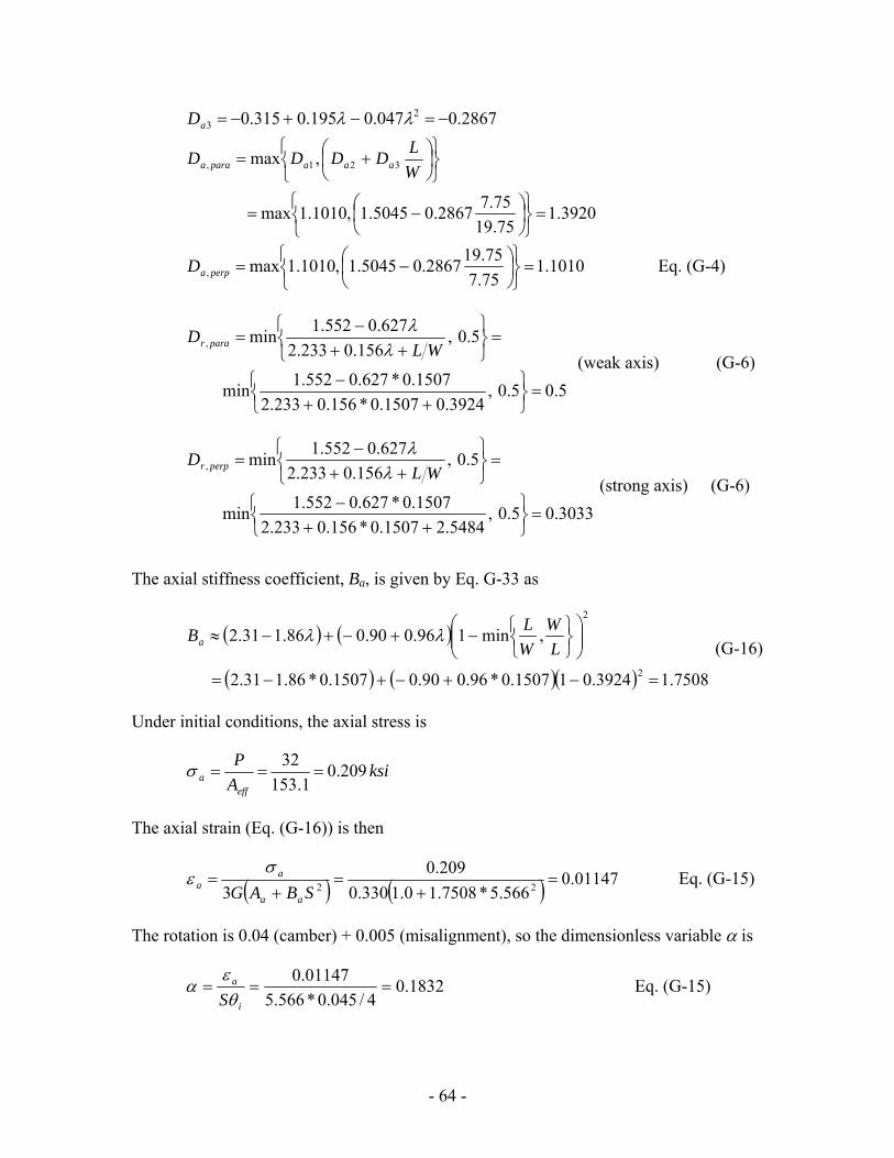
2867.0047.0195.0315.0 23 −=−+−= λλaD

3920.1

75.1975.72867.05045.1,1010.1max

,max 321,

=⎭⎬⎫

⎩⎨⎧

⎟⎠⎞

⎜⎝⎛ −=

⎭⎬⎫

⎩⎨⎧

⎟⎠⎞

⎜⎝⎛ +=

WLDDDD aaaparaa

1010.175.775.192867.05045.1,1010.1max, =

⎭⎬⎫

⎩⎨⎧

⎟⎠⎞


5.05.0,3924.01507.0*156.0233.2

1507.0*627.0552.1min

5.0,156.0233.2

627.0552.1min,

=⎭⎬⎫

⎩⎨⎧

++−

=⎭⎬⎫

⎩⎨⎧

++−

=WL

D parar λλ

(weak axis) (G-6)

3033.05.0,5484.21507.0*156.0233.2

1507.0*627.0552.1min

5.0,156.0233.2

627.0552.1min,

=⎭⎬⎫

⎩⎨⎧

++−

=⎭⎬⎫

⎩⎨⎧

++−

=WL

D perpr λλ

(strong axis) (G-6)

The axial stiffness coefficient, Ba, is given by Eq. G-33 as

( ) ( )

( ) ( )( ) 7508.13924.011507.0*96.090.01507.0*86.131.2

,min196.090.086.131.2

2

2

=−+−+−=

⎟⎟⎠

⎞⎜⎜⎝

⎛

⎭⎬⎫

⎩⎨⎧−+−+−≈

LW

WLBa λλ

(G-16)

Under initial conditions, the axial stress is

ksiAP

effa 209.0

1.15332

===σ

The axial strain (Eq. (G-16)) is then

( ) ( ) 01147.0566.5*7508.10.1330.0

209.03 22 =

+=

+=

SBAG aa

aa

σε Eq. (G-15)

The rotation is 0.04 (camber) + 0.005 (misalignment), so the dimensionless variable α is

1832.04/045.0*566.5

01147.0===

i

a

Sθα

ε Eq. (G-15)

- 64 -

( ) ( ) 0603.0131

34 22 =

⎪⎭

⎪⎬⎫

⎪⎩

⎪⎨⎧

−−⎟⎠⎞

⎜⎝⎛ += ααααf

5.1

(Eq. (G-13)

The hydrostatic tension can be obtained from Eq. (G-30) as

( ) 25.23508.00603.0*4045.0*566.5*33 33 <=⎟

⎠⎞

⎜⎝⎛== αθ

σfS

G ihyd (Eq. (G-12)

Hydrostatic tension exists, but its magnitude is acceptable. If hydrostatic tension had posed a problem it might have been solved by specifying a construction procedure that requires the bearing not to be bolted to the girder until after the slab has been poured and the rotation due to camber had been eliminated. However, such a provision is undesirable because it could be forgotten on site. Making the bearing thicker would be a better alternative.

Under initial load, for rotation about the weak axis, the shear strains due to compression are

475.0566.5*110.0

209.0*3920.1, ===GS

D aparaaa

σγ Eq. (G-3)


351.14045.0

5.075.75000.0

22

, =⎟⎠⎞

⎜⎝⎛

⎟⎠⎞

⎜⎝⎛=⎟⎟

⎠

⎞⎜⎜⎝

⎛= i

ripararr h

LD θγ Eq. (G-6)

Total shear strain is

827.1000.0351.1475.0 =++=++= sratot γγγγ Eq. (G-1)

Under full service load, the calculations are similar to those of Example 1, and are not presented here.

It is instructive to check the bearing against the existing LRDF design specifications under initial conditions, given the large rotation and light axial load. Eq. 14.7.5.3.5-1 of the LRFD Specifications requires

ksihB

nGS

ris 763.1

5.08

4045.0566.5*110.0*0.10.1

22

=⎟⎠⎞

⎜⎝⎛

⎟⎠⎞

⎜⎝⎛=⎟⎟

⎠

⎞⎜⎜⎝

⎛⎟⎠⎞

⎜⎝⎛>θσ

(Note that B and σs in the existing specifications are the same as the quantities L and σa in this report. Also, gross, rather than effective, bearing dimensions are used for all calculations in the existing Specifications). However

However

- 65 -

ksiinch

kipss 200.0

8*2032

==σ

Thus, the bearing fails by a significant margin to satisfy the uplift provisions of the existing Specifications because of the combination of high rotation and low axial load. The fact that the initial conditions prove acceptable under the proposed Method B provisions is an important change.

A girder with such a large camber also poses potential problems during construction. The bottom flange will elongate, and the bearing will move longitudinally, as the girder is stressed by the addition of the dead weight of the deck and other components. An approximate value for the magnitude of the movement can be obtained by considering the two major sources of it. In the interests of simplicity, the girder is assumed here to be symmetric. The girder is assumed to be 5 ft deep (span/depth = 30).

End rotation of the girder gives a movement at each end of

.2.104.02

602

ind===Δ θ

The girder also flattens out from its cambered shape. The neutral axis by definition does not change length, but its horizontal projected length does, because its initial curved shape changes to a straight line by the time the camber has been completely eliminated. The change in length is given by

∫ ⎟⎠⎞

⎜⎝⎛=Δ

L

dxdxdy

0

2

21

If the cambered shape is a parabola, this gives

L

a 20667.2=Δ

If it is sinusoidal

L

aL

a 20

20

2

467.24

≈=Δπ

where a0 = the initial camber height. The exact cambered shape is thus seen to have little effect on the magnitude of the longitudinal movement. Using the parabolic shape, and noting that

La

camber04=θ

.48.01800404.0667.2

4667.2667.2

2220 inL

La

=⎟⎠⎞

⎜⎝⎛=⎟

⎠⎞

⎜⎝⎛==Δθ

A the movement must occur at the non-fixed end of the bridge, where

.88.248.02.1*2 intotal =+=Δ

- 66 -

This is significantly larger than the ±1.0 inches of thermal expansion, so provision should be made for re-setting the girder on the bearings during construction. This problem is more likely to occur in steel bridges because they are typically more flexible than concrete ones.

Example 4. Common bearing, but lift-off allowed. The bridge also has 55 degrees skew. No thermal effects. The complexities in this example pertain to the skew.

Design Criteria.

A steel plate girder bridge is supported on elastomeric bearings. The girders span 150 ft and have 22” wide flanges. Under construction conditions, the load is 32 kips and the rotation is 0.04 radians (bending camber), and there is no torsional rotation. Under full dead load, the girder is exactly horizontal in bending, has a torsional rotation of 0.01 radians, and the total load is 115 kips. The live load causes a load of 70 kips and rotations of 0.002 radians (bending of girder) and 0.003 radians (torsion of girder). Shear displacement due to thermal effects is ± 1.0 inches, all to be taken at one end, in the longitudinal direction. Use an elastomer with G = 0.110 ksi.

The bearings are to be oriented with their long edges parallel to the support. Guides at the support prevent movement perpendicular to the girder axes, but allow longitudinal displacement.

Solution:

Try a rectangular bearing that will fit under the girder flange, with a total rubber thickness of 2”. Trial and error (with a spreadsheet) shows that a bearing 18” x 9” will carry the loads and will fit in the space available. Calculations for the service loading are shown below. The orientation and labeling of the axes are shown in Figure 3.2.

Figure 3.2 Orientation of Axes for Skew Bridge.

long

trans

perp

β para

girder axis

- 67 -


inchesLeff 75.8)5.80.9(*5.0 =+=

inchesW 75.17)5.170.18(*5.0 =+=eff

( ) ( ) 861.575.875.175.0*2

75.8*75.172

=+

=+

=effeffri

effeff

LWhS

LW

2==

3.155 inLWA effeff

1587.0450

11.0*3861.53===

KGSλ


1037.1413.0210.0060.1 21 =++= λλaD

5050.1406.0071.0506.1 22 =+−= λλaD

2852.0047.0195.0315.0 23 −=−+−= λλaD

3643.1

75.1775.82852.05050.1,1037.1max

,max 321,

=⎭⎬⎫

⎩⎨⎧

⎟⎠⎞

⎜⎝⎛ −=

⎭⎬⎫

⎩⎨⎧

⎟⎠⎞

⎜⎝⎛ +=

WLDDDD aaaparaa

1037.175.875.172852.05050.1,1037.1max, =

⎭⎬⎫

⎩⎨⎧

⎟⎠⎞


5.05.0,4930.01587.0*156.0233.2

1587.0*627.0552.1min

5.0,156.0233.2

627.0552.1min

=⎭⎬⎫

⎩⎨⎧

++−

=⎭⎬⎫

⎩⎨⎧

++−

=WL

Dr λλ

(weak axis) Eq. (G-7)

3389.05.0,0286.21587.0*156.0233.2

1587.0*627.0552.1min

5.0,156.0233.2

627.0552.1min

=⎭⎬⎫

⎩⎨⎧

++−

=⎭⎬⎫

⎩⎨⎧

++−

=WL

Dr λλ

(strong axis) Eq. (G-7)

- 68 -

Under service conditions:

Load = 115 kips DL + 70 kips LL

The local rotation and shear demands on the bearing for the strong (“perp”) and weak (“para”) axis rotation directions must be computed from the global coordinate system, defined by the longitudinal and transverse directions. In each case, the rotations due to loading are computed first, then the allowance for misalignment is added. The bearings are oriented at a skew angle of β = 55 degrees. With the positive directions as shown in Figure 3.2, the rotations in the global coordinate system are:

Girder bending: radLLDLtrans )(002.0)(000.0 −=θ

Girder torsion: radLLDLlong )(003.0)(010.0 +=θ

The rotations in the local bearing axes (perp aand para) are obtained by using the transformation matrix:

radLLDLLLDL

trans

long

para

perp

⎭⎬⎫

⎩⎨⎧

−−+

=⎭⎬⎫

⎩⎨⎧

⎥⎦

⎤⎢⎣

⎡−

=⎭⎬⎫

⎩⎨⎧

)(003605.0)(008192.0)(0000824.0)(005736.0

cossinsincos

θθ

ββββ

θθ

The total amplified rotations, including the misalignment allowance, are therefore

radpara

perp

⎭⎬⎫

⎩⎨⎧

−+

=⎭⎬⎫

⎩⎨⎧

−−−++

=⎭⎬⎫

⎩⎨⎧

02040.001090.0

005.0003605.0*2008192.0005.00000824.0*2005736.0

θθ

The shear deformations are obtained using the same transformation matrix

.8192.0

5736.0cossinsincos

intrans

long

para

perp

⎭⎬⎫

⎩⎨⎧

−=

⎭⎬⎫

⎩⎨⎧

ΔΔ

⎥⎦

⎤⎢⎣

⎡−

=⎭⎬⎫

⎩⎨⎧

ΔΔ

ββββ

The amplified axial stress is

ksia 642.13.155

70*0.2115=

+=σ

For shear strains on the long side (rotation about the weak, or parallel, axis), the shear strain due to (amplified) axial load is

475.3861.5*110.0

642.1*3643.1, ===GS

D aparaaa

σγ Eq. (G-3)

Shear strain due to rotation about the weak (“para”) axis is

781.04

02040.05.0

75.85000.022

, =⎟⎠⎞

⎜⎝⎛

⎟⎠⎞

⎜⎝⎛=⎟⎟

⎠

⎞⎜⎜⎝

⎛= i

ripararr h

LD θγ Eq. (G-6)

Shear strain due to shear deformation is

- 69 -

287.00.2

5736.0==

Δ=

inchesinch

hrt

ssγ Eq. (G-10)

The total shear strain check is given by

0.5542.4287.0781.0475.3 ≤=++=++= sratot γγγγ Eq. (G-1)

The shear strain due to the static component the axial load is also acceptable

( ) 0.3567.1861.5*110.03.1551153643.1, <===

GSD a

paraaaσγ Eq. (G-3)

For rotation about the strong, or “perp”, axis, the service level shear strain due to axial load is

811.2861.5*110.0

642.1*1037.1, ====GS

D aperpaa

σγ Eq. (G-3)


164.14

01090.05.075.173389.0

22

, =⎟⎠⎞

⎜⎝⎛

⎟⎠⎞

⎜⎝⎛=⎟⎟

⎠

⎞⎜⎜⎝

⎛= i

riperprr h

LD θγ Eq. (G-6)

The total shear strain is

0.5385.4410.0164.1811.2 ≤=++=++= sratot γγγγ Eq. (G-1)

According to the existing LRFD Method B specifications, this bearing would just fail the compressive stress limit of 1.66GS, and would fail by a substantial margin the uplift provision (about the strong axis) and the combined stress limit Failure to meet the latter two criteria is not surprising, because they are very conservative, and were a large part of the reason for conducting the research.

The bearing also fails to satisfy the proposed Method A requirements. The total axial stress/GS is

( ) ( ) ksiGS

s 25.1848.1861.5*110.0

75.8*75.1770115>=

+=

σ NG

The shear strains due to combined loading about the strong (“perp”) axis also prove to be excessive.

- 70 -

Example 5. Long-span box girder bridge, large bearing, lift-off permitted.

Design Criteria. A prestressed concrete box girder bridge is supported on elastomeric bearings. There is no skew. The girders span 300 ft. Under full dead load, the end rotation is 0.003 (cambered upwards) and the load is 1,200 kips. The live load causes a load of 120 kips and a rotation of 0.0018 radians (downwards). Shear displacement due to thermal effects is -2.75, +1.00 inches. Allow for 0.0015 radians of thermal rotation in the final condition.

Solution For shear displacements,

inchesh srt 5.575.2*22 ==Δ≥ Eq. (G-10)

Axial forces appear to dominate the design. Try a high shape factor bearing (generally good for axial capacity but bad for rotation capacity). Make the bearing approximately 2 to 1 aspect ratio, to minimize the rotational effects. Assume ¼ in. edge cover.

Use G = 0.135 ksi (approx. 55 durometer) to increase the load capacity.

Trial and error shows that a bearing of 30 in. x 15 in., with 11 layers at 0.5 in. each will suffice. Final calculations are as follows:


inchesLeff 75.14)5.140.15(*5.0 =+=

inchesW 75.29)5.290.30(*5.0 =+=eff

( ) ( ) 861.975.1475.295.0*2

75.14*75.292

=+

=+

=effeffri

effeff

LWhS

LW

2==

8.438 inLWA effeff

2958.0450

135.0*3861.93===

KGSλ


1583.1413.0210.0060.1 21 =++= λλaD

5205.1406.0071.0506.1 22 =+−= λλaD

- 71 -

2614.0047.0195.0315.0 23 −=−+−= λλaD

3909.1

75.2975.142614.05205.1,1583.1max

,max 321,

=⎭⎬⎫

⎩⎨⎧

⎟⎠⎞

⎜⎝⎛ −=

⎭⎬⎫

⎩⎨⎧

⎟⎠⎞

⎜⎝⎛ +=

WLDDDD aaaparaa

1583.175.1475.292614.05205.1,1583.1max, =

⎭⎬⎫

⎩⎨⎧

⎟⎠⎞


4924.05.0,4958.02958.0*156.0233.2

2958.0*627.0552.1min

5.0,156.0233.2

627.0552.1min,

=⎭⎬⎫

⎩⎨⎧

++−

=⎭⎬⎫

⎩⎨⎧

++−

=WL

D parar λλ


3181.05.0,0169.22958.0*156.0233.2

2958.0*627.0552.1min

5.0,156.0233.2

627.0552.1min,

=⎭⎬⎫

⎩⎨⎧

++−

=⎭⎬⎫

⎩⎨⎧

++−

=WL

D perpr λλ


The axial stiffness coefficient, Ba, is given by Eq. G-33 as

( ) ( )

( ) ( )( ) 6032.14958.012958.0*96.090.086.131.2

,min196.090.086.131.2

2

2

=−+−+−=

⎟⎟⎠

⎞⎜⎜⎝

⎛⎭⎬⎫

⎩⎨⎧−+−+−≈

λ

λλL

WWLBa Eq. (G-16)

Under service conditions (amplified loads):

ksia 282.38.438

120*0.21200=

+=σ

For rotation about the critical parallel axis, shear strain due to axial load is

429.3861.9*135.0

282.3*3909.1, ===GS

D aparaaa

σγ Eq. (G-3)

DL

DL+LL

Figure 3.3 DL and LL Rotations for Bearing Design

- 72 -

The rotation consists of 0.003 rad (DL) and -0.0018 rad. (live load). These two oppose each other, so the peak rotation theoretically occurs under dead load alone. Therefore the rotations should be treated as a static load of the DL + LL (0.0030 + (-0.0018) = 0.0012 rad.) plus a live load of –(-0.0018) = +0.0018 rad. 1.0 times the static rotation plus 2.0 times the cyclic then gives 1.0*0.0012 + 2.0* 0.0018 = 0.0048 rad, to which must be added the misalignment allowance. The total amplified rotation is then 0.0048+0.005 = 0.0098 rad.


382.0110098.0

5.075.144924.0

22

, =⎟⎠⎞

⎜⎝⎛

⎟⎠⎞

⎜⎝⎛=⎟⎟

⎠

⎞⎜⎜⎝

⎛= i

ripararr h

LD θγ Eq. (G-6)


5.05.575.2

==Δ

=inches

inchhrt

ssγ Eq. (G-10)


0.5311.4500.0382.0429.3 <=++=++= sratot γγγγ Eq. (G-1)

The static axial stress is

ksia 735.28.438

1200==σ

and the corresponding shear strain is

0.3857.2861.9*135.0

735.2*3909.1, <===GS

D aparaaa

σγ Eq. (G-3)

Similar calculations for rotation about the strong axis, with only the construction misalignment rotation of 0.005, give

- 73 -

855.2861.9*135.0

282.3*1583.1, ===GS

D aperpaa

σγ Eq. (G-3)

512.011005.0

5.075.293181.0, =⎟

⎠⎞

⎜⎝⎛

⎟⎠⎞

⎜⎝⎛=⎟⎟

⎠

⎞⎜⎜⎝

⎛= i

riperprr h

LD θγ22

0.5367.3000.0512.0855.2

Eq. (G-6)

=++= <=++sratot γ γ γγ Eq. (G-1)

The shim thickness, based on Fy = 36 ksi, must satisfy

inchesF

hhy

as 1253.0

36008.3*5.0*33 max ==≥

σ AASHTO Eq. (14.7.5.3.7-1)

This thickness requires 10 gage sheet steel, which is slightly thicker than the 11 gage commonly used for convenience in manufacturing. It illustrates the need for thicker shims when the axial stress on the bearing is high. The bearing has no external plates, so hydrostatic tension does not need to be checked. Stability criteria are satisfied. Initial conditions are also satisfactory. Because the bearing thickness is less than 8 inches and its plan area is less than 1000 in2, special testing is not required.

Note that, according to the existing LRFD Specifications, this bearing would fail both the compressive stress limits and the combined stress limits under final conditions. However, it has a shape factor (approx 10) that is higher than in most bridge bearings. It would also fail to satisfy the proposed Method A requirements, because the non-amplified axial stress is 3.01 ksi, which significantly exceeds the limit of 1.25 ksi. While it is quite large, it is still well within the fabrication capabilities of most manufacturers. For example, vibration isolation bearings are often twice as thick as this.

Example 6. Heavily loaded special purpose bearing, lift-off permitted.

Design Criteria. An elastomeric bearing is used to support a steel beam that is intended to yield cyclically under seismic loading in a large bridge. Special installation procedures ensure that there is no misalignment whatsoever. The dead load is the self-weight of the beam, which is negligible. The seismic load consists of 12 cycles of load to 2200 kips, accompanied by a rotation of 0.00167 rad. and a shear displacement of 0.25 in. The space available is 20 in. x 24 in.

Solution. Because the number of cycles of load is much smaller than under traffic load, treat the seismic load as static. The axial load appears to control the design, so use a high shape factor and a relatively hard elastomer with G = 175 psi, (approx 60 durometer). Assume ¼ in. edge cover.

- 74 -

Trial and error show that a bearing of 24 in. x 20 in., with 2 layers at 0.25 in. each will suffice. Final calculations are as follows:


inchesLeff 75.19)5.190.20(*5.0 =+=

inchesW 75.23)5.230.24(*5.0 =+= eff

( ) ( ) 566.2175.1975.2325.0*2

75.19*75.232

=+

=+

=effeffri

effeff

LWhS

LW

2==

1.469 inLWA effeff

7366.0450

175.0*3566.213===

KGSλ

Coefficients needed for shear strains are 4338.1413.0210.0060.1 2

1 =++= λλaD 6740.1406.0071.0506.1 2

2 =+−= λλaD 1969.0047.0195.0315.0 2

3 −=−+−= λλaD

5103.1

75.2375.191969.06740.1,4338.1max

,max 321,

=⎭⎬⎫

⎩⎨⎧

⎟⎠⎞

⎜⎝⎛ −=

⎭⎬⎫

⎩⎨⎧

⎟⎠⎞

⎜⎝⎛ +=

WLDDDD aaaparaa

4338.175.1975.231969.06740.1,4338.1max, =

⎭⎬⎫

⎩⎨⎧

⎟⎠⎞


3429.05.0,8316.07366.0*156.0233.2

7366.0*627.0552.1min

5.0,156.0233.2

627.0552.1min,

=⎭⎬⎫

⎩⎨⎧

++−

=⎭⎬⎫

⎩⎨⎧

++−

=WL

D parar λλ


3070.05.0,2025.17366.0*156.0233.2

7366.0*627.0552.1min

5.0,156.0233.2

627.0552.1min,

=⎭⎬⎫

⎩⎨⎧

++−

=⎭⎬⎫

⎩⎨⎧

++−

=WL

D perpr λλ


Under service conditions (amplified loads):

- 75 -

ksia 690.41.469

2200==σ

Shear strain due to axial load is

877.1566.21*175.0

690.4*5103.1, ===GS

D aparaaa

σγ Eq. (G-3)


783.12

00167.025.075.193429.0

22

, =⎟⎠⎞

⎜⎝⎛

⎟⎠⎞

⎜⎝⎛=⎟⎟

⎠

⎞⎜⎜⎝

⎛= i

ripararr h

LD θγ Eq. (G-6)


500.05.025.0

==Δ

=inches

inchhrt

ssγ Eq. (G-10)


0.5160.4500.0783.1877.1 <=++=++= sratot γγγγ Eq. (G-1)

The bearing has no external plates, so hydrostatic tension does not need to be checked. Stability criteria are satisfied. Initial conditions are also satisfactory. Because the bearing thickness is less than 8 inches and its plan area is less than 1000 in2, special testing is not required.

Note that, according to the existing Method B LRFD Specifications, this bearing would not be permitted, largely because the applied axial stress exceeds the limit of 1.60 ksi, in the presence of shear deformations. However, during the testing phase of the research, some bearings with shape factor 9 were loaded to 12 ksi (i.e. to a stress of 12 GS) with no signs of damage. The bearing in this example is required to carry only 1.876 GS.

Note also that the initial assumption that the axial force dominated proved incorrect. The shear strain due to total (amplified) axial load is 1.877, whereas the shear strain due to rotation is 1.783, so the magnitudes of the axial and rotation effects are similar.

If the total shear strain of 4.160 were to be regarded as unacceptably high, the simplest way to reduce it would be to use more rubber layers and lower the rotation component of the shear strain. However, there is no need to design for lower stresses because the shear strains are already low enough to prevent any debonding under such a small number of cycles. In addition, the loading is caused by the extreme seismic event, so some debonding damage may anyway be tolerable.

- 76 -

3.3 QC/QA Procedures Chapter 2 summarized some issues related to QA/QC testing and evaluation procedures. Evaluation of QA/QC procedures was not the primary goal of this research, so less effort was spent on it than was given to testing and FEA. Nevertheless, several recommendations are appropriate, and are described here.

• It is clear that today’s elastomeric bearings are of higher quality than those made in the past. Two of the causes that have led to this are the concentration of manufacturing into four major companies, and the effectiveness of the QA/QC requirements imposed by the specifications. Each of the four major companies is large enough to support an effective QA/QC operation, and takes pride in producing quality bearings. This is perhaps made possible by the relatively stringent specifications, which tend to inhibit low-cost, low-quality fabricators from entering the market. The presence of such operators would create intense price competition, to the likely detriment of quality, with little if any real reduction in bridge costs. This observation should be taken into account when considering any QA/QC tests for modification or elimination. The cost advantages that might be gained through elimination of some of these tests are small, whereas the potential losses associated with lower quality standards are high. The cost of replacing a bearing in a bridge, including any possible litigation costs, is several orders of magnitude higher than the cost of a material test in a manufacturer’s laboratory. As a result, it is suggested that major changes should be undertaken only after very careful consideration of the costs and benefits.

• The test procedures previously associated with the current Method B were fairly complex and expensive and they appear to have deterred some engineers from using the design method. Yet the compressive stresses allowed by Method B may be only slightly higher than those permitted under Method A. (The increase depends on the amplitude of the rotation, which is not accounted for explicitly by Method A). The long-duration load test was particularly troublesome, but has now been eliminated. Therefore, it is proposed that any additional testing be required for large bearings rather than those designed using Method B. Large bearings are tentatively defined as those thicker than 8 inches or with a plan area larger than 1000 in2. There remains the question of what additional testing to apply to such bearings. The regimes in M251-06 have some serious drawbacks, but the AASHTO T-2 Committee has chosen to eliminate the long term test. It is recommended that the choice of required additional testing be a matter for discussion between the T-2 Committee members, a representative group of manufacturers, and the researchers. Each group is a stakeholder in the issue, and brings specialist knowledge to the table which is necessary to reach a good decision.

• .Very large and unusual bearings pose problems. Their size may make testing them difficult, because the loads needed might exceed the capacity of most test machinery, especially if the test load is to be significantly higher than the service load. However, they are the bearings most in need of testing, both because of the difficulties involved in curing large bodies of rubber and because the

- 77 -

consequences of a failure are more serious large in a large bearing than in a small one. Three possible alternatives are envisaged:

o The first is to require that the manufacturer produce an extra full sized bearing for testing. It should then be cut up as needed, and destructive shear and compressive tests should be performed on the parts to evaluate the material properties throughout the bearing..

o The second is to core the center of one of the large bearings. Portions of the core of the bearing could be tested in shear and compression to provide the information needed through the thickness of the bearing. The cored bearing could then be refilled with pre-cured elastomer and put into service. If the core is taken in the center of the bearing, and the effect of the coring on the strength of the reinforcement is considered during design, the refilled bearing may provide good service if the bearing proves satisfactory in all other ways.

o The third is to test the bearing with a tapered plate. The taper angle should be selected so as to create a combination of rotation and compression on the most heavily stressed edge that leads to the same local shear strain as would be caused by the desired test load applied through parallel load plates. Calculations should be done using the linear theory strain coefficients, Da and Dr.

• The current definitions of the number of test specimens required by the AASHTO M251-06 Specifications are less clear than they should be. For example, the definition of a “lot” of bearings may lead to excessive testing. There is little reason for duplicating tests on bearings of similar bearing sizes and geometries that are made from the same compound. It is suggested that a set of bearings that are made from one compound, and whose dimensions differ by no more than 10%, be grouped into a single lot for the purposes of establishing test requirements. Inconsistencies between various specifications, and within specifications, should also be resolved.

• The definition of the word “batch” should also be reviewed for consistency with practice. The process of mixing the ingredients for a rubber compound is called batching. Some manufacturers batch their own rubber, while others buy it pre-batched, from a separate supplier. Thus the word “batch” could mean the bearings made from a single delivery of pre-mixed rubber, which might be enough for only some of the bearings for a whole bridge, or it could mean a group of bearings for the same job. The different interpretations may lead to different numbers of bearings being tested.

- 78 -

CHAPTER 4 Summary, Conclusions and Recommendations.

4.1 Summary The rotational response of elastomeric bearings was studied using testing and analysis. The program concentrated on steel-reinforced elastomeric bearings. The test bearings were purchased from the four largest manufacturers in the country.

The test program included static and cyclic rotation tests on full bearings, material tests, and diagnostic tests on full bearings to evaluate their instantaneous state of damage. Many of the tests were conducted in a specially constructed test machine that is capable of applying to a bearing independently-controlled, constant axial force, constant shear deformation and cyclic rotation.

In the static test series, the parameters investigated were combinations of axial load and rotation. In the cyclic load tests, they included the effects of axial load, rotation angle and number of cycles, bearing geometry (aspect ratio and shape factor), materials, shim plate edge treatment and manufacturer.

The behavior of the bearings was modeled in three ways. An approximate linear model, based on small deflection theory, was used to investigate basic behavioral phenomena and to derive design equations. FEA were also conducted, using large deformations and special constitutive laws for nonlinear, nearly incompressible materials. The goals were to evaluate the suitability of the simpler linear models, to investigate behaviors that could not be studied in the laboratory and to determine the relationship between local deformations, which could not be measured, and global displacements, which could. Finally, empirical models were developed to predict the fatigue behavior of the bearings under cyclic loading.

The results of the tests and analyses were combined and used to develop design procedures.

4.2 Conclusions The following conclusions were drawn from this research:

4.2.1 Conclusions on Behavior Measured in Tests 1. Steel reinforced elastomeric bearings are extremely robust. In the tests, bearings

that had been subjected to loads of approximately ten times their design value, and had suffered considerable visible damage, were still able to carry the vertical load. While this ability is useful because it would prevent immediate collapse of the bridge, the vertical deflection and the damage to the bearing would seriously impair the bridge’s serviceability.

2. The bearings tested in this study came from the four largest manufacturers in the country. All were of high quality. The test results showed that the quality of bearings today is higher than it was 20 years ago. No one manufacturer stood out as universally superior to the others.

- 79 -

3. No clear and unique definition of failure exists for an elastomeric bearing. The first form of damage is typically local tension debonding of the edge cover from the edge of the shims. More intense static loading, or continued cyclic loading, may lead to delamination, which is characterized by the propagation of a horizontal shear crack back into the elastomer layers. It typically runs in the rubber, close to the steel-rubber interface. At very high axial loads, the steel shims yield and fracture. The debonding and delamination mechanisms tend to be progressive, and to occur more readily under cyclic loading. Shim fracture occurs only in response to very high axial load, either static or cyclic.

4. The tension debonding of the edge cover from the vertical face of the steel shim has no adverse effect on the performance of the bearing. However, it presages the start of shear delamination from the horizontal surface of the shims, which will change the bearing’s stiffness, and will eventually cause the bearing to tear apart. These behaviors will have a negative impact on the bridge superstructure.

5. The lack of a unique definition of failure makes development of design specifications difficult, because the demarcation between acceptable and unacceptable behavior is not binary but rather requires judgment over the level of damage that is acceptable. Furthermore, the difficulties are aggravated by the facts that the quality of the manufacturing influences the loading required to cause a given level of damage, and that damage accumulates as a fatigue process. Fatigue data typically show considerable scatter and the process is difficult to characterize reliably.

6. In this study, tension debonding of the rubber cover from the shim edge was used as the critical damage measure.

7. The fatigue resistance of the rubber did not show a clear correlation with any obvious material property such as tension strength or elongation at break.

8. Sharp edges on the shims promote debonding. If they are deburred with a special tool, or rounded with a belt sander, debonding is delayed. More precise rounding of the edges than that (e.g. with machine tools) provides little additional benefit.

9. Adding shear deformation of 30% causes no noticeable change in the number of cycles required to reach a given level of debonding.

4.2.2 Conclusions on Analytical and Numerical Modeling 1. Bearings made from 60-durometer elastomer performed better under comparable

loads than did nominally identical 50-durometer bearings, because the increased stiffness reduced the maximum shear strain. The observation that they performed even better than predicted by theory supports the view that shear strain rather than stress is an appropriate measure of fatigue demand.

2. Bearings with shape factors of 9 and 12 performed better than did bearings of shape factor 6 under loading that caused similar total shear strains in each. Theory suggests that, when the induced shear strains are the same, the performance should be the same. This finding supports the use of bearings with large shape factors.

3. The approximate linear theory originally developed by Gent and his co-workers provides a reasonable estimate of the rotational stiffness. The compressive

- 80 -

stiffness was harder to match, because it displays significant nonlinearity and because determining the point of zero displacement is difficult.

4. The FEA in general confirmed, at low loads and rotations, the validity of the small displacement analyses. In particular, they showed that superposition of load-cases was valid, that the stiffness and strain coefficients developed by Stanton and Lund using linear theory were accurate enough for use in design, and that the value of internal hydrostatic stress predicted by the simple linear theory was valid.

5. The FEA also showed several behaviors that would otherwise have been very hard to observe. The first was the existence of a small local region of high hydrostatic stress at the outer, vertical edge of the shim, which, in combination with the very large local strains there, appears to be responsible for the tension debonding observed in almost all the tests. The second was the lateral movement of the shims at mid-height, when pure rotation is applied to the bearing. If the bearing is thought of as a very short column, this effect is analogous to the lateral deflection at mid-height of the column when end moments are applied. This shim displacement alters the strain field in the critical region at the edge of the shims, and may affect the debonding behavior there.

4.2.3 Conclusions on Development of Design Procedures. 1. Obtaining reliable laboratory measurements of the local shear strains in the rubber

is impossible. Therefore it was necessary to use computed strains in the models for predicting debonding.

2. Initial debonding under static load occurred at a total shear strain that was nearly the same in a range of tests with different load and rotation combinations. This finding was used to develop a total shear strain limit for monotonic load.

3. Analyses of trucks passing over typical bridges showed that the cyclic axial load effects of the loading create shear strains in the elastomer that are much larger than those caused by the rotation.

4. An empirical but rational fatigue model was developed to predict the level of cyclic debonding as a function of the constant axial load, the amplitude of the cyclic rotation and the number of cycles. It is referred to here as the “Nonlinear Model” because it made use of a nonlinear axial load-displacement relationship. It was able to predict well the fatigue life of the bearings, even though the dataset included a wide variety of loadings and bearing geometries. However, it had to be abandoned because it predicted extensive debonding in a class of bearing that is widely used for freeway overpasses, whereas such damage is not seen in practice. A description of it is retained in Appendix F so that, if suitable cyclic axial test data become available, it could be developed for use in a specification.

5. An alternative and simpler design method was developed. It is referred to herein as the “Linear Model”. It was based on a linear relationship between axial force and deflections, and did not attempt to link the progress of damage continuously to the number of cycles of load. It fitted the test data by relating the total applied shear strain to the number of cycles at a specific level of damage (25% debonding). When applied to bearings commonly used for typical freeway

- 81 -

overpasses, it predicted that very little debonding should occur. This prediction is in agreement with field observations.

6. The Method B design procedure based on the Linear Model is simple to use. The major changes from the present specifications are that: the permissible combinations of load and rotation are controlled by an explicit total strain approach; lift-off is allowed if no external bonded plates exist; and a check is required for rupture by hydrostatic tension if external plates do exist. The limit on absolute axial stress has been removed, but a limit in terms of GS remains.

7. A Method A design procedure was developed from Method B. This was done by computing a maximum probable rotation on the bearing, and finding the corresponding axial stress that would be allowed under the Method B rules. In order to optimize the usefulness of Method B (by keeping the allowable stress as high as reasonably possible) some restrictions on it use proved necessary. Only seldom are these restrictions are likely to provide active constraints.

4.3 Recommendations

4.3.1 Recommendations for Implementation 1. The design methodology proposed in Appendix G for both Method A and Method

B should be considered for adoption in the AASHTO LRFD Specifications. It is written there in language and a format suitable for direct adoption. Those design requirements provide better correlation with the behavior observed in the tests than do the existing ones, they are more transparent to the user, and they are simpler to implement. They also address combinations of loading, including light axial load and large rotations, that prove problematic under the existing specifications.

2. The criteria for additional, more stringent, testing presently required for Method B bearings should be re-considered, and an alternative is proposed. Design by the existing Method B triggers the need for more rigorous testing. The cost of that testing acts as a disincentive to the use of Method B. That in turn inhibits the use of high shape factor bearings, which are encouraged under the proposed Method B and which were shown in the test program to be very effective in inhibiting the initiation and propagation of damage due to debonding and delamination. More rigorous testing is most urgently needed for large bearings, and particularly thick ones, because they are more difficult to fabricate. Consequently, it is proposed that bearing size, and not the design method used, be used as the criterion for more rigorous testing. This raises the practical problem that suitable testing facilities with enough capacity to load such a bearing may not be available. Several approaches are proposed for resolving that problem.

3. The edges of all steel shims in all bearings should be de-burred or otherwise rounded prior to being molded in the bearing. Doing so reduces the stress concentration in the rubber at the critical location at the edge of the shim. The proposed strain limits in Appendix G are contingent on this being done.

- 82 -

4.3.2 Recommendations for Further Research 1. Average axial strains measured in the tests were found to differ from those

calculated by both linear elastic methods and nonlinear elastic FE models. An approximate, semi-empirical, nonlinear model was developed but an improved understanding of axial load effects and their nonlinearities is desirable.

2. The fatigue effects of axial loading should be investigated experimentally and analytically, so that they can be incorporated into the design method in a rational way.

3. Creep of the rubber should be investigated and included in the design method. The axial load tests showed significant continued displacement after the load was reached and held constant, resulting in increased strains for a given stress. For a design method based on shear strain limits, it is important to know the actual strains. The effect of load duration on strength should also be investigated.

4. The effects of aspect ratio should be further investigated. For the limited number of tests in this research, the bearings with smaller aspect ratios performed much better than what was expected on the basis of maximum shear strains calculated using theoretical models.

- 83 -

- 84 -

project no. 12-68 copy no. rotation limits for · pdf fileproject no. 12-68 copy no. rotation...

Documents