Progress on a Spatial Allocation Model of Regional Land-Use Change

Prasanth Meiyappan Graduate Student

University of Illinois at Urbana-Champaign

NCAR IAM Group Annual Meeting July 19, 2012

Problem Statement We need a bridge for land-surface model (ISAM) and demoeconomic

model (PET) – iPETS PET is a regional model - outputs the aggregate areas of cropland,

pastureland and forest for each of the 9 regions covering the entire globe annually

ISAM is a spatially explicit model which requires land-use data at

0.5ox0.5o spatial resolution. To couple PET with ISAM, we need a intermediate model/coupler

which downscales regional land-use areas to 0.5ox0.5o resolution.

Mathematical Formulation Formulate the objective function as a least-square problem of the form For a given number of grid-cells n (for each of the m regions), the

above function finds the n-vector ‘x’ which is closest to the Euclidian norm to a given vector x0 (reference map), subject to a index of land suitability to cultivation defined by ‘s’

Mathematical Formulation (Cont)

Constraints to the Objective Function Cropland + Pastureland + Forest area for each grid cells is < or = area of the grid cell

Sum of Cropland, Pastureland and Forest summed across all grid cells in a given region should be equal to the aggregate area outputted by PET

Mathematical Formulation (Cont)

Constraints to the Objective Function Non-Negativity Constraints: Areas of all land-use types within each grid cell should lie between 0 and area of that grid cell Constraints to force the change of land-use area for each grid cell in the direction determined by suitability factor and at the same time trying to minimize the variations from existing distribution – Essentially a stability constraint to avoid spurious jumps

What goes into Suitability Index Land suitability of a grid cell to cultivation is determined by several known

factors and unknown factors Account for known factors – biophysical/climatic and socio-economic

factors Biophysical/climactic/other factors: soil depth, soil fertility, soil texture,

soil drainage, soil chemicals, terrain/slope, climate conditions, irrigational facilities/proximity to rivers, urban area + population (total of 10 factors)

Socio-economic factors – market price, incentive structure, marginal cost,

etc. However, at global scale biophysical factors form major constraints to

determining cultivation – as will be shown later

Biophysical Factors Develop an index indicating the probability of land suitability to

cultivation for each of the 10 biophysical factors (dynamic) based on existing relations with croplands and pasturelands. We find an empirical relation for each factors based on Probability

Density Function Overall land suitability to cultivation (S) is determined as follows:

Scrop = Ssoil(5)x Sterrain x Sclim x Sirri x Spop x Surb

Spast = Ssoil(4)x Sterrain x Sclim x Spop x Surb

Calculating Individual Factors Overall Soil Suitability to Cultivation (Derived from AEZ) – Fertility + Texture + Drainage + Chemical + Depth constraints

Calculating Individual Factors Terrain/Slope Suitability to Cultivation

Calculating Individual Factors Climate Suitability to Cultivation (Dynamic) LGP can be used as a index of land suitability to cultivation.

LGP is calculated as no of days in a year where PET less than half the

value of precipitation and concurrently the temperature is above 5o C.

CRU TS 3.1 climate data set (precipitation and temperature) was used in ISAM to calculate PET using a variant of Penman-Monteith method (grass reference evapotranspiration method used in FAO)

Annual maps of LGP at 0.5 degree resolution was calculated for the period 1900-

2005.

We choose a suitability function f(LGP), empirically by examining the

existing relationship between LGP and cropland area

PDF for Cropland vs LGP

Point of Normalization

Limit of curve fit

Probability of Croplands = 1.0

PDF for Cropland vs LGP f(LGP) = a1*sin(b1*x+c1) + a2*sin(b2*x+c2) + a3*sin(b3*x+c3) + a4*sin(b4*x+c4) + a5*sin(b5*x+c5) + a6*sin(b6*x+c6) + a7*sin(b7*x+c7) + a8*sin(b8*x+c8) Coefficients (with 95% confidence bounds): a1 = 0.981, b1 = 0.01331, c1 = -0.739, a2 = 0.5782+04, b2 = 0.02405, c2 = 1.268 a3 = 0.07337, b3 = 0.1445, c3 = 1.071, a4 = 0.01604, b4 = 0.08874, c4 = 2.247 a5 = 0.0285, b5 = 0.183, c5 = -0.1863

LGP limit function, f(LGP) – close to sigmoidal curve

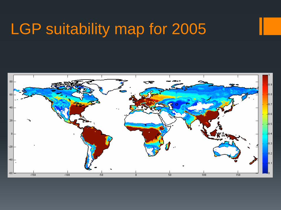
LGP suitability map for 2005

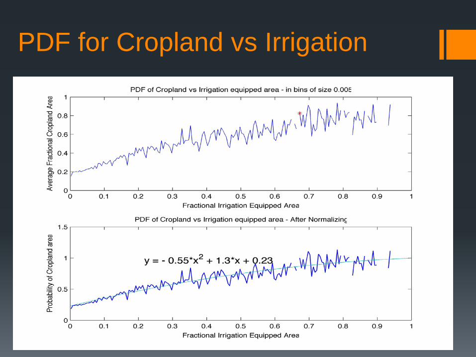
PDF for Cropland vs Irrigation

Irrigation Suitability Map

PDF for Cropland vs Urban land (Dynamic)

Neglect spurious values caused by diff in land mask and data uncertainties

Urban Suitability for Cropland - 2000

Population Suitability for Cropland - 2000

Total Land Suitability for Cropland – For USA (test case) yr: 2005

Empirical Approach

MODIS-IGBP

Getting the Hotspots right

Climate Suitability for Pastureland (Dynamic)

Temperature Constraint > -7oC as compared to 50C for Cropland TGP and LGP give almost same result Irrigation suitability excluded: ~100% pastureland rain fed Soil Chemical Constraints Excluded – No Correlation Found

Crop + Urban relation to Pastureland Regions of Cropland suitability are a subset of Pastureland Suitability

Overall Land Suitability to Pastures

Zoom Through USA - Pastureland

Empirical Approach

RF Data

Getting the Hotspots right

Satellites cannot explicitly differentiate pasture from grass. Considerable uncertainties b/w different estimates

Revisit - Objective Function

Implemented using the SQOPT solver – Meant for solving sparse Quadratic Programming Optimization Problem subject to both equality and inequality constraints (By Philip Gill, SOL, Stanford) Computing time: 5000 grid cells in serial (tramhill) takes ~80 min for a

problem involving 1 land-cover type and ~4 hours for 2 land-cover types

Testing the Model with HYDE Historical Reconstruction – for 5000 grid cells in USA

Model initialized with 1850 cropland and pastureland map from HYDE 3.1 Model Run for 155 years (until 2005) by feeding in the aggregate values of cropland and pastureland for USA annually for the period 1851-2005: Analogous to PET output Forest currently not included in the model for reasons discussed next

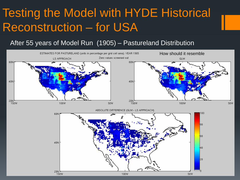
Testing the Model with HYDE Historical Reconstruction – for USA

After 55 years of Model Run (1905) – Cropland Distribution

How should it resemble

Testing the Model with HYDE Historical Reconstruction – for USA

After 55 years of Model Run (1905) – Pastureland Distribution

How should it resemble

Testing the Model with HYDE Historical Reconstruction – for USA

After 151 years of Model Run (2001) – Cropland Distribution

Urban Constraint not yet implemented

Overestimation due to urban constraints not yet being implemented

Underestimating due to overestimate at the other end (sum is conserved as determined by PET)

How should it resemble

Testing the Model with HYDE Historical Reconstruction – for USA

After 151 years of Model Run (2001) – Pastureland Distribution

Ramankutty et al. 2008

HYDE

How should it resemble

HYPOTHESIS FOR DOWNSCALING FOREST

PET LAND-USE DOWNSCALING MODEL

Fore

st C

onst

rain

t

Crop+Past Regional

Crop+Past Gridded

Area of 28 land cover types and underlying transitions

Based on Meiyappan and Jain (2012)

ISAM Biogeophysical & Biogeochemical

Impacts

Summary

Able to reproduce major Cropland and Pastureland trends to a good level of accuracy – little bit of tuning required with urban and population factors Think about Socio-economic factors Forest downscaling and LCLUC –already have the model ready and is flexible to be coupled with ISAM Wood harvest and shifting cultivation ? – Important players Two way interactions between PET and ISAM As biophysical factors seem to dominate where croplands are to be allocated at global level – it might be interesting to look at how per capita cropland would change in the future (population growth itself does not drive land-use change but exerts pressure !)