programming in mathematica using object based...
TRANSCRIPT
HOME
Programming in Mathematica using object based paradigm
by Nasser M. Abbasi
V 1.2, december 23, 2012
This note is here in PDF format
The Mathematica notebook is here
Introduction
Mathematica can be effectively used for object based programming. It is well known that using object based
programming helps in managing the complexity of large programs. Using Object based programming in Mathemat-
ica can lead to the best of both worlds: object based combined with functional programming. Object based can be
used to help in organizing the program in the large and functional programming is used in the actual implementa-
tion of the Classes methods.
The idea is simple. A Module acts as what is the Class in standard OO languages. Inside this module will be
additional inner Modules. These inner Modules act as the Class methods. Inner Modules can be made public or
private.
By adding the name of an inner Module in the list of the local variables of the outer Module, the inner Module
becomes private and is seen and only be called from other inner Modules.
The outer Module local variables are the Class private variables and these variables can be accessed only by the
Class inner modules.
An object is first created as an instance of the outer Module and from then on this object can be used in the same
way as an object is used standard OO by using the notation object@method[parameters] where the @ here acts as
the dot "." acts in common OO languages.
In other words, the dot is replaced by @ and almost everything else remain the same. This makes the notation
easier to use for someone who is more familiar with common OO notations.
The following example illustrates this idea where a Class that represents a second order system is defined and used
to make an instance of a second order system (such as a spring-mass-damper) and the object methods are used for
some basic control system operations to illustrate how to use it.
The Class is called plantClass (which is the outer Module name). To create a specific instance of this Class, the
constructor is first called using plant=plantClass[parameters]
The following diagram summarizes this setup, followed by the Mathematica code itself
Printed by Wolfram Mathematica Student Edition

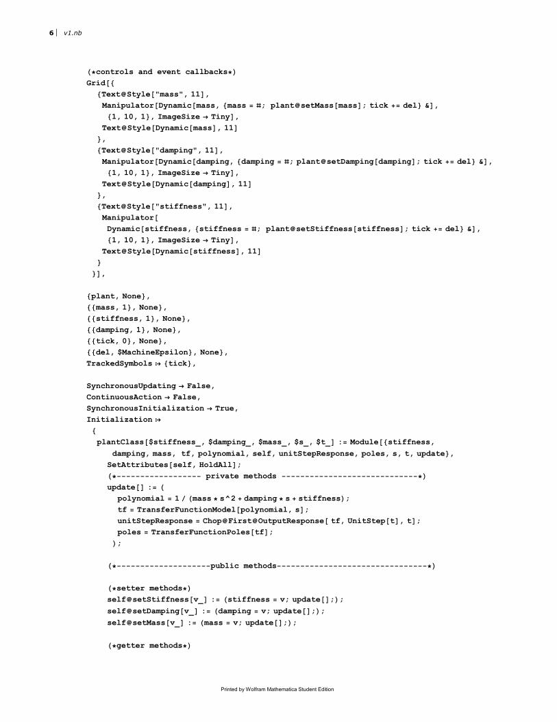
Code implementation of the Class
In the following, the complete code of the Class and example of using it are given. A plant is created, then the step
response is plotted, then a Manipulate is made that uses this Class where the plant’s mass, damping and stiffness
are used as Manipulate sliders control variables to be changed and the plant step response is updated each time.
2 v1.nb
Printed by Wolfram Mathematica Student Edition

ü Class code
In[2]:= plantClass@$stiffness_, $damping_, $mass_, $s_, $t_D := Module@8stiffness, damping, mass, tf, polynomial, self, unitStepResponse, poles, s, t, update<,
SetAttributes@self, HoldAllD;
H∗−−−−−−−−−−−−−−−−−− private methods −−−−−−−−−−−−−−−−−−−−−−−−−−−−−∗Lupdate@D := H
polynomial = 1 ê Hmass ∗ s^2 + damping ∗ s + stiffnessL;
tf = TransferFunctionModel@polynomial, sD;
unitStepResponse = Chop@First@OutputResponse@ tf, UnitStep@tD, tD;
poles = TransferFunctionPoles@tfD;
L;
H∗−−−−−−−−−−−−−−−−−−−−public methods−−−−−−−−−−−−−−−−−−−−−−−−−−−−−−−−∗L
H∗setter methods∗Lself@setStiffness@v_D := Hstiffness = v; update@D;L;
self@setDamping@v_D := Hdamping = v; update@D;L;
self@setMass@v_D := Hmass = v; update@D;L;
H∗getter methods∗Lself@getMass@D := mass;
self@getDamping@D := damping;
self@getStiffness@D := stiffness;
self@getTF@D := tf;
self@getPolynomial@D := polynomial;
self@getStepResponse@D := unitStepResponse;
self@getPoles@D := poles;
self@getBode@D := BodePlot@tfD;
H∗−−−−−−−−−−−−−−−−−−−−−−−− constructor code −−−−−−−−−−−−−−−−−−−−−−−−−−∗Ls = $s;
t = $t;
stiffness = $stiffness;
damping = $damping;
mass = $mass;
update@D;
self
D;
ü Create an instance of the class
In[3]:= mass = 10; damping = 1; stiffness = .5;
plant = plantClass@stiffness, damping, mass, s, tD;
v1.nb 3
Printed by Wolfram Mathematica Student Edition

ü Now the object is created, use it to make a step response plot
In[5]:= Plot@plant@getStepResponse@D, 8t, 0, 50<, FrameLabel →
88y@tD, None<, 8t, Row@8"Step response of a plant represented as transfer function ",
plant@getPolynomial@D<D<<, Frame → True, PlotRange → AllD
Out[5]=
0 10 20 30 40 50
0.0
0.5
1.0
1.5
2.0
2.5
3.0
t
yHtL
Step response of a plant represented as transfer function
1
10 s2
+ s + 0.5
ü Change the plant damping ratio and update the response plot
In[6]:= plant@setDamping@5D;
Plot@plant@getStepResponse@D, 8t, 0, 20<, FrameLabel →
88y@tD, None<, 8t, Row@8"Step response of a plant represented as transfer function ",
plant@getPolynomial@D<D<<, Frame → True, PlotRange → AllD
Out[7]=
0 5 10 15 20
-1.0
-0.5
0.0
0.5
1.0
t
yHtL
Step response of a plant represented as transfer function
1
10 s2
+ 5 s + 0.5
Making a Manipulate to use the above Class to simulate plant response
to different parameters
The above Class is now used inside Manipulate. It is important that the object instantiation occur in the Manipulate
Initialization section, and after the Class code and not before it. In this example, the object is the second order
plant, and one instance is created in the Manipulate Initialization section. Each time a slider changes, the object
internal state is updated using a setter method. Here is a diagram to help illustrate the layout
4 v1.nb
Printed by Wolfram Mathematica Student Edition

The above Class is now used inside Manipulate. It is important that the object instantiation occur in the Manipulate
Initialization section, and after the Class code and not before it. In this example, the object is the second order
plant, and one instance is created in the Manipulate Initialization section. Each time a slider changes, the object
internal state is updated using a setter method. Here is a diagram to help illustrate the layout
ü Manipulate code using object based layout
In[8]:= Manipulate@
tick;
Plot@plant@getStepResponse@D, 8t, 0, 20<,
FrameLabel → 88"y@tD", None<, 8"t", Row@8"Step response of ", plant@getPolynomial@D<D<<,
Frame → True, PlotRange → All
D,
v1.nb 5
Printed by Wolfram Mathematica Student Edition
In[8]:=
H∗controls and event callbacks∗LGrid@8
8Text@Style@"mass", 11D,
Manipulator@Dynamic@mass, 8mass = ð; plant@setMass@massD; tick += del< &D,
81, 10, 1<, ImageSize → TinyD,
Text@Style@Dynamic@massD, 11D<,
8Text@Style@"damping", 11D,
Manipulator@Dynamic@damping, 8damping = ð; plant@setDamping@dampingD; tick += del< &D,
81, 10, 1<, ImageSize → TinyD,
Text@Style@Dynamic@dampingD, 11D<,
8Text@Style@"stiffness", 11D,
Manipulator@Dynamic@stiffness, 8stiffness = ð; plant@setStiffness@stiffnessD; tick += del< &D,
81, 10, 1<, ImageSize → TinyD,
Text@Style@Dynamic@stiffnessD, 11D<
<D,
8plant, None<,
88mass, 1<, None<,
88stiffness, 1<, None<,
88damping, 1<, None<,
88tick, 0<, None<,
88del, $MachineEpsilon<, None<,
TrackedSymbols ¦ 8tick<,
SynchronousUpdating → False,
ContinuousAction → False,
SynchronousInitialization → True,
Initialization ¦
8plantClass@$stiffness_, $damping_, $mass_, $s_, $t_D := Module@8stiffness,
damping, mass, tf, polynomial, self, unitStepResponse, poles, s, t, update<,
SetAttributes@self, HoldAllD;
H∗−−−−−−−−−−−−−−−−−− private methods −−−−−−−−−−−−−−−−−−−−−−−−−−−−−∗Lupdate@D := H
polynomial = 1 ê Hmass ∗ s^2 + damping ∗ s + stiffnessL;
tf = TransferFunctionModel@polynomial, sD;
unitStepResponse = Chop@First@OutputResponse@ tf, UnitStep@tD, tD;
poles = TransferFunctionPoles@tfD;
L;
H∗−−−−−−−−−−−−−−−−−−−−public methods−−−−−−−−−−−−−−−−−−−−−−−−−−−−−−−−∗L
H∗setter methods∗Lself@setStiffness@v_D := Hstiffness = v; update@D;L;
self@setDamping@v_D := Hdamping = v; update@D;L;
self@setMass@v_D := Hmass = v; update@D;L;
H∗getter methods∗L;
6 v1.nb
Printed by Wolfram Mathematica Student Edition

In[8]:=
self@getMass@D := mass;
self@getDamping@D := damping;
self@getStiffness@D := stiffness;
self@getTF@D := tf;
self@getPolynomial@D := polynomial;
self@getStepResponse@D := unitStepResponse;
self@getPoles@D := poles;
self@getBode@D := BodePlot@tfD;
H∗−−−−−−−−−−−−−−−−−−−−−−−− constructor code −−−−−−−−−−−−−−−−−−−−−−−−−−∗Ls = $s;
t = $t;
stiffness = $stiffness;
damping = $damping;
mass = $mass;
update@D;
self
D;
plant = plantClass@1, 1, 1, s, tD;
<D
Out[8]=
mass 3
damping 3
stiffness 5
0 5 10 15 20
0.00
0.05
0.10
0.15
0.20
0.25
t
y@tD
Step response of
1
3 s2
+ 3 s + 5
Conclusion
It is well known that object based programming help to improve the design of software and managing the complex-
ity of large applications. Mathematica can be used effectively as object based and combined with functional
programming, which leads to better overall software. I have used this setup for first time in an actual demonstration
for the simulation of control system successfully, and I have found that it helped better organize my demonstration
code and shortened the development time. The demonstration can be seen here
v1.nb 7
Printed by Wolfram Mathematica Student Edition
It is well known that object based programming help to improve the design of software and managing the complex-
ity of large applications. Mathematica can be used effectively as object based and combined with functional
programming, which leads to better overall software. I have used this setup for first time in an actual demonstration
for the simulation of control system successfully, and I have found that it helped better organize my demonstration
code and shortened the development time. The demonstration can be seen here
References
http://mathematica.stackexchange.com/questions/586/how-can-you-give-a-module-a-context-and-have-its-local-
variables-and-modules-bel
8 v1.nb
Printed by Wolfram Mathematica Student Edition