programmer's reference 5-1 - gordon …s reference 5-1 (21 june 2016) * * * section 5 -...
TRANSCRIPT
Programmer's Reference 5-1
(21 June 2016) ************************************** * * * Section 5 - Programmer's Reference * * * ************************************** This section describes features of GAMESS programming which are true for all machines. See the section 'hardware specifics' for information about specific machines. The contents of this section are:
Installation overview 2 Running Distributed Data Parallel GAMESS 5 parallelization history 5 DDI compute and data server processes 6 memory allocations and check jobs 11 representative performance examples 13
Altering program limits 22 Names of source code modules 24 Programming Conventions 30 Parallel broadcast identifiers 33 Disk files used by GAMESS 35 disk files in parallel runs 41
Contents of the direct access file 'DICTNRY' 43

Programmer's Reference 5-2
Installation overview Very specific compiling directions are given in a file provided with the GAMESS distribution, namely ~/gamess/machines/readme.unix and this should be followed closely. The directions here are of a more general nature. Before starting the installation, you should also see the pages about your computer in the 'Hardware Specifics' section of this manual, and at the compiler version notes that are kept in the script 'comp'. There might be some special instructions for your machine. The first step in installing GAMESS should be to print the manual. If you are reading this, you've got that done! The second step would be to get the source code activator compiled and linked (note that the activator must be activated manually before it is compiled). Third, you should now compile all the quantum chemistry sources. Fourth, compile the DDI message passing library, and its process kickoff program. Fifth, link the GAMESS program. Finally, run all the short examples provided with GAMESS, and very carefully compare the key results shown in the 'sample input' section against your outputs. These "correct" results are from a IBM RS/6000, so there may be very tiny (last digit) precision differences for other machines. That's it! The rest of this section gives a little more detail about some of these steps. * * * * * GAMESS will run on essentially any machine with a FORTRAN 77 compiler. However, even given the F77 standard there are still a number of differences between various machines. For example, some chips still use 32 bit integers, as primitive as that may seem, while many chips allow for 64 bit processing (and hence very large run-time memory usage). It is also necessary to have a C compiler, as the message passing library is implemented entirely in that language. Although there are many types of computers, there is only one (1) version of GAMESS. This portability is made possible mainly by keeping machine dependencies to a minimum (that is, writing in
Programmer's Reference 5-3
FORTRAN77, not vendor specific language extensions). The unavoidable few statements which do depend on the hardware are commented out, for example, with "*I64" in columns 1-4. Before compiling GAMESS on a 64 bit machine, these four columns must be replaced by 4 blanks. The process of turning on a particular machine's specialized code is dubbed "activation". A semi-portable FORTRAN 77 program to activate the desired machine dependent lines is supplied with the GAMESS package as program ACTVTE. Before compiling ACTVTE on your machine, use your text editor to activate the very few machine dependent lines in ACTVTE before compiling it. Be careful not to change the DATA initialization! * * * * * The quantum chemistry source code of GAMESS is in the directory ~/gamess/source and consists almost entirely of unactivated FORTRAN source code, stored as *.src. There is a bit of C code in this directory to implement runtime memory allocation. The task of building an executable for GAMESS is: activate compile link *.SRC ---> *.FOR ---> *.OBJ ---> *.EXE source FORTRAN object executable code code code image where the intermediate files *.FOR and *.OBJ are discarded once the executable has been linked. It may seem odd at first to delete FORTRAN code, but this can always be reconstructed from the master source code using ACTVTE. The advantage of maintaining only one master version is obvious. Whenever any improvements are made, they are automatically in place for all the currently supported machines. There is no need to make the same changes in a plethora of other versions. * * * * * The Distributed Data Interface (DDI) is the message passing layer, supporting the parallel execution of GAMESS. It is stored in the directory tree ~/gamess/ddi It is necessary to compile this software, even if you don't intend to run on more than one processor. This directory contains a file readme.ddi with directions about compiling,

Programmer's Reference 5-4
and customizing your computer to enable the use of System V memory allocation routines. It also has information about some high end parallel computer systems. * * * * * The control language needed to activate, compile, and link GAMESS on your brand of computer involves several scripts, namely: COMP compiles a single quantum chemistry module. COMPALL compiles all quantum chemistry source modules. COMPDDI compiles the distributed data interface, and generates a process kickoff program, ddikick.x. LKED link-edit (links) together quantum chemistry object code, and the DDI library, to produce a binary executable gamess.x. RUNGMS runs a GAMESS job, in serial or parallel. RUNALL uses RUNGMS to run all the example jobs. There are files related to some utility programs: MBLDR.* model builder (internal to Cartesian) CARTIC.* Cartesian to internal coordinates CLENMO.* cleans up $VEC groups DK3.F prepare relativistic AO contractions. There are files related to two-D X-windows graphics, in: ~/gamess/graphics Better back-end graphics (3D as well as 2D) is available in the MacMolPlt program, now available for all popular desktop operating systems.

Programmer's Reference 5-5
Running Distributed Data Parallel GAMESS GAMESS consists of many FORTRAN files implementing its quantum chemistry, and some C language files implementing the Distributed Data Interface (DDI). The directions for compiling DDI, configuring the system parameters to permit execution of DDI programs, and how to use the 'ddikick.x' program which "kicks off" GAMESS processes may be found in the file readme.ddi. If you are not the person installing the GAMESS software, you can skip reading that. Efficient use of GAMESS requires an understanding of three critical issues: The first is the difference between two types of memory (replicated MWORDS and distributed MEMDDI) and how these relate to the physical memory of the computer which you are using. Second, you must understand to some extent the degree to which each type of computation scales so that the proper number of CPUs is selected. Finally, many systems run -two- GAMESS processes on every processor, and if you read on you will find out why this is so. Since all code needed to implement the Distributed Data Interface (DDI) is provided with the GAMESS source code distribution, the program compiles and links ready for parallel execution on all machine types. Of course, you may choose to run on only one processor, in which case GAMESS will behave as if it is a sequential code, and the full functionality of the program is available.
parallelization history We began to parallelize GAMESS in 1991 as part of the joint ARPA/Air Force piece of the Touchstone Delta project. Today, nearly all ab initio methods run in parallel, although some of these still have a step or two running sequentially only. Only the RHF+CI gradients have no parallel method coded. We have not parallelized the semi- empirical MOPAC runs, and probably never will. Additional parallel work occurred as a result of a DoD CHSSI software initiative in 1996. This led to the DDI-based parallel RHF+MP2 gradient program, after development of the DDI programming toolkit itself. Since 2002, the DoE program SciDAC has sponsored additional parallelization. The DDI toolkit has been used since its 1999 introduction to add codes for UHF+MP2 gradient, ROHF+ZAPT2 energy, and MCSCF

Programmer's Reference 5-6
wavefunctions as well as their analytic Hessians or MCQDPT2 energy correction. In 1991, the parallel machine of choice was the Intel Hypercube although small clusters of workstations could also be used as a parallel computer. In order to have the best blend of portability and functionality, we chose in 1991 to use the TCGMSG message passing library rather than one of the early vendor's specialized libraries. As the major companies began to market parallel machines, and as MPI version 1 emerged as a standard, we began to use MPI on some equipment in 1996, while still using the very resilient TCGMSG library on everything else. However, in June 1999, we retired our old friend TCGMSG when the message passing library used by GAMESS changed to the Distributed Data Interface, or DDI. An SMP-optimized version of DDI was included with GAMESS in April 2004. Three people have been extremely influential upon the current parallel methodology. Theresa Windus, a graduate student in the early 1990s, created the first parallel versions. Graham Fletcher, a postdoc in the late 1990s, is responsible for the addition of distributed data programming concepts. Ryan Olson rewrote the DDI software in 2003-4 to support the modern SMP architectures well, and this was released in April 2004 as our standard message passing implementation.
DDI compute and data server processes DDI contains the usual parallel programming calls, such as initialization/closure, point to point messages, and the collective operations global sum and broadcast. These simple parts of DDI support all parallel methods developed in GAMESS from 1991-1999, which were based on replicated storage rather than distributed data. However, DDI also contains additional routines to support distributed memory usage. DDI attempts to exploit the entire system in a scalable way. While our early work concentrated on exploiting the use of p processors and p disks, it required that all data in memory be replicated on every one of the p CPUs. The use of memory also becomes scalable only if the data is distributed across the aggregate memory of the parallel machine. The concept of distributed memory is contained in the Remote Memory Access portion of MPI version 2, but so far MPI-2 is not available from American computer vendors.
Programmer's Reference 5-7
The original concept of distributed memory was implemented in the Global Array toolkit of Pacific Northwest National Laboratory (see http://www.emsl.pnl.gov/pub/docs/global). Basically, the idea is to provide three subroutine calls to access memory on other processors (in the local or even remote nodes): PUT, GET, and ACCUMULATE. These give access to a class of memory which is assumed to be slower than local memory, but faster than disk: <--- fastest slowest ---> registers cache(s) local_memory remote_memory disks tapes <--- smallest biggest ---> Because DDI accesses memory on other CPUs by means of an explicit subroutine call, the programmer is aware that a message must be transmitted. This awareness of the access overhead should encourage algorithms that transfer many data items in a single message. Use of a subroutine call to reach remote memory is a recognition of the non-uniform memory access (NUMA) nature of parallel computers. In other words, the Distributed Data Interface (DDI) is an explicitly message passing implementation of global shared memory. In order to have one CPU pass data items to a second CPU when the second CPU needs them, without significant delay, the computing job on the first CPU must interrupt its computation briefly to furnish the data. This type of communication is referred to as "one sided messages" or "active messages" since the first CPU is an unwitting participant in the process, which is driven entirely by the requirements of the second CPU.

Programmer's Reference 5-8
The Cray T3E has a library named SHMEM to support this type of one sided messages (and good hardware support for this too) so, on the T3E, GAMESS runs as a single process per CPU. Its memory image looks like this: node 0 node 1 p=0 p=1 --------------- --------------- | GAMESS | | GAMESS | | quantum | | quantum | | chem code | | chem code | --------------- --------------- | DDI code | | DDI code | --------------- --------------- input keywords: | replicated | | replicated | <-- MWORDS | data | | data | ----------------------------------------- | | | | | | <-- MEMDDI | | distributed| | distributed | | | | data | | data | | | | | | | | | | | | | | | | | | | | | --------------- --------------- | ----------------------------------------- where the box drawn around the distributed data is meant to imply that a large data array is residing in the memory of all processes (in this example, half on one and half on the other). Note that the input keyword MWORDS gives the amount of storage used to duplicate small matrices on every CPU, while MEMDDI gives the -total- distributed memory required by the job. Thus, if you are running on p CPUs, the memory that is used on any given CPU is total on any 1 CPU = MWORDS + MEMDDI/p Since MEMDDI is very large, its units are in millions of words. Since good execution speed requires that you not exceed the physical memory belonging to your CPUs, it is important to understand that when MEMDDI is large, you will need to choose a sufficiently large number of CPUs to keep the memory on each reasonable. To repeat, the DDI philosophy is to add more processors not just for their compute performance or extra disk space,

Programmer's Reference 5-9
but also to aggregate a very large total memory. Bigger problems will require more CPUs to obtain sufficiently large total memories! We will give an example of how you can estimate the number of CPUs a little ways below. If the GAMESS task running as process p=1 in the above example needs some values previously computed, it issues a call to DDI_GET. The DDI routines in process p=1 then figure out where this "patch" of data actually resides in the big rectangular distributed storage. Suppose this is on process p=0. The DDI routines in p=1 send a message to p=0 to interupt its computations, after which p=0 sends a bulk data message to process p=1's buffer. This buffer resides in part of the replicated storage of p=1, where computations can occur. Note that the quantum chemistry layer of process p=1 was sheltered from most of the details regarding which CPU owned the patch of data that process p=1 wanted to obtain. These details are managed by the DDI layer. Note that with the exception of DDI_ACC's addition of new terms into a distributed array, no arithmetic is done directly upon the distributed data. Instead, distributed data is accessed only by DDI_GET, DDI_PUT (its counterpart for storage of data items), and DDI_ACC (which accumulates new terms into the distributed data). DDI_GET and DDI_PUT can be thought of as analogous to FORTRAN READ and WRITE statements that transfer data between disk storage and local memory where computations may occur. It is the programmer's challenge to minimize the number of GET/PUT/ACC calls, and to design algorithms that maximize the chance that the patches of data are actually within the local CPU's portion of the distributed data.

Programmer's Reference 5-10
Since the SHMEM library is available only on a few machines, all other platforms adopt the following memory model, which involves –two- GAMESS processes running on every processor: node 0 node 1 p=0 p=1 --------------- --------------- | GAMESS X| | GAMESS X| compute | quantum | | quantum | processes | chem code | | chem code | --------------- --------------- | DDI code | | DDI code | --------------- --------------- keyword: | replicated | | replicated | <-- MWORDS | data | | data | --------------- --------------- p=2 p=3 --------------- --------------- | GAMESS | | GAMESS | data | quantum | | quantum | servers | chem code | | chem code | --------------- --------------- | DDI code X| | DDI code X| --------------- --------------- ----------------------------------------- keyword: | | | | | | <-- MEMDDI | | distributed| | distributed | | | | data | | data | | | | | | | | | | | | | | | | | | | | | --------------- --------------- | ----------------------------------------- The first half of the processes do quantum chemistry, and the X indicates that they spend most of their time executing some sort of chemistry. Hence the name "compute process". Soon after execution, the second half of the processes call a DDI service routine which consists of an infinite loop to deal with GET, PUT, and ACC requests until such time as the job ends. The X shows that these "data servers" execute only DDI support code. (This makes the data server's quantum chemistry routines the equivalent of the human appendix). The whole problem of interupts is now in the hands of the operating system, as the data servers are distinct processes. To follow the same example as
Programmer's Reference 5-11
before, when the compute process p=1 needs data that turns out to reside on process 0, a request is sent to the data server p=2 to transfer information back to the compute process p=1. The compute process p=0 is completely unaware that such a transaction has occurred. The formula for the memory required by any single CPU is unchanged, if p is the total number of CPUs used, total on any 1 CPU = MWORDS + MEMDDI/p. As a technical matter, if you are running on a system where all processors are in the same node (the SGI Altix is an example), or if you are running on an IBM SP where LAPI assists in implementing one-sided messaging, then the data server processes are not started. The memory model in the illustration above is correct, if you just mentally omit the data server processes from it. In all cases, where the SHMEM library is not used, the distributed arrays are created by System V memory calls, shmget/shmat, and their associated semaphore routines. Your system may need to be reconfigured to allow allocation of large shared memory segments, see 'readme.ddi' for more details. The parallel CCSD and CCSD(T) programs add a third kind of memory to the mix: node-replicated. This is data (e.g. the doubles amplitudes) that is stored only once per node. Thus, this is more copies of the data than once per parallel job (fully distributed MEMDDI) but fewer than once per CPU (replicated MWORDS). A picture of the memory model for the CCSD(T) program can be found in the "readme.ddi" file, so is not duplicated here. There is presently no keyword for this type of memory, but the system limit on the total SystemV memory does apply. It is important to perform a check run when using CCSD(T) and carefully follow the printout of its memory requirements.
memory allocations and check jobs At present, not all runs require distributed memory. For example, in an SCF computation (no hessian or MP2 to follow) the memory needed is on the order of the square of the basis set size, for such quantities as the orbital coefficients, density, Fock, overlap matrices, and so on. These are simply duplicated on every CPU in the MWORDS (or the older keyword MEMORY in $SYSTEM) region. In this case the data server processes still run, but are dormant because no distributed memory access is attempted.

Programmer's Reference 5-12
However, closed and open shell MP2 calculations, MCSCF wavefunctions, and their analytic hessian or MCQPDT energy correction do use distributed memory when run in parallel. Thus it is important to know how to obtain the correct value for MEMDDI in a check run, and how to compute how many CPUs are needed to do the run. Check runs (EXETYP=CHECK) need to run quickly, and the fastest turn around always comes on one CPU only. Runs which do not currently exploit MEMDDI distributed storage will formally allocate their MWORDS needs, and feel out their storage needs while skipping almost all of the real work. Since MWORDS is replicated, the amount that is needed on 1 CPU remains unchanged if you later do the true computation on more than 1 CPU. Check jobs which involve MEMDDI storage are a little bit trickier. As noted, we want to run on only 1 CPU to get fast turn around. However, MEMDDI is typically a large amount of memory, and this is unlikely to be available on a single CPU. The solution is that the check job will not actually allocate the MEMDDI storage, instead it just remembers what you gave as input and checks to see if this will be adequate. As someone once said, MEMDDI is a "fairy tale number" during a check job. So, you can input a big value like MEMDDI=25000 (25,000 million words is equal to 25,000 * 1,000,000 * 8 = 200 GBytes) and run this check job on a computer with only 1024 MB = 1 GB of memory per processor. Let us say that a closed shell MP2 check run for this case gives the output of SCALED *PER-NODE* MEMORY REQUIREMENT NODES DISTRIBUTED/MWORDS REPLICATED/WORDS TOTAL/MBYTES 1 952 7284508 7624 The real run requires MWORDS=8 MEMDDI=960. Note that we have just rounded up a bit from the 7.3 and 952 in this output, for safety. Of course, the actual computation will have to run on a large number of such processors, because you don't have 200 GB on your CPU, we are assuming 1024 MB (1 GB). Let us continue to compute how many processors are needed. We need to reserve some memory for the operating system (25 MB, say) and for the GAMESS program and local storage (let us say 50 MB, for GAMESS is a big program, and the compute processes should be swapped into memory). Thus our hypothetical 1024 MB processor has 950 MB available, assuming no one else is running. In units of words, this machine has 950/8 = 118 million words available for your run. We must choose the number of processors p to satisfy

Programmer's Reference 5-13
needed <= available MWORDS + MEMDDI/p <= free physical memory 8 + 960/p <= 118 so solving for p, we learn this example requires p >= 9 compute processes. The answer for roughly 8 GB of distributed memory on 1 GB processors was not 8, because the O/S, GAMESS itself, and the MWORDS requirements together mean less than 1 GB could be contributed to the distributed total. More CPUs than 9 do not require changing MWORDS or MEMDDI, but will run faster than 9. Fewer CPUs than 9 do not have enough memory to run! One more subtle point about CHECK runs with MEMDDI is that since you are running on 1 CPU only, the code does not know that you wish to run the parallel algorithm instead of the sequential algorithm. You must force the CHECK job into the parallel section of the program by $system parall=.true. $end There's no harm leaving this line in for the true runs, as any job with more than one compute process is parallel regardless of the input keyword PARALL. The check run for MCQDPT jobs will print three times a line like this MAXIMUM MEMDDI THAT CAN BE USED IN ... IS x MWORDS Typically the 2nd such step, transforming over all occupied and virtual canonical orbitals, will be the largest of the three requirements. Its size can be guesstimated before running, as (Nao*Nao+Nao)/2 * ((Nocc*Nocc+Nocc)/2 + Nocc*Nvirt) where Nocc = NMOFZC+NMODOC+NMOACT, Nvirt=NMOEXT, and Nao is the size of the atomic basis. Unlike the closed shell MP2 program, this section still does extensive I/O operations even when MEMDDI is used, so it may be useful to consider the three input keywords DOORD0, PARAIO, and DELSCR when running this code.
representative performance examples This section describes the way in which the various quantum chemistry computations run in parallel, and shows some typical performance data. This should give you as the user some idea how many CPUs can be efficiently used for various SCFTYP and RUNTYP jobs The performance data you will see below were obtained on a 16 CPU Intel Pentium II Linux (Beowulf-type) cluster

Programmer's Reference 5-14
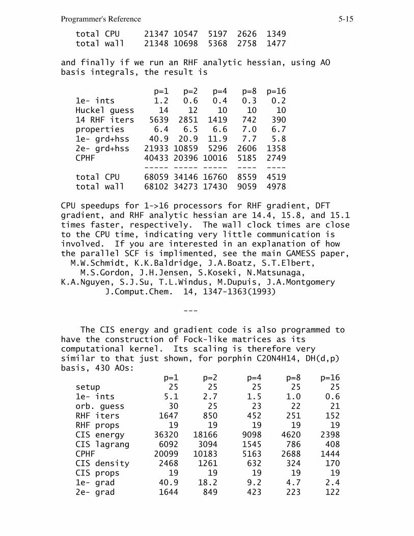
costing $49,000, of which $3,000 went into the switched Fast Ethernet component. 512 MB/CPU means this cluster has an aggregate memory of 8 GB. For more details, see http://www.msg.chem.iastate.edu/GAMESS/dist.pc.shtml. This is a low quality network, which exposes jobs with higher communication requirements, by noting when the wall time is much longer than the CPU. --- The HF wavefunctions can be evaluated in parallel using either conventional disk storage of the integrals, or via direct recomputation of the integrals. Some experimenting will show which is more effective on your hardware. As an example of the scaling performance of RHF, ROHF, UHF, or GVB jobs that involve only computation of the energy or its gradient, we include here a timing table from the 16 CPU PC cluster. The molecule is luciferin, which together with the enzyme luciferase is involved in firefly light production. The chemical formula is C11N2S2O3H8, and RHF/6-31G(d) has 294 atomic orbitals. There's no molecular symmetry. The run is done as direct SCF, and the CPU timing data is p=1 p=2 p=4 p=8 p=16 1e- ints 1.1 0.6 0.4 0.3 0.2 Huckel guess 14 12 11 10 10 15 RHF iters 5995 2982 1493 772 407 properties 6.0 6.6 6.6 6.8 6.9 1e- gradient 9.7 4.7 2.3 1.2 0.7 2e- gradient 1080 541 267 134 68 ---- ---- ---- ---- ---- total CPU 7106 3547 1780 925 492 seconds total wall 7107 3562 1815 950 522 seconds Note that direct SCF should run with the wall time very close to the CPU time as there is essentially no I/O and not that much communication (MEMDDI storage is not used by this kind of run). Running the same molecule as DFTTYP=B3LYP yields p=1 p=2 p=4 p=8 p=16 1e- ints 1.1 0.7 0.3 0.3 0.2 Huckel guess 14 12 10 10 9 23 DFT iters 14978 7441 3681 1876 961 properties 6.6 6.4 6.5 7.0 6.5 1e- gradient 9.7 4.7 2.3 1.3 0.7 2e- grid grad 5232 2532 1225 595 303 2e- AO grad 1105 550 270 136 69 ---- ---- ---- ---- ----
Programmer's Reference 5-15
total CPU 21347 10547 5197 2626 1349 total wall 21348 10698 5368 2758 1477 and finally if we run an RHF analytic hessian, using AO basis integrals, the result is p=1 p=2 p=4 p=8 p=16 1e- ints 1.2 0.6 0.4 0.3 0.2 Huckel guess 14 12 10 10 10 14 RHF iters 5639 2851 1419 742 390 properties 6.4 6.5 6.6 7.0 6.7 1e- grd+hss 40.9 20.9 11.9 7.7 5.8 2e- grd+hss 21933 10859 5296 2606 1358 CPHF 40433 20396 10016 5185 2749 ----- ----- ----- ---- ---- total CPU 68059 34146 16760 8559 4519 total wall 68102 34273 17430 9059 4978 CPU speedups for 1->16 processors for RHF gradient, DFT gradient, and RHF analytic hessian are 14.4, 15.8, and 15.1 times faster, respectively. The wall clock times are close to the CPU time, indicating very little communication is involved. If you are interested in an explanation of how the parallel SCF is implimented, see the main GAMESS paper, M.W.Schmidt, K.K.Baldridge, J.A.Boatz, S.T.Elbert, M.S.Gordon, J.H.Jensen, S.Koseki, N.Matsunaga, K.A.Nguyen, S.J.Su, T.L.Windus, M.Dupuis, J.A.Montgomery J.Comput.Chem. 14, 1347-1363(1993) --- The CIS energy and gradient code is also programmed to have the construction of Fock-like matrices as its computational kernel. Its scaling is therefore very similar to that just shown, for porphin C20N4H14, DH(d,p) basis, 430 AOs: p=1 p=2 p=4 p=8 p=16 setup 25 25 25 25 25 1e- ints 5.1 2.7 1.5 1.0 0.6 orb. guess 30 25 23 22 21 RHF iters 1647 850 452 251 152 RHF props 19 19 19 19 19 CIS energy 36320 18166 9098 4620 2398 CIS lagrang 6092 3094 1545 786 408 CPHF 20099 10183 5163 2688 1444 CIS density 2468 1261 632 324 170 CIS props 19 19 19 19 19 1e- grad 40.9 18.2 9.2 4.7 2.4 2e- grad 1644 849 423 223 122

Programmer's Reference 5-16
----- ----- ---- ---- ---- total CPU 68424 34526 17420 8994 4791 total wall 68443 34606 17853 9258 4985 which is a speedup of 14.3 for 1->16. --- For the next type of computation, we discuss the MP2 correction. For closed shell RHF + MP2 and unrestricted UHF + MP2, the gradient program runs in parallel using distributed memory, MEMDDI. In addition, the ROHF + MP2 energy correction for OSPT=ZAPT runs in parallel using distributed memory, but OSPT=RMP does not use MEMDDI in parallel jobs. All distributed memory parallel MP2 runs resemble RHF+MP2, which is therefore the only example given here. The example is a benzoquinone precursor to hongconin, a cardioprotective natural product. The formula is C11O4H10, and 6-31G(d) has 245 AOs. There are 39 valence orbitals included in the MP2 treatment, and 15 core orbitals. MEMDDI must be 156 million words, so the memory computation that was used above tells us that our 512 MB/CPU PC cluster must have at least three processors to aggregate the required MEMDDI. MOREAD was used to provide converged RHF orbitals, so only 3 RHF iterations are performed. The timing data are CPU and wall times (seconds) in the 1st/2nd lines: p=3 p=4 p=12 p=16 RHF iters 241 181 65 51 243 184 69 55 MP2 step 5,953 4,399 1,438 1,098 7,366 5,669 2,239 1,700 2e- grad 1,429 1,135 375 280 1,492 1,183 413 305 ----- ----- --- --- total CPU 7,637 5,727 1,890 1,440 total wall 9,116 7,053 2,658 2,077 3-->12 4-->16 CPU speedup 4.04 3.98 wall speedup 3.43 3.40 The wall clock time will be closer to the CPU time if the quality of the network between the computer is improved (remember, this run used just switched Fast Ethernet). As noted, the number of CPUs is more influenced by a need to aggregate the necessary total MEMDDI, more than by concerns

Programmer's Reference 5-17
about scalability. MEMDDI is typically large for MP2 parallel runs, as it is proportional to the number of occupied orbitals squared times the number of AOs squared. For more details on the distributed data parallel MP2 program, see G.D.Fletcher, A.P.Rendell, P.Sherwood Mol.Phys. 91, 431-438(1997) G.D.Fletcher, M.W.Schmidt, M.S.Gordon Adv.Chem.Phys. 110, 267-294 (1999) G.D.Fletcher, M.W.Schmidt, B.M.Bode, M.S.Gordon Comput.Phys.Commun. 128, 190-200 (2000) --- The next type of computation we will consider is analytic computation of the nuclear Hessian (force constant matrix). The performance of the RHF program, based on AO integrals, was given above, as its computational kernel (Fock-like builds) scales just as the SCF itself. However, for high spin ROHF, low spin open shell SCF and TCSCF (both done with GVB), the only option is MO basis integrals. The integral transformation is parallel according to T.L.Windus, M.W.Schmidt, M.S.Gordon Theoret.Chim.Acta 89, 77-88(1994). It distributes 'passes' over processors, so as to parallelize the transformation's CPU time but not the replicated memory, or the AO integral time. Finally the response equation step is hardly parallel at all. The test example is an intermediate in the ring opening of silacyclobutane, GVB-PP(1) or TCSCF, 180 AOs for 6-311G(2d,2p): p=1 p=2 p=4 p=8 p=16 2e- ints 83 42 21 11 5 GVB iters 648 333 179 104 67 replicate 2e- n/a 81 81 81 82 transf. 476 254 123 67 51 1e- grd+hss 7 4 2 2 1 2e- grd+hss 4695 2295 1165 596 313 CP-TCSCF 344 339 331 312 325 ---- ---- ---- ---- ---- total CPU 6256 3351 1904 1189 848 total wall 6532 3538 2072 1399 1108 Clearly, the final response equation (CPHF) step is a sequential bottleneck, as is the fact that the orbital hessian in this step is stored entirely on the disk space of CPU 0. Since the integral transformation is run in replicated MWORDS memory, rather than distributing this,

Programmer's Reference 5-18
and since it also needs a duplicated AO integral file be stored on every CPU, the code is clearly not scalable to very many processors. Typically we would not request more than 3 or 4 processors for an analytic ROHF or GVB hessian. The final analytic hessian type is for MCSCF. The scalability of the MCSCF wavefunction will be given just below, but the response equation step for MCSCF is clearly quite scalable. The integral transformation for the response equation step uses distributed memory MEMDDI, and should scale like the MP2 program (documented above). The test case has 8e- in 8 orbitals, and the time reflect this, with most of the work involving the 4900 determinants. Total speedup for 4->16 is 4.11, due to luckier work distributing for 16 CPUs: p=4 p=16 MCSCF wfn 113.5 106.1 DDI transf. 68.4 19.3 1e- grd+hss 1.5 0.6 2e- grd+hss 2024.9 509.8 CPMCHF RHS 878.8 225.8 (RHS=right hand sides) CPMCHF iters 115343.5 27885.9 -------- -------- total CPU 118430.8 28747.6 total wall 119766.0 30746.4 This code can clearly benefit from using many processors, with scalability of the MCSCF step itself almost moot. --- Now lets turn to MCSCF energy/gradient runs. We will illustrate two convergers, SOSCF and then FULLNR. The former uses a 'pass' type of integral transformation (ala the GVB hessian job above), and runs in replicated memory only (no MEMDDI). The FULLNR converger is based on the MP2 program's distributed memory integral transformation, so it uses MEMDDI. In addition, the parallel implementation of the FULLNR step never forms the orbital hessian explicitly, doing Davidson style iterations to predict the new orbitals. Thus the memory demand is almost entirely MEMDDI. The example we choose is at a transition state for the water molecule assisted proton transfer in the first excited stat of 7-azaindole. The formula is C7N2H6(H2O), there are 190 active orbitals, and the active space is the

Programmer's Reference 5-19
10 pi electrons in 9 pi orbitals of the azaindole portion. There are 15,876 determinants used in the MCSCF calculation, and 5,292 CSFs in the perturbation calculation to follow. See Figure 6 of G.M.Chaban, M.S.Gordon J.Phys.Chem.A 103, 185-189(1999) if you are interested in this chemistry. The timing data for the SOSCF converger are p=1 p=2 p=4 p=8 p=16 dup. 2e- ints 327.6 331.3 326.4 325.8 326.5 transform. 285.1 153.6 88.4 57.8 47.3 det CI 39.3 39.4 38.9 38.3 38.1 2e- dens. 0.4 0.5 0.5 0.5 0.5 orb. update 39.2 25.9 17.4 12.8 11.0 iters 2-16 5340.0 3153.5 2043.7 1513.6 1308.5 1e- grad 5.3 2.3 1.3 0.7 0.4 2e- grad 695.6 354.9 179.4 93.2 50.9 ------ ------ ------ ------ ------ total CPU 6,743 4,071 2,705 2,052 1,793 total wall 13,761 8,289 4,986 3,429 3,899 whereas the FULLNR convergers runs like this p=1 p=2 p=4 p=8 p=16 2e- DDI trans. 2547 1385 698 354 173 det. CI 39 39 38 38 38 DM2 0.5 0.5 0.5 0.5 0.5 FULLNR 660 376 194 101 51 iters 2-9 24324 13440 6942 3669 1940 1e- grad 5.3 2.3 1.2 0.7 0.4 2e- grad 700 352 181 95 51 ------ ------ ---- ---- ---- total CPU 28, 15,605 8,066 4,268 2,265 total wall 28,290 20,719 12,866 8,292 5,583 The first iteration is broken down into its primary steps from the integral transformation to the orbital update, inclusive. The SOSCF program is clearly faster, and should be used when the number of processors is modest (say up to 8), however the largest molecules will benefit from using more processors and the much more scalable FULLNR program. One should note that the CI calculation was more or less serial here. This data comes from before the ALDET and ORMAS codes were given a replicated memory parallization, so scaling in the CI step should now be OK, to say 8 or 16 CPUs. However, these two CI code's use of replicated memory in the CI step limits MCSCF scalability in the large active space limit.

Programmer's Reference 5-20
Now let's consider the second order pertubation correction for this example. As noted, it is an excited state, so the test corrects two states simultaneously (S0 and S1). The parallel multireference perturbation program is described in H.Umeda, S.Koseki, U.Nagashima, M.W.Schmidt J.Comput.Chem. 22, 1243-1251 (2001) The run is given the converged S1 orbitals, so that it can skip directly to the perturbation calculation: p=1 p=2 p=4 p=8 p=16 2e- ints 332 332 329 328 331 MCQDPT 87921 43864 22008 11082 5697 ----- ----- ----- ----- ----- total CPU 88261 44205 22345 11418 6028 total wall 91508 45818 23556 12350 6852 This corresponds to a speedup for 1->16 of 14.6. --- In summary, most ab initio computations will run in less time on more than one processor. However, some things can be run only on 1 CPU, namely semi-empirical runs RHF+CI gradient Coupled-Cluster calculations Some steps run with little or no speedup, forming sequential bottlenecks that limit scalability. They do not prevent jobs from running in parallel, but restrict the total number of processors that can be effectively used: ROHF/GVB hessians: solution of response equations MCSCF: Hamiltonian and 2e- density matrix (CI) energy localizations: the orbital localization step transition moments/spin-orbit: the final property step MCQDPT reference weight option Future versions of GAMESS will address these bottlenecks. A short summary of the useful number of CPUs (based on data like the above) would be RHF, ROHF, UHF, GVB energy/gradient, their DFT analogs, and CIS excited states 16-32+ MCSCF energy/gradient SOSCF 4-8 FULLNR 8-32+ analytic hessians RHF 16-32+ ROHF/GVB 4-8 MCSCF 64-128+ MPLEVL=2

Programmer's Reference 5-21
RHF, UHF, ROHF OSPT=ZAPT 8-256+ ROHF OSPT=RMP energy 8 MCSCF 16+

Programmer's Reference 5-22
Altering program limits Almost all arrays in GAMESS are allocated dynamically, but some variables must be held in common as their use is ubiquitous. An example would be the common block /NSHEL/ which holds the ab initio atom's basis set. The following Unix script, which we call 'mung' (see Wikipedia entry for recursive acronyms), changes the PARAMETER statements that set various limitations: #!/bin/csh # # automatically change GAMESS' built-in dimensions # chdir /u1/mike/gamess/source # foreach FILE (*.src) set FILE=$FILE:r echo ===== redimensioning in $FILE ===== echo "C dd-mmm-yy - SELECT NEW DIMENSIONS" \ > $FILE.munged sed -e "/MXATM=2000/s//MXATM=500/" \ -e "/MXAO=8192/s//MXAO=2047/" \ -e "/MXGSH=30/s//MXGSH=30/" \ -e "/MXSH=5000/s//MXSH=1000/" \ -e "/MXGTOT=20000/s//MXGTOT=5000/" \ -e "/MXRT=100/s//MXRT=100/" \ -e "/MXFRG=1050/s//MXFRG=65/" \ -e "/MXDFG=5/s//MXDFG=1/" \ -e "/MXPT=2000/s//MXPT=100/" \ -e "/MXFGPT=12000/s//MXFGPT=2000/" \ -e "/MXSP=500/s//MXSP=100/" \ -e "/MXTS=20000/s//MXTS=2500/" \ -e "/MXABC=6000/s//MXABC=1/" \ $FILE.src >> $FILE.munged mv $FILE.munged $FILE.src end exit The script shows how to reduce memory, by decreasing the number of atoms and basis functions, and reducing the storage for the effective fragment and PCM solvent models. Of course, the 'mung' script can also be used to increase the dimensions!
Programmer's Reference 5-23
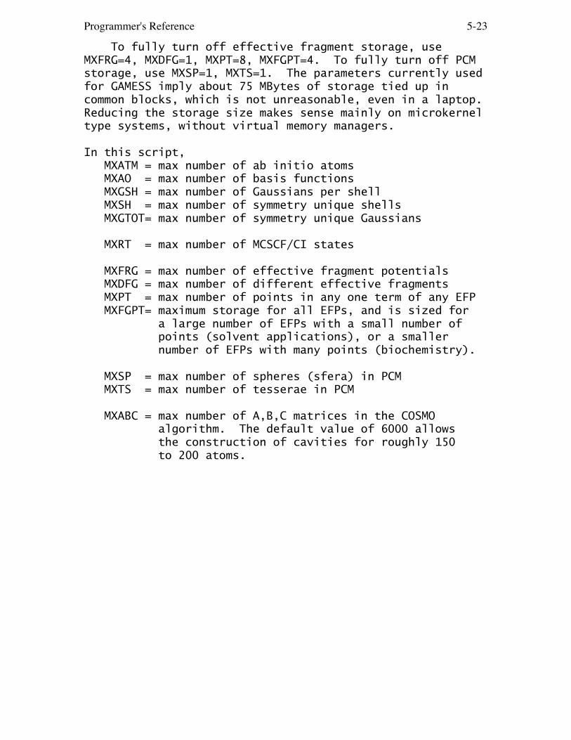
To fully turn off effective fragment storage, use MXFRG=4, MXDFG=1, MXPT=8, MXFGPT=4. To fully turn off PCM storage, use MXSP=1, MXTS=1. The parameters currently used for GAMESS imply about 75 MBytes of storage tied up in common blocks, which is not unreasonable, even in a laptop. Reducing the storage size makes sense mainly on microkernel type systems, without virtual memory managers. In this script, MXATM = max number of ab initio atoms MXAO = max number of basis functions MXGSH = max number of Gaussians per shell MXSH = max number of symmetry unique shells MXGTOT= max number of symmetry unique Gaussians MXRT = max number of MCSCF/CI states MXFRG = max number of effective fragment potentials MXDFG = max number of different effective fragments MXPT = max number of points in any one term of any EFP MXFGPT= maximum storage for all EFPs, and is sized for a large number of EFPs with a small number of points (solvent applications), or a smaller number of EFPs with many points (biochemistry). MXSP = max number of spheres (sfera) in PCM MXTS = max number of tesserae in PCM MXABC = max number of A,B,C matrices in the COSMO algorithm. The default value of 6000 allows the construction of cavities for roughly 150 to 200 atoms.

Programmer's Reference 5-24
Names of source code modules The source code for GAMESS is divided into a number of sections, called modules, each of which does related things, and is a handy size to edit. The following is a list of the different modules, what they do, and notes on their machine dependencies. machine module description dependency ------- ------------------------- ---------- ALDECI Ames Lab determinant full CI code 1 ALGNCI Ames Lab determinant general CI code BASCCN Dunning cc-pVxZ basis sets BASECP SBKJC and HW valence basis sets BASEXT DH, MC, 6-311G extended basis sets BASG3L G3Large basis sets BASHUZ Huzinaga MINI/MIDI basis sets to Xe BASHZ2 Huzinaga MINI/MIDI basis sets Cs-Rn BASKAR Karlsruhe (Ahlrichs) TZV basis sets BASN21 N-21G basis sets BASN31 N-31G basis sets BASPCN Jensen polarization consistent basis sets BASSTO STO-NG basis sets BLAS level 1 basic linear algebra subprograms CCAUX auxiliary routines for CC calculations CCDDI parallel CCSD(T) program CCQAUX auxiliaries for CCSD(TQ) program CCQUAD renormalized CCSD(TQ) corrections CCSDT renormalized CCSD(T) program 1 CEEIS corr. energy extrap. by intrinsic scaling CEPA SR and MR-CEPA,AQCC,CPF calculations CHGPEN screening for charge penetration of EFPs CISGRD CI singles and its gradient 1 COSMO conductor-like screening model COSPRT printing routine for COSMO CPHF coupled perturbed Hartree-Fock 1 CPMCHF multiconfigurational CPHF 1 CPROHF open shell/TCSCF CPHF 1 DCCC divide and conquer coupled cluster DCGRD divide and conquer gradients DCGUES divide and conquer orbital guess DCINT2 divide and conquer AO integrals 1 DCLIB divide and conquer library routines DCMP2 divide and conquer MP2 1 DCSCF divide and conquer SCF DCTRAN divide and conquer integral transf. 1

Programmer's Reference 5-25
DDILIB message passing library interface code DELOCL delocalized coordinates DEMRPT determinant-based MCQDPT DFT grid-free DFT drivers 1 DFTAUX grid-free DFT auxiliary basis integrals DFTDIS empirical dispersion correction to DFT DFTFUN grid-free DFT functionals DFTGRD grid DFT implementation DFTINT grid-free DFT integrals 1 DFTXCA grid DFT functionals, hand coded DFTXCB grid DFT functionals, from repository DFTXCC grid DFT functionals for meta-GGA DFTXCD grid DFT functionals B97, etc DFTXCE grid DFT functionals for PKZB/TPSS family DFTXCF grid DFT functionals for CAMB3LYPdir DFTXCG grid DFT functional for revTPSS DGEEV general matrix eigenvalue problem DGESVD single value decomposition DIAB MCSCF state diabatization DMULTI Amos' distributed multipole analysis DRC dynamic reaction coordinate EAIPCC EA-EOM and IP-EOM method ECP pseudopotential integrals ECPDER pseudopotential derivative integrals ECPLIB initialization code for ECP ECPPOT HW and SBKJC internally stored potentials EFCHTR fragment charge transfer EFDRVR fragment only calculation drivers EFELEC fragment-fragment interactions EFGRD2 2e- integrals for EFP numerical hessian EFGRDA ab initio/fragment gradient integrals EFGRDB " " " " " EFGRDC " " " " " EFINP effective fragment potential input EFINTA ab initio/fragment integrals EFINTB " " " " EFMO EFP + FMO interfacing EFPAUL effective fragment Pauli repulsion EFPCM EFP/PCM interfacing EFPCOV EFP style QM/MM boundary code EFPFMO FMO and EFP interface EFTEI QM/EFP 2e- integrals 1 EIGEN Givens-Householder, Jacobi diagonalization ELGLIB elongation method utility routines ELGLOC elongation method orbital localization ELGSCF elongation method Hartree-Fock 1 EOMCC equation of motion excited state CCSD EWALD Ewald summations for EFP model EXCORR interface to MPQC’s R12 programs

Programmer's Reference 5-26
FFIELD finite field polarizabilitie FMO n-mer drivers for Fragment Molecular Orbital FMOESD elestrostatic potential derivatives for FMO FMOGRD gradient routines for FMO FMOINT integrals for FMO FMOIO input/output and printing for FMO FMOLIB utilities for FMO FMOPBC periodic boundary conditions for FMO FMOPRP properties for FMO FRFMT free format input scanner FSODCI determinant based second order CI G3 G3(MP2,CCSD(T)) thermochemistry GAMESS main program, important driver routines GLOBOP Monte Carlo fragment global optimizer GMCPT general MCQDPT multireference PT code 1 GRADEX traces gradient extremals GRD1 one electron gradient integrals GRD2A two electron gradient integrals 1 GRD2B specialized sp gradient integrals GRD2C general spdfg gradient integrals GUESS initial orbital guess GUGDGA Davidson CI diagonalization 1 GUGDGB " " " 1 GUGDM 1 particle density matrix GUGDM2 2 particle density matrix 1 GUGDRT distinct row table generation GUGEM GUGA method energy matrix formation 1 GUGSRT sort transformed integrals 1 GVB generalized valence bond HF-SCF 1 HESS hessian computation drivers HSS1A one electron hessian integrals HSS1B " " " " HSS2A two electron hessian integrals 1 HSS2B " " " " INPUTA read geometry, basis, symmetry, etc. INPUTB " " " " INPUTC " " " " INT1 one electron integrals INT2A two electron integrals (Rys) 1 INT2B two electron integrals (s,p,L rot.axis) INT2C ERIC TEI code, and its s,p routines 11 INT2D ERIC special code for d TEI INT2F ERIC special code for f TEI INT2G ERIC special code for g TEI INT2R s,p,d,L rotated axis integral package INT2S s,p,d,L quadrature code INT2T s,p,d,L quadrature code INT2U s,p,d,L quadrature code INT2V s,p,d,L quadrature code

Programmer's Reference 5-27
INT2W s,p,d,L quadrature code INT2X s,p,d,L quadrature code IOLIB input/output routines,etc. 2 IVOCAS improved virtual orbital CAS energy 1 LAGRAN CI Lagrangian matrix 1 LOCAL various localization methods 1 LOCCD LCD SCF localization analysis LOCPOL LCD SCF polarizability analysis 1 LOCSVD singular value decomposition localization LRD local response dispersion correction LUT local unitary transformation IOTC MCCAS FOCAS/SOSCF MCSCF calculation 1 MCJAC JACOBI MCSCF calculation MCPGRD model core potential nuclear gradient MCPINP model core potential input MCPINT model core potential integrals MCPL10 model core potential library MCPL20 " " " " MCPL30 " " " " MCPL40 " " " " MCPL50 " " " " MCPL60 " " " " MCPL70 " " " " MCPL80 " " " " MCQDPT multireference perturbation theory 1 MCQDWT weights for MR-perturbation theory MCQUD QUAD MCSCF calculation 1 MCSCF FULLNR MCSCF calculation 1 MCTWO two electron terms for FULLNR MCSCF 1 MDEFP molecular dynamics using EFP particles MEXING minimum energy crossing point search MLTFMO multiscale solvation in FMO MM23 MMCC(2,3) corrections to EOMCCSD MOROKM Morokuma energy decomposition 1 MNSOL U.Minnesota solution models MP2 2nd order Moller-Plesset 1 MP2DDI distributed data parallel MP2 MP2GRD CPHF and density for MP2 gradients 1 MP2GR2 disk based MP2 gradient program MP2IMS disk based MP2 energy program MPCDAT MOPAC parameterization MPCGRD MOPAC gradient MPCINT MOPAC integrals MPCMOL MOPAC molecule setup MPCMSC miscellaneous MOPAC routines MTHLIB printout, matrix math utilities NAMEIO namelist I/O simulator NEOSTB dummy routines for NEO program NMR nuclear magnetic resonance shifts 1
Programmer's Reference 5-28
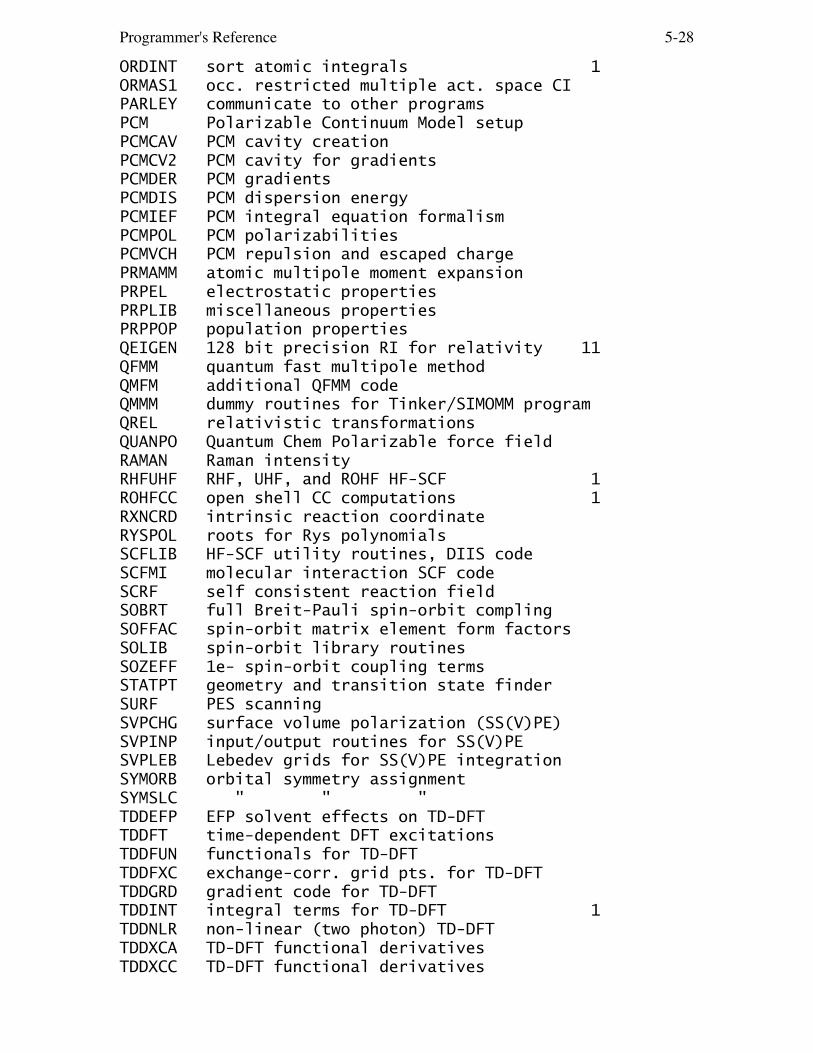
ORDINT sort atomic integrals 1 ORMAS1 occ. restricted multiple act. space CI PARLEY communicate to other programs PCM Polarizable Continuum Model setup PCMCAV PCM cavity creation PCMCV2 PCM cavity for gradients PCMDER PCM gradients PCMDIS PCM dispersion energy PCMIEF PCM integral equation formalism PCMPOL PCM polarizabilities PCMVCH PCM repulsion and escaped charge PRMAMM atomic multipole moment expansion PRPEL electrostatic properties PRPLIB miscellaneous properties PRPPOP population properties QEIGEN 128 bit precision RI for relativity 11 QFMM quantum fast multipole method QMFM additional QFMM code QMMM dummy routines for Tinker/SIMOMM program QREL relativistic transformations QUANPO Quantum Chem Polarizable force field RAMAN Raman intensity RHFUHF RHF, UHF, and ROHF HF-SCF 1 ROHFCC open shell CC computations 1 RXNCRD intrinsic reaction coordinate RYSPOL roots for Rys polynomials SCFLIB HF-SCF utility routines, DIIS code SCFMI molecular interaction SCF code SCRF self consistent reaction field SOBRT full Breit-Pauli spin-orbit compling SOFFAC spin-orbit matrix element form factors SOLIB spin-orbit library routines SOZEFF 1e- spin-orbit coupling terms STATPT geometry and transition state finder SURF PES scanning SVPCHG surface volume polarization (SS(V)PE) SVPINP input/output routines for SS(V)PE SVPLEB Lebedev grids for SS(V)PE integration SYMORB orbital symmetry assignment SYMSLC " " " TDDEFP EFP solvent effects on TD-DFT TDDFT time-dependent DFT excitations TDDFUN functionals for TD-DFT TDDFXC exchange-corr. grid pts. for TD-DFT TDDGRD gradient code for TD-DFT TDDINT integral terms for TD-DFT 1 TDDNLR non-linear (two photon) TD-DFT TDDXCA TD-DFT functional derivatives TDDXCC TD-DFT functional derivatives

Programmer's Reference 5-29
TDDXCD TD-DFT functional der. for metaGGA TDHF time-dependent Hartree-Fock polarzblity 1 TDX extended time-dependent RHF TDXIO input/output for extended TDHF TDXITR iterative procedures in extended TDHF TDXNI non-iterative tasks in extended TDHF TDXPRP properties from extended TDHF TRANS partial integral transformation 1 TRFDM2 two particle density backtransform 1 TRNSTN CI transition moments TRUDGE nongradient optimization UMPDDI distributed data parallel MP2 UNPORT unportable, nasty code 3,4,5,6,7,8 UTDDFT unrestricted TD-DFT 1 VBDUM dummy routines for VB programs VECTOR vectorized version routines 10 VIBANL normal coordinate analysis VSCF anharmonic frequencies VVOS valence virtual orbitals ZAPDDI distrib. data ZAPT2 open shell PT gradient ZHEEV complex matrix diagonalization ZMATRX internal coordinates UNIX versions use the C code ZUNIX.C for dynamic memory. The machine dependencies noted above are: 1) packing/unpacking 2) OPEN/CLOSE statments 3) machine specification 4) fix total dynamic memory 5) subroutine walkback 6) error handling calls 7) timing calls 8) LOGAND function 10) vector library calls 11) REAL*16 data type Note that the message passing support (DDI) for GAMESS is implemented in C (for most machines), and is stored in a separate subdirectory. Please see the ~/games/ddi tree for more information about the Distributed Data Interface's code and usage.

Programmer's Reference 5-30
Programming Conventions The following "rules" should be adhered to in making changes in GAMESS. These rules are important in maintaining portability, and should be adhered to. The following rule is so important that it is not given a number, The Golden Rule: make sure your code not only has no compiler diagnostics (try as many compilers as possible), but that it also has no FTNCHEK diagnostics. The FTNCHEK program of Robert Moniot is a fantastic debugging tool, and results in the great portability of GAMESS. You can learn how to get FTNCHEK, and how to use it from the script ~/gamess/tools/checkgms Rule 1. If there is a way to do it that works on all computers, do it that way. Commenting out statements for the different types of computers should be your last resort. If it is necessary to add lines specific to your computer, PUT IN CODE FOR ALL OTHER SUPPORTED MACHINES. Even if you don't have access to all the types of supported hardware, you can look at the other machine specific examples found in GAMESS, or ask for help from someone who does understand the various machines. If a module does not already contain some machine specific statements (see the above list) be especially reluctant to introduce dependencies. Rule 2. Write a double precision program, and let the source activator handle any conversion to single precision, when that is necessary: a) Use IMPLICIT DOUBLE PRECISION(A-H,O-Z) specification statements throughout. Not REAL*8. Integer type should be just INTEGER, so that compiler flags can select 64 or 32 bit integers at compile time. b) All floating point constants should be entered as if they were in double precision, in a format that the souce code activator can recognize as being uniquely a number. Namely, the constants should contain a decimal point, a number after the decimal, and a signed, two digit exponent. A legal constant is 1.234D-02. Illegal examples are 1D+00, 5.0E+00, 3.0D-2. Check for illegals by grep "[0-9][DE][0-9]" *.src grep "[0-9][.]D" *.src

Programmer's Reference 5-31
grep "[0-9][.][0-9][DE][0-9]" *.src grep "[0-9][DE][+-][1-9][^0-9]" *.src c) Double precision BLAS names are used throughout, for example DDOT instead of SDOT, and DGEMM instead of SGEMM. The source code activator ACTVTE will automatically convert these double precision constructs into the correct single precision expressions for machines that have 64 rather than 32 bit words. Rule 3. FORTRAN 77 allows for generic functions. Thus the routine SQRT should be used in place of DSQRT, as this will automatically be given the correct precision by the compilers. Use ABS, COS, INT, etc. Your compiler manual will tell you all the generic names. Rule 4. Every routine in GAMESS begins with a card containing the name of the module and the routine. An example is "C*MODULE xxxxxx *DECK yyyyyy". The second star is in column 18. Here, xxxxxx is the name of the module, and yyyyyy is the name of the routine. This rule is designed to make it easier for a person completely unfamiliar with GAMESS to find routines. Rule 5. Whenever a change is made to a module, this should be recorded at the top of the module. The information required is the date, initials of the person making the change, and a terse summary of the change. Rule 6. No imbedded tabs, statements must lie between columns 7 and 72, etc. In other words, old style syntax. * * * The next few "rules" are not adhered to in all sections of GAMESS. Nonetheless they should be followed as much as possible, whether you are writing new code, or modifying an old section. Rule 7. Stick to the FORTRAN naming convention for integer (I-N) and floating point variables (A-H,O-Z). If you've ever worked with a program that didn't obey this, you'll understand why. Rule 8. Always use a dynamic memory allocation routine that calls the real routine. A good name for the memory

Programmer's Reference 5-32
routine is to replace the last letter of the real routine with the letter M for memory. Rule 9. All the usual good programming techniques, such as indented DO loops ending on CONTINUEs, IF-THEN-ELSE where this is clearer, 3 digit statement labels in ascending order, no three branch GO TO's, descriptive variable names, 4 digit FORMATs, etc, etc. The next set of rules relates to coding practices which are necessary for the parallel version of GAMESS to function sensibly. They must be followed without exception! Rule 10. All open, rewind, and close operations on sequential files must be performed with the subroutines SEQOPN, SEQREW, and SEQCLO respectively. You can find these routines in IOLIB, they are easy to use. SQREAD, SQWRIT, and various integral I/O routines like PREAD are used to process the contents of such files. The variable DSKWRK tells if you are processing a distributed file (one split between all compute processes, DSKWRK=.TRUE.) or a single file on the master process (DSKWRK=.FALSE., resulting in broadcasts of the data from the master to all other CPUs). Rule 11. All READ and WRITE statements for the formatted files 5, 6, 7 (variables IR, IW, IP, or named files INPUT, OUTPUT, PUNCH) must be performed only by the master task. Therefore, these statements must be enclosed in "IF (MASWRK) THEN" clauses. The MASWRK variable is found in the /PAR/ common block, and is true on the master process only. This avoids duplicate output from the other processes. Rule 12. All error termination is done by "CALL ABRT" rather than a STOP statement. Since this subroutine never returns, it is OK to follow it with a STOP statement, as compilers may not be happy without a STOP as the final executable statment in a routine. The purpose of calling ABRT is to make sure that all parallel tasks get shut down properly.

Programmer's Reference 5-33
Parallel broadcast identifiers GAMESS uses DDI calls to pass messages between the parallel processes. Every message is identified by a unique number, hence the following list of how the numbers are used at present. If you need to add to these, look at the existing code and use the following numbers as guidelines to make your decision. All broadcast numbers must be between 1 and 32767. 20 : Parallel timing 100 - 199 : DICTNRY file reads 200 - 204 : Restart info from the DICTNRY file 210 - 214 : Pread 220 - 224 : PKread 225 : RAread 230 : SQread 250 - 265 : Nameio 275 - 310 : Free format 325 - 329 : $PROP group input 350 - 354 : $VEC group input 400 - 424 : $GRAD group input 425 - 449 : $HESS group input 450 - 474 : $DIPDR group input 475 - 499 : $VIB group input 500 - 599 : matrix utility routines 800 - 830 : Orbital symmetry 900 : ECP 1e- integrals 910 : 1e- integrals 920 - 975 : EFP and SCRF integrals 980 - 999 : property integrals 1000 - 1025 : SCF wavefunctions 1030 - 1041 : broadcasts in DFT 1050 : Coulomb integrals 1200 - 1215 : MP2 1300 - 1320 : localization 1495 - 1499 : reserved for Jim Shoemaker 1500 : One-electron gradients 1505 - 1599 : EFP and SCRF gradients 1600 - 1602 : Two-electron gradients 1605 - 1620 : One-electron hessians 1650 - 1665 : Two-electron hessians 1700 - 1750 : integral transformation 1800 : GUGA sorting 1850 - 1865 : GUGA CI diagonalization 1900 - 1910 : GUGA DM2 generation 2000 - 2010 : MCSCF

Programmer's Reference 5-34
2100 - 2120 : coupled perturbed HF 2150 - 2200 : MCSCF hessian 2300 - 2309 : spin-orbit jobs

Programmer's Reference 5-35
Disk files used by GAMESS These files must be defined by your control language in order to execute GAMESS. For example, on UNIX the "name" field shown below should be set in the environment to the actual file name to be used. Most runs will open only a subset of the files shown below, with only files 5, 6, 7, and 10 used by every run. Files 1, 2, 3 (both), 4, 5, 6, 7, and 35 contain formatted data, while all others are binary (unformatted) files. Files ERICFMT, EXTBAS, and MCPPATH are used to read data into GAMESS. Files MAKEFP, TRAJECT, RESTART, and PUNCH are supplemental output files, containing more concise summaries than the log file for certain kinds of data. unit name contents ---- ---- -------- 1 MAKEFP effective fragment potential from MAKEFP run 2 ERICFMT Fm(t) interpolation table data, a data file named ericfmt.dat, supplied with GAMESS. 3 MCPPATH a directory of model core potentials and associated basis sets, supplied with GAMESS 3 EXTBAS external basis set library (user supplied) 3 GAMMA 3rd nuclear derivatives 4 TRAJECT trajectory results for IRC, DRC, or MD runs. summary of results for RUNTYP=GLOBOP. 35 RESTART restart data for numerical HESSIAN runs, numerical gradients, or for RUNTYP=VSCF. Used as a scratch unit during MAKEFP. 5 INPUT Namelist input file. This MUST be a disk file, as GAMESS rewinds this file often. 6 OUTPUT Print output (main log file). If not defined, UNIX systems will use the file "standard output" for this. 7 PUNCH Punch output. A copy of the $DATA deck, orbitals for every geometry calculated, hessian matrix, normal modes from FORCE, properties output, etc. etc. etc.

Programmer's Reference 5-36
8 AOINTS Two e- integrals in AO basis 9 MOINTS Two e- integrals in MO basis 10 DICTNRY Master dictionary, for contents see below. 11 DRTFILE Distinct row table file for -CI- or -MCSCF- 12 CIVECTR Eigenvector file for -CI- or -MCSCF- 13 CASINTS semi-transformed ints for FOCAS/SOSCF MCSCF scratch file during spin-orbit coupling 14 CIINTS Sorted integrals for -CI- or -MCSCF- 15 WORK15 GUGA loops for Hamiltonian diagonal; ordered two body density matrix for MCSCF; scratch storage during GUGA Davidson diag; Hessian update info during 2nd order SCF; [ij|ab] integrals during MP2 gradient density matrices during determinant CI 16 WORK16 GUGA loops for Hamiltonian off-diagonal; unordered GUGA DM2 matrix for MCSCF; orbital hessian during MCSCF; orbital hessian for analytic hessian CPHF; orbital hessian during MP2 gradient CPHF; two body density during MP2 gradient 17 CSFSAVE CSF data for state to state transition runs. 18 FOCKDER derivative Fock matrices for analytic hess 19 WORK19 used during CP-MCHF response equations 20 DASORT Sort file for various -MCSCF- or -CI- steps; also used by SCF level DIIS 21 DFTINTS four center overlap ints for grid-free DFT 21 DIABDAT density/CI info during MCSCF diabatization 22 DFTGRID mesh information for grid DFT 23 JKFILE shell J, K, and Fock matrices for -GVB-; Hessian update info during SOSCF MCSCF; orbital gradient and hessian for QUAD MCSCF

Programmer's Reference 5-37
24 ORDINT sorted AO integrals; integral subsets during Morokuma analysis 25 EFPIND electric field integrals for EFP 26 PCMDATA gradient and D-inverse data for PCM runs 27 PCMINTS normal projections of PCM field gradients 26 SVPWRK1 conjugate gradient solver for SV(P)SE 27 SVPWRK2 conjugate gradient solver for SV(P)SE 26 COSCAV scratch file for COSMO's solvent cavity 27 COSDATA output file to process by COSMO-RS program 27 COSPOT DCOSMO input file, from COSMO-RS program 28 MLTPL QMFM file, no longer used 29 MLTPLT QMFM file, no longer used 30 DAFL30 direct access file for FOCAS MCSCF's DIIS, direct access file for NEO's nuclear DIIS, direct access file for DC's DIIS. form factor sorting for Breit spin-orbit 31 SOINTX Lx 2e- integrals during spin-orbit 32 SOINTY Ly 2e- integrals during spin-orbit 33 SOINTZ Lz 2e- integrals during spin-orbit 34 SORESC RESC symmetrization of SO ints 35 RESTART documented at the beginning of this list 37 GCILIST determinant list for general CI program 38 HESSIAN hessian for FMO optimisations; gradient for FMO with restarts 39 QMMTEI reserved for future use 40 SOCCDAT CSF list for SOC; fragment densities/orbitals for FMO 41 AABB41 aabb spinor [ia|jb] integrals during UMP2

Programmer's Reference 5-38
42 BBAA42 bbaa spinor [ia|jb] integrals during UMP2 43 BBBB43 bbbb spinor [ia|jb] integrals during UMP2 44 REMD replica exchange molecular dynamics data 45 UNV LUT-IOTC's unitary transf. of V ints 46 UNPV LUT-IOTC's unitary transf. of pVp ints files 50-63 are used for MCQDPT runs. files 50-54 are also used by CODE=IMS MP2 runs. unit name contents ---- ---- -------- 50 MCQD50 Direct access file for MCQDPT, its contents are documented in source code. 51 MCQD51 One-body coupling constants <I/Eij/J> for CAS-CI and other routines 52 MCQD52 One-body coupling constants for perturb. 53 MCQD53 One-body coupling constants extracted from MCQD52 54 MCQD54 One-body coupling constants extracted further from MCQD52 55 MCQD55 Sorted 2e- AO integrals 56 MCQD56 Half transformed 2e- integrals 57 MCQD57 transformed 2e- integrals of (ii|ii) type 58 MCQD58 transformed 2e- integrals of (ei|ii) type 59 MCQD59 transformed 2e- integrals of (ei|ei) type 60 MCQD60 2e- integral in MO basis arranged for perturbation calculations 61 MCQD61 One-body coupling constants between state and CSF <Alpha/Eij/J> 62 MCQD62 Two-body coupling constants between state and CSF <Alpha/Eij,kl/J> 63 MCQD63 canonical Fock orbitals (FORMATTED) 64 MCQD64 Spin functions and orbital configuration functions (FORMATTED) unit name contents ---- ---- -------- for RI-MP2 calculations only 51 RIVMAT 2c-2e inverse matrix 52 RIT2A 2nd index transformation data 53 RIT3A 3rd index transformation data 54 RIT2B 2nd index data for beta orbitals of UMP2

Programmer's Reference 5-39
55 RIT3B 3rd index data for beta orbitals of UMP2 unit name contents ---- ---- -------- for RUNTYP=NMR only 61 NMRINT1 derivative integrals for NMR 62 NMRINT2 " " " " 63 NMRINT3 " " " " 64 NMRINT4 " " " " 65 NMRINT5 " " " " 66 NMRINT6 " " " " for RUNTYP=MAKEFP (or dynamic polarizability run) 67 DCPHFH2 magnetic hessian in dynamic polarizability 68 DCPHF21 magnetic hessian times electronic hessian for NEO runs, only (DAFL30 has nuclear DIIS) 67 ELNUINT electron-nucleus AO integrals 68 NUNUINT nucleus-nucleus AO integrals 69 NUMOIN nucleus-nucleus MO integrals 70 NUMOCAS nucleus-nucleus half transformed integrals 71 NUELMO nucleus-electron MO integrals 72 NUELCAS nucleus-electron half transformed integrals for elongation method, only 70 ELGDOS elongation density of states 71 ELGDAT elongation frozen/active region data 72 ELGPAR elongation geometry optimization info 74 ELGCUT elongation cutoff information 75 ELGVEC elongation localized orbitals 77 ELINTA elongation 2e- for cut-off part 78 EGINTB elongation 2e- for next elongation 79 EGTDHF elongation TDHF (future use) 80 EGTEST elongation test file 99 PT2INT integrals for MPQC’s PT2 R-12 correction 99 PT2RDM 2 particle reduced density for MPQC’s R-12 99 PT2BAS geom/basis/orbs for MPQC’s R-12 correction files 70-98 are used for closed shell Coupled-Cluster, all of these are direct access files. unit name contents ---- ---- -------- 70 CCREST T1 and T2 amplitudes for restarting 71 CCDIIS amplitude converger's scratch data 72 CCINTS MO integrals sorted by classes 73 CCT1AMP T1 amplitudes and some No*Nu intermediates for MMCC(2,3) 74 CCT2AMP T2 amplitudes and some No**2 times Nu**2 intermediates for MMCC(2,3) 75 CCT3AMP M3 moments

Programmer's Reference 5-40
76 CCVM No**3 times Nu - type main intermediate 77 CCVE No times Nu**3 - type main intermediate 78 CCAUADS Nu**3 times No intermediates for (TQ) 79 QUADSVO No*Nu**2 times No intermediates for (TQ) 80 EOMSTAR initial vectors for EOMCCSD calculations 81 EOMVEC1 iterative space for R1 components 82 EOMVEC2 iterative space for R2 components 83 EOMHC1 singly excited components of H-bar*R 84 EOMHC2 doubly excited components of H-bar*R 85 EOMHHHH intermediate used by EOMCCSD 86 EOMPPPP intermediate used by EOMCCSD 87 EOMRAMP converged EOMCCSD right (R) amplitudes 88 EOMRTMP converged EOMCCSD amplitudes for MEOM=2 (if the max. no. of iterations exceeded) 89 EOMDG12 diagonal part of H-bar 90 MMPP diagonal parts for triples-triples H-bar 91 MMHPP diagonal parts for triples-triples H-bar 92 MMCIVEC Converged CISD vectors 93 MMCIVC1 Converged CISD vectors for mci=2 (if the max. no. of iterations exceeded) 94 MMCIITR Iterative space in CISD calculations 95 EOMVL1 iterative space for L1 components 96 EOMVL2 iterative space for L2 components 97 EOMLVEC converged EOMCCSD left eigenvectors 98 EOMHL1 singly excited components of L*H-bar 99 EOMHL2 doubly excited components of L*H-bar the next group of files (70-95) is for open shell CC: unit name contents ---- ---- -------- 70 AMPROCC restart info CCSD/Lambda eq./EA-EOM/IP-EOM 71 ITOPNCC working copy of the same information 72 FOCKMTX subsets of F-alpha and F-beta matrices 73 LAMB23 data during CC(2,3) step 74 VHHAA [i,k|j,l]-[i,l|j,k] alpha/alpha 75 VHHBB [i,k|j,l]-[i,l|j,k] beta/beta 76 VHHAB [i,k|j,l] alpha/beta 77 VMAA [j,l|k,a]-[j,a|k,l] alpha/alpha 78 VMBB [j,l|k,a]-[j,a|k,l] beta/beta 79 VMAB [j,l|k,a] alpha/beta 80 VMBA [j,l|k,a] beta/alpha 81 VHPRAA [a,j|c,l]-[a,l|c,j] alpha/alpha 82 VHPRBB [a,j|c,l]-[a,l|c,j] beta/beta 83 VHPRAB [a,j|b,l] alpha/beta 84 VHPLAA [a,b|k,l]-[a,l|b,k] alpha/alpha 85 VHPLBB [a,b|k,l]-[a,l|b,k] beta/beta 86 VHPLAB [a,b|k,l] alpha/beta 87 VHPLBA [a,b|k,l] beta/alpha

Programmer's Reference 5-41
88 VEAA [a,b|c,l]-[a,l|b,c] alpha/alpha 89 VEBB [a,b|c,l]-[a,l|b,c] beta/beta 90 VEAB [a,j|c,d] alpha/beta 91 VEBA [a,j|c,d] beta/alpha 92 VPPPP all four virtual integrals 93 INTERM1 one H-bar, some two H-bar, etc. 94 INTERM2 some two H-bar, etc. 95 INTERM3 remaining two H-bar intermediates 96 ITSPACE iterative subspace data for EA-EOM/IP-EOM 97 INSTART initial guesses for EA-EOM or IP-EOM runs 98 ITSPC3 triples iterative data for EA-EOM unit name contents ---- ---- -------- files 201-239 may be used by RUNTYP=TDHFX 201 OLI201...running consecutively up to 239 OLI239 files 250-257 are used by divide-and-conquer runs file 30 is used for the DC-DIIS data 250 DCSUB subsystem atoms (central and buffer) 251 DCVEC subsystem orbitals 252 DCEIG subsystem eigenvalues 253 DCDM subsystem density matrices 254 DCDMO old subsystem density matrices 255 DCQ subsystem Q matrices 256 DCW subsystem orbital weights 257 DCEDM subsystem energy-weighted density matrices files 297-299 are used by hyperpolarizability analysis 297 LHYPWRK preordered LMOs 298 LHYPKW2 reassigned LMOs 299 BONDDPF bond dipoles with electric fields Unit 301 is used for direct access using an internally assigned filename during divide and conquer MP2 runs.
disk files in parallel runs When a file is opened by the master compute process (which is rank 0), its name is that defined by the 'setenv'. On other processes (ranks 1 up to p-1, where p is the number of running processes), the rank 'nnn' is appended to the file name, turning the name xxx.Fyy into xxx.Fyy.nnn. The number of digits in nnn is adjusted according to the total number of processes started. Thus the common situation of a SMP node sharing a single disk for several processes, on up to the case of a machine like the Cray XT having only
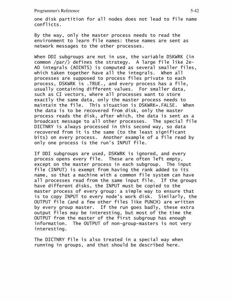
Programmer's Reference 5-42
one disk partition for all nodes does not lead to file name conflicts. By the way, only the master process needs to read the environment to learn file names: these names are sent as network messages to the other processes. When DDI subgroups are not in use, the variable DSKWRK (in common /par/) defines the strategy. A large file like 2e- AO integrals (AOINTS) is computed as several smaller files, which taken together have all the integrals. When all processes are supposed to process files private to each process, DSKWRK is .TRUE., and every process has a file, usually containing different values. For smaller data, such as CI vectors, where all processes want to store exactly the same data, only the master process needs to maintain the file. This situation is DSKWRK=.FALSE. When the data is to be recovered from disk, only the master process reads the disk, after which, the data is sent as a broadcast message to all other processes. The special file DICTNRY is always processed in this second way, so data recovered from it is the same (to the least significant bits) on every process. Another example of a file read by only one process is the run's INPUT file. If DDI subgroups are used, DSKWRK is ignored, and every process opens every file. These are often left empty, except on the master process in each subgroup. The input file (INPUT) is exempt from having the rank added to its name, so that a machine with a common file system can have all processes read from the same input file. If the groups have different disks, the INPUT must be copied to the master process of every group: a simple way to ensure that is to copy INPUT to every node's work disk. Similarly, the OUTPUT file (and a few other files like PUNCH) are written by every group master. If the run goes badly, these extra output files may be interesting, but most of the time the OUTPUT from the master of the first subgroup has enough information. The OUTPUT of non-group-masters is not very interesting. The DICTNRY file is also treated in a special way when running in groups, and that should be described here.

Programmer's Reference 5-43
Contents of the direct access file 'DICTNRY' 1. Atomic coordinates 2. various energy quantities in /ENRGYS/ 3. Gradient vector 4. Hessian (force constant) matrix 5-6. not used 7. PTR - symmetry transformation for p orbitals 8. DTR - symmetry transformation for d orbitals 9. FTR - symmetry transformation for f orbitals 10. GTR - symmetry transformation for g orbitals 11. Bare nucleus Hamiltonian integrals 12. Overlap integrals 13. Kinetic energy integrals 14. Alpha Fock matrix (current) 15. Alpha orbitals 16. Alpha density matrix 17. Alpha energies or occupation numbers 18. Beta Fock matrix (current) 19. Beta orbitals 20. Beta density matrix 21. Beta energies or occupation numbers 22. Error function interpolation table 23. Old alpha Fock matrix 24. Older alpha Fock matrix 25. Oldest alpha Fock matrix 26. Old beta Fock matrix 27. Older beta Fock matrix 28. Oldest beta Fock matrix 29. Vib 0 gradient in FORCE (numerical hessian) 30. Vib 0 alpha orbitals in FORCE 31. Vib 0 beta orbitals in FORCE 32. Vib 0 alpha density matrix in FORCE 33. Vib 0 beta density matrix in FORCE 34. dipole derivative tensor in FORCE. 35. frozen core Fock operator, in AO basis 36. RHF/UHF/ROHF Lagrangian (see 402-404) 37. floating point part of common block /OPTGRD/ int 38. integer part of common block /OPTGRD/ 39. ZMAT of input internal coords int 40. IZMAT of input internal coords 41. B matrix of redundant internal coords 42. pristine core Fock matrix in MO basis (see 87) 43. Force constant matrix in internal coordinates. 44. SALC transformation 45. symmetry adapted Q matrix 46. S matrix for symmetry coordinates

Programmer's Reference 5-44
47. ZMAT for symmetry internal coords int 48. IZMAT for symmetry internal coords 49. B matrix 50. B inverse matrix 51. overlap matrix in Lowdin basis, temp Fock matrix storage for ROHF 52. genuine MOPAC overlap matrix 53. MOPAC repulsion integrals 54. exchange integrals for screening 55. orbital gradient during SOSCF MCSCF 56. orbital displacement during SOSCF MCSCF 57. orbital hessian during SOSCF MCSCF 58. reserved for Pradipta 59. Coulomb integrals in Ruedenberg localizations 60. exchange integrals in Ruedenberg localizations 61. temp MO storage for GVB and ROHF-MP2 62. temp density for GVB 63. dS/dx matrix for hessians 64. dS/dy matrix for hessians 65. dS/dz matrix for hessians 66. derivative hamiltonian for OS-TCSCF hessians 67. partially formed EG and EH for hessians 68. MCSCF first order density in MO basis 69. alpha Lowdin populations 70. beta Lowdin populations 71. alpha orbitals during localization 72. beta orbitals during localization 73. alpha localization transformation 74. beta localization transformation 75. fitted EFP interfragment repulsion values 76. model core potential information 77. model core potential information 78. "Erep derivative" matrix associated with F-a terms 79. "Erep derivative" matrix associated with S-a terms 80. EFP 1-e Fock matrix including induced dipole terms 81. interfragment dispersion values 82. MO-based Fock matrix without any EFP contributions 83. LMO centroids of charge 84. d/dx dipole velocity integrals 85. d/dy dipole velocity integrals 86. d/dz dipole velocity integrals 87. unmodified h matrix during SCRF or EFP, AO basis 88. PCM solvent operator contribution to Fock 89. EFP multipole contribution to one e- Fock matrix 90. ECP coefficients int 91. ECP labels 92. ECP coefficients int 93. ECP labels 94. bare nucleus Hamiltonian during FFIELD runs

Programmer's Reference 5-45
95. x dipole integrals, in AO basis 96. y dipole integrals, in AO basis 97. z dipole integrals, in AO basis 98. former coords for Schlegel geometry search 99. former gradients for Schlegel geometry search 100. dispersion contribution to EFP gradient records 101-248 are used for NLO properties 101. U'x(0) 149. U''xx(-2w;w,w) 200. UM''xx(-w;w,0) 102. y 150. xy 201. xy 103. z 151. xz 202. xz 104. G'x(0) 152. yy 203. yz 105. y 153. yz 204. yy 106. z 154. zz 205. yz 107. U'x(w) 155. G''xx(-2w;w,w) 206. zx 108. y 156. xy 207. zy 109. z 157. xz 208. zz 110. G'x(w) 158. yy 209. U''xx(0;w,-w) 111. y 159. yz 210. xy 112. z 160. zz 211. xz 113. U'x(2w) 161. e''xx(-2w;w,w) 212. yz 114. y 162. xy 213. yy 115. z 163. xz 214. yz 116. G'x(2w) 164. yy 215. zx 117. y 165. yz 216. zy 118. z 166. zz 217. zz 119. U'x(3w) 167. UM''xx(-2w;w,w) 218. G''xx(0;w,-w) 120. y 168. xy 219. xy 121. z 169. xz 220. xz 122. G'x(3w) 170. yy 221. yz 123. y 171. yz 222. yy 124. z 172. zz 223. yz 125. U''xx(0) 173. U''xx(-w;w,0) 224. zx 126. xy 174. xy 225. zy 127. xz 175. xz 226. zz 128. yy 176. yz 227. e''xx(0;w,-w) 129. yz 177. yy 228. xy 130. zz 178. yz 229. xz 131. G''xx(0) 179. zx 230. yz 132. xy 180. zy 231. yy 133. xz 181. zz 232. yz 134. yy 182. G''xx(-w;w,0) 233. zx 135. yz 183. xy 234. zy 136. zz 184. xz 235. zz 137. e''xx(0) 185. yz 236. UM''xx(0;w,-w) 138. xy 186. yy 237. xy 139. xz 187. yz 238. xz 140. yy 188. zx 239. yz

Programmer's Reference 5-46
141. yz 189. zy 240. yy 142. zz 190. zz 241. yz 143. UM''xx(0) 191. e''xx(-w;w,0) 242. zx 144. xy 192. xy 243. zy 145. xz 193. xz 244. zz 146. yy 194. yz 147. yz 195. yy 148. zz 196. yz 197. zx 198. zy 199. zz 245. old NLO Fock matrix 246. older NLO Fock matrix 247. oldest NLO Fock matrix 249. polarizability derivative tensor for Raman 250. transition density matrix in AO basis 251. static polarizability tensor alpha 252. X dipole integrals in MO basis 253. Y dipole integrals in MO basis 254. Z dipole integrals in MO basis 255. alpha MO symmetry labels 256. beta MO symmetry labels 257. dipole polarization integrals during EFP1 258. Vnn gradient during MCSCF hessian 259. core Hamiltonian from der.ints in MCSCF hessian 260-261. reserved for Dan 262. MO symmetry integers during determinant CI 263. PCM nuclei/induced nuclear Charge operator 264. PCM electron/induced nuclear Charge operator 265. pristine alpha guess (MOREAD or Huckel+INSORB) 266. EFP/PCM IFR sphere information 267. fragment LMO expansions, for EFP Pauli 268. fragment Fock operators, for EFP Pauli 269. fragment CMO expansions, for EFP charge transfer 270. reserved for non-orthogonal FMO dimer guess 271. orbital density matrix in divide and conquer int 272. subsystem data during divide and conquer 273. old alpha Fock matrix for D&C Anderson-like DIIS 274. old beta Fock matrix for D&C Anderson-like DIIS 275. not used 276. Vib 0 Q matrix in FORCE 277. Vib 0 h integrals in FORCE 278. Vib 0 S integrals in FORCE 279. Vib 0 T integrals in FORCE 280. Zero field LMOs during numerical polarizability 281. Alpha zero field dens. during num. polarizability 282. Beta zero field dens. during num. polarizability 283. zero field Fock matrix. during num. polarizability

Programmer's Reference 5-47
284. Fock eigenvalues for multireference PT 285. density matrix or Fock matrix over LMOs 286. oriented localized molecular orbitals 287. density matrix of oriented LMOs 288. DM1 during CEPA-style calculations 289. DM2 during CEPA-style calculations 290. pristine (gas phase) h during solvent runs 291. "repulsion" integrals during EFP1 292-299. not used 301. Pocc during MP2 (RHF or ZAPT) or CIS grad 302. Pvir during MP2 gradient (UMP2= 411-429) 303. Wai during MP2 gradient 304. Lagrangian Lai during MP2 gradient 305. Wocc during MP2 gradient 306. Wvir during MP2 gradient 307. P(MP2/CIS)-P(RHF) during MP2 or CIS gradient 308. SCF density during MP2 or CIS gradient 309. energy weighted density in MP2 or CIS gradient 311. Supermolecule h during Morokuma 312. Supermolecule S during Morokuma 313. Monomer 1 orbitals during Morokuma 314. Monomer 2 orbitals during Morokuma 315. combined monomer orbitals during Morokuma 316. RHF density in CI grad; nonorthog. MOs in SCF-MI 317. unzeroed Fock matrix when MOs are frozen 318. MOREAD orbitals when MOs are frozen 319. bare Hamiltonian without EFP contribution 320. MCSCF active orbital density 321. MCSCF DIIS error matrix 322. MCSCF orbital rotation indices 323. Hamiltonian matrix during QUAD MCSCF 324. MO symmetry labels during MCSCF 325. final uncanonicalized MCSCF orbitals 326-329. not used 330. CEL matrix during PCM 331. VEF matrix during PCM 332. QEFF matrix during PCM 333. ELD matrix during PCM 334. PVE tesselation info during PCM 335. PVE tesselation info during PCM 336. frozen core Fock operator, in MO basis 337-339. not used 340. DFT alpha Fock matrix 341. DFT beta Fock matrix 342. DFT screening integrals 343. DFT: V aux basis only 344. DFT density gradient d/dx integrals 345. DFT density gradient d/dy integrals 346. DFT density gradient d/dz integrals
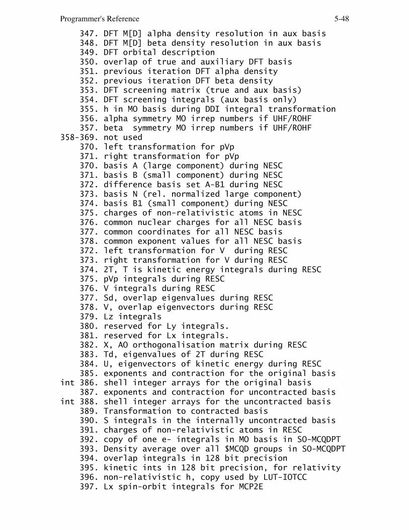
Programmer's Reference 5-48
347. DFT M[D] alpha density resolution in aux basis 348. DFT M[D] beta density resolution in aux basis 349. DFT orbital description 350. overlap of true and auxiliary DFT basis 351. previous iteration DFT alpha density 352. previous iteration DFT beta density 353. DFT screening matrix (true and aux basis) 354. DFT screening integrals (aux basis only) 355. h in MO basis during DDI integral transformation 356. alpha symmetry MO irrep numbers if UHF/ROHF 357. beta symmetry MO irrep numbers if UHF/ROHF 358-369. not used 370. left transformation for pVp 371. right transformation for pVp 370. basis A (large component) during NESC 371. basis B (small component) during NESC 372. difference basis set A-B1 during NESC 373. basis N (rel. normalized large component) 374. basis B1 (small component) during NESC 375. charges of non-relativistic atoms in NESC 376. common nuclear charges for all NESC basis 377. common coordinates for all NESC basis 378. common exponent values for all NESC basis 372. left transformation for V during RESC 373. right transformation for V during RESC 374. 2T, T is kinetic energy integrals during RESC 375. pVp integrals during RESC 376. V integrals during RESC 377. Sd, overlap eigenvalues during RESC 378. V, overlap eigenvectors during RESC 379. Lz integrals 380. reserved for Ly integrals. 381. reserved for Lx integrals. 382. X, AO orthogonalisation matrix during RESC 383. Td, eigenvalues of 2T during RESC 384. U, eigenvectors of kinetic energy during RESC 385. exponents and contraction for the original basis int 386. shell integer arrays for the original basis 387. exponents and contraction for uncontracted basis int 388. shell integer arrays for the uncontracted basis 389. Transformation to contracted basis 390. S integrals in the internally uncontracted basis 391. charges of non-relativistic atoms in RESC 392. copy of one e- integrals in MO basis in SO-MCQDPT 393. Density average over all $MCQD groups in SO-MCQDPT 394. overlap integrals in 128 bit precision 395. kinetic ints in 128 bit precision, for relativity 396. non-relativistic h, copy used by LUT-IOTCC 397. Lx spin-orbit integrals for MCP2E
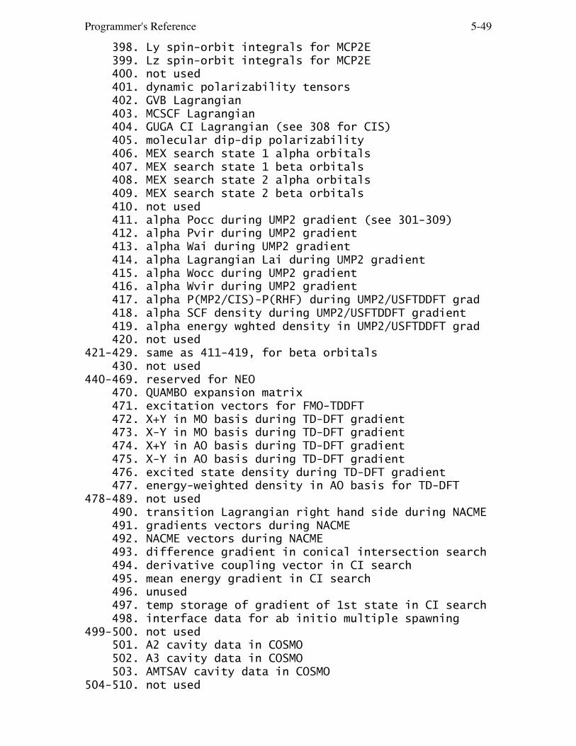
Programmer's Reference 5-49
398. Ly spin-orbit integrals for MCP2E 399. Lz spin-orbit integrals for MCP2E 400. not used 401. dynamic polarizability tensors 402. GVB Lagrangian 403. MCSCF Lagrangian 404. GUGA CI Lagrangian (see 308 for CIS) 405. molecular dip-dip polarizability 406. MEX search state 1 alpha orbitals 407. MEX search state 1 beta orbitals 408. MEX search state 2 alpha orbitals 409. MEX search state 2 beta orbitals 410. not used 411. alpha Pocc during UMP2 gradient (see 301-309) 412. alpha Pvir during UMP2 gradient 413. alpha Wai during UMP2 gradient 414. alpha Lagrangian Lai during UMP2 gradient 415. alpha Wocc during UMP2 gradient 416. alpha Wvir during UMP2 gradient 417. alpha P(MP2/CIS)-P(RHF) during UMP2/USFTDDFT grad 418. alpha SCF density during UMP2/USFTDDFT gradient 419. alpha energy wghted density in UMP2/USFTDDFT grad 420. not used 421-429. same as 411-419, for beta orbitals 430. not used 440-469. reserved for NEO 470. QUAMBO expansion matrix 471. excitation vectors for FMO-TDDFT 472. X+Y in MO basis during TD-DFT gradient 473. X-Y in MO basis during TD-DFT gradient 474. X+Y in AO basis during TD-DFT gradient 475. X-Y in AO basis during TD-DFT gradient 476. excited state density during TD-DFT gradient 477. energy-weighted density in AO basis for TD-DFT 478-489. not used 490. transition Lagrangian right hand side during NACME 491. gradients vectors during NACME 492. NACME vectors during NACME 493. difference gradient in conical intersection search 494. derivative coupling vector in CI search 495. mean energy gradient in CI search 496. unused 497. temp storage of gradient of 1st state in CI search 498. interface data for ab initio multiple spawning 499-500. not used 501. A2 cavity data in COSMO 502. A3 cavity data in COSMO 503. AMTSAV cavity data in COSMO 504-510. not used

Programmer's Reference 5-50
511. effective polarizability in LRD 512. C6 coefficients in LRD 513. C8 coefficients in LRD 514. C10 coefficients in LRD 515. atomic pair LRD energy 520. Malmqvist factorized orb transformation (wrt 325) 521. SVD localized orthogonal orbitals 522. SVD localized nonorthogonal orbitals 523. initial-to-SVD LMO nonorthogonal transformation 524. SVD LMO nonorthogonal-to-orthogonal transformation 525. initial-to-SVD LMO orthog transformation (wrt 15) 526. 1st order density for orthogonal SVD localized MOs 527. collective orbital reordering for Malmqvist 528. atom-to-orbital assignment for SVD orbitals 529. Malmqvist re-ordered set of SVD LMOs 530. oriented SVD density in the order of record 529 531. oriented or SVD atom-to-orbital assignment for CT 532. block zapped 'standard Fock operator' in AO basis 533. overlap of stored atom's MBS with current basis 534. occupied+external orthog loc (natural) orbitals 535. atom-to-orbital assignment for record 534 orbitals 536. specialized SVD density matrix for EXTERNAL NOS 537. VVOS no-transfer orbitals+appropriate LMOs. 538. occupied+VVOS orbitals right after VVOS formation 539. nonorthogonal SVD localized orbitals 540. atom-to-orbital assignment for record 539 orbitals 541. pristine MCSCF orbs during diabatization 542. reference geometry orbs during diabatization 543. PT2 state rotation during diabatization 544. PT2 state energies during diabatization 545. PT2's CAS-CI largest CI coefs, in diabatization 546. Group labels for SVD orbitals. 547. Atom labels for oriented orbitals. 548. Group labels for oriented orbitals. 549. Quasi-atomic orbitals during No Charge Transfer 550. Current guess orbitals during No Charge Transfer 551. Atom labels during No Charge Transfer 552. Determinant NCT density for SVD/oriented orbitals. 553. Total NCT density mtx for SVD/oriented orbitals. 554. pseudodensity mtx from right coupled cluster NOs. 555. Unmodified input orbs for checking active space. 556. DFTB atom-resolved Mulliken populations 557. DFTB shell-resolved Mulliken populations 558. DFTB shell-resolved spin populations 559. DFTB atom-resolved shift contributions 560. DFTB shell-resolved shift contributions 561. DFTB shell-resolved shift contributions from spin 562. DFTB alpha occupation numbers 563. DFTB beta occupation numbers

Programmer's Reference 5-51
564. DFTB non-perturbed Hamiltonian in FMO 565. DFTB HOP contribution in FMO 566. DFTB atom-resolved shift of ESP in FMO 567. DFTB atom-resolved shift of ESP in FMO (DFTB3) 568. DFTB Slater-Kostner tables 569. DFTB reserved 570-579. unused. 580-599. reserved for Aaron 600. alpha loc. transformation in LMOEDA 601. alpha localized orbs in LMOEDA 602. beta loc. transformation in LMOEDA 603. beta localized orbs in LMOEDA 604. alpha Coulomb operator in LMOEDA 605. alpha exchange operator in LMOEDA 606. alpha density in LMOEDA 607. beta Coulomb operator in LMOEDA 608. beta exchange operator in LMOEDA 609. beta density in LMOEDA 610-950. mostly not used, but 801-809. xx,xy,xz,yx,yy,yz,zx,zy,zz quadrupole MO ints. 810-815. xx,xy,xz,yy,yz,xx quadrupole AO ints. 816. LMO dipole-quadrupole polarizability 817. molecular dipole-quadrupole polarizability In order to correctly pass data between different machine types when running in parallel, it is required that a DAF record must contain only floating point values, or only integer values. No logical or Hollerith data may be stored. The final calling argument to DAWRIT and DAREAD must be 0 or 1 to indicate floating point or integer values are involved. The records containing integers are so marked in the list below. Physical record 1 (containing the DAF directory) is written whenever a new record is added to the file. This is invisible to the programmer. The numbers shown above are "logical record numbers", and are the only thing that the programmer need be concerned with.