program analysis methodology office of transportation ... · program analysis methodology office of...

Program Analysis Methodology

Office of Transportation Technologies

Quality Metrics- Final Report -

May 9, 2001

Prepared by:

OTT Analytic Teamhttp://www.ott.doe.gov/facts.html

ScienceScienceScienceScienceCommunicationsCommunicationsCommunicationsCommunicationsPlanningPlanningPlanningPlanning

Prepared for:

Office of Transportation TechnologiesU.S. Department of Energy

Washington, D.C.

2002

OTT Program Analysis Methodology ii May 9, 2001Quality Metrics 2002 Final Report

Table of Contents

Section Page No.

List of Exhibits.............................................................................................................................. iv

Executive Summary ..................................................................................................................... 1

1.0 Introduction ....................................................................................................................... 91.1 Purpose and Scope .................................................................................................. 91.2 Background -The EE/RE Quality Metrics Review Process .................................. 101.3 Background - The Office of Transportation Technologies (OTT) ........................ 121.4 Report Structure/Organization .............................................................................. 14

2.0 Technical Analysis Overview ......................................................................................... 162.1 Background ........................................................................................................... 162.2 Vehicle/Technology/Fuel Baseline Assumptions.................................................. 162.3 Vehicle Attributes ................................................................................................. 17

2.3.1 Light Vehicle Attributes............................................................................ 172.3.2 Heavy Vehicle Attributes .......................................................................... 20

2.4 Summary of Modeling Assumptions and Structures............................................. 212.4.1 VSCC Model ............................................................................................. 232.4.2 IMPACTT Model ...................................................................................... 232.4.3 GREET Model........................................................................................... 232.4.4 HVMP Model............................................................................................ 242.4.5 ESM Model ............................................................................................... 242.4.6 Other Calculations..................................................................................... 24

3.0 Vehicle Choice Analysis .................................................................................................. 253.1 Light Vehicles ....................................................................................................... 253.2 Heavy Vehicles...................................................................................................... 343.3 Stand-Alone Technologies .................................................................................... 44

3.3.1 Sensitivity Study-No Advanced Diesel ..................................................... 493.3.2 Sensitivity Study-Fuel Price/Technology Cost Impacts ............................ 49

OTT Program Analysis Methodology iii May 9, 2001Quality Metrics 2002 Final Report

4.0 Benefits Estimates ........................................................................................................... 514.1 Petroleum and Other Energy Benefits Analysis .................................................... 51

4.1.1 Biomass ..................................................................................................... 514.1.2 Fuel Choice for Flex-Fuel Vehicles .......................................................... 524.1.3 Estimates of the Value of Reducing Imported Oil .................................... 534.1.4 Petroleum Reduction Estimates ................................................................ 56

4.2 Economic and Environmental Benefits Analysis Results ..................................... 594.2.1 Economic Benefits Estimates.................................................................... 594.2.2 Vehicle Infrastructure Capital Requirements ............................................ 614.2.3 Greenhouse Gases, Regulated Emissions, and Energy Use in

Transportation (GREET) Model ............................................................... 644.2.4 Cost of Various Pollutants ........................................................................ 664.2.5 Aggregate Environmental and Economic Benefits Estimates................... 64

5.0 Accomplishments and Future Plans .................................................................................. 665.1 Accomplishments ...................................................................................... 665.2 Future Plans............................................................................................... 66

6.0 References ............................................................................................................................ 69

7.0 Supporting Information...................................................................................................... 727.1 Glossary................................................................................................................. 727.2 Energy Conversion Factors Used .......................................................................... 73

AppendicesA. Quality Metrics 2002 Results

OTT Program Analysis Methodology iv May 9, 2001Quality Metrics 2002 Final Report

List of Exhibits

Exhibit E1. OTT Program Structure and QM Planning Units ........................................................ 2Exhibit E2. Vehicle/Technology Analysis Matrix .......................................................................... 3Exhibit E3. OTT Impacts Assessment Process ............................................................................... 4Exhibit E4. Conventional Vehicle Characteristics – Large Cars (1996)......................................... 5Exhibit E5. Market Penetration Summary ...................................................................................... 5Exhibit E6. QM 2002 Summary...................................................................................................... 6Exhibit E7. Transportation Petroleum Use Projection .................................................................... 7Exhibit E8. Carbon Emissions Reductions ..................................................................................... 8Exhibit 1-1. Relationship Between Quality Metrics and OTT Program ....................................... 13Exhibit 2-1. Conventional Baseline Vehicle Characteristics (1999)............................................. 16Exhibit 2-2. Technology Characteristics - Large Car (1999) ........................................................ 18Exhibit 2-3. Technology Characteristics - Small Car (1999) ........................................................ 18Exhibit 2-4. Technology Characteristics - Sport Utility Vehicle (1999)....................................... 19Exhibit 2-5. Technology Characteristics – Minivan (1999).......................................................... 19Exhibit 2-6. Technology Characteristics - Pickup Trucks and Large Vans (1999)....................... 20Exhibit 2-7. QM Modeling Process............................................................................................... 22Exhibit 3-1. Fuel Economy Ratio.................................................................................................. 27Exhibit 3-2. Cost Ratio.................................................................................................................. 28Exhibit 3-3. Relative Range Ratio................................................................................................. 28Exhibit 3-4. Relative Maintenance................................................................................................ 29Exhibit 3-5. Market Penetration of Alternative Light Vehicles Sales and Stocks ........................ 30Exhibit 3-6. Market Penetration of Alternative Light Vehicles-Sales .......................................... 30Exhibit 3-7. Market Penetration of Small Car Technologies ........................................................ 31Exhibit 3-8. Market Penetration of Large Car Technologies ........................................................ 31Exhibit 3-9. Market Penetration of Minivan Technologies........................................................... 32Exhibit 3-10. Market Penetration of Sport Utility Vehicle Technologies..................................... 32Exhibit 3-11. Market Penetration of Pickup & Large Van Technologies ..................................... 33Exhibit 3-12. Alternative Light Vehicle Sales and Stocks, 2010.................................................. 33Exhibit 3-13. Alternative Light Vehicle Sales and Stocks, 2020.................................................. 34Exhibit 3-14. Alternative Light Vehicle Sales and Stocks, 2030.................................................. 34Exhibit 3-15. Heavy Vehicle Characteristics ................................................................................ 35Exhibit 3-16. Heavy Vehicle Market Characteristics ................................................................... 35Exhibit 3-17. Heavy Vehicle Payback Periods.............................................................................. 35

OTT Program Analysis Methodology v May 9, 2001Quality Metrics 2002 Final Report

Exhibit 3-18. Medium Vehicle Travel Distribution – Central Refueling ..................................... 37Exhibit 3-19. Medium Vehicle Travel Distribution – Non-Central Refueling ............................. 38Exhibit 3-20. Type 1 Heavy Vehicle Travel Distribution – Central Refueling............................. 39Exhibit 3-21. Type 1 Heavy Travel Distribution – Non-Central Refueling.................................. 39Exhibit 3-22. Type 2 Heavy Vehicle Travel Distribution – Central Refueling............................. 40Exhibit 3-23. Type 2 Heavy Vehicle Travel Distribution – Non-Central Refueling .................... 41Exhibit 3-24. Type 3 Heavy Vehicle Travel Distribution – Central Refueling............................. 42Exhibit 3-25. Type 3 Heavy Vehicle Distribution – Non-Central Refueling................................ 42Exhibit 3-26. Incremental Costs and Fuel Economy Improv. for Heavy Vehicles ($1996).......... 43Exhibit 3-27. Heavy Vehicle Market Penetration Results ............................................................ 44Exhibit 3-28. Stand-Alone Technologies and Combinations Examined....................................... 44Exhibit 3-29. Comp. of Stand-Alone Technology Savings with QM Savings: HEVs.................. 45Exhibit 3-30. Comp. of Stand-Alone Technology Savings with QM Savings: Fuel Cells. .......... 46Exhibit 3-31. Comp. of Stand-Alone Technology Savings with QM Savings: SIDI.................... 46Exhibit 3-32. Comp. of Stand-Alone Technology Savings with QM Savings: Advanced Diesel 47Exhibit 3-33. Comp. of Stand-Alone Technology Savings with QM Savings: Elect Vehicle...... 47Exhibit 3-34. Comp. of Stand-Alone Technology Savings with QM Savings: Material Tech. .... 48Exhibit 3-35. Comp. of Stand-Alone Technology Savings with QM Savings: All-OTT ............. 48Exhibit 3-36. Comp. of QM (Combined) Savings with Adv. Diesel Option Removed................ 49Exhibit 3-37. Comparison of Reference QM Savings with Fuel Price/Alternative TechnologyCost Sensitivity Study Results ...................................................................................................... 50Exhibit 4-1. Biomass Fuel Use...................................................................................................... 52Exhibit 4-2. Alternative Fuel Market Share as a Function of Fuel Availability and Fuel Price ... 53Exhibit 4-3. Value of Reducing Imported Oil ............................................................................... 55Exhibit 4-4. Energy Displaced ...................................................................................................... 57Exhibit 4-5. ZEV and EPACT Oil Reductions ............................................................................. 58Exhibit 4-6. Transportation Petroleum Use Projection ................................................................. 58Exhibit 4-7. Employment Impacts by Sector of Economy (Jobs) ................................................. 60Exhibit 4-8. Employment Impacts by Technology (Jobs) ............................................................. 60Exhibit 4-9. GDP Increase............................................................................................................. 61Exhibit 4-10. Capital Infrastructure Costs..................................................................................... 63Exhibit 4-11. Aggregate Capital Expenditures.............................................................................. 64Exhibit 4-12. Carbon Coefficients ................................................................................................ 65

OTT Program Analysis Methodology vi May 9, 2001Quality Metrics 2002 Final Report

Exhibit 4-13. Range of Costs to Control CO2 Emissions.............................................................. 67Exhibit 4-14. Carbon Emissions Reductions ................................................................................ 68

OTT Program Analysis Methodology - i - May 9, 2001Quality Metrics 2002 Final Report

Foreword/Acknowledgement

The Analytic Support Team for the Office of Transportation Technologies, which prepared thisreport, consists of : Phil Patterson of the Office of Transportation Technologies at the U.S.Department of Energy, John Maples of TRANCON, Inc. (subcontractor to Oak Ridge NationalLaboratory), Jim Moore of TA Engineering, Inc. (subcontractor to Argonne NationalLaboratory), and Alicia Birky of the National Renewable Energy Laboratory.

In addition to the analytic team, this report reflects the efforts of many program staff persons andresearchers of the U.S. Department of Energy, the national scientific research laboratories, andrelated contractors. The efforts of these individuals are also acknowledged.

William J. Shadis of TA Engineering provided supporting analyses, contributing authorship,editing and layout of the Final Report. Other unnamed individuals and organizations assistedthis project in a range of capacities.

OTT Program Analysis Methodology - 1 - May 9, 2001Quality Metrics 2002 Final Report

Executive Summary

“Quality Metrics” is the term used to describe the analytical process for measuring andestimating future energy, environmental and economic benefits of US DOE Office of EnergyEfficiency and Renewable Energy programs. This report focuses on the projected benefits of theforty-one (41) programs currently supported through the Office Of Transportation Technologies(OTT) under EE/RE. For analytical purposes, these various benefits are subdivided in terms ofPlanning Units which are related to the OTT program structure.

The scope of this report encompasses light vehicles including passenger automobiles and class 1& 2 (light) trucks, as well as class 3 through 8 (heavy) trucks. The range of light vehicletechnologies investigated include flex-fuel (ethanol/gasoline blends) electric, hybrid electric, fuelcell, advanced diesel, natural gas-fueled, and stratified charge direct-injection. The hybridcategory is further split between two versions, one with twice the fuel economy of conventionalvehicles (2X) and the other with three times the fuel economy (3X). The fuel cell category isfurther subdivided between gasoline-fueled and hydrogen-fueled versions. A future distributionof light vehicle sizes, applications, and performance levels is calculated based on current vehiclestocks and trends, and consumer preferences. The heavy vehicle technologies investigatedinclude hybrid, natural gas-fueled and advanced diesel. The effects of advanced materialstechnologies across all vehicle types are also analyzed.

Analysis results quantify various national benefits including energy and petroleum consumptionreductions, carbon emission reductions, criteria pollutant emissions reductions, and theassociated economic impacts on the Gross Domestic Product (GDP) and jobs. Benefit/costanalyses of the various technologies are also included. The time focus of the analysis is from thepresent to the year 2030.

The programs currently conducted by OTT Offices are shown on the left side of Exhibit E-1.OTT is composed of four line-offices managing many separate programs. For Quality Metrics,OTT activities are aggregated into planning units based on specific program activities that areshown in the right side of Exhibit E-1.

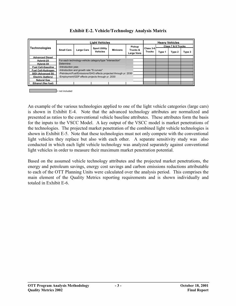
Exhibit E-2 summarizes the specific vehicle technologies and alternative fuel that are evaluatedunder Quality Metrics. Five light vehicle categories and four heavy vehicle categories areconsidered. Each technology-vehicle category/type is analyzed separately as to when and howquickly the new technology can enter the market and its effects on energy use, the environmentand the economy. The estimated total effect of the OTT programs is then simply the sum of theindividual effects.

A variety of analytical models are used to calculate the various projected OTT Program benefits.Various analytical tools and models are used to develop the results produced in this report.Outputs from some of these models become inputs to some of the others. The relationships ofthe various models are shown in Exhibit E-3.


Exhibit E-1. OTT Program Structure and QM Planning Units

OTT Offices and Programs OTT Functions & Planning Units

Office of Fuels Development

(OFD)

Office of Advanced

Automotive Technologies

(OAAT)

Office of Heavy Vehicle

Technologies (OHVT)

Office of Technology Utilization

(OTU)

Fuels Development

Vehicle Technologies

R&D

Materials Technologies

Technology Deployment

Biodiesel ProgramAdvanced Battery Readiness Ad Hoc Working Group

Advanced Petroleum-Based Fuel Program

AFV Incentive Program Blends Hybrid Systems R&D Propulsion System

Materials Household CNG

Biofuels ProgramAlternative Fuels Research and Development

Alternative Fuel Truck Application Program

Alternative Fuels Data Center Flex-Fuel Fuel Cell R&D

Light Vehicle Materials-Household EV

EPACT Fleet

Ethanol Conversion Program Carat Program Atmospheric

Reactions Program Clean Cities Program Dedicated Conventional

Advanced Combustion R&D-SIDI

Light Vehicle Materials-Hybrid Vehicle

Feedstock Development Program

CIDI ProgramDiesel Emissions Control-Sulfur Effects

Credits Program Fuel CellAdvanced Combustion R&D-Car CIDI

Light Vehicle Materials-Fuel Cell Vehicle

Regional Biomass Program

Electric Vehicle Program

Fuel and Engine Technologies Program

EPACT Fleet Leadersip Programs

Advanced Combustion R&D-Light Truck CIDI

Fuel Cell ProgramHeavy Duty Engine Development Program

Federal Alternative Fuels USER Program

Electric Vehicles R&D-Household EV

Fuels Research and Development Program

Heavy Vehicle Emissions Reduction Technologies Program

Federal Fleet Alternative Fuel Vehicle Program

Electric Vehicles R&D-EPACT/ZEV Mandates

GATE ProgramHeavy Vehicle Emissions Testing Program

Field Operations Program

Heavy Vehicle Systems R&D-Class 3-6

HEV Program Heavy Vehicle Program

Infrastructure Working Group

Heavy Vehicle Systems R&D-Class 7&8

PNGV Transit Bus Program

Local Government and Private Fleets-Regulation and Compliance

Heavy Vehicle Systems R&D-Class 7&8 CNG

US Advanced Battery Consortium Pilot Program

Cool Car Program

State and Alternative Provider Fleets-Regulation and Compliance

State and Local Incentives Program

OTT Program Analysis Methodology - 3 - October 18, 2001Quality Metrics 2002 Final Report

Exhibit E-2. Vehicle/Technology Analysis Matrix

An example of the various technologies applied to one of the light vehicle categories (large cars)is shown in Exhibit E-4. Note that the advanced technology attributes are normalized andpresented as ratios to the conventional vehicle baseline attributes. These attributes form the basisfor the inputs to the VSCC Model. A key output of the VSCC model is market penetrations ofthe technologies. The projected market penetration of the combined light vehicle technologies isshown in Exhibit E-5. Note that these technologies must not only compete with the conventionallight vehicles they replace but also with each other. A separate sensitivity study was alsoconducted in which each light vehicle technology was analyzed separately against conventionallight vehicles in order to measure their maximum market penetration potential.

Based on the assumed vehicle technology attributes and the projected market penetrations, theenergy and petroleum savings, energy cost savings and carbon emissions reductions attributableto each of the OTT Planning Units were calculated over the analysis period. This comprises themain element of the Quality Metrics reporting requirements and is shown individually andtotaled in Exhibit E-6.

Light Vehicles Heavy VehiclesClass 7 & 8 Trucks

Type 1 Type 2 Type 3

Advanced DieselHybrid-2XHybrid-3X

Fuel Cell-GasolineFuel Cell-HydrogenSIDI (Advanced SI)Electric (battery)

Natural GasEthanol (flex fuel)

= not included

MinivansPickup

Trucks & Large Vans

Class 3-6 Trucks

TechnnologiesSmall Cars Large Cars Sport Utility

Vehicles

For each technology-vehicle category/type "intersection"Determine:-Introduction year,-Introduction and growth rate "S curves"-Petroleum/Fuel/Emissions/GHG effects projected through yr. 2030-Employment/GDP effects projects through yr. 2030


Exhibit E-3. OTT Impact Assessment Process

Inputs:----------------------------------------------------Fuel Attributes: Price/Gallon of Gasoline Equivalent - Gasoline - Diesel - Ethanol - CNG - Electricity

----------------------------------------------------Fuel Attributes: Price/Gallon of Gasoline Equivalent - Gasoline - Diesel - Ethanol - CNG - Electricity


VSCC ModelCalculates: : Fuel Availability & Market Penetration for - Small Cars - Large Cars - Minivans - Sport Utility Vehicles - Pickup/Large Vans

Emissions ModelCalculates Unit-Vehicle Fuel Cycle Grams Per MileTailpipe Emissions For: - HC - CO - NOx - PM10 - SOx

HVMP ModelCalculates Market Penetration for: - 8 market classes with central/non-central refueling - 11 VMT categories

Sales, Stocks, Vintaging& Emissions Model Calculates: : - Vehicle Sales - Vehicle Stocks - Vehicle-Miles Traveled - Alternative Fuel Used - Petroleum Displaced - Emissions Reductions

ESMCalculates: : - GDP Effects - Jobs impacts

Other Calculations - Green House Gas Reductions - Energy Cost Reductions - Total Incremental Vehicle Cost - Capital Investment Requirements

Key: - VSCC-Vehicle Size/Consumer Choice Model - HVMP-Heavy Vehicle Market Penetration Model - ESM- Employment Spreadsheet Model


Exhibit E-4. Conventional Vehicle Characteristics – Large Cars (1999)

Exhibit E-5. Market Penetration Summary

Vehicle Technology Status YearVehicle

Cost ($000)

Fuel Economy

(mpg)

Relative Range (miles)

Maintenance Cost ($/yr)

Trunk Space

(relative)

Acceleration (0-30 MPH-sec)

Top Speed (MPH)

Conventional 2000 26.69 26.76 325 450 1.000 7.0 131.9

2030 27.13 28.37 325 450 1.000 7.0 131.9

Technology Ratios(1)

Advanced Diesel Initial-2001 1.070 1.350 1.200 1.000 1.000 1.100 0.8002030 1.049 1.350 1.200 1.000 1.000 1.100 0.800

Flex Alcohol Initial-2000 1.000 1.000 1.000 1.000 1.000 1.000 1.0002030 1.000 1.000 1.000 1.000 1.000 1.000 1.000

Fuel Cell-Hydrogen Initial-2007 1.400 2.200 1.000 1.050 0.800 1.000 0.7202030 1.300 3.000 1.000 1.050 0.800 1.000 0.720

Fuel Cell-Gasoline Initial-2005 1.300 2.000 1.000 1.050 0.800 1.000 0.7202030 1.200 3.000 1.000 1.050 0.800 1.000 0.720

SIDI Initial-2004 1.046 1.250 1.000 1.000 1.000 1.000 1.0002030 1.030 1.250 1.000 1.000 1.000 1.000 1.000

CNG Dedicated Initial-2003 1.069 1.000 0.660 0.900 0.750 1.000 1.0002030 1.035 1.000 0.750 0.900 0.850 1.000 1.000

Electric Initial-2009 1.788 4.000 0.360 0.600 0.500 1.000 0.5302030 1.495 4.000 0.360 0.600 0.800 1.000 0.530

Hybrid (2X) Initial-2005 1.250 1.500 1.200 1.050 0.950 1.000 0.7202030 1.100 2.000 1.200 1.050 0.950 1.000 0.720

Hybrid (3X) Initial-2005 1.300 2.000 1.200 1.050 0.950 1.000 0.7202030 1.200 3.000 1.200 1.050 0.950 1.000 0.720

(1) Technology ratio = Value of parameter for the technology/Value for the conventional vehicle in the same year.

0%

10%

20%

30%

40%

50%

60%

70%

80%

90%

2000

2002

2004

2006

2008

2010

2012

2014

2016

2018

2020

2022

2024

2026

2028

2030

Year

Perc

ent o

f Tot

al L

ight

Veh

icle

Sal

es

Gasoline Fuel CellHydrogen Fuel CellHybrid-3XHybrid-2XElectricCNGSIDIAlcohol FlexAdvanced Diesel (CIDI)


Exhibit E-6. QM 2002 Summary

Primary Energy Displaced (quads) Primary Oil Displaced (quads)

PLANNING UNIT 2000 2005 2010 2015 2020 2025 2030 2000 2005 2010 2015 2020 2025 2030Vehicle Technologies R&D 0.001 0.150 0.798 1.887 2.885 4.051 4.819 0.002 0.161 0.813 1.927 2.964 4.185 5.013 Hybrid Systems R&D 0.000 0.041 0.184 0.549 1.073 1.643 2.099 0.000 0.041 0.184 0.549 1.073 1.643 2.099 Fuel Cell R&D 0.000 0.000 0.006 0.059 0.058 0.490 0.794 0.000 0.000 0.006 0.063 0.072 0.537 0.885 Advanced Combustion R&D 0.000 0.084 0.520 1.090 1.444 1.512 1.475 0.000 0.084 0.520 1.090 1.444 1.512 1.475 SIDI 0.000 0.027 0.203 0.444 0.591 0.616 0.592 0.000 0.027 0.203 0.444 0.591 0.616 0.592 Car CIDI 0.000 0.054 0.224 0.405 0.499 0.498 0.477 0.000 0.054 0.224 0.405 0.499 0.498 0.477 Light Truck CIDI 0.000 0.003 0.093 0.242 0.354 0.398 0.406 0.000 0.003 0.093 0.242 0.354 0.398 0.406 Electric Vehicles R&D 0.000 0.008 0.027 0.057 0.103 0.140 0.166 0.001 0.019 0.041 0.093 0.167 0.228 0.269 Household EV 0.000 0.000 0.000 0.020 0.058 0.089 0.108 0.000 0.000 0.000 0.033 0.095 0.144 0.175 EPAct/ZEV Mandates 0.000 0.008 0.027 0.037 0.044 0.051 0.058 0.001 0.019 0.041 0.060 0.072 0.083 0.094 Heavy Vehicle Systems R&D 0.001 0.017 0.061 0.130 0.208 0.266 0.284 0.001 0.017 0.061 0.130 0.208 0.266 0.284 Class 3-6 0.000 0.001 0.005 0.013 0.022 0.030 0.037 0.000 0.001 0.005 0.013 0.022 0.030 0.037 Class 7&8 0.001 0.016 0.057 0.117 0.185 0.235 0.247 0.001 0.016 0.057 0.117 0.185 0.235 0.247 Class 7&8 CNG 0.000 0.000 0.000 0.000 0.000 0.000 0.000 0.000 0.000 0.000 0.000 0.000 0.000 0.000 Rail 0.000 0.000 0.000 0.000 0.000 0.000 0.000 0.000 0.000 0.000 0.000 0.000 0.000 0.000Materials Technologies 0.000 0.001 0.006 0.024 0.043 0.110 0.159 0.000 0.001 0.006 0.026 0.048 0.121 0.175 Propulsion System Materials 0.000 0.000 0.000 0.000 0.000 0.000 0.000 0.000 0.000 0.000 0.000 0.000 0.000 0.000 Light Vehicle Materials 0.000 0.001 0.006 0.024 0.043 0.110 0.159 0.000 0.001 0.006 0.026 0.048 0.121 0.175 Household EV 0.000 0.000 0.000 0.002 0.006 0.009 0.010 0.000 0.000 0.000 0.003 0.009 0.014 0.017 Hybrid Vehicle 0.000 0.001 0.005 0.016 0.031 0.048 0.061 0.000 0.001 0.005 0.016 0.031 0.048 0.061 Fuel Cell Vehicle 0.000 0.000 0.001 0.007 0.006 0.054 0.087 0.000 0.000 0.001 0.007 0.008 0.059 0.097Technology Deployment 0.000 0.000 0.000 0.000 0.000 0.000 0.000 0.071 0.185 0.228 0.366 0.500 0.575 0.590 Household CNG 0.000 0.000 0.000 0.000 0.000 0.000 0.000 0.000 0.000 0.035 0.170 0.301 0.372 0.385 EPAct Fleet 0.000 0.000 0.000 0.000 0.000 0.000 0.000 0.071 0.185 0.194 0.196 0.199 0.202 0.205Fuels Development 0.000 0.017 0.169 0.338 0.508 0.677 0.846 0.000 0.017 0.169 0.338 0.508 0.677 0.846 Blends and Extenders 0.000 0.016 0.161 0.293 0.462 0.638 0.810 0.000 0.016 0.161 0.293 0.462 0.638 0.810 Flex-Fuel 0.000 0.001 0.009 0.045 0.046 0.039 0.036 0.000 0.001 0.009 0.045 0.046 0.039 0.036 Dedicated Conventional 0.000 0.000 0.000 0.000 0.000 0.000 0.000 0.000 0.000 0.000 0.000 0.000 0.000 0.000 Fuel Cell 0.000 0.000 0.000 0.000 0.000 0.000 0.000 0.000 0.000 0.000 0.000 0.000 0.000 0.000TOTAL 0.001 0.168 0.973 2.250 3.436 4.838 5.823 0.073 0.364 1.216 2.657 4.020 5.557 6.624

Note:1) Advanced Materials - metrics shown for Light Vehicle Materials are derived from percentages of total metrics estimated for Electric, Hybrid and Fuel Cell vehicles Electric: 8.8% of total Hybrid: 2.8% of total Fuel Cell 9.9% of total2) EPAct/ZEV Mandate EVs are not included in Materials Technologies Planning Unit3) Calculations use high heating values


The projected effect of the OTT program on U.S. transportation system energy use is shown inExhibit E7. The petroleum “Gap” is defined here as the difference between transportation energyuse and domestic petroleum production. In the baseline case, note that the gap approaches 12million barrels per day by Year 2020. The OTT program impact is projected to reduce thisshortfall by nearly 1.5 million barrels per day, or about twelve percent (12%). About two thirdsof this reduction is in the form of efficiency improvements. The remaining third is obtained viasubstitution of non-petroleum energy sources.

Exhibit E-7: Transportation Petroleum Use Projection

0

2

4

6

8

10

12

14

16

18

20

1970 1980 1990 2000 2010 2020

Mill

ion

Bar

rels

per

Day

Trans portation Oil Us e

Net Im ports

Dom es tic Production

The Gap

Subs titution

Efficiency


A summary of program carbon benefits Exhibit E-8. The combined OTT Program (All fourprogram activities) result in a annual carbon equivalent reduction of 115 million metric tons byyear 2030, which is about 14 percent of the total carbon equivalent produced in the baselinetransportation scenario.

Exhibit E-8: Carbon Emissions Reductions

Carbon ReductionsMillion Metric Tons Equivalent

TechnologyYear 2005 Year 2010 Year 2020 Year 2030

Vehicle Technologies R&D 2.678 14.584 57.038 93.000Hybrid Systems R&D 0.803 3.573 20.822 40.744Fuel Cell R&D 0.000 0.123 3.875 15.245Advanced Combustion R&D 1.539 9.614 26.796 27.379

SIDI 0.516 3.934 11.470 11.499Car CIDI 0.971 4.016 8.966 8.580Light Truck CIDI 0.053 1.663 6.360 7.300

Electric Vehicle R&D 0.006 0.053 1.398 3.968Household EV 0.000 0.003 1.181 2.141EPAct ZEV Mandates 0.006 0.050 0.217 1.826

Heavy Vehicle Systems R&D 0.331 1.220 4.146 5.664Class 3-6 0.020 0.093 0.447 0.744Class 7&8 0.310 1.128 3.698 4.920Class 7&8 CNG 0.000 0.000 0.000 0.000Rail 0.000 0.000 0.000 0.000

Materials Technologies 0.023 0.118 1.146 3.068Propulsion System Materials 0.000 0.000 0.000 0.000Light Vehicle Materials 0.023 0.118 1.146 3.068

Electric Vehicle 0.000 0.000 0.114 0.207Hybrid Vehicle 0.023 0.104 0.606 1.187Fuel Cell Vehicle 0.000 0.014 0.426 1.675

Technology Deployment 0.800 1.009 2.349 2.786Household CNG 0.000 0.173 1.487 1.902EPAct Fleet 0.799 0.836 0.862 0.884

Fuels Development 0.319 3.186 9.557 15.928Blends and Extenders 0.309 3.025 8.695 15.249Flex-Fuel 0.009 0.161 0.861 0.678Dedicated Conventional 0.000 0.000 0.000 0.000Fuel Cell 0.000 0.000 0.000 0.000

Total 3.820 18.896 70.089 114.782Baseline (AEO 00 - Transportation) 573.1 628.5 730.8 849.8Percent Reduction 0.67% 3.01% 9.59% 13.51%

(MMTCE)


1.0 Introduction

1.1 Purpose and Scope

The purpose of this report is to describe the methodology and results obtained from a continuingDOE Office of Transportation Technologies (OTT) activity to estimate future effects of OTTprojects on national energy use, petroleum consumption, criteria emissions, greenhouse gasemissions, and various measures of national income and employment. Assumptions are madeabout the future costs and characteristics of alternative vehicles and fuels. Computer models thattake into account the value that vehicle buyers place on various vehicle characteristics are used toestimate the market penetration of new vehicle technologies. A different set of assumptionswould yield results that are different from what is presented here.

Analysis results quantify benefits including energy and petroleum reductions, carbon equivalentgreenhouse gas emissions, criteria pollutant emissions reductions, and the associated economicimpacts on the Gross Domestic Product (GDP) and jobs. Life-cycle cost analyses also are inprogress to define advanced technology economic performance compared to conventionaltechnology estimates.

The scope of this report addresses light vehicles including passenger automobiles, class 1 & 2trucks, and heavy trucks (classes 3 through 8). The time focus of the analysis is from currentconditions projected through the year 2030. All energy savings start from baseline projections oftransportation sector energy use obtained from the “Annual Energy Outlook,” issued annually bythe US Department of Energy, Energy Information Administration (Ref. 1). This analysis isbased on conventional vehicle fuel economy and purchase price as designated for the “LargeCar” in the AEO Annual Energy Outlook, although the other characteristics of the large car andof the other vehicle types have been generated from other sources

The range of light vehicle technologies investigated includes battery electric, hybrid, fuel cell,advanced diesel (CIDI), natural gas-fueled, and stratified charge direct-injection (SIDI) primemovers. Both conventional automotive fuels (gasoline and diesel fuel) and unconventional fuels(bio-derived fuels, natural gas and hydrogen) are investigated. A representative distribution oflight vehicle sizes, applications, and performance levels is postulated based on current andprojected vehicle stocks and trends. The heavy vehicle technologies investigated include hybrid,natural gas-fueled and advanced diesel power plants. All of these light and heavy vehicletechnologies are projected to become mature and grow significantly over the next two decades.

This report meets two programmatic purposes. First, it constitutes the OTT finaldocumentation for the Quality Metrics 2002 (QM 2002) analytical process of the DOE Officeof Energy Efficiency and Renewable Energy (EE/RE). Quality Metrics has been an active annualDOE EE/RE-wide analysis and review procedure since 1995. QM seeks to monitor and measurethe impacts of all DOE EE/RE programs and to summarize their overall national effects. TheQuality Metrics process is described in more detail in Section 1.2 below.Second, this report serves as an internal OTT program management tool. This report wasinitially developed to meet the reporting requirements set forth in the EPACT 2021 Report to


Congress in 1992 and has been since updated annually for internal reporting and managementpurposes (Ref. 2). This dual purpose led OTT to the development of the analysis methodology,OTT Impacts Assessment, described in Section 1.3 below.

The report updates also reflect annual changes in the DOE/EIA Annual Energy Outlook and inOTT program structure, goals and milestones (Ref. 1). Each publication includes projections forthe budget year identified in the report title. This specific issue is named QM 2002 because theimpacts and benefits are consistent with the FY 2002 budget report to Congress.

1.2 Background-The EE/RE Quality Metrics Review Process

“Quality Metrics” evaluations are conducted annually in the U.S. DOE Office of EnergyEfficiency and Renewable Energy to assess and project the energy and environmental benefits ofEE/RE programs. The Quality Metrics program of EE/RE and the preparation of the EPACT2021 report to Congress led to the development of an impacts assessment methodology for theOffice of Transportation Technologies (OTT), which is continually improved and updated.

Within OTT, the QM methodology is applied to four major functions. Each function relates toan element of the transportation system associated with one or more of the technologiesaddressed by the OTT organizational structure.

Each major function is further subdivided into Planning Units that are separately analyzed. Anelement may be a separate technology or a separate transportation sector or both. The totalenergy savings and emissions reductions attributable to OTT programs is equal to the sum of thesavings from each of these separate elements. Planning Units are similar, but not identical to theOTT program structure. The OTT Quality Metrics Functions and Planning Units are listed anddescribed below:

1. Technology Deployment: This area includes OTT projects that involve moving newtechnologies into the public and private sectors. These include: EPAct Fleet Mandatesand penetration of CNG vehicles in the household market.

2. Fuels Development: This area involves the development of transportation systemtechnologies to make use of some of the more promising fuels that may substitute forgasoline in the future. These currently include biomass-based ethanol used in flexible-fuel vehicles and utilized in fuel blends.

3. Vehicle Technologies R&D: This area includes all light and heavy vehicle technologiescurrently supported in OTT that are intended to increase engine efficiency or reduceparasitic losses and that result in higher vehicle fuel economy in concert with lowercriteria and greenhouse gas emissions. Currently, this includes Light Vehicles (cars andClass 1 and 2 trucks) and Heavy Vehicle Technologies (Classes 3-6, 7 & 8) as follows:

• Fuel Cell R&D: Gasoline-and Hydrogen-fueled vehicles with 2.5 times to 3.0times conventional vehicle fuel economy (mature technology, varying withvehicle category).


• Hybrid Vehicle R&D: Gasoline fueled, with 1.75 to 3.0 times conventionalvehicle fuel economy (mature technology, varying with vehicle category). Thehybrid vehicles analyzed are assumed to be grid-independent (no net electric gridconsumption).

• Light Vehicle Engine R&D: Spark Ignition Direct Injection (SIDI) vehicles with1.25 times conventional fuel economy and Compression Ignition Direct Injection(CIDI) vehicles with 1.35 to 1.45 times conventional fuel economy, dependingupon vehicle category.

• Electric Battery Vehicle R&D, including Zero Emission Vehicle (ZEV) mandates.

• Heavy Vehicle Technologies.

4. Materials Technologies: This area deals with more fundamental issues concerning theuse of advanced materials in light and heavy vehicles. Some of these (such as ceramics)promise higher engine efficiencies while others reduce structural weight and henceincrease fuel economy. The planning units include the following project areas:

• Light Vehicle Materials for electric, hybrid, and fuel cell vehicles, and

• Heavy Vehicle Materials.

It is assumed that the electric, hybrid, and fuel cell vehicle technologies will require theuse of light weight materials to achieve program goals for fuel efficiency.

Prior Quality Metrics (QM 2001) analyses and results are described in Reference 3. The AnalyticTeam has continued to improve the modeling process with improved market penetrationmodeling. For QM 2002, the number and designation of light vehicle classes was maintained atfive (5) as shown below:

1. Small Cars (all other EPA size classes; < 110 ft3 of passenger and luggage volume,e.g., Nissan Altima and smaller);

2. Large Cars (EPA size classes Large and Midsize; 110 ft3 of passenger and luggagevolume and larger, e.g., Dodge Stratus and larger). The Large Car designation usedhere shares common fuel economy and cost assumptions with the conventionalvehicle AEO Large Car designation.

3. Minivans

4. Sport Utility Vehicles and;

5. Pickup trucks and large vans.

It is the intent of this analysis that these vehicle classes be utilized as building blocks to producea reasonable simulation of the current and projected light vehicle fleet in the U.S. over the nextthree decades.


1.3 Background-The Office of Transportation Technologies (OTT)

The OTT seeks to develop and promote advanced highway transportation vehicles, systems andalternative fuel use technologies that lead to reduced imported oil, lower regulated emissions andreduced emission of atmospheric gases that may add to the greenhouse effect. To these ends,OTT develops partnerships with elements of the domestic transportation industry and private andpublic research and development organizations.

The analytic impacts methodology is referred to as “OTT Impacts Assessment.” The scope of theOTT Impacts Assessment contains analyses that supplement those required by QM. Theseinclude:

• Comprehensive end-use criteria and carbon pollutant reductions (QM requires carbon as aCO2 equivalent, hydrocarbon, CO, and NOx reduction benefits only);

- OTT Impacts consider the fuel cycle carbon savings (QM benefits are limited to theend-use, fuel economy benefits);

• Gross Domestic Product/Jobs (in the QM process, macroeconomic effects are determinedby others);

• Cost analyses, including the capital/infrastructure estimates, and oil security costvaluations; and

• The determination of benefit to cost ratios for the target technologies.

All OTT functions and projects are subdivided among four (4) functions:

• Fuels Development strives to increase the use of biologically-derived fuels in highwayvehicle applications.

• Advanced Vehicle Technologies develops advanced technologies for automobiles andother light vehicles including electric and hybrid technologies, advanced heat engines,alternative fuels utilization, and advanced high strength/lightweight materials. The officealso works on technologies applied to heavy duty trucks and buses, and other largehighway vehicles.

• Materials Technologies explore the potential for petroleum conservation through thedevelopment and application of materials technologies that enable propulsion systemswith high energy efficiency, and vehicle structures that reduce weight.

• Technology Utilization works to develop and promote user acceptance of advancedtransportation technologies and alternative fuels within the U.S. highway vehicletransportation sector.

The relationship between the various OTT Program Elements and the Quality Metrics PlanningUnits is shown in Exhibit 1-1 below.


Exhibit 1-1: Relationship Between Quality Metrics Planning Unitsand OTT Program Activities

Quality Metrics Planning Unit Related OTT Program ActivitiesTechnology Deployment

Household CNGEPAct Fleet

Technology UtilizationClean CitiesTesting and EvaluationEnergy Policy Act Replacement Fuels ProgramAdvanced Vehicle Competitions

Fuels DevelopmentBlends and ExtendersFlex FuelDedicated ConventionalFuel Cell

Fuels DevelopmentBiofuels

a) Ethanol Productionb) Biodiesel Productionc) Feedstock Productiond) Regional Biomass Energy Program

Vehicle Technologies R&DHybrid Systems R&DFuel Cell R&DAdvanced Combustion R&D

SIDICar CIDILight Truck CIDI

Electric Vehicles R&DHousehold EVEPAct/ZEV Mandates

Heavy Vehicle Systems R&DClass 3-6Class 7 & 8Class 7 & 8 CNGRail

Advanced Vehicle TechnologiesLight Vehicles - Hybrid Systems R&D

a) Light Vehicles Propulsion & Ancillary Sys.b) High Power Energy Storagec) Advanced Power Electronics

Fell Cell R&Da) Systemsb) Componentsc) Fuel Processor

Electric Vehicle R&Da) Advanced Battery Developmentb) Exploratory Research

Advanced Combustion Enginea) Hybrid Direct Injection Engineb) Combustion and Aftertreatment R&D

Cooperative Automotive Research For AdvancedTechnologiesHeavy VehiclesHybrid Systems R&DAdvanced Combustion Engine R&DMaterials TechnologiesFuels Utilization

a) Advanced Petroleum Based Fuelsb) Alternative Fuels

Fueling Infrastructure

Materials Technologies Propulsion Materials TechnologiesLightweight Materials TechnologiesHigh Temperature Materials Laboratory


The Quality Metrics and OTT Impacts Assessment are conducted using the Reference Caseprojections of the Energy Information Administration to define the world energy marketcharacteristics, U.S. energy consumption by economic sector and energy prices. The reader isreferred to Publication DOE/EIA-0383 (2000), “Annual Energy Outlook 2000, With Projectionsto 2020.” (Ref. 1) The current version of this report is available at the following website address:http://www.eia.doe.gov/oiaf/aeo/index.html.

A number of scenarios are formulated and analyzed in executing the OTT Impacts methodology.Such impacts estimates are needed to accompany each annual budget submission, with finalestimates prepared at the end of each calendar year. Readers are also referred to a recent report another related OTT analytic initiative: Birky, et al,“Future U.S. Highway Energy Use: A Fifty Year Perspective DRAFT”, February 22, 2001. Thisreport evaluates the potential effects on petroleum demand by 2050 of six alternative scenariosinvolving various combinations of energy conserving and alternative fuels technology. OTT also continues to evaluate consumer attitudes toward transportation alternatives, andalternative fuels program strategy options. A description of the Office of TransportationTechnology as well as the results of many DOE OTT analytical efforts are also available on theInternet at http://www.ott.doe.gov/facts.html

1.4 Report Structure/Organization

This report consists of seven principal sections. An overview of the technical analysis process isdescribed in Section 2. The various analytical models used in the analysis are also summarizedhere. Section 3 contains a description of the vehicle choice analysis simulation tools and results.As noted above, the QM 2001 analytical scope includes heavy as well as light vehicles. Section4 discusses the analysis results in terms of energy and petroleum reductions, environmental andeconomic benefits, and also includes a benefit/cost analysis of OTT programs. Accomplishmentsand future plans are discussed in Section 5. References and supporting information including aglossary of technical terms and acronyms as well as energy unit conversion factors follow inSections 6 and 7, respectively. Where available, website addresses for references are included.

Detailed results of the Quality Metrics analyses are presented in Appendix A. Results containedin this Appendix include:

• QM 2002 benefits summary by Planning Unit (Tables A-1 & A-6),

• GPRA Inputs and Analytical Results (Tables A-2 to A-5),

• Market Penetration Estimates – percentages and vehicles sold and in use in the fleet(Tables A-8 to A-13, A-15),

• Energy benefits – gasoline displaced, biofuels demand, EPAct fuel use, ZEV and EPACTelectricity use (Tables A-7, A-14 to A-19),

• Transportation Energy Prices (Table A-20),

http://www.eia.doe.gov/oiaf/aeo99/homepage.html

http://www.ott.doe.gov/facts.html


• Emissions impacts – carbon, NOx, CO, and HC reductions in both physical units anddollars (Tables A-21 to A-28),

• Cost effects – vehicle purchase, aggregate consumer investment, and corporateexpenditures (Tables A-29 to A-32),

• Light Vehicle Fuel Economy Projections (Table A-33) and,

• Medium and Heavy Truck Results (Tables A-34 to A-42).


2.0 Technical Analysis Overview

2.1 Background

The analysis process involves the following four activities:

1) Definition of vehicle characteristics for advanced technologies;

2) Market penetration analysis estimated by vehicle size class;

3) Energy savings, petroleum displacement, environmental and economic benefitsquantification via motive source and vehicle efficiency improvements and alternative fueluse; and

4) Development of summary documentation.

The time frame for the study spans the present to 2030.

2.2 Vehicle/Technology/Fuel Baseline Assumptions

The fuel and vehicle characteristics can be considered in three categories: fuel attributes, lightvehicle attributes and heavy vehicle attributes. These attributes are defined by program staff andare subjected to external peer review. All of these vehicle attributes are tracked since they havebeen identified as pertinent variables in people’s vehicle purchase decisions. The light andheavy attributes for conventional vehicles used in this analysis are presented in Exhibit 2-1. Notethat there are five classes of light vehicles and two “class groupings” of heavy vehicles with threemarket segments of class 7 & 8 vehicles. Heavy vehicle costs are in the form of incrementalcosts and are discussed in Section 3.2.

Exhibit 2-1: Conventional Baseline Vehicle Characteristics (1999)

Vehicle Category Market Segement

Fuel Economy

(MPG)1

Acceleration (0-30 MPH-seconds

Top Speed (MPH)

Vehicle Cost ($)

Light VehiclesLarge Car All 25.9 6.0 131.9 $26,000Small Car All 30.1 7.0 121.1 $24,290Sport Utility Vehicle All 18.1 7.0 108.3 $27,880Minivan All 25.0 7.0 108.3 $23,630Pickup Truch & Large Ven All 20.5 7.0 122.0 $19,800Heavy VehiclesCalss 3-6 Trucks All 7.9 - - See Sect. 3.2

Class 7&8 Trucks Type 1 4.5 - - See Sect. 3.2



1 Gasoline Eguivalent-yr 2000 technology


2.3 Vehicle Attributes

2.3.1 Light Vehicle Attributes

The five classes of light vehicles areas follows:

• Small Car

• Large Car

• Minivan

• Sport Utility Vehicle

• Pickup Truck/Large Van

The various technology options considered are as follows:

Light Vehicles:

• Advanced Diesel-Compression Ignition/Direct Injection (CIDI-Diesel)

• Electric (battery)

• Flex-Fuel (gasoline/alcohol)

• Hybrid-Electric (battery/gasoline-2x and 3x versions(1)

• Fuel Cell (gasoline and hydrogen)

• Natural Gas-Fueled

• Stratified Charge Direct-Injection (SIDI)

(1) Two HEV light vehicles are postulated, one with twice the fuel economy of conventionalautos and the other with three times the fuel economy. These constant ratios are maintained overtime.

The vehicle attributes summaries for the five light vehicle classes are indicated in Exhibits 2-2through 2-6.

Conventional vehicle attributes are projected to change with time. For example, purchase priceis expected to escalate in real terms (See Appendix Table A-29). Flex alcohol vehicles also areconsidered in the analysis, but these vehicles are assumed to have the same attributes as theconventional vehicles. The reference year for conventional vehicles attributes is 1996. Fueleconomy values are assumed to be “Combined Cycle” values (fifty-five percent (55%) CityCycle and forty-five percent (45%) Highway Cycle per EPA emissions certification test data).


Exhibit 2-2: Technology Characteristics - Large Car (1999)

Exhibit 2-3: Technology Characteristics - Small Car (1999)


Cost ($000)

Fuel Economy

(mpg)



Trunk Space

(relative)


Top Speed (MPH)

Conventional 2000 24.96 31.28 372 400 1 7.0 121.1

2030 25.75 32.28 372 400 1 7.0 121.1



Flex Alcohol Initial - - - - - - -2030 - - - - - - -



SIDI Initial-2001 1.046 1.250 1.000 1.000 1.000 1.000 1.0002030 1.020 1.250 1.000 1.000 1.000 1.000 1.000



Hybrid (2X) Initial-2000 1.250 1.600 1.000 1.050 0.900 1.100 0.6402030 1.077 2.000 1.000 1.050 0.950 1.100 0.900

Hybrid (3X) Initial-2005 1.250 2.000 1.000 1.050 0.900 1.100 0.6402030 1.154 3.000 1.000 1.050 0.950 1.100 0.900



Cost ($000)

Fuel Economy

(mpg)



Trunk Space

(relative)


Top Speed (MPH)

Conventional 2000 26.69 26.76 325 450 1.000 7.0 131.9

2030 27.13 28.37 325 450 1.000 7.0 131.9






SIDI Initial-2004 1.046 1.250 1.000 1.000 1.000 1.000 1.0002030 1.030 1.250 1.000 1.000 1.000 1.000 1.000



Hybrid (2X) Initial-2005 1.250 1.500 1.200 1.050 0.950 1.000 0.7202030 1.100 2.000 1.200 1.050 0.950 1.000 0.720

Hybrid (3X) Initial-2005 1.300 2.000 1.200 1.050 0.950 1.000 0.7202030 1.200 3.000 1.200 1.050 0.950 1.000 0.720



Exhibit 2-4: Technology Characteristics – Sport Utility Vehicle (1999)

Exhibit 2-5: Technology Characteristics - Minivan (1999)


Cost ($000)

Fuel Economy

(mpg)



Trunk Space

(relative)


Top Speed (MPH)

Conventional Initial-2000 28.13 18.58 300 450 1 7.0 108.3

2030 28.69 20.28 300 450 1 7.0 108.3






SIDI Initial-2004 1.05 1.25 1.00 1.00 1.00 1.00 1.002030 1.03 1.25 1.00 1.00 1.00 1.00 1.00



Hybrid (2X) Initial-2005 1.25 1.38 1.00 1.06 1.00 1.10 0.752030 1.10 1.75 1.00 1.05 1.00 1.10 0.75

Hybrid (3X) Initial-2013 1.25 1.75 1.00 1.06 1.00 1.10 0.752030 1.20 2.50 1.00 1.05 1.00 1.10 0.75

(1) Technology ratio = Value of parameter for the technologh/Value for the conventional vehicle in the same year.


Cost ($000)

Fuel Economy

(mpg)



Trunk Space

(relative)


Top Speed (MPH)

Conventional 2000 24.38 25.49 350 450 1 7.0 108.3

2030 24.88 26.84 372 450 1 7.0 108.3






SIDI Initial-2004 1.046 1.250 1.000 1.000 1.000 1.000 1.0002030 1.029 1.250 1.000 1.000 1.000 1.000 1.000

CNG Dedicated Initial2005 1.050 1.000 0.750 0.900 0.800 1.000 1.0002030 1.050 1.000 0.750 0.900 0.800 1.000 1.000


Hybrid (2X) Initial-2007 1.200 1.560 1.000 1.050 1.000 1.100 0.7502030 1.100 1.750 1.000 1.050 1.000 1.100 0.750

Hybrid (3X) Initial-2014 1.243 1.980 1.000 1.050 1.000 1.100 0.7502030 1.200 2.500 1.000 1.050 1.000 1.100 0.750



Exhibit 2-6: Technology Characteristics – Pickup Trucks and Large Vans (1999)

The exhibits show year of technology introduction (Initial) and final values in year 2030. Timingof technology maturity varies due to the complexity of the technologies and is determined byOTT Program Manager input as well as goals set forth by the offices. Changes in attributes canbe assumed to occur non-linearly during the analysis period; e.g. significant improvements mayoccur shortly after introduction with lesser changes occurring in later years. In some cases, thetechnology may be assumed to be commercially mature from the time when it is introduced intothe vehicle class.

Years of introduction vary among the car and truck size classes to account for market growth anddevelopment. As Exhibits 2-2 through 2-6 indicate, in some cases, technology characteristicsalso vary among the size classes both for conventional gasoline and alternative technologies.

2.3.2 Heavy Vehicle Attributes

The six heavy vehicle classes (3-8) are divided into two groups (see below) and three marketsegments that differ from each other with respect to end use, average fuel economy and averageannual miles traveled.

• Class 3-6 Trucks (10,000 – 26,000 lbs. gross vehicle weight (GVW))

• Class 7&8 Trucks (26,001 lbs. and greater GVW)

Three market segments of Class 7 & 8 trucks have been identified.

• Type 1 – multi-stop, step van, beverage, utility, winch, crane, wrecker, logging, pipe,refuse collection, dump, and concrete delivery;


Cost ($000)

Fuel Economy

(mpg)



Trunk Space

(relative)


Top Speed (MPH)

Conventional 2000 19.71 20.79 350 500 1 7.0 122

2030 19.96 22.58 350 500 1 7.0 122






SIDI Initial-2004 1.047 1.250 1.000 1.000 1.000 1.000 1.0002030 1.029 1.250 1.000 1.000 1.000 1.000 1.000



Hybrid (2X) Initial-2008 1.188 1.375 1.000 1.050 1.000 1.000 0.8402030 1.100 1.750 1.000 1.050 1.000 1.000 0.840

Hybrid (3X) Initial-2016 1.220 1.975 1.000 1.050 1.000 1.000 0.8402030 1.200 2.500 1.000 1.050 1.000 1.000 0.840



• Type 2 – platform, livestock, auto transport, oil-field, grain, and tank;

• Type 3 – refrigerated van, drop frame van, open top van, and basic enclosed van.

Heavy Vehicle Technologies:

• Advanced Diesel Engine

• CNG Fueled

• Hybrid-Electric

This is discussed in more detail in Section 3.2 – Heavy Vehicles.

2.4 Summary of Modeling Assumptions and Structures

The modeling process is illustrated in Exhibit 2-7. The vehicle attributes for the advancedtechnologies are input into the vehicle choice model and emissions models. The light vehiclechoice model then estimates market penetration by size class. The emissions model estimatestailpipe and upstream emissions on a grams per mile basis for each technology. For lightvehicles, the market penetrations and emissions rates are then input into a model that is based onthe Integrated Market Penetration and Anticipated Cost of Transportation Technologies, orIMPACTT, the vehicle stock/energy/emission model. Finally, energy and vehicle stockinformation is input into the economic model to estimate GDP and jobs impacts.

The heavy vehicle choice model estimates market penetration by market class. For heavyvehicles, the market penetrations are used to calculate benefits, then energy and vehicle stockinformation is input into the economic model to estimate GDP and jobs impacts.

All models shown in Exhibit 2-7 operate in Microsoft Excel format.

OTT Program

Analysis M

ethodology- 22 -

May 9, 2001

Quality M

etrics 2002Final R

eport

Exhibit 2-7: Q

M M

odeling Process

Inputs:----------------------------------------------------Fuel Attributes: Price/Gallon of Gasoline Equivalent - Gasoline - Diesel - Ethanol - CNG - Electricity



VSCC ModelCalculates: : Fuel Availability & Market Penetration for - Small Cars - Large Cars - Minivans - Sport Utility Vehicles - Pickup/Large Vans

Emissions ModelCalculates Unit-Vehicle Fuel Cycle Grams Per MileTailpipe Emissions For: - HC - CO - NOx - PM10 - SOx

HVMP ModelCalculates Market Penetration for: - 8 market classes with central/non-central refueling - 11 VMT categories

Sales, Stocks, Vintaging& Emissions Model Calculates: : - Vehicle Sales - Vehicle Stocks - Vehicle-Miles Traveled - Alternative Fuel Used - Petroleum Displaced - Emissions Reductions

ESMCalculates: : - GDP Effects - Jobs impacts

Other Calculations - Green House Gas Reductions - Energy Cost Reductions - Total Incremental Vehicle Cost - Capital Investment Requirements

Key: - VSCC-Vehicle Size/Consumer Choice Model - HVMP-Heavy Vehicle Market Penetration Model - ESM- Employment Spreadsheet Model


2.4.1 VSCC Model

Vehicle Size/Consumer Choice Model

The VSCC Model is an excel-based spreadsheet model that predicts the future marketpenetration of light vehicles with new technologies based on the measured or estimated attributesof those technologies such as cost, fuel economy, range, and maintenance cost. The model alsocalculates alternative fuel consumption and incremental costs borne by purchasers of advancedtechnology vehicles.

Inputs:

The model, as now operated, has a universe of five (5) light vehicle types/sizes: large car, smallcar, sport utility vehicle, minivan and pickup truck/large van. It also has seven (7) technologygroupings: conventional (gasoline-fueled, spark ignition), CIDI, electric, hybrid-electric, fuelcell, natural gas fueled (spark ignition), and SIDI. More technologies could be added.

The choice among technologies is made by a logit model that has influence coefficientsdetermined in a national survey (Ref. 4). The model includes influence coefficients for purchaseprice, range, maintenance cost, 0-30 mph acceleration time, top speed, luggage space, fuel cost($/mi), whether home refueling is available, whether multiple fuels are available, whether or notthe vehicle can use gasoline and the gasoline range. In addition, fuel-specific factors andalternative fuel availability are also part of the evaluation process. A more detailed discussion ofthe VSCC Model can be found in Section 3.1

2.4.2 IMPACTT Model

Integrated Market Penetration and Anticipated Cost of Transportation Technologies

The IMPACTT model is a spreadsheet model developed by Marianne Mintz of ANL thatcalculates the effects of advanced-technology vehicles and market penetration on baseline fueluse and emissions. For QM analysis purposes, it has been modified to accept the marketpenetration data output from the VSCC model and determine the vehicle stock and miles traveledas a function of time for each technology. In addition, it calculates fuel use and emissionsreduction effects using EPA Mobil 5A and GREET Models. A more detailed discussion of theIMPACTT Model can be found in Section 4.1.1.

2.4.3 GREET Model – Version 1.5

Greenhouse Gases, Regulated Emissions, and Energy in Transportation Model

GREET is an analytical tool developed by Michael Wang of ANL for estimating criteria andgreenhouse gas emissions. It calculates total fuel cycle emissions from feedstock extractionthrough final combustion. It includes both light and heavy vehicles. It has the capability ofanalyzing up to sixteen (16) fuel cycles and twelve (12) vehicle technology/fuel combinations. A


more detailed discussion of the GREET Model can be found in Section 4.2.4.

2.4.4 HVMP Model

The Heavy Vehicle Market Penetration Model serves the same purpose as the VSCC modelexcept that it applies to potential market impacts of new technologies in the medium and heavytruck transportation sectors. This sector is subdivided into two categories with classes 7 & 8disaggregated into 3 types according to application characteristics. Historical market penetrationdata for energy conservation technologies were used to calibrate the model. Cost effectiveness ofthe energy conservation investment is considered a prime determinant in its introduction andgrowth rate. A more detailed discussion of the HVMP Model can be found in Section 3.2.

2.4.5 ESM Model

The Economic Spreadsheet Model developed by NREL calculates the employment effects of theOTT programs by industry sector for each OTT technology.

A more detailed discussion of the ESM Model can be found in Section 4.2.1.

2.4.6 Other Calculations

As required, off-line market penetration and benefits analysis is required. Examples are ZEVsand alternative fuel vehicles commercialized under EPAct “Fleet” provisions. In addition to allof the above models and calculations, results from the IMPACTT model are used to calculateinfrastructure incremental capital requirements for the vehicle manufacturing industry and energycost reductions from OTT technologies.


3.0 Vehicle Choice Analysis

Vehicle choice analysis is used to develop market penetration estimates of advanced technologyand alternative fuel vehicles. These market penetration estimates provide the basis for estimatingthe future energy, environmental, and economic benefits associated with OTT programs. Modelsto estimate consumer behavior have been developed are described below, as well as the marketpenetration results.

3.1 Light Vehicles

Vehicle Size/Consumer Choice Model

The VSCC model was developed to define the successful introduction of technologies in lightvehicles by vehicle size class. This modeling exercise acknowledges that the introduction ofadvanced technologies is a gradual one. The VSCC model is a discrete choice, multi-attributelogit model designed to simulate the household market for alternative-fuel light vehicles. Lightvehicle fleet purchase decisions are assumed to be similar to the household market. Subsequentanalyses will account for any observed differences between household and fleet preferences inthe future when such survey data become available. The model forecasts, through the year 2030,the future sales of conventional and alternatively fueled light vehicles by size class, technologyand fuel type. Market penetration estimates are based on consumer derived utilities related tovehicle attributes that are associated with the different alternative fuels and advanced propulsiontechnologies. As such, the model is “household” based. Other market sectors are considered invarious “off-line” calculations.

The vehicle demand function used in this model is based on the utility-maximization theory inwhich the consumer demand for alternative vehicles is defined as a function of the attributes ofthese vehicles and the fuels they use. The total utility of each light vehicle technology and fuelmakeup is determined by the sum of the attribute utilities of that vehicle for each size class. Thesize class market share penetration estimates for the different technologies are a function of eachtechnology's total utility compared to the total utility of other vehicles and technologies in thatsize class. The technology's total utility is calculated by summing attribute input values that havebeen multiplied by their corresponding coefficient

The attributes of conventional and alternative vehicle technologies were defined for five vehicleclasses:

• small car

• large car

• minivan

• sport utility vehicle

• pickup and large van.

Technologies considered include:


• Conventional -- spark ignition, gasoline. This baseline technology is assumed toimprove slightly through technological innovation and weight reductions to yield a fueleconomy improvement of about 7.2% by yr. 2030 compared to yr. 2000.

• Advanced Diesel-compression-ignition, direct-injection (CIDI) – which offers at least athirty-five percent (35%) fuel economy improvement with the same tailpipe emissions asconventional gasoline vehicles of the same year. This emissions performance assumptionis significant, given historical experience that diesel engines pollute more thancomparable gasoline-fueled, spark ignition engines.

• Hybrid-Electric – grid-independent, parallel or series configuration, using gasoline.

• Fuel cell – proton exchange membrane, fueled with gasoline, ethanol or hydrogen.Currently, gasoline and hydrogen fuel cell vehicles are modeled. Additional fuel cellfueling options (e.g. methanol) are under consideration for investigation during the nextanalysis year.

• Natural gas – spark ignition-powered vehicle, similar to Conventional, but fueled withnatural gas (CNG Dedicated).

• SIDI – spark ignited vehicle with gasoline injected directly into the combustion chamber.This technology also is referred to as spark-ignition direct injection.

• Electric Vehicles

• Flex-fuel vehicles which run on a wide mixture range of gasoline and ethanol.

It was assumed that all technologies apply to all vehicle classes. LPG and methanol were notconsidered in this analysis because: 1) OTT conducts minimal R&D efforts with these fuels; and2) DOE Policy Office analysis indicates that these fuels would be imported in large amounts ifthey were used on a large scale in the transportation sector (Ref. 4). As a result, replacingimported petroleum with imported LPG or methanol would not help the U.S. balance of trade.

Note that the values presented are intended to project the relative effects of the OTT programsonly. Therefore, other market effects outside of OTT’s purview (conventional diesel-poweredlight vehicles, methanol fuel, other fuels, etc.) are not factored-in. Therefore, the totalized valuesshould not be used in external comparisons; only the relative change numbers are valid.

Of principal concern to the analysis is the alternative vehicle fuel economy, cost, relative rangeand maintenance cost in comparison to conventional vehicles. Fuel economy ratio assumptionsare indicated in Exhibit 3-1. For this year, two fuel cell fueling options are considered; gasoline


Exhibit 3-1: Fuel Economy Ratio

and hydrogen. The baseline Large Car gasoline-fueled fuel cell vehicle exhibits an initial fueleconomy ratio of 2.0 increasing to 3.0 at the end of the analysis period. For the hydrogenoption, these same values are 2.2 and 3.0 reflecting a higher initial fuel economy due to theabsence of the gasoline reforming step.

The cost ratios are shown in Exhibit 3-2. Exhibit 3-3 shows the comparison of relative ranges.Exhibit 3-4 shows the comparison of relative maintenance.

As indicated in Exhibit 3-1, the electric, CIDI, hybrid-electric, and fuel cell vehicles havesignificantly better fuel economies than conventional vehicles. All technology fuel economyratios are applicable to the point of use, including electric vehicles, which reflect comparisons atthe plug and the fuel tanks.

The cost comparison indicates that the non-conventional vehicle technologies are consistentlymore expensive than conventional with SIDI being the least expensive. When comparing ranges,electric and natural gas-fueled vehicles are found to have significant range penalties. CIDIvehicles however, have a range benefit, due in part to the higher volumetric energy content ofdiesel fuel compared with gasoline. Maintenance costs differ substantially from conventionalvehicles with ratios ranging from 0.6 to 1.10.

TECHNOLOGY STATUS SMALL CAR LARGE CAR MINIVANSPORT UTILITY VEHICLE

PICKUP & LARGE VAN

ADVANCED DIESEL Initial 1.35 1.35 1.45 1.45 1.35Final 1.35 1.35 1.45 1.45 1.35

FLEX ALCOHOL Initial n/a 1.00 1.00 1.00 1.00Final n/a 1.00 1.00 1.00 1.00

FUEL CELL-Hydrogen Initial 2.20 2.20 2.08 1.84 2.27Final 3.00 3.00 2.50 2.50 2.50

FUEL CELL-Gasoline Initial 2.00 2.00 1.93 1.75 1.98Final 3.00 3.00 2.50 2.50 2.50

SIDI Initial 1.25 1.25 1.25 1.25 1.25Final 1.25 1.25 1.25 1.25 1.25

CNG DEDICATED Initial 1.00 1.00 1.00 1.00 1.00Final 1.00 1.00 1.00 1.00 1.00

ELECTRIC Initial 4.00 4.00 4.00 4.00 2.50Final 4.00 4.00 4.00 4.00 2.50

HYBRID-2X Initial 1.52 1.25 1.47 1.38 1.38Final 2.00 2.00 1.75 2.50 2.50

HYBRID-3X Initial 2.00 2.00 1.93 1.75 1.98Final 3.00 3.00 2.50 2.50 2.50


Exhibit 3-2: Cost Ratio

Exhibit 3-3: Relative Range Ratio


PICKUP & LARGE VAN

ADVANCED DIESEL INITIAL 1.200 1.200 1.200 1.200 1.200FINAL 1.200 1.200 1.200 1.200 1.200

FLEX ALCOHOL INITIAL - 1.000 1.000 1.000 1.000FINAL - 1.000 1.000 1.000 1.000

FUEL CELL-HYDROGEN INITIAL 1.000 1.000 1.000 1.000 0.800FINAL 1.000 1.000 1.000 1.000 0.800

FUEL CELL-GASOLINE INITIAL 1.000 1.000 1.000 1.000 0.800FINAL 1.000 1.000 1.000 1.000 0.800

SIDI INITIAL 1.000 1.000 1.000 1.000 1.000

FINAL 1.000 1.000 1.000 1.000 1.000CNG DEDICATED INITIAL 0.660 0.660 0.750 0.750 0.750

FINAL 0.660 0.750 0.750 0.750 0.900ELECTRIC INITIAL 0.190 0.360 0.280 0.430 0.220

FINAL 0.320 0.360 0.400 0.580 0.200HYBRID-2X INITIAL 1.000 1.200 1.000 1.000 1.000


FINAL 1.000 1.200 1.000 1.000 1.000

TECHNOLOGY STATUS SMALL CAR LARGE CAR MINIVANSPORT UTILITY

VEHICLE

PICKUP & LARGE VAN

ADVANCED DIESEL INITIAL 1.064 1.070 1.074 1.082 1.072

FINAL 1.045 1.049 1.069 1.069 1.069

FLEX ALCOHOL INITIAL - 1.000 1.000 1.000 1.000

FINAL - 1.000 1.000 1.000 1.000

FUEL CELL-HYDROGEN INITIAL 1.300 1.400 1.339 1.350 1.300

FINAL 1.193 1.300 1.250 1.250 1.250

FUEL CELL-GASOLINE INITIAL 1.250 1.300 1.243 1.250 1.220

FINAL 1.154 1.200 1.200 1.200 1.200

SIDI INITIAL 1.046 1.045 1.046 1.053 1.047

FINAL 1.020 1.030 1.029 1.030 1.029

CNG DEDICATED INITIAL 1.075 1.069 1.050 1.050 1.108


FINAL 1.349 1.495 1.492 1.400 1.493

HYBRID-2X INITIAL 1.250 1.250 1.200 1.250 1.188

FINAL 1.077 1.100 1.100 1.100 1.100

HYBRID-3X INITIAL 1.250 1.300 1.243 1.250 1.220

FINAL 1.154 1.200 1.200 1.200 1.200


Exhibit 3-4: Relative Maintenance

The overall light vehicle sales penetration forecast is a weighted average of the sales penetrationestimates provided by the VSCC Model by size class. Exhibit 3-5 details the sales and stocks ofadvanced light vehicle technologies in years 2010, 2020, and 2030. The analyses show that ataggressive market penetration rates, advanced technologies will comprise more than half (62.2%)of light vehicle sales by 2010. In fact, advanced vehicle technologies reach seventy five percent(75.2%) aggregate market penetration in 2020 although stock of advanced vehicles in 2020 is justover fifty five percent (55.2%) as shown in Exhibit 3-5. By 2030, the alternative light vehiclesales are projected to constitute 82.9% of sales and 74.1% of stocks. (See Appendix A, Table A-8). Exhibit 3-6 is a graph developed from the same sales data in Exhibit 3-5.

Exhibits 3-7 through 3-11 are graphical representations of the market penetration of each vehicleclass. In 2010, Advanced Diesel vehicles comprise the largest percentage (35%) of alternativesmall cars (Exhibit 3-7). This share is reduced to twenty eight percent (28%) by 2030. Hybridswith 2X fuel economy and SIDI reach nineteen percent (19%) and twenty one percent (21%),respectively, in 2010, with 2X-Hybrids reducing slightly by 2030 to 18%, being partly supplantedby 3X hybrids. SIDI loses a more considerable market share to 14% over the same period. Asshown in Exhibit 3-8, the scenario for alternative large car penetration indicates that hybrid carsreach ten percent (10%) in 2010, and SIDI is at seventeen percent (17%) in 2010. As shown inExhibit 3-9, Advanced Diesel is the best performer in the minivan class, reaching more than thirypercent (30%) market share by 2030.


PICKUP & LARGE VAN

ADVANCED DIESEL INITIAL 1.000 1.000 1.000 1.000 1.000FINAL 1.000 1.000 1.000 1.000 1.000

FLEX ALCOHOL INITIAL - 1.000 1.000 1.000 1.000FINAL - 1.000 1.000 1.000 1.000

FUEL CELL-HYDROGEN INITIAL 1.050 1.050 1.100 1.050 1.050FINAL 1.050 1.050 1.100 1.050 1.050

FUEL CELL-GASOLINE INITIAL 1.050 1.050 1.100 1.050 1.050FINAL 1.050 1.050 1.100 1.050 1.050

SIDI INITIAL 1.000 1.000 1.000 1.000 1.000

FINAL 1.000 1.000 1.000 1.000 1.000CNG DEDICATED INITIAL 0.900 0.900 0.900 0.900 0.900




FINAL 1.050 1.050 1.050 1.050 1.050


Exhibit 3-5: Market Penetration of Alternative Light Vehicles-Sales and Stocks

Exhibit 3-6: Market Penetration of Alternative Light Vehicles-Sales

0%

10%

20%

30%

40%

50%

60%

70%

80%

90%

2000

2002

2004

2006

2008

2010

2012

2014

2016

2018

2020

2022

2024

2026

2028

2030

Year

Perc

ent o

f Tot

al L

ight

Veh

icle

Sal

es

Gasoline Fuel CellHydrogen Fuel CellHybrid-3XHybrid-2XElectricCNGSIDIAlcohol FlexAdvanced Diesel (CIDI)

YEAR 2010 YEAR 2020 YEAR 2030

TECHNOLOGY SALES%

STOCKS%

SALES%

STOCKS%

SALES%

STOCKS%

Advanced Diesel 21.4% 6.4% 18.5% 16.3% 18.6% 17.9%Flex Alcohol 8.2% 3.8% 4.9% 5.7% 4.7% 4.6%SIDI 19.6% 5.5% 16.6% 15.3% 16.4% 16.6%CNG 1.5% 0.2% 2.2% 1.5% 2.2% 2.1%Electric 0.0% 0.0% 1.9% 0.8% 2.0% 1.8%Hybrid-2X 9.6% 2.8% 18.4% 11.7% 20.0% 17.7%Hybrid-3X 0.9% 0.1% 5.9% 1.8% 8.3% 5.9%GasolineFuel Cell 0.0% 0.1% 0.9% 1.8% 2.5% 5.9%Hydrogen Fuel Cell 0.9% 0.0% 5.9% 0.2% 8.3% 1.5%

TOTAL 62.2% 18.8% 75.2% 55.2% 82.9% 74.1%


Exhibit 3-7: Market Penetration of Small Car Technologies

Exhibit 3-8: Market Penetration of Large Car Technologies

0%

5%

10%

15%

20%

25%

30%

Flex Alcohol SIDI AdvancedDiesel

Fuel CellHydrogen

Fuel CellGasoline

CNGDedicated

Electric Hybrid (2X) Hybrid (3X)

Vehicle Type

Sale

s, % 2010

20202030

0%

5%

10%

15%

20%

25%

30%

35%

40%


Fuel CellHydrogen

Fuel CellGasoline

CNGDedicated


Vehicle Type

Sale

s-% 2010

20202030


Exhibit 3-9: Market Penetration of Minivan Technologies

Exhibit 3-10 shows that sport utility buyers are highly receptive to 2X Hybrid, SIDI andAdvanced Diesel technologies, which perform well from 2010 through 2030. Flex alcohol andhybrids also show lower but still significant market potential.

Advanced Diesel and SIDI tend to dominate the pickup and large van market in 2010 withAdvanced Diesel fading from importance in 2020 and later due to the rapidly growing popularityof the 2X Hybrid as indicated in Exhibit 3-11. Pickup and large van SIDI holds prominence atabout 20% market share through the entire analysis period, fading only slightly.

Exhibit 3-10: Market Penetration of Sport Utility Vehicle Technologies

0%

5%

10%

15%

20%

25%


Fuel CellHydrogen

Fuel CellGasoline

CNGDedicated


Vehicle Type

Sale

s, % 2010

20202030


Exhibit 3-11: Market Penetration of Pickup & Large Van Technologies

Exhibit 3-12 shows the penetration for the combined five vehicle classes for the year 2010.Exhibits 3-13 and 3-14 show the same for the years 2020 and 2030. Cumulative vehicle “stocks”for each technology also are indicated. Note that sales are a percent of overall sales for that year,whereas stocks are a percent of the overall vehicle fleet in that year. In a growth market, salesshares tend to be greater than stock shares. This is reflected in the exhibits where the sales/stockratio is significant greater than 1.0 for 2010 (Exhibit 3-12) but much closer to parity in 2020 and2030 (Exhibits 3-13 & 3-14).

Exhibit 3-12: Alternative Light Vehicle Sales and Stocks, 2010


0%

5%

10%

15%

20%

25%


Fuel CellHydrogen

Fuel CellGasoline


Vehicle Type

Sale

s, % 2010

20202030

0%

5%

10%

15%

20%

25%

AdvancedDiesel (CIDI)

Alcohol Flex SIDI CNG Electric Hybrid-2X Hybrid-3X HydrogenFuel Cell

GasolineFuel Cell

Vehicle Type

Perc

enta

ge

SalesStocks



3.2 Heavy Vehicles

The Heavy Vehicle Market Penetration Model (HVMP) was developed to estimate the potentialmarket impacts of new technologies on the medium and heavy truck market as follows.

• Medium - Classes 3 through 6 and,

• Heavy - Classes 7 and 8 are further subdivided by end-use characteristics:

− Type 1 – multi-stop, step van, beverage, utility, winch, crane, wrecker, logging, pipe,garbage collection, dump, and concrete delivery;

− Type 2 – platform, livestock, auto transport, oil-field, grain, and tank;

0%

5%

10%

15%

20%

25%



GasolineFuel Cell

Vehicle Type

Perc

enta

ge

SalesStocks

0.00%

5.00%

10.00%

15.00%

20.00%

25.00%



GasolineFuel Cell

Vehicle Type

Perc

enta

ge

SalesStocks


− Type 3 – refrigerated van, drop frame van, open top van, and basic enclosed van.

The HVMP was configured using the 1997 Vehicle Inventory and Use Survey (Ref. 6). Datawere examined for all vehicles in use and vehicles two years old or less. The HVMP modelutilizes the data constructed from the two years old or less data base. The heavy vehicle marketwas analyzed to develop market segments with similar operation and use patterns. Refueling andtravel characteristics were specifically addressed by vehicle body type and major useclassification for the two market segments.

Heavy vehicle characteristics are summarized in Exhibit 3-15. In the medium truck marketsegment (Classes 3 through 6), all vehicle types, with the exception of auto transport, on averagetravel about 20,000 miles per year. Heavy trucks, depending on type, travel an average of 40,000miles to 92,000 miles per year. One of the more interesting findings was the significantdifference in fuel economy among the vehicle types with Type 3 heavy vehicles exhibiting anaverage fuel economy nearly twice as high as Type 1 heavy vehicles (8.90 vs 4.55 MPG).

Exhibit 3-15: Heavy Vehicle Characteristics

(1) Vehicles 2 years old or less.

In the HVMP model, the truck classes are further segmented according to refueling location (i.e.central or multiple locations). As shown in Exhibit 3-15, all vehicle segments have centralrefueling occurring at least forty percent (40.1%) of the time. As vehicles age, central refuelingdeclines. This may be explained by the transition from larger fleet operations to smallindependent owner operators as centrally refueled vehicles age.

Overall market characteristics for vehicle stock, travel, and fuel use were also examined usingthe VIUS data (Exhibit 3-16). The data revealed that although medium trucks account foralmost forty-one percent (40.51%) of the combined medium and heavy vehicle stock, theyaccount for just over sixteen percent (16.25%) of vehicle miles traveled and fourteen percent(14.09%) of fuel use. As expected, the data show that Class 7&8 vehicles account for asignificant amount of travel and fuel use in the heavy vehicle market, nearly eighty-four percent(83.77%) and eighty-six percent (85.91%) respectively. It is also important to note that Type 3vehicles show the greatest utilization, accounting for fifty percent (50.4%) of all fuel use and

Vehicle Type Average Annual Miles(1)

Fuel Economy

(MPG)

Percent Centrally

Refueled(1)Class 3-6 20,126 8.90 40.1%

Class 7&8-Type 1 40,043 4.55 59.8%Class 7&8-Type 2 74,066 6.16 41.0%Class 7&8-Type 3 92,434 8.90 42.0%


fifty-eight percent (58.13%) of all travel in the heavy vehicle market, while accounting for onlythirty-five percent (35.45%) of the stock.

In addition to the market characterization, historical market penetration data was obtained fromVIUS surveys for energy conserving technologies including radial tires, aerodynamic devices,and fan clutches. This data was utilized in the calibration of the rate of efficiency technologyadoption in the model. (Ref. 6).

Exhibit 3-16: Heavy Vehicle Market Characteristics

The HVMP model estimates market penetration based on cost effectiveness of the newtechnology. Cost effectiveness is measured as the incremental cost of the new technology lessthe discounted expected energy savings of that technology over a specified time period.

Exhibit 3-17 shows the payback distribution assumed in the HVMP model. This paybackdistribution was generated using data taken from a survey of 224 motor carriers conducted by theAmerican Trucking Association. (Ref. 7)

Exhibit 3-17: Heavy Vehicle Payback PeriodsNumber of Years Percent of Motor Carriers

1 16.4%2 61.7%3 15.5%4 6.4%

The new technology cost and the expected efficiency improvements are exogenous inputs.Energy savings are calculated using the following data and assumptions:

• Annual vehicle miles traveled;

• Fuel efficiency (mpg) without new technology (Ref. 6);

• Fuel efficiency (mpg) with new technology;

• Projected fuel price – diesel, ethanol, and CNG (Ref. 8);

• Incremental cost of new technology over time (economies of scale);

• Discount rate; and

Vehicle Type

Percent of Total Vehicle Stock

Percent of Total VMT

Percent of Total Fuel Use

Class 3-6 40.51% 16.25% 14.09%Class 7&8 59.49% 83.75% 85.91% Type 1 10.60% 7.69% 13.04% Type 2 13.44% 17.93% 22.47% Type 3 35.45% 58.13% 50.40%


• Payback period.

Eleven travel distance categories for medium trucks and twenty-one (21) for heavy trucks arerepresented in the model. These categories were determined using travel distributions developedwith the VIUS data by ORNL (Ref. 9). Graphs of the actual data are shown for each marketsegment, with central refueling and not-central refueling shown separately. All results have beenreduced to eleven distance categories for presentation.

As Exhibits 3-18 and 3-19 show, the majority of medium trucks travel less than 40,000 miles peryear, with about sixty percent (59.9%) in the non-centrally refueled portion. Note that thepercentages on the central and non-central refueling exhibits must be added to characterize 100%of the vehicle market.

Exhibit 3-18: Medium Vehicle Travel Distribution – Central Refueling

18.23%

14.25%

3.45%2.51%

0.35%1.29%

0.00% 0.00% 0.00% 0.00% 0.00%0%

5%

10%

15%

20%

25%

30%

35%

40%

0-19.9 20-39.9 40-59.9 60-79.9 80-99.9 100-119.9

120-139.9

140-159.9

160-179.9

180-199.9

200+

Miles (1000's)


Exhibit 3-19: Medium Vehicle Travel Distribution – Non-Central Refueling

As shown in Exhibits 3-20 and 3-21, Type 1 vehicles exhibit travel patterns similar to that ofmedium vehicles. More than seventy-five percent (75%) of such vehicles travel less than 60,000miles per year. There are fewer non-centrally refueled vehicles in the Type 1 market segment,but both segments have very similar travel characteristics.

0.24% 0.87%0.00% 0.00% 0.00% 0.00% 0.00%

33.71%

18.64%

5.60%

0.86%

0%

5%

10%

15%

20%

25%

30%

35%

40%

0-19.9 20-39.9 40-59.9 60-79.9 80-99.9 100-119.9

120-139.9

140-159.9

160-179.9

180-199.9

200+

Miles (1000's)


Exhibit 3-20: Type 1 Heavy Vehicle Travel Distribution – Central Refueling

Exhibit 3-21: Type 1 Heavy Vehicle Travel Distribution – Non-Central Refueling

14.18%

23.04%

10.56%

5.70%

3.40%2.48%

0.40% 0.00% 0.00% 0.00% 0.00%0%

5%

10%

15%

20%

25%

0-19.9 20-39.9 40-59.9 60-79.9 80-99.9 100-119.9

120-139.9

140-159.9

160-179.9

180-199.9

200+

Miles (1000's)

8.55%

12.94%

7.16%

4.44%3.63%

2.65%

0.34% 0.53%0.00% 0.00% 0.00%

0%

5%

10%

15%

20%

25%

0-19.9 20-39.9 40-59.9 60-79.9 80-99.9 100-119.9

120-139.9

140-159.9

160-179.9

180-199.9

200+

Miles (1000's)


As shown in Exhibits 3-22 and 3-23, the Type 2 vehicle travel distribution shows travel peaks atboth the upper and middle ranges. Further analysis may reveal that some vehicle types in thissegment may fit better in the Type 1 or Type 3 segment. As expected, travel in this marketsegment increases significantly for both the central and non-centrally fueled vehicles.


4.47%

7.20%6.57% 6.90%

5.03% 5.36%

3.03%

1.65%

0.44% 0.00% 0.37%0%

5%

10%

15%

20%

25%

0-19.9 20-39.9 40-59.9 60-79.9 80-99.9 100-119.9

120-139.9

140-159.9

160-179.9

180-199.9

200+

Miles (1000's)



As shown in Exhibits 3-24 and 3-25, type 3 vehicles display the greatest of annual travel of allheavy vehicle classes. Centrally refueled vehicles travel less per year than non-centrally refueledvehicles. In the non-centrally refueled vehicle segment, the majority of travel occurs from100,000 to 140,000 miles per year. In the central refueling segment, the majority of traveloccurs below 140,000 miles per year.

6.84% 7.11%

5.65% 5.53%

7.49%

12.93%

9.72%

2.90%

0.41% 0.26% 0.13%0%

5%

10%

15%

20%

25%

0-19.9 20-39.9 40-59.9 60-79.9 80-99.9 100-119.9

120-139.9

140-159.9

160-179.9

180-199.9

200+

Miles (1000's)




1.50%

5.47% 5.33% 5.64% 5.58%6.55%

7.19%

1.56% 1.29% 0.86% 0.98%

0%

5%

10%

15%

20%

25%

0-19.9 20-39.9 40-59.9 60-79.9 80-99.9 100-119.9

120-139.9

140-159.9

160-179.9

180-199.9

200+

Miles (1000's)

2.82%

4.55%

5.96%

3.97%

7.22%

9.04%

13.60%

5.16%

2.34%1.18%

2.19%

0%

5%

10%

15%

20%

25%

0-19.9 20-39.9 40-59.9 60-79.9 80-99.9 100-119.9

120-139.9

140-159.9

160-179.9

180-199.9

200+

Miles (1000's)


Technologies considered in QM 2002 include natural gas engines, advanced diesel engines thatare highly efficient and emit low levels of pollution in all classes and market segments, andhybrid drive trains in the medium class. The incremental vehicle costs and fuel economy ratiosof the advanced heavy vehicle technologies are indicated in Exhibit 3-26. The table implicitlyindicates the assumption that as a new technology is introduced into the market place and salesshares increase, costs are reduced.

Exhibit 3-26: Incremental Costs and Fuel Economy Improvementsfor Heavy Vehicle Technologies ($1996)

Exhibit 3-27 illustrates market penetration forecasts for heavy vehicles. For the assumptionsutilized, the natural gas truck characteristics are not economically competitive except in the year2000 in Class 7 and 8 trucks. Advanced diesel technology has the best penetration in Type 3trucks, which also have the greatest utilization level in terms of miles driven per year.Penetration in Type 2 trucks is also significant.

2000 2005 2010 2020 2030

Class 7&8Advanced Diesel Incremental Cost 4000 3500 3000 2000 2000 MPG Ratio 1.22 1.22 1.22 1.22 1.22CNG Incremental Cost 9000 9000 9000 6500 6500 MPG Ratio 0.75 0.75 0.75 0.75 0.75Class 3-6Advanced Diesel Incremental Cost 6000 3800 2000 2000 2000 MPG Ratio 1.4 1.4 1.4 1.4 1.4Hybrid Incremental Cost 15000 10000 9000 7000 7000 MPG Ratio 1.35 1.4 1.4 1.4 1.4CNG Incremental Cost 9000 6000 4000 4000 4000 MPG Ratio 0.75 0.75 0.75 0.75 0.75


Exhibit 3-27: Heavy Vehicle Market Penetration Results(1)

(1)All values are percent of new vehicle sales

3.3 Stand-Alone TechnologiesImplicit in the market penetration analysis for light vehicles to this point is the assumption thatall of the advanced vehicle technologies being investigated will enter the market and compete notonly with conventional light vehicles but also with each other. This reduces the potential salesand resulting vehicle stocks of any one of the advanced vehicle technologies investigated.

In an effort to gauge the effects of this inter-technology competition, the VSCC model was rerunfor five separate technologies and three sub-combinations of technologies, as described below inExhibit 2-28.

Exhibit 3-28: Stand-Alone Technologies and Combinations Examined

Stand-alone runs for the Flex Fuel and CNG technologies were not executed since limited fuelavailability would prevent their widespread use.

As expected, this added restriction greatly increases the potential energy and petroleum savings,fuel costs and carbon reductions ascribed to each of the technologies and sub-combinations. Thefive separate technologies are shown in Exhibits 3-29 through 3-33. The primary energydisplaced, primary oil displaced, energy cost savings, and carbon reductions of each of the OTTtechnologies and for each of the applicable OTT Planning Units taken separately are comparedwith the same estimated when all technologies are allowed to freely compete with each other.

Technology 2005 2010 2020 2030Class 3-6 Hybrid 19.0% 11.3% 15.8% 18.3%Class 3-6 Natural Gas 0.0% 0.0% 0.0% 0.0%Class 7&8 Type 1 Advanced Diesel 6.7% 14.1% 25.8% 24.1%Class 7&8 Type 1 Natural Gas 0.0% 0.0% 0.0% 0.0%Class 7&8 Type 2 Advanced Diesel 12.9% 28.4% 51.4% 49.4%Class 7&8 Type 2 Natural Gas 0.0% 0.0% 0.0% 0.0%Class 7&8 Type 3 Advanced Diesel 8.8% 20.8% 44.6% 41.3%Class 7&8 Type 3 Natural Gas 0.0% 0.0% 0.0% 0.0%

Exhibit Number Technology Description Planning Unit

Adv

ance

d D

iese

l

Fle

x Al

coho

l

Hyd

eoge

n Fu

el C

ell

Gas

olin

e Fu

el C

ell

SID

I

CN

G D

edic

ated

Ele

ctric

Hyb

rid 2

X

Hyb

rid 3

X

3-29 Hybrid Vehicle Technologies3-30 Fuel Cell " "3-31 SIDI " "3-32 Advanced Diesel " "3-33 Electric Vehicle " "3-34 All Technologies Material Technologies3-35 All Technologies All-OTT3-36 No Advanced Diesel Vehicle Technologies


The savings presented for the Materials Technology Planning Unit combine all technologies.The values presented in Exhibit 3-29 through 3-33 are for light vehicles only (light trucks &automobiles).

The savings for the Materials Technology Planning Unit are combined and shown in Exhibit 3-34. These values do not include heavy vehicles. The grand total savings for all technologiesover all planning units are presented in Exhibit 3-35 and include all light and heavy vehicles. Itis noted that the heavy vehicle parameter values are constant across all stand-alone scenariospresented.

Note that there is a substantial increase in the potential market penetration of any giventechnology when it is assumed to be competing only with the conventional technology. Forinstance, in Year 2030, the primary energy savings attributable to stand-alone HEVs are about2.4 times higher than when HEV’s are forced to naturally compete with all of the other seventechnologies considered

The total savings for all planning units for each technology stand-alone are compared with thetotal QM 2002 savings when all technologies are permitted to compete with each other is shownin Exhibit 3-35 for Year 2030 estimates. The total savings of the combined technologies isgreater than any of the individual stand-alone savings with one exception: Hybrid Vehicles. TheHEV technology would end up saving more energy, petroleum and carbon if it were the onlyavailable new technology.

Exhibit 3-29. Comparison of Stand-Alone Technology Savingswith QM (Combined Technology) Savings:Planning Unit: Vehicle Technologies R&D

Technology: Hybrid Electric VehiclesYear

2005 2010 2020 2030Combined Estimate(1)

(QM002)

Stand-Alone Estimate (2)

Combined Estimate (QM002)

Stand-Alone Estimate





Primary Energy (quads)

0.041 0.096 0.184 0.416 1.073 2.382 2.099 5.029

Primary Oil Displaced (quads)

0.041 0.096 0.184 0.416 1.073 2.382 2.099 5.029

Energy Cost Savings (Billion 1999$)

0.427 0.994 1.905 4.306 11.049 46.228 21.831 97.612

Carbon Reductions (mmtons)

0.803 1.868 3.573 8.075 20.822 40.152 40.744 97.612

(1) The value attributed to the given vehicle technology as reduced by the market competition of all of the other technologies. (2) The value attributed to the given vehicle technology when no other technologies are present.

Variable



Technology: Fuel Cells


Technology: SIDI

Year2005 2010 2020 2030

Combined Estimate(1)

(QM002)









0.000 0.000 0.006 0.032 0.058 1.005 0.794 3.994


0.000 0.000 0.006 0.032 0.072 1.047 0.885 4.283


0.000 0.000 0.064 0.324 1.655 9.104 5.587 33.051


0.000 0.000 0.123 0.297 3.875 9.940 15.245 41.774


Variable

Year2005 2010 2020 2030


(QM002)









0.027 0.057 0.203 0.421 0.591 1.265 0.592 1.571


0.027 0.057 0.203 0.421 0.591 1.265 0.592 1.571


0.274 0.584 2.098 4.362 6.087 13.034 6.161 16.338


0.516 1.098 3.934 0.421 11.470 24.562 11.499 30.492


Variable



Technology: Advanced Diesel (Cars & Light Trucks)


Technology: Electric Vehicle

Year2005 2010 2020 2030


(QM002)









0.057 0.096 0.317 0.567 0.853 1.673 0.896 1.934


0.057 0.115 0.317 0.608 0.853 1.745 0.896 2.219


0.826 1.318 4.450 7.876 11.791 23.176 12.253 29.560


1.023 1.722 5.680 10.217 15.326 30.278 15.880 40.030


Variable

Year2005 2010 2020 2030


(QM002)









0.008 0.017 0.027 0.058 0.103 0.315 0.166 0.567

Primary Oil Displaced (quads) 0.019 0.030 0.041 0.100 0.167 0.511 0.269 0.916

Energy Cost Savings (Billion 1999$) -0.066 -0.003 -0.084 0.277 0.657 2.944 1.244 5.653


0.006 0.131 0.053 0.772 1.398 5.675 3.968 11.913


Variable


Exhibit 3-34. Comparison of Stand-Alone Technology Savingswith QM (Combined Technology) Savings:

Planning Unit: Material TechnologiesTechnology: All(2)

Exhibit 3-35. Comparison of Stand-Alone Technology Savingswith QM (Combined Technology) Savings:

Planning Unit: All OTTTechnology: All

Year2005 2010 2020 2030


(QM002)









0.001 0.003 0.006 0.018 0.043 0.192 0.159 0.582


0.001 0.004 0.006 0.021 0.048 0.213 0.175 0.644


0.012 0.035 0.063 0.191 0.565 1.850 1.364 5.146


0.023 0.066 0.118 0.363 1.146 3.732 3.068 11.250

(1) Includes all technologies in competition with each other. (2) Includes the sum of the following stand-alone technologies: Fuel Cells, Hybrid Electric, Electric, Advanced Diesel and SIDI

Variable

Year 2030 ComparisonsStand-Alone Technologies (not additive)

Advanced Diesel SIDI Electric

VehicleFuel Cell Vehicle

Hybrid-Electric Vehicle

Primary Energy (quads) 3.254 2.701 1.746 5.416 6.399 5.823

Primary Oil Displaced (quads) 3.553 3.000 2.329 6.036 6.698 4.729

Energy Cost Savings (Billion 1999$) 32.464 19.297 9.097 38.120 57.758 52.425

Carbon Reductions (mmtons) 62.506 54.794 35.362 106.895 126.576 114.782

Variable Total QM 2002


3.3.1 Sensitivity Study: No Advanced Combustion Technology Vehicles

In an effort to gauge the relative importance of the Advanced Combustion Technology planningunit (SIDI and Advanced Diesel), the Combined case was rerun with the SIDI and CIDItechnologies removed. The results of this analysis are shown in Exhibit 3-36 below.

Exhibit 3-36. Comparison of QM (Combined) SavingsCompared to Savings with Advanced Combustion Technologies (SIDI & CIDI) Removed

Note that the lack of an advanced combustion technologies option results in a small reduction inthe energy and oil savings during the early years when this option initially becomes available.However, in the later years, the savings without the advanced combustion technologies is greateras the higher technology vehicles (3X hybrid and hydrogen fuel cell vehicles) replace what wouldhave been lower-efficiency SI and CI power plants. Energy cost savings and carbon reductionsare drastically increased in the out years due to the removal of the SI/CI option.

3.3.2 Sensitivity Study: Fuel Price/Technology Cost Changes

Recent increases in fossil fuel prices have created interest in gauging the effects of possiblefuture increases in gasoline and diesel retail prices on the introduction rates of the selected slateof alternate technologies and their projected effects on petroleum and energy savings, energy costsavings and carbon savings. In the first study, it was assumed that the prices of gasoline anddiesel fuel double over the baseline (AEO) assumptions. In the second study, the incrementalcosts of the alternative technologies were halved. The results of these forced changes in inputassumptions are shown in Exhibit 3-37.

Year2005 2010 2020 2030


(QM002)

Advanced Diesel

Removed


Advanced Diesel

Removed


Advanced Diesel

Removed


Advanced Diesel

Removed

Primery Energy (quads)

0.168 0.140 0.973 0.679 3.436 3.063 5.823 6.103

Primery Oil Displaced (quads)

0.364 0.336 1.216 0.948 4.020 3.899 6.624 7.267

Energy Cost Savings (1999$)

0.147 1.406 0.551 5.236 1.866 26.520 2.578 52.244


0.331 3.362 1.220 13.777 4.146 62.014 5.664 122.442

(1) The value attributed to the all vehicle technologies combined in competition with each other. (2) The value attributed to the all vehicle technologies combined except advanced diesel.

Variable


Exhibit 3-37. Comparison of Reference QM Savings with Fuel Price/AlternativeTechnology Cost Sensitivity Study Results

In the case of the doubling of petroleum prices, note that energy savings are not affectedsubstantially but that primary oil savings are substantially affected, as more alternative vehiclesuse non-petroleum fuels. The energy cost savings is also greatly enhanced, although the carbonreduction potential is about the same.

In the case of a halving of the advanced technology incremental cost, the only substantial effect isan increase in petroleum displacement as more non-petroleum vehicles come on-line. Otherwise,the effects of such a seemingly substantial change are rather subdued.

Year 2030 ComparisonsPrice Sensitivity Studies

Gasoline and Diesel Fuel Prices Doubled

Alternative Technology Incremental Costs Halved

Primary Energy (quads) 6.02 5.99 5.82


7.02 6.81 4.73


138 54.9 52.4


119 118 115

Variable Total QM 2002


4.0 Benefits Estimates

The results of this analysis are presented here and in the appendices. The benefits estimationmethodology and assumptions are described, including: petroleum and energy benefits, economicand environmental benefits, and a benefit/cost analysis. The Quality Metrics results arepresented in their entirety in Appendix A.

4.1 Petroleum and Other Energy Benefits Analysis

Annual petroleum displacement and emission reductions are calculated by projecting the milestraveled by each model year’s conventional vehicles, their petroleum use, and their emissions;and then subtracting from this the projections for comparable projections for advancedtechnology vehicles. The methodology takes into account vehicle stocks and usagecharacteristics based on work by Mintz (Ref 10) and Greene and Rathi (Ref. 11)

4.1.1 Biomass

Ethanol fuel use estimates are based on supply projections provided by the Office of FuelsDevelopment (Ref. 12). The cellulosic ethanol goals for FY2000 and beyond are indicated belowin Exhibit 4-1. All values are in million gallons per year. Initial production is expected to occurat two plants. The Masada Resources’ plant is assumed to start up in 2001 and a second plant,BCI/Jennings in 2002. Subsequent plants expected to start ethanol production are:

• Arkenol in 2003;

• Gridley/BCI’s (2 plants) in 2004;

• Quincy Library Group’s softwoods plant and corn fiber add-ons to corn ethanol plants in2005;

• Masada’s and BCI’s new plants in 2006;

• Corn fiber, stover, and softwoods plants in 2007.


Exhibit 4-1: Biofuels Use

Alternative fuel demand is estimated as the amount of fuel required by dedicated fuel vehiclesplus fuel demanded by multifuel and flex-fuel vehicles. Alternative fuel choice for multifuel andflex-fuel vehicles is estimated using consumer derived utility values associated with the attributesof the fuel. The fuel attributes include:

• Fuel price in dollars per gallon of gasoline equivalent (125,000 BTU-HHV);

• Fuel availability (percent of stations offering the fuel); and

• Vehicle range associated with the use of that fuel.

Exhibit 4-1 shows the amount of fuel demanded by flex-fuel vehicles and the use of fuel blends.The exhibit summarizes a detailed year-by-year estimate of biofuel demand for each technologywhich is presented in Appendix A. Fuel demand is constrained to match supply as indicated inthe Exhibit. Ethanol is used in fuel blends in order to meet EPA requirements such asReformulated Gasoline (RFG) and winter oxygenation, or to reduce petroleum consumption evenin regions of the U.S. that need no RFG or oxygenated fuel.

4.1.2 Fuel Choice for Flex-Fuel Vehicles

Alternative fuel consumer utility values are compared to values for conventional fuels, when fuelchoice estimations are made. Exhibit 4-2 shows the market share that an alternative fuel willachieve given a specified price and availability relative to gasoline. This graph illustrates therelationship between fuel availability and fuel price. For example, at fifty percent (50%)availability and a zero cost increment, the alternative fuel should be chosen forty-five percent(45%) of the time (Point A). If the price increment is decreased twenty percent (20%), it isestimated the alternative fuel will be chosen nearly 90% of the time (Point B). Whereas, if fuelavailability is increased to seventy percent (70%) only marginal increases in alternative fuelselection occur (to 49% at Point C). The calculations for this graph assume no range penalty forusing the alternative fuel.

ITEM 2000 2010 2020 2030

Direct Biomass EthanolUse (million gallons peryear)

0.6 101.1 540.8 425.9

Blends(million gallons per year) 0 1,899 5,459 9574

10000

5.80%

Program Supply Goal(million gallons)Fuel AvailabilityAssumption E-85

0 2,000 6,000

0% 1.0% 1.0%


Exhibit 4-2: Alternative Fuel Market Share as a Function ofFuel Availability and Fuel Price (Ref. 13)

4.1.3 Estimates of the Value of Reducing Imported Oil

Many researchers have developed estimates of the magnitude and cause of cost premiumsassociated with importing oil. The oil import premium exists because the market price of oildoes not cover the societal cost incurred by importing. In order to calculate the value of analternative to imported oil, one must add the market price of oil to the import premium. The“categories” of the oil import premiums, the rationale for including an oil import premium, andthe range of estimates for the value of the oil import premium are explained in this section.

Definitions of the Components of an Imported Oil Premium

Externalities associated with imported oil can be defined as follows: demand costs (“marketpower” or monopsony effects, plus indirect effects such as inflation and balance of payments),disruption costs (economic losses due to price spikes), direct military costs (expenditures tomaintain a military presence in oil producing regions), and environmental costs (costs due to oilspills and other environmental problems associated with importing oil). The demand anddisruption costs are the most commonly used measure of an oil import premium (Ref. 14).

Demand costs can be broken into a direct and indirect component. The direct component isknown as the “market power” or monopsony effects. Monopsony costs occur when the increasein the demand for imported oil causes world oil prices to rise, thus increasing the costs of allimports, not just the incremental demand. Not only is the added cost borne by the demanderresponsible for the increase, but by all importers equally. The market power premium can be

0%10%20%30%40%50%60%70%80%90%

1% 10% 20% 30% 40% 50% 60% 70% 80% 90% 100%

Fuel Availability

-20%-10%-5%0%10%20%

Fuel Price Delta

• A

B•

• C

Points A, B, and C are explained in text

Mar

ket S

hare

, %


illustrated by a simple example. Suppose the U.S. were importing 5.5 million barrels of oil a dayat a price of $30 per barrel. Then the daily import bill would be $165 million. If increasingimports to 6.0 million barrels per day causes prices to rise to $31 per barrel, the daily import billbecomes $186 million. In this situation, the importing country bears an additional cost of $21million per day in order to import an additional 0.5 million barrels per day. The cost to theeconomy is $42 per additional barrel of oil imported. Since the individual oil importers initiallypay only $30 per barrel, the remainder -- $12 per barrel -- is a cost not borne by those who decideto import more oil. In this case, the market power premium is $12 per barrel.

Indirect costs are the macroeconomic costs of importing oil such as inflation impacts, loweringthe level of savings, and terms of trade impacts. Imported oil bills increase the current accountdeficit in the U.S. balance of trade, leading to an excess supply of U.S. dollars in the foreignexchange market and thus lowering the buying power of U.S. consumers. Higher imported oilcosts can lead to “structural” inflation that leads to adverse macroeconomic conditions.

Disruption or “security” costs can also be broken into direct and indirect components. The directcomponent is similar to the above direct component because it is the monopsony affect thatoccurs when prices increase due to a disruption. The indirect, or macroeconomic, component ofdisruption costs are associated with the depressed aggregate demand caused by the disruption andthe accompanying higher inflation and unemployment.

The demand and disruption costs are traditional components of the calculation of an oil importpremium. Somewhat untraditional and harder to quantify, additional components of the oilimport premium are direct military expenditures and environmental costs. The militaryexpenditures are some fraction of the costs to the U.S. to maintain a military presence in theMiddle East to ensure continued access to oil. The environmental costs are less straightforward -- they primarily include the costs of oil spills and emissions from oil combustion. At this time,we have no estimates of the environmental costs. There are a variety of estimates of militarycosts based on the amount of military resources dedicated to the Persian Gulf region. Oak RidgeNational Laboratory recently conducted a literature review and assessment of military costs toassure the supply of oil imports to the U.S. The total estimated cost of defending the Middle EastOil supplies is estimated to be about $32 billion per year in Reference 15. This is a difficultvalue to estimate, since it must be calculated based on allocations of costs to meet various needs.In this respect there is no “real” military cost other than that which is allocated and all allocationschemes are highly subjective. The range of estimates reviewed by Reference 15 is about afactor of ten.

The military cost of Middle East oil is borne by all and it is therefore reasonable to assign thiscost to all petroleum consumed in the country whether from domestic, OPEC, non-OPEC orMiddle East sources. Since the total U.S. petroleum demand is about thirty-nine (39) Quads orabout 6.7 billion barrels per year, the “effective” cost of the military support of the Middle Eastallocated over all petroleum is about $4.78 per barrel. For purposes of this analysis, a benchmark“military cost” charge of $5.00 per barrel (about eleven (11) cents per gallon of gasoline) hasbeen assumed.


Range of Estimates of Imported Oil Premium

Exhibit 4-3 identifies a range of estimates of an oil import premium (the market price of oil plusthe oil import premium equals the value of reducing oil imports). They range from $1 to $225depending on what is included in the estimate, the price of oil, and other assumptions. Thesevalues do not indicate whether or not the price of imported oil has an impact on its premium.

Exhibit 4-3: Value of Reducing Imported Oil ($1996 per bbl)Value, 1996$

Source Demand Costs

Disruption Costs Total Costs Notes

Low $32 $32High $121 $121Low $62 $62High $225 $225

Lemon (1979) $63 $7 $70

Lemon (1980) $104 $25 $129

Low $0 $18 $18High $45 $32 $77Low $12 $6 $18High $12 $38 $50LowHigh $46 $17 $63Low $12 $12High $25 $8 $33

Low $0 $7 $12

Totals Avg $58 $19 $61

High $225 $38 $225

Stobaugh and Yergin (1979)

Stobaugh and Yergin (1980)

Nordhaus (1980)

Based on 9 different models

Plummer (1981)

Hogan (1981)

EMF 6 (1981)

Impacts of Imported Oil

The economic literature suggests that there are indirect economic costs and economic securitycosts associated with imported oil at prices influenced by a cartel. These costs are not capturedin the gross domestic product (GDP) estimates from the economic models that are used in ouranalysis. Therefore, these costs need to be subtracted from any GDP estimate.

Several types of costs are not captured in the standard economic valuations. These are:

• Demand costs that are caused by the oil price increases that will occur when U.S. demandincreases. This will have an effect on GDP.

• Disruption costs which reflect the expected economic costs of sudden shifts in oil price oravailability due to possible political unrest in the Mid-East. Also, unpredictable oil costs


tend to suppress innovations that might otherwise have been implemented, therebyreducing petroleum consumption.

• Other costs which include the military costs of protecting Mid-East oil supplies andenvironmental costs associated with foreign oil production and transport.

The suggested cost associated with the use of imported oil, based on a subjective evaluation ofthe alternative estimates (Exhibit 4-3), and placing greater weight on estimates since 1990, is anominal $5/barrel ($1996). This cost is in addition to the military cost of $5/barrel discussedpreviously.

4.1.4 Petroleum Reduction Estimates

Exhibit 4-4 shows the energy and oil that will be displaced as a result of the OTT programsdiscussed in this report. It can be seen that the total oil displacement that will occur in the year2030 is about 3.1 million barrels per day; about 16% of the projected total transporation energyuse.


Exhibit 4-4: Energy Displaced

The energy use effects of current zero emission vehicle (ZEV) mandates and EPACTrequirements are indicated in Exhibit 4-5. Exhibit 4-6 shows that the OTT programs will havethe effect of decreasing the rise in oil use by transportation.

Primary Energy Displaced Primary Oil DisplacedTechnology MMPDOE MMPDOE

Year 2005 Year 2010 Year 2020 Year 2030 Year 2005 Year 2010 Year 2020 Year 2030

Vehicle Technologies R&D 0.071 0.377 1.363 2.276 0.076 0.384 1.400 2.368Hybrid Systems R&D 0.020 0.087 0.507 0.992 0.020 0.087 0.507 0.992Fuel Cell R&D 0.000 0.003 0.027 0.375 0.000 0.003 0.034 0.418Advanced Combustion R&D 0.040 0.245 0.682 0.697 0.040 0.245 0.682 0.697

SIDI 0.013 0.096 0.279 0.280 0.013 0.096 0.279 0.280Car CIDI 0.026 0.106 0.236 0.225 0.026 0.106 0.236 0.225Light Truck CIDI 0.001 0.044 0.167 0.192 0.001 0.044 0.167 0.192

Electric Vehicle R&D 0.004 0.013 0.049 0.078 0.009 0.020 0.079 0.127Household EV 0.000 0.000 0.028 0.051 0.000 0.000 0.045 0.083EPAct ZEV Mandates 0.004 0.013 0.021 0.027 0.009 0.019 0.034 0.044

Heavy Vehicle Systems R&D 0.008 0.029 0.098 0.134 0.008 0.029 0.098 0.134Class 3-6 0.000 0.002 0.011 0.018 0.000 0.002 0.011 0.018Class 7&8 0.007 0.027 0.088 0.117 0.007 0.027 0.088 0.117Class 7&8 CNG 0.000 0.000 0.000 0.000 0.000 0.000 0.000 0.000Rail 0.000 0.000 0.000 0.000 0.000 0.000 0.000 0.000

Materials Technologies 0.001 0.003 0.020 0.075 0.001 0.003 0.023 0.083Propulsion System Materials 0.000 0.000 0.000 0.000 0.000 0.000 0.000 0.000Light Vehicle Materials 0.001 0.003 0.020 0.075 0.001 0.003 0.023 0.083

Electric Vehicle 0.000 0.000 0.003 0.005 0.000 0.000 0.004 0.008Hybrid Vehicle 0.001 0.003 0.015 0.029 0.001 0.003 0.015 0.029Fuel Cell Vehicle 0.000 0.000 0.003 0.041 0.000 0.000 0.004 0.046

Technology Deployment 0.000 0.000 0.000 0.000 0.088 0.108 0.236 0.279Household CNG 0.000 0.000 0.000 0.000 0.000 0.017 0.142 0.182EPAct Fleet 0.000 0.000 0.000 0.000 0.087 0.091 0.094 0.097

Fuels Development 0.008 0.080 0.240 0.400 0.008 0.080 0.240 0.400Blends and Extenders 0.008 0.076 0.218 0.383 0.008 0.076 0.218 0.383Flex-Fuel 0.000 0.004 0.022 0.017 0.000 0.004 0.022 0.017Dedicated Conventional 0.000 0.000 0.000 0.000 0.000 0.000 0.000 0.000Fuel Cell 0.000 0.000 0.000 0.000 0.000 0.000 0.000 0.000

Total 0.080 0.460 1.623 2.751 0.172 0.575 1.899 3.129Baseline (AEO 00 -Transportation) 14.17 15.54 18.06 20.83 13.73 14.99 17.37 19.99Percent Reduction 0.56% 2.96% 8.99% 13.21% 1.25% 3.83% 10.93% 15.66%


Exhibit 4-5: ZEV and EPACT Oil Reductions

Exhibit 4-6: Transportation Petroleum Use Projection

Program 2005 2010 2015 2020 2030

ZEV Mandates(trillion BTU equivalent) 17.30 39.64 58.68 70.45 92.36

EPACT (thousand barrels/day) 2.05 1.50 1.51 1.59 1.74

94.10Total (thousand barrels/day) 41.14 72.0460.1919.35

0

2

4

6

8

10

12

14

16

18

20

1970 1980 1990 2000 2010 2020

Mill

ion

Barr

els

per D

ay

Transportation Oil Use

Net Imports

Domestic Production

The Gap

SubstitutionEfficiency

OTT Program Analysis Methodology - 59- May 9, 2001Quality Metrics 2002 Final Report

4.2 Economic and Environmental Benefits Analysis Results

In this section, economic and environmental benefits analyses are presented. The scope of theOTT Impacts Assessments contains analyses that supplement those required by QM. Theseinclude total fuel cycle criteria and carbon pollutant reductions, while QM requires direct carbon,hydrocarbon, CO, and NOx reduction benefits only.

The Economic Spreadsheet Model (ESM), a spreadsheet model that estimates employmentimpacts of OTT’s programs, is described first. The next section describes the methodology forestimating vehicle infrastructure capital requirements. The Greenhouse Gases, RegulatedEmissions, and Energy Use in Transportation (GREET) Model, an analytic tool for evaluatingemissions of criteria pollutants and greenhouse gases also is summarized. The next sectionconcerns criteria pollutant emissions reduction values. Finally, estimating reductions in carbonemissions from the commercial utilization of OTT-sponsored technologies is discussed.

4.2.1 Economic Benefit Estimates

The ESM is a spreadsheet model that estimates employment impacts of OTT’s programs. Thespreadsheet takes economic impacts from the Quality Metrics process and applies them toeconomic multipliers, developed with Department of Commerce data, to estimate employmentimpacts of OTT technologies. Key inputs to the model are:

1) incremental vehicle cost of OTT technologies (if any);

2) money spent on alternative fuels associated with OTT’s technologies; and

3) money saved from decreased spending on gasoline or diesel.

Exhibit 4-8 shows a summary of job impacts by sector of the economy. The multipliers used toprovide these numbers are industry specific at an aggregate level. The multipliers are derivedfrom the Regional Input-Output Modeling System (RIMS II) developed by the Bureau ofEconomic Analysis (BEA), U.S. Department of Commerce. They are based on an aggregate U.S.industry structure and updated with 1995 regional data. A detailed analysis of how themultipliers were calculated can be obtained from Reference 32.

The multipliers are used to calculate net jobs and GDP by multiplying them with the spendingquantities associated with the advanced technologies. Expenditures considered are:

• spending on vehicles;

• decreased spending on oil;

• fuel cost savings; and

• increased spending on alternative fuels.


Exhibit 4-7 shows that the mining industry loses jobs while most other industries gain jobs.Advanced transportation technologies create jobs, in large part, because they induce spending inareas with larger multipliers than areas where spending would have occurred. The miningindustry loses jobs because the reduced spending on oil affects the mining industry more thanother industries. Job impacts attributable to the individual technologies fostered by OTT areindicated in Exhibit 4-8.

Exhibit 4-7: Employment Impacts by Sector of Economy (Jobs)

Exhibit 4-8: Employment Impacts by Technology (Jobs)

The increase in GDP is shown in Exhibit 4-9. Like the increase in jobs, the increase in GDP wascalculated by applying the multipliers discussed above and in Appendix C. While the impact onGDP appears to be large, compared to the baseline, it represents an effect of less than one percent(1%).

Jobs by Industry 2000 2010 2020 2030

Farm, forestry, and fishery products 67 3,675 22,010 28,228Mining -359 -30,383 -114,549 -169,740Construction -22 -2,032 -4,145 -5,054Durable goods 283 85,582 169,135 196,603Nondurable goods 111 16,904 46,084 57,393Transportation and public utilities 62 8,464 29,204 41,891Wholesale trade 86 17,727 40,962 50,307Retail trade 252 972 48,654 92,550Finance, insurance, & real estate 87 -5,908 7,728 24,120Service 667 8,002 137,826 253,487Private households 20 -654 2,766 6,362Total 1,253 102,349 385,675 576,149

Jobs by 'Technology 2000 2010 2020 2030

Alternative Fuel Vehicles 1,208 4,172 16,621 22,403Biofuels 0 10,319 24,804 21,704Electric Vehicle R&D -59 -923 6,834 13,941Fuel Cell R&D 0 227 15,244 59,244Heavy Duty R&D 104 5,719 19,565 27,088Hybrid Vehicle R&D 0 16,344 109,971 223,481Light Duty Engine--car 0 32,317 72,107 69,101Light Duty Engine--truck 0 12,329 50,271 57,836SIDI 0 21,180 63,446 64,128Lightweight Materials R&D 0 665 6,812 17,222

1,253 102,349 385,675 576,149


Exhibit 4-9: GDP Increase (Millions of Dollars)

4.2.2 Vehicle Infrastructure Capital Requirements

This section describes the methodology for estimating vehicle infrastructure capital requirements.The basic methodology, rationale for production volume cost estimates, and capital constraints ofauto manufacturers are addressed.

A rough estimate of capital investment necessary to produce advanced light vehicles was made.The methodology consists of three (3) steps:

1. Estimate vehicles sold per technology by year;

2. Estimate production facility costs on a volume basis by technology;

3. Apply the production facility cost factor to vehicle sales that exceed the sales in theprevious year for each technology.

Step 1 is based on the vehicle choice model results--the vehicle choice model provides salesestimates by technology per year. Step 2 is from empirical data and is discussed in more detailbelow. Step 3 is a simple way to estimate the incremental costs. In general, it is anticipated thata minimum of 300,000 vehicle sales per year are required in order for the production of anadvanced technology or alternative fuel vehicle to be sustained.Production Facility Costs

To estimate production facility costs, some recent estimates to develop new car lines werereviewed. Examples used include (Refs. 16-22):

• Saturn production plant costs of $4.5 billion to produce 500,000 vehicles per year.

• Ford Contour costs to retool nine assembly plants for new model costing $6 billion toproduce 700,000 per year.

GDP Totals (millions $1998-net)Techology 2000 2010 2020 2030Alternative Fuel Vehicles $0 $971 $2,236 $706Biofuels ($35) $435 $1,477 $1,712Electric Vehicle R&D $2 $129 $3,148 $3,285Fuel Cell R&D $0 $1,083 $6,705 $8,804Heavy Duty R&D $56 $96 ($165) ($371)Hybrid Vehicle R&D $0 $8,666 $13,337 $10,781Light Duty Engine--car $0 $1,502 $50 $152Light Duty Engine--truck 0 2991 1969 2306SIDI 0 1800 377 483Lightweight Materials R&D $0 $381 $1,438 $1,580

$22 $18,053 $30,572 $29,438


• Various estimates of engine and transmission plants indicating costs of about $300million to build facilities with production outputs of 100,000 engines/transmissions peryear.

• A Congressional Research Service report estimating changeover costs (for producingmore efficient vehicles and engine) of $1.5 billion to $3.0 billion per car line (250,000 to300,000 vehicles per year).

Based on the above information, the following production infrastructure costs by type of vehiclewere estimated:

• CIDI and SIDI: $300 million per 100,000 vehicles. This cost is based primarily on cost tobuild a new engine plant. It is assumed that these technologies would be options for anexisting production line.

• CNG Vehicles: $700 million per 100,000 vehicles. This cost is based on engine costsplus supporting fuel systems costs such as different on-board tanks and fuel supplysystems. It is assumed that CNG vehicles would be adapted from existing car lines.

• Electric, hybrid, and fuel cell vehicles: $2 billion per 100,000 vehicles. This cost is basedon new assembly plant, engine, battery, motor, and supporting technology plant costs. Itis assumed that these vehicles would be totally new car lines.

Exhibit 4-10 shows capital infrastructure costs associated with producing advanced automotivetechnologies. It shows that expenditures are greatest in 2010 at almost $1.155 billion, primarilydue to production of hybrid vehicles. This table is reproduced from Appendix A, Table A-32.


Exhibit 4-10: Capital Infrastructure Costs(Millions of 1998 Dollars)

Capital Constraints of Auto Manufacturers

Exhibit 4-11 shows aggregate capital expenditures by the motor vehicle industry in the U.S. andexpenditures by the major domestic manufacturers globally in billions of dollars for 1991 to1997. The U.S. expenditures column includes expenditures by the major domesticmanufacturers, transplants and parts suppliers.

Our analysis indicates that in most years, the capital spending on production facilities would beless than $2 billion per year, which is substantially less than what the major domestic

Year Advanced Diesel CNG Electric Hybrid

(2X)Hybrid

(3X)Hydrogen Fuel Cell

Gasoline Fuel Cell Total

2005 $127 $0 $0 $220 $0 $0 $0 $3482006 $90 $5 $0 $47 $0 $0 $0 $1412007 $78 $19 $0 $156 $4 $0 $0 $2572008 $126 $31 $0 -$18 $41 $0 $0 $1802009 $105 $42 $0 $355 $166 $0 $0 $6682010 $83 $53 $9 $700 $48 $3 $259 $1,1552011 -$14 $51 $55 $670 $131 $13 $131 $1,0382012 $17 $34 $75 $604 $74 $25 $74 $9042013 $33 $11 $101 $481 $42 $22 $42 $7332014 $20 $12 $121 $504 $32 $14 $32 $7362015 $0 -$11 $120 $364 $25 $8 $25 $5312016 $0 $8 $77 $138 $71 $2 $71 $3692017 $0 $4 $17 -$85 $316 $3 $316 $5722018 $0 -$10 -$5 -$29 $362 $16 $362 $6972019 $0 -$7 $2 $158 $257 $61 $257 $7282020 $0 -$4 $9 $38 $213 $118 $213 $5872021 $0 $0 $17 $56 $222 $123 $222 $6382022 $0 $0 $5 $75 $166 $84 $166 $4962023 $0 $1 $4 $92 $113 $56 $113 $3792024 $0 $1 $2 $96 $91 $43 $91 $3242025 $0 $1 $3 $101 $63 $44 $63 $2762026 $0 $0 $0 $96 $73 $70 $73 $3122027 $0 $1 $3 $73 $38 $34 $38 $1892028 $0 $1 $3 $76 $32 $23 $32 $1672029 $0 $1 $3 $74 $32 $17 $32 $1592030 $0 $1 $3 $73 $31 $14 $31 $154


manufacturers have been spending on capital infrastructure. However, this may mean that otherimprovements may be deferred.

Exhibit 4-11: Aggregate Capital Expenditures(billions of 1996 U.S. dollars)

4.2.3 Greenhouse Gases, Regulated Emissions, and Energy Used in Transportation (GREET)Model

GREET was developed to be used as an analytic tool for evaluating emissions of criteriapollutants and greenhouse gases, energy use, and petroleum consumption of various vehicletechnologies on a full fuel-cycle basis (Ref. 27). For a given transportation fuel, a fuel cyclecovers the processes from energy feedstock (or primary energy) production to on-vehiclecombustion of fuel. In particular, the following stages are included in a fuel cycle:

• Energy feedstock production;

• Feedstock transportation and storage;

• Fuel (or energy product) production;

• Fuel transportation, storage, and distribution; and

• Vehicular fuel combustion.

The GREET model consists of three elements:

• Light vehicles (current version 1.5)

• Light vehicle materials (current version 2.4), and

• Heavy vehicles (current version 3.4).

Exhibit 4-12 lists the Carbon Coefficients for the different fuels. These coefficients are used inthe Appendix A Table A-21, “Total Carbon Emissions Reductions” to calculate the reduction incarbon emissions each year to 2030 due to the market penetration of the advanced vehicletechnologies.

YEAR GM Ford Chrysler TOTAL Big 31997 $10.1 $7.9 $5.0 $23.01996 $9.9 $8.2 $4.6 $22.71995 $9.0 $8.9 $3.7 $21.61994 $5.8 $8.7 $4.0 $18.51993 $5.6 $7.2 $3.2 $16.01992 $5.8 $6.3 $2.5 $14.61991 $6.6 $6.5 $2.5 $15.6


Exhibit 4-12: Carbon Coefficients

GREET includes sixteen (16) fuel cycles. Among them, four (4) are petroleum-based cycles:petroleum to conventional gasoline, petroleum to RFG; petroleum to diesel; and petroleum toLPG. Seven (7) cycles are natural gas (NG)-based: NG to CNG; NG to liquefied natural gas(LNG); NG to LPG; NG to methanol; NG to dimethyl ether; NG to hydrogen; and NG to FischerTropsch diesel. Three (3) cycles are ethanol production cycles: corn to ethanol; woody biomassto ethanol; and herbaceous biomass to ethanol. The remaining two (2) cycles are soybean tobiodiesel, and solar energy to hydrogen.

GREET was developed for estimating emissions and energy use of light and heavy vehicles (i.e.,passenger cars, light, medium, and heavy trucks, and buses). The advanced and conventionaltechnologies included are: electric vehicles; hybrid vehicles; fuel cell vehicles operating onhydrogen, ethanol or methanol; CNG vehicles; LPG vehicles; and internal combustion enginevehicles fueled with RFG, low-sulfur diesel, M85, M100, E85, or E100. Fuel cycle grams permile emissions and Btu per mile energy use are calculated for each vehicle type.

GREET calculates the energy consumption of a fuel cycle by taking into account the amount ofenergy consumed in each of the stages involved in the fuel cycle. In addition, by consideringpetroleum consumption in each fuel-cycle stage, the model calculates petroleum use by differentvehicle types using different fuels.

Calculation of emissions for a particular stage are estimated in grams per million Btu of fuelthroughput from the stage. The calculation of emissions takes into account combustion ofprocess fuels, leakage of fuels, fuel evaporation, and other emission sources.

Outputs resulting from GREET include the following:

• Grams per mile emissions for HC, CO NOx, PM10, and SOx;

• Grams per mile emissions for CO2, CH4, and N2O;

• Global warming potential weighted greenhouse gas emissions;

Fuel Coefficient, MMT/Quad(1)

Gasoline (mkt. average) 19.41#2Diesel Fuel 19.95CNG 14.47LPG 17.16Ethanol 0.5823Electric Utilities (mkt. average) 22.32

Source: DOE/EIA-0573, Emissions of Greenhouse Gases in the United States, Table 6, P. 15

(1) Million metric tons per quad (10^15 BTU)


• Btu per mile fuel-cycle energy consumption; and

• Btu per mile fuel-cycle petroleum consumption.

Currently, the GREET model has been linked with the IMPACTT model so that IMPACTToutput is now directly and automatically used by GREET. Also, Version 1.5 of GREET has beenreleased by the author but has not yet been integrated into the OTT QM/PAM tools.

4.2.4 Costs of Various Pollutants

The criteria pollutant emissions reduction values were calculated using an EPA estimatedeveloped in 1990 which sets the costs of environmental controls at $360/ton for CO, $3660/tonfor HC and $3300/ton for NOx (Ref. 28). Costs in Reference 29 were modified to reflect 1996dollars.

Various CO2 control cost estimates are indicated in Exhibit 4-13. Control costs are used insteadof damage costs due to the great difficulty of calculating damage costs. These costs represent the“value” of reducing CO2 emissions.

For the QM 2001 evaluations, a low-end value of $15/metric ton (tonne) of CO2 reduction wasutilized. This equates to $55/metric ton of carbon reduced. Note that the QM benefit values(carbon reduction) relate to fuel economy/conservation effects only.

4.2.5 Aggregate Environmental and Economic Benefits Estimates

The OTT Program Analysis Methodology includes estimating reductions in carbon emissionsfrom the commercial utilization of OTT-sponsored technologies. Exhibit 4-14 details carbonemission reductions estimated by technology. By 2030, the OTT program impact will reducecarbon emissions by more than thirteen percent (13%).

Emissions reductions for NOx, CO, and HC also are evaluated. Total emissions reductions andvalues for NOx, CO and HC are found in Tables A23 – A28 in Appendix A.


Exhibit 4-13: Range of Costs to Control CO2 Emissions

Study Year Reported Value ($/MMTCE)

$1996 Value ($/MMTCE) Notes

Costs of Tree Planting Used as a Reasonable First ApproximationLow $17.08 $22High $47.44 $61Low $53 $63High $58 $69Low $80 $99High $120 $149

Carbon Tax Required to Meet Stated LevelsLow $15 $17High $150 $165Low $35 $39High $200 $220Low $50 $55High $330 $363

AFL-CIO (1990 levels) 1997 $100 $100 Congressional testimonyLow $150 $150High $200 $200

DOE/EIA (7% below 1990 levels) 1998 $348 $348 "Carbon price" for 2010DOE/EIA (3% below 1990 levels) 1998 $294 $294 "Carbon price" for 2010DOE/EIA (1990 levels) 1998 $250 $250 "Carbon price" for 2010DOE/EIA (9% over 1990 levels) 1998 $163 $163 "Carbon price" for 2010DOE/EIA (14% over 1990 levels) 1998 $134 $134 "Carbon price" for 2010DOE/EIA (24% over 1990 levels) 1998 $67 $67 "Carbon price" for 2010

Cost of Emission Allowances under a Trading SystemClinton Administration (domestic only) 1998 $200 $196 The Oil Daily, 8/4/98Clinton Administration (global trading) 1998 $14 $13.72 The Oil Daily, 8/4/98Cecil Roberts(UMWA) 1998 $100 $98 Assumes global trading; JI; etc.

1998 $200 $196 No global tradingOptimal Tax (taking into account projected damage)

Low $8 $9 Lower value is for 1990High $210 $231 Higher value is for 2200

Maddison 1993 $16.84 $18 Tax for 2000Nordhaus 1993 $5.24 $6Williams 1995 $0 $0

Damage Estimates for Marginal EmissionsLow $5 $5High $25 $27Low $5 $5 Mean value of initial scenarioHigh $29 $29 Mean value for scenario w/ highest cost

Proposed Externality ValuesCalifornia 1990 $29 $35 Proposed value for resource planningMassachusetts 1990 $92 $109 Proposed value for resource planningNew York 1990 $5 $6 Proposed value for resource planningNevada 1990 $61 $73 Proposed value for resource planning

Low $50 $55High $150 $165

Miscellaneous

Ledbetter and Ross (ACEEE) 1990 $176 $209Based on gas tax needed to raise CAFE to 44 mpg

Fankhauser and Pearce

Hope and Maul

EPA (Renewable Electricity Generation )

1992

1992

1992

1997

1992

1993

1996

EMF 12 (10% below 1990 levels)

EMF 12 (20% below 1990 levels)

David Montgomery (Charles R. Assoc.)

Peck and Tiesberg

Buchanan (Bonneville Power Adm.)

Dudek and LeBlanc (EDF)

Chernick and Caverhill

EMF 12 (1990 levels)

Values used for modelling purposes

1988

1990

1989

1992

Summary of 10 models



Congressional testimony


Exhibit 4-14: Carbon Emissions Reductions

Carbon ReductionsMillion Metric Tons Equivalent

TechnologyYear 2005 Year 2010 Year 2020 Year 2030

Vehicle Technologies R&D 2.678 14.584 57.038 93.000Hybrid Systems 0.803 3.573 20.822 40.744Fuel Cell 0.000 0.123 3.875 15.245Advanced Combustion 1.539 9.614 26.796 27.379

SIDI 0.516 3.934 11.470 11.499Car CIDI 0.971 4.016 8.966 8.580Light Truck CIDI 0.053 1.663 6.360 7.300

Electric Vehicle 0.006 0.053 1.398 3.968Household EV 0.000 0.003 1.181 2.141EPAct ZEV Mandates 0.006 0.050 0.217 1.826

Heavy Vehicle Systems 0.331 1.220 4.146 5.664Class 3-6 0.020 0.093 0.447 0.744Class 7&8 0.310 1.128 3.698 4.920Class 7&8 CNG 0.000 0.000 0.000 0.000Rail 0.000 0.000 0.000 0.000

Materials Technologies 0.023 0.118 1.146 3.068Propulsion System 0.000 0.000 0.000 0.000Light Vehicle 0.023 0.118 1.146 3.068

Electric Vehicle 0.000 0.000 0.114 0.207Hybrid Vehicle 0.023 0.104 0.606 1.187Fuel Cell Vehicle 0.000 0.014 0.426 1.675

Technology Deployment 0.800 1.009 2.349 2.786Household 0.000 0.173 1.487 1.902EPAct 0.799 0.836 0.862 0.884

Fuels Development 0.319 3.186 9.557 15.928Blends and 0.309 3.025 8.695 15.249Flex- 0.009 0.161 0.861 0.678Dedicated 0.000 0.000 0.000 0.000Fuel 0.000 0.000 0.000 0.000

Total 3.820 18.896 70.089 114.782Baseline (AEO 00 - Transportation) 573.1 628.5 730.8 849.8Percent Reduction 0.67% 3.01% 9.59% 13.51%

(MMTCE)


5.0 Accomplishments and Future Plans

5.1 Accomplishments

Three principal changes were made in the Quality Metrics calculations compared to thepreceding year. These modifications contributed to the changes in oil savings and other programbenefits:

1. The EIA AEO 00 base case fuel prices were similar to the base case in AEO 99. The lowerpetroleum prices continue to influence benefits estimates.

2. A high fuel price scenario was added to the sensitivity study to reflect the current surge inpetroleum prices. Current long term AEO energy price projections do not yet reflect currentprice increases.

3. A sensitivity scenario was added to reflect a possible future market without the advanceddiesel or SIDI technologies.

4. Changes in the technology input assumptions. For example, hybrid electric vehicles arepresented in two versions: the 2X version (twice conventional fuel economy) is currentlyavailable in limited classes. The 3X version, which is system-optimized, becomes availablein the 2005-2008 time period. Fuel cells were split into two subcategories: gasoline-fueledand hydrogen-fueled, with the hydrogen version becoming available in the mid-teens.

5. Heavy Vehicle technology market performance was analyzed using updated VIUS attributesand considering alternative vehicle cost and fuel price assumptions.

6. Analysis results were extended to year 2030.

5.2 Future Plans

Analytical improvements planned for future QM and OTT Impacts Assessments include thefollowing:

1. Updating the vehicle choice methodology,2. Comparisons to Annual Energy Outlook Projections,3. Disaggregate Truck Class 2 benefits onto Classes 2A and 2B,4. Update the review of estimates of the premium for imported oil.

•


6.0 References

1. “Annual Energy Outlook 2000, With Projections to 2020,” Energy Information Agency,Department of Energy, Washington, DC, Publication DOE/EIA-0383 (00). (Website address:http://www.eia.doe.gov/oiaf/aeo00/homepage.html).

2. “Five-Year Transportation Program Plan,” Office of Transportation Technologies, U.S.Department of Energy, Washington, D.C., August 1, 1994.

3. Maples, J.D., et al., “Program Analysis Methodology: Office of Transportation Technologies,Quality Metrics 2001,” U.S. Department of Energy, Office of Transportation Technologies,Washington, DC. (Web address: http://www.ott.doe.gov/analytical/impact_eval.html).

4. Thompkins, M., et al., “Determinants of Alternative Fuel Vehicle Choices in the ContinentalUnited States,” 77th Annual Meeting of the Transportation Research Board, Washington,D.C., January 1998.

5. “Assessment of the Costs and Benefits of Flexible and Alternative Fuel Use in the U.S.Transportation Sector: Technical Report Fourteen: Market Potential and Impacts ofAlternative Fuel Use in Light-Duty Vehicles: A 2000/2010 Analysis,” U.S. Department ofEnergy, DOE/PO-0042, January 1996.

6. 1997 Vehicle Inventory and Use Survey, EC97TV-US U.S. Bureau of the Census,Washington, DC, 1999.

7. 1997 Return on Investment Survey, American Trucking Association, Arlington, Va., 1997.

8. “Service Report: The Impacts of Increased Diesel Penetration in the Transportation Sector,EIA Office of Integrated Analyses and Forecasting,” SR/OIAF/98-02, August 1998. (Webaddress: http://www.eia.gov/oiaf/servicerpt/preface.html).

9. Personal Communication with Stacy Davis, ORNL, November 1998.

10. Mintz, M.M., et al., “The IMPACTT Model: Structure and Technical Description,”Publication No.: ANL/ESD/TM-93, Argonne National Laboratory, Argonne, Illinois,December 1994.

11. Greene, D. & Rathi, “Alternative Motor Fuel Use Model - Model Theory and Design, andUsers’ Guide,” ORNL/TM-11448, Oak Ridge, Tennessee, March 1990.

12. Personal Communication with Tien Nguyen, USDA Office of Fuels Development,September 1998.

13. Greene, David L., “Survey Evidence on the Importance of Fuel Availability to Choice ofAlternative Fuels and Vehicles,” published with permission of the author, 1997.

14. Kline, D. (NREL), “Long-run Import Dependence and the Import Premium,” StanfordUniversity, Energy Modeling Forum 6, 1981.


15. Hu, P.S. “Estimates of 1996 U.S. Military Expenditures on Defending Oil Supplies from theMiddle East,” Oak Ridge National Laboratory Technical Memorandum, Oak Ridge,Tennessee, January 1997.

16. AAMA, “AAMA Motor Vehicles Facts & Figures ’96,” American AutomobileManufacturers Association, Detroit, MI, 1997.

17. “Center Accelerates Ford R&D: Product Teams’ Goal--Cut Cycle to 36 Months,”Automotive News, February 14, 1994, p.5.

18. “Ford’s New World Car Worth $6 Billion,” PRS Automotive Service, July 14, 1993.

19. “Ford to Refine Engine Plant,” Automotive News, March 7, 1994.

20. Gwenell L. Bass, “Cost Scenarios of Shortening the Normal Product Lives of Cars,”Congressional Research Service, May 29, 1992.

21. Girsky, S.J., et al., Automotive Industry--Industry Report Paine Webber Inc., April 10, 1995.

22. “GM is Expected to Put Saturn Complex in Tennessee as UAW Board Votes,” Wall StreetJournal, Eastern Edition, July 29, 1985, p.31.

23. Vyas, A., H. K. Ng, D. J. Santini, and J. L. Anderson, 1997, “Batteries for Electric DriveVehicles: Evaluation of Future Characteristics and Costs through a Delphi Study,” in State ofAlternative Fuel Technologies - 1997, SAE International Report SP-1274, pp. 13-34,Warrendale, PA.

24. Cuenca, R. and L. L. Gaines, “Estimate of Electric Vehicle Production Cost,” ArgonneNational Laboratory, Argonne, IL, unpublished information, 1997.

25. Cuenca, R., “Simple Cost Model for EV Traction Motors,” Proceedings of the Second WorldCar Conference, University of California at Riverside, Riverside, CA, 1995.

26. Cuenca, R., “Methodologies for Long-Run Cost Estimations of Automotive Products,”presented at the Electric Vehicle Workshop held at the University of California at Davis,Davis, CA, 1996.

27. Wang, M.Q., “GREET 1.0 - Transportation Fuel Cycles Model: Methodology and Use,”Publication No.: ANL/ESD-33, Argonne National Laboratory, Argonne, Illinois, June 1996.

28. Personal Communication from W. Schroeer, U.S. EPA, September 1990.

29. Davis, Stacy C., et al., Transportation Energy Data Book: Edition 18, Oak Ridge NationalLaboratory, Oak Ridge, Tennessee, August 1998.

30. “Reducing Greenhouse Gases in the Transportation Sector,” Presentation to ENOTransportation Foundation 77th Annual Joint Conference on Global Climate Change,Washington, DC, December 9, 1998.

31. Personal Communication with John Maples, December 20, 1996.


32. Fang, Jeffry M., “Multipliers for Assessing the Economic Impacts of Investment inAdvanced Vehicle Transportation Technologies Based on 1992 Industry Structure and 1995Regional Data: An Update”, 1998


7.0 Supporting Information

7.1 Glossary1. APU – Auxiliary Power Unit: APU’s are smaller prime movers typically mounted within a vehicle to

provide power to auxiliary equipment. An example would be to power a refrigeration system on arefrigerated truck. APU’s are often more efficient than using the main power unit to provide power toauxiliary systems.

2. CIDI – Compression Ignition/Direct Injection: Diesel engines produce combustion via high pressurecompression of the air/fuel mixture, rather than with a spark as in conventional automobile engines.Direct Injection (DI) diesel engines inject the fuel directly into the main combustion chamber ratherthan indirectly into a smaller pre-chamber. This tends to be more difficult to control, but yields ahigher efficiency than the indirect injection technique. This term applies in this report to advanceddirect-injected automotive-size diesel engines.

3. CNG: Compressed Natural Gas: When used as a transportation fuel, natural gas is stored on-boardeither as a compressed gas or a cryogenic liquid form. Most CNG systems store compressed naturalgas at pressures up to 3,000 to 3,500 psig. At 3,000 psig, one gallon of compressed natural gascontains about 27,500 BTU, about 30% of the energy density of liquefied natural gas.

4. CV – Conventional Vehicle: In this case, this usually applies to a conventional automobile, poweredwith a spark ignition engine burning gasoline.

5. EE/RE – Office Energy Efficiency and Renewable Energy at DOE

6. EIA – Energy Information Agency

7. EPAct – Environmental Policy Act

8. ESM – Economic Spreadsheet Model

9. ETOH: An acronym abbreviation for ethanol or ethyl alcohol. Ethanol can be used in its “pure” form(95% + ethanol) or as blended with various petroleum-based hydrocarbon fuels.

10. FCV-Fuel Cell (Powered) Vehicle: A vehicle obtaining motive power from an on-board fuel cell.

11. FFV - Flex Fuel Vehicle: A vehicle designed to operate within a range of different fuels or fuelmixtures. For instance, one vehicle may be designed to burn pure ethanol or mixtures if ethanol andgasoline within specific limits. Emissions effects often control the permitted ranges of FFV’s.

12. FLEX FUEL-see FFV

13. FUEL ECONOMY – All fuel economy values presented in this report are normalized equivalentenergy economy values, that is, miles per unit of energy consumed, where the unit of energy isdefined as one gallon of standard-grade gasoline containing 125,000 BTU (high heat value). Toconvert to miles per million BTU, multiply values by 8.0.

14. GREET – Greenhouse Gases, Regulated Emissions, and Energy Use in Transportation Model

15. GPRA – Government Performance Results Act: The basis of the Quality Metrics Program.

16. GVW – Gross Vehicle Weight: This is the maximum total weight (vehicle + passengers + cargo) thatis permitted by the manufacturers.

17. HEV – Hybrid Electric Vehicle: A Vehicle that utilizes two or more power systems for motivepower-typically a combination internal combustion engine and a battery/motor. These systems maybe interconnected in parallel (both providing motive power) or series (the internal combustion enginefeeding the batteries and the batteries feeding the electric motor).


18. HDDV -Heavy Duty Diesel Vehicle: A generic term applied to large diesel-powered trucks.

19. HVMP – Heavy Vehicle Market Penetration Model

20. IMPACTT – Integrated Market Penetration and Anticipated Cost of Transportation TechnologiesModel

21. LV – Light Vehicle: An automobile or light truck under 6500 LB GVW.

22. LNG – Liquefied Natural Gas: Natural gas can be converted into liquid form for on-board storage if itis cooled to approximately -258oF. at atmospheric pressure.

23. LPG – Liquid Propane Gas: LP gas is typically a mixture of propane and butane.

24. MMB/DOE-Millions of Barrels per day of Oil Equivalent: An energy measure expressed in cure oilproduction rate at 5.8 million BTU per barrel.

25. MMTONS – Million Metric Tons: Commonly used as a measure of carbon emissions generation.

26. NG – Natural Gas: A naturally-occurring mixture of light hydrocarbons (mostly methane with someethane and higher carbon gases) as well as other trace gases (hydrogen, carbon dioxide, nitrogen).When gathered into pipelines, natural gas is made more uniform by mixing propane and other gaseswith it.

27. OAAT – Office of Advanced Automotive Technologies

28. OEM – Original Equipment Manufacturer

29. OFD – Office of Fuels Development

30. OTT – Office of Transportation Technologies in the DOE Office of Energy Efficiency andRenewable Energy

31. PNGV – Partnership for a New Generation Vehicle Program

32. QUADS: A measure of energy quantity. One Quad is equal to 1015 (a million-billion) BTU’s. OneQuad of petroleum is equal to 181 million barrels of crude petroleum or 8 billion gallons of gasoline.The US consumes about 100 Quads of energy annually.

33. RIMS II – Regional Input-Output Modeling System

34. RFG – Reformulated Gasoline: Gasoline that has been refined in such a way to reduce emissionsmore than conventional gasoline-typically lower in sulfur and with better control of the volatile sub-fraction.

35. SIDI – Spark ignition direct injection or stratified charge direct injection

36. VIUS – Vehicle Inventory and Use Survey

37. VMT – Vehicle Miles Traveled: This term usually applies to the sum of the miles traveled by eachvehicle within a selected group. It is a measure of overall transportation service.

38. VSCC – Vehicle Size/Consumer Choice Model

39. ZEV – Zero Emissions Vehicle

7.2 Energy Conversion Factors UsedAll energy values and conversion factors units used in this report are based on the values andconversion factors used in the Transportation Energy Data Book, Version 20 ORNL-6959 whichis available on-line at: http//www-cta.ornl.gov/data/tedb.htm. Unless otherwise indicated, grossenergy values (HHV) have been used throughout.

OTT Program Analysis Methodology -A-i- May 9, 2001Quality Metrics 2002 Final Report

Quality Metrics 2002 Results Presentations:

Table 1. QM 2002 Summary Table – Energy savings, oil displaced, energy cost savings,and carbon reductions for OTT Planning Units, 2000 – 2030 (3 pages)

Table 2. GPRA: Advanced Vehicle Technology, 2000 - 2030

Table 2a. GPRA Advanced Automotive Technologies, 2000 - 2030

Table 2b. GPRA Heavy Vehicle Technologies, 2000 - 2030

Table 3. GPRA Materials Technologies, 2000 - 2030

Table 4. GPRA Technology Deployment, 2000 - 2030

Table 5. GPRA Fuels Development, 2000 - 2030

Table 6. OTT QM 2001 Planning Unit Estimates, 2000 - 2030

Table 7. The Transportation Petroleum Gap, 2000 - 2020

Table 8. Light Vehicle Market Penetration, 2000 - 2030

Table 9. Market Penetration within Light Vehicle Size Class, 2000 - 2030

Table 10. Market Penetration in the Light Sector, 2000 - 2030

Table 11. Annual New Light Vehicle Sales – numbers of vehicles sold, 2000 – 2030

Table 12. Percent of Total Light Vehicles in Use, all technologies, 2000 – 2030

Table 13. Number of Light Vehicles in Use by year, all technologies, 2000 – 2030

Table 14. Summation of Gasoline Displaced by Light Vehicles, all technologies,2000 – 2030 ( 3 pages)

Table 15. Light Truck Class 1 & 2 Advanced Diesel, all technologies, 2000 – 2030

Table 16. Projected Biofuels Demand – Ethanol, Blends and Extenders, 2000 – 2030

Table 17. EPACT Light Fleet Alternative Fuel Use Estimates – CNG, LPG, Ethanol,Methanol, 2000 – 2030

Table 18. ZEV and EPACT Light Electric Vehicle Fuel Use Estimates, 2000 – 2030

Table 19. Light Vehicle Energy Cost Savings, 2000 – 2030

Table 20. Transportation Energy Prices AEO ’99, 2000 – 2030

Table 21. Total Carbon Emissions Reductions – all technologies, 2000 – 2030

Table 22. Value of Carbon Emission Reductions – all technologies, 2000 – 2030

Table 23. Light Vehicle NOx Emission Reductions – all technologies, 2000 – 2030

Table 24. Value of Light Vehicle NOx Emission Reductions – all technologies, 2000 – 2030

Table 25. Light Vehicle CO Emission Reductions – all technologies, 2000 – 2030

OTT Program Analysis Methodology -A-ii- May 9, 2001Quality Metrics 2002 Final Report

Table 26. Value of Light Vehicle CO Emissions Reductions – all technologies, 2000 – 2030

Table 27. Light Vehicle HC Emission Reductions – all technologies, 2000 – 2030

Table 28. Value of Light Vehicle HC Emission Reductions – all technologies, 2000 – 2030

Table 29. Light Vehicle Purchase Price

Table 30. Total Consumer Investment-billion $1998

Table 31. Total Incremental Consumer Investment-billion $1998

Table 32. Incremental Capital Expenditure for Advanced Vehicle Production

Table 33. New Light Vehicle Fuel Economy

Table 34. Summary Class 3 – 8 Energy and Emission Reductions

Table 35. Market Penetration of Advanced Diesels and Alternative Fuels in Heavy Vehicles,2000 – 2023

Table 36. Heavy Vehicle (Class 3 – 8) Sales and Stocks of Advanced Diesel and NaturalGas Vehicles, 1995 – 2030

Table 37. Heavy Vehicles (Class 3 – 8) Energy Use and Petroleum Reduction, 2000 –2030

Table 38. Heavy Vehicle (Class 3 – 8) CO2 Emissions and Emissions Reduction (1,000tons), 2000 – 2030

Table 39. Heavy Vehicle (Class 3 – 8) NOx Emissions and Emissions Reduction (1,000tons), 2000 – 2030

Table 40. Heavy Vehicle (Class 3 – 8) CO Emissions and Emissions Reduction (1,000tons), 2000 – 2030

Table 41. Heavy Vehicle (Class 3 – 8) NMHC Emissions and Emissions Reduction(1,000 tons), 2000 – 2030

Table 42. Value of Heavy Vehicle Emission Reductions – Carbon, NOx CO, NMHC,2000 – 2030

TABLE A-1b QM 2002 SUMMARY

Primary Energy Displaced (mbpd) Primary Oil Displaced (mbpd)

PLANNING UNIT 2000 2005 2010 2015 2020 2025 2030 2000 2005 2010 2015 2020 2025 2030Vehicle Technologies R&D 0.001 0.071 0.377 0.891 1.363 1.913 2.276 0.001 0.076 0.384 0.910 1.468 1.977 2.368 Hybrid Systems R&D 0.000 0.020 0.087 0.259 0.507 0.776 0.992 0.000 0.020 0.087 0.259 0.507 0.776 0.992 Fuel Cell R&D 0.000 0.000 0.003 0.028 0.027 0.231 0.375 0.000 0.000 0.003 0.030 0.102 0.254 0.418 Advanced Combustion R&D 0.000 0.040 0.245 0.515 0.682 0.714 0.697 0.000 0.040 0.245 0.515 0.682 0.714 0.697 SIDI 0.000 0.013 0.096 0.210 0.279 0.291 0.280 0.000 0.013 0.096 0.210 0.279 0.291 0.280 Car CIDI 0.000 0.026 0.106 0.191 0.236 0.235 0.225 0.000 0.026 0.106 0.191 0.236 0.235 0.225 Light Truck CIDI 0.000 0.001 0.044 0.114 0.167 0.188 0.192 0.000 0.001 0.044 0.114 0.167 0.188 0.192 Electric Vehicles R&D 0.000 0.004 0.013 0.027 0.048 0.066 0.078 0.000 0.009 0.020 0.044 0.079 0.107 0.127 Household EV 0.000 0.000 0.000 0.010 0.028 0.042 0.051 0.000 0.000 0.000 0.016 0.045 0.068 0.083 EPAct/ZEV Mandates 0.000 0.004 0.013 0.017 0.021 0.024 0.027 0.000 0.009 0.019 0.028 0.034 0.039 0.044 Heavy Vehicle Systems R&D 0.001 0.008 0.029 0.062 0.098 0.125 0.134 0.001 0.008 0.029 0.062 0.098 0.125 0.134 Class 3-6 0.000 0.000 0.002 0.006 0.011 0.014 0.018 0.000 0.000 0.002 0.006 0.011 0.014 0.018 Class 7&8 0.001 0.007 0.027 0.055 0.088 0.111 0.116 0.001 0.007 0.027 0.055 0.088 0.111 0.116 Class 7&8 CNG 0.000 0.000 0.000 0.000 0.000 0.000 0.000 0.000 0.000 0.000 0.000 0.000 0.000 0.000 Rail 0.000 0.000 0.000 0.000 0.000 0.000 0.000 0.000 0.000 0.000 0.000 0.000 0.000 0.000Materials Technologies 0.000 0.001 0.003 0.012 0.020 0.052 0.075 0.000 0.001 0.003 0.012 0.023 0.057 0.083 Propulsion System Materials 0.000 0.000 0.000 0.000 0.000 0.000 0.000 0.000 0.000 0.000 0.000 0.000 0.000 0.000 Light Vehicle Materials 0.000 0.001 0.003 0.012 0.020 0.052 0.075 0.000 0.001 0.003 0.012 0.023 0.057 0.083 Electric Vehicle 0.000 0.000 0.000 0.001 0.003 0.004 0.005 0.000 0.000 0.000 0.002 0.004 0.007 0.008 Hybrid Vehicle 0.000 0.001 0.003 0.008 0.015 0.023 0.029 0.000 0.001 0.003 0.008 0.015 0.023 0.029 Fuel Cell Vehicle 0.000 0.000 0.000 0.003 0.003 0.025 0.041 0.000 0.000 0.000 0.003 0.004 0.028 0.046Technology Deployment 0.000 0.000 0.000 0.000 0.000 0.000 0.000 0.033 0.088 0.108 0.173 0.236 0.271 0.278 Household CNG 0.000 0.000 0.000 0.000 0.000 0.000 0.000 0.000 0.000 0.017 0.080 0.142 0.176 0.182 EPAct Fleet 0.000 0.000 0.000 0.000 0.000 0.000 0.000 0.033 0.087 0.091 0.093 0.094 0.095 0.097Fuels Development 0.000 0.008 0.080 0.160 0.240 0.320 0.400 0.000 0.008 0.080 0.160 0.240 0.320 0.400 Blends and Extenders 0.000 0.008 0.076 0.138 0.218 0.301 0.383 0.000 0.008 0.076 0.138 0.218 0.301 0.383 Flex-Fuel 0.000 0.000 0.004 0.021 0.022 0.018 0.017 0.000 0.000 0.004 0.021 0.022 0.018 0.017 Dedicated Conventional 0.000 0.000 0.000 0.000 0.000 0.000 0.000 0.000 0.000 0.000 0.000 0.000 0.000 0.000 Fuel Cell 0.000 0.000 0.000 0.000 0.000 0.000 0.000 0.000 0.000 0.000 0.000 0.000 0.000 0.000TOTAL 0.001 0.080 0.460 1.063 1.623 2.285 2.751 0.034 0.172 0.575 1.255 1.967 2.625 3.129

Note:1) Advanced Materials - metrics shown for Light Vehicle Materials are derived from percentages of total metrics estimated for Electric, Hybrid and Fuel Cell vehicles Electric: 8.8% of total Hybrid: 2.8% of total Fuel Cell 9.9% of total2) EPAct/ZEV Mandate EVs are not included in Materials Technologies Planning Unit

A. Birky - QM2002 rev2 10/18/01 Summary - 3

Table A-36 Heavy Vehicle (Class 3-8) Sales and Stocks of Advanced Diesel and Natural Gas Vehicles

SALES STOCKS STOCKS (Percent of Total)3-6 7&8 3-6 7&8 3-6 7&8

Year Adv. Diesel CNG Adv. Diesel CNG Adv. Diesel CNG Adv. Diesel CNG Adv. Diesel CNG Adv. Diesel CNG2000 0 0 12910 0 0 0 12910 0 0.0% 0.0% 0.3% 0.0%2001 0 0 14362 0 0 0 27232 0 0.0% 0.0% 0.7% 0.0%2002 0 0 17045 0 0 0 44172 0 0.0% 0.0% 1.1% 0.0%2003 590 0 20254 0 590 0 64221 0 0.0% 0.0% 1.6% 0.0%2004 1245 0 23898 0 1834 0 87756 0 0.1% 0.0% 2.1% 0.0%2005 1585 0 28214 0 3412 0 115373 0 0.2% 0.0% 2.7% 0.0%2006 2498 0 34704 0 5895 0 149139 0 0.4% 0.0% 3.5% 0.0%2007 3769 0 42725 0 9634 0 189376 0 0.6% 0.0% 4.3% 0.0%2008 5265 0 50992 0 14846 0 237131 0 1.0% 0.0% 5.3% 0.0%2009 8945 0 60399 0 23697 0 293241 0 1.5% 0.0% 6.5% 0.0%2010 10084 0 69926 0 33619 0 357552 0 2.1% 0.0% 7.8% 0.0%2011 10618 0 76066 0 43978 0 426388 0 2.8% 0.0% 9.2% 0.0%2012 11332 0 83158 0 54919 0 500140 0 3.4% 0.0% 10.6% 0.0%2013 12052 0 89567 0 66400 0 577676 0 4.1% 0.0% 12.1% 0.0%2014 14521 0 96997 0 80116 0 659591 0 4.9% 0.0% 13.7% 0.0%2015 12835 0 105527 0 91846 0 746646 0 5.7% 0.0% 15.3% 0.0%2016 13492 0 116435 0 103871 0 840785 0 6.4% 0.0% 17.0% 0.0%2017 14246 0 125193 0 116215 0 939493 0 7.1% 0.0% 18.8% 0.0%2018 15039 0 134309 0 128852 0 1043023 0 7.8% 0.0% 20.6% 0.0%2019 17345 0 145764 0 143232 0 1153229 0 8.5% 0.0% 22.6% 0.0%2020 15513 0 161979 0 155160 0 1274544 0 9.2% 0.0% 24.8% 0.0%2025 17887 0 163742 0 215719 0 1795720 0 12.4% 0.0% 33.5% 0.0%2030 19914 0 163223 0 269214 0 2149537 0 14.7% 0.0% 38.4% 0.0%

John Maples April 24, 2001 Hvy Trk Sales and Stocks - 41

program analysis methodology office of transportation ... · program analysis methodology office of...

Documents