Program-Adaptive Mutational Fuzzing

Sang Kil Cha, Maverick Woo, and David BrumleyCarnegie Mellon University

Pittsburgh, PA

{sangkilc, pooh, dbrumley}@cmu.edu

Abstract—We present the design of an algorithm to maximizethe number of bugs found for black-box mutational fuzzing givena program and a seed input. The major intuition is to leveragewhite-box symbolic analysis on an execution trace for a givenprogram-seed pair to detect dependencies among the bit positionsof an input, and then use this dependency relation to computea probabilistically optimal mutation ratio for this program-seedpair. Our result is promising: we found an average of 38.6% morebugs than three previous fuzzers over 8 applications using thesame amount of fuzzing time.

I. INTRODUCTION

Mutational fuzzing [47] (a.k.a. black-box mutationalfuzzing) is one of the most effective testing methodologiesin finding security bugs and vulnerabilities in Commercial Off-The-Shelf (COTS) software. It has been a huge success inpractical security testing and it has been widely used by majorsoftware companies such as Adobe [51] and Google [49] forquality assurance purposes [48].

The effectiveness of fuzzing largely depends on fuzzconfiguration [53], which is the set of parameters for runninga fuzzer. Recent studies [39, 44], for example, showed that thenumber of bugs found for a single program given the samecomputing resources may vary significantly depending on theseed files used. The key challenge is how to find a combinationof fuzzing parameters that maximizes the number of bugs foundgiven a limited resource.

The state of the art for maximizing the fuzzing outcomeis to search over the parameter space of fuzzing [26, 53],which is called Fuzz Configuration Scheduling (FCS). Thatis, fuzzers explore possible combinations of parameters, andexploit the partial information obtained from the exploration tomaximize the fuzzing outcome. This is the classic “explorationvs. exploitation” trade-off, and is often stated as a Multi-ArmedBandit (MAB) problem [5] as noted in [53].

Unfortunately, FCS is challenging when the parameterspace is large because there are too many possible parametercombinations to consider. For example, the mutation ratio—therate between the number of bits to modify and the number oftotal bits of a seed, which is used to confine the Hammingdistance from the seed to generated test cases—is a continuousparameter, and thus it can have arbitrary many values. Thekey question is how to discretize the continuous parameter(mutation ratio); in what granularity should we discretize theparameter? This problem has been left open in [53].

Current mutational fuzzers circumvent this problem byselecting just a single mutation ratio, or by using randomratios from a range. However, there is a fundamental challenge

in the existing methods: they all involve either manual or non-adaptive parameter selection. First, an analyst has to choosethe fuzzing parameters based on their expertise. For example,zzuf [30] runs with either a single or a range of mutation ratios,but the analyst must specify those parameters. Second, if notmanual, the parameters are derived non-adaptively regardlessof the program under test. BFF [26], for instance, splits a setof all possible nonzero mutation ratios into a predefined setof intervals, and performs scheduling (FCS) over the intervals.FuzzSim [53] and zzuf uses a predefined mutation ratio ifa user does not specify a value. AFL-fuzz (American FuzzyLop) [58] also employs several bit-flipping mutation strategiesthat only mutate a fixed number of bits, e.g., flip only a singlerandom bit, regardless of the program under test.

The key question motivating our research is—can adaptivemutation ratio selection help in maximizing the bug finding rateof mutational fuzzing for a given program and a time limit?If so, can we automatically find such a mutation ratio? Thisis further inspired by a preliminary study we performed: wefuzzed 8 applications for one hour with each of 1,000 distinctmutation ratios from 0.001 to 1.000. We found that the numberof bugs found varies significantly over different mutation ratios.Also the distribution of the number of bugs in 1,000 ratioswas indeed biased towards several mutation ratios, and thebest mutation ratio was different for each distinct program-seed pair (§VI-B). This result provides evidence that adaptivemutation ratio selection can benefit fuzzing efficiency. Hence,the question is how to compute these mutation ratios.

In this paper, we introduce a system called SYMFUZZ,which determines an optimal mutation ratio from a givenprogram-seed pair based on the probability of finding crashes.SYMFUZZ augments black-box mutational fuzzing by leverag-ing a white-box technique, which analyzes a program executionto realize an effective mutation ratio for fuzzing. It thenperforms traditional black-box mutational fuzzing with thederived mutation ratio. Although the white-box technique oftenentails heavy cost analysis, it is required only once per program-seed pair as a preprocessing step.

The primary intuition of our work is that a desirablemutation ratio that maximizes the fuzzing efficiency can bededuced from the dependence relations between the input bitsof a seed for a program. Suppose we are given a program and a96-bit seed that consists of a 32-bit magic number followed bytwo consecutive 32-bit integer fields. We also assume that themagic number is 4242424216 and two integer values are zero.The program crashes when an input value satisfies the followingtwo conditions: (1) the magic number remains 4242424216;and (2) the third field is negative integer. To trigger the crash,

2015 IEEE Symposium on Security and Privacy

© 2015, Sang Kil Cha. Under license to IEEE.

DOI 10.1109/SP.2015.50

725

2015 IEEE Symposium on Security and Privacy

© 2015, Sang Kil Cha. Under license to IEEE.

DOI 10.1109/SP.2015.50

725

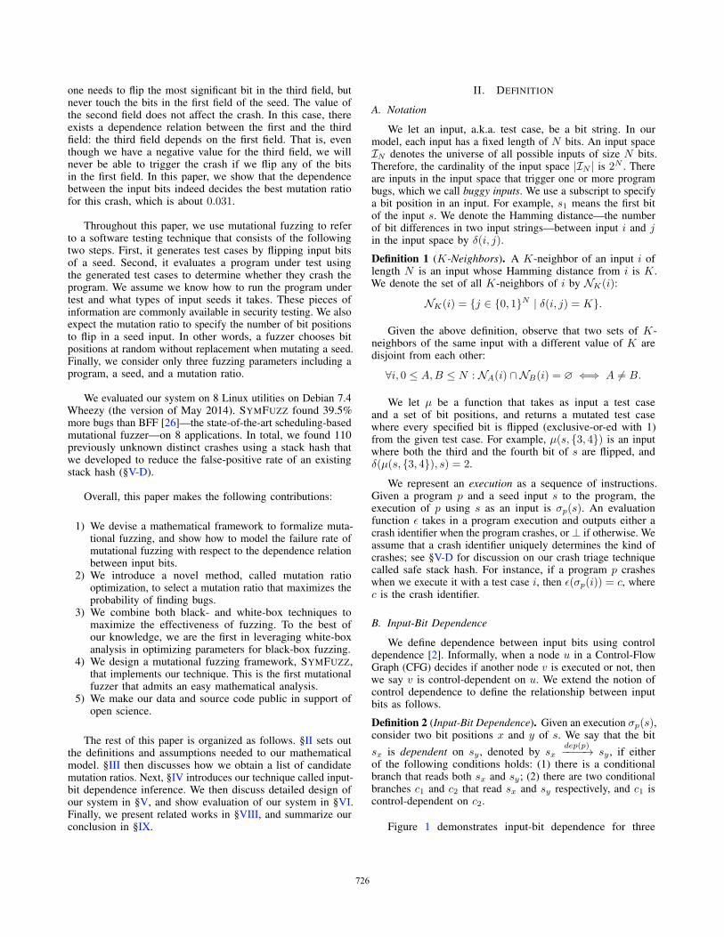
one needs to flip the most significant bit in the third field, butnever touch the bits in the first field of the seed. The value ofthe second field does not affect the crash. In this case, thereexists a dependence relation between the first and the thirdfield: the third field depends on the first field. That is, eventhough we have a negative value for the third field, we willnever be able to trigger the crash if we flip any of the bitsin the first field. In this paper, we show that the dependencebetween the input bits indeed decides the best mutation ratiofor this crash, which is about 0.031.

Throughout this paper, we use mutational fuzzing to referto a software testing technique that consists of the followingtwo steps. First, it generates test cases by flipping input bitsof a seed. Second, it evaluates a program under test usingthe generated test cases to determine whether they crash theprogram. We assume we know how to run the program undertest and what types of input seeds it takes. These pieces ofinformation are commonly available in security testing. We alsoexpect the mutation ratio to specify the number of bit positionsto flip in a seed input. In other words, a fuzzer chooses bitpositions at random without replacement when mutating a seed.Finally, we consider only three fuzzing parameters including aprogram, a seed, and a mutation ratio.

We evaluated our system on 8 Linux utilities on Debian 7.4Wheezy (the version of May 2014). SYMFUZZ found 39.5%more bugs than BFF [26]—the state-of-the-art scheduling-basedmutational fuzzer—on 8 applications. In total, we found 110previously unknown distinct crashes using a stack hash thatwe developed to reduce the false-positive rate of an existingstack hash (§V-D).

Overall, this paper makes the following contributions:

1) We devise a mathematical framework to formalize muta-tional fuzzing, and show how to model the failure rate ofmutational fuzzing with respect to the dependence relationbetween input bits.

2) We introduce a novel method, called mutation ratiooptimization, to select a mutation ratio that maximizes theprobability of finding bugs.

3) We combine both black- and white-box techniques tomaximize the effectiveness of fuzzing. To the best ofour knowledge, we are the first in leveraging white-boxanalysis in optimizing parameters for black-box fuzzing.

4) We design a mutational fuzzing framework, SYMFUZZ,that implements our technique. This is the first mutationalfuzzer that admits an easy mathematical analysis.

5) We make our data and source code public in support ofopen science.

The rest of this paper is organized as follows. §II sets outthe definitions and assumptions needed to our mathematicalmodel. §III then discusses how we obtain a list of candidatemutation ratios. Next, §IV introduces our technique called input-bit dependence inference. We then discuss detailed design ofour system in §V, and show evaluation of our system in §VI.Finally, we present related works in §VIII, and summarize ourconclusion in §IX.

II. DEFINITION

A. Notation

We let an input, a.k.a. test case, be a bit string. In ourmodel, each input has a fixed length of N bits. An input spaceIN denotes the universe of all possible inputs of size N bits.Therefore, the cardinality of the input space |IN | is 2N . Thereare inputs in the input space that trigger one or more programbugs, which we call buggy inputs. We use a subscript to specifya bit position in an input. For example, s1 means the first bitof the input s. We denote the Hamming distance—the numberof bit differences in two input strings—between input i and jin the input space by δ(i, j).

Definition 1 (K-Neighbors). A K-neighbor of an input i oflength N is an input whose Hamming distance from i is K.We denote the set of all K-neighbors of i by NK(i):

NK(i) = {j ∈ {0, 1}N | δ(i, j) = K}.

Given the above definition, observe that two sets of K-neighbors of the same input with a different value of K aredisjoint from each other:

∀i, 0 ≤ A,B ≤ N : NA(i) ∩NB(i) = ∅ ⇐⇒ A �= B.

We let μ be a function that takes as input a test caseand a set of bit positions, and returns a mutated test casewhere every specified bit is flipped (exclusive-or-ed with 1)from the given test case. For example, μ(s, {3, 4}) is an inputwhere both the third and the fourth bit of s are flipped, andδ(μ(s, {3, 4}), s) = 2.

We represent an execution as a sequence of instructions.Given a program p and a seed input s to the program, theexecution of p using s as an input is σp(s). An evaluationfunction ε takes in a program execution and outputs either acrash identifier when the program crashes, or ⊥ if otherwise. Weassume that a crash identifier uniquely determines the kind ofcrashes; see §V-D for discussion on our crash triage techniquecalled safe stack hash. For instance, if a program p crasheswhen we execute it with a test case i, then ε(σp(i)) = c, wherec is the crash identifier.

B. Input-Bit Dependence

We define dependence between input bits using controldependence [2]. Informally, when a node u in a Control-FlowGraph (CFG) decides if another node v is executed or not, thenwe say v is control-dependent on u. We extend the notion ofcontrol dependence to define the relationship between inputbits as follows.

Definition 2 (Input-Bit Dependence). Given an execution σp(s),consider two bit positions x and y of s. We say that the bit

sx is dependent on sy, denoted by sxdep(p)−−−−→ sy, if either

of the following conditions holds: (1) there is a conditionalbranch that reads both sx and sy; (2) there are two conditionalbranches c1 and c2 that read sx and sy respectively, and c1 iscontrol-dependent on c2.

Figure 1 demonstrates input-bit dependence for three

726726

{1,2,3,4}

. . .

. . .

(a) Bits 1, 2, 3, 4 are dependent each other.

{1}

{2}

. . .

(b) Bit 2 is dependent on bit 1.

{1}

{2}

. . .

(c) Bits 1 and 2 are independent.

Fig. 1: Input-bit dependence. Each gray box represents a conditional branch that is controlled by a set of input bit positions.

different cases. Figure 1a and Figure 1b show examples thatsatisfy the first and the second condition of input-bit dependencerespectively. In Figure 1a, every bit involved in the samecondition is dependent on each other due to the first condition

of Definition 2: s1dep(p)−−−−→ s1, s1

dep(p)−−−−→ s2, s1dep(p)−−−−→

s3, s1dep(p)−−−−→ s4, s2

dep(p)−−−−→ s1, · · · , s4 dep(p)−−−−→ s3, s4dep(p)−−−−→

s4. In Figure 1b, s2dep(p)−−−−→ s1. Finally, Figure 1c presents a

case where two input bits are not dependent on each other.

As an example, let us consider the following C program.

1 char x = i n p u t [ 0 ] ; char y = i n p u t [ 1 ] ;2 i f ( x > 42 ) {3 i f ( y > 42 ) {4 . . . / * o m i t t e d * /

Given a program execution that exercises Line 4, the secondbyte (bits 9 to 16) of the input is dependent on the first byte(bits 1 to 8), all the bits in the first byte are dependent uponeach other, and all the bits in the second byte are dependentupon each other.

Based on the definition of the input-bit dependence, wecan compute the set of dependency bits for each bit in a seed;we use the term “dependency” in the same vein to the term“library dependencies”. We call such a set as a dependencybitset, and denote it with a function ↑. The upward arrow isintended to reflect the direction of the dependence relationin a CFG. For instance, ↑ps({3, 4}) is the set of bits that aredepended on either by s3 or by s4 in the execution σp(s).

Definition 3 (Dependency Bitset). Given a set of bit positionsX of a seed s for a program p, the dependency bitset of X isdefined as

↑ps(X) =

{y

∣∣∣∣ x ∈ X, sxdep(p)−−−−→ sy

}.

Intuitively, we have defined input-bit dependence to revealthe approximate syntactic structure of an input. Most inputstructures consist of a series of input fields. For instance, aPNG file has a series of data chunks each of which consists offour input fields. Intuitively, every bit in an input field shoulddepend on each other, because all the bits together decide the

control-flow of the program. Indeed, a notion similar to input-bit dependence has been used in recovering the format of aninput from a given program execution [32]. More precisely,bits in a dependency bitset can be a superset of a bits in aninput field: input-bit dependence can involve multiple inputfields. In this paper, we use the input-bit dependence to inferthe optimal mutation ratio for mutational fuzzing (§III-B).

C. Mutational Fuzzing

Mutational fuzzing is a software testing technique where testcases are derived from a seed—typically a well-formed input—by partially mutating the seed. The number of bit mutations isdetermined by a parameter called the mutation ratio r, whichis the rate between the number of bit positions to flip andthe total number of bit positions in a seed. We assume thatmutational fuzzing selects a set of bit positions at randomwithout replacement, and hence the Hamming distance betweenan N -bit seed and a mutated input of it is always �N · r , i.e.,r is always chosen such that N ·r is an integer. This is differentfrom all current fuzzers that use sampling with replacement.See §V-C for more discussion on mutational fuzzing and itsimplementation.

We view mutational fuzzing as a more targeted version ofrandom testing, which generates only test cases from a subspaceof the input space. The key assumption is that the distributionof buggy inputs are often biased towards a subspace wherethe inputs are not far from a seed in terms of the Hammingdistance. For example, a crashing test case for an MP3 player islikely to be a nearly-valid MP3 file instead of being a randomstring. If a random string is given, the program will likely rejectthe input before it reaches a buggy code. More formally, wedefine mutational fuzzing as follows.

Definition 4 (Mutational Fuzzing). Given a seed input s ofsize N bits and a mutation ratio r, mutational fuzzing generatesand evaluates a set of test cases chosen uniformly at randomfrom NK(s), where K = �N · r .

We model each fuzz trial as a probabilistic experiment thatrandomly selects a test case from an input space IN . Let Bp

Nbe the set of N -bit buggy inputs for program p. Given a sample

727727

space IN , the probability of a randomly chosen input being inBpN is the failure rate θ [13], which is defined as

θ =|Bp

N ||IN | =

|BpN |

2N.

D. Failure Rate based on Mutation Ratio

In this paper, we are interested in finding a mutation ratio rthat maximizes the failure rate of mutational fuzzing. Therefore,we need to represent the failure rate in terms of r. To do so,we first categorize bit positions in a seed into several kinds,and approximate the failure rate in terms of mutation ratio andinput-bit dependence.

Given a program p and a seed s, suppose the programcrashes when it is executed on a mutated s, i.e., there is an inputamong the K-neighbors of s that triggers the crash. Specifically,there is a set of bits in s that, when flipped, generates a buggyinput for p. We call such a set a buggy bitset of s.

Definition 5 (Buggy Bitset). Given a program p and an N -bitseed s, a buggy bitset is a set of bit positions B ⊆ {1, 2, . . . , N}where ε(σp(μ(s,B))) �= ⊥.

Some of the bits in a buggy bitset may not need to beflipped to generate an input that triggers the bug. Among allsubsets of a buggy bitset, there exists a combination of bitswith a minimum cardinality while still producing a buggy inputfor the same bug. We call such a subset a minimum buggybitset.1 Notice that there may be multiple minimum buggybitsets with the same size. Suppose there is an 8-bit seed,and flipping both the first and second bits of the seed leadsa program p to crash. The buggy bitset is therefore {1, 2},and ε(σp(μ(s, {1, 2}))) �= ⊥. Now, suppose flipping only thesecond bit of the seed produces a buggy input that leads to thesame crash, i.e., ε(σp(μ(s, {1, 2}))) = ε(σp(μ(s, {2}))). Sincewe assume that a seed does not produce a program crash byitself, a minimum buggy bitset is {2}.Definition 6 (Minimum Buggy Bitset). Given a buggy bitsetB for a program p and a seed s, a minimum buggy bitset B′of B is an element of the set

argmin{B∗⊆B|ε(σp(μ(s,B∗)))=ε(σp(μ(s,B)))}

|B∗| .

A minimum buggy bitset B′ includes a set of bits that mustbe flipped to generate a buggy input. Any bit position otherthan B′, i.e., any element of {1, 2, . . . , N}\B′, either (1) doesnot affect the crash regardless of its values; or (2) thwarts thecrash when it is flipped. To find a set of bits that must not beflipped for triggering the crash, we overapproximate a set ofbits that changes the program execution with respect to the bitsin B′, which is a dependency bitset of B′ by definition. If anyof the bits in ↑ps(B′) are flipped, it will change the executionof the program. Since all the bits in B′ must be flipped, theother bits in (↑ps(B′) \B′) must not be flipped to maintain the

1 Deriving a minimum buggy bitset is often called bug minimization [25].

same execution path for the crash.2

The above argument can be intuitively explained by anexample. A bug is typically triggered when one or more inputfields have specific values, e.g., one needs to set an integerfield to be greater than the size of a program buffer to triggera buffer overflow. However, even though the integer field hasa value greater than the buffer size, the program might take anexecution path that does not even read the values. This happenswhen the program checks the value of another input field fbefore it reaches the buffer overflow, and jumps to anotherexecution path. Therefore, the integer input field is dependenton f . This is the key intuition of approximating the failure rateof mutational fuzzing in terms of the input-bit dependence.

We now compute a failure rate for each minimum buggybitset. For simplicity, let b be the cardinality of a minimumbuggy bitset (b = |B′|), and let d be the cardinality of thedependency bitset of B′ (d = |↑ps(B′)|). We also let r be themutation ratio. The failure rate of mutational fuzzing for B′follows a multivariate hypergeometric distribution [7], wherethe population size is N and the number of draws is (N × r).Therefore, the failure rate of a minimum buggy bitset that hasb elements is:

θb =

(bb

)(N−dN ·r−b

)(

NN ·r

) =

(N−dN ·r−b

)(

NN ·r

) , when N · r ≥ b (1)

This formula can be explained as follows. Given an N -bit seed,the total number of possible inputs that mutational fuzzing cangenerate is

(NN ·r

). To generate a buggy input from a seed, we

need to flip all the bits in the minimum buggy bitset (this isthe

(bb

)term), while not flipping the bits in the dependency

bitset of B′ (this is the(

N−dN ·r−b

)term). Since

(bb

)= 1, the term

can be eliminated.

The failure rate is only meaningful when the number offlipped bits is not less than the size of B′, i.e., N · r ≥ b.When N · r < b, we simply cannot flip every bit in B′. Bythe definition of the minimum buggy bitset (Definition 6), oneneeds to flip all the bits in B′ in order to generate a buggyinput. Therefore, the failure rate is effectively 0 in this case.

E. Mutation Ratio Optimization Challenge

Now that we have a formal definition of mutational fuzzingand its failure rate, we address mutation ratio optimizationchallenge as follows.

Definition 7 (Mutation Ratio Optimization Challenge). Givena program p and an N -bit seed s, consider a crash that isidentified by a minimum buggy bitset B′, and let b = |B′|. Themutation ratio optimization challenge is to derive a mutationratio r that maximizes the failure rate θb of p.

Notice the cardinality of a minimum buggy bitset (b) is notknown unless we have found the corresponding bug. Moreover,we may have multiple optimal mutation ratios for differentvalues of b. Therefore, several questions remain: How do wesolve the mutation ratio optimization challenge? How do we

2 The dependency bitset of B′ is an over-approximation of the immutablebit positions for the crash, because flipping some bits in (↑ps(B′) \B′) maystill trigger the same crash.

728728

compute the cardinality of the dependency bitsets (d) for agiven program-seed pair? We address these questions in thefollowing sections.

III. MUTATION RATIO OPTIMIZATION

In this section, we introduce a systematic way of deciding aset of mutation ratios for a given program and a seed, which wecall mutation ratio optimization. Our technique automaticallyadapts to a given program-seed pair, and it enables efficientbug finding for mutational fuzzing.

A. Solving for an Optimal Mutation Ratio

Recall in §II-D we described the failure rate θb of mutationalfuzzing with respect to three variables: the bit size of a seed(N ), the cardinality of a minimum buggy bitset (b), and thecardinality of a dependency bitset of the minimum buggy bitset(d). One of the primary challenges is to find a mutation ratio0 < r ≤ 1 that maximizes θb. When d = b, i.e., B′ = ↑ps(B′),it is trivial to show that the maximum failure rate is achievedwith r = 1: we simply let d = b and r = 1 from Equation 1,and then the failure rate θb becomes always 1 regardless ofthe value of b. When d = N , there is no bit position to flipother than the ones in ↑ps(B′), and, as a result, the only wayto trigger the crash is to flip exactly b bit positions. That is,the optimal mutation ratio is b/N . When b < d < N , we solvethe mutation ratio optimization problem by modeling it as aclassic nonlinear programming problem (NLP) [6] as follows.

For N, b, and d, find r to

maximize θb =

(N−dN ·r−b

)(

NN ·r

)subject to (0 < r ≤ 1)

∧ (b < d < N)∧ (b ≤ N · r ≤ N − d+ b).

The first constraint of the NLP is from the definition ofmutation ratio: mutation ratio must be between zero and one.The second constraint (b < d < N ) is to restrict the range ofthe d value. When d = b, the optimal mutation ratio is 1, andwhen d = N , the optimal mutation ratio becomes b/N as wediscussed above. The third constraint (b ≤ N · r ≤ N − d) isdue to our problem definition: (1) we should flip more thanthe cardinality of a minimum buggy bitset in order to generatean input that trigger the bug (b ≤ N · r); (2) we should notflip any bits in (↑ps(B′) \B′), hence the maximum number ofbit flips is (N − d+ b).

We now solve the above NLP to obtain an optimal mutationratio for a given minimum buggy bitset. The solution to it is theoptimal mutation r with respect to b, d and N . See Appendix Afor a complete proof.

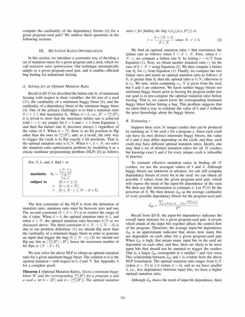
Theorem 1 (Optimal Mutation Ratio). Given a minimum buggybitset B′ and the corresponding ↑ps(B′) for a program p anda seed s, let b = |B′| and d = |↑ps(B′)|. The optimal mutation

ratio r for finding the bug ε(σp(μ(s,B′))) is

r =b× (N + 1)

d×Nwhen N · r > b. (2)

We find an optimal mutation ratio r that maximizes thefailure rate as follows when b < d < N . First, when b =N · r, we compute a failure rate θ1 by letting r = b/N fromEquation (1). Next, we obtain another mutation ratio r2 for thecase of b < N ·r using Equation (2). We then compute a failurerate θ2 for r2 from Equation (1). Finally, we compare the twofailure rates and return an optimal mutation ratio as follows: ifθ1 is greater than θ2 then the optimal ratio is b/N ; otherwise itis r2. We note, when computing r2, N is given from the seed,but b and d are unknown. We know neither buggy bitsets norminimum buggy bitsets prior to fuzzing the program under test:our goal is to pre-compute the optimal mutation ratio beforefuzzing. That is, we cannot know the corresponding minimumbuggy bitset before hitting a bug. This problem suggests thatwe must find a way to estimate the value of b and d withoutthe prior knowledge about the buggy bitsets.

B. Estimating r

Suppose there exist M unique crashes that can be producedby mutating an N -bit seed s for a program p. Since each crashcan have its own distinct minimum buggy bitsets, the valueof b and d may differ depending on the crash, and thus, eachcrash may have different optimal mutation ratios. Ideally, onemay find a set of distinct mutation ratios for all M crashes,but knowing exact b and d for every unique crash is infeasiblein practice.

To estimate effective mutation ratios in finding all Mcrashes, we use the averaged values of b and d. Althoughbuggy bitsets are unknown in advance, we can still computedependency bitsets of every bit in the seed: we can obtain allpossible d values from the given program-seed pair, whichwill expose the trend of the input-bit dependence of the seed.We then use this information to estimate d. Let P(S) be thepowerset of S. We then denote d̄all as the average cardinalityof every possible dependency bitsets for the program-seed pair:

d̄all =

∑x∈P({1,2,...,N}) |↑ps(x)|

2N.

Recall from §II-B, the input-bit dependence indicates theoverall input structure for a given program-seed pair: it revealswhich chunk of the input bits together affects the control flowof the program. Therefore, the average input-bit dependenced̄all is an approximate indicator that shows how many bitsare dependent on each other for a given program-seed pair.When d̄all is high, that means many input bits in the seed aredependent on each other, and thus, there are likely to be moreinput bits that should not be mutated to trigger the crashes.That is, a larger d̄all corresponds to a smaller r and vice versa.This relationship between d̄all and r is evident from the aboveNLP formulation. The optimal mutation ratio ranges from b/N(when d = N ) to 1.0 (when d = b), and as we have smallerd, i.e., less dependence between input bits, we have a higheroptimal mutation ratio.

Although d̄all shows the trend of input-bit dependence, there

729729

Algorithm 1: Computing d̄ using adaptive sampling.

input : A distribution of b values (β)output : d̄

1 prevN ← 02 prevSum ← 03 while true do4 b ← WeightedRand(N , β)5 S ← RandomK(N , b)6 newN ← prevN + b7 newSum ← prevSum + |↑ps(S)|8 if prevN �= 0 ∧ |newSum/newN− prevSum/prevN| < ε

then break9 else prevN ← newN; prevSum ← newSum

10 end11 return prevSum/prevN /* Returns d̄ */

are two remaining problems in using it. First, just averaging thecardinality of all possible dependency bitsets is not necessarilythe best way to represent the trend, because the cardinalityof minimum buggy bitsets (b) may be biased towards severalvalues. Second, the number of dependency bitsets to consideris exponential in N , and N is typically not small.

To mitigate both challenges, we incorporate the distributionof b (β) into the average input-bit dependence by using adaptivesampling [50], which also helps in computing an approximateaverage efficiently. The algorithm is shown in Algorithm 1. First,we select a random cardinality b with the probability associatedwith each cardinality in β (Line 4, WeightedRand). Next, wesample a set of random bit positions S of cardinality b (Line 5,RandomK). RandomK takes in N and b, and returns b distinctrandom numbers from the interval [1, N ]. We then compute|↑ps(S)|, and use the cardinality to compute a new cardinalitysum. Then, we check the difference between the previous andthe new mean values to see if it is smaller than a threshold ε(Line 8). We repeat the process until the difference is negligible(we use ε = 10−7 in our experiment). After breaking out ofthe while loop, the algorithm returns the final average input-bitdependence denoted as d̄.

Since d̄ relies on the distribution of b (β), it is importantto note how the distribution looks like. We obtained a largescale fuzzing dataset from a previous work, and computed thecardinality of minimum buggy bitsets for each unique crashfound in [44]. The average b value was 9 and the standarddeviation was 18. This result conforms to the observations frompractitioners [25]. See §VI-C for further discussion on how weobtained b values from the dataset.

Now that we have a distribution of b values from a large-scale experiment, we need to estimate r using the averagedd value (d̄). Since d̄ is the average cardinality of dependencybitsets per each bit in minimum buggy bitsets, we can estimatethe cardinality of a dependency bitset for a minimum buggybitset of cardinality b using b × d̄. By letting d = d̄ × b, wecan simplify the Equation 2 as follows.

r =b× (N + 1)

b× d̄×N=

1

d̄· N + 1

N. (3)

The value of b is now included in d̄, and we only need to

p ::= stmt∗exp ::= get_input(src) | load(exp) | var

| exp ♦b exp | ♦u exp | vstmt ::= var:= exp

| goto exp| if exp then goto exp1 else goto exp2

| call exp| ret exp| store(exp,exp)

v ::= 〈unsigned integer, a set of affecting bits〉♦b ::= binary operators♦u ::= unary operators

TABLE I: A simple language for IBDI.

consider the value of d̄ to estimate the optimal mutation ratior. Given the distribution of b in crashes, d̄ provides a way toestimate the cardinality of dependency bitsets for the crashes,which, in turn, helps in estimating r.

IV. INPUT-BIT DEPENDENCE INFERENCE

At a high level, Input-Bit Dependence Inference (IBDI) is aprocess of computing the input-bit dependences for every bit ina seed from a program execution. We then use these dependencerelations to compute d̄ as in Algorithm 1. From the perspectiveof program analysis, IBDI is a symbolic analysis that is morespecific than the traditional taint analysis [14, 42, 57], and moreabstract than the traditional symbolic execution [8, 27, 29]. Ourapproach is inspired by several automatic input format recoveryapproaches including [10, 16, 17, 32], where they share acommon theme as us: they use a program execution to revealthe structure of an input. However, our focus is on figuring outthe input-bit dependence rather than precise input formats.

A. The Algorithm

Input-Bit Dependence Inference (IBDI) takes as input aprogram and a seed, and outputs the input-bit dependence forevery bit of the seed. Similar to dynamic symbolic execution[11, 22], IBDI runs the program under test both concretely andsymbolically. The key difference between IBDI and dynamicsymbolic execution is that IBDI operates on a set of dependentbits instead of generating bit-vector-level path formulas, henceit does not rely on SMT solvers [18]. As in dynamic symbolicexecution, IBDI introduces symbolic values whenever readingfrom a user input, e.g., read system call. It then symbolicallyevaluates program statements on a program execution. It alsoconstructs a CFG while symbolically executing the program inorder to compute control dependences between variables andthe corresponding input bits.

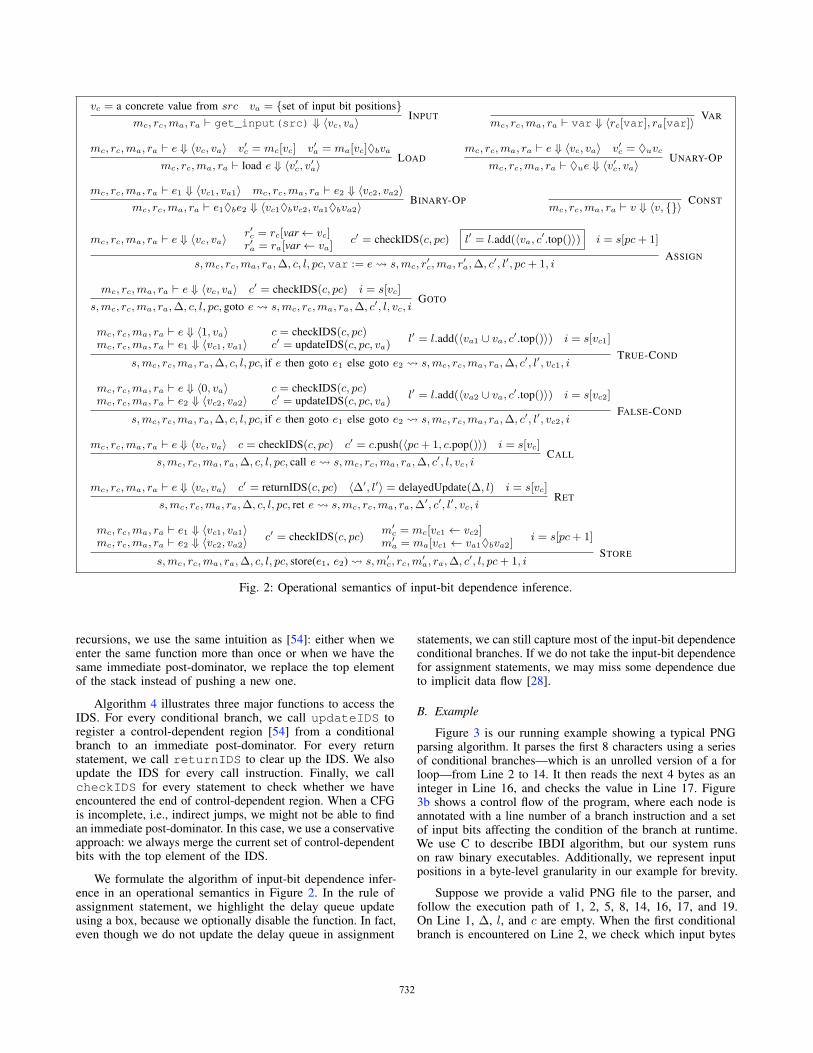
We describe our IBDI algorithm using the formal runtimesemantics over a simple language shown in Table I. In ourlanguage, a program is a sequence of statements. There arefour different jump statements including goto, if-else,call, and ret. The first two are regular jump statements:goto is an unconditional jump statement, and if-else isa conditional jump statement. The last two kinds, call andret, are special jump instructions that represent calls and

730730

Context Meanings a list of program statementsmc mapping from an address to concrete valuerc mapping from a variable to concrete valuema mapping from an address to abstract valuera mapping from a variable to abstract valueΔ current dependence predicatec current input-dependence stackl current delay queuepc current program counteri current statement

TABLE II: The execution context of our analysis.

returns respectively. Notice, however, we do not allow call/retinstructions to implicitly manipulate call-stacks in our language.For example, call instruction in x86 will be jitted into intostack manipulation statements followed by a call statement.

Since we execute a program both concretely and symboli-cally, expressions in our language evaluate to a value v, whichis a tuple of a concrete value and an abstract value. A concretevalue is an unsigned integer, and an abstract value is a set ofinput bits that affects either directly or indirectly the value,which is often called data lineage [32, 33]. We denote datalineage of a variable as a set of bit positions. For example, ifa variable x evaluates to 〈1, {2, 3, 4}〉, it means the variablex has a concrete value of 1, and is also affected by the threeother input bits.

We use ♦b to denote binary operators such as addition,subtraction, etc. Similarly, ♦u represents unary operators suchas minus. When we evaluate ♦b over abstract values (datalineages), we apply set union between them. For example,when we evaluate a subtraction between {1} and {1, 2, 3, 4},we obtain {1, 2, 3, 4}. For ♦u, we simply propagate abstractvalues from a source to a destination.

The execution context of our analysis consists of ten fieldsas shown in Table II. We store abstract and concrete valuesfor variables in ra and rc respectively in a map.3 Similarly,we store abstract and concrete values of memory addressesin ma and mc respectively in a map. To access maps, weuse a bracket notation. For example, ra[x] returns the currentabstract value of x, and rc[x← 1] returns a new map, whichis equivalent to the previous map except that the value of xis 1. We use ⇓ to represent evaluation of an expression undera given context. For example, mc, rc,ma, ra � e ⇓ v is anevaluation of an expression e to a value v in the context givenas 4-tuples (mc, rc,ma, ra).

We encode the input-bit dependence for every bit in an inputusing a data structure that we call dependence predicate (Δ).The dependence predicate is essentially a map from a bit of aninput to a set of bit positions that the bit is dependent on. As weexecute the program under test, we update Δ using a mergefunction. For example, suppose Δ has a mapping from the firstbit to {3, 4}. Then, merge(Δ, {1, 2}, {5, 6}) will return a newdependence predicate which contains two mappings: (1) from

3 Variables at the machine-code level are really registers.

Algorithm 2: Dependence predicate update algorithm.

1 Function merge(Δ, X, Y )2 Δ′ ← Δ3 for x ∈ X do4 Δ′ ← Δ′ [x← (Δ[x] ∪ Y \ {x})]5 end6 return Δ′7 end

Algorithm 3: Delay queue update algorithm.

1 Function delayedUpdate(Δ, l)2 for 〈X,Y 〉 ∈ l do3 if 〈X,Y 〉 is not memoized then4 Δ← merge(Δ, X, Y )5 memoize 〈X,Y 〉6 end7 end8 return 〈Δ, [ ]〉9 end

the first bit to {3, 4, 5, 6}, and (2) from the second bit to {5, 6}.Algorithm 2 describes the merge function. Notice, in Line 4 ofthe algorithm, we compute the relative complement of {x} inorder to exclude the dependence relations that self-referencing.

One may call the merge function for every instructionencountered on the fly. However, we delay the predicate updateuntil we reach a return instruction—thus, update the dependencepredicate per control-dependent region [54]—for two reasons.First, it is more cache-efficient to perform updates once ina while. Second, we can employ a heuristic to eliminateunnecessary updates: there are many duplicated updates, thuswe can memoize the last updates to speed up the process. Toperform delayed update, we employ an additional field in ourexecution context, which we call a delay queue (l). l stores atuple of the current data lineage and the current set of dependentbits from the control stack. To add an entry to a delay queue,we use an add method.

We maintain an input-bit dependence stack (c) to store a setof bit positions that the current instruction is control-dependenton. The idea is similar to dynamic control-dependence analysisin [54], but input-bit dependence stack maintains a set of control-dependent bits instead of storing control-dependent statements.We use three methods to access the input-dependence stack(IDS): top() returns the top element of a stack, pop() returns atuple of the top element of a stack and a new stack without thetop element, and push(X) returns a new stack which containsan additional element X .

Each element on the stack is a 2-tuple (an address of aninstruction that is beyond the scope of the current controldependence, a set of control-dependent bits). In our analysis,control dependence of a conditional branch is valid in twoscenarios: (1) until we reach an immediate post-dominator ofthe conditional branch; (2) until we reach a return instruction.Therefore, we need to update the input-bit dependence stackeither when we enter a function (call instructions), or when weencounter a conditional branch. However, to efficiently handle

731731

vc = a concrete value from src va = {set of input bit positions}mc, rc,ma, ra � get_input(src) ⇓ 〈vc, va〉 INPUT

mc, rc,ma, ra � var ⇓ 〈rc[var], ra[var]〉 VAR

mc, rc,ma, ra � e ⇓ 〈vc, va〉 v′c = mc[vc] v′a = ma[vc]♦bva

mc, rc,ma, ra � load e ⇓ 〈v′c, v′a〉 LOADmc, rc,ma, ra � e ⇓ 〈vc, va〉 v′c = ♦uvc

mc, rc,ma, ra � ♦ue ⇓ 〈v′c, va〉 UNARY-OP

mc, rc,ma, ra � e1 ⇓ 〈vc1, va1〉 mc, rc,ma, ra � e2 ⇓ 〈vc2, va2〉mc, rc,ma, ra � e1♦be2 ⇓ 〈vc1♦bvc2, va1♦bva2〉 BINARY-OP

mc, rc,ma, ra � v ⇓ 〈v, {}〉 CONST

mc, rc,ma, ra � e ⇓ 〈vc, va〉 r′c = rc[var← vc]r′a = ra[var← va]

c′ = checkIDS(c, pc) l′ = l.add(〈va, c′.top()〉) i = s[pc+ 1]

s,mc, rc,ma, ra,Δ, c, l, pc,var := e� s,mc, r′c,ma, r

′a,Δ, c′, l′, pc+ 1, i

ASSIGN

mc, rc,ma, ra � e ⇓ 〈vc, va〉 c′ = checkIDS(c, pc) i = s[vc]

s,mc, rc,ma, ra,Δ, c, l, pc, goto e� s,mc, rc,ma, ra,Δ, c′, l, vc, iGOTO

mc, rc,ma, ra � e ⇓ 〈1, va〉mc, rc,ma, ra � e1 ⇓ 〈vc1, va1〉

c = checkIDS(c, pc)c′ = updateIDS(c, pc, va)

l′ = l.add(〈va1 ∪ va, c′.top()〉) i = s[vc1]

s,mc, rc,ma, ra,Δ, c, l, pc, if e then goto e1 else goto e2 � s,mc, rc,ma, ra,Δ, c′, l′, vc1, iTRUE-COND

mc, rc,ma, ra � e ⇓ 〈0, va〉mc, rc,ma, ra � e2 ⇓ 〈vc2, va2〉

c = checkIDS(c, pc)c′ = updateIDS(c, pc, va)

l′ = l.add(〈va2 ∪ va, c′.top()〉) i = s[vc2]

s,mc, rc,ma, ra,Δ, c, l, pc, if e then goto e1 else goto e2 � s,mc, rc,ma, ra,Δ, c′, l′, vc2, iFALSE-COND

mc, rc,ma, ra � e ⇓ 〈vc, va〉 c = checkIDS(c, pc) c′ = c.push(〈pc+ 1, c.pop()〉) i = s[vc]

s,mc, rc,ma, ra,Δ, c, l, pc, call e� s,mc, rc,ma, ra,Δ, c′, l, vc, iCALL

mc, rc,ma, ra � e ⇓ 〈vc, va〉 c′ = returnIDS(c, pc) 〈Δ′, l′〉 = delayedUpdate(Δ, l) i = s[vc]

s,mc, rc,ma, ra,Δ, c, l, pc, ret e� s,mc, rc,ma, ra,Δ′, c′, l′, vc, i

RET

mc, rc,ma, ra � e1 ⇓ 〈vc1, va1〉mc, rc,ma, ra � e2 ⇓ 〈vc2, va2〉 c′ = checkIDS(c, pc)

m′c = mc[vc1 ← vc2]

m′a = ma[vc1 ← va1♦bva2] i = s[pc+ 1]

s,mc, rc,ma, ra,Δ, c, l, pc, store(e1, e2)� s,m′c, rc,m

′a, ra,Δ, c′, l, pc+ 1, i

STORE

Fig. 2: Operational semantics of input-bit dependence inference.

recursions, we use the same intuition as [54]: either when weenter the same function more than once or when we have thesame immediate post-dominator, we replace the top elementof the stack instead of pushing a new one.

Algorithm 4 illustrates three major functions to access theIDS. For every conditional branch, we call updateIDS toregister a control-dependent region [54] from a conditionalbranch to an immediate post-dominator. For every returnstatement, we call returnIDS to clear up the IDS. We alsoupdate the IDS for every call instruction. Finally, we callcheckIDS for every statement to check whether we haveencountered the end of control-dependent region. When a CFGis incomplete, i.e., indirect jumps, we might not be able to findan immediate post-dominator. In this case, we use a conservativeapproach: we always merge the current set of control-dependentbits with the top element of the IDS.

We formulate the algorithm of input-bit dependence infer-ence in an operational semantics in Figure 2. In the rule ofassignment statement, we highlight the delay queue updateusing a box, because we optionally disable the function. In fact,even though we do not update the delay queue in assignment

statements, we can still capture most of the input-bit dependenceconditional branches. If we do not take the input-bit dependencefor assignment statements, we may miss some dependence dueto implicit data flow [28].

B. Example

Figure 3 is our running example showing a typical PNGparsing algorithm. It parses the first 8 characters using a seriesof conditional branches—which is an unrolled version of a forloop—from Line 2 to 14. It then reads the next 4 bytes as aninteger in Line 16, and checks the value in Line 17. Figure3b shows a control flow of the program, where each node isannotated with a line number of a branch instruction and a setof input bits affecting the condition of the branch at runtime.We use C to describe IBDI algorithm, but our system runson raw binary executables. Additionally, we represent inputpositions in a byte-level granularity in our example for brevity.

Suppose we provide a valid PNG file to the parser, andfollow the execution path of 1, 2, 5, 8, 14, 16, 17, and 19.On Line 1, Δ, l, and c are empty. When the first conditionalbranch is encountered on Line 2, we check which input bytes

732732

Algorithm 4: Input-dependence stack update algorithm.

1 Function updateIDS(c, pc, va)2 pd← immediate post-dominator of the current

instruction at pc3 〈toppd, topdep〉 ← c.top()4 if toppd = pd then5 〈·, c〉 ← c.pop()6 end7 c′ ← c.push(〈pd, va ∪ topdep〉)8 return c′9 end

10 Function returnIDS(c, pc)11 〈toppd, ·〉 ← c.top()12 while c.isNotEmpty() ∧ toppd �= pc do13 〈·, c〉 ← c.pop()14 end15 if c.isNotEmpty() then16 〈·, c〉 ← c.pop()17 end18 return c19 end20 Function checkIDS(c, pc)21 〈toppd, ·〉 ← c.top()22 if c.isNotEmpty() ∧ toppd = pc then23 〈·, c〉 ← c.pop()24 end25 return c26 end

are affecting the condition. Since the first byte is affecting thecondition, we call updateIDS(c, 2, {1}), which first staticallyexpands the control flow from the instruction on Line 2, andcomputes the immediate post-dominator of the instruction,which is Line 14 in this case. Then it updates c to have anelement of 〈14, {1}〉. Next, we push the input byte information〈{1}, {1}〉 into l, which represent a dependence relation fromthe first byte to the first byte itself.4

On Line 5, we reach another conditional branch, which hasa condition affected by the second byte. Since the top elementof c has the same address as the immediate post-dominator ofthe branch, we replace the top element of c with 〈14, {1, 2}〉(due to Line 4-7 of updateIDS). The delayed queue isalso updated with the updated control-dependence, whichwill call merge(Δ, {2}, {1, 2}) later in the delayedUpdatefunction. Similarly, we update the delay queue and the IDSuntil we reach the Line 14. Since the current instruction hasthe same address as in the top element of the IDS, we popone element from the IDS (Line 23 of Algorithm 4), and thenwe call delayedUpdate of Algorithm 3 to update Δ. Afterexecuting Line 14, Δ has a mapping from each byte to the bytepositions that the byte is dependent on. To be more precise, Δshould represent bit-level dependences, but we show byte-leveldependences for simplicity. We perform the similar steps alongthe execution.

4 In a bit-level granularity, this represents the input-bit dependences betweenthe first eight input bits, where each of the bits is dependent on each other.

1 / * i n p u t read i n b u f * /2 i f ( buf [ 0 ] != ' \ x89 ' ) {3 e r r o r ( ) ;4 } e l s e {5 i f ( buf [ 1 ] != ' \ x50 ' ) {6 e r r o r ( ) ;7 } e l s e {8 i f ( buf [ 2 ] != ' \ x4e ' ) {9 e r r o r ( ) ;10 } e l s e {11 . . .12 }13 }14 }15 / * n e x t f i e l d * /16 l e n = * ( ( * i n t 3 2 )& buf [ 8 ] ) ;17 i f ( l e n > PNG_MAX)18 e r r o r ( ) ;19 . . .

(a) A PNG parser in C

1: entry

2: {1}

5: {2}

8: {3}

· · ·

17: {9, 10, 11, 12}

. . .

(b) A control-flow graph.

Line Δ c l

1 · · ·2 · 〈14, {1}〉 〈{1}, {1}〉5 · 〈14, {1, 2}〉 〈{1}, {1}〉;

〈{2}, {1, 2}〉

8 · 〈14, {1, 2, 3}〉〈{1}, {1}〉;〈{2}, {1, 2}〉;〈{3}, {1, 2, 3}〉

14

1 �→ {1}2 �→ {1, 2}3 �→ {1, 2, 3}· · ·

· ·

17

1 �→ {1}2 �→ {1, 2}3 �→ {1, 2, 3}· · ·

〈19, {9, 10, 11, 12}〉 〈{9, 10, 11, 12},{9, 10, 11, 12}〉

19

1 �→ {1}2 �→ {1, 2}3 �→ {1, 2, 3}· · ·9 �→ {9, 10, 11, 12}10 �→ {9, 10, 11, 12}· · ·

· ·

(c) The state transition table where each row is the execution contextafter executing the corresponding line. For delay queue l, each item isseparated with a semicolon. The second column contains a mappingfrom a byte position to a set of byte positions.

Fig. 3: A PNG parser example. We represent the input positionsusing a byte-level granularity in this figure for brevity.

V. SYSTEM DESIGN

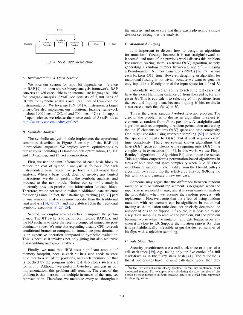
In this section, we describe SYMFUZZ, a system thatautomatically finds an optimal mutation ratio for mutationalfuzzing based on the input-bit dependence inference. Figure 4summarizes our system design, which consists of two majorcomponents: symbolic analysis and mutational fuzzing. Thesymbolic analysis module takes in a program and a seed, andreturns a recommended optimal mutation ratio. The mutationalfuzzing module then uses the mutation ratio to perform fuzzing,and outputs buggy inputs found. Finally, we triage buggy inputsusing our safe stack hash technique described in §V-D.

733733

BugsTriageMutational

FuzzingSymbolicAnalysis

MutationRatios

Program

Seed s

Fig. 4: SYMFUZZ architecture.

A. Implementation & Open Science

We base our system for input-bit dependence inferenceon BAP [9], an open-source binary analysis framework. BAPconverts an x86 executable to an intermediate language suitablefor program analysis. SYMFUZZ consists of 5,300 lines ofOCaml for symbolic analysis and 1,600 lines of C++ code forinstrumentation. We leverage PIN [34] to instrument a targetbinary. We also implement our mutational fuzzing frameworkin about 1900 lines of OCaml and 700 lines of C++. In supportof open science, we release the source code of SYMFUZZ athttp://security.ece.cmu.edu/symfuzz/.

B. Symbolic Analysis

The symbolic analysis module implements the operationalsemantics described in Figure 2 on top of the BAP [9]intermediate language. We employ several optimizations toour analysis including (1) tainted-block optimization, (2) JITand PD caching, and (3) set memoization.

First, we use the taint information of each basic block toreduce the cost of symbolic analysis as follows. For eachinstrumented basic block, we perform a lightweight taintanalysis. When a basic block does not involve any taintedinstructions, we do not perform the symbolic analysis, andproceed to the next block. Notice our symbolic analysisinherently provides precise taint information for each block.Therefore, we do not need to maintain additional data structurefor storing taints. In fact, the data-lineage tracking [32, 33] partof our symbolic analysis is more specific than the traditionaltaint analysis [14, 42, 57], and more abstract than the traditionalsymbolic execution [8, 27, 29].

Second, we employ several caches to improve the perfor-mance. The JIT cache is to cache recently-used BAP ILs, andthe PD cache is to store the recently-computed immediate post-dominator nodes. We note that expanding a static CFG for eachconditional branch to compute an immediate post-dominatoris an expensive operation compared to symbolic evaluation.This is because it involves not only jitting but also recursivedisassembling and graph analysis.

Finally, we note that IBDI uses significant amount ofmemory footprint, because each bit in a seed needs to storea pointer to a set of bit positions, and each memory bit thatis touched by the program under test also stores such a setfor in ma. Although we perform byte-level analysis in ourimplementation, this problem still remains. The crux of theproblem is that there can be multiple instances of the same setrepresentation. Therefore, we memoize every set throughout

the analysis, and make sure that there exists physically a singledistinct set throughout the analysis.

C. Mutational Fuzzing

It is important to discuss how to design an algorithmfor mutational fuzzing, because it is not straightforward asit seems5, and none of the previous works discuss this problem.For random fuzzing, there is a trivial O(N) algorithm, namely,generating a random number between 0 and 2N − 1 usinga Pseudorandom Number Generator (PRNG) [36, 37], whereeach bit takes O(1) time. However, designing an algorithm formutational fuzzing is not trivial, because we want to generateonly inputs in a K-neighbor of the input space for a fixed K.

Particularly, we need an ability to selecting test cases thathave the exact Hamming distance K from the seed s, for anygiven K. This is equivalent to selecting K-bit positions fromthe seed and flipping them, because flipping K bits results ina test case i such that δ(i, s) = K.

This is the classic random k-subset selection problem. Thecrux of the problem is to devise an algorithm to select Kelements at random from N bit positions. A straightforwardalgorithm such as computing a random permutation and takingthe top K elements requires O(N) space and time complexity.One might consider using reservoir sampling [52] to reducethe space complexity to O(K), but it still requires O(N)time complexity. There are several known algorithms thathave O(K) space complexity while requiring only O(K) timecomplexity in expectation [4, 43]. In this work, we use Floyd-Bentley’s algorithm [4, Algorithm F1] to compute the subset.This algorithm outperforms permutation-based algorithms interms of both time and space complexity when K < N . Oncewe obtain K random bits to modify from the Floyd-Bentley’salgorithm, we simply flip the selected K bits (by XORing thebits with s), and generate a new test case.

Someone may argue that the difference between randommutation with or without replacement is negligible when theinput size is reasonably large, and it is even easier to analyzethe probability when we assume the random process withreplacement. However, note that the effect of using randommutation with replacement can be significant in mutationalfuzzing as the mutation ratio does not precisely determine thenumber of bits to be flipped. Of course, it is possible to usea rejection sampling to resolve the problem, but the problembecomes worse when the mutation ratio gets bigger, especiallywhen it is close to 1.0. Suppose the mutation ratio is 0.9, thenit is probabilistically infeasible to get the desired number ofbit flips with a rejection sampling.

D. Safe Stack Hash

Security practitioners use a call-stack trace or a part of acall-stack trace [39], e.g., taking only top five entries of a fullstack-trace as in the fuzzy stack hash [41]. The rationale isthat if two crashes have the same call-stack traces, then they

5In fact, we are not aware of any practical fuzzers that implement exactmutational fuzzing. For example, even calculating the exact number of bitsflipped by these fuzzers is difficult, because there is no closed-form expressionfor their algorithm.

734734

Program #Crashes #Bugs Seed Size(bits) Seed Type

abcm2ps 231,716 32 35,040 abcautotrace 19,452 24 16,304 bmpbib2xml 577 2 177,152 bibcatdvi 2,153,939 8 1,632 dvifigtoipe 467,718 34 8,016 figgif2png 25,346 3 1,816 gifpdf2svg 133 1 23,368 pdfmupdf 39 6 23,368 pdf

Total 2,898,920 110

TABLE III: The ground truth data.

are likely to have an equivalent final program state, and thus,it is an evidence of having the same root cause. This approachworks for many cases, but it exhibits a false bucketing problem:it can put a single bug into multiple buckets.

We note that this false bucketing problem can significantlyincrease the number of bugs found for fuzzing especially whena buffer overflow mangles the return addresses on the stack.For example, suppose a mutated input data overwrites a returnaddress of a call stack. The return address of the stack tracemay contain any arbitrary values due to the mutation. In theworst case, we can have 232 distinct call-stack traces on 32-bitmachine just because of the mangled return address.

To mitigate this problem, we employ a technique, calledsafe stack hash, which stops traversing the call stack when itfinds an unreachable return address. Specifically, we check foreach return address of a call-stack trace starting from the top,i.e., the crashing stack frame, whether each return address fallsin a mapped page. If not, we assume that the stack is mangledin the corresponding stack frame, and discard the rest of thereturn addresses in the call-stack trace. We also use the sameheuristic as the fuzzy stack hash, and consider only the topfive stack entries when computing the hash. Notice the numberof bugs found from safe stack hash can only be less than theone from regular stack hash techniques such as the fuzzy stackhash. We implemented our safe stack hash using a GDB scriptwritten in Python.

VI. EVALUATION

We now evaluate our system SYMFUZZ on 8 real-worldapplications in order to answer the following questions.

1) Does it make sense to optimize the mutation ratio inmutational fuzzing? How does the number of bugs differper mutation ratio? (§VI-B)

2) What is the cardinality of minimum buggy bitsets? Is theconventional wisdom about choosing small mutation ratioscorrect? (§VI-C)

3) How effective is it to use the SYMFUZZ’s adaptive strategyin terms of number of bugs found? (§VI-D)

4) Does SYMFUZZ work well in practice? How many bugsdid we find compared to the practical fuzzers such as BFF,zzuf, AFL-fuzz? (§VI-E)

A. Experimental Setup

We ran experiments on a private cluster consisting of 8virtual machines. Each VM was running Debian Linux 7.4on a single Intel 2.68 GHz Xeon core with 1GB of RAM,and all the applications that we tested were up-to-date as ofMay 2014. Each VM in our cluster was committed to only asingle application throughout the experiments. The number ofbugs reported from this paper is based on our safe stack hashintroduced in §V-D. We also make our source code publiclyavailable at http://security.ece.cmu.edu/symfuzz/.

Collecting Ground Truth. We ran the mutational fuzzingmodule of SYMFUZZ individually to gather the ground-truthdata of mutational fuzzing. We initially obtained a list of 100file-conversion applications of Debian as in [53], and manuallycreated a seed file for each application. We then fuzzed all 100program-seed pairs with BFF [26] to know which programsexhibit crashes. We found 8 programs that resulted in at leastone crash. We first ran our tool on each of the programs for1,000 hours using 1,000 distinct mutation ratios from 0.001 to1.000, i.e., 1 hour per each mutation ratio. Table III summarizesour ground truth experiment. In total, we have spent 8,000CPU hours fuzzing the applications, and found 110 previouslyunknown bugs based on our safe stack hash. Since all theapplications that we tested read in an input file, all the bugsfound are potentially on the attack surface. For example, anattacker can craft a malicious file and upload it to the Internet,or send it as an email attachment in order to compromise usersthat run the applications with the file. We leave it as futurework to check the exploitability of the bugs found [3, 12, 20].

B. Mutation Ratio Optimization

To justify our research, we first studied our ground truth datafrom fuzzing, and measured how the effectiveness of fuzzingchanges with respect to the mutation ratio. We answer twospecific questions as follows. First, is it meaningful to optimizethe mutation ratio? Second, what is the potential benefit ofusing an adaptive optimization for fuzzing?

1) Is Mutation Ratio Optimization Useful?: Optimizingmutation ratio is useful when the result of fuzzing variessignificantly depending on a mutation ratio, and when there isa clear bias in the distribution of mutation ratios in termsof fuzzing efficiency. Figure 5a and Figure 5b illustraterespectively the normalized number of bugs and crashes foundfor each of the 8 programs in our ground truth dataset, thatis, the number of bugs (crashes) divided by the maximumattainable number of bugs (crahses). Both figures show thatthe effectiveness of fuzzing largely depends on the mutationratio. For example, we found the maximum number of bugsfrom abcm2ps using the mutation ratio of 0.055, but didnot find any bug from the same program using the mutationratio of 0.281. However, using the mutation ratio of 0.055 onbib2xml, we found no bug in our dataset.

We note that the optimal mutation ratios differ across theprograms. Figure 6 shows an empirically optimal mutationratio per program based on the number of bugs found. Theoptimal ratios range from 0.002 to 0.055 depending on theprogram under test. We also notice fuzzing efficiency is biasedtowards the optimal mutation ratios from both the figures. Thus,

735735

0.0

0.5

1.0

0 1abcm2ps0.0

0.5

1.0

0 1autotrace0.0

0.5

1.0

0 1bib2xml0.0

0.5

1.0

0 1catdvi

0.0

0.5

1.0

0 1figtoipe0.0

0.5

1.0

0 1gif2png0.0

0.5

1.0

0 1mupdf0.0

0.5

1.0

0 1pdf2svg

(a) The normalized number of unique bugs found per mutation ratio.

0.0

0.5

1.0

0 1abcm2ps0.0

0.5

1.0

0 1autotrace0.0

0.5

1.0

0 1bib2xml0.0

0.5

1.0

0 1catdvi

0.0

0.5

1.0

0 1figtoipe0.0

0.5

1.0

0 1gif2png0.0

0.5

1.0

0 1mupdf0.0

0.5

1.0

0 1pdf2svg

(b) The normalized number of crashes found per mutation ratio.

Fig. 5: The effectiveness of fuzzing per mutation ratio evaluated over 1,000 mutation ratios from 0.001 to 1.000.

●

●

●

●

●

●

●

●

0.00

0.01

0.02

0.03

0.04

0.05

abcm2ps autotrace bib2xml catdvi figtoipe gif2png mupdf pdf2svg

Opt

imal

Mut

atio

n R

atio

Fig. 6: Empirically best mutation ratios for 8 programs.

OptimalOptimalOptimalOptimalOptimalOptimalOptimalOptimalOptimalOptimalOptimalOptimalOptimalOptimalOptimalOptimalOptimalOptimalOptimalOptimalOptimalOptimalOptimalOptimalOptimalOptimalOptimalOptimalOptimalOptimalOptimalOptimalOptimalOptimalOptimalOptimalOptimalOptimalOptimalOptimalOptimalOptimalOptimalOptimalOptimalOptimalOptimalOptimalOptimalOptimalOptimalOptimalOptimalOptimalOptimalOptimalOptimalOptimalOptimalOptimalOptimalOptimalOptimalOptimalOptimalOptimalOptimalOptimalOptimalOptimalOptimalOptimalOptimalOptimalOptimalOptimalOptimalOptimalOptimalOptimalOptimalOptimalOptimalOptimalOptimalOptimalOptimalOptimalOptimalOptimalOptimalOptimalOptimalOptimalOptimalOptimalOptimalOptimalOptimalOptimalOptimalOptimalOptimalOptimalOptimalOptimalOptimalOptimalOptimalOptimalOptimalOptimalOptimalOptimalOptimalOptimalOptimalOptimalOptimalOptimalOptimalOptimalOptimalOptimalOptimalOptimalOptimalOptimalOptimalOptimalOptimalOptimalOptimalOptimalOptimalOptimalOptimalOptimalOptimalOptimalOptimalOptimalOptimalOptimalOptimalOptimalOptimalOptimalOptimalOptimalOptimalOptimalOptimalOptimalOptimalOptimalOptimalOptimalOptimalOptimalOptimalOptimalOptimalOptimalOptimalOptimalOptimalOptimalOptimalOptimalOptimalOptimalOptimalOptimalOptimalOptimalOptimalOptimalOptimalOptimalOptimalOptimalOptimalOptimalOptimalOptimalOptimalOptimalOptimalOptimalOptimalOptimalOptimalOptimalOptimalOptimalOptimalOptimalOptimalOptimalOptimalOptimalOptimalOptimalOptimalOptimalOptimalOptimalOptimalOptimalOptimalOptimalOptimalOptimalOptimalOptimalOptimalOptimalOptimalOptimalOptimalOptimalOptimalOptimalOptimalOptimalOptimalOptimalOptimalOptimalOptimalOptimalOptimalOptimalOptimalOptimalOptimalOptimalOptimalOptimalOptimalOptimalOptimalOptimalOptimalOptimalOptimalOptimalOptimalOptimalOptimalOptimalOptimalOptimalOptimalOptimalOptimalOptimalOptimalOptimalOptimalOptimalOptimalOptimalOptimalOptimalOptimalOptimalOptimalOptimalOptimalOptimalOptimalOptimalOptimalOptimalOptimalOptimalOptimalOptimalOptimalOptimalOptimalOptimalOptimalOptimalOptimalOptimalOptimalOptimalOptimalOptimalOptimalOptimalOptimalOptimalOptimalOptimalOptimalOptimalOptimalOptimalOptimalOptimalOptimalOptimalOptimalOptimalOptimalOptimalOptimalOptimalOptimalOptimalOptimalOptimalOptimalOptimalOptimalOptimalOptimalOptimalOptimalOptimalOptimalOptimalOptimalOptimalOptimalOptimalOptimalOptimalOptimalOptimalOptimalOptimalOptimalOptimalOptimalOptimalOptimalOptimalOptimalOptimalOptimalOptimalOptimalOptimalOptimalOptimalOptimalOptimalOptimalOptimalOptimalOptimalOptimalOptimalOptimalOptimalOptimalOptimalOptimalOptimalOptimalOptimalOptimalOptimalOptimalOptimalOptimalOptimalOptimalOptimalOptimalOptimalOptimalOptimalOptimalOptimalOptimalOptimalOptimalOptimalOptimalOptimalOptimalOptimalOptimalOptimalOptimalOptimalOptimalOptimalOptimalOptimalOptimalOptimalOptimalOptimalOptimalOptimalOptimalOptimalOptimalOptimalOptimalOptimalOptimalOptimalOptimalOptimalOptimalOptimalOptimalOptimalOptimalOptimalOptimalOptimalOptimalOptimalOptimalOptimalOptimalOptimalOptimalOptimalOptimalOptimalOptimalOptimalOptimalOptimalOptimalOptimalOptimalOptimalOptimalOptimalOptimalOptimalOptimalOptimalOptimalOptimalOptimalOptimalOptimalOptimalOptimalOptimalOptimalOptimalOptimalOptimalOptimalOptimalOptimalOptimalOptimalOptimalOptimalOptimalOptimalOptimalOptimalOptimalOptimalOptimalOptimalOptimalOptimalOptimalOptimalOptimalOptimalOptimalOptimalOptimalOptimalOptimalOptimalOptimalOptimalOptimalOptimalOptimalOptimalOptimalOptimalOptimalOptimalOptimalOptimalOptimalOptimalOptimalOptimalOptimalOptimalOptimalOptimalOptimalOptimalOptimalOptimalOptimalOptimalOptimalOptimalOptimalOptimalOptimalOptimalOptimalOptimalOptimalOptimalOptimalOptimalOptimalOptimalOptimalOptimalOptimalOptimalOptimalOptimalOptimalOptimalOptimalOptimalOptimalOptimalOptimalOptimalOptimalOptimalOptimalOptimalOptimalOptimalOptimalOptimalOptimalOptimalOptimalOptimalOptimalOptimalOptimalOptimalOptimalOptimalOptimalOptimalOptimalOptimalOptimalOptimalOptimalOptimalOptimalOptimalOptimalOptimalOptimalOptimalOptimalOptimalOptimalOptimalOptimalOptimalOptimalOptimalOptimalOptimalOptimalOptimalOptimalOptimalOptimalOptimalOptimalOptimalOptimalOptimalOptimalOptimalOptimalOptimalOptimalOptimalOptimalOptimalOptimalOptimalOptimalOptimalOptimalOptimalOptimalOptimalOptimalOptimalOptimalOptimalOptimalOptimalOptimalOptimalOptimalOptimalOptimalOptimalOptimalOptimalOptimalOptimalOptimalOptimalOptimalOptimalOptimalOptimalOptimalOptimalOptimalOptimalOptimalOptimalOptimalOptimalOptimalOptimalOptimalOptimalOptimalOptimalOptimalOptimalOptimalOptimalOptimalOptimalOptimalOptimalOptimalOptimalOptimalOptimalOptimalOptimalOptimalOptimalOptimalOptimalOptimalOptimalOptimalOptimalOptimalOptimalOptimalOptimalOptimalOptimalOptimalOptimalOptimalOptimalOptimalOptimalOptimalOptimalOptimalOptimalOptimalOptimalOptimalOptimalOptimalOptimalOptimalOptimalOptimalOptimalOptimalOptimalOptimalOptimalOptimalOptimalOptimalOptimalOptimalOptimalOptimalOptimalOptimalOptimalOptimalOptimalOptimalOptimalOptimalOptimalOptimalOptimalOptimalOptimalOptimalOptimalOptimalOptimalOptimalOptimalOptimalOptimalOptimalOptimalOptimalOptimalOptimalOptimalOptimalOptimalOptimalOptimalOptimalOptimalOptimalOptimalOptimalOptimalOptimalOptimalOptimalOptimalOptimalOptimalOptimalOptimalOptimalOptimalOptimalOptimalOptimalOptimalOptimalOptimalOptimalOptimalOptimalOptimalOptimalOptimalOptimalOptimalOptimalOptimalOptimalOptimalOptimalOptimalOptimalOptimalOptimalOptimalOptimalOptimalOptimalOptimalOptimalOptimalOptimalOptimalOptimalOptimalOptimalOptimalOptimalOptimalOptimalOptimalOptimalOptimalOptimalOptimalOptimalOptimalOptimalOptimalOptimalOptimalOptimalOptimalOptimalOptimalOptimalOptimalOptimalOptimalOptimalOptimalOptimalOptimalOptimalOptimalOptimalOptimalOptimalOptimalOptimalOptimalOptimalOptimalOptimalOptimalOptimalOptimalOptimalOptimalOptimalOptimalOptimalOptimalOptimalOptimalOptimalOptimalOptimalOptimalOptimalOptimalOptimalOptimalOptimalOptimalOptimalOptimalOptimalOptimalOptimalOptimalOptimalOptimalOptimalOptimalOptimalOptimalOptimalOptimalOptimalOptimalOptimalOptimalOptimalOptimalOptimalOptimalOptimalOptimalOptimalOptimalOptimalOptimalOptimalOptimalOptimalOptimalOptimalOptimalOptimalOptimalOptimalOptimalOptimalOptimalOptimalOptimalOptimalOptimalOptimalOptimalOptimalOptimalOptimalOptimalOptimalOptimalOptimalOptimalOptimalOptimalOptimalOptimalOptimalOptimalOptimalOptimalOptimalOptimalOptimalOptimalOptimalOptimalOptimalOptimalOptimalOptimalOptimalOptimalOptimalOptimalOptimalOptimalOptimalOptimalOptimalOptimalOptimalOptimalOptimalOptimalOptimalOptimalOptimalOptimalOptimalOptimalOptimalOptimalOptimalOptimalOptimalOptimalOptimalOptimalOptimalOptimalOptimalOptimalOptimalOptimalOptimalOptimalOptimalOptimalOptimalOptimalOptimalOptimalOptimalOptimalOptimalOptimalOptimalOptimalOptimalOptimalOptimalOptimalOptimalOptimalOptimalOptimalOptimalOptimalOptimalOptimalOptimalOptimalOptimalOptimalOptimalOptimalOptimalOptimalOptimalOptimalOptimalOptimalOptimalOptimalOptimalOptimalOptimalOptimalOptimalOptimalOptimalOptimalOptimalOptimalOptimalOptimalOptimalOptimal

0

20

40

60

80

0.00 0.25 0.50 0.75 1.00ratio

#Bug

s

Fig. 7: Comparison between a non-adaptive method, whichis to choose a single default mutation ratio, and an adaptive(optimal) method, which is to select an empirically optimalmutation ratio per program.

our data suggest that mutation ratio optimization is useful infuzzing.

2) How Much Better to Use Adaptive Optimization?: Animmediate follow-up question of the first question is: how muchbetter can adaptive optimization strategies be compared to non-adaptive strategies? In particular, we want to know what is thepotential gain of using an adaptive strategy over non-adaptivestrategies such as selecting either (1) a single default mutationratio, or (2) multiple ratios at random from a given range. Boththe approaches are indeed employed in zzuf [30]. To answerthe question, we first computed the maximum possible numberof bugs that can be obtained by an optimal adaptive strategy foreach program from our dataset; it was 77. We then comparedthis number against the number of bugs that can be found fromthe non-adaptive strategies.

The first non-adaptive strategy we checked is to choose

a single default mutation ratio throughout an entire fuzzingcampaign. Figure 7 shows the comparison. For all the mutationratios in our dataset, the optimal adaptive strategy—representedas the horizontal line at the top of the figure—always foundmore bugs than the non-adaptive way. Moreover, even for thebest case of the non-adaptive strategy, which is to choose theratio of 0.028, the adaptive optimization found 18.5% morebugs compared to the non-adaptive method. Additionally, wenotice that if we consider only a single mutation ratio perprogram, even a perfect adaptive strategy can only find 77 bugsout of 110 from our dataset. This result suggests the need forinferring multiple instead of a single mutation ratio, althoughthis is outside the scope of this paper (see §VII for discussion).

The second strategy that we evaluated is to select a fixedrange of mutation ratios throughout a fuzzing campaign. Weused three different ranges suggested by the zzuf manual forthis comparison, namely, [0.00001, 0.01], [0.00001, 0.02], and[0.00001, 0.10]. We fuzzed each application in our dataset for1 hour with each of the ranges. In this experiment, we usedthe same algorithm that zzuf employs for selecting mutationratios from a given range, which works as follows. We firstdiscretize the given range into a set of uniformly distributedmutation ratios, where the cardinality of the set is 65,535. Wethen select a mutation ratio from the set uniformly at randomfor each fuzzing iteration. The best range was [0.00001, 0.02],which results in 44 bugs from our dataset. This was indeed57% less bugs than the optimal adaptive case. From the twoexperiments, we conclude that optimizing the mutation ratiobenefits fuzzing in practice.

C. Distribution of b Values

In this subsection, we answer the following two questions.First, how do we compute b from a crash? Second, what is thedistribution of b in crashes of real-world programs?

Recall from §III-B, we estimate an optimal mutation ratior using d̄, which depends upon the distribution of b values.To obtain the distribution, we first collected 4,255 distinctpairs of a crashing input and a seed from our previous study[44]. The crashing inputs are gathered by fuzzing a variety ofapplications that take in a file as an input for over 650 CPUdays. The size of the seeds in the dataset ranged from 43B

736736

0

500

1000

1500

0 50 100 150 200# of Minimum Buggy Bits (b)

#Cra

shin

g In

puts

Fig. 8: The number of minimum buggy bits for 4,255 crashinginputs derived from previous studies. The average was 9 andthe median was 6.

to 31MB, and the average seed size was 954KB. For eachcrashing input, we computed the Hamming distance from themto the corresponding seeds. The average Hamming distance was151,721; the median was 11,430; and the standard deviationwas 862,055. Notice that the Hamming distance in this casedoes not represent the size of a minimum buggy bitset: itrepresents the size of a buggy bitset instead.

To compute the size of a minimum buggy bitset (b), we useda delta debugging technique [15, 59] called bug minimization,presented by Householder et al. [25]. The idea is simple: givena crashing input and a corresponding seed, bug minimizationiteratively restores bits in the crashing input to the originalvalue of the seed, and determines which bit flips are necessaryto crash the program. After the minimization, we compute theHamming distance from each minimized crashing input to itscorresponding seed, which is essentially the value of b.

We used the above algorithm in order to compute thedistribution of b in the 4,255 distinct crashes that we collected.Figure 8 shows the distribution of b values from our dataset.We found that it is enough to flip 9 bits of a seed on average totrigger crashes in our dataset. The median Hamming distancewas 6, and the standard deviation was 18. More than 80% ofthe b values were less than or equal to 10. In addition, weperformed the same experiment on our ground truth data. Asa result, we obtained the Hamming distance of 5 on average(median 3), and the standard deviation of the Hamming distancewas 10. The result shows that most of the crashes can betriggered by flipping only few bits—less than a byte size inour dataset—from the corresponding seeds.

How Many Bits to Flip? It is important to note that theabove result does not necessarily mean that we need to fliponly few bits of a seed to effectively trigger program crashesin mutational fuzzing. For example, there may be an input fieldthat is independent from crashes: no matter what value the fieldhas, we can still crash the program. Therefore, in this case,we want to flip more than b bits to increase the likelihood offinding crashes. We indeed found the most number of bugs inabcm2ps using a mutation ratio of 0.055, which correspondsto about 2, 000 bit flips. This result highlights the key ideaof this paper: a good mutation ratio depends on the input-bitdependence of a seed.

Program d̄Seed Size

N#Bugs Max.

#Bugs Diff.

abcm2ps 164 35,040 14 23 9autotrace 69 16,304 13 15 2bib2xml 484 177,152 2 2 0catdvi 24 1,632 7 8 1figtoipe 44 8,016 19 22 3gif2png 144 1,816 2 3 1pdf2svg 434 23,368 0 1 1mupdf 201 23,368 3 3 0

TABLE IV: The number of bugs found with IBDI.

D. Estimating r

Recall from §III-B, the core part of SYMFUZZ is to derivethe average number of dependent bits (d̄) from a distributionof b in estimating r. We used Algorithm 1 to compute d̄ andobtained r for each program. Table IV summarizes the result.The second column of the table shows d̄. The third columnof the table is the size of the seed N that is used for each ofthe programs. The fourth column is the number of bugs foundusing the obtained r for 1 hour of fuzzing. The fifth columnis the maximum attainable number of bugs in each programfor 1 hour of fuzzing when the empirically optimal mutationratio is selected. The last column is the difference between thenumber of bugs found with SYMFUZZ and the optimal numberof bugs.

SYMFUZZ successfully estimated effective mutation ratiosfor each program, and found 78% of the bugs that can be foundfrom the optimal adaptive strategy. Most mutation ratios thatwe obtained was close to optimal mutation ratios except forthe case of abcm2ps. To investigate the problem, we first ranbug minimization on every unique crash that we obtained forabcm2ps. We then checked the cardinality of the minimumbuggy bitsets (b) for the crashes, and found that d̄ was 4×greater than the average input-bit dependence for the minimumbuggy bitsets, which results in a smaller mutation ratio thanthe optimal one. This is a corner case where buggy bits arenot close to the other bits in a seed, in which our algorithmcan perform poorly.

E. SYMFUZZ Practicality

In this subsection, we test the practicality of mutation ratiooptimization by comparing the number of bugs found withexisting mutational fuzzers such as BFF, zzuf, and AFL-fuzz.

1) Comparison against BFF and zzuf: The closest practicalmutational fuzzers in terms of the underlying mutation processare BFF and zzuf: they use bit-flipping-based mutation forfuzzing. We fuzzed each of the programs in our dataset for1 hour using zzuf, BFF, and SYMFUZZ, and compared thenumber of bugs found. To run zzuf, we used a single mutationof 0.004, which is a default mutation. Notice BFF uses dynamicscheduling algorithm to automatically find good mutation ratiosto use, whereas zzuf requires an analyst to specify either amutation ratio or a range of mutation ratios. In total, BFF found43 bugs; zzuf found 38 bugs; and SYMFUZZ found 60 bugs. Theresult indicates that SYMFUZZ’s adaptive strategy found 39.5%

737737

0

5

10

15

abcm2ps autotrace bib2xml catdvi figtoipe gif2png mupdf pdf2svg

#Uni

que

Bug

s

bff

symfuzz

zzuf

Fig. 9: Final comparison in the number of bugs found.

and 57.9% more bugs than BFF and zzuf respectively. Forfurther analysis, we show a head-to-head comparison againstBFF and zzuf for each program in Figure 9. Notice thatSYMFUZZ found equal or more number of bugs comparedto BFF for most of the programs except abcm2ps, and found39.5% more bugs in total.

2) Comparison against AFL-fuzz: AFL-fuzz [58] is thestate-of-the-art mutational fuzzer that is used by many securitypractitioners. The mutation process of AFL-fuzz consists oftwo major phases. First, it performs a series of deterministicbit-flipping algorithms based on several heuristics. Second,it uses a random combination of the algorithms in order tonon-deterministically generate test cases. These two steps areapplied for every seed during a fuzzing campaign. If any oneof the generated test cases exhibits a new execution path (basedon branch coverage), AFL-fuzz uses it as a new seed.

Since AFL-fuzz uses radically different mutation algorithmsthan SYMFUZZ, we cannot directly compare the performanceof them. Instead, we replaced the first phase of AFL-fuzzwith SYMFUZZ’s mutation algorithm with mutation ratiooptimization, which allows us to compare the effect of usingour algorithm over their bit-flipping mutation algorithm. Wedownloaded AFL-fuzz 1.45b for this experiment. We ranboth the modified AFL-fuzz and the original AFL-fuzz on7 programs (excluding mupdf because AFL-fuzz does notsupport GUI application) for 24 hours. After 24 hours of fuzzingwe triaged all the crashes found using our safe stack hash. Asa result, we found 54 bugs from the original AFL-fuzz, and 64bugs from the modified AFL-fuzz. In other words, we found18.5% more bugs by applying our technique on AFL-fuzz. Wealso computed the branch coverage per time during the 24hours of fuzzing. Figure 10 shows the coverage differences in4 applications that present the most significant differences; wedid not observe significant coverage differences from the rest.We conclude that AFL-fuzz can benefit from our technique.

VII. LIMITATION & FUTURE WORK

Statistical Significance. Currently, mutation ratios obtainedfrom our algorithm outperform previous fuzzers in our dataset.However, the result may change with other applications thathave different statistical properties in terms of b and d values.Furthermore, our ground truth dataset is based only on fuzzingcampaigns of one hour. Since fuzzing usually runs for severalweeks in practice, fuzzing longer would allow a stronger

3.5

4.0

4.5

5.0

0 20000 40000 60000 80000Time (s)

Cov

erag

e (%

)

afl−mod

afl−orig

bib2xml

1.5

2.0

2.5

3.0

0 20000 40000 60000 80000Time (s)

Cov

erag

e (%

)

afl−mod

afl−orig

catdvi

1.0

1.5

2.0

0 20000 40000 60000 80000Time (s)

Cov

erag

e (%

)

afl−mod

afl−orig

figtoipe

10

15

20

25

0 20000 40000 60000 80000Time (s)

Cov

erag

e (%

)

afl−mod

afl−orig

abcm2ps

Fig. 10: Branch coverage difference between AFL-fuzz andmodified AFL-fuzz (with mutation-ratio-based mutation logic).

conclusion. We leave fuzzing for more time as future work.

Multiple Mutation Ratios. Two distinct bugs can have signif-icantly different d values, although our current strategy focuseson finding a single d̄ from the overall average of d values.This is a fundamental limitation of SYMFUZZ because we donot know exact minimum buggy bitsets prior to fuzzing. Onepotential future direction is to consider multiple d values andperform scheduling over the derived mutation ratios.

Seed File. Currently, we assume a seed file for a program isgiven by an analyst. This is a common assumption for most ofthe fuzzers in practice. Recent work [44] partially addresses theproblem using a coverage-based inference. We leave combiningthe seed selection algorithm with SYMFUZZ as future work.Additionally, our analysis only analyzes a single executionpath based on a given seed. Therefore, it is possible to missseveral input-bit dependence relations that manifest only whena different execution path is taken. Furthermore, our operationalsemantics (§IV-A) do not differentiate bit-level operators suchas logical-AND from other operators. This may result in an over-approximated results for our analysis, i.e., some bits may havemore dependent bits than it is supposed to be. Guaranteeing abit-level accuracy is out of scope of this work.

Input-Format-Aware Fuzzing. Although IBDI is inspired byautomatic input format recovery [10, 17, 32], our techniquecurrently does not leverage the input field information. Onemay use the existing input format recovery techniques to finda set of input fields, and mutate a set of specific input fieldsinstead of fuzzing the entire seed file. One potential researchdirection is to derive the optimal time allocation for each of theinput fields in order to maximize the number of bugs found.

VIII. RELATED WORK

A. Automatic Reversing

Automatic input format recovery (reversing) is close toIBDI in a sense that both techniques try to find the relationshipbetween input bits. However, IBDI does not try to recover theexact structural format of the input. Instead, IBDI tries to findthe input-bit dependence to compute the optimal mutation ratio.Several researches on automatic input format recovery use taintanalysis to recover the basic structure of an input [10, 16, 17].Lin et al. [32] also combined the dynamic control dependenceanalysis with data lineage tracing to reverse the input structurefrom an execution trace. Their work is the closest previous

738738

work, but their algorithm is different from ours due to differentgoals, e.g., they ignore binary operators in their algorithm.There is also a static approach by Lim et al. [31]. We believeautomatic reversing and IBDI are complementary. For example,if we are given an input format, one may be able to extractdependence relation from the format by considering every bitin a record field are dependent each other. One potential futuredirection is to leverage existing input format recovery tools.

B. Combining White-Box and Black-Box

There are several approaches to combining multiple testingtechniques. Hybrid concolic testing [35] is the first attemptin combining symbolic execution and mutational fuzzing. Itinterleaves mutational fuzzing and concolic testing when thereis no more coverage increase with the hope that it can discovernovel execution paths. In contrast, IBDI uses a white-boxanalysis as a pre-processing step of a black-box testing. Yanget al. [55] attempted to use symbolic execution to figureout which input vectors are related. Then they utilized thisinformation to perform combinatorial testing. Unlike theirapproach, IBDI uses an abstract analysis that does not requirean SMT solver, and focuses on the dependence relationshipbetween input bytes.

C. Fuzzing

The term fuzz testing (fuzzing) was coined in the 90s [38]to mean a software testing technique that executes the programunder test using a series of random inputs. Since then, theterm has been overloaded to mean different types of testingtechniques including mutational fuzzing and grammar-basedfuzzing. Our main focus is on mutational fuzzing. Most ofexisting mutational fuzzing algorithms [1, 19, 23, 30, 46, 58]rely on ad-hoc heuristics, which make it hard to mathematicallymodel and analyze them. For example, zzuf [30] uses anarbitrary interval to discretize a continuous parameter suchas mutation ratio, and notSPIKEfile [23] utilizes a predefinedlist of string tokens to construct and mutate inputs. One of ourcontributions is that we designed the first mutational fuzzerwhich we can mathematically analyze.

Grammar-based fuzzing (a.k.a. generation-based fuzzing)[21, 24, 40, 45, 56] is another class of fuzzing, which differsfrom mutational fuzzing since it does not require a seed file.Instead, it generates test cases from a given input specification,e.g., network or file format. Grammar-based fuzzing sharesthe common theme as mutation ratio optimization: exploit theknowledge about the input structure. We leave it as futurework to study the opportunities of applying our technique togrammar-based fuzzing.

IX. CONCLUSION

We designed an algorithm to optimize the mutation ratio inmutational fuzzing given a program and a seed. In particular, weintroduced SYMFUZZ, which runs both black- and white-boxanalysis to find bugs in a program. We also have formulatedthe failure rate of mutational fuzzing in terms of the input-bitdependences among bit positions in an input. Our mathematicalmodel led us to design a novel technique for mutationratio optimization, which estimates a probabilistically optimal

mutation ratio from an execution trace. With our data set, weshowed that SYMFUZZ can find 39.5% more bugs than BFFand 57.9% more bugs than zzuf in the same amount of fuzzingtime. We have also applied our technique to improve AFL-fuzz.With our modifications, AFL-fuzz was able to find 18.5% morebugs in the same 24-hour experiment.

ACKNOWLEDGEMENT

We thank Thanassis Avgerinos for encouragement andfruitful discussions. This work was supported in part bygrants from the National Science Foundation under grant CNS-0720790 and the Department of Defense under Contract No.N66001-13-2-4040. Any opinions, findings and conclusions orrecommendations expressed in this material are those of theauthors and do not necessarily reflect those of the sponsor.

APPENDIX ASOLVING NLP

Recall from §III-A, we solve the NLP problem to optainan optimal mutation ratio for a given minimum buggy bitset.

Theorem 1 (Optimal Mutation Ratio). Given a minimum buggybitset B′ and the corresponding ↑ps(B′) for a program p anda seed s, let b = |B′| and d = |↑ps(B′)|. The optimal mutationratio r for finding the bug ε(σp(μ(s,B

′))) is

r =b× (N + 1)

d×Nwhen N · r > b. (2)

Proof: The goal of the NLP is to maximize the followingfailure rate

θb =

(N−dN ·r−b

)(

NN ·r

) .

For simplicity, we let u to denote N · r − b, and v to denoteN − d. Then the failure rate is simplified as follows.(

vu

)(

Nu+b

) .By expanding the binomial coefficients, we have(

vu

)(

Nu+b

) =

v!u!(v−u)!

N !(b+u)!(N−u−b)!

=v!(b+ u)!(N − b− u)!

u!(v − u)!N !.

When u = 1, the failure rate is

v!(b+ 1)!(N − b− 1)!

1!(v − 1)!N !.

When u = 2, the failure rate is

v!(b+ 2)!(N − b− 2)!

2!(v − 2)!N !.

We note that, as we increase u by one, the failure rate increasesby the factor of

(v − u+ 1)(b+ u)

u(N − b− u+ 1)when u > 0.

Since the factor monotonically decreases in terms of u, the

739739

maximum failure rate can be achieved when the factor becomes1. This relaxation gives us the maximum failure rate when

(v − u+ 1)(b+ u)

u(N − b− u+ 1)= 1 when u > 0.

Solving the equation with respect to u, we have

u =b(v + 1)

N − vwhen u > 0.

Since u = N · r − b and v = N − d, we can further simplifythe equation with respect to the mutation ratio r:

r =b× (N + 1)

d×Nwhen N · r > b.

REFERENCES

[1] P. Amini, A. Portnoy, and R. Sears, “Sulley,”https://github.com/OpenRCE/sulley.

[2] A. Appel, Modern Compiler Implementation in ML.Cambridge University Press, 1998.

[3] T. Avgerinos, S. K. Cha, A. Rebert, E. J. Schwartz,M. Woo, and D. Brumley, “Automatic ExploitGeneration,” Communications of the ACM, vol. 57, no. 2,pp. 74–84, Feb. 2014.

[4] J. Bentley and B. Floyd, “Programming Pearls: ASample of Brilliance,” Communications of the ACM,vol. 30, no. 9, pp. 754–757, 1987.

[5] D. A. Berry and B. Fristedt, Bandit Problems: SequentialAllocation of Experiments. Chapman and Hall, 1985.

[6] D. P. Bertsekas and D. P. Bertsekas, NonlinearProgramming, 2nd ed. Athena Scientific, 1999.

[7] Y. M. Bishop, S. E. Fienberg, and P. W. Holland,Discrete Multivariate Analysis: Theory and Practice.Cambridge: MIT Press, 1975.

[8] R. S. Boyer, B. Elspas, and K. N. Levitt, “SELECT—AFormal System for Testing and Debugging Programs bySymbolic Execution,” ACM SIGPLAN Notices, vol. 10,no. 6, pp. 234–245, Apr. 1975.

[9] D. Brumley, I. Jager, T. Avgerinos, and E. Schwartz,“BAP: A Binary Analysis Platform,” in Proceedings ofthe International Conference on Computer AidedVerification, 2011, pp. 463–469.

[10] J. Caballero, H. Yin, Z. Liang, and D. Song, “Polyglot:Automatic Extraction of Protocol Message Format usingDynamic Binary Analysis,” in Proceedings of the ACMConference on Computer and Communications Security,2007, pp. 317–329.

[11] C. Cadar, D. Dunbar, and D. Engler, “KLEE: Unassistedand Automatic Generation of High-Coverage Tests forComplex Systems Programs,” in Proceedings of theUSENIX Symposium on Operating System Design andImplementation, 2008, pp. 209–224.

[12] S. K. Cha, T. Avgerinos, A. Rebert, and D. Brumley,“Unleashing Mayhem on Binary Code,” in Proceedings ofthe IEEE Symposium on Security and Privacy, 2012, pp.380–394.

[13] T. Y. Chen and Y. T. Yu, “On the Relationship BetweenPartition and Random Testing,” IEEE Transactions on

Software Engineering, vol. 20, no. 12, pp. 977–980,1994.

[14] J. Clause, W. Li, and A. Orso, “Dytan: A GenericDynamic Taint Analysis Framework,” in Proceedings ofthe International Symposium on Software Testing andAnalysis, 2007, pp. 196–206.

[15] H. Cleve and A. Zeller, “Locating Causes of ProgramFailures,” in Proceedings of the International Conferenceon Software Engineering, 2005, pp. 342–351.

[16] P. Comparetti, G. Wondracek, C. Kruegel, and E. Kirda,“Prospex: Protocol Specification Extraction,” inProceedings of the IEEE Symposium on Security andPrivacy, 2009, pp. 110–125.

[17] W. Cui, M. Peinado, K. Chen, H. J. Wang, andL. Irun-Briz, “Tupni: Automatic Reverse Engineering ofInput Formats,” in Proceedings of the ACM Conferenceon Computer and Communications Security, 2008, pp.391–402.

[18] L. De Moura and N. Bjørner, “Satisfiability ModuloTheories: Introduction and Applications,”Communications of the ACM, vol. 54, no. 9, pp. 69–77,2011.

[19] M. Eddington, “Peach Fuzzing Platform,”http://peachfuzzer.com/.

[20] J. Foote, “CERT Linux Triage Tools,” http://www.cert.org/blogs/certcc/2012/04/cert_triage_tools_10.html.

[21] P. Godefroid, A. Kiezun, and M. Y. Levin,“Grammar-based Whitebox Fuzzing,” in Proceedings ofthe ACM Conference on Programming Language Designand Implementation, 2008, pp. 206–215.

[22] P. Godefroid, M. Y. Levin, and D. A. Molnar,“Automated Whitebox Fuzz Testing,” in Proceedings ofthe Network and Distributed System Security Symposium,2008, pp. 151–166.

[23] A. Greene, “notSPIKEfile,”http://www.securiteam.com/tools/5NP031FGUI.html.

[24] C. Holler, K. Herzig, and A. Zeller, “Fuzzing with CodeFragments,” in Proceedings of the USENIX SecuritySymposium, 2012, pp. 445–458.

[25] A. D. Householder, “Well There’s Your Problem:Isolating the Crash-Inducing Bits in a Fuzzed File,”CERT, Tech. Rep. CMU/SEI-2012-TN-018, 2012.

[26] A. D. Householder and J. M. Foote, “Probability-BasedParameter Selection for Black-Box Fuzz Testing,” CERT,Tech. Rep. CMU/SEI-2012-TN-019, 2012.

[27] W. Howden, “Methodology for the Generation ofProgram Test Data,” IEEE Transactions on Computers,vol. C-24, no. 5, pp. 554–560, 1975.

[28] M. G. Kang, S. McCamant, P. Poosankam, and D. Song,“DTA++: Dynamic Taint Analysis with TargetedControl-Flow Propagation,” in Proceedings of theNetwork and Distributed System Security Symposium,2011.

[29] J. C. King, “Symbolic execution and program testing,”Communications of the ACM, vol. 19, no. 7, pp.385–394, 1976.

[30] C. Labs, “Zzuf: Multi-Purpose Fuzzer,”http://caca.zoy.org/wiki/zzuf.

[31] J. Lim, T. Reps, and B. Liblit, “Extracting OutputFormats from Executables,” in Proceedings of the

740740

Working Conference on Reverse Engineering, 2006, pp.167–178.

[32] Z. Lin and X. Zhang, “Deriving Input SyntacticStructure from Execution,” in Proceedings of theInternational Symposium on Foundations of SoftwareEngineering, 2008, pp. 83–93.

[33] Z. Lin, X. Zhang, and D. Xu, “Convicting ExploitableSoftware Vulnerabilities: An Efficient Input ProvenanceBased Approach,” in Proceedings of the InternationalConference on Dependable Systems Networks, June 2008,pp. 247–256.

[34] C.-K. Luk, R. Cohn, R. Muth, H. Patil, A. Klauser,G. Lowney, S. Wallace, V. J. Reddi, and K. Hazelwood,“Pin: building customized program analysis tools withdynamic instrumentation,” in Proceedings of the ACMConference on Programming Language Design andImplementation, 2005, pp. 190–200.

[35] R. Majumdar and K. Sen, “Hybrid Concolic Testing,” inProceedings of the International Conference on SoftwareEngineering, 2007, pp. 416–426.

[36] G. Marsaglia, “Xorshift RNGs,” Journal of StatisticalSoftware, vol. 8, no. 14, pp. 1–6, 2003.

[37] M. Matsumoto and T. Nishimura, “Mersenne Twister: A623-dimensionally Equidistributed UniformPseudo-random Number Generator,” ACM Transactionson Modeling and Computer Simulation, vol. 8, no. 1, pp.3–30, 1998.

[38] B. P. Miller, L. Fredriksen, and B. So, “An EmpiricalStudy of the Reliability of UNIX Utilities,”Communications of the ACM, vol. 33, no. 12, pp. 32–44,1990.

[39] C. Miller, “Babysitting an Army of Monkeys,” inCanSecWest, 2010. [Online]. Available: http://fuzzinginfo.files.wordpress.com/2012/05/cmiller-csw-2010.pdf

[40] C. Miller and Z. N. J. Peterson, “Analysis of Mutationand Generation-Based Fuzzing,” Independent SecurityEvaluators, Tech. Rep., 2007.

[41] D. Molnar, X. C. Li, and D. A. Wagner, “Dynamic TestGeneration to Find Integer Bugs in x86 Binary LinuxPrograms,” in Proceedings of the USENIX SecuritySymposium, 2009, pp. 67–82.

[42] J. Newsome and D. Song, “Dynamic Taint Analysis forAutomatic Detection, Analysis, and Signature Generationof Exploits on Commodity Software,” in Proceedings ofthe Network and Distributed System Security Symposium,2005.

[43] A. Nijenhuis and H. S. Wilf, Combinatorial Algorithmsfor Computers and Calculators, 2nd ed., ser. ComputerScience and Applied Mathematics. Academic Press,1978.

[44] A. Rebert, S. K. Cha, T. Avgerinos, J. Foote, D. Warren,

G. Grieco, and D. Brumley, “Optimizing Seed Selectionfor Fuzzing,” in Proceedings of the USENIX SecuritySymposium, 2014, pp. 861–875.

[45] J. Ruderman, “jsfunfuzz,” http://blog.mozilla.org/security/2007/08/02/javascript-fuzzer-available/, 2007.

[46] M. Sutton, “FileFuzz,” http://osdir.com/ml/security.securiteam/2005-09/msg00007.html.

[47] M. Sutton, A. Greene, and P. Amini, Fuzzing: BruteForce Vulnerability Discovery. Addison-Wesley

Professional, 2007.[48] A. Takanen, J. D. Demott, and C. Miller, Fuzzing for

Software Security Testing and Quality Assurance.Artech House, 2008.

[49] C. S. Team, “Clusterfuzz,”https://code.google.com/p/clusterfuzz/.

[50] S. K. Thompson and G. A. F. Seber, Adaptive Sampling.Wiley, 1996.

[51] P. Uhley, “A Basic Distributed Fuzzing Framework forFOE,” https://blogs.adobe.com/security/2012/05/a-basic-distributed-fuzzing-framework-for-foe.html.

[52] J. S. Vitter, “Random sampling with a reservoir,” ACMTransactions on Mathematical Software, vol. 11, no. 1,pp. 37–57, 1985.

[53] M. Woo, S. K. Cha, S. Gottlieb, and D. Brumley,“Scheduling Black-box Mutational Fuzzing,” inProceedings of the ACM Conference on Computer andCommunications Security, 2013, pp. 511–522.

[54] B. Xin and X. Zhang, “Efficient Online Detection ofDynamic Control Dependence,” in Proceedings of theInternational Symposium on Software Testing andAnalysis, 2007, pp. 185–195.

[55] J. Yang, H. Zhang, and J. Fu, “A Fuzzing FrameworkBased on Symbolic Execution and CombinatorialTesting,” in IEEE International Conference on and IEEECyber, Physical and Social Computing, 2013, pp.2076–2080.

[56] X. Yang, Y. Chen, E. Eide, and J. Regehr, “Finding andUnderstanding Bugs in C Compilers,” in Proceedings ofthe ACM Conference on Programming Language Designand Implementation, 2011, pp. 283–294.

[57] H. Yin, D. Song, M. Egele, C. Kruegel, and E. Kirda,“Panorama: Capturing System-wide Information Flow forMalware Detection and Analysis,” in Proceedings of theACM Conference on Computer and CommunicationsSecurity, 2007, pp. 116–127.

[58] M. Zalewski, “American Fuzzy Lop,”http://lcamtuf.coredump.cx/afl/.

[59] A. Zeller, “Isolating Cause-effect Chains from ComputerPrograms,” in Proceedings of the InternationalSymposium on Foundations of Software Engineering,2002, pp. 1–10.

741741