ProfilingOptimised Haskell

Causal Analysis and Implementation

Submitted in accordance with the requirementsfor the degree of Doctor of Philosophy

to the University of Leeds, School of Computing

June 2014

Author:Peter MoritzWortmann

Supervisor:Prof. David Duke

Advisors:Dr. Simon MarlowDr. Satnam Singh

Prof. S. Peyton-Jones

The candidate confirms that the work submitted is his/her own, except where workwhich has formed part of jointly authored publications has been included. The contri-bution of the candidate and the other authors to this work has been explicitly indicatedbelow. The candidate confirms that appropriate credit has been given within the thesiswhere reference has been made to the work of others.

This thesis is based on the same material as the paper “Causality of optimized Haskell:what is burning our cycles?”, by the thesis author and David Duke, published in theproceedings of the 2013 ACM SIGPLAN symposium on Haskell. Relevant material isreproduced in Chapter 3, Chapter 4 and Chapter 5, and is outside of contributions inthe form of supervision and discussion entirely the author’s original work.

Some parts of Chapter 5 overlap with the master thesis “Stack traces in Haskell” byArash Rouhani from the Chalmers University of Technology. This is due to our jointwork on improving the stack tracing capabilities of Haskell, which is however not integralto the contributions of this thesis.

This copy has been supplied on the understanding that it is copyrighted material andthat no quotation from the thesis may be published without proper acknowledgement.

The right of Peter Moritz Wortmann to be identified as author of this work has beenasserted by him in accordance with the Copyright, Design and Patents Act of 1988.

© 2014 The University of Leeds and Peter Moritz Wortmann

Acknowledgements

It goes without saying that this work would not have been possible without all thepeople around me putting rather unwise amounts of effort into encouraging me to docrazy things.

First off I have to thank David Duke and Microsoft Research for getting the ballrolling by arranging for pretty much everything I could have hoped for going into thisPhD. Second I would especially like to thank my supervisor David Duke again forcontributing quite a bit to making my academic life enjoyable, as well as playing anintegral parts in the few productive bits of it. I always feel like he ends up readingmy texts more often and more thoroughly than I ever could, which given his othercommitments is an incredible feat.

Furthermore, I have to credit my advisers from (formerly) Microsoft Research foralways trying to push me into the right direction. And even though we probably didnot manage to advance much on the project’s original goal, their feedback was alwaysmuch appreciated. I have to especially thank Simon Marlow for arranging a number ofmeetings over the years that ended up shaping this work significantly.

Finally I have to thank all the busy people that found time to read through mythesis, and discovered just how many orthographic, grammatical and semantic errorsa person can hide in a document of this size. In no particular order I would like tocredit Richard Senington, Dragan Šunjka, José Calderón as well as my mother DorotheeWortmann and brother Jonas Wortmann for their tireless efforts trying to digest myheavy prose.

Notes

For brevity, we will use the female form throughout this thesis whenever there aremultiple conceivable ways of address. This is completely arbitrary (I flipped a coin)and in no way a reflection on the role of either gender in modern society.

No actual trees were harmed in the production of this PhD. Well, except for all thatprinting paper. My apologies.

i

Abstract

At the present time, performance optimisation of real-life Haskell programs is a bit ofa “black art”. Programmers that can do so reliably are highly esteemed, doubly so ifthey manage to do it without sacrificing the character of the language by falling backto an “imperative style”. The reason is that while programming at a high-level doesnot need to result in slow performance, it must rely on a delicate mix of optimisationsand transformations to work out just right. Predicting how all these cogs will turn ishard enough – but where something goes wrong, the various transformations will havemangled the program to the point where even finding the crucial locations in the codecan become a game of cat-and-mouse.

In this work we will lift the veil on the performance of heavily transformed Haskellprograms: Using a formal causality analysis we will track source code links from squareone, and maintain the connection all the way to the final costs generated by the program.This will allow us to implement a profiling solution that can measure performance at highaccuracy while explaining in detail how we got to the point in question. Furthermore,we will directly support the performance analysis process by developing an interactiveprofiling user interface that allows rapid theory forming and evaluation, as well as deepanalysis where required.

iii

Contents

1 Introduction 11.1 Problem statement . . . . . . . . . . . . . . . . . . . . . . . . . . . . . . 21.2 Structure . . . . . . . . . . . . . . . . . . . . . . . . . . . . . . . . . . . 2

2 Background 52.1 The Task . . . . . . . . . . . . . . . . . . . . . . . . . . . . . . . . . . . 5

2.1.1 Reasoning . . . . . . . . . . . . . . . . . . . . . . . . . . . . . . . 62.1.2 Tool Support . . . . . . . . . . . . . . . . . . . . . . . . . . . . . 7

2.2 Verbs and Nouns . . . . . . . . . . . . . . . . . . . . . . . . . . . . . . . 82.2.1 Verbs . . . . . . . . . . . . . . . . . . . . . . . . . . . . . . . . . 92.2.2 Nouns . . . . . . . . . . . . . . . . . . . . . . . . . . . . . . . . . 102.2.3 Explanations . . . . . . . . . . . . . . . . . . . . . . . . . . . . . 112.2.4 Metrics . . . . . . . . . . . . . . . . . . . . . . . . . . . . . . . . 12

2.3 Causality . . . . . . . . . . . . . . . . . . . . . . . . . . . . . . . . . . . 132.3.1 Context . . . . . . . . . . . . . . . . . . . . . . . . . . . . . . . . 142.3.2 Application to Programs . . . . . . . . . . . . . . . . . . . . . . . 152.3.3 Alternate Worlds . . . . . . . . . . . . . . . . . . . . . . . . . . . 162.3.4 Minimal Change . . . . . . . . . . . . . . . . . . . . . . . . . . . 172.3.5 Transitivity . . . . . . . . . . . . . . . . . . . . . . . . . . . . . . 18

2.4 Conclusion . . . . . . . . . . . . . . . . . . . . . . . . . . . . . . . . . . 19

3 Haskell 213.1 The Language . . . . . . . . . . . . . . . . . . . . . . . . . . . . . . . . . 22

3.1.1 Purity . . . . . . . . . . . . . . . . . . . . . . . . . . . . . . . . . 223.1.2 Higher Order Programming . . . . . . . . . . . . . . . . . . . . . 233.1.3 Optimisation . . . . . . . . . . . . . . . . . . . . . . . . . . . . . 24

3.2 Objectives . . . . . . . . . . . . . . . . . . . . . . . . . . . . . . . . . . . 253.3 GHC Overview . . . . . . . . . . . . . . . . . . . . . . . . . . . . . . . . 26

3.3.1 Core . . . . . . . . . . . . . . . . . . . . . . . . . . . . . . . . . . 273.3.2 Types . . . . . . . . . . . . . . . . . . . . . . . . . . . . . . . . . 28

v

3.3.3 Cmm . . . . . . . . . . . . . . . . . . . . . . . . . . . . . . . . . 293.4 Transformations Example . . . . . . . . . . . . . . . . . . . . . . . . . . 30

3.4.1 Rules . . . . . . . . . . . . . . . . . . . . . . . . . . . . . . . . . 303.4.2 Basic Floating . . . . . . . . . . . . . . . . . . . . . . . . . . . . 313.4.3 Worker/Wrapper Transformation . . . . . . . . . . . . . . . . . . 333.4.4 Unfolding . . . . . . . . . . . . . . . . . . . . . . . . . . . . . . . 343.4.5 Status Report . . . . . . . . . . . . . . . . . . . . . . . . . . . . . 353.4.6 Arity Analysis . . . . . . . . . . . . . . . . . . . . . . . . . . . . 363.4.7 Observations . . . . . . . . . . . . . . . . . . . . . . . . . . . . . 393.4.8 Case-Of-Case . . . . . . . . . . . . . . . . . . . . . . . . . . . . . 40

3.5 Performance Model . . . . . . . . . . . . . . . . . . . . . . . . . . . . . . 413.5.1 Core Preparation . . . . . . . . . . . . . . . . . . . . . . . . . . . 423.5.2 Abstract Evaluation . . . . . . . . . . . . . . . . . . . . . . . . . 433.5.3 Registers and Stack . . . . . . . . . . . . . . . . . . . . . . . . . 463.5.4 Heap . . . . . . . . . . . . . . . . . . . . . . . . . . . . . . . . . . 473.5.5 Constructors . . . . . . . . . . . . . . . . . . . . . . . . . . . . . 473.5.6 Lambdas . . . . . . . . . . . . . . . . . . . . . . . . . . . . . . . 493.5.7 Applications . . . . . . . . . . . . . . . . . . . . . . . . . . . . . 503.5.8 Lets & Thunks . . . . . . . . . . . . . . . . . . . . . . . . . . . . 513.5.9 Variables . . . . . . . . . . . . . . . . . . . . . . . . . . . . . . . 523.5.10 Case . . . . . . . . . . . . . . . . . . . . . . . . . . . . . . . . . . 533.5.11 Let-No-Escape . . . . . . . . . . . . . . . . . . . . . . . . . . . . 543.5.12 Conclusion . . . . . . . . . . . . . . . . . . . . . . . . . . . . . . 55

4 Causality Analysis 574.1 Introduction . . . . . . . . . . . . . . . . . . . . . . . . . . . . . . . . . . 584.2 Events . . . . . . . . . . . . . . . . . . . . . . . . . . . . . . . . . . . . . 59

4.2.1 Event Causes . . . . . . . . . . . . . . . . . . . . . . . . . . . . . 604.2.2 Cause Annotations . . . . . . . . . . . . . . . . . . . . . . . . . . 624.2.3 Annotated Judgements . . . . . . . . . . . . . . . . . . . . . . . 63

4.3 Deriving Annotations . . . . . . . . . . . . . . . . . . . . . . . . . . . . 644.3.1 Variables . . . . . . . . . . . . . . . . . . . . . . . . . . . . . . . 654.3.2 Local Miracles . . . . . . . . . . . . . . . . . . . . . . . . . . . . 664.3.3 Nested Annotations . . . . . . . . . . . . . . . . . . . . . . . . . 674.3.4 Nested Events . . . . . . . . . . . . . . . . . . . . . . . . . . . . 684.3.5 Variable Rule . . . . . . . . . . . . . . . . . . . . . . . . . . . . . 70

4.4 Heap . . . . . . . . . . . . . . . . . . . . . . . . . . . . . . . . . . . . . . 724.4.1 Laziness . . . . . . . . . . . . . . . . . . . . . . . . . . . . . . . . 724.4.2 Set-Up . . . . . . . . . . . . . . . . . . . . . . . . . . . . . . . . . 73

4.4.3 Proof Part 1 . . . . . . . . . . . . . . . . . . . . . . . . . . . . . 754.4.4 Proof Part 2 . . . . . . . . . . . . . . . . . . . . . . . . . . . . . 774.4.5 Wrapping Up . . . . . . . . . . . . . . . . . . . . . . . . . . . . . 79

4.5 Interrupted Rules . . . . . . . . . . . . . . . . . . . . . . . . . . . . . . . 804.5.1 Miraculous Interruption . . . . . . . . . . . . . . . . . . . . . . . 824.5.2 Application Rule . . . . . . . . . . . . . . . . . . . . . . . . . . . 83

4.6 Closest World Choice . . . . . . . . . . . . . . . . . . . . . . . . . . . . . 854.6.1 Floating Effects . . . . . . . . . . . . . . . . . . . . . . . . . . . . 864.6.2 Floating Annotations . . . . . . . . . . . . . . . . . . . . . . . . 884.6.3 Case Expressions . . . . . . . . . . . . . . . . . . . . . . . . . . . 894.6.4 One-Branch Case . . . . . . . . . . . . . . . . . . . . . . . . . . . 904.6.5 Skipping Scrutinisation . . . . . . . . . . . . . . . . . . . . . . . 914.6.6 Crash Recovery Consistency . . . . . . . . . . . . . . . . . . . . . 92

4.7 Causality Model . . . . . . . . . . . . . . . . . . . . . . . . . . . . . . . 944.7.1 Annotation Encapsulation . . . . . . . . . . . . . . . . . . . . . . 954.7.2 Close Causes . . . . . . . . . . . . . . . . . . . . . . . . . . . . . 964.7.3 Close Effects . . . . . . . . . . . . . . . . . . . . . . . . . . . . . 974.7.4 Complexity . . . . . . . . . . . . . . . . . . . . . . . . . . . . . . 984.7.5 Intuition . . . . . . . . . . . . . . . . . . . . . . . . . . . . . . . . 99

4.8 Optimisations . . . . . . . . . . . . . . . . . . . . . . . . . . . . . . . . . 1004.8.1 Beta Reduction . . . . . . . . . . . . . . . . . . . . . . . . . . . . 1014.8.2 Push Annotations . . . . . . . . . . . . . . . . . . . . . . . . . . 1024.8.3 Effects on Global Profile . . . . . . . . . . . . . . . . . . . . . . . 1034.8.4 Floating Let . . . . . . . . . . . . . . . . . . . . . . . . . . . . . 1044.8.5 Overhead . . . . . . . . . . . . . . . . . . . . . . . . . . . . . . . 1054.8.6 Floating Case . . . . . . . . . . . . . . . . . . . . . . . . . . . . . 1084.8.7 Preemption . . . . . . . . . . . . . . . . . . . . . . . . . . . . . . 1094.8.8 Case-Of-Case . . . . . . . . . . . . . . . . . . . . . . . . . . . . . 1104.8.9 Rules . . . . . . . . . . . . . . . . . . . . . . . . . . . . . . . . . 1124.8.10 Final Notes . . . . . . . . . . . . . . . . . . . . . . . . . . . . . . 114

5 Profiling 1155.1 Design . . . . . . . . . . . . . . . . . . . . . . . . . . . . . . . . . . . . . 1165.2 Metrics . . . . . . . . . . . . . . . . . . . . . . . . . . . . . . . . . . . . 117

5.2.1 Skews . . . . . . . . . . . . . . . . . . . . . . . . . . . . . . . . . 1185.2.2 Time . . . . . . . . . . . . . . . . . . . . . . . . . . . . . . . . . . 1185.2.3 CPU . . . . . . . . . . . . . . . . . . . . . . . . . . . . . . . . . . 1195.2.4 Allocation . . . . . . . . . . . . . . . . . . . . . . . . . . . . . . . 1195.2.5 Residency . . . . . . . . . . . . . . . . . . . . . . . . . . . . . . . 120

5.3 Explanations . . . . . . . . . . . . . . . . . . . . . . . . . . . . . . . . . 1215.3.1 Noun Stacks . . . . . . . . . . . . . . . . . . . . . . . . . . . . . 1225.3.2 Lexical Scopes . . . . . . . . . . . . . . . . . . . . . . . . . . . . 1225.3.3 Evaluation Scopes . . . . . . . . . . . . . . . . . . . . . . . . . . 1245.3.4 Static Context . . . . . . . . . . . . . . . . . . . . . . . . . . . . 1255.3.5 Quality Considerations . . . . . . . . . . . . . . . . . . . . . . . . 1265.3.6 Stack Tracing . . . . . . . . . . . . . . . . . . . . . . . . . . . . . 128

5.4 Core . . . . . . . . . . . . . . . . . . . . . . . . . . . . . . . . . . . . . . 1295.4.1 Tick Framework . . . . . . . . . . . . . . . . . . . . . . . . . . . 1295.4.2 Source Notes . . . . . . . . . . . . . . . . . . . . . . . . . . . . . 1315.4.3 Semantics . . . . . . . . . . . . . . . . . . . . . . . . . . . . . . . 1315.4.4 Annotation Combination . . . . . . . . . . . . . . . . . . . . . . 1325.4.5 Scoping . . . . . . . . . . . . . . . . . . . . . . . . . . . . . . . . 1335.4.6 Scoping Transformation Examples . . . . . . . . . . . . . . . . . 1365.4.7 Counting . . . . . . . . . . . . . . . . . . . . . . . . . . . . . . . 1385.4.8 Floating Ticks . . . . . . . . . . . . . . . . . . . . . . . . . . . . 1385.4.9 Merge Transformations . . . . . . . . . . . . . . . . . . . . . . . 1395.4.10 Placement . . . . . . . . . . . . . . . . . . . . . . . . . . . . . . . 1415.4.11 Example . . . . . . . . . . . . . . . . . . . . . . . . . . . . . . . . 142

5.5 Cmm . . . . . . . . . . . . . . . . . . . . . . . . . . . . . . . . . . . . . . 1435.5.1 Cmm Example . . . . . . . . . . . . . . . . . . . . . . . . . . . . 1445.5.2 Introducing Ticks . . . . . . . . . . . . . . . . . . . . . . . . . . . 1455.5.3 Tick Scopes . . . . . . . . . . . . . . . . . . . . . . . . . . . . . . 1455.5.4 Optimisations . . . . . . . . . . . . . . . . . . . . . . . . . . . . . 147

5.6 Back-End . . . . . . . . . . . . . . . . . . . . . . . . . . . . . . . . . . . 1495.6.1 DWARF . . . . . . . . . . . . . . . . . . . . . . . . . . . . . . . . 1495.6.2 Debugging Information . . . . . . . . . . . . . . . . . . . . . . . 1505.6.3 Source Lines . . . . . . . . . . . . . . . . . . . . . . . . . . . . . 1515.6.4 Source Note Selection . . . . . . . . . . . . . . . . . . . . . . . . 1525.6.5 Unwinding . . . . . . . . . . . . . . . . . . . . . . . . . . . . . . 1535.6.6 GHC debug records . . . . . . . . . . . . . . . . . . . . . . . . . 1565.6.7 Core Notes . . . . . . . . . . . . . . . . . . . . . . . . . . . . . . 1585.6.8 LLVM . . . . . . . . . . . . . . . . . . . . . . . . . . . . . . . . . 160

5.7 Data Collection . . . . . . . . . . . . . . . . . . . . . . . . . . . . . . . . 1625.7.1 Event-Log . . . . . . . . . . . . . . . . . . . . . . . . . . . . . . . 1625.7.2 Samples . . . . . . . . . . . . . . . . . . . . . . . . . . . . . . . . 1645.7.3 Timers . . . . . . . . . . . . . . . . . . . . . . . . . . . . . . . . . 1655.7.4 Hardware Performance Counters . . . . . . . . . . . . . . . . . . 166

5.7.5 Perf-Events . . . . . . . . . . . . . . . . . . . . . . . . . . . . . . 1665.7.6 Allocation . . . . . . . . . . . . . . . . . . . . . . . . . . . . . . . 1675.7.7 Residency . . . . . . . . . . . . . . . . . . . . . . . . . . . . . . . 168

5.8 Analysis . . . . . . . . . . . . . . . . . . . . . . . . . . . . . . . . . . . . 1685.8.1 ThreadScope . . . . . . . . . . . . . . . . . . . . . . . . . . . . . 1685.8.2 Debug Maps . . . . . . . . . . . . . . . . . . . . . . . . . . . . . 1695.8.3 Interface Concept . . . . . . . . . . . . . . . . . . . . . . . . . . . 1705.8.4 Timeline . . . . . . . . . . . . . . . . . . . . . . . . . . . . . . . . 1715.8.5 Performance Data . . . . . . . . . . . . . . . . . . . . . . . . . . 1725.8.6 Source View . . . . . . . . . . . . . . . . . . . . . . . . . . . . . . 1745.8.7 Core View . . . . . . . . . . . . . . . . . . . . . . . . . . . . . . . 1745.8.8 Core Tools . . . . . . . . . . . . . . . . . . . . . . . . . . . . . . 176

6 Evaluation 1796.1 Performance . . . . . . . . . . . . . . . . . . . . . . . . . . . . . . . . . . 180

6.1.1 Test Data . . . . . . . . . . . . . . . . . . . . . . . . . . . . . . . 1806.1.2 Compilation Overhead . . . . . . . . . . . . . . . . . . . . . . . . 1806.1.3 Tick Counts . . . . . . . . . . . . . . . . . . . . . . . . . . . . . . 1826.1.4 Binary Size . . . . . . . . . . . . . . . . . . . . . . . . . . . . . . 1836.1.5 Core Size . . . . . . . . . . . . . . . . . . . . . . . . . . . . . . . 1846.1.6 Run Time Overheads . . . . . . . . . . . . . . . . . . . . . . . . . 1856.1.7 Sampling Overhead . . . . . . . . . . . . . . . . . . . . . . . . . 1886.1.8 Average Overhead . . . . . . . . . . . . . . . . . . . . . . . . . . 188

6.2 Usage Scenario . . . . . . . . . . . . . . . . . . . . . . . . . . . . . . . . 1906.2.1 The Code . . . . . . . . . . . . . . . . . . . . . . . . . . . . . . . 1916.2.2 Profiling . . . . . . . . . . . . . . . . . . . . . . . . . . . . . . . . 1926.2.3 Analysis . . . . . . . . . . . . . . . . . . . . . . . . . . . . . . . . 1926.2.4 Blaze-Builder . . . . . . . . . . . . . . . . . . . . . . . . . . . . . 1946.2.5 Folding . . . . . . . . . . . . . . . . . . . . . . . . . . . . . . . . 1986.2.6 Tailoring . . . . . . . . . . . . . . . . . . . . . . . . . . . . . . . 2006.2.7 Manipulation . . . . . . . . . . . . . . . . . . . . . . . . . . . . . 202

6.3 Wrapping Up . . . . . . . . . . . . . . . . . . . . . . . . . . . . . . . . . 204

7 Conclusion 2057.1 Contributions . . . . . . . . . . . . . . . . . . . . . . . . . . . . . . . . . 2057.2 Prior Work . . . . . . . . . . . . . . . . . . . . . . . . . . . . . . . . . . 206

7.2.1 Haskell Profiling . . . . . . . . . . . . . . . . . . . . . . . . . . . 2067.2.2 General Profiling . . . . . . . . . . . . . . . . . . . . . . . . . . . 207

7.3 Future Work . . . . . . . . . . . . . . . . . . . . . . . . . . . . . . . . . 208

7.3.1 Parallelism . . . . . . . . . . . . . . . . . . . . . . . . . . . . . . 2087.3.2 Technicalities . . . . . . . . . . . . . . . . . . . . . . . . . . . . . 2097.3.3 User Interface . . . . . . . . . . . . . . . . . . . . . . . . . . . . . 210

List of Figures I

List of Listings III

Bibliography VII

Chapter 1

Introduction

“I would like a little more enthusiasm and a little less Latin!”

— Asterix the Gaul, René Goscinny & Albert Uderzo

Program performance is a rather uneasy topic for both application users as well asprogrammers. Most energy is generally expended on functionality: The more usefulan application is, the more value it will have for the end user, and the more likelyit is that the programmer will get paid for their work. However, the more featuresan application accumulates and the higher the complexity rises, the more likely itbecomes that performance problems sneak their way into the program. At this point,things might slowly become more unpleasant – our user will grow impatient, while thesoftware developers might be faced with the troublesome task of revisiting past designdecisions in order to prevent eventual collapse. Every seasoned software developerknows from experience that without constant attention, basically any application underactive development will slowly converge into a similar state.

As a result, program performance is rarely thought of as a positive program property.Instead, in software development we fear bad performance in the same way that wemight fear an empty bank account: We know that no matter how much effort we putinto saving up, we are never more than a few unwise decisions away from a hurtfulreality check. And just like a good budget and responsible spending behaviour mightgive us the feeling of security, programmers also seek to use “safe” strategies in orderto prevent the eventual performance catastrophe. Where doubts about performancecreep in the shadows, we will try to stick to patterns that have served us well in thepast. We will aim to avoid uncertainty, and stick to with what we perceive as “fast”software development practises. This makes performance a major hurdle for introducingnew development methodologies. Raising doubts about performance viability can beas effective as suggesting that a political party might increase taxes: Even where theconcrete effects are negligible, invoking the worst case can yield to dismissal by reflex.

1

1.1. PROBLEM STATEMENT CHAPTER 1. INTRODUCTION

Despite these problems, there has been a remarkable amount of interest in the ideasbehind functional programming languages in recent times. And within this movementthere is particular interest in writing fast real-world programs. A popular reason tocite is that we have found a new scarecrow: As has been known for quite some time,hardware is moving towards parallel architectures. And it is pretty clear that exactly the“safe” strategies for single-core performance will yield us programs that are exceptionallyhard to parallelise. Functional languages promise a way out: A potential safe harbourwhere we can again find performance predictability.

1.1 Problem statement

However, at the most basic level this is still not solving the problem, but simply trying tododge a bigger one. And without trying to oversimplify the matter – can we truly expectto be able to build fast parallel programs until we can assure predictable performancefor sequential code fragments? For this thesis we will therefore attempt to take anotherstab at the classic problem of profiling sequential programs.

We will specifically target the programming language Haskell for this. As we al-luded to in the introduction, the reason is that we see a problem with transparency:The development community seems split between a relatively small group of “crack”programmers squeezing impressive performance results out of the development infras-tructure [Mainland et al., 2013] and beginner programmers struggling to solve evenrelatively basic problems without running into apparently inexplicable performanceproblems [Tibell, 2011].

Therefore our mantra for this work will be honesty: The Haskell infrastructure isof significant complexity, yet for performance purposes we can not simply treat it as ablack box. We will aim to build a novel profiling infrastructure that attempts to conveythe inner workings of a running Haskell program in all detail required to make sense ofits performance characteristics. This especially means that we will take care to changeprogram compilation and execution only as far as it is absolutely required for us tosupport performance analysis. Consequently we will opt for light-weight annotationstrategies that are nevertheless robust against code optimisations. Furthermore, wewill take care to use non-invasive instrumentation methods in order to directly measureprogram performance.

1.2 Structure

For this work we will develop a novel profiling solution for Haskell from the ground up.Our aim will be to have low overhead and stay optimisation-aware at the same time.

2

CHAPTER 1. INTRODUCTION 1.2. STRUCTURE

Implementing this will require quite a few subtle design choices, therefore in Chapter 2we will fundamentally re-evaluate the question of what we should ask from a profilingtool in the first place. We will demonstrate that performance analysis is an instanceof abductive cause/effect analysis, where our causes are program terms and effects arecosts appearing at program execution.

For Chapter 3 we will then take a closer look at the Haskell development environment.We will flesh out the characteristics of the language and identify the core issue thatwe will be trying to address. After that point, we will start explaining the language’scompilation and execution mechanisms in greater detail, focusing specifically on theGlasgow Haskell Compiler. This will lead into an overview of GHC’s optimisation passes,as well as the development of an abstract performance model for Haskell programs.

At this point the stage will be set to get to the primary concerns of this thesis:Chapter 4 performs a formal causal analysis of the performance model developed inthe last chapter. The idea will be that using counter-factual causality theory we canestablish causality between the unoptimised program source code and the abstract causeterms of our performance model. As we will see, we can even make this work in thepresence of program optimisations.

In Chapter 5 we will return into the real world to instantiate our abstract causalitymodel with actual source code locations and costs. We will show how we can viewdifferent profiling approaches as reconstructing different subsets of the “full” causeterms. We will then go on to explain how we can implement our own profiling solutionbased on our findings. To this end we will not only have to modify most importanttransformation stages within GHC, but also settle for a suitable representation to allowour meta data to live alongside object code. Furthermore, we will explain how we cancapture performance data using sampling, and assist the user in performance analysisusing an extension to the ThreadScope profile analysis tool.

Chapter 6 will evaluate our approach, by measuring the different overheads involvedin profiling, and contrasting it against the data collected. We will also consider anextended usage example for our profiling solution in order to convey an idea of how weimagine performance analysis with our tool would work.

Finally, Chapter 7 will summarise our contribution, review prior work and providesome remarks on possible future extensions.

3

1.2. STRUCTURE CHAPTER 1. INTRODUCTION

4

Chapter 2

Background

“Well, it is an untidy sort of forest anyway. Trees all over the place!”

— Asterix the Legionary, René Goscinny & Albert Uderzo

Our idea of how fast programs look like has clearly changed. From the perspectiveof performance analysis and especially profiling tools, this means that we should alsore-evaluate our role critically. Is putting time estimates across from function namestruly the limit to what we can do? Maybe we could do a much better job if we tookanother hard look at what we are actually trying to accomplish? Clearly our job is tohelp the programmer in the development task – but what exactly does that entail?

In this chapter we will explain how we can think of this as a causal reasoning, wherethe user tries to connect the effect of bad program performance with the causes involvedin writing a program. As we will show in Section 2.1, this involves a characteristiccomputer-assisted reasoning process. Our goal for Section 2.2 on page 8 will be todevelop a set of abstractions that will allow us talk about this process more easily.Finally, in Section 2.3 on page 13 we will introduce causality theory, which will give usa better idea of how we can properly reason about causal dependencies.

2.1 The Task

At its very heart, performance analysis is a diagnosis task: We observe an undesiredeffect and want to find ways of fixing it. When a program starts using too muchresources, the programmer is basically in the same spot as a doctor trying to figureout how to treat, say, a tummy ache: We have very good reasons to believe that theprogram or patient should be able to function normally without showing these symptoms.However, this does not mean that trying to suppress them directly is always the rightidea. While throwing in pain medication or more resources might give temporary relief,

5

2.1. THE TASK CHAPTER 2. BACKGROUND

EffectCauses

Deduction

Abduction

Figure 2.1: Deduction vs. Abduction

we might just as well be masking the real problem – and more gravely, end up producingnew ones as an adverse side effect.

Therefore attacking the problem purely from the effect side is clearly short-sighted.We must find the causes - whether it be a bacterial infection or an inefficient loop.Once we have properly understood where the symptoms are coming from, we will havean easier time coming up with an appropriate solution, such as antibiotics or a moreefficient data structure.

2.1.1 Reasoning

However upon close inspection, finding the “right” solution can be a strenuous mentaltask. Ideally we would like to use deduction to find the villain: Just take a hard lookat the program and its inputs, and step through it in our head until we manage todeduce the symptoms. After all, resolving the mystery of a tummy ache might justhappen to be as easy as remembering a heavy meal! However, this method quickly runsinto problems where we lack a sufficient overview of the system’s inner workings. Formedicine, grasping all mechanisms at work within a human organism is nothing but adistant dream. And equally the sheer volume of information produced by a programrun will also quickly eclipse the capacity of the human mind. Where problems raisetheir heads from these depths, we need to employ more elaborate strategies.

Indeed our weapon of choice will not be deduction, but abduction 1: the art ofderiving causes from effects. As shown in Figure 2.1, this flips around the direction ofour reasoning. This is a very good idea here because programs by their very naturebuild up complexity as they go along, processing their own data to produce ever morecomplex behaviour. It is therefore generally much easier to narrow down where an effectmight be coming from than trying to predict all possible effects that a given program

1Not to be confused with abduction as in “Abduct a highly esteemed Haskell expert to solve theproblem for us”. Even though effective, this method has been shown to scale badly.

6

CHAPTER 2. BACKGROUND 2.1. THE TASK

Effect

Implausible Effect(s)

Implausible Cause(s)

Plausible

Figure 2.2: Abduction: Assessing Plausibility

element could have. Consequently, any method that allows us to climb the causal chainbackwards will allow us to locate causes more easily.

How does abduction work? While deduction only makes statements that are true byconstruction, abduction is more heuristic in nature. Our starting point is the principleof sufficient reason, which states that nothing happens without a cause. This meansthat when we enumerate possible causes, we know for a fact that one of them must betrue. To make progress we then filter this set by “plausibility” as shown in Figure 2.2:For some causes we might be able to deduce other effects, which by comparison to ourobservations can lead us to discard the cause as implausible. On the flip side, we canalso use abduction recursively to show that only an entirely improbable combination ofroot causes could lead to the hypothetical cause 2. Such plausibility checks will oftensubstantially reduce the set of possible causes. For example, if a certain loop was atthe heart of the problem, we would expect resources to be wasted there time and timeagain – just like causes for aches might be distinguished by checking for other symptoms.Ideally, cross-examination of all theories will yield us the “only possible explanation” 3

based on virtually nothing but a series of educated guesses.

2.1.2 Tool Support

Our task will be to help out the user with performing precisely this mental task. Notethat we will not actually try to do abduction within our tool: In contrast to compileroptimisations the focus of profiling is explicitly to allow dealing with problems thatare beyond the current scope of automatic program analysis. Instead, the task ofprofiling tools is “just” to offer the user exactly the information needed for facilitatingthe abductive reasoning task. Insight into the reasoning process will however help usto identify at what points we ought to provide assistance, and inform how we shouldpresent our information to the user.

2This principle is known as Occam’s razor in scientific theory. There are a number of parallels tothe black-box problem of natural sciences here, with the notable difference that our box is not actuallyblack, but just very, very confusing.

3A phrase commonly used by Sir Arthur Conan Doyle’s character Sherlock Homes, who still insistson calling the process “deduction”.

7

2.2. VERBS AND NOUNS CHAPTER 2. BACKGROUND

Let us walk through the abduction process step by step. The first task in resolvinga performance problem will be to assess the damage: Get a clear picture of what kindof resources get used – and therefore potentially wasted – in what manner. A profilingtool would support this step by allowing automated collection and classification ofperformance data. For example, at this stage we might point out that garbage collectionseems to be taking a long time, or that we see a surprising amount of context switches.The more precisely we can characterise the problem’s symptoms, the more focused oursearch for root causes can be.

Next, the programmer will have to form theories for the observed program behaviour.Without assistance, this is an exceptionally hard task, as just a quick read through theprogram source will most likely turn up ample potential candidates for any given kindof resource consumption. Therefore it is vital that we can cut down on the number ofpossibilities by identifying “hot spots” that seem to have a close causal connection toheavy resource usage. This is the part that is most commonly thought of as the “core”profiling task: Show program parts annotated with a descriptive break-down of theresource costs. Anecdotal evidence suggests that such statistics often radically reducethe amount of code that has to be considered in the first place: Similar to the Paretorule-of-thumb, just 20% of the code generates about 80% of the cost[Fowler, 2002].

Such performance statistics can be used in several ways to generate plausible theories:Both constructively, by identifying consumption patterns that exceed expectations, aswell as destructively, by noting the absence of certain performance characteristics. Inorder to help the user with this, profiling tools attempt to communicate patterns beyondsimple causality to the user. For example, a standard profiling tool might point out notonly that a certain function can be connected to a significant portion of the program’srunning time, but that there is actually a certain program path that leads to the hotspot. It is clear that the usefulness of the profiling tool will increase the closer we canget to actually suggesting and evaluating possible courses of action for the programmer.

2.2 Verbs and Nouns

Let us take a closer look at what a “complete” explanation would look like. Figure 2.3shows a schematic: The story will start all the way back with the programmer’s designdecisions, then follow the trail throughout the source code, its compilation, optimisationand execution, and finally ends with the effects – in our case unsatisfactory resourceusage. Full comprehension means that programmers can connect all these dots in theirhead, hopefully offering starting points for program improvements.

In order to get there, we have to communicate the nature of the causality graph.The causality network for a program run is a product of systematic program generation

8

CHAPTER 2. BACKGROUND 2.2. VERBS AND NOUNS

MathOps

JumpOps

GCs

Idle

Busy

Time

Func1

Func2

Data

Decision1

Decision2

?

Nouns Verbs

Figure 2.3: Schematic of an Explanation

and execution mechanisms, so the nodes have meaning that we could try to conveyto the user. The closer we can get to the mental model of the programmer with this,the easier it will be for them to understand the causality network underlying programperformance. Finding intuitive abstractions to talk about the causal processes is key.We will follow Irvin [1995] by calling causes close to the design decisions “nouns” andeffects close to resource consumption “verbs”.

2.2.1 Verbs

Verbs are an abstraction tool for reasoning about the “symptoms” of bad programperformance. The “primitive” verb is simply resource usage, which might for examplerefer to time, energy or storage. However as explained, it is a good idea to considerintermediate causes for resource consumption instead in order to narrow the focus. Thisis especially true because modern programs execute on top of a significant stack ofhardware and software, many with complicated performance semantics. For example,complexity arising from heap management is rarely the fault of the garbage collector, butactually of allocation and retention patterns within the program run. The better we candecompose the final performance into factors, the easier it will be for the programmerto influence the outcome.

Especially note that just raw resource consumption by itself is actually a ratherpoor indicator for spotting a performance problem. After all, clearly no amount ofoptimisation will ever reduce the run-time to absolute zero. Where we are looking formore subtle performance improvements, too much emphasis on resource consumption“hot spots” can actually become misleading: Productive work will end up overshadowingthe inefficiencies.

9

2.2. VERBS AND NOUNS CHAPTER 2. BACKGROUND

Therefore decomposing the total performance is also a chance for us to specificallylook for indicators that would not show up during normal operation: Just like a humanwill be able to identify certain symptoms as an “ache” or just “feeling uneasy”, sometypes of program behaviour are a bad sign. For example, swapping significant amountsof data to the hard disk is usually a good indicator that there is an underlying problem,as there is basically no reason that a program should ever have to take advantage ofsuch emergency measures 4. Sometimes the user will even be able to make predictionsabout the kind of performance characteristics we should see: Discovering heavy memoryconsumption will be especially tell-tale where the program would actually suggest heavynumber-crunching. The better we match verbs against the programmer’s performancemodel, the more leads we have for the analysis.

Note that by construction many useful verbs will only reflect parts of the program’sperformance characteristics. This obviously means that focusing too much means werisk missing a performance problem altogether! For example, basing profiling on theamount of user-level CPU cycles might completely overlook the fact that the operatingsystem spent most time swapping the program’s memory to disk. On the opposite endof the spectrum, verbs also often end up overlapping wildly, especially if we considerverbs from different hardware or software “layers”. From the CPU’s point of view,a swapping operation will obviously involve a significant amount of, say, branch mis-predictions, which might be another verb we might want to track. The programmermust understand these inter-dependencies in order to work effectively with verbs.

2.2.2 Nouns

On the other end of the cause-effect relationship, we have all influences that go into theprogram’s execution. Such influences are not created equal: For profiling we will bemost interested in nouns that represent something the programmer has the capabilityto change. It would be rather inappropriate to approach a performance problem bytrying to manipulate input data or the inner workings of the compiler, for example. Themain focus should be the impact of the programmer’s design decisions, as we sketchedback in Figure 2.3 on page 9.

This does not mean that outside influences are categorically not of interest forprofiling. Quite the contrary – it is not hard to think of examples where the program’sperformance behaviour depends chiefly on, say, choosing the right library data structureor a script embedded within the input data. The real cause of the performance problemhere is not the outside influence, but how the program interacts with it. Pointing outsuch connections helps focus the search, facilitating abductive reasoning as explained inSection 2.1.1. For example, if we spend a lot of time traversing lists we might consider

4Notable counter example: Varnish Cache, which uses swapping to speed up web applications.

10

CHAPTER 2. BACKGROUND 2.2. VERBS AND NOUNS

using a different container type. On the other hand, if we could, say, determine thatinput data size does not impact performance we could rule out parsing code.

In the end, everything will most likely boil down to a change to the program, ofwhich the source code is likely the representation most familiar to the programmer.Therefore, we should use the programmer’s vocabulary as much as possible: Definitionsand constructs the programmer wrote directly reflect their mental model of the program.We can refer to this model either by using names that already exist in the code, orby using for example line numbers to steer the programmer’s attention into the rightdirection. This kind of lead should generally be enough for the programmer to be ableto make the connection back to the design decisions that might be at the root of theperformance problem.

2.2.3 Explanations

The whole point of verbs and nouns is that we can break down the performance problemsin terms of simple abstract effects and causes. However, this simplification means thatwe can only ever penetrate the causality graph up to a certain depth. Even if we knewthat a certain source code element causes a very specific performance problem – suchas a stack overflow – this is not always enough to make it quite obvious “how” it allwent down. At this point the programmer will need to be able to reason about the“intermediate” steps leading up to the performance problem as well.

Fortunately, at this stage in the analysis the programmer will most likely havesettled for a certain aspect of program performance to focus on. This means that incontrast to verbs and nouns we do not need to limit ourselves to the user’s mentalmodel anymore. After all, talking about the program’s inner working means reasoningabout a lot of “incidental” information – such as how the compiler chose to applyoptimisations, or how the CPU copes with our specific instruction mix. Not by chance,this is precisely the kind of information that the programmer normally aims to offloadwhen using a high-level language. Yet if we want to talk about anything beyond thebare existence of a causal connection, we need to re-introduce the user to a portion ofthese implementation details.

This does not have to be too painful, as any experienced programmer ought tohave some abstract notion of how the program gets compiled and executed. We canalso ease understanding if we reference verbs and nouns familiar to the user as oftenas we can. For example, for profiling imperative programs it is quite common to linkperformance data to call stacks [Graham et al., 1982], which represent call hierarchieswithin the program. From our point of view, this is a simplified overview of the fullcausality network, as we are glossing over details such as what exactly caused a certaincall to happen in the first place. In fact, this has even been seen to be a useful

11

2.2. VERBS AND NOUNS CHAPTER 2. BACKGROUND

metaphor for functional programs, where the “true” control flow is often even morecomplicated [Sansom, 1994]. We can even extend this to parallel program, where itmight be a good idea to break down exactly how and when threads were scheduled orpreempted [Jones et al., 2009]. At the most extreme, Section 5.6.7 on page 158 will evenadvocate looking at intermediate language representations of our program in order tounpack its performance characteristics.

In the end, while more complex explanations can be unpredictable to the point ofrandomness, they dictate performance in broad enough strokes that involving thembecomes indispensable once performance analysis reaches a certain point. And whilewe still expect explanations to only become relevant once we do a focused analysis,we should still aim to make our explanations as self-contained as possible. An idealexplanation “language” should be allow us to communicate exactly what we need toknow in order to understand the causal dependencies, but nothing more.

2.2.4 Metrics

As the final corner stone, abductive reasoning needs an estimate for how “strong” causalconnections are. After all, individual instances of resource usage are most likely notworth investigating, we are looking for patterns in the performance behaviour thatare substantial enough to actually make a difference for overall program performance.This is where metrics come in: While verbs only identify undesirable events, metricsassociate them with cost values, which we can measure and compare. For example, forFigure 2.3 we can easily map the verbs to quantifiable metrics such as total time spent,mathematical operations executed or garbage collection complexity.

We can use these metrics at multiple points when profiling. First, the user willneed starting points in order to discover theories. Here statistics allow us to suggestplausible verbs, nouns and explanations. This is why we “profile” the program in thefirst place: Interesting causal processes should have large enough footprints that wecan detect them in a program run. We will be much more willing to, say, pursue thetheory that a certain function causes too much stack allocation if we can show that thefunction can actually be linked to a rather large amount of stack consumption.

Furthermore, these measurements come in useful when we want to gauge relativeplausibility of theories. Investigating a certain function will look even more promisingif we can show that no other function can be linked with a comparable amount ofresource usage. On the flip-side, sometimes we can even show that certain theories cannot be true simply because of the absence of certain traces in our data. As we willlater see, there is in fact a good reason why collecting performance statistics is almostsynonymous with the performance optimisation process: It allows us to spot even smallproblems within large and complex programs.

12

CHAPTER 2. BACKGROUND 2.3. CAUSALITY

(a) (b) (c) (d)

Figure 2.4: Causality Analysis of an Unfortunate Event

2.3 Causality

Up to this point we have used terms like “cause” and “effect” without proper definitions.This is not necessarily a problem, as humans generally develop a robust intuitiveunderstanding of causality. However, our intuition can quickly go awry once we considermore abstract objects, such as the nouns or verbs discussed in the last section. Tosee why, let us consider a real-world example and attempt to explain our intuition. InFigure 2.4a we have depicted a car crash. If asked, we would probably say that theexistence of the tree was one of the factors that caused the crash in the first place5. Ifwe furthermore were asked to support that statement, we would most likely point outthat if the tree had not been there, the car would just have driven by, as depicted inFigure 2.4d. But how sure are we of this argument? After all, we can not deny thatthere are many other scenarios (Figure 2.4b-c) that share both the property of the treenot existing and the car crashing!

Let us take a closer look. What we are doing is what Lewis [Lewis, 1973] describesas “counter-factual causality reasoning”: We reason about a world where certain eventsdid not happen. In this case, we could assign the symbol α to the tree’s existence, andthe effect ω would be the crash actually happening. According to Lewis, we now thinkabout the closest world where α is false (the tree does not exist) and check whetherω becomes false as well. If that is the case, we are allowed to derive causation, whichLewis notates as

¬α �→ ¬ω

So according to Lewis, our loophole is that we regard the world depicted in (d) as closerto (a) than either (b) or (c). But what does “closeness” mean then? From a practicalpoint of view, our choice can seem down-right arbitrary. After all, a woodworker mighttell us that getting to (b) would just require us to uproot the tree, while manufacturing

5Even though, as was noted, blaming the tree for these events seems decidedly unfair.

13

2.3. CAUSALITY CHAPTER 2. BACKGROUND

scenario (d) would probably involve levelling the ground afterwards. On the other hand,keeping our physical education in mind we might argue that from these options scenario(c) might have the best chance at upholding the law of conservation of mass.

And as it turns out, Lewis’ formalism does not actually offer too much help in thisregard. Technically we could actually use either way of measuring closeness. Worse:Depending on the kind of scenario under consideration, it might actually make sense.This is a well-documented weakness of Lewis’ theory, and apparently quite hard tosolve conclusively. The best we can generally do is to impose a structured model thatformalises our intuition [Pearl, 2000; Taylor, 1993]. Consequently we will have to makeour intuition concrete in one form or the other at this point, and with Lewis’ theorywe will have this choice front and centre, without prematurely locking us into a certainthought model. As a result, we will generally stick to Lewis’ nomenclature even wherewe were influenced by later work on the topic.

2.3.1 Context

What seems to steer our intuition is the context of the scenario. After all neither trees,walls nor holes normally occur where cars are driving! Therefore to subtract the treefrom the scenario, we instinctively try to compensate by moving towards what we seeas the “default” state. This default can change: Just imagine that we knew that thetree was planted specifically to provide a barrier, scenario Figure 2.4d might suddenlyappear a lot more “normal” than before.

What we want is consistency: It is easy to postulate an event not happening, but ifwe remove a tree, we can not simply assume that there is “nothing” there. We have toassume that something fills the void. These replacement events should cause as littledamage as possible to what we perceive as the consistency of the situation. Just likewith abduction, we can view this from two sides:

1. Cause consistency: It should be plausible that the scenario has come to be byjust some minor “miracles” in the past.

This is essentially the “woodworker” line of reasoning from the last section: If awondrous fairy would have to work too hard to get to the situation, it is probablynot the most plausible alternative. Ideally we would like to simply exchangeexactly one event by a related event.

2. Effect consistency: Any new effects should be as plausible as possible in thecontext of the original world. As mentioned, we might for example challenge thisif nothing being there might lead to an unnatural situation.

Note that this can be formulated as already covered by the first criterion: Weassume an intelligent or otherwise purposeful entity in the past that would try its

14

CHAPTER 2. BACKGROUND 2.3. CAUSALITY

best to retain the effect in question. Our “miracle” would then be exerting the rightamount of pressure on that entity to make it change the actual implementation.This applies strongly to profiling, as we have a guaranteed purposeful entity inour causality network: The programmer!

Note that this definition is somewhat circular: We define plausible causality in terms ofthe causal network it generates. Therefore this is, again, a consistency requirement thatwe need to instantiate on a per-case basis. Especially note that a “plausible change”does not always have to be a small change: If the car in question was carrying a personon her way to starting World War III6, alternate world events might end up completelydifferent. Yet the new scenario would clearly still be “plausible”. As we will see later,we will generally favour small and predictable miracles, even if it means that we needto stretch effect plausibility a bit.

2.3.2 Application to Programs

Let us return to our main objective, which is reasoning about program performance. Incontrast to the example in the last sections, we have to deal with abstract rather thanphysical objects: Our nouns and verbs will be program elements, runtime constructs orcost statistics. We will later see that we can express all of these as languages of someform, so let us have a closer look at how we can reason with them.

Suppose we have the following implementation of the factorial function:

1 f a c :: I n t → I n t2 f a c n = f o l d r (∗ ) 1 [ 1 . . n ]

Listing 2.1: Example Haskell Program

This Haskell program implements the factorial function in a straightforward way: Con-ceptually we request an enumeration of numbers from 1 to n using the [1.. n] syntax,which we proceed to multiply using the foldr higher-order function. We will see laterthat even this simple program has quite complex compilation and execution. For themoment, we only have to know that it has, in fact, a performance problem: In com-parison with more efficient versions its execution consumes excessive amounts of stackspace due to recursion behaviour of foldr .

So our “root” noun here is the decision of the programmer to use foldr , and probablysome of the assumptions that went into that decision. However, a profiling tool cannot look into the mind of the programmer, therefore we use the next closest thing: Weobserve the fact that “ foldr ” was used in line 2 of the listing. To help diagnose the

6Allegedly careless use of unsafePerformIO played a role.

15

2.3. CAUSALITY CHAPTER 2. BACKGROUND

performance problem, we would like to connect this cause to the effect of excessive stackconsumption. Put in terms of causality, we have two events

α ≡ Use of “ foldr ” in line 2

ω ≡ Excessive stack usage

for which we want to decide ¬α �→ ¬ω. Or in words: Would removal of “ foldr ”possibly fix our performance problem? And like in the examples we again bump rightinto the “closest world” question – how would a comparison program without “ foldr ”even look like?

2.3.3 Alternate Worlds

We have a few options. We could play dumb for a moment and simply lexically removethe expression, not entirely unlike uprooting the complete tree like in Figure 2.4b:

f a c :: I n t → I n tf a c n = (∗ ) 1 [ 1 . . n ]

Listing 2.2: Faulty Alternative

This is a rather useless suggestion, as the new “program” is not well-typed, and thereforesimply invalid. Even if we could get it to pass the type-checker, we have significantlychanged how program elements interact: Now we actually apply the (∗) function insteadof passing it as a parameter! Clearly this makes for a poor point of comparison.

On the other hand, we can also try to be “smart”:

f a c :: I n t → I n tf a c n = f o l d l (∗ ) 1 [ 1 . . n ]

Listing 2.3: Smart Alternative

Now we have simply replaced “ foldr ” by its sibling function “ foldl ”. As far as distanceto the original goes, this might seem like an excellent idea: We retain not only type-correctness (at least for this example!), but we actually get the same functionalitywhile just changing around the concrete implementation. This is probably one of theoptions the programmer will be thinking about once she has managed to track downthe problem. However, for our purposes this is actually too smart, as the new code nowcould have a different performance problem 7! We have essentially run into the trap ofconstructing Figure 2.4c: By being too cautious about side effects, we have ended upreproducing the very effect we want to track.

7Even the recent work of Breitner [2004] cannot always prevent this, see e.g. Section 6.2 on page 190.

16

CHAPTER 2. BACKGROUND 2.3. CAUSALITY

2.3.4 Minimal Change

So what would be our best equivalent to the unimpeded car in Figure 2.4d then? Wewant neither implausible causes nor effects, which for us means:

• disturbing the language syntax tree by actually removing the element or

• introducing new behaviour by substituting meaningful code.

Put together, this leaves us no choice but to punch a “hole” into our program:

f a c :: I n t → I n tf a c n = � (∗ ) 1 [ 1 . . n ]

Listing 2.4: Alternative with a Hole

The hole symbol � acts as a place-holder for the removed expression. In fact, in orderto not miss any possible effect we would like the new program to have no behaviour thatdepends on the original “ foldr ” expression. We could for example approximate thisin a real Haskell program by setting “� = undefined”. This would make the programterminate on the first actual usage off “fac”. That might appear rather extreme,but among all of its effects, the new implementation is guaranteed to never have aperformance problem if “ foldr ” was to blame for it! This is exactly the kind of propertywe need to reason reliably about causality.

But is substituting hole values the only way to find alternate worlds for causalityanalysis? After all, this might easily lead us to over-estimate the ultimate effects of anexpression. As explained, context is important to consider, and we might occasionallyfind that there are ways to remove the expression without having to involve place-holders. For the sake of argument, let us add some error checking to our factorialfunction:

f a c :: I n t → I n tf a c n | n < 0 = e r r o r " F a c t o r i a l ␣ unde f i n ed ! "

| True = f o l d r (∗ ) 1 [ 1 . . n ]Listing 2.5: Example with Error Checking

To determine whether this new check has actually introduced the performance problem,comparison with the pathological “fac n = �” alternative would probably not be thebest course of action. After all, we could instead simply eliminate the extra branch andcompare with the original program from Listing 2.1 instead. This would give us thecorrect answer: The performance problem occurs in both cases, therefore the check isclearly not to blame! We will later see that in a few cases we can actually do somethinglike this systematically.

17

2.3. CAUSALITY CHAPTER 2. BACKGROUND

To summarise, there are parallels between reasoning about causality in the real wordand handling it for abstract languages. If anything, it is actually easier to define whatthe “context” of a language construct should mean, and the hole term gives us a gooddefault method for removing program elements.

2.3.5 Transitivity

Causality thus far has been purely about whether or not we can infer a causal connectionbetween a singular cause-effect pair. However, before that point we have been using theterm of causal “networks” as our metaphor for thinking about performance problems.How do we need to extend our reasoning to allow us to cover these?

It is quite clear that we want causal transitivity: If we have a cause α, another causeβ and an effect ω, we would expect that

(¬α �→ ¬β) ∧ (¬β �→ ¬ω)⇒ (¬α �→ ¬ω)

which counter-factually states that if α was to be false, we would see both β as well asω becoming false. The reasoning appears sound, as after all ω depends on β happening,which in turn depends on α. This is how we would commonly think about a causenetwork: Every effect is caused via transitivity by every connected cause preceding it.

However as we should have seen by this point, we should not take consistency forgranted when reasoning about causality. If we return to our car crash example, let usname the car crash ω, the tree’s existence β – and the decision to plant the tree inthe first place α. Normally we would expect α to cause ω now, but what if the treewas planted to prevent the ground from slipping? Again, reversing α would still seeω become true, albeit this time because the ground has eroded away over the years!At heart, this is quite related to our issues with finding good close worlds. When weconsidered causality between β and ω, we made no assumptions about why β becamefalse in the first place. We assumed a small “miracle” and restored consistency fromthere. However here the prior change invalidates our assumptions: In the new alternateworld entirely new outcomes become plausible.

How are we going to handle this? There are basically two ways. First off, we canshift around at what stage we look for causes and effects respectively. If for examplewe only consider causes for the car crash that are in close temporal proximity, we willonly find β, but overlook α. However, if we take a step back and take the full historyinto account, we find that it is much more worthwhile to “short-cut” our reasoning bydirectly considering causality between α and ω. We will later see that this approachcan indeed be used to eliminate spurious causal relationships entirely.

On the other hand, attempting to identify such instances can increase the complexity

18

CHAPTER 2. BACKGROUND 2.4. CONCLUSION

of our task enormously. After all, in the example we could ask tricky questions likewhether changing the original decision might not – via complex mechanisms – end upcausing the car to not attempt this particular trip in the first place. Also consider theprogram we considered in the past sections: A hypothetical decision to not use foldrwould most likely not result in the “hole” program from Listing 2.4. So some of theeffects we would associate with it would, in fact, not be “true” effects. Yet even knowingthis; the complexity of the program design process means that we have basically noway of predicting what the “plausible” alternative is going to be.

However, this was to be expected. After all, if we could perform a “perfect” causalityanalysis, we would be able to connect design decisions with resource usages all byourselves, therefore solving the performance problem. Fortunately, this is not actuallyour task. For supporting abductive reasoning all we need is the ability to point out andevaluate possible causal links. Overestimation at this point merely means that we aresubjecting the user to more false positives. While this is clearly undesirable, it comeswith the nature of our task.

2.4 Conclusion

At this point we have developed a clear picture of what the profiling task is all about:Assist the programmer in finding causality links between the influences on programexecution and the final program performance. We have classified concrete causes andeffects into abstract causes (nouns), effects (verbs) as well as intermediates (explana-tions). We then explained how we can establish causality between these entities. Torecapitulate, we are allowed to view something as an effect of a cause α exactly if:

1. It does not happen in an alternate world where we miraculously invalidated α

2. or – if it turns out that we cannot decide the first criterion – it is indirectly causedby any of the other effects of α.

It is clear that the concrete implementation of our profiling tool will have to vary heavilydepending on the kinds of nouns and verbs we ultimately want to reason about. Not onlywill we have different verbs, nouns and explanations, but the way we reason about themcausally will also heavily depend on the development context. For example, reasoningabout the performance of an imperative language would require a substantially differentanalysis – and therefore tools – than dealing with functional programs. In the followingchapter we are going to instantiate all of these concepts for our work.

19

2.4. CONCLUSION CHAPTER 2. BACKGROUND

20

Chapter 3

Haskell

“What is up? I can like flowers even if I am a barbarian, right?”

Asterix and the Goths, René Goscinny & Albert Uderzo

Our focus for this work will be to develop a new general-purpose profiling solution forcode written in the programming language Haskell [Peyton Jones, 2003]. We have agood motivation for limiting ourselves to a single language: As explained in the lastchapter, if we want to be effective in supporting abductive reasoning, we need to knowas much as possible about the programmer’s mental models. And the programminglanguage is undoubtedly one of the most important factors shaping the user’s mentalimage of the program’s functionality.

This is especially true for Haskell, as it proudly breaks with venerable softwaredevelopment traditions by focusing entirely on purely functional programming withnon-strict semantics. As a result, Haskell programs often end up looking entirelydifferently from programs written in more conventional languages. This goes beyondsimple syntax: It is not uncommon for learning programmers to voice sentiments alongthe lines of “Haskell is changing my brain”, or that it feels like re-learning programmingentirely. For our purposes, this makes it plausible that there will also be unique mentalmodels on the programmer’s part, justifying a specialised treatment of the developmentenvironment.

Furthermore, for an arguably niche programming language Haskell is in the uniqueposition of having a healthy community of “real-world” software development. In fact,functional programming has become main-stream enough that the International Con-ference on Functional Programming regularly hosts special forums to allow commercialusers to discuss the practicality and – indeed – performance of a wide variety of languageuse cases. It is not uncommon for Haskell to take centre stage on these occasions, asits mix of high-level programming combined with efficient implementations has provedto make it remarkably good at tackling problems from the real world.

21

3.1. THE LANGUAGE CHAPTER 3. HASKELL

In this chapter, we explain the particular issues we face with profiling Haskell code.We will start with giving a general overview of the language in Section 3.1, which willinform our priorities for the profiling solution in Section 3.2. To get an idea about thecausal inter-dependencies, we will then proceed to review the Haskell infrastructure.Given the nature of compiler-based programming language implementation, this will besplit into two parts: Section 3.3 on page 26 will serve as an overview of the compilationpipeline of the Glasgow Haskell Compiler, with Section 3.4 on page 30 demonstratinghow its transformations work for an example program. In Section 3.5 on page 41 wewill then explain the execution of Haskell programs, and derive an abstract performancemodel.

3.1 The Language

It is a widely held belief amongst proponents of advanced programming methodologiesthat programming at a high level will lead to better programs. The logic is that thefarther we can remove the programmer from the idiosyncrasy of the hardware platformand the necessity to write noisy boilerplate code, the more brain-space she can dedicateon solving the problems that actually make programming hard: Truly understandingthe problem requirements to the point where we can decide on a program design thatminimises cognitive effort at every step along the way. This approach, conventionalwisdom suggests, leads to software that is both effortless to write as well as maintain.

In practice, this basic idea has inspired a zoo of programming languages to springinto existence, the size of which might actually surprise outside observers. The troubleis that it is surprisingly hard to build programming languages that have clear meaning,can be written in a compact way, and fit our mental models well. What seems to beperfectly intuitive for one application can seem bewildering and forced for another. Asa result, to this day we have not only seen the birth of many programming languages,but also have whole families and paradigms vying for the crown of being the most“expressive”. It stands to reason that this contest will never truly be decided.

3.1.1 Purity

In the ongoing evolution of computer language design Haskell occupies quite a uniquespot. At the present time most main-stream programming languages still rely mostlyon the imperative approach, which uses the metaphor of manipulating some notionof computer-internal state to describe algorithms. This matches both the reality ofprogramming on the hardware level as well as the practice of interacting with anythingoutside the computer. In fact, there are situations where structuring programs in termsof changing state is without much doubt the most natural approach.

22

CHAPTER 3. HASKELL 3.1. THE LANGUAGE

So it might appear puzzling that Haskell instead adopts the purity ideal: Describeas many computations as possible in a way that does not depend on state manipulationof any kind. For example, we saw in Listing 2.1 on page 15 that we can describe thefactorial function as using a fold over a list: a pure computation involving no side-effectsat all. Compare this with a typical imperative implementation:

i n t f a c ( i n t n ) {i n t x = 1 ;f o r ( i n t i = 1 ; i <= n ; i++)

x = x ∗ i ;r e t u r n x ;

}Listing 3.1: Factorial in C

We see that idiomatic imperative programs uses state, such as the counter variable i orthe accumulator x. Experienced programmers will find this easy to read, as they caneasily play through different loop states in their heads.

Yet Haskell actively discourages this kind of programming. Beginning Haskellprogrammers are generally split between bafflement and curiosity when they learn thatthere is simply no straight-forward equivalent to the above implementation in Haskell.Our closest choices would basically be to either encode the loop state as parameters toa recursive helper function, or involve libraries [Launchbury and Peyton Jones, 1994]that emulate imperative paradigms. This will allow us to use to write small imperativeprograms such as the one cited above. However the more we want to share the statebetween functions and procedures, the more of a fight the language will put up: Wewill be forced to explicitly state our intentions in the type of every function that takespart.

3.1.2 Higher Order Programming

Of course there is a good reason why Haskell goes to great lengths to promote purity.The basic idea is that while pure functions might appear harder to write at first, theybecome more straightforward to use. In a purely functional language, we basically knowthat the return value of a function of type “ Int →Int” will depend exactly on the soleparameter we pass in. It does not matter how often, in what order or in what programphase we call the function: Its behaviour will always be the same.

This property might not seem particularly remarkable, but it is in fact very usefulif we consider the context of development of large applications. The reason is that itforces the programmer to think carefully about introducing data dependencies. Thiswill not only make it “physically” harder to write hard-to-understand programs, but

23

3.1. THE LANGUAGE CHAPTER 3. HASKELL

also enables advanced programming techniques that would otherwise be too unsafe touse. Take for example higher order programming, where we use functions as first-classvalues and encourage writing programs by combining them. For example, the foldrfunction we used in Listing 2.1 is defined like follows:

f o l d r :: ( a → b → b ) → b → [ a ] → bf o l d r z [ ] = zf o l d r f z ( x : xs ) = f x ( f o l d r f z xs )

Listing 3.2: Definition of foldr

This function implements a very basic idea: Starting from certain value, we iteratively“fold” all values from the list into it. As Listing 2.1 demonstrated, getting to the factorialfunction from this point is as simple as setting f to the plus operator, use 1 as thestarting value and an enumeration of numbers as the list.

So in the end, arriving at the correct result depends on two functions co-operating:foldr and the plus operator. Neither function knows anything about the other until wechoose to combine them. Without purity, this might be somewhat tricky: Are we surethe two functions will not interact? Will they get called in the order they expect? It isnot hard to see that for larger examples, these sort of questions might become highlynon-trivial to answer. In the end, we might even be tempted to specialise interactingfunctions to fit each other, generating treacherous inter-dependencies between softwarecomponents that could have been independent.

3.1.3 Optimisation

Despite the learning curve, higher order programming with purely functional code isa great match. But for the purpose of this thesis we have to especially acknowledgethe performance angle: Implemented in a straight-forward way, programs using animperative style will often turn out to be substantially faster. The reason is simply thatthe higher-order style promotes combining together a high number of general-purposefunctions. The required “glue points” between functions will make assumptions aboutthe data format of the passed data. It is not hard to see that these might not alwayscoincide with the most efficient choice.

For example, the foldr function from Listing 3.2 has to be able to work with anyHaskell function that might get passed as f. Therefore a direct implementation wouldperform one indirect jump per list element at minimum, even if the only code ever calledwas the plus operator. Compilation of our imperative version would see the hard-codedplus operator at this point, and simply short-cut the jump. Even more gravely, theHaskell way of folding over a list seem to require a list to exist in the first place. Theimperative implementation directly uses a light-weight loop at this point.

24

CHAPTER 3. HASKELL 3.2. OBJECTIVES

However not all hope is lost. In being less specific – or more declarative – about theimplementation, we allow the compiler more freedom for performing optimisations. Forexample, given the compact size of the foldr definition, it is cheap to just copy the codeand specialise it for our purposes. This would trivially restore our ability to in-line theplus operation in the last example. We can even teach the compiler to recognise andeliminate inefficient intermediate data structures where we find them. For example, wecan generalise the enumeration of numbers as follows [Gill et al., 1993]:

e f t I n t :: I n t → I n t → [ r ]e f t I n t n to = bu i l d (λ s t e p s t a r t → e f t I n t s t ep s t a r t n to )

e f t I n t FB :: ( I n t → r → r ) → r → I n t → I n t → re f t I n t FB s t ep s t a r t n to = go n

where go n | n >= to = s t a r t| o t h e rw i s e = n ‘ s tep ‘ go ( n+1)

b u i l d :: ∀ a . (∀ b . ( a → b → b ) → b → b ) → [ a ]b u i l d g = g ( : ) [ ]

Listing 3.3: Fusion-enabled Enumeration

This slightly simplified implementation of eftInt splits its task into two components: Anabstract function for generating numbers (eftIntFB) and a function that parameterisesit to produce the expected list (build). The key observation is that now foldr is actually“dual” to build , allowing for the following transformation:

f o l d r s t e p s t a r t ( b u i l d g ) =⇒ g s t ep s t a r tListing 3.4: Short-cut Fusion Rule

In the example of our tried-and-true factorial function, this rule actually allows thecompiler to eliminate the intermediate list and “fuse” the number creation with thecalculation of the factorial. We will look at the details of this process in Section 3.4.At this point, the critical observation is that this transformation is only valid becausewe know all components to be pure functions. If we had to assume possible inter-dependencies between functions f and g in the above rule, arguing for its correctnesswould be much harder.

3.2 Objectives

For performance the programming style that Haskell promotes can be a blessing and acurse at the same time. On one hand, it is demonstrably true that Haskell programscan perform as fast as comparable programs written in imperative languages. Espe-cially fusion techniques can be powerful enough that even the performance of low-level

25

3.3. GHC OVERVIEW CHAPTER 3. HASKELL

languages can be “beaten” [Mainland et al., 2013]. But on the flip-side, the declarativestyle offers little in terms of performance guarantees. Whether a program achieves highperformance or ends up crawling along at snail’s pace is mostly a matter of whetherthe relevant program optimisations found their chance to shine.

This can lead to problems for real-world programming scenarios. Experiencedprogrammers will obviously try to make use of the optimisation facilities given to them,and write their programs in a way that they expect to optimise well. For example, aprogrammer might opt to restrict herself to use functions with well-defined short-cutfusion rules [Gill et al., 1993], and proceed to reason about the program performancewith deforestation as the expected default. However, this is dangerous, as it is easyfor unforeseen interactions to sneak their way into the process. Suppose we tried tocompute the product as well as the sum of a list of numbers at the same time:

t e s t :: I n t → ( I n t , I n t )t e s t n = ( f o l d r (∗ ) 1 nums , f o l d r (+) 0 nums )

where nums = [ 1 . . n ]

Listing 3.5: Sharing Hindering Rules

The shared [1.. n] list is a hard nut to crack for the compiler, as it has to decide whetherthe cost of duplicating the work of enumerating the numbers is outweighed by the benefitof being able to apply the rules. Here it would actually fall back to the more conservativechoice of skipping the rules, subverting the programmer’s operational expectations. Tomake matters worse, sometimes such sharing can appear without the programmer’sknowledge, and is even quite hard to prevent [Breitner, 2012]. Once code complexityreaches a certain point, these kind of interactions can degrade predicting performanceto a high-level guessing game. In fact, polls among Haskell users consistently results inperformance unpredictability being cited as a primary concern [Tibell, 2011].

Our goal will be to solve this problem from the profiling side. Our main hypothesisis that real-world purely functional programming with aggressive optimisations is hereto stay, and that we can make it more workable by allowing users to trace more easilyhow their program design decisions led to the observed run-time characteristics. As wewill see, program optimisations make this especially challenging, as they substantiallyincrease the complexity of the causality network.

3.3 GHC Overview

Before we can start fleshing out how our profiling solution ought to work, we firstneed a robust understanding of what we are up against. Our primary concern is theinner workings of Haskell compilation, and especially how it shapes the performance of

26

CHAPTER 3. HASKELL 3.3. GHC OVERVIEW

Haskell Core Cmm Back-EndDesugar

Transform

CodeGen

Transform

Figure 3.1: Glasgow Haskell Compiler – Compilation Pipeline

the compiled program. As sketched out earlier, from the compiler’s point of view theunconventional language design choices of Haskell represent a number of challenges aswell as opportunities. Compiler passes, libraries, as well as the runtime system shouldbe tailored to make maximum use of the language’s characteristics.

Given these challenges, it is noteworthy that with the award-winning and allegedlyglorious Glasgow Haskell Compiler GHC [Peyton Jones et al., 1993] we have a compila-tion infrastructure that has managed to build up a reputation for being industry-gradeand fit for real-world programming. It will be our primary point of reference for theanalysis, as well as our target for implementation. Other notable compilers under ac-tive development include the Utrecht Haskell Compiler [Dijkstra et al., 2009], the JhcHaskell Compiler or the Intel labs Haskell research compiler [Liu et al., 2013]. The maindifferences between these compilers concern the exact nature of the used intermediatelanguages, such as GRIN [Boquist and Johnsson, 1997] for UHC and Jhc. Howeverthe transformations performed on the program representations share common themes,and we would expect our analysis to adapt to any given compiler infrastructure in astraightforward way.

3.3.1 Core

Figure 3.1 shows a high-level overview of the GHC compilation pipeline. As customaryfor compilers, the program gets translated through a number of intermediate languages.Given their role in compilation, the primary design goal of these languages is to facilitatetransformations. For this it is paramount to be as general as possible while maintaininga clear understanding of the performance implications of their changes. Consequently,the design of intermediate languages differs notably from actual programming languagesin that they favour simplicity in design and a clearly defined performance model overbrevity or ease of use.

For GHC, the principal intermediate language is called Core [Peyton Jones andLester, 1992; Santos, 1995]. In comparison to the Haskell source language, it is arather simple functional language with its theoretical roots growing down all the wayto System F [Girard et al., 1989], an extension of lambda calculus with types. GHCextends this base language further by introducing primitive types and first-class let and

27

3.3. GHC OVERVIEW CHAPTER 3. HASKELL

case expressions. This makes the program representation just low-level enough to notlimit transformations, while maintaining strong theoretical roots [Peyton Jones, 1992]at the same time. After all, even with these extensions the language is still extremelylight-weight with only 6 distinct expression forms (ignoring types):

data Expr b= Var I d| L i t L i t e r a l| App ( Expr b ) ( Arg b )| Lam b ( Expr b )| Let ( Bind b ) ( Expr b )| Case ( Expr b ) b [ ( AltCon , [ b ] , Expr b ) ]

data Bind b = NonRec b ( Expr b ) | Rec [ ( b , ( Expr b ) ) ]Listing 3.6: Core Definition (Without Types)

This simplicity is why translating the parsed and type-checked Haskell program intoCore is called “desugaring”: We remove all syntactic sugar and break the languagedown to its most basic components.

Our running example, the factorial function from Listing 2.1, would look like followsin pretty-printed Core:

f a c :: I n t → I n tf a c = λn → f o l d r (∗ ) ( I # 1) ( enumFromTo ( I # 1) n )

Listing 3.7: Core Example

The desugared program shows a number of differences: Instead of using a parameterpattern match, fac is now defined using an explicit lambda expression. Integer constantsnow appear in the “boxed” form, using the magic I# constructor to make them non-primitive. Finally the enumeration syntax was simply replaced by the library functionenumFromTo.

3.3.2 Types

Due to its System F heritage, Core will treat types like first-class values, passingthem around as parameters and variables where the type of an expression cannot bedetermined at compile time. These type terms have no run-time representation, andwill simply get eliminated at the end of the Core transformation stage. As we aremainly concerned with profiling of run-time costs, this means that we will pretty muchignore types for the rest of this document. However, strictly speaking this means losingperformance-relevant causality information, as the choice of type can absolutely havean impact on performance.

28

CHAPTER 3. HASKELL 3.3. GHC OVERVIEW

Consider the following program:

squa r e :: I n t → I n tsqua r e n = n ^ 2

Listing 3.8: Type Performance Problem

We would obviously expect this function to be very efficient. Yet in fact, for a numberof GHC releases the compiler did not only miss the obvious n∗n replacement, but alsomade a very poor choice on the type level. To understand how, let us look at the Corecode after desugaring, this time with types:

squa r e :: I n t → I n tsqua r e = λn → (^) @Int @ In t eg e r $fNumInt $ f I n t e g r a l I n t e g e r

n ( i n t e g e r 2)Listing 3.9: Type Performance Problem – Core

Terms preceded by @ are the type terms we were talking about: As the (^) operatorhas type (Num a, Integral b) ⇒ a → b → a, System F demands that we “pass” theconcrete type to use for a and b, as well as two Num and Integral type class dictionar-ies [Hall et al., 1996] to be able to use them1. The important point is that the Haskellcompiler went for the conservative default choice of using the Integer type for b. Thistype is normally meant for operating on arbitrarily large numbers. A rather unfortunatechoice, as we know that the largest number encountered will in fact be 2!

However, we can probably assume that these sort of problems are rare. Even wherewe run into them, it is not too unlikely that the value in question will have as muchof an influence on the result as the type. In our example, a good profile might be ableto pin the performance loss to the “2” literal and Integer primitives, which is enoughto suggest the right connection2. This is rather fortunate for us, as the troubles withaccurate type error reporting have shown that reasoning about causation with typesystems can be a significant challenge (see for example Stuckey et al. [2004]).

3.3.3 Cmm

As we will see later, Core is flexible enough to express all of the most important codetransformations while in essence retaining the functional nature of the original Haskellcode. However eventually GHC will have to break out of this abstraction and dealwith the realities of adapting the program for sequential evaluation. To this end,GHC transforms Core into the high-level portable assembly language Cmm (related toC-- [Peyton Jones et al., 1998]) at this point.

1Dictionary terms carry a $ prefix in our example. In contrast to types, dictionaries correspond tofunction tables at runtime, so we think of them simply as a data structure containing function values.

2Which is, in fact, how this problem was discovered in the first place.

29

3.4. TRANSFORMATIONS EXAMPLE CHAPTER 3. HASKELL

This intermediate language acts as a middle-ground between the functional trans-formation pipeline and the assembly generation in the compiler back-end. This is whereGHC will decide on the concrete stack layout, register allocation as well as interactionswith the run time system. Furthermore, there are some code transformations as thispoint, such as common block elimination or block concatenation. However, we see theseoptimisations as relatively straight-forward local optimisations, with limited influenceon the program’s performance. Therefore, for the coming sections we will simply pre-tend that the program is going to be a “direct” translation of our Core code. We willhowever revisit Cmm in Section 5.5 on page 143 to discuss implementation issues.

3.4 Transformations Example

To get a feel for code transformations at work, let us take a closer look at how GHCwould translate the factorial function from Listing 3.6. The optimisation process wouldstart with the desugared Core shown in the listing, and proceed to apply (presumably)beneficial transformations. We only stop once we are reasonably sure that we haveexploited most opportunities for improving the program.

For our example, we might start with replacing the general enumFromTo and (∗)functions by their specialised counter-parts, eftInt and timesInt :

f a c = λn → f o l d r t im e s I n t ( I # 1) ( e f t I n t ( I # 1) n )Listing 3.10: Core after Specialisations

This corresponds to eliminating types and dictionaries as explained in Section 3.3.2.Note however that foldr is still polymorphic, and cannot be specialised. This is simplybecause it does not care about the element type at all, and therefore does not needspecialised versions. We would have to in-line it in order to exploit our knowledge abouttypes. Yet as we shall see, we can gain even more performance by applying rules.

3.4.1 Rules

The idea behind user-define rule transformations [Peyton Jones et al., 2001] is to matchand replace certain local patterns within the code. The powerful property of this systemis that Haskell libraries can feed it with custom transformation rules that exploit thespecific properties of their data structures and functions. For example, the definitionof eftInt mentioned in Listing 3.3 actually appears as a rule in GHC.Enum:

{−# RULES ‘ ‘ e f t I n t ’ ’ [ ~ 1 ] ∀ x y .e f t I n t x y = bu i l d (λ s t e p s t a r t →

e f t I n t FB s t ep s t a r t x y ) #−}Listing 3.11: eftInt Rule

30

CHAPTER 3. HASKELL 3.4. TRANSFORMATIONS EXAMPLE

The left hand side of the equation clearly matches our program with x = I# 1 and y = n.If we paste the right hand side of the equation into our program and replace x and yby their assigned values, we obtain:

f a c = λn → f o l d r t im e s I n t ( I # 1)( b u i l d (λ s t e p s t a r t →

e f t I n t FB s t ep s t a r t ( I # 1) n ) )Listing 3.12: Core after eftInt Rule

At this point, the rule achieved little more than a slightly more controlled in-lining.However its main function is to ensure that other rules fire correctly. Namely, at thispoint we can apply the rule from Listing 3.4, originating from GHC.Base:

{−# RULES " f o l d / b u i l d " ∀ k z ( g :: ∀ b . ( a→b→b ) → b → b ) .f o l d r k z ( b u i l d g ) = g k z #−}

Listing 3.13: fold/build Rule

We can instantiate this rule with k = timesInt, z = I# 1 and g the lambda term we gotfrom the eftInt rule.

This will “fuse” foldr and build :

f a c = λn → (λ s t e p s t a r t → e f t I n t FB s t ep s t a r t ( I # 1) n )t im e s I n t ( I # 1)Listing 3.14: Core after fold/build Rule

Now we can simply β-reduce the term and obtain:

f a c = λn → e f t I n t FB t im e s I n t ( I # 1) ( I # 1) nListing 3.15: Core after Rules

which is a clear improvement: The build / foldr duality has allowed two rules fromdifferent library paths to collaborate in a structured and arguably predictable manner.As far as local code transformation go, our code is now completely simplified. The onlyway forward is now to unfold eftIntFB.

3.4.2 Basic Floating

For unfolding the definition we need the Core code for eftIntFB. Normally we would havethis available at this point, as GHC would save unfold-able pre-optimised definitionsalong with the compiled library. However for our purposes let us take the small detourand reconstruct the Core by hand by starting from the definition of eftIntFB. Torecapitulate, here is again the definition we gave in Listing 3.3 on page 25:

31

3.4. TRANSFORMATIONS EXAMPLE CHAPTER 3. HASKELL

e f t I n t FB :: ( I n t → r → r ) → r → I n t → I n t → re f t I n t FB s t ep s t a r t n to = go n

where go n | n >= to = s t a r t| o t h e rw i s e = n ‘ s tep ‘ go ( n+1)

Listing 3.16: eftIntFB in Haskell

Which yields us the following Core:

e f t I n t FB :: ∀ r . ( I n t → r → r ) → r → I n t → I n t → re f t I n t FB = λ s t e p s t a r t from to →

l e t go = λn →ca se (>) n to o f

True → s t a r tF a l s e → s t e p n ( go ((+) n ( I # 1 ) ) )

i n go from

Listing 3.17: eftIntFB in Core

The effects of desugaring are a bit more striking this time: The where clause from theoriginal Haskell code becomes a let expression, and the pattern guard was convertedinto an equivalent case expression. Note that we are again dealing with a polymorphicfunction, so for full Core we would also pass the type @r around explicitly. This part ishowever not critical for performance or optimisations, so we will again ignore it.

Let us start optimising this fragment. To get started we can specialise and unfoldthe definitions of the (>) and (+) operator to the Int type. This exposes the primitivenumerical operations:

e f t I n t FB = λ s t e p s t a r t from to →l e t go = λn →

ca se ( ca s e n o f I # n# →ca se to o f I # to # →(># ) n# to # ) o f

True → s t a r tF a l s e → s t e p n ( go ( ca s e n o f I # n# →

I # ((+# ) n# 1 ) ) )i n go from

Listing 3.18: eftIntFB after Specialisations

Unfolding the operators in place has left us with a number of case statements for“unpacking” the boxed integers. This often means overhead, as it is generally betterto directly use primitive values whenever we can. In our case, the code is clearly not

32

CHAPTER 3. HASKELL 3.4. TRANSFORMATIONS EXAMPLE

very efficient: every loop iteration will unpack “to” again, and n will even get unpackedtwice if we follow the False branch.

Fortunately, we can easily fix this by “floating” the case statements outwards:

e f t I n t FB = λ s t e p s t a r t from to →ca se to o f I # to # →l e t go = λn →

ca se n o f I # n# →ca se (># ) n# to # o f

True → s t a r tF a l s e → s t e p n ( go ( I # ((+# ) n# 1 ) ) )

i n go fromListing 3.19: eftIntFB after Floating

Generally speaking, selecting the right position to put a binding is a non-trivial endeav-our [Peyton Jones et al., 1996]. For unpacking operations however, we can stick to therule of thumb that we want to push them as far to the outside as possible. For the n#

binding, this means we have to stop at the lambda where n gets introduced, but to#

can actually float all the way up to the top level of eftIntFB.

3.4.3 Worker/Wrapper Transformation

As result of the floating optimisation, the unpacking of n is now actually the first thinggo does when it is invoked. This begs the question: Why pass a packed integer numberin the first place if it will get immediately unpacked? If the calling code happened tobe operating on unpacked integers in the first place, this would safe us the allocation!

GHC exploits such optimisation potential using the worker/wrapper transforma-tion [Gill and Hutton, 2009]. For our purposes, the basic idea is that where we find astrict parameter, we can move all actual work into a dedicated “worker” function. Thisonly leaves the “wrapper” part in the original function definition:

e f t I n t FB = λ s t e p s t a r t from to →ca se to o f I # to # →l e t wgo = λn# →

ca se (># ) n# to # o fTrue → s t a r tF a l s e → s t e p ( I # n# ) ( go ( I # ((+# ) n# 1 ) ) )

go = λn → ca se n o f I # n# → wgo n#

i n go fromListing 3.20: eftIntFB after Worker-Wrapper Transformation

33

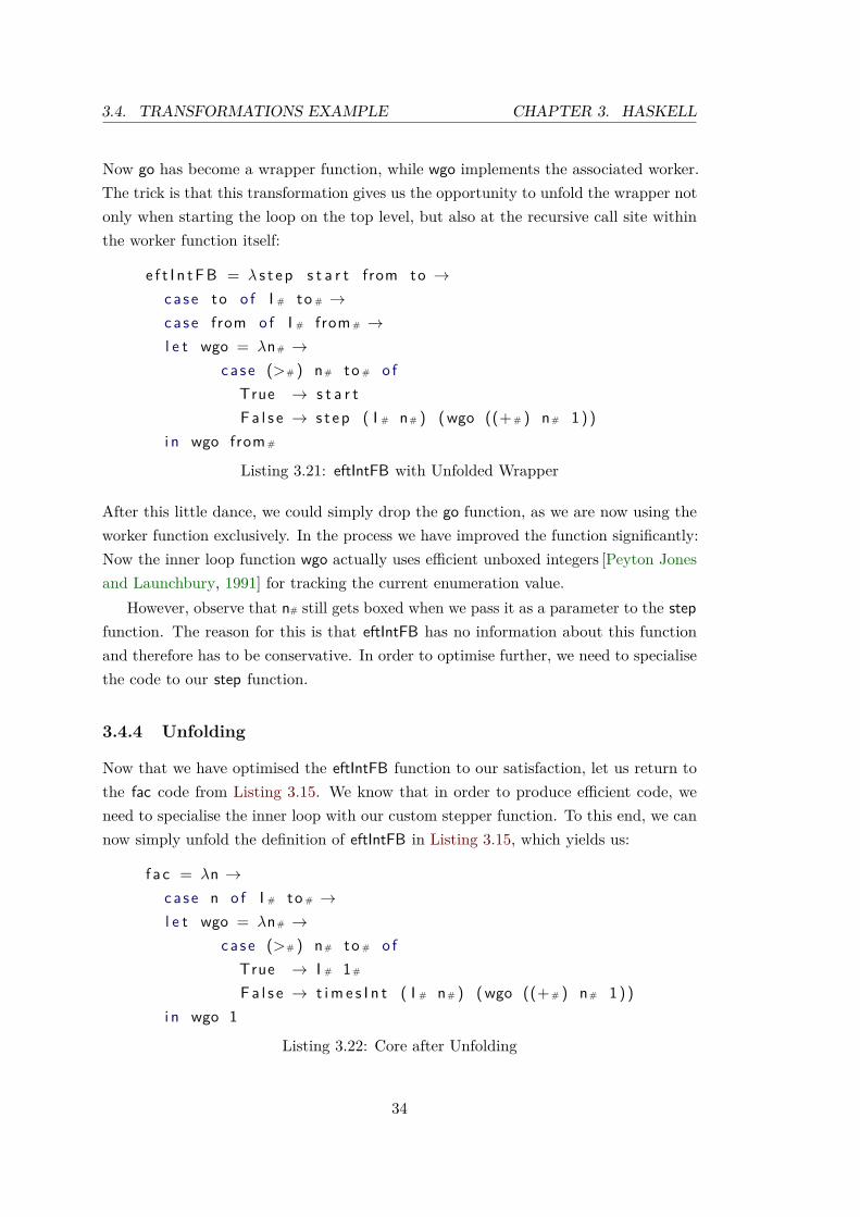
3.4. TRANSFORMATIONS EXAMPLE CHAPTER 3. HASKELL

Now go has become a wrapper function, while wgo implements the associated worker.The trick is that this transformation gives us the opportunity to unfold the wrapper notonly when starting the loop on the top level, but also at the recursive call site withinthe worker function itself:

e f t I n t FB = λ s t e p s t a r t from to →ca se to o f I # to # →ca se from o f I # from # →l e t wgo = λn# →

ca se (># ) n# to # o fTrue → s t a r tF a l s e → s t e p ( I # n# ) (wgo ((+# ) n# 1) )

i n wgo from #

Listing 3.21: eftIntFB with Unfolded Wrapper

After this little dance, we could simply drop the go function, as we are now using theworker function exclusively. In the process we have improved the function significantly:Now the inner loop function wgo actually uses efficient unboxed integers [Peyton Jonesand Launchbury, 1991] for tracking the current enumeration value.

However, observe that n# still gets boxed when we pass it as a parameter to the stepfunction. The reason for this is that eftIntFB has no information about this functionand therefore has to be conservative. In order to optimise further, we need to specialisethe code to our step function.

3.4.4 Unfolding

Now that we have optimised the eftIntFB function to our satisfaction, let us return tothe fac code from Listing 3.15. We know that in order to produce efficient code, weneed to specialise the inner loop with our custom stepper function. To this end, we cannow simply unfold the definition of eftIntFB in Listing 3.15, which yields us:

f a c = λn →ca se n o f I # to # →l e t wgo = λn# →

ca se (># ) n# to # o fTrue → I # 1#

Fa l s e → t im e s I n t ( I # n# ) (wgo ((+# ) n# 1) )i n wgo 1

Listing 3.22: Core after Unfolding

34

CHAPTER 3. HASKELL 3.4. TRANSFORMATIONS EXAMPLE

The inner loop is starting to take shape. Note that most of our optimisations up to thispoint have been instances of unfolding function definitions at their call sites, followedby local transformations. In fact, due to the ubiquity of small functions in Haskellcode, in-lining transformations are one of the most common optimisations performedon functional programs. Note however how this time around we substantially increasedthe code size relative to the last version of fac. This should hint at the fact that inpractice we need to take care, as excessive unfolding could lead to exponential code sizeincrease [Peyton Jones and Marlow, 2002].

But let us continue with our optimisations. We can now unfold timesInt as well toexpose the primitive operator:

f a c = λn →ca se n o f I # to # →l e t wgo = λn# →

ca se (># ) n# to # o fTrue → I # 1#

Fa l s e → ca se wgo ((+# ) n# 1) o fI # r # → I # ( (∗ # ) n# r # )

i n wgo 1Listing 3.23: Core after Nested Unfolding

This bring us close to the finish line. However wgo still boxes and unboxes its returnvalue at every step in the recursion. We can correct this using another worker/wrappertransformation, which yields the final code:

f a c = λn →ca se n o f I # to # →l e t wgo = λn# →

ca se (># ) n# to # o fTrue → 1#

Fa l s e → ca se wgo ((+# ) n# 1) o fr # → (∗ # ) n# r #

i n I # (wgo 1)Listing 3.24: Core after Worker/Wrapper

3.4.5 Status Report

At this point we have exhausted every local Core transformation that we could do.The code from Listing 3.24 is exactly what GHC would produce if we used the facimplementation from Listing 2.1. And even though simplified Core is by far not the last

35

3.4. TRANSFORMATIONS EXAMPLE CHAPTER 3. HASKELL

step in the compilation pipeline, it is noteworthy that if we assume a basic performancemodel [Peyton Jones, 1992] this low-level functional code already says a lot about theperformance we can expect from the program.

Incidentally, we noted earlier that our fac implementation still had a performanceproblem. We can now see why, simply by taking a good look at Listing 3.24: Thefunction wgo needs to call itself recursively, and only multiplies the current counter n#

with the product once the recursive call returns. Running this program, we would beforced to keep n# in a stack frame until the recursive call returns. At the deepest pointthis would mean to# nested stack frames, so our maximum stack size would be O(n).As factorial can be computed in constant space, this is clearly not efficient3.

Thinking about this issue further, we might even recognise that the roots for thisbehaviour run deep: We are folding from the right using foldr and a strict operator,but actually generate the numbers starting from the left. And to make matters evenmore troublesome, we can not even fix this simply by reversing the direction of the foldas proposed back in Listing 2.3 on page 16. The reason is simply that foldl can not befused using GHC’s short-cut fusion techniques, so all the rules that served us so wellwould simply stop matching. Resolving this properly would require more principledchanges to the fusion framework [Coutts et al., 2007a].

3.4.6 Arity Analysis

However as it turns out this performance problem can be fixed without the need toreinvent fusion. The key insight is that the code in Listing 3.24 is inefficient because itaccumulates the counter before the recursive descent, but performs the multiplicationfor the final result on the way back. As multiplication is associative, it should bepossible to move the product calculation in front of the recursion. This would leaveno work to be done after the recursive call, so the compiler could apply the tail-calloptimisation. This would effectively implement the C loop from Listing 3.1 on page 23.

As it happens, we can reach this goal by changing fac as follows:

f a c :: I n t → I n tf a c n = f o l d r (λx c i → c ( i ∗x ) ) i d [ 1 . . n ] 1

Listing 3.25: Fixed Haskell Program

For this solution, the programmer has figuratively “leaned so far right [s]he came backleft again” [Ruehr, 2001]: We use a right fold to construct a function that performs aleft fold, which we then call with the parameter “1”. In the lambda passed to foldr , we

3Our implementation will actually go wrong even before becoming inefficient due to overflowing thevalue range of Int#. As we are only interested in performance, we simply see this as a feature.

36

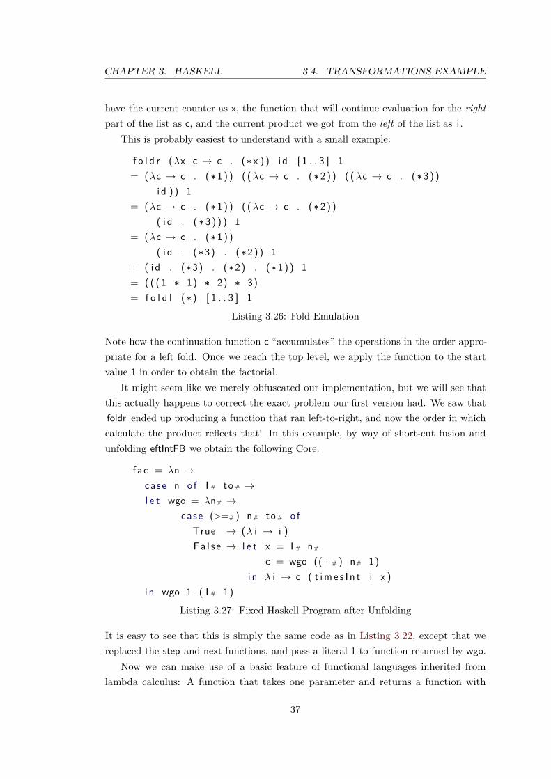
CHAPTER 3. HASKELL 3.4. TRANSFORMATIONS EXAMPLE

have the current counter as x, the function that will continue evaluation for the rightpart of the list as c, and the current product we got from the left of the list as i .

This is probably easiest to understand with a small example:

f o l d r (λx c → c . (∗ x ) ) i d [ 1 . . 3 ] 1= (λc → c . (∗1 ) ) ( (λc → c . (∗2 ) ) ( (λc → c . (∗3 ) )

i d ) ) 1= (λc → c . (∗1 ) ) ( (λc → c . (∗2 ) )

( i d . (∗3 ) ) ) 1= (λc → c . (∗1 ) )

( i d . (∗3) . (∗2 ) ) 1= ( i d . (∗3) . (∗2) . (∗1 ) ) 1= ( ( ( 1 ∗ 1) ∗ 2) ∗ 3)= f o l d l (∗ ) [ 1 . . 3 ] 1

Listing 3.26: Fold Emulation

Note how the continuation function c “accumulates” the operations in the order appro-priate for a left fold. Once we reach the top level, we apply the function to the startvalue 1 in order to obtain the factorial.

It might seem like we merely obfuscated our implementation, but we will see thatthis actually happens to correct the exact problem our first version had. We saw thatfoldr ended up producing a function that ran left-to-right, and now the order in whichcalculate the product reflects that! In this example, by way of short-cut fusion andunfolding eftIntFB we obtain the following Core:

f a c = λn →ca se n o f I # to # →l e t wgo = λn# →

ca se (>=# ) n# to # o fTrue → (λ i → i )F a l s e → l e t x = I # n#

c = wgo ((+# ) n# 1)i n λ i → c ( t im e s I n t i x )

i n wgo 1 ( I # 1)Listing 3.27: Fixed Haskell Program after Unfolding

It is easy to see that this is simply the same code as in Listing 3.22, except that wereplaced the step and next functions, and pass a literal 1 to function returned by wgo.

Now we can make use of a basic feature of functional languages inherited fromlambda calculus: A function that takes one parameter and returns a function with

37

3.4. TRANSFORMATIONS EXAMPLE CHAPTER 3. HASKELL

another parameter is virtually the same as a function that takes two parameters. Wecan especially convert the two forms into each other simply by doing an η-expansion(f = e =⇒ f = λi→ e i). If we do this for the wgo function, float the applicationinwards and β-reduce where possible, we get:

f a c = λn →ca se n o f I # to # →l e t wgo = λn# i →

ca se (>=# ) n# to # o fTrue → iF a l s e → wgo ((+# ) n# 1) ( t im e s I n t ( I # n# ) i )

i n wgo 1 ( I # 1)

Listing 3.28: Fixed Haskell Program after η-Expansion and β-Reduction

Comparing with the program before, we see that we have simply “floated” the lambdafrom the case branches upwards towards the definition of wgo. Note that as simple asthis transformation is, finding the right situations to do this can actually be quite trickyfor the compiler: After all, we have to acknowledge the possibility that the programmight first pass one parameter to wgo and then proceed to call the partially appliedfunction for many different values of i . The η-expanded code would then re-do thecheck of n# against to# for every call to the partially applied function!

However, in this case arity analysis decides that the cost for the check is minorrelative to the cost of constructing and calling a partially applied function. We can alsosee that wgo always gets called with two parameters, so this transformation is in factsafe [Breitner, 2004]. Going forward, strictness analysis now tells us that i always getsevaluated by wgo: Either it is the result, or it gets used by the (strict) timesInt functionto compute the new i parameter for the recursive call. Therefore we can conclude byinduction that wgo itself is strict in that parameter. This is what we need to know forworker/wrapper, so now we are free to displace i in favour of i#:

f a c = λn →ca se n o f I # to # →l e t wgo = λn# i # →

ca se (>=# ) n# to # o fTrue → i #

Fa l s e → wgo ((+# ) n# 1) ( (∗ # ) i # n# )i n I # (wgo 1 1)

Listing 3.29: Fixed Haskell Program after Worker/Wrapper

At which point we have optimised the code to completion.

38

CHAPTER 3. HASKELL 3.4. TRANSFORMATIONS EXAMPLE

3.4.7 Observations

If we compare the result from Listing 3.29 to the Core code we obtained in Listing 3.24on page 35, we observe that paradoxically introducing our “trick” has actually madethe optimised code shorter 4. The new code is also significantly faster : The compilercan implement the tail-call simply by updating the parameters followed by a “jump”back to the function entry. Therefore no stack management is needed, and the back-endwill compile our function into a tight loop.

Yet we have reached this result by “cheating” a little: We specialised our code to theexact optimisations that we knew the compiler would perform. This not only makes ithighly non-obvious why we implemented the function in this way, but also means thatthe performance of our code is fairly fragile. It would be reasonable to expect that fora different compiler or base library our “trick” might stop working completely. Worse,given that we introduced extra code, our new version might end up slower!

This is why generally speaking, the better approach for writing fast programs isto be explicit about performance-relevant aspects of the program. For example, wecould simply write out the loop from Listing 3.29 directly. This might be unsatisfying,as we are essentially writing the Haskell equivalent of the low-level C solution fromListing 3.1 on page 23, but at least we could be reasonably sure about the performancecharacteristics. Fortunately though, there is a better option here. After all, as weexplained the real problem is the direction of the accumulation. So why not simply usefoldl ? As it happens, due to the work of Breitner [2004] this is now actually a goodidea, because foldl is now defined as follows:

f o l d l :: ∀ a b . ( b → a → b ) → b → [ a ] → bf o l d l k i 0 xs = f o l d r (λx c i → c ( k i x ) ) i d xs i 0

Listing 3.30: Definition of foldl :

Which implements exactly the trick we explained above. Note that this is base librarycode, and therefore bound to a specific compiler version and therefore optimisationpipeline! Therefore we can safely “import” this behaviour and could implement a fastfactorial function as follows:

fac ’ :: I n t → I n tfac ’ n = f o l d l (∗ ) 1 [ 1 . . n ]

Listing 3.31: Factorial with foldl

We will however continue to reference the foldr version fac throughout this work, aswe show how to track down the explained performance problem using profiling.

4Which is by no means specific to Haskell – even for low-level languages getting a very specific resultcan often involve complex preparations.

39

3.4. TRANSFORMATIONS EXAMPLE CHAPTER 3. HASKELL

3.4.8 Case-Of-Case

At this point we have exhausted all optimisations that could possibly apply to ourtrusty factorial function. However, we have still barely scratched the surface of all thedifferent transformations that play a role when translating a Haskell program into itsfinal form. We could never hope to cover these completely – especially consideringthat optimisation is a topic that is moving rather quickly, and many transformationsonly become relevant in relatively specialised domains. However, we will still cover onemore rule for its generality and potential to substantially change the control flow of theprogram: The case-of-case transformation [Peyton Jones and Santos, 1998]. Considerthe example from the cited paper:

i f ( not x ) then e1 e l s e e2=⇒ ca se ( ca s e x o f True → Fa l s e ; F a l s e → True ) o f

True → e1Fa l s e → e2

Listing 3.32: Control Flow

After desugaring and unfolding the obvious definition of not, we are left with two nestedcase expressions, which is rather unsatisfactory. After all, it is clear that the branchtaken in the inner case will determine the branch taken on the outer level, thereforewe should be able to eliminate one. And we can, if we simply copy the outer caseexpression into the branches of the inner:

ca se x o f True → ( ca se Fa l s e o f True → e1 ; F a l s e → e2 )Fa l s e → ( ca se True o f True → e1 ; F a l s e → e2 )

=⇒ ca se x o f True → e2Fa l s e → e1Listing 3.33: After Case-Of-Case

This way of simplifying control flow is known for imperative languages as well, where ittakes the form of short-cutting labels for the different branches [Aho and Ullman, 1977,section 7.8]. For most languages this represents a special case, as non-strict semanticsare restricted to boolean operators. In Haskell however, this technique applies nomatter what data structure the case expression scrutinises. We can even generalise thisto constructors with parameters:

ca se ( ca s e f x o f C a b → ( a , b ) ) o f ( a , b ) → . . .=⇒ ca se f x o f C a b → ca se ( a , b ) o f ( a , b ) → . . .=⇒ ca se f x o f C a b → . . .

Listing 3.34: Case-Of-Case for Tuples

40

CHAPTER 3. HASKELL 3.5. PERFORMANCE MODEL

Furthermore, if we are smart about let -binding the branches of the outer case expressionbefore the transformation (called “join points” by Peyton Jones and Santos [1998]), wecan severely limit the amount of code duplication as well. It is not hard to see why thismight be an issue, just consider an inner case expression with more branches:

ca se ( ca s e f x o f C a b → ( a , b )D c d → ( c , d ) )

o f ( a , b ) → . . .=⇒ l e t j o i nP t a b = . . .

i n ca se ( ca se f x o f C a b → ( a , b )D c d → ( c , d ) )

o f ( a , b ) → j o i nP t a b=⇒ l e t j o i nP t a b = . . .

i n ca se f x o f C a b → j o i nP t a bD c d → j o i nP t c d

Listing 3.35: Case-Of-Case with Join Point

Now the compiler can decide separately whether duplicating the branch code – meaninginlining joinPt – would be acceptable. As a result, the case-of-case optimisation can beapplied pretty much anywhere nested case expressions are encountered, which togetherwith let floating means that optimised Core does not often see case scrutinise anythingbut a literal or a function application. This transformation effectively “flattens” thelocal control flow of the program fragment.

3.5 Performance Model

After Core optimisations have run their course, the next step is to translate the programinto an imperative intermediate low-level language. To recapitulate, this is the stagewhere the compiler spells out most of the details of mapping the functional program tohardware: Control flow is encoded using explicit code blocks and jumps, and memorylayout gets broken down to the point where the code is reasoning about individualmemory words. And even though sometimes the compiler can find optimisation oppor-tunities even at this late stage, this is mostly limited to local transformations, such asfiguring out a good register allocation 5.

This is relevant to our considerations: We have now reached the point where we cansee the performance characteristics of the eventual execution start to shine through.After all, a heap check generated at this point will most likely stay in the program

5Note though that the LLVM back-end [Terei and Chakravarty, 2010] can sometimes still improvetight inner loops using low-level assembly tricks [Stewart, 2010].

41

3.5. PERFORMANCE MODEL CHAPTER 3. HASKELL

all the way to the final binary. And while we might not be able to predict the exactcost amount, we know for sure that the check will not be free of charge. This makesthe check a potential performance problem. If we remember our nomenclature fromSection 2.2.1 on page 9, this makes heap usage a verb: A plausible intermediate causefor bad performance.

In this section we are going to build a catalogue of such resource usage types, anabstract performance model for optimised Core. The abstract costs of the model aremeant to directly correspond to our profiling verbs. In contrast to the Core perfor-mance model used by Santos [1995, chapter 9] or Sansom and Peyton Jones [1997]we will not base this primarily on an abstract machine such as the Spineless TaglessG-Machine [Peyton Jones, 1992]. Instead, in this chapter we will approach the problemfrom the practical side, deriving our model from the behaviour of real-world Haskellprograms as compiled with GHC and executed on realistic hardware. And while we willnot quantify the abstract costs just yet, this already allows us to argue that our perfor-mance model covers all relevant runtime costs in some form or another. Therefore ourperformance model exhaustively characterise the performance behavior of a real-worldprogram. Later in Section 5.7 on page 162 we will associate these verbs with actualmeasurable performance metrics. This will allow us to transfer the causal analysis ofthe abstract performance model to real-world performance problems.

3.5.1 Core Preparation

The first step of code generation will be to “prepare” the Core code. The purpose ofthis is not to improve performance: We just normalise some very specific constructsthat would have the same meaning for the purpose of code generation anyway. Furtherreducing the complexity of our language makes it cleaner to talk about performance,as we avoid repeating the same reasoning for different rules.

In GHC, the full Core preparation phase a good number of transformations, withmost of them being inconsequential for our purposes. However, we will assume thefollowing normalisations:

1. Arrange for constructors and primitive operations to appear saturated. We can dothis because we know at every point how many parameter they should receive. Toimplement this, we simply η-expand wherever we find an unsaturated application:

C x =⇒ λy → C x yListing 3.36: Constructor Saturation

This is always possible and means that we have to deal with partial functionalapplications less often.

42

CHAPTER 3. HASKELL 3.5. PERFORMANCE MODEL

2. To simplify dealing with shadowing, we ensure that each variable name onlygets defined exactly once in the program. Variable normalisation just requiresrenaming all variables to use unique names, which GHC does relatively early inthe compilation pipeline:

l e t x = . . . i n l e t x = . . . i n . . . w1=⇒ l e t x0 = . . . i n l e t x1 = . . . i n . . .

Listing 3.37: Variable Normalisation

3. We want A-normal form [Flanagan et al., 1993], where closures are only applied tovariables. This can be achieved simply by let -binding all non-variable arguments:

f ( . . . ) y=⇒ l e t x = . . . i n f x y

Listing 3.38: Conversion to A-normal form

The transformation ensures that we can later cleanly divide concerns betweendetermining the parameter values and performing the function call.

4. Finally we transform strict and primitive let bindings into case statements:

l e t x = . . . i n . . .=⇒ ca se . . . o f x → . . .

Listing 3.39: Convert strict let to case

The reasoning here is that a case statement implies reducing the scrutinee toweak head normal form, which is what we want to do for strict values. Note thatprimitive values always have to be evaluated strictly, but even for non-primitivevalues we can often derive strictness properties using a suitable analysis [Clackand Peyton Jones, 1985].

3.5.2 Abstract Evaluation

After preparation the new language subset is quite suitable for talking about operationalsemantics. Our next aim is to formulate rules that say how much cost we expect eachconstruct to contribute to a program execution. Note that the concrete costs will oftendepend on how often and in what context a given construct gets evaluated, meaningthat in order to be able to truly talk about costs we need to know how the programevaluates. Unsurprisingly, there has been substantial prior work on how to reason aboutprogram evaluation in a formal way. In the following we opt to follow in the footstepsof Launchbury [1993] and Sestoft [1997], with only minor modifications to introduceand maintain cost terms.

43

3.5. PERFORMANCE MODEL CHAPTER 3. HASKELL

Let us introduce our notation. We will be using symbols to refer to specific termtypes as follows:

C – Constructors will be upper-case letters.

We assume them to be constants coming from the original program. Each con-structor has a given arity, corresponding to the number of value arguments.

x – We will notate variables as lower-case letters.

They will be used to refer to names in the program as well as to abstract heaplocations for evaluation. We will on occasion generate fresh ones in order to referto new heap cells.

v – Values are the result of evaluating expressions, and might appear on the heap.

As we are going to ignore primitives for now, we only have saturated constructorsand lambda values:

v ::= C x1 x2... (Constructor)| λy.e (Lambda)| ⊥ (Bottom, Hole)

Note that we include the ⊥ term for undefined behaviour as a value. Makingit a proper value is a rather unusual choice, most notably Launchbury’s originalsemantics introduce it only retroactively. We will later make more active use ofthis both as a value as well as an expression term, therefore it makes sense toemphasise its existence up-front.

e – Expressions form our program representation:

e ::= v (Literal)| e x (Application)| x (Variable)| let {x1 = e1, x2 = e2, . . . } in e ( let expression)| case e of {C x1 x2...→ e1; D y1 y2...→ e2; . . . } (case expression)

Apart from the notation, these expression types correspond closely to the onesused by GHC, which we mentioned in Listing 3.6 on page 28. The most notabledifference is that we have now separated constructor applications and functionapplications, and only allow passing variables in both cases. As we have seen inthe last section, this is just a question of preparing the Core code suitably.

44

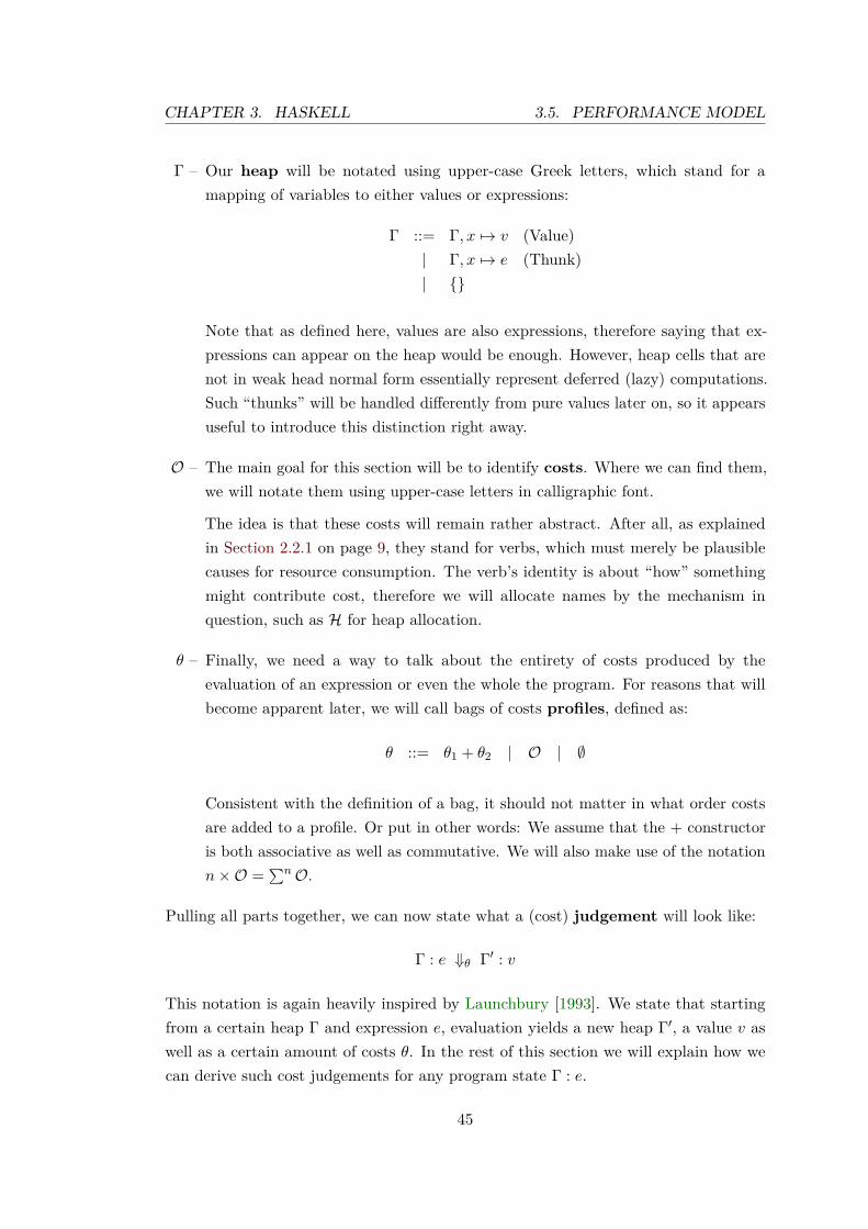
CHAPTER 3. HASKELL 3.5. PERFORMANCE MODEL

Γ – Our heap will be notated using upper-case Greek letters, which stand for amapping of variables to either values or expressions:

Γ ::= Γ, x 7→ v (Value)| Γ, x 7→ e (Thunk)| {}

Note that as defined here, values are also expressions, therefore saying that ex-pressions can appear on the heap would be enough. However, heap cells that arenot in weak head normal form essentially represent deferred (lazy) computations.Such “thunks” will be handled differently from pure values later on, so it appearsuseful to introduce this distinction right away.

O – The main goal for this section will be to identify costs. Where we can find them,we will notate them using upper-case letters in calligraphic font.

The idea is that these costs will remain rather abstract. After all, as explainedin Section 2.2.1 on page 9, they stand for verbs, which must merely be plausiblecauses for resource consumption. The verb’s identity is about “how” somethingmight contribute cost, therefore we will allocate names by the mechanism inquestion, such as H for heap allocation.

θ – Finally, we need a way to talk about the entirety of costs produced by theevaluation of an expression or even the whole the program. For reasons that willbecome apparent later, we will call bags of costs profiles, defined as:

θ ::= θ1 + θ2 | O | ∅

Consistent with the definition of a bag, it should not matter in what order costsare added to a profile. Or put in other words: We assume that the + constructoris both associative as well as commutative. We will also make use of the notationn×O =

∑nO.

Pulling all parts together, we can now state what a (cost) judgement will look like:

Γ : e ⇓θ Γ′ : v

This notation is again heavily inspired by Launchbury [1993]. We state that startingfrom a certain heap Γ and expression e, evaluation yields a new heap Γ′, a value v aswell as a certain amount of costs θ. In the rest of this section we will explain how wecan derive such cost judgements for any program state Γ : e.

45

3.5. PERFORMANCE MODEL CHAPTER 3. HASKELL

3.5.3 Registers and Stack

Before we start with building our abstract model, let us consider what we know abouthow programs execute. Given the speed at which computational units run in this dayand age, a significant portion of run-time cost will simply come from delays involved inobtaining data and saving back results [Patterson, 2004]. The amount of data requiredfor an operation is often a much more reliable predictor of performance than up-frontcomputational complexity. Consequently, we should take special care to account forstorage costs.

Conceptually, there are three stores in a running Haskell program – registers, thestack and the heap. Let us focus on the first two for now: Registers and stack bothhold the current “working” data of the code, such as local variables, parameters or thecode pointer. The characteristics of these stores are as follows:

1. Registers are, by construction, the fastest possible memory to access from theCPU. Therefore it is the first and default choice for holding data. Unfortunately,the register file is rather small, and has to be shared across all recursive calls.

2. On the other hand, access to the stack is generally slower, yet it has the advantagethat we can grow it to virtually unlimited size. Typically the stack is used to“spill” values that we can not fit into registers.

Allocating register and stack words in a way that optimises performance is a highlynon-trivial problem [George and Appel, 1996] that we will not attempt to model here.Instead, for cost we will simply opt to regard registers and stack together as a sin-gle compound store. This essentially makes register allocation an advanced cachingtechnique for the top-most stack frame.

The reasoning is that even if a value might end up never touching the stack, everyallocated register has an associated “opportunity cost”:

• Register pressure might force other register values to get spilt to the stack

• Calls might clobber our register, so we have to save it back

Bottom line is that while it might be quite hard to pin down exactly, every data wordput into a register will often become a data word allocated on the stack. Where registerpressure becomes a performance problem, it is almost assured to do so via increasedstack allocation. Hence we have causation, and therefore can unite both influencestogether using the “stack allocation” verb, represented by the abstract cost S.

46

CHAPTER 3. HASKELL 3.5. PERFORMANCE MODEL

3.5.4 Heap

In contrast to stack data, the life of heap objects is not bound directly to a certainpiece of code being executed. Instead, its function is to enable sharing of complex datastructures between loosely connected code pieces. As a result, even figuring out whetheror not a heap object can be discarded means running a garbage collection heap analysisat program run-time. This pass will have to copy a significant amount of heap data,which means that it will become more complex the more that we allocate but cannotdiscard [Sansom and Peyton Jones, 1993].

That being said, the allocation of a heap object itself is very cheap [Appel, 1987].All we need to do is increase the global heap pointer and write the header word and alldata into the freshly reserved heap region (see Section 3.5.9). Yet the implied cost dueto triggering a garbage collection still means that programs with a high heap allocationquickly suffer in terms of performance. We will therefore assign an abstract cost unitH for every word that gets allocated on the heap.

In addition to allocation we have to acknowledge that keeping a large heap aroundis also a significant factor in slowing the program down. For example, even thoughmodern multiple-generation garbage collection will try to not walk the complete heaptoo often, a large heap will still cause the average time needed for a garbage collectionto increase. More subtly, having a large heap makes it less likely for its contents tofit into processor caches, causing general slowdowns due to reduced memory locality.Therefore there is clearly a heap residency verb. However we will not formalise garbagecollection here, and will therefore not associate an abstract cost with it.

3.5.5 Constructors

Now we have covered the groundwork, so let us start looking at concrete expressionevaluation. We will always do this in a certain way: First we will have a look at howLaunchbury-style semantics encode operational meaning, followed by a more thoroughexploration of how GHC would implement these semantics for a real Haskell program.Finally we will go back to the rule to insert the appropriate cost term and obtain a rulefor our performance model.

First up, we have constructor applications, which require just a simple rule:

Γ : C x1 x2... ⇓O(C x1 x2) Γ : C x1 x2...

Constructors are both expressions and values, and variables uniquely identify theirvalues, therefore we can simply return the expression as our return value.

On the other hand, the cost term O(C x1 x2) is still an unknown for now. To findout what kinds of costs we have to expect, we have to consider this evaluation from

47

3.5. PERFORMANCE MODEL CHAPTER 3. HASKELL

Stack Heap Static Code

Constructor, n = 0: C id

Constructor, n > 0: C (pars) id

Lambda: (live) eval

Thunk: (live) eval+upd

Figure 3.2: Heap Object Construction

the perspective of the compiler. This makes things a bit more involved: Disregardingunboxed tuples or primitives, programs will refer to data structures using pointers, asthis reduces the amount of copying the program has to do when passing data around.How we get there depends on the arity of the constructor. Consider for example thenullary constructors of the Bool algebraic data type:

data Bool = True | F a l s e

Listing 3.40: Definition of Bool

As Haskell is not concerned with object identity, there is no need to ever have morethan one True or False instance per program. Therefore we simply need to staticallyprovide these closures, reducing the “construction” to simply returning a pointer to theprepared memory location. The opportunity cost for holding a pre-allocated closure instatic memory can not be causally connected to the constructor application, and willtherefore be ignored6.

On the other hand, where no such short-cut is available we need to actually allocateheap memory in order to hold our data words. In order to build a valid closure for aconstructor with arity n we will have to allocate and copy n+ 1 data words, as shownin Figure 3.2. Remember from Section 3.5.4 that we use the verb H for the overhead ofallocating and copying a word of heap data. Furthermore, we have some constant costsfor the heap check and returning a value, which we will call C.

6Note that for types like Int or Char the number of constructors makes storage costs significantenough that GHC in fact switches to “normal” allocation for all “rarely” used 0-arity constructors.

48

CHAPTER 3. HASKELL 3.5. PERFORMANCE MODEL

This yields us the abstract cost term:

O(C x1 x2...) = C + n×H

And even though we are not distinguishing between the 0-arity and the n-arity casehere, for our purposes this still gets the main message across: Performance problemscan either happen because too many constructor applications are evaluated (effect of Cterms dominate), or because they are allocating too much memory (effect of H termsdominate). As usual, the actual cost behind these terms are not that interesting, aslong as we are reasonably sure that we have not overlooked a way in which constructorapplications can become expensive without triggering one or both of these scenarios.

3.5.6 Lambdas

Our next literal expression type is the lambda: an anonymous function that we can callvia application at a later point in program execution. Due to the design of the abstractsemantics, we can use the lambda expression as a value as well:

Γ : λy.e ⇓O(λy.e) Γ : λy.e

For a real program, things are a bit trickier. After all, a lambda value must containall information we need for resuming evaluation of the code from a completely differentcontext. We must especially take care of live variables. Recall that while optimisingthe “tricky” factorial function in Listing 3.27 on page 37 we had the following codefragment:

l e t x = I # n#

c = wgo ((+# ) n# 1)i n λ i → c ( t im e s I n t x i )

Listing 3.41: Lambda with Live Variables

There was a good reason we tried to optimise this: The lambda expression has two livenon-global variables, c and x, which would both be out of scope once the lambda valueactually gets applied to a parameter. To evaluate the body meaningfully, we wouldneed a full closure that saves back both of these values in order to restore them later.

In general, constructing a closure for an expression e with lv(e) live variables there-fore requires lv(e) + 1 words of heap space – a code pointer and the values from thecontext (see Figure 3.2). If we again assign a fresh symbol L to stand for the constantcost of the lambda’s evaluation we can therefore state:

O(λy.e) = L+ lv(e)×H

49

3.5. PERFORMANCE MODEL CHAPTER 3. HASKELL

Stack Heap Code

Application:

(live)(pars) (live)

eval

Thunk Evaluation:

(live)(live)

eval

upd

Figure 3.3: Call Implementation

As with constructors, we see two distinct ways in which lambda expressions can causeperformance problems. Note however that in contrast to constructor arity, the numberof live variables is a performance factor that is quite easy to overlook. For example, theabove-mentioned potential problem with the factorial function is not obvious given theoriginal source code from Listing 3.25 on page 36.

3.5.7 Applications

Applications are the counterpart to lambdas, they come into play once the programwants to call the closure with a given set of parameters:

Γ : e ⇓θf Γ′ : λy1.λy2....eb Γ′ : eb[xi/yi · · · ] ⇓θb Γ′′ : vΓ : e x1 x2 · · · ⇓O(e x1 x2··· )+θf+θb Γ′′ : v

This time we need to take a closer look at the abstract semantics. For an applicatione x1 x2 · · · we first need to evaluate e into a closure of matching arity, which in ournotation is written as λy1.λy2....eb

7. We then bind the parameters for the lambdabody eb by substituting the parameter names by the variables from the application(which stand for heap objects). Finally, we can perform the actual call by evaluatingthe prepared body, passing all evaluation results through.

To summarise runtime costs, we need to account for the two nested evaluations θf7Note that in contrast to Launchbury [1993] our application rule binds multiple parameters at the

same time. The sole purpose of this is to bring the semantics more in line with actual Haskell execution.

50

CHAPTER 3. HASKELL 3.5. PERFORMANCE MODEL

and θb plus the expenses for the actual call O(e x1 x2 · · · ). The main work for a call isto re-arrange the context to accommodate the body’s evaluation: Parameters and livevariables have to be arranged to appear at predictable locations on the stack. Unlesswe can derive the application to be a tail call, we also want to be able to return to ourold code position once the call is finished, so we need to push the new code pointer ontop of the stack (refer to Figure 3.3).

As established in Section 3.5.3, we have one unit of abstract cost S for allocating andinitialising a word on the stack. Additionally, we will assign A to the unique constantcosts of an application. Then we have the following expenses for calling a lambda witharity n and m live variables:

Operation CostPass parameters n× SRestore live variables m× SPush new code address SJump to code, Return A

Which gives us:O(e x1 x2 · · · ) = A+ (1 + n+m)× S

So clearly calls can quickly become expensive in terms of stack usage. Remember theoptimised Core code of our first version of factorial in Listing 3.24: The recursive wgo-calls allocated so much stack space that it caused a performance problem. Even moreinsidiously, note that the cost can rise both due to the number of parameters passed aswell as due to live variables – still a tricky property to control, as explained in the lastsection. We will explain a cheaper way to implement calls in Section 3.5.11.

3.5.8 Lets & Thunks

The purpose of the let expression is to bind a certain sub-expression to a name. Thisallows its evaluation result to be shared. The abstract formulation looks like follows:

Γ, yi 7→ ei[yi/xi, ...], ... : e[yi/xi, ...] ⇓θ Γ′ : vΓ : let {xi = ei, ...} in e ⇓O(let {xi=ei,...} in e)+θ Γ′ : v

Most of the rule is concerned with replacing original names xi by yi, which we assumeare fresh for our evaluation. This is required as without renaming the abstract heapΓ might already contain xi bindings originating from an earlier evaluation of the samelet expression [Sestoft, 1997]. Apart from that, the purpose of the rule is simply to addthe bound expressions ei to the abstract heap, and proceed to evaluate the body e. Theresulting profile θ, abstract heap Γ′ as well as the return value v all get passed through

51

3.5. PERFORMANCE MODEL CHAPTER 3. HASKELL

as the evaluation result of the let expression. However, we still have to determine thelet expression’s cost contribution O (let {xi = ei, ...} in e).

To determine the cost, we have to first realise that we actually have two cases here:If a bound expression happens to be a constructor or lambda, the value added to theabstract heap is actually already in normal form. Therefore the runtime equivalent isto construct the proper evaluated values right away. As we established in Sections 3.5.5to 3.5.6 on pages 47–49 this has the abstract costs:

O(x = C x1...) = C + n×H

O(x = λy.e) = L+m×H

with n the arity of the constructor or m the number of live variables respectively.For non-literal expressions on the other hand, this is where lazy evaluation comes

in: Instead of mapping the variable to a value, the abstract semantics push the fullexpression e itself. Similarly, a running Haskell program would construct a delayedcomputation – a thunk. For the purpose of construction, this works exactly the sameas building a hypothetical 0-arity lambda closure. We allocate a new heap object thatcarries a special code pointer as well as all live variables that we need to restore toresume its computation. We therefore obtain for a non-literal e with m non-global livevariables:

O(x = e) = L+m×H

To put things together, we have to finally account for the fact that for each new variablewe will need to save a pointer in the local context. We will account for this using thecost S per binding, which gives us:

O (let {xi = ei, ...} in e) =∑i

(S +O(xi = ei)

)So apart from the relatively minor cost of keeping the pointers around, most work forthe let expression comes from the number and nature of the heap objects.

3.5.9 Variables

As thunks behave a lot like 0-arity lambdas, we can understand executing variableexpressions as performing 0-arity applications. However, we want every thunk to beexecuted at most once, which we achieve by updating the abstract heap:

Γ, x 7→ v : x ⇓Ov(x) Γ, x 7→ v : vΓ : e ⇓θ Γ′ : v

Γ, x 7→ e : x ⇓Oe(x)+θ Γ′, x 7→ v : v

52

CHAPTER 3. HASKELL 3.5. PERFORMANCE MODEL

To summarise, if we find that the heap cell already contains a value, we can simplyreturn it without making any adjustments to the heap. However if the heap contains anexpression (a thunk), the rule evaluates it and writes the value back to prevent repeatedevaluations.

On the runtime side of things, there is an easy way to implement this rule: Wesimply have variable evaluation call the heap object’s entry code. For a thunk thiswill evaluate the body and arrange for updating the heap, meaning pushing an extrastack frame of two words and perform the actual update once evaluation returns (seeFigure 3.3). On the other hand, values will have a dummy “id” entry code that simplyreturns itself right away, as sketched in Figure 3.2 8. Therefore we get:

Ov(x) = V + S

Oe(x) = V + (3 + n)× S + U

with V standing for variable evaluation and U for the raw cost of updating a heap cell.

3.5.10 Case

To finish our discussion of operational semantics, we have only case expressions left.Their purpose is to extract data from the heap cells built by constructor applicationsaccording to Section 3.5.5. The operational semantics are as follows:

Γ : e ⇓θ2 Γ′ : Ci yj ... Γ′ : ei[yj/xj , ...] ⇓θ3 Γ′′ : vΓ1 : case e of {Ci xj ...→ ei, ...} ⇓O(case ...)+θ2+θ3 Γ′′ : v

So we first evaluate the scrutinee expression e, then depending on the returned construc-tor Ci choose the appropriate branch ei. In the second steps, we bind the constructorfields yj to the desired variable names xj using substitution and finally proceed toevaluate ei. All results get passed through as usual.

Note that again we have a duality with constructors, which is unsurprising from atheoretical point of view. After all Church encoding would see constructors as lambdasand case expressions as applications. For actual Haskell programs, we need to evaluatethe scrutinee and identify the constructor behind the pointer. Then we can proceedwith the appropriate branch, pushing constructor parameters on the stack as required.

Recognising a constructor is relatively straightforward, as we know from Section 3.5.4that every heap object has a header word. Apart from the code, this header pointeralso gives us an info table which identifies the constructor type 9. The cost for choosing

8In fact GHC optimises this further by “tagging” pointers according to what they are known topoint to [Marlow et al., 2007]. However there is no guarantee that we can always skip evaluation of id,so we only discuss this method here.

9As with thunks, this can often be detected directly from the pointer tag, saving one indirection

53

3.5. PERFORMANCE MODEL CHAPTER 3. HASKELL

the right branch now depends on the number of branches we have: If we could derivethat there is only one possible branch, we have to do no extra work. On the otherhand, if there is more than one branch to choose from, we have to either use a branchtree or a jump table to identify the right choice. The compiler will chose whateverseems fastest for the task at hand, with the constant overhead of a jump table beingthe default solution.

Binding n variables means pushing the appropriate number of stack words, whichyields us the sum:

O(case e of {Ci xj ...→ ei, ...}

)= E + n× S

where again E stands for all constant costs for case expressions together.

3.5.11 Let-No-Escape

At this point we have covered all expression types of our abstract language. However,there is still one interesting case left to cover: Remember that one of the more expensiveand unpredictable parts of constructing and calling a function closure was saving andrestoring the live variables. However, this is not always necessary. After all, the livevariables might still be in scope when the function body gets executed. Suppose ourcode was shaped as follows:

let {f = λx. ...; ...}

in case ... of {C → f ...;D → f ...}

Assuming that these are the only two references to f , we know that we will have exactlythe same live variables at the application site as we had when the let expression wasexecuted. This means that there is actually no need to either save or restore livevariables: f can simply use the data that is already on the stack!

For GHC, there is a special optimisation pass at the end of Core generation thatdetects such “let-no-escape” optimisation opportunities. The critical part is to provethat no closure reference “escapes”, meaning that all calls to the function are containedin the let body. This implies that the function application has strictly fewer livevariables than the application site, therefore making restoring live variables redundant.In the end, this means not only that the function application can prepare the stackrather quickly, but it can also short-cut the jump to the known function entry code.

This means that “let-no-escape” function applications actually involve no heapaccess whatsoever, making them substantially faster than standard calls. In fact, thisoptimisation is of tremendous importance for generating fast programs. To see why,

54

CHAPTER 3. HASKELL 3.5. PERFORMANCE MODEL

Γ : C x1 x2... ⇓C+n×H Γ : C x1 x2... (Con)

Γ : λy.e ⇓L+lv(e)×H Γ : λy.e (Lam)

Γ : e ⇓θf Γ′ : λy1.λy2....eb Γ′ : eb[xi/yi · · · ] ⇓θb Γ′′ : vΓ : e x1 x2 · · · ⇓A+(1+n+lv(e))×S+θf+θb Γ′′ : v (App)

Γ, yi 7→ ei[yi/xi, ...], ... : e[yi/xi, ...] ⇓θ Γ′ : vΓ : let {xi = ei, ...} in e ⇓∑(S+O(xi=ei))+θ Γ′ : v (Let)

Γ, x 7→ v : x ⇓V+S Γ, x 7→ v : v (Var1)

Γ : e ⇓θ Γ′ : vΓ, x 7→ e : x ⇓V+(3+lv(e))×S+U+θ Γ′, x 7→ v : v (Var2)

Γ : e ⇓θ2 Γ′ : Ci yj ... Γ′ : ei[yj/xj , ...] ⇓θ3 Γ′′ : vΓ1 : case e of {Ci xj ...→ ei, ...} ⇓E+ni×S+θ2+θ3 Γ′′ : v (Case)

Figure 3.4: Performance Model

take another look at the above code: All we do is evaluate the body of f for two differentvalues of x. This type of control flow appears quite often in functional programs: Quitea bit of the ultimate performance of our factorial implementation was based on the factthat the let-no-escape optimisation would apply to our wgo function from Listing 3.23on page 35 forward. Furthermore, the case-of-case transformation we introduced inSection 3.4.8 on page 40 will deliberately generate this type of code for join points.

For our purposes, this rises the question: Do we need to modify our performancemodel in order to account for the let-no-escape transformation? Fortunately, thistransformation has virtually no overhead. This means that for the sake of argument,we could only ever make absence of this transformation a verb. This however makesno real sense for causal reasoning, which is why we can simply ignore this case for ourperformance model.

3.5.12 Conclusion

This concludes our abstract performance considerations. Figure 3.4 shows a summaryof the rules we derived. This allows us to reason about real Haskell programs: Supposewe take a Haskell program and evaluate the equivalent of its Core code with these rules.Then we know that any possible performance-related effect of the program run wouldbe reflected in our abstract model by one or more abstract cost entities. This is exactlywhat we want, as the next chapter will show how we can trace causality for these backto their respective root causes.

55

3.5. PERFORMANCE MODEL CHAPTER 3. HASKELL

56

Chapter 4

Causality Analysis

“Subjected to the influence of so many gods, who both protect and threatenthem, the nations of antiquity would like to have advance notice of theirwhims.”

— Asterix and the Soothsayer, René Goscinny & Albert Uderzo

The past chapter established the main poles of the profiling problem: The first oneis represented by all the possible causes of performance problems. For our purposesthis is the entirety of design decisions that went into development of a program, mostlyencoded as Haskell source code. On the opposing side, we have all the effects that wewant to track. As we have seen, our performance model already enumerates a goodnumber of distinct ways in which the program in question could end up being inefficient.The main question for this chapter is going to be how well we can establish causalitybetween these two sides.

To do that we will systematically employ Lewis’ theory of causation [Lewis, 1973]as introduced in Section 2.3 on page 13. As causality judgements critically dependon our choice of closest world, this will not be a completely passive analysis. In fact,we have to be very careful in how we make these choices, as it is quite easy to eitherover- or under-estimate causality. Note that these two trappings are very different innature: As we explained back in Section 2.3.5, we expect our analysis to overestimatecausality all the time. The reason is that we will never be able to tell essential programcomponents from interchangeable ones. For example, there is simply no way that ouranalysis could know whether usage of the multiplication operator was in fact requiredin order to compute a factorial. Hence for a complete profile we will always have toinclude it as a potential suspect.

On the other hand, underestimating causality would be a severe problem. Thereason lies in our methodology: In order to break down the task, we will reason aboutthe causes of intermediate events, and use transitivity to propagate them. This approach

57

4.1. INTRODUCTION CHAPTER 4. CAUSALITY ANALYSIS

relies on the fact that the causes for these intermediate events will get carried forwardcorrectly. If we miss an effect of one of these event, we might end up losing track ofarbitrarily many causal connections! Therefore our primary motivation throughout willbe to make it easy for us to track down every single effect – even if it means that weare clearly overestimating causality.

This chapter has two parts: We will start by considering causal connections inthe absence of program transformations. To do that, Section 4.2 will translate theperformance model from the last chapter, and show how we can see it as generating anetwork of events. This event interpretation will allow us to analyse causal dependencies.Section 4.3 and Section 4.5 on page 80 will show how we can systematically map thesecausal dependencies to term annotations. Furthermore, Section 3.5.4 on page 47 andSection 4.6 on page 85 will explain how we need to change our viewpoint in orderto make causal reasoning about laziness and bindings intuitive. Section 4.7 will thenpresent the finished causality model and explain its properties and intuition.

In Section 4.8 on page 100 we will then formally reason about how code transforma-tions rewrite the causal network given by these semantics. We will see that dependingon the type of transformation the effects on the profile can be anything from harmlessto fairly severe. However, we will also show that even in the worst case we can stilllimit the damage to – occasionally rather extreme – cases of causality overestimation,promising that we will never actually miss a cause that exists in the program run.

4.1 Introduction

The performance model we derived in the last chapter tells us what abstract costswe would expect if we were to execute a given Core program. The analysis of thiswill yield us causal connections, which as explained in Section 2.2 on page 8 is onecorner stone for abductive reasoning. Later in Chapter 5 we add estimates about actualexecution cost into the mix, so the user can properly gauge plausibility. For the momenthowever, we will focus entirely on causality. Exactly which parts of the program playeda role in shaping a certain part of the profile? Which parts did not actually matter forperformance and can therefore be ignored?

We will answer these questions using systematic analysis of the rules formulated inthe last chapter. Again we have to account for the dynamic nature of program evaluation:The causal context of a cost will critically depend on the concrete run-time control flow.Building the desired cause terms therefore again involves following program execution.Our approach will be the same as in the last section: By extending Launchbury’soperational semantics, we will generate a causal description as a “side-product”.

58

CHAPTER 4. CAUSALITY ANALYSIS 4.2. EVENTS

t

W & W ′ W

W ′

?

Figure 4.1: Causality Reasoning: Past and Future

4.2 Events

Our goal is to ground our semantics in Lewis-style causality theory [Lewis, 1973] asintroduced in Section 2.3. To do that, we have to think about things in the same waywe would when trying to make sense of a car crash: What were the events that led upto the situation in question, and how are they connected? Which ones were actuallyessential, and which could be removed without actually making a difference?

When we formulated our cost semantics in Figure 3.4, we used nested rule matchesto abstractly describe evaluation. To make it more intuitive to think about this interms of causality, it is a good idea to think of this in terms of events 1. Consider forexample the constructor application rule:

Γ : C x1 x2... ⇓C+n×H Γ : C x1 x2...

We can deconstruct the process of applying this rule using three event types:

Event Description

Γ : e ⇓ A rule matches input heap pattern Γ and expression pattern e

⇓O A rule emits a unit of cost O

Γ′ : v A rule returns a new heap Γ′ and a value v.

Clearly we could deconstruct a whole abstract program execution using these eventsand start reasoning about causation between them. However, we need to be careful.After all, let us think exactly about what we are planning to do: For causal reasoningwe expect to depart the original worldW by introducing a single “miracle event”, whichbrings us into a parallel universeW ′ where we can proceed to apply our rules in order to

1Our approach here is inspired by the work by Taylor [1993] on causality semantics.

59

4.2. EVENTS CHAPTER 4. CAUSALITY ANALYSIS

Γ : C x1 x2... ⇓ ⇓C ⇓n×H Γ : C x1 x2...

t

Figure 4.2: Event Decomposition of a Constructor Rule Match

derive the new “future”. For example, back when we introduced causality in Section 2.3on page 13 this miracle event was a tree ceasing to exist, which led us to a situationwhere the car crash existed in the original world W , but not in the alternate world W ′.Therefore, we reasoned that these two events had a causal relationship.

However, what if we make our “miracle” that the car crash does not happen? Clearly,the car passing through means that there cannot be a tree in W ′. So can we concludethat the car crash is what causes the tree to exist? This type of reasoning is clearlydangerous, as it can easily lead us to confusing causes with effects. To ensure consistencyof causal reasoning we therefore demand that our events have a temporal order [Lewis,1979], which tells us in what direction we are “allowed” to look for causation. Figure 4.1shows how we imagine this to work: Our worlds W and W ′ are only allowed to differin terms of events that come after the miracle event. This ensures that “past” eventscan never become effects in our causality analysis.

Fortunately finding a suitable temporal ordering is rather straight-forward for eventsarising from our operational semantics. After all, our underlying machine executionmodel is sequential by nature. Therefore we would naturally assume that the left-handside match happens “before” any potential nested rule matches, the events of whichin turn happen “before” the return value gets produced. For example, evaluating aconstructor application would give us the event order shown in Figure 4.2: The rulematch event “Γ : C x1 x2... ⇓ ” followed by a number of subsequent “result” events.

4.2.1 Event Causes

Our goal is now to take the event network of a rule match and run causality analysison it. Our starting assumption will be that a judgement gets attempted, which willgenerally cause a rule match, which in turn will give rise to events according to our eventdecomposition of the rule. Note that the judgement getting attempted is not self-evident:We might be looking at the top-most rule activation of some program evaluation, or wemight actually be in the middle of a recursive rule match. In either case we will simplysee the judgement getting attempted as axiomatic. We will especially assume that suchjudgements adhere to the form introduced in Section 3.5.2 on page 43 2.

2Formally speaking, we declare worlds with other judgement/event forms as unlawful[Taylor, 1993].

60

CHAPTER 4. CAUSALITY ANALYSIS 4.2. EVENTS

CausesTerms

Expressions

Expressions’

Values

Costs

α

Figure 4.3: Maintaining Cause Links

So our basic scenario is an attempt to obtain a judgement of the form Γ : e ⇓θ Γ′ : v.The concrete rule match will now directly depend on what kind of expression type e is.The cause for this is not immediately known to us, as the answer depends on the historyof the passed expression. For example, if our program was simply the desugaring of:

l e t x1 = . . . ; x2 = . . . ; i n C x1 x2Listing 4.1: Constructor Source

we would say that the source code of the let expression body is what caused us toencounter a constructor here.

On the other hand, we will eventually have to deal with code transformations, whichwill make the story more complicated. It is important that we address this particularproblem generally, as we clearly do not want the complexity of transformations toeventually bleed into our treatment of, say, the constructor application rule. It shouldmake no difference to our causality semantics whether code transformations touchedthe expressions or not. Instead, our causality semantics should be able to see thecausal history simply as a term annotation. Then we can clearly describe what causesa constructor rule match: The fact that a judgement was attempted together with thecause term that was annotated on the constructor expression.

In fact, we will apply this idea generally, as shown in Figure 4.3: Using knowledgeabout a rule’s inner workings, we can derive new annotations for the produced termsusing causal transitivity as explained in Section 2.3.5 on page 18. In fact, we willrepresent the whole causal process using cause-annotated terms: Code transformationswill work entirely on cause-annotated expressions, which evaluation consumes in orderto produce similarly annotated value and cost terms. In the end, we will have costsannotated with their causal history, which is exactly what we want for performanceanalysis.

61

4.2. EVENTS CHAPTER 4. CAUSALITY ANALYSIS

4.2.2 Cause Annotations

An extension to the notation from Section 3.5.2 is in order. The new protagonist forthis section will be the cause term, corresponding to the profiling-related reasons thata certain event happens for our term. In the end, we should be able to look at the costterm annotations of the top-most judgement and obtain a break-down of the reasonsfor the program’s resource usage.

α – We will use lower-case letters from the beginning of the Greek alphabet to referto cause terms. We will leave their definition abstract, but think of them asstanding for properties or parts of the original program source code as explainedin Section 2.3.2.

However we assume that cause terms can be composed using the logical “and”operator ∧. We will make use of a short-hand where it is unambiguous:

α ∧ β = αβ

As usual the order in which causes are combined does not matter, meaning the ∧operator should be both commutative and associative.

Cause terms are used to annotate the previously defined term types. To be concrete,we will have the following types of annotated terms:

〈α〉e = e – cause-annotated expression〈α〉v = v – cause-annotated value〈α〉O = O – cause-annotated cost

with an underlined symbol such as e standing for both the term as well as its annotation.In either case, the annotated term refers to a cause for the expression, value or costhaving its present form in context of the event we want to associate it with.

So for example assume that the constructor rule match events shown in Figure 4.2were the result of matching on the annotated expression term 〈α〉C x1 x2.... Then αstands for the cause of the expression actually being C x1 x2.... The initial match eventdepends causally on this fact, because if we counter-factually assume a different valuewe would presumably get a different match event, Put generally, let us say we have anevent E that successfully matches an annotated term variable such as 〈α〉e. Then weshould have:

¬α �→ ¬E

Which, again, means that in an alternate world W ′ with α false we have to assume thate changes and therefore E does not happen.

62

CHAPTER 4. CAUSALITY ANALYSIS 4.2. EVENTS

4.2.3 Annotated Judgements

Changing our term definitions to include annotations means that we have to adjustevaluation as well. For starters, heaps Γ now store annotated expressions and values,and profiles θ become more truthful to their name by saving not only the costs, buttheir causes as well:

Γ ::= Γ, x 7→ v

| Γ, x 7→ e

| {}θ ::= θ1 + θ2 | O | ∅

If we assemble all these changes together, we now get the new judgement form:

Γ : e ⇓θ Γ′ : v

As explained in Section 4.2.1 we outlaw judgements that do not adhere to this form, soevery single “moving part” of the judgement now carries an annotation.

Similarly, we will not explicitly track the cause for the judgement request, eventhough we could theoretically express it using another annotation:

〈δ〉[Γ : e ⇓θ Γ′ : v

]However there is no need for that. We know that the context term will always tellus that we are either in the top-level judgement or within some nested rule matches.In either case, the entity requesting the judgement has more information about thecontext than we have. Therefore every rule will just regard the match getting attemptedas a precondition and rely on the caller to keep this is mind when interpreting andpropagating cause annotations. For example, if a rule requests a judgement conditionalon a β, it will have to remember to annotate β on everything that depends on the resultof this nested rule match.

Implementing such “context changes” will regularly involve putting extra annota-tions on existing terms. To keep rules compact, we will use the following short-handsfor adding new annotations to already-annotated terms:

〈α〉(θ1 + θ2) = 〈α〉θ1 + 〈α〉θ2

〈α〉O = 〈α〉〈β〉O = 〈αβ〉O

〈α〉∅ = ∅

as well as equivalently 〈α〉〈β〉e = 〈αβ〉e and 〈α〉〈β〉v = 〈αβ〉v.

63

4.3. DERIVING ANNOTATIONS CHAPTER 4. CAUSALITY ANALYSIS

Γ : C x1 x2... ⇓ ⇓C ⇓n×H Γ : C x1 x2...

Figure 4.4: Event Decomposition of a Constructor Rule Match (Repeated)

4.3 Deriving Annotations

Let us return to the constructor application rule. In Figure 4.4 we have repeated theevents as they happened in the original world W : We found a constructor application,and returned a bunch of costs as well as a value. So the causal process we are lookingat has one “input” event that gets triggered from outside – the match – and a numberof “output” events that might in turn trigger other events. Note that we even drawthem differently depending on their role: Input events will have a shape that suggestsan “incoming” arrow, while the shape of output events shows a matching “outgoing”arrow. This should make it clear that we think of them as two sides of the same coin:The output events of one rule will most likely become the input events of another.

For causal reasoning this distinction decides the annotation responsibility: Theterms associated with input events are assumed to already carry valid annotations,while we have to do a causality analysis on the rule in order to decide how to annotatethe terms of the output events. To get us started, we know by assumption that we alwayshave some sort of input event of the form “Γ : e ⇓ ”. For a constructor application,we would specifically handle the case that e = 〈α〉C x1 x2..., which means that α is thecause for the concrete input event shown on the left in Figure 4.4. This is enough to getus started with unravelling the causal processes “inside” the rule application. We cannow ask: Which of the other events would change or disappear in a world W ′ wherethe initial match event did not happen? To answer this, we are not allowed to assumethat the initial match event simply does not happen in W ′, so the only way to changethe course of events is to change e so that it does not match C x1 x2....

Let us use the recipe from Section 2.3.4 on page 17 and simply use the hole term⊥ as a drop-in replacement. Our miracle is therefore that instead of the match event“Γ : C x1 x2... ⇓ ” we somehow find ourselves with the pseudo-event “Γ : ⊥ ⇓ ”3.As no rule is allowed to match this term, the W ′ judgement would effectively look asfollows:

Γ : ⊥ ⇓⊥ Γ : ⊥

Note that while strictly speaking we still have a match event, producing ⊥ is effectivelyequivalent to no event happening at all. After all, no other rule is allowed to consume

3We assume that no matter what situation, we will always be able to name a current heap.

64

CHAPTER 4. CAUSALITY ANALYSIS 4.3. DERIVING ANNOTATIONS

α Γ : C x1 x2... ⇓ ⇓C ⇓n×H Γ : C x1 x2...

? ? ? ?

Figure 4.5: Causality Relations for a Constructor Rule Match

it, so no further events will get triggered according to this viewpoint. In the real world,our program would probably either freeze or crash outright. In the end, we can say withconfidence that a failed match in the alternate world W ′ would mean that all resultevents vanish as well.

This means that we have demonstrated a causal connection! Rather unsurprisingly,emitting results does indeed depend on the rule match. Figure 4.5 summarises thecausality network as we now see it: In context of our judgement the match is causedby the parameterised cause α. From there the match causes all return term events tohappen. We can only assume that these events will then in turn spawn other events inother parts of the program evaluation. For example, the fact that we returned a certainconstructor value might well become the reason we take a certain branch later whenevaluating a case expression.

Consequently, we want to put an annotation on the returned terms to record whatwe derived about their causal history. For our simple example, it is clear that all threeterms depend on α by transitivity over the match event. Formulated as an annotatedevaluation rule, this yields us:

Γ : 〈α〉C x1 x2... ⇓〈α〉C+n×〈α〉H Γ : 〈α〉C x1 x2...

4.3.1 Variables

Studying the constructor rule should have given us a general idea of how causalityanalysis works. Let us now consider the slightly more complicated variable evaluationrule from Section 3.5.9 on page 52, for the case that we need to evaluate a thunk:

Γ : e ⇓θ Γ′ : vΓ, x 7→ e : x ⇓V+(3+lv(e))×S+U+θ Γ′, x 7→ v : v

So when evaluating a variable expression that refers to a heap slot that is not in weakhead normal form, we evaluate the associated expression and update the heap slotbefore returning the result value.

65

4.3. DERIVING ANNOTATIONS CHAPTER 4. CAUSALITY ANALYSIS

Γ, x 7→ e : x ⇓V ⇓···×S ⇓θ ⇓U Γ′, x 7→ v : v

Γ : e ⇓ ⇓θ Γ′ : v (nested)

(top)

Figure 4.6: Ordered Event Decomposition of a Variable Rule Match

As shown in Figure 4.6 we can decompose a match of this rule into 9 distinct events.Like before the match is an input event triggered from outside, and we have a numberof output events corresponding to emitted costs as well as the returned terms. Howeverthis time around we actually have a nested rule match due to the need to evaluatethe expression e. This nesting flips around the responsibilities from our point of view:Initiating the nested rule match becomes an output event, and all costs and results turninto inputs to the rule’s causal process. As depicted in Figure 4.6, we end up with 3input events and 6 output events.

4.3.2 Local Miracles

We already know from Section 4.3 how to handle a mismatch on the initial match event.But this time around this is not our only input event, as the nested rule match returnscosts θ and a result value v back to us. What is more, in this case the rule makes noactual “control flow” decisions based on those values. All we do is pass these termsthrough, so does this simplify our treatment?

Let us again do an alternate world thought experiment. Consider a scenario W ′

where instead of the full costs θ we end up generating a subset θ′ with exactly one costreplaced by ⊥. In an alternate world implied by this change, we can then judge:

Γ : e ⇓θ′

Γ′ : v

Γ, x 7→ e : x ⇓V+(3+lv(e))×S+U+ θ′Γ′, x 7→ v : v

The difference might be hard to spot without the highlights, and for good reason: Thevariable rule makes no actual assumptions about the contents of the profile, therefore itapplies just as it did in the original world W . The only difference is that now we passthrough θ′ instead of θ! As it turns out, this time around removing cost has little actualimpact on the program evaluation process. We conclude that for every cost event thatwe receive from the nested judgement we are going to re-emit exactly an equivalent costevent, but nothing else.

66

CHAPTER 4. CAUSALITY ANALYSIS 4.3. DERIVING ANNOTATIONS

It is not hard to see that the same applies to the value v, both in its function as areturn value and as the new term to be associated with x on the heap. Just suppose aworld W ′′ where we get a ⊥ result. Again the rule will match as before, resulting in aΓ′, x 7→ ⊥ : ⊥ right-hand side. Therefore the result value causes exactly the heap celland the result value to change.

Consider what this means for annotations: We know that the term annotationsnames the cause for the exact same terms to re-appear in the output events. Thereforethese terms need to carry the same annotations (at minimum). Or put another way:Where the term does not matter, we can simply copy the annotation along with it.

4.3.3 Nested Annotations

If we look at the variable rule again, we see that costs and the value are not the onlyterm that gets passed through. After all, at the start of the rule match we extractthe expression e from the heap and pass it through to the nested rule match. As weknow, expressions are actually defined recursively, and therefore can contain further sub-expressions. It is quite likely that different parts of the expression might not originatefrom exactly the same source code, and we could therefore like to associate differentcause terms with them. We have just learnt that carrying around such extra annotationsdoes not have to mean extra effort on our side – so can we introduce additional oneshere without introducing too much additional complexity?

When we defined annotations in Section 4.2.3 on page 63 we were still working onthe back of the original expression definition from back in Section 3.5.2 on page 43. Fornested annotations we need to revise this a bit further. We will now use the followingsyntax to refer to (deeply) annotated values and expressions respectively:

v ::= 〈α〉C 〈β1〉x1 〈β2〉x2...

| 〈α〉λy.e

| ⊥

e ::= v

| 〈α〉e 〈β〉x

| 〈α〉x

| 〈α〉let {x1 = e1, x2 = e2, . . . } in e

| 〈α〉case e of {C x1 x2...→ e1; D y1 y2...→ e2; . . . }

As before we see v and e as short-hands for annotated terms, which can now containentire trees of cause-annotated sub-terms. Especially note that we have put annotationson variables for both constructor as well as the function applications. This will comein useful later when we consider let expressions in Section 4.6.2 on page 88.

67

4.3. DERIVING ANNOTATIONS CHAPTER 4. CAUSALITY ANALYSIS

4.3.4 Nested Events

The nested annotations represent something fundamentally new for our event model.After all, introducing the events underlying our semantics in Section 4.2 on page 59 wesaid that matching a whole expression e – presumably including all its sub-expressions– only took one event. Pulling out just the part of the causal network where the initialrule match of the variable rule causes thunk evaluation to start, we would have thoughtof it as follows:

α Γ, x 7→ e : x Γ : e ⇓

Figure 4.7: Flat Events

Yet the whole point of annotations is that they tell us about the causes of underlyingevents. Therefore in adding in new annotations we also need new events to anchor themto, making the full causal story a good deal more complicated. For example instead ofhaving only one initial match event as pictured above, we now have a decompositionwhere the “main event” of the rule match actually is accompanied by a number of“nested events” for all involved sub-terms. So suppose that the initial match was on theterm “Γ, x 7→ 〈β〉e : 〈α〉x”, then we would have the following event network:

β

α Γ, x 7→ : x Γ : ⇓

e e?

Figure 4.8: Nested Events

The new “e” event on the left represents the (sub-)event that the initial match happenedwith that exact value of e. The cause for this is β as indicated by the annotation. Notethat these new events are a bit different than the events we considered so far. Forexample, we want such nesting events to only ever exist in the context of a “main” eventexplaining where the value in question actually comes into play. We would furthermoreexpect causal dependencies on them to always imply causal involvement of the “parent”event.

To build some intuition let us briefly consider a real-world parallel: We can viewthe original match Γ, x 7→ e : x as being an “envelope” for the contained expression e.Just as a filled envelope is a letter without regard for its concrete contents, our matchevents happens regardless of the actual value of e. This means that it clearly makessense to consider the causes for container and contents separately. After all, receivingan envelope might have a lot to do with the workings of the postal service, whereasthe contents might be the result of an involved word smithing process at a far-away

68

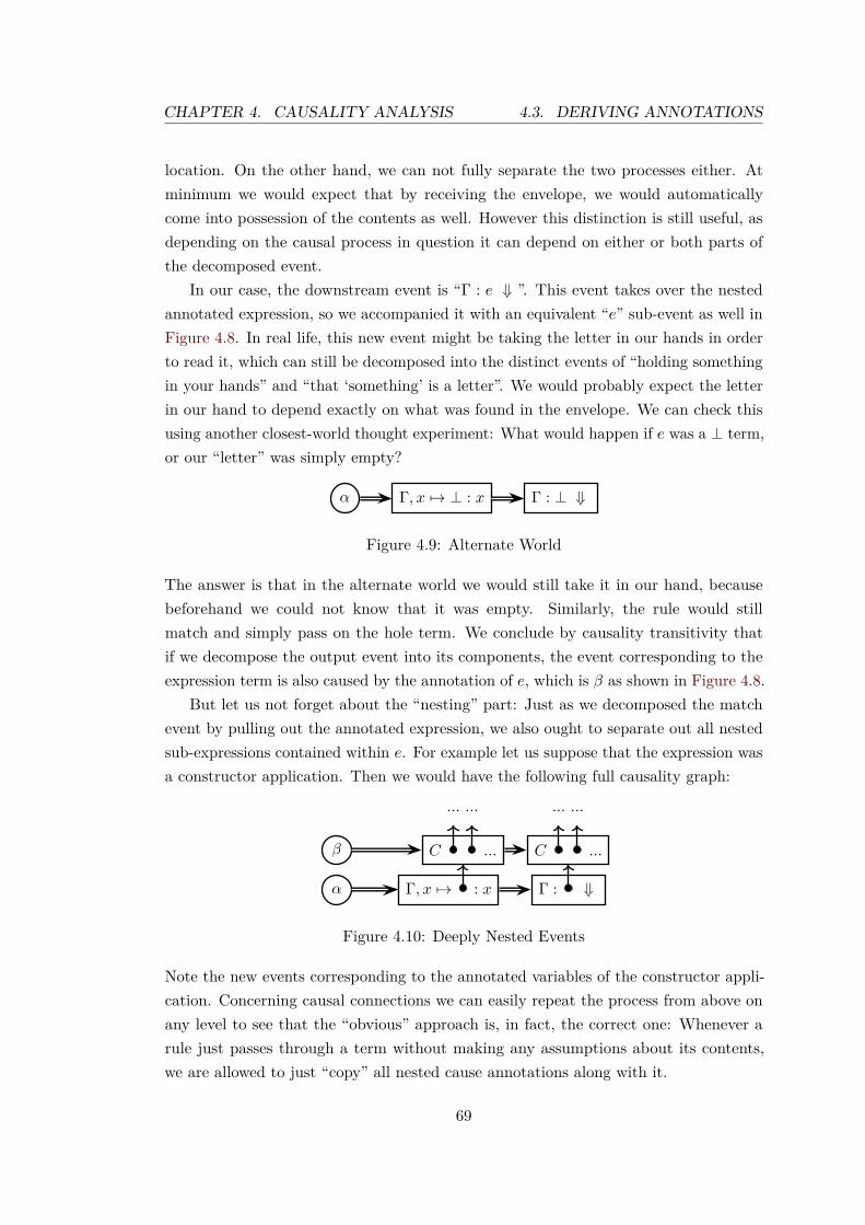
CHAPTER 4. CAUSALITY ANALYSIS 4.3. DERIVING ANNOTATIONS

location. On the other hand, we can not fully separate the two processes either. Atminimum we would expect that by receiving the envelope, we would automaticallycome into possession of the contents as well. However this distinction is still useful, asdepending on the causal process in question it can depend on either or both parts ofthe decomposed event.

In our case, the downstream event is “Γ : e ⇓ ”. This event takes over the nestedannotated expression, so we accompanied it with an equivalent “e” sub-event as well inFigure 4.8. In real life, this new event might be taking the letter in our hands in orderto read it, which can still be decomposed into the distinct events of “holding somethingin your hands” and “that ‘something’ is a letter”. We would probably expect the letterin our hand to depend exactly on what was found in the envelope. We can check thisusing another closest-world thought experiment: What would happen if e was a ⊥ term,or our “letter” was simply empty?

α Γ, x 7→ ⊥ : x Γ : ⊥ ⇓

Figure 4.9: Alternate World

The answer is that in the alternate world we would still take it in our hand, becausebeforehand we could not know that it was empty. Similarly, the rule would stillmatch and simply pass on the hole term. We conclude by causality transitivity thatif we decompose the output event into its components, the event corresponding to theexpression term is also caused by the annotation of e, which is β as shown in Figure 4.8.

But let us not forget about the “nesting” part: Just as we decomposed the matchevent by pulling out the annotated expression, we also ought to separate out all nestedsub-expressions contained within e. For example let us suppose that the expression wasa constructor application. Then we would have the following full causality graph:

β

α Γ, x 7→ : x Γ : ⇓

C ...

... ...

C ...

... ...

Figure 4.10: Deeply Nested Events

Note the new events corresponding to the annotated variables of the constructor appli-cation. Concerning causal connections we can easily repeat the process from above onany level to see that the “obvious” approach is, in fact, the correct one: Whenever arule just passes through a term without making any assumptions about its contents,we are allowed to just “copy” all nested cause annotations along with it.

69

4.3. DERIVING ANNOTATIONS CHAPTER 4. CAUSALITY ANALYSIS

In order to save space in event diagrams, we will notate this as follows:

α Γ, x 7→ e : x Γ : e ⇓

Figure 4.11: Deeply Nested Events Notation

Formally this means that we implicitly assume the existence of sub-events correspondingto all nested annotated terms. Furthermore, where there is a causal dependency betweentwo events mentioning the same annotations as shown above, the two implicit eventtrees should be seen as connected at every node.

Finally note once more that this only applies where a term simply gets passedthrough. Once we have an event that actually depends both on the contents as well asthe container this forces us to “merge” the causes. In our real-world example, actuallyreading a letter sent by post depends on both the letter as well as the contents at thesame time. For our cost semantics, this might be matching the constructor applicationrule:

β

α Γ, x 7→ : x Γ : ⇓ Γ : C ⇓

C ...

... ...

C ...

... ... ... ...

Figure 4.12: Depending on Nested Events

Note that there is a subtle difference between the events in the last two columns: Whilethe first event represents the evaluation of an arbitrary expression, which happens tobe a constructor application, the event on the right is the event of matching exactly aconstructor application.

4.3.5 Variable Rule

Let us recapitulate what we learned about the variable rule up to this point. We knowthat analogous to Section 4.3, all events depend on matching a variable expression inthe first place – if the event vanishes, so do all other events that come after it. On theother hand we know that e, θ and v get passed through no matter their value, thereforethe input events that bind them cause exactly the output events that use them. Thisespecially applies to nested events corresponding to annotated sub-terms.

Figure 4.13 shows the causal diagram with all the mentioned connections. Forillustration we have included one level of nested events corresponding to the values ofe and v. Note that the e expression has further nested annotations, therefore there

70

CHAPTER 4. CAUSALITY ANALYSIS 4.3. DERIVING ANNOTATIONS

Γ : e ⇓ · · · ⇓θ Γ′ : v

β Γ, x 7→ : x

e

⇓V ⇓···×S ⇓θ ⇓U Γ′, x 7→ : v

v

Figure 4.13: Causal Dependencies for a Variable Rule Match

are still more nested events here that we do not show. However, it is not hard toconvince ourselves that we have all causal connections covered: All three input eventsare connected to exactly the appropriate output events as outlined above, with nestedevents following along as required.

Let us now derive annotations. Note that we have very few annotations to choosefrom: We have identified e, θ and v as getting passed through, which means that wedo not need to reason explicitly about their annotations. Therefore the only half-wayinteresting cause term here is the match cause β, which needs to be annotated on alloutput terms. This yields us the following annotated rule:

Γ : e ⇓θ Γ′ : vΓ, x 7→ e : 〈β〉x ⇓〈β〉V+(3+lv(e))×〈β〉S+〈β〉U+〈β〉θ Γ′, x 7→ v : 〈β〉v

At this point it should not be too hard to see how this rule corresponds to the causalnetwork from Figure 4.13. However there are still two notable subtleties here. Let ustackle the easy on first: We are adding an β annotation on θ as well as the return event.Strictly speaking we would expect the output events of the nested rule match to alreadybe caused by our variable match. After all, the nested rule would have had no chanceto produce an output event if we had not passed it an expression to evaluate in the firstplace! Would this mean by transitivity that the θ cost input event is already caused byβ, making the annotation redundant?

While this is a completely valid point, this was exactly what we were talking aboutearlier in Section 4.2.1: For causal reasoning the judgement attempt is a precondition,therefore their cause is not reflected in annotations. We can think of this in terms ofscopes: Our nested rule match will only reason causally within its own scope (shownas a dotted rectangle) and expect the outer rule application to fill in the appropriatecause for the call on the return path. This is what we are doing when we put β on thereturned cost: We see terms leaving the scope, and therefore annotate it with what wesee as causing execution to enter the scope in the first place. This works naturally withour causal semantics rule – we just need to put an annotation on everything we returnno matter where it comes from originally.

71

4.4. HEAP CHAPTER 4. CAUSALITY ANALYSIS

4.4 Heap

However, there is a much more unpleasant issue with what we have not annotated inthe rule from the last section. Have a close look at the returned heap: We have notadded a β annotation on the value v when we put it back on the heap. In Figure 4.13we also neglected to connect the nested v event on the right-hand side with the variableexpression match event and therefore β. What is more, we also pass the heap Γ throughwithout modifying any annotations. Are we sure that all this is the right thing to do?

At this point it should have become a reflex to consult a Lewis-style closest-worldthought experiment. If the match did not happen, what heap would we expect to see?Comparing the answer against the original world should normally guide us to the effectswe are looking for with respect to the cause β. However, this time this tried-and-truerecipe leads us into big trouble. Consider that according to our rule the new heap isΓ′, x 7→ v, which means that we propagate any heap changes by the nested rule, as wellas adding our own update. The easiest alternate world might now be:

Γ : ⊥ ⇓⊥ {} : ⊥

This would have us conclude that every single surviving heap cell is direct effect of usapplying the rule. This is clearly going overboard, as it is pretty clear that the “default”behaviour for a rule is to not touch the heap at all.

Therefore we might propose:

Γ : ⊥ ⇓⊥ Γ : ⊥

Which means that we reduce the effects to all heap changes that happened during therule match. However, this especially includes every single thunk update that happenedin the meantime. If we took this viewpoint systematically, this would mean that athunk update would receive an annotation update from every single active rule match.This is clearly not in the spirit of the operational semantics – the whole point of lazyevaluation is that the location of thunk evaluation does not matter!

4.4.1 Laziness

Remember our goal with putting annotations on terms: Our intention is to track whateffects their respective values will have. Normally we have to assume that any changein a term can have arbitrarily complex consequences down the line due to transitivity.Yet for heap cells we actually happen to know that they only get updated in a veryspecific manner. Namely, thunks only get replaced exactly by their result value, whichwill be the same no matter at what point we decide to perform the evaluation.

72

CHAPTER 4. CAUSALITY ANALYSIS 4.4. HEAP

At this point we have run into the transitivity issue introduced in Section 2.3.5 onpage 18: By being too greedy about identifying our effects we end up overestimatingthem. We should not ask whether having Γ′, x 7→ v constitutes a heap change, butwhether the update ultimately causes a change in the program’s behaviour. If ourintuition is correct, this viewpoint will yield us much more sensible results.

Let us then consider a somewhat different thought experiment. Imagine that in aworldW ′ we successfully matched the variable rule, but this time miraculously neglectedto perform a heap update:

Γ0 : e ⇓θ Γ1 : vΓ0, x 7→ e : x ⇓V+(3+lv(e))×S+U+θ Γ1, x 7→ e : v

How would things differ from the events in our original world? Where should we lookfor the effects? Fortunately, we can easily isolate where the first effects will appear:Of all rules from our semantics in Figure 3.4 on page 55, the (Var) rules are the onlyones to ever read a heap cell. Furthermore, the (Let) rule is careful to never overwriteexisting heap cells by using fresh names. We can conclude that the evaluation inW ′ willremain virtually the same until exactly the point where the expression x gets evaluatedthe next time. Unfortunately, this re-evaluation might then have further side-effects onprogram state 4. After all, repeated evaluation might spawn new thunks, which mightin turn cause even more repeated evaluations!

4.4.2 Set-Up

Let us prove that if we miraculously forget heap updates like this, it will have no“material” effect on program execution. This property would absolve us from puttingan annotation on e in the above example, as well as any other updated heap cell onΓ1. So what would such an effect look like? As per Lewis, we are looking for changesin the alternate world W ′. More specifically, we want events that happen in W butdo not happen in our alternate world W ′. It is important to note that do not careabout additional events in W ′, as for performance analysis we are only interested inevents that happen in W . In the nomenclature of Taylor [1993], we only track positivecausation. It is a good idea to keep this in mind, as duplicated thunk evaluations aregoing to generate quite a few extra events in W ′.

Furthermore, even events that exist in both W and W ′ will not look exactly thesame: After all, we might evaluate more (Let) expressions in W ′, which means thatwe will also see more names freshly generated. And while we expect these names torefer to heap cells that have an equivalent in W , this still forces us to start reasoning interms of equivalence. Let us assume that we have a partial function f mapping variable

4As Marlow and Peyton Jones [2011] remark, laziness ironically causes plentiful side-effects.

73

4.4. HEAP CHAPTER 4. CAUSALITY ANALYSIS

W

(Var2)

eval (Var1)

W ′

(Var2)

eval (Var2)

repeat

[Part 1]

≡f

≡f

[Part 2]

Figure 4.14: Laziness Transparency Proof Overview

names from W to either the name of their clone in W ′ or ⊥ otherwise. Then we defineequivalence on expressions as follows:

x ≡f x′ where x = x′ or f(x) = x′

C x1... ≡f C x′1... where x1 ≡f x′1, ...λy.e ≡f λy.e′ where e ≡f e′

e x ≡f e′ x′ where e ≡f e′ and x ≡f x′

let {xi = ei, . . . } in e ≡f let {xi = e′i, . . . } in e′

where ei ≡f e′i, e ≡f e′, ...case e of {C xij ...→ ei; . . . } ≡f case e′ of {C xij ...→ e′i; . . . }

where e ≡f e′, ei ≡f e′i, ...

and equivalence on heaps along the same lines:

Γ, x 7→ e ≡f Γ′, x 7→ e′ where Γ ≡f Γ′, e ≡f e′ and f(x) 6∈ ΓΓ, x 7→ e ≡f Γ′, x 7→ e′, f(x) 7→ e′′ where Γ ≡f Γ′

and{

e ≡f e′ or e ≡f e′′ if e whnfe ≡f e′ and e ≡f e′′ otherwise

{} ≡f {}

Take note how we treat duplicated heap cells for the W ′ heap: Neither copy is allowedto be further evaluated than the original, and if the original world sees the expressione in weak normal form, at least one of the copies must be evaluated as well.

74

CHAPTER 4. CAUSALITY ANALYSIS 4.4. HEAP

As shown in Figure 4.14, our proof will consist of two parts: First we need to showthat until we evaluate one of the “duplicated” variables from f , evaluation inW andW ′

will proceed in lock-step: All events that happened in W should find their equivalentin W ′. However once we hit one of the duplicated variables, our task changes: Atthis point the original world W will simply return the result, whereas W ′ repeats theevaluation. As there are no equivalent events inW we do not care about how duplicatedevaluation in W ′ looks like, but we need to prove that we arrive at an equivalent returnvalue and heap in order to resume synchronised evaluation.

4.4.3 Proof Part 1

Due to the nature of reasoning about evaluation using nested rule matches, both partsof the proof will take the form of an induction over the rule match tree. Assume thatwe have a mapping f and two rule matches in W and W ′ respectively:

Γa : e ⇓θ Γb : v and Γ′a : e′ ⇓θ′ Γ′b : v′

with Γa ≡f Γ′a and e ≡f e′. Our induction assumption is that we will be able to builda new refined mapping g with g(x) = f(x) where f(x) 6= ⊥ such that Γb ≡g Γ′b andv ≡g v′. Note that this implies Γa ≡g Γ′a and e ≡g e′. We can prove this trivially if ehappens to be a constructor or lambda expression: We know due to e ≡f e′ that wemust find an equivalent expression in W ′, and the structure of the rules allows us tosimply set the new mapping g = f to obtain Γb ≡g Γ′b and v ≡g v′.

However things gets slightly more complicated for other rules. Suppose we find anapplication expression in W :

Γa : e ⇓θf Γb : λy1.λy2....eb Γb : eb[xi/yi · · · ] ⇓θb Γc : vΓa : e x1 x2 · · · ⇓...+θf+θb Γc : v

Again we know that in W ′ we must also have encountered an equivalent applicationexpression, and that Γa ≡f Γ′a and especially e ≡f e′. Therefore it follows by inductionthat we can obtain a new mapping g from the nested rule match, with Γb ≡g Γ′band λy1.λy2....eb ≡g λy1.λy2....e

′b. As this implies eb ≡g e′b and we know that g is

constructed such that xi ≡g x′i it follows that eb[xi/yi] ≡g e′b[x′i/yi] 5. Using ourinduction assumption on the second nested rule match now yields us a final mapping h,which must satisfy Γc ≡h Γ′c and v ≡h v′, which is exactly what we need to be finishedwith this case.

5Note that this is only true if the substitution never changes a name bound by a lambda, letexpression or case expression. This has been proven by Sestoft [1997, section 2.5].

75

4.4. HEAP CHAPTER 4. CAUSALITY ANALYSIS

For let expressions we would have the following W judgement:

Γa, yi 7→ ei[yi/xi, ...], ... : e[yi/xi, ...] ⇓θl Γb : vΓa : let {xi = ei, ...} in e ⇓...+θl Γb : v

As before we will have an equivalent W ′ expression of the form let {xi = e′i, ...} in e′.With no loss of generality we assume that in both W and W ′ we choose the same freshvariables yi to refer to the allocated heap cells. As we also know that the xi will be thesame in W and W ′ it follows trivially that e[yi/xi] ≡f e′[yi/xi]. As this extends to theheap cells we also have Γa, yi 7→ ei[yi/xi, ...], ... ≡f Γ′a, yi 7→ e′i[yi/xi, ...], ..., at whichpoint our hypothesis follows from the induction assumption.

Up to this point tackling rules has been pretty mechanical, as we have of coursedeliberately defined equivalence so terms can only differ in variable names. The mostinteresting part of this proof is actually, again, the variable evaluation rule. Let ussuppose we find the variable in question unevaluated in W . This would prompt us tomatch the (Var2) rule:

Γa : e ⇓θ Γb : vΓa, x 7→ e : x ⇓...+θ Γb, x 7→ v : v

As before we must also encounter a variable expression in the alternate world. However,due to duplication we can find two distinct concrete variables x′ in W ′: The choice isbetween x′ = x and x′ = f(x). However, it follows directly from Γa ≡f Γ′a that neithercan be evaluated on Γ′a. To be specific, we know that we will find an unevaluated thunke′ with e ≡f e′. Therefore we can again conclude by induction that the nested rulematches will yield us a new mapping g complete with new heaps Γb ≡g Γ′b and resultv ≡g v′. If we recall our heap equivalence definition, it is also not hard to convinceourselves that both Γb, x 7→ v ≡g Γ′b, x 7→ v′ as well as Γb, x 7→ v ≡g Γ′b, f(x) 7→ v′ holds,therefore we have heap equivalence no matter whether we have x′ = x or x′ = f(x).

Things start to diverge a bit more if the heap cell happens to be evaluated in W .This would prompt us to match the (Var1) rule:

Γ, x 7→ v : x ⇓V+S Γ, x 7→ v : v

It is easy to prove that the desired properties hold if we assume that the variable inquestion is also evaluated in W ′. However this is not guaranteed, as the prior (Var2)rule match only ever updates one of x or f(x) in W ′. This means that the x′ heap cellmight turn out to not be evaluated, which matches (Var2) in W ′:

Γ′a : e′ ⇓θ′ Γ′b : v′

Γ′a, x′ 7→ e′ : x′ ⇓...+θ′ Γ′b, x′ 7→ v′ : v′

76

CHAPTER 4. CAUSALITY ANALYSIS 4.4. HEAP

4.4.4 Proof Part 2

This is the interesting spot: Matching a different rule means that the histories ofW andW ′ are going to differ at this point. Our goal is to show that we can restore lock-stepevaluation between the two worlds in a way that satisfies our notion of equivalence.First note that we know at this point that world W must have seen a (Var2) rule matchon x in the past. This is because we know that only let expressions add new bindingsto heap, so even if it added a binding in normal form to the heap, it would be in normalform in both W and W ′, making it impossible for the (Var2) to ever match it. Hencethe heap cell must have seen an update at some point W ∗ in the past:

Γ∗a : e∗ ⇓θ∗ Γ∗b : vΓ∗a, x 7→ e : x ⇓...+θ∗ Γ∗b , x 7→ v : v

Even though this event might have happened at an arbitrary point in the past, there area few things we know: The variable matched must also have been x, and the evaluationresult must have been v, as no heap cell ever gets updated twice. A little less obviousis that we also have e∗ ≡f e′. This is due to fact that the only way an unevaluated e∗

expression could exist on the heap of W is due to a let expression binding it. At thatpoint we know that W ′ should bind x as well, so equivalence is guaranteed for x′ = x.And as we will see, we will later guarantee equivalence for when we bind f(x) as well.

Let us then get back to the duplicated thunk evaluation of e′. As mentioned earlier,this evaluation might spawn additional thunks, which we want to associate with the“original” bindings in W using our mapping f . We do this by – again – comparing therule match tree ofW ′ against what happened inW . Only this time we actually compareagainst a different part of W : The point of its history where it originally evaluated x.We will call this part W ∗ from now on to contrast it from the “present” events in W .This means that we see the W heap Γ as fixed for now and assume two parallel rulematches in W ∗ and W ′:

Γ∗a : e∗ ⇓θ∗ Γ∗b : v∗ and Γ′a : e′ ⇓θ′ Γ′b : v′

Again we know that we should have e∗ ≡f e′, and want to derive a new mappingg satisfying at least v∗ ≡g v. This time around we are treating the heap differentlythough: As it does not change in the original evaluation in W , we need to produce amapping g such that Γ ≡g Γ′a as well as Γ ≡g Γ′b. Or put in other words: Every newbinding we add in W ′ during this evaluation must be a duplicate of an existing bindingin W ∗. Note that we do not have any proof obligations regarding Γ∗a or Γ∗b .

We can prove this using a familiar strategy: Using induction we walk the rule matchtrees of W ∗ and W ′ in parallel, upholding our new induction assumption at every step.

77

4.4. HEAP CHAPTER 4. CAUSALITY ANALYSIS

This allows us to easily knock down variables, lambda as well as application expressions.Let us then assume that we encounter a let expression:

Γ∗a, yi 7→ e∗i [yi/xi, ...], ... : e∗[yi/xi, ...] ⇓θ∗l

Γ∗b : v∗

Γ∗a : let {xi = e∗i , ...} in e ⇓...+θ∗l

Γ∗b : v∗

Note that the induction proof in the first part of the proof covered the entire rulematch tree of W , and therefore especially the part that we now refer to as W ∗. Thismeans that back then we must also have added the yi bindings to the past heap in W ′.Consequently yi are no longer fresh in W ′, so we are forced to choose new names y′i. Inorder to track this duplication, we now need to perform our first update to the map,setting g(yi) = y′i and g(y) = f(y) otherwise. We know that f(yi) = ⊥ because let

expressions will remain the only instance where we update the map, and we will onlyever duplicate the evaluation of a let expression once. After all, an expression onlycan get evaluated twice if it a thunk in W , and heap equivalence guarantees that forevery thunk in W there can only be either one or two thunks in W ′.

The updated map establishes yi ≡g g(yi), so once again we have e∗[yi/xi] ≡ge′[g(yi)/xi] as well as e∗i [yi/xi] ≡g e′i[g(yi)/xi]. Furthermore, we know that updatingour heap does not violate equivalence, so we still have Γ ≡g Γ′a, g(yi) 7→ e′i[g(yi)/xi, ...]:In case Γ still maps yi to an unevaluated expression we know it to be e∗i [yi/xi], whichmust be equivalent to both the existing yi mapping in Γ′a as well as the new g(yi)mapping as established. On the other hand if yi is evaluated on Γ we have no furtherdemands to satisfy. Therefore the heap passed to the nested judgement satisfies ourinduction hypothesis, so we can obtain another mapping h for the nested rule matchsatisfying Γ ≡h Γ′b and v∗ ≡h v′, which is what we wanted to show.

However, we still have to take care of the variable rule. After all, our currentrepeated evaluation might spawn further repeated evaluations, which is why we areputting this much effort into this to begin with. We know due to expression equivalencethat where W ∗ has a variable term x∗ we will get a variable x′ in W ′, where eitherx′ = x∗ or x′ = g(x∗). Let us first consider the case that we find x′ to be alreadyevaluated on Γ′a:

Γ′a, x′ 7→ v′ : x′ ⇓V+S Γ′a, x′ 7→ v′ : v′

Note that we are now splitting up the cases by what we find in W ′, as that is moreconvenient in this instance. As we require that Γ ≡f Γ′a this means that x∗ must alsobe evaluated on Γ. Furthermore the value must be v∗, as both (Var1) and (Var2) returnthe value that was pushed on the heap Γ∗b , and as Γ was derived from it we knowthat the same value must still be present. Finally we know that v∗ ≡f v′ and triviallyΓ∗b ≡ Γ′b, which is our final proof obligation for this case.

This leaves only the case that the variable x′ happens to refer to a thunk in W ′,

78

CHAPTER 4. CAUSALITY ANALYSIS 4.4. HEAP

which would mean that we match the (Var2) rule instead:

Γ′a : e′ ⇓θ′ Γ′b : v′

Γ′a, x′ 7→ e′ : x′ ⇓...+θ′ Γ′b, x′ 7→ v′ : v′

Now we again have two cases: If the original-world variable x∗ also had to be evaluatedin W ∗, we can easily use the induction hypothesis to show that we can obtain a newmapping g with v∗ ≡g v′ and Γ′b ≡g Γ, from which we can easily follow through. Onthe other hand if x∗ turns out not to be evaluated, we use the same argument as wedid in part one: Clearly this is another duplicated evaluation, therefore we simply needto compare our current W ′ with another past evaluation W ∗∗. We would still reasonabout the same fixed W heap Γ, so our induction hypothesis would still apply eventhough we have switched out the concrete rule application tree.

It is clear that we can do this recursively: By always jumping to the appropriate pastevaluation point in W , we will always find a way to continue the induction. Especiallynote that we are always going backwards in the (finite) rule application history – so weare not attempting to inductively reason about an infinite tree here.

4.4.5 Wrapping Up

At this point we have set up all the most important ingredients to our proof. We justneed to plug a few holes to put everything together. First note that we have ignoredcase expressions so far, which are however straight-forward to add. More interestingly,we have left no place where we could introduce our “miracle” into the proof. In factdue to the lock-step evaluation between W and W ′, it might seem like we could notintroduce any change to W ′ at any point. This was deliberate, as this means that wecan now introduce it at an arbitrary point.

Let us assume that at some point in the first part of the proof, but have not yetencountered a duplication. This means that f(y) = ⊥ for all y, from which by inductionhypothesis follows that Γa = Γ′a and e = e′. Suppose the judgement will look like follows:

Γa : e ⇓θ Γb : v

Normally we would expect that we would derive the same heap Γb = Γ′b in both worldsas well. But now suppose that we choose an arbitrary binding x from the heap Γabefore evaluation and “forget” its update. If put as a rule, it would look like follows:

Γa;x 7→ e0 : e ⇓θ Γb, x 7→ e1 : vΓa;x 7→ e0 : e ⇓θ Γb, x 7→ e0, g(x) 7→ e1 : v

With g(x) fresh and g(y) = ⊥ otherwise. Note that additionally to forgetting about x,

79

4.5. INTERRUPTED RULES CHAPTER 4. CAUSALITY ANALYSIS

the g(x) binding now refers to an (inaccessible) copy of e1. This might seem like an oddchoice, but this trick means that for Γ′b = Γb, x 7→ e0, g(x) 7→ e1 we now have Γb ≡g Γ′b.As furthermore v ≡g v′ this means that we have not violated the induction hypothesis,which means that the rest of the proof remains valid. Therefore – as long as we startin the same state and introduce one miracle at maximum, we know that we can retainsynchronisation between the two worlds.

We demonstrate that W and W ′ proceed synchronously so we can argue about theunderlying events, which allows us to identify effects – or preferably the lack thereof. Theidea is that in part one we mapped every non-variable rule application in W to exactlythe same rule matching in W ′ and established that there is an equivalence relationbetween the used terms. As we explained in Section 4.2 on page 59 and Section 4.3.4on page 68, every rule match translates systematically to a set of events, therefore weknow that the arising events must be equivalent as well. The only exception is whenwe match (V ar1) in W , but (V ar2) in W ′, but even then we can easily see that (V ar1)produces strictly less events than (V ar2). Note that this is especially true for costevents: Contrasting the cost terms emitted by the two variable evaluation rules we seethat indeed V+S < V+(3+ lv(e))×S+U+θ. Note that this property is actually vitalfor this argument to work – if looking up heap values could possibly be more costlythan evaluation we would have positive causation of cost with the heap update!

The way this proof has worked out, we see that replacing a thunk by its normal-formevaluation result will never produce less costs 6. Therefore there are no effects left totrack, and we can safely omit annotations on updates such as the one in Section 4.3.5.Note that this is especially true if our rule match “inherits” the thunk update in questionfrom a nested rule match. Together with the annotation encapsulation property thatwe are going to show later in Section 4.7.1, this allows us to pass through updatedheaps from nested rule matches without the need for annotation updates.

4.5 Interrupted Rules

At this point we know how to annotate basic nested rules: Annotations are required onall results caused by the rule match, excluding heap updates. However, what happensif we have more than one nested rule match, such as with function applications? Recallfrom Figure 3.4 that we gave the following semantics:

Γ : e ⇓θf Γ′ : λy1.λy2....eb Γ′ : eb[xi/yi · · · ] ⇓θb Γ′′ : vΓ : e x1 x2 · · · ⇓A+(1+n+lv(e))×S+θf+θb Γ′′ : v

6Note that if we tracked residency costs as mentioned in Section 5.2.5 on page 120, there could bescenarios where keeping the normal-form result around is more expensive than reverting to the thunk.However, we regard these cases as too obscure to be relevant for profiling.

80

CHAPTER 4. CAUSALITY ANALYSIS 4.5. INTERRUPTED RULES

Γ : e x1 x2 · · · ⇓ ⇓A ⇓θf ⇓···×S ⇓θb Γ′′ : v

Γ′ : eb[xi/yi · · · ] ⇓ ⇓θb Γ′′ : v

Γ : e ⇓ ⇓θf Γ′ : λy1.λy2....eb

(nested)

(nested)

(top)

Figure 4.15: Ordered Event Decomposition of an Application Rule Match

The high-level view is that after matching the application e x1 x2 · · · we first evaluatethe function expression e, expecting a function body λy1.λy2....eb, nested inside anappropriate number of lambda terms. We then proceed to bind parameters by sub-stituting the variables in eb and evaluate the result to attain the result value, whichwe pass through. We can decompose this process into events as shown in Figure 4.15.Note that we want to be specific about the order in which costs appear: We assumethat constant costs happen first, and that we push the parameters on the stack beforejumping to the closure code. This will become important in a moment.

For causality analysis we now again ask how the events of the rule match could bedisrupted within the constraints of our language and judgement form. As highlighted inthe above rule, our rule makes two assumptions about the input events that could turnout to be false. First we assume again that the expression has the form we expect – afunction application. More interestingly, this time we also assume that evaluation of thefunction expression yields us a suitable lambda expression. All remaining input eventswill not cause the rule to mismatch, and therefore get passed through as explained inSection 4.3.2.

Let us consider the expression under evaluation first, as it comes first according toour temporal order. Once more we apply our basic recipe of substituting ⊥ for forcingan expression match failure in the alternate world W ′:

Γ : ⊥ ⇓⊥ Γ : ⊥

It might seem redundant to re-state this, but we need to remember that we alwaysselect this alternate world by choice. We will see in Section 4.6 on page 85 that for someexpression types it makes sense to choose differently. However, this time we obtain theusual result: all events vanish. We are left with a frozen program and the finding thatall later rule match events causally depend on the initial match happening.

81

4.5. INTERRUPTED RULES CHAPTER 4. CAUSALITY ANALYSIS

4.5.1 Miraculous Interruption

However, let us turn our attention to the point of interest for this rule: The effects of amismatch on the lambda value that supposedly results from evaluation. It might seemlike the type-checker should assure this property – at least ignoring termination – butas explained in Section 4.2, in alternate worlds we are working with miracle events thatare allowed to momentarily ignore such consistency requirements. In our case, whatwe want is another fresh world W ′′ where we did find a function application, yet thereturned expression magically turned out to not have the form λy1.λy2....eb. Againthere is nothing that would strongly suggest otherwise, so let our “miracle” be that thereturn value for some reason turns out to be “⊥”, causing the match to fail.

This leads to a small problem: When consulting Figure 3.4 we see that no rulewould match a result of ⊥. This is not surprising, as provoking a mismatch was thewhole point of this exercise. Accordingly, we would be forced to judge:

Γ : ⊥ ⇓⊥ Γ : ⊥

Yet there are strong reasons why we cannot accept this. Take note that this alternateworld judgement would eradicate all events shown in Figure 4.15, and therefore espe-cially events that precede the miracle result event in the temporal order. Therefore themiracle event has actual effects that lie in its own past, which we outlawed back inSection 4.2 on page 59.

So what can we do? We have to find some meaningful way to continue writing thestory of our alternate world W ′′. Let us think back a bit about how a real Haskellprogram might run through the motions in our alternate world W ′′: It would actuallyevaluate the body, triggering all associated events, proceed with pushing all requiredparameters, then attempt to jump to the sneakily placed non-closure and – presumably– crash. Or put in other words: All events prior to the failed match would happen,but none of the events after that point. Not coincidentally, this also happens to bethe minimal solution satisfying our requirements for causality reasoning. We thereforepropose the following additional rule for W ′′ as the closest-possible description of thelast breaths of our crashing program7:

Γ : e ⇓θf Γ′ : ⊥Γ : e x1 x2 · · · ⇓A+(1+n+lv(e))×S+θf+⊥ Γ′ : ⊥

Consequently, we conclude that the successful match in the original world W causesexactly all rule events to happen that come after it in the temporal order.

7The argument would be cleaner using small-step semantics, as they correspond more closely withthe sketched program behaviour. However, this would make working with the semantics harder overall,so we choose this path instead.

82

CHAPTER 4. CAUSALITY ANALYSIS 4.5. INTERRUPTED RULES

α

βi

Γ : e x1 x2 · · · ⇓ ⇓A ⇓θf ⇓···×S ⇓θb Γ′′ : v

Γ′ : eb[〈γ〉xi/〈γ〉yi · · · ] ⇓ · · · ⇓θb Γ′′ : v

Γ : e ⇓ · · · ⇓θf Γ′ : λy1.λy2....eb

Figure 4.16: Causal Relations for an Application Rule Match

4.5.2 Application Rule

At this point we have collected enough information to complete our picture of the causalrelationships within the application rule. The result is shown in Figure 4.16: We havefive “input” event types that can fail due to outside influences and variously cause five“output” events that are visible to the rule caller. We can summarise as follows:

Cause Input Event Causal Relationship

α Γ : e x1 x2 · · · ⇓ X X X X X

⇓θf X

Γ′ : λy1.λy2....eb X X X

⇓θb X

Γ′′ : v X

Output Events: ⇓A ⇓θf ⇓...×S ⇓θb Γ′′ : v

βi

Figure 4.17: Summary of Causality Relations

We observe that in two instances input events are required for the rule to continue atall, while the remaining causes just represent terms getting passed through accordingto Section 4.3.2 on page 66. We see the profile events as representing all cost eventsemitted by the first and second nested rule match respectively.

Let us get back to the original question: Exactly what annotations should we put onthe terms represented by the “output” events? We know the causes that were annotatedon the input terms, so we apply the transitive property: If what caused the input event

83

4.5. INTERRUPTED RULES CHAPTER 4. CAUSALITY ANALYSIS

“Γ : e x1 x2 · · · ⇓ ” is described by the cause term α, then according to our causalitydiagram this is exactly the cause term we should, say, annotate on the A unit of costemitted, yielding 〈α〉A. Along the same lines we need to annotate the cause on all costgetting passed through in θf , which we would notate as 〈α〉θf .

The rest of the output events have a causal dependency with the lambda resultcoming from the evaluation of the function expression. Especially note that the pattern“Γ′ : λy1.λy2....eb” matches the expression deeply, as we need to substitute all boundvariables in order to proceed with evaluation. As explained in Section 4.3.4 on page 68this means that we are actually looking through a number of annotations, which meansthat we are actually reasoning about a number of causes at the same time:

?...

β2

β1 Γ′ : λy1. Γ′ : λy1.λy2. ⇓ Γ′ : [xi/yi · · · ] ⇓

λy2.

eb

...

ebeb eb

Figure 4.18: Depending on Deeply Nested Annotations

Only once we have looked through enough lambda terms we reach an the term eb whichour rule does not have a causal dependency on anymore. In order to annotate thecomposite cause in a compact way, we will be making use of the following notation:

β1 ∧ β2 ∧ ... =∧i

βi =: βi

Furthermore note that for the variable substitution we used the eb[〈γ〉xi/〈γ〉yi · · · ] syntaxin Figure 4.16. This simply means that instead of copying the entire tree of sub-eventsas explained in Section 4.3.4 on page 68, we perform the given substitution on the way.As we retain annotations, events are still in a causal relationship even after variablesubstitution.

All this allows us to finish up the annotated application rule:

Γ : e ⇓θf Γ′ : 〈β1〉λy1.〈β2〉λy2....eb Γ′ : eb[〈γ〉xi/〈γ〉yi · · · ] ⇓θb Γ′′ : vΓ : 〈α〉(e x1 x2 · · · ) ⇓〈α〉A+(1+n+lv(e))×〈α〉S+〈α〉θf+〈αβi〉θb

Γ′′ : 〈αβi〉v

Just like when we settled on the annotated variable rule in Section 4.3.5 on page 70,most annotations again get passed around implicitly. The only annotations that weneed to mention are the ones that correspond to actual mismatch events, which in ourcase are α and βi respectively.

84

CHAPTER 4. CAUSALITY ANALYSIS 4.6. CLOSEST WORLD CHOICE

4.6 Closest World Choice

The last sections should have demonstrated that reasoning about causality is oftenabout choosing the right viewpoint amongst several possible options. Our goal is alwaysto find a way to see things that allows the sharpest diagnosis, meaning that we nameas few effects as possible that could just be chalked up as happening independent oftheir supposed cause. In this section we will approach another instance where it paysto take a fresh look at how we derive causality. Specifically, we will be looking for agood way to annotate the let rule:

Γ, yi 7→ ei[yi/xi, ...], ... : e[yi/xi, ...] ⇓θ Γ′ : vΓ : let {xi = ei, ...} in e ⇓∑(S+O(xi=ei))+θ Γ′ : v

On the surface, nothing here is too surprising: We are passing a number of terms to anested rule match. As before, we would normally look for effects at the point where therule generates its output events, comparing it against a world where we got a ⊥ termin place of the let expression, yielding the familiar “crash” judgement in W ′:

Γ : ⊥ ⇓⊥ Γ : ⊥

Following this line of reasoning, we would again put annotations on every single costas well as the result value. But is that the right thing to do?

Note that all rules up to this point had heavy influences on the control flow of theprogram. The let expression on the other hand is primarily concerned with updatingthe heap, and barely touches the expression e, value v and cost θ as they pass through.After all, the primary objective of this expression is updating the heap, and at whatpoint we do this does not actually matter too much in the grand scheme of things. Infact, optimising compilers often exploit this property by allowing let bindings to “float”freely within the optimised expressions [Peyton Jones et al., 1996]. We saw an examplefor this back in Section 3.4.2.

So could we find a way to have the program degrade more “gracefully” in thepresence of our miracle? Would it, say, make sense to just “float” the let binding intonothingness and evaluate only its body in its stead? This would make our miraculousrule match “Γ : e ⇓ ”, ideally yielding a new W ′′ judgement of the form:

Γ : e ⇓θ Γ′ : v

This judgement means that we attempt to match the same rule(s) inW ′ that the nestedjudgement in the (Let) rule originally did inW . The only difference is that our alternateworld lacks all the bindings introduced by the let expression. Obviously this might

85

4.6. CLOSEST WORLD CHOICE CHAPTER 4. CAUSALITY ANALYSIS

cause the program to crash at a point further down the line, as leaving free variablesun-renamed deliberately breaks the consistency of the semantics given by Sestoft [1997].Yet the crash is not guaranteed – the new world W ′ might see the program continuenormal operation for some time longer, and possibly even terminate. Therefore our newdefinition of W ′ is actually closer to the original world W than an immediate programcrash, and therefore preferable according to Lewis’ causality model.

4.6.1 Floating Effects

Let us be a bit more formal about this. We will have W as the original world and W ′

as our first alternate world where we simply have the program crash immediately whenattempting the (Let) rule match in question. On the other hand, W ′′ will be our newalternate world where we simply evaluate the body instead of the full let expression.Our claim is that W ′′ has as least as many events in common with W as W ′, and cantherefore plausibly be described as “closer”. Note that this is actually not a particularlyhard requirement to fulfil: The rule mismatch in W ′ will cause parent rule matches tofail, which as we already noted back in Section 4.3 on page 64 pretty much means thatno further events are happening. From that point of view, the miracle event is the lastactual event happening in W ′. It follows that if W ′′ can possibly reproduce any Wevent past the miracle event, we have already shown the above-mentioned property.

Having said that, we are actually very interested in exactly how far we can make Wand W ′′ match up: After all, this determines the effects and therefore the annotations.To do this we first need to recognise that due to skipping the renaming step W ′′ willhave different variable names compared to W . So again we have to employ a notionof event equivalence. Fortunately we can simply use the same equivalence operator ≡fwe used back in Section 4.4.2, except this time we set the mapping function upfront asexactly f(yi) = xi. We also define heap equivalence as follows:

Γ, y 7→ e ≡f Γ′, y 7→ e′ where Γ ≡f Γ′, e ≡f e′

Γ, y 7→ e ≡f Γ′ where f(y) 6= ⊥{} ≡f {}

Capturing that we expect the y bindings to be gone in W ′.Let us then do another induction over the rule match trees of W and W ′′ in parallel.

Our current judgements will be Γa : e ⇓θ Γb : v in W and Γ′′a : e′′ ⇓θ′′ Γ′′b : v′′ inW ′′, with the assumptions being Γa ≡f Γ′′a and e ≡f e′′. What we want to prove is thatwhere a rule matches we get a new heap Γb ≡f Γ′′b and value v ≡f v′′. Note that wedo not require the rule match to succeed in W ′′, as any possibly successful rule matchwould already mean more events happening than in W ′.

86

CHAPTER 4. CAUSALITY ANALYSIS 4.6. CLOSEST WORLD CHOICE

We can easily see this for either a constructor or a lambda expressions in W , forexample: Due to equivalence we encounter the same type of expression in W ′′, and theequivalence of input terms directly proves that all result terms must be equivalent aswell. The remaining rules from Figure 3.4 need a bit more consideration. Let us runthrough them once more, starting with the application rule:

Γ : e ⇓θf Γ′ : λy1.λy2....eb Γ′ : eb[xi/yi · · · ] ⇓θb Γ′′ : vΓ : e x1 x2 · · · ⇓A+(1+n+lv(e))×S+θf+θb Γ′′ : v

If any of the nested rule matches fail, the rule itself fails. If we assume that they succeed,we can easily obtain eb ≡f e′′b . However, the important case here is that we might havef(xi) 6= ⊥ due to xi matching one of the yi variables from the removed let expression.What would happen is that the variable would be propagated into the nested rule matchexpression. Fortunately, this process establishes eb[xi/yi] ≡f e′′b [x′′i /y′′i ], so we know thatour induction hypothesis holds for the second nested rule match as well. From this itfollows directly that the assumption is true for the application rule match as well.

Let us continue with let expressions:

Γa, yi 7→ ei[yi/xi, ...], ... : e[yi/xi, ...] ⇓θ Γb : vΓa : let {xi = ei, ...} in e ⇓∑(S+O(xi=ei))+θ Γb : v

As usual equivalence ensures that W ′′ will encounter a let expression in the sameposition. As far as execution goes, there are two cases: Either we attempt to executethis let expression as normal in W ′′, or this rule application happens to be the onethat we want to miraculously ignore in order to study its effects. Let us tackle the lattercase first. As mentioned before we chose f so it satisfies f(yi) = xi, which means thatwe can directly conclude that e[yi/xi] ≡f e′′. As we also defined heap equivalence toignore the yi cells it also follows that Γa, yi 7→ ei[yi/xi, ...], ... ≡f Γ′′a 8. This means byinduction that we also have Γb ≡f Γ′′b and v ≡f v′′, which is all we need to prove here.

In the case that this is not the location of our miracle, we know due to variablenormalisation (see Section 3.5.1) that our xi variable names cannot match any ofvariables bound by of the removed let expression, which means that we will find ourxi variables in the same positions in e and e′′ as well as ei and e′′i respectively. If weagain assume without loss of generality that we chose the same fresh variables yi in WandW ′′ it easily follows that e[yi/xi, ...] ≡f e′′[yi/xi, ...] and ei[yi/xi, ...] ≡f e′′i [yi/xi, ...].This allows us to derive from the induction hypothesis that again we either propagatea failed rule match, or we get Γb ≡f Γ′′b and v ≡f v′′.

8Note that we actually know that e = e′′ and Γa = Γ′′a , as prior evaluation must have been unchanged.But we do not need this property at the moment.

87

4.6. CLOSEST WORLD CHOICE CHAPTER 4. CAUSALITY ANALYSIS

We can argue very similarly for the case expression:

Γa : e ⇓θ2 Γb : Ci yj ... Γb : ei[yj/xj , ...] ⇓θ3 Γc : vΓa : case e of {Ci xj ...→ ei, ...} ⇓E+n×S+θ2+θ3 Γc : v

Again a nested rule match fail would cause us to propagate the failure. Thus thescrutinee must evaluate to equivalent values Ci yj ... ≡f Ci y′′j ..., from which we gatherthat yj ≡f y′′j and therefore ei[yj/xj , ...] ≡f e′′i [y′′j /xj , ...]. As we also know Γb ≡f Γ′′b wecan easily obtain v ≡f v′′ as well as Γc ≡f Γ′′c . Note that we will have to update thisreasoning later due to changed failure propagation in Section 4.6.6.

So far we have simply propagated the renaming and never actually accessed theheap, which is why evaluation proceeded as normal. This makes it quite plausible thatwe will have more events in W ′′ than in W ′. However, we are still violating programconsistency in a major way, which shows for the variable evaluation rules:

Γ, x 7→ v : x ⇓V+S Γ, x 7→ v : v Γa : e ⇓θ Γb : vΓa, x 7→ e : x ⇓V+(3+lv(e))×S+U+θ Γb, x 7→ v : v

For both rule we have two cases: Either we are trying to access a variable with f(x) = ⊥,which means that x = x′′ and therefore evaluation in W ′′ either yields v ≡f v′′ asexpected or crashes due to the a failed rule match in the nested evaluation.

On the other hand, where f(x) 6= ⊥ we must have x′′ = f(x) 6= x due to the fact thatwe chose the variable name x fresh in W when evaluating the removed let expression,and especially never introduced it into W ′′. We also know that there can be no bindingfor f(x) on the heap Γ′′a. This is because even if we (say) had re-evaluated the let

expression that we skipped the first time, it would have chosen a fresh variable nameinstead of f(x), as f(x) here is just the original variable name from the program text.This means that neither (Var1) nor (Var2) can match in W ′′, so we have to assume amismatch judgement. Therefore our program crashes in W ′′ as well:

Γ′ : ⊥ ⇓⊥ Γ′′ : ⊥

4.6.2 Floating Annotations

The last section has shown that compared to the immediate crash in alternate worldW ′, the program can plausibly continue to run in W ′′. Not only that, but we actuallyknow that the evaluation in W ′′ will be equivalent to that in W exactly up to the pointwhere we try to access one of the variables that we “forgot” to push the bindings for.From this it follows that we will have equivalent events in the alternate world as well.In the end, this means that we have a number of events that happen after the matchon the let expression without causally depending on it!

88

CHAPTER 4. CAUSALITY ANALYSIS 4.6. CLOSEST WORLD CHOICE

This is the first evaluation rule where we could derive this property, a direct resultof us always comparing against an alternate world W ′ with a total program crash. Thisespecially means that we cannot just use the same annotation strategy as before. Afterall, now the effects are not isolated “structurally” anymore: As heap references canescape, access to a given heap cell might happen at an arbitrary point of programexecution. As this is where our effect is, we will have to find a way to introduceannotations at exactly these points.

Fortunately, visiting all usage sites of a variable is exactly what the semantics bySestoft [1997] already do, even though its original purpose is to rename variables. Nowwe can re-use this mechanism for our benefit and put annotations on all variables thatwe know would cause history to diverge in W ′′:

Γa, yi 7→ ei[〈αγ〉yi/〈γ〉xi, ...], ... : e[〈αγ〉yi/〈γ〉xi, ...] ⇓θ Γb : vΓa : 〈α〉let {xi = ei, ...} in e ⇓∑(〈α〉S+〈α〉O(xi=ei))+θ Γb : v

Similar to how we treated substitution in Section 4.5.2, the notation e[〈αγ〉y/〈γ〉x] meansthat we replace the variable while adding the annotation α. This captures the basic factthat in order for the variable expression to evaluate correctly it needs to both exist aswell as have an associated binding. Note especially that the substitution is not limited tomatching variable expressions, but will also add annotations when substituting variablesin constructor or function applications, from where they will get propagated to theactual variable usage sites where appropriate.

Finally, we have to recognise that there is actually another notable difference betweenW and W ′′. Namely, the original world has to pay the cost for allocating heap andstack space for the new bindings, which the alternate worldW ′′ skips. This makes thesecost events effects of the let expression even for our refined alternate world thoughtexperiment, which is why they were annotated with α above. In the end, the jump toW ′ has still provided us with a much tighter causality tracking than we had before.

4.6.3 Case Expressions

Can we repeat this trick with other rules? The only rule from the cost semantics inFigure 3.4 left to cover is the (Case) rule:

Γa : e ⇓θ2 Γb : Ci yj ... Γb : ei[yj/xj , ...] ⇓θ3 Γc : vΓa : case e of {Ci xj ...→ ei, ...} ⇓E+n×S+θ2+θ3 Γc : v

The straight-forward approach here would be to compare with alternate worlds wherethe program crashes either because of a mismatch on the case expression or because wedid not get a constructor back from evaluating the scrutinee. After all, we have alreadylearnt from our discussion of the application rule in Section 4.5.1 how do deal with such

89

4.6. CLOSEST WORLD CHOICE CHAPTER 4. CAUSALITY ANALYSIS

interruptions in the middle of a rule application. Selecting all events that come afterthe mismatch for annotation, we obtain the general annotated case evaluation rule:

Γa : e ⇓θ2 Γb : 〈β〉Ci yj ... Γb : ei[yj/xj , ...] ⇓θ3 Γc : vΓa : 〈α〉case e of {Ci xj ...→ ei, ...} ⇓〈α〉E+〈α〉θ2+ni×〈αβ〉S+〈αβ〉θ3 Γc : 〈αβ〉v

Just as with the let expression, this conservative annotation strategy is valid – but notalways optimal.

4.6.4 One-Branch Case

Let us attempt to improve the accuracy of our causality analysis. Ideally, we wouldlike to again find a world W ′′ that is closer to the original world W in that we have acloser match between events. However, this is not quite as obvious here. After all, oneimportant factor in our treatment of let was that we knew that its let body wouldget evaluated no matter what. We can not generally do the same for case expressions,as we might have a number of branches that evaluation could possibly follow9.

But what about case expression that only have one alternative? Consider a rulespecialised to this scenario:

Γa : e ⇓θ2 Γb : C1 yj ... Γb : e1[yj/xj , ...] ⇓θ3 Γc : vΓa : case e of {C1 xj ...→ e1} ⇓E+n×S+θ2+θ3 Γc : v

Here we have picked out the situation where the control flow is the most predictable:That scrutinee evaluation produces the expected constructor is enough to guaranteethat the highlighted evaluation will occur. And as we are reasoning about the originalworld, in which we assume that we have a terminating program, this is actually anassumption that we are allowed to make. Note that this applies even if C is not theonly constructor of the type in question, as the compiler guarantees that branches coverall possible values. Suppose the following Core code:

let {x = ...} in

case x of {C → ...

D y → case x of {D y2 → e1}}

The inner case expression has only one branch precisely because the compiler couldderive that evaluation can only yield a D constructor. Therefore as long as the scrutineeevaluation terminates, we positively know that e1 is going to get evaluated.

9It would be thinkable however to elect a “default” branch to follow in the alternate world. Thiswould for example allow us to reason about a case expressions branching out specific cases such as inListing 2.5 on page 17. However, it is hard to identify such an intention, see Section 4.7.3 on page 97.

90

CHAPTER 4. CAUSALITY ANALYSIS 4.6. CLOSEST WORLD CHOICE

Consequently it actually makes sense to treat e1 as the alternate-world replacementfor the case expression in W ′′. We would attempt the following judgement:

Γa : e1 ⇓θ′′3 Γ′′c : v′′

Just like with the let rule, we will attempt to match rules while leaving xi bindings ine1 undefined. Therefore we might get a crash at some point down the road. Howeveras we have seen in Section 4.6.2, this does not need to scare us, as we can easily findand annotate these effects using variable substitution.

On the other hand, we are skipping more code this time around: After all, the rulewould normally also evaluate the scrutinee. This not only means that the alternateworld W ′′ loses the cost θ2, but also all heap changes between Γa and Γb. Fortunately,the former effect can easily be tracked by adding annotations on θ2, and the latter canonly introduce extra costs in W ′′ due to extra thunk evaluations. As we are looking forpositive causation, the non-existence of costs in W is not something we need to track10.

4.6.5 Skipping Scrutinisation

So far we have only looked at the effects of matching the one-branch case expression.However as explained back in Section 4.5.1, having two nested sub-matches means thatwe need to investigate the possibility that the rule might mismatch half-way through.To be concrete, we have to account for the alternate-world scenario where we encounterthe case expression intact, but scrutinee evaluation miraculously does not match theexpected C1 yj ... pattern. As before this means that we need to introduce an artificialrule that describes how we suspect the program would react to having the scrutineeresult get miraculously replaced by ⊥. If we just kept the events that temporal orderforces, this would mean we get the following rule:

Γa : e ⇓θ2 Γb : ⊥Γa : case e of {C1 xj ...→ e1} ⇓E+n×S+θ2+⊥ Γb : ⊥

However, this is not satisfactory to us. After all, this means that we would again skipthe evaluation of the branch code. Consequently, we would have to annotate branchevaluation results with the cause for evaluation of the scrutinee. Obviously evaluationof the scrutinee will depend on the existence of the case expression. Therefore bytransitivity the case expression causes the branch evaluation, which is exactly what wewanted to disprove in the last section!

10Note that we could alternatively prove that these thunk evaluations “move” from the evaluation ofthe scrutinee to the evaluation of the branch body, similar to what we did in Section 4.4.4. However, thiswould mean that we would not want to annotate these thunk costs inside θ2. This would be impossibleto notate, so here it actually turns out to be more useful to think of the cost as “reappearing” insteadof “moving”. We will be seeing quite a bit of this distinction once we get to optimisations.

91

4.6. CLOSEST WORLD CHOICE CHAPTER 4. CAUSALITY ANALYSIS

To fix this situation, we need an artificial “crash recovery” rule like follows:

Γa : e ⇓θ2 Γb : ⊥ Γb : e1 ⇓θ3 Γc : vΓa : case e of {C1 xj ...→ e1} ⇓E+n×S+θ2+θ3 Γc : v

So we essentially react to the miraculous scrutinee result mismatch simply by fallingback to the same scenario we had before: The evaluation of the naked e1 branch. Inorder to uphold temporal consistency as introduced in Section 4.2 on page 59 we makesure that all previous events still happen, and especially pass on the cost θ2 originatingfrom the “blocked” scrutinee evaluation.

If we now put all the pieces together, we can obtain the result we wanted: Nomatter whether our miracle is the case expression disappearing or the scrutinee resultmismatching, the alternate world will still end up evaluating the branch until the firstusage site of a bound variable. Therefore all branch costs and results up to that pointare caused by neither. From this realisation we obtain an annotated one-branch case

rule:Γa : e ⇓θ2 Γb : 〈β〉C1 yj ... Γb : e1[〈αβγ〉yj/〈γ〉xj , ...] ⇓θ3 Γc : vΓa : 〈α〉case e of {C1 xj ...→ e1} ⇓〈α〉E+n×〈α〉S+〈α〉θ2+θ3 Γc : v

Note that in comparison to the previous formulation the αβ annotation has now movedfrom θ3 and v respectively to y

i, analogous to what happened when we discussed the

let rule in Section 4.6.2 on page 88.

4.6.6 Crash Recovery Consistency

While the conclusions might sit well with us, we have to take care that we are notintroducing inconsistencies into our causality model. After all, the very structure of theproposed crash recovery rule is worrisome: We are matching on a ⊥ result in order todo a second nested rule match. This violates the assumption that a failed child rulematch will always cause the parent rule match to fail. From the point of view of theevent model, our intention is clearly to have certain events to happen independentlyfrom others, but if we take the rule at face value we are actually proposing for eventsto happen as a reaction to other events not happening.

As a result we should critically review our argumentation up to this point forinconsistencies. Fortunately, we know that the artificial rule will only ever match inthe alternate world, as the original world will never see rule mismatches. Unfortunatelythough, we actually have encountered one scenario where we want to pass a ⊥ scrutineeevaluation result “through”. Specifically, when we were reasoning about the effectsof “forgetting” bindings in Section 4.6.1 we assumed that encountering an undefinedbinding would cause all further events to vanish. However, with our addition this isnow wrong – in the alternate world the program can now “come back from the dead”.

92

CHAPTER 4. CAUSALITY ANALYSIS 4.6. CLOSEST WORLD CHOICE

To understand how, consider the following Core fragment:

let {x = ...} in

case x of {D y → e}

Here the crash recovery rule will actually change the outcome of removing the x binding.After all, we would look for its effects by considering the following alternate-worldscenario:

case ⊥ of {D y → e}

Normally we would expect the evaluation of this to fail, which yields us to the conclusionthat the evaluation result of the program depends causally on x. However, with ourcrash recovery rule, this is not true any more: In the alternate world we would continueevaluating e, which might well end up producing the same result we had in the originalworld. Therefore the result now would not be an effect of x any more!

This change in interpretation means that we need to adapt our reasoning fromSection 4.6.1 on page 86. Back then we assumed that every rule application could eithercrash in the alternate world, or produce equivalent results. Now we have to acknowledgethe fact that at some point we could recover from a crash in W ′′:

Γ′′a : e′′ ⇓θ′′2 Γ′′b : ⊥ Γ′′b : e′′1 ⇓θ′′3 Γ′′c : v′′

Γ′′a : case e′′ of {C1 xj ...→ e′′1} ⇓E+n×S+θ′′2 +θ′′3 Γ′′c : v′′

while naturally encountering a normally evaluated case expression in W :

Γa : e ⇓θ2 Γb : C1 yj ... Γb : e1[yj/xj , ...] ⇓θ3 Γc : vΓa : case e of {C1 xj ...→ e1} ⇓E+n×S+θ2+θ3 Γc : v

Due to our induction hypothesis we know that Γa ≡f Γ′′a and e ≡f e′′. We can evenarrange e1[yj/xj , ...] ≡g e′′1 by deriving a new mapping function g from f with g(yj) = xj .However, note that we have no direct way for establishing Γb ≡f Γ′′b , as we have toassume that while in “limbo” W ′′ might have skipped thunk updates that happened inΓb. However, we can fix the proof by introducing a mapping from unevaluated bindingsin W ′′ to their evaluation in W , allowing us to argue that delayed evaluation in W ′′

yields the same results as in W . Therefore we have again at worst moved extra cost toa later point in W ′′, which we do not need to explicitly track. We have shown beforehow such a proof would work, and will skip the full explanation at this point.

In the end, once we have ironed out the inconsistency the obtained result is basicallythe same as in Section 4.6.1: The concrete “surviving” event set has changed, but theworld W ′′ is still closer to W than W ′. Furthermore, we can show that the new rulestogether propagate annotations exactly to the events that differ between W and W ′′.

93

4.7. CAUSALITY MODEL CHAPTER 4. CAUSALITY ANALYSIS

Γ : 〈α〉C x1 x2... ⇓〈α〉C+n×〈α〉H Γ : 〈α〉C x1 x2... (Con)

Γ : 〈α〉λy.e ⇓〈α〉L+lv(e)×〈α〉H Γ : 〈α〉λy.e (Lam)

Γ : e ⇓θf Γ′ : 〈β1〉λy1.〈β2〉λy2....eb Γ′ : eb[〈γ〉xi/〈γ〉yi · · · ] ⇓θb Γ′′ : vΓ : 〈α〉(e x1 x2 · · · ) ⇓〈α〉A+(1+n+lv(e))×〈α〉S+〈α〉θf+〈αβi〉θb

Γ′′ : 〈αβi〉v(App)

Γa, yi 7→ ei[〈αγ〉yi/〈γ〉xi, ...], ... : e[〈αγ〉yi/〈γ〉xi, ...] ⇓θ Γb : vΓa : 〈α〉let {xi = ei, ...} in e ⇓∑(〈α〉S+〈α〉O(xi=ei))+θ Γb : v (Let)

Γ, x 7→ v : 〈α〉x ⇓〈α〉V+〈α〉S Γ, x 7→ v : 〈α〉v (Var1)

Γ : e ⇓θ Γ′ : vΓ, x 7→ e : 〈β〉x ⇓〈β〉V+(3+lv(e))×〈β〉S+〈β〉U+〈β〉θ Γ′, x 7→ v : 〈β〉v

(Var2)

Γa : e ⇓θ2 Γb : 〈β〉C1 yj ... Γb : e1[〈αβγ〉yj/〈γ〉xj , ...] ⇓θ3 Γc : vΓa : 〈α〉case e of {C1 xj ...→ e1} ⇓〈α〉E+n×〈α〉S+〈α〉θ2+θ3 Γc : v (Case1)

Γa : e ⇓θ2 Γb : 〈β〉Ci yj ... Γb : ei[〈γ〉yj/〈γ〉xj , ...] ⇓θ3 Γc : vΓa : 〈α〉case e of {Ci xj ...→ ei, ...} ⇓〈α〉E+〈α〉θ2+ni×〈αβ〉S+〈αβ〉θ3 Γc : 〈αβ〉v

(CaseN)

Figure 4.19: Causality Model

4.7 Causality Model

At this point we have run through all rules of our performance model, with the resultingcausality model rules collected in Figure 4.19. We have added a good number of ofextensions and annotations to Launchbury’s original semantics, which might make thefull semantics a bit hard to follow. Yet when we look back, the analysis actually boileddown just a few basic principles:

• Every possible point where a rule could mismatch means that we need to puttheir annotation on terms that are produced “after” them.

• The only exceptions are cases where we can identify a better alternate world tocompare with. This has generally to do with bindings, the effects of which wetrack by attaching annotations to the variables.

• Heaps can get passed through freely, and in particular we can update thunkswithout annotating the cause for their evaluation.

This should make it easier to remember later on where exactly we expect annotationsto go. However, before we starting putting this model to work we still have a few looseends to tie up, which we will do in this section.

94

CHAPTER 4. CAUSALITY ANALYSIS 4.7. CAUSALITY MODEL

4.7.1 Annotation Encapsulation

If we look at the list of principles, the last one should stick out: We proved back inSection 4.4 on page 72 that we can update thunks freely, but obviously this is only onetype of change that we could observe on the heap. Let us shed some more light on this.Suppose that we have an arbitrary rule that gives us a judgement:

Γ1 : e ⇓θ Γ2 : v

to find its effects we have at various occasions used “crash” alternative judgements 11.This generally looked like follows:

Γ1 : e ⇓⊥ Γ1 : ⊥

Finding effects is now all about comparing the alternate world with the original, andas the heap stays the same in W ′, this comes down to comparing Γ1 with Γ2. Butwhat exactly constitutes a change here? Clearly heap cells that have the same value donot count. And as we have showed in Section 4.4, replacing a thunk by its value is no“material” change either, as the alternative would be simply re-computing it later.

Given the way that our operational semantics work, this actually covers all but onecase: What happens if a (Let) rule introduces a new binding on Γ2 that did not existon Γ1? Clearly this is no immaterial effect, as “forgetting” the binding might provokea program crash once the variable gets evaluated. However, now that we have finishedour causality semantics, we have actually new tools at our disposal: We argue that allpossible effects will already receive the appropriate annotation from other channels.

Specifically, note that we know that x must have been introduced by a (Let) rule,so it must be a fresh name. For our rule match, this means that the rest of the programcan only access the new heap cell if the return value v has a reference to it – eitherdirectly or indirectly. So suppose an alternate world where our rule miraculously doesnot crash, but returns ⊥ anyway. Then we know that the rest of the program has noway of accessing x, even if it still exists on the heap. Therefore the effects of the xheap cell are strictly fewer than that of returning v, which means that as long as weare consistent with tracking value effects, annotating v with the cause in question isactually enough 12. And as we can see in Figure 4.19, all of our rules generally add theirannotation on the result value, therefore “encapsulating” the heap reference. The onlytwo rules where this is not the case are let and one-branch case, where the differentalternate world does not require us to annotate in the first place.

11This generalises to “intermediate” crashes as explained in Section 4.5.1 on page 82 as well.12It might seem dangerous to rely on consistency while trying to establish consistency – yet in fact

either viewpoint is internally consistent, so we just choose the more intuitive one.

95

4.7. CAUSALITY MODEL CHAPTER 4. CAUSALITY ANALYSIS

Note that this situation bears some familiarities to the nested events we introducedin Section 4.3.4: There we remarked that nested events cannot normally “escape” theirparent event either. However, we have actually already broken this particular principle:In Section 4.6 we took sub-expressions of let and case expressions respectively andevaluated them without causal dependency on the parent expression. In the event model,this means that we actually “looked through” the annotation on the parent expression.Fortunately, there was never any reason to do this for values, or we might have a hardertime arguing here. This should demonstrate how reasoning about causality is all aboutinternal consistency.

4.7.2 Close Causes

Up to this point we have seen two example in Section 4.6.2 and Section 4.6.4 wherewe could make our causality analysis more exact by comparing against a tailor-madealternate world. A hypothetical optimal closest world is firmly outside of our grasp, asit would essentially solve the performance problem for us. But it still begs the question:Are there other – closer – worlds out there that we could use to further enhance theexpressiveness of our model?

Let us remind ourselves of the rule match “miracles” that we have used so far.Keeping in mind the two mentioned exceptions, we use the original-world expression eto chose the alternate-world expression e′ as follows:

e′ =

e1 where e = let {...} in e1

e1 where e = case ... of {...→ e1} with e1 sole branch

⊥ otherwise

It makes sense to limit ourselves to such replacement rules: After all, we ideally wantsmall miracles, and switching out a term by another is the kind of change that disturbsthe consistency of the system the least.

What makes a good replacement for the purpose of our operational semantics?As explained in Section 4.3.3 on page 67 every time we reference a term with nestedannotations this implies a whole tree of abstract events, each corresponding to a certainpart of the expression having a certain form. If we want to study effects of the causeannotated on the top-level, this means that our primary task is eliminating the top-levelevent while maintaining consistency. If we find that we can do this without eliminatingnested events, this means that we can view them as “independent” for the purpose ofthe considered causal process. For example, when we proposed the new alternate worldfor the (Let) rule we essentially thought of the let binding as an “attachment” to itsotherwise independent body.

96

CHAPTER 4. CAUSALITY ANALYSIS 4.7. CAUSALITY MODEL

To summarise, we are looking for replacement rules that keep as many nested events(and therefore sub-terms) as possible while having implications that match the originalworld as closely as possible. However, we must still be careful. Remember from ourintroduction to causality theory in Section 2.3 that we might end up swapping a treefor a wall: We have to be wary of replacing equals with equals. We could for examplepropose the following replacement:

e′ = let {x = C y} in x where e = C y

This “replacement” introduces the very same functionality, just using a different mecha-nism. This is clearly silly, and would be completely useless for causality analysis. Afterall, both versions would allocate the constructor, possibly leading us to the conclusionthat the associated cost was not actually caused by the constructor! Making suchmistakes could lead to subtle errors in our reasoning, so we should be careful in makingsure that our replacement unambiguously encodes a “removal”.

From the point of view of the event model this means that after eliminating all“cause” events we would like to avoid fabricating any extra events in order to restoresome notion of causality. Instead we should make do with re-interpreting existing eventsin new roles. As every annotated sub-term corresponds to an event in our interpretation,this means that the conservative choice here is therefore to restrict ourselves exactly toproper annotated sub-terms of the original.

4.7.3 Close Effects

However, we have to not only consider the miracle itself when deciding on the closestworld to chose. After all, what made this viewpoint work for let and case expressionwas not only that removing the top-level expression in this way required relatively few“miracle” changes, but also that it changed future alternate world events in a controlledfashion: We were able to predict accurately which events would persist and which oneswe would expect to vanish. More critically, we could derive that most of these eventshad equivalents in the original execution, and could find a way to encode this fact asannotations for our causality semantics.

Specifically, in both instances we found that we could predict that executing theoriginal-world expression e would result in a sub-term e′ getting evaluated in a closelyrelated context. This made it plausible that we could simply evaluate “past” the ruleapplication in the alternate world. Even more critically, we could easily describe at whatpoint evaluation would deviate: Variables without associated heap bindings providednice hooks for us to bind annotations to.

Note however that even though we limited ourselves to proper sub-expression re-

97

4.7. CAUSALITY MODEL CHAPTER 4. CAUSALITY ANALYSIS

placements in the last section, most possible choices will not behave as nicely: Forexample, replacing an expression with a replacement term of a different type is boundto have unpredictable consequences, as we are violating the assumptions that went intocompilation. For example, the following replacement rule would simply be nonsensical:

e′ = f where e = f x

This would allow us to see evaluation of the function expression as happening inde-pendent of the function application. However in contrast to let bindings, viewing anapplication as an “attachment” does not make much sense in the context of the largerprogram: The evaluation result will have a higher arity than the rest of the programexpects. This might simply lead to a crash at the next value usage site, but in theworst case it could actually end up leading to a program evaluation that has nothingto do with the original. This would not only be difficult to describe in the form of anannotated evaluation rule, but is also unlikely to gain us any insight.

So at this point the only replacements we are willing to allow are proper sub-expressions that are guaranteed to evaluate with a result that does not clearly disturbcode invariants. This already reduces our options greatly: Looking at the expressiontypes we defined in Section 3.5.2 on page 43 and Section 4.3.3 on page 67 respectively,we observe that indeed only let bodies and case branches are guaranteed to share thetype of their respective parent expressions.

4.7.4 Complexity

This still leaves more deeply nested sub-expressions. Could there be cases where wecould find viable expression replacements buried deeper within the tree? In fact, it isnot hard to construct examples for this. Consider for instance:

e′ = e1[y/x] where e = (λx.e1) y

This rule satisfies all of our requirements, after all e1 is a proper sub-expression andvariable substitution qualifies as simply putting events into a different context in oureyes. Moreover, we know that β-reduction will never change program meaning in anyway, so the changes to program evaluation are about as predictable as they can get.

But still – this rule does not provide much value to us. Note that we would haveto introduce a rather awkward special case into the application rule to implementthis. This technicality is significant, because for considering optimisations later wewant annotations to be predictable, and as Section 4.8.2 will show, the special casesintroduced thus far already make that tricky. “Anticipating” code transformations likethis is something we should only do where it reduces complexity in some way.

98

CHAPTER 4. CAUSALITY ANALYSIS 4.7. CAUSALITY MODEL

1 fun = . . .2 where ! a = . . .3 b = . . .

fun = case ... of {a→let {b = ...} in ...}

(Haskell) (Core)

Figure 4.20: Core Representation of Haskell Bindings

However, let us also briefly consider the possible intuition behind the β-reductionreplacement rule. Can we really view applying a lambda expression as a detachable“term fragment”? Note that we are currently considering unoptimised code, so thisreally comes back to the supposed intention of the programmer: Would we expect themto build such obviously reducible code without a good reason? Would we really helpthem by declaring costs inside e1 as independent of the source code corresponding toeither the application or the lambda expression? The answer is probably “no”, but itis quite hard to pin-point exactly why this is the case.

4.7.5 Intuition

As the last sections highlighted, choosing replacement terms for closest-world thoughtexperiments is not only about technical requirements, but also about the programmer’sintuitive view of the program. This begs the question: How do the special cases forlet and one-branch case expressions fare from this particular angle? There is no waywe can answer this conclusively, as it would be quite hard to come up with a way tomeasure intuitiveness. However, we can observe anecdotal evidence simply by lookingat the Haskell syntax. After all, computer languages are built specifically to make iteasy to express common patterns that come up during programming, so we can expectsuch patterns to correspond closely to the intuition of typical Haskell program authors.

For instance, consider the program fragment from Figure 4.20: Here we bind twovariables a and b, and make use of the BangPatterns language extension in order torequest strict evaluation of the b binding. If we look at the same code after desugaringand preparation (see Section 3.5.1), we observe that lazy and strict where bindingscorrespond directly to let and one-branch case expressions respectively. Not acci-dentally, these happen to be exactly the expressions that we have defined specialisedclosest-world rules for. Therefore there actually is a strong intuition behind this choice:Both correspond directly to a Haskell binding, therefore we can easily interpret ouralternate world thought experiments as simply “commenting out” the line 2 or 3 fromthe Haskell program in Figure 4.20. This is probably what a Haskell programmer wouldhave done if we had asked them to naïvely “remove” the bindings.

99

4.8. OPTIMISATIONS CHAPTER 4. CAUSALITY ANALYSIS

4.8 Optimisations

At this point we have finished our causality analysis of the performance model fromFigure 3.4 on page 55. Our price was on display in Figure 4.19 on page 94: Every rule isnow able to accept and produce fully annotated terms. This means that conditional oninput causes and our analysis being correct, we now have a systematic way of derivinga correct-by-construction cost mapping θ: A program profile. As we have derived theperformance model from an approximation of Haskell program performance behaviour,it is furthermore plausible that we have gained a good idea of the causal dependenciesinvolved in executing an unoptimised program.

However, this means that we still have not quite reached our goal. After all, realHaskell programs generally go through a number of optimisation passes before theyactually get executed. This means that the causal connections that we have identifiedwill get changed and obfuscated by code transformations rewriting the very source codeprogram evaluation takes as input. However, this does not mean that our work hasbeen useless: After all, the whole point of optimisations is that they know enough aboutthe mechanisms of evaluation to arrange expressions so that the program arrives atexactly the same result – just using fewer resources. We will now do the same for causeannotations: Arrange for expression annotations to retain a sensible profiling view ofall remaining costs as well as possibly introduced overheads. From a practical point ofview, limiting ourselves to only changing annotations means that the involvement ofoptimisations does not increase the complexity of generating profiling data in the firstplace. This is a very desirable property.

To get there, we will again employ Lewis [1973] counter-factual causality reasoning,just as we did in the last section. However this time around we will actually do so in avery specific fashion. Given a code transformation of the form

e′ =⇒ e

our original world W will always be the evaluation of the optimised program e whereasthe original evaluation of e′ will act as our point of comparison W ′.

Furthermore, we know that the effects we are looking for are the ones that canbe observed from the “outside”. For the purpose of our performance model, thisexcludes the details about all the events happening during evaluation, but includesvalues and costs produced by the top-level judgement. Fortunately, we already knowthat optimisations will never change the program results, so our goal will simply be tokeep their annotations in place wherever we can. On the other hand, the whole pointof optimisations is to influence the performance of the program, therefore we will haveto take more care with the conclusion we make about the causal history behind costs.

100

CHAPTER 4. CAUSALITY ANALYSIS 4.8. OPTIMISATIONS

4.8.1 Beta Reduction

To get started, consider the situation where we apply a function term which happens tobe a lambda expressions. Such code can be reduced using the well-known β-reductionoptimisation. Incorporating annotations, this rule would look like follows:

〈α〉((〈β〉λy.e) x) =⇒ 〈?〉e[x/y]

The “?” placeholder reminds us of the fact that we do not yet know what annotationswould make sense for the right-hand side. After all, when we considered looking throughsuch constructs in Section 4.7.3, we came to the conclusion that we want to see thistype of code as intentionally constructed, so we would not want to lose our capabilityof following that intention backwards. This means that we need to find a way tore-introduce the causal connections given by α and β into the optimised program.

Let us have a look at how evaluation of the transformed part of the program lookedlike before and after the optimisation. To do that, we simply plug 〈α〉

((〈β〉λy.e) x

)into

the causality model from Figure 4.19, and obtain:

Γa : 〈β〉λy.e ⇓〈β〉L+lv(e)×〈β〉H Γa : 〈β〉λy.e Γa : e[x/y] ⇓θb Γb : vΓa : 〈α〉

((〈β〉λy.e) x

)⇓〈α〉A+

(1+n+lv(e)

)×〈α〉S+〈αβ〉L+lv(e)×〈αβ〉H+〈αβ〉θb

Γb : 〈αβ〉v

If we use the same heap to evaluate the optimised version e[x/y], we simply get:

Γa : e[x/y] ⇓θb Γb : v

Ignoring annotations for a moment, this happens to be how we would prove that β-reduction is valid in the first place. After all, the sub-match in the unoptimised programexactly matches the judgement of the optimised expression, therefore both programsare guaranteed to arrive not only at the same value v but also the same heap Γb.

When bringing causal annotations into play things look a bit different, though. Afterall, the original execution had an extra αβ annotation on the result value. Furthermore,the cost term actually sees substantial changes. We have:

θ = θb

θ′ = 〈α〉A+(1 + n+ lv(e)

)× 〈α〉S + 〈αβ〉L+ lv(e)× 〈αβ〉H+ 〈αβ〉θb

The comparison shows why β-reduction is an optimisation: We see that a significantcost term simply vanishes – and as we only care about events that actually exist in thereal world W , we can ignore them for causality analysis. And yet this still leaves theremaining cost term θb, which along with the result value has a different annotationfrom before.

101

4.8. OPTIMISATIONS CHAPTER 4. CAUSALITY ANALYSIS

4.8.2 Push Annotations

In order to formulate a useful β-reduction rule operating on annotated programs, weideally want to make sure that all surviving costs keep the same annotations as before.As annotations on values can cause annotations on costs to change, this also indirectlyapplies to value annotations. In our case, this means that for the evaluation of theoptimised expression we want an αβ annotation on both the cost term θb as well as theresult value v.

Changing causality or evaluation semantics is out of the question, so the only wayof achieving this is to suitably re-annotate the expression in the course of programoptimisation. Speaking generally, given an expression e and an annotation α, we wantan expression 〈〈α〉〉e such that:

Γ : e ⇓θ v =⇒ Γ : 〈〈α〉〉e ⇓〈α〉θ 〈α〉v

Depending on what kind of expression e happens to be, this might be as simple assetting 〈〈α〉〉e = 〈α〉e. Our causality semantics in Figure 4.19 on page 94 show that thiswould in fact work for constructor, lambda, application, variable as well as non-one-branch case expressions: The rules that consume these expressions share the trait thatthey add the expression annotation both on all costs as well as on the returned value.Therefore an extra annotation on the expression will end up exactly where we wouldlike to see it.

On the other hand, this still leaves the special cases introduced in Section 4.6.2and Section 4.6.4 for us to circumnavigate. After all, in these instances we cameto the conclusion that the expression fragment in question could easily be removedand therefore produced costs and values were not causally dependent on the expression.Fortunately, in both cases the costs and values that would lack an annotation originatedfrom nested expressions, so we can simply “push” the right annotation inwards untilwe hit an expression where they will “stick”:

〈〈α〉〉〈β〉let {...} in e1 = 〈αβ〉let {...} in 〈〈α〉〉e1

〈〈α〉〉〈β〉case ... of {C ...→ e1} = 〈αβ〉case ... of {C ...→ 〈〈α〉〉e1}

〈〈α〉〉e = 〈α〉e otherwise

Note that the structure of this definition is very similar to what we identified as alternate-world replacements in Section 4.7.2, as we are mirroring our earlier choice of alternateworld expression. This should illustrate why we advised caution when injecting extracomplexity into our causality model in Section 4.7.4 on page 98. Any extra effort atthat stage would have to be “undone” at this point!

102

CHAPTER 4. CAUSALITY ANALYSIS 4.8. OPTIMISATIONS

However, the above definition encapsulates these details nicely, which allows us tostate the new causality-aware β-reduction rule in a compact fashion:

〈α〉((〈β〉λy.e) x

)=⇒ 〈〈αβ〉〉e[x/y]

As all cost for evaluating the new expression can be matched to cost generated bythe old expression carrying the very same annotations, this rule retains perfect profileaccuracy.

4.8.3 Effects on Global Profile

At this point we have understood that the β-reduction rule retains profile accuracyif we consider just the evaluation of a single changed expression in the same context.However, strictly speaking this is not what we set out to do. What we want is astatement about the accuracy of the entire program profile.

First note that we actually do not know the heaps to be equal in both worlds(Γa = Γ′a) due to the fact that we might have unevaluated heap cells mentioning theoptimised expression. In order to prove any properties formally we have to talk aboutsome notion of term equivalence, where we define e ≡ e′ in a similar way to Section 4.4.2on page 73. While back then we allowed variable names to change, this time aroundwe make a special case for the optimised expression:

〈〈αβ〉〉e[x/y] ≡ 〈α〉((〈β〉λy.e′) x

)where e ≡ e′

We extend this in the natural way to heap equivalence Γa ≡ Γ′a.Furthermore suppose that a profile comparison function ≤ that behaves as expected

with respect to profile composition and annotation. For example given arbitrary θ1 ≤ θ′1and θ2 ≤ θ′2 we should have θ1 + θ2 ≤ θ′1 + θ′2 as well as 〈α〉θ1 ≤ 〈α〉θ′1 for all α. In thecase of β-reduction we could simply define this as:

∅ ≤ ∅θ +O ≤ θ′ +O where θ ≤ θ′

θ ≤ θ′ +O where θ ≤ θ′

in order to ensure that our optimisation actually led to a strict reduction in cost.This definition quite obviously satisfies the laws, however note that we will revisit thisdefinition later in Section 4.8.5 where we can not establish as strong a result.

Now let us suppose two judgements in the original and alternate world respectively:

Γa : e ⇓θ Γb : v and Γ′a : e′ ⇓θ′ Γ′b : v′

103

4.8. OPTIMISATIONS CHAPTER 4. CAUSALITY ANALYSIS

with Γa ≡ Γ′a and e ≡ e′. Now we can prove inductively that we have Γb ≡ Γ′b, v ≡ v′

as well as θ ≤ θ′. To see this, we note that if e′ does not happen to be transformed,we can derive the property easily simply by the structure of the rules in Figure 4.19.However, if we find an optimised expression, we can use a variant of the argument fromSection 4.8.1 to show that, conditional on all sub-matches adhering to the inductionassumption, it also must be true for the evaluation of the expression itself.

In the end, what we get out is the statement that we must have θ ≤ θ′ for the wholeprogram. Given our definition of profile comparison this means that have not onlypotentially reduced cost, but also more importantly retained all relevant annotations.

4.8.4 Floating Let

The need to define special notation for “pushing” an annotation on costs and valuesmight be surprising. After all, now it might appear like the special cases we introducedfor let and case expressions actually made our job harder! However, the opposite sideof the coin is that there are optimisations where this actually makes sensible annotationpossible in the first place. Consider for example a simple instance of let floating:

〈αc〉case e1 of{C x→ 〈αl〉let {y = e2} in e3, ...

}=⇒ 〈βl〉let {y = e2} in

(〈βc〉case e1 of {C x→ e3, ...}

)What this does is to take the y binding and move it up through the enclosing case

expression. While it might not be quite obvious whether this transformation actually im-proves program performance, this is often an intermediate step to further optimisations,such as turning e2 into a global constant [Peyton Jones et al., 1996].

Our goal is now to derive new annotations βl and βc given the existing ones. To dothis, we first need an idea of how these annotations will actually propagate to the finalprogram profile. Consider the evaluation of the optimised expression in the world W ,assuming that the e3 branch gets taken:

Γ : 〈βl〉let {y = e2} in(〈βc〉case e1 of {C x→ e3, ...}

)Γ, y 7→ e2[〈βlγ〉y/〈γ〉y] : 〈βc〉case e1 of

{C x→ e3[〈βlγ〉y/〈γ〉y], ...

}[Γ, y 7→ e2[〈βlγ〉y/〈γ〉y] : e1 ⇓θ1 Γ1 : 〈δ〉C x[Γ1 : e3[〈βlγ〉y/〈γ〉y][〈γ〉x/〈γ〉x] ⇓θ2 Γ2 : v⇓〈βc〉E+〈βc〉θ1+〈βcδ〉S+〈βcδ〉θ2 Γ2 : 〈βc〉v

⇓〈βl〉κ+〈βc〉E+〈βc〉θ1+〈βcδ〉S+〈βcδ〉θ2 Γ2 : 〈βc〉v

For brevity we are using the symbol κ to refer to cost originating from the let expression,so 〈α〉κ = 〈α〉S + 〈α〉O(y = e2). We know that for the transformation to be valid in the

104

CHAPTER 4. CAUSALITY ANALYSIS 4.8. OPTIMISATIONS

first place, e1 cannot mention y, therefore we especially have e1 = e1[〈βlγ〉y/〈γ〉y] andcan skip renaming.

If we do the same for the unoptimised expression, we obtain a slightly differentevaluation tree:

Γ′ : 〈αc〉case e1 of{C x→ 〈αl〉let {y = e2} in e3, ...

}[Γ′ : e1 ⇓θ′1 Γ′1 : 〈δ〉C xΓ′1 : 〈αl〉let {y = e2} in e3[〈γ〉x/〈γ〉x][

Γ′1, y 7→ e2[〈αlγ〉y/〈γ〉y] : e3[〈αlγ〉y/〈γ〉y][〈γ〉x/〈γ〉x] ⇓θ′2 Γ′2 : v′

⇓〈αl〉κ+θ′2 Γ′2 : v′

⇓〈αc〉E+〈αc〉θ′1+〈αcδ〉S+〈αcδαl〉κ+〈αcδ〉θ′2 Γ′2 : 〈αc〉v′

We assume that we choose the same fresh variable name y in both worlds without lossof generality. We also assume Γ ≡ Γ′, from which follows that x is indeed identical inboth cases, as well as that we arrive at equivalent heaps Γ2 ≡ Γ′2. However, we have totake a closer look at costs. For reference, here are again the two profile terms we getafter evaluating the expressions:

θ = 〈βc〉E + 〈βcδ〉S + 〈βl〉κ + 〈βc〉θ1 + 〈βcδ〉θ2

θ′ = 〈αc〉E + 〈αcδ〉S + 〈αcδαl〉κ + 〈αc〉θ′1 + 〈αcδ〉θ′2

As our aim is to find a way to match these profiles as closely as possible, we clearly wantto set βc = αc, as this allows us to match up all cost apart from the κ term. However,it is less clear how we should set βl. After all, we cannot possibly set βl = αcδαl, as δ isthe value annotation that determines the taken branch, and therefore depends on theconcrete evaluation of the scrutinee e1. This means that the concrete cause will onlyget determined once we run the program – which is incompatible with our intention ofsetting annotations beforehand!

4.8.5 Overhead

There is a good reason why we could not match up the annotations in the last section.After all, before the code transformation took place, evaluation of the let expressionwas conditional on the case expression taking the right branch. This is exactly whatthe δ annotation describes: the reason we encountered the C constructor, and thereforedecided to take the given branch, leading the program to emit the let cost κ. Also notethat we obtained the two profiles under the expressed assumption that we actually takethe e3 branch. If we assume for a moment that evaluation would take a different path,the difference would be even more pronounced, as the cost κ would now completelydisappear from the world W ′.

105

4.8. OPTIMISATIONS CHAPTER 4. CAUSALITY ANALYSIS

What we conclude from this is that even though they are equal, we should notactually attempt to match κ from the original world with κ from the alternate world.Instead, we see them as distinct instances: The optimisation removed what caused theκ cost from the original program, and then reintroduced something else to compensatefor its removal, which just so happens to also emit κ.

What do we learn from this for how to handle the code transformation? The removalis something that we do not need to track, so we can simply drop the cost from theprofile silently. However, then the costs κ “re-appearing” in θ is a W event that doesnot exist in the alternate world W ′. We conclude that these must be effects of ourmiracle, which is the application (or counter-factually the reversal) of the optimisation.This means that the cost becomes an optimisation overhead in our eyes.

What this means is that the cost κ is caused by whatever caused the compiler tofloat the let expression in the first place. Let us suppose that this was the match on theexact expression fragment 〈αc〉case e1 of

{C x → 〈αl〉let {y = e2} in e3, ...

} 13. Thismatch was in turn caused by βlβc by the logic we introduced in Section 4.3.4. Fromthis follows that we should actually set βl = αcαl, which gives us the completed let

floating rule:

〈αc〉case e1 of{C x→ 〈αl〉let {y = e2} in e3, ...

}=⇒ 〈αcαl〉let {y = e2} in

(〈αc〉case e1 of {C x→ e3, ...}

)What can we claim about the properties of this rule? This time, the annotation changesare substantially harder to predict. For starters, note that βl = αcαl gets inserted intothe expression terms when substituting y by the fresh y, which means that we will haveextra αc annotations in e3 that were not present in e′3, from which we would have toconclude that have e3 6≡ e′3. To prevent this, we will define our equivalence relation tonot only allow replacing the optimised expression, but also adding extra αc annotations:

e ≡ 〈αc〉e′ where e ≡ e′

This re-establishes e3 ≡ e′3, and we can show by induction over the nested evaluationthat Γ1 ≡ Γ′1, Γ2 ≡ Γ′2 and v ≡ v′ hold as well.

Note however that this change will never actually “reach” the top-level judgement:We can argue just like we did back in Section 4.7.1 on page 95 that αc actually “encap-sulates” the effects of y already. To be concrete, y was freshly generated by our let

13Which is not strictly speaking true, as we mentioned that this transformation only applies givencertain program properties. For example floating the binding up to become a global constant would becaused by e2 having no live variables. However, we have no way to encode such “negative” properties,therefore we can only ignore them.

106

CHAPTER 4. CAUSALITY ANALYSIS 4.8. OPTIMISATIONS

expression, so the only way that it can influence the rest of the program would be eitherthrough the result value v or the profile θ2. As we have annotated both with αc, thismeans that all effects of the substituted variable must end up carrying this particularannotation anyway.

Apart from extra annotations, we also have substantial profile changes. The reason isnot only that we might have extra instances of κ in θ, but we could also have differencesdue to us changing the αcδαl annotation on the cost to just αcαl. Therefore we need anew profile comparison function ≤l as well:

∅ ≤l ∅θ ≤l θ′ +O where θ ≤l θ′

θ +O ≤l θ′ +O where θ ≤l θ′

θ +O ≤l θ′ + 〈αc〉O where θ ≤l θ′

θ + 〈α〉κ ≤l θ′ where θ ≤l θ′

θ + 〈α〉κ ≤l θ′ + 〈αδ〉κ where θ ≤l θ′, δ arbitrary

This lists all the profile changes we have to allow for this particular optimisation to work:On one hand we must allow αc annotations to appear in θ′ at least for intermediatestates. But on the other hand we have to also account for the profile-specific changesdue to the relocation of the costs associated with the let expression. This means thatwe not only must allow κ terms to vanish, but also to gain additional annotations inW ′. Note that, again, the concrete δ is only determined at runtime, so for the purposeof equivalence we must allow arbitrary changes.

This set-up is what we need in order to be able to claim that θ ≤l θ′. And whileit might appear like we had to concede a lot of rigour with our modification of theprofile comparison function ≤, the result is actually as good as we could hope for: Theannotation changes for κ just truthfully represent the decision of the compiler to changecontrol flow. And the over-annotation of αc is only a temporary effect that will notshow up in the finished program profile. This means that yet again we have a basicallyperfect result: For all costs that remain after the transformation, our annotations areas accurate as they could possibly be.

At this point we should also take a moment to acknowledge that we could onlyobtain this result because of our choice of alternate world in Section 4.6 on page 85.After all, for a simple “crash” alternate world the let annotation βl would have beenseen as a cause for evaluating the contained case expression. This means that forexample the cost E would get assigned with an annotation of βcβl = αcαl, whereasbefore it only got annotated with αc. This would have been a much larger change, asnow let floating would increase the annotations on all expressions that we “pass”!

107

4.8. OPTIMISATIONS CHAPTER 4. CAUSALITY ANALYSIS

4.8.6 Floating Case

We have seen that for the purpose of profiles, floating let bindings outwards workout quite nicely. However, what about if we change things around a bit by floating aone-branch case expression inwards?

〈α1〉case e1 of{C x→ 〈α2〉case e2 of {D y → e3; ...}

}=⇒ 〈α2〉case e2 of

{D y → 〈α1〉case e1 of {C x→ e3}; ...

}Here we have two case expressions, with one branch and multiple branches respectively.What we did is to “float” the one-branch case expression scrutinising e1 into the e3

branch. This is generally a very good idea where we can show that no other branch ofthe inner case expression was using x. This transformation allows these branches toskip the scrutinisation altogether.

Note that we skipped ahead a bit and already attached the “right” annotations tothe above code transformations. Let us play through the evaluations anyway so we canhave a look at the exact consequences this has on the profile. Here is the evaluation ofthe original expression, which is now our alternate world W ′:

Γ′1 : 〈α1〉case e1 of{C x→ 〈α2〉case e2 of {D y → e3; ...}

}[Γ′1 : e1 ⇓θ′1 Γ′2 : 〈δ1〉C xΓ′2 : 〈α2〉case e2 of {D y → e3[〈α1δ1γ〉x/〈γ〉x]; ...}[

Γ′2 : e2 ⇓θ′2 Γ′3 : 〈δ2〉D y[Γ′3 : e3[〈α1δ1γ〉x/〈γ〉x][〈γ〉y/〈γ〉y] ⇓θ′3 Γ′4 : v⇓〈α2〉E+〈α2〉θ

′2+〈α2δ2〉S+〈α2δ2〉θ

′3

Γ′4 : 〈α2δ2〉v

⇓〈α1〉E+〈α1〉θ′1+〈α1〉S+〈α2〉E+〈α2〉θ

′2+〈α2δ2〉S+〈α2δ2〉θ

′3

Γ′4 : 〈α2δ2〉v

From the correctness of the transformation we know both that e2 cannot mention x,and that e1 cannot contain a reference to y.

Let us then continue with the optimised expression:

Γ1 : 〈α2〉case e2 of{D y → 〈α1〉case e1 of {C x→ e3}; ...

}[Γ1 : e2 ⇓θ2 Γ2 : 〈δ2〉D yΓ2 : 〈α1〉case e1 of {C x→ e3[〈γ〉y/〈γ〉y]}[

Γ2 : e1 ⇓θ1 Γ3 : 〈δ1〉C x[Γ3 : e3[〈α1δ1γ〉x/〈γ〉x][〈γ〉y/〈γ〉y] ⇓θ3 Γ4 : v⇓〈α1〉E+〈α1〉θ1+〈α1〉S+θ3 Γ4 : v

⇓〈α2〉E+〈α2〉θ2+〈α2δ2〉S+〈α1α2δ2〉E+〈α1α2δ2〉θ1+〈α1α2δ2〉S+〈α2δ2〉θ3 Γ4 : 〈α2δ2〉v

108

CHAPTER 4. CAUSALITY ANALYSIS 4.8. OPTIMISATIONS

In the end we arrive at the following profiles:

θ = 〈α1α2δ2〉E + 〈α1α2δ2〉S + 〈α1α2δ2〉θ1 + 〈α2〉E + 〈α2δ2〉S + 〈α2〉θ2 + 〈α2δ2〉θ3

θ′ = 〈α1〉E + 〈α1〉S + 〈α1〉θ′1 + 〈α2〉E + 〈α2δ2〉S + 〈α2〉θ

′2 + 〈α2δ2〉θ

′3

And again the changes do not seem too severe – the four terms originating from theevaluation of e2 and e3 have not been touched, therefore most of the profile seems to beleft intact. On the other hand, that we gain extra annotations on the cost originatingfrom the relocated case expression is neither surprising nor concerning: The whole goalwas to change control flow in a way that evaluation of e1 now depends on the branchwe take, and therefore on α2δ. And as the final annotations work out to include α1α2,we even have a consistent causal story here if we just see the cost as “re-appearing” aswe did in the last section.

4.8.7 Preemption

However, there is a more subtle problem with our argument. Specifically, suppose wetry to again show equivalence between the result values, costs and heaps. Quickly werun into an issue: For the first version we evaluated e1 followed by e2 and then e3,whereas after the optimisation the order has changed to e2, then e1 and finally again e3.Now we can easily assert that evaluation of e1 and e2 cannot depend on each other onaccount of not using any of the x or y variables respectively. However, their evaluationscan still “interact” with each other via thunk evaluations.

To see why, simply suppose that we have a variable z referring to an unevaluatedcell on both the heap Γ1 and Γ′1, and just for the sake of the argument that we havee1 = 〈α〉z and e2 = 〈β〉z. Let us suppose that evaluating z in either world would resultin costs θz to be emitted. This means that we would match the (Var1) rule on whateverexpression we evaluate first, but (Var2) on the second. We would obtain the followingprofiles:

θ′1 = 〈α〉V + · · ·+ 〈α〉θz θ1 = 〈α〉V + 〈α〉S

θ′2 = 〈α〉V + 〈β〉S θ2 = 〈β〉V + · · ·+ 〈β〉θz

Clearly it has become quite hard to regard θ1 and θ′1 as well as θ2 and θ2 respectively asequivalent. In fact, due to θz they might arguably even be arbitrarily dissimilar! Thisis worrying, as in the last section we argued that putting similar annotations on these“equivalent” profile portions might be a sign that profile quality was retained. Is therea way we can fix our reasoning?

Let us take another look at the whole process from a causal point of view. Oncemore we are going to do a thought experiment, this time with the question: Would

109

4.8. OPTIMISATIONS CHAPTER 4. CAUSALITY ANALYSIS

θz get emitted if α was false? Given our example this means we need to consideralternate worlds – before and after optimisation – where we have to count on e1 6= z.Setting e′1 = ⊥ would not gain us any useful insight in this matter, so let us instead sete′1 = C x′ for some arbitrary x′. If we now evaluate the whole transformed expression inthe alternate worlds, we observe that θz gets emitted in either case. After all, the waywe have set things up we will always still evaluate e2, which will evaluate the thunk. Soby counter-factual causality analysis this tell us that α is not, in fact, a cause for θz !

Yet this can not be true. After all, we could just as well set e′2 = D y′ and arriveat the conclusion that e2 had nothing to do with θz either. And yet there must clearlybe some causal connection, after all setting both e1 = C x′ as well as e2 = D y′ at thesame time finally makes θz disappear! What we have here is the well-known causalphenomenon of redundant causes preempting each other [McDermott, 1995] 14. For thepurpose of causing θz, we just need either α or β, meaning that if both are present,they are completely interchangeable. Hence we can actually argue that even though,for example, θ1 and θ′1 are not equivalent, we can show that for the completed top-levelprofiles θ and θ′ all cost either has the same cause term as before, or one where we haveexchanged a cause by another equivalent one. Either is equally valid for our analysis,therefore this does not constitute a decrease in profile validity.

4.8.8 Case-Of-Case

Thanks to our careful preparations, all the examples discussed so far have been fairlywell-behaved: We had fairly obvious places to put annotations, and after a bit ofcontemplation it was never hard to see that the resulting profiles worked out nicely inone way or the other. However, there is no guarantee of that, so we have to expect toencounter more difficulties once we go beyond simple floating transformations.

Consider an instance of the case-of-case transformation that we discussed back inSection 3.4.8 on page 40, with some annotations added speculatively:

〈α1〉case(〈α2〉case e1 of {C → e2, ...}

)of{Dy → e3, ...

}=⇒ 〈α1α2〉case e1 of

{C → 〈〉case e2 of {Dy → e3, ...}, ...

}Note that we have left the annotation of the inner case expression empty, and insteadmerged all existing causes into the top-level case expression annotation. To see why,let us once more play through the evaluation of the untransformed expression with our

14Note that the literature generally states the problem the other way around – how can we identifythe “true” cause in such a tricky situation? However, we essentially already implement causal chainsas suggested by Lewis [2000], therefore ending up only with this relatively minor interpretation issue.

110

CHAPTER 4. CAUSALITY ANALYSIS 4.8. OPTIMISATIONS

causality semantics:

Γ′ : 〈α1〉case(〈α2〉case e1 of {C x→ e2, ...}

)of{D y → e3, ...

}Γ′ : 〈α2〉case e1 of {C x→ e2, ...}[

Γ′ : e1 ⇓θ1 Γ′1 : 〈δ1〉C x[Γ′1 : e2[〈γ〉x/〈γ〉x] ⇓θ2 Γ′2 : 〈δ2〉D y

⇓〈α2〉E+〈α2〉θ1+〈α2δ〉S+〈α2δ1〉θ2 Γ′2 : 〈α2δ1δ2〉D y[Γ′2 : e3[〈γ〉y/〈γ〉y] ⇓θ3 Γ′3 : v⇓〈α1〉E+〈α1α2〉E+〈α1α2〉θ1+〈α1α2δ1〉S+〈α1α2δ1〉θ2+〈α1α2δ1δ2〉S+〈α1α2δ1δ2〉θ3

Γ′3 : 〈α1α2δ1δ2〉v

And for the optimised version:

Γ : 〈α1α2〉case e1 of{C x→ 〈〉case e2 of {D y → e3, ...}, ...

}[Γ : e1 ⇓θ1 Γ1 : 〈δ1〉C xΓ1 : 〈〉case e2[〈γ〉x/〈γ〉x] of {D y → e3, ...}[

Γ1 : e2[〈γ〉x/〈γ〉x] ⇓θ2 Γ2 : 〈δ2〉D y[Γ2 : e3[〈γ〉y/〈γ〉y] ⇓θ3 Γ3 : v⇓E+θ2+〈δ2〉S+〈δ2〉θ3 Γ3 : 〈α2δ2〉v

⇓〈α1α2〉E+〈α1α2〉θ1+〈α1α2δ1〉S+〈α1α2δ1〉E+〈α1α2δ1〉θ2+〈α1α2δ1δ2〉S+〈α1α2δ1δ2〉θ3

Γ3 : 〈α1α2δ1δ2〉v

Which means that we arrive at the following cost sum:

θ = 〈α1α2〉E + 〈α1α2δ1〉S + 〈α1α2δ1〉E + 〈α1α2δ1δ2〉S + 〈α1α2〉θ1 + 〈α1α2δ1〉θ2 + 〈α1α2δ1δ2〉θ3

θ′ = 〈α1α2〉E + 〈α1α2δ1〉S + 〈α1〉E + 〈α1α2δ1δ2〉S + 〈α1α2〉θ1 + 〈α1α2δ1〉θ2 + 〈α1α2δ1δ2〉θ3

Which once more is a very close match, especially if we consider that we have no changeof annotations for θ1, θ2 and θ3, which are likely to contribute the lion share of cost ina real program.

On the other hand, note that the cost of the case expression scrutinising theevaluation result of e2 has gained an extra α2δ1 annotation. As before, this is adirect result of the transformation reorganising the control flow in order to push thecase expression in question inside the branches. Unlike last time however, this newannotation does not actually tell us anything useful: The program would execute a copyof the case expression no matter which path we take. Hence α2δ1 is for all intents andpurposes not actually a cause for the cost in question. Consequently, transforming theannotated program as proposed will actually cause a slight drop in profile accuracy!

This might not seem like a big deal at this point, but note that most code transfor-

111

4.8. OPTIMISATIONS CHAPTER 4. CAUSALITY ANALYSIS

mations are applied many times during the optimisation phases, therefore we shouldmake sure that we do not accept this without good reason. Unfortunately, our optionsare quite limited: Clearly we would not want to remove annotations on θ1, θ2 or θ3, asthat would have even more severe consequences.

The most interesting of the bad options would be to get “tricky”:

〈α1〉case(〈α2〉case e1 of {C → e2, ...}

)of{Dy → e3, ...

}=⇒ 〈α1〉case 〈〈α2〉〉e1 of

{C → 〈α2〉case e2 of {Dy → e3, ...}, ...

}Which would yield us the following profile:

θ = 〈α1〉E + 〈α1α2δ1〉S + 〈α1α2δ1〉E + 〈α1α2δ1δ2〉S + 〈α1α2〉θ1 + 〈α1α2δ1〉θ2 + 〈α1α2δ1δ2〉θ3

This would allow us to match the 〈α1〉E profile portion through the back door bycomparing costs of the case expression scrutinising e1 with the one scrutinising e2.While this might look good on paper, it is a bad idea – the assumption that thetwo case costs are comparable is questionable at best. A simple extension of ourperformance model would invalidate this idea.

In the end, we have to admit that we simply cannot retain perfect profiles forevery code transformation within the confines given by our causality model. Our onlyconsolation at this point is that we can argue that the case-of-case transformation istypically a pretty clear one-way optimisation, so we would expect that the number ofapplications in an optimisation pass is expected to be relatively low.

4.8.9 Rules

We have seen that we cannot always preserve the accuracy of our profile when runningour code through transformations. So how bad would our profiles get in the “worstcase”? For our purposes, the most general code transformation we want to support areprogrammer-supplied custom optimisation rules [Peyton Jones et al., 2001].

Recall the fold/build rule we demonstrated in Section 3.4.1:

〈α〉foldr k z (〈β〉build g) =⇒ 〈αβ〉g k z

Assessing this rule is difficult. After all, both foldr and build are non-trivial functions,the effects of which we can not easily tease apart like we did for simple expressionfragments in the previous sections. So unless we are willing to look deeply into theirdefinitions, these functions are simply black boxes to us. Apart from the fact that theevaluation depends on both α and β and that they make use of sub-expressions k, zand g there is very little we can actually know.

112

CHAPTER 4. CAUSALITY ANALYSIS 4.8. OPTIMISATIONS

Therefore, we are forced to assume that the optimisation changes all costs that itcould possibly reach. This means that we assume a “worst case” behaviour for theprogram as it was before code optimisation, namely that evaluating the expression inquestion caused no costs at all (or ⊥) while still producing an equivalent return value.Our miracle would for example be the judgement:

Γ : foldr k z (build g) ⇓⊥ Γ′ : v

By this point we should be quite familiar with how this kind of thing turns out: If weassume this cost term in our alternate world, then every cost produced by the main-world judgement of g k z must be an effect. Just like with overheads, their cause willbe the same as what caused the optimisation. As we know that rules getting applieddepends exactly on the compiler spotting the desired expression pattern, we also knowthat the transformation was caused exactly by the causes annotated on the matchedexpression. In our example, this would be αβ.

To get the appropriate annotations on the effects we have to again employ indirectmeasures, with all their imperfections. By consulting Figure 4.19 we find that inour instance, the most straight-forward way of annotating all cost generated by themodified part of the program is simply to put an annotation on the application g k zitself. Note however that this will not generally work due to let and case expressionannotating their results differently. Fortunately, we have already solved this problemin Section 4.8.2 using push annotations, so we can simply re-use this here. So let ussay that we have a rule matching an expression pattern with unknowns e1, e2... andtransforming it to a new expression opt(e1, e2, ...). The compound pattern match eventwill depend on a number of annotations αβ · · · as explained in Section 4.3.4, which wecan then re-annotate as the cause of the optimisation:

〈α〉...e1...〈β〉...e2... =⇒ 〈〈αβ...〉〉opt(e1, e2, ...)

To reiterate, this is the most conservative way we could annotate given the expressionproperties we know. Note that we could be over-annotating costs here, after all itwould not be too hard to construct an example where, say, β becoming false wouldnot cause a certain profile portion caused by α to change. However due to the limitedamount of information we have to accept this sort of annotation overreach. To makematters worse, note that by using push annotations we might also be adding additionalannotations on the return value. Given that we assume that the result value does notchange, this is almost automatically a reduction in annotation usefulness.

However, things are not all bad. Optimisations often work on functions that arecoordinating heavily, so it is in fact quite hard to find real-world examples for rules

113

4.8. OPTIMISATIONS CHAPTER 4. CAUSALITY ANALYSIS

where the results depend completely on the whole pattern matched. In the example ofthe short-cut rule, we are clearly reducing the number of expressions involved, so it isnot hard to see that bringing together the annotations at the only remaining expressionis our only choice. And simply by looking at the costs involved, we can even determinethat in our example we have not actually introduced any sort of profile degradation.

4.8.10 Final Notes

By this point we have covered the whole spectrum of optimisations present in thecompiler. It should be clear that no matter the code transformation, will find somekind of annotation scheme that guarantees us to never lose annotations. In the worstcase we can always fall back to just push-annotating every cause of the optimisationon top of the transformed expression, which as explained in the last section is alwaysvalid.

However, the more information we have about the transformation, the better a jobwe can do. This is especially true where we can anchor the logic of the transformationinto our causality model as we did with let and case expressions. However, let us takea moment to review all the different types of profile effects we have identified, frombenign to more severe:

1. Firstly we might have cost reductions, as shown in Section 4.8.1. These are bothwhat optimisations want to achieve, as well as easy for us to handle, as we areonly interested in costs that actually appear in the final program.

2. Another profile change that we can gloss over is preemption as investigated inSection 4.8.7. Here we simply have cost and value terms switching out redundantcauses, which means that we neither gain nor lose actual diagnostic accuracy.

3. In Section 4.8.5 we introduced the other side of the coin: overheads. Where atransformation makes a conscious decision to trade one cost for another, we haveto acknowledge that fact by annotating the cause.

4. Finally, in Section 4.8.8 and Section 4.8.9 we encountered the most problematicchange we were forced to make: Annotations overreaching. This was a matter ofus hitting the limits of what causal stories we can express using the tools givento us by the evaluation.

In the end, we expect that the causality model will be able to enumerate all possiblecauses for every effect, while doing a reasonably good job at not introducing too muchnoise on top. As we explained at the beginning of this chapter, this is all we could hopeto achieve. We will show in Chapter 6 that in practice we can actually tolerate falsepositives to a significant degree.

114

Chapter 5

Profiling

“This hourglass keeps very good time. Helvetian made! But you have towatch it. Whenever I shout ‘cuckoo’ it is time for all the hotel guests toturn their hourglasses around.”

— Asterix in Switzerland, René Goscinny & Albert Uderzo

At this point we have developed a sound theoretical foundation for evaluating profilingdesigns. To be concrete, what we have is a working model of how we can take a Haskellprogram, desugar it into our annotated abstract language, and then proceed to optimiseand evaluate it. The result will not only be the program result, but also a perfectcorrect-by-construction cause-annotated abstract cost profile: A full record of the causebehind every abstract cost emitted.

While developing this model we took great care to reflect real-world compilationand execution of Haskell code as closely as possible. The reason is that we go intothis chapter with the intention of mapping the abstract model back to actual Haskellexecution. This means that we are going to translate every element of our model backinto its real-life counter part: Abstract costs will become real costs, abstract evaluationwill reflect the real program evaluation, and cause annotations will be references to thesource code of some form. As we have shown that our abstract model is consistent,this means that if we find cost in our program that corresponds to our performancemodel we only have to ask what cause term we would assign to the abstract cost inour model. As the cause term corresponds to a full history of how the source codeinfluenced cost generation, the result would ideally be a “perfect” explanation of howthe cost in question was emitted.

However, there is a very good reason why we limited our considerations to anabstract model in the first place: For a concrete profiling solution our design space isactually heavily restricted. Instrumentation and sampling will generally only be ableto tell approximately how much cost was generated from each part of the program.

115

5.1. DESIGN CHAPTER 5. PROFILING

This means that our mapping to abstract evaluation will be fairly approximate: Wecan only ever hope to reconstruct very limited parts of the “actual” cause terms. Tomake matters worse, we also have to start thinking about how exactly we are going topresent all of our data to the user. After all, in the end this is about causal analysis,which means that we ought to break our data down using suitable verbs, nouns andexplanations.

We will start this chapter with reviewing our requirements and settling on a concretedesign for our profiling solutions. Section 5.1 will serve as an introduction to this, whileSection 5.2 will review the kinds of performance data we wish to collect. Section 5.3on page 121 will then round out our design with the most important part: How muchof the cost annotations we can reconstruct, as well as what user intuitions these mightcorrespond to. We will especially take this opportunity to evaluate other profilingapproaches with respect to our abstract model.

Starting with Section 5.4 on page 129 we will tackle concrete implementation con-cerns. We will begin with explaining how to adapt GHC’s passes to maintain sourcecode annotations that reflect cause annotations from the last chapter. In Section 5.5on page 143 we will show how we can continue to track these annotations even afterGHC has translated the functional Core code into the imperative Cmm language. Thisonly leaves actual code generation, where Section 5.6 on page 149 will explain how wecan embed our debugging data into executables using a mix of standardised DWARFcode and GHC-specific extensions.

By that point, we will have learned how we can generate the program complete withenough annotations to track virtually any cost back to the source code. However, in orderto solve its performance problems, we still need to collect and interpret performancedata. To this end, Section 5.7 on page 162 will explain how we can extend the run-timesystem of programs compiled with GHC to collect samples telling us about a variety ofperformance metrics. Finally, Section 5.8 on page 168 will describe how we can enablethe user to analyse and evaluate our collected data.

5.1 Design

Let us quickly remind ourselves what the profiling task is according to our earlierdefinition in Section 2.1 on page 5. The whole point of our solution is to allow theuser to map an abstract notion of performance (verbs) to an abstract notion of causes(nouns). As a simple one-to-one mapping seldom contains enough information to allowthe user to fully understand the problem, it is furthermore a good idea to give theprogrammer an idea exactly how the program executed. Such explanations are vital foreffective program analysis, and should ideally strike a balance between saying enough

116

CHAPTER 5. PROFILING 5.2. METRICS

about the program run to analyse performance, and overwhelming the programmerwith too much “incidental” information. In either case, we need statistics that give usan idea of roughly how much cost we are tracking at each point during execution, inorder to allow the user to focus their search.

So what will be the nouns, verbs and explanations for our profiling solution? Let usstart with the easiest part: Given our groundwork from the last chapter, our causes andtherefore nouns will be referring to the program source code. We can easily generatethese causes simply by remembering the original source code spans while generatingCore code during parsing and desugaring. And while maintaining these source code linksthroughout compilation will require a few compilation changes, we can implement thiswith only modest overheads. On the other hand, we have a much broader set of choiceswhen we consider how to collect performance data. We could go by time consumption,processor cycles, or attempt to pinpoint certain hardware processes such as cache misses.Taking inspiration from the performance model we developed in Section 3.5, we alsohave the option to specifically instrument Haskell code characteristics, such as stack orheap usage. Collecting such data will involve working alongside a program execution,which comes with its own set of challenges.

Finally, for explanations we will mainly pursue two approaches. Our main idea willbe a pretty common one for profiling tools: We will be able to derive a good numberof source code links using our abstract model, but this does not explain very well howthe given source code element ended up influencing performance. Therefore we willtake apart the full cause term in a way reminiscent of call stacks. Furthermore, wewill show how we can use intermediate compilation results to allow the user to discoverwhat transformation happened in the compiler. In either case, our implementation willattempt to provide this information without having to do any information gathering onits own. This means that our explanatory data is basically “free”, and especially allowsus to in principle work with any given sampling back-end.

5.2 Metrics

Let us first talk about how we approach performance measurements. Due to our workon the performance model in Section 3.5 on page 41 we generally have a pretty good ideaabout how the program generates cost. Yet as we argued in Section 2.2.4 on page 12,this is not enough for profiling: We need to be able to actually quantify these costs. Tomake matters worse, different verbs will require entirely different performance metricsas well as sampling approaches. For example information collection on low-level verbswill generally mean that we need to interface with the CPU and the operating system,while Haskell-specific metrics will be measured by the run-time system.

117

5.2. METRICS CHAPTER 5. PROFILING

Furthermore, given our approach it is pretty clear that we are highly interested inhigh-quality performance data. After all, we have put considerable effort into makingsure that our view of causality is consistent even after program optimisations have beenapplied. This means that our profiling approach is especially suitable for working withheavily optimised programs, where our main interest might be squeezing out the lastfew percents of performance. Therefore it is important that we proceed in a disciplinedfashion and make sure that our approach is able to even pick out relatively smallregressions in performance.

5.2.1 Skews

Most importantly, we need to make sure that we do not introduce systematic errors intoour profiling: If our performance measurement approach ends up selectively increasingthe cost associated with certain program elements, we might end up seeing performanceproblems where they normally do not exist. This is a very real danger, as gatheringperformance metrics has a cost of its own. In the extreme case, we might end upprofiling our own profiling solution instead of the program.

There are two approaches we can use to prevent this. The easiest way is to simplymake sure that we have as little overhead as possible. After all, where our sampling isso cheap that it has no significant influence on overall program performance, it cannothave a significant influence on profiling results. However this is slightly dangerous forus to rely on, as what we mean by “significant” can quickly change. For instance as wenoted above, we want to be able to identify relatively minor influences on performance.Furthermore, sometimes we might be forced to increase the overhead of our datacollection, for example because a short program run time forces us to collect a lot ofsamples over a relatively short time period.

In these situations we can attempt to prove that our profiling will have few skewsdespite having overhead. Fortunately, this is quite often the case: For example, takingheap residency profiles on garbage collection will introduce basically no skews despiteits moderate cost. After all, garbage collections taking longer is unlikely to have a bigimpact on how the program executes. And even for low-level measurements we canoften prevent skews by leaving most of the work to, say, the operating system, which isoutside of the scope of our performance measurements.

5.2.2 Time

Let us then start considering the different verb implementations. The most basic verbfor us is simply time passing, which is the resource that basically every abstract costwill indirectly consume. Especially most of the “constant” costs for applying a rule

118

CHAPTER 5. PROFILING 5.2. METRICS

(such as C, L, A, V, U and E) will be covered by no specialised verbs, therefore it isalways vital that we can measure this verb in one form.

Yet this does not mean that profiling by time is without design choices. For starters,we have to choose what program phases we want to consider: For example, a standardrestriction for Haskell programs is to only consider “mutator” time, which is the pro-gram run time excluding garbage collections. As we are primarily interested in theperformance of our own compiled code, this makes sense most of the time. After all, itis generally better to analyse garbage collection efficiency using specialised verbs suchas allocation or residency, which we will cover in Section 5.2.4 forward.

Furthermore, there might be other outside influences that might cause time loss,which we might or might not want to discount. For example, our process might getde-scheduled by the operating system because of multi-tasking, or to wait for an I/Orequest to complete. Whether we see these as performance problems depends on whetherwe see these as outside influences or expect our program to have control over them.

5.2.3 CPU

Moreover, where appropriate we can even break down mutator time further. After all,the code produced for our Haskell program will run on a CPU, which is a complexpiece of hardware in its own right. This means that even beyond the relatively simpleperformance model we derived for Haskell programs, there are subtle performancecharacteristics to tease out. For example, depending on the structure of our controlflow and memory access patterns, the processor might spend extra cycles waiting for itstables to reload on a mis-predicted branch. In a similar fashion, accessing an obscurememory region might cause a cache miss followed by a slow reload.

For capturing statistics about these kinds of verbs we have to generally depend onhardware support. However note that once we have located the source of the slowdown,we can use the very same mechanisms to track them back to the source code that wealways employ: After all, for our purposes for example a mis-predicted jump couldsimply be a part of the abstract C cost for a case expression. Therefore it will beindirectly tracked by our abstract semantics, which yields us cost terms just like forany other cost discussed here.

5.2.4 Allocation

The reason that we are interested in low-level statistics such as cache misses is of coursethat memory access can have substantial impact on program performance. We stressedthis point quite a bit when we developed how our performance model would handlememory. Our first verb of note here is allocation, which corresponds to the act ofintroducing new data into our memory system.

119

5.2. METRICS CHAPTER 5. PROFILING

However, we have two different forms of allocation that we might be interestedto track: Let us first discuss the faster options, which is stack or – for our purposessynonymously – register allocation as discussed back in Section 3.5.3 on page 46. Thereason that this option is fast is that we have very predictable access patterns, whichmeans that the top of the stack generally remains in low-level processor caches for a longtime. However, significant allocation on the stack can still be a performance problem, asfor example the factorial function we discussed back in Section 3.4 on page 30 had O(n)stack complexity. Where a program consumes this amount of stack space capturingappropriate measurements would definitely be useful.

The second important form of allocation that a Haskell program performs is heapallocation. For allocation purposes this is actually remarkably cheap, as the initial heapallocation takes place in a nursery memory block, which is also very likely to residein processor caches. Given efficient garbage collection this means that programmingwith short-lived heap objects can be remarkably fast [Sansom and Peyton Jones, 1993].However, not all objects are short-lived enough and will eventually cause complexityby wandering into older heap generations. Furthermore, excessive heap allocation canoften be a sign that optimisations failed to work properly, such as missing ways to unboxprimitives as discussed in Section 3.4.2 on page 31, or failing to eliminate a closureusing let-no-escape as explained in Section 3.5.11 on page 54.

5.2.5 Residency

The problem with heap objects that fail to die in the nursery is that they mightultimately lead to heap residency: Heap data that accumulates over the program run.After all, an object on the heap will be kept alive as long as there is a possibility for theprogram run to access it. Keeping a lot of data around in this way is generally a badidea for performance, as not only makes memory access slower due to lost locality, butalso makes major garbage collections more costly overall. Therefore we will not onlysee heap allocation as a verb, but heap residency as well.

However note that just like before, we can also attempt to partition the heapresidency verb by the concrete cause for the residency. As Röjemo and Runciman[1996] show, we can actually see residence as being composed of four different effects –objects getting created but not accessed (lag), objects getting actively accessed (use),objects getting kept alive after the program does not need them anymore (drag) aswell as objects never getting used (void). All of these correspond to different aspectsof performance problems relating to heap residency: “Lag” means that we might beallocating objects too early, dominant “use” might point towards work not finishing upwith the object quickly enough. Finally, “drag” and “void” correspond to the classicmemory leak problem, where we keep references around for too long.

120

CHAPTER 5. PROFILING 5.3. EXPLANATIONS

Especially note that controlling references in this fashion is quite hard in practice.After all, due to Haskell’s lazy evaluation, the compiler will attempt to delay evaluationas much as possible, which – as shown in Section 3.5.8 – will cause us to capture all livevariables. For the inexperienced Haskell programmer, such references can be somewhathard to predict, and therefore often lead to tricky performance problems. As our workis however not primarily about heap profiling, we will not attempt to go too deeplyinto these problems, and will instead limit our approach to measuring and – ideally –pin-pointing heap allocation as well as basic heap residency.

5.3 Explanations

As the last section should have shown, there are quite a few useful performance metricsthat we could use to inform program optimisation. In theory, all we need to do nowis to actually implement the equivalent of our annotations in order to derive suitablecause terms. However, showing a causal connection is only half the battle in practise.After all, our cause terms are only correct in the sense that the mentioned causes canbe shown to be sufficient for producing the given effect. This does not mean that theproduced compound cause term is especially descriptive of the exact mechanism thatled to the observed effect.

In fact, it is not hard to see the practical problem with full cause terms: Theywill most likely turn out to be absurdly large for any program of non-trivial size. Justconsider the optimisations we investigated in the last chapter: For basically everyconsidered rule there was a case where we had to put all visible cause annotationson one cost or the other. And this is hardly surprising, as programs generally workincrementally by building on top of the information that has been derived so far.Whether it is actual data or control flow – every action the program takes will dependon a significant chunk of the history that led up to the point in question. If we want topicture the extreme case, we could easily see all our cause terms approaching a maximalcause term covering the entire non-dead code base 1.

Such cause terms would not only be really hard to work with, but would also beprohibitively expensive to construct. Consequently our goal for this section will be toidentify ways to decompose our cause terms into its components. We will start outwith explaining what the theoretical basis for annotation decomposition is, followedby mapping these to intuitions borrowed from existing profiling solutions. We willthen proceed explaining our actual solution options, which will generally attempt toreconstruct as much causal information as possible from a bare minimum of samplingdata.

1Which could be useful if coverage checking was our goal [Gill and Runciman, 2007].

121

5.3. EXPLANATIONS CHAPTER 5. PROFILING

5.3.1 Noun Stacks

So what can we do about giant cause collections implied by our abstract model? Weknow that cause terms grow by getting combined from existing ones. This means thatthere must be a composition history behind every single cause term used in the program.Specifically, we can interpret the cause history as a tree of compositions, with eachnode corresponding to a cause term considered at some point during evaluation. Thismeans that the deeper we go into the tree, the more likely it will be that the givencause term is, in fact, shared by other cause terms. After all, the extreme case here isthe evaluation of the “main” function, from which all cost in the program must derive.After all, not evaluating this function means that zero costs would get emitted!

On the flip-side, this means that a primitive cause is more likely to be a significantpart of our cause term if only few compositions happened since it was introduced. So forexample let us say that we saw a certain case expression causing significant performanceproblems. Then we would probably check first whether the case expression itself wascarrying an insightful annotation. Failing that, we would continue asking for the causebehind the expression getting evaluated: Where did we call that function from? Whatcaused us to take that branch? This corresponds directly to how our cause terms wascomposed in the first place.

A popular approach is to focus entirely on the “control flow”, which by our logicis a portion of the full cause terms. Just consider our semantics from Figure 4.19 onpage 94 – we could easily reduce it to considering only control flow by disregarding all αannotations coming from values. Especially note that if we ignore for a moment that let

and case expressions as well as optimisations can change expression annotations, everyexpression annotation would directly conform to a source code location. Therefore ourcause term would directly encode a path of expressions leading back all the way to theprogram entry point. If we map these expressions back to the containing functions, wewould essentially get a typical call stack as known from profiling imperative programs(see for example Graham et al. [1982]).

5.3.2 Lexical Scopes

This is not a new insight, and is commonly exploited by established profiling solu-tions. For example, we can view cost-centre profiling as making relatively coarse causestatement about lexically contained expressions. Then the approach taken in Sansomand Peyton Jones [1995] is essentially to regard the “closest” cost-centre we can findalong the control flow as the one being responsible for the cost. The PhD thesis ofSansom [1994] further extends this to cost centre stacks, which attempts to capture allcost-centres found on this path.

122

CHAPTER 5. PROFILING 5.3. EXPLANATIONS

〈α〉let {f = ...

h = 〈γ〉case y of {C x→ f ;D y → let { g = ...} in g}

in 〈β〉h x

f = ...

h = 〈γ〉...

in 〈β〉h x

lexical

evaluation

value

value

Figure 5.1: Scopes for an application expression

However in practice it is quite hard to say what the most useful interpretation of“control flow” is. For thunks and function applications Sansom [1994] actually advocates“lexical” or “static” scoping, where we only consider the control flow path to where theclosure was allocated instead of where it got called. Consider for example Figure 5.1:Here the lexical scope of f is α, and the lexical scope of g similarly αγ. However, thecontrol flow – or “evaluation” scope – will always go through the call site h x, andtherefore be annotated with γ. The “full” cause term for the cost would of course beαβγ. After all, for the (App) rule in our semantics from Figure 4.19 on page 94 thiscost would be θb, and it gets annotated with both the cause annotation of the closure(including αδ) as well as β for the application expression itself.

Note that our cost causes are therefore the union of both the evaluation scope aswell as the lexical scope. This is in fact always the case. To see why, note that thepaths of the lexical scope and the evaluation scope always join sooner or later in orderto transmit the closure reference. In Figure 5.1, this is the top-level let expression,and as the sketch shows, both evaluation and lexical run in parallel beyond this point.This means that the path from the start of program evaluation to the “join point” mustbe a part of the cost annotation. The key observation here is that the rest of the pathcorresponds to how the closure value travelled back to the join point. Fortunately, weknow that outside of let and one-branch case expression every rule match on the waywill add its expression annotation α to the returned value.

Furthermore, we know that these annotations will appear on the cost generatedfrom the evaluation of the function application. This can be seen either by relyingon the correctness of our causality model, as clearly not returning a reference to theclosure would cause the program to not evaluate the closure. Or we could argue alongthe lines of Section 4.7.1 that our annotated rules respect annotation encapsulation,asserting that if we put an annotation on the only value containing a reference to ourclosure, evaluation must eventually go back through it, causing the cause in questionto be annotated on costs.

123

5.3. EXPLANATIONS CHAPTER 5. PROFILING

5.3.3 Evaluation Scopes

Lexical scoping is often a good idea when making sense of a program written in a lazilyevaluated language. The reason is that whether or not a given thunk gets evaluated isa rather binary choice, and more often than not the answer is “yes, eventually” 2. Theactual evaluation site therefore becomes of little interest to the profiling process.

On the other hand, the situation is a bit different for function applications: functionscan get called any number of times, therefore tracking the cause behind the functionapplication is typically a lot more interesting. Ultimately there is a reason for itspopularity in conventional profiling tools. However, it is quite hard to conclusivelyargue one way or the other. After all, Haskell code often uses higher-order programmingin order to structure its control flow, for example when using monads [Wadler, 1992]:

getName = {−# SCC "getName" #−}do putSt rLn "Who␣might ␣you␣be ?␣"

name ← g e t L i n eputSt rLn $ "How␣ i n t e r e s t i n g , ␣ " ++ name ++ " ! "Listing 5.1: Monad Usage Example

Here we are using the IO monad in do notation [Peyton Jones and Wadler, 1993] in orderto hold a bare-bones conversation with whomever might appear on the other side of thestandard terminal. Note we wrote the above program by spelling out a group of effectfulstatements that will execute in sequence. This monadic style has proved quite useful inpreventing general awkwardness when writing Haskell programs [Peyton Jones, 2001].In our case, it abstracts away the need to pas around a “state” token that actuallyensures the sequence of I/O actions. For example unfolding and eliminating newtypewrappers would yield:

getName = {−# SCC "getName" "␣#−}␣λs0 ␣→␣␣ ca se ␣ putSt rLn #␣"Who might you be ? "␣ s0 ␣ o f ␣ ( ( ) ␣␣ , ␣ s1 ) ␣→␣␣ ca se ␣ g e t L i n e #␣␣␣␣␣␣␣␣␣␣␣␣␣␣␣␣␣␣␣␣␣␣␣ s1 ␣ o f ␣ (name , ␣ s2 ) ␣→␣␣ putSt rLn #␣ ( "How i n t e r e s t i n g , "␣++␣name␣++␣" ! " ) ␣ s2

Listing 5.2: Monad Usage Example – unfolded

As useful as this style is for writing programs in an imperative style, this makes it trickyto reason about the code in terms of control flow. After all, the getName cost centrenow only covers the allocation of the lambda, but the actual call to the “body code”will come from outside once we have acquired an appropriate state tag. This meansthat according to evaluation scoping, the execution stack for this code would actuallynot mention the getName cost centre at all!

2At which point it probably should not be a thunk in the first place, but I digress.

124

CHAPTER 5. PROFILING 5.3. EXPLANATIONS

The trouble here is that these functions behave quite differently than we speculatedearlier: Generally, when we “call” an IO function such as getName, we expect it to getpassed exactly one state token. Just like with thunks, this means that we are steeringthe control flow not by calling functions, but by determining what functions to call.Such higher-order programming practises are therefore inherently incompatible withpure evaluation scoping.

To help with this, Marlow [2012] suggested to combine the best of both worldsby merging the stacks given by evaluation and lexical scoping. This is in fact howcost-centre scoping is currently implemented in GHC. The idea should be fairly familiarto us at this point: As both evaluation and lexical scope are sub-sets of the full causeterm, using a super-set of them is more likely to recover relevant cause terms. In fact,we can liken this approach to how we put both α and βi annotations on the cost emittedby the called code in the (App) rule from Figure 4.19 on page 94.

However note that the combination of evaluation and lexical scoping still does notyield a complete cause term by our standards. After all, if we again consider the examplefrom Figure 5.1 on page 123 we observe that for calling f neither lexical nor evaluationscope would actually mention γ. The reason is that in our model β0 will get updatedalong the way to record the history of how we determined the exact closure value tocall. And while some of this will likely be part of the lexical scope, the example shoulddemonstrate that this is not always the case. Therefore we have to note that strictlyspeaking, even this improved version fails to tell the full causal story.

5.3.4 Static Context

The last sections have discussed how we can break our cost annotations down intomore accessible explanations for the user. However, on the way we made a numberof simplifying assumptions, such as absence of optimisations and perfect informationabout how we arrived at a cause term. This made it a rather academic discussion. Fora real-world implementation, actually obtaining information about cause terms will betricky enough, to say nothing about their composition history. Cost-centre profiling asdiscussed in the last section actually needs to constrain optimisations and do non-trivialrun-time instrumentation just to obtain consistent lexical and evaluation stacks. Forour purposes, we would like to avoid doing either, so how close can we get under thesecircumstances?

Fortunately, just knowing where program evaluation was at a given time alreadyallows us to say a lot about cause terms. Consider for instance:

〈α〉let{f = 〈β〉λx.e1

}in e2

125

5.3. EXPLANATIONS CHAPTER 5. PROFILING

Given that we find a program in the process of evaluating e.g. e1, we can make anumber of assertions about what annotations our cost is going to receive, and how. Justfrom the fact that our expression is contained inside a lambda expression, we know thatthere must have been a function application using a closure derived from f . As thisclosure will still carry the β annotation, it follows that all cost produced by the functionwould get annotated with at least β directly following the return. We furthermore knowthat cost would gain an α annotation on the same occasion, as the (Let) rule wouldpropagate α to usage sites of f , which the program will have to evaluate in order toobtain a reference to the closure in the first place. What we are essentially saying isthat once we know where evaluation was at a certain point, we can always reconstructat least the lexical scope from that piece of information. And as our explanation oflexical scopes in Section 5.3.2 should have shown, this is a useful subset of our full costannotation.

It is possible to infer even richer explanations if we are willing to consult with theuser at this point: The user might not only be able to judge how relevant various piecesof the lexical scope are, but also make educated guesses about past control flow usingknowledge about the source program. Therefore giving the user an idea of the structureof the compiled program at the point of interest can actually be very beneficial. Simplyproviding a view of Core enhanced with source code annotations can allow the user toform a much more well-rounded opinion about the situation at hand. However, placingthis much interpretation burden on the user is obviously not something that we shoulddo by default, so we will only implement this as a technique for those situations wherewe need to drill deep into a performance problem.

5.3.5 Quality Considerations

Our approach to determining cause terms might seem to be minimal to the extreme:After all, where cost-centre profiling collects entire execution and/or lexical scopes, wehave just limited ourselves to only what we can reconstruct from the lexical scope ofthe transformed code and user intuition! We have to confess that this is a lot lesspowerful than what we can do with cost-centre profiling: Using just this approach wewill never be able to tell where function calls were coming from. In the worst case, wemight imagine getting stuck with a completely useless nugget of information, such asthat some low-level function consumed disproportional amounts of resources.

However, we are basically going to accept this risk, because it allows us to reapsignificant benefits in other areas. Let us compare against cost-centre profiling again:The stated goal of Sansom and Peyton Jones [1995] is to produce predictable cost-centrestacks no matter whether the program was optimised or not. While this property makesthe results more expressive, the restrictions it needs to put on optimisations are actually

126

CHAPTER 5. PROFILING 5.3. EXPLANATIONS

fairly severe. After all, it is generally impossible to retain perfect stack consistencythroughout arbitrary code transformations. Take for example floating inwards:

l e t f = e1 i n {−# SCC . . . #−} . . .=⇒

scc <... > l e t f = e1 i n . . .

Listing 5.3: Cost-Centre Float-In

consider the cost for evaluating e1: This transformation means a clear change to thelexical scope, which we could not undo, therefore the only choice is to forbid thistransformations for cost-centre profiling. For our profiling framework, we would liketo retain such optimisations in order to make sure that our measurements correspondclosely to real-world performance.

What is more, cost-centre profiling has to work with more instrumentation cost formanaging stacks than we would be willing to accept. Each time a new cost-centre getsentered, we need to either find or allocate some sort of structure corresponding to thenew noun combination. This is not trivial to implement, especially when we considerthat we might have to spend extra effort to “compress” deep stacks in order to be ableto reason about deep recursion. To make matters worse, maintaining lexical scopingmeans that we need to determine the scope of a thunk when it enters evaluation. Asthere is no way to know this statically, the profiling implementation consequently needsto store a cost-centre-stack representation with every single allocated closure [Sansom,1994]. Such a change in heap layout has to be propagated into all other componentsworking with closure objects – which means that we not only need a version of therun-time system specialised for usage with profiled code, but also one for all linkedHaskell libraries.

When all is said and done, our approach of deriving information purely from stat-ically known properties is substantially cheaper and consequently better suited forlow-overhead profiling. We also have fairly good reason to suspect that the informationderived using our approach will not be completely useless: For example we know thatthe derived cause term sub-set will always be quite relevant to a local performanceproblem. This directly follows by the logic introduced in Section 5.3.1: We will haveperfect information about the “newest” annotation added, as well as some clues aboutrecent annotation sources in the form of parent expressions. Furthermore, paradoxicallyallowing more optimisations to run might actually be beneficial for our purposes. Afterall, every time we inline a function to its call site, this means that the calling contextwill become statically associated with the called code. This means that while the worstcase is still quite possible, we have reason to believe that in reality we will often have alot more contextual information to work with.

127

5.3. EXPLANATIONS CHAPTER 5. PROFILING

5.3.6 Stack Tracing

If we are unsatisfied with the amount of information we can extract from the programand are willing to pay some extra cost, we always have the option of looking a bitbeyond just the current evaluation position. After all, Haskell execution maintains astack, which not only contains our working data and parameters, but more interestinglycode pointers to places that we are planning to return to in future (see the stack updatesketch in Figure 3.3). Often this return pointer will allow us to make conclusion aboutwhat code made the call in the first place. For example if we had code such as

ca se f x o fD y → e

Listing 5.4: Return Pointer Example

when calling f x, we would push a code pointer that allows us to resume computationof the e branch once we are done with that part of evaluation. Therefore in principlewe can find any nouns associated with this call frame simply by walking the stack andidentifying such return closures.

However, this technique is still quite inferior to full causality tracking, and even toevaluation scoping. The reason is that often there is no reason for the compiler to pusha return code pointer. Just consider the following code:

g y = l e t x = f yi n f x

Listing 5.5: No Return Pointer Example

Now we have two calls to f, but neither would cause a proper return closure to getgenerated. The first call will only result in a thunk update, which is something thathappens so often that Haskell has prepared “canned” return pointers for this specific task.This means that all information about where the thunk originated from is effectivelylost – at least, unless we are willing to play tricks with potentially left-over thunkpointers [Rouhani-Kalleh, 2014]. Yet the second call is even worse: Here the functionis called in tail-call position, which means that the compiler will optimise any returncode out and simply arrange for f to return to whatever called g in the first place. Inthis case, the whole stack frame is lost to us.

In the end, we will not pursue this approach any further at this point, as it wouldcause quite a bit of sampling complexity without actually providing any guaranteedbenefit. However, it should be noted that this kind of data can be exceptionally usefulin debugging, such as for locating program exceptions [Rouhani-Kalleh, 2014] or eventracking down crashes through the foreign language interface [Schröder, 2014].

128

CHAPTER 5. PROFILING 5.4. CORE

data Expr b= Var I d| L i t L i t e r a l| App ( Expr b ) ( Arg b )| Lam b ( Expr b )| Let ( Bind b ) ( Expr b )| Case ( Expr b ) b [ ( AltCon , [ b ] , Expr b ) ]| Tick ( T i c k i s h I d ) ( Expr b )

data Bind b = NonRec b ( Expr b ) | Rec [ ( b , ( Expr b ) ) ]Listing 5.6: Ticked Core Definition

5.4 Core

The last section introduced the design concepts behind our profiling solution. We nowknow what performance data we wish to collect and how we plan to explain it to theuser. However, this still leaves quite a few concrete implementation details to address.After all, our goal is to integrate our profiling code into the GHC language tool chain,which is a formidable task as are dealing with a fully-fledged development environment.

This means that we have to account for a significant amount of related infrastructure.On one hand this means that we can count on a stable Haskell implementation withreliable existing frameworks for collecting, processing and analysing profiling-relateddata. Yet on the other hand, these solutions will be geared towards their specific usecases, so we will have to adapt them. This is especially tricky as we want to remain a“good citizen” in the sense that we do not want to disturb existing functionality.

This is especially pronounced for the compilation process, which we are going tostart considering in this section. After all, this is where we want to introduce our nounsand track them all the way to the final compilation output using the causal model weintroduced in Chapter 4. This is one concern where we are definitely not alone: Theintention to annotate intermediate code with references to the original source code issomething that we share with virtually every profiling-type solution in existence. Yetour annotation philosophy is unique enough that we will have to introduce a substantialnumber of special cases at the Core stage.

5.4.1 Tick Framework

In order to keep compiler software complexity low, it is therefore a good idea to generaliseover annotations as much as possible. Fortunately, Marlow [2011] already recognisedthis issue and implemented a framework for Core annotations into GHC. This extensionallows us to insert so-called “ticks” at arbitrary points in the Core syntax tree3. This

3The “tick” name probably derives from HPC ticks [Gill and Runciman, 2007].

129

5.4. CORE CHAPTER 5. PROFILING

means that relative to our first definition of Core in Listing 3.6 on page 28 we gain anew Tick constructor as shown in Listing 5.6.

While this generalisation makes introducing annotations as simple as defining anew constructor for Tickish, we have to acknowledge that not all annotations are bornequal. In fact, depending on the intended use-case ticks might vary greatly in whatinformation they carry and how they are expected to interact with code transformations.To integrate our annotations gracefully into the existing environment, we have to knowthe existing annotation types and their properties:

• The scoping ProfNote is used to maintain the cost-centre stack as used by cost-centre profiling [Sansom, 1994]. This can be used to map performance statisticssuch as execution time, allocation amount or heap residency to cost-centre stacks.We already shed some light on their scoping philosophy in Section 5.3.2 forward,which should have made it clear that retaining these through compilation posescomparatively strict requirements on code transformations.

• The counting ProfNote variation can be used to count entries to cost-centre stacks.These annotations still require cost-centre stacks to be kept consistent, but inpractice we will see that they interact differently with respect to code transforma-tions. Internally, GHC will distinguish both types using flags, but for the purposeof this work we will simply treat “scoping” and “counting” ProfNotes as distincttick types.

• HpcTick works in a similar fashion, with the difference that it actually specialiseson the task of coverage checking [Gill and Runciman, 2007]. In terms of codetransformations, these annotations do not care about scoping, but want thecompiler to ensure that they get invoked exactly if the associated code played arole in program evaluation.

• On the other hand, Breakpoint is a tick type that is purely used by GHCi, theread-eval-print loop of GHC. These annotations mark points in the program wherewe might stop program execution, for example for walking through evaluationstep-by-step or inspecting variables [Himmelstrup, 2006; Iborra and Marlow, 2007].It is fairly important that such breakpoints stay in place, therefore annotationsgenerally restrict transformations heavily. However note that code for GHCi willbarely get optimised in the first place, so in practice these restrictions rarelymatter.

To introduce a new kind of Tickish into this mix means that we will have to figure outexactly where we fit into this continuum of annotation characteristics.

130

CHAPTER 5. PROFILING 5.4. CORE

5.4.2 Source Notes

As our main goal is simply to annotate source code spans, we will be calling our sourcenote type/constructor SourceNote. Here is the concrete definition:

data T i c k i s h i d= [...]| SourceNote { sourceSpan :: Rea lSrcSpan

, sourceName :: S t r i n g }

Listing 5.7: SourceNote definition

As introduced back in Section 2.2.2, our main goal with these annotations is to allowthe user later to easily identify the piece of code that we are talking about. Whetherthis is more easily achieved by pointing out the concrete source code or referring to itusing a name depends on the situation. Hence we retain enough information to allowus to use both identification methods.

Just like all other tick annotations, source notes will be generated by GHC’s Coveragepass, which runs while the parsed Haskell program gets desugared into the intermediateCore representation. At this point it is quite straightforward to obtain the informationmentioned above: Source spans for parsed program elements are automatically generatedby the happy parser [Gill and Marlow, 1995] and we can easily retrieve them from theparse tree. Similarly, courtesy of automatic cost-centre generation there is an existingmechanism for automatically generating meaningful annotation names. The idea hereis simply that we take all declarations that we find on the lexical scope, so for examplea function g defined locally inside another function f would be assigned the name “f .g”.

5.4.3 Semantics

While it is easy to define and generate source notes, we have to be a bit more carefulabout what source notes should actually mean. Clearly our idea is that we want themto model the annotations we introduced on the Core model in Chapter 4, but we stillneed to explain how exactly the mapping should look like. So let us now say that wehave a source note src<a.hs> 4 as an instance of a cause term α, as well as a GHC Coreexpression e corresponding to an expression e in our Core representation.

Then we define the following terms as equivalent:

src<a.hs> e ⇐⇒ 〈〈α〉〉e

using push annotations as defined in Section 4.8.2 on page 102.4We will pretty-print ticks as tick<...>, but remain informal about what information they encode.

131

5.4. CORE CHAPTER 5. PROFILING

We are consciously not using simple annotations here. While this would allow us torepresent causal dependencies more accurately, it would make it more complicated toreason about the meaning of our ticks. After all, using the push annotation we can nowstate that we see it as annotating all effects of code that comes below it in the syntaxtree. A direct annotations would only do this provided the expression in question isnot a let or one-branch case expression. However this means that for the purposesof annotated Core, there are now annotations that can not be represented in GHC’sticked Core. Suppose for example that we have two cause terms α and β, with α notbeing contained in β:

〈α〉let {f = ...} in 〈β〉e

The only way to annotate the let expression in Core would be using one of ourSourceNotes. But if we are limiting ourselves to push annotations, this means that wecannot prevent annotating e at the same time. Given that we assumed that β doesnot already contain α, this unfortunately means that our cause terms have become lessexpressive.

What we will be doing is the same slight dishonesty that Sansom [1994] also com-mitted in the same situation: We will simply ignore the causes of the cost emitted bythe let expression. Instead we can simply attribute this cost to whatever scope thelet expressions ends up in. For the above example this would be β:

〈〈β〉〉let {f = 〈〈α〉〉...} in e

Note that we did not eliminate α entirely, but moved it inside the binding instead. Sowe are essentially ignoring the causal history of the binding here, but retaining it forthe bound expression, which is arguably the more important part. Another notablepoint here is that, after code transformations, the existence of the f binding at a certainpoint is more of a property of β anyway. After all, floating transformations will moveor eliminate f depending largely on the make-up of e. By this line of thinking we arenot even over-annotating the binding costs by putting β on them, as e is essentiallyprotecting the let expression from getting removed.

5.4.4 Annotation Combination

Another property of our abstract annotated Core language from Chapter 4 is thatwe were able to compose annotations freely. In fact, handling code transformationsdepended quite heavily on the ability to merge annotations where it made sense. How-ever at this point we have only described SourceNote ticks in terms of adding a singleprimitive annotation to an expression at a time.

132

CHAPTER 5. PROFILING 5.4. CORE

The obvious solution here is to “decompose” complex annotations into tick “stacks”:

src<a.hs> src<b.hs> e ⇐⇒ 〈〈αβ〉〉e

This lets us “compose” causes in a straight-forward way. Adding a new annotationcorresponds directly to creating a suitable Tick node, not unlike the double-annotationnotation we introduced back in Section 4.2.3 on page 63. Furthermore, we would ideallylike to support various kinds of ticks to be able to co-exist within a Core tree, whichmeans that we need machinery to traverse such nested ticks anyway. However note thatrepresenting compound causes as series of nested Tick expression is not quite optimalas far as compilation performance goes. After all, we are running the risk of boggingdown compilation with re-creating deep tick trees every time the compiler wishes tochange the contained expression.

To help prevent such deep trees from forming, it is important to minimise theamount of duplicated information we introduce. To be specific, note that the sourcecode span referring to a Haskell expression can generally contain the source code spansof many other source code spans. Causally speaking, if parent source span containssome code, it directly implies that the child source span contains the given code as well.This makes the annotation redundant:

(α⇒ β)⇒ (α ∧ β = α)

Consequently we never want to retain an annotation if it is made redundant by anotheron the same expression. This is quite a powerful mechanism, as it limits the annotationsto disjoint pieces of the source code. In practice, Section 6.1.3 on page 182 will showthat this allows us to use quite fine-grained SourceNote annotations without compilationtime increasing significantly.

5.4.5 Scoping

Let us look more closely at how we want source notes to be treated during compilation.At this point we must remember that we are but one type of tick amongst several, andthat each has its own unique set of properties and invariants. Where HPC ticks onlycare about whether or not the source code it refers to gets run, cost-centre profilingnotes cares about the whole tree that they get placed on. We would ideally like tomanage these complexities without the need to introduce separate special cases forevery optimisation pass and every tick type. Therefore we generalise the tick propertiesas well by classifying them by how “fragile” they are against certain kinds of codetransformations. Keeping the characteristics of existing tick types in mind, we end upwith 3 fragility dimensions: “Scoping”, “Placement” as well as “Counting” properties.

133

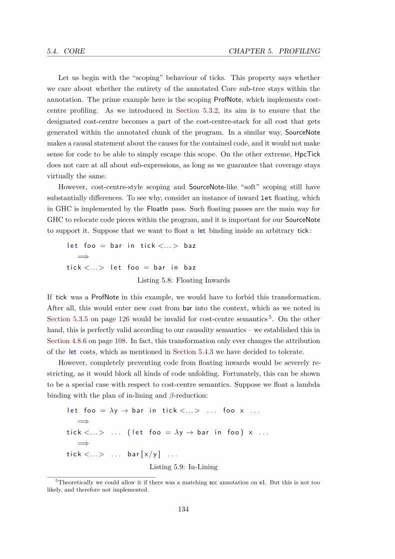
5.4. CORE CHAPTER 5. PROFILING

Let us begin with the “scoping” behaviour of ticks. This property says whetherwe care about whether the entirety of the annotated Core sub-tree stays within theannotation. The prime example here is the scoping ProfNote, which implements cost-centre profiling. As we introduced in Section 5.3.2, its aim is to ensure that thedesignated cost-centre becomes a part of the cost-centre-stack for all cost that getsgenerated within the annotated chunk of the program. In a similar way, SourceNotemakes a causal statement about the causes for the contained code, and it would not makesense for code to be able to simply escape this scope. On the other extreme, HpcTickdoes not care at all about sub-expressions, as long as we guarantee that coverage staysvirtually the same.

However, cost-centre-style scoping and SourceNote-like “soft” scoping still havesubstantially differences. To see why, consider an instance of inward let floating, whichin GHC is implemented by the FloatIn pass. Such floating passes are the main way forGHC to relocate code pieces within the program, and it is important for our SourceNoteto support it. Suppose that we want to float a let binding inside an arbitrary tick :

l e t foo = bar i n t i c k <... > baz=⇒

t i c k <... > l e t foo = bar i n bazListing 5.8: Floating Inwards

If tick was a ProfNote in this example, we would have to forbid this transformation.After all, this would enter new cost from bar into the context, which as we noted inSection 5.3.5 on page 126 would be invalid for cost-centre semantics 5. On the otherhand, this is perfectly valid according to our causality semantics – we established this inSection 4.8.6 on page 108. In fact, this transformation only ever changes the attributionof the let costs, which as mentioned in Section 5.4.3 we have decided to tolerate.

However, completely preventing code from floating inwards would be severely re-stricting, as it would block all kinds of code unfolding. Fortunately, this can be shownto be a special case with respect to cost-centre semantics. Suppose we float a lambdabinding with the plan of in-lining and β-reduction:

l e t foo = λy → bar i n t i c k <... > . . . f oo x . . .=⇒

t i c k <... > . . . ( l e t foo = λy → bar i n foo ) x . . .=⇒

t i c k <... > . . . bar [ x/y ] . . .Listing 5.9: In-Lining

5Theoretically we could allow it if there was a matching scc annotation on e1. But this is not toolikely, and therefore not implemented.

134

CHAPTER 5. PROFILING 5.4. CORE

This particular transformation is actually trivially legal under evaluation scoping (seeSection 5.3.3), as the application site determines what cost-centre stack to put the costof bar in anyway. And after the β-reduction this holds true for the modified scopingproposed by Marlow [2012] as well, as the lexical scope of the call-site is more specificthan the lexical scope of the definition site.

Let us now consider floating into the opposite direction. In the following examplewe are moving a binding towards the top level of the program:

t i c k <... > l e t foo = bar i n baz=⇒

l e t foo = t i c k <... > bar i n t i c k <... > bazListing 5.10: Floating Outwards

This transformation actually happens at a number of places in GHC. For example whenconverting a constructor application to A-normal form [Flanagan et al., 1993] we wantto let-bind certain sub-expressions, which might involve floating through a tick in theprocess. Happily, this time around we have a solid option for retaining lexical scopingproperties: By wrapping bar into a copy of our tick, we ensure that the same code stayscovered after we performed the transformation. Note however that we can not splitevery kind of tick this way, as we will see in Section 5.4.7.

To finish our overview of scoping behaviours, we have to mention that some typesof ticks do not care about scoping at all. For example, HpcTicks would simply allowthe following transformation:

t i c k <... > l e t foo = bar i n baz=⇒

l e t foo = bar i n t i c k <... > bazListing 5.11: Floating Outwards Without Annotation

This means that we have identified three tick scoping behaviours:

• cost-centre: The most restrictive scoping policy. We expect lexical scopes ofcode to neither grow nor shrink. The only exception is where mixed cost-centresemantics by Marlow [2012] provably assigns the same cost-centre stacks.

• soft: A more permissive policy we intend to use for our SourceNote. Here weexpect the lexical scope to only ever grow. Or put another way: Once we put anannotation on code – and therefore its costs – we expect it to still be there afteroptimisations have run their course.

• none: When the tick does not care about lexical scopes.

Figure 5.2 on the next page summarises the resulting tick property mapping.

135

5.4. CORE CHAPTER 5. PROFILING

ProfNote ProfNote HpcTick Breakpoint SourceNote(scoping) (counting)

Scoping: cost-centre none none cost-centre softCounting: no yes yes yes noPlacement: cost-centre runtime runtime runtime non-lambda

Figure 5.2: Tick Classification

5.4.6 Scoping Transformation Examples

While floating transformations are a good way to introduce the characteristics of scopingproperties, optimisation behaviour will actually quite often depend on tick scoping. Letus first have a look at GHC’s Simplify module, which groups together a large numberof local code optimisations. The way that this pass is structured, we walk the programusing a Zipper-like data structure [Huet, 1997]. For example, entering the functionexpression of an application expression (e x) means that simplification recurse into ewith a context of the form (� x). This allows optimisations to react to their surroundings.For example if find that e is – or becomes – a lambda application, we can now look atthe context and decide that fusing the two using β-reduction would be a good idea.

To introduce ticks into this process, we would ideally like to leave this continuationstack untouched. This would guarantee that all transformations see the exact samecontext that they would normally have, and therefore perform the exact same trans-formations. However, this means that we will have no way of retaining ticks insideexpressions that get re-built from the context. As we do not want to lose ticks, wetherefore must put them on top of the result expression, effectively floating all contextexpressions past them.

Fortunately, GHC only tracks context as far as the control flow is static, so forexample we would not traverse out of a let binding or case branch. Therefore there areonly a moderate number of instances where this would change things. To be precise,we would be performing the following transformations:

1 ( t i c k <... > e ) arg =⇒ t i c k <... > ( e arg )2 f ( t i c k <... > ! a ) =⇒ t i c k <... > f ! a3 l e t ! x = t i c k <... > e i n . . . =⇒ t i c k <... > l e t ! x = e i n . . .4 l e t . . . i n t i c k <... > e =⇒ t i c k <... > l e t . . . i n e5 ca se ( t i c k <... > e ) o f . . . =⇒ t i c k <... > case e o f . . .6 ca se . . . o f . . . → t i c k <... > e =⇒ t i c k <... > case . . . o f . . .7 t i c k2 <... > ( t i c k <... > e ) =⇒ t i c k <... > ( t i c k2 <... > e )

Listing 5.12: Floating Ticks

136

CHAPTER 5. PROFILING 5.4. CORE

The “bang” patterns on !x and !a show that strictness analysis could derive usage ofthe given binding to be strict. tick2 stands for another tick in the program, whichmight have different scoping properties and therefore needs to stay in place. Finallynote that transformations (4) and (6) simply refer to let and one-branch case floating,which we have already covered in the last section 6.

Looking at these transformations with lexical scoping in mind, we can attest thatevery single one might move costs into the scope of the tick in question. Even pushinganother tick inside has the potential to produce costs due to instrumentation code.This means that the tick in question must allow this, which is only the case for ticksthat permit at least “soft” scoping, i.e. not ProfNote or Breakpoint. On the other hand,we can explicitly allow this for SourceNote. Doing these transformations has the niceside-effect of pulling annotations on the same control path together, which togetherwith annotation elimination as explained in Section 5.4.4 can significantly reduce theamount of source annotations within the program.

Moving on, another GHC pass that needs to know about ticks is the occurrenceanalysis pass OccAnal. The purpose of this pass is to annotate binders with their usageinformation, which informs decisions about how greedy GHC should be about in-liningit. Consider the following example:

l e t x = e i n t i c k <... > . . . x . . .=⇒

l e t x = e i n t i c k <... > . . . e . . .Listing 5.13: Thunk Unfolding

Here e is a thunk, which we are considering to unfold to a usage site. The conditionsunder which this is a good idea are not quite trivial [Peyton Jones and Marlow, 2002],but the general idea is that we want to check whether we could introduce redundantevaluations of e by changing the program in this way. Ticks complicate this matterfurther: Unfolding e would add more costs into the lexical scope of the tick , thereforewe cannot allow this for ticks that have cost-centre scoping. On the other hand, weallow it both for SourceNote ticks and all other ticks with equally permissive scopingrules.

To close this section out, note that the only point where we distinguished between“soft” scope and “none” scope was when we decided whether to copy ticks on bindingswhen floating outwards. This means that between the two scoping classes, the onlychange will be how optimisations annotate their result. So far soft scoping implementsexactly what we had in mind: Allow arbitrary transformations, simply by moving outof the way where appropriate.

6In the context of GHC both Simplify as well as FloatIn implement floating, but due the staticcontrol flow limitation this version is less powerful.

137

5.4. CORE CHAPTER 5. PROFILING

5.4.7 Counting

The second major tick characteristic is whether they care about entry counts. Themotivating example here is coverage analysis using HpcTick: This tick checks whetherthe annotated expression gets evaluated during program execution.

The requirements work out “backwards” when compared with scoping: Whereasnormally we care about the evaluation of the annotated code, now we care about howoften outside evaluation causes our expression to get visited. This is actually moreproblematic, as now any change in sharing could potentially increase or decrease entrycounts in completely unrelated parts of the program. For this reason we can only trulyguarantee that we will never change the program so that the entry count of a “counting”annotation would fall to zero – or the other way around, for that matter.

However, we still make a best effort to retain realistic entry counts. For example,normally GHC would occasionally decide to inline “cheap” thunks, which would increaseentry counts of any annotations. Moreover, note that “copying” an annotation on afloating let binding like in Listing 5.10 would also increase entry counts. On theother hand, floating outwards like in Listing 5.11 could be allowed. Incidentally, thisdemonstrates why ProfNote needs to be splittable into a scoping and a counting part,as this behaviour would be incompatible with cost-centre style scoping.

5.4.8 Floating Ticks

In the end, there are relatively few transformations where the counting tick propertymakes a difference on its own. However, there are actually a significant number oftransformations that are invalid for both counting and cost-centre scoped ticks. Thisclass of transformations is of special interest to us, because our SourceNote ticks willbe the first tick type in GHC that has neither property, and can therefore support saidoptimisations. The crucial property is that we have maximum freedom with relocatingticks where necessary – as we introduced in Section 4.8.9 on page 112 for rules, “floating”ticks up is always an option according to our semantics.

A good example where we require this sort of freedom is η-reduction:

λx → t i c k <... > ( e x ) =⇒ t i c k <... > eλx → e ( t i c k <... > x ) =⇒ t i c k <... > e

Listing 5.14: η-Reduction

Saving both a closure as well as an application is a big win, so we would really like to dothis wherever we can spot it. Yet both versions would be invalid for either cost-centrescoping as well as counting ticks, as the relocation will change both evaluation scopesas well as entry counts. In contrast, for our causality semantics the first transformationis actually fine, as it would just correspond to adding more annotations on the closure

138

CHAPTER 5. PROFILING 5.4. CORE

value. On the other hand, moving annotations from the parameter to the applicationis clearly a change that could decrease profile accuracy. Unfortunately this is one ofthe situations where we have no other place to put the tick, and we will therefore haveto accept the resulting annotation overreach. Note that ProfNote side-steps the secondcase by not putting ticks on variables, as we will see in Section 5.4.10.

We have a similar situation for Rules: As mentioned in Section 4.8.9 on page 112,this is all about supporting user-supplied transformation rules. As we can generallynot derive where the right place would be to put the ticks afterwards, we have tobe conservative and float all of them out of the way. For example, we would do thefollowing for the short-cut fusion from Listing 3.4 on page 25:

f o l d r ( t i c k <1> s t ep ) ( t i c k <2> s t a r t ) ( t i c k <3> bu i l d g )=⇒ t i c k <1> t i c k <2> t i c k <3> f o l d r s t ep s t a r t ( b u i l d g )=⇒ t i c k <1> t i c k <2> t i c k <3> g s t ep s t a r t

Listing 5.15: Rule Application

Relocating ticks like this is fairly easy, as rule applications let -bind and float non-trivialexpressions where they match rule variables. We can use the same mechanism for“floating” our ticks. This has the nice side effect that the let in question automaticallyends up with the appropriate ticks on it. For example, suppose that expr stands for anon-variable:

f o l d r ( t i c k <1> expr ) ( t i c k <2> s t a r t ) ( t i c k <3> bu i l d g )=⇒ t i c k <1> l e t s t ep = exp r i n t i c k <2> t i c k <3> g s t ep s t a r t

Listing 5.16: Rule Application with Floating

Which in this instance retains exactly the intended ticks on expr. Floating ticks likethis still has significant potential for annotation overreaching, both for the bindings aswell as for the code built by the rule. However as noted in Section 4.8.9 on page 112this is the only way we can support custom rules, and for the fusion rule it actuallyreflects to the underlying causal dependencies quite well.

5.4.9 Merge Transformations

However, we are still not quite done with possible optimisations. In this section wewill get to the most problematic transformations. For our purpose, these are passesthat merge code from different sources. The most obvious example for this is commonsub-expression elimination in module CSE. The core problem is similar to rules: Wewant this pass to match expressions even where they differ in terms of our ticks, butwhat do we do from there?

139

5.4. CORE CHAPTER 5. PROFILING

There is only one place where we could possibly put annotations – the reference tothe replaced expression:

l e t x = t i c k <1> x i n . . . f ( t i c k <2> x ) . . .=⇒ l e t y = t i c k <1> f x i n . . . t i c k <2> ( f x ) . . .=⇒ l e t y = t i c k <1> f x i n . . . t i c k <2> y . . .

Listing 5.17: Common Sub-Expression Elimination

Again moving ticks out of the way makes things work with respect to our causalitysemantics. Yet thinking about this in terms of profiling should make us uneasy. Afterall, both steps in the above example reduce profile quality: First we push tick 2 up soit covers f, only to then replace the code by a reference to y – which according to thedefinition of y means that we associate all costs with tick 1.

Furthermore, ticks on thunk references are basically invisible to our profiling: Ifwe evaluate y we would immediately jump to the definition of y. After that point,the only way sampling code could possibly derive that we were coming from a usagesite annotated with tick 2 would be by stack tracing (see Section 5.3.6), which we donot currently support. Therefore the ultimate effect of this transformation might verywell be that the replaced expression effectively “vanishes” from the profile, leaving allcost with tick 1. A very similar situation happens when we attempt to optimise caseexpressions. Consider the following situation:

ca se . . . o f . . . → t i c k <1> e. . . → t i c k <2> e

=⇒ ca se . . . o f → t i c k <1> t i c k <2> eListing 5.18: Common case Branch Elimination

This is quite similar to common sub-expression elimination: Again we have two ex-pressions that we wish to merge. The difference is that this time we merge both ways,meaning that we are forced to merge all annotations in order to preserve the ticks’ costassociation.

A further example would be case branch elimination:

ca se x o f. . . → t i c k <1> x. . . → t i c k <2> x

=⇒ t i c k <1> t i c k <2> xListing 5.19: Identity case Branch Elimination

Here all case branches simply return the scrutinised value, so there is no reason tobranch in the first place. Again we must annotate in a way that will render profilingunable to detect which branch has been taken.

140

CHAPTER 5. PROFILING 5.4. CORE

In the end, it is pretty clear that there is simply no way to reduce code complexity inthese examples without also losing information for profiling. In fact, we could probablyargue that the optimisations shown in this section are probably rare enough that wemight actually be willing to sacrifice them for getting better profiling results. However,it is still important to know that our profiling solution can in fact work even here whilestill maintaining at least a certain measure of correctness7.

5.4.10 Placement

The final property of ticks mentioned in Figure 5.2 was “Placement”. Where scopingand counting properties speak about general policies for contained code, placement isabout special exceptions to these rules. After all, depending on the semantics of theticks in question, we might have situations where it makes no difference whether weput the tick in one place or the other. Especially where it simplifies reasoning aboutthe code in question, we should therefore aim to establish a certain consistency.

For example, all annotations have in common that they only care about whathappens at program execution time. However, as we noted briefly in Section 3.3.2on page 28, GHC’s version of Core implements a variant of System F [Girard et al.,1989], where the program may refer to purely compile-time entities such as types. Thisconstruction ensures that it is easy to check type-correctness of the intermediate code,but will be stripped before we get to later stages of code generation. Consequently,placing ticks on such type applications, type lambdas or coercions makes no sense, andwe consequently float ticks through them until we hit an expression that has runtimesemantics. We refer to this as “runtime” tick placement.

Furthermore, for our SourceNote ticks we will decide to float ticks through all lambdaexpressions, moving the tick into the lambda body. The motivation for this is rathermundane: It turns out that for supporting arbitrary optimisations, ticks on lambdasget in the way so often that it is just not worth keeping them there. Fortunately itis not too hard to justify this. GHC will let -bind all lambda expressions before codegeneration, which means that we can think of this as transforming a lambda expressions,as follows:

t i c k <... > (λx → exp r )=⇒ t i c k <... > l e t y = λx → exp r i n y=⇒ l e t y = λx → ( t i c k <... > exp r ) i n y

Listing 5.20: let -Bound Lambda Expression

7This also facilitates implementation. After all, just a few missing transformations can have asignificant impact on the produced code. Therefore it is easier to shoot for complete synchronisationbetween optimisations for ticked and un-ticked code than for any partial solution.

141

5.4. CORE CHAPTER 5. PROFILING

The second step only changes cost association in terms of let cost as well as one literal.We especially would not want to let -bind an expression like tick<..> λx →expr, as wecould only interpret this as a thunk producing a lambda! We conclude that floatingsource notes through lambdas is a relatively minor problem.

Finally, while cost-centre scoping is fairly restrictive, it actually has the most per-missive placement behaviour. The reason is that we can often show that certain tickrelocations leave the overall consistency of the cost-centre profile intact. This holds notonly for lambda expressions, but also for a number of other examples:

l e t x = scc <... > C ( scc <... > y ) ( scc <... > 3) i n . . .=⇒ l e t x = C y 3 i n . . .

Listing 5.21: Cost-Centre Placement

Just like with lambda expressions, both a constructor as well as a literal will correspondto a simple allocation, so there is no “code” there to track the cost for. On the otherhand, variable y could at maximum be a thunk. As thunk execution would not careabout the cost-centre stack at the evaluation site, this means that we can eliminate theannotation without significant changes to the cost-centre profile.

5.4.11 Example

To see how this works out in practice, let us return to our running example fromSection 3.4 on page 30, the factorial function. If we run Core optimisations withannotations as explained, GHC will arrive at the following annotated version:

$wfac = λ to # →s r c<f a c . hs :15> src<Enum . l h s :500>l e t wgo = λn# →

s r c<Enum . l h s :534> src<Num. l h s :89>case (==# ) n# to # o f

True →s r c<Enum . l h s :535> src<Num. l h s :89> n#

Fa l s e →s r c<Enum . l h s :536>case $wgo ((+# ) w s2L5 1) o f

r # → s r c<Num. l h s :89> (∗ # ) n# r #

i n s r c<Enum . l h s :532> wgo 1#

Listing 5.22: Core Result

For brevity we have simplified treatment of Bools slightly, and note that compared withListing 3.24 on page 35 GHC has short-cut the last loop iteration to return n# directly.

142

CHAPTER 5. PROFILING 5.5. CMM

However, at this point we are more interested in the annotations that the Coreoptimisations produced: First note that unfolding annotated library code has resultedin a good number of low-level source code links. This is expected and generally agood thing, as it might help us in tracking low-level performance problems. On theother hand, note that we end up with just a single reference to the original program(fac .hs). It is not hard to imagine what happened: We know from Section 3.4.1 onpage 30 that this code is the product of repeated rule applications, which as we havejust explained will cause source annotations to “float” towards the function entry point.Furthermore, as explained in Section 5.4.4 we combine annotations where appropriate,which apparently eliminated all but one tick here.

5.5 Cmm

Most interesting optimisations for GHC happen at the Core as functional code is partic-ularly suitable for applying aggressive program transformations. Once this optimisationpotential has been exploited, GHC will transform the code into a more restricted im-perative representation. This allows for more local transformations to prepare the codefor back-end code generation.

The intermediate language used for this is Cmm [Ramsey et al., 2010], which just likeits cousin C-- [Peyton Jones et al., 1998] is a portable assembly language. The main ideais that we now strip high-level data such as type information from the code and startreasoning in terms of instructions, registers and pointers. While doing this, we leave thelanguage just abstract enough that we can later map it to any back-end configurationwe choose. This allows us to solve common low-level code generation problems such asdata layout, register allocation or runtime system interface in a general way.

However, when we last mentioned Cmm in Section 3.3.3 on page 29, we skippedan in-depth look at these transformations. Our reasoning was that for the purpose ofcausality analysis, the far-reaching Core optimisations were the more interesting targetfor our analysis. After all, in contrast to what we considered at the Core stage, mostCmm transformations will barely change the structure of the generated code, thereforeleaving any annotations trivially correct.

However annotation implementation still faces a unique problem: Both cost-centreannotations as well as coverage ticks will get translated into Cmm code at this point.This means that there is actually no precedent for how to treat annotations at thislevel. Unfortunately, translation to Cmm code is no option for source code links, as wewant to work without instrumentation code. This means that we have no choice but todesign an entirely new solution for maintaining annotations on the Cmm level.

143

5.5. CMM CHAPTER 5. PROFILING

5.5.1 Cmm Example

To get a feel for what this will look like, let us now translate the Core code fromListing 5.22 into Cmm. If we simply ignore annotations, this would result in thefollowing code for the worker function wgo:

$wgo ( ){ A : i f ( Sp−16 < SpLim ) goto B ; e l s e goto C ;

B : c a l l s t g gc fun (R2 , R1 ) ;C : i f (R2 == I64 [ R1 + 7 ] ) goto D; e l s e goto E ;D: R1 = R2 ;

c a l l P64 [ Sp ] ( R1 ) ;E : I 64 [ Sp − 16 ] = F ;

I 64 [ Sp − 8 ] = R2 ;R2 = R2 + 1 ;Sp = Sp − 16 ;c a l l $wgo (R2 , R1) r e t u r n s to F ;

F : R1 = I64 [ Sp + 8 ] ∗ R1 ;Sp = Sp + 16 ;c a l l P64 [ Sp ] ( R1 ) ;

}Listing 5.23: Cmm Example

We can spot immediately that the Cmm version looks very different from the Core code.Instead of nested expressions, Cmm procedures consist of a number of blocks, with eachblock in turn containing a series of instructions. Cmm control flow is explicit, usinginstructions such as goto or call to steer execution.

Furthermore, at this point the implementation of our factorial function has becomea lot more explicit: Blocks A and B start by checking for a stack overflow. Blocks Cand D then handle the case that we are done with calculating the factorial, in whichcase we return to the location given by P64[Sp], passing R1 as our result. Otherwise,block E implements the first part of the calculation: We push a new stack frame withreturn pointer F and a copy of the counter n# (residing in R2). Then we increment thecounter and perform the recursive call. Once the call returns to block F, we will takethe saved-back counter from before and multiply it with the returned product. Thenwe pop the stack frame and return to the code that called our function.

At this point it is not hard to convince ourselves of our earlier diagnosis: As everyrecursive call to this function will increase Sp, we will have O(n) in stack allocation,which will probably cause us to call the stack overflow handler in block B quite often.This is quite likely to be a performance problem!

144

CHAPTER 5. PROFILING 5.5. CMM

5.5.2 Introducing Ticks

In order to bring source code annotations into the fold, we need to find a good wayto incorporate the ticks from Listing 5.22 into our Cmm code. Unfortunately, findinga good solution here is not entirely trivial. To get started, suppose that we simplygenerate a tick “pseudo instruction” every time we encounter a SourceNote in Core:

$wgo ( ){ A : i f ( Sp−16 < SpLim ) goto B ; e l s e goto C ;

B : c a l l s t g gc fun (R2 , R1 ) ;C : s r c<Num. l h s :89> src<Enum . l h s :534>

i f (R2 == I64 [ R1 + 7 ] ) goto D; e l s e goto E ;D: s r c<Num. l h s :89> src<Enum . l h s :535>

R1 = R2 ;c a l l P64 [ Sp ] ( R1 ) ;

E : s r c<Enum . l h s :536>. . .c a l l $wgo (R2 , R1) r e t u r n s to F ;

F : s r c<Num. l h s :89>. . .c a l l P64 [ Sp ] ( R1 ) ;

}Listing 5.24: Cmm Example with Ticks

The good news is that this is a straight-forward translation, and the result seems tomake sense for local annotations. For instance, the references to Num.lhs tells us thatblock D and F together perform a multiplication. Finding these source code links mightalready be useful for performance analysis.

On the other hand, we can also spot a number of problems. The entry code is notannotated at all, and the whole procedure contains no reference to the original sourcecode whatsoever. If this was a larger program, this would make it basically impossibleto tell what code we are looking at. The reason for this is that in Listing 5.22 we onlyhave one source code annotation at the entry point of the function, which is basicallyout of scope for this procedure. This is a severe problem: Unless we can find a way toreconnect our ticks with their associated code, they will lose most of their usefulness.

5.5.3 Tick Scopes

The main disconnect stems from the fact that Cmm code consists of a loose collectionof blocks, whereas Core code is naturally structured. As explained in Section 5.3.4 onpage 125 it is vital that we can discover our static context, but the change in program

145

5.5. CMM CHAPTER 5. PROFILING

A: i f ( Sp−16 < SpLim ) goto B ; e l s e goto C ;B : c a l l s t g gc fun (R2 , R1 ) ;C : s r c<Num. l h s :89> src<Enum . l h s :534>

i f (R2 == I64 [ R1 + 7 ] ) goto D; e l s e goto E ;

D: s r c<Num. l h s :89> src<Enum . l h s :535>R1 = R2 ;c a l l P64 [ Sp ] ( R1 ) ;

E : s r c<Enum . l h s :536>. . .c a l l $wgo (R2 , R1) r e t u r n s to F ;

F : s r c<Num. l h s :89>. . .c a l l P64 [ Sp ] ( R1 ) ;

Figure 5.3: Cmm Tick Scopes

representation has made this a lot harder. After all, in Core we just had to walk theexpression tree upwards towards the root, whereas now we lack such a robust navigationtool 8. This leaves basically two ways to approach this problem: We could eliminatethe need for code context by copying the complete tick context into every single block.However this would mean a massive amount of information duplication.

Therefore we will instead reimpose Core-like scoping behaviour on top of Cmmblocks. Figure 5.3 shows what this would look like for our example: The upper-mostscope corresponds to the top level of the function $wgo, whereas the scopes startingfrom D and E implement the two main case branches respectively. Finally, the Fblock corresponds to the return code after the recursive call to $wgo. Maintaining thisstructure makes it easy for us to identify which ticks apply to which block.

When considering a suitable representation for these scoping rules, we have to keep anumber of secondary factors in mind. Firstly, we want scopes to work even across Cmmprocedures. After all, to resolve the issue of the missing reference to the original sourcefile, we would need to imagine a parent scope containing all other scopes in Figure 5.3.This scope could then establish the causal connection to fac .hs. Furthermore, we haveto remember that there will be optimisations working on the Cmm code. Keeping inline with our philosophy, we would like to be minimally disruptive to other compiler

8We could try to analyse the control flow of the Cmm procedure and e.g. take over ticks fromdominating blocks [Lowry and Medlock, 1969]. While this would correspond nicely to our reasoningand might even be more accurate in some instances, it does not sound like a good idea architecturallyto depend on control flow to conform to our expectations.

146

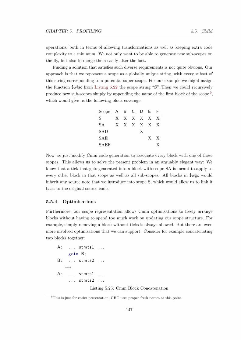
CHAPTER 5. PROFILING 5.5. CMM

operations, both in terms of allowing transformations as well as keeping extra codecomplexity to a minimum. We not only want to be able to generate new sub-scopes onthe fly, but also to merge them easily after the fact.

Finding a solution that satisfies such diverse requirements is not quite obvious. Ourapproach is that we represent a scope as a globally unique string, with every subset ofthis string corresponding to a potential super-scope. For our example we might assignthe function $wfac from Listing 5.22 the scope string “S”. Then we could recursivelyproduce new sub-scopes simply by appending the name of the first block of the scope 9,which would give us the following block coverage:

Scope A B C D E FS X X X X X XSA X X X X X XSAD XSAE X XSAEF X

Now we just modify Cmm code generation to associate every block with one of thesescopes. This allows us to solve the present problem in an arguably elegant way: Weknow that a tick that gets generated into a block with scope SA is meant to apply toevery other block in that scope as well as all sub-scopes. All blocks in $wgo wouldinherit any source note that we introduce into scope S, which would allow us to link itback to the original source code.

5.5.4 Optimisations

Furthermore, our scope representation allows Cmm optimisations to freely arrangeblocks without having to spend too much work on updating our scope structure. Forexample, simply removing a block without ticks is always allowed. But there are evenmore involved optimisations that we can support. Consider for example concatenatingtwo blocks together:

A: . . . s tmts1 . . .goto B ;

B : . . . s tmts2 . . .=⇒

A: . . . s tmts1 . . .. . . s tmts2 . . .

Listing 5.25: Cmm Block Concatenation

9This is just for easier presentation; GHC uses proper fresh names at this point.

147

5.5. CMM CHAPTER 5. PROFILING

This optimisation applies when there is no other jump to B, which is a situation thatcan happen quite often in generated Cmm code. As it can expose further optimisationopportunities, it is important that we allow code generation to take advantage of this.Consider what this means for ticks: Both stmts1 as well as stmts2 might be covered bya number of ticks from their respective scopes as well as all parent scopes. To ensurethat the code remains covered we therefore assign the block a scope string that is theunion of the old scope strings. Scopes of subsequent blocks are often similar, so thisdoes not change much while ensuring proper tick scoping. So for example if we mergedblocks with scopes S and SA, we could assure proper scoping by using the scope SA forthe combined block.

We can do a similar transformation with common block elimination:

A: . . . s tmts . . .B : . . . s tmts . . .

=⇒A: . . . s tmts . . .

Listing 5.26: Cmm Common Block Elimination

Under the assumption that A and B contain equivalent statements we can arrangecontrol flow so we can eliminate one instance. However, note that this time around wehave to take special care of tick annotations: Analogous to our treatment of common sub-expression elimination in Section 5.4.9 on page 139 we want to ignore the annotationswhen looking for candidates for CBE, only to re-annotate all ticks of the merged blockson the final block. For scoping we would again use string union, which for block scopesSA and SB would yield us SAB, for example. This treatment allows us to maintainsource code links throughout GHC’s Cmm stage.

However note that we are actually glossing over a problem here: When assigningthe merged block a scope string like SAB, we might actually reduce tick coverage forother blocks. After all, there might be another block in scope SA, which now has lesscoverage due to us moving the ticks into scope SAB! To solve this, we would have toassign individual ticks a scope – then moving them into new blocks would not changethe scope they apply to.

On the other hand, to our knowledge this issue does not happen in practice, asGHC will only generate more than one block per scope if we have complex control flow.This generally means that the optimisations only get applied in situations where weeliminate complete tick scopes. For example, assume we want to use common blockelimination on blocks from two scopes SA and SB. Then it is quite likely that CBEwould have to merge all blocks from the two scopes at the same time, as jumps betweenthem force equivalence.

148

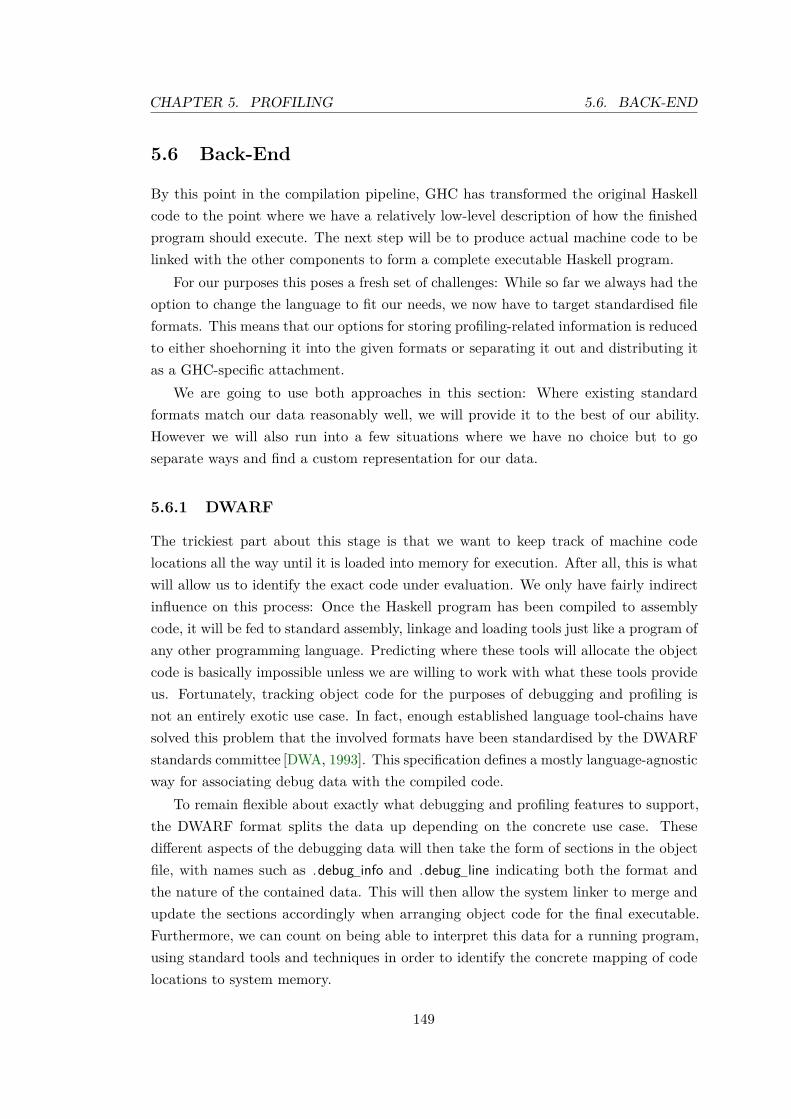
CHAPTER 5. PROFILING 5.6. BACK-END

5.6 Back-End

By this point in the compilation pipeline, GHC has transformed the original Haskellcode to the point where we have a relatively low-level description of how the finishedprogram should execute. The next step will be to produce actual machine code to belinked with the other components to form a complete executable Haskell program.

For our purposes this poses a fresh set of challenges: While so far we always had theoption to change the language to fit our needs, we now have to target standardised fileformats. This means that our options for storing profiling-related information is reducedto either shoehorning it into the given formats or separating it out and distributing itas a GHC-specific attachment.

We are going to use both approaches in this section: Where existing standardformats match our data reasonably well, we will provide it to the best of our ability.However we will also run into a few situations where we have no choice but to goseparate ways and find a custom representation for our data.

5.6.1 DWARF

The trickiest part about this stage is that we want to keep track of machine codelocations all the way until it is loaded into memory for execution. After all, this is whatwill allow us to identify the exact code under evaluation. We only have fairly indirectinfluence on this process: Once the Haskell program has been compiled to assemblycode, it will be fed to standard assembly, linkage and loading tools just like a program ofany other programming language. Predicting where these tools will allocate the objectcode is basically impossible unless we are willing to work with what these tools provideus. Fortunately, tracking object code for the purposes of debugging and profiling isnot an entirely exotic use case. In fact, enough established language tool-chains havesolved this problem that the involved formats have been standardised by the DWARFstandards committee [DWA, 1993]. This specification defines a mostly language-agnosticway for associating debug data with the compiled code.

To remain flexible about exactly what debugging and profiling features to support,the DWARF format splits the data up depending on the concrete use case. Thesedifferent aspects of the debugging data will then take the form of sections in the objectfile, with names such as .debug info and .debug line indicating both the format andthe nature of the contained data. This will then allow the system linker to merge andupdate the sections accordingly when arranging object code for the final executable.Furthermore, we can count on being able to interpret this data for a running program,using standard tools and techniques in order to identify the concrete mapping of codelocations to system memory.

149

5.6. BACK-END CHAPTER 5. PROFILING

5.6.2 Debugging Information

Let us first tackle the general debug information section .debug info. This section isstructured as a nested series of records, each with a number of fields as well as a numberof sub-records. The top level record will always be “compile units”, which stands forthe result of compiling one source file. This would look as follows if we use objdump topretty-print the data:

Abbrev Number : 1 (DW TAG comp i l e u n i t )DW AT name : f a c . hsDW AT produce r : The G l o r i o u s GHC SystemDW AT language : 0 x18 (Unknown : 18)DW AT comp d i r : ~/ l e e d s / t e s t / h a s k e l l / f a c /DW AT stmt l i s t : 0x0

Listing 5.27: Compilation Unit Record

This introduces general data about the compilation, such as source file location as wellas compiler and programming language. Note that the language ID 0x18 was assignedto Haskell on initiative of Howell [2012] and is slated to become part of the DWARF 5standard, but is not yet recognised by standard tools.

Children of compile units will be subprograms, corresponding to Cmm procedures:

Abbrev Number : 2 (DW TAG subprogram )DW AT name : f a cDW AT MIPS l i n k a g e name : s3S f i n f oDW AT low pc : 0 x404360DW AT high pc : 0 x4043b4

Listing 5.28: Sub-Program Record

This establishes just some very basic data that we have about the procedure: Its nameas well as the program counter (PC) range we expect the object code to occupy. Wewill see in Section 5.6.4 how we derive the name from our source notes. Meanwhile,it is not hard to see how we can provide the latter information simply by referencingsuitable code markers placed in the assembly code. For example, we would produce theabove record by generating the following assembly code:

$wgo1 i n f o :l e a q −16(%rbp ) ,% raxcmpq %r15 ,% raxj b c3Tv// . . . imp l ementa t i on . . .

150

CHAPTER 5. PROFILING 5.6. BACK-END

$wgo1 i n f o end :Listing 5.29: Assembly With Bound Markers

Note the stack check, matching the start of the function in Listing 5.24. For debugging,the thing to note are the $wgo1 info and $wgo1 info end markers, which allow us torefer to the function’s bounds. This will ensure that standard linking tools will properlyrelocate code addresses in debug information whenever code changes location.

However, this is not quite enough information for us to represent the full addressmapping that we had in mind. After all, at the end of last section we associated sourceticks with individual blocks. Therefore we would ideally like to get the tool-chain totrack block bounds as well. Unfortunately, this is the first point where we have tostretch the possibilities provided by the DWARF standard a bit, as there is no realequivalent for “block of code in an intermediate language”.

Instead, we will declare Cmm blocks as named “lexical blocks”:

Abbrev Number : 3 (DW TAG l e x i c a l b l o ck )DW AT name : c2Oj e n t r yDW AT low pc : 0 x402ee9DW AT high pc : 0 x402ee f

Listing 5.30: Lexical Block Record

Even though the purpose of this structure is to provide variable scope, using it forassigning names to code portions works just as well. The name will allow us to associateadditional information with each block later on.

5.6.3 Source Lines

While the records contained in .debug info already would allow our tools to reconstructthe structure of the compiled object code, it lacks references to what concrete part ofthe source code the functions and blocks were coming from. In the spirit of the DWARFformat, this is relegated to its own and largely independent section, namely .debug line.One reason for this split is that line number information is normally not similar toother debugging information structurally. While C-like programs often have only acouple of procedures and lexical blocks, a complete program could consist of thousandsof individual code lines. To support debugging, we require a full map connecting theseto the compiled code in the object files.

As a result, there have been significant efforts to keep the encoding of this dataas compact as possible. The DWARF standardDWA [1993] defines an elaborate datacompression scheme, allowing the DWARF producer to customise the encoding formaximum efficiency. Fortunately, GHC can leave the generation of this table to the

151

5.6. BACK-END CHAPTER 5. PROFILING

. f i l e 1 " f a c . hs ". t e x t

// . . . i n f o t a b l e . . .$wgo1 i n f o :c3Tc :

. l o c 1 15 1 /∗ t e s t 3 ∗/l e aq −16(%rbp ) ,% raxcmpq %r15 ,% raxj b c3Tv

. Lc3Tc end :c3Tw :

. l o c 1 15 1 /∗ t e s t 3 ∗/cmpq 7(%rbx ) ,% r14j e c3Ts

. Lc3Tw end :[...]

Listing 5.31: Assembly With Line Annotations

system’s assembly tool. All we have to do is annotate the source code with special“ . file ” and “ . loc” directives as shown in Listing 5.31. This will prompt the assemblerto build the compressed file and line tables for us, as well as generate the .debug linesection. Here is the result, decoded using objdump:

F i l e name L ine number S t a r t i n g add r e s sf a c . hs 15 0 x404360f a c . hs 15 0 x404369f a c . hs 15 0 x40436f

Listing 5.32: Source Line Table

Which is what we were hoping to see.

5.6.4 Source Note Selection

We have now seen how we can represent the information from a SourceNote in DWARF:We can use the name in order to refer to the procedure in .debug info, and the informa-tion about the source code span to produce a matching entry in the .debug line table.However, when we talked about tick scopes in Section 5.5.3 it should have become clearthat we rarely want to think of blocks and source notes as being in a one-to-one corre-spondence. In fact, following static control flow backwards as explained in Section 5.3.4

152

CHAPTER 5. PROFILING 5.6. BACK-END

on page 125, we will generally find many ticks to choose from.Unfortunately, the DWARF format does not allow us to be indecisive about what

source line or name we wish to associate with a piece of generated code. Therefore weare forced to pick: Which source note is the “most” useful for debugging the generatedpiece of code? We obviously want to throw away as little information as possible. Thismakes referencing, say, the multiplication operation a bad choice. After all, the programis most likely using multiplication often enough that it would not identify the codein question very well. On the other hand, knowing the current module function willgenerally allow us to discover roughly what low-level annotations we should expect.

This is why we will heuristically prefer source ticks that are from the source filethat corresponds to the currently compiled module. The nice property of such sourcenotes is that as long as we have implemented annotations correctly with respect to codetransformation, it is virtually guaranteed that all generated code will be directly orindirectly annotated with a SourceNote corresponding to the original source file. Afterall, this was the case right after desugaring, and we would expect code to only gainannotations from there.

Bottom-line is that we will always chose the source tick that matches the compilationunit and is most relevant to the execution site according to Section 5.3.1. This has theadditional benefit that the output also closely matches the expectations of debuggingtools, as the source references now essentially allow “stepping” through the source file.

5.6.5 Unwinding

Providing source file information in DWARF format was our main goal, but we canactually improve on this further by taking advantage of more elaborate DWARF features.Remember that in Section 5.3.6 on page 128 we explained that we could recover moreinformation about the current program state by walking the Haskell stack and analysingthe return code pointers we encounter. This corresponds to the common debuggingtechnique of stack unwinding: By successively removing stack frames from the heap werecover information about the call hierarchy.

And despite the fact that the Haskell stack is actually maintained in a fairly non-standard way, we can communicate the unroll procedure to the debugger using DWARFunwind instructions. For example, Listing 5.33 shows the unwind specification for theCmm code from Listing 5.23. First, the Common Information Entry (CIE) establishesthe general heap format. For us, this means that we expect the stack to grow downwardsin steps of 64 bits, making the data alignment -8 bytes. Furthermore we establish howto unwind a stack frame: Set the instruction pointer to the value we find at the currentCanonical Frame Address (CFA), and set the stack pointer rbp to the current CFA10.

10Note that rbp is the default x86-64 back-end register used for the Sp Cmm register.

153

5.6. BACK-END CHAPTER 5. PROFILING

CIECode a l i gnment f a c t o r : 1Data a l i gnment f a c t o r : −8Return add r e s s column : 16DW CFA o f f s e t : r16 ( r i p ) at c f a+0DW CFA va l o f f s e t : r6 ( rbp ) at c f a+0DW CFA de f c f a : r6 ( rbp ) o f s 0

FDE c i e =00000000 pc=0040435 f . . 0 04043 b4DW CFA s e t l o c : 00404397DW CFA de f c f a o f f s e t : 16DW CFA s e t l o c : 004043 aaDW CFA de f c f a o f f s e t : 0

Listing 5.33: Unwind Instructions

By default, we set the frame base address CFA to the current rbp, which describesthe situation at the point where a function is entered: Unwinding the stack wouldsimply mean resetting the instruction pointer using the return pointer from the stack,leaving rbp unchanged. However, once a function does actual stack allocation, this hasto be updated using a Frame Description Entry (FDE). In our example we instruct theunwind process that after the update of Sp in block E of Listing 5.23 we will have toroll the stack pointer back suitably.

Note however that there are subtleties to this. Firstly, typical debugging tools willactually decrease the return pointer by one byte before trying to look up its information.This is under the assumption that typical code would looks like follows:

c a l l fun. . . // r e t u r n code

Listing 5.34: Expected Assembly

If executed, the call instruction in this assembly would push a return pointer pointingto the return code. However, for debugging we are actually interested in where executionwas coming from, not where it is going to take us next. And in this specific case wecan easily reconstruct that, simply by decreasing the instruction pointer. In the abovecode this clearly leads us back to the original call instruction.

Unfortunately, this small trick does not work for Haskell code, as we have noguarantee that the calling code can be found anywhere near the return pointer. Let ushave a quick look at the recursive call in our running example:

154

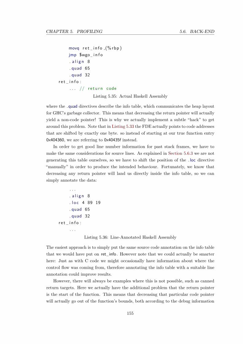
CHAPTER 5. PROFILING 5.6. BACK-END

movq r e t i n f o ,(% rbp )jmp $wgo i n f o. a l i g n 8. quad 65. quad 32

r e t i n f o :. . . // r e t u r n code

Listing 5.35: Actual Haskell Assembly

where the .quad directives describe the info table, which communicates the heap layoutfor GHC’s garbage collector. This means that decreasing the return pointer will actuallyyield a non-code pointer! This is why we actually implement a subtle “hack” to getaround this problem. Note that in Listing 5.33 the FDE actually points to code addressesthat are shifted by exactly one byte. so instead of starting at our true function entry0x404360, we are referring to 0x40435f instead.

In order to get good line number information for past stack frames, we have tomake the same considerations for source lines. As explained in Section 5.6.3 we are notgenerating this table ourselves, so we have to shift the position of the . loc directive“manually” in order to produce the intended behaviour. Fortunately, we know thatdecreasing any return pointer will land us directly inside the info table, so we cansimply annotate the data:

. . .. a l i g n 8. l o c 4 89 19. quad 65. quad 32

r e t i n f o :. . .

Listing 5.36: Line-Annotated Haskell Assembly

The easiest approach is to simply put the same source code annotation on the info tablethat we would have put on ret info . However note that we could actually be smarterhere: Just as with C code we might occasionally have information about where thecontrol flow was coming from, therefore annotating the info table with a suitable lineannotation could improve results.

However, there will always be examples where this is not possible, such as cannedreturn targets. Here we actually have the additional problem that the return pointeris the start of the function. This means that decreasing that particular code pointerwill actually go out of the function’s bounds, both according to the debug information

155

5.6. BACK-END CHAPTER 5. PROFILING

records as discussed in Section 5.6.2 as well as the symbol table. The latter is morecritical, as we can not manipulate it due to its role in the linking process. Unfortunately,debugging tools such as gdb use it to lookup function names, leading to unhelpful ??entries in stack traces. For example, the following stack trace would be generated foran exception raised inside a thunk update:

#0 s tg r a i s e z h ( ) at r t s / Excep t i on .cmm:433#1 0x694330 i n ?? ( ) at r t s /Updates .cmm:57#2 0x4047a0 i n $wf ib e r r ( ) a t s tack−t r a c e . hs : 7

Listing 5.37: Example Stack Trace

Unfortunately, we cannot correct this from the compiler. A proper solution would mostlikely require a patch to the debugging tool in question.

5.6.6 GHC debug records

At this point we have pretty much exhausted what we can meaningfully express withthe DWARF standard. However, we have a lot more information in store: In ourmind every piece of object code is covered by a number of possible source annotations,each potentially providing valuable information about the nature of the code at hand.Furthermore, we might want to mix in additional information about the compilationprocess, as we will see in the next section.

In order to maintain such data alongside existing DWARF debugging information, wewill allocate our own object file section, called .debug ghc. For overall data organisationwe will choose the event log format [Jones et al., 2009]. This is in anticipation forcollected profiling information getting appended later on. Note that we cannot relyon debugging tools to know about the format of our section, which means that wewill only be able to identify code addresses by comparing against information fromthe .debug info section. This is why we took great care in Section 5.6.2 to associate aunique name with every procedure and block.

As we have seen in Figure 5.3 on page 146 tick scopes naturally form a tree structure,so it is a straight-forward choice to use a block tree for our debug records as well. Notethough that scopes will not always directly conform to this, as shown in Figure 5.4.Firstly we might encounter multiple blocks sharing the same scope, as happens for ABin the example. We then choose a “representative” for the scope11, which will carry allticks as well as becoming parent to all other blocks covered by the scope. Furthermore,we might have scopes with more than one parent scope, such as ABC in the example.Then we have to settle for just one parent, and restore all “lost” ticks by replicating

11The choice is pretty arbitrary – to reduce randomness we select the first block according to pre-ordertraversal. This allows us to guarantee that the entry block will become root of its scope, if nothing else.

156

CHAPTER 5. PROFILING 5.6. BACK-END

A

AB

AC

ABC

Figure 5.4: Block Tree from Scopes

1 Debug module main : f a c . hs2 Debug b l o ck l a b e l c3TG en t r y i d 1 pa r en t 03 Debug b l o ck l a b e l c3TH en t r y i d 2 pa r en t 04 Debug b l o ck l a b e l c3Tw en t r y i d 5 pa r en t 45 Debug b l o ck l a b e l c3Tv en t r y i d 6 pa r en t 46 Debug b l o ck l a b e l c3Tj i n f o i d 8 pa r en t 77 Debug sou r c e ∗ (Num. l h s : 8 9 )8 Debug b l o ck l a b e l c3Tt e n t r y i d 7 pa r en t 49 Debug sou r c e e f t I n t FB . go (Enum . l h s : 5 36 )10 Debug b l o ck l a b e l c3Ts en t r y i d 9 pa r en t 411 Debug sou r c e ∗ (Num. l h s : 8 9 )12 Debug sou r c e e f t I n t FB . go (Enum . l h s : 5 35 )13 Debug b l o ck l a b e l s 3S f i n f o i d 4 pa r en t 314 Debug sou r c e ∗ (Num. l h s : 8 9 )15 Debug sou r c e e f t I n t FB (Enum . l h s : 5 34 )16 Debug b l o ck l a b e l c3TD en t r y i d 3 pa r en t 017 Debug sou r c e e f t I n t FB (Enum . l h s : 5 32 )18 Debug b l o ck l a b e l c3TC en t r y i d 10 pa r en t 019 Debug sou r c e e f t I n t FB (Enum . l h s : 5 31 )20 Debug b l o ck l a b e l Main zdwfac i n f o i d 021 Debug sou r c e e f t I n t FB (Enum . l h s : 5 31 )22 Debug sou r c e enumFromTo (Enum . l h s : 5 00 )23 Debug sou r c e f a c ( f a c . hs : 1 5 )

Listing 5.38: Debug Records

157

5.6. BACK-END CHAPTER 5. PROFILING

$wfac = λ to # →

l e t wgo = λn# →

ca se (==# ) n# to # o f

True → n#

Fa l s e →ca se $wgo ((+# ) w s2L5 1) o f

r # → (∗ # ) n# r #

i n wgo 1#

Figure 5.5: “Scopes” in Core

them in the appropriate block. For our sketch, this would mean copying the ticksassociated with scope AB into the block contained in ABC.

Once we have obtained such a block tree, we emit a series of event messages thatdescribe its structure and payload. Listing 5.38 on page 157 shows the result for ourrunning example: The entry block Main zdwfac info with ID 0 (line 20) is the root of ourtree, corresponding to the top level in Listing 5.22 on page 142. One level below we findthe entry block of the $wgo with instrumentation ID 4 (line 13). Note that as shown inListing 5.28 on page 150, GHC has assigned it the unique name s3Sf, which we can useto identify the correspond .debug info record and therefore its code range. As eventsare written as a series, associating further properties with these blocks simply meansemitting extra block property events right after the event declaring the correspondingblock. For our example, the root node 0 will receive three source annotations fromfac .hs and Enum.lhs respectively.

5.6.7 Core Notes

When we talked about what information we could infer from just a static context inSection 5.3.4, we noted that it will be useful to allow the user to trace compilationbackwards in detail. After all, while explaining source code causation for a programstate might require us to bring a large number of possibly relevant source locations intoplay, we can generally pin-point exactly where we found ourselves in terms of Cmm oroptimised Core code. This offers the user a great deal of information, especially makingthem independent of heuristics such as the one discussed in Section 5.6.4.

158

CHAPTER 5. PROFILING 5.6. BACK-END

To make use of this property, we want to link up a block tree like the one shown inFigure 5.4 with a Core program, such as the optimised Core we derived for factorialback in Listing 5.22 on page 142. After all, as Figure 5.5 shows we can easily map tickscopes back to the structure of the Core program. In order to track this association,we need to define yet another tick type just like we did in Listing 5.7 for source codelinks. This time however, we track Core:

[...]| CoreNote { co reB ind :: Var

, coreNote :: ExprPtr Var }Listing 5.39: Core Note

with the coreBind providing a unique identifier for the Core location, and the ExprPtrreferencing the Core expression or binding in question.

The unique property of the CoreNote is that it will only get generated once wetranslate the intermediate Code into Cmm. So it is guaranteed not to exist on the Corestage, so there is no need to decide floating or placement properties like in Section 5.4on page 129. In terms of treatment on the Cmm stage we simply expect that they willremain in their associated tick scopes, just like source notes. In the end, this yields usa straightforward map of tick scopes to one or multiple locations in the Core code.

In order to save the Core for later inspection we then encode the Core code in theevent-log format. We can simply achieve this by inserting appropriate “Core” eventmessages with the messages the other block records. However, this process is not quiteobvious: To reduce space usage we aim to never emit any single piece of core twice.Therefore we partition the full Core code into separate chunks, using references in orderto assemble them back together.

In our example, this means that we would generate the following Core pieces:

<A> (∗ # ) n# r #

<B> case $wgo ((+# ) w s2L5 1) o f r # → <A><C> n#

<D> case (==# ) n# to # o f True → <C>; Fa l s e → <B><E> $wfac = l e t wgo = λn# → <D> in wgo 1#

Listing 5.40: Core Pieces

To further increase the usefulness, we can also add type information into the mix. Notehowever that retaining too much data at this point can quickly lead to the producedbinary growing excessively. After all, if we go through with this we will not only saveevery single piece of optimised Core that the compiler produces, but also pretty muchall types encountered in intermediate code.

159

5.6. BACK-END CHAPTER 5. PROFILING

The latter can be surprisingly problematic, as for example heavy usage of monadtransformers [Espinosa, 1995] in the popular haskeline library at one point producedtypes that spanned about 20 000 lines when pretty-printed. This is why we took greatcare to be space-efficient, and will make Core tracking an optional feature.

5.6.8 LLVM

To this point we have described what debugging data we would like to ship with ourbinaries in order to link object code back to profiling and debugging data. We evenused examples of what we would like the produced assembly code to look like. Yetwe have to note that for GHC compilation, we will not always have full control overthe produced assembly. While it is generally recommended to have GHC handle theproduction of the assembly code directly, there are cases where it is beneficial to leavethis task to an external tool. For our purposes, this means that we have to deal withan additional layer of indirection.

The alternative we want to cover here is the LLVM backend [Terei and Chakravarty,2010], which generates high-level assembly code to be compiled using the LLVM com-piler infrastructure [Lattner and Adve, 2004]. This allows us to make use of its low-leveloptimisation facilities, which are much more advanced than the fairly basic transfor-mations that GHC can perform on Cmm and assembly code. For our purposes, thismeans that we have to find a way to instruct LLVM to generate the suitable DWARFcode. Fortunately, there is fairly direct support for this in the form of LLVM metadata. For example, generating the .debug info records for the compilation unit as wellas the $wgo function would look as shown in Listing 5.41. Note the similarity withthe structure of .debug info as discussed Section 5.6.2 on page 150: Using metadatalinks we define a tree-like structure, assigning every node a tag deriving from the recordtypes from the .debug info section. Note that while most of the meta data is comprisedof literals and other meta data, @s1E8 info is actually a reference to the function of thesame name, which we supposedly defined earlier in the same file. This allows us to linkthe debug information to the definition in question.

Generating line number annotations also has parallels to how we generated the linetable by inserting . loc directives into the assembly in Section 5.6.3. For LLVM, wesimply annotate the code with suitable metadata links as shown in Listing 5.42. Noticethe !dbg annotations, which connect LLVM code lines with the source code line inquestion. For example, meta data node !4 here stands for line 15 column 17 in fac .hs.This is also where we introduce lexical blocks, which serve the same purpose they didpreviously: Introduce unique names for Cmm blocks.

In the end, while LLVM allows us to get good results with relatively little effort, thereis also a lot that we simply cannot express using LLVM’s intermediate representation.

160

CHAPTER 5. PROFILING 5.6. BACK-END

! 0 = metadata !{ metadata ! " f a c . cpp " ,metadata ! "~/ l e e d s / t e s t / h a s k e l l / f a c /" }

!1 = metadata !{ i 3 2 786473 , // DW TAG f i l e typemetadata !0 }

!2 = metadata !{ i 3 2 786449 , // DW TAG comp i l e u n i tmetadata ! 0 , i 3 2 24 ,metadata ! "The␣ G l o r i o u s ␣GHC␣System " , . . . }

!3 = metadata !{ i 3 2 786478 , // DW TAG subprogrammetadata ! 0 , metadata ! 1 ,metadata ! "$wgo" , metadata ! "$wgo" ,metadata ! " s1E8 i n f o " ,. . . ,v o i d ( . . . ) ∗ @s1E8 i n f o }

Listing 5.41: LLVM Debug Meta Data

d e f i n e i n t e r n a l cc10 vo i d @s1E8 i n f o ( . . . ) a l i g n 8 {c1Fk :

%ln1Gp = add i 64 %R1 Arg , 7 , ! dbg !4%ln1Gr = i n t t o p t r i 6 4 %ln1Gp to i 6 4 ∗ , ! dbg !4[...]

}[...]! 4 = metadata !{ i 3 2 15 , i 3 2 17 , metadata ! 5 , . . . }!5 = metadata !{ i 3 2 786443 , // DW TAG l e x i c a l b l o ck

metadata ! 0 , . . . ,metadata ! 1 , . . . }

Listing 5.42: LLVM Line Meta Data

161

5.7. DATA COLLECTION CHAPTER 5. PROFILING

Most prominently, LLVM expects to handle its own stack, so there are no facilities forexplaining how to unwind the custom GHC-style stack. Furthermore, there is no directway of assigning names to lexical blocks like we did in Section 5.6.3, so to retain links toCmm code we can only mark them indirectly, for example by creating dummy variables.This means that while profiling and debugging using the LLVM backend is possible, wehave to accept further downsides on top of DWARF’s inherent restrictions.

5.7 Data Collection

We have now obtained a complete debug information map for our object code. Thismeans that at this point a single object-file code pointer would be enough for us to beable to tell the full story of how the code in question was produced, and especially whatparts of the original source code played a role. All we need now in order to start ouranalysis is some performance data that yields us such code pointers.

In this section we will show how to collect such profiling data. Conceptually,this means that we are now leaving the part of the implementation that is primarilyconcerned with the “cause” side (source code) and enter the phase where we are lookingfor “effects” (resource consumption). Therefore this section will be about implementingthe verbs and metrics introduced back in Section 5.2 on page 117. However, we stillhave to make sure that we carry along all data we have collected so far about nounsand explanations, as this will later allow the analysis tools to link up the two sides ofthe profiling problem.

5.7.1 Event-Log

As mentioned in Section 5.6.6 on page 156, we will be using the event-log format asdefined by Jones et al. [2009]. Using a common standard format for profiling has theadvantage that we can integrate various approaches both on the producer as well as theconsumer side: Existing profiling infrastructure can provide further performance data tohelp put ours into context, and other profiling tools might decide to also take advantageof the data we collect. For example, apart from the original ThreadScope applicationthe format is also understood by the Eden trace viewer [Berthold and Loogen, 2007],HdpHProf [Al Saeed et al., 2012] as well as the ghc-events-analyze tool [de Vries andCoutts, 2014], all covering different use-case for profiling analysis.

In order to produce a useful event-log file, we will first write out a “prefix” consistingof the program’s debug records as defined in Section 5.6.6 on page 156. As we alreadygenerated these records in event log format, this mostly means copying data from ourown .debug ghc section into the fresh event-log file. However, this task is not entirelystraightforward, as we want to provide debug information for all involved libraries as

162

CHAPTER 5. PROFILING 5.7. DATA COLLECTION

well, for which we have to resolve both compile-time as well as run-time relocations.This means that the runtime system needs to be able to read the .debug info section

of both its “own” executable as well as all dynamically linked libraries. Fortunately,there are standard libraries available for this task, so we simply use libelf [Riepe,2009] and libdwarf [Anderson, 2011] in order to extract all required information. Wefurthermore relocate all code pointers using our process’ memory map12 which yields usthe actual address ranges for every code block with a DWARF record. By interleavingthese pointer ranges with the existing debug block records, we obtain a full mapping ofdebug information to pointer ranges:

Debug module main : f a c . hsDebug p rocedu r e l a b e l c3TG en t r y i n s t r 1 pa r en t 0Debug p o i n t e r range 0x004043dd−0x004043e3Debug p rocedu r e l a b e l c3TH en t r y i n s t r 2 pa r en t 0Debug p o i n t e r range 0x0040440c−0x00404420Debug p rocedu r e l a b e l c3Tw en t r y i n s t r 5 pa r en t 4Debug p o i n t e r range 0x00404369−0x0040436fDebug p rocedu r e l a b e l c3Tv en t r y i n s t r 6 pa r en t 4Debug p o i n t e r range 0x004043b0−0x004043b4Debug p rocedu r e l a b e l c3Tj i n f o i n s t r 8 pa r en t 7Debug sou r c e ∗ ( l i b r a r i e s / base /GHC/Num. l h s :89 :19 −89 :30)

Listing 5.43: Debug Records with Pointer Ranges

Where we have more information on source ranges than we have records in .debug ghc,we can even synthesise new records that describe them. This might happen for examplewhen we are linking with C libraries:

Debug module :SYMTAB: / l i b 6 4 / l i b p t h r e a d −2.12. soDebug p rocedu r e l a b e l p th r ead cond wait@GLIBC 2 . 2 . 5Debug p o i n t e r range 0 x3aa3c0c070−0x3aa3c0c108Debug p rocedu r e l a b e l p th r ead s e t a f f i n i t y np@@GLIBC 2 . 3 . 4Debug p o i n t e r range 0 x3aa3c0fac0−0x3aa3c0fb65

Listing 5.44: Debug Records for C Library

Note however that this is limited to information extracted from the symbol table andthe .debug info section. Therefore instead of complete source references we end up withjust symbol names. Extending this to cover full DWARF information would require usto decode the information in .debug line as well, which we currently skip.

12Which we currently obtain by reading /proc/self/map, basically abandoning all hope of portability.

163

5.7. DATA COLLECTION CHAPTER 5. PROFILING

sample weight · · ·· · ·

samplemode op wdt0x00 + 80x10 - 80x40 + 320x50 - 320xf0 = 64

weightmode wdt0x0 0*0x1 80x2 160x4 320x8 64

Figure 5.6: Sample Encoding

5.7.2 Samples

With the debug map established, referencing debug data becomes as easy as saving apointer, leaving the actual lookup to the analysis tool. As Section 5.2.1 on page 118explained this is good news, as low overhead is the easiest way to prevent skews.

On the other hand, putting some effort into our encoding scheme is a good ideaanyway. Remember that this is about providing evidence for a connection betweencertain causes (nouns) and effects (verb). As explained in Section 2.2.4 on page 12 thisis not just about a one-to-one connection, but we will want to associate weights withconnections, corresponding to the approximate strength of the link. Depending on ourcollection method, the value range of these weights might vary quite a bit. For example,sampling only the instruction pointer we might only ever get one sample at a time,while inventory-type samples such as heap residency profiles will produce much moredata (see Figure 6.12 on page 190). If we add the fact that our noun representation willgenerally be a 64 bit code pointer, it becomes clear that we might quickly be lookingat about 16 bytes per sample, which could add up quickly unless we invest into somebasic pre-processing.

To help with this, we use a basic compression system shown in Figure 5.6: A modebyte tells us for every weighted sample how both the sample value as well as the weight isgoing to be encoded. For values, we exploit that subsequent samples are often expectedto be in close proximity to each other, making it more compact to emit a distance tothe last sample instead of the full 64 bit pointer. We want to be especially mindfulof small hot-spots, where samples are often in very close proximity (< 256 bytes), andunless samples jump between libraries pointer differences will generally fit into a 32 bitinteger. On the other hand, for weights we have to account for the full range of values,with no expected proximity between neighbouring values. Therefore we cover the wholerange of integers from 0 up to 8 bytes, with 0 standing for the constant weight of 1.

164

CHAPTER 5. PROFILING 5.7. DATA COLLECTION

Furthermore, we will allow sample events to specify what noun and verb they aretalking about. This will make our sampling infrastructure open for future extensions,for example using cost-centre nouns instead of instructions pointers. For the moment,here is how an example sample event would look like when carrying instruction pointers,collected by processor cycles:

Sample Samp l e I n s t rP t r by SampleByCycle cap 0 :2∗0 x404fe9 , 0 x404 f f0 , 2∗0 x404fe9 , 3∗0 x404 f f0 ,0 x404fe9 , 4∗0 x404 f f0 , 0 x404fe9 , 2∗0 x404 f f0 ,0 x404 f f0 , 0 x405074

Listing 5.45: Samples in Event-Log

Especially note the distinct “hotspot” behaviour here: In this example most samplesare from a region that spans just two bytes! We also observe that multiple sampleshave a weight greater than 1, as shown by the n∗ prefixes, even though the underlyingsampling process actually produces samples individually. The explanation is that ourencoding algorithm actually coalesces subsequent samples with the same sample value,exploiting another easy compression opportunity.

5.7.3 Timers

Now that the sample tracing infrastructure is in place, we just need to acquire actualsampling data in order to produce proper Haskell program profiles. Namely we wantan approximate map of where certain effects (verbs) occurred. The most direct wayto do this is sampling: We take snap-shots of the execution state at frequencies thatconform roughly to the amount of (abstract) resource usage.

Just consider our primitive verb from Section 5.2.2 on page 118: Time passing.Finding program states where most time is spent is as simple as interrupting the programat set intervals, each time taking a sample of the current instruction pointer. Clearlya program state that only appears briefly will have a very low chance of appearing inour profile. On the flip-side, with enough data collection we can also expect programstates to feature more often the more time was wasted.

On paper implementation is also relatively straightforward: All operating systemsoffer some sort of timer support. Often we can even obtain data about the threadstate on these occasions. For example, we can use setitimer and sigaction on typicalUnix systems to program a timer to pass us the thread’s “context” in certain intervals,including the full register set. On Windows systems, we can might be able to achieve asimilar effect by using SuspendThread followed by GetThreadContext. Access to registersmeans that we can sample instruction pointers and generate the sample messagesexplained in the last section, making “time” the first verb that we can provide profiling

165

5.7. DATA COLLECTION CHAPTER 5. PROFILING

support for. Note that the register set will normally also include the current stackpointer – this could allow us to do stack tracing as explained in Section 5.3.6, potentiallyproviding more expressive nouns13.

In practice however, working with timers can be a bit of a challenge due the factthat the operating system interfaces are not strictly meant to be used for profiling. Thismeans that we will often have to help things along a bit in order to get exactly what wewant. For example, setitimer will only ever raise the signal for one thread, therefore weopt to manually replicate the signal across our program for multi-threaded applications.Such tricks are not only prone to bugs, but also tend to result in bad performance.

5.7.4 Hardware Performance Counters

Profiling by time is rather simplistic; as explained in Section 5.2.3 we might want tounpack program performance further by focusing on the different influences on CPUexecution speed. Fortunately, this is again a concern that we share with a lot of existingprofiling tools. And in fact the art of collecting specialised profiling information hasmatured to the point where we even have hardware support in the form of hardwareperformance counters. The idea is that we can program these counters to track somekind of low-level performance metric such as processor cycles or cache misses. This willgive the operating system a notification whenever a certain threshold is reached. Giventhat modern processors support dozens of possible counter configurations, this gives usa lot of flexibility for data collection.

The principal “standard” library for programming hardware performance countersis the Performance API, or PAPI for short [Browne et al., 2000]. It is portable across anumber of different Unix systems, and allows us to define “overflow” handlers for a widevariety of performance counters from cache statistics over branching data to simpleinstruction counts. However, performance is limited due to the fact that it needs tocall the program every time to allow taking samples. Furthermore, support on modernmachines does not seem to be completely stable 14. Fortunately, most modern operatingsystems offer better alternatives.

5.7.5 Perf-Events

Linux is a popular kernel for Unix systems. Where it is present we can obtain perfor-mance data much more directly by talking directly to the operating system. The ideais that the perf_event kernel interface [Eranian, 2009] allows us to instruct the kernelto take over the task of collecting instruction pointer samples entirely. The collected

13However a possible implementation would have to ensure that we are in valid Haskell code to beginwith, or the sampling code might end up crashing the program!

14Based on the episodic evidence that it mysteriously stopped working on the author’s computer.

166

CHAPTER 5. PROFILING 5.7. DATA COLLECTION

data will then “stream” back to the process using a memory map, which reduces ourjob to copying it into our event log in regular intervals.

The advantage of this approach is that we have to accept a lot less overhead thanbefore. After all, performance counter events have to be handled by the operatingsystem at some level anyway, so having sample collection happen without anothercontext switch is a significant win. On the other hand, we also have to accept lessinfluence over the collection process. For example, now we do not have the option towalk the Haskell stack – while the Linux kernel supports a limited form of stack tracing,it is quite unlikely that it will be able to make sense of the Haskell stack anytime soon 15.

5.7.6 Allocation

Going beyond simple hardware statistics, Section 5.2.4 argued that we also have anactive interest in more Haskell-specific aspects of program performance. One very basiccharacteristic of code generated by Haskell is that it often involves allocation of varioustypes of memory. In the Cmm example in Listing 5.23 on page 144 we actually saw thisspelled out: Whenever stack allocation reached a certain threshold, the generated codewould call into the run-time system in order to request a fresh block of memory. Suchrequests are an indirect sign of either heap or stack allocation, both verbs that we wouldlike to track. After all, in either case we are making a call into the memory subsystem,which is already quite costly on its own. Therefore the locations of allocation can bevery interesting for performance analysis.

Therefore, instrumenting these calls into the runtime system is an obvious choice.Unfortunately, while the runtime routine receives a continuation code pointer, thispointer does not always directly refer to where the allocation took place. This meansthat if we have code like the following:

ca se x o fC → . . . −− l o t s o f heap a l l o c a t i o nD → . . . −− l i t t l e heap a l l o c a t i o n

Listing 5.46: Ambiguous Heap Allocation Location

the heap check might assign the same return pointer to both of them, which meansthat we cannot tell which branch was actually causing the heap allocation in the firstplace. Unfortunately, this happens quite frequently with GHC-generated code.

15The kernel would essentially have to track down, relocate and use the unwind information wegenerated in Section 5.6.5 – which would be quite a bit of complexity even for a monolithic kernel.

167

5.8. ANALYSIS CHAPTER 5. PROFILING

5.7.7 Residency

Apart from allocation we also want to keep track of how much memory actually survivesgarbage collections. As explained in Section 5.2.5 this can have an indirect effect onprogram performance by reducing locality and increasing garbage-collection time. Tomeasure the amount of residency, we want to generate an inventory of how much dataof every type is left on the heap, as well as – ideally – why it is being kept there.Fortunately, the GHC runtime already contains an adequate mechanism for generatingheap residency profiles, courtesy of Sansom and Peyton Jones [1995]. We can simplyadapt their implementation to yield us a statistic of which type of heap object consumedhow much memory in total. As noted back in Section 3.5.9 on page 52, heap object infopointers double as code pointers, therefore we can directly treat them as input to ourprofiling process. Note that looking at the code pointer not only allows us to identifyconstructors, but also the concrete code point for thunks. This can be especially usefulfor identifying situations where thunk evaluation gets delayed excessively.

5.8 Analysis

We have now learnt everything there is to know about how to obtain profiling datafrom Haskell programs using our approach. With our implementation, we can nowrun arbitrary programs with suitable compilation and runtime parameters and have itproduce an eventlog containing both detailed debug records as well as raw samplingdata to match. Conceptually we just need to put these two together in order to obtaina full performance analysis.

Yet there are still engineering challenges to consider. Firstly, when we generatedthe eventlog we put emphasis on making sample generation as light-weight as possible.This almost automatically means that analysis will have to make up for it by processingquite a bit of raw data in order to locate relevant trends. This task is not made easierby the fact that as shown in Section 5.3 on page 121 it is not easy to explain whatthe data means in the first place. Our aim must be to break the data down in termsof notions that the programmer understands, and work with them in unravelling thecausal processes within the program.

5.8.1 ThreadScope

When we explained the requirements for our profiling solution back in Section 2.1.2 onpage 7 we defined our role as supporting the user’s abductive reasoning process. Bynature this process will be incremental, requiring step-wise theory development andevaluation. In order to seamlessly assist the user with this, we therefore want to providean interactive graphical user interface.

168

CHAPTER 5. PROFILING 5.8. ANALYSIS

It is therefore fortunate for us that when Jones et al. [2009] implemented the event-log system for GHC, they also developed a sophisticated analysis application, namelyThreadScope. Implementing our profiling analysis as an extension to this tool allowsus to make use of a significant amount of existing infrastructure: The applicationalready allows the user to browse an activity profile of the program run, complete withgarbage collection statistics. As we will see, the user can allow this to easily browse ourperformance data.

5.8.2 Debug Maps

However, let us cover some technical details first. The fact that we will have to processquite a bit of data within the analysis tool means that we cannot spend too much timeon individual look-ups. This is in fact vital for establishing adequate responsiveness:After all, the sheer volume of the static debug information can easily go up to severalhundred megabytes of data for larger applications!

Consequently, the first task for our profiling extension to ThreadScope will be tobuild indexes for the debug records. Specifically, we construct the following “maps":

Debug Map: All records organised as a tree as defined in Section 5.6.6. This meansresolving all IDs used in the event-log, recovering the tree structure.

Range Map: A mapping of memory locations to their Cmm blocks. Note that wemight end up with memory locations being covered by multiple ranges 16, in whichcase we chose the most specific one.

Core Map: As explained in Section 5.6.7, we allow the user to save Core code in orderto provide a look “inside” the optimised program. This provides fast access to allCore pieces involved.

Sample Map: An index providing quick access to sample messages within the event-log. This will allow us to easily navigate our profiling data, as we can look-up allsamples of a certain type in a given time period.

When fully evaluated, these maps index quite a considerable amount of data. In fact,we have been struggling quite a bit with memory overflows simply due to the factthat the maps depend on the complete static debug data block, which is already quitesubstantial before unpacking. Unfortunately, the architecture of the event log readinglibrary ghc−events does not support navigating on-disk data, which reduces our optionsconsiderably. We now simply leave data in ByteString form for as long as possible, butthis is not a viable long-term solution.

16This happens if our data was generated by the LLVM backend, and got inlined.

169

5.8. ANALYSIS CHAPTER 5. PROFILING

Figure 5.7: ThreadScope User Interface

5.8.3 Interface Concept

With all profiling data readily accessible, we can face our main challenge for thissection: Presenting the information in a way that assists the programmer in solving theperformance problem. As we explained in Section 2.1.2 on page 7, for our purposes wethink of this process as divided into two stages. First, the programmer will want to gainan overview of the program’s performance characteristics. This is both about surveyingthe collected data as well as comparing it against the expectations. After all, this iswhere we expect the programmer to come up with a lead: Something that does notfit into the picture, and warrants further investigation. Once a starting point is found,focused data exploration might yield an explanation for the measured phenomenon.

This philosophy is directly reflected in the layout of our user interface. In Figure 5.7we see a typical view of the ThreadScope profiling tool. Analysis naturally starts atthe top “timeline” overview, visualising the whole program run. The programmer willthen proceed to hunt for more specific leads in the performance data overview in thebottom-left part of the interface. Once we have an idea what we are looking for, thecombined Haskell & Core view on the right bottom side allows drilling deeper into thecausal processes at work, ideally yielding an explanation for the problem at hand.

170

CHAPTER 5. PROFILING 5.8. ANALYSIS

By default, all these information panes will be visible at the same time, which allowsthe user to jump between them quickly. However, once we get to deeper investigation,the programmer might want to resize and collapse certain parts of the interface. Forexample, we would typically remove the timeline from view once we have settled for aprogram phase to investigate – and good knowledge of the source code might make thesource view redundant.

5.8.4 Timeline

The time-line view is a standard component of the profiling facilities developed by Joneset al. [2009]. It visualises the program’s activity profile over its runtime. Consequently,the data shown is actually not a result of our instrumentation, but is simply won fromruntime system status messages emitted into the event log. And even though this datadoes not say too much about the underlying program, this visualisation can alreadyyield interesting observation about the program. For example, we can often immediatelyspot certain “phases” in program evaluation, such as pronounced “set-up” periods forloading data into memory. Furthermore, ThreadScope introduces information abouttime spent on garbage collections into the graph, which an experienced user can alsouse to assess the general heap allocation behaviour of the program.

Apart from providing the “big picture” view of our data, the timeline is also ourfirst interactive user interface component. Simply by selecting a portion of the profile,the user is able to focus the investigation on a certain part of the complete profile. Thetool also actively helps to identify program phases: For example, after selecting fac3 inFigure 5.7 the program added bright green markings to the program’s activity profileto highlight the phase where this function was most active. The reason such a phaseexists is because the program benchmarks a number of factorial implementations:

fac1 , fac2 , fac3 , f a c4 :: I n t → I n tf a c1 m = produc t [ 1 . .m]f a c2 m = f o l d l (∗ ) 1 [ 1 . .m]f a c3 m = f o l d r (∗ ) 1 [ 1 . .m]f a c4 m = f o l d r (λx g → g . ( x ∗ ) ) i d [ 1 . .m] 1main = forM [ fac1 , fac2 , fac3 , f a c4 ] $ λ f a c →

r e p l i c a t eM 100 $ forM [ 4 0 0 0 . . 5 0 0 0 ] $ λn →e v a l u a t e ( f a c n )

Listing 5.47: Factorial Implementations

So it is no surprise that fac3 is only active during a part of the program run. Howevernote that our tools will be able to identify and investigate such phases even where theyarise indirectly from the program’s behavior.

171

5.8. ANALYSIS CHAPTER 5. PROFILING

5.8.5 Performance Data

However, for present purposes we focus on how to present our own performance data.For this, we first need the user to select which kind of samples they would like to view.After all, as we saw in Section 5.7 on page 162 we might have a significant number ofdifferent sampling methods at our disposal. Just like with the time-line, this allows usto shift the focus to different aspects of the program’s performance characteristics. Forexample, in Figure 5.7 we see that “by CPU cycles” is selected, which means that we areviewing data sampled by the CPU cycle counter, via the perf events profiling back-end.Using such general-purpose verbs is generally a good idea to get a first impression ofthe “hot spots” within the program.

Once the data set of interest is selected, our profiling tool can make use of theprepared debug maps: The sample map will tell us where we find the samples inquestion, and doing a range map lookup on the sample values gives us a total “weight”for each individual back-end block – a proper low-level program profile. However forthe purpose of presenting an overview this is far too low-level. After all, the structureof back-end blocks will at best correspond loosely to the program that was originallywritten. Consequently, this is the point where we want to use source code links tobetter aggregate our data.

We explained our general approach to this problem back in Section 5.3.4 on page 125:Given a debug block we can reconstruct a number of causal relationships to source codelocations simply by making use of the static context of the block. After all, we took greatcare in Section 5.6.6 on page 156 to organise blocks in a way that we retain informationabout which set of blocks every tick scopes over. However, this still leaves us with twoproblems. Firstly, due to our approach we will inevitably end up in situations wherewe have more than one source tick associated with a given performance figure. At thispoint we have basically the choice of either heuristically selecting a most “significant”one – as we did in Section 5.6.4 on page 152 – or simply represent the data as we see it.

As it is our philosophy that performance is often a product of multiple disconnectedpieces of code interacting, we choose the latter approach. As a result, we can see inFigure 5.7 that multiple list entries end up with more than 50% of the cost allocatedto them. We can especially see that the package ghc−prim ends up with a rather largeamount of cost. And this is hardly surprising, given that we expect most code tocausally depend on how primitive operations are defined. An extreme example hereis the ($) Haskell operator, which due to its use in program layout is so ubiquitousthat it is not uncommon to find it associated with a large chunk of performance data.The user will have to take care to disregard such outliers, as from the viewpoint of ourprofiling tool it is a perfectly valid concern that the wide-spread use of ($) might someday cause a subtle and well-spread-out performance problem.

172

CHAPTER 5. PROFILING 5.8. ANALYSIS

1%

1%

80%

fuzz 0

2%

81%

80%

fuzz 1

82%

81%

80%

fuzz 2

src<fac.hs:15>

src<Enum.lhs:532>

src<Num.lhs:89>

Figure 5.8: Performance Data Fuzz

However, even given that we are willing to associate multiple source code links witha given sample, we still have a choice in how far we want to go. After all, as we arguedin Section 5.3.1 depending on context some causes can end up being more telling aboutthe underlying events than others. Specifically, we know that the closer we find a sourcecode annotation to our block, the more likely it is that it will be specific enough toidentify it in the user’s eyes. This is a rather two-edged sword. After all, by this logicthe most specific source code link might well be the definition of, say, a multiplicationoperation. For example consider Figure 5.8, where each node corresponds to a blockof code, annotated with the amount of cost we associate with it. For the scope pathon the left, the “hot spot” is clearly in the bottom-most “leaf” block, which howeveronly carries a source code annotation to Num.lhs. In order to establish a connectionbetween this performance data and the original source code in fac .hs, we therefore haveto “fuzz” the performance data by propagating it towards the root of the block scopetree. Note though that weakening the narrowness of the mapping also substantiallyincreases the spread of our performance data: Now the source code from Enum.lhs alsogets attributed with more than 80 % of the cost in question. Choosing the right “sweet”spot here is again a task that we will have to leave to the user 17. In our example wechose a fuzz of 6, which is exactly enough to be able to track all cost to the originatingtop-level function.

Finally, due to our inclusiveness the total list of source code locations associatedwith performance data can become quite long and hard to manage. We remedy thisissue by structuring the source code locations by source module, associating anotheraggregated performance statistic with their respective entry. For example, we see in

17While our interface choice might be somewhat unconventional, the act of subsuming performancedata upwards in “stacks” is something that most profilers support. Keeping in mind that we are notactually using call stacks, we can loosely liken a fuzz 0 to “individual cost”, and fuzz ∞ to “inheritedcost” for cost-centre profiling.

173

5.8. ANALYSIS CHAPTER 5. PROFILING

Figure 5.7 that 97.3 % performance data could be mapped to some source tick fromthe fac .hs module. Structuring the data like this is quite useful, as the spread of theperformance data across modules already tells us a rough story about what the programis currently doing. Furthermore once we put our focus on a certain source file, thestructured list allows us to quickly access related source code nouns.

5.8.6 Source View

Up to this point, we have simply used the name attribute of source notes to referto source code locations. As defined in Section 5.4.2, this name is composed fromprogram names and likely to allow the programmer to quickly identify the source ofthe referenced code. However, once we have a concrete performance problem thatwe want to investigate, we will not only be interested in the identity of the involvedfunctions, but also in their concrete implementation. In order to reduce the amountof footwork involved, we integrate this directly into our user interface: When a sourcenoun gets selected we automatically look for the associated source file, and highlightthe appropriate source code portion if successful. This does not always have to be thewhole function – depending on the current fuzz value and the size of the static context,we might only highlight a part of the function. This could for example be a parameterthat got inlined into an inner loop, such as the operation passed to a map function.

5.8.7 Core View

Using a source-based profiling overview works well while we are trying to get an overviewof our performance data. However in subsuming the costs by source annotation weare actually throwing away information. After all, simple source code links will tell usthat resource usage could be linked to a combination of source nouns – but not howand in which context these source nouns interacted. When calculating the factorialfunction, we would hardly be surprised by the finding that most cost is associatedwith the factorial function, number enumeration or multiplication operations. Relatingperformance statistics to bare source code locations does not explain the problem verywell.

Fortunately, our sampling back-ends collects data at a significantly finer granularity:Pointers into the object code allow us to theoretically pin-point resource usage at theaccuracy of a single instruction. In our case we bound debug-information on the blocklevel in Section 5.6 on page 149, which reduces the precision somewhat. On the otherhand the implementation of a single Haskell function can easily consist of hundreds ofback-end blocks, so this is still quite a step up in accuracy.

This leaves the question of how we should present the data. As we introduced backin Section 2.2.3 on page 11, the main way that we can assist the programmer at this

174

CHAPTER 5. PROFILING 5.8. ANALYSIS

Figure 5.9: Core View

point is by making the compilation process more transparent. This would be basicallyimpossible to convey just by pointing out certain source code locations. Instead, we haveto speak the same language as the processes that make these decisions, which in thiscase means the Core intermediate language. This choice has a number of advantages:Not only is it a good middle ground between the high-level Haskell source code and thethoroughly obfuscated back-end code, but as we showed back in Section 3.5 on page 41it is also not too hard to predict performance characteristics at this level.

Reconstructing the Core code means that we need to reassemble and pretty-printthe CoreNote fragments we generated in Section 5.6.7 on page 158. Figure 5.9 showswhat this would look like for our running example: On the left-hand side we annotatehow much resource usage we found at every visible location. For our example, we seethat we spent 4.9% entering the worker function $wgo and comparing the counter wagainst the upper limit ww. However most of the cost happens once we have determinedthat we need to recurse: Incrementing w and performing the recursive call consumes9.2% of our time, while we spend 17.8% of our time simply performing multiplicationson the return value. As we observe on the left, the remaining 67.6% processor time areactually spent inside the runtime system, which struggles to remain efficient given theamount of strain we put on the stack allocator.

175

5.8. ANALYSIS CHAPTER 5. PROFILING

Figure 5.10: Tracking Stack Allocation

This means that we have actually come very close to identifying the source ofinefficiency in the function: Having this much cost on the “return path” is alreadysuspicious. However, we can do even better: If we go back and use the “stack allocation”verb instead, we see in Figure 5.10 that the picture becomes even more clear. Thestack allocation shown is 6.96GB, which equals 1.2GB/s or about 69 kB per evaluationof fac3 18! Furthermore, we can actually see that virtually all of the stack allocationoriginates from the function entry point of the worker function $wgo.

5.8.8 Core Tools

For working with Core we have to keep in mind that it is still primarily an intermediatelanguage of the Haskell compiler. This means that readability is not one of its designgoals, and we can not count on Core code being as compact as it was in the last section.In fact, a number of Haskell optimisations such as in-lining, worker/wrapper [Gill andHutton, 2009] and call pattern specialisation [Peyton Jones, 2007] have a tendency toblow up the code size up significantly. Especially the latter optimisations tend to

18About what we would expect from Listing 5.47 on page 171, as this is just a bit less than the 72 kBrequired for 4500 stack frames of 16 bytes each. The remaining difference comes from the fact that theprogram will never deallocate its initial stack chunk.

176

CHAPTER 5. PROFILING 5.8. ANALYSIS

produce Core code where we have a lot of set-up code surrounding a relatively smallinner loop. While this is a great idea for performance, navigating such Core trees canfeel like being stuck in a maze.

Fortunately, we can again count on the Pareto principle, which as introduced inSection 2.1.2 on page 7 states that most of the time, our performance problem will belocated in a rather small portion of the complete program. This applies to Core codetoo: While the offending piece of code might be buried deep within the Core tree ofa big function, it is quite likely that we will also find resource consumption in closeproximity. For the purpose of our profiling tool, it is therefore essential that we allowthe user to easily navigate around the tree. In order to avoid distraction, we shouldespecially never display too much information by default.

Fortunately, tree navigation is a well-studied field in information visualisation [Hermanet al., 2000]. In fact, we can cut out most information simply by

1. Limiting ourselves to one concrete sub-tree at a time and

2. “folding” child sub-trees that are not of interest.

By default, the sub-tree we choose to show is the one that contains all sampling dataover a certain threshold 19. As a result, if an “inner loop” is found deep within a wrapperfunction, the user never needs to see these wrappers in the first place. Along the samelines, we automatically fold away any piece of code that does not contribute to thecurrently considered profile portion. This means that any function or case alternativethat seemingly has no connection to our performance problem gets removed from viewautomatically. However note that these are only default choices. If the need arises, theuser can override each of these decisions: The left “gutter” of the Core view allows theuser to both extend the view by moving the root of the shown tree “upwards” as wellas folding and un-folding arbitrary parts of the code.

Finally, it has proved to be useful if we allow the user to query the types of vari-ables within the Core code. This can be used not only for identifying rare type-basedperformance problems as shown in Section 3.3.2 on page 28, but also for making senseof variables within the Core code. After all, it is not uncommon for program transfor-mations to significantly garble variable names, yet their type often stays predictable.In order to make our Core view as compact as possible we do not show these types bydefault, but instead make them available on request as a tool-tip.

19Actually, we ascend until the next function definition. This way we get a better feel for the function’soverall control flow, as well as keeping parameter names in view.

177

5.8. ANALYSIS CHAPTER 5. PROFILING

178

Chapter 6

Evaluation

“Young man! I make the classical remarks around here, alea iacta est andall that, and what is more, you have not answered my question: What areyou going to do with all these menhirs?”

— Obelix and Co., René Goscinny & Albert Uderzo

We have covered the theory behind our profiling solution and have explained how wehave brought it to life. As far as our design work is concerned, this should have yieldedus a tool that is useful in a wide variety of situations. After all, we took care to trackcausality without regard for the nature of the connection. Only once we hit technicallimits we allowed ourselves to compromise on this principle. Furthermore, we identifieda large set of verbs, corresponding to an equally rich family of potential performanceproblems that we might want to track down.

However, it is quite clear the we can not meaningfully claim completeness: Inpractice constructing full causality terms is simply unrealistic, and we will not be ableto collect samples for every interesting verb. The reason is that we have limits on ourown resource consumption: Virtually everything we do comes with a price tag. Trackingcauses at compile time will slow down compilation and increase the size of producedbinaries. Collecting a useful amount of sampling data might slow down the program,and introduce skews in the process. And in the end, we might even find out that one ofour assumptions turned out to be wrong, rendering us unable to break the performanceproblem down with verbs or connect it the original cause nouns.

While we cannot prove usefulness, we can still attempt to ease our doubts byshowing that our tool does the right thing in realistic scenarios. Section 6.1 will startwith looking at the performance of our profiling tool itself. Our goal will be to showthat we can produce the desired debug records and samples in a realistic setting. InSection 6.2 on page 190 we proceed to walk through a usage scenario of our profilingtool for a small real-world performance problem.

179

6.1. PERFORMANCE CHAPTER 6. EVALUATION

6.1 Performance

It might seem redundant to stress that we have to care about the performance of ourprofiling solution. After all, the quicker we can be about our results, the faster theuser will be able to arrive at a solution. However, we are actually under especially highpressure to deliver good performance. After all, instrumentation is a secondary concernfor the program. Furthermore, as we argued back in Section 2.1.2 on page 7 the actualperformance optimisation process often consists of a lot of trial-and-error on the user’spart. This means that we should not only perform well – ideally our work should bevirtually invisible to the user.

6.1.1 Test Data

In order to identify the overheads of our profiling framework systematically, we willuse the “nofib” benchmark suite [Partain, 1993] as our reference. For our purposes thisbenchmark suite features a large set of Haskell programs, which are largely regardedas typical representatives for the even greater variety of Haskell code out there. Ourgeneral approach will simply be to run this benchmark suite with different compilerand runtime systems options, and observe how our results change as a result.

We will run all benchmarks on a personal computer running CentOS 6.5, with anIntel® Xeon® CPU clocked at 3.1GHz and 32.1GB system memory. As virtually everyrun will generate too much data to show in the context of this document, we willgenerally only show a few representative results. Averages and standard deviations willbe for the complete data set. Where we consider run times, we will however excludesmall results (< 0.2 s) in order to reduce noise.

6.1.2 Compilation Overhead

The first point where our profiling solution comes into play is during the compilationof the program. Recall from Section 5.4 on page 129 forward that we generate variousTickish annotations that will be kept around throughout all code transformation stages,eventually culminating in the generation of debug sections for the final binary. We arewilling to accept a moderate slowdown at this point. After all, our annotations affectsome of the most busy data structures used by the compiler: intermediate programrepresentations. This means that every time the compiler reconstructs a certain Coreexpression or Cmm block, we will have to generate copies of Tickish nodes or CmmTickpseudo-instructions, to say nothing about the complexity involved in making sure thatoptimisations can look through them correctly.

Let us test this using our benchmarks. We will run the four configurations shownin Figure 6.1. Each set of compiler command line options will result in more informa-

180

CHAPTER 6. EVALUATION 6.1. PERFORMANCE

Program Libraries DescriptionBase Baseline build without annotationsDbg -g Only annotations from program sourceLibs -g -g Annotations from program and librariesCore -g -fsave-core -g Core gets retained for analysis

Figure 6.1: Benchmark Configurations

Base Dbg Libs Core[s] [%] [%] [%]

cacheprof Arch_x86 0.95 +15.8 +15.8 +16.8Generics 0.28 +21.4 +28.6 +32.1Main 3.05 +12.1 +20.0 +21.6

calendar Main 0.40 +7.5 +17.5 +17.5cichelli Auxil 0.24 +12.5 +16.7 +20.8

Prog 0.22 +13.6 +27.3 +31.8circsim Main 1.04 +10.6 +19.2 +22.1clausify Main 0.42 +7.1 +14.3 +16.7comp_lab_zift Main 0.91 +12.1 +20.9 +24.2compress Decode 0.25 +8.0 +24.0 +28.0

Encode 0.26 +7.7 +11.5 +15.4compress2 Encode 0.53 +17.0 +20.8 +34.0

−1 s.d. —– +5.1 +13.5 +16.4+1 s.d. —– +17.9 +26.4 +30.6Average —– +11.3 +19.8 +23.3

Figure 6.2: Compilation Time

tion being available for later analysis. For our purposes “Core” is the most completeconfiguration, having full source code annotations as well as Core notes for deep perfor-mance analysis as explained in Section 5.6.7 on page 158. We do not consider compilinglibraries with Core notes here, as Core annotations in libraries make no difference formodules using them.

The results are shown in Figure 6.2. The modules listed were chosen arbitrarily, butwe made sure to not show modules with low compilation times (< 0.2 s). As expected,we are facing a moderate slow-down of between roughly 11.3% for simple source codeannotations and 23.3% for complete Core information. As expected, the performance hitis definitely measurable, but fortunately not too severe to pose a problem for usability.Our price tag might in fact be low enough to warrant keeping debugging on by defaultfor anything but production builds.

181

6.1. PERFORMANCE CHAPTER 6. EVALUATION

Dbg Libs[Terms] [Ticks] [Ticks]

cacheprof Arch_x86 4733 937 1729Generics 1105 568 912Main 10868 3851 7722

calendar Main 1087 249 956cichelli Auxil 1067 344 567

Prog 827 239 524circsim Main 3563 1212 2511clausify Main 1328 398 672comp_lab_zift Main 3441 1395 2099compress Decode 924 210 460

Encode 2262 620 709compress2 Encode 4148 824 1479

WriteRoutines 804 314 534constraints Main 2074 420 1073

Figure 6.3: Tick Count

6.1.3 Tick Counts

However, we do expect to get something in return. After all, the usefulness of ourprofiling approach depends on a suitable granularity of source code annotations. Thisbegs the question: How high was the tick concentration in the given programs in thefirst place? Let us attempt to answer this for the Core level. Figure 6.3 shows thenumber of ticks after Core simplification (-ddump-simpl)e for configurations “Dbg” and“Libs”. We skip “Base” and “Core” here, as their tick count will be 0 and the same as“Libs” respectively. For comparison, we have put the Core “size” according to CoreStatson the left-hand side, which roughly corresponds to the number of expressions presentin the program.

We observe that while the concrete proportion fluctuates somewhat, it stays around1:2 to 1:5. We can take this as a encouraging sign that programs will tend to likelyneither be over- nor under-annotated. Finding stability here is not entirely surprising:As we noted on several occasions, ticks tend to accumulate at characteristics controlflow points within the program’s Core code. As introduced in Section 5.4.4 on page 132,this will often allow us to merge ticks, leading to a soft self-regulation of tick counts.We can therefore say with some confidence that at the Core level annotations seem toact as expected. Transformations leave us enough source code links to work with in thefollowing stages.

182

CHAPTER 6. EVALUATION 6.1. PERFORMANCE

Base Dbg Libs Core[kB] [%] [%] [%]

cacheprof Arch_x86 341 +84.4 +96.8 +117.5Generics 64 +183.9 +208.2 +261.3Main 586 +165.1 +196.0 +247.2

calendar Main 47 +157.1 +223.2 +281.1cichelli Auxil 41 +196.0 +224.1 +297.0

Prog 45 +165.2 +200.3 +262.3circsim Main 146 +181.4 +224.5 +317.0clausify Main 58 +224.8 +248.3 +306.2comp_lab_zift Main 162 +204.5 +228.3 +293.2compress Decode 51 +164.9 +187.2 +259.5

Encode 77 +55.3 +60.7 +83.7compress2 Encode 142 +204.5 +225.6 +335.3

WriteRoutines 29 +223.8 +263.6 +353.9constraints Main 85 +185.0 +222.1 +294.6

−1 s.d. —– +105.9 +120.5 +150.3+1 s.d. —– +215.0 +263.1 +357.2Average —– +154.6 +183.0 +238.3

Figure 6.4: Module Object File Sizes

6.1.4 Binary Size

During compilation, the annotations will get transformed into the various debugginginformation representations explained back in Section 5.6 on page 149. As our goalis to affect program execution as little as possible by default, this information will becompletely contained in separate object file sections. This has the interesting side effectthat if we now use standard tools like strip or objcopy to strip these sections away,we actually obtain essentially the same program we would have arrived at if we hadnot compiled with debug annotations in the first place! This level of separation makesit quite plausible that the increased size itself will only have an negligible effect onprogram performance.

However even given these considerations, program size is far from unimportant.Building programs with GHC is already notorious for resulting in rather large exe-cutables, due to statically linking all libraries by default. What we are doing is likelyto make this situation even worse. And as we see in Figure 6.4, the effect is quitepronounced: Compilation with debug annotations will blow up the size of producedobject files by a factor of two to four! Even with storage space being plentiful in thisday and age, this is quite a pill to swallow.

183

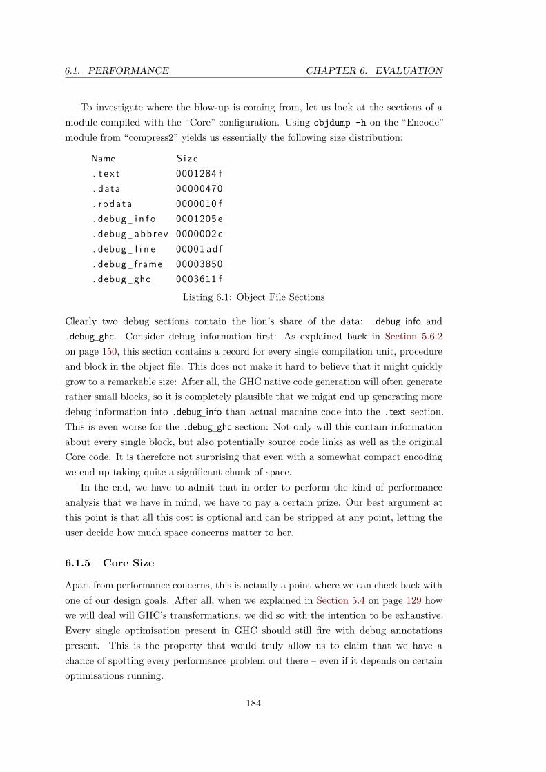
6.1. PERFORMANCE CHAPTER 6. EVALUATION

To investigate where the blow-up is coming from, let us look at the sections of amodule compiled with the “Core” configuration. Using objdump -h on the “Encode”module from “compress2” yields us essentially the following size distribution:

Name S i z e. t e x t 0001284 f. data 00000470. r oda ta 0000010 f. debug i n f o 0001205 e. debug abbrev 0000002 c. debug l i n e 00001 ad f. debug frame 00003850. debug ghc 0003611 f

Listing 6.1: Object File Sections

Clearly two debug sections contain the lion’s share of the data: .debug info and.debug ghc. Consider debug information first: As explained back in Section 5.6.2on page 150, this section contains a record for every single compilation unit, procedureand block in the object file. This does not make it hard to believe that it might quicklygrow to a remarkable size: After all, the GHC native code generation will often generaterather small blocks, so it is completely plausible that we might end up generating moredebug information into .debug info than actual machine code into the . text section.This is even worse for the .debug ghc section: Not only will this contain informationabout every single block, but also potentially source code links as well as the originalCore code. It is therefore not surprising that even with a somewhat compact encodingwe end up taking quite a significant chunk of space.

In the end, we have to admit that in order to perform the kind of performanceanalysis that we have in mind, we have to pay a certain prize. Our best argument atthis point is that all this cost is optional and can be stripped at any point, letting theuser decide how much space concerns matter to her.

6.1.5 Core Size

Apart from performance concerns, this is actually a point where we can check back withone of our design goals. After all, when we explained in Section 5.4 on page 129 howwe will deal will GHC’s transformations, we did so with the intention to be exhaustive:Every single optimisation present in GHC should still fire with debug annotationspresent. This is the property that would truly allow us to claim that we have achance of spotting every performance problem out there – even if it depends on certainoptimisations running.

184

CHAPTER 6. EVALUATION 6.1. PERFORMANCE

Dbg[Terms] [%]

cacheprof Arch_x86 4733 0.0Generics 1105 +2.9Main 10868 +0.1

calendar Main 1087 0.0cichelli Auxil 1067 0.0

Prog 827 0.0circsim Main 3563 0.0clausify Main 1328 0.0comp_lab_zift Main 3441 -2.4compress Decode 924 0.0

Encode 2262 0.0compress2 Encode 4148 0.0

WriteRoutines 804 0.0constraints Main 2074 -1.3

−1 s.d. —– -1.8+1 s.d. —– +1.7Average —– -0.1

Figure 6.5: Core Size

However, as we see in Figure 6.5, our work up to this point is not quite enough:While the Core size stays the same for most modules, we can see a few instances wherethe Core code seems to change. This demonstrates how hard it is to claim completenessfor a compiler as complex as GHC. For example, here is one of the issues:

f = λx y → ( , ) x y

Listing 6.2: Constructor Application

where (,) is the constructor of the pair. Here we could η-reduce f by setting f = (,).This is a really minor optimisation, as the only difference here is that slightly less objectcode gets generated. Apart from this, there are further issues, for example with fullysupporting the call pattern specialisation [Peyton Jones, 2007].

6.1.6 Run Time Overheads

The reason that we care so much about optimisations in the first place is of coursebecause they influence runtime performance of our program. While good behaviourat compile time is a nice bonus, what happens at runtime will make or break theusefulness of our whole profiling infrastructure. No matter whether it is due to missingoptimisations or sampling overheads – if it ends up altering the performance of the

185

6.1. PERFORMANCE CHAPTER 6. EVALUATION

Compilation Runtime DescriptionBase Baseline without eventlog generationDbg -g Simple build with debug annotationsEv -eventlog -ls Eventlog gets generatedDbgEv -g -eventlog -ls Eventlog with debug records

Figure 6.6: Runtime Configurations

Base Dbg Ev EvDbg[MB] [%] [%] [%]

k-nucleotide 3921 0.0 0.0 0.0integer 3338 0.0 0.0 0.0pidigits 2885 0.0 0.0 0.0constraints 2104 0.0 0.0 0.0cryptarithm1 2051 0.0 0.0 0.0n-body 1600 0.0 0.0 0.0circsim 1299 0.0 0.0 0.0hidden 1084 0.0 0.0 0.0binary-trees 956 0.0 0.0 0.0scs 917 0.0 0.0 0.0fannkuch-redux 870 0.0 0.0 0.0transform 680 0.0 0.0 0.0exp3_8 597 0.0 0.0 0.0atom 537 0.0 0.0 0.0−1 s.d. —– -0.0 -0.0 -0.0+1 s.d. —– +0.0 +0.0 +0.0Average —– -0.0 -0.0 -0.0

Figure 6.7: Allocation Overhead

program too much, all of our collected data might turn out to be nothing but smokeand mirrors. This is why it is especially important that we take a look at the runtimeperformance of the compiled programs. Even if we cannot guarantee the Core to becompletely identical, a good performance match across the benchmark suite would bean encouraging sign that we are not likely to encounter any significant “heisenbugs”that vanish upon inspection. This goes not only for our own debug annotations, butalso for the existing eventlog infrastructure, which we are going to use for generatingprogram profiles. The four configurations in Figure 6.6 cover different combinations ofthese debug options.

The results are shown in Figure 6.7 and Figure 6.8. The first performance metricshown is allocation amount. As the allocation amount of a given Haskell program ismostly deterministic, this is an excellent metric for comparing two Haskell program

186

CHAPTER 6. EVALUATION 6.1. PERFORMANCE

Base Dbg Ev DbgEv[s] [%] [%] [%]

k-nucleotide 5.0000 +0.5 -0.1 +0.4fannkuch-redux 3.6467 -0.2 -0.1 0.0spectral-norm 2.4550 0.0 -0.2 -0.2integer 1.5300 -0.8 +0.7 -2.6n-body 1.1300 0.0 -0.4 -0.9constraints 0.6600 +2.0 +0.3 +1.5cryptarithm1 0.4350 +1.1 -1.1 -1.1fasta 0.3850 -0.4 -1.3 -1.3pidigits 0.3700 0.0 -1.8 -2.7circsim 0.3633 +1.8 -0.9 -0.5binary-trees 0.3600 +2.8 +6.0 +8.3hidden 0.3000 0.0 +3.3 +1.1wheel-sieve1 0.2783 +0.6 -3.0 -3.0scs 0.2517 +3.3 -0.7 +3.3−1 s.d. —– -1.8 -3.9 -4.1+1 s.d. —– +2.0 +2.0 +2.5Average —– +0.1 -1.0 -0.9

Figure 6.8: Mutator Time Base Overhead

RTS optionsBase -lsTime -ls -EtTime2 -ls -Et100Alloc -ls -EaStack -ls -Es -kc8kHeap -ls -Eh

RTS optionsCycle -ls -EyCycle2 -ls -Ey100000Cache -ls -EcCmiss -ls -ECBranch -ls -EbBmiss -ls -EB

Figure 6.9: Sampling Configurations

runs for functional differences. And as we can see, for this statistic we manage a prettymuch perfect match between all configurations.

However, things get less predictable when we consider actual run time. Note thatin Figure 6.8 we deliberately consider only “mutator” time, which is the program timeexcluding start-up time and garbage collections. This is a good idea here, as copyingdebug records into the eventlog might cause a significant amount of delay when startingthe program. Furthermore, we are not going to profile garbage collections, thereforepossible performance changes there do not concern us. Even without these factors, it isquite clear that the results are still quite noisy: Paradoxically, on average performanceeven improves with event-logging active. However, the good averages should show thatwe have not introduced any severe biases, and can sensibly profile the code resultingfrom either configuration.

187

6.1. PERFORMANCE CHAPTER 6. EVALUATION

6.1.7 Sampling Overhead

The next important influence on program performance that we have to acknowledgeis sampling overhead: The act of capturing and emitting samples causes performanceto be lost, therefore any significant overhead could introduce skews. Figure 6.9 showsan overview of the sample collection configurations that we will test. Due to our workin Chapter 5 we have quite a few back-ends to choose from, with perf_events aloneproviding 6 different hardware performance counter configurations (on the right). Onthe other hand, the left hand side represents the 3 remaining sampling approaches,using timers, allocation and heap residency profiling respectively. Also note that we willadjust the sampling rate in a few cases: For the configurations “Time2” and “Cycle2”we overrode the sampling rates to 100µs and 100 000 cycles, which are 10 times higherthan their respective defaults. Furthermore, for stack allocation we decrease the stackblock size (8 kB, default 32 kB) to force more stack overflows and therefore samples.

In Figure 6.10 and Figure 6.11 we have collected data about the sampling overheadof using the different sampling back-ends. Because we are generally interested in therunning Haskell code, we again focus on mutator time. The exception is heap profiling,which actually runs as part of the garbage collection pass and therefore does notinfluence mutator time. Consequently we switch to comparing runtime overhead. Theresults work out as expected: Moderate slowdowns across the board. The exact amountvaries quite a bit due to run-time noise, but we generally stay well below 5 % overhead.The most notable outlier is the “Cycle2” configuration, where the low sampling ratecaused costs to spike up noticeably. On the other end of the spectrum we have the“Alloc” configuration, which is cheap enough to incur basically no overhead. As the“Stack” configuration uses the same mechanism, we would normally expect the samegood performance characteristics. However the increase in stack block size can havequite dramatic effects on program performance, as the +32.1 % outlier for “ansi” shoulddemonstrate.

6.1.8 Average Overhead

These performance measurements should convince us that all of our profiling back-endshave the ability to work well alongside program evaluation. However, we still haveto show that each back-end was successful in collecting enough sample data in orderto inform performance analysis. Figure 6.12 therefore shows us two statistics aboutthe generated data: First we give the average sampling rate over all program runs(weighted by run time). Heap profiling achieves a very high rate as this point, as it willset weights based on heap object size – which basically makes every single byte on theheap a sample. The next notable configuration is, again, heap allocation profiling, which

188

CHAPTER 6. EVALUATION 6.1. PERFORMANCE

Base Time Time2 Alloc Stack Heap ∗[s] [%] [%] [%] [%] [%]

k-nucleotide 49.76 -0.3 +1.5 -0.2 -0.5 -0.7fannkuch-redux 48.67 +0.5 +2.0 +0.0 +0.0 +0.0n-body 11.23 +0.6 +2.3 +1.0 -0.0 +0.8binary-trees 8.42 +1.3 +3.7 +0.2 +0.4 +76.7spectral-norm 8.23 +0.1 +1.5 -0.1 -0.1 -0.1fasta 3.79 +0.5 +5.5 +0.3 0.0 +0.0integer 1.49 +0.2 +2.7 0.0 0.0 +0.3exp3_8 1.26 0.0 +2.5 +0.3 +7.5 0.0pidigits 1.06 0.0 +3.8 -0.3 -0.2 +0.0wheel-sieve1 0.92 0.0 +2.2 0.0 +0.5 +7.4reverse-complem 0.83 0.0 +2.2 0.0 -0.4 -0.4kahan 0.81 -0.4 +1.6 0.0 -0.4 +0.0knights 0.69 +1.4 +2.9 0.0 0.0 +1.5ansi 0.56 +0.6 +3.5 +1.5 +32.1 +0.5primes 0.48 0.0 +2.1 0.0 +10.4 +0.2-1 s.d. —– -0.5 +1.9 -0.4 -3.9 -5.0+1 s.d. —– +1.6 +4.7 +1.2 +9.5 +12.0Average —– +0.6 +3.3 +0.4 +2.6 +3.1

(∗ Heap configuration compares run time)

Figure 6.10: Sampling Mutator Time Overhead (1/2)

Base Cycle Cycle2 Cache Cmiss Branch Bmiss[s] [%] [%] [%] [%] [%] [%]

k-nucleotide 49.4817 +2.1 +10.1 +1.2 +3.3 +0.9 +0.8fannkuch-redux 48.6900 +1.2 +9.5 +0.2 +0.3 +0.7 +1.9n-body 11.2550 +2.4 +9.6 +0.6 +0.5 +0.8 +0.7binary-trees 8.4233 +1.8 +9.9 +1.2 +1.9 +0.8 +2.3spectral-norm 8.2283 +0.9 +8.9 +0.0 +0.0 +0.0 +0.0fasta 3.7917 +1.9 +10.5 +1.0 +0.6 +0.7 +0.7integer 1.4900 +2.1 +11.0 +1.3 +1.3 +1.3 +3.4exp3_8 1.2600 +2.4 +11.9 +4.4 +1.5 +1.7 +1.3pidigits 1.0583 +5.7 +16.1 +7.7 +3.9 +3.9 +3.9wheel-sieve1 0.9200 +1.1 +9.8 0.0 0.0 +0.2 +0.2reverse-complem 0.8200 +2.4 +9.8 +1.2 +1.2 +2.0 +1.2kahan 0.8183 +1.0 +9.0 -0.6 -0.2 -0.2 +1.8sched 0.7000 +2.9 +11.4 +1.4 +1.4 +1.4 +4.3knights 0.6900 +1.9 +10.1 +1.4 +0.2 +1.4 +1.4-1 s.d. —– +1.6 +9.9 +0.7 +0.4 +0.5 +1.1+1 s.d. —– +4.6 +14.2 +4.5 +3.4 +4.0 +4.6Average —– +3.1 +12.0 +2.5 +1.9 +2.2 +2.8

Figure 6.11: Sampling Mutator Time Overhead (2/2)

189

6.2. USAGE SCENARIO CHAPTER 6. EVALUATION

Sample Rate Overhead Message Rate Overhead[Sample/s] [µs/Sample] [Msg/s] [µs/Msg]

Time 998.7 2.649 603.3 4.39Time2 9 980.1 2.169 1 458.1 14.84Alloc 208 610.3 0.003 1 760.9 0.40Stack 4 662.4 0.468 4 662.4 0.47Heap 43 139 691.9 0.001 7.7 7 270.24Cycle 3 091.4 4.607 1 154.6 12.34Cycle2 27 557.7 3.278 1 408.5 64.14Cache 976.6 9.445 562.4 16.40Cmiss 3 292.4 4.089 193.1 69.74Branch 975.7 7.149 580.5 12.02Bmiss 2 428.5 4.491 503.5 21.66

Figure 6.12: Sampling Overhead Overview

manages to collect a high number of samples, especially considering its low overhead.This means that heap allocation sampling is especially efficient at producing a lot of

sampling data without inducing overhead – the perfect combination. To see how otherapproaches stack up, we additionally calculate an overhead estimate per sample. Notunsurprisingly, heap allocation profiling is way ahead of the pack at 0.001µs per sample.Apart from that we see that most profiling approaches just take a few microsecondsper sample, which still makes it realistic to collect significant amounts of sampling data.Especially note that the cost remains relatively stable when we change sampling ratefor “Time2” and “Alloc2”, suggesting that the rate can be used to regulate overheads.

6.2 Usage Scenario

The main claim that we make about our profiling solution is that it is useful for resolvingreal-life performance problems. We covered performance and data quality in the lastsections, yet while these are necessary for a useful profiling tool, they are by no meanssufficient. However, in contrast to these quantifiable characteristics it will be very hardfor us to actually prove usefulness: There will always be performance problems thatwe cannot help with, and probably even programmers that will find our approach toprofiling especially hard to work with.

Therefore at best we could claim relative usefulness for a given set of problems anda certain type of user, ideally through a user study. This could give us a proper basisto argue about intuitiveness and usefulness of our user interface. However due to timeconstraints we will not be able to do this for this thesis. Instead, we opt to get our ownhands dirty, and show how analysing a non-trivial real-world example could look like.

190

CHAPTER 6. EVALUATION 6.2. USAGE SCENARIO

6.2.1 The Code

We will lift our example from the StackExchange website, where on 13th of March 2012user “Joey Adams” asked the following question in the code review section 1:

“I wrote a string escaping function in C, and I’m trying to rewrite it toHaskell. [...]

Here’s a naïve implementation based on Data.ByteString.concatMap:”

1 escape1 :: Word8 → By t eS t r i n g2 escape1 c3 | w2c c == ’\\ ’ = B. r e p l i c a t e 4 ( c2w ’\\ ’ )4 | c >= 32 && c <= 126 = B. s i n g l e t o n c5 | o t h e rw i s e = B. pack6 [ c2w ’\\ ’ , c2w ’\\ ’7 , c2w ’0 ’ + ( ( c ‘ s h i f tR ‘ 6) .&. 0x7 )8 , c2w ’0 ’ + ( ( c ‘ s h i f tR ‘ 3) .&. 0x7 )9 , c2w ’0 ’ + ( c .&. 0x7 ) ]

1011 e scape :: By t eS t r i n g → By t eS t r i n g12 e scape = B. concatMap escape11314 main :: IO ( )15 main = L . ge tConten t s >>= L . pu tS t r .16 L . fromChunks . map escape . L . toChunks

Listing 6.3: Original Escaping

We have slightly refactored the code to make it fit into the context of this thesis, but theimplementation is identical: We process one single byte at a time into an escaped form.For this example, the code author has handled three cases – basic ASCII characters,backslashes and extended characters.

Despite the author’s warning about the code’s naïvety, it already uses quite advancedimplementation techniques: For example, instead of using Haskell’s standard Stringtype to handle the data stream, it employs ByteStrings [Coutts et al., 2007b], whichare well known for their speed in dealing with I/O tasks. In fact, the author seemsto be well aware that fast streaming is a matter of processing data in chunks that areincrementally read from the disk. Therefore, the escaping process first uses map inorder to apply escape to every single chunk, followed by using concatMap in order toprocess single bytes.

1http://codereview.stackexchange.com/questions/9998/optimizing-bytestring-escaping

191

6.2. USAGE SCENARIO CHAPTER 6. EVALUATION

6.2.2 Profiling

Given the effort, the performance of this code is quite discouraging:

“I’d expect this to be a few times slower than the C version. Nope, it is 125times slower than the C version.”

Let us therefore compile the program with our debug annotations and profile it:

$ ghc Original.hs -O2 -rtsopts -eventlog -g -fsave-core

$ ./Original +RTS -ls -Ey -Ea < Original > /dev/null

$ threadscope Original.eventlog -d ~/ghc

These three lines compile and run the program, and start our analysis tool. Note thecommand line options: When compiling the program we activate full optimisations, butalso pass -g in order to request our debug annotations. Due to our work in Section 5.4on page 129 we are confident that these command line options do not conflict: We canprofile a fully optimised program. Furthermore, we requested the optimised Core codeto be saved along with the program. This will become useful shortly.

When running our program, we pass it its own executable as text data, and pipeits results into the void. More interesting are the options that we pass to the runtimesystem (RTS): The −ls option will cause a basic eventlog to be generated, while −Eyand −Ea will cause our profiling infrastructure to collect samples by both cycles as wellas allocation. Due to the fact that both have very low skews, there is no strong reasonto not combine sampling back-ends like this.

6.2.3 Analysis

If we take a look at the resulting profile view in Figure 6.13 on the next page, itshould be clear that we have a pretty tricky performance problem here. The activitygraph shows that the program is spending most of its time in garbage collection, and istherefore clearly allocating a lot of data. Unfortunately, even our profiling view turnsout to be all over the place: Even with increased fuzz the performance is spread wellover a number of modules. We especially cannot associate much performance with theOriginal.hs source file. This suggests that most cost was not found in our code orany portion that could get in-lined into it. Instead, we have apparently pushed most ofour complexity into the internals of the bytestring library itself. Given that we wouldstrongly suspect that an efficient implementation using ByteString should be possible,this means that we are probably mis-using the library somehow.

If we further focus on the 40 % CPU cycles spent inside the bytestring library, thepicture becomes slightly cleaner. We can easily determine that inlinePerformIO and w2care basically cost-free, but on the other hand we have two actual “worker” functions that

192

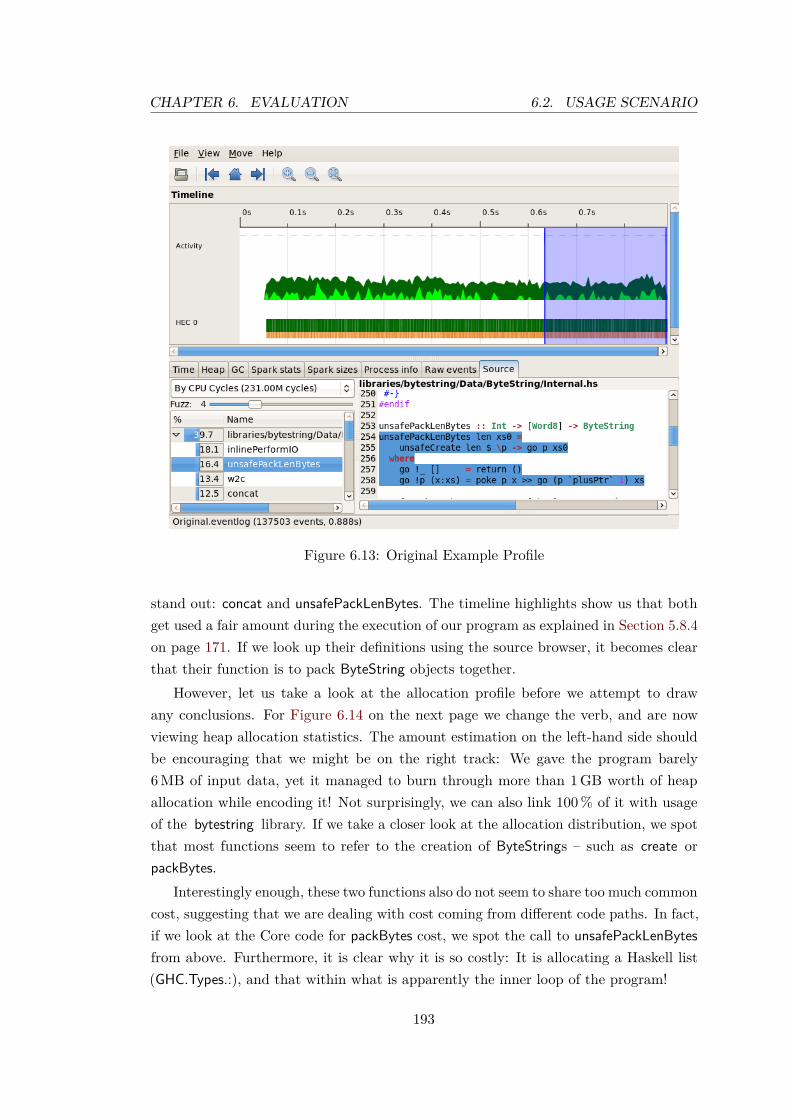
CHAPTER 6. EVALUATION 6.2. USAGE SCENARIO

Figure 6.13: Original Example Profile

stand out: concat and unsafePackLenBytes. The timeline highlights show us that bothget used a fair amount during the execution of our program as explained in Section 5.8.4on page 171. If we look up their definitions using the source browser, it becomes clearthat their function is to pack ByteString objects together.

However, let us take a look at the allocation profile before we attempt to drawany conclusions. For Figure 6.14 on the next page we change the verb, and are nowviewing heap allocation statistics. The amount estimation on the left-hand side shouldbe encouraging that we might be on the right track: We gave the program barely6MB of input data, yet it managed to burn through more than 1GB worth of heapallocation while encoding it! Not surprisingly, we can also link 100% of it with usageof the bytestring library. If we take a closer look at the allocation distribution, we spotthat most functions seem to refer to the creation of ByteStrings – such as create orpackBytes.

Interestingly enough, these two functions also do not seem to share too much commoncost, suggesting that we are dealing with cost coming from different code paths. In fact,if we look at the Core code for packBytes cost, we spot the call to unsafePackLenBytesfrom above. Furthermore, it is clear why it is so costly: It is allocating a Haskell list(GHC.Types.:), and that within what is apparently the inner loop of the program!

193

6.2. USAGE SCENARIO CHAPTER 6. EVALUATION

Figure 6.14: Original Allocation Profile

The amount of information that our interface provides might make it hard at first tospot the patterns, but the signs should become clearer: While concat contributed a lotof cost, it contributes almost no allocation, therefore we are apparently concatenatingmassive numbers of ByteString objects. That we spend a lot of allocation “creating”ByteString objects fits into that picture very well. While all this is going on, we are alsoclearly spending quite some time constructing lists and reducing them to even moreByteString objects.

If we look at the original program, the problem should now be apparent: We arecreating one ByteString object per byte from the original file, which means that overthe program run we create roughly 6 million instances. A good number of them evenget generated from a list using pack, which is not particularly efficient. The final verdictis simple: We should not try to concatenate millions of tiny ByteStrings – this is notwhat the library was designed to do.

6.2.4 Blaze-Builder

Fortunately, the author of the original program guessed as much even without goingthrough a detailed performance analysis. In his StackExchange query, he continues:

194

CHAPTER 6. EVALUATION 6.2. USAGE SCENARIO

“Then, I tried using blaze-builder:”

1 escape1 :: Word8 → Bu i l d e r2 escape1 c3 | c == 92 = fromWrite $ mconcat [ bs , bs , bs , bs ]4 | c >= 32 && c <= 126 = fromWrite $ writeWord8 c5 | o t h e rw i s e = fromWrite $ mconcat6 [ bs , bs7 , wr i teWord8 $ 48 + ( ( c ‘ s h i f tR ‘ 6) .&. 0x7 )8 , wr i teWord8 $ 48 + ( ( c ‘ s h i f tR ‘ 3) .&. 0x7 )9 , wr i teWord8 $ 48 + ( c .&. 0x7 ) ]

10 where bs = writeWord8 921112 e scape :: By t eS t r i n g → Bu i l d e r13 e scape = B. f o l d l ’ f mempty14 where f b c = b ‘mappend ‘ e scape1 c1516 main :: IO ( )17 main = L . ge tConten t s >>= L . pu tS t r .18 t oLa z yBy t eS t r i n g . mconcat . map escape . L . toChunks

Listing 6.4: Blaze-Builder Escaping

Given our knowledge from the last section, this is a smart choice. In contrast tobytestring , the blaze-builder library addresses exactly the use-case we identified: Build-ing large strings efficiently. In the example, we even see that the author applied thefromWrite optimisation, which basically allows blaze-builder to skip range checks forcases where we statically know how many characters we are going to emit.

However, this version does not fare much better:

“This made a difference. It’s even slower, 300 times slower than the Cversion. I thought blaze-builder was supposed to be really fast!”

At this point, our user is clearly frustrated. From his point of view, he is doing everythinghe can in order to allow the Haskell program to perform well, yet it does not seem tohelp. In fact, this is where he gave up and fell back to using an imperative style.

Fortunately, using our profiling solution we do not have to jump to such conclusions.Figure 6.15 on the following page shows the result of running the new program, usingexactly the same parameters as in the last sub-section. A look at ThreadScope’s statusbar confirms the program author’s performance claims: Instead of 0.8 s we are nowtaking 2.8 s to complete our test run! Also now we are allocating even more memory

195

6.2. USAGE SCENARIO CHAPTER 6. EVALUATION

Figure 6.15: Blaze-Builder Profile

on the heap, up to 1.46GB from 1.12GB we had previously. Somehow, things havegone even more wrong than before. On the other hand, we can now spot a proper “hotspot” in our performance data: Even low amounts of fuzzing allow us to pin 100% ofthe allocation on foldl ’ .go, the worker function of foldl ’ from the bytestring library.We actually have a similar kind of problem as our “factorial” example: GHC pulled allimportant parts into a self-contained inner loop, but has failed to optimise it well.

This makes a good starting point for some Core exploration, so let us have a closerlook at Figure 6.15. Core folding as explained in Section 5.8.8 exposes the inner loopfrom foldl ’ : The function starts by comparing addresses ww and ww1, continues withreading one byte from ww, followed by increasing the address by 1. If we scroll a bitfurther down, we find a recursive call. So where exactly is our allocation coming from?In fact, we are looking right at it: The let bindings shown are the main source ofallocations, due to the fact that each of them will capture our current address as wellas the last read byte. The reason that the let expression is not directly annotatedwith the 50.9 % allocation is an idiosyncrasy of heap allocation as discussed back inSection 5.7.6 on page 167: The problem is that due to the case expression we can nottell what branch the allocation is coming from. On the other hand, here the False isclearly the “loop” case, so this is where our problem must stem from.

196

CHAPTER 6. EVALUATION 6.2. USAGE SCENARIO

But why are we allocating so many closures in the first place? If we look at thestructure of the remainder of the Core code, it looks as follows:

go = λb ld addr end s t a t e → {− . . . −}l e t { a = {− . . . −} , $wa1 = {− . . . −} , {− . . . −} } i nca se p lusAddr # addr 1 o f addr ’ →l e t b ld ’ = λ s t e p →

l e t s tep ’ = case byte o f92 → l e t s tep ’ = λ range s → {− . . . −}

i n step ’→ l e t s tep ’ = λ range s → {− . . . −}

i n step ’i n b l d step ’

i n go bld ’ addr ’ end s t a t e ’Listing 6.5: Blaze-Builder Core

This small forest of lambda expression spawns the rest of the allocation of our program.Note that we renamed variables to reflect their type here, so for example byte is nowthe byte that was read using readWord8OffAddr# in Figure 6.15.

So what is going on here? Well, we see the recursive call, and we are clearly passinga new builder bld ’ , just as we would expect. However, we might be slightly surprised athow complicated the definition of bld ’ has turned out: In fact, it is a lambda value thatpasses our step to the bld closure we got as a parameter! So we are, in fact, passingour step back to the lambda we got from our left. This should start sounding awfullyfamiliar at this point: When we “hacked” our factorial implementation to turn a rightfold into a left fold, we were also passing continuations between fold iterations. Exceptthat this time, we are apparently turning a left fold into a right fold!

The reason for this whole debacle is of course that the program author apparentlyhad a wrong intuition about what a Builder is in the first place. Here is the slightlysimplified definition from the blaze-builder library:

newtype Bu i l d e r= Bu i l d e r (∀ r . Bu i l dS t ep r → Bu i l dS t ep r )

newtype Bu i l dS t ep r= Bu i l dS t ep ( BufRange → IO ( Bu i l d S i g n a l r ) )

Listing 6.6: Builder definition

As we might have guessed from the Core code, we are actually dealing with a nestedfunction type here. BuildStep encapsulates a primitive write: It takes a buffer positionand attempts to write some data into it. The point of Builder is that we string themtogether using continuation passing style.

197

6.2. USAGE SCENARIO CHAPTER 6. EVALUATION

We can see roughly how this works by considering the escape1 function from List-ing 6.4 on page 195. If we expand the newtype wrappers we obtain:

escape1 :: Word8 → ( BufRange → IO ( Bu i l d S i g n a l a ) )→ BufRange → IO ( Bu i l d S i g n a l a )

Listing 6.7: escape1 type

Which is basically saying “give me a byte and a way to continue writing”. The point ofpassing a continuation is simple: If we find that our content does not actually fit intothe current buffer, blaze-builder will have to allocate a new buffer to fill. ConstructingBuilder like this means that every function naturally receives its buffer from the Builderon its left, therefore this becomes a very low-overhead operation. In the end, this meansthat for efficient execution we want the following recursive structure:

escape1 byte0( e scape1 byte1

( e scape1 byte2 ) )buf

Listing 6.8: Recursive escape1

It is not hard to see that this is, in fact, a right fold. Therefore the choice of foldl ’ hasclearly been mistaken.

6.2.5 Folding

Of course this suggests that we might want to try to use a right fold. So let us simplyflip the direction of the fold in the program from Listing 6.4:

escapeCopyBytea2 :: By t eS t r i n g → Bu i l d e rescapeCopyBytea2 = B. f o l d r f mempty

where f c b = escape1 c ‘mappend ‘ bListing 6.9: Right Fold Version

In Figure 6.16 we have opened the profile generated by the resulting program. Andclearly we are on the right track: As the status bar shows, just this small change hasincreased the performance almost 8-fold relative to our first blaze-builder version, and2-fold over the initial bytestring code. Not bad!

However, a closer look at the profile might lessen our enthusiasm: The new versionactually allocates even more memory than all our previous versions. This might seemslightly surprising given our good performance, and is a great example for why reasoningabout verbs can sometimes be tricky: While allocation always has some overhead, theconcrete cost depends on how long we keep references around. And given that we are

198

CHAPTER 6. EVALUATION 6.2. USAGE SCENARIO

Figure 6.16: Blaze-Builder Right-Fold Profile

now walking through the ByteString in the “right” order, this basically means that ourallocated objects will die very quickly, leading to low actual overhead.

However, this does not explain why we are allocating so much data in the firstplace. As we see in Figure 6.16, folding away unrelated Core code exposes a familiarstructure: address comparison, followed by reading one byte, followed – again – by awhole bunch of closure allocations. So what is going on this time? If we pull out theCore code structure again, we see that our inner loop has changed to the structureshown in Listing 6.10 on the next page. Note that while in Listing 6.5 we built closuresas arguments, this time around the whole function is basically a big nested lambda-term.The expanded type of go even looks remarkably similar to the escape1 type: Given twoaddresses and a continuation we promise to fill a buffer.

However, note that instead of matching all arguments at the top level, GHC has leftlambdas “inside” wherever it could. The worry behind this is the same as we explainedback in Section 3.4.6 on page 36: What if our worker function go gets called often withthe same two addresses, but different step and range parameters? The allocated closuresare basically GHC organising thunks in order to save back work if this should happento be the case. And apparently, this time around the control flow is too complicatedfor the arity analysis of Breitner [2004] to figure out that this is a bad idea.

199

6.2. USAGE SCENARIO CHAPTER 6. EVALUATION

go :: Addr#

→ Addr#

→ ( BufRange → IO ( Bu i l d S i g n a l a ) )→ BufRange→ IO ( Bu i l d S i g n a l a )

go = λ addr end →{− . . . −}l e t {− . . . −}

b ld =λ s t e p →

l e t a = {− . . . −}i n ca se byte o f

92 → l e t s tep ’ = λ range s → {− . . . −}i n step ’

→ l e t s tep ’ = λ range s → {− . . . −}i n step ’

i n b l dListing 6.10: Blaze-Builder Core – Right Fold

6.2.6 Tailoring

At this point we have run out of easy solutions. The reason that the worker functiongo ends up getting composed out of three layers of lambda expressions is somethingthat comes naturally from the way we have structured our computation. However, bythis point we know exactly what the core of the problem is: We need the inner workerfunction derived for foldr to receive the right arity so it can perform Builder operationsefficiently. To achieve this, we simply take the definitions of foldr from bytestring andmappend and mempty from blaze-builder and “manually” inline them into each other.As we see in Listing 6.11, this means unravelling the internals of both libraries quitea bit. However, this allows us to force GHC to use the arity we want: Now the loopgo explicitly iterates over the input buffer (p and q) and the output buffer (range) inparallel.

As Figure 6.17 shows, this relatively straightforward change makes a significantdifference. In fact, is has reduced the runtime down to just 93ms! This is low enoughthat even the set-up cost of event log generation becomes significant (see Section 5.7.1on page 162). In fact, without profiling the program now achieves a total run time ofaround 41ms, which is a substantial 8-fold improvement over the previous version.

200

CHAPTER 6. EVALUATION 6.2. USAGE SCENARIO

f o l d B u i l d e r :: (Word8 → Bu i l d e r ) → B. By t eS t r i n g→ Bu i l d e r

f o l d B u i l d e r f (PS fp s l ) =f romBui ldStepCont $ λcont range → do

l e t p t r = unsa f eFo r e i gnPt rToPt r fpgo ! p ! q ! range ’

| p == q = cont range ’| o t h e rw i s e = do

touchFo r e i gnP t r p t rc ← peek pl e t p ’ = p ‘ p l u sP t r ‘ 1

s t ep = Bu i l dS t ep ( go p ’ q )r unBu i l dS t ep ( unBu i l d e r ( f c ) s t e p )

range ’l g o ( p t r ‘ p l u sP t r ‘ s ) ( p t r ‘ p l u sP t r ‘ ( s+l ) ) range

Listing 6.11: Specialised Fold

Figure 6.17: Blaze-Builder Profile – Optimised Fold

201

6.2. USAGE SCENARIO CHAPTER 6. EVALUATION

6.2.7 Manipulation

At this point, we have almost managed to push the performance of the Haskell versioninto the same realm as the C implementation, which takes 13ms to complete the sametask. What is more, the Core is now compact enough that it becomes quite easy tospot the source of the remaining inefficiencies. For example, in Figure 6.17 on page 201we spot that the program is still allocating about 212MB worth of heap data. This is alot better than before, but can certainly still be improved. This time, the analysis leadsus to where data gets written into the buffer. Here is what this looks like for escapedcharacters:

{− . . . d e t e rm ine what to w r i t e . . . −}l e t s t e p :: Addr# → Addr# → Sta t e # RealWor ld

→ ( # Sta t e # RealWorld , B u i l d S i g n a l r # )s t e p = λ addr end rw →ca se p lusAddr # addr 5# o f addr ’ →ca se l eAddr # addr ’ end o f

F a l s e → l e t cont = λ buf ’ rw ’ →ca se buf ’ o f BufRange addr ’ l i m i t ’ →s t e p addr ’ l i m i t ’ rw ’

i n ( # rw , B u f f e r F u l l 5 addr cont # )True → {− . . . w r i t e out data . . . −}

i n s t ep addr end rwListing 6.12: Blaze-Builder Writing Core

Note that this time the two addresses addr and end refer to the output buffer. Weconclude that the point of this code is to check whether enough space is available tooutput the desired number of bytes – here 5 for a character in escaped form. If werun into the end of the buffer, we return a BufferFull signal, which will invoke thecontinuation with a fresh buffer.

In this case, the allocation can be shown to originate from the step lambda 2. Incontrast to what one might expect, this is no instance of Let-No-Escape as explainedback in Section 3.5.11 on page 54. After all, a reference to writer clearly can escapethrough the cont closure! While we know that this is a very rare event, this still forcesGHC to actually allocate the writer closure on the heap, complete with all life variablesjust in case we need to interrupt and then resume our writing process.

2Unfortunately, the code generator plays a trick on us here – the code generated for the step lambdaadvances the heap pointer in anticipation of allocating cont, only to reset it in the (expected) case thatwe take the second branch. As it happens, this temporary increase of the heap pointer is what causesall calls into the memory system, therefore “shadowing” the true source of the allocation. Fortunately,it is not far away, so it is not hard to make the connection.

202

CHAPTER 6. EVALUATION 6.2. USAGE SCENARIO

In our example, it would clearly be better if we could just directly invoke the codewithout the need to wrap it into a closure first. However, this is not as easy as it sounds,as the data to write out comes from either the stack or the closure depending on thecode path that led us there. This means that in order to improve the code, we need toduplicate the writing code. Fortunately, in this instance this is quite easy, at least if weare advantageous enough to directly manipulate the implementation of blaze-builder. Tobe specific, the Core code from Listing 6.12 derives directly from the library’s fromWritefunction. We can simply adapt this function to look as follows:

f romWrite ’ :: Write → Bu i l d e rfromWrite ’ w r i t e = f romBui ldStepCont s t ep

where s t ep k ( BufRange op ope )| op ‘ p l u sP t r ‘ getBound w r i t e <= ope = do

op ’ ← runPoke ( getPoke w r i t e ) opl e t ! br ’ = BufRange op ’ opek br ’

| o t h e rw i s e =r e t u r n $ b u f f e r F u l l ( getBound w r i t e ) op

( s tep ’ k )s tep ’ k ( BufRange op ope ) = do

op ’ ← runPoke ( getPoke w r i t e ) opl e t ! br ’ = BufRange op ’ opek br ’

Listing 6.13: Custom fromWrite implementation

We have not changed much, the only difference is the step ’ function. Originally thelibrary passed a (step k) closure to bufferFull here, which is what led to the Core codeshown in Listing 6.12. Now we have set up a specialised code path for resuming thewrite process, which should allow GHC to either let-no-escape or inline the originalstep function. Having a separate function also gives us the opportunity to skip theseemingly redundant size check for the fresh buffer.

This change brings the total runtime of the program down to 21ms, another im-provement by a factor of 2. In fact, as Figure 6.18 on the following page shows, thetotal allocation of the program is now just 385 kB, which is less than the size of theinput file. This means that we have eliminated virtually all heap allocation from theinner loop! At this point, we have optimised the program as far as we can. In fact, wehave come fairly close to the reference point of 13ms that the C version took.

203

6.3. WRAPPING UP CHAPTER 6. EVALUATION

Figure 6.18: Blaze-Builder Profile – Optimised Write

6.3 Wrapping Up

The data we have collected in this chapter is no proof of usefulness, but it gives usan idea how the practice of using our tool might look like. Our case study has shownthat we can optimise a Haskell program to the point where it can compete with C interms of performance. Especially note that while we had to replace certain key partsof the infrastructure, the structure of the code did not change much compared to ourfirst version in Listing 6.4 on page 195! This means that we have indeed managed toimprove performance while remaining high-level in our top-level implementation. It isnot unrealistic that in future, libraries and compiler optimisations might mature to thepoint where we can skip some of the “hacks” we had to employ here.

Furthermore, as the first part of the chapter should have shown, we can be quiteconfident that our tool will work well in a lot of scenarios. We ourselves have tested ourtool on a number of programs ranging from small examples to large applications (suchas GHC itself), and have found that with careful analysis we can find evidence for mostkinds of performance problems. And while such an investigation might admittedly stilloften require expert knowledge and experience, the added information and guidancemakes the optimisation job much easier than it had been before.

204

Chapter 7

Conclusion

“– We have been torturing you for hours, and it does not even seem to hurt.This will not help you!”

“– Oh yes, it will: It will help to pass the time...”

Asterix the Gaul, René Goscinny & Albert Uderzo

When we started out with this thesis, our claim was that we would be able to providea novel profiling solution for the programming language Haskell. Our goal was not todisplace existing solutions, but to provide new options to users that have struggledwith making sense of Haskell’s occasionally erratic performance behaviour so far. Ouraim was to directly address one of the hardest problems that plagues reasoning aboutHaskell program performance today: The disconnect between rapidly evolving librariespromising to marry high performance with purely functional programming, and theunfortunate realities of attempting to diagnose the ever more complicated performanceproblems that this combination can lead to.

7.1 Contributions

In the end, we can claim that we were successful in attacking the profiling problem ina rigorous fashion. As a result, we have found a few novel ways of thinking about theprofiling task.

This started in Chapter 2, where we set out to build a foundation for our work. Hereis where we defined the terms that we were going to use throughout this thesis. Theverb/noun nomenclature we introduce was originally formulated by Irvin [1995], howeverwe believe that the way we have linked it to the causal reasoning process is a freshinterpretation of the concept. Similarly, Chapter 3 mainly serves to introduce existingmaterial, while putting our own spin on existing themes. For example, the performancemodel we introduce is intended to make stronger claims about the performance of

205

7.2. PRIOR WORK CHAPTER 7. CONCLUSION

Haskell programs than usual, as we want to obtain guarantees that we are not going tomiss the causal connection of certain verbs in profiling.

The central contributions of this thesis can however be found in Chapter 4. To ourknowledge there has been no previous attempt at formally applying causal theory tooperational semantics. Our approach of decomposing rule matches into a network ofevents and determining causality by employing closest-world thought experiments hasbeen specifically developed as a theoretical foundation for this work. The purpose ofthis is to enable the reasoning about optimisations as shown in Section 4.8: At thispoint we are able to make well-grounded claims about what the “right” annotationschemes are in every situation. Before the link with causality was established, reasoningat this point was effectively based on worst-case scenarios and consistency concerns.And while the results might not be particularly spectacular, in a language with suchtricky semantics as Haskell it is a good idea to have strong guarantees about our claims.

The profiling framework we developed in Chapter 5 forms the second main body ofcontributions. Apart from the engineering work involved, we believe that our designbrings a few new concepts to the table as well. For example, our causality semantics canserve as a baseline for comparing different ways of explaining performance problems.In Section 5.3 on page 121 we used this to evaluate various iterations of cost-centreprofiling as introduced by Sansom and Peyton Jones [1995]. Furthermore, our insightsinto the performance analysis process has led to a novel user interface design tailoredtowards the specific requirements of working with heavily optimised programs. To bespecific, we realised that talking about causal processes involving transformations meantthat we can not always determine a singular villain in the source code. Consequently weshowed in Section 5.8 on page 168 how we can design the interface so it allows the userto work with such “ambiguous” source code links. To offset the inevitable uncertainty,our Core viewer fills the role of a one-stop analysis tool for unraveling the program’sinner workings. This especially allows us to making sense of exactly how the compiler’sdecision gave rise to the program’s performance characteristics. To our knowledge thisform of analysis is unprecedented, at minimum within the Haskell world.

7.2 Prior Work

7.2.1 Haskell Profiling

Clearly our work was heavily inspired by the work on previous profiling solutions. Tostart with, our approach targets the Haskell ecosystem, so our main reference point isobviously the work by Sansom and Peyton Jones [1995], which was recently revisitedby Marlow [2012]. The problems of cost attribution led us down similar paths – forexample, we argued in Section 4.4.1 on page 72 that laziness is transparent with respects

206

CHAPTER 7. CONCLUSION 7.2. PRIOR WORK

to cause annotations, which has parallels to Sansom and Peyton Jones [1997, Section3.5]. Furthermore as explicitly explored in Section 5.3.2 on page 122 forwards, we caneven map lexical and evaluation scoping to subsets of our full cause terms. Howeverthe aim of our works still vary significantly, with our work prioritising the ability todo low-overhead profiling of optimised program over concerns such as cost centre stackconsistency.

Next we have to acknowledge the work of Jones et al. [2009] on the eventlog tracinginfrastructure as well as the ThreadScope profiling tool, which we extended in order toanalyse our data. The main focus of their profiling is reasoning about the behaviour ofparallel Haskell programs, which has further improved over the years due to the workof Coutts et al. [2011]. In fact, the format has become something of a lingua franca forprofiling parallelism in Haskell variants, with a good number of consumers in the Edentrace viewer [Berthold and Loogen, 2007], HdpHProf [Al Saeed et al., 2012] as well as therecent ghc-events-analyze utility [de Vries and Coutts, 2014]. It has even been usedfor profiling Mercurial programs [Bone and Somogyi, 2011]. And even though profilingparallel programs is out of scope of this work, the high variety of profiling approacheshas certainly been an inspiration for developing our general noun/verb nomenclature.

On a similar note, we have to acknowledge work on Haskell profiling that we donot actively touch here. There has been the work of Röjemo and Runciman [1996]on decomposing what we see as the heap residency verb. The work by the samegroup on coverage analysis [Gill and Runciman, 2007] could also be interpreted as adistant relative to program profiling. Returning to parallel profiling, there have been anumber of interesting profiling approaches exploring parallel programs executed usingGranSim [Loidl, 1996], such as the work of Hammond et al. [1997]. The approach ofCharles and Runciman [1999] to make profile exploration interactive can be seen ashaving parallels with our work. As Charles [2001] shows, effectively climbing the causalchain backwards is an equally non-trivial pursuit in the parallel context.

7.2.2 General Profiling

Quite obviously Haskell has not been the only language environment that has seenactive work on profiling questions. The field is way too large to give a comprehensibleliterature review. We will therefore mainly focus on instances where existing workinspired our choice of approaching profiling of optimised code using causality theory.

On this account we first have to credit the work of Irvin [1995] which inspired theverb/noun nomenclature used throughout this work, even if it was not interpreted ina causal context. As he notes, verbs and nouns can exist on many different levelsof abstractions, which we can “map” in order to obtain more useful views. However,no formal connection to causality is made. The work of Shende [2001] continues this

207

7.3. FUTURE WORK CHAPTER 7. CONCLUSION

effort of multi-level verb mapping in a distributed context, with their implementationalso explicitly addressing the problem of working with compiler optimisations. Themore complex verb structure of distributed and parallel systems has also given rise tosome work on more complex performance metrics, such as for example in Eyerman andEeckhout [2008], or the key performance indicators used for assessing performance ofcloud computing services [Garg et al., 2013].

Profiling in presence of compiler optimisations has also addressed quite a few times inthe past, with for example Appel et al. [1988] already noting that “The machine-code fora function is not necessarily all contiguous. A function may be turned into several piecesof code, with portions of the code for other functions interspersed.”. To our knowledge,Brooks et al. [1992] is the first time that it was considered that the proper way toapproach profiling optimised code might be to see it as generated by multiple pieces ofsource code at the same time. The work of Kaneshiro and Shindo [1996] tackles trackingsource code relations on object code moved by program transformations. Finally, it hasto be mentioned that the LLVM infrastructure [Lattner and Adve, 2004] as explainedin Section 5.6.8 on page 160 also supports somewhat optimisation-resistant debuggingannotations via line annotations. Neither work formally approached this problem froma perspective of causal reasoning.

7.3 Future Work

We have made some significant progress on realising our vision for how optimisation-aware low-level profiling could look like for Haskell. On the other hand, it is prettymuch the nature of the profiling task that we can never truly claim completeness inany shape or form. In fact, we can easily number fairly straight-forward ways that thiswork could be otherwise applied or extended.

7.3.1 Parallelism

In this day and age, it seems almost antiquated to focus as much on single-core per-formance as we have for this thesis. The slow change in hardware architectures meansthat in future we might have entirely new profiling challenges arising from the needto run programs on parallel architectures. Fortunately, most of our ground work stillapplies: The user would be facing an abductive reasoning task, and would apply verband noun abstractions in order to find causal links. The main difference would concernthe verb side of things, where we should now be talking about communication delaysand idle times.

In fact, in the context of this work we developed a preliminary solution for profilingprograms written using the monad−par library by Marlow et al. [2011]. The basic idea

208

CHAPTER 7. CONCLUSION 7.3. FUTURE WORK

Figure 7.1: Parallel Profile

here is that the main verb we are trying to track is data locality: Do parallel processesprogress on the work load in an orderly fashion, or are we jumping so much that we arelikely to incur significant communication delays? This shows that it can sometimes behard to express verbs in numbers – instead we could use a visual approach as shownin Figure 7.1: Here we arrange the directed job dependency graph of an instrumentedmonad−par library in a way that highlights the structure of data dependencies, whilereflecting how the program executed. In this view, poor locality would show as vertical“jumps”, whereas idle times would correspond to horizontal free space. However, wehave not had the chance to develop this work much, but still expect the future of parallelprofiling to lie in similar concepts.

7.3.2 Technicalities

Furthermore, the amount of technical work that went into this thesis also uncovered alot of potential for further improvements. One of the most glaring problems with ourprofiling solution at this point is that unless the compiler helps us by in-lining, we havebasically no chance to figure out where a function was called from. While we arguethat GHC will do this quite often, this is still a significant blind spot. Fortunately,as we reported in Section 5.3.6 on page 128 it is quite realistic to introduce Haskell

209

7.3. FUTURE WORK CHAPTER 7. CONCLUSION

stack walking at some point, with Rouhani-Kalleh [2014] and Schröder [2014] alreadyinvestigating interesting angles of attack.

Furthermore, it is quite unsatisfactory that so far our profiling solution can onlytarget Linux systems. The list of problems ranges from rather trivial problems such asidentifying the current memory map (see Section 5.7.1 on page 162) to more involvedissues such as how to access hardware performance pointers reliably, as investigatedbriefly in Section 5.7.4 on page 166. It would be especially nice if we could fullysupport the LLVM infrastructure as sketched in Section 5.6.8, as this back-end willoften generate faster code than the native code generator. On the other hand, this isquite hard to achieve due to the limitations in meta data, as well as apparent data lossduring low-level optimisations.

Finally, due to the fact that our profiling approach is mostly based on instructionpointers, it is relatively easy to introduce new verbs. This leaves ample space forfuture extensions, such as verbs tracking the movement of heap object types throughgenerations. In a similar vain we might attempt to extend our system on the nounside: As Irvin [1995] already notes, it might make sense to track causality for user-defined nouns instead of just source code locations. This could take the form of simpleevent-log markers identifying program phases as implemented by Coutts et al. [2011],or full-blown noun trees that the program automatically generates in order to explainits own structure. We could for example imagine program interpreters communicatingthe call stack of the interpreted program to a profiling tool in order to inform analysis.

7.3.3 User Interface

Our extension of the ThreadScope user interface has proved to be a powerful tool fordrilling deep into complicated performance problems. However, we could make ourapproach even more useful if we were better about integrating existing information intoour view. For example, there is no direct reason why we could not use our interfaceto reason about cost-centre profiling data as well – this would allow us to properlyreason about stack traces where it is appropriate. From the user’s point of view, thereis probably little that we would have to change, with even fuzzing as explained inSection 5.8.5 on page 172 having a straightforward equivalent.

Furthermore, one of the unique aspects of our work was that we tried to integrate aview of the intermediate Core language into our profiling view. However, as we noted inSection 5.8.8 on page 176 showing unfiltered Core to the user can be overwhelming, andtherefore extra efforts might be warranted. For example, the work on HERMIT [Farmeret al., 2012] shows a number of ways that we can make Core code easier on the eyesand less error-prone to reason about, such as using better variable names than theones generated by GHC. For the purpose of profiling we would also really like to have

210

CHAPTER 7. CONCLUSION 7.3. FUTURE WORK

basic navigation tools, such as being able to quickly “jump” to a given definition orreturn to a prior view. Finally, we show Core primarily to allow the user to reasonabout performance, therefore we could do a better job communicating the performancemodel to the user. This could be as easy as simply emphasising allocation spotsand non-primitive variables. On the other hand we also have quite a few interestingopportunities for code analysis here, which might help identify instances of let-no-escape(see Section 3.5.11 on page 54) or find the amount of live variables of closures.

211

7.3. FUTURE WORK CHAPTER 7. CONCLUSION

212

List of Figures

2.1 Deduction vs. Abduction . . . . . . . . . . . . . . . . . . . . . . . . . . 62.2 Abduction: Assessing Plausibility . . . . . . . . . . . . . . . . . . . . . . 72.3 Schematic of an Explanation . . . . . . . . . . . . . . . . . . . . . . . . 92.4 Causality Analysis of an Unfortunate Event . . . . . . . . . . . . . . . 13

3.1 Glasgow Haskell Compiler – Compilation Pipeline . . . . . . . . . . . . 273.2 Heap Object Construction . . . . . . . . . . . . . . . . . . . . . . . . . . 483.3 Call Implementation . . . . . . . . . . . . . . . . . . . . . . . . . . . . . 503.4 Performance Model . . . . . . . . . . . . . . . . . . . . . . . . . . . . . . 55

4.1 Causality Reasoning: Past and Future . . . . . . . . . . . . . . . . . . . 594.2 Event Decomposition of a Constructor Rule Match . . . . . . . . . . . . 604.3 Maintaining Cause Links . . . . . . . . . . . . . . . . . . . . . . . . . . . 614.4 Event Decomposition of a Constructor Rule Match (Repeated) . . . . . 644.5 Causality Relations for a Constructor Rule Match . . . . . . . . . . . . 654.6 Ordered Event Decomposition of a Variable Rule Match . . . . . . . . . 664.7 Flat Events . . . . . . . . . . . . . . . . . . . . . . . . . . . . . . . . . . 684.8 Nested Events . . . . . . . . . . . . . . . . . . . . . . . . . . . . . . . . . 684.9 Alternate World . . . . . . . . . . . . . . . . . . . . . . . . . . . . . . . 694.10 Deeply Nested Events . . . . . . . . . . . . . . . . . . . . . . . . . . . . 694.11 Deeply Nested Events Notation . . . . . . . . . . . . . . . . . . . . . . . 704.12 Depending on Nested Events . . . . . . . . . . . . . . . . . . . . . . . . 704.13 Causal Dependencies for a Variable Rule Match . . . . . . . . . . . . . . 714.14 Laziness Transparency Proof Overview . . . . . . . . . . . . . . . . . . . 744.15 Ordered Event Decomposition of an Application Rule Match . . . . . . 814.16 Causal Relations for an Application Rule Match . . . . . . . . . . . . . 834.17 Summary of Causality Relations . . . . . . . . . . . . . . . . . . . . . . 834.18 Depending on Deeply Nested Annotations . . . . . . . . . . . . . . . . . 844.19 Causality Model . . . . . . . . . . . . . . . . . . . . . . . . . . . . . . . 944.20 Core Representation of Haskell Bindings . . . . . . . . . . . . . . . . . . 99

I

LIST OF FIGURES LIST OF FIGURES

5.1 Scopes for an application expression . . . . . . . . . . . . . . . . . . . . 1235.2 Tick Classification . . . . . . . . . . . . . . . . . . . . . . . . . . . . . . 1365.3 Cmm Tick Scopes . . . . . . . . . . . . . . . . . . . . . . . . . . . . . . 1465.4 Block Tree from Scopes . . . . . . . . . . . . . . . . . . . . . . . . . . . 1575.5 “Scopes” in Core . . . . . . . . . . . . . . . . . . . . . . . . . . . . . . . 1585.6 Sample Encoding . . . . . . . . . . . . . . . . . . . . . . . . . . . . . . . 1645.7 ThreadScope User Interface . . . . . . . . . . . . . . . . . . . . . . . . . 1705.8 Performance Data Fuzz . . . . . . . . . . . . . . . . . . . . . . . . . . . 1735.9 Core View . . . . . . . . . . . . . . . . . . . . . . . . . . . . . . . . . . . 1755.10 Tracking Stack Allocation . . . . . . . . . . . . . . . . . . . . . . . . . . 176

6.1 Benchmark Configurations . . . . . . . . . . . . . . . . . . . . . . . . . . 1816.2 Compilation Time . . . . . . . . . . . . . . . . . . . . . . . . . . . . . . 1816.3 Tick Count . . . . . . . . . . . . . . . . . . . . . . . . . . . . . . . . . . 1826.4 Module Object File Sizes . . . . . . . . . . . . . . . . . . . . . . . . . . 1836.5 Core Size . . . . . . . . . . . . . . . . . . . . . . . . . . . . . . . . . . . 1856.6 Runtime Configurations . . . . . . . . . . . . . . . . . . . . . . . . . . . 1866.7 Allocation Overhead . . . . . . . . . . . . . . . . . . . . . . . . . . . . . 1866.8 Mutator Time Base Overhead . . . . . . . . . . . . . . . . . . . . . . . . 1876.9 Sampling Configurations . . . . . . . . . . . . . . . . . . . . . . . . . . . 1876.10 Sampling Mutator Time Overhead (1/2) . . . . . . . . . . . . . . . . . . 1896.11 Sampling Mutator Time Overhead (2/2) . . . . . . . . . . . . . . . . . . 1896.12 Sampling Overhead Overview . . . . . . . . . . . . . . . . . . . . . . . . 1906.13 Original Example Profile . . . . . . . . . . . . . . . . . . . . . . . . . . . 1936.14 Original Allocation Profile . . . . . . . . . . . . . . . . . . . . . . . . . . 1946.15 Blaze-Builder Profile . . . . . . . . . . . . . . . . . . . . . . . . . . . . . 1966.16 Blaze-Builder Right-Fold Profile . . . . . . . . . . . . . . . . . . . . . . 1996.17 Blaze-Builder Profile – Optimised Fold . . . . . . . . . . . . . . . . . . . 2016.18 Blaze-Builder Profile – Optimised Write . . . . . . . . . . . . . . . . . . 204

7.1 Parallel Profile . . . . . . . . . . . . . . . . . . . . . . . . . . . . . . . . 209

II

List of Listings

2.1 Example Haskell Program . . . . . . . . . . . . . . . . . . . . . . . . . . 152.2 Faulty Alternative . . . . . . . . . . . . . . . . . . . . . . . . . . . . . . 162.3 Smart Alternative . . . . . . . . . . . . . . . . . . . . . . . . . . . . . . 162.4 Alternative with a Hole . . . . . . . . . . . . . . . . . . . . . . . . . . . 172.5 Example with Error Checking . . . . . . . . . . . . . . . . . . . . . . . . 17

3.1 Factorial in C . . . . . . . . . . . . . . . . . . . . . . . . . . . . . . . . . 233.2 Definition of foldr . . . . . . . . . . . . . . . . . . . . . . . . . . . . . . 243.3 Fusion-enabled Enumeration . . . . . . . . . . . . . . . . . . . . . . . . . 253.4 Short-cut Fusion Rule . . . . . . . . . . . . . . . . . . . . . . . . . . . . 253.5 Sharing Hindering Rules . . . . . . . . . . . . . . . . . . . . . . . . . . . 263.6 Core Definition (Without Types) . . . . . . . . . . . . . . . . . . . . . . 283.7 Core Example . . . . . . . . . . . . . . . . . . . . . . . . . . . . . . . . . 283.8 Type Performance Problem . . . . . . . . . . . . . . . . . . . . . . . . . 293.9 Type Performance Problem – Core . . . . . . . . . . . . . . . . . . . . . 293.10 Core after Specialisations . . . . . . . . . . . . . . . . . . . . . . . . . . 303.11 eftInt Rule . . . . . . . . . . . . . . . . . . . . . . . . . . . . . . . . . . 303.12 Core after eftInt Rule . . . . . . . . . . . . . . . . . . . . . . . . . . . . 313.13 fold/build Rule . . . . . . . . . . . . . . . . . . . . . . . . . . . . . . . . 313.14 Core after fold/build Rule . . . . . . . . . . . . . . . . . . . . . . . . . . 313.15 Core after Rules . . . . . . . . . . . . . . . . . . . . . . . . . . . . . . . 313.16 eftIntFB in Haskell . . . . . . . . . . . . . . . . . . . . . . . . . . . . . . 323.17 eftIntFB in Core . . . . . . . . . . . . . . . . . . . . . . . . . . . . . . . 323.18 eftIntFB after Specialisations . . . . . . . . . . . . . . . . . . . . . . . . 323.19 eftIntFB after Floating . . . . . . . . . . . . . . . . . . . . . . . . . . . . 333.20 eftIntFB after Worker-Wrapper Transformation . . . . . . . . . . . . . . 333.21 eftIntFB with Unfolded Wrapper . . . . . . . . . . . . . . . . . . . . . . 343.22 Core after Unfolding . . . . . . . . . . . . . . . . . . . . . . . . . . . . . 343.23 Core after Nested Unfolding . . . . . . . . . . . . . . . . . . . . . . . . . 353.24 Core after Worker/Wrapper . . . . . . . . . . . . . . . . . . . . . . . . . 35

III

LIST OF LISTINGS LIST OF LISTINGS

3.25 Fixed Haskell Program . . . . . . . . . . . . . . . . . . . . . . . . . . . . 363.26 Fold Emulation . . . . . . . . . . . . . . . . . . . . . . . . . . . . . . . . 373.27 Fixed Haskell Program after Unfolding . . . . . . . . . . . . . . . . . . . 373.28 Fixed Haskell Program after η-Expansion and β-Reduction . . . . . . . 383.29 Fixed Haskell Program after Worker/Wrapper . . . . . . . . . . . . . . . 383.30 Definition of foldl : . . . . . . . . . . . . . . . . . . . . . . . . . . . . . . 393.31 Factorial with foldl . . . . . . . . . . . . . . . . . . . . . . . . . . . . . 393.32 Control Flow . . . . . . . . . . . . . . . . . . . . . . . . . . . . . . . . . 403.33 After Case-Of-Case . . . . . . . . . . . . . . . . . . . . . . . . . . . . . . 403.34 Case-Of-Case for Tuples . . . . . . . . . . . . . . . . . . . . . . . . . . . 403.35 Case-Of-Case with Join Point . . . . . . . . . . . . . . . . . . . . . . . . 413.36 Constructor Saturation . . . . . . . . . . . . . . . . . . . . . . . . . . . . 423.37 Variable Normalisation . . . . . . . . . . . . . . . . . . . . . . . . . . . . 433.38 Conversion to A-normal form . . . . . . . . . . . . . . . . . . . . . . . . 433.39 Convert strict let to case . . . . . . . . . . . . . . . . . . . . . . . . . . 433.40 Definition of Bool . . . . . . . . . . . . . . . . . . . . . . . . . . . . . . . 483.41 Lambda with Live Variables . . . . . . . . . . . . . . . . . . . . . . . . . 49

4.1 Constructor Source . . . . . . . . . . . . . . . . . . . . . . . . . . . . . . 61

5.1 Monad Usage Example . . . . . . . . . . . . . . . . . . . . . . . . . . . . 1245.2 Monad Usage Example – unfolded . . . . . . . . . . . . . . . . . . . . . 1245.3 Cost-Centre Float-In . . . . . . . . . . . . . . . . . . . . . . . . . . . . . 1275.4 Return Pointer Example . . . . . . . . . . . . . . . . . . . . . . . . . . . 1285.5 No Return Pointer Example . . . . . . . . . . . . . . . . . . . . . . . . . 1285.6 Ticked Core Definition . . . . . . . . . . . . . . . . . . . . . . . . . . . . 1295.7 SourceNote definition . . . . . . . . . . . . . . . . . . . . . . . . . . . . . 1315.8 Floating Inwards . . . . . . . . . . . . . . . . . . . . . . . . . . . . . . . 1345.9 In-Lining . . . . . . . . . . . . . . . . . . . . . . . . . . . . . . . . . . . 1345.10 Floating Outwards . . . . . . . . . . . . . . . . . . . . . . . . . . . . . . 1355.11 Floating Outwards Without Annotation . . . . . . . . . . . . . . . . . . 1355.12 Floating Ticks . . . . . . . . . . . . . . . . . . . . . . . . . . . . . . . . 1365.13 Thunk Unfolding . . . . . . . . . . . . . . . . . . . . . . . . . . . . . . . 1375.14 η-Reduction . . . . . . . . . . . . . . . . . . . . . . . . . . . . . . . . . . 1385.15 Rule Application . . . . . . . . . . . . . . . . . . . . . . . . . . . . . . . 1395.16 Rule Application with Floating . . . . . . . . . . . . . . . . . . . . . . . 1395.17 Common Sub-Expression Elimination . . . . . . . . . . . . . . . . . . . 1405.18 Common case Branch Elimination . . . . . . . . . . . . . . . . . . . . . 1405.19 Identity case Branch Elimination . . . . . . . . . . . . . . . . . . . . . . 140

IV

LIST OF LISTINGS LIST OF LISTINGS

5.20 let -Bound Lambda Expression . . . . . . . . . . . . . . . . . . . . . . . 1415.21 Cost-Centre Placement . . . . . . . . . . . . . . . . . . . . . . . . . . . . 1425.22 Core Result . . . . . . . . . . . . . . . . . . . . . . . . . . . . . . . . . . 1425.23 Cmm Example . . . . . . . . . . . . . . . . . . . . . . . . . . . . . . . . 1445.24 Cmm Example with Ticks . . . . . . . . . . . . . . . . . . . . . . . . . . 1455.25 Cmm Block Concatenation . . . . . . . . . . . . . . . . . . . . . . . . . 1475.26 Cmm Common Block Elimination . . . . . . . . . . . . . . . . . . . . . 1485.27 Compilation Unit Record . . . . . . . . . . . . . . . . . . . . . . . . . . 1505.28 Sub-Program Record . . . . . . . . . . . . . . . . . . . . . . . . . . . . . 1505.29 Assembly With Bound Markers . . . . . . . . . . . . . . . . . . . . . . . 1505.30 Lexical Block Record . . . . . . . . . . . . . . . . . . . . . . . . . . . . . 1515.31 Assembly With Line Annotations . . . . . . . . . . . . . . . . . . . . . . 1525.32 Source Line Table . . . . . . . . . . . . . . . . . . . . . . . . . . . . . . 1525.33 Unwind Instructions . . . . . . . . . . . . . . . . . . . . . . . . . . . . . 1545.34 Expected Assembly . . . . . . . . . . . . . . . . . . . . . . . . . . . . . . 1545.35 Actual Haskell Assembly . . . . . . . . . . . . . . . . . . . . . . . . . . . 1545.36 Line-Annotated Haskell Assembly . . . . . . . . . . . . . . . . . . . . . . 1555.37 Example Stack Trace . . . . . . . . . . . . . . . . . . . . . . . . . . . . . 1565.38 Debug Records . . . . . . . . . . . . . . . . . . . . . . . . . . . . . . . . 1575.39 Core Note . . . . . . . . . . . . . . . . . . . . . . . . . . . . . . . . . . . 1595.40 Core Pieces . . . . . . . . . . . . . . . . . . . . . . . . . . . . . . . . . . 1595.41 LLVM Debug Meta Data . . . . . . . . . . . . . . . . . . . . . . . . . . 1615.42 LLVM Line Meta Data . . . . . . . . . . . . . . . . . . . . . . . . . . . . 1615.43 Debug Records with Pointer Ranges . . . . . . . . . . . . . . . . . . . . 1635.44 Debug Records for C Library . . . . . . . . . . . . . . . . . . . . . . . . 1635.45 Samples in Event-Log . . . . . . . . . . . . . . . . . . . . . . . . . . . . 1655.46 Ambiguous Heap Allocation Location . . . . . . . . . . . . . . . . . . . 1675.47 Factorial Implementations . . . . . . . . . . . . . . . . . . . . . . . . . . 171

6.1 Object File Sections . . . . . . . . . . . . . . . . . . . . . . . . . . . . . 1846.2 Constructor Application . . . . . . . . . . . . . . . . . . . . . . . . . . . 1856.3 Original Escaping . . . . . . . . . . . . . . . . . . . . . . . . . . . . . . . 1916.4 Blaze-Builder Escaping . . . . . . . . . . . . . . . . . . . . . . . . . . . . 1956.5 Blaze-Builder Core . . . . . . . . . . . . . . . . . . . . . . . . . . . . . . 1976.6 Builder definition . . . . . . . . . . . . . . . . . . . . . . . . . . . . . . . 1976.7 escape1 type . . . . . . . . . . . . . . . . . . . . . . . . . . . . . . . . . . 1986.8 Recursive escape1 . . . . . . . . . . . . . . . . . . . . . . . . . . . . . . . 1986.9 Right Fold Version . . . . . . . . . . . . . . . . . . . . . . . . . . . . . . 1986.10 Blaze-Builder Core – Right Fold . . . . . . . . . . . . . . . . . . . . . . 200

V

LIST OF LISTINGS LIST OF LISTINGS

6.11 Specialised Fold . . . . . . . . . . . . . . . . . . . . . . . . . . . . . . . . 2016.12 Blaze-Builder Writing Core . . . . . . . . . . . . . . . . . . . . . . . . . 2026.13 Custom fromWrite implementation . . . . . . . . . . . . . . . . . . . . . 203

VI

Bibliography

DWARF debugging information format, version 2. Technical report, UNIX InternationalProgramming Languages SIG, 1993. (pages 149, 151)

Alfred V. Aho and Jeffrey D. Ullman. Principles of Compiler Design. Addison-WesleySeries in Computer Science and Information Processing. Addison-Wesley LongmanPublishing Co., Inc., Boston, MA, USA, 1977. (page 40)

Majed Al Saeed, Patrick Maier, Phil Trinder, and Lilia Georgieva. HdpHprof — aprofiler for Haskell distributed parallel Haskell. In The Draft Proceedings of theSymposium on Trends in Functional Programming, TFP’12, St Andrews, Scotland,June 2012. (pages 162, 207)

David Anderson. libdwarf and dwarfdump, 2011. URL www.prevanders.net/dwarf.

html. (page 163)

Andrew W. Appel. Garbage collection can be faster than stack allocation. InformationProcessing Letters, 25:275–279, June 1987. (page 47)

Andrew W. Appel, Bruce F. Duba, and David B. MacQueen. Profiling in the presenceof optimization and garbage collection. Technical Report CS-TR-197-88, PrincetonUniversity, November 1988. (page 208)

Jost Berthold and Rita Loogen. Visualizing parallel functional program runs: Casestudies with the Eden trace viewer. In Proceedings of the International Conference onParallel Computing: Architectures, Algorithms and Applications, PARCO ’07, pages121–128, September 2007. (pages 162, 207)

Paul Bone and Zoltan Somogyi. Profiling parallel Mercury programs with ThreadScope.CoRR, abs/1109.1421, 2011. (page 207)

Urban Boquist and Thomas Johnsson. The GRIN project: A highly optimising back endfor lazy functional languages. In Implementation of Functional Languages, volume1268 of Lecture Notes in Computer Science, pages 58–84. Springer Berlin Heidelberg,1997. (page 27)

VII

BIBLIOGRAPHY BIBLIOGRAPHY

Joachim Breitner. Call arity. In Preproceedings of the 15th Symposium on Trends inFunctional Programming, TFP2014, pages 203–212, May 2004. (pages 16, 38, 39,199)

Joachim Breitner. dup – Explicit un-sharing in Haskell. CoRR, abs/1207.2017, 2012.(page 26)

Gary Brooks, Gilbert J. Hansen, and Steve Simmons. A new approach to debuggingoptimized code. In Proceedings of the SIGPLAN conference on programming languagedesign and implementation, PLDI ’92, pages 1–11, 1992. (page 208)

Shirley Browne, Jack Dongarra, Nathan Garner, Goerge Ho, and Philip Mucci. Aportable programming interface for performance evaluation on modern processors.International Journal of High Performance Computing Applications, 14:189–204, Au-gust 2000. (page 166)

Nathan R. Charles. Data Model Refinement, Generic Profiling, and Functional Pro-gramming. PhD thesis, University of York, May 2001. (page 207)

Nathan R. Charles and Colin Runciman. An interactive approach to profiling parallelfunctional programs. In Implementation of Functional Languages, volume 1595 ofLecture Notes in Computer Science, pages 650–650. 1999. (page 207)

Chris Clack and Simon L. Peyton Jones. Strictness analysis—a practical approach. InProceedings Of a Conference on Functional Programming Languages and ComputerArchitecture, pages 35–49, New York, NY, USA, 1985. Springer-Verlag New York,Inc. (page 43)

Duncan Coutts, Roman Leshchinskiy, and Don Stewart. Stream fusion: From lists tostreams to nothing at all. In ICFP ’07: Proceedings of the 12th ACM SIGPLANinternational conference on functional programming, pages 315–326, New York, NY,USA, 2007a. ACM. (page 36)

Duncan Coutts, Don Stewart, and Roman Leshchinskiy. Rewriting Haskell strings. InPractical Aspects of Declarative Languages 8th International Symposium, PADL 2007,pages 50–64, January 2007b. (page 191)

Duncan Coutts, Mikolaj Konarski, and Andres Loeh. Spark visualiza-tion in ThreadScope. September 2011. URL haskell.org/haskellwiki/

HaskellImplementorsWorkshop/2011/Coutts. (pages 207, 210)

Edesko de Vries and Duncan Coutts. Performance profiling with ghc-events-analyze,February 2014. URL www.well-typed.com/blog/86/. Well-Typed Blog. (pages 162,207)

VIII

BIBLIOGRAPHY BIBLIOGRAPHY

Atze Dijkstra, Jeroen Fokker, and S. Doaitse Swierstra. The architecture of the UtrechtHaskell Compiler. In Proceedings of the 2Nd ACM SIGPLAN Symposium on Haskell,Haskell ’09, pages 93–104, New York, NY, USA, 2009. ACM. (page 27)

Stephane Eranian. Overview of the perf_event API. 2009. URL cscads.rice.

edu/workshops/summer09/slides/performance-tools/cscads09-eranian.pdf.(page 166)

David A. Espinosa. Semantic Lego. PhD thesis, Columbia University, 1995. (page 160)

Stijn Eyerman and Lieven Eeckhout. System-level performance metrics for multiprogramworkloads. IEEE micro, 28(3):42–53, 2008. (page 208)

Andrew Farmer, Andy Gill, Ed Komp, and Neil Sculthorpe. The HERMIT in themachine: A plugin for the interactive transformation of GHC Core language programs.SIGPLAN Notices, 47(12):1–12, September 2012. ISSN 0362-1340. (page 210)

Cormac Flanagan, Amr Sabry, Bruce F. Duba, and Matthias Felleisen. The essence ofcompiling with continuations. In Proceedings of the ACM SIGPLAN 1993 Conferenceon Programming Language Design and Implementation, PLDI ’93, pages 237–247,New York, NY, USA, 1993. ACM. (pages 43, 135)

Martin Fowler. Yet another optimisation article. IEEE Software, 19(3):20–21, May2002. (page 8)

Saurabh Kumar Garg, Steve Versteeg, and Rajkumar Buyya. A framework for rankingof cloud computing services. Future Generation Computer Systems, 29(4):1012–1023,2013. (page 208)

Lal George and Andrew W. Appel. Iterated register coalescing. ACM Transactionson Programming Languages and Systems, 18(3):300–324, May 1996. ISSN 0164-0925.(page 46)

Andrew Gill, John Launchbury, and Simon L. Peyton Jones. A short cut to deforestation.In Proceedings of the conference on functional programming languages and computerarchitecture, FPCA ’93, pages 223–232, New York, NY, USA, 1993. ACM. (pages 25,26)

Andy Gill and Graham Hutton. The worker/wrapper transformation. Journal ofFunctional Programming, 19(2):227–251, March 2009. (pages 33, 176)

Andy Gill and Simon Marlow. Happy: The parser generator for Haskell, 1995. URLwww.haskell.org/happy. (page 131)

IX

BIBLIOGRAPHY BIBLIOGRAPHY

Andy Gill and Colin Runciman. Haskell program coverage. In Proceedings of the ACMSIGPLAN workshop on Haskell, Haskell ’07, pages 1–12, 2007. (pages 121, 129, 130,207)

Jean-Yves Girard, Paul Taylor, and Yves Lafont. Proofs and types, volume 7. CambridgeUniversity Press Cambridge, 1989. (pages 27, 141)

Susan L. Graham, Peter B. Kessler, and Marshall K. McKusick. gprof: A call graphexecution profiler. In Proceedings of the symposium on compiler construction, pages120–126, New York, NY, USA, 1982. ACM. (pages 11, 122)

Cordelia V. Hall, Kevin Hammond, Simon L. Peyton Jones, and Philip L. Wadler. Typeclasses in Haskell. ACM Transactions on Programming Languages and Systems, 18(2):109–138, March 1996. (page 29)

Kevin Hammond, Hans-Wolfgang Loidl, and Phil Trinder. Parallel cost centre profil-ing. In Proceedings of 1997 Glasgow Workshop on Functional Programming, 1997.(page 207)

I. Herman, G. Melancon, and M.S. Marshall. Graph visualization and navigationin information visualization: A survey. IEEE Transactions on Visualization andComputer Graphics, 6(1):24–43, January 2000. (page 177)

David Himmelstrup. Interactive debugging with GHCi. In Proceedings of the 2006ACM SIGPLAN Workshop on Haskell, Haskell ’06, pages 107–107, New York, NY,USA, 2006. ACM. (page 130)

Nathan Howell. Adding Haskell to source languages list. April 2012. URL dwarfstd.

org/ShowIssue.php?issue=120218.1. (page 150)

Gérard Huet. The zipper. Journal of Functional Programming, 7(5):549–554, September1997. ISSN 0956-7968. (page 136)

José Iborra and Simon Marlow. Examine your laziness. Technical Report DSIC-II/09/07,Departamento de Sistemas Informáticos y Computación, Technical University ofValencia, April 2007. (page 130)

R. Bruce Irvin. Performance measurement tools for high-level parallel programminglanguages. PhD thesis, University of Wisconsin, 1995. (pages 9, 205, 207, 210)

Don Jones, Jr., Simon Marlow, and Satnam Singh. Parallel performance tuning forHaskell. In Proceedings of the 2nd ACM SIGPLAN symposium on Haskell, Haskell’09, pages 81–92, New York, NY, USA, 2009. ACM. (pages 12, 156, 162, 169, 171,207)

X

BIBLIOGRAPHY BIBLIOGRAPHY

Shaun Kaneshiro and Tatsuya Shindo. Profiling optimized code: A profiling systemfor an hpf compiler. In Proceedings of the 10th International Parallel ProcessingSymposium, IPPS ’96, pages 469–473, Washington, DC, USA, 1996. IEEE ComputerSociety. (page 208)

Chris Lattner and Vikram Adve. LLVM: A compilation framework for lifelong programanalysis & transformation. In Proceedings of the international symposium on codegeneration and optimization, CGO ’04, pages 75–86, Washington, DC, USA, March2004. IEEE Computer Society. (pages 160, 208)

John Launchbury. A natural semantics for lazy evaluation. In Proceedings of the 20thACM SIGPLAN-SIGACT symposium on principles of programming languages, POPL’93, pages 144–154, New York, NY, USA, 1993. ACM. (pages 43, 45, 50)

John Launchbury and Simon L. Peyton Jones. Lazy functional state threads. In Proceed-ings of the ACM SIGPLAN 1994 Conference on Programming Language Design andImplementation, PLDI ’94, pages 24–35, New York, NY, USA, 1994. ACM. (page 23)

David Lewis. Counterfactuals. Blackwell Publishers, Oxford, 1973. ISBN 978-0-631-22425-9. (pages 13, 57, 59, 100)

David Lewis. Counterfactual dependence and time’s arrow. Noûs, 13(4):455–476, 1979.(page 60)

David Lewis. Causation as influence. Journal of Philosophy, (97):82–72, 2000. (page 110)

Hai Liu, Neal Glew, Leaf Petersen, and Todd A. Anderson. The Intel labs Haskellresearch compiler. In Proceedings of the 2013 ACM SIGPLAN Symposium on Haskell,Haskell ’13, pages 105–116, New York, NY, USA, 2013. ACM. (page 27)

Hans-Wolfgang Loidl. GranSim’s User Guide. Department of Computing Science, Uni-versity of Glasgow, 0.03 edition, July 1996. URL www.dcs.gla.ac.uk/fp/software/

gransim/user_toc.html. (page 207)

Edward S. Lowry and Cleburne W. Medlock. Object code optimization. Communica-tions of the ACM, 12(1):13–22, January 1969. (page 146)

Geoffrey Mainland, Roman Leshchinskiy, and Simon L. Peyton Jones. Exploitingvector instructions with generalized stream fusion. In Proceedings of the 18th ACMSIGPLAN international conference on Functional programming, ICFP ’13, pages37–48, New York, NY, USA, 2013. ACM. (pages 2, 26)

Simon Marlow. Overhaul of infrastructure for profiling, coverage (HPC) and breakpoints.GHC Git repository, November 2011. commit 7bb0447df9a783c. (page 129)

XI

BIBLIOGRAPHY BIBLIOGRAPHY

Simon Marlow. Why can’t I get a stack trace? September 2012. URL haskell.org/

haskellwiki/HaskellImplementorsWorkshop/2012. (pages 125, 135, 135, 206)

Simon Marlow and Simon L. Peyton Jones. Multicore garbage collection with localheaps. In Proceedings of the International Symposium on Memory management,ISMM ’11, pages 21–32, 2011. (page 73)

Simon Marlow, Alexey Rodriguez Yakushev, and Simon L. Peyton Jones. Faster lazinessusing dynamic pointer tagging. In ICFP ’07: Proceedings of the 12th ACM SIGPLANinternational conference on Functional programming, pages 277–288, 2007. (page 53)

Simon Marlow, Ryan Newton, and Simon L. Peyton Jones. A monad for deterministicparallelism. In Proceedings of the 4th ACM Symposium on Haskell, Haskell ’11, pages71–82, 2011. (page 208)

Michael McDermott. Redundant causation. British Journal for the Philosophy ofScience, pages 523–544, 1995. (page 110)

Will Partain. The nofib benchmark suite of Haskell programs. In Functional Program-ming, Glasgow 1992, pages 195–202. Springer, 1993. (page 180)

David A. Patterson. Latency lags bandwith. Communications of the ACM, 47:71–75,October 2004. (page 46)

Judea Pearl. Causality: Models, Reasoning, and Inference. Cambridge University Press,March 2000. ISBN 978-0-521-77362-1. (page 14)

Simon L. Peyton Jones. Implementing lazy functional languages on stock hardware:the Spineless Tagless G-machine. Journal of Functional Programming, 2(02):127–202,1992. (pages 28, 36, 42)

Simon L. Peyton Jones. Tackling the awkward squad: monadic input/output, concur-rency, exceptions, and foreign-language calls in Haskell. In Engineering theories ofsoftware construction, pages 47–96. IOS Press, 2001. (page 124)

Simon L. Peyton Jones, editor. Haskell 98 Language and Libraries: The Revised Report.Cambridge University Press, May 2003. ISBN 978-0-521-82614-3. (page 21)

Simon L. Peyton Jones. Call-pattern specialisation for Haskell programs. In Proceedingsof the 12th ACM SIGPLAN International Conference on Functional Programming,ICFP ’07, pages 327–337, 2007. (pages 176, 185)

Simon L. Peyton Jones and John Launchbury. Unboxed values as first class citizensin a non-strict functional language. In Proceedings of the 5th ACM conference on

XII

BIBLIOGRAPHY BIBLIOGRAPHY

Functional programming languages and computer architecture, pages 636–666, 1991.(page 34)

Simon L. Peyton Jones and David Lester. Implementing functional languages: A tutorial.Prentice Hall, 1992. (page 27)

Simon L. Peyton Jones and Simon Marlow. Secrets of the Glasgow Haskell compilerinliner. Journal of Functional Programming, 12(5):393–434, July 2002. (pages 35,137)

Simon L. Peyton Jones and André Luís de Medeiros Santos. A transformation-basedoptimiser for Haskell. Science of Computer Programming, 32(1-3):3 – 47, September1998. 6th European Symposium on Programming. (pages 40, 41)

Simon L. Peyton Jones and Philip Wadler. Imperative functional programming. InProceedings of the 20th ACM SIGPLAN-SIGACT Symposium on Principles of Pro-gramming Languages, POPL ’93, pages 71–84, New York, NY, USA, 1993. ACM.(page 124)

Simon L. Peyton Jones, Cordelia V. Hall, Kevin Hammond, Will Partain, and PhilipWadler. The Glasgow Haskell compiler: a technical overview. In Proceedings of JointFramework for Information Technology Technical Conference, JFIT ’93, March 1993.(page 27)

Simon L. Peyton Jones, Will Partain, and André Luís de Medeiros Santos. Let-floating:moving bindings to give faster programs. In Proceedings of the first ACM SIGPLANinternational conference on functional programming, ICFP ’96, pages 1–12, New York,NY, USA, 1996. ACM. (pages 33, 85, 104)

Simon L. Peyton Jones, Thomas Nordin, and Dino Oliva. C--: A portable assemblylanguage. In Implementation of Functional Languages, pages 1–19. Springer, 1998.(pages 29, 143)

Simon L. Peyton Jones, Andrew Tolmach, and Tony Hoare. Playing by the rules:Rewriting as a practical optimization technique in GHC. In Proceedings of the 2001Haskell Workshop, Haskell ’01, pages 203–233, September 2001. (pages 30, 112)

Norman Ramsey, João Dias, and Simon L. Peyton Jones. Hoopl: a modular, reusablelibrary for dataflow analysis and transformation. In Proceedings of the third ACMHaskell symposium on Haskell, Haskell ’10, pages 121–134, New York, NY, USA,2010. ACM. (page 143)

Michael Riepe. libelf, 2009. URL www.mr511.de/software. (page 163)

XIII

BIBLIOGRAPHY BIBLIOGRAPHY

Niklas Röjemo and Colin Runciman. Lag, drag, void and use—heap profiling andspace-efficient compilation revisited. In Proceedings of the first ACM SIGPLANinternational conference on Functional programming, ICFP ’96, pages 34–41, 1996.(pages 120, 207)

Arash Rouhani-Kalleh. Stack traces in Haskell. Master’s thesis, Chalmers Universityof Technology, Göteborg, Sweden, March 2014. (pages 128, 128, 210)

Fritz Ruehr. The evolution of a Haskell programmer, August 2001. URL www.

willamette.edu/~fruehr/haskell/evolution.html. (page 36)

Patrick M. Sansom. Execution Profiling for Non-strict Functional Languages. PhDthesis, University of Glasgow, 1994. (pages 12, 122, 123, 127, 130, 132)

Patrick M. Sansom and Simon L. Peyton Jones. Generational garbage collection forhaskell. In FPCA ’93: Proceedings of the conference on Functional programminglanguages and computer architecture, pages 106–116, New York, NY, USA, 1993.ACM. (pages 47, 120)

Patrick M. Sansom and Simon L. Peyton Jones. Time and space profiling for non-strict,higher-order functional languages. In Proceedings of the 22nd ACM SIGPLAN-SIGACT symposium on Principles of programming languages, POPL ’95, pages 355–366, 1995. (pages 122, 126, 168, 206, 206)

Patrick M. Sansom and Simon L. Peyton Jones. Formally based profiling for higher-orderfunctional languages. ACM Transactions on Programming Languages and Systems,19(2):334–385, March 1997. (pages 42, 207)

André Luís de Medeiros Santos. Compilation by Transformation in Non-Strict Func-tional Languages. PhD thesis, University of Glasgow, July 1995. (pages 27, 42)

Tim C. Schröder. Hacking GHC’s stack for fun and profit, January 2014. URL github.

com/blitzcode/ghc-stack. GitHub repository. (pages 128, 210)

Peter Sestoft. Deriving a lazy abstract machine. Journal of Functional Programming,7(03):231–264, 1997. (pages 43, 51, 75, 86, 89)

Sameer S. Shende. The role of instrumentation and mapping in performance measure-ment. PhD thesis, University of Oregon, August 2001. AAI3024533. (page 207)

Don Stewart. Smoking fast Haskell code using GHC’s new LLVMcodegen, February 2010. URL donsbot.wordpress.com/2010/02/21/

smoking-fast-haskell-code-using-ghcs-new-llvm-codegen. (page 41)

XIV

BIBLIOGRAPHY BIBLIOGRAPHY

Peter J. Stuckey, Martin Sulzmann, and Jeremy Wazny. Improving type error diagnosis.In Proceedings of the 2004 ACM SIGPLAN Workshop on Haskell, Haskell ’04, pages80–91, New York, NY, USA, 2004. ACM. (page 29)

Chris Taylor. A Formal Logical Analysis of Causal Relations. PhD thesis, Universityof Sussex, 1993. (pages 14, 59, 60, 73)

David A. Terei and Manuel M.T. Chakravarty. An LLVM backend for GHC. InProceedings of the third ACM Haskell symposium, Haskell ’10, pages 109–120, NewYork, NY, USA, 2010. ACM. (pages 41, 160)

Johan Tibell. State of Haskell, 2011 Survey, August 2011. URL blog.johantibell.

com/2011/08/results-from-state-of-haskell-2011.html. (pages 2, 26)

Philip Wadler. The essence of functional programming. In Proceedings of the 19thsymposium on principles of programming languages, POPL ’92, pages 1–14, NewYork, NY, USA, 1992. ACM. (page 124)

XV