productivity growth and poverty reduction in developing ... · iv trends and levels in...

Centre for the Study of Living Standards 111 Sparks Street, Suite 500, Ottawa, ON K1P 5B5

Tel 613-233-8891 Fax 613-233-8250 [email protected]

Productivity Growth and Poverty Reduction in Developing Countries

Final Report: September 29, 2003 CSLS Research Report 2003-06

Background Paper prepared for the 2004 World Employment Report of the International Labour Organization

by the Centre for the Study of Living Standards

3

TABLE OF CONTENTS

Productivity Growth and Poverty Reduction

in Developing Countries Abstract ................................................................................................................................ 5 Executive Summary.......................................................................................................... 6 Exhibits, Tables, Charts and Appendix Tables and Charts................................... 11 Introduction....................................................................................................................... 15 I Concepts of Productivity and Poverty..................................................................... 15

A. Definition of Productivity .................................................................................. 15 B. Definitions of Poverty ........................................................................................ 16

1. The Measurement of Poverty ....................................................................... 17 2. The Problematic Use of Purchasing Power Parities..................................... 20 3. Alternative Measures of Poverty.................................................................. 20

II Data Sources................................................................................................................. 21 A. Productivity Data Sources .................................................................................. 21

1. KILM-GGDC............................................................................................... 21 2. Penn World Tables ....................................................................................... 22

B. Poverty Data Sources ......................................................................................... 22 1. Sala-i-Martin ................................................................................................ 22 2. World Bank Estimates.................................................................................. 23 3. UNDP........................................................................................................... 23

C. Income Distribution Data Sources ..................................................................... 24 1. WIDER Data Set ........................................................................................... 24 2. World Bank Estimates................................................................................... 24

D. Wage Data Sources ............................................................................................. 25 III Review of the Recent Literature on the Relation Between

Economic Growth, Productivity, Inequality and Poverty in Developing Countries ....................................................................................25 A. The Relationship Between Economic Growth, Inequality and Poverty.............26

1. The Relationship Between Economic Growth and Poverty Measures ..........26 2. The Relationship Between Inequality, Economic Growth, and Poverty........28 3. The Role of Policy and Institutions ...............................................................31

B. The Relationship Between Productivity and Poverty..........................................33 C. Summary of the Literature Review .....................................................................36

IV Trends and Levels in Productivity, Poverty, Income Distribution, and Real Wages in Developing Countries.....................................................39 A. Trends and Levels in Labour Productivity ..........................................................39 B. Trends and Levels in Poverty ..............................................................................40 C. Trends and Levels in Income Inequality .............................................................42 D. Trends in Real Wages..........................................................................................43

4

V Contribution of Productivity Growth to Economic and GDP per Capita Growth in Developing Countries ...............................................................44

A. The Contribution of Productivity Growth to Economic Growth ........................... 44 B. The Contribution of Productivity Growth to GDP Per Capita Growth .................. 45

VI The Empirical Relationship Between Productivity, Poverty, Income Inequality, and Wages in Developing Countries............................. 46 A. The Relationship Between Productivity and Poverty Using Simple

Regression Analysis ....................................................................................... 47 1. Using Sala-i-Martin Poverty estimates ....................................................... 47 2. Using World bank Poverty estimates .......................................................... 53

B. The Relationship Between Productivity, Poverty, and Income Distribution Using Multiple Regression Analysis………………………………………... 57

C. The Relation Between Productivity and Poverty Using Alternative Measures of Poverty…………………………………………… ........................................ 60

D. The Relationship Between Productivity and Wages…………………………… .. 62 VII Conclusion ……………………………………………………………………………62 Bibliography……………………………………………………………………………… 66

5

Abstract

The United Nations has set as a goal for the world community the halving of the rate of poverty between 1990 and 2015. Previous literature and empirical work provides a strong consensus that growth reduces poverty, and several recent studies have also found that the higher is income inequality within a country the more limited is the impact of growth on reducing poverty. But in dynamic economies most economic growth comes from productivity growth, and few studies have tested the relationships between productivity growth, poverty and inequality. The present study uses several sources of international data on labour productivity, poverty and income inequality, and finds that across the developing countries for which data are available productivity growth plays a substantial role in reducing poverty. This effect is also found to be stronger in countries with relatively low income inequality. Furthermore, productivity growth is found to account for changes in poverty better than the more commonly used economic growth. This conclusion suggests that developing countries, in attempting to reach their poverty reduction objectives, should pursue policies that foster productivity growth. However, a strong social safety net is also required to ensure that the adjustment costs that come with productivity increases do not fall disproportionately on the poor and that all members of society realize the gains from growth.

6

Productivity Growth and Poverty Reduction

in Developing Countries

EXECUTIVE SUMMARY

The United Nations has set as a goal for the world community the halving of the rate of poverty between 1990 and 2015. Strong economic growth is correctly considered the driving force behind such a pace of poverty reduction. But in dynamic economies, most of the economic growth comes from productivity growth. From this perspective, it is productivity growth that is the key for attaining this global objective. The objective of this background paper is to examine the relationship between productivity growth and poverty reduction in developing countries. The paper is divided into seven main sections. The first section discusses the concepts of productivity and poverty and the second presents data sources used in the paper. The third section reviews the recent literature on the relationship between economic growth, poverty, income inequality, and productivity. The fourth section describes the trends in income inequality, poverty and real wages in developing countries since 1970. The fifth section analyses the contribution labour productivity made to per capita income and economic growth in developing countries between 1970 and 1998. The sixth section presents the results from the statistical analysis of the relation between productivity, poverty, income inequality and wages. The conclusion analyses the mechanisms by which labour productivity growth may reduce the incidence of poverty, and looks as well at the political economy implications of labour productivity growth in developing countries. A Review of the Recent Literature on the Relationship Between Economic Growth and Poverty Reduction The impact of economic growth on poverty incidence in developing countries has been studied by economists for over forty years. This has lead to an abundant literature on the subject. According to the literature, the availability and quality of poverty and income inequality data have improved significantly since the 1980s. This new and improved data made possible the inclusion of most of the developing countries in studies published in recent years. Although there are still debates on which types of data are preferable or which methodologies are more reliable, mainstream development economists seem to have reach a consensus on the relationship between economic growth and poverty incidence in developing countries using the newly available data.

Even if income and poverty data sources are not the same and are for different country samples, the regression results are sufficiently similar and consistent to allow economists to believe that economic growth actually reduces the incidence of poverty. The elasticities of poverty incidence growth to economic growth are of the same magnitude, ranging between -2.12 to -2.59. A high initial level of income inequality is also frequently observed to have a limiting impact on the poverty reducing effect of economic growth. Policy and institutions do not appear to be systematically related to inequality, probably because similar policies or reforms will have different effects depending on the initial political and institutional context.

Unfortunately, consensus has not been developed on the relationship between

productivity and poverty because there are so few studies on this subject. Nevertheless, it

7

appears that rising productivity does contribute to poverty reduction. Productivity gains can reduce poverty since they are shared between factor owners (higher input prices) and

consumers (lower relative prices). A study by Datt and Ravallion (1998) shows that poverty in India was reduced in part through higher wages and lower food prices because of rising agricultural productivity. But poverty has an impact as well on productivity as Hayes et al. (1994) show in their study. Poverty, through low investment in human capital, reduces labour productivity growth. Despite the lack of literature on productivity and poverty, it appears that the relationship between the two is an important one. Contribution of Productivity Growth to Economic and GDP per Capita Growth in Developing Countries Part V decomposes economic growth into labour productivity growth, population growth, and growth in the employment to population ratio in order to show the importance of labour productivity growth for economic growth and hence, for poverty reduction. Labour productivity’s impact on economic growth varies depending on the region of the developing world. The very weak labour productivity growth in Africa lead to population growth accounting for almost all (89 per cent) of economic growth between 1970 and 1998. In contrast, in Asia, the robust productivity growth accounted for roughly 58 per cent of output growth, with population growth accounting for 31 per cent. Latin America was between Africa and Asia, with productivity growth accounting for 22 per cent of output growth, population growth 60 per cent, and growth in the employment to total population ratio 17 per cent. Output per worker growth accounted for slightly over half of GDP per capita (income) growth in Latin America (55.8 per cent). Increases in the employment to total population ratio accounted for the remaining growth in income (43.9 per cent). In Asia, almost all the growth in GDP per capita was accounted for by productivity gains (85.1 per cent). The percentage contributions for Africa have little meaning because of the low value for GDP per capita growth (0.32 per cent) upon which the calculations are based.

The decomposition of GDP growth into growth in GDP per worker, the employment to population ratio and population showed that the greater is GDP growth, the greater the productivity growth is in both absolute and relative terms. Consequently, the importance of population growth for economic growth is in inverse proportion to the strength of economic growth. In a similar way, the decomposition of GDP per capita into GDP per worker and the employment to population ratio showed that the greater the GDP per capita growth, the greater the productivity growth in both absolute and relative terms. When productivity growth is robust, increases in GDP per capita follow. The bottom line from section five is that productivity gains have been the driving force behind income gains and economic growth in Asia and Latin America between 1970 and 1998. The decomposition of GDP and GDP per capita growth also suggests that the relative importance of productivity growth actually increases as productivity growth picks up. This means that African countries need to improve their labour productivity if they hope to experience faster economic and income growth, and to reduce poverty.

8

The Empirical Relationship Between Productivity, Poverty, and Income Inequality in Developing Countries

Part VI regroups the statistical analysis that was done using the different data sources to study the relationship between key variables. The first set of relationships studied is the one between productivity and poverty, focusing on both changes in productivity and poverty reduction and on the level of productivity and poverty incidence. The relationships between GDP growth and poverty and per capita GDP and poverty are also examined and compared and contrasted to the productivity/poverty relationships. The second set of relationships is the more complex relationship between labour productivity, poverty and income inequality, both in terms of levels and growth. The third set of relationships examined are those between labour productivity levels and growth and poverty incidence and changes, but using alternative measures of poverty developed by the UNDP, namely the Human Development Index (HDI) and the Human Poverty Index (HPI). Using the Sala-i-Martin (2002) poverty incidence estimates and the Key Indicators of the Labour Market and Groningen Growth and Development Centre (KILM-GGDC) productivity data set, we present R-squared coefficients from regressions of poverty incidence on labour productivity. The fit of the linear relationship between productivity and poverty incidence is affected by the measure of poverty used. The R-squared coefficients for the two dollars a day poverty measure are always higher than the one dollar a day estimates. This reflects the higher poverty rates for the two dollar measure and hence the greater potential for decline. This potential is often realized, meaning that there are fewer countries displaying no change in poverty so that the linear relationship fits more accurately, producing a higher R-squared coefficient. The R-squared coefficients for the productivity/poverty level relationship are the highest in Africa, independent of the productivity estimate used. The KILM-GGDC estimates produce a coefficient of 0.512 when the one dollar a day poverty measure is used and a higher coefficient of 0.671 for the two dollars a day measure. The linear relationship between poverty and productivity levels is not as well explained in Latin America. The R-squared coefficients for the one and two dollars a day measures based on the KILM-GGDC data set are 0.239 and 0.593 respectively. The relationship between labour productivity and poverty levels is also weak in the Asian region. Based on the KILM-GGDC estimates and the one dollar a day poverty measure, the correlation coefficient is 0.295, higher than the one for Latin America. Overall, when the three regions are aggregated, the correlation coefficients take intermediate values between the results of Africa and Latin America. The fit of the relationship between the level of GDP per capita and poverty is very similar to that between the level of productivity and poverty. For certain geographical areas and poverty measures, it is stronger, for others it is weaker. But in most of the cases, there is not much difference in the values the R-squared coefficients take. Generally speaking, neither of the two variables seems to be a better explanatory variable than the other.

Using the World Bank poverty and income distribution database and the KILM-GGDC data set, we estimate elasticities of poverty incidence with respect to labour productivity. Elasticities are calculated using GDP per capita as well as GDP per worker, for both low and high income inequality countries.

9

The poverty incidence to labour productivity elasticities derived from our data set indicate that growth in labour productivity reduces the incidence of poverty. When all data

points are used in the regression, the elasticity indicates that a one per cent rise in labour productivity will be associated with a 0.74 per cent decline in the incidence of poverty on average. By separating our data set based on the GINI index rankings, it was found that income inequality has a negative impact on the poverty reducing power of labour productivity growth. In countries with the lowest GINI indexes, we found that a one per cent rise in labour productivity was associated with a 1.02 per cent decline in the incidence of poverty. In countries with the highest GINI indexes, we found that a one per cent rise in labour productivity was associated with a 0.45 per cent decline in the incidence of poverty.

The previous results were obtained using the percentage of the population living with less than one dollar a day. When the two dollars a day poverty measure is used, the elasticities are systematically lower indicating that the poverty reducing power of labour productivity is lower when the poverty line is set higher. Although the elasticities derived from the two dollars a day poverty rates are lower, the use of this broader poverty measure systematically yields a higher R-squared value, indicating that labour productivity variations explain a larger portion of the variations in poverty. The negative impact of higher income inequality on the poverty reducing power of labour productivity growth also applies when the two dollar a day poverty measure is used. Elasticities of poverty incidence to GDP per capita are also estimated in the same way and the results are similar in terms of magnitude but were all lower. This result shows the importance of giving as much attention to labour productivity growth as a poverty reducing variable than to GDP per capita growth.

We also estimate an equation with the poverty rate as the dependent variable and labour productivity and inequality (measured by the GINI coefficient) as the explanatory variables, using again the Sala-i-Martin poverty incidence estimates and the KILM-GGDC data set. Both levels and growth rates were regressed.

In the cross-sectional regression using the one dollar a day poverty measure for the year closest to 1970, the estimated coefficient for labour productivity predicts that a $1,000 per worker higher level of labour productivity would be associated with a 1.5 percentage point lower poverty rate. The income inequality coefficient is not statistically significant. The estimated labour productivity coefficient is smaller from the regression for the year closest to 1998. It predicts that a $1,000 dollars per worker higher labour productivity level will be associated with a 0.6 percentage point lower poverty rate. The coefficient for inequality is again not statistically significant. The independent variables have less explanatory power when data for the year closest to 1998 are used. Only 21 per cent of the variation in the poverty rate is explained by variation in labour productivity and inequality compared to 41 per cent when data for the earliest years are used. When the two dollars a day poverty measure is used, productivity has more poverty reduction power and productivity and inequality have more explanatory power.

Regressions between the percentage point change in the poverty rate and the average annual growth rates of labour productivity and income inequality are also estimated using both poverty measures. The slope coefficient of productivity growth predicts that a one percentage point higher average annual growth rate in labour productivity will lead to a 1.75 percentage point reduction in the percentage point change in the poverty rate between the earliest and

10

latest year of availability. The income inequality coefficient is not statistically significant. The model does not have much explanatory power since only 26 per cent of the variation in

the percentage point change in the poverty rate is explained by variations in the average annual growth rates in labour productivity and income inequality. Using the two dollars a day poverty measure yields similar results. The bottom line from the multivariate analysis is that income distribution does indeed affect the extent to which productivity gains are passed on to poor workers as income gains and so reduce poverty, but the relationship certainly appears weaker than the more basic relationship between productivity and poverty. In addition to the use of the conventional poverty measures based on one and two dollars per day, we examine the relationship between the UNDP poverty measures and productivity.

Using a linear functional form, we obtain a high R-squared value of 0.636 for the relationship between the HDI and labour productivity. Comparing the relationship between the HPI and labour productivity is of more interest since the HPI is not based on any variable that comprises real GDP. The relationship is quite strong between the KILM-GGDC labour productivity estimates and the HPI shown by the R-squared value of 0.524. There appears to be a somewhat stronger relationship between these broader measures of poverty and productivity levels compared to the results obtained using conventional measures of poverty. For the KILM-GGDC productivity estimates, the R-squared coefficients between both the HDI and the HPI levels and the productivity levels are both greater than that for the two conventional poverty measures and productivity. Conclusion The preliminary results in this paper suggest that the relationship between productivity growth and poverty reduction in developing countries over the last three decades appears even stronger than that between economic growth and poverty reduction, and about as important as that between GDP per capita growth and poverty reduction. It is also found that the level of income inequality mediates the relationship between productivity growth and poverty reduction. The greater the level of inequality and any increase in inequality, the less an increase in productivity or income will reduce poverty.

11

Exhibits, Tables, Charts and Appendix Tables and Charts

List of Exhibits Exhibit 1: Summary Table on the Relation Between Economic Growth, Productivity, Poverty

and Inequality in Developing Countries Exhibit 2: GDP Growth and its Components in Developing Regions, 1970-1998, based on the

Penn World Table and the KILM-GGDC data set Exhibit 3: GDP Per Capita Growth and its Components in Developing Regions, 1970-1998,

based on the Penn World Table and the KILM-GGDC data set Exhibit 4: R-Squared Coefficients between Economic Growth and Productivity Growth and

Changes in Poverty Exhibit 5: R-Squared Coefficients between Levels of GDP per Capita and Labour

Productivity, and Poverty Incidence, 1998 Exhibit 6: Labour Productivity Growth Rate (in italics) Required to Leave the Number of

Poor Unchanged Given Population Growth Rates Exhibit 7: Comparison of R-Squared Coefficients: The Relationship Between Labour

Productivity and Poverty Incidence, Conventional and Alternative Poverty Measures, Growth and Levels in Developing Countries

Exhibit 8: R-Squared Coefficients between Labour Productivity Growth and Changes in the Human Development Index

List of Tables Table 1: Changes in GINI Coefficients in Selected Developing Countries Table 2: Poverty Rates in Developing Countries, 1970-1998 Table 3: Real GDP per Worker and Real Compensation per Worker in Latin America, 1980-

1998 Table 4: Decomposition of Economic Growth into Productivity Growth and Growth in

Labour Market Variables, in Developing Countries, 1970-1998 Table 5: Decomposition of GDP per Capita Growth into Labour Productivity Growth and

Employment to Population Ratio Growth in Developing Countries, 1970-1998 Table 6: Decomposition of GDP per Capita Growth into Productivity Growth and Growth in

Labour Market Variables, in Developing Countries, 1970-1998 Table 7: Decomposition of GDP per Capita Growth into Labour Productivity Growth and

Employment to Population Ratio Growth in Developing Countries, 1970-1998 Table 8: Multiple Regression Results on the Relationship Between Poverty Incidence, Labour

Productivity and Income Inequality, Using Penn World Table Estimates, 1970-1998

Table 8a: Multiple Regression Results on the Relationship Between Poverty Incidence, Labour Productivity and Income Inequality, Using KILM-GGDC Estimates, 1970-1998 Table 9: Real GDP per Worker levels, KILM-GGDC and Penn World Table Estimates, 1998 Table 10: Trends in the Index of Human Development, 1975-2000 Table 11: Regression Results on the Relationship Between Real Wage Growth and Labour Productivity Growth Table 12: Comparison of Labour Productivity Growth Rates, Based on Hours and Employment in Selected Developing Countries, 1960-2000 Table 13: GDP Shares by Continent in 1998 Table 14: Estimation of Poverty Incidence to Labour Productivity Elasticities

12

List of Charts

Chart 1: Relationship Between GDP per Worker Growth and the Change in the $1 a day

Poverty Rate in Developing Countries, 1970-1998 Chart 2: Relationship Between GDP per Worker Growth and the Change in the $2 a day

Poverty Rate in Developing Countries, 1970-1998 Chart 3: Relationship Between GDP per Worker and the $1 a day Poverty Rate in Developing

Countries, 1998 Chart 4: Relationship Between GDP per Worker and the $2 a day Poverty Rate in Developing

Countries, 1998 Chart 5: Relationship Between Real GDP per Worker and the Human Poverty Index in

Developing Countries, 2000 Chart 6: Relationship Between Real GDP per Worker and the Human Development Index in

Developing Countries, 2000 Chart 7: Relationship Between Real GDP per Worker (GGDC Estimates) and the Human

Development Index in Developing Countries, 2000 Chart 8: Relationship Between Real GDP per Worker (GGDC Estimates) and the Human

Poverty Index in Developing Countries, 2000 Chart 9: Relationship Between Real GDP per Worker and Real Compensation per Worker

Average Annual Growth Rates in Latin America for the 1980-1998 Period List of Appendix Tables and Charts Appendix Tables, KILM-GGDC Data Set (available at www.csls.ca with this paper under Reports) Table 1: GDP in Asia, in millions of 1990 US$ (converted at Geary Khamis PPPs), 1950-

2000 Table 2: GDP in Latin America, in millions of 1990 US$ (converted at Geary Khamis PPPs),

1950-2000 Table 3: GDP in Africa, in millions of 1990 US$ (converted at Geary Khamis PPPs), 1950-

2000 Table 4: GDP in the Middle East, in millions of 1990 US$ (converted at Geary Khamis PPPs),

1950-2000 Table 5: Civilian Employment in Asia (in thousands of workers), 1950-2000 Table 6: Civilian Employment in Latin America (in thousands of workers), 1950-2000 Table 7: Labour Force in Africa (in thousands of workers), 1950-2000 Table 8: Labour Force in the Middle East (in thousands of workers), 1950-2000 Table 9: Midyear Population in Asia (in thousands of persons), 1950-2000 Table 10: Midyear Population in Latin America (in thousands of persons), 1950-2000 Table 11: Midyear Population in Africa (in thousands of persons), 1950-2000 Table 12: Midyear Population in the Middle East (in thousands of persons), 1950-2000 Table 13: Employment to Population Ratio in Asia, 1950-2000 Table 14: Employment to Population Ratio in Latin America, 1950-2000 Table 15: Employment to Population Ratio in Africa, 1950-2000 Table 16: Employment to Population Ratio in the Middle East, 1950-2000 Table 17: GDP per Capita in Asia, in 1990 US$ (converted at Geary Khamis PPPs), 1950-

2000

13

Table 18: GDP per Capita in Latin America, in 1990 US$ (converted at Geary Khamis PPPs), 1950-2000

Table 19: GDP per Capita in Africa, in 1990 US$ (converted at Geary Khamis PPPs), 1950-2000

Table 20: GDP per Capita, in 1990 US$ (converted at Geary Khamis PPPs), 1950-2000 Table 21: GDP per Worker in Asia, in 1990 US$ (converted at Geary Khamis PPPs), 1950-

2000 Table 22: GDP per Worker in Latin America, in 1990 US$ (converted at Geary Khamis

PPPs), 1950-2000 Table 23: GDP per Worker in Africa, in 1990 US$ (converted at Geary Khamis PPPs), 1950-

2000 Table 24: GDP per Worker in the Middle East, in 1990 US$ (converted at Geary Khamis

PPPs), 1950-2000 Table 25: R-Squared Values for Regressions Between Poverty Rates and GDP per Worker in

Selected Developing Countries Table 26: R-Squared Values for Regressions Between Economic Growth, Income Growth, and Productivity Growth and Changes in Poverty, 1970-1998 Appendix Tables, Penn World Table Data Set (available at www.csls.ca with this paper under Reports) Table 1: Real GDP (in thousands of chained 1996 US$) in Selected African Countries, 1950-

2000 Table 2: Real GDP (in thousands of chained 1996 US$) in Selected Latin American

Countries, 1950-2000 Table 3: Real GDP (in thousands of chained 1996 US$) in Selected Asian Countries, 1950-

2000 Table 4: Total Employment (in thousands of workers) in Selected African Countries, 1950-

2000 Table 5: Total Employment (in thousands of workers) in Selected Asian Countries, 1950-2000 Table 6: Total Employment (in thousands of workers) in Selected Asian Countries, 1950-2000 Table 7: Total Population (in thousands of persons) in Selected African Countries, 1950-2000 Table 8: Total Population (in thousands of persons) in Selected Latin American Countries,

1950-2000 Table 9: Total Population (in thousands of persons) in Selected Asian Countries, 1950-2000 Table 10: Real GDP per capita (in chained 1996 US$) in Selected African Countries, 1950-

2000 Table 11: Real GDP per capita (in chained 1996 US$) in Selected Latin American Countries,

1950-2000 Table 12: Real GDP per capita (in chained 1996 US$) in Selected Asian Countries, 1950-

2000 Table 13: Real GDP per worker (in chained 1996 US$) in Selected African Countries, 1950-

2000 Table 14: Real GDP per worker (in chained 1996 US$) in Selected Latin American Countries,

1950-2000 Table 15: Real GDP per worker (in chained 1996 US$) in Selected Asian Countries, 1950-

2000 Table 16: Employment to Population Ratio (in percentage) in Selected African Countries,

1950-2000

14

Table 17: Employment to Population Ratio (in percentage) in Selected Asian Countries, 1950-2000

Table 18: Employment to Population Ratio (in percentage) in Selected Asian Countries, 1950-2000

Appendix Charts (available at www.csls.ca with this paper under Reports) Chart 1: Relationship Between GDP per Worker Growth and the Change in the $1 a day

Poverty Rate in Africa, 1970-1998 Chart 2: Relationship Between GDP per Worker Growth and the Change in the $2 a day

Poverty Rate in Africa, 1970-1998 Chart 3: Relationship Between GDP per Worker Growth and the Change in the $1 a day

Poverty Rate in Latin America, 1970-1998 Chart 4: Relationship Between GDP per Worker Growth and the Change in the $2 a day

Poverty Rate in Latin America, 1970-1998 Chart 5: Relationship Between GDP per Worker Growth and the Change in the $1 a day

Poverty Rate in Asia, 1970-1998 Chart 6: Relationship Between GDP per Worker Growth and the Change in the $2 a day

Poverty Rate in Asia, 1970-1998 Chart 7: Relationship Between GDP per Worker Growth and the Change in the $1 a day

Poverty Rate in Asia, excluding Korea, Taiwan and Hong Kong, 1970-1998 Chart 8: Relationship Between GDP per Worker Growth and the Change in the $2 a day

Poverty Rate in Asia, excluding Korea, Taiwan and Hong Kong, 1970-1998 Chart 9: Relationship Between GDP per Worker and the $1 a day Poverty Rate in Africa,

1998 Chart 10: Relationship Between GDP per Worker and the $2 a day Poverty Rate in Africa,

1998 Chart 11: Relationship Between GDP per Worker and the $1 a day Poverty Rate in Latin

America, 1998 Chart 12: Relationship Between GDP per Worker and the $2 a day Poverty Rate in Latin

America, 1998 Chart 13: Relationship Between GDP per Worker and the $1 a day Poverty Rate in Asia,

1998 Chart 14: Relationship Between GDP per Worker and the $2 a day Poverty Rate in Asia, 1998 Chart 15: Relationship Between GDP per Worker and the $1 a day Poverty Rate in Asia,

excluding Korea, Taiwan and Hong Kong, 1998 Chart 16: Relationship Between GDP per Worker and the $2 a day Poverty Rate in Asia,

excluding Korea, Taiwan and Hong Kong, 1998

15

Productivity Growth and Poverty Reduction in Developing Countries1

Introduction

The United Nations has set as a goal for the world community the halving of the rate of poverty between 1990 and 2015. Strong economic growth is correctly considered the driving force behind such a pace of poverty reduction. But in dynamic economies, most of the economic growth comes from productivity growth. From this perspective, it is productivity growth that is the key for attaining this global objective. The objective of this background paper is to examine the relationship between productivity growth and poverty reduction in developing countries.2 The paper is divided into seven main sections. The first section discusses the concepts of productivity and poverty and the second presents data sources used in the paper. The third section reviews the recent literature on the relationship between economic growth, poverty, income inequality, and productivity. The fourth section describes the trends in income inequality, poverty and real wages in developing countries since 1970. The fifth section analyses the contribution labour productivity made to per capita income and economic growth in developing countries between 1970 and 1998. The sixth section presents the results from the statistical analysis of the relation between productivity, poverty, income inequality and wages. The conclusion analyses the mechanisms by which labour productivity growth may reduce the incidence of poverty, and looks as well at the political economy implications of labour productivity growth in developing countries. I Concepts of Productivity and Poverty Defining the important concepts of productivity and poverty sheds light on the relationship between these two variables. A. Definition of Productivity3

Productivity is defined as the relationship between output and inputs. Partial productivity indicators may be defined in terms of output per unit of labour, per unit of capital, per unit of land, and per unit of raw materials or intermediate goods. Total factor productivity growth is defined as output growth in relation to a weighted average of the growth of inputs (usually labour and capital) where the weights are the income shares of the

1 This paper was written by Olivier Guilbaud under the supervision of Andrew Sharpe. We would like to thank Dorothea Schmidt, Marva Corley, and Rodney Schmidt for comments, and Jeremy Smith and Geraldeen Fitzgerald for editorial assistance. 2 Developing countries are all the non OECD countries less transition economies. Although they are not as developed as OECD countries, the transition economies have most of the characteristics of OECD countries. For example, agriculture does not account for an important part of GDP in those countries. We have tried to include as many developing countries as possible in this paper, but we have been constrained by data availability. Middle East countries are not included because of a lack of poverty data. 3 For a detailed discussion of productivity concepts, see Sharpe (2002).

16

factors of production.4 In this paper, the productivity measure that will be used is labour productivity, as labour productivity is much more closely related to potential increases in

real income and living standards than total factor productivity growth.5

The preferred measure of labour productivity is output per hour as this measure takes account of changes in average hours worked. However, because of the limited availability of reliable data on hours for developing countries, labour productivity in this paper will be defined as output per worker. Table 12 provides a basic comparison of output per worker and per hour for the few countries that do have hours data available. It is very important to always be specific about whether one is referring to productivity levels, that is the amount of output per unit of input at a point in time, or to productivity growth rates, that is the per cent change in productivity between two points in time. In this paper, both concepts are used, but the emphasis is on productivity growth rates. Productivity is both a physical and value relationship. The physical dimension refers to changes over time in the amount of output produced by a unit of input measured in real terms that is expressed in constant prices. This is what we have traditionally meant by productivity growth. The value dimension refers to the value, expressed in current dollars, of output produced by a unit of input. This measure is used to compare productivity levels across firms or sectors, or across countries. There is no necessary relationship between physical and value concepts of productivity. For example, the agricultural sector in most developed countries has enjoyed very rapid long-term productivity growth, but the value productivity of the sector (current dollar value of output per worker) is well below the economy-wide average due to the fall in the relative price of agricultural goods. The productivity gains have been passed on to consumers through lower prices. Conversely, certain services sectors that have experienced no growth in physical productivity may have a high value productivity level. This may be because of a strong demand for the output of the sectors, the high costs of factor inputs in the sectors, or the monopoly power of firms in the sectors allowing them to raise prices. B. Definitions of Poverty

The concept of poverty is much broader than lack of income as it includes deficiencies in terms of assets, health, life expectancy, education, empowerment, and other social indicators. However, the quantification of the non-income attributes of poverty is much more difficult than the quantification of income poverty. Nevertheless, the UNDP has produced poverty measures that are based on a broader definition of poverty and these will be used in this paper, as well as conventional measures of poverty based on income. Of course, there is a strong correlation between trends in income poverty and non-income measures of poverty. For example, the correlation coefficient between the Human Poverty Index (HPI) and

4 The reader interested in the evolution of TFP in developed and developing countries over the 1960-1990 period should see Islam (2003). In this very recent paper, the author uses a sample of 83 countries (including 59 developing countries) to estimate TFP levels (and rankings) relative to the United States as well as changes in those levels. The author finds that a large number of countries saw their TFP level improve relative to the United States but since most of these improvements were relatively small, most countries have TFP levels lower than half the United States level. The author also notes that rankings have changed between 1960 and 1990 as 36 countries saw their ranking improve and 36 saw it decline over the period. 5 For a paper that addresses the differences between total factor productivity and labour productivity, see Hulten (2001).

17

conventional poverty measures, which measures the intensity of the linear relation between the two variables, varies between 0.7 and 0.85.6

A key distinction can be made between relative and absolute measures of poverty. The

former refers to the proportion of the population below a certain relative income level and is insensitive to trends in real income over time if the income distribution is constant. The latter refers to the proportion of the population with real income below a certain level and it will fall over time if real income increases and the income distribution is unchanged. The literature on cross-national trends of poverty in developed countries is largely based on the relative poverty concept, generally defined as one-half median equivalent after-tax household income.

In contrast, the literature on poverty in developing countries generally uses the absolute poverty concept, which one can argue is more relevant in poor countries where many people are close to the physiological minimum needed for survival. Absolute poverty is defined as the proportion of the population living on one or two U.S. dollars per day. The World Bank in particular has popularized this notion of poverty.

A second measure of poverty used by some researchers on poverty trends in

developing countries is the share of income going to the bottom quintile of the population, and the rate of growth of the income of this quintile relative to average income (Dollar and Kraay, 2001). This is more a relative concept of poverty than an absolute concept. 1. The Measurement of Poverty

Griffin (2003) provides a good overview of poverty measurement issues.7 The two most frequent ways to measure poverty in the literature are the poverty head count and the 6 The correlation coefficients between the HPI-1 (for developing countries) and the one and two dollar a day poverty measures developed by Sala-I-Martin (2002) are 0.72 and 0.84 respectively. For the one and two dollar a day poverty measures calculated by the World Bank the correlation coefficients are 0.73 and 0.84 respectively. See the next section on data sources. 7 The World Institute for Development Economics Research (WIDER) of the United Nations University organized a conference on inequality, poverty and human well-being (held in Helsinki on May 30 and 31 2003). Papers presented at the conference are available in PDF format on the WIDER website at www.wider.unu.edu/conference/conference-2003-2/conference2003-2.htm under Conferences. The reader interested in the conceptualization and measurement of poverty may want to look at the following papers: Ravi Kanbur (Conceptual Challenges in Poverty and Inequality: One Development Economist’s Perspective) and Andrew Sumner (Economic and Non-Economic Well-Being: A Review of Progress on the Meaning and Measurement of Poverty). Both adopt a historical perspective on the subject. Kanbur reviews the theoretical advances in inequality and poverty measurement and their policy implications over the last 30 years while Sumner reviews the advances in the measurement of poverty as well as well-being and discusses indicators of those concepts. Thornbeck (Conceptual and Measurement Issues in Poverty Analysis) is concerned with the dynamics of poverty since a better understanding of this subject is the key to better poverty-alleviating strategies. Frances Stewart et al. (Everyone agrees we need poverty reduction, but not what this means: does this matter?) show that the definition of poverty affects the design of poverty-reducing policies and targeting of the poor. The authors review four approaches to poverty definition and measurement and conclude that definition does matter. Two papers on pro-poor growth are also of interest. Cling et al. (Growth and poverty reduction: Inequalities matter) simulate the evolution of poverty incidence in developing countries by varying economic growth rates and changes in income inequality without using elasticities derived from multiple regressions (an example of this procedure can be found in Hanmer and Naschold (2000)). Their results suggest that reducing inequality should be given more importance in poverty reduction strategies. Hyun Hwa Son (A note on measuring pro-poor growth) presents a method to assess the degree to which economic growth is pro-poor. He found that out of 241 episodes of growth during the 1980s and 1990s in developing countries, 94 were pro-poor, i.e. poorer individuals saw their incomes grow faster than richer individuals.

18

poverty gap. The first measure is one of incidence. It is the ratio of the people falling below the poverty threshold over total population. This measure of poverty will be used in this

paper. The other one is the poverty gap, which is a measure of the depth of poverty. It is equal to the difference between the poverty line and the average income of the poor (those who fall below the poverty line), divided by the poverty line. It represents the percentage rise in income that is needed to lift a person out of poverty on average. But to use these measures of poverty which are based on a lack of money income, the unit of observation, the type of income and the poverty threshold have to be defined.

The household is typically the unit of observation. An obvious problem with using

this unit is its variable size. For an equal income, members of a larger household will probably have a lower standard of living. For this reason, income has to be divided by the number of persons in the household. This yields household income per capita. In developed economies, this procedure leads to underestimation due to economies of scale in consumption, as a larger household needs less income to experience the same standard of living than a smaller household because of the sharing of fixed costs such as consumer durables and living space. This has led economists to develop measures of adult and child equivalents to take into account such economies of scale. But this may be less of a problem in developing countries where consumer durables are not an important part of household expenditure for poor families. Assuming members of a household receive household income per capita, each household can be weighted according to its size and the individual becomes the unit of observation. There are several difficulties in defining the appropriate type of income to measure. For one, in some traditional societies, income is not the determinant of poverty, instead it is household wealth. Griffin (2003) gives the examples of nomadic Mongolian tribes that define poverty in terms of a certain amount of animal equivalent. But even when income is the determinant of poverty, the nature of the society will determine which type of income should be measured. In advanced societies, money income is used because income in kind is not an important proportion of total income. But in societies where agriculture is the main source for subsistence, money income is not the main source of income. For many, it is therefore important to include self-provided goods in the definition of income. But this may be very difficult since one cannot value these goods in the absence of a market for them.

Income can also fluctuate during the course of a year or over a life cycle. Researchers

therefore try to derive measures of yearly income that take into account transitory variations. Furthermore, reliance on income as a measure of well-being may overestimate poverty because it does not take into account consumption smoothing across time through changes in savings. During more difficult times, a household may decide to borrow or sell assets to compensate for falling income. In certain circumstances, expenditure may be the more appropriate definition of income used to measure poverty as it is more accurate in showing the number of individuals failing to consume at the minimum threshold level. The poverty threshold is usually defined as the minimum level of income required to purchase a combination of goods that cover the basic needs, i.e. nutrition, clothing, shelter, health services, etc. In the United States for example, the minimum diet requirement should account for one-third of the poverty line income level. Minimum income for other goods is therefore a residual. For its poverty studies, the World Bank has defined the poverty

19

threshold as an income of one dollar a day per individual in 1993 prices, based on purchasing power parities (PPP) (the World Bank also produces a two dollars a day poverty

measure).8

Two sources of consumption data can be used to derive poverty headcounts: the National Accounts (NA) and household surveys. But the two sources provide consumption data that are of different magnitude. Household survey consumption is always lower than NA consumption and the gap tends to be wider over time. Deaton (2001) discusses the factors that explain this gap. The first factor that contributes to the gap is the inclusion in NA consumption of consumption of non-profit organizations and the imputed rent of owner occupied dwellings. The second factor is that the NA consumption is not calculated directly but is rather a residual that includes what is omitted in other NA categories. Household surveys also contribute to the gap. If the survey questionnaires are not updated regularly to reflect new consumption goods and services, household consumption will be underestimated. Some households also refuse to answer to surveyors, typically the richer households, which contributes to the underestimation of household consumption.

The World Bank uses household survey data from a representative sample of the

population of a country and applies the poverty rates calculated from these surveys to the whole population. The other methodology is to use consumption or GDP from the National Accounts and derive the number of poor from it. There is more than one way to do so (see Deaton 2003b). Some authors use household consumption and multiply each observation by the ratio of National Accounts consumption to survey-based consumption.9 This procedure assumes that each household consumption level is underestimated, including the poorest household, and needs to be corrected upwards. This procedure has the impact of putting more households above the poverty line. Another way is to construct income distributions using income shares and kernel function estimations like Sala-i-Martin does or assume a particular income distribution (log-normal) and use GINI indexes. From the income distributions it is then possible to derive the number of poor. These procedures also produce lower numbers of persons living below the poverty line.

Deaton (2003b) recommends that one compare World Bank poverty incidence with

mean consumption derived from household surveys or poverty incidence derived from National Accounts with measures of mean consumption (or GDP per capita) also derived from National Accounts data. This will assure that elasticities are not underestimated. In this paper we are not able to respect this recommendation since we calculate elasticities of poverty incidence to labour productivity with poverty data from the World Bank and available labour productivity estimates based on real GDP. The reason is that although household surveys underestimate total and average consumption compared to the NA, we do not think that consumption of the poor is significantly underestimated since it is the rich households that have the incentive to refuse to answer to surveyors. This means that absolute poverty measures such as the incidence of persons living on less than one or two dollars a day should be comparable with NA labour productivity measures. 8 See Chen and Ravallion (2001) for a description of how the World Bank poverty lines were set, the methodology followed by the World Bank experts on poverty and estimates of world poverty. 9 For an example of this method see Bhalla (2002). For an account of the debate between proponents of household survey data and national accounts data, see Zettelmeyer (2003).

20

2. The Problematic Use of Purchasing Power Parities

The use of PPPs as they are currently constructed is the source of major problems for the measurement of poverty in developing countries as Pogge and Reddy (2003) show. The general problem is that PPPs are based on a typical basket of goods that does not reflect the consumption habits of the poor. Pogge and Reddy point out that these include services, consumer durables and luxury items. PPPs are thus an average price level of hundreds of single prices weighted according to the share of world income spent on them.

The authors provide a simple example to illustrate this point. Suppose there are only

two goods, food and services. The price of food in the national currency is 30 times the price in U.S. dollars and the price of services is three times the price in the United States. If we considered only food in calculating the PPPs, a one dollar poverty line would be equal to a 30 national currency units poverty line in the developing country. But since we are considering as well the price of services, PPPs will be lower and accordingly, the poverty line as defined by the World Bank will be lower. And yet, the poor consume very few services. Therefore, PPP-based measures of poverty will underestimate the number of poor if goods consumed by the poor are relatively more expensive in developing countries than in the United States. Using data on foodstuffs for a small sample of developing countries, Pogge and Reddy found that poverty lines would be 30 to 40 per cent higher if the PPPs used to define poverty lines were based on the consumption habits of the poor. Updates to PPPs are also problematic because trends in poverty incidence reflect shifts in the composition of world consumption expenditure rather than changes in absolute poverty. Since 1985, the World Bank has updated the composition of the reference basket of goods to reflect changes in world consumption, as services account for an ever-larger share of world expenditure. This has made the newer reference basket even more inappropriate to define poverty lines. Pogge and Reddy have calculated alternative 1993 PPPs based on the 1985 composition using consumer price indexes. They find that the resulting poverty lines are higher than the ones derived from the revised World Bank 1993 PPPs in 77 of the 92 countries for which the World Bank publishes poverty incidence estimates. Estimates of poverty incidence are therefore not comparable across time because the international poverty line of one 1985 $U.S. per person (or 1.08 1993 $U.S.) is not constant. Furthermore, the updated PPPs reduce the national poverty line which in turn leads to underestimation of the number of poor people. Thus poverty incidence levels and trends derived from poverty lines based on PPPs should be treated as downwardly biased estimates. 3. Alternative Measures of Poverty Poverty measures based on money income have been judged uni-dimensional since the poverty lines are set so as to define the poor as people who do not eat the minimum vital calorie intake. As well, income poverty does not take into account the provision of public goods by the public sector. In 1976, The International Labour Organization proposed a multidimensional measure of poverty based on a variable bundle of goods that should cover the basic needs of an individual as they are defined in each society. And a person remains poor as long as all his or her basic needs are not satisfied. That is to say there are no possibilities of substitution between basic needs. This more relativist definition of poverty was different from the mainstream economic definition of poverty but was close to the ones proposed by classical economists.

21

Another type of multidimensional definition of poverty is the capabilities approach that was put forward by Amartya Sen (1999). This approach views income as a means to

achieve human capabilities, which include among other things the probability of living a long and healthy life and freedom of choice. As was the case for the ILO measure of poverty, there is no substitutability between capabilities. The United Nations Development Programme (UNDP) has developed the Human Poverty Index (HPI) to estimate poverty incidence, in terms of deprivation of capabilities rather than lack of income. This measure of poverty will also be used in this paper, as well as the Human Development Index (HDI), which measures fulfillment of human capabilities.

The HPI is an average of the percentages of the population that are deprived of

capabilities in terms of life expectancy, knowledge and decent standard of living (for details of the construction of these indexes, see Part II of this paper). Keeping in mind that the capabilities approach defines poverty as deprivation of at least one capability, the method of calculating the HPI as the average of deprivation in the three categories leads to underestimation of poverty since it is not possible to know if the persons deprived of one capability are the same as those deprived of the other two. For example, if 30 per cent of the population is deprived of life expectancy and a different 30 per cent of the population is deprived of the other two capabilities, then the true poverty rate should be 60 per cent. Yet the HPI only shows a 30 per cent poverty rate due to the averaging method. This will remain a problem for as long as the HPI is based on an aggregate. As was the case for the absolute income poverty measure, one should consider the HPI as a downwardly biased estimate of poverty incidence. II Data Sources The analysis of the empirical relationship between poverty and labour productivity in developing countries is based on data sets that were constructed using various data sources. Data sources used in this paper are regrouped according to the variable they measure. This section describes these data sources and provides an explanation of the construction of the data as it will be used in the statistical analysis. A. Productivity Data Sources 1. KILM-GGDC The International Labour Organization publication, Key Indicators of the Labour Market (KILM), provides data on labour productivity at the total economy level. The ILO has supplied us with data from the forthcoming KILM CD-ROM. Estimates of labour productivity are available for the 1980-2001 period. Since these estimates are derived directly from the input and output tables from the Groningen Growth and Development Centre (GGDC) total economy database, we used the GGDC data to construct a more complete data set. 10 Besides labour productivity estimates, it includes data on real GDP, population and employment (see the Data Appendix).

10 The Groningen Growth and Development Centre was created in 1992 by faculty members from the Economics Department of the University of Groningen in the Netherlands to conduct research on economic performance between countries, both in terms of levels and growth.

22

Series on real output per person employed from the GGDC total economy database are available for 14 Asian countries, seven Latin American countries, 10 African countries,

and eight countries from the Middle East. Real output per person employed series range from 1960 to 2000 except for Latin American countries, for which data are available from 1950 to 2000. The series are available in 1990 Geary-Khamis U.S. dollars.11 Series in 1999 U.S. dollars are limited to a few countries.

The output data used to derive the Groningen labour productivity estimates are taken

from various sources but mostly from the OECD publication by Angus Maddison, The World Economy, a Millennial Perspective, published in 2001. Real output series based on PPPs from Maddison are extended for Asian countries using data from the Asian Development Bank, while series for other developing countries are extended with data from the International Monetary Fund’s World Economic Outlook database. The employment data source for Middle East and African countries is the World Bank publication World Development Indicators 2002. Data for Asia and Latin America are based as well on the World Development Indicators, as well as on data from the Asian Development Bank, and various country specific data sources. 2. The Penn World Tables

We also use a second main source of labour productivity estimates, namely the Penn World Tables version 6.1, September 2002. These data are available from the Center for International Comparisons at the University of Pennsylvania at http://pwt.econ.upenn.edu, and were prepared by Alan Heston, Robert Summers and Bettina Aten. The labour productivity estimates are real GDP (in chained 1996 U.S. dollars) per worker (variable name: rgdpwok). The Penn World Tables estimates are based on extrapolations from benchmark studies across countries and over time. The time coverage of the estimates is 1950 to 2000 for most countries. Our data set includes 27 African countries, 21 Latin American countries and 14 Asian countries. All countries, along with their share of output of their entire continent, are shown in Table 13.

B. Poverty Data Sources 1. Sala-i-Martin

Xavier Sala-i-Martin (2002), a professor at Columbia University has produced a data set on income distribution that includes one and two dollars a day poverty rates for 63 developing countries for the years 1970, 1980, 1990 and 1998, thus making it possible to test long term relationships between poverty and other variables. The estimates are available on the NBER website, at www.nber.org, under working papers. While the World Bank estimates are based on survey data, Sala-i-Martin constructed income distribution functions using PPP adjusted GDP estimates from the Penn World Tables and income shares from the Deininger and Squire 1996 paper “A New Data Set Measuring Income Inequality”. He uses kernel density functions with one hundred points, which he then normalizes (so the area under the curve is equal to one) and then multiplies by the country’s population. These kernel density functions provide the number of persons associated with each of the one hundred income categories. Sala-i-Martin derives the one and two dollars a day poverty rates by dividing the

11 The Geary-Khamis method of aggregation is used in the construction of Purchasing Power Parities. It has desirable properties, such as not being affected by the choice of the base country.

23

area under the density function to the left of the one dollar a day line (and two dollars) by the total area. Because of the time series nature of the Sala-i-Martin estimates, they will be used

in this paper. Note that the use of the Sala-i-Martin poverty estimates do not eliminate the problems linked to the use of PPPs to derive poverty lines since the Sala-i-Martin estimates are based on PPP adjusted GDP data. 2. World Bank Estimates

The traditional source of estimates of the proportion of the population living under one or two U.S. dollars per day has been the World Bank. It has constructed absolute poverty estimates for most developing countries for different years through special household surveys. One problem with these estimates is that they do not represent a long time series, which is not useful for examining the long-run relationship between productivity growth and poverty reduction. In the literature reviewed, researchers usually create “spells” using World Bank estimates of poverty, time series of various length depending on data availability to test the relationship between poverty changes and usually economic growth. We use the World Bank estimates in section VI-A. Both the Sala-i-Martin and World Bank poverty rates are shown in Table 2. 3. UNDP

The Human Development Index (HDI) and the Human Poverty Index (HPI) developed by the UNDP are used in this paper as alternative measures of poverty. The most recent estimate was published in the 2003 Human Development Report. HDI estimates for 173 countries (for both OECD and developing countries) were published as well as HPI estimates for 88 developing countries (HPI-1) and 17 OECD countries (HPI-2).

The HDI is an average of three sub-indexes that reflect three dimensions of human

development, which are: 1) a long and healthy life, 2) knowledge, and 3) a decent standard of living. These indexes are the Life Expectancy index, the Education index and the GDP per Capita index. The first one is the scaled value of life expectancy at birth so that values for all countries lie in a 0 to 1 range. The second index is a weighted average of the scaled adult literacy rate (with a 2/3 weight) and the scaled gross enrollment ratio (with a 1/3 weight). Again, the maximum possible value will be one and the lowest zero. The last index is the scaled value of the natural logarithm of GDP per capita. This index should in principle be negatively related to poverty because we would expect the index to be lower as the incidence of poverty is higher since poorer people have less resources to access food, medical and educational services. The relationship between the HDI and labour productivity should therefore be positive.

The UNDP publishes two versions of the HPI, one for developing countries (HPI-1)

and a second one for developed countries (HPI-2). One of the differences is that the second includes the long-term unemployment rate as an indicator of social exclusion. In contrast to the HDI, the HPI measures deprivation in the three dimensions of human development. It also uses different indicators that are not scaled because they are percentages (and therefore are already in a range of zero to 100). The deprivation of a long and healthy life is measured by the probability at birth of not surviving to the age of forty. The knowledge deprivation indicator is the adult illiteracy rate. The deprivation indicator is measured by an average of the percentage of the population not using improved water sources and of the percentage of

24

children under five who are underweight. 12 This index is positively related to poverty since it measures deprivation. The relationship between the HPI and labour productivity levels

should therefore be negative. It is interesting to note that contrary to the HDI, the HPI does not include an income component. Trends in both the HDI and HPI are shown in Table 10. C. Income Distribution Data Sources: 1. WIDER Data Set

In this study, the GINI coefficients used are from the World Income Inequality Database (WIID), version 1.0, 12 September 2000. This database, based on the 1997 data set by Deininger and Squire, was developed by the World Institute for Development Economics Research (WIDER) in Helsinki and is available online at www.wider.unu.edu/wiid/wiid.htm. The WIID collects inequality data from various sources, including the World Bank. The database provides a large amount of data (5067 GINI coefficients) and each estimate is assigned a quality rating. Some data are less reliable “due to missing information, inconsistencies or possibly large errors in grouping or estimation methods, small population coverage, and generally limited data quality” (World Income Inequality Database, version 1.0 user guide, p. 10). We used only the reliable estimates that referred to total population. The GINI coefficient we use for China is a weighted average of the coefficients for rural and urban China. In 1978, the rural weight is 0.8 while in 1995-97 it is 0.7. The urban China GINI coefficient is for 1995 and the rural China GINI coefficient is for 1997.

The user guide advises using the same series to compare inequality across time. But it

is possible to create longer time series by combining series that have the same reference unit (household, person, etc.) and the same income definition (net income, gross income, etc.). We have followed this method whenever possible. The objective is to obtain time series for the 1970-1998 period, in order to study the impact of inequality on poverty rates, which we have for 1970-1998 from Sala-i-Martin. The WIID user guide does not recommend cross section analysis using the GINI coefficients as they are provided in the database: “Various differences across countries in the definitions of income concepts, sampling, demography, etc. require important corrections and extra allowance in statistical tests if any type of cross-sectional analysis is desired.” Nevertheless, we have decided to perform cross-sectional analysis, conscious of the impact that not perfectly comparable estimates may have on our results. 2. World Bank Estimates

The World Bank publishes GINI indexes in the World Development Indicators. These are constructed from income distribution data based on household surveys. Since consumption is a better welfare indicator, the World Bank publishes GINI indexes based on consumption distribution whenever possible.

12 The indicators are aggregated in a different manner than for the HDI. Instead of an arithmetic average, the UNDP uses a power average that has the following form: HPI-1 = [1/3 {(first indicator)a + (second indicator)a + (third indicator)a }]1/a. The UNDP uses the value a = 3 in its calculation in order to give more importance to the dimension of human development where deprivation is highest, but still take into account the deprivation in the other dimensions. If the power “a” was equal to infinity, the HPI-1 would be equal to the indicator where deprivation is highest. For more details, see Salzman (2003).

25

D. Wage Data Sources

The initial objective was to study the relationship between real wages and productivity growth in developing countries, but we were only able to obtain data for Latin America at the total economy level. To approximate aggregate average wages in Latin America, we use aggregate labour compensation from the Latin American countries national accounts and divide it by total employment. Aggregate nominal labour compensation data are from the Statistical Yearbook for Latin America and the Caribbean 2001, published in by the Economic Commission for Latin America and the Caribbean (ECLAC), a UN organization. It is available on the ECLAC web site at www.eclac.org. In the Yearbook, GDP is divided into three components: (1) compensation of employees, (2) operating surplus, and (3) consumption of fixed capital. Therefore we assume that compensation of employees would correspond to total employment income.

Data on labour compensation is available for the following countries: Brazil, Chile,

Colombia, Costa Rica, Ecuador, Jamaica, Mexico, Panama, Peru, Trinidad and Tobago, and Venezuela. The data in Table 3 do not match exactly the data in the Yearbook for Brazil, Mexico and Peru, because it has been scaled in order to make the data comparable across time. In Brazil, data for 1980, 1985 and 1990 were in Cruzeiros instead of Reals (1 Real = 2,750,000 Cruzeiros) and in thousands of units instead of millions of units in 1980. In Mexico for 1980, labour compensation was in millions of units rather than billions. And in Peru for 1980 and 1985, the data was in units rather than thousands of units.

The labour compensation data had to be deflated but the price index series provided in

the Yearbook did not allow us to do so. The earliest part of the index (1980 to 1990) is in 1990 prices and the latest part (1992-2000) is in 1995 prices, so it is not possible to link the two indexes together and then deflate the nominal labour compensation series. Instead, we use the International Monetary Fund (IMF) inflation series published in the World Economic Outlook Database, September 2002, available on the IMF web site at www.imf.org. We use these series to obtain real labour compensation series in 1998 prices.

We use employment data derived from the Penn World Tables, to calculate series of

real compensation per worker. Since employment data is not directly available from the Penn World Tables, we divide real GDP per Capita (variable “rgdpch”) by total population (variable “pop”) to obtain real GDP, and then divide real GDP by real GDP per worker (variable “rgdpwok”) to obtain employment. By dividing real compensation by employment, we obtain real compensation per worker. III Review of the Recent Literature on the Relation between

Economic Growth, Productivity, Inequality and Poverty in Developing Countries

This literature survey synthesizes the most recent findings on the relation between

productivity and poverty in developing countries. Unfortunately, literature on this subject appears to be limited. Therefore studies linking economic growth to poverty and inequality have been included, since productivity growth and economic growth are closely related. Indeed, productivity growth can account for the lion’s share of economic growth and leads to rising living standards. The focus is on recent literature since more extensive and reliable data

26

have become available in the 1990s and most previous studies have now been superceded. The review is divided into two main sections. The first synthesizes the findings on the

relationship between economic growth, poverty and inequality in developing countries. The second reviews studies on productivity and poverty. A. The Relationship Between Economic Growth, Inequality and Poverty

Household surveys conducted in developing countries during the 1990s led to the production of good quality poverty and inequality indicators that allowed researchers to investigate the relationship between economic growth, inequality and poverty. Three major themes are developed in the papers surveyed and each of these will be reviewed. One theme is the testing of the impact of economic growth on poverty. The relationship between inequality and growth, both in terms of changes in inequality and initial inequality is very important as well, maybe even more so.13 The second theme is the relationship between inequality and economic growth as it relates to poverty. Finally, the role of policy and social and political institutions in determining the pace of economic growth, poverty reduction and inequality takes an important place in recent literature, and therefore, we will review the main points of the discussion and the empirical results. 14

1. The Relationship Between Economic Growth and Poverty Measures

There seems to be a strong relationship between economic growth, which usually translates into a rise in household income, and reductions in the incidence of poverty. Based on the 2001 paper by Chen and Ravallion, the World Development Report (WDR) 2000/2001 presents a scatter plot of average annual growth of one dollar a day poverty incidence and per capita consumption that shows the strong relationship between the two variables.15 According to the regression, a one per cent rise in the growth of per capita consumption is associated with roughly a 2 per cent decline in the one dollar a day poverty incidence. The WDR also provides examples to show that the relation holds on a regional basis as well.

This type of result is not an unusual finding. All the surveyed papers present similar

estimates of the relation between economic growth and poverty reduction. Adams (2002) estimated equations relating growth in mean income (based on household surveys) and three different poverty measures: the one dollar a day poverty incidence, the poverty gap and the squared poverty gap. His country sample includes developing countries from around the world including in Central Asia and Eastern Europe (ex-socialist republics or countries). To test relations between growth of income and poverty variables, he constructed 101 data intervals of more than two years and then calculated growth rates. He finds that the estimated coefficients from the regressions of poverty on growth have the expected sign (i.e. negative) and are statistically significant.

13 For a recent theoretical and empirical analysis of the relationship between income inequality and health, see Deaton (2003a). For a study of inequality among individuals across the world based on both inequality among and within countries for the 1820-1992 period, see Bourgignon and Morrisson (2002). For a balanced analysis of world income inequality, see Sutcliffe (2003). The author reviews the arguments presented to show that world income inequality rose as well as those presented to show that it declined over the last twenty years. For an investigation of the effects of changes in inequality on present poverty, see Lübker (2002). 14 For a critical account of policy failures in developing countries and their impact on economic growth, see Easterly (2001). 15 All dollar measures refer to U.S. dollars.

27

The point elasticity estimate using mean income and the one dollar a day measures is

-5.75 when Central Asian and Eastern European countries are included and -2.59 when they are excluded. We therefore expect a one per cent rise in mean income growth to be associated with a 2.6 per cent reduction in the one dollar a day poverty measure. When Adams uses the poverty gap and squared poverty gap variables, the point elasticities are higher, 3.04 and 3.39 respectively compared to 2.59, indicating that these measures of poverty are more sensitive to economic growth. The regression coefficients are very similar for sub samples based on income: low income countries have a -2.52 point elasticity while lower middle income countries have a -2.75 point elasticity. Adams points out that when he uses GDP per capita, the results are not as clear, that is they are not as statistically significant.

Martin Ravallion (2001) conducted the same test but using a different data set. The

poverty data used by the author are based on household surveys in LDCs and are the basis of the official World Bank estimates. The author constructed “spells” using successive survey results in order to study changes over time (as did Adams). Most of the “spells” are in the 1990s. The author uses the proportion of the population living on one dollar (at 1993 purchasing power parity) a day or less as the poverty measure. The slope coefficient of the regression between proportionate changes in income and poverty has the expected sign (-2.5), and the intercept coefficient is close to zero, which implies that no growth is associated with no reduction in poverty. We can note that this result is almost identical to the one derived by Adams (which was -2.59). The model therefore predicts a 2.5 per cent reduction in the poverty rate for each one per cent rise in the survey income mean, although the 95 per cent confidence interval implies that the reduction in poverty could range from 0.6 per cent to 3.5 per cent.

Bruno et al. (1998) study the relation between poverty and economic growth using

data from the World Bank for 20 countries over the 1984-1993 period. The authors report they obtained point elasticity estimates of -2.12 for the headcount poverty measure and -3.46 for the squared poverty gap measure. These results are again very similar to the ones obtained by Adams and Ravallion for different samples for different years.

Christiaensen, Demery and Paternostro (2002) study the impact of household income

growth on poverty. But since income and poverty data for Africa are scarce, they do not attempt to estimate average elasticities statistically. Their African country sample is composed of eight countries only: Ethiopia, Ghana, Mauritania, Uganda, Madagascar, Zambia, Nigeria and Zimbabwe and the authors only use data from the 1990s. The poverty headcount measure they use is not one dollar a day, but rather is based on a minimal food basket. Although the authors do not find any strong trend in consumption poverty incidence, by decomposing their poverty incidence estimates, the authors find that growth in mean income is responsible for most poverty reduction during times of economic growth, while the impact of the redistribution effect (the result of changes in income inequality) is small. In contrast, during recession times, the redistribution effect is important in explaining changes in poverty as it reduces the negative impact of declining mean expenditure on poverty incidence.

The authors also compute an index of pro-poor growth (which is the ratio of the

observed elasticity of headcount poverty with respect to mean household expenditure to the elasticity of headcount poverty with respect to mean expenditure assuming no changes in the income distribution), which indicates that growth has been pro-poor if the index value is larger than one. Their results show that economic growth (positive or negative) in Ghana,

28

Madagascar, Mauritania, Uganda and Zimbabwe was pro-poor. During times of economic growth, better off households experienced relatively less growth in expenditure than poorer

households, while during times of recession, poorer households suffered relatively less decline in expenditure than richer households.

A further very recent contribution in this area is Besley and Burgess (2003). The

authors use World Bank data to study the relationship between the level of GDP per capita and the incidence of $1 a day poverty, finding that across all developing countries in their sample a 1.00 per cent increase in GDP per capita leads to a 0.73 per cent decline in the poverty rate. This paper also provides a useful review of additional policies believed to aid in poverty reduction, discussed briefly later.

Overall, there is a consensus in recent literature on the relation between economic

growth and poverty reduction in developing countries. Although income growth data sources are not the same and different poverty measures yield different results, these are sufficiently similar and consistent to allow us to believe that economic growth actually reduces the incidence of poverty.

2. The Relationship Between Inequality, Economic Growth, and Poverty

Bruno et al. (1998) review recent tests that have been made to verify the Kuznets hypothesis, which dates back to the 1950s. According to the Kuznets hypothesis, income inequality rises with economic growth as the labour force progressively leaves the lower inequality rural economy for the richer, more unequal urban economy. Inequality starts decreasing once all workers are in the urban sector. This type of relation between income inequality and economic growth has been observed prior to the 1980s, but Bruno et al. believe it was the result of the use of biased data (comparing income inequality and consumption inequality for example). Furthermore, a positive relation between economic growth and income inequality is no longer observed in more recent studies. The authors estimated the possible relation between the two variables using data for the 1981-1992 period for a sample of 44 countries. The regression coefficients they obtained were not statistically different from zero, implying that there is no relation between the two variables.

Adams (2002) also conducted a test looking at the relationship between economic

growth (change in the log of survey mean income) and the change in the log of the GINI coefficient. Contrary to previous studies, he found that economic growth had a statistically significant negative effect on inequality, that is, growth reduces inequality. He found the same result when he divided his sample between low income countries and lower middle income countries. Since this result was not found elsewhere in the literature, Adams conducted another test excluding Eastern European and Central Asian countries. The inclusion in the country sample of former Soviet Republics and socialist countries affects the results. Since the collapse of the Soviet Union, economic growth has been negative while inequality has been rising in those countries. By excluding Eastern European and Central Asian countries, Adams’ regression results were consistent with the literature. He found no systematic relation between the two variables in his reduced sample, nor in his two sub samples based on income levels.

Ravallion had previously studied the relation between inequality and growth using

data from which the World Bank derives its measures of poverty and inequality (Ravallion 1995 and Ravallion and Chen 1997) and each time he did not find any correlation between the

29

two variables. Using the most recent version of this database, Ravallion repeated the exercise and once again, did not find a systematic relation between the change in the log of

the GINI index and the change in the log of the survey mean income, the correlation coefficient being close to zero at -0.09.

Christiaensen et al. (2002) do not find a relation between economic growth and

income inequality in their small African country sample. Based on their GINI index source, income inequality varies between countries (although the authors warn that the inequality measures may not be comparable between countries) but there was not much change during the 1990s.

Dollar and Kraay (2001) in a frequently cited paper test the relation between

inequality and growth but in a different manner. Instead of regressing economic growth and inequality like the other authors do, they test the relation between growth in mean income and growth in the mean income of the poorest quintile. An elasticity of one would mean that the income of the poorest quintile rises in the same proportion as the mean income. Therefore, the inequality level would not be affected by economic growth. The authors used GDP per capita from the Penn World Tables as the measure of mean income. They derived mean income of the poorest quintile using quintile income share data from the World Income Inequality database and the Deininger-Squire database. Their sample contains over 400 time-country income estimates separated by at least 5 years within a country.

The authors use different model specifications to test the relation between mean

income and income of the poor. They use both the ordinary least squares (OLS) procedure and two stage OLS, linear and differenced models, as well as regional and time period dummy variables. For each test, the authors obtain point elasticity estimates that are not statistically different from one. Furthermore, there are no signs that the relationship between mean income of the poor and mean income is different across regions of the world and over time. The authors conclude that economic growth does not affect income inequality systematically.

A possible explanation for this result is that composition of growth is different in each

country. If aggregate economic growth is the result of growth in only a few sectors of the economy or parts of a country where the poor are relatively less present, inequality may rise. On the contrary, if economic growth is well distributed in all sectors and regions, changes in the distribution of income is less likely.

Although Dollar and Kraay show that income distribution changes are uncorrelated

with economic growth, this is not the case when initial income inequality is related to economic growth. As the World Development Report (WDR) points out, it was once thought that income inequality could be good for growth since the richest part of the population had a larger propensity to save, which was favorable to capital accumulation. But inequality could also have negative effects on growth, if income inequality leads to assets inequality. Following the argument presented in the WDR and Ravallion (2001), poor people may be unable to borrow in order to finance investment, in education in particular. This lack of investment in human capital will limit skill levels of the work force and ultimately will reduce the pace of economic growth. Since economic growth reduces poverty, inequality will slow down poverty reduction indirectly through weaker growth. Furthermore, asset inequality will probably limit opportunities for the poor to gain larger incomes, slowing down poverty reduction directly.

30

To find out if there is any relationship between initial income inequality levels and economic growth, Adams (2002) divided his sample in two groups, one with GINI

coefficients lower than 0.40 and another one with GINI coefficients over 0.40. He then estimated elasticities of poverty incidence with respect to economic growth and found that countries with lower initial income inequality had elasticities almost two times higher on average than countries with higher initial income inequality. The elasticity ranged between -5.67 and -6.07 in low inequality countries and from -2.44 to -3.27 in high inequality countries.

Ravallion (2001) comes to the same conclusion by regressing the rate of change in

poverty incidence on what the author calls the distribution-corrected growth rate of mean income. It is equal to the growth rate of mean income multiplied by one minus the initial inequality level. He finds that a one per cent higher distribution-corrected income growth will be associated with a 3.74 percentage point lower poverty rate. In this model, it is clear that for a given mean income growth rate, the higher the initial level of inequality, the lower will be the reduction in poverty. The author gives the example of two countries having a 2 per cent mean income growth assuming a regression coefficient value of 3 for simplicity (he found 3.74). The country with a GINI coefficient of 0.60 will experience a 2.4 per cent reduction in poverty incidence while the country with a 0.30 GINI coefficient will experience a 4.2 per cent reduction in poverty.

The African sample used by Christiaensen et al. (2002), although it is quite small, still

shows that initial inequality level has a negative impact on poverty reduction. The authors plot the base year GINI coefficients and the subsequent changes in poverty headcount and found a positive relationship. The higher the initial GINI coefficient, the larger the positive change in poverty.

These statistical results confirm that high initial income inequality is likely to limit the

poverty reducing impact of economic growth. If income inequality is favorable to growth through a higher savings rate, it may constitute an impediment to growth and poverty reduction because it excludes the poor from the growth process. The latter effect seems to be more important according to the statistical results from recent literature.

Reducing the incidence of poverty through economic growth has been shown to be

effective in the papers reviewed so far. Dagdeviren et al. (2002) agree but they believe growth alone may not be the quickest way to reduce poverty. To start with, they present a table showing that the economic growth rates observed over the last 35 years are lower than the ones needed to reduce poverty rates to their target levels. Consequently, if growth rates do not increase, the UN poverty targets will not be met. The authors construct a model that relates the percentage change in the incidence of poverty to the percentage change in GDP.

This model shows formally that the less inequality is reduced over time, the faster

economic growth will have to be to attain the same reduction in incidence of poverty. Dollar and Kraay (2001) found that economic growth was as good for the poor as for anybody else, in the sense that the observed growth process is distribution-neutral on average. The objective of Dagdeviren et al. is to show that in most countries, redistribution policies that make the poor better off relative to the richer households (growth would be better for the poor than for others) is the quickest way to reduce poverty. Furthermore, the authors add that faster economic growth has an opportunity cost in terms of reduced consumption. If poverty is to be reduced only through economic growth, more consumption will have to be sacrificed. They add that the opportunity cost rises with GDP per capita.

31

Based on their formal model, the authors calculate the impact on poverty of three

economic growth paths: one in which there is no growth and only redistribution; second in which there is only growth and no redistribution (the type of impact observed on average by Dollar and Kraay); and a third one in which there is growth as well as redistribution. The data source for poverty estimates is the World Bank absolute poverty measures (one dollar a day). They also use income shares from the World Income Inequality Database.

For all but three countries in their 50 country sample, the authors find that the fastest

way to reduce poverty is to redistribute income in addition to fostering growth. For those countries, the effectiveness ratio (the ratio of the reduction of poverty incidence from equally distributed growth and from distribution-neutral growth) is equal or larger than one. For 34 of the countries, redistribution alone would be even faster in reducing the incidence of poverty but as the authors point out, that may be politically unfeasible. Even equally distributed growth implies that the relative benefit will be higher the poorer the household. The authors argue that if redistribution (and therefore some sort of taxation) creates disincentives for richer households to contribute to growth, it will create incentives for the poorer household to contribute to the growth process. For example, taxation will affect the amount of labour that will be supplied. If the income distribution is skewed (there are relatively fewer persons who will pay taxes compared to people who do not), then the impact of redistribution on growth should be positive, since people with incentives to contribute to growth will outnumber people with disincentives. We can link this point to the finding that on average, countries that had higher initial income inequality tended to have lower economic growth rates subsequently. This being said, not all policies to redistribute income will be effective in each country.

3. The Role of Policy and Institutions The 2000/2001 World Development Report emphasizes the possible impact of policy and political and juridical institutions on economic growth and poverty reduction. According to the literature on economic growth, the WDR reports that “openness to international trade, sound monetary and fiscal policy (reflected in moderate budget deficits and the absence of high inflation), a well-developed financial system, and moderately sized government are also strongly conducive to economic growth” (WDR 2000/2001: 49). The absence of corruption and a strong rule of law also contribute to an environment conducive to economic growth.

Dollar and Kraay (2001) wanted to test the possible impact of policies and institutions which are believed to be favorable to economic growth on the growth in mean income of the poorest quintile. The authors started by testing bivariate relations between mean income of the poor and five policy and institutions indicators, namely inflation, government consumption (both are supposed to have a negative impact on economic growth), a measure of trade openness (exports and imports relative to GDP), a measure of financial development (taken from a 2000 paper by Levine, Loayza and Beck), and a measure of rule of law (taken from a 1999 paper by Kaufmann, Kraay and Zoido-Lobaton).16 The last three indicators are supposed to have a positive effect on growth. The scatter charts and regression results indicate that there is no systematic relationship between any of the policy and institution measures and growth in mean income of the poor.

16 For a recent paper on globalization and trade and and their link with poverty and inequaltity, see Fischer (2003)

32

The authors continue their testing by including the five policy and institution indicators (first in turn and then all five) in their regression model relating economic growth

to growth in income of the poor. The purpose of adding the five indicators to their original model without taking out economic growth as an explanatory variable is to obtain the residual effect of the five indicators on income of the poor. When each policy and institution indicator is included separately, trade openness, inflation and government expenditure coefficients have negative signs while financial development and rule of law coefficients have positive signs. Yet none of these regression coefficients are statistically different from zero. The regression coefficients do not change much when all five indicators are included simultaneously in the model, although the coefficient for government consumption is statistically significant at the 10 per cent level. These results of Dollar and Kraay tend to show that policy and institutions do not have a strong direct effect on income of the poor.

Ravallion (2001) discusses in his paper the absence of correlation between changes in inequality and policy reforms from Dollar and Kraay (2000). The author writes that although poverty and inequality may not change much at the aggregate level following reforms, there may be much larger variation within countries. As well, some persons may go out of poverty as others fall into it. Policy could therefore have an impact that could not be measured. The author also points out that the same policy reform could have the opposite effect in different countries. He gives the example of trade liberalization. Liberalizing trade in countries where trade restrictions keep inequality artificially high will reduce inequality while liberalizing trade in countries where trade restrictions keep inequality artificially low will lead to higher inequality. There seems to be convergence in inequality across the world. Countries with initial high inequality tend to be less unequal over time while countries with initial low inequality tend to be more unequal over time. But the author points out that reduction in inequality may not necessarily contribute to faster growth, if inequality reduction is the result of adding distortions to international trade or to the economy.

Christiaensen et al. (2002) are also interested in the impact of policy on poverty

reduction. To test the relationship between the two variables, they construct an index of macro policy based on fiscal, monetary and exchange rate policy and compare it to changes in poverty in their sample of African countries. They find that there is a negative relation between the two variables. A reduction in poverty is associated with an improved macro policy index. The relation between institutions and poverty is also tested using the International Country Risk Guide Index, which is an indicator of political stability. The relation between political stability and poverty seems to be negative: poverty declines when political stability is improved.

The authors use the results from two studies based on micro econometric analysis of

household income and poverty in Ethiopia and Uganda to study the relation between policy and the two variables at a disaggregated level. These results show that not all households gained from policy reforms. Market liberalization will have more or less impact on income depending on household production and consumption. It will have more impact if the household has better access to markets and infrastructure. Endowments in land or human capital will also affect the extent to which households take advantage of policy reforms.

Dagdeviren et al. (2002) suggest some income redistribution policies reduce poverty

faster. Tax and expenditure policies can contribute to redistribution of income but only in middle income countries. The reason is the formal sector needs to be important because it is only in this setting that efficient progressive taxation of wages and business income is

33

possible. Taxation policies may also help in lower income countries where modern corporations derive a large part of the national income from natural resources. Provision of

free public goods such as infrastructure, education and health services may be another way of redistributing income in all developing countries.

The role of policy in reducing income poverty and contributing to social development

and economic growth is also the main focus of Taylor et al. (1997). Their argument is based on a series of case studies which present different combinations of economic growth rates, poverty reduction and social progress (health services and food consumption).17 The authors argue that governments must play a role in allocating resources to achieve growth and development goals. But since the economic growth, poverty reduction and social development variables are interrelated through what the authors call synergies, a successful policy will be one that focuses on the three variables at the same time and not just on one. That is because the authors believe there is no necessary causality between the three variables. For example, providing better health care and nourishment may improve potential productivity of workers, but the improvement will not be realized if there are no employment opportunities. Higher returns on capital and higher wages, which reduce poverty, are the result of the combination of increasing social development and growing economic activity. Focusing solely on economic growth does not guarantee social development nor poverty reduction as the South American experience shows.

Besley and Burgess (2003) provide a useful discussion of recent but so far limited

research into other policy areas believed to contribute to poverty reduction. These additional areas include expanding human capital, access to credit, property rights, regulation and government accountability.

B. The Relationship Between Productivity and Poverty The following section reviews literature linking poverty and productivity in developing countries. But productivity measures are rarely studied in relation to poverty. Economic growth or income growth are the most frequent variables used in econometric tests, which explains why the literature on poverty and productivity is so limited. Therefore, in addition to reviewing a study on the impact of agricultural productivity in India, this section also includes a study by Fluet and Lefebvre (1987). Their study is not recent nor about developing countries (it is about the Canadian manufacturing sector), yet it has been included since it gives insights as to how productivity gains in one sector might be transferred to the economy as a whole through changes in prices. The study by Hayes et al. (1994) is included as well although it studies labour productivity and poverty in the United States. Nevertheless, this paper shows that there may be a two-way relationship between productivity and poverty.

Datt and Ravallion (1998) study the impact of agricultural productivity (yield per acre) on poverty. They restrict their attention to India since it is the only developing country with quality household survey data for a sufficiently long period. In the authors’ model of the Indian rural economy, the poor can benefit directly and indirectly from rising agricultural productivity. Agricultural workers can gain directly from higher yields, either on their land, or through new employment opportunities on other lands or in businesses made possible because of higher yields. Rural workers can gain indirectly from higher yields through higher 17 Mehrotra and Jolly (1997) present a series of case studies of policy achievement in raising social development in developing countries. These studies show that policies and institutions can play an important role in helping the populations of developing countries expand their capabilities (better health and education for instance).

34

wages or from food price reductions. The direct gains take the form of a linear equation in logarithms that relates poverty to wages, relative prices of food and agricultural productivity.

The indirect gains of higher yields come from the fact that wages and relative food prices depend on yields themselves in the econometric model. The authors use two types of poverty measures to test their model.

The authors use standard absolute poverty measures (headcount, poverty gap, squared

poverty gap), as well as relative poverty measures, where the poverty line is a proportion rather than an absolute value (one dollar a day for example). Using relative poverty measures the authors were able to find out if rising yields allow the income of the poor to rise as much as the mean income. The poverty and income data are from the India National Sample Survey and cover the 1958-1994 period. Since data are not available for all years, there are only 24 observations. They use the male agricultural wage rate, and deflate it using the agricultural CPI. Agricultural productivity is measured using a weighted quantity index per acre. The relative price of food is the ratio of the food component of the CPI divided by the total index.

Although their original model was unrestricted (the regression coefficients could take

any value), the authors restricted their model after noticing that the coefficient for real wages and agricultural yields were never statistically different. By doing so, the authors could combine the two variables to obtain a new one, namely agricultural labour productivity times real labour earnings per acre. The authors then re-estimated their model with the new variable. The estimated elasticities of poverty (using absolute poverty measures) with respect to the modified agricultural productivity variable have the expected negative signs. Poverty is reduced as yields go up. The elasticities of poverty with respect to relative food prices are positive, indicating that rising relative food prices are associated with rising poverty. The model has very strong explanatory power, with R-squared coefficients of over 90 % for all three absolute poverty measures.

Using the same model but switching to the relative poverty measures affected the

results. The relative price of food has no significant statistical effect on relative poverty for all three types of poverty measures. The same is true for the modified agricultural productivity variable when regressed with the headcount poverty measure. But the regression coefficients are statistically significant for the poverty gap and squared poverty gap poverty measures. Since there is not much gain in terms of relative poverty, the poor do not gain relatively to mean income, but do gain in absolute terms (higher standards of living) as the regressions using absolute poverty measures indicate.

The relations between agricultural productivity and wages and food prices (the

channels through which the poor gain indirectly from higher yields) were tested as well. Both coefficients have the expected signs. Increases in farm yields are associated with increases in real wages and reductions in the relative price of food.

The authors construct a table comparing short-term and long-term elasticities of

poverty to farm yields. The difference between the short-term and the long-term is that the long-term elasticities take into account the impact of lagged variables (through the wage and relative food price equations). In the short run, the direct effect of higher yields on poverty dominates the indirect effect through wages and prices. But in the long run, the indirect effects are much more important and are comparable in magnitude to the direct effect. The total elasticities (which are the sum of the partial elasticities) are larger than the short run elasticities (roughly five times). This result suggests that the full effect of higher agricultural

35

productivity takes time, especially when considering the indirect effect through wages and prices. This is an indication of price stickiness in the short run.

Fluet and Lefebvre (1987), both from the University of Quebec at Montreal, study the

sharing of productivity gains in manufacturing for the Canadian economy between 1965 and 1980. Like Ravallion and Datt (1998), they are concerned with the impact of productivity gains but at the aggregate level rather than at the agricultural level only. As well, they do not consider the impact of lower relative prices on the poor explicitly. Their data sources for outputs, inputs and prices are from Statistics Canada publications. Using a dual formulation of growth accounting, the authors construct a model allowing them to measure the distribution of productivity gains (total factor productivity gains). Productivity gains will either lead to a rise in factor prices (wage rate for example) and/or to a decrease in the price of output, reducing the relative price of manufactured goods. In the first case workers and capital owners will gain directly from productivity growth, and in the second case the consumers of the manufactured goods will gain (workers and capital owners will gain as well if they are consumers of those goods).

The authors find that for Canadian manufacturing as a whole, about half of the average

productivity gain was passed on to the rest of the economy through changes in relative prices. At the manufacturing sub industry level, they find that in most industries in which productivity gains had been higher than the average, the portions of the productivity gains passed on were larger than average as well. Lower than average productivity growth industries on the contrary had lower than average productivity transfers.

Just as poverty affects economic growth because it limits the capacity of the poor to

invest in human capital, it also affects the productivity of the poor for the same reason. Studying the relation between poverty and productivity in the United States, Hayes et al. (1994) believe that low educational attainment leads the poor to work in low skill jobs for low wages, and therefore makes them more susceptible to remaining poor. The authors believe poverty and productivity relate to each other in a circle, affecting one another. To test for the bi-directional relationship between poverty and productivity they hypothesize, the authors use a statistical model that takes into account feedback effects between variables. Controlling for other variables (such as the unemployment rate, the tax rate, etc.), they find that poverty growth rates affect productivity growth rates. As well, they find that rising productivity growth is associated with decreasing poverty growth. These results tend to confirm the bi-directional relationship between poverty and productivity and allow the authors to conclude that fighting poverty could improve productivity growth and improving productivity could help fight poverty.

In addition to these empirical investigations, the McKinsey Global Institute is active in producing in-depth case studies and reports on the crucial role of productivity for both developing and developed countries in increasing living standards. Some reports of interest discuss productivity performance and outlooks by industry for Korea, India, Thailand, Turkey and Latin America. Although not referencing poverty incidence directly, the fundamental focus on productivity reform, especially at the industry level, in improving living standards is clear. The reports are available to download from the McKinsey Global Institute website at www.mckinsey.com/knowledge/mgi.

36

C. Summary of the Literature Review

The purpose of this literature survey has been to synthesize the most recent findings on both the relationship between economic growth, poverty and income inequality and the relationship between productivity and poverty in developing countries.

After reviewing recent literature on economic growth, poverty and income inequality,

it seems there is a strong consensus on the relationship between these variables. Even if income and poverty data sources are not the same and are for different country samples, the regression results are sufficiently similar and consistent to allow us to believe that economic growth actually reduces the incidence of poverty. The statistical relationship between income inequality growth and economic growth is also consistent across studies despite different sources, samples, and years. The limiting impact of high initial income inequality levels on the poverty reducing effect of economic growth is also frequently observed. Policy and institutions do not appear to be systematically related to inequality, probably because similar policies or reforms will have different effects depending on the initial political and institutional context.

Unfortunately, consensus has not been developed on the relationship between

productivity and poverty because there are so few studies on this subject. Nevertheless, it appears that rising productivity does contribute to poverty reduction. Productivity gains can reduce poverty since they are shared between factor owners (higher input prices) and consumers (lower relative prices). Datt and Ravallion (1998) found that poverty in India was reduced in part through higher wages and lower food prices because of rising agricultural productivity. But poverty has an impact as well on productivity as Hayes et al. (1994) have shown in their study. Poverty, through low investment in human capital, reduces labour productivity growth. Despite the lack of literature on productivity and poverty, it appears that the relationship between the two is an important one and further research on the subject could make the fight against poverty more effective. Exhibit 1: Summary Table on the Relation Between Economic Growth,

Productivity, Poverty and Inequality in Developing Countries Literature on Economic Growth , Inequality and Poverty Authors Countries

Included Period Major Findings

Adams (2002)

50 developing countries, including former socialist countries

1980s-1990s

• There is a negative relationship between poverty growth and mean income growth (elasticity = -2.59).

• When leaving out the former socialist economies, there is no relation between economic growth and income inequality.

• Countries with lower initial income inequality experience stronger declines in poverty incidence than countries with higher initial income inequality.

37

Bruno Ravallion Squire (1998)

Inequality tests: 44 developing countries Poverty tests: 20 developing countries

1981-1992 1984-1993

• There is a negative relationship between poverty growth and mean income growth (elasticity = -2.12).

• There is no statistically significant relationship between economic growth and income inequality.

Christiaen-sen Demery Paternostro (2002)

8 African Countries ( Ethiopia, Ghana, Mauritania, Uganda, Madagascar, Zambia, Nigeria and Zimbabwe)

1990s

• No trend in consumption poverty

incidence. • Growth has been pro-poor in their

sample during the 1990s. • There is no systematic relationship

between economic growth and income inequality.

• Initial income inequality is related to weaker poverty reducing economic growth.

• Changes in poverty are negatively related to changes in macro policy and institutions quality indicators.

Dagdeviren Van der Hoeven Weeks (2002)

50 developing countries

1980s-1990s

• Economic growth only is not always the best way to reduce poverty.

• A combination of economic growth and income redistribution is the most effective way in most countries in the authors’ sample.

• But all redistribution policies are not equally effective in all developing countries.

Dollar Kraay (2001)


1950s-1990s

• The elasticity of mean income and mean income of the poorest quintile is close to 1, implying that economic growth has no systematic impact on income inequality.

• There is no systematic relationship between policy and institutions quality indicators and income of the poor.

Ravallion (2001)


1990s • There is a negative relationship between poverty growth and mean income growth (elasticity -2.5).

• There is no relationship between economic growth and income inequality.

• Economic growth will have a stronger poverty reducing impact if the initial income inequality level is lower.

• There are signs of convergence in inequality across the world.

38

World Bank (2001)


1980s-1990s

• Negative relationship between growth in per capita consumption and growth in poverty incidence (elasticity is roughly equal to -2).

Literature on Productivity and Poverty Authors Countries

included Period Major Findings

Datt Ravallion (1998)

India 1958-1994 • There is a positive relationship between poverty incidence and relative food prices.

• Increasing agricultural productivity is associated with rising wages and decreasing relative food prices.

• In the short run, higher agricultural productivity reduces poverty trough expanded employment opportunities or more abundant harvests.

• In the long run, higher agricultural productivity reduces poverty through higher wages and lower relative food prices.

Fluet Lefebvre (1987)

Canada 1965-1980 • Productivity gains will either lead to rising factor prices or to a reduction in the price of output.

• In the first case, workers and capital owners gain, in the second, consumers gain.

• About half of the manufacturing productivity gains were passed on to the rest of the economy through lower relative prices during the 1965-1980 period.

Hayes Slottje Nieswia-domy Wolff (1994)

United States 1948-1990 • There seems to be a bi-directional relationship between labour productivity and poverty.

• Poverty reduces the ability of workers to become more productive.

• Rising productivity growth is associated with decreasing poverty growth.

39

IV Trends and Levels in Productivity, Poverty, Income

Distribution, and Real Wages in Developing Countries This section highlights the trends and levels in the variables studied in this paper. Trends and levels in income inequality, poverty and real wages are found in Tables 1, 2 and 3 respectively. Trends in labour productivity can be observed from Tables 4 and 5 while levels can be observed in the Appendix Tables. A. Trends and Levels in Labour Productivity 1. Trends Among the three regions of developing countries, output per worker growth was by far the worst in Africa over the 1970-98 period, falling 0.08 per cent per year based on the Penn World Tables but growing 0.36 per cent according to the KILM-GGDC data set (see Table 4 and 5). The advance of 0.81 per cent in Latin America was modest compared to the robust 3.81 per cent gain in Asia. In comparison, real GDP per worker grew 0.76 per cent in Latin America and 3.42 per cent in Asia according to the KILM-GGDC data set. The experiences of certain countries are noteworthy (Table 4 and 5). Despite the dismal performance of Africa, two countries on this continent did extremely well in both output growth and productivity growth – Botswana and Mauritius. These two countries are absent from the KILM-GGDC data set, where Egypt shows up as the country that experienced the fastest economic growth and productivity growth. According to the Penn World Tables data, Nicaragua had the worst productivity performance in all three regions, with output per worker falling 3.13 per cent per year over 28 years. But from the KILM-GGDC data set, Zaire did the worst with GDP declining at the rate of 3.70 per cent per year. Most Asian countries experienced very strong productivity growth, with Taiwan, Korea, and Hong Kong the star performers at over 5 per cent per year. Asian countries also did very well based on the KILM-GGDC data. 2. Levels On the basis of labour productivity estimates from the Penn World Tables, Latin American countries are much more productive on average than developing countries in other parts of the world (see Table 9). Asian countries are usually perceived as very productive, which is true of the Tigers but is not so for China and India. Because of these two giants, the 1998 productivity level (in terms of real value added per worker) of our Asian sub-sample was only $6,782 (1996 U.S. dollars), compared to $17, 151 in Latin America. And yet, Hong Kong, Taiwan and Korea had productivity levels above $30,000. In Latin America, only Barbados had a productivity level above that figure. Of the 21 Latin American countries in the sample, 15 had productivity levels ranging between $10,000 and $30,000. The lowest productivity level was in Nicaragua, at $5,413. But this level does not seem too bad when compared with the ones observed in Africa. The African average productivity level in 1998 was $3,650, almost six times lower than the Latin American average and slightly more than half the Asian level. There are a few over-achievers that have productivity levels over the $20,000 mark: Mauritius, South Africa and

40

Botswana, with respective levels of $27,579, $21,860 and $20,767. But at the other end of the spectrum, there are 20 countries on a total of 26 with productivity levels lower than the

lowest level observed in Latin America. The lowest of all levels was in Tanzania, at $976. The KILM-GGDC labour productivity estimates for 1998 show a similar story but with less details (see Table 9). The productivity levels for the regions’ aggregates are very close to the Penn levels despite the fact that they are in 1990 $U.S. while the others are in 1996 $U.S. Latin America is again largely more productive than the other two regions with an aggregate productivity level of $17,707, compared to $6,520 in Asia and $3,447 in Africa. In Asia, the best performers are Hong Kong, Singapore, Taiwan and Korea with respective levels of $42,684, $41,864, $36,023 and $27,964. India is the worst performer with $4,684. In Latin America, Chile is ahead of the seven countries included in the sample with a level of $27,428, but is closely followed by Venezuela, with a level of $26,153. Peru comes last in this region with $9,851. And yet, this is not so bad compared to African countries, especially since the African country sample does not include Mauritius and Botswana, which were good performers in our other sample. South Africa has the highest productivity level, but it is almost half that recorded in the Penn World Tables estimates. In this data set, Ethiopia has the lowest level of labour productivity with a production of $859 of value added per worker a year on average. B. Trends and Levels in Poverty 1. Trends We use Sala-i-Martin’s poverty rates to statistically test the relationship between the incidence of poverty and labour productivity, both in terms of levels and change through time (see Table 2). These data show that in the 61 country sample, the incidence of poverty generally decreased between 1970 and 1998. In terms of the one and two dollars a day poverty measures, the incidence of poverty decreased in 38 and 40 countries respectively.

Every Asian country saw the incidence of poverty decrease during this period and for eight of the 14 countries, the 1998 level was zero in terms of the one dollar a day measure. Indonesia experienced a spectacular decrease in one dollar a day poverty as the incidence went from 37 per cent in 1970 to zero per cent in 1998. All 14 Asian countries had a lower two dollars a day poverty incidence in 1998 than in 1970, yet in Nepal, Bangladesh and Pakistan, the incidence remained above the 20 per cent mark.

The decline of poverty was not as widespread in Latin America as six of the 21

countries saw the incidence of one dollar a day poverty rise between 1970 and 1998. Honduras and Nicaragua went from being countries with low incidence of one dollar a day poverty to countries with poverty rates exceeding 25 per cent (26.6 per cent in Nicaragua and 30.1 per cent in Honduras). This strong rise is also noticeable in terms of the two dollars a day poverty measure. Four other countries experienced a rise in the incidence of two dollars day poverty. Bolivia also experienced a strong rise, as the two dollars a day poverty incidence went from 7.2 per cent in 1970 to 40.1 per cent in 1998.

The case of African countries is even worse. Half of the 26 countries in the sample had

higher incidence of one dollar a day poverty in 1998 than in 1970. The rises were especially high in Madagascar, Mozambique and Nigeria. The two dollars a day poverty measure tells a similar story as again, 13 countries saw the incidence of poverty rise. But a few African

41

countries still significantly managed to reduce the incidence of poverty. The most notable case is Botswana, where the incidence of one dollar a day poverty was reduced from 35.4 per

cent in 1970 to 0.4 per cent in 1998, and the incidence of two dollars a day poverty went from 60 per cent of the population to 9 per cent. 2. Levels The incidence of poverty was the lowest in Asia in 1998. Of the 14 countries in our sample, eight of them had no poverty at the one dollar a day threshold (four were at the dollars a day threshold). Nepal had the highest incidence at 15 per cent. Poverty at the two dollars a day threshold was higher with Nepal having again the highest incidence with 49 per cent of the population living on less than two dollars a day. The percentage of population living on less than one dollar a day per person was also quite low in Latin American countries but with a few notable exceptions. The incidence of poverty was of 30.1 per cent in Honduras in 1998, followed closely by Nicaragua and Bolivia, with poverty incidence of 26.6 per cent and 23.8 per cent respectively. These same countries were also the ones with the highest incidence of two dollars a day poverty. The incidence of poverty was spectacular in Africa when compared with the other two regions. In 1998, 11 of the 26 African countries of the sample had 40 per cent or more of their population living on less than one dollar a day, and worse, eight had 50 per cent or more of their population living on less than one dollar a day. The two dollar poverty rates mirror the one dollar a day poverty rates. 18 of the 26 African countries in the sample had 50 per cent or more of their population living on less than two dollars a day, and 11 had 70 per cent or more of their population living on less than two dollars a day. The incidence of poverty was highest in Tanzania, as 70.2 per cent of the population lived on less than a dollar a day and 89 per cent on less than two dollars a day. 3. Divergent poverty rate estimates Poverty rates estimates based on survey data from the World Bank are too scarce to allow for comparison of longer-term trends. The database created by Sala-i-Martin is therefore helpful, on the condition that his results are representative of reality. As was mentioned earlier, the Sala-i-Martin poverty rates were derived from kernel density functions that were constructed using quintile income shares. We include the poverty rates from the World Bank in Table 2 to compare the two sources to find out if the Sala-i-Martin estimates corresponded to survey based estimates. The two sources tend to produce comparable estimates of poverty incidence for most countries but in some cases, they strongly diverge. For example, according to the World Bank, India had 44.2 per cent of its population living on less than a dollar a day in 1997 while according to Sala-I-Martin, only one per cent of the Indian population lived on less than a dollar a day in 1998. In the case of Tanzania, the World Bank estimate is significantly lower than the one provided by Sala-i-Martin. The first estimates puts 19.9 per cent of the population at less than a dollar of income per day while the second estimate puts 70.2 per cent of the population in this situation. These are of course extreme cases but it shows that the data derived by Sala-i-Martin may not always reflect what is observed through surveys.

42

C. Trends and Levels in Income Inequality

1. Trends Using GINI index data from the WIID, we construct the longest possible spells for the 1970-1998 period (see Table 1). These spells allow us to study the trends in income distribution for most of the largest developing countries of the world. African countries are underrepresented but data for Asian and Latin American countries are sufficient to provide a good overview of trends in those continents. Based on our sample of 27 countries, ten countries saw income inequality as measured by the GINI index decrease during their respective spell. The fastest decline occurred in Bangladesh between 1973 and 1996 at an average annual rate of -0.67 per cent. Income inequality decreased at an average annual rate below 0.5 per cent in the other nine countries. Income inequality rose most rapidly in China, in both urban and rural regions. Income inequality rose 2.29 per cent a year on average in rural China between 1978 and 1997 while it rose at an even faster 3.35 per cent a year in urban China. During the same period, real GDP grew at around 8 per cent a year, which suggests that fast growth may have contributed to reducing income equality. But that was not the case in all the other Asian countries where economic growth was fast. Hong Kong, Indonesia, Korea, Malaysia, Singapore, Thailand and Taiwan all experienced economic growth rates higher than 7 per cent a year on average during their respective spells. Income inequality grew at less than 1.0 per cent per year in those countries and even decreased in Malaysia, Singapore and Thailand. Income inequality increased significantly in the two African countries for which we have data. Ethiopia saw its GINI coefficient grow 2.09 per cent a year on average between 1981 and 1996. Economic growth during the same period was modest at 1.79 per cent a year. Income inequality grew 1.90 per cent a year in Tanzania during the 1969-1991 period, while economic growth was 2.68 per cent a year on average. Income inequality growth was slower in Latin American countries when it occurred. Only Panama, Ecuador and Chile experienced faster than one per cent per year income inequality growth. We would like to know if our country sample exhibits income inequality convergence over time. Convergence occurs if countries with higher than average income inequality experience declining income inequality, while at the same time, countries with below average income inequality experience rising income inequality. To find out, we divide our sample into two sub samples according to the type of inequality measures, since inequality in terms of income is usually higher than inequality in terms of consumption. We then calculate the average of the GINI indexes for the earliest year in each sub sample and then subtract the result from the individual GINIs. If there is convergence, then a positive deviation from the sample mean should be associated with a declining GINI index. This relationship is observed for 18 of the 27 countries, which suggests that there is convergence across those countries. From the 18 countries, eight had declining GINI indexes while ten had rising GINI indexes. As for the nine countries that did not show signs of convergence, eight of them saw their GINI indexes rise despite having above average initial levels of income inequality. Only Singapore had initial income inequality below average and still saw it decrease between 1973 and 1993.

43

2. Levels

The comparison of levels of income inequality is required to compare GINI indexes based on the same measure of income. Since GINI indexes based on expenditure are, all other things equal, lower than indexes based on income, it would be inappropriate to compare the measures. The level comparison is for the year closest to 1998 since data from the WIID database are not available for 1998 for all countries. Latin American countries appear to have more unequal income distributions than Asian countries. Of the 11 Latin American countries with income based GINI indexes, seven of them had indexes above the 0.5 mark. In comparison, of the eight Asian countries with income based GINI indexes, only Hong Kong was above that mark. Within Latin America, Brazil, with a GINI index of 0.581, is the country where income is the most unequally distributed. But Panama and Chile follow closely with respective GINI indexes of 0.565 and 0.564. Venezuela has the lowest GINI index for Latin American countries with an index of 0.444. Asian countries in general have more equal income distributions than Latin American countries. When the GINI indexes are based on income, the score ranges between 0.3 and 0.5. When it is based on consumption expenditure, they range between 0.3 and 0.35. Taiwan is the country with the most equal income distribution. Pakistan has a slightly lower GINI index but it is based on consumption expenditure. Following Hong Kong, the Philippines and Malaysia have the highest GINI indexes, with respective scores of 0.496 and 0.480. It is difficult to tell if African countries are generally more unequal than Asian countries since only two countries are present in out table. These two countries do have unequal income distributions compared to Asian countries. Tanzania’s income distribution seems to be especially unequal since its GINI index is the highest of all countries in our sample at 0.59, even though it is based on consumption expenditure. Tanzania also experienced one of the fastest growths in income inequality among the countries included in Table 1. D. Trends in Real Wages As a proxy for real wages, real compensation per worker has been calculated for Latin America only, because the UN organizations for Africa and Asia do not provide sufficiently detailed national accounts data (see Table 3). Real compensation per worker grew in Brazil, Costa Rica and Panama between 1980 and 1998, with modest average annual rates of 0.39 per cent, 1.20 per cent and 0.84 per cent respectively. The decreases however were much more important in Peru and Trinidad and Tobago, where the annual rates of growth were -7.65 per cent and -3.80 per cent respectively. Real compensation per worker decreased as well in Mexico and Columbia over the same period. Workers in Ecuador also suffered a severe loss in real compensation as it decreased -5.27 per cent a year on average between 1980 and 1995. Workers in Chile and Jamaica were in the opposite situation between 1985 and 1998 as they saw real compensation per worker rise 4.92 per cent and 1.74 per cent a year on average.

44

V Contribution of Productivity Growth to Economic and GDP per Capita Growth in Developing Countries

In this section, economic growth and income growth (GDP per capita growth) in the three regional aggregates of developing countries will be decomposed to show the relative contribution labour productivity has made to these two variables. Two different data sets have been used to conduct this analysis and both show similar trends. The first one is based on the Penn World Tables, version 6.1. The regional aggregates do not include all of the countries available from the Penn World Tables. The data set was built to include only the countries for which Sala-i-Martin (2002) has calculated poverty rates. Therefore the growth rates for the African aggregate should be interpreted as a proxy of the African growth rate and the same goes for the other two regional aggregates. The other data set is the KILM-GGDC data set, which includes all countries from the KILM database, which are the same as the ones included in the GGDC database. A. The Contribution of Productivity Growth to Economic Growth Economic growth can be decomposed into growth in output per worker and growth in employment, with the latter in turn decomposable into population growth and growth in the employment to total population ratio. Tables 4 and 5 present estimates of real GDP growth, real output per worker growth, changes in the employment/total population ratio, and population growth for the 1970-98 period. The first table is based on data from the Penn World Tables and includes 27 African countries, 21 Latin American countries and 14 Asian countries. The second one is based on data from the KILM-GGDC data set and includes 10 African countries, 7 Latin American countries, and 14 Asian countries, as well as 8 Middle East countries. Both provide the percentage contribution of each of the three components to economic growth. Exhibit 2 provides summaries for the three regions or continents.

Based on both the Penn World Tables and the KILM-GGDC data set, economic

growth was the slowest in Africa over the last three decades, with real GDP rising at only an average annual rate of 2.71 per cent and 3.10 per cent respectively. It was followed by Latin America at 3.65 per cent per year and Asia at 5.97 per cent based on the Penn World Tables. The KILM-GGDC equivalents were 3.49 per cent and 5.94 per cent respectively. Given the negative productivity growth observed from the Penn World Tables data, output per worker made a negative contribution to output growth in Africa, with population growth accounting for all economic growth. In contrast, in Asia, the robust productivity growth accounted for 63.8 per cent of output growth, with population growth accounting for 30.8 per cent. Latin America was between Africa and Asia, with productivity growth accounting for 22.2 per cent of output growth, population growth 59.7 per cent, and growth in the employment to total population ratio 18.4 per cent. The story is essentially the same using KILM-GGDC data with the difference that labour productivity growth contributed positively to economic growth in Africa.

One observes that the greater the output growth, the greater the productivity growth in both absolute and relative terms. When economic growth is strong, productivity growth will represent the lion’s share of output growth, in part because employment and population are supply-constrained. Consequently, the importance of population growth for economic growth is in inverse proportion to the strength of economic growth.

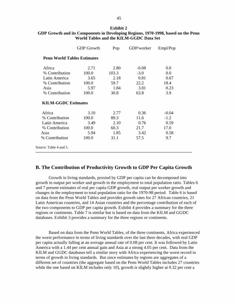
45

Exhibit 2 GDP Growth and its Components in Developing Regions, 1970-1998, based on the Penn

World Tables and the KILM-GGDC Data Set

GDP Growth Pop GDP/worker Empl/Pop Penn World Tables Estimates Africa 2.71 2.80 -0.08 0.0 % Contribution 100.0 103.3 -3.0 0.0 Latin America 3.65 2.18 0.81 0.67 % Contribution 100.0 59.7 22.2 18.4 Asia 5.97 1.84 3.81 0.23 % Contribution 100.0 30.8 63.8 3.9 KILM-GGDC Estimates Africa 3.10 2.77 0.36 -0.04 % Contribution 100.0 89.3 11.6 -1.2 Latin America 3.49 2.10 0.76 0.59 % Contribution 100.0 60.3 21.7 17.0 Asia 5.94 1.85 3.42 0.58 % Contribution 100.0 31.1 57.5 9.7 Source: Table 4 and 5.

B. The Contribution of Productivity Growth to GDP Per Capita Growth Growth in living standards, proxied by GDP per capita can be decomposed into growth in output per worker and growth in the employment to total population ratio. Tables 6 and 7 present estimates of real per capita GDP growth, real output per worker growth and changes in the employment to total population ratio for the 1970-98 period. Table 6 is based on data from the Penn World Tables and provides growth rates for 27 African countries, 21 Latin American countries, and 14 Asian countries and the percentage contribution of each of the two components to GDP per capita growth. Exhibit 4 provides a summary for the three regions or continents. Table 7 is similar but is based on data from the KILM and GGDC databases. Exhibit 3 provides a summary for the three regions or continents.

Based on data from the Penn World Tables, of the three continents, Africa experienced the worst performance in terms of living standards over the last three decades, with real GDP per capita actually falling at an average annual rate of 0.08 per cent. It was followed by Latin America with a 1.44 per cent annual gain and Asia at a strong 4.05 per cent. Data from the KILM and GGDC databases tell a similar story with Africa experiencing the worst record in terms of growth in living standards. But since estimates by regions are aggregates of a different set of countries (the aggregate based on the Penn World Tables includes 27 countries while the one based on KILM includes only 10), growth is slightly higher at 0.32 per cent a

46

year on average. GDP per capita growth in Latin America and Asia are very close to their Penn World Tables equivalents at 1.35 per cent and 4.02 per cent respectively.

Output per worker growth accounted for slightly over half of GDP per capita growth

in Latin America, irrespective of the data source used (56.3 per cent based on the Penn World Tables and 55.8 per cent based on the KILM and GGDC databases). Increases in the employment to total population ratio accounted for the remaining growth in living standards (46.5 per cent according to the Penn World Tables and 43.9 per cent based on KILM-GGDC). In Asia, almost all the growth in living standards was accounted for by productivity gains (94.1 per cent and 85.1 per cent). The percentage contributions for Africa have little meaning because of the low value of GDP per capita growth (-0.08 per cent and 0.32 per cent) upon which the calculations are based.

One observes that the greater the GDP per capita growth, the greater the productivity

growth in both absolute and relative terms. When productivity growth is robust, increases in living standards follow.

Again, the experiences of certain countries are noteworthy (Table 6). Despite the dismal performance of Africa, two countries on this continent exhibited very significant increases in living standards because of their strong productivity growth – Botswana and Mauritius. In the KILM-GGDC data set (Table 7), Botswana and Mauritius are not available and therefore, Egypt has the fastest growth in living standards. Barbados enjoyed the strongest increases in living standards in Latin America and also had the strongest productivity gains in the region. According to the KILM-GGDC data set, Chile had the highest real GDP per capita growth rate in Latin America. Most Asian countries experienced strong GDP per capita growth thanks to their strong productivity growth and this true is in both data sets.

The bottom line from the discussion above is that productivity gains are the driving force behind income gains, and their relative importance actually increases as productivity growth picks up.

VI The Empirical Relationship Between Productivity, Poverty, Income Inequality, and Wages

This section regroups the statistical analysis that was done using the different

data sources to study the relationship between key variables. The first set of relationships studied is the one between productivity and poverty, focusing on both changes in productivity and poverty reduction and on the level of productivity and poverty incidence. The relationships between GDP growth and poverty and per capita GDP and poverty are also examined and compared and contrasted to the productivity/poverty relationships. The second set of relationships is the more complex relationship between labour productivity, poverty and income inequality, both in terms of levels and growth.18 The third set of relationships examined is that between labour productivity levels and growth and poverty incidence and changes, but using alternative measures of poverty developed by the UNDP, namely the Human Development Index (HDI) and the Human Poverty Index (HPI). The fourth relationship studied is between labour productivity growth and real wage growth. 18 See CSLS (2003) for an examination of this relationship for China.

47

Exhibit 3

GDP Per Capita Growth and its Components in Developing Regions, 1970-1998, based on the Penn World Tables and the KILM-GGDC data set

GDP/Capita GDP/Worker Empl/Pop

Penn World Tables Estimates Africa -0.08 -0.08 0.00 % Contribution 100.0 100.0 0.0 Latin America 1.44 0.81 0.67 % Contribution 100.0 56.3 46.5 Asia 4.05 3.81 0.23 % Contribution 100.0 94.1 5.7 KILM-GGDC Estimates Africa 0.32 0.36 -0.04 % Contribution 100.0 111.3 -11.3 Latin America 1.35 0.76 0.59 % Contribution 100.0 55.8 43.9 Asia 4.02 3.42 0.58 % Contribution 100.0 85.1 14.4 Source: Table 6 and 7. A. The Relationship Between Productivity and Poverty Using Simple

Regression Analysis 1. Using the Sala-i-Martin Poverty Estimates Trends As shown in Section III, the literature has focused on the relationship between economic growth and poverty and not on the relationship between productivity and poverty. This is the first time to our knowledge that the relationship between productivity and poverty has been investigated for developing countries. One reason that may explain why productivity has been neglected in the literature as a determinant of poverty reduction is that economic growth already subsumes productivity growth. It may have been felt that its impact was already covered. Economic growth can reduce poverty both by raising real wages and creating jobs. The difficulty of obtaining reliable labour input data in most developing countries, needed to calculate labour productivity, may have contributed to the use of GDP per capita or mean income in poverty reduction studies as well. Exhibit 4, based on data from the Penn World Tables and the KILM-GGDC data set, presents the R-squared coefficients from regressions of changes in poverty on economic growth, changes in poverty on per capita GDP growth, and changes in poverty on productivity

48

growth as measured by output per worker growth, and for both the one dollar and two dollar poverty measures over the 1970-98 period for the three regions of the developing world and

the overall developing world (see Charts 5 and 6).19 The relationship between growth in real GDP, per capita GDP, or productivity and changes in poverty is negative in all instances. Poverty tends to fall with economic growth, with income growth, and with productivity growth.

A first observation is that there are significant differences in results between the two data sets. In general, the relationship between growth in the three economic variables and poverty reduction is considerably better explained using the Penn World Tables data than the KILM-GGDC data. Out of 24 R-squared coefficients (three variables for four geographical areas, and two poverty measures), the Penn World Tables values are higher in 20 cases. The only exceptions are the two dollar poverty estimates for all three economic variables and one dollar poverty estimates for real GDP for Latin America where the KILM-GGDC estimates are higher. The most dissimilar results between the two data sets are for Africa where the Penn World Tables show a consistently tight relationship between the three economic variables and poverty while the same relationships are in most cases poorly explained by the KILM-GGDC data.

The differences in results between data sets may reflect differences in the number of countries in the sample. For the Penn World Tables, the results are based on data for 20 African countries, 19 Latin American countries, and 13 Asian countries for a total of 52 countries. For the KILM-GGDC data set, the results are based on data for 6 Latin American countries, 7 African countries, and 13 Asian countries for a total of 26 countries. The fact that the number of countries in the Penn World Table is double that of the KILM-GGDC data set suggests the former results may be more robust as the greater sample size provides more degrees of freedom.

Despite the stronger fit of the relationship between the three economic variables and poverty reduction found in the Penn World Tables compared to the KILM-GGDC data set, there is one common pattern in the results across the two data sets. The R-squared coefficients for the two dollar poverty measure are always higher than the one dollar estimates. This reflects the higher poverty rates for the two dollar measure and hence the greater potential for decline. This potential is often realized, meaning that there are fewer countries displaying no change in poverty so that the linear relationship fits more accurately, producing a higher R-squared coefficient. Focusing on the Penn World Table results because of their potentially greater robustness, the most significant observation is that the R-squared coefficients in all three regions (but not for all developing countries) for both poverty measures from the regressions of changes in poverty on productivity growth are greater than those from the regressions of changes in poverty on economic growth. Productivity growth thus seems to have more explanatory power in terms of changes in poverty than economic growth.

Part of economic growth reflects employment growth arising from population growth. This growth, which does not increase the employment to population ratio, may have little impact on poverty reduction. Its effect is more to keep poverty from rising than to reduce it. This would explain why the relationship between economic growth and poverty is, at least for 19 See Appendix Charts 1-7 for scatter diagrams on the relationship between GDP per worker growth and poverty reduction for both the one dollar and two dollar poverty measures for Latin America, Africa, and Asia.

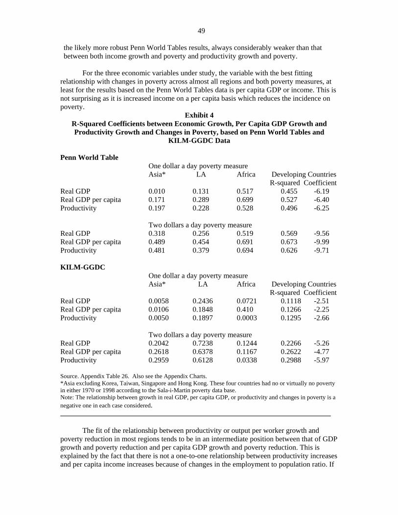
49

the likely more robust Penn World Tables results, always considerably weaker than that between both income growth and poverty and productivity growth and poverty.

For the three economic variables under study, the variable with the best fitting

relationship with changes in poverty across almost all regions and both poverty measures, at least for the results based on the Penn World Tables data is per capita GDP or income. This is not surprising as it is increased income on a per capita basis which reduces the incidence on poverty.

Exhibit 4 R-Squared Coefficients between Economic Growth, Per Capita GDP Growth and Productivity Growth and Changes in Poverty, based on Penn World Tables and

KILM-GGDC Data Penn World Table

One dollar a day poverty measure Asia* LA Africa Developing Countries

R-squared Coefficient Real GDP 0.010 0.131 0.517 0.455 -6.19 Real GDP per capita 0.171 0.289 0.699 0.527 -6.40 Productivity 0.197 0.228 0.528 0.496 -6.25

Two dollars a day poverty measure Real GDP 0.318 0.256 0.519 0.569 -9.56 Real GDP per capita 0.489 0.454 0.691 0.673 -9.99 Productivity 0.481 0.379 0.694 0.626 -9.71 KILM-GGDC One dollar a day poverty measure Asia* LA Africa Developing Countries R-squared Coefficient Real GDP 0.0058 0.2436 0.0721 0.1118 -2.51 Real GDP per capita 0.0106 0.1848 0.410 0.1266 -2.25 Productivity 0.0050 0.1897 0.0003 0.1295 -2.66

Two dollars a day poverty measure Real GDP 0.2042 0.7238 0.1244 0.2266 -5.26 Real GDP per capita 0.2618 0.6378 0.1167 0.2622 -4.77 Productivity 0.2959 0.6128 0.0338 0.2988 -5.97 Source. Appendix Table 26. Also see the Appendix Charts. *Asia excluding Korea, Taiwan, Singapore and Hong Kong. These four countries had no or virtually no poverty in either 1970 or 1998 according to the Sala-i-Martin poverty data base. Note: The relationship between growth in real GDP, per capita GDP, or productivity and changes in poverty is a negative one in each case considered.

The fit of the relationship between productivity or output per worker growth and poverty reduction in most regions tends to be in an intermediate position between that of GDP growth and poverty reduction and per capita GDP growth and poverty reduction. This is explained by the fact that there is not a one-to-one relationship between productivity increases and per capita income increases because of changes in the employment to population ratio. If

50

productivity rises, but proportionately fewer persons are working because of layoffs, poverty will not fall just as per capita income will not rise. Consequently, one would expect a tighter

relationship between per capita income changes and poverty reduction than between productivity growth and poverty reduction. On the other hand, the relationship between changes in productivity and poverty will tend to be stronger than the relationship between GDP growth and poverty as the latter includes employment growth associated with population growth which has no effect on poverty reduction.

The results based on the Penn World Tables (in stark contrast to the KILM-GGDC based results) show high R-squared coefficients between all three economic variables and poverty reduction for Africa. This reflects the high poverty rates in this region and hence the greater scope for poverty reduction in absolute terms.

In terms of the magnitude of these relationships, the final column in Exhibit 4 shows the estimated slope coefficients. All estimates are statistically significant at the 5 per cent level or better. These estimates indicate by how much the change in poverty is reduced by a given change in the independent variable (the growth rate of either GDP, GDP per capita or productivity) across all developing countries on average. For example, a 1.00 percentage point increase in the annual rate of growth of productivity decreases the change in the $1 a day poverty rate between 1970 and 1998 by 6.25 percentage points.

Looking first at the estimates based on Penn data, it is GDP per capita growth that has

the greatest power in reducing changes in poverty, both when the $1 measure is used and when the $2 measure is used. Productivity growth is a close second, while GDP growth has the least power in reducing changes in poverty. Note that the coefficients are larger in absolute magnitude in the $2 regressions than in the $1 regressions in each case, however. This implies that a given percentage point increase in one of the independent variables decreases the change in the $2 a day poverty rate to a larger degree than the change in the $1 a day poverty rate. This is a favourable result because it means that income growth, for example, lifts the extremely poor not just above the $1 a day poverty line but above the $2 a day poverty line as well. In the example, the estimated coefficient tells us that the $2 poverty rate grows by 10 points less than it otherwise would if GDP per capita grows at a rate 1.00 percentage points higher, while the $1 poverty rate grows by only 6.4 points less. The $2 poverty rate is composed of two parts though, the $1 poverty rate and the proportion of the population with between $1 and $2 a day. The results tell us that the change in this latter part is reduced to a larger degree than the change in the former part, so in other words, growth is not reducing the change in the proportion of the population with less than $1 a day simply by increasing the change in the proportion of the population with between $1 and $2 a day.20

20 It is important to realize, however, that part of this result of larger coefficients from the $2 regressions could be interpreted as an artefact of the treatment of the data. The poverty rates are measured in percentage points, and the change in the poverty rates is an absolute change rather than a per cent change, thus the changes are measured in percentage points as well. But the $2 poverty rates are by nature larger than the $1 poverty rates, and a 10 percentage point change from a large number (for example from 70 per cent to 60 per cent) does not necessarily represent a larger relative change than a 6.4 percentage point change from a smaller number (for example from 45 per cent to 38.6 per cent). In the example each percentage point change corresponds roughly to a relative change of -14 per cent. Thus, in response to a given increase in the rate of growth of income, for example, the relative change in the growth of the $2 poverty rate may not be as much greater than the relative change in the growth of the $1 poverty rate as compared to the difference in absolute changes. Whether one values relative decreases in the change in the poverty rate over absolute decreases is a normative question though.

51

Turning now to the results of the KILM-GGDC regressions, this same conclusion holds, that is, the decrease in the change of the $2 poverty rate in response to a given

increase in the growth of productivity, GDP per capita or GDP is larger than the decrease in the change of the $1 poverty rate. The effects in both cases are much smaller in magnitude than in the Penn regressions though. There is another difference with the Penn results as well, namely, productivity growth and GDP growth both have more power in reducing the change in poverty than GDP per capita growth. This is a somewhat unexpected result, although not entirely implausible. However, it should be stated again that the KILM-GGDC sample is much smaller than the Penn sample and hence the results may not be as reliable. Levels The previous results suggest that growth in the incidence of poverty is reduced as labour productivity growth rises. We expect a similar result to hold in terms of the levels of productivity and poverty (see Charts 3 and 4). Countries having higher levels of labour productivity should have lower levels of poverty incidence. We report the R-squared coefficients from regressions of poverty incidence on real GDP per worker using both the Penn World Tables and the KILM-GGDC estimates for the year 1998. R-squared coefficients are also reported for the relationship between the level of per capita GDP and poverty (Exhibit 5).21 All estimated slope coefficients from these regressions have a negative sign as expected but the goodness of fit varies across regions. For the eight R-squared coefficients from the regressions of the poverty rate on the productivity level for each data set (four geographical regions and two productivity measures), the estimates based on the Penn World Tables exceeded those of the KILM-GGDC data set four times and the KILM-GGDC data set exceeded the Penn World table estimates four times. In contrast to the growth rate estimates in the previous section, the relationship between productivity levels and poverty rates does not appear to be tighter in the Penn World Tables than in the KILM-GGDC data set. The R-squared coefficients for the productivity/poverty level relationship are the highest in Africa, independent of the productivity estimate used. The KILM-GGDC estimates produce a coefficient of 0.512 when the one dollar a day poverty measure is used and a higher coefficient of 0.671 for the two dollar a day measure. Using the Penn World Tables estimates yields a higher R-squared coefficient of 0.717 using the two dollars a day poverty measure, but a lower one using the one dollar a day measure of 0.482.

The fit of the linear relationship between poverty and productivity levels is weaker in Latin America than in Africa. The R-squared coefficients for the one and two dollars a day poverty measures based on the KILM-GGDC data set are 0.239 and 0.593 respectively. The coefficients derived from the Penn World Tables estimates were of the same magnitude, 0.339 and 0.539 respectively.

The fit of the relationship between labour productivity and poverty levels is also weak

in the Asian region. Based on the KILM-GGDC estimates and the one dollar poverty measure, the R-squared coefficient is 0.295, higher than the one for Latin America. When the two dollars a day poverty measure is used, the correlation coefficient for Asia is lower at 21 See Appendix Charts 8-16 for scatter diagrams on the relationship between the level of GDP per worker and the poverty rate for both the one dollar and two dollar poverty measures for Latin America, Africa, and Asia.

52

0.492. Using the Penn World Tables estimates did not improve the goodness of fit as the R-squared coefficients for Asia associated with the one and two dollars a day poverty measures

are 0.188 and 0.336 respectively. Overall, when the three regions are aggregated, the R-squared coefficients take

intermediate values between the results of Africa and Latin America. The fit of the linear relationship between poverty and labour productivity is tighter when the Penn World Tables estimates are used for both the one and two dollars a day poverty measures. The relationship between the level of GDP per capita and poverty is very similar to that between the level of productivity and poverty. For certain geographical areas and poverty measures the fit is stronger, for others it is weaker. When the Penn World Tables estimates of income and labour productivity are used in the regressions, the labour productivity variable has more explanatory power three times and the income variable has more explanatory power five times. When the KILM-GGDC estimates are used in the regressions, the labour productivity variable has the most explanatory power five times and the income variable three times. But in most of the cases, there is not much difference in the values the R-squared coefficients take. Generally speaking, neither of the two variables seems to be a better explanatory variable than the other.

In terms of the magnitude of these relationships, per capita GDP has more power in reducing poverty incidence than productivity, with both poverty measures and in both data sets. For an increase of $1,000 in real value added per worker the $1 a day poverty rate falls by about 1.7 percentage points according to the Penn estimates or about 0.7 points according to the KILM-GGDC estimates. The corresponding declines in the poverty rate for an equal increase in GDP per capita are 3.9 and 1.5 percentage points respectively, more than twice as large as the productivity effects. A similar story holds for the estimates based on the $2 poverty rates. Once again a given change in the independent variable (this time either the level of GDP per capita or the level of productivity) has a greater effect on the $2 poverty rate than the $1 poverty rate. This indicates that a given increase in the level of GDP per capita or productivity lifts the extremely poor not just above the $1 a day poverty line but above the $2 a day poverty line as well. Another similarity with the results from the growth regressions is that the independent variable has a smaller effect on the poverty rate according to the KILM-GGDC sample. Looking at Charts 3 and 4 it appears that the linear functional form does not fit the entire sample well. The countries are divided into two fairly distinct clusters, one with low poverty levels spread across a broad range of high levels of output per worker, and the other with a broad range of poverty levels across a narrow band of low productivity levels. The fit of these regressions could therefore be much improved in either of two ways. First, an inverse functional form could be adopted, or second, the samples could be separated into countries with low productivity levels and countries with high productivity levels (or by distinguishing between countries with high and low poverty rates) based on some arbitrary break point. In any case, the more important point is that the average effect of productivity on poverty incidence across all countries in the sample does not represent well the relationship that is likely to hold for any individual country in the sample. Countries with very low levels of productivity seem to get a much larger reward for increasing their productivity levels in

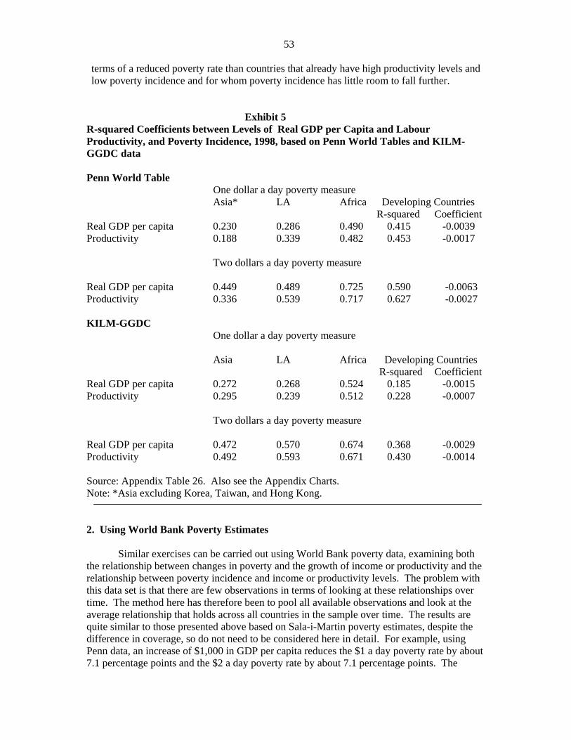
53

terms of a reduced poverty rate than countries that already have high productivity levels and low poverty incidence and for whom poverty incidence has little room to fall further.

Exhibit 5 R-squared Coefficients between Levels of Real GDP per Capita and Labour Productivity, and Poverty Incidence, 1998, based on Penn World Tables and KILM-GGDC data Penn World Table

One dollar a day poverty measure Asia* LA Africa Developing Countries

R-squared Coefficient Real GDP per capita 0.230 0.286 0.490 0.415 -0.0039 Productivity 0.188 0.339 0.482 0.453 -0.0017

Two dollars a day poverty measure Real GDP per capita 0.449 0.489 0.725 0.590 -0.0063 Productivity 0.336 0.539 0.717 0.627 -0.0027 KILM-GGDC One dollar a day poverty measure

Asia LA Africa Developing Countries

R-squared Coefficient Real GDP per capita 0.272 0.268 0.524 0.185 -0.0015 Productivity 0.295 0.239 0.512 0.228 -0.0007

Two dollars a day poverty measure Real GDP per capita 0.472 0.570 0.674 0.368 -0.0029 Productivity 0.492 0.593 0.671 0.430 -0.0014 Source: Appendix Table 26. Also see the Appendix Charts. Note: *Asia excluding Korea, Taiwan, and Hong Kong. 2. Using World Bank Poverty Estimates

Similar exercises can be carried out using World Bank poverty data, examining both the relationship between changes in poverty and the growth of income or productivity and the relationship between poverty incidence and income or productivity levels. The problem with this data set is that there are few observations in terms of looking at these relationships over time. The method here has therefore been to pool all available observations and look at the average relationship that holds across all countries in the sample over time. The results are quite similar to those presented above based on Sala-i-Martin poverty estimates, despite the difference in coverage, so do not need to be considered here in detail. For example, using Penn data, an increase of $1,000 in GDP per capita reduces the $1 a day poverty rate by about 7.1 percentage points and the $2 a day poverty rate by about 7.1 percentage points. The

54

effects are of smaller magnitude when productivity is the independent variable and when the KILM-GGDC data set is used.

Since the World Bank poverty database has been the traditional data source for cross-

country investigations of growth’s effect on poverty, it would be interesting to use this data source along with the KILM-GGDC data for productivity and GDP per capita in following more closely the methods of other studies. Using the World Bank poverty and income distribution database and the KILM-GGDC data set, we estimate elasticities of poverty incidence with respect to labour productivity. Elasticities are calculated using GDP per capita as well as GDP per worker, for both low and high income inequality countries. We classify countries based on their GINI index ranking within our sample. The half with the lowest GINI indexes are considered low inequality and the rest are considered high inequality. Our definition of inequality is therefore relative in the sense that a GINI index value is considered high or low depending on the other GINI indexes in the sample. Since our sample includes GINI indexes based on expenditure and income as well, we subtract ten percentage points from GINI indexes based on income in order to make data comparable although in a non-rigorous way.22

We start by regressing the natural logarithm of productivity on the natural logarithm of

poverty incidence (see Table 14). All countries and years are pooled together. By doing so, the slope coefficient is an elasticity. The interpretation of an elasticity is: a one per cent rise in labour productivity is associated with a X per cent decline in the incidence of poverty (not percentage point). All the elasticity estimates calculated using this methodology are statistically significant at the one per cent level (with the exception of some estimates from regressions of high inequality countries using the one dollar a day poverty measure). Yet there seems to be an auto-correlation problem when all countries and years are pooled together without distinction between high and low inequality countries. The Durbin-Watson Statistic indicates the presence of auto-correlation if it is significantly lower than 2. The presence of auto-correlation prevents any reliable inference from statistical results. Note that the Durbin-Watson statistics derived from the models with high inequality and all countries are very low, which calls for caution when interpreting these results.

This problem has motivated the use of a second methodology. We regress the average

annual growth rate of labour productivity on the average annual growth of the incidence of poverty (yearly average of log differences). Under this method, average growth is calculated between each data point available within a country. This is not strictly speaking an elasticity. It is rather a growth elasticity and its interpretation differs from the elasticity interpretation as we will explain later. Using the second methodology, there are almost no signs of auto-correlation but the statistical significance of the slope coefficients is not as good, but still quite strong. The inequality rankings of log differences are based on the GINI index of the latest year used in calculating the average log difference. The elasticities of poverty incidence with respect to labour productivity derived from our data set indicate that growth in labour productivity reduces the incidence of poverty. When all data points are used in the regression, the elasticity indicates that a one per cent rise in labour productivity will be associated with a 0.74 per cent decline in the incidence of poverty on average. The separation of our data set based on the GINI index rankings allows 22 As noted in the WIDER database on inequality user guide, inequality tends to be higher when income is used to construct GINI indexes instead of expenditure. On average, GINIs are generally ten percentage points higher but this observation is an average and may not apply to each country each year.

55

us to evaluate the impact of income inequality on the poverty reducing power of labour productivity growth. In countries with the lowest GINI indexes, we find that a one per cent

rise in labour productivity is associated with a 1.02 per cent decline in the incidence in poverty. The impact of a one per cent rise in labour productivity on poverty incidence is less important when income inequality is higher as the -0.45 elasticity estimate indicates.

The previous results are obtained using the percentage of population living with less than one dollar a day (1.08 dollars based on 1993 PPPs). When the two dollars a day poverty measure is used, the elasticities are systematically lower indicating that the poverty reducing power of labour productivity is lower when the poverty line is set higher. This is in contrast to the slope coefficients, which are simple rates of change rather than elasticities, from previous regressions, where the independent variable had a larger effect on the $2 poverty rate compared to the $1 poverty rate. The difference is that elasticities look at per cent changes, so the effect on the poverty rate is in relative (per cent) terms rather than absolute (percentage point) terms. Footnote 20 also discusses this issue. Briefly, the two dollars a day poverty rates are by nature larger than the one dollar poverty rates, and in relative terms a large absolute change from a large number is not necessarily as large as a small absolute change from a small number. Although the elasticities derived from the two dollars a day poverty rate are lower, the use of this broader poverty measures systematically yields a higher R-squared value, indicating that labour productivity variations explain a larger portion of the variations in poverty. The negative impact of higher income inequality on the poverty reducing power of labour productivity growth also applies when the two dollar a day poverty measure is used. Elasticities of poverty incidence with respect to GDP per capita are also estimated in the same way and the results are similar in terms of magnitude but are all lower. This result shows the importance of giving as much attention to labour productivity as a poverty reducing variable than to GDP per capita growth. As was mentioned earlier, we also estimate elasticities of growth by regressing average log differences instead of just logs. When all countries are pooled together, we obtain an elasticity of -3.39, which is considerably larger than the -0.74 estimate we obtained from the log-log model. The interpretation of the slope coefficient is different and this explains why the two types of elasticities calculated are of different magnitudes. A -3.39 growth elasticity means that a one percentage point higher average annual growth rate in labour productivity will be associated on average to a 3.39 percentage point lower average annual growth rate in the incidence of poverty. Therefore, when the growth elasticity is lower than -1, the acceleration in the decline of the incidence in poverty will be larger than the acceleration in the growth of labour productivity. Based on our sample, an acceleration in labour productivity growth has more impact on the acceleration of the decline in the incidence of poverty in countries with higher levels of income inequality. High inequality countries have on average a growth elasticity of -4.93 compared to -3.17 for low inequality countries. The growth elasticity estimates derived from the two dollars a day poverty rates are systematically lower, as was the case when elasticities were calculated. When all countries are pooled together, the growth elasticity is -1.26. When countries are separated based on their level of income inequality, the growth elasticities are -1.09 and -1.91 for low inequality and high inequality countries respectively. Contrary to what was observed when elasticities were estimated, the use of the two dollars a day poverty measure does not yield a higher R-squared coefficient. In fact, variations in labour productivity growth explain more of the variations in poverty incidence growth when the one dollar a day poverty measure is used.

56

The results using GDP per capita average annual growth rates are quite different than

the ones obtained with labour productivity. The elasticity estimates are lower and have less statistical significance. The R-squared values are also very low, meaning that GDP per capita average annual growth has almost no explanatory power of variations in poverty incidence average annual growth. Following Moore and White (2003), we construct a table of annual labour productivity growth rates required to leave the absolute number of poor unchanged, given population growth rates and elasticities of poverty incidence with respect to labour productivity. From Exhibit 6, we see that for a given elasticity, the growth in labour productivity has to be higher the larger is population growth in order to leave the poverty headcount unchanged. And unsurprisingly, given a population rate of change, labour productivity growth can be lower as the elasticity of poverty incidence with respect to labour productivity (which measures the impact of a one per cent change in labour productivity on the incidence of poverty) is larger, in order to leave the number of poor unchanged. If labour productivity growth exceeds the value in the table for given population growth and elasticity, then the number of poor will decrease. The values in Exhibit 6 are derived using the following formula:

l* = - p / ε

where l* is the annual rate of change in labour productivity required to leave the number of poor unchanged, p is the annual rate of change in population, and ε is the poverty incidence to labour productivity elasticity.23

Given our poverty dataset it is impossible to calculate elasticities for individual countries. The elasticities we derive are averages for the developing countries included in our sample. Our formula can only help us predict the impact of labour productivity growth on the number of poor in countries in our sample as a whole (or sub sample based on inequality levels). Furthermore, our prediction assumes that labour productivity growth is not accompanied by a change in the distribution of income that could affect poverty that is not already taken into account in the elasticity estimate. We reproduce the elasticities derived for developing countries by simple regression in Exhibit 6 to show the required labour productivity growth to leave the number of poor unchanged.

23 The poverty rate (I) is equal to poverty headcount (D) divided by population (P). Therefore

i = d - p (1) where lowercase letters denote per cent change. The elasticity of poverty incidence with respect to labour productivity is given by

ε = i / l (2) where l is the per cent change in labour productivity. If the poverty headcount is to remain unchanged, then d=0 and equation (1) become

i = -p (3) We can express the per cent change in labour productivity in terms of the elasticity and the per cent change in labour productivity from equation (2):

i = ε · l (4) Substitute (3) into (4) to obtain

ε · l = -p (5) and rearrange to obtain

l* = -p / ε (6)

57

Exhibit 6: Labour Productivity Growth Rate (in italics) Required to Leave the Number of Poor Unchanged Given Population Growth Rates Population Growth rates Countries Elasticities 1.0 1.5 2.0 2.5 High Inequality -0.45 Developing Countries -0.74 Low Inequality -1.02

2.22 1.35 0.98

3.33 2.03 1.47

4.44 2.70 1.96

5.56 3.38 2.45

Given the numerous results reported here it is not possible to definitively say whether

productivity is a more important driver of reductions in poverty than GDP per capita. In some cases labour productivity has a larger effect, but in most cases this does not hold. However, the fit of the relationship seems to be stronger for productivity even though the magnitude of the relationship itself is not as strong. The most important point is that all of these results, in combination with previous studies, give compelling evidence that both productivity and GDP per capita are important in reducing poverty. Furthermore, increases in GDP per capita are themselves strongly driven by productivity gains. B. The Relationship Between Productivity, Poverty, and Income Distribution Using Multiple Regression Analysis

Income inequality is important in mediating the relationship between economic growth and productivity growth and changes in poverty. Indeed, the fact that correlation coefficients between economic growth and poverty reduction or between productivity growth and poverty reduction are not larger is in part explained by the different levels of income inequality across countries. In countries with low initial levels of income inequality, a given per cent increase in income, even though it affects all quintiles proportionately, has a greater impact in reducing absolute poverty than the same per cent increase in income in countries with high levels of income inequality. This is simply because the absolute size of the income gains are greater in the low inequality country. The same reasoning applies for countries that experience a fall in their income inequality relative to those who experience an increase.

This section of the report examines the relationship between productivity, poverty and

income distribution. The first step in constructing the database needed to undertake multivariate analysis of the relationship between poverty, labour productivity and income inequality is to select countries from the Penn World Tables and World Income Inequality databases for which Sala-i-Martin (2002) has provided poverty rate estimates. We then retain the countries for which GINI coefficient time series are available for at least ten years. There are only 27 countries left after the selection: 12 in Latin America (Brazil, Chile, Colombia, Costa Rica, Dominican Republic, Ecuador, Jamaica, Mexico, Panama, Peru, El Salvador, Venezuela), 13 in Asia (Bangladesh, China, Hong Kong, Indonesia, India, Korea, Sri Lanka, Malaysia, Pakistan, Philippines, Singapore, Thailand, Taiwan) and 2 in Africa (Ethiopia, Tanzania).

Initially, we wanted to undertake a cross-section analysis for the years 1970 and 1998 using levels of each of the three variables. But because of the incomplete GINI coefficient times series, we did a cross-section analysis for the earliest year for which the GINI coefficient was available (and closest to 1970) and another one for the latest year (and closest to 1998). Associating labour productivity levels to GINI coefficients was easy because labour

58

productivity estimates are available for each year from 1970 to 1998. But this was not the case for poverty rates. We therefore had to assign poverty rates to GINI coefficients on the

basis of closeness to the years of availability. For example, if the earliest year of availability of a GINI coefficient was 1972, we assigned it the 1970 poverty rate. We then used the Ordinary Least Squares procedure with linear functional form to estimate the coefficients.

We also want to study the relationship between variations over time in each variable. We use the earliest and latest year available to calculate average annual growth rates for labour productivity and GINI coefficients and percentage changes for the poverty rates. Therefore, the growth rates for some countries are for shorter periods than for others. We then use the same statistical procedure as used for level comparisons. 1. Level Comparisons

We estimate an equation with the poverty rate as the dependent variable and labour productivity and inequality (measured by the GINI coefficient) as the explanatory variables (Table 8). We use the one dollar a day poverty measure as well as the two dollars a day measure. We would expect a negative coefficient for labour productivity since higher aggregate productivity will be associated with higher income. We would expect a positive coefficient for income inequality since higher income inequality, every thing else being equal, would be associated with a higher poverty rate.

In the regression using the one dollar a day poverty measure for the earliest year, the

coefficient for labour productivity has the expected sign and is statistically different from zero at the 1 per cent level. It predicts that a $1,000 per worker higher level of labour productivity would be associated with a 1.5 percentage point lower poverty rate. The income inequality coefficient also has the expected sign but it is not statistically different from zero (at the 10 per cent level). The regression predicts that a 1 per cent increase in the GINI coefficient will be associated with a 0.068 percentage point higher poverty rate. The intercept coefficient is statistically different from zero at the 5 per cent level. Based on the R-squared value, 41 per cent of the variation in the poverty rate is explained by variations in labour productivity and income inequality.

The regression results also report on the one dollar a day poverty measure with the

latest year available (and closest to 1998). The labour productivity coefficient has the expected sign, and is statistically different from zero at the 5 per cent level. The regression predicts that a $1,000 dollars per worker higher labour productivity level will be associated with a 0.6 percentage point lower poverty rate. The coefficient for income inequality has the expected sign as well but again, is not statistically different from zero (at the 10 per cent level). The intercept coefficient is significantly different from zero at the 10 per cent level. The independent variables have less explanatory power when data for the latest year is used. Only 21 per cent of the variation in the poverty rate is explained by variation in labour productivity and inequality compared to 41 per cent when data for the earliest years are used.

When the two dollars a day poverty measure and earliest year available are used, the

coefficient for labour productivity has the expected sign and is statistically different from zero at the 1 per cent level (Table 8). The regression results predict that a $1,000 per worker higher labour productivity level will be associated with a 2.6 percentage point lower poverty rate. The coefficient for income inequality does not have the expected sign but is not statistically different from zero at the 10 per cent level. The intercept coefficient is

59

statistically different from zero at the 1 per cent level. The model has good explanatory power since variation in labour productivity and income inequality explain almost 62 per

cent of the variation in the poverty rate. The labour productivity coefficient still has the expected sign when data for the latest

year available and the two dollars a day poverty measure are used. It is statistically different from zero at the 1 per cent level. A 1.1 percentage point lower poverty rate is expected from a $1,000 per worker higher labour productivity level. The income inequality coefficient has the expected sign but again is not statistically different from zero at the 10 per cent level. A one per cent higher GINI coefficient is expected to be associated with 0.5 percentage point lower poverty rate. The intercept coefficient is not statistically different from zero at the 10 per cent level. As was the case when using the $1 a day poverty measure, the explanatory power of the model is lower if data for the latest year available is used. Only 38 per cent of the variation in the poverty rate is explained by the variation in labour productivity and income inequality compared to 62 per cent when the data for the earliest year available are used. 2. Growth Comparisons

Regressions of the percentage point change in the poverty rate on the average annual growth rates of labour productivity and income inequality are also estimated using both poverty measures (see Table 8). We expect the coefficient for labour productivity to be negative, because growth in aggregate labour productivity would lead to growth in income and would reduce poverty if inequality remains constant. We expect a positive coefficient for income inequality growth because growth in inequality could lead to growth in poverty although not necessarily. If the income of only the top income quintile rises over time, inequality would rise, but absolute poverty would not.

Using the one dollar a day poverty measure, the regression results have the expected

sign. The average annual growth rate in labour productivity has a coefficient statistically different from zero at the 5 per cent level. The regression predicts that a one percentage point higher average annual growth rate in labour productivity would lead to a 1.75 percentage point reduction in the per cent change in the poverty rate between the earliest and latest year of availability. The income inequality coefficient is not statistically different from zero at the 10 per cent level. From the regression results, it is expected that a one per cent higher income inequality average annual growth rate will be associated with a 3.3 percentage point lower percentage point increase in the poverty rate between the earliest and latest year of availability. This model does not have much explanatory power since only 26 per cent of the variation in the percentage point change in the poverty rate is explained by variations in the average annual growth rates in labour productivity and income inequality.

Using the two dollars a day poverty measure yields similar results. Both coefficients

have the expected sign, yet only the average annual growth rate in labour productivity coefficient is statistically different from zero at the 1 per cent level. From the regression results, it is expected that a one per cent higher labour productivity growth rate will be associated with 3.5 percentage point reduction of the change in the poverty rate between the earliest and latest year of data availability. It is also predicted that a one percentage point rise in the GINI coefficient will be associated with a 2.8 percentage point larger change in the poverty rate between the earliest and latest year of data availability. According to the model, the variation in the two independent variables explains 32 per cent of the variation in the percentage point change in the poverty rate.

60

The bottom line from the multivariate analysis is that income distribution does indeed

affect the extent to which productivity gains are passed on to poor workers as income gains and reductions in poverty, but the relationship certainly appears weaker than the more basic relationship between productivity and poverty. C. The Relation Between Productivity and Poverty Using Alternative Measures of Poverty In addition to the use of the conventional poverty measures based on one and two dollars per day, the United Nations Development Programme (UNDP) produces indices of poverty based on a much more multi-dimensional conception of poverty. This section of the report examines the relationship between these measures and productivity and compares the results to those between conventional poverty measures and poverty.

Using labour productivity estimates from both the KILM-GGDC data set and the Penn World Tables, we plot labour productivity against the Human Development Index (HDI) and the Human Poverty Index (HPI) produced by the UNDP to ascertain if the relationship is different from the one observed using income poverty measures. There are 108 countries for which the UNDP publishes the HDI and we have labour productivity estimates from the Penn World Tables. This number falls to 31 when the KILM-GGDC estimates are used. As for the countries for which the HPI for developing countries (HPI-1) is available, the Penn World Tables have labour productivity estimates for 83 of them while the KILM-GGDC data set have estimates for 28.

1. Level Analysis

From Chart 7 and Exhibit 7, it appears that the relationship between the KILM-GGDC

labour productivity estimates and the HDI is positive as expected. Using a linear functional form, we obtain a high R-squared value of 0.636. With the Penn World Tables estimates, the value was slightly lower at 0.540 (Chart 6). Comparing the relationship between the HPI and labour productivity is of more interest since the HPI is not based on any variable that comprises real GDP. The relationship is quite tight between the KILM-GGDC labour productivity estimates and the HPI as the R-squared value of 0.524 shows (see Chart 8). The R-squared value using Penn World Tables estimates is again lower at 0.334. As labour productivity is higher in a country, its HPI score tends to be lower (Chart 5).

There appears to be a somewhat tighter relationship between these broader measures

of poverty and productivity levels compared to the results obtained using conventional measures of poverty (Exhibit 8). For the KILM-GGDC productivity estimates, the R-squared coefficients between both the HDI and the HPI levels and the productivity levels are both greater than that for the two conventional poverty measures and productivity. For the Penn World Tables estimates, the HDI/productivity relationship is tighter than the conventional poverty/productivity relationships, but the HPI/productivity relationship is weaker.

61

Exhibit 7

Comparison of R-Squared Coefficients: The Relationship Between Labour Productivity and Poverty incidence, Conventional and Alternative Poverty Measures, Growth and Levels in Developing Countries

HDI HPI-1 Sala-i-Martin Sala-i-Martin $1 a day $2 a day

Levels KILM-GGDC 0.6364 0.5239 0.2275 0.4298 Penn World Tables 0.5397 0.3340 0.3850 0.5600 Growth KILM-GGDC 0.4851 NA 0.1295 0.2988 Penn World Tables 0.3223 NA 0.3880 0.5099 2. Trend Analysis The results from the regression analysis show that there is a relatively strong negative relationship between growth in real GDP per worker and changes in poverty incidence. We use the HDI to verify that this relationship still exists when alternative measures of poverty are used. It would be more interesting to use the HPI instead since that index is not based on GDP per capita but no time series are available yet from the UNDP on this variable. Since the HDI measures achievement in capabilities, the relationship between labour productivity growth and changes in the HDI should be positive. To investigate the relationship between labour productivity growth and changes in the HDI, we consider all developing countries for which a HDI time series is available for the 1975-2000 period. Of these countries, labour productivity estimates from the Penn World Tables are available for 68 of them (17 in Asia, 21 in Latin America, and 30 in Africa), while estimates from the KILM-GGDC data set are available for 28 of them (14 in Asia, 7 in Latin America, and 7 in Africa). We present the R-squared coefficients for Asia, Latin America, Africa, and developing countries. All correlation coefficients had a positive sign indicating a positive relationship between the two variables as we expected.

The R-squared coefficients derived from the use of the HDI differ from the ones based on conventional poverty measures. The estimates from the Penn World Tables suggest labour productivity growth seems to have significantly less success in explaining changes in the HDI as the lower R-squared coefficient shows (see Exhibit 7). The coefficients are even lower than the ones obtained from the use of the one dollar a day poverty measure. The R-squared coefficients are also different when the KILM-GGDC labour productivity estimates are used.

Labour productivity has the strongest explanatory power in Africa when the HDI is the measure of poverty. But it is in Africa that labour productivity has the weakest explanatory power when conventional measures of poverty are used (see Exhibit 8). But in general, the KILM-GGDC estimates of labour productivity have success in explaining changes in the HDI, except in Asian countries. A possible reason that could explain these divergences is the different composition of the country samples.

62

Exhibit 8

R-Squared Coefficients between Labour Productivity Growth and Changes in the Human Development Index, based on Penn World Tables and KILM-GGDC data

Asia LA Africa Developing Countries

Penn World Tables Productivity growth 0.307 0.057 0.145 0.322 KILM-GGDC Productivity growth 0.128 0.430 0.708 0.485

D. The Relationship Between Productivity and Wages

In the long run, real wage growth is driven by labour productivity growth. We had hoped to test this relationship in developing countries, but data constraints confined the analysis to Latin American for which data on labour compensation was available. To test the relationship between growth in labour productivity and real labour compensation, we estimated a linear model for the 1980-1998 period. Because of lack of data, the average annual growth rates for Chile, Jamaica and Venezuela are for the 1985-1998 period instead. For the same reason the growth in Ecuador is for the 1980-1995 period. We expect a positive relationship between the two variables since labour productivity growth would lead to a faster rise in real wages if workers benefit from growing nominal wages or declines in prices.

Most of the data were within the -1 and +1 per cent range in terms of average annual

labour productivity growth and within the -6 and +2 per cent range in terms of average annual labour compensation growth (Table 3). Peru is at the lowest extremity with the worst growth record both in terms of labour productivity and labour compensation (Chart 9). At the opposite end of the spectrum, Chile experienced the fastest growth in both labour productivity and labour compensation. The labour productivity coefficient has the expected sign and is statistically significant at the one per cent level. The estimated equation predicts that a 1.66 percentage point faster labour compensation growth rate will be associated with a one percentage point faster labour productivity growth rate (Table 11). VII Conclusion The preliminary results in this paper suggest that the relationship between productivity growth and poverty reduction in developing countries over the last three decades appears even stronger than that between economic growth and poverty reduction, and about as important as that between GDP per capita growth and poverty reduction. It has also been found that the level of income inequality mediates the relationship between productivity growth and poverty reduction. The greater the level of inequality and any increase in inequality, the less an increase in productivity and income will reduce poverty.

63

The general mechanism that explains why productivity growth reduces poverty is that productivity growth is the main determinant of income growth. The relationship

between labour productivity growth and income growth is at the total economy or aggregate level. Gains in aggregate labour productivity mean that there is more real income in the economy that can be distributed to factors of production. In an economy with competitive product and factor markets, the relationship does not hold, and should not hold, at the firm or industry level. Workers in a sector that enjoy above average productivity growth will not see their wages increase more than the economy-wide average because of inter-sectoral wage competition due to labour mobility between sectors. What happens in these above average productivity growth sectors is that firms experience a decline in the relative price of their products. All members of society share in the productivity gains through lower prices, which raises real wages and incomes.

Aggregate labour productivity growth accrues from two sources. The first is intersectoral shifts of workers from low productivity level industries such as agriculture to high productivity level sectors such as manufacturing. Growth accounting studies have shown that this has historically been a very important source of productivity gains in the developed countries and it is currently a significant source of gains in the developing world. The workers who make this move enjoy large income gains, allowing many to move out of poverty. The second is intra-sectoral productivity growth. Again, because of labour and product market competition the wage gains of workers are not related to the productivity gains in their sector, but to the aggregate labour productivity growth, although there may be many exceptions to this rule in non-competitive settings.

Through government fiscal policies, all members of society, not just workers, can benefit from growth productivity. Part of the higher factor incomes arising from productivity growth can be taxed from the factors of productions and the proceeds used for transfers or public services potentially targeted at the poor.

It is important to note that there is a two-way relationship or virtuous circle between productivity growth and poverty reduction (See Sharpe, St-Hilaire and Banting (2002) for discussion of this relationship). Productivity growth raises incomes and reduces poverty. But the reduction in poverty can in turn feedback to improved productivity performance as those that move from poor to non-poor status enjoy better health and acquire more education. Both these developments enhance productivity growth. Since the Industrial Revolution, there have been both winners and losers in the economy’s quest for productivity growth. Technological change, the key driver of both economic and productivity growth, both creates and destroys jobs. Economists often note that in the long run higher productivity makes everyone better off by raising the material base of society. But the path to such an outcome can be difficult for those displaced and made redundant by the creative destruction of the growth process. Since the Luddites, the destruction or “restructuring” caused by the introduction of new productivity-enhancing technologies has provoked resistance on the part of those affected, which can have the effect of slowing the pace of technological change.

A growing economy that offers ample re-employment opportunities is crucial to minimizing the social costs from creative destruction, particularly over longer periods. But it is unlikely that the market will solve all social problems associated with restructuring. Public policy has an important role to play, particularly in the short-to-medium term. In principle,

64

one can compensate the losers of the growth process. Their suffering can be lessened through income support programs and measures which foster their re-employment in other

sectors and occupations, such as retraining programs. But in poor countries there are significant barriers to the development of such programs, including their cost and ineffective governance structures. The results in this report provide strong support for the view that productivity growth is essential for poverty reduction and should be a priority for developing countries. Consequently, the challenge developing countries face is to foster productivity growth, but at the same time to develop adjustment mechanisms that can protect those negatively affected by such productivity growth. It is important that productivity growth be seen by the population as the basis of the material advance of society and not associated with permanent job loss and catastrophic falls in income and living conditions. This is an issue of political economy. Two examples of creative destruction in developing countries illustrate the need for a deeper understanding of the economic and political ramifications of productivity growth. The first is the restructuring that has affected state enterprises in China. These firms have recorded very large productivity gains, often through massive layoffs of workers. Often these workers receive little if any compensation and have no access to retraining programs. For these workers, productivity can be a dirty word. A related study (CSLS, 2003) discusses the economic reforms in China over the past 25 years and the effect the consequent productivity gains have had on reducing poverty. As well, the need for a strong social security system is addressed, and China’s progress in this direction monitored. The second example of creative destruction is the restructuring that is affecting the traditional low productivity agricultural sector in developing countries. The introduction of productivity-enhancing technologies in agriculture, while a necessary condition for development, can cause much suffering for the landless farm wage earners who no longer have work and are forced to migrate to the urban areas. It is easy to say that productivity is crucial for increases in living standards and poverty reduction. It is much harder to identify policies that will increase productivity growth. In dynamic economies, economic growth is largely accounted for by productivity. Policies that foster economic growth will therefore by definition increase or maintain productivity growth. The literature has shown that the types of public policies that stimulate growth include policies that maintain strong levels of non-inflationary aggregate demand through appropriate fiscal and monetary policies, policies that promote openness and competition, policies that foster human capital development, policies that stimulate investment in machinery and equipment and innovation, and policies that facilitate the transfer of resources from low productivity sectors to high productivity sectors. The United Nations has set as a goal for the world community the halving of the rate of world poverty between 1990 and 2015. Over this period, the achievement of such a goal would require an annual rate GDP per capita growth of 3.6 per cent. This is equivalent to a rate of productivity growth of a minimum of 3 per cent as in most countries there is limited potential for increases in the employment to total population ratio to make large long-term contributions to living standards growth. The poor are already in the labour force. Based on a continuation of developments in the 1990s, Asia is on track to meet this poverty-reduction objective because of strong productivity growth and poverty reduction in China. However, Latin America, and even more so, Africa are greatly off track in attaining this goal given their

65

dismal economic performance in the 1990s. Drastic action is required in these regions if they are to meet the 2015 poverty objective.

66

Bibibliography

Adams, Richard H. (2002) “Economic Growth, Inequality and Poverty: Findings from a New Data Set”. World Bank Policy Research Working Paper no. 2972, February 14.

Besley, Timothy and Robin Burgess (2003) “Halving Global Poverty”. Journal of Economic

Perspectives, Summer, vol. 17 (3), pp. 3-22. Bhalla, Surjit. (2002) Imagine There’s No Country-Poverty, Inequality and Growth in the

Era of Globalization. Institute for International Economics, Washington, 248p. Bourgignon, François and Christian Morrisson. “Inequality among World Citizens: 1820-

1992”. The American Economic Review, September, vol. 92 (4), pp. 727-744. Bruno, Michael, Martin Ravallion and Lyn Squire. (1998) “Equity and Growth in Developing

Countries: Old and New Perspectives on the Policy Issues”. in Vito Tani and Ke-Young Chu (eds), Income Distribution and High Quality Growth. Cambridge, MA: MIT Press.

Centre for the Study of Living Standards (2003) “China’s Productivity Performance and Its

Impact on Poverty in the Transition Period”. Background Paper Prepared for the 2004 World Employment Report of the International Labour Organization. CSLS Research Report number 2003-07, (Ottawa: CSLS).

Chen, Shaohua and Martin Ravallion. (2001) “How Did the World’s Poorest Fare in the

1990s?”. The Review of Income and Wealth, September, series 47 (3), pp. 283-300. Christiaensen, Luc, Lionel Demery and Stefano Paternostro. (2002) “Growth, Distribution

and Poverty in Africa. Messages from the 1990s”. World Bank, Working Paper no. 2810, March 21.

Cling, Jean-Pierre, Philippe De Vreyer, Mirelle Razafindrakoto and François Roubaud. (2003)

Growth and Poverty Reduction: Inequalities Matter. Paper presented at the 2003 Wider Conference on Inequality, Poverty and Human Well-being, available at www.wider.unu.edu/conference/conference-2003-2/conference2003-2.htm\ under Conferences.

Dagdeviren, Hulya, Rolph Van der Hoeven and John Weeks. (2002) “Poverty Reduction with

Growth and Redistribution”. Development and Change, vol. 33 (3), June, pp. 383-412.

Datt, Gaurav and Martin Ravallion. (1998) “Farm Productivity and Rural Poverty in India”.

Journal of Development Studies, April, vol. 34 (4), pp.62-85. Deaton, Angus. (2001) Counting the World’s Poor: Problems and Possible Solutions”. The

World Bank research Observer, vol. 16 (2), pp. 125-147. Deaton, Angus. (2003a) “Health, Inequality and Economic Development”. Journal of

Economic Literature, March, vol. 41(1), pp.113-158.

67

Deaton, Angus. (2003b) “How to Monitor Poverty for the Millenium Development Goals”, Research Program in Development Studies, Working Paper 221, available at

www.wws.princeton.edu/~rpds/working.htm. Deininger, Klaus and Lynn Squire. (1996) “A New Data Set Measuring Income Inequality.”

World Bank Economic Review, Vol. 10, No. 3: 565-591. Dollar, David and Aart Kraay. (2001) “Growth is Good for the Poor”. Development Research

Group, World Bank, Working Paper No. 2587, April 12. Easterly, William (2000) “The Effect of International Monetary Fund and World Bank

Programs on Poverty”. unpublished paper, World Bank. Easterly, William (2001) The Elusive Quest for Growth: Economists Adventures and

Misadventures in the Tropics (Cambridge, Mass.: MIT Press): Fields, Gary (2001) Development and Distribution (Cambridge, Mass. MIT Press). Fischer, Stanley. (2003) Globalization and its Challenges. The American Economic Review,

vol. 93 (2), pp. 1-30. Fluet, Claude and Pierre Lefebvre. (1987) “The Sharing of Total Factor Productivity Gains in

Canadian Manufacturing: A Price Accounting Approach”. 1965-1980, Applied Economics, February, vol. 19 (2), pp. 245-257.

Griffin, Keith. “Problems of Poverty and Marginalization”. Indicators: The Journal of Social

Health, vol. 2, no 2 (Spring 2003), pp 22-48. Hanmer, Lucia and Felix Naschold. (2000) “Attaining the International Development Targets:

Will Growth be Enough?” Development Policy Review vol. 18, pp. 11-36 Hayes, K. J., D. J. Slottje, Michael L. Nieswiadomy and Edward N. Wolff. (1994) “The

Relationship Between Productivity Changes and Poverty in the United States”. Journal of Income Distribution, vol. 4 (1), pp. 107-119.

Hulten, Charles R. (2001) “Total Factor Productivity. A Short Biography”. In Charles R.

Hulten, Edwin R. Dean and Michael J. Harper eds. New Developments in Productivity Analysis. The University of Chicago Press, Chicago, 2001, pp. 1-47.

Islam, Nazrul. (2003) Productivity Dynamics in a Large Sampleof Countries: A Panel Study.

The Review of Income and Wealth, series 49 (2), pp. 247-272. Kanbur, Ravi. (2003) Conceptual Challenges in Poverty and Inequality: One Development

Economist’s Perspective. Paper presented at the 2003 Wider Conference on Inequality, Poverty and Human Well-being, available at www.wider.unu.edu/conference/conference-2003-2/conference2003-2.htm\ under Conferences.

Kaufmann, Daniel, Aart Kraay, and Pablo Zoido-Lobaton. (1999) “Governance Matters”.

World Bank, Working Paper No. 2196.

68

Levine, Ross, Norman Loayza, and Thorsten Beck. (2000) “Financial Intermediation and

Growth: Causality and Causes”. Journal of Monetary Economics, 46;31-77. Lübker, Malte: Assessing the impact of past distributional shifts on global poverty levels,

Employment Paper 2002/37, ILO Geneva 2002. Mehrotra, Santosh and Richard Jolly (eds.) (1997) Development with a Human Face:

Experiences in Social Achievement and Economic Growth. Oxford, Oxford University Press. 512 p.

Moore, Mick and Howard White (2003) “Meeting the Challenge of Poverty and Inequality”.

In Atul Kohli, Chung-in Moon and Georg Sorensen (eds), States, Markets and Just Growth: Development in the Twenty-first Century, Tokyo: UN University Press.

Pogge, Thomas W. and Sanjay G. Reddy. “Unknown: The Extent, Distribution, and Trend of

Global Income Poverty”. Version 2.0, March 26th, 2003. Available at: www.columbia.edu/~sr793/

Ravallion, Martin (1995) “Growth and Poverty: Evidence for Developing Countries in the

1980s”. Economics Letters 48: pp. 411-17. Ravallion, Martin. (2001) “Growth, Inequality and Poverty: Looking Beyond Averages”.

Development Research Group, World Bank, Working Paper No. 2558, February 26. Ravallion, Martin and S. Chen (1997) “What Can New Survey Data Tell Us about Recent

Changes in Distribution and Poverty?”, World Bank Economic Review, 11(2): pp. 357-82.

Sala-i-Martin, Xavier (2002) “The World Distribution of Income (Estimated from Individual

Country Distributions),” Working Paper 8933, National Bureau of Economic Research, May. available at www.nber.org/papers/w8933.

Salzman, Julia (2003). Methodological Choices Encountered in the Construction of

Composite Indices of Economic well-Being. Paper presented to the annual meeting of the Canadian Economics Association, Carleton University, Ottawa, Ontario, May 31-June 2. Available at www.csls.ca under Events.

Sen, Amartya (1999). Development as Freedom. Alfred A. Knoff. New York, 366 p. Sharpe, Andrew, France St-Hilaire and Keith Banting (2002) Towards a Social

Understanding of Productivity: Second Issue of the Review of Economic Performance and Social Progress (Ottawa: Centre for the Study of Living Standards and Montreal: Institute for Research on Public Policy, distributed by McGill-Queens University Press). Posted at www.csls.ca

Sharpe, Andrew (2002) “Productivity Concepts, Trends and Prospects: An Overview”. In

Towards a Social Understanding of Productivity: Second Issue of the Review of Economic Performance and Social Progress (Ottawa: Centre for the Study of Living

69

Standards and Montreal: Institute for Research on Public Policy, distributed by McGill-Queens University Press). Posted at www.csls.ca

Sharpe, Andrew (2003) “Linkages between Economic Growth and Inequality: Introduction

and Overview,” Special Issue of Canadian Public Policy on the Linkages between Economic Growth and Inequality, January. Posted at www.csls.ca

Son, Hyun Hwa. (2003) A Note on Measuring Pro-poor Growth. Paper presented at the 2003

Wider Conference on Inequality, Poverty and Human Well-being, available at www.wider.unu.edu/conference/conference-2003-2/conference2003-2.htm\ under Conferences.

Stewart, Frances, Caterina Ruggeri Laderchi and Ruhi Saith. (2003) Everyone Agrees We

Need Poverty Reduction, But Not What This Means: Does This Matter? Paper presented at the 2003 Wider Conference on Inequality, Poverty and Human Well-being, available at www.wider.unu.edu/conference/conference-2003-2/conference2003-2.htm\ under Conferences.

Sumner, Andrew. (2003) Economic and Non-Economic Well-Being: A Review of Progress on

the Meaning and Measurement of Poverty. Paper presented at the 2003 Wider Conference on Inequality, Poverty and Human Well-being, available at www.wider.unu.edu/conference/conference-2003-2/conference2003-2.htm\ under Conferences.

Sutcliffe, Bob. (2003) A more or Less Unequal World, World Income Distribution in the

Twentieth Century. Indicators, The Journal of Social Health. Summer, Vol. 2 (3), pp. 24-70

Taylor, Lance, Santosh Mehrotra and Enrique Delamonica. (1997) “The Links Between

Economic Growth, Poverty Reduction, and Social Development: Theory and Policy”. In Mehrotra, Santosh and Richard Jolly (eds.) (1997) Development with a Human Face: Experiences in Social Achievement and Economic Growth. Oxford, Oxford University Press, pp. 435-467.

Thornbeck, Erik. (2003) Conceptual and Measurement Issues in Poverty Analysis. Paper

presented at the 2003 Wider Conference on Inequality, Poverty and Human Well-being, available at www.wider.unu.edu/conference/conference-2003-2/conference2003-2.htm\ under Conferences.

United Nations Conference on Trade and Development (2002) The Least Developed

Countries Report, 2002: Escaping the Poverty Trap (New York and Geneva: United Nations).

World Bank. “Growth, Inequality and Poverty”. (2001) Chapter 3 in The World Development

Report 2000/2001: Attacking Poverty. The World Bank/Oxford University Press, pp. 45-59.

World Bank (2002) Poverty Reduction and the World Bank: Progress in Operationalizing the

WDR 2000/2001.

70

Zettelmeyer, Jeromin. (2003) Bhalla Versus the World Bank: An Outsider’s Perspective. Finance and Development, June, vol. 40 (2), pp. 50-53.

productivity growth and poverty reduction in developing ... · iv trends and levels in...

Documents