Chapter 1

Introduction

1.1 Scope

Coupling energy intensive endothermic reaction systems with suitable exothermic

reactions improves the thermal efficiency of the processes and reduces the size of the

reactors. The aim of this dissertation is to investigate and provide comprehensive

information on different modes of coupling exothermic and endothermic reactions,

especially the recuperative and direct mode of coupling, using suitable mathematical

models. It is to be noted that the efficient coupling of exothermic and endothermic

reactions increases the profitability of the reactor operation. In Chapter 1 the

background and the motivation for this research are briefly described. The objectives of

this thesis are listed in Section 1.3. An outline of the thesis is presented in the final

section of this chapter.

1.1 Motivation for Research

Multifunctional reactors integrate, in one vessel, one or more transport processes and a

reaction system (Agar, 1999; Zanfir and Gavriilidis, 2003) and are increasingly used in

industries as process intensification tools. These multifunctional reactors make the

process more efficient and compact and result in large savings of operational and capital

costs (Dautzenberg and Mukherjee, 2001; Freide et al., 2003). A multifunctional reactor

can be used, for example, for coupling exothermic and endothermic reactions. In it, an

exothermic (combustion) reaction is used as the energy (heat) source to drive the

endothermic reaction(s). The auto-thermal reformer is an example of a multifunctional

reactor which is used to produce syngas from natural gas.

1

The coupling of exothermic and endothermic reactions can be achieved in the following

reactor configurations: (i) Direct coupling (directly coupled adiabatic reactor); (ii)

Regenerative coupling (reverse-flow reactor); (iii) Recuperative coupling (counter-

current heat exchanger reactor and co-current heat exchanger reactor). Figure 1-1 shows

the schematic of the flow pattern in these reactors.

In directly coupled adiabatic reactors (Figure 1-1a), both reactions take place

simultaneously in the same bed. In reverse flow reactors (Figure 1-1b), the exothermic

and endothermic reactions occur periodically in the same reactor space but separated in

time. In the recuperative reactors (with counter-current and co-current flow, Figures 1-

1C and 1-1d), the endothermic reactions are carried out on the one (tube) side and the

exothermic reactions on the other (shell) side of the heat exchanger reactors.

Most of the available literature on reactors for coupling exothermic and endothermic

reactions has focused either on wall coated reactors (Venkataraman et al., 2003; Zanfir

2

and Gavriilidis, 2003) or on monolith reactors (Hickman and Schmidt, 1992, 1993;

Bharadwaj and Schmidt, 1994, 1995; Kolios et al., 2001, 2002). In this work, we

investigate the packed bed reactors, which are simple to construct, easy to operate, and

can handle the amount of gas produced on an industrial scale. The steady state and

transient performance of different packed bed reactor schemes, like the previously

mentioned counter-current, co-current and directly coupled adiabatic reactors, are

compared using the pseudo-homogeneous model to identify the best reactor for our

applications.

As we couple highly exothermic reactions with endothermic reactions, there is a

possibility that the exothermic reactions will reach complete conversion very near the

reactor inlet, resulting in a high temperature peak. These hot spots can deactivate the

catalyst and hence decrease the performance of the reactor. Our research addresses this

issue and introduces suitable measures to reduce the hot spot by optimizing the design

and operating variables, such as varying the flow rate of the streams, activity profiling

of the catalysts, using inert packing etc. A parametric study of the effects of wall heat

transfer coefficients, Damkohler number of the exothermic reaction, and other operating

variables, on the conversion of the endothermic reaction and on the temperature peak of

the exothermic reaction is also studied. The guidelines for the selection of suitable

modes of coupling exothermic and endothermic reactions, for a given process of

interest, are not available in the literature. Hence, this work presents a preliminary

strategy for the reactor selection.

The search for efficient new reactor concepts for coupling exothermic and endothermic

reactions has been intensified in the last decade in an attempt to produce syngas,

commercially, in a cost-effective manner. Syngas (a mixture of carbon mono-oxide and

hydrogen) is a primary feedstock for the production of pollutant free synthetic

automotive fuel, various chemicals like methanol and its derivatives, and for the

production of hydrogen gas for fuel cell applications. These applications are gaining

importance in reducing the dependence on non-renewable crude oil (De Groote and

Froment, 1996; Pena et al., 1996). Syngas is produced from natural gas (mostly

3

methane) or any other hydrocarbon fuels (e.g. naphtha etc.) and from coal, by partial

oxidation reactions or by energy intensive steam reforming reactions.

Syngas production by the catalytic partial oxidation route proceeds through the coupled

exothermic combustion reaction and the endothermic reforming reactions. In partial

oxidation reactors, the exothermic and endothermic reactions are carried out in the same

bed. Hence, a proper strategy for coupling these reactions should be studied to tailor the

product quality and control the reactors. In reformers, the coupling of steam reforming

reactions with suitable exothermic reactions could supply the necessary energy demand

for reforming while minimizing the energy losses. Thus, detailed knowledge on the

coupling of exothermic and endothermic reactions is important to maximize both the

conversion of the desired reaction and the yield of the desired product. Hence, our goal

is to develop reactor models suitable for improved understanding of these coupling

phenomena and to design a reactor for the production of syngas from methane.

In the available literature, most of the work on syngas generation by partial oxidation

route has focused on the fuel cell applications, which are normally carried out at

atmospheric conditions (de Smet et al., 2001). On the other hand, the production of

syngas at higher operating pressure conditions is attractive to gas-to-liquids,

intermediates (methanol synthesis) and specialty chemicals industries due to the ease of

integration with downstream processes and due to larger volumetric reactor

productivity. However, only a limited amount of experimental work is available at

higher reactor operating pressures in the open literature (Poirier et al., 1992; Gomez et

al., 1995; Basini et al., 2001). In this work, we propose to investigate the operation of

these reactors for syngas generation at higher operating pressures.

Several ongoing research studies suggest that with the advent of high activity catalysts,

the desired conversion of methane and desired selectivity to CO/ H2 can be obtained in

short contact time (SCT) reactors (Hohn and Schmidt, 2001). In short contact time

reactors, the desired yield of syngas is attained in a very short length of the order of 1-5

cm., with the temperature peak around 1400 K. In such reactors, the interaction of the

4

exothermic and the endothermic reaction time scales with other transport and flow time

scales results in non-intuitive and interesting steady state and dynamic behavior which

has not been fully described in the literature. In general, not much information is

available on the dynamic behavior of coupling exothermic and endothermic reactions,

in particular in short contact time reactors. Yet, understanding such behavior is very

important from the start-up, shut-down and a control point of view. For that reason we

investigate the steady state and transient behavior of catalytic partial oxidation of

methane in short contact time packed bed reactors using the transient heterogeneous

plug flow and axial dispersion models. Additionally, the coupling of exothermic and

endothermic reactions at the catalyst particle scale is investigated for the first time.

The performance of different modes of coupling is compared based on the conversion

of the desired reaction and the magnitude of the temperature peak (hot spot), if any,

observed in the reactor. Another mode of comparison of the reactor performance is

based on the exergy loss. The concept of exergy, a measure of available energy of any

mechanical or material stream, incorporates the energy balance (first law of

thermodynamics) and the entropy balance (second of law of thermodynamics) and

hence it accounts for any process irreversibility occurring in the system. The procedure

to calculate exergy losses in the recuperative and directly coupled adiabatic reactors is

presented and is used to compare various modes of coupling. Similarly, suitable

algorithms are developed and implemented to calculate the exergy losses in an

industrial reactor and, as a case study, the exergy losses in the catalytic partial oxidation

of methane to syngas in a packed bed reactor is presented.

1.2 Research Objectives

The overall objective of this research is to develop steady state and transient

mathematical models for studying and comparing different modes of coupling solid

catalyzed exothermic and endothermic chemical reactions in a packed bed reactor, as

indicated in Section 1.2. The itemized scope of work includes:

5

1. Develop a one dimensional transient and steady state models (a pseudo-

homogeneous model is presented) for co-current, counter-current, and directly

coupled adiabatic reactors.

2. Develop a two dimensional model to study the radial effects in a recuperative

reactor. (This model is necessary because the temperature profile in the radial

direction is important in determining the heat flux transferred between the shell and

tube side of the reactor.)

3. Develop a particle level governing model to study the coupling mechanism at the

catalyst pellet scale.

4. Develop an effective numerical solution procedure to solve the reactor level one

dimensional and two dimensional transient models, which includes:

i) Use the Method Of Lines (MOL) to solve transient partial differential

equations

ii) Implement the Total Variation Diminishing (TVD) (Harten, 1984) scheme to

avoid Gibbs Phenomenon / spurious oscillations in the solution.

5. Develop a technique to identify and analyze the multiple steady states at particle

level using BEM and continuation techniques.

6. Simulate the catalytic partial oxidation of methane to syngas in a short contact time

packed bed reactors.

7. Finally, perform a thermal efficiency analysis based on the exergy losses to compare

the performance of different reactors.

1.3 Organization of the Thesis

This thesis has been structured as follows. Chapter 2 provides a brief literature survey

on the work carried out on (i) the coupling of exothermic and endothermic reactions,

and (ii) the production of syngas from methane. This includes both experimental and

theoretical work. Chapter 3 presents a detailed steady state and transient analyses of

recuperative reactors using 1-D model. Chapter 4 discusses the coupling of exothermic

and endothermic reactions in heat exchanger reactors using the 2-D model. The direct

coupling of exothermic and endothermic reactions at the reactor level, in DCAR, is

6

investigated in Chapter 5, and at the particle level in Chapter 6. The steady state and

dynamic analysis of partial oxidation of methane to syngas in short contact time packed

bed reactors are discussed in Chapter 7. The exergy analysis and the comparison of

performance of different modes of coupling are presented in Chapter 8. Conclusions

and the recommendations for further work are outlined in Chapter 9. The references are

listed at the end.

7

Chapter 2

Background

2.1 Scope

This chapter presents a brief background of the work reported in the literature on the

coupling of exothermic and endothermic reactions in different reactor schemes and on

the catalytic partial oxidation of methane to syngas. Several reactor configurations have

been tested and evaluated in the literature to couple these two classes of reactions but a

comprehensive understanding of the performance of various modes of coupling and the

guidelines for selection of the best reactor choice are still not complete. Also as stated in

Chapter 1, we noted that not much information is available in the literature on the

dynamics of coupling exothermic and endothermic reactions. Similarly, a detailed

steady state and transient analyses of interaction of exothermic and endothermic

reactions in a short contact time reactors, which is very important for the processes like

catalytic partial oxidation of methane to syngas, is not recorded in the literature. Thus,

the scope of this chapter is to document the state of the art information on coupling of

exothermic and endothermic reactions.

2.2 Coupling of Exothermic and Endothermic Reactions

The energy coupling between exothermic and endothermic reactions can be broadly

classified into Recuperative, Direct and Regenerative (Kolios et al., 2000). In

recuperative coupling, exothermic and endothermic reactions are spatially segregated

(Zanfir and Gavriilidis, 2003) in the reactor with heat transfer occurring through the

wall. On the other hand, in the direct and regenerative mode of coupling the same

8

catalytic bed is used to conduct both the exothermic and endothermic reactions. Further,

in the direct coupling, both the reactions occur simultaneously in the bed where, as in

the regenerative mode of coupling, the reactions are segregated in time (also known as

periodic coupling).

2.2.1 Reactors for Recuperative Coupling

In recuperative reactors, heat is transferred between the exothermic and the endothermic

reactions through the wall that separates the reactor space in which they occur. In 2002,

BP installed a compact syngas reformer of 3 million scfd of natural gas processing

capacity using the counter-current technology at their Nikiski Test Facility in Nikiski,

Alaska. Here, the endothermic steam reforming of natural gas is coupled to the

combustion of hydrogen. These compact reformers offer major cost and size advantages

(Ruhl et al., 2000; Freide et al., 2003).

Reactors for recuperative coupling can be operated in either counter-current or co-

current modes. In these heat exchanger type reactors, air (or oxygen) mixed with fuel

gas is employed for the combustion reaction, and the reactants for the endothermic

reactions are fed either counter-currently or co-currently through the adjacent passages

of the reactor (Frauhammer et al., 1999; Kolios et al., 2001, 2002). These passages can

be channels in a monolith or catalyst packed (or catalyst coated) tubes and annular

spaces in the shell and tube reactor. This type of coupling of exothermic and

endothermic reactions allows the operation to be carried out in a steady-state fashion

(Frauhammer et al., 1999).

Monoliths can handle large volume of gases with relatively low pressure drop but

require special distributors to feed the reactants for exothermic and endothermic

reactions in the alternate channels (Frauhammer et al., 1999). In packed bed reactors,

both the exothermic and endothermic reactions have their respective catalyst beds. The

reactions occur at the catalyst surface with or without the homogenous reactions. The

packed bed reactors are simple to construct and operate and are well suited for industry.

9

In catalytic wall reactors, the wall separating the exothermic and endothermic reactions

is coated with the respective catalysts on the two sides. This arrangement minimizes the

heat-transfer resistance in thermal boundary layers and reduces the needed residence

times (Venkataraman et al., 2002; Venkataraman et al., 2003). Some of the

experimental and modeling work carried out using the recuperative reactors is discussed

in the following sections.

Experimental Work: Hunter and McGuire (1980) were among the first to suggest the

coupling of an exothermic and endothermic reaction in a recuperative fashion. Koga

and Watanabe (1991) described a plate type reformer that coupled catalytic combustion

and reforming, which took place in alternate channels. Here, the catalysts filled the gaps

between the plates and were not deposited on the walls, which resulted in a higher heat-

transfer resistance. Igarshi et al. (1992) described a wall reactor that used a heating

medium to supply heat to endothermic reactions which occur on walls in alternate

channels. Here the combustion side offered high heat transfer resistance. The “dual flow

chemical reactor” of Kaminsky et al., (1997) employed oxidative coupling of methane

on catalytically coated surfaces to provide heat for thermal hydrocarbon cracking. In

this process, useful compounds are obtained from both sides of the reactor. Ioannides

and Verykios (1997, 1998) later introduced a new reactor concept, where the reactor is

an open ended non-porous ceramic tube whose surfaces are coated with catalytic layers.

In this scheme, the methane and oxygen feeds enter the tube and part of it combusts on

its inner catalytic surface. Subsequently, the reaction mixture comes in contact with the

outside wall where the endothermic reforming reactions occur.

Frauhammer et al., (1999) described a reactor that coupled catalytic combustion and

methane steam reforming in alternate channels with catalysts coated on both sides of the

walls. They studied the process both experimentally and theoretically, mainly in a

counter-current fashion using a ceramic honey-comb monolith with specially designed

distribution channels for combustion and process gases. In the counter-current scheme,

the cold feeds are heated up by the respective hot effluents on the both sides of the

reactor. The temperature profiles for both the reactions exhibited a peak around the

10

same axial position in the reactor. These peaks usually occurred near the reactor inlet

for the exothermic reaction but, depending on the kinetics, this high temperature region

may be shifted to the middle of the reactor. Kolios et al. (2001, 2002) showed that the

hot spots could be avoided by using a suitable co-current arrangement or by distributing

the fuel feed along the reactor.

Venkataraman et al., (2002) experimentally and theoretically explored ethane

dehydrogenation coupled with methane catalytic combustion in a concentric tube

configuration operating at about 1000 oC in both co-current and counter-current

fashions. They showed that the counter-current mode of operation results in a hot spot

with a higher conversion of ethane and a lower selectivity to ethylene compared to the

co-current reactor mode. The system showed comparable performance to a conventional

cracker, but at a much shorter contact time. They also showed that by employing

multiple passes on the combustion side, the heat losses can be reduced and both the

conversion and selectivity can be increased. In addition, they extended the above study

to a parallel plate catalytic reactor (Venkataraman et al., 2003). From this study, they

found that the two pass parallel plate systems give better conversion and selectivity than

the one pass parallel plate system and the respective two pass tubular system. Finally,

they introduced the extended two pass system, wherein the plates on the endothermic

side are larger than the plates on the combustion side. In the extended reactor

configuration, water-gas shift reaction is promoted and more hydrogen is produced. In

these reactors, the mass-transfer rates to the catalyst walls play a key role in conversion

and selectivity.

Ismagilov et al., (2001) developed and tested a heat exchanging tubular reactor where

methane combustion and steam reforming catalysts were incorporated within metal

foams attached to the external and internal surfaces of the metal tube. The addition of

hydrogen to the combustion chamber increases the conversion of methane in the steam

reforming section while maintaining a more uniform reactor temperature profile in the

range of 850 to 900 oC.

11

Robbins et al., (2003) studied the CH4 reforming and H2/CH4 combustion reactions in a

wall coated co-current flow reactor, experimentally and theoretically, and showed the

importance of the ratio of the reforming fuel flow rate to the combustion fuel flow rate

on the desired conversion and temperature peak. Table 2-1 summarizes some of the key

reaction systems studied in the recuperative reactors. The operating conditions used and

the dimensions of the reactors used are also listed in the same table.

Table 2-1: Reaction Systems Studied, in the Literature using Recuperative ReactorsNo. Reaction Systems Reactor

DimensionsType of Study (Experiments / Model)

Reference

1 CH4 steam reforming (water gas shift reaction and reverse methanation) on Ni-Mg-Al2O3 coupled with CH4 oxidation (homogeneous and catalytic)

L = 50 cm 1-D steady-state dispersion model

Frauham-mer et al., 1999

2 CH4 reforming coupled with CH4

oxidationL = 25 cm Experiments

Tin = 653 K (reformer)Tin = 803 K (combustor)

Polman et al., 1999

3 C2H6 dehydrogenation on Pd coupled with CH4 combustion on Pd

L = 1 mW = 2 mmT = 2 mmH = 1 m

2D Steady-state dispersion modelTin = 923 K

Zanfir & Gavrillidis, 2001

4 CH4 reforming coupled with CH4

combustion(Ni/Ni-Cr foam on Al2O3 as catalyst for both reactions)

L = 15 cmD = 18 mmT = 2 mm

Experiments (tubular reactor)Tin = 373-573 K

Ismagilov et al., 2001

5 CH4 steam reforming (WGS and reverse methanation) on Ni-MgO-Al2O3 coupled with CH4 oxidation on Pt-Al2O3

L = 40 cm (bench scale)L = 12 m(industrial)

Experiments and 1-D steady-state modelTin = 650 – 800 K

Avci et al., 2001

6 CH4 steam reforming coupled with CH4 oxidation (homogeneous and catalytic)

L = 1 m 1-D steady-state model Kolios et al., 2002

7 C2H6 dehydrogenation (homogeneous) coupled with CH4 combustion on Pt-Al2O3

L = 30 cmD = 4 mm

Experiments (tubular reactor)And 1-D PFR model

Venkatar-aman et al., 2002

8 CH4 steam reforming (WGS and reverse methanation) on Ni-Mg-Al2O3 coupled with CH4 oxidation on Pt

L = 30 cmW = 1-4 mmT = 0.5 mm

2-D steady-state modelTin = 793 K

Zanfir & Gavrillidis, 2003

9 CH4 steam reforming on Rh (with Pt-ceria extended reactor for WGS) coupled with CH4 oxidation on Pt

L = 8 cmW = 4 mmT = 0.1 mmH = 5 cm

Experiments and CFD simulations Tin = 573 K (reformer)Tin = 298 K (combustor)

Venkatar-aman et al., 2003

10 CH4 steam reforming on Rh/Al2O3 coupled with CH4 or

L = 10 cmW = 3 mm

Experiments and 1-D transient model

Robbins et al., 2003

12

H2 combustion on Pd/Al2O3 (Wall coated co-current reactor)

H = 2 cm Tin = 673 – 873 K

11 CH3OH steam reforming on Cu/ZnO coupled with CH3OH combustion on cobalt oxide

L = 3 cmW = 0.32 mmT = 0.2 mm

experiments Reuse et al., 2004

12 CH4 steam reforming (WGS and reverse methanation) on Ni-Mg-Al2O3 coupled with CH4 oxidation on Pt

L = 30 cmW = 2 mmT = 0.5 mm

2-D steady-state modelTin = 793 K

Zanfir & Gavrillidis, 2004

13 C4H10 combustion on Pt-Al2O3 coupled with NH3 cracking on Ir-Al2O3

L = 3 mmW = 200 μmH = 500 μmT = 2 μm

Experiments in a suspended tube reactor and heat transfer modeling

Arana et al., 2003

14 CH4 (hexane and isooctane) steam reforming on a Ni-GIAP-3 catalyst coupled with H2

oxidation on Pt-Al2O3

L = 20 cmT = 1 mmW = 1.5 cmH = 7 cm

Experiments and 2-D mathematical modelingTin = 293 K (combustor)Tin = 473 K (reformer)

Kirillov et al., 2001

15 Ammonia decomposition on catalytic wall (Ru) with Propane combustion (homogeneous) in counter current micro-channel reactor

L = 1 cmWcomb = 600 μmWref = 300 μmT = 300 μmH = 5-10 mm

2-D CFD simulationTin = 300 K (combustor)Tin = 300 K (reformer)

Deshmukh & Vlachos, 2005

16 Methanol decomposition (Ni/Al) coupled with methane combustion (Pt/Al2O3) (co-current and counter current wall type reactor and packed bed)

L = 20 cmW = 40 mmH = 10 mmT = 2 mm

2-D modelTin = 350 C (combustor)Tin = 350 C (reformer)

Fukuhara & Igarashi, 2005

L is the length, W is the width of the reactor channel, D is the diameter of the inner tube in a tubular reactor, T is the wall thickness and H is the height.

Modeling Work: Modeling studies were carried out to understand steady state

behavior exhibited by the reactors mentioned above.

Eigenberger’s group (Frauhammer et al., 1999; Kolios et al., 2001, 2002) used a one

dimensional modeling approach to study mainly the axial temperature profiles in

counter-current systems. Frauhammer et al.(1999) studied the influence of fuel gas flow

rates, the varying axial distribution of the catalyst and of the homogeneous reactions on

the internal heat exchange of the reactor. The maximum temperature on the exothermic

side is the main concern in these types of reactors and an optimal overlapping of both

reaction zones minimizes the temperature peak (Kolios et al., 2001, 2002).

13

Zanfir and Gavriilidis (2001) studied the coupling of the dehydrogenation and

combustion reactions in a co-current catalytic plate reactor. Their (Zanfir and

Gavriilidis, 2001) primary results show the importance of the catalyst loading to avoid

hot spots, and the effect of wall conductivity on the axial and radial temperature

gradients. They also studied methane steam reforming and methane catalytic

combustion systems using a two dimensional model (Zanfir and Gavriilidis, 2003) and

showed that the channel height and the thickness of the catalyst layer play a very

important role in the temperature profile and in the exit conversion. From this study it is

clear that the Fourier Number, defined as the ratio of the local space time and the

transverse diffusion time, should be greater than unity so that the reactant molecules can

have enough time to reach the catalyst wall.

Fukuhara and Igarashi (2005) recently compared the performance of coupling

exothermic and endothermic reactions recuperatively in the wall coated reactors and in

packed bed reactors using 2-D models. They showed that the temperature difference

between the exothermic and endothermic side is larger in the packed bed reactors

compared to the wall coated reactors (due to effective wall heat transfer in catalyst

coated wall reactors). The magnitude of the hotspot in packed bed reactors is larger in

the counter-current reactors compared to the co-current flow mode. A detailed

explanation for the larger temperature difference in the packed bed reactors is not

provided.

Recently, due to the need for the production of hydrogen for fuel cell applications, there

is a renewed interest in coupling of exothermic and endothermic reactions and the

compact reformers. The flexibility of using independent choice of fuel, catalysts and the

reaction conditions for the combustor and the reformer with the smaller size of the

micro-devices (which facilitates heat transfer and can also be used as onboard reformer)

renders recuperative coupling attractive for the micro-devices. Deshmukh and Vlachos

(2005) studied the homogenous propane combustion coupled to catalytic ammonia

decomposition, experimentally and using CFD models, in a micro-channel reactor in

counter current flow mode. They have showed that the flow rate of the endothermic

14

streams (ammonia in this case, which should be larger than the flow rate of the

combustion fuel) plays a huge role in self-sustaining this process and in controlling the

temperature peak.

It is to be noted from the above studies that the understanding of these coupled systems

is not complete and, in particular for the packed bed reactors, the effects of design and

operating parameters on the steady state behavior are not systematically documented in

the literature. Similarly, transient behavior exhibited by these reactors, such as the start-

up and shut down features, which are important from a control point of view, is also not

investigated at length.

2.2.2 Reactors for Direct Coupling

In the direct mode of coupling, both exothermic and endothermic reactions are carried

out in the same catalytic bed. For example, the catalytic partial oxidation of methane to

syngas can be carried out in a single bed in the above fashion. This is an active area of

research and to date there is no plant operating commercially to produce syngas by the

catalytic partial oxidation route.

Directly coupled adiabatic reactor (DCAR) has also been applied industrially in

secondary methane steam reforming within the ammonia synthesis (Ridler and Twigg,

1989) and hydrogen cyanide processes (Agar, 1999), where hydrogen combustion is

employed to produce in situ heat for the endothermic synthesis reactions. Other

examples of its use are in-situ hydrogen combustion in oxidative dehydrogenations

(Grasselli et al. 1999 a,b; Henning and Schmidt, 2002), coupling of propane combustion

and endothermic thermal cracking of propane to propylene and ethylene (Chaudhary et

al., 2000), coupling of methane steam reforming with catalytic oxidation of methane in

partial oxidation reactors (De Groote and Froment, 1996; Ma and Trimm, 1996; Avci et

al. 2001). The major concern in directly coupled adiabatic reactor is that the catalyst bed

should favor both exothermic and endothermic reaction and is not deactivated by the

former.

15

Directly coupled adiabatic reactor can be further classified into Simultaneous DCAR

(SIMDCAR) and Sequential DCAR (SEQDCAR). In SIMDCAR, the bed is made of a

catalyst that favors both the exothermic and endothermic reaction or it is made of

uniformly mixed exothermic and endothermic catalysts (Biesheuvel and Kramer, 2003).

The SEQDCAR has an alternating exothermic and endothermic catalyst bed. An

example of sequential DCAR is the new auto-thermal reformer (ATR) being developed

by The Institute of Applied Energy, Tokyo for steam reforming of natural gas into

hydrogen and carbon monoxide (Ondrey, 2003). This new ATR consists of a reactor

packed with alternating layers of oxidation and reforming catalysts. The new endeavor

of ABB Lummus (SMART) in developing the reactor for producing styrene by

dehydrogenation of ethyl benzene and combustion of hydrogen is an example of

SEQDCAR. More information on some of the earlier experimental and modeling

activities, available in the literature, carried out in the directly coupled adiabatic

reactors, in particular for the catalytic partial oxidation of methane to syngas process,

will be presented in Section 2.3.

2.2.3 Reactors for Regenerative Coupling

Reverse flow reactor is a chronologically segregated reactor and is an example for

regenerative mode of coupling exothermic and endothermic reactions. Reverse flow

reactors are well suited for weakly exothermic reactions such as the catalytic

purification of exhaust streams contaminated by volatile organic compounds (Kulkarni,

1996).

In this reactor, both the exothermic and endothermic reactions occur in the same

catalyst bed but are separated in time. Here, the exothermic fuel combustion takes place

in the first half of the cycle. Then, in the next half cycle, the flow is reversed and the

endothermic reaction takes place using the energy stored in the bed during the previous

exothermic half cycle (de Groote et al., 1996; Kulkarni and Dudukovic, 1996, 1998;

Kolios et al., 2000; Gosiewski, 2001; van Sint Annaland and Nijssen, 2002). Hence, the

reverse flow reactors are operated in a periodic and dynamic mode. Various

16

investigators have studied reverse flow reactors and have concluded that one of the key

issues is the development of hot spots that can damage the catalyst and the reactor

walls. The dynamics of this scheme are complex and good operation requires proper

switching time between the exothermic and endothermic reactions (Kulkarni and

Dudukovic, 1998; Frauhammer et al., 1999). Research on the integration of air

separation membrane unit in a reverse flow reactor is also underway (Smit et al., 2003),

which is important for catalytic partial oxidation of methane to syngas. Smit et al.

(2005) have recently demonstrated that the catalytic partial oxidation process can be

carried out in both the half cycles in reverse flow packed bed reactor and with the

distribution of oxygen through the membranes (for controlling the temperature

excursions). More details on this mode of coupling can be found in the dissertation of

Kulkarni (1996) and in the references cited above.

2.3 The Production of Syngas from Methane

Production of syngas (a mixture of CO and H2) and/or hydrogen has been gaining

importance in recent years because of the increased demand in (i) petroleum refining

processes such as hydro de-sulphurisation, and hydrocracking (Prins et al., 1989), (ii)

petrochemical applications, such as synthesis of methanol and its derivatives

(Hindermann et al., 1993), methanol-to-gasoline conversion (Chang, 1988), ammonia

synthesis (Nielsen, 1981) and Fischer-Tropsch synthesis, and (iii) fuel cell applications

(Kolios et al., 2005). Industrially, syngas (or hydrogen) is produced by steam reforming

of fuels such as methane, naphtha, heavy oil, and coal. The production of synfuels and

chemicals from natural gas and coal through the syngas route could reduce the

consumption of crude oil. The research on the conversion of methane to synthesis gas

has recently gained momentum due to the availability of pollutant free natural gas and

the ability of this process to produce syngas with the desired ratio of CO/H 2 (~0.5)

required for downstream processes (such as methanol synthesis etc.). In large-scale

conversions of natural gas into liquid fuels, 60-70% of the cost of the overall process is

associated with syngas production (Aasberg-Petersen, 2001). Hence, a reduction in

17

syngas generation costs would have a large impact on the overall economics of these

industrial processes.

2.3.1 Available Technologies to Produce Syngas

Syngas can be produced by one of the following methods based on its end use (de

Groote and Froment, 1996; Pena et al., 1996):

i) Steam reforming (SR)

ii) Autothermal reforming

iii) Non-catalytic partial oxidation with oxygen or air

iv) Catalytic partial oxidation (CPO) with oxygen or air

v) Combined reforming of methane

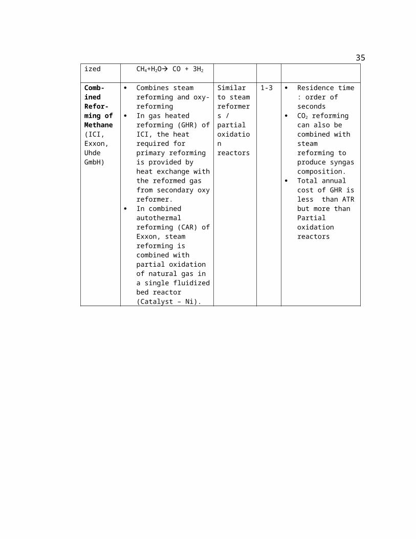
Table 2-2 summarizes the different technologies available for the production of syngas

from methane commercially. It also provides the process description, operating

conditions, hydrogen-to-carbon mono-oxide ratio in syngas, conversion etc. From Table

2-2, it is clear that by the catalytic partial oxidation route, more feed can be processed at

a lower temperature and can produce syngas of required composition for downstream

Fischer-Tropsch / Methanol processes. The packed bed reactor used for catalytic

methane partial oxidation is a directly coupled adiabatic reactor.

2.3.2 Experimental Work on Catalytic Partial Oxidation of Methane

A number of experimental studies on the catalytic partial oxidation (CPO) of methane

to syngas, at atmospheric pressure, in fixed beds, honey-comb monoliths, and fluidized

beds are available in the literature (Pena et al.,1996). The mean residence times in these

reactors are generally of the order of seconds. Chaudhary et al., 1993) and Schmidt’s

group (Hickman and Schmidt, 1992, 1993; Bharadwaj and Schmidt, 1994, 1995; Hohn

and Schmidt, 2001) have studied the production of syngas in a millisecond contact time

packed bed reactor and monolith reactor, respectively, at atmospheric conditions. The

18

production of syngas at higher operating pressure conditions is attractive to industry due

to the ease of integration with the downstream processes and due to larger volumetric

reactor productivity. However, only a limited amount of experimental work is available

at higher operating pressure in the open literature (Poirier et al., 1992; Gomez et al.,

1995; Basini et al., 2001). It is to be recognized, however, that at higher pressure, the

conversion of methane is limited by the thermodynamic equilibrium and the

homogeneous gas phase reactions also occur along with the heterogeneous reactions (de

Smet et al., 2001; Bizzi et al., 2003).

The issue which is still much debated regarding CPO is the mechanism by which

methane is converted to syngas. Although the possibility of performing the reaction via

the direct route (in one step from methane to syngas) has been reported by several

researchers, there seems to be an increasing consensus that the reaction occurs mainly

via the indirect route. Only at very high temperatures the reaction may partially proceed

through the direct route. It is to be noted that the hot spot could be eliminated if the

reaction occurs via the direct route.

Because of the complexity of the processes involved and because of interactions of

exothermic and endothermic reactions, a suitable mathematical model (both steady state

and dynamic) is required for the optimization of the process and for reactor control.

19

Table 2-2: A brief review on technologies available for syngas Production (Pena et al., 1996; Aasberg-Petersen, 2001).

Process and

Techno-logy

licensors

Description Operating Conditions

H2/ CO

ratio

Remarks

Steam Reforming(Davy Process)

· Multi-tubular catalytic reactor employed with exterior heat supply

· Catalyst: Ni/Al2O3

· Main Reaction:CH4+H2O CO + 3H2

· Press.: 15-30 atm

· Temp.:~ 1200 K

3 - 5 · Residence time: order of seconds

· Excess steam required to reduce carbon deposition (H2O / CH4 mole ratio ~ 2-5)

· Conversion ~ 90-92%

· Capital Cost is High· BP commercialized

compact reformer (counter-current reactor coupling hydrogen combustion and steam reforming) in 2002

Auto thermal Reforming(Haldor-Topsoe, Lurgi)

· Preheated feed streams are mixed in a burner, where partial oxidation takes place followed by steam reforming and equilibration in the catalyst bed

· Catalyst : Ni· Main Reactions:

CH4+0.5O2CO+2H2

CH4+H2O CO + 3H2

· Press.: 25 atm (exit)

· Temp.:a. catalyst

zone - 1200 – 1400 K

b. Combustion zone – ~2200K

~ 2.5 · Residence time: order of seconds

· Conversion ~ 90%· Feasibility of

operating at low steam-to-carbon ratio of 0.2-0.6 is demonstrated in pilot plants.

· Total annual cost 17-18% less than steam reforming

Non-Catalytic Partial Oxidation(Texaco, Shell)

· Mixture of O2 and CH4 is preheated, mixed and ignited in a burner

· Main Reaction:CH4+0.5O2CO+2H2

· Temp.: ~ 1800 K

· Press.: 1–40 atm.

~1.7-1.8

· Residence time: order of seconds

· Addition of steam increases soot formation

· Expensive next to steam reforming

Catalytic · Mixture of O2 / air and · Temp.: ~ 2 · Residence time :

20

Partial Oxidation(Exxon Mobil,Conoco Philips)Not yet commercial-ized

CH4 with or without steam· Catalyst: Ni /Pt, Rh· Reactors: Packed beds,

Monoliths, Fluidized beds.· Reaction Scheme (still in

debate):CH4+0.5O2CO+2H2

OrCH4+2O2CO2+2H2OCH4+H2O CO + 3H2

1000-1500 K

· Press.: 1 – 40 atm.

order of milliseconds to seconds

· Conversion : 90%· Selectivity : 95%· Offers best economic

advantage

Comb-ined Refor-ming of Methane(ICI, Exxon, Uhde GmbH)

· Combines steam reforming and oxy-reforming

· In gas heated reforming (GHR) of ICI, the heat required for primary reforming is provided by heat exchange with the reformed gas from secondary oxy reformer.

· In combined autothermal reforming (CAR) of Exxon, steam reforming is combined with partial oxidation of natural gas in a single fluidized bed reactor (Catalyst – Ni).

Similar to steam reformers / partial oxidation reactors

1-3 · Residence time : order of seconds

· CO2 reforming can also be combined with steam reforming to produce syngas composition.

· Total annual cost of GHR is less than ATR but more than Partial oxidation reactors

21

2.3.3 Modeling Work on Catalytic Partial Oxidation of Methane

A lot of research has been carried out in recent years in the development of steady state

and dynamic models for the syngas process. This section reviews some of the most

pertinent studies.

De Groote and Froment (1996) developed a steady state 1-D heterogeneous model to

simulate the adiabatic fixed bed reactor (directly coupled reactor) based upon the

kinetics of total combustion, steam reforming, water-gas shift on a Ni catalyst using

methane/oxygen or methane/air mixtures as feed. The steam reforming reactions and

water gas shift reaction are parallel or more or less consecutive to combustion,

depending upon the degree of reduction of the catalyst, which is determined by the

temperature and the gas phase composition. Their kinetic models are the Langmuir-

Hinshelwood-Houghen-Watson (LHHW) type and have the partial pressure of

hydrogen in the denominator and so the feed should have some amount of hydrogen. In

their model, intraparticle diffusion limitations are expressed in terms of a constant

effectiveness factor for each reaction. They had developed two sub-models to

understand the reaction mechanisms. In the first sub-model, the catalyst has a varying

degree of reduction (VDR), where the combustion and reforming reactions occur

sequentially. In the second sub-model the catalyst is bivalent (BV), where the catalytic

combustion and steam reforming operate in parallel. The exit and maximum

temperatures are smaller in the BV model and hence the predicted conversion is lower.

With the VDR model, a peak appears in the temperature profile after which

endothermic reaction proceeds. But in the BV model, a plateau is observed in the

temperature profile. De Groote and Froment (1996) also studied the effect of the

addition of CO2 / Steam to the feed mixture on product yield and temperature profile.

De Smet et al. (2001) developed a steady state one dimensional heterogeneous reactor

model to simulate the syngas process for methanol production (high pressure process

with oxygen as oxidant) and for fuel cell applications (atmospheric process with air as

oxidant). They considered external concentration and temperature gradients as well as

22

intra particle concentration gradients. The catalyst particle is assumed to be isothermal.

They used two models for reforming kinetics, one proposed by Xu and Froment (XF)

(1989) and the other proposed by Numaguchi and Kikuchi (NK) (1988). De Smet et al.

also showed that for a catalytic partial oxidation reactor for methanol production, gas

phase reactions need to be considered because the time scale for complete conversion of

oxygen is much lower in homogeneous systems than in heterogeneous systems.

Veser and Frauhammer (2000) developed a transient state 1-D two phase dispersion

model of a Pt monolithic reactor. They neglected gas phase reactions and the mass

transfer limitations in the catalyst boundary layer. Here, the coupling of the two phases

is through the convective heat transfer. They used the full adaptive method of lines

approach to solve the set of coupled partial differential equations. Their simulation

shows that the syngas production occurs by direct oxidation method.

Deutschmann and Schmidt (1998 a,b) developed a steady state 2-D detailed flow model

of a monolithic channel. They considered both the gas phase and the surface reactions

and used the commercial software FLUENT to solve the governing equations. They

observed that the time scale of flow and solid thermal response are decoupled. And,

they used a time independent formulation for channel calculations and the transient heat

conduction equation for the solid. In their model, the axial temperature profile was used

as the boundary conditions for the channel calculations, which returns the heat flux for

the monolith heat transfer calculations. The time required for convergence of the model

is 20 minutes without gas phase reactions and more than 10 hours with the gas phase

reactions. Hence, we need a simple and robust model for control and optimization

purposes. They observed that at the reactor inlet, total oxidation dominates and CO

formation starts much before H2 formation. They demonstrated that at high pressures,

homogeneous reactions are important and the syngas yield decreases.

Avci et al., (2001) studied the catalytic oxidation and steam reforming of methane using

a 1-D steady state heterogeneous model at high and low pressure conditions for two

cases – one with a mixed bed (physical mixture) of oxidation and reforming catalysts

23

and the other with a dual bed where the two catalyst beds (in SEQDCAR arrangement)

are placed consecutively. They observed that the mixed bed configuration exhibited

better performance compared to dual bed schemes. The transient behaviors of these

reactors were not discussed. Recently, Bizzi et al., (2003, 2004) studied the partial

oxidation of methane in short contact time packed bed reactors using the rhodium

catalyst with and without detailed chemistry. They also observed that gas phase

reactions do not affect the overall reactivity of the partial oxidation of methane in short

contact time packed bed reactors.

In a nutshell, most of the reported modeling studies discuss the steady state behavior of

this process, in particular, the focus of investigations has been on the effects of feed

temperature, importance of gas phase reactions at higher operating pressure and the role

of thermal conductivity of the catalyst bed and GHSV on the methane conversion and

on the product pattern.

2.4 Roadmap of this Thesis

Our literature study shows that a detailed comparative performance study of various

modes of coupling of exothermic and endothermic reactions has not been done. Also,

the studies available in the literature have mainly focused on the steady state behavior

of some of the reactor systems. The transient behavior of such systems is not available

in the literature and is very important in the design of reactors-from a reactor startup,

shut down, and a control point of view. Hence, we propose to investigate and then

compare the performance of different reactor systems using steady state and transient

state mathematical models.

The reactors for coupling exothermic and endothermic reactions received wide attention

due to their potential to provide compact hydrogen generation systems for fuel cells.

Hence, most of the studies, including the theoretical ones, were carried out at

atmospheric operating conditions. The energy efficiency of syngas generation and the

reduction in its associated production costs are very important for large process

24

industries like methanol synthesis plants, which operate at higher pressures. Also, the

dynamic behaviors of the partial oxidation reactors are not analyzed in depth in the

literature. Hence, we have attempted to develop a robust transient 1-D heterogeneous

model of short contact time packed bed reactor using the kinetics reported in the

literature (de Smet et al., 2001; Dupont et al., 2002) to analyze this process.

In summary, this thesis focuses on answering some of the following questions:

1. How does the performances of counter-current, co-current and directly coupled

reactors compare to one another?

2. How can we select a mode of coupling for the application / reaction system of

our choice?

3. What are the features exhibited if both exothermic and endothermic reactions

occur within a catalyst particle?

4. How does the interaction of exothermic and endothermic reaction time scale

affect the performance, in particular conversion, selectivity and hotspot, in the

catalytic partial oxidation of methane to syngas process in a short contact time

reactor?

5. Do short contact time reactors exhibit wrong way behavior and, if they do, how?

6. Is there a measure to quantify and compare the performance of these reactors?

Some of the following steady state and transient models are used, based on the level of

complexities demanded by the problem, to analyze the various features exhibited by

these reactor systems and to answer the above questions:

Pseudo homogeneous plug flow model: This model assumes that the interphase

transport processes (gas-solid film heat and mass transfer rates) are much faster than

reaction processes and the gas moves like a slug within the reactor. These assumptions

result in the model consisting of a set of first order differential equations. The steady

state solutions for co-current and directly coupled adiabatic reactors are obtained by

integrating these equations using the commercially available stiff solver from Netlib

libraries. For the counter-current reactor, a two point boundary value problem results

25

and can be solved by discretizing the spatial derivatives (convective terms) and solving

the resulting non-linear algebraic equations using a Newton-Powell type algorithm. In

this work, the pseudo-transient approach is used to obtain the steady state solution. In

this approach, the transient model equations are integrated until the steady state solution

is obtained. This method seems to be faster and more robust for this reactor scheme.

Heterogeneous Plug Flow Model: The use of highly active catalysts increases the

importance of transport resistances between the gas and the solid. The heterogeneous

model accounts for the gas-solid film transfer effects. Several criteria are available in

the literature (Mears, 1971; Hudgins, 1972) that helps us decide when to use the

heterogeneous model instead of the pseudo homogenous model. Some of these criteria

are listed in Appendix A. The heterogeneous model results in a set of differential and

algebraic equations (DAE), which are solved using the commercially available DAE

solver, DASSL from Netlib. The heterogeneous model equations can also be solved by

sequential approach, which is explained in Chapter 7.

Axial Dispersion Model: Heat and mass dispersion are added to the heterogeneous

model to account for the species and thermal dispersion which occur at high

temperature. Mears (1971) provided the necessary criteria for using the axial dispersion

model compared to plug flow model. This model results in a second order differential

algebraic boundary value problem. These second order ODEs can be solved directly

using the commercially available BVP solver, like COLDAE, etc., or the problem can

be converted to algebraic equations by discretizing the spatial derivatives and solving

the resulting equations using any non-linear algebraic solver. Instead, we employed the

pseudo transient approach to obtain steady state profiles. This is computationally fast

and efficient compared to using any other steady state solver especially for a complex

and stiff systems. The axial dispersion models can exhibit multiple steady states. A

detailed analysis of these models for short reactors (Hlavacek and Hoffman, 1970;

Varma and Amundson, 1973) and long reactors (Vortuba et al., 1972) can be found in

the literature. The axial dispersion models are important in simulating the syngas

26

generation in short contact time reactors, since the dispersion effects have been

observed experimentally in the reactor systems (Basini et al., 2001).

Transient Models: The unsteady state pseudo-homogeneous, heterogeneous plug flow

and axial dispersion models are developed to study the dynamics of coupling

exothermic and endothermic reactions. These models are important for studying the

evolution of state variables during start-up and for studying control strategies and safe

shut-down of these reactors. Several interesting non-intuitive behavior of these reactors,

like multiplicity and stability of the solution profiles etc., can be unveiled by the

transient models. The transient models result in stiff partial differential equations and

are solved by the Method-of-Lines (Vande wouwer et al., 2001).

The appropriate mathematical model and the corresponding numerical procedure used

to analyze the reactor systems are mentioned and dealt with in detail in the respective

sections / chapters studying the particular reactor configuration.

27

Chapter 3

Recuperative Coupling of Exothermic and

Endothermic Reactions

3.1 Scope

In this chapter, a one dimensional pseudo-homogeneous plug flow model is used to

analyze and compare the performance of co-current and counter-current heat exchanger

reactors. The numerical schemes used to solve the model equations are presented. A

parametric analysis is carried out to address the vital issues, such as the exit conversion

of the endothermic reaction, the temperature peak (hot spot) of the exothermic reaction

and the reactor volumetric productivity. The measures to reduce the hot spot by

different catalyst profiling techniques are also addressed. Some features of the dynamic

behavior exhibited by these reactors, such as temperature evolution profiles and wrong-

way phenomena, are presented. The design and operational flexibilities of the

recuperative reactors over other possible reactor configurations are discussed.

3.1 Introduction

In the heat exchanger reactors, the spaces where exothermic and endothermic reaction

take place simultaneously in time are separated by the walls of the tubes and heat

transfer between the two sides occurs through the tube wall. For example, endothermic

reactions can be carried out on one side (say, the tube side) and the exothermic reactions

on the other side (say, the shell side) of the shell and tube reactor and heat is transferred

between the exothermic and the endothermic reactions through the tube wall. These

reactors can be operated either in counter-current or in co-current flow mode depending

28

on the relative direction of flow of the reactant streams for the exothermic and

endothermic reaction.

The recuperative, or heat exchanger, reactor offers several advantages over the directly

coupled adiabatic reactor and the reverse flow reactor. Here, the products of the

endothermic reaction are always separated from the combustion products. Since the

exothermic side is spatially separated from the endothermic side, air can also be used

for combustion instead of oxygen and the challenge of nitrogen separation from the

product mixture does not exist. This in turn avoids the capital cost resulting from the

installation of an oxygen separation unit and / or the operational cost resulting from

compressing the air (along with nitrogen) to the process pressure. Heat exchanger

reactors offer other operational flexibilities since the operating parameters of

exothermic and endothermic streams, such as the inlet velocity, feed concentration etc.,

can be adjusted independently without affecting the other stream.

A review on coupling of exothermic and endothermic reactions and some discussion of

the merits and demerits of various modes of coupling are discussed by Kolios et al.,

(2000), Zanfir and Gavriilidis (2003), Deshmukh and Vlachos, (2005). Most of the

work on heat exchanger reactors for coupling exothermic and endothermic reactions, as

mentioned earlier, was focused either on wall catalyst-coated reactors (Ismagilov et al.,

2001; Venkataraman et al., 2002; Venkataraman et al., 2003; Zanfir and Gavriilidis,

2001, 2003) or on monolith reactors (Kolios et al., 2001, 2002). Recently, there are

several research activities directed towards developing micro-reactors for coupling

exothermic and endothermic reactions (Kolios et al., 2005; Deshmukh and Vlachos,

2005). However, a full discussion of steady state and dynamic behavior exhibited by

these reactor systems is not available in the literature. In this chapter, we have made an

attempt to analyze and compare the performance of counter-current and co-current

packed bed reactors. A parametric study showing the effects of the wall heat transfer

coefficients and the Damkohler number for the exothermic reaction on the conversion

of the endothermic reaction and on the temperature peak of the exothermic reaction is

presented. Hot-spot formation and suitable measures to reduce the hot spot by catalyst

29

activity profiling are also discussed. The reactor length and the flow rate are treated, as

the design and operational parameters, respectively, and their implications on the

reactor performance are analyzed. Some of the key features of the transient behavior

exhibited by the recuperative coupling of exothermic and endothermic reactions are also

presented.

3.2 One Dimensional Pseudo-homogeneous Plug Flow Model

This section presents the pseudo-homogeneous plug flow model for counter-current and

co-current reactors with irreversible first order exothermic and endothermic reactions.

These model equations are used to examine the richness of the behavior exhibited by

these reactors. The following assumptions are made in the development of the model:

i) The resistance across the gas-solid film for heat and mass transfer is assumed to

be negligible.

ii) Axial mass and heat dispersions are neglected.

iii) Axial conduction in the wall is not included, and a constant heat transfer coeffi-

cient has been assumed along the length of the reactor.

iv) Physical properties of fluids and the heat of reactions are assumed to be inde-

pendent of temperature, and the total pressure of the system is constant.

The dimensionless governing equations are:

a) for the endothermic side,

Mass Balance:

(3.1)

30

Energy Balance:

(3.2)

b) for the exothermic side,

Mass Balance:

(3.3)

Energy Balance:

(3.4)

In Eqs. 3.3 and 3.4, the positive sign is used for the co-current reactor and the negative

sign for the counter-current reactor. Here, η(ξ) and are the position dependent

catalyst activity for the endothermic and exothermic reactions, respectively. Both η(ξ)

and are set as unity for the cases with no catalyst activity profiling. The boundary

conditions and initial conditions used for solving Eqs. 3.1-3.4 are given below.

Co-current reactor:

at ξ = 0,

31

at τ = 0,

Counter-current reactor:

at ξ = 0,

at ξ = 1,

at τ = 0,

The other dimensionless parameters used in the model are given below with j = c and h

for the cold and hot side respectively:

,

, ,

The parameters considered in the sensitivity analysis are the Damkohler number ( ,

the ratio of flow time to the reaction time), dimensionless wall heat transfer coefficient (

), dimensionless heat of reaction ( ), and dimensionless activation energy ( ).

Some of the correlations used to estimate the wall heat transfer coefficient are provided

in Appendix B. For the counter-current reactor, the feed for the endothermic reaction

32

enters at the axial position, ξ=0, and the feed for the exothermic reaction enters at the

opposite end of the reactor, i.e. at the axial position, ξ=1 (position-1). For the co-current

reactor, the feed for both exothermic and endothermic reactions enter at the axial

position, ξ=0 (position-0).

3.3 Solution Procedure

The transient model equations (Eqs. 3.1-3.4) are solved by the Method-Of-Lines (MOL)

approach (van de Wouwer et al., 2001). In the MOL approach, partial differential

equations (PDE) are converted to a set of ordinary differential equations (ODE) by

suitable discretization of spatial derivatives and the resulting ODEs in time are

integrated by stiff solvers. Here, we have used a second order upwind finite difference

scheme for the discretization of spatial derivatives. The discretization scheme used is

modified to have the Total Variation Diminishing (TVD) property to avoid spurious

oscillations (Tannehill et al., 1997) and is explained in the Section 3.4.1. The grid

independence of the solution is verified and the number of nodes used for the simulation

in this work is 250, unless otherwise stated. The ODEs are integrated using LSODE

solver from the Netlib libraries.

3.4.1 Total Variation Diminishing Scheme (TVD)

The numerical solution to the hyperbolic partial differential equations employing higher

order spatial discretization schemes results in artificial oscillations. This is called the

Gibbs phenomenon. Godunov (1959) has shown that the monotone behavior of a

solution cannot be assured for finite-difference methods with more than first order

accuracy. This monotone property is very desirable when discontinuities are computed

as part of the solution. Though the first order discretization schemes avoid the

oscillations, they suffer from poor solution accuracy (highly dissipative). Harten (1983)

proved that if higher order schemes can be modified using total variation diminishing

algorithms then those schemes will be, in turn, montonicity preserving and then the

higher-order method will avoid spurious oscillations.

33

Lax (1973) defined total variation (TV) of a variable, u = f(x) as,

A numerical method is said to be total variation diminishing, or TVD, if

TV(un+1) ≤ TV(un)

Here x is the independent variable and n refers to the instant of time (second

independent variable). For TVD preserving high order discretization schemes, the

solution is first order near discontinuities and higher order in smooth regions. The

transition to higher order is accomplished by the use of slope limiters on the dependent

variables or flux limiters. We have employed the guidelines provided by Harten (1984)

to make our second order discretization scheme, TVD preserving. We have also used

the van Leer limiter (1982) in the above scheme. The numerical first derivatives

calculated with and without TVD algorithm are presented below.

First derivatives based on II order upwind discretization scheme without TVD

preserving algorithm are:

with

.

The first derivatives based on TVD preserving II order upwind discretization scheme

are:

34

where,

In the above formulation N refers to number of nodes used for the discretization and δ is

arbitrarily set as 1.0e-5.

Different discretization schemes, such as first order, second order and fourth-order, and

the second order with TVD preserving discretization scheme, were tested for standard

steady state and transient problems such as: the analytical solutions of the hyperbolic

Burger equations, propagation front of the combustion flame, temperature profiles in a

methanator (tubular reactor carrying out combustion of methane). It was found that first

order discretization schemes could capture the solution only with larger number of

nodes.

Axial Distance

Tem

pera

ture

Dac = 10.0 Dah = 4.0γc = 15.0 γh = 15.0βc = - 0.8 βh = 0.8U*c = U*h = 4.0

0.7 0.8 0.9 1-0.3

-0.2

-0.1

0

0.1

0.2

0.3

0.4

0.5

0.6

0.7

0.8

I order, 1000 nodesI order, 250 nodesII order, 250 nodesIV order, 150 nodesII order, 150 nodes with TVD

Axial Distance

Tem

pera

ture

Dac = 10.0 Dah = 4.0γc = 15.0 γh = 15.0βc = - 0.8 βh = 0.8U*c = U*h = 4.0

0.7 0.8 0.9 1-0.3

-0.2

-0.1

0

0.1

0.2

0.3

0.4

0.5

0.6

0.7

0.8

I order, 1000 nodesI order, 250 nodesII order, 250 nodesIV order, 150 nodesII order, 150 nodes with TVD

35

Figure 3-1: Effect of Different Discretization Schemes on Exothermic Temperature Profiles in Counter-current Reactors (Parameters as shown in Table 3-1)

Higher order discretization schemes capture the solution with lower number of nodes

but suffer from Gibb’s oscillations near the shock or wave/reaction front. On the other

hand, the second order discretization scheme with TVD preserving algorithm avoids the

spurious oscillations with lower number of nodes. The spurious oscillations mask the

real solution especially during the transients (wrong-way in packed beds).

All the above schemes were tested for the counter-current heat exchanger reactor for the

parameters shown in Table 3-1 and the temperature profile at the exothermic side

simulated with different discretization schemes are presented in Figure 3-1. The profile

simulated with 1000 nodes (minimum number of nodes to produce the grid independent

solution) and first order discretization scheme is used as the bench-mark (Kulkarni,

1996). The profiles obtained with 250 nodes closely match the bench-mark for all the

discretization schemes (with and without TVD algorithm) except for the first order

discretization (with 250 nodes) scheme. With lower number of nodes, say 150 nodes,

there is a discrepancy between the bench-mark case and the profiles simulated with

other discretization schemes. The fourth order backward upwind discretization scheme,

with 150 nodes, results in a wrong (unconverged) profile (with lower temperature peak

and lower conversion for endothermic reaction). This may be due to the propagation of

error as the exothermic and the endothermic sides are coupled and the convection

direction is opposite to each other, in the counter-current reactor. It is found that for

TVD preserving II order scheme, with 150 nodes, the calculated temperature peak, as

well as the exit conversion for endothermic reaction, closely match that of the bench-

mark case.

36

As TVD schemes are important to capture the transients accurately, they are used in this

work, and the number of nodes chosen for the simulation of the counter-current reactor

is 250. For the co-current reactors 150 nodes were sufficient to produce the grid-

independent solution.

Table 3-1: The Parameters Used for Base Case Simulation (For 1-D Models)

Parameters Endothermic Exothermic

Da 10 4

β -0.8 0.8

γ 15 15

U* 4 4

Activity η = 1 α = 1

3.4.2 Arrangement of Variables

The partial differential transient model equations are converted to ordinary differential

equations by the method-of-lines. The resulting ordinary differential equation in time

can be integrated using Adam’s explicit solver (using the option, MF=10, in LSODE) or

by the implicit solver (option MF = 22 in LSODE). While using the explicit solver, the

spatial and temporal steps are chosen such that the Courant criterion (Tannehill et al.,

1997) is satisfied. The implicit solvers have an infinite domain of stability and, hence, a

larger spatial and/or time step could be used. Often, in such situation, the time step is

limited by the fastest time scale in the problem. The implicit solver used in LSODE is a

modified Gear’s algorithm for stiff differential equations. The Gear’s algorithm

involves matrix inversion / LU decomposition and, hence, is prone to longer

computation time especially if the matrix becomes very sparse.

A proper strategy of arranging the differential equations and the variables reduces the

total time for computation with the implicit solving procedure. The total number of

variables in the discretized transient model (discretized partial differential equations) is

37

the product of the number of nodes and the number of variables in the governing

equations / model (Ntot = Nnode*Nmodel) and all these differential equations are solved

simultaneously.

n: 1 2 3 …. Nmodel Nmodel+1 …. …. …. Ntot

ui,j: u1,1 u1,2 …. …. u1,Nmodel u2,Nmodel …. …. …. uNnode,Nmodel

Scheme-i

n: 1 2 3 …. Nnode Nnode+1 Nnode+2 …. …. Ntot

ui,j: u1,1 u2,1 …. …. uNnode,1 u1,2 u2,2 …. …. uNnode,Nmodel

Scheme-ii

Figure 3-2: Two different schemes to arrange the variables (uij) and the differential equations ( i (= 1 to Nnode) – node index, j (=1 to Nmodel) – variable index, n (=1 to Ntot) – running index of all the variables in the system with Ntot=Nnode*Nmodel)

There are two ways by which the variables are arranged (numbered): (i) All the model

variables at first node are arranged first (numbered) and then the model variables at the

second node are numbered. This procedure is repeated until the last node of the domain

is covered. Once the variables and the equations are numbered in this fashion, then they

are integrated in time. (ii) In the second approach, the first variable of the governing

equations at all the nodes is arranged first. Then the second variable of the governing

equations is numbered for all the nodes. This procedure is repeated until all the

variables of the governing equations (and for all the nodes) are arranged. The schematic

of these two schemes, with the positioning and numbering of the variables, are shown in

Figure 3-2.

It is observed that the second scheme (Scheme-ii) of arranging the variables / equations

results in larger computation time. This is due the fact that sparseness is scattered

throughout the domain of the matrix in the second scheme and, hence, takes more time.

It is to be noted that the model equations at node i relate all the variables at the node i

38

strongly compared to the variables in the neighboring nodes. And usually in physical

systems the number of model variables is much less than the number of nodes. Hence,

the first scheme (Scheme-i) of arranging the variables brings the dependent variables

close together in the matrix representation and reduces the computation time. This

phenomenon of reduction in the computation time is similar to that observed in solving

the steady state models for crude distillation columns by the Newton method. The

model equations for the crude distillation columns result in a block tri-diagonal matrix.

The numbering and positioning of pump-arounds and side strippers (extra features of

the distillation column) determine the placement of variables near the diagonal

elements. It is observed that if variables corresponding to pump-arounds and side-

strippers are placed close to the diagonal variables, then the computation time

decreases. More details on the variable placement and the effect of computation time

can be found in Ramaswamy (1999). We have used Scheme-i for all our computations

in this work.

3.4 Results and Discussions

In this section, steady state (Section 3.5.1) and dynamic behavior (Section 3.5.2)

observed in the counter-current and co-current reactors are analyzed and the predicted

conversion, temperature profiles and the volumetric productivity are presented. The

effects of design and operational parameters on the performance of these reactors and in

reducing the hot spot are discussed. The role of inert packing in some sections of the

reactor is also addressed with reference to improving the efficiency of these reactors.

3.5.1 Steady State Behavior

Temperature Profiles: The computed temperature profiles in the counter-current and

co-current heat exchanger reactors, for the base case, are presented in Figure 3-3. The

parameters used for this base case simulation are reported in Table 3-1. The counter-

current reactor exhibits a phenomenon termed here as cold pinch and hot pinch cross-

over points. At these cross-over points both the exothermic and endothermic streams

have identical temperature.

39

Figure 3-3: Temperature Profiles in Counter-current and Co-current Reactors

The cold pinch cross-over point occurs near the inlet for the endothermic feed (position-

0) because of two simultaneous phenomena – (i) heat exchange between exothermic and

endothermic stream, and (ii) the endothermic chemical reaction. Here, the reactants for

the endothermic reaction transfer heat to the effluent of the exothermic reaction from

the inlet (position-0) up to the cold pinch cross over point. In addition to this, the

endothermic reaction occurs in this region and, hence, a drop in the temperature (from

the inlet value) is observed in the temperature profile on the endothermic reaction side.

There is also a hot pinch cross-over point near the inlet of the feed for the exothermic

reaction (position-1). From this hot pinch cross-over point to position-1, the effluent of

the endothermic reaction heats the reactants for the exothermic reaction.

In some of the experimental and modeling studies published in the literature, the cold-

pinch cross over point is not mentioned. This may be attributed to a number of reasons

such as dissimilar reaction rates and heats of exothermic and endothermic reactions, the

use of shorter reactors, etc. One way of eliminating this cold pinch cross-over is by

0 0.1 0.2 0.3 0.4 0.5 0.6 0.7 0.8 0.9 1-0.3

-0.2

-0.1

0

0.1

0.2

0.3

0.4

0.5

0.6

0.7

0.8

Counter - EndoCounter - ExoCo-current - EndoCo-current - Exo

Axial Distance

Tem

pera

ture

Dac = 10.0 Dah = 4.0γc = 15.0 γh = 15.0βc = - 0.8 βh = 0.8U*c = U*h = 4.0

Axial Distance

Tem

pera

ture

Dac = 10.0 Dah = 4.0γc = 15.0 γh = 15.0βc = - 0.8 βh = 0.8U*c = U*h = 4.0

40

reducing the activity of the catalyst (by using inert packing in a section of the reactor,

etc) for the endothermic reaction near position-0, which alters the effective length of the

catalyst bed. The effect of the length of the reactor on the cold pinch cross-over point

and the hot spot are discussed in a later section. The second way of avoiding the cold

pinch cross-over point is by using non-similar feed temperature for the exothermic and

endothermic streams. Figure 3-4 shows a case where the cold pinch cross-over is not

observed. Here the inlet temperature of the exothermic stream is higher than the inlet

temperature for the endothermic stream. This arrangement requires the pre-heating of

the exothermic stream and that can be carried out by utilizing the sensible heat of the

endothermic stream leaving the reactor.

Figure 3-3 shows that the temperature peak observed in the counter-current reactor is

higher than that of the co-current reactor. This higher peak on the exothermic side in the

counter-current reactor, near position-1, is due to the increase in the rate of the

exothermic reaction because of heating of its feed by the hot effluent of the endothermic

reaction.

The above observation is in line with that of Venkataraman et al. (2002) where it was

shown that the counter-current operation results in a higher temperature peak compared

to the co-current reactor (for catalytic wall coated reactor).

0 0.1 0.2 0.3 0.4 0.5 0.6 0.7 0.8 0.9 1-0.3

-0.2

-0.1

0

0.1

0.2

0.3

0.4

0.5

EndoExo

Axial Distance

Tem

pera

ture

Dac = 10.0 Dah = 4.0γc = 15.0 γh = 15.0βc = - 0.2 βh = 0.4U*c = U*h = 4.0

Axial Distance

Tem

pera

ture

Dac = 10.0 Dah = 4.0γc = 15.0 γh = 15.0βc = - 0.2 βh = 0.4U*c = U*h = 4.0

41

Figure 3-4: Temperature Profiles in Counter-current Reactor without Cold Pinch Cross-Over Point

Figure 3-5: Conversion Profiles in Counter-current and Co-current Reactors

Conversion Profiles: Figure 3-5 shows the conversion profiles for the co-current and

counter-current reactors. The exit conversion of the endothermic reaction in the co-

current reactor is greater than that in the counter-current reactor. This higher conversion

in the co-current reactor is due to the endothermic stream spending more time in the

reactor at higher temperature than in the counter-current reactor. The conversion for the

endothermic reaction in the adiabatic reactor is also calculated (by setting U*c= U*h = 0,

in the model) for similar parameters used in Table 3-1. It is found that the recuperative

reactors results in higher exit conversion for the endothermic reaction compared to that

in the adiabatic reactor because of coupling with the exothermic reaction. The

Axial Distance

Con

vers

ion

Dac = 10.0 Dah = 4.0γc = 15.0 γh = 15.0βc = - 0.8 βh = 0.8U*c = U*h = 4.0

0 0.1 0.2 0.3 0.4 0.5 0.6 0.7 0.8 0.9 10

0.1

0.2

0.3

0.4

0.5

0.6

0.7

0.8

0.9

1

Counter - EndoCounter - ExoCo-current - EndoCo-current - Exo

42

percentage increase in the volumetric productivity (the rate of product produced per unit

reactor volume, based on products of the endothermic reaction) is 262 % in the co-

current reactor with respect to the adiabatic reactor. Similarly the percentage increase in

the volumetric productivity between the adiabatic and the counter-current reactor is 252

%, which is less than that observed with co-current reactor for the parameters reported

in Table 3-1.

The simulation studies with an irreversible exothermic reaction and a reversible

endothermic reaction are also carried out, and the temperature and conversion profiles

obtained were qualitatively similar to those being discussed in this chapter for the

identical conditions. The thermodynamic equilibrium becomes favorable at higher

temperatures for the endothermic systems and this is one reason for obtaining the

similar qualitative behavior with reversible kinetics.

Effect of Damkohler Number (Dah) for Exothermic Reaction: We carried out the

parametric sensitivity analysis to determine the effect of Dah on the temperature peak

and on the exit conversion of the endothermic reaction.

Co-current Reactor: Figure 3-6a shows the temperature peak on the exothermic side

and the conversion for the endothermic reaction, for the co-current reactor. With an

increase in Dah, the rate of exothermic reaction increases, hence the temperature peak

on the exothermic side and the conversion for the endothermic reaction increase. Above

a critical value of Dah (~ 4 for this case) conversion for the endothermic reaction

remains at unity. A further increase in Dah, increases the temperature peak of the

exothermic reaction and the corresponding exit temperature of both streams. Hence, in a

real system, if an excessive hot spot is anticipated in the co-current reactor, an effort

could be made to reduce it (by either diluting the catalyst bed or by increasing the inlet

velocity, both of which reduces the Damkohler number), without sacrificing the

conversion for the endothermic reaction.

0 1 2 3 4 5 6 70

0.1

0.2

0.3

0.4

0.5

0.6

0.7

0.8

0.9

1

0

0.1

0.2

0.3

0.4

0.5

0.6

0.7

0.8

0.9

1

ConversionTemperature Peak

Dah

Con

vers

ion

Dac = 10.0 Dah = variedγc = 15.0 γh = 15.0βc = - 0.8 βh = 0.8U*c = U*h = 4.0

Tem

pera

ture

Pea

k

Dah

Con

vers

ion

Dac = 10.0 Dah = variedγc = 15.0 γh = 15.0βc = - 0.8 βh = 0.8U*c = U*h = 4.0

Dah

Con

vers

ion

Dac = 10.0 Dah = variedγc = 15.0 γh = 15.0βc = - 0.8 βh = 0.8U*c = U*h = 4.0

Tem

pera

ture

Pea

k

43

Figure 3-6a: Effect of Damkohler Number for the Exothermic Reaction on Conversion of the Endothermic Reaction and Temperature Peak of the Exothermic Reaction in the Co-current Reactor

Counter-current Reactor: In counter-current reactor, the effect of Dah is more

complex and the system exhibits multiple steady states for the parameter range studied.

Kolios et al. (2002) have also observed multiple steady states in the counter-current

reactors. The typical ignition (cold bed) and extinction branch (hot bed) for the exit

conversion of the endothermic reaction is shown in Figure 3-6b. It is seen that beyond

the parametric range where hysteresis occurs, an increase in Dah gradually decreases the

conversion for the endothermic reaction. At higher Dah, the temperature peak for the

exothermic reaction (and also for the endothermic reaction) and the hot pinch cross-over

occur very near the inlet for the exothermic feed (position-1).

Dah

Con

vers

ion

Dac = 10.0 Dah = variedγc = 15.0 γh = 15.0βc = - 0.8 βh = 0.8U*c = U*h = 4.0

Dah

Con

vers

ion

Dac = 10.0 Dah = variedγc = 15.0 γh = 15.0βc = - 0.8 βh = 0.8U*c = U*h = 4.0

0 1 2 3 40

0.1

0.2

0.3

0.4

0.5

0.6

0.7

0.8

0.9

1

Cold bedHot bed

44

Figure 3-6b: Effect of Damkohler Number for the Exothermic Reaction on Conversion of the Endothermic Reaction in the Counter-current Reactor

Hence, the endothermic stream leaves the reactor at a higher temperature. The residence

time between the position of the endothermic peak and the endothermic exit decreases

for high Dah, and hence, the exit conversion for the endothermic reaction decreases. For

lower Dah, the temperature peak for the exothermic reaction (and hence that of the

endothermic reaction) occurs further away from the feed inlet for the exothermic

reaction (position-1). This increases the conversion of the endothermic reaction.

Frauhammer et al. (1999) have also observed a similar trend in a monolith reactor,

where they have shown that by decreasing the length of the combustion catalyst bed, the

temperature peak for the exothermic reaction and the conversion for the endothermic

reaction increase in the counter-current reactor.

Effect of Wall Heat Transfer Coefficient: The effect of wall heat transfer coefficient

on the heat exchanger reactor performance is reported below.

Co-current Reactor: The exit conversion for the endothermic reaction and the

temperature peak on the exothermic side of the co-current reactor are plotted in Figure

3-7 for different dimensionless wall heat transfer coefficients, U* (=U*c = U*h). The

parameters reported in Table 3-1 were used for the simulation except for U*. The

magnitude of the temperature peak on the exothermic side is the largest when U* = 0

and is equal to the adiabatic temperature of the exothermic reaction, βh. As U*

increases, the magnitude of the temperature peak on the exothermic side decreases and

the exothermic reaction is suppressed at a critical U*. Figure 3-8 shows the temperature

45

profiles for the exothermic reaction side along the reactor length for different U*. The

conversion of the endothermic reaction increases for lower U* (< 4) and reaches a

plateau at complete conversion. Further beyond the plateau, the conversion decreases

with an increase in U*. The thermal coupling supplies the heat to the endothermic

reaction and, hence, the conversion increases for lower U*. For sufficiently higher U*,

the exothermic reaction is strongly affected by the endothermic reaction, and since the

rate of heat consumption by the endothermic reaction is greater than the rate of heat

generation (βcDac > βhDah), the exothermic reaction is quenched (Figure 3-8).

This results in lower temperature along the reactor on both sides. This in turn yields

lower conversions for the endothermic and exothermic reactions at very high U*. The

suppression of the exothermic reaction is largely pronounced at higher U*, say U* = 10

in Figure 3-8. This suppression of the exothermic reaction by the endothermic reaction

is similar to that observed in a directly coupled adiabatic reactor (Ramaswamy et al.,

2005a) and is discussed in Chapter 5.

0 5 10 15 20 25 300

0.1

0.2

0.3

0.4

0.5

0.6

0.7

0.8

0.9

1

0

0.1

0.2

0.3

0.4

0.5

0.6

0.7

0.8

0.9

1

ConversionTemperature Peak

U*

Con

vers

ion

Dac = 10.0 Dah = 4.0γc = 15.0 γh = 15.0βc = - 0.8 βh = 0.8U*c = U*h = varied

Tem

pera

ture

Pea

k

U*

Con

vers

ion

Dac = 10.0 Dah = 4.0γc = 15.0 γh = 15.0βc = - 0.8 βh = 0.8U*c = U*h = varied

U*

Con

vers

ion

Dac = 10.0 Dah = 4.0γc = 15.0 γh = 15.0βc = - 0.8 βh = 0.8U*c = U*h = varied

Tem

pera

ture

Pea

k

46

Figure 3-7: Effect of Dimensionless Wall Heat Transfer Coefficient on the Conversion of Endothermic Reaction and the Temperature Peak of the Exothermic Reaction in the Co-current Reactor

Figure 3-8: Effect of Dimensionless Wall Heat Transfer Coefficient on the Temperature Profiles for the Exothermic Reaction (Parameters same as Figure 3-7)

Axial Distance

Tem

pera

ture

Axial Distance

Tem

pera

ture

0 0.1 0.2 0.3 0.4 0.5 0.6 0.7 0.8 0.9 1-0.1

0

0.1

0.2

0.3

0.4

0.5

0.6

0.7

0.8

0.9

U* = 0.0U* = 0.5U* = 4.0U* = 10.0

0 5 10 15 200

0.1

0.2

0.3

0.4

0.5

0.6

0.7

0.8

0.9

1

0

0.1

0.2

0.3

0.4

0.5

0.6

0.7

0.8

0.9

1

ConversionTemperature Peak

U*

Con

vers

ion

Dac = 10.0 Dah = 2.0γc = 15.0 γh = 15.0βc = - 0.8 βh = 0.8U*c = U*h = varied

Tem

pera

ture

Pea

k

47

Figure 3-9: Effect of Dimensionless Wall Heat Transfer Coefficient on Temperature Peak of Exothermic Reaction and Conversion of the Endothermic Reaction in the Counter-current Reactor

Counter-current Reactor: For the counter-current reactor (Figure 3-9), the

temperature peak on the exothermic side gradually decreases with increase in U* and

falls drastically upon reaching a critical U* (exothermic reaction is extinguished). The

conversion (Figure 3-9) of the endothermic reaction increases with U* for lower heat

transfer coefficients, plateaus and then decreases for higher heat transfer coefficients. At

higher wall heat transfer coefficients, the exothermic reaction is suppressed, yielding

poor conversion for the endothermic reaction, and beyond the critical U*, the

conversion is even less than that observed in the adiabatic reactor (corresponding to U*

= 0). This is due to the counter-current mode of heat exchange and the resulting cold

pinch cross-over. The temperature and conversion profiles for the case with U* = 17 are

compared with those of the equivalent adiabatic reactor in Figures 3-10a and 3-10b. It is

to be noted that for this case, the magnitude of the cold pinch cross-over point is not

only less than the feed temperature but also less than the exit temperature of the

equivalent adiabatic reactor and this cross-over point occurs close to the centre of the

reactor. From the position-0 to the cold pinch cross-over point, the endothermic stream

heats the exothermic stream while exactly the opposite occurs in the next half of the

reactor. This additional heat loss along with the heat loss due to endothermic reaction

lowers the temperature of the cold pinch-cross over point below the exit temperature of

the adiabatic reactor. Hence, the rate of the endothermic reaction is reduced in the first

part of the reactor and this in turn lowers the conversion at the exit. This case has been

simulated with Dah = 2 and the other parameters as reported in Table 3-1. The results

obtained with Dah = 4 follow the same trend but the critical U* is larger than the one

observed with Dah = 2.

0 0.1 0.2 0.3 0.4 0.5 0.6 0.7 0.8 0.9 1-0.3

-0.2

-0.1

0

Endo. - U*=17Exo. - U*=17Adiabatic

Axial Distance

Tem

pera

ture

Axial Distance

Tem

pera

ture

48

Figure 3-10a: Temperature Profiles in the Counter-current Reactor (for U* = 17 and other parameters as reported in Table 3-1) compared to Temperature Profile in the Adiabatic Endothermic Reactor

Axial Distance

Con

vers

ion

Axial Distance

Con

vers

ion

0 0.1 0.2 0.3 0.4 0.5 0.6 0.7 0.8 0.9 10

0.1

0.2

0.3

Endo. - U*=17Exo. - U*=17Adiabatic

49

Figure 3-10b: Conversion Profiles in the Counter-current Reactor (for U* = 17 and other parameters as reported in Table 3-1) compared to that in the Adiabatic Endothermic Reactor

Effect of Catalyst Activity Profiling: We have carried out simulations with a position

dependent catalyst activity profile for the exothermic reactions, in an attempt to reduce

the hot spot temperature without sacrificing the exit conversion for the endothermic

reaction. A simple exponential catalyst profiling was assumed. This can be modeled by

setting α = 1-exp(-k1ξ), where k1 is set to 20. The observed temperature profile is plotted

in Figure 3-11 for the co-current and counter-current reactors. The effect of activity

profiling on reducing the peak temperatures are discussed below. The implementation

of a spatially varying activity profiling may be difficult from the practical point of view,

but this study provides an insight into such possibilities. An easier way of activity

profiling, using inert packing is discussed later.

Co-current Reactor: The activity profiling reduces the steady state temperature peak

of the exothermic reaction by around 58% (compare Figures 3-3 and 3-11), while the

exit conversion for the endothermic reaction remains constant, for the co-current

reactor.

Axial Distance

Tem

pera

ture

Axial Distance

Tem

pera

ture

Dac = 10.0γc = 15.0 γh = 15.0βc = -0.8 βh = 0.8U*c = U*h = 4.0Dah = 4.0 (co-current)Dah = 2.0 (counter-current)

0 0.1 0.2 0.3 0.4 0.5 0.6 0.7 0.8 0.9 1-0.3

-0.2

-0.1

0

0.1

0.2

0.3

0.4

0.5

0.6

0.7

0.8

Counter - EndoCounter - ExoCo-current - EndoCo-current - Exo

50

Figure 3-11: Effect of Catalyst Activity Profiling on the Temperature Profile in the Co-current and Counter-current Reactors

The reduction in catalyst activity near the reactor inlet, on the exothermic side, delays

the ignition of the exothermic reaction. As the activity of the catalyst for the

endothermic reaction and the progress of the endothermic reaction are unaltered,

temperature drops more rapidly in the endothermic section compared to the base case.

This phenomenon reduces the temperature peak and the magnitude of the temperature

profile along the exothermic section. A proper balance of the rate of heat generation and

the heat consumption rate by the exothermic and exothermic reaction, respectively, is to

be ensured while altering the catalyst activity to avoid either a fall in conversion or the

extinction of the exothermic reaction.

Counter-current Reactor: For the counter-current reactor no significant effect of

catalyst profiling is observed. The response of counter-current reactors to the reduction

in catalyst activity is best explained by analogy to a decrease in Dah. Reducing the

catalyst activity (equivalent to a decrease in Dah) near the inlet for exothermic reaction

pushes the temperature peak inward into the reactor and the temperature peak and the

conversion of the endothermic reaction are higher (till the extinction point).

Design and Operational Implications: For the co-current and counter-current reactors,

the design issues such as the selection of tube material with desired heat transfer

coefficients and the size and spacing between the tubes are to be addressed as these

parameters affect the conversion of the desired reactions. A two dimensional model is

required to address the effect of some of these parameters, and this is investigated in the

next chapter. This section is limited to the analysis of the effect of two of the design and

operational parameters, namely, the length of the reactor and the velocity of the feed

streams.

51

In the model, varying the reactor length is equivalent to varying the Damkohler

numbers of both reactions and the dimensionless heat transfer coefficients

correspondingly. Table-3-2 reports the results for the key properties of interest in

counter-current and co-current reactors for the parameter set mentioned. The first row in

the table corresponds to the base case simulation. The reactor length is ‘L’ for the base

case. The results corresponding to the reduced reactor length are reported in rows 2-4 in

Table 3-2. The length of the reactor and the velocities of individual streams for each

case are also tabulated in parenthesis. For the co-current reactors, with decrease in the

reactor length, the conversion of endothermic reaction decreases. This is because of the

corresponding reduction in the residence time. The maximum temperature on the

exothermic side remains the same for co-current reactors for the range of parameters

investigated. On the other hand, for the counter-current reactor, the maximum

temperature on the exothermic side varies. For the cases investigated, with decrease in

reactor length, the conversion for the endothermic reaction decreases but is higher than

that of the co-current reactor for most of the cases. The temperature peak on the

exothermic side is always higher than that in the co-current reactor and is close to the

adiabatic temperature. The product temperature at the exit of the endothermic side is

also reported in Table 3-2. This exit temperature decreases with decrease in reactor

length for the counter-current reactors whereas it increases for the co-current reactors. It

is to be noted that for the case corresponding to Row 4 in Table 3-2, no cold pinch cross

over point is observed in the counter-current reactor.

Table 3-2: Design and Operational Implications (Recuperative Reactors)

No. ParametersCounter-Current Reactor Co-Current Reactor

Temper-ature Peak on the Exo. side

Exit Conver-sion for Endo. Reaction

Exit Temper-ature of the Endo. Stream

Temper-ature Peak on the Exo. side

Exit Conver-sion for Endo. Reaction

Exit Temper-ature of the Endo. Stream

1 Dac=10, Dah=4U*c=U*h=4(L, )

0.78 0.970 0.130 0.48 0.998 0.000

2 Dac=5, Dah=2U*c=U*h=2(0.5L, )

0.78 0.974 0.106 0.48 0.968 0.010

52

3 Dac=3.75, Dah=1.5U*c=U*h=1.5(0.375L, )

0.77 0.964 0.090 0.48 0.932 0.020

4 Dac=1.875, Dah=0.75U*c=U*h=0.75(0.1875L, )

0.71 0.850 0.024 0.48 0.680 0.050

5 Dac=10, Dah=2U*c=4,U*h=2(L, )

0.97 1.000 0.640 0.48 1.000 0.270

6 Dac=5, Dah=4.0U*c=2,U*h=4(L, )

0.65 0.540 0.003 0.50 0.710 -0.113

The heat exchanger reactors offer significant operational flexibility, better than directly

coupled adiabatic reactors. The operating parameters such as velocity, feed

concentration (and hence Da, β) etc., of any stream can be changed independently

without affecting the other stream. Rows 5 and 6 in Table 3-2 report the effect of

varying individual stream velocity on the performance of the heat exchanger reactors.

With doubling the velocity of the exothermic stream, the conversion and the exit

temperature of the endothermic stream increase in both the reactors (compare Row1 and

Row5 in Table 3-2). This is due to higher rate of consumption of the fuel for

combustion. In the counter current reactor, the maximum temperature on the exothermic

side is higher than the base case and it exceeds the adiabatic temperature of the

exothermic reaction. This is because of heating up of the exothermic feed by the

endothermic effluent, which leaves the reactor at very high temperature. Not much

change in the maximum temperature is observed in the co-current reactor when

doubling the velocity of the reactants for the exothermic reaction. On the other hand,

doubling the velocity of the endothermic stream decreases its exit conversion, and the

temperature of the endothermic effluent in both co-current and counter-current reactors.

In this case, the temperature peak for the exothermic reaction decreases in the counter-

current reactor but it increases slightly in the co-current reactor. These studies show that

the flow rates of individual streams can be optimized to get a desired performance in

these reactors.

53

The concentration of the individual feed streams, and hence the dimensionless heat of

reaction, can also be varied independently to obtain the desired temperature peak and

conversion. In all the cases investigated, the counter current reactor gives a higher

temperature peak than the equivalent co-current reactor, whereas the counter-current

reactor can yield higher conversion with shorter reactor length. These findings are

similar to those in counter-current and co-current cooling of exothermic reactions in a

fixed bed reactor (de Morais et al., 2004).

Role of Inert Packing: The temperature profiles of the counter-current heat exchanger

show the presence of a cold pinch cross-over point near the inlet of the endothermic

stream. As mentioned earlier, the cold pinch cross-over point occurs because of the

additional heat loss due to the endothermic reaction encountered in the counter-current

heat exchanger reactor. The elimination of the cold pinch cross-over without sacrificing

the desired volumetric productivity for endothermic reaction may reduce the amount of

catalyst requirement. From the earlier discussion, it is clear that a reasonable reduction

in the reactor length does not eliminate the cold pinch cross-over point. A drastic

reduction in reactor length could eliminate the cold pinch cross-over but at the expense

of the exit conversion for the endothermic reaction and the exothermic one as well.

Therefore, there is a need to improve the design of these reactors so that this cross over

point can be eliminated. Such improved design should incorporate the following criteria

: i) The exothermic and endothermic reaction zones should overlap (occur at the same

axial position in both sides, (Frauhammer et al.,1999)). ii) The endothermic reaction

should be avoided near the inlet section.

Figure 3-12: Counter-current Heat Exchanger Reactor with Inert Packing

For the counter-current heat exchanger reactor, inert packing is placed from the

dimensionless position 0 to 0.5 on the endothermic side. Similarly, inert packing is

54

placed on the exothermic side from position 0.75 to 1.0. Figure 3-12 shows the

schematic for this arrangement. This arrangement can be simulated by setting proper

values for the activity parameters in the model. Here, η = 0 when 0 ≤ ξ ≤ 0.5 or unity

otherwise. Similarly, α is set to zero when 0.75 ≤ ξ ≤ 1.0 and is set to unity otherwise.

The position and the length of the inert packing should be carefully chosen so that the

optimal conversion and temperature peak are obtained. Figures 3-13a and 3-13b

compare the temperature and conversion profiles obtained in the reactor of new design

with those of original design without inert packing. For both the cases, βc = -0.4 and βh

= 0.4, and the other parameters are the same as those reported in Table 3-1. This

particular set of heats of reaction is used in this part of the work so that the role of inert

packing is explained in a better way. From Figure 3-13a it is clear that the cold pinch

cross-over point is not observed for the reactor design with inert packing. The

magnitude of maximum temperature on the exothermic side is reduced and the

endothermic effluent leaves the reactor at much lower temperature. From Figure 3-13b

it is seen that conversion for the endothermic reaction is almost the same in both reactor

designs but the reaction front for the exothermic reaction is pushed inside the reactor for

the case with inert packing.

0 0.1 0.2 0.3 0.4 0.5 0.6 0.7 0.8 0.9 1-0.3

-0.2

-0.1

0

0.1

0.2

0.3

0.4

Without Inert - EndoWithout Inert - ExoWith Inert- EndoWith Inert - Exo

Axial Distance

Tem

pera

ture

Dac = 10.0 Dah = 4.0γc = 15.0 γh = 15.0βc = - 0.4 βh = 0.4U*c = U*h = 4.0

55

Figure 3-13a: The Role of Inert Packing on the Temperature Profiles of the Counter-current Reactor

Figure 3-13b: The Role of Inert Packing on the Conversion Profiles of the Counter-current Reactor

The percentage increase in the productivity per unit mass of catalyst (endothermic), in

the new design with inert packing, is 99% compared to the case without inert packing.

In other words, the same productivity can be achieved with 50% lower catalyst loading

in the new design. Thus, by using the inert packing in a part of the counter-current

reactor, the length of the catalyst bed and, hence, the amount of catalyst required can be

reduced without sacrificing the volumetric productivity.

3.5.2 Dynamic Behavior

This section discusses the key transient features exhibited by heat exchanger reactors.

Evolution of the Temperature Profiles for the Co-current Reactor: The evolution of

temperature profiles (at different dimensionless times) at the side of the exothermic

0 0.1 0.2 0.3 0.4 0.5 0.6 0.7 0.8 0.9 10

0.1

0.2

0.3

0.4

0.5

0.6

0.7

0.8

0.9

1

Without Inert - EndoWithout Inert - ExoWith Inert- EndoWith Inert - Exo

Axial Distance

Con

vers

ion

Dac = 10.0 Dah = 4.0γc = 15.0 γh = 15.0βc = -0.4 βh = 0.4U*c = U*h = 4.0

56

reaction for the co-current reactor without catalyst activity profiling is shown in Figure

3-14a. Here, the transient profiles are bounded by the steady state profile. Similarly, the

temperature profiles for the case with catalyst activity profiling (exponential activity

profile mentioned earlier) is shown in Figure 3-14b and in this case, the transient

temperature peaks are no longer bounded for the parameters studied and are greater than

the steady state temperature peak. For the catalyst bed with activity profiling, the

reduced activity in the initial section of the reactor curtails the exothermic reaction. As a

consequence, the concentration of the reactants for the exothermic reaction is high, in

this section, and these reactants are convected into the reactor. These reactants, upon

contacting the highly active catalyst further downstream, react vigorously resulting in

high temperature peaks. With the passage of time, the temperature peak decreases due

to convection and cooling by the endothermic reaction. Hence, a careful protocol for

the start-up of the reactor has to be established to avoid, for example, catalyst sintering

etc.

Axial Distance

Tem

pera

ture

Dac = 10.0 Dah = 4.0γc = 15.0 γh = 15.0βc = -0.8 βh = 0.8U*c = U*h = 4.0

Axial Distance

Tem

pera

ture

Dac = 10.0 Dah = 4.0γc = 15.0 γh = 15.0βc = -0.8 βh = 0.8U*c = U*h = 4.0

0 0.05 0.1 0.15 0.2 0.25 0.3 0.35-0.1

0

0.1

0.2

0.3

0.4

0.5

0.6

0.7Initial200300600Steady

57

Figure 3-14a: Evolution of the Temperature Profiles of the Exothermic Reaction in a Co-current Reactor (without Activity Profiling)

Figure 3-14b: Evolution of the Temperature Profiles of the Exothermic Reaction in a Co-current Reactor (with Catalyst Activity Profiling)

Evolution of the Temperature Profiles for the Counter-current Reactor: The

temperature profiles for the exothermic reaction, during the start-up of the counter-

current reactor are presented in Figure 3-15. For the parameters used in this simulation,

the transient profiles exceed the final steady temperature. This is due to the wrong-way

behavior which arises due to coupling of exothermic and endothermic reactions. The

temperature peak in this case initially moves from right to left and then moves back to

right. Activity profiling does not help in reducing the temperature peak in counter-

current reactors.

Wrong-Way Behavior: Wrong-way behavior in the packed bed reactors is well studied

for exothermic reactions (Pinjala et al., 1988; Chen and Luss, 1989). The wrong-way is

caused by a sudden drop in feed temperature which results in the temperature excursion

leading to higher temperatures in the bed due to the different propagation speeds of the

Axial Distance

Tem

pera

ture

Dac = 10.0 Dah = 4.0γc = 15.0 γh = 15.0βc = -0.8 βh = 0.8U*c = U*h = 4.0

Axial Distance

Tem

pera

ture

Dac = 10.0 Dah = 4.0γc = 15.0 γh = 15.0βc = -0.8 βh = 0.8U*c = U*h = 4.0

0 0.1 0.2 0.3 0.4 0.5 0.6-0.1

0

0.1

0.2

0.3

0.4

0.5

0.6

0.7

Initial200600900Steady

58

concentration and the temperature profiles (for exothermic reaction). In this work, we

have studied the wrong way behavior in the heat exchanger reactor where the coupling

of exothermic and endothermic reactions takes place. Two examples showing the effect

of reducing the feed temperature of the endothermic and exothermic streams in a co-

current reactor (without catalyst activity profiling) are presented.

The effect of reducing the feed temperature for the exothermic reaction on the

exothermic temperature profile is shown in Figure 3-16a. The initial steady state

temperature profile is generated with θh = 0.0323 and θc = 0.0 (all other parameters are

the same as shown in Table 3-1). The reduction in the feed temperature of exothermic

reactants (to θh = 0.0), results in the temperature excursions due to wrong-way behavior

and the corresponding temperature profiles for different dimensionless time (τ) are

shown in Figure 3-16a. The temperature peak during these excursions may be as high as

the adiabatic temperature. The final steady state, in Figure 3-16a, corresponds to the

base case shown in Figure 3-3. It is also to be noted that with the increase in the feed

temperature, the temperature peak increases and moves towards the reactor inlet.

Axial Distance

Tem

pera

ture

Axial Distance

Tem

pera

ture

Dac = 10.0 Dah = 4.0γc = 15.0 γh = 15.0βc = -0.8 βh = 0.8U*c = U*h = 4.0

0.75 0.8 0.85 0.9 0.95 1-0.3

-0.2

-0.1

0

0.1

0.2

0.3

0.4

0.5

0.6

0.7

0.8

0.9Initial3004001500Steady

59

Figure 3-15: Evolution of the Temperature Profiles of the Exothermic Reaction in a Counter-current Reactor (without Catalyst Activity Profiling)

Figure 3-16a: Wrong-way Behavior in the Co-current Reactor due to the Drop in the Feed Temperature on the Exothermic Side (Temperature Profiles for Exothermic Reaction)

Axial Distance

Tem

pera

ture

Dac = 10.0 Dah = 4.0γc = 15.0 γh = 15.0βc = -0.8 βh = 0.8U*c = U*h = 4.0

0 0.05 0.1 0.15 0.2-0.1

0

0.1

0.2

0.3

0.4

0.5

0.6

0.7

0.8

Initial41118Steady

Axial Distance

Tem

pera

ture

Dac = 10.0 Dah = 4.0γc = 15.0 γh = 15.0βc = -0.8 βh = 0.8U*c = U*h = 4.0

0 0.05 0.1 0.15 0.2 0.25-0.1

0

0.1

0.2

0.3

0.4

0.5

0.6

Initial201315401Steady

60

Figure 3-16b: Thermal Waves on the Exothermic Side of the Co-current Reactor due to the Rise in the Temperature of the Feed for the Endothermic reaction

Figure 3-16c: Thermal Waves on the Endothermic Side of the Co-current Reactor due to the Rise in the Temperature of the Feed for the Endothermic reaction

Similar temperature peaks and excursion profiles are observed on the endothermic side

because of coupling with exothermic reaction and are not shown here. Figures 3-16b

and 3-16c show the transient temperature profiles for the exothermic and endothermic

side, respectively, in a co-current reactor for the case where the feed temperature for the

endothermic reaction is increased. Here, the initial steady state temperature profile is

generated with θh = 0.0 and θc = -0.0323. The wrong-way behavior is observed in this

case when the temperature of the feed to the endothermic side is increased. The

transient temperature profiles exhibit wavy patterns, for this case. With an increase in

the feed temperature of the endothermic reaction, the temperature gradient between the

exothermic and endothermic side decreases, resulting in a higher temperature peak for

the exothermic reaction. The temperature peak for the exothermic reaction moves

towards the reactor inlet. The temperature profiles also show troughs and the

0 0.05 0.1 0.15 0.2 0.25-0.07

-0.06

-0.05

-0.04

-0.03

-0.02

-0.01

0

0.01

0.02

0.03

0.04

0.05

0.06

0.07

Initial201315401Steady

Axial Distance

Tem

pera

ture

Dac = 10.0 Dah = 4.0γc = 15.0 γh = 15.0βc = -0.8 βh = 0.8U*c = U*h = 4.0

61

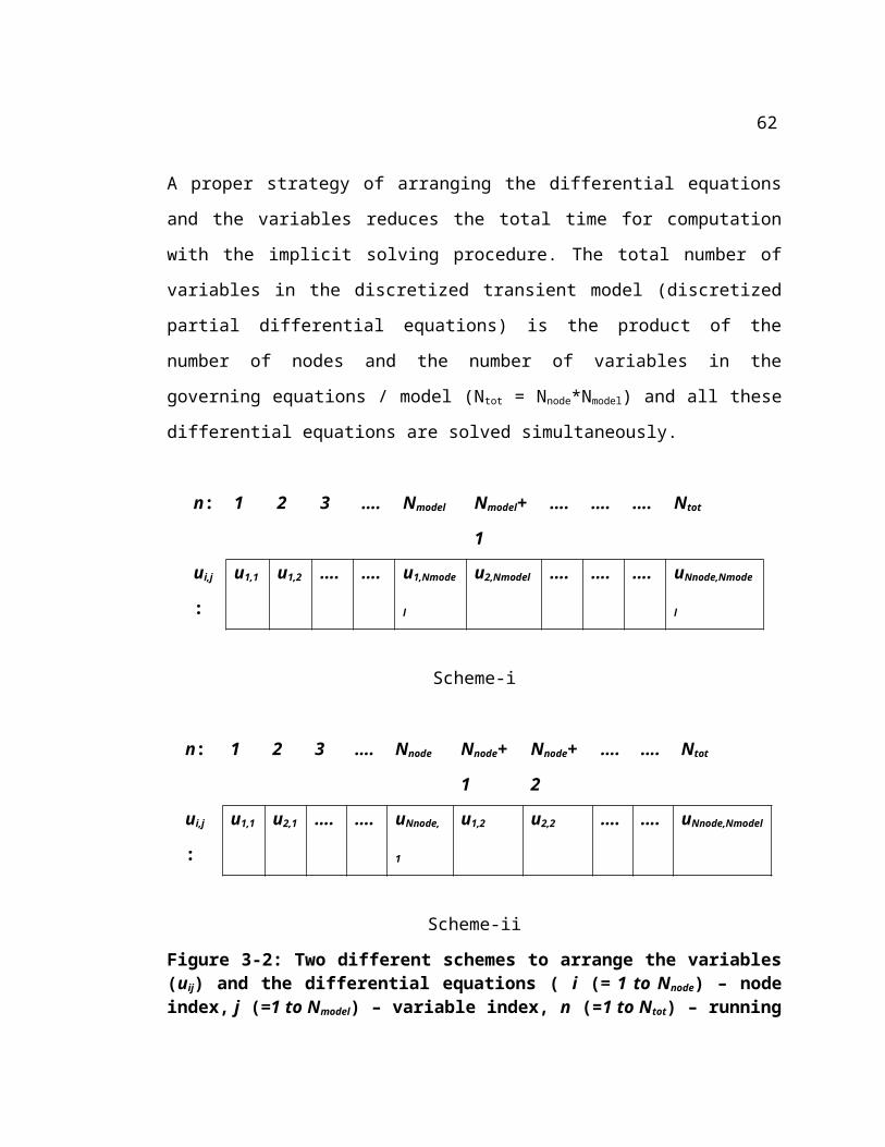
temperature troughs on the endothermic side are observed due to an increase in the rate

of endothermic reaction as the reactants are hotter (due to the rise in the feed

temperature) compared to the initial state. Similar troughs are also seen on the

exothermic temperature profiles because of thermal coupling. Some of these troughs /

peaks disappear with time but during the transient these traveling thermal waves show

two temperature peaks / troughs because of the different time scales of convection and

heat transfer between the exothermic and endothermic sides.

The counter-current reactor also exhibits similar wrong-way behavior. These transient

thermal patterns are important in developing suitable control systems for these reactors.

The transient studies also aid in understanding the possible catalyst sintering and

deactivation during the evolution / perturbation.

3.6 Summary

The steady state and dynamic behavior of counter-current and co-current heat exchanger

reactors coupling exothermic and endothermic reactions are analyzed using the pseudo-

homogeneous plug flow model. In general, the heat exchanger reactors yield higher exit

conversion for the endothermic reaction than the adiabatic reactor. The temperature

peak on the exothermic side is lower in co-current reactor than that in the counter-cur-

rent reactor. The hotspot on the exothermic side is a major concern in these reactors

and we observed that these hot-spots could be reduced drastically by suitable catalyst

activity profiling in the co-current reactors. By activity profiling, the reaction front

spreads over the reactor providing a more uniform heat source to the endothermic side.

However, during the transient mode of operation the temperature peaks on the exother-

mic side exceed the steady state temperature peak. This may have adverse impact on the

catalyst used. Hence, a suitable protocol has to be established for the safe start-up of

these reactors especially for the case with activity profiling.

The counter-current reactor exhibits a phenomenon termed here as hot pinch and cold

pinch cross-over points. At these points, both the exothermic and endothermic streams

62

have identical temperatures. The counter-current reactors exhibit multiple steady states

for the range of parameters investigated. The hot spot is also an issue in the counter-

current reactor and the exponential catalyst activity profiling did not help much in

reducing it. One way of reducing the hot-spot is by using the inert packing in some

section of the reactor. It is found that the inert packing reduces the magnitude of the

cold pinch cross-over point temperature in the counter-current reactor and also the

catalyst requirement. It is also observed that the counter-current configuration yields

higher conversion for the endothermic reaction than the co-current configuration in

shorter reactors. This may be advantageous for some equilibrium limited reactions.

Compared to directly coupled adiabatic reactors, the heat exchanger reactors offer

operational flexibility. This is demonstrated by showing that the flow rates of individual

streams can be adjusted independently to obtain the desired conversion with lower

temperature peak. More detailed analyses of the heat exchanger reactors, especially the

variation of temperature profiles and hot spots radially, are presented in the next

chapter.

Chapter 4

Analysis of Recuperative Reactors using Two

Dimensional Models

4.1 Scope

63

In this chapter, a two dimensional mathematical model was used to analyze the coupling

exothermic and endothermic reactions in co-current and counter-current heat exchanger

reactors. Some of the features of the recuperative reactors identified using 1-D, in the

previous chapter, are verified with the 2-D model. The effects of design parameters like

tube spacing and the operational parameters, like concentration of the reactants on the

maximum temperature within the reactor and on the exit conversion are discussed. The

role played by the radial dispersion on the hot-spot is also investigated. The need to use

2-D model instead of 1-D model, for the recuperative reactors, is also discussed.

4.2 Introduction

As discussed earlier, the heat exchanger or recuperative reactor is one of the good

choices for coupling exothermic and endothermic reactions. In this reactor, the

exothermic (combustion) and the endothermic reactions are separated in space and the

heat transfer occurs through the wall. The separation of exothermic and endothermic

reaction spaces in this reactor offers several design and operational flexibilities. Some

of the advantages of the heat exchanger reactor over the directly coupled adiabatic

reactors or the reverse flow reactors are the steady state operation of the process,

flexibility to use different catalysts for the exothermic and endothermic reactions, etc.

The flow rates and the reactant composition of any stream can be adjusted

independently of the other stream. It is also to be noted that, in the future, by wise

selection of the exothermic and the endothermic reactions, two different valuable

products – respectively from the exothermic and the endothermic reactions – can be

produced using a single reactor in an energy efficient manner. A detailed analysis and

the comparison of the performance of the heat exchanger reactors, using a 1-D

mathematical model has been presented in Chapter 3 (see also Ramaswamy et al.,

2006). It is also seen that between the co-current and the counter-current heat mode of

coupling, for the parameters investigated, the co-current reactors result in the desired

conversion with lower temperature peak. The comparison of the performance of the

heat exchanger reactors and the directly coupled adiabatic reactors are taken up in the

next chapter.

64

Two dimensional models are often required for a detailed design of heat exchanger

reactors and to gain further insight into their performance. The important design

parameters like the tube diameter and the optimized spacing of the tubes, etc., are

selected based on the predictions of the higher dimensional models. Though 1-D models

predict the cross sectional averaged concentration and temperature profiles, they do not

provide a comprehensive understanding of the transverse variation of these profiles. The

radial temperature profiles, predominantly dictate the heat transfer between the

exothermic side and the endothermic side. Also the presence of hotspot at any stream

line within the tube and/or shell side of the heat exchanger reactor can be identified

using the 2-D model, thus enabling one to adopt proper corrective measures for control.

In this chapter, a two dimensional homogeneous model is used to the study and

compare coupling exothermic and endothermic reactions in the co-current and counter

current packed bed reactors. In this reactor, the rate of heat generation and the rate of

heat consumption can also be balanced by optimization of the tube spacing (at constant

stream velocity). Hence, in this chapter, the effects of tube diameter / tube spacing on

the radial temperature profiles, the hot spot and on the endothermic conversion are

presented. The effect of varying the inlet concentration of the exothermic stream to

minimize the hot spot within the reactor is also discussed. The effect of radial

dispersion on the temperature profiles is also presented.

4.3 Two Dimensional Pseudo-Homogeneous Model for a Recupera-

tive Reactor

In this section, the governing equations for the two dimensional pseudo-homogeneous

model of the heat exchanger reactors, used in this work are presented. A schematic of

the domain of the heat exchanger reactor used in the modeling is shown in Figure 4-1.

In this model, the axial thermal and mass dispersions are not included, to restrict our

attention to the radial effects. A first order irreversible kinetics has been assumed for

both the exothermic and endothermic reactions. Though we could use any kinetics in

our model, we have restricted our analyses to first order irreversible kinetics in an

65

attempt to understand the overall performance of coupling of exothermic and

endothermic reactions. We have also shown that use of reversible kinetics did not

change the qualitative trends of the profiles obtained. The equivalent 1-D model,

without radial dispersions, can be found in the previous chapter.

Figure 4-1: Schematic of the Reactor Domain used for the Development of the Model

The transient dimensionless governing equations for the counter-current and the co-

current reactors are given below:

For the tube side,

Mass Balance:

(4.1)

Energy Balance:

(4.2)

For the shell side,

Mass Balance:

Tube

Shell R2

R1

RTTT

Tube side:

Shell side:

66

(4.3)

Energy Balance:

(4.4)

In Eqs. 4.3 and 4.4, the positive sign in the convection term is used for the co-current

reactor and the negative sign for the counter-current reactor. Here is the position

dependent catalyst activity for the exothermic reaction and is set as unity for the cases

with no catalyst activity profiling. The boundary conditions and initial conditions used

for solving Eqs. 4.1-4.4 are given next.

Radial Boundary Conditions:

67

Axial Boundary Conditions:

Co-current reactor:

at ξ = 0,

Counter-current reactor:

at ξ = 0,

at ξ = 1,

Initial conditions (for both counter-current and co-current reactors):

at τ = 0,

The other dimensionless parameters used in the model are given below with j = c and h

for the cold and hot side respectively:

68

,

,

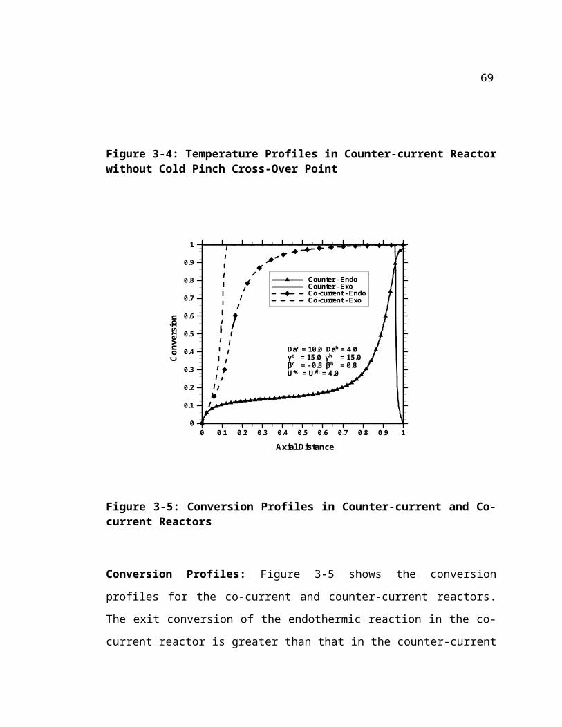
The parameters considered in the model are the Damkohler number ( , the ratio of

flow time to the reaction time), the radial mass and thermal Peclet numbers ( ,

), dimensionless heat of reaction (βj), and dimensionless activation energy ( ). Here,

and are the mass and thermal Peclet number based on the catalyst particle size

and the correlations used to calculate them are presented in Appendix B (Iordanidis,

2002). For the counter-current reactor, the feed for the endothermic reaction enters at

the axial position, ξ=0, and the feed for the exothermic reaction enters at the axial

position, ξ=1 (position-1). For the co-current reactor, the feed for both exothermic and

endothermic reactions enter at the axial position, ξ=0 (position-0).

4.4 Solution Procedure

The transient model equations (Eqs. 4.1-4.4) are solved by the method-of-lines (MOL)

(van de Wouwer et al., 2001) where the partial differential equations (PDE) are

converted to a set of ordinary differential equations (ODE) by suitable discretization of

the spatial axial (convection term) and radial derivatives (dispersion terms). The

resulting ODEs in time are integrated by stiff solvers. We have used a second order

upwind finite difference scheme for the discretization of the axial derivatives and the

second order central differencing scheme for the discretization of the radial derivatives.

The ODEs are integrated using LSODE solver from the NETLIB libraries. The two

69

dimensional steady state model equations can be derived by setting the time derivatives

in the above equations (Eqs. 4.1-4.4) to zero. The steady state model equations of the

co-current reactor are solved using PDEPE solver in the MATLAB by the method of

lines. The steady state model for the co-current reactor is slightly modified so that it can

be implemented easily in the MATLAB. The procedure for scaling and the resulting set

of modified equations are presented in Appendix C. For the counter-current reactor, the

steady state model results in a boundary value problem, with a set of coupled non-linear

algebraic equations. These equations are to be solved either by shooting algorithm or

by Newton-Raphson type algorithm and the solutions of which highly depends on the

initial guesses used. Hence, the MOL approach is used to obtain the steady state

solution (from the transient model) for the counter-current reactor, which is fast and

robust. The transient model equations are solved in an explicit fashion. The time step

required for the integration is chosen based on the Courant criterion.

4.4.1 Arrangement of Variables

As discussed in Chapter 3, the arrangement of variables plays an important role in

determining the computation time of the model, especially while solving the differential

equations implicitly. We have used the scheme shown in Figure 4-2 to arrange the

variables / differential equations. In this scheme, the indexing of variables / equations

starts from the first axial node (reactor inlet, i = 1) and the first radial node (center of

the tube, j = 1). First, all the model variables corresponding to the chosen axial node

and the first radial position are numbered sequentially. Then the model variables at the

next radial position (but at the same axial position) are numbered subsequently. This

procedure is repeated until all the model variables in all the radial positions of the first

axial node are numbered. Then the numbering is carried out for the variables in the next

(second) axial node, starting again from the first radial position. This procedure is

repeated until all the variables are numbered (i.e. all the model variables in the last axial

node and the last radial node, i = Nnode-axi, j = Nnode-rad are accounted for).

n: 1 2 …. Nmodel Nmodel+1 …. Nmodel* Nmodel* …. Ntot-(Nnode- …. Ntot

70

Nnode-rad Nnode-

rad+1rad*Nmodel)+1

ui,j,k: u1,1,1 u1,1,2 …. u1,1,Nmodel u1,2,1 …. u1,Nnode-

rad,Nmodel

u2,1,1 …. uNnode-axi,1,1 …. uNnode-

axi,Nnode-

rad,Nmodel

Figure 4-2: Variables (uij) Arrangement Scheme( i (= 1 to Nnode-axi) – axial node index, j (=1 to Nnode-rad) – radial node index, k (=1 to Nmodel) – variable index , n (=1 to Ntot) – running index of all the variables in the system with Ntot=Nnode-axi* Nnode-rad

*Nmodel). Here the variables of the model correspond to the variables in respective sides (exothermic or endothermic side) of the recuperative reactor.

4.5 Results and Discussions

A detailed analysis of the steady state and dynamic behavior, and the comparison of the

performance of co-current and counter-current heat exchanger reactors using the 1-D

model were shown earlier. In this chapter, some case studies illustrating the importance

of 2-D model in the design of these reactors are carried out. These include the effect of

tube diameter, tube spacing, radial dispersion and the feed concentration on the radial

temperature profiles and exit conversion. These studies primarily focus on avoiding or

minimizing the hot spot in the heat exchanger reactors.

4.5.1 Co-current Reactor

Base Case: Figure 4-3 shows the axial temperature profiles observed in a co-current

reactor at various radial positions for the parameters reported in Table 4-1. Here, the

wall of the heat exchanger reactor tubes has been assumed to be highly conductive and,

hence, a large value of the wall heat transfer coefficient (~ 500) is used in the model.

From Figure 4-3 it is clear that, for the value of the heat transfer coefficient used, the

endothermic and the exothermic temperature profiles at the tube wall almost overlap

with each other. On the exothermic side (shell side), the temperature profile

71

corresponding to the centre stream line is higher than that of the wall. Also the

maximum temperature on the stream line corresponding to the centre of the shell side

(exothermic side) is higher than the maximum temperature predicted at the wall. The

maximum temperature observed in the heat exchanger reactors plays a great role in the

selection of the tube material and the catalyst used. The magnitude of the maximum

temperature can be minimized by introducing some inert materials / packing on the

exothermic side near the reactor inlet.

Table 4-1: Parameters used for the simulation (Base Case – 2D Model)

Dah 10.0 2.0

Dac 4.0 2.0

βh -0.8 L, m 5.0

βc 0.8 dp, m 0.001

γh 15.0 0.5

γc 15.0 R1, m 0.0256

2.0 R2, m 0.0256

2.0 twall, m 0.003

Effect of Tube Spacing: Figure 4-4 shows the cross sectional area averaged

temperature profiles on the exothermic and the endothermic sides of the co-current

reactors for two cases of different tube spacing – one with R2 = 0.0126 m and the

second with R2 = 0.02m. With increase in the tube spacing (R2 = 0.02 m), the cross

sectional averaged maximum temperature and the exit temperature increase. This is due

to increase in the amount of the feed processed at shell side (as the velocity of the

exothermic stream (Damkohler Number) is constant in both the cases). The

temperature profiles corresponding to R2 = 0.0126m, qualitatively resemble those

obtained using the 1-D model (refer Figure 3-3) (It is to be noted that the one

dimensional model predicts higher maximum temperature for the counter-current

reactor than that of the co-current reactor. Also, the conversion of the endothermic

72

reaction, predicted by the 1-D model, is 98% for the counter-current reactor and 100%

for the co-current reactor.).

Figure 4-3: Axial Temperature Profiles of Endothermic and Exothermic Reactions at Different Radial Positions within the Co-current Reactor (Parameters as reported in Table 4-1)

Figure 4-5 shows the cross sectional area averaged point conversion for the exothermic

and endothermic reactions in the co-current reactor, predicted by the 2-D model, for the

two cases of different tube spacing. The exit conversion goes to completion for these

two cases.

Axial Distance

Tem

pera

ture

0 0.1 0.2 0.3 0.4 0.5 0.6 0.7 0.8 0.9 1-0.1

0

0.1

0.2

0.3

0.4

0.5

0.6

Endo. - CenterEndo. - WallExo. - WallExo. - Center

0 0.1 0.2 0.3 0.4 0.5 0.6 0.7 0.8 0.9 1-0.1

0

0.1

0.2

0.3

0.4

0.5

0.6

0.7

0.8

Endo. - R2 = 0.0126 mExo. - R2 = 0.0126 mEndo. - R2 = 0.02 mExo. - R2 = 0.02 m

Axial Distance

Tem

pera

ture

73

Figure 4-4: Cross-sectional Area Averaged Axial Temperature Profiles of Endothermic and Exothermic Reactions in the Co-current Reactor for Two Different Tube Spacing (other parameters as reported in Table 4-1)

Figure 4-5: Cross-sectional Area Averaged Point Conversion Profiles of Endothermic and Exothermic Reactions in the Co-current Reactor for Two Different Tube Spacing (other parameters as reported in Table 4-1)

This study shows that, at constant velocity, increase in the tube spacing (exothermic

side) increases the flow rate of the feed for exothermic reaction which in turn increases

the magnitude of temperature peak and the exit temperature. Hence, it is clear that to

reduce the magnitude of temperature peak, the rate of heat generation by the exothermic

reaction has to be balanced by the rate of heat consumption by the endothermic

reactions. One way of balancing the heat of these reactions is by using the optimized

tube spacing and/or by using the reduced fuel rate in the heat exchanger reactors

(reducing the cross sectional area of the exothermic side reduces the fuel consumption

and the magnitude of the temperature peak). Other ways to reduce the exothermic

0 0.1 0.2 0.3 0.4 0.5 0.60

0.1

0.2

0.3

0.4

0.5

0.6

0.7

0.8

0.9

1

Endo. - R2 = 0.0126 mExo. - R2 = 0.0126 mEndo - R2 = 0.02 mExo. - R2 = 0.02 m

Axial Distance

Con

vers

ion

74

temperature peak by using activity profiling of the catalysts, etc., are discussed in the

previous chapter.

Effect of Feed Concentration for Exothermic Reaction / Heat of Exothermic

Reaction: The concentration of the feed for the exothermic reaction and, in turn, the

dimensionless heat of reaction is varied to study its effect on the conversion of the

endothermic reaction and on the hotspot within the reactor. Figure 4-6 shows the

temperature profiles corresponding to the wall and the center (shell center) for the

exothermic side with βh = 0.4 (this is also equivalent to decreasing the heat of

exothermic reaction) for two different tube spacing. For this case, the amount of heat

released by the exothermic reaction is reduced and is less than that shown in Figure 4-4

and, hence, the predicted temperature rise is also low. It is observed that by decreasing

the half length of the tube spacing from 0.0256 m to 0.02 m, the reduction in the

maximum temperature, corresponding to centerline (shell center) temperature profile, is

around 70%. The larger tube spacing also results in the larger exit temperature of the

stream leaving the reactor. Figure 4-7 plots the mixing-cup conversion profiles for these

two tube spacings.

Axial Distance

Tem

pera

ture

0 0.1 0.2 0.3 0.4 0.5 0.6 0.7 0.8 0.9 1-0.1

0

0.1

0.2

0.3

Wall - 0.0256 mCenter - 0.0256 mWall - 0.02 mCenter - 0.02 m

75

Figure 4-6: Axial Temperature Profiles of Exothermic Reactions in the Co-current Reactor for Two Different Tube Spacing with βh = 0.4 (other parameters as reported in Table 4-1)

Figure 4-7: Conversion Profiles for Endothermic Reactions in the Co-current Reactor for Two Different Tube Spacing with βh = 0.4 (other parameters as reported in Table 4-1)Both tube spacings result in almost complete conversion at the reactor exit and the case

with less tube spacing requires the full length of the reactor (or longer length) to reach

the complete conversion. This study again confirms that the temperature peak and the

effluent temperature can be reduced by optimizing the design variables such as the

spacing between the tubes etc.(i.e. by reducing the tube spacing), while maintaining the

similar conversion for the endothermic reaction. The desired conversion and the

temperature profile can also be obtained by suitable optimization of the operating

conditions, like concentration of the combustion fuel or by the selection of proper fuel

with reduced heat of reaction.

Axial Distance

Con

vers

ion

0 0.1 0.2 0.3 0.4 0.5 0.6 0.7 0.8 0.9 10

0.1

0.2

0.3

0.4

0.5

0.6

0.7

0.8

0.9

1

R2 = 0.0256 mR2 = 0.02 m

76

Effect of Radial Dispersion: The mass and thermal dispersion terms, in particular Pe,

describe the effect of radial dispersion within the reactor. Figure 4-8 shows the effect of

Peclet numbers on the wall and centre line temperature profiles on the exothermic side.

In these simulations, the mass and thermal Peclet numbers for both the exothermic and

the endothermic side are assumed to be identical. For real cases, these Peclet numbers

are system dependent and are to be calculated based on experimental data or any

available correlation. For this set of simulations, βh = 0.4 and R1 = R2 = 0.0256m were

used. The other parameters are as reported in Table 4-1.

The temperature profile and the maximum temperature are larger for the case with high

Pe. As Pe increases, the radial dispersion or uniformity of temperature decreases and

hence the maximum temperature increase. Here, the amount of heat transferred to the

endothermic side decreases and, hence, the endothermic temperature profile decreases

in magnitude. One would also anticipate a larger temperature drop on the endothermic

temperature profiles.

Thus, effective radial dispersion in both sides of the heat exchanger reactor plays a very

important role in determining the hot spot in the reactor and the dispersion pattern is

often dictated by type of packing and other hydrodynamic factors.

Axial Distance

Tem

pera

ture

0 0.1 0.2 0.3 0.4 0.5 0.6 0.7 0.8 0.9 1-0.1

0

0.1

0.2

0.3

0.4

Wall - Pes = 2.0Center - Pes = 2.0Wall - Pes = 7.0Center - Pes = 7.0

77

Figure 4-8: Effect of Peclet Number on the Axial Temperature Profiles for the Exothermic Reactions in the Co-current Reactor with βh = 0.4 and R2 = 0.0256 m (other parameters as reported in Table 4-1)

4.5.2 Counter-current Reactor

The analysis using the 1-D model shows that the counter-current reactor exhibits cold

pinch and hot pinch cross-over points in the temperature profiles, for a certain set of

parameters. At these cross-over points both the exothermic and endothermic streams

have identical temperature. The cold pinch cross-over point occurs near the inlet for the

endothermic feed (position-0). Here, the reactants for the endothermic reaction transfer

heat to the effluent of exothermic reaction from the inlet (position-0) up to the cold

pinch cross over point. The hot pinch cross-over point occurs near the inlet of the feed

for the exothermic reaction (position-1). From this hot pinch cross-over point to

position-1, the effluent of the endothermic reaction heats the reactants for the

exothermic reaction. These cross-over points manifest themselves differently when

using the 2-D model, because of series of axial temperature profiles, one corresponding

to each radial location. Hence, for the 2-D model the cross-over points are redefined as

the positions in the reactor where the temperatures corresponding to the stream line at

the center of the shell side (or the center of tube spacing) and the centre of tube side are

identical. In other words, one could also define the cross over points as the points where

the cross sectional area averaged temperatures corresponding to shell and tube sides are

identical.

Figure 4-9 shows the axial temperature profiles on the exothermic and endothermic side

of the counter-current reactor at the two different radial locations (wall and the center of

the tube and the shell sides), predicted by the two dimensional model. The figure clearly

shows the occurrence of the cold pinch and hot pinch cross-over points (for this case,

78

even the cross sectional area averaged temperature profiles show the occurrence of

these cross-over points). The parameters used for the simulation are as reported in

Table 4-1 except βh = 0.4 and R2 = 0.0126 m. The temperature profiles on the wall sides

for the exothermic and endothermic reactions overlap each other due to the use of large

heat transfer coefficients.

Figure 4-9: Axial Temperature Profiles of Endothermic and Exothermic Reactions at Different Radial Positions within the Counter-current Reactor with βh = 0.4 and R2 = 0.0126 m (other parameters as reported in Table 4-1)

Axial Distance

Tem

pera

ture

0 0.1 0.2 0.3 0.4 0.5 0.6 0.7 0.8 0.9 1-0.2

-0.1

0

0.1

0.2

0.3

0.4

Endo. - CenterEndo. - WallExo.- WallExo. - Center

Axial Distance

Con

vers

ion

0 0.1 0.2 0.3 0.4 0.5 0.6 0.7 0.8 0.9 10

0.1

0.2

0.3

0.4

0.5

0.6

0.7

0.8

0.9

1

Endo. - CenterEndo. - WallExo. - WallExo. - Center

79

Figure 4-10: Axial Conversion Profiles for Endothermic and Exothermic Reactions at Different Radial Positions within the Counter-current Reactor with βh = 0.4 and R2 = 0.0126 m (other parameters as reported in Table 4-1)

The temperature profiles show the temperature peaks near the position-1. The

temperature peak can be as large as the adiabatic temperature of the exothermic

reaction. These profiles qualitatively match those of the 1-D model. The mixing–cup

exit conversion of the endothermic reaction is around 90% for this case. Figure 4-10

plots the conversion profiles at different radial locations within the counter-current

reactor for this case.

Using the two dimensional model the effects of the ratio of tube diameter on the

conversion and on the temperature rise can be analyzed. Figure 4-11 shows the

exothermic temperature profile corresponding to the centre of the shell side for three

different tube spacing. With decrease in the tube spacing, the magnitude of the

temperature peak (the hot spot) decreases. For the tube spacing of 0.0126 m, the

exothermic reaction is extinguished and, hence, the temperature decreases from

Position-1. The exit conversions (mixing-cup) for the endothermic reaction for these

cases are: 100% for R2 = 0.02 m, 90% for R2 = 0.016m, and 40% for R2 = 0.0126m.

Hence, it is clear that there exists a window of tube spacing for which the desired

conversion is obtained with lower temperature peak (without the exothermic reaction

getting extinguished).

Axial Distance

Tem

pera

ture

0 0.1 0.2 0.3 0.4 0.5 0.6 0.7 0.8 0.9 1-0.3

-0.2

-0.1

0

0.1

0.2

0.3

0.4

0.5

R2 = 0.02R2 = 0.016R2 = 0.0126

80

Figure 4-11: Effect of Tube Spacing on the Axial Temperature Profile of Exothermic Reaction at the Centre of the Shell side (Parameters as used in Figure 4-11)

4.6 Summary

A two dimensional pseudo-homogeneous model was used to study the recuperative

coupling of exothermic and endothermic reactions in co-current and counter-current

heat exchanger reactors. It was found that the spacing between the tubes, within the heat

exchanger reactors, plays a great role in controlling the temperature peak. Hence the

optimized tube spacing will result in desired conversion for the endothermic reaction

with a lower temperature peak, due to efficient heat transfer between the exothermic

and the endothermic sides. The inlet concentration of the reactants should also be

optimized to control the hot spot within the reactor. The effect of radial dispersion on

the performance of these reactors was shown, and it is observed that the good radial

mixing, or lower Pe, favors the uniform transverse temperature distribution resulting in

lower temperature peak. It is also observed that predictions by the 1-D and 2-D models

qualitatively match each other. The temperature profiles of counter-current reactor,

predicted by the 2-D model also exhibit the occurrence of the cold-pinch and hot-pinch

cross over points. The cold pinch cross over point can be avoided by using either inert

packing in some sections of the reactor, or by using non-similar inlet temperature for

the exothermic and endothermic streams, as discussed in Chapter 3.

81

82

Chapter 5

Coupling of Exothermic and Endothermic Reactions in

Directly Coupled Adiabatic Reactors

5.1 Scope

In this chapter, a one-dimensional pseudo-homogeneous plug flow model is used to

investigate the steady state and the dynamic behavior of coupling exothermic and

endothermic reactions in directly coupled adiabatic packed bed reactors (DCAR). Two

different configurations of DCAR (Simultaneous DCAR - SIMDCAR and Sequential

DCAR - SEQDCAR) are investigated. In SIMDCAR, the catalyst bed favors both

exothermic and endothermic reactions and both reactions occur simultaneously.

SEQDCAR has alternating layers of catalyst beds for exothermic and endothermic

reactions and hence the exothermic and endothermic reactions occur in a sequential

fashion. The performance of both reactors, in terms of conversion achieved and

manifested hotspot behavior, is compared with that of the co-current heat exchanger

type reactor. The preliminary criteria for the selection of desirable reactor type, based

on the relative magnitudes of heat generation rate and the heat consumption rate, are

proposed. The dynamic behavior of these reactors is non-intuitive and we have analyzed

some of the transient behavior.

5.1 Introduction

The coupling of exothermic and endothermic reactions is gaining importance in recent

years as attempts are being made to reduce the thermal losses associated with the supply

of heat to endothermic reactions such as synthesis gas generation. The recuperative

83

mode of coupling has been analyzed in detail in Chapters 3 and 4 and in this chapter the

direct mode of coupling is investigated.

In directly coupled adiabatic reactors (DCAR), both exothermic and endothermic

reactions occur in the same reactor space subject to a direct heat transfer within the

reacting mixture. The directly coupled adiabatic reactor can be further classified into

Simultaneous DCAR (SIMDCAR) and Sequential DCAR (SEQDCAR). The schematic

of DCAR is shown in Figure 5-1.

Figure 5-1: Schematic of DCAR - SIMDCAR and SEQDCAR

In SIMDCAR, the bed is made of catalyst that favors both the exothermic and

endothermic reactions or the bed is made of uniformly mixed catalysts for exothermic

and endothermic reactions (Biesheuvel and Kramer, 2003). SIMDCAR has been

practiced industrially in methane steam reforming within the ammonia synthesis process

(Ridler and Twigg, 1989) and hydrogen cyanide process (Agar, 1999) etc. It is also

being used in the coupling of methane steam reforming with the catalytic oxidation of

methane in partial oxidation reactors (De Groote and Froment, 1996; Ma and Trimm,

1996; Avci et al., 2001). The major disadvantage of SIMDCAR is that the catalyst bed

Mixed Catalyst Bed

SIMDCAR SEQDCAR

Products

Reactants

Catalyst forExothermic Reaction

Catalyst for EndothermicReaction

Reactants

Products

84

should favor both exothermic and endothermic reactions. On the other hand,

SEQDCAR has the alternating beds of catalyst for exothermic and endothermic

reactions.

In this chapter, a detailed comparative study of the steady state and the dynamic

behavior of the SEQDCAR and SIMDCAR is carried out. The performance of DCARs

is also compared with that of the co-current reactor. The conditions for the existence of

hotspots in SIMDCAR are analytically derived with a first order irreversible kinetics for

both exothermic and endothermic reactions. The preliminary criteria for the selection of

different reactor configurations for any application of interest are proposed based on the

rate of heat generation and rate of heat consumption.

5.2 One Dimensional Pseudo-homogeneous Plug Flow Model

This section presents the reactor model used for the analyses. The following

assumptions are made in the development of the model:

i) Axial and radial, mass and heat dispersions are neglected.

ii) Axial conduction in the wall (for the co-current reactor) is not included, and a

constant heat transfer coefficient has been assumed along the length of the reac-

tor.

iii) Physical properties of the fluids and the heat of the reaction are assumed to be

independent of temperature, and the total pressure of the system is constant.

iv) Irreversible first order kinetics is considered for both reactions.

The respective governing equations are:

Mass Balance

(5.1)

85

(5.2)

Energy Balance:

(5.3)

The dimensionless parameters used are given below:

,

, ,

The parameters involved in the model are the reaction Damkohler number ( ),

dimensionless heat of reaction ( ), dimensionless activation energy ( ) and the

activity parameter ( ). The feed (the reactants for both the exothermic and the

endothermic reactions) enters at axial position, ξ=0.

5.3 Solution Procedure

The method-of-lines (MOL) approach is employed to solve the transient model

equations (Vande Wouwer et al., 2001). Here, the partial differential equations are

converted to ordinary differential equations (ODE) by suitable discretization of the

spatial derivatives and the resulting ODEs are solved using the commercially available

stiff integrator. We have used automatic step size adjustable LSODE routine from

Netlib as an ODE integrator. The second order finite difference upwind discretisation

86

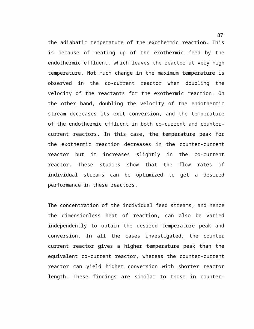
scheme is used to discretise the spatial derivatives. The discretization scheme is

modified to preserve monotinicity by total variation diminishing (TVD) algorithms

(using van-leer splitter) to avoid spurious oscillations (Tannehill et al., 1997). The

details of the numerical scheme can be found in Chapter 3. The steady state model

equations are obtained by equating the transient derivatives in the above equations (Eqs.

5.1 – 5.3) to zero and are a set of ordinary differential equations in the spatial

coordinate. The steady model equations are also solved by LSODE routine from

NETLIB libraries.

5.4 Theoretical Analysis of Existence of Hot / Cold Spots in a Di-

rectly Coupled Adiabatic Reactor

The analysis presented in this section shows that SIMDCAR exhibits different operating

patterns based on the relative magnitudes of the heat generation rate (βhDah) and the

heat consumption rate (βcDac). This analysis is restricted to the cases where both the

exothermic and the endothermic reactions are represented by irreversible first order

kinetics and the activation energies of both the reactions are identical (γc = γh). This

simplified analysis based on the steady state pseudo-homogeneous model reveals

different operational behavior exhibited by SIMDCAR. It can behave as an isothermal

reactor, an exothermic or an endothermic reactor. This reactor can also exhibit a hot or

cold spot within the reactor. For this case, the temperature and the conversion at the hot

spot can be calculated analytically.

The steady state pseudo-homogeneous model for SIMDCAR can be derived from Eq.

5.1 to Eq. 5.3 by setting the time derivatives to zero.

For γc = γh , dividing Eq. 5.1 by Eq. 5.2 gives (in steady state),

(5.4)

87

Integrating Eq. 5.4 based on separation of variables yields,

(5.5)

Eq. 5.5 is valid at any point in the reactor. Now, the condition for the hot spot / cold

spot in the reactor is given by,

=0 (5.6)

Hence, Eq. 5.6 and Eq. 5.3 (with no transient terms) yield,

(5.7)

and are respectively the dimensionless concentration of the reactants for the

endothermic and the exothermic reactions at the hot spot / cold spot.

Combining Eqs. 5.5 and 5.7 we get,

(5.8)

Eqs. 5.7 and 5.8 are valid only at the position of hot spot / cold spot. From Eq. 5.8, at

the hot / cold spot can be calculated (and (1- ) is bounded between 0 and 1). Using

these equations (Eqs. 5.5 - 5.8), different patterns exhibited by SIMDCAR can be

88

classified and are shown in Figure 5-2. Equation 5.8 is not applicable when

since Eq. 5.5 and Eq. 5.7 cannot be satisfied simultaneously. Hence for these cases,

there is no hot spot / cold spot observed within the reactor.

Figure 5-2: A Composite Diagram Showing the Different Patterns Exhibited by

SIMDCAR

89

Combining Eq. 5.1 to Eq. 5.3, we have at the steady state,

(5.9)

Hence at any point in the reactor,

(5.10)

From Eq. 5.10, the hot spot temperature can be calculated by using and

obtained from Eqs. 5.5 and 5.8. It is to be noted that the occurrence of hot spot / cold

spot is not bounded by the spatial co-ordinate, ξ ε [0,1]. Hence the conditions, ≤

and ≤ are also to be satisfied to confirm the occurrence of hot spot /

cold spot within the reactor. The concentration and the temperature profiles along the

reactor (hence the concentration / temperature at the reactor exit) can be obtained

through numerical analysis, which are presented in the next section.

5.5 Results and Discussions

In this section, we analyze the steady state and dynamic behavior of different

configurations of reactors based on the relative magnitudes of the rate of heat

consumption and the rate of heat generation. We also compare the performance of

DCARs with that of the co-current reactor. The discussion on the design and operational

flexibility of different reactors is also presented.

5.6.1 Steady State Behavior

βcDac > βhDah : This condition simulates the case when the rate of heat consumption per

unit volume (based on the inlet concentration) is greater than the rate of heat generation.

Figures 5-3a and 5-3b show respectively the temperature and the conversion profiles in

three reactor configurations: i) SIMDCAR ii) SEQDCAR and iii) a co-current reactor.

90

Four alternating beds of exothermic and endothermic catalysts are used in SEQDCAR.

The positions of various catalyst beds used in SEQDCAR are i) exothermic from ξ=0 to

ξ=0.1 ii) endothermic from ξ=0.1 to ξ=0.15 iii) exothermic from ξ=0.15 to ξ=0.5 and iv)

endothermic from ξ=0.5 to ξ=1.0. In simulation, c and h are assigned 1 and 0

respectively in the bed with catalyst for endothermic reactions and vice versa in the

catalyst bed for exothermic reaction. Care should be taken in deciding the length of the

exothermic section near the reactor inlet since the chance of exothermic reaction going

to completion and hence the temperature peak reaching the respective adiabatic

temperature (hence the hot spot) exists.

Figure 5-3a: Temperature Profiles in DCAR and Co-current Reactor predicted by

Pseudo-homogeneous Model (βcDac > βhDah)

From Figure 5-3 it is clear that at these conditions, SIMDCAR qualitatively operates as

an endothermic reactor with temperature decreasing from the reactor inlet and with a

lower conversion. This behavior is in line with the discussion presented in Section 3. On

the other hand, the sequential mode of operation results in a higher conversion. Two

temperature peaks are observed in the temperature profile for SEQDCAR as shown in

Figure 5-3a. This is because the exothermic reaction is carried out in the two sections of

0 0.1 0.2 0.3 0.4 0.5 0.6 0.7 0.8 0.9 1-0.3

-0.2

-0.1

0

0.1

0.2

0.3

0.4

0.5

0.6

0.7

0.8

Co-current - EndoCo-current - ExoSIMDCARSEQDCAR

Axial Distance

Tem

pera

ture

Dac = 10.0 Dah = 4.0γc = 15.0 γh = 15.0βc = - 0.4 βh = 0.4 (DCAR)βc = - 0.8 βh = 0.8 (Co-current)U*c = U*h = 4.0

91

the reactor. For the similar set of parameters, in the co-current reactor, the conversion

for the endothermic reaction is around 99% and the temperature peak for the exothermic

reaction is around 0.5 (using an optimal wall heat transfer coefficient).

Figure 5-3b: Temperature Profiles in DCAR and Co-current Reactor predicted by

Pseudo-homogeneous Model (βcDac > βhDah)

By catalyst activity profiling (by modifying the activity of the catalyst bed axially) in

the co-current reactor, this temperature peak could be reduced to around 0.2 without

sacrificing the conversion (Ramaswamy et al., 2006), as discussed in Chapter 3. Thus

the co-current reactors are better than DCAR in obtaining the desired conversion for the

parameters used. This is due to the controlled transfer of heat from the exothermic side

to the endothermic side of the co-current reactor without the exothermic reaction getting

extinguished. In SIMDCAR, because of the thermal mixing on micro scale, temperature

of the system remains low and hence the conversions for both endothermic and the

exothermic reactions remain low. For these parameters, SEQDCAR results in a higher

conversion for the endothermic reaction than SIMDCAR. In SEQDCAR, the lengths of

different sections of the reactors should be optimally chosen in order to avoid any hot

spots and to obtain higher conversion. Hence, we observe that for the cases when βcDac

0 0.1 0.2 0.3 0.4 0.5 0.6 0.7 0.8 0.9 1-0.3

-0.2

-0.1

0

0.1

0.2

0.3

0.4

0.5

0.6

0.7

0.8

Co-current - EndoCo-current - ExoSIMDCARSEQDCAR

Axial Distance

Tem

pera

ture

Dac = 10.0 Dah = 4.0γc = 15.0 γh = 15.0βc = - 0.4 βh = 0.4 (DCAR)βc = - 0.8 βh = 0.8 (Co-current)U*c = U*h = 4.0

92

> βhDah, co-current reactor is better than the adiabatic reactors and in adiabatic reactors,

SEQDCAR gives better conversion than SIMDCAR.

βcDac < βhDah : This refers to the case when the rate of heat consumption per unit

volume (based on inlet concentration) is less than the rate of heat generation.

Figures 5-4a and 5-4b compare the temperature and conversion profiles respectively in

SIMDCAR and SEQDCAR with those of the co-current reactor. It is also clear from

Figures 5-4a and 5-4b that SIMDCAR results in the lower temperature peak compared

to SEQDCAR. The thermal mixing occurring at the micro scale level in SIMDCAR

reduces the occurrence of the high temperature peak since the endothermic reactions

consumes the heat as and when it is released by the exothermic reaction. The magnitude

of the maximum temperature in SEQDCAR is three times greater than that in

SIMDCAR.

Figure 5-4b shows that the conversion of endothermic reaction in SEQDCAR is less

than that in SIMDCAR. This is due to the fact that the available length for the

endothermic reaction is less in the sequential arrangement. Figures 5-4a and 5-4b also

reveals that the temperature profile in SIMDCAR is more or less equivalent to the

temperature profile on the endothermic side of the co-current reactor and, hence, the

conversion profiles for endothermic streams are also qualitatively identical in both the

reactors. For these parameters, if the exothermic and the endothermic reactions are

segregated in space with resistive heat transfer, as in the co-current reactor, it exhibits a

large hot spot on the exothermic side. If the exothermic temperature peak and the

conversion of the endothermic reaction are taken as a measure of the reactor

performance, then SIMDCAR is better than co-current reactor when βcDac < βhDah.

Also for this case, SIMDCAR gives better conversion with lower temperature peak than

SEQDCAR.

0 0.1 0.2 0.3 0.4 0.5 0.6 0.7 0.8 0.9 1-0.1

0

0.1

0.2

0.3

0.4

0.5

0.6

0.7

0.8

Co-current - EndoCo-current - ExoSIMDCARSEQDCAR

Axial Distance

Tem

pera

ture Dac = 4.0 Dah = 10.0

γc = 15.0 γh = 15.0βc = - 0.4 βh = 0.4 (DCAR)βc = - 0.8 βh = 0.8 (Co-current)U*c = U*h = 4.0

93

Figure 5-4a: Temperature Profiles of in DCAR and Co-current Reactor predicted

by Pseudo-homogeneous Model (βcDac < βhDah)

Figure 5-4b: Conversion Profiles of in DCAR and Co-current Reactor predicted

by Pseudo-homogeneous Model (βcDac < βhDah)

0 0.1 0.2 0.3 0.4 0.5 0.6 0.7 0.8 0.9 10

0.1

0.2

0.3

0.4

0.5

0.6

0.7

0.8

0.9

1

Co-currentSIMDCARSEQDCAR

Axial Distance

Con

vers

ion

Dac = 4.0 Dah = 10.0γc = 15.0 γh = 15.0βc = - 0.4 βh = 0.4 (DCAR)βc = - 0.8 βh = 0.8 (Co-current)U*c = U*h = 4.0

94

βcDac = βhDah : Three cases arise when the rate of heat consumption equals the rate of

heat generation. In this case, the reactors can be classified based on Damkohler number

or dimensionless heat of reactions. If Dah = Dac (or βc = βh) both the co-current and the

adiabatic reactors give the desired conversion with lower temperature peak, for the

parameters studied. If Dac > Dah, (the dimensionless heat of the reaction for the

exothermic reaction is higher than the dimensionless heat of reaction for the

endothermic reaction) then the SIMDCAR is better than the co-current reactor. Here,

SIMDCAR favors the thermal mixing at the molecular scale, which reduces the

temperature peak compared to that of the co-current reactor. If Dac < Dah , the co-

current reactor gives better conversion than DCAR because of the controlled release of

heat liberated by the exothermic reaction to the endothermic reaction through the wall.

In SIMDCAR, the exothermic reaction is suppressed and hence enough heat is not

available to increase the reaction rate and to enhance the conversion of the endothermic

reaction.

We have also developed a heterogeneous model and used it to simulate the above cases.

The predictions with the heterogeneous model qualitatively agree well with that of the

pseudo-homogeneous model for the cases investigated and hence the results are not

presented here.

5.6.2 Transient Behavior

The reactor dynamics is important for developing suitable control strategies and for the

safe start-up and shut down of the reactors. Here, we present some key results that show

the different dynamic behavior exhibited by coupling exothermic and endothermic

reactions in the directly coupled adiabatic reactors. Figure 5-5 shows the temperature

profiles obtained in a SEQDCAR during the startup of the reactor (for various

dimensionless time) when βcDac > βhDah. The activity profiles used for the simulation of

SEQDCAR are same as those mentioned in Section 5.6.1. It is clear from Figure 5-5

that during evolution, the temperature peak may be higher than the steady state profile.

The observed traveling wave pattern is due to the interaction of different time scales,

95

like time scales of exothermic and endothermic reactions, time scale of convection of

heat affected by the heat capacity of the bed. Because of the interaction of various time

scales, some of the profiles have three peaks, while the steady state profile has only two

peaks. These traveling hot spots could reduce the activity of the catalyst during the

start-up of the reactor. Figures 5-6a and 5-6b show the evolution of temperature profiles

in SIMDCAR and SEQDCAR, respectively, for the case when βcDac < βhDah.

Figure 5-5: Evolution of Temperature Profiles in a SEQDCAR (βcDac > βhDah)

In these cases, the evolving transient profiles are bounded by the steady state profile.

The temperature overshoot is not observed in this case, which may be due to the fact

that the exothermic reaction attains 90% conversion in the first section of the reactor.

The decrease in concentration of the feed for the exothermic reaction reduces the rate of

exothermic reaction and hence avoids the occurrence of any wrong-way behavior / hot

spots. Figures 5-6a and 5-6b show that there is a drop in some of the temperature

profiles during evolution near the reactor exit. This is due to the occurrence of

endothermic reaction near the reactor exit. The traveling waves are observed in

SEQDCAR compared to SIMDCAR for these cases.

0 0.1 0.2 0.3 0.4 0.5 0.6 0.7 0.8 0.9 1-0.2

-0.1

0

0.1

0.2

0.3

0.4

0.5

Initial1206411282Steady

Axial Distance

Tem

pera

ture

Dac = 10.0 Dah = 4.0γc = 15.0 γh = 15.0βc = - 0.4 βh = 0.4

96

Figure 5-6a: Evolution of Temperature Profiles in a SEQDCAR (βcDac < βhDah)

Figure 5-6b: Evolution of Temperature Profiles in a SIMDCAR (βcDac < βhDah)

0 0.1 0.2 0.3 0.4 0.5 0.6 0.7 0.8 0.9 1-0.1

0

0.1

0.2

0.3

0.4

Initial16144768Steady

Axial Distance

Tem

pera

ture

Dac = 4.0 Dah = 10.0γc = 15.0 γh = 15.0βc = - 0.4 βh = 0.4

Axial Distance

Tem

pera

ture

Dac = 4.0 Dah = 10.0γc = 15.0 γh = 15.0βc = - 0.4 βh = 0.4

0 0.1 0.2 0.3 0.4 0.5 0.6 0.7 0.8 0.9 1-0.05

0

0.05

0.1

0.15

0.2

Initial16144352Steady

97

5.6.3 Heterogeneous Models

The heterogeneous plug flow and axial dispersion models were also developed to ana-

lyze the performance of various modes of coupling. It is observed that the predictions

by the higher order models were qualitatively similar to those of pseudo-homogenous

models. Quantitatively there is a difference between pseudo-homogenous and heteroge-

neous models, in some cases, in the magnitude of hot spot and/or the position at which

the hot spot occurs etc. This is due to the values of heat and mass transfer coefficients

(transport resistances) and the dispersion coefficients used in the model. The main ad-

vantage of the heterogeneous model is that the temperature and the concentration at the

catalyst surface can be predicted. It is observed that, in SIMDCAR, in the portion of the

reactor where the exothermic reaction is predominant, the temperature at the catalyst

surface is greater than that of bulk phase temperature. Similarly, in the region of the re-

actors where the endothermic reaction is predominant, it is observed that the bulk phase

temperature is greater than the temperature at the solid surface. The results and the plots

displaying the above observation are shown for a practical case study of catalytic partial

oxidation of methane to syngas in Chapter 7.

Additionally, in the porous catalysts, the reactions (both exothermic and endothermic)

may occur within the catalyst particle. In such a situation, the internal transport (diffu-

sion) limitations play an important role in determining the reactor performance in addi-

tion to the external transport limitation. Depending on Thiele moduli (ratio of diffusion

time scale within the catalyst pellet to the reaction time scale) for exothermic and en-

dothermic reactions, the hot spot may occur within the catalyst pellet. Some of these

conditions are studied in more detail in the next chapter.

5.6.4 Design and Operational Implications

The design of SIMDCAR is simpler compared to SEQDCAR and co-current reactors.

In SEQDCAR the depth of individual beds has to be optimally chosen to obtain desired

conversion and to avoid any hotspots. Similarly, in the co-current reactors, the issues

98

like the selection of tube material with the desired heat transfer coefficients, the spacing

between the tubes are to be addressed and these parameters affect the conversion of the

desired reactions, as shown in Chapters 3 and 4. On the contrary, the co-current reactors

offer better operational flexibility compared to DCAR. The problems associated with

product separation are generally not present in the co-current reactors. But in DCAR,

the exothermic and the endothermic reactions have to be carefully chosen so that further

downstream purification of the products is eliminated or the products could be easily

separated. In co-current reactors, the operating parameters of any stream like Da, β etc.,

can be changed independently without affecting the other stream. Thus, the operating

regime can be switched i.e., from βcDac < βhDah to βcDac > βhDah, easily in the co-

current reactor. DCAR does not offer this operational convenience.

5.6 Summary

This chapter investigated the simultaneous and sequential modes of conducting

exothermic and endothermic reactions in the adiabatic reactors (SIMDCAR and

SEQDCAR) and the reactor performance is compared with that of the co-current

reactor. The conditions for the existence of hot spot and/or the cold spot in SIMDCAR

are presented.

It is observed that if βcDac > βhDah, the conversion in the adiabatic reactor is lower than

that in the co-current reactor and between the directly coupled adiabatic reactors;

SEQDCAR should be used to obtain higher conversion. If βcDac < βhDah, then

SIMDCAR results in higher conversion with a lower temperature peak compared to the

co-current reactor and SEQDCAR. For the case, where βhDah = βcDac, the reactors are to

be chosen based on the relative magnitudes of the exothermic and endothermic heats of

reactions. The dynamic behaviors of these reactors are also investigated. SEQDCAR

exhibits stronger traveling waves than SIMDCAR during evolution. These reactors

exhibit hot spots during evolution for some of the cases and hence the detailed transient

studies are to be considered for the design and optimization of directly coupled

adiabatic reactors.

99

The SIMDCAR exhibits a wide range of temperature profile patterns based on the

relative magnitudes of the heat generation rate (βhDah) and the heat consumption rate

(βcDac). Thus, it can behave as an isothermal reactor, an exothermic or an endothermic

reactor or the reactor where the endothermic reaction follows the exothermic reaction or

the exothermic reaction follows the endothermic reaction. Hence it is clear that,

especially for the packed bed reactor of latter cases with porous particles, when the

exothermic and endothermic reactions compete (somewhere in the interior of the

reactor), the catalyst particles undergo both the reactions. Some of the interesting

behavior exhibited by the porous catalyst particles is studied in the next chapter.

100

Chapter 6

Coupling of Exothermic and Endothermic Reactions

within the Porous Catalyst Particle

6.1 Scope

In the previous chapter it is discussed that the directly coupled adiabatic packed bed

reactor can be operated as an isothermal reactor, an exothermic or an endothermic

reactor or the reactor where the rate of endothermic reaction increases once the limited

reactant of the exothermic reaction is completely consumed or the rate of the

exothermic reaction increases once the limited reactant for the endothermic reaction

completely disappeared. In the cases where the operating regime shifts from

predominantly exothermic to predominantly endothermic (the latter two cases) or vice

versa, there exists a region in the reactor where both exothermic and endothermic

reactions compete with each other. In such regions, the porous catalyst particle

undergoes both the reactions. The understanding of coupling behavior within the

particle is essential for the robust design of catalysts to meet the required performance

target. These systems are complex as the exothermic reaction within the catalyst particle

could result in the multiple steady states. Hence the scope of this chapter includes the

development of a robust numerical procedure to analyze the coupling behavior and to

determine the multiple steady states in diffusion-reaction types of problems using a

combination of the boundary element method (BEM) and the arc length continuation

technique. The BEM based numerical procedure has been used to analyze the coupling

in the catalyst particle and BEM combined arc length continuation technique has been

used to investigate the multiple steady states in the current distributed parameter

101

system. The use of boundary element method eliminates the numerical errors associated

with the process of discretization of the differential operators and hence the use of BEM

in continuation methods could reduce the spurious steady states. Another advantage is

that the Jacobian required for the continuation techniques is directly available from the

BEM formulation. Hence BEM and continuation methods complement each other and

can be used to predict the multiple steady states in the distributed parameter systems.

Several standard problems are studied to demonstrate the usefulness of this method and

the results are only presented for single exothermic reaction system and a coupled

exothermic and endothermic reactions system. The particle level coupling of

exothermic and endothermic reactions shows the dependence of heat source and heat

sink in determining the region of multiple steady states in such systems and the region

of multiplicity in narrowed in general.

6.2 Introduction

Several examples of the distributed parameter systems (DPS) can be found in the

chemical engineering discipline like the mathematical models describing the diffusion-

reaction process within a catalyst, dispersion-convection-reaction models for the packed

bed reactors (one such case will be shown in the next chapter) etc. Some of these

systems exhibit multiple steady states in the parameter range of practical interest (Hu et

al., 1985a-c; Burghardt and Berezowski, 1989, 1991; Ramachandran, 1994; Dommeti et

al., 1999; Liu and Jacobsen, 2004; etc.). The prediction of the multiple steady states is

important for the optimization and control of these processes (Mancusi et al., 2000;

Burghardt and Berezowski, 2003). Various numerical procedures used for the prediction

of the multiple steady states and stability analysis are available in the literature

(Kubicek and Marek, 1983; Golubitsky and Schaeffer, 1985; Liu and Jacobsen, 2004).

The free domain software like AUTO (Doedel et al., 1997), XPPAUT (Ermentrout,

2002), LOCA (Salinger et al., 2002), CONT (Kohout et al., 2002) etc could also be used

for the determination of multiplicity and for the related bifurcation and stability

analysis. These algorithms and software are very effective in predicting the multiple

steady states of the differential systems (lumped parameter systems) and have also been

102

used for DPS. However, the determination of multiple steady states for the distributed

system is still a difficult compared to that for the lumped parameter system (LPS) as

indicated by Kubicek and Marek (1983), Liu and Jacobsen (2004) and others..

The multiple steady states of DPS are usually obtained by a two step procedure

(Kubicek and Marek, 1983). In the first step, the distributed parameter system is

converted to the lumped parameter system by suitable discretization of the spatial

derivatives. For example, the finite difference, finite element discretization or

orthogonal collocation techniques can be used for the reduction of the DPS to LPS

(Burghardt and Berezowski, 2003; Liu and Jacobsen, 2004). In the second step, a

suitable continuation technique (for example, the arc length methods), is used on the

LPS to determine the multiple steady states. In the overall computational process, the

discretization of spatial derivatives (first step) introduces errors resulting in prediction

of spurious bifurcation points and steady states (Liu and Jacobsen, 2004) in the second

step. Hence, higher order discretization schemes with a larger number of discretization

nodes are often required to obtain a reasonable accuracy in the solution. The finer

approximations of DPS can increase the dimension of the resulting LPS used in the

continuation method. Hence the determination of multiple steady states for DPS is

numerically challenging.

As mentioned above, the techniques used in the first step to reduce DPS to LPS are

prone to introduce numerical errors. This problem can be circumvented by using the

boundary element method (BEM) for the step to generate equivalent LPS. Compared to

other methods, BEM obviates the need to approximate the derivative operators and

casts the problem in an integral format. This provides an extra element of accuracy and

the solution based on this method has excellent convergence properties. The boundary

element method has been successfully applied to diffusion with reaction

(Ramachandran, 1990), electrochemical transport (Barbero et al., 1994) and packed bed

heat transfer (Lesage et al., 2000). Also BEM requires fewer nodes / elements to capture

the solution with higher accuracy compared to other methods (Ramachandran, 1994,

2005). Thus BEM stands out as a good choice to be used along with the continuation

103

algorithm to determine the multiple steady states in DPS. In this approach, the

Jacobians required for the continuation algorithms are also directly obtained from the

BEM formulation. This chapter focuses on the development and testing of such a

numerical procedure for the determination of all the steady states of the diffusion-

reaction processes using boundary element method (Ramachandran, 1994) and the arc

length continuation algorithm (Kubicek and Marek, 1983). The developed technique is

used to investigate the coupling of exothermic and endothermic reactions in a catalyst

particle.

This chapter is arranged in the following manner. The next section presents the BEM

for the diffusion reaction problems. The continuation algorithm applied on BEM

formulation of diffusion reaction problems is provided in Section 6.4. Section 6.5

demonstrates the usefulness of this BEM-Continuation algorithm in determining

multiple steady states in some benchmark chemical engineering problems (the cases

with single reaction). Section 6.6 investigates the case where the coupling of exothermic

and endothermic reactions taking place in a catalyst pellet is studied for multiplicity.

Summary is presented at the end.

6.3 Boundary Element Method

Here, the diffusion-reaction problem is treated as a representative of DPS and the

boundary element formulation for the diffusion reaction problems is presented for

completeness. More details on BEM can be found in Ramachandran (1994). The multi-

component diffusion-reaction process, in the steady state, can be represented

mathematically as a set of second order differential equations:

(6.1)

where r = 0, 1, and 2 for slab, cylinder and sphere respectively and k denotes the

equation index; k = 1 to m with m being the total number of differential equation. The

104

function Rk is the forcing function (non-linear rate expressions) for the kth equation. The

dependent variable Ck is usually the concentration of the various species k as well as the

temperature in the non-isothermal system. is the parameter or the vector of parameters

whose dependency on the solution is often required.

Due to the non linear nature of the problem (Eq. 6.1) BEM is usually applied on a sub-

domain basis. Thus the domain is discretized into N-1 subdomains, with x = 0 being the

node 1 and x = 1, designated as the node N. Over any subdomain (a,b) the solution

proceeds by forming a weighted residual formulation of Eq. 6.1 with weighting

functions G. Thus multiplying Eq. 6.1 by xrG and integrating with respect to x from a

to b we obtain the weighted residual formulation for any kth equation:

(6.2)

The weighting function, G, is determined as the solution to the adjoint operator:

(6.3)

Two linearly independent solutions of Eq. 6.3 form the weighting functions G1 and G2

and a choice of these functions, for three standard geometries is specified as follows:

Slab : G1 = x-a, G2 = b-x (6.4a)

Cylinder : G1 = ln(x), G2 = 1 (6.4b)

Sphere : G1 = -1/x, G2 = 1 (6.4c)

With this choice for G, Eq. 6.2 can be reformulated (by integrating by parts twice) as

the boundary integral element formulation:

105

(6.5)

where, the gradient of the dependent variable is represented as p. Thus,

(6.6)

and G` is the derivative of G with respect to x.

The non-linear forcing function, R, can be represented in quasi-linearized sense at each

stage of iteration as,

(6.7)

where,

(6.8a)

(6.8b)

K0,k and K1,kM are respectively the zero and first order terms in the Taylor’s expansion

used for the quasi-linearization and represents the average value of the concentration

of species M over a given element at the current level of iteration.

The integral terms on Eq. 6.5 are substituted in Eq. 6.7, resulting in:

106

(6.9)

To evaluate the integral term containing CM on Eq. 6.9, an osculating polynomial for CM

for each sub domain is constructed and is given by,

CM = (b-a)φ1paM+ φ 2CaM+(b-a) φ 3pbM+ φ 4CbM (6.10)

The functions φ i are given below (Ramachandran, 1994).

(6.11a-d)

where, (6.12)

Upon substituting Eqs. 6.10, 6.11, and 6.12 in Eq. 6.9, the discretized boundary element

equations for each of the k species is obtained. The kth equation can be compacted by

using the Kronecker delta (δkM) notation. Thus for any subinterval, the discretized

version of the kth equation is,

(6.13)

Various coefficients used in Eq. 6.13 are provided in Table 6-1. The two equations, Eq.

6.13, along with the respective boundary conditions represent the original diffusion

reaction problem (Eq. 6.1) in the discretized form. A steady solution is obtained by

solving Eq. 6.13 with the respective boundary conditions iteratively.

107

The above set of equations, Eq. 6.13, can be compactly represented as

(6.14)

where, (which are the coefficients, H, appearing in Eq. 6.13) and yj s are the

total 2Nm variables used in BEM formulation, which are the dependent variables (Ck)

and its respective flux (pk) at each node. The next section explains the implementation

of continuation algorithm using Eq. 6.14.

Table 6-1: Element level coefficient matrix in BEM discretization as per Eq. 6.13;

Note l = 1 and 2

6.4 Continuation Algorithm

The multiple steady states are predicted using the continuation algorithm on the

discretized representation given by Eq. 6.14. The procedure used in this work to

calculate the multiple steady states is arc length continuation technique as prescribed by

Kubicek and Marek (1983).

108

Here, let us consider α, as a parameter of the model and determine the solution of the

problem as a function this parameter. Then Eq. 6.14 can be rewritten as,

(6.15)

In this continuation technique, the arc length of the solution curve is considered as an

independent parameter of the method. Upon differentiating Eq. 6.15 with respect to z,

the arc length, we get,

(6.16)

The additional equation needed to determine z, the length of the arc of the solution

curve, is given by the Pythagorean rule

(6.17)

The initial conditions for Eq. 6.16 are given as,

z = 0, , α = αo .

The initial conditions are the solutions of the original set of differential equations (Eq.

6.1) known at any particular value of α, say αo. It is clear by comparing Eq. 6.14 and Eq.

6.16 that BEM provides the jacobi (which are the coefficients, H, appearing in Eq.

6.13), and only the extra derivatives, are to be calculated. In this work, are

calculated numerically for simplicity and this proved to be sufficiently accurate as

shown by the results.

109

The details of implementation of this method are now described. The solution vector is

now augmented by defining y2Nm+1 as α. Also, Eqs. 6.16 and 6.17 are rearranged in

terms of a chosen control variable, yk:

(6.18)

(6.19)

Note that the parameter α itself is chosen as the control variable (kth variable) to start the

calculations. Once |dyk/dz| becomes less than a prescribed tolerance (close to zero), then

a new variable (say i) with highest derivative |dyi/dz| is selected as the new control

variable.

Now, the solutions along the arc length z are calculated from the following set of

differential equations:

(6.20)

where and are obtained as shown below.

Substitution of Eq. 6.20 in Eq. 6.18 leads to the set of linear algebraic equations:

(6.21)

The solutions of Eq. 6.21 provide the values of . Then using Eq. 6.19, we find,

110

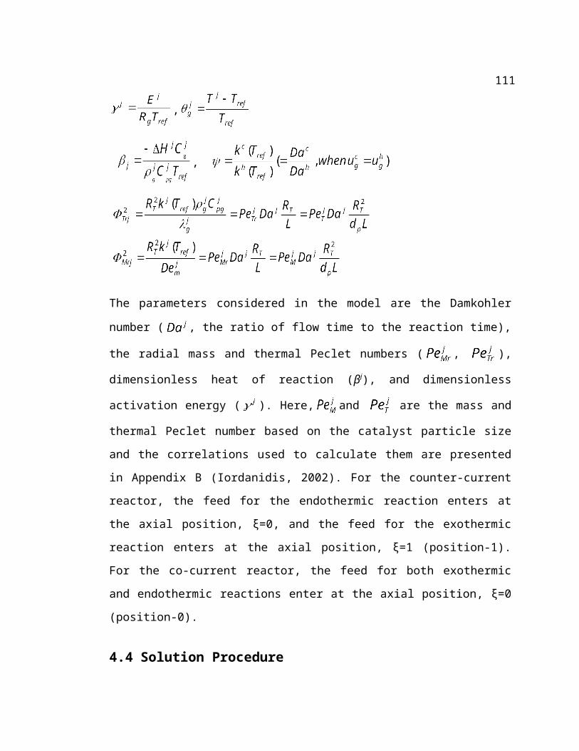
(6.22)

The sign of the derivative dyk/dz in Eq. 6.22 is given by the orientation of the parameter

z along the curve – the direction of movement along the curve. The system of equations,

Eq. 6.20, can now be solved and marched along the arc length by a suitable numerical

integration solver. In this work, we have used LSODE solver from Netlib libraries for

the integration.

This algorithm generates a continuous solution curve and passes through limit points

without any difficulties and continues at bifurcation points on the next branch (usually

at a random direction). Some of the examples presented in the next section demonstrate

the applications of BEM-continuation algorithm in determining the multiple steady

states.

6.5 Illustrations

The multiple steady states are predicted using BEM-Continuation method for some

chemical engineering test problems for the purpose of validation of the numerical

method and are illustrated in this section.

6.5.1 Example 1a: A Non-isothermal Chemical Reaction in a Slab Catalyst

The mass balance and energy balance equations describing the diffusion process with

irreversible first order reaction kinetics in slab geometry can be combined in the

absence of external transport processes into a single equation. The resulting governing

equation is given as,

111

Here, C is the concentration of the reactants and Φ, γ, β are respectively Thiele

modulus, dimensionless activation energy and dimensionless heat of reaction (includes

the thermal conductivity of the solid) . The boundary conditions used are:

(i) at the catalyst centre, x = 0,

(ii) and at the surface, x = 1, C = 1.

For certain range of parameters, (for example, Φ=0.15, γ=20, β=0.8), this system

exhibits multiple steady states. Figure 6-1 shows the concentration profile within the

catalyst pellet for this set of parameters. All the three multiple steady states were

predicted by BEM using different initial guesses.

In order to obtain the complete solution as a function of Φ, BEM-continuation method

described earlier was used with Thiele modulus as the continuation parameter (α = Φ).

The concentration at the centre of pellet for different Thiele modulus is plotted in Figure

6-2. Here, the continuation analysis indicates that multiple steady states exist in the

range of Φ = 0.069 to Φ = 0.25 and these results are in agreement with earlier studies.

The three steady state concentrations at the catalyst centre, corresponding to Φ=0.15,

shown in Figure 6-2 match with those reported in Figure 6-1. In this example, ten

elements are used in the BEM discretization and the obtained results match those of

with the larger number of nodes.

0 0.1 0.2 0.3 0.4 0.5 0.6 0.7 0.8 0.9 10

0.1

0.2

0.3

0.4

0.5

0.6

0.7

0.8

0.9

1

Distance within the Pellet

Con

cent

ratio

n, C

112

Figure 6-1: Concentration Profiles in a Catalyst Pellet for Example 1a Predicted by BEM using Different Initial Guesses (Φ=0.15, γ=20, β=0.8)

Figure 6-2: Concentration at the Centre of the Catalyst for Example 1a predicted by BEM-Continuation Technique (γ=20, β=0.8)6.5.2 Example 1b: Reaction in the Catalyst Pellet with External Transport

Resistances

+ + +++++++++++++++++++++++++++++++++++++++++++++++++++++++++++++++++++++++++++ +

+ ++++++++++

0 0.1 0.2 0.30

0.1

0.2

0.3

0.4

0.5

0.6

0.7

0.8

0.9

1

Thiele Modulus, Φ

Con

cent

ratio

n at

the

Cat

alys

t Cen

tre

113

The diffusion reaction problem, same as the above is considered with external mass and

heat transport resistance. This system is modeled as a set of two second order

differential equations one for concentration and the other for temperature with the

respective boundary conditions. The model equations and the respective boundary

conditions used and the other details can be found in Aris and Hatfield (1969). It was

shown in the original paper that this system exhibits multiple steady states for a certain

range of transport parameters. We tested BEM-continuation method for this problem by

simulating a case with the set of parameters (Bi=10, Sh=30) reported in the original

paper. Figure 6-3 shows the effect of Thiele modulus on the effectiveness factor and

one could observe two peaks in the effectiveness factor. This result is in agreement with

that reported by Aris and Hatfield (1969). Twenty boundary elements are used to

simulate this case and BEM-continuation approach is robust and accurate in capturing

the five steady states occurring at a particular Thiele modulus (around 0.25).

Figure 6-3: Effectiveness Factor vs. Thiele Modulus for a First-Order Reaction in a Slab Catalyst (γ=27, β=1/3, Sh=30, Bi=10) (Example 1b)6.6 Coupling of Exothermic and Endothermic Reactions in a Porous

Catalyst Particle

0 0.2 0.4 0.6 0.8 1 1.2 1.4 1.60

50

100

150

200

250

300

350

Thiele Modulus, Φ

Effe

ctiv

enes

s Fa

ctor

114

Several catalyst systems favor both exothermic and endothermic reactions like rhodium

catalyst used for partial oxidation of methane to syngas production. Here we evaluate a

model catalyst system that favors both exothermic and endothermic reactions. Two

parallel reactions, A R (Exothermic) and C S (Endothermic) are considered in this

work. A first order irreversible kinetics is assumed for both exothermic and

endothermic reactions.

The governing equations for this system are:

Here C1 and C2 are the dimensionless concentrations of the reactant for exothermic (A)

and endothermic (C) reactions respectively, non-dimensionalised using the total

concentration (Ctot) at the catalyst surface (i.e. Ci = Cactual,,i / Ctot). T is the dimensionless

temperature of the system (= Tactual / Tref). The other parameters are:

Thiele Modulus,

Activation Energy,

Heat of Reaction,

where j = c, h (c for endothermic reaction - C S, and h for exothermic reaction - A

R), L is characteristic length of the catalyst, k is the reaction rate constant, E and ΔH are

respectively activation energy and heat of reaction , and Dem and ke are respectively the

effective diffusivity of species and the effective thermal conductivity of the solid. Note

115

that β is positive for exothermic reaction (j = h) and negative for endothermic reaction (j

= c).

The boundary conditions are:

at the catalyst surface (x = 1) :C1 = C1s; C2 = C2s; T = Ts (with C1s+C2s = 1)

at the catalyst centre (x = 0):

We carried out a simulation study using BEM to obtain the steady state temperature

profile within the catalyst pellet. The parameters used are: γh=27, βh=1/3, Φc=0.25,

γc=27, βc=-2/3, C1s=0.9, C2s =0.1. Figure 6-4 shows the temperature profile within the

catalyst pellet for two different Thiele moduli, Φh=0.35 and Φh=2.5. It is clear from

these results that for lower Thiele modulus, the system exhibits multiple steady states

whereas for Φh=2.5, the system has a unique steady state. In Figure 6-4, the temperature

profiles for Φh=0.35 resemble those of the cases with exothermic reaction. In other

words, the maximum temperature is reached at the centre of the pellet. On the other

hand for the case with higher Thiele modulus, maximum temperature occurs at some

intermediate point within the pellet. This is because the exothermic reaction is

predominant very near the pellet surface, thus the temperature increases from pellet

surface to that point. Once the exothermic reactants are completely consumed, the

endothermic reaction dominates and hence the temperature decreases further till the

centre of the catalyst pellet.

The range, at which the multiplicity occurs in this system, is predicted using BEM-

continuation method. Figure 6-5 presents the temperature at the centre of the catalyst as

a function of Thiele modulus for exothermic reaction (Φh) for different reactant

concentration at the catalyst surface (C1s and C2s). All other parameters are the same as

provided in Figure 6-4.

0 0.2 0.4 0.6 0.8 10

0.15

0.3

0.45

0.6

0.75

0.9

1.05

1.2

1.35

1.5

Dimensionless Distance within the Catalyst

Dim

ensi

onle

ss T

empe

ratu

re

Φh = 2.5Φh = 0.35 (1)Φh = 0.35 (2)Φh = 0.35 (3)

116

Figure 6-4: Concentration Profile within a Catalyst Pellet where both Exothermic and Endothermic Reactions Occur (γh=27, βh=1/3, Φc=0.25, γc=27, βc=-2/3, C1s=0.9, C2s=0.1)

0.9

1.1

1.3

1.5

0 0.2 0.4 0.6 0.8 1

Thiele Modulus for Exothermic Reaction

Tem

pera

ture

at t

he C

entre

C1s=1C1s=0.9C1s=0.8C1s=0.7

Figure 6-5: Multiple Steady States in a Catalyst Pellet with First Order Exothermic Reaction and Endothermic Reactions (Φh - varied, γh=27, βh=1/3, Φc=0.25, γc=27, βc=-2/3)At any Thiele Modulus, with decrease in the surface concentration of C1 (hence increase

in C2s), the temperature at the centre of the catalyst decreases. Also it is clear from

117

Figure 6-5 that with decrease in the surface concentration of the reactants of exothermic

reaction, the region of multiple steady states shifts to higher Thiele moduli. The range

of Thiele modulus for which the multiple steady states exist, decreases with increase in

the concentration of endothermic reactants at the catalyst surface and further, the

multiplicity disappears after a critical surface composition (below C1s = 0.7).

The results obtained by coupling exothermic and endothermic reactions are compared to

a case with only exothermic reaction in order to examine the region of multiplicity.

Table 6-2 presents the region of multiplicity for different composition at the catalyst

surface for these two cases. The case where only the exothermic reaction takes place,

can be simulated by setting = 0 for comparison purposes. In this case C2 represents

the concentration of inert species in the system. The other parameters are same as the

base case. From Table 6-2 it is clear that the range of Thiele modulus at which

multiplicity occurs increases with increase in the composition of exothermic reactants at

the surface for both the cases. Also it is observed that for the system with only

exothermic reaction, the multiplicity occurs when C1s is higher than 0.6. However, for

the case with both exothermic and endothermic reactions, the multiplicity occurs only

when C1s is higher than 0.8.

Hence the presence of endothermic reaction stabilizes the reaction system and reduces

the range of Thiele modulus, at which multiplicity occurs. The occurrence of multiple

steady states with respect other parameters like γh, γc, βh, βc etc., can also be examined

using the developed BEM-Continuation technique and are not addressed in this work.

Table 6-2: Region of Multiplicity for Different Surface Concentrations (γh=27,

βh=1/3, γc=27, βc= -2/3)

Concentration of Range of Thiele Modulus with Multiple Steady States

118

Exothermic

Reactants at the

surface, C1s

(Φh)Only Exothermic Reaction, Exothermic and

Endothermic Reaction,

Φc = 0.25

0.1-0.5 No Multiplicity No Multiplicity

0.6 0.468-0.487 No Multiplicity

0.7 0.370-0.424 No Multiplicity

0.8 0.305-0.399 0.456-0.457

1.0 0.192-0.340 0.192-0.340

6.7 Summary

The boundary element combined arc length continuation technique was shown to be an

effective method to determine the multiple steady states in the multi variable distributed

parameter systems like diffusion-reaction problems. The BEM approach eliminates the

discretization errors in the derivatives while the arc length continuation method

smoothly captures the complete dependency of the solution on any parameter including

the region of multiple steady states. This combined procedure is quite reliable and easy

to implement and use. Several illustrative examples demonstrate the robustness of this

method. This approach was also used to determine the multiple steady states in the

catalyst particles where both exothermic and endothermic reactions take place. It was

found that the multiple steady states were vanished by the presence of endothermic

reactions for certain reactant composition at the catalyst surface. This study is important

for controlling the hot spot in the interior of the catalyst, thus avoiding the catalyst

deactivation through sintering, and for stabilizing the process system.

119

Chapter 7

Modeling of Catalytic Partial Oxidation of Methane to

Syngas in Short Contact Time Packed Bed Reactors

7.1 Scope

The catalytic partial oxidation of methane to syngas is investigated as a case study

because of the interesting challenges it offers due to the interaction of exothermic

combustion and endothermic reforming reactions. In this system, methane is a common

reactant for both the exothermic and the endothermic reactions. The steam produced in

the exothermic combustion step undergoes the endothermic reforming reactions with

methane. Hence, at the reactor inlet, the rate of heat generation by exothermic reaction

is greater than the rate of heat consumption by endothermic reaction, in general. From

the guidelines discussed in Chapter 5, it is clear that the directly coupled reactor, such

as packed bed reactor, is suitable for this partial oxidation process. Hence, in this

chapter, the steady state and dynamic behavior exhibited by this process in a short

contact time packed bed reactor is analyzed using the heterogeneous plug flow and axial

dispersion models. The effects of inlet mass velocity and feed quality (such as the

presence of steam in the feed and the effects of methane-to-oxygen ratio and methane-

to-steam ratio in the feed) on the product yield and hotspots are analyzed. The effects of

film transfer coefficients and axial dispersion coefficients on the steady state profiles

are also discussed. The evidence for the occurrence of wrong way behavior, due to the

perturbation of the inlet temperature and the feed quality, in this short contact time

reactor is presented.

120

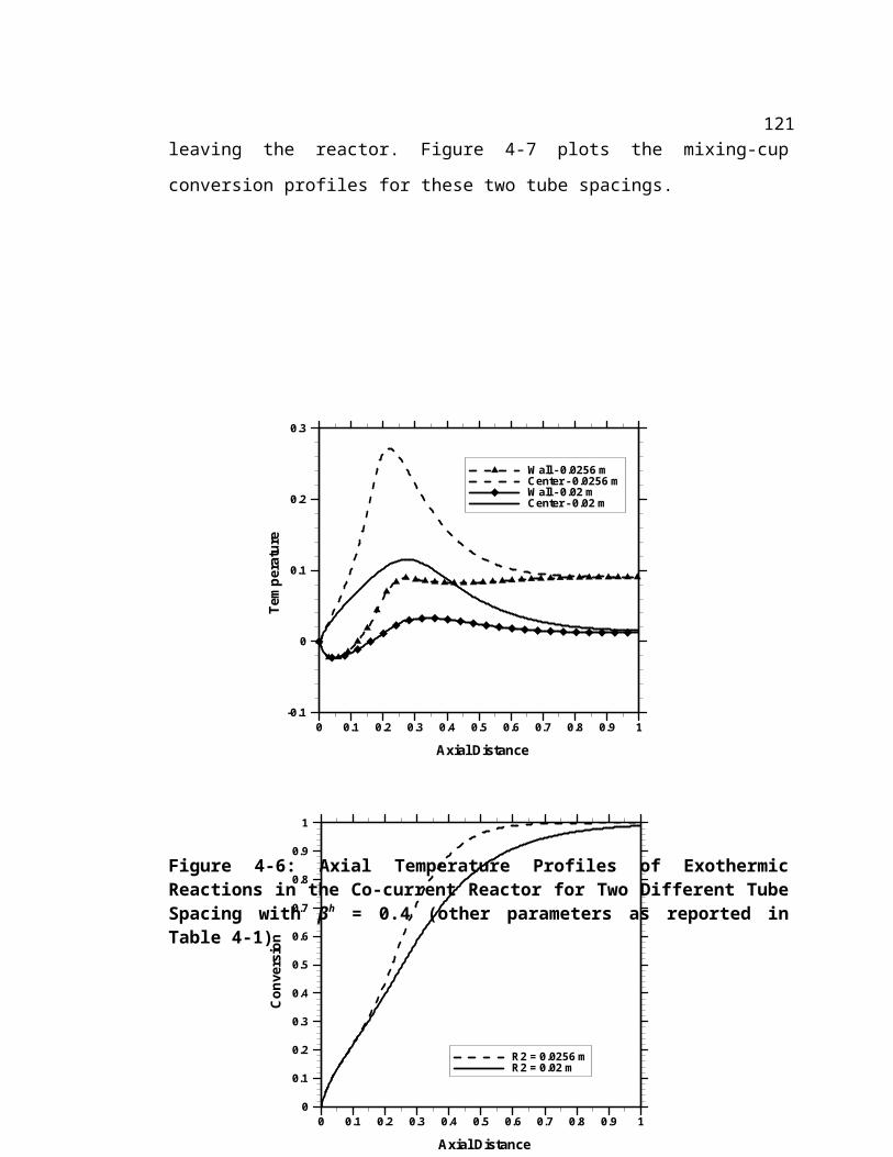
7.2 Introduction

Syngas is an important feedstock for the production of synthetic automotive fuels

(synfuels) and for a variety of chemicals like methanol and its derivatives. Syngas is

produced from wide range of hydrocarbons, such as natural gas (mostly methane),

naphtha, coal, etc., and the different methods used to produce syngas were discussed in

Chapter 2. Several oil companies, such as ExxonMobil, Shell and others are building

plants in Qatar, Middle East, to be commissioned in the second part of this decade, to

convert natural gas to Fischer-Tropsch liquids (fuels). The production of synfuels and

chemicals from natural gas and coal, through the syngas route, could reduce the

consumption of crude oil.

The availability of pollutant free natural gas and the ability to produce the desired ratio

of CO/H2 (~0.5 for methanol synthesis), have attracted much research on the conversion

of methane to synthesis gas by the catalytic partial oxidation route. Syngas production

by the catalytic partial oxidation route proceeds through the coupled exothermic

combustion reaction(s) and the endothermic reforming reactions, in the same catalyst

bed. The simultaneous occurrence of combustion and reforming reactions, in this partial

oxidation processes, makes this route more attractive as it minimizes the energy

requirement for the production of syngas compared to the steam reforming route.

The mechanism of methane conversion to syngas is still debated in the literature.

Although the possibility of performing the reaction via the direct route (in one step from

methane to syngas) has been reported by several researchers, there seems to be an

increasing consensus that (for most of the catalysts) the reaction occurs mainly via the

indirect route. It is to be noted that the hot spot could be eliminated if the reaction

occurs via the direct route. Schmidt’s group (2001) reported that with highly active Rh

based catalysts the entire process could be completed in a short contact time of the order

of milliseconds and the reactors used for this process are called short contact time

reactors. Because of the complexity of the processes due to the interactions of

exothermic and endothermic reactions in a system where the flow time scale is also

121

short, a suitable mathematical model is required for the optimization of the process and

for reactor control.

The reported modeling studies in the literature discuss, mostly, the steady state behavior

of this process, in particular, the effects of feed temperature, importance of gas phase

reactions at higher operating pressure and the role of thermal conductivity of the

catalyst bed and gas hourly space velocity (GHSV) on the methane conversion and on

the product pattern. The interaction between exothermic and endothermic reactions

becomes more significant especially during the transient operations and there is not

much information available in the literature on the dynamic behavior of these reactors.

In this work, we investigate some of the transient aspects in more detail using 1-D

transient heterogeneous plug flow and axial dispersion models of the short contact time

packed bed reactors. Some of the key transient behavior, including the wrong way

phenomenon, resulting in response to a sudden increase or decrease in the feed

temperature (from a steady state profile) is analyzed. The steady state and dynamic

behavior resulting from the interaction of the exothermic and endothermic reactions due

to the addition of steam in the feed is investigated. The effects of the inlet mass velocity

(hence gas hourly space velocity, GHSV) on the temperature profile and on the product

distribution are also discussed. Here, we attempt to resolve the debated issue of increase

in the conversion of methane with increase in GHSV in the short contact time reactors.

The effects of transport coefficients and dispersion coefficients on the hot spot, length

of the reactor and on the time taken to reach the steady state are presented.

The next section (Section 7.3) presents the heterogeneous plug flow and axial

dispersion models and the solution procedure used in this work. The steady state and

dynamic behavior exhibited by the partial oxidation process are discussed in Section

7.5. The summary is provided at the end.

122

7.3 Model Development

This section presents the transient heterogeneous plug flow and axial dispersion models

for the packed bed reactors. The rate of the reactions and other correlations for the

transport properties used are also presented here. The solution procedure employed in

this work is discussed in Section 7.4.

7.3.1 Transient Plug Flow Model : The species mass balance and energy balance

equations for the gas phase and the solid phase are presented here:

Species Mass Balance in the Gas Phase:

(7.1)

Continuity Equation:

(7.2)

where,

, is the mass flux (equals the inlet mass flux at the steady state)

Species Mass Balance in the Solid Phase:

(7.3)

where,

ρis is the mass density of species i in the solid phase and,

(7.4)

123

where, kgi is the mass transfer coefficient of species i. The accumulation and reaction of

the species in the gas film surrounding solid particles is neglected in this work.

Energy Balance for the Gas Phase:

(7.5)

Energy Balance for the Solid Phase:

(7.6)

The species densities / concentrations are calculated using the ideal gas law. The total

density of mixture is given as, . The above equations (Eqs. 7.3-

7.6) are rendered dimensionless as follows:

The resulting dimensionless equations of the transient heterogeneous plug flow model

are:

Mass Balance for the Gas Phase:

124

(7.7)

Mass Balance for the Solid Phase:

(7.8)

Energy Balance for the Gas Phase:

(7.9)

Energy Balance for the Solid Phase:

(7.10)

In this work, Ergun equation is used to calculate the pressure drop at each and every

axial position, which complements the above set of model equations. The above set of

model equations is solved with the appropriate inlet and initial conditions.

7.3.2 Dimensionless Transient Axial Dispersion Model: The species mass balance

and energy balance equations for the gas phase and the solid phase are given as

follows:

Mass Balance for the Gas Phase:

125

(7.11)

Mass Balance for the Solid Phase:

(7.12)

Energy Balance for the Gas Phase:

(7.13)

Energy Balance for the Solid Phase:

(7.14)

Here,

The boundary conditions used to solve the above set of axial dispersion equations are:

126

(7.15a-c)

(7.16)

The initial conditions may vary depending on the simulation study and are mentioned in

Section 7.5. In the simulation study presented in this work, instead of using

Danckwert’s boundary condition (Eq. 7.15a-b), Dirichlet boundary conditions (

) are used because of large Pemg and PeTg values. The

correlations to estimate the axial heat and mass transfer coefficients are provided in

Appendix B. The heat loss due to radiation is not included in our model as we found

that the effect of radiation on the temperature profiles is not significant for the range of

parameters we investigated. The steady state plug flow and axial dispersion models can

be easily obtained by equating the terms corresponding to time derivatives in the

respective transient models (Eq. 7.7 to Eq. 7.14) to zero.

7.3.3 Reaction Rates

The following reactions are considered to represent the partial oxidation of methane to

syngas process and the corresponding rate expressions are obtained from the literature

(de Smet et al., 2001)

(7.17a-d)

127

The respective rate equations for the chemical reactions (7.17a)-(7.17d) are,

(7.18a)

(7.18b)

(7.18c)

(7.18d)

where,

The values of pre-exponential factors, activation energies, heats of adsorption, and

equilibrium constants are given in Table 7-1. We have used the above global kinetics to

demonstrate the coupling and interactions of exothermic and endothermic reactions in

packed bed reactors. These rate expressions are developed for the Ni/Pt catalyst system

and it is to be noted that the temperature and product profiles obtained with Ni/Pt and

Rh catalyst systems are qualitatively similar. De Smet et al. (2001) used the above

kinetics (Eq. 7.18a-7.18d) with an effectiveness factor of around 10-3 (for all reactions)

to simulate the industrial reactor. The effectiveness factor has been used in their work as

the catalyst is assumed to be porous. The studies with the rhodium catalyst (Hohn and

128

Schmidt, 2001; Bizzi et al., 2002), which is non-porous, shows that the catalyst is

highly active for the partial oxidation process and the reaction is completed in a very

short contact time, of the order of milliseconds. However, the global kinetic scheme for

the partial oxidation processes with the rhodium catalyst is not well established. Hence

we decided to use this kinetics without any effectiveness factor to qualitatively simulate

the short contact time reactor and to analyze the coupling of exothermic and

endothermic reactions in the partial oxidation process.

Table 7-1: Pre-exponential factors for reaction rates, heats of adsorption and activation

energies

Constant Pre-exponential factor A(kk); A(Ki) Activation energy, Ek (kJ/mol)

Heat of adsorption (ΔH)k

(kJ/mol)

k1a (kmol / kgcat bar2 h) 2.92 x 106 86.0

k1b (kmol / kgcat bar2 h) 2.46 x 106 86.0

k2 (kmol bar0.5/ kgcat h) 4.225 x 1015 240.1

k3 (kmol bar0.5/ kgcat h) 1.020 x 1015 243.9

k4 (kmol / kgcat bar h) 1.955 x 106 67.13

KCO (bar-1) 8.23 x 10-5 70.65

KCH4 (bar-1) 6.65 x 10-4 38.28

KH2O 1.77 x 105 -88.68

KH2 (bar-1) 6.12 x 10-9 82.9

(bar-1) 1.26 x 10-1 27.3

(bar-1) 7.87 x 10-7 92.8

Ke,2 (bar2)= exp(-26830/T+30.114)

Ke,3 (bar2)= exp(-22430/T+26.078)

Ke,4 (-)= exp(4400/T-4.036)

At higher operating pressures, the gas phase reactions become important and therefore

in some of the simulations, the following gas phase reactions (Dupont et al., 2002) were

considered in addition to the previously listed heterogeneous reactions:

129

(7.19a)

(7.19b)

The rate expressions for the above homogeneous reactions are:

rhom,1 (mol/m3-s) = 1.585 x 105 exp(-202600/RgT)[CH4]0.7[O2]0.8 (7.20a)

rhom,2 (mol/m3-s) = 5.623 x 106 exp(-180000/ RgT)[CO][H2O]0.5[O2]0.25 (7.20b)

The pre-exponential factors in Eqs. 7.20a and 7.20b are slightly modified from those

reported in the literature (Dupont et al., 2002).

7.3.4 Transport Properties

The heterogeneous models require the particle to fluid heat and mass transfer

coefficients. These film transfer coefficients are calculated based on the correlations

recommended by Wakao and Kaguei (1982) and Mills (1995) and are given below:

Heat transfer correlation:

(7.21)

Mass transfer correlation

130

(7.22)

The viscosity, thermal conductivity, specific heat and the diffusivity of the species used

in this work are corrected for the temperature and / or pressure. The respective mixture

properties at any point in the reactor are calculated based on the mixture rule for gases

(Mills, 1995).

7.4 Solution Procedure

The transient plug flow and transient axial dispersion model equations (Eqs. 7.7-7.14)

are solved by the method-of-lines (MOL) approach (van de Wouwer et al., 2001). In

this approach, the partial differential equations (PDE) are converted to a set of ordinary

differential equations (ODE) by suitable discretization of spatial derivatives and the

resulting ODEs in time are then integrated using an explicit algorithm. We have used

automatic step size adjustable LSODE routine from Netlib as an ODE integrator. It is

observed that the explicit solver (corresponding to the feature MF = 10, in the LSODE

solver) is more robust and faster compared to the stiff solver (MF = 22) for this

problem. The second order finite difference upwind discretization scheme is used to

discretize the spatial derivatives. The discretization scheme has been made robust to

spurious oscillations using total variation diminishing (TVD) algorithms (using van-leer

splitter) (Tannehill et al., 1997). The grid independence of the solution is verified and

the number of nodes used for the simulation in this work is 250, unless otherwise stated.

In our model the pressure drop at each point along the reactor length is updated at every

time step using Ergun equation, which is a steady state equation. The discretization of

Ergun equation results in a set of algebraic equations, which are solved using modified

Newton-Powell hybrid solver (HYBRD) from the Netlib libraries.

131

7.5 Results and Discussions

7.5.1 Steady State BehaviorHere we analyze the effect of mass and heat transfer coefficients on the temperature and

concentration profiles. The effects of feed quality (in particular the addition of steam in

the feed) and the mass flow rate on the methane conversion, the product pattern and on

the hot spot are discussed (using plug flow heterogeneous model). The influence of the

axial dispersion coefficients (within the limitation of Dirichlet boundary conditions) on

the performance of the short contact time reactor is also presented.

Effect of Heat and Mass Transfer Coefficients: The temperature profiles predicted

using the plug flow model for two sets of heat and mass transfer coefficients are shown

in Figure 7-1a. The input parameters used in the simulation are presented in Table 7-2.

The heat and mass transfer coefficients are smaller for Case 2 compared to Case 1. For

Case 2 the mass transfer coefficients are around 10% and the heat transfer coefficients

are 30 % lower than those of Case 1 (multiply the heat and mass transfer correlations

Eqs. 7.21 and 7.22, by the respective factors). The temperature profiles corresponding

to Case 1 qualitatively match some of the experimental and other modeling results

published in the literature (Bizzi et al., 2002; Biesheuvel and Kramer, 2003). In this

process, the exothermic reaction is dominant initially and, hence, the temperature

increases near the inlet of the reactor. The increase in the reactor temperature favors the

endothermic reaction subsequently. Once the concentration of one of reactants (here,

oxygen which is the limiting reactant) participating in the exothermic reaction decreases

(or if it is completely consumed), the endothermic reaction becomes predominant and,

therefore, a drop in temperature in observed in the later section of the reactor. In the

portion near the reactor inlet, where the exothermic reaction is dominant, the solid

phase temperature is higher than the gas phase temperature. On the other hand, the gas

phase temperature is higher than the solid phase temperature when the endothermic

reaction is dominant (near the reactor exit). This also shows that there exists a point in

the reactor where the gas and solid phase may have similar temperature and at that point

132

the rate of heat generation by the exothermic reaction matches the rate of heat

consumption by the endothermic reaction, in an adiabatic reactor. For the cases

discussed in Figure 7-1a, the temperature profiles reach the equilibrium value, for both

sets of film coefficients, near the exit. Also Case-2 requires more reactor length to reach

the equilibrium compared to Case-1. It is to be noted that the magnitude of temperature

peak is higher for the case with higher transport coefficient. We also observed that the

temperature peak is higher for the case simulated with pseudo-homogeneous model (de

Groote and Froment (1996) also have showed sharp temperature peak), for the

parameters reported in Table 7-2. This shows that the presence of heat and mass transfer

resistances minimizes the hot spot in the reactor, for this process.

Table 7-2: Model Input Parameters (Base Case)

Reactor length, m 0.1

Catalyst diameter, m 0.002

Inlet Temperature, K 700

Inlet Pressure, atm 40

Reactant Mass Flow Rate, kg/m2-s 20

Feed Composition (mole fraction)CH4

O2

CO2

H2OCOH2

0.66660.33330.00000.00000.00000.0001

Bed Porosity 0.43Heat Capacity of Catalyst, J/kg-k 750

The predicted concentration profiles (for film transfer coefficients corresponding to

Case 1) are shown in Figure 7-1b. The methane and oxygen concentration falls

drastically near the reactor inlet with the production of CO and H2. The equilibrium

conversion is achieved in these reactors at short length of about 0.02 m. The ratio of

CO/H2 at the reactor exit is 0.52. It is to be noted that the non-equilibrium conditions

can result when the reactor length is very small, say 0.015m. For further work, the film

coefficients corresponding to Case 1 were used.

133

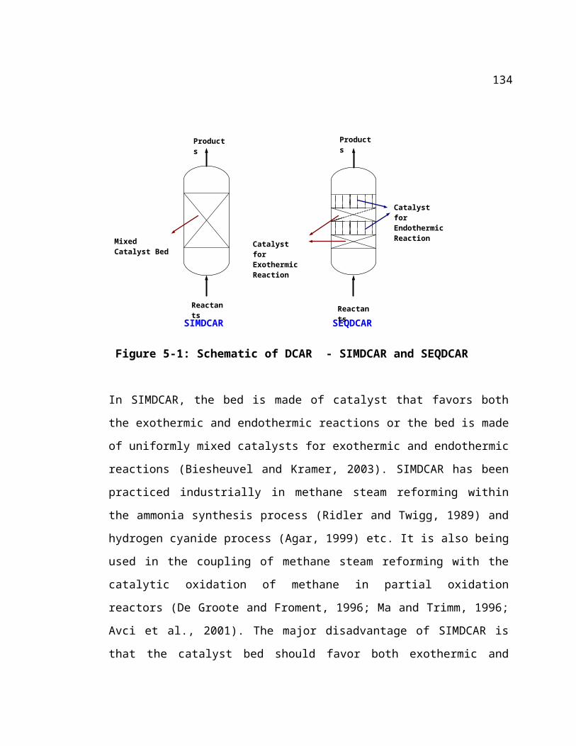
Figure 7-1a: Temperature Profiles Predicted by the Heterogeneous Plug Flow Model for Two Sets of Heat and Mass Transfer Coefficients (Parameters used are reported in Table 7-2)

Axial Distance, m

Tem

pera

ture

, K

0 0.01 0.02 0.03 0.04 0.05 0.06 0.07 0.08 0.09 0.1700

800

900

1000

1100

1200

1300

1400

1500

1600

Case 1 - GasCase 1 - SolidCase 2 - GasCase 2 - Solid

0 0.01 0.020

0.1

0.2

0.3

0.4

0.5

0.6

0.7

CH4O2CO2H2OCOH2CH4 (s)CO (s)H2 (s)

Axial Distance, m

Mol

e Fr

actio

n

0 0.01 0.020

0.1

0.2

0.3

0.4

0.5

0.6

0.7

CH4O2CO2H2OCOH2CH4 (s)CO (s)H2 (s)

Axial Distance, m

Mol

e Fr

actio

n

134

Figure 7-1b: Concentration Profiles Predicted by the Heterogeneous Plug Flow Model for Case 1 (s – for catalyst surface; Other parameters reported in Table 7-2)Effect of Operating Pressure: Higher operating pressure favors the homogeneous

reactions in addition to the heterogeneous reactions. Figures 7-2a and 7-2b show the

effect of pressure on the temperature profile and on methane conversion respectively

with and without gas phase reactions. As the operating pressure increases, the

combustion reaction (homogeneous / heterogeneous) is enhanced. Hence, the

temperature peak moves closer to the reactor inlet (Figure 7-2a). Also higher pressure

favors more methane and water formation due to the thermodynamic equilibrium, and,

hence decreases methane conversion (Figure 7-2b). This reduction in the reforming rate

compared to the combustion rate can be attributed to the increase in the temperature

peak at higher pressures.

Figure 7-2a: Effect of Operating Pressure on the Gas Phase Temperature Profiles

The observed temperature profile shown in Figure 7-2a reveals that the gas phase

reaction is not favored at lower pressures. At higher pressures, the predicted

temperature peak is higher for the case with exothermic gas phase reactions than for the

case without gas phase reactions. It is also clear from Figure 7-2a that gas phase

reactions are relatively slow and take a while to kick on. The occurrence of gas phase

reactions increases the production of CO2 and H2O, as evident from Figure 7-2c.

Axial Distance, m

Tem

pera

ture

, K

0 0.01 0.02 0.03 0.04 0.05 0.06 0.07 0.08 0.09 0.1700

800

900

1000

1100

1200

1300

1400

1500

1600

1700 10 bar40 bar60 bar - no gas rxn.60 bar - with gas rxn.

135

Figure 7-2b: Effect of Operating Pressure on Methane Point Conversion

Figure 7-2c: Effect of Gas Phase Reactions on the Concentration Profiles (Gas – with gas phase reactions, No Gas – without gas phase reactions)

Axial Distance, m

Met

hane

Con

vers

ion

0 0.01 0.02 0.03 0.04 0.05 0.06 0.07 0.08 0.09 0.10

0.1

0.2

0.3

0.4

0.5

0.6

0.7

0.8

0.9

1

10 bar40 bar60 bar

0 0.01 0.020

0.1

0.2

0.3

0.4

0.5

0.6

0.7

Axial Distance, m

Mol

e Fr

actio

n

CH4 (Gas)CO2 (Gas)CO (Gas)H2 (Gas)CH4 (No Gas)CO2 (No Gas)CO (No Gas)H2 (No Gas)

0 0.01 0.020

0.1

0.2

0.3

0.4

0.5

0.6

0.7

Axial Distance, m

Mol

e Fr

actio

n

CH4 (Gas)CO2 (Gas)CO (Gas)H2 (Gas)CH4 (No Gas)CO2 (No Gas)CO (No Gas)H2 (No Gas)

136

Effect of Steam in the Feed: It is known, in general, that the addition of steam to the

feed increases hydrogen generation and reduces the exit / equilibrium temperature. This

is due to increase in the rate of reforming reactions (endothermic). We observed that,

for some cases, the magnitude of the temperature peak increases with the addition of

steam (compared to the case without steam in the feed) and this is due to the ratios of

steam-to-methane and methane-to-oxygen in the feed. Hence, in this section, the effects

of addition of steam at constant and varying methane-to-oxygen ratio are analyzed and

the observed behavior is explained.

Varying Methane-to-Oxygen Ratio (fixed amount of steam in the feed): First, the

amount of steam (molar percent) in the feed was kept constant but the methane-to-

oxygen ratio was varied. Figure 7-3a shows the resulting axial temperature profiles.

With the increase in the feed methane-to-oxygen ratio at fixed molar percentage of

steam, the temperature peak as well as the exit temperature decreases. This is due to the

preferential occurrence of the reforming reactions with respect to the combustion

reaction because of the availability of more methane and less oxygen. The temperature

peak shifts to the right, away from the reactor inlet, with the addition of steam due to

the increased rate of endothermic reactions in addition to the lowered rate of the

exothermic combustion reactions. For the cases studied, the temperature peak is higher

for the feed with lower methane-to-oxygen ratio. The CO-to-H2 profiles for these cases

are plotted in Figure 7-3b. Carbon mono-oxide to hydrogen ratio at the reactor exit

decreases with the addition of steam compared to the case without steam in the feed.

Among the cases with steam in the feed, the CO-to-H2 ratio decreases, at the reactor

exit, with increase in the feed methane to oxygen ratio due to the formation of more

hydrogen. It is to be noted that CO can be produced in this process (inferred from

Figures 7-3b and 7-3c and Eq. 7.17b and 7.17c) by the reverse water gas shift reaction.

Figure 7-3c shows the CO2 profile and it reveals that for the lower methane to oxygen

feed ratio, more CO2 is produced (initially) which then participates in the shift reaction

further downstream to produce larger CO to H2 ratio. This study shows that for the fixed

137

amount of water in the feed, the lower methane-to-oxygen ratio in the feed results in the

higher temperature peak, higher CO-to-H2 ratio and lower CO2 in the product.

Figure 7-3a: Effect of Water in the Feed on Temperature Profiles (Gas Phase) – with varying Methane-to-Oxygen Ratio

Axial Distance, m

Tem

pera

ture

, K

0 0.01 0.02 0.03 0.04 0.05 0.06700

800

900

1000

1100

1200

1300

1400

1500

1600

1700

1800

67%CH4, 33% O260%CH4, 30% O2, 10%H2O57%CH4, 33% O2, 10%H2O67%CH4, 23% O2, 10%H2O

0 0.01 0.02 0.03 0.04 0.050

0.1

0.2

0.3

0.4

0.5

0.6

67%CH4, 33% O260%CH4, 30% O2, 10%H2O57%CH4, 33% O2, 10%H2O67%CH4, 23% O2, 10%H2O

Axial Distance, m

CO

/H2

ratio

in th

e pr

oduc

t

0 0.01 0.02 0.03 0.04 0.050

0.1

0.2

0.3

0.4

0.5

0.6

67%CH4, 33% O260%CH4, 30% O2, 10%H2O57%CH4, 33% O2, 10%H2O67%CH4, 23% O2, 10%H2O

Axial Distance, m

CO

/H2

ratio

in th

e pr

oduc

t

138

Figure 7-3b: Effect of Water in the Feed on CO/H2 Profiles – with varying Methane-to-Oxygen Ratio

Figure 7-3c: Effect of Water in the Feed on CO2 Mole Fraction Profiles– with varying Methane-to-Oxygen Ratio

Fixed Methane-to-Oxygen Ratio (with varying amount of steam in the feed): Here

the molar ratio of methane to oxygen in the feed is kept constant at 2 and the amount of

steam in the feed is varied. Figure 7-4a shows the predicted temperature peak and the

respective equilibrium temperature as a function of the molar percentage of steam in the

feed. The equilibrium temperature is calculated at the constant inlet pressure (reported

in Table 7-2) using CHEMKIN software. Here, the equilibrium temperature (and also

the temperature at the reactor exit) drops with the addition of steam whereas the

temperature peak passes through a maximum at about 20% steam in the feed. The CO-

to-H2 ratios corresponding to the equilibrium conversion and at the position 0.025m in

the reactor are plotted in Figure 7-4b. The CO-to-H2 ratio decreases with the addition of

steam. In the absence of steam, or in presence of small percentage of steam in the feed,

the equilibrium composition is achieved at the shorter reactor length. For larger

percentage of steam in the feed, more reactor length is needed to attain the equilibrium

Axial Distance, m

Mol

e Fr

actio

n of

CO

2

0 0.01 0.02 0.03 0.040

0.025

0.05

0.075

0.167%CH4, 33% O260%CH4, 30% O2, 10%H2O57%CH4, 33% O2, 10%H2O67%CH4, 23% O2, 10%H2O

Axial Distance, m

Mol

e Fr

actio

n of

CO

2

0 0.01 0.02 0.03 0.040

0.025

0.05

0.075

0.167%CH4, 33% O260%CH4, 30% O2, 10%H2O57%CH4, 33% O2, 10%H2O67%CH4, 23% O2, 10%H2O

139

conversion. The initial increase in the temperature peak with water addition in the feed

is due to water gas shift reaction. An increased percentage of water in the feed lowers

the amount of methane and oxygen in the feed and, hence, reduces the amount of CO2

produced by the combustion reaction. Additionally, the presence of water favors the

exothermic shift gas reaction attributing to slight temperature rise along with reduction

in CO/H2 ratio. This is further confirmed by Figure 7-4c where CO2 profiles for three

different feed qualities are plotted. In the presence of steam, the amount of CO2

produced per mole of methane reacted decreases (near the reactor inlet). On the other

hand, the conversion of CO2 (at the reactor exit) decreases (mole fraction of CO2

increases) with the addition of steam in the feed due to the equilibrium gas shift

reaction. When the amount of water exceeds a certain critical limit, the rate of

exothermic combustion reaction is reduced and, hence, the temperature peak decreases

(which is the case with 30% water in the feed)

The above two studies show that the addition of water in the feed may increase the

maximum temperature in the reactor depending on the methane-to-oxygen and /or

methane-to-steam ratio and, hence, a proper protocol has to be established to control the

temperature peak and the exit temperature.

0 10 20 30 401200

1300

1400

1500

1600

Temp. PeakEqlbm. Temp

Water in Feed, Mole %

Tem

pera

ture

, K

140

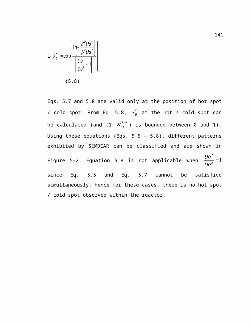
Figure 7-4a: Effect of Water in the Feed on Temperature Peak and the Equilibrium Temperature – with Constant Methane-to-Oxygen Ratio

Figure 7-4b: Effect of Water in the Feed on CO/H2 ratio – with Constant Methane-to-Oxygen Ratio

Water in Feed, Mole %

CO

/H2

ratio

0 10 20 30 400

0.1

0.2

0.3

0.4

0.5

0.6

at 0.025 mEquilibrium

Axial Distance, m

Mol

e Fr

actio

n of

CO

2

0 0.01 0.02 0.03 0.04 0.05 0.060

0.01

0.02

0.03

0.04

0.05

0.06

0.07

0.08

0.09

0.167%CH4, 33% O253%CH4, 27% O2, 20% H2O47%CH4, 27% O2, 30% H2O

Axial Distance, m

Mol

e Fr

actio

n of

CO

2

0 0.01 0.02 0.03 0.04 0.05 0.060

0.01

0.02

0.03

0.04

0.05

0.06

0.07

0.08

0.09

0.167%CH4, 33% O253%CH4, 27% O2, 20% H2O47%CH4, 27% O2, 30% H2O

141

Figure 7-4c: Effect of Water in the Feed on CO2 Mole Fraction Profiles– with Constant Methane-to-Oxygen Ratio

Effect of Inlet Mass Velocity: The increase in the reactant mass velocity increases the

productivity (if the level of conversion is assumed constant) and decreases the contact

time in the reactor. The effect of the mass velocity on the temperature profile, predicted

by the heterogeneous plug flow model, is shown in Figure 7-5. The temperature peak

increases with increase in the inlet velocity but is shifted towards the reactor exit. This

shift is due to the decrease in the Damkohler numbers of the exothermic and

endothermic reactions. Thus, the process needs more reactor length for the reactions (in

particular the exothermic reaction) to click on. The increase in the temperature peak can

be attributed to the reduced rate of endothermic reforming reactions and thus, the rise in

temperature due to the exothermic combustion reaction is not curbed by the

endothermic reaction. This increase in the temperature peak, due to increase in the inlet

mass flow rate, increases the methane conversion slightly. There is some experimental

evidence for the increase in methane conversion with the increase in gas hourly space

velocity in the literature (Hohn and Schmidt, 2001; Bizzi et al., 2002). The methane

conversion and the selectivity to CO and H2 for the range of mass velocity investigated

are shown in Table 7-3.

Axial Distance, m

Tem

pera

ture

, K

0 0.01 0.02 0.03 0.04 0.05 0.06 0.07 0.08 0.09 0.1700

800

900

1000

1100

1200

1300

1400

1500

1600

1700

20 kg/m2-s40 kg/m2-s80 kg/m2-s150 kg/m2-s

142

Figure 7-5: Effect of Inlet Mass Velocity on the Temperature Profiles (Other parameters reported in Table 7-2)

There is another school of thought regarding the increase in methane conversion with

GHSV, which needs some clarification and is discussed here. Bizzi et al. (2002, 2003,

and 2004) attributed such increase in methane conversion with mass velocity to the

increase in the mass transfer rate. It is generally observed that the conversion decreases

with increase in the mass velocity, which is due to decrease in the residence time for the

reactants. This can be illustrated for an isothermal reaction system. For the

heterogeneous systems, the dependence of mass transfer coefficients on the velocity

scales as Reα where α ranges from 1/3 to a maximum of about 0.8 (This is true for the

heat transfer rate also). Thus, for a simple isothermal irreversible (or reversible) kinetics

for reaction of types A B (or A=B), the conversion of the reactant A (XA), in the limit

of mass transfer controlled regime is given as,

XA=1-exp(-KmL/ug), (7.23)

where Km is the volumetric mass transfer coefficient (1/s) and L is the length of the

reactor and ug is the inlet superficial velocity. Equation 7.23 shows that the conversion

decreases with increase in the velocity. The conversion can only increase initially or

pass through a maximum if the dependence of the mass transfer coefficient on velocity

scales as a power greater than one (α > 1). This suggests that the increase in conversion

due to increase in the mass transfer rate can not be the sole reason for the

experimentally observed behavior in short contact time reactors. The expressions for the

dependence of conversion on the velocity, similar to Eq. 7.23, for the non-isothermal

case can be derived analytically with some approximations or can be determined

numerically.

In contrast to the above explanation, there are two different ways by which methane

conversion could increase in this non-isothermal system. Firstly, the increase in the

mass transfer rate supplies more reactants to the catalyst surface. The presence of more

143

methane and oxygen increases the rate of exothermic reaction and thus increases the

temperature at the catalyst surface. This higher temperature at the catalyst surface favors

the endothermic reforming reactions (which also uses methane) and thus contributing to

increase in the methane conversion. Often, the above phenomenon is offset by the

convection and the short residence time and thereby, methane conversion increases,

initially, slightly. This slight increase in the methane conversion with the mass velocity

is reported in Table 7.3. Secondly, there is a possibility that increase in the temperature

peak, increases the temperature at upstream of the reactor (due to the dispersion) and at

the inlet to the catalyst bed and, hence, resulting in higher methane conversion. This is

explained in the next section.

As discussed earlier, when the convection dominates, methane conversion decreases

with increase in the mass velocity, which is normally the case with larger velocity.

From Table 7-3, it is clear that for much larger inlet mass velocity (or GHSV) the exit

methane conversion is reduced. For this case, the temperature peak occurs very near the

reactor exit (and for ever larger velocity the temperature peak can be pushed out of the

reactor) as shown in Figure 7-5. When the temperature peak occurs near the exit of the

reactor, the residence time for the predominant endothermic reactions (between the

position of the temperature peak and the reactor exit) decreases and thereby contributing

to decrease in the methane conversion, and the product selectivity. This is true for the

mass velocity 150 kg/m2-s shown in Table 7-3. The increase in the conversion due to

the increase in the inlet linear or mass velocity is counter balanced by the increase in the

pressure drop across the reactor. The pressure drop calculated using the Ergun equation

for different mass flow rates is reported in Table 7-3. This increase in the pressure drop

may limit the commercial application of these reactors at higher GHSV.

Table 7-3: Effect of Inlet Mass Velocity on the Reactor Performance

Mass Flow

Rate,

kg/m2-s

Inlet linear

Velocity,

m/s

Methane

Conversion

at the Exit, %

H2

Selectivity

at the exit

CO

selectivity

at the exit

Pressure drop

at the reactor

exit, atm

20 1.36 84.9 1.856 0.967 0.58

144

40 2.73 85.0 1.857 0.967 2.17

80 5.46 85.6 1.864 0.968 7.77

150 10.22 80.7 1.877 0.917 18.00

Figure 7-6: Temperature Profiles Predicted by Axial Dispersion Model (Parameters as reported in Table 7-2)

Effect of Axial Dispersion Coefficients: Bizzi et al. (2003, 2004) have shown that the

mass and gas phase thermal dispersion coefficients can be neglected in the modeling of

the short contact time packed bed reactors due to large Pemg and PeTg. In this work, we

have analyzed the influence of these dispersion coefficients on the temperature profiles.

The mass and thermal dispersion coefficients can be calculated from the literature

(Rase, 1990 and also refer Appendix B) and in this work an average value of Daxi,m =

1.4e-3 m2/s, λe,g = 0.07 W/m-K are used. The effective thermal conductivity for the solid

can be obtained from Wakao and Kaguei (1982) and here, λe,c = 1 W/m-K (Bizzi et al.,

2003) is used. The effect of the dispersion coefficients on the temperature profiles for

the base case parameters reported in Table 7-2, are presented in Figure 7-6. The

temperature profiles are qualitatively similar for the cases with and without dispersion

coefficients. The presence of thermal dispersion coefficients did not have much

0 0.01 0.02 0.031200

1300

1400

1500

1600

Axial Distance, m

Tem

pera

ture

, K

Di,m= 0.0, λe,g= 0.0Di,m= 1.4e-3, λe,g= 0.0Di,m= 0.0, λe,g= 0.07Di,m= 1.4e-3, λe,g= 0.07

145

influence on the temperature profile, whereas the mass dispersion coefficient affects the

profile. In the presence of mass dispersion coefficient, the temperature peak and the exit

temperature decrease.

It is to be noted that the dispersion effects play a huge role in these reactors if the

reaction zone is sandwiched between two conducting inert packing sections, as seen in

some of the experiments (Bizzi et al., 2002). In such a reactor arrangement, with

increase in the mass velocity, the temperature peak increases. This in turn increases the

temperature at upstream of the reactor (due to dispersion) and at the inlet to the catalyst

bed resulting in higher methane conversion. In this work for further simulation studies,

Daxi,m = 0.0, λe,g = 0.07 W/m-K, λe,c = 1 W/m-K (predominantly focusing on the thermal

dispersions) were used.

7.5.2 Dynamic Behavior

The transient characteristics are important for the design, operation and control of the

partial oxidation reactors. The phenomena such as wrong way behavior are commonly

observed in packed bed reactors (where, say, exothermic reaction is conducted) due to

the perturbation in the feed temperature and flow rates and are important to be

understood for the steady-state and stable operation of the reactor. Suitable control

protocols and operation protocols are developed based on the temperature excursion

observed during this transient behavior. Similarly, the evolution of the temperature

profiles (from initial conditions) is important for the safe start-up of the partial

oxidation reactor where the exothermic and endothermic reactions occur

simultaneously. Hence in this section, we analyze the evolution of the temperature and

concentration profiles during the start-up of these short contact time packed bed

reactors. Some wrong-way behavior observed in these reactors due to changes in feed

temperature and due to the addition of steam in the feed is also presented.

Evolution Profile: Figure 7-7a shows the time series of the maximum gas phase

temperature in the reactor predicted by the heterogeneous plug flow and the axial

dispersion models for two cases – one with steam in the feed and the other without

146

steam in the feed. The feed composition of these two cases are: - (i) with steam: 53%

CH4, 27% O2 and 20% H2O and (ii) without steam: 67% CH4, 33% O2. In this

simulation, the initial conditions along the reactor are kept the same as the inlet

conditions.

Figure 7-7a: Evolution of the Maximum Gas Phase Temperature in the Reactor Predicted by the Plug Flow and Axial Dispersion Models (Feed Composition: Water -: 53% CH4, 27% O2 and 20% H2O and No Water - 67% CH4, 33% O2 )

Here, the exothermic reaction clicks on around 0.3 s and, hence, the magnitude of the

maximum temperature in the reactor increases sharply. The time at which this sharp

increase in temperature occurs is predicted to be the same by both the plug flow and the

axial dispersion models. The maximum temperature for the case with steam in the feed

is higher than for the case without steam and is consistent with the steady state results

discussed earlier (for the feed composition used). Also, for the case with steam, the time

taken for the exothermic reactions to click on is slightly longer than that for the case

without steam. This may be due to the reduced combustion rate (because of the decrease

in the partial pressure of oxygen and methane in the feed) and increased reforming rate

(due to water in the feed). It is to be noted that, for these cases, the temperature profile

evolves smoothly and finally reaches the steady state. This trend may not be expected

Time, s

Max

. Tem

pera

ture

, K

0 0.5 1 1.5 2700

800

900

1000

1100

1200

1300

1400

1500

1600

Ax. Disp. No WaterAx. Disp. WaterPlug Flow No WaterPlug Flow Water

147

for the processes with very high exothermic reaction rate and/or heat of reaction or for

the case with the lower heat capacity of the catalyst bed (one such extreme case will be

the coupling of homogeneous exothermic and endothermic reactions). In such

situations, the maximum temperature in the reactor may overshoot the steady state

temperature peak due to the short exothermic reaction time scale compared to other

time scales involved in the process such as endothermic reaction time scale, the time

scale of dissipation of heat by the solids etc.

Figure 7-7b: Evolution of the Reactor Exit Temperature Predicted by the Plug Flow and Axial Dispersion Models (Feed Composition: Water -: 53% CH4, 27% O2

and 20% H2O and No Water - 67% CH4, 33% O2 )

Figure 7-7b shows the evolution of the gas phase temperature at the reactor exit. Here,

the exit temperature for the case with water in the feed is lower than the one without

water, consistent with the equilibrium limitations and our earlier discussions. The time

taken to reach the steady state is slightly longer for the axial dispersion model compared

to the plug flow model, which is due to the presence of the dispersion time scale in the

problem. This study shows, for the parameters and initial conditions used in this work

that the time taken to reach the steady state is around 1.2s. Though this time seems very

short, it is several orders of magnitude greater than the residence time of the reactants

Time, s

Exit

Tem

pera

ture

, K

0 0.5 1 1.5 2 2.5700

800

900

1000

1100

1200

1300

1400

Ax. Disp. No WaterAx. Disp. WaterPlug Flow No WaterPlug Flow Water

148

(based on inlet conditions) in the reactor. This type of transient behavior with shorter

time to reach the steady state should be anticipated in the system with very active

catalysts.

Wrong Way Behavior: Wrong-way behavior in packed bed reactors is well recorded

for the reactions of the same type, like all exothermic reactions (Pinjala et al., 1988;

Chen and Luss, 1989). The wrong-way phenomenon is caused by a sudden drop in the

feed temperature, which results in the temperature excursion in the bed due to the

different propagation speeds of the concentration and temperature profiles within the

reactor. In this work, we have studied the wrong way behavior in the packed bed reactor

where both exothermic and endothermic reactions take place. The occurrence of wrong

way due to sudden decrease and increase in the feed temperature is analyzed. Similarly

the transient temperature profiles observed in this reactor due to the introduction of

steam in the feed are also investigated.

Decrease in the Feed Temperature: Here, the reactor is assumed to be operating at the

steady state corresponding to the base case parameters reported in Table 7-2. Then, the

feed temperature is decreased from 700 K to 650 K and the temperature profiles and

concentration profiles during this transient period are monitored. The maximum

temperature observed in the reactor and the temperature at the reactor exit are plotted in

Figure 7-8a. The wrong way behavior is observed in this case with the magnitude of

temperature peak increasing initially. The maximum increase in the magnitude of the

temperature peak is not greater than 2% of the temperature peak corresponding to the

initial temperature profile (steady state profile corresponding to the feed temperature of

700K). The temperature excursion due to wrong way is reduced or controlled, in this

process, due to the presence of endothermic reactions.

Figure 7-8a shows a wavy (oscillatory) pattern in the profile of maximum temperature

and a smooth pattern in the profile of the reactor exit temperature. These oscillations are

the indication of the traveling hot and cold waves resulting due to decrease in the feed

149

temperature and the simultaneous occurrence of the exothermic and endothermic

reactions.

Figure 7-8a: Maximum temperature in the Reactor and the Exit Temperature Profiles Predicted by Axial Dispersion Models (Feed Temperature is reduced from 700 K to 650 K and Feed Composition: 67% CH4, 33% O2)

0 2 4 6 81300

1350

1400

1450

1500

1550

1600

Temperature PeakExit Temperature

Time, s

Tem

pera

ture

, K

Axial Distance, m

Tem

pera

ture

, K

0 0.01 0.02 0.03 0.04 0.05 0.06 0.07 0.08 0.09 0.1600

700

800

900

1000

1100

1200

1300

1400

1500

1600

Initial0.35 s2.56 sSteady

150

Figure 7-8b: Axial Temperature Profiles as a Function of Time (Feed Temperature is reduced from 700 K to 650 K and Feed Composition: 67% CH4, 33% O2)The rate of endothermic reactions increases as and when the temperature increases in

the reactor (due to wrong way), and these in turn contribute to controlling the

temperature excursion. Figure 7-8b shows the axial temperature profiles within the

reactor during this transient period. These profiles also reveal that, as the feed

temperature is reduced, the reaction rates are reduced and, hence, the reactants with

higher concentration meet the catalyst with higher temperature in the downstream part

of the reactor. This results in wrong way with the temperature peak increasing beyond

the steady state value. The sudden increase in the temperature promotes the

endothermic reactions and hence the temperatures tend to decrease slightly. During this

transient period, the reaction front moves right, away from the reactor inlet. This

phenomenon continues until the steady state is achieved. The magnitude of the

temperature peak at the steady state corresponding to the feed temperature of 650 K is

lower than that of 700 K and is shifted to the right of reactor inlet.

Increase in the Feed Temperature: The sudden increase in the feed temperature also

results in the wrong-way behavior in this process and is investigated in this section. The

initial conditions for the temperature and concentration of the species within the reactor

correspond to those of the base case steady state. Now, the feed temperature is increased

from 700 K to 750 K. The maximum gas phase temperature and the temperature at the

reactor exit during the transient period are plotted in Figure 7-9a. There is a drop in the

maximum temperature observed, initially, followed by the temperature rise to the steady

state. This is observed due to different traveling speeds of the concentration and thermal

waves and, thereby, resulting interaction between the exothermic and endothermic

reactions. The axial temperature profiles at the different instants of time are shown in

Figure 7-9b. Due to the increase in the feed temperature, the rate of the exothermic

reaction is increased near the reactor inlet. This in turn increases the rate of endothermic

reaction, thereby the temperature peak is reduced. With further increase in time, both

exothermic and endothermic reaction balance and finally settle at the steady state with

temperature peak greater than that for 700K.

151

Figure 7-9a: Maximum temperature in the Reactor and the Exit Temperature Profiles Predicted by Axial Dispersion Models (Feed Temperature is increased from 700 K to 750 K and Feed Composition: 67% CH4, 33% O2)

0 1 2 31250

1300

1350

1400

1450

1500

1550

1600

Max. TemperatureExit Temperature

Time, s

Tem

pera

ture

, K

Axial Distance, m

Tem

pera

ture

, K

0 0.01 0.02 0.03 0.04600

700

800

900

1000

1100

1200

1300

1400

1500

1600

Initial0.135 s0.180 s0.770 sSteady

152

Figure 7-9b: Axial Temperature Profiles as a Function of Time (Feed Temperature is increased from 700 K to 750 K and Feed Composition: 67% CH4, 33% O2)In some of the transient temperature profiles, as shown in Figure 7-9b, two temperature

peaks are observed. The first temperature peak occurs near the reactor inlet and is due to

the increased exothermic rate because of increase in the feed temperature. This

temperature peak occurs around the location where the final (steady state) temperature

peak corresponding to the imposed feed temperature is expected. The increase in the

exothermic reaction rate increases the temperature which in turn favors the endothermic

reaction and hence the temperature drop is observed (after the temperature peak). The

gas stream within the reactor has some unreacted methane and oxygen. Once this gas

stream (cooled) contacts the high temperature bed (from previous instant of time), the

exothermic combustion reaction occurs, due to the presence of oxygen, resulting in the

second peak in the temperature profile. However, during this transient period, the

magnitudes of both these peaks are less than that of the initial profile and with increase

in time, the second peak disappears. It is to be noted that the temperature peak

corresponding to 750 K is greater than that for 700 K and is moved towards the reactor

inlet, due to the accelerated exothermic rate near the reactor inlet.

The axial concentration profiles for methane and CO in the reactor are shown in Figures

7-9c and 7-9d respectively. It is clear that the methane conversion increases (near the

reactor inlet) with the increase in the feed temperature. The increase in CO

concentration in the region near the inlet confirms the simultaneous occurrence of

endothermic reactions along with the exothermic reactions. During the initial transients,

methane conversion decreases at the exit, with the production of less CO and with

increase in time, the methane conversion and CO production increases. The methane

conversion and CO selectivity are higher at 750 K compared to 700 K. The total

duration of the transient lasts for less than 2s. It is clear from this study that, for the

cases investigated, the occurrence of wrong-way phenomena does not affect the reactor

performance severely and the reactor is able to attain the steady state.

153

Figure 7-9c: Axial Concentration Profiles of Methane as a Function of Time (Feed Temperature is increased from 700 K to 750 K and Feed Composition: 67% CH4, 33% O2)

Axial Distance, m

Mol

e Fr

actio

n

0 0.01 0.02 0.03 0.040

0.1

0.2

0.3

0.4

0.5

0.6

0.7

Initial0.135 s0.180 s0.770 sSteady

Axial Distance, m

Mol

e Fr

actio

n

0 0.01 0.02 0.03 0.040

0.1

0.2

0.3

Initial0.135 s0.180 s0.770 sSteady

154

Figure 7-9d: Axial Concentration Profiles of CO as a Function of Time (Feed Temperature is increased from 700 K to 750 K and Feed Composition: 67% CH4, 33% O2)Transient Profiles Due to the Addition of Steam in the Feed: As mentioned steam is

added to the process to control the temperature and to increase the hydrogen selectivity.

The steady state analysis shows that the decrease in the temperature at the reactor exit is

independent of the maximum temperature observed in the reactor. The magnitude of the

maximum temperature may increase with steam addition and it depends on the

methane-to-oxygen ratio and steam-to-methane ratio in the feed. In this section, some of

the dynamic behavior, in particular, the transient profiles observed due to sudden

introduction of steam in the feed are analyzed. This study provides an insight in using

water as a manipulated variable to control the temperature peak / excursion. The feed

temperature chosen for this study is 700 K and the initial steady state profiles

correspond to those reported in Table 7-2. Two cases with 10% steam in the feed are

studied. The respective feed compositions are – a) 60% CH4, 30 % O2, 10% H2O and b)

67% CH4, 23% O2, 10% H2O. These two cases exhibit different dynamic behavior due

to different mode of interaction of the exothermic and endothermic reactions. The

temperature at the reactor exit and the maximum temperature within the reactor for

these two cases are presented in Figures 7-10a and 7-10b. The exit temperature profiles

smoothly settles to the final steady state for both the cases and the exit temperature for

the cases with the water addition is lower than that for the initial profile. The maximum

temperature in the reactor exhibits different dynamic behavior for these two cases.

For the case with CH4/O2 ~ 2.9 (Figure 7-10a), the maximum temperature decreases

from the initial profile to the final steady state profile. This is due to the presence of

limiting amount of oxygen and hence the rate of exothermic reaction is reduced. The

endothermic reaction is enhanced at the same time due to the presence of more methane

and water and hence the maximum temperature decreases. On the other hand, the

maximum temperature for the case with CH4/O2 ~ 2 (Figure 7-10b), increases from the

initial profile. During this transient period, until the steady state, the temperature peaks

greater than the steady states profile is observed, which are shown as humps in the

Figure 7-10b. The magnitudes of these temperature peaks are not greater than 30 K

155

from the steady state value. The occurrence of these humps depends on the amount of

water in the feed used and it also depends on the other operating conditions.

Figure 7-10a: Maximum Temperature and the Exit Temperature as a Function of Time. Water is introduced into the Feed Suddenly (Final Feed Composition: 67% CH4, 23% O2 and 10% H2O)

Time, s

Tem

pera

ture

, K

0 0.5 1 1.51100

1200

1300

1400

1500

1600

Max. TemperatureExit Temperature

Time, s

Tem

pera

ture

, K

0 0.2 0.4 0.6 0.8 1 1.21250

1300

1350

1400

1450

1500

1550

1600

1650

Max. TemperatureExit Temperature

156

Figure 7-10b: Maximum Temperature and the Exit Temperature as a Function of Time. Water is introduced into the Feed Suddenly (Final Feed Composition: 60% CH4, 30% O2 and 10% H2O)7.6 Summary

The interaction of exothermic and endothermic reactions in the catalytic partial

oxidation of methane to syngas in a short contact time packed bed reactor is analyzed

using the heterogeneous plug flow and axial dispersion models. It was shown that the

increase in the mass velocity of the reactants increases the productivity and the methane

conversion slightly but at the expense of increased pressure drop. The addition of water

in the feed reduces the exit temperature / equilibrium temperature but has the potential

of increasing the temperature peak within the reactor. The magnitude of the temperature

peak in the reactor depends on the methane-to-oxygen ratio and methane-to-steam ratio

in the feed. The water should be added to the process if the increase in the selectivity of

hydrogen is the primary focus. If one wants to use water as the manipulated variable to

control the temperature excursions, then an appropriate control strategy has to be

implemented in maintaining the desired methane-to-oxygen and methane-to-steam ratio.

The dynamic behavior of this process in the short contact time packed bed reactor is

also analyzed. The wrong way behavior could result in this process by decreasing or

increasing the feed temperature and/or by the sudden addition of steam to the feed. We

also identified that the wrong way could also result in cold spot in these reactors, due to

the presence of endothermic reactions. It was also found that the rise in the temperature

peak, due to wrong way, is limited due to the simultaneous occurrence of the

endothermic reforming reactions along with the combustion reactions. For the range of

parameters investigated, the wrong-way behavior does not affect the reactor

performance or pose any severe challenge to the catalyst used.

157

Chapter 8

Exergy Analysis and Comparison of Reactor

Performance

8.1 Scope

In this chapter the performance of various reactor systems, such as recuperative and

directly coupled adiabatic reactors is compared based on the first and second law of

thermodynamics using exergy analysis. This procedure provides additional guidance in

selecting the reactor choice and, in practical cases, quantifies the energy losses

associated with the process irreversibilities in each reactor. The methods to calculate the

total exergy of streams and the exergy losses in the reactors are presented. Additionally,

for the recuperative reactors, the conversion obtained in the co-current and the counter-

current reactors are compared against that in the newly proposed “bench-mark model”

and the proposed treatment of comparing the reactor performance through the achieved

conversion is presented.

8.2 Introduction

The thermal efficiency of coupling exothermic and endothermic reactions is a key

parameter in comparing the performance of different modes of coupling. The first law

of thermodynamics simply guarantees that the total energy of the system is conserved

and it can be transformed to other forms of energy. An example for such energy

transformation is the conversion of potential energy into mechanical energy and then

158

later into electrical energy, in the case of power generation. The decrease in the quality

of energy during the transformation is not explained by the first law of thermodynamics.

The quality of an energy stream can be defined as the capacity to do useful work with

respect to the surrounding / environment. The second law of thermodynamics quantifies

the quality of energy streams in terms of entropy losses. Entropy of a reversible system

can be defined as follows:

(8.1)

where ds, is the change in entropy of the system, δQ is the amount of heat (energy)

supplied to the system at the temperature, T. Entropy is a non-conservable property with

the entropy of thermodynamic universe constantly increasing. The entropy of a system

can increase or decrease depending on supply or removal of heat and is created in all

spontaneous processes (isolated irreversible processes). Hence, the efficiency of energy-

use can be determined effectively by combining both the first and the second law of

thermodynamics, through the concept of exergy.

The exergy of a stream is defined as the useful energy, thermodynamically available, to

perform work (exergy is also defined as ‘availability’). To perform exergy analyses, one

needs to know the exergy (available energy) of every material stream in a process in

addition to the exergy of the heat streams and work. In the absence of kinetic and

potential exergy terms, the basic exergy/mol (of a stream) can be defined as,

Ex = (H - Ho) - To(S - So) (8.2)

where Ho, and So are enthalpy and entropy of the stream at reference conditions (To).

This chapter discusses the procedure to calculate the exergy losses in the reacting

systems and demonstrate the use of exergy analysis in comparing the performance of

various reactor systems. The derivation of stream exergy for chemical and non-chemical

159

systems and the calculation of exergy losses in a process vessel / system are presented

in the following sections.

8.3 Exergy Losses in a System at Steady State

The first law of thermodynamics states that the sum of all forms of energy flowing into

the system at steady state equals the sum of the energy flows leaving the system:

(8.3a)

Eq. 8.3a can also be rewritten as following (Eq. 8.3b):

(8.3b)

where n is the molar flow rates, h, the molar enthalpies, Q, the heat flows in or out of

the system, Ws the shaft work crossing the boundaries of the system.

The second law of thermodynamics predicts, the production of entropy, ΔSirr, which is

the irreversible increase in the entropy, and is given by,

(8.4)

where, s is the molar entropy and Ts the temperature at which heat, Q, is transferred.

Combining the above two equations (Eqs. 8.3b and 8.4), the availability balance or the

exergy balance can be derived.

(8.5)

160

Where, To is the reference temperature, b is the stream availability function which is a

measure of the maximum amount of stream energy that can be converted into shaft

work if the stream is taken to the reference temperature, and is given by,

b = h – Tos (8.6)

LW is the lost work, which is always a positive quantity. The greater its value, the

greater is the energy inefficiency of the system and is given by

LW = To ΔSirr (8.7)

Lost work tends to zero for a reversible process and it has the same units of energy. The

magnitude of lost work depends on the extent of process irreversibilities like fluid

friction, heat transfer due to finite temperature-driving forces, mass transfer due to finite

concentration or activity driving forces, mixing of streams at differing conditions of

temperature, pressure, concentrations etc.

8.4 Extra Loss Work due to Recuperative Coupling

The entire recuperative reactor, with shell and tubes, can be considered as an isolated

system (Figures 1-1a and 1-1b). There is no heat transfer between the system and the

surrounding. Hence for this case, Q =0. Therefore the lost work (LWisolated) calculated

based on Eq. 8.5 for this reactor system is

(8.8)

Now let us calculate the lost work on an individual side basis (for tube and shell sides).

For the endothermic side,

161

(8.9)

For the exothermic side,

(8.10)

Hence, in the recuperative coupling, the total lost work is,

LWsystem = LWendo +LWexo

= + (8.11)

We know,

(8.12)

Eqs. 8.8, 8.11 and 8.12 reveal that there is an extra lost work in the recuperative reactor.

The extra lost work in the recuperative reactor is given as follows:

Extra lost work = (8.13)

In a dimensionless form, the extra lost work (LWextra) for the recuperative reactor is

given as:

LWextra = (8.14)

This extra lost work occurs because the temperature at which Q is transferred from, say,

exothermic reaction and the temperature at which Q is received by endothermic side are

different. This extra lost work always occurs as long as Q and / or T of exothermic and

162

endothermic sides are different. If recuperative reactors operate in a way such that the

exothermic and endothermic temperature are nearly the same, due to large heat transfer

coefficients of the wall, then this extra lost work is zero (This corresponds to as close as

we can get to “perfect reversibility”).

From Eqs. 8.11 and 8.12, the lost work due to entropy contribution can be given as:

Lost Workentropy = (8.15)

If the endothermic and exothermic streams are assumed to be ideal gas then the change

in entropy is given as:

(8.16)

Hence, the lost work due to entropy, in dimensionless form, is given as:

LWentropy = (8.17)

The variables used for non-dimensionalizing are similar to those reported in Chapter 3.

In the foregoing discussions in this chapter, the extra lost work and the entropy

contribution of the lost work (LWextra and LWentropy) are used as the measures to compare

the performance and/or thermal efficiency of coupling exothermic and endothermic

reactions in the recuperative reactor. For directly coupled adiabatic reactor, the extra

lost work is zero but the lost work due to entropy contribution exists [ ] and

it can be used as a measure to compare the reactor performance.

Table 8-1: References to the Parameter Sets Used in the Different Cases

Cases Parameter Set

Case A (Base Case) Same as the cases presented in Figure 3-3 and 3-5

Case B Same as Row 4 of Table 3-2

163

Case C.1 Same as the case presented in Figure 3-12

Case C.2 Same as the case presented in Figure 3-12

Table 8-1 provides the references to the model parameters for the cases studied in this

chapter. In Table 8-2 the lost work for various reactor systems are compared for

different cases. For the base case, Case-A, it is clear that lost work due to entropy

contribution and the extra lost work are higher for the counter-current reactor compared

to the co-current reactor. For SIMDCAR, the extra lost work is not present. In this case,

SIMDCAR behaves as an endothermic reactor, with the exit temperature lower than the

inlet temperature and hence the lost work due to entropy contribution is negative. It

should be noted that for this case, the exit conversion in SIMDCAR is lower than in the

other two reactors. For Case-B, with smaller reactors, LWextra is lower for co-current

reactor whereas LWentropy is higher than the counter-current reactor. For this case, the

reactor is short and hence not enough time was available to transfer heat from the

exothermic side to the endothermic side, in the case of co-current reactor, and this

resulted in larger LWentropy (due to higher exit temperature of exothermic stream). Cases

C.1 and C.2 show that extra lost work is reduced with the introduction of inert packing

in a section of the counter-current reactors (at similar level of conversion). For any

reactor system with real species, then the addition of these two terms (in dimensional

form) will give the total exergy loss in the reactor. It is to be noted that the exergy loss

in a reactor should be treated as an independent parameter in addition to conversion and

the hotspot for comparing the performance of the various reactor systems.

Table 8-2: Comparison of Lost Work is Different Modes of Coupling Exothermic and

Endothermic Reactions

Cases LWentropy

(dimensionless)

LWextra

(dimensionless)

Conversion for

Endothermic

Reaction

Case A

Counter-current 3.97e-3 4.96e-2 0.98

164

Co-current 2.03e-3 3.79e-2 1.00

DCAR -0.13 0 0.67

Case B

Counter-current 0.116 0.224 0.85

Co-current 0.233 0.157 0.69

DCAR -0.082 0 0.37

Case C.1 – Without inert

Counter-current -1.7e-3 1.58e-2 0.99

Co-current -5.2e-2 2.96e-3 0.95

DCAR -0.064 0 0.88

Case C.2 – With inert

Counter-current 5.7e-3 1.07e-2 0.98

It should be noted that the chemical exergies of the species are to be considered for the

real systems and the method to calculate those will be presented in the next section. The

exergy analysis for the catalytic partial oxidation of methane to syngas in an adiabatic

packed bed reactor is also presented. The exergy analysis should be coupled with the

economic analysis to quantify the cost associated with the exergy losses / lost work.

There is another way of comparing the performance of counter-current and co-current

reactors, apart from the exergy analysis, and is presented in the Section 8.6.

8.5 Exergy of Chemical Streams

For the material stream with chemical constituents, the exergy arising due to chemical

composition of the stream with respect to the reference environment has also to be

accounted in addition to physical exergies. The reference environment is chosen to

165

possess zero exergy and some of the standard reference environments can be found in

Szargut et al., (1988). The exergy of any material stream can be defined as a summation

of three different terms, such as exergy due to the chemical term, the physical term and

a mixing term and is given as:

Ex = Exchem+Exphys+ΔmixEx (8.18)

The procedure to calculate the individual contributions to the total exergy, prescribed by

Hinderink et al., (1996), is described below:

8.5.1 Calculation of Chemical Exergy

The chemical exergy of a material stream refers to that part of its total exergy that

results from the difference in chemical potential – evaluated at reference conditions (To,

Po) – between the pure process components and the reference environment components

at their environmental concentration. For an example, one such reference environment

has the following components with the respective partial pressures: N2O (2.2 kPa), N2

(75.78 kPa), CO2 (0.0335 kPa), O2 (20.39 kPa), Ar (0.906 kPa).

In calculating the chemical exergy, the first step is the determination of the standard

chemical exergy values of the pure reference environment components (denoted as REF

– species). By assuming ideal gas behavior, the standard chemical exergy of the gaseous

REF-species is calculated as follows (Moran, 1982; Szargut et al., 1988):

(8.19)

Here, denotes the standard chemical exergy of a REF-species i and PREF-i

denotes its partial pressure evaluated at a mean atmospheric pressure of 99.31 kPa

166

according to Szargut et al., (1988). P0 is the defined reference overall pressure (101.325

kPa).

In the second step, the chemical exergies of the species which do not exist in the

reference environment (non-REF species) are determined. Here, the standard chemical

exergy values of the stable form of the pure elements at To, Po are evaluated from a

consistent set of REF-species. Then the non-REF-species are formed from their

elements. The formula with which the chemical exergy of a component can be

calculated according to its formation reaction from its constituent elements is given by:

(8.20)

In Eq. 8.20, denotes the standard chemical exergy of any species i,

denotes the standard chemical exergy of the element j in species i and νj denotes the

stoichiometric coefficient of element j in species i. For calculating the standard

chemical exergy values of the elements from REF-species, the above expression (Eq.

8.20) must be used in addition to Eq. 8.19. When dealing with mixtures, the phase(s) at

which the species components are present at reference conditions should be considered,

since the standard chemical exergies are also phase dependent. The standard chemical

exergy of any species i in its phase α can be calculated from the value in its phase β

according to:

(8.21)

in which

(8.22)

Hence the chemical exergy of a multi component material stream is given by,

167

(8.23)

It is clear that for calculating the chemical exergy of material streams, the flash

calculations at the reference conditions have to be carried out for obtaining the required

phase and composition data. We have used the commercial software, Aspen Plus, to do

the flash calculations.

8.5.2 Calculation of Physical Exergy

The physical exergy of a material stream is the maximum obtainable amount of shaft

work when this stream is brought from actual conditions (T, P) to thermo-mechanical

equilibrium at ambient temperature (To, Po), by reversible processes and heat being only

exchanged with the environment at To.

Here the material stream is adiabatically brought to the temperature of the environment

To. Then, the material stream is isothermally brought to thermo-mechanical equilibrium

with the environment at To, Po. The physical exergy depends on the initial and final

states of the system such as enthalpy and entropy and is given as:

(8.24)

8.5.3 Calculation of the Exergy Change of Mixing

In the calculations of chemical exergies and physical exergy, the mixture has been

treated as a collection of individual components. The final step in the determination of

the total exergy of a material stream comprises the determination of the mixing term

resulting from the isothermal and isobaric mixing of the pure process components at

actual thermo-mechanical conditions (T, P). The mixing term, denoted as exergy change

168

of mixing, has a negative value relative to the pure process components. The concept of

‘property change of mixing’ has to be utilized to determine the exergy change of

mixing. The enthalpy and entropy change of mixing can be found from in standard text

books (e.g. Smith et al.,1996). Using these property changes of mixing, the exergy of

mixing can be defined as:

(8.25)

Thus, the total exergy of any material streams can be calculated using chemical exergy,

physical exergy and the exergy of mixing. Physical exergy and the exergy of mixing

depend on the state of the system, whereas chemical exergies depend on the standard

chemical exergy values of the process components with respect to a reference

environment. Once the exergy of the individual streams, i.e., inlet and outlet steams, are

calculated, the exergy loss can be estimated.

Table 8-3 shows the exergy losses in an adiabatic packed bed reactor, carrying out the

catalytic partial oxidation of methane to syngas. Other operating conditions used for the

simulation are reported in Table 7-1. From Table 8-4, it is clear that although the

process takes place adiabatically, there is a loss in exergy due to the process

spontaneity. The penalty for the exergy losses has to be accounted in the optimization

routine to improve the process performance.

Table 8-3: Exergy Losses in the Catalytic Partial Oxidation of Methane to Syngas in an

Adiabatic Packed Bed ReactorNo. Feed

Conditions

(mole %)

Inlet

Enthalpy

(kJ/g)

Outlet

Enthalpy

(kJ/g)

Inlet

Entr-

opy

(kJ/g-

K)

Outlet

Entr-

opy

(kJ/g-

K)

Inlet

Exergy

(kJ/g)

Outlet

Exergy

(kJ/g)

Exergy

Loss

(kJ/g)

1 CH4: 67

O2 : 33

-1.549 -1.549 0.00943 0.01549 26.64 25.00 1.64

169

2

CH4: 60

O2 : 30

H2O: 10

-2.503 -2.503 0.00965 0.01519 24.59 22.93 1.66

The minimization of exergy losses results from the reduction in process irreversibilities

and leads to improvement in cost-saving. The incorporation of exergy analysis in the

economic evaluation / analysis should help industry in identifying the potential areas for

cost-saving and choosing the reactor choice for the applications. The exergy analysis

can be carried out in a plant scale (flow-sheet analysis), which will help industry in

identifying the thermal losses such as steam losses etc.

8.6 Comparison of Reactor Performance against a Bench Mark

Model

A bench mark model is developed to compare the performance of counter-current and

co-current heat exchanger reactors. The schematic of the bench mark model is shown in

Figure 8-1. The bench-mark model represents the ideal case where ‘almost’ all of the

heat released by the exothermic reaction is transferred to the endothermic reaction and

the conversion obtained in this bench-mark model is compared to those obtained in

recuperative reactor. The bench-mark model also accounts for the original design and

operating conditions of the recuperative reactor and, hence, the heat released by the

exothermic reaction will be the maximum heat theoretically available for the exchange.

In the bench-mark model, at first, the exothermic reaction is conducted adiabatically

(keeping the same design and operating conditions of the recuperative reactor or shell

side and setting U* = 0). Then the sensible heat of the exothermic effluent is transferred

reversibly to preheat the endothermic feed. The endothermic reaction is conducted

adiabatically in the next reactor (here the feed temperature of endothermic reaction is

higher due to preheating of the endothermic stream) and the conversion of the

endothermic stream at the reactor exit is calculated. The exit conversion of the

endothermic reaction is compared with those of counter-current and co-current heat

exchanger reactor. This procedure is suited for the recuperative reactor and not for the

170

directly coupled adiabatic reactor, because the separation of endothermic and

exothermic streams (to carry out the reaction adiabatically), in particular if a reactant

and/or a product participates in both exothermic and endothermic reactions, is less

meaningful.

Figure 8-1: Schematic of the Bench-Mark Model

The performance of counter-current and co-current reactors for the parameter set shown

in Table 8-1 is presented in Table 8-4. It is clear from Table 8-4 that the co-current

reactor results in lower deviation from the maximum achievable conversion (bench-

mark model) for Case A. Co-current reactor results in higher conversion compared to

the counter-current reactor with lower exit temperature for endothermic stream. For the

similar set of parameters, the conversion for the endothermic reaction and the

dimensionless exit temperature of the endothermic stream in DCAR are 0.6666 and -

0.124 respectively. Case B in Table 8-4 corresponds to a shorter reactor, where it is

found that the counter-current reactors results in higher conversion (comparing the

percentage change in conversion between the bench-mark model and the respective co-

current and counter-current cases).

Table 8-4: Performance of Recuperative Reactor against the Bench-Mark Model

Reactors Tendo-out

(dimensionless)

Conversion

for

Endothermic

Reactions

(Xendo)

Percentage change in

Xendo

Case A

Bench-Mark 2.75e-4 0.9997 -

171

Counter-current 0.1187 0.9792 2.05

Co-current 8.57e-4 0.9978 0.19

Case B

Bench-Mark 2.11e-2 0.9737 -

Counter-current 0.024 0.8500 12.7

Co-current 0.051 0.6854 29.6

Case C.1 – without

inert

Bench-Mark 2.69e-4 0.9993 -

Counter-current 8.20e-2 0.9854 1.4

Co-current -2.84e-2 0.9498 5.0

Case C.1 – with

inert

Bench-Mark 3.42e-3 0.9914 -

Counter-current -1.45e-3 0.9810 1.04

Cases C.1 and C.2 correspond to the cases presented in Figures 3-12a and 3-12b where

the role of inert packing on reducing the cold-pinch cross over point was demonstrated.

For the case without inert packing, it is observed that the co-current reactor results in

lower conversion compared to the counter-current reactor. This is due to the fact that for

this case the dimensionless heat of the reaction is low (βh = βc = 0.4) and hence the

observed temperature rise is low. In the counter-current reactor, on the other hand, the

heat source and heat sink are separated from each other (as the exothermic and the

endothermic feeds enter at the opposite sides of the shell and tube reactor). This results

in a higher temperature profile in the exothermic side and thereby increases the

temperature (exit, temperature peak and/or average) and the conversion on the

endothermic side. Comparing C.1 and C.2 it is clear that the presence of inert packing

did not affect the performance of counter-current reactor from the conversion point of

172

view, where as from Figure 3-12a, it is known that the case with inert packing

minimizes/avoids the cold-pinch cross over points and the hot spots. This procedure

also confirms that the presence of inert packing results in a similar level of conversion

(as one without inerts) while reducing the catalyst requirement.

8.7 Summary

The performance comparison of coupling exothermic and endothermic reactions in the

recuperative reactors and DCAR has been demonstrated using exergy analysis. The

procedure to calculate the lost work or exergy losses in the reactor has been outlined. A

detailed procedure for estimating the total exergies of the reacting material stream has

been discussed. A sample calculation showing the exergy losses in the catalytic partial

oxidation of methane to syngas in an adiabatic packed bed reactor is presented. These

analyses show that recuperative reactors result in extra lost work due to resistive heat

transfer through the wall. It is to be noted that the exergy loss in a reactor should be

treated as an independent measure of the reactor performance in addition to the

conversion and the hotspot for comparing the performance of the various reactor

systems. A bench mark model has been proposed, which predicts the maximum

achievable conversion due to efficient coupling of exothermic and endothermic

reactions. The difference in conversion obtained in the co-current / counter-current

recuperative reactor to that obtained in the bench-mark model provides a measure of

efficiency of thermal coupling in the heat exchanger reactors.

Chapter 9

Summary, Conclusions and Recommendations

173

In this work, the coupling of exothermic and endothermic reactions in the recuperative

and in the directly coupled adiabatic reactors is theoretically investigated using the

steady state and transient pseudo-homogeneous plug flow models. The performance of

different reactor systems was compared and the preliminary criteria for the selection of

the reactors based on the rate of heat generation and the rate of heat consumption are

proposed. The coupling of exothermic and endothermic reactions at the catalyst particle

level is analyzed using the boundary-element method. The occurrence of multiple

steady states in the catalyst particle is also examined using the newly developed

boundary element combined continuation algorithm. The catalytic partial oxidation of

methane to syngas in a short contact time packed bed reactor is studied, as a test system,

using the plug flow and axial dispersion heterogeneous models. The finite difference

based method of lines approach is used to solve the transient models through out this

work. It is found that this approach of solving the partial differential equations is robust,

simple to develop and easy to implement. Some of the specific conclusions are listed

below.

The counter-current reactor for coupling exothermic and endothermic reactions can

exhibit the hot pinch and cold pinch cross-over points in its temperature profiles for

some of the parameters investigated as indicated by 1-D and 2-D models. At these

points, both the exothermic and endothermic streams have identical temperatures. The

counter-current reactors also exhibit multiple steady states. The hot spot is an issue in

the counter-current reactor, and the use of inert packing in a portion of the reactor

reduces the hot spot, whereas the length of inert packing has to be optimized for the

specific operating conditions. It is also found that the inert packing reduces the

magnitude of the cold pinch cross-over point temperature in the counter-current reactor

as well as the catalyst requirement. In general, it is observed that the counter-current

configuration yields higher conversion than the co-current configuration in shorter

reactors.

The co-current reactors, generally, result in lower temperature peak on the exothermic

side than the counter-current reactor. The magnitude of the temperature peak could be

174

further reduced considerably by suitable catalyst activity profiling in the co-current

reactors. However, during the transient mode of operation the temperature peaks on the

exothermic side exceed the steady state temperature peak. The wrong-way behavior

occurs in counter-current and co-current reactors with both increase and decrease in the

feed temperature, and dynamic studies are essential for the optimization of operating

variables in these reactors.

Two dimensional models were used to study the effect of design and operational

variables on reducing the temperature peak in the recuperative reactors. It is found that

the increase in the distance between the tubes (exothermic side, at constant exothermic

stream velocity), or increase in the flow rates of the exothermic streams, increase the

magnitude of the temperature peak. The radial mixing also plays an important role in

determining the magnitude of the hot spot, and the case with lower radial Peclet

Number favors the uniform transverse temperature distribution resulting in the lower

temperature peak.

In the direct mode of coupling SIMDCAR and SEQDCAR were investigated and

compared with the co-current reactor. It is observed that if βcDac > βhDah, the

conversion in the adiabatic reactor is lower than that in the co-current reactor, and

between the directly coupled adiabatic reactors; SEQDCAR should be used to obtain

higher conversion. If βcDac < βhDah, then SIMDCAR results in higher conversion with

a lower temperature peak compared to the co-current reactor and SEQDCAR. For the

case where βhDah = βcDac, the reactors are to be chosen based on the relative

magnitudes of the exothermic and endothermic heats of reactions. It is found that as the

catalyst particles in SIMDCAR undergo both exothermic and endothermic reactions

simultaneously, they exhibit multiple steady states, for some parametric range. The

presence of endothermic reaction reduces the range of the Thiele Modulus for which

multiple steady states occur and multiple steady states vanish at a critical reactant

composition (i.e. with more reactants for endothermic reaction) at the catalyst surface.

175

Exergy analysis of the recuperative and the directly coupled adiabatic reactor show the

extra entropic loss (lost work) in the heat exchanger reactor due to the heat transfer

across the tube wall between the exothermic and endothermic sides. For most of the

cases, the counter current reactor results in a higher exergy loss compared to the co-

current or directly coupled adiabatic reactor. The exergy analysis should be combined

with other performance parameters such as the exit conversion and the hot spot to

obtain a comprehensive understanding of the different modes of coupling. The reactor

performance (e.g. achieved conversion) of the co-current and counter-current reactors is

also compared against that of the bench-mark model and this procedure of comparing

the performance helps in choosing the suitable reactor for the desired application.

In the case study of catalytic partial oxidation of methane to syngas, investigated using

the heterogeneous models, it is found that the packed bed reactor exhibits

‘predominantly exothermic’ and ‘predominantly endothermic’ regions. In the region

where the exothermic reaction dominates, the temperature at the catalyst surface is

greater than the gas phase temperature and the opposite being observed where the

endothermic reaction is dominant. It is shown that the increase in the mass velocity of

the reactants increases the productivity and methane conversion slightly in this short

contact time reactors but only at the expense of increased pressure drop. The increase in

the conversion is due to the increase in the temperature peak (because of increase in the

transport coefficients) and/or due to the increase in the feed temperature due to

dispersion. The addition of water in the feed reduces the exit temperature / equilibrium

temperature but has the potential of increasing the temperature peak within the reactor.

The magnitude of the temperature peak in the reactor depends on the methane-to-

oxygen ratio and methane-to-steam ratio in the feed.

The dynamic behavior of this process in the short contact time packed bed reactor is

also analyzed. The wrong way behavior in this process is observed both by decreasing

or increasing the feed temperature and/or by the sudden addition of steam to the feed.

The wrong way could also result in a cold spot in the reactor, due to the presence of

endothermic reactions. It is also found that the rise in the temperature peak, due to

176

wrong way, is limited due to the simultaneous occurrence of the endothermic reforming

reactions along with the combustion reactions. For the range of parameters investigated,

the wrong-way behavior does not affect the reactor performance or pose any severe

challenge to the catalyst used.

9.1 Recommendations for Further Work

This research provides the foundation for further investigations in this field. The

following are to be studied to understand the phenomenon of coupling exothermic and

endothermic reactions and to design an efficient reactor:

i) Various modes of coupling have to be compared using the heterogeneous

models accounting for the deactivation of the catalyst. The catalyst used for

these systems, especially for exothermic reactions, could deactivate due to

sintering etc., and its effect on the coupling has to be analyzed.

ii) Different modes of coupling in the catalyst wall coated reactor (such as in

monolith reactor) has to be studied and compared with that of the packed bed

reactor. This will aid in selecting the appropriate reactor choice.

iii) Some relevant experiments are to be conducted to confirm the observations

reported in this thesis, especially the transient behavior.

iv) The modeling of the integrated system comprising the reactor for coupling

exothermic and endothermic reactions with other heat exchange vessels (such as

exchanging heat between the hot effluent and feed stream), to achieve the

desired inlet temperature of the feed, is essential for commercializing some of

the reactor systems (for an example, in onboard reformers for generating

hydrogen for fuel cell applications in automobiles etc.) and is to be undertaken.

177

v) In this work, the conversion and the hotspot obtained in a plug flow type reactor

are analyzed. The other limit on the conversion and the hotspot is obtained in a

mixed flow reactor. The reactor behavior, with and without the reaction within

the porous particles, should be analyzed based on the procedure outlined in one

of our papers (Ramaswamy et al., 2005). This may help us in avoding the

hotspot in the reactors.

vi) The effect of presence of trace higher hydrocarbons in the feed on the ignition

temperature and on the product slate has to be analyzed, which are important

from the industrial point of view. Similarly one should also study the effect of

recycle of the product stream on the reactor performance and on the syngas

selectivity.

vii) The catalytic partial oxidation of reactors in the radial flow reactors has to be

studied. By this approach the short residence time can be achieved (as the flow

occurs radially, the length traveled by gases will be short) with lower pressure

drop, while maintaining higher productivity. This study provides a guide in the

scale-up of short contact time reactors.

viii) The packed bed reactor with distributed oxygen, through appropriate

membranes, has to be studied. The distribution of oxygen reduces the magnitude

of the hot spot observed in the reactor, as the partial pressure of oxygen at any

point in the reactor will be lower compared to the non-distributed case. This

should help in improving the thermal efficiency of the process.

178

Appendix A

Criteria for Using Different Models

A.1. Homogeneous Vs Heterogeneous Models

Mears (1971) proposed a criterion to determine the onset of interphase heat transfer

limitation (for Arrhenius type of reaction with negligible interphase mass transfer

resistance). This states that the actual reaction rate deviates less than 5% from that

calculated based on the bulk conditions, if:

(A.1)

For any arbitrary reaction scheme, it is modified as (Iordanidis, 2002):

(A.2)

A similar criterion for the interphase concentration difference was given by Hudgins

(1972), if

(A.3)

Based on the above concepts, we can say that the homogeneous model differs by not

more that 5% of the predictions by the heterogeneous models if:

179

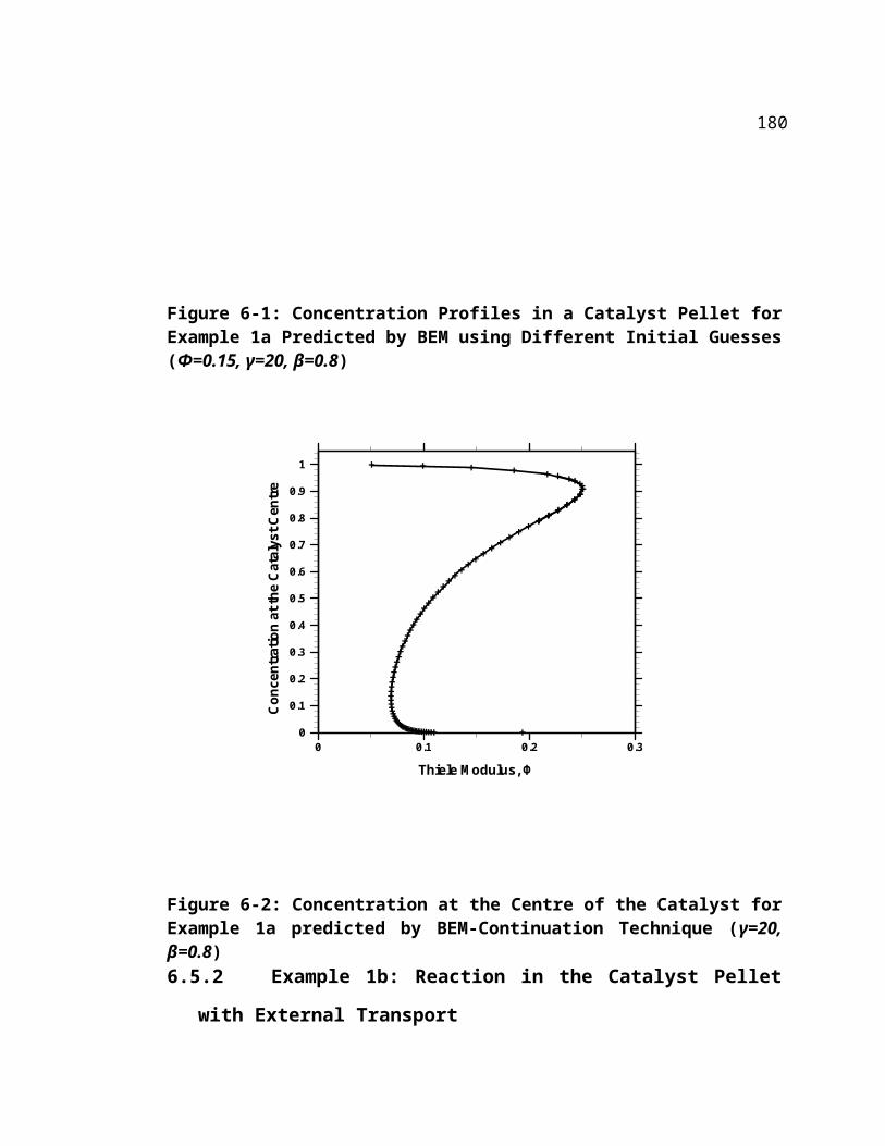
(A.4)

The other ways of determining the effect of film transport resistances and the criterion

to check the onset on internal transport resistances within the porous catalyst particles

are provided in Ramachandran and Chaudhari (1983).

A.2. Plug Flow Vs. Axial Dispersion Model

As a rule of thumb, if L/dp > 30 then axial dispersion can be neglected. Mears (1971)

proposed for a single nth order reaction, the deviation from the plug flow model is less

than 5% if the following holds:

(A.5)

A.3. Importance of Radial Variation in Temperature

For Arrhenius type kinetics with negligible axial heat dispersion, the influence of a non-

uniform cross section temperature profile on the heat generation (consumption) is less

than 5% (Mears, 1971) if:

(A.6)

180

Appendix B

Some of the Correlations for Predicting Transport

Properties

B.1. Effective Radial Thermal Conductivity

(i) Yagi and Wakao (1960)

(B.1)

For glass spheres and broken cement clinkers:

For metal spheres

Other correlations:

(ii) Bauer and Schlunder (1978a, 1978b)

(iii) Dixon and Cresswell (1979), Dixon (1988)

(iv) Specchia et al. (1980)

B.2. Effective Radial Diffusivity

181

(i) Specchia et al. (1980)

(B.2)

Other correlations:

(ii) Bauer and Schlunder (1978)

(iii) Rase, H.F. (1990)

B.3. Wall Heat Transfer Coefficient

(i) Li and Finlayson (1977)

Spherical particle, 0.05 < dh/dt < 0.3, 20 < Reh < 7600 :

(B.3a)

Cylindrical particle, 0.03 < dh/dt < 0.2, 20 < Reh < 800 :

(B.3b)

Other correlations:

(ii) Dixon (1988)

(iii) Specchia et al. (1980)

B.4. Overall heat transfer coefficient for 1-D model, U

182

(i) Li and Finlayson (1977)

Spherical particle, 0.05 < dh/dt < 0.3, 20 < Reh < 7600 :

(B.4a)

Cylindrical particle, 0.03 < dh/dt < 0.2, 20 < Reh < 800 :

(B.4b)

Other correlations:

(ii) Dixon (1988)

B.5. Axial Heat Dispersion Coefficient, λez

(i) Yagi et al.. (1960)

(B.5)

δ = 0.7 for steel balls, δ = 0.8 for glass beads. More data on δ and are available in

Yagi et al., (1960)

Other correlations:

(ii) Vortuba et al., (1972)

(iii) Dixon and Cresswell (1979)

B.6. Axial Mass Dispersion Coefficient, Dez

183

(i) Wen and Fan (1975)

0.008 < Re < 400, 0.28 < Sc < 2.2 (B.6)

184

Appendix C

2-D Steady State Model for Co-current Current Heat

Exchanger Reactor

The 2-D steady state model equations for the co-current reactor is modified (from those

presented in Chapter 4) as follows:

1) Scaling of the problem: In Eqs. 4.1-4.4, the radial coordinates for tube and shell

side are respectively from to and to . The radial co-

ordinates are rescaled so that it runs from 0 to 1, respectively, for both the sides

(to match the MATLAB convention and let us call this new variable as ).

2) Expand the radial diffusion term : By this modification, the option correspond-

ing to that of the slab geometry, in PDEPE, can be easily employed for both the

sides.

The modified governing equations for the co-current reactor are:

Tube side:

185

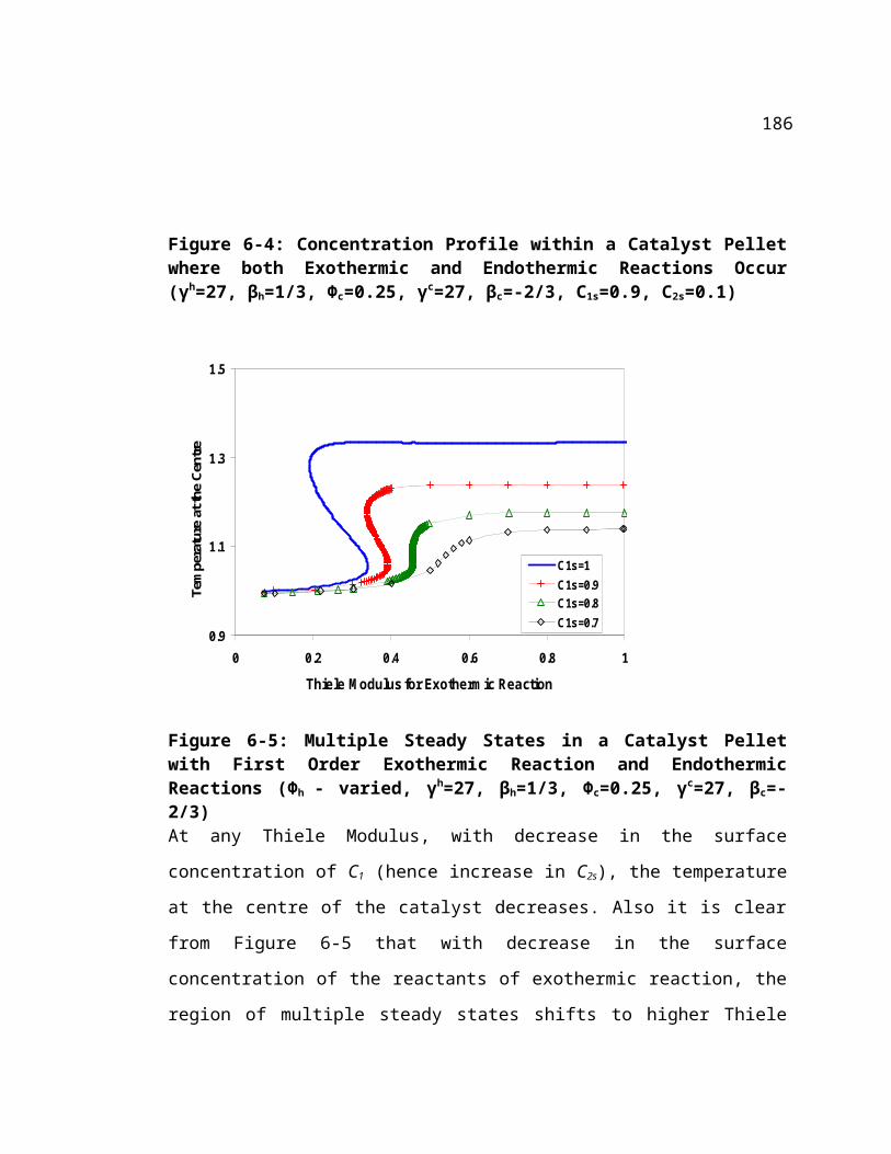
Shell side:

Here, [0,1]

Note that for the shell side, the variable at =0 corresponds to the wall and for the tube

side, =1, corresponds to the wall side.

The corresponding boundary conditions are:

186

187

References

Aasberg-Petersen et al., Technologies for large-scale gas conversion. Applied Catalysis A: General, 221, 2001, 379.

Agar, D.W., Multifunctional reactors: Old preconceptions and new dimensions. Chemical Engineering Science, 54, 1999, 1299

Arana, L.R. et al., A microfabricated suspended-tube chemical reactor for thermally efficient fuel processing. Journal of MEMS, 12, 2003, 600.

Aris, R., & Hatfield, B., Communications on the theory of diffusion and reaction – IV Combined effects of internal and external diffusion in the non-isothermal case. Chemical Engineering Science, 24(8), 1969, 1213.

Avci, A.K., Trimm, D.L., & Ilsen Onsan, Z., Heterogeneous reactor modeling for simulation of catalytic oxidation and steam reforming of methane. Chemical Engineering Science, 56, 2001, 641.

Barbero, A.J., Mafe, S., & Ramirez, P., Application of the boundary element method to convective electrodiffusion problems in charged membranes. Electrochimica Acta, 39, 1994, 2031.

Basini, L., Aasberg-Petersen, K., Guarinoni, A., & Ostberg, M., Catalytic partial oxidation of natural gas at elevated pressure and low residence time. Catalysis Today, 64, 2001, 9.

Bauer, R, and Schlunder, E.U., Effective radial thermal conductivity of packing in gas flow. Part I. Convective transport coefficient. Int. Chem. Eng,. 18 (2), 1978, 181

Bauer, R, and Schlunder, E.U., Effective radial thermal conductivity of packing in gas flow. Part II. Thermal conductivity of the packing fraction without gas flow. Int. Chem. Eng., 18 (2), 1978, 189.

188

Bharadwaj, S.S., & Schmidt, L.D., Synthesis gas formation by catalytic oxidation of methane in fluidized bed reactors. Journal of Catalysis, 146, 1994, 11.

Bharadwaj, S.S., & Schmidt, L.D., Catalytic partial oxidation of natural gas to syngas. Fuel Processing and Technology, 42, 1995, 109.

Biesheuvel, P.M., & Kramer, G.J., Two-section reactor model for autothermal reforming of methane to synthesis gas. AIChE Journal, 49, 2003, 1827.

Bizzi, M., Basini, L., Saracco, G., & Specchia, V., Short contact time catalytic partial oxidation of methane : analysis of transport phenomena effects. Chemical Engineering Journal, 90, 2002, 97.

Bizzi, M., Basini, L., Saracco, G., & Specchia, V., Modeling a transport phenomena limited reactivity in short contact time catalytic partial oxidation reactors. Industrial & Engineering Chemistry Research, 42(1), 2003, 62.

Bizzi, M., Schwiedernoch, R., Deutschmann, O., & Saracco, G., Modeling the partial oxidation of methane in a fixed bed with detailed chemistry. AIChE Journal, 50, 2004, 1289.

Burghardt, A., & Berezowski, M., Analysis of the structure of steady-state solutions for a porous catalyst pellet – I. Determination of parameter regions with different bifurcation diagrams. Chemical Engineering and Processing, 26, 1989, 45.

Burghardt, A., & Berezowski, M., Stability Analysis of steady-solutions for porous catalytic pellets. Chemical Engineering Science, 46, 1991, 2669.

Burghardt, A., & Berezowski, M., Periodic solutions in a porous catalyst pellet – homoclinic orbits. Chemical Engineering Scienc,. 58, 2003, 2657.

Chang, C.D., Mechanism of hydrocarbon formation from methanol. Studies of Surface Sciences and Catalysis, 36, 1988, 127.

189

Chaudhary, V.R., Rajput, A.M., & Prabhakar, B., Non-equilibrium oxidative conversion of methane to synthesis gas with high selectivity and productivity over nickel alumina at low temperatures. Journal of Catalysis, 139, 1993, 326.Chaudhary, V.R., Rane, V.H., & Rajput, A.M., High temperature catalytic oxidative conversion of propane to propylene and ethylene involving coupling of exothermic and endothermic reactions. Industrial and Engineering Chemistry Research, 39, 2000, 904.

Chen, Y.C., & Luss, D., Wrong-way behavior of packed bed reactors: influence of interphase transport. AIChE Journal, 35(7), 1989, 1148.

Dautzenberg.F.M., & Mukherjee, M., Process intensification using multifunctional reactors. Chemical Engineering Science, 56, 2001, 251.

de Groote, A.M., & Froment, G.F., Simulation of the catalytic partial oxidation of methane to synthesis gas. Applied Catalysis A: General ,138, 1996, 245.

de Groote, A.M., Froment, G.F., & Kobylinski, Th., Synthesis gas production from natural gas in a fixed bed reactor with reversed flow. Canadian Journal of Chemical Engineering, 74, 1996, 735.

de Morais, E.R., de Toledo, E.C.V., Filho, R.M., & Maciel, M.R.W., Alternative designs for fixed bed catalytic reactors. International Journal of Chemical Reactor Engineering, 2, 2004, A28.

de Smet, C.R.,H., de Croon, M.H.J.M., Berger, R.J., Marin, G.B., & Schouten, J.C., Design of adiabatic fixed-bed reactors for the partial oxidation of methane to synthesis gas. Application to production of methanol and hydrogen-for-fuel cells. Chemical Engineering Science ,56, 2001, 4849.

Deshmukh, S.R., & Vlachos, D.G., CFD Simulations of coupled, countercurrent combustor/reformer microdevices for hydrogen production. Industrial and Engineering Chemistry Research, 44(14), 2005, 4982.

Deutschmann, O. & Schmidt, L.D., Twenty-Seventh Symposium (International) on Combustion / The Combustion Institute, 1998, 2283.

190

Deutschmann,O., & L.D. Schmidt, Modeling the partial oxidation of methane in a short-contact-time reactor. AIChE Journal, 44, 1998, 2465.

Dixon, A.G., & Cresswell, D.L. Theoretical prediction of effective heat transfer parameters in packed beds. AIChE Journal, 25 (4), 1979, 663.

Dixon, A.G. Wall and particle shape effects on heat transfer in packed bed. Chemical Engineering Communications, 71, 1988, 217.

Doedel, E.J., Champneys, A.R., Fairgrieve, T.F., Kuznetsov, Y.A., Sandstede, B., & Wang, X. (1997). AUTO97: continuation and bifurcation software for ordinary differential equations, Technical report, computational mathematics laboratory. Concordia University.

Dommeti, S.M.S., Balakotaiah, V., & West, D.H., Analytical Criterial for Validity of pseudohomogeneous models of packed-bed catalytic reactors. Industrial Engineering and Chemistry Research, 38, 1999, 767.

Dupont, V., Zhang, S., Bentley, R., & Williams, A., Experimental and modeling studies of the catalytic combustion of methane. Fuel, 81, 2002, 799.

Ermentrout (2002). Simulating, analyzing, and animating dynamical systems: a guide to XPPAUT for researchers and students. SIAM, Philadelphia.

Frauhammer, J., Eigenberger, G., Hippel, L.v., & Arntz, D., A new reactor concept for endothermic high-temperature reactions. Chemical Engineering Science, 54, 1999, 3661.

Freide, J.F., Gamlin, T., & Ashley, M., The ultimate ‘clean’ fuel – Gas-to-liquids products. Hydrocarbon Processing, February 2003, 53.

Fukuhara, C., & Igarashi, A. Performance simulation of a wall-type reactor in which exothermic and endothermic reactions proceed simultaneously, comparing with that of a fixed-bed reactor. Chemical Engineering Science, 60, 2005, 6824.

Godunov, S.K., Finite-difference method for numerical computation of discontinuous solutions of the equations of fluid dynamics. Mat. Sb., 47, 1959, 271.

191

Golubitsky, M., & Schaeffer, D., Singularities and groups in bifurcation theory, Volume 1, Springer, New York, USA, first edition, 1985.Gomez, J.P., Jimenez, J.M., Vic, S., Lezaun, J., Terreros, P., Pena, M.A, & Fierro, J.L.G., Hydrogen production on nickel monolith structure by partial oxidation of methane at high pressure. 4th International Natural Gas Conversion Symposium, South Africa, 1995.

Grasselli, R.K., Stern, D.L., & Tsikoyiannis, J.G., Catalytic dehydrogenation (DH) of light paraffins combined with selective hydrogen combustion (SHC).I.DH SHC DH catalysts in series (co-fed process mode). Applied Catalysis A: General, 189, 1999a, 1.

Grasselli, R.K., Stern, D.L., & Tsikoyiannis, J.G., Catalytic dehydrogenation (DH) of light paraffins combined with selective hydrogen combustion (SHC).I.DH SHC DH catalysts physically mixed (redox process mode). Applied Catalysis A: General, 189, 1999b, 9.

Gosiewski, K., Simulations of non-stationary reactors for the catalytic conversion of methane to synthesis gas. Chemical Engineering Science, 56, 2001, 1501.

Harten, A., High resolution schemes for hyperbolic conservation laws. Journal of Computational Physics, 49, 1983, 357.

Harten, A., On a class of high resolution total variation stable finite difference schemes. SIAM Journal of Numerical Analysis, 21, 1984, 1.

Henning, D.A., & Schmidt, L.D., Oxidative dehydrogenation of ethane at short contact times: Species and temperature profiles within and after the catalyst. Chemical Engineering Science, 57, 2002, 2615.

Hickman, D.A., & Schmidt, L.D., Synthesis gas formation by direct oxidation of methane over Pt. monoliths. Journal of Catalysis, 138, 1992, 267.

Hickman, D.A., & Schmidt, L.D., Production of synthesis gas by direct oxidation of methane. Science, 259, 1993, 343.

192

Hinderink, A.P. et al., Exergy analysis with a flow sheeting simulation – I. Theory, calculating exergies of material streams. Chemical Engineering Science, 51(20), 1996, 4693.

Hindermann, J.P., Hutchings, G.J., & Kieennemann, A., Mechanistic aspects of the formation of hydrocarbons and alcohol from carbon monoxide hydrogenation. Catalyst Reviews: Science and Engineering, 35, 1993, 1.

Hlavacek, V., & Hoffman, H., Modeling of chemical reactors – XVII. Steady state heat and mass transfer in tubular reactors. Numerical investigation of multiplicity. Chemical Engineering Science, 25, 1970, 173.

Hohn , K.L., & Schmidt, L.D., Partial oxidation of methane to syngas at high space velocities over Rh-coated spheres. Applied Catalysis A: General ,211, 2001 53.

Hu, R., Balakotaiah, V., & Luss, D., Multiplicity features of porous catalytic pellets-I. Single zeroth order reaction case. Chemical Engineering Science, 40, 1985a, 589.

Hu, R., Balakotaiah, V., & Luss, D., Multiplicity features of porous catalytic pellets-II. Influence of reaction order and pellet geometry. Chemical Engineering Science, 40, 1985b, 599.

Hu, R., Balakotaiah, V., & Luss, D., Multiplicity features of porous catalytic pellets-III. Uniqueness criteria for the lumped thermal model. Chemical Engineering Science, 41, 1985c, 1525.

Hudgins, R.R., A general criterion for avoiding film diffusion control in heterogeneous catalytic reaction. Canadian Journal of Chemical Engineering, 50, 1972, 427.

Hunter, J.B., & McGuire, G., Method and apparatus for catalytic heat exchange. US Patent 4 214 867, 1980.

Igarshi, A., Fukuhara, C., Takeshita, S., Nishino, C., & Hanawa, M., Apparatus and method for preparing reformed gas by means of electroless plating, US Patent 5167865, 1992.

193

Ioannides, Th., & Verykios, X.E., Catalytic partial oxidation of methane in a novel heat integrated wall reactor. Catalysis Letters, 47, 1997, 183.

Ioannides, Th., & Verykios, X.E., Development of a novel heat-integrated wall reactor for the partial oxidation of methane to synthesis gas. Catalysis Today, 46, 1998, 71.

Iordanidis, A.A. Mathematical modeling of catalytic fixed bed reactors. Ph.D. Dissertation. University of Twente, 2002.

Ismagilov, Z.R., Pushkarev, V.V., Podyacheva, Yu. O., Koryabkina, N.A., & Veringa, H., A catalytic heat-exchanging tubular reactor for combining of high temperature exothermic and endothermic reactions. Chemical Engineering Journal, 82, 2001, 355.

Kaminsky, M.P., Huff Jr., G.A., Calamur, N., & Spangler, M.J., Catalytic wall reactors and use of catalytic wall reactors for methane coupling and hydrocarbon cracking reaction. US Patent 05599510, 1997.

Kirillov, V.A., Kuzin, N.A., Mescheryakov, V.D., & Droboshevich, V.I., Catalytic heat-exchanger reactor for strongly exothermic reactions. Chemical Engineering Science, 56, 2001 381.

Koga, M., & Watanabe, T., Plate type reformer, US Patent 5015444, 1991.

Kohout, M., Schreiber, I., & Kubicek, M., A computational tool for nonlinear dynamical and bifurcation analysis of chemical engineering problems. Computers and Chemical Engineering, 26, 2002, 517-527.

Kolios, G., Frauhammer, J., & Eigenberger, G., Autothermal fixed bed reactor concepts. Chemical Engineering Science, 55, 2000, 5945.

Kolios, G., Frauhammer, J., & Eigenberger, G., A simplified procedure for the optimal design of autothermal reactors for endothermic high-temperature reactions. Chemical Engineering Science, 56, 2001, 351.

194

Kolios, G., Frauhammer, J., & Eigenberger, G., Efficient reactor concepts for coupling of endothermic and exothermic reactions. Chemical Engineering Science, 57, 2002, 1505.

Kolios, G., Gloeckler, B., Gritsch, A., Morillo, A., & Eigenberger, G., Heat-integrated reactor concepts for hydrogen production by methane steam reforming. Fuel Cells, 5(1), 2005, 52.

Kubicek, M., & Marek, M., Computational methods in bifurcation theory and dissipative structures. Springer Verland, New York, USA, 1983

Kulkarni, M.S., Dynamics of asymmetric fixed-bed reactors – coupling of exothermic and endothermic reactions (creep, autothermal). D.Sc. Dissertation, Washington University, St. Louis, Missouri, USA, 1996.

Kulkarni, M.S., & Dudukovic, M.P., Dynamics of gas phase and solid phase reactions in a fixed bed reactors. Chemical Engineering Science, 51, 1996, 3083.

Kulkarni, M.S., & Dudukovic, M.P., Periodic operation of asymmetric bidirectional fixed-bed reactors with temperature limitations. Industrial and Engineering Chemistry Research, 37, 1998, 770.

Lax, P.D., Hyperbolic systems of conservation laws and mathematical theory of shock waves. Society for Industrial and Applied Mathematics, 1973, Philadelphia, PA.

Lesage, F., Latifi, M.A., & Midoux, N., Boundary element method in modeling of momentum transport and liquid-to-wall mass transfer in a packed bed reactor. Chemical Engineering Science, 55, 2000, 455-460.

Li, C., & Finlayson, B.A., Chemical Engineering Science, 32, 1977, 1055.

Liu, Y., & Jacobsen, E.W., On the use of reduced order models in the bifurcation analysis of distributed parameter systems. Computers and Chemical Engineering, 28, 2004, 161.

195

Ma, L., & Trimm, D.L., Alternative catalyst bed configurations for the autothermic conversion of methane to hydrogen. Applied Catalysis A: General, 138, 1996, 265.

Mancusi, E., Merola, G., & Crescitelli, S., Multiplicity and hysteresis in an industrial ammonia reactor. AIChE Journal, 44, 2000, 888.Mears, D.E., Diagnostics criteria for heat transport limitations in fixed bed reactors. Journal of Catalysis, 20, 1971, 127.

Mills, A.F., Heat and Mass Transfer, Irwin Inc., 1995.

Moran, M.J. Availability Analysis: A Guide to Efficient Energy Use. Prentice-Hall, Englewood Cliffs, New Jersey, 1982.

Nielsen, A., Ammonia synthesis : exploratory & applied research. Catalysis Reviews – Science and Engineering, 23, 1981, 17.

Numaguchi, T., & Kikuchi, K., Intrinsic kinetics and design simulation in a complex reaction network: Steam-methane reforming. Chemical Engineering Science, 43, 1988, 2295.

Ondrey, G., Autothermal reformer promises to lower investment costs for making syngas, Chemical Engineering, September 2003, 17.

Pena, M.A., Gomez, J.P., & Fierro, J.L.G., New catalytic routes for syngas and hydrogen production. Applied Catalysis A: General 144, 1996, 7.

Pinjala, V., Chen Y.C., & Luss, D., Wrong-way behavior of packed-bed reactors: II Impact of thermal dispersion. AIChE J., 34(10), 1988, 1148.

Poirier, M.G., Jean, G, & Poirier, M.P., Partial oxidation of methane over a praseodymium / ruthenium pyrochlore catalyst. Studies in surface science and catalysis, 73, 1992, 359.

Polman, E.A., Der Kinderen, J.M., & Thuis, F.M.A., Novel compact steam reformer for fuel cells with heat generation by catalytic combustion augmented by induction heating. Catalysis Today, 47, 1999, 347.

196

Prins, R., de Beer, V.H.J., & Somorjai, G.A., Structure and function of the catalyst and the promoter in cobalt molybdenum hydrodesulphurization catalysts. Catalyst Science : Reviews and Engineering, 31, 1989, 1.

Ramachandran, P.A., & Chaudhari, R.V. Three-phase catalytic reactors. Gordon and Breach Science Publishers, New York, 1983.

Ramachandran, P.A., Application of the boundary element method to non-linear diffusion with reaction problems. International Journal of Numerical Methods in Engineering, 29, 1990, 1021.

Ramachandran, P.A., Boundary element methods in transport phenomena. Elsevier Applied Science, New York, USA, 1994.

Ramachandran, P.A., Boundary element methods for solution of dispersion models for packed bed reactors. Industrial & Engineering Chemistry Research, 44(14), 2005, 5364.

Ramaswamy, R.C., Reduced order models for simulation of crude distillation unit, M.Tech. Thesis, IIT Kanpur, India, 1999.

Ramaswamy, R.C., Ramachandran, P.A., & Dudukovic, M.P. Coupling of exothermic and endothermic reactions in simultaneous and sequential directly coupled adiabatic reactors. Proceedings of 7th World Congress on Chemical Engineering, 2005.

Ramaswamy, R.C., Ramachandran, P.A., & Dudukovic, M.P. Modeling of solid acid catalyzed alkylation reactors. International Journal of Chemical Reactor Engineering, Vol.3, 2005, A42.

Ramaswamy, R.C.; Ramachandran, P.A.; Dudukovic, M.P. Recuperative Coupling of Exothermic and Endothermic Reactions. Chemical Engineering Science, 2006, 61, 459.

Rase, H.F., Fixed-bed reactor design and diagnostics, Butterworth publishers, 1990Reuse, P. et al. Hydrogen production for fuel cell application in an autothermal micro-channel reactor. Chemical Engineering Journal, 101, 2004, 133.

197

Ridler, D.E., & Twigg, M.V., Steam Reforming. In M.V. Twigg (Ed.), Catalyst handbook. London: Wolfe Publishing Ltd, 1989.

Robbins F.A., Zhu, H., & Jackson, G.S., Transient modeling of combined catalytic combustion/CH4 steam reforming. Catalysis Today, 83, 2003, 141.

Ruhl, R.C., Hardman, S., Kenyon, M.R., & McFarlane, R.A., Endothermic reaction apparatus. US Patent 6,096,106, 2000.

Salinger, A.G., Bou-Rabee, N.M., Pawlowski, R.P., Wilkes, E.D., Burroughs, E.A., Lehoucq, R.B., Romero, L.A. (2002). LOCA 1.1 - Library of continuation algorithms: Theory and implementation manual. Sandia National Laboratories, USA.

Smit, J., van Sint Annaland, M., & Kuipers, J.A.M., Modeling of a Reverse Flow Catalytic Membrane Reactor for the Partial Oxidation of Methane. International Journal of Chemical Reactor Engineering, 1, 2003, A54.

Smit, J., Bekink, G.J., van Sint Annaland, M., & Kuipers, J.A.M., A reverse flow catalytic membrane reactor for the production of syngas: An experimental study. International Journal of Chemical Reactor Engineering, 2005, 3, Article A12.

Smith, J. M., van Ness, H. C., & Abbott, M. Introduction to Chemical Engineering Thermodynamics, 5th ed. McGraw-Hill, New York, 1996.

Specchia, V., Baldi, G., & Sicardi, S. Heat transfer in packed bed reactors with one phase flow. Chemical Engineering Communications, 4, 361-380, 1980.

Szargut, J., Morris, D., & Stewart, F. Exergy Analysis of Thermal, Chemical and Metallurgical Processes, Hemisphere Publications Company, New York, 1988.

Tannehill, J.C., Anderson, D.A., & Pletcher, R.H., Computational Fluid Mechanics and Heat Transfer – second edition, Taylor & Francis, Philadelphia, 1997.

198

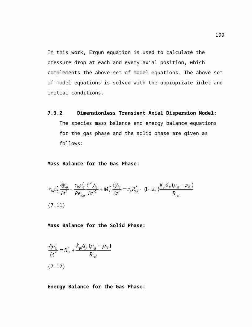
Vande Wouwer, A., Saucez, Ph., & Schiesser, W.E., Adaptive Method of Lines, CRC Press, Boca Raton, 2001.

van Leer, B., Flux vector splitting for the Euler equations, Proceedings of the 8 th

International Conference on Numerical Methods in Fluid Dynamics. Lecture Notes in Physics, 170 (1982) Springer-Verlag, New York.

van Sint Annaland, M, & Nijssen, R.C., A novel reverse flow reactor coupling exothermic and endothermic reactions : an experimental study. Chemical Engineering Science, 57, 2002, 4967-4985.

Varma, A., & Amundson, N.R., Some observations on uniqueness and multiplicity of steady states in non-adiabatic chemically reacting systems. Canadian Journal of Chemical Engineering, 51, 1973, 206.

Venkataraman, K., Redenius, J.M., & Schmidt, L.D., Millisecond catalytic wall reactors: Dehydrogenation of ethane. Chemical Engineering Science, 57, 2002, 2355.

Venkataraman, K., Wanat, E.C., & Schmidt, L.D., Steam reforming of methane and water-gas shift in catalytic wall reactors. AIChE Jounal, 49, 2003, 1277.

Veser, G., & Frauhammer, J., Modelling steady state and ignition during catalytic methane oxidation in a monolith reactor. Chemical Engineering Science, 55, 2000, 2271.

Vortuba, I., Hlavacek, V., & Marek, M., Packed bed axial thermal conductivity. Chemical Engineering Science, 27, 1972, 1845.

Wakao, N., & Kaguei, S., Heat and mass transfer in packed beds. Gordon and Breach Science Publishers, New York, 1982.

Wen, C.Y. & Fan, L.T., Models for flow systems and chemical reactors, Dekker, New York, 1975.

Xu, J. & Froment, G.F., Methane steam reforming, methanation and water-gas shift: I. intrinsic kinetics. AIChE Journal, 35, 1989, 88.

199

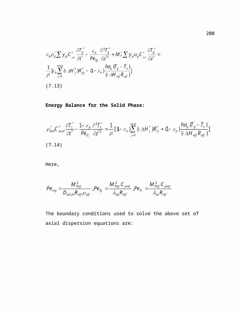
Yagi, S., Kuni, D., & Wakao, N., Studies on axial thermal conductivities in packed beds. AIChE Journal, 6(4), 1960, 543.

Zanfir, M., & Gavriilidis, A., Modelling of a catalytic plate reactor for dehydrogenation-combustion coupling, Chemical Engineering Science, 56, 2001, 2671.

Zanfir, M., & Gavriilidis, A., Catalytic combustion assisted methane steam reforming in a catalytic plate reactor. Chemical Engineering Science, 58, 2003, 3947.

Zanfir, M., & Gavriilidis, A., Influence of flow arrangement in catalytic plate reactors for methane steam reforming. Chemical Engineering Research and Design, 82, 2004, 252.

200

VITA

Name: Ramaswamy C. Ramaswamy

Date of Birth: June 11, 1976

Place of Birth: Tenkasi, India

Education

D. Sc. in Chemical Engineering, May 2006 Thesis: Steady State and Dynamic Reactor Models for Coupling Exothermic and Endothermic Reactions Chemical Reaction Engineering Laboratory, Washington University, St. Louis, Missouri, USA

M.Tech. in Chemical Engineering, May 1999Thesis: Reduced Order Models for Simulation of Crude Distillation UnitIndian Institute of Technology, Kanpur (IITK), India

B.Tech. in Chemical Engineering, May 1997A.C. College of Technology (A.C. Tech), Anna University, Chennai, India

Work Experience

· Research Scientist, R&D, Bharat Petroleum Corporation Limited (BPCL), Mumbai – 74 (July 1999 – July 2001)

Other Technical Assignments

· Kinetic and Reactor Modeling of Hydrogenation of Maleic Acid to Butanediol– BP Chem-icals, USA : design of laboratory experiments, data analysis, development of kinetic and reactor mod-els, trouble-shooting (January 2005 – March 2006)

· Modeling of Solid Acid Catalyzed Alkylation Processes at the Center for Environmentally Ben-eficial Catalysis (CEBC, a National Science Foundation Engineering Research Center) : development of multi-scale steady state and dynamic reactors models, optimization of reactor and catalyst perfor -mance (Summer 2004 – February, 2006)

Publications

· R.C. Ramaswamy, P.A. Ramachandran, and M.P. Duduković, “Recuperative Coupling of Exothermic and Endothermic Reactions”, Chemical Engineering Science, 61, 459-472, 2006

201

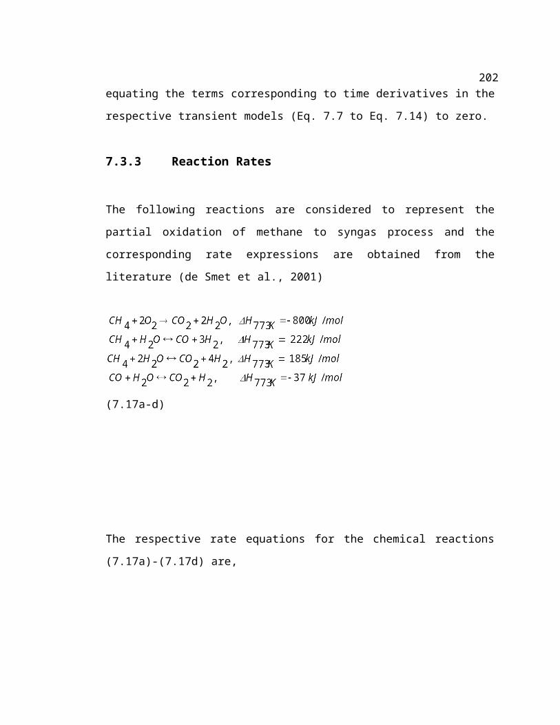
· R.C. Ramaswamy, P.A. Ramachandran, and M.P. Duduković, “Modeling of Solid Acid Cat-alyzed Alkylation Reactors”, International Journal of Reactor Engineering, A42, Vol.3, 2005

· R.C. Ramaswamy, P.A. Ramachandran, and M.P. Duduković, “Exothermic and Endothermic Reactions in Simultaneous and Sequential Directly Coupled Adiabatic Reactors”, proceedings of 7th World Congress of Chemical Engineering, Glasgow, Scotland (10-14 July 2005)

· R.C. Ramaswamy, and D.N. Saraf, “Reduced Order Modeling of a Crude Distillation Unit for Online Applications”, Journal of Chemical Engineering of Japan, 35 (8), 714-728, 2002

· R.C. Ramaswamy, and P.A. Ramachandran, “Multiple Steady States in Distributed Parame-ter Systems using Boundary Element and Arc Length Continuation Methods”, sent for publica-tion

· R.C. Ramaswamy, V. Venkataramani, K. Arora, and B. Khomami, “Effect of Energetics on In-terfacial Stability of Two Polymeric Fluids”, in preparation

· R.C. Ramaswamy, P.A. Ramachandran, and M.P. Duduković, “Modeling of Catalytic Partial Oxidation of Methane to Synthesis Gas in Short Contact Time Packed Bed Reactors”, in prepara-tion

· R.C. Ramaswamy, P.A. Ramachandran, and M.P. Duduković, “Analysis of Heat Exchanger Reactors using Two Dimensional Models”, in preparation

Presentations

· Modeling of Catalytic Partial Oxidation of Methane to Syngas in Short Contact Time Packed Bed Reactors, AIChE Annual Meeting 2005, Cincinnati, OH, USA, November 2005

· Reactors for Solid Acid Catalyzed Alkylation Processes, AIChE Annual Meeting 2005, Cincin-nati, OH, USA, November 2005

· Modeling of Solid Acid Catalyzed Alkylation Reactors, Tenth Conference on Reactor Engineer-ing (CRE-X), Zacatecas, Mexico, August 2005

· Exothermic and Endothermic Reactions in Simultaneous and Sequential Directly Coupled Adiabatic Reactors, 7th World Congress of Chemical Engineering, Glasgow, Scotland, July 2005

· Dynamics of Coupling Exothermic and Endothermic Reactions in Directly Coupled Adiabatic Reactors, AIChE Annual Meeting 2004, Austin, TX, USA, November 2004

· Steady State and Dynamic Reactor Models for Coupling Exothermic and Endothermic Reac-tions, ISCRE-18, Chicago, USA, June 2004

· Fuel for Fuel Cells, Annual Graduate Student Symposium, Washington University, St. Louis, April 2004 (received second prize)

· Dynamics of Coupling Exothermic and Endothermic Reactions, AIChE Annual Meeting 2003, San Francisco, USA, November 2003

· Gamma Scanning as a Diagnostic Tool for Refinery Plant Trouble Shooting, PETROTECH-2001, 4th International Petroleum Conference and Exhibition, New Delhi, India, January 2001

· Enhancement of Selectivity of Extraction of Aromatics from Petroleum Naphtha – a Simula-tion Study, Chemcon 2000, Calcutta, India, December 2000

Honors

· Recipient of award for Outstanding Departmental Seminar Presented by a Graduate Student, 2004-2005, Washington University in St. Louis

· Recipient of EIL Merit Scholarship for 1998-1999, Indian Institute of Technology, Kanpur· Recipient of A.C.Tech. Alumni Association Merit Scholarship for 1995-1996 and 1996-1997,

A.C.Tech, Anna University

Extra-Curricular Activities

· Member, AIChE· President of Umang, Indian Graduate Student Association of Washington University (2003-2004)· Teaching Assistant - ChE 471, ChE 512 etc. (Fall 2001 – Fall 2005, Washington University in St.

Louis)

202

May, 2006

Short Title: Coupling Exo-Endo Reactions Ramaswamy, D.Sc. 2006

203