production of biodiesel from soybean oil using
TRANSCRIPT
University of South FloridaScholar Commons
Graduate Theses and Dissertations Graduate School
3-10-2016
Production of Biodiesel from Soybean Oil UsingSupercritical MethanolShriyash Rajendra Deshpande
Follow this and additional works at: http://scholarcommons.usf.edu/etd
Part of the Oil, Gas, and Energy Commons, and the Statistics and Probability Commons
This Thesis is brought to you for free and open access by the Graduate School at Scholar Commons. It has been accepted for inclusion in GraduateTheses and Dissertations by an authorized administrator of Scholar Commons. For more information, please contact [email protected].
Scholar Commons CitationDeshpande, Shriyash Rajendra, "Production of Biodiesel from Soybean Oil Using Supercritical Methanol" (2016). Graduate Thesesand Dissertations.http://scholarcommons.usf.edu/etd/6080
Production of Biodiesel from Soybean Oil Using Supercritical Methanol
by
Shriyash R. Deshpande
A thesis submitted in partial fulfillment
of the requirements for the degree of
Master of Science in Chemical Engineering
Department of Chemical and Biomedical Engineering
College of Engineering
University of South Florida
Co-Major Professor: Aydin K. Sunol, Ph.D.
Co-Major Professor: George P. Philippidis, Ph.D.
John N. Kuhn, Ph.D.
Date of Approval:
March 8, 2016
Keywords: Vegetable Oils, Transesterification, Methyl Esters,
Gas Chromatography, Factorial Design, Supercritical Alcohol
Copyright © 2016, Shriyash R. Deshpande
ACKNOWLEDGMENTS
I would like to thank the faculty members of my committee, Dr. Aydin Sunol, Dr. George
Philippidis, and Dr. John Kuhn. The completion of this work would not have been possible without
the guidance of Dr. Aydin Sunol whom I thank for his support and motivation throughout the
duration of this work. Working with Dr. Sunol has been a great learning experience. I would also
like to thank Dr. George Philippidis for his support and his timely advice in moving the project
forward on the right path. Dr Philippidis has been an invaluable resource. I would like to extend
my acknowledgements to Dr. Laurent Calcul and Andrew Shilling from the Chemodiversity
facility (CDDI) for their assistance in sample analysis.
I would like to thank Vignesh Subramanian for assisting me in reviewing the experimental
design and its analyses. This work would be incomplete without acknowledging the assistance and
support from the other members of the EFES research group. I thank Kyle Cogswell, Aaron
Driscoll, Ahmet Manisali and Zachary Cerniga for their assistance throughout the completion of
this project.
I would like to thank my parents for giving me an opportunity to pursue my dreams, and
supporting me through the ups and downs during the completion of this work. Fruitful research
needs patience and dedication. I thank my parents and my brother Yashodhan, for believing in me
and for pushing me through the hard times. I owe this accomplishment to your loving support. Last
but not the least, I would like to take this opportunity to thank my close friends, Prasad, Abhijeet,
Amol, Kaustubh, Bhuvan, Lokesh, Gunjan, Vishal, Vaishnavi, Rishi and Rashmi. Without the
strong bonds of our friendship, this work would not have been possible.
i
TABLE OF CONTENTS
LIST OF TABLES ......................................................................................................................... iii
LIST OF FIGURES .........................................................................................................................v
ABSTRACT .................................................................................................................................. vii
CHAPTER 1: INTRODUCTION ....................................................................................................1
CHAPTER 2: CONVENTIONAL BIODIESEL PRODUCTION TECHNOLOGIES ...................5
2.1 Direct Use of Vegetable Oils .........................................................................................5 2.2 Pyrolysis .........................................................................................................................5 2.3 Microemulsions..............................................................................................................6
2.4 Transesterification..........................................................................................................7 2.4.1 Base-Catalyzed Transesterification ................................................................8
2.4.2 Acid-Catalyzed Transesterification ................................................................9 2.4.3 Enzyme-Catalyzed Transesterification .........................................................11
CHAPTER 3: BIODIESEL PRODUCTION USING SUPERCRITICAL FLUID
TECHNOLOGY ................................................................................................................12
3.1 Supercritical Fluids ......................................................................................................12 3.2 Supercritical Transesterification ..................................................................................14 3.3 Advantages and Disadvantages of Supercritical Transesterification ...........................17
CHAPTER 4: FEEDSTOCKS FOR BIODIESEL PRODUCTION ..............................................19 4.1 Vegetable Oils ..............................................................................................................20
4.2 Animal Fats ..................................................................................................................21 4.3 Microalgae ...................................................................................................................22
CHAPTER 5: EXPERIMENTAL WORK ....................................................................................25 5.1 Experimental Setup and Equipment.............................................................................25 5.2 Chemicals and Raw Materials .....................................................................................28
5.3 Experimental Design ....................................................................................................29 5.4 Experimental Procedure ...............................................................................................31 5.5 Analysis of Samples .....................................................................................................33
5.5.2 Calibration Plots............................................................................................35
5.5.3 Sample Preparation and Quantitative Analysis.............................................37 5.6 Analysis Results ...........................................................................................................40
CHAPTER 6: ANALYSIS OF VARIANCE (ANOVA) AND DEVELOPMENT OF
REGRESSION EQUATION .............................................................................................46
ii
6.1 Surface Plots ................................................................................................................49 6.2 Residual Analysis.........................................................................................................51
CHAPTER 7: A SIMPLE LUMPED TENDENCY MODEL FOR
TRANSESTERIFICATION ..............................................................................................52
7.1 Kinetic Tendency of the Reaction and Estimation of Rate Constants .........................52 7.2 Arrhenius Plot and Activation Energy .........................................................................56
CHAPTER 8: CONCLUSIONS AND RECOMMENDATIONS .................................................58 8.1 Conclusions ..................................................................................................................58 8.2 Recommendations and Future Work ...........................................................................59
REFERENCES ..............................................................................................................................61
APPENDIX A: LIST OF NOMENCLATURE .............................................................................70
APPENDIX B: ELECTRON IONISATION SPECTRA FOR METHYL ESTERS ....................71
B.1 Relative Size of Biodiesel Peaks .................................................................................71 B.2 Electron Ionization (EI) Spectra for Methyl Esters .....................................................72
APPENDIX C: CALCULATIONS ...............................................................................................76
C.1 Biodiesel Yield Calculation Methodology ..................................................................76 C.2 Coded Variables ..........................................................................................................77
C.3 Analysis of Variance (ANOVA) Calculations ............................................................77 C.4 Test for Non-Linearity of the Model ...........................................................................81 C.5 Calculations for Arrhenius Plot ...................................................................................82
iii
LIST OF TABLES
Table 3-1 Comparison of typical values of transport properties of gases, supercritical
fluids and liquids ...........................................................................................................13
Table 3-2 Comparison of transesterification processes .................................................................15
Table 4-1 Comparison of energy efficiency and fossil energy consumption between
feedstocks ......................................................................................................................24
Table 5-1 Front inlet and column flow settings .............................................................................35
Table 5-2 Temperature programming of GC .................................................................................35
Table 5-3 Yield data.......................................................................................................................42
Table 6-1 Coded values .................................................................................................................47
Table 6-2 Analysis of variance (ANOVA) ....................................................................................47
Table 6-3 P-values for the factors and interactions .......................................................................48
Table 6-4 Test for curvature ..........................................................................................................48
Table 6-5 P-values and regression models.....................................................................................49
Table 7-1 Rate constants determined with non-linear regression ..................................................54
Table 7-2 Activation energy and pre-exponential factor for the forward reaction ........................57
Table C-1 Peak areas for methyl esters ..........................................................................................76
Table C-2 Yield of biodiesel ..........................................................................................................77
Table C-3 ANOVA table with sum of output ................................................................................78
Table C-4 Contrasts, effects, sum of squares and mean squares for the factors and
interactions ....................................................................................................................78
Table C-5 Calculations for z-value ................................................................................................79
Table C-6 F-test to determine significance ....................................................................................81

iv
Table C-7 Calculations for Arrhenius plot.....................................................................................82
v
LIST OF FIGURES
Figure 1-1 Distillate fuel oil price projections in three cases through 2040 ....................................2
Figure 1-2 Biodiesel production capacities ......................................................................................3
Figure 2-1 General transesterification mechanism. .........................................................................7
Figure 3-1 Schematic phase diagram for pure fluid in supercritical state .....................................13
Figure 3-2 Three step transesterification mechanism ....................................................................16
Figure 4-1 Microalgae pretreatment flowchart ..............................................................................23
Figure 5-1 Autoclave, heating tape and Magnedrive assembly .....................................................26
Figure 5-2 Sampling chamber ........................................................................................................27
Figure 5-3 Spray nozzle. ................................................................................................................28
Figure 5-4 Process diagram ...........................................................................................................28
Figure 5-5 Experimental design .....................................................................................................29
Figure 5-6 Controller screen. .........................................................................................................32
Figure 5-7 Gas chromatograph ......................................................................................................33
Figure 5-8 HP-INNOWax column .................................................................................................34
Figure 5-9 Chromatograms for the calibration standard ................................................................36
Figure 5-10 Calibration plot for methyl heptadecanoate internal standard. ..................................37
Figure 5-11 Collected sample and phases after 24 hour disengagement period ............................38
Figure 5-12 Biodiesel chromatogram. ...........................................................................................40
Figure 5-13 Integrated methyl ester peaks .....................................................................................41
Figure 5-14 Yield versus Time plot for biodiesel samples (center point at 317.5 °C and 36.5
molar ratio) .................................................................................................................43
vi
Figure 5-15 Yield vs Time plot for 325 °C and 43:1 molar ratio. .................................................43
Figure 5-16 Yield vs Time plot for 310 °C and 43:1 molar ratio. .................................................44
Figure 5-17 Yield vs Time plot for 325 °C and 30:1 molar ratio. .................................................44
Figure 5-18 Yield vs Time plot for 310 °C and 30:1 molar ratio. .................................................45
Figure 5-19 Yield vs Time plot for 317.5 °C and 36.5:1 molar ratio (center point) .....................45
Figure 6-1 Surface plot of Yield vs Molar Ratio ...........................................................................50
Figure 6-2 Surface plot of Yield vs Temperature ..........................................................................50
Figure 6-3 Normality plot of residuals...........................................................................................51
Figure 7-1 Experimental and predicted data at 325 °C and 43:1 molar ratio. ...............................55
Figure 7-2 Experimental and model data at 310 °C and 30:1 molar ratio. ....................................56
Figure 7-3 Arrhenius plot for forward reaction. ............................................................................57
Figure B-1 Relative size of peaks ..................................................................................................71
Figure B-2 EI Spectra for Palmitic acid methyl ester ....................................................................72
Figure B-3 EI Spectra for Margaric acid methyl ester (internal standard) ....................................72
Figure B-4 EI Spectra for Stearic acid methyl ester ......................................................................73
Figure B-5 EI Spectra for Oleic acid methyl ester .........................................................................73
Figure B-6 EI Spectra for Linoleic acid methyl ester ....................................................................74
Figure B-7 EI Spectra for Linolenic acid methyl ester ..................................................................74
Figure B-8 EI Spectra for Eicosanoic acid methyl ester ................................................................75
Figure B-9 EI Spectra for 9-Cis-11-Trans-Octadecadenoic acid methyl ester ..............................75
Figure C-1 Normal probability plot of effects ...............................................................................80
vii
ABSTRACT
The slow yet steady expansion of the global economies, has led to an increased demand for
energy and fuel, which would eventually lead to shortage of fossil fuel resources in the near future.
Consequently, researchers have been investigating other fuels like biodiesel. Biodiesel refers to
the monoalkyl esters which can be derived from a wide range of sources like vegetable oils, animal
fats, algae lipids and waste greases. Currently, biodiesel is largely produced by the conventional
route, using an acid, a base or an enzyme catalyst. Drawbacks associated with this route result in
higher production costs and longer processing times. Conversely, supercritical transesterification
presents several advantages over conventional transesterification, such as, faster reaction rates,
catalyst free reaction, less product purification steps and higher yields.
This work focused on the supercritical transesterification of cooking oil, soybean in
particular. The experimental investigation was conducted using methanol at supercritical
conditions. These conditions were milder in terms of pressure than those reported in literature. A
batch setup was designed, built and used to carry out the supercritical transesterification reactions.
The biodiesel content was analyzed using gas chromatography-mass spectrometry to calculate
reaction yields. Methyl ester yield of 90% was achieved within 10 minutes of reaction time using
supercritical transesterification. A maximum yield of 97% was achieved with this process in 50
minutes of reaction time. Two key factors, temperature and molar ratio were studied using variance
analysis and linear regression and their significance on the biodiesel yield was determined. The
kinetic tendency of the reaction was investigated and the values of rate constants, activation energy
and the pre-exponential factor were estimated.
1
CHAPTER 1: INTRODUCTION
The world energy demands are soaring on one hand, while on the other hand the fossil fuel
reserves are limited. The markets for petroleum and other liquid fuels have entered a phase of
dynamic change, with the supply and demand sides of the chain being unstable. Considering a
“high oil price” case, the world crude oil prices will increase in the long run due to the higher
demands and lower supplies of crude oil in non-OECD countries. As a result, the weighted average
price for U.S. petroleum products is projected to rise by 84% from $3.16/gallon back in 2013 to
$5.81/gallon by 2040 [1]. Considering a “low oil price” case, the crude oil prices will go down due
to the higher supply from oil producing countries and the lower demand in non-OECD countries.
Subsequently, the weighted average price for U.S. petroleum products will drop by 26% from
$3.16/gallon in 2013 to $2.32/gallon in 2040. The price for U.S. distillate fuel (diesel) is projected
to rise by 23% through 2040, due to the demand in freight requirements and the shift of light-duty
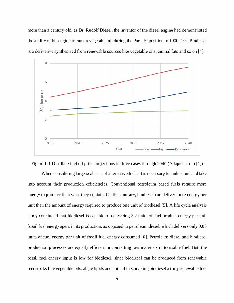
vehicles from gasoline to diesel [1]. Figure 1-1 shows the projections of distillate fuel oil prices
through 2040 for the “high oil price”, “reference”, and “low oil price” cases.
With such uncertainty about fuel availability and price in the near future, a dependable
liquid fuel is needed that can provide us with energy security, particularly in the transportation
sector. Bioenergy can play a major role in replacing fossil fuels and meeting the future demands
of the transportation sector. Modern bioenergy resources like biodiesel and ethanol are the
prominent biofuels currently in use. Biodiesel seems to be a better option considering the fact that
the processing technology for biodiesel is simpler than that of ethanol [2]. The concept itself is
2
more than a century old, as Dr. Rudolf Diesel, the inventor of the diesel engine had demonstrated
the ability of his engine to run on vegetable oil during the Paris Exposition in 1900 [10]. Biodiesel
is a derivative synthesized from renewable sources like vegetable oils, animal fats and so on [4].
Figure 1-1 Distillate fuel oil price projections in three cases through 2040.(Adapted from [1])
When considering large-scale use of alternative fuels, it is necessary to understand and take
into account their production efficiencies. Conventional petroleum based fuels require more
energy to produce than what they contain. On the contrary, biodiesel can deliver more energy per
unit than the amount of energy required to produce one unit of biodiesel [5]. A life cycle analysis
study concluded that biodiesel is capable of delivering 3.2 units of fuel product energy per unit
fossil fuel energy spent in its production, as opposed to petroleum diesel, which delivers only 0.83
units of fuel energy per unit of fossil fuel energy consumed [6]. Petroleum diesel and biodiesel
production processes are equally efficient in converting raw materials in to usable fuel. But, the
fossil fuel energy input is low for biodiesel, since biodiesel can be produced from renewable
feedstocks like vegetable oils, algae lipids and animal fats, making biodiesel a truly renewable fuel
0
2
4
6
8
2015 2020 2025 2030 2035 2040
$/g
allo
n p
rice
Year Low High Reference
3
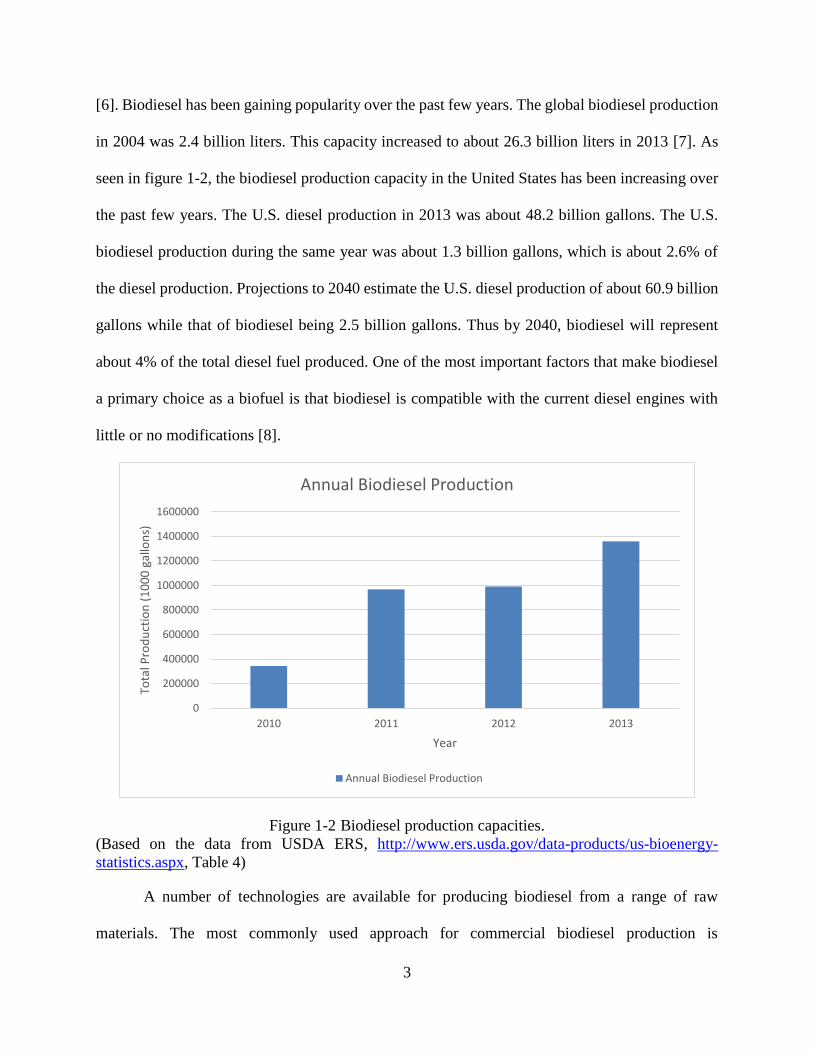
[6]. Biodiesel has been gaining popularity over the past few years. The global biodiesel production
in 2004 was 2.4 billion liters. This capacity increased to about 26.3 billion liters in 2013 [7]. As
seen in figure 1-2, the biodiesel production capacity in the United States has been increasing over
the past few years. The U.S. diesel production in 2013 was about 48.2 billion gallons. The U.S.
biodiesel production during the same year was about 1.3 billion gallons, which is about 2.6% of
the diesel production. Projections to 2040 estimate the U.S. diesel production of about 60.9 billion
gallons while that of biodiesel being 2.5 billion gallons. Thus by 2040, biodiesel will represent
about 4% of the total diesel fuel produced. One of the most important factors that make biodiesel
a primary choice as a biofuel is that biodiesel is compatible with the current diesel engines with
little or no modifications [8].
Figure 1-2 Biodiesel production capacities.
(Based on the data from USDA ERS, http://www.ers.usda.gov/data-products/us-bioenergy-
statistics.aspx, Table 4)
A number of technologies are available for producing biodiesel from a range of raw
materials. The most commonly used approach for commercial biodiesel production is
0
200000
400000
600000
800000
1000000
1200000
1400000
1600000
2010 2011 2012 2013
Tota
l Pro
du
ctio
n (
10
00
gal
lon
s)
Year
Annual Biodiesel Production
Annual Biodiesel Production
4
transesterification [9]. Although, transesterification through the catalyzed route is most commonly
used in the industry, this technique does come with a few drawbacks such as, longer processing
times, catalyst regeneration and recovery, biodiesel washing, and undesired saponification.
Supercritical transesterification on the other hand alleviates the problems faced during catalyzed
transesterification, without compromising on the quality of biodiesel.
The main objective of this research was to study the production of biodiesel from cooking
oil, in a single catalyst-free step using the supercritical transesterification process. Further, this
study also focused on analyzing the biodiesel samples using gas chromatography-mass
spectrometry based approach to determine the biodiesel yields. The work in this thesis consisted
of the following tasks:
Designing and building an experimental setup capable of withstanding the supercritical
reaction conditions and further fine tuning its performance to conduct a successful
experimental study.
Identifying the key parameters in supercritical transesterification and assessing their effect
on biodiesel yield with the least number of experimental runs.
Developing a GC-MS based analysis method for the determination of methyl ester yields
at each of the chosen experimental conditions.
Analysis of variance and development of a regression model to determine the significant
factors affecting the reaction conversion.
Preliminary estimate of the kinetic tendency of the reaction.
Each of these steps is described in the subsequent chapters, followed by the results and
conclusions drawn from the research findings. The next chapter provides in-depth information on
the various biodiesel production technologies.
5
CHAPTER 2: CONVENTIONAL BIODIESEL PRODUCTION TECHNOLOGIES
Vegetable oils are the most widely used raw materials for biodiesel production. The fact
that vegetable oils are renewable and have an energetic content close to diesel fuels make them an
attractive raw material for biodiesel [10]. Vegetable oils can be directly used with diesel engines,
but certain drawbacks make them unsuitable for use over a prolonged period. Techniques like
pyrolysis (or thermal cracking), microemulsions and transesterification can be used to convert
vegetable oils to biodiesel. The following sections give in-depth information on each of these
methods, and their merits and challenges.
2.1 Direct Use of Vegetable Oils
Vegetable oil was proposed to be used as an alternative to petroleum in the 1980’s [11].
Vegetable oils have a high heat content (about 88% of D2 fuel), they are biodegradable, have low
aromatic content and are readily available. But on the downside, they have high viscosities, lower
volatilities and the unsaturated hydrocarbon chains are reactive. Although, vegetable oil can be
directly used in compression engines for a short term, its long term use poses many problems. The
major problem arises from the high viscosity of vegetable oil [3]. In long term engine tests, injector
coking, higher carbon deposits, sticking of piston rings, thickening and gelling of engine
lubrication oil and other issues have been reported [3,12].
2.2 Pyrolysis
Pyrolysis or thermal cracking involves the breaking of long chains of carbon-, hydrogen-
and oxygen- containing compounds (mainly biomass) into smaller molecules at high temperature
and in the absence of oxygen. A wide range of raw materials, like vegetable oils, animal fats, and
6
natural fatty acids can be pyrolyzed. The organic components in these materials start decomposing
at around 350 °C – 550 °C in the absence of oxygen, and continue decomposing as the temperature
rises up to 700 °C – 800 °C [13]. Pyrolysis studies were reported in literature as early as 1947.
Tung oil calcium soaps were subjected to thermal cracking to yield crude oil. The crude was further
refined to produce diesel fuel, gasoline and kerosene [14].
Based on the operating conditions, pyrolysis can be classified as conventional (slow)
pyrolysis, fast pyrolysis and flash pyrolysis. Conventional pyrolysis is carried out at 276 °C – 676
°C. The process is characterized by long gas residence times (7-8 minutes) and low heat transfer
rates, which affects the quality of the fuel produced. Fast pyrolysis is characterized by high heat
transfer, high heating rates, and short residence times. The reaction occurs within the temperature
range of 576 °C – 976 °C [13]. In case of flash pyrolysis, the reactants undergo rapid
devolatilization at temperatures to the order of 776 °C – 1026 °C. Flash pyrolysis is characterized
by very short gas residence times (less than 1 second) and high heating rate of particles [15]. Even
though the process is fast, it has some technological shortcomings like poor thermal stability,
presence of solids in the oils, corrosive nature of oil, dissolved char in oil and the production of
pyrolytic water as a by-product [16]. Since pyrolysis undergoes various reaction pathways and a
variety of reaction products can be obtained from pyrolysis, pyrolytic chemistry is rather difficult
to characterize [4].
2.3 Microemulsions
A microemulsion can be defined as a clear and thermodynamically stable dispersion of two
immiscible liquids, which contains a certain amount of surfactant or a surfactant and a co-
surfactant [17]. Microemulsion droplets are small with diameters within the range of 100 to 1000
°A. Vegetable oils with an ester or a dispersant, or a vegetable oil, alcohol and a surfactant could
7
form a microemulsion. Although the presence of alcohol in the microemulsion improves latent
heat of vaporization and cools the combustion chamber, reducing the nozzle coking effect,
microemulsions have lower volumetric heating values as compared to diesel [18].
Ziejewski et al., prepared a microemulsion with 53.3% of alkali refined and winterized
sunflower oil, 13.3% of 190-proof ethanol and 33.4% of 1-butanol. In their engine tests they found
that the fuel mass ratio increased due to higher density and viscosity of the microemulsion. Since
the heating value of the microemulsion was 19% lower than that of diesel, a lower energy input
and consequently a lower power output was observed. One of the major problems reported was
the difficulty in starting the engine even at room temperature [19]. Although microemulsions show
a considerable promise as low viscosity fuel blends with vegetable oils, their cetane numbers are
lower and they have low heating values as compared to D2 grade diesel fuel [20].
2.4 Transesterification
Transesterification is a reaction where one ester is transformed into another ester by the
interchange of the alkoxy moiety [21]. The process is also known as alcoholysis, since the alcohol
from the ester is replaced by another alcohol. The process is similar to that of hydrolysis, except
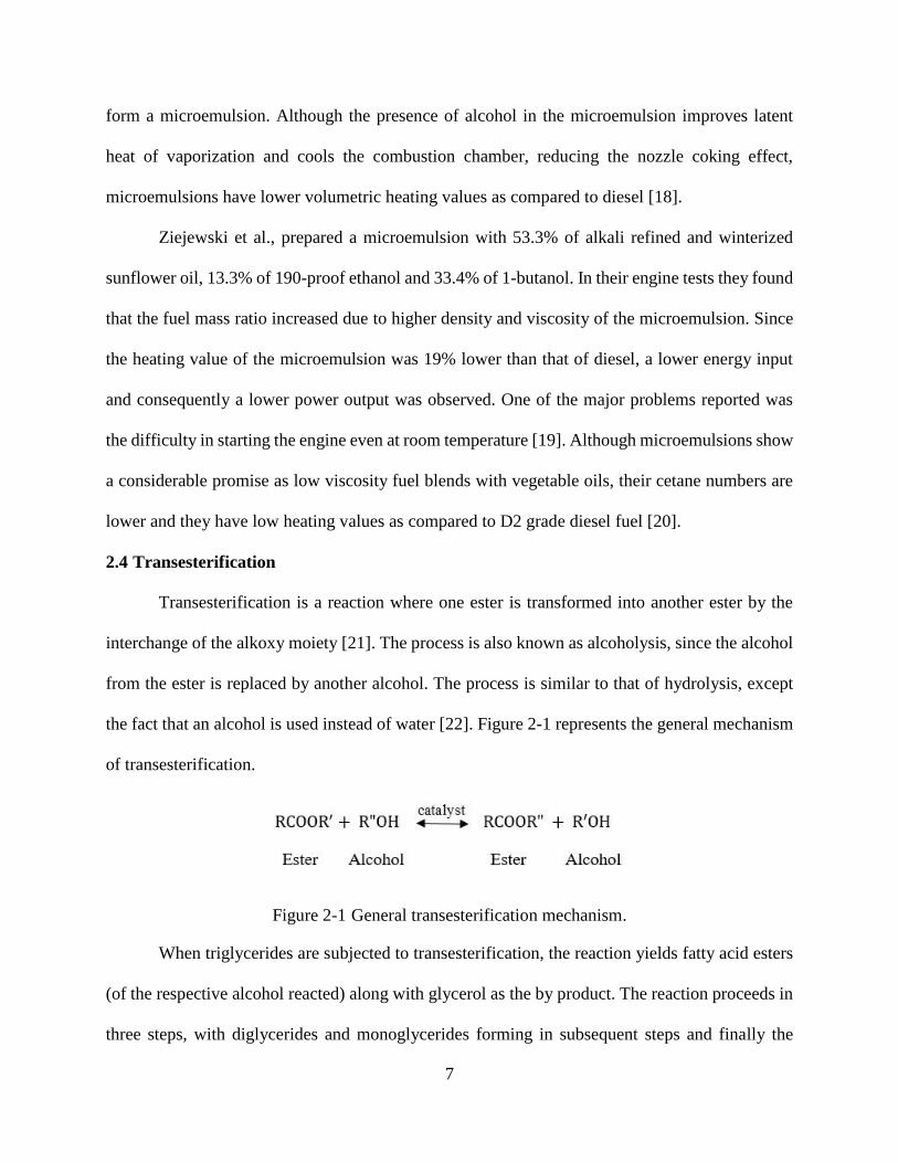
the fact that an alcohol is used instead of water [22]. Figure 2-1 represents the general mechanism
of transesterification.
Figure 2-1 General transesterification mechanism.
When triglycerides are subjected to transesterification, the reaction yields fatty acid esters
(of the respective alcohol reacted) along with glycerol as the by product. The reaction proceeds in
three steps, with diglycerides and monoglycerides forming in subsequent steps and finally the
8
esters along with glycerol in the last step [23]. The mechanism of transesterification is discussed
in detail in chapter 3. More than often the transesterification reaction is catalyzed by bases [24],
acids [25] or enzymes [26].
2.4.1 Base-Catalyzed Transesterification
The most commonly used commercial process for biodiesel production is base-catalyzed
transesterification. This is due to the fact that base-catalyzed transesterification reactions proceed
at considerable faster rates as compared to acid-catalyzed transesterification reactions. Also, base
catalysts are far less corrosive to the equipment than acid catalysts [27]. Although base catalysts
like sodium hydroxide (NaOH) and potassium hydroxide (KOH) are widely available and
inexpensive, their ability to catalyze transesterification is limited when the oil has a high free fatty
acid (FFA) content [28]. FFA’s are made up of a long carbon chain disconnected from the glycerol
backbone. The alkali catalyst can react with the FFA to form soap [29]. This side reaction is
undesirable since soap formation hinders the production of fuel grade biodiesel, resulting in high
product separation costs. Although homogenous base catalysts are able to catalyze the
transesterification reaction at low reaction temperature and atmospheric pressure, are widely
available and inexpensive, and produce high yields, their use is limited to the oils where the FFA
content is no more than 0.5% by weight [30] and acid value less than 1 mg KOH/g [31].
Solid base catalysts, also known as heterogeneous base catalysts like basic zeolites,
alkaline earth metal oxides and hydrotalcites have been developed and used for biodiesel
production in the past. Alkaline earth metal oxides like calcium oxide have recently attracted much
attention since it possesses high basicity, dissolves very slowly in alcohol and can be synthesized
from relatively inexpensive sources like limestone and calcium hydroxide [32]. Although these
catalysts separate easily from the liquid reaction products since they are in solid form, an extra
9
purification step may be needed in certain cases. Some researchers have found that these catalysts
can dissolve to some extent in the reaction products and may form other compounds, for example,
calcium oxide can react with glycerol to form calcium diglyceroxide, which is soluble in biodiesel
[33]. Further, catalysts like calcium oxide are rapidly hydrated in air. The catalyst may undergo
poisoning due to the chemisorption of water and carbon dioxide on the active surface sites,
affecting the performance of the catalyst. Magnesium oxide (MgO) is among the other options for
heterogeneous base catalysts. It can be synthesized by direct heating of magnesium carbonate or
magnesium hydroxide and can catalyze the transesterification reaction, but only at higher reaction
temperatures (above 180 °C) [34]. At lower reaction temperatures and pressures, the catalyst loses
its activity [32]. Strontium oxide is another metal oxide that is highly active. Although it is soluble
in the reaction medium, research suggests that using just 3% catalyst by weight, the reaction can
produce 90% yields of methyl esters in 30 minutes at 65 °C, even with the specific surface area of
the catalyst being as small as 1.05 m2/g [35].
2.4.2 Acid-Catalyzed Transesterification
Liquid base-catalyzed transesterification has certain limitations with respect to the
presence of free fatty acids (FFA’s), soap formation and catalyst separation. To overcome these
limitations, liquid acid catalysts have been proposed for the transesterification reaction. Sulfuric
acid (H2SO4) and hydrochloric acid (HCl) are the most commonly used homogeneous acid
catalysts [32]. It has been reported that acid catalysts can be used where the free fatty acid content
of the raw material is higher. In other words, unlike alkali catalysts, acid catalysts do not get
affected by the presence of free fatty acids [27]. On the downside, acid-catalyzed
transesterification reactions have slower reaction rates with relatively lower conversion ratios,
10
need a catalyst separation step, and have environmental as well as corrosion related problems
[29,30].
Due to these limitations, researchers focused on exploring solid or heterogeneous acid
catalysts for transesterification. Solid acid catalysts are unaffected by the presence of free fatty
acids (FFA’s), can catalyze esterification and transesterification reactions simultaneously [36], are
easy to separate from the reaction products, regenerate and recycle, and reduce the problems
associated with corrosion even in the presence of acid species. A solid acid catalyst having an
interconnected porous structure with a high concentration of acid sites and a hydrophobic surface
is ideal for transesterification. The pore system minimizes the diffusion problems for molecules
with larger chain structures and the high concentration of acid sites helps the reaction to proceed
at faster rates [28].
Catalysts like zirconium oxide (ZrO2), titanium oxide (TiO2), tin oxide (SnO2), zeolites and
ion exchange resins have been shown to be effective for transesterification. Moreover, modifying
the metal oxide surface acidity has shown to improve the transesterification yields [29]. For
example, sulfated zirconia (SO42-/ZnO2) was found to produce methyl ester yields as high as 90.3%
and 86.3% in the transesterification of palm kernel oil and crude coconut oil respectively, as
compared to 64.5% and 49.3% when unsulfated ZnO2 was used [37]. But catalysts like SO42-/ZnO2
are prone to deactivation due to sulfate leaching. This will effectively cause transesterification by
the homogeneous route and will interfere with the measurements of heterogeneous catalytic
activity. Catalysts like TiO2 have been evaluated for transesterification. Although SO42-/ TiO2 was
found to achieve a yield of 90%, the reaction is slow and requires high temperatures as compared
to base catalyzed transesterification [29].
11
2.4.3 Enzyme-Catalyzed Transesterification
Enzymes can be used to catalyze the transesterification reaction. Both intracellular and
extracellular lipases can be used for enzymatic production of biodiesel. In both cases the enzyme
is immobilized to be reused. Also, immobilizing the enzyme eliminates the issues with catalyst
separation from final products [38]. Extracellular lipases like Mucor miehei and Candida
antarctica (Novozym 435) have been used for transesterification of sunflower oil with primary
alcohols like methanol and ethanol [39]. The ester yields were found to be around 70% with
methanol and 72% with absolute ethanol.
This process operates at a much lower temperature (50 °C) as compared to other processes.
On the downside, the commercial application of enzyme catalyzed transesterification is limited
due to the fact that the costs of these catalysts per kg ester produced are high compared to those of
alkali catalysts. Slow reaction times and low yields also limit enzymatic transesterification [40].
Enzyme catalyzed transesterification remains an active area of research wherein researchers are
focusing on improving the yields and minimizing the reaction times. From the studies so far, vast
data have been collected and the efforts to optimize the process continue. Along with optimization,
focusing on other aspects like efficient recovery and utilization of glycerol byproduct can make
the process economically feasible and environmentally friendly [40].
12
CHAPTER 3: BIODIESEL PRODUCTION USING SUPERCRITICAL FLUID
TECHNOLOGY
3.1 Supercritical Fluids
Supercritical fluids date back to the discovery of the critical point by Baron Cagniard de la
Tour in 1822. In his experiments, he found that the gas-liquid phase boundary disappeared when
materials were heated above a certain temperature [41]. A supercritical fluid can be defined as any
substance whose temperature and pressure are higher than their critical values and which has a
density close to or higher than its critical density [42]. This temperature and pressure are referred
to as the critical temperature (Tc) and the critical pressure (Pc) respectively, which are the
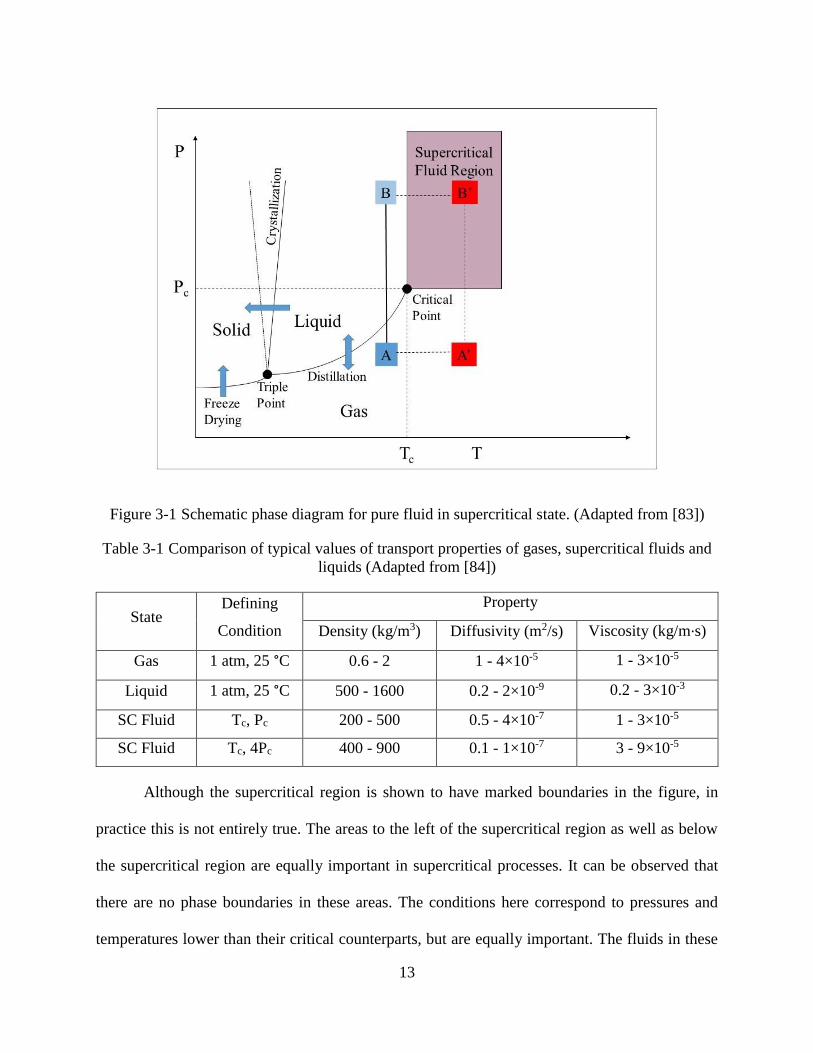
coordinates of the critical point on the phase diagram. Figure 3-1 shows the phase diagram for a
pure substance.
As the temperature and pressure increases, the fluid reaches the critical state, and beyond
the critical point the distinction between liquid and gas phases disappears. This is the supercritical
fluid region. It is in this region that the fluid exhibits both gas-like and liquid-like properties and
exists as a non-condensable dense fluid whose density ranges from 20 to 50% of that in the liquid
state and its viscosity is close to that in its gaseous state [43]. The properties of these fluids are
tunable and can be adjusted to be liquid-like or gas-like, by changing the pressure or temperature,
without crossing the phase boundary [44]. Table 3-1 shows a comparison between typical values
of physical properties of gases, liquids and supercritical fluids.
13
Figure 3-1 Schematic phase diagram for pure fluid in supercritical state. (Adapted from [83])
Table 3-1 Comparison of typical values of transport properties of gases, supercritical fluids and
liquids (Adapted from [84])
State Defining
Condition
Property
Density (kg/m3) Diffusivity (m2/s) Viscosity (kg/m·s)
Gas 1 atm, 25 °C 0.6 - 2 1 - 4×10⁻⁵ 1 - 3×10⁻⁵
Liquid 1 atm, 25 °C 500 - 1600 0.2 - 2×10⁻⁹ 0.2 - 3×10⁻³
SC Fluid Tc, Pc 200 - 500 0.5 - 4×10⁻⁷ 1 - 3×10⁻⁵
SC Fluid Tc, 4Pc 400 - 900 0.1 - 1×10⁻⁷ 3 - 9×10⁻⁵
Although the supercritical region is shown to have marked boundaries in the figure, in
practice this is not entirely true. The areas to the left of the supercritical region as well as below
the supercritical region are equally important in supercritical processes. It can be observed that
there are no phase boundaries in these areas. The conditions here correspond to pressures and
temperatures lower than their critical counterparts, but are equally important. The fluids in these
14
regions are referred to as near-critical fluids or subcritical fluids [45]. As seen in the figure, the
isotherm below the critical region (isotherm AB) involves phase transition, while the isotherm
above the critical region (isotherm A’B’) is a single phase with no phase transitions [83].
Supercritical fluids have promising applications in many fields including but not limited to
chemical processing, extraction, chemical reactions, waste treatment, recycling, pollution
prevention, and others. The book, “Supercritical Fluids – Molecular interactions, physical
properties and new applications” illustrates some of the most important and useful applications of
supercritical fluids and the technology itself, focusing on the key areas of extraction and
separation, material processing, and reactions [46].
3.2 Supercritical Transesterification
Before supercritical transesterification came into picture, researchers investigated the
transesterification of soybean oil in the absence of a catalyst, under subcritical conditions. They
reacted methanol with soybean oil at 220-235 °C, 55-62 bar and 6:1-27:1 mol/mol ratio [47]. They
were able to achieve methyl ester yields of about 85 weight percent after 10 hours of reaction time
at 235 °C. Thus, it was concluded that transesterification was possible even without using catalysts,
with the downside being slow reaction rates. Although, triglyceride and diglyceride conversion
rates were high, monoglyceride to glycerol conversion rates were found to be very slow [47]. Then
in 2001, Saka and Kusdiana pioneered the technique of producing biodiesel using supercritical
transesterification. They reacted rapeseed oil with methanol under supercritical conditions (350 °C
and 45-65 MPa) to produce methyl esters. The reaction was completed within 6 minutes with about
95% conversion to methyl esters [48].
The reaction mechanism of supercritical transesterification is predicted to be similar to that
of acid-catalyzed transesterification. In case of methanol (or any other alcohol at supercritical
15
conditions), the hydrogen bond is weakened at higher temperatures. However, while acid-
catalyzed transesterification is a much slower process even in comparison with base-catalyzed
transesterification, the supercritical transesterification process on the other hand is much faster in
terms of complete conversion of the triglycerides to esters [43]. This can be attributed to the fact
that the hydrogen bonding between OH oxygen and OH hydrogen, which forms methanol clusters,
decreases with increasing temperature, thereby decreasing the polarity of methanol in the
supercritical state. Thus non-polar triglycerides can get solvated in supercritical methanol, forming
a single phase of oil and methanol. This phenomenon results in accelerated kinetics under
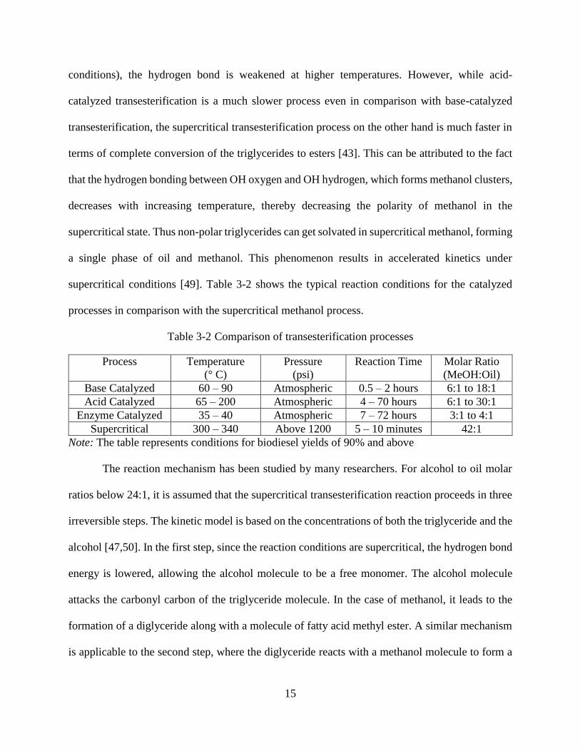
supercritical conditions [49]. Table 3-2 shows the typical reaction conditions for the catalyzed
processes in comparison with the supercritical methanol process.
Table 3-2 Comparison of transesterification processes
Process Temperature
(° C)
Pressure
(psi)
Reaction Time Molar Ratio
(MeOH:Oil)
Base Catalyzed 60 – 90 Atmospheric 0.5 – 2 hours 6:1 to 18:1
Acid Catalyzed 65 – 200 Atmospheric 4 – 70 hours 6:1 to 30:1
Enzyme Catalyzed 35 – 40 Atmospheric 7 – 72 hours 3:1 to 4:1
Supercritical 300 – 340 Above 1200 5 – 10 minutes 42:1
Note: The table represents conditions for biodiesel yields of 90% and above
The reaction mechanism has been studied by many researchers. For alcohol to oil molar
ratios below 24:1, it is assumed that the supercritical transesterification reaction proceeds in three
irreversible steps. The kinetic model is based on the concentrations of both the triglyceride and the
alcohol [47,50]. In the first step, since the reaction conditions are supercritical, the hydrogen bond
energy is lowered, allowing the alcohol molecule to be a free monomer. The alcohol molecule
attacks the carbonyl carbon of the triglyceride molecule. In the case of methanol, it leads to the
formation of a diglyceride along with a molecule of fatty acid methyl ester. A similar mechanism
is applicable to the second step, where the diglyceride reacts with a methanol molecule to form a
16
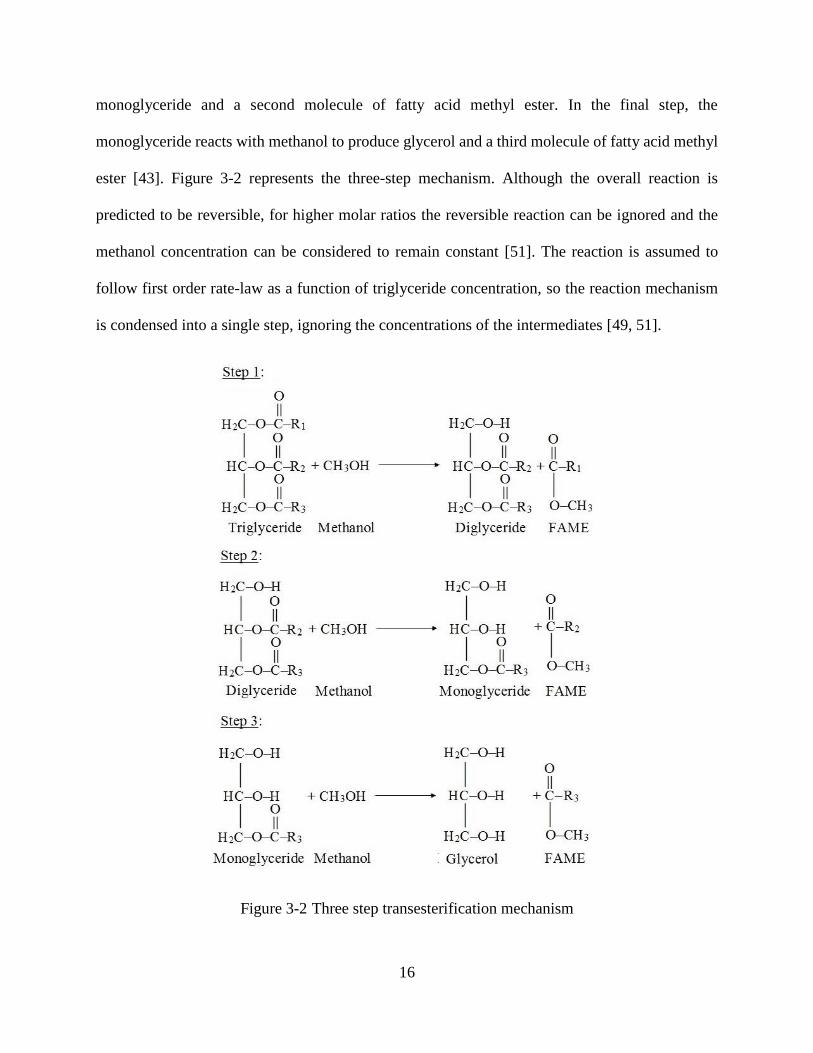
monoglyceride and a second molecule of fatty acid methyl ester. In the final step, the
monoglyceride reacts with methanol to produce glycerol and a third molecule of fatty acid methyl
ester [43]. Figure 3-2 represents the three-step mechanism. Although the overall reaction is
predicted to be reversible, for higher molar ratios the reversible reaction can be ignored and the
methanol concentration can be considered to remain constant [51]. The reaction is assumed to
follow first order rate-law as a function of triglyceride concentration, so the reaction mechanism
is condensed into a single step, ignoring the concentrations of the intermediates [49, 51].
Figure 3-2 Three step transesterification mechanism
17
3.3 Advantages and Disadvantages of Supercritical Transesterification
In the case of conventional catalyst-based transesterification, product separation and
catalyst recovery are the most energy intensive stages, and consequently economically unfavorable
[52]. Since supercritical transesterification does not rely on catalysts, it completely eliminates the
problems faced during catalyzed transesterification, thereby reducing the cost of separation and
purification of final products [53]. The supercritical transesterification reaction is completed
within minutes as compared to the base-, acid-, or enzyme-catalyzed processes that take hours
[48,54]. When considering biodiesel production methods, it is essential to take into account the
flexibility of the feedstock that can be processed using those methods. As compared to the
conventional base-catalyzed process, the supercritical process is more tolerant to the presence of
water and free fatty acids [36]. In fact, it was found that the presence of water positively affected
the formation of methyl esters by supercritical transesterification [55]. Thus supercritical
transesterification can also be used with low grade or moisture containing feedstocks [56]. Thus
the steps for feedstock pretreatment like moisture and free fatty acid removal as well as post
production treatments like washing, drying and catalyst removal are not needed. This results in
supercritical transesterification having much higher production efficiency than the conventional
catalytic processes [43].
On the downside, supercritical transesterification does require higher temperatures, higher
pressures and higher molar ratios, resulting in higher capital and operating costs [57]. Due to the
higher molar ratios, the preheating and recycling steps become energy intensive. The presence of
higher amount of alcohol in the products slows down the biodiesel-glycerol phase separation [43].
In a techno-economic study by Marchetti and Errazu, simulation models were employed to analyze
the productivity, raw material requirements, environmental impacts and economic advantages of
different processes for biodiesel production. They concluded that although supercritical

18
transesterification technology has the most technical advantages, it also has the highest capital
investment compared to the other available technologies, as well as the highest cost per kilo of
biodiesel produced [58]. However, taking advantage of heat integration opportunities it is possible
to reduce the energy demands for this process and improve its economic feasibility [43].
19
CHAPTER 4: FEEDSTOCKS FOR BIODIESEL PRODUCTION
The cost of biodiesel is largely dependent on the cost of feedstock. The cost of feedstock
accounts for about 88% of the total production costs [59]. The dependence of production costs on
the costs of feedstock was analyzed by Haas et al., who indicated the existence of a direct linear
relationship between the two, such that a US$ 0.075/gal change in product cost was caused by a
US$ 0.01/lb change in the feedstock cost. This makes the choice of feedstock critically important.
Furthermore, it signifies the need to develop technologies such as supercritical transesterification,
which can handle lower quality inexpensive feedstock without affecting the quality of biodiesel
produced.
Biodiesel feedstocks can be classified as first generation, second generation and third
generation feedstocks. Feedstocks of edible oils like rapeseed, soybean, palm and sunflower fall
under the first generation feedstock category, primarily because these were the first oil crops to be
used as feedstock for biodiesel synthesis [60]. Alternative non-edible sources like oil crops of
jatropha, tobacco seed, jojoba oil, salmon oil, mahua, and seamango are categorized as the second
generation feedstocks [60]. This category also includes used cooking oils, restaurant greases, and
animal fats [61]. The second generation feedstock reduce the dependence of biodiesel production
on the edible oils. The third generation biodiesel feedstock are lipids derived from microalgae [60].
Since microalgae have sustainability advantages over the first and second generation feedstocks,
interest in using microalgae for biodiesel production has been growing over the years. This section
will stress upon the currently available feedstocks in the market.
20
4.1 Vegetable Oils
The original diesel engine was designed to run on vegetable oil. Eventually, vegetable oils
were used to synthesize biodiesel via transesterification [54]. Vegetable oils are composed of about
98% triglycerides and the rest being mono- and diglycerides [62]. The triglyceride molecule is the
major component of vegetable oils, consisting of three esters of the fatty acid chain attached to a
backbone of glycerol [63]. Depending on the region of production and the climate in that area, the
type of vegetable oil used may vary. Soybean oil is prevalent in the United States, rapeseed oil in
Canada and the European nations, and palm oil in Malaysia, Indonesia and Latin America [63].
Although vegetable oils are abundantly available, they represent a major food staple and
their use for biodiesel production competes with their primary use as food sources, giving rise to
“food vs fuel” concerns. A solution to this problem is to utilize the used cooking oils and other
non-edible oils as raw material sources. Large amounts of used cooking oils are available around
the world. According to the projections of the Energy Information Administration, about 100
million gallons of waste cooking oil is produced in the United States every day [64]. Theoretically,
this amount can produce about 99.5 million gallons of biodiesel per day, which translates to 36.3
billion gallons of biodiesel produced annually. If the potential of available used cooking oil is fully
utilized, the biodiesel obtained can replace more than 50% of the diesel fuel in comparison with
the projections of 2040 (60.9 billion gallons). Thus, there is a huge potential in utilizing the used
cooking oils for producing biodiesel. Further, the disposal and management of used oils is a
challenge in itself due to the possibility of contamination of water and land resources. Using these
oils for biodiesel production would provide a solution to their disposal as well as to the food versus
fuel debate. The large-scale availability of restaurant oil waste can reduce the overall production
costs and significantly enhance the economic viability of biodiesel [61,64].
21
One critical consideration while selecting used or waste cooking oils as biodiesel feedstock
is the change in oil properties due to cooking, which may affect the quality of the final product.
During the frying process, the oil undergoes thermolytic, oxidative and hydrolytic reactions. Many
undesirable volatile compounds are formed due to the combined effect of these reactions. These
compounds could affect the properties of biodiesel or could affect the transesterification reaction
itself. Repetitive heating cycles during frying increase the polar content of oil, negatively affecting
the biodiesel quality. [36,65,66]. Hence, it is essential to know the amount and the type of these
undesirable compounds. Usually, high-performance size exclusion chromatography is used to
examine such oil fractions. Some pretreatment is needed to remove these compounds from the oil.
Thus, an additional cost with waste cooking oil is the pretreatment step. With that being said, waste
cooking oil is still an economical source for biodiesel production [36].
4.2 Animal Fats
The greases primarily collected from animal meat-processing facilities refer to animal fats
[61]. Wastes generated by the meat processing industries are inexpensive, as a result of which the
interest in producing biodiesel from fats of animal origin like beef tallow and pork lard has
increased [67]. Animal fats have similar chemical structures to vegetable oils, but the fatty acids
are distributed in a different way. They are a promising source of feedstock for biodiesel
production, but have not been as extensively studied as vegetable oils [68]. Although animal fats
like pork lard, beef tallow and chicken fat can be used as raw materials to produce biodiesel by
conventional transesterification methods, their yields are limited due the significant presence of
FFA’s in animal fats. [28]. Higher FFA content leads to soap formation in the presence of base
catalysts, making product separation costly and reducing the overall efficiency of the process [69].
Supercritical transesterification has shown to address these issues. Past research indicates
that supercritical methanolysis of chicken fat at 350 °C was able to produce FAME yields up to
22
80%. Although, these yields are valid for shorter residence times and molar ratios up to 9:1, they
are still significant, given the fact that chicken fat had a much higher free fatty acid content as
compared to soybean oil. It was observed that, under longer residence times and higher molar
ratios, the fatty acid methyl esters were subject to thermal decomposition. This was evident from
the brownish color of the sample and the decrease in the FAME yields for reactions longer than 7
minutes [69]. Biodiesel synthesized from animal fats has its own advantages and disadvantages.
Although it has a high cetane number, it is more vulnerable to oxidation since animal fats lack the
presence of natural antioxidants [70]. Biodiesel obtained from fats like tallow have a lower flash
point and lower heating values. Furthermore, it also has a lower pour point which makes its use in
cold weather conditions difficult [71].
4.3 Microalgae
Microalgae consist of both groups of photosynthetic microorganisms; those that have cell
walls, nucleus, chloroplasts and mitochondria (eukaryotic) and those that do not (prokaryotic).
They grow rapidly, can sustain harsh conditions and are rich in lipids [72]. Depending on the strain
of the microalgae, the lipid content can be as high as 80% of the total dry weight. A significant
portion of these lipids can be extracted using various extraction techniques. Up to 80% of this lipid
mass consists of triacylglycerols (TAGs) [73]. These TAGs can be converted to biodiesel via the
transesterification process. Microalgae can be cultivated in brackish or salt water as opposed to
potable water and on non-arable land. Moreover, microalgae have high growth rates and
productivity as well as high photosynthetic efficiency to produce biomass. Thus, they represent a
promising feedstock source for producing biodiesel [60].
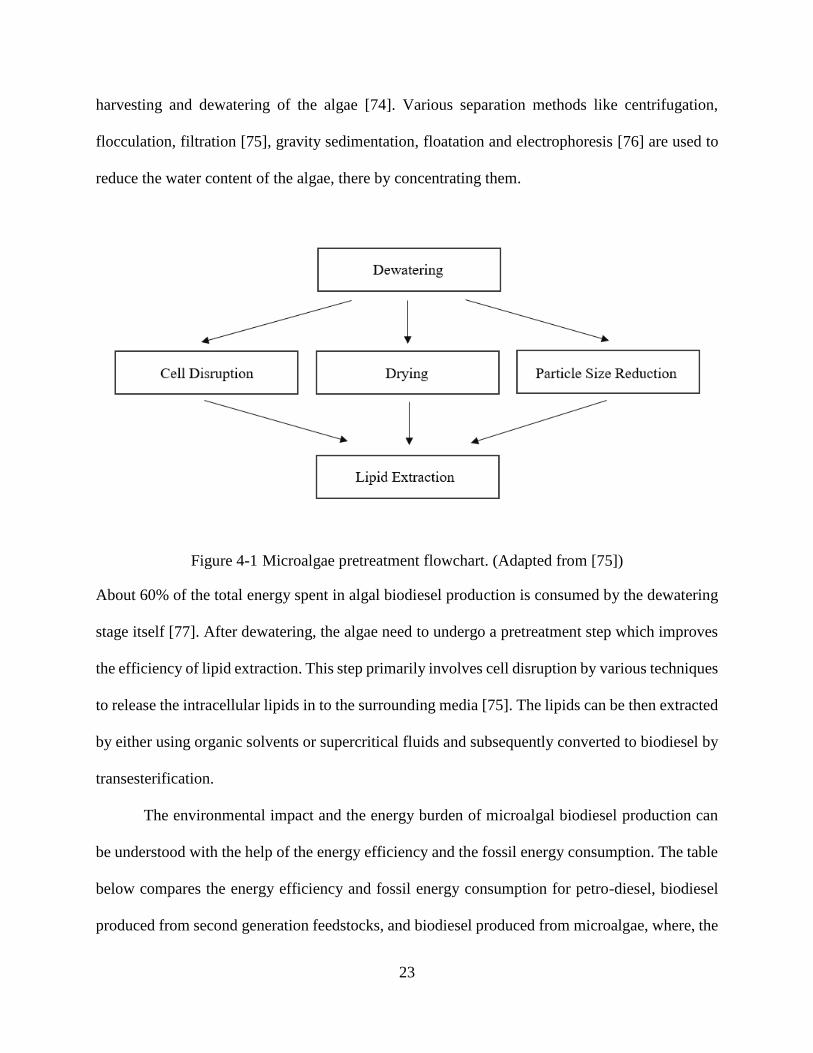
Microalgae require a series of pretreatment and processing steps before the lipids in them
can be converted to biodiesel. Figure 4-1 shows the microalgae pretreatment flowchart. The
process starts with the cultivation of microalgae in open ponds or closed bioreactors, followed by
23
harvesting and dewatering of the algae [74]. Various separation methods like centrifugation,
flocculation, filtration [75], gravity sedimentation, floatation and electrophoresis [76] are used to
reduce the water content of the algae, there by concentrating them.
Figure 4-1 Microalgae pretreatment flowchart. (Adapted from [75])
About 60% of the total energy spent in algal biodiesel production is consumed by the dewatering
stage itself [77]. After dewatering, the algae need to undergo a pretreatment step which improves
the efficiency of lipid extraction. This step primarily involves cell disruption by various techniques
to release the intracellular lipids in to the surrounding media [75]. The lipids can be then extracted
by either using organic solvents or supercritical fluids and subsequently converted to biodiesel by
transesterification.
The environmental impact and the energy burden of microalgal biodiesel production can
be understood with the help of the energy efficiency and the fossil energy consumption. The table
below compares the energy efficiency and fossil energy consumption for petro-diesel, biodiesel
produced from second generation feedstocks, and biodiesel produced from microalgae, where, the
24
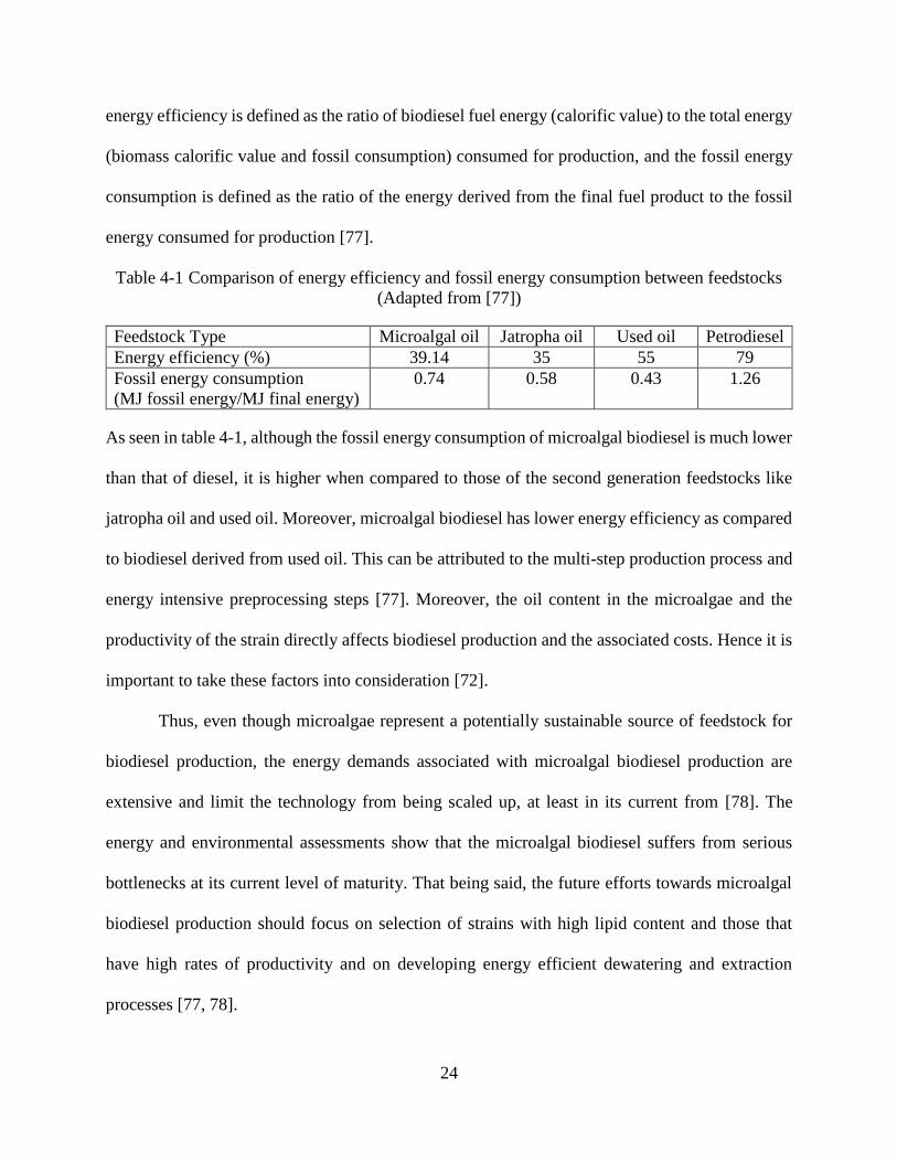
energy efficiency is defined as the ratio of biodiesel fuel energy (calorific value) to the total energy
(biomass calorific value and fossil consumption) consumed for production, and the fossil energy
consumption is defined as the ratio of the energy derived from the final fuel product to the fossil
energy consumed for production [77].
Table 4-1 Comparison of energy efficiency and fossil energy consumption between feedstocks
(Adapted from [77])
Feedstock Type Microalgal oil Jatropha oil Used oil Petrodiesel
Energy efficiency (%) 39.14 35 55 79
Fossil energy consumption
(MJ fossil energy/MJ final energy)
0.74 0.58 0.43 1.26
As seen in table 4-1, although the fossil energy consumption of microalgal biodiesel is much lower
than that of diesel, it is higher when compared to those of the second generation feedstocks like
jatropha oil and used oil. Moreover, microalgal biodiesel has lower energy efficiency as compared
to biodiesel derived from used oil. This can be attributed to the multi-step production process and
energy intensive preprocessing steps [77]. Moreover, the oil content in the microalgae and the
productivity of the strain directly affects biodiesel production and the associated costs. Hence it is
important to take these factors into consideration [72].
Thus, even though microalgae represent a potentially sustainable source of feedstock for
biodiesel production, the energy demands associated with microalgal biodiesel production are
extensive and limit the technology from being scaled up, at least in its current from [78]. The
energy and environmental assessments show that the microalgal biodiesel suffers from serious
bottlenecks at its current level of maturity. That being said, the future efforts towards microalgal
biodiesel production should focus on selection of strains with high lipid content and those that
have high rates of productivity and on developing energy efficient dewatering and extraction
processes [77, 78].
25
CHAPTER 5: EXPERIMENTAL WORK
This study used a pilot scale batch reactor setup. Pilot scale experiments allow for a stable
experimental environment, which can be tuned, improved and studied. Further, pilot scale
experimental setups are larger in capacity as compared to laboratory scale experimental setups.
Using such a setup allows us to determine the scalability of the process. The main focus of this
work was to produce biodiesel using supercritical transesterification and to study the effects of
different reaction parameters on the biodiesel yields. Construction of a reaction setup that could
withstand the harsh reaction conditions was a key element. This section describes the overall
reaction setup, the equipment and materials used, the experimental procedure and the analysis
procedure.
5.1 Experimental Setup and Equipment
The main reaction vessel (autoclave) was obtained from Autoclave Engineers, with SS-316
construction, rated for 9100 psi at 720 F. A magnetic drive stirrer with variable speed control was
mounted on the autoclave to keep the contents of the reaction vessel well mixed. The autoclave
was fitted with a safety head assembly (rupture disc) capable of venting the reaction contents in
case of pressure buildup in excess of 5000 psi. The autoclave was heated using a jacketed heater
controlled by the Autoclave Sentinel series temperature controller. The heating jacket covered only
the lower 2/3rd of the autoclave. Hence, to keep the conditions isothermal, the upper 1/3rd including
the head of the autoclave was wrapped with heating tape obtained from Omega Engineers. The
heating tape was rated up to 400 °C and the temperature on the tape was controlled by the Omega
26
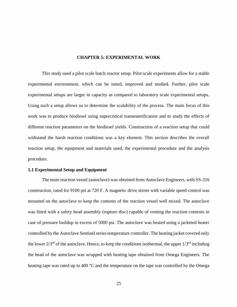
Platinum series temperature controller via a solid state relay (also from Omega Engineers). A dip
tube, along with an isolation and cool-down chamber, was installed on the autoclave to draw out
the sample. Figures 5-1 and 5-2 show the autoclave assembly, the heating tape assembly, the
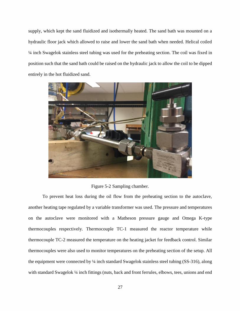
Magnedrive assembly and the sampling chamber. A spray nozzle was used to disperse the oil flow
in the autoclave, to allow for better mixing and higher surface area for the reaction to occur. The
nozzle is shown in figure 5-3.
Figure 5-1 Autoclave, heating tape and Magnedrive assembly.
Two separate syringe pumps, from Teledyne ISCO were used for pumping the oil and
methanol into the reactor. The pumps are capable of producing pressure up to 5000 psi, while
operating under constant flow or constant pressure modes. A fluidized sand bath (from Techne-
VWR International) with four 1-kW heaters was used to preheat the oil before exposing it to
supercritical methanol in the autoclave. The sand bath was provided with a 4-psi regulated air
27
supply, which kept the sand fluidized and isothermally heated. The sand bath was mounted on a
hydraulic floor jack which allowed to raise and lower the sand bath when needed. Helical coiled
¼ inch Swagelok stainless steel tubing was used for the preheating section. The coil was fixed in
position such that the sand bath could be raised on the hydraulic jack to allow the coil to be dipped
entirely in the hot fluidized sand.
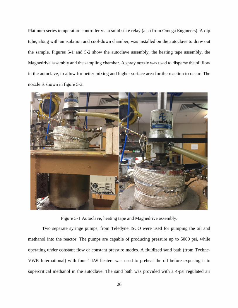
Figure 5-2 Sampling chamber.
To prevent heat loss during the oil flow from the preheating section to the autoclave,
another heating tape regulated by a variable transformer was used. The pressure and temperatures
on the autoclave were monitored with a Matheson pressure gauge and Omega K-type
thermocouples respectively. Thermocouple TC-1 measured the reactor temperature while
thermocouple TC-2 measured the temperature on the heating jacket for feedback control. Similar
thermocouples were also used to monitor temperatures on the preheating section of the setup. All
the equipment were connected by ¼ inch standard Swagelok stainless steel tubing (SS-316), along
with standard Swagelok ¼ inch fittings (nuts, back and front ferrules, elbows, tees, unions and end
28
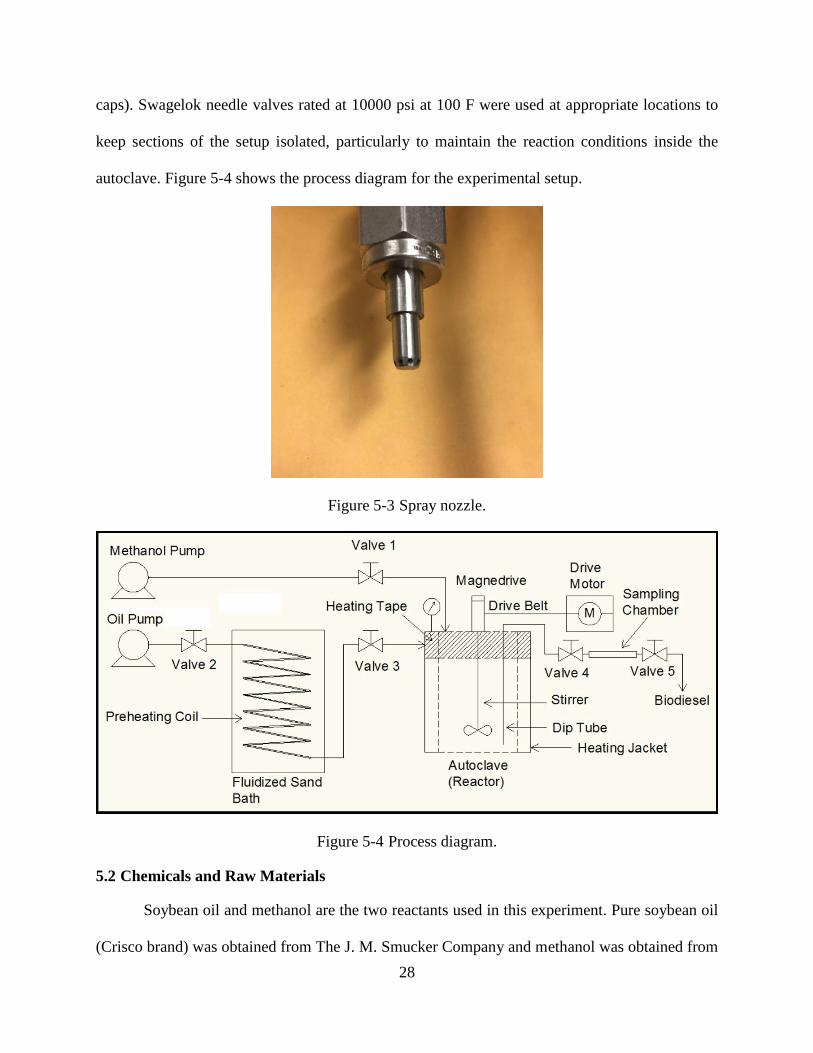
caps). Swagelok needle valves rated at 10000 psi at 100 F were used at appropriate locations to
keep sections of the setup isolated, particularly to maintain the reaction conditions inside the
autoclave. Figure 5-4 shows the process diagram for the experimental setup.
Figure 5-3 Spray nozzle.
Figure 5-4 Process diagram.
5.2 Chemicals and Raw Materials
Soybean oil and methanol are the two reactants used in this experiment. Pure soybean oil
(Crisco brand) was obtained from The J. M. Smucker Company and methanol was obtained from
29
Sigma Aldrich. The methyl heptadecanoate standard needed during the analysis was obtained from
Sigma Aldrich. The sample solutions were prepared in hexane (HPLC grade), which was obtained
from Fischer Scientific.
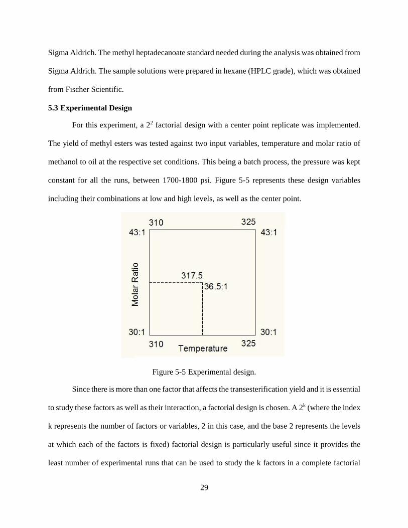
5.3 Experimental Design
For this experiment, a 22 factorial design with a center point replicate was implemented.
The yield of methyl esters was tested against two input variables, temperature and molar ratio of
methanol to oil at the respective set conditions. This being a batch process, the pressure was kept
constant for all the runs, between 1700-1800 psi. Figure 5-5 represents these design variables
including their combinations at low and high levels, as well as the center point.
Figure 5-5 Experimental design.
Since there is more than one factor that affects the transesterification yield and it is essential
to study these factors as well as their interaction, a factorial design is chosen. A 2k (where the index
k represents the number of factors or variables, 2 in this case, and the base 2 represents the levels
at which each of the factors is fixed) factorial design is particularly useful since it provides the
least number of experimental runs that can be used to study the k factors in a complete factorial

30
design [79]. Thus, a factorial design saves time due to the small sample size, and also allows to
assess the interactions between the factors.
In chapter 6, the changes in output response (biodiesel yield) with respect to the changes
in the factor levels (low and high for both temperature and molar ratio) are analyzed. A linear
regression model is built based on the significant factors. All the experiments in the 22 design are
run once (single replicate). Conducting an experiment that has only one run at each combination
of the design conditions could be risky since there is a possibility of fitting the data against noise.
In order to avoid this experimental error, a good strategy is to spread out the factor levels as apart
as possible [79]. The factor levels in this design were chosen such that beyond their set values,
unwanted effects were observed in the experimental output, during the preliminary testing. For
example, there were effects of degradation at T > 325 °C, very poor conversion at T < 310 °C,
incomplete reaction for molar ratio < 30:1 and yield saturation for molar ratio > 43:1. Thus, with
a considerable difference between the low and high levels of the factors, we can obtain a reasonable
estimate of the true factor effect.
One drawback associated with two-level factorial designs is the assumption of linearity.
When two levels, low and high, are selected to develop a regression model, usually, the first
obvious step is to try and fit a first order model. Adding the factor interaction terms to this model
will allow us to anticipate the curvature of the model. But, in certain circumstances, the model may
not accurately represent this curvature. Moreover, while running a two-level two factor experiment
it may be more appropriate to fit a second order model [79]. In order to allow us to estimate the
second order effects and give us a better prediction of the non-linearity, center points are added in
replicates to the design. The addition of center points replicates allow us to get an independent
estimate of the error, without affecting the error estimates of the original 22 design [79].
31
5.4 Experimental Procedure
Before the very first experiment was run, the setup was charged with nitrogen up to 2200
psi to check for any possible leakages. Since the setup was to be used at high pressures, it was
essential to make sure that the setup was free of any leaks, and could withstand the operating
conditions. The pumps were then set to refill mode to be charged with oil and methanol. The outlet
valve of the reactor was shut and the inlet valve for methanol was opened. The methanol pump
was activated and methanol was pumped into the reactor under constant flow mode. The amount
of methanol was fixed for all the experiments. The amount of oil on the other hand was adjusted
based on the molar ratio needed for that particular experiment.
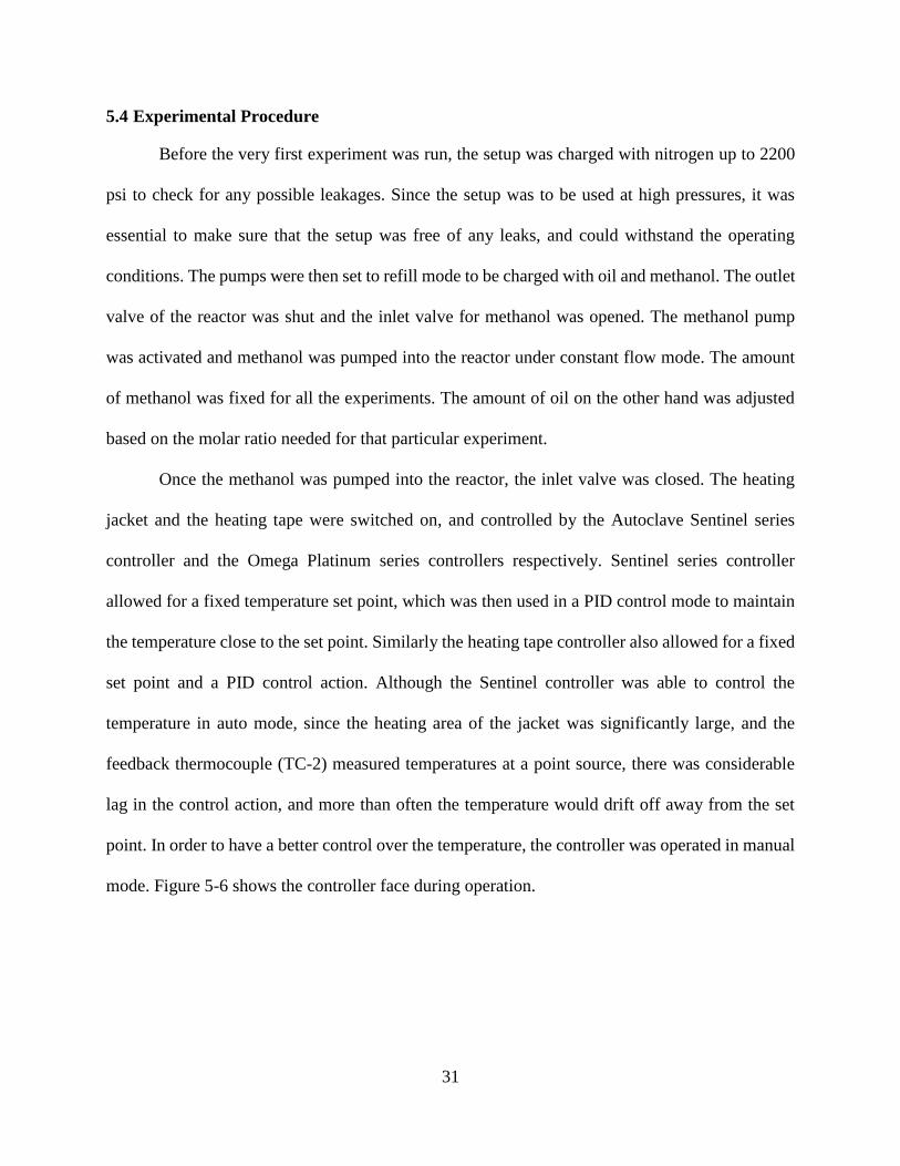
Once the methanol was pumped into the reactor, the inlet valve was closed. The heating
jacket and the heating tape were switched on, and controlled by the Autoclave Sentinel series
controller and the Omega Platinum series controllers respectively. Sentinel series controller
allowed for a fixed temperature set point, which was then used in a PID control mode to maintain
the temperature close to the set point. Similarly the heating tape controller also allowed for a fixed
set point and a PID control action. Although the Sentinel controller was able to control the
temperature in auto mode, since the heating area of the jacket was significantly large, and the
feedback thermocouple (TC-2) measured temperatures at a point source, there was considerable
lag in the control action, and more than often the temperature would drift off away from the set
point. In order to have a better control over the temperature, the controller was operated in manual
mode. Figure 5-6 shows the controller face during operation.
32
Figure 5-6 Controller screen.
The Magnedrive stirrer was switched on and set at a stirring speed of 900 rpm. The sand
bath was heated to the reaction temperature. Once the autoclave temperature reached the set point,
oil was pumped through the preheating coil into the autoclave, making sure that the upstream
pressure was greater than the autoclave pressure to prevent back flow of methanol. This was done
by adjusting the oil flow rate. The nozzle orifice was small, to allow upstream pressure buildup at
high flowrates. Once the oil was pumped, the inlet valve was shut. The reaction was allowed to
proceed and samples were collected at time intervals of 10 minutes each. Five samples were
collected at 10, 20, 30, 40 and 50 minutes in glass test tubes and sealed with cork stoppers. For
collecting the sample, the first valve in the sample isolation chamber was opened, which allowed
the product to flow under pressure into the chamber. The valve was then closed and the sample
was allowed to cooldown for a few minutes. The second valve was then opened and the sample
33
was withdrawn in a glass test tube and capped with a cork. All samples were stored in the
refrigerator.
After all samples were collected, the heater and the heating tape were switched off, and the
reactor was allowed to cooldown. The reactor contents were gradually withdrawn, taking care to
prevent the methanol from suddenly flashing off.
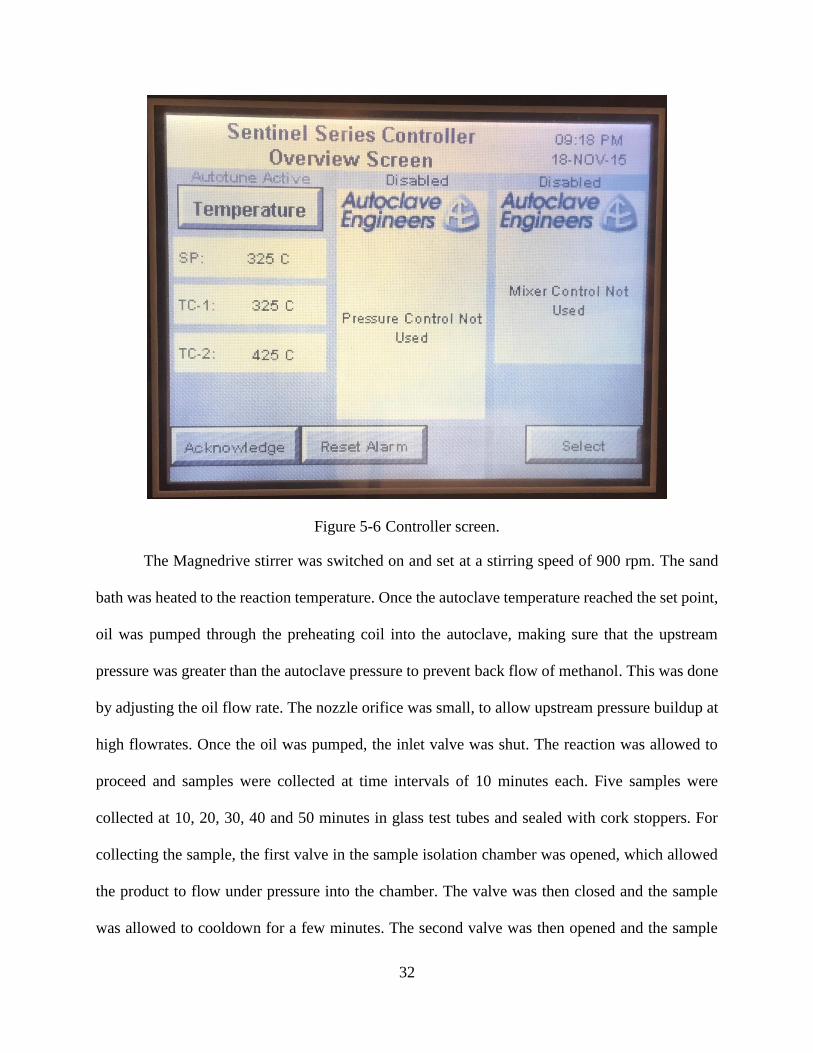
5.5 Analysis of Samples
In the field of analytical chemistry, approaches using chemical methods are simpler, but
there is lack of specificity and procedures tend to be time consuming. Moreover, chemical methods
lack versatility and their accuracy falls off with lower concentration samples [80]. Hence, an
analytical method based on an instrumental approach was used in this experimental process.
Instrumental methods are faster in detection, can handle samples of complex nature and low
concentration, have high sensitivities and provide reliable measurements [80].
Figure 5-7 Gas chromatograph.
34
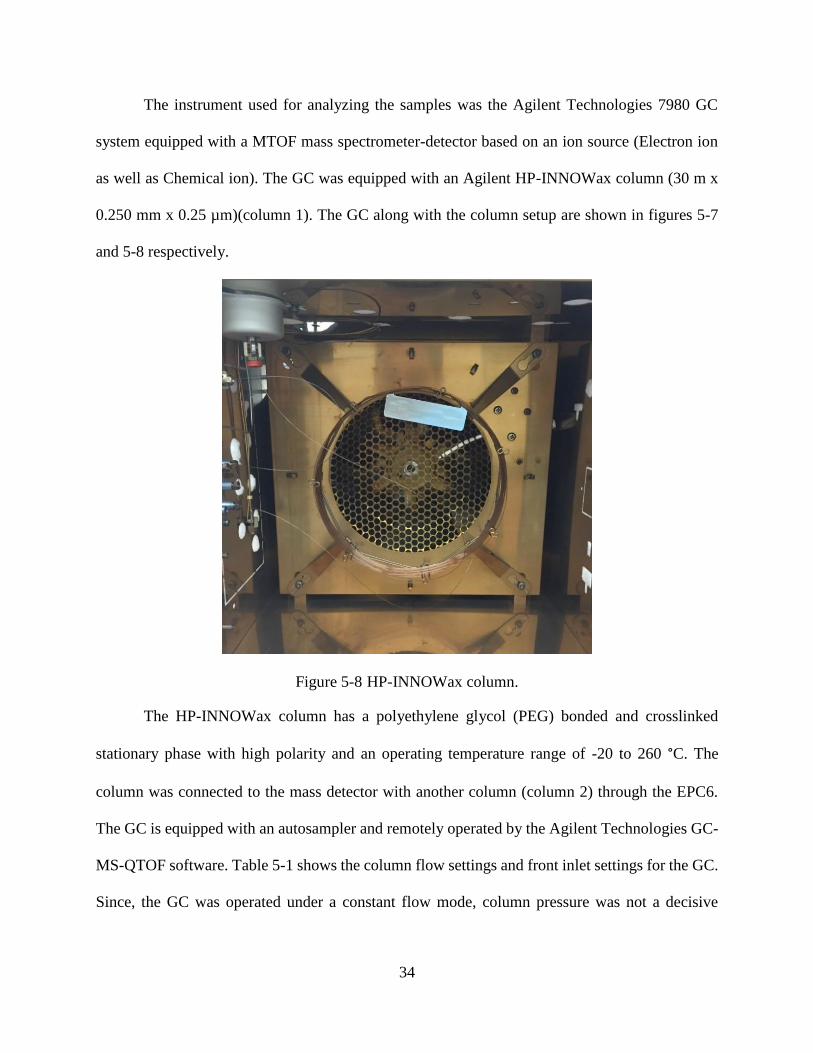
The instrument used for analyzing the samples was the Agilent Technologies 7980 GC
system equipped with a MTOF mass spectrometer-detector based on an ion source (Electron ion
as well as Chemical ion). The GC was equipped with an Agilent HP-INNOWax column (30 m x
0.250 mm x 0.25 µm)(column 1). The GC along with the column setup are shown in figures 5-7
and 5-8 respectively.
Figure 5-8 HP-INNOWax column.
The HP-INNOWax column has a polyethylene glycol (PEG) bonded and crosslinked
stationary phase with high polarity and an operating temperature range of -20 to 260 °C. The
column was connected to the mass detector with another column (column 2) through the EPC6.
The GC is equipped with an autosampler and remotely operated by the Agilent Technologies GC-
MS-QTOF software. Table 5-1 shows the column flow settings and front inlet settings for the GC.
Since, the GC was operated under a constant flow mode, column pressure was not a decisive
35
variable. The temperature programming of the oven for both the calibration samples as well as the
biodiesel samples is shown in table 5-2
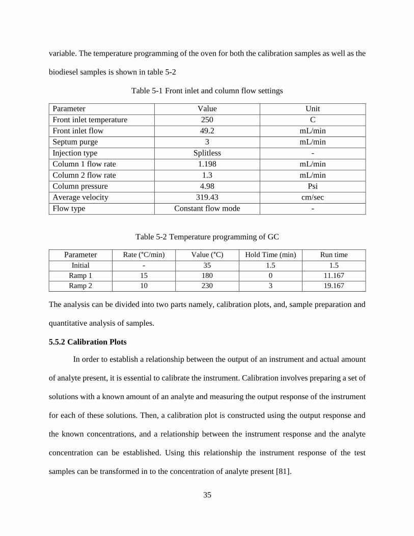
Table 5-1 Front inlet and column flow settings
Parameter Value Unit
Front inlet temperature 250 C
Front inlet flow 49.2 mL/min
Septum purge 3 mL/min
Injection type Splitless -
Column 1 flow rate 1.198 mL/min
Column 2 flow rate 1.3 mL/min
Column pressure 4.98 Psi
Average velocity 319.43 cm/sec
Flow type Constant flow mode -
Table 5-2 Temperature programming of GC
Parameter Rate (°C/min) Value (°C) Hold Time (min) Run time
Initial - 35 1.5 1.5
Ramp 1 15 180 0 11.167
Ramp 2 10 230 3 19.167
The analysis can be divided into two parts namely, calibration plots, and, sample preparation and
quantitative analysis of samples.
5.5.2 Calibration Plots
In order to establish a relationship between the output of an instrument and actual amount
of analyte present, it is essential to calibrate the instrument. Calibration involves preparing a set of
solutions with a known amount of an analyte and measuring the output response of the instrument
for each of these solutions. Then, a calibration plot is constructed using the output response and
the known concentrations, and a relationship between the instrument response and the analyte
concentration can be established. Using this relationship the instrument response of the test
samples can be transformed in to the concentration of analyte present [81].
36
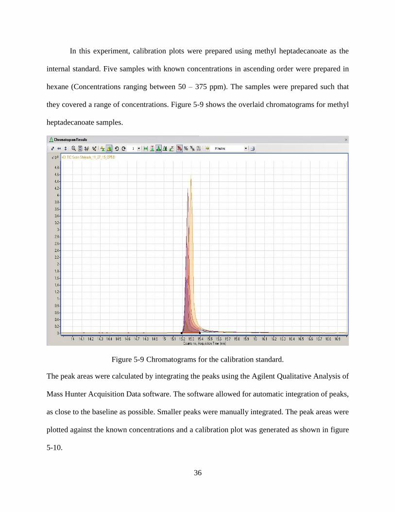
In this experiment, calibration plots were prepared using methyl heptadecanoate as the
internal standard. Five samples with known concentrations in ascending order were prepared in
hexane (Concentrations ranging between 50 – 375 ppm). The samples were prepared such that
they covered a range of concentrations. Figure 5-9 shows the overlaid chromatograms for methyl
heptadecanoate samples.
Figure 5-9 Chromatograms for the calibration standard.
The peak areas were calculated by integrating the peaks using the Agilent Qualitative Analysis of
Mass Hunter Acquisition Data software. The software allowed for automatic integration of peaks,
as close to the baseline as possible. Smaller peaks were manually integrated. The peak areas were
plotted against the known concentrations and a calibration plot was generated as shown in figure
5-10.
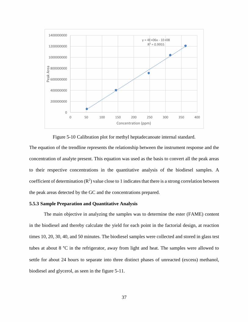
37
Figure 5-10 Calibration plot for methyl heptadecanoate internal standard.
The equation of the trendline represents the relationship between the instrument response and the
concentration of analyte present. This equation was used as the basis to convert all the peak areas
to their respective concentrations in the quantitative analysis of the biodiesel samples. A
coefficient of determination (R2) value close to 1 indicates that there is a strong correlation between
the peak areas detected by the GC and the concentrations prepared.
5.5.3 Sample Preparation and Quantitative Analysis
The main objective in analyzing the samples was to determine the ester (FAME) content
in the biodiesel and thereby calculate the yield for each point in the factorial design, at reaction
times 10, 20, 30, 40, and 50 minutes. The biodiesel samples were collected and stored in glass test
tubes at about 8 °C in the refrigerator, away from light and heat. The samples were allowed to
settle for about 24 hours to separate into three distinct phases of unreacted (excess) methanol,
biodiesel and glycerol, as seen in the figure 5-11.
y = 4E+06x - 1E+08R² = 0.9955
0
200000000
400000000
600000000
800000000
1000000000
1200000000
1400000000
0 50 100 150 200 250 300 350 400
Pea
k A
rea
Concentration (ppm)
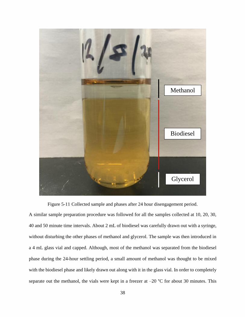
38
Figure 5-11 Collected sample and phases after 24 hour disengagement period.
A similar sample preparation procedure was followed for all the samples collected at 10, 20, 30,
40 and 50 minute time intervals. About 2 mL of biodiesel was carefully drawn out with a syringe,
without disturbing the other phases of methanol and glycerol. The sample was then introduced in
a 4 mL glass vial and capped. Although, most of the methanol was separated from the biodiesel
phase during the 24-hour settling period, a small amount of methanol was thought to be mixed
with the biodiesel phase and likely drawn out along with it in the glass vial. In order to completely
separate out the methanol, the vials were kept in a freezer at –20 °C for about 30 minutes. This
Methanol
Biodiesel
Glycerol
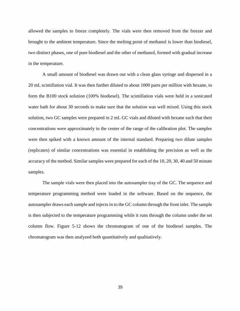
39
allowed the samples to freeze completely. The vials were then removed from the freezer and
brought to the ambient temperature. Since the melting point of methanol is lower than biodiesel,
two distinct phases, one of pure biodiesel and the other of methanol, formed with gradual increase
in the temperature.
A small amount of biodiesel was drawn out with a clean glass syringe and dispersed in a
20 mL scintillation vial. It was then further diluted to about 1000 parts per million with hexane, to
form the B100 stock solution (100% biodiesel). The scintillation vials were held in a sonicated
water bath for about 30 seconds to make sure that the solution was well mixed. Using this stock
solution, two GC samples were prepared in 2 mL GC vials and diluted with hexane such that their
concentrations were approximately in the center of the range of the calibration plot. The samples
were then spiked with a known amount of the internal standard. Preparing two dilute samples
(replicates) of similar concentrations was essential in establishing the precision as well as the
accuracy of the method. Similar samples were prepared for each of the 10, 20, 30, 40 and 50 minute
samples.
The sample vials were then placed into the autosampler tray of the GC. The sequence and
temperature programming method were loaded in the software. Based on the sequence, the
autosampler draws each sample and injects in to the GC column through the front inlet. The sample
is then subjected to the temperature programming while it runs through the column under the set
column flow. Figure 5-12 shows the chromatogram of one of the biodiesel samples. The
chromatogram was then analyzed both quantitatively and qualitatively.
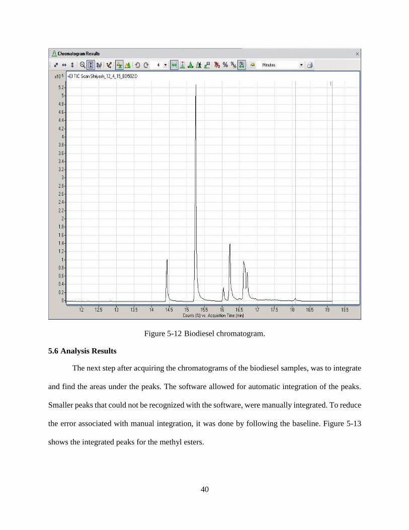
40
Figure 5-12 Biodiesel chromatogram.
5.6 Analysis Results
The next step after acquiring the chromatograms of the biodiesel samples, was to integrate
and find the areas under the peaks. The software allowed for automatic integration of the peaks.
Smaller peaks that could not be recognized with the software, were manually integrated. To reduce
the error associated with manual integration, it was done by following the baseline. Figure 5-13
shows the integrated peaks for the methyl esters.
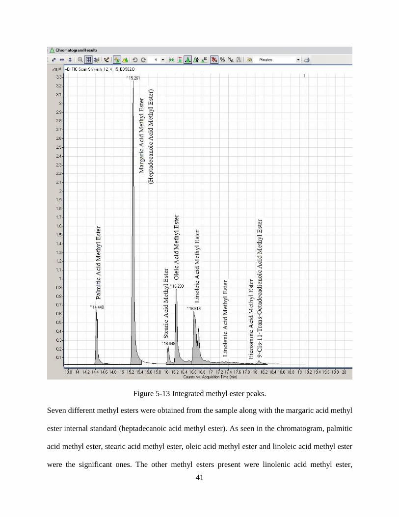
41
Figure 5-13 Integrated methyl ester peaks.
Seven different methyl esters were obtained from the sample along with the margaric acid methyl
ester internal standard (heptadecanoic acid methyl ester). As seen in the chromatogram, palmitic
acid methyl ester, stearic acid methyl ester, oleic acid methyl ester and linoleic acid methyl ester
were the significant ones. The other methyl esters present were linolenic acid methyl ester,
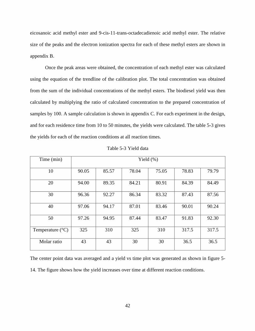
42
eicosanoic acid methyl ester and 9-cis-11-trans-octadecadienoic acid methyl ester. The relative
size of the peaks and the electron ionization spectra for each of these methyl esters are shown in
appendix B.
Once the peak areas were obtained, the concentration of each methyl ester was calculated
using the equation of the trendline of the calibration plot. The total concentration was obtained
from the sum of the individual concentrations of the methyl esters. The biodiesel yield was then
calculated by multiplying the ratio of calculated concentration to the prepared concentration of
samples by 100. A sample calculation is shown in appendix C. For each experiment in the design,
and for each residence time from 10 to 50 minutes, the yields were calculated. The table 5-3 gives
the yields for each of the reaction conditions at all reaction times.
Table 5-3 Yield data
Time (min) Yield (%)
10 90.05 85.57 78.04 75.05 78.83 79.79
20 94.00 89.35 84.21 80.91 84.39 84.49
30 96.36 92.27 86.34 83.32 87.43 87.56
40 97.06 94.17 87.01 83.46 90.01 90.24
50 97.26 94.95 87.44 83.47 91.83 92.30
Temperature (°C) 325 310 325 310 317.5 317.5
Molar ratio 43 43 30 30 36.5 36.5
The center point data was averaged and a yield vs time plot was generated as shown in figure 5-
14. The figure shows how the yield increases over time at different reaction conditions.
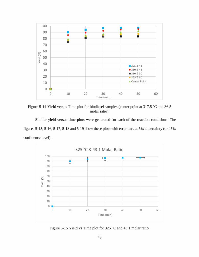
43
Figure 5-14 Yield versus Time plot for biodiesel samples (center point at 317.5 °C and 36.5
molar ratio).
Similar yield versus time plots were generated for each of the reaction conditions. The
figures 5-15, 5-16, 5-17, 5-18 and 5-19 show these plots with error bars at 5% uncertainty (or 95%
confidence level).
Figure 5-15 Yield vs Time plot for 325 °C and 43:1 molar ratio.
0
10
20
30
40
50
60
70
80
90
100
0 10 20 30 40 50 60
Yiel
d (
%)
Time (min)
325 & 43
310 & 43
310 & 30
325 & 30
Center Point
0
10
20
30
40
50
60
70
80
90
100
0 10 20 30 40 50 60
Yiel
d (
%)
Time (min)
325 °C & 43:1 Molar Ratio
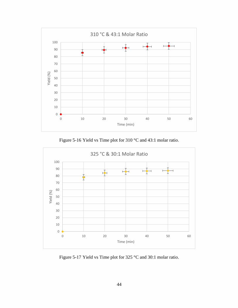
44
Figure 5-16 Yield vs Time plot for 310 °C and 43:1 molar ratio.
Figure 5-17 Yield vs Time plot for 325 °C and 30:1 molar ratio.
0
10
20
30
40
50
60
70
80
90
100
0 10 20 30 40 50 60
Yiel
d (
%)
Time (min)
310 °C & 43:1 Molar Ratio
0
10
20
30
40
50
60
70
80
90
100
0 10 20 30 40 50 60
Yiel
d (
%)
Time (min)
325 °C & 30:1 Molar Ratio
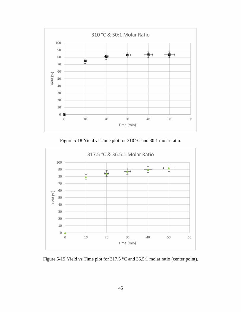
45
Figure 5-18 Yield vs Time plot for 310 °C and 30:1 molar ratio.
Figure 5-19 Yield vs Time plot for 317.5 °C and 36.5:1 molar ratio (center point).
0
10
20
30
40
50
60
70
80
90
100
0 10 20 30 40 50 60
Yiel
d (
%)
Time (min)
310 °C & 30:1 Molar Ratio
0
10
20
30
40
50
60
70
80
90
100
0 10 20 30 40 50 60
Yiel
d (
%)
Time (min)
317.5 °C & 36.5:1 Molar Ratio
46
CHAPTER 6: ANALYSIS OF VARIANCE (ANOVA) AND DEVELOPMENT OF
REGRESSION EQUATION
The experimental design chosen here is a 22 factorial design with a single replicate and
with added center points. In a two-level factorial design like this, we can define the factor effects
and the interaction effects. The factor effects can be defined as the change in output produced due
to the change in the level of one factor. It is important to note that this change is averaged over the
levels of the other factor. The interaction effect can be defined as the average difference between
the effect of one factor at the highest and at the lowest levels of the other factor [79]. In this design,
there are two main factor effects and one interaction effect. Variance analysis methods have been
used to determine the significance of the factors, temperature and molar ratio, as well as the
significance of the interaction between temperature and molar ratio.
Analysis of variance involves treating the output of the experiment (yield in this case) as a
random variable. The output is based on the factor levels that need to be compared. Before
generating the analysis of variance table, we need to convert the design factors from their natural
engineering units to coded design variables. This implies changing the numeric values of the
design factors to -1 ≤ xi ≤ +1, where xi is the design factor. Coding the variables has many
advantages. By coding the variables, it is possible to compare the magnitudes of the model
coefficients directly. Coding the variables makes them dimensionless, further, the effect of
changing each design factor over one unit interval can be measured. Moreover, the model
coefficients are estimated with the same precision. Coded variables also help in determining the
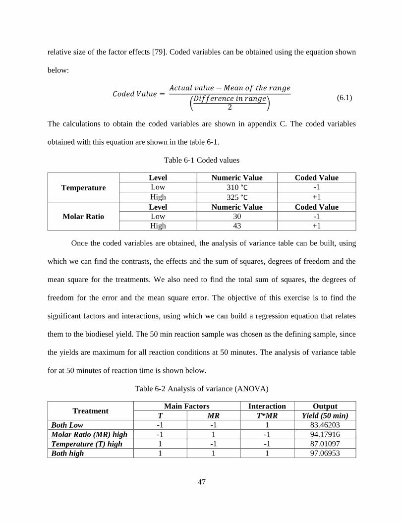
47
relative size of the factor effects [79]. Coded variables can be obtained using the equation shown
below:
𝐶𝑜𝑑𝑒𝑑 𝑉𝑎𝑙𝑢𝑒 =
𝐴𝑐𝑡𝑢𝑎𝑙 𝑣𝑎𝑙𝑢𝑒 − 𝑀𝑒𝑎𝑛 𝑜𝑓 𝑡ℎ𝑒 𝑟𝑎𝑛𝑔𝑒
(𝐷𝑖𝑓𝑓𝑒𝑟𝑒𝑛𝑐𝑒 𝑖𝑛 𝑟𝑎𝑛𝑔𝑒
2 )
(6.1)
The calculations to obtain the coded variables are shown in appendix C. The coded variables
obtained with this equation are shown in the table 6-1.
Table 6-1 Coded values
Temperature
Level Numeric Value Coded Value
Low 310 °C -1
High 325 °C +1
Molar Ratio
Level Numeric Value Coded Value
Low 30 -1
High 43 +1
Once the coded variables are obtained, the analysis of variance table can be built, using
which we can find the contrasts, the effects and the sum of squares, degrees of freedom and the
mean square for the treatments. We also need to find the total sum of squares, the degrees of
freedom for the error and the mean square error. The objective of this exercise is to find the
significant factors and interactions, using which we can build a regression equation that relates
them to the biodiesel yield. The 50 min reaction sample was chosen as the defining sample, since
the yields are maximum for all reaction conditions at 50 minutes. The analysis of variance table
for at 50 minutes of reaction time is shown below.
Table 6-2 Analysis of variance (ANOVA)
Treatment Main Factors Interaction Output
T MR T*MR Yield (50 min)
Both Low -1 -1 1 83.46203
Molar Ratio (MR) high -1 1 -1 94.17916
Temperature (T) high 1 -1 -1 87.01097
Both high 1 1 1 97.06953
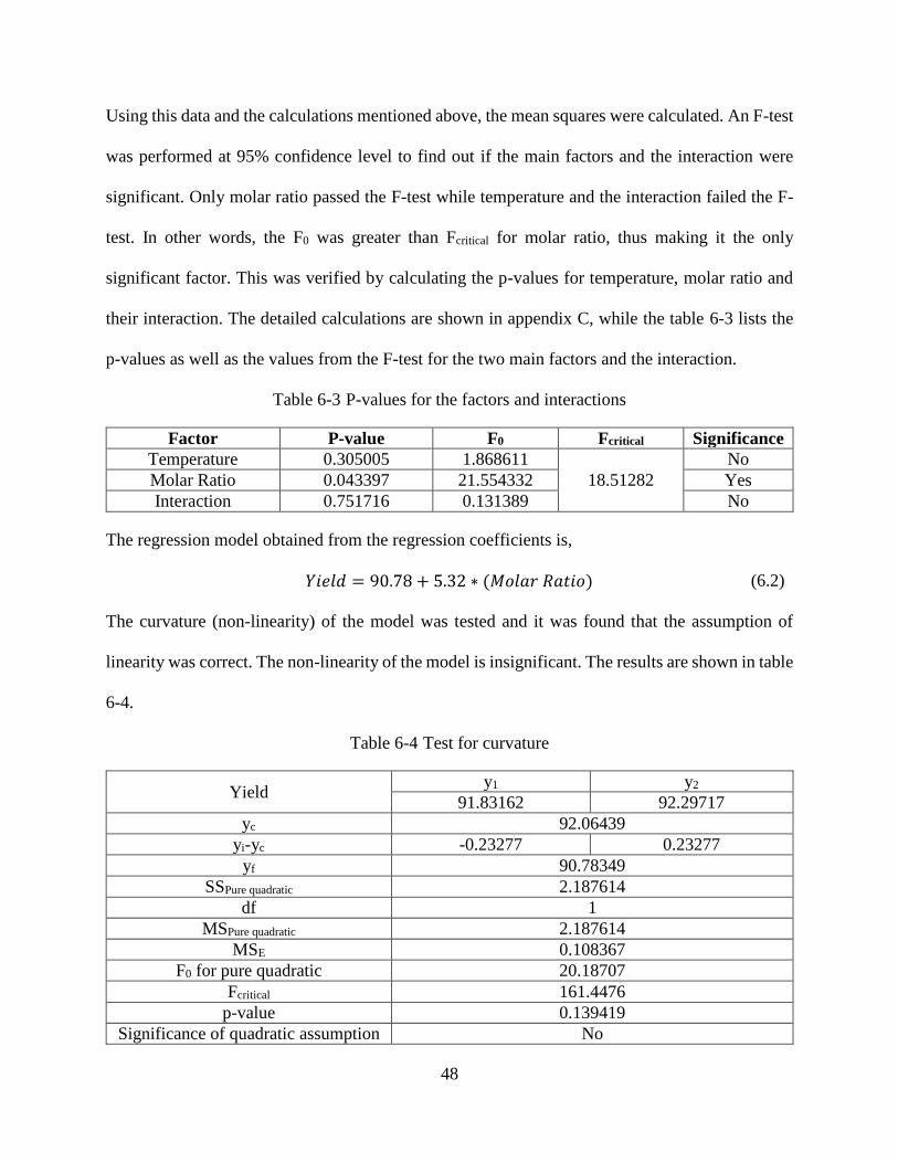
48
Using this data and the calculations mentioned above, the mean squares were calculated. An F-test
was performed at 95% confidence level to find out if the main factors and the interaction were
significant. Only molar ratio passed the F-test while temperature and the interaction failed the F-
test. In other words, the F0 was greater than Fcritical for molar ratio, thus making it the only
significant factor. This was verified by calculating the p-values for temperature, molar ratio and
their interaction. The detailed calculations are shown in appendix C, while the table 6-3 lists the
p-values as well as the values from the F-test for the two main factors and the interaction.
Table 6-3 P-values for the factors and interactions
Factor P-value F0 Fcritical Significance
Temperature 0.305005 1.868611
18.51282
No
Molar Ratio 0.043397 21.554332 Yes
Interaction 0.751716 0.131389 No
The regression model obtained from the regression coefficients is,
𝑌𝑖𝑒𝑙𝑑 = 90.78 + 5.32 ∗ (𝑀𝑜𝑙𝑎𝑟 𝑅𝑎𝑡𝑖𝑜) (6.2)
The curvature (non-linearity) of the model was tested and it was found that the assumption of
linearity was correct. The non-linearity of the model is insignificant. The results are shown in table
6-4.
Table 6-4 Test for curvature
Yield y1 y2
91.83162 92.29717
yc 92.06439
yi-yc -0.23277 0.23277
yf 90.78349
SSPure quadratic 2.187614
df 1
MSPure quadratic 2.187614
MSE 0.108367
F0 for pure quadratic 20.18707
Fcritical 161.4476
p-value 0.139419
Significance of quadratic assumption No
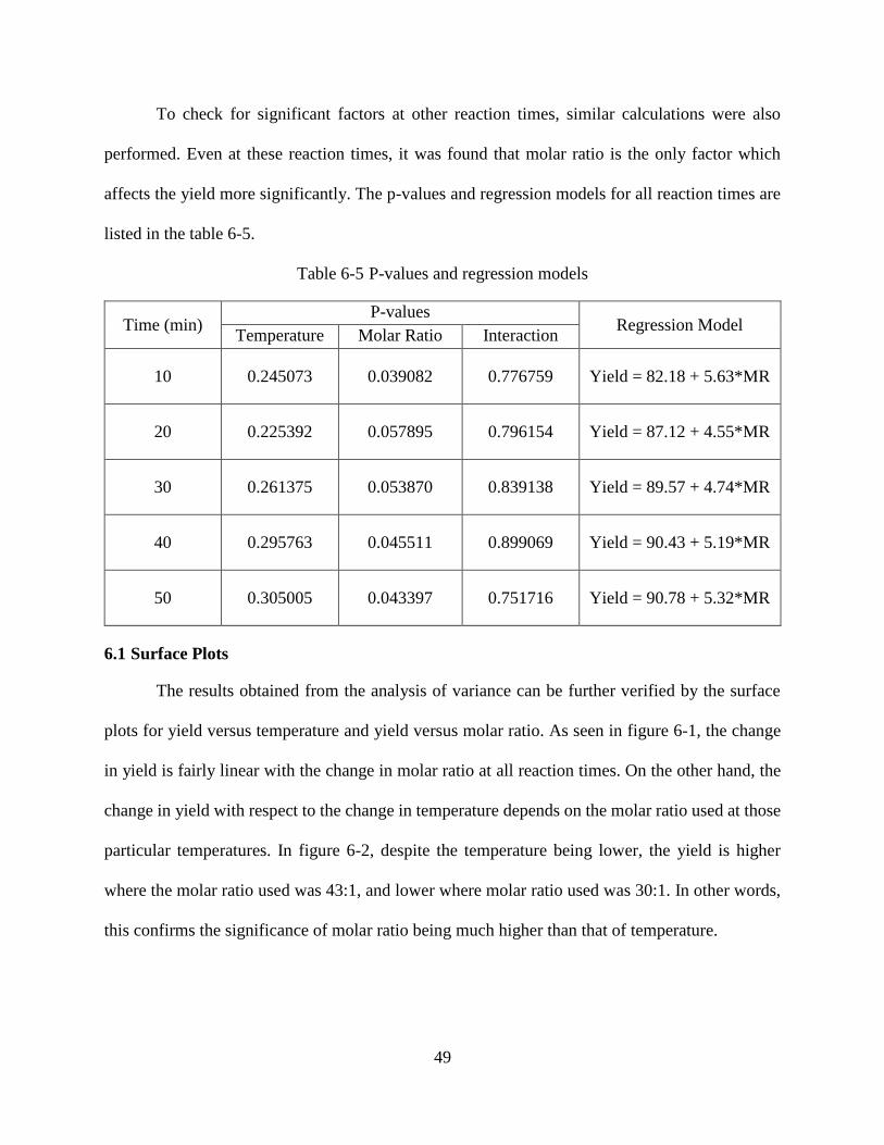
49
To check for significant factors at other reaction times, similar calculations were also
performed. Even at these reaction times, it was found that molar ratio is the only factor which
affects the yield more significantly. The p-values and regression models for all reaction times are
listed in the table 6-5.
Table 6-5 P-values and regression models
Time (min) P-values
Regression Model Temperature Molar Ratio Interaction
10 0.245073 0.039082 0.776759 Yield = 82.18 + 5.63*MR
20 0.225392 0.057895 0.796154 Yield = 87.12 + 4.55*MR
30 0.261375 0.053870 0.839138 Yield = 89.57 + 4.74*MR
40 0.295763 0.045511 0.899069 Yield = 90.43 + 5.19*MR
50 0.305005 0.043397 0.751716 Yield = 90.78 + 5.32*MR
6.1 Surface Plots
The results obtained from the analysis of variance can be further verified by the surface
plots for yield versus temperature and yield versus molar ratio. As seen in figure 6-1, the change
in yield is fairly linear with the change in molar ratio at all reaction times. On the other hand, the
change in yield with respect to the change in temperature depends on the molar ratio used at those
particular temperatures. In figure 6-2, despite the temperature being lower, the yield is higher
where the molar ratio used was 43:1, and lower where molar ratio used was 30:1. In other words,
this confirms the significance of molar ratio being much higher than that of temperature.
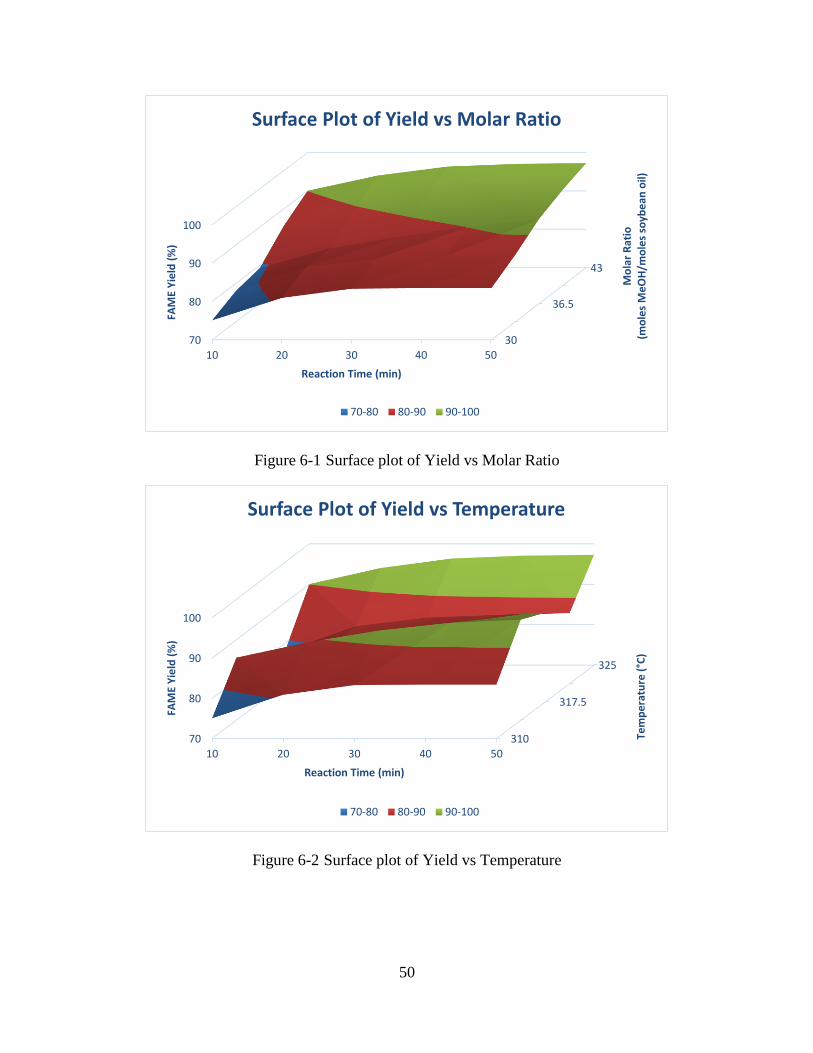
50
Figure 6-1 Surface plot of Yield vs Molar Ratio
Figure 6-2 Surface plot of Yield vs Temperature
30
36.5
43
70
80
90
100
10 20 30 40 50
Mo
lar
Rat
io(m
ole
s M
eO
H/m
ole
s so
ybe
an o
il)
FAM
E Y
ield
(%
)
Reaction Time (min)
Surface Plot of Yield vs Molar Ratio
70-80 80-90 90-100
310
317.5
325
70
80
90
100
10 20 30 40 50
Tem
pe
ratu
re (
°C)
FAM
E Y
ield
(%
)
Reaction Time (min)
Surface Plot of Yield vs Temperature
70-80 80-90 90-100

51
6.2 Residual Analysis
Using the regression equation of the model and the coded variables at the design conditions,
the model based yields are calculated. The difference in the actual yields and the model based
yields gives the residuals. A normality plot can be then generated for the residuals to check the
error distribution. The normality plot for the residuals is shown in figure 6-3.
Figure 6-3 Normality plot of residuals.
As seen in the figure, the errors are normally distributed without any departure from
normality. This implies that the model assumptions have been satisfied.
-1.5
-1
-0.5
0
0.5
1
1.5
-2.5 -2 -1.5 -1 -0.5 0 0.5 1 1.5 2 2.5Z-va
lues
Residuals
Normality Plot of Residuals

52
CHAPTER 7: A SIMPLE LUMPED TENDENCY MODEL FOR
TRANSESTERIFICATION
This chapter briefly describes the preliminary study to determine the kinetic tendency of
the reaction. Based on the integral method, a kinetic equation was obtained for the first order
reversible reaction. Using this equation the rate constants were predicted based on a non-linear
regression approach. The Arrhenius plot was generated for the rate constants and the values of
activation energy and pre-exponential factor were determined.
7.1 Kinetic Tendency of the Reaction and Estimation of Rate Constants
Using the collected experimental data, a preliminary study was performed to determine the
kinetic tendency of the supercritical transesterification reaction. Although at high molar ratios, the
reverse reaction can be ignored, for the purpose of estimating the kinetic tendency the effect of the
reverse reaction is taken into account. Thus, for kinetic purposes, the reaction is assumed to follow
first order reversible rate-law as a function of triglyceride concentration. Assuming the
supercritical transesterification reaction to follow the first order reversible rate law, the rate
constants were estimated.
For a first order reversible reaction,
𝑟𝐴 = 𝑘𝑓𝐶𝐴 − 𝑘𝑏𝐶𝐵 = −𝑑𝐶𝐴
𝑑𝑡 (7.1)
At t = 0, CA = CAo and CB = 0, then equation (7.1) can be integrated as follows
− ∫𝑑𝐶𝐴
𝑘𝑓𝐶𝐴 − 𝑘𝑏(𝐶𝐴𝑜 − 𝐶𝐴)
𝐶𝐴
𝐶𝐴0
= ∫ 𝑑𝑡𝑡
0
(7.2)
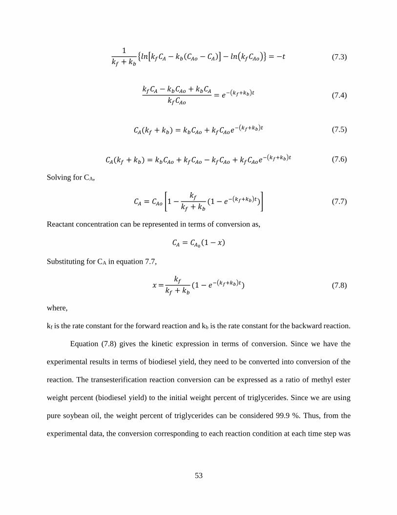
53
1
𝑘𝑓 + 𝑘𝑏{𝑙𝑛[𝑘𝑓𝐶𝐴 − 𝑘𝑏(𝐶𝐴𝑜 − 𝐶𝐴)] − 𝑙𝑛(𝑘𝑓𝐶𝐴𝑜)} = −𝑡 (7.3)
𝑘𝑓𝐶𝐴 − 𝑘𝑏𝐶𝐴𝑜 + 𝑘𝑏𝐶𝐴
𝑘𝑓𝐶𝐴𝑜= 𝑒−(𝑘𝑓+𝑘𝑏)𝑡 (7.4)
𝐶𝐴(𝑘𝑓 + 𝑘𝑏) = 𝑘𝑏𝐶𝐴𝑜 + 𝑘𝑓𝐶𝐴𝑜𝑒−(𝑘𝑓+𝑘𝑏)𝑡 (7.5)
𝐶𝐴(𝑘𝑓 + 𝑘𝑏) = 𝑘𝑏𝐶𝐴𝑜 + 𝑘𝑓𝐶𝐴𝑜 − 𝑘𝑓𝐶𝐴𝑜 + 𝑘𝑓𝐶𝐴𝑜𝑒−(𝑘𝑓+𝑘𝑏)𝑡 (7.6)
Solving for CA,
𝐶𝐴 = 𝐶𝐴𝑜 [1 −𝑘𝑓
𝑘𝑓 + 𝑘𝑏(1 − 𝑒−(𝑘𝑓+𝑘𝑏)𝑡)] (7.7)
Reactant concentration can be represented in terms of conversion as,
𝐶𝐴 = 𝐶𝐴0(1 − 𝑥)
Substituting for CA in equation 7.7,
𝑥 =𝑘𝑓
𝑘𝑓 + 𝑘𝑏(1 − 𝑒−(𝑘𝑓+𝑘𝑏)𝑡) (7.8)
where,
kf is the rate constant for the forward reaction and kb is the rate constant for the backward reaction.
Equation (7.8) gives the kinetic expression in terms of conversion. Since we have the
experimental results in terms of biodiesel yield, they need to be converted into conversion of the
reaction. The transesterification reaction conversion can be expressed as a ratio of methyl ester
weight percent (biodiesel yield) to the initial weight percent of triglycerides. Since we are using
pure soybean oil, the weight percent of triglycerides can be considered 99.9 %. Thus, from the
experimental data, the conversion corresponding to each reaction condition at each time step was
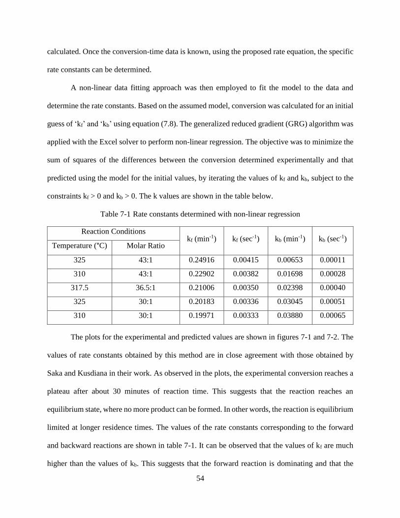
54
calculated. Once the conversion-time data is known, using the proposed rate equation, the specific
rate constants can be determined.
A non-linear data fitting approach was then employed to fit the model to the data and
determine the rate constants. Based on the assumed model, conversion was calculated for an initial
guess of ‘kf’ and ‘kb’ using equation (7.8). The generalized reduced gradient (GRG) algorithm was
applied with the Excel solver to perform non-linear regression. The objective was to minimize the
sum of squares of the differences between the conversion determined experimentally and that
predicted using the model for the initial values, by iterating the values of kf and kb, subject to the
constraints kf > 0 and kb > 0. The k values are shown in the table below.
Table 7-1 Rate constants determined with non-linear regression
Reaction Conditions kf (min-1) kf (sec-1) kb (min-1) kb (sec-1)
Temperature (°C) Molar Ratio
325 43:1 0.24916 0.00415 0.00653 0.00011
310 43:1 0.22902 0.00382 0.01698 0.00028
317.5 36.5:1 0.21006 0.00350 0.02398 0.00040
325 30:1 0.20183 0.00336 0.03045 0.00051
310 30:1 0.19971 0.00333 0.03880 0.00065
The plots for the experimental and predicted values are shown in figures 7-1 and 7-2. The
values of rate constants obtained by this method are in close agreement with those obtained by
Saka and Kusdiana in their work. As observed in the plots, the experimental conversion reaches a
plateau after about 30 minutes of reaction time. This suggests that the reaction reaches an
equilibrium state, where no more product can be formed. In other words, the reaction is equilibrium
limited at longer residence times. The values of the rate constants corresponding to the forward
and backward reactions are shown in table 7-1. It can be observed that the values of kf are much
higher than the values of kb. This suggests that the forward reaction is dominating and that the
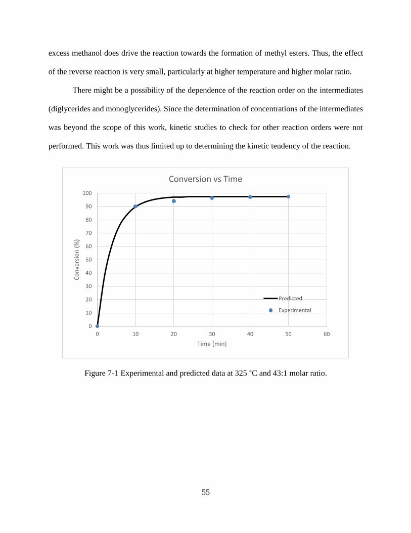
55
excess methanol does drive the reaction towards the formation of methyl esters. Thus, the effect
of the reverse reaction is very small, particularly at higher temperature and higher molar ratio.
There might be a possibility of the dependence of the reaction order on the intermediates
(diglycerides and monoglycerides). Since the determination of concentrations of the intermediates
was beyond the scope of this work, kinetic studies to check for other reaction orders were not
performed. This work was thus limited up to determining the kinetic tendency of the reaction.
Figure 7-1 Experimental and predicted data at 325 °C and 43:1 molar ratio.
0
10
20
30
40
50
60
70
80
90
100
0 10 20 30 40 50 60
Co
nve
rsio
n (
%)
Time (min)
Conversion vs Time
Predicted
Experimental
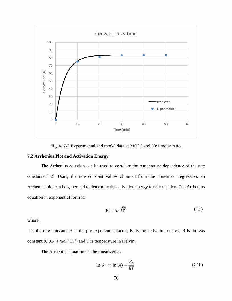
56
Figure 7-2 Experimental and model data at 310 °C and 30:1 molar ratio.
7.2 Arrhenius Plot and Activation Energy
The Arrhenius equation can be used to correlate the temperature dependence of the rate
constants [82]. Using the rate constant values obtained from the non-linear regression, an
Arrhenius plot can be generated to determine the activation energy for the reaction. The Arrhenius
equation in exponential form is:
k = A𝑒−𝐸𝑎𝑅𝑇 (7.9)
where,
k is the rate constant; A is the pre-exponential factor; Ea is the activation energy; R is the gas
constant (8.314 J mol-1 K-1) and T is temperature in Kelvin.
The Arrhenius equation can be linearized as:
ln(𝑘) = ln(𝐴) −𝐸𝑎
𝑅𝑇 (7.10)
0
10
20
30
40
50
60
70
80
90
100
0 10 20 30 40 50 60
Co
nve
rsio
n (
%)
Time (min)
Conversion vs Time
Predicted
Experimental
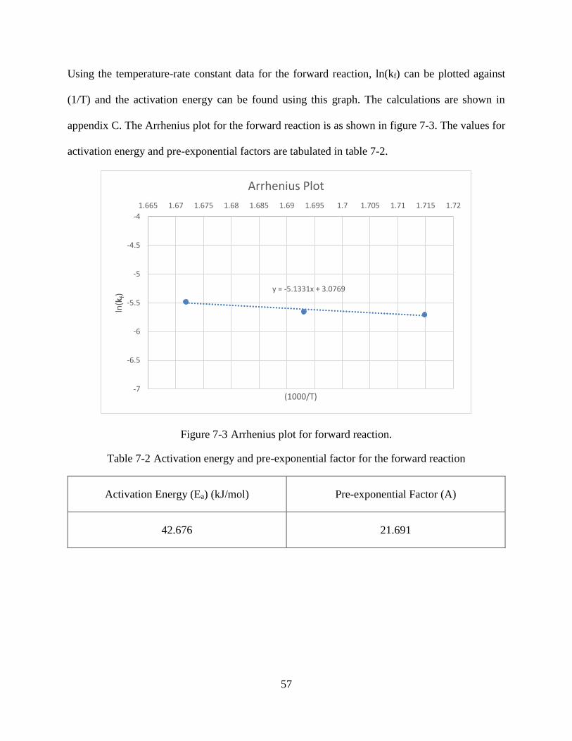
57
Using the temperature-rate constant data for the forward reaction, ln(kf) can be plotted against
(1/T) and the activation energy can be found using this graph. The calculations are shown in
appendix C. The Arrhenius plot for the forward reaction is as shown in figure 7-3. The values for
activation energy and pre-exponential factors are tabulated in table 7-2.
Figure 7-3 Arrhenius plot for forward reaction.
Table 7-2 Activation energy and pre-exponential factor for the forward reaction
Activation Energy (Ea) (kJ/mol) Pre-exponential Factor (A)
42.676 21.691
y = -5.1331x + 3.0769
-7
-6.5
-6
-5.5
-5
-4.5
-4
1.665 1.67 1.675 1.68 1.685 1.69 1.695 1.7 1.705 1.71 1.715 1.72
ln(k
f)
(1000/T)
Arrhenius Plot
58
CHAPTER 8: CONCLUSIONS AND RECOMMENDATIONS
The production of biodiesel under supercritical conditions was studied in a batch reactor.
Biodiesel was produced from soybean oil through transesterification with methanol at supercritical
conditions. Past research has proved that transesterification using supercritical fluids has several
advantages over conventional transesterification methods. This study was conducted using a pilot
scale experimental system which is scalable to a continuous operation. Milder operating pressures
than those presented in earlier studies were used. This chapter is aimed at providing the conclusions
of this research as well as recommendations to enhance the intrinsic merits of this study.
8.1 Conclusions
The work presented a methodology to produce biodiesel from transesterification of
vegetable oils using supercritical methanol. This study included the method development for
analyzing the biodiesel samples using a gas chromatograph. Biodiesel yields were determined
using gas chromatography and the effects of the key reaction variables like molar ratio and
temperature on yield were studied. Variance analysis was carried out to determine which factor(s)
and factor interactions significantly affect biodiesel yield. It was found that molar ratio has the
strongest effect on biodiesel yield. Although the reaction yield depends on temperature as well,
this dependence was observed to be far weaker as compared to that on molar ratio. Using linear
regression, a regression model was developed which relates the molar ratio and the biodiesel yield.
A preliminary kinetic study was performed to determine the rate constants of the
transesterification reaction under supercritical conditions. The reaction was assumed to be first
order reversible and the rate constants were determined by non-linear regression. The values of
59
rate constants suggest that the forward reaction is dominating and that the effect of the reverse
reaction is negligible. The data predicted by the model and that obtained experimentally is in close
agreement. From the experimental data, it can be observed that the reaction conversion approaches
a steady state at longer residence times. This suggests that the reaction is equilibrium limited,
particularly at long residence times.
Significant work has been done in the past on biodiesel production using supercritical
technology, particularly the work done by Saka and Kusdiana (2001), and He et al. (2007), is
notable. Although this thesis presents the work on a similar technology for biodiesel production,
the reactor used in this work is 1 liter in volume, as opposed to the 5 ml to 200 ml reaction vessels
used in the studies before. Thus, the scale of the reactor used here is significantly larger as
compared to that in any of the past work. From a perspective of the kinetic study, the reactor used
here is by far the largest reactor used till date. Further, the batch type setup used here can be easily
converted to a continuous mode thereby allowing a much higher production capacity. These key
differences in the equipment represent the true scalability of this technology. The pressures used
here were within 11-13 MPa range as opposed to the 28 MPa to 65 MPa pressures used in the past.
Although the pressures used in this work are much milder (but within the supercritical region) in
comparison with the past work, the yields are comparable and still within the 90% plus range.
Thus, it can be seen that supercritical transesterification can give promising results even at milder
conditions.
8.2 Recommendations and Future Work
Each experiment in the factorial design was performed once, with the exception of the
center point. In other words, the factorial design involved one replicate (n=1) experiments. One
replicate experiments were chosen to maintain a balance between the time consuming nature of
the experiment and the time constraints associated with the completion of this project. The choice
60
of this sample size plays a significant role in controlling the type II error (β error) associated with
the experiment, with the aim being, the selection of sample size to reduce the β error. It is
recommended to carry out the experiments with more than one replicate and then perform variance
analysis to observe the change in error.
The quantitative analysis of the intermediate reaction products (monoglycerides and
diglycerides) was beyond the scope of this work due to certain constraints like derivatization and
the limitation of the GC column. Derivatization involves altering the compounds chemically to
change their affinity towards the GC column which allows for an easier separation. But, this is a
multi-step process, often introducing large error in the sample-preparation stage. Hence, an error
free derivatization process needs to be developed that can easily quantify these intermediates.
Further, the quantification of these intermediates can also help in improving the results of the
kinetic study. Using the quantification data, it will be possible to fit kinetic models for higher order
reactions.
61
REFERENCES
[1] (2015). Annual Energy Outlook. U.S. Energy Information Administration, Washington, DC
[2] Yuan, J. S., Tiller, K. H., Al-Ahmad, H., Stewart, N. R., & Stewart, C. N. (2008). Plants to
power: bioenergy to fuel the future. Trends in Plant Science, 13(8), 421-429
[3] Demirbas, A. (2003). Biodiesel fuels from vegetable oils via catalytic and non-catalytic
supercritical alcohol transesterifications and other methods: a survey. Energy conversion and
Management, 44(13), 2093-2109
[4] Ma, F., Hanna, M. A. (1999). Biodiesel production: a review. Bioresource Technology, 70(1),
1-15
[5] Hanna, M. A., Isom, L., & Campbell, J. (2005). Biodiesel: current perspectives and future.
Journal of Scientific and Industrial Research, 64(11), 854-857
[6] Sheehan, J., Camobreco, V., Duffield, J., Shapouri, H., Graboski, M., & Tyson, s. (2000). An
overview of biodiesel and petroleum diesel life cycles (No. NREL/TP-580-24772). National
Renewable Energy Lab, Golden, CO (US).
[7] Lins, C., Williamson, L. E., Leitner, S., & Teske, S. (2014). The first decade: 2004-2014, 10
years of renewable energy progress, REN21 Secretariat, Paris, France
[8] http://biodiesel.org/what-is-biodiesel/biodiesel-faq's, Biodiesel FAQ’s. (2015), last accessed
8/24/2015
[9] Abbaszaadeh, A., Ghobadian, B., Omidkhah, M. R., & Najafi, G. (2012). Current biodiesel
production technologies: a comparative review. Energy conversion and Management, 63, 138-148
62
[10] Demirbas, A. (2005). Biodiesel production from vegetable oils via catalytic and non-catalytic
supercritical methanol transesterification methods. Progress in Energy and Combustion Science,
31(5-6), 466-487
[11] Bartholomew, D. (1981). Vegetable oil fuel. J. Am. Oil. Chem. Soc., 58 (4)
[12] Ramadhas, A. S., Jayaraj, S., & Muraleedharan, C. (2004). Use of vegetable oils as I.C. engine
fuels – A review. Renewable Energy, 29(5), 727-742
[13] Jahirul, M. I., Rasul, M. G., Chowdhury, A. A., & Ashwath, N. (2012). Biofuels production
through biomass pyrolysis – a technological review. Energies, 5(12), 4952-5001
[14] Chang, C., & Wan, S. W. (1947). China’s motor fuels from tung oil. Industrial and
Engineering Chemistry, 39(12), 1543-1548
[15] Aguado, R., Gaisan, B., Prieto, R., & Bilbao, J. (2003). Kinetics of polystyrene pyrolysis in a
conical spouted bed reactor. Chemical Engineering Journal, 92(1), 91-99
[16] Cornelissen T., Yperman, J., Reggers, G., Schreurs, S., & Carleer, R. (2008). Flash co-
pyrolysis of biomass with polylactic acid. Part 1: Influence on bio-oil yield and heating value.
Fuel, 87(7), 1031-1041
[17] Sharma, M. K., & Shah D. O. (1983). Introduction to macro- and microemulsions. In ACS
symposium series (No. 272, pp. 1-18). Oxford University Press
[18] Yusuf, N. N. A. N., Kamarudin, S. K., & Yaakub, Z. (2011). Overview on the current trends
in biodiesel production. Energy conversion and Management, 52(7), 2741-2751
[19] Ziejewski, M., Kaufman, K. R., Schwab, A. W., & Pryde, E. H. (1984). Diesel engine
evaluation of a nonionic sunflower oil-aqueous ethanol microemulsion. Journal of the American
Oil Chemists’ Society, 61(10), 1620-1626
63
[20] Ali, Y., & Hanna, M. A. (1994). Alternative diesel fuels from vegetable oils. Bioresource
Technology, 50(2), 153-163
[21] Otera, J. (1993). Transesterification. Chemical Reviews, 93(4), 1449-1470
[22] Srivastava, A., & Prasad, R. (2000). Triglyceride-based diesel fuels. Renewable and
Sustainable Energy Reviews, 4(2), 111-133
[23] Meher, L. C., Sagar, D. V., & Naik, S. N. (2006). Technical aspects of biodiesel production
by transesterification – a review. Renewable and Sustainable Energy Reviews, 10(3), 248-268
[24] Gryglewicz, S. (1999). Rapeseed oil methyl ester preparation using heterogeneous catalysts.
Bioresource Technology, 70(3), 249-253
[25] Canacki, M., & Van Gerpen, J. (1999). Biodiesel production via acid catalysts. Transactions
of the ASAE – American Society of Agricultural Engineers, 42(5), 1203-1210
[26] Briand, D., Dubreucq, E., & Galzy, P. (1994). Enzymatic fatty ester synthesis in aqueous
medium with lipase from Candida parapsilosis (Ashford) Langeron and Talice. Biotechnolgy
Letters, 16(8), 813-818
[27] Freedman, B., Butterfield, R. O., & Pryde, E. H. (1986). Transesterifcation kinetics of soybean
oil. Journal of American Oil Chemists’ Society, 63(10), 1375-1380
[28] Lotero, E., Lui, Y., Lopez, D. E., Suwannakam, K., Bruce, D. A., & Goodwin, J. G. (2005).
Synthesis of biodiesel via acid catalysts. Industrial and Engineering Chemistry Research, 44(14),
5353-5363
[29] Lam, M. K., Lee, K. T., & Mohamed, A. R. (2010). Homogeneous, heterogeneous and
enzymatic catalysis for transesterification of high free fatty acid oil (waste cooking oil) to
biodiesel: a review. Biotechnology Advances, 28(4), 500-518
64
[30] Wang, Y., Ou, S., Liu, P., Xue, F., & Tang, S. (2006). Comparison of two different processes
to synthesize biodiesel by waste cooking oil. Journal of Molecular Catalysis A: Chemical, 252(1-
2), 107-112
[31] Felizardo, P., Correia, M. J. N., Raposo, I., Mendes, J. F., Berkemeier, R., & Bordado, J. M.
(2006). Production of biodiesel from waste frying oils. Waste Management, 26(5), 487-494
[32] Zabeti, M., Daud, W. M. A. W., & Aroua, M. K. (2009). Activity of solid catalysts for
biodiesel production: a review. Fuel Processing Technology, 90(6), 770-777
[33] Kouzu, M., Kasuno, T., Tajika, M., Sugimoto, Y., Yamanaka, S., & Hidaka, J. (2008).
Calcium oxide as a solid base catalyst for transesterification of soybean oil and its application to
biodiesel production. Fuel, 87(12). 2798-2806
[34] Di Serio, M., Ledda, M., Cozzolino, M., Minutillo, G., Tesser, R., & Santacesaria, E. (2006).
Transesterification of soybean oil to biodiesel by using heterogeneous basic catalyst. Industrial &
Engineering Chemistry Research, 45(9), 3009-3014
[35] Liu, X., He, H., Wang, Y., & Zhu, S. (2007). Transesterification of soybean oil to biodiesel
using SrO as a solid base catalyst. Catalysis Communications, 8(7), 1107-1111.
[36] Kulkarni, M. G., & Dalai, A. K., (2006). Waste cooking oil an economic source for biodiesel:
a review. Industrial and & Engineering Chemistry Research, 45(9), 2901-2913.
[37] Jitputti, J., Kitiyanan, B., Rangsunvigit, P., Bunyakiat. K., Attanatho, L., & Jenvanitpankajul,
P. (2006). Tranesterification of crude palm kernel oil and coconut oil by different solid catalysts.
Chemical Engineering Journal, 116(1), 61-66.
[38] Ranganathan, S. V. Narasimhan, S. L., & Muthukumar, K. (2008). An overview of enzymatic
production of biodiesel. Bioresource Technology, 99(10), 3975-3981.
65
[39] Mittelbach, M. (1990). Lipase catalyzed alcoholysis of sunflower oil. Journal of the American
Oil Chemists’ Society, 67(3), 168-170.
[40] Bajaj, A., Lohan, P., Jha, P. N., Mehrotra, R. (2010). Biodiesel production through lipase
catalyzed transesterification: An overview. Journal of Molecular Catalysis B: Enzymatic, 62(1),
9-14.
[41] Cagniard De La Tour, C. (1822). Presentation of some results obtained by the combined action
of heat and compression on certain liquids, such as water, alcohol, ether [i.e., diethyl ether], and
distilled petroleum spirit. Annales de Chimie et de Physique, 21(2), 127-132.
[42] Darr. J. A., & Poliakoff. M. (1999). New directions in inorganic and metal-organic
coordination chemistry in supercritical fluids. Chemical Reviews, 99(2), 495-542.
[43] Ngamprasertsith, S., & Sawangkeaw, R. (2011). Transesterification in supercritical
conditions. Biodiesel Feedstocks and Processing Technologies, Rejika: InTech, 247-268.
[44] Kemmere, M. F., & Meyer, T. (Eds.). (2006). Supercritical carbon dioxide in polymer reaction
engineering,, John Wiley & Sons, Weinheim, Germany.
[45] Clifford, A., & Clifford, T. (1999). Fundamentals of Supercritical Fluids, Oxford University
Press.
[46] Arai, Y., Sako, Y., & Takebayashi, Y. (Eds). (2013). Supercritical fluids molecular
interactions, physical properties and new applications. Springer Science & Business Media.
[47] Daisakou, M., Louloudi, A; & Papayannakos, N. (1998). Kinetics of the non-catalytic
transesterification of soybean oil. Fuel, 77(12), 1297-1302
[48] Saka, S., & Kusdiana, D. (2001). Biodiesel fuel from rapeseed oil as prepared in supercritical
methanol. Fuel, 80(2), 225-231
66
[49] Kusdiana, D., & Saka, S. (2001). Kinetics of transesterification in rapeseed oil to biodiesel
fuel as treated in supercritical methanol. Fuel, 80(5), 693-698
[50] Song, E., Lim, J., Le, H., & Lee, Y. (2008). Transesterification of RBD palm oil using
supercritical methanol. The Journal of Supercritical Fluids, 44(3), 356-363
[51] He, H., Sun, S., Wang, T., & Zhu, S. (2007). Transesterification kinetics of soybean oil for
production of biodiesel in supercritical methanol. Journal of the American Oil Chemists’ Society,
84(4), 399-404
[52] Bernal, J. M., Lozano, P., Garcia-Verdugo, E., Burguet, M. I., Sanchez-Gomez, G., Lopez-
Lopez, G., Pucheault, M., Vaultier, M., & Luis, S. V. (2012). Supercritical synthesis of biodiesel.
Molecules, 17(7), 8696-8719
[53] Bunyakiat, K., Makmee, S., Sawangkeaw, R., & Ngamprasertsith, S. (2006). Continuous
production of biodiesel via transesterification from vegetable oils in supercritical methanol.
Energy & Fuels, 20(2). 812-817.
[54] Demirbas, A. (2002). Biodiesel from vegetable oils via transesterification in supercritical
methanol. Energy Conversion & Management, 43(17), 2349-2356
[55] Kusdiana, D., & Saka, S. (2004). Effects of water on biodiesel fuel production by supercritical
methanol treatment. Bioresource Technology, 91(3), 289-295
[56] Vietez, I., Pardo, M. J., Da Silva, C., Bertoli, C., De Castilhos, F., Oliveira, J. V., Grompone,
M. A., & Jachmanian, I. (2011). Continuous synthesis of castor oil ethyl esters under supercritical
ethanol. The Journal of Supercritical Fluids, 56(3), 271-276
[57] Diaz, M. S., Espinosa, S., & Brignole, E. A. (2009). Model-based cost minimization in non-
catalytic biodiesel production plants. Energy & Fuels, 23(11), 5587-5595
67
[58] Marchetti, J. M., & Errazu, A. F. (2008). Technoeconomic study of supercritical biodiesel
production plant. Energy Conversion and Management, 49(8), 2160-2164.
[59] Haas, M. J., McAloon, A. J., Yee, W. C., & Foglia, T. A. (2006). A process model to estimate
biodiesel production costs. Bioresource Technology, 97(4), 671-678
[60] Ahmad, A., Yasin, N. M., Derek, C., & Lim, J. (2011). Microalgae as a sustainable energy
source for biodiesel production: a review. Renewable and Sustainable Energy Reviews, 15(1),
584-593
[61] Canakci, M. (2007). The potential of restaurant waste lipids as biodiesel feedstocks.
Bioresource Technology, 98(1), 183-190
[62] Barnwal, B. K., & Sharma, M. P. (2005). Prospects of biodiesel production from vegetable
oils in India. Renewable and Sustainable Energy Reviews, 9(4), 363-378
[63] Issariyakul, T., & Dalai, A. K. (2014). Biodiesel from vegetable oils. Renewable and
Sustainable Energy Reviews, 31, 446-471
[64] Chhetri, A. B., Watts, K. C., & Islam, M. R. (2008). Waste cooking oil as an alternate
feedstock for biodiesel production. Energies, 1(1), 3-18
[65] Nawar, W. W. (1984). Chemical changes in lipids produced by thermal processing. Journal
of Chemical Education, 61(4), 299
[66] Mittelbach, M., & Enzelsberger, H. (1999). Transesterification of heated rapeseed oil for
extending diesel fuel. Journal of the American Oil Chemists’ Society, 76(5), 545-550
[67] Zheng, D., & Hanna, M. (1996). Preparation and properties of methyl esters of beef tallow.
Bioresource Technology, 57(2), 137-142
[68] Karmarkar, A., Karmarkar, S., & Mukherjee, S. (2010). Properties of various plants and
animals feedstocks for biodiesel production. Bioresource Technology, 101(19), 7201-7210
68
[69] Marulanda, V. E., Anitescu, G., & Tavlarides, L. L. (2009). Biodiesel fuels through a
continuous flow process of chicken fat supercritical transesterification. Energy & Fuels, 24(1),
253-260
[70] Lebedevas, S., Vaicekauskas, A., Lebedeva, G., Makareviciene, V., Janulis, P., & Kazancev,
K. (2006). Use of waste fats of animal and vegetable origin for the production of biodiesel fuel:
quality, motor properties, and emissions of harmful components. Energy & fuels, 20(5), 2274-
2280.
[71] Öner, C., & Altun, Ş. (2009). Biodiesel production from inedible animal tallow and an
experimental investigation of its use as alternative fuel in a direct injection diesel engine. Applied
Energy, 86(10), 2114-2120.
[72] Mata, T. M., Martins, A. A., & Caetano, N. S. (2010). Microalgae for biodiesel production
and other applications: a review. Renewable and Sustainable Energy Reviews, 14(1), 217-232
[73] Suen, Y., Hubbard, J. S., Holzer, G., & Tornabene, T. G. (1987). Total lipid production of the
green alga Nannochloropsis Sp. QII under different nitrogen regimes. Journal of
Phycology, 23(s2), 289-296.
[74] Grima, E. M., Belarbi, E. H., Fernández, F. A., Medina, A. R., & Chisti, Y. (2003). Recovery
of microalgal biomass and metabolites: process options and economics. Biotechnology
advances, 20(7), 491-515.
[75] Halim, R., Danquah, M. K., & Webley, P. A. (2012). Extraction of oil from microalgae for
biodiesel production: a review. Biotechnology advances, 30(3), 709-732.
[76] Uduman, N., Qi, Y., Danquah, M. K., Forde, G. M., & Hoadley, A. (2010). Dewatering of
microalgal cultures: a major bottleneck to algae-based fuels.Journal of renewable and sustainable
energy, 2(1), 012701.
69
[77] Yanfen, L., Zehao, H., & Xiaoqian, M. (2012). Energy analysis and environmental impacts
of microalgal biodiesel in China. Energy Policy, 45, 142-151.
[78] Lardon, L., Helias, A., Sialve, B., Steyer, J. P., & Bernard, O. (2009). Life-cycle assessment
of biodiesel production from microalgae. Environmental science & technology, 43(17), 6475-
6481.
[79] Montgomery, D. C., & Montgomery, D. C. (1984). Design and analysis of experiments (Vol.
7). New York: Wiley.
[80] Pietrzyk, D. J., & Frank, C. W. (1979). Development of an analytical method (Edition 2).
New York: Academic Press.
[81] Barwick, V. (2003). Preparation of calibration curves – A guide to best practices. LGC
Limited.
[82] Foggler Scott, H. (2010). Elements of Chemical Reaction Engineering (Edition 4). Prentice
Hall International Series in the Physical and Chemical Engineering Sciences. Boston, MA.
[83] Sunol, A. K., & Sunol, S. G. (2001). Safer solvents and processes, Handbook of Solvents
(Edition 2, 2014), Ed. Wypych, G., Chem Tech Publishing.
[84] Sunol, A. K., Sunol, S. G., & Aslam, N. (2005). Supercritical fluid technology – reactions,
Ed. Sunggyu Lee, C. W., Encyclopedia of Chemical Processing (ECHP), Marcel Dekker, Inc.
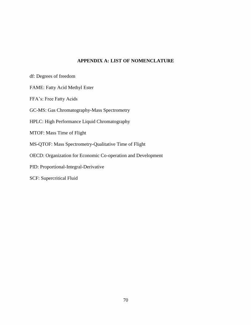
70
APPENDIX A: LIST OF NOMENCLATURE
df: Degrees of freedom
FAME: Fatty Acid Methyl Ester
FFA’s: Free Fatty Acids
GC-MS: Gas Chromatography-Mass Spectrometry
HPLC: High Performance Liquid Chromatography
MTOF: Mass Time of Flight
MS-QTOF: Mass Spectrometry-Qualitative Time of Flight
OECD: Organization for Economic Co-operation and Development
PID: Proportional-Integral-Derivative
SCF: Supercritical Fluid
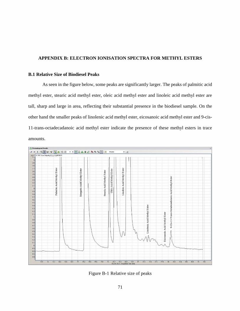
71
APPENDIX B: ELECTRON IONISATION SPECTRA FOR METHYL ESTERS
B.1 Relative Size of Biodiesel Peaks
As seen in the figure below, some peaks are significantly larger. The peaks of palmitic acid
methyl ester, stearic acid methyl ester, oleic acid methyl ester and linoleic acid methyl ester are
tall, sharp and large in area, reflecting their substantial presence in the biodiesel sample. On the
other hand the smaller peaks of linolenic acid methyl ester, eicosanoic acid methyl ester and 9-cis-
11-trans-octadecadanoic acid methyl ester indicate the presence of these methyl esters in trace
amounts.
Figure B-1 Relative size of peaks
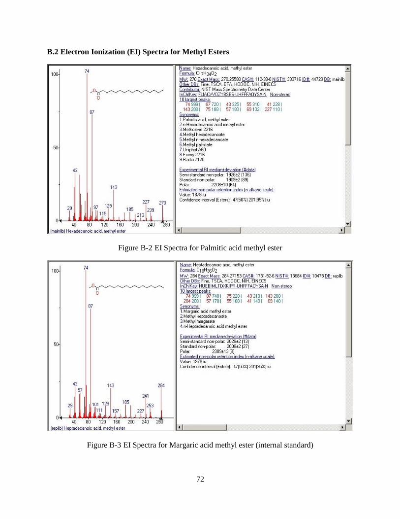
72
B.2 Electron Ionization (EI) Spectra for Methyl Esters
Figure B-2 EI Spectra for Palmitic acid methyl ester
Figure B-3 EI Spectra for Margaric acid methyl ester (internal standard)
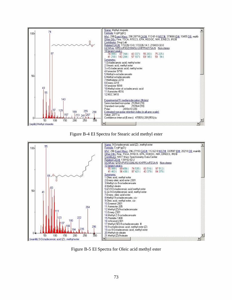
73
Figure B-4 EI Spectra for Stearic acid methyl ester
Figure B-5 EI Spectra for Oleic acid methyl ester
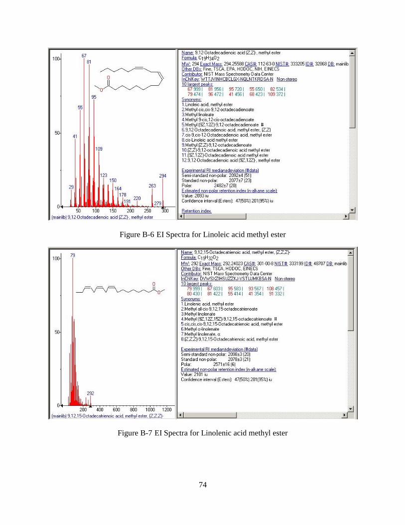
74
Figure B-6 EI Spectra for Linoleic acid methyl ester
Figure B-7 EI Spectra for Linolenic acid methyl ester
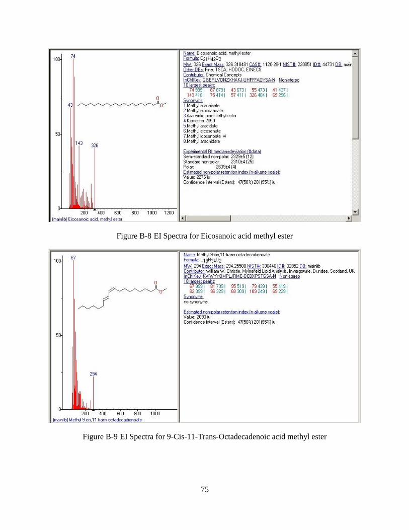
75
Figure B-8 EI Spectra for Eicosanoic acid methyl ester
Figure B-9 EI Spectra for 9-Cis-11-Trans-Octadecadenoic acid methyl ester
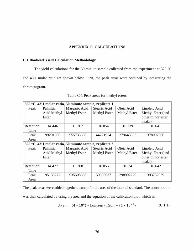
76
APPENDIX C: CALCULATIONS
C.1 Biodiesel Yield Calculation Methodology
The yield calculations for the 50 minute sample collected from the experiment at 325 °C
and 43:1 molar ratio are shown below. First, the peak areas were obtained by integrating the
chromatogram.
Table C-1 Peak areas for methyl esters
325 °C, 43:1 molar ratio, 50 minute sample, replicate 1
Peak Palmitic
Acid Methyl
Ester
Margaric Acid
Methyl Ester
Stearic Acid
Methyl Ester
Oleic Acid
Methyl Ester
Linoleic Acid
Methyl Ester (and
other minor ester
peaks)
Retention
Time
14.446 15.267 16.054 16.239 16.641
Peak
Area
99201506 555735630 44721954 279648553 378097506
325 °C, 43:1 molar ratio, 50 minute sample, replicate 2
Peak Palmitic
Acid Methyl
Ester
Margaric Acid
Methyl Ester
Stearic Acid
Methyl Ester
Oleic Acid
Methyl Ester
Linoleic Acid
Methyl Ester (and
other minor ester
peaks)
Retention
Time
14.477 15.268 16.055 16.24 16.642
Peak
Area
95135277 535508636 50390037 298992220 393752939
The peak areas were added together, except for the area of the internal standard. The concentration
was then calculated by using the area and the equation of the calibration plot, which is:
𝐴𝑟𝑒𝑎 = (4 ∗ 106) ∗ 𝐶𝑜𝑛𝑐𝑒𝑛𝑡𝑟𝑎𝑡𝑖𝑜𝑛 − (1 ∗ 10−8) (C.1.1)
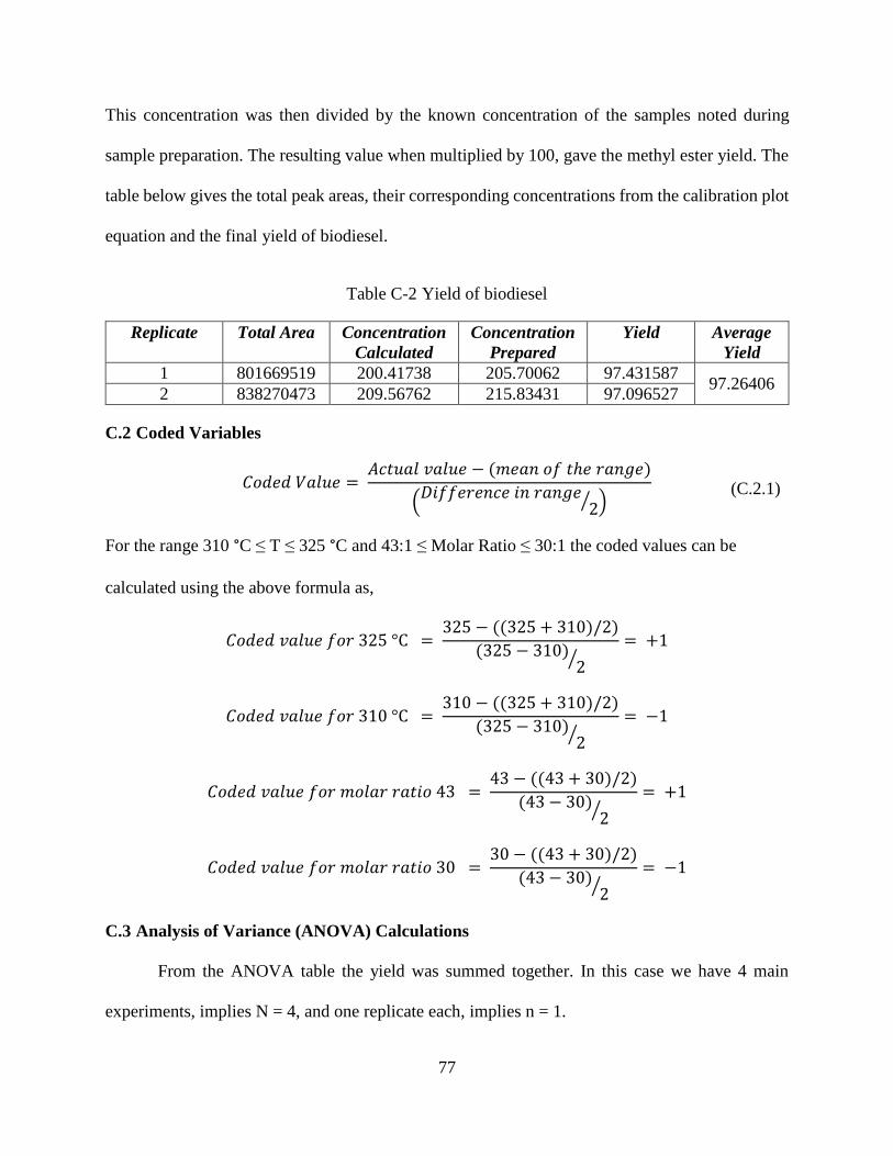
77
This concentration was then divided by the known concentration of the samples noted during
sample preparation. The resulting value when multiplied by 100, gave the methyl ester yield. The
table below gives the total peak areas, their corresponding concentrations from the calibration plot
equation and the final yield of biodiesel.
Table C-2 Yield of biodiesel
Replicate Total Area Concentration
Calculated
Concentration
Prepared
Yield Average
Yield
1 801669519 200.41738 205.70062 97.431587 97.26406
2 838270473 209.56762 215.83431 97.096527
C.2 Coded Variables
𝐶𝑜𝑑𝑒𝑑 𝑉𝑎𝑙𝑢𝑒 = 𝐴𝑐𝑡𝑢𝑎𝑙 𝑣𝑎𝑙𝑢𝑒 − (𝑚𝑒𝑎𝑛 𝑜𝑓 𝑡ℎ𝑒 𝑟𝑎𝑛𝑔𝑒)
(𝐷𝑖𝑓𝑓𝑒𝑟𝑒𝑛𝑐𝑒 𝑖𝑛 𝑟𝑎𝑛𝑔𝑒
2⁄ ) (C.2.1)
For the range 310 °C ≤ T ≤ 325 °C and 43:1 ≤ Molar Ratio ≤ 30:1 the coded values can be
calculated using the above formula as,
𝐶𝑜𝑑𝑒𝑑 𝑣𝑎𝑙𝑢𝑒 𝑓𝑜𝑟 325 °C = 325 − ((325 + 310)/2)
(325 − 310)2⁄
= +1
𝐶𝑜𝑑𝑒𝑑 𝑣𝑎𝑙𝑢𝑒 𝑓𝑜𝑟 310 °C = 310 − ((325 + 310)/2)
(325 − 310)2⁄
= −1
𝐶𝑜𝑑𝑒𝑑 𝑣𝑎𝑙𝑢𝑒 𝑓𝑜𝑟 𝑚𝑜𝑙𝑎𝑟 𝑟𝑎𝑡𝑖𝑜 43 = 43 − ((43 + 30)/2)
(43 − 30)2⁄
= +1
𝐶𝑜𝑑𝑒𝑑 𝑣𝑎𝑙𝑢𝑒 𝑓𝑜𝑟 𝑚𝑜𝑙𝑎𝑟 𝑟𝑎𝑡𝑖𝑜 30 = 30 − ((43 + 30)/2)
(43 − 30)2⁄
= −1
C.3 Analysis of Variance (ANOVA) Calculations
From the ANOVA table the yield was summed together. In this case we have 4 main
experiments, implies N = 4, and one replicate each, implies n = 1.
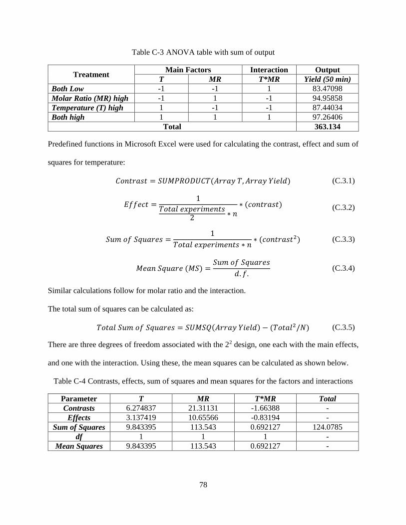
78
Table C-3 ANOVA table with sum of output
Treatment Main Factors Interaction Output
T MR T*MR Yield (50 min)
Both Low -1 -1 1 83.47098
Molar Ratio (MR) high -1 1 -1 94.95858
Temperature (T) high 1 -1 -1 87.44034
Both high 1 1 1 97.26406
Total 363.134
Predefined functions in Microsoft Excel were used for calculating the contrast, effect and sum of
squares for temperature:
𝐶𝑜𝑛𝑡𝑟𝑎𝑠𝑡 = 𝑆𝑈𝑀𝑃𝑅𝑂𝐷𝑈𝐶𝑇(𝐴𝑟𝑟𝑎𝑦 𝑇, 𝐴𝑟𝑟𝑎𝑦 𝑌𝑖𝑒𝑙𝑑) (C.3.1)
𝐸𝑓𝑓𝑒𝑐𝑡 =1
𝑇𝑜𝑡𝑎𝑙 𝑒𝑥𝑝𝑒𝑟𝑖𝑚𝑒𝑛𝑡𝑠2 ∗ 𝑛
∗ (𝑐𝑜𝑛𝑡𝑟𝑎𝑠𝑡) (C.3.2)
𝑆𝑢𝑚 𝑜𝑓 𝑆𝑞𝑢𝑎𝑟𝑒𝑠 =1
𝑇𝑜𝑡𝑎𝑙 𝑒𝑥𝑝𝑒𝑟𝑖𝑚𝑒𝑛𝑡𝑠 ∗ 𝑛∗ (𝑐𝑜𝑛𝑡𝑟𝑎𝑠𝑡2) (C.3.3)
𝑀𝑒𝑎𝑛 𝑆𝑞𝑢𝑎𝑟𝑒 (𝑀𝑆) =𝑆𝑢𝑚 𝑜𝑓 𝑆𝑞𝑢𝑎𝑟𝑒𝑠
𝑑. 𝑓. (C.3.4)
Similar calculations follow for molar ratio and the interaction.
The total sum of squares can be calculated as:
𝑇𝑜𝑡𝑎𝑙 𝑆𝑢𝑚 𝑜𝑓 𝑆𝑞𝑢𝑎𝑟𝑒𝑠 = 𝑆𝑈𝑀𝑆𝑄(𝐴𝑟𝑟𝑎𝑦 𝑌𝑖𝑒𝑙𝑑) − (𝑇𝑜𝑡𝑎𝑙2/𝑁) (C.3.5)
There are three degrees of freedom associated with the 22 design, one each with the main effects,
and one with the interaction. Using these, the mean squares can be calculated as shown below.
Table C-4 Contrasts, effects, sum of squares and mean squares for the factors and interactions
Parameter T MR T*MR Total
Contrasts 6.274837 21.31131 -1.66388 -
Effects 3.137419 10.65566 -0.83194 -
Sum of Squares 9.843395 113.543 0.692127 124.0785
df 1 1 1 -
Mean Squares 9.843395 113.543 0.692127 -
79
The next step was to find the mean square of error. Since n = 1, the degrees of freedom
would be zero and the above equation becomes invalid to determine the mean square of error. With
one replicate there is no internal estimate of error. In order to estimate the error, we can plot the
effects ordered from low to high versus their corresponding z-values, where,
𝑍 𝑣𝑎𝑙𝑢𝑒 = 𝑁𝑂𝑅𝑀𝑆𝐼𝑁𝑉((𝑗 − 0.5)/𝑁) (C.3.6)
This is known as a normal probability plot. The small effects will have a mean of zero and tend to
lie on a straight line. These effects can be clubbed together as an error estimate. The significant
effects will have non-zero means and will not lie on the straight line. In mathematical
representation, a line is plotted incorporating points that lie as close to each other as possible
(ideally joining the 25th and 75th percentile, but in this case the closest points are clubbed together).
The sum of squares corresponding to these points can be combined together to represent the sum
of squares of the error. The calculations are shown in the table below:
Table C-5 Calculations for z-value
Effects Ordered Effects j (j-0.5)/3 Z
3.137419 -0.83194 1 0.166667 -0.96742
10.65566 3.137419 2 0.5 0
-0.83194 10.65566 3 0.833333 0.967422
The normal probability plot is as shown in figure C-1.
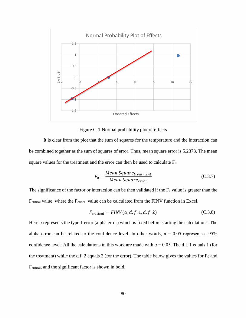
80
Figure C-1 Normal probability plot of effects
It is clear from the plot that the sum of squares for the temperature and the interaction can
be combined together as the sum of squares of error. Thus, mean square error is 5.2373. The mean
square values for the treatment and the error can then be used to calculate F0
𝐹0 =𝑀𝑒𝑎𝑛 𝑆𝑞𝑢𝑎𝑟𝑒𝑡𝑟𝑒𝑎𝑡𝑚𝑒𝑛𝑡
𝑀𝑒𝑎𝑛 𝑆𝑞𝑢𝑎𝑟𝑒𝑒𝑟𝑟𝑜𝑟 (C.3.7)
The significance of the factor or interaction can be then validated if the F0 value is greater than the
Fcritical value, where the Fcritical value can be calculated from the FINV function in Excel.
𝐹𝑐𝑟𝑖𝑡𝑖𝑐𝑎𝑙 = 𝐹𝐼𝑁𝑉(𝛼, 𝑑. 𝑓. 1, 𝑑. 𝑓. 2) (C.3.8)
Here α represents the type 1 error (alpha error) which is fixed before starting the calculations. The
alpha error can be related to the confidence level. In other words, α = 0.05 represents a 95%
confidence level. All the calculations in this work are made with α = 0.05. The d.f. 1 equals 1 (for
the treatment) while the d.f. 2 equals 2 (for the error). The table below gives the values for F0 and
Fcritical, and the significant factor is shown in bold.
-1.5
-1
-0.5
0
0.5
1
1.5
-2 0 2 4 6 8 10 12z-va
lue
Ordered Effects
Normal Probability Plot of Effects
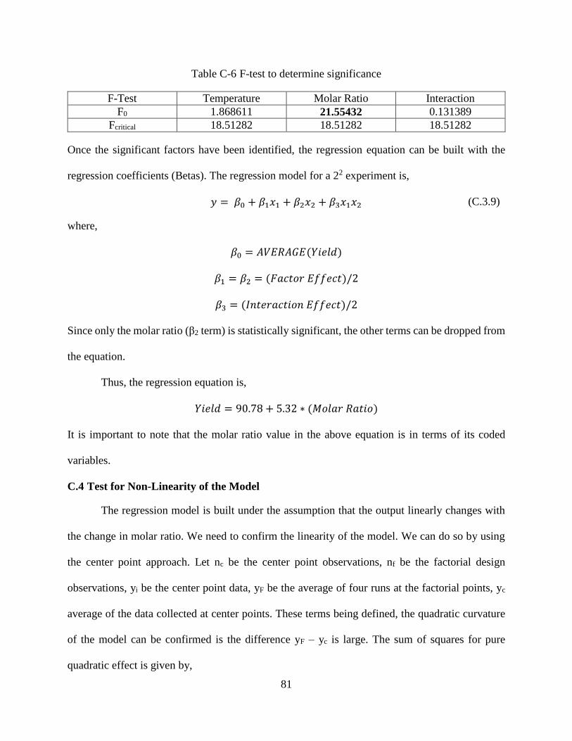
81
Table C-6 F-test to determine significance
F-Test Temperature Molar Ratio Interaction
F0 1.868611 21.55432 0.131389
Fcritical 18.51282 18.51282 18.51282
Once the significant factors have been identified, the regression equation can be built with the
regression coefficients (Betas). The regression model for a 22 experiment is,
𝑦 = 𝛽0 + 𝛽1𝑥1 + 𝛽2𝑥2 + 𝛽3𝑥1𝑥2 (C.3.9)
where,
𝛽0 = 𝐴𝑉𝐸𝑅𝐴𝐺𝐸(𝑌𝑖𝑒𝑙𝑑)
𝛽1 = 𝛽2 = (𝐹𝑎𝑐𝑡𝑜𝑟 𝐸𝑓𝑓𝑒𝑐𝑡)/2
𝛽3 = (𝐼𝑛𝑡𝑒𝑟𝑎𝑐𝑡𝑖𝑜𝑛 𝐸𝑓𝑓𝑒𝑐𝑡)/2
Since only the molar ratio (β2 term) is statistically significant, the other terms can be dropped from
the equation.
Thus, the regression equation is,
𝑌𝑖𝑒𝑙𝑑 = 90.78 + 5.32 ∗ (𝑀𝑜𝑙𝑎𝑟 𝑅𝑎𝑡𝑖𝑜)
It is important to note that the molar ratio value in the above equation is in terms of its coded
variables.
C.4 Test for Non-Linearity of the Model
The regression model is built under the assumption that the output linearly changes with
the change in molar ratio. We need to confirm the linearity of the model. We can do so by using
the center point approach. Let nc be the center point observations, nf be the factorial design
observations, yi be the center point data, yF be the average of four runs at the factorial points, yc
average of the data collected at center points. These terms being defined, the quadratic curvature
of the model can be confirmed is the difference yF – yc is large. The sum of squares for pure
quadratic effect is given by,
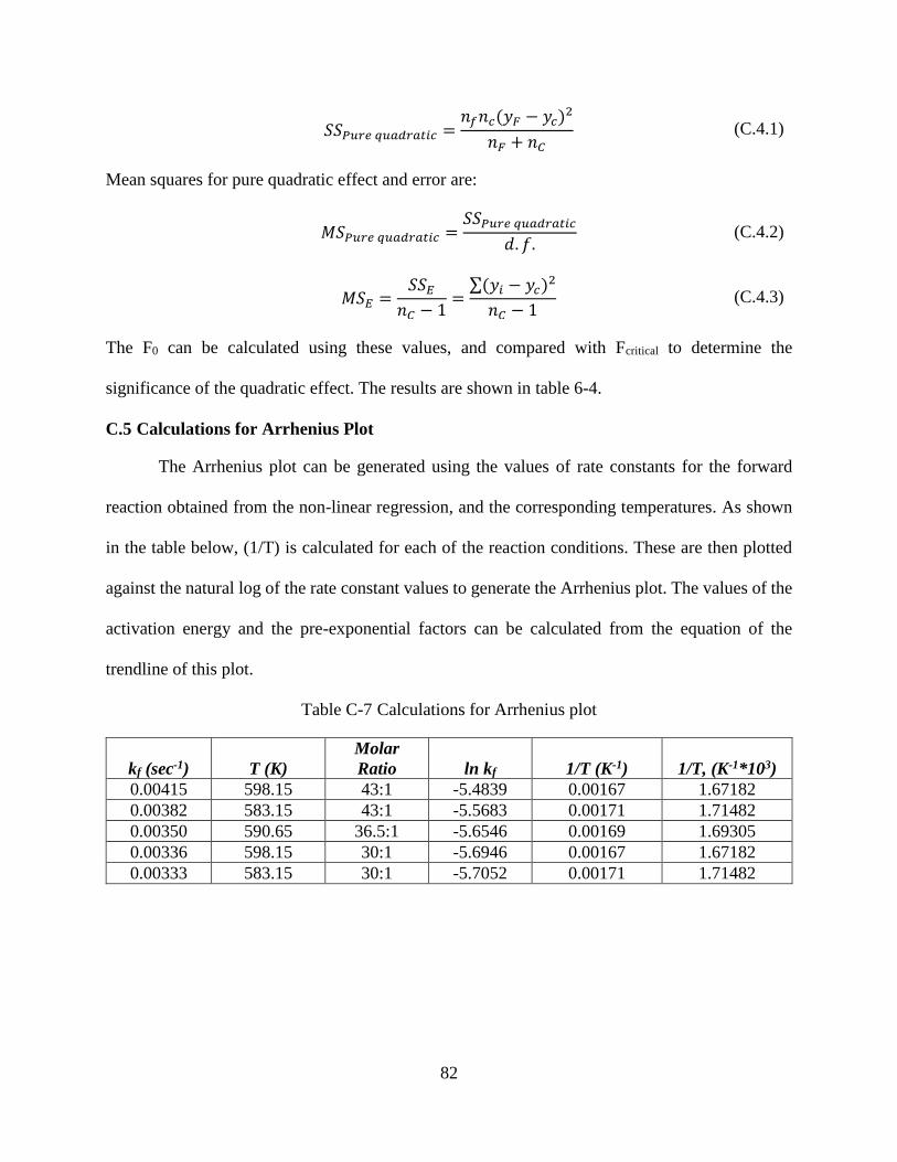
82
𝑆𝑆𝑃𝑢𝑟𝑒 𝑞𝑢𝑎𝑑𝑟𝑎𝑡𝑖𝑐 =𝑛𝑓𝑛𝑐(𝑦𝐹 − 𝑦𝑐)2
𝑛𝐹 + 𝑛𝐶 (C.4.1)
Mean squares for pure quadratic effect and error are:
𝑀𝑆𝑃𝑢𝑟𝑒 𝑞𝑢𝑎𝑑𝑟𝑎𝑡𝑖𝑐 =𝑆𝑆𝑃𝑢𝑟𝑒 𝑞𝑢𝑎𝑑𝑟𝑎𝑡𝑖𝑐
𝑑. 𝑓. (C.4.2)
𝑀𝑆𝐸 =𝑆𝑆𝐸
𝑛𝐶 − 1=
∑(𝑦𝑖 − 𝑦𝑐)2
𝑛𝐶 − 1 (C.4.3)
The F0 can be calculated using these values, and compared with Fcritical to determine the
significance of the quadratic effect. The results are shown in table 6-4.
C.5 Calculations for Arrhenius Plot
The Arrhenius plot can be generated using the values of rate constants for the forward
reaction obtained from the non-linear regression, and the corresponding temperatures. As shown
in the table below, (1/T) is calculated for each of the reaction conditions. These are then plotted
against the natural log of the rate constant values to generate the Arrhenius plot. The values of the
activation energy and the pre-exponential factors can be calculated from the equation of the
trendline of this plot.
Table C-7 Calculations for Arrhenius plot
kf (sec-1) T (K)
Molar
Ratio ln kf 1/T (K-1) 1/T, (K-1*103)
0.00415 598.15 43:1 -5.4839 0.00167 1.67182
0.00382 583.15 43:1 -5.5683 0.00171 1.71482
0.00350 590.65 36.5:1 -5.6546 0.00169 1.69305
0.00336 598.15 30:1 -5.6946 0.00167 1.67182
0.00333 583.15 30:1 -5.7052 0.00171 1.71482