production cycle optimisation

Production cycle optimisation

Constantine Goulimis About the authorpage 38

32

Introduction

n many manufacturing situations, there is a combination of:

n Product complexity, with a plant/process manufacturingmultiple products

n Non-constant demand

n Significant switchover costs when transitioning from oneproduct to another

Consequently, in such industries there is a difficult and hithertounsolved scheduling problem: how to balance the conflictingobjectives of maximum production efficiency, optimal customerservice and minimum inventory – see Figure 1. The readers ofOperations Management certainly do not need a reminder thatsquaring this particular circle is far from easy!

So what are we looking at? We are looking at optimisedmulti-machine scheduling, with sequence-dependentswitchover costs and non-constant demand. Greycon calls thissolution D-Opt. The input is in two classes: the demand andthe production.

Demand and inventory policy

We distinguish between make-to-order and make-to-stocksituations. In practice, of course, reality is often mixed andD-Opt is fully capable of dealing with the mixed mode scenario.Typically, in a make-to-stock scenario, there is a manual orautomated forecasting process that gives a daily forecastconsumption of each stock keeping unit (SKU) – see Figure 2.In real-world situations there can be many thousands of SKUs,each with its own forecast consumption curve. The initialinventory of each SKU will be consumed at a rate dictated bythe forecast, until it is replenished by manufacturing, giving riseto a familiar saw-tooth curve – see Figure 3.

The general aim is to stay between the minimum andmaximum levels – that is, the white zone, sometimes called thetunnel. The minimum and maximum range is called the item’sinventory policy. The values of an inventory policy are notnecessarily constant, but can be time-varying, as shown inFigure 3. A common approach is to express them as days ofcover – for example, the minimum could be set to seven daysand the maximum to 21, noting that there are several softwarevendors that sell tools that allow this inventory policy to beoptimised; generally these are called inventory optimisationtools.1 How the inventory policy is determined is outside thescope of the solution presented here.

The working assumption for the make-to-stock scenario is thatfor each SKU we have a forecast and a defined inventory policy.For the make-to-order scenario, we distinguish two cases:

n Already existing firm orders with a desired delivery date:generally the aim is to deliver these as close as possible tothis date, neither too early – and D-Opt contains theconcept of last date of change, basically a ‘do not startbefore’ date – nor too late

n Demand forecast: the system minimises total inventorycosts plus notional lateness for this portion of the demand

In mixed scenarios, there is a complication insofar as we needto avoid double counting between the demand forecast and thefirm orders. This involves a netting process of some kind.

Production

The kinds of processes we are interested in have significantset-up costs. The presence of these set-up costs encouragesthe grouping of similar products to minimise these set-up costs.For a single product on a single uncapacitated machine, there isthe well-known EOQ formula to calculate economic runlength – see Figure 4.

Quite often these set-up costs are sequence dependent – seeFigure 5. To distinguish the case when the set-up costs dependon the sequence, we label them switchover costs.

I

D-Opt: from forecast to schedule

Manufacturers must balance the conflicting objectives of maximum production efficiency,optimal customer service and minimum inventory

8product_cycle.qxp:Layout 1 4/2/08 16:09

Objectives

The objectives of a schedule are:

n Minimise inventory policy deviations: for make-to-stockitems to be minimised, with particular attention to not goingbelow zero inventory levels

n Maximise customer service: items made to order to bedelivered as close as possible to the requested date

n Maximise production efficiency: focusing attention on theminimisation of switchover costs and the allocation ofdemand to the most cost-effective manufacturing resource

As mentioned previously, these objectives are conflicting and wemust balance them against each other.

Current practice

So how do manufacturers currently schedule their workcentres? In Greycon’s experience most companies employ ateam of ‘master planners’ who are responsible for defining ablock schedule for each work centre. This block schedule isessentially a time period during which one particular productfamily, possibly many SKUs, will be made. The frequency andextent of each of these runs is determined empirically, oftenrepeating previous cycles – see Figure 6.

The next cycle/iteration may have different run lengths – forexample, see Figure 7. Alternatively, a particular product familymay be missing, in which case it is not truly a cycle – seeFigure 8. Once such a block schedule is created, then theassociated replenishment orders are generated, either manuallyor automatically. The logic employed is illustrated in Figure 9.This demonstrates clearly how the magnitude of thereplenishment orders depends on the schedule itself. Formulti-machine situations, where some products can beproduced on more than one machine, the situation is evenmore complex – see Figure 10. The further apart the runs are,the larger the replenishment quantities have to be.

Limitations of current practice

The creation of an optimal schedule is a very difficultcombinatorial problem whose dimensionality overwhelmshuman capacity; people have assumed that the problem is notamenable to optimisation techniques. For instance, over atypical 90-day horizon, there may well be around 200 runs for50 basic materials and 1,000 SKUs. We estimate that there aremore than 1080 possible schedules. In multi-machine situations,there are even more possibilities.

In the absence of optimisation algorithms such as D-Opt,planners have to create a campaign schedule manually. Thequality of this schedule is uncertain, but it is used in conjunctionwith the demand, based on forecasts and firm orders, togenerate replenishment orders. Some systems are then able todetermine customer service implications – that is, predicted

The creation of an optimal schedule is a very difficultcombinatorial problem whose dimensionality overwhelmshuman capacity; people have assumed that the problem isnot amenable to optimisation techniques.

Three conflicting objectivesFigure 1

Demand over time for an SKUFigure 2

Inventory of an SKU over time, being replenished at certaintimes. Between replenishments, consumption is dictated bythe forecast. The minimum desired inventory is in greenand the maximum is in yellow; red shows negative territory.The white zone is the target zone, called the tunnel.Figure 3


33


over or under stock and earliness or lateness – in the form ofalerts. However, the process of handling these alerts andrescheduling to eliminate them is left to the planner, while thereis no prescriptive methodology for this. The situation is furtherexacerbated when the replenishment order creation processtakes hours, as it often does. This slowness makes the overallsystem unresponsive to external events.

In summary, current practice is:

n Of unknown quality and likely to be suboptimal

n Unlikely to be very good in multi-machine situations

n Possibly a chicken-and-egg situation between replenishmentorders and campaigns

n Very slow to respond to external events

n Time and resource-consuming

New solution

We have developed a new solution to this problem calledD-Opt, which applies advanced optimisation technology toaddress the problems discussed above. Figure 11 shows therequired inputs and outputs.

Inputs to D-Opt

Initial conditions

These consist of the opening inventory at the beginning of thehorizon for each item and also the current production status.

Demand

Regardless of whether forecasts are for make-to-stock ormake-to-order items, the system uses a daily forecast input.Most forecasting systems operate at aggregated time periods,such as weeks or months. Nevertheless, empirical rules areoften available that allow the demand to be apportioned intodaily units, taking into account the number of working days in amonth, weekends, any non-uniform behaviour – for example,‘two-thirds of the orders come in during the last week of themonth’. This breakdown into daily buckets is handled externallyto D-Opt.

In addition to the daily forecast demand, the system uses anyfirm make-to-order items. Care must be taken so as not todouble count demand, as may happen when mixing forecastswith firm orders.

Inventory policy

For each inventory item, a time-varying policy is defined throughtwo levels: minimum and maximum. Sometimes the two arereferred to in literature as the tunnel; the minimum is alsoreferred to as safety stock level and the maximum is referred toas order up to. In the D-Opt system, we could have had twopenalties for each item, one for going below minimum and onefor going above maximum. However, for additional flexibility andcontrol there are four penalties in total, measured in units ofmonetary value per day per unit of material:

n Over maximum

n Below minimum

n Below alarm: this additional level is introduced in order toprovide a level of control between the minimum levels andzero; the alarm level is defined as a percentage of theminimum, typically 50–75%

n Below zero

34

Operations Managementwww.iomnet.org.uk

Number 12008

Manufacturing cost and the supply chain cost as a functionof the production frequency of a particular item or family.The optimal frequency appears to be around 15 days, butthis is an imprecise approximation to the real-worldproblem where there are many conflicting products,time-varying demand, sequence-dependent setups, othersources of supply and so on.Figure 4

In the two alternative schedules, we show two families ofproducts, yellow (items 1-4) and blue (items 5-8); the timetaken to switch between these two families is �t and thecost is �$. The cost depends on the sequence.Figure 5

Repeating cycle of product families A >B >C >D > A…Figure 6

Duration of the A family changes from the first cycleto the secondFigure 7

Second cycle does not contain a C familyFigure 8

First run of B ends at time t1; the next time B is producedis t2; so the B inventory at time t1 should cover all of thedemand until t2Figure 9


D-Opt allows for all penalties to be time-varying, which can besignificant because often the short-term future is more importantthan the long-term one, for which there can be greateruncertainty. For firm orders earliness and lateness costs aredefined. Demand forecasts for make-to-order items can behandled in a number of ways, including an approach thatminimises total inventory plus notional lateness.

Master data

D-Opt naturally requires master data such as production rates,production costs and any planned downtime. In addition tothese, the following complexities need to be addressed:

n Time-varying production rates and costs, typically due toengineering changes of the underlying process – forexample, after a planned engineering change in May,production of a particular item may be speeded by 30%,which, of course, affects the schedule

n Ability to schedule around planned downtime

n Production capability by exception, the need to handle byexception – for example, you can specify that a certainproduct cannot be made on a work centre during aparticular period

n Ability to take into account predefined blocks, for certainlong-lead-time operations, such as manufacturing trials; theproblem here is the transition into these predefined blocksand the transition out of them

n Minimum run length by product

n Frozen section – that is, treat part of the original schedulefor, say, the next three days as fixed and optimise from thatpoint onwards; D-Opt can handle different frozen sectionsfor different machines

n Production costs: these are important in multi-machinesituations, as well as when there is opportunity to switchproduction of a particular item from one machine to another

n Switchover costs and times: rather than force the user todefine an n2 matrix of switchovers, we employ a rule-basedmechanism based on physical properties; even very complexmanufacturing situations can be distilled down to less than100 rules, which makes the rule base easily maintainable bythe end user

n Multiplicity: when demand is expressed in a unit of measuresuch as weight or surface area, it is sometimes the case thatproduction must be in certain multiples – for example,whole rolls

Optimisation parameters

The user may control a number of parameters, such as theextent of the horizon. In addition, there is also a decay factor,which captures the requirement that the near-term schedule ismore important than the far-term one. There are two reasonsfor this: firstly, forecasts become less certain; secondly, in practiceD-Opt is applied on a rolling basis, so any imperfections – forexample, 10 weeks out – can be dealt with next week and theweek after. The decay factor is expressed as an exponentialhalf-life – that is, a value of 40 days means that the objectivefunction penalties at 40 days are half the values they are at thebeginning of the schedule.

Outputs from D-Opt

The outputs from D-Opt consist of the block schedule itself andthe associated replenishment orders and reservations.2 Theseare passed to other systems, primarily the ERP system andthe manufacturing execution system (MES), using suitable

Production of B takes place in two machines. Inventory must coverthe demand for the periods indicated by red arrows.Figure 10

D-Opt logical inputs and outputsFigure 11

Thirteen-week view of the schedule. In the top half are the blocks,runs and replenishment orders. The user-configurable colour codingof the replenishment orders is governed by the state of the SKU at thetime the run starts – for example, white indicates that at the time ofthe run the inventory is between minimum and maximum, yellowabove maximum, and so on.Figure 12


35


middleware technology, such as XML and Netweaver. Furtherinformation gathered by the optimisation algorithm during itsexecution, such as number of days below minimum or variouscosts, are also summarised and presented to the user, butnormally these are not passed to external systems.

Because the amount of data to analyse and present is so huge, incollaboration with the pilot customer, we have come up with anumber of elegant displays – see Figures 12–15.

One interesting aspect is that the upward steps of the inventorycurve are not vertical. This is because multiple SKUs for a singleproduct family are replenished during each run. Rather than usethe end of the run as the time when the product becomesavailable, D-Opt proportionately distributes the quantitiesthroughout the run. In the dimensional industries, where trimoptimisation is an issue, after the run has been trimmed using X-Trim,the replenishment will be tied to the actual slitting patterns.

Algorithm design and implementation

It would be difficult to discuss the internal workings of D-Opt’salgorithm in this article. Suffice it to say that the algorithm uses avariety of techniques in order to come up with a good solution.This has been verified in different scenarios – for example, tightvs loose capacity – with the pilot customers. The D-Optalgorithm is patent pending.

A key difficulty has been to make the algorithm fast enough. Thetarget is to optimise any single machine in less than five minuteson modern PC hardware with a cold start – that is, nopre-existing schedule: significantly less for a ‘warm’ start – andconsiderable thought, work and ingenuity has been put towardsachieving this objective.

Integration with external systemsD-Opt follows the obvious pattern of integration requirements– see Figures 16 and 17. Integration with other systems istypically via XML messages, but other possibilities exist as well.

Case studies

Paper company, two mills, four paper machinesBackground

One of our customers conducted a short engagement with us toanalyse the potential benefits of D-Opt as applied to a subset ofits production. The model encompasses four large papermachines and demand data for 61 days .The annual sales valueof these four paper machines is hundreds of millions of dollars.The supplied data included the runs that were manually planned.This was particularly useful, as it allows a direct comparison ofthe schedules.

Results

The manual schedule was rather poor – see Figure 18. A D-Optparameter controls whether idle time is allowed. If not, D-Optwill ensure that schedules completely utilise the available capacity

36


Number 12008

Results are also available by SKUFigure 13

Multi-machine situations are also represented. Dependingon master data, an item can be manufactured on more thanone machine, generating an additional optimisation degreeof freedom.Figure 14

Run schedule can be displayed in the familiar staircasemannerFigure 15

Care must be taken so as not todouble count demand, as mayhappen when mixing forecastswith firm orders.


within the horizon. This is done by inflating the demand asappropriate and, although it results in some suboptimality(over-stock plus lack of detection of opportunities to either takedowntime or go to the market with an incentive plan), thisparticular study was conducted under the no idle timeassumption. The optimised schedule is shown in Figure 19,with the same colour coding as before.

The customer summarised the benefits as follows; somenumbers have been removed protect confidentiality:

n From ‘Red and Yellow’ to ‘White and Green’

n Make what is needed, when it is needed; demand-drivensupply network (DDSN)

n Projected inventory reduction

n 20% in 90 days

n $700,000 annual carry cost savings

n $2 million annual warehouse savings

n Improved service, increased sales

n $400,000 increased margin, annualised, based on reducedstock outs by 1,000t in 90 days

n Production costs are not materially changed

Based on the above numbers, the system justifies itself in lessthan three months, but actually there are many additionalbenefits. The Friday before the presentation, one of therecovery boilers went down, with the consequent loss of fivedays of production for one of the paper machines. The effort toplan around this event to mitigate its consequences took manyhours and generated a stack of paperwork. In the words of thecustomer again:

n Add a shutdown period to the machine; let D-Opt runthrough iterations to find optimal solution

n D-Opt will also identify those items that become late or gobelow zero

D-Opt’s algorithm took 15–30 minutes on a laptop to optimisethese scenarios.

Film company, one site, six BOPP lines

Background

This company produces film on six lines, five of which produceabout 25t/day and the sixth produces about 75t/day. Each ofthe film types can typically be made on two or three lines. Theanalysis was conducted for a 30-day horizon, representing amonth’s worth of production. There are 60+ film types in avariety of thicknesses. The business is totally make-to-order,without any make-to-stock component.

Results

The problem takes about two minutes to optimise – see Figure20. The differences between the manual schedule and D-Optare shown in Table 1.

In summary, although there is a slight increase in switchovers,due to additional runs, this is amply compensated by savingselsewhere. The above maximum figure are based onreal-world holding costs, so the reduction representsproduction taking place closer to the delivery date. Similarly, thebelow zero costs are, in effect, lateness costs.

Integration of D-Opt with third-party components, such aswarehouse management systemsFigure 16

In an SAP context, with APO, D-Opt naturallycomplements SAP functionality, dealing with multi-machineissues, treating the inventory tunnel as a target andgenerating the appropriate planned replenishment ordersand optimised campaign simultaneouslyFigure 17

Manual schedule. The colour code is: red if the supplieditem is below 0 at the time of the event; yellow if it isabove maximum; green if it is below minimum; blue if it isbelow alarm; and white if it is within the tunnel. Note thatmany items are produced when they are red – customerservice failure – or yellow – overstocking.Figure 18


37


Discussion and extensions

D-Opt is new and, as always, software is struggling to catch upwith new requirements. Things that are not in the system at thetime of writing are:

n Transportation issues: transportation impacts the selectionof a site in terms of cost and in terms of time; a particularcustomer may be closer to one site than to another; it isalso common to encounter multiple transportation modes,which introduces another optimisation degree of freedom

n Coupling constraints: for multi-machine situations, thesewould cause the schedule of one machine to affect another,not just through the demand; examples include energyusage and effluent plant load

n Limited shelf life: in some situations – for example, food orphotographic film – inventory has a shelf life; this iscurrently handled through higher penalties

None of the above issues represent serious obstacles to thefundamental algorithm. The application of D-Opt to otherindustries therefore remains an intriguing possibility.

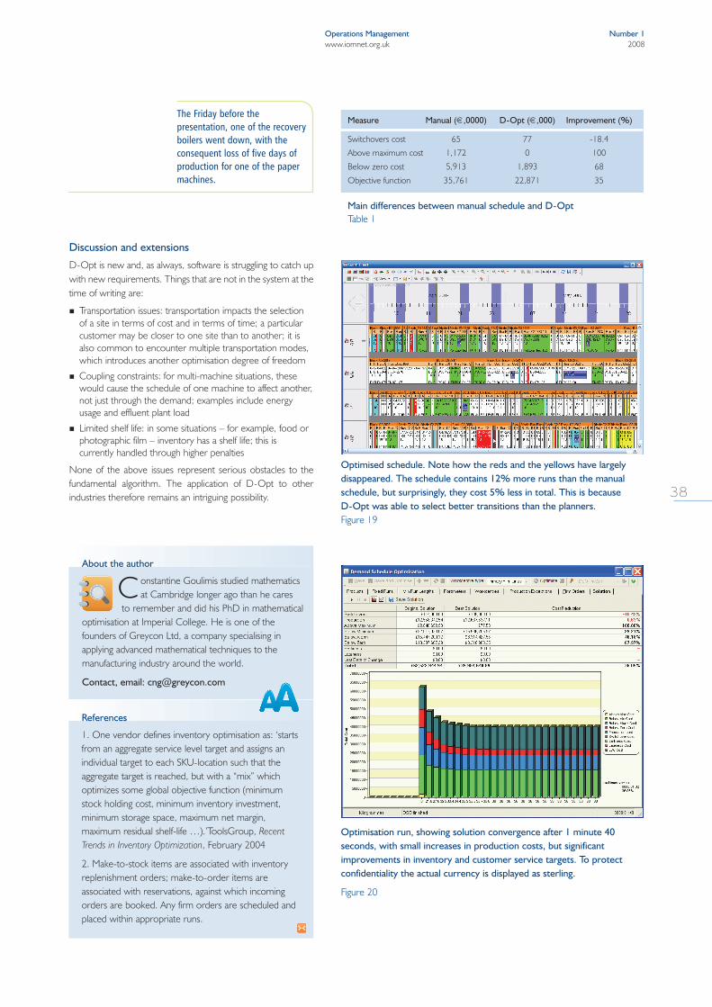
Optimised schedule. Note how the reds and the yellows have largelydisappeared. The schedule contains 12% more runs than the manualschedule, but surprisingly, they cost 5% less in total. This is becauseD-Opt was able to select better transitions than the planners.Figure 19

Optimisation run, showing solution convergence after 1 minute 40seconds, with small increases in production costs, but significantimprovements in inventory and customer service targets. To protectconfidentiality the actual currency is displayed as sterling.

Figure 20

References

1. One vendor defines inventory optimisation as: ‘startsfrom an aggregate service level target and assigns anindividual target to each SKU-location such that theaggregate target is reached, but with a “mix” whichoptimizes some global objective function (minimumstock holding cost, minimum inventory investment,minimum storage space, maximum net margin,maximum residual shelf-life …).’ToolsGroup, RecentTrends in Inventory Optimization, February 2004

2. Make-to-stock items are associated with inventoryreplenishment orders; make-to-order items areassociated with reservations, against which incomingorders are booked. Any firm orders are scheduled andplaced within appropriate runs.

About the author

onstantine Goulimis studied mathematicsat Cambridge longer ago than he cares

to remember and did his PhD in mathematicaloptimisation at Imperial College. He is one of thefounders of Greycon Ltd, a company specialising inapplying advanced mathematical techniques to themanufacturing industry around the world.

Contact, email: [email protected]

C

Measure Manual (€,0000) D-Opt (€,000) Improvement (%)

Switchovers cost 65 77 -18.4

Above maximum cost 1,172 0 100

Below zero cost 5,913 1,893 68

Objective function 35,761 22,871 35

Main differences between manual schedule and D-OptTable 1

The Friday before thepresentation, one of the recoveryboilers went down, with theconsequent loss of five days ofproduction for one of the papermachines.

38


Number 12008


production cycle optimisation

Documents

minimum inventory

items inventory policy

defined inventory policy

initial inventory

total inventory costs

late n demand forecast

inventory optimisation

nonconstant demand