production and operations management · 2 production and operations management module contents unit...
TRANSCRIPT

1
Master of Business Administration (MBA)
GBS 660
Production and Operations
Management
Course Lecturer
Prof Levy Siaminwe, Phd
Email: [email protected]
2
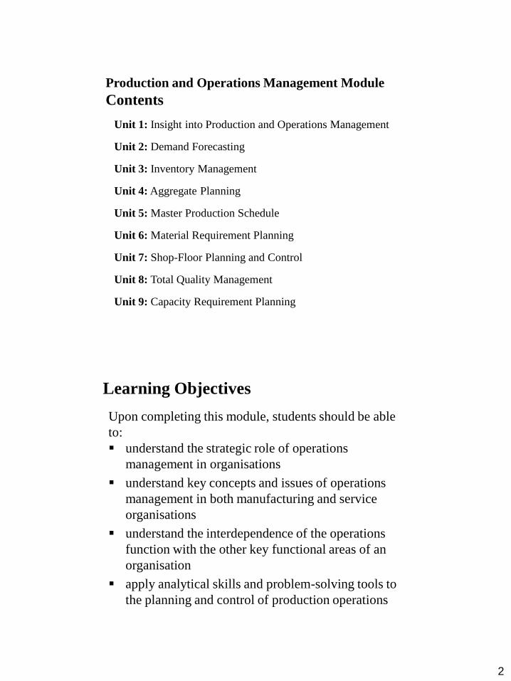
Production and Operations Management Module
Contents
Unit 1: Insight into Production and Operations Management
Unit 2: Demand Forecasting
Unit 3: Inventory Management
Unit 4: Aggregate Planning
Unit 5: Master Production Schedule
Unit 6: Material Requirement Planning
Unit 7: Shop-Floor Planning and Control
Unit 8: Total Quality Management
Unit 9: Capacity Requirement Planning
Learning Objectives
Upon completing this module, students should be able
to:
understand the strategic role of operations
management in organisations
understand key concepts and issues of operations
management in both manufacturing and service
organisations
understand the interdependence of the operations
function with the other key functional areas of an
organisation
apply analytical skills and problem-solving tools to
the planning and control of production operations
3
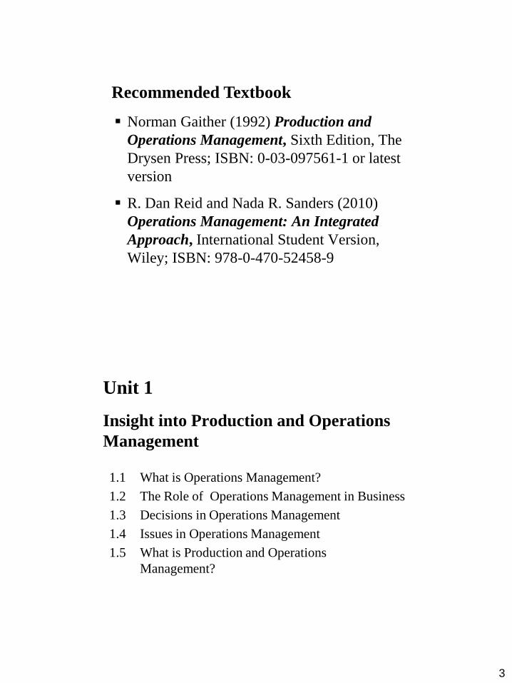
Recommended Textbook
Norman Gaither (1992) Production and
Operations Management, Sixth Edition, The
Drysen Press; ISBN: 0-03-097561-1 or latest
version
R. Dan Reid and Nada R. Sanders (2010)
Operations Management: An Integrated
Approach, International Student Version,
Wiley; ISBN: 978-0-470-52458-9
Unit 1
Insight into Production and Operations
Management
1.1 What is Operations Management?
1.2 The Role of Operations Management in Business
1.3 Decisions in Operations Management
1.4 Issues in Operations Management
1.5 What is Production and Operations
Management?
4
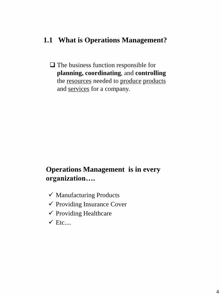
1.1 What is Operations Management?
The business function responsible for
planning, coordinating, and controlling
the resources needed to produce products
and services for a company.
Operations Management is in every
organization….
Manufacturing Products
Providing Insurance Cover
Providing Healthcare
Etc....
5
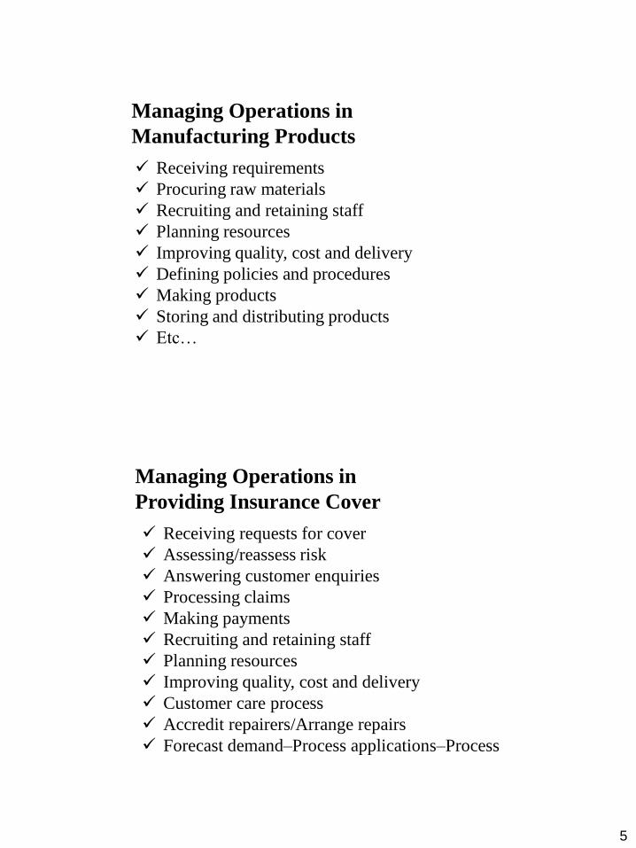
Managing Operations in
Manufacturing Products
Receiving requirements
Procuring raw materials
Recruiting and retaining staff
Planning resources
Improving quality, cost and delivery
Defining policies and procedures
Making products
Storing and distributing products
Etc…
Managing Operations in
Providing Insurance Cover
Receiving requests for cover
Assessing/reassess risk
Answering customer enquiries
Processing claims
Making payments
Recruiting and retaining staff
Planning resources
Improving quality, cost and delivery
Customer care process
Accredit repairers/Arrange repairs
Forecast demand–Process applications–Process
6
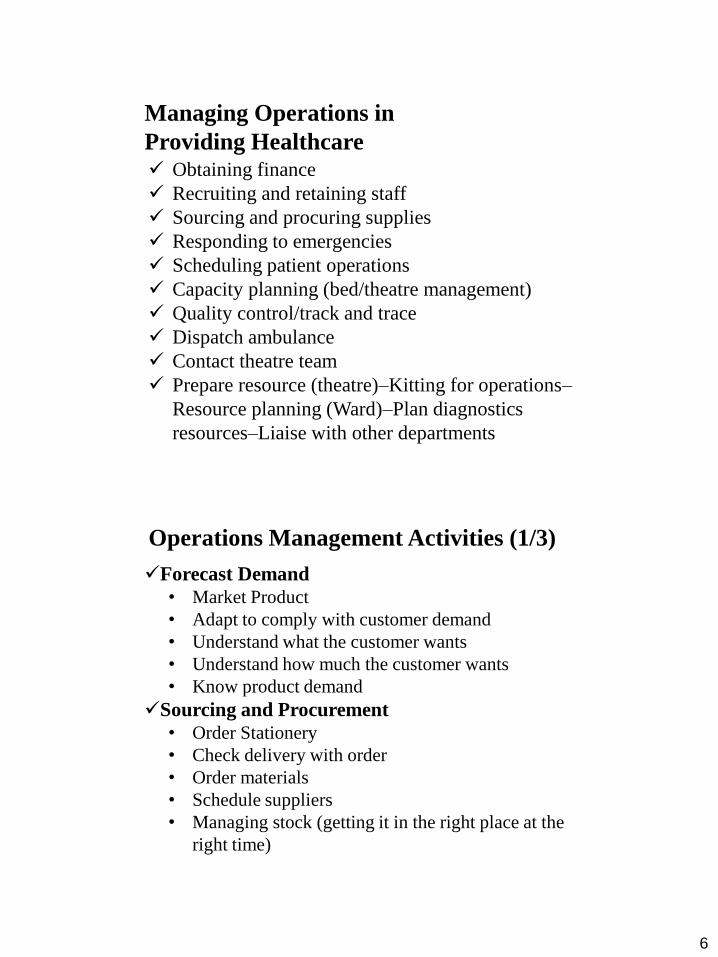
Managing Operations in
Providing Healthcare Obtaining finance
Recruiting and retaining staff
Sourcing and procuring supplies
Responding to emergencies
Scheduling patient operations
Capacity planning (bed/theatre management)
Quality control/track and trace
Dispatch ambulance
Contact theatre team
Prepare resource (theatre)–Kitting for operations–
Resource planning (Ward)–Plan diagnostics
resources–Liaise with other departments
Operations Management Activities (1/3)
Forecast Demand
• Market Product
• Adapt to comply with customer demand
• Understand what the customer wants
• Understand how much the customer wants
• Know product demand
Sourcing and Procurement
• Order Stationery
• Check delivery with order
• Order materials
• Schedule suppliers
• Managing stock (getting it in the right place at the
right time)

7
Operations Management Activities (2/3)
Creation of Output
• Arrange for necessary equipment
• Schedule material/staff/equipment to produce
goods and services
• Plan ‘work order’
• Produce goods
• Quality control
Delivery
• Deliver finished products
• Consider logistics/delivery
• Dispatching the goods or service to the customer
• Arrange packaging/presentation
Operations Management Activities (3/3)
Manage People • Employ people
• Train people
• Outsource
• Delegation
• Managing people
• Recruit and train staff
• Schedule labour
8
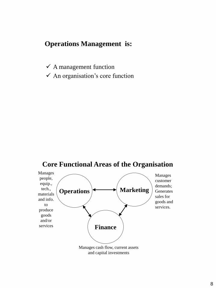
Operations Management is:
A management function
An organisation’s core function
Core Functional Areas of the Organisation
Operations
Finance
Marketing
Manages cash flow, current assets
and capital investments
Manages
customer
demands;
Generates
sales for
goods and
services.
Manages
people,
equip.,
tech.,
materials
and info.
to
produce
goods
and/or
services
9
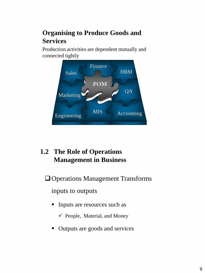
Organising to Produce Goods and
Services Production activities are dependent mutually and
connected tightly
Marketing
MIS Engineering
HRM
QA
Accounting
Sales
Finance
POM
1.2 The Role of Operations
Management in Business
Operations Management Transforms
inputs to outputs
Inputs are resources such as
People, Material, and Money
Outputs are goods and services
10
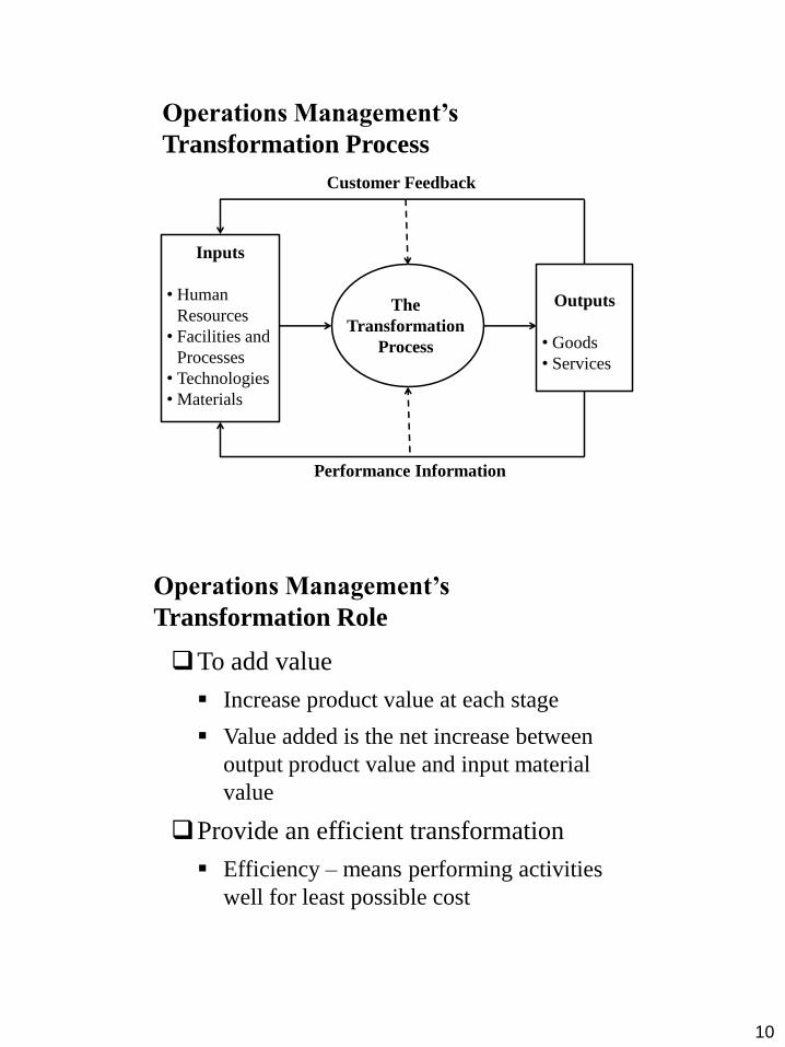
Operations Management’s
Transformation Process
Inputs
• Human
Resources
• Facilities and
Processes
• Technologies
• Materials
The
Transformation
Process
Outputs
• Goods
• Services
Customer Feedback
Performance Information
Operations Management’s
Transformation Role
To add value
Increase product value at each stage
Value added is the net increase between
output product value and input material
value
Provide an efficient transformation
Efficiency – means performing activities
well for least possible cost
11
Manufacturers and Service
Organizations
Both use technology
Both have quality, productivity, & response
issues
Both must forecast demand
Both can have capacity, layout, and location
issues
Both have customers, suppliers, scheduling
and staffing issues
1.3 Decisions in Operations
Management
Strategic Decisions – set the direction for the
entire company; they are broad in scope and
long-term in nature.
Tactical and Operational Decisions – focus
on specific day-to-day issues like resource
needs, schedules, and quantities to produce.
Strategic and Tactical decisions must align.
12
Strategic Decisions
Responsible for, and decisions about:
What to make (product development)
How to make it (process and layout
decisions) –or should we buy it
Where to make it (site location)
How much is needed (high level capacity
decisions)
Tactical Decisions
Address material and labour resourcing
within strategy constraints, for example:
How many workers are needed and when
(labour planning)
What level of stock is required and when
should it be delivered (inventory and
replenishment planning)
How many shifts to work. Whether
overtime or subcontractors are required
(detailed capacity planning)

13
Operational Decisions
Detailed lower-level
(daily/weekly/monthly) planning,
execution and control decisions, for
example:
What to process and when (scheduling),
The order to process requirements
(sequencing)
How work is put on resources (loading)
Who does the work (assignments)
1.4 Issues in Operations Management
Environmental sustainability, recycling , reuse
Customers demand better quality, greater speed, and lower
costs
Globalisation of supply and demand
Achieving and sustaining high quality while controlling cost
Integrating new technologies and control systems into
existing processes
Obtaining, training, and keeping qualified workers and
managers
Increased cross-functional decision making
Integrating production and service activities at multiple sites
in decentralized organizations
Recognized need to better manage information using ERP
and CRM systems

14
1.5 What is Production and Operations
Management?
The creation of goods
and services by turning
inputs into outputs,
which are products
and services
Production
Management of the
production process
Operations
Management
Production and operations management
(POM) is the management of an organization’s
production system
A production system takes inputs and converts
them into outputs
The conversion process is the predominant
activity of a production system
The primary concern of an operations manager is
the activities of the conversion process
15
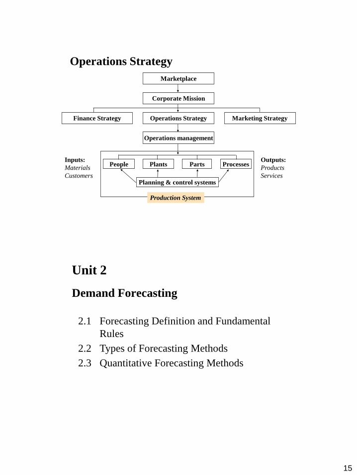
Operations Strategy
Marketplace
Corporate Mission
Operations Strategy
Operations management
Marketing Strategy Finance Strategy
People Plants Parts Processes
Planning & control systems
Production System
Inputs:
Materials
Customers
Outputs:
Products
Services
Unit 2
Demand Forecasting
2.1 Forecasting Definition and Fundamental
Rules
2.2 Types of Forecasting Methods
2.3 Quantitative Forecasting Methods

16
2.1 Forecasting Definition and Rules
Forecasting is the prediction of future events
on the basis of either:
historical data
Opinions
trend of events, or
known future variables
Demand forecasting is estimating the future
demand for products and services and the
resources necessary to produce these outputs
It is the first step in planning in any business
Forecasting in Business
Forecasts provide information that assist
managers in guiding future activities toward
organizational goals
Forecasting is critical to management of all
organizational functional areas :
Marketing relies on forecasting to predict demand
and future sales
Finance forecasts stock prices, financial performance,
capital investment needs
Information systems provides ability to share
databases and information
Human resources forecasts future hiring requirements
17
General Characteristics of Forecasts
Forecasts are seldom perfect
The prediction does not take account of all
factors; The environment is complex and
subject to rapid change
Forecasts are more accurate for groups or
families of items
Forecasts are more accurate for shorter time
periods; Long term forecasting is problematic
Every forecast should include an error estimate
Elements of a Good Forecast
The forecast should be timely
The forecast should be accurate
The forecast should be reliable
The forecast should be expressed in
meaningful units
The forecasting technique should be simple
to understand and use
18
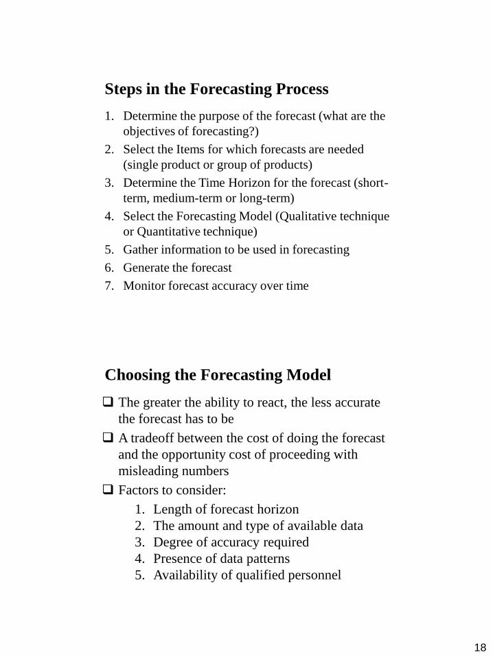
Steps in the Forecasting Process
1. Determine the purpose of the forecast (what are the
objectives of forecasting?)
2. Select the Items for which forecasts are needed
(single product or group of products)
3. Determine the Time Horizon for the forecast (short-
term, medium-term or long-term)
4. Select the Forecasting Model (Qualitative technique
or Quantitative technique)
5. Gather information to be used in forecasting
6. Generate the forecast
7. Monitor forecast accuracy over time
Choosing the Forecasting Model
The greater the ability to react, the less accurate
the forecast has to be
A tradeoff between the cost of doing the forecast
and the opportunity cost of proceeding with
misleading numbers
Factors to consider:
1. Length of forecast horizon
2. The amount and type of available data
3. Degree of accuracy required
4. Presence of data patterns
5. Availability of qualified personnel
19
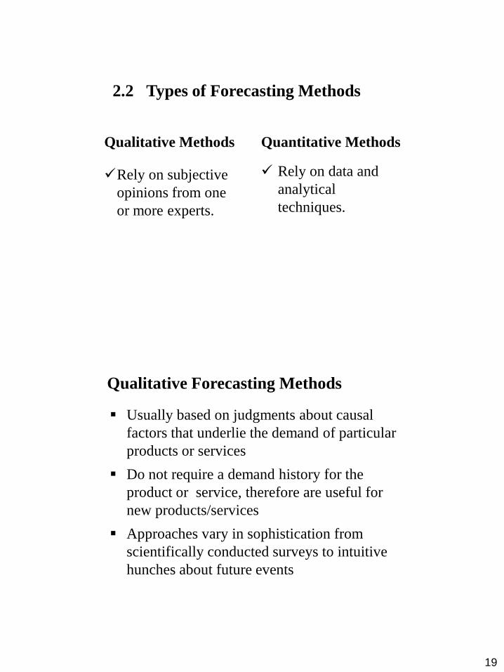
2.2 Types of Forecasting Methods
Qualitative Methods
Rely on subjective
opinions from one
or more experts.
Quantitative Methods
Rely on data and
analytical
techniques.
Qualitative Forecasting Methods
Usually based on judgments about causal
factors that underlie the demand of particular
products or services
Do not require a demand history for the
product or service, therefore are useful for
new products/services
Approaches vary in sophistication from
scientifically conducted surveys to intuitive
hunches about future events
20
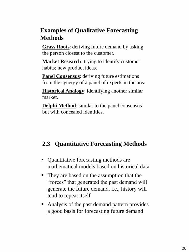
Examples of Qualitative Forecasting
Methods
Grass Roots: deriving future demand by asking
the person closest to the customer.
Market Research: trying to identify customer
habits; new product ideas.
Panel Consensus: deriving future estimations
from the synergy of a panel of experts in the area.
Historical Analogy: identifying another similar
market.
Delphi Method: similar to the panel consensus
but with concealed identities.
2.3 Quantitative Forecasting Methods
Quantitative forecasting methods are
mathematical models based on historical data
They are based on the assumption that the
“forces” that generated the past demand will
generate the future demand, i.e., history will
tend to repeat itself
Analysis of the past demand pattern provides
a good basis for forecasting future demand
21
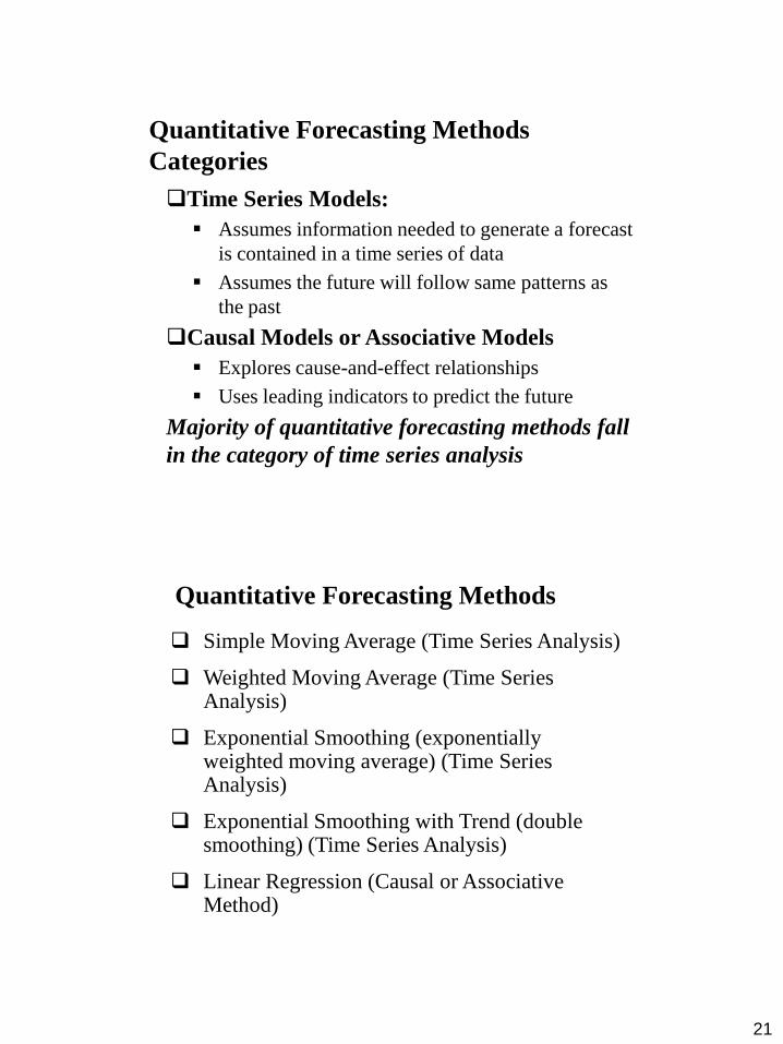
Quantitative Forecasting Methods
Categories
Time Series Models:
Assumes information needed to generate a forecast
is contained in a time series of data
Assumes the future will follow same patterns as
the past
Causal Models or Associative Models
Explores cause-and-effect relationships
Uses leading indicators to predict the future
Majority of quantitative forecasting methods fall
in the category of time series analysis
Quantitative Forecasting Methods
Simple Moving Average (Time Series Analysis)
Weighted Moving Average (Time Series Analysis)
Exponential Smoothing (exponentially weighted moving average) (Time Series Analysis)
Exponential Smoothing with Trend (double smoothing) (Time Series Analysis)
Linear Regression (Causal or Associative Method)
22
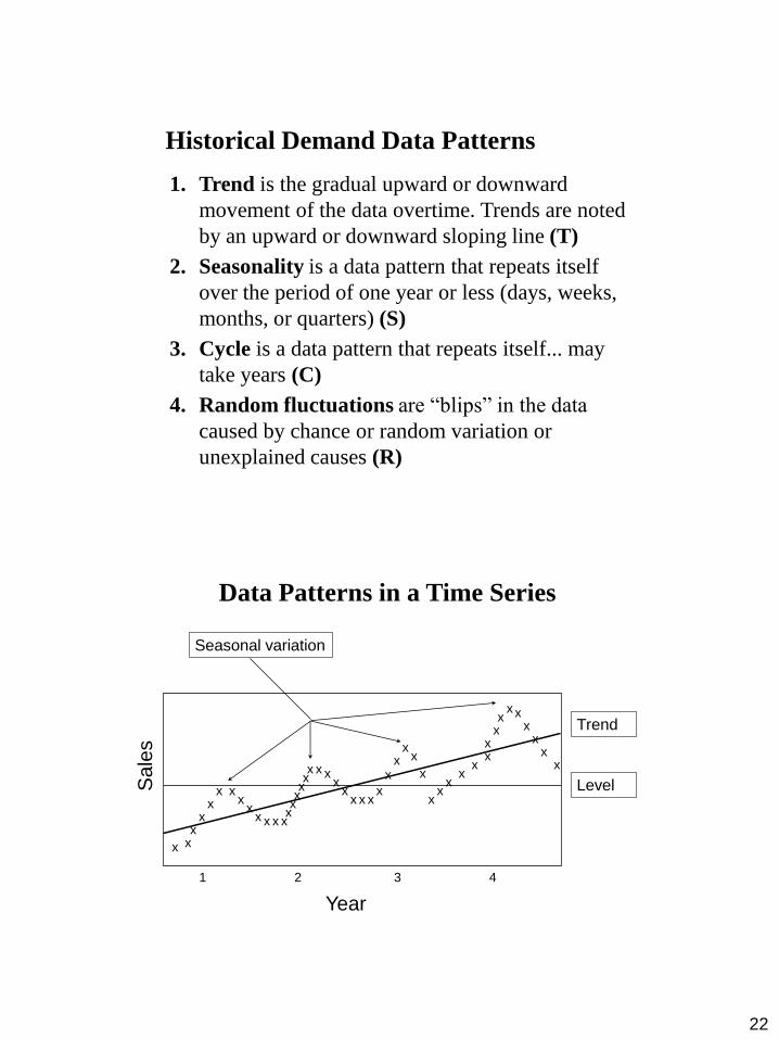
Historical Demand Data Patterns
1. Trend is the gradual upward or downward
movement of the data overtime. Trends are noted
by an upward or downward sloping line (T)
2. Seasonality is a data pattern that repeats itself
over the period of one year or less (days, weeks,
months, or quarters) (S)
3. Cycle is a data pattern that repeats itself... may
take years (C)
4. Random fluctuations are “blips” in the data
caused by chance or random variation or
unexplained causes (R)
Data Patterns in a Time Series
1 2 3 4
x
x x x
x x
x x x
x x x x x
x x x x x x x x
x x
x x x x
x x
x x
x
x x
x x
x x
x
x x
x x
x
x
x
Year
Sale
s
Seasonal variation
Trend
Level
23
Short Range Forecasts
In cases in which the time series is fairly stable and has no significant trend, seasonal, or cyclical effects, one can use smoothing methods to average out the irregular components of the time series
Three common smoothing methods are:
Simple moving average
Weighted moving average
Exponential smoothing
Simple Moving Average
Used if demand is not growing nor declining
rapidly
Used often for smoothing, that is removing random
fluctuations in the data
Equation
where:
Ft = forecast for period t,
n = number of periods to be averaged (AP)
At-1 = actual demand realized in the past period
for up to n periods
n
A+...+A +A +A =F n-t3-t2-t1-t
t
24
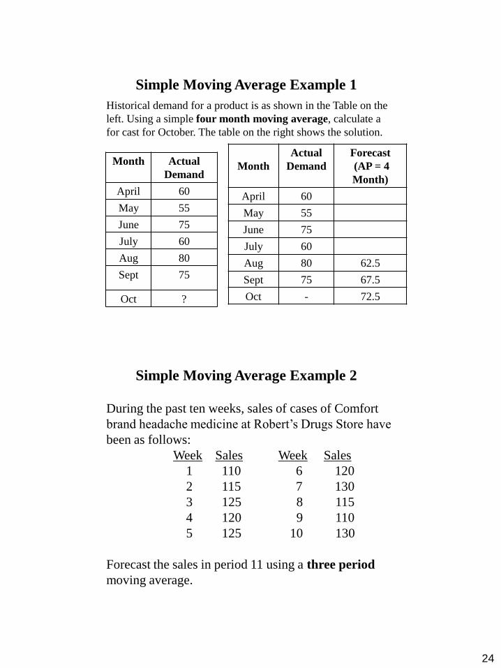
Simple Moving Average Example 1
Historical demand for a product is as shown in the Table on the
left. Using a simple four month moving average, calculate a
for cast for October. The table on the right shows the solution.
Month Actual
Demand
April 60
May 55
June 75
July 60
Aug 80
Sept 75
Oct ?
Month
Actual
Demand
Forecast
(AP = 4
Month)
April 60
May 55
June 75
July 60
Aug 80 62.5
Sept 75 67.5
Oct - 72.5
Simple Moving Average Example 2
During the past ten weeks, sales of cases of Comfort
brand headache medicine at Robert’s Drugs Store have
been as follows:
Week Sales Week Sales
1 110 6 120
2 115 7 130
3 125 8 115
4 120 9 110
5 125 10 130
Forecast the sales in period 11 using a three period
moving average.

25
Simple Moving Average Example 2 Solution
Solution performed in Microsoft Excel software
Ft is the forecast for week t.
F4 (forecast for week 4)=116.7
F11 (forecast for week 11)=118.3
Thus we would forecast the sales for Week 11 to be 118.3
Robert's Drug
n=3
Week (t ) At Ft
1 110
2 115 #N/A
3 125 #N/A
4 120 116.7
5 125 120.0
6 120 123.3
7 130 121.7
8 115 125.0
9 110 121.7
10 130 118.3
11 118.3
Weighted Moving Average
This is a variation on the simple moving
average where instead of the weights used to
compute the average being equal, they are not
equal
This allows more recent demand data to have
a greater effect on the moving average,
therefore the forecast
The weights must add to 1.0 and generally
decrease in value with the age of the data
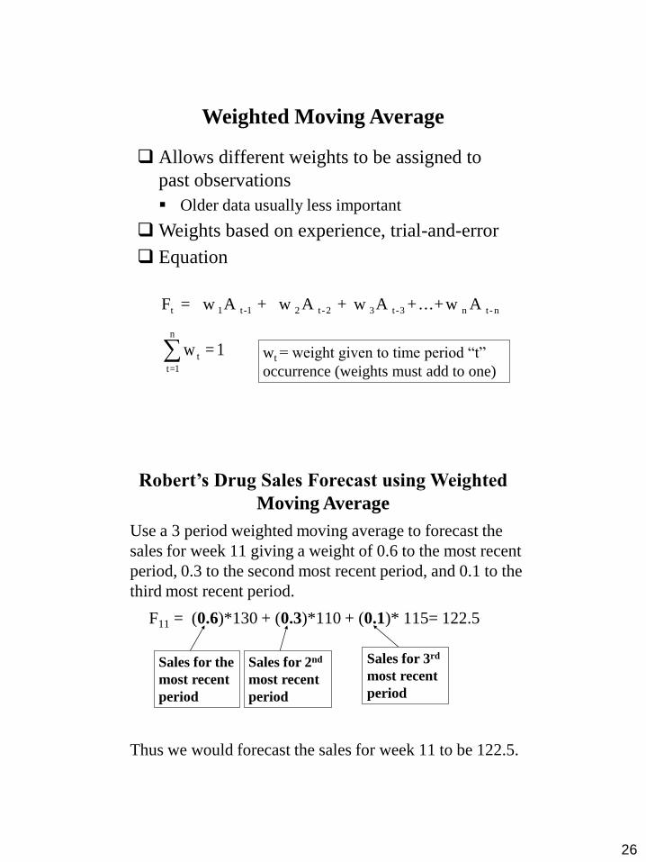
26
Weighted Moving Average
Allows different weights to be assigned to
past observations
Older data usually less important
Weights based on experience, trial-and-error
Equation
F = w A + w A + w A +...+w At 1 t-1 2 t-2 3 t-3 n t- n
1=wn
1=t
t wt = weight given to time period “t”
occurrence (weights must add to one)
Robert’s Drug Sales Forecast using Weighted
Moving Average
Use a 3 period weighted moving average to forecast the
sales for week 11 giving a weight of 0.6 to the most recent
period, 0.3 to the second most recent period, and 0.1 to the
third most recent period.
F11 = (0.6)*130 + (0.3)*110 + (0.1)* 115= 122.5
Thus we would forecast the sales for week 11 to be 122.5.
Sales for the
most recent
period
Sales for 2nd
most recent
period
Sales for 3rd
most recent
period
27
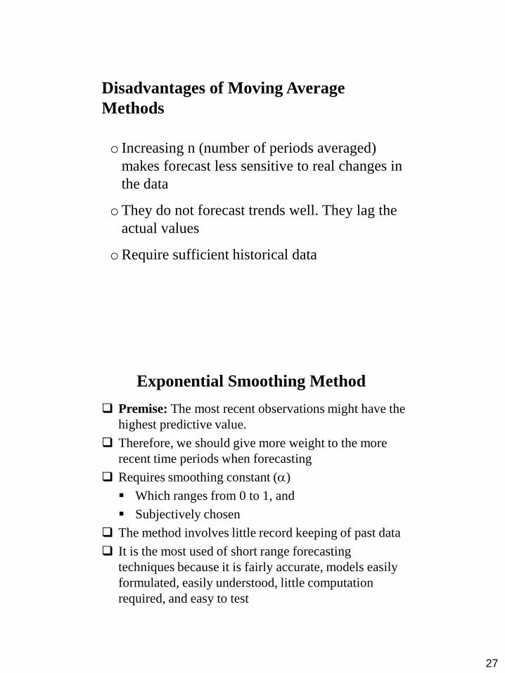
Disadvantages of Moving Average
Methods
o Increasing n (number of periods averaged)
makes forecast less sensitive to real changes in
the data
oThey do not forecast trends well. They lag the
actual values
oRequire sufficient historical data
Exponential Smoothing Method
Premise: The most recent observations might have the
highest predictive value.
Therefore, we should give more weight to the more
recent time periods when forecasting
Requires smoothing constant ()
Which ranges from 0 to 1, and
Subjectively chosen
The method involves little record keeping of past data
It is the most used of short range forecasting
techniques because it is fairly accurate, models easily
formulated, easily understood, little computation
required, and easy to test
28
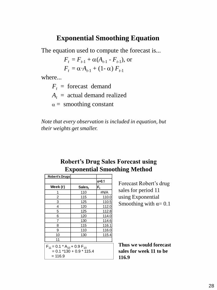
Exponential Smoothing Equation
The equation used to compute the forecast is...
Ft = Ft-1 + (At-1 - Ft-1), or
Ft = ·At-1 + (1- ) Ft-1
where...
Ft = forecast demand
At = actual demand realized
= smoothing constant
Note that every observation is included in equation, but
their weights get smaller.
Robert’s Drug Sales Forecast using
Exponential Smoothing Method
F11 = 0.1 * A10 + 0.9 F10
= 0.1 *130 + 0.9 * 115.4
= 116.9
Robert's Drugs
α=0.1
Week (t ) Salest Ft
1 110 #N/A
2 115 110.0
3 125 110.5
4 120 112.0
5 125 112.8
6 120 114.0
7 130 114.6
8 115 116.1
9 110 116.0
10 130 115.4
11
Thus we would forecast
sales for week 11 to be
116.9
Forecast Robert’s drug
sales for period 11
using Exponential
Smoothing with α= 0.1

29
Responsiveness with Different Values
3000
2500
2000
1500
1000
1 2 3 4 5 6 7 8 9 10 11 12
Actual demand
alpha = .1
alpha = .5
alpha = .9
Questions that You should be Asking
For the Moving Average technique, how do I determine
the best value of AP (n) to use for forecasting?
For Exponential Smoothing, how do I determine the
best value of α to use?
If I realize that a smoothing technique should be
employed, how do you know which smoothing
technique is best?
In order to answer the above questions, we need a
criteria for judging the accuracy of a forecasting
technique. Once we select a criterion, the method (or
parameter) which provides the best value for our
criterion is the best method (or parameter) to use for
forecasting our scenario.
30
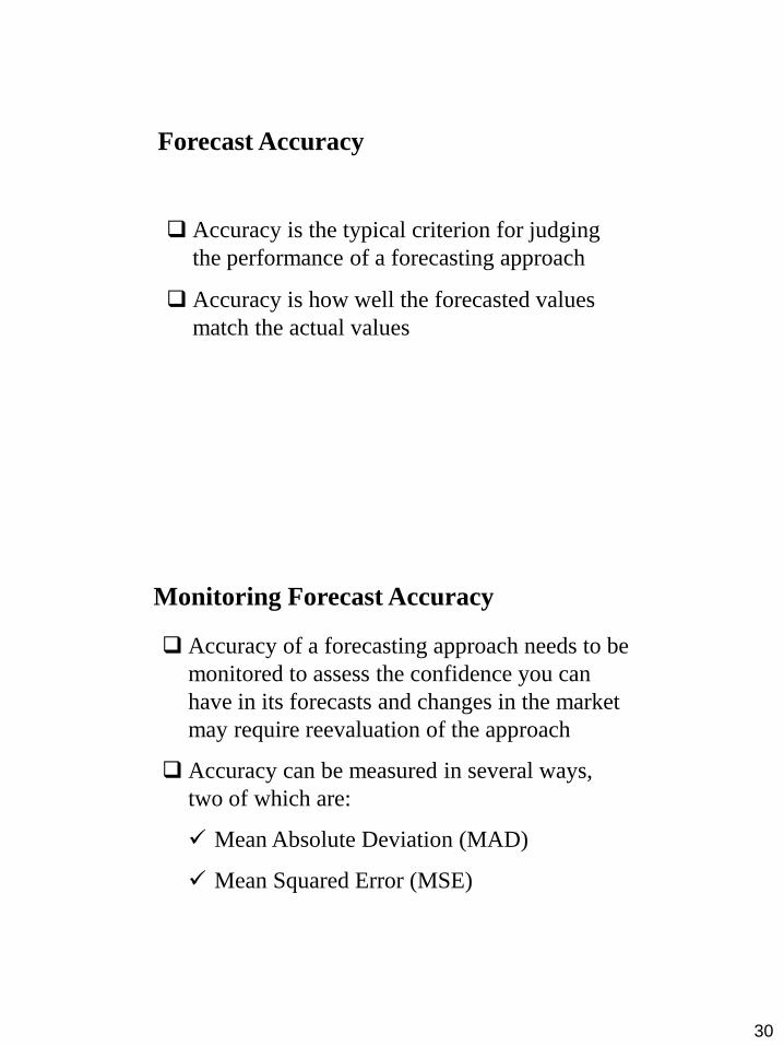
Forecast Accuracy
Accuracy is the typical criterion for judging
the performance of a forecasting approach
Accuracy is how well the forecasted values
match the actual values
Monitoring Forecast Accuracy
Accuracy of a forecasting approach needs to be
monitored to assess the confidence you can
have in its forecasts and changes in the market
may require reevaluation of the approach
Accuracy can be measured in several ways,
two of which are:
Mean Absolute Deviation (MAD)
Mean Squared Error (MSE)

31
Mean Absolute Deviation (MAD)
The mean of the absolute values of all forecast errors
is calculated, and the forecasting method or
parameter(s) which minimize this measure is selected.
MAD =
A - F
n
t tt=1
n
n
demandForecast -demand Actual
=MAD
n
1=i
i
Mean Squared Error (MSE)
MSE = (Syx)2
Small value for Syx means data points tightly
grouped around the line and error range is small.
The smaller the standard error the more accurate
the forecast.
MSE = 1.25(MAD)
when the forecast errors are normally distributed

32
Selecting the Smoothing Technique for
Robert’s Drugs Sales Forecasting
Determine the smoothing technique that is best for
forecasting Robert’s Drug sales: A two period
moving average, a three period moving average,
exponential smoothing (α=0.1), or exponential
smoothing (α=0.2)
Realistically we should have experimented with more
values of n for the moving average, and α for
exponential smoothing to determine the absolute best
parameters to use for our technique
We randomly chose to use the MSE criterion to judge
the best technique
MSE for Moving Average with AP = 2
Robert's Drug
Sales n=2 Error
Week (t ) At Ft (At - Ft) (At - Ft)2
1 110
2 115 #N/A
3 125 112.5 12.5 156.25
4 120 120.0 0.0 0.00
5 125 122.5 2.5 6.25
6 120 122.5 -2.5 6.25
7 130 122.5 7.5 56.25
8 115 125.0 -10.0 100.00
9 110 122.5 -12.5 156.25
10 130 112.5 17.5 306.25
11 120.0
MSE 98.44
33
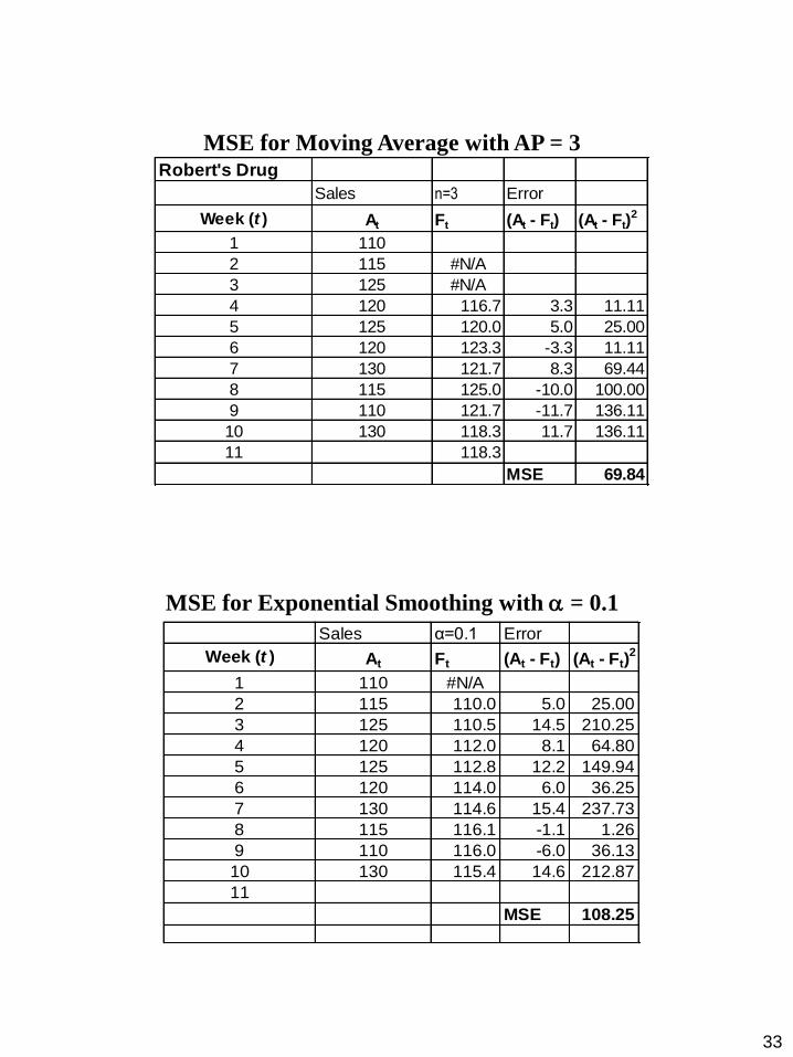
MSE for Moving Average with AP = 3 Robert's Drug
Sales n=3 Error
Week (t ) At Ft (At - Ft) (At - Ft)2
1 110
2 115 #N/A
3 125 #N/A
4 120 116.7 3.3 11.11
5 125 120.0 5.0 25.00
6 120 123.3 -3.3 11.11
7 130 121.7 8.3 69.44
8 115 125.0 -10.0 100.00
9 110 121.7 -11.7 136.11
10 130 118.3 11.7 136.11
11 118.3
MSE 69.84
MSE for Exponential Smoothing with = 0.1
Sales α=0.1 Error
Week (t ) At Ft (At - Ft) (At - Ft)2
1 110 #N/A
2 115 110.0 5.0 25.00
3 125 110.5 14.5 210.25
4 120 112.0 8.1 64.80
5 125 112.8 12.2 149.94
6 120 114.0 6.0 36.25
7 130 114.6 15.4 237.73
8 115 116.1 -1.1 1.26
9 110 116.0 -6.0 36.13
10 130 115.4 14.6 212.87
11
MSE 108.25
34
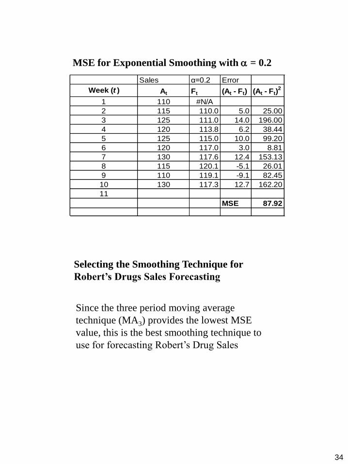
MSE for Exponential Smoothing with = 0.2
Sales α=0.2 Error
Week (t ) At Ft (At - Ft) (At - Ft)2
1 110 #N/A
2 115 110.0 5.0 25.00
3 125 111.0 14.0 196.00
4 120 113.8 6.2 38.44
5 125 115.0 10.0 99.20
6 120 117.0 3.0 8.81
7 130 117.6 12.4 153.13
8 115 120.1 -5.1 26.01
9 110 119.1 -9.1 82.45
10 130 117.3 12.7 162.20
11
MSE 87.92
Since the three period moving average
technique (MA3) provides the lowest MSE
value, this is the best smoothing technique to
use for forecasting Robert’s Drug Sales
Selecting the Smoothing Technique for
Robert’s Drugs Sales Forecasting

35
Exponential Smoothing with Trend
Attempts to correct (somewhat) the lag in the
exponential smoothing method
Trend equation with a smoothing constant,
(delta)
Formulae…
FITt = Forecast including trend
FITt = Ft + Tt
Ft = FITt-1 + (At-1 - FITt-1)
Tt = Tt-1 + (Ft - FITt-1)
Trend-Adjusted Forecasting
Three steps to compute a Trend-Adjusted
Forecast:
Step 1: Compute Ft , the exponentially
smoothed forecast for period t
Step 2: Compute the smoothened trend, Tt
Step 3: Calculate the forecast including
trend, FITt = Ft + Tt

36
Trend-Adjusted Forecasting Exercise
A large cement manufacturer uses exponential smoothing to forecast demand for a piece of pollution-control equipment. It appears that an increasing trend is present. Month At Month At 1 700 5 713 2 685 6 728 3 648 7 754 4 717 8 762 If the initial forecast for month 1 was 650 units and the trend over that period was 0 units, calculate FIT for the 9-month period. Use smoothing constants, = 0.1 and = 0.2.
Linear Regression in Forecasting
Linear regression is based on
1. Fitting a straight line to data
2. Explaining the change in one variable
through changes in other variables.
dependent variable = a + b (independent
variable)
By using linear regression, we are trying to explore
which independent variables affect the dependent
variable
37
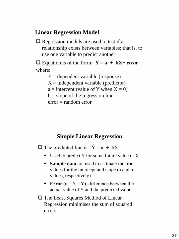
Linear Regression Model
Regression models are used to test if a
relationship exists between variables; that is, to
use one variable to predict another
Equation is of the form: Y = a + bX+ error
where:
Y = dependent variable (response)
X = independent variable (predictor)
a = intercept (value of Y when X = 0)
b = slope of the regression line
error = random error
Simple Linear Regression
The predicted line is: Ŷ = a + bX
Used to predict Y for some future value of X
Sample data are used to estimate the true
values for the intercept and slope (a and b
values, respectively)
Error ( = Y – Ŷ), difference between the
actual value of Y and the predicted value
The Least Squares Method of Linear
Regression minimises the sum of squared
errors
38
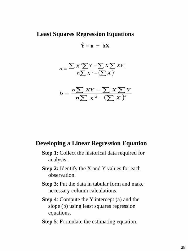
Least Squares Regression Equations
Ŷ = a + bX
22
2
XXn
XYXYXa
22
XXn
YXXYnb
Developing a Linear Regression Equation
Step 1: Collect the historical data required for
analysis.
Step 2: Identify the X and Y values for each
observation.
Step 3: Put the data in tabular form and make
necessary column calculations.
Step 4: Compute the Y intercept (a) and the
slope (b) using least squares regression
equations.
Step 5: Formulate the estimating equation.

39
Manufacturing Example
Step 1: Collect the historical data required for analysis
Step 2 and 3: Put the data in Tabular form.
X = manufacturing direct labour hours in hundreds of hours
(00’s)
Y = manufacturing overhead in thousands of dollars ($000’s)

40
Step 5: Formulate the Estimating Equation
Ŷ = a + bX
Ŷ = 5.8269 + 5.6322X
Where:
Ŷ = Manufacturing Overhead ($000’s)
X = Manufacturing Direct Labour Hours (00’s)
Estimate manufacturing overhead given an estimate
for manufacturing direct labour hours of 2,100:
Ŷ = 5.8269 + 5.6322X
Ŷ = 5.8269 + 5.6322(21)
Ŷ = 5.8269 + 118.2762
Ŷ = 124.1031 thousand dollars
Rounded to the nearest dollar, the estimate
would be $ 124,103.
41
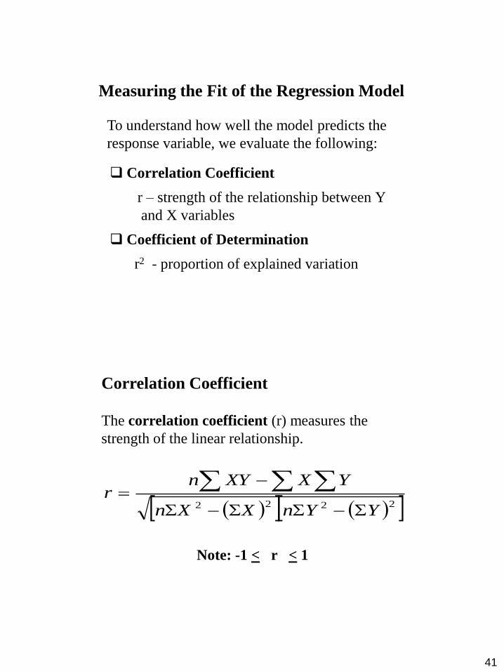
Measuring the Fit of the Regression Model
Correlation Coefficient
r – strength of the relationship between Y
and X variables
Coefficient of Determination
r2 - proportion of explained variation
To understand how well the model predicts the
response variable, we evaluate the following:
Correlation Coefficient
The correlation coefficient (r) measures the
strength of the linear relationship.
Note: -1 < r < 1
2222 YYnXXn
YXXYnr
42
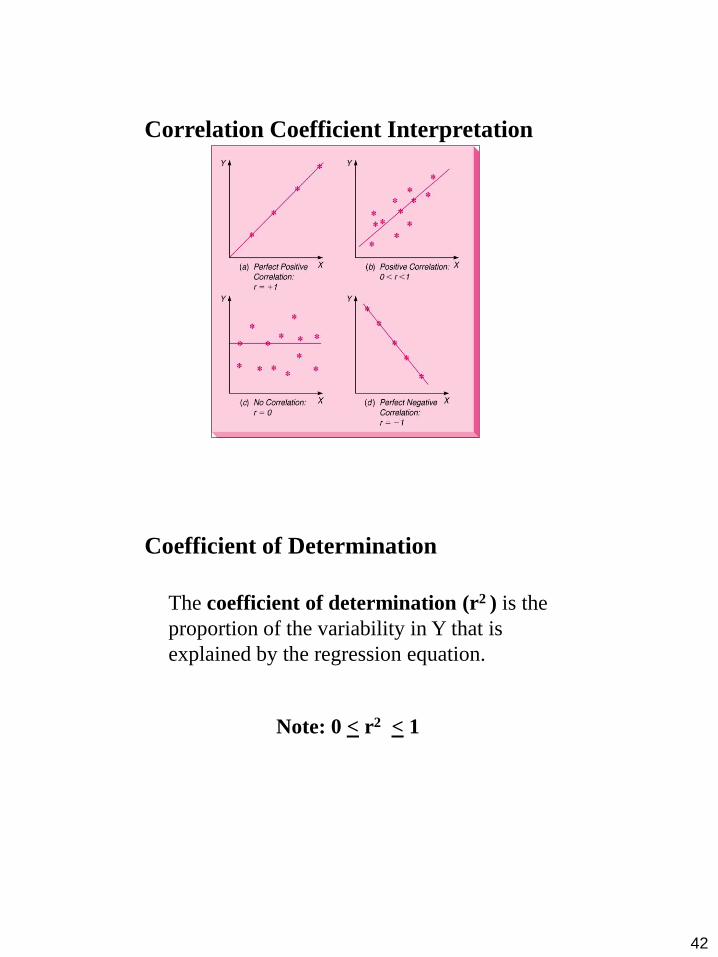
Correlation Coefficient Interpretation
Coefficient of Determination
The coefficient of determination (r2 ) is the
proportion of the variability in Y that is
explained by the regression equation.
Note: 0 < r2 < 1

43
Manufacturing Example Model Fit
This means that approximately 94% of the
variation in manufacturing overhead (Y) can
be explained by its relationship with
manufacturing direct labour hours (X).
r2 = 0.94 r = 0.97
Forecasts with Seasonality
Seasonal indices can be used to make
adjustments in the forecast for seasonality.
A seasonal index indicates how a particular
season compares with an average season.
The seasonal index can be found by
dividing the average value for a particular
season by the average of all the data.

44
Calculating Seasonal Indices
Month Demand Yr 1 Demand Yr 2 2-Yr Avge Monthly Avge Seasonal Index
Jan 80 100 90 94 0.957
Feb 75 85 80 94 0.851
Mar 80 90 85 94 0.904
Apr 90 110 100 94 1.064
May 115 131 123 94 1.309
Jun 110 120 115 94 1.223
Jul 102 108 105 94 1.117
Aug 88 102 100 94 1.064
Sep 85 95 90 94 0.957
Oct 77 83 80 94 0.851
Nov 75 85 80 94 0.851
Dec 82 78 80 94 0.851
1,128 (1,128/12) (2Yr-Ag/M-Ag)
Decomposition Method with Trend and
Seasonal Components in historical data
Decomposition is the process of isolating linear trend and seasonal factors to develop more accurate forecasts.
There are five steps to decomposition:
1. Compute the seasonal index for each season.
2. Deseasonalize the data by dividing each number by its seasonal index.
3. Compute a trend line with the deseasonalized data.
4. Use the trend line to forecast.
5. Multiply the forecasts by the seasonal index.
45
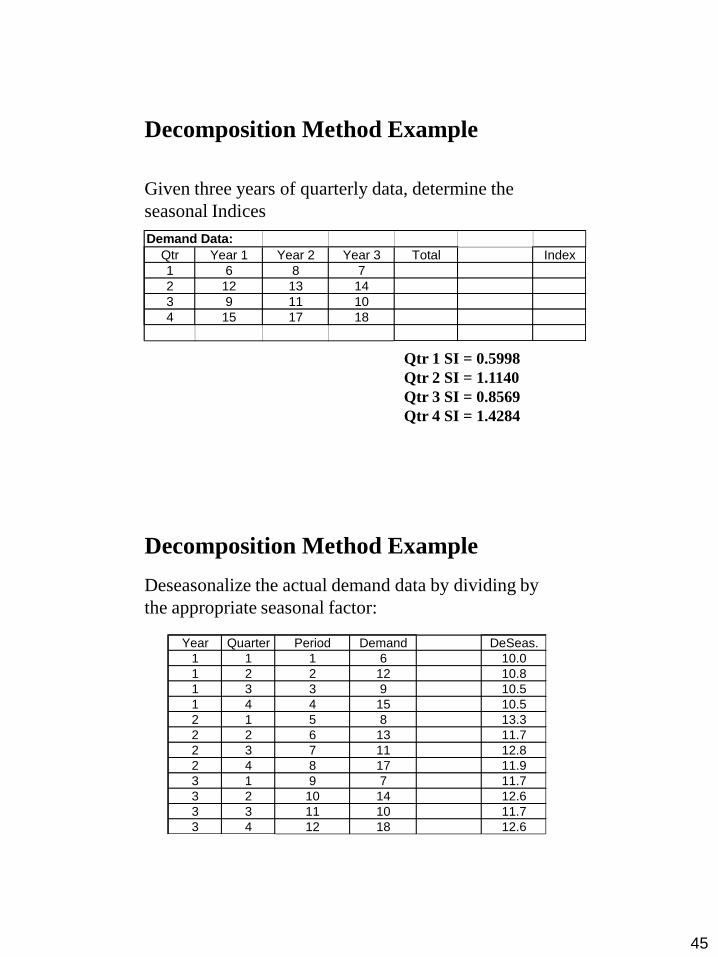
Decomposition Method Example
Given three years of quarterly data, determine the
seasonal Indices
Demand Data:
Qtr Year 1 Year 2 Year 3 Total Index
1 6 8 7
2 12 13 14
3 9 11 10
4 15 17 18
Qtr 1 SI = 0.5998
Qtr 2 SI = 1.1140
Qtr 3 SI = 0.8569
Qtr 4 SI = 1.4284
Decomposition Method Example
Deseasonalize the actual demand data by dividing by
the appropriate seasonal factor:
Year Quarter Period Demand DeSeas.
1 1 1 6 10.0
1 2 2 12 10.8
1 3 3 9 10.5
1 4 4 15 10.5
2 1 5 8 13.3
2 2 6 13 11.7
2 3 7 11 12.8
2 4 8 17 11.9
3 1 9 7 11.7
3 2 10 14 12.6
3 3 11 10 11.7
3 4 12 18 12.6

46
Decomposition Method Example
• Then perform a linear regression, least squares
approximation of the relationship between
quarter (X) and deseasonalized sales (Y)
• Form of a Linear Equation:
Y = a + b X
• From the equations:
a = 10.44
b = 0.1899
X Y XY XX
1 10.0 10.0 1
2 10.8 21.6 4
3 10.5 31.5 9
4 10.5 42.0 16
5 13.3 66.5 25
6 11.7 70.2 36
7 12.8 89.6 49
8 11.9 95.2 64
9 11.7 105.3 81
10 12.6 126.0 100
11 11.7 128.7 121
12 12.6 151.2 144
78 140.1 937.8 650
47
Decomposition Method Example
Project the trend using the predictive equation for
each quarter of year 4:
Quarter 13: F13 = 10.44 + 0.1899 (13) = 12.9
Quarter 14: F14 = 10.44 + 0.1899 (14) = 13.1
Quarter 15: F15 = 10.44 + 0.1899 (15) = 13.3
Quarter 16: F16 = 10.44 + 0.1899 (16) = 13.5
Decomposition Method Example
Adjust for seasonality by multiplying by the
seasonal factors for the appropriate quarters:
Qtr Proj. ReSeas.
13 12.9 7.7
14 13.1 14.6
15 13.3 11.4
16 13.5 19.2
Therefore, year four forecasts are:
Qtr 1 = 7.7
Qtr 2 = 14.6
Qtr 3 = 11.4
Qtr 4 = 19.2
48
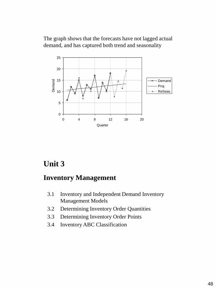
The graph shows that the forecasts have not lagged actual
demand, and has captured both trend and seasonality
0
5
10
15
20
25
0 4 8 12 16 20
Quarter
De
ma
nd Demand
Proj.
ReSeas.
Unit 3
Inventory Management
3.1 Inventory and Independent Demand Inventory
Management Models
3.2 Determining Inventory Order Quantities
3.3 Determining Inventory Order Points
3.4 Inventory ABC Classification
49
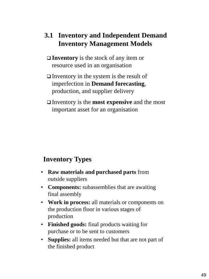
3.1 Inventory and Independent Demand
Inventory Management Models
Inventory is the stock of any item or
resource used in an organisation
Inventory in the system is the result of
imperfection in Demand forecasting,
production, and supplier delivery
Inventory is the most expensive and the most
important asset for an organisation
Inventory Types
• Raw materials and purchased parts from
outside suppliers
• Components: subassemblies that are awaiting
final assembly
• Work in process: all materials or components on
the production floor in various stages of
production
• Finished goods: final products waiting for
purchase or to be sent to customers
• Supplies: all items needed but that are not part of
the finished product

50
Independent Demand versus Dependent
Demand
A
B(4) C(2)
D(2) E(1) D(3) F(2)
Dependent Demand:
Raw Materials,
Component parts,
Sub-assemblies, etc.
Independent Demand:
Finished Goods/Parts
Product Tree
Why Do We Want to hold Inventory (1/3)
Finished Goods Inventory:
– Essential produce to stock positioning, of strategic
importance
– Necessary in level aggregate capacity plans
– Products can be displayed to customers
In-Process (Work-in-Process (WIP)):
– Necessary in process-focused production, uncouples
the states of production, increases flexibility
– Producing and transporting larger batches of
products creates more inventory but may reduce
materials-handling and production costs

51
Why Do We Want to hold Inventory (2/3)
Raw Materials Inventory:
– Suppliers produce and ship raw materials in batches
– Larger purchases result in more inventory, but
quantity discounts and reduced freight and
materials-handling costs may result
– Raw material sourcing has long and variable lead
times
Improve customer service: meet or exceed
customer’s expectations of product availability
Why Do We Want to hold Inventory (3/3)
Reduce certain costs such as:
– ordering costs (processing the purchase order,
expediting, record keeping and receiving the order
into the warehouse)
– stockout costs (lost sales, dissatisfied customers,
disruptions to production)
– acquisition costs (quantity discount, lower
transportation and handling costs)
– start-up quality costs (learning curve, less
changeovers and less scrap)
Contribute to the efficient and effective operation
of the production system (decoupling)
52
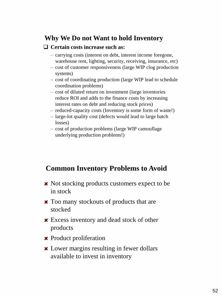
Why We Do not Want to hold Inventory
Certain costs increase such as:
– carrying costs (interest on debt, interest income foregone,
warehouse rent, lighting, security, receiving, insurance, etc)
– cost of customer responsiveness (large WIP clog production
systems)
– cost of coordinating production (large WIP lead to schedule
coordination problems)
– cost of diluted return on investment (large inventories
reduce ROI and adds to the finance costs by increasing
interest rates on debt and reducing stock prices)
– reduced-capacity costs (Inventory is some form of waste!)
– large-lot quality cost (defects would lead to large batch
losses)
– cost of production problems (large WIP camouflage
underlying production problems!)
Common Inventory Problems to Avoid
Not stocking products customers expect to be
in stock
Too many stockouts of products that are
stocked
Excess inventory and dead stock of other
products
Product proliferation
Lower margins resulting in fewer dollars
available to invest in inventory

53
Use Inventory Policies to solve the
common Inventory Problems
Inventory Policies specify decision rules with
respect to the point in time when a
replenishment of the inventory should be
initiated, as well as to the replenishment
quantity that should be ordered from the
supplying node in the supply network
Independent Demand Inventory
Management Models
1. Fixed Order Quantity System: this
involves placing orders for the same quantity
of the item each time that item reaches a pre-
set minimum stocking level, or reorder point
2. Fixed Order Period System: this involves
review of inventory at fixed time intervals,
and orders are placed for enough items to
bring its inventory levels back up to some
predetermined level

54
Inventory Control Decisions
Two fundamental decisions in controlling
inventory:
1. How much to order
2. When to order
Overall goal is to minimize total
inventory cost
Inventory Costs
Cost of the Items (Acquisition costs)
Cost of Ordering or Setup
Cost of Carrying or Holding inventory
Cost of safety stock
Cost of stockouts

55
Inventory Carrying Costs
Capital Costs: based on inventory
investment
Inventory Service Costs: relate to insurance
and taxes paid
Storage Space Costs: relate to warehousing
of inventory
Inventory Risk Costs: arising from
obsolescence, damages, pilferage and
relocation costs
3.2 Determining Inventory Order
Quantities
The procedure of determining inventory
order quantities would depend on the
inventory management system
Fixed Order Quantity System rely on the
behaviour of inventory costs to identify
the quantities with minimum total
inventory stocking costs
This section uses the Fixed Order
Quantity System

56
Inventory Costs Behaviour
Costs associated with ordering too much (represented by carrying costs)
Costs associated with ordering too little (represented by ordering costs)
These costs are opposing costs, that is, as one increases the other decreases
The sum of the two costs is the Total Stocking Cost (TSC)
When plotted against order quantity, the TSC decreases to a minimum cost and then increases
This cost behaviour is the basis for answering the first fundamental question: how much to order?
Inventory Cost Behaviour Plot
Annual Cost ($)
Order Quantity
Minimum
Total Annual
Stocking Costs
Annual Carrying Costs
Annual Ordering Costs
Total Annual Stocking Costs
Smaller Larger
Lo
we
r H
igh
er
EOQ
57
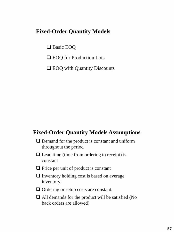
Fixed-Order Quantity Models
Basic EOQ
EOQ for Production Lots
EOQ with Quantity Discounts
Fixed-Order Quantity Models Assumptions
Demand for the product is constant and uniform
throughout the period
Lead time (time from ordering to receipt) is
constant
Price per unit of product is constant
Inventory holding cost is based on average
inventory.
Ordering or setup costs are constant.
All demands for the product will be satisfied (No
back orders are allowed)
58
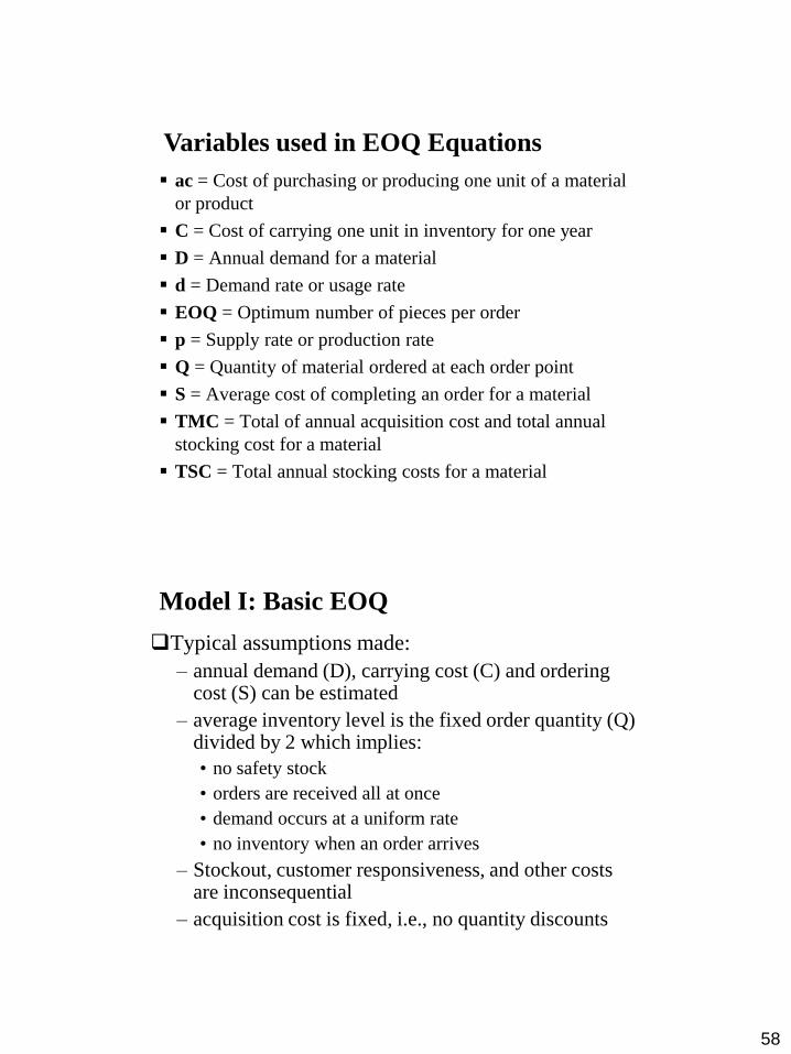
Variables used in EOQ Equations
ac = Cost of purchasing or producing one unit of a material
or product
C = Cost of carrying one unit in inventory for one year
D = Annual demand for a material
d = Demand rate or usage rate
EOQ = Optimum number of pieces per order
p = Supply rate or production rate
Q = Quantity of material ordered at each order point
S = Average cost of completing an order for a material
TMC = Total of annual acquisition cost and total annual
stocking cost for a material
TSC = Total annual stocking costs for a material
Model I: Basic EOQ
Typical assumptions made:
– annual demand (D), carrying cost (C) and ordering cost (S) can be estimated
– average inventory level is the fixed order quantity (Q) divided by 2 which implies:
• no safety stock
• orders are received all at once
• demand occurs at a uniform rate
• no inventory when an order arrives
– Stockout, customer responsiveness, and other costs are inconsequential
– acquisition cost is fixed, i.e., no quantity discounts
59
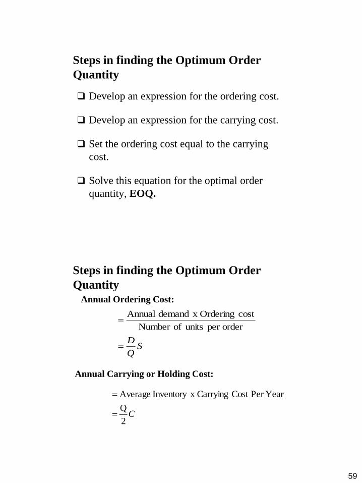
Steps in finding the Optimum Order
Quantity
Develop an expression for the ordering cost.
Develop an expression for the carrying cost.
Set the ordering cost equal to the carrying
cost.
Solve this equation for the optimal order
quantity, EOQ.
Steps in finding the Optimum Order
Quantity Annual Ordering Cost:
Annual Carrying or Holding Cost:
SQ
D
orderper units ofNumber
cost Ordering x demand Annual
C2
Q
YearPer Cost Carryingx Inventory Average
60
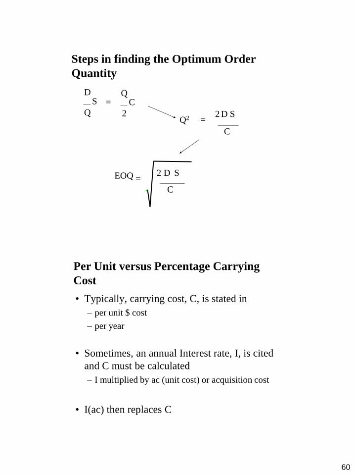
Steps in finding the Optimum Order
Quantity
C
2
Q S
Q
D =
Q2
C
2 S D =
EOQ =
C
2 S D
Per Unit versus Percentage Carrying
Cost
• Typically, carrying cost, C, is stated in
– per unit $ cost
– per year
• Sometimes, an annual Interest rate, I, is cited
and C must be calculated
– I multiplied by ac (unit cost) or acquisition cost
• I(ac) then replaces C

61
Per Unit versus Percentage Carrying
Cost
EOQ =
Per Unit Carrying Cost:
Percentage Carrying Cost:
C
2DS
EOQ = I(ac)
2DS
Denominator
Change
Calculating other Parameters
Total Stocking Cost:
C2
QS
Q
D TSC
Expected Number of Orders:
EOQ
D
N
QuantityOrder
Demand
Expected Time between Orders:
N
Days
T
Yearper Orders ofNumber
Yearper Days WorkingofNumber
62
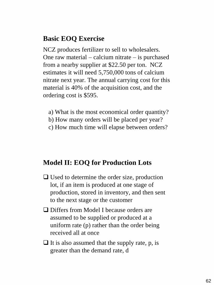
Basic EOQ Exercise
NCZ produces fertilizer to sell to wholesalers.
One raw material – calcium nitrate – is purchased
from a nearby supplier at $22.50 per ton. NCZ
estimates it will need 5,750,000 tons of calcium
nitrate next year. The annual carrying cost for this
material is 40% of the acquisition cost, and the
ordering cost is $595.
a) What is the most economical order quantity?
b) How many orders will be placed per year?
c) How much time will elapse between orders?
Model II: EOQ for Production Lots
Used to determine the order size, production
lot, if an item is produced at one stage of
production, stored in inventory, and then sent
to the next stage or the customer
Differs from Model I because orders are
assumed to be supplied or produced at a
uniform rate (p) rather than the order being
received all at once
It is also assumed that the supply rate, p, is
greater than the demand rate, d
63
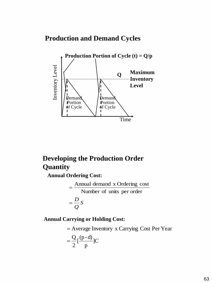
Production and Demand Cycles
Inv
ento
ry L
evel
Demand Portion of Cycle
Demand Portion of Cycle
Maximum
Inventory
Level
Time
Production Portion of Cycle (t) = Q/p
Q
Developing the Production Order
Quantity Annual Ordering Cost:
Annual Carrying or Holding Cost:
SQ
D
orderper units ofNumber
cost Ordering x demand Annual
C]p
d)-(p[
2
Q
YearPer Cost Carryingx Inventory Average

64
Setting the Equations equal to Solve for
EOQ
C]p
d)-(p[
2
Q S
Q
D
]d)-(p
p[
C
2DS EOQ
Note the similarities with Model I equation
EOQ for Production Lots Exercise
A Power Company buys coal from a Coal mine to
generate electricity in rural areas. The Coal mine
can supply coal at the rate of 3,500 tons per day for
$10.50 per ton. The Power Company uses the coal
at a rate of 800 tons per day and operates 365 days
per year. The annual carrying cost for coal is 20%
of the acquisition cost, and the ordering cost is
$5,000.
a) What is the economical production lot size?
b) What is the Power Company’s maximum
inventory level for coal?
65
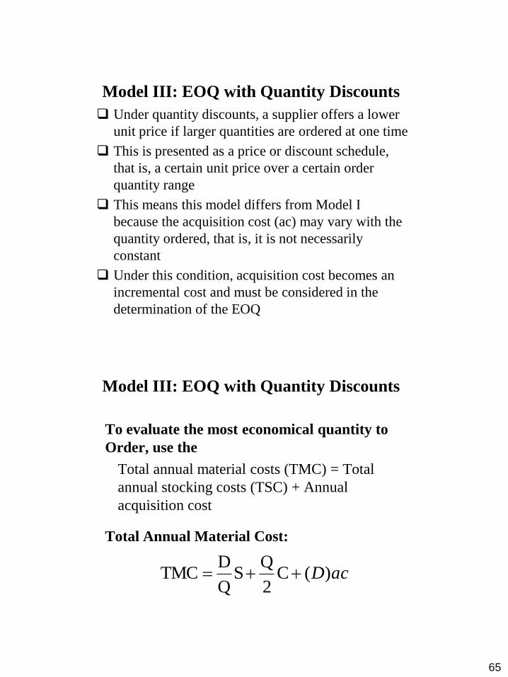
Model III: EOQ with Quantity Discounts
Under quantity discounts, a supplier offers a lower
unit price if larger quantities are ordered at one time
This is presented as a price or discount schedule,
that is, a certain unit price over a certain order
quantity range
This means this model differs from Model I
because the acquisition cost (ac) may vary with the
quantity ordered, that is, it is not necessarily
constant
Under this condition, acquisition cost becomes an
incremental cost and must be considered in the
determination of the EOQ
Model III: EOQ with Quantity Discounts
To evaluate the most economical quantity to
Order, use the
Total annual material costs (TMC) = Total
annual stocking costs (TSC) + Annual
acquisition cost
Total Annual Material Cost:
acD)(C2
QS
Q
D TMC

66
EOQ with Quantity Discounts Steps
To find the EOQ, the following procedure is used:
1. Compute the EOQ using the lowest acquisition
cost.
– If the resulting EOQ is feasible (the quantity
can be purchased at the acquisition cost
used), this quantity is optimal and you are
finished.
– If the resulting EOQ is not feasible, go to
Step 2
2. Identify the next higher acquisition cost.
EOQ with Quantity Discounts Steps
3. Compute the EOQ using the acquisition cost from
Step 2.
– If the resulting EOQ is feasible, go to Step 4.
– Otherwise, go to Step 2.
4. Compute the TMC for the feasible EOQ (just found
in Step 3) and its corresponding acquisition cost.
5. Compute the TMC for each of the lower acquisition
costs using the minimum allowed order quantity for
each cost.
6. The quantity with the lowest TMC is optimal.

67
EOQ with Quantity Discounts Exercise
A Motor Vehicle parts supplier has a regional engine
oil warehouse in Lusaka. One popular engine oil,
Castrol GTX, has estimated demand of 25,000 next
year. It costs the supplier $100 to place an order for
this oil, and the annual carrying cost is 30% of the
acquisition cost. Determine the optimal order quantity
if the supplier quotes these prices for the oil:
Q ac
1 – 499 $21.60
500 – 999 20.95
1,000 + 20.90
3.3 Determining Inventory Order
Points
Basis for Setting the Order Point
Demand During Lead Time (DDLT)
Distributions
Setting Order Points
68
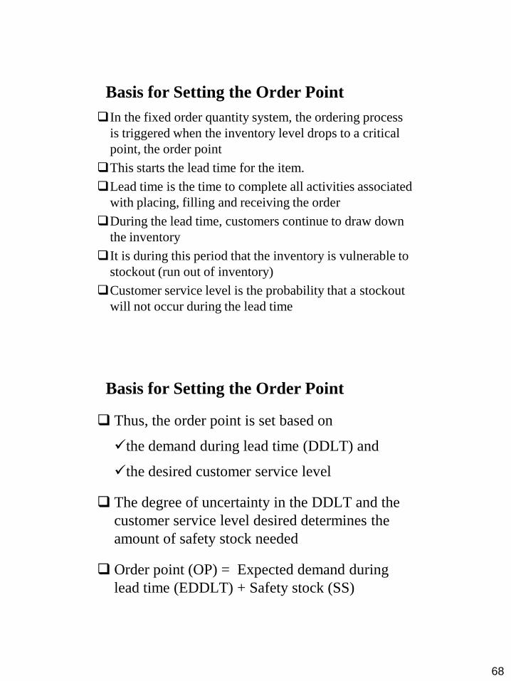
Basis for Setting the Order Point
In the fixed order quantity system, the ordering process
is triggered when the inventory level drops to a critical
point, the order point
This starts the lead time for the item.
Lead time is the time to complete all activities associated
with placing, filling and receiving the order
During the lead time, customers continue to draw down
the inventory
It is during this period that the inventory is vulnerable to
stockout (run out of inventory)
Customer service level is the probability that a stockout
will not occur during the lead time
Basis for Setting the Order Point
Thus, the order point is set based on
the demand during lead time (DDLT) and
the desired customer service level
The degree of uncertainty in the DDLT and the
customer service level desired determines the
amount of safety stock needed
Order point (OP) = Expected demand during
lead time (EDDLT) + Safety stock (SS)

69
Demand During Lead Time (DDLT)
Distributions
If there is variability in the DDLT, the DDLT is
expressed as a distribution
discrete
continuous
In a discrete DDLT distribution, values
(demands) can only be integers
A continuous DDLT distribution is appropriate
when the demand is very high
Setting Order Point for a Discrete DDLT
Distribution
1. Assume a probability distribution of actual
DDLTs is given or can be developed from a
frequency distribution
2. Starting with the lowest DDLT, accumulate the
probabilities. These are the service levels for the
DDLTs
3. Select the DDLT that will provide the desired
customer service level as the order point

70
Setting Order Point for a Discrete DDLT
Distribution Example
One of Emerging Technologies’ inventory items
is being analyzed to determine an appropriate
level of safety stock. The manager wants an 80%
service level during lead time. The item’s
historical DDLT is:
DDLT (cases) Occurrences
3 8
4 6
5 4
6 2
Setting Order Point for a Discrete DDLT
Distribution Example
Construct a Cumulative DDLT Distribution
Probability Probability of
DDLT (cases) of DDLT DDLT or Less
2 0 0
3 .4 .4
4 .3 .7
5 .2 .9
6 .1 1.0
To provide 80% service level, OP = 5 cases
71
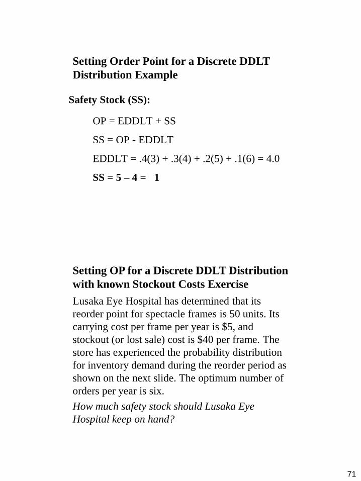
Setting Order Point for a Discrete DDLT
Distribution Example
Safety Stock (SS):
OP = EDDLT + SS
SS = OP - EDDLT
EDDLT = .4(3) + .3(4) + .2(5) + .1(6) = 4.0
SS = 5 – 4 = 1
Setting OP for a Discrete DDLT Distribution
with known Stockout Costs Exercise
Lusaka Eye Hospital has determined that its
reorder point for spectacle frames is 50 units. Its
carrying cost per frame per year is $5, and
stockout (or lost sale) cost is $40 per frame. The
store has experienced the probability distribution
for inventory demand during the reorder period as
shown on the next slide. The optimum number of
orders per year is six.
How much safety stock should Lusaka Eye
Hospital keep on hand?
72
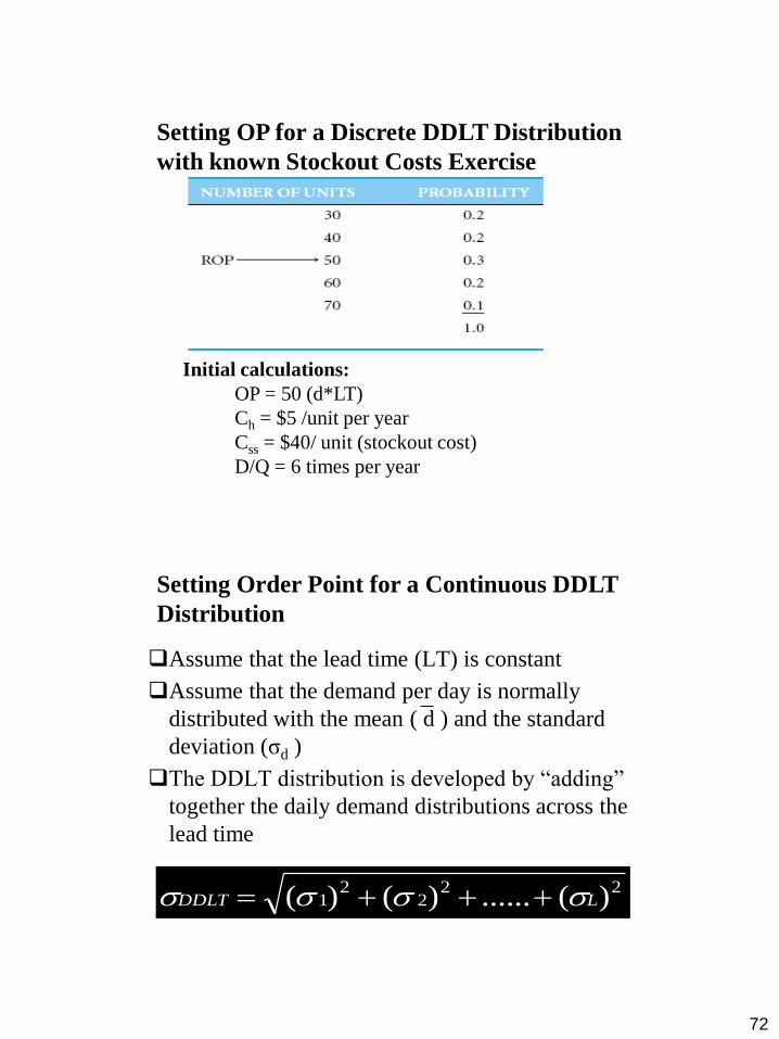
Setting OP for a Discrete DDLT Distribution
with known Stockout Costs Exercise
Initial calculations:
OP = 50 (d*LT)
Ch = $5 /unit per year
Css = $40/ unit (stockout cost)
D/Q = 6 times per year
Setting Order Point for a Continuous DDLT
Distribution
Assume that the lead time (LT) is constant
Assume that the demand per day is normally
distributed with the mean ( d ) and the standard
deviation (σd )
The DDLT distribution is developed by “adding”
together the daily demand distributions across the
lead time
222
21 )(......)()( LDDLT

73
Setting Order Point for a Continuous DDLT
Distribution
The resulting DDLT distribution is a normal
distribution with the following parameters:
EDDLT = LT(d )
2)( dDDLT LT
Setting Order Point for a Continuous DDLT
Distribution
The customer service level is converted into a
Z value using the normal distribution table
The safety stock is computed by multiplying
the Z value by σDDLT.
The order point is set using OP = EDDLT +
SS, or by substitution:
2
dOP = LT(d) + z LT(σ )
74
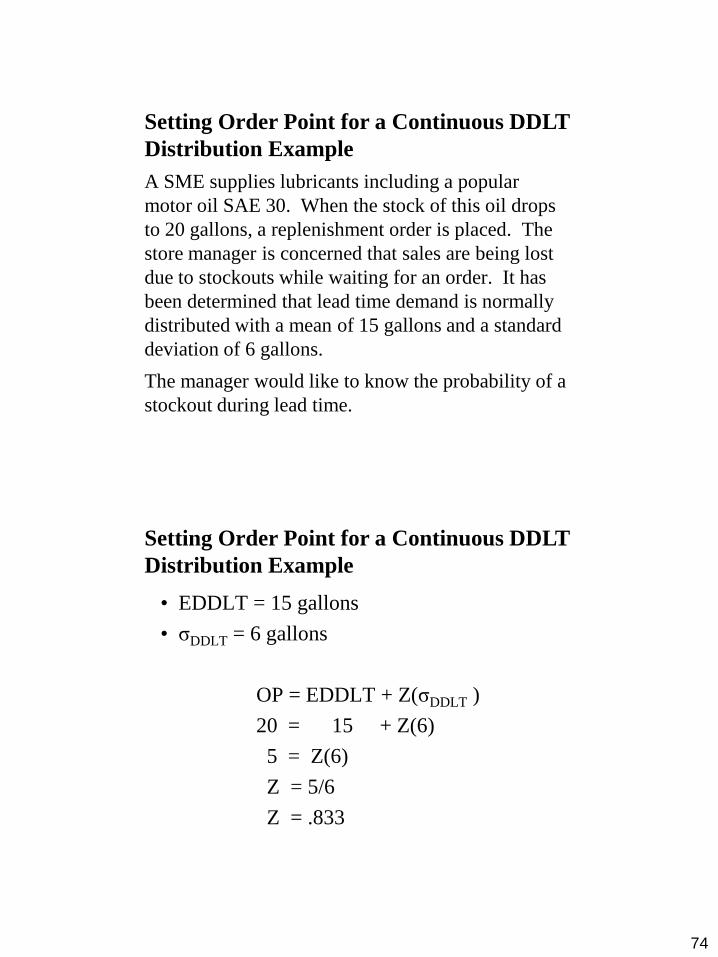
Setting Order Point for a Continuous DDLT
Distribution Example
A SME supplies lubricants including a popular
motor oil SAE 30. When the stock of this oil drops
to 20 gallons, a replenishment order is placed. The
store manager is concerned that sales are being lost
due to stockouts while waiting for an order. It has
been determined that lead time demand is normally
distributed with a mean of 15 gallons and a standard
deviation of 6 gallons.
The manager would like to know the probability of a
stockout during lead time.
Setting Order Point for a Continuous DDLT
Distribution Example
• EDDLT = 15 gallons
• σDDLT = 6 gallons
OP = EDDLT + Z(σDDLT )
20 = 15 + Z(6)
5 = Z(6)
Z = 5/6
Z = .833

75
Setting Order Point for a Continuous DDLT
Distribution Example
Standard Normal Distribution
0 .833
Area = .2967
Area = .5
Area = .2033
z
The probability of a stockout during lead time is .2033.
Setting Order Point for a Continuous DDLT
Distribution Exercise Daily demand for product EPD101 is normally
distributed with a mean of 50 units and a standard
deviation of 5. Shipping is usually certain with a lead
time of 6 days. The cost of placing an order is $8 and
annual carrying costs are 20% of unit price of $1.20. A
95% service level is desired for the customers who
place orders during the reorder period. Backorders are
not allowed. Once stocks are depleted, orders are filled
as soon as stocks arrive. No stockout costs. Assume
sales made over the entire year.
What is the reorder point? What is the cost of carrying
safety stocks?.

76
3.4 Inventory ABC Classification
Start with the inventoried items ranked by dollar
value in inventory in descending order
Plot the cumulative dollar value in inventory versus
the cumulative items in inventory
Typical observations
– A small percentage of the items (Class A) make up a
large percentage of the inventory value
– A large percentage of the items (Class C) make up a
small percentage of the inventory value
These classifications determine how much attention
should be given to controlling the inventory of
different items
ABC Classification
Items kept in inventory are not of equal
importance in terms of:
– dollars invested
– profit potential
– sales or usage volume
– stock-out penalties
0
30
60
30
60
A B
C
% of
$ Value
% of
Use

77
ABC Classification
Group A Items - Critical
Group B Items - Important
Group C Items - Not That Important
Inventory
Group
Dollar
Usage (%)
Inventory
Items (%)
Are Complex
Quantitative
Control
Techniques
Used?
A
B
C
70
20
10
10
20
70
Yes
In some cases
No
ABC Classification
100
90
80
70
60
50
40
30
20
10
0
Percent of Inventory Items
Per
cen
t of
An
nu
al
Doll
ar
Usa
ge
1 2 3 4 5 6 7 8 9 10
A
Items
B
Items C
Items
78
ABC Classification and Inventory Policy
Greater expenditure on supplier development
for A items than for B items or C items
Tighter physical control on A items than on B
items or on C items
Greater expenditure on forecasting A items
than on B items or on C items
Unit 4
Aggregate Planning
4.1 Production Planning Hierarchy and Aggregate
Planning
4.2 Role of Aggregate Planning in Production
Management
4.3 The Aggregate Planning Problem
4.4 Aggregate Planning Strategies
79
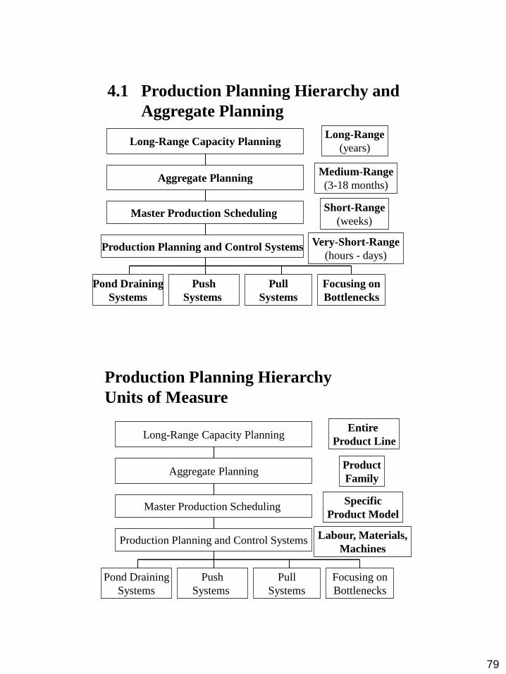
4.1 Production Planning Hierarchy and
Aggregate Planning
Master Production Scheduling
Production Planning and Control Systems
Pond Draining
Systems
Aggregate Planning
Push
Systems
Pull
Systems
Focusing on
Bottlenecks
Long-Range Capacity Planning Long-Range
(years)
Medium-Range
(3-18 months)
Short-Range
(weeks)
Very-Short-Range
(hours - days)
Production Planning Hierarchy
Units of Measure
Master Production Scheduling
Production Planning and Control Systems
Pond Draining
Systems
Aggregate Planning
Push
Systems
Pull
Systems
Focusing on
Bottlenecks
Long-Range Capacity Planning Entire
Product Line
Product
Family
Specific
Product Model
Labour, Materials,
Machines
80
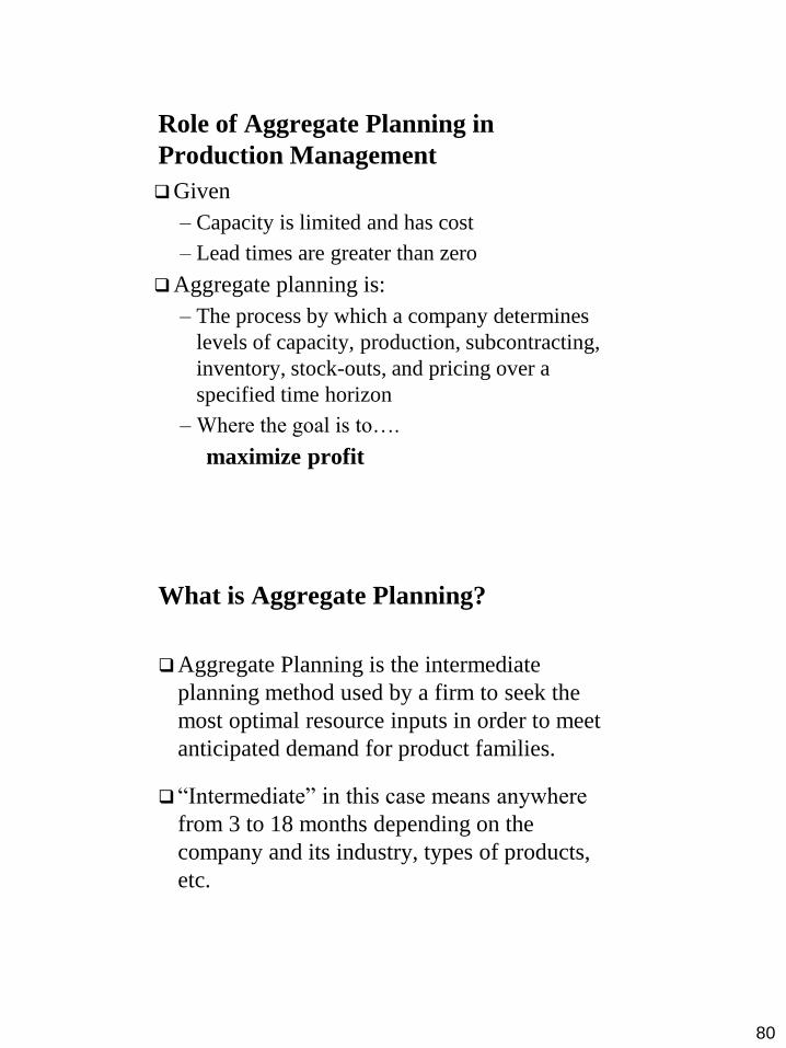
Role of Aggregate Planning in
Production Management
Given
– Capacity is limited and has cost
– Lead times are greater than zero
Aggregate planning is:
– The process by which a company determines
levels of capacity, production, subcontracting,
inventory, stock-outs, and pricing over a
specified time horizon
– Where the goal is to….
maximize profit
What is Aggregate Planning?
Aggregate Planning is the intermediate
planning method used by a firm to seek the
most optimal resource inputs in order to meet
anticipated demand for product families.
“Intermediate” in this case means anywhere
from 3 to 18 months depending on the
company and its industry, types of products,
etc.

81
Aggregate Planning Scope
Decisions are usually made at a product family (not
Stock Keeping Unit (SKU)) level
– SKUs within product families tend to use same
capacities, have similar costs
– Avoids too much detail- there might be 10 product
families for 1500 SKUs
The time frame is generally 3 to 18 months
– Too early to schedule by SKU
– Too late to make strategic, long term plans (“build
another plant”)
– Answers question of “How can a firm best use the
facilities it has?” with possibly “Do we need to outsource
or subcontract?”
Aggregate Planning Problem
Given the demand forecast for each period in the
planning horizon, determine the production
level, inventory level, and the capacity level for
each period that maximizes the firm’s profit over
the planning horizon
Specify the planning horizon
Specify the duration of each period (time
bucket) typically 1 month
Specify key information required to develop an
aggregate plan
82
Medium-Term Capacity Adjustments
Workforce level
– Hire or layoff full-time workers
– Hire or layoff part-time workers
– Hire or layoff contract workers
Utilization of the work force
– Overtime
– Idle time (under time)
– Reduce hours worked
Inventory level
– Finished goods inventory
– Backorders/lost sales
Subcontract
Information Needed for an Aggregate Plan
Demand forecast in each period
Production costs – Machine costs
– labour costs, regular time ($/hr) and overtime ($/hr)
– subcontracting costs ($/hr or $/unit)
– cost of changing capacity: hiring or layoff ($/worker) and cost
of adding or reducing machine capacity ($/machine)
Labour/machine hours required per unit
Material requirements per unit, material cost and availability
Inventory holding cost ($/unit/period)
Stock-out or backlog cost ($/unit/period)
Yield rates, if applicable (% loss in production or inventory)
Constraints: physical or policy limits on overtime, layoffs,
capital available, warehousing, stock-outs and backlogs
83
Aggregate Planning Goals
Specify the optimal combination of:
– production rate (units completed per unit of time)
– workforce level (number of workers)
– inventory on hand (inventory carried from previous
period)
Meet demand (Sales Forecast)
Use capacity efficiently
Satisfy inventory policy
Minimize cost (Labour, Inventory, Subcontract,
Plant and Equipment)
Aggregate Plan Outputs
Production quantity from regular time, overtime,
and subcontracted time: used to determine
number of workers and supplier purchase levels
Inventory held: used to determine how much
warehouse space and working capital is needed
Backlog/stock-out quantity: used to determine
what customer service levels will be
Machine capacity increase/decrease: used to
determine if new production equipment needs to
be purchased or capacities need to be rededicated

84
Why Aggregate Planning is Necessary
Fully load facilities and minimize overloading
and underloading
Make sure enough capacity available to satisfy
expected demand
Plan for the orderly and systematic change of
production capacity to meet the peaks and
valleys of expected customer demand
Get the most output for the amount of
resources available
Aggregate Planning Strategies
1. Chase strategy: match production rate to production
requirements by varying the workforce (no inventory
buildup or shortage allowed)
2. Level strategy: keep a constant workforce who work at
maximum capacity (inventory will vary from period to
period); workforce level chosen such that the total
requirement over the planning horizon can be exactly met
3. Stable workforce: keep a constant workforce who work at
maximum capacity; outsource in order to match
production and requirements (no inventory buildup or
shortage allowed); workforce level chosen such that they
can exactly satisfy the requirements in the period with the
minimum requirement level
85
Aggregate Planning Inputs
A forecast of aggregate demand covering the
selected planning horizon (3-18 months)
The alternative means available to adjust short-
to medium-term capacity, to what extent each
alternative could impact capacity and the related
costs
The current status of the system in terms of
workforce level, inventory level and production
rate
Aggregate Planning Production Plans
A production plan: aggregate decisions for
each period in the planning horizon about
– workforce level;
– inventory level;
– Backorders/Lost sales;
– production rate; and
– Units subcontracted/Outsourced
Projected costs if the production plan was
implemented
86
Aggregate Planning Methods
Informal or Trial-and-Error Approach (Cut
and Try Approach)
Mathematically Optimal Approaches
– Linear Programming
– Linear Decision Rules
Computer Search
General Steps in Cut and Try Method
1. Convert demand forecasts into production
requirements
2. Identify pertinent company policies
3. Develop alternative production plans for the
company (pure or mixed strategies?)
4. Calculate the cost of each plan
5. Choose the best plan that fits (minimal costs)
87
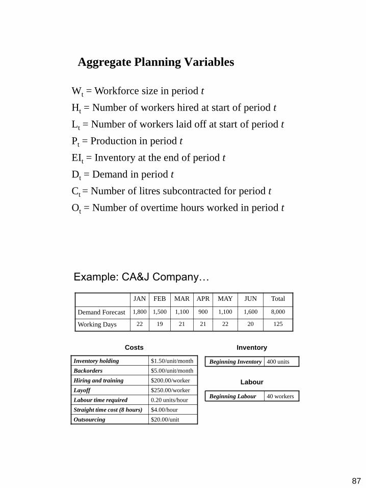
Aggregate Planning Variables
Wt = Workforce size in period t
Ht = Number of workers hired at start of period t
Lt = Number of workers laid off at start of period t
Pt = Production in period t
EIt = Inventory at the end of period t
Dt = Demand in period t
Ct = Number of litres subcontracted for period t
Ot = Number of overtime hours worked in period t
Example: CA&J Company…
JAN FEB MAR APR MAY JUN Total
Demand Forecast 1,800 1,500 1,100 900 1,100 1,600 8,000
Working Days 22 19 21 21 22 20 125
Inventory holding $1.50/unit/month
Backorders $5.00/unit/month
Hiring and training $200.00/worker
Layoff $250.00/worker
Labour time required 0.20 units/hour
Straight time cost (8 hours) $4.00/hour
Outsourcing $20.00/unit
Costs
Beginning Inventory 400 units
Inventory
Labour
Beginning Labour 40 workers

88
First step: Analyze the requirements…
JAN FEB MAR APR MAY JUN
Beginning Inventory 400
Demand Forecast 1,800 1,500 1,100 900 1,100 1,600
Production requirement
Ending Inventory
JAN FEB MAR APR MAY JUN
Beginning Inventory 400 0 0 0 0 0
Demand Forecast 1,800 1,500 1,100 900 1,100 1,600
Production requirement 1,400 1,500 1,100 900 1,100 1,600
Ending Inventory 0 0 0 0 0 0
First step: Analyze the requirements…
89
JAN FEB MAR APR MAY JUN
Production requirement 1,400 1,500 1,100 900 1,100 1,600
Production hours
required
Days per month 22 19 21 21 22 20
Worker hours per month
Workers required
Workers hired
Hiring cost
Workers laid off
Layoff cost
Labour cost
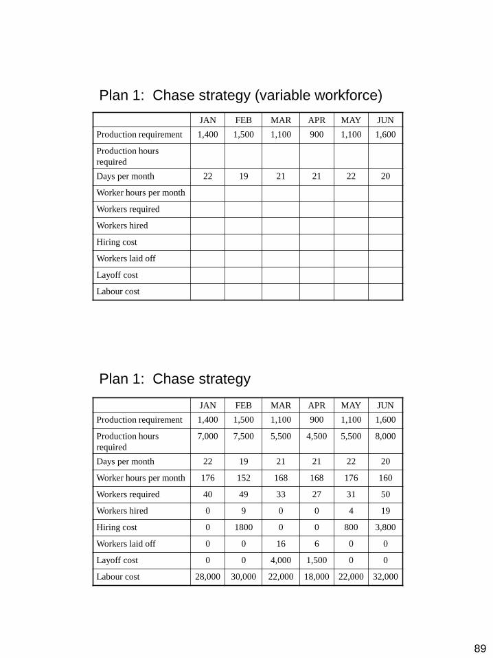
Plan 1: Chase strategy (variable workforce)
JAN FEB MAR APR MAY JUN
Production requirement 1,400 1,500 1,100 900 1,100 1,600
Production hours
required
7,000 7,500 5,500 4,500 5,500 8,000
Days per month 22 19 21 21 22 20
Worker hours per month 176 152 168 168 176 160
Workers required 40 49 33 27 31 50
Workers hired 0 9 0 0 4 19
Hiring cost 0 1800 0 0 800 3,800
Workers laid off 0 0 16 6 0 0
Layoff cost 0 0 4,000 1,500 0 0
Labour cost 28,000 30,000 22,000 18,000 22,000 32,000
Plan 1: Chase strategy

90
Hiring cost 6,400
Layoff cost 5,500
Labour cost 152,000
Total Cost 163,900
Plan 1: Chase strategy
Plan 2: Level strategy (Level Capacity)
JAN FEB MAR APR MAY JUN
Beginning inventory 400
Working days per month 22 19 21 21 22 20
Production hours available
Monthly production level
Demand Forecast 1,800 1,500 1,100 900 1,100 1,600
Ending Inventory
Shortage Cost
Inventory cost
Labour cost

91
Plan 2: Level strategy
JAN FEB MAR APR MAY JUN
Beginning inventory 400 -62 -407 -230 147 385
Working days per month 22 19 21 21 22 20
Production hours available 6688 5776 6384 6,384 6,688 6,080
Monthly production level 1,338 1,155 1,277 1,277 1,338 1,216
Demand Forecast 1,800 1,500 1,100 900 1,100 1,600
Ending Inventory -62 -407 -230 147 385 1
Shortage Cost 310 2035 1150 0 0 0
Inventory cost 0 0 0 220.5 577.5 1.5
Labour cost 26752 23104 25536 25536 26752 24320
Number of workers required
= Total hours required over planning horizon/(8*total days)
= 38,000/(8*125) = 38. This is the no. of workers for each month
Layoff cost 500
Shortage
cost 3,495
Inventory
cost 799.50
Labour cost 152,000
Total Cost 156,794.50
Plan 2: Level strategy
92
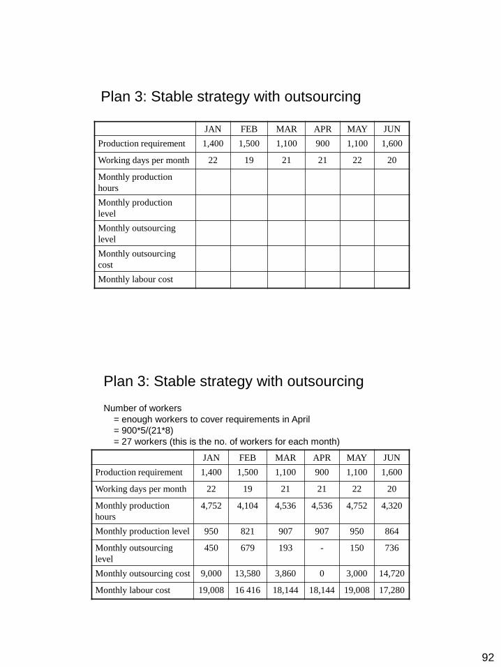
Plan 3: Stable strategy with outsourcing
JAN FEB MAR APR MAY JUN
Production requirement 1,400 1,500 1,100 900 1,100 1,600
Working days per month 22 19 21 21 22 20
Monthly production
hours
Monthly production
level
Monthly outsourcing
level
Monthly outsourcing
cost
Monthly labour cost
Plan 3: Stable strategy with outsourcing
JAN FEB MAR APR MAY JUN
Production requirement 1,400 1,500 1,100 900 1,100 1,600
Working days per month 22 19 21 21 22 20
Monthly production
hours
4,752 4,104 4,536 4,536 4,752 4,320
Monthly production level 950 821 907 907 950 864
Monthly outsourcing
level
450 679 193 - 150 736
Monthly outsourcing cost 9,000 13,580 3,860 0 3,000 14,720
Monthly labour cost 19,008 16 416 18,144 18,144 19,008 17,280
Number of workers
= enough workers to cover requirements in April
= 900*5/(21*8)
= 27 workers (this is the no. of workers for each month)
93
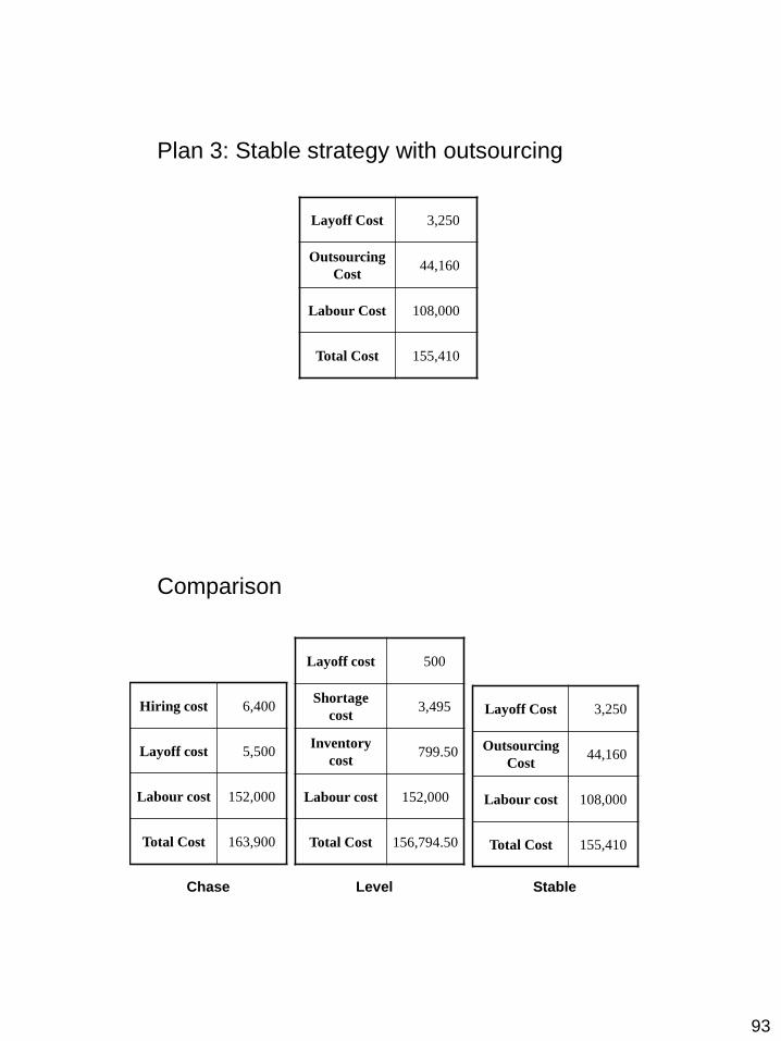
Layoff Cost 3,250
Outsourcing
Cost 44,160
Labour Cost 108,000
Total Cost 155,410
Plan 3: Stable strategy with outsourcing
Comparison
Hiring cost 6,400
Layoff cost 5,500
Labour cost 152,000
Total Cost 163,900
Chase Level Stable
Layoff cost 500
Shortage
cost 3,495
Inventory
cost 799.50
Labour cost 152,000
Total Cost 156,794.50
Layoff Cost 3,250
Outsourcing
Cost 44,160
Labour cost 108,000
Total Cost 155,410
94
The cost of each option
Work environment harmony (management-
union relations)
Ergonomics aspects during increased overtime
durations (fatigue, morale, productivity)
Impact on product quality due to overworking
(excessive overtime)
Flexibility of increasing or decreasing
unplanned production levels
Factors important in the choice of the option
Unit 5
Master Production Schedule (MPS)
5.1 Master Production Schedule (MPS)
5.2 Time Fences in MPS
5.3 Developing an MPS
5.4 Rough-Cut Capacity Planning

95
5.1 Master Production Schedule (MPS)
A Master Production Schedule (MPS) is a
realistic, detailed, manufacturing plan for
which all possible demands upon the
manufacturing facilities (such as available
personnel, working hours, management policy
and goals) have been considered and are
visualized
The MPS is a statement of what the company
expects to produce and purchase expressed in
selected items, specific quantities and dates
Objectives of MPS
Determine the quantity and timing of
completion of end items over a short-range
planning horizon
Schedule end items (finished goods and parts
shipped as end items) to be completed
promptly and when promised to the customer
Avoid overloading or underloading the
production facility so that production
capacity is efficiently utilized and low
production costs result

96
Effective MPS…
Give management the information to control
the manufacturing operation
Tie overall business planning and forecasting
to detail operations
Enable marketing to make legitimate delivery
commitments to warehouses and customers
Greatly increase the efficiency and accuracy of
a company's manufacturing as it drives detailed
material and production requirements in
Material Requirements Planning (MRP) phase
5.2 Time Fences in MPS
The rules for scheduling
No Change
+/- 5%
Change
+/- 10%
Change
+/- 20%
Change Frozen
Firm
Full Open
1-2
weeks
2-4
weeks
4-6
weeks
6+
weeks

97
The Rules of Scheduling
Do not change orders in the frozen zone
Do not exceed the agreed on percentage
changes when modifying orders in the other
zones
Try to level load as much as possible
Do not exceed the capacity of the system when
promising orders
If an order must be pulled into level load, pull
it into the earliest possible week without
missing the promise
5.3 Developing an MPS
Using input information:
– Customer orders (end items quantity, due dates)
– Forecasts (end items quantity, due dates)
– Inventory status (balances, planned receipts)
– Production capacity (output rates, planned
downtime)
Schedulers place orders in the earliest
available open slot of the MPS
98
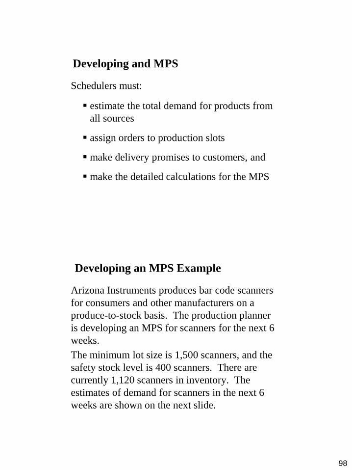
Developing and MPS
Schedulers must:
estimate the total demand for products from
all sources
assign orders to production slots
make delivery promises to customers, and
make the detailed calculations for the MPS
Developing an MPS Example
Arizona Instruments produces bar code scanners
for consumers and other manufacturers on a
produce-to-stock basis. The production planner
is developing an MPS for scanners for the next 6
weeks.
The minimum lot size is 1,500 scanners, and the
safety stock level is 400 scanners. There are
currently 1,120 scanners in inventory. The
estimates of demand for scanners in the next 6
weeks are shown on the next slide.
99
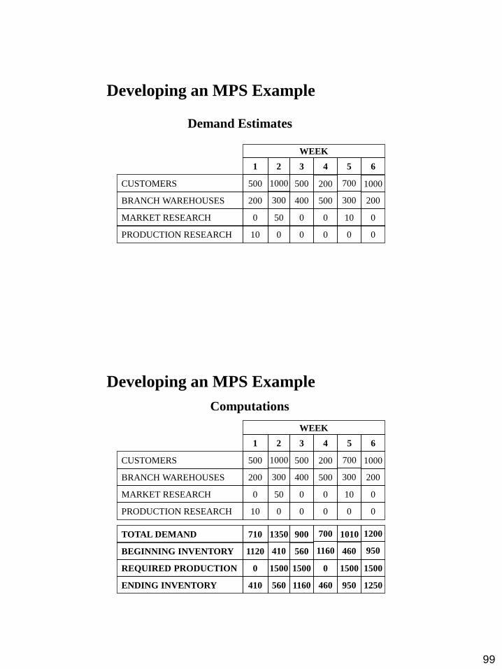
Developing an MPS Example
Demand Estimates
CUSTOMERS
BRANCH WAREHOUSES
MARKET RESEARCH
PRODUCTION RESEARCH
500
200
0
10
1
0
50
300
1000
0
0
500
400
2 3 4
200
0 0 0
300 500
0 10 0
700
6 5
1000
200
WEEK
Developing an MPS Example
Computations
CUSTOMERS
BRANCH WAREHOUSES
MARKET RESEARCH
PRODUCTION RESEARCH
500
200
0
10
1
0
50
300
1000
0
0
500
400
2 3 4
200
0 0 0
300 500
0 10 0
700
6 5
1000
200
WEEK
TOTAL DEMAND
BEGINNING INVENTORY
REQUIRED PRODUCTION
ENDING INVENTORY
710
1120
0
410 560
1500
410
1350
1160
1500
900
560
700
1250 950 460
460 1160
1500 1500 0
1010 1200
950
100
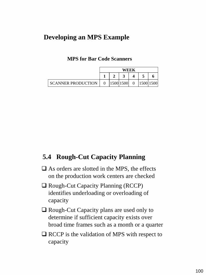
Developing an MPS Example
MPS for Bar Code Scanners
SCANNER PRODUCTION 0 1500 1500 1500 1500 0
1 2 3 4 6 5
WEEK
5.4 Rough-Cut Capacity Planning
As orders are slotted in the MPS, the effects
on the production work centers are checked
Rough-Cut Capacity Planning (RCCP)
identifies underloading or overloading of
capacity
Rough-Cut Capacity plans are used only to
determine if sufficient capacity exists over
broad time frames such as a month or a quarter
RCCP is the validation of MPS with respect to
capacity

101
Rough-Cut Capacity Planning Example
Emerging Technologies makes a line of computer
printers on a produce-to-stock basis for other
computer manufacturers. Each printer requires an
average of 24 labour-hours. The plant uses a
backlog of orders to allow a level-capacity
aggregate plan. This plan provides a weekly
capacity of 5,000 labour-hours.
Emerging Technologies’ rough-draft of an MPS
for its printers is shown on the next slide. Does
enough capacity exist to execute the MPS? If not,
what changes do you recommend?
Rough-Cut Capacity Planning Example
Rough-Cut Capacity Analysis
PRODUCTION 100 200 200 280 250
1 2 3 4 5
WEEK
TOTAL
1030
LOAD 2400 4800 4800 6720 6000 24720
CAPACITY 5000 5000 5000 5000 5000 25000
UNDER or (OVER) LOAD 2600 200 200 (1720) (1000) 280

102
Rough-Cut Capacity Planning Example
Rough-Cut Capacity Analysis:
The plant is underloaded in the first 3 weeks
(primarily week 1) and it is overloaded in the
last 2 weeks of the schedule.
Some of the production scheduled for week
4 and 5 should be moved to week 1.
Rough-Cut Capacity Planning Example 2
A firm produces two products, A and B, on a produce-to-
stock basis. The safety stock for A is 30 and for B it is 40.
The fixed lot size for A is 50 and for B it is 60. The
beginning inventory for A is 70 and for B it is 50. Prepare
an MPS for these two products for the next 6 weeks using
the demand estimates given on the next slide.
Suppose that the final assembly for the two products is
done on the same line, determine if the MPS developed is
underloaded or overloaded given that the final assembly
line has a weekly capacity of 100 hours available, while
each Product A requires 0.9 hours and each Product B
requires 1.6 hours of final assembly capacity.

103
Rough-Cut Capacity Planning Example 2
INTRA-COMPANY
BRANCH WAREHOUSES
R&D
CUSTOMER DEMAND
0
0
0
20
1
20
0
0
0
20
10
0
20
2 3 4
20
20 20 20
0 0
0 0 10
10
6 5
10
0
WEEK
INTRA-COMPANY
BRANCH WAREHOUSES
R&D
CUSTOMER DEMAND
0
0
0
30
1
30
0
0
0
30
0
10
0
2 3 4
0
20 20 20
0 20
10 10 0
10
6 5
0
0
WEEK
Product A
Product B
Rough-Cut Capacity Planning Example 2
TOTAL DEMAND
BEGINNING INVENTORY
REQUIRED PRODUCTION
ENDING INVENTORY
20
70
0
50
1
30
0
50
20
30
50
50
30
2 3 4
50
70 50 30
30 30
50 50 50
30
6 5
30
50
WEEK
TOTAL DEMAND
BEGINNING INVENTORY
REQUIRED PRODUCTION
ENDING INVENTORY
30
50
60
80
1
50
0
80
30
70
60
40
50
2 3 4
40
80 50 90
90 70
60 0 60
40
6 5
30
50
WEEK
Product A
Product B
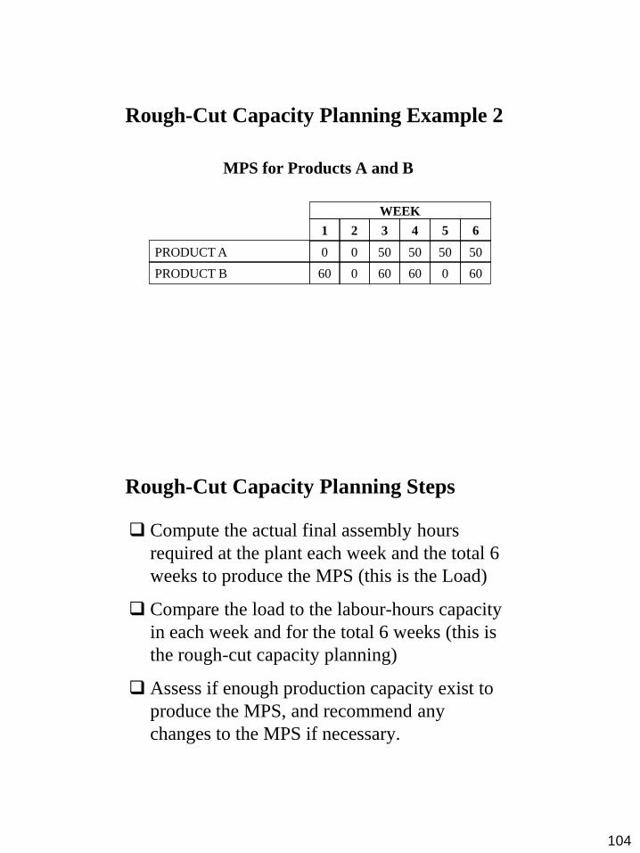
104
Rough-Cut Capacity Planning Example 2
MPS for Products A and B
PRODUCT A 0 0 50 50 50 50
1 2 3 4 6 5
WEEK
PRODUCT B 60 0 60 60 0 60
Rough-Cut Capacity Planning Steps
Compute the actual final assembly hours
required at the plant each week and the total 6
weeks to produce the MPS (this is the Load)
Compare the load to the labour-hours capacity
in each week and for the total 6 weeks (this is
the rough-cut capacity planning)
Assess if enough production capacity exist to
produce the MPS, and recommend any
changes to the MPS if necessary.
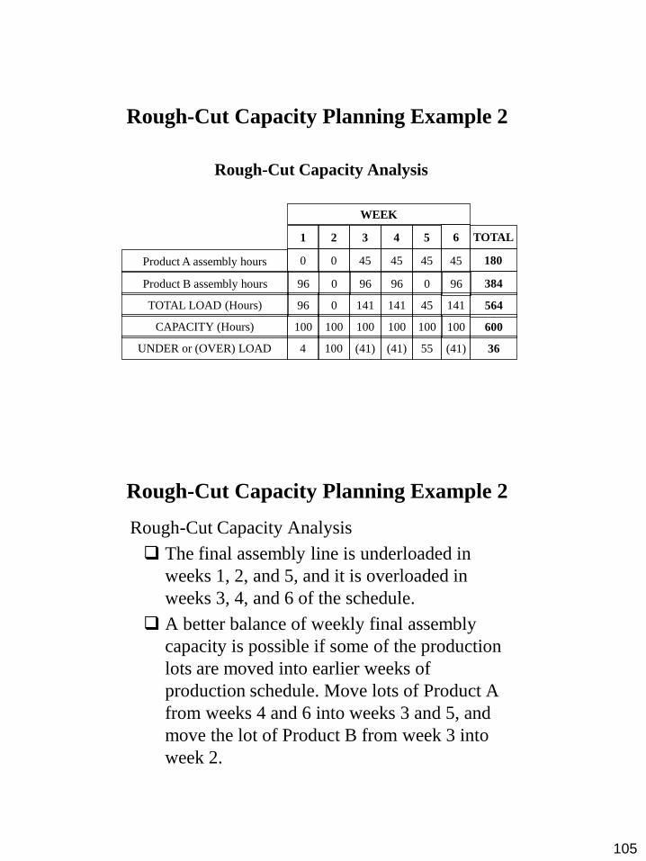
105
Rough-Cut Capacity Planning Example 2
Rough-Cut Capacity Analysis
Product A assembly hours 0 0 45 45 45
1 2 3 4 5
WEEK
TOTAL
180
TOTAL LOAD (Hours) 96 0 141 45 141 564
CAPACITY (Hours) 100 100 100 100 100 600
UNDER or (OVER) LOAD 4 100 (41) 55 (41) 36
Product B assembly hours 96 0 96 0 96 384
45
6
141
100
(41)
96
Rough-Cut Capacity Planning Example 2
Rough-Cut Capacity Analysis
The final assembly line is underloaded in
weeks 1, 2, and 5, and it is overloaded in
weeks 3, 4, and 6 of the schedule.
A better balance of weekly final assembly
capacity is possible if some of the production
lots are moved into earlier weeks of
production schedule. Move lots of Product A
from weeks 4 and 6 into weeks 3 and 5, and
move the lot of Product B from week 3 into
week 2.
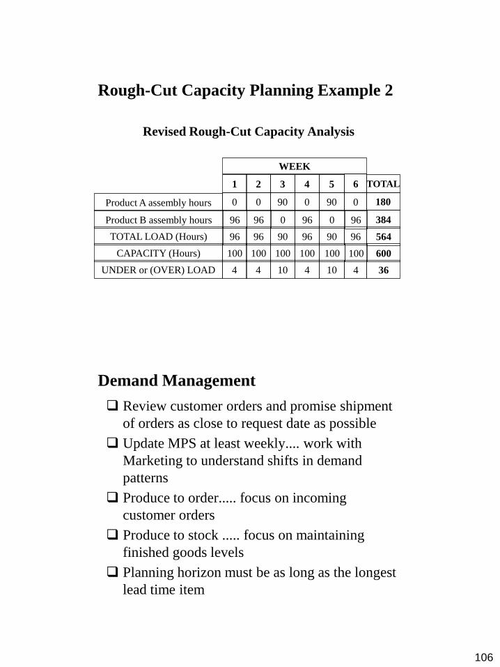
106
Rough-Cut Capacity Planning Example 2
Revised Rough-Cut Capacity Analysis
Product A assembly hours 0 0 90 90 0
1 2 3 4 5
WEEK
TOTAL
180
TOTAL LOAD (Hours) 96 96 90 90 96 564
CAPACITY (Hours) 100 100 100 100 100 600
UNDER or (OVER) LOAD 4 4 10 10 4 36
Product B assembly hours 96 96 0 0 96 384
0
6
96
100
4
96
Demand Management
Review customer orders and promise shipment
of orders as close to request date as possible
Update MPS at least weekly.... work with
Marketing to understand shifts in demand
patterns
Produce to order..... focus on incoming
customer orders
Produce to stock ..... focus on maintaining
finished goods levels
Planning horizon must be as long as the longest
lead time item

107
Unit 6
Material Requirement Planning (MRP)
6.1 Material Requirement Planning (MRP)
6.2 MRP System
6.3 MRP: Typical Procedures
6.4 Lot-Sizing in MRP
6.1 Material Requirement Planning(MRP)
Computer-based system for determining the
quantity and timing for the acquisition of
dependent demand items needed to satisfy the
MPS requirements
Explodes Master Schedule (MPS) into required
amounts of raw materials and subassemblies to
support MPS
Nets against current orders and inventories to
develop production and purchased material
ordering schedules

108
Relationship of MRP and other Plans
Firm orders
from known
customers
Forecast
of demand
from random
customers
Aggregate
Product Plan
Master
Production
Schedule
(MPS)
Material
Requirements
Planning
(MRP)
Engineering
design changes
Bill of
Materials
(BOM) file
Inventory
transactions
Inventory
records
file
Reports
7/4/2016
6.2 MRP System
Order Changes
Planning Reports
MRP
System
Inventory
Transaction Data
Bill of
Materials File
Master
Production
Schedule
Inventory
Status File
Service-Parts
Orders and
Forecasts
Performance Reports
Inputs Outputs
Planned Order
Schedule
Exception Reports

109
Inventory Status File
Includes information on the status of each
item by time period
– Gross requirements
– Scheduled receipts
– Amount on hand
– Lead times
– Lot sizes
– and more …
MRP Logic Terminology (1/6)
Gross Requirements
– These requirements are typically forecast for
independent demand items
– Assumes no on-hand inventory

110
MRP Logic Terminology (2/6)
On-hand inventory
– The inventory physically present in the
facility
Allocated inventory
– The inventory physically present in the
facility but allocated to a particular work
order or purchase order
MRP Logic Terminology (3/6)
Net requirements
– A quantity of an item that must be purchased
or manufactured in order to be able to fully
deliver independent demand requirements in a
timely fashion
– Presence of positive net requirements signals
that an order must be planned to be received in
a given period
111
MRP Logic Terminology (4/6)
Planned order receipts
– Quantities that must be planned to be
received in some future periods in order to
meet the requirements
Planned order released
– Quantities that must be planned to be
released in some future periods in order to
meet the requirements
MRP Logic Terminology (5/6)
Scheduled receipts
– Quantities that will be received in some
future periods as their corresponding orders
have been released in the past
• Planned order receipts become scheduled
receipts at the time when they are released to
the shop or to suppliers
112
MRP Logic Terminology (6/6)
Gross to Net logic:
Net Requirements = Gross Requirements
+ Allocated Inventory
+ Safety Stock
- Inventory On Hand
+ Backorders
6.3 MRP: Typical Procedures
1. Develop a Bill of Materials (BOM). The BOM
identifies
– The components
– Component descriptions
– Amount required to produce 1 unit of final product
2. Develop a Material Structure Tree
– The tree has several levels depending on the depth of
subcomponent required
– Parents and components are identified 1. Items above any level are parents
2. Items below any level are components
– The tree shows how many units are needed at each
level of production

113
3. Determine the Gross Material Requirements
– Once the materials structure tree is done, construct
a gross material requirements plan.
– This is a time schedule that shows when an item
must be ordered
1. when there is no inventory on hand, or
2. when the production of an item must be started in
order to satisfy the demand for the finished product
at a particular date.
4. Determine the Net Material Requirements Plan
– A net material requirements plan is constructed
using
the gross materials requirements plan
and the inventory on-hand information
– This plan includes, for each item:
Gross requirements,
On-hand inventory,
Net requirements,
Planned-order receipts (Scheduled receipts), and
Planned-order releases

114
Material Structure Tree Example
Assume demand for product A is 50 units. Each
unit of A requires
1. 2 units of B, which in turn requires
1. 2 units of D
2. 3 units of E
2. 3 units of C, which in turn requires
1. 1 unit of E
2. 2 units of F
Material Structure Tree: An Example
115
This structure tree has 3 levels:
• 0, 1, and 2
There are 3 parents:
• A, B, C
There are 5 components:
• B, C, D, E, F
B and C are parents and components
Numbers in parentheses next to the levels indicate
the amounts needed for 1 unit of final product of A
For example, B(2) indicates that it takes 2 units of
B to make 1 unit of A
Component Calculations to meet Demand of 50
units of Product A:
Part B: 2×# of A = 2×50 = 100
Part C: 3×# of A = 3×50 = 150
Part D: 2×# of B = 2×100 = 200
Part E: 3×# of B + 1×# of C = 3×100 + 1×150 =
450
Part F: 2×# of C = 2×150 = 300

116
A Material Requirement Plan (MRP) for
Awesome Speakers is shown as an example,
starting with the product tree. Fifty Awesome
speakers are required.
7/4/2016
Product Structure for “Awesome” A
117
Component Calculations:
Part B: 2×# of A = 2×50 = 100
Part C: 3×# of A = 3×50 = 150
Part D: 2×# of B + 2×# of F = 2×100 + 2×300 =
800
Part E: 2×# of B + 2×# of C = 2×100 + 2×150 =
500
Part F: 2×# of C = 2×150 = 300
Part G: 1×# of F = 1×300 = 300
Requirements for 50 “Awesome” A
Lead Times for “Awesome” Speaker Kits (As)
COMPONENT LEAD TIME (Weeks)
A 1
B 2
C 1
D 1
E 2
F 3
G 2
118
Using Lead Times a Time-Phased Product Structure can be
constructed. Note: this is not necessary if you know the
delivery date
1 2 3 4 5 6 7 8
3 weeks
F
2 weeks E
A
1 week 1 week
C G 2 weeks
D
1 week
E
2 weeks
Start production
of D
D 1 week
B
2 weeks to produce
Must have D and E
completed here so
production can begin on B
7/4/2016
Gross Materials Requirements Plan for 50 Speaker Kits A
WEEK LT
1 2 3 4 5 6 7 8
A Required date
Order release date
50
50 1 wk
B Required date
Order release date
100
100 2 wks
C Required date
Order release date
150
150 1 wk
D Required date
Order release date
200
200 1 wk
E Required date
Order release date
200
300
200 300 2 wks
F Required date
Order release date
300
300 3 wks
D Required date
Order release date
600
600 1 wk
G Required date
Order release date
300
300 2 wks
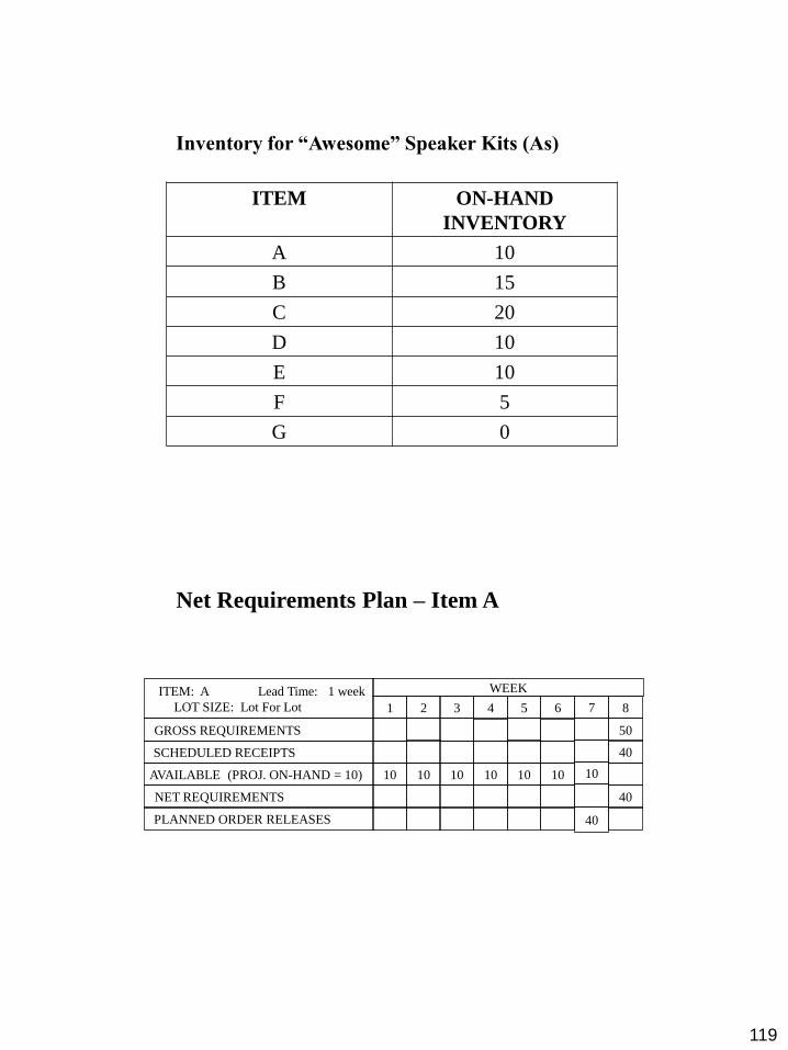
119
Inventory for “Awesome” Speaker Kits (As)
ITEM ON-HAND
INVENTORY
A 10
B 15
C 20
D 10
E 10
F 5
G 0
Net Requirements Plan – Item A
GROSS REQUIREMENTS
SCHEDULED RECEIPTS
AVAILABLE (PROJ. ON-HAND = 10)
NET REQUIREMENTS
PLANNED ORDER RELEASES
ITEM: A Lead Time: 1 week
LOT SIZE: Lot For Lot
10
1
10 10
2 3 4
10 10 10 10
6
40
5 7
WEEK
40
50
40
8
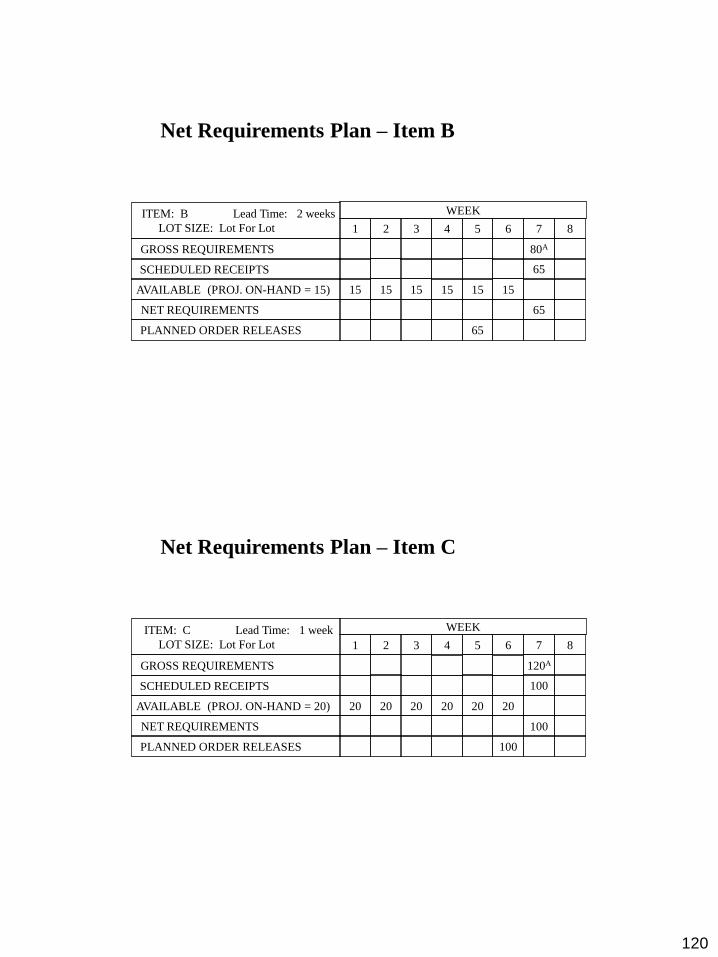
120
Net Requirements Plan – Item B
GROSS REQUIREMENTS
SCHEDULED RECEIPTS
AVAILABLE (PROJ. ON-HAND = 15)
NET REQUIREMENTS
PLANNED ORDER RELEASES
ITEM: B Lead Time: 2 weeks
LOT SIZE: Lot For Lot
15
1
15 15
2 3 4
65
15 15 15
65
6 5
80A
65
7
WEEK
8
Net Requirements Plan – Item C
GROSS REQUIREMENTS
SCHEDULED RECEIPTS
AVAILABLE (PROJ. ON-HAND = 20)
NET REQUIREMENTS
PLANNED ORDER RELEASES
ITEM: C Lead Time: 1 week
LOT SIZE: Lot For Lot
20
1
20 20
2 3 4
100
20 20 20
100
6 5
120A
100
7
WEEK
8

121
Net Requirements Plan – Item E
GROSS REQUIREMENTS
SCHEDULED RECEIPTS
AVAILABLE (PROJ. ON-HAND = 10)
NET REQUIREMENTS
PLANNED ORDER RELEASES
ITEM: E Lead Time: 2 weeks
LOT SIZE: Lot For Lot
10
1
10
120
10
2 3 4
200 120
200
120
10
130B
6 5
200C
200
7
WEEK
8
Net Requirements Plan – Item F
GROSS REQUIREMENTS
SCHEDULED RECEIPTS
AVAILABLE (PROJ. ON-HAND = 5)
NET REQUIREMENTS
PLANNED ORDER RELEASES
ITEM: F Lead Time: 3 weeks
LOT SIZE: Lot For Lot
5
1
5
195
5
2 3 4
195
5 5
6 5
200C
195
7
WEEK
8
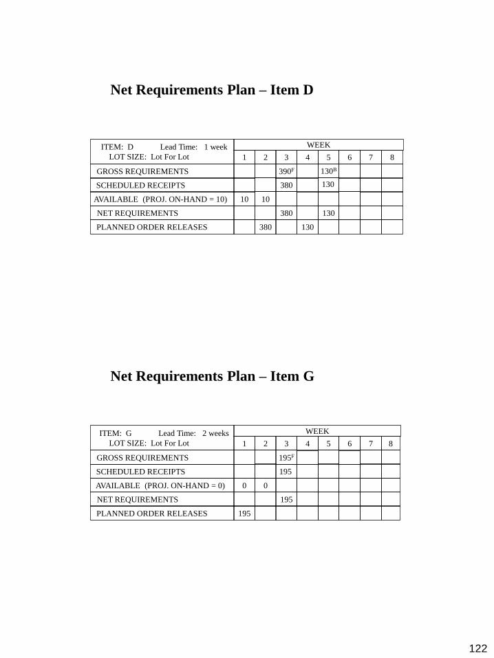
122
Net Requirements Plan – Item D
GROSS REQUIREMENTS
SCHEDULED RECEIPTS
AVAILABLE (PROJ. ON-HAND = 10)
NET REQUIREMENTS
PLANNED ORDER RELEASES
ITEM: D Lead Time: 1 week
LOT SIZE: Lot For Lot
10
1
380
10
380
390F
380
2 3 4
130
130
130B
6 5 7
WEEK
8
130
Net Requirements Plan – Item G
GROSS REQUIREMENTS
SCHEDULED RECEIPTS
AVAILABLE (PROJ. ON-HAND = 0)
NET REQUIREMENTS
PLANNED ORDER RELEASES
ITEM: G Lead Time: 2 weeks
LOT SIZE: Lot For Lot
0
195
1
0
195
195F
195
2 3 4 6 5 7
WEEK
8
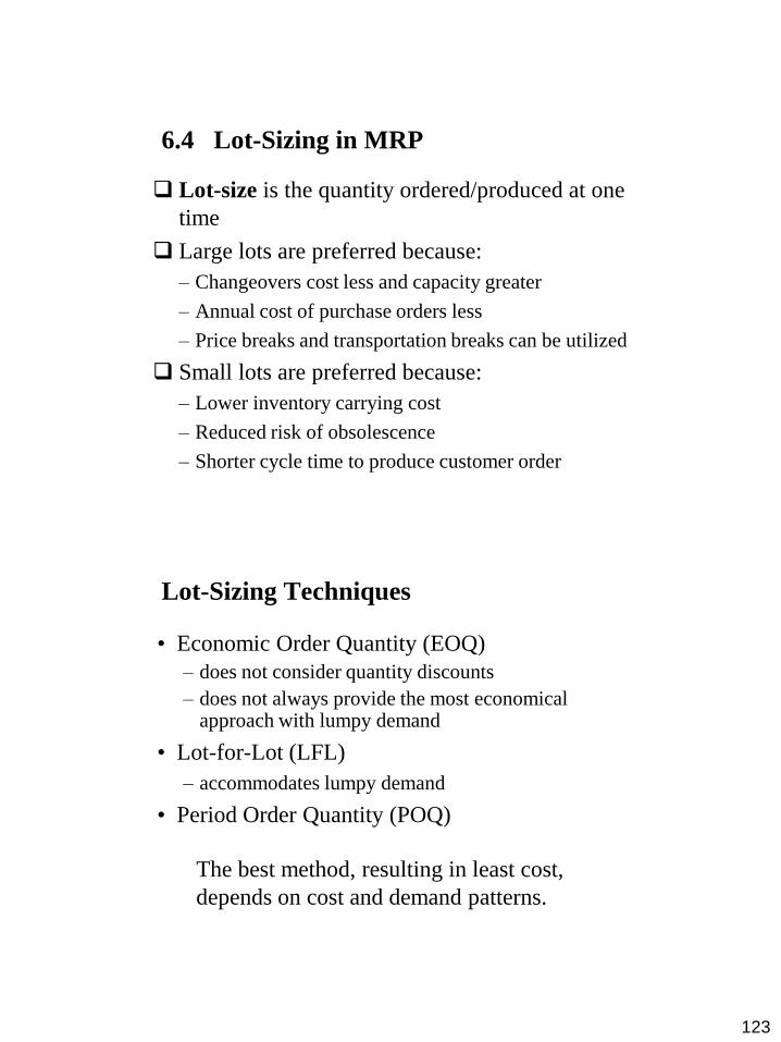
123
6.4 Lot-Sizing in MRP
Lot-size is the quantity ordered/produced at one
time
Large lots are preferred because:
– Changeovers cost less and capacity greater
– Annual cost of purchase orders less
– Price breaks and transportation breaks can be utilized
Small lots are preferred because:
– Lower inventory carrying cost
– Reduced risk of obsolescence
– Shorter cycle time to produce customer order
The best method, resulting in least cost,
depends on cost and demand patterns.
Lot-Sizing Techniques
• Economic Order Quantity (EOQ)
– does not consider quantity discounts
– does not always provide the most economical approach with lumpy demand
• Lot-for-Lot (LFL)
– accommodates lumpy demand
• Period Order Quantity (POQ)
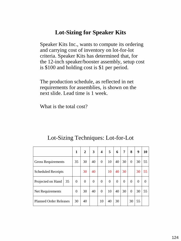
124
Lot-Sizing for Speaker Kits
Speaker Kits Inc., wants to compute its ordering and carrying cost of inventory on lot-for-lot criteria. Speaker Kits has determined that, for the 12-inch speaker/booster assembly, setup cost is $100 and holding cost is $1 per period.
The production schedule, as reflected in net requirements for assemblies, is shown on the next slide. Lead time is 1 week.
What is the total cost?
Lot-Sizing Techniques: Lot-for-Lot
1 2 3 4 5 6 7 8 9 10
Gross Requirements 35 30 40 0 10 40 30 0 30 55
Scheduled Receipts 30 40 10 40 30 30 55
Projected on Hand 35 0 0 0 0 0 0 0 0 0 0
Net Requirements 0 30 40 0 10 40 30 0 30 55
Planned Order Releases 30 40 10 40 30 30 55

125
Lot-Sizing Techniques: Economic Order
Quantity
1 2 3 4 5 6 7 8 9 10
Gross Requirements 35 30 40 0 10 40 30 0 30 55
Scheduled Receipts 73 73 73 73
Projected on Hand 35 0 43 3 3 66 26 69 69 39 57
Net Requirements 0 30 0 0 7 0 4 0 0 16
Planned Order Releases 73 73 73 73
Lot-Sizing Techniques: Part Period Balancing
1 2 3 4 5 6 7 8 9 10
Gross Requirements 35 30 40 0 10 40 30 0 30 55
Scheduled Receipts 80 100 55
Projected on Hand 35 0 50 10 10 0 60 30 30 0 0
Net Requirements 0 30 40 0 10 40 30 0 30 55
Planned Order Releases 80 100 55

126
Example: Bill of Material – Product A &
Product B
A
C (3)
D(2) Other
Subcomponents
Other
Components
B
C (2)
D(2) Other
Subcomponents
Other
Components
Demand and other information for Products A and B
Month
Product 1 2 3 4 5 6 7 8 9 10 11 12
A 0 0 80 0 0 80 0 0 80 0 0 80
B 0 50 0 50 0 50 0 50 0 50 0 50
It takes two months to produce a unit of C and one month to produce a unit
of D. At the beginning of month 1, there are 150 units of C and 600 units of
D in stock from previously planned manufacturing or purchasing orders,
while 50 units of C and 100 units of D are scheduled to be received at the
beginning of month 2.
Develop MRP using the Lot-for-Lot, Period Order Quantity (POQ) with
period (P) = 3, Economic Order Quantity (EOQ) and Part-Period Balancing
(PPB) lot sizing strategies. For the EOQ assume that the average demand for
component C is 225 units per month, the set up cost of producing C during a
month is $225 and the cost of holding one unit of C in inventory for one
month is $0.5.

127
Equations to use in developing the MRP
NRt (C)=[(GRt (C ) – SRt (C ) –OHIt-1 (C)]+
OHIt (C)=[SRt (C) + OHIt-1 (C ) –GRt (C)]+
Where:
NRt : Net Requirements in period t
GRt : Gross Requirements in period t
SRt : Scheduled Receipts in period t
OHIt : On-Hand Inventory in period t
Net Requirements Plan – Item C
1 2 3 4 5 6 7 8 9 10 11 12
GR 0 100 240 100 0 340 0 100 240 100 0 340
OHI
(150) 150 100 0 0 0 0 0 0 0 0 0 0
SR 0 50 0 0 0 0 0 0 0 0 0 0
NR 0 0 140 100 0 340 0 100 240 100 0 340
PP ? ? ? ? ? ? ? ? ? ? ? ?
Month

128
Lot-for-Lot with 2 Months Lead Time-Item C
1 2 3 4 5 6 7 8 9 10 11 12
GR 0 100 240 100 0 340 0 100 240 100 0 340
OHI
(150) 150 100 0 0 0 0 0 0 0 0 0 0
SR 0 50 140 100 0 340 0 100 240 100 0 340
NR 0 0 140 100 0 340 0 100 240 100 0 340
PP 140 100 0 340 0 100 240 100 0 340 X X
Month
Lot-for-Lot with 1 Months Lead Time-Item D
1 2 3 4 5 6 7 8 9 10 11 12
GR 280 200 0 680 0 200 480 200 0 680 X X
OHI
(600) 320 220 220 0 0 0 0 0 0 0 0 0
SR 0 100 0 460 0 200 480 200 0 680 X X
NR 0 0 0 460 0 200 480 200 0 680 X X
PP 0 0 460 0 200 480 200 0 680 X X X
Month

129
MRP Record – Item C (POQ; P = 3)
1 2 3 4 5 6 7 8 9 10 11 12
GR 0 100 240 100 0 340 0 100 240 100 0 340
OHI
(150) 150 100 440 340 340 0 0 340 100 0 0 0
SR 0 50 580 0 0 0 0 440 0 0 0 340
NR 0 0 140 100 0 340 0 100 240 100 0 340
PP 580 0 0 0 0 440 0 0 0 340 X X
Month
MRP Record – Item C (EOQ)
1 2 3 4 5 6 7 8 9 10 11 12
GR 0 100 240 100 0 340 0 100 240 100 0 340
OHI
(150) 150 100 310 210 210 320 320 220 430 330 330 440
SR 0 50 450 0 0 450 0 0 450 0 0 450
NR 0 0 140 100 0 340 0 100 240 100 0 340
PP 450 0 0 450 0 0 450 0 0 450 X X
Month
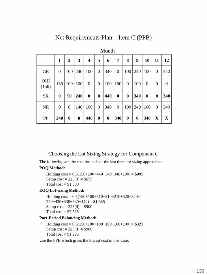
130
Net Requirements Plan – Item C (PPB)
1 2 3 4 5 6 7 8 9 10 11 12
GR 0 100 240 100 0 340 0 100 240 100 0 340
OHI
(150) 150 100 100 0 0 100 100 0 100 0 0 0
SR 0 50 240 0 0 440 0 0 340 0 0 340
NR 0 0 140 100 0 340 0 100 240 100 0 340
PP 240 0 0 440 0 0 340 0 0 340 X X
Month
Choosing the Lot Sizing Strategy for Component C
The following are the cost for each of the last three lot sizing approaches:
POQ Method:
Holding cost = 0.5(150+100+440+340+340+100) = $905
Setup cost = 225(3) = $675
Total cost = $1,580
EOQ Lot-sizing Method:
Holding cost = 0.5(150+100+310+210+210+320+320+
220+430+330+330+440) = $1,685
Setup cost = 225(4) = $900
Total cost = $2,585
Part-Period Balancing Method:
Holding cost = 0.5(150+100+100+100+100+100) = $325
Setup cost = 225(4) = $900
Total cost = $1,225
Use the PPB which gives the lowest cost in this case.
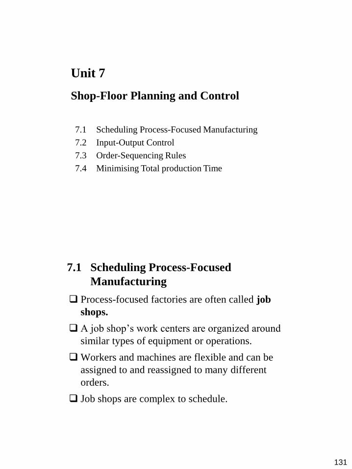
131
Unit 7
Shop-Floor Planning and Control
7.1 Scheduling Process-Focused Manufacturing
7.2 Input-Output Control
7.3 Order-Sequencing Rules
7.4 Minimising Total production Time
7.1 Scheduling Process-Focused
Manufacturing
Process-focused factories are often called job
shops.
A job shop’s work centers are organized around
similar types of equipment or operations.
Workers and machines are flexible and can be
assigned to and reassigned to many different
orders.
Job shops are complex to schedule.
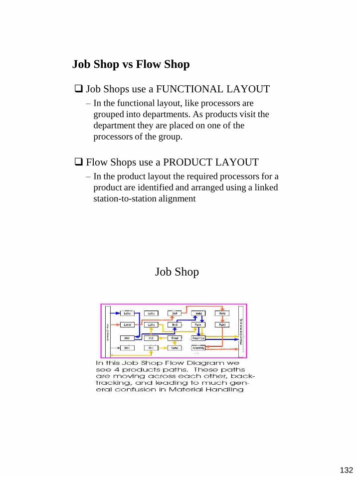
132
Job Shops use a FUNCTIONAL LAYOUT
– In the functional layout, like processors are
grouped into departments. As products visit the
department they are placed on one of the
processors of the group.
Flow Shops use a PRODUCT LAYOUT
– In the product layout the required processors for a
product are identified and arranged using a linked
station-to-station alignment
Job Shop vs Flow Shop
Job Shop
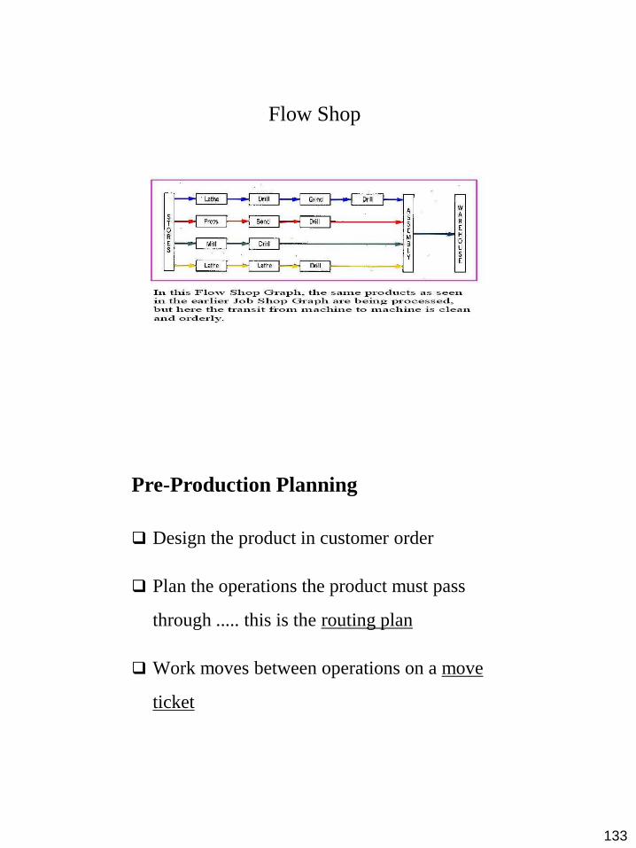
133
Flow Shop
Design the product in customer order
Plan the operations the product must pass
through ..... this is the routing plan
Work moves between operations on a move
ticket
Pre-Production Planning
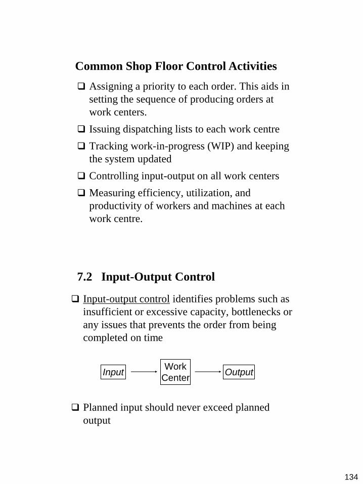
134
Assigning a priority to each order. This aids in
setting the sequence of producing orders at
work centers.
Issuing dispatching lists to each work centre
Tracking work-in-progress (WIP) and keeping
the system updated
Controlling input-output on all work centers
Measuring efficiency, utilization, and
productivity of workers and machines at each
work centre.
Common Shop Floor Control Activities
7.2 Input-Output Control
Input-output control identifies problems such as
insufficient or excessive capacity, bottlenecks or
any issues that prevents the order from being
completed on time
Planned input should never exceed planned
output
Input Output Work
Center
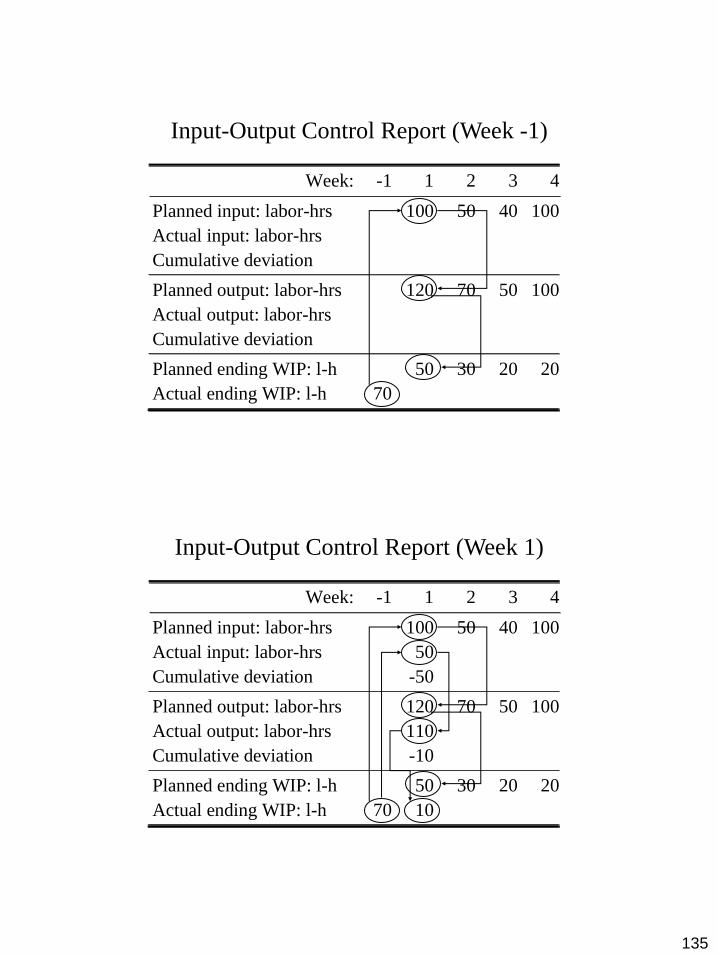
135
Input-Output Control Report (Week -1)
Week: -1 1 2 3 4
Planned input: labor-hrs 100 50 40 100
Actual input: labor-hrs
Cumulative deviation
Planned output: labor-hrs 120 70 50 100
Actual output: labor-hrs
Cumulative deviation
Planned ending WIP: l-h 50 30 20 20
Actual ending WIP: l-h 70
Input-Output Control Report (Week 1)
Week: -1 1 2 3 4
Planned input: labor-hrs 100 50 40 100
Actual input: labor-hrs 50
Cumulative deviation -50
Planned output: labor-hrs 120 70 50 100
Actual output: labor-hrs 110
Cumulative deviation -10
Planned ending WIP: l-h 50 30 20 20
Actual ending WIP: l-h 70 10
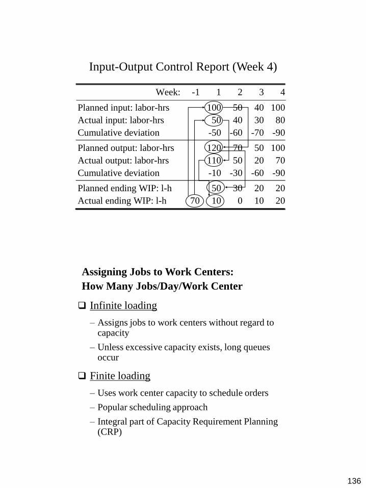
136
Input-Output Control Report (Week 4)
Week: -1 1 2 3 4
Planned input: labor-hrs 100 50 40 100
Actual input: labor-hrs 50 40 30 80
Cumulative deviation -50 -60 -70 -90
Planned output: labor-hrs 120 70 50 100
Actual output: labor-hrs 110 50 20 70
Cumulative deviation -10 -30 -60 -90
Planned ending WIP: l-h 50 30 20 20
Actual ending WIP: l-h 70 10 0 10 20
Infinite loading
– Assigns jobs to work centers without regard to capacity
– Unless excessive capacity exists, long queues occur
Finite loading
– Uses work center capacity to schedule orders
– Popular scheduling approach
– Integral part of Capacity Requirement Planning (CRP)
Assigning Jobs to Work Centers:
How Many Jobs/Day/Work Center

137
Forward scheduling
– Jobs are given earliest available time slot in
operation
– excessive WIP usually results
Backward scheduling
– Start with promise date and work backward through
operations reviewing lead times to determine when a
job has to pass through each operation
– Less WIP but must have accurate lead times
Assigning Jobs to Work Centers:
Which Job Gets Built First?
Today Due Date
B E
Forward Scheduling
Today Due Date
B E
Backward Scheduling
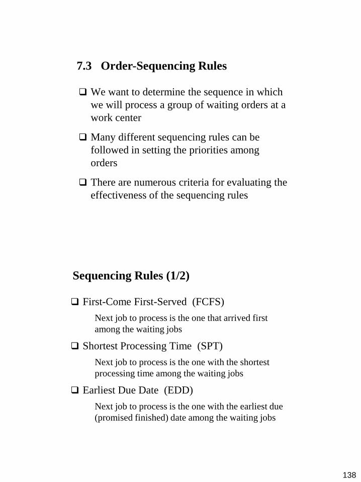
138
We want to determine the sequence in which
we will process a group of waiting orders at a
work center
Many different sequencing rules can be
followed in setting the priorities among
orders
There are numerous criteria for evaluating the
effectiveness of the sequencing rules
7.3 Order-Sequencing Rules
First-Come First-Served (FCFS)
Next job to process is the one that arrived first
among the waiting jobs
Shortest Processing Time (SPT)
Next job to process is the one with the shortest
processing time among the waiting jobs
Earliest Due Date (EDD)
Next job to process is the one with the earliest due
(promised finished) date among the waiting jobs
Sequencing Rules (1/2)
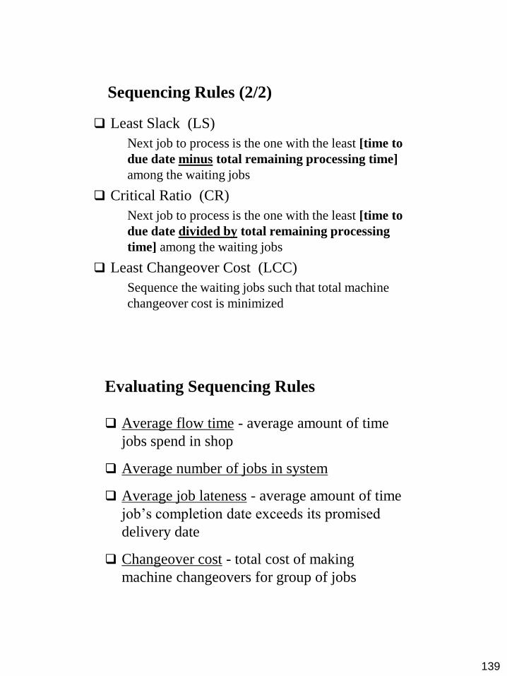
139
Least Slack (LS)
Next job to process is the one with the least [time to
due date minus total remaining processing time]
among the waiting jobs
Critical Ratio (CR)
Next job to process is the one with the least [time to
due date divided by total remaining processing
time] among the waiting jobs
Least Changeover Cost (LCC)
Sequence the waiting jobs such that total machine
changeover cost is minimized
Sequencing Rules (2/2)
Average flow time - average amount of time
jobs spend in shop
Average number of jobs in system
Average job lateness - average amount of time
job’s completion date exceeds its promised
delivery date
Changeover cost - total cost of making
machine changeovers for group of jobs
Evaluating Sequencing Rules

140
Example: Evaluating Sequencing Rules
Use the FCFS, SPT, and Critical Ratio rules to sequence
the five jobs below. Evaluate the rules on the bases of
average flow time, average number of jobs in the system,
and average job lateness.
Job Processing Time Time to Promised Completion
A 6 hours 10 hours
B 12 16
C 9 8
D 14 14
E 8 7
FCFS Rule Sequence: A > B > C > D > E
Processing Promised Flow Job Time Completion Time Lateness
A 6 10 6 0
B 12 16 18 2
C 9 8 27 19
D 14 14 41 27
E 8 7 49 42
49 141 90

141
FCFS Rule Performance:
– Average flow time:
141/5 = 28.2 hours
– Average number of jobs in the system:
141/49 = 2.88 jobs
– Average job lateness:
90/5 = 18.0 hours
SPT Rule Sequence: A > E > C > B > D
Processing Promised Flow
Job Time Completion Time Lateness
A 6 10 6 0
E 8 7 14 7
C 9 8 23 15
B 12 16 35 19
D 14 14 49 35
49 127 76

142
SPT Rule Performance:
– Average flow time:
127/5 = 25.4 hours
– Average number of jobs in the system:
127/49 = 2.59 jobs
– Average job lateness:
76/5 = 15.2 hours
Critical Ratio Rule Sequence: E > C > D > B > A
Processing Promised Flow
Job Time Completion Time Lateness
E (.875) 8 7 8 1
C (.889) 9 8 17 9
D (1.00) 14 14 31 17
B (1.33) 12 16 43 27
A (1.67) 6 10 49 39
49 148 93
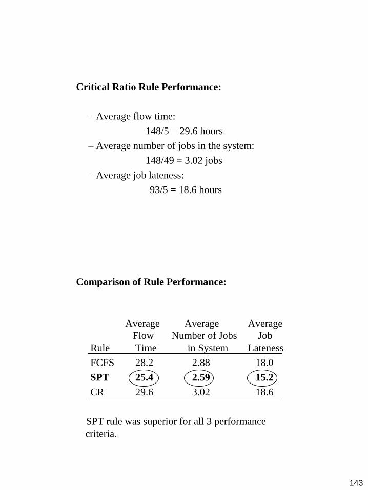
143
Critical Ratio Rule Performance:
– Average flow time:
148/5 = 29.6 hours
– Average number of jobs in the system:
148/49 = 3.02 jobs
– Average job lateness:
93/5 = 18.6 hours
Comparison of Rule Performance:
Average Average Average
Flow Number of Jobs Job
Rule Time in System Lateness
FCFS 28.2 2.88 18.0
SPT 25.4 2.59 15.2
CR 29.6 3.02 18.6
SPT rule was superior for all 3 performance
criteria.
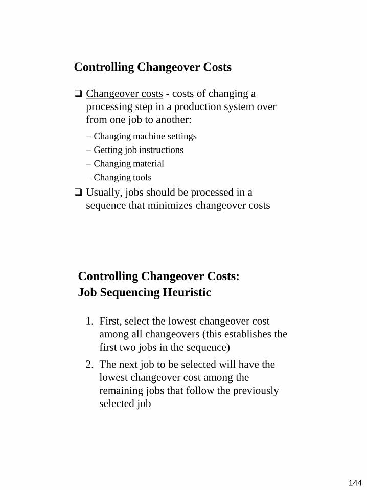
144
Changeover costs - costs of changing a
processing step in a production system over
from one job to another:
– Changing machine settings
– Getting job instructions
– Changing material
– Changing tools
Usually, jobs should be processed in a
sequence that minimizes changeover costs
Controlling Changeover Costs
1. First, select the lowest changeover cost
among all changeovers (this establishes the
first two jobs in the sequence)
2. The next job to be selected will have the
lowest changeover cost among the
remaining jobs that follow the previously
selected job
Controlling Changeover Costs:
Job Sequencing Heuristic
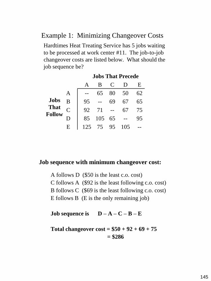
145
Example 1: Minimizing Changeover Costs
Hardtimes Heat Treating Service has 5 jobs waiting
to be processed at work center #11. The job-to-job
changeover costs are listed below. What should the
job sequence be?
Jobs That Precede
A B C D E
A -- 65 80 50 62
B 95 -- 69 67 65
C 92 71 -- 67 75
D 85 105 65 -- 95
E 125 75 95 105 --
Jobs
That
Follow
A follows D ($50 is the least c.o. cost)
C follows A ($92 is the least following c.o. cost)
B follows C ($69 is the least following c.o. cost)
E follows B (E is the only remaining job)
Job sequence is D – A – C – B – E
Total changeover cost = $50 + 92 + 69 + 75
= $286
Job sequence with minimum changeover cost:

146
Example 2: Minimizing Changeover Costs
A printing company does custom printing jobs for
local firms and schools. The operations manager is
currently developing a weekly printing schedule
for the printing press. He has developed
changeover costs for six waiting jobs. All jobs
carry equal priority, so the deciding factor in
selecting a job sequence is the total changeover
cost for the six jobs.
What is the preferred job sequence?
Jobs with Changeover Costs
Jobs That Precede
A B C D E F
A -- 12 15 10 35 20
B 25 -- 20 20 25 20
C 27 15 -- 12 20 15
D 16 30 10 -- 25 30
E 35 20 25 30 -- 30
F 20 25 15 25 30 --
Jobs
That
Follow
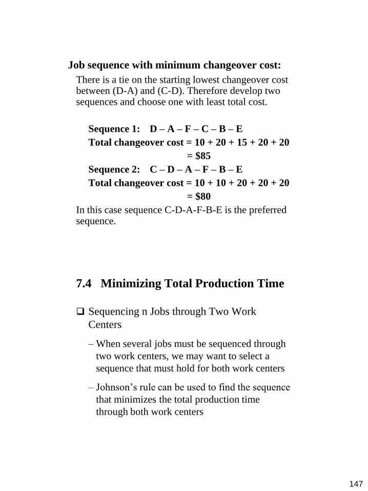
147
There is a tie on the starting lowest changeover cost between (D-A) and (C-D). Therefore develop two sequences and choose one with least total cost.
Sequence 1: D – A – F – C – B – E
Total changeover cost = 10 + 20 + 15 + 20 + 20
= $85
Sequence 2: C – D – A – F – B – E
Total changeover cost = 10 + 10 + 20 + 20 + 20
= $80
In this case sequence C-D-A-F-B-E is the preferred sequence.
Job sequence with minimum changeover cost:
7.4 Minimizing Total Production Time
Sequencing n Jobs through Two Work
Centers
– When several jobs must be sequenced through
two work centers, we may want to select a
sequence that must hold for both work centers
– Johnson’s rule can be used to find the sequence
that minimizes the total production time
through both work centers
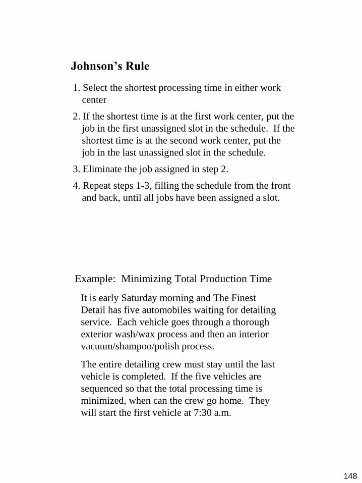
148
Johnson’s Rule
1. Select the shortest processing time in either work
center
2. If the shortest time is at the first work center, put the
job in the first unassigned slot in the schedule. If the
shortest time is at the second work center, put the
job in the last unassigned slot in the schedule.
3. Eliminate the job assigned in step 2.
4. Repeat steps 1-3, filling the schedule from the front
and back, until all jobs have been assigned a slot.
Example: Minimizing Total Production Time
It is early Saturday morning and The Finest
Detail has five automobiles waiting for detailing
service. Each vehicle goes through a thorough
exterior wash/wax process and then an interior
vacuum/shampoo/polish process.
The entire detailing crew must stay until the last
vehicle is completed. If the five vehicles are
sequenced so that the total processing time is
minimized, when can the crew go home. They
will start the first vehicle at 7:30 a.m.
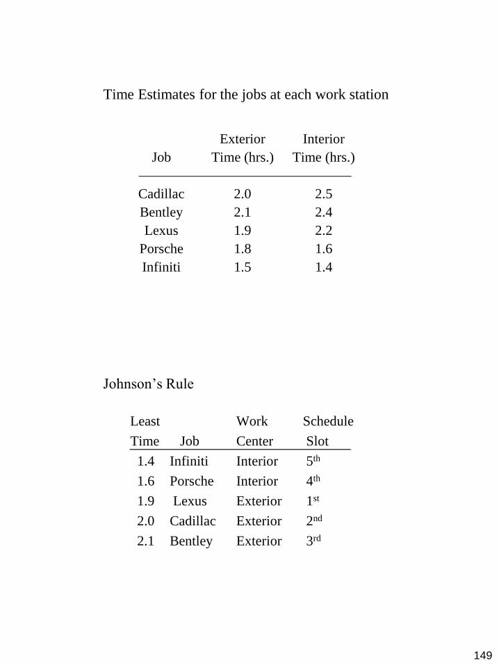
149
Time Estimates for the jobs at each work station
Exterior Interior
Job Time (hrs.) Time (hrs.)
Cadillac 2.0 2.5
Bentley 2.1 2.4
Lexus 1.9 2.2
Porsche 1.8 1.6
Infiniti 1.5 1.4
Johnson’s Rule
Least Work Schedule
Time Job Center Slot
1.4 Infiniti Interior 5th
1.6 Porsche Interior 4th
1.9 Lexus Exterior 1st
2.0 Cadillac Exterior 2nd
2.1 Bentley Exterior 3rd
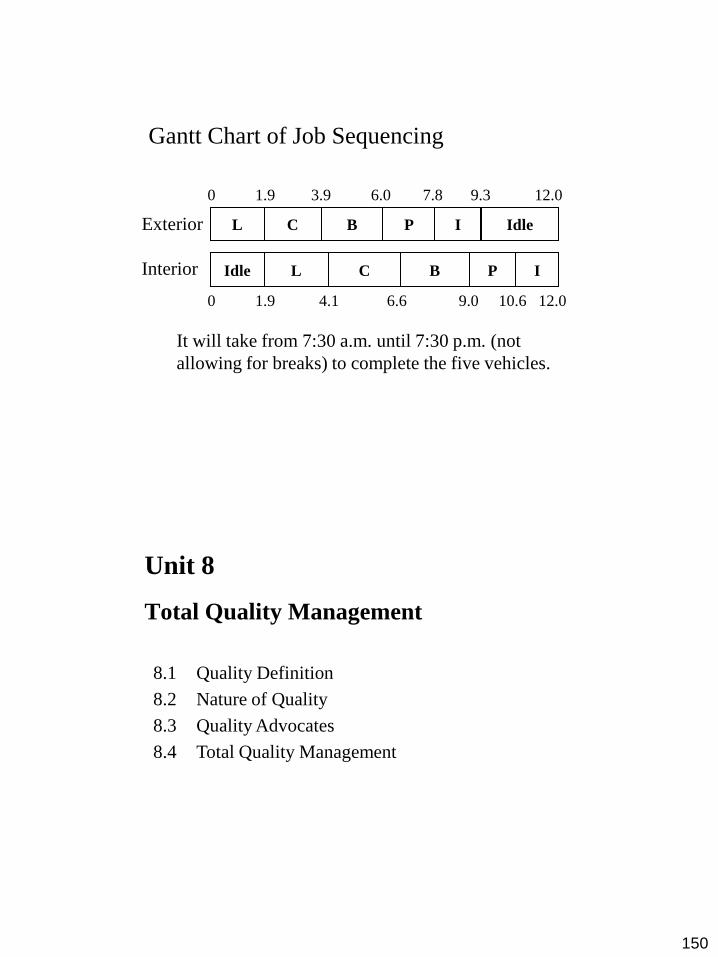
150
Gantt Chart of Job Sequencing
Exterior
Interior
0 1.9 3.9 6.0 7.8 9.3 12.0
0 1.9 4.1 6.6 9.0 10.6 12.0
L C B
L
P I
Idle C B P I
Idle
It will take from 7:30 a.m. until 7:30 p.m. (not
allowing for breaks) to complete the five vehicles.
Unit 8
Total Quality Management
8.1 Quality Definition
8.2 Nature of Quality
8.3 Quality Advocates
8.4 Total Quality Management

151
8.1 Quality Definition
“The quality of a product or service is a
customer’s perception of the degree to which the
product or service meets his or her expectations.”
Design quality
– How does the product or service appear in pre-
production or pre-delivery phases (i.e. on a
CAD terminal, on a blueprint, etc.)
Conformance quality
– Degree to which the design specifications are met by the production or delivery system
Quality Definitions (1/2)
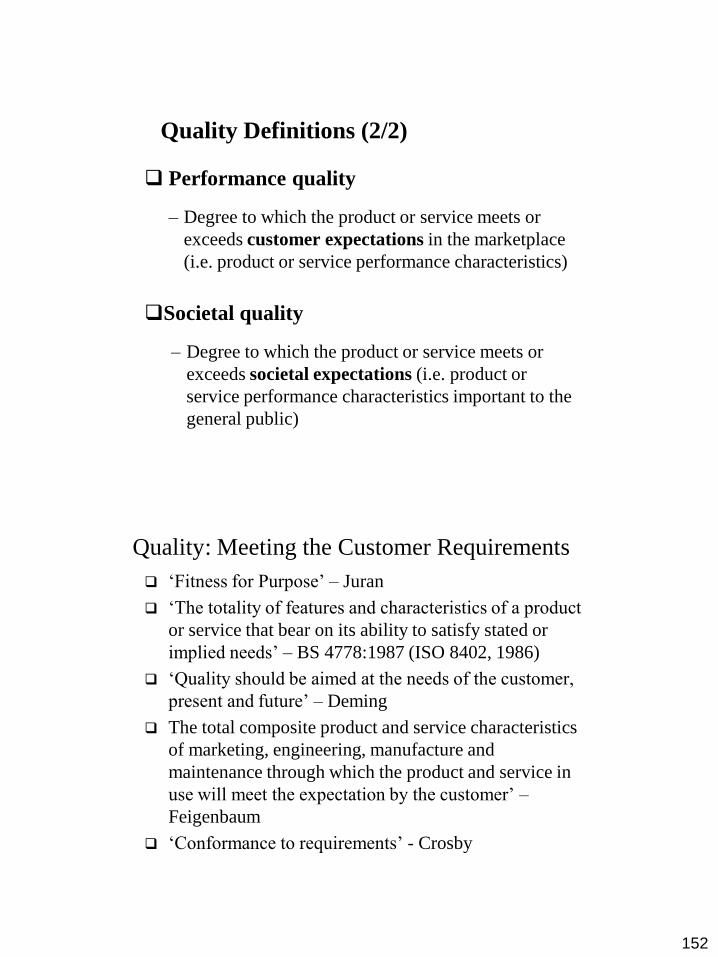
152
Performance quality
– Degree to which the product or service meets or
exceeds customer expectations in the marketplace
(i.e. product or service performance characteristics)
Societal quality
– Degree to which the product or service meets or
exceeds societal expectations (i.e. product or
service performance characteristics important to the
general public)
Quality Definitions (2/2)
‘Fitness for Purpose’ – Juran
‘The totality of features and characteristics of a product
or service that bear on its ability to satisfy stated or
implied needs’ – BS 4778:1987 (ISO 8402, 1986)
‘Quality should be aimed at the needs of the customer,
present and future’ – Deming
The total composite product and service characteristics
of marketing, engineering, manufacture and
maintenance through which the product and service in
use will meet the expectation by the customer’ –
Feigenbaum
‘Conformance to requirements’ - Crosby
Quality: Meeting the Customer Requirements
153
“Meeting or exceeding customer
expectations”
Customers can be...
External customers
Internal customers
Customer-Driven Quality
Dimensions of Quality
Determinants of Quality
Costs of Quality
8.2 Nature of Quality
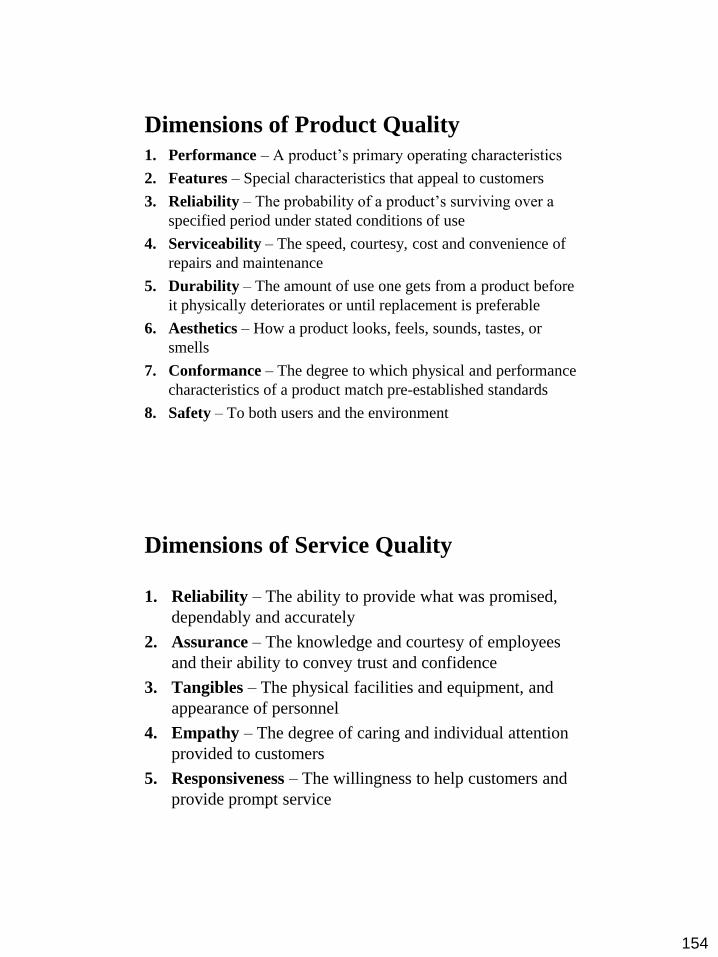
154
1. Performance – A product’s primary operating characteristics
2. Features – Special characteristics that appeal to customers
3. Reliability – The probability of a product’s surviving over a
specified period under stated conditions of use
4. Serviceability – The speed, courtesy, cost and convenience of
repairs and maintenance
5. Durability – The amount of use one gets from a product before
it physically deteriorates or until replacement is preferable
6. Aesthetics – How a product looks, feels, sounds, tastes, or
smells
7. Conformance – The degree to which physical and performance
characteristics of a product match pre-established standards
8. Safety – To both users and the environment
Dimensions of Product Quality
1. Reliability – The ability to provide what was promised,
dependably and accurately
2. Assurance – The knowledge and courtesy of employees
and their ability to convey trust and confidence
3. Tangibles – The physical facilities and equipment, and
appearance of personnel
4. Empathy – The degree of caring and individual attention
provided to customers
5. Responsiveness – The willingness to help customers and
provide prompt service
Dimensions of Service Quality
155
Quality of design – products/service designed based on customers’ expectations and desires
Quality capability of production processes – processes must be capable of producing the products designed for the customers
Quality of conformance – capable processes can produce inferior product if not operated properly
Quality of customer service – a superior product does not mean success; must have quality service also
Organization quality culture – superior product and service requires organization-wide focus on quality
Determinants of Quality
Cost of Quality (COQ) provides a basis for
identifying improvement opportunities and
success of quality improvement programs
A quality cost is considered to be any cost
that the company or organization would not
have incurred if the quality of the product or
service were perfect
Cost of Quality (COQ) is the cost of avoiding
poor quality, or incurred as a result of poor
quality
Costs of Quality
156
Cost of Quality Categories
Prevention Costs: investments made to keep
nonconforming products from occurring and reaching
the customer
Appraisal Costs: associated with efforts to ensure
conformance to requirements, generally through
measurement and analysis of data to detect non-
conformances
Internal Failure Costs: incurred as a result of
unsatisfactory quality found before product delivery to
the customer
External Failure Costs: occur after poor-quality
products reach the customer
Prevention costs: training, redesigns, inspection
procedures, supplier quality surveys, etc.
Appraisal costs: tests and inspections, process
measurement and control, etc.
Internal failure costs: scrap and rework, costs of
correcting errors before they reach the
customer, and downgrading costs.
External failure costs: warranty repairs,
replacements, complaints, legal expenses, lost
business and goodwill.
Costs of Quality Examples
157
Contrasting Traditional and Modern
Approaches to Quality
Passive (Inspect)
Find it and fix it
Emphasize on Acceptable Quality Level
It is a job of Quality Control department
Quantity is top priority
Quality is expensive
Active (Prevent)
Build Quality into the product
Focus on Process Control and Continuous Improvement
It is a company-wide concern
Quality is top priority
Higher Quality means lower cost
Traditional Modern
Edwards W. Deming
Joseph M. Juran
Philip B. Crosby
Armand V. Feigenbaum
Kaoru Ishikawa
8.3 Quality Advocates
158
Edwards W. Deming
Assisted Japan in improving productivity and
quality after World War II
In 1951 Japan established Deming Prize
US was slow in recognizing his contributions
Introduced Japanese companies to the Plan-
Do-Check-Act (PDCA) cycle
Developed 14 Points for managers
PDCA Cycle
2. DO
Try plan on a test basis
1. PLAN
Identify Improvement And develop
plan
3. CHECK
Evaluate plan to see if it works
4. ACT
Permanently implement
improvements
159
Deming’s 14 Points for Managers
1. Create constancy of purpose toward product quality to achieve organizational goals
2. Refuse to allow commonly accepted levels of poor quality
3. Stop depending on inspection to achieve quality
4. Use fewer suppliers, selected based on quality and dependability instead of price
5. Instill programs for continuous improvement of costs, quality, service, and productivity
Deming’s 14 Points for Managers (contd)
6. Train all employees on quality concepts
7. Focus supervision on helping people do a better
job
8. Eliminate fear, create trust, and encourage two-
way communications between workers and
management
9. Eliminate barriers between departments and
encourage joint problem-solving
10. Eliminate the use of numerical goals and slogans
to make workers work harder

160
Deming’s 14 Points for Managers (contd)
11. Use statistical methods for continuous
improvement of quality and productivity
instead of numerical quotas
12. Remove barriers to pride of workmanship
13. Encourage education and self-improvement
14. Clearly define management’s permanent
commitment to quality and productivity
Joseph M. Juran
Like Deming, discovered late by US
companies
Played early role in teaching Japan about
quality
Wrote Quality Control Handbook

161
Philip B. Crosby
Wrote Quality Is Free in 1979
Company should have the goal of zero defects
Cost of poor quality is greatly underestimated.
It should include all the costs of not doing the
job right the first time!
Traditional trade-off between costs of
improving quality and costs of poor quality is
erroneous
Armand V. Feigenbaum
Developed concept of total quality control
(TQC) (book published in 1983)
Responsibility for quality must rest with the
persons who do the work (quality at the
source)
Product quality is more important than
production rates (workers are given authority
to stop production whenever quality problems
occur)
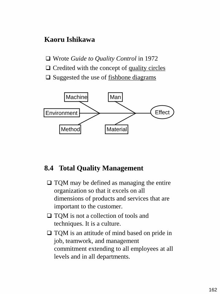
162
Kaoru Ishikawa
Wrote Guide to Quality Control in 1972
Credited with the concept of quality circles
Suggested the use of fishbone diagrams
Effect
Man Machine
Material Method
Environment
TQM may be defined as managing the entire
organization so that it excels on all
dimensions of products and services that are
important to the customer.
TQM is not a collection of tools and
techniques. It is a culture.
TQM is an attitude of mind based on pride in
job, teamwork, and management
commitment extending to all employees at all
levels and in all departments.
8.4 Total Quality Management
163
Elements of TQM
Top management commitment and
involvement
Customer involvement
Design products for quality
Design production processes for quality
Control production processes for quality
Develop supplier partnerships
Customer service, distribution and installation
Building teams of empowered employees
Benchmarking and continuous improvement
Top Management
Commitment and Involvement
Support must be genuine or TQM will be seen
as just another passing fad
Fundamental changes must occur in the
culture of the organization
Such fundamental changes are not easy, but
are impossible without top management’s
commitment and involvement

164
Customer Involvement
Mechanisms to involve the customer
– Focus groups
– Market surveys
– Customer questionnaires
– Market research programs
Quality Function Deployment (QFD)
– Formal system for identifying customer wants
– Eliminate wasteful product features and activities
that do not contribute
Building Teams of Empowered
Employees
Employee training programs
– Employees at all levels are trained in quality
Works teams and empowerment
– Workers are given the authority to act
Quality at the source
– Workers are responsible for their own work
Quality circles
– Small groups of employees who analyze and solve
quality problems and implement improvement
programs

165
Quality Circles
Group of 6-12 employees from same work
area
Meet regularly to solve work-related
problems
4 hours/month
Facilitator trains and helps with meetings
Benchmarking and Continuous
Improvement
Benchmarking
– The practice of establishing internal standards of
performance by looking to how world-class
companies run their businesses
Continuous Improvement
– The company makes small incremental
improvements toward excellence on a continual
basis
166
Obstacles to Implementing TQM
Lack of management commitment
Inability to change organisational culture
Improper planning
Lack of continuous training and education
Incompatible organisational structure and isolated
individuals and departments
Paying inadequate attention to internal and
external customers
Inadequate use of empowerment and teamwork
Failure to continually improve
Unit 9
Capacity Requirement Planning
9.1 Definitions of Capacity
9.2 Measurements of Capacity
9.3 Capacity Planning Process
9.4 Decision Tree Analysis
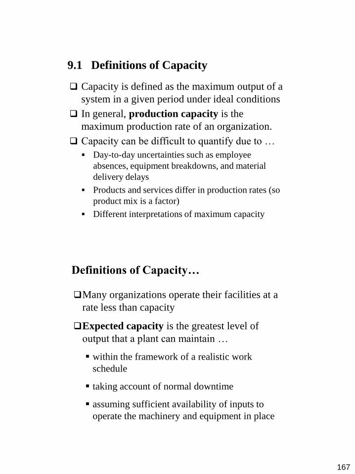
167
9.1 Definitions of Capacity
Capacity is defined as the maximum output of a
system in a given period under ideal conditions
In general, production capacity is the
maximum production rate of an organization.
Capacity can be difficult to quantify due to …
Day-to-day uncertainties such as employee
absences, equipment breakdowns, and material
delivery delays
Products and services differ in production rates (so
product mix is a factor)
Different interpretations of maximum capacity
Many organizations operate their facilities at a
rate less than capacity
Expected capacity is the greatest level of
output that a plant can maintain …
within the framework of a realistic work
schedule
taking account of normal downtime
assuming sufficient availability of inputs to
operate the machinery and equipment in place
Definitions of Capacity…
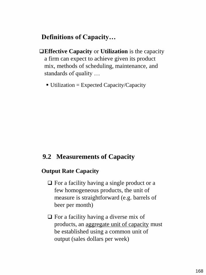
168
Effective Capacity or Utilization is the capacity
a firm can expect to achieve given its product
mix, methods of scheduling, maintenance, and
standards of quality …
Utilization = Expected Capacity/Capacity
Definitions of Capacity…
Output Rate Capacity
For a facility having a single product or a
few homogeneous products, the unit of
measure is straightforward (e.g. barrels of
beer per month)
For a facility having a diverse mix of
products, an aggregate unit of capacity must
be established using a common unit of
output (sales dollars per week)
9.2 Measurements of Capacity

169
Input Rate Capacity
Commonly used for service operations
where output measures are particularly
difficult
Hospitals use available beds per month
Airlines use available seat-miles per month
Movie theatres use available seats per month
Measurements of Capacity…
Capacity Utilization Percentage (Efficiency)
Relates actual output to output capacity
Example: Actual automobiles produced in a
quarter divided by the quarterly automobile
production capacity
Relates actual input used to input capacity
Example: Actual accountant hours used in a
month divided by the monthly account-hours
available
Measurements of Capacity…
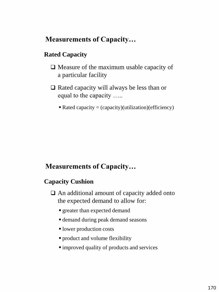
170
Rated Capacity
Measure of the maximum usable capacity of
a particular facility
Rated capacity will always be less than or
equal to the capacity …..
Rated capacity = (capacity)(utilization)(efficiency)
Measurements of Capacity…
Capacity Cushion
An additional amount of capacity added onto
the expected demand to allow for:
greater than expected demand
demand during peak demand seasons
lower production costs
product and volume flexibility
improved quality of products and services
Measurements of Capacity…
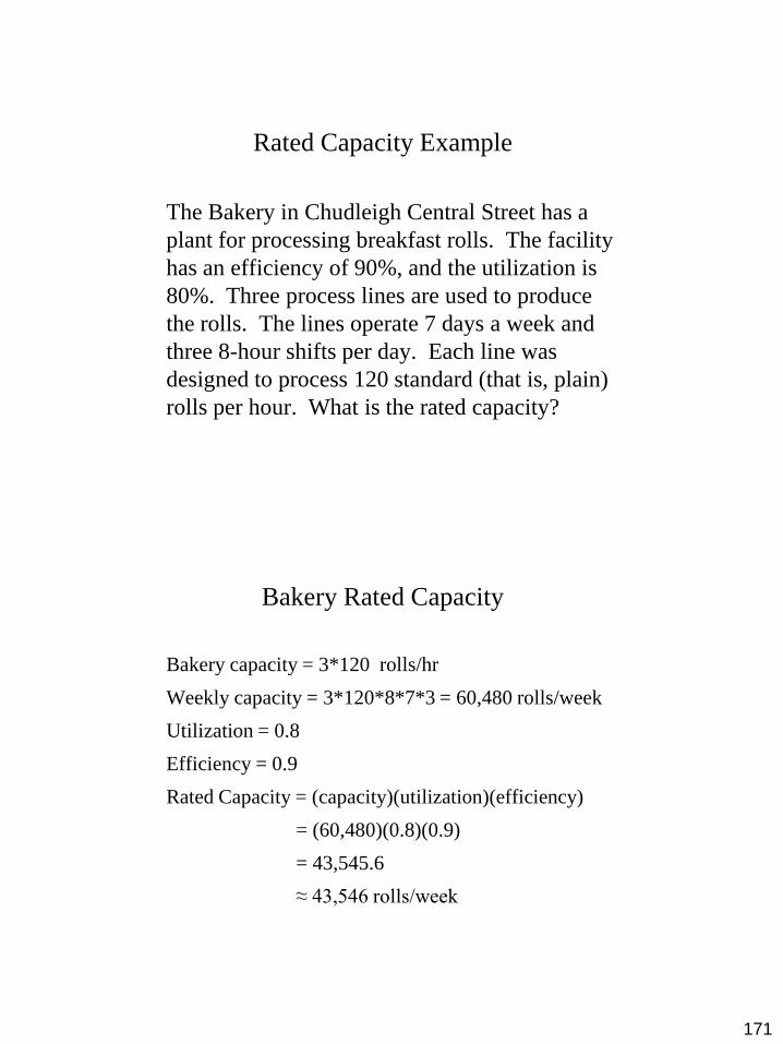
171
Rated Capacity Example
The Bakery in Chudleigh Central Street has a
plant for processing breakfast rolls. The facility
has an efficiency of 90%, and the utilization is
80%. Three process lines are used to produce
the rolls. The lines operate 7 days a week and
three 8-hour shifts per day. Each line was
designed to process 120 standard (that is, plain)
rolls per hour. What is the rated capacity?
Bakery Rated Capacity
Bakery capacity = 3*120 rolls/hr
Weekly capacity = 3*120*8*7*3 = 60,480 rolls/week
Utilization = 0.8
Efficiency = 0.9
Rated Capacity = (capacity)(utilization)(efficiency)
= (60,480)(0.8)(0.9)
= 43,545.6
≈ 43,546 rolls/week

172
Estimate the capacity of the present
facilities
Forecast the long-range future capacity
needs
Identify and analyze sources of capacity to
meet these needs
Select from among the alternative sources
of capacity
9.3 Capacity Planning Process
Consider the life of the input (e.g. facility is 10-
30 yr)
Understand product life cycle as it impacts
capacity
Anticipate technological developments
Anticipate competitors’ actions
Forecast the firm’s demand
Resource availability
Accuracy of the long-range forecast
Capacity cushion
Changes in competitive environment
Forecasting Capacity Requirements

173
Subcontract with other companies
Acquire other companies, facilities, or
resources
Develop sites, construct buildings, buy
equipment
Expand, update, or modify existing facilities
Reactivate standby facilities
Expansion of Long-Term Capacity
Sell off existing resources, lay off
employees
Mothball facilities, transfer employees
Develop and phase in new
products/services
Reduction of Long-Term Capacity

174
All at Once – build the ultimate facility now
and grow into it
Incrementally – build incrementally as
capacity demand grows
Approaches to Expanding Long-Term
Capacity
Little risk of having to turn down business due
to inadequate capacity
Less interruption of production
One large construction project costs less than
several smaller projects
Due to inflation, construction costs will be
higher in the future
Most appropriate for mature products with
stable demand
Expanding Long-Term Capacity
All at Once

175
Less risky if forecast needs do not
materialize
Funds that could be used for other types of
investments will not be tied up in excess
capacity
More appropriate for new products
Expanding Long-Term Capacity
Incrementally
Structures complex multiphase decisions,
showing:
What decisions must be made
What sequence the decisions must occur
Interdependence of the decisions
Allows objective evaluation of alternatives
Incorporates uncertainty
Develops expected values
9.4 Decision Tree Analysis

176
Decision Tree Analysis Example
News Café is about to build a new restaurant.
An architect has developed three building
designs, each with a different seating capacity.
News Café estimates that the average number of
customers per hour will be 80, 100, or 120 with
respective probabilities of 0.4, 0.2, and 0.4. The
payoff table showing the profits for the three
designs is shown next.
Average Number of Customers Per Hour
c1 = 80 c2 = 100 c3 = 120
Design A $10,000 $15,000 $14,000
Design B $ 8,000 $18,000 $12,000
Design C $ 6,000 $16,000 $21,000
News Café Designs’ Payoff Table
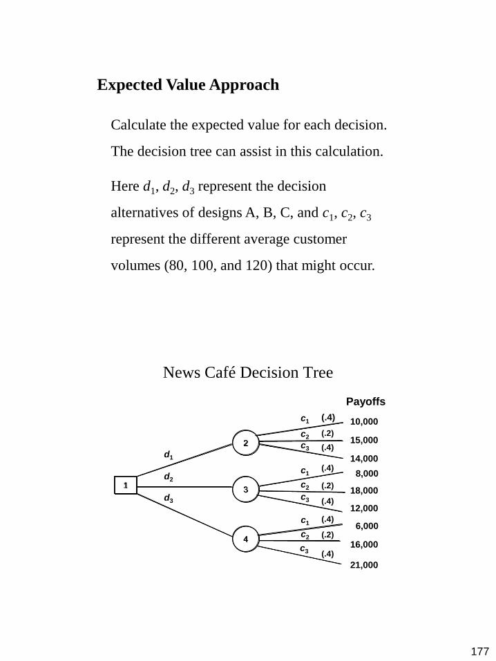
177
Calculate the expected value for each decision.
The decision tree can assist in this calculation.
Here d1, d2, d3 represent the decision
alternatives of designs A, B, C, and c1, c2, c3
represent the different average customer
volumes (80, 100, and 120) that might occur.
Expected Value Approach
1
(.2)
(.4)
(.4)
(.4)
(.2)
(.4)
(.4)
(.2)
(.4)
d1
d2
d3
c1
c1
c1
c2
c3
c2
c2
c3
c3
Payoffs
10,000
15,000
14,000
8,000
18,000
12,000
6,000
16,000
21,000
2
3
4
News Café Decision Tree

178
Choose the design with largest EV -- Design C.
3
4
d1
d2
d3
EV = .4(10,000) + .2(15,000) + .4(14,000)
= $12,600
EV = .4(8,000) + .2(18,000) + .4(12,000)
= $11,600
EV = .4(6,000) + .2(16,000) + .4(21,000)
= $14,000
Design A
Design B
Design C
2
1
News Café Expected Value for Each Decision
Capacity Decisions Exercise 1
Nitrogen Chemicals is considering capacity expansion. Its
major alternatives are; to do nothing, build a small plant, build a
medium plant or build a large plant. The new facility would
produce a new type of fertiliser and currently the potential or
marketability for this product is unknown. If a large plant is
built and a favourable market exists, a profit of $100,000 could
be realized. An unfavourable market would yield a $90,000
loss. However, a medium plant would earn a $60,000 profit
with a favourable market. A $10,000 loss would result from an
unfavourable market. A small plant, on the other hand, would
return $40, 000 with favourable market conditions and lose only
$5,000 in an unfavourable market. Of course, there is always
the option of doing nothing.

179
Capacity Decisions Exercise 1
If recent market research indicates that there is a 0.4
probability of a favourable market, which means that there
is also 0.6 probability of an unfavourable market. With
this information, the alternative that will result in the
highest expected monetary value (EMV) can be selected:
EMV (large plant) = (0.4)($100,000) + (0.6)(-$90,000)
= -$14,000
EMV (medium plant) = (0.4)($60, 000) + (0.6)(-$10,000)
= +$18,000
EMV (small plant) = (0.4)($40,000) + (0.6)(-$5,000)
= +$13,000
EMV (do nothing) = $0
CompuServ is considering what to do with his business over
the next five years. Sales growth over the past couple of
years has been good, but sales could grow substantially if a
major electronics firm is built in the Store’s area as
proposed. CompuServ’s owner sees three options:
1. Enlarge the current store; 2. Locate at a new site; 3. Do
nothing.
Options 1 and 2 would take little time and, therefore, the
store would not lose revenue. If nothing was done the first
year and strong growth occurred, then the decision to
expand would be reconsidered. Waiting longer than one year
would allow competition to move in and make expansion no
longer feasible.
Capacity Decisions Exercise 2
180
CompuServ has gathered the following information:
1. Strong growth has a 55% probability
2. Strong growth with new site annual returns $195,000; Weak
growth with new site mean annual returns $115,000.
3. Strong growth with an expansion annual returns $190,000;
Weak growth with an expansion mean annual returns $100,000.
4. Strong growth with existing store and do nothing annual returns
$170,000 while weak growth $105,000 per year.
5. Expansion at current site cost $87,000.
6. Moving to new site cost $210,000.
7. If growth is strong and expanding in second year cost $87,000.
8. Operating costs for all options are equal.
What is the best option for CompuServ?
Capacity Decisions Exercise 2
GBS 660 – Production and Operations
Management
2016 version of the module study notes compiled by
Levy Siaminwe , PhD
Adjunct Associate Professor – University of Lusaka