1

Processing Top-N Relational Queries by Learning∗

Liang Zhu a,b, Weiyi Meng c, Chunnian Liu a, Wenzhu Yang b, Dazhong Liu b

a College of Computer Science and Technology, Beijing University of Technology, Beijing 100022, China b Key Laboratory of Machine Learning and Computational Intelligence, School of Mathematics and Computer Science, Hebei University, Baoding, Hebei 071002, China c Department of Computer Science, State University of New York at Binghamton, Binghamton, NY 13902, USA

Abstract. A top-N selection query against a relation is to find the N tuples that satisfy the query

condition the best but not necessarily completely. In this paper, we propose a new method for

evaluating top-N queries against a relation. This method employs a learning-based strategy.

Initially, this method finds and saves the optimal search spaces for a small number of random top-

N queries. The learned knowledge is then used to evaluate new queries. Extensive experiments are

carried out to measure the performance of this strategy and the results indicate that it is highly

competitive with existing techniques for both low-dimensional and high-dimensional data.

Furthermore, the knowledge base can be updated based on new user queries to reflect new query

patterns so that frequently submitted queries can be processed most efficiently. The maintenance

and stability of the knowledge base are also addressed in the paper.

Keywords: Top-N Query, Relational Database, Learning-Based Strategies, Time Series

1. Introduction

Researches on top-N selection queries have intensified since late 1990s. A top-N selection query

against a relation is to find the N tuples that satisfy the query condition the best but not necessarily

completely.

Example 1. Consider a database of used cars. Let the schema of the used cars be:

Usedcars(id#, make, model, year, price, mileage). Suppose a customer wants to buy a used car

with a price about $5,000 and mileage about 6,000. One possible way is to specify the query as

follows:

select * from Usedcars where price = 5000 and mileage = 6000

There may not be a car that satisfies all conditions exactly. This prevents the user from finding

used cars that satisfy the conditions approximately. Another possible way is to specify the range

query as below:

select * from Usedcars where (price between 4000 and 6000)

and (mileage between 1000 and 10000)

∗Part of the contents of this paper was published in the Proceedings of WAIM’04. E-mail addresses: zhu@hbu.edu.cn (L. Zhu), meng@cs.binghamton.edu (W. Meng), ai@bjut.edu.cn (C. Liu), wenzhuyang@hbu.edu.cn (W. Yang), liudazhong@hbu.edu.cn (D. Liu)

2

There are two problems associated with the above standard SQL range query: (1) There may be

too many used cars that satisfy the conditions and these cars may not be appropriately ordered to

help the customer find desired cars. (2) It is difficult for the customer to define the proper range for

each attribute – too tight may lead to too few results and too loose may lead to too many results. �

The top-N query is a better solution to the above problems, that is, for a given query condition,

to retrieve a sorted set of the N tuples that are closest to the query according to a given distance

function, for some user specified integer N, say, N = 10, 20, or 100.

A simple way to evaluate a top-N query is to retrieve all tuples in the relation, compute their

distances with the query condition using a distance function and output the N tuples that have the

smallest distances. The main problem with this solution is its poor efficiency, especially when the

number of tuples of the relation is large. For example, for a relation with 100,000 tuples and a top-

10 query, this simple solution would retrieve 100,000 tuples (i.e., bring them from disk to

memory), perform 100,000 distance computations and sort 100,000 distances.

Finding efficient strategies to evaluate top-N queries has been the primary focus of top-N query

research and has received much attention in recent years (see Section 2). In (Bruno et al., 2002;

Chen and Ling, 2002), for instance, the basic idea of these strategies is to find a small search space

centered at the query point of any given top-N query such that all of the desired tuples (i.e., the top

N tuples) but very few undesired ones are contained in this search space.

Generally, a top-N query may be evaluated in three steps: (1) Determine a search distance r > 0

based on some technique (say the techniques in (Bruno et al., 2002; Chen and Ling, 2002)), and

form an n-dimensional square (i.e., a small search space) centered at the query point with side

length 2r if n attributes are involved. (2) Retrieve the tuples (data points) in the search space. (3)

Rank the retrieved tuples based on their distances with the query and display the top N tuples.

Obviously, the first step – determining a search distance r – is the key step.

In this paper, we propose a new method for evaluating top-N queries against a relation. The

main difference between this method and existing ones is that the new method employs a learning-

based strategy. A knowledge base is built initially by finding the optimal (i.e., the smallest

possible) search spaces for a small number of random top-N queries and by saving some related

information for each optimal solution. This knowledge base is then used to derive search spaces

for new top-N queries. The initial knowledge base can be continuously updated while new top-N

queries are evaluated. Clearly, if a query has been submitted before and its optimal solution is

stored in the knowledge base, then this query can be most efficiently processed. As a result, this

method is most favorable for repeating queries. It is known that database queries usually follow a

Zipfian distribution (Bruno et al., 2001). Therefore, being able to support frequently submitted

queries well is important for the overall performance of the database system. Our experimental

results confirm that our method is indeed well suited for query sets with many repeating queries.

What is attractive about this method is that even in the absence of repeating queries, our method

still compares favorably to existing methods with comparable storage size for storing information

needed for top-N query evaluation. In addition, this method is not sensitive to the dimensionality

of the data and it works well for both low-dimensional and high-dimensional data.

3

The rest of the paper is organized as follows. In Section 2, we review some related works and

compare our method with the existing ones. In Section 3, we introduce some notations and provide

a brief analysis on the effect of dimensionality to top-N query evaluation. In Section 4, we present

our learning-based top-N query evaluation strategy. In Section 5, we present the experimental

results. Finally in Section 6, we conclude the paper.

2. Related Work

The need to rank the results of database queries has long been recognized. Motro (1988) gave the

definitions of vague queries. He emphasized the need to support approximate and ranked matches

in a database query language, and introduced vague predicates. Carey and Kossmann (1997; 1998)

proposed techniques to optimize top-N queries when the scoring is done through the SQL “Order

By” clause by reducing the size of intermediate results. Donjerkovic and Ramakrishnan (1999) use

a probabilistic approach to optimize top-N queries and the ranking condition involves a single

attribute. Onion (Chang et al., 2000) and Prefer (Hristidis et al., 2001; 2004) are preprocessing-

based techniques for top-N queries. In addition, a variety of algorithms for materialized top-N

views have been proposed in (Yi et al., 2003; Das et al., 2006). Xin et al. (2006) proposed a

computational model, ranking cube, for efficient answering of top-N queries with

multidimensional selections.

Fagin et al. (2001) introduced the threshold algorithms (TA) that perform index scans over pre-

computed index lists, one for each attribute or keyword in the query, which are sorted in

descending order of per-attribute or per-keyword scores. Variations of TA have been proposed for

several applications, including similarity search in multimedia repositories (Chaudhuri et al.,

2004), approximate top-N retrieval with probabilistic guarantees (Theobald et al., 2004),

scheduling methods based on a Knapsack-related optimization for sequential accesses and a cost

model for random accesses (Bast et al., 2006), and the distributed TA-style algorithm has been

presented in (Marian et al. 2004; Michel et al., 2005).

Top-N queries involving joins have also been considered (Carey and Kossmann, 1997; Habich

et al., 2005; Ilyas et al., 2002; 2004a; 2004b; Li et al., 2005; Zhu et al., 2005). Ilyas et al. (2002)

proposed an algorithm that is suitable for evaluating a hierarchy of join operators. Ilyas et al.

(2004a) introduced a pipelined rank-join operator, based on the ripple join technique. The

RankSQL work (Ilyas et al., 2004b; Li et al., 2005) considered the order of binary rank joins at

query-planning time. For the planning time optimization, RankSQL uses simple statistical models,

assuming that scores within a list follow a normal distribution (Ilyas et al., 2004b). We consider

only selection queries in this paper and join queries will be considered in the future.

Recently, Xin et al. (2007) studied an index-merge paradigm that performs progressive search

over the space of joint states composed by multiple index nodes; Soliman et al. (2007) introduced

new probabilistic formulations of top-N queries in uncertain databases; Hwang and Chang (2007a;

2007b) developed the algorithms and framework by a cost-based optimization. Yiu et al. (2007)

proposed an aR-tree method to process top-N dominating queries. Zhu et al. (2008) proposed

region-clustering methods to evaluate concurrently a set of multiple top-N queries submitted

(almost) at the same time.

4

Yu et al. (2001; 2003) introduced the methods for processing top-N queries in multiple database

environments. The techniques are based on ranking databases. Yu et al. (2001) used histograms

and they (2003) considered the information of past queries in top-N query evaluation. Balke et al.

(2005) and Vlachou et al. (2008) developed methods to optimize the communication costs in P2P

networks. Zhao et al. (2007) proposed the algorithm BRANCA for performing top-N retrieval in

distributed environments. Our paper considers environments with a single database at a central

location.

In (Chaudhuri and Gravano, 1999; Bruno et al., 2002; Chen and Ling, 2002) and this paper, the

query model for top-N queries is consistent with the definitions in (Motro, 1988).

In (Chaudhuri and Gravano, 1999), histogram-based approaches are used to map a top-N query

on a relational database into a traditional range selection query. Two different strategies, one

optimistic and the other pessimistic, are proposed to determine the “Restarts” (additional queries

may be evaluated if the initial mapped range query does not retrieve enough results) and “No

Restarts” search distances as dRq and dNRq, respectively. In addition, two intermediate strategies,

Inter1 and Inter2, with search distances (2dRq + dNRq)/3 and (dRq + 2dNRq)/3, respectively, are

studied. In (Bruno et al., 2002), the above four strategies are extended to a new technique called

Dynamic, expressed as dq(α) = dRq + α(dNRq − dRq). Then, α*, the estimated value of the

optimal α, is calculated using a designed workload of training queries. The value of α* depends on

the training workload and the data distribution of the relation. The histogram-based approaches

can guarantee the retrieval of all top-N tuples for each query, but a significant weakness of

histogram-based approaches is that their performance deteriorates quickly when the number of

dimensions of the data exceeds 3 (Bruno et al., 2002; Lee et al., 1999). Therefore, histogram-based

approaches are suitable for only low-dimensional data in practice.

In (Chen and Ling, 2002), a sampling-based method is proposed to translate a top-N query into

an approximate range query that modifies the strategies in (Chaudhuri and Gravano, 1999) for

evaluating top-N queries over relational databases. Unlike histogram-based approaches, this

method is suitable for high-dimensional data and is easy to implement in practice. However, this

method only provides an approximate answer to a given top-N query, i.e., it does not guarantee the

retrieval of all of the top-N tuples. In addition, for large databases, this method may be inefficient.

For example, for a relation with 1 million tuples and using a 5% sample set (as reported in (Chen

and Ling, 2002)), 50,000 tuples need to be evaluated in order to find the approximate range query

for a top-N query.

Except for (Yu et al. 2003), none of the above methods learns from past queries. The only

method that considers past queries in top-N query evaluation that we are aware of is proposed in

(Yu et al. 2003). However, there are key differences between the FQ method in (Yu et al. 2003)

and the method to be presented in this paper. First, FQ focuses on ranking databases in a

distributed relational database environment to determine potentially useful local databases to

search for finding the top-N tuples and it does not guarantee the retrieval of all of the top-N tuples.

In contrast, this paper concentrates on finding the top-N tuples from a single database and it

guarantees the retrieval of the entire top-N tuple set. Second, the information stored for each

processed top-N query is very different between the two approaches. FQ stores the best-matched

5

tuples from searched databases for frequent queries while our method stores the optimal search

distance and the number of tuples in the corresponding search space for each query. Finally, FQ

depends entirely on user queries to collect needed knowledge for future queries, whereas the new

method delivers very good performance even with the initial knowledge base that is built using

randomly generated queries.

Our learning-based method is fundamentally different from all existing techniques. It can learn

from either randomly generated training queries or real user queries so it can adapt to changes of

query patterns. Furthermore, it delivers good performance for both low-dimensional and high-

dimensional data and guarantees the retrieval of all top-N tuples for each query as will be

demonstrated by our extensive experimental results.

This paper is an extension of our previous conference paper (Zhu and Meng 2004). The main

differences between this paper and the previous version are as follows. (1) An analysis of the

reason of dimensionality curse is added. (2) A strategy of maintaining the knowledge base is added.

(3) Based on the time series techniques and methods, discussions on the stability issue of the

knowledge base are added. (4) More details and descriptions of experimental results and related

works are provided. (5) Experimental results on the stability of the knowledge base are reported.

3. Problem Definition and Analysis

Let ℜ n be an n-dimensional metric space with distance (or, metric) function d(.,.), where ℜ is the

real line. Suppose R ⊂ ℜ n is a relation (or dataset) with n attributes (A1, …, An). A tuple t ∈ R is

denoted by t = (t1, …, tn). Consider a query point Q = (q1,…, qn)∈ ℜ n and an integer N > 0. A top-

N selection query (Q, N), or top-N query Q for short, is to find a sorted set of N tuples in R that are

closest to Q according to the given distance function. The results of a top-N query are called top-N

tuples. We assume N < |R| (the size of R); otherwise, we just retrieve all tuples in R.

Suppose Q = (q1,…, qn) is a top-N query and r > 0 is a real number. We use S(Q, r) to denote

the n-square ],[1∏=

+−n

i ii rqrq centered at Q with side length 2r. Our goal is to find a search

distance r that is as small as possible such that S(Q, r) contains the top-N tuples of Q according to

the given distance function. We use S(Q, r, N) to denote this smallest possible n-square and the

corresponding r is called the optimal search distance for the top-N query Q. Some example

distance functions are (Bruno et al., 2002; Chen and Ling, 2002; Yu et al., 2001):

Summation distance (i.e., L 1 -norm or Manhattan distance):

d 1 (x, y) = ||x - y|| 1 = ∑=−

n

i ii yx1

|| .

Euclidean distance (i.e., L 2 -norm distance):

d 2 (x, y) = ||x - y|| 2 = ∑=−

n

i ii yx1

2)( .

Maximum distance (i.e., L ∞ -norm distance):

d ∞ (x, y) =||x - y|| ∞ = |}{|max1 iini

yx −≤≤

.

6

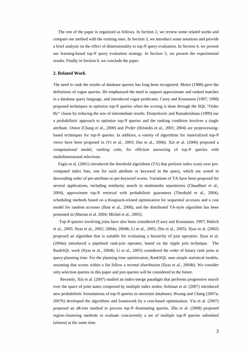
In the case of 2-dimensional space, the “hyperspheres” of the distance functions of d 1 (x, y),

d 2 (x, y) and d ∞ (x, y) are described as diamond, circle and square, respectively, as illustrated in

Figure 1. Note that for any given distance function, the distance between any point on the edge of

the corresponding hypersphere and the query point is the same. This guarantees that if the

hypersphere contains at least N tuples, then the top-N tuples of the query are contained in this

hypersphere. Current database systems are not capable of efficiently searching spaces whose sides

are not parallel to the axes that correspond to the attributes. For example, the hypersphere of the

Euclidean function is a circle and current database systems do not provide efficient techniques to

retrieve only the tuples in the circle. Instead, the smallest n-square (2-square or simply square in

the case of 2-dimensional space) that contains the circle and whose sides are parallel to the axes is

used to specify the search space (see Section 4.2.2). It is easy to see that when such an n-square is

obtained for the hypersphere of the sum function, the size of the search space will be increased the

most (the size is doubled when the number of dimensions is 2). In contrast, there is no increase to

the size of the search space when the max function is used. Therefore, among the three distance

functions mentioned above, the sum function is the most expensive to process and the max

function is the least expensive.

Q

Fig. 1 The “hyperspheres” of common distance functions (“x” indicates the query point)

Clearly, the results of a top-N query, i.e., the top-N tuples, depend on the distance function used.

Different distance functions may lead to different sets of the top-N tuples. Most existing work on

top-N query research proposes to let the user specify the distance (or scoring) function as part of

the top-N query (Chaudhuri and Gravano, 1999; Yu et al., 2001).

Frequently, it is not suitable to apply a distance function to the values of different attributes

directly due to the unit/scaling difference of the values in different attributes. For example, when

buying a used car, a 100-dollar difference in price is probably more significant than a 100-mile

difference in mileage. This can be resolved by multiplying appropriate importance/scaling factors

to the raw distances based on the values of different attributes (Chen and Meng, 2003; Yu et al.,

2001). These importance/scaling factors are specified by the user as part of the top-N query

specification. Without loss of generality, we assume that all attributes are of the same importance

for ranking tuples so that the distance functions can be applied directly (otherwise, we use adjusted

units after appropriate importance factors are applied).

Now we discuss the effect of dimensionality on the problem of efficient top-N query evaluation.

For simplicity, we assume that the tuples are uniformly distributed with distribution density ρ. For

a top-N query Q, N ∝ v(S(Q, r, N))ρ, where v(S(Q, r, N)) denotes the volume of S(Q, r, N), i.e.,

7

v(S(Q, r, N)) = nr)2( . Consider S(Q, r, N) and S(Q, r~ , N~ ) for top-N and top- N~ tuples of Q,

respectively, r~ > r. Since ρ is a constant, the number of tuples in S(Q, r, N) only depends on

v(S(Q, r, N)), which in turn depends on the search distance r and the dimensionality n. Assume

r~ = r + δ, we obtain

nrr

rrr

NrQSvNrQSv

NN

n

n

n

n

)1()()2()~2(

)),,(())~,~,((~ δδ +==== +

If δ = r/n, then v(S(Q, r~ , N~ ))/v(S(Q, r, N)) = (1+ n1 ) n . It is known that 2 ≤ (1+ n

1 ) n < e < 3.

Thus, if r~ = r + r/n, we have

2≤ N~ /N = v(S(Q, r~ , N~ ))/v(S(Q, r, N)) < 3 (1)

From (1), we can see that the difference between the search distance r of top-N tuples and r~ of

Top-2N tuples is less than or equal to r/n. If the dimensionality n is large enough, the difference

will be very small. In general, for a fixed real number a > 0, the function f(x) = (1 + a/x) x , x > 0,

is an increasing function and (1 + a/x) x ae→ as x → ∞, and 2 a ax exa <+≤ )/1( < 3 a , for

x ≥ a. Thus, for a natural number m, if δ = (m/n)r, for n = m, m+1, …, we obtain

2 m ≤ N~ /N= v(S(Q, r~ , N~ ))/v(S(Q, r, N)) < 3 m (2)

From (2), for n≥m, we can see that the difference of the search distances between top-N tuples

and top-2 m N tuples is less or equal to (m/n)r when data are uniformly distributed.

For example, if the relation R has a uniform distribution and 100 dimensions, the search

distance of top-10 tuples is r = 1, m = 10, then the search distance of top-2 m *10 = top-10240

tuples, or roughly top-10000 tuples, is no more than (1 + 10/100)r = 1.1.

The above analysis indicates that for uniformly distributed high-dimensional data, when the

search distance increases only a little, the n-square will contain so many more tuples, leading to a

much higher search cost. This explains the problem of high search overhead when using the

histogram-based approaches for high-dimensional data.

4. Learning-based Top-N Query Evaluation

In this section, we introduce our learning-based method for top-N query evaluation. The idea of

the method is rather simple and can be described as follows. First, keep track of frequently

submitted queries and save the evaluation strategies for these queries in a knowledge base. Next,

for each newly submitted query, if its evaluation strategy has been saved or it is similar to some

queries whose evaluation strategies have been saved, then derive an evaluation strategy for the

new query from the saved relevant strategy/strategies. Intuitively, this method will be effective if

the percentage of repeating queries is high. In this paper, we study issues related to this method.

These issues include: (1) What queries should be saved and what information should be saved for

these queries? (2) How to use the saved knowledge to evaluate newly submitted queries? (3) How

8

to maintain the knowledge base in light of newly evaluated queries and changes in the database?

(4) How stable is the knowledge base? These issues will be discussed in the following subsections.

4.1 Query Information to Save

Initially, the knowledge base is empty. When a new query arrives at the system, an existing

method such as the one proposed in (Bruno et al., 2002) or in (Chen and Ling, 2002) is employed

to evaluate the query. Basically, such a method finds an n-square query (range-conditions along all

involved attributes) to retrieve the tuples in the n-square. After the query is evaluated and the

results are returned to the user, an offline process is initiated when the system is not busy to find

the smallest n-square that contains the top-N tuples with respect to the query. This smallest n-

square is likely to be smaller than the initial n-square obtained for the query. The smallest n-square

can be obtained from the distances between the query and the retrieved top-N tuples. Let Q = (q1,

…, qn) be the query and ti = (ti1, …, tin), 1 ≤ i ≤ N, be the top-N tuples, respectively. Then the search

distance of the smallest n-square is r = Ni≤≤1

max {d ∞ (Q, it )} = |}}{|max{max11 ijjnjNi

tq −≤≤≤≤

. When

the smallest n-square is obtained, several pieces of information are collected and saved to form the

profile of the query.

Definition 1 (query profile). For a top-N query Q, the profile of the query is a 6-nary tuple ζ(Q)

= (Q, N, r, f, c, d), where r is the search distance of S(Q, r, N) – the smallest n-square that contains

the top-N tuples of Q, f is the cardinality of S(Q, r, N), i.e., the number of tuples in S(Q, r, N)

(obviously N ≤ f ), c is the number of times that Q has been submitted, and d is the most recent

time when Q was submitted.

After the system has been used for sometime, a number of query profiles are created and saved

in the knowledge base. Let P = {ζ1, ζ2, …, ζm} denote the set of all query profiles, i.e., the

knowledge base, maintained by the system. Queries in P will be called profile queries. Clearly, it

may not be possible to store the profiles for all queries that have ever been submitted, due to the

large overhead in storage and maintenance. To deal with this problem, profiles should be kept only

for queries that are frequently submitted recently as reflected by the values of c and d in the profile

of each query. The detail on the maintenance of P will be provided in Section 4.3.

In our implementation, the initial knowledge base is not built based on real user queries.

Instead, it is based on randomly selected queries from a possible query space (see Section 5 for

more details).

4.2 New Query Evaluation

When a newly submitted top-N query Q is received by the system, we need to find an appropriate

search distance r for it. In a system that does not store query profiles, this query will be processed

just like any new query and the methods discussed in (Bruno et al., 2002; Chen and Ling, 2002)

may be used to find r. When query profiles are stored, it becomes possible to obtain the r for some

new user queries from these profiles. In this section, we discuss how to incorporate the query

profiles in the evaluation process of new queries. The basic idea of this process is sketched below.

9

1. Determine if P contains queries that are similar to Q based on the distance between query

points. If yes, derive the search distance r for Q based on the profiles of these queries. If no,

find r and retrieve the top-N tuples using an existing method (say the one in (Bruno et al.,

2002; Chen and Ling, 2002) ) and go to Step 3.

2. Retrieve all tuples in the n-square S(Q, r). If the number of tuples retrieved is greater than or

equal to N, sort them in non-decreasing order of the distances, output the top-N tuples, and go

to Step 3. Else, choose a larger value for r to guarantee the retrieval of the top-N tuples for Q.

(In general, the sorted orders of a set of tuples under different distance functions are different.)

3. Maintain P. The maintenance of P is needed when a new top-N query has been processed or

the database has been changed (see Section 4.3).

QQ'

Q

Q'

Q

Q'

(a) Q = Q′ (b) Q ∈ S(Q′, r′, N′ ) (c) Q ∉ S(Q′, r′, N′ )

Fig. 2 The three cases of Q and its closest profile query Q′

4.2.1 Determining the search distance r

As mentioned in Section 1, the key step is to determine the search distance r in the three-step

evaluation of a new top-N query Q. In this step, we first identify the profiles whose query points

are closest to Q, then we use the information in these profiles to estimate the local distribution

density of Q, and finally we obtain the search distance r for Q based on its local distribution

density. The details of obtaining the search distance r for Q are described below.

First we identify Q′ = ( nqqq ′′′ ,...,, 21 ) from P that is the closest to Q under the distance

function d(.,.). Let {Q1, Q2, …, Qm} be the set of profile queries for P, and d(.,.) be one of the three

distance functions in Section 3, say, d(.,.) = d∞(.,.). Suppose Q = (q1, q2, …, qn), and Qi = (qi1,

qi2,…, qin), 1 ≤ i ≤ m, then Q′ = ( nqqq ′′′ ,...,, 21 ) is the profile query such that d(Q, Q′ ) = d∞ (Q,

Q′ ) = mi≤≤1

min {d ∞ (Q, Qi)} = |}}{|max{min11 ijjnjmi

qq −≤≤≤≤

. The following cases exist.

1. d(Q, Q′ ) = 0, i.e., Q′ = Q . In this case, find all profiles in P whose query point is Q′, but have

different result size N, say, N1 < N2 < …< Nk. An example of a 2-dimension case is depicted in

Figure 2(a), where squares of solid lines represent the search spaces of profile queries (i.e.,

those in P) and the square of dotted lines represents the search space of the new query Q. We

now consider three subcases.

a. There is N′ ∈ {N1, N2, …, Nk} such that N = N′. That is, there is a top-N query in P that is

identical to the new query in both the query point and result size N. In this case, let r := r′,

10

where r′ is from the profile ζ′ = (Q′, N′, r′, f′, c′, d′ ). Clearly, r′ is the optimal search

distance for Q.

b. There is no N′ ∈ {N1, N2, …, Nk} such that N = N′ , but there is N′ ∈ {N1, N2, …, Nk} such

that N′ > N and it is the closest to N among N1, N2, …, Nk (Figure 2(a)). In this case, let r :=

r′, which guarantees the retrieval of all the top-N tuples for Q. In practice, the difference

between different N’s is not likely to be too large, as a result, using r′ won’t cause too many

useless tuples to be retrieved.

c. Nk < N. In this case, we assume that the search space for Q has the same local distribution

density as that for Q′. Based on this assumption, we have N/(2r)n = Nk/(2rk)n. As a result, we

let r := ( nkNN )rk. However, this r does not guarantee the retrieval of the top-N tuples for

Q. If not enough top-N tuples are retrieved, a larger r will be used (see Section 4.2.2).

2. d(Q, Q′ ) ≠ 0, i.e., Q′ ≠ Q. We consider two subcases.

a. Q is in the search space S(Q′, r′, N′ ) of Q′ . Find out all query points in P whose search

spaces contain Q. Let these query points be (Q1, …, Qk) (see Figure 2(b)). To estimate the

search distance r for Q, we first use a weighted average of the local distribution densities of

the search spaces for Q1, …, Qk to estimate the local density of search space for Q. The

weight wi for the search space corresponding to Qi is computed based on its size and the

distance between Qi and Q. Weight wi is an increasing function of the size of the search

space and a decreasing function of the distance. In this paper, wi is computed by the

following formula:

wi = v(S(Qi, ri, Ni)) * 1/(d(Q, Qi))α

where α is a parameter and its best value is obtained by experiments (α = 3n/4 is a good

value based on our experiments). Let ρi = fi / (2 ri)n be the local density of the search space

for Qi. Then the local density of the search space for Q is estimated by:

ρ = (∑ ki 1= wi ρ i ) / (∑ k

i 1= wi).

Based on the above ρ, we estimate the search distance r to be ( n N ρ/2 )/2. Note that to

increase the possibility that all of the top-N tuples for Q are retrieved, we replaced N by 2N

in the estimation for r (i.e., aim to retrieve 2N tuples).

b. Q is not in the search space S(Q′, r′, N′ ) of Q′ (see Figure 2(c)). Let h := d(Q, Q′ ) be the

distance between Q and Q′ . Construct an n-square S(Q, h) and let (Q1, …, Qk) be all the

query points in P whose search spaces intersect with S(Q, h). Obviously, k ≥ 1 as Q′ is in this

query set. Now the same technique used above (i.e., step 2.a) is used to estimate the search

distance r for Q.

The search distance r obtained above (2.a and 2.b) may sometimes be either too small or too

large. To remedy this, the following adjustments to r are implemented. The following two cases

are considered.

(1) N = N′ .

11

(i) If r < r′ or r < d(Q, Q′ ), then r may be too small. For example, since the same number of

tuples need to be retrieved for Q and Q′, if the search spaces for Q and Q′ have similar density

(this is likely as Q and Q′ are the closest), then r and r′ should be about the same. Therefore, “r

< r′ ” would indicate that r may be too small. We use the following formula to adjust r:

r = max(r_Median, r_Mean, r)/2 + (r′ + d(Q, Q′ ))/2

where r_Median = ( nmedianNN /2 ) medianr , medianr is the search distance of the search space

whose density is the median among all search spaces in the knowledge base P and medianN is

the N value of the corresponding profile; r_Mean = ( nmeanN ρ/2 )/2 and meanρ is the

average of all densities of the search spaces in P. The above formula is an attempt to combine

the global information (i.e., r_Median and r_Mean) with some related local information (i.e., r,

r′ and d(Q, Q′ )) to come up with a reasonable r. Note that if search distance r′ + d(Q, Q′ ) were

used for Q, then the entire search space for Q′ would be contained, guaranteeing the retrieval of

all the top-N tuples for Q, but it may lead to an excessive search space.

(ii) If r > r′ + d(Q, Q′ ), then r is too large as r = r′ + d(Q, Q′ ) can already guarantee the

retrieval of all the top-N tuples of Q. In this case, we simply lower r to r′ + d(Q, Q′ ).

(2) N ≠N′ . This is handled in a similar manner as in case (1) except that a constant factor λ =

n NN ′/ is utilized to take into consideration the difference between N and N′ .

(i) If r < λ r′ or r < d(Q, Q′ ), then r := max(r_Median, r_Mean, r)/2 + (λr′ + d(Q, Q′ ))/2.

(ii) If r > λ r′ + d(Q, Q’ ), then r := λ r′ + d(Q, Q′ ).

4.2.2 Query Mapping Strategies

For a given top-N query Q = (q1,…, qn), to retrieve all tuples in S(Q, r), one strategy is to map each

top-N query to a simple selection range condition query of the following format (Bruno et al.,

2002):

select * from R where (q1 – r ≤ A1 ≤ q1 + r) and … and (qn – r ≤ An ≤ qn + r)

If the query returns ≥ N results, sort them in non-descending distance values and output the top N

tuples.

A potential problem that needs to be handled is that the estimated search distance r is not large

enough, i.e., less than N tuples are in S(Q, r). In this case, the value of r needs to be increased to

guarantee that there are at least N tuples in S(Q, r). One solution to this problem is provided below.

Choose N query points in P, which are closest to the top-N query Q, and sort them in ascending

order of their distances with Q with respect to the used distance function d(.,.). Let the order be

Q1, …, QN and their corresponding profiles be ζ1, ζ2, …, ζN. There exists a number h, 1 < h ≤N,

such that N1 + … + Nh ≥ N. During the computation of the sum, if S(Qi, ri, Ni) ∩ S(Qj, rj, Nj) ≠ ∅,

then Ni + Nj in the above sum was replaced by max{Ni, Nj} to ensure that the search spaces of the

first h queries in (Q1, …, QN) contain at least N unique tuples. Let r := hi≤≤1

max {d(Q, Qi) + ri}. It is

easy to see that these h search spaces are all contained in S(Q, r). Thus, by using this r as the

12

search distance for Q to generate the restart query, the restart query will guarantee the retrieval of

all the top-N tuples for Q. Using this method, at most one restart query is needed for each top-N

query.

If there is a histogram over the relation R, by using dNRq in (Bruno et al., 2002) (dNRq is a

search distance that guarantees the retrieval of all top-N tuples and it is estimated using a

histogram (Bruno et al., 2002)), the search distance r for the restart query can be obtained as

follows. If the sum of all N’s in P is less than N, then set r to be dNRq. Otherwise, find the number

h as mentioned above and let r := min{hi≤≤1

max {d(Q, Qi) + ri}, dNRq}.

Example 2. In ℜ2, as shown in Figure 3, Q is a newly submitted top-10 query, Q′ is its closest

profile query in P, Q ∈ S(Q′, r′, N′ ) (the square of solid lines), where two symbols “×” denote the

query points Q and Q′ . The top-10 query Q is evaluated in three steps: (1) Using the algorithms in

Section 4.2.1, the search distance r of Q is determined and its search space is formed, which is the

square of dotted lines. (2) The 14 tuples in the search space are retrieved from database. (3)

Computing the distances between Q and the 14 tuples, and sorting the distances, we obtain top 10

tuples. However, if the original search distance r is not large enough and the search space of Q

contains only 8 tuples as shown in Figure 4, we enlarge the value of r according to the solution

described in section 4.2.2 such that the new search space (the larger square of dotted lines in

Figure 4) has at least 10 tuples, and then restart the evaluation.

Q

Q'

Q

Q'

Fig. 3 The original search space of Q Fig. 4 The original search distance r of Q is

has at least 10 tuples not large enough, it needs to be enlarged

4.3 Maintenance of Knowledge base P

The maintenance of P includes two aspects: (1) Update of P, i.e., the addition of new profiles or

the replacement of some existing profiles in P. (2) Tuning of a profile in P, i.e., for a profile, the

collected information is changed but its query point is not changed.

Two situations will affect the maintenance of P, (1) after a query is evaluated, and (2) after the

database is changed. The former may cause both the update of P and the tuning of some profiles in

P. However, the latter leads to only the tuning of some profiles in P.

4.3.1 Maintenance of P after a Query is Evaluated

In order to manage the profiles of all queries effectively, we introduce the concept of profile

priority. The priority of a profile is a numerical value that reflects the likelihood that the query in

13

the profile would appear again in the near future. Intuitively, a query that has appeared frequently

and recently is more likely to appear again in the near future. Based on this intuition, for a profile ζ

= (Q, N, r, f, c, d), we define its priority as I1∗c/(|I2∗(w-d)|+1), where I1 and I2 are the weights (or

scaling factors), c is the count of Q, d is the most recent submission time of Q and w is the current

system time. Note that for a new query, w = d and therefore w - d = 0.

We divide the profiles of all queries into two sets, the primary set and the secondary set. The

former contains a small number of high-priority profiles based on a priority threshold and the latter

contains the remaining profiles (Note: those profiles whose corresponding queries have not been

submitted for a long time, as defined by a time threshold, need not be kept to keep the size of the

secondary set manageable). The knowledge base P corresponds to the primary set and will be kept

in the main memory. The secondary set will be stored on secondary storage with index based on

the query points.

The goal of maintaining P is to make sure that P has “good knowledge” about the distribution

of the data and the queries such that good search spaces can be estimated for new queries based on

the knowledge in P. In a query profile, the cardinality f and search distance r are essential

information because they can be used to estimate the local density of the query’s search space.

After a top-N query Q is processed and the smallest search distance r* is obtained for the query

(note that r* may be different from the original search distance r obtained in Section 4.2.1), the

knowledge base P will be updated or tuned. The update of the knowledge base includes two cases:

addition or replacement, depending on whether or not P is full. Here full means the size of P,

denoted by |P|, has reached its limit.

For a new top-N query (Q, N), let ζ′ = (Q′, N′, r′, f′, c′, d′ ) ∈ P be the nearest profile to Q. We

consider the following four cases:

(1) Type-1 query: Q = Q′ and no restart is needed (e.g., the case of Figure 2(a) with no restart

needed). In this case, query (Q, N) is the same as or similar to query (Q′, N′), and the

knowledge in P is good enough to obtain the right search distance for (Q, N). As a result, it

is unnecessary to add the profile of (Q, N) into P and we only need to tune ζ′. The tuning is

accomplished by replacing N′ by N, r′ by r*, increasing c′ by 1, and replacing f′ and d′ by

the new cardinality and the new timestamp, respectively.

(2) Type-2 query: Q ∈ S(Q′, r′ ) but Q ≠ Q′ and no restart is needed (e.g., the case of Figure

2(b) with no restart needed). In this case, query (Q, N) is still reasonably similar to query

(Q′, N′) and the knowledge in P is also good enough to obtain the right search distance for

(Q, N). Therefore, in this case, we do not force to replace any existing profile using the new

profile when there is no space in P for the new profile. Specifically, for a Type-2 query, we

first search its profile in the secondary set using the index on query points. If not found, a

new profile is created for it. If P is not full, the new profile is added to P. If found, the

profile will be tuned as in the case for a Type-1 query and its priority is updated. If its

priority becomes larger than the lowest priority among the existing profiles P, it will be

moved into P and the profile in P that has the lowest priority will be moved to the secondary

set.

14

(3) Type-3 query: Q ∉ S(Q′, r′ ) and no restart is needed. Figure 2(c) shows an example of this

case. In this case, Q and Q′ are not similar (i.e., their distance is large). It may not

necessarily cause a restart, but the chance of causing a restart will be high for a different N.

Thus, its profile should be saved in P. Therefore, if P is not full, we add the profile into P;

otherwise, we use it to replace the profile in P that has the lowest priority.

(4) Type-4 query: (Q, N) causes a restart. This indicates that the knowledge in P is not good

enough for this query. Thus, in such a case, the new profile of Q should be added into P or

used to replace the existing profile with the lowest priority, same as in the case for a Type-3

query.

In our experiments, only the primary set is used (see Section 5.5). In this case, after P

becomes full, we do not make any updates to P for Type-2 queries as the knowledge in P is still

good (see (2) above). Furthermore, we consider the worst-case scenarios where very few repeating

queries exist (except for high dimensional datasets with biased workloads). Consequently, Type-1

queries are rare. In subsequent discussions, we will focus mostly on Type-3 and Type-4 queries.

4.3.2 Maintenance of P after the Database is Changed

When the database is changed by the operations of insertion, deletion, or update, the knowledge

base P may also need to be maintained. As an update may be considered as a deletion followed by

an insertion. Thus, we consider only insertions and deletions here.

Suppose t is the tuple that is inserted into or deleted from the relation R. Let d(t, Q) denote the

distance between t and a given query Q.

1. Insertion. For each profile ζ = (Q, N, r, f, c, d) in P, consider the following three cases:

• d(t, Q) > r. No change is needed.

• d(t, Q) = r. Simply increase f by 1 and no other change is needed.

• d(t, Q) < r. Increase both N and f by 1 and no other change is needed.

2. Deletion. For each ζ = (Q, N, r, f, c, d) in P, consider the following three cases:

• d(t, Q) > r. No change is needed.

• d(t, Q) = r. If f > N, simply decrease f by 1 and no other change is needed. If f = N,

decrease both f and N by 1 and no other change is needed.

• d(t, Q) < r. Decrease both N and f by 1 and no other change is needed.

Obviously, the changes of database neither affect the size of P nor cause the replacement of

any existing query profile in P, though they may lead to the tuning of some profiles in P. Therefore,

for the update of P, we do not consider the changes of database.

Note: If the database is changed too frequently, there may be lots of insertions and/or deletions.

In the case of insertion, if N becomes very large, we can sort the N tuples again, and obtain the

new N, r and f. Similarly, in the case of deletion, if the number of tuples in the search space of a

profile becomes too small, we can enlarge r and tune the profile for the desired N using the

methods described in Section 4.2.2.

15

4.4 Stability of Knowledge base P

Let P = {ζk : k = 1, 2, …, p} be the knowledge base with size p, and Q1, Q2, …, Qi, … be a

sequence of top-N queries. Denote c(i) to be the function that counts the number of times P has

been updated right after Qi is evaluated. As discussed in Section 4.3, after query Qi is evaluated, P

may be updated, i.e., a new profile may be added into P or an existing profile may be replaced by a

new one. c(i) is increased by 1 each time P is updated. Clearly, c(i) is a monotonically non-

decreasing function.

Intuitively, when the size of P becomes sufficiently large, the number of updates to P should

become less frequent, that is, the increase to the value of c(i) will slow down, because most of the

needed changes will become tunings. We use stability to measure how likely P will change after a

query is evaluated. Clearly, a more stable P is desired because it means less maintenance overhead

for P.

We define another function p(i), which is the size of P after the i-th query is executed. If there is

no limit on the size of P, then we can keep adding new profiles to P and in this case, p(i) = c(i);

else (i.e., the size of P is limited), then there will be a number i0 such that p(i) = c(i) for i ≤ i0 and

p(i) = |P| for i > i0.

In this section we will discuss the stability of the knowledge base P using the techniques of time

series and the difference quotient of c(i).

A time series is a set of observations zt, each of which is recorded at a specified time t. A time

series is stationary if the statistical properties such as the mean and the variance of the time series

are essentially constant through time. Some time series display seasonality, i.e., they show

periodic fluctuations. For example, retail sales tend to peak during the Christmas season and then

decline after the holidays.

Sample autocorrelation function (SAC) can be used to determine whether a time series is

stationary or nonstationary. For time series values zb, zb+1, …, zm, the sample autocorrelation at lag

k is

rk = ( Σ kmbt−= ( zt −μ ) ( zt+k −μ ))/( Σ m

bt= ( zt −μ )2 ) , whereμ = Σ mbt= zt /(m−b+1).

SAC is a listing, or graph, of the sample autocorrelation at lag k = 1, 2, …. In general, it can be

shown that for nonseasonal data (Bowerman and O'Connell, 1993):

(1) if the SAC of the time series values zb, zb+1, …, zm either cuts off fairly quickly or dies

down fairly quickly, then the time series should be considered stationary;

(2) if the SAC of the time series values zb, zb+1, …, zm dies down extremely slowly, then the

time series should be considered nonstationary.

Now, we discuss the stability of P when the size of P is unlimited. Based on Heine-Borel

theorem in mathematical analysis (Fleming, 1977), if the size of P is unlimited, there exist finite

profiles such that the open hyper-squares constructed by the profiles will cover the closed hyper-

rectangle Π nj 1= [αj, βj], where [αj, βj] = [min (Aj), max (Aj)] is the domain of the j-th attribute Aj.

Therefore, Type-3 queries (see Section 4.3) will not occur when enough profiles have been saved

in P.

16

If the size of P is large enough, then for any top-N query Q, it will be in the hyper-square(s) of

some profile(s) whose corresponding query/queries are close to Q. As a result, the local density of

the search space for Q can be estimated reasonably accurately. Combining this with the fact that

our learning based method uses 2N to compute the search distance r for N, the probability of

needing to restart Q will be very small based on the estimated r. Therefore, when P is unlimited,

the number of Type-4 queries is likely to be very small.

To sum up, if the size of P is unlimited, P will be stable. However, in practice, P will have a

limited size. An interesting problem is how to obtain the suitable size of P such that P is

reasonably stable and at the same time |P| is not excessively large. In this paper, we tackle this

problem by employing a polynomial trendline of c(i) and a training method.

Suppose C(x) is a polynomial trendline of c(i),

C(x) = amxm + am-1xm-1 +…+ a1x + a0

then C(x) will be very close to c(i), i.e., |C(i) - c(i)| will be very small for all i in its domain. In our

experiments, m = 5, C(x) = a5x5 + a4x4 + a3x3+a2x2+ a1x + a0. Moreover, C′(x) and C″(x) denote

the derivative and the second derivative of C(x), respectively. Let M denote the size of a training workload (M = 10,000, in our experiment), we determine the

suitable size of P by using C′ (x) (and C″(x) if necessary). Firstly, suppose P has unlimited size, for

1≤ i ≤ M, we obtain c(i) (i.e., p(i), note p(i) = c(i) in the case of unlimited P). Secondly, get C(x),

C′(x) and C″(x). c(i) is monotonically non-decreasing, so is C(x) for 1≤ x ≤ M. If there is a number

i0 <M such that C′(i0) is the smallest value for 1≤ i ≤ M, the change of C(x) will be the smallest at

i0 . Thus we consider p = p(i0) = c(i0) to be the suitable size of P. If C′(i) does not have the smallest

value for all i<M, we use C″(x) to determine an i0 such that i0 < M and the change of C′(x) is the

smallest at i0, and then take p = p(i0) = c(i0) as the suitable size of P.

Note: Since function c(i) is monotonically non-decreasing, the change to c(i) will become

smaller and smaller when i increases. C(x) is very close to c(i) for 1≤ x ≤ M and 1≤ i ≤ M if P has

unlimited size. However, if x is large enough, the first item amxm will play the dominating role in

C(x) and it is possible that C′(x) is not monotonically non-increasing for 1≤ x ≤ M. If C′(x) is

monotonically non-increasing, we have to use C″(x).

To define the stability of P, we introduce the difference quotient of c(i):

z(i) = [c(i+h) - c(i)]/h

where h is a fixed integer. Sometimes, z(i) is also called the difference quotient of P in this paper.

Let i = k∗h, and z(k) = z(k∗h), where k = 0, 1, 2, …K. Then z(k) can be regarded as a “time series”.

z(k) is at a specified index of the queries and observations are made at intervals of h queries in this

paper. It can indicate exactly the update of c(i) over h queries. From the definition of c(i), it is

clear that 0≤ z(k) ≤1. Consequently, the expected value (or the mean) of z(k) falls in [0, 1].

In our experiments, the simulations will use 16000-query sequences. Let c(0) = 0, h =100, then

the time series z(k) := z(k∗100) , k = 0,1, 2,…, 159, is also the percentage of change of c(i).

Definition 2. Let P be a knowledge base with fixed finite size p, c(i) be the count function of

updating P, z(k) be the difference quotient of c(i), and i0 = min{i : c(i) = p}, where i = 0, 1, 2, …. If

the time series z(k) is stationary, and the expected value of z(k) is ε, for all k ≥ i0, then P is called

17

1− ε stable. As special cases, if ε = 0, P is called stable; if ε = 1, or z(k) is nonstationary, P is

called nonstable. �

In Definition 2, i0 = min{i : c(i) = p} means “i0 is the first number such that c(i0) = p ”. As

discussed above, ε →0 as p→∞, that is, larger p means smaller ε.

5. Experimental Results

In this section, we report our experimental results. In Section 5.1, we describe the datasets used in

our experiments and the performance metrics. In Section 5.2, we compare our learning-based (LB)

method against the histogram-based method reported in (Bruno et al., 2002) and the sampling-

based technique reported in (Chen and Ling, 2002). For this part of the experiments, the

knowledge base is entirely built based on randomly generated queries. This is to demonstrate that

even when learning based on user queries is not implemented, our method is still highly

competitive with the best existing methods. In Section 5.3, we report additional experimental

results that provide more insights about our learning based method. In Section 5.4, we report the

results when certain percentages of the queries are repeating queries, i.e., their profiles are already

in the knowledge base P. This is to test the effectiveness of the learning based strategy for

applications where many queries are repeatedly submitted. From Sections 5.2 to 5.4, the

knowledge base is static, i.e., it is not updated. Finally, in Section 5.5, we report the simulation

results of our learning based method and show the stability of the knowledge base.

5.1 Data Sets and Preparations

5.1.1 Data Sets

To facilitate comparison, the same datasets and parameters used in (Bruno et al., 2002; Chen and

Ling, 2002) are used in this paper. These datasets include data of both low dimensionality (2, 3,

and 4 dimensions) and high dimensionality (25, 50, and 104 dimensions). For low-dimensional

datasets, both synthetic and real datasets used in (Bruno et al., 2002) are used. The real datasets

include Census2D and Census3D (both with 210,138 tuples), and Cover4D (581,010 tuples). The

synthetic datasets are Gauss3D (500,000 tuples) and Array3D (507,701 tuples). In the names of all

datasets, suffix nD indicates that the dataset has n dimensions. For high-dimensional datasets, real

datasets derived from LSI are used in our experiments. They have 20,000 tuples and the same 25,

50 and 104 attributes as used in (Chen and Ling, 2002) are used to create datasets of 25, 50 and

104 dimensions, respectively.

All of our experiments are carried out using Microsoft's SQL Server 2000 and VC++6.0 on a

PC with Windows XP and a Pentium 4 processor with 2.8GHz CPU and 768MB memory.

5.1.2 Workloads of Test Queries

We write a program to create test queries (called a workload) for each experiment. The workloads

follow two distinct query distributions, which are considered representatives of user behaviors

(Bruno et al., 2002):

Biased: Each query is a random existing point in the dataset used.

Uniform: The queries are random points uniformly distributed in the dataset used.

18

For convenience, we report results based on a default setting. This default setting uses a 100-

query Biased workload. For low dimensional datasets (2, 3, and 4 dimensions), the default setting

has N = 100 (i.e., retrieve top 100 tuples for each query) and the distance function is the maximum

distance (i.e., L∞-norm distance); for high dimensional datasets (25, 50, and 104 dimensions), the

default setting has N = 20 and the distance function is Euclidean distance (i.e., L2-norm distance).

When a different setting is used, it will be explicitly mentioned.

5.1.3 Techniques to Be Evaluated

The most basic way of processing a top-N query is the sequential scan method (Carey and

Kossmann, 1997; 1998). It requires one sequential scan of the entire relation to compute the

distances of the tuples and then sorting the results to obtain the top-N tuples. This method is

obviously not efficient for large databases and therefore will not be evaluated. In this paper, we

compare the following four top-N query evaluation techniques:

Optimum technique (Bruno et al., 2002). As a baseline, we consider the ideal technique that uses

the smallest search space containing the actual top-N tuples for a given query. The smallest search

space is obtained using the sequential scan technique in advance.

Histogram-based techniques (Bruno et al., 2002). We only cite the results produced by the

dynamic (Dyn) mapping strategy described in (Bruno et al., 2002) for comparison purpose. Dyn is

the best among all histogram-based techniques studied in (Bruno et al., 2002).

Sampling-based technique (Chen and Ling, 2002). In this paper, we only cite the experimental

results produced by the parametric (Para) strategy described in (Chen and Ling, 2002). The Para

strategy is the best of all sampling-based strategies discussed in (Chen and Ling, 2002).

Learning-based (LB) technique. This is our method described in Sections 4.

To compare with Dyn and Para, for a given dataset D, the knowledge base (or profile set) P is

constructed as follows. First, a set of random tuples from D is selected. The size of the random

tuple set is determined in such a way such that the size of P does not exceed the size of the

histogram or the size of the sampling set when the corresponding method is being compared. For

the histogram-based technique in (Bruno et al., 2002), 250 buckets are used in their experiments.

Each bucket uses 2 points and 1 frequency value. Thus, in an n-dimensional space, each bucket has

2n+1 values (each point has n values, one for each dimension). Since each profile ζ = (Q, N, r, f, c,

d) has n + 5 values when the dataset has n-dimensions, the number of profiles in P is determined

by m = 250(2n+1)/(n+5). As a result, for datasets of 2, 3 and 4 dimensions, 178, 218 and 250

profiles are used, respectively. For each high-dimensional dataset, since the sample set used in

(Chen and Ling, 2002) is 5% of the dataset, the formula m = |D|∗n∗5%/(n+5) is used to determine

the size of the profile set, where |D| is the number of tuples in the dataset D (i.e., the size of D).

Consequently, the sizes of the profile sets are 833, 909 and 954 for datasets of 25, 50 and 104

dimensions, respectively. For each query point chosen for P, the sequential scan technique is used

to obtain its profile during the knowledge base construction phase.

5.1.4 Performance Metrics

19

For easy comparison, we use the following performance metrics used in (Bruno et al., 2002) in this

paper.

Percentage of restarts: This is the percentage of the queries in the workload for which the

associated selection range query failed to retrieve the N best tuples, hence leading to the need of a

restart query. Clearly, the lower the percentage of restarts for a method, the better the method is as

restarts incur additional processing cost. When presenting experimental results, Method(x%) is

used to indicate that when evaluation strategy Method is used, the percentage of restart queries is

x%. For example, LB(3%) means that there are 3% restart queries when the learning-based method

is used.

Percentage of tuples retrieved: This is the average percentage of tuples retrieved from the

respective datasets for all queries in the workload. When at least N tuples are retrieved, lower

percentage of tuples retrieved is an indication of better efficiency. We report SOQ (Successful

Original Query) percentages and IOQ (Insufficient Original Query) percentages. The former is the

percentage of the tuples retrieved by the initial selection range query and the latter is the

percentage of the tuples retrieved by a restart query when the initial query failed to retrieve enough

tuples.

We also report the execution time, the SOQ time and the IOQ time (Bruno et al., 2002) in our

experiments; however, we do not compare them with those obtained in (Bruno et al., 2002) due to

different experimental environments involved.

5.2 Performance Comparison

5.2.1 Comparison with Dyn

The experimental results that compared Dyn and Para (sampling-based method) were reported for

low-dimensional datasets and for both Biased and Uniform workloads in (Bruno et al., 2002) and

the differences between the two methods are very small. Therefore, it is sufficient to compare LB

with one of these two methods for low-dimensional datasets.

0.0%0.5%1.0%1.5%2.0%

Opt

LB(0

%)

Dyn

(5%

)O

ptLB

(1%

)D

yn(1

%)

Opt

LB(0

%)

Dyn

(3%

)O

ptLB

(1%

)D

yn(1

0%)

Opt

LB(1

%)

Dyn

(0%

)

Gau3D Arr3D Cen2D Cen3D Cov4D

% o

f Tup

les

Ret

rieve

d SOQ Tuples IOQ Tuples

0.0%0.5%1.0%1.5%2.0%2.5%

Opt

LB(9

5%)

Dyn

(12%

)O

ptLB

(3%

)D

yn(7

%)

Opt

LB(1

0%)

Dyn

(7%

)O

ptLB

(18%

)D

yn(6

%)

Opt

LB(3

1%)

Dyn

(7%

)

Gau3D Arr3D Cen2D Cen3D Cov4D

% o

f Tup

les

Ret

rieve

d

SOQ Tuples IOQ Tuples

(a) Biased workloads (b) Uniform workloads

Fig. 5 Comparison of LB and Dyn

Figure 5 compares the performance of LB and that of Dyn for different datasets and for both

Biased and Uniform workloads. From Figure 5(a), it can be seen that when Biased workloads are

20

used, for datasets Gauss3D and Census3D, LB outperforms Dyn significantly; for Array3D,

Census2D and Cover4D, LB and Dyn have similar performance. When Uniform workloads are

used (see Figure 5(b)), LB is significantly better than Dyn for 4 datasets and is slightly better for 1

dataset. However, LB has much higher restart percentages for Gauss3D and Cover4D (95% and

31%, respectively).

5.2.2 Comparison with Para for High-Dimensional Datasets

Note that the Para method does not aim to guarantee the retrieval of all top-N tuples. In (Chen and

Ling, 2002), results for top-20 (i.e., N = 20) queries when retrieving 90% (denoted Para/90) and

95% (denoted Para/95) were reported. In contrast, LB guarantees the retrieval of all top-N tuples

for each query.

0%

5%

10%

15%

Opt

LB(9

%)

Para

/90

Para

/95

Opt

LB(7

%)

Para

/90

Para

/95

Opt

LB(8

%)

Para

/90

Para

/95

Lsi25D Lsi50D Lsi104D

% o

f Tup

les

Ret

rieve

d SOQ Tuples IOQ Tuples

0%

10%

20%

30%

Opt

LB(6

%)

Para

/90

Para

/95

Opt

LB(7

%)

Para

/90

Para

/95

Opt

LB(1

7%Pa

ra/9

0Pa

ra/9

5

50D_Sum 50D_Eucl 50D_Max

% o

f tup

les

Retri

eved

SOQ Tuples IOQ Tuples

(a) Eucl-distance, 25, 50, 104 dimensions (b) Lsi50D, Sum, Eucl and Max

Fig. 6 Comparison of LB and Para

Figure 6 compares the performances of LB and Para for top-20 queries when Biased workloads

are used. From Figure 6(a), it can be seen that when Euclidean distance function is used, LB

slightly under-performs Para/95 for 25- and 50-dimensional data but significantly outperforms

Para/95 for 104-dimensional data. Figure 6(b) shows the results using different distance functions

for 50-dimensional data. It can be seen that for the most expensive sum function, LB is

significantly better than Para/95; for Euclidean distance function, Para/95 is slightly better than LB

and for the max function, Para/95 is significantly better than LB.

In summary, it appears that LB compares most favorably with Para for extremely high-

dimensional data (e.g., number of dimensions = 104) and for the most expensive sum function. For

other cases, the results are less conclusive as no results for Para/100 were reported in (Chen and

Ling, 2002) for comparison. But judging from the big changes of performance between Para/90

and Para/95, it is reasonable to expect a sharp worsening of performance from Para/95 to Para/100.

Consequently, we expect LB to be highly competitive with Para for these cases.

5.3 Additional Experimental Results for LB

We carried out a number of additional experiments to gain more insights regarding the behavior of

the LB method. In this section, we report the results of these experiments.

21

5.3.1 Sensitivity to Workloads

As mentioned earlier, each test workload contains 100 queries that are randomly selected but

follow certain distribution (biased or uniform). To see the impact of using different workloads on

performance, experiments using different randomly generated workloads are carried out. While

changes on performance are observed when different workloads are used, the difference is

reasonably small. Figure 7 depicts the numbers of tuples retrieved by queries in three different

workloads of top-100 queries using dataset Census2D when 2,000 profiles are used to build the

knowledge base. The results are sorted in ascending order of the numbers of tuples retrieved by

queries in each workload.

0

600

1200

1800

1 20 40 60 80 100

Queries of Workload

Tupl

es R

etrie

ved

WL1WL2WL3

Fig. 7 Comparison of three workloads Fig. 8 Effect of different N

5.3.2 Effect of Different Result Size N

When building the knowledge base for the LB method, some randomly generated top-N queries

are used for some integer N. We would like to see how the choice of different values for N may

affect the performance for evaluating top-N queries with possibly different N’s. For example, we

may build the knowledge base using some top-100 queries (N = 100) and then use the knowledge

base to evaluate top-50 queries. We design two sets of experiments to evaluate the effect.

In the first set of experiments, based on dataset Census2D, we construct 4 different knowledge

bases using top-50, top-100, top-250 and top-1000 queries, respectively. For each knowledge base,

the number of queries used is the same (1,459 queries). These knowledge bases are then used to

evaluate a test workload of 100 top-100 queries. Figure 8 shows the results. It can be seen that

using the knowledge bases of top-50 and top-100 queries yields almost the same performance. The

best performance is obtained when using the knowledge base of top-250 queries and the worst

result is produced when the knowledge base of top-1000 queries is used.

22

0.0%

0.5%

1.0%

1.5%

2.0%

N=5

0(0%

)N

=100

(0%

)N

=250

(1%

)N

=100

0(3%

)N

=50(

1%)

N=1

00(1

%)

N=2

50(1

%)

N=1

000(

20%

)N

=50(

4%)

N=1

00(0

%)

N=2

50(1

0%)

N=1

000(

39%

)N

=50(

4%)

N=1

00(1

%)

N=2

50(5

%)

N=1

000(

37%

)N

=50(

2%)

N=1

00(1

%)

N=2

50(2

%)

N=1

000(

2%)

Gau3D Arr3D Cen2D Cen3D Cov4D

% o

f Tup

les

Ret

rieve

d

IOQ TuplesSOQ TuplesOPT tuples

Fig. 9 Tuples retrieved for different values of N

In the second set of experiments, we use some top-100 queries to build a knowledge base for

each of the 5 low-dimensional datasets (see Section 5.1.1). As mentioned in Section 5.1.3, 178,

218 and 250 queries are used to build the knowledge base for 2-, 3- and 4-dimensional datasets,

respectively. Each knowledge base is then used to evaluate a workload of top-50, top-100, top-250

and top-1000 queries. The results of the experiments are shown in Figure 9. Overall, the results are

quite good except when top-1000 queries are evaluated. But even for top-1000 queries, on the

average, no more than 2% of the tuples are retrieved in the worst-case scenario. By comparing this

figure with Figure 22(b) in (Bruno et al., 2002), it can be seen that the LB method performs overall

much better than the Dyn method. For example, in Figure 9, only in two cases, more than 1% of

the tuples are retrieved, but in Figure 22(b) in (Bruno et al., 2002), there are 10 cases where more

than 1% of the tuples are retrieved.

The following preliminary conclusions can be reached from our experimental results. First,

knowledge base constructed using top-N queries of certain N can be used to evaluate top-N queries

of different N’s effectively (e.g., the gap between the best and the worst performers in Figure 8 is

reasonably small). Second, the best performance can be achieved when the N in the knowledge

base is approximately twice as large as that in user queries.

5.3.3 Effect of the Size of the Knowledge base

Intuitively, if more queries are used to build the knowledge base, the search distance for new

queries can be estimated more accurately, and as a result, the performance of the system will be

better. To see how the sizes of the knowledge base may affect the performance, we carried out a

set of experiments based on knowledge bases that are constructed using 100, 200, 400, 800, 1,000

and 2,000 queries using the Census2D dataset. A workload of 100 top-100 queries is used for

evaluation. The experimental results are shown in Figure 10. From the figure it can be seen that

when only 100 queries are used to build the knowledge base, for about 20 queries in the test

workload, more than 2,000 tuples are retrieved. In contrast, when 2,000 queries are used to

construct the knowledge base, all test queries retrieved less than 1,000 tuples. The results

confirmed our intuition about the impact of the size of the knowledge base on the performance,

23

that is, when more queries are used to build the knowledge base, more accurate estimation of the

search distances for new queries can be made.

0

2000

4000

6000

1 10 20 30 40 50 60 70 80 90 100

Queries of Workload

Tupl

es R

etrie

ved

P2000 P1000 P800

P400 P200 P100

0.0%

0.2%

0.4%

0.6%

MAX

(0%

)EU

C(0

%)

SUM

(0%

)

MAX

(1%

)EU

C(1

%)

SUM

(0%

)M

AX(0

%)

EUC

(0%

)SU

M(0

%)

MAX

(1%

)EU

C(0

%)

SUM

(0%

)

MAX

(1%

)EU

C(1

%)

SUM

(0%

)

Gau3D Arr3D Cen2D Cen3D Cov4D

% o

f Tup

les

Ret

rieve

d

SOQ Tupl es I OQ Tupl es Opt i mum Tupl es

Fig. 10 Effect of size of knowledge base Fig. 11 Effect of different distance functions

5.3.4 Effect of Different Distance Functions

The effectiveness of the LB method may change depending on the distance function used. Our

experimental results (see Figure 11) using various low-dimensional datasets indicate that the LB

method produces similar performance for the three widely used distance functions (i.e., max,

Euclidean and sum). By comparing this figure with Figure 21 (b) in (Bruno et al., 2002), it can be

seen that the LB method significantly outperforms the Dyn method for datasets Gauss3D,

Census3D and Cover4D. For example, for dataset Gauss3D, Dyn retrieves about 2% of the tuples

while LB retrieves less than 0.6% of the tuples. For the other two datasets, namely Array3D and

Census2D, the two methods have similar performance.

5.3.5 Execution Time

In this subsection, we report the running time of our learning based method for eight datasets;

however, we do not compare running time of different methods due to the different computational

environments involved.

Table 1. The average execution time (millisecond)

Datasets OPT LB SCAN OPT/SCAN LB/SCAN

Census2D 173 320 13017 1.33% 2.46% Census3D 118 252 13651 0.86% 1.85% Array3D 707 853 34389 2.06% 2.48% Gauss3D 492 688 32948 1.49% 2.09% Cover4D 756 902 39816 1.90% 2.27% Lsi25D 240 341 2961 8.11% 11.52% Lsi50D 447 528 4245 10.53% 12.44%

Lsi104D 724 850 6031 12.00% 14.09%

It is well known that the cost of all the algorithms that we consider depends on the size of the

buffer in main memory. When presenting cost estimates we generally assume the worst-case

scenario (Silberschatz et al., 2002) and let the size of the buffer be as small as possible. In

24

Microsoft's SQL Server 2000, we configure the 'max server memory' to be 5MB for Lsi50D, 8MB

for Lsi104D, and 4MB for the other datasets in this subsection. Note that 4MB is the smallest

value for the 'max server memory' in Microsoft's SQL Server 2000.

Based on the default setting, i.e., N = 100 and the distance function being the maximum

distance for low dimensional datasets (2, 3, and 4 dimensions), and N = 20 and the distance

function being Euclidean distance for high dimensional datasets (25, 50, and 104 dimensions),

Table 1 lists the average executing time of the queries in the workload for three kinds of

techniques, i.e., Optimum (OPT), Learning-based (LB) and sequential scan (SCAN) techniques,

and presents run times of OPT and LB techniques as a percentage of that of a sequential scan. For

LB, the execution time is the sum of the SOQ time and the IOQ time (Bruno et al., 2002) including

the times of (1) determining search distance, (2) retrieving tuples in the search space, and (3)

computing distances and sorting them. For OPT or SCAN, the execution time is only the SOQ time

with latter two parts of the above three times. As mentioned in Section 1, the main problem with

SCAN technique is its poor efficiency, especially when the number of tuples of the relation is

large. The results in Table 1 confirm the assertion, and the cost is very large for datasets Array3D,

Gauss3D and Cover4D since they are large.

5.4 Effect of Repeat Queries

As pointed out in (Bruno et al., 2001), queries usually follow a Zipfian distribution in practice.

Therefore, it is important to support frequently submitted queries well. As mentioned before, the

LB method is particularly suitable for applications that have high percentage of repeating queries.

Intuitively, if the profile of a query is stored in the knowledge base, then the optimal solution will

be provided by LB if the query is submitted again. Figure 12 reports the results of workloads with

80%, 50% and 20% repeating queries for datasets Census2D and LSI104D. In the figure, T

denotes the expected result (i.e., theoretical result) based on the percentage of repeating queries

and E denotes the experimental result. These results confirm that LB is indeed favorable for

repeating queries.

0.0%

0.2%

0.4%

Opt

80%

T

80%

E(0%

)

50%

T

50%

E(0%

)

20%

T

20%

E(0%

)

Census2D

% o

f Tup

els

Ret

rieve

d SOQ Tuples IOQ Tuples

0%

4%

8%

Opt

80%

T

80%

E(2

%)

50%

T

50%

E(4

%)

20%

T

20%

E(8

%)

Lsi104D

% o

f Tup

les

Ret

rieve

d

SOQ Tuples IOQ Tuples

Fig. 12 Effect of repeat queries

5.5 Stability of Knowledge base P

25

In this subsection, we report the results of finding the suitable size of P by training, the simulations

of our LB strategy, and the stability of the knowledge base P.

1. Find suitable size of P by training. For each dataset D, we take 10000-query sequences as

training workloads, and suppose |P|, the size of P, is unlimited. As discussed in Section 4.4,

we can obtain the “suitable size” p = p(i0) by using c(i), C(x), and C′(x) (and C″(x) if

necessary).

2. Obtain simulation results. Get the results of simulations using sequences with 16000 queries

based on the results of the found suitable size of P for each of the eight datasets.

3. Analyze the stability. We will do the analysis based on the results of simulation for each P.

For simplicity, we assume that in the beginning P has only one profile, which is called the initial

profile of P. The initial profile can be chosen randomly from the profile set in Section 5.2. Without

loss of generality, we assume it is the first in the profile set in Section 5.2.

Because the size of the LSI dataset has only 20000 tuples, the 10000-query and 16000-query

biased workloads will have many repeating queries for each high dimensional dataset. On the

other hand, based on the values of the attributes of LSI, a huge number of possible tuples could be

generated. We generate the uniform workloads for LSI as follows: for each query Q = (q1, …, qi,

…, qn), for each i, i =1, 2, …, n, generate a random number j, 1≤ j≤20000, choose the tuple tj from

LSI, and let qi = tj [Ai]. Thus, for each uniform workload of high dimensionality, all queries are

distinct in the following experiments.

All workloads are chosen or generated randomly. Except for high dimensional biased

workloads, for other workloads, the number of repeating queries is either zero or very small.

Therefore, our experiments are based on the worst-case scenario for our LB algorithm.

5.5.1 Finding Suitable Size of P

Suppose |P| is unlimited for finding the suitable size of P by training. The queries are submitted

one by one for both biased and uniform 10000-query workloads; according to the rules of

maintaining P in Section 4.3.1, we add a profile into P after a top-N query is evaluated if it is a

Type-3 or a Type-4 query, but we do not remove any profile from P, i.e., there is no replacement of

existing profiles in P. c(i) is the counter of adding a new profile into P, c(i) = p(i) (see Section 4.4).

To get the suitable size for each P, we use the strategy described in Section 4.4.2. Firstly, for

c(i), obtain its 5-order polynomial trendline C(x). Secondly, get the derivative C′ (x), if there is a

number i0, 1≤ i0 <10000 such that C′ (i0) = min{C′ (i): 1≤ i <10000}, we determine the suitable size

of P to be p = c(i0) = p(i0); otherwise, if C′ (10000) is the minimum value for all 1≤ i ≤10000, get

the second derivative C″ (x), and i0, 1≤ i0 <10000 such that C″ ( i0) = max{C″ ( i): 1≤ i <10000},

then we use p = c(i0) = p(i0) as the suitable size of P.

26

(a) c(i) and polynomial trendline C(x) (b) The derivative C′(x) of polynomial

Fig.13 c(i) , C(x), and C′ (x) for the biased workloads of Census2D and Lsi104D

Example 3. Consider datasets Census2D and Lsi104D for biased workloads. Figure 13(a)

shows c(i) for the two datasets. The two curves Cen2D and L104D are for Census2D and Lsi104D,

respectively1

In Figure 13(b), C2DyDx and L104DyDx are the derivatives of p_Cen2D and p_L104D,

respectively. For L104DyDx, it is easy to get C′(8626) as the minimum value of C′(i) for i = 1, 2,

…, 10000. This leads to the suitable size of P as p = c(8626) =1387 for dataset Lsi104D.

. For each curve, we get its 5-order polynomial trendline shown in Figure 13(a),

denoted by curves p_Cen2D and p_L104D, respectively. Note that each curve is almost the same

as its 5-order polynomial trendline. There are four curves in Figure 13(a), the curves Cen2D and

L104D are the thick ones with light colors; the other ones are thin curves p_Cen2D and p_L104D

with dark colors. Cen2D and L104D look like the shadows of p_Cen2D and p_L104D,

respectively.

However, for C2DyDx, the minimum value of C′(i) is C′(10000). We have to use the second

derivative C2ddydx as shown in Figure 14. When the second derivative gets its maximum value,

i.e., it is the closest to 0, the update of the derivative C′(x) will be the smallest for 1≤ x ≤10000.

Since C″(7736) is the maximum value for i = 1,2, …, 10000, we obtain the suitable size of P to be

p = c (7736) = 2871 for dataset Census2D. Moreover, we can see that L104ddydx has a zero point

in Figure 14, which is just the minimum point of C′(x) for dataset Lsi104D. �

Fig. 14 The second derivative

1 In all the figures in Section 5.5, we arrange the legends and the corresponding curves in the same

order to reduce confusion; the order of legends is from left to right (if any), and then from top to

bottom.

27

Table 2 lists the suitable size of P and i0 for each dataset using the method illustrated above,

where |P| denotes the suitable size of knowledge base P, and i0 is the index of top-N query, 1≤ i0

<10000, such that p(i0) reaches |P|.

Table 2. The size of knowledge base P

Datasets Biased Uniform

|P| i0 |P| i0

Census2D 2871 7736 401 1996

Census3D 3186 9924 815 5622

Array3D 3141 6655 3438 6112

Gauss3D 4662 9284 1249 8338

Cover4D 4659 8756 2953 8892

Lsi25D 1255 8522 3292 9613

Lsi50D 1319 8485 4081 6742

Lsi104D 1387 8626 5156 8893

In the subsequent sections, we will discuss the simulation and stability based on the results in

Table 2 for each dataset.

5.5.2 Simulation Results

Let P have the fixed finite size obtained in Table 2 above. For both biased and uniform 16000

queries submitted one by one, according to the rules of maintenance of P in Section 4.3.1, c(i) is

the counter of additions or replacements of the profiles for P. Then p(i) = c(i) if i ≤ i0 and p(i) = |P|

if i > i0 (see Section 4.4).

Figure 15 shows c(i) (the results of update of P) for each low dimensional dataset when P has a

finite size. Figure 15(a) is for biased workloads while Figure 15 (b) is for uniform workloads. For

each dataset, we can see that the increase of c(i) is large in the beginning; however, after the size

of P reaches its fixed size, c(i) mostly trends to a line with slope < 0.5.

(a) Biased workloads (b) Uniform workloads

Fig. 15 The update of P when |P| is finite for low dimensional datasets

28

(a) Biased workloads (b) Uniform workloads

Fig. 16 The update of P with finite size for high dimensional datasets

Figure 16 displays the situations for high dimensional datasets. Figure 16(a) is for biased

workload and Figure 16(b) is for uniform workload. The curves for Lsi104D and Lsi50D are

almost the same in Figure 16(b). The three curves in Figure 16(a) have “better trends” than those

in (b), because many queries are repeating in the biased workload while queries in uniform

workload are distinct.

Notice that our workloads are chosen randomly and c(i) trends to a line with slope < 0.5 after

the size of P reaches its fixed size for each database. On the other hand, Figure 16(a) shows our LB

strategy is indeed well suited for workloads with many repeating queries because the slope of

trend line is almost zero for each curve in Figure 16(a).

5.5.3 Stability Analysis Using Different Quotient and SAC

In this subsection, we discuss the stability of P using the different quotient z(k) and SAC (i.e., rk,

see Section 4.4). If the SAC of the time series values {z(k): k = 0, 1, …, 159} either cuts off fairly

quickly or dies down fairly quickly, then the time series should be considered stationary and then

P will be stable (see Definition 2 in Section 4.4). In fact, the different quotients are percentages of

update for P in our experiments, because the interval is 100 queries. In the following Figures, z(k)

and SAC are denoted by DQ and r(k), respectively.

(a) Different quotients, biased workloads (b) SAC, biased workloads

29

(c) Different quotients, uniform workloads (d) SAC, uniform workloads

Fig. 17 The different quotients and SAC for low dimensional datasets

Figure 17 (a) and (c) illustrate different quotient z(k) for each low dimensional dataset with

biased and uniform workloads, respectively. We can see that each time series of different quotients

is nonseasonal and it randomly fluctuates within a band after enough queries have been submitted

(i.e., after P has enough profiles with fixed size). For example, the values of C2DQ are between 0

and 0.2 after 6000 queries have been evaluated (i.e., the number of 100-query groups is 60 in

Figure 17(a)) for Cenuss2D. This means less than 20% of the new queries will cause updates of P

after P has enough profiles. Figure 17 (b) and (d) show the SAC of the different quotients. All

curves die down fairly quickly in Figure 17 (b) and (d); therefore, each time series of different

quotients is stationary, and P is stable. The expected value of each time series is reported in Table

3.

Figure 18 (a) and (c) show different quotients for high dimensional datasets with biased and

uniform workloads, respectively. Figure 18 (b) and (d) illustrate the SAC of the different

quotients. Clearly, each time series of different quotients is nonseasonal and it randomly fluctuates

within a band after enough queries have been submitted. All curves die down fairly quickly in

Figure 18 (b) and (d); therefore, each time series of different quotients is stationary, and P is

stable. From Figure 18(a), we can see that each P is almost 1-stable for high dimensional datasets

with biased workloads since the expected value ε is almost zero (see the last three lines of the

second column in Table 3).

(a) Different quotients, biased workloads (b) SAC, biased workloads

30

(c) Different quotients, uniform workloads (d) SAC, uniform workloads

Fig. 18 The different quotients and SAC for high dimensional datasets

Table 3 shows the expected value (or the mean) ε of the difference quotient z(k) for each

dataset, we can see that the knowledge base P has “good” stability and (1−ε) is between 0.52 and 1

for all eight datasets with Biased and Uniform workload. For each high dimensional dataset

(Lsi25D, Lsi50D or Lsi104D) with the biased workload, P is almost 1-stable because the biased

workload has many repeating queries.

Table 3. Some simulation results

Datasets Biased workloads Uniform workloads

ε 1−ε ε 1−ε

Census2D 0.128072 0.8719277 0.163688 0.8363121 Census3D 0.152459 0.847541 0.108942 0.891058 Array3D 0.291702 0.7082979 0.384141 0.615859 Gauss3D 0.276471 0.7235294 0.098182 0.9018182 Cover4D 0.310685 0.6893151 0.262083 0.7379167 Lsi25D 0.008831 0.9911688 0.20375 0.79625 Lsi50D 0.002895 0.9971053 0.476237 0.5237634

Lsi104D 0.002838 0.9971622 0.474444 0.5255556

5.6 Summary of Experimental Results

The eight datasets we used include data of both low dimensionality (2, 3, and 4 dimensions) and

high dimensionality (25, 50, and 104 dimensions). Among them six are real datasets and two are

synthetic datasets. The workloads (i.e., test queries) follow two distinct query distributions: Biased

and Uniform. We first compared our learning-based (LB) method with the histogram-based (Dyn)

method on five low-dimensional datasets and the sampling-based (Para) technique on three high-

dimensional datasets, and the results indicate that the performance of LB is significantly better

than Dyn, is competitive with Para/95 but is expected to be much better than Para/100. We carried

out a number of additional experiments to gain more insights regarding the behavior of the LB

method including: sensitivity to workloads, effect of different result size N, effect of the size of the

knowledge base, effect of different distance functions, execution time, and effect of repeat queries.

The results confirmed that the LB technique is robust in the above several aspects, and is indeed

favorable for repeating queries. We also reported the simulation results of our LB strategy and

31

showed that the knowledge base has “good” stability and (1−ε) is between 0.52 and 1 for all eight

datasets when both biased and uniform workloads are used.

6. Conclusions

In this paper, we proposed a learning-based strategy to translate top-N selection queries into

traditional selection queries. In our solution, a knowledge base is built initially by finding the

optimal search spaces for a small number of random top-N queries and by saving some related

information for each optimal solution. This knowledge base is then used to derive search spaces

for new top-N queries. The initial knowledge base can be continuously updated while new top-N

queries are evaluated. The maintenance and stability issues of the knowledge base were also

addressed. Our learning-based technique is robust in several important aspects. First, it can cope

with a variety of distance functions. Second, it does not suffer the much feared “dimensionality

curse” as it remains effective for high-dimensional data. Third, it can automatically adapt to user

query patterns so that frequently submitted queries can be processed most efficiently.

We carried out extensive experiments using a variety of datasets of different dimensions (from 2 to

104). These results demonstrated that the learning-based method compares favorably with the

current best processing techniques for top-N selection queries and showed that the knowledge base

has “good” stability and (1−ε) is between 0.52 and 1 for all eight datasets when both biased and

uniform workloads are used. For each high dimensional datasets (Lsi25D, Lsi50D or Lsi104D)

with the biased workload, P is almost 1-stable because the biased workload has many repeating

queries. For other datasets, the number of repeating queries is either zero or very small and (1−ε)

between 0.52 and 0.9 is achieved. In general, the stability of the knowledge base is related to the

percentage of repeating queries – more repeating queries will lead to higher stability, which means

better effectiveness and efficiency.

Acknowledgments: This work is supported in part by: the NSFC major research program "Basic

Theory and Core Techniques of Non-Canonical Knowledge" (60496322, 60496327) and NSFHEE

(2004305). The authors would also like to express their gratitude to Nicolas Bruno (an author of

(Bruno et al., 2002)) and Chung-Min Chen (an author of (Chen and Ling, 2002)) for providing us

some of the test datasets used in this paper. Furthermore, they provided us some experimental

results of their approaches and these results made it possible for us to compare with their results

directly in this paper.

References Balke, W., Nejdl, W., Siberski, W., & Thaden, U. ( 2005). Progressive Distributed Top-k Retrieval

in Peer-to-Peer Networks. In Proceedings of the 21st International Conference on Data

Engineering (ICDE’05). (pp.174 –185). Tokyo, Japan.

Bast. H., Majumdar. D., Schenkel. R., Theobald. M., & Weikum. G.(2006). IO-Top-k: Index-

access Optimized Top-k Query Processing. In Proceedings of 29th International Conference

on Very Large Data Bases (VLDB’06). (pp. 475 – 486). Seoul, Korea.

Bowerman, B. L. & O'Connell, R. T. (1993). Forecasting and Time Series: an applied approach

(third Edition), Brooks/Cole.

32

Bruno, N., Chaudhuri, S. & Gravano, L. (2001). STHoles: A Multidimensional Workload-Aware

Histogram. In Proceedings ACM International Conference on Management of Data

(SIGMOD ’01). (pp. 211-222). Santa Barbara, California, USA.

Bruno, N., Chaudhuri, S., & Gravano, L. (2002). Top-k Selection Queries over Relational

Databases: Mapping Strategies and Performance Evaluation. ACM Transactions on Database

Systems. 27(2), 153 -187.

Carey, M. & Kossmann, D. (1997). On saying “Enough Already!” in SQL. In Proceedings ACM

International Conference on Management of Data (SIGMOD ’97). (pp. 219-230). Tucson,

Arizona, USA.

Carey, M. & Kossmann, D. (1998). Reducing the braking distance of an SQL query engine. In

Proceedings of 24th International Conference on Very Large Data Bases (VLDB’98).

(pp.158-169). New York City, New York, USA.

Chang, Y.-C., Bergman, L. D., Castelli, V., Li, C.-S., Lo, M.-L., & Smith, J. R. (2000). The Onion

Technique: Indexing for Linear Optimization Queries. In Proceedings ACM International

Conference on Management of Data (SIGMOD ’00). (pp. 391-402). Dallas, Texas, USA.

Chaudhuri, S. & L. Gravano. (1999) Evaluating top-k selection queries. In Proceedings of 25th

International Conference on Very Large Data Bases (VLDB'99). (pp. 397-410). Edinburgh,

Scotland, UK.

Chaudhuri, S., Gravano, L., & Marian, A. (2004). Optimizing top-k selection queries over

multimedia repositories. IEEE Trans. Knowl. Data Eng. 16(8), 992–1009.

Chen, C. & Ling, Y. (2002). A sampling-based estimator for top-k selection query. In Proceedings

of the 18th International Conference on Data Engineering (ICDE’02). (pp. 617-627). San

Jose, California.

Chen, Y., & Meng. W. (2003). Top-N Query: Query Language, Distance Function, and Processing

Strategies. In international Conference on Web-Age Information Management. (pp. 458-470).

Chengdu, China: Springer.

Das, G., Gunopulos, D., & Koudas, N. (2006). Answering Top-k Queries Using Views. In

Proceedings of 29th International Conference on Very Large Data Bases (VLDB’06). (pp. 451

– 462). Seoul, Korea.

Donjerkovic, D. & Ramakrishnan, R. (1999). Probabilistic optimization of top N queries. In

Proceedings of 25th International Conference on Very Large Data Bases (VLDB'99). (pp.

411-422). Edinburgh, Scotland, UK.

Fagin, R., Lotem, A., & Naor, M. (2001). Optimal aggregation algorithms for middleware. In

Proceedings of the Twentieth ACM Symposium on Principles of Database Systems (PODS

’01). (pp. 102 – 113). Santa Barbara, California, USA.

Fleming W (1977). Functions of Several Variables, Addison-Wesley, 1965, 2nd ed., Springer-

Verlag, 1977.

Habich, D., Lehner, W., & Hinneburg, A. (2005). Optimizing multiple top-K queries over joins. In

Proceedings of the 17th international conference on Scientific and statistical database

management. (pp. 195 – 204). Santa Barbara, CA, USA.

33

Hristidis, V., Koudas, N., & Papakonstantinou, Y. (2001). PREFER: A System for the Efficient

Execution of Multi-parametric Ranked Queries. In Proceedings of the 2001 ACM

International Conference on Management of Data (SIGMOD ’01). (pp. 259-270). Santa

Barbara, California, USA.

Hristidis, V. & Papakonstantinou, Y. (2004). Algorithms and applications for answering ranked

queries using ranked views. VLDB Journal, 13(1), 49–70.

Hwang, S.-W. and Chang, K. C.-C. (2007a). Probe Minimization by Schedule Optimization:

Supporting Top-k Queries with Expensive Predicates. IEEE Trans. Knowl. Data Eng., 19(5),

646-662.

Hwang, S.-W. & Chang, K. C.-C. (2007b). Optimizing Top-k Queries for Middleware Access: A

Unified Cost-based Approach. ACM Transactions on Database Systems, 32(1).

Ilyas, I., Aref, W., & Elmagarmid, A. (2002). Joining ranked inputs in practice. In Proceedings of

28th International Conference on Very Large Data Bases (VLDB’02). (pp. 950–961). Hong

Kong, China.

Ilyas, I., Aref, W., & Elmagarmid, A. (2004a). Supporting top-k join queries in relational

databases. VLDB Journal. 13(3), 207-221.

Ilyas, I., Shah, R., Aref, W., Vitter, J., & Elmagarmid, A. (2004b). Rank-aware query

optimization. In Proceedings ACM International Conference on Management of Data

(SIGMOD’04). (pp. 203–214). Paris, France.

Lee, J., Kim, D., & Chung, C. (1999). Multi-dimensional Selectivity Estimation Using

Compressed Histogram Information. In Proceedings ACM International Conference on

Management of Data (SIGMOD’99). (pp. 205-214). Philadelphia, Pennsylvania, USA.

Li, C., Chang, K., Ilyas, I., & Song, S. (2005). RankSQL, Query Algebra and Optimization for

Relational Top-k Queries. In Proceedings ACM International Conference on Management of

Data (SIGMOD’05). (pp. 131-142). Baltimore, Maryland, USA.

Marian, A., Bruno, N., & Gravano, L. (2004). Evaluating top-k queries over web-accessible

databases, ACM Trans. Database Syst. 29(2), 319-362.

Michel, S., Triantafillou, P., & Weikum, G. (2005). KLEE: A Framework for Distributed Top-k

Query Algorithms. In Proceedings of the 31st International Conference on Very Large Data

Bases (VLDB’05). (pp. 637-648). Trondheim, Norway.

Motro, A. (1988). VAGUE: A user interface to relational databases that permits vague queries,

ACM Trans. Office Inf. Syst. 6(3), 187–214.

Silberschatz, A., Korth, H. F., Sudarshan, S. (2002). Database System Concepts, 4th Edition.

McGraw-Hill.

Soliman, M. A., Chang, K. C.-C., and Ilyas, I. F.(2007). Top-k Query Processing in Uncertain

Databases. In Proceedings of the 2007 IEEE 23rd International Conference on Data

Engineering (ICDE’0 7), (pp.896-905), Istanbul, Turkey.

Theobald, M., Weikum, G., & Schenkel, R. (2004). Top-k Query Evaluation with Probabilistic

Guarantees. In Proceedings of the Thirtieth International Conference on Very Large Data

Bases (VLDB’04). (pp. 648-659). Toronto, Canada.

34

Vlachou, A., Doulkeridis, C., Nørvåg, K., Vazirgiannis, M. (2008). On Efficient Top-k Query

Processing in Highly Distributed Environments. In Proceedings ACM International

Conference on Management of Data (SIGMOD’08). (pp 753- 764). Vancouver, BC, Canada.

Xin, D., Han, J., Cheng, H., & Li, X. (2006). Answering Top-k Queries with Multi-Dimensional

Selections: The Ranking Cube Approach. In Proceedings of 29th International Conference on

Very Large Data Bases (VLDB’06). (pp. 463 – 474). Seoul, Korea.

Xin, D., Han, J., & Chang, K. C.-C.(2007). Progressive and Selective Merge. Computing Top-K

with Ad-hoc Ranking Functions. In Proceedings ACM International Conference on

Management of Data (SIGMOD’07). (pp. 103 -114). Beijing, China.

Yi, K., Yu, H., Yang, J., Xia, G., & Chen, Y. (2003). Efficient maintenance of materialized top-k

views. In Proceedings of the 19th International Conference on Data Engineering (ICDE’03).

(pp. 189–200). Bangalore, India.

Yiu, M. L., & Mamoulis, N. (2007). Efficient Processing of Top-k Dominating Queries on Multi-

Dimensional Data. In Proceedings of 33rd International Conference on Very Large Data

Bases (VLDB ’07). (pp. 483-494). Vienna, Austria.

Yu, C., Philip, G., & Meng, W. (2003). Distributed Top-N Query Processing with Possibly

Uncooperative Local Systems. In Proceedings of 29th International Conference on Very

Large Data Bases (VLDB’03). (pp. 117-128). Berlin, Germany.

Yu, C., Sharma, P., Meng, W., & Qin, Y. (2001). Database selection for processing k nearest

neighbors queries in distributed environments. In ACM/IEEE Joint Conference on Digital

Libraries (JCDL’01). (pp. 215-222). Roanoke, Virginia, USA.

Zhao, K., Tao, Y., Zhou, S. (2007) Efficient Top-k Processing in Large-Scaled Distributed

Environments. Data Knowl. Eng., 63(2): 315-335.

Zhu, L., & Meng, W. (2004). Learning-Based Top-N Selection Query Evaluation over Relational

Databases. In Advances in Web-Age Information Management: 5th International Conference

(WAIM’04), (pp. 197-207). Dalian, China.

Zhu, L., Meng, W., Yang, W., & Liu, C. (2008). Region clustering based evaluation of multiple

top-N selection queries. Data Knowl. Eng. 64(2), 439 - 461.

Zhu, M., Papadias, D., Zhang, J., & Lee, D. (2005). Top-k Spatial Joins, IEEE Trans. Knowl.

Data Eng. 17(4), 567-579.