Processes That Influence the Downstream Propagation of Heat in

Streams below Clearcut Harvest Units: Hinkle Creek Paired Watershed

Study

AN ABSTRACT OF THE THESIS OF

Timothy Otis for the degree of Master of Science in Forest Engineering presented on November 27,

2007.

Title: Processes That Influence the Downstream Propagation of Heat in Streams from Clearcut

Harvest Units: Hinkle Creek Paired Watershed Study.

Abstract approved:

________________________________________________________________________________

Arne E. Skaugset III

This research investigates the direct and downstream impacts of clearcut harvest units on

stream temperature as a part of the Hinkle Creek Paired Watershed Study. The Hinkle Creek

watershed is located in the foothills of the Cascade Mountains about 30 kilometers northeast of

Roseburg, Oregon, is privately owned, and supports a 60-year old, harvest-regenerated, Douglas-fir

forest. The study watershed contains four treatment and two control sub-watersheds within the

larger treatment and control watersheds, respectively. The first harvest entry, which took place

during the winter 2005–2006, consisted of five clearcut harvest units located adjacent to perennial,

non-fish-bearing streams. One year each of calibration and post-harvest data are analyzed. The

experimental design for the study was a Before-After-Control-Impact (BACI) design. Maximum

daily stream temperatures (MDST) were analyzed for the four treatment streams for one year before

and one year after harvest. A multiple linear regression model was used to compare the 2005 data

with the 2006 data for each stream. Stream temperature data from Myers Creek (temperature probe

C04) was the control. The model for this analysis was:

ttit xy εβαμ +++=

where yt is the temperature of the stream on a day t, μ is the overall mean value of y, αi is the effect

of year, xt is the corresponding temperature of the control stream on a day t, β is the coefficient

estimated by regression, and εt is the error term. This method is an analysis of variance of values

that are adjusted for regression with an independent variable, in this case the maximum daily

temperatures of the control stream. The impact of timber harvest on MDST is small when compared

to the spatial (between-stream) variation in MDST and this impact decreased downstream. At 300

meters, nominally, downstream of the harvest units the impact of timber harvest on MDST was not

statistically significant for two streams and only moderately statistically significant for the other two

streams.

Stream velocity, discharge, and groundwater advection in the streams downstream of the

harvest units were quantified using dye tracer dilution techniques. The One-dimensional Transport

with Inflow and Storage (OTIS) model was used to quantify longitudinal dispersions, transient

storage volumes, storage transfer rates, and hyporheic residence times in four 75 meter reaches in

each of the four treatment streams. Stream velocities calculated with OTIS ranged from 0.24 to 0.40

m/sec for the four streams. Dispersions ranged from 0.18 and 0.84 m2/sec. The estimated cross-

sectional area of the ‘immobile’ zones of water storage divided by the stream cross-sectional area,

As/A or the storage ratio, varied from near zero to 7.2. The residence times of water in hyporheic

storage ranged from 2.3 hrs to 32 hrs. Water stored in a shaded reach of stream, in pools, and in

hyporheic zones provides a volume of water that can be exchanged with the water in the active

stream channel. This provides for physical mixing with cooler water and heat transfer to the stream

bed.

Latent heat, Sensible heat, Longwave Radiant heat and Photosynthetically Active

Radiation (PAR) were calculated for August 7-17, 2006 at the center of the 300 meter study reach in

Russell Creek. The air temperature was lower than stream temperature during four of those nights

and the stream cooled due to a net loss of longwave radiation and evaporative cooling.

©Copyright by Timothy Leonard Otis

November 27, 2007

All Rights Reserved

Processes That Influence the Downstream Propagation of Heat in Streams from Clearcut Harvest

Units:

Hinkle Creek Paired Watershed Study

by

Timothy Leonard Otis

A THESIS

submitted to

Oregon State University

in partial fulfillment of

the requirements for the

degree of

Master of Science

Presented November 27, 2007

Commencement June 2008

Master of Science thesis of Timothy Leonard Otis presented on November 27, 2007.

APPROVED:

Major Professor, representing Forest Engineering

Head of the Department of Forest Engineering

Dean of the Graduate School

I understand that my thesis will become part of the permanent collection of Oregon State University

libraries. My signature below authorizes release of my thesis to any reader upon request.

Timothy Leonard Otis, Author

ACKNOWLEDGEMENTS

I wish to express my sincere appreciation for the individuals that made this research

possible. Rick Strachan representing the Gibbet Hill Foundation provided generous support for my

graduate studies and field research. The Department of Forest Engineering at Oregon State

University also provided significant financial support. Roseburg Forest Products has allowed the

use of their forest land, devoted staff time, and had the vision to make the entire Hinkle Creek

project possible.

I would like to thank the College of Forestry faculty and staff at Oregon State University,

who inspire graduate students to find their best selves. In particular, a heartfelt thank you to Arne

Skaugset, my major professor, who taught me how to think critically, and to love the Oregon rain.

I would also like to thank all my fellow Forest Engineering graduate students and staff,

who both inspired and entertained; in particular: Kelly Kibler, Matt Meadows, Nick Zegre, Amy

Simmons, Tim Royer, Dennis Feeney, Chris Surfleet, Elizabeth Toman, and Matt Thompson.

Finally, I thank my family for supporting this project; my son Steve who showed me that I

need not fear the unknown, my daughter Erin who shares my thirst for knowledge, and my wife

Kathy, whose love and support are most responsible for this milestone.

TABLE OF CONTENTS

Page

1. INTRODUCTION...........................................................................................................................1

2. OBJECTIVES..................................................................................................................................2

3. LITERATURE REVIEW ................................................................................................................2

3.1 Stream Energy Budget...............................................................................................................3 3.1.1 Tributary and Hillslope inflows.......................................................................................... 5 3.1.2 Longitudinal transport and dispersion ................................................................................ 5 3.1.3 Bed Conduction .................................................................................................................. 6 3.1.4 Sensible/Latent Heat........................................................................................................... 6 3.1.5 Shortwave Radiation/Reflection ......................................................................................... 7 3.1.6 Longwave Heat Exchanges................................................................................................. 8 3.1.7 Hyporheic Exchange Flows................................................................................................ 8

3.2 Downstream and Cumulative Effects ........................................................................................9 3.2.1 Downstream Cooling and Temporal Cycles ..................................................................... 10 3.2.2 Stream Temperature Science and Policy .......................................................................... 12

3.3 Literature Review Conclusions................................................................................................14

4. STUDY AREA..............................................................................................................................15

4.1 Location...................................................................................................................................15 4.2 Study Site Characteristics ........................................................................................................16 4.3 First Harvest Entry...................................................................................................................16

5. METHODS....................................................................................................................................18

5.1 Stream Temperature Sampling ................................................................................................18 5.2 Stream Tracer Dilution Studies................................................................................................19 5.3 Stream Flow Measurement ......................................................................................................21 5.4 Meteorological Measurements.................................................................................................22 5.5 Data Analysis...........................................................................................................................23

5.5.1 Statistical Analysis ........................................................................................................... 23 5.5.2 One-dimensional Transport with Inflow and Storage (OTIS) Modeling.......................... 24 5.5.3 Stream Energy Budget Calculations ................................................................................. 25

6. RESULTS......................................................................................................................................25

6.1 Multiple Linear Regression .....................................................................................................25 6.2 Hillslope Inflows from Steady State Dye Study ......................................................................31 6.3 One-dimensional Transport with Inflow and Storage (OTIS) Modeling.................................34

7. DISCUSSION................................................................................................................................38

7.1 Statistical Analysis Results......................................................................................................38 7.2 Mass Transfer and Transient Storage ......................................................................................38

7.2.1Advection of Hillslope Water ............................................................................................ 39 7.2.2 Hillslope Groundwater Temperature ................................................................................ 39 7.2.3 Diurnal variation in Hillslope Groundwater Flowrate ...................................................... 40 7.2.4 Storage/Dispersion............................................................................................................ 42 7.2.5 Stream Velocity and Mean Hyporheic Storage Time ....................................................... 42

7.3 Energy Budget Factors Which May Cool Stream Water .........................................................43 7.3.1 Longwave Radiation......................................................................................................... 45 7.3.2 Latent and Sensible Heat Exchange.................................................................................. 45

7.4 Heated Stream Water Entering a Shaded Study Reach............................................................46 7.5 Temperature Effect of Hillslope Advection Alone ..................................................................47 7.6 Future Research Needs ............................................................................................................48

7.6.1Energy Budget Studies ...................................................................................................... 49 7.6.2 Buffered Stream Characteristics ....................................................................................... 49

7.7 Management Implications .......................................................................................................49 7.7.1 Stream Thermal Classification ......................................................................................... 50 7.7.2 Stream Structure and Storage Volume.............................................................................. 50

8. CONCLUSIONS ...........................................................................................................................51

9. LITERATURE CITED..................................................................................................................52

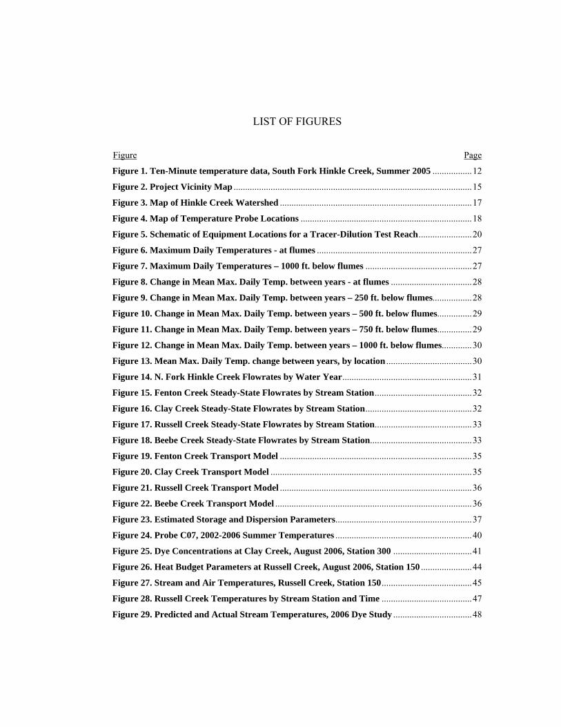
LIST OF FIGURES

Figure Page

Figure 1. Ten-Minute temperature data, South Fork Hinkle Creek, Summer 2005 .................12 Figure 2. Project Vicinity Map .......................................................................................................15 Figure 3. Map of Hinkle Creek Watershed ...................................................................................17 Figure 4. Map of Temperature Probe Locations ..........................................................................18 Figure 5. Schematic of Equipment Locations for a Tracer-Dilution Test Reach.......................20 Figure 6. Maximum Daily Temperatures - at flumes ...................................................................27 Figure 7. Maximum Daily Temperatures – 1000 ft. below flumes ..............................................27 Figure 8. Change in Mean Max. Daily Temp. between years - at flumes ...................................28 Figure 9. Change in Mean Max. Daily Temp. between years – 250 ft. below flumes.................28 Figure 10. Change in Mean Max. Daily Temp. between years – 500 ft. below flumes...............29 Figure 11. Change in Mean Max. Daily Temp. between years – 750 ft. below flumes...............29 Figure 12. Change in Mean Max. Daily Temp. between years – 1000 ft. below flumes.............30 Figure 13. Mean Max. Daily Temp. change between years, by location .....................................30 Figure 14. N. Fork Hinkle Creek Flowrates by Water Year........................................................31 Figure 15. Fenton Creek Steady-State Flowrates by Stream Station..........................................32 Figure 16. Clay Creek Steady-State Flowrates by Stream Station..............................................32 Figure 17. Russell Creek Steady-State Flowrates by Stream Station..........................................33 Figure 18. Beebe Creek Steady-State Flowrates by Stream Station............................................33 Figure 19. Fenton Creek Transport Model ...................................................................................35 Figure 20. Clay Creek Transport Model .......................................................................................35 Figure 21. Russell Creek Transport Model ...................................................................................36 Figure 22. Beebe Creek Transport Model .....................................................................................36 Figure 23. Estimated Storage and Dispersion Parameters...........................................................37 Figure 24. Probe C07, 2002-2006 Summer Temperatures ...........................................................40 Figure 25. Dye Concentrations at Clay Creek, August 2006, Station 300 ..................................41 Figure 26. Heat Budget Parameters at Russell Creek, August 2006, Station 150 ......................44 Figure 27. Stream and Air Temperatures, Russell Creek, Station 150.......................................45 Figure 28. Russell Creek Temperatures by Stream Station and Time .......................................47 Figure 29. Predicted and Actual Stream Temperatures, 2006 Dye Study ..................................48

LIST OF TABLES

Table Page

Table 1. Harvest Area Summary .......................................................................................................17

Table 2. Temperature Probes (*Summer data, late May through early September, typically) ..........19

Table 3. Temperature data collected at flumes (**Continuous data).................................................19

Table 4. Comparison of flow measurement techniques.....................................................................22

Table 5. Statistical Summary.............................................................................................................26

LIST OF EQUATIONS

Equation Page

Equation 1: Brown and Kryger 1970 Temp. Change...........................................................................4

Equation 2: Brown and Kryger 1970 Two-part mixing.......................................................................5

Equation 3: Moore Two-part mixing ...................................................................................................5

Equation 4: Streambed conduction ......................................................................................................6

Equation 5: Bowen Sensible heat exchange ........................................................................................7

Equation 6: Latent heat exchange........................................................................................................7

Equation 7: Shortwave radiation .........................................................................................................8

Equation 8: Longwave radiation..........................................................................................................8

Equation 9: Dye mixing model..........................................................................................................20

Equation 10: Salt slug flowrate calculation .......................................................................................21

Equation 11: Salt slug flowrate approximation .................................................................................21

Equation 12: Wind Function..............................................................................................................25

Equation 13. Mean hyporheic residence time....................................................................................42

Processes That Influence the Downstream Propagation of Stream Temperature from Clearcut Harvest Units:

Hinkle Creek Paired Watershed Study

1. INTRODUCTION

Stream temperature is a water quality parameter of concern in Pacific Northwest forests.

The Oregon Department of Environmental Quality (DEQ) established criteria for Total Maximum

Daily Loads (TMDL) for heat, as measured by stream temperature, in Oregon streams and rivers.

The National Marine Fisheries Service (NMFS) of the National Oceanic and Atmospheric

Administration (NOAA) prepared recovery strategies for species listed under the Endangered

Species Act (ESA), which includes salmonids for which stream temperature is a monitored water

quality parameter. Salmonid species have optimum temperature ranges for growth and

development. High stream temperatures can cause changes in rates of development and increased

susceptibility to disease. (Beschta et al. 1987). Maximum daily stream temperatures increase when

shade over the stream channel is removed (Brown and Krygier 1970). Whether the increase in

maximum daily stream temperature results in heat being propagated downstream is the subject of

research which has had conflicting results (Poole and Berman 2001), (Zwieniecki and Newton

1999), (Johnson and Jones 2000). The processes that affect the propagation of heat downstream are

poorly understood. There is agreement that solar radiation is the primary influence on increasing

maximum stream temperatures in unshaded reaches compared to shaded reaches (Brown and

Krygier 1970), (Webb and Zhang 1999). (Johnson 2004) suggest that changes in stream

temperature after they reenter the forest canopy are more complex and variable. Since solar

radiation is dramatically smaller under the forest canopy, the other heat exchanges between the

stream and its environment also become significant in understanding stream heat. Thus, a reasonable

approach to tracking stream temperature in these shaded reaches is to model the physics of energy

exchanges between the stream and its environment (Sinokrot and Stefan 1993).

A first step in the process of understanding the downstream propagation of stream heat

energy is to measure stream temperature with enough spatial and temporal resolution to aid in

determining the magnitudes of the various heat transfer processes affecting stream heat energy.

This high-resolution data can provide insight into the variability of stream temperature in space and

time and hopefully provides tools for future management, as well as direction for future research.

Toward that end, the amount and variability of changes in stream temperature immediately

2

downstream of clear-cut harvest units in four adjacent small non-fish bearing streams were

measured. Then, the major sources and sinks of energy were quantified to characterize the

magnitudes of the heat exchange processes in these downstream shaded stream reaches.

2. OBJECTIVES

The first objective of this study was to use statistical tests to detect change in temperature

patterns downstream of harvest units between the last year pre-harvest and the first year post-

harvest.

The second objective was to use tracer-dilution dye study data to characterize the flowrates,

velocities, and advection of groundwater on 300-meter reaches immediately downstream of harvest

units. This data was then to be used to estimate the longitudinal dispersion of stream water, the in-

stream storage volume in stream pools and hyporheic zones, and the transfer of stream flow between

the active channel and these storage zones.

The third objective was to estimate the major stream heat budget components on one

stream segment, including longwave radiation, shortwave radiation, latent heat, and sensible heat.

The fourth objective was to compare these three research results.

In addition, it is important to place this research in the context of the body of stream

temperature studies in the Pacific Northwest, since the overall objective of this study was to add to

this body of knowledge. To this end, the following literature review is presented within the

framework of the stream energy budget, providing an organizing method for stream temperature

analysis and discussion.

3. LITERATURE REVIEW

Stream temperature in forests has been the subject of study in the Pacific Northwestern US

for 50 years. In 1958, concern about the growth and development of aquatic species, particularly

salmonids (Brett 1956), resulted in the initiation of the Alsea Logging-Aquatic Resources Study

(Brown and Krygier 1970). This research documented increases of average monthly maximum

stream temperatures of 14°F (7.8°C) following clear-cut logging of a small watershed (Needle

Branch) in the Oregon Coast Range. The details of the Alsea study, including logging methods,

broadcast burning and stream clearing represent a unique suite of treatments, which may account for

the large increases in stream temperature rarely seen elsewhere. Since the time of the Alesa study,

other field experiments have characterized stream temperature changes after forest harvesting in the

region. The H.J. Andrews Experimental Forest in the Western Cascades, Oregon is the site of

ongoing stream temperature studies (Levno et al. 1967); (Johnson and Jones 2000); (Johnson 2004).

3

These studies have examined temperature patterns and the mechanisms that control stream

temperature. Several studies in the Malcolm-Knapp Research Forest in British Columbia, Canada

(Moore et al. 2005);(Gomi et al. 2006) examined thermal response of headwater streams within

clear-cut harvest areas, and examined both above-stream and stream-bed processes. These studies

and other research in this region have shown that changes in stream temperatures resulting from

harvest activities vary from no change, to the magnitude of changes observed in the Alsea study

(Beschta et al. 1987). The range of geology, forest types, and climate these studies represent, as

well as a variety of harvest methods contribute to this range of thermal response.

Following the Alsea study, policies were changed, and state forest practice laws were

enacted to identify and manage the forest activities that had significant impacts on aquatic

ecosystems and the ability of a forest stream to support fish. Each of the western timber producing

states (Oregon, Washington, California) has regulations that require buffer strips to protect riparian

areas and provide shade for large perennial (and typically fish-bearing) streams. However, there

remains an ongoing disagreement regarding the impact of forest harvest on the downstream

propagation of stream heat measured as water temperature. Small, non-fish-bearing headwater

streams have minimal or no requirements for buffer strips in many jurisdictions, and forests in these

regions are typically harvested to stream boundaries. The amount and variability of stream heating

of these streams, as well as the downstream fate of the thermal load are still topics of research and

discussion. “Despite decades of research on stream temperature response to forest harvesting, there

are still vigorous debates in the Pacific Northwest about the thermal impacts of forestry and how to

manage them (Moore et al. 2005)”. The fact that forest management practices vary between study

sites, and that forest practices have changed on any particular site over the last several decades, also

complicates comparisons between studies.

3.1 Stream Energy Budget

The geographic variability of the forested landscapes that are studied confounds efforts to

discern clear patterns of stream behavior, even within the Pacific Northwest (PNW) region. Both

climate, driving above ground energy processes, and geology, dictating below stream energy

exchange, vary spatially. The results of a study from one geographic region are not easily

extrapolated to another region. Both climate and geology vary in time to a lesser degree. Climate

change and erosion processes can change the thermal characteristics of a particular site. This has

led researchers to expand their tools beyond statistical analysis to include physics-based models of

stream temperature behavior.

4

Pioneering this effort was George Brown, who proposed that, during summer clear-sky

conditions, direct solar radiation received by the stream surface dominates the energy budget for

small forest streams in clear cut harvest areas. Sensible heat exchanges with the air or latent heat

exchange from evaporative cooling were small by comparison. The net heat exchange due to

incoming and outgoing longwave radiation between the stream surface and the atmosphere was also

small enough to be ignored (Brown and Krygier 1970). The increase in stream temperature was

directly proportional to the amount of incoming solar radiation, and inversely proportional to the

volume of water in the stream. The equation proposed to determine the amount of increase in the

maximum daily temperature change, (ΔT, °F) in a stream flowing through a clearcut harvest unit is:

Equation 1: )000267.0(⋅⋅=Δ

DHAT

In Equation 1, A is the surface area of stream exposed to solar radiation (ft2), H is the rate

of solar insolation for the day, year, and latitude of interest (BTU/ ft2-min.), D is the discharge

(ft3/sec), 0.000267 is a conversion factor from (ft3 of water/sec) to (lb. of water/min.), and a BTU is

defined as the heat required to raise the temperature of 1 lb. of water 1°F. Brown presented a more

comprehensive method to predict increases in stream temperature that included latent heat

(evaporation), sensible heat (convection), and stream-bed conduction to the energy budget (Brown

1969(2)). Several reach-scale, physics-based stream temperature models have since been

developed. These include TEMPEST (Adams et al. 1989), MNSTREAM (Sinokrot and Stefan 1993),

and Heat Source (Boyd 1996). These modeling efforts have been valuable in understanding stream

temperature processes. However, they are still limited. First, a significant amount of data, both in

climate and stream geometry, is required for input, making them impractical for general use. In

addition, subsurface conditions are difficult to determine, and hyporheic exchange within the stream

channel is poorly understood, and thus may be inadequately modeled. Finally, models must make

simplifying assumptions for mass and energy exchange processes which are inherent in model

development, and may not adequately represent the complexity of energy exchanges in actual

streams. In summary, models can be valuable tools, but given their limitations should not be the

only tool used to understand the stream energy budget. Indeed, the first step in modeling the

physical environment is an understanding of which processes are significant, and the nature of their

interaction. This research explores the stream energy exchange processes downstream of harvest

units within forested reaches, with a goal of increasing the understanding for forest managers and

modelers.

The components or categories of stream energy fall logically into three categories: 1) those

components that involve exchanges of the mass of water only [tributary and hillslope inflow, and

5

downstream movement of stream water defined by velocity and dispersion] 2) those components

that involve exchanges of energy of the water only [bed conduction, sensible/latent exchange,

shortwave radiation/reflection, longwave heat exchange, and internal friction of turbulence], and 3)

the component that involves the mass and energy of the water [hyporheic exchange].

3.1.1 Tributary and Hillslope inflows

The effect on stream temperature from small tributary inflows into larger streams can be

calculated with a simple two-part mixing model. The temperature of the mixture of stream and

tributary flows is (Brown and Krygier 1970):

Equation 2: st

ssttm DD

TDTDT++

=

where Dt is discharge of the tributary, Ds is the main stream discharge at the upper end of

the reach, Tt is the temperature of the tributary, and Ts is the main stream temperature at the upper

end of the reach.

If the fraction of total flow in a reach which enters from a tributary is defined as fi = Dt /(Ds

+ Dt), then this relationship of temperature for a mixture can be expressed as (Moore et al. 2005):

Equation 3: Tm = Ts + fi (Tt – Ts.)

This statement of the mixing model illustrates how both the fraction of tributary inflow fi, and the

difference in its temperature from the stream, (Tt – Ts.) modify stream temperature. The effect of

the influx of groundwater on stream temperature can be calculated in the same manner if the

temperature and flowrate of the groundwater are known (Brown and Krygier 1970).

3.1.2 Longitudinal transport and dispersion

The velocity of the water in a stream varies across the stream cross-section. This results in

longitudinal dispersion of the water and its heat energy as the water moves downstream. The

relative importance of dispersion of stream water on stream temperature has been debated. One

modeling study of river temperatures found that longitudinal dispersion did not affect modeled

temperatures, and thus was set to zero. However all the streams in the study had relatively high

velocities and low longitudinal temperature gradients compared to headwater streams (Sinokrot and

Stefan 1993). In his review of the literature, (Moore et al. 2005) commented on the impact of

longitudinal dispersion on stream temperatures that “no published studies appear to have evaluated

its influence in small streams”. Clearly, streams with variable cross-sections and depths, and those

that have a longitudinal pool/step structure have more potential for longitudinal dispersion than river

6

systems. Thus, further study would be instructive in characterizing the role of longitudinal

dispersion on temperatures in headwater stream systems.

3.1.3 Bed Conduction

Heat conduction between the stream water and stream bed depends on the temperature

gradient between the stream and stream bed and the thermal conductivity of the substrate (Brown

1985); (Gauger and Skaugset 2004). Bed conduction of the heat in a stream is a significant

predictor the diel variations in stream temperature (Brown 1969(2)); (Hondzo and Stefan 1994).

Solving for the magnitude of streambed conduction in a one-dimensional advection-

dispersion model requires knowledge of the temperature profile of the stream bed, and how it

changes in time. This can be estimated using a slab approximation (Hondzo and Stefan 1994):

Equation 4: dx

TdkdtdTcP

2

=⋅ρ

where ρ is the density of water, cp is the heat capacity of water per unit mass, T is the streambed

temperature, k is the effective heat conductivity of the streambed medium, x is the distance into the

streambed, and t is time. Since the heat exchange with the streambed varies with both depth and

time, the temperature of the streambed from this differential equation can be estimated using a finite

difference approximation of equation 4.

The magnitude of bed conduction in the overall budget of stream heat also depends on the

time of contact and the area of contact between the stream and bed. (Brown 1969) initially

hypothesized that bedrock was more important to the heat exchange process than gravel substrate.

A recent study found that conduction in a bedrock reach of a headwater stream, conduction was a

minor portion of the overall heat budget. (Johnson 2004). The stream in the Johnson study

(Watershed 3 [WS3], H. J. Andrews Experimental Forest) flows from a bedrock reach into an

alluvial reach, where the velocity of the stream decreased dramatically, and the contact area of the

surface of the streambed increased accordingly. The significant dampening of maximum and

minimum daily temperatures in this alluvial reach suggested that streambed conduction, in addition

to hyporheic exchange play an important role in low-velocity, high-contact area stream reaches

(Johnson and Jones 2000).

3.1.4 Sensible/Latent Heat

Sensible heat in air (heat stored as an increase in air temperature, often called convective

heat) can be exchanged between air and water. The magnitude of the rate of change is a function of

the difference in temperature between the air and water, and of the wind speed, which affects the

7

thickness of the laminar boundary layer at the air/water interface. Sensible heat exchange, Hc, can

be expressed as (Bowen 1926):

Equation 5: )()(1000

61.0 aZSZa

C TTWftnLPH −⋅⋅= ρ

where Pa is the atmospheric pressure, ρ is the water density, L is the latent heat of vaporization of

water, (Wftn)z is a wind function using wind velocity at height z above the water, TS is the water

surface temperature, and TaZ is the air temperature at height z (Sinokrot and Stefan 1993).

Latent or evaporative heat is the energy transferred between water and air when water

evaporates from the stream surface (which removes heat from the system) or condenses on it (which

adds heat). It is a function of wind speed, and the vapor pressure gradient between the air and

water, and can be calculated as:

Equation 6: )()( aZSWZe eeWftnLH −= ρ

where eSW is the saturation vapor pressure at the water surface, eaZ is the vapor pressure in air at

height z above the stream, and the same wind function as was used for sensible heat. When

equations 5 and 6 are compared, the evaporative heat flux and sensible heat flux at a given

atmospheric pressure are related by the ratio of the temperature gradient to vapor pressure gradient

between the water surface and the overlying air, which is called the Bowen Ratio.

Sensible and latent heat flux terms have been considered to be small and unimportant to the

stream energy budget in forest environments, since wind speeds in are typically low, and vapor

pressures above streams are typically high (Beschta et al. 1987). Even though Sensible and Latent

heat fluxes tend to be small and counteract each other in forest stream settings, one study

hypothesized that evaporative cooling during the day may have been underestimated in closing the

energy budget for a shaded headwater stream. (Moore et al. 2005).

3.1.5 Shortwave Radiation/Reflection

Incoming shortwave or solar radiation (Hsi) is a parameter that is typically measured, and

its magnitude at the stream surface varies according to the path of the sun, and any intervening

topography or vegetation between the sun and the stream surface. Solar radiation can be diffused or

reflected by landscape or plant surfaces. To characterize this complexity, solar (shortwave)

radiation can be measured at, or directly above, the stream surface. When the sun angle is within

30° of vertical, more than 90% of the available solar insolation is available to enter the water surface

and become available for stream (or streambed) heating, provided it is not intercepted by shade-

producing vegetation (Johnson 2004). The remaining solar radiation is reflected, Hsr. For modeling

8

purposes, net shortwave solar radiation entering a stream (HS) can be expressed as the difference

between the incoming and reflected solar radiation, modified by a shading factor (SF), which is the

percentage of radiation blocked by vegetation or topography. Incoming solar radiation is quantified

using the expression (Sinokrot and Stefan 1993):

Equation 7: )1)(( SFHHH srsiS −−=

3.1.6 Longwave Heat Exchanges

Incoming longwave radiation from above the stream is the sum of longwave radiation

emitted by the atmosphere, vegetation, and surrounding soil or rock. Outgoing longwave radiation

is the longwave radiation emitted by the water into the atmosphere. Net longwave radiation

exchange is calculated using the Stefan-Boltzman law:

Equation 8: )( 44aaSWL TTH εεσ −=

where σ is the Stefan-Boltzman constant, εw is the emissivity of the stream water surface, εa is the

emissivity of the atmosphere, Ts is the stream temperature, and Ta is the air temperature. For Pacific

Northwest forest streams, net longwave radiation adds heat to streams during the day, and is a net

heat loss from streams at night (Story et al. 2003).

3.1.7 Hyporheic Exchange Flows

Hyporheic exchange flow is defined as the transfer of water between the stream and the

saturated sediments in the stream bed and adjacent riparian zone (Moore et al. 2005). (Bilby 1984),

in an early study fish habitat in a Western Washington stream (Thrash Creek), found 39 local cool

spots in a 3.5 km reach. These cool spots included lateral seeps, pool bottom seeps, cold tributaries,

and flow through the bed (hyporheic exchange). They accounted for 1.6% of the stream surface

area, and 2.9% of the water volume. Since these areas were considered to be rare by this study,

hyporheic exchange has often thought to be a small part of the stream energy budget (Beschta et al.

1987). More recent studies, however, have shown that the hyporheic zone can be an important flow

pathway in headwater streams (Haggerty et al. 2002); (Kasahara and Wondzell 2003). The

influence of hyporheic flow on stream temperature was dramatically demonstrated in the Watershed

(WS3) experiment H. J. Andrews. After the stream had flowed through a bedrock reach, the daily

maximum stream temperatures had increased by several degrees. In an alluvial reach immediately

downstream, where the stream flowed through a sediment deposit, the daily maximum temperatures

then decreased by as much as 8.7°C, and the daily minimum temperatures increased by 3.9°C.

(Johnson 2004). (Story et al. 2003), in a study of stream cooling linked to subsurface hydrology,

9

found that maximum daily temperatures in a forested stream reach downstream of a clear-cut

cooled 2.3°C in less than 250 meters. Conduction by the stream bed and hyporheic exchange

accounted for approximately 60% of the total cooling effect, and groundwater inflow accounted for

the rest.

3.2 Downstream and Cumulative Effects

In the context of this research history, two questions have been explored relative to

downstream effects:

1) What happens to the temperature of a stream when it re-enters the forest downstream of a clear-

cut harvest unit?

2) What factors are responsible for these temperature changes?

A range of testable hypotheses have been presented to explain empirical results. One hypothesis is

that forested streams have an equilibrium temperature inherent to the local environment, and any

water that is warmer or cooler than that equilibrium temperature will move toward it upon entering

the forested reach (Zwieniecki and Newton 1999). Under this hypothesis, this recovery zone, or

thermal transition reach, is the only region where temperatures exist above or below the stream’s

equilibrium temperature.

(Beschta et al. 1987) has offered an alternative hypothesis.

“Once a stream’s temperature is increased, the heat is not readily dissipated to the atmosphere as it flows through a shaded reach. Hence, additional energy inputs to small streams can have an additive effect on downstream temperatures”.

They further suggest that:

“where cooler inflows do not occur, temperature increases from each exposed reach will not decrease appreciably through the shaded reaches, and the result is a ‘stair-step’ temperature increase in the downstream direction”.

Another perspective is that stream energy in the headwater reaches of forest streams are

dominated by groundwater inputs, whereas stream energy in the lower reaches is dominated by

atmospheric inputs (Poole and Berman 2001). In this context, Poole suggests that any stream

temperature increases in the transitional middle reaches between these two thermal regimes can both

decrease local cool water habitat, and transport this added heat downstream.

Finally, the downstream effects of timber harvest on stream temperature can be analyzed

using statistical tests for change detection. (Beschta and Taylor 1988) analyzed 30 years of stream

temperature data (1955 to 1984) from the Salmon Creek watershed, in the Oregon Cascades. An

index of ‘cumulative harvesting effects’ was calculated for the watershed, based on five years of full

10

sun exposure following harvest, and then a linear decrease to zero exposure at twenty years. This

sun exposure factor was multiplied by the area harvested in each exposure level. This index was

correlated with the average of the maximum daily stream temperatures for the ten warmest days of

each year. Using this metric, the authors concluded that ‘the cumulative effect of forest land use has

apparently been an important factor (r2=0.65) in stream temperature increases that have occurred in

the Salmon Creek drainage over the past 30 years’. They note, however, that several factors make it

difficult to draw cause-and-effect conclusions. These factors include the large peak flows in 1964-

65 and 1971, and the associated mass soil movements that occurred in riparian areas; the extensive

salvage logging that occurred along many streams in the late 1960’s and the 1970’s; and the

introduction of the Oregon Forest Practices Act harvest methods in the late 1970’s. Also noted was

the historic low summer flows during the years 1976-1981, averaging 20 percent lower than the 30-

year average. As with any statistical analysis, the effect of human-caused change (forest harvest, in

this case) must, as the authors suggest, be considered in the larger context of all factors that

influence the measured impact (here, stream temperature).

3.2.1 Downstream Cooling and Temporal Cycles

The temperatures of headwater streams in the PNW vary primarily in two temporal cycles,

diel and annual. The diel cycle typically varies between daytime heating and nighttime cooling

during the summer. The question of how much energy received by headwater streams is transported

downstream is thus linked to the magnitude of these diel energy exchanges relative to magnitude of

energy received by the stream in forest openings such as clear cuts. As water warmed in a clear cut

re-enters a forested reach and goes through an overnight cooling cycle, the mass and heat transfer

processes operate, resulting in the stream water moving toward an equilibrium energy condition

with its environment.

There is disagreement among researchers whether the processes that lead to downstream

cooling by this diel cycle can bring stream temperatures back to pre-disturbance levels. (Zwieniecki

and Newton 1999) concluded that forested streams in western Oregon cooled to an equilibrium

temperature pattern within 150 meters after entering forest below harvest unit. (Bartholow 2002)

simulated the cumulative effects of harvest and temperature ‘recovery’ using the SSTEMP model,

and found that downstream equilibrium conditions strongly influenced downstream temperatures,

but suggest that more study is needed to quantify the rates of recovery and processes involved.

(Johnson 2004) notes that longitudinal temperature dynamics in forested streams are complex and

dynamic, and a better understanding of the mechanisms of energy exchange is important in future

research. In a case study of diel energy flux downstream of a forest harvest unit in the Oregon

11

Cascades, a drop of 3°C was observed in maximum daily temperature in a 300 meter forested stream

reach. An energy budget of the stream reach showed that the sum of ‘above stream’ energy flux

and advection of hillslope water could not account for the magnitude of this temperature drop.

Conduction by the stream bed and hyporheic exchange were suggested as mechanisms that may be

important factors (Gauger and Skaugset 2004).

The annual cycle of stream temperature during the summer season is dominated by two

processes, solar input (solar elevation and day length), and the discharge of the stream. The date of

maximum solar angle roughly coincides with the end of spring rainfall in the PNW. Thus, as the

length of day and sun angle decrease, stream discharge also decreases. This results in a period of

approximately two months (July and August) where these two primary determinants of stream

temperature (Brown 1969) create a period of highest potential for stream heating. Prior to this

period, high stream flows moderate water temperatures. After this period, lower solar angles and

shorter day length minimize solar inputs. This annual cycle may be significant in determining the

temperature dynamics in streams where summer flows are dominated by the contributions of water

that has been stored in the hillslope during the winter and spring seasons, or in previous years

(McDonnell 1990). Forested streams may be sensitive to seasonal patterns of rain and snow fall that

can influence their temperature during the summer, when maximum stream heating potential exists.

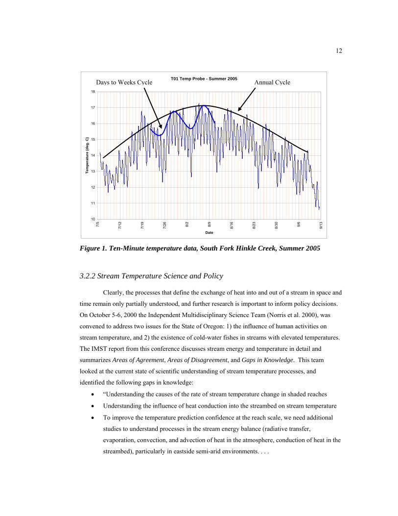
Summers in western Oregon are typically characterized by warm weather and clear skies,

but periods of warmer and cooler weather do occur on a cycle of days to weeks. This variation in

weather overlays a third cycle to the pattern of stream temperature. Figure 1 shows the stream

temperature for the South fork of Hinkle Creek during the summer of 2005, and it illustrates the

three cyclical patterns.

12

T01 Temp Probe - Summer 2005

10

11

12

13

14

15

16

17

187/

5

7/12

7/19

7/26 8/2

8/9

8/16

8/23

8/30 9/6

9/13

Date

Tem

pera

ture

(deg

. C)

Figure 1. Ten-Minute temperature data, South Fork Hinkle Creek, Summer 2005

3.2.2 Stream Temperature Science and Policy

Clearly, the processes that define the exchange of heat into and out of a stream in space and

time remain only partially understood, and further research is important to inform policy decisions.

On October 5-6, 2000 the Independent Multidisciplinary Science Team (Norris et al. 2000), was

convened to address two issues for the State of Oregon: 1) the influence of human activities on

stream temperature, and 2) the existence of cold-water fishes in streams with elevated temperatures.

The IMST report from this conference discusses stream energy and temperature in detail and

summarizes Areas of Agreement, Areas of Disagreement, and Gaps in Knowledge. This team

looked at the current state of scientific understanding of stream temperature processes, and

identified the following gaps in knowledge:

• “Understanding the causes of the rate of stream temperature change in shaded reaches

• Understanding the influence of heat conduction into the streambed on stream temperature

• To improve the temperature prediction confidence at the reach scale, we need additional

studies to understand processes in the stream energy balance (radiative transfer,

evaporation, convection, and advection of heat in the atmosphere, conduction of heat in the

streambed), particularly in eastside semi-arid environments. . . .

Annual Cycle Days to Weeks Cycle

13

• Heat transfer from convection and evaporation . . .

• How much localized heating is transferred downstream and for what distance can it be

detected? . . .

• Understanding the relationship between Hyporheic flow and stream temperature.”

These comments highlight the need for additional research concerning stream energy

processes downstream of forest harvest areas. This thesis adds to the growing body of knowledge

which seeks to fill some of the ‘Knowledge Gaps’ identified by the IMST.

There is also a growing debate regarding the legal meaning of a “downstream impact”. In

January, 2001 the US Supreme Court ruled in the case of Solid Waste Agency of Northern Cook

County (SWANCC) v. U.S. Army Corps of Engineers (COE), holding that the COE exceeded their

use of the Clean Water Act (CWA) in regulating intrastate, non-navigable, isolated waters as ‘waters

of the U. S.’. In the majority opinion, the court gave the reasoning that the CWA intended that there

be some ‘connection’ between upland waters and the waters regulated as ‘navigable waters’, stating

that there must be a ‘significant nexus’ to the navigable waters for the CWA to apply. Since this

decision, there have been numerous lawsuits that challenge the jurisdiction of the CWA, specifically

dealing with the meaning of the terms ‘tributary’, ‘significant nexus’ and ‘adjacency’ (Nadeau and

Rains 2007). Federal Court decisions in most of these cases have upheld the CWA jurisdiction,

despite the SWANCC decision. Two cases in the Fifth Circuit Court, however, have succeeded in

using the SWANCC decision to deny CWA jurisdiction. On February 21, 2006 the Supreme Court

heard oral arguments in these two cases, John A Rapanos et al. v. United States (Rapanos) and June

Carabell et. al. v. United States Army COE and United States Environmental Protection Agency

(Carabell). Both cases argued that if the CWA covers any wetlands other than those that abut

navigable waters, those bodies enforcing the law have exceeded the intent of the commerce clause

under which the CWA was enacted. On June 19, 2006, the U.S. Supreme Court handed down a 4-1-

4 split decision on these two cases, which had three principle opinions. Four Justices held that the

cases should be remanded to the lower courts, and four held that the Fifth Circuit had ruled

correctly. Justice Kennedy held with the four judges that remanded the cases, but did not agree with

their opinion that the CWA did not apply to ephemeral or intermittent flowing water. He held that

the CWA could apply to “wetlands, either alone or in combination with similarly situated lands in

the region, that significantly affect the chemical, physical, and biological integrity of other covered

waters more readily understood as ‘navigable.’ ” He further stated that, where there are not specific

regulations, the COE “must establish a significant nexus on a case-by-case basis”.

Scientists are now faced with defining what these words mean in application. In the

forested streams of this study, future management regulations, either State or Federal, will certainly

14

be driven by whether there may be a “chemical, physical, and biological” impact on downstream

receiving waters. Specific to this study, the question of whether heat added to headwater streams

has downstream impacts becomes relevant.

3.3 Literature Review Conclusions

A summary of the present understanding of headwater stream temperature dynamics from

the literature is as follows:

• The primary energy input to forest streams during the summer season is direct solar

radiation

• Streamside shade is an effective method of limiting the input of solar radiation.

• The factors that influence stream temperature in shaded reaches are complex and variable

in both time and space.

• Both mass transfer processes (advection of hillslope water, hyporheic flows) and energy

transfer processes (radiation balance, latent and sensible heat exchanges) are important in

understanding stream temperature dynamics.

15

4. STUDY AREA

4.1 Location

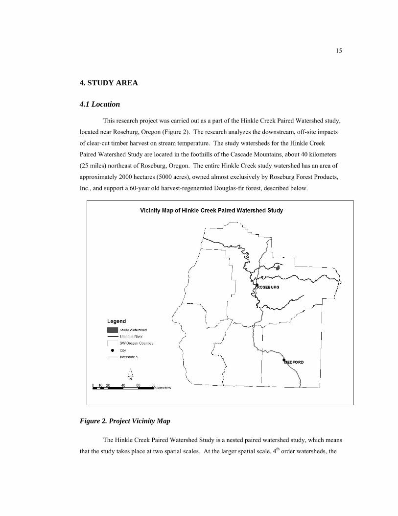
This research project was carried out as a part of the Hinkle Creek Paired Watershed study,

located near Roseburg, Oregon (Figure 2). The research analyzes the downstream, off-site impacts

of clear-cut timber harvest on stream temperature. The study watersheds for the Hinkle Creek

Paired Watershed Study are located in the foothills of the Cascade Mountains, about 40 kilometers

(25 miles) northeast of Roseburg, Oregon. The entire Hinkle Creek study watershed has an area of

approximately 2000 hectares (5000 acres), owned almost exclusively by Roseburg Forest Products,

Inc., and support a 60-year old harvest-regenerated Douglas-fir forest, described below.

Figure 2. Project Vicinity Map

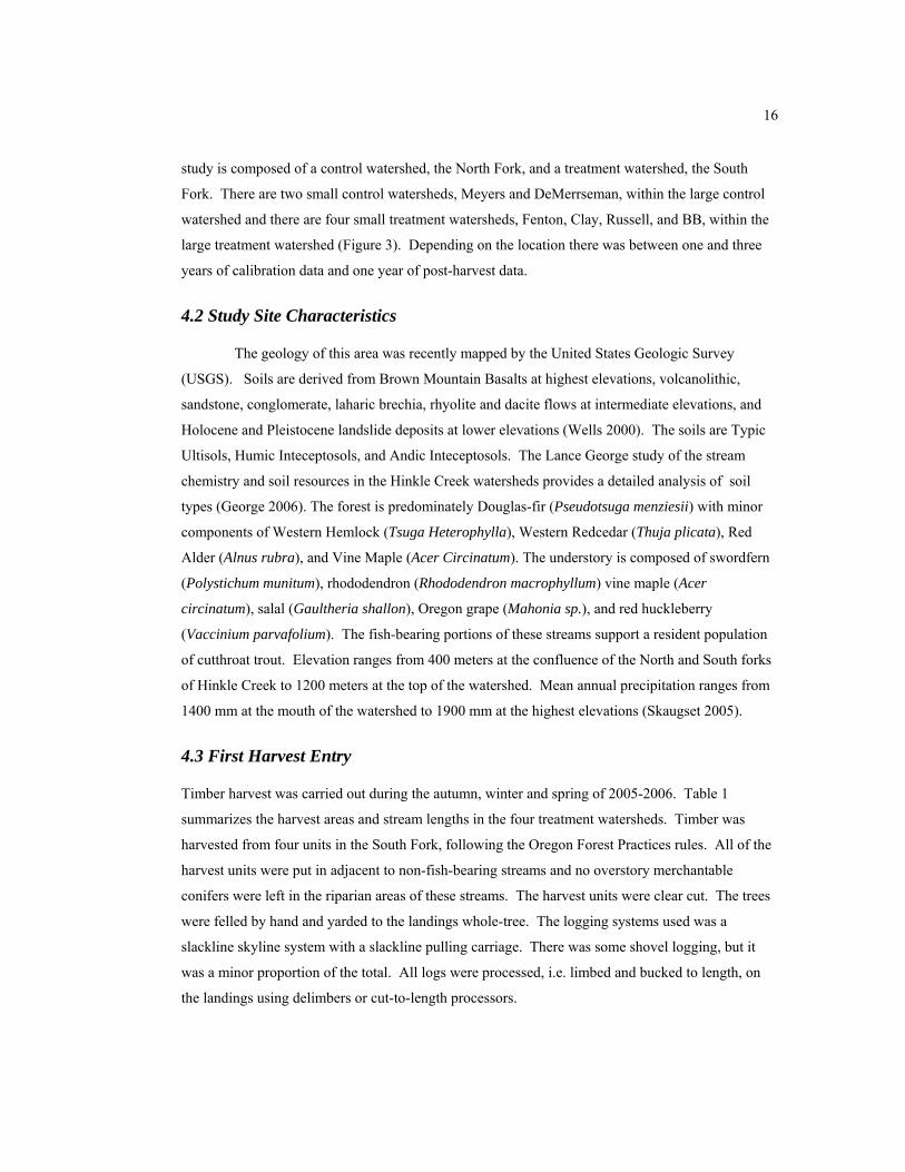
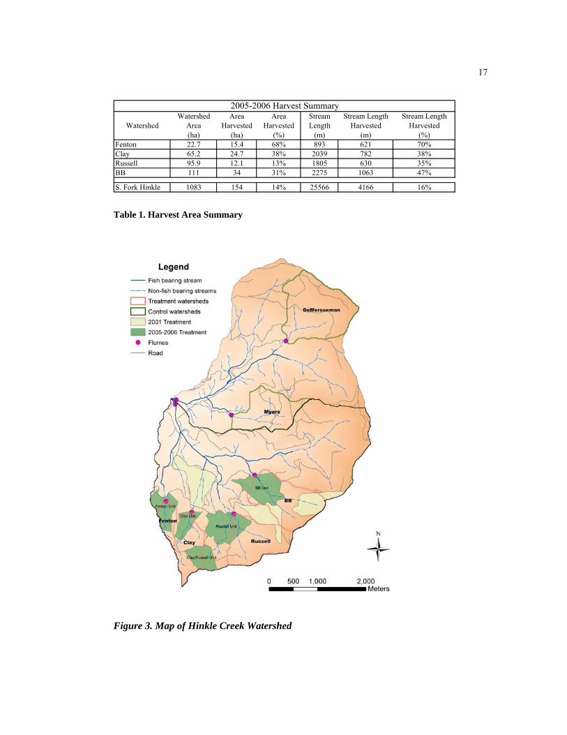
The Hinkle Creek Paired Watershed Study is a nested paired watershed study, which means

that the study takes place at two spatial scales. At the larger spatial scale, 4th order watersheds, the

16

study is composed of a control watershed, the North Fork, and a treatment watershed, the South

Fork. There are two small control watersheds, Meyers and DeMerrseman, within the large control

watershed and there are four small treatment watersheds, Fenton, Clay, Russell, and BB, within the

large treatment watershed (Figure 3). Depending on the location there was between one and three

years of calibration data and one year of post-harvest data.

4.2 Study Site Characteristics

The geology of this area was recently mapped by the United States Geologic Survey

(USGS). Soils are derived from Brown Mountain Basalts at highest elevations, volcanolithic,

sandstone, conglomerate, laharic brechia, rhyolite and dacite flows at intermediate elevations, and

Holocene and Pleistocene landslide deposits at lower elevations (Wells 2000). The soils are Typic

Ultisols, Humic Inteceptosols, and Andic Inteceptosols. The Lance George study of the stream

chemistry and soil resources in the Hinkle Creek watersheds provides a detailed analysis of soil

types (George 2006). The forest is predominately Douglas-fir (Pseudotsuga menziesii) with minor

components of Western Hemlock (Tsuga Heterophylla), Western Redcedar (Thuja plicata), Red

Alder (Alnus rubra), and Vine Maple (Acer Circinatum). The understory is composed of swordfern

(Polystichum munitum), rhododendron (Rhododendron macrophyllum) vine maple (Acer

circinatum), salal (Gaultheria shallon), Oregon grape (Mahonia sp.), and red huckleberry

(Vaccinium parvafolium). The fish-bearing portions of these streams support a resident population

of cutthroat trout. Elevation ranges from 400 meters at the confluence of the North and South forks

of Hinkle Creek to 1200 meters at the top of the watershed. Mean annual precipitation ranges from

1400 mm at the mouth of the watershed to 1900 mm at the highest elevations (Skaugset 2005).

4.3 First Harvest Entry

Timber harvest was carried out during the autumn, winter and spring of 2005-2006. Table 1

summarizes the harvest areas and stream lengths in the four treatment watersheds. Timber was

harvested from four units in the South Fork, following the Oregon Forest Practices rules. All of the

harvest units were put in adjacent to non-fish-bearing streams and no overstory merchantable

conifers were left in the riparian areas of these streams. The harvest units were clear cut. The trees

were felled by hand and yarded to the landings whole-tree. The logging systems used was a

slackline skyline system with a slackline pulling carriage. There was some shovel logging, but it

was a minor proportion of the total. All logs were processed, i.e. limbed and bucked to length, on

the landings using delimbers or cut-to-length processors.

17

Watershed Area Area Stream Stream Length Stream LengthWatershed Area Harvested Harvested Length Harvested Harvested

(ha) (ha) (%) (m) (m) (%)Fenton 22.7 15.4 68% 893 621 70%Clay 65.2 24.7 38% 2039 782 38%Russell 95.9 12.1 13% 1805 630 35%BB 111 34 31% 2275 1063 47%

S. Fork Hinkle 1083 154 14% 25566 4166 16%

2005-2006 Harvest Summary

Table 1. Harvest Area Summary

Figure 3. Map of Hinkle Creek Watershed

18

5. METHODS

5.1 Stream Temperature Sampling

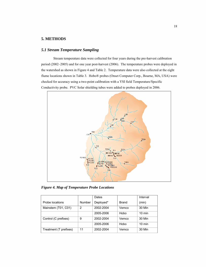
Stream temperature data were collected for four years during the pre-harvest calibration

period (2002–2005) and for one year post-harvest (2006). The temperature probes were deployed in

the watershed as shown in Figure 4 and Table 2. Temperature data were also collected at the eight

flume locations shown in Table 3. Hobo® probes (Onset Computer Corp., Bourne, MA, USA) were

checked for accuracy using a two-point calibration with a YSI field Temperature/Specific

Conductivity probe. PVC Solar shielding tubes were added to probes deployed in 2006.

Figure 4. Map of Temperature Probe Locations

Probe locations Number

Dates

Deployed* Brand

Interval

(min)

Mainstem (T01, C01) 2 2002-2004 Vemco 30 Min

2005-2006 Hobo 10 min

Control (C prefixes) 9 2002-2004 Vemco 30 Min

2005-2006 Hobo 10 min

Treatment (T prefixes) 11 2002-2004 Vemco 30 Min

19

2005-2006 Hobo 10 min

Below Treatment

Flumes (FE, CL, RUS,

and BB prefixes) 16 2005-2006 Hobo 10 min

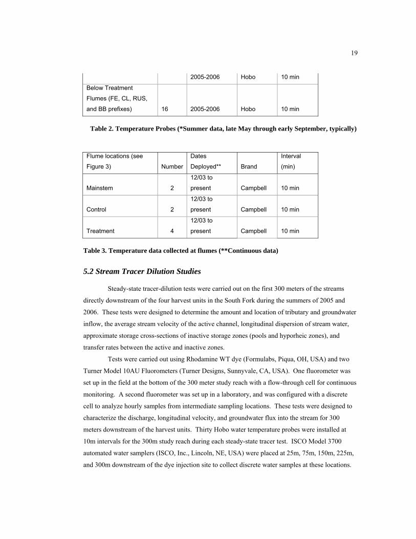
Table 2. Temperature Probes (*Summer data, late May through early September, typically)

Flume locations (see

Figure 3) Number

Dates

Deployed** Brand

Interval

(min)

Mainstem 2

12/03 to

present Campbell 10 min

Control 2

12/03 to

present Campbell 10 min

Treatment 4

12/03 to

present Campbell 10 min

Table 3. Temperature data collected at flumes (**Continuous data)

5.2 Stream Tracer Dilution Studies

Steady-state tracer-dilution tests were carried out on the first 300 meters of the streams

directly downstream of the four harvest units in the South Fork during the summers of 2005 and

2006. These tests were designed to determine the amount and location of tributary and groundwater

inflow, the average stream velocity of the active channel, longitudinal dispersion of stream water,

approximate storage cross-sections of inactive storage zones (pools and hyporheic zones), and

transfer rates between the active and inactive zones.

Tests were carried out using Rhodamine WT dye (Formulabs, Piqua, OH, USA) and two

Turner Model 10AU Fluorometers (Turner Designs, Sunnyvale, CA, USA). One fluorometer was

set up in the field at the bottom of the 300 meter study reach with a flow-through cell for continuous

monitoring. A second fluorometer was set up in a laboratory, and was configured with a discrete

cell to analyze hourly samples from intermediate sampling locations. These tests were designed to

characterize the discharge, longitudinal velocity, and groundwater flux into the stream for 300

meters downstream of the harvest units. Thirty Hobo water temperature probes were installed at

10m intervals for the 300m study reach during each steady-state tracer test. ISCO Model 3700

automated water samplers (ISCO, Inc., Lincoln, NE, USA) were placed at 25m, 75m, 150m, 225m,

and 300m downstream of the dye injection site to collect discrete water samples at these locations.

20

The ISCO sampler located at 25m was used to diagnose any problems with the injection equipment.

Dye fluorescence was continuously monitored by the field fluorometer located at 300m (the bottom

of the study reach). Fluorescence was converted to dye concentration, so a continuous trace of real

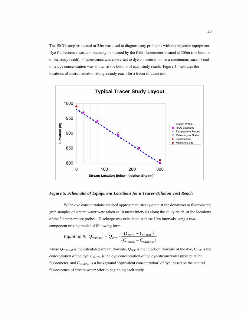
time dye concentration was known at the bottom of each study reach. Figure 3 illustrates the

locations of instrumentation along a study reach for a tracer dilution test.

Typical Tracer Study Layout

800

850

900

950

1000

0 100 200 300Stream Location Below Injection Site (m)

Elev

atio

n (m

) Stream ProfileISCO LocationsTemperature ProbesMeterological StationInjection SiteMonitoring Site

Figure 5. Schematic of Equipment Locations for a Tracer-Dilution Test Reach

When dye concentrations reached approximate steady-state at the downstream fluorometer,

grab samples of stream water were taken at 10 meter intervals along the study reach, at the locations

of the 30 temperature probes. Discharge was calculated at these 10m intervals using a two-

component mixing model of following form:

Equation 9: )(

)(

STREAMTOTAL

TOTALDYEDYESTREAM CC

CCQQ−−

⋅=

where QSTREAM is the calculated stream flowrate, QDYE is the injection flowrate of the dye, CDYE is the

concentration of the dye, CTOTAL is the dye concentration of the dye/stream water mixture at the

fluorometer, and CSTREAM is a background ‘equivalent concentration’ of dye, based on the natural

fluorescence of stream water prior to beginning each study.

21

The discharges of the study streams were measured at the monitoring sites prior to each

tracer test to determine the volume, concentration, and injection rates of dye needed. These

discharge measurements were made with a Marsh McBirney Flowmate Model 2000 Portable

Flowmeter and top-setting rod. For each steady-state tracer test, dye was injected with an FMI

Model QG150 Lap pump (115 V.AC, 0-15 ml/min.) for 2005 tests and the first two 2006 tests. This

pump was replaced by an FMI Model QBC-1 Lab Pump, (12V.DC, 0-19.2ml/min.)(Fluid Metering,

Inc., Syosset, NY, USA) for the balance of the 2006 field season. Stream water/dye mixture for the

monitoring site fluorometer was continuously pumped using a 12V. DC peristaltic pump

(Masterflex Model 7518-12). All 12Volt equipment was powered with Exide Orbital or Trojan

brands Marine Deep cycle batteries. All AC power was supplied from batteries using a Vector

VECO 43 750 Watt DC to AC converter.

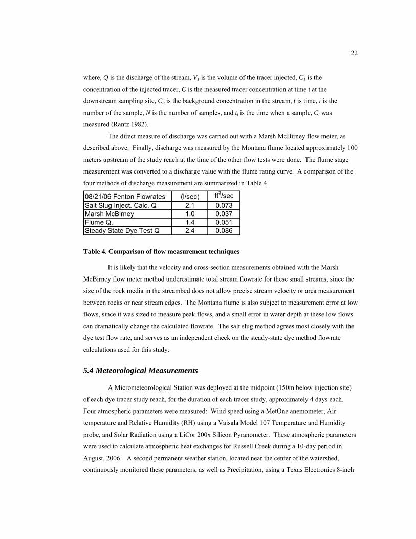
5.3 Stream Flow Measurement

Tracer dilution measurements of discharge were compared to measurements of discharge

obtained with other methods. Three other measurement techniques were compared to the tracer

dilution results on August 21, 2006 on Fenton Creek at the top of the study reach. These methods

were 1) Slug test using salt, and 2) Direct measurement with a Marsh McBirney flow meter, and 3)

the Montana Flume installed at this location. The slug test used salt (NaCl) as a tracer (Rantz 1982;

Moore et al. 2005). A YSI Model 556 multiprobe (YSI Environmental, Inc.) was used to measure

and record Specific Conductance (SC) of the stream water. A solution containing 0.8 liters of

stream water and 155 grams of NaCl (193.75 g/l concentration) was injected at the upper end of a

road culvert at upstream end the Fenton study reach. SC measurements, corrected for temperature,

were recorded in the stream at one second intervals below the culvert, approximately 30m

downstream, until values returned to background levels. A linear calibration relationship was

developed between electrical conductance (µS/cm) and NaCl concentration (mg/l) to determine

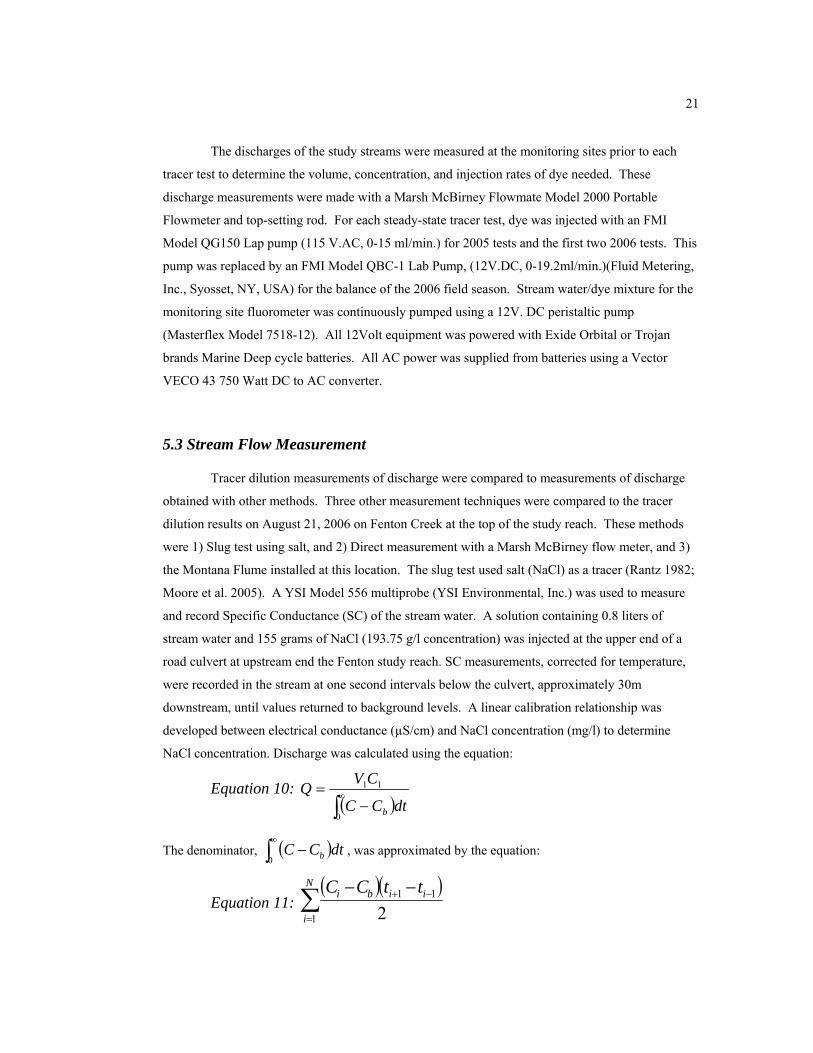
NaCl concentration. Discharge was calculated using the equation:

Equation 10: ( )∫∞

−=

0

11

dtCC

CVQb

The denominator, ( )∫∞

−0

dtCC b , was approximated by the equation:

Equation 11: ( )( )∑

=

−+ −−N

i

iibi ttCC1

11

2

22

where, Q is the discharge of the stream, V1 is the volume of the tracer injected, C1 is the

concentration of the injected tracer, C is the measured tracer concentration at time t at the

downstream sampling site, Cb is the background concentration in the stream, t is time, i is the

number of the sample, N is the number of samples, and ti is the time when a sample, Ci was

measured (Rantz 1982).

The direct measure of discharge was carried out with a Marsh McBirney flow meter, as

described above. Finally, discharge was measured by the Montana flume located approximately 100

meters upstream of the study reach at the time of the other flow tests were done. The flume stage

measurement was converted to a discharge value with the flume rating curve. A comparison of the

four methods of discharge measurement are summarized in Table 4.

08/21/06 Fenton Flowrates (l/sec) ft3/secSalt Slug Inject. Calc. Q 2.1 0.073Marsh McBirney 1.0 0.037Flume Q, 1.4 0.051Steady State Dye Test Q 2.4 0.086

Table 4. Comparison of flow measurement techniques

It is likely that the velocity and cross-section measurements obtained with the Marsh

McBirney flow meter method underestimate total stream flowrate for these small streams, since the

size of the rock media in the streambed does not allow precise stream velocity or area measurement

between rocks or near stream edges. The Montana flume is also subject to measurement error at low

flows, since it was sized to measure peak flows, and a small error in water depth at these low flows

can dramatically change the calculated flowrate. The salt slug method agrees most closely with the

dye test flow rate, and serves as an independent check on the steady-state dye method flowrate

calculations used for this study.

5.4 Meteorological Measurements

A Micrometeorological Station was deployed at the midpoint (150m below injection site)

of each dye tracer study reach, for the duration of each tracer study, approximately 4 days each.

Four atmospheric parameters were measured: Wind speed using a MetOne anemometer, Air

temperature and Relative Humidity (RH) using a Vaisala Model 107 Temperature and Humidity

probe, and Solar Radiation using a LiCor 200x Silicon Pyranometer. These atmospheric parameters

were used to calculate atmospheric heat exchanges for Russell Creek during a 10-day period in

August, 2006. A second permanent weather station, located near the center of the watershed,

continuously monitored these parameters, as well as Precipitation, using a Texas Electronics 8-inch

23

tipping-bucket rain gage. Permanent weather station data was not used in this study, but was useful

in verification of the mobile station data.

5.5 Data Analysis

5.5.1 Statistical Analysis

A first step in understanding this downstream process is to measure temperatures with

enough spatial and temporal resolution to determine where further research and management effort

should be focused. As noted above, this study seeks to characterize the variability of downstream

temperatures before and after the clear-cut harvest in four small non-fish-bearing streams.

Specifically, changes in Maximum Daily Temperature are analyzed between the last summer season

pre-harvest (2005), and the first summer season post-harvest (2006). Stream temperatures at the

harvest boundary are compared to measurements taken at 75m intervals for 300m downstream.

The effect of timber harvest on maximum daily stream temperature downstream of the

harvest units was evaluated using statistical tests in the context of a Before-After-Control-Impact

(BACI) study design. This method is considered to be the most rigorous method of detecting

changes to hydrologic processes following forest harvesting (Gomi et al. 2006). Traditional paired

watershed studies, in which stream temperatures were evaluated using one annual maximum value,

required many years of calibration to detect a statistically significant effect. This paper, however,

documents changes in stream temperature pre- and post-harvest, using maximum daily stream

temperatures of the four treatment streams for a single year before and after harvest. A multiple

linear regression model compared 2005 data with 2006 for each stream, using Myers Creek data

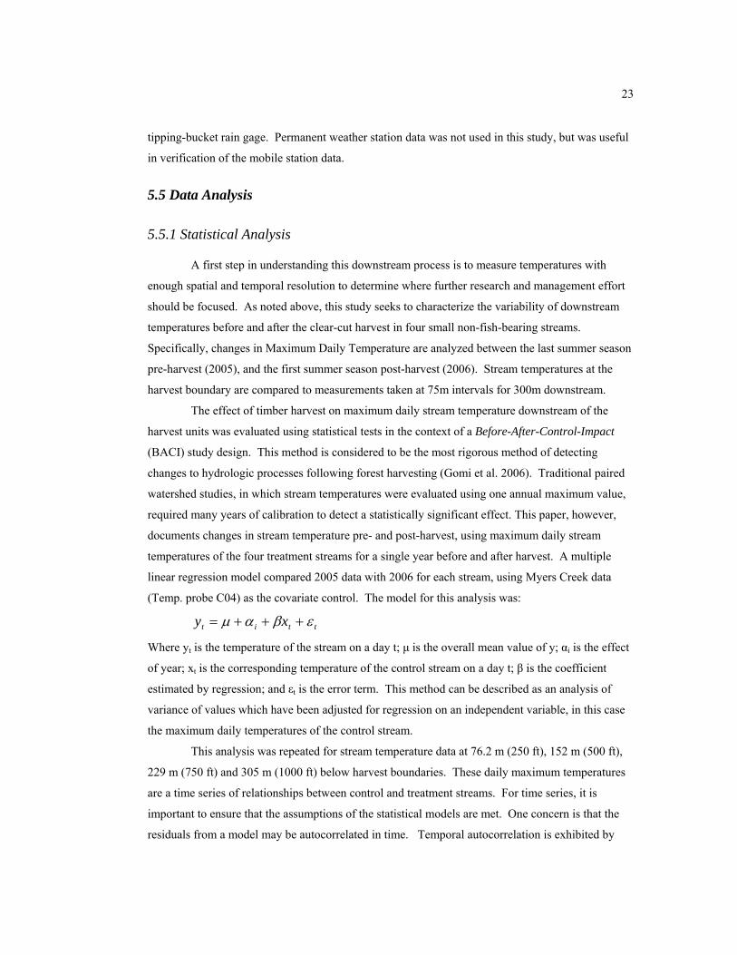
(Temp. probe C04) as the covariate control. The model for this analysis was:

ttit xy εβαμ +++=

Where yt is the temperature of the stream on a day t; μ is the overall mean value of y; αi is the effect

of year; xt is the corresponding temperature of the control stream on a day t; β is the coefficient

estimated by regression; and εt is the error term. This method can be described as an analysis of

variance of values which have been adjusted for regression on an independent variable, in this case

the maximum daily temperatures of the control stream.

This analysis was repeated for stream temperature data at 76.2 m (250 ft), 152 m (500 ft),

229 m (750 ft) and 305 m (1000 ft) below harvest boundaries. These daily maximum temperatures

are a time series of relationships between control and treatment streams. For time series, it is

important to ensure that the assumptions of the statistical models are met. One concern is that the

residuals from a model may be autocorrelated in time. Temporal autocorrelation is exhibited by

24

departures from the regression relationship that are not random but can follow multi-day departures

or some cyclic pattern. Thus, data from consecutive days may not be independent. In this case,

autocorrelation was found and had a one or two day lag for all streams (Kibler 2007). To ensure

independent data, a random start date was chosen, and the maximum daily temperature from every

third day was used for analysis. Another statistical concern is that the residuals from modeling be

normally distributed and have equal variance in time. Maximum Daily Temperature relationships

between treatment and control streams were found to have larger variance during autumn, winter,

and spring seasons than during the summer. To improve the residual structure, early and late season

data were not used. The analysis presented here uses daily maximum temperatures for the same 21

calendar days in July and August of 2005 and 2006 for all streams.

5.5.2 One-dimensional Transport with Inflow and Storage (OTIS) Modeling

Tracer studies offer the opportunity to estimate the characteristics of both the mobile and

immobile water in these headwater streams. The mean stream velocity and discharge, including the

inflow of groundwater can be calculated and are important in characterizing the active channel. The

amount of immobile water in pools and in the streambed can also be estimated.

The 2006 tracer dilution study data was modeled using the One-dimensional Transport with

Inflow and Storage (OTIS) model parameter estimation (OTIS-p) routine (Runkle 1998), originally

published in 1991(Runkle and Broshears 1991). This model uses the advection-dispersion equation,

with additional terms to account for lateral inflow of water, transient storage, first-order decay, and

sorption. These equations are solved using the Crank-Nicolson finite difference method. The

parameter estimation routine (OTIS-p) uses a Non-linear Least Squares (NLS) method (Donaldson

and Tryon 1990) to minimize the squared differences between the measured and simulated

concentrations.

For this study, Rhodamine dye concentrations were modeled assuming no decay. Since

this study was concerned with short time-scale processes of transfer between mobile and immobile

stream zones, sorption was not modeled. Three parameters were estimated: longitudinal dispersion

(D) of dye, transfer rate (α) between the active channel and storage zones, and the cross-sectional

area (A2) of the storage zones. These parameters were estimated as averages for each 75m stream

reach. Stream advection velocity was determined by a trial-and-error visual fit to the increasing

(arrival) portion of the dye breakthrough curves (Figures 19-22), and a constant velocity was

assumed for the entire 300m reach of each study stream. Average stream cross-sectional areas for

each 75m reach were calculated by dividing the mean flowrate for each reach by the stream

velocity.

25

5.5.3 Stream Energy Budget Calculations

Four components of the stream energy budget were calculated for the Russell Creek study

reach for the time period of August 7-17, 2006 (the post-harvest study period). These were based on

measurements taken at 150 meters downstream of the harvest boundary. Photosynthetically Active

Radiation (PAR), relative humidity, air temperature, and wind speed were continuously measured

during this period at a point one meter above the stream surface. PAR measurements are presented

as measured. Latent and Convective heat were calculated using Equations 5 and 6. For these

calculations, water density, ρ = 1000 kg/m2, and specific heat, L = 4184 J/kg-°K. The wind function

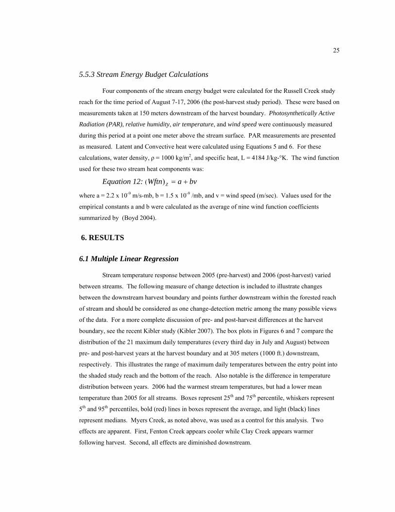
used for these two stream heat components was:

Equation 12: ( bvaWftn Z +=)

where a = 2.2 x 10-9 m/s-mb, b = 1.5 x 10-9 /mb, and v = wind speed (m/sec). Values used for the

empirical constants a and b were calculated as the average of nine wind function coefficients

summarized by (Boyd 2004).

6. RESULTS

6.1 Multiple Linear Regression

Stream temperature response between 2005 (pre-harvest) and 2006 (post-harvest) varied

between streams. The following measure of change detection is included to illustrate changes

between the downstream harvest boundary and points further downstream within the forested reach

of stream and should be considered as one change-detection metric among the many possible views

of the data. For a more complete discussion of pre- and post-harvest differences at the harvest

boundary, see the recent Kibler study (Kibler 2007). The box plots in Figures 6 and 7 compare the

distribution of the 21 maximum daily temperatures (every third day in July and August) between

pre- and post-harvest years at the harvest boundary and at 305 meters (1000 ft.) downstream,

respectively. This illustrates the range of maximum daily temperatures between the entry point into

the shaded study reach and the bottom of the reach. Also notable is the difference in temperature

distribution between years. 2006 had the warmest stream temperatures, but had a lower mean

temperature than 2005 for all streams. Boxes represent 25th and 75th percentile, whiskers represent

5th and 95th percentiles, bold (red) lines in boxes represent the average, and light (black) lines

represent medians. Myers Creek, as noted above, was used as a control for this analysis. Two

effects are apparent. First, Fenton Creek appears cooler while Clay Creek appears warmer

following harvest. Second, all effects are diminished downstream.

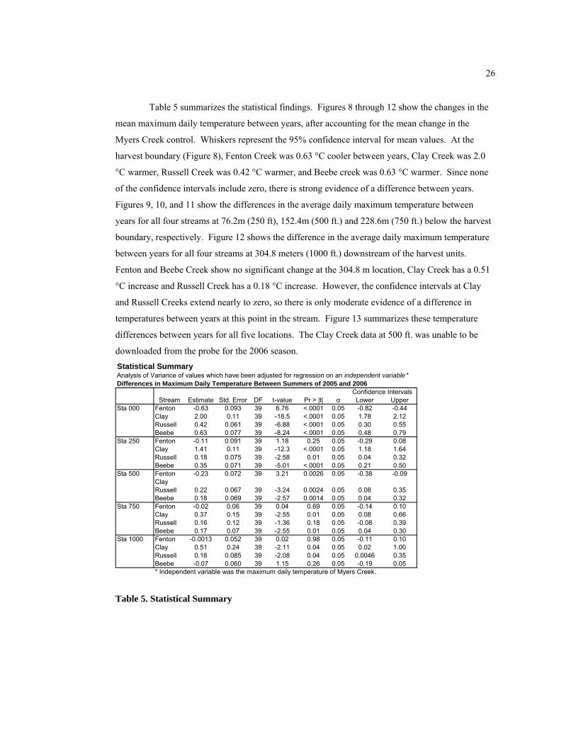
26

Table 5 summarizes the statistical findings. Figures 8 through 12 show the changes in the

mean maximum daily temperature between years, after accounting for the mean change in the

Myers Creek control. Whiskers represent the 95% confidence interval for mean values. At the

harvest boundary (Figure 8), Fenton Creek was 0.63 °C cooler between years, Clay Creek was 2.0

°C warmer, Russell Creek was 0.42 °C warmer, and Beebe creek was 0.63 °C warmer. Since none

of the confidence intervals include zero, there is strong evidence of a difference between years.

Figures 9, 10, and 11 show the differences in the average daily maximum temperature between

years for all four streams at 76.2m (250 ft), 152.4m (500 ft.) and 228.6m (750 ft.) below the harvest

boundary, respectively. Figure 12 shows the difference in the average daily maximum temperature

between years for all four streams at 304.8 meters (1000 ft.) downstream of the harvest units.

Fenton and Beebe Creek show no significant change at the 304.8 m location, Clay Creek has a 0.51

°C increase and Russell Creek has a 0.18 °C increase. However, the confidence intervals at Clay

and Russell Creeks extend nearly to zero, so there is only moderate evidence of a difference in

temperatures between years at this point in the stream. Figure 13 summarizes these temperature

differences between years for all five locations. The Clay Creek data at 500 ft. was unable to be

downloaded from the probe for the 2006 season. Statistical SummaryAnalysis of Variance of values which have been adjusted for regression on an independent variable *Differences in Maximum Daily Temperature Between Summers of 2005 and 2006

Stream Estimate Std. Error DF t-value Pr > |t| α Lower UpperSta 000 Fenton -0.63 0.093 39 6.76 <.0001 0.05 -0.82 -0.44

Clay 2.00 0.11 39 -18.5 <.0001 0.05 1.78 2.12Russell 0.42 0.061 39 -6.88 <.0001 0.05 0.30 0.55Beebe 0.63 0.077 39 -8.24 <.0001 0.05 0.48 0.79

Sta 250 Fenton -0.11 0.091 39 1.18 0.25 0.05 -0.29 0.08Clay 1.41 0.11 39 -12.3 <.0001 0.05 1.18 1.64Russell 0.18 0.075 39 -2.58 0.01 0.05 0.04 0.32Beebe 0.35 0.071 39 -5.01 <.0001 0.05 0.21 0.50

Sta 500 Fenton -0.23 0.072 39 3.21 0.0026 0.05 -0.38 -0.09ClayRussell 0.22 0.067 39 -3.24 0.0024 0.05 0.08 0.35Beebe 0.18 0.069 39 -2.57 0.0014 0.05 0.04 0.32

Sta 750 Fenton -0.02 0.06 39 0.04 0.69 0.05 -0.14 0.10Clay 0.37 0.15 39 -2.55 0.01 0.05 0.08 0.66Russell 0.16 0.12 39 -1.36 0.18 0.05 -0.08 0.39Beebe 0.17 0.07 39 -2.55 0.01 0.05 0.04 0.30

Sta 1000 Fenton -0.0013 0.052 39 0.02 0.98 0.05 -0.11 0.10Clay 0.51 0.24 39 -2.11 0.04 0.05 0.02 1.00Russell 0.18 0.085 39 -2.08 0.04 0.05 0.0046 0.35Beebe -0.07 0.060 39 1.15 0.26 0.05 -0.19 0.05* Independent variable was the maximum daily temperature of Myers Creek.

Confidence Intervals

Table 5. Statistical Summary

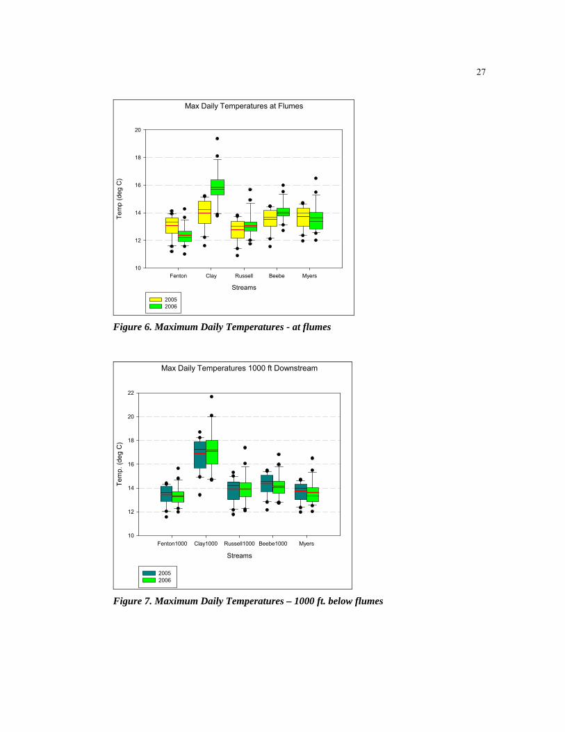
27

Max Daily Temperatures at Flumes

Streams

Fenton Clay Russell Beebe Myers

Tem

p (d

eg C

)

10

12

14

16

18

20

20052006

Figure 6. Maximum Daily Temperatures - at flumes

Max Daily Temperatures 1000 ft Downstream

Streams

Fenton1000 Clay1000 Russell1000 Beebe1000 Myers

Tem

p. (d

eg C

)

10

12

14

16

18

20

22

2005 2006

Figure 7. Maximum Daily Temperatures – 1000 ft. below flumes

28

Stream Temp Change (000) 2005-2006, With Myers Covariate

-0.44

2.21

-0.63

2.00

-0.82

1.78

0.480.55

0.79

0.420.63

0.30

-1.0

0.0

1.0

2.0

Fen Cla Rus Bbe

Treatment Stream

Tem

p C

hang

e B

etw

een

Year

s (d

eg. C

)

Figure 8. Change in Mean Max. Daily Temp. between years - at flumes

Stream Temp Change (250) 2005-2006, With Myers Covariate

0.08

1.64

-0.11

1.41

-0.29

1.18

0.21

0.320.50

0.180.35

0.04

-1.0

0.0

1.0

2.0

Fen250 Cla250 Rus250 Bbe250

Treatment Stream

Tem

p C

hang

e B

etw

een

Year

s (d

eg. C

)

Figure 9. Change in Mean Max. Daily Temp. between years – 250 ft. below flumes

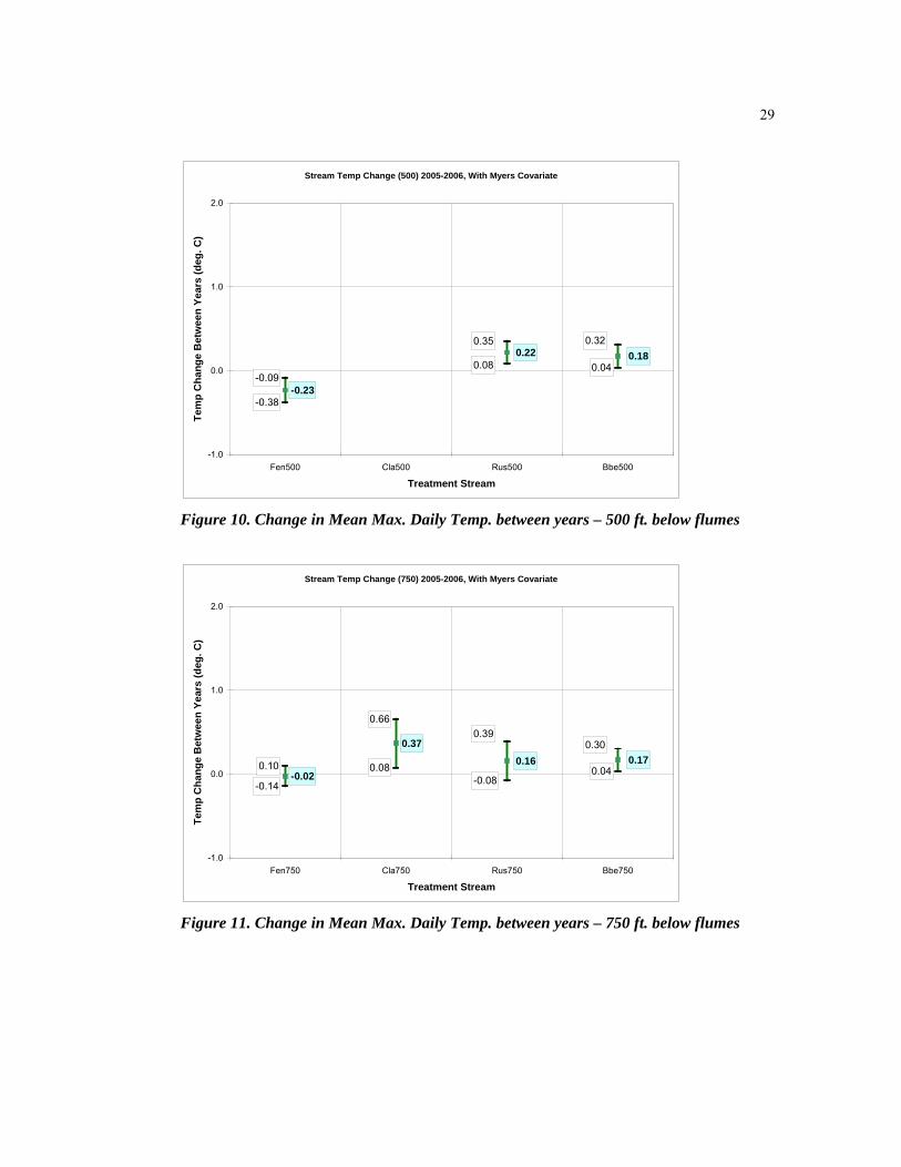
29

Stream Temp Change (500) 2005-2006, With Myers Covariate

-0.09-0.23

-0.38

0.040.08

0.320.22 0.18

0.35

-1.0

0.0

1.0

2.0

Fen500 Cla500 Rus500 Bbe500

Treatment Stream

Tem

p C

hang

e B

etw

een

Year

s (d

eg. C

)

Figure 10. Change in Mean Max. Daily Temp. between years – 500 ft. below flumes

Stream Temp Change (750) 2005-2006, With Myers Covariate

0.10

0.66

-0.02

0.37

-0.14

0.08 0.04

0.390.30

0.16 0.17

-0.08

-1.0

0.0

1.0

2.0

Fen750 Cla750 Rus750 Bbe750

Treatment Stream

Tem

p C

hang

e B

etw

een

Year

s (d

eg. C

)

Figure 11. Change in Mean Max. Daily Temp. between years – 750 ft. below flumes

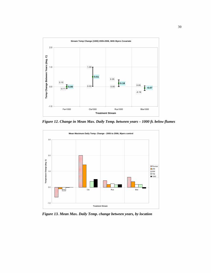
30

Stream Temp Change (1000) 2005-2006, With Myers Covariate

-0.110.020.00

0.51

0.18

1.00

0.00

-0.19

-0.070.05

0.350.10

-1.0

0.0

1.0

2.0

Fen1000 Cla1000 Rus1000 Bbe1000

Treatment Stream

Tem

p C

hang

e B

etw

een

Year

s (d

eg. C

)

Figure 12. Change in Mean Max. Daily Temp. between years – 1000 ft. below flumes

Mean Maximum Daily Temp. Change - 2005 to 2006, Myers control

-1.0

0.0

1.0

2.0

3.0

Fen Cla Rus Bbe

Treatment Stream

Tem

pera

ture

Cha

nge

(deg

. C)

Flumes2505007501000

Figure 13. Mean Max. Daily Temp. change between years, by location

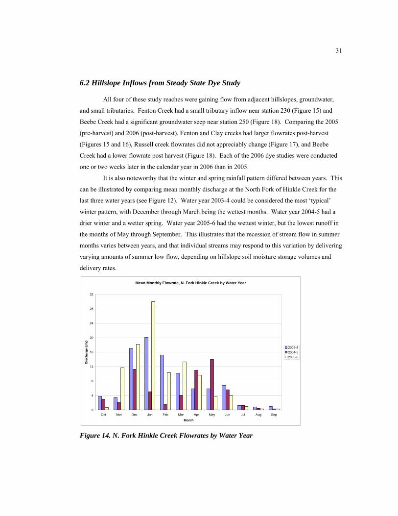
31

6.2 Hillslope Inflows from Steady State Dye Study

All four of these study reaches were gaining flow from adjacent hillslopes, groundwater,

and small tributaries. Fenton Creek had a small tributary inflow near station 230 (Figure 15) and

Beebe Creek had a significant groundwater seep near station 250 (Figure 18). Comparing the 2005

(pre-harvest) and 2006 (post-harvest), Fenton and Clay creeks had larger flowrates post-harvest

(Figures 15 and 16), Russell creek flowrates did not appreciably change (Figure 17), and Beebe

Creek had a lower flowrate post harvest (Figure 18). Each of the 2006 dye studies were conducted

one or two weeks later in the calendar year in 2006 than in 2005.

It is also noteworthy that the winter and spring rainfall pattern differed between years. This

can be illustrated by comparing mean monthly discharge at the North Fork of Hinkle Creek for the

last three water years (see Figure 12). Water year 2003-4 could be considered the most ‘typical’

winter pattern, with December through March being the wettest months. Water year 2004-5 had a

drier winter and a wetter spring. Water year 2005-6 had the wettest winter, but the lowest runoff in

the months of May through September. This illustrates that the recession of stream flow in summer

months varies between years, and that individual streams may respond to this variation by delivering

varying amounts of summer low flow, depending on hillslope soil moisture storage volumes and

delivery rates.

Mean Monthly Flowrate, N. Fork Hinkle Creek by Water Year

0

4

8

12

16

20

24

28

32

Oct Nov Dec Jan Feb Mar Apr May Jun Jul Aug Sep

Month

Dis

char

ge (c

fs)

2003-42004-52005-6

Figure 14. N. Fork Hinkle Creek Flowrates by Water Year

32

Fenton Creek - Calculated Stream Discharge

0

1

2

3

4

5

6

7

8

90 20 40 60 80 100

120

140

160

180

200

220

240

260

280

300

Distance from Injection Site (m)

Dis

char

ge, Q

(L/s

ec)

20062005

Figure 15. Fenton Creek Steady-State Flowrates by Stream Station

Clay Creek Calculated Stream Discharge

0

1

2

3

4

5

6

7

8

9

0 20 40 60 80 100

120

140

160

180

200

220

240

260

280

300

Distance from Injection Site (m)

Flow

rate

, Q (L

/sec

)

20062005

Figure 16. Clay Creek Steady-State Flowrates by Stream Station

33

Russell Creek - Calculated Stream Discharge

0

1

2

3

4

5

6

7

8

90 20 40 60 80 100

120

140

160

180

200

220

240

260

280

300

Distance from Injection Site (m)

Flow

rate

(L/s

ec)

20062005

Figure 17. Russell Creek Steady-State Flowrates by Stream Station

Beebe Creek - Calculated Stream Discharge

0

2

4

6

8

10

12

14

16

18

0 20 40 60 80 100

120

140

160

180

200

220

240

260

280

300

Distance from Injection Site (m)

Dis

char

ge, Q

(L/s

ec)

20062005

Figure 18. Beebe Creek Steady-State Flowrates by Stream Station

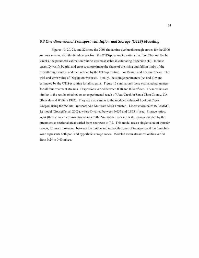
34

6.3 One-dimensional Transport with Inflow and Storage (OTIS) Modeling

Figures 19, 20, 21, and 22 show the 2006 rhodamine dye breakthrough curves for the 2006

summer season, with the fitted curves from the OTIS-p parameter estimation. For Clay and Beebe

Creeks, the parameter estimation routine was most stable in estimating dispersion (D). In these

cases, D was fit by trial and error to approximate the shape of the rising and falling limbs of the

breakthrough curves, and then refined by the OTIS-p routine. For Russell and Fenton Creeks, The

trial-and-error value of Dispersion was used. Finally, the storage parameters (As and α) were

estimated by the OTIS-p routine for all streams. Figure 16 summarizes these estimated parameters

for all four treatment streams. Dispersions varied between 0.18 and 0.84 m2/sec. These values are

similar to the results obtained on an experimental reach of Uvas Creek in Santa Clara County, CA

(Bencala and Walters 1983). They are also similar to the modeled values of Lookout Creek,

Oregon, using the ‘Solute Transport And Multirate Mass Transfer – Linear coordinates (STAMMT-

L) model (Gooseff et al. 2003), where D varied between 0.055 and 0.863 m2/sec. Storage ratios,

As/A (the estimated cross-sectional area of the ‘immobile’ zones of water storage divided by the

stream cross-sectional area) varied from near zero to 7.2. This model uses a single value of transfer

rate, α, for mass movement between the mobile and immobile zones of transport, and the immobile

zone represents both pool and hyporheic storage zones. Modeled mean stream velocities varied

from 0.24 to 0.40 m/sec.

35

OTIS Model - Fenton Creek

0

20

40

60

80

100

120

140

160

180

200

220

240

260

0 4 8 12 16 20 24 28 32 36

Time (hrs)

Con

cent

ratio

n (p

pb) 0+75

1+502+253+000+75 data1+50 data2+25 data3+00 data

Figure 19. Fenton Creek Transport Model

OTIS Model - Clay Creek

0

20

40

60

80

100

120

140

0 4 8 12 16 20 24 28 32 36 40 44 48 52 56 60 64 68 72 76 80 84 88 92

Time (hrs)

Con

cent

ratio

n (p

pb)

0+751+502+253+000+75 data1+50 data2+25 data3+00 data

Figure 20. Clay Creek Transport Model

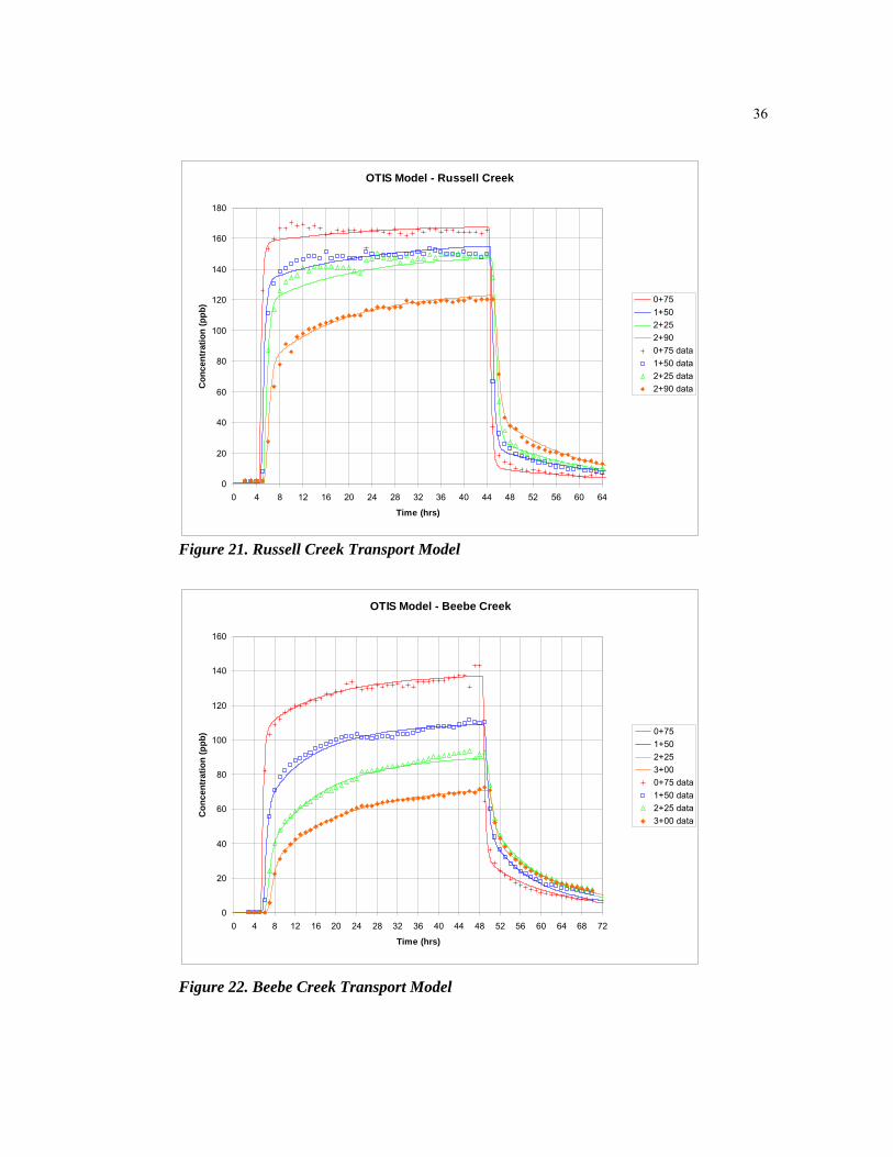
36

OTIS Model - Russell Creek

0

20

40

60

80

100

120

140

160

180

0 4 8 12 16 20 24 28 32 36 40 44 48 52 56 60 64

Time (hrs)

Con

cent

ratio

n (p

pb) 0+75

1+502+252+900+75 data1+50 data2+25 data2+90 data

Figure 21. Russell Creek Transport Model

OTIS Model - Beebe Creek

0

20

40

60

80

100

120

140

160

0 4 8 12 16 20 24 28 32 36 40 44 48 52 56 60 64 68 72

Time (hrs)

Con

cent

ratio

n (p

pb) 0+75

1+502+253+000+75 data1+50 data2+25 data3+00 data

Figure 22. Beebe Creek Transport Model

37

Reach Stream Fen Stor. Storage Trans. Rate Hyporheic Hyporheic FenFen Reach Length Fen Disp. Area, A Area, As Fen Ratio Fen Alpha Res. Time, tS Res. Time, tS VelocityEnding at (m) (m2/sec) (m2) (m2) (As/A) (/sec) (sec) (hr) (m/sec)

0+75 75 0.459 0.074 0.158 2.14 0.0000616 34661 9.61+50 75 0.673 0.085 0.134 1.58 0.0001875 8408 2.32+25 75 0.148 0.118 0.135 1.14 0.0000920 12436 3.53+00 75 0.177 0.190 0.279 1.47 0.0000564 26036 7.2Mean 300 0.364 0.117 0.177 1.581 0.0000994 15910 4.4 0.037

Reach Stream Cla Stor. Storage Trans. Rate Hyporheic Hyporheic ClaCla Reach Length Cla Disp. Area, A Area, As Cla Ratio Cla Alpha Res. Time, tS Res. Time, tS VelocityEnding at (m) (m2/sec) (m2) (m2) (As/A) (/sec) (sec) (hr) (m/sec)

0+75 75 0.4 0.184 0.6222 3.38 0.0000807 41902 11.61+50 75 0.6 0.207 1.4982 7.24 0.0000840 86163 23.92+25 75 0.6 0.245 0.1278 0.52 0.0000046 113398 31.52+90 75 0.6 0.295 1.1223 3.80 0.0002085 18247 5.1Mean 300 0.550 0.233 0.843 3.736 0.0000945 39559 11.0 0.024

Reach Stream Rus Stor. Storage Trans. Rate Hyporheic Hyporheic RusRus Reach Length Rus Disp. Area, A Area, As Rus Ratio Rus Alpha Res. Time, tS Res. Time, tS VelocityEnding at (m) (m2/sec) (m2) (m2) (As/A) (/sec) (sec) (hr) (m/sec)

0+75 75 0.771 0.124 0.3180 2.56 0.0000306 83698 23.21+50 75 0.835 0.135 0.5500 4.07 0.0000749 54415 15.12+25 75 0.426 0.142 0.0001 0.00 0.0000001 14085 3.92+90 75 0.719 0.161 0.8210 5.10 0.0001694 30111 8.4Mean 300 0.688 0.141 0.422 2.935 0.0000687 42700 11.9 0.040

Reach Stream Bbe Stor. Storage Trans. Rate Hyporheic Hyporheic BbeBbe Reach Length Bbe Disp. Area, A Area, As Bbe Ratio Bbe Alpha Res. Time, tS Res. Time, tS VelocityEnding at (m) (m2/sec) (m2) (m2) (As/A) (/sec) (sec) (hr) (m/sec)

0+75 75 0.7 0.180 1.1120 6.18 0.0001286 48039 13.31+50 75 0.5 0.241 0.4318 1.79 0.0001097 16333 4.52+25 75 0.5 0.292 0.9421 3.23 0.0001349 23917 6.63+00 75 0.4 0.382 1.8142 4.75 0.0000522 90981 25.3Mean 300 0.525 0.274 1.075 3.986 0.0001064 37483 10.4 0.028

Beebe Creek

Russell Creek

Fenton Creek

Clay Creek

Figure 23. Estimated Storage and Dispersion Parameters

D isp ersio ns, D ( m2 / sec)

0.0

0.2

0.4

0.6

0.8

1.0

0+75 1+50 2+25 3+00

St at io n

Fen Disp.Cla Disp.Rus Disp.Bbe Disp.

Storage Ratios, As/A (m2/m2)

0.00

2.00

4.00

6.00

8.00

10.00

0+75 1+50 2+25 3+00

Station

X-se

c A

rea

of s

tora

ge (m

2)

Fen Ratio

Cla Ratio

Rus Ratio

Bbe Ratio

38

7. DISCUSSION

7.1 Statistical Analysis Results

Using statistical tools to detect change requires that the observed changes be

distinguishable from background variation. The response variable used to detect change in this

study of downstream effects is Maximum Daily Stream Temperatures (MDST) as described in

Section 6.1. In this case, the observed effect on MDST between the pre-harvest and post-harvest

years is small when compared to the spatial (between-stream) variation in MDST, and this effect

decreased in the downstream direction (Figure 13). At 305 meters below the harvest boundary, the

difference in MDST between years was not statistically significant different on two treatment

streams, and showed only a moderate possibility of difference on the other two treatment streams

(Figure 12).

This study will be instructive as it is compared with future analysis of the between-year

variability of pre-harvest MDST downstream of these harvest units. For example, if future years

show large variability in MDST on a particular stream, but little variability on another stream, a

more complete picture of spatial and temporal variability may emerge. As data is collected in future

years, the change during the first year following the harvest disturbance can be compared with

variability between future years. Thus, year-to-year variability in future years will provide valuable

context to characterize changes attributable to harvest.

Time-series analysis is another tool available to researchers which would give additional

insight to this study [see (Gomi et al. 2006)]. A model using daily temperature data could account

for temporal autocorrelation within the model, and would provide another valuable metric of change

detection.

7.2 Mass Transfer and Transient Storage

The tracer dilution study results highlight the importance of understanding the downstream

mass and energy process changes. First, three processes of mass water movement are explored:

1)Advection of hillslope water, 2)Dispersion/storage, and 3)Stream velocity.

It is noteworthy that, in addition to the transfers of heat into and out of the stream, the heat

stored in the stream water is not fixed in time and space. One purpose of this study was to

characterize the patterns of movement of the ‘mobile’ stream water, the ‘immobile’ water in pools

and hyporheic zone, and the hillslope advective flows which are the primary source of summer

stream water.

39

7.2.1Advection of Hillslope Water

Since Oregon Forest Practice Rules do not require conifer buffers on small non-fish-

bearing streams, the first harvest in the Hinkle Creek Study was designed to characterize the impact

this harvest at the lowest extent of these un-buffered portions of stream. In this study’s location,

300-meter reaches below these clear-cut harvest units, all four of these perennial streams are

typically gaining water from the hillslopes throughout the summer season. Though variable by both

stream and year, all four of these 300m stream reaches gained hillslope flow during both (2005 and

2006) summer low-flow measurement periods. The steady-state dye studies used to quantify these

hillslope flows were compared to other flow measurement techniques as described in Section 3.4.

There are inherent limits to the steady-state dye injection methods used here, which are noteworthy.

The assumption that dye has reached a steady state concentration between the flowing stream water

and storage zones, is a simplification of reality, since hyporheic flowpaths longer than the period of

injection (two to three days) are not reached by the dye. This limitation tends to overestimate the

advection of hillslope water, particularly at the lower portion of the 300m study reaches where dye

would have been present for a shorter period of time, and at lower concentrations. As noted above,

dye is stored in both pools and hyporheic zones. Thus, the storage zone areas and transfer rates in

this study represent an average of these two storage processes.

A future steady-state tracer study would benefit from making redundant measurements of

stream flow, using a second tracer, or using another flow measurement technique to confirm the

hillslope contribution of water. Though the precision of advected flow measurements can be

refined, the methods used for this study represent an important spatial estimate of headwater stream

flowrates.

7.2.2 Hillslope Groundwater Temperature

It is evident that the primary mechanism of stream cooling is mixing with advected

hillslope and groundwater. Groundwater temperature varies spatially and temporally, and was not

quantified for this study. In these headwater gaining reaches, a complete stream heat energy budget

benefit from multiple measurements of groundwater temperature. (Mellina et al. 2002) averaged the

temperatures of four groundwater seeps during the study period. (Story et al. 2003) assumed the

advected groundwater temperature to be the soil temperatures observed below the water table (at

100cm depth) in the stream banks. (Moore et al. 2005) assumed groundwater temperature to be

equal to the daily minimum temperature measured 10 meters upstream of the harvest unit edge.

This study also notes that the mean annual air temperature is often used to approximate

groundwater temperature.

40

One temperature probe (C07) in this control side (North Fork Hinkle Creek) of this study is

located near an apparent groundwater seep. This probe has little diel temperature variation. The

minimum nightly temperatures at this probe varied by year and by date. Figure 24 shows the

temperature variation at this probe for the same 10-week summer period for years 2002 through

2006. If the minimum daily temperature at this probe is assumed as groundwater temperature for

the study reaches, a value of 12-13°C could be used for the summer months. Year 2002 shows

significant departures from the other years minimal temperature variations, possibly due to the

probe being out of the water during these low-flow periods. Another anomaly occurred between

7/20/06 and 8/10/06, and no reason was apparent for this variation. Clearly the issue of the temporal

variation in advected groundwater temperature merits further research.

Probe C07 Temperatures by Year

10

11

12

13

14

15

16

17

18

19

7/6 7/13 7/20 7/27 8/3 8/10 8/17 8/24 8/31 9/7 9/14

Date

Tem

pera

ture

(deg

. C)

20022003200420052006

Figure 24. Probe C07, 2002-2006 Summer Temperatures

7.2.3 Diurnal variation in Hillslope Groundwater Flowrate

A visual examination of the dye concentration at the bottom of the study reach shows the

transition toward steady-state concentration is shown for the 2006 Clay Creek test (see Figure 25).

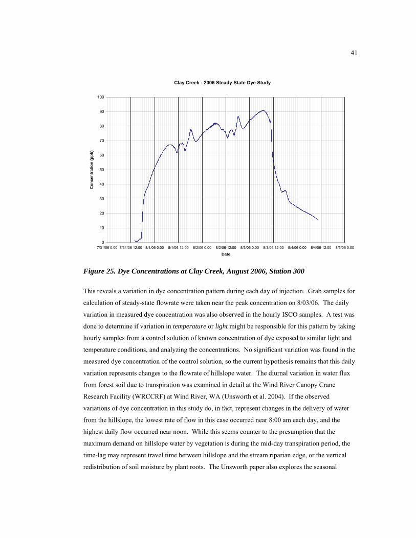
41

Clay Creek - 2006 Steady-State Dye Study

0

10

20

30

40

50

60

70

80

90

100

7/31/06 0:00 7/31/06 12:00 8/1/06 0:00 8/1/06 12:00 8/2/06 0:00 8/2/06 12:00 8/3/06 0:00 8/3/06 12:00 8/4/06 0:00 8/4/06 12:00 8/5/06 0:00

Date

Con

cent

ratio

n (p

pb)

Figure 25. Dye Concentrations at Clay Creek, August 2006, Station 300

This reveals a variation in dye concentration pattern during each day of injection. Grab samples for

calculation of steady-state flowrate were taken near the peak concentration on 8/03/06. The daily

variation in measured dye concentration was also observed in the hourly ISCO samples. A test was

done to determine if variation in temperature or light might be responsible for this pattern by taking

hourly samples from a control solution of known concentration of dye exposed to similar light and

temperature conditions, and analyzing the concentrations. No significant variation was found in the

measured dye concentration of the control solution, so the current hypothesis remains that this daily

variation represents changes to the flowrate of hillslope water. The diurnal variation in water flux

from forest soil due to transpiration was examined in detail at the Wind River Canopy Crane

Research Facility (WRCCRF) at Wind River, WA (Unsworth et al. 2004). If the observed

variations of dye concentration in this study do, in fact, represent changes in the delivery of water

from the hillslope, the lowest rate of flow in this case occurred near 8:00 am each day, and the

highest daily flow occurred near noon. While this seems counter to the presumption that the

maximum demand on hillslope water by vegetation is during the mid-day transpiration period, the

time-lag may represent travel time between hillslope and the stream riparian edge, or the vertical

redistribution of soil moisture by plant roots. The Unsworth paper also explores the seasonal

42

variation in water flux from the soil. Further investigation of this phenomenon could provide

insight into both diurnal and seasonal mechanisms of hillslope flow.

7.2.4 Storage/Dispersion

These headwater streams provide significant storage in pools and hyporheic zones. Storage

varied between the 75m study reaches from almost none to over seven times the cross-sectional area

of the active stream channel. Studies have shown that water stored on pools varies thermally from

the active channel (Bilby 1984; Beschta et al. 1987). While there has been ongoing discussion

regarding the importance of these storage zones, some researchers have noted that pool storage

(Gooseff et al. 2005) and hyporheic exchange (Story et al. 2003) may be significant contributors to

downstream cooling within shaded stream reaches. Particularly where residence times are short

(hours), such as in pools or rapidly down-welling pool-step sequences, the physical mixing process

with stored water provides a mechanism to decrease maximum daily stream temperatures as water

moves downstream.

In addition, a longitudinal dispersion of stream water results from the range of stream

velocities across the stream cross-section. Thus, as water that is heated by solar exposure (such as

in a clear-cut) moves into a shaded reach, the ‘pulse’ of heated water is dispersed along the length of

the shaded reach. This mixing with water within the active channel would tend to lower daily

maximum temperatures, since the shaded reaches of these streams are receiving hillslope

groundwater which is typically cooler than water entering from upstream during the peak mid-day

heating times.

7.2.5 Stream Velocity and Mean Hyporheic Storage Time

Modeled mean stream velocities for the four study reaches varied between 0.024 and 0.040

m/sec. Thus, the average transit time for the 300m reaches ranged from 7,500 sec (2.1 hrs) to

12,500 sec (3.5 hrs). This was most readily evident from the rising limb of the breakthrough curves

of the dye study (see Figures 19-22). For the active channel flow in these streams to complete a 24-

hour diurnal temperature cycle in the shaded reach, at these mean velocities, would require 2.1 to

3.5 km. The mean transit times can be compared with the mean hyporheic residence time, tS, which

is defined as:

Equation 13. α⋅

=AAt S

S

where As is the average cross-sectional area of the immobile (storage) zone (m2), A is the average

cross-sectional area of the stream (m2), and α is the transfer rate between them (sec-1).

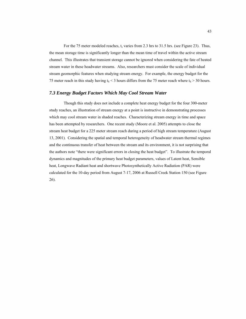
43

For the 75 meter modeled reaches, ts varies from 2.3 hrs to 31.5 hrs. (see Figure 23). Thus,

the mean storage time is significantly longer than the mean time of travel within the active stream

channel. This illustrates that transient storage cannot be ignored when considering the fate of heated

stream water in these headwater streams. Also, researchers must consider the scale of individual

stream geomorphic features when studying stream energy. For example, the energy budget for the

75 meter reach in this study having tS < 3 hours differs from the 75 meter reach where tS > 30 hours.

7.3 Energy Budget Factors Which May Cool Stream Water

Though this study does not include a complete heat energy budget for the four 300-meter

study reaches, an illustration of stream energy at a point is instructive in demonstrating processes

which may cool stream water in shaded reaches. Characterizing stream energy in time and space

has been attempted by researchers. One recent study (Moore et al. 2005) attempts to close the

stream heat budget for a 225 meter stream reach during a period of high stream temperature (August

13, 2001). Considering the spatial and temporal heterogeneity of headwater stream thermal regimes

and the continuous transfer of heat between the stream and its environment, it is not surprising that

the authors note “there were significant errors in closing the heat budget”. To illustrate the temporal

dynamics and magnitudes of the primary heat budget parameters, values of Latent heat, Sensible

heat, Longwave Radiant heat and shortwave Photosynthetically Active Radiation (PAR) were

calculated for the 10-day period from August 7-17, 2006 at Russell Creek Station 150 (see Figure

26).

44

Major Heat Flux Components, Russell Ck., 2006

-40

-20

0

20

40

60

80

100

120

140

160

08/0

7/06

08/0

8/06

08/0

9/06

08/1

0/06

08/1

1/06

08/1

2/06

08/1

3/06

08/1

4/06

08/1

5/06

08/1

6/06

08/1

7/06

08/1

8/06

Date

Hea

t Exc

hang

e (w

att/m

2)

HTOTALHCONVHLONGPARHEVAP

Figure 26. Heat Budget Parameters at Russell Creek, August 2006, Station 150

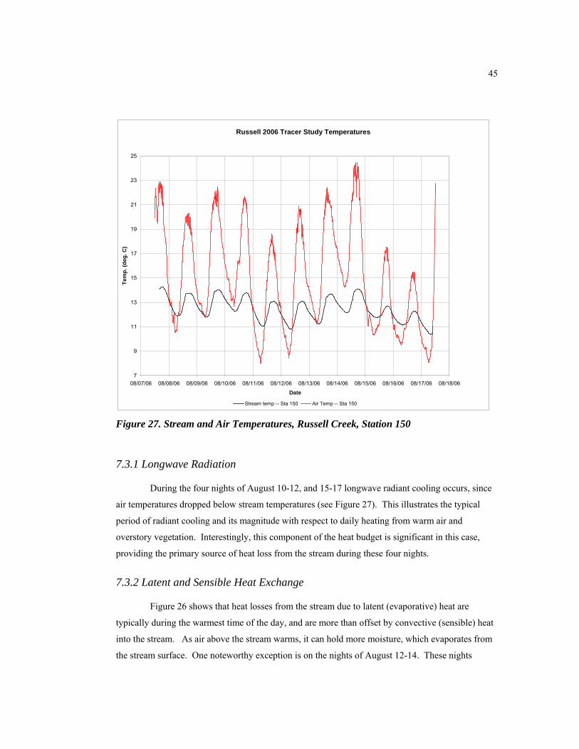
45

Russell 2006 Tracer Study Temperatures

7

9

11

13

15

17

19

21

23

25

08/07/06 08/08/06 08/09/06 08/10/06 08/11/06 08/12/06 08/13/06 08/14/06 08/15/06 08/16/06 08/17/06 08/18/06

Date

Tem

p. (d

eg. C

)

Stream temp -- Sta 150 Air Temp -- Sta 150

Figure 27. Stream and Air Temperatures, Russell Creek, Station 150

7.3.1 Longwave Radiation

During the four nights of August 10-12, and 15-17 longwave radiant cooling occurs, since

air temperatures dropped below stream temperatures (see Figure 27). This illustrates the typical

period of radiant cooling and its magnitude with respect to daily heating from warm air and

overstory vegetation. Interestingly, this component of the heat budget is significant in this case,

providing the primary source of heat loss from the stream during these four nights.

7.3.2 Latent and Sensible Heat Exchange

Figure 26 shows that heat losses from the stream due to latent (evaporative) heat are

typically during the warmest time of the day, and are more than offset by convective (sensible) heat

into the stream. As air above the stream warms, it can hold more moisture, which evaporates from

the stream surface. One noteworthy exception is on the nights of August 12-14. These nights

46

experienced some wind (~1-4 m/sec) and relatively low relative humidity (~50-60%). However,

these conditions occurred at times of relatively warm overnight minimum temperatures, so the

evaporative cooling was not enough to overcome other positive heat inputs to the stream. This does

illustrate, however, the potential importance of wind speed in promoting evaporative cooling. As

shown here, air temperature must be below stream temperature for a net cooling from the sum of

latent and sensible heat exchanges. Further study of up- and down-valley winds in these forested

areas would be instructive in characterizing the importance of this heat budget parameter.

7.4 Heated Stream Water Entering a Shaded Study Reach

To illustrate the spatial dynamics of maximum daily stream temperature below a clearcut

harvest unit, consider the 10-minute stream temperature data from Russell Creek dye study on

August 13, 2006, between noon and 3:00 pm, from station 10 meters (just below the harvest

boundary) to station 150 meters (Figure 28). At noon, all points within the 150m reach are between

approximately 12.1 and 12.4 °C. By 2:40 pm, warmer stream water entering the study reach has

created a temperature difference of greater than 1.2°C between station 30 and station 150. By 3:00

pm, the highest stream temperatures begin to decrease, as the downstream temperatures continue to

increase. This wave of heat energy which arrives during the peak stream heating period has begun

to exchange energy with the shaded stream environment. This process includes the mass and energy

exchanges discussed above. If we assume that the peak stream temperature moves from station 10m

to station 80m in this 3-hour period, the velocity of temperature propagation in this case is 0.0065

m/sec., slower than the modeled mean stream velocity of 0.04 m/sec. by approximately a factor of 6.

47

Russell Creek Temps. - 2006 Dye Study

12.0

12.2

12.4

12.6

12.8

13.0

13.2

13.4

13.6

13.8

14.0

0 10 20 30 40 50 60 70 80 90 100 110 120 130 140 150

Reach Location (m)

Tem

p (d

eg. C

)

8/13/06 12:00 PM8/13/06 12:10 PM8/13/06 12:20 PM8/13/06 12:30 PM8/13/06 12:40 PM8/13/06 12:50 PM8/13/06 1:00 PM8/13/06 1:10 PM8/13/06 1:20 PM8/13/06 1:30 PM8/13/06 1:40 PM8/13/06 1:50 PM8/13/06 2:00 PM8/13/06 2:10 PM8/13/06 2:20 PM8/13/06 2:30 PM8/13/06 2:40 PM8/13/06 2:50 PM8/13/06 3:00 PM

Figure 28. Russell Creek Temperatures by Stream Station and Time

7.5 Temperature Effect of Hillslope Advection Alone

Since the addition of cool water from hillslope groundwater tends to cool streams during

the time when stream temperatures are greatest, a calculation was done to predict this effect,

assuming no other heat transfer processes were occurring. This prediction of temperatures was then

compared with actual stream temperatures. Figure 29 illustrates data from highest two hours of

stream temperature during each of the 2006 dye studies on the four treatment streams. Groundwater

temperature was assumed to be 12°C. Predicted temperatures at Station 0+00, the top of each reach,

was set to the actual highest temperature, and was held constant during the two-hour period.

Downstream temperature predictions are based only on two-part mixing with advected. Fenton and

Clay creeks had a pattern of cooling in the downstream direction during these periods, which is

consistent in scale and direction with the groundwater mixing prediction. Russell Creek had little

actual temperature difference along the reach, and the moderate addition of groundwater in this

reach is not a good predictor of actual temperatures. Beebe Creek warmed in the downstream

direction, counter to the prediction of cooling by groundwater.

48

While the addition of cool groundwater is clearly an important component of the heat

budget in these shaded headwater streams, other energy exchanges cannot be ignored in

characterizing their thermal regimes.

Comparison of Actual stream temperatures with a prediction of stream temperatures based on mean inflowtemperature during the highest two hours of daily stream temperature during the 2006 dye testTwo part mixing model*

Tm = temp. of mixtureDt = Discharge of tributary or groundwaterTt = Temp. of tributary or groundwater (assumed 12° C)Ds = Discharge of the stream at upstream end of reachTs = Temperature of stream at upstream end of reach

st

ssttm DD

TDTDT++

=*

Predicted Temperatures, Groundwater Mixing Only, and Actual Temperatures: At stations within study reaches

12.0

13.0

14.0

15.0

16.0

17.0

FentonPredicted

Fenton Actual

ClayPredicted

Clay Actual RussellPredicted

RussellActual

BeebePredicted

BeebeActual

Stream

Tem

pera

ture

(deg

. C)

0+000+751+502+253+00

Figure 29. Predicted and Actual Stream Temperatures, 2006 Dye Study

7.6 Future Research Needs

Any consideration of stream energy is necessarily limited by the selection of energy

exchange measurements taken. A thorough understanding of these stream energy processes within

an intact forest requires that both spatial and temporal scope be carefully planned. If year-to-year

variability is of interest, researchers must determine what period of years is necessary to

characterize this variability. This primarily relates to variation in the ‘above stream’ climate.

Similarly, if stream-to-stream or broader geographic variability is of interest, a study design must

consider the range of variability which needs to be included. This is primarily an issue of ‘below

stream’ structure and geology. Both of these approaches face the challenge of requiring a

significant financial investment.

49

7.6.1Energy Budget Studies

However, a study of limited geographic scope and time would be useful as a starting point

for characterizing the stream energy budget within a forested stream. In clearcut harvest areas, the

stream heat budget is dominated by radiant heating and cooling (Brown 1969(2)). Within a closed-

canopy forest (such as this study), however, radiant heating and cooling are attenuated, and many of

the heat exchange dynamic processes may be of similar magnitude. Any such study should attempt

to measure as many of the energy budget parameters as possible, and know the range of error

associated with those which are assumed or approximated. In an environment similar to Hinkle

Creek, it may be beneficial to extend the spatial scope to greater than 300 meters to capture

additional variability and further characterize downstream effects. In addition, given the

uncertainties of climate, it may be prudent to take measurements for longer than one week. Finally,

redundancy in measurement, where possible, provides a check on instrument accuracy, as well as

ensures data continuity in the event of equipment failure.

One research question of interest is: When heated stream water exchanges energy in a

downstream forested reach, how much energy is exported to the above-stream atmosphere by the

diel thermal cycle, and how much is stored in the streambed to be reset by the annual thermal cycle?

7.6.2 Buffered Stream Characteristics

Since stream buffers are the primary source of shade in fish-bearing streams in Oregon, an

understanding of their energy dynamics would be instructive to both those who administer current

forest practice rules and those who write new ones. The question of how buffered streams differ

from intact forest has been explored, but a before-after energy budget comparison of forest streams

would certainly add to current knowledge.

7.7 Management Implications

Oregon currently manages forests under a set of rules which have evolved since their

creation in the 1971. As scientific understanding has increased, the rules have changed in response

to those findings. The stated goal of the Forest Practice Rules is as follows:

“. . .encourage economically efficient forest management in Oregon and the continuous

growing and harvesting of trees and maintenance of forestland for such purposes as the leading use

on privately owned land, consistent with sound management of soil, air, water, fish and wildlife

resources . . . and to ensure the continuous benefit of those resources for future generations of

Oregonians” ORS 527.620.

50

Toward these goals, the following paragraphs suggest two themes which may be of interest

in discussions regarding forest headwater stream management.

7.7.1 Stream Thermal Classification

This study demonstrates the difficulty of regulating across a varied geography. These four

adjacent streams of similar size, geology, and climate had a range of thermal environments

downstream from clear-cut harvest units. One approach to minimizing downstream thermal impacts

could be to create a thermal classification system for forest streams. “Sensitive” streams could have

buffers increased from current rules, based on buffer-width research findings. “Average” streams

could maintain existing buffers, and “Insensitive” streams could have reduced buffers, based on

their insensitivity to stream heating. This system would have the benefit of decreasing downstream

thermal impact, while maintaining current harvest potential. Since stream buffers provide other

ecological and physical benefits to streams, a carefully drafted plan would be required.

7.7.2 Stream Structure and Storage Volume

Many of the recent stream temperature studies emphasize the significance of both step-pool

and hyporheic zone storage in moderating peak stream temperatures, and providing thermal refuge

areas for fish. One of the goals of forest management, therefore, should be to both maintain these

existing stream structures and to improve streams which lack them. These structures allow

decreases in stream velocity, and mixing with stored water. This research suggests that these

structures may be keys to enhancing the stream’s processes where water heated from upstream

clear-cut areas to returns to the thermal equilibrium of the downstream environment.

51

8. CONCLUSIONS

Based on this study, and a review of the literature, downstream temperature responses to

timber harvest in western Oregon is variable between streams. The processes by which heat is

transferred between the stream and its environment within these shaded reaches must be considered

relative to the diel fluctuation of these transfer mechanisms. Heat losses from the stream to the

atmosphere can be significant contributors to the overall stream heat budget. In particular,

evaporative cooling during the day, and longwave radiant cooling at night are important.

Streams where the air temperature at night drops below the stream temperature have

potential to lose heat to the atmosphere from longwave cooling. If the air is both cooler than the

stream and moving, the stream has potential to lose heat by evaporative cooling. Thus, climatic

periods during the summer heating season when stream cooling occurs, such as cloud and/or windy

days, are important in understanding the mechanisms of downstream cooling.

Water stored within a shaded stream reach, both in pools and in hyporheic zones, can

provide a mixing volume through which the active stream channel can exchange stream water,

providing both physical mixing with cooler water, and an effective heat transfer to the stream bed.

In these study streams, the storage volumes varied from almost none to about seven times the stream

active channel volume among the 75-meter reaches. This mixing with stored water, as well as the

heat transfer to the streambed tends to dampen temperatures on the daily cycle, lowering maximum

temperatures and raising minimum temperatures. In addition, if heat is stored in the stream bed and

hyporheic zones during the summer months, this stored heat is then reset over the winter season to

provide a heat sink for the next summer season. Thus the annual cycle of heat transfer can be

important in closing the heat budget in these streams.

52

9. LITERATURE CITED

Adams, T. N., K. Sullivan, et al. (1989). The Physics of Forest Stream Heating: A Simple Model, Timber, Fish & Wildlife.

Bartholow, J. M. (2002). "Estimating cumulative effects of clearcutting on stream temperatures." Rivers 7(4): 284-297.

Bencala, K. E. and R. A. Walters (1983). "Simulation of solute transport in a mountain pool-and-riffle stream: A transient storage model." 19(3): 718-724.

Beschta, R. L., R. E. Bilby, et al. (1987). Stream temperature and aquatic habitat: forestry and fishery interactions. Streamside management : forestry and fishery interactions / edited by Ernest O. Salo, Terrance, W. Cundy, Seattle, Wash. : College of Forest Resources, University of Washington, 1987: 191-232.

Beschta, R. L. and R. L. Taylor (1988). "Stream temperature increases and land use in a forested Oregon watershed." Water resources bulletin 24(1): 19-25.

Bilby, R. E. (1984). "Characteristics and frequency of cool-water areas in a western Washington stream." Journal of Freshwater Ecology 2(6): 593-602.

Bowen, I. S. (1926). "The ratio of heat losses by conduction and by evaporation from any water surface." Physical review 27: 779-787.

Boyd, M. S. (1996). Heat Source: stream temperature prediction. Civil and Bioresource Engineering. Corvallis, OR, Master’s Thesis. Departments of Civil and Bioresource Engineering, Oregon State University, Corvallis, Oregon. MS.

Boyd, M. S., Casper, B. (2004). "HeatSource 7.0." from http://www.heatsource.info. Brett, J. R. (1956). "Some principles in the thermal requirements of fishes." The Quarterly Review

of Biology 31(2): 75-87. Brown, G. W. (1969). "Predicting the effect of clearcutting on stream temperature." JOURNAL OF

SOIL AND WATER CONSERVATION 25(1): 11-13. Brown, G. W. (1969(2)). "Predicting temperatures of small streams." Water Resources Research

5(1): 68-75. Brown, G. W. (1985). Forestry and Water Quality. Corvallis, Oregon, Oregon State University

Press. Brown, G. W. and J. T. Krygier (1970). Effects of clear-cutting on stream temperature. Water

Resources Res: 1133-1139. Donaldson, J. R. and P. V. Tryon (1990). User’s guide to STARPAC—The standards, time series,

and regression package., National Institute of Standards and Technology. Gauger, H. and A. Skaugset (2004). Cooling downstream of a harvest operation in Oregon

Cascades. Riparian Ecosystems and Buffers: Multi-scale Structure, Function, and Management; AWRA Summer Specialty Conference. Olympic Valley, California.

George, R. L. (2006). Baseline stream chemistry and soil resources for the Hinkle Creek research and demonstration area project. Forest Engineering. Corvallis, OR, Oregon State University. Master of Science.

Gomi, T., R. D. Moore, et al. (2006). "Headwater stream temperature response to clear-cut harvesting with different riparian treatments, coastal British Columbia, Canada." Water Resources Research 42(8).

Gooseff, M. N., J. Lanier, et al. (2005). "Determining in-channel (dead-zone) transient storage by comparing solute transport in a bedrock channel-alluvial channel sequence, Oregon." Water Resources Research 41(W06014): doi:10.1029/2004WR003513.

Gooseff, M. N., S. M. Wondzell, et al. (2003). "Comparing transient storage modeling and residence time distribution (RTD) analysis and geomorphically varied reaches in the Lookout Creek basin, Oregon, USA." Advances in Water Resources 26: 925-937.

53

Haggerty, R., S. M. Wondzell, et al. (2002). "Power-law residence time distribution in the hyporheic zone of a 2nd-order mountain stream." GEOPHYSICAL RESEARCH LETTERS 29(13): 1640.

Hondzo, M. and H. G. Stefan (1994). "Riverbed heat conduction prediction." Water Resources Research 30(5): 1503-1514.

Johnson, S. L. (2004). "Factors influencing stream temperatures in small streams: substrate effects and a shading experiment." Canadian Journal of Fisheries and Aquatic Sciences 61(6): 913-923.

Johnson, S. L. and J. A. Jones (2000). "Stream temperature responses to forest harvest and debris flows in western Cascades, Oregon." Canadian Journal of Fisheries and Aquatic Sciences 57(supplement 2): 30-39.

Kasahara, T. and S. M. Wondzell (2003). "Geomorphic controls on hyporheic exchange flow in mountain streams." WATER RESOURCES RESEARCH 39(1): 1005.

Kibler, K. (2007). Changes in stream temperature and canopy cover following timber harvesting adjacent to non-fish bearing headwater streams. Forest Engineering. Corvallis, Oregon, Oregon State University. M.S.

Levno, A., J. Rothacher, et al. (1967). Increases in maximum stream temperatures after logging in old-growth Douglas-fir watersheds. Portland, Or., Pacific Northwest Forest and Range Experiment Station.

McDonnell, J. J. (1990). "A Rationale for Old Water Discharge Through Macropores in a Steep, Humid Catchment." Water Resources Research 26(11): 2821-2832.

Mellina, E., R. D. Moore, et al. (2002). "Stream temperature responses to clearcut logging in British Columbia: the moderating influences of groundwater and headwater lakes." Canadian Journal of Fisheries and Aquatic Sciences 59: 1886-1900.

Moore, R. D., A. Story, et al. (2005). "Riparian microclimate and stream temperature response to forest harvesting: a review." Journal of the American Water Resources Association 41: 813-834.

Moore, R. D., P. Sutherland, et al. (2005). "Thermal regime of a headwater stream within a clear-cut, coastal British Columbia, Canada." Hydrological Processes 19: 2591-2608.

Nadeau, T. and M. C. Rains (2007). "Hydrological connectivity between headwater streams and downstream waters: How science can inform policy." Journal of the American Water Resources Association 43(1): 118-133.

Norris, L., J. Buckhouse, et al. (2000). Influences of human activity on stream temperatures and existence of cold-water fish in streams with elevated temperature: Report of a workshop. IMST. Corvallis, Oregon, Oregon State University.

Poole, G. C. and C. H. Berman (2001). "An ecological perspective on in-stream temperature: natural heat dynamics and mechanisms of human-caused thermal degradation." Environmental management 27(6): 787-802.

Rantz, S. (1982). Measurement and Computation of Streamflow: Volume 1. Measurement of Stage and Discharge USGS: 284.

Runkle, R. L. (1998). One-dimensional Transport with Inflow and Storage (OTIS): A Solute Transport Model for Streams and Rivers. Water-Resources Investigations Report 98–4018. Denver, CO, United States Geological Survey (USGS).

Runkle, R. L. and R. E. Broshears (1991). One-dimensional Transport with Inflow and Storage (OTIS): A Solute Transport Model for Small Streams. CADSWES Technical Report 91-01. Boulder, CO, University of Colorado: 85.

Sinokrot, B. A. and H. G. Stefan (1993). "Stream temperature dynamics: measurements and modeling." Water Resources Research 29(7): 2299-2312.

Skaugset, A., Li J., Kromack, K., Gresswell, R., Adams, M. (2005). Cumulative Environmental Effects of Contemporary Forest Management Activities in Headwater Basins of Western

54

Oregon: The Hinkle Creek Paired Watershed Study. Corvallis, OR, Oregon State University.

Story, A., R. D. Moore, et al. (2003). "Stream temperatures in two shaded reaches below cutblocks and logging roads: downstream cooling linked to subsurface hydrology." Canadian Journal of Forest Research 33(8): 1383-1396.

Unsworth, M. H., N. Phillips, et al. (2004). "Components and controls of water flux in an old-growth Douglas-fir--Western Hemlock ecosystem." Ecosystems 7: 468-481.

Webb, B. W. and Y. Zhang (1999). "Water temperatures and heat budgets in Dorset chalk water courses." Hydrological Processes 13(3): 309-321.

Wells, R. E., Jayko, A.S., Niem, A.R., Black, G., Wiley, T., Baldwin, E., Molenaar, K.M., Wheeler, K.L., DuRoss, C.B., and Givler, R.W. (2000). Geologic map and database of the Roseburg 30 x 60 minute quadrangle, Douglas and Coos Counties, Oregon. M. P. U.S. Geological Survey, CA.

Zwieniecki, M. A. and M. Newton (1999). "Influence of streamside cover and stream features on temperature trends in forested streams of Western Oregon." Western Journal of Applied Forestry 14(2): 106-113.